Relevant factors for the impact of social media marketing ... · Project title: Relevant factors...
119
FINAL PROJECT / BACHELOR-THESIS Relevant factors for the impact of social media marketing strategies. Empirical study of the internet travel agency sector. Philipp Robert Lebherz October 2011 Supervisors: Ferran Sabaté Garriga PhD. – Universitat Politècnica de Catalunya Antonio Cañabate Carmona PhD. – Universitat Politècnica de Catalunya Dr. Andreas Geyer-Schulz – Karlsruher Institut für Technologie Student: Philipp Robert Lebherz Karlsruher Institut für Technologie (KIT) & Universitat Politècnica de Catalunya (UPC)
-
Upload
nguyendieu -
Category
Documents
-
view
214 -
download
0
Transcript of Relevant factors for the impact of social media marketing ... · Project title: Relevant factors...
FINAL PROJECT / BACHELOR-THESIS
Relevant factors for the impact of social
media marketing strategies.
Empirical study of the internet travel agency sector.
Philipp Robert Lebherz October 2011
Supervisors: Ferran Sabaté Garriga PhD. – Universitat
Politècnica de Catalunya Antonio Cañabate Carmona PhD. – Universitat
Politècnica de Catalunya Dr. Andreas Geyer-Schulz – Karlsruher Institut
für Technologie
Student: Philipp Robert Lebherz Karlsruher Institut für Technologie (KIT) & Universitat Politècnica de Catalunya (UPC)

II
Philipp Robert Lebherz
III
Philipp Robert Lebherz
PROJECT
Project title: Relevant factors for the impact of social media marketing strategies. Emprical study of the internet travel agency sector.
Name of student: Philipp Robert Lebherz
Major: Ingeniería Técnica en Informática de Gestión
Credits: 22,5
Director: Ferran Sabaté Garriga
Co-director: Antonio Cañabate Carmona
Department: Organització d’Empreses
TRIBUNAL MEMBERS (name and signature)
President: Joaquim Deulofeu Aymar
Vocal: Erik Cobo Valeri
GRADE
Numerical grade:
Description:
Date:
IV Index
Philipp Robert Lebherz
Index
Index ............................................................................................................................... IV
List of figures ................................................................................................................... VI
List of tables ................................................................................................................... VII
0. Preface ......................................................................................................................... 1
1. Introduction .................................................................................................................. 2
1.1. General introduction .................................................................................................................... 2
1.2. Introduction to topic .................................................................................................................... 3
2. State of the art .............................................................................................................. 5
2.1. Importance of social media marketing ......................................................................................... 5
2.2. Social media marketing strategies ............................................................................................... 6
2.3. Knowledge & insights about publishing in social media .............................................................. 9
2.3.1. Soft criteria .......................................................................................................................... 10
2.3.2. Hard criteria ......................................................................................................................... 10
2.3.3. Social media channels in general ........................................................................................ 11
2.4. EXCURSUS: Obtaining data of OSNs through APIs, crawlers or existing data sets. .................... 12
3. Objectives of the study ................................................................................................ 16
4. Methodology of the study ........................................................................................... 17
4.1. Selection of the sample .............................................................................................................. 17
4.1.1. Travel agencies .................................................................................................................... 17
4.1.1.1. Criteria for selection ..................................................................................................... 17
4.1.1.2. Comparison .................................................................................................................. 19
4.1.2. Social media channels ......................................................................................................... 23
4.1.2.1. Criteria for selection ..................................................................................................... 23
4.1.2.2. Comparison .................................................................................................................. 24
4.2. Data ............................................................................................................................................ 26
4.2.1. Explanation of the data set. ................................................................................................ 26
4.2.2. Explanation of variables ...................................................................................................... 27
4.2.2.1. Facebook ...................................................................................................................... 27
4.2.2.2. Twitter .......................................................................................................................... 29
5. Economic study and timeline ....................................................................................... 31
V Index
Philipp Robert Lebherz
5.1. Timeline, Gantt chart .................................................................................................................. 31
5.2. Economic study .......................................................................................................................... 34
6. Analysis of gathered data ............................................................................................ 36
6.1. Facebook .................................................................................................................................... 36
6.1.1. Variables .............................................................................................................................. 37
6.1.2. Correlation ........................................................................................................................... 47
6.1.3. Regression ........................................................................................................................... 49
6.1.3.1. Dependent Variable FPost#Comments ........................................................................ 49
6.1.3.1.1. General .................................................................................................................. 49
6.1.3.1.2. ES ........................................................................................................................... 60
6.1.3.1.3. GE .......................................................................................................................... 62
6.1.3.2. Dependent Variable FPost#Likes .................................................................................. 63
6.1.3.2.1. General .................................................................................................................. 63
6.1.3.2.2. ES ........................................................................................................................... 65
6.1.3.2.3. GE .......................................................................................................................... 67
6.2. Twitter ........................................................................................................................................ 69
6.2.1. Variables .............................................................................................................................. 70
6.2.2 Correlation ............................................................................................................................ 79
6.2.3. Regression ........................................................................................................................... 80
6.2.3.1. General ......................................................................................................................... 80
6.2.3.2. ES .................................................................................................................................. 82
6.2.3.3. GE ................................................................................................................................. 84
7. Conclusion .................................................................................................................. 85
8. Future Work ................................................................................................................ 87
Bibliography ................................................................................................................... 88
Appendix ........................................................................................................................ 91
VI List of figures
Philipp Robert Lebherz
List of figures
Figure 1: Overview Facebook (59), (60). ............................................................................................... 24Figure 2: Overview Twitter (59), (60). ................................................................................................... 25Figure 3: Example of Facebook variable declaration. ........................................................................... 27Figure 4: Example of Twitter variable declaration. ............................................................................... 29Figure 5: Example of Twitter variable declaration. ............................................................................... 29Figure 6: Gantt-Chart, first part. ............................................................................................................ 32Figure 7: Gantt-Chart, second part. ....................................................................................................... 32Figure 9: Histogram, Facebook variable followers. ............................................................................... 37Figure 10: Histogram, Facebook variable followers transformed to LN(followers). ............................. 37Figure 11: Histogram, Facebook variable FPost#Letters. ...................................................................... 38Figure 12: Histogram, Facebook variable FPost#Links. ......................................................................... 39Figure 13: Histogram, Facebook variable LinksDummy. ....................................................................... 39Figure 15: Histogram, Facebook variable FPost#Images. ...................................................................... 40Figure 16: Histogram, Facebook variable ImagesDummy. .................................................................... 40Figure 18: Histogram, Facebook variable FPost#VideoClips. ................................................................ 41Figure 19: Histogram, Facebook variable VideoClipsDummy. .............................................................. 41Figure 20: Histogram, Facebook variable FPostTime. ........................................................................... 42Figure 21: Histogram, Facebook variable TimeDummy. ....................................................................... 42Figure 22: Histogram, Facebook variable FPostDateDay. ..................................................................... 43Figure 23: Histogram, Facebook variable DateDayDummy. ................................................................. 43Figure 24: Histogram, Facebook variable FPost#Likes. ......................................................................... 44Figure 25: Histogram, Facebook variable LN(Likes+1). ......................................................................... 44Figure 26: Histogram, Facebook variable FPost#Comments. ................................................................ 45Figure 27: Histogram, Facebook variable LN(Comments+1). ................................................................ 45Figure 14: Histogram, Facebook variable ImagesDummy+LinksDummy. ............................................. 46Figure 17: Histogram, Facebook variable ImagesDummy-LinksDummy. .............................................. 46Figure 28: Histogram, Twitter variable TTweet#Characters. ................................................................ 70Figure 29: Histogram, Twitter variable TTweetDateDay. ...................................................................... 71Figure 30: Histogram, Twitter variable DateDayDummy. ..................................................................... 71Figure 31: Histogram, Twitter variable TTweet#ReTweets. .................................................................. 72Figure 32: Histogram, Twitter variable LN_TTweet#ReTweets. ............................................................ 72Figure 33: Histogram, Twitter variable TTweetIsAnswer. ..................................................................... 73Figure 35: Histogram, Twitter variable TTweet#Links. .......................................................................... 74Figure 36: Histogram, Twitter variable LinksDummy. ........................................................................... 74Figure 37: Histogram, Twitter variable TTweet#Mentions. .................................................................. 75Figure 38: Histogram, Twitter variable MentionsDummy. .................................................................... 75Figure 40: Histogram, Twitter variable TTweet#Tags. .......................................................................... 76Figure 41: Histogram, Twitter variable TagsDummy. ............................................................................ 76Figure 42: Histogram, Twitter variable Followers. ................................................................................ 77Figure 43: Histogram, Twitter variable LN_Followers. .......................................................................... 77Figure 34: Histogram, Twitter variable MentionsDummy-TweetIsAnswer. ......................................... 78Figure 39: Histogram, Twitter variable MentionsDummy+TweetIsAnswer. ......................................... 78
VII List of tables
Philipp Robert Lebherz
List of tables
Table 1: Overview travel agencies. ........................................................................................................ 20Table 2: German travel agencies ranked by Traffic Rank. ..................................................................... 20Table 3: Spanish travel agencies ranked by Traffic Rank. ..................................................................... 20Table 4: German travel agencies ranked by revenue. ........................................................................... 21Table 5: Spanish travel agencies ranked by revenue. ........................................................................... 21Table 6: Spanish travel agencies ranked by number of channels. ........................................................ 21Table 7: German travel agencies ranked by number of channels ......................................................... 21Table 8: Overall ranking of Spanish travel agencies. ............................................................................. 22Table 9: Overall ranking of German travel agencies. ............................................................................ 22Table 10: Labor time in days. ................................................................................................................ 33Table 11: Labor time in hours. ............................................................................................................... 33Table 12: Labor time allocated to employees. ...................................................................................... 34Table 13: Labor costs for the employer. ................................................................................................ 35Table 14: Office costs for the employer. ............................................................................................... 35Table 15: Total costs of the project. ...................................................................................................... 35

1 0. Preface
Philipp Robert Lebherz
0. Preface
This work was written during my exchange year at the Universitat Politècnica de Catalunya (UPC) in Barcelona, Spain. It was supervised by Ferran Sabaté Garriga PhD and Antonio Cañabate Carmona PhD at UPC and Prof. Dr. Andreas Geyer-Schulz at the Karlsruher Institut für Technologie (KIT) in Karlsruhe, Germany.
I would like to thank my supervisors Mr. Sabaté Garriga PhD and Mr. Cañabate Carmona PhD for giving me the opportunity to write my bachelor thesis at the chair of management at the faculty of informatics. Furthermore I would like to thank my supervisors for their always attentive, cooperative and friendly support and for giving me the opportunity to learn a lot during this time.
Additionally, I would like to thank my supervisor Prof. Dr. Geyer-Schulz for supervising my bachelor thesis at the KIT and thus making it possible to write it during my exchange year.
Especially I would like to thank my parents Rita and Willy Lebherz, my sister Annina Lebherz and my cousins Barbara and Cornelia Witt for listening to my thoughts, doubts and ideas, for motivating and supporting me and for proofreading.
I would like to thank my friends Oretta Irmler and Yvonne Konrad for encouraging me in hard times and for proofreading my work. Thank you!
I am student of the Karlsruher Institut für Technologie in Karlsruhe, Germany. The work in hand is the bachelor thesis of my bachelor course of studies with the name Information Engineering and Management. I chose to write it during my exchange year from September 2010 to September 2011 at the UPC. I decided to choose this topic after some meetings with my supervisors. While informing myself about the topic I considered it to be interesting, up-to-date and practical and I still think so.
2 1. Introduction
Philipp Robert Lebherz
1. Introduction
1.1. General introduction
"Too many marketers manage their approach as if they were "stuck in the 60s", an era of mass markets, mass media, and impersonal transactions. Yet never before have companies had such powerful technologies for interacting directly with customers, collecting and mining information about them and tailoring their offerings accordingly. And never before have customers expected to interact so deeply with companies and each other, to shape the products and services they use." (1)
The core of marketing is about connecting with the customers and developing products and services that they need, want and value (2). However, today the term marketing is used in many different ways. Related to this work marketing is used as an instrumental sense as suggested by Hettler meaning that it is about the tools, the processes and the ways of how marketing objectives can be achieved (3). While the term marketing can also be understood by describing the whole economic concept of orientating the management decisions on the market and according to this, to the consumers. In the context of this work we do better understanding social media marketing as marketing through the instrument of social media. Thus marketing with the targeted use of the new possibilities of user created content web 2.0 enables. Tuten mentions some of these new possibilities social media offers in her definition of social media marketing, including (online) social networks like YouTube, MySpace, and Facebook, virtual worlds like second life, social news sites like delicious and social opinion sharing sites like epinions (4). It is important to be able to distinguish the terms is important since a lot of them seem to be quite similar but mean different things. social media marketing should not be mixed up with social marketing. social marketing is a marketing discipline that was affected by Philip Kotler and Geralt Zaltman in the 1970s. They define Social Marketing as follows:
“Social marketing seeks to influence social behaviors, not to benefit the marketer, but to benefit the target audience and the general society.” (5)
Apparently this describes another set of ideas than social media marketing does. In addition the term social network is often used together with social media although it should not only be considered in an online context. As Xu & Zhang mention, a social network is a representation of relationships between social entities existing within a community (6). Social networks and social network analysis already appeared decades ago in social science and psychology. For better understanding I will avoid the term social networks and use online social networks (OSN) instead.
Tuten brings up that there exist two different types of online social networks namely egocentric and object-centric ones (4). While egocentric OSN such as Facebook, Twitter or LinkedIn place the individual as the core of the network experience, object-centric OSN focus on other elements like video clips in YouTube or pictures in Flickr, as focus. However, literature agrees in the point that the core of social media and social media marketing is large scale user-created and co created content (3) (2) (4). Meaning content that is made publicly available online reflects some creative effort of the user and is created outside professional practice (4). What makes social media social is that there is no distinction of content provider and consumer anymore, as everybody is able to create, read, rate and share content (7) (8). So action takes place in a bidirectional way. From a marketing point of view this implies a shift from impressions to
3 1. Introduction
Philipp Robert Lebherz
connections and from campaigns to conversations. Obviously social media marketing is a new way of doing marketing differently to the one-way interruptive marketing known from television, print media and other one-to-many media (2) (9). Respectively Kilian states blogs, online social networks, sharing communities, knowledge communities and consumer communities were the most important Social-Media applications (8). Consistent with that Heymann-Reder lists Facebook, Twitter and YouTube as some of the eleven most important Social-Media-Marketing channels (10). It is not only the new possibilities social media marketing gives for marketing but also the steadily increasing penetration level of the internet. In EU, Japan and North America the penetration level already reaches 70 % (4). While television has about 98 % for decades now it is unavoidable to also take in account that huge amounts of money are spend for television strategies while according to studies people spend less than 25 % of their time to television. On the other hand less than 3 % of the budget is used for Online Media although people are engaged almost 20% of their time (11). Further insights to the importance of social media marketing are given in a) Importance of social media marketing.
1.2. Introduction to topic
Web 2.0 enabled online social media which in turn enabled users to publish content to other users. This change from the former one-way communication with a provider that shares content to the consumers to a many-to-many communication environment where every user can act as content provider changes the way business can communicate to its customers (12). Now there is the possibility for dialogue, interactivity, consumer involvement and consumer interaction with the brand. Those possibilities offer big benefits for business as business now can assess what the brand means to their consumers and thereby strengthen brands personality, differentiate the brand from other brands and build tight relationships. High exposure time for brands message supports internalization of the branding message and strengthens brands equity (4). However, this requires that the consumer engages to the brand. The Advertising Reach Foundation defines brand engagement as:
"Turning on a prospect to a brand idea enhanced by the surrounding context". Engagement occurs as a "subtle, subconscious process in which consumers begin to combine the ad's message with their own associations, symbols, and metaphors to make the brand more personally relevant" (13)
Obviously a social media marketing strategy is thought to achieve the target audience to engage with the brand. This brand engagement of the consumer through brand’s marketing is what is meant by the “impact of the social media marketing strategy”. While there are a lot of different types of social media channels and thus a lot of different strategies (further explanation to social media marketing strategies is given in chapter 2.2.), this work deals with strategies for obtaining brand engagement through Facebook fan-pages and Twitter publications. Business publishes different types of content through those channels and consumer view and contribute. When observing high contribution to a publication this means by nature a high exposure of the brands message to the consumers and thereby a connection of brand and consumers. Contribution of a consumer means being connected and being connected shows engagement to the brand, and vice versa. To measure the consumer contribution in order to be able to classify later on the effectiveness of the efforts done, is crucial. It is not far-fetched to question oneself if there are quantitative factors favoring a higher contribution and thus exposure of consumers to the social media marketing efforts.

4 1. Introduction
Philipp Robert Lebherz
In this work quantitative factors of the published contents in different social media channels are analyzed for their impact on consumer contribution.
Those quantitative factors are characteristics of the published content. They differ from one channel to another and are for example, the day of publication, the time of publication, the number of characters and the number of links, videos and/or photos. Further description to the objectives of the study of this work is given in section 3. and to the data that was collected in section 4.2. Due to a shortage of preparation time the data for this work was gathered manually, however in 2.4. you can find an excursus on how to gather data from online social networks automatically by using the provided APIs, HTTP crawling/scraping or by using big data sets that have been gathered for previous research and afterwards been made publicly available. 3. states the objectives and hypothesis of this work that are answered in 6. , with the results of the data analysis. An economic study of the hypothetical costs of this work is done in 5. Last but not least the conclusion in section 7. Sums up the most important results.
5 2. State of the art
Philipp Robert Lebherz
2. State of the art
2.1. Importance of social media marketing
“Facebook Reaches Top Ranking in US, March 15, 2010.
Facebook reached an important milestone for the week ending March 13, 2010 and surpassed Google in the US to become the most visited website for the week. […] The market share of visits to Facebook.com increased 185 % last week as compared to the same week in 2009, while visits to Google.com increased 9 % during the same time frame”. (14)
By this news published by Hitwise Intelligence on March 15th 2010, at the latest one knows about the change taking place in the internet. Today online social networks count about 6 % of all website visits done (4). Consumers have reallocated their time and increasingly spend it in online activities. According to Smith and Zook the way consumers search in the internet nowadays has changed (15). Social media is achieving more and more importance as a channel for gathering information about products and services. According to him 18 % of all searches begin in online social networks. People are searching for information provided by non professionals like them. They increasingly shift their trust to recommendations and experiences of other consumers. This opposite of professional advertising is known under the term of word-of-mouth (2). Corresponding to Tuten people using the internet are all but the category of the most elderly, people of the categories of middle and high income and with moderate to high levels of education (4). At the same time these categories are the most pursued target markets. The data about the user group of one specific online social network, Facebook, Zarella published, goes hand in hand with the before mentioned. He states that the fastest growing age category in Facebook is the one of users from 35 to 54 and that this category has become bigger than the category of people of the ages 18 to 24 (16). Increasingly those users are using online social networking sites for regular communication to other persons while they abandon more traditional communication mechanisms as for example e-mail (12). Interesting information for business as well as consumers are being agglomerated in online social networks making them a platform where both can meet and dialogue can take place. This is what makes online social networks and social media in whole so interesting for business. Since the very beginning it has been an objective for business to get as close to their consumers as possible (2). When being in dialogue with their customers, business can involve them in product innovation processes by listening to their ideas, wishes and visions or make them communicate the brand message to their peers (3). These are two ideas connected to product policy and distribution policy for what can be done when there is an on-going dialogue between those two parties. It can lead to consistent and everlasting relationships and it is not possible not comparable to the possibilities other media used to have. Consumers were receiving branding information only when watching the spot or reading the advertisement but later being “offline” and not being exposed to the message of the advertisement anymore (15). The brand awareness reached through social media can be used to convert users to consumers, to change their attitudes and to make them lifetime customers (15). This drives brand equity what basically is the financial value of the brand. This value is derived from the facts that consumers prefer buying this product instead of another one because of brand’s strength, favorability and uniqueness of the brand and in the end the brand’s image (4). All these factors, of course, increase product sales. When it is not about direct influence of social media marketing on the customer then there also is the supporting role for Search Engine Optimization (SEO). SEO already is on everyone’s lips and social media marketing can help obtaining the SEO objectives too (15). The content created for social media marketing what is being spread out to other conversations, pages and blogs; content that is cited
6 2. State of the art
Philipp Robert Lebherz
or linked or in the case of twitter retweeted increase the page ranking and thus drives the position where the website appears in search engine results. When talking about virality of online content that is exactly what is being referred to. Viral online content has the characteristic that it is made public and later being spread by consumers without any enforcement just because consumers like to share the content with the rest of the community. The possibility to do this appeared together with social media in the context of user created content and the liberty of every user to publish things with only little effort. Content can have exponential reach, amazing economic efficiency and big influence when going viral. Not only in a way of directly influencing the consumers but also in Search Engine Optimization mentioned before (2). To sum it up, these are some of the benefits of social media marketing (4) (3) (15):
- Insights in consumer behavior and preferences. - Reacting to opinion expressions and using social media for the purpose of improving
support. - Make consumers share the brand’s message as word of mouth to their peers. - Increase brand message exposure, brand engagement and internalization. - Connecting to consumer for Research and Development. - Build and increase brand awareness. - Increase brand equity. - Improve search engine rankings. - Drive traffic to corporate websites. - Increasing product sales.
A survey by the Society of Digital Agencies shows that social media marketing is not only to be seen as a theoretically useful method to acquire the benefits listed before but that business rates social media marketing as a truly useful and trendsetting way of marketing that is worth spending rare resources like time and money.
81 % of the asked brand executives expect an increase in digital projects for 2010 (11). 50 % of the asked businesses will be shifting funds from traditional to digital media (11). 78 % of global participants asked believe that the current economy will spawn more funds and allocate them to digital media (11).
2.2. Social media marketing strategies
Social media marketing is not about reaching as many potential consumers as possible. While in television huge amounts of money are paid for coverage of a spot during times when most people are watching to have high reach of potential customers, social media marketing is about connecting, having meaningful and impactful conversations with the consumers (4) and delivering them the content they want to have when and where they need it (9).
To categorize consumers in different groups and to investigate in more information to each of the groups is important for supplying targeted content (9)For the business thus it is important to find out what their buyers really care about, what they want to hear and what they are eager to consume. To find this out businesses needs to know why consumers are buying products. This means that businesses need to understand its clientele in order to create custom-made content and a fitting strategy for them. It is important to evaluate the reasons for consumer choice of buying products like luxury, customer service, quality or prestige (9). However, the provided content then should be used to communicate the brand in a way that strengthens the reputation and has a positive effect on the image (3). The term thought leadership, used in this context,
7 2. State of the art
Philipp Robert Lebherz
means showing consumers that the business owns a leadership role in their domain. Thought leadership content can be research and survey reports, whitepapers, online seminars and any other kind of multimedia content that consumer’s rate as up-to-date content which has the ability to solve their problems or answer their questions (9). Thought leadership content in general shows consumers that the brand is smart and worth doing business with. On the other hand, to engage consumers with the content Tuten suggests providing action-oriented content that make the consumer have an interactive experience with the brand (4). Hettler calls this supplying “pro-active content”. Business does the first step by providing content that contains the message that has to be spread and users later consume (3). Providing the content is the first step to get in touch with the users, to build a point of contact and to deepen the relation to the consumer with further dialogue.
Before starting with implementing the above described ideas Tuten mentions that a business should think about whether social media and marketing through social media fits their brands or not (4). The question in general is whether the culture of social media fits the brands positioning or not. Imagine a product that targets a very special group of consumers. It might be senseless to try to reach them through a channel that they do not use. Apparently a media audit where business assesses in which social media channels the target group mainly acts, what the competitors do and what the restrictions for possible content are is an important thing to do. It ensures that the effort made sense (2). It also should be checked if the channel’s community is welcoming to the participation of the brand and willing to interact. If there are enough resources to mount the marketing strategy and if you are willing to take the risk are questions that every management decision contains, thus they should be answered, too. When having decided to build up a marketing strategy the first thing to be done is setting the goals which should be achieved (16). Objectives for social media marketing can be distinct and differ from situation to situation. Goals can be for example to strengthen brands reputation, to provide customer service, to reach more potential customers, crowd-sourcing, achieve thought leadership, influence and to obtain a higher search engine ranking (10). However, the main point of interest of social media marketing is to connect to the target group and to achieve influence to later manipulate them with the desired strategic goals in mind (3). Connecting to the target group is essential, as according to Kilian to influence a conversation you need to be part of first (8). Therefore, understanding the way your consumers speak is important (9). You need to know the words and phrases they use, not at last to align the content you provide, its title, description, tags and links with what your target group is searching for (15). Kilian lists three steps in order to get in dialogue: first, getting part of the community by listening, understanding, testing and then interacting. Second by integrating the community in marketing and third by observing and participating in changes and progress of the community (8) (10). Yet the business must be willing to adapt to the rules the community sets. When you are part of the community and in dialogue with your consumers building awareness of the brand is the first step, followed by boosting the consumer’s engagement, persuasion, conversion and retention (17). A nine step plan for social media marketing could look like this (15) (4):
1. Set objectives and check if SMM is appropriate to obtain those. 2. Analyze brand situation, including strengths, weaknesses, opportunities and threats. 3. Specify target group and its characteristics. 4. Specify goals in a SMART way. 5. Allocate budget. 6. Define SMM strategy. 7. Specify tactics including the social media channels, brand positioning, a plan how to
get part of the community and how to get into dialogue. 8. Execute by starting to listen, create presence, join the conversation and provide
content … 9. Govern the community. 10. Measure and evaluate effectiveness.
8 2. State of the art
Philipp Robert Lebherz
Social media marketing is a long-term engagement that needs to be grown sincere. Neither it is for free as it requires sophisticated and fresh content all time (15) (8). Budget allocation most time requires justification. Thus it is important to measure the degree of success that was reached, by comparing the objectives with the outcome that was accomplished (4). Success of social media marketing cannot be defined in a homogeneous way. At last the understanding of success depends on the goals that were set. As previously mentioned those goals can be very distinct, therefore success also is. Business needs to think about metrics that enable it to review the grade of goal achievement. Good metrics are numerical, objective, comparable and concrete enough to be used as base for decision making (10). As an example, the number of friends/followers of the brand and sharing or liking of things published by the brand can be seen as indicators for content engagement (4). Nevertheless those numbers should be compared to a benchmark to correctly interpret and value them (17). Comparing to the performance of former years or to the performance of competitors are two examples. Advanced measuring of goal achievement would be to calculate the Return On Investment (ROI) for the social media marketing. The ROI is the ratio of money gained or lost on an investment, relative to the amount of money invested. There is few but some research done on this topic. Even though there is no consensus about how to measure the ROI of social media marketing yet. Difficulties that show up are for example the network effect of social media marketing. It is hard to measure if a user that has been influenced might have influenced others, later on (18). Likely, Rockland and Weiner published a paper about various approaches to measure the ROI of media relations in 2006. Tuten picks up their work and suggests using it to measure the social media Return On Investment (SMROI) (4). They provide 4 distinct models for different applications but say that the usefulness of the results is very dependent on the data that is being used as base to calculate the ROI and that this data sometimes might be hard to collect (19). However, according to Smith and Zook it is one of the 10 most usual mistakes in social media marketing to assume that the ROI is impossible to be calculated (15). In addition they mention other common mistakes like ignoring to use metrics for to measure your success, trying to use every tool that is available, letting the low-level employee manage your social media marketing and not training them, assuming that social media is for free or over following.
Last but not least, to end this chapter a list of random tips concerning social media marketing strategies is given:
- “The best social media marketing is always going to be done by your fans, not by you, so get out of their way.” (16).
- “Avoid hard selling dialogues that pressure or obligate your community to do something. However this doesn’t mean that it is not allowed to promotion for yourself.” (3).
- “When you write, start with your buyers, not with your product.” (9). - “It is okay to ask the community for feedback.” (8). - Customers are the core of every business so letting them participate in important
management decisions makes sense (8). - Invite consumer participation and encourage consumer to engage with the brand by
providing interactive, new and relevant content and keep the asset fresh and inspiring (4).
- “Reach people who are influentials and can act as multiplicators.” (17). - Use Twitter for real time conversations and Facebook for engaging target groups and
share multimedia content (2). - Use Twitter as part of customer service program (2). - Fast support for problems shows valuation, is useful for the community and enables
further dialogue (3). - Use video only to amplify a message while the message should already exist and not be
embodied in the video (2).
9 2. State of the art
Philipp Robert Lebherz
2.3. Knowledge & insights about publishing in social media
Is there any knowledge yet about how the content that is published in social media should look like to have a positive effect on the business? That is the question this chapter is concerned to.
Contribution of users in social media is voluntarily and is based only on their personal utility decision. So it is about finding incentives to influence them in order to contribute. According to Singh, Jain & Kankanhalli there are no theoretical frameworks available yet that could be used to analyze why and how users contribute to social media. Some approaches for analyzing however already exist (21). Sterne suggests that the act of retweeting content in Twitter can be seen as a solid measurement of the consumer’s opinion about the value of a tweet (17). Retweeting means that a user takes the content and republishes it to its community. This is comparable to telling one’s friends about something one has seen. The number of comments also is a good measure for the value, community and engagement of the content, although one should be careful, as controversial content is more commented and not having any comments does not mean that the provided content is without value (16). Another function that is provided for users, in Facebook for example, is that they have got the possibility to like content. Liking can be seen as a positive vote or positive rating and is done by a user through clicking a button that is connected to the content. A study by Buddy Media Inc. uses the number of likes and comments as a metric for success of wall posts in Facebook (22). Han et al. evaluate the user’s reputation on YouTube and concluded that content is popular when it is put on favorite lists and when it has many comments (7). Thus their conclusion coincides with the study of Buddy Media Inc. Additionally they found out that the number of subscriptions to a brand’s social media channel (in this case YouTube channel, but might be a Twitter channel, Facebook Fan-page etc.) indicates the popularity of the channel and the number of valuable content. Zarella, Tuten and Sterne agree with that, however Cha et al. note that this number represents only the popularity of the channel but has no influence on how engaged the consumers really are to the content (16) (4) (17) (23). They justify this by showing that the number of retweets occurring for a channel is not necessarily correlated with the number of subscription the channel has. Having demonstrated that comments, likes and retweets are meaningful measurements for the value of content we can now change the previous stated question to:
Is there yet any knowledge about how content published in social media should look like to achieve as much likes, retweets and comments as possible?
10 2. State of the art
Philipp Robert Lebherz
2.3.1. Soft criteria
Giving a simple formula that guides in how to publish in social media is not possible. This is not only due to the circumstances that every brand has different consumers, but also because of the very distinct set of goals and possibilities every business has (2). However literature gives thought provoking impulses that help in planning the content. This work categorizes those hints in soft and hard criteria for content. Hard criteria are hints that were proved in a quantitative, empiric way, whereas soft criteria are more qualitative hints.
Scott gives a basic idea of soft criteria for content. According to him one should think like a publisher and align the content with questions like: Who are my readers? What entertains and informs them at the same time? What are their problems and how can I help in solving them (9)? According to Heymann-Reder trends, recent information for your branch, links to interesting content, funny things of the working environment, news that affect your business and multimedia content, can be seen as interesting content (10). Heymann-Reder and Agresta & Bough agree in the point that asking questions to your community is a good thing to get feedback or to start a dialogue (10) (2). Besides being interesting, the content should also be up-to-date, for example information about new products, recent management information, life coverage from exhibitions and events or expert advice to problem solving. However you should always make sure that the content you provide fits to the brand image or brand message you want to transmit and that the content is adding value (2). High value content generally is content that consumers cannot get elsewhere. Special content that can be received only through the social media is one example. Also encouraging consumers to share content of theirs remixed with your content, like having your consumers taking photos that include both them and some kind of brand related content, creates a unique experience (16). Other high value content is discounts for products or special offers that can be accessed through the social media channel only (3). In general, content should be positive and useful, never destructive or negative, it should address the consumer in a friendly, familiar but also respectful way (2). Never to forget, that the content is provided for the consumer not for the brand, so “you’re writing for your buyers, not your own ego” (9).
2.3.2. Hard criteria
In contrary to the soft criteria the hard criteria might be seen only related to a special social media channel, at least there is no proof for the impact in other than the investigated channels. To catch up with the before stated hints on what kind of content consumers value Hettler states that 43,5 % of consumers rate direct economic benefits as incentive. Nearly 25 % name customer relations as the reason for following, whereas information about products do not have a significant value (3).
When observing Facebook a study released by aDigital states that the content receiving most response are 36,1 % for special promotions for products, 31,9 % for content that is of interest for consumers and 23,9 % for contents concerning events, studies and press releases (24). The before mentioned study by Buddy Media Inc. reveals that content that ends with a question to the customer has a 15 % higher engagement rate than others, whereas to question one should avoid to use why but better ask with words like where, when, would and should. When about words also the engagement with softer sell words like event and winning is higher than with more direct words like contest or promotion. According to the study, asking for likes and
11 2. State of the art
Philipp Robert Lebherz
comments also works for getting those, although the resulting consumer engagement might be questionable. Further the study discovers that posts with 80 characters or less have an 27 % higher engagement rate and that the engagement rate for posts including links with full length URL is three times higher than for shortened links. Concerning the time and day of publications the study found out that approximately 60 % of all brand postings are done during core business hours from 10 am to 4 pm and that 86 % are done from Monday through Friday although this might sometimes be a disadvantage because engagement rates of consumers differ from industry to industry according to the study. In addition it says that customer engagement rates on Thursday and Friday were 18 % higher than on other week days however the automotive industry, entertainment and sports industry for example had their peak engagement on Sunday. Food and beverage industry on Saturdays and Wednesdays, fashion industry on Thursday, business and finance on Wednesday and Thursday, and travel and hospitality industry on Thursday and Friday.
In Twitter one of the main questions seem to be the frequency of tweeting, so, namely how many tweets are sent each day. Sterne suggests the more you communicate the better but here it is important to keep in mind, that it is about adding value (17). Heymann-Reder however suggests that one should start with twittering once a day (10). Whereas the average of tweets is four per day and the highest opportunity of growth is approximated with 20 to 30 tweets a day. When using twitter for customer service Agresta & Bough do not see a need of limiting the number of tweets (2). For tweeting in general they recommend to tweet conversation and promotion in a proportion of 80 to 20 per cent. Zarella emphasizes this with mentioning that one should respond to as many messages as possible. A study about retweets in Twitter by Zarella showed that (16):
- Monday and Friday have the highest percentage of retweets to normal tweets. Opinions differ on this statement, according to Hettler Monday to Wednesday retweeting takes place mostly (3).
- Between 11am and 6pm is the most popular time for retweeting. - Asking for retweets gets you retweets. - Retweets contain words that other tweets do not contain. - Retweets have more complex content.
2.3.3. Social media channels in general
For social media channels in general, although it is not that important for this work, there also are some hints that one should act upon. Quite obvious but not less important is that the name used for the social media channel should be the same as the brand’s name. If not, consumers would have a hard time both finding and connecting the content that is shared with the brand (16). The study by aDigital, mentioned before, states that only 20 % of channels have more than 5000 followers when it’s about Facebook (24). An interesting fact, however, was observed by Sun et al. According to them diffusion of content in Facebook reaches up to 82 levels. Compared to the real world content spreads in Facebook spreads a lot more, more people are involved and it is longer lasting. They found out that the origin (the first publisher) and its community do not influence the spreading of the content but that the levels of spreading is influenced by the likelihood that a fanning/republishing action appears (25). Meaning, if the content has a high possibility that people like it, it will spread wide no matter if the original publisher has 10 or 1000 followers. According to Kwak et al. there are also mechanisms in Twitter that show a similar image of diffusion. They discover, that content that is retweeted reaches about 1000 users no matter how many followers the original tweet source has (26). The research of Cha et
12 2. State of the art
Philipp Robert Lebherz
al. gives consistent insights, saying that popular users with large number of followers do not necessarily get more retweets or mentions for the content they publish (23). Zarella does not conform with his research and mentions, that the number of followers of a user determine the number of retweets this user gets. However, he adds that there are users with low numbers of followers that regardless get a lot of retweets (27). Interpreting this point brings the conclusion, that their content is very valuable for their followers and that these users are willing to spread it. This falls in line with the hint of Sterne, saying that one should identify the consumers that carry out the message and then adjust the content to them (17). Seen from a more social and not that mechanical point of view literature suggests to follow everyone that follows you as it signals the willingness to listen to the customers, their opinions and their perspective. When about the decision of proactive following a brand should follow users with a profile that matches well with the brand and its target group (2).
2.4. EXCURSUS: Obtaining data of OSNs through APIs, crawlers or existing data sets.
This chapter will give some slight insights in how to gather data from online social networks. More specifically, data of Twitter and Facebook. The data for this work has been gathered manually by copy pasting into a database (more about the data gathered for this work in chapter 4.2.). However, this turned out to be very time consuming and far not as effective as automatic gathering. For automatic gathering of data of OSNs there are two main methodologies, either accessing the data through APIs provided by the OSN or scrapping the data with a crawler/scraper tool from the webpage.
APIs are Application Programming Interfaces. Basically APIs are used to facilitate the interconnection of software programs. Whether to provide an API for accessing a service or not is the choice of the service provider as the rules and limitations its usage are. Twitter offers an extensive collection of APIs with documentation and discussion forum for those. Namely the REST API1, the Streaming API2 and the Search API that allow retrieving the data directly from Twitter. The REST API is used for receiving more static data like user profiles, for sending tweets and so on, while the Streaming API is used to receive real-time streams of Tweets and the Search API to do searches and receive the results. Requesting data from the API is done by an API Call. An API call requests a selected and well-specified set of data from the service. For example the GET friendships/show call of the Twitter REST API3
Call: GET friendships/show
:
Response: Returns detailed information about the relationship between two users. Resource URL: http://api.twitter.com/1/friendships/show.format
Parameters: source_id: optional, the user_id of the subject user,
example: 319132; source_screen_name: optional, screen_name of the subject user,
example: raffi; target_id: optional, user_id of the target user,
1 Twitter developers, REST API Resources, https://dev.twitter.com/docs/api, last checked 18.07.2011. 2 Twitter developers, Streaming API, https://dev.twitter.com/docs/streaming-api, last checked 18.07.2011. 3 Twitter developers, Get friendships/show, https://dev.twitter.com/docs/api/1/get/friendships/show, last checked 18.07.2011.
13 2. State of the art
Philipp Robert Lebherz
example: 20; target_screen_name: optional, screen_name of the target user,
example: noradio Response Formats: JSON, XML HTTP Methods: GET
However when not using a registered white-listed IP a call limit of 350 API calls per hour for authenticated requests on the REST API and 150 calls per hour for anonymous requests is set (28). Thus the amount of gatherable data is limited. Its likely that these limits are set to keep servers from overloading. How to get white-listed for accessing more frequently is explained on twitter support websites4
Open Authorization describes a standard for the process of exchanging information between the consumer who wants to access the protected data, the provider (online social network) that stores the data and the user who owns the protected data. This means, that the user on whose data one is trying to access, needs to allow the access. Twitter implements OAuth 1.0
. Ye et al. explain the way they collected data through the Twitter APIs for the study they published (29). When trying to access protected, non public data, like a protected user profile, an authorization through OAuth 1.0 needs to be done.
5 while Facebook implemented OAuth 2.0. The idea is the same. To get access to protected data the owner needs to authorize that. When unauthorized the only accessible data of a protected user profile for example is ID, name, gender and profile picture. Accessing Facebook data can be done by using the Facebook Graph API 6
. An example for the usage of Facebook’s Graph API:
Call: Facebook page Response: Returns information to the requested page. Resource URL: https://graph.facebook.com/page E.g. https://graph.facebook.com/cocacola Parameters: - Response Formats: JSON
To access the Facebook Graph API however one always seems to need an OAuth access token meaning that one needs to log into a Facebook account before getting access even to unprotected content. For further information the books Mining the Social Web and 21 Recipes for Mining Twitter by Russel are recommended. The second methodology to collect this data is to set up a web crawler that crawls the selected websites and collects the requested data.
“A Web crawler (also known as a Web spider or a Web robot) is a program or an automated script which browses the web in a methodical, automated manner. In general, the crawler starts with a list of URLs to visit, called the seeds. As the crawler visits these URLs, it extracts all the hyperlinks in the page and ads them to the list of URLs to visit, called the crawl frontier. The URLS from the frontier are recursively visited according to a set of crawl policies or strategies. This process is repeated until the crawl frontier is empty or some other criteria are met” (6)
4 Twitter developers, how do I get white listed? http://support.twitter.com/entries/160385-how-do-i-get-whitelisted, last checked 18.07.2011. 5 Twitter developers, Using OAuth 1.0a, https://dev.twitter.com/docs/auth/oauth#oauth, last checked 18.07.2011. 6 Facebook developers, Graph API, http://developers.facebook.com/docs/reference/api/
14 2. State of the art
Philipp Robert Lebherz
Catanese et al. describe their process of data collection like this: First preparing the robot for execution, resuming the process of data extraction, executing the crawler that extracts the data and store the raw data until the extraction process ends, cleaning the data, and finally structure the data (30). There are different approaches for crawling websites. They differ in the objective, like preferential crawling for example is crawling of only certain types of pages or topics, in the methodology, like BFS (Breadth-first Search) crawling and execution, like parallel crawling with one common queue but a lot of clients using it (31) (6) (30). There are different open source projects implementing those tools and offering them for free use. Like Arachnode, Scrappy, Dinejs, just to name some of them7. Technically there is no problem scraping online social networks and extracting the publicly available data, consolidating it in a data base and analyzing it later on. However there are legal problems regarding this procedure. According to the robots exclusion standard protocol a web crawler has to read a file called robots.txt in the root directory of the domain before starting to crawl the website. In the robots.txt a webmaster can specify which crawlers and directories are admitted to crawl or not8
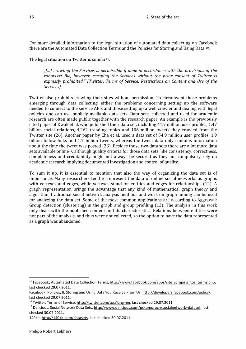
. When having a look at the robots.txt of Twitter and Facebook,
… User-agent: * Disallow: / … (Facebook robots.txt, http://www.facebook.com/robots.txt, last checked 27.07.2011)
… # Every bot that might possibly read and respect this file. User-agent: * Disallow: /*? Disallow: /*/with_friends Disallow: /oauth Disallow: /1/oauth … (Twitter robots.txt, http://www.twitter.com/robots.txt, last checked 27.07.2011)
one can see, that Facebook and Twitter both do not allow crawling of their sites when it is a robot that does not match the exceptions (Google, Bing, …). Also the Terms of Service do not seem to permit collecting and using data when not being permitted9
“You will not collect users' content or information, or otherwise access Facebook, using automated means (such as harvesting bots, robots, spiders, or scrapers) without our permission.” (Facebook, Statement of Rights and Responsibilities, 3.2.)
. Facebook’s Rights and Responsibilities state:
“If you collect information from users, you will: obtain their consent, make it clear you (and not Facebook) are the one collecting their information, and post a privacy policy explaining what information you collect and how you will use it.” (Facebook, Statement of Rights and Responsibilities, 5.7)
7 Arachnode, http://www.arachnode.net/, last checked 26.07.2011. Dinejs, http://code.google.com/p/dinejs/, last checked 26.07.2011. Scrapy, http://scrapy.org/, last checked 26.07.2011. 8 The Web Robots page, http://www.robotstxt.org/orig.html, last checked 27.07.2011. 9 Facebook, Statement of Rights and Responsibilities, http://www.facebook.com/terms.php, last checked 29.07.2011.
15 2. State of the art
Philipp Robert Lebherz
For more detailed information to the legal situation of automated data collecting on Facebook there are the Automated Data Collection Terms and the Policies for Storing and Using Data 10
The legal situation on Twitter is similar
.
11
„[…] crawling the Services is permissible if done in accordance with the provisions of the robots.txt file, however, scraping the Services without the prior consent of Twitter is expressly prohibited.” (Twitter, Terms of Service, Restrictions on Content and Use of the Services)
.
Twitter also prohibits crawling their sites without permission. To circumvent those problems emerging through data collecting, either the problems concerning setting up the software needed to connect to the service APIs and those setting up a web crawler and dealing with legal policies one can use publicly available data sets. Data sets, collected and used for academic research are often made public together with the research paper. An example is the previously cited paper of Kwak et al. who published their data set, including 41.7 million user profiles, 1.47 billion social relations, 4,262 trending topics and 106 million tweets they crawled from the Twitter site (26). Another paper by Cha et al. used a data set of 54.9 million user profiles, 1.9 billion follow links and 1.7 billion tweets, whereas the tweet data only contains information about the time the tweet was posted (23). Besides those two data sets there are a lot more data sets available online12
To sum it up, it is essential to mention that also the way of organizing the data set is of importance. Many researchers tend to represent the data of online social networks as graphs with vertexes and edges, while vertexes stand for entities and edges for relationships (12). A graph representation brings the advantage that any kind of mathematical graph theory and algorithm, traditional social network analysis methods and work on graph mining can be used for analyzing the data set. Some of the most common applications are according to Aggrawal: Group detection (clustering) in the graph and group profiling (12). The analysis in this work only deals with the published content and its characteristics. Relations between entities were not part of the analysis, and thus were not collected, so the option to have the data represented as a graph was abandoned.
, although quality criteria for those data sets, like consistency, correctness, completeness and creditability might not always be secured as they not compulsory rely on academic research implying documented investigation and control of quality.
10 Facebook, Automated Data Collection Terms, http://www.facebook.com/apps/site_scraping_tos_terms.php, last checked 29.07.2011. Facebook, Policies, II. Storing and Using Data You Receive From Us, http://developers.facebook.com/policy/, last checked 29.07.2011. 11 Twitter, Terms of Service, http://twitter.com/tos?lang=en, last checked 29.07.2011. 12 Delicious, Social Network Data Sets, http://www.delicious.com/pskomoroch/socialnetwork+dataset, last checked 30.07.2011. 140kit, http://140kit.com/datasets, last checked 30.07.2011.
16 3. Objectives of the study
Philipp Robert Lebherz
3. Objectives of the study
The objective of the study is to identify, and if possible quantify, the relation of the content’s characteristics with the impact the content has. This work assumes that there are some measurable content attributes that influence the impact. To analyze these relations the statistical methods of correlation analysis and linear regression modeling, if the data fulfills the requirements, will be used. The idea is to build a linear model using multiple linear regressions for quantifying and predicting the behavior of likes/comments/retweets as a function of content characteristics. The hypotheses are:
1.a.) Facebook shows correlation between the attributes presence of links, images, video clips, the number of followers of a channel, the number of characters of a post, the time of publication, the day of publication and the impact (the number of likes and the number of comments).
1.b.) Twitter has correlation between the attributes like the presence of links, tags, mentions, the number of followers of a channel, the number of characters of a tweet, the day of publishing and the impact (the number of retweets) a tweet has.
2.a.) In Facebook the relationship of the attributes to the number of likes and the number of comments can be explained by multiple linear regressions. The resulting model reaches enough explanation power to be meaningful.
2.b.) In Twitter the relationship of the attributes to the number of likes and the number of comments can be explained using multiple linear regressions as well. The resulting model reaches enough explanation power to be meaningful.
17 4. Methodology of the study
Philipp Robert Lebherz
4. Methodology of the study
4.1. Selection of the sample
4.1.1. Travel agencies
4.1.1.1. Criteria for selection
According to a study in 2008 by the Interactive Advertising Bureau (IAB) and PricewaterhouseCoopers (PwC) the sector of travel agencies is the sector that invests the most in internet (32). This leads to the conclusion that the use of internet forms is an important channel of distribution for the travel agency sector. This implies that in order to reach the customers the usage of new trends in internet marketing like, social media marketing, is an essential competitive advantage (33). Assuming this it is obvious to take samples from travel agencies. As criteria for selecting a set of travel agencies this work used economic criteria as well as criteria regarding the usage of social media and Internet in general.
To determine the economical importance of a company the revenues of the years 2008/2009 were used. The revenue measures the income a company receives. By this it was secured that the travel agencies observed met a minimum of economic comparability. However problems showed up. Revenue is stated in the financial statement of a company. Many of the companies observed have a wide placement not only including the travel agency service. Thus their revenue numbers not only represent the situation of the travel agency branch but the situation of the company in whole. Depending on the size of the company and its economic results, there are different laws about publishing the financial statement, e.g. German laws give small size companies easement by requesting less information in the financial statement 13
As criteria for the usage of internet in general the Alexa web site traffic rank was used
. This on the other hand, made it in some cases made it impossible to split up the numbers to later compare the rare outcome of the travel branch of the company.
14
For approximating the influence of the companies in social media, in this work the Vitrue Social Media Index was used
. This traffic rank has been used in other research before (34). Indeed the exact metric for calculating the rank is not public, some language areas are underrepresented and the samples are not representative so that clear evidence for the whole internet cannot be given by using this rank (34). However, the rank in this context is thought to give an impression of how excessively internet and new media is used by the company. The lower the rank is, the higher frequented the site.
15
13 §326 and §267 HGB.
. This index gives information about how many times a brand is mentioned in social media. More information about the functionality and to how the index is
14 Alexa The Web Information Company, http://www.alexa.com, last checked 25.07.2011. 15 Vitrue, http://vitrue.com/smi/, last checked 25.07.2011.

18 4. Methodology of the study
Philipp Robert Lebherz
being composed is not available. However, it seems to be a ratio scale type with a zero point when no mentions to the given search term is found. Bias using this index can occur when a brand name is not a standalone term or name but a composed term or a normal language word.
Last but not least, the most important criteria was to have a look at the social media channels used or not used by the companies. To secure a comparable sample for the subsequent data gathering and analyzing the objective was to find companies that all use the same social media channels. It occurred that Facebook fan-pages, Twitter, YouTube channels and Blogs were the most used ones.
19 4. Methodology of the study
Philipp Robert Lebherz
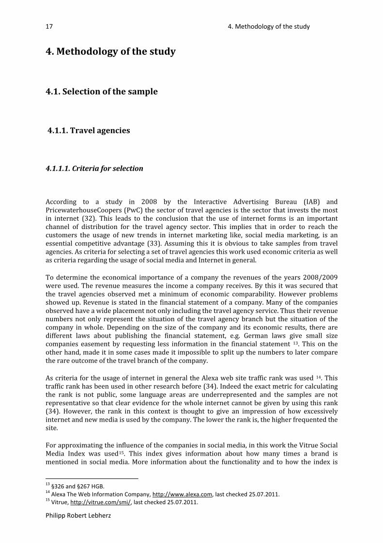
4.1.1.2. Comparison
The following table is an overview of the previously mentioned criteria for the companies that were checked for the possibility to use them in the study.
Company name Domain Revenue in TEUR 16
Alexa Traffic Rank 17
Vitrue SMI
18Face-book 19 Twitter Youtube 29 Blog 29 Other 29 29
R U M B O Rumbo.es
330000 20 3008 136021 + + + + +
eDreams eDreams.es 308000 5407 30 15 + 31 + + + +
Atrapalo Atrapalo.com 160000 4178 30 96,3 + 31 + + + +
Mucho Viaje Muchoviaje.com 107100 19157 30 29,4 + 31 + + + +
Halcón Viajes Halconviajes.com 1507000 68663 5,39 + + + + +
Lastminute Networks S.L Lastminute.es / .com 40566 18262308
/ 2002 13100 31 /
215 - 31 - - - +
Terminal A Es.terminala.com/.com 140100 652620 / 146378
30 17,5 - 31 - - -
El Corte Ingles Elcorteingles.es 2140000 3809 78,2 + 31 - + - +
Marsans Marsans.com 1187000 33317 43,7 + 31 + - - +
R U M B O Viajar.com 330000 43945 14900 - 31 + - + +
Lastminute.com Lastminute.de / .com 40566 16770 / 2002
98,6 31 / 215 + 31 + + + +
Travel24 Travel24.com 3700 34529 2,59 + + + +
Tomorrow Focus Holidaycheck.de 774 2684 72,1 + + + + +
Unister Ab-in-den-urlaub.de 63530 6206 19,8 + 31 + + - +
Urlaub-shop Urlaub.de 155723 106 + 31 + - -
COMVEL Weg.de 22419 9820 + 31 + - +
COMVEL Ferien.de 279371 493 - 31 - - -
16 Elektronischer Bundesanzeiger, http://www.ebundesanzeiger.de/, Jahresabschlüsse 2008/2009. registro mercantil, http://www.rmc.es, cuentas annuals de 2008/2009. 17 Alexa The Web Information Company, http://www.alexa.com, 04.04.2011. 18 Vitrue, http://vitrue.com/smi/, 05.04.2011. 19 March, 2011. 20 (33). 21 Possible bias.
20 4. Methodology of the study
Philipp Robert Lebherz
FTI Touristik Reise.de 733700 184069 274 - 31 + - -
Unister Reisen.de 63530 22012 294 - 31 - - -
L’Tur Ltur.com
357000 13345 17,3 + + + -
Necker-mann Reisen Neckermann-reisen.de 118600 2939 4,07 + + + -
Tui Tui.de 4178 65,2 + + + -
Alltours Alltours.de 11057000 112651 2,98 + - - -
Viajes Barceló Barceloviajes.com 673000 56923 14,1 31 + + + + +
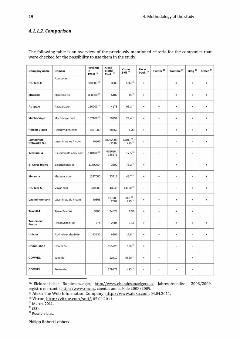
Table 1: Overview travel agencies.
Grouped into German and Spanish companies. The data sample shell consist of 5 German agencies and 5 Spanish agencies this determines the selection after the grouping. In the following tables the companies are ranked after the different criteria to see which are the most adequate ones for the study. First by Alexa Traffic Rank, then by revenue and then by number of social media channels. The final ranking is by social media channels first as first priority and by Alexa Traffic Rank second.
Spanish travel agencies ranked by Alexa Traffic Rank:
1 Rumbo.es 3008
2 Elcorteingles.es 3809
3 Atrapalo.com 4178
4 eDreams.es 5407
5 MuchoViaje.com 19157
6 Marsans.com 33317
7 Viajar.com 43945
8 Barceloviajes.com 56923
9 HalconViajes.com 68663
10 Es.terminala.com 652620
11 Es.lastminute.com 18262308
Table 3: Spanish travel agencies ranked by Traffic Rank.
German travel agencies ranked by Alexa Traffic Rank:
1 HolidayCheck.de 2684
2 Neckermann-Reisen.de 2939
3 Tui.de 4178
4 Ab-in-den-Urlaub.de 6206
5 Ltur.com 13345
6 Lastminute.de 16770
7 Reisen.de 22012
8 Weg.de 22419
9 Travel24.de 34529
10 Alltours.de 112651
11 Urlaub.de 155723
12 Reise.de 184069
13 Ferien.de 279371
Table 2: German travel agencies ranked by Traffic Rank.

21 4. Methodology of the study
Philipp Robert Lebherz
Spanish travel agencies ranked by revenue:
1 Elcorteingles.es 2140000
2 HalconViajes.com 1507000
3 Marsans.com 1187000
4 Barceloviajes.com 673000
5 Rumbo.es 330000
5 Viajar.com (Rumbo.es) 330000
6 eDreams.es 308000
7 Atrapalo.com 160000
8 Es.terminala.com 140100
9 MuchoViaje.com 107100
10 Es.lastminute.com 40566
Table 5: Spanish travel agencies ranked by revenue.
Geman travel agencies ranked by revenue:
1 Alltours.de 11057000
2 FTI Touristik 733700
3 L’Tur 357000
4 Neckermann Reisen 118600
5 Ab-in-den-urlaub.de (unister) 63530
Reisen.de (unister) 63530
6 Lastminute.de/ .com 40566
8 Travel24 3700
9 Holidaycheck.de 774
Urlaub.de
Weg.de
Ferien.de
Tui.de
Table 4: German travel agencies ranked by revenue.
Spanish travel agencies ranked by the number of social media channels used:
1 Rumbo.es 4
Atrapalo.com 4
eDreams.es 4
MuchoViaje.com 4
HalconViajes.com 4
Barceloviajes.com 4
2 Viajeselcorteingles.es 2
Marsans.com 2
Viajar.com 2
3 Es.terminala.com 0
Es.lastminute.com 0
Table 6: Spanish travel agencies ranked by number of channels.
German travel agencies ranked by the number of social media channels used:
1 HolidayCheck.de 4
Lastminute.de 4
Travel24.de 4
2 Ab-in-den-Urlaub.de 3
Weg.de 3
Ltur.com 3
Neckermann-reisen.de 3
Tui.de 3
3 Urlaub.de 2
4 Reise.de 1
Alltours.de 1
5 Ferien.de 0
Reisen.de 0
Table 7: German travel agencies ranked by number of channels

22 4. Methodology of the study
Philipp Robert Lebherz
Spanish travel agencies ranked by the number of social media channels used first, and by Alexa Traffic Rank second:
1 Rumbo.es 4 3008
2 Atrapalo.com 4 4178
3 eDreams.es 4 5407
4 MuchoViaje.com 4 19157
5 Barceloviajes.com 4 56923
6 HalconViajes.com 4 68663
7 Viajeselcorteingles.es 2 3809
8 Marsans.com 2 33317
9 Viajar.com 2 43945
10 Es.terminala.com 0 146378
11 Es.lastminute.com 0 2002
Table 8: Overall ranking of Spanish travel agencies.
German travel agencies ranked by the number of social media channels used, and by Alexa Traffic Rank second:
1 Lastminute.de 4 2002
2 HolidayCheck.de 4 2684
3 Travel24.de 4 34529
4 Neckermann-reisen.de 3 2939
5 Tui.de 3 4178
6 Ab-in-den-Urlaub.de 3 6206
7 Ltur.com 3 13345
8 Weg.de 3 22419
9 Urlaub.de 2 155723
10 Reise.de 1 184069
11 Alltours.de 1 112651
12 Ferien.de 0 279371
13 Reisen.de 0 22012
Table 9: Overall ranking of German travel agencies.
23 4. Methodology of the study
Philipp Robert Lebherz
According to the results, the companies Rumbo.es, Atrapalo.com, eDreams.es, MuchoViaje.com and Barceloviajes.com were chosen for the Spanish group.
In the case of the German group the results were not strictly followed for selecting the sample. The influencing factor was, that Neckermann-reisen.de as well as Tui.de ad Ltur.com primarily are travel agencies that sell their products offline through catalogues and own travel bureaus. So they do not depend on the internet selling as much as a travel agency that only sells through the internet. It was estimated that social media marketing is less important for those travel agencies and thus Lastminute.de, Holidaycheck.de, Travel24.de, Ab-in-den-Urlaub.de and Weg.de were taken as samples instead.
4.1.2. Social media channels
4.1.2.1. Criteria for selection
The main criteria for selecting the social media to observe it was, that the previously selected sample of companies had to maintain this kind of social media channel. Table 1: Overview travel agencies shows, that Facebook, Twitter, Youtube and Blogs were the most commonly used social media channels. Besides those also MySpace and LinkedIn were used, but not as broadly as the before mentioned. An as homogeneous sample as possible was aimed what provoked to dismiss Myspace and LinkedIn. Blogs and Youtube neither were included in the sample. A Blog is an abbreviation for weblog and describes an online log-book that is mostly used as a diary or a journal where one or more than one author publishes texts (35). When the blog is conceptualized as a journal then the published texts are most times related to one specific topic. Companies use blogs in general for marketing, to update the consumer for example on new products and to push branding (36). Apparently a Blog specifies a category of online social media, but does not specify one product like Facebook, Twitter or Youtube. This implicates, that the structure of blogs is not homogeneous and by that less comparable. This is the reason why also Blogs were dismissed from the sample. Another important factor for this work was that old publications were needed to be able to access through the normal user interface. This is due to the fact, that the information of publications that were collected needed to be more or less a month old to give the consumers enough time to react and contribute on the content. Facebook and Twitter as well give the possibility to access old content. For the analysis of the collected content only publicly available data about the content was gathered, so there were no further selection criteria dealing with the restriction of data access.
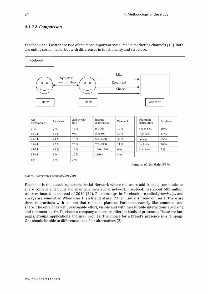
24 4. Methodology of the study
Philipp Robert Lebherz
4.1.2.2. Comparison
Facebook and Twitter are two of the most important social media marketing channels (10). Both are online social media, but with differences in functionality and structure.
Facebook is the classic egocentric Social Network where the users add friends, communicate, share content and build and maintain their social network. Facebook has about 585 million users estimated at the end of 2010 (24). Relationships in Facebook are called friendships and always are symmetric. When user 1 is a friend of user 2 then user 2 is friend of user 1. There are three interactions with content that can take place on Facebook, namely like, comment and share. The only ones with reasonable effort, visible and with measurable interactions are liking and commenting. On Facebook a company can create different kinds of presences. Those are fan-pages, groups, applications and user profiles. The choice for a brand’s presence is a fan-page. One should be able to differentiate the four alternatives (2).
User User
Symetric relationship
Content
Like
Comment Share
Age distribution Facebook Avg. across
OSN
0-17 7 % 15 %
18-24 11 % 9 %
25-34 24 % 18 %
35-44 22 % 25 %
45-54 26 % 19 %
55-64 8 % 10 %
65+ 3 % 3 %
Income distribution Facebook
0-24,9k 12 %
25k-49k 36 %
50k-74,9k 32 %
75k-99,9k 11 %
100k-150k 6 %
150k+ 3 %
Female: 61 %; Male: 39 %
Education distribution Facebook
< High Sch. 10 %
High Sch. 11 %
College 55 %
Bachelor 16 %
Graduate 3 %
Figure 1: Overview Facebook (59), (60).
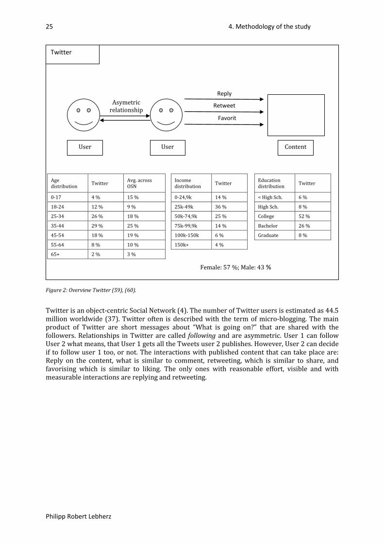
25 4. Methodology of the study
Philipp Robert Lebherz
Twitter is an object-centric Social Network (4). The number of Twitter users is estimated as 44.5 million worldwide (37). Twitter often is described with the term of micro-blogging. The main product of Twitter are short messages about “What is going on?” that are shared with the followers. Relationships in Twitter are called following and are asymmetric. User 1 can follow User 2 what means, that User 1 gets all the Tweets user 2 publishes. However, User 2 can decide if to follow user 1 too, or not. The interactions with published content that can take place are: Reply on the content, what is similar to comment, retweeting, which is similar to share, and favorising which is similar to liking. The only ones with reasonable effort, visible and with measurable interactions are replying and retweeting.
User User Content
Reply
Retweet
Favorit
Asymetric relationship
Age distribution Twitter Avg. across
OSN
0-17 4 % 15 %
18-24 12 % 9 %
25-34 26 % 18 %
35-44 29 % 25 %
45-54 18 % 19 %
55-64 8 % 10 %
65+ 2 % 3 %
Income distribution Twitter
0-24,9k 14 %
25k-49k 36 %
50k-74,9k 25 %
75k-99,9k 14 %
100k-150k 6 %
150k+ 4 %
Education distribution Twitter
< High Sch. 6 %
High Sch. 8 %
College 52 %
Bachelor 26 %
Graduate 8 %
Figure 2: Overview Twitter (59), (60).
Female: 57 %; Male: 43 %
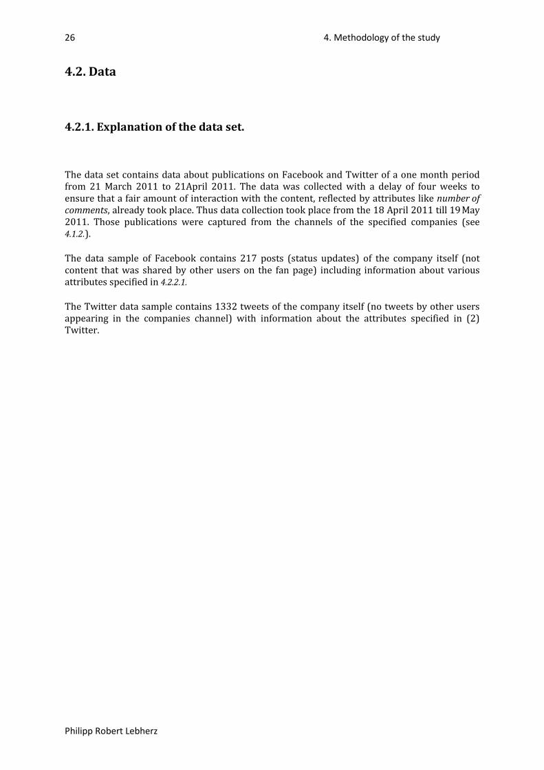
26 4. Methodology of the study
Philipp Robert Lebherz
4.2. Data
4.2.1. Explanation of the data set.
The data set contains data about publications on Facebook and Twitter of a one month period from 21 March 2011 to 21April 2011. The data was collected with a delay of four weeks to ensure that a fair amount of interaction with the content, reflected by attributes like number of comments, already took place. Thus data collection took place from the 18 April 2011 till 19
4.1.2.
May 2011. Those publications were captured from the channels of the specified companies (see
).
The data sample of Facebook contains 217 posts (status updates) of the company itself (not content that was shared by other users on the fan page) including information about various attributes specified in 4.2.2.1.
The Twitter data sample contains 1332 tweets of the company itself (no tweets by other users appearing in the companies channel) with information about the attributes specified in (2) Twitter.
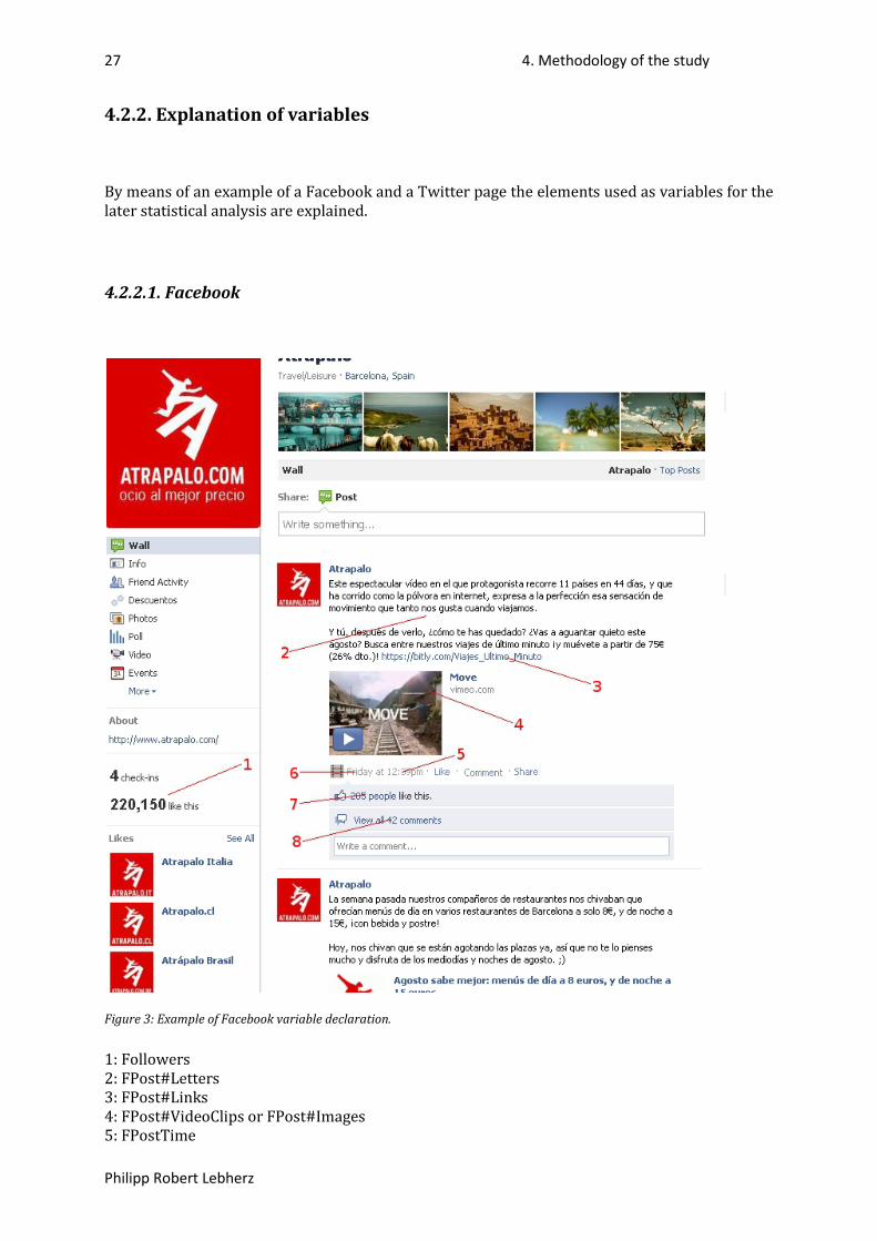
27 4. Methodology of the study
Philipp Robert Lebherz
4.2.2. Explanation of variables
By means of an example of a Facebook and a Twitter page the elements used as variables for the later statistical analysis are explained.
4.2.2.1. Facebook
Figure 3: Example of Facebook variable declaration. 1: Followers 2: FPost#Letters 3: FPost#Links 4: FPost#VideoClips or FPost#Images 5: FPostTime

28 4. Methodology of the study
Philipp Robert Lebherz
6: FPostDateDay 7: FPost#Likes 8: FPost#Comments For more details see section 6.1.1. Variables.
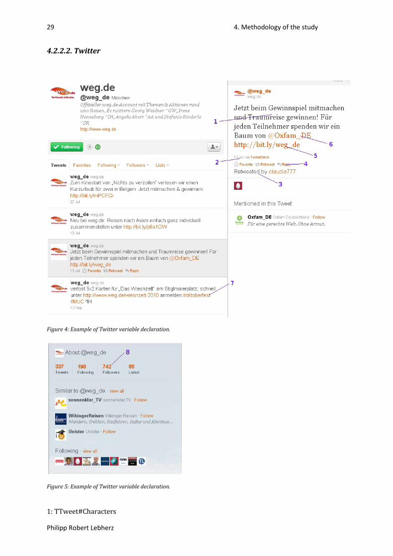
29 4. Methodology of the study
Philipp Robert Lebherz
4.2.2.2. Twitter
Figure 4: Example of Twitter variable declaration.
Figure 5: Example of Twitter variable declaration. 1: TTweet#Characters

30 4. Methodology of the study
Philipp Robert Lebherz
2: TTweetDateDay 3: TTweet#ReTweets 4: TTweetIsAnswer 5: TTweet#Links 6: TTweet#Mentions 7: TTweet#Tags 8: Followers For more details see section 6.2.1. Variables.
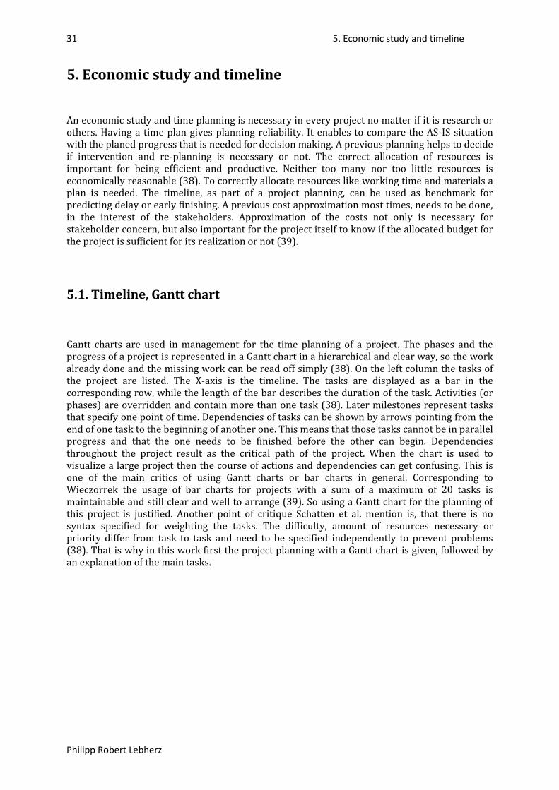
31 5. Economic study and timeline
Philipp Robert Lebherz
5. Economic study and timeline
An economic study and time planning is necessary in every project no matter if it is research or others. Having a time plan gives planning reliability. It enables to compare the AS-IS situation with the planed progress that is needed for decision making. A previous planning helps to decide if intervention and re-planning is necessary or not. The correct allocation of resources is important for being efficient and productive. Neither too many nor too little resources is economically reasonable (38). To correctly allocate resources like working time and materials a plan is needed. The timeline, as part of a project planning, can be used as benchmark for predicting delay or early finishing. A previous cost approximation most times, needs to be done, in the interest of the stakeholders. Approximation of the costs not only is necessary for stakeholder concern, but also important for the project itself to know if the allocated budget for the project is sufficient for its realization or not (39).
5.1. Timeline, Gantt chart
Gantt charts are used in management for the time planning of a project. The phases and the progress of a project is represented in a Gantt chart in a hierarchical and clear way, so the work already done and the missing work can be read off simply (38). On the left column the tasks of the project are listed. The X-axis is the timeline. The tasks are displayed as a bar in the corresponding row, while the length of the bar describes the duration of the task. Activities (or phases) are overridden and contain more than one task (38). Later milestones represent tasks that specify one point of time. Dependencies of tasks can be shown by arrows pointing from the end of one task to the beginning of another one. This means that those tasks cannot be in parallel progress and that the one needs to be finished before the other can begin. Dependencies throughout the project result as the critical path of the project. When the chart is used to visualize a large project then the course of actions and dependencies can get confusing. This is one of the main critics of using Gantt charts or bar charts in general. Corresponding to Wieczorrek the usage of bar charts for projects with a sum of a maximum of 20 tasks is maintainable and still clear and well to arrange (39). So using a Gantt chart for the planning of this project is justified. Another point of critique Schatten et al. mention is, that there is no syntax specified for weighting the tasks. The difficulty, amount of resources necessary or priority differ from task to task and need to be specified independently to prevent problems (38). That is why in this work first the project planning with a Gantt chart is given, followed by an explanation of the main tasks.
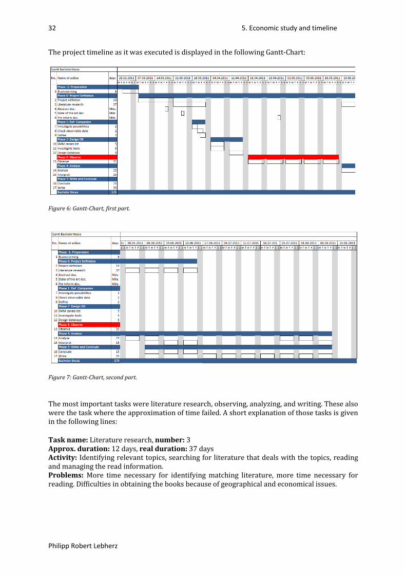
32 5. Economic study and timeline
Philipp Robert Lebherz
The project timeline as it was executed is displayed in the following Gantt-Chart:
Figure 6: Gantt-Chart, first part.
Figure 7: Gantt-Chart, second part.
The most important tasks were literature research, observing, analyzing, and writing. These also were the task where the approximation of time failed. A short explanation of those tasks is given in the following lines:
Task name: Literature research, number: 3 Approx. duration: 12 days, real duration: 37 days Activity: Identifying relevant topics, searching for literature that deals with the topics, reading and managing the read information. Problems: More time necessary for identifying matching literature, more time necessary for reading. Difficulties in obtaining the books because of geographical and economical issues.

33 5. Economic study and timeline
Philipp Robert Lebherz
Task name: Observe, number: 13 Approx. duration: 10 days, real duration: 32 days Activity: Collecting the specified data from the social media channels of the previously selected companies and saving it in a database. To execute this task the phase 1 and phase 2 must be completed before.
Task name: Analyze, number: 14 Approx. duration: 10 days, real duration: 25 days Activity: Statistical analysis of the previously gathered data using a special statistics software (SPSS). For to execute this task the task observe (no. 13) has to be finished before. Problems: Duration was badly approximated. Some problems using the software at the beginning.
Task name: Write, number: 17 Approx. duration: 20 days, real duration: 35 days Activity: Finalizing the work by consolidating all information and the already done work. Problems: Duration was badly approximated.
The project was started the 26 of February and ended the 19 of August. The following table calculates the labor time in days that was necessary.
Days of work Duration Additional information Project duration 175 days 26.02.11 – 19.08.2011 Non labor days - 50 days weekends Work on non labor days + 13 days During 1st and 3rd phase Labor days = 138 days Days of work Table 10: Labor time in days.
The next table calculates the labor time in hours.
Hours of work Duration Additional information Labor days 138 days Days of work Avg. working time 7 hours per day Hours of work = 966 hours Table 11: Labor time in hours.
The project took a total of 138 labor days and 966 hours of work.

34 5. Economic study and timeline
Philipp Robert Lebherz
5.2. Economic study
The planning of the budget for realizing a project is done with the objective to know the costs that are to expect. Previously calculated costs are useful for comparing alternative ways of realizing the project. The different options can be compared based on benefits and costs. Also funds can be assigned previously what gives reliability and a buffer amount for certain situations can be arranged. Later in realization phase the cost planning can be used as benchmark for the quality of execution, meaning when the actual costs differ a lot from the planned costs then the project is not being realized in the way it should be. The project budget specifies the sum of all funds that can be used for realizing the project (39). Calculating the project budget is done based on the cost and time plan. The costs the planning consists of can be categorized in two basic categories as there are labor costs and resource costs. To estimate the price for this project this basic categorization is used. The resulting cost planning is not thought to be an exact calculation but to give a reference for the costs dimension.
Table 12: Labor time allocated to employees. calculate the number of days of work the different personnel groups have to carry out for realizing the project.
𝑬𝒎𝒑𝒍𝒐𝒚𝒆𝒆𝑻𝒂𝒔𝒌
Project manager Analyst Worker % of task days assigned % of task days assigned % of task days assigned
1 Brainstorming 33 1,98 33 1,98 33 1,98 2 Project definition 50 6,5 50 6,5 0 0 3 Literature research Control (=5) 1,85 50 18,5 45 16,65 7 Investigate possibilities Control (=5) 0,1 50 1 45 0,9 8 Check observable data Control (=5) 0,1 30 1 65 0,9 9 Define Control (=5) 0,1 75 1 20 0,9 10 SMM canal list Control (=5) 0,5 20 1 75 3,5 11 Investigate tools Control (=5) 0,5 20 1 75 3,5 12 Design database Control (=5) 0,5 75 3,5 20 1 13 Observe Control (=5) 1,6 10 3,2 85 27,2 14 Analyse Control (=5) 1,25 80 20 15 3,75 15 Interpret Control (=5) 0,75 80 12 15 2,25 16 Conclude Control (=5) 0,75 80 12 15 2,25 17 Write Control (=5) 1,75 80 28 15 5,25
Total 9,16 18,23 55,6 110,68 35,2 70,03 Table 12: Labor time allocated to employees.
Table 13: Labor costs for the employer. calculates first the percentage of work the employee carries out as part of the sum of all days. Then this percentage is applied on the real time effort of the project (199 days is the sum of the duration of all tasks, this does not respect the parallelism of some tasks). The result of the second line thus is the days of work the employee needs to spend. Now the annual salary can be divided by the quotient of annual workdays and days the employee needs to spend. The result of this is the quota of the annual salary of the employee that is spent on this project. A number of 250 days of work per year, a salary of 45 000€ for the project manager, 35 000€ for the analyst and 20 000€ for the worker were assumed. Furthermore additional costs that arise for the company are approximated with 33 %.
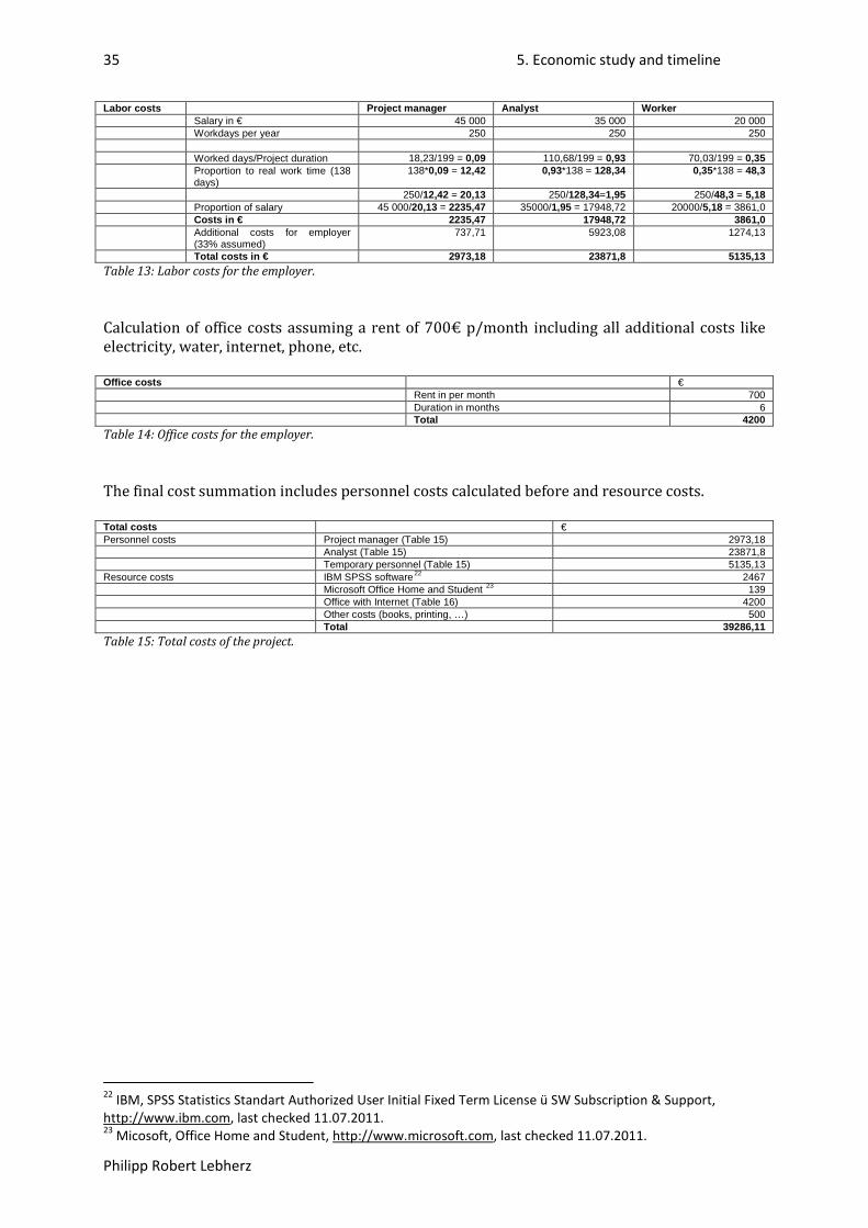
35 5. Economic study and timeline
Philipp Robert Lebherz
Labor costs Project manager Analyst Worker Salary in € 45 000 35 000 20 000 Workdays per year 250 250 250 Worked days/Project duration 18,23/199 = 0,09 110,68/199 = 0,93 70,03/199 = 0,35 Proportion to real work time (138
days) 138*0,09 = 12,42 0,93*138 = 128,34 0,35*138 = 48,3
250/12,42 = 20,13 250/128,34=1,95 250/48,3 = 5,18 Proportion of salary 45 000/20,13 = 2235,47 35000/1,95 = 17948,72 20000/5,18 = 3861,0 Costs in € 2235,47 17948,72 3861,0 Additional costs for employer
(33% assumed) 737,71 5923,08 1274,13
Total costs in € 2973,18 23871,8 5135,13 Table 13: Labor costs for the employer.
Calculation of office costs assuming a rent of 700€ p/month including all additional costs like electricity, water, internet, phone, etc.
Office costs € Rent in per month 700 Duration in months 6 Total 4200 Table 14: Office costs for the employer.
The final cost summation includes personnel costs calculated before and resource costs.
Total costs € Personnel costs Project manager (Table 15) 2973,18 Analyst (Table 15) 23871,8 Temporary personnel (Table 15) 5135,13 Resource costs IBM SPSS software22 2467 Microsoft Office Home and Student 23 139 Office with Internet (Table 16) 4200 Other costs (books, printing, …) 500 Total 39286,11 Table 15: Total costs of the project.
22 IBM, SPSS Statistics Standart Authorized User Initial Fixed Term License ü SW Subscription & Support, http://www.ibm.com, last checked 11.07.2011. 23 Micosoft, Office Home and Student, http://www.microsoft.com, last checked 11.07.2011.

36 6. Analysis of gathered data
Philipp Robert Lebherz
6. Analysis of gathered data
6.1. Facebook
The variables included in the statistical analysis of Facebook are on the one hand the two dependent variables LN(Likes+1) and LN(Comments+1) and on the other hand the independent variables LN_Followers, DateDayDummy, TimeDummy, FPost#Letters, ImagesDummy+LinksDummy, ImagesDummy-LinksDummy and VideoclipsDummy.
To distinguish the sample in Spanish and German observations the variable country is used.
LR model of LN(Comments+1) and complete sample: On the basis of this regression model the procedure of regression modeling and verification is explained.
Followed by: LR model of LN(Comments+1) and Spanish sample, LR model of LN(Comments+1) and German sample, LR model of LN(Likes+1) and complete sample, LR model of LN(Likes+1) and Spanish sample, LR model of LN(Likes+1) and German sample.
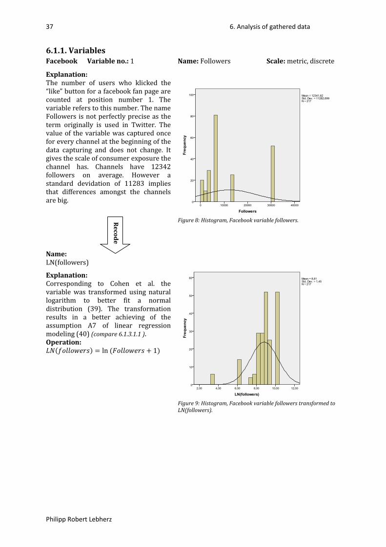
37 6. Analysis of gathered data
Philipp Robert Lebherz
6.1.1. Variables Facebook Variable no.: 1 Name: Followers Scale: metric, discrete
Explanation: The number of users who klicked the “like” button for a facebook fan page are counted at position number 1. The variable refers to this number. The name Followers is not perfectly precise as the term originally is used in Twitter. The value of the variable was captured once for every channel at the beginning of the data capturing and does not change. It gives the scale of consumer exposure the channel has. Channels have 12342 followers on average. However a standard devidation of 11283 implies that differences amongst the channels are big.
Figure 8: Histogram, Facebook variable followers.
Name: LN(followers)
Explanation: Corresponding to Cohen et al. the variable was transformed using natural logarithm to better fit a normal distribution (39). The transformation results in a better achieving of the assumption A7 of linear regression modeling (40) (compare 6.1.3.1.1 ).
Figure 9: Histogram, Facebook variable followers transformed to LN(followers).
Operation: 𝐿𝑁(𝑓𝑜𝑙𝑙𝑜𝑤𝑒𝑟𝑠) = ln (𝐹𝑜𝑙𝑙𝑜𝑤𝑒𝑟𝑠 + 1)
Recode
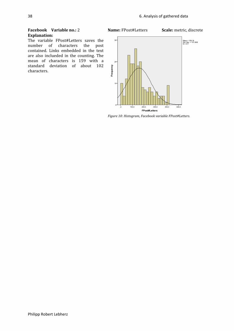
38 6. Analysis of gathered data
Philipp Robert Lebherz
Facebook Variable no.: 2 Name: FPost#Letters Scale: metric, discrete Explanation: The variable FPost#Letters saves the number of characters the post contained. Links embedded in the text are also inclueded in the counting. The mean of characters is 159 with a standard deviation of about 102 characters.
Figure 10: Histogram, Facebook variable FPost#Letters.
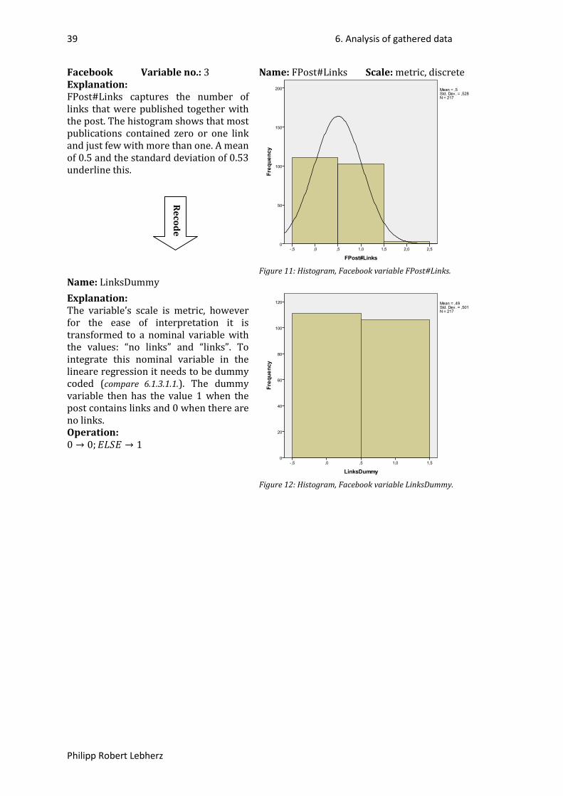
39 6. Analysis of gathered data
Philipp Robert Lebherz
Facebook Variable no.: 3 Name: FPost#Links Scale: metric, discrete Explanation: FPost#Links captures the number of links that were published together with the post. The histogram shows that most publications contained zero or one link and just few with more than one. A mean of 0.5 and the standard deviation of 0.53 underline this.
Figure 11: Histogram, Facebook variable FPost#Links.
Name: LinksDummy Explanation: The variable’s scale is metric, however for the ease of interpretation it is transformed to a nominal variable with the values: “no links” and “links”. To integrate this nominal variable in the lineare regression it needs to be dummy coded (compare 6.1.3.1.1.). The dummy variable then has the value 1 when the post contains links and 0 when there are no links.
Figure 12: Histogram, Facebook variable LinksDummy.
Operation: 0 → 0;𝐸𝐿𝑆𝐸 → 1
Recode
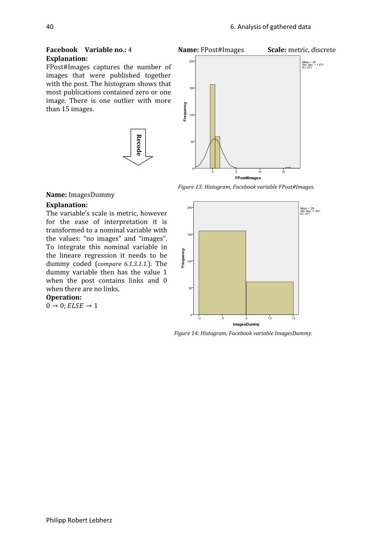
40 6. Analysis of gathered data
Philipp Robert Lebherz
Facebook Variable no.: 4 Name: FPost#Images Scale: metric, discrete Explanation: FPost#Images captures the number of images that were published together with the post. The histogram shows that most publications contained zero or one image. There is one outlier with more than 15 images.
Figure 13: Histogram, Facebook variable FPost#Images.
Name: ImagesDummy Explanation: The variable’s scale is metric, however for the ease of interpretation it is transformed to a nominal variable with the values: “no images” and “images”. To integrate this nominal variable in the lineare regression it needs to be dummy coded (compare 6.1.3.1.1.). The dummy variable then has the value 1 when the post contains links and 0 when there are no links.
Figure 14: Histogram, Facebook variable ImagesDummy.
Operation: 0 → 0;𝐸𝐿𝑆𝐸 → 1
Recode
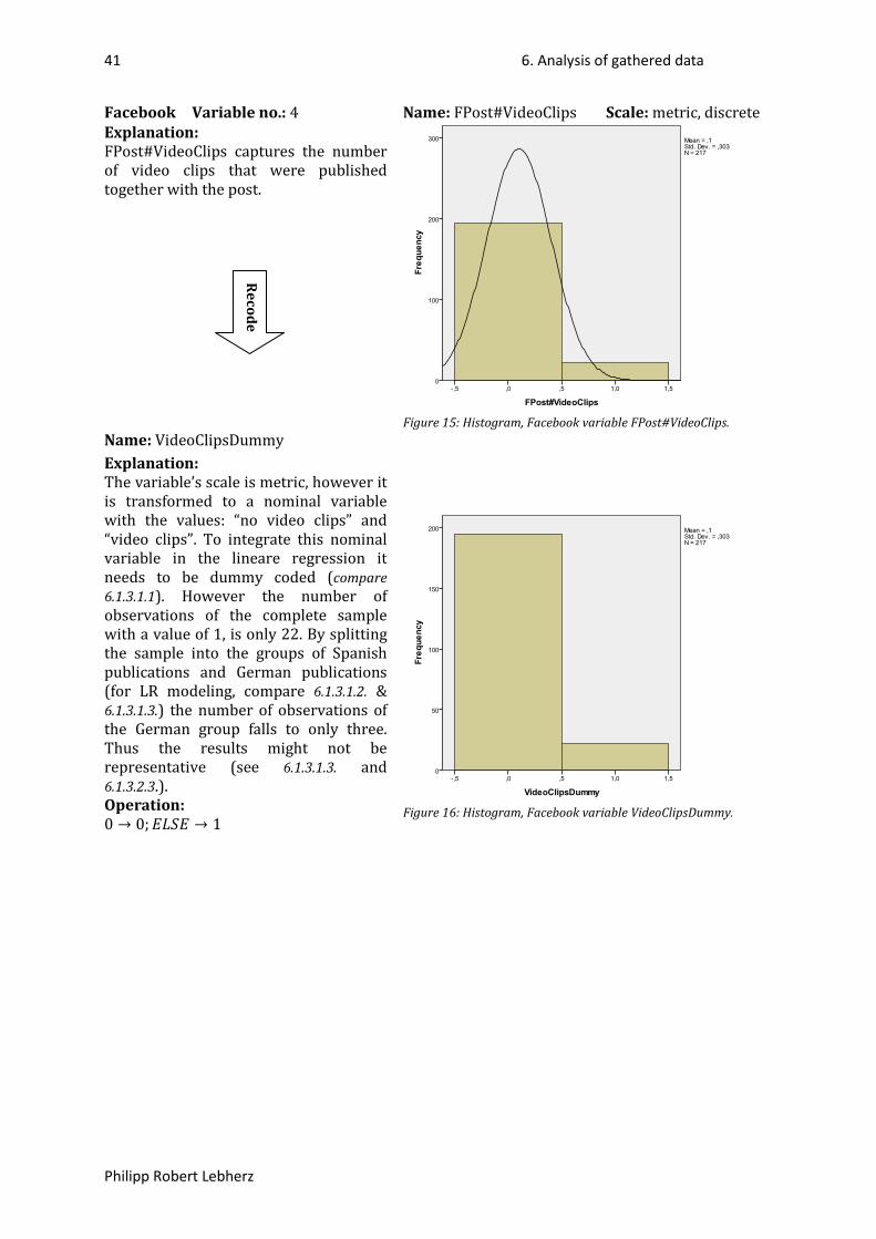
41 6. Analysis of gathered data
Philipp Robert Lebherz
Facebook Variable no.: 4 Name: FPost#VideoClips Scale: metric, discrete Explanation: FPost#VideoClips captures the number of video clips that were published together with the post.
Figure 15: Histogram, Facebook variable FPost#VideoClips.
Name: VideoClipsDummy Explanation: The variable’s scale is metric, however it is transformed to a nominal variable with the values: “no video clips” and “video clips”. To integrate this nominal variable in the lineare regression it needs to be dummy coded (compare 6.1.3.1.1). However the number of observations of the complete sample with a value of 1, is only 22. By splitting the sample into the groups of Spanish publications and German publications (for LR modeling, compare 6.1.3.1.2. & 6.1.3.1.3.) the number of observations of the German group falls to only three. Thus the results might not be representative (see 6.1.3.1.3. and 6.1.3.2.3.).
Figure 16: Histogram, Facebook variable VideoClipsDummy. Operation:
0 → 0;𝐸𝐿𝑆𝐸 → 1
Recode
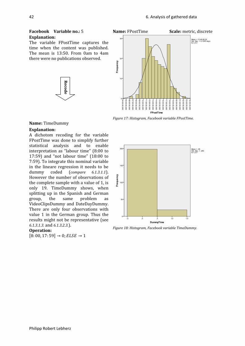
42 6. Analysis of gathered data
Philipp Robert Lebherz
Facebook Variable no.: 5 Name: FPostTime Scale: metric, discrete Explanation: The variable FPostTime captures the time when the content was published. The mean is 13:50. From 0am to 4am there were no publications observed.
Figure 17: Histogram, Facebook variable FPostTime.
Name: TimeDummy Explanation: A dichotom recoding for the variable FPostTime was done to simplify further statistical analysis and to enable interpretation as “labour time” (8:00 to 17:59) and “not labour time” (18:00 to 7:59). To integrate this nominal variable in the lineare regression it needs to be dummy coded (compare 6.1.3.1.1). However the number of observations of the complete sample with a value of 1, is only 19. TimeDummy shows, when splitting up in the Spanish and German group, the same problem as VideoClipsDummy and DateDayDummy. There are only four observations with value 1 in the German group. Thus the results might not be representative (see 6.1.3.1.3. and 6.1.3.2.3.).
Figure 18: Histogram, Facebook variable TimeDummy. Operation: [8: 00, 17: 59] → 0;𝐸𝐿𝑆𝐸 → 1
Recode
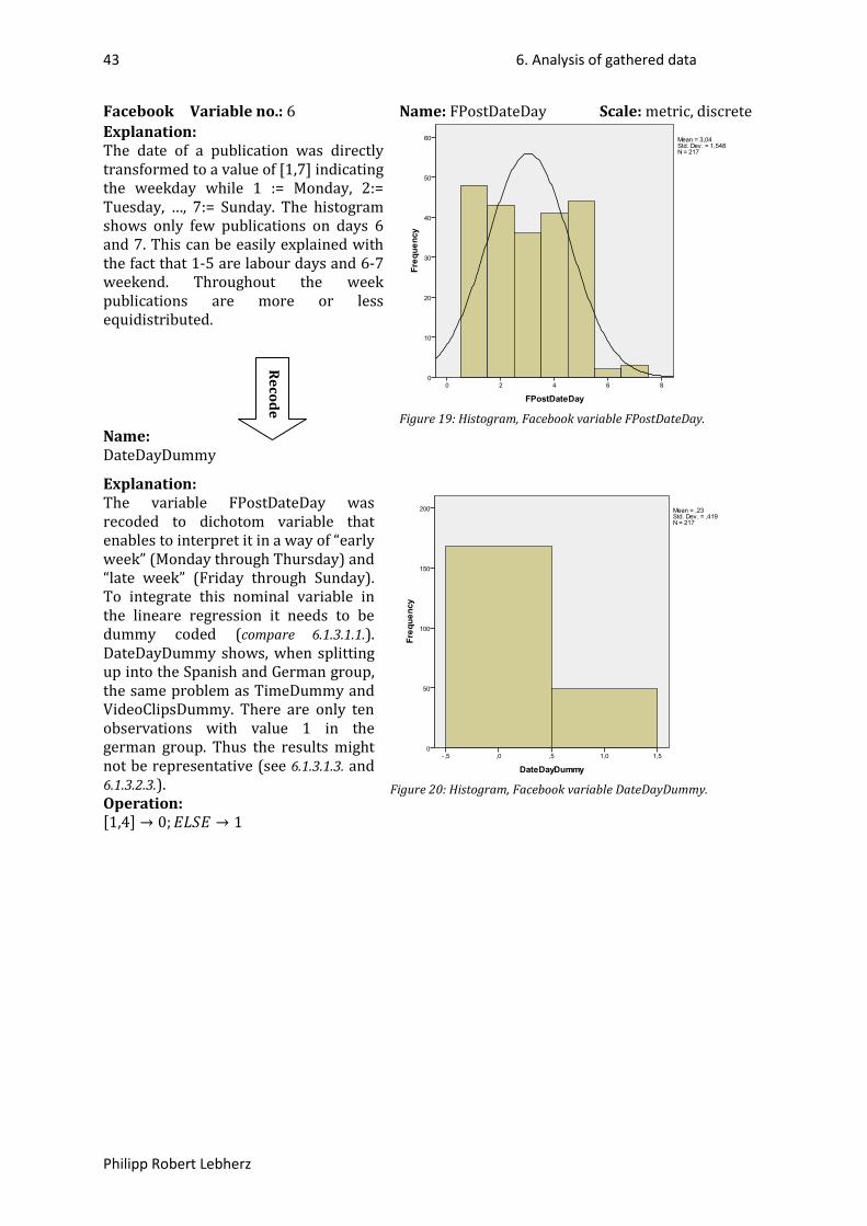
43 6. Analysis of gathered data
Philipp Robert Lebherz
Facebook Variable no.: 6 Name: FPostDateDay Scale: metric, discrete Explanation: The date of a publication was directly transformed to a value of [1,7] indicating the weekday while 1 := Monday, 2:= Tuesday, …, 7:= Sunday. The histogram shows only few publications on days 6 and 7. This can be easily explained with the fact that 1-5 are labour days and 6-7 weekend. Throughout the week publications are more or less equidistributed.
Figure 19: Histogram, Facebook variable FPostDateDay.
Name: DateDayDummy
Explanation: The variable FPostDateDay was recoded to dichotom variable that enables to interpret it in a way of “early week” (Monday through Thursday) and “late week” (Friday through Sunday). To integrate this nominal variable in the lineare regression it needs to be dummy coded (compare 6.1.3.1.1.). DateDayDummy shows, when splitting up into the Spanish and German group, the same problem as TimeDummy and VideoClipsDummy. There are only ten observations with value 1 in the german group. Thus the results might not be representative (see 6.1.3.1.3. and 6.1.3.2.3.).
Figure 20: Histogram, Facebook variable DateDayDummy. Operation:
[1,4] → 0;𝐸𝐿𝑆𝐸 → 1
Recode
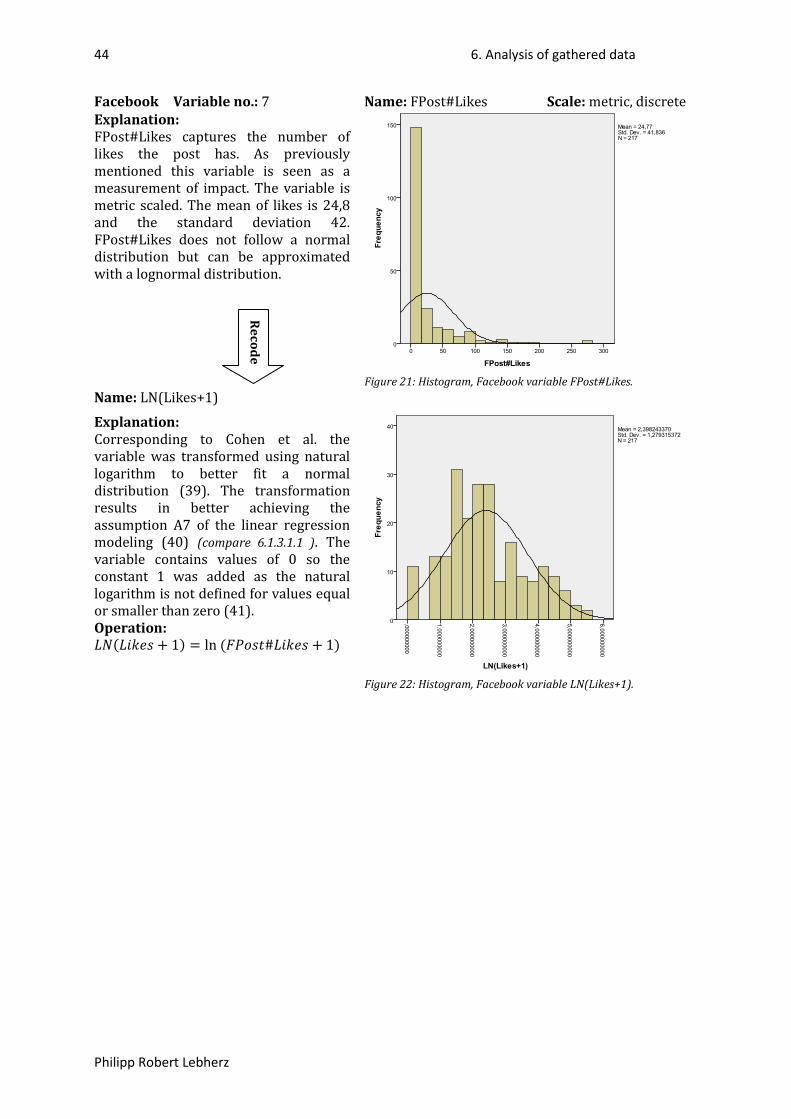
44 6. Analysis of gathered data
Philipp Robert Lebherz
Facebook Variable no.: 7 Name: FPost#Likes Scale: metric, discrete Explanation: FPost#Likes captures the number of likes the post has. As previously mentioned this variable is seen as a measurement of impact. The variable is metric scaled. The mean of likes is 24,8 and the standard deviation 42. FPost#Likes does not follow a normal distribution but can be approximated with a lognormal distribution.
Figure 21: Histogram, Facebook variable FPost#Likes.
Name: LN(Likes+1)
Explanation: Corresponding to Cohen et al. the variable was transformed using natural logarithm to better fit a normal distribution (39). The transformation results in better achieving the assumption A7 of the linear regression modeling (40) (compare 6.1.3.1.1 ). The variable contains values of 0 so the constant 1 was added as the natural logarithm is not defined for values equal or smaller than zero (41).
Figure 22: Histogram, Facebook variable LN(Likes+1).
Operation: 𝐿𝑁(𝐿𝑖𝑘𝑒𝑠 + 1) = ln (𝐹𝑃𝑜𝑠𝑡#𝐿𝑖𝑘𝑒𝑠 + 1)
Recode
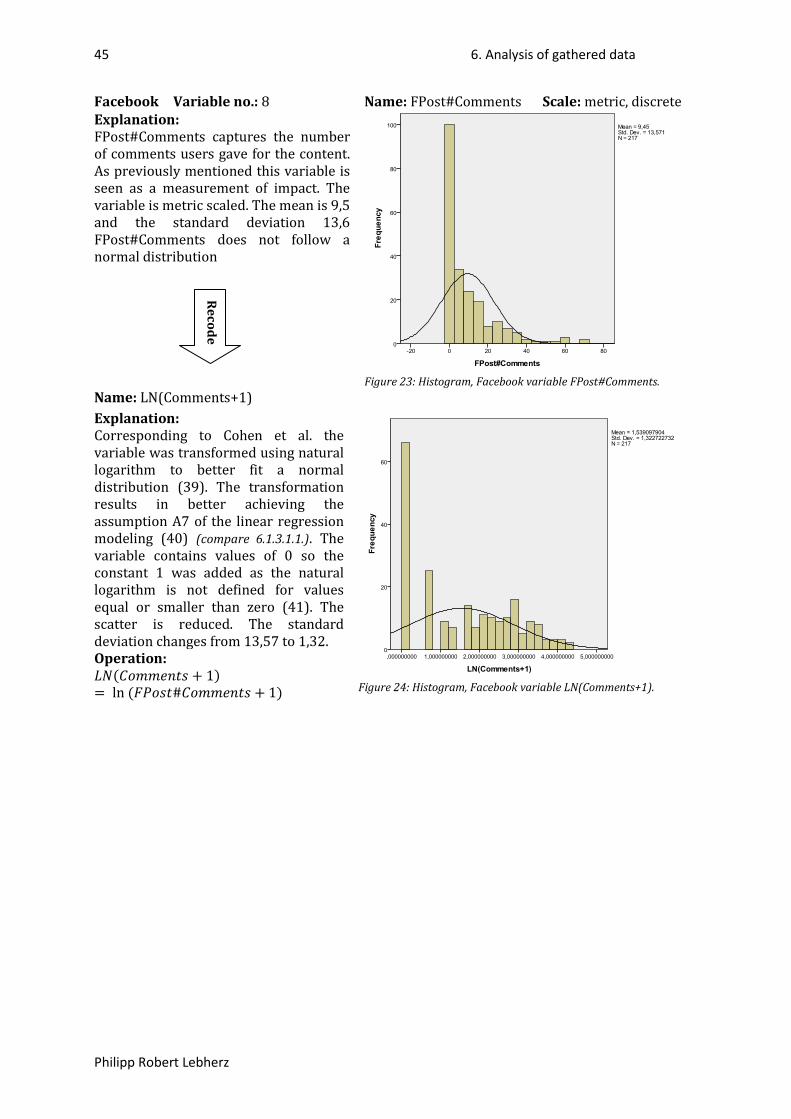
45 6. Analysis of gathered data
Philipp Robert Lebherz
Facebook Variable no.: 8 Name: FPost#Comments Scale: metric, discrete Explanation: FPost#Comments captures the number of comments users gave for the content. As previously mentioned this variable is seen as a measurement of impact. The variable is metric scaled. The mean is 9,5 and the standard deviation 13,6 FPost#Comments does not follow a normal distribution
Figure 23: Histogram, Facebook variable FPost#Comments.
Name: LN(Comments+1) Explanation: Corresponding to Cohen et al. the variable was transformed using natural logarithm to better fit a normal distribution (39). The transformation results in better achieving the assumption A7 of the linear regression modeling (40) (compare 6.1.3.1.1.). The variable contains values of 0 so the constant 1 was added as the natural logarithm is not defined for values equal or smaller than zero (41). The scatter is reduced. The standard deviation changes from 13,57 to 1,32.
Figure 24: Histogram, Facebook variable LN(Comments+1).
Operation: 𝐿𝑁(𝐶𝑜𝑚𝑚𝑒𝑛𝑡𝑠 + 1)= ln (𝐹𝑃𝑜𝑠𝑡#𝐶𝑜𝑚𝑚𝑒𝑛𝑡𝑠 + 1)
Recode
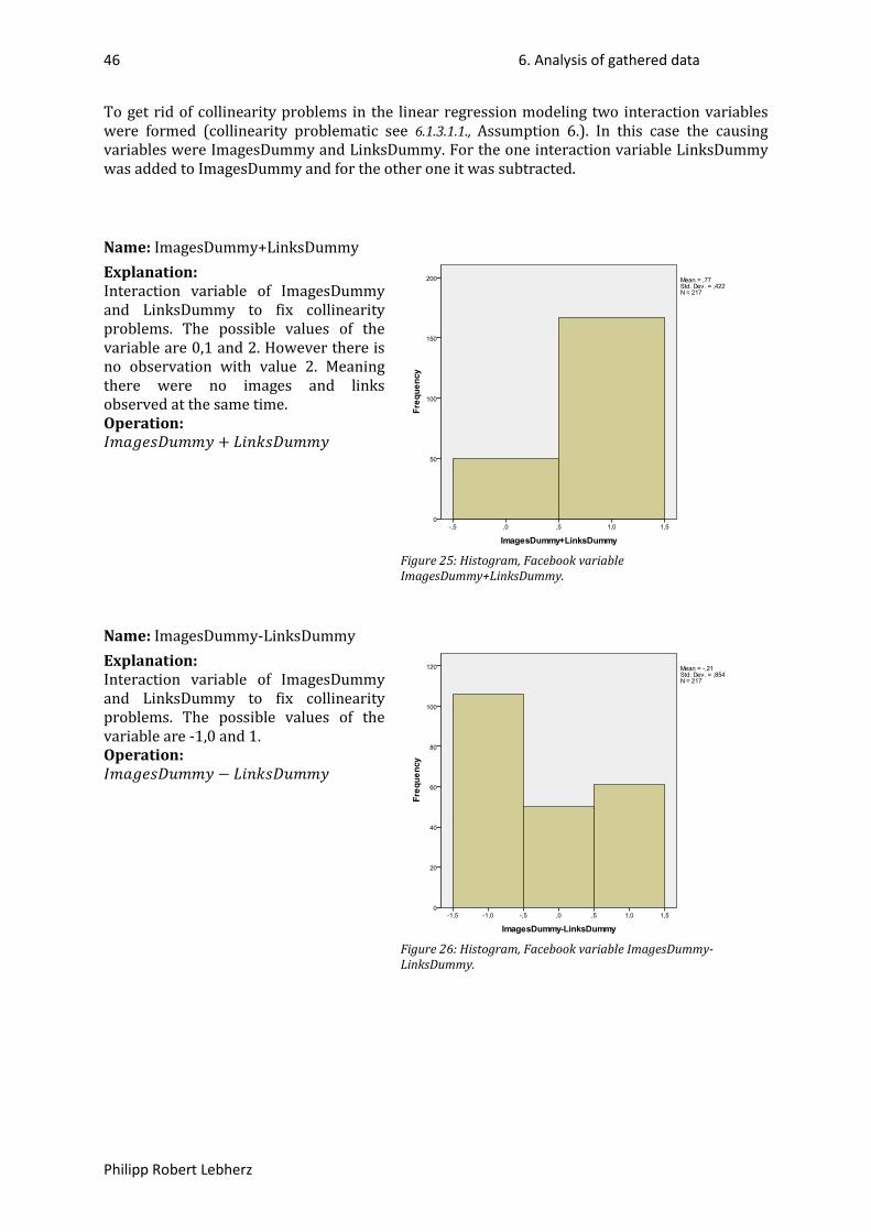
46 6. Analysis of gathered data
Philipp Robert Lebherz
To get rid of collinearity problems in the linear regression modeling two interaction variables were formed (collinearity problematic see 6.1.3.1.1., Assumption 6.). In this case the causing variables were ImagesDummy and LinksDummy. For the one interaction variable LinksDummy was added to ImagesDummy and for the other one it was subtracted.
Name: ImagesDummy+LinksDummy Explanation: Interaction variable of ImagesDummy and LinksDummy to fix collinearity problems. The possible values of the variable are 0,1 and 2. However there is no observation with value 2. Meaning there were no images and links observed at the same time.
Figure 25: Histogram, Facebook variable ImagesDummy+LinksDummy.
Operation: 𝐼𝑚𝑎𝑔𝑒𝑠𝐷𝑢𝑚𝑚𝑦 + 𝐿𝑖𝑛𝑘𝑠𝐷𝑢𝑚𝑚𝑦
Name: ImagesDummy-LinksDummy Explanation: Interaction variable of ImagesDummy and LinksDummy to fix collinearity problems. The possible values of the variable are -1,0 and 1.
Figure 26: Histogram, Facebook variable ImagesDummy-LinksDummy.
Operation: 𝐼𝑚𝑎𝑔𝑒𝑠𝐷𝑢𝑚𝑚𝑦 − 𝐿𝑖𝑛𝑘𝑠𝐷𝑢𝑚𝑚𝑦

47 6. Analysis of gathered data
Philipp Robert Lebherz
6.1.2. Correlation
The correlation analyses two variables for linear relationship. The correlation coefficient is a characteristic that indicates the type and strength of the relationship. There exists two types of relationships. On the one hand if variable x increases in value then variable y also increases. This is called positive correlation and indicates a positive correlation coefficient. On the other hand if variable x increases in value then variable y decreases. This is called negative correlation and implies a negative correlation coefficient. When there is no relation the correlation coefficient is 0. For different types of data there are different types of correlation coefficients.
The most common correlation coefficients are Bravais-Pearson’s correlation coefficient and Spearman’s correlation coefficient.
Bravais-Pearson’s assumes the examined variables to be normally distributed and metric scale. It not only indicates the type of linear relationship but also the strength.
Spearman’s correlation coefficient assumes at least ordinal scaled variables and has no requirements on the distribution type. It may only indicate the direction and the strength of the monotone relationship (there also is Kendall’s Tau as correlation coefficient for at least ordinal scaled variables, however literature suggests to use Spearman’s for bigger samples like in this case).
In this analysis not only metric scaled and normally distributed variables are examined. Thus Spearman’s correlation coefficient is used. Further the correlation coefficient is tested on statistical significance. Significance on a level of 0,05 is demanded at least. If the null hypothesis 𝐻0: 𝑟𝑠 = 0 is refused then the value in row “Sig. (2-tailed)” indicates a number ≤0,05.
Correlations
LN(Likes+1)
LN(Comments+1)
DateDayDummy
TimeDummy
LN(followers)
FPost#Letters
VideoClipsDummy
ImagesDummy+LinksDummy
ImagesDummy-LinksDummy
Spearman's rho
LN(Likes+1) Correlation Coefficient
1,000 ,651** -,019 -,049 ,750** ,120 ,208** ,165* ,130
Sig. (2-tailed)
. ,000 ,779 ,474 ,000 ,077 ,002 ,015 ,056
N 217 217 217 217 217 217 217 217 217 LN(Comments+1)
Correlation Coefficient
,651** 1,000 -,060 -,142* ,539** -,200** -,023 ,021 ,409**
Sig. (2-tailed)
,000 . ,379 ,036 ,000 ,003 ,739 ,755 ,000
N 217 217 217 217 217 217 217 217 217 **. Correlation is significant at the 0.01 level (2-tailed). *. Correlation is significant at the 0.05 level (2-tailed).
There is significant positive correlation between the variable LN(Likes+1) and LN(followers), VideoClipsDummy and ImagesDummy+LinksDummy. For LN(Comments+1) there is significant negative correlation to TimeDummy and FPost#Letters while there is significant positive correlation to LN(followers) and ImagesDummy-LinksDummy. Also the variables LN(Likes+1) and LN(Comments+1) are significantly positively correlated. Both variables are used as dependent variables for the regression analysis. This correlation observation is not integrated in further analysis as the study treats the effect of static, not changing attributes of the content that were influenced by the publisher only. All those correlations are significant on a level of at least 0,05.

48 6. Analysis of gathered data
Philipp Robert Lebherz
However, the correlation analysis only checks bivariate relationships meaning relationships between two variables. Regression analysis enables to observe the influence of more than two variables (independent variables) on one variable (dependent variable) and also has predictive capabilities. If a correct regression model has been calculated, one can predict the value of the dependent variable by knowing the values of the independent variables.
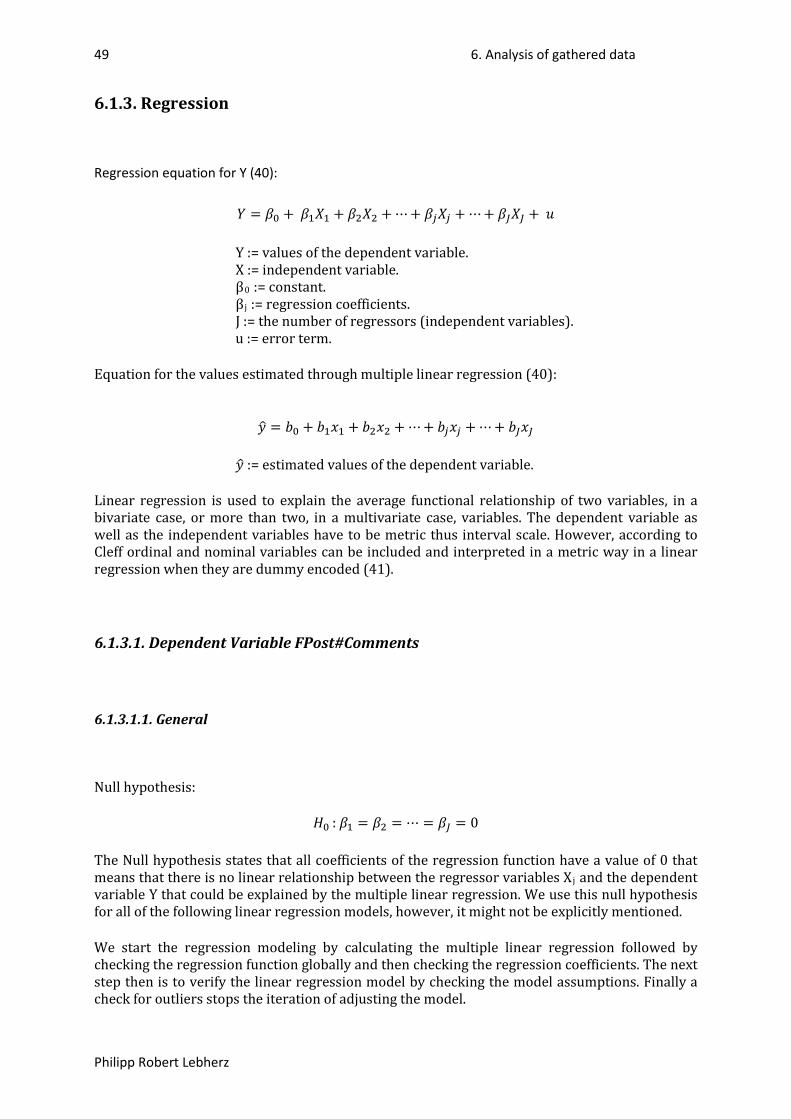
49 6. Analysis of gathered data
Philipp Robert Lebherz
6.1.3. Regression
Regression equation for Y (40):
𝑌 = 𝛽0 + 𝛽1𝑋1 + 𝛽2𝑋2 +⋯+ 𝛽𝑗𝑋𝑗 + ⋯+ 𝛽𝐽𝑋𝐽 + 𝑢 Y := values of the dependent variable. X := independent variable. β0
β := constant.
j
J := the number of regressors (independent variables). := regression coefficients.
u := error term.
Equation for the values estimated through multiple linear regression (40):
𝑦� = 𝑏0 + 𝑏1𝑥1 + 𝑏2𝑥2 + ⋯+ 𝑏𝑗𝑥𝑗 +⋯+ 𝑏𝐽𝑥𝐽
𝑦� := estimated values of the dependent variable.
Linear regression is used to explain the average functional relationship of two variables, in a bivariate case, or more than two, in a multivariate case, variables. The dependent variable as well as the independent variables have to be metric thus interval scale. However, according to Cleff ordinal and nominal variables can be included and interpreted in a metric way in a linear regression when they are dummy encoded (41).
6.1.3.1. Dependent Variable FPost#Comments
6.1.3.1.1. General
Null hypothesis:
𝐻0 : 𝛽1 = 𝛽2 = ⋯ = 𝛽𝐽 = 0
The Null hypothesis states that all coefficients of the regression function have a value of 0 that means that there is no linear relationship between the regressor variables Xj
We start the regression modeling by calculating the multiple linear regression followed by checking the regression function globally and then checking the regression coefficients. The next step then is to verify the linear regression model by checking the model assumptions. Finally a check for outliers stops the iteration of adjusting the model.
and the dependent variable Y that could be explained by the multiple linear regression. We use this null hypothesis for all of the following linear regression models, however, it might not be explicitly mentioned.

50 6. Analysis of gathered data
Philipp Robert Lebherz
Regression
Model Summaryd
Model R R Square Adjusted R Square
Std. Error of the Estimate
Change Statistics
Durbin-Watson R Square Change F Change df1 df2 Sig. F Change
3 ,642 ,412 c ,404 1,021581156005 ,019 7,002 1 213 ,009 1,873 c. Predictors: (Constant), LN(followers), ImagesDummy-LinksDummy, TimeDummy d. Dependent Variable: LN(Comments+1)
R: Pearson’s correlation coefficient
In the bivariate case the R is Pearson’s correlation coefficient. In the multivariate case the R is the multiple correlation coefficient. It is the square root of R² (40).
R²: Coefficient of determination
𝑅² =∑ (𝑦�𝑘 − 𝑦�)²𝐾𝑘=1
∑ (𝑦𝑘 − 𝑦�)²𝐾𝑘=1
K := the number of observations.
The coefficient of determination R² measures goodness of fit of the regression function to the empirical data. R² is the difference of the statistical spread explained by the function and the complete statistical spread (40). R² can take values in the interval of [0,1] while 0 meaning that there is no measured linear relationship and the regression line does not explain any of the variance and 1 meaning that the regression explains all of the variance of the dependent variable. When the variance is completely explained by the regression then the error term of the regression function is 0 and the values of the dependent variable lie exactly on the regression line (42). R² may also be calculated as the square of the correlation R of the observed values of the dependent variable and the estimated y (40).
In this case the regression reaches moderate power with a R² of 0,412. Thus the three independent variables explain 41,2 % of the variance of the Y.
Adj. R²: adjusted coefficient of determination
𝑅𝑎𝑑𝑗2 = 𝑅² −𝐽 ∗ (1 − 𝑅2)𝐾 − 𝐽 − 1
K-J-1 := degree of freedom.
The adjusted R² punishes the R² for each independent variable added (41). The reason for doing this is to avoid the use of too many parameters in multiple regressions. By simply adding independent variables to the model one can push the R² due to the fact that the worst case situation is that the R² stays the same (41). The idea of explaining real life relationships with models is to describe them with the smallest number of influencing variables. That’s why adding as much independent variables to the model as possible is not in the sense of linear modeling (41). The more the R² and adjusted R² differ the more overspecialized the regression model is.
In this case the adjusted R² is 0,404 and differs only 0,008 from R².

51 6. Analysis of gathered data
Philipp Robert Lebherz
Standard error of the estimate:
𝑠 = �∑ 𝑒𝑘2𝑘
𝐾 − 𝐽 − 1
ek
The standard error of the estimate is the standard deviation of the residuals and represents another measurement for the quality of the regression (40).
:= residual of observation k.
In this case the std. error of the estimate is 1,022.
Global check of the regression
ANOVAModel
d Sum of Squares df Mean Square F Sig.
3 Regression 155,620 3 51,873 49,705 ,000c Residual 222,293 213 1,044 Total 377,913 216
c. Predictors: (Constant), LN(followers), ImagesDummy-LinksDummy, TimeDummy d. Dependent Variable: LN(Comments+1)
Evaluation the significance of R² through a F-Test:
ANOVA means analysis of variances. Here the complete regression model is checked by testing the coefficient of determination R² for statistic significance. We define the level of significance (also called probability of error) with 0,05. That means if the p-value is less then 0,05 then we can say with 95 % probability of not making an error and that the null hypothesis is not correct. Thus not all β j
In this case the result of the F-Test is 49,705 what is highly statistically significant (even on 0,01 R² is significant). This means the R² of 0,412 is statistically significant and H
are 0 thus we can say that the linear relationship the regression model states is statistically significant (40).
0
is refused.
Mean square of regression:
This is the variance explained by the regression model.
Mean square of residual:
This is the variance that is not explained by the regression model.
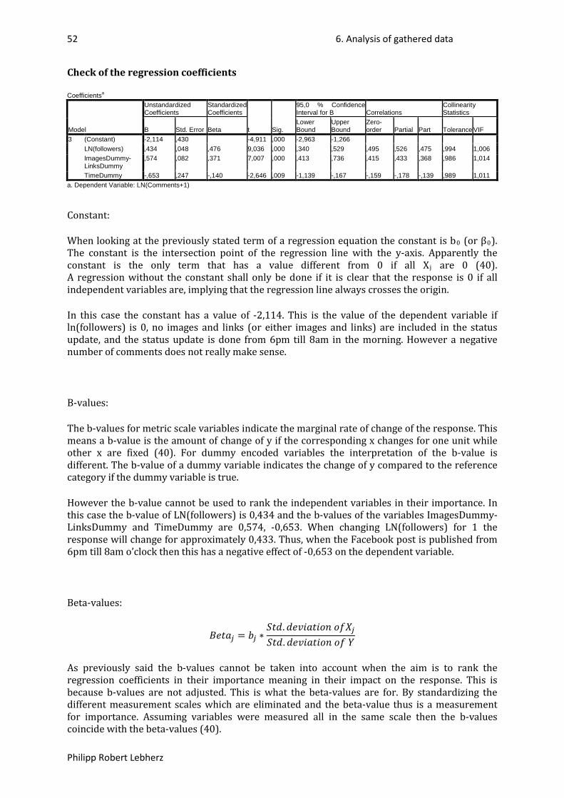
52 6. Analysis of gathered data
Philipp Robert Lebherz
Check of the regression coefficients
Coefficientsa
Model
Unstandardized Coefficients
Standardized Coefficients
t Sig.
95,0 % Confidence Interval for B Correlations
Collinearity Statistics
B Std. Error Beta Lower Bound
Upper Bound
Zero-order Partial Part Tolerance VIF
3 (Constant) -2,114 ,430 -4,911 ,000 -2,963 -1,266 LN(followers) ,434 ,048 ,476 9,036 ,000 ,340 ,529 ,495 ,526 ,475 ,994 1,006 ImagesDummy-LinksDummy
,574 ,082 ,371 7,007 ,000 ,413 ,736 ,415 ,433 ,368 ,986 1,014
TimeDummy -,653 ,247 -,140 -2,646 ,009 -1,139 -,167 -,159 -,178 -,139 ,989 1,011 a. Dependent Variable: LN(Comments+1)
Constant:
When looking at the previously stated term of a regression equation the constant is b0 (or β0). The constant is the intersection point of the regression line with the y-axis. Apparently the constant is the only term that has a value different from 0 if all Xj
In this case the constant has a value of -2,114. This is the value of the dependent variable if ln(followers) is 0, no images and links (or either images and links) are included in the status update, and the status update is done from 6pm till 8am in the morning. However a negative number of comments does not really make sense.
are 0 (40). A regression without the constant shall only be done if it is clear that the response is 0 if all independent variables are, implying that the regression line always crosses the origin.
B-values:
The b-values for metric scale variables indicate the marginal rate of change of the response. This means a b-value is the amount of change of y if the corresponding x changes for one unit while other x are fixed (40). For dummy encoded variables the interpretation of the b-value is different. The b-value of a dummy variable indicates the change of y compared to the reference category if the dummy variable is true.
However the b-value cannot be used to rank the independent variables in their importance. In this case the b-value of LN(followers) is 0,434 and the b-values of the variables ImagesDummy-LinksDummy and TimeDummy are 0,574, -0,653. When changing LN(followers) for 1 the response will change for approximately 0,433. Thus, when the Facebook post is published from 6pm till 8am o’clock then this has a negative effect of -0,653 on the dependent variable.
Beta-values:
𝐵𝑒𝑡𝑎𝑗 = 𝑏𝑗 ∗𝑆𝑡𝑑.𝑑𝑒𝑣𝑖𝑎𝑡𝑖𝑜𝑛 𝑜𝑓𝑋𝑗𝑆𝑡𝑑.𝑑𝑒𝑣𝑖𝑎𝑡𝑖𝑜𝑛 𝑜𝑓 𝑌
As previously said the b-values cannot be taken into account when the aim is to rank the regression coefficients in their importance meaning in their impact on the response. This is because b-values are not adjusted. This is what the beta-values are for. By standardizing the different measurement scales which are eliminated and the beta-value thus is a measurement for importance. Assuming variables were measured all in the same scale then the b-values coincide with the beta-values (40).
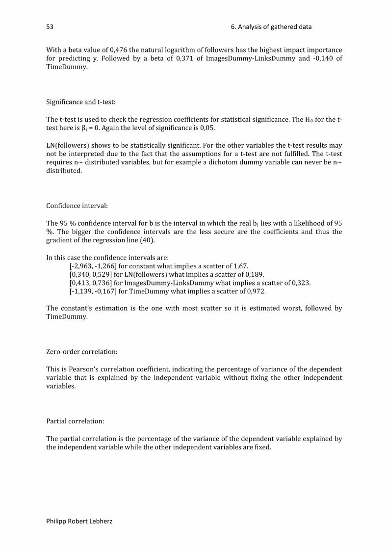
53 6. Analysis of gathered data
Philipp Robert Lebherz
With a beta value of 0,476 the natural logarithm of followers has the highest impact importance for predicting y. Followed by a beta of 0,371 of ImagesDummy-LinksDummy and -0,140 of TimeDummy.
Significance and t-test:
The t-test is used to check the regression coefficients for statistical significance. The H0 for the t-test here is β j
LN(followers) shows to be statistically significant. For the other variables the t-test results may not be interpreted due to the fact that the assumptions for a t-test are not fulfilled. The t-test requires n~ distributed variables, but for example a dichotom dummy variable can never be n~ distributed.
= 0. Again the level of significance is 0,05.
Confidence interval:
The 95 % confidence interval for b is the interval in which the real bj
In this case the confidence intervals are:
lies with a likelihood of 95 %. The bigger the confidence intervals are the less secure are the coefficients and thus the gradient of the regression line (40).
[-2,963, -1,266] for constant what implies a scatter of 1,67. [0,340, 0,529] for LN(followers) what implies a scatter of 0,189. [0,413, 0,736] for ImagesDummy-LinksDummy what implies a scatter of 0,323. [-1,139, -0,167] for TimeDummy what implies a scatter of 0,972.
The constant’s estimation is the one with most scatter so it is estimated worst, followed by TimeDummy.
Zero-order correlation:
This is Pearson’s correlation coefficient, indicating the percentage of variance of the dependent variable that is explained by the independent variable without fixing the other independent variables.
Partial correlation:
The partial correlation is the percentage of the variance of the dependent variable explained by the independent variable while the other independent variables are fixed.
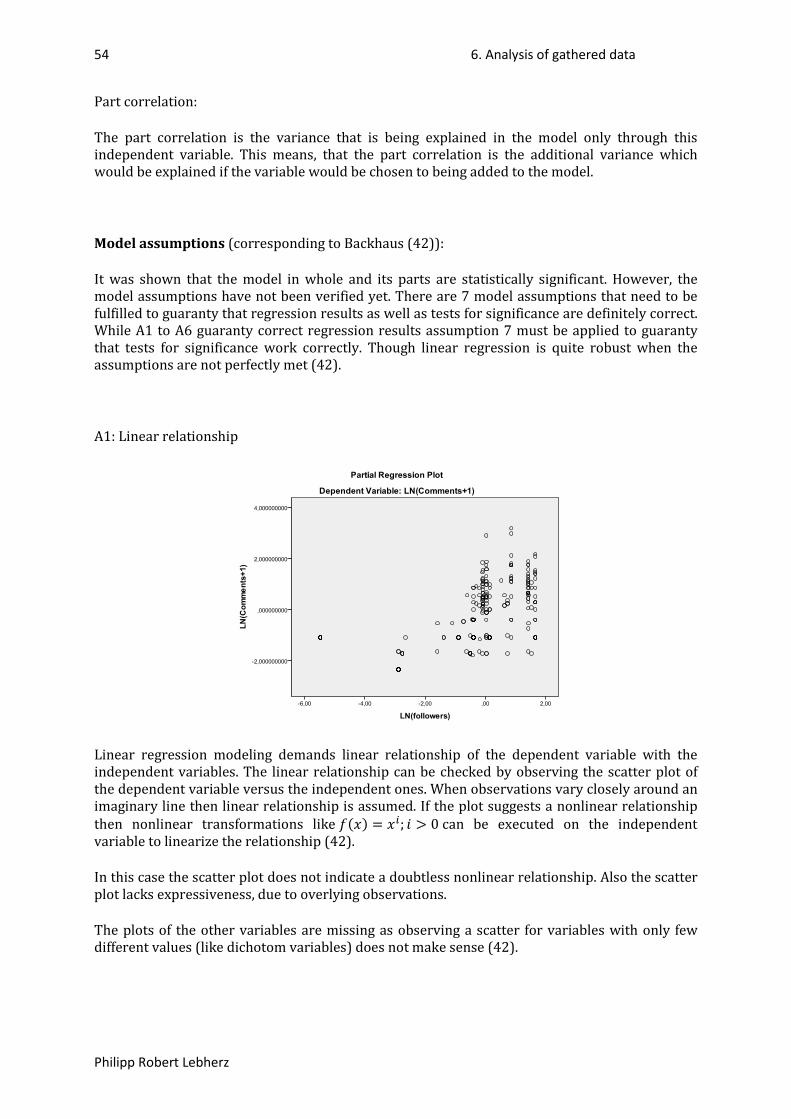
54 6. Analysis of gathered data
Philipp Robert Lebherz
Part correlation:
The part correlation is the variance that is being explained in the model only through this independent variable. This means, that the part correlation is the additional variance which would be explained if the variable would be chosen to being added to the model.
Model assumptions (corresponding to Backhaus (42)):
It was shown that the model in whole and its parts are statistically significant. However, the model assumptions have not been verified yet. There are 7 model assumptions that need to be fulfilled to guaranty that regression results as well as tests for significance are definitely correct. While A1 to A6 guaranty correct regression results assumption 7 must be applied to guaranty that tests for significance work correctly. Though linear regression is quite robust when the assumptions are not perfectly met (42).
A1: Linear relationship
Linear regression modeling demands linear relationship of the dependent variable with the independent variables. The linear relationship can be checked by observing the scatter plot of the dependent variable versus the independent ones. When observations vary closely around an imaginary line then linear relationship is assumed. If the plot suggests a nonlinear relationship then nonlinear transformations like 𝑓(𝑥) = 𝑥𝑖; 𝑖 > 0 can be executed on the independent variable to linearize the relationship (42).
In this case the scatter plot does not indicate a doubtless nonlinear relationship. Also the scatter plot lacks expressiveness, due to overlying observations.
The plots of the other variables are missing as observing a scatter for variables with only few different values (like dichotom variables) does not make sense (42).
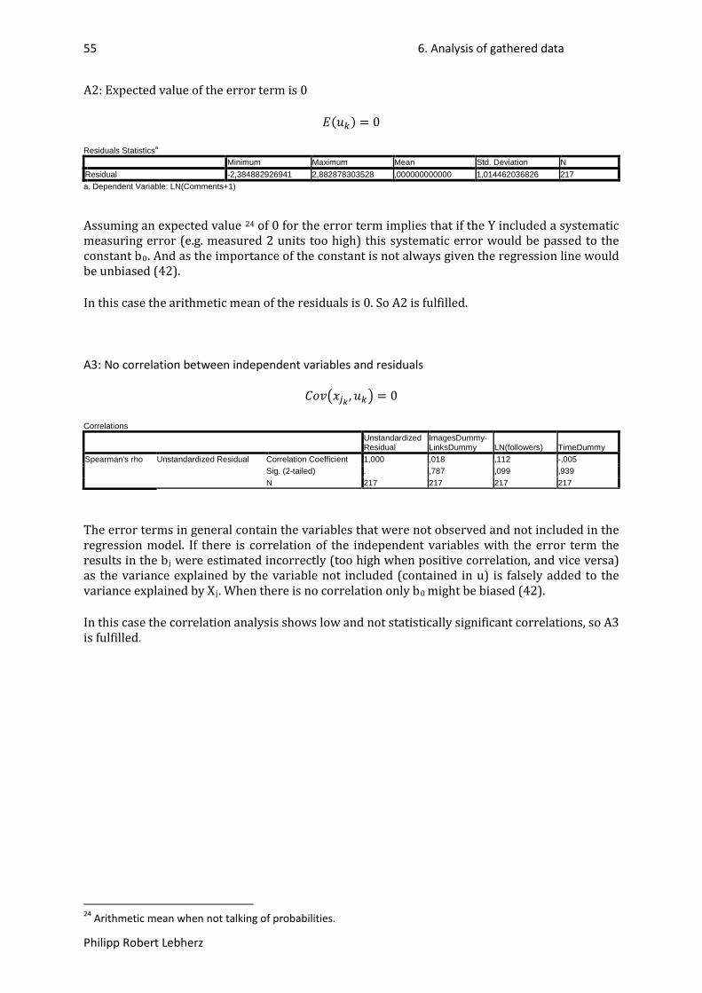
55 6. Analysis of gathered data
Philipp Robert Lebherz
A2: Expected value of the error term is 0
𝐸(𝑢𝑘) = 0
Residuals Statistics
a Minimum Maximum Mean Std. Deviation N
Residual -2,384882926941 2,882878303528 ,000000000000 1,014462036826 217 a. Dependent Variable: LN(Comments+1)
Assuming an expected value 24 of 0 for the error term implies that if the Y included a systematic measuring error (e.g. measured 2 units too high) this systematic error would be passed to the constant b0
In this case the arithmetic mean of the residuals is 0. So A2 is fulfilled.
. And as the importance of the constant is not always given the regression line would be unbiased (42).
A3: No correlation between independent variables and residuals
𝐶𝑜𝑣�𝑥𝑗𝑘 ,𝑢𝑘� = 0
Correlations
Unstandardized Residual
ImagesDummy-LinksDummy LN(followers) TimeDummy
Spearman's rho Unstandardized Residual Correlation Coefficient 1,000 ,018 ,112 -,005 Sig. (2-tailed) . ,787 ,099 ,939 N 217 217 217 217
The error terms in general contain the variables that were not observed and not included in the regression model. If there is correlation of the independent variables with the error term the results in the bj were estimated incorrectly (too high when positive correlation, and vice versa) as the variance explained by the variable not included (contained in u) is falsely added to the variance explained by Xj. When there is no correlation only b0
In this case the correlation analysis shows low and not statistically significant correlations, so A3 is fulfilled.
might be biased (42).
24 Arithmetic mean when not talking of probabilities.
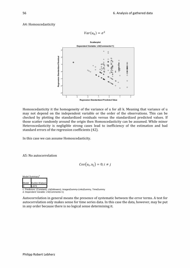
56 6. Analysis of gathered data
Philipp Robert Lebherz
A4: Homoscedasticity
𝑉𝑎𝑟(𝑢𝑘) = 𝜎2
Homoscedasticity it the homogeneity of the variance of u for all k. Meaning that variance of u may not depend on the independent variable or the order of the observations. This can be checked by plotting the standardized residuals versus the standardized predicted values. If those scatter randomly around the origin then Homoscedasticity can be assumed. While minor Heteroscedasticity is negligible strong cases lead to inefficiency of the estimation and bad standard errors of the regression coefficients (42).
In this case we can assume Homoscedasticity.
A5: No autocorrelation
𝐶𝑜𝑣�𝑢𝑖,𝑢𝑗� = 0; 𝑖 ≠ 𝑗
Model Summaryd
Model Durbin-Watson 3 1,873 c. Predictors: (Constant), LN(followers), ImagesDummy-LinksDummy, TimeDummy d. Dependent Variable: LN(Comments+1)
Autocorrelation in general means the presence of systematic between the error terms. A test for autocorrelation only makes sense for time series data. In this case the data, however, may be put in any order because there is no logical sense determining it.
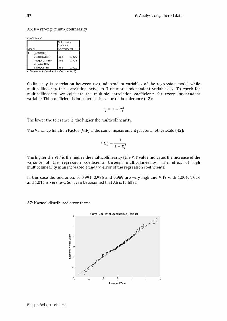
57 6. Analysis of gathered data
Philipp Robert Lebherz
A6: No strong (multi-)collinearity
Coefficientsa
Model
Collinearity Statistics Tolerance VIF
3 (Constant) LN(followers) ,994 1,006 ImagesDummy-LinksDummy
,986 1,014
TimeDummy ,989 1,011 a. Dependent Variable: LN(Comments+1)
Collinearity is correlation between two independent variables of the regression model while multicollinearity the correlation between 3 or more independent variables is. To check for multicollinearity we calculate the multiple correlation coefficients for every independent variable. This coefficient is indicated in the value of the tolerance (42):
𝑇𝑗 = 1 − 𝑅𝑗2
The lower the tolerance is, the higher the multicollinearity.
The Variance Inflation Factor (VIF) is the same measurement just on another scale (42):
𝑉𝐼𝐹𝑗 =1
1 − 𝑅𝑗2
The higher the VIF is the higher the multicollinearity (the VIF value indicates the increase of the variance of the regression coefficients through multicollinearity). The effect of high multicollinearity is an increased standard error of the regression coefficients.
In this case the tolerances of 0,994, 0,986 and 0,989 are very high and VIFs with 1,006, 1,014 and 1,011 is very low. So it can be assumed that A6 is fulfilled.
A7: Normal distributed error terms
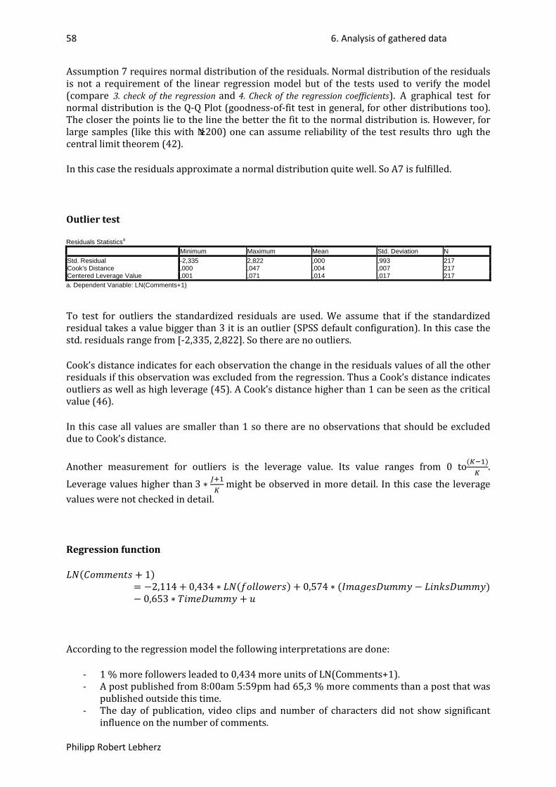
58 6. Analysis of gathered data
Philipp Robert Lebherz
Assumption 7 requires normal distribution of the residuals. Normal distribution of the residuals is not a requirement of the linear regression model but of the tests used to verify the model (compare 3. check of the regression and 4. Check of the regression coefficients). A graphical test for normal distribution is the Q-Q Plot (goodness-of-fit test in general, for other distributions too). The closer the points lie to the line the better the fit to the normal distribution is. However, for large samples (like this with N≥200) one can assume reliability of the test results thro ugh the central limit theorem (42).
In this case the residuals approximate a normal distribution quite well. So A7 is fulfilled.
Outlier test
Residuals Statistics
a Minimum Maximum Mean Std. Deviation N
Std. Residual -2,335 2,822 ,000 ,993 217 Cook's Distance ,000 ,047 ,004 ,007 217 Centered Leverage Value ,001 ,071 ,014 ,017 217 a. Dependent Variable: LN(Comments+1)
To test for outliers the standardized residuals are used. We assume that if the standardized residual takes a value bigger than 3 it is an outlier (SPSS default configuration). In this case the std. residuals range from [-2,335, 2,822]. So there are no outliers.
Cook’s distance indicates for each observation the change in the residuals values of all the other residuals if this observation was excluded from the regression. Thus a Cook’s distance indicates outliers as well as high leverage (45). A Cook’s distance higher than 1 can be seen as the critical value (46).
In this case all values are smaller than 1 so there are no observations that should be excluded due to Cook’s distance.
Another measurement for outliers is the leverage value. Its value ranges from 0 to(𝐾−1)𝐾
.
Leverage values higher than 3 ∗ 𝐽+1𝐾
might be observed in more detail. In this case the leverage values were not checked in detail.
Regression function
𝐿𝑁(𝐶𝑜𝑚𝑚𝑒𝑛𝑡𝑠 + 1)= −2,114 + 0,434 ∗ 𝐿𝑁(𝑓𝑜𝑙𝑙𝑜𝑤𝑒𝑟𝑠) + 0,574 ∗ (𝐼𝑚𝑎𝑔𝑒𝑠𝐷𝑢𝑚𝑚𝑦 − 𝐿𝑖𝑛𝑘𝑠𝐷𝑢𝑚𝑚𝑦)− 0,653 ∗ 𝑇𝑖𝑚𝑒𝐷𝑢𝑚𝑚𝑦 + 𝑢
According to the regression model the following interpretations are done:
- 1 % more followers leaded to 0,434 more units of LN(Comments+1). - A post published from 8:00am 5:59pm had 65,3 % more comments than a post that was
published outside this time. - The day of publication, video clips and number of characters did not show significant
influence on the number of comments.

59 6. Analysis of gathered data
Philipp Robert Lebherz
As hypothesized in section 3. the content attributes (here: followers, images, links and publication time) explain a justifiable amount (41,2 %) of the impact (here: comments) of the content.

60 6. Analysis of gathered data
Philipp Robert Lebherz
6.1.3.1.2. ES
The model reaches an R² of 0,353. Thus 35,3 % of the variance of the dependent variable can be explained by the 3 independent variables included in the model (compare Appendix 1: Model Summary, Facebook, LN(Comments+1), ES.).
The ANOVA results indicate that the resulting R² is highly statistically significant so the null hypothesis is refused (compare Appendix 2: ANOVA, Facebook, LN(Comments+1), ES.).
All included independent variables are statistically significant on a level of 0,05. The independent variable that is most important for determining the value of the dependent variable is ImagesDummy-LinksDummy with a beta-value of 0,489 (compare Appendix 3: Coefficients, Facebook, LN(Comments+1), ES.). So far the regression model is verified. However the model assumptions are still to check.
A1 is assumed as fulfilled as the scatter plot does not show evidence for non-linear relationships (compare Appendix 4: A1, Facebook, LN(Comments+1), ES.).
Also A2 and A3 are fulfilled. Neither the expected value of the residuals is different from 0 nor there is correlation of the residuals and the independent variables (compare Appendix 5: A2, Facebook, LN(Comments+1), ES. and Appendix 6: A3, Facebook, LN(Comments+1), ES.).
Checking the plot of the standardized predicted values versus the standardized residuals there is no systematic structure of the scatter observable. So there is no evidence for heteroscedasticity and thus A4 is fulfilled (compare Appendix 7: A4, Facebook, LN(Comments+1), ES.).
As mentioned in section 6.1.3.1.1 there is no need for a test for autocorrelation on this data, so A5 is fulfilled.
Tolerances are higher than 0,985 and VIF lower than 1,023 so there is no problem of strong (multi-)collinearity (compare Appendix 9: A6, Facebook, LN(Comments+1), ES.).
In addition, normal distribution of the residuals can be assumed (compare Appendix 10: A7, Facebook, LN(Comments+1), ES. and 6.1.3.1.1.).
Model assumptions are met and there are no observations that should be treated for outlier problematic (compare Appendix 11: Outlier test, Facebook, LN(Comments+1), ES.).
Regression function
𝐿𝑁(𝐶𝑜𝑚𝑚𝑒𝑛𝑡𝑠 + 1)= −0,837 + 0,719 ∗ (𝐼𝑚𝑎𝑔𝑒𝑠𝐷𝑢𝑚𝑚𝑦 − 𝐿𝑖𝑛𝑘𝑠𝐷𝑢𝑚𝑚𝑦) − 0,811 ∗ 𝑇𝑖𝑚𝑒𝐷𝑢𝑚𝑚𝑦+ 0,316 ∗ 𝐿𝑁(𝑓𝑜𝑙𝑙𝑜𝑤𝑒𝑟𝑠) + 𝜀

61 6. Analysis of gathered data
Philipp Robert Lebherz
According to the regression model the following interpretations are done:
- 1 % more followers leaded to 0,316 more units of LN(Comments+1). - A post published from 8:00am to 5:59pm it had 81,1 % more comments than a post
published outside this time span. - Video clips did not influence the number of comments significantly. - The publication day did not influence the number of comments significantly. - The number of characters did not influence the number of comments significantly.
As hypothesized in section 3. the content attributes (here: followers, images, links and publication time) explain a justifiable amount (35,3 %) of the impact (here: comments) of the content for the Spanish sample.

62 6. Analysis of gathered data
Philipp Robert Lebherz
6.1.3.1.3. GE
The model reaches an R² of 0,148 including one independent variable. Thus it lacks in explanatory power (compare Appendix 12: Model summary, Facebook, LN(Comments+1), GE. and Appendix 13: Excluded variables, Facebook, LN(Comments+1), GE.).
In contrary to the hypothesis in section 3. the content attributes cannot explain a justifiable amount (only 14,8 %) of the impact (here: comments) of the content for the German sample.

63 6. Analysis of gathered data
Philipp Robert Lebherz
6.1.3.2. Dependent Variable FPost#Likes
6.1.3.2.1. General
In this and the following 2 models the dependent variable was changed to LN(Likes+1). The model reaches an R² of 0,638. Thus 63,8 % of the variance of the dependent variable can be explained by the five independent variables included in the model (compare Appendix 14: Model summary, Facebook, LN(Likes+1), General.).
The ANOVA results indicate that the resulting R² is highly statistically significant so the null hypothesis is refused (compare Appendix 15: ANOVA, Facebook, LN(Likes+1), General.).
All included independent variables are statistically significant on a level of 0,01. The independent variable that is most important for determining the value of the dependent variable is LN(followers) with a beta-value of 0,663 (compare Appendix 16: Coefficients, Facebook, LN(Likes+1), General.). So far the regression model is verified; however, the model assumptions are still to check.
The scatter-plot of LN(Likes+1) with LN(followers) might show a slight exponential structure. While the scatter-plot of LN(Likes+1) and FPost#Letters scatters nearly without structure. Checking of A4 will reveal problems with Heteroscedasticity if there is no linear relationship underlying (compare Appendix 17: A1, Facebook, LN(Likes+1), General.)
Also A2 and A3 are fulfilled. Neither the expected value of the residuals differs from 0 nor there is significant correlation of the residuals and the independent variables (compare Appendix 18: A2, Facebook, LN(Likes+1), General. and Appendix 19: A3, Facebook, LN(Likes+1), General.)
The plot of the standardized predicted values versus the standardized residuals scatters well around the origin besides some outliers on the left. Nevertheless those residuals still have a distance ≤ 3 to t he mean of the standardized residuals, so they are not classified as outliers. There is no evidence for Heteroscedasticity and thus A4 is fulfilled (compare Appendix 20: A4, Facebook, LN(Likes+1), General.). As the test for Homoscedasticity also is a test for linearity of the relationship we assume by this that also A1 is fulfilled.
As mentioned in section 6.1.3.1.1. General there is no need for a test for autocorrelation on this data, so A5 is fulfilled.
Tolerances are higher than 0,773 and VIF lower than 1,293 and so there is no problem of strong (multi-)collinearity (compare Appendix 22: A6, Facebook, LN(Likes+1), General.).
Moreover normal distribution of the residuals can be assumed (compare Appendix 23: A7, Facebook, LN(Likes+1), General. and 6.1.3.1.1. General).
Model assumptions are met and there are no observations that should be treated for outliers problematically (compare Appendix 24: Outlier test, Facebook, LN(Likes+1), General.).
64 6. Analysis of gathered data
Philipp Robert Lebherz
Regression function
𝐿𝑁(𝐿𝑖𝑘𝑒𝑠 + 1) = −3,751 + 0,584 ∗ 𝐿𝑁(𝑓𝑜𝑙𝑙𝑜𝑤𝑒𝑟𝑠) + 0,003 ∗ 𝐹𝑃𝑜𝑠𝑡#𝐿𝑒𝑡𝑡𝑒𝑟𝑠 + 1,013∗ 𝑉𝑖𝑑𝑒𝑜𝐶𝑙𝑖𝑝𝑠𝐷𝑢𝑚𝑚𝑦 + 0,694 ∗ (𝐼𝑚𝑎𝑔𝑒𝑠𝐷𝑢𝑚𝑚𝑦 + 𝐿𝑖𝑛𝑘𝑠𝐷𝑢𝑚𝑚𝑦) + 0,239∗ (𝐼𝑚𝑎𝑔𝑒𝑠𝐷𝑢𝑚𝑚𝑦 − 𝐿𝑖𝑛𝑘𝑠𝐷𝑢𝑚𝑚𝑦) + 𝜀
According to the regression model the following interpretations are done:
- 1 % more followers leaded to 0,584 more units of LN(Likes+1). - When a post contained one character more this changed the number of likes by 0,3 %. - Video clips added to a post changed the number of likes positively to 100,13 %. - The publication day did not significantly influence the number of likes. - The publication time did not significantly influence the number of likes.
As hypothesized in section 3. the content attributes (here: followers, images, links, number of characters and video clips) explain a justifiable amount (63,8 %) of impact (here: likes) of the content.

65 6. Analysis of gathered data
Philipp Robert Lebherz
6.1.3.2.2. ES
Here the influence of the independent variables on the variable LN(Likes+1) limited to only Spanish observations is modeled. The model reaches an R² of 0,547. Thus 54,7 % of the variance of the dependent variable can be explained by the five independent variables included in the model (compare Appendix 25: Model summary, Facebook, LN(Likes+1), ES.).
The ANOVA results indicate that R² is statistically significant on a level of 0,05 so the null hypothesis is refused (compare Appendix 26: ANOVA, Facebook, LN(Likes+1), ES.).
All included independent variables are statistically significant on a level of 0,05. The independent variable that is most important for determining the value of the dependent variable is LN(followers) with a beta-value of 0,421 (compare Appendix 27: Coefficients, Facebook, LN(Likes+1), ES.). So far the regression model is verified. We can see that it lost power by limiting the data on only Spanish observations. However the model assumptions are still to check.
The scatter-plot of LN(Likes+1) with LN(followers) shows linearity. While in the scatter-plot of LN(Likes+1) and FPost#Letters it is hard to see a structure (compare Appendix 28: A1, Facebook, LN(Likes+1), ES.). A1 is assumed as fulfilled.
Also A2 and A3 are fulfilled. Neither the expected value of the residuals differs from 0 nor there is significant correlation of the residuals and the independent variables (compare Appendix 29: A2, Facebook, LN(Likes+1), ES. and Appendix 30: A3, Facebook, LN(Likes+1), ES).
The plot of the standardized predicted values versus the standardized residuals scatters well around the origin. A4 can be assumed as fulfilled (compare Appendix 31: A4, Facebook, LN(Likes+1), ES.).
As mentioned in section 6.1.3.1.1. General there is no need for a test for autocorrelation on this data, so A5 is fulfilled.
Tolerances are higher than 0,707 and VIF lower than 1,414 so there is no problem of strong (multi-)collinearity (compare Appendix 33: A6, Facebook, LN(Likes+1), ES.).
Furthermore normal distribution of the residuals can be assumed (compare Appendix 34: A7, Facebook, LN(Likes+1), ES. and 6.1.3.1.1. General).
Model assumptions are met and there are no observations that should be treated for outlier problematic (compare Appendix 35: Outlier test, Facebook, LN(Likes+1), ES.).
Regression function
𝐿𝑁(𝐿𝑖𝑘𝑒𝑠 + 1) = −4,186 + 0,646 ∗ 𝐿𝑁(𝑓𝑜𝑙𝑙𝑜𝑤𝑒𝑟𝑠) + 0,003 ∗ 𝐹𝑃𝑜𝑠𝑡#𝐿𝑒𝑡𝑡𝑒𝑟𝑠 + 1,066∗ 𝑉𝑖𝑑𝑒𝑜𝐶𝑙𝑖𝑝𝑠𝐷𝑢𝑚𝑚𝑦 + 0,566 ∗ (𝐼𝑚𝑎𝑔𝑒𝑠𝐷𝑢𝑚𝑚𝑦 + 𝐿𝑖𝑛𝑘𝑠𝐷𝑢𝑚𝑚𝑦) + 0,271∗ (𝐼𝑚𝑎𝑔𝑒𝑠𝐷𝑢𝑚𝑚𝑦 − 𝐿𝑖𝑛𝑘𝑠𝐷𝑢𝑚𝑚𝑦) + 𝜀

66 6. Analysis of gathered data
Philipp Robert Lebherz
According to the regression model the following interpretations are done:
- 1 % more followers leaded to 0,646 more units of LN(Likes+1). - When a post contained one character more this changed the number of likes by 0,3 %. - Video clips added to a post changed the number of likes positively to 106,6 %. - The publication day did not significantly influence the number of comments. - The publication time did not significantly influence the number of comments.
As hypothesized in section 3. the content attributes (here: followers, images, links, number of characters and video clips) explain a justifiable amount (54,7 %) of impact (here: likes) of the content for the Spanish sample.

67 6. Analysis of gathered data
Philipp Robert Lebherz
6.1.3.2.3. GE
The model for the dependent variable LN(Likes+1) limited to the sample of the German observations reaches an R² of 0,619. Thus 61,9 % of the variance of the dependent variable can be explained by the 2 independent variables included in the model (compare Appendix 36: Model summary, Facebook, LN(Likes+1), GE.).
The ANOVA results indicate that R² is statistically significant on a level of 0,05 so the null hypothesis is refused (compare Appendix 37: ANOVA, Facebook, LN(Likes+1), GE.).
All included independent variables are statistically significant on a level of 0,05. The independent variable that is most important for determining the value of the dependent variable is LN(followers) with a beta-value of 0,421 (compare Appendix 38: Coefficients, Facebook, LN(Likes+1), GE.).
So far the regression model is verified. We can see that the model has more power in comparison to the one limited to the Spanish sample. However, this is obtained by having three independent variables less than in the Spanish model.
The scatter-plot of LN(Likes+1) with LN(followers) does not show any evidence for non-linear relationships (compare Appendix 39: A1, Facebook, LN(Likes+1), GE.). So A1 is fulfilled.
In addition A2 and A3 are fulfilled. Neither the expected value of the residuals differs from 0 nor there is significant correlation of the residuals and the independent variables (compare Appendix 40: A2, Facebook, LN(Likes+1), GE. and Appendix 41: A3, Facebook, LN(Likes+1), GE.).
The plot of the standardized predicted values versus the standardized residuals does not show any structure. There are some outliers on the left, but those are (like before) outlying for the standardized predicted value and not the residual. A4 can be assumed as fulfilled (compare Appendix 42: A4, Facebook, LN(Likes+1), GE.).
As mentioned in section 6.1.3.1.1. there is no need for a test for autocorrelation on this data, so A5 is fulfilled.
Tolerances are higher than 0,979 and VIF lower than 1,022 so there is no problem of strong collinearity (compare Appendix 44: A6, Facebook, LN(Likes+1), GE.).
Additionally, normal distribution of the residuals can be assumed. Due to the smaller sample size it is important for the residuals to show good fit in the Q-Q plot (compare Appendix 45: A7, Facebook, LN(Likes+1), GE and 6.1.3.1.1.).
Model assumptions are met and there are no observations that should be treated for outlier problematically (compare Appendix 46: Outlier test, Facebook, LN(Likes+1), GE.).
Regression function
𝐿𝑁(𝐿𝑖𝑘𝑒𝑠 + 1) = −0,854 + 0,297 ∗ 𝐿𝑁(𝑓𝑜𝑙𝑙𝑜𝑤𝑒𝑟𝑠) − 0,945 ∗ 𝑉𝑖𝑑𝑒𝑜𝐶𝑙𝑖𝑝𝑠𝐷𝑢𝑚𝑚𝑦 + 𝜀

68 6. Analysis of gathered data
Philipp Robert Lebherz
According to the regression model the following interpretations are done:
- 1 % more followers leaded to 0,297 more units of LN(Likes+1). - Video clips added to a post changed the number of likes positively to 95,5 %. - The publication time did not significantly influence the number of likes. - The publication day did not significantly influence the number of likes. - ImagesDummy-LinksDummy did not significantly influence the number of likes - ImagesDummy+LinksDummy did not significantly influence the number of likes - The number of characters of the post did not significantly influence the number of likes.
As hypothesized in section 3. the content attributes (here: followers and video clips) explain a justifiable amount (61,9 %) of impact (here: likes) of the content.

69 6. Analysis of gathered data
Philipp Robert Lebherz
6.2. Twitter
The variables included in the statistical analysis of Twitter are on the one hand the dependent variable LN_TTweet#ReTweets and on the other hand the independent variables TTweet#Characters, DateDayDummy, MentionsDummy+TweetIsAnswer, MentionsDummy-TweetIsAnswer, LinksDummy, TagsDummy, LN_Followers
To distinguish the sample in Spanish and German observations the variable country was used.
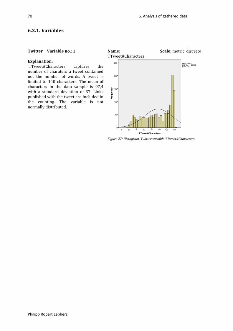
70 6. Analysis of gathered data
Philipp Robert Lebherz
6.2.1. Variables
Twitter Variable no.: 1 Name: TTweet#Characters
Scale: metric, discrete
Explanation: TTweet#Characters captures the number of charaters a tweet contained not the number of words. A tweet is limited to 140 characters. The mean of characters in the data sample is 97,4 with a standard deviation of 37. Links published with the tweet are included in the counting. The variable is not normally distributed.
Figure 27: Histogram, Twitter variable TTweet#Characters.
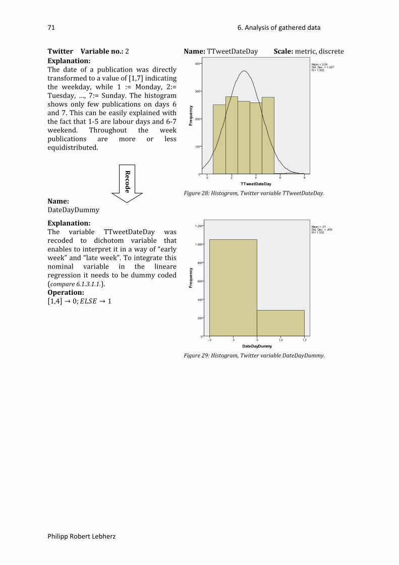
71 6. Analysis of gathered data
Philipp Robert Lebherz
Twitter Variable no.: 2 Name: TTweetDateDay Scale: metric, discrete Explanation: The date of a publication was directly transformed to a value of [1,7] indicating the weekday, while 1 := Monday, 2:= Tuesday, …, 7:= Sunday. The histogram shows only few publications on days 6 and 7. This can be easily explained with the fact that 1-5 are labour days and 6-7 weekend. Throughout the week publications are more or less equidistributed.
Figure 28: Histogram, Twitter variable TTweetDateDay.
Name: DateDayDummy
Explanation: The variable TTweetDateDay was recoded to dichotom variable that enables to interpret it in a way of “early week” and “late week”. To integrate this nominal variable in the lineare regression it needs to be dummy coded (compare 6.1.3.1.1.).
Figure 29: Histogram, Twitter variable DateDayDummy.
Operation: [1,4] → 0;𝐸𝐿𝑆𝐸 → 1
Recode
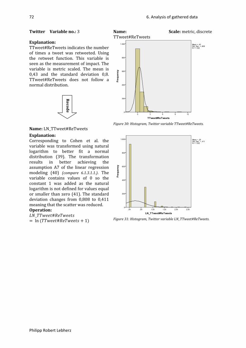
72 6. Analysis of gathered data
Philipp Robert Lebherz
Twitter Variable no.: 3 Name: TTweet#ReTweets
Scale: metric, discrete
Explanation: TTweet#ReTweets indicates the number of times a tweet was retweeted. Using the retweet function. This variable is seen as the measurement of impact. The variable is metric scaled. The mean is 0,43 and the standard deviation 0,8. TTweet#ReTweets does not follow a normal distribution.
Figure 30: Histogram, Twitter variable TTweet#ReTweets.
Name: LN_TTweet#ReTweets Explanation: Corresponding to Cohen et al. the variable was transformed using natural logarithm to better fit a normal distribution (39). The transformation results in better achieving the assumption A7 of the linear regression modeling (40) (compare 6.1.3.1.1.). The variable contains values of 0 so the constant 1 was added as the natural logarithm is not defined for values equal or smaller than zero (41). The standard deviation changes from 0,808 to 0,411 meaning that the scatter was reduced.
Figure 31: Histogram, Twitter variable LN_TTweet#ReTweets.
Operation: 𝐿𝑁_𝑇𝑇𝑤𝑒𝑒𝑡#𝑅𝑒𝑇𝑤𝑒𝑒𝑡𝑠= ln (𝑇𝑇𝑤𝑒𝑒𝑡#𝑅𝑒𝑇𝑤𝑒𝑒𝑡𝑠 + 1)
Recode
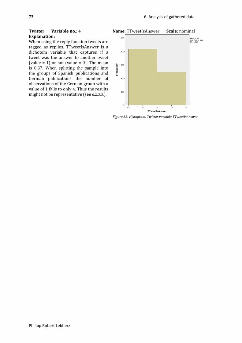
73 6. Analysis of gathered data
Philipp Robert Lebherz
Twitter Variable no.: 4 Name: TTweetIsAnswer Scale: nominal Explanation: When using the reply function tweets are tagged as replies. TTweetIsAnswer is a dichotom variable that captures if a tweet was the answer to another tweet (value = 1) or not (value = 0). The mean is 0,37. When splitting the sample into the groups of Spanish publications and German publications the number of observations of the German group with a value of 1 falls to only 4. Thus the results might not be representative (see 6.2.3.3.).
Figure 32: Histogram, Twitter variable TTweetIsAnswer.
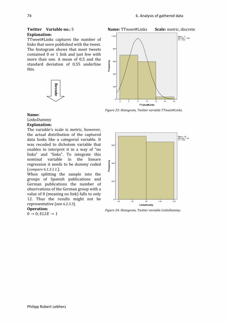
74 6. Analysis of gathered data
Philipp Robert Lebherz
Twitter Variable no.: 5 Name: TTweet#Links Scale: metric, discrete Explanation: TTweet#Links captures the number of links that were published with the tweet. The histogram shows that most tweets contained 0 or 1 link and just few with more than one. A mean of 0,5 and the standard deviation of 0,55 underline this.
Figure 33: Histogram, Twitter variable TTweet#Links.
Name: LinksDummy
Explanation: The variable’s scale is metric, however, the actual distribution of the captured data looks like a categorial variable. It was recoded to dichotom variable that enables to interpret it in a way of “no links” and “links”. To integrate this nominal variable in the lineare regression it needs to be dummy coded (compare 6.1.3.1.1.). When splitting the sample into the groups of Spanish publications and German publications the number of observations of the German group with a value of 0 (meaning no link) falls to only 12. Thus the results might not be representative (see 6.2.3.3).
Figure 34: Histogram, Twitter variable LinksDummy. Operation:
0 → 0;𝐸𝐿𝑆𝐸 → 1
Recode
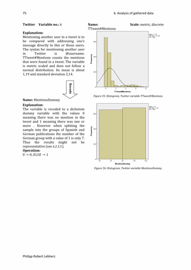
75 6. Analysis of gathered data
Philipp Robert Lebherz
Twitter Variable no.: 6 Name: TTweet#Mentions
Scale: metric, discrete
Explanation: Mentioning another user in a tweet is to be compared with addressing one’s message directly to this or those users. The syntax for mentioning another user in Twitter is @username. TTweet#Mentions counts the mentions that were found in a tweet. The variable is metric scaled and does not follow a normal distribution. Its mean is about 1,19 and standard deviation 2,14.
Figure 35: Histogram, Twitter variable TTweet#Mentions.
Name: MentionsDummy Explanation: The variable is recoded to a dichotom dummy variable with the values 0 meaning there was no mention in the tweet and 1 meaning there was one or more . However when splitting the sample into the groups of Spanish and German publications the number of the German group with a value of 1 is only 7. Thus the results might not be representative (see 6.2.3.3.).
Figure 36: Histogram, Twitter variable MentionsDummy.
Operation: 0 → 0;𝐸𝐿𝑆𝐸 → 1
Recode
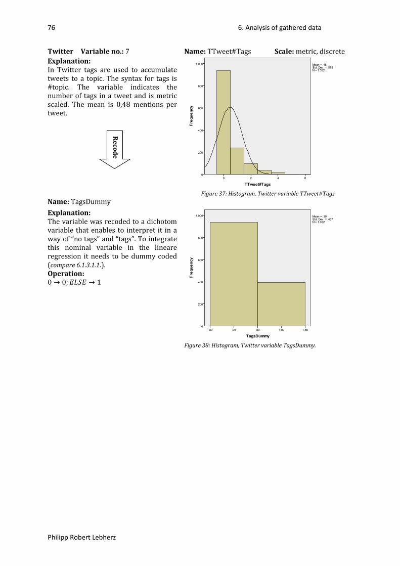
76 6. Analysis of gathered data
Philipp Robert Lebherz
Twitter Variable no.: 7 Name: TTweet#Tags Scale: metric, discrete Explanation: In Twitter tags are used to accumulate tweets to a topic. The syntax for tags is #topic. The variable indicates the number of tags in a tweet and is metric scaled. The mean is 0,48 mentions per tweet.
Figure 37: Histogram, Twitter variable TTweet#Tags.
Name: TagsDummy Explanation: The variable was recoded to a dichotom variable that enables to interpret it in a way of “no tags” and “tags”. To integrate this nominal variable in the lineare regression it needs to be dummy coded (compare 6.1.3.1.1.).
Figure 38: Histogram, Twitter variable TagsDummy.
Operation: 0 → 0;𝐸𝐿𝑆𝐸 → 1
Recode
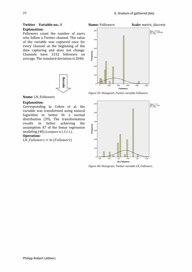
77 6. Analysis of gathered data
Philipp Robert Lebherz
Twitter Variable no.: 8 Name: Followers Scale: metric, discrete Explanation: Followers count the number of users who follow a Twitter channel. The value of the variable was captured once for every channel at the beginning of the data capturing and does not change. Channels have 3152 followers on average. The standard deviation is 2040.
Figure 39: Histogram, Twitter variable Followers.
Name: LN_Followers Explanation: Corresponding to Cohen et al. the variable was transformed using natural logarithm to better fit a normal distribution (39). The transformation results in better achieving the assumption A7 of the linear regression modeling (40) (compare 6.1.3.1.1.).
Figure 40: Histogram, Twitter variable LN_Followers.
Operation: 𝐿𝑁_𝐹𝑜𝑙𝑙𝑜𝑤𝑒𝑟𝑠 = ln (𝐹𝑜𝑙𝑙𝑜𝑤𝑒𝑟𝑠)
Recode
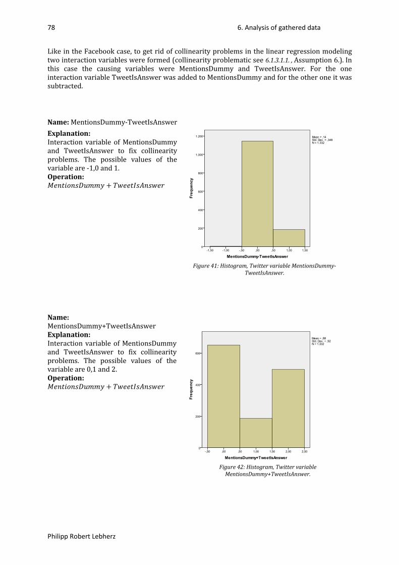
78 6. Analysis of gathered data
Philipp Robert Lebherz
Like in the Facebook case, to get rid of collinearity problems in the linear regression modeling two interaction variables were formed (collinearity problematic see 6.1.3.1.1. , Assumption 6.). In this case the causing variables were MentionsDummy and TweetIsAnswer. For the one interaction variable TweetIsAnswer was added to MentionsDummy and for the other one it was subtracted.
Name: MentionsDummy-TweetIsAnswer Explanation: Interaction variable of MentionsDummy and TweetIsAnswer to fix collinearity problems. The possible values of the variable are -1,0 and 1. Operation: 𝑀𝑒𝑛𝑡𝑖𝑜𝑛𝑠𝐷𝑢𝑚𝑚𝑦 + 𝑇𝑤𝑒𝑒𝑡𝐼𝑠𝐴𝑛𝑠𝑤𝑒𝑟
Figure 41: Histogram, Twitter variable MentionsDummy-
TweetIsAnswer.
Name: MentionsDummy+TweetIsAnswer
Explanation: Interaction variable of MentionsDummy and TweetIsAnswer to fix collinearity problems. The possible values of the variable are 0,1 and 2. Operation: 𝑀𝑒𝑛𝑡𝑖𝑜𝑛𝑠𝐷𝑢𝑚𝑚𝑦 + 𝑇𝑤𝑒𝑒𝑡𝐼𝑠𝐴𝑛𝑠𝑤𝑒𝑟
Figure 42: Histogram, Twitter variable
MentionsDummy+TweetIsAnswer.

79 6. Analysis of gathered data
Philipp Robert Lebherz
6.2.2 Correlation
Correlations
LN_TTweet#ReTweets
TTweet#Characters
LN_Followers
DateDayDummy
LinksDummy
TagsDummy
MentionsDummy+TweetIsAnswer
MentionsDummy-TweetIsAnswer
Spearman's rho
LN_TTweet#ReTweets
Correlation Coefficient
1,000 ,126** ,051 -,046 ,227** ,118** -,356** ,063*
Sig. (2-tailed)
. ,000 ,062 ,094 ,000 ,000 ,000 ,022
N 1332 1332 1332 1332 1332 1332 1332 1332 **. Correlation is significant at the 0.01 level (2-tailed). *. Correlation is significant at the 0.05 level (2-tailed).
Spearman’s rho shows significant negative correlation on a level of 0,05 of LN_TTweet#ReTweets to MentionsDummy+TweetIsAnswer and significant positive correlation to TTweet#Characters, LinksDummy, TagsDummy and MentionsDummy-TweetIsAnswer. Compare section 6.1.2.
80 6. Analysis of gathered data
Philipp Robert Lebherz
6.2.3. Regression
6.2.3.1. General
The regression model for Twitter with the dependent variable LN_TTweet#ReTweets reaches an R² of 0,193 implying that the included independent variables MentionsDummy+TweetIsAnwer and LN_Followers explain 19,3 % of the whole variance of the dependent variable. The other variables not included in the regression model do not contribute enough to be added (compare Appendix 47: Model summary, Twitter, General.). The low R² leads to the suspicion that there are other variables, not included in the data sample that have more power to explain the variance of the dependent variable. If this suspicion reveals as true then there should be correlation of the independent variables with the error term (compare 6.1.3.1.1. General) and A3 would not be fulfilled. The ANOVA proofs statistical significance of the R² on a level of 0,05 so the null hypothesis is refused (compare Appendix 48: ANOVA, Twitter, General).
All included independent variables are statistically significant on a level of 0,05. The independent variable that is most important for determining the value of the dependent variable is MentionsDummy+TweetIsAnswer with a beta-value of -0,484 (compare Appendix 49: Coefficients, Twitter, General.).
The scatter-plot of LN(Likes+1) with LN(followers) does not show any evidence for non-linear relationships but neither does it indicate a strong linear relationship (compare Appendix 50: A1, Twitter, General.).
A2 is fulfilled (compare Appendix 51: A2, Twitter, General.).
A3 is violated. LN_Followers as well as MentionsDummy+TweetIsAnswer show significant correlation with the residuals. This implies that the error term includes variables, not included in the sample, that have influence on both the dependent and the independent variables. The consequences of the violation of A3 are biased correlation coefficients (compare 6.1.3.1.1..). In this case the correlation coefficients are positive, so bMentionsDummy-TweetIsAnswer is estimated more negative than it should be and bLN_Followers Appendix 52: A3, Twitter, General.
is more positive than it should be (compare ).
The scatter-plots show slight heteroscedasticity (compare Appendix 53: A4, Twitter, General.). This results in inefficiency of the estimations and might be caused by non-linear relationships of the dependent variable with the independent ones.
As mentioned in section 6.1.3.1.1. there is no need for a test for autocorrelation on this data, so A5 is fulfilled.
Tolerances are higher than 0,617 and VIF lower than 1,620 (compare Appendix 55: A6, Twitter, General.). A VIF of 1,7 is often mentioned as the limit from the point one should search for possibilities to eliminate (multi-)collinearity. 1,620 lies close to this threshold, so this might lead to inaccurate estimation.
The residuals when checked with the Q-Q plot do not follow a normal distribution. However, we can assume that the tests for significance give reliable results due to the central limit theorem (compare Appendix 56: A7, Twitter, General. and 6.1.3.1.1.).

81 6. Analysis of gathered data
Philipp Robert Lebherz
There are no observations that should be treated for outlier problematic (compare Appendix 57: Outlier test, Twitter, General.).
Regression function
𝐿𝑁_𝑇𝑇𝑤𝑒𝑒𝑡#𝑅𝑒𝑇𝑤𝑒𝑒𝑡𝑠= −0,436− 0,198 ∗ (𝑀𝑒𝑛𝑡𝑖𝑜𝑛𝑠𝐷𝑢𝑚𝑚𝑦 + 𝑇𝑤𝑒𝑒𝑡𝐼𝑠𝐴𝑛𝑠𝑤𝑒𝑟) + 0,109∗ 𝐿𝑁_𝐹𝑜𝑙𝑙𝑜𝑤𝑒𝑟𝑠 + 𝜀
A3 is strongly violated while A1, A4, A5 and A7 cannot be seen as fulfilled without any qualification. This leads to biased and inaccurate estimations of the model that already has bad explanation power of 19,3 %. Due to this fact this model is not further interpreted as the validity is not guaranteed.
The captured variables do not determine the variance of retweets. This means tags, links, the number of followers, if the tweet is an answer or not, the day and the number of characters as well lack in significant influence on the number of retweets for the intra German/Spanish sample.
In contrary to the hypothesis in section 3. the content attributes cannot explain a justifiable amount of impact of a tweet.

82 6. Analysis of gathered data
Philipp Robert Lebherz
6.2.3.2. ES
The regression model for Twitter with the dependent variable LN_TTweet#ReTweets reaches an R² of 0,439 implying that the included independent variables explain 43,9 % of the whole variance of the dependent variable (compare Appendix 58: Model summary, Twitter, ES.). The ANOVA proofs statistical significance of the R² on a level of 0,05, so the null hypothesis is refused (compare Appendix 59: ANOVA, Twitter, ES.).
All included independent variables are statistically significant on a level of 0,05. The independent variable that is most important for determining the value of the dependent variable is MentionsDummy+TweetIsAnswer with a beta-value of -0,513 (compare Appendix 60: Coefficients, Twitter, ES.).
The scatter-plot of LN(Likes+1) with TTweet#Characters does not show any evidence for non-linear relationships but neither does it indicate a strong linear relationship (compare Appendix 61: A1, Twitter, ES.).
A2 is fulfilled (compare Appendix 62: A2, Twitter, ES.).
A3 is violated. MentionsDummy-TweetIsAnswer as well as MentionsDummy+TweetIsAnswer show significant correlation with the residuals. LinksDummy as well has significant correlation. However, the coefficient is very small so it is insubstantial. The consequence of the violation of A3 is biased correlation coefficients (compare 6.1.3.1.1.). In this case the correlation coefficients are negative, so bMentionsDummy-TweetIsAnswer is estimated less negative than it should be and bMentionsDummy+TweetIsAnswer Appendix 63: A3, Twitter, ES.
is also is less negative than it should be (compare ).
The scatter-plots show slight Heteroscedasticity (compare Appendix 64: A4, Twitter, ES.). This results in inefficiency of the estimations and might be caused by non-linear relationship of the dependent variable with the independent ones. A4 is violated.
As mentioned in section 6.1.3.1.1. there is no need for a test for autocorrelation on this data, so A5 is fulfilled.
Tolerances are higher than 0,589 and VIF lower than 1,744 (compare Appendix 66: A6, Twitter, ES.). A VIF of 1,744 implicates problems of (multi-)collinearity. One possibility would be to delete the variable that shows the highest VIF. In this case this would be LinksDummy. LinksDummy, however is with a beta-value of 0,126 and a partial correlation of 0,126 relatively important for the R². It is chosen to keep the variable in the model, running the risk of inaccuracy of the estimations but keeping more explanation power. A6 is violated.
The residuals when checked with the Q-Q plot do not follow a normal distribution. However, we can assume that the tests for significance give reliable results due to the central limit theorem (compare Appendix 67: A7, Twitter, ES. and 6.1.3.1.1.). A7 is fulfilled.
There are no observations that should be treated for outlier problematic (compare Appendix 68: Outlier test, Twitter, ES.).

83 6. Analysis of gathered data
Philipp Robert Lebherz
Regression function
𝐿𝑁_𝑇𝑇𝑤𝑒𝑒𝑡#𝑅𝑒𝑇𝑤𝑒𝑒𝑡𝑠= 0,411− 0,233 ∗ (𝑀𝑒𝑛𝑡𝑖𝑜𝑛𝑠𝐷𝑢𝑚𝑚𝑦 + 𝑇𝑤𝑒𝑒𝑡𝐼𝑠𝐴𝑛𝑠𝑤𝑒𝑟) + 0,02∗ 𝑇𝑇𝑤𝑒𝑒𝑡#𝐶ℎ𝑎𝑟𝑎𝑐𝑡𝑒𝑟𝑠 + 0,109 ∗ 𝐿𝑖𝑛𝑘𝑠𝐷𝑢𝑚𝑚𝑦 − 0,07 ∗ 𝐷𝑎𝑡𝑒𝐷𝑎𝑦𝐷𝑢𝑚𝑚𝑦− 0,063 ∗ 𝑀𝑒𝑛𝑡𝑖𝑜𝑛𝑠𝐷𝑢𝑚𝑚𝑦 − 𝑇𝑤𝑒𝑒𝑡𝐼𝑠𝐴𝑛𝑠𝑤𝑒𝑟+ 𝜀
Model assumptions A3 and A6 are not fulfilled. Estimations thus might be inaccurate and biased.
When interpreting the results their validity may not be guaranteed, however:
- Adding one character to the tweet increased the number of retweets by 2 %. - Tweets with links had 10 % more retweets than without. - Publishing a tweet from Friday through Sunday had a negative influence of 7 % on the
number of retweets. - Tags did not have significant influence on the number of retweets. - The number of followers did not have significant influence on the number of retweets.
As hypothesized in section 3. the content attributes (here: mentions, tweet is answer, links, number of characters and the publication day) explain a justifiable amount (43,9 %) of the impact (here: retweets) of the content for the Spanish sample.

84 6. Analysis of gathered data
Philipp Robert Lebherz
6.2.3.3. GE
The linear regression model of Twitter using the dependent variable LN_TTweet#ReTweets and the sample limited to German observations shows a R² of 0,017. Thus the independent variable LN_Followers explains 1,7 % of the whole variance of the dependent variable. Further interpretation of this model is abandoned due to the low explanatory power (compare Appendix 69: Model summary, Twitter, GE.).
This means that the captured variables do not determine the number of retweets for the German sample. This means that they lack in influence on the dependent variable.
In contrary to the hypothesis in section 3. the content attributes cannot explain a justifiable amount of the impact of a tweet.
85 7. Conclusion
Philipp Robert Lebherz
7. Conclusion
Online social media already is very commonly used. The market of online social networks like Facebook and Twitter is steadily increasing and it is in constant change. It is creating innovative services for consumers and it brings up new possibilities for businesses to connect to those consumers. The increasing number of users worldwide approves the increasing importance of those services brought up by Web 2.0. The Logic consequence of this is emerging research. Businesses want to find out about the utility of those new possibilities and their profitability. This work makes a contribution to the investigation in online social media as it reveals mechanisms of interaction in online social networks. Possible triggers for liking, commenting and retweeting are verified and quantified using the explanation capabilities of correlation analysis and linear regression modeling. This results in new insights and in affirmation of previous works. However, some of the statements of previous studies cannot be confirmed nor declined.
The data sample contained about 215 Facebook posts and about 1000 Twitter tweets. after checking the general case for each OSN, was split up in the data sample of Spanish interactions and the data sample of German interactions and run separately.
In the general case of Facebook (whole sample) the analysis showed that comments on a post increase with the size of the audience and the presence of images. The presence of links turned out to decrease the number of comments. A bigger audience implies more people reading and, assuming the same willingness to comment as in smaller audiences, more people commenting. Adding images to posts augments their expressiveness and the amount of information communicated. Also it works as eye-catcher and provokes more willingness to comment. Links work the other way round as they drive the consumer away from the post to exterior content. Previously mentioned studies state a peak contribution of consumers for the travel and hospitality industry on Thursdays and Fridays. The analysis neither approves nor decline this. In the case of video clips and the length of a post no significant evidence for influence on the willingness of commenting was found. The R² for this model reached 0,412.
Analyzing the triggers for likes showed a similar picture; however, video clips played a very important role in augmenting the number of likes. The number of likes slightly increased with increasing length of the post. The R² for this model reached 0,638.
After analyzing the split data sample of the Spanish and German group, the Spanish one showed the same influences as the unsplit sample. Previously mentioned studies state that the most posts in Facebook are publicized Monday through Friday and from 10:00am to 4pm. This study observed the same and thus reinforces these statements. The R² for this model with the Spanish data sample reaches 0,547.
In general the model for likes has more explicative power than the model for comments. Less explicative power might imply that there are variables in the model missing. In this case this meant that there are factors that trigger a comment that are not included in the model and thus cannot be used to explain the number of comments. The model used to explain the number of likes might be more complete than the model used to explain the number of comments. Further research could include more possible triggers and explain the mechanisms in more detail.
In the case of Twitter the models resulted inaccurate and unreliable. Additionally they have low explicative power with a R² of 0,193 only. A reason for this might be that the attributes triggering retweets were not covered in the data capturing and thus not included in the data sample. That means that triggers for retweets might be others than the size of the audience,

86 7. Conclusion
Philipp Robert Lebherz
links, the day of publication, tags, mentions and replies or at least they are factors that impact the number of retweets more than the captured ones do.
The explanatory power of the twitter data sample limited to Spanish observations scored higher and results were more reliable. The R² reached 0,439. Analysis showed that including links increases the number of retweets, as well as the length of the tweet does. As the length of a Tweet is limited to 140 characters it is to be interpreted as the use of the full capacity of a tweet or not. The information that can be broadcasted with 140 characters is very limited. Leaving out characters dramatically reduces the amount of information. The influence of links might be explained in a similar way. The content provided with 140 characters is very limited thus a link adds a lot of content to the tweet. On the one hand the analysis of the Spanish twitter sample has no significant evidence for the influence of the size of the audience on the number of retweets. On the other hand it turned out, that publication days from Fridays through Sundays have a negative influence on the number of retweets. Both these results go hand in hand with previously mentioned studies and confirm those.
87 8. Future Work
Philipp Robert Lebherz
8. Future Work
Research could include text mining and sentiment mining methods to extract more information from the posts/tweets and to add more variables to the analysis. Potentially this would lead to models with more predictive and explanatory power.
Other techniques for detecting and measuring the relationships between dependent variables and independent variables might be advisable then. To verify the model results and to guarantee their robustness on other data sets the technique of cross-validation should be used in following investigations.
Automated data capturing methods would enable to capture bigger data samples and would make the results more reliable. The bigger data samples on the other hand would make the results more representative. In chapter 2.4. some alternative data gathering methods are presented.
When it comes to the data it might be of value to add additional impact variables (dependent variables) for example the times the content was shared to others or the times a tweet was added as favorite. Also investigation in other social media channels like YouTube or diverse Blogs could reveal interesting facts. Broadening the captured data from travel agency data only to diverse data would also increase the representativeness and reliability of following investigations.
Last but not least it might be considered to check upcoming investigations for legal issues concerning as mentioned in section 2.4.

88 Bibliography
Philipp Robert Lebherz
Bibliography
1. Rust, Roland T., Moorman, Christine and Bhalla, Gaurav. Rethink Marketing. Havard Business Review. January 2010. 2. Agresta, Stephanie and Bough, B. Bonin. Perspectives on social media marketing. Boston : Course Technology a part of Cengage Learning, 2011. p. 278. 1435456521. 3. Hettler, Uwe. Social media marketing. München : Oldenbourg-Verl., 2010. pp. X, 303 S. : Ill., graph. Darst., Kt. 978-3-486-59115-6. 4. Tuten, Tracy L. Advertising 2.0. Westport, Conn. : Praeger, 2008. p. 202. 9780313352966. 5. Kotler and Zaltman. Social Marketing. 1970. 6. Xu, Guandong, Zhang, Yanchun and Li, Lin. Web Mining and Social Networking. 1. New York : Springer, 2011. 978-1-441-97735-9. 7. Han, Yo-Sub, Kim, Laehyun and Cha, Jeong-Won. Evaluation of User Reputation on YouTube. [book auth.] A. Ant Ozok. Online communities and social computing. Berlin, Heidelberg, New York, NY : Springer, 2009, pp. 346-353. 8. Kilian, Thomas. Online-Kommunikation. [ed.] Sascha Langner. Wiesbaden : Gabler, 2010. 978-3-8349-8897-3. 9. Scott, David Meerman. The new rules of marketing and PR. Hoboken, N.J : Wiley, 2007. p. 275. 0470113456. 10. Heymann-Reder, Dorothea. Social Media Marketing. 1. Aufl. s.l. : Addison-Wesley, 2011. soci978-3-8273-3021-5. 11. Two Thousand and Ten Digital Marketing Outlook. [Online] 2010. [Cited: 8 21, 2011.] http://www.scribd.com/doc/25441346/Two-Thousand-and-Ten-Digital-Marketing-Outlook. 12. Aggarwal, Charu C. Social Network Data Analytics. 1. s.l. : Springer Science+Business Media, LLC, 2011. 978-1-441-98462-3. 13. Moving Engagment Forward. [Online] May 2008. [Cited: 8 12, 2011.] http://www.thearf.org/assets/engagement-council. 14. Dougherty, Heather. [Online] 2010. [Cited: 8 21, 2011.] http://weblogs.hitwise.com/heather-dougherty/2010/03/facebook_reaches_top_ranking_i.htm. 15. Smith, P. R. and Zook, Ze. Marketing communications. 5. London, Philadelphia, Pa. : Kogan Page, 2011. p. 483. 9780749461935. 16. Zarrella, Dan. Das Social-Media-Marketing-Buch. Beijing , Köln : O'Reilly, 2010. pp. 245 S. : Ill., graph. Darst. 978-3-89721-657-0. 17. Sterne, Jim. Social media metrics. Hoboken, NJ : Wiley, 2010. pp. XXXI, 240 S. : Ill., graph. Darst. 978-0-470-58378-4. 18. Domingos, Pedro and Richardson, Matt. Mining the Network Value of Customers. [book auth.] Foster Provost. Proceedings of the Seventh ACM SIGKDD International Conference on Knowledge Discovery and Data Mining / KDD-2001. New York, NY : ACM Press, 2001. 19. Likely, Fraser, Rockland, David and Weiner, Mark. Perspectives on the ROI of Media Relations Publicity Efforts. s.l. : The Institute for Public Relations, 2006. 20. Singh, Vivek K., Jain, Ramesh and Kankanhalli, Mohan. Mechanism Design for Incentivizing Social Media Contributions. [book auth.] Steven C.H Hoi. Social media modeling and computing. Berlin : Springer, 2011.

89 Bibliography
Philipp Robert Lebherz
21. Strategies for effective facebook wallposts: a statistical review. [Online] 2011. [Cited: 8 1, 2011.] www.buddymedia.com. 22. Cha, Meeyoung, et al. Measuring User Influence in Twitter: The Million Follower Fallacy. [book auth.] William W. Cohen and Samuel Gosling. Proceedings of the 4th International AAAI Conference on Weblogs and Social Media. Washington, DC : The AAAI Press, 2010. 23. Estudios de Uso de Facebook por parte de las empresas españolas. [Online] 2011. [Cited: 8 11, 2011.] http://www.adigital.org/resources/image/adigital_Estudio_Uso_Facebook_Empresas_enEspana_2011.pdf. 24. Sun, Eric, et al. Gesundheit modeling contagion through facebook news feed. [book auth.] Eytan Adar, et al. Proceedings of the Third International AAAI Conference on Weblogs and Social Media. Menlo Park, California : AAAI Press, 2009. 25. Kwak, Haewoon, et al. What is Twitter a Social Network or a News Media? [book auth.] Michael Rappa and Paul Jones. Proceedings of the 19th International Conference on World Wide Web. New York : ACM Press, 2010. 26. Zarrella, Dan. The Science of ReTweets. [Online] 2009. [Cited: 8 10, 2011.] http://danzarrella.com/science-of-retweets.pdf. 27. Russell, Matthew A. 21 recipes for mining Twitter. 1. Sepastopol, Calif. : O'Reilly, 2011. p. 60. 9781449303167. 28. Ye, Shaozhi and Wu, S. Felix. Measureing message propagation and social influence on twitter.com. [book auth.] Leonard Bolc, Marek Makowski and Adam Wierzbicki. Social Informatics. Berlin, Heidelberg : Springer, 2010. 29. Catanese, Salvatore A., et al. Crawling Facebook for Social Network Analysis Purposes. [book auth.] Rajendra Akerkar. Proceedings of the International Conference on Web Intelligence, Mining and Semantics, WIMS'11. New York : ACM, 2011. 30. Chau, Duen Horng, et al. Parallel Crawling for Online Social Networks. [book auth.] Carey Williamson and M. E. Zurko. Proceedings of the 16th International Conference on World Wide Web 2007. New York, N.Y : ACM Press, 2007. 31. Internet Advertising Revenue Report. [Online] 2008. [Cited: 8 20, 2011.] http://www.iab.net/media/file/IAB_PwC_2008_full_year.pdf. 32. Sabaté, Ferran, et al. Uso de estrategias de comunicación en internet de las agencias de viaje españolas. El profesional de la información. 2010, Vol. 19, 2, pp. 149-159. 33. Sunyaev, Ali, Kaletsch, Alexander and Krcmar, Helmut. Erfassung, Analyse und Bewertung von Domainnamen. Informatik-Spektrum. 2010, pp. 1-9. 34. Hewitt, Hugh. Blog. Nashville, Tenn. : Nelson, 2005. p. 225. 078528804X. 35. Holtz, Shel. Blogging for business. [ed.] Ted Demopoulos. Chicago, IL : Kaplan Pub., 2006. p. 247. 1419536451. 36. Okazaki, Makoto and Matsuo, Yutaka. Semantic Twitter: Analyzing Tweets for Real-Time Event Notification. [book auth.] John G. Breslin. Recent trends and developments in social software. Berlin ;, Heidelberg [u.a.] : Springer, 2010, Vol. 6045, pp. 63-74. 37. Schatten, Alexander, et al. Best Practice Software-Engineering. Heidelberg, Neckar : Spektrum Akademischer Verlag, 2010. 9783827424877. 38. Wieczorrek, Hans W. and Mertens, Peter. Management von IT-Projekten. 4. Berlin, Heidelberg : Springer, 2011. 9783642161278. 39. Cohen, Jacob. Applied multiple regression/correlation analysis for the behavioral sciences. 3. Mahwah, NJ : Erlbaum, 2003. p. 703. 9780805822236.
90 Bibliography
Philipp Robert Lebherz
40. Tabachnick, Barbara G. and Fidell, Linda S. Using multivariate statistics. 5. ed., internat. Boston, Mass : Pearson/Allyn and Bacon, 2007. p. 980. 9780205459384. 41. Mosteller, Frederick and Tukey, John W. Data analysis and regression. Reading/Mass : Addison-Wesley, 1977. p. 588. 42. Backhaus, Klaus. Multivariate Analysemethoden. 13. Berlin, Heidelberg : Springer, 2011. 3-642-16490-0. 43. Cleff, Thomas. Deskriptive Statistik und moderne Datenanalyse. Wiesbaden : Gabler, 2008. 978-3-8349-9652-7. 44. Kohn, Wolfgang and Öztürk, Riza. Statistik für Ökonomen. Berlin, Heidelberg : Springer, 2011. 978-3-642-14584-1. 45. Bingham, N. H. and Fry, John M. Regression. 1. London : Springer, 2010. 978-1-84882-968-8. 46. Weisberg, Sanford. Applied linear regression. 2. New York : Wiley, 1985. p. 324. 0471879576. 47. twitter corp. How Do I Get Whitelisted? [Online] [Cited: 8 10, 2011.] http://support.twitter.com/entries/160385-how-do-i-get-whitelisted. 48. Kane, Gerald C., et al. Community Relations 2.0. Havard Business Review. 2009, 87(11), pp. 45-50. 49. Statement of Rights and Responsibilites. [Online] 50. Robots.txt. [Online] [Cited: 8 20, 2011.] http://www.facebook.com/robots.txt. 51. Facebook Platform Policies. [Online] [Cited: 8 10, 2011.] http://developers.facebook.com/policy/. 52. Facebook Graph API. [Online] [Cited: 7 5, 2011.] http://developers.facebook.com/docs/reference/api/. 53. Automated Data Collection Terms. [Online] [Cited: 7 25, 2011.] http://www.facebook.com/apps/site_scraping_tos_terms.php. 54. Russell, Matthew A. Mining the social web. 1. s.l. : O‘Reilly, 2011. 978-1-449-38834-81-449-38834-5. 55. Two Thousand and Ten Digital Marketing Outlook. [Online] 2010. [Cited: 8 21, 2011.] http://www.scribd.com/doc/25441346/Two-Thousand-and-Ten-Digital-Marketing-Outlook. 56. Dougherty, Heather. Hitwise.com. [Online] 2010. [Cited: 08 21, 2011.] http://weblogs.hitwise.com/heather-dougherty/2010/03/facebook_reaches_top_ranking_i.html. 57. Sabate, Ferran, et al. La utilización de estrategias SEO en el sector de la venta de libros. Intangible Capital. 2009, Vol. 5, 3, pp. 321-346. 58. Sabate, Ferran, et al. Is the Internet making markets more efficient? Intangible Capital. 2009, Vol. 5, 2, pp. 126-151. 59. Royal Pingdom, study: ages of social netwok users, 2010, http://royal.pingdom.com/2010/02/16/study-ages-of-social-network-users/, last checked 08.08.2011. Study: Ages of social netwok users. [Online] Royal Pingdom, 2010. [Cited: 08 08, 2011.] http://royal.pingdom.com/2010/02/16/study-ages-of-social-network-users/. 60. 2011 social network analysis report. [Online] Ignite social media, 2011. [Cited: 08 05, 2011.] http://www.ignitesocialmedia.com/social-media-stats/2011-social-network-analysis-report/.
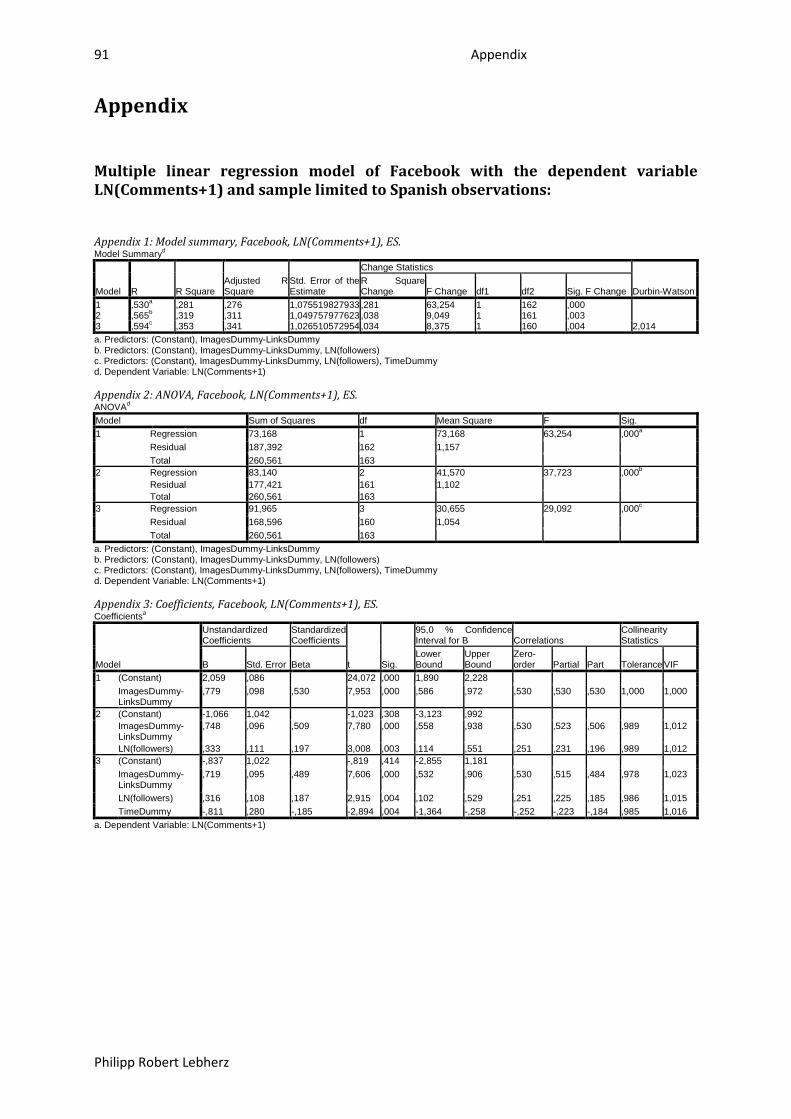
91 Appendix
Philipp Robert Lebherz
Appendix
Multiple linear regression model of Facebook with the dependent variable LN(Comments+1) and sample limited to Spanish observations: Appendix 1: Model summary, Facebook, LN(Comments+1), ES. Model Summaryd
Model R R Square Adjusted R Square
Std. Error of the Estimate
Change Statistics
Durbin-Watson R Square Change F Change df1 df2 Sig. F Change
1 ,530 ,281 a ,276 1,075519827933 ,281 63,254 1 162 ,000 2 ,565 ,319 b ,311 1,049757977623 ,038 9,049 1 161 ,003 3 ,594 ,353 c ,341 1,026510572954 ,034 8,375 1 160 ,004 2,014 a. Predictors: (Constant), ImagesDummy-LinksDummy b. Predictors: (Constant), ImagesDummy-LinksDummy, LN(followers) c. Predictors: (Constant), ImagesDummy-LinksDummy, LN(followers), TimeDummy d. Dependent Variable: LN(Comments+1) Appendix 2: ANOVA, Facebook, LN(Comments+1), ES. ANOVAModel
d Sum of Squares df Mean Square F Sig.
1 Regression 73,168 1 73,168 63,254 ,000a Residual 187,392 162 1,157 Total 260,561 163
2 Regression 83,140 2 41,570 37,723 ,000b Residual 177,421 161 1,102 Total 260,561 163
3 Regression 91,965 3 30,655 29,092 ,000c Residual 168,596 160 1,054 Total 260,561 163
a. Predictors: (Constant), ImagesDummy-LinksDummy b. Predictors: (Constant), ImagesDummy-LinksDummy, LN(followers) c. Predictors: (Constant), ImagesDummy-LinksDummy, LN(followers), TimeDummy d. Dependent Variable: LN(Comments+1) Appendix 3: Coefficients, Facebook, LN(Comments+1), ES. Coefficientsa
Model
Unstandardized Coefficients
Standardized Coefficients
t Sig.
95,0 % Confidence Interval for B Correlations
Collinearity Statistics
B Std. Error Beta Lower Bound
Upper Bound
Zero-order Partial Part Tolerance VIF
1 (Constant) 2,059 ,086 24,072 ,000 1,890 2,228 ImagesDummy-LinksDummy
,779 ,098 ,530 7,953 ,000 ,586 ,972 ,530 ,530 ,530 1,000 1,000
2 (Constant) -1,066 1,042 -1,023 ,308 -3,123 ,992 ImagesDummy-LinksDummy
,748 ,096 ,509 7,780 ,000 ,558 ,938 ,530 ,523 ,506 ,989 1,012
LN(followers) ,333 ,111 ,197 3,008 ,003 ,114 ,551 ,251 ,231 ,196 ,989 1,012 3 (Constant) -,837 1,022 -,819 ,414 -2,855 1,181
ImagesDummy-LinksDummy
,719 ,095 ,489 7,606 ,000 ,532 ,906 ,530 ,515 ,484 ,978 1,023
LN(followers) ,316 ,108 ,187 2,915 ,004 ,102 ,529 ,251 ,225 ,185 ,986 1,015 TimeDummy -,811 ,280 -,185 -2,894 ,004 -1,364 -,258 -,252 -,223 -,184 ,985 1,016
a. Dependent Variable: LN(Comments+1)
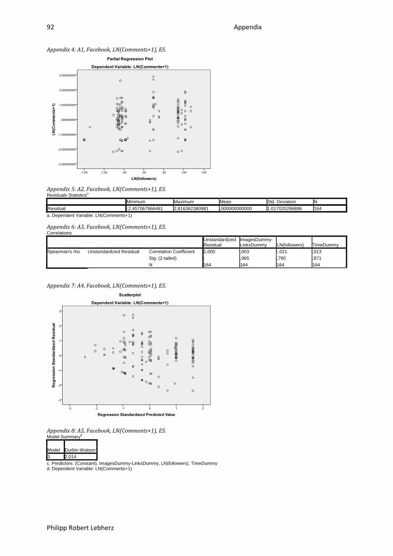
92 Appendix
Philipp Robert Lebherz
Appendix 4: A1, Facebook, LN(Comments+1), ES.
Appendix 5: A2, Facebook, LN(Comments+1), ES. Residuals Statistics
a Minimum Maximum Mean Std. Deviation N
Residual -2,457067966461 2,816362380981 ,000000000000 1,017020286886 164 a. Dependent Variable: LN(Comments+1) Appendix 6: A3, Facebook, LN(Comments+1), ES. Correlations
Unstandardized Residual
ImagesDummy-LinksDummy LN(followers) TimeDummy
Spearman's rho Unstandardized Residual Correlation Coefficient 1,000 ,003 -,021 ,013 Sig. (2-tailed) . ,965 ,790 ,871 N 164 164 164 164
Appendix 7: A4, Facebook, LN(Comments+1), ES.
Appendix 8: A5, Facebook, LN(Comments+1), ES. Model Summaryd
Model Durbin-Watson 3 2,014 c. Predictors: (Constant), ImagesDummy-LinksDummy, LN(followers), TimeDummy d. Dependent Variable: LN(Comments+1)
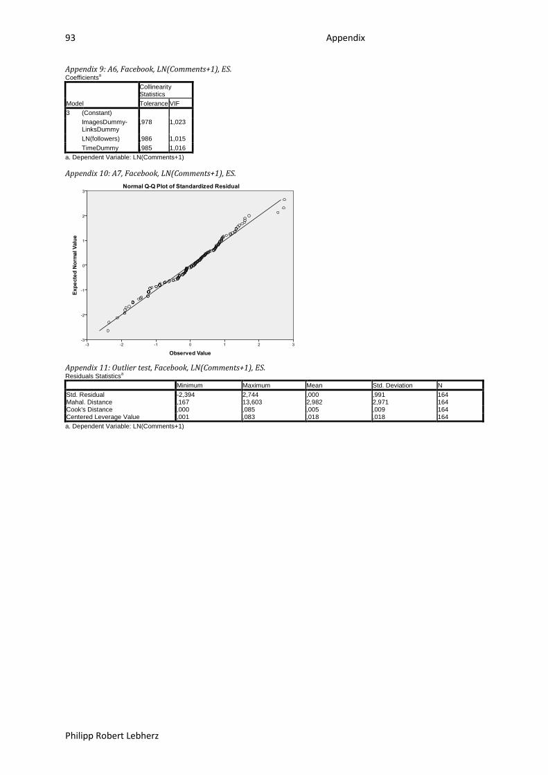
93 Appendix
Philipp Robert Lebherz
Appendix 9: A6, Facebook, LN(Comments+1), ES. Coefficientsa
Model
Collinearity Statistics Tolerance VIF
3 (Constant) ImagesDummy-LinksDummy
,978 1,023
LN(followers) ,986 1,015 TimeDummy ,985 1,016
a. Dependent Variable: LN(Comments+1) Appendix 10: A7, Facebook, LN(Comments+1), ES.
Appendix 11: Outlier test, Facebook, LN(Comments+1), ES. Residuals Statistics
a Minimum Maximum Mean Std. Deviation N
Std. Residual -2,394 2,744 ,000 ,991 164 Mahal. Distance ,167 13,603 2,982 2,971 164 Cook's Distance ,000 ,085 ,005 ,009 164 Centered Leverage Value ,001 ,083 ,018 ,018 164 a. Dependent Variable: LN(Comments+1)
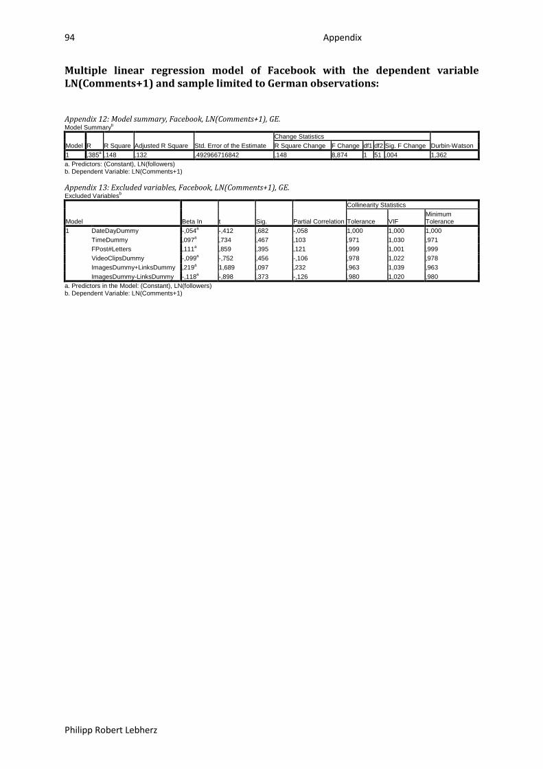
94 Appendix
Philipp Robert Lebherz
Multiple linear regression model of Facebook with the dependent variable LN(Comments+1) and sample limited to German observations: Appendix 12: Model summary, Facebook, LN(Comments+1), GE. Model Summaryb
Model R R Square Adjusted R Square Std. Error of the Estimate Change Statistics
Durbin-Watson R Square Change F Change df1 df2 Sig. F Change 1 ,385 ,148 a ,132 ,492966716842 ,148 8,874 1 51 ,004 1,362 a. Predictors: (Constant), LN(followers) b. Dependent Variable: LN(Comments+1) Appendix 13: Excluded variables, Facebook, LN(Comments+1), GE. Excluded Variablesb
Model Beta In t Sig. Partial Correlation
Collinearity Statistics
Tolerance VIF Minimum Tolerance
1 DateDayDummy -,054 -,412 a ,682 -,058 1,000 1,000 1,000 TimeDummy ,097 ,734 a ,467 ,103 ,971 1,030 ,971 FPost#Letters ,111 ,859 a ,395 ,121 ,999 1,001 ,999 VideoClipsDummy -,099 -,752 a ,456 -,106 ,978 1,022 ,978 ImagesDummy+LinksDummy ,219 1,689 a ,097 ,232 ,963 1,039 ,963 ImagesDummy-LinksDummy -,118 -,898 a ,373 -,126 ,980 1,020 ,980
a. Predictors in the Model: (Constant), LN(followers) b. Dependent Variable: LN(Comments+1)
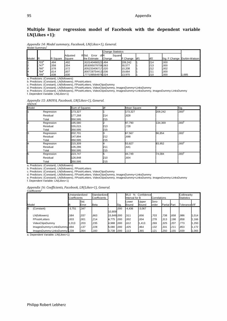
95 Appendix
Philipp Robert Lebherz
Multiple linear regression model of Facebook with the dependent variable LN(Likes +1): Appendix 14: Model summary, Facebook, LN(Likes+1), General. Model Summaryf
Model R R Square Adjusted R Square
Std. Error of the Estimate
Change Statistics
Durbin-Watson R Square Change F Change df1 df2 Sig. F Change
1 ,703 ,494 a ,492 ,910140466523 ,494 209,242 1 214 ,000 2 ,747 ,558 b ,554 ,853095079708 ,063 30,577 1 213 ,000 3 ,760 ,578 c ,572 ,835233406717 ,020 10,208 1 212 ,002 4 ,784 ,614 d ,607 ,800728754413 ,036 19,664 1 211 ,000 5 ,799 ,638 e ,630 ,777198564978 ,024 13,970 1 210 ,000 1,685 a. Predictors: (Constant), LN(followers) b. Predictors: (Constant), LN(followers), FPost#Letters c. Predictors: (Constant), LN(followers), FPost#Letters, VideoClipsDummy d. Predictors: (Constant), LN(followers), FPost#Letters, VideoClipsDummy, ImagesDummy+LinksDummy e. Predictors: (Constant), LN(followers), FPost#Letters, VideoClipsDummy, ImagesDummy+LinksDummy, ImagesDummy-LinksDummy f. Dependent Variable: LN(Likes+1) Appendix 15: ANOVA, Facebook, LN(Likes+1), General. ANOVAModel
f Sum of Squares df Mean Square F Sig.
1 Regression 173,327 1 173,327 209,242 ,000a Residual 177,268 214 ,828 Total 350,595 215
2 Regression 195,580 2 97,790 134,369 ,000b Residual 155,015 213 ,728 Total 350,595 215
3 Regression 202,701 3 67,567 96,854 ,000c Residual 147,894 212 ,698 Total 350,595 215
4 Regression 215,309 4 53,827 83,952 ,000d Residual 135,286 211 ,641 Total 350,595 215
5 Regression 223,747 5 44,749 74,084 ,000e Residual 126,848 210 ,604 Total 350,595 215
a. Predictors: (Constant), LN(followers) b. Predictors: (Constant), LN(followers), FPost#Letters c. Predictors: (Constant), LN(followers), FPost#Letters, VideoClipsDummy d. Predictors: (Constant), LN(followers), FPost#Letters, VideoClipsDummy, ImagesDummy+LinksDummy e. Predictors: (Constant), LN(followers), FPost#Letters, VideoClipsDummy, ImagesDummy+LinksDummy, ImagesDummy-LinksDummy f. Dependent Variable: LN(Likes+1) Appendix 16: Coefficients, Facebook, LN(Likes+1), General. Coefficientsa
Model
Unstandardized Coefficients
Standardized Coefficients
t Sig.
95,0 % Confidence Interval for B Correlations
Collinearity Statistics
B Std. Error Beta
Lower Bound
Upper Bound
Zero-order Partial Part Tolerance VIF
5 (Constant) -3,751 ,347 -10,809
,000 -4,436 -3,067
LN(followers) ,584 ,037 ,663 15,849 ,000 ,511 ,656 ,703 ,738 ,658 ,986 1,014 FPost#Letters ,003 ,001 ,214 4,775 ,000 ,002 ,004 ,278 ,313 ,198 ,858 1,166 VideoClipsDummy 1,013 ,203 ,235 4,988 ,000 ,612 1,413 ,269 ,325 ,207 ,773 1,293 ImagesDummy+LinksDummy ,694 ,137 ,228 5,080 ,000 ,425 ,964 ,132 ,331 ,211 ,853 1,172 ImagesDummy-LinksDummy ,239 ,064 ,160 3,738 ,000 ,113 ,365 ,121 ,250 ,155 ,939 1,065
a. Dependent Variable: LN(Likes+1)
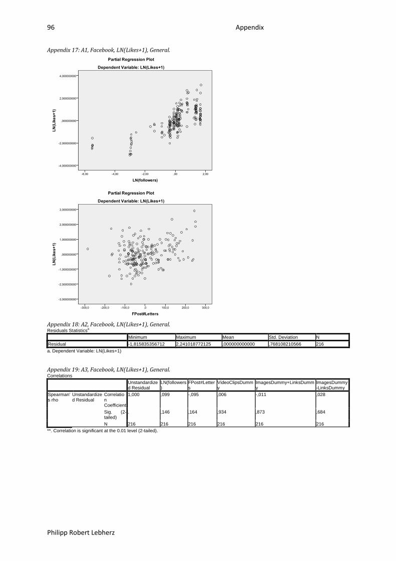
96 Appendix
Philipp Robert Lebherz
Appendix 17: A1, Facebook, LN(Likes+1), General.
Appendix 18: A2, Facebook, LN(Likes+1), General. Residuals Statistics
a Minimum Maximum Mean Std. Deviation N
Residual -1,815835356712 2,241018772125 ,000000000000 ,768108210566 216 a. Dependent Variable: LN(Likes+1) Appendix 19: A3, Facebook, LN(Likes+1), General. Correlations
Unstandardized Residual
LN(followers)
FPost#Letters
VideoClipsDummy
ImagesDummy+LinksDummy
ImagesDummy-LinksDummy
Spearman's rho
Unstandardized Residual
Correlation Coefficient
1,000 ,099 -,095 ,006 -,011 ,028
Sig. (2-tailed)
. ,146 ,164 ,934 ,873 ,684
N 216 216 216 216 216 216 **. Correlation is significant at the 0.01 level (2-tailed).
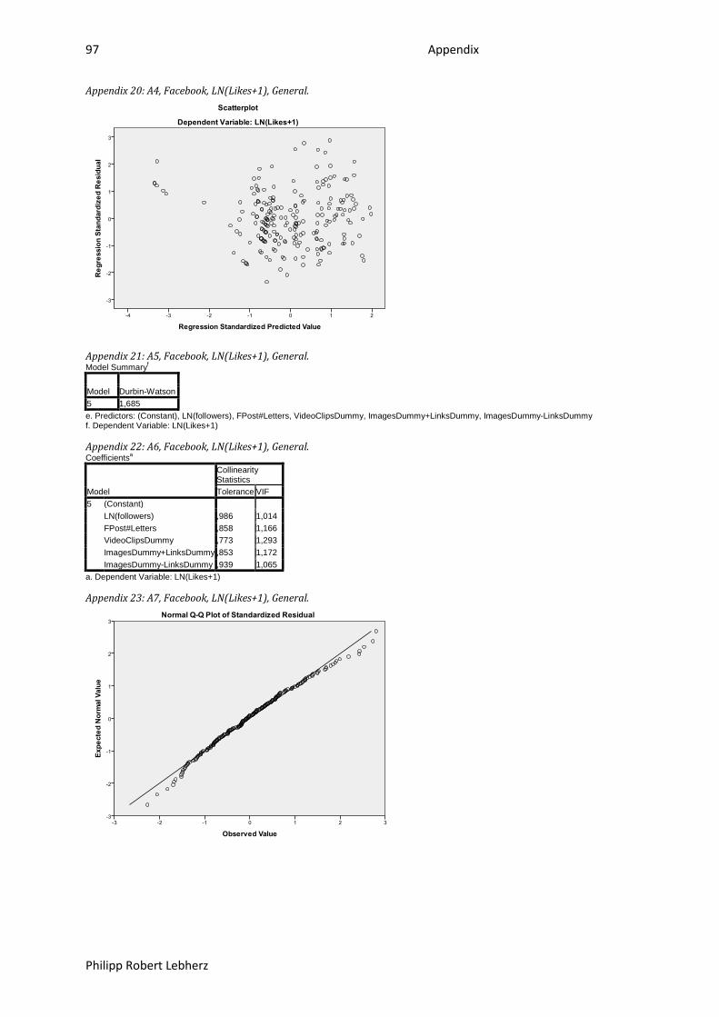
97 Appendix
Philipp Robert Lebherz
Appendix 20: A4, Facebook, LN(Likes+1), General.
Appendix 21: A5, Facebook, LN(Likes+1), General. Model Summaryf
Model Durbin-Watson 5 1,685 e. Predictors: (Constant), LN(followers), FPost#Letters, VideoClipsDummy, ImagesDummy+LinksDummy, ImagesDummy-LinksDummy f. Dependent Variable: LN(Likes+1) Appendix 22: A6, Facebook, LN(Likes+1), General. Coefficientsa
Model
Collinearity Statistics Tolerance VIF
5 (Constant) LN(followers) ,986 1,014 FPost#Letters ,858 1,166 VideoClipsDummy ,773 1,293 ImagesDummy+LinksDummy ,853 1,172 ImagesDummy-LinksDummy ,939 1,065
a. Dependent Variable: LN(Likes+1) Appendix 23: A7, Facebook, LN(Likes+1), General.

98 Appendix
Philipp Robert Lebherz
Appendix 24: Outlier test, Facebook, LN(Likes+1), General. Residuals Statistics
a Minimum Maximum Mean Std. Deviation N
Std. Residual -2,336 2,883 ,000 ,988 216 Mahal. Distance 1,100 22,278 4,977 3,934 216 Cook's Distance ,000 ,067 ,006 ,011 216 Centered Leverage Value ,005 ,104 ,023 ,018 216 a. Dependent Variable: LN(Likes+1)
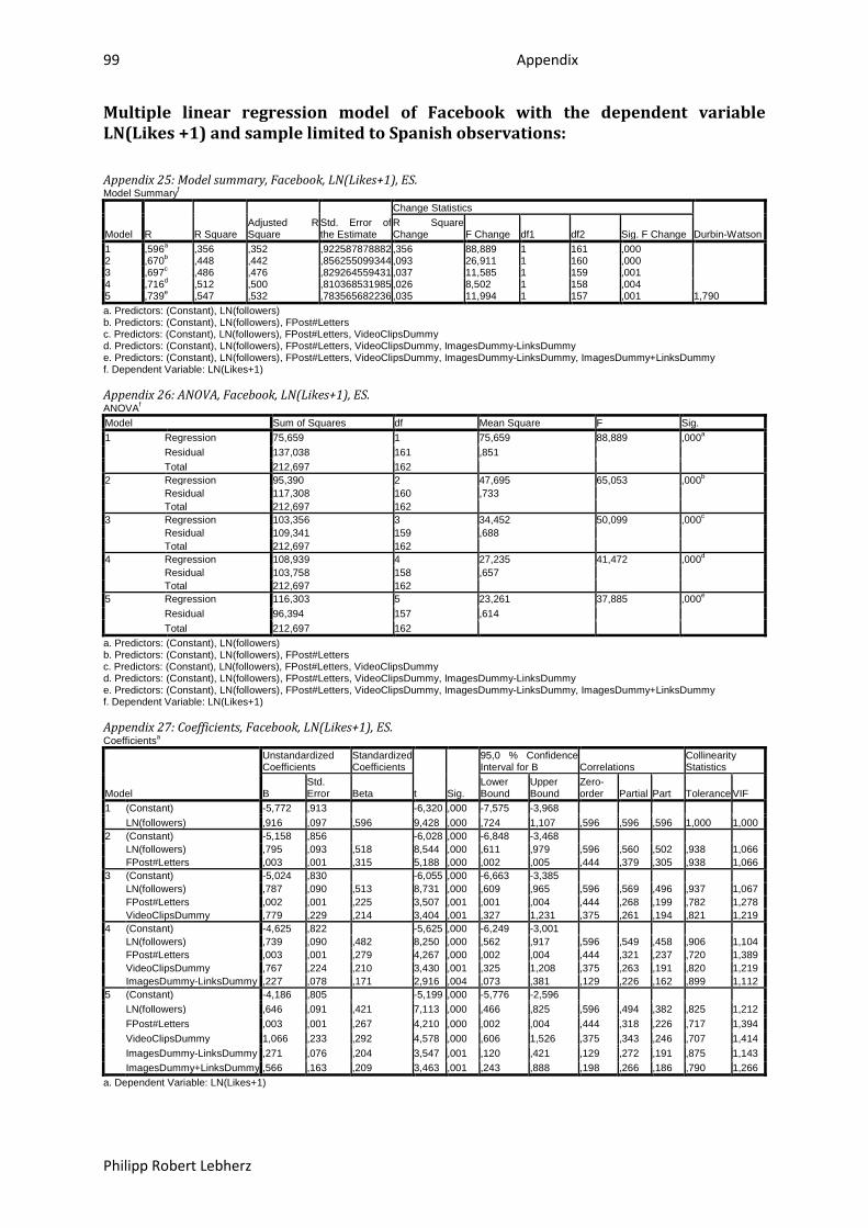
99 Appendix
Philipp Robert Lebherz
Multiple linear regression model of Facebook with the dependent variable LN(Likes +1) and sample limited to Spanish observations: Appendix 25: Model summary, Facebook, LN(Likes+1), ES. Model Summaryf
Model R R Square Adjusted R Square
Std. Error of the Estimate
Change Statistics
Durbin-Watson R Square Change F Change df1 df2 Sig. F Change
1 ,596 ,356 a ,352 ,922587878882 ,356 88,889 1 161 ,000 2 ,670 ,448 b ,442 ,856255099344 ,093 26,911 1 160 ,000 3 ,697 ,486 c ,476 ,829264559431 ,037 11,585 1 159 ,001 4 ,716 ,512 d ,500 ,810368531985 ,026 8,502 1 158 ,004 5 ,739 ,547 e ,532 ,783565682236 ,035 11,994 1 157 ,001 1,790 a. Predictors: (Constant), LN(followers) b. Predictors: (Constant), LN(followers), FPost#Letters c. Predictors: (Constant), LN(followers), FPost#Letters, VideoClipsDummy d. Predictors: (Constant), LN(followers), FPost#Letters, VideoClipsDummy, ImagesDummy-LinksDummy e. Predictors: (Constant), LN(followers), FPost#Letters, VideoClipsDummy, ImagesDummy-LinksDummy, ImagesDummy+LinksDummy f. Dependent Variable: LN(Likes+1) Appendix 26: ANOVA, Facebook, LN(Likes+1), ES. ANOVAModel
f Sum of Squares df Mean Square F Sig.
1 Regression 75,659 1 75,659 88,889 ,000a Residual 137,038 161 ,851 Total 212,697 162
2 Regression 95,390 2 47,695 65,053 ,000b Residual 117,308 160 ,733 Total 212,697 162
3 Regression 103,356 3 34,452 50,099 ,000c Residual 109,341 159 ,688 Total 212,697 162
4 Regression 108,939 4 27,235 41,472 ,000d Residual 103,758 158 ,657 Total 212,697 162
5 Regression 116,303 5 23,261 37,885 ,000e Residual 96,394 157 ,614 Total 212,697 162
a. Predictors: (Constant), LN(followers) b. Predictors: (Constant), LN(followers), FPost#Letters c. Predictors: (Constant), LN(followers), FPost#Letters, VideoClipsDummy d. Predictors: (Constant), LN(followers), FPost#Letters, VideoClipsDummy, ImagesDummy-LinksDummy e. Predictors: (Constant), LN(followers), FPost#Letters, VideoClipsDummy, ImagesDummy-LinksDummy, ImagesDummy+LinksDummy f. Dependent Variable: LN(Likes+1) Appendix 27: Coefficients, Facebook, LN(Likes+1), ES. Coefficientsa
Model
Unstandardized Coefficients
Standardized Coefficients
t Sig.
95,0 % Confidence Interval for B Correlations
Collinearity Statistics
B Std. Error Beta
Lower Bound
Upper Bound
Zero-order Partial Part Tolerance VIF
1 (Constant) -5,772 ,913 -6,320 ,000 -7,575 -3,968 LN(followers) ,916 ,097 ,596 9,428 ,000 ,724 1,107 ,596 ,596 ,596 1,000 1,000
2 (Constant) -5,158 ,856 -6,028 ,000 -6,848 -3,468 LN(followers) ,795 ,093 ,518 8,544 ,000 ,611 ,979 ,596 ,560 ,502 ,938 1,066 FPost#Letters ,003 ,001 ,315 5,188 ,000 ,002 ,005 ,444 ,379 ,305 ,938 1,066
3 (Constant) -5,024 ,830 -6,055 ,000 -6,663 -3,385 LN(followers) ,787 ,090 ,513 8,731 ,000 ,609 ,965 ,596 ,569 ,496 ,937 1,067 FPost#Letters ,002 ,001 ,225 3,507 ,001 ,001 ,004 ,444 ,268 ,199 ,782 1,278 VideoClipsDummy ,779 ,229 ,214 3,404 ,001 ,327 1,231 ,375 ,261 ,194 ,821 1,219
4 (Constant) -4,625 ,822 -5,625 ,000 -6,249 -3,001 LN(followers) ,739 ,090 ,482 8,250 ,000 ,562 ,917 ,596 ,549 ,458 ,906 1,104 FPost#Letters ,003 ,001 ,279 4,267 ,000 ,002 ,004 ,444 ,321 ,237 ,720 1,389 VideoClipsDummy ,767 ,224 ,210 3,430 ,001 ,325 1,208 ,375 ,263 ,191 ,820 1,219 ImagesDummy-LinksDummy ,227 ,078 ,171 2,916 ,004 ,073 ,381 ,129 ,226 ,162 ,899 1,112
5 (Constant) -4,186 ,805 -5,199 ,000 -5,776 -2,596 LN(followers) ,646 ,091 ,421 7,113 ,000 ,466 ,825 ,596 ,494 ,382 ,825 1,212 FPost#Letters ,003 ,001 ,267 4,210 ,000 ,002 ,004 ,444 ,318 ,226 ,717 1,394 VideoClipsDummy 1,066 ,233 ,292 4,578 ,000 ,606 1,526 ,375 ,343 ,246 ,707 1,414 ImagesDummy-LinksDummy ,271 ,076 ,204 3,547 ,001 ,120 ,421 ,129 ,272 ,191 ,875 1,143 ImagesDummy+LinksDummy ,566 ,163 ,209 3,463 ,001 ,243 ,888 ,198 ,266 ,186 ,790 1,266
a. Dependent Variable: LN(Likes+1)
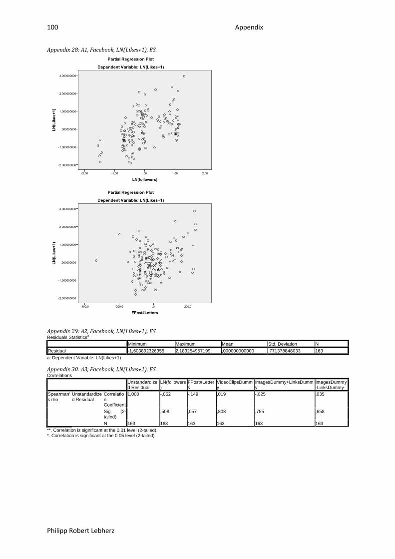
100 Appendix
Philipp Robert Lebherz
Appendix 28: A1, Facebook, LN(Likes+1), ES.
Appendix 29: A2, Facebook, LN(Likes+1), ES. Residuals Statistics
a Minimum Maximum Mean Std. Deviation N
Residual -1,603892326355 2,183254957199 ,000000000000 ,771378848033 163 a. Dependent Variable: LN(Likes+1) Appendix 30: A3, Facebook, LN(Likes+1), ES. Correlations
Unstandardized Residual
LN(followers)
FPost#Letters
VideoClipsDummy
ImagesDummy+LinksDummy
ImagesDummy-LinksDummy
Spearman's rho
Unstandardized Residual
Correlation Coefficient
1,000 -,052 -,149 ,019 -,025 ,035
Sig. (2-tailed)
. ,508 ,057 ,808 ,755 ,658
N 163 163 163 163 163 163 **. Correlation is significant at the 0.01 level (2-tailed). *. Correlation is significant at the 0.05 level (2-tailed).
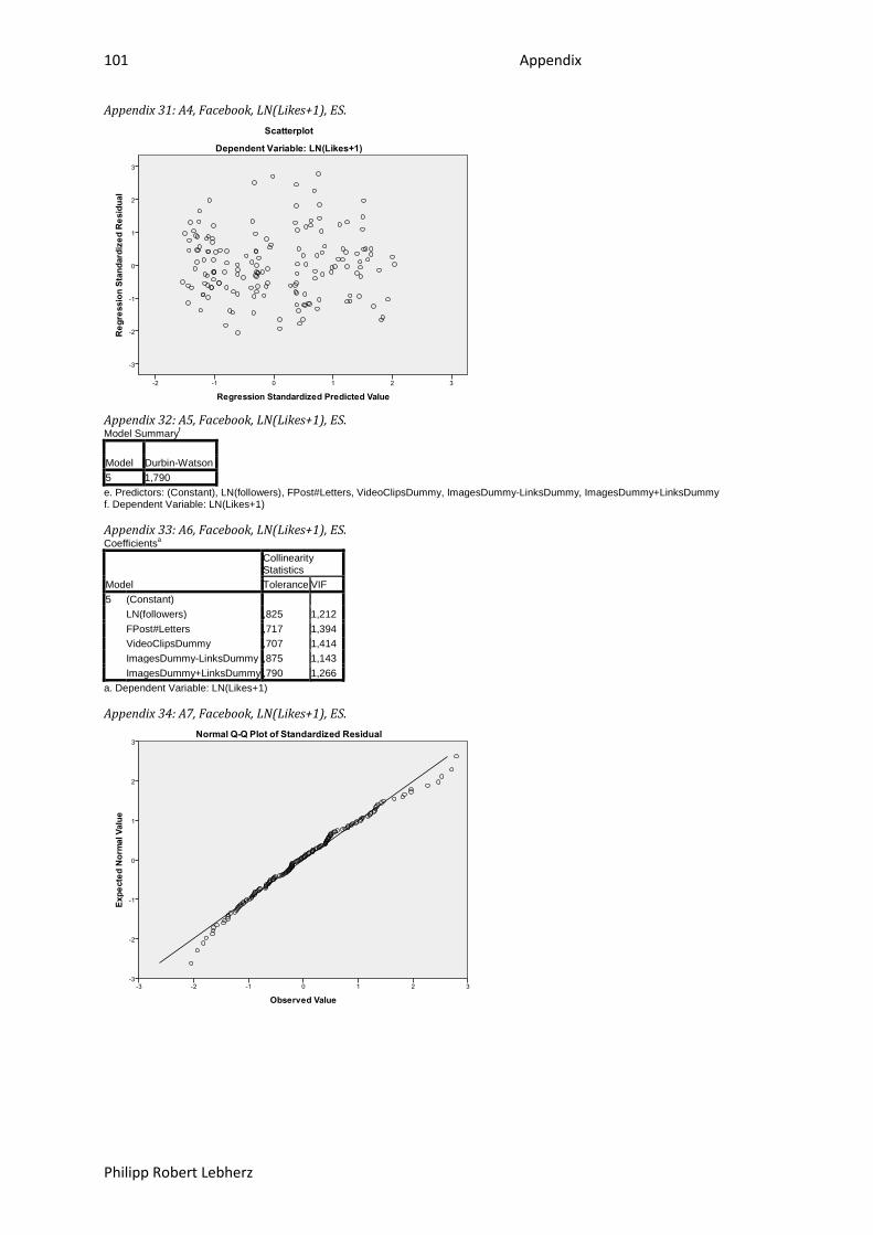
101 Appendix
Philipp Robert Lebherz
Appendix 31: A4, Facebook, LN(Likes+1), ES.
Appendix 32: A5, Facebook, LN(Likes+1), ES. Model Summaryf
Model Durbin-Watson 5 1,790 e. Predictors: (Constant), LN(followers), FPost#Letters, VideoClipsDummy, ImagesDummy-LinksDummy, ImagesDummy+LinksDummy f. Dependent Variable: LN(Likes+1) Appendix 33: A6, Facebook, LN(Likes+1), ES. Coefficientsa
Model
Collinearity Statistics Tolerance VIF
5 (Constant) LN(followers) ,825 1,212 FPost#Letters ,717 1,394 VideoClipsDummy ,707 1,414 ImagesDummy-LinksDummy ,875 1,143 ImagesDummy+LinksDummy ,790 1,266
a. Dependent Variable: LN(Likes+1) Appendix 34: A7, Facebook, LN(Likes+1), ES.

102 Appendix
Philipp Robert Lebherz
Appendix 35: Outlier test, Facebook, LN(Likes+1), ES. Residuals Statistics
a Minimum Maximum Mean Std. Deviation N
Std. Residual -2,047 2,786 ,000 ,984 163 Mahal. Distance 1,346 24,166 4,969 2,980 163 Cook's Distance ,000 ,082 ,007 ,013 163 Centered Leverage Value ,008 ,149 ,031 ,018 163 a. Dependent Variable: LN(Likes+1)
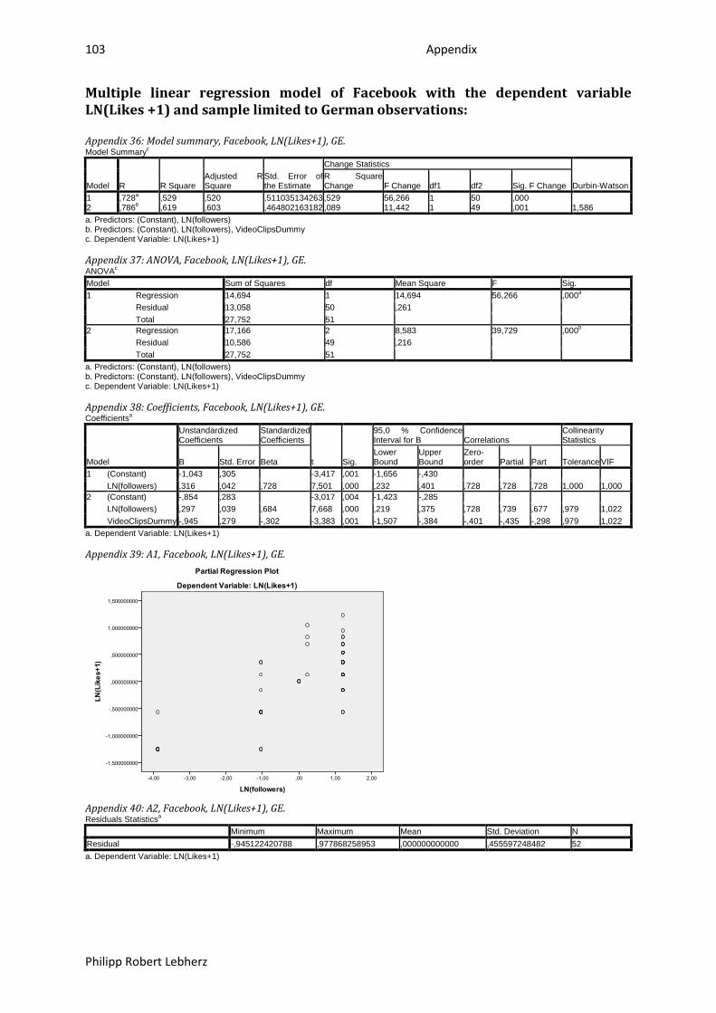
103 Appendix
Philipp Robert Lebherz
Multiple linear regression model of Facebook with the dependent variable LN(Likes +1) and sample limited to German observations: Appendix 36: Model summary, Facebook, LN(Likes+1), GE. Model Summaryc
Model R R Square Adjusted R Square
Std. Error of the Estimate
Change Statistics
Durbin-Watson R Square Change F Change df1 df2 Sig. F Change
1 ,728 ,529 a ,520 ,511035134263 ,529 56,266 1 50 ,000 2 ,786 ,619 b ,603 ,464802163182 ,089 11,442 1 49 ,001 1,586 a. Predictors: (Constant), LN(followers) b. Predictors: (Constant), LN(followers), VideoClipsDummy c. Dependent Variable: LN(Likes+1) Appendix 37: ANOVA, Facebook, LN(Likes+1), GE. ANOVAModel
c Sum of Squares df Mean Square F Sig.
1 Regression 14,694 1 14,694 56,266 ,000a Residual 13,058 50 ,261 Total 27,752 51
2 Regression 17,166 2 8,583 39,729 ,000b Residual 10,586 49 ,216 Total 27,752 51
a. Predictors: (Constant), LN(followers) b. Predictors: (Constant), LN(followers), VideoClipsDummy c. Dependent Variable: LN(Likes+1) Appendix 38: Coefficients, Facebook, LN(Likes+1), GE. Coefficientsa
Model
Unstandardized Coefficients
Standardized Coefficients
t Sig.
95,0 % Confidence Interval for B Correlations
Collinearity Statistics
B Std. Error Beta Lower Bound
Upper Bound
Zero-order Partial Part Tolerance VIF
1 (Constant) -1,043 ,305 -3,417 ,001 -1,656 -,430 LN(followers) ,316 ,042 ,728 7,501 ,000 ,232 ,401 ,728 ,728 ,728 1,000 1,000
2 (Constant) -,854 ,283 -3,017 ,004 -1,423 -,285 LN(followers) ,297 ,039 ,684 7,668 ,000 ,219 ,375 ,728 ,739 ,677 ,979 1,022 VideoClipsDummy -,945 ,279 -,302 -3,383 ,001 -1,507 -,384 -,401 -,435 -,298 ,979 1,022
a. Dependent Variable: LN(Likes+1) Appendix 39: A1, Facebook, LN(Likes+1), GE.
Appendix 40: A2, Facebook, LN(Likes+1), GE. Residuals Statistics
a Minimum Maximum Mean Std. Deviation N
Residual -,945122420788 ,977868258953 ,000000000000 ,455597248482 52 a. Dependent Variable: LN(Likes+1)
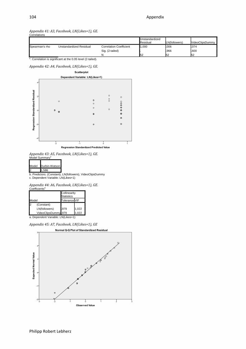
104 Appendix
Philipp Robert Lebherz
Appendix 41: A3, Facebook, LN(Likes+1), GE. Correlations
Unstandardized Residual LN(followers) VideoClipsDummy
Spearman's rho Unstandardized Residual Correlation Coefficient 1,000 ,006 ,074 Sig. (2-tailed) . ,966 ,600 N 52 52 52
*. Correlation is significant at the 0.05 level (2-tailed). Appendix 42: A4, Facebook, LN(Likes+1), GE.
Appendix 43: A5, Facebook, LN(Likes+1), GE. Model Summaryc
Model Durbin-Watson 2 1,586 b. Predictors: (Constant), LN(followers), VideoClipsDummy c. Dependent Variable: LN(Likes+1) Appendix 44: A6, Facebook, LN(Likes+1), GE. Coefficientsa
Model
Collinearity Statistics Tolerance VIF
2 (Constant) LN(followers) ,979 1,022 VideoClipsDummy ,979 1,022
a. Dependent Variable: LN(Likes+1) Appendix 45: A7, Facebook, LN(Likes+1), GE

105 Appendix
Philipp Robert Lebherz
Appendix 46: Outlier test, Facebook, LN(Likes+1), GE. Residuals Statistics
a Minimum Maximum Mean Std. Deviation N
Std. Residual -2,033 2,104 ,000 ,980 52 Mahal. Distance ,079 16,019 1,962 3,852 52 Cook's Distance ,000 ,088 ,011 ,017 52 Centered Leverage Value ,002 ,314 ,038 ,076 52 a. Dependent Variable: LN(Likes+1)
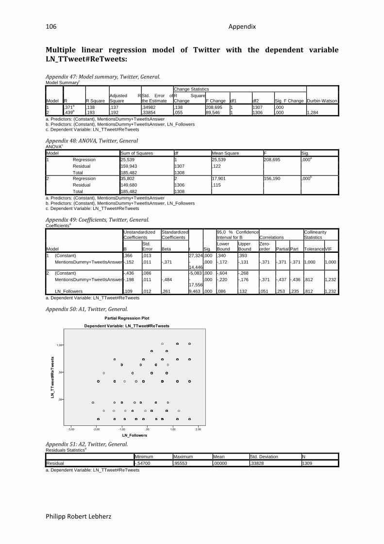
106 Appendix
Philipp Robert Lebherz
Multiple linear regression model of Twitter with the dependent variable LN_TTweet#ReTweets: Appendix 47: Model summary, Twitter, General. Model Summaryc
Model R R Square Adjusted R Square
Std. Error of the Estimate
Change Statistics
Durbin-Watson R Square Change F Change df1 df2 Sig. F Change
1 ,371 ,138 a ,137 ,34982 ,138 208,695 1 1307 ,000 2 ,439 ,193 b ,192 ,33854 ,055 89,546 1 1306 ,000 1,284 a. Predictors: (Constant), MentionsDummy+TweetIsAnswer b. Predictors: (Constant), MentionsDummy+TweetIsAnswer, LN_Followers c. Dependent Variable: LN_TTweet#ReTweets Appendix 48: ANOVA, Twitter, General ANOVAModel
c Sum of Squares df Mean Square F Sig.
1 Regression 25,539 1 25,539 208,695 ,000a Residual 159,943 1307 ,122 Total 185,482 1308
2 Regression 35,802 2 17,901 156,190 ,000b Residual 149,680 1306 ,115 Total 185,482 1308
a. Predictors: (Constant), MentionsDummy+TweetIsAnswer b. Predictors: (Constant), MentionsDummy+TweetIsAnswer, LN_Followers c. Dependent Variable: LN_TTweet#ReTweets Appendix 49: Coefficients, Twitter, General. Coefficientsa
Model
Unstandardized Coefficients
Standardized Coefficients
t Sig.
95,0 % Confidence Interval for B Correlations
Collinearity Statistics
B Std. Error Beta
Lower Bound
Upper Bound
Zero-order Partial Part Tolerance VIF
1 (Constant) ,366 ,013 27,324 ,000 ,340 ,393 MentionsDummy+TweetIsAnswer -,152 ,011 -,371 -
14,446 ,000 -,172 -,131 -,371 -,371 -,371 1,000 1,000
2 (Constant) -,436 ,086 -5,083 ,000 -,604 -,268 MentionsDummy+TweetIsAnswer -,198 ,011 -,484 -
17,556 ,000 -,220 -,176 -,371 -,437 -,436 ,812 1,232
LN_Followers ,109 ,012 ,261 9,463 ,000 ,086 ,132 ,051 ,253 ,235 ,812 1,232 a. Dependent Variable: LN_TTweet#ReTweets Appendix 50: A1, Twitter, General.
Appendix 51: A2, Twitter, General. Residuals Statistics
a Minimum Maximum Mean Std. Deviation N
Residual -,54700 ,95553 ,00000 ,33828 1309 a. Dependent Variable: LN_TTweet#ReTweets
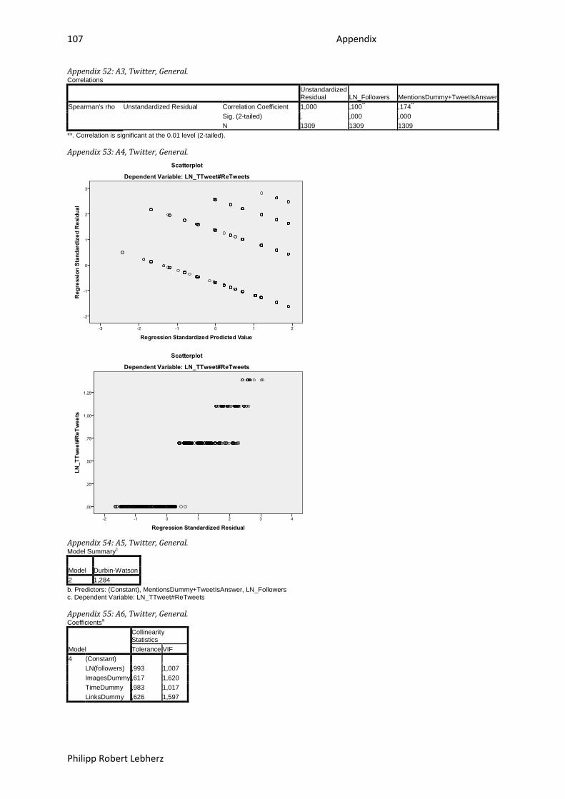
107 Appendix
Philipp Robert Lebherz
Appendix 52: A3, Twitter, General. Correlations
Unstandardized Residual LN_Followers MentionsDummy+TweetIsAnswer
Spearman's rho Unstandardized Residual Correlation Coefficient 1,000 ,100 ,174** ** Sig. (2-tailed) . ,000 ,000 N 1309 1309 1309
**. Correlation is significant at the 0.01 level (2-tailed). Appendix 53: A4, Twitter, General.
Appendix 54: A5, Twitter, General. Model Summaryc
Model Durbin-Watson 2 1,284 b. Predictors: (Constant), MentionsDummy+TweetIsAnswer, LN_Followers c. Dependent Variable: LN_TTweet#ReTweets Appendix 55: A6, Twitter, General. Coefficientsa
Model
Collinearity Statistics Tolerance VIF
4 (Constant) LN(followers) ,993 1,007 ImagesDummy ,617 1,620 TimeDummy ,983 1,017 LinksDummy ,626 1,597
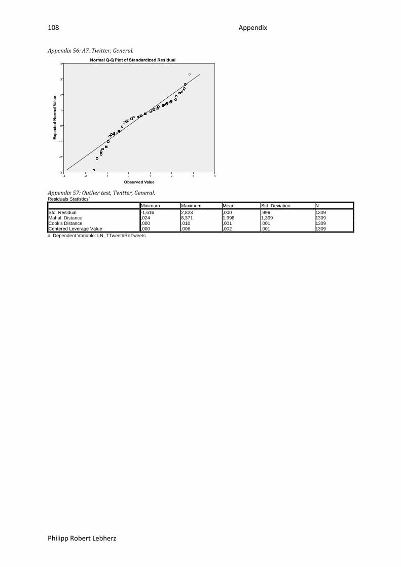
108 Appendix
Philipp Robert Lebherz
Appendix 56: A7, Twitter, General.
Appendix 57: Outlier test, Twitter, General. Residuals Statistics
a Minimum Maximum Mean Std. Deviation N
Std. Residual -1,616 2,823 ,000 ,999 1309 Mahal. Distance ,024 8,371 1,998 1,399 1309 Cook's Distance ,000 ,010 ,001 ,001 1309 Centered Leverage Value ,000 ,006 ,002 ,001 1309 a. Dependent Variable: LN_TTweet#ReTweets
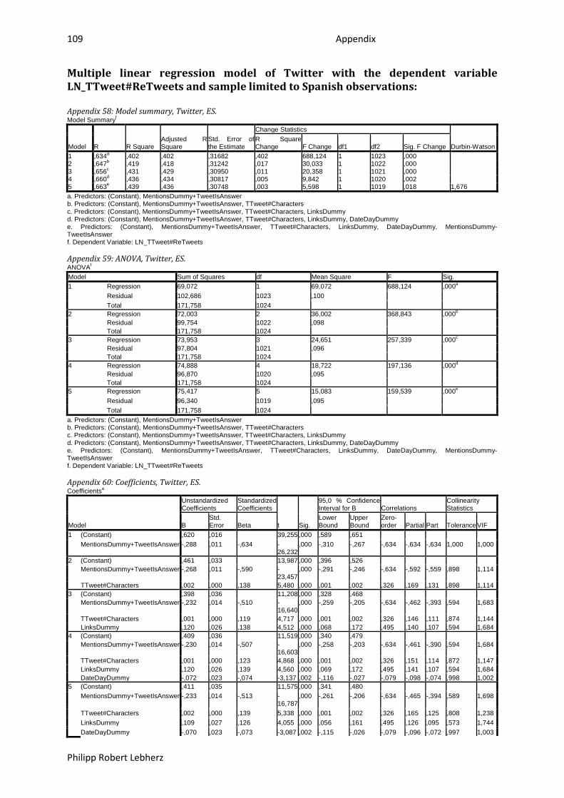
109 Appendix
Philipp Robert Lebherz
Multiple linear regression model of Twitter with the dependent variable LN_TTweet#ReTweets and sample limited to Spanish observations: Appendix 58: Model summary, Twitter, ES. Model Summaryf
Model R R Square Adjusted R Square
Std. Error of the Estimate
Change Statistics
Durbin-Watson R Square Change F Change df1 df2 Sig. F Change
1 ,634 ,402 a ,402 ,31682 ,402 688,124 1 1023 ,000 2 ,647 ,419 b ,418 ,31242 ,017 30,033 1 1022 ,000 3 ,656 ,431 c ,429 ,30950 ,011 20,358 1 1021 ,000 4 ,660 ,436 d ,434 ,30817 ,005 9,842 1 1020 ,002 5 ,663 ,439 e ,436 ,30748 ,003 5,598 1 1019 ,018 1,676 a. Predictors: (Constant), MentionsDummy+TweetIsAnswer b. Predictors: (Constant), MentionsDummy+TweetIsAnswer, TTweet#Characters c. Predictors: (Constant), MentionsDummy+TweetIsAnswer, TTweet#Characters, LinksDummy d. Predictors: (Constant), MentionsDummy+TweetIsAnswer, TTweet#Characters, LinksDummy, DateDayDummy e. Predictors: (Constant), MentionsDummy+TweetIsAnswer, TTweet#Characters, LinksDummy, DateDayDummy, MentionsDummy-TweetIsAnswer f. Dependent Variable: LN_TTweet#ReTweets Appendix 59: ANOVA, Twitter, ES. ANOVAModel
f Sum of Squares df Mean Square F Sig.
1 Regression 69,072 1 69,072 688,124 ,000a Residual 102,686 1023 ,100 Total 171,758 1024
2 Regression 72,003 2 36,002 368,843 ,000b Residual 99,754 1022 ,098 Total 171,758 1024
3 Regression 73,953 3 24,651 257,339 ,000c Residual 97,804 1021 ,096 Total 171,758 1024
4 Regression 74,888 4 18,722 197,136 ,000d Residual 96,870 1020 ,095 Total 171,758 1024
5 Regression 75,417 5 15,083 159,539 ,000e Residual 96,340 1019 ,095 Total 171,758 1024
a. Predictors: (Constant), MentionsDummy+TweetIsAnswer b. Predictors: (Constant), MentionsDummy+TweetIsAnswer, TTweet#Characters c. Predictors: (Constant), MentionsDummy+TweetIsAnswer, TTweet#Characters, LinksDummy d. Predictors: (Constant), MentionsDummy+TweetIsAnswer, TTweet#Characters, LinksDummy, DateDayDummy e. Predictors: (Constant), MentionsDummy+TweetIsAnswer, TTweet#Characters, LinksDummy, DateDayDummy, MentionsDummy-TweetIsAnswer f. Dependent Variable: LN_TTweet#ReTweets Appendix 60: Coefficients, Twitter, ES. Coefficientsa
Model
Unstandardized Coefficients
Standardized Coefficients
t Sig.
95,0 % Confidence Interval for B Correlations
Collinearity Statistics
B Std. Error Beta
Lower Bound
Upper Bound
Zero-order Partial Part Tolerance VIF
1 (Constant) ,620 ,016 39,255 ,000 ,589 ,651 MentionsDummy+TweetIsAnswer -,288 ,011 -,634 -
26,232 ,000 -,310 -,267 -,634 -,634 -,634 1,000 1,000
2 (Constant) ,461 ,033 13,987 ,000 ,396 ,526 MentionsDummy+TweetIsAnswer -,268 ,011 -,590 -
23,457 ,000 -,291 -,246 -,634 -,592 -,559 ,898 1,114
TTweet#Characters ,002 ,000 ,138 5,480 ,000 ,001 ,002 ,326 ,169 ,131 ,898 1,114 3 (Constant) ,398 ,036 11,208 ,000 ,328 ,468
MentionsDummy+TweetIsAnswer -,232 ,014 -,510 -16,640
,000 -,259 -,205 -,634 -,462 -,393 ,594 1,683
TTweet#Characters ,001 ,000 ,119 4,717 ,000 ,001 ,002 ,326 ,146 ,111 ,874 1,144 LinksDummy ,120 ,026 ,138 4,512 ,000 ,068 ,172 ,495 ,140 ,107 ,594 1,684
4 (Constant) ,409 ,036 11,519 ,000 ,340 ,479 MentionsDummy+TweetIsAnswer -,230 ,014 -,507 -
16,603 ,000 -,258 -,203 -,634 -,461 -,390 ,594 1,684
TTweet#Characters ,001 ,000 ,123 4,868 ,000 ,001 ,002 ,326 ,151 ,114 ,872 1,147 LinksDummy ,120 ,026 ,139 4,560 ,000 ,069 ,172 ,495 ,141 ,107 ,594 1,684 DateDayDummy -,072 ,023 -,074 -3,137 ,002 -,116 -,027 -,079 -,098 -,074 ,998 1,002
5 (Constant) ,411 ,035 11,575 ,000 ,341 ,480 MentionsDummy+TweetIsAnswer -,233 ,014 -,513 -
16,787 ,000 -,261 -,206 -,634 -,465 -,394 ,589 1,698
TTweet#Characters ,002 ,000 ,139 5,338 ,000 ,001 ,002 ,326 ,165 ,125 ,808 1,238 LinksDummy ,109 ,027 ,126 4,055 ,000 ,056 ,161 ,495 ,126 ,095 ,573 1,744 DateDayDummy -,070 ,023 -,073 -3,087 ,002 -,115 -,026 -,079 -,096 -,072 ,997 1,003
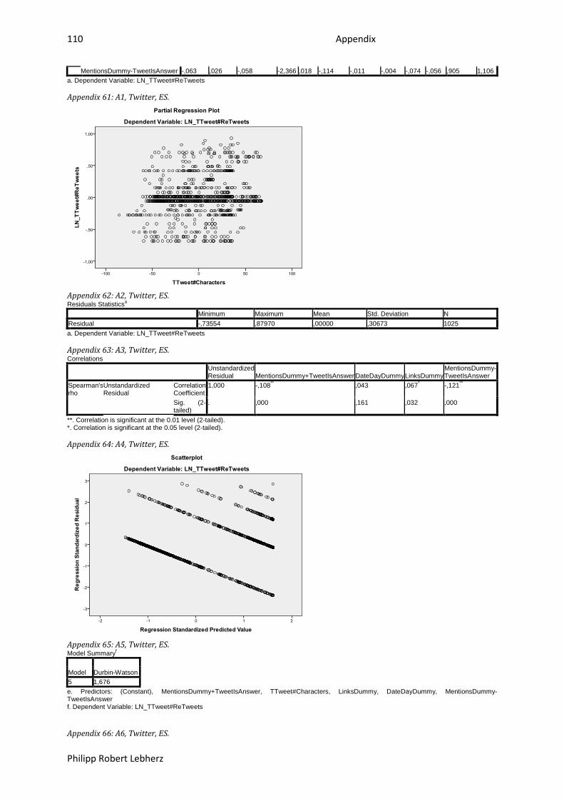
110 Appendix
Philipp Robert Lebherz
MentionsDummy-TweetIsAnswer -,063 ,026 -,058 -2,366 ,018 -,114 -,011 -,004 -,074 -,056 ,905 1,106 a. Dependent Variable: LN_TTweet#ReTweets Appendix 61: A1, Twitter, ES.
Appendix 62: A2, Twitter, ES. Residuals Statistics
a Minimum Maximum Mean Std. Deviation N
Residual -,73554 ,87970 ,00000 ,30673 1025 a. Dependent Variable: LN_TTweet#ReTweets Appendix 63: A3, Twitter, ES. Correlations
Unstandardized Residual MentionsDummy+TweetIsAnswer DateDayDummy LinksDummy
MentionsDummy-TweetIsAnswer
Spearman's rho
Unstandardized Residual
Correlation Coefficient
1,000 -,108** ,043 ,067* -,121**
Sig. (2-tailed)
. ,000 ,161 ,032 ,000
**. Correlation is significant at the 0.01 level (2-tailed). *. Correlation is significant at the 0.05 level (2-tailed). Appendix 64: A4, Twitter, ES.
Appendix 65: A5, Twitter, ES. Model Summaryf
Model Durbin-Watson 5 1,676 e. Predictors: (Constant), MentionsDummy+TweetIsAnswer, TTweet#Characters, LinksDummy, DateDayDummy, MentionsDummy-TweetIsAnswer f. Dependent Variable: LN_TTweet#ReTweets Appendix 66: A6, Twitter, ES.
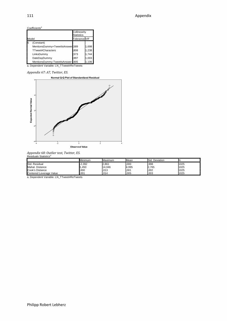
111 Appendix
Philipp Robert Lebherz
Coefficientsa
Model
Collinearity Statistics Tolerance VIF
5 (Constant) MentionsDummy+TweetIsAnswer ,589 1,698 TTweet#Characters ,808 1,238 LinksDummy ,573 1,744 DateDayDummy ,997 1,003 MentionsDummy-TweetIsAnswer ,905 1,106
a. Dependent Variable: LN_TTweet#ReTweets Appendix 67: A7, Twitter, ES.
Appendix 68: Outlier test, Twitter, ES. Residuals Statistics
a Minimum Maximum Mean Std. Deviation N
Std. Residual -2,392 2,861 ,000 ,998 1025 Mahal. Distance 1,450 14,046 4,995 2,765 1025 Cook's Distance ,000 ,013 ,001 ,002 1025 Centered Leverage Value ,001 ,014 ,005 ,003 1025 a. Dependent Variable: LN_TTweet#ReTweets

112 Appendix
Philipp Robert Lebherz
Multiple linear regression model of Twitter with the dependent variable LN_TTweet#ReTweets and sample limited to German observations: Appendix 69: Model summary, Twitter, GE. Model Summaryb
Model R R Square Adjusted R Square
Std. Error of the Estimate
Change Statistics
Durbin-Watson R Square Change F Change df1 df2 Sig. F Change
1 ,131 ,017 a ,014 ,13173 ,017 4,996 1 288 ,026 2,104 a. Predictors: (Constant), LN_Followers b. Dependent Variable: LN_TTweet#ReTweets