RELEASE NOTES SAFETITM 8.0 Release Notes.pdf · includes a document entitled Results differences...
45
Version: 8.0 Date: October 2017 RELEASE NOTES SAFETI TM Taking hazard and risk analysis one step further
Transcript of RELEASE NOTES SAFETITM 8.0 Release Notes.pdf · includes a document entitled Results differences...

Version: 8.0
Date: October 2017
RELEASE NOTES
SAFETITM Taking hazard and risk analysis one step further

Reference to part of this report which may lead to misinterpretation is not permissible.
Date: October 2017
Prepared by: DNV GL - Software
© DNV GL AS. All rights reserved
This publication or parts thereof may not be reproduced or transmitted in any form or by any means,
including copying or recording, without the prior written consent of DNV GL AS

| RELEASE NOTE | Safeti version 8.0 Page i
Table of contents
1 NEW FEATURES APPLICABLE TO ALL SAFETI USERS ......................................................... 3 1.1 Improved dispersion calculations for short-duration releases ......................................................... 3
1.2 Modelling of crater formation for breaches in long pipelines .......................................................... 8
1.3 Improvements in modelling and results for time-varying discharge calculations ............................ 9
1.4 Time-varying modelling of fireball size and intensity ..................................................................... 10
1.5 Improved options for modelling expansion at the beginning of the release ................................. 11
1.6 Warehouse Model for modelling toxic plumes from a warehouse fire .......................................... 11
1.7 Improved modelling of wind direction in calculations for individual risk ....................................... 13
1.8 Parallel processing available for aspects of consequence and risk calculations ............................ 14
2 NEW FEATURES APPLICABLE TO USERS OF THE FULL SAFETI PROGRAM ............................ 16
2.1 Improvements in inputs and reporting for Long pipeline Section breach Scenario ....................... 16
2.2 The GIS Input View can show the effect of Location Offsets .......................................................... 17
3 OTHER DIFFERENCES AND BUG FIXES ......................................................................... 18
3.1 More options for specifying process flow conditions for Short pipe Scenarios ............................. 18
3.2 New option for modelling of a Standalone BLEVE Blast explosion ................................................. 19
3.3 New option for modelling jet flames that impinge on the ground ................................................. 19
3.4 New options for modelling a bund ................................................................................................. 19
3.5 New option to reduce disk requirements by producing only top-level risk results........................ 20
3.6 Maximum now set to the number of release locations modelled for a long pipeline ................... 20
3.7 Materials can be exported and imported between workspaces .................................................... 20
3.8 Explosion Methods simplified with removal of 2D Damage Zone option ...................................... 21
3.9 Calculations for dispersion, flammable and toxic effects now all use the same height of interest 21
3.10 Building wake modelling now selected by default ......................................................................... 21
3.11 Baker-Strehlow-Tang explosions now involve entire cloud volume ............................................... 22
3.12 Simplification of options for initial view time for Dispersion Graphs ............................................. 22
3.13 Simplification of consequence reporting for explosion .................................................................. 22
3.14 Simplification of some options for explosions ................................................................................ 23
3.15 Simplification of options for free field modelling of delayed ignition ............................................ 23
3.16 Some Long pipeline inputs simplified and clarified ........................................................................ 24
3.17 The options for Risk Results are presented more clearly in the Risk Gallery ................................. 25
3.18 Bug fixes .......................................................................................................................................... 26
| RELEASE NOTE | Safeti version 8.0 Page ii
4 PERFORMING A LARGE ANALYSIS ................................................................................ 28
4.1 Why is special attention needed for a large analysis? .................................................................... 28
4.2 At what point should an analysis be considered “large”? .............................................................. 29
4.3 What can I do to make a large analysis easier to perform?............................................................ 29
5 ALERTS AND WORKAROUNDS ..................................................................................... 38
| RELEASE NOTE | Safeti version 8.0 Page 3
1 NEW FEATURES APPLICABLE TO ALL SAFETI USERS
The following features are applicable to users of Safeti and Safeti Lite, and to users with and without the
extensions for multi-component modelling and 3D explosion modelling.
1.1 Improved dispersion calculations for short-duration releases
Releases with short durations pose a particular challenge for modelling, because the modelling of
continuous releases performed in the core dispersion calculations assumes that the duration is sufficient
for the release to reach a steady state in which air is entrained only through the sides of the cloud, and
in which entrainment in front of and behind the cloud can be neglected. For short releases which do not
reach a steady state, this approach to the modelling underestimates the overall entrainment rate and the
concentration calculated at a given downwind distance is likely to be too high. These challenges apply
also to releases with time-varying release rates or pool vaporisation rates; the total release duration
might be relatively long, but the length of time for which the release has a given rate is too short to
allow the cloud to reach a steady state for that particular rate.
The methods that were available for modelling such releases in previous versions had serious limitations,
either taking a simplistic approach that introduced visible discontinuities in the dispersion results, or
producing such limited information about the conditions in the cloud that the results could not be used in
the risk calculations. A new method is now available which has none of these limitations, but is a
rigorous method that produces smooth, consistent, time-dependent dispersion profiles that include all of
the information required by the risk calculations. This new method is called the along wind diffusion
(AWD) method. It is set as the default method, so it will be used for all new workspaces, and for all
upgraded workspaces for which the Dispersion Parameters are set to use the default method.
The along wind diffusion method will give differences in the concentration results for many continuous
releases and for releases with pool vaporisation. The technical documentation supplied with the program
includes a document entitled Results differences between Phast and Safeti versions that describes
the type of differences to expect.
Implementing the Along wind diffusion method has involved making changes in some of the concepts
underlying the dispersion calculations, and you will see the effect of these changes in the Reports and
Graphs, and also in the form of the input data for some types of Scenario. These concepts and the main
effects are described briefly below; for a fuller description, enter “Dispersion modelling overview” in the
Index tab of the online Help.
The main changed concept: the core dispersion calculations are now performed for “release observers”
instead of “release segments”
The core dispersion calculations model the changing conditions for observers that are released over the
course of the event to move downwind with the cloud. An observer can be imagined as a particle-sized
sensor that is released at the centreline of the cloud at a particular time and is then carried along with it.
The modelling considers two types of observer: instantaneous observers that are used to model the
start of an instantaneous release, and continuous observers that are used to model continuous
releases and the vapour generated by an evaporating pool.
| RELEASE NOTE | Safeti version 8.0 Page 4
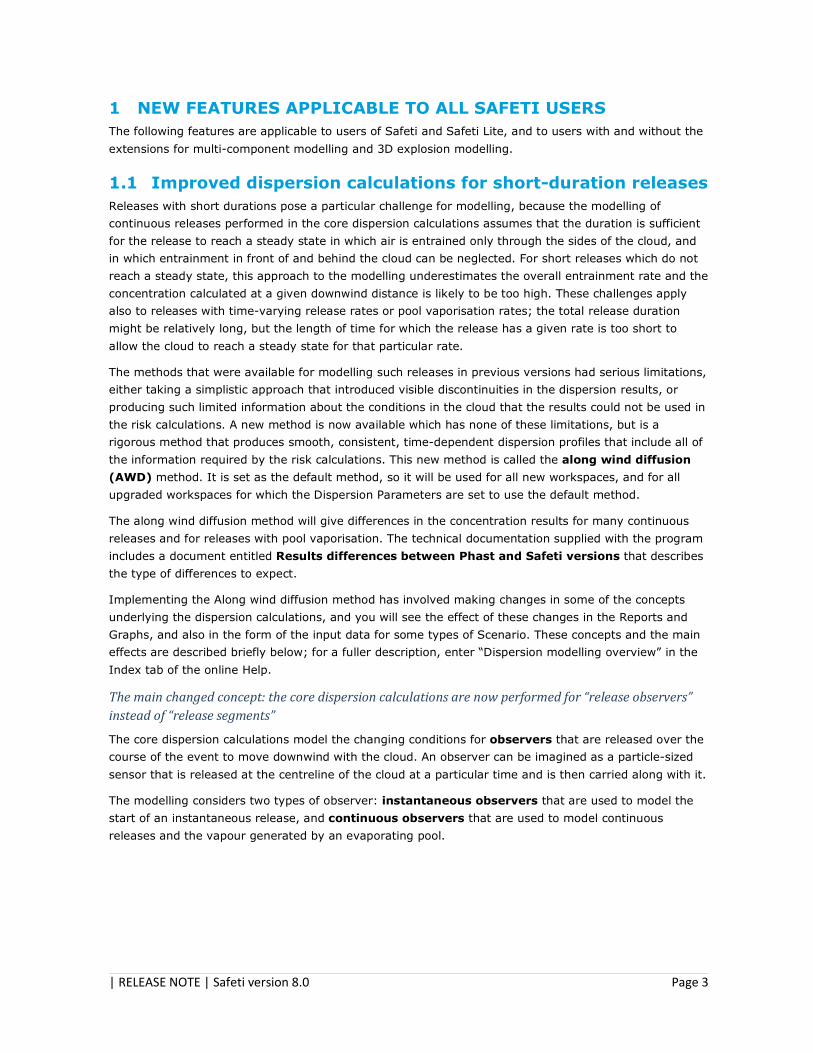
The observers used in the modelling of a particular Scenario and Weather are listed at the start of the
Dispersion Report, as shown below for an instantaneous release with rainout and evaporation.
The illustration above shows that each observer has a start time but no duration, and this is because
each observer is tracking the cloud from the specific conditions associated with its start time, in a release
that is recognised as being in a state of continuous change. This is different from the previous approach
using release segments, in which each segment had an associated duration because it was used to
represent the conditions over a particular period of the release, with the conditions assumed to be
constant over the duration of the segment. The Observer method is designed to be able to interpolate
between the results for the different observers to give smooth results for intermediate situations,
whereas the previous approach was only able to treat the release as a series of step-changes.
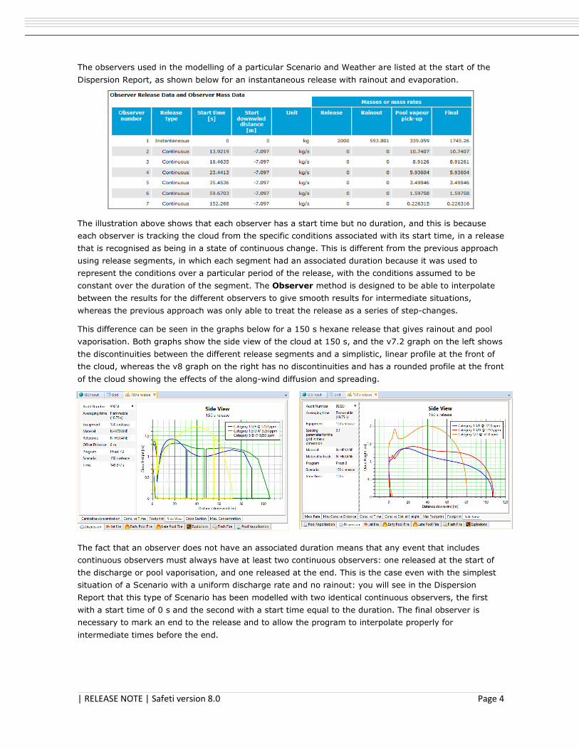
This difference can be seen in the graphs below for a 150 s hexane release that gives rainout and pool
vaporisation. Both graphs show the side view of the cloud at 150 s, and the v7.2 graph on the left shows
the discontinuities between the different release segments and a simplistic, linear profile at the front of
the cloud, whereas the v8 graph on the right has no discontinuities and has a rounded profile at the front
of the cloud showing the effects of the along-wind diffusion and spreading.
The fact that an observer does not have an associated duration means that any event that includes
continuous observers must always have at least two continuous observers: one released at the start of
the discharge or pool vaporisation, and one released at the end. This is the case even with the simplest
situation of a Scenario with a uniform discharge rate and no rainout: you will see in the Dispersion
Report that this type of Scenario has been modelled with two identical continuous observers, the first
with a start time of 0 s and the second with a start time equal to the duration. The final observer is
necessary to mark an end to the release and to allow the program to interpolate properly for
intermediate times before the end.
| RELEASE NOTE | Safeti version 8.0 Page 5
The modelling of along-wind effects is included in the core dispersion calculations for an instantaneous
observer, but for continuous observers it is performed in a new post-processing stage
The core dispersion calculations treat the modelling of along-wind effects in the same way as in previous
versions, which means that these calculations include these effects for an instantaneous observer, but
not for a continuous observer. For a continuous observer, the core dispersion calculations assume that
the observer is in a steady-state cloud in which the along-wind gradients in concentration and density
are small and not able to drive mixing of air in the along-wind direction, and so the mixing of air into the
cloud takes place only in the cross-wind direction.
The modelling of along-wind diffusion and gravity spreading for continuous observers is performed
instead through post-processing of the results of the core dispersion calculations, where the along-wind
diffusion is accounted for by a process of Gaussian integration of the concentrations calculated for the
observers. The type of post-processing that is performed depends on the settings in the Time-varying
and finite duration tab of the Dispersion Parameters. A range of options are provided for different
aspects of the post-processing, but the choice is provided mainly to allow comparison with earlier
versions of the program, and the options that will give the most accurate modelling of along-wind
behaviour are set as the defaults.
In some situations you may see the results for the core dispersion calculations referred to as the "pre-
AWD" results, or as the results "before along-wind-diffusion effects".
The Equipment Reports give concentration values from the core dispersion calculations, whereas the
Summary Reports and the Graphs give the results after the post-processing
In the group of Equipment Reports, the Dispersion, Commentary and Averaging Times Reports give the
results of the core dispersion calculations, without any post-processing, whereas the Summary Reports
and the Graphs give the results with post-processing.
For a Scenario that is modelled with only an instantaneous observer, the results in the three Equipment
Reports will match the results in the Summary Report and the Graphs, because the core dispersion
calculations for an instantaneous observer include the modelling of along-wind effects so no additional
post-processing is needed in this situation. However, if the modelling for a Scenario includes any
continuous observers, the different forms of results may show differences in the concentrations
calculated for a given downwind distance at a given time.
The size of the differences will depend on the time-scale for the event-duration compared with the
release duration that would be required for a steady-state, fully-developed cloud to become established.
For example, if a release duration of 600 s would be required for a cloud with a given mass-rate to reach
a steady state, then a Scenario that maintains that mass-rate for 600 s will show differences only at the
beginning and end of the release, whereas a Scenario that maintains the mass-rate for only 10 s will
show significant differences at all times and distances.
| RELEASE NOTE | Safeti version 8.0 Page 6
There have been some changes in the Dispersion Graphs as part of the new method
This can be seen in the illustrations of the Side View graphs on the previous page, where the list of
graphs are different in v7.2 and v8. The graphs of cloud concentration in the Dispersion group are now
as follows:
Graph Name Description Equivalent in
previous version
Mass Rate Shows the initial release rate, and if rainout occurs, the graph will
also show the Rainout Rate and the Pool Vaporisation Rate. All
rates are shown as a function of time.
None
Max Conc vs
Distance
Shows the maximum concentration reached at a given height as a
function of distance downwind, as calculated at a given averaging
time.
None
Conc vs. Time Shows the change in concentration during the course of the
dispersion, measured at a location specified by a given downwind
distance and height above the ground, and calculated using a
given averaging time.
Concentration vs.
Time
Conc vs Dist. at
Height
Shows the concentration at a given height and time as a function
of distance downwind, as calculated at a given averaging time.
Animation is available for this Graph.
None
Footprint Shows the shape of the contours for up to four concentrations
inside the cloud, measured at a given height and time, and
calculated using a given averaging time. The graph also shows
the maximum extent reached by the liquid pool (if one is
formed).
Animation is available for this Graph.
Footprint
Max Footprint Shows the shape of the contours of the maximum concentration
reached during the dispersion, for up to four concentrations inside
the cloud, measured at a given height and calculated using a
given averaging time. The graph also shows the maximum extent
reached by the liquid pool (if one is formed).
Maximum
Concentration
Side View Shows the shape of the contours for up to four concentrations
inside the cloud, measured at a given time, and calculated using
a given averaging time.
Animation is available for this Graph.
Side View
There is no equivalent in v8.0 of the Centerline Concentration and Cross Section Graphs that were
available in previous versions. The Conc vs. Time and Side View graphs now always give the results
along the downwind axis, i.e. with a crosswind offset of zero, and there is now no option to specify a
different value for the crosswind offset.
In previous versions, a Dynamic Concentration Report was available for the Graphs that have animation
showing the details of the cloud concentrations at the time currently displayed. This Report is no longer
available.
For further details of the Graphs, enter “Graphs” in the Index tab of the online Help.
| RELEASE NOTE | Safeti version 8.0 Page 7
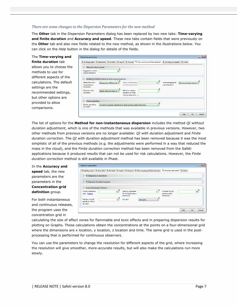
There are some changes to the Dispersion Parameters for the new method
The Other tab in the Dispersion Parameters dialog has been replaced by two new tabs: Time-varying
and finite duration and Accuracy and speed. These new tabs contain fields that were previously on
the Other tab and also new fields related to the new method, as shown in the illustrations below. You
can click on the Help button in the dialog for details of the fields.
The Time-varying and
finite duration tab
allows you to choose the
methods to use for
different aspects of the
calculations. The default
settings are the
recommended settings,
but other options are
provided to allow
comparisons.
The list of options for the Method for non-instantaneous dispersion includes the method QI without
duration adjustment, which is one of the methods that was available in previous versions. However, two
other methods from previous versions are no longer available: QI with duration adjustment and Finite
duration correction. The QI with duration adjustment method has been removed because it was the most
simplistic of all of the previous methods (e.g. the adjustments were performed in a way that reduced the
mass in the cloud), and the Finite duration correction method has been removed from the Safeti
applications because it produced results that can not be used for risk calculations. However, the Finite
duration correction method is still available in Phast.
In the Accuracy and
speed tab, the new
parameters are the
parameters in the
Concentration grid
definition group.
For both instantaneous
and continuous releases,
the program uses the
concentration grid in
calculating the size of effect zones for flammable and toxic effects and in preparing dispersion results for
plotting on Graphs. These calculations obtain the concentrations at the points on a four-dimensional grid
where the dimensions are x location, y location, z location and time. The same grid is used in the post-
processing that is performed for continuous observers.
You can use the parameters to change the resolution for different aspects of the grid, where increasing
the resolution will give smoother, more-accurate results, but will also make the calculations run more
slowly.
| RELEASE NOTE | Safeti version 8.0 Page 8
There have been some changes in reports for Source Scenarios
The change from release segments to release observers and the introduction of the concentration grid
for calculating effect zones required changes to some of the reports for Source Scenarios. In the process
of these changes, some aspects of the reporting were clarified and made more straightforward:
• In previous versions the Pool Vaporisation report included details of the representative pool
vaporisation segments modelled. These are no longer relevant and the Pool Vaporisation report
now gives only a small amount of summary information about the pool vaporisation calculations.
• The Hazard Zones Report has been renamed the Flammable Hazards report. This is the report
that gives the details of the effect zones for hazardous flammable effects and the description of
the flammable cloud, as they will be used as input to the risk calculations.
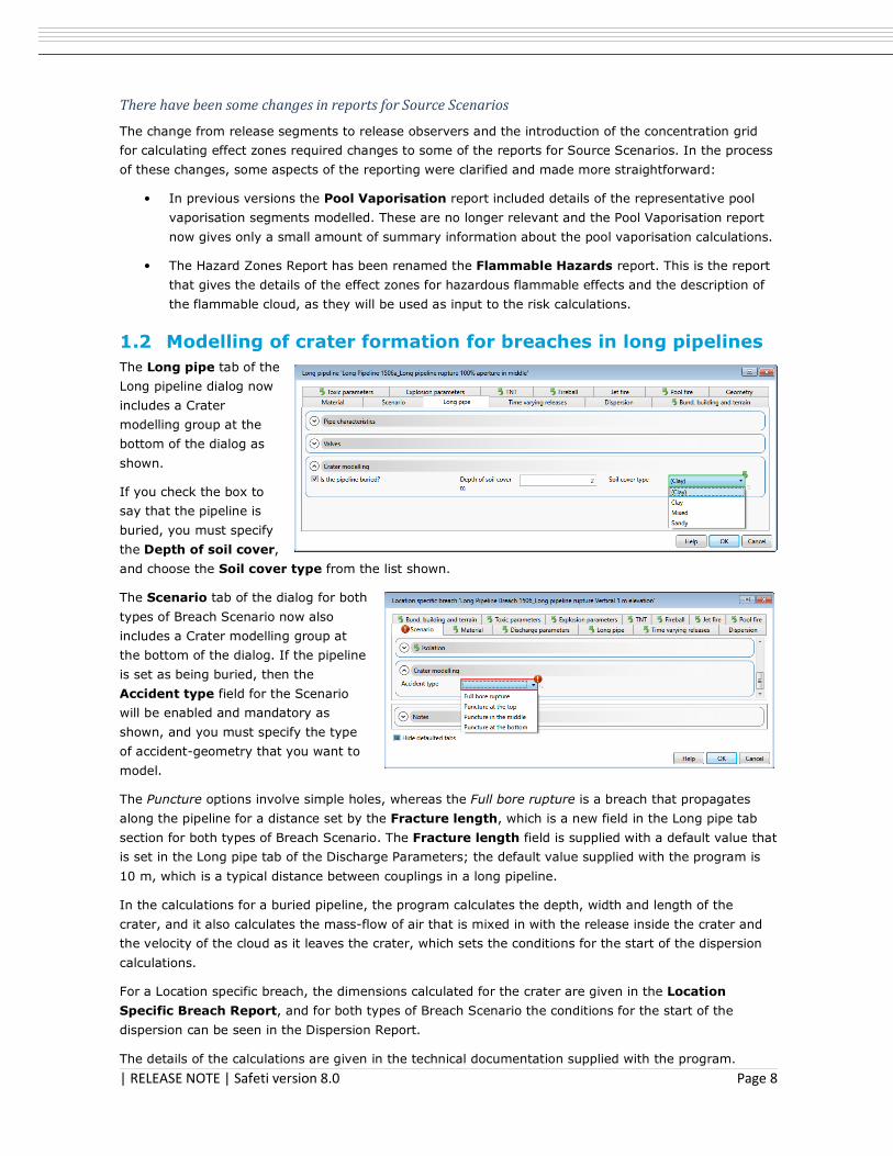
1.2 Modelling of crater formation for breaches in long pipelines
The Long pipe tab of the
Long pipeline dialog now
includes a Crater
modelling group at the
bottom of the dialog as
shown.
If you check the box to
say that the pipeline is
buried, you must specify
the Depth of soil cover,
and choose the Soil cover type from the list shown.
The Scenario tab of the dialog for both
types of Breach Scenario now also
includes a Crater modelling group at
the bottom of the dialog. If the pipeline
is set as being buried, then the
Accident type field for the Scenario
will be enabled and mandatory as
shown, and you must specify the type
of accident-geometry that you want to
model.
The Puncture options involve simple holes, whereas the Full bore rupture is a breach that propagates
along the pipeline for a distance set by the Fracture length, which is a new field in the Long pipe tab
section for both types of Breach Scenario. The Fracture length field is supplied with a default value that
is set in the Long pipe tab of the Discharge Parameters; the default value supplied with the program is
10 m, which is a typical distance between couplings in a long pipeline.
In the calculations for a buried pipeline, the program calculates the depth, width and length of the
crater, and it also calculates the mass-flow of air that is mixed in with the release inside the crater and
the velocity of the cloud as it leaves the crater, which sets the conditions for the start of the dispersion
calculations.
For a Location specific breach, the dimensions calculated for the crater are given in the Location
Specific Breach Report, and for both types of Breach Scenario the conditions for the start of the
dispersion can be seen in the Dispersion Report.
The details of the calculations are given in the technical documentation supplied with the program.
| RELEASE NOTE | Safeti version 8.0 Page 9
1.3 Improvements in modelling and results for time-varying
discharge calculations
There have been several improvements that affect the Time-varying Leak and Time-varying short pipe
Scenarios.
The value for the inventory is now taken as the total inventory rather than the liquid inventory
The changes in the time-varying modelling did not involve any visible changes in the input fields, but the
interpretation of the inventory value in the Material tab for the Equipment item has changed.
In previous versions, the value given for the inventory was taken as the inventory for the liquid side
only, and the program would calculate the additional vapour mass needed to fill the vapour space. The
value is now taken as the total inventory of both liquid and vapour.
This change means that v8 will typically give less conservative results as there is less liquid to release
and the liquid level is more likely to be below the hole in the vessel.
Improvements in modelling for greater consistency and stability
The calculations have been improved in several areas:
• In previous versions, the entire liquid inventory would typically be released, even in situations in
which the liquid level fell below the height of the hole, and this has now been improved. For a
pressurised liquid vessel, the release will now stop when the liquid level drops below the height
of the hole, and for saturated conditions, the release will change from liquid to vapour.
• The modelling is more robust, and the calculations should no longer stop prematurely because of
issues with numerical convergence.
• The modelling is less likely to fail with conditions near the critical point. Some simplifying
assumptions have been made for conditions in the vicinity of the critical point, and these make
an error in the calculations much less likely.
• The removal of the velocity cap for expansion to atmospheric pressure.
The details of the calculations are given in the technical documentation supplied with the program.
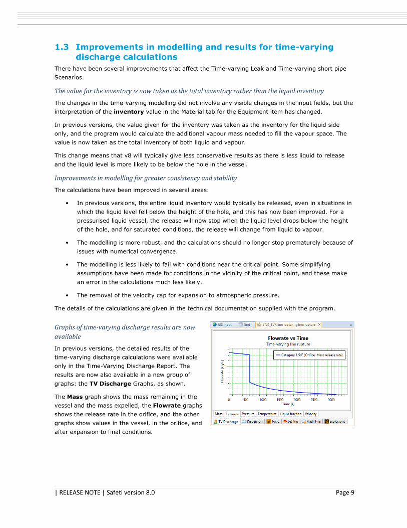
Graphs of time-varying discharge results are now
available
In previous versions, the detailed results of the
time-varying discharge calculations were available
only in the Time-Varying Discharge Report. The
results are now also available in a new group of
graphs: the TV Discharge Graphs, as shown.
The Mass graph shows the mass remaining in the
vessel and the mass expelled, the Flowrate graphs
shows the release rate in the orifice, and the other
graphs show values in the vessel, in the orifice, and
after expansion to final conditions.
| RELEASE NOTE | Safeti version 8.0 Page 10
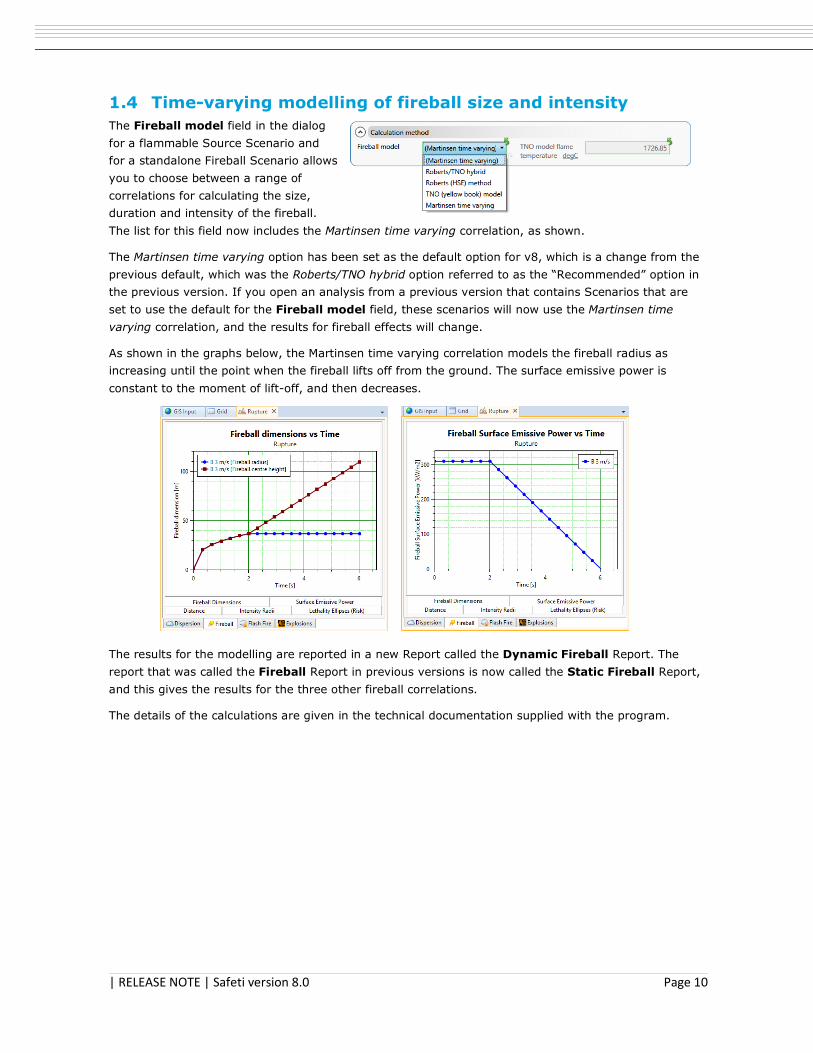
1.4 Time-varying modelling of fireball size and intensity
The Fireball model field in the dialog
for a flammable Source Scenario and
for a standalone Fireball Scenario allows
you to choose between a range of
correlations for calculating the size,
duration and intensity of the fireball.
The list for this field now includes the Martinsen time varying correlation, as shown.
The Martinsen time varying option has been set as the default option for v8, which is a change from the
previous default, which was the Roberts/TNO hybrid option referred to as the “Recommended” option in
the previous version. If you open an analysis from a previous version that contains Scenarios that are
set to use the default for the Fireball model field, these scenarios will now use the Martinsen time
varying correlation, and the results for fireball effects will change.
As shown in the graphs below, the Martinsen time varying correlation models the fireball radius as
increasing until the point when the fireball lifts off from the ground. The surface emissive power is
constant to the moment of lift-off, and then decreases.
The results for the modelling are reported in a new Report called the Dynamic Fireball Report. The
report that was called the Fireball Report in previous versions is now called the Static Fireball Report,
and this gives the results for the three other fireball correlations.
The details of the calculations are given in the technical documentation supplied with the program.
| RELEASE NOTE | Safeti version 8.0 Page 11
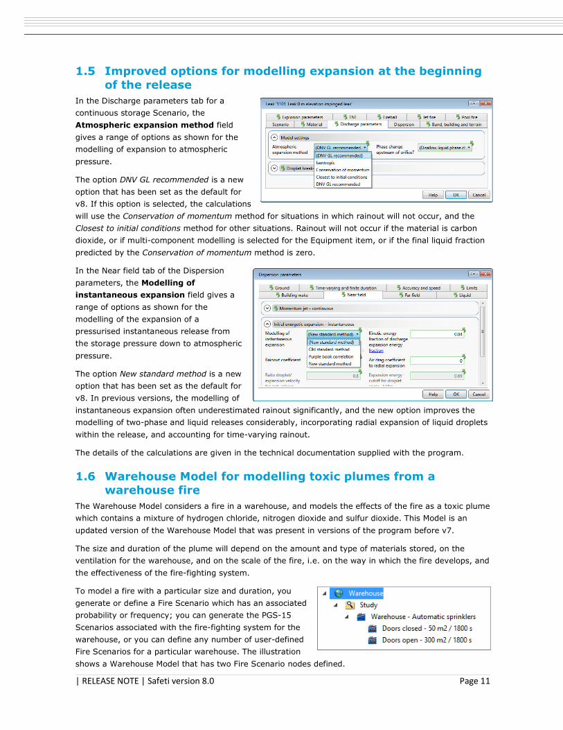
1.5 Improved options for modelling expansion at the beginning
of the release
In the Discharge parameters tab for a
continuous storage Scenario, the
Atmospheric expansion method field
gives a range of options as shown for the
modelling of expansion to atmospheric
pressure.
The option DNV GL recommended is a new
option that has been set as the default for
v8. If this option is selected, the calculations
will use the Conservation of momentum method for situations in which rainout will not occur, and the
Closest to initial conditions method for other situations. Rainout will not occur if the material is carbon
dioxide, or if multi-component modelling is selected for the Equipment item, or if the final liquid fraction
predicted by the Conservation of momentum method is zero.
In the Near field tab of the Dispersion
parameters, the Modelling of
instantaneous expansion field gives a
range of options as shown for the
modelling of the expansion of a
pressurised instantaneous release from
the storage pressure down to atmospheric
pressure.
The option New standard method is a new
option that has been set as the default for
v8. In previous versions, the modelling of
instantaneous expansion often underestimated rainout significantly, and the new option improves the
modelling of two-phase and liquid releases considerably, incorporating radial expansion of liquid droplets
within the release, and accounting for time-varying rainout.
The details of the calculations are given in the technical documentation supplied with the program.
1.6 Warehouse Model for modelling toxic plumes from a
warehouse fire
The Warehouse Model considers a fire in a warehouse, and models the effects of the fire as a toxic plume
which contains a mixture of hydrogen chloride, nitrogen dioxide and sulfur dioxide. This Model is an
updated version of the Warehouse Model that was present in versions of the program before v7.
The size and duration of the plume will depend on the amount and type of materials stored, on the
ventilation for the warehouse, and on the scale of the fire, i.e. on the way in which the fire develops, and
the effectiveness of the fire-fighting system.
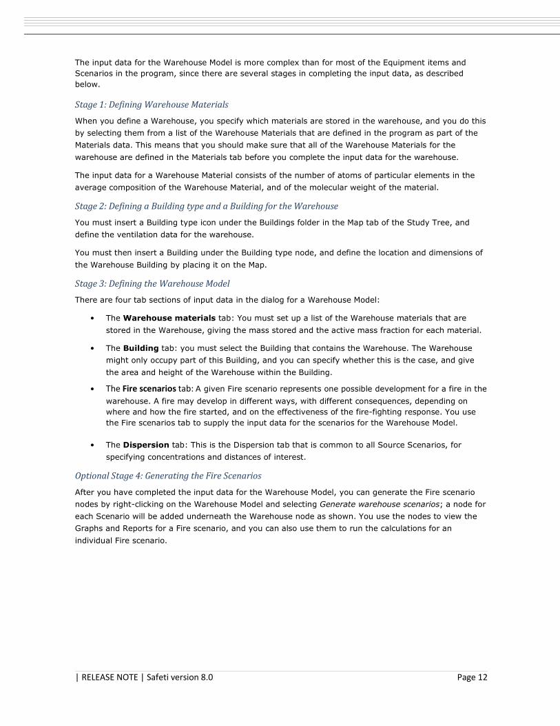
To model a fire with a particular size and duration, you
generate or define a Fire Scenario which has an associated
probability or frequency; you can generate the PGS-15
Scenarios associated with the fire-fighting system for the
warehouse, or you can define any number of user-defined
Fire Scenarios for a particular warehouse. The illustration
shows a Warehouse Model that has two Fire Scenario nodes defined.
| RELEASE NOTE | Safeti version 8.0 Page 12
The input data for the Warehouse Model is more complex than for most of the Equipment items and
Scenarios in the program, since there are several stages in completing the input data, as described
below.
Stage 1: Defining Warehouse Materials
When you define a Warehouse, you specify which materials are stored in the warehouse, and you do this
by selecting them from a list of the Warehouse Materials that are defined in the program as part of the
Materials data. This means that you should make sure that all of the Warehouse Materials for the
warehouse are defined in the Materials tab before you complete the input data for the warehouse.
The input data for a Warehouse Material consists of the number of atoms of particular elements in the
average composition of the Warehouse Material, and of the molecular weight of the material.
Stage 2: Defining a Building type and a Building for the Warehouse
You must insert a Building type icon under the Buildings folder in the Map tab of the Study Tree, and
define the ventilation data for the warehouse.
You must then insert a Building under the Building type node, and define the location and dimensions of
the Warehouse Building by placing it on the Map.
Stage 3: Defining the Warehouse Model
There are four tab sections of input data in the dialog for a Warehouse Model:
• The Warehouse materials tab: You must set up a list of the Warehouse materials that are
stored in the Warehouse, giving the mass stored and the active mass fraction for each material.
• The Building tab: you must select the Building that contains the Warehouse. The Warehouse
might only occupy part of this Building, and you can specify whether this is the case, and give
the area and height of the Warehouse within the Building.
• The Fire scenarios tab: A given Fire scenario represents one possible development for a fire in the
warehouse. A fire may develop in different ways, with different consequences, depending on
where and how the fire started, and on the effectiveness of the fire-fighting response. You use
the Fire scenarios tab to supply the input data for the scenarios for the Warehouse Model.
• The Dispersion tab: This is the Dispersion tab that is common to all Source Scenarios, for
specifying concentrations and distances of interest.
Optional Stage 4: Generating the Fire Scenarios
After you have completed the input data for the Warehouse Model, you can generate the Fire scenario
nodes by right-clicking on the Warehouse Model and selecting Generate warehouse scenarios; a node for
each Scenario will be added underneath the Warehouse node as shown. You use the nodes to view the
Graphs and Reports for a Fire scenario, and you can also use them to run the calculations for an
individual Fire scenario.
| RELEASE NOTE | Safeti version 8.0 Page 13
Running the calculations and viewing the results
You do not have to generate the Fire scenarios yourself. If you have not already generated the nodes
using the option in the right-click menu, the program will generate the nodes automatically when you
run the calculations for the Warehouse Model, and it will then run the calculations for all of the
Scenarios.
There is a Report called the Warehouse Overview Report that is specific to the Warehouse Model itself,
giving details of the input data and of warehouse-level results. The Fire Scenarios have all of the Reports
and Graphs applicable to any toxic Source Scenario, and also a Warehouse Results Report that gives
input data for the Warehouse as a whole and for the Fire scenario, and details of the modelling of the
generation of the toxic plume.
For further details of the input data and the results, enter “Warehouse” in the Index tab of the online
Help The details of the calculations are given in the technical documentation supplied with the program.
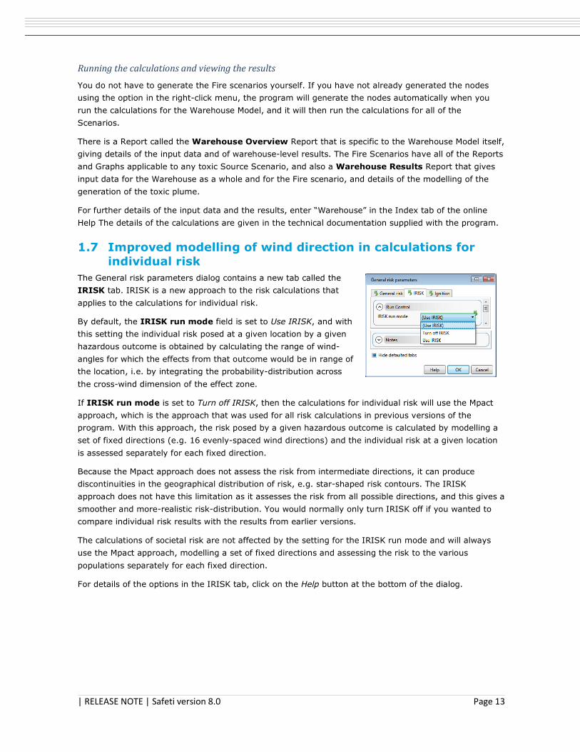
1.7 Improved modelling of wind direction in calculations for
individual risk
The General risk parameters dialog contains a new tab called the
IRISK tab. IRISK is a new approach to the risk calculations that
applies to the calculations for individual risk.
By default, the IRISK run mode field is set to Use IRISK, and with
this setting the individual risk posed at a given location by a given
hazardous outcome is obtained by calculating the range of wind-
angles for which the effects from that outcome would be in range of
the location, i.e. by integrating the probability-distribution across
the cross-wind dimension of the effect zone.
If IRISK run mode is set to Turn off IRISK, then the calculations for individual risk will use the Mpact
approach, which is the approach that was used for all risk calculations in previous versions of the
program. With this approach, the risk posed by a given hazardous outcome is calculated by modelling a
set of fixed directions (e.g. 16 evenly-spaced wind directions) and the individual risk at a given location
is assessed separately for each fixed direction.
Because the Mpact approach does not assess the risk from intermediate directions, it can produce
discontinuities in the geographical distribution of risk, e.g. star-shaped risk contours. The IRISK
approach does not have this limitation as it assesses the risk from all possible directions, and this gives a
smoother and more-realistic risk-distribution. You would normally only turn IRISK off if you wanted to
compare individual risk results with the results from earlier versions.
The calculations of societal risk are not affected by the setting for the IRISK run mode and will always
use the Mpact approach, modelling a set of fixed directions and assessing the risk to the various
populations separately for each fixed direction.
For details of the options in the IRISK tab, click on the Help button at the bottom of the dialog.

| RELEASE NOTE | Safeti version 8.0 Page 14
1.8 Parallel processing available for aspects of consequence and
risk calculations
The Workspace dialog has an option for parallel processing of consequence calculations
The Calculations and messages tab of the
Workspace dialog now includes the option
Enable multithreading for dispersion
and toxic calculations as shown.
If this option is checked, then different
aspects of the consequence calculations
for a given Scenario will be run
simultaneously on different CPU cores, which has the potential to allow the calculations to run more
quickly. If the option is not checked, the program will run all of the consequence calculations for all
Scenarios on a single core, with no parallel processing for any aspects of the consequence calculations.
The IRISK tab of the General risk parameters has options for parallel processing of IRISK calculations
Another difference between the IRISK and the Mpact calculations is that the Mpact calculations are
limited to running on a single processor core, whereas IRISK calculations are able to run with parallel
processing using multiple processor cores, including CUDA cores in an NVidia GPU, and this allows the
IRISK calculations to run more quickly than the Mpact calculations.
The IRISK tab of the General risk
parameters contains options for
Parallelization control, as shown. These
options are enabled only if IRISK run mode
is set to Use IRISK, and they allow you to
choose between a range of approaches to
the parallel processing for IRISK
calculations.
When you run the risk calculations, the
calculations for a given Scenario will involve both Mpact and IRISK calculations. The setting for
CPU/GPU Parallelization mode determines the processing relationship between the two types of
calculation:
Option Behaviour
Serial (single threaded) The calculations for both Mpact and IRISK will run on a single
processor core, with no parallel processing, and Mpact will wait for the
IRISK calculations for a given outcome to finish before proceeding to
the calculations for the next outcome.
Synchronous (multi-threaded) The calculations will run in parallel on multiple processor cores, but
Mpact will wait for the IRISK calculations for a given outcome to finish
before proceeding to the calculations for the next outcome
Asynchronous (multi-threaded) The calculations will run in parallel on multiple processor cores, and
Mpact will not wait for the IRISK calculations for a given outcome to
finish before proceeding to the calculations for the next outcome. With
this option, both Mpact and IRISK will run at maximum speed.
| RELEASE NOTE | Safeti version 8.0 Page 15
The Asynchronous parallelization mode field is enabled if CPU/GPU Parallelization mode is set to
Asynchronous (multi-threaded). The field controls which processors are used for parallel running of the
IRISK calculations:
Option Behaviour
Serial (Single Threaded) With this option, the Mpact calculations will run on one CPU core (the
parent CPU core), and the IRISK calculations will run on a second
CPU core, i.e. the risk calculations will never use more than 2 CPU
cores at the same time.
Multi threaded (CPU-OpenMP) With this option, the Mpact calculations will run on the parent CPU
core, and the IRISK calculations will run in parallel on all of the other
CPU cores, using the maximum number of CPU cores available.
MT-Single-Precision (GPU-CUDA) With this option, the Mpact calculations will run on the parent CPU
core, and the IRISK calculations will run in parallel on CUDA cores in
the GPU using the fastest run-mode for CUDA cores (i.e. single-
precision mode).
MT-SP_DP (GPU-CUDA) With this option, the Mpact calculations will run on the parent CPU
core, and the IRISK calculations will run in parallel on CUDA cores in
the GPU using double-precision run-mode, which runs more slowly
but gives the highest numerical precision in the results.
Note: If your computer's GPU does not have CUDA capability, a warning will be written to the Output
View at the start of the risk calculations, saying that CUDA calculations are disabled. In this situation, if
the Asynchronous parallelization mode field is set to one of the GPU-CUDA options, the calculations
will run in Multi threaded (CPU-OpenMP) mode instead.
Note: Even when a computer's GPU has CUDA capability, the CUDA processing might not be functioning
properly on the computer. In this situation the program does not automatically use the Multi threaded
(CPU-OpenMP) mode instead, and the risk calculations will give warnings and errors about the CUDA
calculations. To allow the risk calculations to run successfully, you should either set the mode to Multi
threaded (CPU-OpenMP), or use the control panel for your GPU to turn off the CUDA capability.
| RELEASE NOTE | Safeti version 8.0 Page 16
2 NEW FEATURES APPLICABLE TO USERS OF THE FULL SAFETI
PROGRAM
2.1 Improvements in inputs and reporting for Long pipeline Section breach Scenario
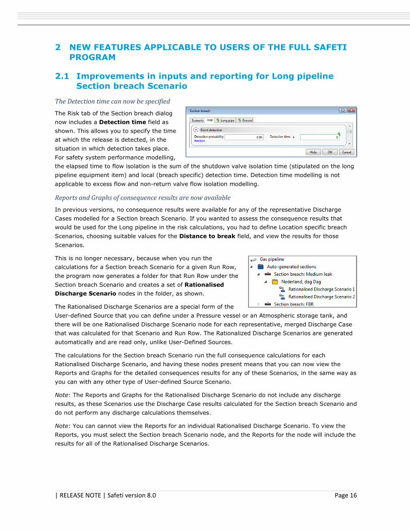
The Detection time can now be specified
The Risk tab of the Section breach dialog
now includes a Detection time field as
shown. This allows you to specify the time
at which the release is detected, in the
situation in which detection takes place.
For safety system performance modelling,
the elapsed time to flow isolation is the sum of the shutdown valve isolation time (stipulated on the long
pipeline equipment item) and local (breach specific) detection time. Detection time modelling is not
applicable to excess flow and non-return valve flow isolation modelling.
Reports and Graphs of consequence results are now available
In previous versions, no consequence results were available for any of the representative Discharge
Cases modelled for a Section breach Scenario. If you wanted to assess the consequence results that
would be used for the Long pipeline in the risk calculations, you had to define Location specific breach
Scenarios, choosing suitable values for the Distance to break field, and view the results for those
Scenarios.
This is no longer necessary, because when you run the
calculations for a Section breach Scenario for a given Run Row,
the program now generates a folder for that Run Row under the
Section breach Scenario and creates a set of Rationalised
Discharge Scenario nodes in the folder, as shown.
The Rationalised Discharge Scenarios are a special form of the
User-defined Source that you can define under a Pressure vessel or an Atmospheric storage tank, and
there will be one Rationalised Discharge Scenario node for each representative, merged Discharge Case
that was calculated for that Scenario and Run Row. The Rationalized Discharge Scenarios are generated
automatically and are read only, unlike User-Defined Sources.
The calculations for the Section breach Scenario run the full consequence calculations for each
Rationalised Discharge Scenario, and having these nodes present means that you can now view the
Reports and Graphs for the detailed consequences results for any of these Scenarios, in the same way as
you can with any other type of User-defined Source Scenario.
Note: The Reports and Graphs for the Rationalised Discharge Scenario do not include any discharge
results, as these Scenarios use the Discharge Case results calculated for the Section breach Scenario and
do not perform any discharge calculations themselves.
Note: You can cannot view the Reports for an individual Rationalised Discharge Scenario. To view the
Reports, you must select the Section breach Scenario node, and the Reports for the node will include the
results for all of the Rationalised Discharge Scenarios.
| RELEASE NOTE | Safeti version 8.0 Page 17
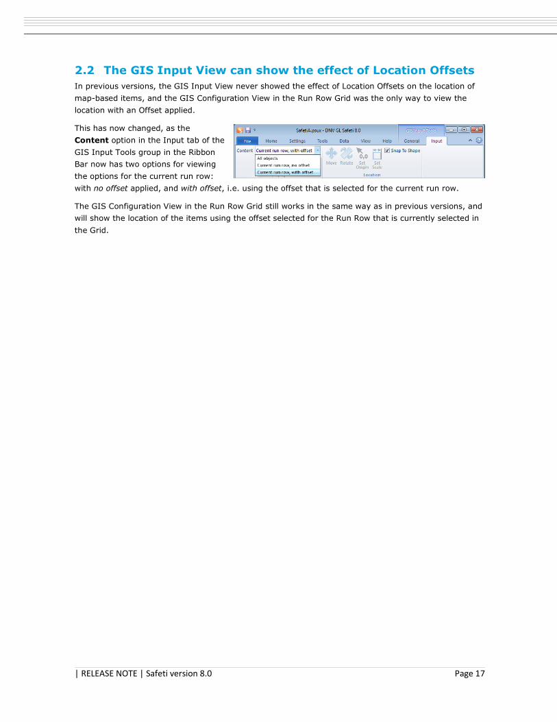
2.2 The GIS Input View can show the effect of Location Offsets
In previous versions, the GIS Input View never showed the effect of Location Offsets on the location of
map-based items, and the GIS Configuration View in the Run Row Grid was the only way to view the
location with an Offset applied.
This has now changed, as the
Content option in the Input tab of the
GIS Input Tools group in the Ribbon
Bar now has two options for viewing
the options for the current run row:
with no offset applied, and with offset, i.e. using the offset that is selected for the current run row.
The GIS Configuration View in the Run Row Grid still works in the same way as in previous versions, and
will show the location of the items using the offset selected for the Run Row that is currently selected in
the Grid.
| RELEASE NOTE | Safeti version 8.0 Page 18
3 OTHER DIFFERENCES AND BUG FIXES
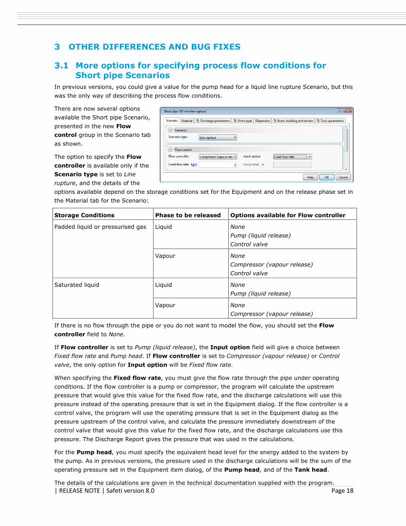
3.1 More options for specifying process flow conditions for Short pipe Scenarios
In previous versions, you could give a value for the pump head for a liquid line rupture Scenario, but this
was the only way of describing the process flow conditions.
There are now several options
available the Short pipe Scenario,
presented in the new Flow
control group in the Scenario tab
as shown.
The option to specify the Flow
controller is available only if the
Scenario type is set to Line
rupture, and the details of the
options available depend on the storage conditions set for the Equipment and on the release phase set in
the Material tab for the Scenario:
Storage Conditions Phase to be released Options available for Flow controller
Padded liquid or pressurised gas Liquid None
Pump (liquid release)
Control valve
Vapour None
Compressor (vapour release)
Control valve
Saturated liquid Liquid None
Pump (liquid release)
Vapour None
Compressor (vapour release)
If there is no flow through the pipe or you do not want to model the flow, you should set the Flow
controller field to None.
If Flow controller is set to Pump (liquid release), the Input option field will give a choice between
Fixed flow rate and Pump head. If Flow controller is set to Compressor (vapour release) or Control
valve, the only option for Input option will be Fixed flow rate.
When specifying the Fixed flow rate, you must give the flow rate through the pipe under operating
conditions. If the flow controller is a pump or compressor, the program will calculate the upstream
pressure that would give this value for the fixed flow rate, and the discharge calculations will use this
pressure instead of the operating pressure that is set in the Equipment dialog. If the flow controller is a
control valve, the program will use the operating pressure that is set in the Equipment dialog as the
pressure upstream of the control valve, and calculate the pressure immediately downstream of the
control valve that would give this value for the fixed flow rate, and the discharge calculations use this
pressure. The Discharge Report gives the pressure that was used in the calculations.
For the Pump head, you must specify the equivalent head level for the energy added to the system by
the pump. As in previous versions, the pressure used in the discharge calculations will be the sum of the
operating pressure set in the Equipment item dialog, of the Pump head, and of the Tank head.
The details of the calculations are given in the technical documentation supplied with the program.
| RELEASE NOTE | Safeti version 8.0 Page 19
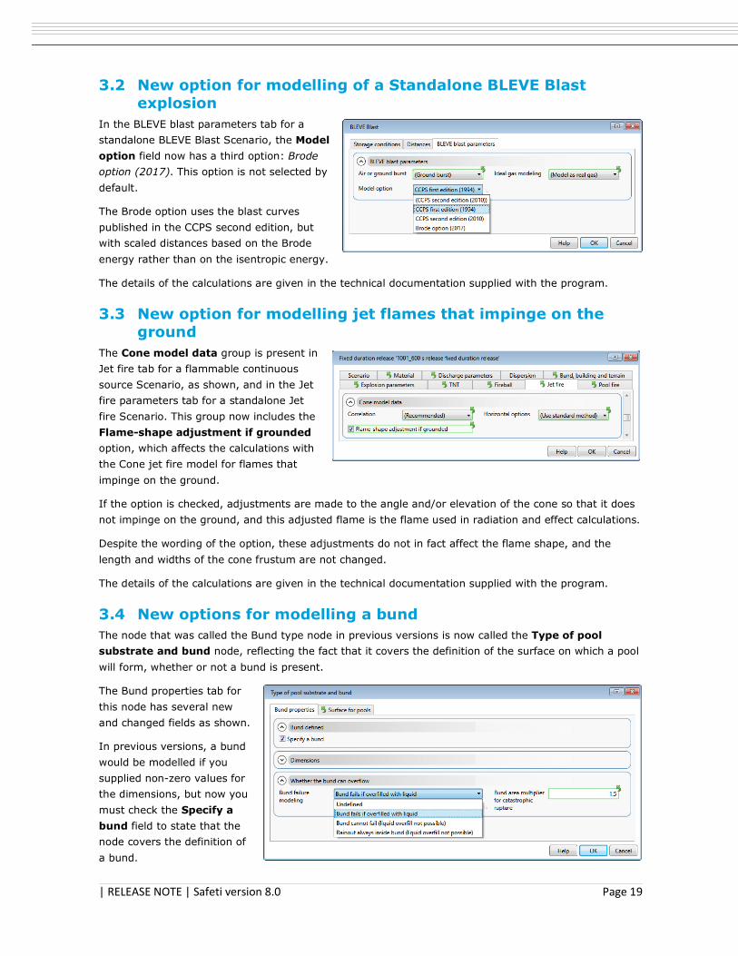
3.2 New option for modelling of a Standalone BLEVE Blast
explosion
In the BLEVE blast parameters tab for a
standalone BLEVE Blast Scenario, the Model
option field now has a third option: Brode
option (2017). This option is not selected by
default.
The Brode option uses the blast curves
published in the CCPS second edition, but
with scaled distances based on the Brode
energy rather than on the isentropic energy.
The details of the calculations are given in the technical documentation supplied with the program.
3.3 New option for modelling jet flames that impinge on the
ground
The Cone model data group is present in
Jet fire tab for a flammable continuous
source Scenario, as shown, and in the Jet
fire parameters tab for a standalone Jet
fire Scenario. This group now includes the
Flame-shape adjustment if grounded
option, which affects the calculations with
the Cone jet fire model for flames that
impinge on the ground.
If the option is checked, adjustments are made to the angle and/or elevation of the cone so that it does
not impinge on the ground, and this adjusted flame is the flame used in radiation and effect calculations.
Despite the wording of the option, these adjustments do not in fact affect the flame shape, and the
length and widths of the cone frustum are not changed.
The details of the calculations are given in the technical documentation supplied with the program.
3.4 New options for modelling a bund
The node that was called the Bund type node in previous versions is now called the Type of pool
substrate and bund node, reflecting the fact that it covers the definition of the surface on which a pool
will form, whether or not a bund is present.
The Bund properties tab for
this node has several new
and changed fields as shown.
In previous versions, a bund
would be modelled if you
supplied non-zero values for
the dimensions, but now you
must check the Specify a
bund field to state that the
node covers the definition of
a bund.
| RELEASE NOTE | Safeti version 8.0 Page 20
The list of options for Bund failure modelling has changed, with the addition of an option to force
rainout to occur inside the bund, and with changes to the wording to make the effect clearer.
The Bund area multiplier for catastrophic rupture is a new field. For a Rupture Scenario under a
Pressure Vessel, the calculations will apply this multiplier to the value for Bund area (internal) to
obtain an effective bund area for use in the rainout and vaporisation calculations.
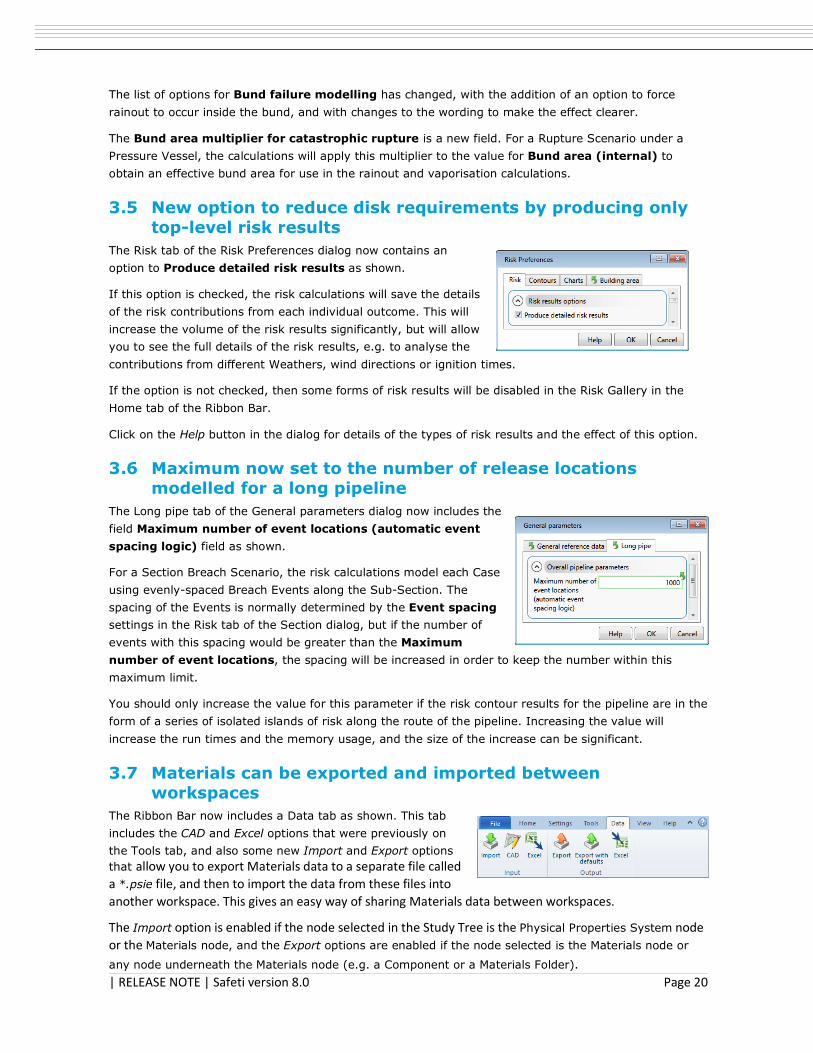
3.5 New option to reduce disk requirements by producing only
top-level risk results
The Risk tab of the Risk Preferences dialog now contains an
option to Produce detailed risk results as shown.
If this option is checked, the risk calculations will save the details
of the risk contributions from each individual outcome. This will
increase the volume of the risk results significantly, but will allow
you to see the full details of the risk results, e.g. to analyse the
contributions from different Weathers, wind directions or ignition times.
If the option is not checked, then some forms of risk results will be disabled in the Risk Gallery in the
Home tab of the Ribbon Bar.
Click on the Help button in the dialog for details of the types of risk results and the effect of this option.
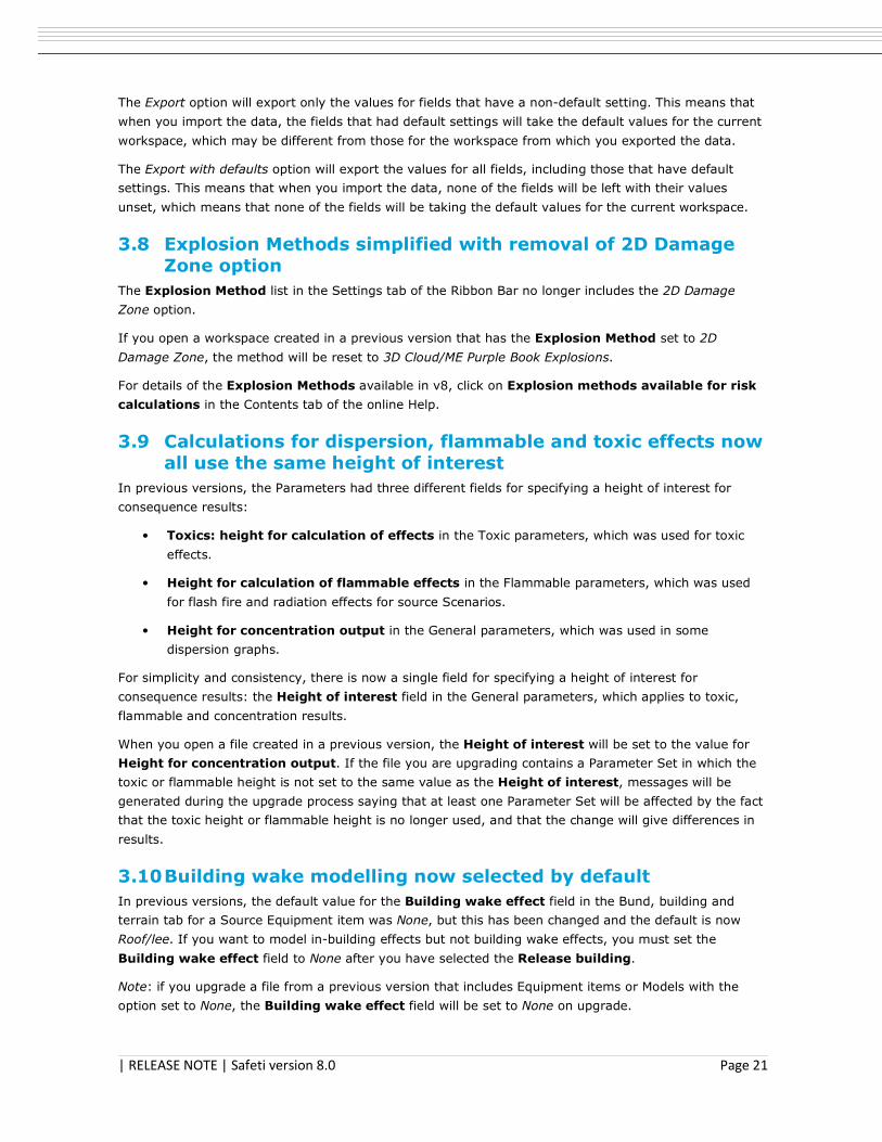
3.6 Maximum now set to the number of release locations
modelled for a long pipeline
The Long pipe tab of the General parameters dialog now includes the
field Maximum number of event locations (automatic event
spacing logic) field as shown.
For a Section Breach Scenario, the risk calculations model each Case
using evenly-spaced Breach Events along the Sub-Section. The
spacing of the Events is normally determined by the Event spacing
settings in the Risk tab of the Section dialog, but if the number of
events with this spacing would be greater than the Maximum
number of event locations, the spacing will be increased in order to keep the number within this
maximum limit.
You should only increase the value for this parameter if the risk contour results for the pipeline are in the
form of a series of isolated islands of risk along the route of the pipeline. Increasing the value will
increase the run times and the memory usage, and the size of the increase can be significant.
3.7 Materials can be exported and imported between
workspaces
The Ribbon Bar now includes a Data tab as shown. This tab
includes the CAD and Excel options that were previously on
the Tools tab, and also some new Import and Export options
that allow you to export Materials data to a separate file called
a *.psie file, and then to import the data from these files into
another workspace. This gives an easy way of sharing Materials data between workspaces.
The Import option is enabled if the node selected in the Study Tree is the Physical Properties System node
or the Materials node, and the Export options are enabled if the node selected is the Materials node or
any node underneath the Materials node (e.g. a Component or a Materials Folder).
| RELEASE NOTE | Safeti version 8.0 Page 21
The Export option will export only the values for fields that have a non-default setting. This means that
when you import the data, the fields that had default settings will take the default values for the current
workspace, which may be different from those for the workspace from which you exported the data.
The Export with defaults option will export the values for all fields, including those that have default
settings. This means that when you import the data, none of the fields will be left with their values
unset, which means that none of the fields will be taking the default values for the current workspace.
3.8 Explosion Methods simplified with removal of 2D Damage
Zone option
The Explosion Method list in the Settings tab of the Ribbon Bar no longer includes the 2D Damage
Zone option.
If you open a workspace created in a previous version that has the Explosion Method set to 2D
Damage Zone, the method will be reset to 3D Cloud/ME Purple Book Explosions.
For details of the Explosion Methods available in v8, click on Explosion methods available for risk
calculations in the Contents tab of the online Help.
3.9 Calculations for dispersion, flammable and toxic effects now
all use the same height of interest
In previous versions, the Parameters had three different fields for specifying a height of interest for
consequence results:
• Toxics: height for calculation of effects in the Toxic parameters, which was used for toxic
effects.
• Height for calculation of flammable effects in the Flammable parameters, which was used
for flash fire and radiation effects for source Scenarios.
• Height for concentration output in the General parameters, which was used in some
dispersion graphs.
For simplicity and consistency, there is now a single field for specifying a height of interest for
consequence results: the Height of interest field in the General parameters, which applies to toxic,
flammable and concentration results.
When you open a file created in a previous version, the Height of interest will be set to the value for
Height for concentration output. If the file you are upgrading contains a Parameter Set in which the
toxic or flammable height is not set to the same value as the Height of interest, messages will be
generated during the upgrade process saying that at least one Parameter Set will be affected by the fact
that the toxic height or flammable height is no longer used, and that the change will give differences in
results.
3.10 Building wake modelling now selected by default
In previous versions, the default value for the Building wake effect field in the Bund, building and
terrain tab for a Source Equipment item was None, but this has been changed and the default is now
Roof/lee. If you want to model in-building effects but not building wake effects, you must set the
Building wake effect field to None after you have selected the Release building.
Note: if you upgrade a file from a previous version that includes Equipment items or Models with the
option set to None, the Building wake effect field will be set to None on upgrade.

| RELEASE NOTE | Safeti version 8.0 Page 22
3.11 Baker-Strehlow-Tang explosions now involve entire cloud
volume
The Baker-Strehlow-Tang tab is present in the dialog for a flammable Source Scenario if the Explosion
method is set to Baker-Strehlow-Tang in the Explosion parameters tab. It contains input values for use
in the explosion calculations performed in the consequence calculations, which are separate from those
performed in the risk calculations.
The tab contains a Confined volume field for defining the maximum volume of the confined region of
the explosion. If the volume of the cloud is less than the value given for Confined volume, then the
program will use the volume of the cloud in the calculations.
In previous versions, the Confined volume field had a default value of 1 m3, which was non-
conservative. The default has been changed to zero, and with this value the entire volume of the cloud
will be used in the calculations.
3.12 Simplification of options for initial view time for Dispersion
Graphs
The Reports and graphs tab of the Workspace dialog contains the
group Initial view for Dispersion graphs, as shown. These fields
set the time used for the “initial view” of a cloud in the various
Dispersion Graphs i.e. the default view that the program displays
when it generates the Graph in the Graphs View.
In previous versions there were several different methods available
for choosing the initial view time, but the options have now been
simplified to the two fields shown.
For an instantaneous Scenario, the initial view will always be at the time set by the Initial view time.
For a continuous Scenario, the initial view depends on the setting for the option to Use release
duration for continuous releases. If the option is selected, the initial view will be at the last moment
of the release, but if the option is not selected, the initial view will be at the time set by the Initial view
time.
3.13 Simplification of consequence reporting for explosion
In previous versions there were four reports for explosion results, with a separate report for early
explosions for each explosion model, and a separate report for late explosions.
The distinction between early explosions and late explosions is no longer made in the program, and the
results for the different explosion models are now all presented in the same form, which means that the
reporting has been consolidated to give a single report called Explosion which covers all aspects of the
explosion calculations performed in the consequence calculations.
| RELEASE NOTE | Safeti version 8.0 Page 23
3.14 Simplification of some options for explosions
The options available for two input fields have been simplified.
Option for use of explosion mass modification factor
The Explosion parameters tab for a source
Equipment item or Scenario includes the
option Use explosion mass
modification factor as shown. For a two-
phase cloud, this factor is used in
calculating the mass of the cloud that is
involved in the explosion.
In previous versions this field gave the
choice between using the mass modification factor for both early and late explosions and using it only for
early explosions. The distinction between early and late explosions in no longer made in the program,
and the option has been changed to a choice between Yes and No. If the option is set to No, then the
explosion calculations will use the total flammable mass in the cloud, and if the option is set to Yes, then
the explosion calculations will use a reduced explosive mass that depends on the vapour fraction at the
time of the explosion.
Option for location of explosion
The Overpressures tab of the Explosion
parameters dialog includes the Explosion
location criterion field as shown.
In previous versions the list of options
included Cloud front (LFL), but this has been
removed, leaving the two options shown.
3.15 Simplification of options for free field modelling of delayed
ignition
In previous versions, the Use free field modelling field in the Flammable risk tab section of the
Flammable Parameters included the option Free field (Pre 6.54). This option had been included to allow
comparison with versions of the program before v6.54, but this comparison is no longer considered
relevant and the option has been removed. The only option now available for free field ignition modelling
is Free field (plant boundary).
Note for users of Safeti Lite: the option Free field (Pre 6.54) was the only option for free field ignition
modelling that was available in Safeti Lite. The removal of this option means that free field ignition
modelling is no longer relevant to Safeti Lite, and the input fields associated with this modelling are no
longer present in the Flammable Parameters dialog in Safeti Lite.
| RELEASE NOTE | Safeti version 8.0 Page 24
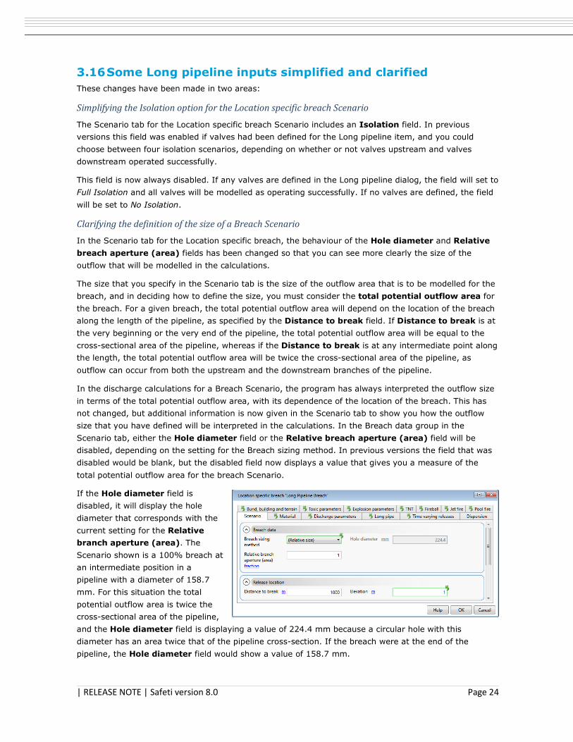
3.16 Some Long pipeline inputs simplified and clarified
These changes have been made in two areas:
Simplifying the Isolation option for the Location specific breach Scenario
The Scenario tab for the Location specific breach Scenario includes an Isolation field. In previous
versions this field was enabled if valves had been defined for the Long pipeline item, and you could
choose between four isolation scenarios, depending on whether or not valves upstream and valves
downstream operated successfully.
This field is now always disabled. If any valves are defined in the Long pipeline dialog, the field will set to
Full Isolation and all valves will be modelled as operating successfully. If no valves are defined, the field
will be set to No Isolation.
Clarifying the definition of the size of a Breach Scenario
In the Scenario tab for the Location specific breach, the behaviour of the Hole diameter and Relative
breach aperture (area) fields has been changed so that you can see more clearly the size of the
outflow that will be modelled in the calculations.
The size that you specify in the Scenario tab is the size of the outflow area that is to be modelled for the
breach, and in deciding how to define the size, you must consider the total potential outflow area for
the breach. For a given breach, the total potential outflow area will depend on the location of the breach
along the length of the pipeline, as specified by the Distance to break field. If Distance to break is at
the very beginning or the very end of the pipeline, the total potential outflow area will be equal to the
cross-sectional area of the pipeline, whereas if the Distance to break is at any intermediate point along
the length, the total potential outflow area will be twice the cross-sectional area of the pipeline, as
outflow can occur from both the upstream and the downstream branches of the pipeline.
In the discharge calculations for a Breach Scenario, the program has always interpreted the outflow size
in terms of the total potential outflow area, with its dependence of the location of the breach. This has
not changed, but additional information is now given in the Scenario tab to show you how the outflow
size that you have defined will be interpreted in the calculations. In the Breach data group in the
Scenario tab, either the Hole diameter field or the Relative breach aperture (area) field will be
disabled, depending on the setting for the Breach sizing method. In previous versions the field that was
disabled would be blank, but the disabled field now displays a value that gives you a measure of the
total potential outflow area for the breach Scenario.
If the Hole diameter field is
disabled, it will display the hole
diameter that corresponds with the
current setting for the Relative
branch aperture (area). The
Scenario shown is a 100% breach at
an intermediate position in a
pipeline with a diameter of 158.7
mm. For this situation the total
potential outflow area is twice the
cross-sectional area of the pipeline,
and the Hole diameter field is displaying a value of 224.4 mm because a circular hole with this
diameter has an area twice that of the pipeline cross-section. If the breach were at the end of the
pipeline, the Hole diameter field would show a value of 158.7 mm.
| RELEASE NOTE | Safeti version 8.0 Page 25
If the Relative branch aperture (area) field is disabled, it will display the relative aperture that
corresponds with the current setting for the Hole diameter. For a pipeline size of 158.7 mm and an
intermediate breach location, if the Hole diameter were enabled and set to 158.7 mm, the Relative
branch aperture would be showing a value of 0.5, i.e. half the total potential outflow area.
Note: For a Section breach Scenario the breach is always assumed to be in an intermediate location, so
the total potential outflow area will always be twice the cross-sectional area of the pipeline. The Hole
diameter and Relative branch aperture (area) fields behave in the same way in the Section breach
dialog as in the Location specific breach dialog, for both types of breach Scenario, so you will get the
same reminder of how the size you have defined will be interpreted.
3.17 The options for Risk Results are presented more clearly in
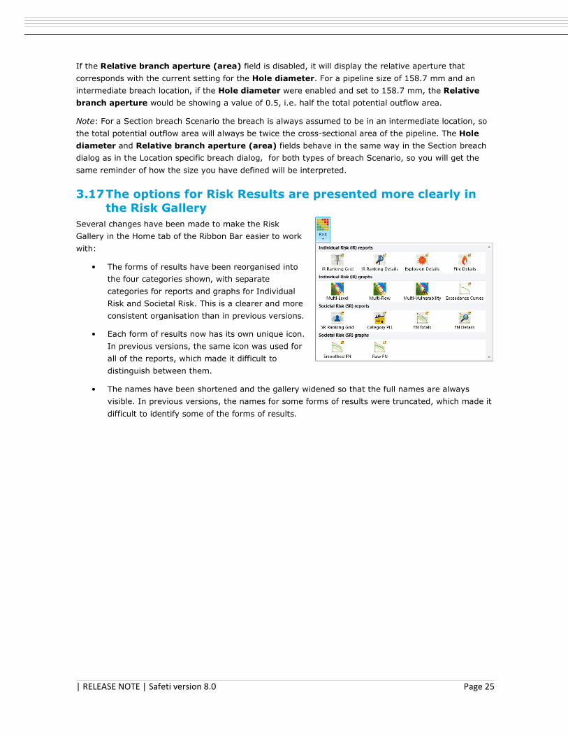
the Risk Gallery
Several changes have been made to make the Risk
Gallery in the Home tab of the Ribbon Bar easier to work
with:
• The forms of results have been reorganised into
the four categories shown, with separate
categories for reports and graphs for Individual
Risk and Societal Risk. This is a clearer and more
consistent organisation than in previous versions.
• Each form of results now has its own unique icon.
In previous versions, the same icon was used for
all of the reports, which made it difficult to
distinguish between them.
• The names have been shortened and the gallery widened so that the full names are always
visible. In previous versions, the names for some forms of results were truncated, which made it
difficult to identify some of the forms of results.
| RELEASE NOTE | Safeti version 8.0 Page 26
3.18 Bug fixes
The following bugs have been fixed in v8:
1 B-13586 Issues with reporting of Material to Track
Description Some reports of toxic and flammable effects included the value set for the material
to track, which could be taken as implying that the results in the reports were based
on the concentrations for that material. This is incorrect, as these results are always
based on the concentration for the whole mixture.
The value for material to track reported was the value set at the Equipment level,
not the value set at the Scenario level.
2 B-14536 Checks for self-crossing polygons are now done for ignition as well as population
Description In versions of the program before v7.2, it was possible to define a polygon shape in
which one line of the shape crossed over another line, which is not a valid shape for
the purposes of a risk analysis. When you opened a file from one of these versions,
the program would check population polygons for this error and give messages
about any that were found, but it would not perform the checks for ignition
polygons.
3 D-10757 Pool fire not modelled for a source Scenario when jet axis impinges on ground
Description If the axis of the jet flame impinges on the ground, the jet fire calculations will fail
and not produce results, and in this situation the program used to omit the
modelling of pool fires, even though this modelling should not have been affected by
the jet flame impingement.
Note: you can prevent the jet fire calculations from failing because of ground
impingement if you make sure that the new Flame-shape adjustment if
grounded option is checked. With this option, the position of the flame will be
adjusted so that the grounding does not occur, and the jet fire calculations will
produce results.
4 D-11050 Negative times in vapour discharge calculations for long pipeline
Description In some situations, the discharge calculations for a long vapour pipeline with valves
would produce results with negative times and give an error.

| RELEASE NOTE | Safeti version 8.0 Page 27
5 D-11066 Improved warning messages for Toxic Dose footprint graphs
Description When you view the graphs for a toxic Scenario, the initial levels used for the toxic
footprint graphs are those set in the Toxic parameters tab for the Scenario. For
probit and lethality, the default values for the levels cover the likely range of results
of interest, but for dose, the default values may be much lower than the levels
calculated for the Scenario because the toxic lethality for the Scenario had dropped
below the minimum level of interest when the dose level was still above the
maximum default level. In this situation the dose footprint graphs will initially be
blank, and a warning message about the lack of results will be written to the Output
View.
The warning message used to suggest reducing the minimum probability of death in
order to see dose footprint results. This would not be an efficient approach, as it
would be much easier to use the Edit Settings dialog in the Consequence tab of the
Ribbon Bar to increase the values for the dose levels that you want to plot for the
current Graph View. The warning message has been changed to be more helpful,
and now suggests increasing the target dose value.
6 D-11649 Graphs show distances that are clearly not to the concentration stated
Description In some situations where a given Scenario had results for more than one Run Row
and the settings for the Parameters meant that different Run Rows had different
concentrations of interest, the legend in the Footprint, Side View and Max
Concentration Dispersion Graphs could display concentrations of interest that were
not the correct values for the Run Row being plotted (e.g. the legend might state
that the footprint results were for 100 ppm when in fact they were for 5000 ppm).
7 D-11734 Negative concentrations in dispersion results
Description For a short-duration time-varying Scenario modelled with multiple rates, the
Dispersion Report could sometimes show negative values for concentration.
| RELEASE NOTE | Safeti version 8.0 Page 28
4 PERFORMING A LARGE ANALYSIS
Performing a large analysis with Safeti 8.0 may require planning and the use of particular techniques and
tools. You should make sure that you understand the issues involved before you start work on a new
analysis that is likely to be large, or before you upgrade an existing large analysis.
4.1 Why is special attention needed for a large analysis?
There are two main factors that can make an analysis with a large workspace file difficult to work with:
Some operations can be very slow with a large workspace
Many operations become slower as the size of the workspace increases, including the following:
• Working with the nodes in the Study Tree, especially with Equipment and Scenario nodes in the
Models tab.
• Using the Grid View to change or view the values for input data.
• Using the GIS Input View, e.g. adding new data, or moving around the view.
• Using the GIS Configuration View in the Run Row Grid to view the set of map-based data
selected for an individual Run Row.
• Exporting input data values to Excel.
• Running the calculations.
• Viewing consequence results for a large number of Scenarios.
• Saving an analysis to a workspace file, if the workspace contains results.
• Opening a workspace that contains results.
• Upgrading a large analysis from a previous version of the program (e.g. from version 6.7.).
For example, saving a large analysis with results to a workspace file may take several hours.
The risk of running out of memory or disk space increases with a large analysis
With most of the operations listed above, there is also a risk that the program may run out of memory
and crash, which will mean that you will lose any work that you did on the workspace after the last time
you saved it to file.
The risk results can occupy a large amount of disk space, and there is the risk of running out of disk
space during the risk calculations, which will cause the program to crash and may also cause problems
for other programs on the computer.

| RELEASE NOTE | Safeti version 8.0 Page 29
4.2 At what point should an analysis be considered “large”?
As a rule of thumb, the size S of an workspace from the point of view of performance can be assessed as
follows:
where Nscenarios is the number of scenarios that are selected for Run Rows, Nweathers is the number of
Weathers that are selected for Run Rows, and NParameter Sets is the number of Parameter Sets that are
selected for Run Rows. These variables affect the volume of consequence results that have to be held in
memory during calculations, and a workspace can be considered large if S is greater than 1000. If
your analysis is large by this measure, there are steps that you can take to make the analysis more
manageable and reliable.
Other factors that affect the performance are the number of ignition sources selected (including
populations that are being modelled as ignition sources), the number of vulnerabilities defined for the
workspace, and the number of obstructed regions in the Sets that are selected for the Run Rows (if the
Explosion Method is set to “3D Obstructed Regions”). However, the three factors that affect the volume
of consequence results are those that have the largest effect on performance.
4.3 What can I do to make a large analysis easier to perform?
The options for approaching a large analysis are described below, in the order in which they should be
considered or employed in an analysis.
Use a computer with the highest specifications that you can obtain
The recommended specification for a large analysis in version 8.0 is as follows:
Operating system Microsoft Vista SP2 (32 bit version), Windows7 SP1, Windows 8, Windows 8.1
and Windows 10 (32 or 64 bit version).
Type of hard drive Solid State Drive (SSD)
This is the most important recommendation.
Size of hard drive The program itself requires up to 10 GB of free disk space on a standard
Windows 7 SP1 machine, and the input data and results for a single large
workspace can occupy 100 GB of disk space or more.
CPU Recommended: Intel i7, 64-bit CPU from Intel
Minimum: Intel Quad Core 2.7 GHz
The fastest machines we are currently aware of are the DELL Precision 7000
laptops.
Memory Recommended: 16GB
Minimum spare memory: 4GB
Microsoft Excel Safeti requires Excel for the Excel input/output tool
If you are purchasing a new computer you should make sure it has a NVIDIA graphics card that is CUDA
enabled (e.g. the M series), as the calculations for individual risk are able to run on either multiple CUDA
cores or multiple CPU cores, depending on the settings in the IRISK tab of the General risk parameters.
Aspects of the consequence calculations will run on multiple CPU cores if the option to Enable
multithreading for dispersion and toxic calculations is checked in the Workspace dialog.

| RELEASE NOTE | Safeti version 8.0 Page 30
Build up the analysis gradually, examining intermediate results and performing sensitivity assessments
to see if the number of variables can be reduced
You should run consequence calculations and examine the results before proceeding to the risk
calculations. If the results for particular scenarios or weathers are very similar, you can reduce the size
of the workspace by combining or removing scenarios and weathers.
Having examined the range of consequence results, you might decide to perform some limited runs of
the risk calculations, with a selection of scenarios of different sizes and types, and with different levels of
detail in the modelling of the number of weather directions, populations, ignition sources, vulnerabilities
and obstructed regions. If these sensitivity assessments show that the differences in the levels of detail
do not give significant differences in the calculated levels of risk, you can reduce the size of the
workspace by using a lower level of detail.
Use the Excel input/output tool when setting up input data
The process of exporting and importing input data with Excel using the options in the Tools tab of the
Ribbon Bar is quicker and requires less memory than inserting nodes directly in the Study Tree and using
the input dialogs or the Grid View to set the input values. Having the input data defined in Excel also
means that you can edit and maintain the data easily over the course of an analysis, i.e. to make
changes that affect a large number of Scenarios as assumptions change, and then reimport the data into
the program.
If you need to copy or move a large number of Equipment and Scenario nodes from one part of the
Study Tree to another, it is better to export the data to Excel, edit the Excel file to set the path for the
Equipment items to the path for the new location (i.e. under a different Study or Folder), and then
import from the Excel file. If you try to copy (or cut) and paste a large number of nodes directly in the
Study Tree, the demands on memory may cause the program to freeze, but this will not happen if you
use Excel.
Consider dividing the analysis between separate workspace files and using the Study Manager to
combine the high level risk results
The Study Manager is installed when you install Safeti 8.0. It allows you import risk contour results and
Smoothed FN results from any number of separate workspace files, and then to add these results
together to obtain the full results for the analysis. The Study Manager has its own online Help and
Release Notes, that explain how to use it.
There are two approaches to dividing an analysis between separate workspace files:
1. Dividing different aspects of the input data between different files, but running all types of
relevant risk calculations for each file.
For example, you might define the Equipment for different units in different files, or you might
define the daytime and the nighttime conditions for weather, population and ignition sources in
different files.
2. Having the same input data in each file, but running separate aspects of the risk calculations for
each file.
The Diagnostics option in the Settings tab of the Ribbon Bar allows you to control which aspects
of the risk calculations to run for that workspace file, e.g. whether to calculate only individual
risk, or only societal risk, or both.
For a very large analysis, you might use both approaches.
| RELEASE NOTE | Safeti version 8.0 Page 31
Use Excel input/output to maintain the input data across multiple files
With both approaches, you will have several workspace files that have a lot of data in common, e.g.
population and ignition data, weather data, etc. Input values are frequently revised during the course of
an analysis, and the Excel input/output tool is the quickest and most reliable way of keeping the values
consistent across all of the files in the analysis.
Save the consequence results to file before starting the risk calculations
If you use the second approach - or if you think that you might use it- you should start with a single
workspace file, run the consequence calculations for that workspace and then save the file with the
results. You can then create a copy of the workspace file for each type of risk results that you want to
run separately, set the Diagnostic options in each file, and then proceed to run the risk calculations for
each file. It is always advisable to run the consequence calculations on their own before proceeding to
the risk calculations so that you can examine the results and make any appropriate adjustments to the
assumptions and input values, but running them separately in this way also makes it easier to adopt the
second approach, as you will not have to rerun the consequence calculations for each separate file.
Use Export Workspace instead of Save / Save As to save the workspace file after running the risk
calculations
The Export Workspace option in the File tab of the Ribbon Bar saves the workspace as a special format of
*.psux file that has the database of risk results embedded inside it, along with any map image files that
are used by the workspace. The Study Manager only allows you to import workspace files that are in this
format, and will give an error message if you try to import a workspace file that was saved with either
the Save or Save As options.
Note: if you use the Console tool to run the calculations for a workspace (as described in a later section),
the Console will always save the calculated workspace in the exported format. This means that you will
be able to import the calculated workspace into the Study Manager immediately after the Console has
completed the calculations, and you do not have to open the workspace in the Safeti program first in
order to use Export Workspace to create a version of the workspace in the exported format.
Divide Equipment between different Run Rows in a workspace to increase the level of detail available
from the Study Manager results
The types of results that are summed and displayed in the Study Manager do not allow you to drill down
to see which individual Scenarios or Weathers or types of effect or types of population contribute most to
the risk levels, and the lowest level of detail that is available in the Study Manager is the level of the
individual Run Rows in a particular workspace. To obtain a full breakdown of the contributions to the risk
levels, you must use the additional forms of results that are available in the Safeti program itself.
However, if you structure the workspace files so that different types of Equipment items or Scenarios are
divided between different Run Rows, the risk results for the individual Run Rows as presented in the
Study Manager will give you good information about the main sources of risk.
Put Route Models and Long Pipeline Models in separate workspace files
The Route Model and the Long Pipeline Model can involve modelling a large number of Scenarios at a
large number of different locations, and the calculations can consume a lot of time and memory.
To make the analysis more manageable, you should place each Route Model and each Long Pipeline
Model in its own workspace file.
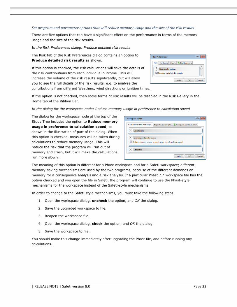
| RELEASE NOTE | Safeti version 8.0 Page 32
Set program and parameter options that will reduce memory usage and the size of the risk results
There are five options that can have a significant effect on the performance in terms of the memory
usage and the size of the risk results.
In the Risk Preferences dialog: Produce detailed risk results
The Risk tab of the Risk Preferences dialog contains an option to
Produce detailed risk results as shown.
If this option is checked, the risk calculations will save the details of
the risk contributions from each individual outcome. This will
increase the volume of the risk results significantly, but will allow
you to see the full details of the risk results, e.g. to analyse the
contributions from different Weathers, wind directions or ignition times.
If the option is not checked, then some forms of risk results will be disabled in the Risk Gallery in the
Home tab of the Ribbon Bar.
In the dialog for the workspace node: Reduce memory usage in preference to calculation speed
The dialog for the workspace node at the top of the
Study Tree includes the option to Reduce memory
usage in preference to calculation speed, as
shown in the illustration of part of the dialog. When
this option is checked, measures will be taken during
calculations to reduce memory usage. This will
reduce the risk that the program will run out of
memory and crash, but it will make the calculations
run more slowly.
The meaning of this option is different for a Phast workspace and for a Safeti workspace; different
memory-saving mechanisms are used by the two programs, because of the different demands on
memory for a consequence analysis and a risk analysis. If a particular Phast 7.* workspace file has the
option checked and you open the file in Safeti, the program will continue to use the Phast-style
mechanisms for the workspace instead of the Safeti-style mechanisms.
In order to change to the Safeti-style mechanisms, you must take the following steps:
1. Open the workspace dialog, uncheck the option, and OK the dialog.
2. Save the upgraded workspace to file.
3. Reopen the workspace file.
4. Open the workspace dialog, check the option, and OK the dialog.
5. Save the workspace to file.
You should make this change immediately after upgrading the Phast file, and before running any
calculations.
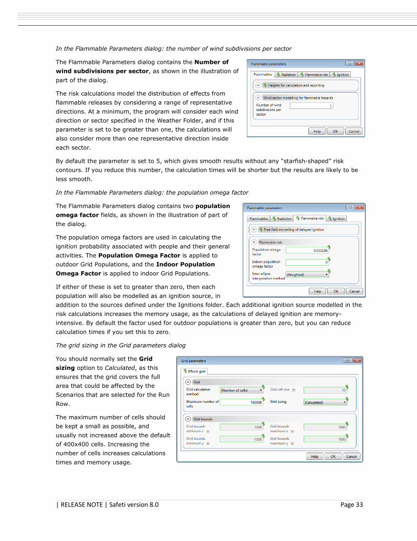
| RELEASE NOTE | Safeti version 8.0 Page 33
In the Flammable Parameters dialog: the number of wind subdivisions per sector
The Flammable Parameters dialog contains the Number of
wind subdivisions per sector, as shown in the illustration of
part of the dialog.
The risk calculations model the distribution of effects from
flammable releases by considering a range of representative
directions. At a minimum, the program will consider each wind
direction or sector specified in the Weather Folder, and if this
parameter is set to be greater than one, the calculations will
also consider more than one representative direction inside
each sector.
By default the parameter is set to 5, which gives smooth results without any “starfish-shaped” risk
contours. If you reduce this number, the calculation times will be shorter but the results are likely to be
less smooth.
In the Flammable Parameters dialog: the population omega factor
The Flammable Parameters dialog contains two population
omega factor fields, as shown in the illustration of part of
the dialog.
The population omega factors are used in calculating the
ignition probability associated with people and their general
activities. The Population Omega Factor is applied to
outdoor Grid Populations, and the Indoor Population
Omega Factor is applied to indoor Grid Populations.
If either of these is set to greater than zero, then each
population will also be modelled as an ignition source, in
addition to the sources defined under the Ignitions folder. Each additional ignition source modelled in the
risk calculations increases the memory usage, as the calculations of delayed ignition are memory-
intensive. By default the factor used for outdoor populations is greater than zero, but you can reduce
calculation times if you set this to zero.
The grid sizing in the Grid parameters dialog
You should normally set the Grid
sizing option to Calculated, as this
ensures that the grid covers the full
area that could be affected by the
Scenarios that are selected for the Run
Row.
The maximum number of cells should
be kept a small as possible, and
usually not increased above the default
of 400x400 cells. Increasing the
number of cells increases calculations
times and memory usage.
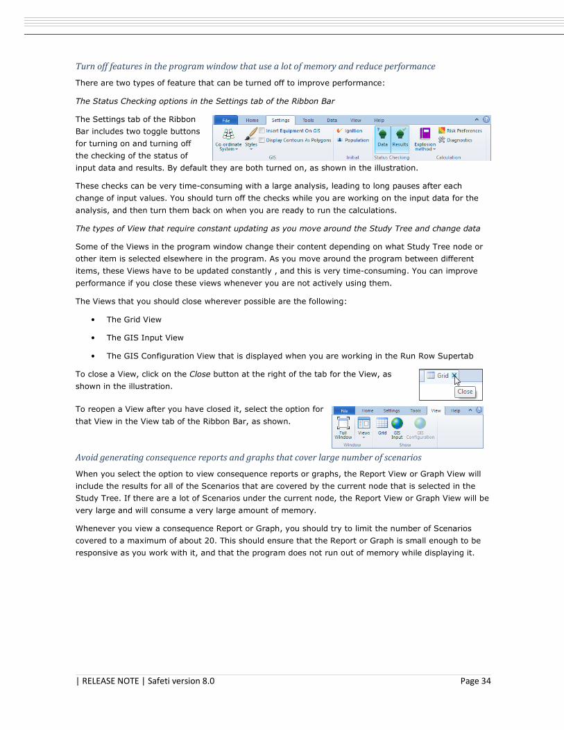
| RELEASE NOTE | Safeti version 8.0 Page 34
Turn off features in the program window that use a lot of memory and reduce performance
There are two types of feature that can be turned off to improve performance:
The Status Checking options in the Settings tab of the Ribbon Bar
The Settings tab of the Ribbon
Bar includes two toggle buttons
for turning on and turning off
the checking of the status of
input data and results. By default they are both turned on, as shown in the illustration.
These checks can be very time-consuming with a large analysis, leading to long pauses after each
change of input values. You should turn off the checks while you are working on the input data for the
analysis, and then turn them back on when you are ready to run the calculations.
The types of View that require constant updating as you move around the Study Tree and change data
Some of the Views in the program window change their content depending on what Study Tree node or
other item is selected elsewhere in the program. As you move around the program between different
items, these Views have to be updated constantly , and this is very time-consuming. You can improve
performance if you close these views whenever you are not actively using them.
The Views that you should close wherever possible are the following:
• The Grid View
• The GIS Input View
• The GIS Configuration View that is displayed when you are working in the Run Row Supertab
To close a View, click on the Close button at the right of the tab for the View, as
shown in the illustration.
To reopen a View after you have closed it, select the option for
that View in the View tab of the Ribbon Bar, as shown.
Avoid generating consequence reports and graphs that cover large number of scenarios
When you select the option to view consequence reports or graphs, the Report View or Graph View will
include the results for all of the Scenarios that are covered by the current node that is selected in the
Study Tree. If there are a lot of Scenarios under the current node, the Report View or Graph View will be
very large and will consume a very large amount of memory.
Whenever you view a consequence Report or Graph, you should try to limit the number of Scenarios
covered to a maximum of about 20. This should ensure that the Report or Graph is small enough to be
responsive as you work with it, and that the program does not run out of memory while displaying it.
| RELEASE NOTE | Safeti version 8.0 Page 35
Check that you have at least 100 GB of hard disk space free before starting the risk calculations for a
large workspace
The risk results for a single large workspace can occupy 100 GB of disk space or more. Before you start
the risk calculations for any large workspace, you should check that the hard disk has at least this much
space free.
If you wish to remove old database of risk results which might be taking up space on your C: drive, you
can simply delete them from the following locations:
C:\ProgramData\DNVGL\Safeti_Phast_Phoenix\DatabaseStorage
C:\ProgramData\DNVGL\Safeti_Phast_ Phoenix\DatabaseStorage\temp
Consider using the Console tool in order to run the calculations without using the program window
The Console is an applications that runs in a Windows Command Prompt window, and that runs the
Safeti consequence and risk calculations completely separate from the program window. The program
window and the operations of its various features consume memory, so using the Console maximises the
amount of memory available for the calculations.
The Console will run the calculations for all of the workspace files in a specified folder, which means that
you can run the entire analysis with a single command.
Once the calculations have been run in the Console, you can run either the Safeti program or the Study
Manager and view the results. The Console always save the calculated workspaces in the exported
format which means that you will be able to import the calculated workspace into the Study Manager
immediately after the Console has completed the calculations, and you do not have to open the
workspace in the Safeti program first in order to use Export Workspace to create a version of the
workspace in the exported format.
To use the Console, take the following steps:
1. Ensure you have local administration rights for the computer. If you do not, ask your IT
department to arrange this for you.
2. Create or choose a folder for storing the workspace files for the analysis. The path to the
workspaces folder must not contain any spaces.
3. Create or choose a folder for storing the consequence and risk results for the analysis. The
results folder must be different from the workspaces folder, and the path must not
contain any spaces.
4. For each workspace in the analysis, set up the input data in Safeti, and save the workspace to a
*.psux file in the folder for the analysis. The names of the *.psux files must not include any
spaces.
5. Exit from the Safeti program.
6. If you have made any changes to the administration files in setting up the data for the analysis,
you must copy the changed administration files from the folder that is used by the full Safeti
program to the folder that is used by the Console.
The full Safeti program works with administration files located in this folder:
C:\ProgramData\DNVGL\Safeti_Phast_Phoenix\Admin
whereas the Console uses files located in this folder:
C:\Program Files (x86)\DNVGL\Safeti_Phast_Phoenix\configuration
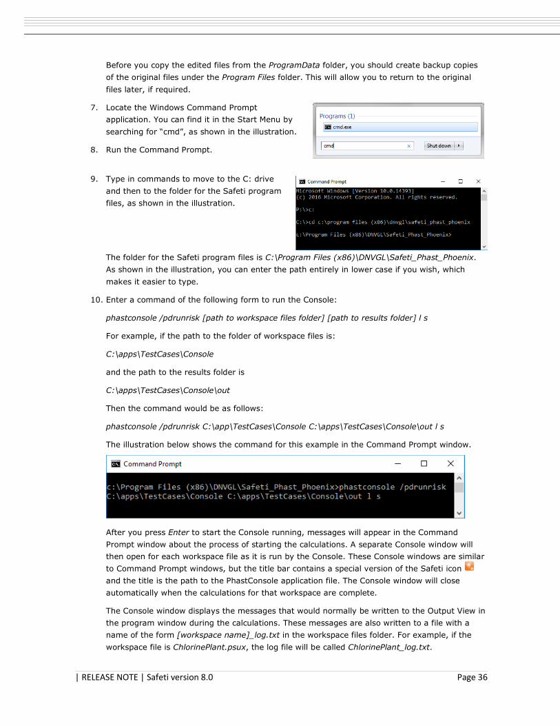
| RELEASE NOTE | Safeti version 8.0 Page 36
Before you copy the edited files from the ProgramData folder, you should create backup copies
of the original files under the Program Files folder. This will allow you to return to the original
files later, if required.
7. Locate the Windows Command Prompt
application. You can find it in the Start Menu by
searching for “cmd”, as shown in the illustration.
8. Run the Command Prompt.
9. Type in commands to move to the C: drive
and then to the folder for the Safeti program
files, as shown in the illustration.
The folder for the Safeti program files is C:\Program Files (x86)\DNVGL\Safeti_Phast_Phoenix.
As shown in the illustration, you can enter the path entirely in lower case if you wish, which
makes it easier to type.
10. Enter a command of the following form to run the Console:
phastconsole /pdrunrisk [path to workspace files folder] [path to results folder] l s
For example, if the path to the folder of workspace files is:
C:\apps\TestCases\Console
and the path to the results folder is
C:\apps\TestCases\Console\out
Then the command would be as follows:
phastconsole /pdrunrisk C:\app\TestCases\Console C:\apps\TestCases\Console\out l s
The illustration below shows the command for this example in the Command Prompt window.
After you press Enter to start the Console running, messages will appear in the Command
Prompt window about the process of starting the calculations. A separate Console window will
then open for each workspace file as it is run by the Console. These Console windows are similar
to Command Prompt windows, but the title bar contains a special version of the Safeti icon
and the title is the path to the PhastConsole application file. The Console window will close
automatically when the calculations for that workspace are complete.
The Console window displays the messages that would normally be written to the Output View in
the program window during the calculations. These messages are also written to a file with a
name of the form [workspace name]_log.txt in the workspace files folder. For example, if the
workspace file is ChlorinePlant.psux, the log file will be called ChlorinePlant_log.txt.
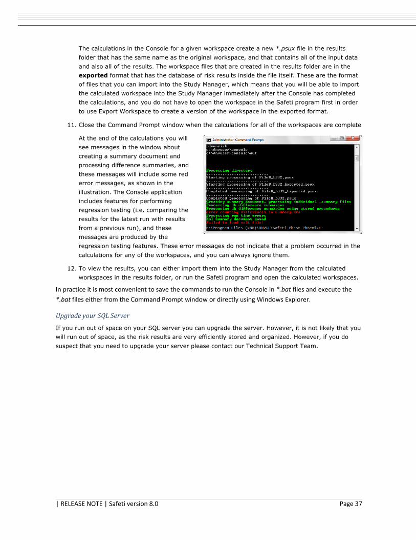
| RELEASE NOTE | Safeti version 8.0 Page 37
The calculations in the Console for a given workspace create a new *.psux file in the results
folder that has the same name as the original workspace, and that contains all of the input data
and also all of the results. The workspace files that are created in the results folder are in the
exported format that has the database of risk results inside the file itself. These are the format
of files that you can import into the Study Manager, which means that you will be able to import
the calculated workspace into the Study Manager immediately after the Console has completed
the calculations, and you do not have to open the workspace in the Safeti program first in order
to use Export Workspace to create a version of the workspace in the exported format.
11. Close the Command Prompt window when the calculations for all of the workspaces are complete
At the end of the calculations you will
see messages in the window about
creating a summary document and
processing difference summaries, and
these messages will include some red
error messages, as shown in the
illustration. The Console application
includes features for performing
regression testing (i.e. comparing the
results for the latest run with results
from a previous run), and these
messages are produced by the
regression testing features. These error messages do not indicate that a problem occurred in the
calculations for any of the workspaces, and you can always ignore them.
12. To view the results, you can either import them into the Study Manager from the calculated
workspaces in the results folder, or run the Safeti program and open the calculated workspaces.
In practice it is most convenient to save the commands to run the Console in *.bat files and execute the
*.bat files either from the Command Prompt window or directly using Windows Explorer.
Upgrade your SQL Server
If you run out of space on your SQL server you can upgrade the server. However, it is not likely that you
will run out of space, as the risk results are very efficiently stored and organized. However, if you do
suspect that you need to upgrade your server please contact our Technical Support Team.
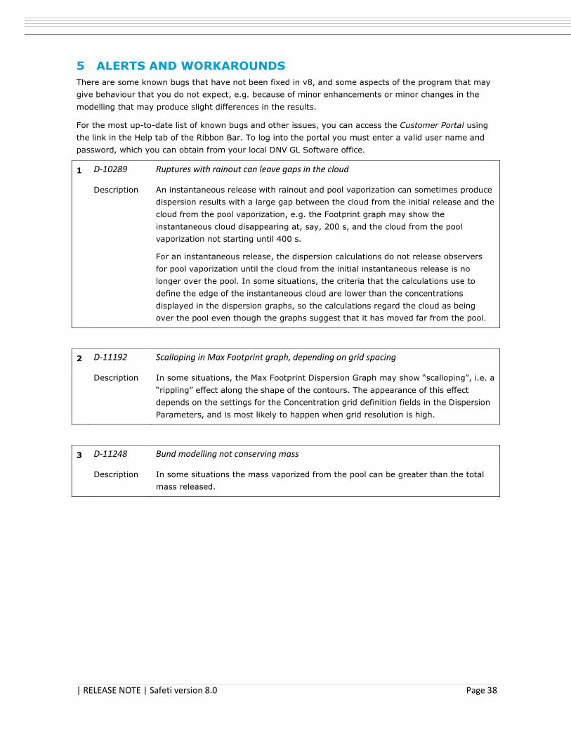
| RELEASE NOTE | Safeti version 8.0 Page 38
5 ALERTS AND WORKAROUNDS
There are some known bugs that have not been fixed in v8, and some aspects of the program that may
give behaviour that you do not expect, e.g. because of minor enhancements or minor changes in the
modelling that may produce slight differences in the results.
For the most up-to-date list of known bugs and other issues, you can access the Customer Portal using
the link in the Help tab of the Ribbon Bar. To log into the portal you must enter a valid user name and
password, which you can obtain from your local DNV GL Software office.
1 D-10289 Ruptures with rainout can leave gaps in the cloud
Description An instantaneous release with rainout and pool vaporization can sometimes produce
dispersion results with a large gap between the cloud from the initial release and the
cloud from the pool vaporization, e.g. the Footprint graph may show the
instantaneous cloud disappearing at, say, 200 s, and the cloud from the pool
vaporization not starting until 400 s.
For an instantaneous release, the dispersion calculations do not release observers
for pool vaporization until the cloud from the initial instantaneous release is no
longer over the pool. In some situations, the criteria that the calculations use to
define the edge of the instantaneous cloud are lower than the concentrations
displayed in the dispersion graphs, so the calculations regard the cloud as being
over the pool even though the graphs suggest that it has moved far from the pool.
2 D-11192 Scalloping in Max Footprint graph, depending on grid spacing
Description In some situations, the Max Footprint Dispersion Graph may show “scalloping”, i.e. a
“rippling” effect along the shape of the contours. The appearance of this effect
depends on the settings for the Concentration grid definition fields in the Dispersion
Parameters, and is most likely to happen when grid resolution is high.
3 D-11248 Bund modelling not conserving mass
Description In some situations the mass vaporized from the pool can be greater than the total
mass released.
| RELEASE NOTE | Safeti version 8.0 Page 39
4 D-11540 Upgraded standalone pool vaporization Models from v6 not included in any Model
Selection
Description If you upgrade a v6.54 or v6.7 file that includes a standalone Pool Vaporization
Model, the Model will be upgraded as a Spill Scenario under an AST Equipment item,
but it will be removed from the Model Selection which means that it will not be
included when you run the calculations, no matter which Run Row is selected.
The upgrade is handled in this way because the standalone Pool Vaporization Model
can not be used in the risk calculations, but the Spill Scenario can. The Spill
Scenario will be incomplete on upgrade because there is no event frequency
specified, and it is removed from the Model Selection so that it does not cause
problems with the risk calculations.
You should decide whether or not you want to include the Scenario in the risk
calculations. If you decide not to include it but you do want to be able to run the
consequence calculations for it, you should create a separate Model Selection and
Run Row for it, and only run the consequences calculations for that Run Row.
5 D-11777 Mandation of plant boundary in run row grid
Description In the Run Row Grid, the Plant Boundary field is never shown as mandatory even
if Use free field modelling is set to Free field (plant boundary) in the Flammable
parameters.
6 D-11858 Problem on changing Material when Material to Track is set
Description If a mixture was selected for an Equipment item, and one of the components of the
mixture was selected as the material to track for the Equipment or a Scenario, this
component will remain selected if you change the selection of Material to something
that does not include the selected component. The Equipment and Scenario will not
be shown as having an error in the input data, but the Scenario will give errors in
the dispersion calculations about the chosen component not being present in the
mixture.
7 D-11985 Risk Results not generated when Ribbon Bar is minimized
Description There is a minimize option at the right side of the Ribbon Bar, and if you turn this
option on, the Ribbon Bar will be “collapsed” so that only the names of the tabs are
visible. You have to click on the name of a particular tab to expand the Ribbon Bar
and view and use the options.
When the option is turned on, you will be able to view the list of Risk Results in the
Home tab of the Ribbon Bar, but nothing will happen when you click on one of the
types of results in the Risk Gallery. To view Risk Results, you must turn off the
option to minimize the Ribbon Bar.
| RELEASE NOTE | Safeti version 8.0 Page 40
8 D-12104 Dispersion Graphs are always present for time-varying Scenarios even if only the
discharge calculations have been run
Description If you set the Mode to Discharge in the Home tab of the Ribbon Bar, run the
calculations for a time-varying Scenario or a Long pipeline breach Scenario and then
view the Graphs, you will find that the full set of Dispersion Graphs are present,
though all of the graphs are blank except for the Mass Rate Graph.
9 D-12221 Reports flagged out of date when you change the averaging time for the graph
Description If you have both Reports and Graphs open for a Scenario, and you use the Edit
Settings dialog for the Graphs to change the selection of averaging time, you will
find that the Reports are shown as being out of date, even though the change to the
averaging time is only relevant to the Graphs.
10 D-12256 Limited support for long pipelines under Routes
Description In versions of the program before v7.2, it was possible to insert a Long pipeline
Model under a Route Model. This is no longer possible, but if you upgrade a file that
contains a Route Model with a Long pipeline item defined underneath it, the Long
pipeline item will not be deleted and you will be able to use it in the calculations.
However, some features of the program will not be available for a Long pipeline
under a Route Model, e.g. the Long pipeline will not be included if you export the
workspace data to Excel.
11 D-12286 Some functions are disabled for a Warehouse Model created by copying and pasting
Description If you create a Warehouse Model by copying and pasting another Warehouse
Model, some functions will not work for the second Warehouse Model:
• If the Warehouse Model is in a folder and you right-click on the folder and
select Generate warehouse scenarios, Fire Scenarios will not be generated
for the second Warehouse Model. However, if you right-click on the second
Warehouse Model itself and select Generate warehouse scenarios, the Fire
Scenarios will be generated.
• The Run option will be disabled for the second Warehouse Model, although
it will be enabled for the individual Fire Scenarios under the Model.
12 D-12335 Consequence results are cleared for a Long pipeline item when you change the failure
frequency data
Description If you run the consequence calculations for a Long pipeline and then change any of
the settings for the failure frequency in the Risk tab for the item, the results of the
consequence calculations will be cleared even though the values for frequency are
not relevant to the consequence calculations.
| RELEASE NOTE | Safeti version 8.0 Page 41
13 D-12362 Jet Fire Contour graph for a standalone Jet Fire Scenario shown as out of date after
checking option to Show Flame Shape
Description If the option to plot side view contours is selected for a standalone Jet Fire
Scenario, the option to Show Flame Shape will be enabled in the Consequence
tab of the Ribbon Bar when the Jet Fire Contour Graph is selected. If you check this
option, the Graphs will be shown incorrectly as being out of date.
14 D-12390 Time-varying Scenarios not shown in the Study Tree as run successfully when the
Calculation Mode is set to Discharge
Description If the Calculation Mode is set to Discharge in the Home tab of the Ribbon Bar and
you run the calculations for a set of source Scenarios, the Scenarios whose
discharge calculations run successfully should be shown with green ticks in the
Study Tree. These green ticks are shown for most types of source Scenario, but not
for Time-varying leak Scenarios or Time-varying short pipe Scenarios.
15 D-12431 A User-defined Source Scenario generated from a Scenario with multi-rate time-
varying discharge results will give Jet Fire results that are different from those for the
original Scenario
Description The right-click menu for a source Scenario that has results present will include the
option to generate a User-defined Source Scenario. The discharge results for the
selected Scenario will be used as the definition of the release observers for the
User-defined Source Scenario.
If the original Scenario is a Time-varying leak Scenario, a Time-varying short pipe
Scenario or a Location specific breach Scenario, and the Method for calculating
average rate is set to Up to 10 rates in the Time varying releases tab section, then
if you compare the results between the original Scenario and the generated User-
defined Source Scenario, you will find that the results for dispersion, toxic results
and delayed flammable effects are identical, but that the jet fire results are
different. For the original Scenario, the jet fire calculations use discharge conditions
based on the full, detailed discharge results, whereas for the generated User-
defined Source Scenario, the calculations use discharge conditions based on the list
of release observers in the Scenario tab section. These discharge conditions can be
quite different between the two Scenarios, giving different jet fire results, especially
if the release rate changes rapidly at the start of the release. Typically, the
calculations for the User-defined Source will use a higher discharge rate and give a
larger jet fire with greater effect distances.
When you generate a User-defined Source Scenario from a Scenario that has
Method for calculating average rate set to Up to 10 rates, a warning message
about the differences in jet fire results will be written to the Output View.

| RELEASE NOTE | Safeti version 8.0 Page 42
16 D-12478 Results for a User-defined Source Scenario are not cleared on changing the input data
Description If you run the calculations for a User-defined Source Scenario and then change the
input data for the Scenario, the results will not be cleared and the Scenario will be
shown with a green tick in the Study Tree, showing that it has results that the
program regards as up to date. To be able to rerun the calculations for the Scenario
with the changed input data, you must right-click on the Scenario and select Clear
results.
ABOUT DNV GL Driven by our purpose of safeguarding life, property and the environment, DNV GL enables organizations
to advance the safety and sustainability of their business. We provide classification and technical
assurance along with software and independent expert advisory services to the maritime, oil and gas, and
energy industries. We also provide certification services to customers across a wide range of industries.
Operating in more than 100 countries, our 16,000 professionals are dedicated to helping our customers
make the world safer, smarter and greener.
SOFTWARE
DNV GL is the world-leading provider of software for a safer, smarter and greener future in the energy,
process and maritime industries. Our solutions support a variety of business critical activities including
design and engineering, risk assessment, asset integrity and optimization, QHSE, and ship management.
Our worldwide presence facilitates a strong customer focus and efficient sharing of industry best practice
and standards.