![Interference coordination for millimeter wave ... · frequency reuse factor of one or a universal frequency re-use (UFR) factor [1] to save spectrum. This deployment creates high](https://static.fdocuments.in/doc/165x107/5e91cdeb1cc9f43a86032c4d/interference-coordination-for-millimeter-wave-frequency-reuse-factor-of-one.jpg)
Relay Deployment in Single Frequency Network · PDF fileRelay Deployment in Single Frequency...
101
HELSINKI UNIVERSITY OF TECHNOLOGY Faculty of Electronics, Communications and Automation Department of Signal Processing and Acoustics Renaud-Alexandre Pitaval Relay Deployment in Single Frequency Network Master’s Thesis submitted in partial fulfillment of the requirements for the degree of Master of Science in Technology. Espoo (Finland), August 14, 2009 Supervisor: Professor Risto Wichman Instructor: Taneli Riihonen, M.Sc. (Tech.)
Transcript of Relay Deployment in Single Frequency Network · PDF fileRelay Deployment in Single Frequency...
HELSINKI UNIVERSITY OF TECHNOLOGYFaculty of Electronics, Communications and AutomationDepartment of Signal Processing and Acoustics
Renaud-Alexandre Pitaval
Relay Deployment in Single Frequency
Network
Master’s Thesis submitted in partial fulfillment of the requirements for the degreeof Master of Science in Technology.
Espoo (Finland), August 14, 2009
Supervisor: Professor Risto Wichman
Instructor: Taneli Riihonen, M.Sc. (Tech.)

HELSINKI UNIVERSITY ABSTRACT OF THE
OF TECHNOLOGY MASTER’S THESIS
Author: Renaud-Alexandre Pitaval
Name of the Thesis: Relay Deployment in Single Frequency Network
Date: August 14, 2009 Number of pages: 89
Faculty: Faculty of Electronics, Communications and Automation
Department: Department of Signal Processing and Acoustics
Supervisor: Prof. Risto Wichman
Instructor: Taneli Riihonen, M.Sc. (Tech.)
Future wireless communication systems would have to support very high data rates. As
this vision is not feasible with the conventional cellular architecture without increasing
the density of the base stations, in order to increase the capacity, different transmit
diversity schemes have been heavily investigated in the past years. Relaying has been
one of those areas investigated and has been proposed as a costly advantageous method
to increase the radio coverage area. The scope of this thesis is to build a Matlab simula-
tor for Digital Video Broadcasting - Handheld/Terrestrial (DVB-H/T) and Multimedia
Broadcast Multicast Service (MBMS) in 3G systems and evaluate the performance of
different relaying concepts. The simulated network is a single-frequency network (SFN)
using orthogonal frequency-division multiplexing (OFDM) and the program is a phys-
ical layer simulator. The performance metric is the cumulative distribution function
of the signal-to-interference-plus-noise-ratio (SINR) for different user positions in the
network.
Different simulations have been run to assess the impact of inter-site distance, asyn-
chronity, and other factors such as distance from the border of two SFNs and effect
of possible holes in the SFN grid. Then, the focus is on the impact of fixed relaying
deployment using the amplify and forward protocol. The impact on the SINR is com-
pared for different relaying gain and densities of relays, as well as different transmission
protocol such as the full-duplex and half-duplex protocols. An investigattion is also
made of where the relays should be located in the cells to obtain the best performance.
Analysis is done at the center of the network and at the border of two SFNs.
Keywords: Radio communication, shadowing cross-correlation, OFDM, relays, gain,duplex, SFN.
ii
Acknowledgements
The research work for this thesis was mostly carried out in the Signal Processing
Laboratory at Helsinki University of Technology (TKK) during the years 2007 to
2008 in parallel with my studies as a degree student of the International Master in
Communication Engineering.
I wish to express my gratitude to my supervisor, Prof. Risto Wichman, for offering
me the opportunity to work with him, his understanding and patience during the
writing process, and all the academic helps he provided me.
Many thanks go to my instructor, M.Sc. Taneli Riihonen, for his advices, support
and numerous comments.
Among the contributors to this thesis, I thank sincerely William Martin for the
language comments.
I would like also to thank my former French professors Jerome Mars and Jocelyn
Chanussot, and the international student advisor of ENSIEG Max Ginier-Gillet for
all their help, support and kindliness to make possible my stay at TKK possible and
even more.
I naturally thank Viet-Anh for all the good working time we have spent together
and for other rewarding experiences in the future.
iii

Contents
Acknowledgements iii
Abbreviations vii
List of Figures xi
List of Tables xii
1 Introduction 1
1.1 Background . . . . . . . . . . . . . . . . . . . . . . . . . . . . . . . . 1
1.2 Research problem and scope . . . . . . . . . . . . . . . . . . . . . . . 2
1.3 Outline of the thesis . . . . . . . . . . . . . . . . . . . . . . . . . . . 2
2 Review of the mobile radio channel 4
2.1 Time-varying multipath channel . . . . . . . . . . . . . . . . . . . . 4
2.1.1 Multipath propagation . . . . . . . . . . . . . . . . . . . . . . 4
2.1.2 Doppler effect . . . . . . . . . . . . . . . . . . . . . . . . . . . 5
2.2 Baseband channel model . . . . . . . . . . . . . . . . . . . . . . . . . 6
2.2.1 Time selectivity . . . . . . . . . . . . . . . . . . . . . . . . . . 7
2.2.2 Frequency selectivity . . . . . . . . . . . . . . . . . . . . . . . 8
2.3 Statistical channel modeling . . . . . . . . . . . . . . . . . . . . . . . 10
2.3.1 Small scale propagation model . . . . . . . . . . . . . . . . . 12
2.3.2 Large scale propagation model . . . . . . . . . . . . . . . . . 14
3 Correlation among large scale parameters 18
3.1 Correlated shadowing . . . . . . . . . . . . . . . . . . . . . . . . . . 19
3.1.1 Auto-correlation models . . . . . . . . . . . . . . . . . . . . . 20
iv

3.1.2 Cross-correlation models . . . . . . . . . . . . . . . . . . . . . 20
3.1.3 Correlation among links without a common node . . . . . . . 28
3.2 Correlated angle spread, correlated delay spread . . . . . . . . . . . 28
3.3 Correlation among the “three spreads” . . . . . . . . . . . . . . . . 28
3.4 The problem of a positive definite correlation matrix . . . . . . . . . 29
3.4.1 Cross-correlation model . . . . . . . . . . . . . . . . . . . . . 29
3.4.2 Overall model . . . . . . . . . . . . . . . . . . . . . . . . . . . 30
4 OFDM 32
4.1 Principles of OFDM . . . . . . . . . . . . . . . . . . . . . . . . . . . 32
4.2 Performance analysis . . . . . . . . . . . . . . . . . . . . . . . . . . . 35
4.3 Time of reference . . . . . . . . . . . . . . . . . . . . . . . . . . . . . 38
4.4 Systems exploiting OFDM/DMT . . . . . . . . . . . . . . . . . . . . 39
5 Cooperative communication 40
5.1 Basic relaying concepts . . . . . . . . . . . . . . . . . . . . . . . . . . 41
5.1.1 Relay station type . . . . . . . . . . . . . . . . . . . . . . . . 41
5.1.2 Decode-and-forward and amplify-and-forward relaying . . . . 42
5.1.3 Full-duplex and half-duplex protocols . . . . . . . . . . . . . 42
5.2 A&F relay channel model . . . . . . . . . . . . . . . . . . . . . . . . 43
5.3 Performance with full-duplex protocol . . . . . . . . . . . . . . . . . 45
5.4 Performance with half-duplex protocol . . . . . . . . . . . . . . . . . 48
5.4.1 Selection combining . . . . . . . . . . . . . . . . . . . . . . . 48
5.4.2 Equal gain combining . . . . . . . . . . . . . . . . . . . . . . 49
5.4.3 Maximum ratio combining . . . . . . . . . . . . . . . . . . . . 51
6 Simulator development 52
6.1 Network architecture . . . . . . . . . . . . . . . . . . . . . . . . . . . 52
6.1.1 Cellular network . . . . . . . . . . . . . . . . . . . . . . . . . 52
6.1.2 Single frequency network . . . . . . . . . . . . . . . . . . . . 53
6.2 Simulation scenario . . . . . . . . . . . . . . . . . . . . . . . . . . . 53
6.3 Simulation parameters . . . . . . . . . . . . . . . . . . . . . . . . . . 54
6.3.1 OFDM parameters . . . . . . . . . . . . . . . . . . . . . . . . 55
6.3.2 Network parameters . . . . . . . . . . . . . . . . . . . . . . . 57
v
6.3.3 Transmit power, antenna gain and antenna pattern . . . . . . 57
6.3.4 Channel models . . . . . . . . . . . . . . . . . . . . . . . . . . 58
6.4 Summary tables . . . . . . . . . . . . . . . . . . . . . . . . . . . . . 61
7 Simulation results 63
7.1 SFN area deployment aspects . . . . . . . . . . . . . . . . . . . . . . 63
7.1.1 Impact of asynchronity and ISD . . . . . . . . . . . . . . . . 63
7.1.2 Cells switched off or sending another MBMS . . . . . . . . . 65
7.2 SFN with relays . . . . . . . . . . . . . . . . . . . . . . . . . . . . . . 68
7.2.1 Impact of the relay gains . . . . . . . . . . . . . . . . . . . . 68
7.2.2 Half-duplex versus full-duplex . . . . . . . . . . . . . . . . . . 69
7.2.3 Impact of relay topology . . . . . . . . . . . . . . . . . . . . . 73
7.2.4 Performance at the SFN area borders . . . . . . . . . . . . . 77
8 Conclusions and future work 78
A SINR map 80
Bibliography 83
vi

Abbreviations
3G 3rd Generation
3GPP 3rd Generation Partnership Project
6TU 6 typical urban channel
ADSL Asymmetric Digital Subscriber Line
A&F Amplify and forward
AOA Angle of arrival
AOD Angle of departure
AP Access point
AS Angle spread
AWGN Additive white Gaussian noise
BPSK Binary phase shift keying
BS Base station
CDMA Code division multiple access
COFDM Codes orthogonal frequency division multiplexing
CP Cyclic prefix
CSI Channel state information
D&F Decode and forward
DS Delay spread
vii

DFT Discrete Fourier transformation
DMT Discrete multi-tone modulation
DOA Direction of arrival
DAB Digital Audio Broadcasting
DVB Digital Video Broadcasting
DVB-H Digital Video Broadcasting - Handheld
DVB-T Digital Video Broadcasting - Terrestrial
FCC Federal Communications Commission
FF Fast fading
FFT Fast Fourier transform
FRS Fixed relay station
GSM Global System for Mobile Communication
IEEE Institute of Electrical and Electronics Engineers
ISD Inter-site distance
ISDB Integrated Services Digital Broadcasting
ISI Inter-symbol interference
ISI Inter-carrier interference
LAN Local area network
LOS Line-of-sight
LTE Long Term Evolution
LSP Large scale parameters
MAN Metropolitan area network
MBMS Multimedia Broadcast Multicast Service
MIMO Multiple-input multiple-output
viii

MMAC Mobile Multimedia Access Communication
MRS Mobile relay station
MS Mobile station
NLOS Non-line-of-sight
NRS Nomadic relay station
OFDM Orthogonal frequency division multiplexing
PHY Physical
PL Path loss
QAM Quadrature amplitude modulation
QoS Quality of service
QPSK Quadrature phase-shift keying
RMS Root mean square
RS Relay station
SF Shadow fading
SFN Single frequency network
SINR Signal to interference and noise ratio
SNR Signal to noise ratio
TOR Time of reference
UMTS Universal Mobile Telecommunications System
WiMAX Worldwide Interoperability for Microwave Access
WLAN Wireless local area network
WMAN Wireless Metropolitan area network
ix

List of Figures
2.1 Illustation of the fading effect along the BS-MS distance . . . . . . . 12
2.2 RMS delay spread on Typical Urban channel . . . . . . . . . . . . . 17
3.1 Large scale parameters of different links . . . . . . . . . . . . . . . . 18
3.2 Physical model for shadowing cross-correlation . . . . . . . . . . . . 24
3.3 Angular behavior of the different shadowing cross-correlation models
(RdB = 0). . . . . . . . . . . . . . . . . . . . . . . . . . . . . . . . . . 26
3.4 Exemplification of different shadowing cross-correlation models be-
tween two BSs distant of 2km. . . . . . . . . . . . . . . . . . . . . . 27
4.1 Subcarriers in time and frequency . . . . . . . . . . . . . . . . . . . . 33
4.2 Cyclic Prefix . . . . . . . . . . . . . . . . . . . . . . . . . . . . . . . 34
4.3 Bias function . . . . . . . . . . . . . . . . . . . . . . . . . . . . . . . 38
5.1 Simple cooperative communication . . . . . . . . . . . . . . . . . . . 41
5.2 Full-duplex and half-duplex protocols . . . . . . . . . . . . . . . . . . 42
5.3 Relay channel model . . . . . . . . . . . . . . . . . . . . . . . . . . . 43
6.1 Cellular network . . . . . . . . . . . . . . . . . . . . . . . . . . . . . 53
6.2 5000 random locations of the MS . . . . . . . . . . . . . . . . . . . . 54
6.3 Comparaison between the different TOR algorithms . . . . . . . . . 56
6.4 CDF of the SINR for different number of tiers . . . . . . . . . . . . . 57
6.5 Three sectors antenna pattern . . . . . . . . . . . . . . . . . . . . . . 58
6.6 Path loss models . . . . . . . . . . . . . . . . . . . . . . . . . . . . . 59
x
6.7 SINR with different correlation models . . . . . . . . . . . . . . . . . 60
7.1 The impact of asynchronity and ISD on SINR distribution at the
center of the SFN . . . . . . . . . . . . . . . . . . . . . . . . . . . . . 64
7.2 The impact of asynchronity and ISD on SINR distribution at the
border of the SFN . . . . . . . . . . . . . . . . . . . . . . . . . . . . 65
7.3 Cells guard interval concept . . . . . . . . . . . . . . . . . . . . . . . 66
7.4 Cell sending other service than the requested MBMS . . . . . . . . 67
7.5 Comparision of the relay gains . . . . . . . . . . . . . . . . . . . . . 69
7.6 Comparison of full-duplex and half-duplex protocol - ISD: 2 km . . . 71
7.7 Comparison of full-duplex and half-duplex protocol - ISD: 10 km . . 72
7.8 Corresponding SINR of the six different scenarios depicted in Figure
7.9 . . . . . . . . . . . . . . . . . . . . . . . . . . . . . . . . . . . . . 73
7.9 Six topology scenarios . . . . . . . . . . . . . . . . . . . . . . . . . . 74
7.10 Evolution of the SINR with the relay positions . . . . . . . . . . . . 75
7.11 Evolution of the SINR with the relay positions . . . . . . . . . . . . 76
7.12 SFN with relays - area border performance . . . . . . . . . . . . . . 77
A.1 Cell without relays . . . . . . . . . . . . . . . . . . . . . . . . . . . . 80
A.2 Cell with 3 relays . . . . . . . . . . . . . . . . . . . . . . . . . . . . . 81
A.3 Cell with 6 relays . . . . . . . . . . . . . . . . . . . . . . . . . . . . . 82
xi

List of Tables
6.1 Simulation parameters for SFN without relays . . . . . . . . . . . . . 61
6.2 Simulation parameters for SFN with relays . . . . . . . . . . . . . . 62
xii
Chapter 1
Introduction
1.1 Background
Future wireless communication network would have to support very high data
rates. As this vision is not feasible with the conventional cellular architecture,
in order to increase the capacity, different transmit diversity schemes have been
investigated heavily in the past years. Relaying has been proposed as a cost effective
method to increase both transmission rate and radio coverage area. The main idea
of relaying is to support wireless nodes by receiving and retransmitting the signals
in addition to the direct communication between a source node and a destination
node.
Modern broadcast networks such as Terrestrial Digital Video Broadcasting (DVB-
T) make use of wireless networks where multiple transmitters simultaneously trans-
mit the same data. Such wireless networks are termed as single frequency networks
(SFN) and are extensively being used throughout Europe.
Orthogonal frequency division multiplexing (OFDM) has been chosen as a mul-
ticarrier modulation technology for various high data rate wireless communication
systems (e.g. WiMAX, IEEE 802.16, WLAN, IEEE 802.11). OFDM system has
also been chosen as the multiplexing technique for the next generation cellular mo-
bile phone networks in the Long Term Evolution (LTE) 3GPP project. In OFDM,
the system bandwidth is divided into several orthogonal subchannels. A separate
subcarrier is set for each of these narrowband subchannels. Since the OFDM sub-
channels are designed narrower than the coherence bandwidth of the radio channel,
each of these orthogonal subchannels can be treated as a flat fading channel. In
addition to this, OFDM is resistant against multipath fading due to utilization of
a cyclic prefix, and as a result, OFDM systems are effective against inter-symbol
1

CHAPTER 1. INTRODUCTION 2
interference (ISI) in various environments. OFDM modulation is the preferred so-
lution in broadband wireless systems due to its simple equalization and its inherent
resistance to interference in multipath propagation environments.
In broadcast networks, the simultaneous transmission of the same data from mul-
tiple transmitters causes the effective channel to have a longer delay spread. The
existence of a channel delay spread longer than the cyclic prefix length causes severe
performance degradation due to the contribution of inter-symbol interference and
inter-carrier interference (ICI) into the received OFDM symbol. The introduction
of relays in the network, while increasing the received signal strength, will extend
further the delay spread of the effective channel and as a consequence increase the
interference.
1.2 Research problem and scope
The objective of this thesis is to study the impact of a fixed relay deployment in
a single frequency network using OFDM. A Matlab simulator has been built for an
OFDM-based SFN and the performance of different relaying concepts has been eval-
uated in downlink broadcast communication. We have observed and analyzed the
evolution of the signal-to-interference-plus-noise-ratio (SINR) distribution for dif-
ferent changes of the SFN parameters, relay densities, topologies and protocols. We
have studied if the network can be established efficiently in the sense of maximizing
the SINR distribution in a cell.
1.3 Outline of the thesis
The rest of this thesis is organized as follows. The first part of the thesis consists of
theoretical works. In the first chapter, the state of the art in wireless communication
is reviewed through the radio channel model. Chapter 3 gives a extensive literature
review on correlations among the large-scale parameters defined in Chapter 2. The
principles of OFDM are introduced in Chapter 4, as well as a performance metric
for this kind of system, the average SINR. Chapter 5 reviews some basic relaying
concepts and gives theoretical results for the derivation of the average SINR defined
in Chapter 4 using relay transmission.
The second part of the thesis presents the simulation works and conclusions.
Chapter 6 describes the simulator development. We describe in this chapter the
network architecture, the simulation scenario and the chosen parameters. Chapter 7
presents the simulation results for a classical SFN in a first step and then with the

CHAPTER 1. INTRODUCTION 3
introduction of relays in the network. The impact of the relays gain, transmission
protocol, topologies and densities are among the things studied. The analysis is
made both at the center of the network and at its border. Finally in the last
chapter, we conclude and give an outlook to topics of future research.

Chapter 2
Review of the mobile radio
channel
This chapter reviews the classical modeling of wireless mobile communications
channels. This type of channel is not only perturbed by additive noise, but also by
time-varying multipath propagation. The great variation of the resulting received
signal’s amplitude, referred to as signal fading, which may vary with time, frequency
and geographical position is often modeled as a random process. This chapter is a
short summary of the analysis presented in [16,19,47,56].
2.1 Time-varying multipath channel
The propagation environment of the wireless channel is plagued by different phys-
ical nuisances, the most important to deal with being multipath propagation and
Doppler effect.
2.1.1 Multipath propagation
In a wireless channel, the transmitter and the receiver are surrounded by objects
which reflect, diffract and scatter the transmitted signal via different routes with dif-
ferent attenuations, delays and phases. Transmissions are severely degraded by the
effects of so-called multipath propagation. Examples of obstructions include build-
ings, trees, and cars in outdoor settings, and walls, furniture, and people in indoor
settings. Scattering and propagation over longer distances increasingly attenuates
signal power (path loss effect). Thus, a radio receiver observes multiple attenuated
and time-delayed versions of the transmitted signal that are further corrupted by
4

CHAPTER 2. REVIEW OF THE MOBILE RADIO CHANNEL 5
additive receiver thermal noise and other forms of interference. The copies of the
transmitted signal might add constructively, thereby increasing the signal-to-noise
ratio (SNR), or destructively, thereby decreasing the SNR. Usually, the effects of
path loss and fading are modeled as a time-varying linear filter.
2.1.2 Doppler effect
As a result of the motion of the receiver (or of some scatterers), a change from the
Doppler effect occurs in the observed frequency f of waves from different directions.
This variation, called the Doppler shift fd, is proportional to the mobile velocity.
For wireless propagation, the speed of the waves through the atmosphere is equal to
the speed of light c, then the observer detects waves with a frequency f is given by
f = fc
(c
c ± vr
)
= fc
(
1 ± vr
c ± vr
)
.
where vr is the speed of the source with respect to the medium, radial to the observer,
and fc is the frequency emitting by the source.
With relatively slow movement, vr is small in comparison to c and the equation
approximates to
f ≈ fc
(
1 ± vr
c
)
.
The radial velocity does not remain constant, but instead varies as a function of
the angle between its line of sight and the mobile’s velocity:
vr = v · cos θ
where v is the velocity of the receiver with respect to the medium, and θ is the angle
of arrival of the wave with respect to the direction of motion of the receiver.
So,
f = fc
(
1 ± v cos θ
c
)
= fc ± fd
where fd = vcfc cos θ = ∆fd · cos θ is the Doppler shift, and ∆fd the maximum
Doppler shift or Doppler spread which occurs for θ = 0.
Thus the received signal through a multipath channel has a frequency range of
(fc − ∆fd) ≤ f ≤ (fc + ∆fd). With relative motion of the transmitters, receivers,
and scatterers in the multipath environment, SNR fluctuations occur across both
time and frequency, and are generally called fading.

CHAPTER 2. REVIEW OF THE MOBILE RADIO CHANNEL 6
2.2 Baseband channel model
Signals transmitted over mobile radio channels contain a set of frequencies within
a bandwidth which is narrow compared with the central frequency of the channel. In
simulations based on a 3GPP parameter (Table 6.4), a 10 MHz signal is modulated
onto a carrier at 2GHz, the resulting ratio is 10 MHz/2 GHz = 0.05%. Since the
carrier does not carry information, the bandpass transmitted signal sc(t) is often
expressed as a function of the baseband signal s(t), and the channel is model in
baseband representation
sc(t) = Re(
s(t)ej2πfct)
.
The received bandpass signal is the sum of multiple attenuated and delayed copies
of the original signal:
rc(t) =∑
i
ai(t)sc(t − τi(t)) = Re
(∑
i
ais(t − τi(t))ej2πfc(t−τi(t))
)
where τi(t) and ai(t) are respectively the time varing delay and path gain of the
ith path depending on the reflection coefficient and scattering characteristics of the
scatterer. Here the noise effects are omitted to lighten the writing.
Equivalently, we can consider the received baseband signal
r(t) =∑
i
ai(t)e−j2πfcτi(t)s(t − τi(t)).
Now considering motion at the receiver, the Doppler effect is modeled as follows in
the received signal:
r(t) =∑
i
ai(t)ej2π(νit−fcτi(t))s(t − τi(t)) =
∑
i
ai(t)ejθi(t)s(t − τi(t))
where νi and θi are the Doppler shift and the fading phase of the ith path, respec-
tively. The equation can be modified as follows to obtain a linear filter:
r(t) =∑
i
ai(t)ejθi(t)
∫ ∞
−∞s(t − τ)δ(τ − τi(t))dτ
r(t) =
∫ ∞
−∞s(t − τ)
∑
i
ai(t)ejθi(t)δ(τ − τi(t))dτ.

CHAPTER 2. REVIEW OF THE MOBILE RADIO CHANNEL 7
By setting h(τ, t) =∑
i ai(t)ejθi(t)δ(τ − τi(t)), which is a time variant linear filter,
r(t) =
∫ ∞
−∞s(t − τ)h(t, τ)dτ = [s ∗ h(·, t)](t).
Thus the time-variant impulse response of the discrete M -path channel is:
h(τ, t) =M−1∑
k=0
ak(t)ej2π(νkt−fcτk(t))δ(τ − τk(t)) (2.1)
h(τ, t) =M−1∑
k=0
ak(t)ejθk(t)δ(τ − τk(t)). (2.2)
If the mobile stations move in a small area with a constant speed under one trans-
mission frame, ai, τi, θi and the total number of paths are approximately constant.
No delay changes in the envelope are mentioned, only the frequency offset of the
carrier, due to its relatively small bandwidth as explained at the beginning of this
paragraph.
From Equation (2.2), a Fourier transform relative to the time delay domain τ
results in the time variant-transfer function, which gives the fading profile as a
function of signal frequency and movement time,
H(f, t) = Fτ{h(τ, t)} =M−1∑
k=0
ak(t)ejθk(t)e−j2πfτk . (2.3)
As one can see from Equation (2.3), in practice a wireless transmission in a certain
environment including a certain velocity of objects is described by two values, the
Doppler spread ∆fd and the delay spread ∆τ , which described respectively the time
and frequency selectivity behavior of the channel.
2.2.1 Time selectivity
The Doppler shift induces frequency dispersion. Due to Doppler spreading, the
fading would also vary in time. The wireless channel, therefore, becomes time
selective. At some time instances the received signal is not attenuated and could
appear even enhanced; at other time instances the signal is severely attenuated.
Thus the channel model varies in time.
The time selectivity behavior caused by the Doppler spread ∆fd depends on
the ratio of the symbol duration Ts and the channel coherence time Tcoh ∝ 1∆fd
CHAPTER 2. REVIEW OF THE MOBILE RADIO CHANNEL 8
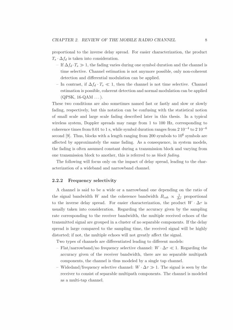
proportional to the inverse delay spread. For easier characterization, the product
Ts · ∆fd is taken into consideration.
– If ∆fd ·Ts ≫ 1, the fading varies during one symbol duration and the channel is
time selective. Channel estimation is not anymore possible, only non-coherent
detection and differential modulation can be applied.
– In contrast, if ∆fd · Ts ≪ 1, then the channel is not time selective. Channel
estimation is possible, coherent detection and normal modulation can be applied
(QPSK, 16-QAM . . . ).
These two conditions are also sometimes named fast or fastly and slow or slowly
fading, respectively, but this notation can be confusing with the statistical notion
of small scale and large scale fading described later in this thesis. In a typical
wireless system, Doppler spreads may range from 1 to 100 Hz, corresponding to
coherence times from 0.01 to 1 s, while symbol duration ranges from 2·10−4 to 2·10−6
second [9]. Thus, blocks with a length ranging from 200 symbols to 106 symbols are
affected by approximately the same fading. As a consequence, in system models,
the fading is often assumed constant during a transmission block and varying from
one transmission block to another, this is referred to as block fading.
The following will focus only on the impact of delay spread, leading to the char-
acterization of a wideband and narrowband channel.
2.2.2 Frequency selectivity
A channel is said to be a wide or a narrowband one depending on the ratio of
the signal bandwidth W and the coherence bandwidth Bcoh ∝ 1∆τ proportional
to the inverse delay spread. For easier characterization, the product W · ∆τ is
usually taken into consideration. Regarding the accuracy given by the sampling
rate corresponding to the receiver bandwidth, the multiple received echoes of the
transmitted signal are grouped in a cluster of no separable components. If the delay
spread is large compared to the sampling time, the received signal will be highly
distorted; if not, the multiple echoes will not greatly affect the signal.
Two types of channels are differentiated leading to different models:
– Flat/narrowband/no frequency selective channel: W · ∆τ ≪ 1. Regarding the
accuracy given of the receiver bandwidth, there are no separable multipath
components, the channel is thus modeled by a single tap channel.
– Widedand/frequency selective channel: W · ∆τ ≫ 1. The signal is seen by the
receiver to consist of separable multipath components. The channel is modeled
as a multi-tap channel.

CHAPTER 2. REVIEW OF THE MOBILE RADIO CHANNEL 9
The notion of frequency selectivity increases with regard to the frequency depen-
dence of the transfer function. Since the delays τk are different for several paths,
some frequencies are attenuated while others are not. If the delay difference between
the paths is very small or even does not exist, then frequencies are attenuated in
the same manner by the delay spread. The delay spread gives the speed of change
of the mobile channel in the frequency domain.
Narrowband channel model
In the narrowband channel, multipath fading comes from path length differences
between rays coming from different scatterers. Nevertheless, all rays arrive at es-
sentially the same time with regard to the sampling frequency of the receiver, so
the fading affects all frequencies in the same way and it can be modeled as a sin-
gle multiplicative process. Consider a receiver, which moves through a multipath
environment with a certain fixed speed. Further consider all path delays in this
environment to be negligibly small, such that s(t − τi) ≈ s(t). Then the received
signal is simplified and turns into
r(t) = s(t) ·∑
i
ai(t)ejθi(t) = s(t) · a(t)ejθ(t) = s(t) · h(t)
where a(t) is the complex fading coefficient at time t. Here h(t) is called the complex
gain of the channel. In this case, the input and output of the channel are connected
by a simple multiplicative relationship.
Wideband channel model
The wideband mobile radio channel has assumed increasing importance in recent
years as transmission bandwidths increase to support multimedia services. In prac-
tice, the impulse response would always be experienced via a receiver filter of finite
bandwidth, which will be unable to distinguish between a discrete and continuous
case. Therefore, the effects of scatterers in discrete delay ranges are regrouped into
individual taps with the same delay.
The model of N-tap delay channel is as follows:
h(τ, t) =N∑
n=1
hn(t)δ(τ − τn)

CHAPTER 2. REVIEW OF THE MOBILE RADIO CHANNEL 10
where
hn(t) =
Mn−1∑
k=0
ak(t)ejθk(t).
The separable multipath components arrive at different delays; if a too long delay
spread occurs, the previous symbol is still arriving at the receiver when the initial
energy of the next symbol arrives. The wideband channel can be regarded as a
combination of several paths subject to narrowband fading, combined together with
appropriate delays. Since large delays involve long paths between the scatterers
and the terminals, there is a tendency for the power per tap delay to reduce with
increasing delay. The taps are usually assumed to be uncorrelated with each other,
since each arises from scatterers which are physically distinct and separated by many
wavelengths.
It is often practical to regard the power delay profile of the channel in function of
the tapped delay line
p(τ, t) = |h(τ, t)|2 =N∑
n=1
|hn(t)|2δ(τ − τn(t)).
This power delay profile is characterized by the delay spread: the maximum delay
spread ∆τ or root-mean-square (RMS) delay spread ∆τrms. If the RMS delays
spread is very much less than the symbol duration, no significant interference among
the transmitted frames is encountered and the channel may be assumed narrowband.
Here is a summary table:
Selectivity/ Cause parameter Effects
fading changes in
time motion ∆fd frequency dispersion
frequency multipath ∆τ time dispersion
2.3 Statistical channel modeling
In the previous section the time variability of the fading has been addressed, no
attempt is usually made to predict the exact value of the signal strength arising from
multipath fading, as this would require a very exact knowledge of the position and
electromagnetic characteristics of all the scatterers. Instead a statistical description

CHAPTER 2. REVIEW OF THE MOBILE RADIO CHANNEL 11
is used, which will be different for different environments (mainly Line-Of-Sight
(LOS) / Non-Line-Of-Sight (NLOS) propagation).
Statistical models are traditionally based on measurements made for a specific
system or spectrum allocation. When modeling the channel, the propagation effects
are normally broken down into three main categories: path loss (PL), shadow fading
(SF), and fast fading (FF). The shadow fading and fast fading are also commonly
known as large scale and short scale fading respectively, where the name refers to
the size of the area where substantial correlation is observed. The received signal
power attenuation in mobile wireless communications can be, so, described as the
product of three-scale factors:
– the deterministic part of the local average received power which is distance-
dependent (average path loss)
– the stochastic part of the local average received power often modeled as a
lognormal variation (large-scale fading also called shadow fading or slow fading)
– and a small-scale fading due to movements in the order of the wavelength (fast
fading)
ChannelGain = (PathLoss)−1 × ShadowFading × FastFading.
Let us assume flat fading, the instantaneous power of the channel is Ph = |h|2,averaging on the local area one obtain Eh = E{Ph} = PL−1×SF and now averaging
on a large area E{PL−1 × SF} = PL−1. Sometimes the fast fading refers to the
whole instantaneous variation and not only the variation around the local mean.
Several models have been investigated for path loss. Shadow fading is the least well
understood of these three factors. It has been empirically observed to obey approxi-
mately lognormal distribution in a wide variety of propagation environments [28,56].
This lognormality is usually explained as a result of multiplication of large number
of random attenuating factors in the radio channel while this assumption is difficult
to justify from a physical propagation point of view; an interesting discussion with
a alternative model may be found in [55]. The fast fading of a radio channel re-
sults from multipath propagation due to reflection, diffraction and scattering. These
physical phenomena could arise when the transmitted signal encounters obstacles
(like buildings, mountains...) in its propagation path. For small-scale fading, nu-
merous statistical models have been proposed, most notably the Rayleigh, Rice and
Nagakami-m probability distributions. In order to enhance the design of mobile
radio systems, the modeling of fading is essential.

CHAPTER 2. REVIEW OF THE MOBILE RADIO CHANNEL 12
5 10 15 20 25 30 35 40 45−120
−100
−80
−60
−40
−20
0
20
distance from the source to the destination [m]
dB
The three−scale factor of fading
Path Loss Path Loss and shadowingPath Loss, shadowing and fast fading
Figure 2.1: Illustation of the fading effect along the BS-MS distance
2.3.1 Small scale propagation model
Let us consider the wideband channel equation h(τ, t) =∑
hn(t)δ(τ − τn(t)).
Each path hn(t) is modeled as a continuous-time stochastic process, which means
that at a fixed time t, hn(t) is the realization of a random variable that we will
simply write hn.
First-order fast-fading statistics
The channel coefficients per tap hn(t) are assumed to be the sum of Mn non-
separable paths. If the number of paths is high such as Mn → ∞ and the coefficients
from each paths are modeled as random variables with a uniformly distributed angles
of arrival and path gain. From the central limit theorem, hn arises to have a zero
mean complex Gaussian distribution, hn ∼ CN (0, 2σ2hn
):
p(hn) =1
2πσ2hn
e
−|hn|2
2σ2hn .
The complex variable hn can be decomposed into amplitude and phase terms hn =
aneiθn , due to the complex Gaussian distribution of hn, an is Rayleigh distributed,
an ∼ Rayleigh (σhn) :
p(an) =an
σ2hn
e
−a2n
2σ2hn an ≥ 0

CHAPTER 2. REVIEW OF THE MOBILE RADIO CHANNEL 13
and θn is uniformly distributed over [−π, π]. The tap power Pn = |hn|2 = a2n has an
exponential distribution, Pn ∼ Exponential(E−1
n
):
p(Pn) =1
Ene
−PnEn
where En = 2σ2hn
is the tap average power (path loss and shadowing).
It is obvious that for a flat channel which is equivalent to a single-tap channel, the
whole channel h follows the same distribution, or inversely for a wideband channel,
each taps have a gain which varies in time according to the standard narrowband
statistics. The Rayleigh distribution is an excellent approximation to measured
fading amplitude statistics for a mobile fading channel in NLOS situations. Such
channels are called Rayleigh-fading channels or simply Rayleigh channels.
In a LOS situation the received signal is composed of a random multipath com-
ponent, whose amplitude is described by Rayleigh distribution, plus a coherent line-
of-sight component which has essentially constant power (within the bounds set by
path loss shadowing). This is given by the Rice distribution for the amplitude:
p(an) =an
σ2hn
e−(a2
n+a20)
2σ2 I0
(
a a0
σ2hn
)
where I0 is the zero order modified Bessel function of the first kind. Then the power
is distributed as follow:
p(Pn|K) =(1 + K)e−K
Ene(1+K)−Pn
En I0
(√
4K(1 + K)Pn
En
)
where K is the so called “Ricean K-factor” representing the power ration of the
specular and random components.
A more general statistical model is given by the Nakagami-m distribution where
the power is Gamma distributed:
p(Pn, m) =mm
Emn Γ(m)
Pm−1n e
−mPnEn
where m ≥ 1/2 is a parameter describing the fading severity. The previously cited
fading can be formulated as a specific case of Nakagami fading. The Rayleigh
distribution is equal to Nakagami distribution with m = 1 and Rice distribution can
be approximated by m ≈ (K+1)2
2K+1 .
CHAPTER 2. REVIEW OF THE MOBILE RADIO CHANNEL 14
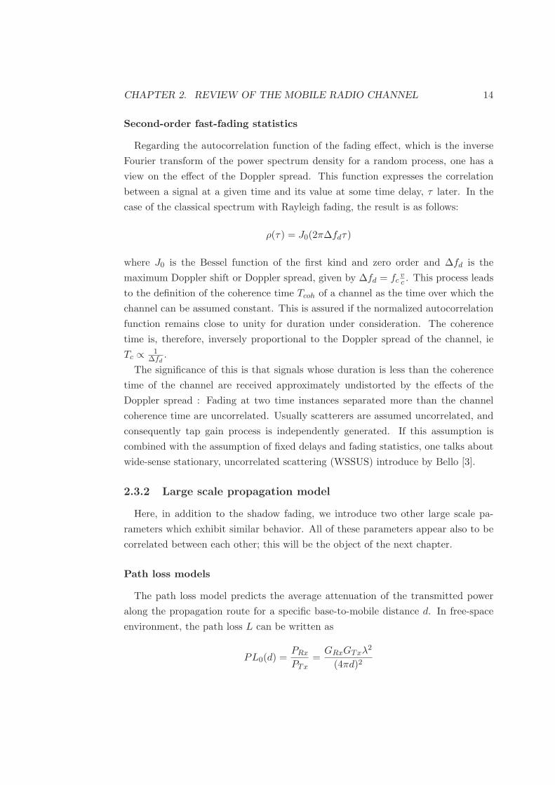
Second-order fast-fading statistics
Regarding the autocorrelation function of the fading effect, which is the inverse
Fourier transform of the power spectrum density for a random process, one has a
view on the effect of the Doppler spread. This function expresses the correlation
between a signal at a given time and its value at some time delay, τ later. In the
case of the classical spectrum with Rayleigh fading, the result is as follows:
ρ(τ) = J0(2π∆fdτ)
where J0 is the Bessel function of the first kind and zero order and ∆fd is the
maximum Doppler shift or Doppler spread, given by ∆fd = fcvc . This process leads
to the definition of the coherence time Tcoh of a channel as the time over which the
channel can be assumed constant. This is assured if the normalized autocorrelation
function remains close to unity for duration under consideration. The coherence
time is, therefore, inversely proportional to the Doppler spread of the channel, ie
Tc ∝ 1∆fd
.
The significance of this is that signals whose duration is less than the coherence
time of the channel are received approximately undistorted by the effects of the
Doppler spread : Fading at two time instances separated more than the channel
coherence time are uncorrelated. Usually scatterers are assumed uncorrelated, and
consequently tap gain process is independently generated. If this assumption is
combined with the assumption of fixed delays and fading statistics, one talks about
wide-sense stationary, uncorrelated scattering (WSSUS) introduce by Bello [3].
2.3.2 Large scale propagation model
Here, in addition to the shadow fading, we introduce two other large scale pa-
rameters which exhibit similar behavior. All of these parameters appear also to be
correlated between each other; this will be the object of the next chapter.
Path loss models
The path loss model predicts the average attenuation of the transmitted power
along the propagation route for a specific base-to-mobile distance d. In free-space
environment, the path loss L can be written as
PL0(d) =PRx
PTx=
GRxGTxλ2
(4πd)2
CHAPTER 2. REVIEW OF THE MOBILE RADIO CHANNEL 15
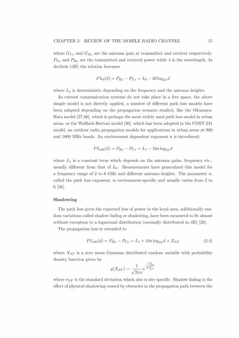
where GTx and GRx are the antenna gain at transmitter and receiver respectively.
PTx and PRx are the transmitted and received power while λ is the wavelength. In
decibels (dB) the relation becomes
PL0(d) = PRx − PTx = L0 − 20 log10 d
where Lo is deterministic depending on the frequency and the antenna heights.
As current communication systems do not take place in a free space, the above
simple model is not directly applied, a number of different path loss models have
been adapted depending on the propagation scenario studied, like the Okumura-
Hata model [27,66], which is perhaps the most widely used path loss model in urban
areas, or the Walfisch-Bertoni model [30], which has been adopted in the COST-231
model, an outdoor radio propagation models for applications in urban areas at 900
and 1800 MHz bands. An environment dependent exponent n is introduced:
PLdB(d) = PRx − PTx = L1 − 10n log10 d
where L1 is a constant term which depends on the antenna gains, frequency etc.,
usually different from that of L0. Measurements have generalized this model for
a frequency range of 2 to 6 GHz and different antenna heights. The parameter n,
called the path loss exponent, is environment-specific and usually varies from 2 to
6 [56].
Shadowing
The path loss gives the expected loss of power in the local area, additionally ran-
dom variations called shadow fading or shadowing, have been measured to fit almost
without exception to a lognormal distribution (normally distributed in dB) [28].
The propagation loss is extended to
PLdB(d) = PRx − PTx = L1 + 10n log10 d + XSF (2.4)
where XSF is a zero mean Gaussian distributed random variable with probability
density function given by
p(XSF ) =1√2πσ
e
−X2SF
2σ2SF
where σSF is the standard deviation which also is site specific. Shadow fading is the
effect of physical shadowing caused by obstacles in the propagation path between the

CHAPTER 2. REVIEW OF THE MOBILE RADIO CHANNEL 16
mobile and the base station like buildings, mountains, and other objects. Numerous
measurement results have been reported for different environment types since the
phenomenon has been observed. Normal values for standard deviation reported in
literature are between 5 to 12 dB [20].
Delay spread
Another important large scale parameter for modeling is the root mean square
(rms) delay spread ∆τrms, the standard deviation of the different delay paths, which
has been also measured to behave alike the path loss and shadowing with a stochas-
tic distance dependant component and a random component. Furthermore it is
lognormal distributed and correlated to the shadow fading [33]. Given an average
power delay profile {E′i, τi} for i = 1 . . . Npaths where the power per taps has been
normalized by the total channel power E′i = Ei/
∑
i Ei. The rms delay spread can
be simply computed as
∆τrms =
√√√√∑
i
τ2i E′
i −(∑
i
τiE′i
)2
. (2.5)
As expected, the delay spread has been measured to increase with the distance
as follows [33]:
∆τrms = T1dǫyDS (2.6)
where T1 is the median value, ǫ is an exponent that lies between 0.5 − 1.0 and yDS
is a lognormal variable. Typical standard deviation of YDS = 10 log10 yDS , σDS lies
from 2 to 6 dB.
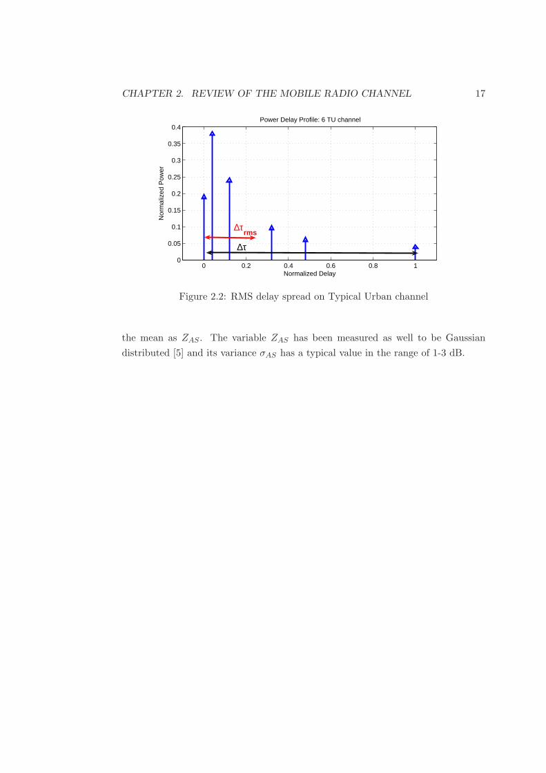
Throughout this thesis, we will simply refer to the rms delay spread as the delay
spread. Figure 2.2 gives an illustration of the RMS delay spread for a type of channel
called a Typical Urban channel with a normalized total delay spread and normalized
total power.
Angle spread
In the same manner, we may define the standard deviation of the angles of arrival
(AOAs) of the multipath components at the receiving antenna as the angle spread
at the receiver. Similarly, the angle spread at the transmitter refers to the standard
deviation of the angles of departures (AODs) of the multipath that have reached
the receiver. In this thesis we will only and briefly consider the angle spread at
the transmitter and we will note the random variation in the log domain around
CHAPTER 2. REVIEW OF THE MOBILE RADIO CHANNEL 17
0 0.2 0.4 0.6 0.8 10
0.05
0.1
0.15
0.2
0.25
0.3
0.35
0.4Power Delay Profile: 6 TU channel
Normalized Delay
Nor
mal
ized
Pow
er
∆τ
∆τrms
Figure 2.2: RMS delay spread on Typical Urban channel
the mean as ZAS . The variable ZAS has been measured as well to be Gaussian
distributed [5] and its variance σAS has a typical value in the range of 1-3 dB.

Chapter 3
Correlation among large scale
parameters
In this chapter we review the literature on correlation among shadow fading (SF),
delay spread (DS) and angle spread (AS) for the same transmission link and different
links as well. Considering a transmission from transceiver i to receiver j, we express
the random variation of the SF, DS and AS, as Xij , Yij and Zij , respectively. These
random variables are all lognormal distributed with variance σSF , σDS and σAS . The
variances are assumed independent of the transmission link for simplicity which is
realistic in the case of a uniform propagation environment. Then, the correlation
of two of these variables, let us say SF and AS, for two different paths ij and kl is
expressed as follows
ρ(Xij , Ykl) =E{XijYkl}σSF σAS
.
A scheme of the problem statement is depicted in Figure 3.1.
Figure 3.1: Large scale parameters of different links
18

CHAPTER 3. CORRELATION AMONG LARGE SCALE PARAMETERS 19
3.1 Correlated shadowing
Shadowing has been analyzed to be the consequence of physical obstructions, thus
signals which have crossed and been attenuated by the same obstacles are likely to
present dependency. This proposal has been supported by measured correlation
since the 70’s [20].
Measurements campaigns and models of shadowing correlation in the literature
have specially addressed the problem of correlation between links with a common
node. We will distinguish two simple cases. The first case aims to depict the correla-
tion between two close locations on a path of a moving MS, and more generally when
two links from the same BS end in a different receiver. This will be called in the se-
quel the shadowing auto-correlation. Further measurements have then investigated
the correlation between the two received signals at the same terminal from different
source locations, often named the shadowing cross-correlation. A well-agreed model
exists for the shadowing auto-correlation, but for the cross-correlation many models
have been published and will be presented in the following. A third case of correla-
tion between links which do not share any node in common has also been addressed
recently in the literature.
Correlations between links could have a significant effect on the performance of
a system. The lognormal shadowing from two different below rooftop RSs at a
given MS location will have some level of correlation. In addition, the shadowing
components from a given RS site at two different MS locations will be correlated
if they are within the spatial de-correlation distance of the shadowing. In order to
correctly model the benefits of relaying this correlation needs to be taken in account.
Nevertheless, the auto-correlation can be assumed negligible if receivers’ locations
are far enough, but a certain amount of cross-correlation is often measured even if
the BSs are far from each other. The reason is that the shadowing results mainly
from obstructing objects closely surrounding the terminal. Thus, even if they arise
from the same causes, auto-correlation and cross-correlation are modeled differently.
Let us call Xij the shadow effect from transmitter i to receiver j. In a uniform
propagation environment, the same values of shadowing standard deviation will be
assumed for all links, thus the correlation for the two different paths, ij and kl, is
expressed as follows
ρij,kl =E{XijXkl}
σ2SF
.
As an example, ρij,kj is the cross-correlation between transmitter i and k at receiver
j; and ρij,il is the auto-correlation between receiver j and l from transmitter i. In

CHAPTER 3. CORRELATION AMONG LARGE SCALE PARAMETERS 20
the following, if there is no confusion for receiving terminal j this cross-correlation
will be simply expressed as ρik; and if there is no confusion for the transmitter this
auto-correlation will be denoted by ρjl.
3.1.1 Auto-correlation models
Several measurements fields have suggested that an exponential decaying function
is an appropriate model for the auto-correlation function of the shadow fading [24,
35]. The model is characterized by the so-called shadowing decorrelation distance
dc:
ρjl = e−∆jl
dc (3.1)
where ∆jl is the distance between receiver j and receiver l. The decorrelation
distance dc is typically a few tens or hundreds of meters depending how far the
receivers are from the BS [35,56].
The above model suggests that the shadowing process is a first order Markovian
process [15], which can be generated easily. A modification of this model which com-
plies with the level crossing theory of a Gaussian process is proposed in [17]. Some
other studies proposed to generalize the model by a composite of two exponential
functions in order to match better some measurements [5, 57].
3.1.2 Cross-correlation models
The shadowing cross-correlation represents the correlation among the shadow ef-
fect of different links merging at the same receiver but emerging from different trans-
mitters. Since cross-correlation has been early evidenced in the work by Graziano
in 1978 [20], several measurement campaigns have been carried out in order to catch
the physical behavior as well as to derive mathematical modeling [6,46,61,69]. Field
measurements were performed under a different environment supporting the intu-
itive conjecture that links with a common terminal are in general correlated. Arnold
et al. [6] studied this issue in the context of macrodiversity gain, analyzing 800 MHz
data collected in a residential environment with indoor and outdoor transmitters
for a single mobile receiver. Interestingly, some field measurements failed to bare
significant correlation. In [46], data were obtained from a 1900 MHz GSM system in
rural and suburban areas, in both environments the measured correlation was rela-
tively low, ranging even in the negative value in rural areas. The authors specified
that the negative correlation was from a particular drive route and BS locations of a
specific site. They also investigated the dependency of the cross-correlation on the
CHAPTER 3. CORRELATION AMONG LARGE SCALE PARAMETERS 21
angle between the mobile and the cell sites, but no dependency was found.
The primary models consist of empiric tables from measurements. More recently,
more elaborated model using analytic functions have been derived. On the other
hand, despite the fact that field tests have suggested that the cross-correlation has
a decisive effect upon the system performance, cross-correlation is often set to zero
in system simulations avoiding complication of the analysis. It has been shown,
for example, that cross-correlation effects cannot be ignored in the performance
analysis of the co-channel interference probability for microcellular and picocellular
systems [70]; it also has a significant impact on the rates of level crossings [39].
In [68], the authors evaluate the performance of downlink in hard handover and soft
handover based CDMA cellular systems for different shadowing correlation models
and show that different correlation models lead to different simulation performances.
They analyze also the impacts of cross-correlated shadowing on the soft handover
gain in downlink through simulations in a UMTS (Universal Mobile Telecommuni-
cations System) vehicular environment. Handoff performance with cross-correlation
of the shadowing process was also analyzed by Viterbi in [62]. In [63], Viterbi et al.
has also modeled cross-correlation in the interference evaluation for CDMA cellu-
lar networks. Ignoring correlation could lead to pessimistic results while predicting
mobile systems performance through simulations according to [69].
Physical basis and modeling
Empirical measurements have supported the modeling of shadowing component
as a lognormal variation around the path loss. This variation is known to be largely
determined by the surrounding terrain at the terminal location and by obstructing
objects in close proximity to the MS.
An extension of this model in order to introduce dependency between link attenu-
ations is to break the shadowing effect into two independent components [6,63]. The
first component is dependent of the near field of the receiver and thus common for all
signals from different BSs; the second component depends of terrain and obstucting
objects belonging exclusively to a specific BS-MS link. Second components among
different links are assumed uncorrelated. This model, first suggested by Arnold et
al. in 1988 [6], was shown to well match the measured data for outdoor to indoor
links having similar length. In other words the random component of the dB loss
for the ith base station is expressed as:
Xi =√
ρξ +√
1 − ρξi (3.2)

CHAPTER 3. CORRELATION AMONG LARGE SCALE PARAMETERS 22
such that ξ and ξi are uncorrelated zero-mean Gaussian variables of the same vari-
ance σ2SF ; the component ξi, ξj from BSs i and j are independent for all i and j,
i 6= j.
The normalized covariance (correlation coefficient) of the losses to two base sta-
tions, i and j, isE[XiXj ]
σ2SF
= ρ. This model includes the limiting cases of independent
attenuations (ρ = 0) and of highly correlated attenuations (ρ = 1), which might
apply when the mobile is completely shadowed in all directions. In [63], the authors
chose the reasonable assumption that the two random components have equal stan-
dards deviations in which case the normalized covariance is ρ = 1/2 for all pairs of
base stations. This assumption is widely used in literature and in many standards
such as 3GPP. This special case of a constant correlation model may reasonably
approximate closely spaced base stations in a circular array [70].
Because the two random components have the same contribution in every link,
this model induces a constant correlation between all the links. A more general
model was developed by Graziosi et al in 1999 [21] based on the work of Viterbi
where the shadowing is a sum of multiple components having different contributions.
Xi =∑
m
√ρimξim where
∑
m
ρim = 1 (3.3)
Modeling the shadowing as the sum of different random variables, some being
correlated, does not say much about the level of correlation. Two channels links
crossing common obstacles should suffer similar attenuation. In order to introduce
a dependency in the statistical model of the shadowing component, we must esti-
mate the amount of correlation. The terrain of propagation of the link is the key
factor in the amount of correlation, for example in [69], the authors noticed that
the streets orientation has an influence on the measurements. Parallel streets to
the base stations axis imply a higher correlation than orthogonal ones to this same
axis. Without knowing the exact terrain of the transmission, we can assumed that
spatially-close links should cross the same kind of obstacles. In order to determine
the amount of common routes for the two links, two key variables have been investi-
gated: the angle-of-arrival difference θij which represents the angle between the two
paths from different base stations to the mobile and the relativity of the two path
lengths Rij = ri
rj, for ri ≤ rj [32, 56]. When the angle-of-arrival difference is small,
the two path profiles are assumed to share many common elements and are expected
to have high correlation. On the other hand, as the longer path length increases, it
incorporates more elements, which are not common to the shorter path; therefore,
the correlation decreases. These issues have been recognized by many researchers

CHAPTER 3. CORRELATION AMONG LARGE SCALE PARAMETERS 23
and, in particular, those interested in macrodiversity (for example, see [6] and [20]).
In most cases, the correlation is considered as a function of θij only [20,21,37,58],
because the angle-of-arrival difference has the strongest influence on the results.
The dependence of the correlation function on θij is suggested by the measurements
conducted by Zayana and Guisnet [69] in two French cities, and also by previous
measurements reported in [20] and [61]. In [20], Graziano measures the correlation
of the signals as a function of angle using data at 900 MHz using data from two
sets of transmitters. Using this relatively limited data set, Graziano observed cor-
relations on the order of 0.6 to 0.8 at angles less than about 10 degrees. In [6], the
authors observed that the macroscopic diversity gain is more significant for links
well separated in angle. The fact that links from relatively close directions should
be strongly correlated was assumed by Bell Laboratories’ researchers in [18,25], for
this they designed a correlation function on the angle-of-arrival difference; the same
model being developed later and independently by Graziosi [21].
On the contrary, from a measurements field in Boston (urban and suburban
terrain) at 1900 MHz [65], the authors did not find significant dependency from
the angle-of-arrival even for small angles. They argue that the data set used by
Graziano [20] was relatively limited and collected only on a relatively flat terrain.
They finally concluded that the correlation should be low even at small angles, if the
length of terrain causing shadowing which is not common to the two paths is larger
or on the same order as the terrain distance that is common to the two paths. This
last observation is taken in account with the other key variable Rij introduced by
Zayana and Guisnet in 1998 [69]. From a set of measurements and simulations, Za-
yana and Guisnet [69] proposed a model where the cross-correlation depends upon
two variables: the angular separation between the two base stations as seen from
the mobile and the ratio between the distances from the mobile to the base stations.
From this, in 2001, Avidor [7, 39] suggests that the correlation can be modeled
as the product of two functions: ρij = g(θij) × h(Rij),where g and f should be
positive-definite functions with maximum at zero, and g even and 2π-periodic. The
authors provided potential candidates in [7].
Constant correlation model
A constant cross-correlation of 0.5 is the adopted value in [2]. As mentioned
above, this particular model is suggested by the measurements in [6] and assumed,
for example, in [63,70].
CHAPTER 3. CORRELATION AMONG LARGE SCALE PARAMETERS 24
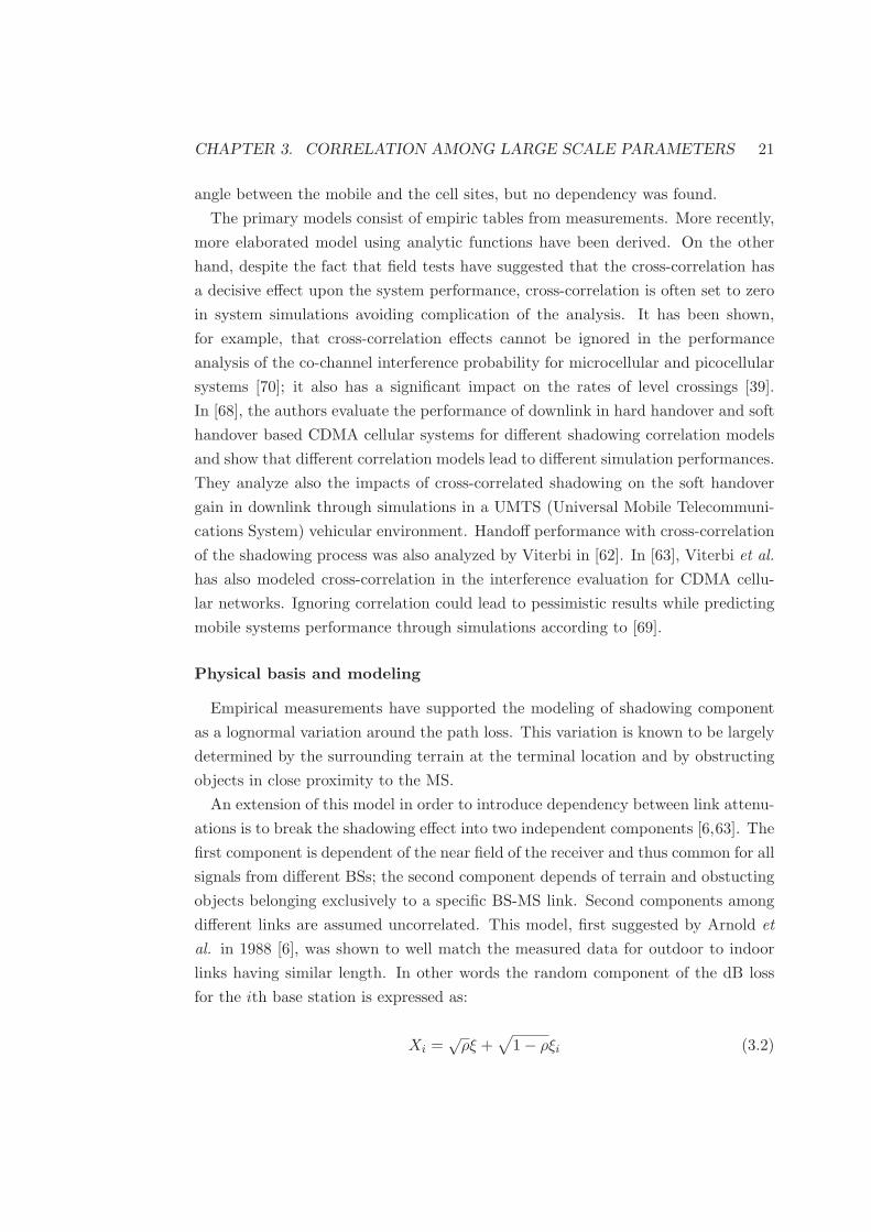
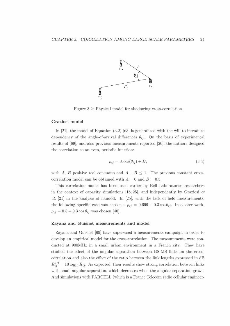
Figure 3.2: Physical model for shadowing cross-correlation
Graziosi model
In [21], the model of Equation (3.2) [63] is generalized with the will to introduce
dependency of the angle-of-arrival differences θij . On the basis of experimental
results of [69], and also previous measurements reported [20], the authors designed
the correlation as an even, periodic function:
ρij = A cos(θij) + B, (3.4)
with A, B positive real constants and A + B ≤ 1. The previous constant cross-
correlation model can be obtained with A = 0 and B = 0.5.
This correlation model has been used earlier by Bell Laboratories researchers
in the context of capacity simulations [18, 25], and independently by Graziosi et
al. [21] in the analysis of handoff. In [25], with the lack of field measurements,
the following specific case was chosen : pij = 0.699 + 0.3 cos θij . In a later work,
ρij = 0.5 + 0.3 cos θij was chosen [40].
Zayana and Guisnet measurements and model
Zayana and Guisnet [69] have supervised a measurements campaign in order to
develop an empirical model for the cross-correlation. The measurements were con-
ducted at 900MHz in a small urban environment in a French city. They have
studied the effect of the angular separation between BS-MS links on the cross-
correlation and also the effect of the ratio between the link lengths expressed in dB
RdBij = 10 log10 Rij . As expected, their results show strong correlation between links
with small angular separation, which decreases when the angular separation grows.
And simulations with PARCELL (which is a France Telecom radio cellular engineer-

CHAPTER 3. CORRELATION AMONG LARGE SCALE PARAMETERS 25
ing tool) results that the cross-correlation falls, for a fixed angle, when module RdBij
grows. The model is expressed by the table below:
ρ(θ, R) θ ∈ [0◦; 30◦] θ ∈ [30◦; 60◦] θ ∈ [60◦; 90◦] θ ≥ 90◦
RdB ∈ [0; 2] ρ = 0.8 ρ = 0.5 ρ = 0.4 ρ = 0.2
RdB ∈ [2; 4] ρ = 0.6 ρ = 0.4 ρ = 0.4 ρ = 0.2
RdB ≥ 4 ρ = 0.4 ρ = 0.2 ρ = 0.2 ρ = 0.2
Linear models
The publication [32] extends the work of Zayana and Guisnet by taking the table
of result of [69] and comparing with other experimental results from [20,36,58]. The
model is a linear variation between the different experimental values. They provide
different models with or without taking account of the ratio of distance of the path
links:
– Model 0.8/0.4 approximates the measurement results by Graziano [20]:
ρ(θ) =
0.8 − θ150 if θ ≤ 60◦
0.4 if θ > 60◦(3.5)
– Model 0.8/0.0 approximates the measurement results by Sorensen [58]:
ρ(θ) =
0.8 − θ75 if θ ≤ 60◦
0.0 if θ > 60◦(3.6)
– Model 1.0/0.4 RX :
ρ(θ, R) =
f(X, R)(0.6 − θ150) + 0.4 if θ ≤ 60◦
0.4 if θ > 60◦(3.7)
– Model 1.0/0.0 RX :
ρ(θ, R) =
f(X, R)(1.0 − θ75) if θ ≤ 60◦
0.0 if θ > 60◦(3.8)

CHAPTER 3. CORRELATION AMONG LARGE SCALE PARAMETERS 26
where
f(X, R) =
1 − RX if R ≤ XdB
0 if R > XdB
(3.9)
and X denotes the point where the distance-dependent correlation reaches its min-
imum value. The authors assumed that X is in the range of 6-20dB.
Saunders model
In [56], the following cross-correlation model is proposed:
ρ(θ, R, ri) =
√R for 0 ≤ θ ≤ θT
(θT
θ
)γ √R for θT ≤ θ ≤ π
with θT = 2 arcsindc
2ri(3.10)
where γ is a parameter depending of the terrain and dc is the auto-correlation
distance which is the distance taken for the normalized auto-correlation to fall below
1/e.
It is worthy to notice that this is the only model taking in account both value ri
and rj rather than just its ratio.
0 20 40 60 80 100 120 140 160 1800
0.1
0.2
0.3
0.4
0.5
0.6
0.7
0.8
0.9
1
Angle in degree
Graziosi: A=0.3, B=0.5Zayana and GuisnetModel 0.8/0.4Model 0.8/0.0Saunders model: dc=300, γ=0.3
(a) Cartesian plot
0.2
0.4
0.6
0.8
30
210
60
240
90
270
120
300
150
330
180 0
Graziosi: A=0.3, B=0.5Zayana and GuisnetModel 0.8/0.4Model 0.8/0.0Saunders model: dc=300, γ=0.3
(b) Polar plot
Figure 3.3: Angular behavior of the different shadowing cross-correlation models(RdB = 0).

CHAPTER 3. CORRELATION AMONG LARGE SCALE PARAMETERS 27
0.1
0.1
0.2
0.20.
3
0.3
0.4
0.4
0.4
0.5
0.5
0.5
0.5
0.6 0.60.6 0.60.6 0.6
km
km
Graziosi: A=B=0.3
−4 −3 −2 −1 0 1 2 3 4
−4
−3
−2
−1
0
1
2
3
4
0.4
0.4
0.4
0.40.4
0.6
0.6
0.6
0.6
0.6
0.6
0.6
0.6
0.8
0.8
0.8
0.8
0.8
0.8
0.8
0.8
km
km
Zayana and Guisnet
−4 −3 −2 −1 0 1 2 3 4
−4
−3
−2
−1
0
1
2
3
4
0.5
0.5 0.5
0.5
0.6
0.6
0.6
0.6
0.7
0.70.7
0.7
0.7 0.7
0.8
0.8
0.80.8
0.8
0.8
0.8 0.8
0.9
0.9
0.9
0.9
0.9
0.9
0.9
0.9
km
km
Model 1.0/0.4 RX, X=6dB
−4 −3 −2 −1 0 1 2 3 4
−4
−3
−2
−1
0
1
2
3
4
0.1
0.1 0.1
0.1
0.2
0.2
0.2
0.2
0.3
0.30.3
0.3
0.3 0.3
0.4
0.4
0.40.4
0.4
0.4
0.4 0.4
0.5
0.5
0.5
0.5
0.5
0.5
0.5
0.5
km
km
Model 1.0/0.0 RX, X=6dB
−4 −3 −2 −1 0 1 2 3 4
−4
−3
−2
−1
0
1
2
3
4
0.4
0.4
0.6
0.6
0.6
0.6
0.6
0.6
km
km
Saunders: γ=0.3, dc=300m
−4 −3 −2 −1 0 1 2 3 4
−4
−3
−2
−1
0
1
2
3
4
0 0.2 0.4 0.6 0.8 1
Figure 3.4: Exemplification of different shadowing cross-correlation models betweentwo BSs distant of 2km.
CHAPTER 3. CORRELATION AMONG LARGE SCALE PARAMETERS 28
3.1.3 Correlation among links without a common node
The correlation among links without a common node haa been recently studied in
the literature [22,67]. In [67], the correlation is modeled by an exponential function
of the distances between the receivers and transmitters. In [22], the correlation is
generated by multiplying the auto-correlation and cross-correlation. This method
was also used in [21, 69], see also [31]. The authors of [22] attempt to rigorously
prove that combining of auto- and cross-correlation is done by multiplication. The
proof is unfortunately weak, by taking independent increment to model the random
variable; the authors implicitly assumed that the model is Markovian which results
by a multiplication of the correlation.
3.2 Correlated angle spread, correlated delay spread
Angle spread (AS) and delay spread (DS) have been shown to be also lognor-
mal distributed. Contrary to the shadow fading, auto- and cross-correlation of
AS and DS for different transmission links have raised little interest in the litera-
ture. Nevertheless, auto-correlation of AS and auto-correlation of DS seem to follow
also an exponential decaying with different decorrelation distances than the shadow
fading [5, 42]. Angle-spread and delay spread fluctuations between different base
stations (cross-correlation) have been assumed to be uncorrelated due to the lack
of investigation. Some measurement fields can be found in [42]. In [42], the au-
thors conclude that when the BSs are close, the angle spread is correlated but less
significantly than the shadow fading and can be thus neglected.
3.3 Correlation among the “three spreads”
In the literature shadow fading, angle spread and delay spread have been mea-
sured to be correlated among each other [5] (for the same transmission link). Green-
stein [33] presents a significant model which results in negative correlation between
delay spread and lognormal shadow fading. In some standard channel models, the
following values of the cross-correlations between path-loss, delay spread and angle
spread for the same base station have been adopted [23] from [12]:
– Correlation between shadowing and delay spread: ρXY = −0.75
– Correlation between shadowing and angle spread: ρXZ = −0.75
– Correlation between delay spread and angle spread: ρY Z = 0.5
The associated correlation matrix is:
CHAPTER 3. CORRELATION AMONG LARGE SCALE PARAMETERS 29
A =
1 ρXY ρXZ
ρXY 1 ρY Z
ρXZ ρY Z 1
. (3.11)
The problem of correlation between the large scale parameters of different links
have not been investigated, but it is to expected that these correlations are negligible.
3.4 The problem of a positive definite correlation ma-
trix
In this section, we consider M links merging at the same receiver. Assuming
that the random variation of the large scale parameters (SF,DS,AS) of all links are
jointly Gaussian in the log-domain, they should thus possess the proper statistical
characteristic that the full correlation matrix for the M BSs is positive semidefinite.
As a first step we will only discuss the problem for shadow fading. In this section,
as the statement of the problem suggests, we only consider the cross-correlation,
nevertheless the auto-correlation model of (3.1) leads to a positive correlation matrix
due to its inherent Markovian assumption.
3.4.1 Cross-correlation model
For a given network of BSs with one MS, a correlation matrix Rxx of the shad-
owing for every transmission link has to be calculated for simulation. If a vector of
independent lognormal samples are generated at a given MS location, representing
the shadowing from each BS, then these samples can be correlated using Rxx.
Most of the cross-correlation models have the main drawback to randomly lead
to a non positive semidefinite matrix which is a necessary condition for a matrix
to be a correlation one. Surprisingly, many authors assumed de facto the positive-
definiteness and state that the Cholesky decomposition can be applied, this property
is, of course, totally dependent on the way of choosing the entries of the aforesaid
matrix. However, this important feature has been recognized, for example, in [7,21,
40, 68]. In [21], the authors provided a proof that their model leads to a positive-
definite correlation matrix relying on a Fourier series expansion (provided also for
a more general class of cross-correlation laws). In [7], the authors extend the work
of Zayana and Guisnet by determining different correlation function using the fact
CHAPTER 3. CORRELATION AMONG LARGE SCALE PARAMETERS 30
that the covariance matrix must be positive definite. By using the assumption those
covariances can be separated into the product of two terms that depend only on the
angular difference and the ratio of distances respectively, one can write
ρ(Xij , Xkj) = g(θik)h(RikdB)
It follows that g and h are even, positive-definite functions with the maximum at
zero and g has a period 2π. Since g is even and periodic, it can be written as a
Fourier series g(θ) =∑∞
n=−∞ cnejnθ, where the Fourier coefficients cn are all real.
Using measure theory and applying Bochner’s theorem, the authors show that g is
positive definite if and only if ∀n cn ≥ 0 and 0 <∑∞
n=−∞ cn < ∞. It is sufficient for
h to be convex on the right half-axis [0,∞) to be positive definite. Then the product
of g and h is positive definite on [−π, π]×R by Schur’s Theorem. The authors leave
the specific shape of the function h open and note that this decomposition in two
functions which are independent may not be the best.
We summarize in the table below which of the models described previously fulfill
this requirement.
Model Always leading to a semi-positive matrix
constant ρ = 0.5 yes
Graziosi yes [21]
Zayana and Guisnet no
linear models no
Saunders model no
3.4.2 Overall model
When generating the three spreads for a network of M base stations, the prob-
lem of non-negative correlation matrix is complicated drastically. Given a link the
correlation among the three spread is given according to the matrix A (3.11), which
is positive definite with the adopted value. On the other hand, the correlated shad-
owing is represent by Rxx. When accounting the entire variable together we must
define the cross-correlation of the AS and DS, as well as the correlation among all
the spread for the different links. The latter correlations are often assumed to be
zero, which leads to non semi-positive definite overall matrix in most of the cases

CHAPTER 3. CORRELATION AMONG LARGE SCALE PARAMETERS 31
even if A and Rxx are non negative definite. In [38], assuming that the shadowing
cross-correlation is constant and equal to 0.5, the authors proposed as a solution
to modify the entries of the matrix A in order to force the overall eigenvalue to be
positive. The adopted new values can be found in [10]:
– Correlation between shadowing and delay spread: ρXY = −0.6
– Correlation between shadowing and angle spread: ρXZ = −0.6
– Correlation between delay spread and angle spread: ρY Z = 0.5
Nevertheless, for another type of shadowing cross-correlation model, no other so-
lution exists. Alternatively, without any experimental backing, we may assume that
the shadowing cross-correlation model may apply to the other large scale parameter
and the overall correlation matrix can be obtain by a Kronecker product between
A and Rxx : A⊗
Rxx . Then by the properties of the Kronecker product, the
overall matrix is positive semidefinite if A and Rxx are.

Chapter 4
OFDM
Orthogonal frequency-division multiplexing (OFDM) is a widely used modulation
technique in current and future wireless standards. OFDM is a multichannel mod-
ulation that sends multiple symbols in parallel, by dividing the given channel into
many narrow subchannels called subcarriers. A good overview of OFDM can be
found in [29].
Multichannel modulation systems have been studied since the middle of the 20th
century. Its relevance has been contested until the use of discrete Fourier transform
(DFT) with a cyclic prefix. Fast Fourier transform (FFT) makes the implementation
of DFT efficient, and the cyclic prefix brings robustness against inter-symbol, inter-
carrier interference (ISI, ICI) and fading caused by multipath propagation.
In the following sections of this chapter, the principles of the OFDM transmission
technique will be described with a short performance analysis.
4.1 Principles of OFDM
OFDM is a block transmission technique where complex-valued data symbols
are not modulated by using the full allocated radio resource, but are parted into
different low-rate data streams modulated by different narrow baseband carriers.
The transmitted OFDM signal is the sum of all the subcarriers which are chosen
orthogonal. The main advantage of this concept is that in a frequency selective
channel, the channel for each of the subcarrier can be considered flat. In a time-
invariant fading channel, ISI and ICI can be avoided with a cyclic prefix.
In the baseband domain, an OFDM block signal consists of N orthogonal subcar-
32

CHAPTER 4. OFDM 33
riers φk(t) modulated by parallel streams of complex data symbol {xk}:
s(t) =1√N
N−1∑
k=0
xkφk(t), 0 < t < NT
where NT is the length of the OFDM block. Each baseband subcarriers are designed
to be orthogonal on 0 < t < NT :
φk(t) = ej2πfkt
where the subcarrier frequencies are equally spaced fk = kNT .
The left half of Figure 4.1 illustrates three different subcarriers in time, the right
half of Figure 4.1 illustrates the orthogonality of the subcarriers in the frequency
domain and the resulting total spectrum.
0 20 40 60 80−1
0
1
Time [µs]
Am
plitu
de
3 orthogonal subcarriers
0 20 40 60 80−1
0
1
Time [µs]
Am
plitu
de
0 20 40 60 80−1
0
1
Time [µs]
Am
plitu
de
−5 0 5 10 15−0.4
−0.2
0
0.2
0.4
0.6
0.8
1
1.2
Frequency [Subcarrier index]
Am
plitu
de
Figure 4.1: Subcarriers in time and frequency
At the receiver side, the signal is sampled (here the fading and the noise is ig-
nored):
s(nT ) =1√N
N−1∑
k=0
xkej2π nk
N , 0 < n < N − 1.
From this equation we can see that the OFDM symbols can be expressed in terms
of an inverse discrete Fourier transform (IDFT), and can be easily demodulated via
a DFT, which make the implementation of OFDM very attractive using the fast
Fourier transform algorithm.
However, if we consider that the signal has been sent through a multi-tap channel
and the transmitter sent successive OFDM blocks, the dispersion of the channel
creates ISI between the OFDM blocks as well as ICI between the modulated data
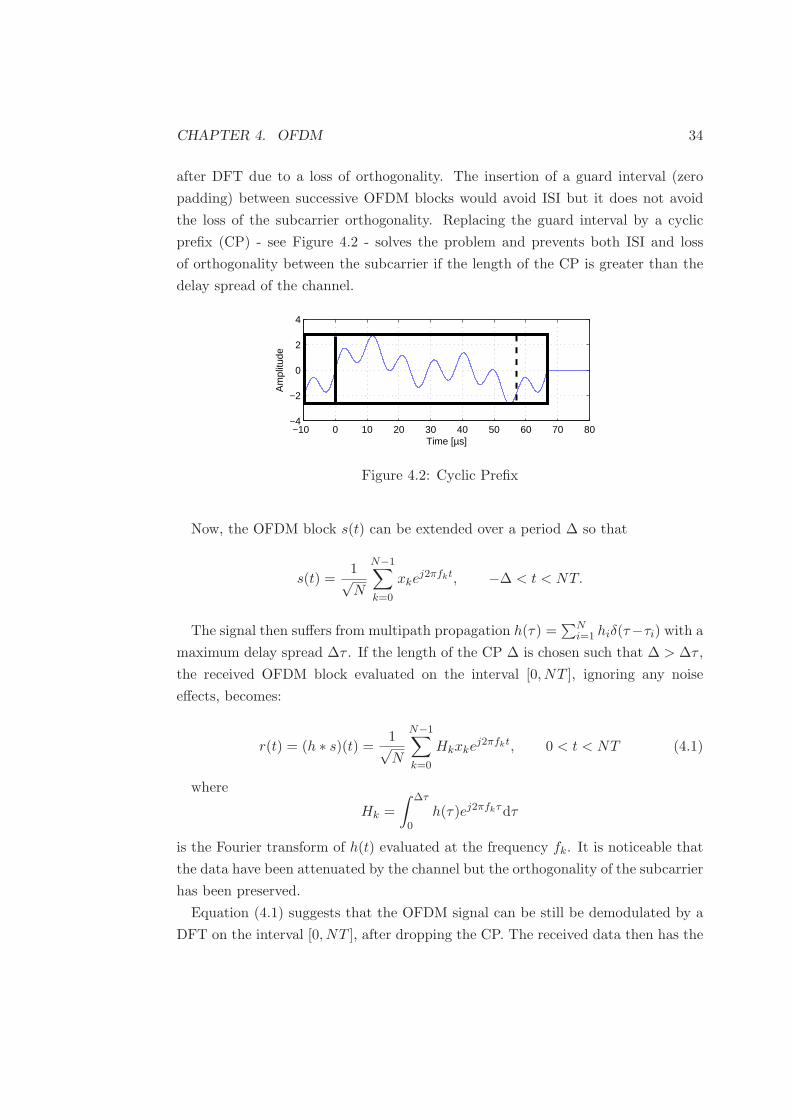
CHAPTER 4. OFDM 34
after DFT due to a loss of orthogonality. The insertion of a guard interval (zero
padding) between successive OFDM blocks would avoid ISI but it does not avoid
the loss of the subcarrier orthogonality. Replacing the guard interval by a cyclic
prefix (CP) - see Figure 4.2 - solves the problem and prevents both ISI and loss
of orthogonality between the subcarrier if the length of the CP is greater than the
delay spread of the channel.
−10 0 10 20 30 40 50 60 70 80−4
−2
0
2
4
Time [µs]
Am
plitu
de
Figure 4.2: Cyclic Prefix
Now, the OFDM block s(t) can be extended over a period ∆ so that
s(t) =1√N
N−1∑
k=0
xkej2πfkt, −∆ < t < NT.
The signal then suffers from multipath propagation h(τ) =∑N
i=1 hiδ(τ−τi) with a
maximum delay spread ∆τ . If the length of the CP ∆ is chosen such that ∆ > ∆τ ,
the received OFDM block evaluated on the interval [0, NT ], ignoring any noise
effects, becomes:
r(t) = (h ∗ s)(t) =1√N
N−1∑
k=0
Hkxkej2πfkt, 0 < t < NT (4.1)
where
Hk =
∫ ∆τ
0h(τ)ej2πfkτdτ
is the Fourier transform of h(t) evaluated at the frequency fk. It is noticeable that
the data have been attenuated by the channel but the orthogonality of the subcarrier
has been preserved.
Equation (4.1) suggests that the OFDM signal can be still be demodulated by a
DFT on the interval [0, NT ], after dropping the CP. The received data then has the
CHAPTER 4. OFDM 35
form
yk = Hkxk, k = 0, . . . , N − 1
This is equivalent to a transmission of parallel data streams through flat channels.
4.2 Performance analysis
In practice, the CP is rarely long enough to cover the maximum delay spread of the
channel and completely prevent ICI/ISI. In consequence, interferences from other
symbols transmitted in the considered block (ICI) and all other symbols transmitted
in other blocks (ISI) occur and lead to a loss in per-subcarrier signal-to-interference
and noise ratio (SINR).
Denoting xi,n the nth symbol of the ith block (0 ≤ n ≤ N − 1, −∞ < i < +∞),
the ith transmitted block with CP contains N + ν time-domain samples, of which
the mth sample, for −ν ≤ m ≤ N − 1, is given by
si[m] =1√N
N−1∑
l=0
xi,lej2π lm
N . (4.2)
Given a continuous-time channel h(τ), we may associate the corresponding discrete-
time channel h[l] = h(lT ) where T is the sampling period. Assuming an infinite-
taps, time-invariant, discrete-time channel h[l] =∑
k h[k]δl−k, for each transmitted
block of N + ν samples, the receiver selects N consecutive samples and drops the
other ν samples. The remaining samples r[k] of the jth block, assuming perfect
synchronization between the receiver and the transmitter, given for k = j(N +
ν), · · · , j(N + ν) + N − 1 by
r[k] =+∞∑
i=−∞
N−1∑
m=−ν
si[m]h[k − m − i(N + ν)] + n[k] (4.3)
are demodulated using a DFT. For the block j = 0, the nth output of the DFT can
be written as
y[n] = x0,nHn,n,0 +N−1∑
l=0l 6=n
x0,lHl,n,0
︸ ︷︷ ︸
ICI
++∞∑
i=−∞i6=0
N−1∑
l=0
xi,lHl,n,i
︸ ︷︷ ︸
ISI
+n[n] (4.4)

CHAPTER 4. OFDM 36
where n is the post-processed noise with power N0, and
Hl,n,i =1
N
N−1∑
m=−ν
N−1∑
k=0
h[k − m − i(N + ν)]ej2π lm−knN
denotes the signal component at the nth DFT output during the block j = 0, caused
by the symbol xi,l which is transmitted on the lth carrier during the ith block. As
an example, by substituting the summation variable r = k − m in Hn,n,0, we may
write
Hn,n,0 =
∞∑
r=−∞
c[r]h[r]e−j 2πnrN (4.5)
where c[r] is a weight function defined as
c[r] =
N+rN −N ≤ r < 0
1 0 ≤ r < ν
N−(r−ν)N ν ≤ r < N + ν
0 elsewhere
.
We thus see that in the case of a causal channel h[r] =∑Nh
k=0 h[k]δr−k where the last
tap index is in less or equal than the CP length, Nh ≤ ν, Hn,n,0 =∑Nh
r=0 h[r]e−j 2πnrN
is the Fourier transform of the channel evaluated at the n subcarrier.
Assuming the data symbols are statistically independent and have an average en-
ergy of σ2x, i.e., E
[
xi,nx∗j,k
]
= σ2xδijδnk, the instantaneous SINR of the nth subcarrier
is
γ(n) =|Hn,n,0|2
N−1∑
l=0l 6=n
|Hl,n,0|2 ++∞∑
i=−∞i6=0
N−1∑
l=0
|Hl,n,i|2 + N0/σ2x
. (4.6)
The instantaneous SINR may be used to express the corresponding ergodic capacity
of the system:
C =∑
n
C(n) =∑
n
E [log(1 + γ(n))]. (4.7)
Applying Jensen’s inequality due to the concavity of the logarithm, we have the
following upper bound:
C ≤∑
n
log(1 + E [γ(n)]). (4.8)

CHAPTER 4. OFDM 37
The average of the instantaneous SINR, E [γ(n)], may be hard to find as it implies
the ratio of dependent random variables. In order to simplify the performance
analysis, rather than using the expectation of the instantaneous SINR, we will use
as an approximation the ratio between the average of the useful signal power and
the average interference plus noise power. Rewriting γ(n) = S(n)I(n)+N0/σ2
x, where S(n)
and I(n) are dependent random variables, from the definition of the covariance of
two random variable we have
E [γ(n)] =E [S(n)]
E [I(n)] + N0/σ2x
− Cov [γ(n), I(n)]
E [I(n)] + N0/σ2x
. (4.9)
As the ratio Γ = E[S(n)]E[I(n)]+N0/σ2
xhas already been calculated in closed-form [59] and
shown to be independent of the subcarrier index if all the carriers are modulated,
for simplicity we assumed that Γ ≈ E [γ(n)] which gives an approximation of the
capacity as follows
C / N log(1 + Γ). (4.10)
An exact derivation of the performance metric Γ has been provided for a time-
varying, frequency-selective, discrete-time channel in [59] and for a continuous time
channel in [41]. In this thesis, as in [8], we will only consider a time-flat channel
and we will use the simplified expression of the SINR Γ of [8] for a continuous time
channel. Given a channel h(τ) =∑
i hiδ(τ − τi) with complex gains per taps hi, we
note the average power of every taps by Ei = E[|hi|2
]. The useful signal power and
interference power are independent of the subcarrier index and equal to
PS = E [S] =∑
i
c(τi)2Ei (4.11)
PI = E [I] =∑
i
(1 − c(τi)2)Ei (4.12)
where c(τ) is a bias function defined as follows:
c(τ) =
0 τ < −NT
NT+τNT −NT ≤ τ < 0
1 0 ≤ τ < ∆
NT−(τ−∆)NT ∆ ≤ τ < NT + ∆
0 NT + ∆ ≤ τ

CHAPTER 4. OFDM 38
with T the sample interval in seconds, N the FFT length in samples, so the OFDM
symbol interval is NT . The CP length is ∆ = νT seconds and the combined length
of the OFDM symbol and the CP is NT + ∆. The biased function is depicted in
Figure 4.3. Finally the SINR, Γ, may be expressed by
−8 −6 −4 −2 0 2 4 6 8
x 10−5
−1
0
1
2
Delay τ [s]
Bias function c(τ)c(
τ)
∆NT
Figure 4.3: Bias function
Γ =PS
PI + N0/σ2x
. (4.13)
The average SINR may be expressed in the same manner for a discrete-time channel
using the equivalent discrete bias function c[r].
In the following, we will refer to “average SINR” as the ratio of the average useful
signal power onto the average interference plus noise power, Γ.
4.3 Time of reference
Timing synchronization is an important aspect for OFDM systems. The OFDM
receiver is assumed to remove the CP and demodulate the data only over the symbol
interval NT . At the receiver side, when performing the demodulation (FFT), a syn-
chronization error may occur and degraded as well the performance of the OFDM
system. We will call this synchronization instant the time-of-reference (TOR). Sev-
eral OFDM timing algorithms have been analyzed, e.g., in order to choose the TOR
that minimize the overall interference power and thus maximize the SINR [11,59].
In fact the SINR expression (4.13), Γ, may be expressed simply as a function of
the TOR. During the demodulation, if the FFT starts at time tor, the resulting

CHAPTER 4. OFDM 39
post-FFT average signal and interference power per subcarrier are given by [8]:
PS(tor) =∑
i
c(τi − tor)2Ei (4.14)
PI(tor) =∑
i
(1 − c(τi − tor)2)Ei. (4.15)
The corresponding SINR is
Γ(tor) =PS(tor)
PI(tor) + N0/σ2x
. (4.16)
4.4 Systems exploiting OFDM/DMT
OFDM is currently used for both wireless and wire-line communication networks,
mainly under essentially identical schemes known as coded OFDM (COFDM) and
discrete multi-tone modulation (DMT).
COFDM is an implementation of OFDM that includes coding for error detection
and correction. DMT often refers to a baseband wire-line communication where
the system adapts the transmission to the channel conditions individually for each
sub-carrier. DMT is used for the asynchronous digital subscriber loop (ADSL).
The robustness of OFDM under multipath propagation has made it a strong
candidate for future wireless standards. To date, most important contributions
of OFDM are in Digital Audio Broadcasting (DAB), Digital Video Broadcasting
(DVB), Integrated Services Digital Broadcasting (ISDB), Wireless LANs (WLAN),
and Wireless MANs (WMAN).
In DVB, OFDM is considered for DVB-T (terrestrial) and DVB-H (handheld).
In WLANs, OFDM is considered for IEEE 802.16 a and g systems, Hyper-LAN/2
and MMAC. More recently, OFDM has been also considered for 3G Long Term
Evolution (LTE) mobile systems.
Chapter 5
Cooperative communication
It will be a core requirement of any future wireless communication systems to be
able to support very high data rates. As this vision is not feasible with the con-
ventional cellular architecture, in order to increase the capacity, different transmit
diversity schemes have been thoroughly investigated over the past decade.
Cooperative communication is a method which enables different receivers in the
network to share their antennas and generate a virtual multiple-antenna transmis-
sion in order to achieve transmit diversity. A relay station (RS) is a transceiver
that forwards radio signals in the wireless network. It has been a main research
topic as communication beyond third generation will have spectrum band above the
2 GHz where radio propagation is significantly more vulnerable to nonline-of-sight
conditions. A solution would be to increase the BS density but the resulting high
operator cost has motivated research into the use of relay transceivers to increase
the number of network access points. Relays have many cost advantages and cost is
the main argument for relay-based deployments [13]. Unlike the BSs, relays do not
have to cover a large area which means that the transmit power requirements are
significantly less critical than for the BSs. Furthermore, relays do not have a wired
connection to the backbone network, and the mast on which the relay is placed does
not need to be as high as for a BS, reducing operating expenses and maintenance
costs for the service provider [48]. The use of multihop transmission through relays
in a existing cellular systems has been shown to improve the performance for a lower
cost than increasing the density of base stations [60]. However, introducing relay
nodes creates new problem such as amplification of the noise and interference power.
Literature has foreseen cooperative communication between users where the user
terminal would be also a relay station, relaying a duplicate of the same signal through
different paths creating spatial diversity. In the following parts of this chapter, the
40

CHAPTER 5. COOPERATIVE COMMUNICATION 41
different types of relaying concept will be introduced. Figure 5.1 depicts a simple
cooperative communication scenario.
Figure 5.1: Simple cooperative communication
5.1 Basic relaying concepts
The expected benefits of different relay concepts are radio coverage extension and
quality of service (QoS) enhancement. For this purpose different types of relays
have been proposed as well as different types of transmission protocols to enhance
the coverage, throughput and system capacity of the networks.
5.1.1 Relay station type
Relay stations have been discussed in, e.g., DVB-T/H and WiMAX (IEEE 802.16j)
technical reports as a fixed, nomadic or mobile relay station.
– Fixed relay station (FRS): a relay station that is permanently installed at a
fixed location.
– Nomadic relay station (NRS): a relay station that is intended to function from
a location that is fixed for periods of time comparable to a user session.
– Mobile relay station (MRS): a relay station that is intended to function while
in motion.
Meanwhile, this thesis will only consider the case of fixed relay stations introduced
in a pre-established network.

CHAPTER 5. COOPERATIVE COMMUNICATION 42
5.1.2 Decode-and-forward and amplify-and-forward relaying
Depending on their nature and complexity, relays systems can be classified as
either decode-and-forward (D&F) or amplify-and-forward (A&F) systems [26, 44].
D&F relaying, sometimes referred to as digital repeater, is more robust. It fully
decodes the received signal from the first hop, and re-encodes and retransmits the
decoded signal through the second hop. But the encoding and re-encoding process
add non negligible delay. On the other hand, A&F relaying is a less complex system
that just amplifies and forward the incoming signal without performing any forward
error correction decoding and encoding. A&F relays have the advantage of intro-
ducing a minimum delay but have the drawback of amplifying the noise. Due to its
simplicity, only A&F relaying will be consider in this thesis.
5.1.3 Full-duplex and half-duplex protocols
The broadcast nature of the wireless medium (usually seen as a drawback) can be
exploited in cooperative relaying to achieve diversity with either the full-duplex or
half-duplex protocol. In the full-duplex protocol, the relays receive and retransmit
at the same time, so in full-duplex relaying, both, the signal from the BS and from
the RS are received simultaneously. In half-duplex protocol the relays receive and
Figure 5.2: Full-duplex and half-duplex protocols

CHAPTER 5. COOPERATIVE COMMUNICATION 43
retransmit separately. In a first period of time only the BS sends the signal which
is received by both the MS and the RS. In a second period of time, when the BS
transmission is over, the relay forwards the signal. Unlike the full-duplex protocol,
the half-duplex protocol allows different combining methods of the direct and relayed
transmissions.
These two protocols are illustrated in Figure 5.2.
5.2 A&F relay channel model
We only consider downlink transmission as shown in Figure 5.3. The communica-
tion from the source (BS) to the destination (MS) goes through two links, the direct
link and the relay link. The relay link is partitioned into two hops, the first hop is
the link from the source to the relay and the second hop is the link from the relay
to the source. We do not consider multi-hop transmission via several relays and we
assume no interference from the relay itself [50].
Figure 5.3: Relay channel model
The channel of the direct link is denoted hSD. On the relay link, the RS received
a noisy, attenuated version of the transmitted signal s(t) after the first hop:
r1(t) = hSR ∗ s(t) + n1(t) (5.1)
where ‘∗’ stands for convolution, hSR is the channel of the first hop, and n1 the noise
at the relay receiver. The relay does not proceed to any processing and the signal
is directly amplify by a factor β, and forward the following signal to the MS
βr1(t) = βhSR ∗ s(t) + βn1(t) (5.2)
The overall channel of the relay link is thus hSRD = βhSR ∗ hRD. The processing

CHAPTER 5. COOPERATIVE COMMUNICATION 44
delay of the relay may be included in one of the channels hSR or hRD.
The notation hXY (τ) =∑
hxyi δ(τ − τxy
i ) is used to described a multipath channel
on the ‘XY ’ link . EXY is the total channel energy and Exyi is the energy of the ith
tap.
A&F relays can be classified into two subcategories, depending on their capa-
bility to perform and use channel state information (CSI). CSI-assisted relays use
instantaneous CSI of the first hop to control the gain introduced by the relay in
order to have a constant retransmitted signal power [26]. In contrast, relays which
do not use instantaneous CSI, amplify the signal with a fixed gain which results in
a variable power at the relay output. Although relays which are not CSI-assisted
are not expected to perform as well as CSI-assisted relays, their low complexity and
ease of deployment make them attractive from a practical point of view.
The most commons relay gains have been set for a flat fading channel. Next
the three most common gains from the literature [53] are given with the follow-
ing notation: σ2bs and σ2
rn are the average transmit power for the BS and the RS
respectively.
Fixed gain
The relay does not use any channel state information, it forwards the incoming
signal with a fixed gain which guarantee a constant transmit power. The amplify-
and-forward gain factor is defined as:
βFG =
√
σ2rn
σ2bsESR + N0
(5.3)
Unlimited gain
The relay inverts the channel impulse response regardless of its magnitude, there-
fore if the channel is nearly null the relay may require an infinite gain which makes
this gain not feasible.
βUG =
√
σ2rn
σ2bs | hSR |2 (5.4)

CHAPTER 5. COOPERATIVE COMMUNICATION 45
Variable gain
For this last gain, the channel state information must be available. The relays use
this knowledge to equalize the fluctuation of the amplitude of the first hop channel.
βV G =
√
σ2rn
σ2bs | hSR |2 +N0
(5.5)
The fixed gain and variable gain are two well-known relaying strategies. Fixed
gain increases more the noise level but is easier to implement as it does not require
CSI. The unlimited gain may require an infinite gain and transmitted power that
are not feasible in practice but the resulting theoretical performance for this ideal
gain is used as a benchmark for practical protocols.
5.3 Performance with full-duplex protocol
We now consider an OFDM transmission as described in Chapter 4. With the
full-duplex protocol, the received signal from the source and the relay are directly
combined:
r2(t) = hSD ∗ s(t) + βhRD ∗ r1(t) + n2(t) (5.6)
= (hSD + hSRD) ∗ s(t) + βhRD ∗ n1(t) + n2(t) (5.7)
= heq ∗ s(t) + neq(t) (5.8)
where heq is the overall equivalent channel attenuation
heq(τ) = hSD(τ) + hSRD(τ) (5.9)
and neq is the total equivalent noise which include the noise amplification due to
the relay
neq(t) = βhRD ∗ n1(t) + n2(t). (5.10)
For an OFDM signal, assuming the same noise power N0 at the relay and the
destination, the instantaneous SINR after demodulation of the block i = 0 is
γFD(n) =|Heq
n,n,0|2N−1∑
l=0l 6=n
|Heql,n,0|2 +
+∞∑
i=−∞i6=0
N−1∑
l=0
|Heql,n,i|2 +
∑
j
|βhrdj |2 + 1
N0/σ2x
. (5.11)

CHAPTER 5. COOPERATIVE COMMUNICATION 46
where Heql,n,i denotes the equivalent channel component at the nth DFT output
caused by the symbol transmitted on the lth carrier during the ith block.
The corresponding average SINR for an OFDM system as describe in Equa-
tion 4.13 is
ΓFD =PSFD
PIFD + PNFD/σ2x
. (5.12)
where
PSFD=
∑
i
c(τ eqi )2Eeq
i (5.13)
PIFD=
∑
i
(1 − c(τ eqi )2)Eeq
i (5.14)
PNFD=
(E[|β|2
]ERD + 1
)N0 (5.15)
The average power Eeqi and the expectation E
[|β|2
]may be calculated by direct
integration according to the channel and relay gain statistics. Fixed gain and vari-
able gain relaying will have a different impact on the SINR. As relay gains have been
only defined for a flat channel, we will assume hSR flat but hRD frequency selective.
Assuming that the relay does not have any CSI of the second hop and the two hops
are independent, we have
Eeqi = E
[|hSD(τ eq
i )|2]+ E
[|hRD(τ eq
i )|2]E[| βhSR |2
]. (5.16)
We finally see that every paths of hRD is multiplied by the same power. We then
derive the two useful expectations, E[| βhSR |2
]and E
[|β|2
], for the fixed and
variable gain respectively.
Fixed gain
The fixed relay gain depends only of the average energy of the channel: βFG =√
σ2rn
σ2bs
ESR+σ2n, where σ2
bs and σ2rn are the average transmit power for the BS and the
RS respectively. So, the relay amplifies the signal power by
E[| βFGhSR |2
]= |βFG|2E
[| hSR |2
]=
σ2rnESR
σ2bsESR + N0
, (5.17)

CHAPTER 5. COOPERATIVE COMMUNICATION 47
and the relay amplifies the noise by
E[| βFG |2
]=
σ2rn
σ2bsESR + N0
. (5.18)
Variable gain
The variable relay gain fluctuates as a function of the instantatenous fading of
the first hop: βV G =
√
σ2rn
σ2bs|hSR|2+N0
. The relay amplifies the useful power by
E[| βV GhSR |2
]= E
[σ2
rn | hSR |2σ2
bs | hSR |2 +N0
]
(5.19)
which can be derived for the general Nakagami fading where the power of the link
is Gamma distributed such that
| hSR |2∼ G(x, m,ESR
m) =
xm−1
(ESR
m )mΓ(m)e
−mxESR =
mm
EmSRΓ(m)
xm−1e−mxESR . (5.20)
Therefore,
E[| βV GhSR |2
]=
mm
EmSRΓ(m)
∫ ∞
0
σ2rnxm
σ2bsx + N0
e− mx
ESR dx (5.21)
E[| βV GhSR |2
]=
σ2rnm
σ2bs
emN0
ESRσ2bs Em+1
(mN0
ESRσ2bs
)
. (5.22)
The exponential integral can be express in term of the incomplete gamma function:
En(x) = xn−1 Γ (1 − n, x) (5.23)
E[| βV GhSR |2
]=
σ2rnm
σ2bs
emN0
ESRσ2bs
(mN0
ESRσ2bs
)m
Γ
(
−m,mN0
ESRσ2bs
)
. (5.24)
The relay amplifies the noise by
E[| βV G |2
]= E
{σ2
rn
σ2bs | hSR |2 +N0
}
. (5.25)
Where both results are given using in term of the exponential integral function or

CHAPTER 5. COOPERATIVE COMMUNICATION 48
incomplete gamma function:
E[| βV G |2
]=
σ2rnm
ESRσ2bs
emN0
ESRσ2bs Em
(mN0
ESRσ2bs
)
(5.26)
E[| βV G |2
]=
σ2rnm
ESRσ2bs
emN0
ESRσ2bs
(mN0
ESRσ2bs
)m
Γ
(
1 − m,mN0
ESRσ2bs
)
.d (5.27)
5.4 Performance with half-duplex protocol
The half-duplex protocol allows us to apply different combining strategies. In
an OFDM system, different combining methods can be applied before or after the
DFT, and hence called pre-DFT combining or post-DFT combining [45]. We will
only consider post-DFT combining, we assume that the receiver is able to estimated
the instantaneous SINR on the nth subcarrier γ(n) as in Equation (4.13). On the
nth subcarrier, after demodulation, we have the two receive signals
ySD[n] = x0,nHsdn,n,0 +
N−1∑
l=0l 6=n
x0,lHsdl,n,0 +
+∞∑
i=−∞i6=0
N−1∑
l=0
xi,lHsdl,n,i + nSD[n] (5.28)
ySRD[n] = x0,nHsrdn,n,0 +
N−1∑
l=0l 6=n
x0,lHsrdl,n,0 +
+∞∑
i=−∞i6=0
N−1∑
l=0
xi,lHsrdl,n,i + nSRD[n] (5.29)
with the corresponding instantaneous SINR and average SINR γSD(n), γSRD(n), ΓSD
and ΓSRD, respectively.
Next, are reviewed the most common combining methods known as selection,
equal gain and maximum ratio combining.
5.4.1 Selection combining
The receiver chooses to select only the received signal with the best SINR as
follows,
yHD−SC[n] = arg maxyXY [n]∈{ySD [n],ySRD [n]}
γXY (n) (5.30)
thus
γHD−SC(n) = max(γSD(n), γSRD(n)). (5.31)
We are not able to compute the average SINR of this scheme, ΓHD−SC, but we have
the straightforward lower bound:
ΓHD−SC ≥ max(ΓSD, ΓSRD). (5.32)
CHAPTER 5. COOPERATIVE COMMUNICATION 49
This bound will be achieved if the receiver does not choose the best instantaneous
link but the best link on average.
5.4.2 Equal gain combining
The receiver sums each received signal after a co-phased operation.
yHD−EGC[n] = e−jθsdySD[n] + e−jθsrdySRD[n] (5.33)
where θsd = ∠Hsdn,n,0 and θsrd = ∠Hsrd
n,n,0.
The resulting instantaneous SINR is
γHD−EGC(n) =SHD−EGC(n)
IHD−EGC(n) + NHD−EGC/σ2x
. (5.34)
with
SHD−EGC(n) =(
|Hsdn,n,0| + |Hsrd
n,n,0|)2
(5.35)
IHD−EGC(n) =N−1∑
l=0l 6=n
|Hsdl,n,0e
−jθsd + Hsrdl,n,0e
−jθsrd |2 (5.36)
++∞∑
i=−∞i6=0
N−1∑
l=0
|Hsdl,n,ie
−jθsd + Hsrdl,n,ie
−jθsrd |2 (5.37)
NHD−EGC =
∑
j
|βhrdj |2 + 2
N0. (5.38)
Assuming that the channels on the relay and direct link are independent, the
corresponding average SINR, ΓHD−EGC is
ΓHD−EGC =PSHD−EGC
PIHD−EGC+ PNHD−EGC
/σ2x
(5.39)
where

CHAPTER 5. COOPERATIVE COMMUNICATION 50
PSHD−EGC=
∑
i
c(τ eqi )2Eeq
i + 2E[
|Hsdn,n,0|
]
E[
|Hsrdn,n,0|
]
(5.40)
PIHD−EGC=
∑
i
(1 − c(τ eqi )2)Eeq
i (5.41)
PNHD−EGC=
(E[|β|2
]ERD + 2
)N0. (5.42)
Furthermore, if we assumed as well the channel taps of hSD distributed such as
hsdi ∼ CN (0, Esd
i ); since
Hsdn,n,0 =
∑
i
c(iT )hSD(iT )e−j 2πniN
is the sum of independent Gaussian variables, we have
Hsdn,n,0 ∼ CN (0,
∑
i
c(τ sdi )2Esd
i ).
As a consequence, its norm is Rayleigh distributed
|Hsdn,n,0| ∼ Rayleigh
(√
1
2
∑
i
c(τ sdi )2Esd
i
)
with a mean of
E[
|Hsdn,n,0|
]
=
√π
4
∑
i
c(τ sdi )2Esd
i .
In order to evaluate E[|Hsrd
n,n,0|], we will assume that the first hop of the relay link
is a single tap channel, we may then write
Hsrdn,n,0 =
∑
i
c(iT )hSRD(iT )e−j 2πniN = βhSR
∑
i
c(iT )hRD(iT )e−j 2πniN .
Accordingly, its expectation simplied to
E[
|Hsrdn,n,0|
]
= E [|βhSR|]E[
|Hrdn,n,0|
]
.
In the same manner if hSR and the taps of hRD are complex Gaussian, we may show
that
E[
|Hrdn,n,0|
]
=
√π
4
∑
i
c(τ rdi )2Erd
i

CHAPTER 5. COOPERATIVE COMMUNICATION 51
and
E [|βhSR|] =
√π
4βESR
with fixed relay gain. Combining these results, we have
E[
|Hsrdn,n,0|
]
=π
4
√√√√β2ESR
(∑
i
c(τ rdi )2Erd
i
)
=π
4
√∑
i
c(τ srdi )2Esrd
i .
Finally, with the assumptions stated above, the average useful power is equal to
PSHD−EGC=∑
i
c(τ eqi )2Eeq
i + 2(π
4
)3/2√∑
i
c(τ sdi )2Esd
i
√∑
i
c(τ srdi )2Esrd
i . (5.43)
5.4.3 Maximum ratio combining
The optimum combining scheme in terms of instantaneous SINR is given by max-
imum ratio combining. All received signals are co-phased and scaled as follows
yHD−MRC[n] =
(Hsd
n,n,0
)∗
ISD(n) + N0/σ2x
ySD[n] +
(Hsrd
n,n,0
)∗
ISRD(n) + NSRD/σ2x
ySRD[n]. (5.44)
The resulting instantaneous SINR is
γHD−MRC(n) =SHD−MRC(n)
IHD−MRC(n) + NHD−MRC/σ2x
(5.45)
with
SHD−MRC(n) = (γSD(n) + γSRD(n))2 (5.46)
IHD−MRCC(n) =N−1∑
l=0l 6=n
∣∣∣∣∣
Hsdl,n,0
(Hsd
n,n,0
)∗
ISD(n) + N0/σ2x
+Hsrd
l,n,0
(Hsrd
n,n,0
)∗
ISRD(n) + NSRD/σ2x
∣∣∣∣∣
2
(5.47)
++∞∑
i=−∞i6=0
∣∣∣∣∣
Hsdl,n,i
(Hsd
n,n,0
)∗
ISD(n) + N0/σ2x
+Hsrd
l,n,i
(Hsrd
n,n,0
)∗
ISRD(n) + NSRD/σ2x
∣∣∣∣∣
2
(5.48)
NHD−MRC =N0
|ISD(n) + N0/σ2x|2
+NSRD
|ISRD(n) + NSRD|2. (5.49)
Unfortunately, we are not able to derive the average SINR of this combining
scheme.

Chapter 6
Simulator development
In order to evaluate the performance of different relaying concepts for DVB-H/T
and MBMS in 3G, a simulator was built. The air interface is OFDM and most of
the simulation parameters have been selected from 3G long-term evolution (LTE).
The chosen performance metric is the average SINR for an OFDM system described
as in Chapter 4. This chapter describes the network architecture, the simulation
scenario, parameters and variables.
6.1 Network architecture
The network is a cellular, single frequency network.
6.1.1 Cellular network
The radio network is modeled as a cellular network. The set of BSs is assumed
to form a hexagonal lattice meaning that a single BS has six closest neighbors at
equal distances from each other. The inter-site distance (ISD) which is the distance
from one BS to its closest neighbor is a parameter in the program. The total area
is divided into sub-areas called cells each cell being mainly covered by a single BS.
We assume that the network is the superposition of cells tiers around a central cell.
It is easy to see that the first tier has 6 cells, the second tier has 12, and the nth
tier comprises 6n cells. The total number of cells is thus 1 + 3Ntier(Ntier + 1) where
Ntier is the total number of tiers around the central cell. We are interested in two
types of cells, a simple hexagonal cell and a “sectorized” cell where each sector has
a hexagonal shape. The Figure 6.1 is an example of this two network topologies
with one tier of cells around the central cell.
52

CHAPTER 6. SIMULATOR DEVELOPMENT 53
(a) Hexagonal cell (b) 3 sectors cell
Figure 6.1: Cellular network
6.1.2 Single frequency network
A single frequency network (SFN) is a broadcast network where transmitters send
the same signal through the same radio resources aiming an efficient utilization of
the spectrum. This type of network is exploited, e.g., for the standardization of
MBMS (Multimedia Broadcast Multicast Service) in 3GPP. As the receiver will
receive multiple signals from all the transmitters, an SFN transmission increases
the time dispersion phenomenon. The time dispersion is then the mixture of the
initial dispersion of each BS-MS links, and dispersion due to the reception of signals
from several transmitters placed at different distances from the receiver. For an
OFDM system, while superposition of multiple signals will increase the received
signal power, the resulting long delay spread will increase the interferences. In
order to enhance the performance, the transmitters are usually synchronized among
each other.
6.2 Simulation scenario
Downlink OFDM-based transmission is considered. The network is composed
of base stations, possibly relays, and one mobile station which is roaming in the
central cell. The shape of the cells can be chosen as describe above. The MS is
placed randomly in the central cell 10000 times; its location is uniformly distributed
over the area. Figure 6.2 shows an example of a simulation for 5000 times with a
sectorized cell. At each location the average SINR as described in Chapter 4 are
computed. The distances from the MS to every transmitter is computed in order to
calculate the path loss and the median of the delay spread according to the distance.
We do not consider fast fading but, for every iteration, a different shadowing and
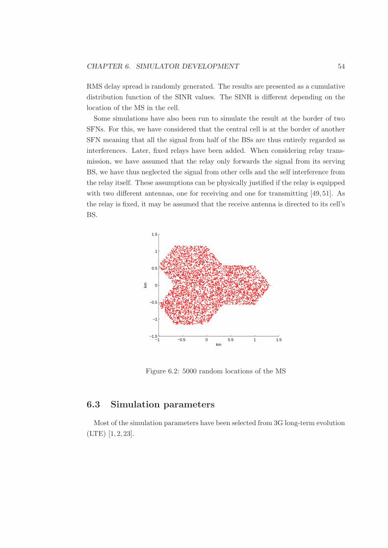
CHAPTER 6. SIMULATOR DEVELOPMENT 54
RMS delay spread is randomly generated. The results are presented as a cumulative
distribution function of the SINR values. The SINR is different depending on the
location of the MS in the cell.
Some simulations have also been run to simulate the result at the border of two
SFNs. For this, we have considered that the central cell is at the border of another
SFN meaning that all the signal from half of the BSs are thus entirely regarded as
interferences. Later, fixed relays have been added. When considering relay trans-
mission, we have assumed that the relay only forwards the signal from its serving
BS, we have thus neglected the signal from other cells and the self interference from
the relay itself. These assumptions can be physically justified if the relay is equipped
with two different antennas, one for receiving and one for transmitting [49, 51]. As
the relay is fixed, it may be assumed that the receive antenna is directed to its cell’s
BS.
−1 −0.5 0 0.5 1 1.5−1.5
−1
−0.5
0
0.5
1
1.5
km
km
Figure 6.2: 5000 random locations of the MS
6.3 Simulation parameters
Most of the simulation parameters have been selected from 3G long-term evolution
(LTE) [1, 2, 23].
CHAPTER 6. SIMULATOR DEVELOPMENT 55
6.3.1 OFDM parameters
The parameters are outlined below, taken from [1]. For all the simulations these
parameters are unchanged, we have concentrated on the 10 MHz bandwidth option
and the corresponding parameters. The bandwidth is 10 MHz with the center
frequency at 2 GHz, the number of subcarriers in the OFDM frame is 1024 but only
601 are considered occupied. The length of the cyclic prefix is chosen as 16.67µs.
The sampling frequency is at 15.36 MHz, the CP is thus of length 256.
Time of reference
As discussed in Chapter 4, the average SINR is a variable of the time of reference,
which is the starting demodulation (FFT) time at the receiver. In order to maximize
the useful signal power, it is important to synchronize the bias function with the
time delay profile in such a way that most of the channel energy lies within the CP
interval of the bias function. We have implemented three simple algorithms:
– “Zero” method. The MS is only synchronized with its own base station.
– “First” method. The receiver starts to demodulate the signal since the first
received path.
– “Max” method. The receiver starts to demodulated the signal at the maximum
power path.
The “First” method positions the time delay profile at the beginning of the CP
interval of the bias function. The SINR is calculated at this position keeping in
mind that the signal from the closest BS is also the signal with the highest power
reaching the receiver and hence contains most of the channel energy.
However, as this method does not have the capacity to adjust to any unexpected
changes, especially in cases of longer distances being involved, we have implemented
the “Max” method. This method shifts the bias function over the power delay profile
to have its initial time at the maximum power received path. The idea behind this
method is to assume that most of the power is concentrated around the strongest
path and avoids the loss of useful power if most of the delays are rather long.
These two methods have few complexities to implement while they provide good
results as can be seen in the comparison of Figure 6.3. As shown in Figure 6.3(b),
the “First” method gives the best result. Figure 6.3(a) exemplifies when the bias
function of the “First” method is placed in such a way that the CP interval contains
most of the channel energy. According to this result, all the next simulation will be
performed with the “First” method.

CHAPTER 6. SIMULATOR DEVELOPMENT 56
Finally, we note that an optimum method would have been to shift the bias
function over the power delay profile and determine the best position yielding to
the maximum SINR. This adaptive method always finds the best possible SINR by
positioning the bias function. However, the method is time consuming since it needs
to shift over all taps to calculate and compare for the maximum useful signal power.
1 2 3 4 5 6 7 8 9
x 10−5
0
0.2
0.4
0.6
0.8
1
1.2
1.4
1.6
1.8x 10
−14
second
Taps delay profile‘‘Zero´´ method‘‘First´´ method‘‘Max´´ method
(a) A power delay profile versus the bias functions
0 10 20 30 40 500
0.1
0.2
0.3
0.4
0.5
0.6
0.7
0.8
0.9
1
SINR[dB]
CD
F
‘‘Zero´´ method‘‘First´´ method‘‘Max´´ method
(b) Empirical CDF of the SINR
Figure 6.3: Comparaison between the different TOR algorithms
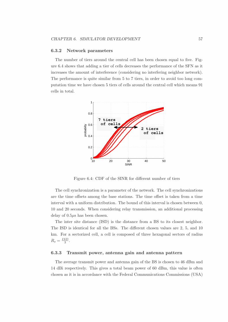
CHAPTER 6. SIMULATOR DEVELOPMENT 57
6.3.2 Network parameters
The number of tiers around the central cell has been chosen equal to five. Fig-
ure 6.4 shows that adding a tier of cells decreases the performance of the SFN as it
increases the amount of interference (considering no interfering neighbor network).
The performance is quite similar from 5 to 7 tiers, in order to avoid too long com-
putation time we have chosen 5 tiers of cells around the central cell which means 91
cells in total.
10 20 30 40 500
0.2
0.4
0.6
0.8
1
SINR
prob
abilt
y
7 tiers of cells
2 tiers of cells
Figure 6.4: CDF of the SINR for different number of tiers
The cell synchronization is a parameter of the network. The cell synchronizations
are the time offsets among the base stations. The time offset is taken from a time
interval with a uniform distribution. The bound of this interval is chosen between 0,
10 and 20 seconds. When considering relay transmission, an additional processing
delay of 0.5µs has been chosen.
The inter site distance (ISD) is the distance from a BS to its closest neighbor.
The ISD is identical for all the BSs. The different chosen values are 2, 5, and 10
km. For a sectorized cell, a cell is composed of three hexagonal sectors of radius
Rs = ISD3 .
6.3.3 Transmit power, antenna gain and antenna pattern
The average transmit power and antenna gain of the BS is chosen to 46 dBm and
14 dBi respectively. This gives a total beam power of 60 dBm, this value is often
chosen as it is in accordance with the Federal Communications Commissions (USA)
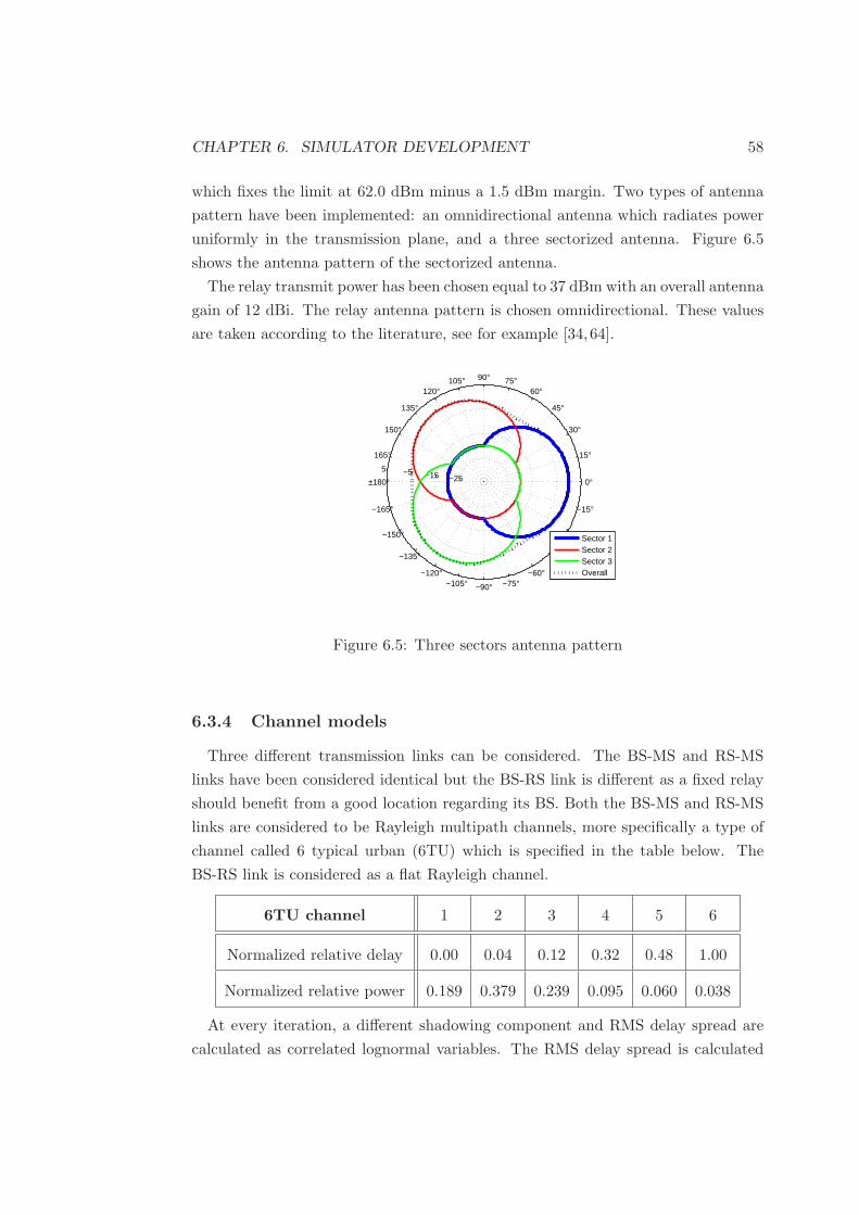
CHAPTER 6. SIMULATOR DEVELOPMENT 58
which fixes the limit at 62.0 dBm minus a 1.5 dBm margin. Two types of antenna
pattern have been implemented: an omnidirectional antenna which radiates power
uniformly in the transmission plane, and a three sectorized antenna. Figure 6.5
shows the antenna pattern of the sectorized antenna.
The relay transmit power has been chosen equal to 37 dBm with an overall antenna
gain of 12 dBi. The relay antenna pattern is chosen omnidirectional. These values
are taken according to the literature, see for example [34,64].
0°
15°
30°
45°
60°75°90°105°
120°
135°
150°
165°
±180°
−165°
−150°
−135°
−120°−105° −90° −75°
−60°
−45°
−30°
−15°
−25−15−55
Sector 1Sector 2Sector 3Overall
Figure 6.5: Three sectors antenna pattern
6.3.4 Channel models
Three different transmission links can be considered. The BS-MS and RS-MS
links have been considered identical but the BS-RS link is different as a fixed relay
should benefit from a good location regarding its BS. Both the BS-MS and RS-MS
links are considered to be Rayleigh multipath channels, more specifically a type of
channel called 6 typical urban (6TU) which is specified in the table below. The
BS-RS link is considered as a flat Rayleigh channel.
6TU channel 1 2 3 4 5 6
Normalized relative delay 0.00 0.04 0.12 0.32 0.48 1.00
Normalized relative power 0.189 0.379 0.239 0.095 0.060 0.038
At every iteration, a different shadowing component and RMS delay spread are
calculated as correlated lognormal variables. The RMS delay spread is calculated

CHAPTER 6. SIMULATOR DEVELOPMENT 59
according to Equation (2.6), with a median value of 0.65 µs and an exponent of 0.5.
The standard deviation of the delay spread is chosen as 2 dB. From the RMS delay
spread the channel taps delay are calculated using the 6TU table and Equation (2.5).
In the same manner the tap energy are computed from the generated lognormal
component, the 6TU table and Equation (2.4). The shadowing deviation has been
chosen equal to 8 dB for the BS-MS and RS-MS links, and equal to 4 dB for the
BS-RS link.
For the initial SFN simulation without relay the path loss model was chosen
according to [1]. We have then used the more general model from IEEE 802.16
which takes into account the height of the transmitters and receivers in order to
more realistically model the benefit of relaying. The BS, RS and MS heights have
been chosen equal to 32, 12 and 1.5 respectively. The first hop of the relay is assumed
to be line of sight and does not suffer from interference. The second hop of the relay
link and the direct link are assumed to transmit under NLOS channel conditions.
The different path losses are plotted in Figure 6.6. It is assumed that there are no
loopback interferences and interfering signals from a relay output to another relay’s
input. These interferences may be avoided by, e.g. placing receive antennas on
rooftops and transmit antennas at the street level, using highly directive receive
antennas at relays and employing interference cancellation algorithms [52].
0 2 4 6 8 1080
100
120
140
160
180
200
distance [km]
dB
Path loss models
BS−MS link (NLOS, SCM macro)RS−MS link (NLOS, SCM macro)BS−RS link (LOS,IEEE 802.16 type C)BS−MS link (3GPP)
Figure 6.6: Path loss models

CHAPTER 6. SIMULATOR DEVELOPMENT 60
We have also implemented different correlation models among the large scale
parameters (LSP) as presented in Chapter 3. Figure 6.7 shows the CDF of the
SINR for different models:
– no correlation among the LSP
– correlation between the delay spread and shadowing of the same link is equal
to ρXY = −0.75, no other correlations are considered
– cross-correlated shadowing between two links are equal to 0.5, the correla-
tion between the delay spread and shadowing of the same link is changed to
ρXY = −0.6 in order to end up with a positive definite matrix
– cross-correlation between two links are calculated according to the “Graziosi”
model, the correlation between the delay spread and shadowing of the same link
is ρXY = −0.6, the overall correlation matrix is calculated with a Kronecker
product as explained at the end of Chapter 3
– cross-correlation between two links are calculated according to the “Saunders”
model, the correlation between the delay spread and shadowing of the same
link is ρXY = −0.6, the overall correlation matrix is also calculated with a
Kronecker product.
In this figure, we see that most of those models almost do not have an impact on
the SINR distribution. As there are no well-agreed models, we have just kept the
correlation between the RMS delay spread and the shadowing of the same link equal
to −0.75 and omitted any other correlations.
5 10 15 200
0.1
0.2
0.3
0.4
0.5
0.6
0.7
SINR[dB]
CD
F
No correlation among LSP
ρXY = −0.75, Rxx = Ryy = I
ρXY = −0.6, Rxx: Constant 0.5, Ryy = I
ρXY = −0.6, Rxx = Ryy : “Graziosi” model
ρXY = −0.6, Rxx = Ryy : “Saunders” model
Figure 6.7: SINR with different correlation models
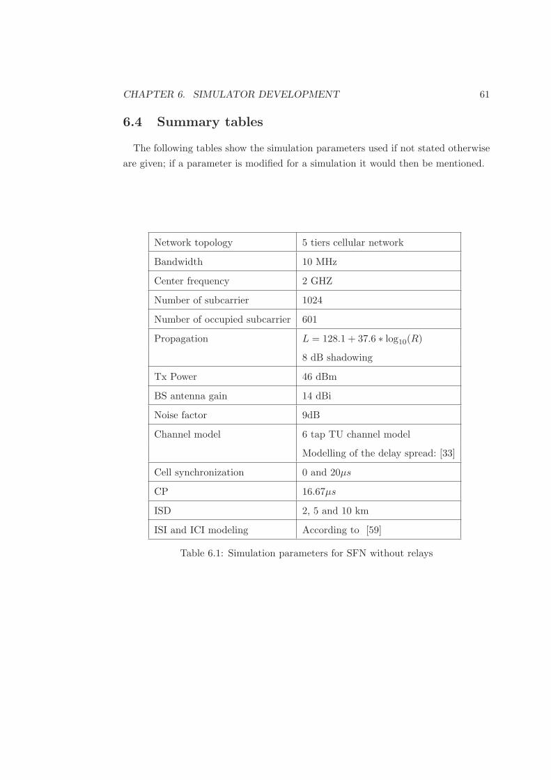
CHAPTER 6. SIMULATOR DEVELOPMENT 61
6.4 Summary tables
The following tables show the simulation parameters used if not stated otherwise
are given; if a parameter is modified for a simulation it would then be mentioned.
Network topology 5 tiers cellular network
Bandwidth 10 MHz
Center frequency 2 GHZ
Number of subcarrier 1024
Number of occupied subcarrier 601
Propagation L = 128.1 + 37.6 ∗ log10(R)
8 dB shadowing
Tx Power 46 dBm
BS antenna gain 14 dBi
Noise factor 9dB
Channel model 6 tap TU channel model
Modelling of the delay spread: [33]
Cell synchronization 0 and 20µs
CP 16.67µs
ISD 2, 5 and 10 km
ISI and ICI modeling According to [59]
Table 6.1: Simulation parameters for SFN without relays
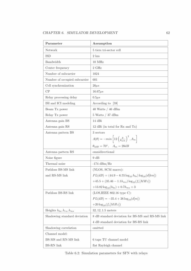
CHAPTER 6. SIMULATOR DEVELOPMENT 62
Parameter Assumption
Network 5 tiers tri-sector cell
ISD 2 km
Bandwidth 10 MHz
Center frequency 2 GHz
Number of subcarrier 1024
Number of occupied subcarrier 601
Cell synchronization 20µs
CP 16.67µs
Relay processing delay 0.5µs
ISI and ICI modeling According to [59]
Beam Tx power 40 Watts / 46 dBm
Relay Tx power 5 Watts / 37 dBm
Antenna gain BS 14 dBi
Antenna gain RS 12 dBi (in total for Rx and Tx)
Antenna pattern BS 3 sectors
A(θ) = −min
[
12(
θθ3dB
)2
, Am
]
θ3dB = 70◦, Am = 20dB
Antenna pattern RS omnidirectional
Noise figure 9 dB
Thermal noise -174 dBm/Hz
Pathloss BS-MS link (NLOS, SCM macro):
and RS-MS link PL(dB) = (44.9 − 6.55 log10
hbs) log10
(d[km])
+45.5 + (35.46 − 1.1hms) log10
(fc[MHz])
+13.82 log10
(hbs) + 0.7hms + 3
Pathloss BS-RS link (LOS,IEEE 802.16 type C):
PL(dB) = −35.4 + 26 log10
(d[m])
+20 log10
(fc[MHz])
Heights hbs, hrs, hms 32, 12, 1.5 meters
Shadowing standard deviation 8 dB standard deviation for BS-MS and RS-MS link
4 dB standard deviation for BS-RS link
Shadowing correlation omitted
Channel model:
BS-MS and RN-MS link 6 taps TU channel model
BS-RN link flat Rayleigh channel
Table 6.2: Simulation parameters for SFN with relays

Chapter 7
Simulation results
In this chapter different simulation results are presented. As a first step, an SFN
without relay has been implemented and simulated. These first simulations were
used as a benchmark to gauge the quality of the simulator with comparison to the
results of [43]. Relays have then been introduced into the network and different
relaying concepts have been evaluated as introduced in Chapter 5, as well as the
impact of relay topology chosen among different numbers and repartitions.
7.1 SFN area deployment aspects
As a first step in the simulation work, this section reviews the result of [43] on
SFN area deployment aspects. Different simulations have been run to assess the
impact of inter-site distance (ISD), asynchronity, and other factors such as distance
from the border of two SFNs and the effect of possible holes in the SFN grid. The
asynchronity refers to the time offset an OFDM frame is sent among the BSs. In our
model each BS in the network has a random offset which is uniformly distributed
in the range [0, Async], where the upper bound is the maximum time offset in the
SFN. The simulation parameters used in this section are issued from Table 6.4.
7.1.1 Impact of asynchronity and ISD
From Figure 7.1, the SINR distribution is clearly dependent on the ISD value: the
smaller the ISD is, the higher the SINR. One can notice also, that the synchroniza-
tion of the BSs has a real impact in the low ISD case but not in the high ISD case.
Being far from the sources reduces naturally the signal-to-noise ratio because the
attenuation mainly increases with the distance. Interference suffers from the same
attenuation as the useful signal so even if the proportion of the interfering signal is
63
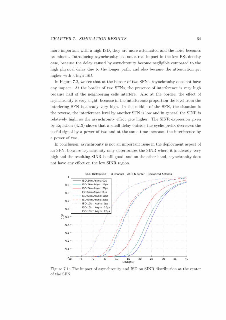
CHAPTER 7. SIMULATION RESULTS 64
more important with a high ISD, they are more attenuated and the noise becomes
prominent. Introducing asynchronity has not a real impact in the low BSs density
case, because the delay caused by asynchronity become negligible compared to the
high physical delay due to the longer path, and also because the attenuation get
higher with a high ISD.
In Figure 7.2, we see that at the border of two SFNs, asynchronity does not have
any impact. At the border of two SFNs, the presence of interference is very high
because half of the neighboring cells interfere. Also at the border, the effect of
asynchronity is very slight, because in the interference proportion the level from the
interfering SFN is already very high. In the middle of the SFN, the situation is
the reverse, the interference level by another SFN is low and in general the SINR is
relatively high, so the asynchronity effect gets higher. The SINR expression given
by Equation (4.13) shows that a small delay outside the cyclic prefix decreases the
useful signal by a power of two and at the same time increases the interference by
a power of two.
In conclusion, asynchronity is not an important issue in the deployment aspect of
an SFN, because asynchronity only deteriorates the SINR where it is already very
high and the resulting SINR is still good, and on the other hand, asynchronity does
not have any effect on the low SINR region.
−10 −5 0 5 10 15 20 25 30 35 400
0.1
0.2
0.3
0.4
0.5
0.6
0.7
0.8
0.9
1
SINR[dB]
CD
F
SINR Distribution − TU Channel − At SFN center − Sectorized Antenna
ISD:2km Async: 0µs
ISD:2km Async: 10µs
ISD:2km Async: 20µs
ISD:5km Async: 0µs
ISD:5km Async: 10µs
ISD:5km Async: 20µs
ISD:10km Async: 0µs
ISD:10km Async: 10µs
ISD:10km Async: 20µs
Figure 7.1: The impact of asynchronity and ISD on SINR distribution at the centerof the SFN
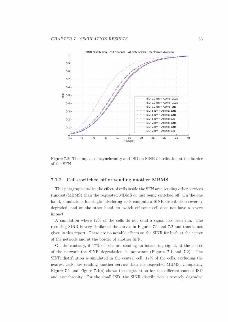
CHAPTER 7. SIMULATION RESULTS 65
−10 −5 0 5 10 15 20 25 30 35 400
0.1
0.2
0.3
0.4
0.5
0.6
0.7
0.8
0.9
1
SINR[dB]
CD
F
SINR Distribution − TU Channel − At SFN border − Sectorized Antenna
ISD: 10 km − Async: 20µs
ISD: 10 km − Async: 10µs
ISD: 10 km − Async: 0µs
ISD: 5 km − Async: 20µs
ISD: 5 km − Async: 10µs
ISD: 5 km − Async: 0µs
ISD: 2 km − Async: 20µs
ISD: 2 km − Async: 10µs
ISD: 2 km − Async: 0µs
Figure 7.2: The impact of asynchronity and ISD on SINR distribution at the borderof the SFN
7.1.2 Cells switched off or sending another MBMS
This paragraph studies the effect of cells inside the SFN area sending other services
(unicast/MBMS) than the requested MBMS or just being switched off. On the one
hand, simulations for single interfering cells compute a SINR distribution severely
degraded, and on the other hand, to switch off some cell does not have a severe
impact.
A simulation where 17% of the cells do not send a signal has been run. The
resulting SINR is very similar of the curves in Figures 7.1 and 7.2 and thus is not
given in this report. There are no notable effects on the SINR for both at the center
of the network and at the border of another SFN.
On the contrary, if 17% of cells are sending an interfering signal, at the center
of the network the SINR degradation is important (Figures 7.1 and 7.2). The
SINR distribution is simulated in the central cell; 17% of the cells, excluding the
nearest cells, are sending another service than the requested MBMS. Comparing
Figure 7.1 and Figure 7.4(a) shows the degradation for the different case of ISD
and asynchronity. For the small ISD, the SINR distribution is severely degraded

CHAPTER 7. SIMULATION RESULTS 66
up to 10dB. This degradation is attenuated if the network incorporates already
asynchronity. For the high ISD case, interfering cells are further and there is almost
no repercussion. The same simulation can be computed at the SFN border, but as
the interference level is already high, no real degradation can be noticed.
In general, for an SFN, the entire cells must send the same service to preserve the
quality of the SINR among the network.
Simulation in a cell sending unicast or an other MBMS than the rest of the
network shows that the performance in this type of cell are really poor (Figure
7.4(b)). Alternatively, unicast or other service transmission in a single network
could be improved by introducing a guard interval of cells around the cell sending
its own service. Simulations have been run by switching a tier of cells around the
central cell, but the performance inside the central cell is still low (and worse in
the guard interval). However, it can be noticed that the simulation is close to the
performance at the border of a SFN especially for the low ISD case. For an ISD
equivalent to 10 km, the SINR is more degraded because at the edge of the cell the
only supporting source is very far.
Figure 7.3: Cells guard interval concept
To conclude, allowing single cell services degrades the SINR in the overall of the
network only in the low ISD case. Introducing a guard interval permits enhancing
the SINR in the cell sending the unicast, but the performance is still low.

CHAPTER 7. SIMULATION RESULTS 67
−10 −5 0 5 10 15 20 25 30 35 400
0.1
0.2
0.3
0.4
0.5
0.6
0.7
0.8
0.9
1
SINR[dB]
CD
F
SINR Distribution − TU Channel − At SFN center − Sectorized Antenna − 17% unicast
ISD: 2 km − Async: 0µs
ISD: 2 km − Async: 10µs
ISD: 2 km − Async: 20µs
ISD: 10 km − Async: 0µs
ISD: 10 km − Async: 10µs
ISD: 10 km − Async: 20µs
ISD: 20 km − Async: 0µs
ISD: 20 km − Async: 10µs
ISD: 20 km − Async: 20µs
(a) SINR in the SFN where 17% of the cells (excluding the nearest cell) are sending another servicethan the requested MBMS
−10 −5 0 5 10 15 20 25 30 35 400
0.1
0.2
0.3
0.4
0.5
0.6
0.7
0.8
0.9
1
SINR[dB]
CD
F
SINR Distribution − TU Channel − In a cell sending unicast in the SFN − Sectorized Antenna
ISD: 10 kmISD: 5 kmISD: 2 kmISD: 10 km − Guard intervalISD: 5 km − Guard intervalISD: 2 km − Guard interval
(b) In a cell sending unicast
Figure 7.4: Cell sending other service than the requested MBMS

CHAPTER 7. SIMULATION RESULTS 68
7.2 SFN with relays
In this section, relays are now introduced in the SFN and the empirical SINR cu-
mulative distribution is simulated. The impact of relays numbers, positions, gains
and protocols are studied. Each cell is fed by fixed RSs with omnidirectional trans-
mit antenna and a macro BS with a sectorized antenna located at the center of the
cell. Most of the simulation parameters are from Table 6.4. If not specified, the
simulations are run with 3 relay stations per cell applying fixed gain relaying under
full-duplex protocol. The default ISD is 2 km.
7.2.1 Impact of the relay gains
In Chapter 5, the theoretical average SINR of the different relay gains has been
derived for the general Nakagami fading. In this chapter, we just consider the case
of Rayleigh fading which is a specific case of Nakagami fading with m = 1. Now
recalling these results, the signal/interference amplification and noise amplification
term for both fixed gain and variable gain are
E{|βFGhSR|2} =σ2
rnESR
σ2bsESR + N0
(7.1)
E{|βV GhSR|2} =σ2
rn
σ2bs
eN0
ESRσ2bs E2
(N0
ESRσ2bs
)
(7.2)
E{|βFG|2} =σ2
rn
σ2bsESR + N0
(7.3)
E{|βV G|2} =σ2
rn
ESRσ2bs
eN0
ESRσ2bs E1
(N0
ESRσ2bs
)
. (7.4)
Interestingly for Rayleigh fading, it can be shown that the variable gain amplifies
more the noise in average than the fixed gain. If we denote x = N0
ESRσ2bs
, we can
rewrite the noise amplification factor such that,
E{|βFG|2} =σ2
rn
N0
x
1 + x(7.5)
E{|βV G|2} =σ2
rn
N0ex E1(x)x, (7.6)
by using [4, Eq. 5.1.19]: 1x+1 < ex E1(x) for x > 0, the result follows that
E{|βFG|2} < E{|βV G|2} (7.7)
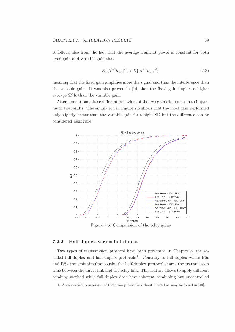
CHAPTER 7. SIMULATION RESULTS 69
It follows also from the fact that the average transmit power is constant for both
fixed gain and variable gain that
E{|βV GhSR|2} < E{|βFGhSR|2} (7.8)
meaning that the fixed gain amplifies more the signal and thus the interference than
the variable gain. It was also proven in [14] that the fixed gain implies a higher
average SNR than the variable gain.
After simulations, these different behaviors of the two gains do not seem to impact
much the results. The simulation in Figure 7.5 shows that the fixed gain performed
only slightly better than the variable gain for a high ISD but the difference can be
considered negligible.
−15 −10 −5 0 5 10 15 20 25 30 35 400
0.1
0.2
0.3
0.4
0.5
0.6
0.7
0.8
0.9
1
SINR[dB]
CD
F
FD − 3 relays per cell
No Relay − ISD: 2kmFix Gain − ISD: 2kmVariable Gain − ISD: 2km No Relay − ISD: 10kmVariable Gain − ISD: 10kmFix Gain − ISD: 10km
Figure 7.5: Comparision of the relay gains
7.2.2 Half-duplex versus full-duplex
Two types of transmission protocol have been presented in Chapter 5, the so-
called full-duplex and half-duplex protocols 1. Contrary to full-duplex where BSs
and RSs transmit simultaneously, the half-duplex protocol shares the transmission
time between the direct link and the relay link. This feature allows to apply different
combing method while full-duplex does have inherent combining but uncontrolled
1. An analytical comparison of these two protocols without direct link may be found in [49].
CHAPTER 7. SIMULATION RESULTS 70
unless feedback information may be obtained [54]. Another advantage of half-duplex
is the fact that the time of reference for the demodulation is chosen separately for
the two branches. Nevertheless, in order to overcome the full-duplex protocol, half-
duplex should improve the SINR in a consequent amount to compensate for the
loss of 1/2 in the transmission rate. Using the approximation of Equation 4.10, the
capacity for one subcarrier is approximately
CFD / log2(1 + ΓFD), CHD /1
2log2(1 + ΓHD) (7.9)
for full-duplex and half-duplex, respectively.
If the average SINR is much greater than one, Γ ≫ 1, which from the previ-
ous simulation is the case for example when the ISD is equal to 2 km, we may
approximate the capacity further as follows
CFD / log2(ΓFD) ≈ ln 10
10 ln 2ΓFD[dB] (7.10)
CHD /1
2log2(ΓHD) ≈ 1
2
ln 10
10 ln 2ΓHD[dB]. (7.11)
So, in order to attain the same transmission rate we must have ΓHD[dB] = 2ΓFD[dB],
which means that the SINR with half-duplex should be the square of the SINR with
full-duplex in a linear scale. Not surprisingly, simulations show that the half-duplex
protocol does not manage to reach the performance with selection combining and
equal gain combining (Figure 7.6). The gap is so important that the performance
is worse than for an SFN without relays and there are few reasons to believe that
applying maximum ratio combining will help.
On the other hand, if the average SINR is very close to zero, by Taylor expansion
we may approximate the capacity as follows
CFD / log2(1 + ΓFD) ≈ 1
ln 2ΓFD (7.12)
CHD /1
2log2(1 + ΓHD) ≈ 1
2
1
ln 2ΓHD. (7.13)
So, in order to attain the same transmission rate we must have ΓHD[dB] = ΓFD[dB]+
3dB. Unfortunately, simulations shows that half-duplex protocol does not manage to
reach this gain in the context of a low SINR in a high ISD case of 10 km (Figure 7.7).
To conclude, according to our simulations, the full-duplex protocol offers largely
better performance than the half-duplex protocol.

CHAPTER 7. SIMULATION RESULTS 71
5 10 15 20 25 30 35 400
0.1
0.2
0.3
0.4
0.5
0.6
0.7
0.8
0.9
1
SINR[dB]
CD
F
3 relays per cell − ISD: 2km
No Relay − ISD: 2kmFull−duplexHalf−duplex − Lower bound Sel. comb.Half−duplex − Eq. gain comb.
0 2 4 6 8 100
0.1
0.2
0.3
0.4
0.5
0.6
0.7
0.8
0.9
1
Capacity per subcarrier [bit/s/Hz]
CD
F
3 relays per cell − ISD: 2km
No RelayFull−duplexHalf−duplex − Lower bound Sel. comb.Half−duplex − Eq. gain comb.
Figure 7.6: Comparison of full-duplex and half-duplex protocol - ISD: 2 km

CHAPTER 7. SIMULATION RESULTS 72
−15 −10 −5 0 5 10 150
0.1
0.2
0.3
0.4
0.5
0.6
0.7
0.8
0.9
1
SINR[dB]
CD
F
3 relays per cell − ISD: 10km
No Relay − ISD: 10kmFull−duplexHalf−duplex − Lower bound Sel. combHalf−duplex − Eq.gain comb.
0 0.5 1 1.5 2 2.5 3 3.5 40
0.1
0.2
0.3
0.4
0.5
0.6
0.7
0.8
0.9
1
Capacity per subcarrier [bit/s/Hz]
CD
F
3 relays per cell − ISD: 10km
No RelayFull−duplexHalf−duplex − Lower bound Sel. combHalf−duplex − Eq.gain comb.
Figure 7.7: Comparison of full-duplex and half-duplex protocol - ISD: 10 km
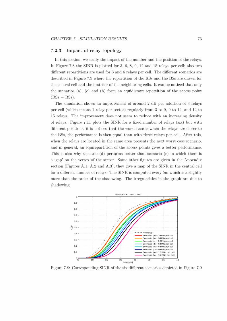
CHAPTER 7. SIMULATION RESULTS 73
7.2.3 Impact of relay topology
In this section, we study the impact of the number and the position of the relays.
In Figure 7.8 the SINR is plotted for 3, 6, 8, 9, 12 and 15 relays per cell; also two
different repartitions are used for 3 and 6 relays per cell. The different scenarios are
described in Figure 7.9 where the repartition of the RSs and the BSs are drawn for
the central cell and the first tier of the neighboring cells. It can be noticed that only
the scenarios (a), (e) and (h) form an equidistant repartition of the access point
(BSs + RSs).
The simulation shows an improvement of around 2 dB per addition of 3 relays
per cell (which means 1 relay per sector) regularly from 3 to 9, 9 to 12, and 12 to
15 relays. The improvement does not seem to reduce with an increasing density
of relays. Figure 7.11 plots the SINR for a fixed number of relays (six) but with
different positions, it is noticed that the worst case is when the relays are closer to
the BSs, the performance is then equal than with three relays per cell. After this,
when the relays are located in the same area presents the next worst case scenario,
and in general, an equirepartition of the access points gives a better performance.
This is also why scenario (d) performs better than scenario (c) in which there is
a ‘gap’ on the vertex of the sector. Some other figures are given in the Appendix
section (Figures A.1, A.2 and A.3), they give a map of the SINR in the central cell
for a different number of relays. The SINR is computed every 5m which is a slightly
more than the order of the shadowing. The irregularities in the graph are due to
shadowing.
5 10 15 20 25 30 35 400
0.1
0.2
0.3
0.4
0.5
0.6
0.7
0.8
0.9
1
SINR[dB]
CD
F
Fix Gain − FD −ISD: 2km
No RelayScenario (a) − 3 RNs per cellScenario (b) − 3 RNs per cellScenario (c) − 6 RNs per cellScenario (d) − 6 RNs per cellScenario (e) − 8 RNs per cellScenario (f ) − 9 RNs per cellScenario (g) − 12 RNs per cellScenario (h) − 15 RNs per cell
Figure 7.8: Corresponding SINR of the six different scenarios depicted in Figure 7.9

CHAPTER 7. SIMULATION RESULTS 74
(a) 3 relays per cell (b) 3 relays per cell
(c) 6 relays per cell (d) 6 relays per cell
(e) 8 relays per cell (f) 9 relays per cell
(g) 12 relays per cell (h) 15 relays per cell
Figure 7.9: Six topology scenarios

CHAPTER 7. SIMULATION RESULTS 75
10 15 20 25 30 350
0.1
0.2
0.3
0.4
0.5
0.6
0.7
0.8
0.9
1
SINR[dB]
CD
F
Fix Gain − FD − ISD: 2km
No Relay3 relays per cell6 relays per cell − 20% of the sector diameter6 relays per cell − 30% of the sector diameter6 relays per cell − 40% of the sector diameter6 relays per cell − 50% of the sector diameter6 relays per cell − 60% of the sector diameter6 relays per cell − 70% of the sector diameter6 relays per cell − 80% of the sector diameter
(a)
20 30 40 50 60 70 800
0.1
0.2
0.3
0.4
0.5
0.6
0.7
% of the sector diameter
CD
F
Fix Gain − FD − ISD: 2km
10 dB − 6 relays per cell15 dB − 6 relays per cell20 dB − 6 relays per cellNo Relay3 relays per cell
(b)
Figure 7.10: Evolution of the SINR with the relay positions

CHAPTER 7. SIMULATION RESULTS 76
(a) (b)
(c) (d)
(e) (f)
(g)
Figure 7.11: Evolution of the SINR with the relay positions
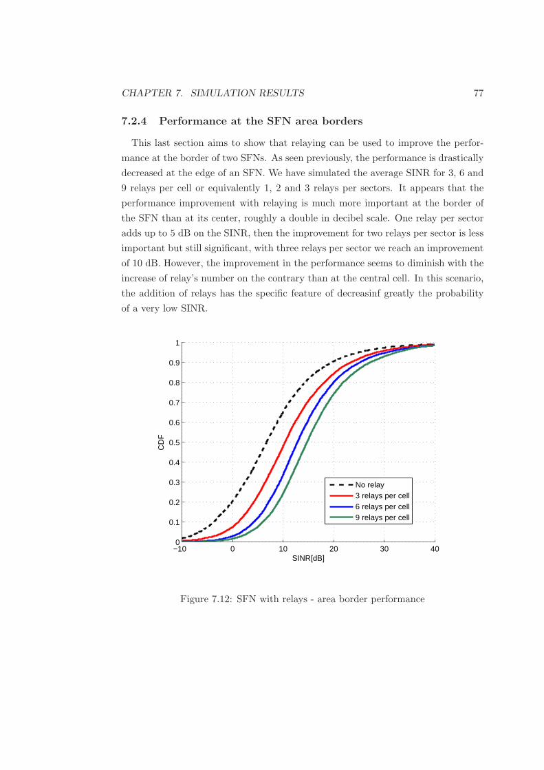
CHAPTER 7. SIMULATION RESULTS 77
7.2.4 Performance at the SFN area borders
This last section aims to show that relaying can be used to improve the perfor-
mance at the border of two SFNs. As seen previously, the performance is drastically
decreased at the edge of an SFN. We have simulated the average SINR for 3, 6 and
9 relays per cell or equivalently 1, 2 and 3 relays per sectors. It appears that the
performance improvement with relaying is much more important at the border of
the SFN than at its center, roughly a double in decibel scale. One relay per sector
adds up to 5 dB on the SINR, then the improvement for two relays per sector is less
important but still significant, with three relays per sector we reach an improvement
of 10 dB. However, the improvement in the performance seems to diminish with the
increase of relay’s number on the contrary than at the central cell. In this scenario,
the addition of relays has the specific feature of decreasinf greatly the probability
of a very low SINR.
−10 0 10 20 30 400
0.1
0.2
0.3
0.4
0.5
0.6
0.7
0.8
0.9
1
SINR[dB]
CD
F
No relay3 relays per cell6 relays per cell9 relays per cell
Figure 7.12: SFN with relays - area border performance
Chapter 8
Conclusions and future work
Conventionally, broadcast is considered as a drawback in wireless communication
systems due to interference and requirement for frequency planning. This thesis con-
siders the recent single-frequency relay network concept which exploits the broadcast
nature of the wireless channel.
As a background, the mobile radio channel and its statistical modeling was re-
viewed . A summary was made of the basic principles of the widely used OFDM
modulation. Some classical relaying concepts were presented with derivations of
corresponding average SINRs used later in simulations.
A simulator of an OFDM-based SFN was built in order to evaluate different
relaying concept in downlink broadcast communication. The simulator development
was described and explained. Simulations were presented with results on the SFN
area deployment aspect: impact of asyncronity in the SFN, size of the ISD, as well
as introduction of unicast transmission in the SFN.
Finally, simulations of the SFN performance with fixed relay deployment are pre-
sented. The difference in behaviors of the fixed and variable gain shown theoretically
appears to be negligible in the simulation. Our simulations have verified the capabil-
ity of relaying to improve the system capacity and specially cell edge performance.
According to our simulation, it was concluded that full-duplex protocol outperforms
greatly the half-duplex protocol. The last results are concentrated in the optimiza-
tion of the relays positions.
Future possible work could include a deeper mathematical analysis on the condi-
tion for correlation models among the large scale parameters to be valid; statistical
analysis for the instantaneous SINR of an OFDM system and a justification by
78

CHAPTER 8. CONCLUSIONS AND FUTURE WORK 79
mathematical analysis or/and simulations of the approximation of the average of
the instantaneous SINR used in Chapter 4. A last suggestion would be to consider
the relay self-interference.
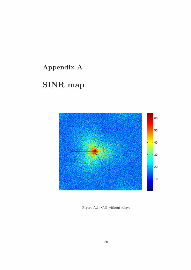
Appendix A
SINR map
10
20
30
40
50
60
Figure A.1: Cell without relays
80

APPENDIX A. SINR MAP 81
10
20
30
40
50
60
Figure A.2: Cell with 3 relays

APPENDIX A. SINR MAP 82
10
20
30
40
50
60
Figure A.3: Cell with 6 relays

Bibliography
[1] 3GPP. Physical layer for evolved utra. Technical Report TR 25.814, 3GPP,
September 2006.
[2] WG3/WG5 TSG-C 3GPP2. 1xev-dv evaluation methodology - addendum - v6.
Technical Report MSU-CSE-00-2, 3GPP2, July 2001.
[3] Bello P. A. Characterization of randomly time-variant linear channels. IEEE
Trans. Comm. Syst., 11:360–393, 1963.
[4] M. Abramowitz and I. A. Stegun. Handbook of Mathematical Functions with
Formulas, Graphs, and Mathematical Tables. Dover, 1970.
[5] A. Algans, K.I. Pedersen, and P.E. Mogensen. Experimental analysis of the
joint statistical properties of azimuth spread, delay spread, and shadow fading.
Selected Areas in Communications, IEEE Journal on, 20(3):523–531, Apr 2002.
[6] H.W. Arnold, D.C. Cox, and R.R. Murray. Macroscopic diversity performance
measured in the 800-mhz portable radio communications environment. Anten-
nas and Propagation, IEEE Transactions on, 36(2):277–281, Feb 1988.
[7] Dan Avidor and Sayandev Mukherjee. Hidden issues in the simulation of fixed
wireless systems. Wirel. Netw., 7(2):187–200, 2001.
[8] M. Batariere, K. Baum, and T.P. Krauss. Cyclic prefix length analysis for 4G
OFDM systems. In Vehicular Technology Conference, 2004. VTC2004-Fall.
2004 IEEE 60th, volume 1, pages 543–547 Vol. 1, Sept. 2004.
[9] E. Biglieri. Coding for Wireless Channels. Springer, 2005.
[10] G. Calcev, D. Chizhik, B. Goransson, S. Howard, H. Huang, A. Kogiantis, A.F.
Molisch, A.L. Moustakas, D. Reed, and Hao Xu. A wideband spatial channel
model for system-wide simulations. Vehicular Technology, IEEE Transactions
on, 56(2):389–403, March 2007.
[11] S. Celebi. Interblock interference (ibi) and time of reference (tor) computation
in OFDM systems. Communications, IEEE Transactions on, 49(11):1895–1900,
Nov 2001.
83

BIBLIOGRAPHY 84
[12] L. M. Correia. Wireless Flexible Personalized Communications. COST.
[13] Bernhard Walke Daniel C. Schultz. Fixed relays for cost efficient 4g network
deployments: An evaluation. The 18th Annual IEEE International Symposium
on Personal, Indoor and Mobile Radio Communications (PIMRC’07), 2007.
[14] Xitirnin Deng and A.M. Haimovich. Power allocation for cooperative relaying in
wireless networks. Communications Letters, IEEE, 9(11):994–996, Nov. 2005.
[15] William Feller. An Introduction to Probability Theory and Its Applications.
Wiley, 1968.
[16] R. G. Gallager. Information Theory and Reliable Communication. New York:
Wiley, 1968.
[17] D. Giancristofaro. Correlation model for shadow fading in mobile radio chan-
nels. Electron. Lett., 32:958–959, May 1996.
[18] N. Gogate, D. Avidor, and S.S. Panwar. Simulation study of a fixed wireless
access system. Universal Personal Communications, 1998. ICUPC ’98. IEEE
1998 International Conference on, 1:209–215 vol.1, Oct 1998.
[19] Andrea J. Goldsmith. Design and Performance of High-Speed Communication
Systems over Time-Varying Radio Channels. PhD thesis, EECS Department,
University of California, Berkeley, 1994.
[20] V. Graziano. Propagation correlations at 900 mhz. IEEE Transactions on
Vehicular Technology, VT-27, 1978.
[21] F. Graziosi, M. Pratesi, M. Ruggieri, and F. Santucci. A multicell model of
handover initiation in mobile cellular networks. Vehicular Technology, IEEE
Transactions on, 48(3):802–814, May 1999.
[22] F. Graziosi and F. Santucci. A general correlation model for shadow fading
in mobile radio systems. Communications Letters, IEEE, 6(3):102–104, Mar
2002.
[23] 3GPP/3GPP2 SCM Ad-Hoc Group. Spatial channel model text description.
v3.3, March 2003.
[24] M. Gudmundson. Correlation model for shadow fading in mobile radiosystems.
Electron. Lett., 27:2145–2146, Nov. 1991.
[25] M.A. Haleem, D. Avidor, and R. Valenzuela. Fixed wireless access system
with autonomous resource assignment. Personal, Indoor and Mobile Radio
Communications, 1998. The Ninth IEEE International Symposium on, 3:1438–
1442 vol.3, Sep 1998.

BIBLIOGRAPHY 85
[26] M.O. Hasna and M.-S. Alouini. A performance study of dual-hop transmis-
sions with fixed gain relays. Wireless Communications, IEEE Transactions on,
3(6):1963–1968, Nov. 2004.
[27] M. Hata. Empirical formula for propagation loss in land mobile radio services.
IEEE Transactions on Vehicular Technology, 29, 1980.
[28] L. Vuokko J. Salo and P. Vainikainen. Why is shadow fading lognormal? Proc.
International Symposium on Wireless Personal Multimedia Communications
Aalborg, Denmark, pages 522–526, 2005.
[29] S.K. Wilson P.O. Borjesson J.J. van de Beek, P. Odling. Orthogonal frequency-
division multiplexing (OFDM). the International Union of Radio Science
(URSI), 2002.
[30] J.Walfisch and H.L. Bertoni. A theoretical model of uhf propagation in urban
environments. IEEE Trans. Antennas Propagat., 36, 1988.
[31] Hoon Kim and Youngnam Han. Enhanced correlated shadowing generation in
channel simulation. Communications Letters, IEEE, 6(7):279–281, Jul 2002.
[32] T. Klingenbrunn and P. Mogensen. Modelling cross-correlated shadowing in
network simulations. Vehicular Technology Conference, 1999. VTC 1999 - Fall.
IEEE VTS 50th, 3:1407–1411 vol.3, 1999.
[33] Yu Shuan Yeh Larry J. Greenstein, Vinko Erceg and Martin V. Clark. A new
path-gain/delay-spread propagation model for digital cellular channels. IEEE
Transactions on Vehicular Technology, VOL.46, MAY 1997.
[34] Ki-Ho Lee and Dong-Ho Cho. Hierarchical constellation based adaptive relay
scheme in multi-hop networks. Communications Letters, IEEE, 11(3):225–227,
March 2007.
[35] M.J. Marsan, G.C. Hess, and S.S. Gilbert. Shadowing variability in an urban
land mobile environment at 900 mhz. Electronics Letters, 26(10):646–648, May
1990.
[36] A. Mawira. Models for the spatial correlation functions of the (log)- normal
component of the variability of vhfrthf field strength in urban environment.
PIMRC Proceedings, pages 436–440, Boston 1992.
[37] A. Mawira. Models for the spatial correlation functions of the (log)-normal com-
ponent of the variability of vhf/uhf field strength in urban environment. Per-
sonal, Indoor and Mobile Radio Communications, 1992. Proceedings, PIMRC
’92., Third IEEE International Symposium on, pages 436–440, Oct 1992.

BIBLIOGRAPHY 86
[38] Aris Moustakas and Achilles Kogiantis. Lognormal correlations between shad-
owing, delay-spread and angle-spread and for different base-stations: A unified
approach. Lucent Technologies, SCM-125-LUC-LognormalCorrelations, July
2001.
[39] S. Mukherjee and D. Avidor. Dynamics of path losses between a mobile terminal
and multiple base stations in a cellular environment. Vehicular Technology,
IEEE Transactions on, 50(6):1590–1603, Nov 2001.
[40] S. Mukherjee and D. Avidor. Effect of microdiversity and correlated macro-
diversity on outages in a cellular system. Wireless Communications, IEEE
Transactions on, 2(1):50–58, Jan. 2003.
[41] Van Duc Nguyen and H.-P. Kuchenbecker. Intercarrier and intersymbol in-
terference analysis of OFDM systems on time-invariant channels. In Personal,
Indoor and Mobile Radio Communications, 2002. The 13th IEEE International
Symposium on, volume 4, pages 1482–1487 vol.4, Sept. 2002.
[42] Bjorn Ottersten Niklas Jalden, Per Zetterberg and Laura Garcia. Inter and
intra-site correlation of large scale parameters from macro cellular measure-
ments at 1800mhz. EURASIP Journal on Wireless Communications and Net-
working, August 2007.
[43] Nokia. SFN area deployement aspect. 3GPP TSG-RAN WG3 Meeting 53 bis,
October 2006.
[44] A. Nosratinia, T.E. Hunter, and A. Hedayat. Cooperative communication in
wireless networks. Communications Magazine, IEEE, 42(10):74–80, Oct. 2004.
[45] Minoru Okada and Shozo Komaki. Pre-dft combining space diversity assisted
cOFDM. IEEE Transactions on Vehicular Technology, VOL. 50, NO. 2, March
2001.
[46] E. Perahia, D.C. Cox, and S. Ho. Shadow fading cross correlation between
basestations. Vehicular Technology Conference, 2001. VTC 2001 Spring. IEEE
VTS 53rd, 1:313–317 vol.1, 2001.
[47] J.G Proakis. Digital Communications. New York:McGraw-Hill, 1989.
[48] Bernhard H. Walke Ralf Pabst, Sayandev Mukherjee Daniel C. Schultz, Patrick
Herhold; Halim Yanikomeroglu, Matthias Lott Harish Viswanathan, Wolf-
gang Zirwas; Mischa Dohler, and David D. Falconer; Gerhard P. Fettweis
Hamid Aghvami. Relay-based deployment concepts for wireless and mobile
broadband radio. IEEE Communications Magazine, September 2004.

BIBLIOGRAPHY 87
[49] T. Riihonen, S. Werner, and R. Wichman. Comparison of full-duplex and
half-duplex modes with a fixed amplify-and-forward relay. In Wireless Com-
munications and Networking Conference, 2009. WCNC 2009. IEEE, pages 1–5,
April 2009.
[50] T. Riihonen, S. Werner, and R. Wichman. Optimized gain control for single-
frequency relaying with loop interference. Wireless Communications, IEEE
Transactions on, 8(6):2801–2806, June 2009.
[51] T. Riihonen, S. Werner, R. Wichman, and J. Hamalainen. Outage probabilities
in infrastructure-based single-frequency relay links. In Wireless Communica-
tions and Networking Conference, 2009. WCNC 2009. IEEE, pages 1–6, April
2009.
[52] T. Riihonen and R. Wichman. Power allocation for a single-frequency fixed-
gain relay network. In Personal, Indoor and Mobile Radio Communications,
2007. PIMRC 2007. IEEE 18th International Symposium on, pages 1–5, Sept.
2007.
[53] T. Riihonen, R. Wichman, and J. Hamalainen. Diversity analysis of a parallel
amplify and forward relay network. In Signal Processing Advances in Wireless
Communications, 2007. SPAWC 2007. IEEE 8th Workshop on, pages 1–5, June
2007.
[54] T. Riihonen, R. Wichman, and J. Hamalainen. Co-phasing full-duplex relay
link with non-ideal feedback information. In Wireless Communication Systems.
2008. ISWCS ’08. IEEE International Symposium on, pages 263–267, Oct.
2008.
[55] J. Salo, L. Vuokko, H. M. El-Sallabi, and P. Vainikainen. An additive model as
a physical basis for shadow fading. Vehicular Technology, IEEE Transactions
on, 56(1):13–26, Jan. 2007.
[56] S. R. Saunders. Antennas and Propagation for Wireless Communication. Sys-
tems. New York: Wiley, 1999.
[57] T.B. Sorensen. Correlation model for slow fading in a small urban macro cell.
In Personal, Indoor and Mobile Radio Communications, 1998. The Ninth IEEE
International Symposium on, volume 3, pages 1161–1165 vol.3, Sep 1998.
[58] T.B. Sorensen. Slow fading cross-correlation against azimuth separation of base
stations. Electronics Letters, 35(2):127–129, Jan 1999.
BIBLIOGRAPHY 88
[59] H. Steendam and M. Moeneclaey. Analysis and optimization of the performance
of OFDM on frequency-selective time-selective fading channels. Communica-
tions, IEEE Transactions on, 47(12):1811–1819, Dec 1999.
[60] Bogdan Timus. Cost analysis issues in a wireless multihop architecture with
fixed relays. Vehicular Technology Conference. Spring 2005 IEEE 61st.
[61] J. van Rees. Cochannel measurements for interference limited small cell plan-
ning. Int. J. Electron. Commun., 41(5):318–320, 1987.
[62] A. J. Viterbi. CDMA: Principles of Spread Spectrum Communication. MA:
Addison-Wesley, 1995.
[63] A.J. Viterbi, A.M. Viterbi, K.S. Gilhousen, and E. Zehavi. Soft handoff ex-
tends cdma cell coverage and increases reverse link capacity. Selected Areas in
Communications, IEEE Journal on, 12(8):1281–1288, Oct 1994.
[64] R. Wang, D.C. Cox, H. Viswanathan, and S. Mukherjee. A first step toward dis-
tributed scheduling policies in cellular ad hoc networks. In Mobile and Wireless
Communications Network, 2002. 4th International Workshop on, pages 8–12,
2002.
[65] J. Weitzen and T.J. Lowe. Measurement of angular and distance correlation
properties of log-normal shadowing at 1900 mhz and its application to design
of pcs systems. Vehicular Technology, IEEE Transactions on, 51(2):265–273,
Mar 2002.
[66] T. Kawano Y. Okumura, E. Ohmori and K. Fukada. Field strength and its
variability in vhf and uhf land-mobile radio service. Review of the Electrical
Communication Laboratory, 16, 1968.
[67] K. Yamamoto, A. Kusuda, and S. Yoshida. Impact of shadowing correlation
on coverage of multihop cellular systems. In Communications, 2006. ICC ’06.
IEEE International Conference on, volume 10, pages 4538–4542, June 2006.
[68] X. Yang, S. Ghaheri-Niri, and R. Tafazolli. Downlink soft handover gain in
cdma cellular network with cross-correlated shadowing. Vehicular Technology
Conference, 2001. VTC 2001 Fall. IEEE VTS 54th, 1:276–280 vol.1, 2001.
[69] K. Zayana and B. Guisnet. Measurements and modelisation of shadowing cross-
correlations between two base-stations. Universal Personal Communications,
1998. ICUPC ’98. IEEE 1998 International Conference on, 1:101–105 vol.1,
Oct 1998.

BIBLIOGRAPHY 89
[70] Jingiun Zhang and V.A. Aalo. Effect of branch correlation on a macrodiversity
system in a shadowed rician fading channel. Electronics Letters, 34(1):18–20,
Jan 1998.