RELAXATION IN SHAPE-MEMORY ALLOYS-PART I. MECHANICAL …

Pergamon

Acta mater. Vol. 45, No. 11, pp. 45474560, 1997 0 1997 Acta Metallurgica Inc.

Published by Elsevier Science Ltd. All rights reserved Printed in Great Britain

PII: S1359-6454(97)00124-9 1359-6454/97 $17.00 + 0.00

RELAXATION IN SHAPE-MEMORY ALLOYS-PART I. MECHANICAL MODEL

K. BHA’ITACHARYA’T, R. D. JAMES and P. J. SWART3 ‘Division of Engineering and Applied Science, 104-44 California Institute of Technology, Pasadena, CA 91125, ‘Department of Aerospace Engineering and Mechanics, University of Minnesota, Minneapolis, MN 55455, and ‘Theoretical Division, MS-B284, Los Alamos National Laboratory, Los Alamos,

NM 87545. U.S.A.

(Received 12 November 1996; accepted 27 March 1997)

Abstract-A variety of relaxation phenomena such as the stabilization of martensite, rubber-like behavior, evolving hysteresis loops and stabilization of interfaces have been observed in various shape-memory alloys, These effects adversely impact technological applications. Despite a great deal of experimental evidence, there is no consensus on the mechanism. However, there is universal agreement on certain fundamental aspects of these phenomena. Based on these areas of agreement, we propose a phenomenological, but predictive, model in this paper. This model is based on the framework of thermoelasticity augmented with an internal variable. In this part, we discuss the basic mechanical model and show that it reproduces the experimental observations remarkably well. In Part II of this paper, we extend this model to include thermal effects and use these models to propose new experiments in order to clarify longstanding issues. 0 1997 Acta Metallurgica Inc.

1. INTRODUCTION

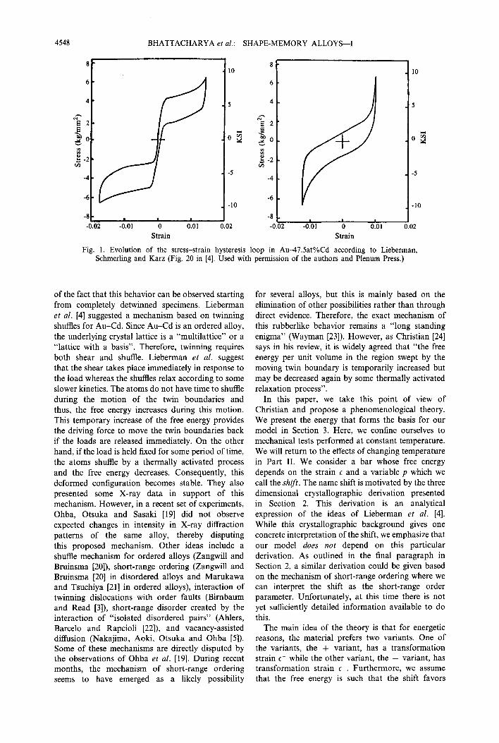
Since olander [1] in 1932, various investigators have observed a “rubberlike behavior” in Au- 47.5at.%Cd. This alloy undergoes a martensitic transformation from a cubic austenite to an orthorhombic martensite phase. When an aged specimen consisting of fine twins of two variants of martensite is stressed, it suffers large deformations due to the motion of the twin boundaries until the specimen is completely detwinned. If the loads are released immediately, the twins reappear and all the strain is recovered. On the other hand, if the loads are held for sufficient time before being released, the twins do not reappear and no strain is recovered. Over the years, this phenomenon has been studied extensively in this and other alloys (for example, Au_475at.%Cd [2-41, Au49.5at.%Cd [5], Au-29at.%Cu45at.%Zn [6], In-20.7at.%Tl [7], In(68)at. %Pb [8], Cu-14wt.%All4wt.%Ni [9] and Cu-12at.%Zn-18at.%Al [lo]). In particular, Lieberman, Schmerling and Karz [4] conducted an extensive series of mechanical tests on Au- 47.5at.%Cd. The results of one of their most striking experiments is shown in Fig. 1. An aged bar consisting of fine twins of two variants of martensite is subjected to tension-compression cyclic loading. In the initial cycles, the bar displays “rubber-like behavior” both in tension and compression, and there are two hysteresis loops in the load-displacement curves as shown on the left. As cycling

tTo whom all correspondence should be addressed.

continues, the two loops move closer to each other until they merge at about 30,000 cycles, after which there is only one hysteresis loop as shown on the right. More recently, there has been a great interest in the phenomenon of stabilization of martensite (see, for example, [1 1, 121 and the references therein). There is some evidence that the phenomenon of stabilization and that of rubber-like behavior is related [13]. Similarly, the phenomenon of “pseudo- twinning”, which may be related to the rubberlike behavior, has been observed in Fe-Be [ 141, Fe-Al [ 151 and the ferroelastic material NdNb04 [16].

Despite this wealth of experimental results, several questions remain unanswered. In this paper, we present a simple phenomenological model to account for this relaxation phenomenon and its consequences on mechanical behavior. We show that this model provides very good agreement with the current experimental observations. In Part II [17] of this paper (henceforth referred to as Part II) we show that this model also provides a method to make predictions of behavior for new loading programs and heat treatments. By identifying the important material constants and showing how they affect behavior, our model provides a framework for discussions of the mechanism. The mathematical analysis of this model will be presented elsewhere [ 181.

There appears to be no consensus regarding the exact mechanism that leads to the rubberlike behavior. Burkart and Read [7] proposed that this phenomenon was a result of the “stabilization of interfaces”. However this was discounted in view

4547

4548 BHATTACHARYA et al.: SHAPE-MEMORY ALLOYS-I

Ilt - 10

6.

4. -5

-6 - . -10

-8 . . I I -0.02 -0.01 0 0.0 I 0.02

Strain

8

6

4

-6

. 10

_ 5

,o z M

_ -5

-10

-8C -0.02 -0.01 0 0.01 0.02

Strain

Fig. 1. Evolution of the stress-strain hysteresis loop in Au47.5at%Cd according to Lieberman, Schmerling and Karz (Fig. 20 in [4]. Used with permission of the authors and Plenum Press.)

of the fact that this behavior can be observed starting from completely detwinned specimens. Lieberman et al. [4] suggested a mechanism based on twinning shuffles for Au-Cd. Since Au-Cd is an ordered alloy, the underlying crystal lattice is a “multilattice” or a “lattice with a basis”. Therefore, twinning requires both shear and shuffle. Lieberman et al. suggest that the shear takes place immediately in response to the load whereas the shuffles relax according to some slower kinetics. The atoms do not have time to shuffle during the motion of the twin boundaries and thus, the free energy increases during this motion. This temporary increase of the free energy provides the driving force to move the twin boundaries back if the loads are released immediately. On the other hand, if the load is held fixed for some period of time, the atoms shuffle by a thermally activated process and the free energy decreases. Consequently, this deformed configuration becomes stable. They also presented some X-ray data in support of this mechanism. However, in a recent set of experiments, Ohba, Otsuka and Sasaki [19] did not observe expected changes in intensity in X-ray diffraction patterns of the same alloy, thereby disputing this proposed mechanism. Other ideas include a shuffle mechanism for ordered alloys (Zangwill and Bruinsma [20]), short-range ordering (Zangwill and Bruinsma [20] in disordered alloys and Marukawa and Tsuchiya [21] in ordered alloys), interaction of twinning dislocations with order faults (Birnbaum and Read [3]), short-range disorder created by the interaction of “isolated disordered pairs” (Ahlers, Barcelo and Rapcioli [22]), and vacancy-assisted diffusion (Nakajima, Aoki, Otsuka and Ohba [5]). Some of these mechanisms are directly disputed by the observations of Ohba et al. [19]. During recent months, the mechanism of short-range ordering seems to have emerged as a likely possibility

for several alloys, but this is mainly based on the elimination of other possibilities rather than through direct evidence. Therefore, the exact mechanism of this rubberlike behavior remains a “long standing enigma” (Wayman [23]). However, as Christian [24] says in his review, it is widely agreed that “the free energy per unit volume in the region swept by the moving twin boundary is temporarily increased but may be decreased again by some thermally activated relaxation process”.

In this paper, we take this point of view of Christian and propose a phenomenological theory. We present the energy that forms the basis for our model in Section 3. Here, we confine ourselves to mechanical tests performed at constant temperature. We will return to the effects of changing temperature in Part II. We consider a bar whose free energy depends on the strain E and a variable p which we call the shift. The name shift is motivated by the three dimensional crystallographic derivation presented in Section 2. This derivation is an analytical expression of the ideas of Lieberman et al. [4]. While this crystallographic background gives one concrete interpretation of the shift, we emphasize that our model does not depend on this particular derivation. As outlined in the final paragraph in Section 2, a similar derivation could be given based on the mechanism of short-range ordering where we can interpret the shift as the short-range order parameter. Unfortunately, at this time there is not yet sufficiently detailed information available to do this.

The main idea of the theory is that for energetic reasons, the material prefers two variants. One of the variants, the + variant, has a transformation strain t+ while the other variant, the - variant, has transformation strain t-. Furthermore, we assume that the free energy is such that the shift favors

BHATTACHARYA et a/.: SHAPE-MEMORY ALLOYS-1 4549

2. CRYSTALLOGRAPHIC BACKGROUND the value + 1 in the + variant and - 1 in the - variant. Using this free energy, we propose a model of shift relaxation in Section 4.

In the materials studied here, the relaxation of twin boundaries is much faster than shift relaxation. We take this point of view to the extreme in the model presented here and introduce kinetics only for the shifts: we assume that the twin boundaries move (at infinite speeds if necessary) when the driving force that they experience reaches a critical value, while the shift relaxes according to simple gradient-flow kinetics. A generalization of the model that includes both the kinetics of shift relaxation and of twin boundary motion is given elsewhere [25]. Section 5 provides a parameter study of this model. We show that the results of this model agree with the experimental observations in a wide variety of loading programs in Section 6. For example, the simulations under cyclic loading show a transition from two hysteresis loops to one loop, in agreement with the observations shown in Fig. 1. (It is important to emphasize that our model does not contain any ad hoc criteria for this transition.) An important lesson of our investigations is that the simple statement of Christian [24], together with some easily measured material constants, is sufficient to predict many aspects of the behavior of these alloys.

Even though there remains substantial contro- versy about the mechanism of the rubber-like behavior, and our models in the end are largely mechanism-independent, we believe it is useful to describe briefly one possible atomic route to our models. For this purpose we choose the mechanism that is the most concrete: that of Lieberman, Schmerling and Karz [4]. The derivation below could be adapted to other mechanisms, given sufficiently precise information about the associated atomic movements.

In Part II, we extend this theory to include temperature changes and study the stabilization of martensite. Once again, the predictions of the models agree with experimental observations. We also propose new experiments to resolve some of the remaining open problems.

We would like to emphasize here that our models are deterministic dynamical systems. Once we set initial data for the shift and strain, together with the applied loading as a function of time, the subsequent evolution of shift and strain is completely determined as a solution of our equations, including the motions of twin boundaries. From this solution we calculate the overall length of the bar at each time and then plot stress vs overall strain. In this way hysteresis loops and their evolution are obtained directly from solutions of these equations. In this paper there is no a priori modeling of the hysteresis, as is done for example with Preisach models,

The shuffle mechanism concerns multilattices. These are not Bravais lattices, but can be viewed as a collection of interpenetrating Bravais lattices (see Fig. 2). They are described mathematically by a set of three linearly independent lattice Uectors {e,, ez, e:}, which describes one of the underlying Bravais lattices, together with a set of v vectors p,, , pV, called shifts (Ericksen [27], Pitteri [28, 291) which describe the relative positions of the constituent Bravais lattices. A general point x of a multilattice is given by the formula x = v’e, + p., where v’, v’, v3 are integers and a is an integer in the set {l, , vi. We use the summation convention so that repeated indices denote summation (for example, v’e, = v’e, + v2e2 + v’e?). For our purposes we consider just two interpenetrating Bravais lattices (v = 2). It is known that two sets of lattice vectors and shifts {ei, po} and {t, qa} generate the same multilattice if

e, = $4,

p. = vie, + S,“q h, (2.1)

where A{ is a 3 x 3 matrix of integers with determinant _t 1, v: are any integers and

s,” =

I

(0 y) or ( tll (lj) ~af’hd,“~?a~sJao~

1 0

( >

if the two Bravais lattices have 0 1 different atoms.

(2.2)

Finally, we would like to contrast our viewpoint with the mechanisms of relaxation treated in the classic text of Zener [26]. He discusses separately atomic relaxation and relaxation near twin boundaries. Each of these mechanisms by itself leads to either Boltzmann integral models or rate-type models. Consequently, a sinusoidal applied stress results in a sinusoidal strain. In contrast, the model studied here consider simultaneously both moving twin boundaries and atomic relaxation. Their interaction is highly nonlinear and the resulting equations are quite different. In particular, a sinusoidal applied stress does not lead to anything like a sinusoidal strain.

The conditions (2.1) and (2.2) are also necessary for {e,, pa} and {f,, qa> to generate congruent multilattices under certain mild conditions (Pitteri [29];

(4 (b)

Fig. 2. (a) Bravais lattice; (b) multilattice with p, = 0, pz = p.


(4 (b)

Fig. 3. Twinning in multilattices usually requires a shuffle: (a) multilattice after shear; (b) after shear and shuffle (white

atoms along twin boundary not shown).

Note that our notation is slightly different from Pitteri’s).

We shall be primarily interested in inhomogeneous deformations of multilattices, especially twinning and shuffling. Consider a a-lattice _!Z’+ generated by lattice vectors and shifts {e,+ , p:, p:} restricted to a region {x:x.n > 0) above a plane and another 2-lattice Y- with {e; , q;, q;} restricted to the region (x:x.n < 0} below the plane.

The shuffle mechanism of Lieberman et al. [4] can then be formulated as follows. Imagine that _%- is not an arbitrary lattice, but that it is obtained up to a translation by an exact shear of the lattice g+, i.e., that there is a vector a such that

(1 + a 0 a)e+ = e;, i = 1,2, 3,

(I + a 0 n)(pZ - P:) = q; - q; (2.3)

Here, a @I n is the matrix with components ainj. This is shown in Fig. 3. As can be seen from this figure, it is generally not true that dp+ is obtained from dp- by an exact rigid rotation and translation, so the structure shown in Fig. 3(a) does not represent a mechanical twin. However, it is possible for the Bravais sublattices generated by {e: } and {e;} to be twinned, as in the case of Fig. 3(a). This happens when there is a rotation matrix R and a 3 x 3 matrix of integers 1; with determinant k 1 such that

e; = iiRe,+ . (2.4)

Instead of placing the lattice 8- on {x:x.n < 0}, suppose we had placed the lattice p- with lattice vectors and shifts {e;, p;, p;) on this region, where

p; = v:Re: + G,bRp,+ , (2.5)

R is given by (2.4), VI, v* and v’ are any integers and St is an appropriate matrix from (2.2). Then by (2.1) the resulting structure would be a twin as shown in Fig. 3(b). Since the only difference between 8- and die- is the value of the shifts, it is possible to “relax” q; to p; and obtain a mechanical twin. The idea of Lieberman et al. [4] is that a rapid shear causes atoms to go to the positions _%‘+/U- described above, and

this is followed by a slow relaxation of the shift (I; + P; .

We now wish to extract a more general energetic interpretation of the above which will have wider application. Introduce now a fixed reference 2-lattice y” defined by lattice vectors and shifts {ep, pe} interpreted as the lattice of undistorted austenite. A typical situation encountered in martensitic transformations is to have the lattice vectors e,+ and e; given by the formulas,

e: = RIU+eo I ,

e; =R*U-e!, i= 1,2,3,

where R, and R2 are rotations and U+ symmetry-related Bain strains, that is,

U+ = QU-Q’,

(2.6) and U- are

(2.7)

where Q is a member of the point group of the austenite (see Bhattacharya [30] or Ball and James [31] for a derivation of these conditions).

Given a 2-lattice occupying a large region W, the positions of all atoms are determined by the assignment of the lattice vectors e,, the shifts p. and 9. It is plausible that, whatever atomic model is used, the free energy is completely determined by the positions of the atoms and 9. This statement may also be extended to finite temperatures by interpreting “position” as the time-averaged positions of the atoms and then using statistical mechanics to calculate the temperature dependence of the free energy. Following this thinking, we assume the existence of a free energy function

cp&, , P., 0 (2.8)

where 0 is the temperature. This function will satisfy the following regardless of the (reasonable) atomic model:

(1)

(2)

(3)

Additivity over (large) volumes: cps(ei, py, 0) = cp(ei, pa, 0) volume (W), i.e. cp is the energy per unit volume; Frame-indifference: cp(ei, pa, 0) = @(eZ, PZ - PI, 0) = @(Re,, R(p, - pl), 13) for all rotations R and all (et, P., 0); Potential-well structure:

&U+eP, P:, Q> = cpVeP, PY, 0)

< cp(FeP, pa, e) for all (F, P., 0). (2.9)

We wish to apply this energy in a continuum framework where the shift and deformation change inhomogeneously. For the continuum model we consider a reference domain R, interpreted as undistorted austenite, with material points x in R. Deformations are described by functions y:n -+ R”. To relate lattice to continuum deformation, we take the viewpoint of Born and Huang [ 19321, summarized by the so-called Born rule. This rule states that any function of lattice vectors g(eZ, . . .) is replaced, in the continuum framework, by g(Vy(x)ep, . . .). The

BHATTACHARYA er al.: SHAPE-MEMORY ALLOYS-I 4551

intuitive idea here is that the deformation of each of the Bravais sublattices is associated to the macroscopic deformation gradient, while the displacements between these sublattices are free to adjust themselves to secure equilibrium of the lattice.

The above represents an outline of one possible route from an atomic mechanism to a continuum theory. A more complete derivation would have to confront the statistical nature of the shuffle (i.e., the fact that at any one time during relaxation, there is a statistical distribution of shuffles on the lattice). The underlying principles of such a derivation are hopefully clear: identify variables that describe the atomic changes, separate these into one group that relates to macroscopic deformation and another group that relates to atomic rearrangement that is independent of macroscopic deformation, identify how conditions of symmetry and frame-indifference act on these variables, pass to continuum level. In the discussion below we continue to use the terminology “shift”, but think of it more generally as representing any atomic rearrangement, not associated with macroscopic deformation, which affects the free energy of the lattice.

3. ONE-DIMENSIONAL THEORY

In this section we propose the energy that forms the basis for our theory. For definiteness, one may regard this as the specialization of the energy given in Section 2 to one-dimensional motions. We consider a bar of length L with material points x E [0, L]. A(x) denotes the area of the cross-section of the bar at the point x. The deformation is denoted by y(x, t). The value ~(x, t) gives the position of the particle x at time t. The displacement U(X, t) and the strain t(x, t) are given by

u(x, t) = y(x, t) - x, t(x, t) = @&. (3.1)

Without any loss of generality, we fix one end of the bar throughout this paper: ~(0, t) = 0. We let p(x, t) denote the value of the shift at particle x and time t.

The crystallographic background given in Section 2 suggests a free energy per unit reference volume of the form q(~,p, f3) where 0 is the temperature. In Part I we hold 0 fixed at a value below the austenite-martensite transformation temperature (M,), and suppress 0 from the notation. We return to the effects of the austenite-martensite transformation and temperature dependence in Part II, Section 2. The crystallographic background further suggests that cp should have preferred values of the strain corresponding to distinct values of the shift. Thus, we assume there are values C+ > t- such that

cp(c’, 1) = cp(c-9 - 1) < cp(~,P) (3.2)

holds for all (6,~) # (c+, 1) or (CC, - 1). The preferred strains (or the stress-free strains of the two variants of martensite) C+ and t- generally depend on temperature, but we neglect this dependence. Also, without loss of generality, we have normalized the preferred shifts to be + 1 and -1.

We have done all of our particular calculations with a special cp, which is the minimum of two quadratic wells. This function is

cp(t, p) = i min(a(c - c+)*

+ 26(t - t+)(p - 1) + p(p - l)l,

cX(E - EC)’ + 26(t - t-)(p + 1) + /Qp + l)‘>.

(3.3)

Here, min means that for each (6,~) we take the minimum of the two numbers in braces. cp depends implicitly on the temperature through the parameters CC, p, and 6. It turns out that it is convenient to group these parameters as follows.

(3.4)

We call CI the elastic modulus, B the normalized shift modulus, cr the normalized twinning strain and D the normalized coupling constant. We will regard LX, B, D and tr as the material parameters to be obtained from experiment; from these we may readily obtain c(, /I, 6 and (c+ - EC) if necessary. We assume that CI > 0, B > 0 and tT > 0. We refer the interested reader to Bhattacharya, James and Swart [18] for the general assumptions on cp under which our theory holds. In particular we note that we could have used different moduli for the two variants, but for the loading programs we use, this has little effect on the hysteresis loops.

Since cp represents the free energy per unit reference volume, the total free energy of the bar at time t is given by

s

L A(x)&+, t),P(x, t)) dx. (3.5)

II

Most of the experiments we wish to study were performed in a soft loading device (under load control). Here, we assign the function F(t) representing the force (or load) applied at the end of the bar. The total energy for the soft device is

L

s A(x)cp(&, t),p(x, t)) dx - Rt)u(L, t)

0

= s

‘4x){ CP(~G t),P(x, 0) - 4x, tk(x, t,} dx 0

(3.6)


where 0(x, t) = F(t)/A(x) is the stress at time t at the position x. In (3.6), we have used the assumption U(0, t) = 0.

4. A MODEL OF SHIFT RELAXATION

We want to develop a theory in which the shift relaxes more slowly than the strain. We take this point of view to an extreme and assume that the strain adjusts instantaneously to minimize the elastic energy at fixed shift. Simultaneously, we assume that the shift evolves according to gradient-flow kinetics.

For a prescribed load F(t) and initial distribution of shift pO(x), the functions u(x, t) and p(x, 1) are determined by

L

(i) min tie, 0 = 0 s &){cp(& 0,P(X, 0) o

- a(x, t&(x, t)) dx at each t,

(ii) ap at (x9 t) = -P $ (% t), P(X, t)),

(iii) Ax, 0) = PO(X), 6(x, 0) = h(x),

O,<x,<L. (4.1)

Here, 0(x, t) = F(t)/A(x) is the stress (from (3.6)) and p > 0 is the mobility. The minimization problem (4.l)i is solved by inserting the current shift p(x, t) into the integrand of (4.1), and then minimizing the integral over all strains E(X, t) = au(x, t)/ax subject to the constraint ~(0, t) = 0.

The gradient flow in the shift (4.l)i, models the relaxation mechanism at some mesoscopic length scale. Since we expect the relaxation to be thermally activated, it seems natural to expect that the mobility will depend implicitly on the temperature in the form p w exp( -Q/k@) for some activation energy Q. Since we are interested in experiments conducted at a constant temperature, we will not pursue this now, but regard p as a material parameter.

We now specialize to the free energy given in (3.3), describe the solution procedure and then illustrate it with an example. We begin with (4.l)i at any given t and g(x, t). With t and p(x, t) given, this minimization problem, which has a double- well structure, is exactly the one that Ericksen [33] studied in his landmark paper on the equilibrium of bars. To minimize the total energy, we need to choose a strain that minimizes the integrand at each x. Thus, for fixed x and 1, we choose c(x, t) to minimize

f(E) = rp(GP(X, t)) - 0, 06. (4.2)

Since C+J has a double-well structure, the equation af@ = 0 has two solutions: 6 = E+ + C~/OZ - D(p - 1) and L = C- + a/cl - D@ + 1). By comparing the

values of f on these two solutions, we conclude that ~_ + & t) - - D(p(x, t) f 1)

a

6(X, t) =

i

if 0(x, 0 < - yp(x, t),

E+ + - 4x3 0 - D@(x, t) - 1) c(

if 0(x, t) 2 - YP(X, t),

where

(4.3)

(4.4)

In typical physical cases, c <<c(. Then (4.3) implies that when the stress a(x, t) is relatively large (a(x, t) > - yp), the strain is near C+ and the material is in the + variant. Similarly, when the stress is sufficiently small, the strain is near E- and the material is in the - variant. The material transforms from one variant to another at a(x, t) = -yp(x, t). Following the traditional terminology, we call -yp the Maxwell stress. The source of most of the interesting behavior of the model, as well as the strong nonlinearity, is that the Maxwell stress depends on the shift. Speaking physically, the critical stress for twinning depends on the local atomic arrangement, as measured by the shift.

We now turn to (4.1),. Differentiating the free energy (3.3) with respect to p and substituting for c using (4.3), we obtain

r -m(p(x, t) + 1) + do(x, t)

z (x, 1) =

i

for 4x, t) G - YP(~, t>, (4.5)

-m(p(x, t) - 1) + da(x, t)

1 for (T(x, t) 2 - YP(X, t),

where the constants m and d are given by

m = @ = A@ - a”) a ’

d=-pD= *. (4.6) a

We have to solve the ordinary differential equations (4.5) at each x subject to the initial condition p(x, 0) = PO(X), obtained from (4.l)iii. The fact that we may use either branch in (4.3) or (4.5) when a@, t) = -yp(x, t) does not cause any problems (see [18] for a complete explanation of this point).

It is easy to integrate (4.5). We fix x and suppress it from the notation. Suppose o(O) < - ypo. Then (4.9, applies, at least for short time. Integrating (4.5), subject to p(0) =po, we get

p(t) = p-(t) = - 1 f (PO + l)e-mr

+ d s

’ c(s)e-m(‘-S) ds. (4.7) 0

We continue with this solution until the first time t, at which o(t) = -yp(t). At t = t,, we switch to the

BHATTACHARYA et al.: SHAPE-MEMORY ALLOYS-I 4553

+ branch, (4.5)?. Integrating (4.92 with the initial condition p+(t,) = p(t,) = PI, we get

p(t) =p+(t) = 1 + (PI - l)e-m(i-‘~’

+d

i ’ a(s)e-mli-~~ ds. (4.8)

We continue with this solution until the next time when a(t) = -yp(t) and then switch back to the _ branch, (4.5),. We continue this procedure, alternating between the two equations in (4.5). Depending on the loading program, it may happen that after a certain time, o(t) never again becomes equal to - yp(t); in this case, we simply take the solution on the current branch for all future time. We follow an analogous procedure if a(O) > - ypo. We thus obtain p(t) at this fixed point X. We repeat this procedure at each particle x in [0, L] and obtain p(x, t). Plugging this back in (4.4), we obtain E(X, t). We now calculate u(x, t) from

u(x, t) = s

‘i t(z, t) dz; (4.9)

0

u(x, t) and p(x, t) are the solutions to (4.1). We obtain the overall strain i from

u(L, t) 1 L r(t) = 7 = z

s c(z, t) dz. (4.10)

0

Our hysteresis loops are parametric plots of the stress vs overall strain: i.e. 0(x, t) vs E, where x is chosen in some convenient way. For specimens of hourglass shape, we follow Lieberman et al. [4] and plot the stress at the center point x = L/2 vs the overall strain.

We now illustrate the procedure for solving (4.1). We choose the problem of cyclic loading of an aged finely twinned specimen which was studied by Lieberman et al. [4] and whose observations are shown in Fig. 1. We choose a bar with uniform cross-section A(x) = 1. Therefore, in this bar cr(x,t) = F(t) at each x and t. Our initial condition is as follows. We divide the bar into two parts I, and I. of equal total length and set

PO(X) = {

+l if XE~+, -1 if XE/_,

co(x) = 1 t+ if XEI+, t- if x~l_.

(4.11)

This corresponds to stabilized + variant in 1, and - variant in I-.

We choose the parameters, t( = 5000, B = 0.05, tr = 0.02, D = 0 and p = 2 for convenience of illustration (arbitrary consistent units; see Section 6 for realistic parameters for Au_47S%Cd). In particular, we have chosen a large p to speed up computations and also D = 0 to turn off the energetic

Fig. 4. Evolution of p(x, t) vs t for x E I+ (bold) and for x E 1_ (dashed).

coupling between strain and shift. We take F(t) = o(t) = 6.5 sin t. We calculate u(x, t) and p(x, t) according to the procedure outlined above. The computed solution p(x, t) corresponding to the initial conditions (4.11) is shown in Fig. 4, and the hysteresis loops (parametric plots of the stress vs overall strain: c(t) vs F(t)) are shown in Fig. 5. In Fig. 4, -~(t)/v is the sinusoidal curve, p(x, t) for x E 1, is the bold curve, and p(x, t) for x E 1_ is the dashed curve. Notice how p changes direction as it crosses -g(t)/?, i.e., as the load crosses the Maxwell load. Figure 5(a) plots a(t) vs t(t) for the first stress cycle. For small loads, both 1, and I- respond elastically. As the load increases beyond the Maxwell load, I_ transforms to the + variant and the strain in this region increases from close to c_ to close to t+. At this time 1, is already in the + variant and responds elastically. Consequently, there is a big increase in the overall strain at this load. As the load increases further, both regions behave elastically. At the same time, the shift p in the region I_ begins to evolve towards + 1. p does not evolve in 1, because it is already + 1 there. Now the load increases to its peak and then begins to decrease. Though p is evolving towards + 1 in l-, it does not get there in finite time; so I_ transforms back to the - variant at the Maxwell load and there is a decrease in the overall strain. But now, the Maxwell load is lower than before because p has changed from - 1 towards + 1 in the meantime. Therefore the large decrease in strain takes place at a lower value of the applied stress. This gives the

(4 b) (4

Fig. 5. Hysteresis loops, o(t) vs C = u(L, t)/L: (a) cycle 1; (b) cycle 4; and (c) cycle 12. The material parameters are x = 5000, B = 0.05, tr = 0.02, D = 0, p = 2 (and o,, = 0),

while the loading is F(t) = cr(t) = 6.5 sin t.


upper-right hysteresis loop of Fig. 5(a). We obtain the lower-left hysteresis loop of Fig. 5(a) by looking at the negative part of the cycle.

As the load is cycled, we see from Fig. 4 that the two values of the shift p (in I, and l-) converge with time and asymptotically approach one periodic path. Therefore, as we cycle through the hysteresis loops move closer and closer, as shown in Fig. 5(b), until they merge into one big loop, which then evolves toward the terminal loop shown in Fig. 5(c). For the chosen parameters, we reach the terminal loop in about 12 cycles. Comparing Fig. 5 with Fig. 1, we see good qualitative agreement.

It turns out that when we use realistic mobility to simulate the experiments of Lieberman et al. [4], we find that the hysteresis loops are too thin, especially at very high frequencies. Therefore, we make a modification to the model above: rather than switching branches when the stress reaches the Maxwell stress, we switch when the difference between the applied and the Maxwell stress exceeds a given material constant rrXs. We assume that cXs 2 0 and we call it the inherent hysteresis. In other words, we switch from the “ - ” to the “ + ” when a(x, t) = -yp(x, t) + oXs and we switch from the “ + ” to the “ - ” branch when a(x, t) = -yp(x, t) - ou. Therefore, rather than allowing the strain to minimize the total energy, we introduce some hysteresis in the motion of the twin boundaries through Q,. In Bhattacharya, James and Swart [25], we show that this modification may be interpreted as a (rather degenerate) special case of a model which has kinetics in both the shift and the twin boundary motion.

We now summarize our model. The behavior of a bar of length L, with

cross-section A(x), with initial shift p,,(x) and strain c,(t), with one end held fixed (i.e., ~(0, t) = 0), and subjected to a force F(t) (co, must be consistent with F(0)) is determined as follows:

1. The shift p(x, t) is given by a function continuous in time t consistent with

c p-(t)

i

for ptx, t) =

u(x, t) < -yp(x, t) + u,,

p+(t)

1 for 0(x, t) 2 - yp(x, t) - u,, (4.12)

where

P-(t) = - 1 + (p(X, to) + l)e-ti’-“)

+ d s

(a(s)e-m(f-JJ ds, 10

P+(t) = 1 + (p(X, to) - l)e-*‘-b)

+ d I

‘a(s)e-“+‘) ds; (4.13) 10

2. The strain E(X, t) is given by

1 E- + * - D(p(x, t) + 1)

i

if E(X, t) =

4x, t) < - Y&C, t) + u,,

E+ + y - D(p(x, t) - 1)

1 if utx, t) 2 -YP(X, t) - a,;

(4.14)

3. At time t, if -yp(x, t) - uxs < u(x, t) < -yp(x, t) - uXs, we choose the “ + ” or the ‘1 - ” branch to be exactly the same as that at the immediate past instant t = t-, i.e., we stay on the same branch as long as possible;

4. The overall strain in the bar E is given by the total displacement u(L, t) divided by the length of the bar L:

u(L t) 1 L c(t) = L = I t(z, t) dz; (4.15)

5. The material constants are

?? a, the elastic modulus, ??B, the normalized shift modulus, ??D, the normalized coupling constant, ??cT, the normalized twinning strain, ??p, the mobility, ??uXs, the inherent hysteresis;

6. And other useful definitions are

?? the stress u(x, t) = F(t)/A(x), ??m = pB and l/m is the time constant for the

shift, a d= -pD and ??y=2B/cr.

5. PARAMETER STUDY OF THE MODEL

We now embark on a parameter study of our model. We start with a bar of unit length and cross-section, initial data as in (4.11) and material parameters shown just below (4.11). Again, we use arbitrary consistent units.

Figures 6 and 7 show the effect of changing the normalized coupling constant D. We use the same constants as in Fig. 5, except for D. A positive D results in the self-intersecting hysteresis loops as shown in Fig. 6 (D = 0.003). We note here that the small triangular loops shown in Fig. 6 do not violate any principle of thermodynamics, even though these loops are traversed counterclockwise. This is because the shift is not periodic on these loops and, consequently, neither is the free energy (see [18] for details). A negative D results in a gap at zero stress in the first cycle as well as tails in both the first and terminal loops as shown in Fig. 7 (D = -0.003). Note that the experimental loops in Fig. 1 have these features.


(4 (b)

Fig. 6. The effect of positive coupling D on the (a) initial and (b) terminal hysteresis loops, a(t) vs C(t). The material parameters and loading are the same as in Fig. 5, except

D = 0.003.

The effect of changing B is shown in Fig. 8; we use the same parameters as Fig. 7 except that B has been increased to 0.06. Note that the stress levels as well as the size of the loops have increased. Further, the rate of relaxation increases; it took only about 8 cycles to reach the terminal loop.

The mobility and the frequency of cyclic loading have a significant effect on the width of the hysteresis loop. In fact, when D = 0 and oXs = 0, it is possible to show that

1 _ e-W2 stress width of terminal loop = 2y 1 + e_mT,2,

(5.1)

where T is the period of loading. This simple formula captures the effect of frequency, p and B. (If D # 0, the width of the terminal loop depends on the amplitude of loading in addition to these parameters.) Notice that the width of the hysteresis loop increases with increasing mobility p or decreasing frequency l/T. As the mobility increases, the material relaxes faster and consequently, the difference in the stress for the + to - and - to + transformations is large. Similarly, if the frequency is low, the shift p has more time to evolve as the stress reaches its peak and turns back. Consequently the difference in the stresses for the + to - and - to + transformations is large. This is illustrated by the simulations presented in Section 6. The mobility and the frequency of cyclic loading also affect the number of cycles that one needs to reach the terminal loop. Fewer cycles are required to reach

.$e .&JZ

(a) (b) Fig. 7. The effect of negative coupling D on the (a) initial and (b) terminal hysteresis loops, u(t) vs Z(t). The material parameters are a = 5000, B = 0.05, cT = 0.02, D = -0.003, p = 2 and uXS = 0, while the loading is F(t) = a(f) = 6.5 sin t

(same as in Fig. 5, except for D).

(4 (b)

Fig. 8. The effect of increasing the normalized shift modulus B on the (a) initial and (b) terminal hysteresis loops, u(t) vs C(t). The material parameters and loading are the same

as in Fig. 7, except that B = 0.06.

the terminal loop as p gets larger or the frequency gets smaller.

Increasing tr stretches out the loops horizontally and also reduces stress levels of the loops. The elastic modulus GI mainly affects the slope of elastic branches, as expected. The width of the hysteresis loop increases with increasing 6,. We have omitted simulations of these trends for brevity.

We now look at two applied loading programs which are periodic, but not purely sinusoidal. First we consider a(t) = 6.5 sin t + 0.5 for the same initial data and parameters as in Fig. 7. We find that the terminal loop is displaced downwards as shown in Fig. 9. By examining the solution, the reason for this odd behavior becomes clear; by displacing the stress upward, we give the shift more time to evolve toward + 1, thereby decreasing the stress levels during the transformation from one variant to another.

Secondly, we consider the applied loading

o(t) = S(sin t + 0.75 sin 2t) (5.2)

with the same initial data and parameters as in Fig. 7. It turns out that for this loading, the initial hysteresis plot has two loops as before (Fig. 10(a)). As the load is cycled, they move closer. However, they never meet or merge; instead they attain the terminal loop shown in Fig. 10(b). One may understand this from Fig. 11: for the given load, it is possible for p in the two parts of the bar I+ and I_ to reach two very different terminal trajectories.

Finally, we examine the model for a bar whose cross-section is not uniform, but which is similar to the hourglass specimens of Lieberman et al. [4].

0

6

& -0 1 0. T

1 -61 Fig. 9. The effect of off-set loading on the hysteresis loop, e(t) vs E(t). When the stress is biased up (u(t) = 6.5 sin t + 0.5), the hysteresis loop is lowered. The material

parameters are the same as in Fig. 7.


cl

6

FF -0.01 r

0.01

-6

(4 (b)

Fig. 10. Predicted hysteresis loops for an applied loading u(t) = S(sin t + 0.75 sin 2t) vs E(t): (a) first loop; (b)

Fig. 12. Hysteresis loops, (r(L/2 t) vs E(t), for bar of

terminal loop. The material parameters are the same as in non-uniform cross-section with ,4,.,&i, = 1.5: (a) first loop;

Fig. 8. (b) terminal loop. The material parameters and loading are

the same as in Fig. 7.

We assume that the cross-section varies with position as follows.

Thus, the bar is symmetric about its midpoint, which has the smallest cross-section A,,,. The ends have the largest A = A,,,.

We choose the same material parameters and loading as in Fig. 7 with a ratio of cross-sections A,,,/A,i, = 1.5 (since we plot the stress, we need only the ratio of maximum to minimum cross-sections rather than their individual values). We take the initial conditions (4.11) and assume that 1, and 1_ come from equispaced fine twins so that the bar alternates between I, and I_ at a length scale much smaller than the length of the bar. Figure 12(a) and (b) show the first and the terminal loops. It is clear from Fig. 12(a) that, unlike a bar with uniform cross-section, the entire bar does not transform at the same time. Depending on the cross-section, the applied stress reaches the critical stress for transforming at different times and this gives rise to the “slanting of the hysteresis loops”. Comparing the first and terminal loop, notice that the effect of non-uniform cross-section is more pronounced in the first loop rather than in the final loop. We can understand this as follows. Roughly, the ratio of the loads at transformation will be equal to the ratio of the cross-sections. Since the transformation takes place at much higher values of the load in the first

1

t 0

-1

Fig. 11. Evolution of p(x, t) vs t for x E 1, (bold) and for x E I_ (dashed) with the loading program given in Fig. 10.

cycle, the effect of cross-section is much more visible there.

Figure 13(a) and (b) show the first and the terminal loops when A,,,/&, = 2 and everything else is kept the same. In this case, the cross-section of some parts of the bar is so large that the stress never reaches the critical value for transforming. Thus, only part of the bar transforms and the total elongation is much smaller.

6. COMPARISON OF THEORY AND EXPERIMENT

In this section, we look at the mechanical tests conducted by Lieberman, Schmerling and Karz [4] at some length (also see Karz [34]). They performed their experiments on single crystal bars of Au47S%Cd. They transformed these bars from austenite to martensite by a single interface transformation to obtain one set of fine twins of two variants of martensite and aged it in this state.

Experiment 1

They subjected this aged, finely twinned bar to a tension-compression cyclic loading. They plotted the stress versus overall strain during the different cycles. Their results are shown in Fig. 1. In the initial cycles, the bar displays “rubber-like behavior” both in tension and compression, and there are two hysteresis loops in their stress-strain curves as shown on the left of Fig. 1. Let us term a hysteresis loop of this type a double-loop. As cycling continues, the two loops move closer to each other until they merge after a large number of cycles; beyond this there is only one

I I -6

(4 (b)

Fig. 13. Hysteresis loops, o(t) vs E(t), for bar of non-uniform cross-section wtth A,,&,,, = 2: (a) first loop; (b) terminal loop. The material parameters and loading are the same as

in Fig. 7.


hysteresis loop (single-loop) as shown on the right. Continued cycling does not change the hysteresis loop and they called this the “terminal loop”.

Experiment 2

Lieberman et al. [4] started with an aged finely twinned bar and subjected it to cyclic loads as described above. Once the bar had reached the terminal loop, they stopped the test at zero stress, held the bar in the unloaded state for a given period of time, and then restarted the cyclic loading. They repeated the whole experiment with different holding times, each time beginning with an aged, finely twinned specimen. Figure 14(a) shows their observed hysteresis loops during the first cycle after the delay, for the various delay periods. With increasing holding times, the first loop after delay resembles more and more the initial loop. Figure 14(b) shows the continued evolution of the hysteresis loop upon cyclic loading after a delay of 400 min. Notice that the terminal loop achieved by this method is the same as the original one.

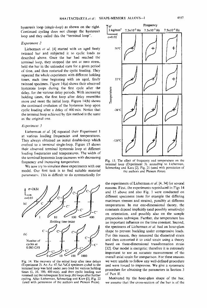
Experiment 3

Lieberman et al. [4] repeated their Experiment 1 at various loading frequencies and temperatures. They always obtained an initial double-loop which evolved to a terminal single-loop. Figure 15 shows their observed terminal hysteresis loop at different loading frequencies and temperatures. The width of the terminal hysteresis loop increases with decreasing frequency and increasing temperature.

We now try to simulate these experiments with our model. Our first task is to find suitable material parameters. This is difficult to do systematically for

Holding time (min)

Fig. 14. The recovery of the initial loop after time delays (Experiment 2). An Au_47Sat.%Cd specimen cycled to the terminal loop was held under zero load for various holding times (1, 10, 100, 400 min), and then cyclic loading was resumed: (a) the subsequent first loop; (b) loops after further cycling. After Liebennan, Schmerling and Karz [2], Fig. 22 (used with permission of the authors and Plenum Press).

T OS Frequency 2 kg/mm’ 7.5x10-* Hz 7.5~10-~Hz 7.5~10-~ Hz

56°C

22°C

-26°C

-126”(

Fig. 15. The effect of frequency and temperature on the terminal loop (Experiment 3), according to Lieberman, Schmerling and Karz [2], Fig. 21 (used with permission of

the authors and Plenum Press).

the experiments of Lieberman et al. [4, 341 for several reasons. First, the experiments reproduced in Figs 14 and 15 above and also Fig. 1 were conducted on different specimens (note for example the differing maximum stresses and strains), possibly at different temperatures. In our one-dimensional theory, the constants depend implicitly (and possibly sensitively) on orientation, and possibly also on the sample preparation technique. Further, the temperature has an important influence on the time constant. Second, the specimens of Lieberman et al. had an hour-glass shape to prevent buckling under compressive loads. For this reason, they measured the diametral strain and then converted it to axial strain using a theory based on three-dimensional transformation strain [32]. Our model is energetic; therefore it is extremely important to use an accurate measurement of the overall axial strain for comparison. For these reasons we were unable to follow any well-defined procedure and were forced to improvise. We give a systematic procedure for obtaining the parameters in Section 3 of Part II.

Motivated by the hour-glass shape of the bar, we assume that the cross-section of the bar is of the


(4 (b)

Fig. 16. Simulation results of Experiment 1: (a) initial hysteresis loop; (b) terminal hysteresis loop (after about 30 000 cycles). The simulation uses the parameters in (6.1)

and loading (6.2).

form shown in equation (5.3) with the smallest value A,,, at the center and the largest value A,,, at the ends. We take the ratio A,,,/A,i, = 1.5.

We assume that the initial distribution of the shifts is as earlier: half the bar starts at the + phase with p. = + 1 while the other half starts at the - phase with p0 = - 1. This corresponds to aged finely twinned bar with equal proportion of the two twin variants.

We use the following material simulate Experiment 1.

CI = 4000 kg/mm2,

B = 0.044 kg/mm2,

D = -0.5 kg/mm2,

tT = 0.025,

oXs = 0.8 kg/mm2,

p = 0.8 mm2/(kg min)

parameters to

(6.1)

These parameters were chosen simply to give a good match with the experiment. We assume that the loading is

472, t) = F(t)/&,

= 6.5 sin(27c60 x 7.5t) kg/mm2, (6.2)

where t is time in minutes and the frequency of loading is 7.5 Hz. Our results are shown in Fig. 16. Compare this with the experimental observations in Fig. 1. Note that our model clearly captures the transition from a double to a single loop. It also captures various details: the constancy of the stress-width of the hysteresis loop during cycling, the gap in strain at zero stress, the tails in the initial and terminal loops. The loops of Lieberman et al. are somewhat more rounded, slope upward a bit more and have slightly larger tails. This is to be expected due to the following real world experimental issues: hour-glass specimens, diametral strain measurements, the effect of grips and the difficulties of achieving pure load control. We propose new experiments in Part II (Section 3) to address some of these issues.

We note here that we have been able to dispel one possible reason for the shapes of the hysteresis

loops-the kinetics of twin boundary motion. We augmented our model to include the kinetics of twin boundary motion in the form of a kinetic relation which relates the velocity of a twin boundary to the driving traction acting on it. The rounded shape of the experimentally observed hysteresis loops in Fig. 2 can then be easily reproduced at any given frequency with a proper choice of a kinetic relation. However, the model was unable to reproduce the frequency dependence satisfactorily. We either had to choose a rather degenerate kinetic relation which gave flat loops; or we obtained the wrong qualitative dependence when compared over a large, but experimentally relevant, range of frequencies. We shall present the details of this elsewhere [25].

For Experiments 2 and 3 conducted by Lieberman et al., which were done on a different specimen than Experiment 1, we choose the parameters,

tl = 3000 kg/mm2,

B = 0.017 kg/mm2,

D = -0.003 kg/mm2,

tr = 0.02,

oXs = 0.2 kg/mm2,

p = 0.8 mm2/(kg min). (6.3)

We take the loading to be

G/2, t) = F(t)IA,,,

= 3.1 sin(2x60wt) kg/mm2, (6.4)

where o is the frequency in Hertz.

(4

(b)

Fig. 17. Results of the simulation of Experiment 2, in which a specimen is cycled for a long time, then held at zero stress for the indicated period, then cycled again. (a) The first hysteresis loop after holding for (0, 1, 10, 100, 400) min. (b) The time-evolution of the hysteresis loops after holding for 400 min; shown after (0, 10, 100, 1000) cycles. Both these simulations use the parameters in (6.3) and the loading (6.4) with frequency 0.083 Hz; the units of stress

are kg/mm2.


The results of our simulation of Experiment 2 are shown in Fig. 17. Figure 17(a) shows the simulated hysteresis loops of the first loading cycle after delay. Figure 17(b) shows the subsequent evolution of the hysteresis loop. Compare these with Fig. 14 to see good qualitative and quantitative agreement.

Figure 18 shows results of our simulation of Experiment 3. We start with the initial condition corresponding to the aged finely twinned bar and subject it to the cyclic load (6.4) at different frequencies o. Of all our material parameters, the mobility ~1 is expected to increase sensitively with temperature (as described in the paragraph following equation (4.1), it is obtained from a thermally activated process). The experiments of Lieberman et al. [4, 321 give a few data points of a relation p = p(e), but not enough to reliably evaluate a thermal activation energy Q. Therefore, we repeat our simulations with different values of p corresponding to different temperatures. The corresponding terminal loops are shown in Fig. 18. Compare with Fig. 15, once again to find good agreement.

Finally, notice that in Fig. 15, some of the hysteresis loops are offset “downwards” i.e., towards negative stresses. Notice further, that in each of these,

I

0=2 Frequency

7.5~10-~ Hz 7.5~10‘~ Hz 7.5~10.~ Hz I E = 0.02

Mobility

p=t3

p = 0.8

i=1 P +

-:

t

+

+

Fig. 18. Results of the simulation of Experiment 3. The terminal loops obtained using the parameters (6.3) and loading (6.4) at different frequencies and values of the mobility p; the units of stress are kg/mm2. The columns correspond to frequencies 7.5 x lo-* Hz, 7.5 x lo-’ Hz and 7.5 x 10m4 Hz from left to right, while the rows correspond

to p = 8, 0.8 and 0.08 from the top to the bottom.

the magnitude of the maximum stress is less than that of the minimum stress. In other words, the load that they applied was not purely sinusoidal, but slightly offset probably due to a drift in their controller over all these cycles. Recall from the parameter study in Section 5 (specifically Fig. 9 there), that when we apply a loading which is offset in the positive stress direction in our model, the simulated hysteresis loop moves downwards in agreement with the experimental observations.

In summary, our model is able to capture the qualitative details of the wide range and variety of mechanical tests conducted by Lieberman et al. [4]. Unfortunately, a detailed quantitative comparison was not possible given the nature of the experimental data. However, wherever such a comparison was possible, we found reasonable agreement.

7. CONCLUSION

In this paper, we have proposed a phenomenological model of the relaxation and the consequent behavior that is observed in some shape-memory alloys at constant temperature. We have compared the predictions of this model with experimental results. In Part II, we extend the model to include the effects of temperature and the austenite-martensite transformation. We also propose new experiments to clarify some outstanding issues.

Acknowledgements-We gratefully acknowledge many useful and colorful discussions with David Lieberman. Part of this work was conducted when KB and PJS held post-doctoral positions at the Courant Institute. This work was partially supported through grants from the AFOSR (KB, PJS:90-0090 at Courant, KB:F49620-95-1- 0109 at Caltech, RDJ:91-0301), ARO(KB:DAAL03-92- G-0011 at Courant, PJS:DAAH04-95-l-0100 at Courant), DOE(PJS:W-7405-ENG-36 and KC-07-Ol-Ol), NSF(RDJ: DMS-9505077, PJS:DMS-9402763 at Courant), and ONR (KB:N00014-93-1-0240 at Caltech, RDJ:N/N00014-95-1- 1145 and 91-J-4304).

5.

6.

7.

8.

9.

10.

REFERENCES

Colander, A., J. Amer. Chem. Sot., 1932, 54, 3819. Chang, L. C. and Read, T. A., Trans. AIME J. Metals, 1951, 191, 47. Bimbaum, H. K. and Read, T. A., Trans. Metal. Sot. AIME, 1960, 218, 662. Lieberman, D. S., Schmerling, M. A. and Karz, R. S., in Shape Memory Effect in Alloys, ed. J. Perkins, Plenum Press, New York, 1975, pp. 203-242. Nakajima, Y., Aoki, S., Otsuka, K. and Ohba, T., Mater. Lett., 1994, 21, 271. Miura, S.. Maeda. S. and Nakanishi. N.. Phil. Map.. 1974, $365.

I u j

Burkart, M. W. and Read, T. A., Trans. AIME J. Metals, 1953, 197, 1516. Lubenets, S. V., Startsev, V. I. and Fomenko, L. S., Physica Status Solidi (a), 1985, 92, 11. Sakamoto, H., Otsuka, K. and Shim& K., Scripta Metall., 1977, 11, 607. Barcelo, G., Rapacioli, R. and Ahlers, M., Scripta Metall., 1978, 12, 1069.

4560 BHATTACHARYA et al.: SHAPE-MEMORY ALLOYS--I

11.

12.

13.

14.

15.

16.

11.

18.

19.

20.

21.

Murakami, Y., Morito, S., Nakajima, Y., Otsuka, K., Suzuki, T. and Ohba, T., Mater. Left., 1994, 21, 275. Saule, F. and Ahlers, M., Acta MetaN. Mater., 1995,43, 2373. Tsuchiya, K., Tateyama, K., Sugino, K. and Marukawa, K., Scripta MetaN. Mater., 1995, 32, 259. Green, M. L. and Cohen, M., Acta Metall., 1979, 27, 1523. Guedou, J. Y. and Rieu, J., Scripta Metall., 1978, 12, 927. Tsunekawa, S., Suezawa, M. and Takei, H., Physica Status Solidi (a), 1977, 40, 437. Bhattacharya, K., James, R. D. and Swart, P. J., Acta Mat. 1997, 45, 4561. Bhattacharya, K., James, R. D. and Swart, P. J., In preparation. Ohba, T., Otsuka, K. and Sasaki, S., Mater. Sci. Forum, 1990, 56-58, 317. Zangwill, A. and Bruinsma, R., Phys. Review Lett., 1984, 53, 1073. Marukawa, S. K. and Tsuchiya, K., Scripta Metall. Mater., 1995, 32, 71.

22.

23. 24. 25.

26.

27.

28. 29.

30. 31.

32.

33. 34.

Ahlers, M., Barcelo, G. and Rapcioli, R., Scripta Metall., 1978 12, 1075. Wayman, C. M., Prog. Mater. Sci., 1992, 36, 203. Christian, J. W., Metall. Trans. A, 1982, 13A, 509. Bhattacharya, K., James, R. D. and Swart, P. J., In preparation. Zener,. C., Elasticity and Anelasticity of Metals, Universitv of Chicaeo Press. Chicaeo. 1948. Ericksen,*J. L., Arci. Rational Meci.' Anal., 1980, 73, 99. Pitteri, M., J. Elasticity, 1984, 14, 3. Pitteri, M., Continuum Mech. Thermodyn., 1990, 2, 99. Bhattacharya, K., Acta Metall., Mater., 1991,39,2431. Ball, J. M. and James, R. D., Phil. Trans. R. Sot. London A, 1992, 338, 389. Born. M. and Huana. K.. Dvnamical Theorv of Crvstal Lattices. Clevendon%ess, &ford, 1954. - _ Ericksen, J. L., J. Elasticity, 1975, 5, 191. Karz, R. S., The cyclic mechanical and fatigue properties of ferroanelastic beta prime gold cadmium, Ph.D. Thesis, University of Illinois at Urbana- Champaign, 1972.

RELAXATION IN SHAPE-MEMORY ALLOYS-PART I. MECHANICAL …

Documents

Transcript of RELAXATION IN SHAPE-MEMORY ALLOYS-PART I. MECHANICAL …