1

Relative quiescence in the stress-shadow regions prior to the large earthquakes

off the east coast of Miyagi Prefecture, northern Japan, and its implication for

the intermediate-term prediction

Yosihiko Ogata

Institute of Statistical Mathematics, Tokyo. Email; ogata@ism.ac.jp

Abstract.

This paper is concerned with the intermediate-term prediction of the forthcoming M7 ~ 8

class earthquake on the plate boundary, off the east coast of Miyagi Prefecture, northern

Japan, which is the highest probability among the long-term forecast announced to the public.

Regional seismicity in the regions of stress-shadow preceding each of the previous ruptures in

1936 and 1978 shows quiescence relative to the predicted rate by the ETAS model (the relative

quiescence), whereas the seismicity is well predicted in the regions of neutral or increasing

Coulomb failure stress (CFS), which leads to the effect of possible precursory slip within or

near the source. Anticipating similar scenarios, a number of sequences of earthquakes or

aftershocks from the activities during 1979-2004 in northern Japan are analyzed by fitting the

ETAS model to examine the relation to the CFS increments in the considered regions using the

source model of the 1793, 1936 and 1978 ruptures. Surmising the precursory slips, it is likely

that the results of the normal activity and relative quiescence in respective activities are due to

those of the 2003 Miyagi-Ken-Oki intra-slub earthquake of M7.0 rather than those of the

expected rupture on the plate boundary. Thus, it is unlikely that the predicted rupture will

imminently occur within a couple of years from the analyzed time of 2004, but it is

recommended to monitor the future activity to detect the anticipated relative quiescence in the

stress shadow areas due to the interplate rupture models.

Key words; Aftershock sequences, Coulomb failure stress, ETAS model, Seismicity rate change,

Precursory slips

2

1. Introduction.

Precursory seismic quiescence as a predictor of large earthquakes has attracted much attention

amongst seismologists in the last several decades ever since Inouye (1965) first proposed the

concept. Utsu (1968), Ohtake et al. (1977), Wyss and Burford (1987) and Kisslinger (1988) have

successfully predicted subsequence large earthquakes in the past, although many other papers

regarding the precursory seismic quiescence have been retrospective (postdiction). This suggests

that we need much more research into the relation between the quiescence and subsequent

earthquake activity for an effective prediction. We should also explain how quiescence can take

place in a much wider area than the rupture source (e.g., Inouye, 1965 and Ogata, 1992).

On the other hand, the concept that the stress changes due to a slip can be the mechanism by which

another event is triggered (Reasenberg and Simpson, 1992; King et al., 1994; Stein, 1999; Toda et

al., 2002) has also received much attention of late. Additionally, seismic quiescence due to

coseismic stress-lowering transferred from a rupture (stress shadow, e.g., Harris, 1998; Toda and

Stein, 2002) has been discussed as a general phenomenon. Typically, quiescence is visible in

regions where activity has been high, while activation is visible in regions where activity has been

low.

Ogata (2004a, b, c, d and 2005) discusses the precursory quiescence relative to the modeled rate

(the relative quiescence) in the stress shadow regions owing to the possible silent slips in and

around asperities (e.g., Yamanaka and Kikuchi, 2004; Uchida et al., 2003, 2004) in the focal rupture.

However, given relative quiescence, the difficulty is to identify the location and meaning of slips;

that is, how close the slip is to the major asperity and how imminent it is to the main rupture.

Further, it may be in an area of the habitual slipping only. Thus, in order to make a probability

forecast of a large earthquake, we need to make and examine possible scenarios based on the

available knowledge in seismology, tectonics etc.

The Headquarters for Earthquake Research Promotion of Japan (2005) recently announced a high

probability for the long term forecast (about 50%, 90% and 99% within 10, 20 and 30 years,

respectively, at the time instance of January 2005) of a strong interplate earthquake of M7 ~ 8 class

on the plate boundary off the coast of Miyagi Prefecture (Miyagi-Ken-Oki), northern Japan, which

was predicted based on a recompiled historical data of the earthquakes of 1793 (M8.2), 1835 (M7.3),

1861 (M7.4), 1897 (M7.4), 1936 (M7.4), and 1978 (M7.4). Here the 1793 event of M8.2 has an

3

extraordinarily wider rupture area than the others. This is based on a recalculation of Utsu (1984),

by fitting renewal process models to the data of the region compiled by Seno (1979).

In 28 May 2003, the M7.1 earthquake at Miyagi-Ken-Oki (Miyagi Prefecture offshore) took place

within the Pacific Plate subducting beneath the Tohoku District (North American Plate), an event

that was followed by a destructive inland earthquake of M6.2 (e.g., Ogata, 2005). These made

people more concerned about the occurrence of the predicted interplate strong earthquake.

This paper is concerned with some seismic features inland and in the vicinity of the Tohoku District,

northern Japan (cf. Figure 1 and others) prior to the interplate earthquakes, which may be useful for

the intermediate term prediction of such earthquakes. Specifically, I first study the earthquake

sequences from the neighboring offshore areas, Tohoku District inland and the western offshore

region in the Sea of Japan prior to the last two Miyagi-Ken-Oki earthquakes in November 1936

(M7.4) and in June 1978 (M7.4). These features are then compared with recent seismic activities

from various regions. This paper assumes that significant intermittent slips occur within and near

the source of the respective earthquake due to the acceleration of quasi-static (slow) slips on the

plate boundary as the time of rupture of the major asperity approaches, which is indicated by the

analysis of small repeating earthquake data (Uchida et al., 2003, 2004). Thus, this paper looks

carefully at the seismicity in the stress-shadow transferred from the slip, including aftershocks of

other large earthquakes. Such a scenario for intermediate earthquake prediction is expected to be

useful for explaining the features of data set from the current seismicity.

2. Method

In order to recognize slight systematic seismicity changes, we need to fit a suitable statistical model

to the normal seismic activity, prior to the suspected anomaly time. Consider the ETAS model

(described in the Appendix) representing the occurrence rate of earthquakes )(tθλ at time t in a

well-defined seismic region; the occurrence rate is formally the differential of occurrence

probability of an event, and is dependent not only on the elapsed time t but also on the occurrence

times and magnitudes of previous events. The characterizing parameter θ and the occurrence history

do not depend on the location of earthquakes. Given a dataset of the occurrence times associated

with corresponding magnitudes, we can obtain estimates of the parameters of the model as shown in

the Appendix.

4

We can then see clearly the goodness-of-fit of the estimated model to an earthquake sequence by

comparing the cumulative number of earthquakes against elapsed time with the predicted number.

Suppose that a series of events { Nttt ...,,, 10 } are generated by a statistical model )(tλ , which is the

predicted occurrence rate of events per unit time (i.e., day). Then consider the integral

�=Λt

sdts σσλ )(),( (1)

which is the theoretical cumulative number of the events in the time interval (s, t) to be compared

with the actual number of earthquakes N(s, t) in the same interval. For example, ),( tSΛ =

K{ln(t+c) - ln(S+c)} in the case of the original Omori model )(tλ = 1)( −+ ctK . See Ogata and

Shimazaki (1984), Matsu’ura (1986), Ogata (1988, 1992, 1999), Utsu et al. (1995) for further

examples. If we consider the time change ),( ii tSΛ=τ from t toτ , then { Nttt ...,,, 21 } is transformed

one-to-one to { Nτττ ...,,, 21 }, which distribute uniformly random in the interval [0, Λ(S, T)].

Therefore, if the seismicity rate )(ˆ tθλ estimated from the events in the interval [S, T] is a good

approximation to the real seismicity, then we can expect not only that the function curve ),( tSΛ of

time t and the empirical cumulative function N(S, t) of events are fairly overlapping to each other

until time T, but also that the extrapolated cumulative function ),( tSΛ of t ≥ T offers a good

prediction of the actual cumulative number of earthquakes in the period after time T. Similarly, the

transformed data { MN +τττ ˆ...,,ˆ,ˆ 21 } from the real occurrence data are uniformly distributed on the

interval [ ),(,0 tSΛ ] where N = N(S, T) and M = N(T, t) if and only if the model is correct; namely,

we see that the cumulative number (i.e., i) becomes a linear function of the transformed

time ),(ˆˆ ii tSθτ Λ= .

Our concern is then with the significant activation and lowering of the seismicity relative to that

predicted by the model, from which we explore the relationship to the change pattern of the

Coulomb failure stress (CFS) transferred from a rupture or silent slip elsewhere. Changes in seismic

activity rate are often reported to correlate with the calculated Coulomb failure stress change

)()( stressnormalstressshearCFS ∆−∆=∆ µ (4)

(e.g., Reasenberg and Simpson, 1992; Toda and Stein, 2002), where µ represents the apparent

friction coefficient, and positive normal stress means the compression. Throughout this paper we

5

set µ = 0.4, so as to minimize the uncertainty of ∆CFS in µ as discussed by King et al. (1994), with

the results of CFS∆ patterns generally being stable against their perturbation, unless receiver faults

are close to the ruptured fault. The Coulomb stress change in an elastic half-space (Okada, 1992) is

calculated by assuming a shear modulus 211102.3 −× cmdyn and a Poisson ratio of 0.25. Positive

values of CFS∆ promote failure and negative ones inhibit failure. The negative CFS∆ is called a

stress shadow. To set the receiver fault mechanisms in Table 2 and 3, the readers are referred to

Ichikawa (1971), Research group for active faults in Japan (1992), Japan Meteorological Agency

(2004), Kikuchi and Yamanaka (2003), and Tohoku University (1995). Throughout this paper the

size of the precursory slip is assumed to be 10% as large as the rupture, and as is the ∆CFS value of

the precursory relative to the coseismic one. We then rely on the seismicity rate change based on the

rate-and-state friction law (Dieterich, 1994) as the quantitative basis of the triggering (cf.,

Discussions of this paper).

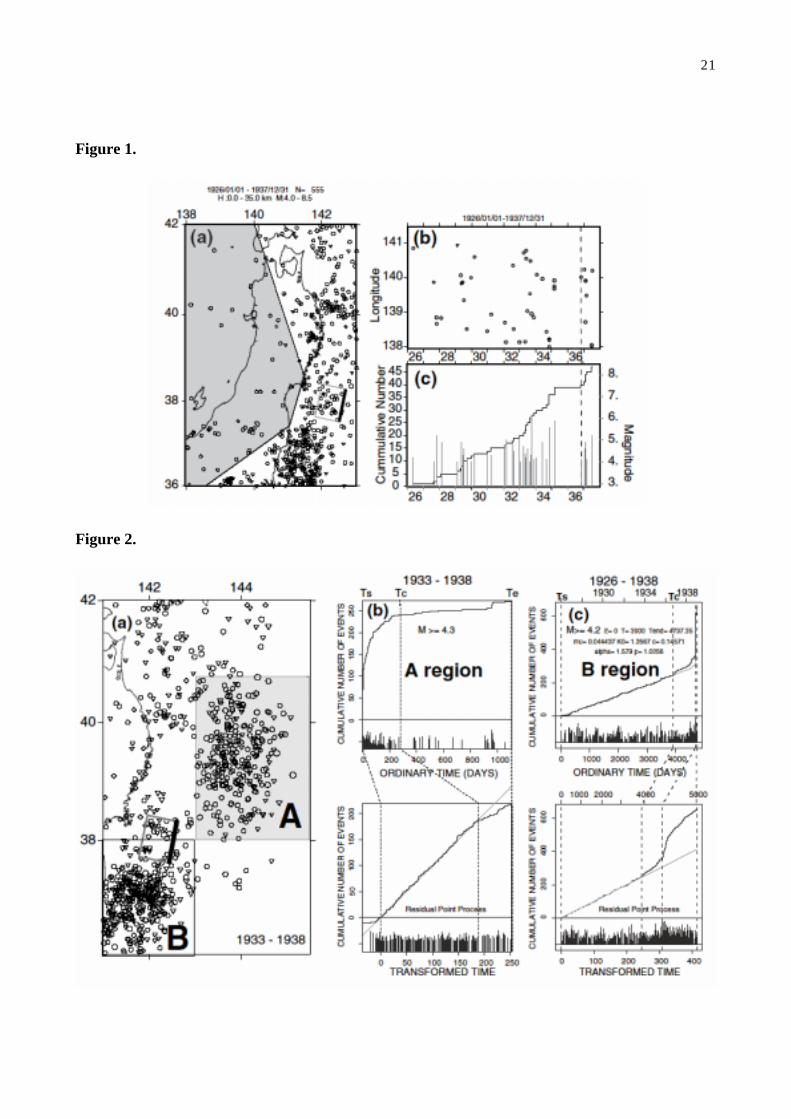
3. Relative quiescence in the stress-shadow regions prior to the 1937 and 1978 earthquakes

The source model of the 1937 earthquake is listed in Table 1. The first available hypocenter data

prior to the occurrence of this rupture is the shallow activity (depth < 35km) of earthquakes of M4.0

or larger that occurred during the period 1926-1937, in and around the Tohoku District, as shown in

Figure 1. Figure 1a shows the 1937 source model and the epicenter map of shallow moderate

earthquakes. Consider the earthquakes from the stress shadow regions (gray region) where the

predominant mechanism is the E-W compression reverse fault type (cf., Table 2). The quiescence

during the period 1935-36 prior to the main event (dotted vertical line) can be seen in the

stress-shadow region, where the ∆CFS ranges - 1 ~ - 20 millibars by assuming 10% of the slip-size

of the 1936 rupture. Hereafter, preslips are assumed to be 10% of the size of the main rupture.

The next earthquake sequence is taken from the seismic activity that mostly includes the

aftershocks of the 1933 great Sanriku-Oki earthquake of M8.3, which caused a disastrous tsunami

and which is also famous for being a normal faulting type (Kanamori, 1972) due to its proximate

location to the subducting trench (Lin and Stein, 2004). The aftershock area (grey color rectangle) is

mostly covered by the stress-shadow with ∆CFS value ranging - 5 ~ - 1 millibars, transferred from

the assumed preslip of the 1936 Miyagi-Ken-Oki earthquake of M7.5. Here I have assumed that the

majority of aftershocks and background events around this region have similar normal faulting to

6

the 1933 event (cf., Table 2). The ETAS model is applied to the events in the gray region of stress

shadow in Figure 2a (cf., Table 2). The result shown in Figure 2b suggests that the quiescence

relative to the ETAS model started around the end of 1933; that is, about three years prior to the

focal rupture of 1937.

At the same time, we investigate the seismicity during the period 1926-1938 in region B in Figure

2a, where the great swarm at Shioya-Oki (Ms 7.4, 7.7, 7.7, 7.6, and 7.0) started in November 1938.

Abe (1977) noted several unusual features of these shocks, such as a swarm of large earthquakes,

the large energy release comparable to Ms=8.1, and the inferred fact that there had been no major

earthquakes about the focal region for at least the past 800 years, whereas the ordinary recurrence

time of the large earthquakes of M ≥ 7.5 occurring in the other parts of the same plate boundary was

usually less than a hundred years. The ruptures of the great swarm seem to be accelerated by the

1936 Miyagi-Ken-earthquake. Indeed, Figure 2c shows that the coseismic activation due to the

1936 rupture where ∆CFS value ranges 0.05 ~ 2 bars in the region B. However, we see that the

activity up until the 1936 event is well predicted by the ETAS model, and the relative activation of

the activity before the 1936 event is not seen: Readers are referred to a discussion of this paper for

the reasons of the detection insensivity of the relative activation compared to the relative

quiescence.

The last interplate rupture of M7.4 in this region occurred on June 12, 1978, the source model of

which is also listed in Table 1. Figure 3a shows the epicenter map of moderate earthquakes that

occurred from 1964 through 1980, including the aftershocks of the 1964 Niigata earthquake of

M7.5. Figure 3a also shows the considered stress shadow regions (gray region) where E-W

compression reverse fault type mechanisms are predominant. Then, Figure 3b indicates that the

relative quiescence lasted about 7 years from 1970 up until the time of the rupture (vertical dotted

line).

On the other hand, the seismicity (M ≥ 5.0) including the aftershocks of the 1968 great Tokachi-Oki

earthquake of M7.9 shown in Figure 4a is the region of the neutral or very slight CFS increase (cf.,

Table 2), assuming preslip of the 1978 Miyagi-Ken-Oki earthquake of M7.4 and also assuming that

the majority of the aftershocks are of thrust type mechanisms similar to the 1968 mainshock (Table

2). In this case, we see no seismicity changes even after the 1978 rupture (Figure 4b).

About 4 months before the interplate M7.5 rupture, the Ojika-Hanto-Oki earthquake of M6.7

7

occurred at 20 February, 1978, within the subducting slub at (142.20E, 38.75N), the northern

vicinity of the M7.5 interplate source, while this is intraplate thrust rupture within the subducting

Pacific Plate (cf., Table 2). Figure 5 shows that the aftershock activity of M4 or larger is inhibited

for about two months before the rupture. The aftershocks are in the stress shadow region with ∆CFS

of about -100 millibars transferred from the assumed preslip which is 10% of the size of the M7.4

interplate rupture. Incidentally, such a slip could be triggered by the former mainshock, with a few

bars’ ∆CFS.

To summarize, the seismicity in the regions of stress-shadow shows quiescence relative to the

predicted rate by the ETAS model (the relative quiescence) before each of the previous ruptures in

1936 and 1978, whereas the seismicity is well predicted in the regions of neutral or increasing

Coulomb failure stress (CFS). Thus, the possible precursory slip within or near the source are

anticipated for the scenario of predicting a forthcoming rupture.

4. Analyses of the recent seismicity and the scenarios of the precursory slips

In this section we examine whether the relative quiescence can be seen in the sequences of recent

earthquakes from the stress shadow regions, assuming the occurrence of precursory slips within or

in the vicinity of the interplate sources. Here I consider all the source models of the 1793, 1936 and

1978 interplate ruptures (top three rows of Table 1) in addition to the recent intra-slub rupture, i.e.,

the 2003 event of M7.1 at Miyagi-Ken-Oki (the bottom row of Table 1) that has a similar

mechanism to that of the 1978 Ojika-Hanto-Oki earthquake (cf., Table 2). The results are then

interpreted in view of the CFS increment.

In the first case, we consider the earthquakes that occurred during the period from 1978 to 20 July,

2003, including aftershocks of the 1984 Central Sea of Japan earthquake of M7.7, in the

stress-shadow region (gray region) indicated in Figure 6a, where E-W compression reverse fault

type mechanisms are predominant. Figure 6b shows that the sequence of events took place as

predicted by the ETAS model. This seems to indicate no significant slips have taken place yet for a

stress-shadow that could inhibit the normal aftershock activity, since a preslip of 10% of the size of

the rupture models should decrease the stress with the ∆CFS ranging - 10 ~ - 1 millibars. On the

other hand, if we assume the pre-slip of the 2003 May Miyagi-Ken-Oki earthquake, the region

8

would have an increase of the ∆CFS ranging +0.3 ~ +2 millibars, which may well explain the fact

that we do not see any relative quiescence.

The second case considers earthquakes in the region indicated in Figure 7a, which includes the

aftershocks of the 1994 Sanriku-Haruka-Oki earthquake of M7.5 and background activity in and

around the region where reverse fault type mechanisms are predominant due to the plate boundary.

Figure 7b shows that the sequence of events occurred as predicted by the ETAS model. Assuming

that the majority of the aftershocks are of thrust type mechanisms similar to the 1994 mainshock of

M7.5 (Table 2), the aftershock area (grey color rectangle) is in the stress increase with ∆CFS values

ranging +0.5 ~ +8 millibars or +0.1 ~ +0.5 millibars, transferred from the assumed preslips of the

interplate rupture models or the 2003 intra-slub rupture of M8.1, respectively.

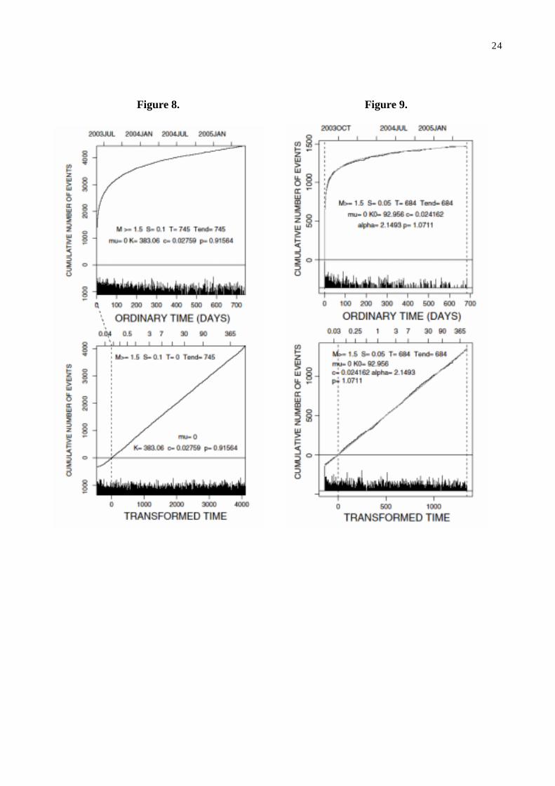
The third case examines the aftershock sequence of the 26 May, 2003 Miyagi-Ken-Oki earthquake

of M7.1 itself (cf., Table 1). This occurred within the subducting slub with a similar mechanism to

the previously mentioned 1978 Ojika-Hanto-Oki earthquake (see Tables 2 for Fig. 5). In this case,

we see no seismicity changes and the cumulative number of aftershocks up until now (June 2005) is

very well predicted by the Omori-Utsu formula (Figure 8), unlike the case of the Ojika-Hanto-Oki

earthquake (Figure 5).

Finally, the ETAS model is fitted to the aftershock sequences of the 26 July, 2003 inland shallow

earthquake of M6.3 in northern Miyagi-Ken, occurring until the present (10 June 2005). From

Figure 9 we see no seismicity changes and the cumulative number of aftershocks up until now (June

2005) is very well predicted by the ETAS model.

To summarize, all the analyzed results in this section are normally predicted by either the

Omori-Utsu formula or the ETAS model. There may be no significant preslips to make the

seismicity changes in the considered cases. However, if any preslip took place during the

considered period, that of the 2003 Miyagi-Ken-Oki intra-slub earthquake of M7.1 is more likely

than those of the expected ruptures on the plate boundary.

5. Analyses of recent inland seismicity clusters, and their relation to stress-changes based on

the possible scenarios of precursory slips

In this section, the earthquake sequences from local clusters in the vicinity of the forthcoming focal

interplate event are examined by fitting the ETAS to discriminate whether it is well adapted

9

throughout the entire period up to the present time or whether it becomes quiet relative to the

modeled rate. Also, we calculate the ∆CFS in the region transferred from the possible precursory

slips on the plate boundary (cf., top three rows of Table 1), in addition to the 2003 intraplate rupture

of M7.1 (the bottom row of Table 1). The results are then interpreted in view of the CFS increment.

Figure 10 shows the regions A - E of the seismic clusters during the period 1995 – July 2003. The

considered clusters are (A) recent aftershock activity of the 1962 Miyagi-Ken-Hokubu earthquake

of M6.5, (B) swarm activities of the 1996 Miyagi-Ken Naruko-Machi earthquake of M5.9, (C) the

seismicity including the aftershocks of the 1998 Miyagi-Ken-Nanbu earthquake of M5.0 that

occurred in Sendai city, (D) the seismicity including the aftershocks of the 1998

Iwate-Ken-Shizukuishi earthquake of M6.1, and (E) aftershocks of the 2002 Miyagi-Ken-Oki

earthquake of M6.1. The predominant angle of the receiver fault in each cluster is assumed to be

similar to their mainshock mechanism (cf., Table 3).

Table 3 also lists ∆CFS values assuming precursory slips due to either the 2003 Miyagi-Ken-Oki

intra-slub earthquake of M7.1 or the interplate rupture models in Table 1. All the results are

consistent with the assumed preslip of the 2003 Miyagi-Ken-Oki earthquake of M7.1, rather than

that of the forthcoming interplate rupture models.

In addition, the quiescence preceding the 2003 Miyagi-Ken-Oki earthquake of M7.1 is clearly seen

in the depth versus time plot in Figure 3 of Ogata (2005) due to the precursory slip within the

source, the onset of which appeared to be triggered by the 2002 event of M6.1 with about +50

millibars, and in turn the precursory slip seems to have inhibited the activity in the neighboring

plate boundary region with - 20~ - 5 millibars (cf., Figure 3 in Ogata, 2005) including the

aftershock activity of the M6.1 event itself (see Figure 9E). Incidentally it is less likely that the

quiescence of the aftershock activity of the M6.1 event is triggered by the preslip of the

forthcomming interplate rupture of the 1978 Miyagi-Ken-Oki type, because of the positive ∆CFS

values ranging +8~+10 millibars in the same region.

To summarize, all the analyzed results in this section are consistent with the assumed preslip of the

2003 Miyagi-Ken-Oki earthquake of M7.1, contrary to the assumed preslip of the expected

interplate rupture. Thus, it is likely that the results of the normal and relative quiescence are due to

those of the 2003 Miyagi-Ken-Oki intra-slub earthquake of M7.0, rather than those of the expected

rupture on the plate boundary.

10

6. Discussions

Since a sequence of aftershocks is triggered by complex mechanisms under fractal random media, it

is difficult to calculate the transfer of stresses both within and near to the field. That is, triggering

mechanics within an aftershock sequence are too complex to calculate the effect of stress changes.

Therefore, the statistical empirical laws of aftershocks are very useful as a practical solution to the

proximate triggering effect. In other words, fitting and extrapolating a suitable statistical model for

normal seismic activity in a situation without exogenous stress changes provides us with an

alternative method through which we can detect the seismicity changes sensitively. Thus, the

diagnostic analysis based on fitting the ETAS model is helpful in detecting small exogenous stress

changes. Indeed, these changes are so slight that even current state of the art methods and the

geodetic records from the GPS network can barely recognize systematic anomalies in the time

series of displacement records.

Few results in the present manuscript agree with the claim that there should be a threshold value of

∆CFS capable of affecting seismic changes. Although the stress change values can be very small in

the order of a few millibars or less, the number of earthquakes in the receiver region is fairly large

so that we have statistically significant seismicity rate change depending on the sample size, too.

Thus, we expect that significant deviation of actual activity from the predicted rates is sensitive

enough to detect a slight stress-change.

Compared to the relative quiescence, the relative activation is not very sensitive, because the

shear-stress-increase triggered by the large aftershock surpasses the exogenously triggered effect

from other sources. Therefore, its effect is hard to see in the diagnostic analysis by the ETAS model

unless the b-value of the G-R magnitude frequency significantly increases (i.e., increase of the ratio

of the smaller events to the larger events). The reason why the regional activation is not easy to

detect compared to the quiescence is because of the definition of the ETAS model itself, and

because many aftershocks are triggered by much higher ∆CFS values than the regional ∆CFS effect.

Also, the ratio of future to past seismicity rates (R/r) due to Dieterich (1994) for a positive Coulomb

failure increment is less effective than the negative increment of the same absolute value, where

11

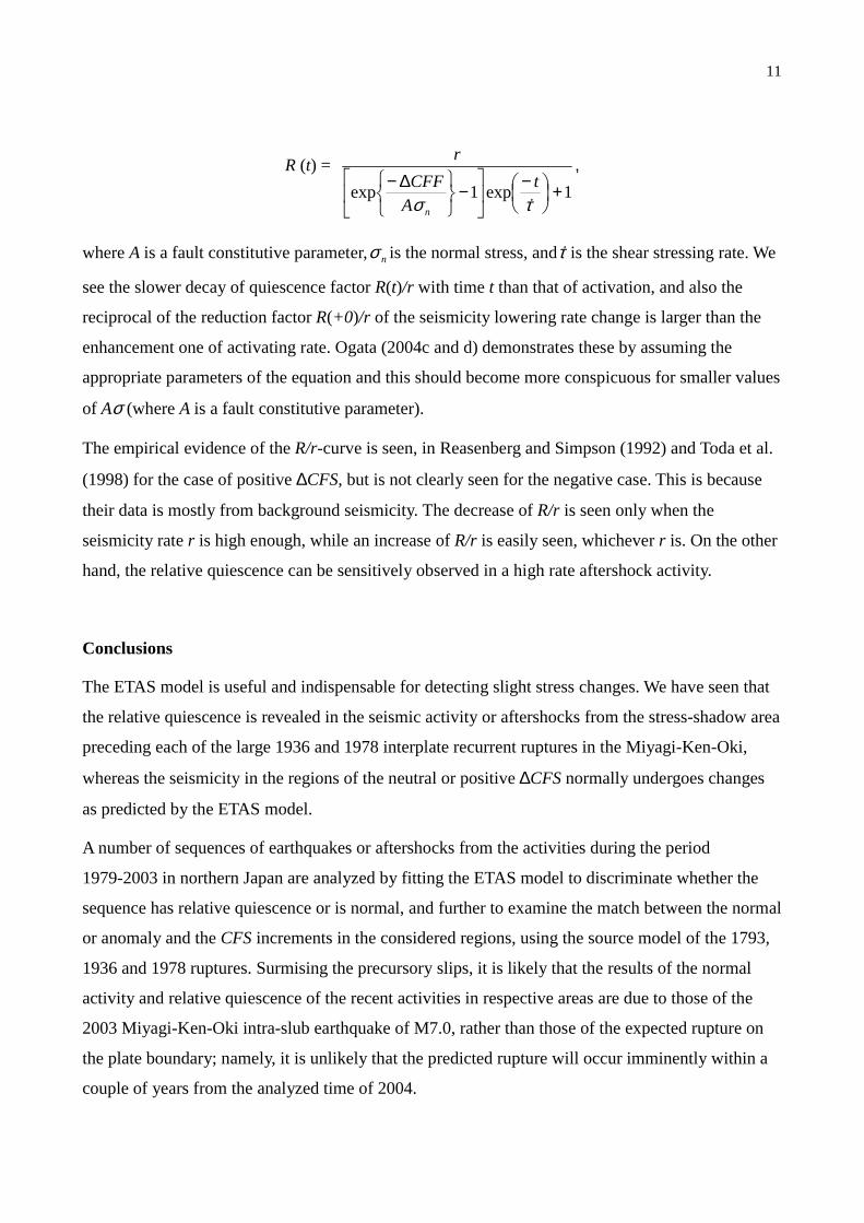
R (t) = 1exp1exp +�

�

���

� −��

�

�−

��

��� ∆−

τσ �

tACFF

r

n

,

where A is a fault constitutive parameter, nσ is the normal stress, andτ� is the shear stressing rate. We

see the slower decay of quiescence factor R(t)/r with time t than that of activation, and also the

reciprocal of the reduction factor R(+0)/r of the seismicity lowering rate change is larger than the

enhancement one of activating rate. Ogata (2004c and d) demonstrates these by assuming the

appropriate parameters of the equation and this should become more conspicuous for smaller values

of Aσ (where A is a fault constitutive parameter).

The empirical evidence of the R/r-curve is seen, in Reasenberg and Simpson (1992) and Toda et al.

(1998) for the case of positive ∆CFS, but is not clearly seen for the negative case. This is because

their data is mostly from background seismicity. The decrease of R/r is seen only when the

seismicity rate r is high enough, while an increase of R/r is easily seen, whichever r is. On the other

hand, the relative quiescence can be sensitively observed in a high rate aftershock activity.

Conclusions

The ETAS model is useful and indispensable for detecting slight stress changes. We have seen that

the relative quiescence is revealed in the seismic activity or aftershocks from the stress-shadow area

preceding each of the large 1936 and 1978 interplate recurrent ruptures in the Miyagi-Ken-Oki,

whereas the seismicity in the regions of the neutral or positive ∆CFS normally undergoes changes

as predicted by the ETAS model.

A number of sequences of earthquakes or aftershocks from the activities during the period

1979-2003 in northern Japan are analyzed by fitting the ETAS model to discriminate whether the

sequence has relative quiescence or is normal, and further to examine the match between the normal

or anomaly and the CFS increments in the considered regions, using the source model of the 1793,

1936 and 1978 ruptures. Surmising the precursory slips, it is likely that the results of the normal

activity and relative quiescence of the recent activities in respective areas are due to those of the

2003 Miyagi-Ken-Oki intra-slub earthquake of M7.0, rather than those of the expected rupture on

the plate boundary; namely, it is unlikely that the predicted rupture will occur imminently within a

couple of years from the analyzed time of 2004.

12

However, from the long-term prediction, it is very likely that we will have the predicted interplate

rupture within the next couple of decades. From the results summarized in this paper, it will be

useful to continue monitoring the activity to detect the relative quiescence in the stress shadow

areas, such as the wide regions in Figures 1, 2A, 3, and 6, intra-slub aftershocks like Figure 5, and

inland cluster activity in Figures 9, 10A and 10B (cf., Tables 2 and 3).

Acknowledgments

I have used the TSEIS visualization program package (Tsuruoka, 1997) for the study of hypocenter

data, and also used the PC program MICAP-G for spatial visualization of Coulomb stress changes

(Naito and Yoshikawa, 1998). This study is partly supported by Grant-in-Aid B2-14380123 and

A-17200021 for Scientific Research, Ministry of Education, Science, Sports and Culture.

Appendix: Models and model fitting

The typical aftershock decay is represented by the Omori-Utsu formula (Omori, 1894; Utsu, 1961;

Ogata, 1983; Utsu et al., 1995),

ν (t) = K (t + c) p− , (K, c, p; constant), (2)

initiated by the main shock at time origin t=0. In general, this formula holds for quite a long period

in the order of some tens of years or more, depending on the background seismicity rate in the

neighboring area (Utsu, 1969; Ogata and Shimazaki, 1984; Utsu et al., 1995). As we consider small

aftershocks, however, occurrence-time clustering of the events within the aftershock sequence

becomes apparent. Thus, aftershock activity is not best predicted by the single Omori-Utsu formula,

especially when it includes conspicuous secondary aftershock activities of large aftershocks, as

demonstrated in Guo and Ogata (1997) and Ogata et al. (2003). Indeed, we see cascading complex

features of aftershocks, such as interactively triggered aftershocks, including off-fault aftershocks.

Therefore, we assume that every aftershock can trigger its own further aftershocks or remote events

greater or small in magnitudes, and that the occurrence rate at time t is given by a (weighted)

superposition of the Omori-Utsu functions ν in (2) shifted in time

,)()( }{0 � −+= −

jj

MMj ttet c νλλ αθ (3)

13

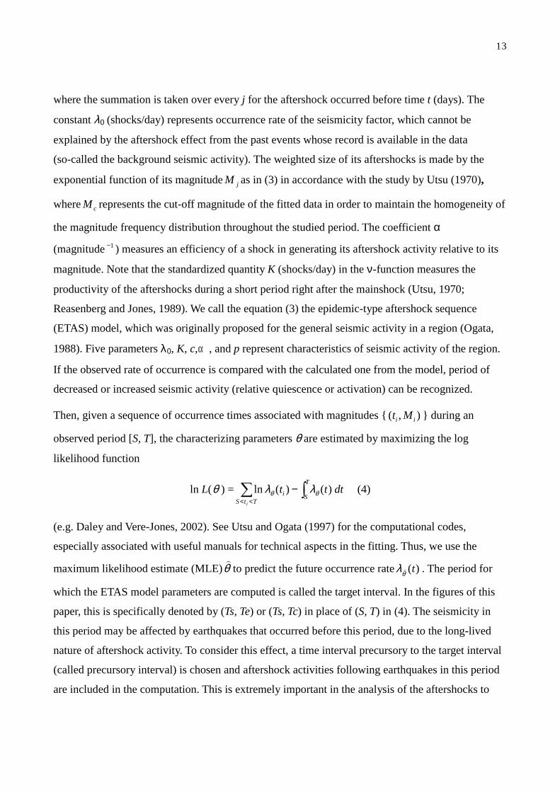
where the summation is taken over every j for the aftershock occurred before time t (days). The

constant λ0 (shocks/day) represents occurrence rate of the seismicity factor, which cannot be

explained by the aftershock effect from the past events whose record is available in the data

(so-called the background seismic activity). The weighted size of its aftershocks is made by the

exponential function of its magnitude jM as in (3) in accordance with the study by Utsu (1970),

where cM represents the cut-off magnitude of the fitted data in order to maintain the homogeneity of

the magnitude frequency distribution throughout the studied period. The coefficient α

(magnitude 1− ) measures an efficiency of a shock in generating its aftershock activity relative to its

magnitude. Note that the standardized quantity K (shocks/day) in the ν-function measures the

productivity of the aftershocks during a short period right after the mainshock (Utsu, 1970;

Reasenberg and Jones, 1989). We call the equation (3) the epidemic-type aftershock sequence

(ETAS) model, which was originally proposed for the general seismic activity in a region (Ogata,

1988). Five parameters λ0, K, c,α, and p represent characteristics of seismic activity of the region.

If the observed rate of occurrence is compared with the calculated one from the model, period of

decreased or increased seismic activity (relative quiescence or activation) can be recognized.

Then, given a sequence of occurrence times associated with magnitudes { ),( ii Mt } during an

observed period [S, T], the characterizing parameters θ are estimated by maximizing the log

likelihood function

ln L(θ ) = �� −<<

T

STtS

i dttti

)()(ln θθ λλ (4)

(e.g. Daley and Vere-Jones, 2002). See Utsu and Ogata (1997) for the computational codes,

especially associated with useful manuals for technical aspects in the fitting. Thus, we use the

maximum likelihood estimate (MLE)θ�

to predict the future occurrence rate )(tθλ � . The period for

which the ETAS model parameters are computed is called the target interval. In the figures of this

paper, this is specifically denoted by (Ts, Te) or (Ts, Tc) in place of (S, T) in (4). The seismicity in

this period may be affected by earthquakes that occurred before this period, due to the long-lived

nature of aftershock activity. To consider this effect, a time interval precursory to the target interval

(called precursory interval) is chosen and aftershock activities following earthquakes in this period

are included in the computation. This is extremely important in the analysis of the aftershocks to

14

maintain the homogeneity or the completeness of the data, where the target period should exclude a

short period immediately after the mainshock, due to the substantial exclusion of smaller

aftershocks, whereas the mainshock and the large aftershocks are highly effective as the history to

the future of the aftershock activity (e.g., see Ogata, 2001). When the ETAS parameters are

estimated for two or more successive periods (usually divided at turning points Tc of seismicity), it

is better to set a precursory period before each target period.

References

Abe, K., 1977. Tectonic implications of the large Shioya-Oki earthquakes of 1938, Tectonophysics, 41, 269-289.

Aida, I., 1977. Simulations of large tsunamis occurring in the past off the coast of Sanriku district (in Japanese),

Bull. Earthq. Res. Inst., 52, 71-101.

Daley, D.J., Vere-Jones, D., 2002. An Introduction to the Theory of Point Processes, Volume 1, 2nd edition,

Springer-Verlag, New York, 2002.

Dieterich, J., 1994. A constitutive law for rate of earthquake production and its application to earthquake

clustering. J. Geophys. Res., 99, 2601–2618.

Geographical Survey Institute of Japan, 2004. Crustal movement in the Tohoku District, Report of the

Coordinating Committee for Earthquake Prediction, 71, 52.

Guo, Z., Ogata, Y., 1993. Statistical relations between the parameters of aftershocks in time, space and magnitude.

J. Geophys. Res. 102, 2857-2873.

Harris, R. A., 1998, Introduction to special section: Stress triggers, stress shadows, and implications for seismic

hazard, J. Geophys. Res., 103, 24,347–24,358.

Headquarter for Earthquake Research Promotion of Japan, 2005. Updating of probabilities of the long-term

earthquake forecasts and sizes of earthquakes based on the active fault data (in Japanese),

http://www.jishin.go.jp/main/chousa/05jan_kakuritsu/p04_kaikou.pdf.

Ichikawa, M., 1971. Reanalyses of mechanism of earthquakes which occurred in and near Japan, and statistical

studies on the nodal plane solutions obtained, 1926-1968, Geophys. Mag. (Tokyo), 35, 207-274.

Inouye, W., 1965., On the seismicity in the epicentral region and its neighborhood before the Niigata earthquake

(in Japanese), Kenshin-jiho (Q. J. Seismol.), 29, 139-144.

Japan Meteorological Agency, 2004. Mechanism data file, The Annual Seismological Bulletin of Japan.

Kanamori, H., 1972. Relation between tectonic stress, great earthquakes, and earthquake swarms, Tectonophysics,

4, 1-12.

15

Kikuchi, M., Yamanaka, Y., 2003. EIC Seismological Note, Earthquake Research Institute, University of Tokyo,

http://www.eri.u-tokyo.ac.jp/sanchu/Seismo_Note/index-e.html, No. 0, 50, 128, 135, 137

King, G.C.P., Stein, R., Lin, J., 1994. Static stress changes and the triggering of earthquakes. Bull. Seismol. Soc.

Am., 84, 935-953.

Kisslinger, C., 1988. An experiment in earthquake prediction and the 7th May 1986 Andreanof Islands

Earthquake. Bull. Seismol. Soc. Am., 78, 218-229.

Naito, H. and Yoshikawa, S., 1996. A program to assist crustal deformation analysis (in Japanese). Zisin ii (J.

Seismol. Soc. Japan) 52, 101-103.

Lin, J., Stein, R.S., 2004. Stress triggering in thrust and subduction earthquakes, and stress interaction between the

southern San Andreas and nearby thrust and strike-slip faults, Journal of Geophysical Research, 109, B02303,

doi:10.1029/2003JB002607

Matsu'ura, R.S., 1986. Precursory quiescence and recovery of aftershock activities before some large aftershocks, Bull. Earthquake Res. Inst. Univ. Tokyo, 61, 1–65.

Ohtake, M., Matumoto, T., Latham, G.V., 1977. Seismicity gap near Oaxaca, southern Mexico as a probable

precursor to a large earthquake. Pure Apple. Geophys., 115, 375-385.

Ogata, Y., 1983. Estimation of the parameters in the modified Omori formula for aftershock frequencies by the

maximum likelihood procedure, J. Phys. Earth 31, 115-124.

Ogata, Y., 1988. Statistical models for earthquake occurrences and residual analysis for point processes. J. Amer.

Statist. Assoc. 83, 9-27.

Ogata, Y., 1992. Detection of precursory relative quiescence before great earthquakes through a statistical model,

J. Geophys. Res., 97, 19,845–19,871.

Ogata, Y. 1999. Seismicity analyses through point-process modeling: A review, Pure Appl. Geophys., 155,

471–507.

Ogata, Y., 2001. Increased probability of large earthquakes near aftershock regions with relative quiescence, J.

Geophys. Res., 106, 8729–8744.

Ogata, Y., 2004a. Space-time model for regional seismicity and detection of crustal stress changes. J. Geophys.

Res., 109, 10.1029/2003JB002621.

Ogata, Y., 2004b. Seismicity quiescence and activation in western Japan associated with the 1944 and 1946 great

earthquakes near the Nankai trough. J. Geophys. Res., 109, 10.1029/2003JB002634.

Ogata, Y., 2004c. Statistical Analysis of seismic activities in and around Tohoku District, northern Japan, prior to

the large interpolate earthquakes off the coast of Miyagi Prefecture (in Japanese), Report of the Coordinating

Committee for Earthquake Prediction，71, 268-278.

16

Ogata, Y., 2004d. Static triggering and statistical modelling (in Japanese), Report of the Coordinating Committee

for Earthquake Prediction，72, 631-637.

Ogata, Y., 2005. Detection of anomalous seismicity as a stress change sensor, J. Geophys. Res., Vol. 110, No. B5,

B05S06, 10.1029/2004JB003245.

Ogata, Y., Shimazaki, K., 1984. Transition from aftershock to normal activity: The 1965 Rat Islands earthquake

aftershock sequence, Bull. Seismol. Soc. Am., 74, 1757–1765.

Ogata, Y., Jones, L. M., Toda, S., 2003. When and where the aftershock activity was depressed: Contrasting decay

patterns of the proximate large earthquakes in southern California, J. Geophys. Res., 108(B6), 2318,

doi:10.1029/2002JB002009.

Okada, Y., 1992. Internal deformation due to shear and tensile faults in a half-space. Bull. Seism. Soc. Am. 82,

1018-1040.

Omori, F., 1894. On the aftershocks of earthquakes, J. Coll. Sci. Imp. Univ. Tokyo 7, 111-200.

Reasenberg, P., Jones, L.M., 1989. Earthquake hazard after a mainshock in California, Science, 243, 1173–1176.

Reasenberg, P.A., Simpson, R.W., 1992. Response of regional seismicity to the static stress change produced by

the Loma Prieta earthquake. Science, 255, 1687-1690.

Research group for active faults in Japan, 1992. Maps of Active Faults in Japan with an Explanatory Text,

University of Tokyo Press,

Seno, T., 1979. On the earthquake expected off the Miyagi prefecture (in Japanese), Report of the Coordinating

Committee for Earthquake Prediction, 21, 38-43.

Seno, T., K. Sudo, Eguchi, T., 1979a. Focal mechanism of the Miyagi-Ken-Oki earthquake of June 12, 1978 (in

Japanese), Report of the Coordinating Committee for Earthquake Prediction，21, 10-12.

Stein, R.S., 1999. The role of stress transfer in earthquake occurrence, Nature. 402, 605-609.

Toda, S., Stein, R.S., Reasenberg, P., Dieterich, J.H., Yoshida, A., 1998. Stress transferred by the Mw = 6.9 Kobe,

Japan, shock: Effect on aftershocks and future earthquake probabilities, J. Geophys. Res., 103, , 24543-24545.

Toda, S. and R.S. Stein, 2002. Response of the San Andreas Fault to the 1983 Coalinga-Nuñez Earthquakes: An

Application of Interaction-based Probabilities for Parkfield. J. Geophys. Res. 107, 10.1029/2001JB000172.

Tohoku University, 1995. Faulting process of the 1994 Far East Off Sanriku earthquake inferred from GPS

observation. Report of the Coordinating Committee for Earthquake Prediction, 54, 97-101.

Tsuruoka, H., 1996. Development of seismicity analysis software on workstation (in Japanese). Tech. Res. Rep. 2

34-42, Earthquake Res. Inst., Univ. Tokyo.

17

Uchida, N., Matsuzawa, T., Igarashi T., Hasegawa, A., 2003. Interplate quasi-static slip off Sanriku, NE Japan,

estimated from repeating earthquakes, Geophys. Res. Lett., 30, 10.1029/2003GL017452.

Uchida, N., Hasegawa, A., Matsuzawa, T., Igarashi, T., 2004. Pre- and post-seismic slow slip on the plate

boundary off Sanriku, NE Japan associated with three interplate earthquakes as estimated from small

repeating earthquake data, Tectonophysics, 385, 1-15.

Utsu, T., 1961. A statistical study on the occurrence of aftershocks, Geophys. Mag. 30, 521-605.

Utsu, T., 1968. Seismic activity in Hokkaido and its vicinity (in Japanese). Geophys. Bull. Hokkaido Univ., 13,

99-103.

Utsu, T., 1969, Aftershocks and earthquake statistics (I): some parameters which characterize an aftershock sequence and their interaction, J. Faculty Sci., Hokkaido Univ., Ser. VII, 3, 129-195.

Utsu, T., 1970. Aftershocks and earthquake statistics (II): Further investigation of aftershocks and other

earthquakes sequence based on a new classification of earthquake sequences, J. Faculty Sci., Hokkaido Univ., Ser.

VII 3, 379-441.

Utsu, T., 1984. Estimation of parameters for reccurrence models of earthquakes, Bull. Earthq. Res. Inst., 59,

53-66.

Utsu, T., Ogata, Y., Matsu'ura, R. S., 1995, The centenary of the Omori formula for a decay law of aftershock activity, J. Phys. Earth, 43, 1–33.

Utsu, T., Ogata, Y., 1997. Statistical Analysis of point processes for Seismicity (SASeis). IASPEI Software

Library 6, 13-94, International Association of Seismology and Physics of Earth's Interior.

Wyss, M., Burford, R.O., 1987. A predicted earthquake on the San Andreas fault, California. Nature 329,

323-325.

Yamanaka, Y., Kikuchi, M., 2001. Asperity map based on the analysis of historical seismograms: Tohoku version,

Abstracts of the 2001 Joint Meeting for Earth and Planetary Science, Sy-005.

Yamanaka Y., Kikuchi, M., 2004. Asperity map along the subduction zone in northeastern Japan inferred from

regional seismic data, J. Geophys. Res., 109, B07307, doi:10.1029/2003JB002683.

18

Table 1. Assumed source fault parameters of the Miyagi-Ken-Oki earthquakes

Year M Long. Lat. Dep (km)

Strike(deg)

Dip (deg)

Rake(deg)

L (km)

W (km)

Slip (cm)

References

1793 8.2 143.58 39.16 1 205 40 90 120. 30. 390. Aida (1977) 1936 7.4 142.7 38.3 15 190 20 90 80. 60. 200. Seno et al. (1979) 1978 7.4 142.43 38.42 25 190 20 76 30. 80. 170. Seno et al. (1979) 2003 7.0 141.81 38.94 52 192 68 73 17. 19. 210 G. S. I. J. (2003)

Table 2. Assumed receiver fault angles and ∆CFS values Regions Strike

(deg.) Dip

(deg.) Rake (deg.)

Depth(km)

∆CFS *1

(milli-bars) Seismicity

Fig. 1 Fig. 2A Fig. 2B Fig. 3 Fig. 4 Fig. 5

200 180 200 200 190 194

45 45 20 45 30 74

90 270 90 90 76 85

20 20 -- *2

20 -- *2

50

-5. ~ -1. -3. ~ -1.

+50. ~ +200.-10. ~ -5.

-0.05 ~ +0.4-100.

Quiet Quiet

Normal Quiet

Normal Quiet

(*1) 10% of the slip-size of the rupture model in Table 1 is assumed for the precursory slip. The depth in (*2) is on descending interface between the inland plate and subducting slub. The bold face numbers indicate the consistency of the ∆CFS signs with the analyzed result of the seismic activity.

Table 3. Assumed receiver fault angles and ∆CFS values

Angles*1 ∆CFS *2 (millibars) Receiver regions θ δ λ

dep km

1973 1936 1978 2003 Seismicity

Fig. 6 10 30 90 20 -3 ~ -2 -10 ~ -1 -3 ~ -1 ++++.3.3.3.3~ ++++2222 Normal Fig. 7 190 30 76 --*4 ++++5555~ ++++8888 ++++.5.5.5.5~ ++++2222 ++++.5.5.5.5~ ++++1111 ++++.1.1.1.1~ ++++.5.5.5.5 Normal Fig. 8 192 68 73 52 ++++10101010 ++++50505050 ++++7777 ------------ Normal Fig. 9 201 42 102 10 -20 ----////++++ *5 -50 ++++10101010 *3 Normal

Fig. 10A 211 41 128 10 -20 -10 -20 ++++5555 Normal Fig. 10B 199 45 105 10 -20 -20 -10 ++++4444 Normal Fig. 10C 187 37 52 10 -/+ +5 ----30303030 ----1111 Quiet Fig. 10D 216 41 131 10 -8 ++++2222 ++++1111 ++++.5.5.5.5 Normal Fig. 10E 181 22 70 46 +80 +50 +20 ----20202020 Quiet

(*1) θ, δ and λ represents strike, dip and rake angles in degrees, respectively. (*2) 10% of the slip-size of the rupture model in Table 1 is assumed for the precursory slip except for (*3) that is coseismic. The depth in (*4) is along descending interface between the inland plate and subducting slub. (*5) ‐/+ means neutral. The bold face numbers indicate the consistency of the signs with the analyzed result of the seismic activity.

19

Figure Captions:

Fig.1. Shallow earthquakes (M ≥ 4) in the stress-shadow region during the period 1926–1937, before

and after the 1936 Miyagi-Ken-Oki earthquake of M7.4: (a) epicenters, (b) longitude versus time,

and (c) cumulative numbers and magnitude against time. The gray color shows the stress-shadow

region of thrust-type faults under EW-compression (cf., Table 2) at a 10km depth, assuming the

preslip within or around the 1936 rupture fault. The vertical dotted line indicates the 1936 event.

Fig.2. Aftershocks of the 1933 Sanriku-Oki earthquake of M8.1 (Region A ; M≥ 4.3), and seismic

activity before 1938 great swarm at Shioya-Oki (Region B; M≥ 4.2): (a) epicenters and the 1936

source model, (b) and (c) cumulative numbers and magnitude against the ordinary time (top panel)

and transformed time (bottom panel) for the regions A and B, respectively. Hereafter, vertical dotted

lines denoted by Ts, Te, and Tc show that ETAS is fitted to the events in the target periods of either

(Ts, Te) or (Ts, Tc) where the time Tc is the turning point to the quiescence. In the cases of (b) and

(c), the time Ts is 0.15 day after the mainshock and beginning of 1926, respectively, and the time Te

for both cases is the end of 1938. The vertical line at Tc in (c) indicates the occurrence of the 1936

rupture.

Fig.3. Shallow earthquakes (M ≥ 4) during the period 1964-1980, including the aftershocks of the

1964 Niigata earthquake of M7.5 in the stress-shadow region, before and after the 1978

Miyagi-Ken-Oki earthquake of M7.4: (a) epicenters, the 1978 source model, and longitude versus

time, and (b) cumulative numbers and magnitude against the ordinary and transformed times. The

gray color in the epicenter plots shows stress-shadow region at a 10km depth, assuming the preslip

within or around the 1978 rupture fault. The quiescence after 1975 (dotted vertical line at Tc) is seen

in the stress-shadow region, where the ∆CFS ranges - 5 ~ - 10 millibars transferred from the

assumed preslip of the 1978 rupture.

Fig.4. Aftershocks (M ≥ 5) of the 1968 Tokachi-Oki earthquake of M7.9. (a) epicenters and the 1978

source model, and (b) cumulative numbers and magnitude against the ordinary and transformed

times. In this case, Ts is 0.2 days after the mainshock and Te is the occurrence time of the 1978

Miyagi-Ken-Oki event. We see no seismicity changes, even after the 1978 rupture.

Fig.5. Panels show that the aftershocks (M ≥ 4) of the Ojika-Hanto-Oki earthquake of M6.7

occurred on 20 February, 1978. We see the relative quiescence one and a half months after the

20

mainshock up until the main rupture of M7.4 on 12 June, 1978.

Fig.6. Shallow earthquakes (M ≥ 4) including the aftershocks of the 1983 Central Sea of Japan

earthquake of M7.7 in the stress-shadow (gray color) region during 1978 - 20 July, 2003, assuming

the preslips of the interplate rupture (cf., Table 1), (a) epicenters and (b) cumulative numbers and

magnitude against the ordinary and transformed times. (Ts, Te) in this case covers the entire period

of the data.

Fig.7. The aftershocks (M≥ 3.5) of the 1994 Sanriku-Haruka-Oki earthquake of M7.5 and

background activity in and around the region. In this case, the time Ts is 10 days after the

mainshock (i.e., after the largest aftershock of M7.2) and the time Te is 20 July, 2003.

Fig.8. Aftershock sequences (M ≥ 1.5) of the 2003 Miyagi-Ken-Oki earthquake of M7.0, which has

a similar mechanism to that of the Ojika-Hanto-Oki earthquake, where Ts = 0.1 days after the

mainshock.

Fig.9 Aftershock sequences (M ≥ 1.5) of the 2003 Northern Miyagi-Ken earthquake of M6.3, where

Ts = 0.05days after the mainshock.

Fig.10. Recent aftershock or swarm activity of (A) the 1962 Miyagi-Ken-Hokubu earthquake of

M6.5, (B) the 1996 Miyagi-Ken Naruko-Machi earthquake of M5.9, (C) the 1998

Miyagi-Ken-Nanbu earthquake of M5.0, (D) the 1998 Iwate-Ken Shizukuishi earthquake of M6.1,

and (E) the 2002 Miyagi-Ken-Oki earthquake of M6.1. The values of Ts, Tc and Te are indicated in

the panel.

21

Figure 1.

Figure 2.

22

Figure 3.

Fugure 4.

23

Figure 5. Figure6.

Figure 7.

24

Figure 8. Figure 9.

25

Figure 10.