WP-2011-026

Relative Prices, the Price Level and Inflation: Effects of Asymmetricand Sticky Adjustment

Shruti Tripathi and Ashima Goyal

Indira Gandhi Institute of Development Research, MumbaiOctober 2011

http://www.igidr.ac.in/pdf/publication/WP-2011-026.pdf

Relative Prices, the Price Level and Inflation: Effects of Asymmetricand Sticky Adjustment

Shruti Tripathi and Ashima GoyalIndira Gandhi Institute of Development Research (IGIDR)

General Arun Kumar Vaidya Marg Goregaon (E), Mumbai- 400065, INDIA

Email (corresponding author): ashima@igidr.ac.in

Abstract

The paper examines how relative price shocks can affect the price level and then inflation. Using Indian

data we find: (i) price increases exceed price decreases. Aggregate inflation depends on the distribution

of relative price changes—inflation rises when the distribution is skewed to the right, (ii) such

distribution based measures of supply shocks perform better than traditional measures, such as prices of

energy and food. They moderate the price puzzle, whereby a rise in policy rates increases inflation, and

are significant in estimations of New Keynesian aggregate supply, (iii) an average Indian firm changes

prices about once in a year; the estimated Calvo parameter implies half of Indian firms reset their

prices in any period, and 66 percent of firms are forward looking in their price setting. The implication

of these estimated real and nominal price rigidities for policy are drawn out.

Keywords:

WPI, NKPC, asymmetric, stickiness, size, frequency, inflation

JEL Code:

E31, E12, C26, C32

Acknowledgements:

We thank Reshma Aguiar for help with the word processing.

i

1

Relative Prices, the Price Level and Inflation: Effects of

Asymmetric and Sticky Adjustment

Shruti Tripathi and Ashima Goyal

1.1 Introduction

Many studies have examined data underlying nationally-representative consumer and

producer price indices from national statistical agencies. A smaller set of studies have

focused on micro level data for a subset of manufacturing industries. They offer many

insights on price setting, price stickiness and determinants of inflation in the short run, which

have direct consequences for the conduct of monetary policy.

In this paper, the focus is on price setting in India and its responses to shocks. Klenow and

Malin (2010), found that one of the features of price setting in developing countries are more

frequent price changes reflecting higher inflation rate existing in the country. We try to test

this hypothesis using non parametrical approach and examine the link between frequency and

size of price changes. When a firm experiences a shock to its desired relative price, it

changes its price only when the change in price is large enough to cover the cost of the

process of change. It implies that firms may respond to large shocks and not to small shocks.

This hints that distribution of desired changes in relative price may have a role to play in

determining average price level.

Results in the literature1 are: First, individual prices change at least once a year. The

frequency is closer to twice a year in the U.S. versus once a year in the Euro Area. Second,

goods differ significantly in how frequently their prices change. At one extreme are goods

whose prices change at least once a month (food, energy), and at the other extreme are

services that change prices much less often than once a year. Such heterogeneity makes mean

price durations much longer than median durations. Third, goods with more cyclical qualities

1 See Alvarez et.al (2008), Goldberg-Hellerstein (2009), Bunn and Ellis (2009), Gautier (2008), Fabiani et.al

(2005), and Blinder (1998).

2

(cars and apparel) exhibit greater micro price flexibility than goods that doesn’t show much

cyclicality. Durables prices as a whole change more frequently than nondurables and

services. Fourth, the timing of price changes is little synchronized across products. In the US

most movements in inflation (from month to month or quarter to quarter) are due to changes

in the size rather than the frequency of price changes. In countries with more volatile

inflation, such as Mexico, the frequency of price changes has shown more meaningful

variation. Fifth, changes in price level are positively related to the skewness of relative price

changes. Suppose, for example that the distribution of desired changes in relative prices are

skewed to the right. In this case a few firms desire a large price increase, which gets balanced

with small price decreases by most of the firms. However, due to existence of menu cost,

firms respond more quickly to a large change in price then to a small change. Desired

increases occur more quickly than desired decreases. Hence, the price level rises in the short

run.

We found average price increase over time is greater than average price decrease. While price

increase is around 10 percent price decrease is less than 5 percent. This suggests that the

positive rate of inflation in India might be driven by much higher price increases compared to

price decreases. It takes around one year for the Indian market to change the price of the

products which implies both real and nominal rigidities in the market.

We also found changes in the price level are positively related to skewness of relative price

changes. Results suggest that the asymmetry variable is a better measure of supply shocks

than the traditional variables. Traditional variables performed well in earlier studies because

they were acting as proxy for asymmetries. The results also suggest that the relationship

between asymmetries and inflation holds across all time period.

The paper has three main sections. The first on price stickiness and the second on

asymmetric behavior of prices and the third on estimation of Phillips curve for India. The

last, section four, concludes and draws out some implications.

2. Price Stickiness

There are two theories regarding the correlation between frequency and size of price change.

The majority of price setting models predict a negative correlation between the frequency and

size of price changes. If prices are rigid and change less often, the size of price change tends

3

to be larger, as the new optimal price is likely to be further from the original price (Mankiw,

1985). In contrast, Rotemberg (1982) argues that in case of convex costs of price adjustment,

the frequency and size of price changes will exhibit positive correlation. To supplement this

literature from a developing country’s perspective, this paper studies the relationship between

frequency and size of price change non-parametrically using Indian disaggregated WPI data.

2.1 Data Set

The data set contains the wholesale price index (WPI) records of 90 products collected at

monthly frequency by the Office of Economic Adviser, Government of India from M4 1971

to M4 2010.

2.2 Measuring Frequency and Size of Price Changes

To define frequency of price changes and the duration of a single price spell formally we

follow Horvath (2011). Let pit be the price of product i at time t.

Then we define:

(1)

As a result, the product-specific frequency of price changes, μ, is computed as:

(2)

T

he frequency of price changes is calculated as the ratio of price changes in the month to the

number of observations for which the price of the particular product is available.

The product-specific size of price increases, λi, is computed as:

(3)

Similarly, the product-specific size of price decreases

(4)

4

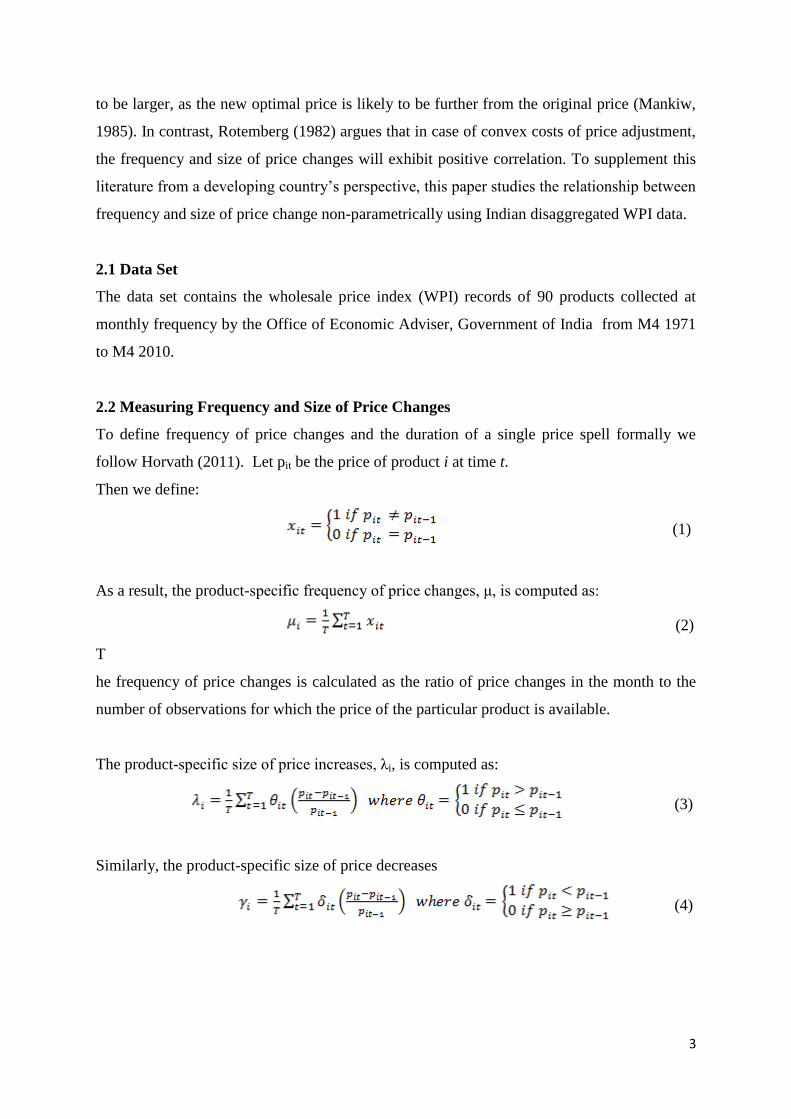
That is, the size of price changes is calculated as the percentage increase (decrease) of the

price of a particular item in the month t compared to the price of the same item in the month

t-1, conditional on the occurrence of a price change (i.e. zero percent price changes are not

included).

Figure 1: Frequency and Size of Price Changes

Figure 1 gives descriptive statistics on frequency of price changes, size of price increase, size

of price decrease and correlation between sizes of price increase vis-à-vis decrease. The first

three figures give the kernel density for the frequency and price increase and decrease. Y-axis

gives density values and x-axis gives the points at which these density values are evaluated.

Kernel density estimation is a non-parametric way of estimating the probability density

function of a random variable.

The result represented by the first graph indicates the most common frequency of price

change is around one, so the typical price changed in about one year during the sample

period, reflecting price rigidity in the Indian market.

5

The second graph gives kernel density for the size of price increase. Conditional on

frequency of price change, the result suggests that the magnitude of the price increase is

around 10 percent. The magnitude of price decrease, given by the lower left graph, is much

lower, slightly less than 5 percent.

According to the Kernel density graph price falls are more frequent but lower in magnitude.

On the other hand frequency of price increase is lower but the magnitude is higher. The result

may be due to bi-annual sales in the Indian consumer products market. But price increases

only when the magnitude is large enough to cover menu cost.

The last part of Figure 1 gives the correlation between the magnitude of price increases and

decreases. It indicates high correlation between the two. In value terms it comes to -0.865.

This result may point to the pricing method followed at the retail level. It is possible price

decreases with temporary sales, and prices increase with the end of sales as well as with

positive inflation.

The correlation value between frequency of price change and the size of price increase was

found to be highly significant (0.22 with t-value = 2.076), while the correlation value

between frequency of price change and the size of price decrease turned out to be

insignificant (-0.16 with t-value = -1.43). This means that if there is a change in prices, there

is a higher probability of price rise. Our finding is in confirmation with the literature for

developing countries2.

The main findings of this section are: average price increase over time is greater than average

price decrease. While price increase is around 10% price decrease is less than 5%. This

suggests that the positive rate of inflation in India might be driven by much higher price

increases compared to price decrease. Prices of Indian products are changed in around one

year which implies both real and nominal rigidities in the market.

2In a study for Brazil price increases are less frequent after a period of exchange rate appreciation and more

frequent when inflation is higher; in periods of high economic activity; and when macroeconomic uncertainty is

higher (Barro et.al. 2009). Duration of price spells is just above 6 months. In a study for Hungary the mean

duration of prices is 8 months. The average size of increases is 11.2 percent, and the average size of decreases is

8 percent (Gabriel and Reiff 2008). However, Medina et.al (2007) found, that at a firm level, prices are adjusted

on average every three months.

6

3. Asymmetric Price Changes

3.1 The distribution of price change

To give an initial sense of asymmetries, Figure 2 presents histograms of log industry price

changes for four years. In constructing these histograms, each industry is weighted as in the

WPI. Here weights are taken as a proxy for relative importance of industries in the reference

year.

Figure 2 shows considerable variation in the distribution of price changes. While 1974 and

2006 show a distribution skewed to the right, implying an increase in the overall price level,

1984 gives a left skewed distribution. In this case, the lower tail is larger than the upper tail

implying a fall in the price level. However the distribution in 2000 is more or less symmetric.

In this case, firms or industries with desired change in the upper tail of distribution raise their

price and those in the lower tail lower their price, so the effect on the price level is low. The

first two years correspond to OPEC shocks oil prices rose in both the years.

It is also noticeable that the number of products changing price was much higher in 2006, at

around 60, compared to the number changing prices in 1974 (little more than 40). In the

earlier period oil prices were administered and other prices were also controlled, so fewer

industries may have felt the need to adjust their prices during a supply side shock than in the

more recent period.

Table A1 in the Appendix presents the inflation, standard deviation and skewness of the log

wholesale price index for each year. The table reflects the scenarios given by the four year

example of Figure 2. The skewness of price changes varies over time, and it varies together

with the inflation rate. Years of negative skewness (1978, 1982, 1995, 1996, 1999) coincides

with years of decreasing inflation whereas years of positive and high value skewness tend to

be years of high inflation.

7

Figure 2: Histogram of Log of Wholesale Price Changes for Four Years

3.2 Data Set

The data set contains the wholesale price index (WPI) collected at monthly frequency by the

Office of Economic Adviser, Government of India from M4 1971 to M4 2010. Crude oil

prices in US dollar per barrel for the same period was taken from International Energy

Agency and data on call money rate as an instrument of monetary policy was taken from

Reserve Bank of India website.

3.3 Estimating Inflation

We now turn to more systematic analysis of the data and test whether skewness and variance

have inflationary effect on price change. It’s been well documented that inflation in any

period depends on demand and supply shocks and monetary policy changes. So, we estimate

a benchmark model which includes oil price shock as supply shock, monetary policy variable

8

as affecting demand, and lagged inflation, to capture persistence. Then sequentially we

introduce standard deviation, skewness, interaction term and all variables together and

attempt to confirm the relationship between inflation and skewness.

In the literature, a number of transformations have been suggested as a proxy for an oil price

shock3. A final transformation for oil shocks was proposed by Hamilton (1996a), who also

advocated an investment-uncertainty transmission mechanism. He argued that ―[i]f one wants

a measure of how unsettling an increase in the price of oil is likely to be for the spending

decisions of consumers and firms, it seems more appropriate to compare the current price of

oil with where it has been over the previous year rather than during the previous quarter alone

(p.216)‖. Specifically, his ―net oil price increase‖ (NOPI) transformation equals the

percentage increase over the previous year’s high if that is positive, and zero otherwise. This

creates a series which is similar to other measures of oil price shocks until 1986 (when price

increases were infrequent they usually set new annual highs), but filters out many of the small

choppy movements since then. It also explicitly rules out effects from price decreases.

In our estimation we use Hamilton’s definition of oil price shock. For monetary policy

variable (Monpol) change in call money market rate is taken. In all regressions, the left hand

side variable is the log change in WPI4. Tables 1 and 2 test the inflationary effect of the

variance and skewness in relative price changes. Table 1 presents results using un-weighted

moments of relative price changes or moments with equal weighting of all prices and Table 2

uses weighted moments. That is each component is weighted as in the official WPI

calculation. (Specifically, each component’s price change is weighted by the "relative

importance" of the industry in 1993-94). Column 1 is benchmark equation that uses only

lagged inflation to explain current inflation. Columns 2 to 4 introduce the standard deviation

of relative price changes, the skewness and both variables together. Columns 5 and 6 add the

3 Mork (1989) defined oil price as the producer price index for crude oil. To construct a proxy for oil shock he

simply set values less than zero (price decreases) equal to zero in log differences of PPI. Ferderer (1996)

examined the hypothesis that oil prices affect the economy via a sectoral shifts transmission mechanism as in

Lilien (1982) and Loungani (1986), whereby oil price changes in either direction induce costly sectoral

reallocations of resources, or via an investment-uncertainty mechanism (Bernanke (1983) and Pindyck (1991)),

whereby increased uncertainty increases the option value of waiting and leads to delayed investment. His proxy

for the sectoral shifting and uncertainty that oil prices generate is a weighted within-month standard deviation of

daily spot prices of different petroleum products.

4 All the variables were found to be stationary using the ADF test. The estimation method was OLS.

9

interaction between the standard deviation and skewness. All the regressions also include

lagged inflation to capture persistence, NOPI and the monetary policy variable.

Skewness is a measure of the asymmetry of the probability distribution of a real-valued

random variable. The skewness value can be positive or negative, or even undefined.

Qualitatively, a negative skew indicates that the tail on the left side of the probability density

function is longer than the right side and the bulk of the values (possibly including the

median) lie to the right of the mean. A positive skew indicates the tail on the right side is

longer than the left side and the bulk of the values lie to the left of the mean. A zero value

indicates that the values are relatively evenly distributed on both sides of the mean, typically

but not necessarily implying a symmetric distribution.

These regressions confirm the relation between skewness and inflation and its contribution to

R2. The standard deviation turns out to be insignificant, but the two moments interact

positively. Standard deviation magnifies the effect of skewness. When both weighted

moments and their interaction are included there is significant increase in R2 (centered).

Table 1 and 2 also brings out the price puzzle.

The coefficient of Monpol is consistently positive. The frequent positive relationship between

the interest rate and inflation in empirical estimations is known as the ―price puzzle‖

(Bernanke and Blinder (1992) and Sims (1992)). It is a puzzle because an unexpected

tightening of monetary policy (that is, an unexpected increase in the policy rate) is expected

to be followed by a decrease in inflation so that the coefficient of the interest rate in an

equation for inflation should be negative. However, we see a decline in coefficient of Monpol

after the inclusion of a variable (SD, Skewness) representing asymmetric behavior of prices

and thereby capturing some effects of supply shocks. In the literature the price puzzle

normally disappears when supply shock variables are introduced, since these tend to raise

prices. Here it does not disappear with NOPI, but is considerably reduced with skewness

variable, suggesting skewness is better measure of supply shocks. In view of this impact we

next develop another more robust measure of asymmetry.

10

Table 1: Inflation and Distribution of Price Changes

Dependent Variable: Inflation (unweighted measures of dispersion)

(1) (2) (3) (4) (5) (6)

Constant 0.021(0.005)** 0.017(0.007)** 0.019(0.006)** 0.007(0.007)** 0.012(0.005)** 0.004(0.007)*

Lagged

inflation

0.375(0.154)** 0.268(0.120)** 0.323(0.156)** 0.429(0.150)** 0.505(0.148)** 0.428(0.105)**

Standard

deviation

0.017(0.167) 0.17(0.109) 0.178(0.112)

Skewness 0.007(0.002)* 0.041(0.001)** 0.047(0.004)* 0.005(0.004)*

Skew*SD -0.004(0.044) -0.016(0.156)

NOPI 0.003(0.00)** 0.003(0.00)** 0.003(0.00)** 0.003(0.00)** 0.003(0.00)** 0.003(0.00)**

Mon pol 0.007(0.01)* 0.007(0.01)* 0.002(0.01)* 0.002(0.01)* 0.004(0.01)* 0.001(0.01)*

R2

0.52 0.55 0.59 0.61 0.65 0.73

D.W. 1.766 1.738 1.828 1.795 1.801 1.804

Breusch-

pagan

0.21(0.645) 0.47(0.49) 0.39(0.53) 0.41(0.52) 0.44(0.51) 0.28(0.62)

Note: Standard errors in the brackets; ** significant at 5%; *significant at 10%. If the errors are white noise,

D.W. will be close to 2. Breusch Pagan tests the null of homoskedasticity.

Table 2: Inflation and Distribution of Price Changes

Dependent Variable: Inflation (Weighted measures of dispersion)

(1) (2) (3) (4) (5) (6)

Constant 0.021(0.005)** 0.017(0.007)** 0.019(0.006)** 0.007(0.007)** 0.012(0.005)** 0.004(0.007)*

Lagged

inflation

0.375(0.154)** 0.268(0.130)* 0.323(0.156)** 0.429(0.150)** 0.505(0.148)** 0.428(0.105)**

Standard

deviation

0.017(0.167) 0.17(0.109) 0.178(0.112)

Skewness 0.007(0.002)* 0.041(0.001)** 0.047(0.004)* 0.005(0.004)*

Skew*SD -0.004(0.044)* -0.016(0.156*

NOPI 0.003(0.00)** 0.003(0.00)** 0.003(0.00)** 0.003(0.00)** 0.003(0.00)** 0.003(0.00)**

Mon pol 0.007(0.01)* 0.001(0.01)* 0.007(0.01)* 0.002(0.01)* 0.007(0.01)* 0.007(0.01)*

R2

0.52 0.55 0.60 0.68 0.73 0.78

D.W. 1.766 1.738 1.828 1.795 1.801 1.804

Breusch-

Pagan

0.3(0.85) 0.40(0.53) 0.34(0.56) 0.68(0.41) 0.56(0.29) 0.91(0.33)

3.4 Alternative Measure of Asymmetry

Ball and Mankiw (1995) measure of asymmetry is a weighted average of relative price

movements that are greater in absolute value than some cut off X. That is their measure is:

11

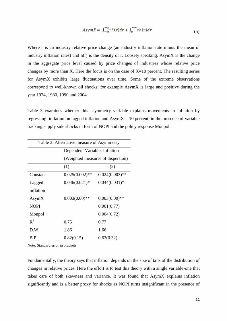
(5)

Where r is an industry relative price change (an industry inflation rate minus the mean of

industry inflation rates) and h(r) is the density of r. Loosely speaking, AsymX is the change

in the aggregate price level caused by price changes of industries whose relative price

changes by more than X. Here the focus is on the case of X=10 percent. The resulting series

for AsymX exhibits large fluctuations over time. Some of the extreme observations

correspond to well-known oil shocks; for example AsymX is large and positive during the

year 1974, 1980, 1990 and 2004.

Table 3 examines whether this asymmetry variable explains movements in inflation by

regressing inflation on lagged inflation and AsymX = 10 percent, in the presence of variable

tracking supply side shocks in form of NOPI and the policy response Monpol.

Table 3: Alternative measure of Asymmetry

Dependent Variable: Inflation

(Weighted measures of dispersion)

(1) (2)

Constant 0.025(0.002)** 0.024(0.003)**

Lagged

inflation

0.046(0.021)* 0.044(0.031)*

AsymX 0.003(0.00)** 0.003(0.00)**

NOPI 0.001(0.77)

Monpol 0.004(0.72)

R2

0.75 0.77

D.W. 1.86 1.66

B.P. 0.82(0.15) 0.63(0.32)

Note: Standard error in brackets

Fundamentally, the theory says that inflation depends on the size of tails of the distribution of

changes in relative prices. Here the effort is to test this theory with a single variable-one that

takes care of both skewness and variance. It was found that AsymX explains inflation

significantly and is a better proxy for shocks as NOPI turns insignificant in the presence of

12

AsymX. That the Monpol variable is also insignificant suggests the dominance of supply

shocks for inflation.

Main Findings:

Changes in the price level are positively related to skewness of relative price changes.

Which leads to inflation in following way: suppose, for example, the distribution of

desired changes in relative prices is skewed to the right. In this case, few firms would

like to make large increases in price, which gets balanced by small desired decreases

by other firms. Since firms respond more quickly to large shocks than to small shocks,

the desired increase occurs more quickly. Thus the average price rises in the short run.

The result suggests menu cost models of price adjustment.

These results suggest that an asymmetry variable is a better measure of supply shocks

than the traditional variables. Traditional variables performed well in earlier studies

because they were acting as proxy for asymmetries.

The results also suggest the relationship between asymmetries and inflation holds

across all time periods. In contrast, energy prices affect inflation only when they have

major effect on asymmetries.

4. Estimation of the Phillips Curve

A large literature on the dynamics of inflation takes the Phillips curve as the starting point of

the analysis. In the Phillips curve literature, inflation depends on past inflation, on supply

shocks and on a measure of the business cycle such as the output gap, or marginal cost, or

unemployment. From this outlook the above regression is like an estimated Phillips curve,

with the omission of a business cycle variable. To relate this study with the Phillips curve

literature, we estimate a Phillips curve for India on the basis of various definitions and then

modify it to include supply shocks. However the supply shock included in the estimation

would not be the traditional variables defining supply shock but the AsymX as defined above.

Data used for estimation of the Phillips curve are WPI, IIP, Interest rates (CMR), exchange

rate and oil prices at monthly frequency. The period of estimation was from 1986M5 to

2010M12. Data is mainly taken from Reserve Bank of India (RBI) website. All variables

were converted into logs and first differenced except for interest rate. IIP was taken as a

measure of output gap and hence the HP detrended series of IIP were taken.

13

4.1 The Traditional Phillips Curve:

The Friedman-Phelps description of the Phillips curve was predicated on the assumption that

expectations about inflation evolved over time as a result of actual past experience— that is,

that expectations were formed adaptively. In empirical evaluations of the hypothesis,

therefore, researchers used a distributed lag of past inflation rates to proxy for expectations,

and then tested whether such proxies received a coefficient of unity:

All the coefficients were significant. The output term enters significantly with a positive sign.

Sum of coefficients on lagged inflation does not differ significantly from unity.

When we include the variable representing asymmetric changes in price (AsymX), the

equation changes to:

Criticism:

This form of Phillips curve strategy was criticized in two remarkable papers by Sargent

(1971) and Lucas (1972). For these economists, the treatment of expectations implicit in

estimates of above equation was deficient in that it was inconsistent with forward looking

rational behavior. Sargent argued (at the time) the U.S. inflation process appeared to be

mean-stationary, so it was quite reasonable for the public to formulate inflation expectations

in a manner that was consistent with mean-reversion. Thus, forcing the distributed lags on

past inflation to sum to one was inconsistent with the forecasts that a rational agent would

make, and would lead to empirical estimates of sum of coefficients to be less than one even if

the hypothesis were correct. In Lucas’s almost simultaneous analysis, the central bank

pursues a monetary policy in which money growth (and hence inflation) is mean stationary,

so reduced-form regressions for inflation would yield values of sum of coefficients less than

one even though agents had rational expectations and the economy by construction did not

manifest a long-run tradeoff between output and inflation.

4.2 The New Phillips Curve

Lucas and Sargent’s introduction of rational expectation into the field of economic modeling

made the traditional Philips curve obsolete. The challenge was then to demonstrate that

persistent effects of nominal disturbances can be obtained in a rational expectations

14

framework. By far the most popular formulation, the new-Keynesian Phillips curve, is based

on Calvo’s (1983) model of firms’ random price adjustment. This formulation has several

advantages, but most important of all is that it provides micro founded formulation of

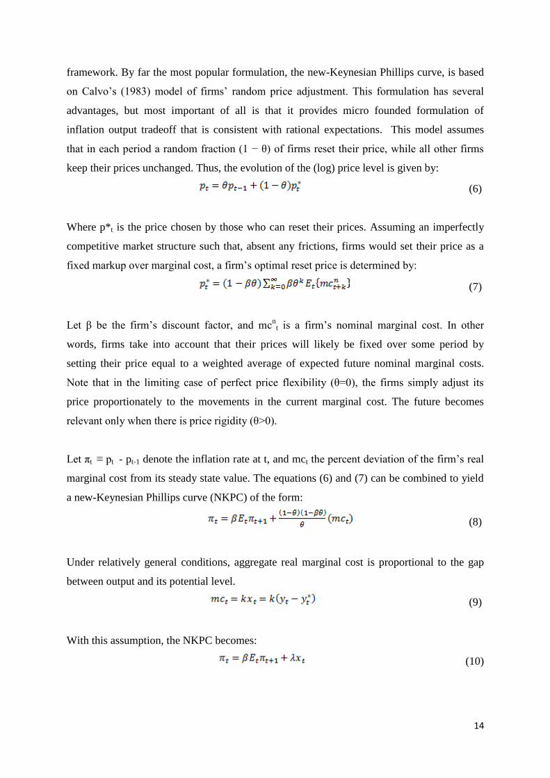
inflation output tradeoff that is consistent with rational expectations. This model assumes

that in each period a random fraction (1 − θ) of firms reset their price, while all other firms

keep their prices unchanged. Thus, the evolution of the (log) price level is given by:

(6)

Where p*t is the price chosen by those who can reset their prices. Assuming an imperfectly

competitive market structure such that, absent any frictions, firms would set their price as a

fixed markup over marginal cost, a firm’s optimal reset price is determined by:

(7)

Let β be the firm’s discount factor, and mcn

t is a firm’s nominal marginal cost. In other

words, firms take into account that their prices will likely be fixed over some period by

setting their price equal to a weighted average of expected future nominal marginal costs.

Note that in the limiting case of perfect price flexibility (θ=0), the firms simply adjust its

price proportionately to the movements in the current marginal cost. The future becomes

relevant only when there is price rigidity (θ>0).

Let πt ≡ pt - pt-1 denote the inflation rate at t, and mct the percent deviation of the firm’s real

marginal cost from its steady state value. The equations (6) and (7) can be combined to yield

a new-Keynesian Phillips curve (NKPC) of the form:

(8)

Under relatively general conditions, aggregate real marginal cost is proportional to the gap

between output and its potential level.

(9)

With this assumption, the NKPC becomes:

(10)

15

Where λ . This model of inflation has several appealing features. As with the

traditional Philips curve, inflation depends positively on the output gap and a ―cost push‖

term that reflects the influence of expected inflation. A key difference is that it is Et{ πt +1} as

opposed to Et-1{ πt } that matters. As a consequence, inflation depends exclusively on the

discounted sequence of future output gaps. This can be seen by iterating equation 10 forward,

which yields:

(11)

Implications:

While standard econometric models include lagged inflation, these lags are often understood

to be proxying for expectations, so the NKPC bears some resemblance to the original Phillips

model. However, the strength of this statistical correlation is likely to vary across monetary

policy regimes: In periods when the Central Bank (CB) has little credibility, the public may

formulate its inflation expectations based on actual recent inflation performance, rather than

on the public statements of the CB. By contrast, if the CB maintains a credible inflation

target, then recent lagged values of inflation may play only a small role in the formulation of

expectations.

Probably the most important implication of the NKPC model is that there is no ―intrinsic‖

inertia in inflation, in the sense that there is no structural dependence of inflation on its own

lagged values. Instead, inflation is determined in a completely forward-looking manner. The

idea that there is considerable inertia in inflation, and hence that it is difficult to reduce

inflation quickly, does not hold in this framework. According to the NKPC, the CB can

costlessly control inflation due to excess demand by committing to keep the output close to

its potential level in the future, although there is a tradeoff between output and inflation

variability under supply shocks.

To estimate equation (10) we used Generalized Methods of Moments (GMM)5 which

removes any simultaneity bias in a single equation. The instruments used to proxy expected

future inflation were; interest rate, exchange rate depreciation, oil price inflation and older

lags of inflation.

5In the GMM technique valid instruments take care of the problem of endogeneity in explanatory variables when

the data distribution function is not known, so maximum likelihood estimation is not applicable

16

We found that all coefficients turned out to be significant. However, coefficient of output gap

comes in with wrong sign. Statistic for J test for over identification is 6.633(0.084) (the null

hypothesis that the model is ―valid‖). F test for weak instruments 271.5 (0.00) (null

hypothesis instruments are weak).

In the presence of AsymX the equation changes to:

Problem with this approach:

When equation (10) of NKPC, which relates inflation to the next period expected inflation

and output gap, is solved forward, we get that inflation should equal a discounted stream of

expected future output gap (11). Thus, the model predicts that higher inflation should lead

increases in output relative to trend. In fact, however, there is little evidence of such a pattern

in the literature and data. The coefficient associated with the output gap is negative and

significant, which is at odds with the theory.

These poor results suggest two possible interpretations: Either the rational-expectations

NKPC provides a bad description of inflation, or else this particular measure of the output

gap is flawed. Perhaps unsurprisingly, the latter explanation has proven popular in recent

years with proponents of the model. Typically, these researchers criticize traditional measures

of the output gap on the grounds that naive detrending procedures assume that potential GDP

evolves smoothly over time. In theory, however, changes in potential output will be affected

by any number of shocks, and so could fluctuate significantly from period to period.

1.3 NKPC Estimation: Industry level analysis

The theoretical model that underpins the NKPC, equation (8), predict that it is real marginal

cost that drives inflation. In recent years this workable model of NKPC has been estimated

using empirical proxies for marginal cost. In particular Gali and Gertler (2000), Gali, Gertler

and Salido (2001) and Shapiro (2007) have proposed using real average unit cost to measure

real marginal cost. This proxy is labor’s share of income.

17

Let’s assume that existing technology takes form of Cobb Douglas function. Let At denote

technology, Kt denote capita; and Nt denote labor. Then output Yt is given by:

(12)

Real marginal cost is then given as ratio of the wage rate to the marginal product of labor.

(13)

Solving for from production function, gives us:

(14)

Denote percent deviation from the steady state by lower case letters, the real marginal cost

can be written as:

(15)

The data we use is yearly for India over the period 1990 to 2008. We use data for prices,

interest rate, fuel consumption, wages (total value = W*N), value of output and quantity for

35 manufacturing industries (three digit NIC code). While marginal cost proxy is calculated

form ASI data, prices are taken as WPI prices at disaggregated level. The resulting estimated

equation is given by:

All coefficients are significant. Coefficient of log of marginal cost comes in with right sign. J

test for over-identification is 7.911(0.063) (the null hypothesis is the model is ―valid‖)

Instruments used were per unit fuel consumption, interest rate, lags of inflation and exchange

rate.

In presence of AsymX:

The mct coefficient is now correctly signed. It is positive, and coefficient is significantly

different from zero. However, the model fails to fully capture the empirical dependence of

18

inflation on its own lagged values. The so-called ―hybrid‖ variant of the NKPC, is the

standard NKPC estimated in the literature.

4.4 Hybrid Phillips Curve

Hybrid Phillips curve became popular as it dealt with the issue of apparent inertia in inflation.

To do so, Gali and Gertler (2000), extended the basic Calvo model to allow a fraction of

firms to use a backward looking rule of thumb to set prices. By doing so they claim to obtain

a measure of the residual inertia in inflation that NKPC leaves unexplained.

In the paper, they continue to assume that each firm is able to adjust its price in any given

period with fixed probability 1-θ as given by equation (1). They also assume that out of those

which are changing their prices in period t, there exist two types of firm. A fraction 1-ω of the

firms are ―forward looking‖, they set prices optimally, given the constraints on the timing of

adjustments and using all the available information to forecast marginal costs. The remaining

firms are backward looking firms; they use a simple rule of thumb that is based on the recent

history of aggregate price behavior.

Let pft denote the price set by forward looking firm at t and p

bt the price set by backward

looking firm. Then the index of newly set prices in period t is given by:

(16)

Now, forward looking firms behave exactly as in the baseline Calvo model described by

equation (7). But backward looking firms obey a rule of thumb which has following two

features: first, there are no persistent deviations between the rule and optimal behavior; that is

in steady state the rule is consistent with optimal behavior. Second, the price in period t,

given by the rule, depends only on information dated t-1 or earlier.

Therefore the backward looking firms follow the rule given by:

(17)

Which states that a firm set its price equal to the average price set in the t-1 period, with a

correction for inflation. It also reflects that lagged inflation is used in a simple way to forecast

current inflation.

19

Combining all the above expressions with equation (6) gives us the hybrid Philips curve

Where:

In this specification, all the coefficients are explicit functions of three model parameters: θ,

which measures the degree of price stickiness; ω, measures the degree of backwardness in

price settings and the discount factor β.

The empirical version of the hybrid Philips curve is estimated as

Coefficient of log of marginal cost comes in with right sign. J test for over-identification

0.218 (0.896) (the null hypothesis is that the model is ―valid‖). Sum of coefficients on both

lagged and lead inflation does not differ significantly from unity.

Structural estimates:

The parameter θ is estimated to be about 0.516. The parameter ω is estimated to be about

0.34 that is 34 percent of the prices setting industries are backward looking. The parameter β

came out to be 0.96

Final form of NKPC with AsymX:

In all the above mentioned cases, though AsymX comes in with small coefficients but has

always been significant. We interpret the coefficients on the asymmetry variable as showing

how this variable shifts the short run inflation and some output gap or marginal cost measure.

However, there are two fundamental problems that we can attribute to using the labor income

share as our proxy for real marginal cost: firstly, the labor share of income is countercyclical,

whereas theory suggests marginal cost should be procyclical; and second, the assumption

20

used in order to obtain the labor income share as the proxy for real marginal cost is overly

restrictive.

Conclusion

The paper examines different ways in which relative price shocks affect the price level and

then inflation. Using India data we found evidence that: Average price increase over time is

greater than average price decrease. While price increase is around 10 percent price decrease

is less than 5 percent. It takes around one year for Indian markets to change price of the

products implying both real and nominal rigidities in the market. Changes in the price level

are positively related to skewness of relative price changes. There is evidence for menu cost

models of price adjustment.

The results also suggest that the asymmetry variable is better measure of supply shocks than

the traditional variables. And traditional variables performed well in earlier studies because

they were acting as proxy for asymmetries. Model also confirms that the relationship between

asymmetries and inflation holds across all time periods. In contrast energy prices affect

inflation only when they have major effect on asymmetries.

Such distribution based measures of supply shocks perform better than traditional measures,

such as prices of energy and food, in regressions explaining inflation. They moderate the

price puzzle, whereby a rise in policy rates increases inflation, and are significant in

estimations of New Keynesian aggregate supply. Our results show that an average Indian

firm changes prices about once in a year, the estimated Calvo parameter implies half of

Indian firms reset their prices in any period, and 66 percent of firms are forward looking in

their price setting.

These estimated real and nominal price rigidities imply that a sharp policy response to a rise

in expected future excess demand can prevent 66 percent of firms from raising prices. Since

the higher prices would persist for about a year, policy that anchored inflation expectations

would reduce persistence of inflation. This is without any cost to output since inflation is

reduced by reducing future, not current, output gaps.

However, about 34 percent of firms are backward looking, so there would be some

persistence of inflation and lagged effects of policy rate changes. Since supply shocks affect

21

inflation independently of demand, there is an output cost in reducing demand in response to

a supply shock. Therefore policy may allow the price level effect of a temporary price shock

without tightening, or consider alternatives such as a temporary appreciation that can

neutralize the supply shock.

References:

Álvarez, Luis J. and Ignacio Hernando (2006), Price Setting Behavior in Spain. Evidence

from Consumer Price Micro-data, Economic Modeling 23, 699-716.

Ball, L. and Mankiw Gregory, (1994) Asymmetric Price adjustment and Economic

Fluctuations, The Economic Journal,104 (423), 247-62.

Ball, L. and Mankiw Gregory, (1995) Relative-Price Changes as Aggregate Supply Shocks,

Quarterly Journal of Economics, 110 (1), 161-93

Barros, Rebecca, Marco Bonomo, Carlos Carvalho, and Silvia Matos (2009), Price Setting in

a Variable Macroeconomic Environment: Evidence from Brazilian CPI, unpublished paper,

Getulio Vargas Foundation and Federal Reserve Bank of New York.

Bernanke, Ben S. (1983), Irreversibility, Uncertainty, and Cyclical Investment, Quarterly

Journal of Economics 98 (February), 85-106.

Bernanke, Ben S., and Alan S. Blinder (1992), The Federal Funds Rate and the Channels of

Monetary Transmission, American Economic Review 82 (September), 901–21.

Blinder, Alan S., Elie Canetti, David Lebow, and Jeremy Rudd (1998), Asking About Prices:

A New Approach to Understanding Price Stickiness. New York: Russell Sage Foundation.

Bunn, Philip and Colin Ellis (2009), Price-Setting Behaviour in the United Kingdom: A

Microdata Approach, Bank of England Quarterly Bulletin, 2009 Q1.

Calvo, Guillermo A. (1983). Staggered Prices in a Utility-Maximizing Framework, Journal

of Monetary Economics 12 (3), 383–398.

Dias, Mónica, Daniel Dias and Pedro D. Neves (2004), ―Stylised Features of Price Setting

Behaviour in Portugal: 1992-2001,‖ ECB Working Paper 332.

Fabiani, Silvia, Martine Druant, Ignacio Hernando, Claudia Kwapil, Bettina Landau, Claire

Loupias, Fernando Martins, Thomas Y. Mathä, Roberto Sabbatini, Harald Stahl, and Ad C.

J. Stokman (2005). The Pricing Behavior of Firms in the Euro Area: New Survey

Evidence, ECB Working Paper 535.

Ferderer, J. Peter. (1996) Oil Price Volatility and the Macroeconomy, Journal of

Macroeconomics 18, 1-16.

22

Gabriel, Peter and Adam Reiff (2008), Price setting in Hungary – a Store-level Analysis,

unpublished paper, Magyar Nemzeti Bank.

Galí, Jordi, and Mark Gertler (2000). Inflation Dynamics: A Structural Econometric

Analysis, Journal of Monetary Economics 44 (2), 195–222.

Galí, Jordi, Mark Gertler, J. David López-Salido (2001). European Inflation Dynamics,

European Economic Review 45 (7), 1237–1270.

Gautier, Erwan (2008). The Behaviour of Producer Prices: Some Evidence from the French

PPI Micro Data, Empirical Economics, 35 (September): 301-332.

Goldberg, Pinelopi K. and Rebecca Hellerstein (2009). How Rigid are Producer Prices,

FRBNY Staff Report 407.

Hamilton, James D. (1996), This is What Happened to the Oil Price-Macroeconomy

Relationship, Journal of Monetary Economics 38 (2), 215-20.

Horvath, Roman. (2011). The Frequency and Size of Price Changes: Evidence from non-

parametric estimation. Macroeconomics and Finance in Emerging Market Economies, 4 (2):

263-268.

Lilien, David (1982), Sectoral Shifts and Cyclical Unemployment, Journal of Political

Economy 90 (4), 777-93.

Loungani, Prakash. (1986), Oil Price Shocks and the Dispersion Hypothesis, Review of

Economics and Statistics 68 (3), 536-39.

Lucas, Robert Jr., 1972. Expectations and the neutrality of money, Journal of Economic

Theory, Elsevier, 4(2), pages 103-124,

Mankiw, G. (1985). Small Menu Costs and Large Business Cycles: A Macroeconomic

Model, The Quarterly Journal of Economics, 100(2), 529-538

Medina, Juan Pablo, David Rappoport, and Claudio Soto (2007), ―Dynamics of Price

Adjustment: Evidence from Micro Level Data for Chile,‖ Central Bank of Chile Working

Paper 432

Klenow, P. and Malin, B. (2010). Microeconomic Evidence on Price Setting, NBER WP, No.

15826.

Mork, Knut Anton. (1989) Oil Shocks and the Macroeconomy When Prices Go Up and

Down: An Extension of Hamilton’s Results, Journal of Political Economy 97 (3), 740-44.

Pindyck, Robert,(1991) Irreversibility, Uncertainty, and Investment, Journal of Economic

Literature 29 (3), 1110-48.

Rotemberg, J. (1982). Sticky Prices in the United States, Journal of Political Economy, 90

(3), 1187-1211

23

Sargent, Thomas J. 1971. Interest rates and prices in the long run: a study of the Gibson

paradox, Working Papers 75, Federal Reserve Bank of Minneapolis

Shapiro, Adam Hale. (2008) Estimating the New Keynesian Phillips Curve: A Vertical

Production Chain Approach, Journal of Money, Credit and Banking, Blackwell Publishing,

vol. 40(4), pages 627-666.

Sims, Christopher A. (1992), Interpreting the Macroeconomic Time Series Facts: The Effects

of Monetary Policy, European Economic Review 36 (June): 975 –1000.

Appendix

Kernel density

[f,yi] = ksdensity(y)

f = ksdensity(y,yi)

plot(yi,f);

Spline function:

y=TR; %TR is my signal

x=1:30000; % time axis

b=1:10:30000; % knots

a=spline(b,y(:)'/spline(b,eye(length(b)),x(:)'));

v=ppval(x,a);

plot(x,y,'*',x,v,'.')

Table A1. Statistics used in the Regression

Years Inflation SD Skew Laginf SD*Skew NOPI Monpol AsymX

1973 0.08 0.13 2.07 0.04 0.26 8.78 1.95 10.61

1974 0.10 0.17 2.55 0.08 0.43 167.85 6.88 20.30

1975 0.00 0.10 0.05 0.10 0.00 7.59 -3.12 -4.13

1976 0.01 0.06 0.41 0.00 0.03 13.31 0.88 -1.68

1977 0.02 0.07 0.86 0.01 0.06 13.05 -1.10 -1.05

1978 0.00 0.08 -0.73 0.02 -0.06 3.88 -2.13 -4.45

1979 0.07 0.12 3.32 0.00 0.40 50.87 0.42 6.77

1980 0.07 0.13 3.61 0.07 0.47 66.82 -1.23 8.03

1981 0.04 0.09 1.67 0.07 0.15 0.00 1.37 0.41

1982 0.01 0.08 -0.75 0.04 -0.06 0.00 -1.34 -2.04

24

1983 0.03 0.06 1.56 0.01 0.09 0.00 1.03 -0.23

1984 0.03 0.05 1.39 0.03 0.07 0.00 1.65 -0.57

1985 0.02 0.08 2.28 0.03 0.18 0.00 0.05 -2.66

1986 0.02 0.06 2.45 0.02 0.15 0.00 -0.05 0.46

1987 0.03 0.07 2.06 0.02 0.14 33.84 -0.12 1.34

1988 0.03 0.08 1.67 0.03 0.14 0.00 -0.10 -2.99

1989 0.03 0.07 2.23 0.03 0.16 23.29 1.66 0.12

1990 0.04 0.06 2.00 0.03 0.13 24.51 4.18 2.35

1991 0.06 0.09 1.96 0.04 0.18 0.00 3.78 3.75

1992 0.04 0.12 1.30 0.06 0.16 0.00 -4.11 1.76

1993 0.03 0.05 1.59 0.04 0.08 0.00 -6.60 -0.84

1994 0.05 0.17 6.75 0.03 1.16 0.00 -1.50 12.30

1995 0.03 0.17 -7.21 0.05 -1.20 7.26 8.44 -2.28

1996 0.02 0.06 -1.12 0.03 -0.07 20.07 -4.53 -1.00

1997 0.02 0.06 1.72 0.02 0.10 0.00 -5.75 -2.17

1998 0.03 0.07 2.41 0.02 0.16 0.00 2.72 0.91

1999 0.01 0.05 -0.33 0.03 -0.02 32.95 0.84 -2.63

2000 0.03 0.07 2.36 0.01 0.17 58.17 0.41 0.73

2001 0.02 0.04 3.13 0.03 0.14 0.00 -1.61 -1.22

2002 0.01 0.05 2.06 0.02 0.11 0.95 -1.50 -1.09

2003 0.02 0.07 5.09 0.01 0.34 19.07 -1.19 0.09

2004 0.03 0.08 5.69 0.02 0.44 33.29 -0.40 2.42

2005 0.02 0.05 0.20 0.03 0.01 36.19 0.52 -2.41

2006 0.02 0.04 1.87 0.02 0.07 17.02 1.38 0.35

2007 0.02 0.06 0.81 0.02 0.05 9.44 0.29 -1.44

2008 0.04 0.07 4.30 0.02 0.29 37.77 1.02 1.23

2009 0.02 0.09 3.20 0.04 0.30 0.00 -4.22 -1.22

2010 0.03 0.01 2.52 0.02 0.02 28.71 0.59 -0.81

Inflation: refers to year on year change in log WPI index over all commodities.

Laginf: WPI Inflation with one period lag.

25

SD: standard deviation of the log wholesale price changes for each year in our sample.

Skew: skewness of the log industry price changes for each year in our sample.

NOPI: net oil price increase as defined by Hamilton

MonPol: Change in call money rate.

AsymX: variable measuring asymmetric behavior of prices as defined in the text.