Relative Abundances of Mineral Species: A Statistical ...
16
Math Geosci DOI 10.1007/s11004-016-9661-y Relative Abundances of Mineral Species: A Statistical Measure to Characterize Earth-like Planets Based on Earth’s Mineralogy Grethe Hystad 1 · Robert T. Downs 2 · Robert M. Hazen 3 · Joshua J. Golden 2 Received: 7 December 2015 / Accepted: 15 October 2016 © International Association for Mathematical Geosciences 2016 Abstract The mineral frequency distribution of Earth’s crust provides a mineralogy- based statistical measure for characterizing Earth-like planets. It has previously been shown that this distribution conforms to a generalized inverse Gauss–Poisson large number of rare events model. However, there is no known analytic expression for the probability distribution of this model; therefore, the population probabilities do not exist in closed forms. Consequently, in this paper, the population probabilities are calculated numerically for all mineral species in Earth’s crust, including the pre- dicted undiscovered species. These population probabilities provide an estimate of the occurrence probabilities of species in a random sample of N mineral species–locality pairs. These estimates are used to characterize Earth in terms of its mineralogy. The study demonstrates that Earth is mineralogically unique in the cosmos. In spite of this uniqueness, the frequency distribution of minerals from Earth can be used to quantify the extent to which another planet is Earth-like. Quantitative criteria for characterizing Earth-like planets are given. An example, involving mineral species found on Mars by the CheMin instrument during the Mars Science Laboratory mission suggests that Mars is mineralogically similar to an Earth-like planet. Keywords Statistical mineralogy · Mineral frequency distribution · Large number of rare events distribution · Mineral ecology · Earth-like planets · Mars mineralogy B Grethe Hystad [email protected] 1 Mathematics, Statistics, and Computer Science, Purdue University Northwest, 2200 169th Street, Hammond, IN 46323-2094, USA 2 Department of Geosciences, University of Arizona, Tucson, AZ 85721-0077, USA 3 Geophysical Laboratory, Carnegie Institution for Science, Washington, DC 20015, USA 123
Transcript of Relative Abundances of Mineral Species: A Statistical ...
Math GeosciDOI 10.1007/s11004-016-9661-y
Relative Abundances of Mineral Species: A StatisticalMeasure to Characterize Earth-like Planets Basedon Earth’s Mineralogy
Grethe Hystad1 · Robert T. Downs2 ·Robert M. Hazen3 · Joshua J. Golden2
Received: 7 December 2015 / Accepted: 15 October 2016© International Association for Mathematical Geosciences 2016
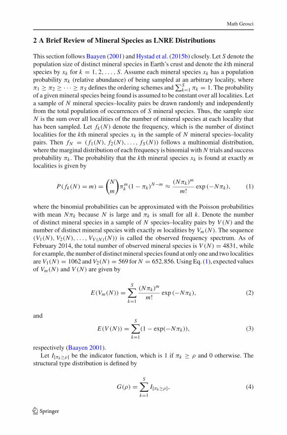
Abstract The mineral frequency distribution of Earth’s crust provides a mineralogy-based statistical measure for characterizing Earth-like planets. It has previously beenshown that this distribution conforms to a generalized inverse Gauss–Poisson largenumber of rare events model. However, there is no known analytic expression forthe probability distribution of this model; therefore, the population probabilities donot exist in closed forms. Consequently, in this paper, the population probabilitiesare calculated numerically for all mineral species in Earth’s crust, including the pre-dicted undiscovered species. These population probabilities provide an estimate of theoccurrence probabilities of species in a random sample of N mineral species–localitypairs. These estimates are used to characterize Earth in terms of its mineralogy. Thestudy demonstrates that Earth is mineralogically unique in the cosmos. In spite of thisuniqueness, the frequency distribution of minerals from Earth can be used to quantifythe extent to which another planet is Earth-like. Quantitative criteria for characterizingEarth-like planets are given. An example, involving mineral species found on Marsby the CheMin instrument during the Mars Science Laboratory mission suggests thatMars is mineralogically similar to an Earth-like planet.
Keywords Statistical mineralogy · Mineral frequency distribution · Large number ofrare events distribution · Mineral ecology · Earth-like planets · Mars mineralogy
B Grethe [email protected]
1 Mathematics, Statistics, and Computer Science, Purdue University Northwest,2200 169th Street, Hammond, IN 46323-2094, USA
2 Department of Geosciences, University of Arizona, Tucson, AZ 85721-0077, USA
3 Geophysical Laboratory, Carnegie Institution for Science, Washington, DC 20015, USA
123

Math Geosci
1 Introduction
Humans have long asked questions about their place in the cosmos. How did Earthform? How did life emerge? Are we alone in the universe? What constitutes an Earth-like planet and its requisite life-generating processes is a pervasive theme in planetaryscience and astrobiology. However, a comprehensive definition of Earth-like planetdoes not exist, in part because each research group tends to emphasize their particularscientific specialty (Ward and Brownlee 2003; Hystad et al. 2015a). For instance, inthe study of (Donahoe 1966), the definition of Earth-like planets was related to thecomposition of the atmosphere, whereas Seager (2003) emphasized the gravitationalrelationship between a star and its potential Earth-like planets and the importanceof direct detection of planetary radiation. The Kepler spacecraft was launched byNASA in 2009 to search for Earth-size planets that occur near the habitable zoneof solar-like stars by monitoring the brightness patterns of the stars during planetarytransits (Borucki et al. 2003, 2008). Hystad et al. (2015a) suggested mineralogicalcriteria for classification as Earth-like, based on the relationship between diversity anddistribution of near-surface beryllium mineral species. The distribution of berylliumminerals was chosen because a comprehensive study on these minerals had alreadybeen completed and the data were readily available (Grew and Hazen 2014). Theprobability distribution of Earth’s beryllium minerals was found to exist in a closedform, for which simulations could easily be made. The paper of Hystad et al. (2015a)argued that, in spite of deterministic physical, chemical, and biological factors thatcontrol most of the planet’s mineral diversity, Earth’s mineralogy is unique in thecosmos.
The data in the present study consist of a list of mineral species and their localitiesas of February 2014 from the crowd-sourced web site Mindat.org. There are 135,415distinct localities and, when counted over all mineral species, these data provide asample size of 652,856 observations, where each observation is a unique mineralspecies–locality pair. The mineral species frequency distribution, which records thenumber of localities for each mineral species, is right skewed with a heavy tail (Hystadet al. 2015b). As of February 2014, there were 4831 approvedmineral species reportedfrom Earth’s crust, where 22 % of the mineral species are found at only one locality,12 % are found at only two localities, while more than half of all mineral speciesare found at five or fewer localities. Hazen et al. (2015a) suggested that the mineralfrequency distribution in Earth’s near-surface environment, as well as on other ter-restrial planets and moons, is a consequence of both deterministic factors and chanceevents.
Hystad et al. (2015b) introduced a population model for the mineral species fre-quency distribution in Earth’s crust. The mineral species coupled with their localitiesconforms to a large number of rare events (lnre) distribution since most of Earth’smineral species are rare, known from only a few localities worldwide. Lnre modelsformulated in terms of a type distribution allow the estimation of Earth’s undiscov-ered mineralogical diversity and the prediction of the percentage of observed mineralspecies that would differ if Earth’s history were replayed. The sample relative fre-quency of each mineral species tends to overestimate the corresponding populationprobability because there is no knowledge about the weight of the unobserved por-
123

Math Geosci
tion of the distribution. A parametric model from the family of lnre models that takesinto account the unobserved species was used to handle this problem in the study byHystad et al. (2015b). The mineral frequency spectrum of all mineral species on Earthconforms to the generalized inverse Gauss–Poisson structural type (giGP) lnre model(Hystad et al. 2015b). Most subsets of the mineral species frequency spectrum fit intothe giGP lnre model and/or the finite Zipf–Mandelbrot (fZM) lnre model (Hazen et al.2015b). For example, the frequency spectrum of beryllium mineral species conformsto the fZM lnre model (Hystad et al. 2015a), which carries the advantage of a knownanalytic form for the probability distribution. The population probabilities can then befound in closed forms. There is no known analytic form reported for the probabilitydistribution of the giGP model (Evert and Baroni 2008).
The objective of this paper is to numerically calculate the relative abundances forall mineral species in Earth’s crust, including the undiscovered species. The paperbuilds on the results given by Hystad et al. (2015b), which included an estimate ofthe total number of undiscovered mineral species on Earth. Computing these popu-lation probabilities provides a statistical measure to characterize Earth-like planetsbased on their mineralogy. In the study by Hystad et al. (2015a), the argument thatEarth is unique in the cosmos was based on a calculation involving the relationshipbetween beryllium-containing minerals to all mineral species. In this paper, a moreaccurate estimate of the probability of duplicating Earth’s mineralogy on an Earth-likeplanet is provided. Subsequently, Monte Carlo simulations with samples drawn froma multinomial distribution with the population probabilities as the marginal distribu-tions can be made. These bootstraps samples are used to obtain standard errors for theestimated population size of all mineral species, as well as error estimates for the threefree parameters of the giGP lnre model that were not included in the paper of Hystadet al. (2015b). Finally, using the population probabilities, samples from the populationof mineral species from two Earth-like planets can be simulated to predict the num-ber of mineral species that would be different if Earth’s history were to be replayed.The simulation method leads to the same estimate as the method of extrapolating thespecies accumulation curve that was derived from the giGP lnre model, as given byHystad et al. (2015b).
A replay of Earth’s history requires knowledge of how the mineral frequency distri-bution changes with time. Hazen and coworkers (Grew and Hazen 2014; Hazen et al.2008, 2011) demonstrated that the diversity and distribution of minerals on Earthhas evolved through a combination of physical, chemical, and biological processesover a period of more than 4.5 billion years. For example, 4.56 billion years ago,the Solar nebula incorporated approximately 60 different mineral species, whereas3 billion years ago an estimated 1500 mineral species occurred on Earth (Hazenet al. 2008). As a result of co-evolution of the geo- and biospheres, Hystad et al.(2015b) predicted that there are, as of February 2014, 1563 not-yet-observed speciesin addition to 4831 known species for a total of 6394 mineral species in Earth’s crust.Clearly, the characterization of Earth-like planets should be based on the mineral-ogy of Earth at any time in its evolution. Unfortunately, the important variable oftime cannot be addressed in this paper until age data are available for all mineralspecies.
123
Math Geosci
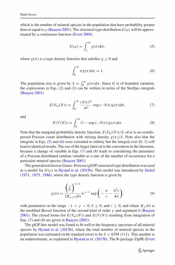
2 A Brief Review of Mineral Species as LNRE Distributions
This section follows Baayen (2001) and Hystad et al. (2015b) closely. Let S denote thepopulation size of distinct mineral species in Earth’s crust and denote the kth mineralspecies by xk for k = 1, 2, . . . , S. Assume each mineral species xk has a populationprobability πk (relative abundance) of being sampled at an arbitrary locality, whereπ1 ≥ π2 ≥ · · · ≥ πS defines the ordering schemes and
∑Sk=1 πk = 1. The probability
of a given mineral species being found is assumed to be constant over all localities. Leta sample of N mineral species–locality pairs be drawn randomly and independentlyfrom the total population of occurrences of S mineral species. Thus, the sample sizeN is the sum over all localities of the number of mineral species at each locality thathas been sampled. Let fk(N ) denote the frequency, which is the number of distinctlocalities for the kth mineral species xk in the sample of N mineral species–localitypairs. Then fN = ( f1(N ), f2(N ), . . . , fS(N )) follows a multinomial distribution,where themarginal distribution of each frequency is binomial with N trials and successprobability πk . The probability that the kth mineral species xk is found at exactly mlocalities is given by
P( fk(N ) = m) =(N
m
)
πmk (1 − πk)
N−m ≈ (Nπk)m
m! exp (−Nπk), (1)
where the binomial probabilities can be approximated with the Poisson probabilitieswith mean Nπk because N is large and πk is small for all k. Denote the numberof distinct mineral species in a sample of N species–locality pairs by V (N ) and thenumber of distinct mineral species with exactly m localities by Vm(N ). The sequence(V1(N ), V2(N ), . . . , VV (N )(N )) is called the observed frequency spectrum. As ofFebruary 2014, the total number of observed mineral species is V (N ) = 4831, whilefor example, the number of distinctmineral species found at only one and two localitiesare V1(N ) = 1062 and V2(N ) = 569 for N = 652,856.UsingEq. (1), expected valuesof Vm(N ) and V (N ) are given by
E(Vm(N )) =S∑
k=1
(Nπk)m
m! exp (−Nπk), (2)
and
E(V (N )) =S∑
k=1
(1 − exp(−Nπk)), (3)
respectively (Baayen 2001).Let I[πk≥ρ] be the indicator function, which is 1 if πk ≥ ρ and 0 otherwise. The
structural type distribution is defined by
G(ρ) =S∑
k=1
I[πk≥ρ], (4)
123
Math Geosci
which is the number of mineral species in the population that have probability greaterthan or equal to ρ (Baayen 2001). The structural type distributionG(ρ)will be approx-imated by a continuous function (Evert 2004)
G(ρ) =∫ ∞
ρ
g(π)dπ, (5)
where g(π) is a type density function that satisfies g ≥ 0 and
∫ ∞
0πg(π)dπ = 1. (6)
The population size is given by S = ∫ ∞0 g(π)dπ . Since G is of bounded variation,
the expressions in Eqs. (2) and (3) can be written in terms of the Stieltjes integrals(Baayen 2001)
E(Vm(N )) =∫ ∞
0
(Nπ)m
m! exp (−Nπ)g(π)dπ, (7)
and
E(V (N )) =∫ ∞
0(1 − exp (−Nπ))g(π)dπ. (8)
Note that the marginal probability density function, E(Vm(N ))/S, of m is an overdis-persed Poisson count distribution with mixing density g(π)/S. Note also that theintegrals in Eqs. (5) and (6) were extended to infinity but the integral over [0, 1] willlead to identical results. The use of the larger interval is the convention in the literature,because a change of variable in Eqs. (7) and (8) leads to considering the parameterof a Poisson-distributed random variable as a rate of the number of occurrence for aparticular mineral species (Baayen 2001).
The generalized inverseGauss–Poisson (giGP) structural type distributionwas usedas a model for G(ρ) in Hystad et al. (2015b). This model was introduced by Sichel(1971, 1975, 1986), where the type density function is given by
g(π) =
(2bc
)γ+1
2Kγ+1(b)πγ−1 exp
(
− π
c− b2c
4π
)
, (9)
with parameters in the range −1 < γ < 0, b ≥ 0, and c ≥ 0, and where Kγ (b) isthe modified Bessel function of the second kind of order γ and argument b (Baayen2001). The closed forms for E(Vm(N )) and E(V (N )) resulting from integration ofEqs. (7) and (8) are given in Baayen (2001).
The giGP lnre model was found to fit well to the frequency spectrum of all mineralspecies by Hystad et al. (2015b), where the total number of mineral species in thepopulation was estimated (with standard error) to be S = 6394 (111). This number isan underestimate, as explained in Hystad et al. (2015b). The R-package ZipfR (Evert
123
Math Geosci
and Baroni 2007, 2008) was employed to fit the model, where the parameters wereestimated by minimizing, through the Nelder–Mead algorithm, the simplified versionof the multivariate Chi-squared test for goodness-of-fit using the first 11 spectrumelements. The parameters (with standard errors) are γ = −0.42 (0.01), b = 0.0132(0.0003), and c = 0.014 (0.001), with χ2 = 10.36, d f = 13, and p value = 0.66(Hystad et al. 2015b).
3 Relative Abundances of Mineral Species in Earth’s Crust
In this section, the relative abundances (population probabilities) for allmineral speciesin Earth’s crust are calculated numerically. Knowing the population probabilities willallow the simulationof samples taken from the estimatedpopulationofmineral species.Furthermore, it enables the calculation of standard errors of the estimates of the para-meters in the giGP lnremodel and for the population size S usingmultinomial bootstrapsampling.
Recall from the previous section that the number ofmineral species in the populationwith probably greater than or equal to ρ is approximated by the continuous function
G(ρ) =∫ 1
ρ
g(π)dπ, (10)
where g(π) is the type density function given in Eq. (9). Here, the upper limit of theintegral was restricted to 1 since the type probabilities are in the interval 0 < π < 1.The structural type distribution given in Eq. (4) is a step function with G(πk) = ksince there are k mineral species with probability greater than or equal to πk , namelyx1, x2, . . . , xk (Evert 2004). Using the continuous approximation to G in Eq. (10), theequation of interest isG(ρk) = k, where the population probabilitiesπk asymptoticallyare equal to ρk for k = 1, 2, . . . , 6394 = S.
Define the function f : (0, 1) → R, where f (ρk) = G(ρk) − k. Notice thatf ′(ρk) = G ′(ρk) = −g(ρk). To solve the equation f (ρk) = 0, the Newton–Raphsonmethod is employed. Letρ(l)
k denote the lth iterated value ofρk in theNewton–Raphsonalgorithm. Then
ρ(l+1)k = ρ
(l)k + G(ρ
(l)k ) − k
g(ρ(l)k )
,
for l = 0, 1, 2, . . . , L , where ρk = ρ(L+1)k for some positive integer L .
Define the interval I = [ρk − ε, ρk + ε] for some ε ≥ |ρk −ρ(0)k | with ρk > ε > 0,
where ρ(0)k is the initial value in the Newton–Raphson algorithm. It is easy to check
that f ′(ρ) = −g(ρ) is different from zero and f ′′(ρ) = −g′(ρ) is continuous andbounded for ρ in I . The initial value ρ
(0)k can be chosen sufficiently close to ρk such
that the convergence is quadratic (Ryaben’kii and Tsynkov 2006) (in this paper, thebisection method was used to find the initial values ρ
(0)k ). Using Eq. (6), define for
0 ≤ ρ ≤ 1
123
Math Geosci
F(ρ) =∫ 1
ρ
πg(π)dπ.
Then the population probabilities πk are given by
π1 = F(ρ1) =∫ 1
ρ1
πg(π)dπ, (11)
πk = F(ρk) − F(ρk−1) =∫ ρk−1
ρk
πg(π)dπ, (12)
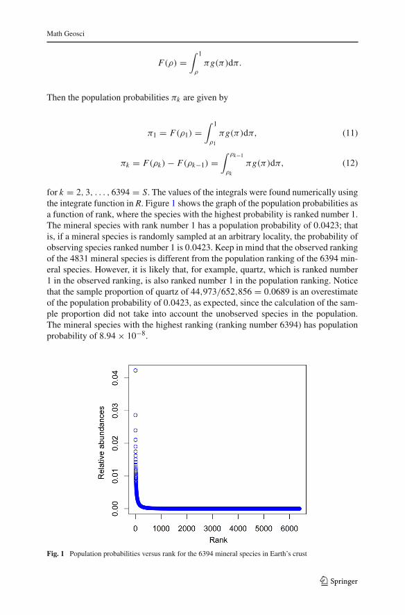
for k = 2, 3, . . . , 6394 = S. The values of the integrals were found numerically usingthe integrate function in R. Figure 1 shows the graph of the population probabilities asa function of rank, where the species with the highest probability is ranked number 1.The mineral species with rank number 1 has a population probability of 0.0423; thatis, if a mineral species is randomly sampled at an arbitrary locality, the probability ofobserving species ranked number 1 is 0.0423. Keep in mind that the observed rankingof the 4831 mineral species is different from the population ranking of the 6394 min-eral species. However, it is likely that, for example, quartz, which is ranked number1 in the observed ranking, is also ranked number 1 in the population ranking. Noticethat the sample proportion of quartz of 44,973/652,856 = 0.0689 is an overestimateof the population probability of 0.0423, as expected, since the calculation of the sam-ple proportion did not take into account the unobserved species in the population.The mineral species with the highest ranking (ranking number 6394) has populationprobability of 8.94 × 10⁻⁸.
Fig. 1 Population probabilities versus rank for the 6394 mineral species in Earth’s crust
123
Math Geosci
4 Differences in the Number of Mineral Species from Two ModeledEarth-like Planets
In the study by Hystad et al. (2015b), the expected number of mineral species thatwill be different in two random samples of the same size from two modeled Earth-likeplanets was estimated by extrapolating from the expected species accumulation curveusing the giGP lnre model from size N to 2N . The resulting value was multiplied by 2to estimate the number of different mineral species distributed over the two samples.Because the population probabilities for findingmineral species at an arbitrary localityare now estimated, the differences between randomly generated samples from theestimated population ofmineral species can bemodeled.Onemeasure of the differencebetween two randomly generated samples is the number of minerals in one sample thatare not in the other. Thus, two randomsamples of size N = 652,856 are generated fromthe multinomial distribution with the probabilities computed in Sect. 3 as the marginaldistributions. Two thousand pairs of simulations, called A and B, are generated. Themineral species of simulationAare comparedwith those of simulationB; the differenceis defined as the number of species in A that are not in B plus the number of speciesin B that are not in A; that is, the number of species that are not common to A and Bor the symmetric difference of A and B. The average value of the differences betweenthese two samples is then calculated. This value is the estimated true value of theexpected number of different species in two random samples from the population ofmineral species. This number was found to be 1324 with a standard error of 28, whichis the same number as computed by Hystad et al. (2015b) using extrapolation fromthe species accumulation curve. The standard errors given in Sect. 2 of the estimatedparameters in the giGP lnre model, as well as for the estimated population size S, arealso computed using the 2000 bootstrap samples from the multinomial distribution.
5 How to Characterize Earth-like Planets
In this section, probabilities for the occurrence of each of the 6394 mineral species in arandom sample of N = 652,856 mineral species–locality pairs from Earth’s crust areestimated using the relative abundances outlined in Sect. 3. Subsequently, the numberof mineral species that should be present in a random sample of size N mineralspecies–locality pairs is determined for varying values of N . These results provide astatistical measure to characterize Earth-like planets in terms of their mineralogy usinga snapshot of the surface of today’s Earth. Finally, it will be shown that even thoughEarth is mineralogically unique in the Universe, there are mineralogical criteria thatcan be used to quantify how Earth-like a given planet might be.
Using the binomial distribution in Eq. (1) and the estimated relative abundances πk
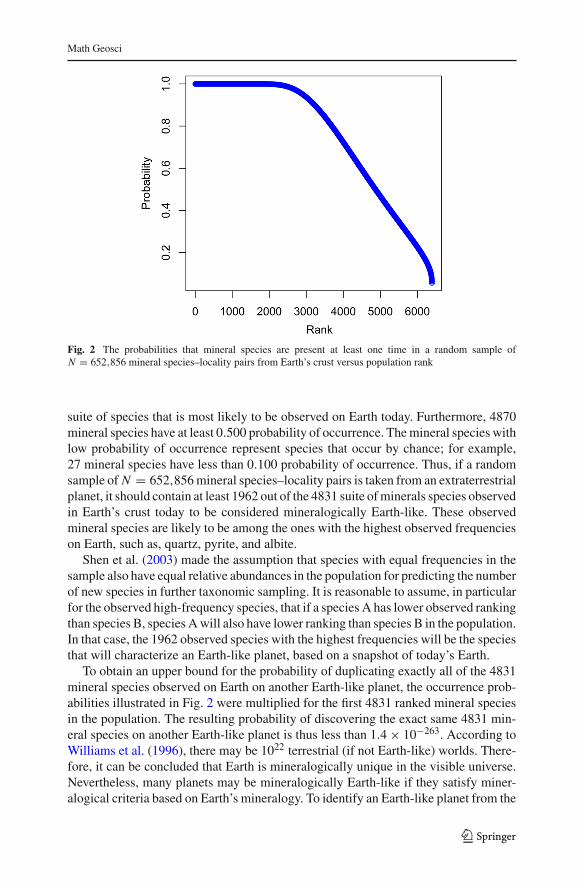
outlined in Eqs. (11) and (12), the probabilities were calculated that each of themineralspecies in the population will occur at least once in a random sample of N = 652,856mineral species–locality pairs from Earth’s crust. The results are illustrated in Fig. 2.Rounded to three decimal places, there are 1962 mineral species with greater than0.999 probability of occurring on all Earth-like planets, whereas 2908 mineral specieshave at least a 0.950 probability of occurrence. These mineral species represent the
123
Math Geosci
Fig. 2 The probabilities that mineral species are present at least one time in a random sample ofN = 652,856 mineral species–locality pairs from Earth’s crust versus population rank
suite of species that is most likely to be observed on Earth today. Furthermore, 4870mineral species have at least 0.500 probability of occurrence. Themineral species withlow probability of occurrence represent species that occur by chance; for example,27 mineral species have less than 0.100 probability of occurrence. Thus, if a randomsample of N = 652,856mineral species–locality pairs is taken from an extraterrestrialplanet, it should contain at least 1962 out of the 4831 suite ofminerals species observedin Earth’s crust today to be considered mineralogically Earth-like. These observedmineral species are likely to be among the ones with the highest observed frequencieson Earth, such as, quartz, pyrite, and albite.
Shen et al. (2003) made the assumption that species with equal frequencies in thesample also have equal relative abundances in the population for predicting the numberof new species in further taxonomic sampling. It is reasonable to assume, in particularfor the observed high-frequency species, that if a species A has lower observed rankingthan species B, species Awill also have lower ranking than species B in the population.In that case, the 1962 observed species with the highest frequencies will be the speciesthat will characterize an Earth-like planet, based on a snapshot of today’s Earth.
To obtain an upper bound for the probability of duplicating exactly all of the 4831mineral species observed on Earth on another Earth-like planet, the occurrence prob-abilities illustrated in Fig. 2 were multiplied for the first 4831 ranked mineral speciesin the population. The resulting probability of discovering the exact same 4831 min-eral species on another Earth-like planet is thus less than 1.4 × 10−263. According toWilliams et al. (1996), there may be 1022 terrestrial (if not Earth-like) worlds. There-fore, it can be concluded that Earth is mineralogically unique in the visible universe.Nevertheless, many planets may be mineralogically Earth-like if they satisfy miner-alogical criteria based on Earth’s mineralogy. To identify an Earth-like planet from the
123
Math Geosci
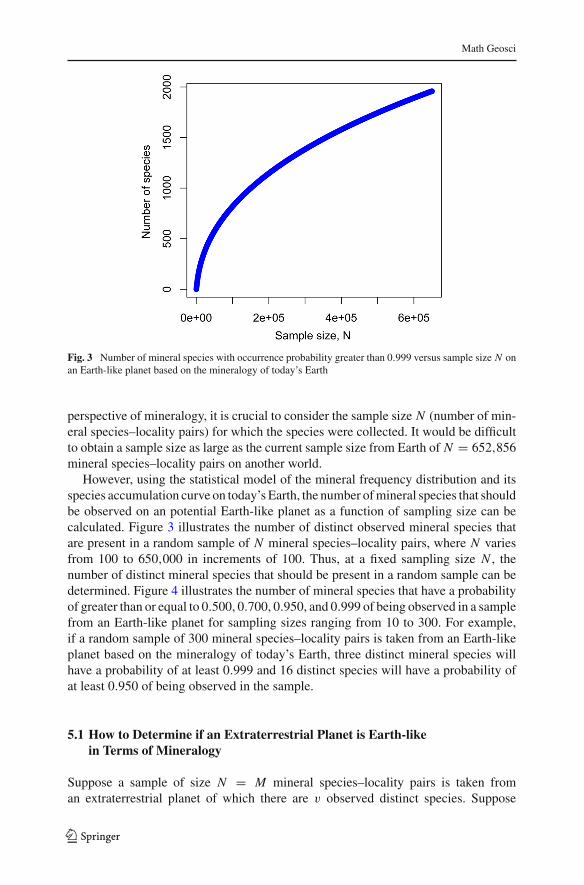
Fig. 3 Number of mineral species with occurrence probability greater than 0.999 versus sample size N onan Earth-like planet based on the mineralogy of today’s Earth
perspective of mineralogy, it is crucial to consider the sample size N (number of min-eral species–locality pairs) for which the species were collected. It would be difficultto obtain a sample size as large as the current sample size from Earth of N = 652,856mineral species–locality pairs on another world.
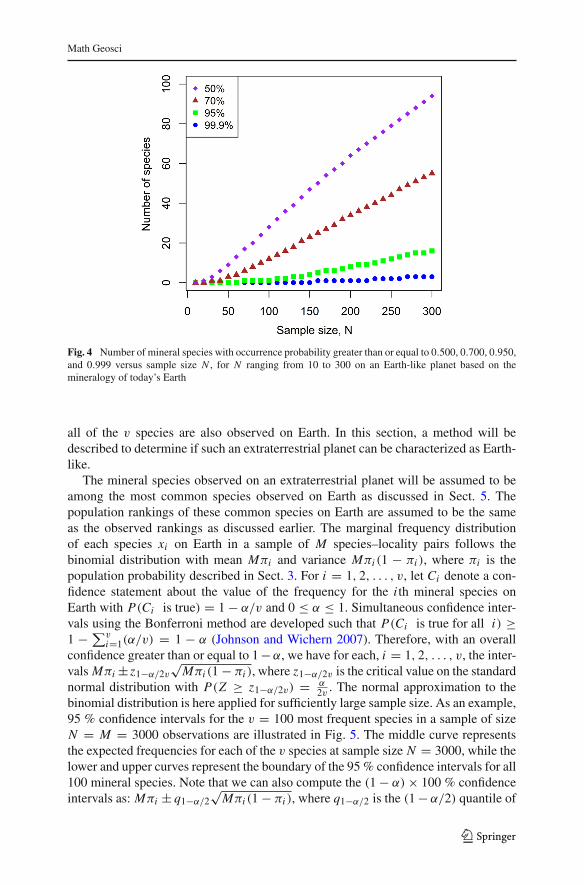
However, using the statistical model of the mineral frequency distribution and itsspecies accumulation curve on today’s Earth, the number ofmineral species that shouldbe observed on an potential Earth-like planet as a function of sampling size can becalculated. Figure 3 illustrates the number of distinct observed mineral species thatare present in a random sample of N mineral species–locality pairs, where N variesfrom 100 to 650,000 in increments of 100. Thus, at a fixed sampling size N , thenumber of distinct mineral species that should be present in a random sample can bedetermined. Figure 4 illustrates the number of mineral species that have a probabilityof greater than or equal to 0.500, 0.700, 0.950, and 0.999 of being observed in a samplefrom an Earth-like planet for sampling sizes ranging from 10 to 300. For example,if a random sample of 300 mineral species–locality pairs is taken from an Earth-likeplanet based on the mineralogy of today’s Earth, three distinct mineral species willhave a probability of at least 0.999 and 16 distinct species will have a probability ofat least 0.950 of being observed in the sample.
5.1 How to Determine if an Extraterrestrial Planet is Earth-likein Terms of Mineralogy
Suppose a sample of size N = M mineral species–locality pairs is taken froman extraterrestrial planet of which there are v observed distinct species. Suppose
123
Math Geosci
Fig. 4 Number of mineral species with occurrence probability greater than or equal to 0.500, 0.700, 0.950,and 0.999 versus sample size N , for N ranging from 10 to 300 on an Earth-like planet based on themineralogy of today’s Earth
all of the v species are also observed on Earth. In this section, a method will bedescribed to determine if such an extraterrestrial planet can be characterized as Earth-like.
The mineral species observed on an extraterrestrial planet will be assumed to beamong the most common species observed on Earth as discussed in Sect. 5. Thepopulation rankings of these common species on Earth are assumed to be the sameas the observed rankings as discussed earlier. The marginal frequency distributionof each species xi on Earth in a sample of M species–locality pairs follows thebinomial distribution with mean Mπi and variance Mπi (1 − πi ), where πi is thepopulation probability described in Sect. 3. For i = 1, 2, . . . , v, let Ci denote a con-fidence statement about the value of the frequency for the i th mineral species onEarth with P(Ci is true) = 1 − α/v and 0 ≤ α ≤ 1. Simultaneous confidence inter-vals using the Bonferroni method are developed such that P(Ci is true for all i) ≥1 − ∑v
i=1(α/v) = 1 − α (Johnson and Wichern 2007). Therefore, with an overallconfidence greater than or equal to 1−α, we have for each, i = 1, 2, . . . , v, the inter-vals Mπi ± z1−α/2v
√Mπi (1 − πi ), where z1−α/2v is the critical value on the standard
normal distribution with P(Z ≥ z1−α/2v) = α2v . The normal approximation to the
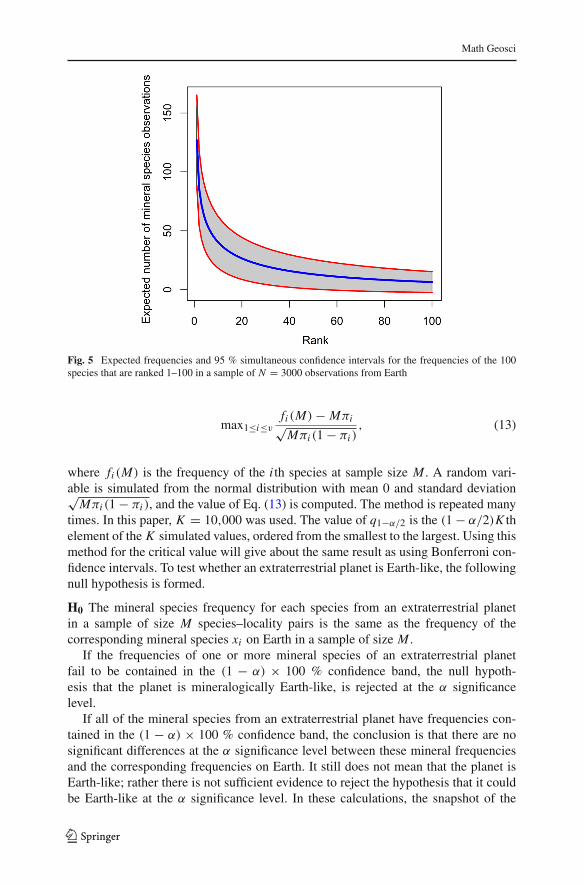
binomial distribution is here applied for sufficiently large sample size. As an example,95 % confidence intervals for the v = 100 most frequent species in a sample of sizeN = M = 3000 observations are illustrated in Fig. 5. The middle curve representsthe expected frequencies for each of the v species at sample size N = 3000, while thelower and upper curves represent the boundary of the 95 % confidence intervals for all100 mineral species. Note that we can also compute the (1 − α) × 100 % confidenceintervals as: Mπi ± q1−α/2
√Mπi (1 − πi ), where q1−α/2 is the (1− α/2) quantile of
123
Math Geosci
Fig. 5 Expected frequencies and 95 % simultaneous confidence intervals for the frequencies of the 100species that are ranked 1–100 in a sample of N = 3000 observations from Earth
max1≤i≤v
fi (M) − Mπi√Mπi (1 − πi )
, (13)
where fi (M) is the frequency of the i th species at sample size M . A random vari-able is simulated from the normal distribution with mean 0 and standard deviation√Mπi (1 − πi ), and the value of Eq. (13) is computed. The method is repeated many
times. In this paper, K = 10,000 was used. The value of q1−α/2 is the (1 − α/2)K thelement of the K simulated values, ordered from the smallest to the largest. Using thismethod for the critical value will give about the same result as using Bonferroni con-fidence intervals. To test whether an extraterrestrial planet is Earth-like, the followingnull hypothesis is formed.
H0 The mineral species frequency for each species from an extraterrestrial planetin a sample of size M species–locality pairs is the same as the frequency of thecorresponding mineral species xi on Earth in a sample of size M .
If the frequencies of one or more mineral species of an extraterrestrial planetfail to be contained in the (1 − α) × 100 % confidence band, the null hypoth-esis that the planet is mineralogically Earth-like, is rejected at the α significancelevel.
If all of the mineral species from an extraterrestrial planet have frequencies con-tained in the (1 − α) × 100 % confidence band, the conclusion is that there are nosignificant differences at the α significance level between these mineral frequenciesand the corresponding frequencies on Earth. It still does not mean that the planet isEarth-like; rather there is not sufficient evidence to reject the hypothesis that it couldbe Earth-like at the α significance level. In these calculations, the snapshot of the
123
Math Geosci
current Earth is used to obtain the confidence intervals. Note that when data on Earth’smineral diversity through deep time are organized we may have information about theabundances of mineral species in its earlier time.
Baayen (2001) introduced the concept of an lnre-zone, which is the range of valuesof the sample size N for which the expected species accumulation curve is still increas-ing, while the expected number of rare species is non-negligible. The distribution ofthe most common mineral species found on Earth is located in the late lnre-zone oreven outside the lnre-zone, where there are no species with only a few localities as wellas no predicted new species. The mineral frequency distributions on an extraterrestrialplanet with no bio-mineral species present will likely be located in the late lnre-zoneor outside the zone.
5.2 Is Mars Earth-like?
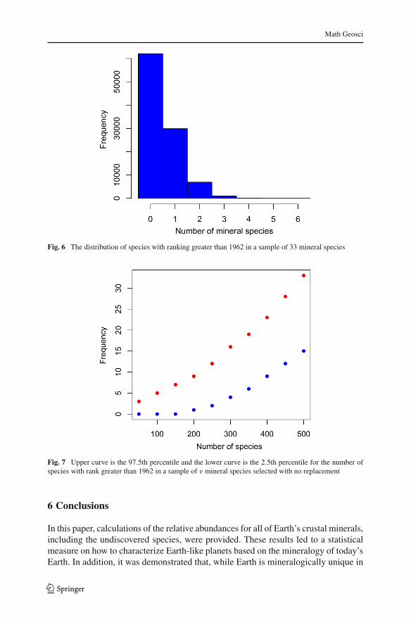
On Mars, 33 mineral species have been found by the CheMin instrument during theMars Science Laboratory mission as of July 2015 (Downs 2015). All of the speciesfound on Mars appear in Earth’s crust; furthermore, 32 of Mars’ mineral species areamong the first 1713 ranked species observed on Earth, while one of the species isranked number 3643 on Earth. Furthermore, almost half of the species found on Marsare among the 100most common observed species on Earth. Recall that there are 1962mineral species on Earth that have greater than 99.9 % chance of being observed ina sample of N = 652,856 observations. To determine if the mineral species foundon Mars are in coincidence with the ranking of species from an Earth-like planet, thefollowing simulation was performed. A random sample of 33 mineral species withno replacement is generated from the population of mineral species on Earth. Theexperiment is repeated 105 times and the number of species that are ranked 1963 orhigher are counted. The result is provided in Fig. 6. The histogram shows that 30% ofthe samples from Earth that contain 33 mineral species have exactly one species withrank greater than 1962. In comparison, Mars has one species, sanderite, which hasrank greater than 1962 on Earth. Even though one cannot say for sure which speciesamong the 4831 observed species on Earth have a population ranking from 1 to 1962,it is highly likely that the observed ranking is approximately equal to the populationranking for these common mineral species. Thus, 32 of the 33 mineral species foundon Mars are among the species that are likely to be present on an Earth-like planet. Itcan be concluded that, on the continuous scale of what can be termed Earth-likeness,Mars is mineralogically Earth-like.
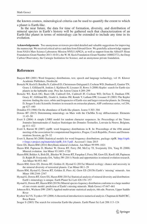
Figure 7 illustrates the 2.5th and 97.5th percentiles for the number of species thathave rank greater than 1962 in a sample of v mineral species from Earth. The sim-ulation was run with 105 samples of v species, each sampled with no replacementfrom the population of mineral species on Earth. For example, if a sample from anextraterrestrial planet has 300 mineral species, the 97.5th percentile for the numberof species with rank greater than 1962 is 16, that is, if the number of mineral specieswith rank greater than 1962 is larger than 16 in a sample of 300 species, the planet isnot likely Earth-like.
123
Math Geosci
Fig. 6 The distribution of species with ranking greater than 1962 in a sample of 33 mineral species
Fig. 7 Upper curve is the 97.5th percentile and the lower curve is the 2.5th percentile for the number ofspecies with rank greater than 1962 in a sample of v mineral species selected with no replacement
6 Conclusions
In this paper, calculations of the relative abundances for all of Earth’s crustal minerals,including the undiscovered species, were provided. These results led to a statisticalmeasure on how to characterize Earth-like planets based on the mineralogy of today’sEarth. In addition, it was demonstrated that, while Earth is mineralogically unique in
123
Math Geosci
the known cosmos, mineralogical criteria can be used to quantify the extent to whicha planet is Earth-like.
In the near future, the data for time of formation, diversity, and distribution ofmineral species in Earth’s history will be gathered such that characterization of anEarth-like planet in terms of mineralogy can be extended to include any time in itsevolution.
Acknowledgements Two anonymous reviewers provided detailed and valuable suggestions for improvingthemanuscript.We received critical advice and data fromEdwardGrew.We gratefully acknowledge supportfrom NASAMars Science Laboratory Mission NNX11AP82A, as well as support from the Alfred P. SloanFoundation (Grant Number 2013-10-01), theW.M.Keck Foundation (Grant Number 140002372), the DeepCarbon Observatory, the Carnegie Institution for Science, and an anonymous private foundation.
References
Baayen RH (2001) Word frequency distributions, text, speech and language technology, vol 18. KluwerAcademic Publishers, Dordrecht
BoruckiW,KochD,BatalhaN,CaldwellD,Christensen-Dalsgaard J, CochranWD,DunhamE,Gautier TN,Geary J, Gilliland R, Jenkins J, Kjeldsen H, Lissauer JJ, Rowe J (2008) Kepler: search for Earth-sizeplanets in the habitable zone. Proc Int Astron Union 4:289–299
Borucki WJ, Koch DG, Basri GB, Caldwell DA, Caldwell JF, Cochran WD, DeVore E, Dunham EW,Geary JC, Gilliland RL, Gould A, Jenkins JM, Kondo Y, Latham DW, Lissauer JJ (2003) The Keplermission: finding the sizes, orbits and frequencies of Earth-size and larger extrasolar planets. In: DemingD, Seager S (eds) Scientific frontiers in research on extrasolar planets, ASP conference series, vol 294,pp 427–440
Donahoe FJ (1966) On the abundance of Earth-like planets. Icarus 5:303–304Downs RT (2015) Determining mineralogy on Mars with the CheMin X-ray diffractometer. Elements
11:45–50Evert S (2004) A simple LNRE model for random character sequences. In: Proceedings of the 7èmes
Journées Internationales d’Analyse Statistique des Données Textuelles, Louvain-la-Neuve, Belgium,pp 411–422
Evert S, Baroni M (2007) zipfR: word frequency distributions in R. In: Proceedings of the 45th annualmeeting of the association for computational linguistics, Prague, Czech Republic, Posters and Demon-strations Session, pp 29–32
Evert S, Baroni M (2008) Statistical models for word frequency distributions, package zipfR. http://zipfr.r-forge.r-project.org/materials/zipfR_0.6-5.pdf. Accessed 1 June 2015
Grew ES, Hazen RM (2014) Beryllium mineral evolution. Am Miner 99:999–1021Hazen RM, Papineau D, Bleeker W, Downs RT, Ferry JM, McCoy TJ, Sverjensky DA, Yang H (2008)
Mineral evolution. Am Miner 93:1693–1720Hazen RM, Bekker A, BishDL, BleekerW,Downs RT, Farquhar J, Ferry JM,GrewES, Knoll AH, Papineau
D, Ralph JP, Sverjensky DA, Valley JW (2011) Needs and opportunities in mineral evolution research.Am Miner 96:953–963
Hazen RM, Grew ES, Downs RT, Golden JJ, Hystad G (2015a) Mineral ecology: chance and necessity inthe mineral diversity of terrestrial planets. Can Miner 00:1–29
Hazen RM, Hystad G, Downs RT, Golden JJ, Pires AJ, Grew ES (2015b) Earth’s ‘missing’ minerals. AmMiner 100:2344–2347
Hystad G, Downs RT, GrewES, Hazen RM (2015a) Statistical analysis of mineral diversity and distribution:Earth’s mineralogy is unique. Earth Planet Sci Lett 426:154–157
Hystad G, Downs RT, Hazen RM (2015b)Mineral species fequency distribution conforms to a large numberof rare events model: prediction of Earth’s missing minerals. Math Geosci 47:647–661
Johnson RA, Wichern DW (2007) Applied multivariate statistical analysis, 6th edn. Pearson, Upper SaddleRiver
Ryaben’kiiVS, TsynkovSV (2006)A theoretical introduction to numerical analysis. Chapman&Hall/CRC,Boca Raton
Seager S (2003) The search for extrasolar Earth-like planets. Earth Planet Sci Lett 208:113–124
123
Math Geosci
Shen TJ, Chao A, Lin CF (2003) Predicting the number of new species in further taxonomic sampling.Ecology 84(3):798–804
Sichel HS (1971) On a family of discrete distributions particularly suited to represent long-tailed frequencydata. In: Proceedings of the third symposium on mathematical statistics, Pretoria, South Africa, pp51–97
Sichel HS (1975) On a distribution law for word frequencies. J Am Stat Assoc 70:542–547Sichel HS (1986) Word frequency distributions and type-token characteristics. Math Sci 11:45–72Ward PD, Brownlee D (2003) Rare Earth: why complex life is uncommon in the universe. Copernicus, New
YorkWilliams RE, Blacker B, Dickinson M, Dixon WVD, Ferguson HC, Fruchter AS, Giavalisco M, Gilliland
RL, Heyer I, Katsanis R, Levay Z, Lucas RA, McElroy DB, Petro L, Postman M, Adorf HM, Hook R(1996) The Hubble deep field: observations, data reduction, and galaxy photometry. Astron J 112:1335
123