Relational Database Systems 1 - TU Braunschweig · Wolf-Tilo Balke Jan-Christoph Kalo Institut für...

Wolf-Tilo Balke

Jan-Christoph Kalo

Institut für Informationssysteme

Technische Universität Braunschweig

www.ifis.cs.tu-bs.de

Relational

Database Systems 1

• SQL

– Queries• SELECT

– Data Manipulation Language (next lecture)• INSERT

• UPDATE

• DELETE

– Data Definition Language (next lecture)• CREATE TABLE

• ALTER TABLE

• DROP TABLE

Relational Database Systems 1 – Wolf-Tilo Balke – Institut für Informationssysteme – TU Braunschweig 2

8.0 Overview of SQL

• There are three major classes of DB operations

– defining relations, attributes, domains, constraints, ...

• Data Definition Language (DDL)

– adding, deleting and modifying tuples

• Data Manipulation Language (DML)

– asking queries

• often part of the DML

• SQL covers all these classes

• In this lecture, we will use IBM DB2’s SQL dialect

– similar notation in other RDBMS

(at least for the part of SQL taught in this lecture)


8.0 Overview of SQL

• According to the SQL standard, relations and other database objects exist in an environment

– think: environment = RDBMS

• Each environment consists of catalogs

– think: catalog = database

• Each catalog consists of a set of schemas

– think: schema = group of tables (and other stuff)

• A schema is a collection of database objects (tables, domains, constraints, ...)

– each database object belongs to exactly one schema

– schemas are used to group related database objects


8.0 Overview of SQL


8.0 Overview of SQL

Environment

BigCompany database server

Catalog

human_resources

Schema

people

Schema

training

Catalog

production

Schema products

Schema testing

Schema taxes

Table staff

Table

has_office

...

...

...

...

• When working with the environment,users connect to a single catalog andhave access to all database objects in this catalog

– however, accessing/combining data objects from different catalogs usually is not possible

– thus, typically, catalogs are the maximum scopeover that SQL queries can be issued

– in fact, the SQL standard defines an additional layerin the hierarchy on top of catalogs

• clusters are used to group related catalogs

• according to the standard, they provide the maximum scope

• however, hardly any vendor supports clusters


8.0 Overview of SQL

• After connecting to a catalog, database objects can be referenced using their qualified name– e.g. schemaname.objectname

• However, when working only with objects from asingle schema, using unqualified names would be nice– e.g. objectname

• One schema always is defined to be the default schema– SQL implicitly treats objectname asdefaultschema.objectname

– the default schema can be set with SET SCHEMA:• SET SCHEMA schemaname

– initially, after login the default schema corresponds to the current user name• remember to change the default schema accordingly!


8.0 Overview of SQL

• Basic SQL Queries

– SELECT, FROM, WHERE

• Advanced SQL Queries

– Joins

– Set operations

– Aggregation and GROUP BY

– ORDER BY

– Subqueries

• Writing Good SQL Code


8 SQL 1

• SQL queries are statements that

retrieve information from a DBMS

– simplest case: from a single table,

return all rows matching some given condition

– SQL queries may return multi-sets (bags) of rows

• duplicates are allowed by default

(but can be eliminated on request)

• even just a single value is a result set

(one row with one column)

• This is different in Relational Algebra, TRC, DRC, etc.

• however, often it’s just called a result set…


8.1 SQL Queries

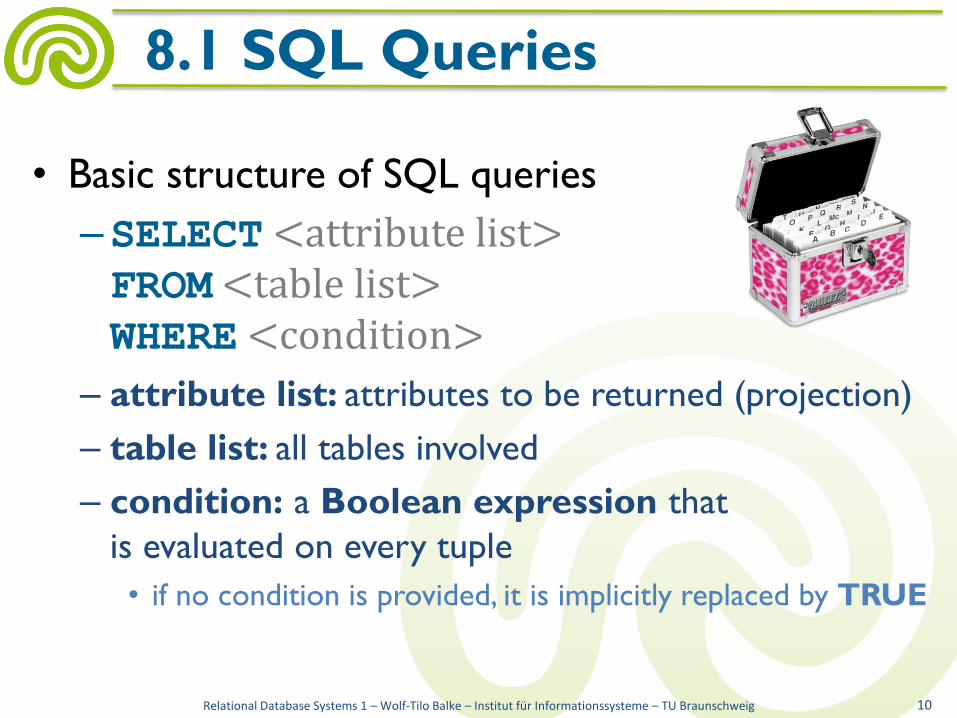
• Basic structure of SQL queries

–SELECT <attribute list> FROM <table list> WHERE <condition>

– attribute list: attributes to be returned (projection)

– table list: all tables involved

– condition: a Boolean expression that

is evaluated on every tuple

• if no condition is provided, it is implicitly replaced by TRUE


8.1 SQL Queries

• The SELECT keyword is often confused with selectionfrom relational algebra– actually SELECT corresponds to projection

• Example: – Table student with attributes id, fname, lname

SELECT id, lname FROM student

WHERE id >= 100

– TRC:

{t.id, t.lname | student(t) ˄ t.id ≥ 100}– DRC:

{id, ln | ∃fn(student(id, fn, ln) ˄ id ≥ 100)}Rel. Algebra:

πid,lnameσid≥100student


8.1 Attribute Names

• To return all attributes under consideration,

the wildcard * may be used

• Examples– SELECT * FROM <list of tables>

Return all attributes of the tables in the FROM clause.

– SELECT movie.* FROM movie, person WHERE...

Return all attributes of the movies table.


8.1 Attribute Names

• SQL can perform duplicate elimination

of rows in result set

– may be expensive (due to sorting)

– DISTINCT keyword is used

• Example– SELECT DISTINCT name FROM staff

• returns all different names of staff members,

without duplicates


8.1 Enforcing Sets in SQL

• Attribute names are qualified or unqualified

– unqualified: just the attribute name

• only possible, if attribute name is unique amongthe tables given in the FROM clause

– qualified: tablename.attributename

• necessary if tables share identical attribute names

• if tables in the FROM clause share identical attribute names

and also identical table names, we need even more

qualification:

schemaname.tablename.attributename


8.1 Attribute Names

• The attributes in the result set are defined in a SELECT clause

• However, result attributes can be renamed

– remember the renaming operator ρ fromrelational algebra…

– SQL uses the AS keyword for renaming

– the new names can also be used in the WHERE clause

• Example – SELECT person.person_name AS name

FROM person WHERE name = 'Smith'

• person_name is now called name in the result table


8.1 Attribute Names

• Table names can be referenced in the same wayas attribute names (qualified or unqualified)

• However, renaming works slightly different– the result table of an SQL query has no name

– but tables can be given alias names to simplify queries(also called tuple variables or just aliases)

– indicated by the AS keyword

• ExampleSELECT title, genre FROM movie AS m, genre AS g WHERE m.id = g.id

• The AS keyword is optional: FROM movie m, genre g

• Compare to TRC: { m.title, g.genre | movie(m) ˄ genre(g) ˄ m.id = g.id }


8.1 Table Names


8.1 Basic Select

SELECT expression

ALL

DISTINCT

,

table name

*

.

column nameAS

FROM table name

alias name

AS

,

query )(

WHERE search condition GROUP BY column name

,

HAVING search condition

attribute names

table names

query block

• One of the basic building blocks of SQL queries is

the expression

– Expressions represent a literal, i.e. a number, a string, or

a date

– column names or constants

– additionally, SQL provides some special expressions

• functions

• CASE expressions

• CAST expressions

• scalar subqueries


8.1 Expressions

• Expressions can be combined usingexpression operators

– arithmetic operators:+, -, *, and / with the usual semantics• age + 2

• price * quantity

– string concatenation ||: (also written as CONCAT ) combines two strings into one• first_name || ' ' || lastname || ' (aka ' || alias || ')'

• 'Hello' CONCAT ' World' → 'Hello World'

– parenthesis:used to modify the evaluation order• (price + 10) * 20


8.1 Expressions

• Usually, SQL queries return exactly those tuples

matching a given search condition

– indicated by the WHERE keyword

– the condition is a logical expression which can be

applied to each row and may have one of three values TRUE, FALSE, and NULL

• again, NULL might mean unknown, does not apply,

is missing, ...


8.1 Conditions

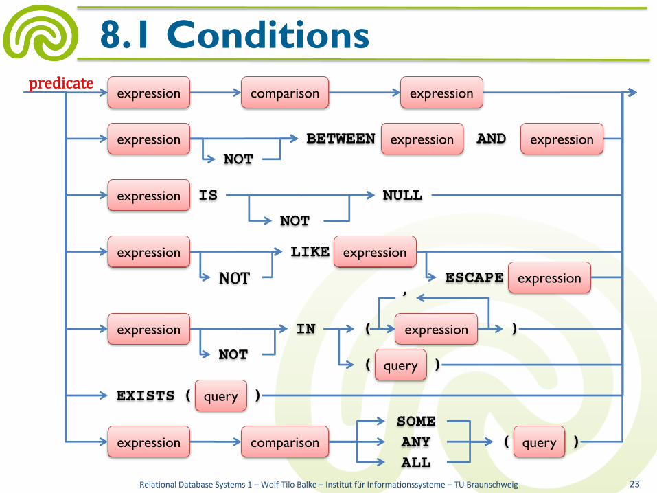
• Search conditions are conjunctions of predicates

– each predicate evaluates to TRUE, FALSE, or NULL


8.1 Conditions

search condition

NOT

predicate

search condition( )

AND

OR

• Why TRUE, FALSE, and NULL?

– SQL uses so-called ternary (three-valued) logic

– when a predicate cannot be evaluated because itcontains some NULL value, the result will be NULL

• Example: power_strength > 10 evalutes to NULLiff power_strength is NULL

• NULL = NULL also evaluates to NULL

• Handling of NULL by the operators AND and OR:


8.1 Conditions

AND TRUE FALSE NULL

TRUE TRUE FALSE NULL

FALSE FALSE FALSE FALSE

NULL NULL FALSE NULL

OR TRUE FALSE NULL

TRUE TRUE TRUE TRUE

FALSE TRUE FALSE NULL

NULL TRUE NULL NULL

NOT

TRUE FALSE

FALSE TRUE

NULL NULL


8.1 Conditionspredicate

expression

expression

expression

expression

NOT

comparison expression

expression expressionBETWEEN AND

NOT

NULLIS

expression

NOT

LIKE

expressionESCAPE

expression

NOT

IN

query( )

( )expression

,

EXISTS query( )

expression comparison

SOME

ANY

ALL

query( )

• Simple comparisons– valid comparison operators are

• =, <, <=, >=, and >

• <> (meaning: not equal)

– data types of expressions need to be compatible (if not, CAST has to be used)

– character values are usually compared lexicographically (while ignoring case)

– examples• powerStrength > 10

• name = 'Magneto'

• 'Magneto' <= 'Professor X'


8.1 Conditions

expression comparison expression

• BETWEEN predicate:

– X BETWEEN Y AND Z is a shortcut for

Y <= X AND X <= Z

– note that you cannot reverse the order of Z and Y

• X BETWEEN Y AND Z is different from

X BETWEEN Z AND Y

• the expression can never be true if Y > Z

– examples• year BETWEEN 2000 AND 2008

• score BETWEEN target_score-10 AND target_score+10


8.1 Conditions

expression

NOT

expression expressionBETWEEN AND

• IS NULL predicate

– the only way to check if a value is NULL or not

• recall: NULL = NULL returns NULL

– returns either TRUE or FALSE

– examples• real_name IS NOT NULL

• power_strength IS NULL

• NULL IS NULL


8.1 Conditions

expression

NOT

NULLIS

• LIKE predicate– the predicate is for matching character strings to patterns

– match expression must be a character string

– pattern expression is a (usually constant) string• may not contain column names

– escape expression is just a single character

– during evaluation, the match expression is compared to the pattern expression with following additions• _ in the pattern expression represents any single character

• % represents any number of arbitrary characters

• the escape character prevents the special semantics of _ and %

– most modern database nowadays also support more powerful regular expressions (introduced in SQL-99)


8.1 Conditionsmatch

expression

pattern

expressionLIKE

escape

expressionESCAPENOT

• Examples• address LIKE '%City%'

– 'Manhattan' → FALSE

– 'Gotham City Prison' → TRUE

• name LIKE 'M%_t_'

– 'Magneto' → TRUE

– 'Matt' → TRUE

– 'Mtt' → FALSE

• status LIKE '_/_%' ESCAPE '/'

– '1_inPrison' → TRUE

– '1inPrison' → FALSE

– '%_%' → TRUE

– '%%%' → FALSE


8.1 Conditions

match

expression

pattern

expressionLIKE

escape

expressionESCAPENOT

• IN predicate

– evaluates to true if the value of the test expression is

within a given set of values

– particularly useful when used with a subquery (later)

– examples• name IN ('Magneto', 'Batman', 'Dr. Doom')

• name IN (SELECT title FROM movie)

– Those people having a film named after them…


8.1 Conditions

expression

NOT

IN

query( )

( )expression

,

• EXISTS predicate:

– evaluates to TRUE if a given subquery

returns at least one result row

• always returns either TRUE or FALSE

– examples• EXISTS (SELECT * FROM hero)

• Do we have any hero stored in our database?

– EXISTSmay also be used to express semi-joins


8.1 Conditions

EXISTS query( )

• SOME/ANY and ALL– compares an expression to each value provided by

a subquery

– TRUE if • SOME/ANY: At least one comparison returns TRUE

– SOME and ANY are synonyms

• ALL: All comparisons return TRUE

– examples• result <= ALL(SELECT result FROM results)

– TRUE if the current result is the smallest one

• result < SOME(SELECT result FROM results)

– TRUE if the current result is not the largest one


8.1 Conditions

expression comparison

SOME

ANY

ALL

query( )

• Simple SQL Queries



– Joins

– Set operations


– ORDER BY

– Subqueries



8 SQL 1

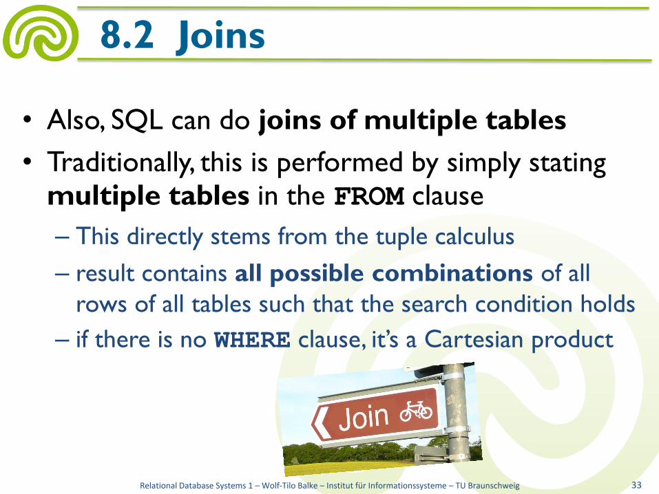
• Also, SQL can do joins of multiple tables

• Traditionally, this is performed by simply stating multiple tables in the FROM clause

– This directly stems from the tuple calculus

– result contains all possible combinations of all

rows of all tables such that the search condition holds

– if there is no WHERE clause, it’s a Cartesian product


8.2 Joins

• Example– SELECT * FROM hero, has_alias

• TRC: {h, ha | hero(h) ˄ has_alias(ha)}• Rel. Algebra: hero × has_alias

– SELECT * FROM hero h, has_alias haWHERE h.id = ha.hero_id

• TRC: – { h, ha | hero(h) ˄ has_alias(ha) ˄ h.id = ha.hero_id }

• Rel. Algebra (naïve): – σid=hero_id hero × has_alias

• Rel. Algebra (optimized):– hero ⨝id=hero_id has_alias

• Besides this common implicit notation of joins, SQL also supports explicit joins– Burrowed from Relational Algebra


8.2 Joins

• Explicit joins are specified in the FROM clause– SELECT * FROM table1

JOIN table2 ON <join condition>WHERE <some other condition>

– often, attributes in joined tables have the same names,

so qualified attributes are needed

– INNER JOIN and JOIN are equivalent

• explicit joins improve readability of your SQL code!


8.2 Joins

table name

INNER JOIN

table name

JOIN

LEFT JOIN

RIGHT JOIN

FULL JOIN

joined table

ON condition

Inner join: List students and their exam results.– π lastname, course, result (Student ⋈mat_no=student exam)

– SELECT lastname, course, result FROM student AS s JOIN exam AS e ON s.mat_no = e.student


8.2 Joins

mat_no firstname lastname sex

1005 Clark Kent m

2832 Louise Lane f

4512 Lex Luther m

5119 Charles Xavier m

student course result

9876 100 3.7

2832 102 2.0

1005 101 4.0

1005 100 1.3

Student exam

lastname course result

Kent 100 1.3

Kent 101 4.0

Lane 102 2.0

πlastname, course, result (Student ⋈mat_no=courseexam)

We lost Lex Luther and Charles Xavier

because they didn’t take any exams!

Also information on student 9876 disappears…

Left outer join: List students and their exam results– π lastname, course, result (Student ⎧mat_no=student exam)

– SELECT lastname, course, result FROM student AS s LEFT JOIN exam AS e ON s.mat_no = e.student


8.2 Joins


1005 Clark Kent m

2832 Louise Lane f

4512 Lex Luther m



9876 100 3.7

2832 102 2.0

1005 101 4.0

1005 100 1.3

Student exam


Kent 100 1.3

Kent 101 4.0

Lane 102 2.0

Luther NULL NULL

Xavier NULL NULL

π lastname, course, result (Student ⎧mat_nr=student exam)

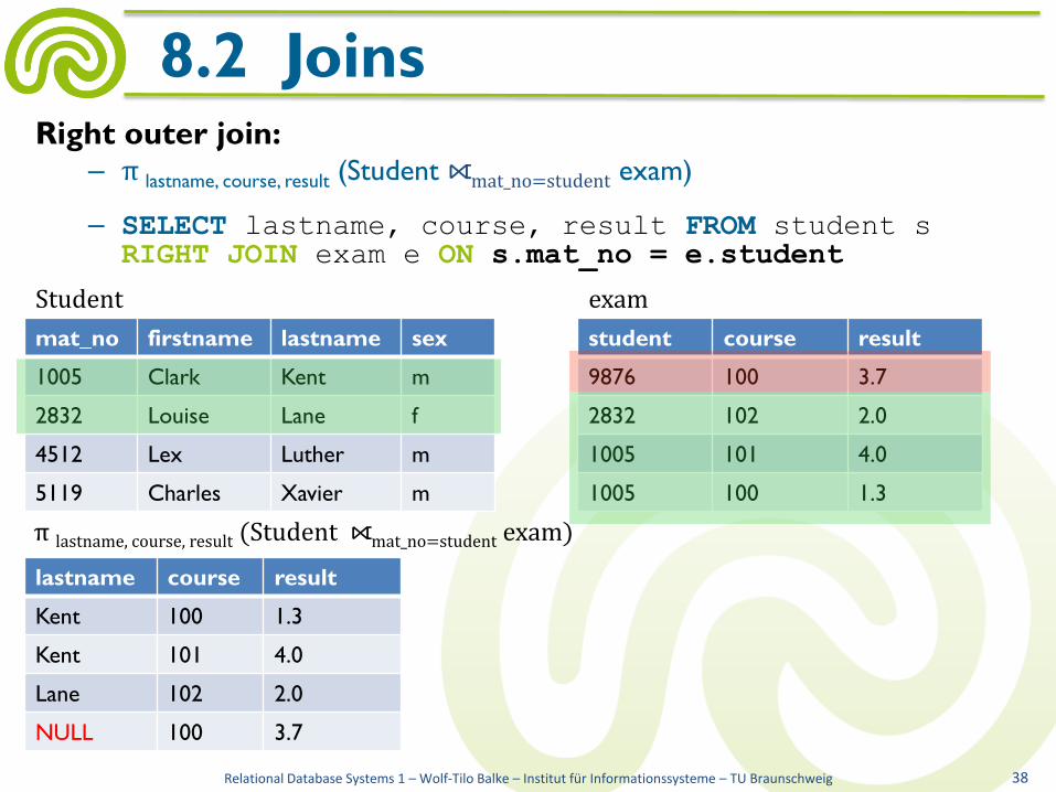
Right outer join:– π lastname, course, result (Student ⎨mat_no=student exam)

– SELECT lastname, course, result FROM student s RIGHT JOIN exam e ON s.mat_no = e.student


8.2 Joins


1005 Clark Kent m

2832 Louise Lane f

4512 Lex Luther m



9876 100 3.7

2832 102 2.0

1005 101 4.0

1005 100 1.3

Student exam


Kent 100 1.3

Kent 101 4.0

Lane 102 2.0

NULL 100 3.7

π lastname, course, result (Student ⎨mat_no=student exam)

Full outer join:– π lastname, course, result (Student ⎩mat_no=student exam)

– SELECT lastname, course, result FROM student sFULL JOIN exam e ON s.mat_no = e.student


8.2 Joins

matNr firstname lastname sex

1005 Clark Kent m

2832 Louise Lane f

4512 Lex Luther m



9876 100 3.7

2832 102 2.0

1005 101 4.0

1005 100 1.3

Student exam


Kent 100 1.3

Kent 101 4.0

Lane 102 2.0

Luther NULL NULL

NULL 100 3.7

Xavier NULL NULL

π lastname, course, result (Student ⎩mat_no=student exam)

• SQL also supports the common set operators

– set union ∪: UNION

– set intersection ∩ : INTERSECT

– set difference ∖: EXCEPT

• By default, set operators eliminate duplicates unlessthe ALL modifier is used

• Sets need to be union-compatible to use set operators

– row definition must match (data types)


8.2 Set Operators

queryINTERSECT

queryquery-block

literal table

( )

EXCEPT

UNION

ALL query

query-block

literal table

( )

• Example– ((SELECT course, result FROM exam

WHERE course = 100)

EXCEPT

(SELECT course, result FROM exam

WHERE result IS NULL))

UNION VALUES (100, 2.3), (100, 1.7)


8.2 Set Operators


9876 100 3.7

2832 102 2.0

1005 101 4.0

1005 100 NULL

6676 102 4.3

3412 NULL NULL

exam

course result

100 3.7

100 2.3

100 1.7

query block

query

literal table

• Column functions are used to performstatistical computations

– similar to aggregate function in relational algebra

– column functions are expressions

– they compute a scalar value for a set of values

• Examples

– compute the average score over all exams

– count the number of exams each student has taken

– retrieve the best student

– ...


8.2 Column Function

• Column functions in the SQL standard– MIN, MAX, AVG, COUNT, SUM:

each of these are applied to some other expression• NULL values are ignored

• function columns in result set just get their column number as name

– if DISTINCT is specified, duplicates are eliminated in advance• by default, duplicates are not eliminated (ALL)

– COUNT may also be applied to *• simply counts the number of rows

– typically, there are many more column functions available in your RDBMS (e.g. in DB2: CORRELATION, STDDEV, VARIANCE, ...)


8.2 Column Function

function

name

column functionexpression

COUNT(*)

( )

ALL

DISTINCT

expression

• Examples– SELECT COUNT(*) FROM hero

• Returns the number of rows of the heroes table.

– SELECT COUNT(name), COUNT(DISTINCT name)

FROM hero

• Returns the number of rows in the hero table for that name

is not null and the number of non-null unique names.

– SELECT MIN(strength), MAX(strength),

AVG(strength) FROM power

• Returns the minimal, maximal, and average power strength

in the power table.


8.2 Column Function

• Similar to aggregation in relation algebra,

SQL supports grouping

– GROUP BY <column names>

– creates a group for each combination of

distinct values within the provided columns

– a query containing GROUP BY can access

non-group-by-attributes only by column functions


8.2 Grouping

Examples– SELECT course, AVG(result), COUNT(*), COUNT(result) FROM exam GROUP BY course

• For each course, list the average result, the number of results,and the number of non-null results.

• Rel. Alg.: course𝔉avg(result), count(result)exam– count(*) is not defined in Relational Algebra


8.2 Grouping


9876 100 3.7

2832 102 2.0

1005 101 4.0

1005 100 NULL

6676 102 4.3

3412 NULL NULL

exam

course 2 3 4

100 3,7 2 1

101 4.0 1 1

102 3.15 2 2

NULL NULL 1 0

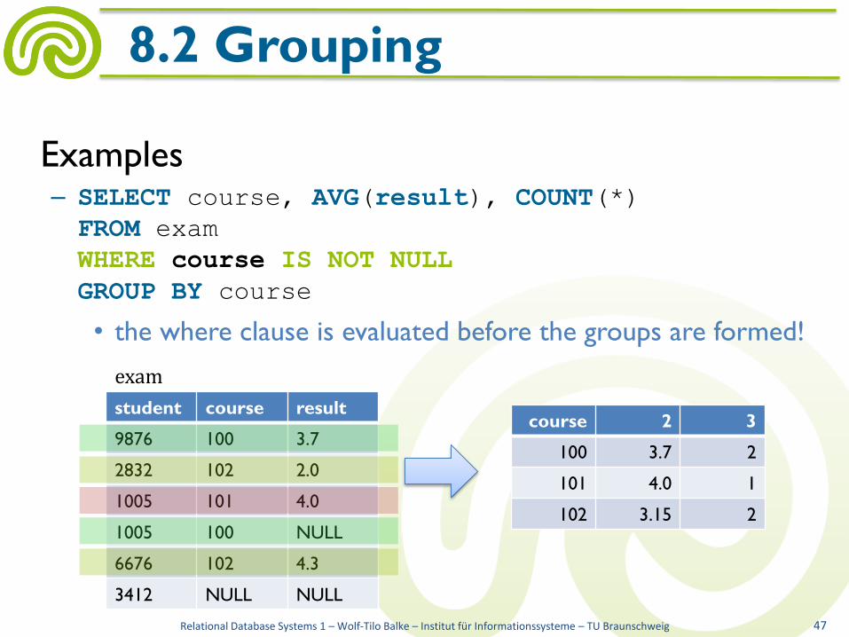
Examples– SELECT course, AVG(result), COUNT(*)

FROM exam

WHERE course IS NOT NULL

GROUP BY course

• the where clause is evaluated before the groups are formed!


8.2 Grouping


9876 100 3.7

2832 102 2.0

1005 101 4.0

1005 100 NULL

6676 102 4.3

3412 NULL NULL

exam

course 2 3

100 3.7 2

101 4.0 1

102 3.15 2

• Additionally, there may be restrictions onthe groups themselves

– HAVING <condition>

– the condition may involve group properties andcolumn functions

– only those groups are created that fulfill theHAVING condition

– a query may have a WHERE and a HAVING clause

– also, it is possible to have HAVING without GROUP BY

• then, the whole table is treated as a single group – which is rarely useful


8.2 Grouping

• Examples– SELECT course, AVG(result), COUNT(*)

FROM exam

WHERE course <> 100

GROUP BY course

HAVING COUNT(*) > 1


8.2 Grouping


9876 100 3.7

2832 102 2.0

1005 101 4.0

1005 100 NULL

6676 102 4.3

3412 NULL NULL

exam

course 1 2

102 3.15 2

• As last step in the processing pipeline,(unordered) result sets may be converted into lists– impose an order on the rows

– this concludes the SELECT statement

– ORDER BY keyword

• Please note:Ordering completely breaks with set calculus/algebra– result after ordering is a list, not a (multi-)set!


8.2 Ordering

SELECT statement

query

column nameORDER BY

ASC

DESC

,

• ORDER BY may order ascending or descending

– default: ascending (ASC)

• Ordering on multiple columns possible

• Columns used for ordering arereferenced by their name

• Example– SELECT * FROM exam

ORDER BY student, course DESC

– returns all exam results ordered by student id (ascending)

– if student ids are identical, we sort in descending orderby course number


8.2 Ordering

• When working with result lists, often only the first krows are of interest

• How can we limit the number of result rows?

– since SQL:2008, the SQL standard offers theFETCH FIRST clause (supported e.g. in DB2)

• ExampleSELECT name, salary

FROM salaries

ORDER BY salary

FETCH FIRST 10 ROWS ONLY

– FETCH FIRST can also be used without ORDER BY

• get a quick impression of the result set


8.2 Ordering

• SQL queries are evaluated in this order

5. SELECT<attribute list>

1. FROM <table list>

2. [WHERE<condition>]

3. [GROUP BY <attribute list>]

4. [HAVING<condition>]

6. [UNION/INTERSECT/EXCEPT <query>]

7. [ORDER BY <attribute list>]


8.2 Evaluation Order of SQL

• In SQL, you may embed a query block withina query block (so called subquery, or nested query)

– subqueries are written in parenthesis

– scalar subqueries can be used as expressions

• if query returns only one row with one column

– subqueries may be used for IN or EXISTS conditions

– each subquery within the table list createsa temporary source table

• called inline view


8.2 Subqueries

• Subqueries may either be correlated

or uncorrelated

– if the WHERE clause of the inner query uses an

attribute within a table declared in the outer query,

the two queries are correlated

• the inner query needs to be re-evaluated for every tuple

in the outer query

• this is rather inefficient, so avoid correlated subqueries

whenever possible!

– otherwise, the queries are uncorrelated

• the inner query needs to be evaluated just once


8.2 Subqueries


8.2 Subqueries

id real_namehero

hero alias_namehas_alias

hero power power_strengthhas_power

id name descriptionpower

• Expressions– SELECT hero.* FROM hero, has_power p

WHERE hero.id = p.hero

AND power_strenth = (

SELECT MAX(power_strength)

FROM has_power

)

• Select all those heroes having powers with maximal strength.

• IN-condition– SELECT * FROM hero WHERE id IN (

SELECT hero FROM has_alias

WHERE alias_name LIKE 'Super%'

)

• Select all those heroes having an alias starting with Super.


8.2 Subqueries

scalar subquery

• EXISTS-condition:– SELECT * FROM hero h

WHERE EXISTS (

SELECT * FROM has_alias a WHERE h.id = a.hero

)

• Select heroes having at least one alias.

• this pattern is normally used to express a semi join

• if the DBMS would not optimize this into a semi join, the subquery has to be evaluated for each tuple (uncorrelated subquery!)

• Inline view– SELECT h.real_name, a.alias_name

FROM has_alias a, (

SELECT * FROM hero WHERE real_name LIKE 'A%'

) h

WHERE h.id < 100 AND a.hero = h.id

• Get real_name-alias pairs for all heroes with a real name staring with A and an id smaller than 100.


8.2 Subqueries

• WITH-clause (temporary tables):WITH hero_num_powers AS(

SELECT hero AS h_id, COUNT(*) AS num_pow

)

SELECT * FROM hero h

JOIN hero_num_powers hnp ON h.id = hnp.h_id

WHERE hnp.num_pow = (

SELECT MAX(num_pow) FROM hero_num_powers

)

• Select heroes having most powers

• Extremely useful if the expression in the WITH-clause is used multiple times

• Also useful for readability


8.2 Subqueries

• Simple SQL Queries



– Joins

– Set operations


– ORDER BY

– Subqueries



8 SQL 1

• What is good SQL code?

– easy to read

– easy to write

– easy to understand!

• There is no official SQL style guide,

but here are some general hints


8.3 Writing Good SQL Code

1. Write SQL keywords in uppercase,

names in lowercase!



GOOD

BADSELECT MOVIE_TITLE

FROM MOVIE

WHERE MOVIE_YEAR = 2009;

SELECT movie_title

FROM movie

WHERE movie_year = 2009;

2. Use proper qualification!



GOOD

BADSELECT imdbraw.movie.movie_title,

imdbraw.movie.movie_year

FROM imdbraw.movie

WHERE imdbraw.movie.movie_year = 2009;

SET SCHEMA imdbraw;

SELECT movie_title, movie_year

FROM movie

WHERE movie_year = 2009;

3. Use aliases to keep your code short

and the result clear!



GOOD

BADSELECT movie_title, movie_year

FROM movie, genre

WHERE movie.movie_id = genre.movie_id

AND genre.genre = 'Action';

SELECT movie_title, movie_year

FROM movie m, genre g

WHERE m.movie_id = g.movie_id

AND g.genre = 'Action';

4. Use joins to join!



GOOD

BAD

SELECT movie_title title, genre g

FROM movie m

JOIN genre g ON m.movie_id = g.movie_id

WHERE g.genre='Action'

SELECT movie_title title, genre g

FROM movie m

JOIN genre g ON g.genre='Action'


5. Separate joins from conditions!



GOOD

BAD

SELECT movie_title title, movie_year year

FROM movie m, genre g, actor a


AND g.genre = 'Action'

AND m.movie_id = a.movie_id

AND a.person_name LIKE '%Schwarzenegger%';


FROM movie m


JOIN actor a ON g.movie_id = a.movie_id

WHERE g.genre = 'Action'


6. Use proper indentation!



GOOD

BAD


FROM movie m JOIN genre g ON m.movie_id =

g.movie_id JOIN actor a ON g.movie_id =

a.movie_id WHERE g.genre = 'Action' AND

a.person_name LIKE '%Schwarzenegger%';


FROM movie m


JOIN actor a ON g.movie_id = a.movie_id

WHERE g.genre = 'Action'


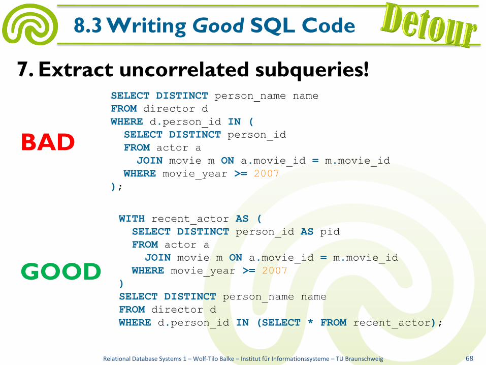
7. Extract uncorrelated subqueries!



GOOD

BAD

WITH recent_actor AS (

SELECT DISTINCT person_id AS pid

FROM actor a

JOIN movie m ON a.movie_id = m.movie_id

WHERE movie_year >= 2007

)

SELECT DISTINCT person_name name

FROM director d

WHERE d.person_id IN (SELECT * FROM recent_actor);

SELECT DISTINCT person_name name

FROM director d

WHERE d.person_id IN (

SELECT DISTINCT person_id

FROM actor a

JOIN movie m ON a.movie_id = m.movie_id

WHERE movie_year >= 2007

);

• SQL data definition language

• SQL data manipulation language

(apart from querying)

• SQL ≠ SQL

• Some advanced SQL concepts


8 Next Lecture

SELECT expression

ALL

DISTINCT

table name

*

.

column nameAS

attribute names

query block

Relational Database Systems 1 - TU Braunschweig · Wolf-Tilo Balke Jan-Christoph Kalo Institut für...

Documents

Transcript of Relational Database Systems 1 - TU Braunschweig · Wolf-Tilo Balke Jan-Christoph Kalo Institut für...