Relational Database Design
59
Dr. Kalpakis CMSC 461, Database Management Systems URL: http://www.csee.umbc.edu/~kalpakis/Courses/461 Relational Database Design
-
Upload
leila-johnson -
Category
Documents
-
view
38 -
download
4
description
Relational Database Design. Outline. First Normal Form Pitfalls in Relational Database Design Functional Dependencies Decomposition Boyce-Codd Normal Form Third Normal Form Overall Database Design Process. First Normal Form. - PowerPoint PPT Presentation
Transcript of Relational Database Design
Dr. Kalpakis
CMSC 461, Database Management Systems
URL: http://www.csee.umbc.edu/~kalpakis/Courses/461
Relational Database Design

CMSC 461 – Dr. Kalpakis
2
Outline
First Normal Form
Pitfalls in Relational Database Design
Functional Dependencies
Decomposition
Boyce-Codd Normal Form
Third Normal Form
Overall Database Design Process

CMSC 461 – Dr. Kalpakis
3
First Normal Form
A domain is atomic if its elements are considered to be
indivisible units
A relational schema R is in first normal form if the domains of
all attributes of R are atomic
Non-atomic values complicate storage and encourage redundant
(repeated) storage of data
We assume all relations are in first normal form

CMSC 461 – Dr. Kalpakis
4
First Normal Form
Atomicity is actually a property of how the elements of the
domain are used.
E.g. Strings would normally be considered indivisible
Suppose that students are given roll numbers which are
strings of the form CS0012 or EE1127
If the first two characters are extracted to find the
department, the domain of roll numbers is not atomic.
Doing so is a bad idea
leads to encoding of information in application program rather than
in the database.
CMSC 461 – Dr. Kalpakis
5
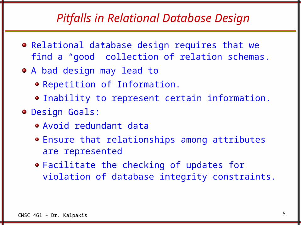
Pitfalls in Relational Database Design
Relational database design requires that we find a “good” collection of relation schemas.
A bad design may lead to
Repetition of Information.
Inability to represent certain information.
Design Goals:
Avoid redundant data
Ensure that relationships among attributes are represented
Facilitate the checking of updates for violation of database integrity constraints.

CMSC 461 – Dr. Kalpakis
6
Example
Consider the relation schema: Lending-schema = (branchName, branchCity, assets,
customerName, loanNumber, amount)
Redundancy:Data for branchName, branchCity, assets are repeated for each loan that a branch makes
Wastes space
Complicates updating, introducing possibility of inconsistency of assets value
Null valuesCannot store information about a branch if no loans exist
Can use null values, but they are difficult to handle.

CMSC 461 – Dr. Kalpakis
7
Decomposition
Decompose the relation schema Lending-schema into:BranchSchema = (branchName, branchCity,assets)
LoanSchema = (customerName, loanNumber,branchName, amount)
All attributes of an original schema (R) must appear in the
decomposition (R1, R2):
R = R1 R2
Lossless-join decomposition.
For all possible relations r on schema R
r = R1 (r) R2 (r)

CMSC 461 – Dr. Kalpakis
8
Example of Non Lossless-Join Decomposition
Decomposition of R = (A, B)
R2 = (A) R2 = (B)
A B
121
A
B
12
rA(r)
B(r)
A (r) B (r)A B
1212

CMSC 461 – Dr. Kalpakis
9
Goal — Devise a Theory for the Following
Decide whether a particular relation R is in “good” form.
In the case that a relation R is not in “good” form, decompose it
into a set of relations {R1, R2, ..., Rn} such that
each relation is in good form
the decomposition is a lossless-join decomposition
Our theory is based on:
functional dependencies
multivalued dependencies
CMSC 461 – Dr. Kalpakis
10
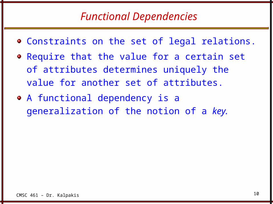
Functional Dependencies
Constraints on the set of legal relations.
Require that the value for a certain set of attributes determines
uniquely the value for another set of attributes.
A functional dependency is a generalization of the notion of a
key.

CMSC 461 – Dr. Kalpakis
11
Functional Dependencies
Let R be a relation schema
R and R
The functional dependency
holds on R if and only if for any legal relations r(R), whenever any two tuples t1 and t2 of r agree on the attributes , they also agree on
the attributes . That is,
t1[] = t2 [] t1[ ] = t2 [ ]
Example: Consider r(A,B) with the following instance of r.
On this instance, A B does NOT hold, but B A does hold.
1 41 53 7

CMSC 461 – Dr. Kalpakis
12
Functional Dependencies
K is a superkey for relation schema R if and only if K RK is a candidate key for R if and only if
K R, andfor no K, R
Functional dependencies allow us to express constraints that cannot be expressed using superkeys. Consider the schema:LoanSchema = (customerName, loanNumber, branchName, amount).
We expect this set of functional dependencies to hold:loanNumber amountloanNumber branchName
but would not expect the following to hold: loanNumber customerName

CMSC 461 – Dr. Kalpakis
13
Use of Functional Dependencies
We use functional dependencies to:
test relations to see if they are legal under a given set of functional
dependencies.
If a relation r is legal under a set F of functional dependencies, we say that r
satisfies F.
specify constraints on the set of legal relations
We say that F holds on R if all legal relations on R satisfy the set of functional
dependencies F.
Note: A specific instance of a relation schema may satisfy a functional
dependency even if the functional dependency does not hold on all legal
instances.
For example, a specific instance of Loan-schema may, by chance, satisfy
loanNumber customerName.

CMSC 461 – Dr. Kalpakis
14
Functional Dependencies
A functional dependency is trivial if it is satisfied by all
instances of a relation
E.g.
customerName, loanNumber customerName
customerName customerName
In general, is trivial if

CMSC 461 – Dr. Kalpakis
15
Closure of a Set of Functional Dependencies
Given a set F set of functional dependencies, there are certain other functional dependencies that are logically implied by F.
E.g. If A B and B C, then we can infer that A C
The set of all functional dependencies logically implied by F is the closure of F.
We denote the closure of F by F+.
We can find all of F+ by applying Armstrong’s Axioms:
if , then (reflexivity)
if , then (augmentation)
if , and , then (transitivity)
These rules are
sound (generate only functional dependencies that actually hold) and
complete (generate all functional dependencies that hold).
CMSC 461 – Dr. Kalpakis
16
Example
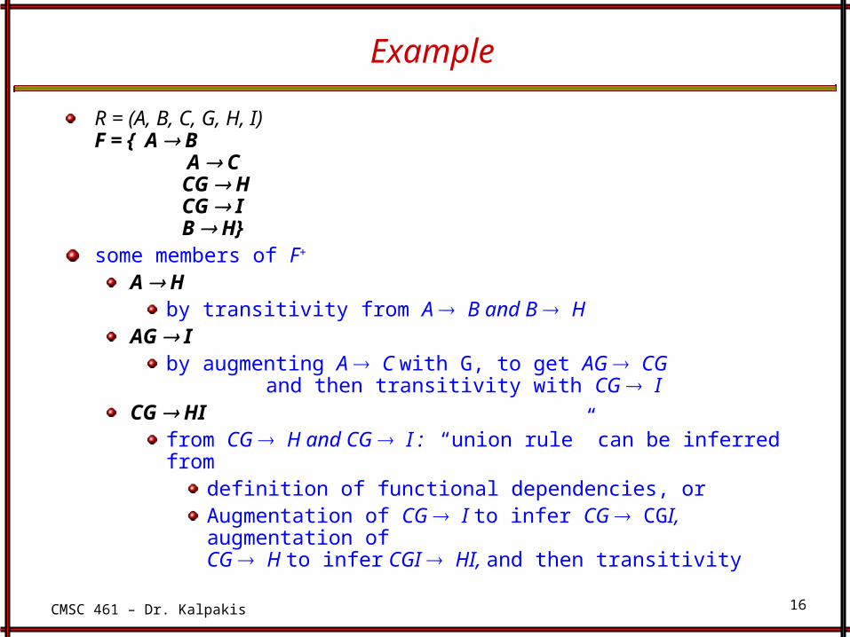
R = (A, B, C, G, H, I)F = { A B
A C CG H CG I B H}
some members of F+
A H by transitivity from A B and B H
AG I by augmenting A C with G, to get AG CG and then transitivity with CG I
CG HI from CG H and CG I : “union rule” can be inferred from
definition of functional dependencies, or Augmentation of CG I to infer CG CGI, augmentation ofCG H to infer CGI HI, and then transitivity

CMSC 461 – Dr. Kalpakis
17
Procedure for Computing F+
To compute the closure of a set of functional dependencies F:
F+ = F
repeat
for each functional dependency f in F+
apply reflexivity and augmentation rules on f
add the resulting functional dependencies to F+
for each pair of functional dependencies f1and f2 in F+
if f1 and f2 can be combined using transitivity
then add the resulting functional dependency to F+
until F+ does not change any further
NOTE: We will see an alternative procedure for this task later

CMSC 461 – Dr. Kalpakis
18
Closure of Functional Dependencies
We can further simplify manual computation of F+ by using
the following additional rules.
If holds and holds, then holds
(union)
If holds, then holds and holds
(decomposition)
If holds and holds, then holds
(pseudotransitivity)
The above rules can be inferred from Armstrong’s axioms.

CMSC 461 – Dr. Kalpakis
19
Closure of Attribute Sets
Given a set of attributes define the closure of under F
(denoted by +) as the set of attributes that are functionally
determined by under F:
is in F+ +
Algorithm to compute +, the closure of under F
result := ;
while (changes to result) do
for each in F do
begin
if result then result := result
end

CMSC 461 – Dr. Kalpakis
20
Example of Attribute Set Closure
R = (A, B, C, G, H, I)F = {A B
A C CG HCG IB H}
(AG)+
1. result = AG2. result = ABCG (A C and A B)3. result = ABCGH (CG H and CG AGBC)4. result = ABCGHI (CG I and CG AGBCH)
Is AG a candidate key? 1. Is AG a super key?
1. Does AG R? == Is (AG)+ R
2. Is any subset of AG a superkey?1. Does A R? == Is (A)+ R
2. Does G R? == Is (G)+ R

CMSC 461 – Dr. Kalpakis
21
Uses of Attribute Closure
There are several uses of the attribute closure algorithm:
Testing for superkey
To test if is a superkey, we compute +, and check if + contains all attributes of R.
Testing functional dependenciesTo check if a functional dependency holds (or, in other words, is
in F+), just check if +.
That is, we compute + by using attribute closure, and then check if it contains .
Is a simple and cheap test, and very useful
Computing closure of F
For each R, we find the closure +, and for each S +, we output a functional dependency S.

CMSC 461 – Dr. Kalpakis
22
Canonical Cover
Sets of functional dependencies may have redundant
dependencies that can be inferred from the others
Eg: A C is redundant in: {A B, B C, A C}
Parts of a functional dependency may be redundant
E.g. on RHS: {A B, B C, A CD} can be simplified to
{A B, B C, A D}
E.g. on LHS: {A B, B C, AC D} can be simplified to
{A B, B C, A D}
Intuitively, a canonical cover of F is a “minimal” set of
functional dependencies equivalent to F, having no redundant
dependencies or redundant parts of dependencies

CMSC 461 – Dr. Kalpakis
23
Extraneous Attributes
Consider a set F of functional dependencies and the functional dependency in F.
Attribute A is extraneous in if A and F logically implies (F – { }) {( – A) }.Attribute A is extraneous in if A and the set of functional dependencies (F – { }) { ( – A)} logically implies F.
Note: implication in the opposite direction is trivial in each of the cases above, since a “stronger” functional dependency always implies a weaker one

CMSC 461 – Dr. Kalpakis
24
Testing if an Attribute is Extraneous
Consider a set F of functional dependencies and the functional
dependency in F.
To test if attribute A is extraneous in
1. compute ({} – A)+ using the dependencies in F
2. check that ({} – A)+ contains A; if it does, A is extraneous
To test if attribute A is extraneous in
1. compute + using only the dependencies in
F’ = (F – { }) { ( – A)},
2. check that + contains A; if it does, A is extraneous

CMSC 461 – Dr. Kalpakis
25
Extraneous Attributes - Examples
Given F = {A C, AB C }Is B is extraneous in AB C?
Given F = {A C, AB CD}Is C is extraneous in AB CD?

CMSC 461 – Dr. Kalpakis
26
Canonical Cover
A canonical cover for F is a set of dependencies Fc such that
F logically implies all dependencies in Fc, and
Fc logically implies all dependencies in F, and
No functional dependency in Fc contains an extraneous attribute, and
Each left side of functional dependency in Fc is unique.

CMSC 461 – Dr. Kalpakis
27
Computing Canonical Covers
To compute a canonical cover for F
repeatUse the union rule to replace any dependencies in F
1 1 and 1 1 with 1 1 2 Find a functional dependency with an
extraneous attribute either in or in If an extraneous attribute is found, delete it from
until F does not change
Note: the Union rule may become applicable after some extraneous attributes have been deleted, so it has to be re-applied

CMSC 461 – Dr. Kalpakis
28
Example of Computing a Canonical Cover
R = (A, B, C)F = {A BC
B C A B AB C}
Combine A BC and A B into A BCSet is now {A BC, B C, AB C}
A is extraneous in AB CSet is now {A BC, B C}
C is extraneous in A BC The canonical cover is: { A B, B C }

CMSC 461 – Dr. Kalpakis
29
Goals of Normalization
Decide whether a particular relation R is in “good” form.
In the case that a relation R is not in “good” form, decompose it into
a set of relations {R1, R2, ..., Rn} such that
each relation is in good form
the decomposition is a lossless-join decomposition
Our theory is based on:
functional dependencies
multivalued dependencies

CMSC 461 – Dr. Kalpakis
30
Lossless Join Decomposition
Consider a decomposition of schema (R) into (R1, R2):
All attributes of R must appear in the decomposition (R1, R2):
R = R1 R2
Lossless-join decomposition.For all possible relations r on schema R
r = R1 (r) R2 (r)
A decomposition of R into R1 and R2 is lossless join if and only if at least one of the following dependencies is in F+:
R1 R2 R1
R1 R2 R2
CMSC 461 – Dr. Kalpakis
31
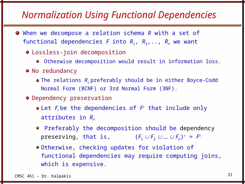
Normalization Using Functional Dependencies
When we decompose a relation schema R with a set of functional
dependencies F into R1, R2,.., Rn we want
Lossless-join decomposition
Otherwise decomposition would result in information loss.
No redundancy
The relations Ri preferably should be in either Boyce-Codd Normal Form
(BCNF) or 3rd Normal Form (3NF).
Dependency preservation
Let Fi be the dependencies of F+ that include only attributes in Ri.
Preferably the decomposition should be dependency preserving,
that is, (F1 F2 … Fn)+ = F+
Otherwise, checking updates for violation of functional
dependencies may require computing joins, which is expensive.

CMSC 461 – Dr. Kalpakis
32
Testing for Dependency Preservation
To check if a dependency is preserved in a decomposition of R into
R1, R2, …, Rn we apply the following simplified test (with attribute closure
done w.r.t. F)
result = while (changes to result) do
for each Ri in the decomposition
t = (result Ri)+ Ri
result = result t
If result contains all attributes in , then the functional dependency
is preserved.
We apply the test on all dependencies in F to check if a decomposition is
dependency preserving
This procedure takes polynomial time, instead of the exponential time
required to compute F+ and (F1 F2 … Fn)+
CMSC 461 – Dr. Kalpakis
33
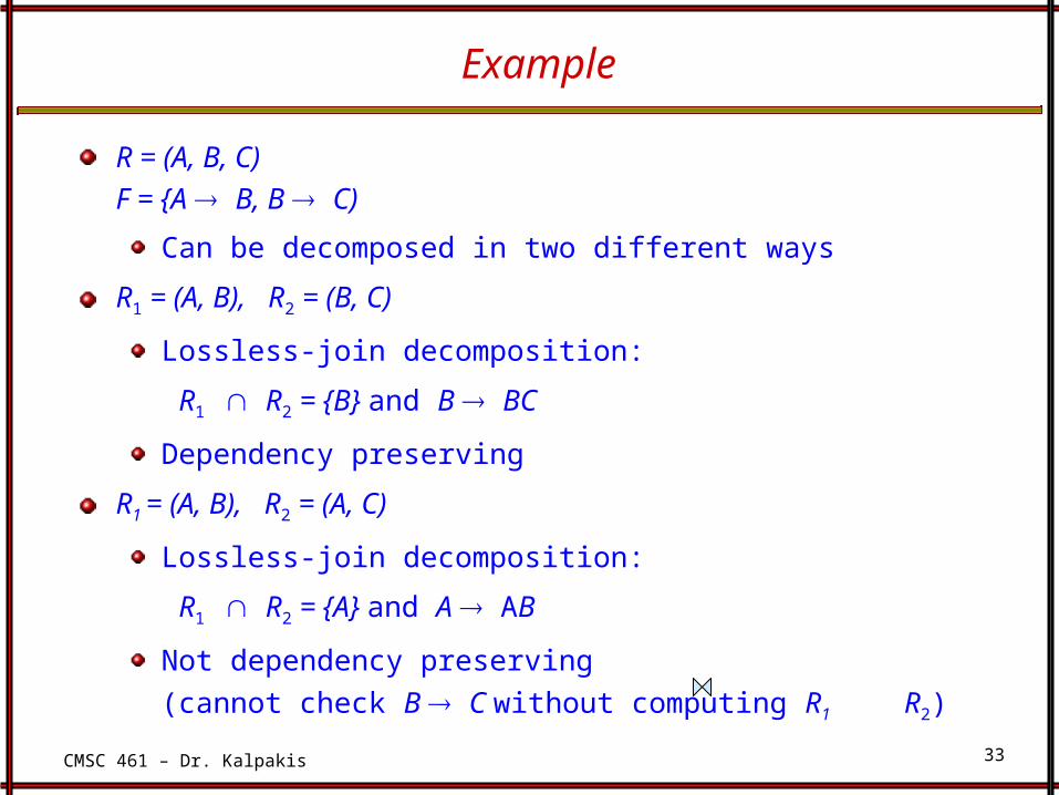
Example
R = (A, B, C)
F = {A B, B C)
Can be decomposed in two different ways
R1 = (A, B), R2 = (B, C)
Lossless-join decomposition:
R1 R2 = {B} and B BC
Dependency preserving
R1 = (A, B), R2 = (A, C)
Lossless-join decomposition:
R1 R2 = {A} and A AB
Not dependency preserving
(cannot check B C without computing R1 R2)

CMSC 461 – Dr. Kalpakis
34
Boyce-Codd Normal Form
A relation schema R is in BCNF with respect to a set F of
functional dependencies if for all functional dependencies in
F+ of the form , where R and R, at least one
of the following holds:
is trivial (i.e., )
is a superkey for R
CMSC 461 – Dr. Kalpakis
35
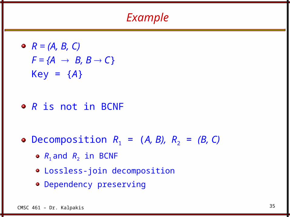
Example
R = (A, B, C)
F = {A B, B C}
Key = {A}
R is not in BCNF
Decomposition R1 = (A, B), R2 = (B, C)
R1 and R2 in BCNF
Lossless-join decomposition
Dependency preserving

CMSC 461 – Dr. Kalpakis
36
Testing for BCNF
To check if a non-trivial dependency causes a violation of BCNF1. compute + (the attribute closure of ), and 2. verify that it includes all attributes of R, that is, it is a
superkey of R.
Simplified test: To check if a relation schema R is in BCNF, it suffices to check only the dependencies in the given set F for violation of BCNF, rather than checking all dependencies in F+.
If none of the dependencies in F causes a violation of BCNF, then none of the dependencies in F+ will cause a violation of BCNF either.
CMSC 461 – Dr. Kalpakis
37
Testing for BCNF
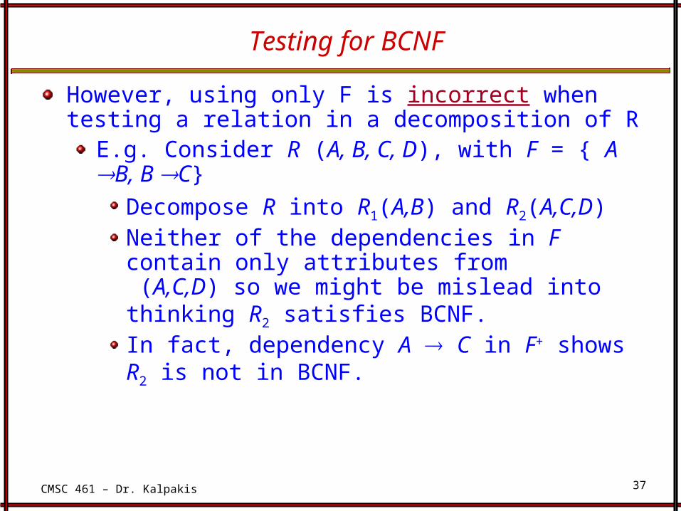
However, using only F is incorrect when testing a relation in a decomposition of R
E.g. Consider R (A, B, C, D), with F = { A B, B C}
Decompose R into R1(A,B) and R2(A,C,D) Neither of the dependencies in F contain only attributes from (A,C,D) so we might be mislead into thinking R2 satisfies BCNF.
In fact, dependency A C in F+ shows R2 is not in BCNF.

CMSC 461 – Dr. Kalpakis
38
BCNF Decomposition Algorithm
result := {R};
done := false;
compute F+;
while (not done) do
if (there is a schema Ri in result that is not in BCNF)
then begin
let be a nontrivial functional dependency that holds on Ri
such that
Ri is not in F+,
and = ;
result := (result – Ri ) (Ri – ) (, );
end
else done := true;
Note: each Ri is in BCNF, and decomposition is lossless-join.

CMSC 461 – Dr. Kalpakis
39
Example of BCNF Decomposition
R = (branchName, branchCity, assets,customerName, loanNumber, amount)
F = {branchName assets branchCity
loanNumber amount branchName}
Key = {loanNumber, customerName}
DecompositionR1 = (branchName, branchCity, assets)
R2 = (branchName, customerName, loanNumber, amount)
R3 = (branchName, loanNumber, amount)
R4 = (customerName, loanNumber)
Final decomposition R1, R3, R4

CMSC 461 – Dr. Kalpakis
40
Testing Decomposition for BCNF
To check if a relation Ri in a decomposition of R is in BCNF,
Either test Ri for BCNF with respect to the restriction of F to Ri (that
is, all FDs in F+ that contain only attributes from Ri)
or use the original set of dependencies F that hold on R, but with the
following test:
for every set of attributes Ri, check that + (the attribute
closure of ) either includes no attribute of Ri- , or includes
all attributes of Ri.
If the condition is violated by some in F, the dependency
(+ - ) Ri
can be shown to hold on Ri, and Ri violates BCNF.
We use above dependency to decompose Ri

CMSC 461 – Dr. Kalpakis
41
BCNF and Dependency Preservation
It is not always possible to get a BCNF decomposition that
is dependency preserving
R = (J, K, L)
F = {JK L, L K}
Two candidate keys = JK and JL
R is not in BCNF
Any decomposition of R will fail to preserve
JK L

CMSC 461 – Dr. Kalpakis
42
3rd Normal Form (3NF) - Motivation
There are some situations where
BCNF is not dependency preserving, and
efficient checking for FD violation on updates is important
Solution: define a weaker normal form, called 3rd Normal
Form.
Allows some redundancy (with resultant problems; we will see
examples later)
But FDs can be checked on individual relations without computing a
join.
There is always a lossless-join, dependency-preserving decomposition
into 3NF.
CMSC 461 – Dr. Kalpakis
43
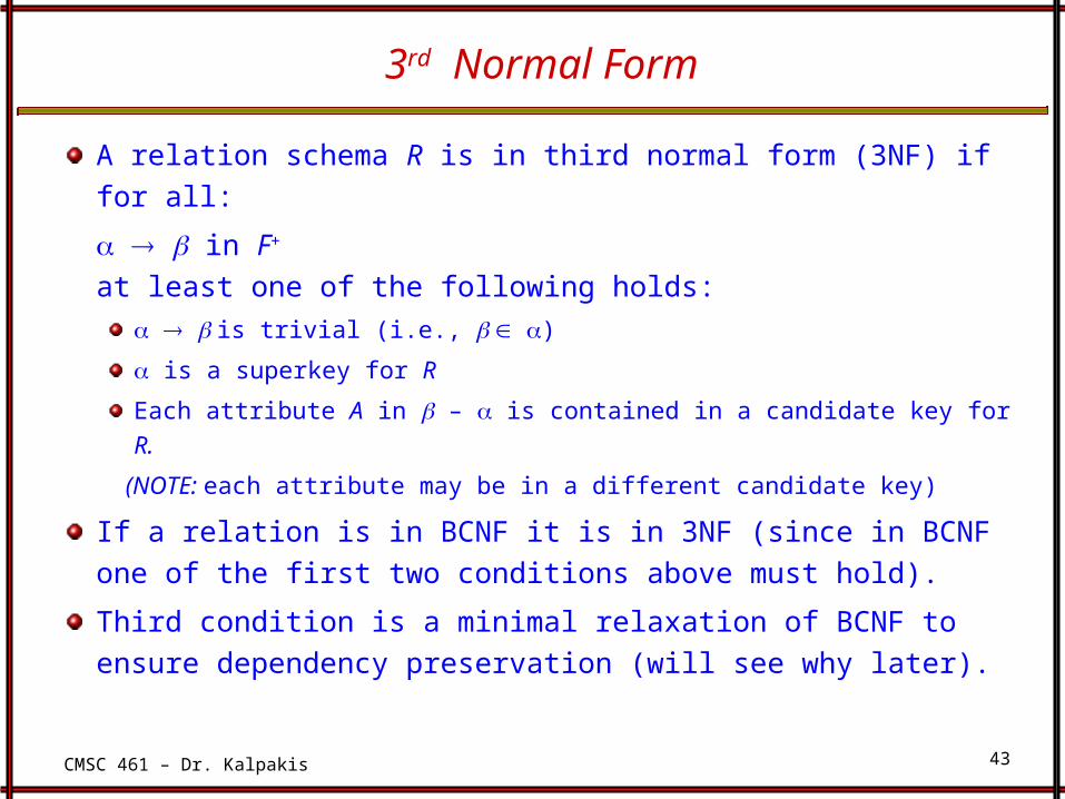
3rd Normal Form
A relation schema R is in third normal form (3NF) if for all:
in F+
at least one of the following holds:
is trivial (i.e., )
is a superkey for R
Each attribute A in – is contained in a candidate key for R.
(NOTE: each attribute may be in a different candidate key)
If a relation is in BCNF it is in 3NF (since in BCNF one of the
first two conditions above must hold).
Third condition is a minimal relaxation of BCNF to ensure
dependency preservation (will see why later).

CMSC 461 – Dr. Kalpakis
44
3NF
Example
R = (J, K, L)F = {JK L, L K}
Two candidate keys: JK and JL
R is in 3NF
JK L JK is a superkeyL K K is contained in a candidate key
BCNF decomposition has (JL) and (LK) Testing for JK L requires a join
There is some redundancy in this schema
Equivalent to example in book:
Banker-schema = (branchName, customerName, bankerName)
bankerName branch name
branch name customerName bankerName

CMSC 461 – Dr. Kalpakis
45
Testing for 3NF
Optimization: Need to check only FDs in F, need not check all FDs in F+.
Use attribute closure to check for each dependency , if is a superkey.
If is not a superkey, we have to verify if each attribute in is contained in a candidate key of R
this test is rather more expensive, since it involve finding candidate keys
testing for 3NF has been shown to be NP-hard
Interestingly, decomposition into 3NF can be done in polynomial time

CMSC 461 – Dr. Kalpakis
46
3NF Decomposition Algorithm
Let Fc be a canonical cover for F;
i := 0;
for each functional dependency in Fc do
if none of the schemas Rj, 1 j i contains
then begin
i := i + 1;
Ri :=
end
if none of the schemas Rj, 1 j i contains a candidate key for R
then begin
i := i + 1;
Ri := any candidate key for R;
end
return (R1, R2, ..., Ri)

CMSC 461 – Dr. Kalpakis
47
3NF Decomposition Algorithm
Above algorithm ensures:
each relation schema Ri is in 3NF
decomposition is dependency preserving and lossless-join
Example 3NF decomposition
Relation schema:
Banker-info-schema = (branchName, customerName,
bankerName, officeNumber)
The functional dependencies for this relation schema are:
bankerName branchName officeNumber
customerName branchName bankerName
The key is:
{customerName, branchName}

CMSC 461 – Dr. Kalpakis
48
Applying 3NF to Banker-info-schema
The for loop in the algorithm causes us to include the following schemas
in our decomposition:
Banker-office-schema = (bankerName, branchName,
officeNumber)
Banker-schema = (customerName, branchName,
bankerName)
Since Banker-schema contains a candidate key for
Banker-info-schema, we are done with the decomposition process.

CMSC 461 – Dr. Kalpakis
49
Comparison of BCNF and 3NF
It is always possible to decompose a relation into relations in
3NF and
the decomposition is lossless
the dependencies are preserved
It is always possible to decompose a relation into relations in
BCNF and
the decomposition is lossless
it may not be possible to preserve dependencies.

CMSC 461 – Dr. Kalpakis
50
Example of problems due to redundancy in 3NF
R = (J, K, L)
F = {JK L, L K}
A schema that is in 3NF but not in BCNF has the problems of
repetition of information (e.g., the relationship l1, k1)
need to use null values (e.g., to represent the relationship l2, k2 where
there is no corresponding value for J).
Comparison of BCNF and 3NF
J L Kj1
j2
j3
null
l1
l1
l1
l2
k1
k1
k1
k2

CMSC 461 – Dr. Kalpakis
51
Design Goals
Goal for a relational database design is:
BCNF.
Lossless join.
Dependency preservation.
If we cannot achieve this, we accept one of
Lack of dependency preservation
Redundancy due to use of 3NF
Interestingly, SQL does not provide a direct way of specifying functional
dependencies other than superkeys.
Can specify FDs using assertions, but they are expensive to test
Even if we had a dependency preserving decomposition, using SQL we
would not be able to efficiently test a functional dependency whose left hand
side is not a key.

CMSC 461 – Dr. Kalpakis
52
Testing for FDs Across Relations
If decomposition is not dependency preserving, we can have an extra materialized view for each dependency in Fc that is not preserved in the decompositionThe materialized view is defined as a projection on of the join of the relations in the decompositionMany newer database systems support materialized views and database system maintains the view when the relations are updated.
No extra coding effort for programmer.
The functional dependency is expressed by declaring as a candidate key on the materialized view.Checking for candidate key cheaper than checking BUT:
Space overhead: for storing the materialized viewTime overhead: Need to keep materialized view up to date when relations are updatedDatabase system may not support key declarations on materialized views

CMSC 461 – Dr. Kalpakis
53
Overall Database Design Process
We have assumed schema R is given
R could have been generated when converting E-R
diagram to a set of tables.
R could have been a single relation containing all attributes
that are of interest (called universal relation).
Normalization breaks R into smaller relations.
R could have been the result of some ad hoc design of
relations, which we then test/convert to normal form.
CMSC 461 – Dr. Kalpakis
54
ER Model and Normalization
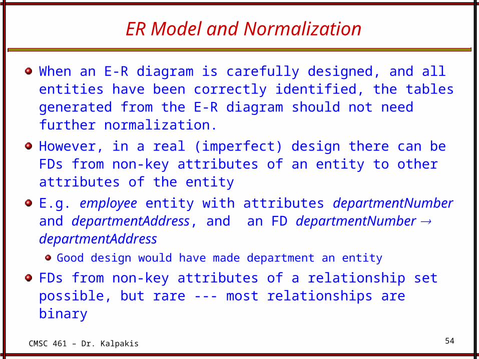
When an E-R diagram is carefully designed, and all entities have been correctly identified, the tables generated from the E-R diagram should not need further normalization.
However, in a real (imperfect) design there can be FDs from non-key attributes of an entity to other attributes of the entity
E.g. employee entity with attributes departmentNumber and departmentAddress, and an FD departmentNumber departmentAddress
Good design would have made department an entity
FDs from non-key attributes of a relationship set possible, but rare --- most relationships are binary

CMSC 461 – Dr. Kalpakis
55
Universal Relation Approach
Dangling tuples – Tuples that “disappear” in computing a join.
Let r1 (R1), r2 (R2), …., rn (Rn) be a set of relations
A tuple r of the relation ri is a dangling tuple if r is not in the relation:
Ri (r1 r2 … rn)
The relation r1 r2 … rn is called a universal relation since it involves
all the attributes in the “universe” defined by
R1 R2 … Rn
If dangling tuples are allowed in the database, instead of decomposing a
universal relation, we may prefer to synthesize a collection of normal form
schemas from a given set of attributes.
CMSC 461 – Dr. Kalpakis
56
Universal Relation Approach
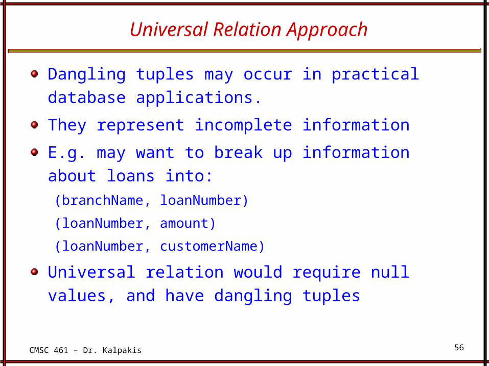
Dangling tuples may occur in practical database applications.
They represent incomplete information
E.g. may want to break up information about loans into:
(branchName, loanNumber)
(loanNumber, amount)
(loanNumber, customerName)
Universal relation would require null values, and have dangling
tuples
CMSC 461 – Dr. Kalpakis
57
Universal Relation Approach
A particular decomposition defines a restricted form of
incomplete information that is acceptable in our database.
Above decomposition requires at least one of customerName,
branchName or amount in order to enter a loan number without using
null values
Rules out storing of customerName, amount without an appropriate
loanNumber (since it is a key, it can't be null either!)
Universal relation requires unique attribute names - unique role
assumption
e.g. customerName, branchName
Reuse of attribute names is natural in SQL since relation names
can be prefixed to disambiguate names

CMSC 461 – Dr. Kalpakis
58
Denormalization for Performance
May want to use non-normalized schema for performance
E.g. displaying customerName along with accountNumber and balance
requires join of account with depositor
Alternative 1: Use denormalized relation containing attributes of
account as well as depositor with all above attributes
faster lookup
Extra space and extra execution time for updates
extra coding work for programmer and possibility of error in extra code
Alternative 2: use a materialized view defined as
account depositor
Benefits and drawbacks same as above, except no extra coding work for
programmer and avoids possible errors

CMSC 461 – Dr. Kalpakis
59
Other Design Issues
Some aspects of database design are not caught by normalizationExamples of bad database design, to be avoided: Instead of earnings(company-id, year, amount), could use
earnings-2000, earnings-2001, earnings-2002, etc., all on the schema (company-id, earnings).
Above are in BCNF, but make querying across years difficult and needs new table each year
company-year(company-id, earnings-2000, earnings-2001, earnings-2002)
Also in BCNF, but also makes querying across years difficult and requires new attribute each year.Is an example of a crosstab, where values for one attribute become column namesUsed in spreadsheets, and in data analysis tools