RELATION METHODS - Chapman Universitymath.chapman.edu/~jipsen/.../SchmidtApplicRel2006... ·...
338
RELATION METHODS IN VARIOUS APPLICATION FIELDS GUNTHER SCHMIDT in co-operation with NN, NN, NN, . . . NN c Gunther Schmidt 2006
Transcript of RELATION METHODS - Chapman Universitymath.chapman.edu/~jipsen/.../SchmidtApplicRel2006... ·...
RELATION
METHODS
IN VARIOUS
APPLICATION FIELDS
GUNTHER SCHMIDT
in co-operation with
NN, NN, NN, . . . NN
c© Gunther Schmidt 2006

Gunther Schmidtin co-operation with
NN, NN, NN, . . . NN
Relation Methods
in Various Application Fields
With 100 Figures


Preface
This book addresses the broad community of researchers in various applications fields who userelations and graphs in their scientific work. It is expected to be of use in such diverging areasas psychology, padagogics (?), sociology, coalition formation, social choice theory, linguistics,preference modeling, ranking, multicriteria decision studies, machine learning, voting theories,spatial reasoning, data base optimization, and many more. In all these, and in a lot of otherfields, relations are used to express, to model, to reason etc.
In some areas specialized developments have taken place, not least reinventing the wheel everagain. Some areas are highly mathematical ones, others restrict to only a moderate use ofmathematics. Not all are aware of recent developments which relational methods enjoyed overrecent years.
It is intended to provide something as an easy to read overview of the field that nevertheless istheoretically sound and up to date. The exposition will not stress the mathematical side toomuch. Visualizations of ideas will often be presented instead.
One main point of the conception of this book is surprising: We try to get rid of some traditionalabstractions. Mathematicians have developed the concept of a set, e.g., and computer sciencepeople use it indiscriminately. At several occasions occurring in practice it would be wise to goone step down to a less abstract level, i.e., mention also how the respective set is represented.Trying to abandon over-abstraction is not a common feature in science. Nevertheless, we feelwe should try it here.
The reason for doing so is the observation that people were always so hesitant in using relations.Notation was eagerly used that — by gross estimation — was six times as voluminous than thatfor an algebraic treatment of relations. As this was the case, concepts were often not writtenwith the necessary care, nor could one easily see at which points rules should be applied.
In former years, we attributed this to simply not being acquainted with relations; later we beganto look for additional reasons. What we identified was that people often could not properlyinterpret relational tasks or their results. Even if explained thoroughly, they stayed hesitant.Over the years this became so dominant that we looked for additional problems. One majorsuch seems to be that the for now hundred years traditional concept of a set is one of theobstacles. A set, e.g., is not immediately a data structure for a computer scientist. Some arewilling to identify it with a list without duplicates regardless of the ordering of elements, butthis is obviously not an ideal concept.
We try here to make visible that a set is the abstraction of may be six or seven conceptsfor which we give all the methods of conversion. So we first show how a (finite) set may berepresented and how these representations may easily be changed. Then one will see that some
6
representations are better than others, not just with regard to some measure of complexitybut with regard to visualization. Once this is understood, also the concept of a subset changesslightly. Then one will also more easily conceive what a relation is like. Altogether it is a ratherconstructive approach to basic mathematics — as well as to theoretical computer science.
Today problems are increasingly handled using relational means. Many new application fieldscame to our attention not least during the COST Action 274 TARSKI (Theory and Appli-cations of Relational Structures as Knowledgs Instruments). Regrettably, a common way ofdenotation, formulation, proving, and programming around relations is not yet agreed upon.To address this point, the multi-purpose relational reference language TITUREL is currentlyunder development; for an intermediate version see [Sch04, Sch03, Sch05].
Such a language must firstly be capable of expressing whatever has shown up in relationalmethods and structures so far — otherwise it will not get acceptence. A second point is toconvince people that the language developed is indeed useful and brings added value. This canbest be done designing it to be immediately operational. To formulate in the evolving languagemeans to write a program (in Haskell) which can directly be executed at least for moderatelysized problems. One should, however, remember that this means interpretation, not translation.To make this efficient deserves yet a huge amount of work which may be compared with all thework people have invested in numerical algorithms over decades.
In the course of this development a lot of relational concepts have been formulated in thelanguage in order to find out whether expressibility is sufficient. A certain amount of workhas also been invested in I/O. It came as a benefit that instantaneous interpretation in toyexamples clarified concepts to a great extent.
The book is intended to be a help for scientists even if they are not so versed in mathematicsbut have to employ it. Therefore, it strives to visualize how things work, mainly via matricesbut also via graphs. Proofs have been executed, of course, but are not all presented except forsome key situations.
Munich, August 2006 Gunther Schmidt
Acknowledgments. Cooperation and communication around the writing of this book waspartly sponsored by the European COST Action 274: TARSKI I had the honour to chair from2001 to 2005. This is gratefully acknowledged. Among the friends and colleagues who havediscussed matters let me mention . . .

Contents
1 Introduction 11
I How Discrete Tasks are Presented 15
2 Sets, Subsets, and Elements 192.1 Baseset Representation . . . . . . . . . . . . . . . . . . . . . . . . . . . . . . . . . . . . 192.2 Element Representation . . . . . . . . . . . . . . . . . . . . . . . . . . . . . . . . . . . 212.3 Subset Representation . . . . . . . . . . . . . . . . . . . . . . . . . . . . . . . . . . . . 22
3 Relations 293.1 Relation Representation . . . . . . . . . . . . . . . . . . . . . . . . . . . . . . . . . . . 293.2 Relations Describing Graphs . . . . . . . . . . . . . . . . . . . . . . . . . . . . . . . . . 333.3 Relations Generated by Cuts . . . . . . . . . . . . . . . . . . . . . . . . . . . . . . . . 343.4 Relations Generated Randomly . . . . . . . . . . . . . . . . . . . . . . . . . . . . . . . 363.5 Functions . . . . . . . . . . . . . . . . . . . . . . . . . . . . . . . . . . . . . . . . . . . 373.6 Permutations . . . . . . . . . . . . . . . . . . . . . . . . . . . . . . . . . . . . . . . . . 393.7 Partitions . . . . . . . . . . . . . . . . . . . . . . . . . . . . . . . . . . . . . . . . . . . 42
II Visualizing Relational Constructions 43
4 Algebraic Operations on Relations 474.1 Typing Relations . . . . . . . . . . . . . . . . . . . . . . . . . . . . . . . . . . . . . . . 474.2 Boolean Operations . . . . . . . . . . . . . . . . . . . . . . . . . . . . . . . . . . . . . 484.3 Relational Operations Proper . . . . . . . . . . . . . . . . . . . . . . . . . . . . . . . . 504.4 Composite Operations . . . . . . . . . . . . . . . . . . . . . . . . . . . . . . . . . . . . 53
5 Order and Function: The Standard View 575.1 Functions and Mappings . . . . . . . . . . . . . . . . . . . . . . . . . . . . . . . . . . . 575.2 Mappings . . . . . . . . . . . . . . . . . . . . . . . . . . . . . . . . . . . . . . . . . . . 625.3 Order and Strictorder . . . . . . . . . . . . . . . . . . . . . . . . . . . . . . . . . . . . 655.4 Equivalence and Quotient . . . . . . . . . . . . . . . . . . . . . . . . . . . . . . . . . . 735.5 Transitive Closure . . . . . . . . . . . . . . . . . . . . . . . . . . . . . . . . . . . . . . 775.6 Relations and Vectors . . . . . . . . . . . . . . . . . . . . . . . . . . . . . . . . . . . . 795.7 Properties of the Symmetric Quotient . . . . . . . . . . . . . . . . . . . . . . . . . . . 86
6 Relational Domain Construction 916.1 Domains of Ground Type . . . . . . . . . . . . . . . . . . . . . . . . . . . . . . . . . . 916.2 Direct Product . . . . . . . . . . . . . . . . . . . . . . . . . . . . . . . . . . . . . . . . 926.3 Direct Sum . . . . . . . . . . . . . . . . . . . . . . . . . . . . . . . . . . . . . . . . . . 1006.4 Quotient Domain . . . . . . . . . . . . . . . . . . . . . . . . . . . . . . . . . . . . . . . 1046.5 Subset Extrusion . . . . . . . . . . . . . . . . . . . . . . . . . . . . . . . . . . . . . . . 1076.6 Direct Power . . . . . . . . . . . . . . . . . . . . . . . . . . . . . . . . . . . . . . . . . 1106.7 Domain Permutation . . . . . . . . . . . . . . . . . . . . . . . . . . . . . . . . . . . . . 1156.8 Further Constructions . . . . . . . . . . . . . . . . . . . . . . . . . . . . . . . . . . . . 1166.9 Equivalent Representations . . . . . . . . . . . . . . . . . . . . . . . . . . . . . . . . . 117
7
8 Contents
III How to Use the Relational Language 119
7 Relation Algebra 1237.1 Laws of Relation Algebra . . . . . . . . . . . . . . . . . . . . . . . . . . . . . . . . . . 1237.2 Visualizing the Schroder Equivalences . . . . . . . . . . . . . . . . . . . . . . . . . . . 1247.3 Visualizing the Dedekind-Formula . . . . . . . . . . . . . . . . . . . . . . . . . . . . . 1287.4 Elementary Properties of Relations . . . . . . . . . . . . . . . . . . . . . . . . . . . . . 129
8 Orderings and Lattices 1338.1 Maxima and Minima . . . . . . . . . . . . . . . . . . . . . . . . . . . . . . . . . . . . . 1338.2 Bounds and Cones . . . . . . . . . . . . . . . . . . . . . . . . . . . . . . . . . . . . . . 1348.3 Least and Greatest Elements . . . . . . . . . . . . . . . . . . . . . . . . . . . . . . . . 1368.4 Greatest Lower and Least Upper Bounds . . . . . . . . . . . . . . . . . . . . . . . . . 1388.5 Lattices . . . . . . . . . . . . . . . . . . . . . . . . . . . . . . . . . . . . . . . . . . . . 1398.6 Cut Completion of an Ordering . . . . . . . . . . . . . . . . . . . . . . . . . . . . . . . 140
9 Rectangles 1459.1 Maximal Rectangles . . . . . . . . . . . . . . . . . . . . . . . . . . . . . . . . . . . . . 1459.2 Pairs of independent and pairs of covering sets . . . . . . . . . . . . . . . . . . . . . . 1499.3 Concept Lattices . . . . . . . . . . . . . . . . . . . . . . . . . . . . . . . . . . . . . . . 1539.4 Difunctionality . . . . . . . . . . . . . . . . . . . . . . . . . . . . . . . . . . . . . . . . 1589.5 Application in Knowledge Acquisition . . . . . . . . . . . . . . . . . . . . . . . . . . . 1649.6 Fringes . . . . . . . . . . . . . . . . . . . . . . . . . . . . . . . . . . . . . . . . . . . . . 1669.7 Ferrers Property/Biorders Heterogeneous . . . . . . . . . . . . . . . . . . . . . . . . . 173
10 Preorder and Equivalence: An Advanced View 18310.1 Equivalence and Preorder . . . . . . . . . . . . . . . . . . . . . . . . . . . . . . . . . . 18310.2 Ferrers Property/Biorders Homogeneous . . . . . . . . . . . . . . . . . . . . . . . . . . 18410.3 Relating Preference and Utility . . . . . . . . . . . . . . . . . . . . . . . . . . . . . . . 19010.4 Well-Ordering . . . . . . . . . . . . . . . . . . . . . . . . . . . . . . . . . . . . . . . . . 20510.5 Data Base Congruences . . . . . . . . . . . . . . . . . . . . . . . . . . . . . . . . . . . 20610.6 Preferences and Indifference . . . . . . . . . . . . . . . . . . . . . . . . . . . . . . . . . 20710.7 Scaling . . . . . . . . . . . . . . . . . . . . . . . . . . . . . . . . . . . . . . . . . . . . . 207
11 Function Properties: An Advanced View 20911.1 Homomorphy . . . . . . . . . . . . . . . . . . . . . . . . . . . . . . . . . . . . . . . . . 20911.2 Congruences . . . . . . . . . . . . . . . . . . . . . . . . . . . . . . . . . . . . . . . . . . 214
IV Applications 223
12 Relational Graph Theory 22712.1 Types of Graphs . . . . . . . . . . . . . . . . . . . . . . . . . . . . . . . . . . . . . . . 22712.2 Roots in a Graph . . . . . . . . . . . . . . . . . . . . . . . . . . . . . . . . . . . . . . . 22812.3 Reducible Relations . . . . . . . . . . . . . . . . . . . . . . . . . . . . . . . . . . . . . 22912.4 Difunctionality and Irreducibility . . . . . . . . . . . . . . . . . . . . . . . . . . . . . . 23312.5 Hammocks . . . . . . . . . . . . . . . . . . . . . . . . . . . . . . . . . . . . . . . . . . 23712.6 Feedback Vertex Sets . . . . . . . . . . . . . . . . . . . . . . . . . . . . . . . . . . . . . 23912.7 Helly and Conformal Property . . . . . . . . . . . . . . . . . . . . . . . . . . . . . . . 239
13 Modeling Preferences 24113.1 Modeling Preferences . . . . . . . . . . . . . . . . . . . . . . . . . . . . . . . . . . . . . 24113.2 Introductory Example . . . . . . . . . . . . . . . . . . . . . . . . . . . . . . . . . . . . 24213.3 Relational Measures . . . . . . . . . . . . . . . . . . . . . . . . . . . . . . . . . . . . . 24313.4 Relational Integration . . . . . . . . . . . . . . . . . . . . . . . . . . . . . . . . . . . . 24813.5 Defining Relational Measures . . . . . . . . . . . . . . . . . . . . . . . . . . . . . . . . 25113.6 Focal Sets . . . . . . . . . . . . . . . . . . . . . . . . . . . . . . . . . . . . . . . . . . . 25613.7 De Morgan Triples . . . . . . . . . . . . . . . . . . . . . . . . . . . . . . . . . . . . . . 257
Contents 9
14 Mathematical Applications 26314.1 Homomorphism and Isomorphism Theorems . . . . . . . . . . . . . . . . . . . . . . . . 26314.2 Covering of Graphs and Path Equivalence . . . . . . . . . . . . . . . . . . . . . . . . . 269
15 Standard Galois Mechanisms 27115.1 Galois Iteration . . . . . . . . . . . . . . . . . . . . . . . . . . . . . . . . . . . . . . . . 27115.2 Termination . . . . . . . . . . . . . . . . . . . . . . . . . . . . . . . . . . . . . . . . . . 27315.3 Correctness and wp . . . . . . . . . . . . . . . . . . . . . . . . . . . . . . . . . . . . . . 27715.4 Games . . . . . . . . . . . . . . . . . . . . . . . . . . . . . . . . . . . . . . . . . . . . . 27815.5 Specialization to Kernels . . . . . . . . . . . . . . . . . . . . . . . . . . . . . . . . . . . 28215.6 Matching and Assignment . . . . . . . . . . . . . . . . . . . . . . . . . . . . . . . . . . 28315.7 Koenig’s Theorems . . . . . . . . . . . . . . . . . . . . . . . . . . . . . . . . . . . . . . 288
V Advanced Topics 291
16 Demonics 29516.1 Demonic Operators . . . . . . . . . . . . . . . . . . . . . . . . . . . . . . . . . . . . . . 295
17 Implication Structures 30117.1 Dependency Systems . . . . . . . . . . . . . . . . . . . . . . . . . . . . . . . . . . . . . 301
18 Partiality Structures 307
19 Other Relational Structures 30919.1 Compass Relations . . . . . . . . . . . . . . . . . . . . . . . . . . . . . . . . . . . . . . 30919.2 Compass Relations Refined . . . . . . . . . . . . . . . . . . . . . . . . . . . . . . . . . 31019.3 Interval Relations . . . . . . . . . . . . . . . . . . . . . . . . . . . . . . . . . . . . . . . 31119.4 Relational Grammar . . . . . . . . . . . . . . . . . . . . . . . . . . . . . . . . . . . . . 31219.5 Mereology . . . . . . . . . . . . . . . . . . . . . . . . . . . . . . . . . . . . . . . . . . . 313
A Notation 315
B Postponed Proofs 319
C History 323
Bibliography 327
Index 332

10 Contents

1 Introduction
A comparison may help to describe the intention of this book. Natural sciences and engineeringsciences have their corresponding differential and integral calculi. Whenever practical work isto be done, one will easily find a numerical algebra package and be able to use it. This appliesto solving linear equations or determining eigenvalues in connection, e.g., with Finite ElementMethods.
A different situation holds for various forms of information sciences. Also these have theircalculi, namely the calculi of logic, of sets, and the calculus of relations. When practical workis to be done, however, people will mostly apply Prolog-like calculi. Nearly nobody will knowhow to apply relational calculi. There is usually no package to handle problems beyond toysize. One will have to approach theoreticians since there are not many practitioners in suchfields.
We have found out that engineers and even mathematicians frequently encounter problemswhen relations show up. While they willingly apply matrices, they hesitate to accept that inthe same way as for real or complex matrices linearity is a great help in the case of logicalpredicates. Here, relational theory is conceived much in the same way as Linear Algebra in theclassic form — but now for Logics.
With this text we will present a smooth introduction into the field that is theoretically soundand leads to reasonably efficient computer programs. It takes into account problems peopleencountered earlier. Although mainly dealing with Discrete Mathematics, the text will atmany places differ from what is presented in classical texts on this topic. Most importantly,complexity considerations are outside the scope, the presentation of basic principles that arebroadly applicable is favoured. In several cases, therefore, the exposition is different from whatone may read at other places in case it better subsumes under a line of argument.
Also basic distinction will be made for the elements of set theory in order to come to a verygeneral layout. We distinguish basesets from their subsets because they are handled completelydifferently when bringing them on a computer.
In general, we pay attention to the process of delivering a problem to be handled by computer.This means that we anticipate the diversity of representations of the basic constituents. Itshall no longer occur that somebody comes with a relation in set function representation andis confronted with a computer program where matrices are used. From the very beginning weprovide many conversions to make this work together.
There is one further point to mention. We might have chosen to develop a data structure for setsand relations and then formulate with respect to these. This seemed, however, not the method of
11
12 Chapter 1 Introduction
choice. We rather assume in any case a far more logic-oriented scenario: After the introductoryexamples, always a formal theory is conceived which may afterwards be interpreted. We thusrestrict expressibility in a certain way — but it pays. The formal theory allows us often toprove correctness of what we have developed.
Proceeding this way brings many aspects of semantical domain construction and programmingmethodology into effect, in which fields the author has worked over the years. Not least will anaccount be given on so-called dependent types. Typing and transformation are omnipresent,based on a long experience with earlier systems such as RALF [HBS94a] and HOPS [SBK90,BGK+96, Kah02]. Also graph theory shows up at various places, however, handled from therelational point of view, already put forward in [SS89, SS93].
When working with relations, one will have to prepare ones tasks so as to be able to give themas input to the computer program. But one will also have to formulate the functions to beapplied. Along this line we make a subdivision of this book into parts.
The experience of the author is that there are several main reasons that relations do not receivethe attention they deserve:
• Neither education for nor even abilities in structuring discrete and finite environmentsare widely distributed.
• Problems arising in practice come with a wide variety of techniques to write them down.This usually makes things look far more different than they actually are.
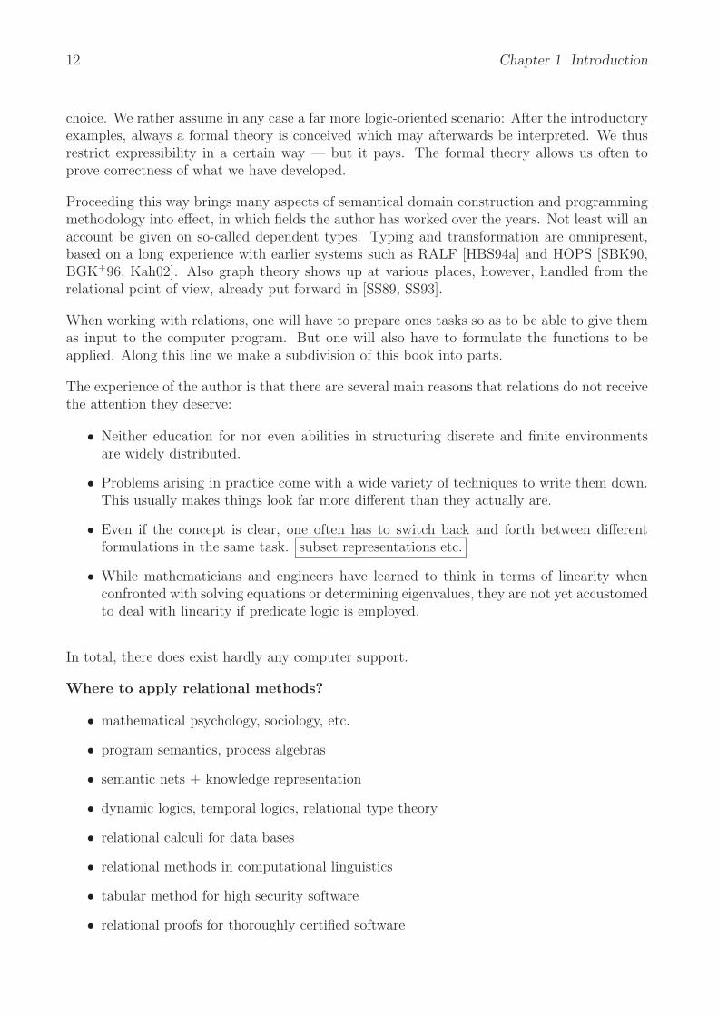
• Even if the concept is clear, one often has to switch back and forth between differentformulations in the same task. subset representations etc.
• While mathematicians and engineers have learned to think in terms of linearity whenconfronted with solving equations or determining eigenvalues, they are not yet accustomedto deal with linearity if predicate logic is employed.
In total, there does exist hardly any computer support.
Where to apply relational methods?
• mathematical psychology, sociology, etc.
• program semantics, process algebras
• semantic nets + knowledge representation
• dynamic logics, temporal logics, relational type theory
• relational calculi for data bases
• relational methods in computational linguistics
• tabular method for high security software
• relational proofs for thoroughly certified software

13
• supporting software certification
• quantum computing and biological paradigms
• investigating relations to reason about fuzzyness
• BDDs and state chart support
• heuristic approaches to program derivation
• natural language studies
• database and software decomposition
• program fault tolerance
• logics of dynamic information incrementation
• data abstraction
• rough sets and fuzzyness
• program semantics and program development
• spacial reasoning in artificial intelligence
• modal, nonclassical, and program logics
• helping in telecommunications
• unified relational theory “eigenvectors”
• refinement ordering and nondeterministic specifications
Modeling by engineersEngineering
. . .surface structures. . .steel frame structures. . .metal matrix
composites. . .metal foames
⎫⎪⎪⎪⎪⎪⎪⎪⎪⎪⎪⎪⎪⎪⎬⎪⎪⎪⎪⎪⎪⎪⎪⎪⎪⎪⎪⎪⎭
Finite elementssolve matrix eqs
Ax = bdetermine
eigenvaluesfrom Ax = λx
⎫⎪⎪⎪⎪⎪⎬⎪⎪⎪⎪⎪⎭
Standardsoftware
Mathematics + computing

14 Chapter 1 Introduction
Situation as it was . . .Modeling by application people
forest damagehealth servicesimage processingmulti-criteria
decision aidvoting schemataknowledge
engineeringspatial informationdata mining
vaguefuzzyspatialtemporaluncertainroughqualitativediscrete
Privateprograms
Standardsoftwareunavailableor unknown
Privateprograms
Logic and mathematics
Situation as it deserves to be . . .Modeling by application people
forest damagehealth servicesimage processingmulti-criteria
decision aidvoting schemataknowledge
engineeringspatial informationdata mining
⎫⎪⎪⎪⎪⎪⎪⎪⎪⎪⎪⎪⎪⎪⎬⎪⎪⎪⎪⎪⎪⎪⎪⎪⎪⎪⎪⎪⎭
Relational
structures
Standard
software
Logic and mathematics
The following shall further illustrate the situation. During the last months, Sudoku puzzlesbecame increasingly popular and were even recognized in the scientific community. The Ger-man Mathematical Society (DMV, Deutsche Mathematikervereinigung), e.g., devoted parts ofthe 2nd quarter volume of its Mitteilungen to Sudoku solving [KK06]. The approach chosen,however, seemed completely queer. Sudoku is a purely relational task. The numbers do nothave any numeric meaning; one could use colours, letters, or images instead without changingthe task. The solutions offered by DMV, however, were heavily laden with numerics in so faras linear programming software was used and numeric effects were discussed. This was as if afemale screw was unscrewed with tweezers. Of course, in case of an emergency, this may be thefinal choice, and may even work, but it is inadequate. The programs to solve such problemsusing real numbers are usually well-tuned so that a Sudoku will be solved immediately. Butwhy do people juggle around with floating point numbers, may be of double precision insteadof a boolean?

Part I
How Discrete Tasks are Presented
15

17
Here we restrict to represent sets, elements, subsets, and relations in different ways. We willdrop certain abstractions that are standard. Not least will we assume our ground sets to beordered. Then another ordering chosen may serve certain purposes. We will put particularemphasis on different forms of representations and the methods to switch from one form toanother.
Such transitions may be achieved on the representation level; they may, however, also touch ahigher relation algebraic level which we hide at this early stage.
We are going to learn how a partition is presented, or a permutation. Permutations may leadto a different presentation of a set or of a relation on or between sets. There may be functionsbetween sets given in various forms, as a table, as a list, or in some other form. A partition mayreduce problem size when factorizing according to it. We show, how relations emerge. Thismay be simply by writing down a matrix, but also by abstracting with a cut from a real-valuedmatrix. For testing purposes, it may be that the relation is generated randomly.


2 Sets, Subsets, and Elements
Usually, we are confronted with sets already in a very early period of our education. Dependingon the respective nationality, it is approximately an age of 10 or 11 years. So we carry withus quite a burden of concepts combined with sets. At least in Germany, Mengenlehre will raisebad feelings when talking on it to parents of school children. All too often will one be remindedthat already Georg Cantor, its creator, ended with psychic disease. Then one will be told thatthere exist so many antinomies making all this questionable.
The situation will not improve when addressing logicians. Most of them think in just oneuniverse of discourse containing numbers, letters, pairs of numbers, etc., altogether renderingthemselves to a lot of semantic problems. While these can in principle be overcome, they shouldnevertheless be avoided at the beginning. Working with relations, we will mostly restrict tofinite situations, where to work is much easier and to which practical work is necessarily confinedto.
To benefit from this, we will make a fundamental distinction between basesets and subsetsof such. Basesets will be finite sets, or sets generated in a clear way from those. Subsets ofbasesets, on the other hand, refer to a baseset and are — starting from explicitly enumeratedones — formed via union and intersection, e.g. While in earlier times nearly everything wascoded in natural numbers, we explicitly construct the set we are going to work with.
We will be able to denote elements of basesets explicitly and to represent basesets for presen-tation purposes in an accordingly permuted form. To compute these permutations, we alreadyhere need some relational facilities.
2.1 Baseset Representation
For basesets we start with (hopefully sufficiently small) finite ground sets as we call them.To denote a ground set we need a name for the set and a list of the different names for all thenames of its elements as, e.g., in
Politicians = Clinton,Bush,Mitterand,Chirac,Schmidt,Kohl,Schroder,Thatcher,Major,Blair,ZapateroNations = American,French,German,British,Spanish
Continents = North-America,South-America,Asia,Africa,Australia,Antartica,EuropeMonths = January,February,March,April,May,June,July,August,September,October,November,December
MonthsS = Jan,Feb,Mar,Apr,May,Jun,Jul,Aug,Sep,Oct,Nov,DecGermPres = Heuß,Lubke,Heinemann,Scheel,Carstens,Weizsacker,Herzog,Rau,KohlerGermSocc = Bayern Munchen,Borussia Dortmund,Werder Bremen,Schalke 04,
Bayer Leverkusen, VfB StuttgartIntSocc = Arsenal London,FC Chelsea,Manchester United,Bayern Munchen,Borussia Dortmund,
Real Madrid,Juventus Turin,Lazio Rom,AC Parma,Olympique Lyon,
19
20 Chapter 2 Sets, Subsets, and Elements
Ajax Amsterdam,Feijenoort Rotterdam,FC Liverpool,Austria Wien,Sparta Prag,FC Porto,Barcelona
There cannot arise much discussion about the nature of ground sets as we assume them tobe given “explicitly”. Also an easy form of representation in a computer language is possiblefollowing the scheme to denote a “named baseset” as
BSN String [String]
In this way, antinomies as the set of all sets that do not contain themselves as an elementcannot occur; these are possible only when defining sets “descriptively”.
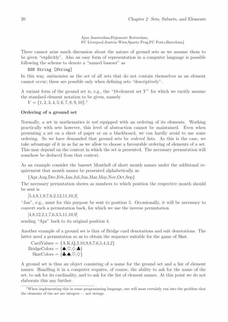
A variant form of the ground set is, e.g., the “10-element set Y ” for which we tacitly assumethe standard element notation to be given, namely
Y = 1, 2, 3, 4, 5, 6, 7, 8, 9, 10.1
Ordering of a ground set
Normally, a set in mathematics is not equipped with an ordering of its elements. Workingpractically with sets however, this level of abstraction cannot be maintained. Even whenpresenting a set on a sheet of paper or on a blackboard, we can hardly avoid to use someordering. So we have demanded that ground sets be ordered lists. As this is the case, wetake advantage of it in as far as we allow to choose a favourable ordering of elements of a set.This may depend on the context in which the set is presented. The necessary permutation willsomehow be deduced from that context.
As an example consider the baseset MonthsS of short month names under the additional re-quirement that month names be presented alphabetically as
Apr,Aug,Dec,Feb,Jan,Jul,Jun,Mar,May,Nov,Oct,SepThe necessary permutation shown as numbers to which position the respective month shouldbe sent is
[5,4,8,1,9,7,6,2,12,11,10,3]
“Jan”, e.g., must for this purpose be sent to position 5. Occasionally, it will be necessary toconvert such a permutation back, for which we use the inverse permutation
[4,8,12,2,1,7,6,3,5,11,10,9]
sending “Apr” back to its original position 4.
Another example of a ground set is that of Bridge card denotations and suit denotations. Thelatter need a permutation so as to obtain the sequence suitable for the game of Skat.
CardValues = A,K,Q,J,10,9,8,7,6,5,4,3,2BridgeColors = ♠,♥,♦,♣
SkatColors = ♣,♠,♥,♦
A ground set is thus an object consisting of a name for the ground set and a list of elementnames. Handling it in a computer requires, of course, the ability to ask for the name of theset, to ask for its cardinality, and to ask for the list of element names. At this point we do notelaborate this any further.
1When implementing this in some programming language, one will most certainly run into the problem thatthe elements of the set are integers — not strings.

2.2 Element Representation 21
What should be mentioned is that our exposition here does not completely follow the sequencein which the concepts have to be introduced theoretically. When we show that sets may bepermuted to facilitate some vizualisation, we already use the concept of relations which isintroduced only later. So we cannot avoid to use it here in a naive way.
Constructing new basesets
Starting from ground sets, further basesets will be obtained by construction, as pair sets, asvariant sets, as power sets, or as the quotient of a baseset modulo some equivalence. Otherconstructions that are not so easily identified as such are subset extrusion and also basesetpermutation. The former serves the purpose to promote a subset of a baseset to a baseset ofits own right2, while the latter enables us, e.g., to present sets in a nice way. For all theseconstructions we will give explanations and examples only later.
Something ignored in test edition!
2.2 Element Representation
So far we have been concerned with the baseset as a whole. Now we concentrate on its elements.There are several methods to identify an element, and we will learn how to switch from oneform to the other. In every case we assume that the baseset is known when we try to denotean element in one of these forms
NUMBElem BaseSet Int
MARKElem BaseSet [Bool]
NAMEElem BaseSet String
DIAGElem BaseSet [[Bool]]
First we might choose to indicate the element of a ground baseset giving the position in theenumeration of elements of the baseset, as in, e.g., Politicians5, Colors7, Nationalities2.As our basesets are in addition to what is normal for mathematical sets, endowed with thesequence for their elements, we have a perfect way of identifying the element. Of course, weshould not try an index above the cardinality which will result in an error.
There is, however, also another form which is useful when using a computer. It is very similar toa bit sequence and may, thus, be helpful. We choose to represent such an element identificationas
2The literate reader may identify basesets with objects in a category of sets. Category objects genericallyconstructed as direct sums, direct products, and direct powers will afterwards be interpreted using projections,injections, and membership relations. Later category objects will also be constructed as abstract data typesand as dependent types.

22 Chapter 2 Sets, Subsets, and Elements
ClintonBush
MitterandChirac
SchmidtKohl
SchroderThatcher
MajorBlair
Zapatero
⎛⎜⎜⎜⎜⎜⎜⎜⎜⎜⎜⎜⎜⎜⎜⎝
00100000000
⎞⎟⎟⎟⎟⎟⎟⎟⎟⎟⎟⎟⎟⎟⎟⎠
ClintonBush
MitterandChirac
SchmidtKohl
SchroderThatcher
MajorBlair
Zapatero
⎛⎜⎜⎜⎜⎜⎜⎜⎜⎜⎜⎜⎜⎜⎝
0 0 0 0 0 0 0 0 0 0 00 0 0 0 0 0 0 0 0 0 00 0 1© 0 0 0 0 0 0 0 00 0 0 0 0 0 0 0 0 0 00 0 0 0 0 0 0 0 0 0 00 0 0 0 0 0 0 0 0 0 00 0 0 0 0 0 0 0 0 0 00 0 0 0 0 0 0 0 0 0 00 0 0 0 0 0 0 0 0 0 00 0 0 0 0 0 0 0 0 0 00 0 0 0 0 0 0 0 0 0 0
⎞⎟⎟⎟⎟⎟⎟⎟⎟⎟⎟⎟⎟⎟⎠
Fig. 2.2.1 Element as marking vector or as marking diagonal matrix
Again we see that combination with the baseset is needed to make the columnlike vector of0 ’s and 1 ’s meaningful. We may go even further and consider, in a fully naive way, a partialidentity relation with just one entry 1 , or a partial diagonal matrix with just one entry 1 onthe baseset.
With all these attempts, we have demonstrated heavy notation for simply saying the name ofthe element, namely Mitterand∈Politicians. Using such a complicated notation is justifiedonly when it brings added value. Mathematicians have a tendency of abstracting over allthese representations, and they have often reason for doing so. On the other hand, people inapplications cannot so easily switch between representations. Sometimes this prevents themfrom seeing possibilities of economic work or reasoning.
An element of a baseset B in the mathematical sense is here assumed to be transferable to theother forms of representation via function calls
elemAsNUMB, elemAsMARK, elemAsNAME, elemAsDIAG,
as required. All this works fine for ground sets. Later we will ask how to denote elements ingenerically constructed basesets such as direct products etc.
Something ignored in test edition!
2.3 Subset Representation
We now extend element notation slightly to notation of subsets. Given a baseset, subsets mayat least be defined in five different forms which may be used interchangeably:
— as a list of element numbers drawn from the baseset,— as a list of element names drawn from the baseset,— as a predicate over the baseset,— as an element in the powerset of the baseset— marked True or False along the baseset— as partial diagonal matrix on the baseset
To denote in this way is trivial as long as the baseset is ground3. In this case we have thepossibility to either give a set of numbers or a set of names of elements in the baseset. One
3It is only in principle a trivial point when the baseset is finite, but we better concentrate on how the tinypart of expressible subsets is constructed.

2.3 Subset Representation 23
has, however, to invest some more care for constructed basesets or for nonfinite ones. For thelatter, negation of a subset may well be infinite, and thus more difficult to represent.
LISTSet BaseSet [Int]
LINASet BaseSet [String]
PREDSet BaseSet (Int -> Bool)
POWESet BaseSet [Bool]
MARKSet BaseSet [Bool]
DIAGSet BaseSet [[Bool]]
Given the name of the baseset, we may list numbers of the elements of the subset as in the firstvariant or we may give their names explicitly as in the second.
Politicians1,2,6,10 Clinton,Bush,Kohl,Blair
ClintonBush
MitterandChirac
SchmidtKohl
SchroderThatcher
MajorBlair
Zapatero
⎛⎜⎜⎜⎜⎜⎜⎜⎜⎜⎜⎜⎜⎜⎜⎝
11000100010
⎞⎟⎟⎟⎟⎟⎟⎟⎟⎟⎟⎟⎟⎟⎟⎠
ClintonBush
MitterandChirac
SchmidtKohl
SchroderThatcher
MajorBlair
Zapatero
⎛⎜⎜⎜⎜⎜⎜⎜⎜⎜⎜⎜⎜⎜⎝
1 0 0 0 0 0 0 0 0 0 00 1 0 0 0 0 0 0 0 0 00 0 0 0 0 0 0 0 0 0 00 0 0 0 0 0 0 0 0 0 00 0 0 0 0 0 0 0 0 0 00 0 0 0 0 1 0 0 0 0 00 0 0 0 0 0 0 0 0 0 00 0 0 0 0 0 0 0 0 0 00 0 0 0 0 0 0 0 0 0 00 0 0 0 0 0 0 0 0 1 00 0 0 0 0 0 0 0 0 0 0
⎞⎟⎟⎟⎟⎟⎟⎟⎟⎟⎟⎟⎟⎟⎠
Fig. 2.3.1 Different subset representations
We may, however, also use marking along the baseset as in variant three, and we may, as alreadyexplained for elements, use the partial diagonal matrix over the baseset.
In any case, given that
Politicians = Clinton,Bush,Mitterand,Chirac,Schmidt,Kohl,Schroder, Thatcher,Major,Blair,Zapatero,
what we intended to denote was simply something as
Clinton,Bush,Kohl,Blair ⊆ Politicians
Given subsets, we assume available functions
setAsLIST, setAsLINA, setAsPRED, setAsPOWE, setAsMARK, setAsDIAG
to convert back and forth between the different representations of subsets. Of course, theinteger lists must provide numbers in the range of 1 to the cardinality of the baseset.
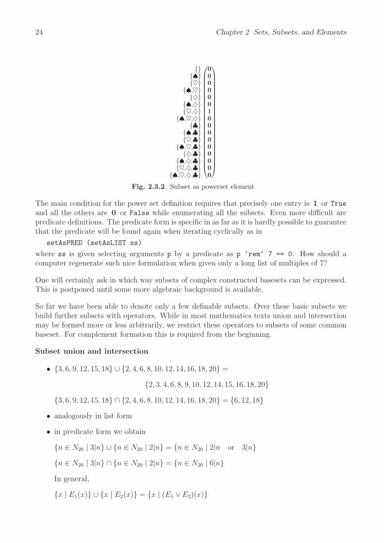
Another technique should only be used for sets of minor cardinality, although a computer willhandle even medium sized ones. We may identify the subset as an element in the powerset. Forreasons of space, it will only be presented for the subset ♥,♦ of the 4-element Bridge suitset ♠,♥,♦,♣4.
4Another well-known notation for the empty subset is ∅ instead of .
24 Chapter 2 Sets, Subsets, and Elements
♠♥
♠,♥♦
♠,♦♥,♦
♠,♥,♦♣
♠,♣♥,♣
♠,♥,♣♦,♣
♠,♦,♣♥,♦,♣
♠,♥,♦,♣
⎛⎜⎜⎜⎜⎜⎜⎜⎜⎜⎜⎜⎜⎜⎜⎜⎜⎜⎜⎜⎜⎜⎜⎜⎝
0000001000000000
⎞⎟⎟⎟⎟⎟⎟⎟⎟⎟⎟⎟⎟⎟⎟⎟⎟⎟⎟⎟⎟⎟⎟⎟⎠
Fig. 2.3.2 Subset as powerset element
The main condition for the power set definition requires that precisely one entry is 1 or Trueand all the others are 0 or False while enumerating all the subsets. Even more difficult arepredicate definitions. The predicate form is specific in as far as it is hardly possible to guaranteethat the predicate will be found again when iterating cyclically as in
setAsPRED (setAsLIST ss)
where ss is given selecting arguments p by a predicate as p ‘rem‘ 7 == 0. How should acomputer regenerate such nice formulation when given only a long list of multiples of 7?
One will certainly ask in which way subsets of complex constructed basesets can be expressed.This is postponed until some more algebraic background is available.
So far we have been able to denote only a few definable subsets. Over these basic subsets webuild further subsets with operators. While in most mathematics texts union and intersectionmay be formed more or less arbitrarily, we restrict these operators to subsets of some commonbaseset. For complement formation this is required from the beginning.
Subset union and intersection
• 3, 6, 9, 12, 15, 18 ∪ 2, 4, 6, 8, 10, 12, 14, 16, 18, 20 =
2, 3, 4, 6, 8, 9, 10, 12, 14, 15, 16, 18, 20
3, 6, 9, 12, 15, 18 ∩ 2, 4, 6, 8, 10, 12, 14, 16, 18, 20 = 6, 12, 18
• analogously in list form
• in predicate form we obtain
n ∈ N20 | 3|n ∪ n ∈ N20 | 2|n = n ∈ N20 | 2|n or 3|n
n ∈ N20 | 3|n ∩ n ∈ N20 | 2|n = n ∈ N20 | 6|n
In general,
x | E1(x) ∪ x | E2(x) = x | (E1 ∨ E2)(x)

2.3 Subset Representation 25
x | E1(x) ∩ x | E2(x) = x | (E1 ∧ E2)(x)
• in vector form
123456789
1011121314151617181920
⎛⎜⎜⎜⎜⎜⎜⎜⎜⎜⎜⎜⎜⎜⎜⎜⎜⎜⎜⎜⎜⎜⎜⎜⎜⎜⎜⎜⎜⎜⎜⎝
00100100100100100100
⎞⎟⎟⎟⎟⎟⎟⎟⎟⎟⎟⎟⎟⎟⎟⎟⎟⎟⎟⎟⎟⎟⎟⎟⎟⎟⎟⎟⎟⎟⎟⎠
∪
⎛⎜⎜⎜⎜⎜⎜⎜⎜⎜⎜⎜⎜⎜⎜⎜⎜⎜⎜⎜⎜⎜⎜⎜⎜⎜⎜⎜⎜⎜⎜⎝
01010101010101010101
⎞⎟⎟⎟⎟⎟⎟⎟⎟⎟⎟⎟⎟⎟⎟⎟⎟⎟⎟⎟⎟⎟⎟⎟⎟⎟⎟⎟⎟⎟⎟⎠
=
⎛⎜⎜⎜⎜⎜⎜⎜⎜⎜⎜⎜⎜⎜⎜⎜⎜⎜⎜⎜⎜⎜⎜⎜⎜⎜⎜⎜⎜⎜⎜⎝
01110101110101110101
⎞⎟⎟⎟⎟⎟⎟⎟⎟⎟⎟⎟⎟⎟⎟⎟⎟⎟⎟⎟⎟⎟⎟⎟⎟⎟⎟⎟⎟⎟⎟⎠
123456789
1011121314151617181920
⎛⎜⎜⎜⎜⎜⎜⎜⎜⎜⎜⎜⎜⎜⎜⎜⎜⎜⎜⎜⎜⎜⎜⎜⎜⎜⎜⎜⎜⎜⎜⎝
00100100100100100100
⎞⎟⎟⎟⎟⎟⎟⎟⎟⎟⎟⎟⎟⎟⎟⎟⎟⎟⎟⎟⎟⎟⎟⎟⎟⎟⎟⎟⎟⎟⎟⎠
∩
⎛⎜⎜⎜⎜⎜⎜⎜⎜⎜⎜⎜⎜⎜⎜⎜⎜⎜⎜⎜⎜⎜⎜⎜⎜⎜⎜⎜⎜⎜⎜⎝
01010101010101010101
⎞⎟⎟⎟⎟⎟⎟⎟⎟⎟⎟⎟⎟⎟⎟⎟⎟⎟⎟⎟⎟⎟⎟⎟⎟⎟⎟⎟⎟⎟⎟⎠
=
⎛⎜⎜⎜⎜⎜⎜⎜⎜⎜⎜⎜⎜⎜⎜⎜⎜⎜⎜⎜⎜⎜⎜⎜⎜⎜⎜⎜⎜⎜⎜⎝
00000100000100000100
⎞⎟⎟⎟⎟⎟⎟⎟⎟⎟⎟⎟⎟⎟⎟⎟⎟⎟⎟⎟⎟⎟⎟⎟⎟⎟⎟⎟⎟⎟⎟⎠
Subset complement
3, 6, 9, 12, 15, 18 = 1, 2, 4, 5, 7, 8, 10, 11, 13, 14, 16, 17, 19, 20
These had been operators on subsets. There is also an important binary predicate for subseetsnamely
Subset containment
• 6, 12, 18 ⊆ 2, 4, 6, 8, 10, 12, 14, 16, 18, 20holds, since the first subset contains only elements which are also contained in the second.
• analogously in list form
• predicate form n ∈ N20 | 6|n ⊆ n ∈ N20 | 2|n. In general, x | E1(x) ⊆ x | E2(x)holds if for all x ∈ V E1(x) → E2(x), which may also be written as ∀ x ∈ V : E1(x) →E2(x)
• in vector form: If a 1 is on the left, then also on the right

26 Chapter 2 Sets, Subsets, and Elements
123456789
1011121314151617181920
⎛⎜⎜⎜⎜⎜⎜⎜⎜⎜⎜⎜⎜⎜⎜⎜⎜⎜⎜⎜⎜⎜⎜⎜⎜⎜⎜⎜⎜⎜⎜⎝
00000100000100000100
⎞⎟⎟⎟⎟⎟⎟⎟⎟⎟⎟⎟⎟⎟⎟⎟⎟⎟⎟⎟⎟⎟⎟⎟⎟⎟⎟⎟⎟⎟⎟⎠
⊆
⎛⎜⎜⎜⎜⎜⎜⎜⎜⎜⎜⎜⎜⎜⎜⎜⎜⎜⎜⎜⎜⎜⎜⎜⎜⎜⎜⎜⎜⎜⎜⎝
01010101010101010101
⎞⎟⎟⎟⎟⎟⎟⎟⎟⎟⎟⎟⎟⎟⎟⎟⎟⎟⎟⎟⎟⎟⎟⎟⎟⎟⎟⎟⎟⎟⎟⎠
We have presented the definition of such basic subsets in some detail, although many personsknow what intersecting two sets, or uniting these, actually means. The purpose of our detailedexplanation is as follows. Mathematicians in everyday work are normally not concerned withbasesets; they unite sets as they come, red,green,blue∪ 1, 2, 3, 4, e.g. This is also possible ona computer which works with a text representation of these sets, but it takes some time. When,however, maximum efficiency of such algorithms is needed, one has to go back to sets representedas bits in a machine word. Then the position of the respective bit becomes important. This inturn is best dealt with in the concept of a set as an ordered list with every position meaningsome element, i.e., with a baseset.
If we have two finite basesets, X, Y say, we are able — at least in principle — to denote everyelement and, thus, every subset. In practice, however, we will never try to denote an arbitrarysubset of a 300 × 5000 set while we can easily work with such matrices. It is highly likely thatwe will restrict ourselves to subsets that are formed in a simple way based on subsets of thetwo basesets. A simple calculation makes this clear. There are 2300×5000 subsets — only finitelymany, but a tremendous number. What we are able to achieve is to denote those subsets thatare composed of subsets of the first or second component set. This is far less, namely only2300×25000, or 0.000 . . . % of the latter. If the set with 5000 elements is itself built as a productof a 50 and a 100 element set, it is highly likely that also the interesting ones of the 25000 subsetsare only built from smaller sets of components.
It is indeed one of the major mistakes of nowadays computer science that people are so muchconcentrated on asymptotically increasing sequences, while only the very first steps are impor-tant.
Permuting Subset Representations
One will know permutations from early school experience. They may be given as a function,decomposed into cycles, or as a permutation matrix:

2.3 Subset Representation 27
1 → 42 → 63 → 54 → 75 → 36 → 27 → 1 or
[4,6,5,7,3,2,1]
[[1,4,7],[3,5],[6,2]]
⎛⎜⎜⎜⎜⎜⎜⎝
0 0 0 1 0 0 00 0 0 0 0 1 00 0 0 0 1 0 00 0 0 0 0 0 10 0 1 0 0 0 00 1 0 0 0 0 01 0 0 0 0 0 0
⎞⎟⎟⎟⎟⎟⎟⎠
Fig. 2.3.3 Representing a permutation as a function, using cycles, or as a matrix
Either form has its specific merits5. Sometimes also the inverted permutation is useful. It isimportant that also subsets may be permuted. Permuting a subset means that the correspond-ing baseset is permuted followed by a permutation of the subset — conceived as a marked set— in reverse direction. Then the listed baseset will show a different sequence, but the markingvector will again identify the same set of elements.
When we apply a permutation to a subset representation, we insert it in between the row entrycolumn and the marking vector. While the former is subjected to the permutation, the latterwill undergo the reverse permutation. In effect we have applied p followed by inverse(p), i.e.,the identity. The subset has not changed, but its appearence has.
To make this claim clear, we consider the month names baseset and what is shown in themiddle as the subset of “J-months”, namely January, June, July. This is then reconsideredwith month names ordered alphabetically; cf. the permutation from Page 20.
AprilAugust
DecemberFebruaryJanuary
JulyJune
MarchMay
NovemberOctober
September
names sent to positions[4,8,12,2,1,7,6,3,5,11,10,9]i.e., permutation p
JanuaryFebruary
MarchAprilMayJuneJuly
AugustSeptember
OctoberNovemberDecember
⎛⎜⎜⎜⎜⎜⎜⎜⎜⎜⎜⎜⎜⎜⎜⎜⎜⎝
100001100000
⎞⎟⎟⎟⎟⎟⎟⎟⎟⎟⎟⎟⎟⎟⎟⎟⎟⎠
boolean values sent to positions[5,4,8,1,9,7,6,2,12,11,10,3]i.e., permutation inversep
⎛⎜⎜⎜⎜⎜⎜⎜⎜⎜⎜⎜⎜⎜⎜⎜⎜⎝
000011100000
⎞⎟⎟⎟⎟⎟⎟⎟⎟⎟⎟⎟⎟⎟⎟⎟⎟⎠
Fig. 2.3.4 Permutation of a subset and its baseset: The outermost describe the permuted subset
5In particular, we observe that permutations partly subsume to relations.

28 Chapter 2 Sets, Subsets, and Elements
3 Relations
Already in the preceding chapters relations have shown up in a more or less naive form, e.g.,as permutation matrices or as (partial) identity relations. Here we provide more stringent datatypes for relations. Not least will these serve to model graph situations, be these graphs on aset, bipartitioned graphs, or hypergraphs.
What is at this point even more important is the question of denotation. We have developedsome scrutiny when denoting basesets, elements, and subsets; all the more will we now becareful in denoting relations. As we restrict ourselves mostly to binary relations, this will meanto denote the domain of the relation as well as its range or codomain and then denote therelation proper. It is this seemingly trivial point which will here be stressed, namely fromwhich baseset to which baseset the relation actually leads.
3.1 Relation Representation
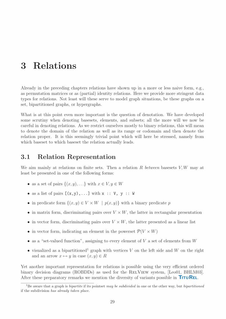
We aim mainly at relations on finite sets. Then a relation R between basesets V, W may atleast be presented in one of the following forms:
• as a set of pairs (x, y), . . . with x ∈ V, y ∈ W
• as a list of pairs [(x,y),...] with x :: V, y :: W
• in predicate form (x, y) ∈ V × W | p(x, y) with a binary predicate p
• in matrix form, discriminating pairs over V × W , the latter in rectangular presentation
• in vector form, discriminating pairs over V × W , the latter presented as a linear list
• in vector form, indicating an element in the powerset P(V × W )
• as a “set-valued function”, assigning to every element of V a set of elements from W
• visualized as a bipartitioned1 graph with vertices V on the left side and W on the rightand an arrow x → y in case (x, y) ∈ R
Yet another important representation for relations is possible using the very efficient orderedbinary decision diagrams (ROBDDs) as used for the RelView system, [Leo01, BHLM03].After these preparatory remarks we mention the diversity of variants possible in TITUREL.
1Be aware that a graph is bipartite if its pointset may be subdivided in one or the other way, but bipartitionedif the subdivision has already taken place.
29

30 Chapter 3 Relations
MATRRel BaseSet BaseSet [[Bool]]
PREDRel BaseSet BaseSet (Int -> Int -> Bool)
SETFRel BaseSet BaseSet (Int -> [Int])
SNAFRel BaseSet BaseSet (Int -> [String])
PALIRel BaseSet BaseSet [(Int,Int)]
VECTRel BaseSet BaseSet [Bool]
POWERel BaseSet BaseSet [Bool]
These variants are explained with the following examples that make the same relation lookcompletely differently. First we present the matrix form together with the set function thatassigns sets given via element numbers and then via element names lists. (It is, of course,purely by incidence that there are always three items in a line!)
Star
t≤
60St
art≥
60O
neP.
Tw
oP.
CD
USP
DFD
P
HeußLubke
HeinemannScheel
CarstensWeizsacker
HerzogRau
Kohler
⎛⎜⎜⎜⎜⎜⎜⎜⎜⎜⎝
0 1 0 1 0 0 10 1 0 1 1 0 00 1 1 0 0 1 01 0 1 0 0 0 10 1 1 0 1 0 00 1 0 1 1 0 00 1 1 0 1 0 00 1 1 0 0 1 01 0 1 0 1 0 0
⎞⎟⎟⎟⎟⎟⎟⎟⎟⎟⎠
fR(Heuß) = properties2,4,7
fR(Lubke) = properties2,4,5
fR(Heinemann) = properties2,3,6
fR(Scheel) = properties1,3,7
fR(Carstens) = properties2,3,5
fR(Weizsacker) = properties2,4,5
fR(Herzog) = properties2,3,5
fR(Rau) = properties2,3,6
fR(Kohler) = properties1,3,5
HeußLubke
HeinemannScheel
CarstensWeizsacker
HerzogRau
Kohler
Start ≥ 60,Two P.,FDPStart ≥ 60,Two P.,CDUStart ≥ 60,One P.,SPDStart ≤ 60,One P.,FDPStart ≥ 60,One P.,CDUStart ≥ 60,Two P.,CDUStart ≥ 60,One P.,CDUStart ≥ 60,One P.,SPDStart ≤ 60,One P.,CDU
Fig. 3.1.1 Different representations of the same relation
Then we show the relation with pairs of row and column numbers, which requires that oneknows the domain and range not just as sets but as element sequences. It is also possible tomark the relation along the list of all pairs.
(1,2),(1,4),(1,7),(2,2),(2,4),(2,5), (3,2),(3,3),(3,6),(4,1),(4,3),(4,7),(5,2),(5,3),(5,5),(6,2),(6,4),(6,5),(7,2),(7,3), (7,5),(8,2),(8,3),(8,6),(9,1),(9,3),(9,5)

3.1 Relation Representation 31
(Heuß,Start ≤ 60)(Lubke,Start ≤ 60)(Heuß,Start ≥ 60)
(Heinemann,Start ≤ 60)(Lubke,Start ≥ 60)
(Heuß,One P.)(Scheel,Start ≤ 60)
(Heinemann,Start ≥ 60)(Lubke,One P.)(Heuß,Two P.)
(Carstens,Start ≤ 60)(Scheel,Start ≥ 60)
(Heinemann,One P.)(Lubke,Two P.)
(Heuß,CDU)(Weizsacker,Start ≤ 60)
(Carstens,Start ≥ 60)(Scheel,One P.)
(Heinemann,Two P.)(Lubke,CDU)
(Heuß,SPD)(Herzog,Start ≤ 60)
(Weizsacker,Start ≥ 60)(Carstens,One P.)
(Scheel,Two P.)(Heinemann,CDU)
(Lubke,SPD)(Heuß,FDP)
(Rau,Start ≤ 60)(Herzog,Start ≥ 60)(Weizsacker,One P.)
(Carstens,Two P.)(Scheel,CDU)
(Heinemann,SPD)(Lubke,FDP)
(Kohler,Start ≤ 60)(Rau,Start ≥ 60)(Herzog,One P.)
(Weizsacker,Two P.)(Carstens,CDU)
(Scheel,SPD)(Heinemann,FDP)
(Kohler,Start ≥ 60)(Rau,One P.)
(Herzog,Two P.)(Weizsacker,CDU)
(Carstens,SPD)(Scheel,FDP)
(Kohler,One P.)(Rau,Two P.)
(Herzog,CDU)(Weizsacker,SPD)
(Carstens,FDP)(Kohler,Two P.)
(Rau,CDU)(Herzog,SPD)
(Weizsacker,FDP)(Kohler,CDU)
(Rau,SPD)(Herzog,FDP)(Kohler,SPD)
(Rau,FDP)(Kohler,FDP)
⎛⎜⎜⎜⎜⎜⎜⎜⎜⎜⎜⎜⎜⎜⎜⎜⎜⎜⎜⎜⎜⎜⎜⎜⎜⎜⎜⎜⎜⎜⎜⎜⎜⎜⎜⎜⎜⎜⎜⎜⎜⎜⎜⎜⎜⎜⎜⎜⎜⎜⎜⎜⎜⎜⎜⎜⎜⎜⎜⎜⎜⎜⎜⎜⎜⎜⎜⎜⎜⎜⎜⎜⎜⎜⎜⎜⎜⎜⎜⎜⎜⎜⎜⎜⎜⎜⎜⎜⎜⎜⎜⎜⎜⎜⎜⎜⎜⎜⎜⎜⎜⎜⎜⎜⎜⎜⎜⎜⎜⎜⎝
001010110100110011010011000101000101111100010101101000000110000
⎞⎟⎟⎟⎟⎟⎟⎟⎟⎟⎟⎟⎟⎟⎟⎟⎟⎟⎟⎟⎟⎟⎟⎟⎟⎟⎟⎟⎟⎟⎟⎟⎟⎟⎟⎟⎟⎟⎟⎟⎟⎟⎟⎟⎟⎟⎟⎟⎟⎟⎟⎟⎟⎟⎟⎟⎟⎟⎟⎟⎟⎟⎟⎟⎟⎟⎟⎟⎟⎟⎟⎟⎟⎟⎟⎟⎟⎟⎟⎟⎟⎟⎟⎟⎟⎟⎟⎟⎟⎟⎟⎟⎟⎟⎟⎟⎟⎟⎟⎟⎟⎟⎟⎟⎟⎟⎟⎟⎟⎟⎠
Fig. 3.1.2 The relation of Fig. 3.1.1 as a vector
32 Chapter 3 Relations
With isConsistentRel we check consistency, and with
relAsMATRRel, relAsPREDRel, relAsSETFRel, relAsSNAFRel,
relAsVECTRel, relAsPALIRel, relAsPOWERel
we may switch back and forth between such representations — as far as this is possible. Rep-resenting relations is, thus, possible in various ways, starting with the version
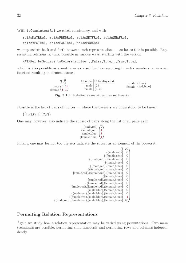
MATRRel bsGenders bsColorsRedBlue [[False,True],[True,True]]
which is also possible as a matrix or as a set function resulting in index numbers or as a setfunction resulting in element names.
red
blue
malefemale
(0 11 1
) Gendersmale
female
ColorsInjected21, 2
malefemale
bluered,blue
Fig. 3.1.3 Relation as matrix and as set function
Possible is the list of pairs of indices — where the basesets are understood to be known
(1,2),(2,1),(2,2)One may, however, also indicate the subset of pairs along the list of all pairs as in
(male,red)(female,red)(male,blue)
(female,blue)
⎛⎜⎝
0111
⎞⎟⎠
Finally, one may for not too big sets indicate the subset as an element of the powerset.
(male,red)
(female,red)(male,red),(female,red)
(male,blue)(male,red),(male,blue)
(female,red),(male,blue)(male,red),(female,red),(male,blue)
(female,blue)(male,red),(female,blue)
(female,red),(female,blue)(male,red),(female,red),(female,blue)
(male,blue),(female,blue)(male,red),(male,blue),(female,blue)
(female,red),(male,blue),(female,blue)(male,red),(female,red),(male,blue),(female,blue)
⎛⎜⎜⎜⎜⎜⎜⎜⎜⎜⎜⎜⎜⎜⎜⎜⎜⎜⎜⎜⎜⎜⎜⎜⎝
0000000000000010
⎞⎟⎟⎟⎟⎟⎟⎟⎟⎟⎟⎟⎟⎟⎟⎟⎟⎟⎟⎟⎟⎟⎟⎟⎠
Permuting Relation Representations
Again we study how a relation representation may be varied using permutations. Two maintechniques are possible, permuting simultaneously and permuting rows and columns indepen-dently.

3.2 Relations Describing Graphs 33
A =
1 2 3 4 5 6 7 8 9 10 11 12 13 14
1
2
3
4
5
6
7
8
9
10
11
12
⎛⎜⎜⎜⎜⎜⎜⎜⎜⎜⎜⎜⎜⎜⎜⎜⎝
1 0 1 0 1 0 0 1 1 0 1 1 0 10 1 0 1 0 0 1 0 0 1 0 0 0 00 0 0 0 0 1 0 0 0 0 0 0 1 01 0 1 0 1 0 0 1 1 0 1 1 0 10 1 0 1 0 0 1 0 0 1 0 0 0 01 0 1 0 1 0 0 1 1 0 1 1 0 10 1 0 1 0 0 1 0 0 1 0 0 0 00 0 0 0 0 0 0 0 0 0 0 0 0 00 0 0 0 0 1 0 0 0 0 0 0 1 01 0 1 0 1 0 0 1 1 0 1 1 0 10 0 0 0 0 1 0 0 0 0 0 0 1 01 0 1 0 1 0 0 1 1 0 1 1 0 1
⎞⎟⎟⎟⎟⎟⎟⎟⎟⎟⎟⎟⎟⎟⎟⎟⎠
Arearranged =
1 3 5 8 9111214 2 4 710 613146
101225739
118
⎛⎜⎜⎜⎜⎜⎜⎜⎜⎜⎜⎜⎜⎜⎜⎜⎝
1 1 1 1 1 1 1 1 0 0 0 0 0 01 1 1 1 1 1 1 1 0 0 0 0 0 01 1 1 1 1 1 1 1 0 0 0 0 0 01 1 1 1 1 1 1 1 0 0 0 0 0 01 1 1 1 1 1 1 1 0 0 0 0 0 00 0 0 0 0 0 0 0 1 1 1 1 0 00 0 0 0 0 0 0 0 1 1 1 1 0 00 0 0 0 0 0 0 0 1 1 1 1 0 00 0 0 0 0 0 0 0 0 0 0 0 1 10 0 0 0 0 0 0 0 0 0 0 0 1 10 0 0 0 0 0 0 0 0 0 0 0 1 10 0 0 0 0 0 0 0 0 0 0 0 0 0
⎞⎟⎟⎟⎟⎟⎟⎟⎟⎟⎟⎟⎟⎟⎟⎟⎠
Fig. 3.1.4 A relation with many coinciding rows and columns, original and rearranged
In many cases, results of some investigation automatically bring information that might be usedfor a partition of the set of rows and the set of columns, respectively. In this case, a partitioninto groups of identical rows and columns is easily obtained. It is a good idea to permuterows and columns so as to have the identical rows of the groups side aside. This means toindependently permute rows and columns.
There may, however, also occur a homogeneous relation, for which rows and columns shouldnot be permuted independently, but simultaneously. Fig. 3.1.5 shows, how also in this case ablock form may be reached.
Ξ =
1 2 3 4 5
12345
⎛⎜⎜⎝
1 0 1 0 00 1 0 0 11 0 1 0 00 0 0 1 00 1 0 0 1
⎞⎟⎟⎠ P =
1 3 2 5 4
12345
⎛⎜⎜⎝
1 0 0 0 00 0 1 0 00 1 0 0 00 0 0 0 10 0 0 1 0
⎞⎟⎟⎠
1 3 2 5 4
13254
⎛⎜⎜⎝
1 1 0 0 01 1 0 0 00 0 1 1 00 0 1 1 00 0 0 0 1
⎞⎟⎟⎠ = P ; Ξ; P T
Fig. 3.1.5 Equivalence relation Ξ with simultaneous permutation P to a block-diagonal form
Something ignored in test edition!
3.2 Relations Describing Graphs
One of the main sources of relational considerations is graph theory. Usually, however, graphtheory stresses another aspect of graphs than our relational approach. So we will here presentwhat we mean is relational graph theory.
1-graphbipartite graphhypergraphsimple graph
We present a relation between two sets as an example.
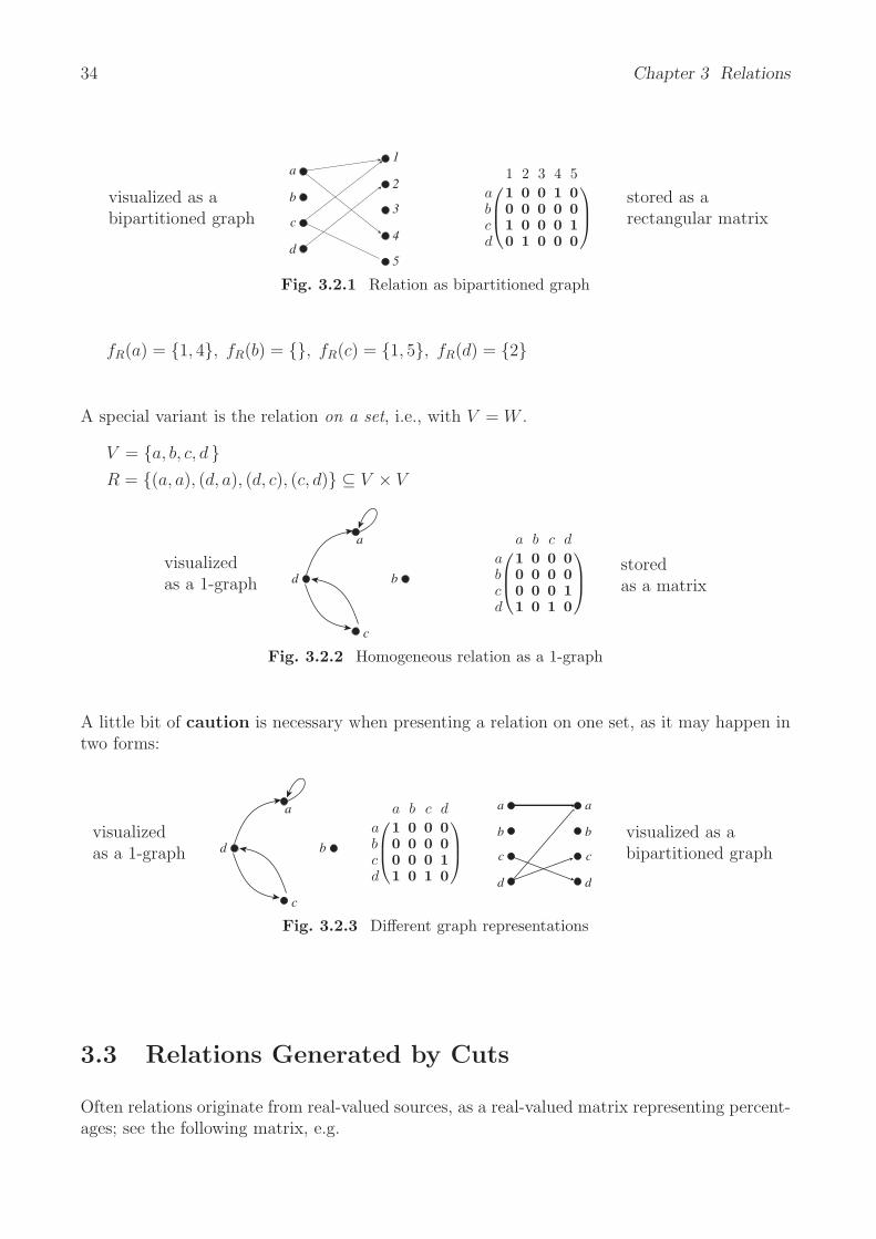
V = a, b, c, d W = 1, 2, 3, 4, 5 R = (a, 1), (a, 4), (c, 1), (c, 5), (d, 2) ⊆ V × W
34 Chapter 3 Relations
visualized as abipartitioned graph
a
b
c
d
1
2
3
4
5
⎛⎜⎝
1 2 3 4 5a 1 0 0 1 0b 0 0 0 0 0c 1 0 0 0 1d 0 1 0 0 0
⎞⎟⎠ stored as a
rectangular matrix
Fig. 3.2.1 Relation as bipartitioned graph
fR(a) = 1, 4, fR(b) = , fR(c) = 1, 5, fR(d) = 2
A special variant is the relation on a set, i.e., with V = W .
V = a, b, c, d R = (a, a), (d, a), (d, c), (c, d) ⊆ V × V
visualizedas a 1-graph
a
b
c
d
⎛⎜⎝
a b c d
a 1 0 0 0b 0 0 0 0c 0 0 0 1d 1 0 1 0
⎞⎟⎠ stored
as a matrix
Fig. 3.2.2 Homogeneous relation as a 1-graph
A little bit of caution is necessary when presenting a relation on one set, as it may happen intwo forms:
visualizedas a 1-graph
a
b
c
d
⎛⎜⎝
a b c d
a 1 0 0 0b 0 0 0 0c 0 0 0 1d 1 0 1 0
⎞⎟⎠
a
b
c
d
a
b
c
d
visualized as abipartitioned graph
Fig. 3.2.3 Different graph representations
3.3 Relations Generated by Cuts
Often relations originate from real-valued sources, as a real-valued matrix representing percent-ages; see the following matrix, e.g.

3.3 Relations Generated by Cuts 35
38.28 9.91 28.42 36.11 25.17 11.67 87.10 84.73 81.53 35.64 34.36 11.92 99.7393.35 93.78 18.92 44.89 13.60 6.33 25.26 36.70 34.22 98.15 8.32 4.99 21.585.69 94.43 47.17 95.23 86.50 80.26 41.56 86.84 47.93 40.38 3.75 19.76 12.00
93.40 20.35 25.94 38.96 36.10 25.30 89.17 19.17 87.34 85.25 5.58 18.67 1.136.37 83.89 23.16 41.64 35.56 36.77 21.71 37.20 43.61 18.30 97.67 27.67 42.59
30.26 43.71 90.78 37.21 16.76 8.83 88.93 15.18 3.58 83.60 96.60 18.44 24.3029.85 14.76 82.21 35.70 43.34 99.82 99.30 88.85 46.29 24.73 47.90 92.62 46.6519.37 88.67 5.94 38.30 48.56 87.40 46.46 34.46 17.92 24.30 33.46 34.30 43.9597.89 96.70 4.13 44.50 23.23 81.56 95.75 34.30 41.59 47.39 39.29 86.14 22.9818.82 93.00 17.50 16.10 9.74 14.71 21.30 45.32 19.57 24.78 82.43 41.00 43.295.38 36.85 4.38 28.10 17.30 45.30 33.14 81.20 13.24 33.39 23.42 18.33 83.87
14.82 18.37 1.87 19.30 4.82 93.26 28.10 26.94 19.10 43.25 85.85 15.48 49.577.63 28.80 10.40 89.81 17.14 7.33 96.57 16.19 35.96 8.96 47.42 39.82 8.16
89.70 14.16 7.59 41.67 34.39 88.68 18.80 99.37 7.67 8.11 86.54 86.65 44.3431.55 13.16 86.23 45.45 92.92 33.75 43.64 46.74 27.75 89.96 37.71 84.79 86.3225.48 7.40 43.67 1.69 85.18 27.50 89.59 100.00 89.67 11.30 2.41 83.90 96.3148.32 93.23 14.16 17.75 14.60 90.90 3.81 41.30 4.12 3.87 2.83 95.35 81.12
Fig. 3.3.1 A real-valued 17 × 13-matrix
A closer look in this case shows that the coefficients are clustered around 0–50 and around 80–100. So it will not be the deviation between 15 and 20, or 83 and 86, e.g., which is importantbut the huge gap between the two clusters. Constructing a histogram is, thus, a good idea; itlooks as follows.
0.0 10.0 20.0 30.0 40.0 50.0 60.0 70.0 80.0 90.0 100.0
Fig. 3.3.2 Histogram for value frequency in Fig. 3.3.1
So one may be tempted to apply what is known a cut at e.g., 60, considering entries below asFalse and above as True in order to arrive at the boolean matrix to follow.⎛
⎜⎜⎜⎜⎜⎜⎜⎜⎜⎜⎜⎜⎜⎜⎜⎜⎜⎜⎜⎜⎜⎜⎜⎜⎝
0 0 0 0 0 0 1 1 1 0 0 0 11 1 0 0 0 0 0 0 0 1 0 0 00 1 0 1 1 1 0 1 0 0 0 0 01 0 0 0 0 0 1 0 1 1 0 0 00 1 0 0 0 0 0 0 0 0 1 0 00 0 1 0 0 0 1 0 0 1 1 0 00 0 1 0 0 1 1 1 0 0 0 1 00 1 0 0 0 1 0 0 0 0 0 0 01 1 0 0 0 1 1 0 0 0 0 1 00 1 0 0 0 0 0 0 0 0 1 0 00 0 0 0 0 0 0 1 0 0 0 0 10 0 0 0 0 1 0 0 0 0 1 0 00 0 0 1 0 0 1 0 0 0 0 0 01 0 0 0 0 1 0 1 0 0 1 1 00 0 1 0 1 0 0 0 0 1 0 1 10 0 0 0 1 0 1 1 1 0 0 1 10 1 0 0 0 1 0 0 0 0 0 1 1
⎞⎟⎟⎟⎟⎟⎟⎟⎟⎟⎟⎟⎟⎟⎟⎟⎟⎟⎟⎟⎟⎟⎟⎟⎟⎠
Fig. 3.3.3 Boolean matrix corresponding to Fig. 3.3.1 according to a cut at 60
In principle one may use every real number between 0 an 100 as a cut, but this will not in allcases make sense. In order to obtain qualitatively meaningful subdivisions, one should obey

36 Chapter 3 Relations
certain rules. Often one will also introduce several cuts together with an ordering to cluster areal-valued matrix.
We will later develop techniques to analyze real-valued matrices by investigating a selected cutat one or more levels. Typically, a cut is an acceptable one when the cut number may be movedup and down to a certain extent without affecting the relational structure. In this case, onemay thus shift the cut between 50 % and 80 %.
It may, however, be the case that there is one specific entry of the matrix according to whosebeing 1 or 0 structure changes dramatically. When this is just one entry, one has severaloptions how to react. The first is to check whether it is just a typographic error, or an error ofthe underlying test. Should this not be the case, it is an effect to be mentioned, and may bean important one. It is not easy to execute a sensitivity test to find out whether the respectiveentry of the matrix has such key property. But there exist graph-theoretic methods.
Something ignored in test edition!
3.4 Relations Generated Randomly
The programming language Haskell provides for a mechanism to generate random numbers ina reproducible way. This allows to generate random relations. To this end one can convert anyinteger into a “standard generator”, which serves as a reproducible off-set.
As we are interested in random matrices with some given degree of filling density, we furtherprovide 0 and 100 as lower and upper bound and assume a percentage parameter to be givenas well as the desired row and column number.
randomMatrix startStdG perc r c =
Here, first the randoms between 0 and 100 produced from the off-set are generated infinitely,but afterwards only r × c are actually taken. Then they are filtered according to whether theyare less than or equal to the prescribed percentage. Finally, they are grouped into r rows of celements each.
It is more elaborate to generate random relations with one or the other prescribed properties.A greater univalent and injective relation, e.g., may be found inserting one row entry randomlyand extinguishing what is in excess.
randomUnivAndInject startStdG m n =
Here, we construct a random permutation matrix for n items.
randomPermutation startStdG n =
Another attempt is to construct a random r × c difunctional block.
Something ignored in test edition!

3.5 Functions 37
3.5 Functions
A most important class of relations are, of course, mappings or totally defined functions. Whilethey may easily be handled as relations with some additional properties, they are so centralthat it is often more appropriate to give them a special treatment.
We distinguish unary and binary functions. In both cases, a matrix representation as well as alist representation is provided as a standard.
data FuncOnBaseSets = MATRFunc BaseSet BaseSet [[Bool]] |LISTFunc BaseSet BaseSet [Int]
data Fct2OnBaseSets = TABUFct2 BaseSet BaseSet BaseSet [[Int]] |MATRFct2 BaseSet BaseSet BaseSet [[Bool]]
Functions switch between the two versions and check whether a function is given in a consistentform: isConsistentFunc, funcAsMATR, funcAsLIST, fct2AsTABU, fct2AsMATR.
The politicians mentioned belong to certain nationalities as indicated by a function in list form
politiciansNationalities =LISTFunc bsPoliticians bsNationalities [1,1,2,2,3,3,3,4,4,4,5]
It is rather immediate how this may be converted to the relation
funcAsMATR politiciansNationalities =
Am
eric
anFr
ench
Ger
man
Bri
tish
Span
ish
ClintonBush
MitterandChirac
SchmidtKohl
SchroderThatcher
MajorBlair
Zapatero
⎛⎜⎜⎜⎜⎜⎜⎜⎜⎜⎜⎜⎜⎜⎝
1 0 0 0 01 0 0 0 00 1 0 0 00 1 0 0 00 0 1 0 00 0 1 0 00 0 1 0 00 0 0 1 00 0 0 1 00 0 0 1 00 0 0 0 1
⎞⎟⎟⎟⎟⎟⎟⎟⎟⎟⎟⎟⎟⎟⎠
Fig. 3.5.1 Function in matrix representation
As a further example we choose the operations in the famous Klein-4-Group (????). Assume arectangular playing card such as for Bridge or Skat and consider transforming it with barycenterfixed in 3-dimensional space. The possible transformations are limited to identity , flippingvertically or horizontally , and finally rotations by 180 degrees . Composing suchtransformations one will most easily observe the group table.
groupTableKlein4 =let bs = BSN "KleinFour" ["identical", "flipVerti","flipHoriz","rotate180"]in TABUFct2 bs bs bs
[[1,2,3,4],[2,1,4,3],[3,4,1,2],[4,3,2,1]]

38 Chapter 3 Relations
fct2AsMATR groupTableKlein4 =
( , )( , )( , )( , )( , )( , )( , )( , )( , )( , )( , )( , )( , )( , )( , )( , )
⎛⎜⎜⎜⎜⎜⎜⎜⎜⎜⎜⎜⎜⎜⎜⎜⎜⎜⎜⎜⎜⎜⎜⎝
1 0 0 00 1 0 00 1 0 00 0 1 01 0 0 00 0 1 00 0 0 10 0 0 10 0 0 10 0 0 10 0 1 01 0 0 00 0 1 00 1 0 00 1 0 01 0 0 0
⎞⎟⎟⎟⎟⎟⎟⎟⎟⎟⎟⎟⎟⎟⎟⎟⎟⎟⎟⎟⎟⎟⎟⎠
iden
tica
lfli
pVer
tifli
pHor
izro
tate
180
(identical,identical)(flipVerti,identical)(identical,flipVerti)(flipHoriz,identical)(flipVerti,flipVerti)(identical,flipHoriz)
(rotate180,identical)(flipHoriz,flipVerti)(flipVerti,flipHoriz)
(identical,rotate180)(rotate180,flipVerti)(flipHoriz,flipHoriz)(flipVerti,rotate180)(rotate180,flipHoriz)(flipHoriz,rotate180)
(rotate180,rotate180)
⎛⎜⎜⎜⎜⎜⎜⎜⎜⎜⎜⎜⎜⎜⎜⎜⎜⎜⎜⎜⎜⎜⎜⎝
1 0 0 00 1 0 00 1 0 00 0 1 01 0 0 00 0 1 00 0 0 10 0 0 10 0 0 10 0 0 10 0 1 01 0 0 00 0 1 00 1 0 00 1 0 01 0 0 0
⎞⎟⎟⎟⎟⎟⎟⎟⎟⎟⎟⎟⎟⎟⎟⎟⎟⎟⎟⎟⎟⎟⎟⎠
Fig. 3.5.2 Composition in the Klein-4-group
As yet another example we consider addition and multiplication modulo 5. The results arethen again given correctly.
fct2AsMATR
addMod5Table =
0 1 2 3 4(0,0)(1,0)(0,1)(2,0)(1,1)(0,2)(3,0)(2,1)(1,2)(0,3)(4,0)(3,1)(2,2)(1,3)(0,4)(4,1)(3,2)(2,3)(1,4)(4,2)(3,3)(2,4)(4,3)(3,4)(4,4)
⎛⎜⎜⎜⎜⎜⎜⎜⎜⎜⎜⎜⎜⎜⎜⎜⎜⎜⎜⎜⎜⎜⎜⎜⎜⎜⎜⎜⎜⎜⎜⎜⎜⎜⎜⎜⎜⎜⎜⎜⎝
1 0 0 0 00 1 0 0 00 1 0 0 00 0 1 0 00 0 1 0 00 0 1 0 00 0 0 1 00 0 0 1 00 0 0 1 00 0 0 1 00 0 0 0 10 0 0 0 10 0 0 0 10 0 0 0 10 0 0 0 11 0 0 0 01 0 0 0 01 0 0 0 01 0 0 0 00 1 0 0 00 1 0 0 00 1 0 0 00 0 1 0 00 0 1 0 00 0 0 1 0
⎞⎟⎟⎟⎟⎟⎟⎟⎟⎟⎟⎟⎟⎟⎟⎟⎟⎟⎟⎟⎟⎟⎟⎟⎟⎟⎟⎟⎟⎟⎟⎟⎟⎟⎟⎟⎟⎟⎟⎟⎠
fct2AsMATR
multMod5Table =
0 1 2 3 4(0,0)(1,0)(0,1)(2,0)(1,1)(0,2)(3,0)(2,1)(1,2)(0,3)(4,0)(3,1)(2,2)(1,3)(0,4)(4,1)(3,2)(2,3)(1,4)(4,2)(3,3)(2,4)(4,3)(3,4)(4,4)
⎛⎜⎜⎜⎜⎜⎜⎜⎜⎜⎜⎜⎜⎜⎜⎜⎜⎜⎜⎜⎜⎜⎜⎜⎜⎜⎜⎜⎜⎜⎜⎜⎜⎜⎜⎜⎜⎜⎜⎜⎝
1 0 0 0 01 0 0 0 01 0 0 0 01 0 0 0 00 1 0 0 01 0 0 0 01 0 0 0 00 0 1 0 00 0 1 0 01 0 0 0 01 0 0 0 00 0 0 1 00 0 0 0 10 0 0 1 01 0 0 0 00 0 0 0 10 1 0 0 00 1 0 0 00 0 0 0 10 0 0 1 00 0 0 0 10 0 0 1 00 0 1 0 00 0 1 0 00 1 0 0 0
⎞⎟⎟⎟⎟⎟⎟⎟⎟⎟⎟⎟⎟⎟⎟⎟⎟⎟⎟⎟⎟⎟⎟⎟⎟⎟⎟⎟⎟⎟⎟⎟⎟⎟⎟⎟⎟⎟⎟⎟⎠
Fig. 3.5.3 Addition and multiplication modulo 5 as tables
alternating group
Something ignored in test edition!

3.6 Permutations 39
3.6 Permutations
Permutations will often be used for presentation purposes, but are interesting also in their ownright. They may be given as a matrix, a sequence, via cycles, or as a function. We providemechanisms to convert between these forms and to apply permutations to some set.
1 2 3 4 5 6 71234567
⎛⎜⎜⎜⎜⎜⎜⎝
0 0 0 1 0 0 00 0 1 0 0 0 00 0 0 0 1 0 00 0 0 0 0 0 10 0 0 0 0 1 00 1 0 0 0 0 01 0 0 0 0 0 0
⎞⎟⎟⎟⎟⎟⎟⎠
1 4 7 2 3 5 61472356
⎛⎜⎜⎜⎜⎜⎜⎝
0 1 0 0 0 0 00 0 1 0 0 0 01 0 0 0 0 0 00 0 0 0 1 0 00 0 0 0 0 1 00 0 0 0 0 0 10 0 0 1 0 0 0
⎞⎟⎟⎟⎟⎟⎟⎠
Fig. 3.6.1 Permutation and permutation rearranged to cycle form
One will easily confirm that both matrices represent the same permutation. The second form,however, gives an easier access to how this permutation works in cycles. Specific interestarose around permutations with just one cycle of length 2 and all the others of length 1, i.e.,invariant, namely transpositions. Every permutation may (in many ways) be generated by aseries of transpositions.
Univalent and injective heterogeneous relation
We now study some examples showing in which way permutations help visualizing. First weassume a heterogeneous relation that is univalent and injective. This obviously gives a one-to-one correspondence where it is defined, that should be made visible.
1 2 3 4 5 6 7 8 910abcdefghijk
⎛⎜⎜⎜⎜⎜⎜⎜⎜⎜⎜⎜⎜⎜⎝
0 0 0 0 0 0 0 1 0 00 1 0 0 0 0 0 0 0 00 0 0 0 0 0 0 0 0 00 0 0 0 1 0 0 0 0 00 0 0 1 0 0 0 0 0 00 0 0 0 0 0 0 0 0 00 0 1 0 0 0 0 0 0 00 0 0 0 0 1 0 0 0 00 0 0 0 0 0 0 0 1 00 0 0 0 0 0 0 0 0 00 0 0 0 0 0 1 0 0 0
⎞⎟⎟⎟⎟⎟⎟⎟⎟⎟⎟⎟⎟⎟⎠
8 2 5 4 3 6 9 7 110abdeghikcfj
⎛⎜⎜⎜⎜⎜⎜⎜⎜⎜⎜⎜⎜⎜⎝
1 0 0 0 0 0 0 0 0 00 1 0 0 0 0 0 0 0 00 0 1 0 0 0 0 0 0 00 0 0 1 0 0 0 0 0 00 0 0 0 1 0 0 0 0 00 0 0 0 0 1 0 0 0 00 0 0 0 0 0 1 0 0 00 0 0 0 0 0 0 1 0 00 0 0 0 0 0 0 0 0 00 0 0 0 0 0 0 0 0 00 0 0 0 0 0 0 0 0 0
⎞⎟⎟⎟⎟⎟⎟⎟⎟⎟⎟⎟⎟⎟⎠
Fig. 3.6.2 A univalent and injective relation, rearranged to diagonal-shaped form;rows and columns permuted independently
Univalent and injective homogeneous relations
It is more involved to visualize the corresponding property when satisfied by a homogeneousrelation. One is then no longer allowed to permute independently. Nonetheless, an appealingform can always be reached.

40 Chapter 3 Relations
1 2 3 4 5 6 7 8 910111213141516171819123456789
10111213141516171819
⎛⎜⎜⎜⎜⎜⎜⎜⎜⎜⎜⎜⎜⎜⎜⎜⎜⎜⎜⎜⎜⎜⎜⎜⎜⎜⎜⎜⎜⎝
0 0 0 0 0 0 0 0 0 0 1 0 0 0 0 0 0 0 00 0 0 1 0 0 0 0 0 0 0 0 0 0 0 0 0 0 00 0 0 0 0 0 0 0 0 1 0 0 0 0 0 0 0 0 00 0 0 0 0 0 0 0 0 0 0 0 0 0 0 0 0 0 00 0 0 0 0 0 0 0 0 0 0 0 0 0 0 1 0 0 00 0 0 0 0 0 0 0 0 0 0 0 0 0 0 0 1 0 00 0 0 0 0 0 0 0 0 0 0 0 0 0 0 0 0 0 00 0 0 0 0 0 1 0 0 0 0 0 0 0 0 0 0 0 00 0 0 0 0 0 0 0 0 0 0 0 0 0 0 0 0 0 01 0 0 0 0 0 0 0 0 0 0 0 0 0 0 0 0 0 00 0 1 0 0 0 0 0 0 0 0 0 0 0 0 0 0 0 00 0 0 0 0 0 0 1 0 0 0 0 0 0 0 0 0 0 00 0 0 0 0 0 0 0 0 0 0 0 0 0 1 0 0 0 00 0 0 0 0 1 0 0 0 0 0 0 0 0 0 0 0 0 00 0 0 0 0 0 0 0 0 0 0 0 1 0 0 0 0 0 00 0 0 0 0 0 0 0 0 0 0 0 0 0 0 0 0 0 00 0 0 0 0 0 0 0 0 0 0 0 0 0 0 0 0 0 00 0 0 0 0 0 0 0 0 0 0 0 0 0 0 0 0 0 00 0 0 0 0 0 0 0 0 0 0 0 0 0 0 0 0 0 0
⎞⎟⎟⎟⎟⎟⎟⎟⎟⎟⎟⎟⎟⎟⎟⎟⎟⎟⎟⎟⎟⎟⎟⎟⎟⎟⎟⎟⎟⎠
1315 2 4 310 11114 617 51612 8 719 9181315243
101
11146
175
161287
199
18
⎛⎜⎜⎜⎜⎜⎜⎜⎜⎜⎜⎜⎜⎜⎜⎜⎜⎜⎜⎜⎜⎜⎜⎜⎜⎜⎜⎜⎜⎝
0 1 0 0 0 0 0 0 0 0 0 0 0 0 0 0 0 0 01 0 0 0 0 0 0 0 0 0 0 0 0 0 0 0 0 0 00 0 0 1 0 0 0 0 0 0 0 0 0 0 0 0 0 0 00 0 0 0 0 0 0 0 0 0 0 0 0 0 0 0 0 0 00 0 0 0 0 1 0 0 0 0 0 0 0 0 0 0 0 0 00 0 0 0 0 0 1 0 0 0 0 0 0 0 0 0 0 0 00 0 0 0 0 0 0 1 0 0 0 0 0 0 0 0 0 0 00 0 0 0 1 0 0 0 0 0 0 0 0 0 0 0 0 0 00 0 0 0 0 0 0 0 0 1 0 0 0 0 0 0 0 0 00 0 0 0 0 0 0 0 0 0 1 0 0 0 0 0 0 0 00 0 0 0 0 0 0 0 0 0 0 0 0 0 0 0 0 0 00 0 0 0 0 0 0 0 0 0 0 0 1 0 0 0 0 0 00 0 0 0 0 0 0 0 0 0 0 0 0 0 0 0 0 0 00 0 0 0 0 0 0 0 0 0 0 0 0 0 1 0 0 0 00 0 0 0 0 0 0 0 0 0 0 0 0 0 0 1 0 0 00 0 0 0 0 0 0 0 0 0 0 0 0 0 0 0 0 0 00 0 0 0 0 0 0 0 0 0 0 0 0 0 0 0 0 0 00 0 0 0 0 0 0 0 0 0 0 0 0 0 0 0 0 0 00 0 0 0 0 0 0 0 0 0 0 0 0 0 0 0 0 0 0
⎞⎟⎟⎟⎟⎟⎟⎟⎟⎟⎟⎟⎟⎟⎟⎟⎟⎟⎟⎟⎟⎟⎟⎟⎟⎟⎟⎟⎟⎠
Fig. 3.6.3 Arranging a univalent and injective relation by simultaneous permutation
The principle is as follows. The univalent and injective relation clearly subdivides the set intocycles and/or linear strands as well as possibly a set of completely unrelated elements. Theseare obtained as classes of the symmetric, reflexive and transitive closure of the correspondingmatrix. (The unrelated elements should be collected in one class.) Now every class is arrangedside aside. To follow a general principle, let cycles come first, then linear strands, and finallythe group of completely unrelated elements.
Inside every group, one will easily arrange the elements so that the relation forms an upperneighbour of the diagonal, if a strand is given. When a cycle is presented, the lower left cornerof the block will also carry a 1 .
It is easy to convince oneself that these are two different representations of the same relation;the right form, however, facilitates the overview on the action of this relation: When applyingrepeatedly, 13 and 15 will toggle infinitely. A 4-cycle is made up by 3, 10, 1, 11. From 2 wewill reach the end in just one step. The question arises as to how such a decomposition can befound.
Arranging an ordering
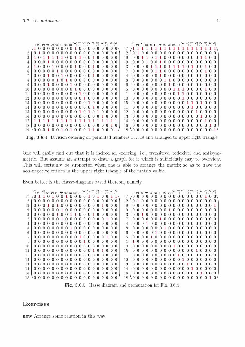
The basic scheme to arrange an ordering is obviously to present it contained in the upper righttriangle of the matrix. When given the relation on the left of Fig. 3.6.4, it is not at all clearwhether it is an ordering; when arranged nicely, it immediately turns out that it is. It is, thus,a specific task to identify the techniques according to which one may get a nice arrangement.For a given example, this will easily be achieved. But what about an arbitrary input? Can onedesign a general procedure?
3.6 Permutations 41
1 2 3 4 5 6 7 8 9 10 11 12 13 14 15 16 17 18 19
123456789
10111213141516171819
⎛⎜⎜⎜⎜⎜⎜⎜⎜⎜⎜⎜⎜⎜⎜⎜⎜⎜⎜⎜⎜⎜⎜⎜⎜⎜⎜⎜⎜⎝
1 0 0 0 0 0 0 0 0 1 0 0 0 0 0 0 0 0 00 1 0 0 0 0 0 0 0 0 0 0 0 0 0 0 0 0 01 0 1 1 1 1 1 0 0 1 1 0 0 1 0 0 0 0 00 0 0 1 0 0 0 0 0 0 0 0 0 0 0 0 0 0 01 0 0 0 1 0 0 0 0 1 0 0 0 1 0 0 0 0 00 0 0 0 0 1 0 0 0 0 0 0 0 0 0 0 0 0 00 0 0 1 0 0 1 0 0 0 0 0 0 1 0 0 0 0 00 0 0 0 0 1 0 1 0 0 0 0 0 0 0 0 0 0 00 0 0 1 0 0 0 0 1 0 0 0 0 0 0 0 0 0 00 0 0 0 0 0 0 0 0 1 0 0 0 0 0 0 0 0 00 0 0 0 0 0 0 0 0 0 1 0 0 0 0 0 0 0 00 0 0 0 0 0 0 0 0 0 0 1 0 0 0 0 0 0 00 0 0 0 0 0 0 0 0 0 0 0 1 0 0 0 0 0 00 0 0 0 0 0 0 0 0 0 0 0 0 1 0 0 0 0 00 0 0 0 0 0 0 0 0 0 1 0 1 0 1 0 0 0 00 0 0 0 0 0 0 0 0 0 0 0 0 0 0 1 0 0 01 1 1 1 1 1 1 1 1 1 1 1 1 1 1 1 1 1 10 0 0 0 0 0 0 0 0 0 0 0 0 0 0 0 0 1 00 0 0 1 0 0 1 0 1 0 0 0 1 1 0 0 0 0 1
⎞⎟⎟⎟⎟⎟⎟⎟⎟⎟⎟⎟⎟⎟⎟⎟⎟⎟⎟⎟⎟⎟⎟⎟⎟⎟⎟⎟⎟⎠
17 2 19 9 3 7 4 8 6 5 1 10 15 11 12 13 14 16 18
172
1993748651
1015111213141618
⎛⎜⎜⎜⎜⎜⎜⎜⎜⎜⎜⎜⎜⎜⎜⎜⎜⎜⎜⎜⎜⎜⎜⎜⎜⎜⎜⎜⎜⎝
1 1 1 1 1 1 1 1 1 1 1 1 1 1 1 1 1 1 10 1 0 0 0 0 0 0 0 0 0 0 0 0 0 0 0 0 00 0 1 1 0 1 1 0 0 0 0 0 0 0 0 1 1 0 00 0 0 1 0 0 1 0 0 0 0 0 0 0 0 0 0 0 00 0 0 0 1 1 1 0 1 1 1 1 0 1 0 0 1 0 00 0 0 0 0 1 1 0 0 0 0 0 0 0 0 0 1 0 00 0 0 0 0 0 1 0 0 0 0 0 0 0 0 0 0 0 00 0 0 0 0 0 0 1 1 0 0 0 0 0 0 0 0 0 00 0 0 0 0 0 0 0 1 0 0 0 0 0 0 0 0 0 00 0 0 0 0 0 0 0 0 1 1 1 0 0 0 0 1 0 00 0 0 0 0 0 0 0 0 0 1 1 0 0 0 0 0 0 00 0 0 0 0 0 0 0 0 0 0 1 0 0 0 0 0 0 00 0 0 0 0 0 0 0 0 0 0 0 1 1 0 1 0 0 00 0 0 0 0 0 0 0 0 0 0 0 0 1 0 0 0 0 00 0 0 0 0 0 0 0 0 0 0 0 0 0 1 0 0 0 00 0 0 0 0 0 0 0 0 0 0 0 0 0 0 1 0 0 00 0 0 0 0 0 0 0 0 0 0 0 0 0 0 0 1 0 00 0 0 0 0 0 0 0 0 0 0 0 0 0 0 0 0 1 00 0 0 0 0 0 0 0 0 0 0 0 0 0 0 0 0 0 1
⎞⎟⎟⎟⎟⎟⎟⎟⎟⎟⎟⎟⎟⎟⎟⎟⎟⎟⎟⎟⎟⎟⎟⎟⎟⎟⎟⎟⎟⎠
Fig. 3.6.4 Division ordering on permuted numbers 1 . . . 19 and arranged to upper right triangle
One will easily find out that it is indeed an ordering, i.e., transitive, reflexive, and antisym-metric. But assume an attempt to draw a graph for it which is sufficiently easy to overview.This will certainly be supported when one is able to arrange the matrix so as to have thenon-negative entries in the upper right triangle of the matrix as in:
Even better is the Hasse-diagram based thereon, namely
17 2 19 9 3 7 4 8 6 5 1 10 15 11 12 13 14 16 18
172
1993748651
1015111213141618
⎛⎜⎜⎜⎜⎜⎜⎜⎜⎜⎜⎜⎜⎜⎜⎜⎜⎜⎜⎜⎜⎜⎜⎜⎜⎜⎜⎜⎜⎝
0 1 1 0 1 0 0 1 0 0 0 0 1 0 1 0 0 1 10 0 0 0 0 0 0 0 0 0 0 0 0 0 0 0 0 0 00 0 0 1 0 1 0 0 0 0 0 0 0 0 0 1 0 0 00 0 0 0 0 0 1 0 0 0 0 0 0 0 0 0 0 0 00 0 0 0 0 1 0 0 1 1 0 0 0 1 0 0 0 0 00 0 0 0 0 0 1 0 0 0 0 0 0 0 0 0 1 0 00 0 0 0 0 0 0 0 0 0 0 0 0 0 0 0 0 0 00 0 0 0 0 0 0 0 1 0 0 0 0 0 0 0 0 0 00 0 0 0 0 0 0 0 0 0 0 0 0 0 0 0 0 0 00 0 0 0 0 0 0 0 0 0 1 0 0 0 0 0 1 0 00 0 0 0 0 0 0 0 0 0 0 1 0 0 0 0 0 0 00 0 0 0 0 0 0 0 0 0 0 0 0 0 0 0 0 0 00 0 0 0 0 0 0 0 0 0 0 0 0 1 0 1 0 0 00 0 0 0 0 0 0 0 0 0 0 0 0 0 0 0 0 0 00 0 0 0 0 0 0 0 0 0 0 0 0 0 0 0 0 0 00 0 0 0 0 0 0 0 0 0 0 0 0 0 0 0 0 0 00 0 0 0 0 0 0 0 0 0 0 0 0 0 0 0 0 0 00 0 0 0 0 0 0 0 0 0 0 0 0 0 0 0 0 0 00 0 0 0 0 0 0 0 0 0 0 0 0 0 0 0 0 0 0
⎞⎟⎟⎟⎟⎟⎟⎟⎟⎟⎟⎟⎟⎟⎟⎟⎟⎟⎟⎟⎟⎟⎟⎟⎟⎟⎟⎟⎟⎠
1 2 3 4 5 6 7 8 9 10 11 12 13 14 15 16 17 18 19
172
1993748651
1015111213141618
⎛⎜⎜⎜⎜⎜⎜⎜⎜⎜⎜⎜⎜⎜⎜⎜⎜⎜⎜⎜⎜⎜⎜⎜⎜⎜⎜⎜⎜⎝
0 0 0 0 0 0 0 0 0 0 0 0 0 0 0 0 1 0 00 1 0 0 0 0 0 0 0 0 0 0 0 0 0 0 0 0 00 0 0 0 0 0 0 0 0 0 0 0 0 0 0 0 0 0 10 0 0 0 0 0 0 0 1 0 0 0 0 0 0 0 0 0 00 0 1 0 0 0 0 0 0 0 0 0 0 0 0 0 0 0 00 0 0 0 0 0 1 0 0 0 0 0 0 0 0 0 0 0 00 0 0 1 0 0 0 0 0 0 0 0 0 0 0 0 0 0 00 0 0 0 0 0 0 1 0 0 0 0 0 0 0 0 0 0 00 0 0 0 0 1 0 0 0 0 0 0 0 0 0 0 0 0 00 0 0 0 1 0 0 0 0 0 0 0 0 0 0 0 0 0 01 0 0 0 0 0 0 0 0 0 0 0 0 0 0 0 0 0 00 0 0 0 0 0 0 0 0 1 0 0 0 0 0 0 0 0 00 0 0 0 0 0 0 0 0 0 0 0 0 0 1 0 0 0 00 0 0 0 0 0 0 0 0 0 1 0 0 0 0 0 0 0 00 0 0 0 0 0 0 0 0 0 0 1 0 0 0 0 0 0 00 0 0 0 0 0 0 0 0 0 0 0 1 0 0 0 0 0 00 0 0 0 0 0 0 0 0 0 0 0 0 1 0 0 0 0 00 0 0 0 0 0 0 0 0 0 0 0 0 0 0 1 0 0 00 0 0 0 0 0 0 0 0 0 0 0 0 0 0 0 0 1 0
⎞⎟⎟⎟⎟⎟⎟⎟⎟⎟⎟⎟⎟⎟⎟⎟⎟⎟⎟⎟⎟⎟⎟⎟⎟⎟⎟⎟⎟⎠
Fig. 3.6.5 Hasse diagram and permutation for Fig. 3.6.4
Exercises
new Arrange some relation in this way

42 Chapter 3 Relations
Solution new
3.7 Partitions
Partitions are frequently used in mathematical modeling. We introduce them rather naively.They shall subdivide here a baseset, i.e., shall consist of a set of mutually disjoint nonemptysubsets of that baseset.
The following example shows an equivalence relation Ξ on the left. Its elements are, however,not sorted in a way that lets elements of an equivalence class stay together. It is a rather simpleprogramming task to arrive at the rearranged matrix Θ := P ;Ξ;P T on the right, where P is thepermutation used to simultaneously rearrange rows and columns. It is not so simple to defineP in terms of the given Ξ, but also this can be achieved. To this end, take the baseset orderingE of the rows and columns into consideration.
1 2 3 4 5 6 7 8 9 10 11 12 13
123456789
10111213
⎛⎜⎜⎜⎜⎜⎜⎜⎜⎜⎜⎜⎜⎜⎜⎜⎜⎜⎝
1 1 0 0 0 0 0 1 0 0 0 0 11 1 0 0 0 0 0 1 0 0 0 0 10 0 1 0 1 0 1 0 1 0 0 1 00 0 0 1 0 1 0 0 0 1 1 0 00 0 1 0 1 0 1 0 1 0 0 1 00 0 0 1 0 1 0 0 0 1 1 0 00 0 1 0 1 0 1 0 1 0 0 1 01 1 0 0 0 0 0 1 0 0 0 0 10 0 1 0 1 0 1 0 1 0 0 1 00 0 0 1 0 1 0 0 0 1 1 0 00 0 0 1 0 1 0 0 0 1 1 0 00 0 1 0 1 0 1 0 1 0 0 1 01 1 0 0 0 0 0 1 0 0 0 0 1
⎞⎟⎟⎟⎟⎟⎟⎟⎟⎟⎟⎟⎟⎟⎟⎟⎟⎟⎠
1 2 8 13 3 5 7 9 12 4 6 10 11⎛⎜⎜⎜⎜⎜⎜⎜⎜⎜⎜⎜⎜⎜⎜⎜⎜⎜⎝
1 0 0 0 0 0 0 0 0 0 0 0 00 1 0 0 0 0 0 0 0 0 0 0 00 0 0 0 1 0 0 0 0 0 0 0 00 0 0 0 0 0 0 0 0 1 0 0 00 0 0 0 0 1 0 0 0 0 0 0 00 0 0 0 0 0 0 0 0 0 1 0 00 0 0 0 0 0 1 0 0 0 0 0 00 0 1 0 0 0 0 0 0 0 0 0 00 0 0 0 0 0 0 1 0 0 0 0 00 0 0 0 0 0 0 0 0 0 0 1 00 0 0 0 0 0 0 0 0 0 0 0 10 0 0 0 0 0 0 0 1 0 0 0 00 0 0 1 0 0 0 0 0 0 0 0 0
⎞⎟⎟⎟⎟⎟⎟⎟⎟⎟⎟⎟⎟⎟⎟⎟⎟⎟⎠
1 2 8 13 3 5 7 9 12 4 6 10 11
128
133579
1246
1011
⎛⎜⎜⎜⎜⎜⎜⎜⎜⎜⎜⎜⎜⎜⎜⎜⎜⎜⎝
1 1 1 1 0 0 0 0 0 0 0 0 01 1 1 1 0 0 0 0 0 0 0 0 01 1 1 1 0 0 0 0 0 0 0 0 01 1 1 1 0 0 0 0 0 0 0 0 00 0 0 0 1 1 1 1 1 0 0 0 00 0 0 0 1 1 1 1 1 0 0 0 00 0 0 0 1 1 1 1 1 0 0 0 00 0 0 0 1 1 1 1 1 0 0 0 00 0 0 0 1 1 1 1 1 0 0 0 00 0 0 0 0 0 0 0 0 1 1 1 10 0 0 0 0 0 0 0 0 1 1 1 10 0 0 0 0 0 0 0 0 1 1 1 10 0 0 0 0 0 0 0 0 1 1 1 1
⎞⎟⎟⎟⎟⎟⎟⎟⎟⎟⎟⎟⎟⎟⎟⎟⎟⎟⎠
Fig. 3.7.1 Rearranging an equivalence relation to block-diagonal form: Ξ, P,Θ
Observe the first four columns of P . They regulate that 1,2,8,13 are sent to positions 1,2,3,4.A nested recursive definition for this procedure is possible. From Ξ, we obtain the orderingΞ ∩ E and its Hasse relation HΞ. Let H be the Hasse relation of E. Assume the process ofrearranging in progress with several classes already rearranged and others not yet, so that P isdeveloped only partly. The next element to accomodate is e1 = lea(P ; ). The next positionfor an element is e2 = lea(P T; ). So we start adding P ∪ e1;e
T2 and proceed iterating HT
Ξ;P ;HP .
This is executed as long as P ; =/ . Following this idea, a function
partitionToPermutation rt
has been designed. It is often used when presenting ideas that rest also on the way the relationis represented.
Exercises
new Find permutation for partition
Solution new

Part II
Visualizing Relational Constructions
43


45
At this point of the book, a major break of style may be observed. So far we have used free-handformulations, not least in Haskell, and have presented basics of set theory with much intensityon how to represent sets, subsets, elements, relations and mappings. We have, however, so farnot used relations in an algebraic form.
From now on, we will mainly concentrate on topics that inherently need some algebraic treat-ment. We can, however, not immediately start with formal algebraic proofs and with therelational language TITUREL in which all this has been formulated. Rather will we first insertthe chapters of the present Part II full of examples that demonstrate the basics of algebraicrules. Whenever one of these early rules needs a proof, this proof will be very simple, butnevertheless omitted at this point. One will find the postponed proofs in Appendix B.
What we will present, however, is how component-free versions are derived from a predicate-logic form. These deductions are definitely not an aim of this book; they seem, however,necessary for many colleagues who are not well-trained in expressing themselves in a component-free algebraic form. These deductions are by no means executed strictly formal in some rigorousform. Rather, they are included so as to convince scientists that there is reason to use therespective component-free form.
There is another point to mention concerning the domain constructions, or data structures,that we are going to present. Considered from one point of view, they are rather trivial.Historically, however, they did not seem so. The first theoretically reasonable programminglanguage ALGOL 60 did not provide data structures beyond arrays. When improved withPASCAL, variant handling was not handled as a basic construct and offered only in combinationwith tuple forming. Dependent types were long considered theory-laden and are not yet broadlyoffered in programming languages. When we here offer generic domain construction methodsat an early stage, we face the problem that there is not yet a sufficiently developed apparatusavailable to prove that the respective construct is unique up to isomorphism — of course, ourconstructs are. We present them here mentioning always that there is essentially one form, asone is in a position to provide a bijection based on the syntactic material already given. Thisis then shown via examples. For the literate reader these examples will be sufficiently detailedto replace a proof.
Several concepts may be expressed in either style, in a programming language (Haskell) as wellas in algebraic form. So one or the other topic we have already dealt with will now be rewrittenin the new style. This will make the difference visible.


4 Algebraic Operations on Relations
Not a full account of relation algebra can be given here; just the amount that enables us to workwith it in practice. This will be accompanied by examples showing the effects. When relationsare studied in practice, they are conceived as subsets R ⊆ X × Y of the Cartesian product ofthe two sets X, Y between which they are defined to hold. Already in Chapt. 3 we have givenenough examples of relations between sets together with a diversity of ways to represent them.We will now present the operations on relations in a way that is both, algebraically correct andsufficiently underpinned with examples.
4.1 Typing Relations
In many cases, we are interested in solving just one problem. More often, however, we wantto find out how a whole class of problems may be solved. While in the first case, we mayuse the given objects directly, we must work with constants and variables for relations in thelatter case. These variables will then be instantiated at the time when the concrete problem ispresented.
Let us consider timetabling as an example. It may be the case that a timetable has to beconstructed at some given school. It would, however, not be wise to write a timetabling programjust for this school with the present set of teachers and classrooms. When it is intended to sellthe program several times so that it may be applied also to other schools, one must care forthe possibility of different sets of teachers, different sets of classrooms, etc.
The standard technique in such cases is to introduce types. One will have to be able to handlethe type teacher, the type classroom, etc. At one school, there may exist 15 teachers and10 classrooms, while instantiation at another school will give 20 teachers and 15 classrooms.Although the concept of time is in a sense universal, one will also introduce the type hour; itmay well be the case that at one school they use a scheme of hours or timeslots 8.00–9.00, 9.00–10.00 while at the other 8.15–9.00, 9.00–9.45. It is therefore wise, to offer even an instantiableconcept of “hour”.
In any case, a type is a denotation of a set of items that may afterwards be interpreted with abaseset. In this strict sense, the following relations are of different type — in spite of the factthat their constituent matrices are equal.
47

48 Chapter 4 Algebraic Operations on Relations
R1=
Mon
Tue
Wed
Thu
Fri
Sat
redgreenblue
orange
⎛⎜⎝
0 1 1 0 1 01 0 1 0 0 10 0 0 1 1 01 0 0 1 0 1
⎞⎟⎠ R2=
1 2 3 4 5 6♠♥♦♣
⎛⎜⎝
0 1 1 0 1 01 0 1 0 0 10 0 0 1 1 01 0 0 1 0 1
⎞⎟⎠
Fig. 4.1.1 Differently typed relations
While R : X −→ Y is the type, the concrete instantiation of the first relation is
R1 ⊆ red, green, blue, orange × Mon, Tue, Wed, Thu, Fri, Sat.In the other case, R : X −→ Y is the type but
R2 ⊆ ♠,♥,♦,♣ × 1, 2, 3, 4, 5, 6the instantiation. We see, that X is instantiated in two ways, namely as
red, green, blue, orange or as ♠,♥,♦,♣.When we do not ask for both, X, Y , we will frequently determine domain and codomain bydom R = X and cod R = Y .
Something ignored in test edition!
4.2 Boolean Operations
We recall in a more formal way what has already been presented in the examples of Part I.Relations with type R : X −→ Y when interpreted may be understood as subsets of a Cartesianproduct: R ⊆ V ×W . Being interpreted as a subset immediately implies that certain conceptsare available for relations that we know from subsets.
4.2.1 Definition. Given two relations R : X −→ Y and S : X −→ Y , i.e., relations of thesame type, we define
union R ∪ S (x, y) ∈ X × Y | (x, y) ∈ R ∨ (x, y) ∈ Sintersection R ∩ S (x, y) ∈ X × Y | (x, y) ∈ R ∧ (x, y) ∈ Scomplementation R (x, y) ∈ X × Y | (x, y)∈/ Rnull relation or ∅universal relation X × Y
On the right we have indicated what we intend this to mean when the relations are interpretedas R, S ⊆ X × Y .
It makes no sense to unite, e.g., relations of different types, and therefore this is not allowed.Concerning the top and bottom relations, we have been a bit sloppy here. The symbols forthe empty or null and for the universal relation should have been X,Y and X,Y , respectively.While we know the typing in cases of union, intersection, and negation from the operands R, S,we should provide this information for the null and the universal relation. It is absolutelyevident that
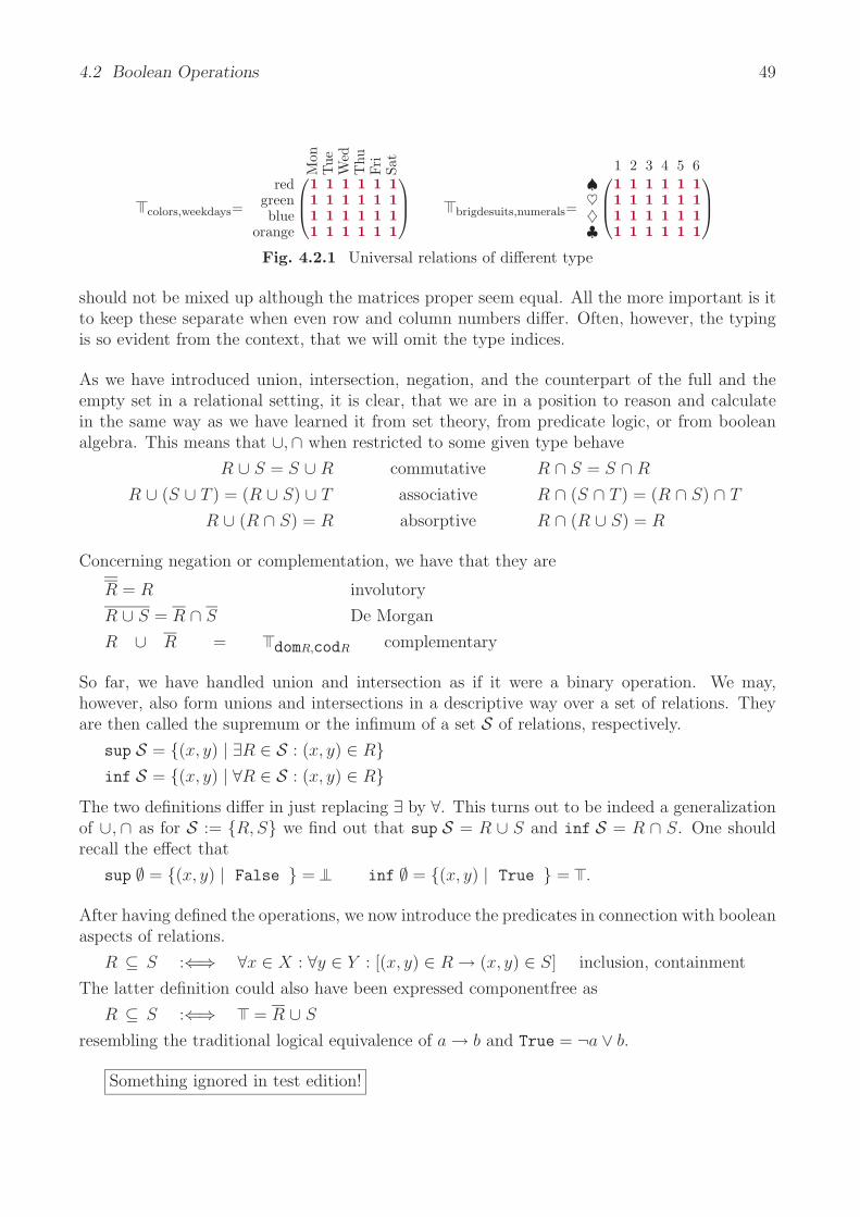
4.2 Boolean Operations 49
colors,weekdays=
Mon
Tue
Wed
Thu
Fri
Sat
redgreenblue
orange
⎛⎜⎝
1 1 1 1 1 11 1 1 1 1 11 1 1 1 1 11 1 1 1 1 1
⎞⎟⎠ brigdesuits,numerals=
1 2 3 4 5 6♠♥♦♣
⎛⎜⎝
1 1 1 1 1 11 1 1 1 1 11 1 1 1 1 11 1 1 1 1 1
⎞⎟⎠
Fig. 4.2.1 Universal relations of different type
should not be mixed up although the matrices proper seem equal. All the more important is itto keep these separate when even row and column numbers differ. Often, however, the typingis so evident from the context, that we will omit the type indices.
As we have introduced union, intersection, negation, and the counterpart of the full and theempty set in a relational setting, it is clear, that we are in a position to reason and calculatein the same way as we have learned it from set theory, from predicate logic, or from booleanalgebra. This means that ∪,∩ when restricted to some given type behave
R ∪ S = S ∪ R commutative R ∩ S = S ∩ R
R ∪ (S ∪ T ) = (R ∪ S) ∪ T associative R ∩ (S ∩ T ) = (R ∩ S) ∩ T
R ∪ (R ∩ S) = R absorptive R ∩ (R ∪ S) = R
Concerning negation or complementation, we have that they are
R = R involutory
R ∪ S = R ∩ S De Morgan
R ∪ R = domR,codR complementary
So far, we have handled union and intersection as if it were a binary operation. We may,however, also form unions and intersections in a descriptive way over a set of relations. Theyare then called the supremum or the infimum of a set S of relations, respectively.
sup S = (x, y) | ∃R ∈ S : (x, y) ∈ Rinf S = (x, y) | ∀R ∈ S : (x, y) ∈ R
The two definitions differ in just replacing ∃ by ∀. This turns out to be indeed a generalizationof ∪, ∩ as for S := R, S we find out that sup S = R ∪ S and inf S = R ∩ S. One shouldrecall the effect that
sup ∅ = (x, y) | False = inf ∅ = (x, y) | True = .
After having defined the operations, we now introduce the predicates in connection with booleanaspects of relations.
R ⊆ S :⇐⇒ ∀x ∈ X : ∀y ∈ Y : [(x, y) ∈ R → (x, y) ∈ S] inclusion, containment
The latter definition could also have been expressed componentfree as
R ⊆ S :⇐⇒ = R ∪ S
resembling the traditional logical equivalence of a → b and True = ¬a ∨ b.
Something ignored in test edition!

50 Chapter 4 Algebraic Operations on Relations
4.3 Relational Operations Proper
The first operation on relations beyond the boolean ones is conversion or transposition; it ischaracteristic for relations.
4.3.1 Definition. Given a relation R : X −→ Y , its converse (or transposed) RT : Y −→ Xis that relation in opposite direction in which for all x, y containment (y, x) ∈ RT holds preciselywhen (x, y) ∈ R.
Colloquially transposition is often expressed in separate wordings.
Bob is taller than Chris −→ Chris is smaller than Bob
Dick is boss of Erol −→ Erol is employee of Dick
Here, as well as in set function representation conversion is sometimes not easily recognized:
R1 =
♠♥♦♣
Tue,Wed,FriMon,Wed,SatThu,FriMon,Thu,Sat
RT1 =
MonTueWedThuFriSat
♥,♣♠♠,♥♦,♣♠,♦♥,♣
Fig. 4.3.1 Transposition in set function representation
For matrices it is more schematical; it means exchanging row and column type and mirroringthe matrix along the diagonal upper left to lower right.
R1 =
Mon
Tue
Wed
Thu
Fri
Sat
♠♥♦♣
⎛⎜⎝
0 1 1 0 1 01 0 1 0 0 10 0 0 1 1 01 0 0 1 0 1
⎞⎟⎠ RT
1 =
♠ ♥ ♦ ♣MonTueWedThuFriSat
⎛⎜⎜⎜⎜⎝
0 1 0 11 0 0 01 1 0 00 0 1 11 0 1 00 1 0 1
⎞⎟⎟⎟⎟⎠
Fig. 4.3.2 Transposition in matrix representation
Obviously, conversion is involutory, i.e., applied twice results in the original argument again:
(RT)T = R
It is mathematical standard to check how a newly introduced operation behaves when appliedtogether with those available already earlier. Such algebraic rules are rather intuitive. It isimmaterial whether one first negates a relation and then transposes or the other way round:
RT
= RT
R =
Mon
Tue
Wed
Thu
Fri
Sat
♠♥♦♣
⎛⎜⎝
0 1 1 0 1 01 0 1 0 0 10 0 0 1 1 01 0 0 1 0 1
⎞⎟⎠ R =
Mon
Tue
Wed
Thu
Fri
Sat⎛
⎜⎝1 0 0 1 0 10 1 0 1 1 01 1 1 0 0 10 1 1 0 1 0
⎞⎟⎠ RT =
♠ ♥ ♦ ♣MonTueWedThuFriSat
⎛⎜⎜⎜⎜⎝
0 1 0 11 0 0 01 1 0 00 0 1 11 0 1 00 1 0 1
⎞⎟⎟⎟⎟⎠ R
T= RT =
♠ ♥ ♦ ♣⎛⎜⎜⎜⎜⎝
1 0 1 00 1 1 10 0 1 11 1 0 00 1 0 11 0 1 0
⎞⎟⎟⎟⎟⎠
Fig. 4.3.3 Transposition commutes with negation

4.3 Relational Operations Proper 51
In a similar way, transposition commutes with union and intersection of relations.
(R ∪ S)T = RT ∪ ST (R ∩ S)T = RT ∩ ST
When a relation is contained in another relation, then the same will be true for their converses.
R ⊆ S ⇐⇒ RT ⊆ ST
Alles mit Matrix-Beispielen??
The next vital operation to be mentioned is relational composition. Whenever x and y arein relation R and y and z are in relation S, one says that x and z are in relation R; S. It isunimportant whether there is just one intermediate y or many. The point to stress is that thereexists an intermediate element.
4.3.2 Definition. Let R : X −→ Y and S : Y −→ Z be relations. Their (relational)composition, or their multiplication, or their product R; S : X −→ Z is defined as therelation
R; S := (x, z) ∈ X × Z | ∃y ∈ Y : (x, y) ∈ R ∧ (y, z) ∈ SConcerning composition, there exist left resp. right unit elements , the so-called identityrelations.
We illustrate composition and identity relation with a completely fictitious example in whichindeed three different types are involved1. Assume owners of cars who travel and have to rent acar, but not all car rental companies offer every car. The following composition of the relationownsCar with the relation isOfferedBy results in a relation
mayRentOwnedCarTypeFrom = ownsCar ; isOfferedBy.
Dod
geA
udi
Ren
ault
Ben
tley
BM
WSe
atFo
rd
ArbuthnotPerez
DupontBotticelliSchmidt
Larsen
⎛⎜⎜⎜⎜⎝
0 1 0 1 0 0 10 1 0 0 0 0 00 1 1 0 0 1 01 0 0 0 0 0 10 0 0 1 0 0 00 1 1 0 1 0 0
⎞⎟⎟⎟⎟⎠ ;
Bud
get
Sixt
Her
tzA
lam
oE
uroC
arA
vis
Ren
tAC
arD
olla
r
DodgeAudi
RenaultBentley
BMWSeatFord
⎛⎜⎜⎜⎜⎜⎜⎝
1 0 0 0 1 0 0 00 0 1 0 0 0 0 10 1 0 0 0 1 0 01 0 0 0 1 0 0 00 1 0 1 0 0 0 10 0 1 0 0 0 0 11 0 0 1 0 1 0 0
⎞⎟⎟⎟⎟⎟⎟⎠
=
Bud
get
Sixt
Her
tzA
lam
oE
uroC
arA
vis
Ren
tAC
arD
olla
r
ArbuthnotPerez
DupontBotticelliSchmidt
Larsen
⎛⎜⎜⎜⎜⎝
1 0 1 1 1 1 0 10 0 1 0 0 0 0 10 1 1 0 0 1 0 11 0 0 1 1 1 0 01 0 0 0 1 0 0 00 1 1 1 0 1 0 1
⎞⎟⎟⎟⎟⎠
Fig. 4.3.4 Car owners chance to rent a car of one of the types he already owns
For the unit relations, we have again the choice to denote in full precision or not
R; Y = R, X ; R = R as opposed to R; = R, ; R = R
1We apologize for blaming RentACar to offer no car type at all.
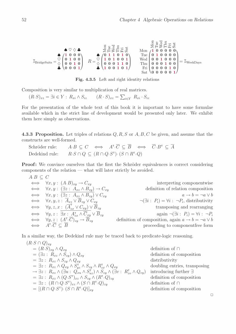
52 Chapter 4 Algebraic Operations on Relations
BridgeSuits =
♠ ♥ ♦ ♣♠♥♦♣
⎛⎜⎝
1 0 0 00 1 0 00 0 1 00 0 0 1
⎞⎟⎠ R =
Mon
Tue
Wed
Thu
Fri
Sat
♠♥♦♣
⎛⎜⎝
0 1 1 0 1 01 0 1 0 0 10 0 0 1 1 01 0 0 1 0 1
⎞⎟⎠
Mon
Tue
Wed
Thu
Fri
Sat
MonTueWedThuFriSat
⎛⎜⎜⎜⎜⎝
1 0 0 0 0 00 1 0 0 0 00 0 1 0 0 00 0 0 1 0 00 0 0 0 1 00 0 0 0 0 1
⎞⎟⎟⎟⎟⎠= WeekDays
Fig. 4.3.5 Left and right identity relations
Composition is very similar to multiplication of real matrices.
(R; S)xz = ∃i ∈ Y : Rxi ∧ Siz (R · S)xz =∑
i∈Y Rxi · Siz
For the presentation of the whole text of this book it is important to have some formulaeavailable which in the strict line of development would be presented only later. We exhibitthem here simply as observations.
4.3.3 Proposition. Let triples of relations Q, R, S or A, B, C be given, and assume that theconstructs are well-formed.
Schroder rule: A; B ⊆ C ⇐⇒ AT; C ⊆ B ⇐⇒ C ; BT ⊆ A
Dedekind rule: R; S ∩ Q ⊆ (R ∩ Q; ST); (S ∩ RT; Q)
Proof : We convince ourselves that the first the Schroder equivalences is correct consideringcomponents of the relation — what will later strictly be avoided.
A; B ⊆ C⇐⇒ ∀x, y : (A; B)xy → Cxy interpreting componentwise⇐⇒ ∀x, y : (∃z : Axz ∧ Bzy) → Cxy definition of relation composition
⇐⇒ ∀x, y : (∃z : Axz ∧ Bzy) ∨ Cxy a → b = ¬a ∨ b⇐⇒ ∀x, y, z : Axz ∨ Bzy ∨ Cxy ¬(∃i : Pi) = ∀i : ¬Pi, distributivity
⇐⇒ ∀y, z, x : (AT
zx ∨ Cxy) ∨ Bzy transposing and rearranging
⇐⇒ ∀y, z : ∃x : ATzx ∧ Cxy ∨ Bzy again ¬(∃i : Pi) = ∀i : ¬Pi
⇐⇒ ∀y, z : (AT; C)zy → Bzy definition of composition, again a → b = ¬a ∨ b⇐⇒ AT; C ⊆ B proceeding to componentfree form
In a similar way, the Dedekind rule may be traced back to predicate-logic reasoning.
(R; S ∩ Q)xy
= (R; S)xy ∧ Qxy definition of ∩= (∃z : Rxz ∧ Szy) ∧ Qxy definition of composition= ∃z : Rxz ∧ Szy ∧ Qxy distributivity= ∃z : Rxz ∧ Qxy ∧ ST
yz ∧ Szy ∧ RTzx ∧ Qxy doubling entries, transposing
→ ∃z : Rxz ∧ (∃u : Qxu ∧ STuz) ∧ Szy ∧ (∃v : RT
zv ∧ Qvy) introducing further ∃= ∃z : Rxz ∧ (Q; ST)xz ∧ Szy ∧ (RT; Q)zy definition of composition= ∃z : (R ∩ Q; ST)xz ∧ (S ∩ RT; Q)zy definition of ∩= [(R ∩ Q; ST); (S ∩ RT; Q)]xy definition of composition
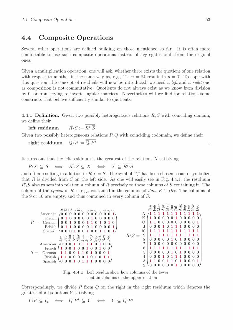
4.4 Composite Operations 53
4.4 Composite Operations
Several other operations are defined building on those mentioned so far. It is often morecomfortable to use such composite operations instead of aggregates built from the originalones.
Given a multiplication operation, one will ask, whether there exists the quotient of one relationwith respect to another in the same way as, e.g., 12 · n = 84 results in n = 7. To cope withthis question, the concept of residuals will now be introduced; we need a left and a right oneas composition is not commutative. Quotients do not always exist as we know from divisionby 0, or from trying to invert singular matrices. Nevertheless will we find for relations someconstructs that behave sufficiently similar to quotients.
4.4.1 Definition. Given two possibly heterogeneous relations R, S with coinciding domain,we define their
left residuum R\S := RT; S
Given two possibly heterogeneous relations P, Q with coinciding codomain, we define their
right residuum Q/P := Q; P T
It turns out that the left residuum is the greatest of the relations X satisfying
R; X ⊆ S ⇐⇒ RT; S ⊆ X ⇐⇒ X ⊆ RT; S
and often resulting in addition in R;X = S. The symbol “\” has been chosen so as to symbolizethat R is divided from S on the left side. As one will easily see in Fig. 4.4.1, the residuumR\S always sets into relation a column of R precisely to those columns of S containing it. Thecolumn of the Queen in R is, e.g., contained in the columns of Jan, Feb, Dec. The columns ofthe 9 or 10 are empty, and thus contained in every column of S.
R =
A K Q J 10 9 8 7 6 5 4 3 2
AmericanFrench
GermanBritish
Spanish
⎛⎜⎜⎝
0 0 0 0 0 0 0 0 0 0 0 0 10 1 0 0 0 0 0 1 0 0 0 0 00 0 1 0 0 0 1 1 0 1 0 1 00 1 1 0 0 0 0 1 0 0 0 0 10 0 0 1 0 0 1 0 0 1 1 0 1
⎞⎟⎟⎠
S =
Jan
Feb
Mar
Apr
May
Jun
Jul
Aug
Sep
Oct
Nov
Dec
AmericanFrench
GermanBritish
Spanish
⎛⎜⎜⎝
0 0 0 1 0 1 1 1 0 1 0 01 0 0 1 0 0 1 0 0 1 0 01 1 0 0 1 1 0 1 0 0 0 11 1 0 0 0 0 1 0 1 0 1 10 0 0 1 0 1 1 1 0 0 0 0
⎞⎟⎟⎠
R\S =
Jan
Feb
Mar
Apr
May
Jun
Jul
Aug
Sep
Oct
Nov
Dec
AKQJ
1098765432
⎛⎜⎜⎜⎜⎜⎜⎜⎜⎜⎜⎜⎜⎜⎜⎜⎜⎜⎝
1 1 1 1 1 1 1 1 1 1 1 11 0 0 0 0 0 1 0 0 0 0 01 1 0 0 0 0 0 0 0 0 0 10 0 0 1 0 1 1 1 0 0 0 01 1 1 1 1 1 1 1 1 1 1 11 1 1 1 1 1 1 1 1 1 1 10 0 0 0 0 1 0 1 0 0 0 01 0 0 0 0 0 0 0 0 0 0 01 1 1 1 1 1 1 1 1 1 1 10 0 0 0 0 1 0 1 0 0 0 00 0 0 1 0 1 1 1 0 0 0 01 1 0 0 1 1 0 1 0 0 0 10 0 0 0 0 0 1 0 0 0 0 0
⎞⎟⎟⎟⎟⎟⎟⎟⎟⎟⎟⎟⎟⎟⎟⎟⎟⎟⎠
Fig. 4.4.1 Left residua show how columns of the lowercontain columns of the upper relation
Correspondingly, we divide P from Q on the right in the right residuum which denotes thegreatest of all solutions Y satisfying
Y ; P ⊆ Q ⇐⇒ Q; P T ⊆ Y ⇐⇒ Y ⊆ Q; P T
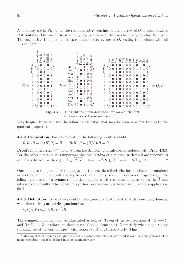
54 Chapter 4 Algebraic Operations on Relations
As one may see in Fig. 4.4.2, the residuum Q/P sets into relation a row of Q to those rows ofP it contains. The row of the King in Q, e.g., contains in the rows belonging to Mar, Sep, Nov.The row of Mar is empty, and thus contained in every row of Q, leading to a column with all1 ’s in Q/P .
Q =
Am
eric
anFr
ench
Ger
man
Bri
tish
Span
ish
AKQJ
1098765432
⎛⎜⎜⎜⎜⎜⎜⎜⎜⎜⎜⎜⎜⎜⎜⎜⎜⎜⎝
0 0 0 0 00 1 0 1 00 0 1 1 00 0 0 0 10 0 0 0 00 0 0 0 00 0 1 0 10 1 1 1 00 0 0 0 00 0 1 0 10 0 0 0 10 0 1 0 01 0 0 1 1
⎞⎟⎟⎟⎟⎟⎟⎟⎟⎟⎟⎟⎟⎟⎟⎟⎟⎟⎠
P =
Am
eric
anFr
ench
Ger
man
Bri
tish
Span
ish
JanFebMarAprMayJunJul
AugSepOctNovDec
⎛⎜⎜⎜⎜⎜⎜⎜⎜⎜⎜⎜⎜⎜⎜⎜⎝
0 1 1 1 00 0 1 1 00 0 0 0 01 1 0 0 10 0 1 0 01 0 1 0 11 1 0 1 11 0 1 0 10 0 0 1 01 1 0 0 00 0 0 1 00 0 1 1 0
⎞⎟⎟⎟⎟⎟⎟⎟⎟⎟⎟⎟⎟⎟⎟⎟⎠
Jan
Feb
Mar
Apr
May
Jun
Jul
Aug
Sep
Oct
Nov
Dec
AKQJ
1098765432
⎛⎜⎜⎜⎜⎜⎜⎜⎜⎜⎜⎜⎜⎜⎜⎜⎜⎜⎝
0 0 1 0 0 0 0 0 0 0 0 00 0 1 0 0 0 0 0 1 0 1 00 1 1 0 1 0 0 0 1 0 1 10 0 1 0 0 0 0 0 0 0 0 00 0 1 0 0 0 0 0 0 0 0 00 0 1 0 0 0 0 0 0 0 0 00 0 1 0 1 0 0 0 0 0 0 01 1 1 0 1 0 0 0 1 0 1 10 0 1 0 0 0 0 0 0 0 0 00 0 1 0 1 0 0 0 0 0 0 00 0 1 0 0 0 0 0 0 0 0 00 0 1 0 1 0 0 0 0 0 0 00 0 1 0 0 0 0 0 1 0 1 0
⎞⎟⎟⎟⎟⎟⎟⎟⎟⎟⎟⎟⎟⎟⎟⎟⎟⎟⎠
= Q/P
Fig. 4.4.2 The right residuum describes how rows of the firstcontain rows of the second relation
Very frequently we will use the following identities that may be seen as a first test as to thequotient properties.
4.4.2 Proposition. For every relation the following identities hold
R; RT; R = R; (R\R) = R R; RT; R = (R/R); R = R
Proof : In both cases, “⊆ ” follows from the Schroder equivalences introduced with Prop. 4.3.3.For the other direction it is important that the residua of a relation with itself are reflexive as
can easily be seen with, e.g., ⊆ RT; R ⇐⇒ RT; R ⊆ ⇐⇒ R; ⊆ R
Once one has the possibility to compare in the way described whether a column is containedin another column, one will also try to look for equality of columns or rows, respectively. Thefollowing concept of a symmetric quotient applies a left residuum to A as well as to A andintersects the results. The construct syq has very successfully been used in various applicationfields.
4.4.3 Definition. Given two possibly heterogeneous relations A, B with coinciding domain,we define their symmetric quotient2 as
syq(A, B) := AT; B ∩ AT; B
The symmetric quotient can be illustrated as follows: Taken of the two relations A : X −→ Yand B : X −→ Z, it relates an element y ∈ Y to an element z ∈ Z precisely when y and z havethe same set of “inverse images” with respect to A or B respectively. Thus
2Observe that the symmetric quotient is not a symmetric relation, nor need it even be homogeneous! Thename resembles that it is defined in some symmetric way.
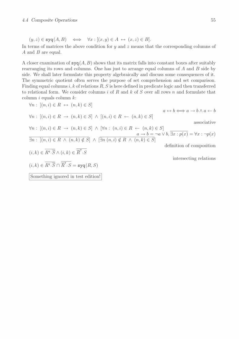
4.4 Composite Operations 55
(y, z) ∈ syq(A, B) ⇐⇒ ∀x : [(x, y) ∈ A ↔ (x, z) ∈ B].
In terms of matrices the above condition for y and z means that the corresponding columns ofA and B are equal.
A closer examination of syq(A, B) shows that its matrix falls into constant boxes after suitablyrearranging its rows and columns. One has just to arrange equal columns of A and B side byside. We shall later formulate this property algebraically and discuss some consequences of it.The symmetric quotient often serves the purpose of set comprehension and set comparison.Finding equal columns i, k of relations R, S is here defined in predicate logic and then transferredto relational form. We consider columns i of R and k of S over all rows n and formulate thatcolumn i equals column k:
∀n : [(n, i) ∈ R ↔ (n, k) ∈ S]a ↔ b ⇐⇒ a → b ∧ a ← b
∀n : [(n, i) ∈ R → (n, k) ∈ S] ∧ [(n, i) ∈ R ← (n, k) ∈ S]associative
∀n : [(n, i) ∈ R → (n, k) ∈ S] ∧ [∀n : (n, i) ∈ R ← (n, k) ∈ S]a → b = ¬a ∨ b, ∃x : p(x) = ∀x : ¬p(x)
∃n : [(n, i) ∈ R ∧ (n, k) /∈ S] ∧ [∃n (n, i) /∈ R ∧ (n, k) ∈ S]definition of composition
(i, k) ∈ RT; S ∧ (i, k) ∈ RT; S
intersecting relations
(i, k) ∈ RT; S ∩ RT; S = syq(R, S)
Something ignored in test edition!

56 Chapter 4 Algebraic Operations on Relations
5 Order and Function:The Standard View
Many relations enjoy specific properties. The most prominent ones are related with orderingsand with functions. That at most one or precisely one value is assigned to an argument ischaracteristic for functions or mappings, respectively. Mankind has also developed a multitudeof concepts to reason about something that is better than or is more attractive than somethingelse or similar to something else. Concepts related with functions or with orderings lead toan enormous bulk of formulae and interdependencies. In this chapter, we recall the classics;first in the heterogeneous setting of functions and mappings and afterwards in a homogeneoussetting of orderings and equivalences.
5.1 Functions and Mappings
A notational distinction between a (partially defined) function and a mapping (i.e., a totallydefined function) is regrettably not commonly being made. Many people use both words assynonyms and usually mean a totally defined function. Traditionally, we speak of functions
f(x) = 1x−1
or g(y) =√
y − 3
and then separately discuss their somehow peculiar behaviour for x = 1 or that there exist no,one, or two results for y < 3, y = 3, and y > 3. Relations typically assign arbitrary sets ofresults. We introduce a definition to concentrate on the more specific cases.
5.1.1 Definition. Let a relation R : V −→ W be given. We say that the relation
R is univalent :⇐⇒ ∀x ∈ V : ∀y, z ∈ W : [(x, y) ∈ R ∧ (x, z) ∈ R] → y = z
⇐⇒ RT; R ⊆Univalent relations are often called (partially defined) functions1. A relation R is injectiveif its converse is univalent.
A univalent relation R associates to every x ∈ V at most one y ∈ W . In more formal terms:Assuming that y as well as z should be attached as values to some x, it follows that y = z.This is a rather long formulation, which may be shortened to the componentfree version.
We give a sketch of how the first version of the definition above can successively be madecomponentfree — and thus be transformed into a TITUREL-program. These transition steps
1The property of being univalent or a (partially defined) function is met very frequently and most oftenradically simplifies the setting. Postulating a (totally defined) mapping brings additional power, but not toomuch; therefore functions deserve to be studied separately.
57

58 Chapter 5 Order and Function: The Standard View
shall give intuition to the reader how the second shorthand version is invented; it should bestressed that this is not a calculus we aim at.
∀y, z ∈ W : ∀x ∈ V : [(x, y) ∈ R ∧ (x, z) ∈ R] → y = za → b = ¬a ∨ b
∀y, z ∈ W : ∀x ∈ V : (x, y) ∈ R ∧ (x, z) ∈ R ∨ y = z¬
[∃x : p(x)
]= ∀x : ¬p(x)
∀y, z ∈ W : ¬∃x ∈ V : (x, y) ∈ R ∧ (x, z) ∈ R ∧ y =/ z
(a ∧ c) ∨ (b ∧ c) = (a ∨ b) ∧ c
∀y, z ∈ W : ¬[
∃x ∈ V : (x, y) ∈ R ∧ (x, z) ∈ R]∧ y =/ z
definition of transposition
∀y, z ∈ W : ¬[
∃x ∈ V : (y, x) ∈ RT ∧ (x, z) ∈ R]∧ y =/ z
definition of composition
∀y, z ∈ W : ¬
(y, z) ∈ RT; R ∧ y =/ z
De Morgan
∀y, z ∈ W : (y, z) ∈ RT; R ∨ y = za → b = ¬a ∨ b and definition of identity
∀y, z ∈ W : (y, z) ∈ RT; R → (y, z) ∈transition to componentfree version
RT; R ⊆transferred to TITUREL
(Convs r) :***: r :<==: Ident (dom r)
One may again consider the univalency condition from the point of view of triangles:
R
RII
Fig. 5.1.1 Triangle to define the essence of being univalent
When going back from an image point to one of its arguments and proceeding to the imageside again, one will always arrive at the point one has been starting from — if the relation isassumed to be univalent.
When considering a univalent relation R as a function fR, it is typically denoted in prefixnotation:
fR(x) = y resp. fR(x) = undefined
instead of
(x, y) ∈ R resp. ∀y ∈ W : (x, y) /∈ R.
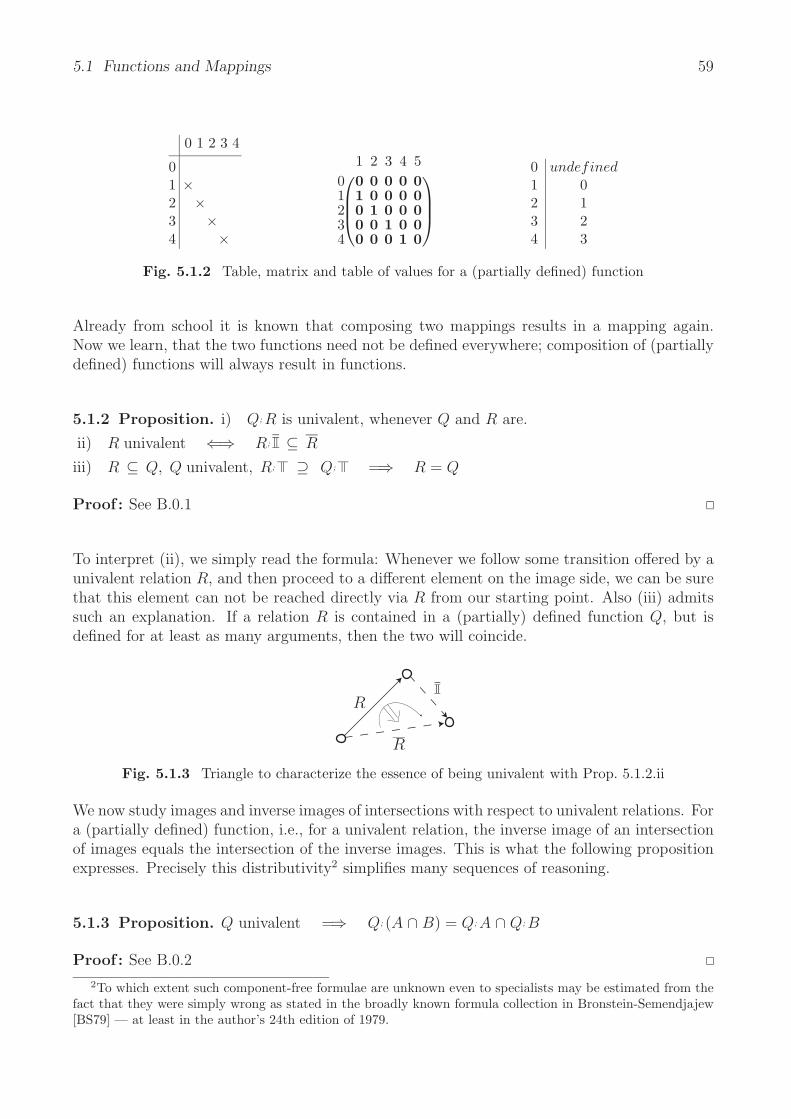
5.1 Functions and Mappings 59
0 1 2 3 4
01 ×2 ×3 ×4 ×
01234
1 2 3 4 5⎛⎜⎜⎝
0 0 0 0 01 0 0 0 00 1 0 0 00 0 1 0 00 0 0 1 0
⎞⎟⎟⎠
0 undefined1 02 13 24 3
Fig. 5.1.2 Table, matrix and table of values for a (partially defined) function
Already from school it is known that composing two mappings results in a mapping again.Now we learn, that the two functions need not be defined everywhere; composition of (partiallydefined) functions will always result in functions.
5.1.2 Proposition. i) Q; R is univalent, whenever Q and R are.
ii) R univalent ⇐⇒ R; ⊆ R
iii) R ⊆ Q, Q univalent, R; ⊇ Q; =⇒ R = Q
Proof : See B.0.1
To interpret (ii), we simply read the formula: Whenever we follow some transition offered by aunivalent relation R, and then proceed to a different element on the image side, we can be surethat this element can not be reached directly via R from our starting point. Also (iii) admitssuch an explanation. If a relation R is contained in a (partially) defined function Q, but isdefined for at least as many arguments, then the two will coincide.
R
R
Fig. 5.1.3 Triangle to characterize the essence of being univalent with Prop. 5.1.2.ii
We now study images and inverse images of intersections with respect to univalent relations. Fora (partially defined) function, i.e., for a univalent relation, the inverse image of an intersectionof images equals the intersection of the inverse images. This is what the following propositionexpresses. Precisely this distributivity2 simplifies many sequences of reasoning.
5.1.3 Proposition. Q univalent =⇒ Q; (A ∩ B) = Q; A ∩ Q; B
Proof : See B.0.2
2To which extent such component-free formulae are unknown even to specialists may be estimated from thefact that they were simply wrong as stated in the broadly known formula collection in Bronstein-Semendjajew[BS79] — at least in the author’s 24th edition of 1979.

60 Chapter 5 Order and Function: The Standard View
A set of persons among which women may have given birth to other persons will give intuition.Should it be the case that every woman in the group considered has had only one child, thefollowing is clear:
“women with a blonde son” = “women with a son” ∩ “women with a blonde child”
In case there exist women with more than one child, it is possible that ⊆ but =/ holds instead.Indeed, as there may exist a woman with a dark-haired son and in addition a blonde daughter.
We now give this example a slightly different flavour and consider a set of persons among whichmay be pregnant women. The set
“Gives birth to a person that is at the same time a son and a daughter”
will be empty — hermaphrodites assumed to be excluded. In contrast, the set of womenobtained by intersection
“Gives birth to a son” ∩ “Gives birth to a daughter”
need not be empty in case of certain twin pregnancies; i.e., if Q is not univalent.
Prop. 5.1.3 was about inverse images of an intersection. Images of an intersection are a bitmore difficult to handle. Only when one of the intersecting constituents is “cylindric over itsimage”, we find a nice formula to relate both sides. Then the image of the intersection equalsthe image of the other constituent intersected with the basis of the cylinder.
Q
AA;QT
B B;Q
B =
Ace
Kin
gQ
ueen
Jack
Ten
WinDrawLoss
(1 0 1 0 01 1 1 1 01 0 0 1 0
) Q =
♠ ♥ ♦ ♣Ace
KingQueen
JackTen
⎛⎜⎜⎝
0 0 0 00 1 0 01 0 0 00 0 1 00 0 0 0
⎞⎟⎟⎠ A =
♠ ♥ ♦ ♣Win
DrawLoss
(0 0 1 10 1 0 10 0 1 1
)
A; QT =
Ace
Kin
gQ
ueen
Jack
Ten
WinDrawLoss
(0 0 0 1 00 1 0 0 00 0 0 1 0
) B ; Q =
♠ ♥ ♦ ♣Win
DrawLoss
(1 0 0 01 1 1 00 0 1 0
)
(A; QT ∩ B); Q =
♠ ♥ ♦ ♣Win
DrawLoss
(0 0 0 00 1 0 00 0 1 0
)= A ∩ B ; Q
Fig. 5.1.4 Image of a “cylindric” intersection
5.1.4 Proposition. Q univalent =⇒ (A; QT ∩ B); Q = A ∩ B ; Q

5.1 Functions and Mappings 61
Proof : See B.0.3
5.1.5 Example. We give an easier to grasp example for the idea behind Prop. 5.1.4, withA, B assumed to resemble sets, however, in different representations. Let Q denote the relationassigning to persons their nationalities — assuming that everybody has at most one. Thenassume A as a column-constant relation derived from the subset of European nations and Bas a diagonal-shaped relation derived from the subset of women among the persons considered.So A ; QT describes persons with European nationality and B ; Q are the nations assigned tothe women in the set of persons considered. The result will now give the same relation for thefollowing two operations:
• “Determine European persons that are female and relate them to their nationalities”
• “Determine the nationalities for women and extract those that are European”
Soph
iaLor
enO
mar
Shar
ifG
race
Kel
lyLiv
Ullm
ann
Cur
dJu
rgen
sC
ath.
Den
euve
No-
Nat
ion-
Lad
yH
ildeg
ard
Kne
fA
lain
Del
on
Sophia LorenOmar SharifGrace KellyLiv Ullmann
Curd JurgensCath. Deneuve
No-Nation-LadyHildegard Knef
Alain Delon
⎛⎜⎜⎜⎜⎜⎜⎜⎜⎜⎝
1 0 0 0 0 0 0 0 00 0 0 0 0 0 0 0 00 0 1 0 0 0 0 0 00 0 0 1 0 0 0 0 00 0 0 0 0 0 0 0 00 0 0 0 0 1 0 0 00 0 0 0 0 0 0 0 00 0 0 0 0 0 0 1 00 0 0 0 0 0 0 0 0
⎞⎟⎟⎟⎟⎟⎟⎟⎟⎟⎠
Am
eric
anFr
ench
Ger
man
Bri
tish
Span
ish
Egy
ptia
nSw
edis
hIt
alia
n
⎛⎜⎜⎜⎜⎜⎜⎜⎜⎜⎝
0 0 0 0 0 0 0 10 0 0 0 0 1 0 01 0 0 0 0 0 0 00 0 0 0 0 0 1 00 0 1 0 0 0 0 00 1 0 0 0 0 0 00 0 0 0 0 0 0 00 0 1 0 0 0 0 00 1 0 0 0 0 0 0
⎞⎟⎟⎟⎟⎟⎟⎟⎟⎟⎠
Am
eric
anFr
ench
Ger
man
Bri
tish
Span
ish
Egy
ptia
nSw
edis
hIt
alia
n⎛⎜⎜⎜⎜⎜⎜⎜⎜⎜⎝
0 1 1 1 1 0 1 10 1 1 1 1 0 1 10 1 1 1 1 0 1 10 1 1 1 1 0 1 10 1 1 1 1 0 1 10 1 1 1 1 0 1 10 1 1 1 1 0 1 10 1 1 1 1 0 1 10 1 1 1 1 0 1 1
⎞⎟⎟⎟⎟⎟⎟⎟⎟⎟⎠
Am
eric
anFr
ench
Ger
man
Bri
tish
Span
ish
Egy
ptia
nSw
edis
hIt
alia
n
⎛⎜⎜⎜⎜⎜⎜⎜⎜⎜⎝
0 0 0 0 0 0 0 10 0 0 0 0 0 0 00 0 0 0 0 0 0 00 0 0 0 0 0 1 00 0 0 0 0 0 0 00 1 0 0 0 0 0 00 0 0 0 0 0 0 00 0 1 0 0 0 0 00 0 0 0 0 0 0 0
⎞⎟⎟⎟⎟⎟⎟⎟⎟⎟⎠
B Q A (A; QT ∩ B); Q = A ∩ B ; Q
Fig. 5.1.5 Prop. 5.1.4 illustrated with nationalities of European women
Theoretically assuming Catherine Deneuve to have French and also US citizenship, thus, makingQ a non-univalent relation, the first set would be bigger than the second.
It is obviously difficult to make the intention of Prop. 5.1.4 clear in spoken language. In asense, the algebraic form is the only way to make such things precise — with the additionaladvantage that it then may be manipulated in algebraic form.
Now a univalent relation is studied in combination with negation. If an element of the domainhas no image, the row of the matrix representation is empty. When complementing, this wouldresult in a row full of 1 ’s. Already now, we expect this rule to simplify later when restrictingto totally defined functions, i.e., mappings; see Prop. 5.2.6.
5.1.6 Proposition. Q univalent =⇒ Q; A = Q; ∩ Q; A
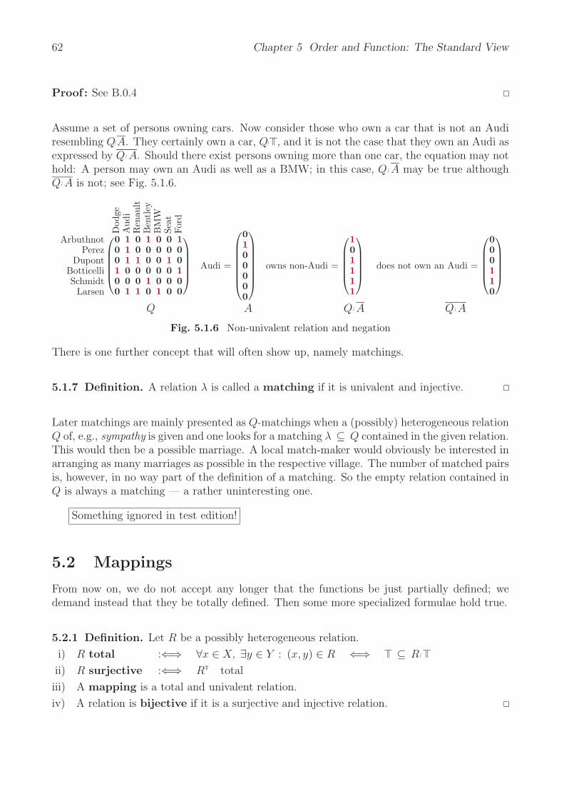
62 Chapter 5 Order and Function: The Standard View
Proof : See B.0.4
Assume a set of persons owning cars. Now consider those who own a car that is not an Audiresembling Q;A. They certainly own a car, Q; , and it is not the case that they own an Audi asexpressed by Q; A. Should there exist persons owning more than one car, the equation may nothold: A person may own an Audi as well as a BMW; in this case, Q; A may be true althoughQ; A is not; see Fig. 5.1.6.
Dod
geA
udi
Ren
ault
Ben
tley
BM
WSe
atFo
rd
ArbuthnotPerez
DupontBotticelliSchmidt
Larsen
⎛⎜⎜⎜⎜⎝
0 1 0 1 0 0 10 1 0 0 0 0 00 1 1 0 0 1 01 0 0 0 0 0 10 0 0 1 0 0 00 1 1 0 1 0 0
⎞⎟⎟⎟⎟⎠ Audi =
⎛⎜⎜⎜⎜⎜⎜⎝
0100000
⎞⎟⎟⎟⎟⎟⎟⎠
owns non-Audi =
⎛⎜⎜⎜⎜⎝
101111
⎞⎟⎟⎟⎟⎠ does not own an Audi =
⎛⎜⎜⎜⎜⎝
000110
⎞⎟⎟⎟⎟⎠
Q A Q; A Q; A
Fig. 5.1.6 Non-univalent relation and negation
There is one further concept that will often show up, namely matchings.
5.1.7 Definition. A relation λ is called a matching if it is univalent and injective.
Later matchings are mainly presented as Q-matchings when a (possibly) heterogeneous relationQ of, e.g., sympathy is given and one looks for a matching λ ⊆ Q contained in the given relation.This would then be a possible marriage. A local match-maker would obviously be interested inarranging as many marriages as possible in the respective village. The number of matched pairsis, however, in no way part of the definition of a matching. So the empty relation contained inQ is always a matching — a rather uninteresting one.
Something ignored in test edition!
5.2 Mappings
From now on, we do not accept any longer that the functions be just partially defined; wedemand instead that they be totally defined. Then some more specialized formulae hold true.
5.2.1 Definition. Let R be a possibly heterogeneous relation.
i) R total :⇐⇒ ∀x ∈ X, ∃y ∈ Y : (x, y) ∈ R ⇐⇒ ⊆ R;
ii) R surjective :⇐⇒ RT total
iii) A mapping is a total and univalent relation.
iv) A relation is bijective if it is a surjective and injective relation.
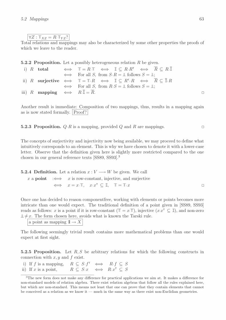
5.2 Mappings 63
∀Z : XZ = R; Y Z?Total relations and mappings may also be characterized by some other properties the proofs ofwhich we leave to the reader.
5.2.2 Proposition. Let a possibly heterogeneous relation R be given.
i) R total ⇐⇒ = R; ⇐⇒ ⊆ R; RT ⇐⇒ R ⊆ R;
⇐⇒ For all S, from S ; R = follows S = ;
ii) R surjective ⇐⇒ = ; R ⇐⇒ ⊆ RT; R ⇐⇒ R ⊆ ; R⇐⇒ For all S, from R; S = follows S = ;
iii) R mapping ⇐⇒ R; = R.
Another result is immediate: Composition of two mappings, thus, results in a mapping againas is now stated formally. Proof?
5.2.3 Proposition. Q; R is a mapping, provided Q and R are mappings.
The concepts of surjectivity and injectivity now being available, we may proceed to define whatintuitively corresponds to an element. This is why we have chosen to denote it with a lower-caseletter. Observe that the definition given here is slightly more restricted compared to the onechosen in our general reference texts [SS89, SS93].3
5.2.4 Definition. Let a relation x : V −→ W be given. We call
x a point :⇐⇒ x is row-constant, injective, and surjective
⇐⇒ x = x; , x; xT ⊆ , = ; x
Once one has decided to reason componentfree, working with elements or points becomes moreintricate than one would expect. The traditional definition of a point given in [SS89, SS93]reads as follows: x is a point if it is row-constant ( = x; ), injective (x;xT ⊆ ), and non-zero
=/ x. The form chosen here, avoids what is known the Tarski rule.
a point as mapping 1l → X
The following seemingly trivial result contains more mathematical problems than one wouldexpect at first sight.
5.2.5 Proposition. Let R, S be arbitrary relations for which the following constructs inconnection with x, y and f exist.
i) If f is a mapping, R ⊆ S ; fT ⇐⇒ R; f ⊆ Sii) If x is a point, R ⊆ S ; x ⇐⇒ R; xT ⊆ S
3The new form does not make any difference for practical applications we aim at. It makes a difference fornon-standard models of relation algebra. There exist relation algebras that follow all the rules explained here,but which are non-standard. This means not least that one can prove that they contain elements that cannotbe conceived as a relation as we know it — much in the same way as there exist non-Euclidian geometries.

64 Chapter 5 Order and Function: The Standard View
iii) If x, y are points, y ⊆ S ; x ⇐⇒ x ⊆ ST; y
Proof : See B.0.6
R =
Dod
geA
udi
Ren
ault
Ben
tley
BM
WFia
tFo
rdArbuthnot
PerezDupont
BotticelliSchmidt
Larsen
⎛⎜⎜⎜⎜⎝
0 1 0 1 0 0 10 1 0 0 0 0 00 1 1 0 0 1 01 0 0 0 0 0 10 0 0 1 0 0 00 1 1 0 1 0 0
⎞⎟⎟⎟⎟⎠ f =
Am
eric
anFr
ench
Ger
man
Bri
tish
Span
ish
DodgeAudi
RenaultBentley
BMWFiatFord
⎛⎜⎜⎜⎜⎜⎜⎝
1 0 0 0 00 0 1 0 00 1 0 0 00 0 0 1 00 0 1 0 00 0 0 0 11 0 0 0 0
⎞⎟⎟⎟⎟⎟⎟⎠
S =
Am
eric
anFr
ench
Ger
man
Bri
tish
Span
ish
ArbuthnotPerez
DupontBotticelliSchmidt
Larsen
⎛⎜⎜⎜⎜⎝
1 0 1 1 00 0 1 0 10 1 1 0 11 0 0 0 10 0 1 1 00 1 1 0 0
⎞⎟⎟⎟⎟⎠
R; f =
Am
eric
anFr
ench
Ger
man
Bri
tish
Span
ish
ArbuthnotPerez
DupontBotticelliSchmidt
Larsen
⎛⎜⎜⎜⎜⎝
1 0 1 1 00 0 1 0 00 1 1 0 11 0 0 0 00 0 0 1 00 1 1 0 0
⎞⎟⎟⎟⎟⎠ S ; fT =
Dod
geA
udi
Ren
ault
Ben
tley
BM
WFia
tFo
rd
ArbuthnotPerez
DupontBotticelliSchmidt
Larsen
⎛⎜⎜⎜⎜⎝
1 1 0 1 1 0 10 1 0 0 1 1 00 1 1 0 1 1 01 0 0 0 0 1 10 1 0 1 1 0 00 1 1 0 1 0 0
⎞⎟⎟⎟⎟⎠ = S ; fT
Fig. 5.2.1 Rolling a mapping to the other side of a containment
An interpretation of this result with Fig. 5.2.1 runs as follows. The relations given are R, f, Sindicating the cars owned, the country where the respective car is produced, and the preferenceof the owner as to the country his car should come from. We see that everybody has boughtcars following his preference, R ; f ⊆ S. Should an owner intend to buy yet another car, hemight wish to consult S ; fT which indicates the car types restricted by his preferences.
Anticipating the following proposition, we mention in passing that S ; fT = S ; fT. The slightlymore complicated construct would allow to handle also the case of cars not stemming from justone country, i.e., f not necessarily a mapping.
We add one more fact on mappings specializing Prop. 5.1.6: For a mapping, the inverse imageof the complement is equal to the complement of the inverse image. In more primitive words: Amapping may slip under a negation when multiplied from the left — and a transposed mappingwhen multiplied from the right.
5.2.6 Proposition. Let A, R be possibly heterogeneous relations. Proof?
i) f mapping =⇒ f ; A = f ; A
ii) x is a point =⇒ R; x = R; x

5.3 Order and Strictorder 65
A
A
x
Q
Fig. 5.2.2 Inverse image of the complement is equal to the complement of the inverse image
With these concepts we will now handle a classic riddle (see [Cop48], e.g.). One man looks ata second man and says:
“Brothers and sisters I have none, but that man’s father is my father’s son”
We need, of course, relations such as child-of, son-of, father-of that follow the intended scheme,meaning that they are irreflexive, e.g. They are assumed to hold on a set of individuals, fromwhich a, b are two different elements. Brothers or sisters of a person we get with f ; fT. As ahas neither brothers nor sisters we have f ; fT ∩ a; ⊆ , meaning that there is just one whenlooking for those with the same father as a. The question is as to the relationship between aand b specified as f ; fT; fT ∩ a; .
f ; fT; fT ∩ a; ⊆ (f ; fT ∩ a; ; f); (fT ∩ f ; fT; a; ) ⊆ ; fT = fT
Applying the Dedekind rule, we get that the other person is the son of a.
Something ignored in test edition!
5.3 Order and Strictorder
Until the 1930s, orderings were mostly studied along the linearly ordered real axis IR, but soondiverse other concepts such as weakorder, semiorder, interval order, etc. were also handled.Here the basic properties of orderings and equivalences are recalled in predicate form as well asin matrix form. The transition between the two levels is more or less immediate. We have alsoincluded several variants of the algebraic forms of the definitions, which are so obviously equiv-alent that they do not justify mentioning them in a separate proposition. Later, in Chapt. 10,also unifying but more advanced concepts will be presented.
Reflexivity
Identity on a set is a homogeneous relation; domain and codomain are of the same type. Forsuch homogeneous relations some properties in connection with the identity are standard.
5.3.1 Definition (Reflexivity properties). Given a homogeneous relation R : V −→ V , we call
R reflexive :⇐⇒ ∀x ∈ V : (x, x) ∈ R :⇐⇒ ⊆ RR irreflexive :⇐⇒ ∀x ∈ V : (x, x) ∈/ R :⇐⇒ R ⊆

66 Chapter 5 Order and Function: The Standard View
It should be immediately clear in which way the identity or diagonal relation models that all thepairs (x, x) are in relation R. A relation on the one element set is either reflexive or irreflexive,and there is no third possibility as in the following example.
⎛⎜⎝
1 1 1 10 1 0 01 1 1 10 1 0 1
⎞⎟⎠
⎛⎜⎝
1 0 0 10 0 0 01 0 0 10 0 0 1
⎞⎟⎠
⎛⎜⎝
0 0 0 11 0 1 11 1 0 10 0 0 0
⎞⎟⎠
Fig. 5.3.1 Relations that are reflexive, neither/nor, and irreflexive
Let R be an arbitrary relation. Then R/R; is trivially reflexive. As R/R; = R; RT, this meansafter negation that R ; RT ⊆ ; this, however, follows directly from Schroder’s equivalencesas ; R ⊆ R. We have (r1, r2) ∈ R/R precisely when row r1 is equal to or contains row r2.Similarly, (c1, c2) ∈ R\R if and only if column c1 is equal to or contained in column c2. Theresidua thus clearly contain the full diagonal.
1 2 3 4 5
12345
⎛⎜⎜⎝
1 1 1 1 10 1 0 0 01 1 1 1 10 1 0 1 10 1 0 1 1
⎞⎟⎟⎠
1 2 3 4 512345
⎛⎜⎜⎝
1 0 0 1 00 0 0 0 01 0 0 1 00 0 0 1 00 0 0 1 0
⎞⎟⎟⎠
1 2 3 4 5
12345
⎛⎜⎜⎝
1 0 0 1 01 1 1 1 11 1 1 1 10 0 0 1 01 1 1 1 1
⎞⎟⎟⎠
Fig. 5.3.2 Example relations R/R, R, R\R
One will also find out that (R/R);R ⊆ R and R;(R\R) ⊆ R. The relation R/R is the greatestamong the relations X with X ; R ⊆ R. Also R\R is the greatest among the relations Y withR ; Y ⊆ R. So indeed, some sort of calculations with fractions is possible when interpreting/ and \ as division symbols and compare with 2
3. Relations do not multiply commutatively,
so that we have to indicate on which side division has taken place. One will find similarity ofnotation with 2
3× 3 = 2 and 3 × 2
3= 2.
It is worth noting that by simultaneous permutation of rows and columns a block-staircasemay be obtained for the left and the right residuum. The original R underwent differentpermutations for rows and columns. We will later find out that this is not just incidental.
1 3 4 5 2
13452
⎛⎜⎜⎝
1 1 1 1 11 1 1 1 10 0 1 1 10 0 1 1 10 0 0 0 1
⎞⎟⎟⎠
2 3 5 1 4
13452
⎛⎜⎜⎝
0 0 0 1 10 0 0 1 10 0 0 0 10 0 0 0 10 0 0 0 0
⎞⎟⎟⎠
2 3 5 1 4
23514
⎛⎜⎜⎝
1 1 1 1 11 1 1 1 11 1 1 1 10 0 0 1 10 0 0 0 1
⎞⎟⎟⎠
Fig. 5.3.3 Permuted forms of R/R, R, R\R
In the example, R should not be Ferrers
The following property asks whether a relation together with its converse fills the whole matrix.Also this property requires homogeneous relations as we demand that R and RT be of the sametype, or “may be united”.
5.3.2 Definition (Connexity properties). Let a homogeneous relation R be given.
R semi-connex :⇐⇒ ⊆ R ∪ RT :⇐⇒ ∀x, y : x =/ y → [(x, y) ∈ R ∨ (y, x) ∈ R]

5.3 Order and Strictorder 67
R connex :⇐⇒ ⊆ R ∪ RT :⇐⇒ ∀x, y : (x, y)∈/ R → (y, x) ∈ R
In the literature, often semi-connex will be found denoted as complete and connex as stronglycomplete.
The formal definition does not say anything about the diagonal of a semi-connex relation; nordoes it require just one or both of (x, y) and (y, x) to be contained in R.
⎛⎜⎝
0 0 0 11 1 1 11 0 0 10 1 0 0
⎞⎟⎠
⎛⎜⎝
1 1 1 10 1 0 01 1 1 10 1 0 1
⎞⎟⎠
Fig. 5.3.4 Semi-connex and connex relation
Symmetry
Relations are also traditionally classified according to their symmetry properties. Again, wehave from the definition that the relation and its converse be of the same type, which makesthem homogeneous relations.
5.3.3 Definition (Symmetry properties). Given again a homogeneous relation R : V −→ V ,we call
R symmetric :⇐⇒ ∀x, y : (x, y) ∈ R → (y, x) ∈ R⇐⇒ RT ⊆ R ⇐⇒ RT = R
R asymmetric :⇐⇒ ∀x, y : (x, y) ∈ R → (y, x) /∈ R⇐⇒ R ∩ RT ⊆ ⇐⇒ RT ⊆ R
R antisymmetric :⇐⇒ ∀x, y : x =/ y → (x, y) /∈ R ∨ (y, x) /∈ R ⇐⇒ R ∩ RT ⊆ ⇐⇒ RT ⊆ R ∪
A first minor consideration relates reflexivity with symmetry as follows: An asymmetric relationR is necessarily irreflexive. This results easily from the predicate logic version of the definitionof asymmetry when specializing the two variables to x = y. Then ∀x : (x, x) ∈ R → (x, x)∈/ Rwhich implies that (x, x) ∈ R cannot be satisfied for any x.
⎛⎜⎝
0 1 1 00 0 0 00 1 0 10 1 0 0
⎞⎟⎠
⎛⎜⎝
0 0 0 11 1 1 00 0 0 00 1 0 1
⎞⎟⎠
Fig. 5.3.5 An asymmetric and an antisymmetric relation
Symmetry concepts enable us to define that
R is a tournament :⇐⇒ R is asymmetric and complete
It is indeed typical for sports tournaments that a team cannot play against itself. Just oneround is assumed to take place and no draw result is assumed to be possible. Then a tournamentdescribes a possible outcome.

68 Chapter 5 Order and Function: The Standard View
Transitivity
Transitivity is used in many application areas; it is central for defining an ordering and anequivalence. We recall the definition more formally and give it its algebraic form.
5.3.4 Definition. Let R be a homogeneous relation. We call
R transitive :⇐⇒ ∀x, y, z ∈ V :[(x, y) ∈ R ∧ (y, z) ∈ R
]→ (x, z) ∈ R
⇐⇒ R ; R ⊆ R
Intuitively, a relation R is transitive, if whenever x is related to y and y is related to z, thenalso x will be related to z.
R
RR
Fig. 5.3.6 Triangular situation for transitivity
We observe the triangle structure and show how these two rather different looking variants ofthe definition are formally related. On the right we roughly indicate the quite well-known ruleswe have applied for the respective transition.
∀x, y, z ∈ V :[(x, y) ∈ R ∧ (y, z) ∈ R
]→ (x, z) ∈ R
a → b = ¬a ∨ b∀x, z ∈ V : ∀y ∈ V : (x, y) ∈ R ∧ (y, z) ∈ R ∨ (x, z) ∈ R
∀v : ¬p(v) = ¬[∃v : p(v)
]∀x, z ∈ V : ¬
∃y ∈ V : (x, y) ∈ R ∧ (y, z) ∈ R ∧ (x, z) ∈ R
(a ∧ c) ∨ (b ∧ c) = (a ∨ b) ∧ c
∀x, z ∈ V :¬[
∃y ∈ V : (x, y) ∈ R ∧ (y, z) ∈ R]∧ (x, z) ∈ R
definition of composition
∀x, z ∈ V : ¬[
(x, z) ∈ R; R]∧ (x, z) ∈ R
De Morgan
∀x, z ∈ V : (x, z) ∈ R; R ∨ (x, z) ∈ R¬a ∨ b = a → b
∀x, z ∈ V : (x, z) ∈ R; R → (x, z) ∈ Rcomponentfree formulation
R; R ⊆ R
We remember that an asymmetric relation turned out to be irreflexive. Now we obtain as afirst easy exercise a result in opposite direction:
5.3.5 Proposition. A transitive relation is irreflexive precisely when it is asymmetric.
Proof : Writing down transitivity and irreflexivity, we obtain R;R ⊆ R ⊆ . Now the Schroderequivalence is helpful as it allows to get directly RT; ⊆ R, the condition of asymmetry.

5.3 Order and Strictorder 69
For the other direction, we do not need transitivity.
= ( ∩ R) ∪ ( ∩ R) ⊆ ( ∩ R) ∪ R ⊆ R.
since ∩ R = ∩ RT ⊆ RT ⊆ R.
Another application of the Schroder equivalence shows a property of an arbitrary relation R:Its residuals R/R as well as R\R are trivially transitive. This may in the first case, e.g., beshown with
(R/R); (R/R) ⊆ (R/R) ⇐⇒by definition
R; RT; R; RT ⊆ R; RT ⇐⇒Schroder equivalence
R; RT; R; RT ⊆ R; RT ⇐=
composition is monotonic
R; RT; R ⊆ R ⇐⇒
Schroder equivalenceR; R
T ⊆ R; RT
which is obviously satisfied
As (r1, r2) ∈ R/R indicates that row r1 is equal to or contains row r2, transitivity is notsurprising at all. What needs to be stressed is that such properties may be dealt with inalgebraic precision.
Orderings
Using these elementary constituents, we now build well-known composite definitions. We havechosen to list several equivalent versions leaving the equivalence proofs to the reader.
5.3.6 Definition. Let homogeneous relations E, C : V −→ V be given. We call
E order :⇐⇒ E transitive, antisymmetric, reflexive
⇐⇒ E2 ⊆ E, E ∩ ET ⊆ , ⊆ E
C strictorder :⇐⇒ C transitive and asymmetric
⇐⇒ C2 ⊆ C, C ∩ CT ⊆⇐⇒ C2 ⊆ C, CT ⊆ C
⇐⇒ C transitive and irreflexive
⇐⇒ C2 ⊆ C, C ⊆
As an example we show the divisibility ordering on the set 1, . . . , 12. From the picture wemay in an obvious way deduce the reflexive order as well as the strictorder4.
with row and column numbers!
4There is one point to mention when we talk on orderings. People often speak of a “strict ordering”. This isnot what they intend it to mean, as it is not an ordering with the added property to be strict or asymmetric. Bydefinition, this cannot be. So we have chosen to use a german style compound word strictorder. A strictorderis not an order! (Later, in the same way, a preorder need not be an order.)

70 Chapter 5 Order and Function: The Standard View
2
1
3
4
5
6
7
8
910
11
12⎛⎜⎜⎜⎜⎜⎜⎜⎜⎜⎜⎜⎜⎜⎜⎜⎜⎜⎝
1 1 1 1 1 1 1 1 1 1 1 10 1 0 1 0 1 0 1 0 1 0 10 0 1 0 0 1 0 0 1 0 0 10 0 0 1 0 0 0 1 0 0 0 10 0 0 0 1 0 0 0 0 1 0 00 0 0 0 0 1 0 0 0 0 0 10 0 0 0 0 0 1 0 0 0 0 00 0 0 0 0 0 0 1 0 0 0 00 0 0 0 0 0 0 0 1 0 0 00 0 0 0 0 0 0 0 0 1 0 00 0 0 0 0 0 0 0 0 0 1 00 0 0 0 0 0 0 0 0 0 0 1
⎞⎟⎟⎟⎟⎟⎟⎟⎟⎟⎟⎟⎟⎟⎟⎟⎟⎟⎠
⎛⎜⎜⎜⎜⎜⎜⎜⎜⎜⎜⎜⎜⎜⎜⎜⎜⎜⎝
0 1 1 1 1 1 1 1 1 1 1 10 0 0 1 0 1 0 1 0 1 0 10 0 0 0 0 1 0 0 1 0 0 10 0 0 0 0 0 0 1 0 0 0 10 0 0 0 0 0 0 0 0 1 0 00 0 0 0 0 0 0 0 0 0 0 10 0 0 0 0 0 0 0 0 0 0 00 0 0 0 0 0 0 0 0 0 0 00 0 0 0 0 0 0 0 0 0 0 00 0 0 0 0 0 0 0 0 0 0 00 0 0 0 0 0 0 0 0 0 0 00 0 0 0 0 0 0 0 0 0 0 0
⎞⎟⎟⎟⎟⎟⎟⎟⎟⎟⎟⎟⎟⎟⎟⎟⎟⎟⎠
Fig. 5.3.7 Division ordering on numbers 1..12 as Hasse diagram, as reflexive and irreflexive relation
Orders and strictorders always come closely side aside as “≤” and “<” do; however, theiralgebraic properties must not be mixed up. Orders and strictorders do occur so often in variouscontexts that it is helpful to have at least a hint in notation. We have chosen, to use E fororders and C for strictorders as E is closer to “≤ ” and C is closer to “ < ”.
5.3.7 Definition. i) Given an ordering E, we call CE := ∩ E its associated strictorder.
ii) Given a strictorder C, we call EC := ∪ C its associated ordering.
iii) Given an ordering E or a strictorder C, we call H := CE ∩ C2E resp. H := C ∩ C2 the
corresponding Hasse relation, more often called Hasse diagram.
Indeed, it is easily shown that EC is an ordering and CE is a strictorder. Obviously, we have
ECE= E and CEC
= C.
When representing an ordering as a graph, on will obtain something as the left figure ofFig. 5.3.8. It is, however, not a good idea to draw all these many arrows on a blackboardduring teaching a lesson. So one will usually omit arrow heads replacing them with the con-vention that arrows always lead upwards. What one can not reinvent in a unique manner areloops. For an ordering every vertex carries a loop, for a strictorder none. But as these twoalways occur in pairs, this makes not a big problem.
Fig. 5.3.8 Order, strictorder and associated Hasse diagram

5.3 Order and Strictorder 71
There is one further traditional way of reducing effort when representing orderings. It is eco-nomical to represent the ordering by its Hasse diagram. In general, however, the relationshipof an ordering with its Hasse diagram H is less obvious than expected. For the finite case, wewill give a definitive answer once the transitive closure is introduced and prove that C = H+
and E = H∗. In a finite strictorder, one may ask whether there are immediate successors orpredecessors. Figure 5.3.8 shows an ordering, its associated strictordering and its correspondingHasse diagram.5
For certain purposes, one considers the dual of the relation R. Forming the dual of a relationis an involutory operation. It exchanges properties as follows.
5.3.8 Proposition. For the so-called dual Rd := RT
of a relation R the following hold:Rd reflexive ⇐⇒ R irreflexiveRd asymmetric ⇐⇒ R connexRd transitive ⇐⇒ R negatively transitiveRd antisymmetric ⇐⇒ R semi-connexRd symmetric ⇐⇒ R symmetric
The concept of the dual is particularly interesting when the order is a so-called linear one.
Linear Orderings
In earlier times it was not at all clear that orderings need not be linear orderings. But since thedevelopment of lattice theory in the 1930s it became more and more evident that most of ourreasoning with orderings was also possible when they failed to be linear ones. So it is simply amatter of economy to present orders first and then specialize to linear ones6.
5.3.9 Definition. Given again homogeneous relations E, C : V −→ V , we call
E linear order :⇐⇒ E is an ordering which is in addition connex
⇐⇒ E ; E ⊆ E, E ∩ ET ⊆ , = E ∪ ET
C linear strictorder :⇐⇒ C is a strictorder which is in addition semi-connex
⇐⇒ C ; C ⊆ C, C ∩ CT ⊆ , = C ∪ CT
Sometimes a linear order is called a total order or a chain and a linear strictorder is called astrict total order, complete order, or strict complete order.
When nicely arranged, the matrix of a linear order has the upper right triangle and the diagonalfilled with 1 ’s, leaving the lower left triangle full of 0 ’s. It is rather obvious, see Prop. 5.3.10,that the negative of a linear order is a linear strictorder in reverse direction.
5In case immediate successors and predecessors exist, i.e., for discrete orderings in the sense of [BS83], theordering can be generated by its Hasse diagram.
6Today a tendency may be observed that makes the even less restricted preorder the basic structure.

72 Chapter 5 Order and Function: The Standard View
♦ ♥ ♠ ♣♦♥♠♣
⎛⎜⎝
1 1 1 10 1 1 10 0 1 10 0 0 1
⎞⎟⎠
♦ ♥ ♠ ♣♦♥♠♣
⎛⎜⎝
0 1 1 10 0 1 10 0 0 10 0 0 0
⎞⎟⎠
♦ ♥ ♠ ♣♦♥♠♣
⎛⎜⎝
0 1 0 00 0 1 00 0 0 10 0 0 0
⎞⎟⎠
Fig. 5.3.9 Linear order, linear strictorder, and Hasse diagram in case of the Skat suit ranking
We now exhibit characteristic properties of a linear order. The dual of a linear order is itsassociated strictorder, and the dual of a linear strictorder is its associated order.
5.3.10 Proposition. i) A linear order E and its associated strictorder C satisfy ET
= C.
ii) A linear order E satisfies E ; ET; E = C ⊆ E.
iii) A linear strictorder C satisfies C ; C ; CT
= C ; CT; C = C2 ⊆ C.
iv) E is a linear order precisely when Ed is a linear strictorder.
v) C is a linear strictorder precisely when Cd is a linear order.
Proof : See B.0.5
Of course, Cd = CT
= E is an equivalent form of (i). With (ii,iii) we gave (i) a more complicated
form, thus anticipating a property of Ferrers relations, see Sect. 9.7. The equation E ; ET; E =
E ; ET
= ET
holds for arbitrary orderings E.
We now anticipate a result that seems rather obvious, at least for the finite case. Nevertheless,it needs a proof which we can give only later; see Prop. 10.3.15. In Computer Science, one rou-tinely speakes of topological sorting of an ordering. It may colloquially be expressed demandingthat there shall exist a permutation such that the resulting matrix resides in the upper righttriangle, in which case the Szpilrajn extension is completely obvious.
5.3.11 Proposition (Topological sorting). For every order E there exists a linear order E1,the so-called Szpilrajn7 extension, with E ⊆ E1.
The idea of a proof is easy to communicate: Assume E were not yet linear, i.e., E ∪ ET =/ .Then there will exist two incomparable elements x, y with x ; yT ⊆ E ∪ ET. With these, wedefine an additional ordering relation as E1 := E ∪ E;x;yT;E. In the finite case, this argumentmay be iterated, and En will eventually become linear. This is one of the more basic algorithmsa student in Computing Science has to learn: topological sorting.
7Edward Marczewski, ∗ November 15, 1907 in Warsaw, † October 17, 1976 in Wroclaw, a Polish mathemati-cian. He used the surname Szpilrajn, until 1940. He was a member of the Warsaw School of Mathematics. Hislife and work after the Second World War were connected with Wroclaw, where he was among the creators of thePolish scientific centre. Marczewski’s main fields of interest were measure theory, descriptive set theory, generaltopology, probability theory and universal algebra. He also published papers on real and complex analysis,applied mathematics and mathematical logic. (Wikipedia)
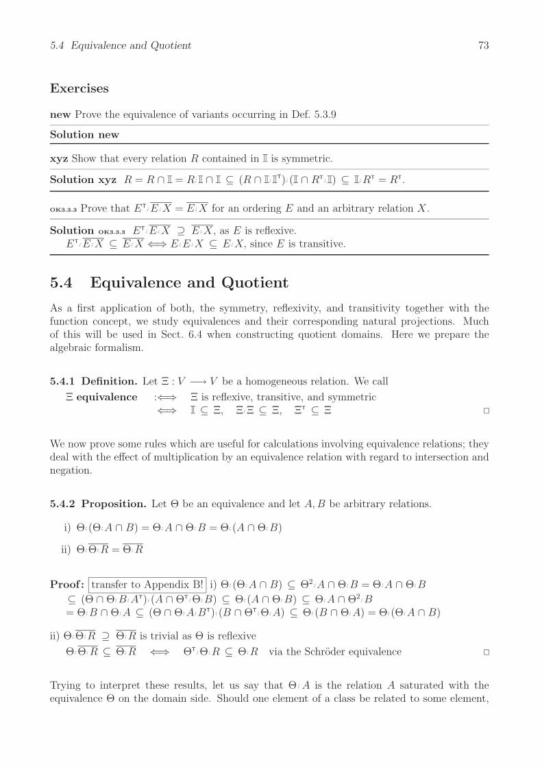
5.4 Equivalence and Quotient 73
Exercises
new Prove the equivalence of variants occurring in Def. 5.3.9
Solution new
xyz Show that every relation R contained in is symmetric.
Solution xyz R = R ∩ = R; ∩ ⊆ (R ∩ ;T); ( ∩ RT; ) ⊆ ; RT = RT.
OK3.3.3 Prove that ET; E ; X = E ; X for an ordering E and an arbitrary relation X.
Solution OK3.3.3 ET; E ; X ⊇ E ; X, as E is reflexive.ET; E ; X ⊆ E ; X ⇐⇒ E ; E ; X ⊆ E ; X, since E is transitive.
5.4 Equivalence and Quotient
As a first application of both, the symmetry, reflexivity, and transitivity together with thefunction concept, we study equivalences and their corresponding natural projections. Muchof this will be used in Sect. 6.4 when constructing quotient domains. Here we prepare thealgebraic formalism.
5.4.1 Definition. Let Ξ : V −→ V be a homogeneous relation. We call
Ξ equivalence :⇐⇒ Ξ is reflexive, transitive, and symmetric⇐⇒ ⊆ Ξ, Ξ; Ξ ⊆ Ξ, ΞT ⊆ Ξ
We now prove some rules which are useful for calculations involving equivalence relations; theydeal with the effect of multiplication by an equivalence relation with regard to intersection andnegation.
5.4.2 Proposition. Let Θ be an equivalence and let A, B be arbitrary relations.
i) Θ; (Θ; A ∩ B) = Θ; A ∩ Θ; B = Θ; (A ∩ Θ; B)
ii) Θ; Θ; R = Θ; R
Proof : transfer to Appendix B! i) Θ; (Θ; A ∩ B) ⊆ Θ2; A ∩ Θ; B = Θ; A ∩ Θ; B
⊆ (Θ ∩ Θ; B ; AT); (A ∩ ΘT; Θ; B) ⊆ Θ; (A ∩ Θ; B) ⊆ Θ; A ∩ Θ2; B= Θ; B ∩ Θ; A ⊆ (Θ ∩ Θ; A; BT); (B ∩ ΘT; Θ; A) ⊆ Θ; (B ∩ Θ; A) = Θ; (Θ; A ∩ B)
ii) Θ; Θ; R ⊇ Θ; R is trivial as Θ is reflexive
Θ; Θ; R ⊆ Θ; R ⇐⇒ ΘT; Θ; R ⊆ Θ; R via the Schroder equivalence
Trying to interpret these results, let us say that Θ ; A is the relation A saturated with theequivalence Θ on the domain side. Should one element of a class be related to some element,
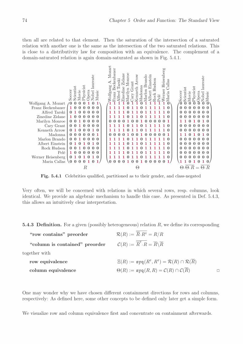
74 Chapter 5 Order and Function: The Standard View
then all are related to that element. Then the saturation of the intersection of a saturatedrelation with another one is the same as the intersection of the two saturated relations. Thisis close to a distributivity law for composition with an equivalence. The complement of adomain-saturated relation is again domain-saturated as shown in Fig. 5.4.1.
Socc
erSc
ient
ist
Mov
ieP
hysi
cist
Ope
raN
obel
laur
eate
Mus
ic
Wolfgang A. MozartFranz Beckenbauer
Alfred TarskiZinedine ZidaneMarilyn Monroe
Cary GrantKenneth Arrow
MadonnaMarlon BrandoAlbert Einstein
Rock HudsonPele
Werner HeisenbergMaria Callas
⎛⎜⎜⎜⎜⎜⎜⎜⎜⎜⎜⎜⎜⎜⎜⎜⎜⎜⎜⎜⎝
0 0 0 0 1 0 11 0 0 0 0 0 00 1 0 0 0 0 01 0 0 0 0 0 00 0 1 0 0 0 00 0 1 0 0 0 00 1 0 0 0 1 00 0 0 0 0 0 10 0 1 0 0 0 00 1 0 1 0 1 00 0 1 0 0 0 01 0 0 0 0 0 00 1 0 1 0 1 00 0 0 0 1 0 1
⎞⎟⎟⎟⎟⎟⎟⎟⎟⎟⎟⎟⎟⎟⎟⎟⎟⎟⎟⎟⎠
Wol
fgan
gA
.M
ozar
tFr
anz
Bec
kenb
auer
Alfr
edTar
ski
Zin
edin
eZid
ane
Mar
ilyn
Mon
roe
Car
yG
rant
Ken
neth
Arr
owM
adon
naM
arlo
nB
rand
oA
lber
tE
inst
ein
Roc
kH
udso
nPel
eW
erne
rH
eise
nber
gM
aria
Cal
las
⎛⎜⎜⎜⎜⎜⎜⎜⎜⎜⎜⎜⎜⎜⎜⎜⎜⎜⎜⎜⎝
1 1 1 1 0 1 1 0 1 1 1 1 1 01 1 1 1 0 1 1 0 1 1 1 1 1 01 1 1 1 0 1 1 0 1 1 1 1 1 01 1 1 1 0 1 1 0 1 1 1 1 1 00 0 0 0 1 0 0 1 0 0 0 0 0 11 1 1 1 0 1 1 0 1 1 1 1 1 01 1 1 1 0 1 1 0 1 1 1 1 1 00 0 0 0 1 0 0 1 0 0 0 0 0 11 1 1 1 0 1 1 0 1 1 1 1 1 01 1 1 1 0 1 1 0 1 1 1 1 1 01 1 1 1 0 1 1 0 1 1 1 1 1 01 1 1 1 0 1 1 0 1 1 1 1 1 01 1 1 1 0 1 1 0 1 1 1 1 1 00 0 0 0 1 0 0 1 0 0 0 0 0 1
⎞⎟⎟⎟⎟⎟⎟⎟⎟⎟⎟⎟⎟⎟⎟⎟⎟⎟⎟⎟⎠
Socc
erSc
ient
ist
Mov
ieP
hysi
cist
Ope
raN
obel
laur
eate
Mus
ic
⎛⎜⎜⎜⎜⎜⎜⎜⎜⎜⎜⎜⎜⎜⎜⎜⎜⎜⎜⎜⎝
0 0 0 0 0 0 00 0 0 0 0 0 00 0 0 0 0 0 00 0 0 0 0 0 01 1 0 1 0 1 00 0 0 0 0 0 00 0 0 0 0 0 01 1 0 1 0 1 00 0 0 0 0 0 00 0 0 0 0 0 00 0 0 0 0 0 00 0 0 0 0 0 00 0 0 0 0 0 01 1 0 1 0 1 0
⎞⎟⎟⎟⎟⎟⎟⎟⎟⎟⎟⎟⎟⎟⎟⎟⎟⎟⎟⎟⎠
R Θ Θ; Θ; R = Θ; R
Fig. 5.4.1 Celebrities qualified, partitioned as to their gender, and class-negated
Very often, we will be concerned with relations in which several rows, resp. columns, lookidentical. We provide an algebraic mechanism to handle this case. As presented in Def. 5.4.3,this allows an intuitively clear interpretation.
5.4.3 Definition. For a given (possibly heterogeneous) relation R, we define its corresponding
“row contains” preorder R(R) := R; RT = R/R
“column is contained” preorder C(R) := RT; R = R\R
together with
row equivalence Ξ(R) := syq(RT, RT) = R(R) ∩ R(R)
column equivalence Θ(R) := syq(R, R) = C(R) ∩ C(R)
One may wonder why we have chosen different containment directions for rows and columns,respectively: As defined here, some other concepts to be defined only later get a simple form.
We visualize row and column equivalence first and concentrate on containment afterwards.

5.4 Equivalence and Quotient 75
Mon
day
Tue
sday
Wed
nesd
ayT
hurs
day
Frid
aySa
turd
aySu
nday
MondayTuesday
WednesdayThursday
FridaySaturday
Sunday
⎛⎜⎜⎜⎜⎜⎜⎝
1 0 1 0 0 0 00 1 0 1 1 0 01 0 1 0 0 0 00 1 0 1 1 0 00 1 0 1 1 0 00 0 0 0 0 1 10 0 0 0 0 1 1
⎞⎟⎟⎟⎟⎟⎟⎠
A K Q J 10 9 8 7 6 5 4 3 2⎛⎜⎜⎜⎜⎜⎜⎝
0 1 0 0 1 1 0 0 1 1 1 0 01 0 1 0 1 1 0 0 0 0 0 1 10 1 0 0 1 1 0 0 1 1 1 0 01 0 1 0 1 1 0 0 0 0 0 1 11 0 1 0 1 1 0 0 0 0 0 1 10 1 0 0 0 0 0 0 1 1 1 0 00 1 0 0 0 0 0 0 1 1 1 0 0
⎞⎟⎟⎟⎟⎟⎟⎠
A K Q J 10 9 8 7 6 5 4 3 2
AKQJ
1098765432
⎛⎜⎜⎜⎜⎜⎜⎜⎜⎜⎜⎜⎜⎜⎜⎜⎜⎜⎝
1 0 1 0 0 0 0 0 0 0 0 1 10 1 0 0 0 0 0 0 1 1 1 0 01 0 1 0 0 0 0 0 0 0 0 1 10 0 0 1 0 0 1 1 0 0 0 0 00 0 0 0 1 1 0 0 0 0 0 0 00 0 0 0 1 1 0 0 0 0 0 0 00 0 0 1 0 0 1 1 0 0 0 0 00 0 0 1 0 0 1 1 0 0 0 0 00 1 0 0 0 0 0 0 1 1 1 0 00 1 0 0 0 0 0 0 1 1 1 0 00 1 0 0 0 0 0 0 1 1 1 0 01 0 1 0 0 0 0 0 0 0 0 1 11 0 1 0 0 0 0 0 0 0 0 1 1
⎞⎟⎟⎟⎟⎟⎟⎟⎟⎟⎟⎟⎟⎟⎟⎟⎟⎟⎠
Ξ(R) R Θ(R)
Fig. 5.4.2 A relation R with its row and column equivalences Ξ(R),Θ(R)
The situation will become more clear when we arrange the matrix of the relation so as to haveequal rows, and columns respectively, side by side as in Fig. 5.4.3.
Mon
day
Wed
nesd
ayTue
sday
Thu
rsda
yFr
iday
Satu
rday
Sund
ay
MondayWednesday
TuesdayThursday
FridaySaturday
Sunday
⎛⎜⎜⎜⎜⎜⎜⎝
1 1 0 0 0 0 01 1 0 0 0 0 00 0 1 1 1 0 00 0 1 1 1 0 00 0 1 1 1 0 00 0 0 0 0 1 10 0 0 0 0 1 1
⎞⎟⎟⎟⎟⎟⎟⎠
A Q 3 2 K 6 5 4 J 8 7 10 9⎛⎜⎜⎜⎜⎜⎜⎝
0 0 0 0 1 1 1 1 0 0 0 1 10 0 0 0 1 1 1 1 0 0 0 1 11 1 1 1 0 0 0 0 0 0 0 1 11 1 1 1 0 0 0 0 0 0 0 1 11 1 1 1 0 0 0 0 0 0 0 1 10 0 0 0 1 1 1 1 0 0 0 0 00 0 0 0 1 1 1 1 0 0 0 0 0
⎞⎟⎟⎟⎟⎟⎟⎠
[A]
[K]
[J]
[10]
[Monday][Tuesday]
[Saturday]
(0 1 0 11 0 0 10 1 0 0
)
A Q 3 2 K 6 5 4 J 8 7 10 9
AQ32K654J87
109
⎛⎜⎜⎜⎜⎜⎜⎜⎜⎜⎜⎜⎜⎜⎜⎜⎜⎜⎝
1 1 1 1 0 0 0 0 0 0 0 0 01 1 1 1 0 0 0 0 0 0 0 0 01 1 1 1 0 0 0 0 0 0 0 0 01 1 1 1 0 0 0 0 0 0 0 0 00 0 0 0 1 1 1 1 0 0 0 0 00 0 0 0 1 1 1 1 0 0 0 0 00 0 0 0 1 1 1 1 0 0 0 0 00 0 0 0 1 1 1 1 0 0 0 0 00 0 0 0 0 0 0 0 1 1 1 0 00 0 0 0 0 0 0 0 1 1 1 0 00 0 0 0 0 0 0 0 1 1 1 0 00 0 0 0 0 0 0 0 0 0 0 1 10 0 0 0 0 0 0 0 0 0 0 1 1
⎞⎟⎟⎟⎟⎟⎟⎟⎟⎟⎟⎟⎟⎟⎟⎟⎟⎟⎠
Fig. 5.4.3 Relation of Fig. 5.4.2 rearranged to block formwith an obvious possibility to condense
In view of the rearranged representation, almost immediate results follow.
5.4.4 Proposition. For an arbitrary relation R and its row and column equivalence, always
i) R = Ξ(R); R = R; Θ(R) = Ξ(R); R; Θ(R)
ii) R(R) =(R(R)
)TΞ(R) = Ξ(R) R(RT) = C(R)
Proof : i) Ξ(R);R;Θ(R) = syq(RT, RT);R;syq(R, R) = syq(RT, RT);R = R with an applicationof Prop. 5.7.2.
ii) These proofs are trivial.
The concept of a difunctional relation generalizes that of a (partial) equivalence relation in asfar as domain and range need no longer be identical.
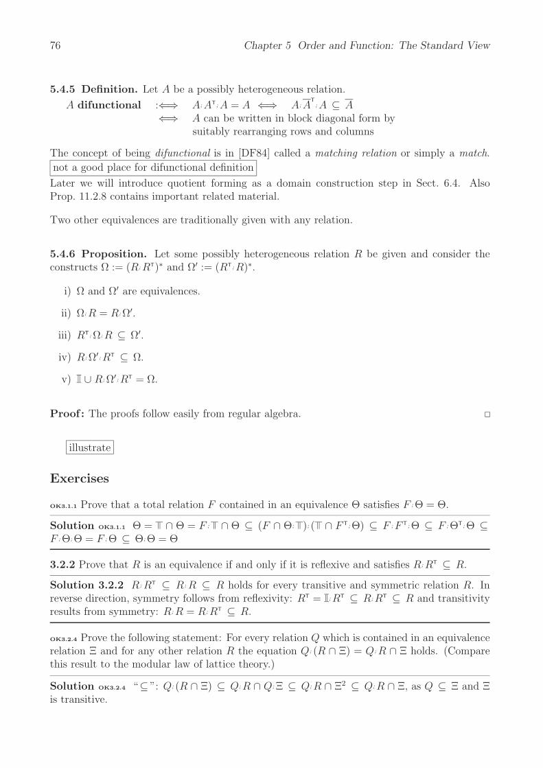
76 Chapter 5 Order and Function: The Standard View
5.4.5 Definition. Let A be a possibly heterogeneous relation.
A difunctional :⇐⇒ A; AT; A = A ⇐⇒ A; AT; A ⊆ A
⇐⇒ A can be written in block diagonal form bysuitably rearranging rows and columns
The concept of being difunctional is in [DF84] called a matching relation or simply a match.
not a good place for difunctional definition
Later we will introduce quotient forming as a domain construction step in Sect. 6.4. AlsoProp. 11.2.8 contains important related material.
Two other equivalences are traditionally given with any relation.
5.4.6 Proposition. Let some possibly heterogeneous relation R be given and consider theconstructs Ω := (R; RT)∗ and Ω′ := (RT; R)∗.
i) Ω and Ω′ are equivalences.
ii) Ω; R = R; Ω′.
iii) RT; Ω; R ⊆ Ω′.
iv) R; Ω′; RT ⊆ Ω.
v) ∪ R; Ω′; RT = Ω.
Proof : The proofs follow easily from regular algebra.
illustrate
Exercises
OK3.1.1 Prove that a total relation F contained in an equivalence Θ satisfies F ; Θ = Θ.
Solution OK3.1.1 Θ = ∩ Θ = F ; ∩ Θ ⊆ (F ∩ Θ; ); ( ∩ F T; Θ) ⊆ F ; F T; Θ ⊆ F ; ΘT; Θ ⊆F ; Θ; Θ = F ; Θ ⊆ Θ; Θ = Θ
3.2.2 Prove that R is an equivalence if and only if it is reflexive and satisfies R; RT ⊆ R.
Solution 3.2.2 R; RT ⊆ R; R ⊆ R holds for every transitive and symmetric relation R. Inreverse direction, symmetry follows from reflexivity: RT = ;RT ⊆ R;RT ⊆ R and transitivityresults from symmetry: R; R = R; RT ⊆ R.
OK3.2.4 Prove the following statement: For every relation Q which is contained in an equivalencerelation Ξ and for any other relation R the equation Q; (R ∩ Ξ) = Q; R ∩ Ξ holds. (Comparethis result to the modular law of lattice theory.)
Solution OK3.2.4 “⊆ ”: Q; (R ∩ Ξ) ⊆ Q; R ∩ Q; Ξ ⊆ Q; R ∩ Ξ2 ⊆ Q; R ∩ Ξ, as Q ⊆ Ξ and Ξis transitive.

5.5 Transitive Closure 77
“ ⊇ ”: Q;R ∩ Ξ ⊆ (Q ∩ Ξ;RT); (R ∩ QT; Ξ) ⊆ Q; (R ∩ ΞT; Ξ) = Q; (R ∩ Ξ; Ξ) ⊆ Q; (R ∩ Ξ), asQ ⊆ Ξ and Ξ is symmetric and transitive.
OK3.2.5 Prove the following statement: For every reflexive and transitive relation A there exists
a relation R such that A = RT; R.
Solution OK3.2.5 We choose R := A and obtain AT ; A ⊆ A, as A is transitive, but alsoAT; A ⊇ A, as A is reflexive.
5.5 Transitive Closure
It is folklore that every homogeneous relation R has a transitive closure R+ which is the leasttransitive relation it is contained in. Alternatively, one might say that it is the result of “makingR increasingly more transitive”.
5.5.1 Definition. Given any homogeneous relation R, we define its transitive closure
R+ := infX | R ⊆ X, X ; X ⊆ X = sup i≥1 Ri
in two forms and give also the two definitions of its reflexive-transitive closure
R∗ := infX | ∪ R ⊆ X, X ; X ⊆ X = sup i≥0 Ri
We do not recall here the proof justifying that one may indeed use two versions, i.e., that therelations thus defined will always coincide. We mention, however, in which way the reflexive-transitive and the transitive closure are related:
R+ = R; R∗ R∗ = ∪ R+
These interrelationships are by now well-known. Typically, the infimum definition (the “de-scriptive version”) will be made use of in proofs while the supremum version is computed (the“operational version”). To use the descriptive part to compute the closure would be highlycomplex as the intersection of all transitive relations above R is formed, which can only bedone for toy examples. The better idea for computing R+ is approximating it from below asR ⊆ R ∪ R2 ⊆ R ∪ R2 ∪ R3 . . . in the operational version. Yet far better are the traditionalalgorithms such as the Warshall algorithm.
5.5.2 Proposition. The following holds for an arbitrary finite homogeneous relation R:
i) Rn ⊆ ( ∪ R)n−1
ii) R∗ = sup0≤i<n Ri
iii) R+ = sup0<i≤n Ri
iv) ( ∪ R); ( ∪ R2); ( ∪ R4); ( ∪ R8); . . . ; ( ∪ R2log n) = R∗
Proof : We use the pigeon-hole principle and interpret ( ∪ R)n−1 = sup0≤i<n Ri as
Rnxz = ∃y1 : ∃y2 : . . .∃yn−1 : Rxy1 ∩ Ry1y2 ∩ . . . ∩ Ryn−1z.
This means n + 1 indices y0 := x, y1, . . . , yn−1, yn := z of which at least two will coincide; e.g.,
yr = ys, 0 ≤ r < s ≤ n. From Rnxz = 1 follows then R
n−(s−r)xz = 1 .
ii), iii), and iv) are then obvious.

78 Chapter 5 Order and Function: The Standard View
Strongly Connected Components
Closely related to the transitive closure is the determination of strongly connected components.Let A be a homogeneous relation be given and consider the preorder A∗ generated by A. ThenA∗∩A∗T is the equivalence generated by A which provides a partition of rows as well as columns.
1 2 3 4 5 6 7 8 910111213123456789
10111213
⎛⎜⎜⎜⎜⎜⎜⎜⎜⎜⎜⎜⎜⎜⎜⎜⎝
1 0 0 0 0 0 0 0 0 0 0 0 10 0 0 0 0 0 0 0 0 0 0 1 10 0 1 0 0 1 0 0 0 1 0 0 00 0 0 0 0 0 0 0 0 0 0 0 00 0 0 0 0 0 0 0 0 0 1 0 00 0 0 0 0 1 0 0 0 0 0 1 00 0 0 0 0 0 0 0 1 0 0 0 00 1 0 0 0 0 0 0 0 0 0 0 00 0 0 0 1 0 0 0 1 0 0 0 00 0 0 0 0 0 0 0 1 0 0 0 00 0 0 0 0 0 0 0 1 0 0 0 01 0 1 0 0 0 0 0 0 0 0 0 00 0 1 0 0 0 0 0 0 0 1 0 0
⎞⎟⎟⎟⎟⎟⎟⎟⎟⎟⎟⎟⎟⎟⎟⎟⎠
8 2 1 3 61213 4 710 5 91182136
121347
1059
11
⎛⎜⎜⎜⎜⎜⎜⎜⎜⎜⎜⎜⎜⎜⎜⎜⎝
1 1 1 1 1 1 1 0 0 1 1 1 10 1 1 1 1 1 1 0 0 1 1 1 10 0 1 1 1 1 1 0 0 1 1 1 10 0 1 1 1 1 1 0 0 1 1 1 10 0 1 1 1 1 1 0 0 1 1 1 10 0 1 1 1 1 1 0 0 1 1 1 10 0 1 1 1 1 1 0 0 1 1 1 10 0 0 0 0 0 0 1 0 0 0 0 00 0 0 0 0 0 0 0 1 0 1 1 10 0 0 0 0 0 0 0 0 1 1 1 10 0 0 0 0 0 0 0 0 0 1 1 10 0 0 0 0 0 0 0 0 0 1 1 10 0 0 0 0 0 0 0 0 0 1 1 1
⎞⎟⎟⎟⎟⎟⎟⎟⎟⎟⎟⎟⎟⎟⎟⎟⎠
Fig. 5.5.1 A relation with its transitive closure arranged in blocks by simultaneous permutation
insert some text here!
8 2 1 3 61213 4 710 5 91182136
121347
1059
11
⎛⎜⎜⎜⎜⎜⎜⎜⎜⎜⎜⎜⎜⎜⎜⎜⎝
0 1 0 0 0 0 0 0 0 0 0 0 00 0 0 0 0 1 1 0 0 0 0 0 00 0 1 0 0 0 1 0 0 0 0 0 00 0 0 1 1 0 0 0 0 1 0 0 00 0 0 0 1 1 0 0 0 0 0 0 00 0 1 1 0 0 0 0 0 0 0 0 00 0 0 1 0 0 0 0 0 0 0 0 10 0 0 0 0 0 0 0 0 0 0 0 00 0 0 0 0 0 0 0 0 0 0 1 00 0 0 0 0 0 0 0 0 0 0 1 00 0 0 0 0 0 0 0 0 0 0 0 10 0 0 0 0 0 0 0 0 0 1 1 00 0 0 0 0 0 0 0 0 0 0 1 0
⎞⎟⎟⎟⎟⎟⎟⎟⎟⎟⎟⎟⎟⎟⎟⎟⎠
Fig. 5.5.2 The original relation of Fig. 5.5.1 grouped accordingly
In the following proposition, we resume our explanation of the Szpilrajn extension and oftopological sorting.
5.5.3 Proposition. Any given homogeneous relation R can by simultaneously permutingrows and columns be transformed into a matrix of the following form: It has upper triangularpattern with square diagonal blocks⎛
⎜⎜⎝∗ ∗ ∗
∗ ∗∗
⎞⎟⎟⎠
where ∗ = unless the generated permuted preorder R∗ allows entries =/ . The reflexive-transitive closure of every diagonal block is the universal relation for that block.

5.6 Relations and Vectors 79
Exercises
3.2.3 Show that the following hold for every homogeneous relation R
i) infH | R ∪ R; H ⊆ H = infH | R ∪ R; H = H = R+
ii) infH | S ∪ R; H ⊆ H = R∗; S
Solution 3.2.3 i) Wenn diese Infima existieren, gilt sicherlich “⊆ ”. Das linke Infimum ex-istiert in einem vollstandigen Verband, denn wenn statt H auch H ′ die Bedingung R∪R;H ⊆ Herfullt, so auch H∩H ′; sie vererbt sich selbst auf nichtendliche Durchschnitte. Wie es in solchenFallen ofter geschieht, entartet fur das Infimum die Inklusion zur Gleichheit. Die hierfur nochfehlende Beziehung
R ∪ R;infH | R ∪ R; H ⊆ H ⊇ infH ′ | R ∪ R; H ′ ⊆ H ′ ist in der Tat erfullt, denn sogar bei jedem H mit R ∪ R; H ⊆ H, also auch fur das Infimum,erfullt die linke Seite R ∪ R; H =: H ′ die Beziehung
R ∪ R; H ′ = R ∪ R; (R ∪ R; H) = R ∪ R; R ∪ R; R; H ⊆ R ∪ R; H ∪ R; H = H ′.
Die zweite behauptete Gleichheit ist ein Spezialfall von (ii).
ii) Zu zeigen ist inf A = H ′, mit A := infH | S ∪ R; H ⊆ H , H ′ := R∗; S.“⊆ ”: Es gilt H ′ ∈ A, da sogar S ∪ R; H ′ = H ′. Also gilt inf A ⊆ H ′, da inf A untere
Schranke von A ist.“ ⊇ ”: Wir werden zeigen () ∀H ∈ A : H ′ ⊆ H, i. e. H ′ untere Schranke von A. Dann ist
H ′ ⊆ inf A, da inf A großte untere Schranke von A ist. Zum Nachweis von () zeigt man –im Hinblick auf die Supremum-Definition R∗ = sup i≥0 Ri – die Aussage ∀i ∈ IN : Ri ; S ⊆ H;dies ergibt sich durch Induktion: R0; S = S ⊆ H und Ri; S ⊆ H =⇒ Ri+1; S ⊆ R; H ⊆ H.
5.6 Relations and Vectors
When working with real-valued matrices, it is typical to ask for their eigenvalues and eigenvec-tors. In the relational case one can not hope for interesting properties of eigenvalues, as thesewould be restricted to 0 , 1 . Nevertheless is there an important field of studying eigenvectors.This may be embedded in an advanced study of general Galois mechanisms, which is ratherinvolved and, thus, postponed to Ch. 15.
There are, however, some very simple concepts that may already be studied here in order toget ways to denote several effects coherently.
Definition Area and Image Area
Relations are used mainly as they allow to express more than functions or mappings do: Theymay assign more than one value to an argument or none. It is of cause interesting whicharguments get assigned values and which do not. In the same way will one ask which elementson the range side occur as images and which do not. The next definition provides an algebraicformulation.
5.6.1 Definition. Given a (possibly heterogeneous) relation R, we always have the vectors
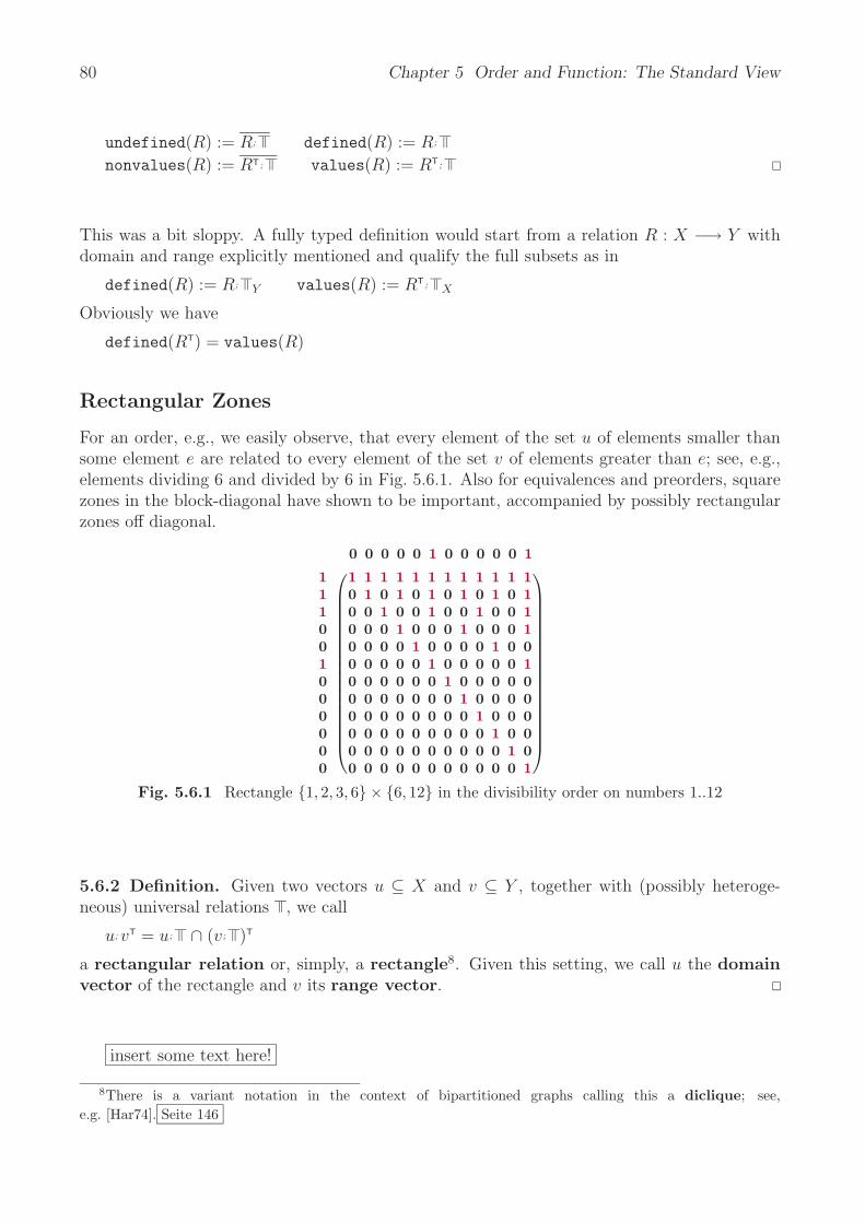
80 Chapter 5 Order and Function: The Standard View
undefined(R) := R; defined(R) := R;
nonvalues(R) := RT; values(R) := RT;
This was a bit sloppy. A fully typed definition would start from a relation R : X −→ Y withdomain and range explicitly mentioned and qualify the full subsets as in
defined(R) := R; Y values(R) := RT; X
Obviously we have
defined(RT) = values(R)
Rectangular Zones
For an order, e.g., we easily observe, that every element of the set u of elements smaller thansome element e are related to every element of the set v of elements greater than e; see, e.g.,elements dividing 6 and divided by 6 in Fig. 5.6.1. Also for equivalences and preorders, squarezones in the block-diagonal have shown to be important, accompanied by possibly rectangularzones off diagonal.
111001000000
0 0 0 0 0 1 0 0 0 0 0 1⎛⎜⎜⎜⎜⎜⎜⎜⎜⎜⎜⎜⎜⎜⎜⎜⎜⎜⎝
1 1 1 1 1 1 1 1 1 1 1 10 1 0 1 0 1 0 1 0 1 0 10 0 1 0 0 1 0 0 1 0 0 10 0 0 1 0 0 0 1 0 0 0 10 0 0 0 1 0 0 0 0 1 0 00 0 0 0 0 1 0 0 0 0 0 10 0 0 0 0 0 1 0 0 0 0 00 0 0 0 0 0 0 1 0 0 0 00 0 0 0 0 0 0 0 1 0 0 00 0 0 0 0 0 0 0 0 1 0 00 0 0 0 0 0 0 0 0 0 1 00 0 0 0 0 0 0 0 0 0 0 1
⎞⎟⎟⎟⎟⎟⎟⎟⎟⎟⎟⎟⎟⎟⎟⎟⎟⎟⎠
Fig. 5.6.1 Rectangle 1, 2, 3, 6 × 6, 12 in the divisibility order on numbers 1..12
5.6.2 Definition. Given two vectors u ⊆ X and v ⊆ Y , together with (possibly heteroge-neous) universal relations , we call
u; vT = u; ∩ (v; )T
a rectangular relation or, simply, a rectangle8. Given this setting, we call u the domainvector of the rectangle and v its range vector.
insert some text here!
8There is a variant notation in the context of bipartitioned graphs calling this a diclique; see,e.g. [Har74]. Seite 146

5.6 Relations and Vectors 81
u
v
Fig. 5.6.2 Rectangle generated by intersection of a row-constant and a column-constant relation
There are two definitional variants, and we should convince ourselves that they mean the same.While “⊆ ” is clear, the other direction is involved requiring the Dedekind formula, the Tarskirule, and a case distinction:
u; ∩ (v; )T ⊆ (u ∩ (v; )T; ); ( ∩ uT; (v; )T) ⊆ (u ∩ ; vT; ); uT; vT
= (u ∩ ; vT; ); ; uT; vT
Now either u, or v, or both are equal to , in which case the spanned relation is the emptyrelation in both versions. When u and v are =/ , the Tarski rule shows us that ; u; = aswell as ; v; = , so that the righthand side is indeed u; ; vT = u; vT
As we will see, rectangles are often studied in combination with some given relation. They maybe inside that relation, outside, or contain or frame that relation.
v
u
R
u =
⎛⎜⎜⎜⎜⎜⎜⎜⎜⎜⎜⎝
011001100
⎞⎟⎟⎟⎟⎟⎟⎟⎟⎟⎟⎠
(0 0 1 1 1 0 0 1 1 0 0)= vT⎛⎜⎜⎜⎜⎜⎜⎜⎜⎜⎜⎝
1 0 0 0 0 0 0 0 0 0 00 0 1 1 1 0 0 1 1 0 00 0 1 1 1 0 0 1 1 0 00 0 1 0 1 0 1 0 1 0 00 1 0 1 0 1 0 1 0 0 10 0 1 1 1 0 0 1 1 0 00 0 1 1 1 0 0 1 1 0 00 1 0 0 0 0 0 0 1 0 01 0 0 0 0 0 1 0 0 0 0
⎞⎟⎟⎟⎟⎟⎟⎟⎟⎟⎟⎠
Fig. 5.6.3 Rectangles inside a relation
5.6.3 Definition. Given a relation R, we say that the subsets u, v, define a
i) rectangle inside R :⇐⇒ u; vT ⊆ R ⇐⇒ R; v ⊆ u ⇐⇒ RT; u ⊆ v.
ii) rectangle containing R :⇐⇒ R ⊆ u; vT.
We say that u, v is a rectangle outside R if u, v is a rectangle inside R.
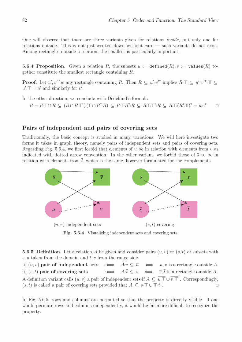
82 Chapter 5 Order and Function: The Standard View
One will observe that there are three variants given for relations inside, but only one forrelations outside. This is not just written down without care — such variants do not exist.Among rectangles outside a relation, the smallest is particularly important.
5.6.4 Proposition. Given a relation R, the subsets u := defined(R), v := values(R) to-gether constitute the smallest rectangle containing R.
Proof : Let u′, v′ be any rectangle containing R. Then R ⊆ u′; v′T implies R; ⊆ u′; v′T; ⊆u′; = u′ and similarly for v′.
In the other direction, we conclude with Dedekind’s formula
R = R; ∩R ⊆ (R∩R;T);( ∩RT;R) ⊆ R; ;RT;R ⊆ R; ;
T;R ⊆ R; ;(RT; )T = u;vT
Pairs of independent and pairs of covering sets
Traditionally, the basic concept is studied in many variations. We will here investigate twoforms it takes in graph theory, namely pairs of independent sets and pairs of covering sets.Regarding Fig. 5.6.4, we first forbid that elements of u be in relation with elements from v asindicated with dotted arrow convention. In the other variant, we forbid those of s to be inrelation with elements from t, which is the same, however formulated for the complements.
u v
u v
(u, v) independent sets
s t
s t
(s, t) covering
Fig. 5.6.4 Visualizing independent sets and covering sets
5.6.5 Definition. Let a relation A be given and consider pairs (u, v) or (s, t) of subsets withs, u taken from the domain and t, v from the range side.
i) (u, v) pair of independent sets :⇐⇒ A;v ⊆ u ⇐⇒ u, v is a rectangle outside A.
ii) (s, t) pair of covering sets :⇐⇒ A; t ⊆ s ⇐⇒ s, t is a rectangle outside A.
A definition variant calls (u, v) a pair of independent sets if A ⊆ u; ∪ v;T. Correspondingly,
(s, t) is called a pair of covering sets provided that A ⊆ s; ∪ ; tT.
In Fig. 5.6.5, rows and columns are permuted so that the property is directly visible. If onewould permute rows and columns independently, it would be far more difficult to recognize theproperty.

5.6 Relations and Vectors 83
000000000000000000000000000000000000000000000000000000000000000000000000000000000000000000000000000000000000000000000000000000000000
u
v
1111
111111111111111111111111111111111
A
arbitrary
(u, v) independent
000000000000000000000000000000000000000000000000000000000000000000000000000000000000000000000000000000000000000000000000000000000000
s
t1111111111111
A
arbitrary11111111
(s, t) covering
Fig. 5.6.5 A pair of independent sets and a pair of covering sets
The idea for the following statement is immediate.
5.6.6 Proposition. For a given relation A together with a pair (s, t) we have
(s, t) line-covering ⇐⇒ (s, t) is independent.
On the right side, (s, t) is indeed a pair of covering sets, as the columns of t together with therows of s cover all the 1 ’s of the relation A. The covering property A; t ⊆ s follows directlyfrom the algebraic condition: When one follows relation A and finds oneself ending outside t,then the starting point is covered by s. Algebraic transformation shows that A ⊆ s; ∪ ; tT
is an equivalent form, expressing that rows according to s and columns according to t cover allof A.
In the same way, one will find no relation between elements of rows of u with elements ofcolumns of v on the left side. We can indeed read this directly from the condition A; v ⊆ u:When following the relation A and ending in v, it turns out that one has been starting fromoutside u. With Schroder’s rule we immediately arrive at u; vT ⊆ A; this also expresses thatfrom u to v, there is no relationship according to A.
The predicate-logic formulation is more complicated:
〈∀x : (〈∃y : ((x, y) ∈ A) ∧ (y ∈ t)〉) −→ (¬ (x ∈ s))〉〈∀x : 〈∀z : (x ∈ s) ∨ (((x, z) ∈ A) ∨ (z ∈ t))〉〉
It is a trivial fact that with (u, v) a pair of independent sets and u′ ⊆ u, v′ ⊆ v, also the smaller(u′, v′) will be a pair of independent sets. In the same way, if (s, t) is a pair of covering setsand s′ ⊇ s, t′ ⊇ t, also (s′, t′) will be a pair of covering sets. For pairs of independent sets, oneis therefore interested in greatest ones and for covering pairs for smallest ones. For algebraicconditions see Sect. 9. There exists, however, no simple minimality (respectively maximality)criterion as one may see in Fig. 9.2.3.
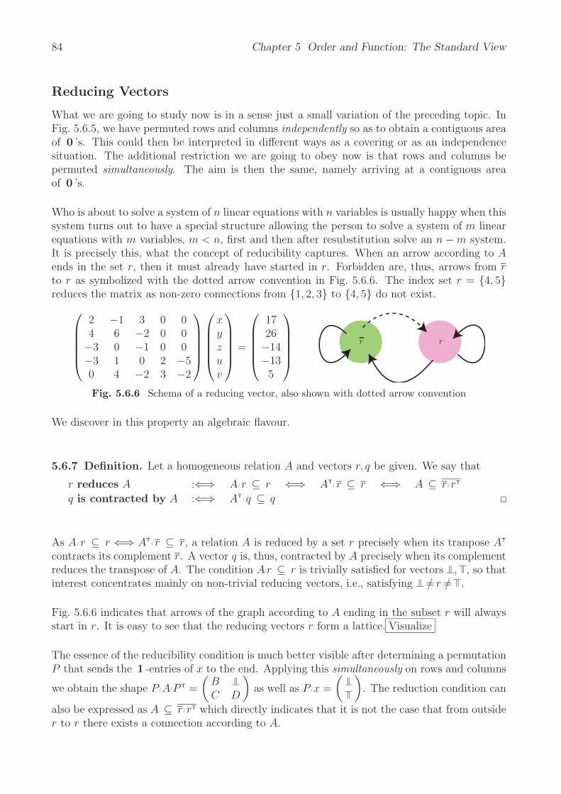
84 Chapter 5 Order and Function: The Standard View
Reducing Vectors
What we are going to study now is in a sense just a small variation of the preceding topic. InFig. 5.6.5, we have permuted rows and columns independently so as to obtain a contiguous areaof 0 ’s. This could then be interpreted in different ways as a covering or as an independencesituation. The additional restriction we are going to obey now is that rows and columns bepermuted simultaneously. The aim is then the same, namely arriving at a contiguous areaof 0 ’s.
Who is about to solve a system of n linear equations with n variables is usually happy when thissystem turns out to have a special structure allowing the person to solve a system of m linearequations with m variables, m < n, first and then after resubstitution solve an n − m system.It is precisely this, what the concept of reducibility captures. When an arrow according to Aends in the set r, then it must already have started in r. Forbidden are, thus, arrows from rto r as symbolized with the dotted arrow convention in Fig. 5.6.6. The index set r = 4, 5reduces the matrix as non-zero connections from 1, 2, 3 to 4, 5 do not exist.⎛
⎜⎜⎜⎜⎝2 −1 3 0 04 6 −2 0 0−3 0 −1 0 0−3 1 0 2 −50 4 −2 3 −2
⎞⎟⎟⎟⎟⎠
⎛⎜⎜⎜⎜⎝
xyzuv
⎞⎟⎟⎟⎟⎠ =
⎛⎜⎜⎜⎜⎝
1726−14−135
⎞⎟⎟⎟⎟⎠
rr
Fig. 5.6.6 Schema of a reducing vector, also shown with dotted arrow convention
We discover in this property an algebraic flavour.
5.6.7 Definition. Let a homogeneous relation A and vectors r, q be given. We say that
r reduces A :⇐⇒ A; r ⊆ r ⇐⇒ AT; r ⊆ r ⇐⇒ A ⊆ r; rT
q is contracted by A :⇐⇒ AT; q ⊆ q
As A; r ⊆ r ⇐⇒ AT ; r ⊆ r, a relation A is reduced by a set r precisely when its tranpose AT
contracts its complement r. A vector q is, thus, contracted by A precisely when its complementreduces the transpose of A. The condition A;r ⊆ r is trivially satisfied for vectors , , so thatinterest concentrates mainly on non-trivial reducing vectors, i.e., satisfying =/ r =/ .
Fig. 5.6.6 indicates that arrows of the graph according to A ending in the subset r will alwaysstart in r. It is easy to see that the reducing vectors r form a lattice. Visualize
The essence of the reducibility condition is much better visible after determining a permutationP that sends the 1 -entries of x to the end. Applying this simultaneously on rows and columns
we obtain the shape P ;A;P T =
(BC D
)as well as P ;x =
( ). The reduction condition can
also be expressed as A ⊆ r; rT which directly indicates that it is not the case that from outsider to r there exists a connection according to A.
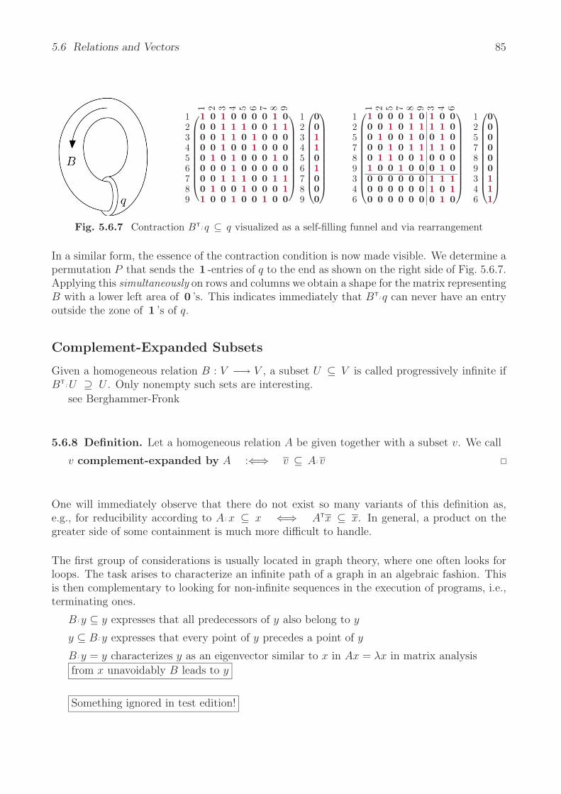
5.6 Relations and Vectors 85
1 2 3 4 5 6 7 8 9
123456789
⎛⎜⎜⎜⎜⎜⎜⎜⎜⎜⎝
1 0 1 0 0 0 0 1 00 0 1 1 1 0 0 1 10 0 1 1 0 1 0 0 00 0 1 0 0 1 0 0 00 1 0 1 0 0 0 1 00 0 0 1 0 0 0 0 00 0 1 1 1 0 0 1 10 1 0 0 1 0 0 0 11 0 0 1 0 0 1 0 0
⎞⎟⎟⎟⎟⎟⎟⎟⎟⎟⎠
123456789
⎛⎜⎜⎜⎜⎜⎜⎜⎜⎜⎜⎝
001101000
⎞⎟⎟⎟⎟⎟⎟⎟⎟⎟⎟⎠
1 2 5 7 8 9 3 4 6
125789346
⎛⎜⎜⎜⎜⎜⎜⎜⎜⎜⎜⎝
1 0 0 0 1 0 1 0 00 0 1 0 1 1 1 1 00 1 0 0 1 0 0 1 00 0 1 0 1 1 1 1 00 1 1 0 0 1 0 0 01 0 0 1 0 0 0 1 00 0 0 0 0 0 1 1 10 0 0 0 0 0 1 0 10 0 0 0 0 0 0 1 0
⎞⎟⎟⎟⎟⎟⎟⎟⎟⎟⎟⎠
125789346
⎛⎜⎜⎜⎜⎜⎜⎜⎜⎜⎜⎝
000000111
⎞⎟⎟⎟⎟⎟⎟⎟⎟⎟⎟⎠
Fig. 5.6.7 Contraction BT;q ⊆ q visualized as a self-filling funnel and via rearrangement
In a similar form, the essence of the contraction condition is now made visible. We determine apermutation P that sends the 1 -entries of q to the end as shown on the right side of Fig. 5.6.7.Applying this simultaneously on rows and columns we obtain a shape for the matrix representingB with a lower left area of 0 ’s. This indicates immediately that BT;q can never have an entryoutside the zone of 1 ’s of q.
Complement-Expanded Subsets
Given a homogeneous relation B : V −→ V , a subset U ⊆ V is called progressively infinite ifBT; U ⊇ U . Only nonempty such sets are interesting.
see Berghammer-Fronk
5.6.8 Definition. Let a homogeneous relation A be given together with a subset v. We call
v complement-expanded by A :⇐⇒ v ⊆ A; v
One will immediately observe that there do not exist so many variants of this definition as,e.g., for reducibility according to A; x ⊆ x ⇐⇒ ATx ⊆ x. In general, a product on thegreater side of some containment is much more difficult to handle.
The first group of considerations is usually located in graph theory, where one often looks forloops. The task arises to characterize an infinite path of a graph in an algebraic fashion. Thisis then complementary to looking for non-infinite sequences in the execution of programs, i.e.,terminating ones.
B ; y ⊆ y expresses that all predecessors of y also belong to y
y ⊆ B ; y expresses that every point of y precedes a point of y
B ; y = y characterizes y as an eigenvector similar to x in Ax = λx in matrix analysis
from x unavoidably B leads to y
Something ignored in test edition!

86 Chapter 5 Order and Function: The Standard View
5.7 Properties of the Symmetric Quotient
Algebraic properties of the symmetric quotient are important and not broadly known. There-fore, they are here recalled, proved, and also visualized.
Gre
enpe
ace
Red
Cro
ssA
mne
sty
Inte
rnat
iona
lW
orld
Wild
life
Fund
sA
ttac
Doc
tors
Wit
hout
Bor
ders
Red
Cre
scen
t
ArbuthnotPerez
DupontBotticelliSchmidt
Larsen
⎛⎜⎜⎜⎜⎝
1 0 0 1 0 0 10 0 0 0 0 0 00 1 1 0 1 0 01 0 0 1 0 0 10 1 1 0 1 0 00 0 0 0 0 0 0
⎞⎟⎟⎟⎟⎠
Gen
eral
Mot
ors
Siem
ens
Viv
endi
LLoy
dsM
icro
soft
App
leV
odaf
one
Mic
roso
ft
⎛⎜⎜⎜⎜⎝
1 0 0 0 1 0 1 00 0 0 0 0 0 0 01 0 1 1 0 1 0 01 0 0 1 1 0 1 00 0 1 0 0 1 0 00 0 0 0 0 0 0 0
⎞⎟⎟⎟⎟⎠
Gen
eral
Mot
ors
Siem
ens
Viv
endi
LLoy
dsM
icro
soft
App
leV
odaf
one
Mic
roso
ft
GreenpeaceRed Cross
Amnesty InternationalWorld Wildlife Funds
AttacDoctors Without Borders
Red Crescent
⎛⎜⎜⎜⎜⎜⎜⎝
0 0 0 0 1 0 1 00 0 1 0 0 1 0 00 0 1 0 0 1 0 00 0 0 0 1 0 1 00 0 1 0 0 1 0 00 1 0 0 0 0 0 10 0 0 0 1 0 1 0
⎞⎟⎟⎟⎟⎟⎟⎠
Fig. 5.7.1 The symmetric quotient: A, B and syq(A, B)
In Fig. 5.7.1, we assume a group of individuals and two relations in which these are involvedand that are typically neither functions nor mappings: the non-governmental organizationsthey give donations to and the stocks they own. It is immediately clear that (i,ii) of Prop. 5.7.1hold. As the symmetric quotient of Def. 4.4.3 compares columns, it is immaterial whether itcompares the columns or their complements. Also, when comparing the columns of A to thoseof B, one will obtain the converse when comparing the columns of B to those of A.
Two trivial observations follow without proof.
5.7.1 Proposition. Let A, B be arbitrary relations with the same domain.
i) syq(A, B) = syq(A, B)
ii) syq(B, A) = [syq(A, B)]T
For truely heterogeneous relations with different codomains, e.g., the construct syq(AT, BT)cannot be built for typing reasons. In case A = B, however, even more can be proved, as thenalso syq(AT, AT) is defined. We demonstrate this with the relation “has sent a letter to” on aset of individuals considered.
A =
Arb
uthn
otPer
ezD
upon
tB
otti
celli
Schm
idt
Lar
sen
ArbuthnotPerez
DupontBotticelliSchmidt
Larsen
⎛⎜⎜⎜⎜⎝
1 0 1 1 0 10 1 1 0 1 10 1 1 0 1 11 0 1 1 0 10 0 1 0 0 10 1 1 0 1 1
⎞⎟⎟⎟⎟⎠ syq(AT, AT) =
Arb
uthn
otPer
ezD
upon
tB
otti
celli
Schm
idt
Lar
sen
⎛⎜⎜⎜⎜⎝
1 0 0 1 0 00 1 1 0 0 10 1 1 0 0 11 0 0 1 0 00 0 0 0 1 00 1 1 0 0 1
⎞⎟⎟⎟⎟⎠ syq(A, A) =
Arb
uthn
otPer
ezD
upon
tB
otti
celli
Schm
idt
Lar
sen
⎛⎜⎜⎜⎜⎝
1 0 0 1 0 00 1 0 0 1 00 0 1 0 0 11 0 0 1 0 00 1 0 0 1 00 0 1 0 0 1
⎞⎟⎟⎟⎟⎠
Fig. 5.7.2 Symmetric quotients of a homogeneous relation give their row resp. column equivalence
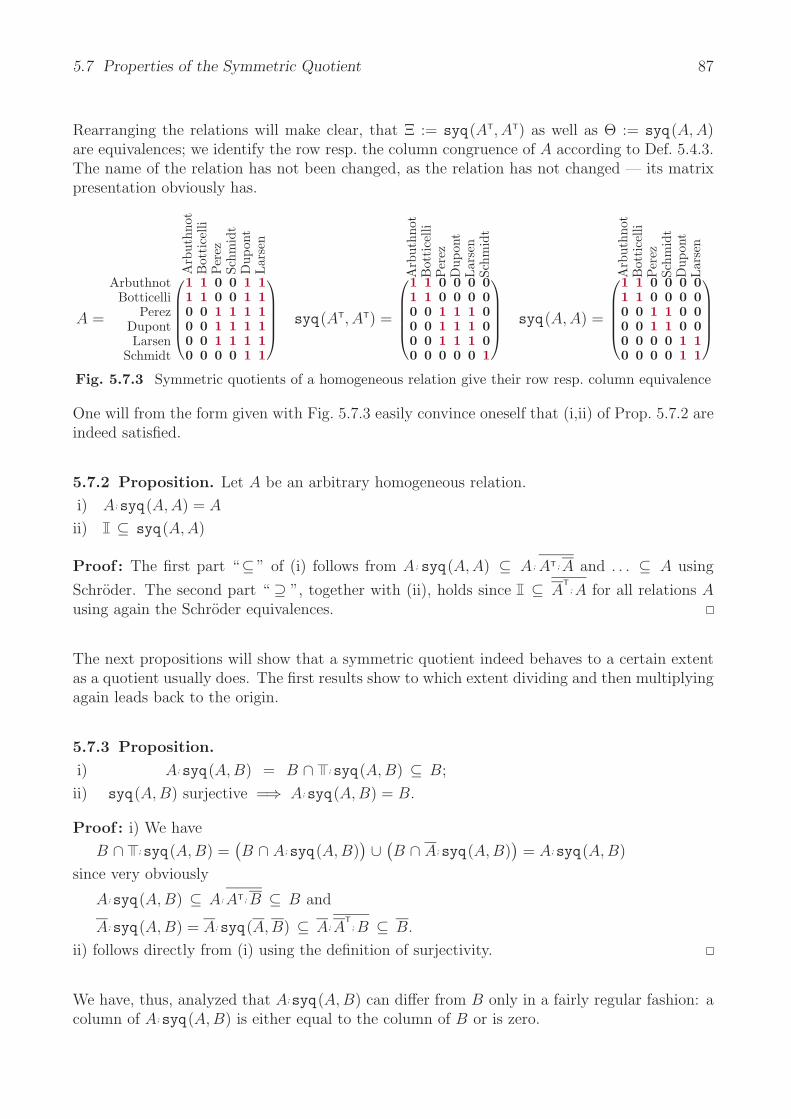
5.7 Properties of the Symmetric Quotient 87
Rearranging the relations will make clear, that Ξ := syq(AT, AT) as well as Θ := syq(A, A)are equivalences; we identify the row resp. the column congruence of A according to Def. 5.4.3.The name of the relation has not been changed, as the relation has not changed — its matrixpresentation obviously has.
A =
Arb
uthn
otB
otti
celli
Per
ezSc
hmid
tD
upon
tLar
sen
ArbuthnotBotticelli
PerezDupontLarsen
Schmidt
⎛⎜⎜⎜⎜⎝
1 1 0 0 1 11 1 0 0 1 10 0 1 1 1 10 0 1 1 1 10 0 1 1 1 10 0 0 0 1 1
⎞⎟⎟⎟⎟⎠ syq(AT, AT) =
Arb
uthn
otB
otti
celli
Per
ezD
upon
tLar
sen
Schm
idt
⎛⎜⎜⎜⎜⎝
1 1 0 0 0 01 1 0 0 0 00 0 1 1 1 00 0 1 1 1 00 0 1 1 1 00 0 0 0 0 1
⎞⎟⎟⎟⎟⎠ syq(A, A) =
Arb
uthn
otB
otti
celli
Per
ezSc
hmid
tD
upon
tLar
sen
⎛⎜⎜⎜⎜⎝
1 1 0 0 0 01 1 0 0 0 00 0 1 1 0 00 0 1 1 0 00 0 0 0 1 10 0 0 0 1 1
⎞⎟⎟⎟⎟⎠
Fig. 5.7.3 Symmetric quotients of a homogeneous relation give their row resp. column equivalence
One will from the form given with Fig. 5.7.3 easily convince oneself that (i,ii) of Prop. 5.7.2 areindeed satisfied.
5.7.2 Proposition. Let A be an arbitrary homogeneous relation.
i) A;syq(A, A) = A
ii) ⊆ syq(A, A)
Proof : The first part “⊆ ” of (i) follows from A ; syq(A, A) ⊆ A ; AT; A and . . . ⊆ A using
Schroder. The second part “ ⊇ ”, together with (ii), holds since ⊆ AT; A for all relations A
using again the Schroder equivalences.
The next propositions will show that a symmetric quotient indeed behaves to a certain extentas a quotient usually does. The first results show to which extent dividing and then multiplyingagain leads back to the origin.
5.7.3 Proposition.
i) A;syq(A, B) = B ∩ ;syq(A, B) ⊆ B;
ii) syq(A, B) surjective =⇒ A;syq(A, B) = B.
Proof : i) We have
B ∩ ;syq(A, B) =(B ∩ A;syq(A, B)
)∪
(B ∩ A;syq(A, B)
)= A;syq(A, B)
since very obviously
A;syq(A, B) ⊆ A; AT; B ⊆ B and
A;syq(A, B) = A;syq(A, B) ⊆ A; AT; B ⊆ B.
ii) follows directly from (i) using the definition of surjectivity.
We have, thus, analyzed that A;syq(A, B) can differ from B only in a fairly regular fashion: acolumn of A;syq(A, B) is either equal to the column of B or is zero.
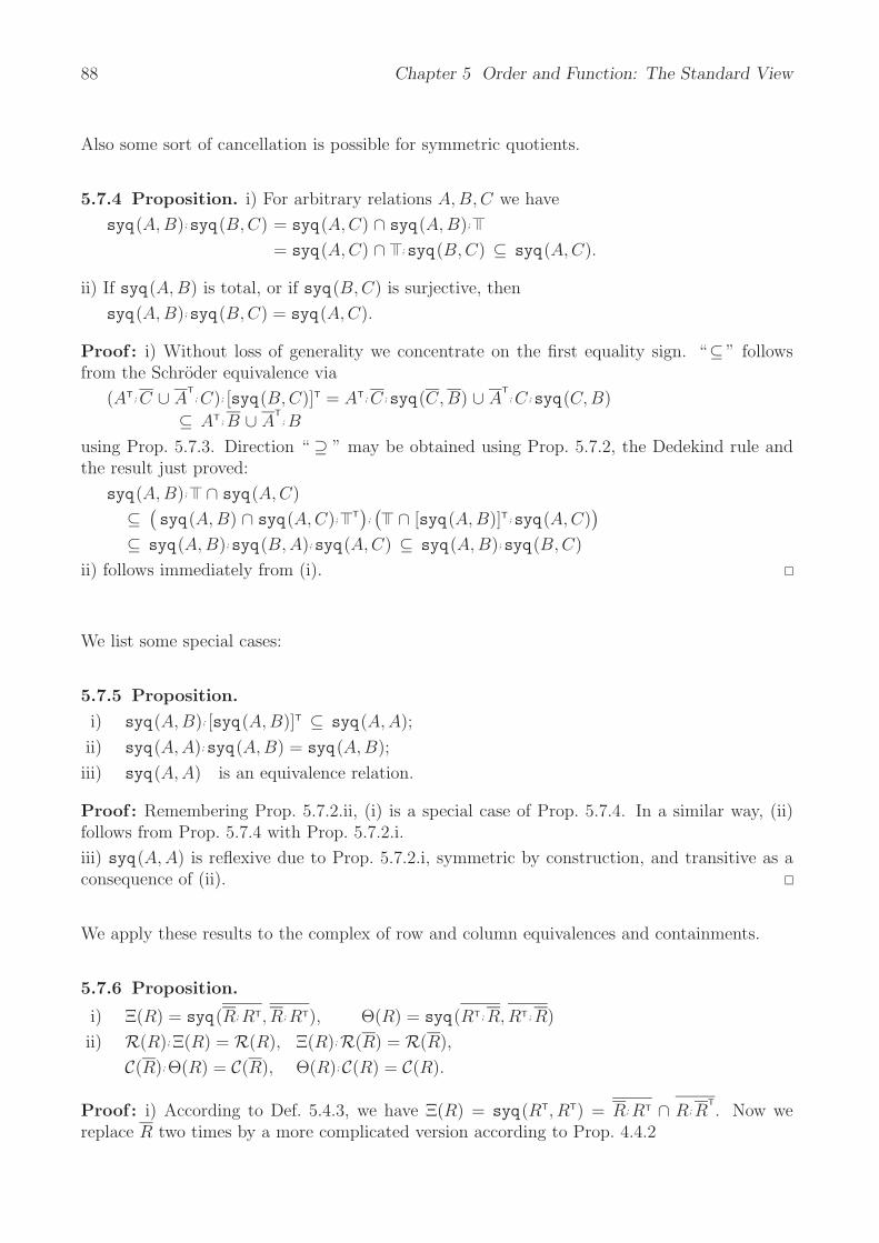
88 Chapter 5 Order and Function: The Standard View
Also some sort of cancellation is possible for symmetric quotients.
5.7.4 Proposition. i) For arbitrary relations A, B, C we have
syq(A, B);syq(B, C) = syq(A, C) ∩ syq(A, B);
= syq(A, C) ∩ ;syq(B, C) ⊆ syq(A, C).
ii) If syq(A, B) is total, or if syq(B, C) is surjective, then
syq(A, B);syq(B, C) = syq(A, C).
Proof : i) Without loss of generality we concentrate on the first equality sign. “⊆ ” followsfrom the Schroder equivalence via
(AT; C ∪ AT; C); [syq(B, C)]T = AT; C ;syq(C,B) ∪ A
T; C ;syq(C, B)
⊆ AT; B ∪ AT; B
using Prop. 5.7.3. Direction “ ⊇ ” may be obtained using Prop. 5.7.2, the Dedekind rule andthe result just proved:
syq(A, B); ∩ syq(A, C)
⊆(syq(A, B) ∩ syq(A, C);
T)
;
(∩ [syq(A, B)]T;syq(A, C)
)⊆ syq(A, B);syq(B, A);syq(A, C) ⊆ syq(A, B);syq(B, C)
ii) follows immediately from (i).
We list some special cases:
5.7.5 Proposition.
i) syq(A, B); [syq(A, B)]T ⊆ syq(A, A);
ii) syq(A, A);syq(A, B) = syq(A, B);
iii) syq(A, A) is an equivalence relation.
Proof : Remembering Prop. 5.7.2.ii, (i) is a special case of Prop. 5.7.4. In a similar way, (ii)follows from Prop. 5.7.4 with Prop. 5.7.2.i.
iii) syq(A, A) is reflexive due to Prop. 5.7.2.i, symmetric by construction, and transitive as aconsequence of (ii).
We apply these results to the complex of row and column equivalences and containments.
5.7.6 Proposition.
i) Ξ(R) = syq(R; RT, R; RT), Θ(R) = syq(RT; R, RT; R)
ii) R(R); Ξ(R) = R(R), Ξ(R);R(R) = R(R),
C(R); Θ(R) = C(R), Θ(R);C(R) = C(R).
Proof : i) According to Def. 5.4.3, we have Ξ(R) = syq(RT, RT) = R; RT ∩ R; RT. Now we
replace R two times by a more complicated version according to Prop. 4.4.2

5.7 Properties of the Symmetric Quotient 89
R → R; RT; R
so as to obtain the result (up to trivial manipulations).
ii) We prove only the very first equality and use Ξ(R) according to (i). It is now trivial accordingto Prop. 5.7.7 as it means
R; RT;syq(R; RT, R; RT) = R; RT
In proofs or computations it is often useful to know how composition with a relation leads toan effect on the symmetric quotient, or composition with a mapping. This is captured in thefollowing proposition.
5.7.7 Proposition.
i) syq(A, B)⊆ syq(C ; A, C ; B) for every C;
ii) F ;syq(A, B) = syq(A; F T, B) for every mapping F .
iii) syq(A, B); F T = syq(A, B ; F T) for every mapping F .
Proof : i) C ; B ⊆ C ; B ⇐⇒ CT ; C ; B ⊆ B =⇒ (C ; A)T ; C ; B ⊆ AT ; B. The second case isproved analogously.
ii) Following Prop. 5.2.6, we have F ; S = F ; S for a mapping F and arbitrary S, so that
F ;syq(A, B)= F ; AT; B ∩ F ; AT; B = F ; AT; B ∩ F ; A
T; B
= (A; F T)T; B ∩ A; F TT; B = syq(A; F T, B).
iii) is proved similarly.
AT; B =
Arb
uthn
otPer
ezD
upon
tB
otti
celli
Schm
idt
Lar
sen
ArbuthnotPerez
DupontBotticelliSchmidt
Larsen
⎛⎜⎜⎜⎜⎝
1 0 1 1 0 10 1 1 0 1 10 0 1 0 0 11 0 1 1 0 10 1 1 0 1 10 0 1 0 0 1
⎞⎟⎟⎟⎟⎠ A
T; B =
Arb
uthn
otPer
ezD
upon
tB
otti
celli
Schm
idt
Lar
sen
ArbuthnotPerez
DupontBotticelliSchmidt
Larsen
⎛⎜⎜⎜⎜⎝
1 0 0 1 0 00 1 0 0 1 01 1 1 1 1 11 0 0 1 0 00 1 0 0 1 01 1 1 1 1 1
⎞⎟⎟⎟⎟⎠
Fig. 5.7.4 The intersecting parts of a symmetric quotient
Always holds A;syq(A, B) ⊆ B and we analyze in which way A;syq(A, B) can differ from B.According to our next proposition it is contained in B in a fairly regular fashion: a column ofA;syq(A, B) is either equal to the corresponding column of B or it is zero.
Exercises
NEW Prove that syq(R, R) ⊆ RT; R whenever R is surjective.
Solution NEW = ; R = (RT ∪ RT); R ⊆ RT; R ∪ (RT ∪ R
T); R, so that
syq(R, R) = RT; R ∩ RT; R ⊆ RT; R

90 Chapter 5 Order and Function: The Standard View

6 Relational Domain Construction
It has in Chapters 2 and 3 been shown in which way moderately sized basesets, elements, vectors,and relations may be represented. There is a tendency of trying to extend these techniquesindiscriminately to all finite situations. We do not follow this idea. Instead, basesets, elements,vectors, or relations — beyond what is related to ground sets — will carefully be constructed;in particular if they are “bigger” ones. Only a few generic techniques are necessary for thatwhich shall here be presented as detailed as appropriate.
These techniques are far from being new. We routinely apply them in an informal way sinceour former school environment. What is new in the approach chosen here is that we begin totake those techniques seriously: pair forming, if . . . then . . . else-handling of variants, quotientforming, etc. For pairs, we routinely look for the first and second component; when a set isconsidered modulo an equivalence, we work with the corresponding equivalence classes andobey carefully that our results do not dependent on the specific representative chosen, etc.
What has been indicated here requires, however, a more detailed language to be expressed. Thisin turn means that a distinction between language and interpretation suddenly is importantwhich one would like to abstract from when handling relations “directly”. It turns out thatonly one or two generically defined relations are necessary for each construction step withquite simple and intuitive algebraic properties. Important is that the same generically definedrelations will serve to define new elements, new vectors, and new relations — assuming that weknow how this definition works in the constituents.
The point to stress is that once a new category object has been constructed, all elements,vectors, and relations touching this domain will be defined using the generic tools while otherscan simply not be formulated.
6.1 Domains of Ground Type
Relations on ground types are typically given explicitly, i.e., with whatever method mentionedin Chapt. 3. This is where we usually start from. Also elements and vectors are given explicitlyand not constructed somehow; this follows the lines of Chapt. 2.
Another specific way to construct a relation on ground sets will start from vectors v ⊆ X andw ⊆ Y and result in the rectangular relation v ; wT : X −→ Y . In Ex. 6.1.1, we thus definethe relation between all the red Bridge suits and all the picture-carrying Skat card levels. Itis a constructed relation although between ground sets — in contrast to R, a relation givenmarking arbitrarily.
91

92 Chapter 6 Relational Domain Construction
e =
♠♥♦♣
⎛⎜⎝
0010
⎞⎟⎠ v =
⎛⎜⎝
0110
⎞⎟⎠ w =
AKDB10987
⎛⎜⎜⎜⎜⎜⎜⎜⎜⎜⎝
01110000
⎞⎟⎟⎟⎟⎟⎟⎟⎟⎟⎠
v; wT =
A K D B 10 9 8 7
♠♥♦♣
⎛⎜⎝
0 0 0 0 0 0 0 00 1 1 1 0 0 0 00 1 1 1 0 0 0 00 0 0 0 0 0 0 0
⎞⎟⎠ R =
A K D B 10 9 8 7
♠♥♦♣
⎛⎜⎝
0 0 0 0 0 1 0 00 0 1 1 0 0 1 00 1 0 1 0 0 0 10 0 0 1 0 0 0 0
⎞⎟⎠
Fig. 6.1.1 Element, vectors, constructed rectangular relation; explicit relation of ground type
6.2 Direct Product
Pairs, triples, and n-tuples are omnipresent in everyday situations. All pairs with elementsof sets X, Y as components make up a Cartesian product X × Y of these sets. The notation(x, y) ∈ X × Y for pairs with parentheses and separating comma in between is very commonand need not be explained any further.
We have, however, introduced the concept of types t1, t2 that may — possibly only later —be interpreted by sets. So we have to show in a generic fashion how such pair-forming canbe achieved. Assuming a type t1 and a type t2 to be given, we constructively generate theirdirect product DirPro t1 t2, As an example we provide different interpretations for thesetypes, namely for t1
BrigeHonourValues = A,K,Q,J,10 or SkatCardLevels = A,K,D,B,10,9,8,7and in addition for t2
BridgeSuits = ♠,♥,♦,♣ or SkatSuits = ♣,♠,♥,♦
Constructively generating the direct product DirPro t1 t2 means to obtain, depending on theinterpretation, either one of the following
Bridge honour cards(Ace,♠),(King, ♠),(Queen,♠),(Jack,♠),(10,♠),(Ace,♥),(King, ♥),(Queen,♥),(Jack,♥),(10,♥),(Ace,♦),(King, ♦),(Queen,♦),(Jack,♦),(10,♦),(Ace,♣),(King, ♣),(Queen,♣),(Jack,♣),(10,♣)
or
Skat cards(A,♣),(K,♣),(D,♣),(B,♣), (10,♣),(9,♣),(8,♣),(7,♣),(A,♠),(K,♠),(D,♠),(B,♠), (10,♠),(9,♠),(8,♠),(7,♠),(A,♥),(K,♥),(D,♥),(B,♥), (10,♥),(9,♥),(8,♥),(7,♥),(A,♦),(K,♦),(D,♦),(B,♦), (10,♦),(9,♦),(8,♦),(7,♦)
Projections
What we actually need are the projections from a pair to its components. In both cases, we caneasily observe the projection on the first respectively second component of the direct productwhich we denote as π, ρ. This is, however, a bit sloppy in the same way as notation for theidentity was: We have not indicated the product we are working with as in the full form
π : X × Y −→ X and ρ : X × Y −→ Y
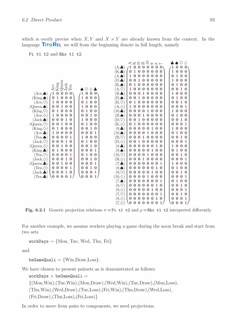
6.2 Direct Product 93
which is overly precise when X, Y and X × Y are already known from the context. In thelanguage TITUREL we will from the beginning denote in full length, namely
Pi t1 t2 and Rho t1 t2A
ceK
ing
Que
enJa
ckTen
(Ace,♠)(King,♠)(Ace,♥)
(Queen,♠)(King,♥)(Ace,♦)(Jack,♠)
(Queen,♥)(King,♦)(Ace,♣)(Ten,♠)(Jack,♥)
(Queen,♦)(King,♣)(Ten,♥)(Jack,♦)
(Queen,♣)(Ten,♦)(Jack,♣)(Ten,♣)
⎛⎜⎜⎜⎜⎜⎜⎜⎜⎜⎜⎜⎜⎜⎜⎜⎜⎜⎜⎜⎜⎜⎜⎜⎜⎜⎜⎜⎜⎜⎜⎝
1 0 0 0 00 1 0 0 01 0 0 0 00 0 1 0 00 1 0 0 01 0 0 0 00 0 0 1 00 0 1 0 00 1 0 0 01 0 0 0 00 0 0 0 10 0 0 1 00 0 1 0 00 1 0 0 00 0 0 0 10 0 0 1 00 0 1 0 00 0 0 0 10 0 0 1 00 0 0 0 1
⎞⎟⎟⎟⎟⎟⎟⎟⎟⎟⎟⎟⎟⎟⎟⎟⎟⎟⎟⎟⎟⎟⎟⎟⎟⎟⎟⎟⎟⎟⎟⎠
♠ ♥ ♦ ♣⎛⎜⎜⎜⎜⎜⎜⎜⎜⎜⎜⎜⎜⎜⎜⎜⎜⎜⎜⎜⎜⎜⎜⎜⎜⎜⎜⎜⎜⎜⎜⎝
1 0 0 01 0 0 00 1 0 01 0 0 00 1 0 00 0 1 01 0 0 00 1 0 00 0 1 00 0 0 11 0 0 00 1 0 00 0 1 00 0 0 10 1 0 00 0 1 00 0 0 10 0 1 00 0 0 10 0 0 1
⎞⎟⎟⎟⎟⎟⎟⎟⎟⎟⎟⎟⎟⎟⎟⎟⎟⎟⎟⎟⎟⎟⎟⎟⎟⎟⎟⎟⎟⎟⎟⎠
A K D B 10 9 8 7
(A,♣)(K,♣)(A,♠)(D,♣)(K,♠)(A,♥)(B,♣)(D,♠)(K,♥)(A,♦)(10,♣)(B,♠)(D,♥)(K,♦)(9,♣)
(10,♠)(B,♥)(D,♦)(8,♣)(9,♠)
(10,♥)(B,♦)(7,♣)(8,♠)(9,♥)
(10,♦)(7,♠)(8,♥)(9,♦)(7,♥)(8,♦)(7,♦)
⎛⎜⎜⎜⎜⎜⎜⎜⎜⎜⎜⎜⎜⎜⎜⎜⎜⎜⎜⎜⎜⎜⎜⎜⎜⎜⎜⎜⎜⎜⎜⎜⎜⎜⎜⎜⎜⎜⎜⎜⎜⎜⎜⎜⎜⎜⎜⎜⎜⎜⎜⎜⎜⎝
1 0 0 0 0 0 0 00 1 0 0 0 0 0 01 0 0 0 0 0 0 00 0 1 0 0 0 0 00 1 0 0 0 0 0 01 0 0 0 0 0 0 00 0 0 1 0 0 0 00 0 1 0 0 0 0 00 1 0 0 0 0 0 01 0 0 0 0 0 0 00 0 0 0 1 0 0 00 0 0 1 0 0 0 00 0 1 0 0 0 0 00 1 0 0 0 0 0 00 0 0 0 0 1 0 00 0 0 0 1 0 0 00 0 0 1 0 0 0 00 0 1 0 0 0 0 00 0 0 0 0 0 1 00 0 0 0 0 1 0 00 0 0 0 1 0 0 00 0 0 1 0 0 0 00 0 0 0 0 0 0 10 0 0 0 0 0 1 00 0 0 0 0 1 0 00 0 0 0 1 0 0 00 0 0 0 0 0 0 10 0 0 0 0 0 1 00 0 0 0 0 1 0 00 0 0 0 0 0 0 10 0 0 0 0 0 1 00 0 0 0 0 0 0 1
⎞⎟⎟⎟⎟⎟⎟⎟⎟⎟⎟⎟⎟⎟⎟⎟⎟⎟⎟⎟⎟⎟⎟⎟⎟⎟⎟⎟⎟⎟⎟⎟⎟⎟⎟⎟⎟⎟⎟⎟⎟⎟⎟⎟⎟⎟⎟⎟⎟⎟⎟⎟⎟⎠
♣ ♠ ♥ ♦⎛⎜⎜⎜⎜⎜⎜⎜⎜⎜⎜⎜⎜⎜⎜⎜⎜⎜⎜⎜⎜⎜⎜⎜⎜⎜⎜⎜⎜⎜⎜⎜⎜⎜⎜⎜⎜⎜⎜⎜⎜⎜⎜⎜⎜⎜⎜⎜⎜⎜⎜⎜⎜⎝
1 0 0 01 0 0 00 1 0 01 0 0 00 1 0 00 0 1 01 0 0 00 1 0 00 0 1 00 0 0 11 0 0 00 1 0 00 0 1 00 0 0 11 0 0 00 1 0 00 0 1 00 0 0 11 0 0 00 1 0 00 0 1 00 0 0 11 0 0 00 1 0 00 0 1 00 0 0 10 1 0 00 0 1 00 0 0 10 0 1 00 0 0 10 0 0 1
⎞⎟⎟⎟⎟⎟⎟⎟⎟⎟⎟⎟⎟⎟⎟⎟⎟⎟⎟⎟⎟⎟⎟⎟⎟⎟⎟⎟⎟⎟⎟⎟⎟⎟⎟⎟⎟⎟⎟⎟⎟⎟⎟⎟⎟⎟⎟⎟⎟⎟⎟⎟⎟⎠
Fig. 6.2.1 Generic projection relations π ≈ Pi t1 t2 and ρ ≈ Rho t1 t2 interpreted differently
For another example, we assume workers playing a game during the noon break and start fromtwo sets
workDays = Mon, Tue, Wed, Thu, Fri
and
bsGameQuali = Win,Draw,Loss.
We have chosen to present pairsets as is demonstrated as follows:
workDays × bsGameQuali =
(Mon,Win),(Tue,Win),(Mon,Draw),(Wed,Win),(Tue,Draw),(Mon,Loss),
(Thu,Win),(Wed,Draw),(Tue,Loss),(Fri,Win),(Thu,Draw),(Wed,Loss),
(Fri,Draw),(Thu,Loss),(Fri,Loss)
In order to move from pairs to components, we need projections.
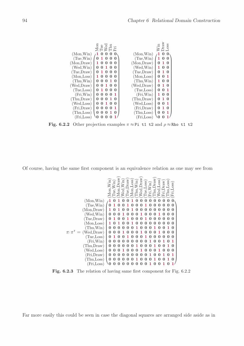
94 Chapter 6 Relational Domain Construction
Mon
Tue
Wed
Thu
Fri
(Mon,Win)(Tue,Win)
(Mon,Draw)(Wed,Win)(Tue,Draw)(Mon,Loss)(Thu,Win)
(Wed,Draw)(Tue,Loss)(Fri,Win)
(Thu,Draw)(Wed,Loss)(Fri,Draw)(Thu,Loss)(Fri,Loss)
⎛⎜⎜⎜⎜⎜⎜⎜⎜⎜⎜⎜⎜⎜⎜⎜⎜⎜⎜⎜⎜⎝
1 0 0 0 00 1 0 0 01 0 0 0 00 0 1 0 00 1 0 0 01 0 0 0 00 0 0 1 00 0 1 0 00 1 0 0 00 0 0 0 10 0 0 1 00 0 1 0 00 0 0 0 10 0 0 1 00 0 0 0 1
⎞⎟⎟⎟⎟⎟⎟⎟⎟⎟⎟⎟⎟⎟⎟⎟⎟⎟⎟⎟⎟⎠
Win
Dra
wLos
s
(Mon,Win)(Tue,Win)
(Mon,Draw)(Wed,Win)(Tue,Draw)(Mon,Loss)(Thu,Win)
(Wed,Draw)(Tue,Loss)(Fri,Win)
(Thu,Draw)(Wed,Loss)(Fri,Draw)(Thu,Loss)(Fri,Loss)
⎛⎜⎜⎜⎜⎜⎜⎜⎜⎜⎜⎜⎜⎜⎜⎜⎜⎜⎜⎜⎜⎝
1 0 01 0 00 1 01 0 00 1 00 0 11 0 00 1 00 0 11 0 00 1 00 0 10 1 00 0 10 0 1
⎞⎟⎟⎟⎟⎟⎟⎟⎟⎟⎟⎟⎟⎟⎟⎟⎟⎟⎟⎟⎟⎠
Fig. 6.2.2 Other projection examples π ≈ Pi t1 t2 and ρ ≈ Rho t1 t2
Of course, having the same first component is an equivalence relation as one may see from
π; πT =
(Mon
,Win
)(T
ue,W
in)
(Mon
,Dra
w)
(Wed
,Win
)(T
ue,D
raw
)(M
on,L
oss)
(Thu
,Win
)(W
ed,D
raw
)(T
ue,L
oss)
(Fri
,Win
)(T
hu,D
raw
)(W
ed,L
oss)
(Fri
,Dra
w)
(Thu
,Los
s)(F
ri,L
oss)
(Mon,Win)(Tue,Win)
(Mon,Draw)(Wed,Win)(Tue,Draw)(Mon,Loss)(Thu,Win)
(Wed,Draw)(Tue,Loss)(Fri,Win)
(Thu,Draw)(Wed,Loss)(Fri,Draw)(Thu,Loss)(Fri,Loss)
⎛⎜⎜⎜⎜⎜⎜⎜⎜⎜⎜⎜⎜⎜⎜⎜⎜⎜⎜⎜⎜⎝
1 0 1 0 0 1 0 0 0 0 0 0 0 0 00 1 0 0 1 0 0 0 1 0 0 0 0 0 01 0 1 0 0 1 0 0 0 0 0 0 0 0 00 0 0 1 0 0 0 1 0 0 0 1 0 0 00 1 0 0 1 0 0 0 1 0 0 0 0 0 01 0 1 0 0 1 0 0 0 0 0 0 0 0 00 0 0 0 0 0 1 0 0 0 1 0 0 1 00 0 0 1 0 0 0 1 0 0 0 1 0 0 00 1 0 0 1 0 0 0 1 0 0 0 0 0 00 0 0 0 0 0 0 0 0 1 0 0 1 0 10 0 0 0 0 0 1 0 0 0 1 0 0 1 00 0 0 1 0 0 0 1 0 0 0 1 0 0 00 0 0 0 0 0 0 0 0 1 0 0 1 0 10 0 0 0 0 0 1 0 0 0 1 0 0 1 00 0 0 0 0 0 0 0 0 1 0 0 1 0 1
⎞⎟⎟⎟⎟⎟⎟⎟⎟⎟⎟⎟⎟⎟⎟⎟⎟⎟⎟⎟⎟⎠
Fig. 6.2.3 The relation of having same first component for Fig. 6.2.2
Far more easily this could be seen in case the diagonal squares are arranged side aside as in

6.2 Direct Product 95
π; πT =
(Mon
,Win
)(M
on,D
raw
)(M
on,L
oss)
(Tue
,Win
)(T
ue,D
raw
)(T
ue,L
oss)
(Wed
,Win
)(W
ed,D
raw
)(W
ed,L
oss)
(Thu
,Win
)(T
hu,D
raw
)(T
hu,L
oss)
(Fri
,Win
)(F
ri,D
raw
)(F
ri,L
oss)
(Mon,Win)(Mon,Draw)(Mon,Loss)(Tue,Win)
(Tue,Draw)(Tue,Loss)(Wed,Win)
(Wed,Draw)(Wed,Loss)(Thu,Win)
(Thu,Draw)(Thu,Loss)(Fri,Win)
(Fri,Draw)(Fri,Loss)
⎛⎜⎜⎜⎜⎜⎜⎜⎜⎜⎜⎜⎜⎜⎜⎜⎜⎜⎜⎜⎜⎝
1 1 1 0 0 0 0 0 0 0 0 0 0 0 01 1 1 0 0 0 0 0 0 0 0 0 0 0 01 1 1 0 0 0 0 0 0 0 0 0 0 0 00 0 0 1 1 1 0 0 0 0 0 0 0 0 00 0 0 1 1 1 0 0 0 0 0 0 0 0 00 0 0 1 1 1 0 0 0 0 0 0 0 0 00 0 0 0 0 0 1 1 1 0 0 0 0 0 00 0 0 0 0 0 1 1 1 0 0 0 0 0 00 0 0 0 0 0 1 1 1 0 0 0 0 0 00 0 0 0 0 0 0 0 0 1 1 1 0 0 00 0 0 0 0 0 0 0 0 1 1 1 0 0 00 0 0 0 0 0 0 0 0 1 1 1 0 0 00 0 0 0 0 0 0 0 0 0 0 0 1 1 10 0 0 0 0 0 0 0 0 0 0 0 1 1 10 0 0 0 0 0 0 0 0 0 0 0 1 1 1
⎞⎟⎟⎟⎟⎟⎟⎟⎟⎟⎟⎟⎟⎟⎟⎟⎟⎟⎟⎟⎟⎠
Fig. 6.2.4 The relation of having the same first component for Fig. 6.2.2 rearranged
ρ; ρT =
(Mon
,Win
)(T
ue,W
in)
(Wed
,Win
)(T
hu,W
in)
(Fri
,Win
)(M
on,D
raw
)(T
ue,D
raw
)(W
ed,D
raw
)(T
hu,D
raw
)(F
ri,D
raw
)(M
on,L
oss)
(Tue
,Los
s)(W
ed,L
oss)
(Thu
,Los
s)(F
ri,L
oss)
(Mon,Win)(Tue,Win)(Wed,Win)(Thu,Win)(Fri,Win)
(Mon,Draw)(Tue,Draw)(Wed,Draw)(Thu,Draw)(Fri,Draw)(Mon,Loss)(Tue,Loss)(Wed,Loss)(Thu,Loss)(Fri,Loss)
⎛⎜⎜⎜⎜⎜⎜⎜⎜⎜⎜⎜⎜⎜⎜⎜⎜⎜⎜⎜⎜⎝
1 1 1 1 1 0 0 0 0 0 0 0 0 0 01 1 1 1 1 0 0 0 0 0 0 0 0 0 01 1 1 1 1 0 0 0 0 0 0 0 0 0 01 1 1 1 1 0 0 0 0 0 0 0 0 0 01 1 1 1 1 0 0 0 0 0 0 0 0 0 00 0 0 0 0 1 1 1 1 1 0 0 0 0 00 0 0 0 0 1 1 1 1 1 0 0 0 0 00 0 0 0 0 1 1 1 1 1 0 0 0 0 00 0 0 0 0 1 1 1 1 1 0 0 0 0 00 0 0 0 0 1 1 1 1 1 0 0 0 0 00 0 0 0 0 0 0 0 0 0 1 1 1 1 10 0 0 0 0 0 0 0 0 0 1 1 1 1 10 0 0 0 0 0 0 0 0 0 1 1 1 1 10 0 0 0 0 0 0 0 0 0 1 1 1 1 10 0 0 0 0 0 0 0 0 0 1 1 1 1 1
⎞⎟⎟⎟⎟⎟⎟⎟⎟⎟⎟⎟⎟⎟⎟⎟⎟⎟⎟⎟⎟⎠
Fig. 6.2.5 The relation of having the same second component for Fig. 6.2.2 rearranged
As we conceive basesets as ordered entities, we have to decide for the ordering of the Cartesianproduct of two basesets. The most immediate way would be rowwise which gives nice andintuitive projection matrices as in

96 Chapter 6 Relational Domain Construction
Ace
Kin
gQ
ueen
Jack
Ten
π =
(Ace,♠)(Ace,♥)(Ace,♦)(Ace,♣)
(King,♠)(King,♥)(King,♦)(King,♣)
(Queen,♠)(Queen,♥)(Queen,♦)(Queen,♣)
(Jack,♠)(Jack,♥)(Jack,♦)(Jack,♣)(Ten,♠)(Ten,♥)(Ten,♦)(Ten,♣)
⎛⎜⎜⎜⎜⎜⎜⎜⎜⎜⎜⎜⎜⎜⎜⎜⎜⎜⎜⎜⎜⎜⎜⎜⎜⎜⎜⎜⎜⎜⎜⎝
1 0 0 0 01 0 0 0 01 0 0 0 01 0 0 0 00 1 0 0 00 1 0 0 00 1 0 0 00 1 0 0 00 0 1 0 00 0 1 0 00 0 1 0 00 0 1 0 00 0 0 1 00 0 0 1 00 0 0 1 00 0 0 1 00 0 0 0 10 0 0 0 10 0 0 0 10 0 0 0 1
⎞⎟⎟⎟⎟⎟⎟⎟⎟⎟⎟⎟⎟⎟⎟⎟⎟⎟⎟⎟⎟⎟⎟⎟⎟⎟⎟⎟⎟⎟⎟⎠
♠ ♥ ♦ ♣
ρ =
(Ace,♠)(Ace,♥)(Ace,♦)(Ace,♣)
(King,♠)(King,♥)(King,♦)(King,♣)
(Queen,♠)(Queen,♥)(Queen,♦)(Queen,♣)
(Jack,♠)(Jack,♥)(Jack,♦)(Jack,♣)(Ten,♠)(Ten,♥)(Ten,♦)(Ten,♣)
⎛⎜⎜⎜⎜⎜⎜⎜⎜⎜⎜⎜⎜⎜⎜⎜⎜⎜⎜⎜⎜⎜⎜⎜⎜⎜⎜⎜⎜⎜⎜⎝
1 0 0 00 1 0 00 0 1 00 0 0 11 0 0 00 1 0 00 0 1 00 0 0 11 0 0 00 1 0 00 0 1 00 0 0 11 0 0 00 1 0 00 0 1 00 0 0 11 0 0 00 1 0 00 0 1 00 0 0 1
⎞⎟⎟⎟⎟⎟⎟⎟⎟⎟⎟⎟⎟⎟⎟⎟⎟⎟⎟⎟⎟⎟⎟⎟⎟⎟⎟⎟⎟⎟⎟⎠
Fig. 6.2.6 Projection when the product is ordered rowwisely
But this immediate form has a drawback, so that we decided for a second one as a resultof Cantor’s diagonal enumeration. This diagonal-oriented sequence seems rather difficult tohandle; it allows to a certain extent to visualize the pairset when non-finite sets are involved.
The sequence of presenting its elements is depicted in the following diagonal schema:
Win
Dra
w
Los
s
MonTueWedThuFri
⎛⎜⎜⎜⎝
1 3 62 5 94 8 127 11 1410 13 15
⎞⎟⎟⎟⎠
Fig. 6.2.7 Enumeration scheme for a direct product
1 2 3 4 5 6 7 . . .
a
b
c
d
e
(a,1) (a,2)
(b,1)
(c,1)
(b,2)
(a,3) (a,4) (a,5) (a,6)
(b,3) (b,4) (b,5)
(c,2) (c,3) (c,4)
(d,1) (d,2) (d,3)
(e,1) (e,2) . . .
Fig. 6.2.8 Exhaustion of an infinite pair set
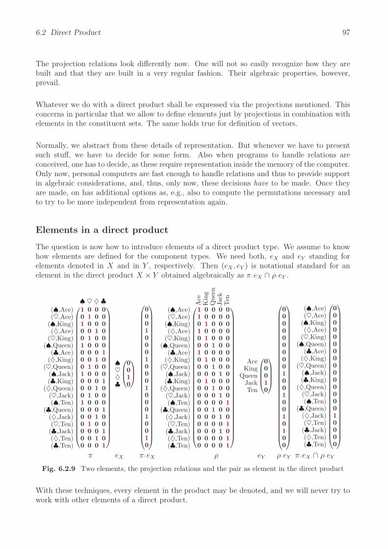
6.2 Direct Product 97
The projection relations look differently now. One will not so easily recognize how they arebuilt and that they are built in a very regular fashion. Their algebraic properties, however,prevail.
Whatever we do with a direct product shall be expressed via the projections mentioned. Thisconcerns in particular that we allow to define elements just by projections in combination withelements in the constituent sets. The same holds true for definition of vectors.
Normally, we abstract from these details of representation. But whenever we have to presentsuch stuff, we have to decide for some form. Also when programs to handle relations areconceived, one has to decide, as these require representation inside the memory of the computer.Only now, personal computers are fast enough to handle relations and thus to provide supportin algebraic considerations, and, thus, only now, these decisions have to be made. Once theyare made, on has additional options as, e.g., also to compute the permutations necessary andto try to be more independent from representation again.
Elements in a direct product
The question is now how to introduce elements of a direct product type. We assume to knowhow elements are defined for the component types. We need both, eX and eY standing forelements denoted in X and in Y , respectively. Then (eX , eY ) is notational standard for anelement in the direct product X × Y obtained algebraically as π; eX ∩ ρ; eY .
♠ ♥ ♦ ♣(♠,Ace)(♥,Ace)
(♠,King)(♦,Ace)
(♥,King)(♠,Queen)
(♣,Ace)(♦,King)
(♥,Queen)(♠,Jack)(♣,King)
(♦,Queen)(♥,Jack)(♠,Ten)
(♣,Queen)(♦,Jack)(♥,Ten)(♣,Jack)(♦,Ten)(♣,Ten)
⎛⎜⎜⎜⎜⎜⎜⎜⎜⎜⎜⎜⎜⎜⎜⎜⎜⎜⎜⎜⎜⎜⎜⎜⎜⎜⎜⎜⎜⎜⎜⎝
1 0 0 00 1 0 01 0 0 00 0 1 00 1 0 01 0 0 00 0 0 10 0 1 00 1 0 01 0 0 00 0 0 10 0 1 00 1 0 01 0 0 00 0 0 10 0 1 00 1 0 00 0 0 10 0 1 00 0 0 1
⎞⎟⎟⎟⎟⎟⎟⎟⎟⎟⎟⎟⎟⎟⎟⎟⎟⎟⎟⎟⎟⎟⎟⎟⎟⎟⎟⎟⎟⎟⎟⎠
π
♠♥♦♣
⎛⎜⎝
0010
⎞⎟⎠
eX
⎛⎜⎜⎜⎜⎜⎜⎜⎜⎜⎜⎜⎜⎜⎜⎜⎜⎜⎜⎜⎜⎜⎜⎜⎜⎜⎜⎜⎜⎜⎜⎜⎝
00010001000100010010
⎞⎟⎟⎟⎟⎟⎟⎟⎟⎟⎟⎟⎟⎟⎟⎟⎟⎟⎟⎟⎟⎟⎟⎟⎟⎟⎟⎟⎟⎟⎟⎟⎠
π; eX
Ace
Kin
gQ
ueen
Jack
Ten
(♠,Ace)(♥,Ace)
(♠,King)(♦,Ace)
(♥,King)(♠,Queen)
(♣,Ace)(♦,King)
(♥,Queen)(♠,Jack)(♣,King)
(♦,Queen)(♥,Jack)(♠,Ten)
(♣,Queen)(♦,Jack)(♥,Ten)(♣,Jack)(♦,Ten)(♣,Ten)
⎛⎜⎜⎜⎜⎜⎜⎜⎜⎜⎜⎜⎜⎜⎜⎜⎜⎜⎜⎜⎜⎜⎜⎜⎜⎜⎜⎜⎜⎜⎜⎝
1 0 0 0 01 0 0 0 00 1 0 0 01 0 0 0 00 1 0 0 00 0 1 0 01 0 0 0 00 1 0 0 00 0 1 0 00 0 0 1 00 1 0 0 00 0 1 0 00 0 0 1 00 0 0 0 10 0 1 0 00 0 0 1 00 0 0 0 10 0 0 1 00 0 0 0 10 0 0 0 1
⎞⎟⎟⎟⎟⎟⎟⎟⎟⎟⎟⎟⎟⎟⎟⎟⎟⎟⎟⎟⎟⎟⎟⎟⎟⎟⎟⎟⎟⎟⎟⎠
ρ
AceKing
QueenJackTen
⎛⎜⎜⎜⎝
00010
⎞⎟⎟⎟⎠
eY
⎛⎜⎜⎜⎜⎜⎜⎜⎜⎜⎜⎜⎜⎜⎜⎜⎜⎜⎜⎜⎜⎜⎜⎜⎜⎜⎜⎜⎜⎜⎜⎜⎝
00000000010010010100
⎞⎟⎟⎟⎟⎟⎟⎟⎟⎟⎟⎟⎟⎟⎟⎟⎟⎟⎟⎟⎟⎟⎟⎟⎟⎟⎟⎟⎟⎟⎟⎟⎠
ρ; eY
(♠,Ace)(♥,Ace)
(♠,King)(♦,Ace)
(♥,King)(♠,Queen)
(♣,Ace)(♦,King)
(♥,Queen)(♠,Jack)(♣,King)
(♦,Queen)(♥,Jack)(♠,Ten)
(♣,Queen)(♦,Jack)(♥,Ten)(♣,Jack)(♦,Ten)(♣,Ten)
⎛⎜⎜⎜⎜⎜⎜⎜⎜⎜⎜⎜⎜⎜⎜⎜⎜⎜⎜⎜⎜⎜⎜⎜⎜⎜⎜⎜⎜⎜⎜⎜⎝
00000000000000010000
⎞⎟⎟⎟⎟⎟⎟⎟⎟⎟⎟⎟⎟⎟⎟⎟⎟⎟⎟⎟⎟⎟⎟⎟⎟⎟⎟⎟⎟⎟⎟⎟⎠
π; eX ∩ ρ; eY
Fig. 6.2.9 Two elements, the projection relations and the pair as element in the direct product
With these techniques, every element in the product may be denoted, and we will never try towork with other elements of a direct product.
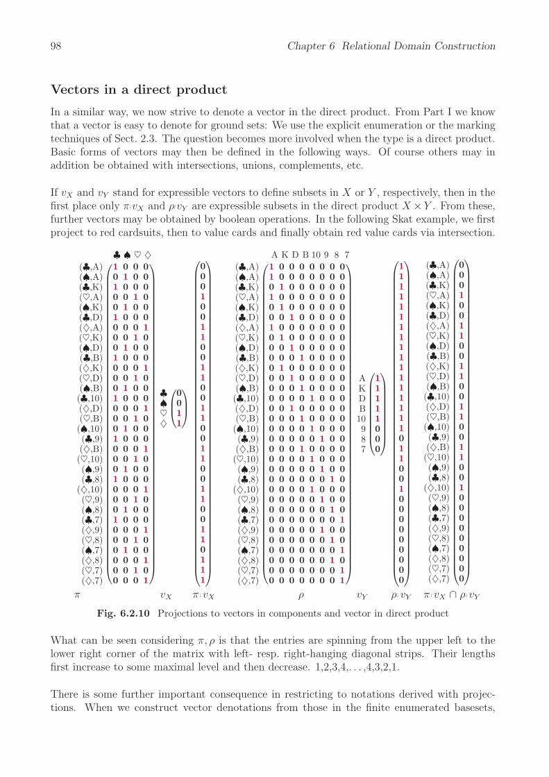
98 Chapter 6 Relational Domain Construction
Vectors in a direct product
In a similar way, we now strive to denote a vector in the direct product. From Part I we knowthat a vector is easy to denote for ground sets: We use the explicit enumeration or the markingtechniques of Sect. 2.3. The question becomes more involved when the type is a direct product.Basic forms of vectors may then be defined in the following ways. Of course others may inaddition be obtained with intersections, unions, complements, etc.
If vX and vY stand for expressible vectors to define subsets in X or Y , respectively, then in thefirst place only π;vX and ρ;vY are expressible subsets in the direct product X ×Y . From these,further vectors may be obtained by boolean operations. In the following Skat example, we firstproject to red cardsuits, then to value cards and finally obtain red value cards via intersection.
♣ ♠ ♥ ♦(♣,A)(♠,A)(♣,K)(♥,A)(♠,K)(♣,D)(♦,A)(♥,K)(♠,D)(♣,B)(♦,K)(♥,D)(♠,B)(♣,10)(♦,D)(♥,B)(♠,10)(♣,9)(♦,B)(♥,10)(♠,9)(♣,8)
(♦,10)(♥,9)(♠,8)(♣,7)(♦,9)(♥,8)(♠,7)(♦,8)(♥,7)(♦,7)
⎛⎜⎜⎜⎜⎜⎜⎜⎜⎜⎜⎜⎜⎜⎜⎜⎜⎜⎜⎜⎜⎜⎜⎜⎜⎜⎜⎜⎜⎜⎜⎜⎜⎜⎜⎜⎜⎜⎜⎜⎜⎜⎜⎜⎜⎜⎜⎜⎜⎜⎜⎜⎜⎝
1 0 0 00 1 0 01 0 0 00 0 1 00 1 0 01 0 0 00 0 0 10 0 1 00 1 0 01 0 0 00 0 0 10 0 1 00 1 0 01 0 0 00 0 0 10 0 1 00 1 0 01 0 0 00 0 0 10 0 1 00 1 0 01 0 0 00 0 0 10 0 1 00 1 0 01 0 0 00 0 0 10 0 1 00 1 0 00 0 0 10 0 1 00 0 0 1
⎞⎟⎟⎟⎟⎟⎟⎟⎟⎟⎟⎟⎟⎟⎟⎟⎟⎟⎟⎟⎟⎟⎟⎟⎟⎟⎟⎟⎟⎟⎟⎟⎟⎟⎟⎟⎟⎟⎟⎟⎟⎟⎟⎟⎟⎟⎟⎟⎟⎟⎟⎟⎟⎠
π
♣♠♥♦
⎛⎜⎝
0011
⎞⎟⎠
vX
⎛⎜⎜⎜⎜⎜⎜⎜⎜⎜⎜⎜⎜⎜⎜⎜⎜⎜⎜⎜⎜⎜⎜⎜⎜⎜⎜⎜⎜⎜⎜⎜⎜⎜⎜⎜⎜⎜⎜⎜⎜⎜⎜⎜⎜⎜⎜⎜⎜⎜⎜⎜⎜⎜⎝
00010011001100110011001100110111
⎞⎟⎟⎟⎟⎟⎟⎟⎟⎟⎟⎟⎟⎟⎟⎟⎟⎟⎟⎟⎟⎟⎟⎟⎟⎟⎟⎟⎟⎟⎟⎟⎟⎟⎟⎟⎟⎟⎟⎟⎟⎟⎟⎟⎟⎟⎟⎟⎟⎟⎟⎟⎟⎟⎠
π; vX
A K D B 10 9 8 7(♣,A)(♠,A)(♣,K)(♥,A)(♠,K)(♣,D)(♦,A)(♥,K)(♠,D)(♣,B)(♦,K)(♥,D)(♠,B)(♣,10)(♦,D)(♥,B)(♠,10)(♣,9)(♦,B)(♥,10)(♠,9)(♣,8)
(♦,10)(♥,9)(♠,8)(♣,7)(♦,9)(♥,8)(♠,7)(♦,8)(♥,7)(♦,7)
⎛⎜⎜⎜⎜⎜⎜⎜⎜⎜⎜⎜⎜⎜⎜⎜⎜⎜⎜⎜⎜⎜⎜⎜⎜⎜⎜⎜⎜⎜⎜⎜⎜⎜⎜⎜⎜⎜⎜⎜⎜⎜⎜⎜⎜⎜⎜⎜⎜⎜⎜⎜⎜⎝
1 0 0 0 0 0 0 01 0 0 0 0 0 0 00 1 0 0 0 0 0 01 0 0 0 0 0 0 00 1 0 0 0 0 0 00 0 1 0 0 0 0 01 0 0 0 0 0 0 00 1 0 0 0 0 0 00 0 1 0 0 0 0 00 0 0 1 0 0 0 00 1 0 0 0 0 0 00 0 1 0 0 0 0 00 0 0 1 0 0 0 00 0 0 0 1 0 0 00 0 1 0 0 0 0 00 0 0 1 0 0 0 00 0 0 0 1 0 0 00 0 0 0 0 1 0 00 0 0 1 0 0 0 00 0 0 0 1 0 0 00 0 0 0 0 1 0 00 0 0 0 0 0 1 00 0 0 0 1 0 0 00 0 0 0 0 1 0 00 0 0 0 0 0 1 00 0 0 0 0 0 0 10 0 0 0 0 1 0 00 0 0 0 0 0 1 00 0 0 0 0 0 0 10 0 0 0 0 0 1 00 0 0 0 0 0 0 10 0 0 0 0 0 0 1
⎞⎟⎟⎟⎟⎟⎟⎟⎟⎟⎟⎟⎟⎟⎟⎟⎟⎟⎟⎟⎟⎟⎟⎟⎟⎟⎟⎟⎟⎟⎟⎟⎟⎟⎟⎟⎟⎟⎟⎟⎟⎟⎟⎟⎟⎟⎟⎟⎟⎟⎟⎟⎟⎠
ρ
AKDB10987
⎛⎜⎜⎜⎜⎜⎜⎜⎜⎜⎝
11111000
⎞⎟⎟⎟⎟⎟⎟⎟⎟⎟⎠
vY
⎛⎜⎜⎜⎜⎜⎜⎜⎜⎜⎜⎜⎜⎜⎜⎜⎜⎜⎜⎜⎜⎜⎜⎜⎜⎜⎜⎜⎜⎜⎜⎜⎜⎜⎜⎜⎜⎜⎜⎜⎜⎜⎜⎜⎜⎜⎜⎜⎜⎜⎜⎜⎜⎜⎝
11111111111111111011001000000000
⎞⎟⎟⎟⎟⎟⎟⎟⎟⎟⎟⎟⎟⎟⎟⎟⎟⎟⎟⎟⎟⎟⎟⎟⎟⎟⎟⎟⎟⎟⎟⎟⎟⎟⎟⎟⎟⎟⎟⎟⎟⎟⎟⎟⎟⎟⎟⎟⎟⎟⎟⎟⎟⎟⎠
ρ; vY
(♣,A)(♠,A)(♣,K)(♥,A)(♠,K)(♣,D)(♦,A)(♥,K)(♠,D)(♣,B)(♦,K)(♥,D)(♠,B)(♣,10)(♦,D)(♥,B)(♠,10)(♣,9)(♦,B)(♥,10)(♠,9)(♣,8)
(♦,10)(♥,9)(♠,8)(♣,7)(♦,9)(♥,8)(♠,7)(♦,8)(♥,7)(♦,7)
⎛⎜⎜⎜⎜⎜⎜⎜⎜⎜⎜⎜⎜⎜⎜⎜⎜⎜⎜⎜⎜⎜⎜⎜⎜⎜⎜⎜⎜⎜⎜⎜⎜⎜⎜⎜⎜⎜⎜⎜⎜⎜⎜⎜⎜⎜⎜⎜⎜⎜⎜⎜⎜⎜⎝
00010011001100110011001000000000
⎞⎟⎟⎟⎟⎟⎟⎟⎟⎟⎟⎟⎟⎟⎟⎟⎟⎟⎟⎟⎟⎟⎟⎟⎟⎟⎟⎟⎟⎟⎟⎟⎟⎟⎟⎟⎟⎟⎟⎟⎟⎟⎟⎟⎟⎟⎟⎟⎟⎟⎟⎟⎟⎟⎠
π; vX ∩ ρ; vY
Fig. 6.2.10 Projections to vectors in components and vector in direct product
What can be seen considering π, ρ is that the entries are spinning from the upper left to thelower right corner of the matrix with left- resp. right-hanging diagonal strips. Their lengthsfirst increase to some maximal level and then decrease. 1,2,3,4,. . . ,4,3,2,1.
There is some further important consequence in restricting to notations derived with projec-tions. When we construct vector denotations from those in the finite enumerated basesets,

6.2 Direct Product 99
we cannot assume to formulate arbitrarily complex sets in the product, e.g. Rather, we arerestricted to the constructions that are offered1.
Relations starting or ending in a direct product
Let two relations R : U −→ W and S : V −→ W be given, i.e., with the same codomain. Thenit is typical to construct the relations π ; R : U × V −→ W and ρ; S : U × V −→ W startingfrom the direct product of domains. From these, others such as π;R ∩ ρ;S, may be built usingboolean operators.
Bild, Matrizen, Striktheit
In a rather similar way we build relations with the same domain ending in a direct product.Let two relations R : U −→ V and S : U −→ W be given, i.e., with the same domain. Then itis typical to construct the relations R;πT : U −→ V ×W and S;ρT : U −→ V ×W ending in thedirect product. From these further relations such as R; πT ∪ S ; ρT may be built using booleanoperators. A standard way of construction is the well-known fork operator
R∇S : U −→ V × W as R∇S := R; πT ∩ S ; ρT.diagram + matrices
Algebraic properties of the generic projection relations
Product definitions have long been investigated by relation algebraists and computer scientists.A considerable part of [TG87] is devoted to various aspects of that. The concept of a productshould cover both aspects, Cartesian product as product of sets combined with tupeling (some-times called construction) as product of operations. The following definition of a direct productproduces a Cartesian product of sets that is characterized in an essentially unique way2.
We observe that whatever projection version we decide for, it will satisfy the algebraic rules ofthe following definition. Once this had been observed, mathematicians turned it around andasked whether this was characteristic for projections — and it is.
6.2.1 Definition. If any two heterogeneous relations π, ρ with common domain are given,they are said to form a direct product if
πT; π = , ρT; ρ = , π; πT ∩ ρ; ρT = , πT; ρ = .
In particular, π, ρ are mappings, usually called projections.
It would even suffice to require only πT ; π ⊆ . Interpreting the condition π; πT ∩ ρ; ρT ⊆ inthe case of two sets A, B and their Cartesian product A × B, it ensures that there is at mostone pair with given images in A and B. In addition, “= ” means that π, ρ are total, i.e., thatthere are no “unprojected pairs”. Finally, the condition πT;ρ = implies that for every elementin A and every element in B there exists a pair in A × B.
1Pretending to be able to work with arbitrary subsets of a set of 250 elements, e.g., is really ridiculous. Thisis one of the crimes even educated computer scientists routinely commit. There is no way to denote more thanjust a tiny percentage of these.
2We avoid here to speak of “up to isomorphism”, which would be the mathematically correct form. In thischapter, we try to convince the reader and we give visual help, not yet fully formal proofs.
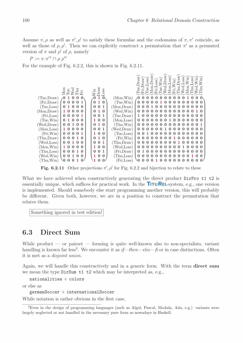
100 Chapter 6 Relational Domain Construction
Assume π, ρ as well as π′, ρ′ to satisfy these formulae and the codomains of π, π′ coincide, aswell as those of ρ, ρ′. Then we can explicitly construct a permutation that π′ as a permutedversion of π and ρ′ of ρ, namely
P := π; π′T ∩ ρ; ρ′T
For the example of Fig. 6.2.2, this is shown in Fig. 6.2.11.M
onTue
Wed
Thu
Fri
(Tue,Draw)(Fri,Draw)(Tue,Loss)
(Mon,Draw)(Fri,Loss)
(Tue,Win)(Wed,Draw)(Mon,Loss)
(Fri,Win)(Thu,Draw)(Wed,Loss)(Mon,Win)(Thu,Loss)(Wed,Win)(Thu,Win)
⎛⎜⎜⎜⎜⎜⎜⎜⎜⎜⎜⎜⎜⎜⎜⎜⎜⎜⎜⎜⎜⎝
0 1 0 0 00 0 0 0 10 1 0 0 01 0 0 0 00 0 0 0 10 1 0 0 00 0 1 0 01 0 0 0 00 0 0 0 10 0 0 1 00 0 1 0 01 0 0 0 00 0 0 1 00 0 1 0 00 0 0 1 0
⎞⎟⎟⎟⎟⎟⎟⎟⎟⎟⎟⎟⎟⎟⎟⎟⎟⎟⎟⎟⎟⎠
Win
Dra
wLos
s⎛⎜⎜⎜⎜⎜⎜⎜⎜⎜⎜⎜⎜⎜⎜⎜⎜⎜⎜⎜⎜⎝
0 1 00 1 00 0 10 1 00 0 11 0 00 1 00 0 11 0 00 1 00 0 11 0 00 0 11 0 01 0 0
⎞⎟⎟⎟⎟⎟⎟⎟⎟⎟⎟⎟⎟⎟⎟⎟⎟⎟⎟⎟⎟⎠
(Tue
,Dra
w)
(Fri
,Dra
w)
(Tue
,Los
s)(M
on,D
raw
)(F
ri,L
oss)
(Tue
,Win
)(W
ed,D
raw
)(M
on,L
oss)
(Fri
,Win
)(T
hu,D
raw
)(W
ed,L
oss)
(Mon
,Win
)(T
hu,L
oss)
(Wed
,Win
)(T
hu,W
in)
(Mon,Win)(Tue,Win)
(Mon,Draw)(Wed,Win)(Tue,Draw)(Mon,Loss)(Thu,Win)
(Wed,Draw)(Tue,Loss)(Fri,Win)
(Thu,Draw)(Wed,Loss)(Fri,Draw)(Thu,Loss)(Fri,Loss)
⎛⎜⎜⎜⎜⎜⎜⎜⎜⎜⎜⎜⎜⎜⎜⎜⎜⎜⎜⎜⎜⎝
0 0 0 0 0 0 0 0 0 0 0 1 0 0 00 0 0 0 0 1 0 0 0 0 0 0 0 0 00 0 0 1 0 0 0 0 0 0 0 0 0 0 00 0 0 0 0 0 0 0 0 0 0 0 0 1 01 0 0 0 0 0 0 0 0 0 0 0 0 0 00 0 0 0 0 0 0 1 0 0 0 0 0 0 00 0 0 0 0 0 0 0 0 0 0 0 0 0 10 0 0 0 0 0 1 0 0 0 0 0 0 0 00 0 1 0 0 0 0 0 0 0 0 0 0 0 00 0 0 0 0 0 0 0 1 0 0 0 0 0 00 0 0 0 0 0 0 0 0 1 0 0 0 0 00 0 0 0 0 0 0 0 0 0 1 0 0 0 00 1 0 0 0 0 0 0 0 0 0 0 0 0 00 0 0 0 0 0 0 0 0 0 0 0 1 0 00 0 0 0 1 0 0 0 0 0 0 0 0 0 0
⎞⎟⎟⎟⎟⎟⎟⎟⎟⎟⎟⎟⎟⎟⎟⎟⎟⎟⎟⎟⎟⎠
Fig. 6.2.11 Other projections π′, ρ′ for Fig. 6.2.2 and bijection to relate to these
What we have achieved when constructively generating the direct product DirPro t1 t2 isessentially unique, which suffices for practical work. In the TITUREL-system, e.g., one versionis implemented. Should somebody else start programming another version, this will probablybe different. Given both, however, we are in a position to construct the permutation thatrelates them.
Something ignored in test edition!
6.3 Direct Sum
While product — or pairset — forming is quite well-known also to non-specialists, varianthandling is known far less3. We encounter it as if—then—else—fi or in case distinctions. Oftenit is met as a disjoint union.
Again, we will handle this constructively and in a generic form. With the term direct sumwe mean the type DirSum t1 t2 which may be interpreted as, e.g.,
nationalities + colors
or else asgermanSoccer + internationalSoccer
While notation is rather obvious in the first case,
3Even in the design of programming languages (such as Algol, Pascal, Modula, Ada, e.g.) variants werelargely neglected or not handled in the necessary pure form as nowadays in Haskell.

6.3 Direct Sum 101
nationalities + colors =
American,French,German,British,Spanish,red,green,blue,orange,
we have to take care for overlapping element notations in the second:
germanSoccer + internationalSoccer =[Bayern Munchen<,
>Arsenal London,Borussia Dortmund<,
>FC Chelsea,>Austria Wien,
>Juventus Turin,Werder Bremen<,
>Manchester United,Schalke 04<,
>Bayern Munchen,Bayer Leverkusen<,
>Borussia Dortmund,>FC Liverpool,
>Ajax Amsterdam,VfB Stuttgart<,
>Real Madrid,>Olympique Lyon,
>FC Porto]
Borussia Dortmund was formerly considered as a German soccer team as well as an interna-tional soccer team. It is wise to keep these two concepts separate. One will therefore introducesome piece of notation to make clear from which side the elements come. Here, we have chosenangle marks. Whenever the two sets are disjoint, we will not use these marks.
There is one further point to observe. In some examples sets will be infinite. In such cases itwould be boring to see elements of just the first set infinitely often before any element of thesecond shows up. The procedure of showing elements has to be interrupted anyway. In orderto see elements from both variants and so to get an increasing impression of the variant set, wehave chosen to show elements of the two variants alternately.
Injections
The constructive generation of the direct sum DirSum t1 t2 out of types t1, t2 is achievedwith the two generic constructs
Iota t1 t2 and Kappa t1 t2
In a mathematical text, we will use the sloppier form ι, κ, or sometimes ι : X −→ X + Y andκ : Y −→ X + Y . Fig. 6.3.1 shows an example interpretation of injections.

102 Chapter 6 Relational Domain Construction
ι =♠ M
on♥ Tue ♦ Wed
♣ Thu
Fri
Sat
Sun
♠♥♦♣
⎛⎜⎝
1 0 0 0 0 0 0 0 0 0 00 0 1 0 0 0 0 0 0 0 00 0 0 0 1 0 0 0 0 0 00 0 0 0 0 0 1 0 0 0 0
⎞⎟⎠ κ =
♠ Mon
♥ Tue ♦ Wed
♣ Thu
Fri
Sat
Sun
MonTueWedThuFriSatSun
⎛⎜⎜⎜⎜⎜⎜⎝
0 1 0 0 0 0 0 0 0 0 00 0 0 1 0 0 0 0 0 0 00 0 0 0 0 1 0 0 0 0 00 0 0 0 0 0 0 1 0 0 00 0 0 0 0 0 0 0 1 0 00 0 0 0 0 0 0 0 0 1 00 0 0 0 0 0 0 0 0 0 1
⎞⎟⎟⎟⎟⎟⎟⎠
Fig. 6.3.1 Injection relations ι ≈ Iota t1 t2 and κ ≈ Kappa t1 t2
Elements in a direct sum
We need either eX denoting an element in X or eY denoting an element in Y . Then ι(eX) orκ(eY ), respectively, denote an element in the direct sum X + Y when denoting traditionallywith injection mappings. As an example we consider the direct sum of Bridge suits and Bridgehonour cards, thereby switching to relational notation
ιT; eX and κT; eY
eX =
♠♥♦♣
⎛⎜⎝
0010
⎞⎟⎠
♠ Ace ♥ Kin
g♦ Q
ueen
♣ Jack
Ten
ι =
⎛⎜⎝
1 0 0 0 0 0 0 0 00 0 1 0 0 0 0 0 00 0 0 0 1 0 0 0 00 0 0 0 0 0 1 0 0
⎞⎟⎠ eY =
AceKing
QueenJackTen
⎛⎜⎜⎜⎝
00010
⎞⎟⎟⎟⎠
♠ Ace ♥ Kin
g♦ Q
ueen
♣ Jack
Ten
κ =
⎛⎜⎜⎝
0 1 0 0 0 0 0 0 00 0 0 1 0 0 0 0 00 0 0 0 0 1 0 0 00 0 0 0 0 0 0 1 00 0 0 0 0 0 0 0 1
⎞⎟⎟⎠
(0 0 0 0 1 0 0 0 0)= eTX
; ι eTY
; κ = (0 0 0 0 0 0 0 1 0)
Fig. 6.3.2 An element, the injection relations and the injected elements as row vectors
The elements ιT;eX and κT;eY in the direct sum are shown horizontally just for reasons of space.
Vectors in a direct sum
If vX and vY stand for two expressible vectors in X or Y , respectively, then in the first placeonly ι(vX) or κ(vY ) are expressible vectors in the direct sum X +Y . This is based on injectionsconceived as mappings and their usual notation. We may, however, also denote this as ιT ; vX
and κT;vY in a relational environment. In the example we have the set of red suits first amongall four suits and then among the direct sum of suits plus value-carrying cards in the game ofSkat. The rightmost column shows a union of such vectors.
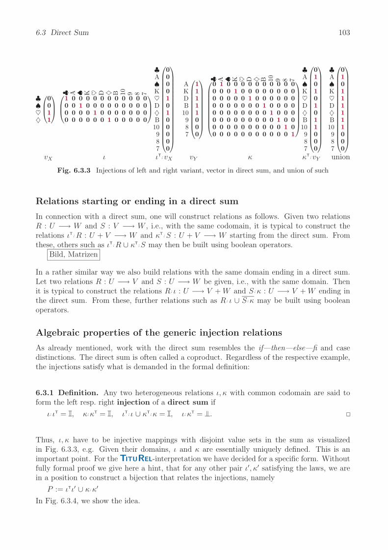
6.3 Direct Sum 103
♣♠♥♦
⎛⎜⎝
0011
⎞⎟⎠
♣ A ♠ K ♥ D ♦ B 10 9 8 7⎛⎜⎝
1 0 0 0 0 0 0 0 0 0 0 00 0 1 0 0 0 0 0 0 0 0 00 0 0 0 1 0 0 0 0 0 0 00 0 0 0 0 0 1 0 0 0 0 0
⎞⎟⎠
♣A♠K♥D♦B10987
⎛⎜⎜⎜⎜⎜⎜⎜⎜⎜⎜⎜⎜⎜⎜⎜⎜⎝
000010100000
⎞⎟⎟⎟⎟⎟⎟⎟⎟⎟⎟⎟⎟⎟⎟⎟⎟⎠
AKDB10987
⎛⎜⎜⎜⎜⎜⎜⎜⎜⎜⎝
11111000
⎞⎟⎟⎟⎟⎟⎟⎟⎟⎟⎠
♣ A ♠ K ♥ D ♦ B 10 9 8 7⎛⎜⎜⎜⎜⎜⎜⎜⎜⎝
0 1 0 0 0 0 0 0 0 0 0 00 0 0 1 0 0 0 0 0 0 0 00 0 0 0 0 1 0 0 0 0 0 00 0 0 0 0 0 0 1 0 0 0 00 0 0 0 0 0 0 0 1 0 0 00 0 0 0 0 0 0 0 0 1 0 00 0 0 0 0 0 0 0 0 0 1 00 0 0 0 0 0 0 0 0 0 0 1
⎞⎟⎟⎟⎟⎟⎟⎟⎟⎠
♣A♠K♥D♦B10987
⎛⎜⎜⎜⎜⎜⎜⎜⎜⎜⎜⎜⎜⎜⎜⎜⎜⎝
010101011000
⎞⎟⎟⎟⎟⎟⎟⎟⎟⎟⎟⎟⎟⎟⎟⎟⎟⎠
♣A♠K♥D♦B10987
⎛⎜⎜⎜⎜⎜⎜⎜⎜⎜⎜⎜⎜⎜⎜⎜⎜⎝
010111111000
⎞⎟⎟⎟⎟⎟⎟⎟⎟⎟⎟⎟⎟⎟⎟⎟⎟⎠
vX ι ιT; vX vY κ κT; vY union
Fig. 6.3.3 Injections of left and right variant, vector in direct sum, and union of such
Relations starting or ending in a direct sum
In connection with a direct sum, one will construct relations as follows. Given two relationsR : U −→ W and S : V −→ W , i.e., with the same codomain, it is typical to construct therelations ιT ; R : U + V −→ W and κT ; S : U + V −→ W starting from the direct sum. Fromthese, others such as ιT; R ∪ κT; S may then be built using boolean operators.
Bild, Matrizen
In a rather similar way we also build relations with the same domain ending in a direct sum.Let two relations R : U −→ V and S : U −→ W be given, i.e., with the same domain. Thenit is typical to construct the relations R; ι : U −→ V + W and S ; κ : U −→ V + W ending inthe direct sum. From these, further relations such as R ; ι ∪ S ; κ may be built using booleanoperators.
Algebraic properties of the generic injection relations
As already mentioned, work with the direct sum resembles the if—then—else—fi and casedistinctions. The direct sum is often called a coproduct. Regardless of the respective example,the injections satisfy what is demanded in the formal definition:
6.3.1 Definition. Any two heterogeneous relations ι, κ with common codomain are said toform the left resp. right injection of a direct sum if
ι; ιT = , κ; κT = , ιT; ι ∪ κT; κ = , ι; κT = .
Thus, ι, κ have to be injective mappings with disjoint value sets in the sum as visualizedin Fig. 6.3.3, e.g. Given their domains, ι and κ are essentially uniquely defined. This is animportant point. For the TITUREL-interpretation we have decided for a specific form. Withoutfully formal proof we give here a hint, that for any other pair ι′, κ′ satisfying the laws, we arein a position to construct a bijection that relates the injections, namely
P := ιTι′ ∪ κ; κ′
In Fig. 6.3.4, we show the idea.

104 Chapter 6 Relational Domain Construction
♥ Kin
g♣ Ten ♠ Ace ♦ Que
enJa
ck
♠♥♦♣
⎛⎜⎝
0 0 0 0 1 0 0 0 01 0 0 0 0 0 0 0 00 0 0 0 0 0 1 0 00 0 1 0 0 0 0 0 0
⎞⎟⎠
♥ Kin
g♣ Ten ♠ Ace ♦ Que
enJa
ck
AceKing
QueenJackTen
⎛⎜⎜⎝
0 0 0 0 0 1 0 0 00 1 0 0 0 0 0 0 00 0 0 0 0 0 0 1 00 0 0 0 0 0 0 0 10 0 0 1 0 0 0 0 0
⎞⎟⎟⎠
♥ Kin
g♣ Ten ♠ Ace ♦ Que
enJa
ck
♠Ace♥
King♦
Queen♣
JackTen
⎛⎜⎜⎜⎜⎜⎜⎜⎜⎜⎝
0 0 0 0 1 0 0 0 00 0 0 0 0 1 0 0 01 0 0 0 0 0 0 0 00 1 0 0 0 0 0 0 00 0 0 0 0 0 1 0 00 0 0 0 0 0 0 1 00 0 1 0 0 0 0 0 00 0 0 0 0 0 0 0 10 0 0 1 0 0 0 0 0
⎞⎟⎟⎟⎟⎟⎟⎟⎟⎟⎠
Fig. 6.3.4 Other injections ι′, κ′ than in Fig, 6.3.1 and bijection P := ιTι′ ∪ κ;κ′ to relate to these
Something ignored in test edition!
Something ignored in test edition!
6.4 Quotient Domain
Equivalence relations are omnipresent in all our thinking and reasoning. We are accustomedto consider quotient sets modulo an equivalence since we have learned in school how to add ormultiply natural numbers modulo 5, e.g. This quotient set will exist not so independently asother sets. On the other hand are we interested to use the quotient set for further constructionsin the same way as the sets introduced earlier. The introduction of the quotient set will employthe natural projection relation, in fact a mapping.
When forming the quotient set of politicians modulo nationality, e.g., one will as usualput a representative in square brackets and thus get its corresponding class.
[Bush],[Chirac],[Schmidt],[Thatcher],[Zapatero]Notation should be a bit more precise here, mentioning the equivalence relation used each timeas in [Thatcher]SameNationality. But usually the relation is known from the context so that wedo not mention it explicitly every time. The mapping η : x → [x] is called the natural projection.This natural projection, however, raises minor problems as one obtains more notations thanclasses, since, e.g.,
[Bush] = [Clinton]
So η : Bush → [Bush] as well as η : Bush → [Clinton] is correct. Mathematicians areaccustomed to show for such situations that their results are “independent of the choice of therepresentative”.
When trying to constructively generate quotients and natural projections, one will need a typet, later interpreted by some set X, e.g., and a relation xi on t, later interpreted by a relationΞ on X that must be an equivalence. As all our relations carry their typing directly with them,the language TITUREL allows to formulate
QuotMod xi, the quotient domain, corresponding to X/Ξ, and
Project xi, the natural projection, corresponding to η : X −→ X/Ξ.
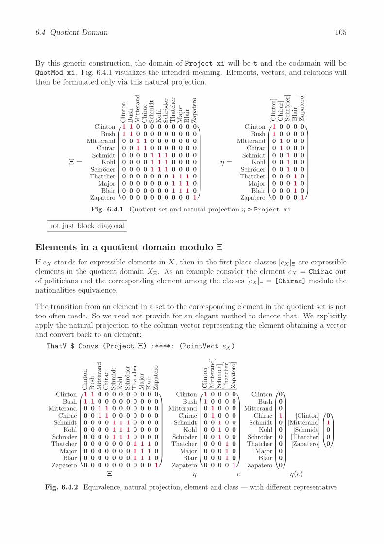
6.4 Quotient Domain 105
By this generic construction, the domain of Project xi will be t and the codomain will beQuotMod xi. Fig. 6.4.1 visualizes the intended meaning. Elements, vectors, and relations willthen be formulated only via this natural projection.
Ξ =
Clin
ton
Bus
hM
itte
rand
Chi
rac
Schm
idt
Koh
lSc
hrod
erT
hatc
her
Maj
orB
lair
Zap
ater
o
ClintonBush
MitterandChirac
SchmidtKohl
SchroderThatcher
MajorBlair
Zapatero
⎛⎜⎜⎜⎜⎜⎜⎜⎜⎜⎜⎜⎜⎜⎝
1 1 0 0 0 0 0 0 0 0 01 1 0 0 0 0 0 0 0 0 00 0 1 1 0 0 0 0 0 0 00 0 1 1 0 0 0 0 0 0 00 0 0 0 1 1 1 0 0 0 00 0 0 0 1 1 1 0 0 0 00 0 0 0 1 1 1 0 0 0 00 0 0 0 0 0 0 1 1 1 00 0 0 0 0 0 0 1 1 1 00 0 0 0 0 0 0 1 1 1 00 0 0 0 0 0 0 0 0 0 1
⎞⎟⎟⎟⎟⎟⎟⎟⎟⎟⎟⎟⎟⎟⎠
η =
[Clin
ton]
[Chi
rac]
[Sch
rode
r][B
lair
][Z
apat
ero]
ClintonBush
MitterandChirac
SchmidtKohl
SchroderThatcher
MajorBlair
Zapatero
⎛⎜⎜⎜⎜⎜⎜⎜⎜⎜⎜⎜⎜⎜⎝
1 0 0 0 01 0 0 0 00 1 0 0 00 1 0 0 00 0 1 0 00 0 1 0 00 0 1 0 00 0 0 1 00 0 0 1 00 0 0 1 00 0 0 0 1
⎞⎟⎟⎟⎟⎟⎟⎟⎟⎟⎟⎟⎟⎟⎠
Fig. 6.4.1 Quotient set and natural projection η ≈ Project xi
not just block diagonal
Elements in a quotient domain modulo Ξ
If eX stands for expressible elements in X, then in the first place classes [eX ]Ξ are expressibleelements in the quotient domain XΞ. As an example consider the element eX = Chirac outof politicians and the corresponding element among the classes [eX ]Ξ = [Chirac] modulo thenationalities equivalence.
The transition from an element in a set to the corresponding element in the quotient set is nottoo often made. So we need not provide for an elegant method to denote that. We explicitlyapply the natural projection to the column vector representing the element obtaining a vectorand convert back to an element:
ThatV $ Convs (Project Ξ) :****: (PointVect eX)
Clin
ton
Bus
hM
itte
rand
Chi
rac
Schm
idt
Koh
lSc
hrod
erT
hatc
her
Maj
orB
lair
Zap
ater
o
ClintonBush
MitterandChirac
SchmidtKohl
SchroderThatcher
MajorBlair
Zapatero
⎛⎜⎜⎜⎜⎜⎜⎜⎜⎜⎜⎜⎜⎜⎝
1 1 0 0 0 0 0 0 0 0 01 1 0 0 0 0 0 0 0 0 00 0 1 1 0 0 0 0 0 0 00 0 1 1 0 0 0 0 0 0 00 0 0 0 1 1 1 0 0 0 00 0 0 0 1 1 1 0 0 0 00 0 0 0 1 1 1 0 0 0 00 0 0 0 0 0 0 1 1 1 00 0 0 0 0 0 0 1 1 1 00 0 0 0 0 0 0 1 1 1 00 0 0 0 0 0 0 0 0 0 1
⎞⎟⎟⎟⎟⎟⎟⎟⎟⎟⎟⎟⎟⎟⎠
[Clin
ton]
[Mit
tera
nd]
[Sch
mid
t][T
hatc
her]
[Zap
ater
o]
ClintonBush
MitterandChirac
SchmidtKohl
SchroderThatcher
MajorBlair
Zapatero
⎛⎜⎜⎜⎜⎜⎜⎜⎜⎜⎜⎜⎜⎜⎝
1 0 0 0 01 0 0 0 00 1 0 0 00 1 0 0 00 0 1 0 00 0 1 0 00 0 1 0 00 0 0 1 00 0 0 1 00 0 0 1 00 0 0 0 1
⎞⎟⎟⎟⎟⎟⎟⎟⎟⎟⎟⎟⎟⎟⎠
ClintonBush
MitterandChirac
SchmidtKohl
SchroderThatcher
MajorBlair
Zapatero
⎛⎜⎜⎜⎜⎜⎜⎜⎜⎜⎜⎜⎜⎜⎜⎝
00010000000
⎞⎟⎟⎟⎟⎟⎟⎟⎟⎟⎟⎟⎟⎟⎟⎠
[Clinton][Mitterand]
[Schmidt][Thatcher][Zapatero]
⎛⎜⎜⎜⎝
01000
⎞⎟⎟⎟⎠
Ξ η e η(e)
Fig. 6.4.2 Equivalence, natural projection, element and class — with different representative

106 Chapter 6 Relational Domain Construction
Vectors in a quotient domain modulo Ξ
If vX stands for expressible subsets in X, then only classes ηT;vX corresponding to [eX ] | eX ∈vX are expressible subsets in the quotient XΞ.
Clin
ton
Bus
hM
itte
rand
Chi
rac
Schm
idt
Koh
lSc
hrod
erT
hatc
her
Maj
orB
lair
Zap
ater
o
ClintonBush
MitterandChirac
SchmidtKohl
SchroderThatcher
MajorBlair
Zapatero
⎛⎜⎜⎜⎜⎜⎜⎜⎜⎜⎜⎜⎜⎜⎝
1 1 0 0 0 0 0 0 0 0 01 1 0 0 0 0 0 0 0 0 00 0 1 1 0 0 0 0 0 0 00 0 1 1 0 0 0 0 0 0 00 0 0 0 1 1 1 0 0 0 00 0 0 0 1 1 1 0 0 0 00 0 0 0 1 1 1 0 0 0 00 0 0 0 0 0 0 1 1 1 00 0 0 0 0 0 0 1 1 1 00 0 0 0 0 0 0 1 1 1 00 0 0 0 0 0 0 0 0 0 1
⎞⎟⎟⎟⎟⎟⎟⎟⎟⎟⎟⎟⎟⎟⎠
[Clin
ton]
[Mit
tera
nd]
[Sch
mid
t][T
hatc
her]
[Zap
ater
o]
ClintonBush
MitterandChirac
SchmidtKohl
SchroderThatcher
MajorBlair
Zapatero
⎛⎜⎜⎜⎜⎜⎜⎜⎜⎜⎜⎜⎜⎜⎝
1 0 0 0 01 0 0 0 00 1 0 0 00 1 0 0 00 0 1 0 00 0 1 0 00 0 1 0 00 0 0 1 00 0 0 1 00 0 0 1 00 0 0 0 1
⎞⎟⎟⎟⎟⎟⎟⎟⎟⎟⎟⎟⎟⎟⎠
ClintonBush
MitterandChirac
SchmidtKohl
SchroderThatcher
MajorBlair
Zapatero
⎛⎜⎜⎜⎜⎜⎜⎜⎜⎜⎜⎜⎜⎜⎜⎝
00110000100
⎞⎟⎟⎟⎟⎟⎟⎟⎟⎟⎟⎟⎟⎟⎟⎠
[Clinton][Mitterand]
[Schmidt][Thatcher][Zapatero]
⎛⎜⎜⎜⎝
01010
⎞⎟⎟⎟⎠
Fig. 6.4.3 Equivalence, natural projection, subset and subset of classes
Relations starting from or ending in a quotient domain
All relations starting from a quotient set shall begin with ηT. All relations ending in a quotientset shall correspondingly terminate with η. Of course, this will often be less visible inside morecomplex constructions.
example
Algebraic properties of the generic natural projection relation
It was a novel situation that we had to define a set from an already available one togetherwith an equivalence relation. In earlier cases, constructions started from one or more sets. Wehave to introduce the requirements we demand to hold for the quotient set and the naturalprojection.
6.4.1 Definition. Given an arbitrary equivalence Ξ, a relation η will be called the naturalprojection onto the quotient domain modulo Ξ, provided
Ξ = η; ηT, ηT; η = .
(For a proof that this is an essentially unique definition, see Appendix Prop. B.0.7.)
One need not give the set on which the equivalence is defined to hold as every relation carriesits domain and codomain information with it. In a very natural way the question arises towhich extent η is uniquely defined. Should the two natural projections η, ξ be presented, onewill immediately have the bijection between the two codomains.
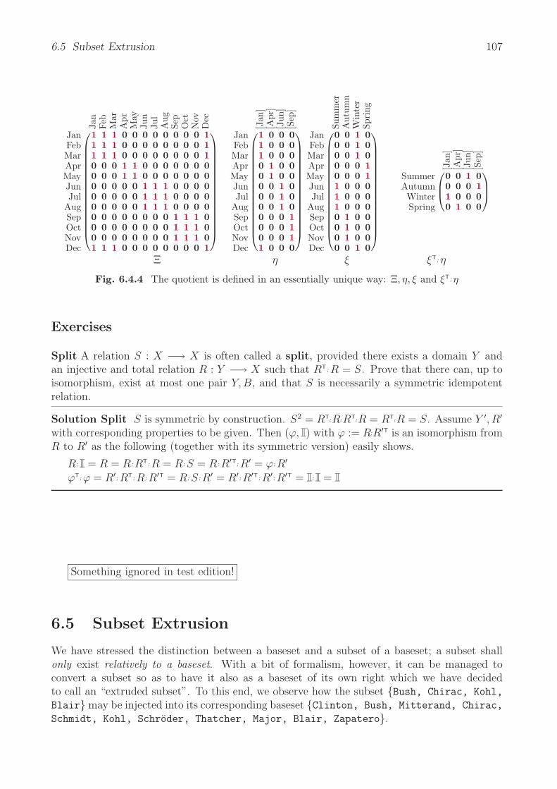
6.5 Subset Extrusion 107
Jan
Feb
Mar
Apr
May
Jun
Jul
Aug
Sep
Oct
Nov
Dec
JanFebMarAprMayJunJul
AugSepOctNovDec
⎛⎜⎜⎜⎜⎜⎜⎜⎜⎜⎜⎜⎜⎜⎜⎜⎝
1 1 1 0 0 0 0 0 0 0 0 11 1 1 0 0 0 0 0 0 0 0 11 1 1 0 0 0 0 0 0 0 0 10 0 0 1 1 0 0 0 0 0 0 00 0 0 1 1 0 0 0 0 0 0 00 0 0 0 0 1 1 1 0 0 0 00 0 0 0 0 1 1 1 0 0 0 00 0 0 0 0 1 1 1 0 0 0 00 0 0 0 0 0 0 0 1 1 1 00 0 0 0 0 0 0 0 1 1 1 00 0 0 0 0 0 0 0 1 1 1 01 1 1 0 0 0 0 0 0 0 0 1
⎞⎟⎟⎟⎟⎟⎟⎟⎟⎟⎟⎟⎟⎟⎟⎟⎠
[Jan
][A
pr]
[Jun
][S
ep]
JanFebMarAprMayJunJul
AugSepOctNovDec
⎛⎜⎜⎜⎜⎜⎜⎜⎜⎜⎜⎜⎜⎜⎜⎜⎝
1 0 0 01 0 0 01 0 0 00 1 0 00 1 0 00 0 1 00 0 1 00 0 1 00 0 0 10 0 0 10 0 0 11 0 0 0
⎞⎟⎟⎟⎟⎟⎟⎟⎟⎟⎟⎟⎟⎟⎟⎟⎠
Sum
mer
Aut
umn
Win
ter
Spri
ng
JanFebMarAprMayJunJul
AugSepOctNovDec
⎛⎜⎜⎜⎜⎜⎜⎜⎜⎜⎜⎜⎜⎜⎜⎜⎝
0 0 1 00 0 1 00 0 1 00 0 0 10 0 0 11 0 0 01 0 0 01 0 0 00 1 0 00 1 0 00 1 0 00 0 1 0
⎞⎟⎟⎟⎟⎟⎟⎟⎟⎟⎟⎟⎟⎟⎟⎟⎠
[Jan
][A
pr]
[Jun
][S
ep]
SummerAutumnWinterSpring
⎛⎜⎝
0 0 1 00 0 0 11 0 0 00 1 0 0
⎞⎟⎠
Ξ η ξ ξT; η
Fig. 6.4.4 The quotient is defined in an essentially unique way: Ξ, η, ξ and ξT;η
Exercises
Split A relation S : X −→ X is often called a split, provided there exists a domain Y andan injective and total relation R : Y −→ X such that RT ; R = S. Prove that there can, up toisomorphism, exist at most one pair Y, B, and that S is necessarily a symmetric idempotentrelation.
Solution Split S is symmetric by construction. S2 = RT;R;RT;R = RT;R = S. Assume Y ′, R′
with corresponding properties to be given. Then (ϕ, ) with ϕ := R;R′T is an isomorphism fromR to R′ as the following (together with its symmetric version) easily shows.
R; = R = R; RT; R = R; S = R; R′T; R′ = ϕ; R′
ϕT; ϕ = R′; RT; R; R′T = R; S ; R′ = R′; R′T; R′; R′T = ; =
Something ignored in test edition!
6.5 Subset Extrusion
We have stressed the distinction between a baseset and a subset of a baseset; a subset shallonly exist relatively to a baseset. With a bit of formalism, however, it can be managed toconvert a subset so as to have it also as a baseset of its own right which we have decidedto call an “extruded subset”. To this end, we observe how the subset Bush, Chirac, Kohl,
Blair may be injected into its corresponding baseset Clinton, Bush, Mitterand, Chirac,
Schmidt, Kohl, Schroder, Thatcher, Major, Blair, Zapatero.

108 Chapter 6 Relational Domain Construction
When trying to constructively generate extruded subsets and natural injections, one will needa type t, later interpreted by some set X, e.g., and a vector u of type t, later interpretedby a subset U ⊆ X. As all our relations carry their typing directly with them, the languageTITUREL allows to formulate
Extrude u, the extruded subset, corresponding to a new set DU , and
Inject u, the natural injection, corresponding to ιU : DU −→ X.
By this generic construction, the domain of Inject u will be Extrude u and the codomain willbe t. Fig. 6.5.1 visualizes the intended meaning. Elements, vectors, and relations will then beformulated only via this natural injection. In order to demonstrate that the subset is now a setof equal right, we apply the powerset construction to a smaller example.
Bush→,Chirac→,Kohl→,Blair→
Clin
ton
Bus
hM
itte
rand
Chi
rac
Schm
idt
Koh
lSc
hrod
erT
hatc
her
Maj
orB
lair
Zap
ater
o
Bush→Chirac→
Kohl→Blair→
⎛⎜⎝
0 1 0 0 0 0 0 0 0 0 00 0 0 1 0 0 0 0 0 0 00 0 0 0 0 1 0 0 0 0 00 0 0 0 0 0 0 0 0 1 0
⎞⎟⎠
Bus
h→
Chi
rac→
B
ush→
,Chi
rac→
K
ohl→
B
ush→
,Koh
l→
Chi
rac→
,Koh
l→
Bus
h→,C
hira
c→,K
ohl→
B
lair→
Bus
h→,B
lair→
Chi
rac→
,Bla
ir→
Bus
h→,C
hira
c→,B
lair→
Koh
l→,B
lair→
Bus
h→,K
ohl→
,Bla
ir→
Chi
rac→
,Koh
l→,B
lair→
Bus
h→,C
hira
c→,K
ohl→
,Bla
ir→
Bush→Chirac→
Kohl→Blair→
⎛⎜⎝
0 1 0 1 0 1 0 1 0 1 0 1 0 1 0 10 0 1 1 0 0 1 1 0 0 1 1 0 0 1 10 0 0 0 1 1 1 1 0 0 0 0 1 1 1 10 0 0 0 0 0 0 0 1 1 1 1 1 1 1 1
⎞⎟⎠
Fig. 6.5.1 Subset as dependent set with natural injection, and in further construction
Elements in an extruded subset Y
If e stands for expressible elements in X, then only injected elements e→ are expressible inthe injected subset Y ⊆ X, provided e ∈ Y . In mathematical standard notation, we havee→:= ιU(e); when denoting algebraically, it becomes e→:= ιT
U; e. As an example consider the
politician Major, first as one among our set of politicians and then as one of the subset ofBritish politicians.
e =
ClintonBush
MitterandChirac
SchmidtKohl
SchroderThatcher
MajorBlair
Zapatero
⎛⎜⎜⎜⎜⎜⎜⎜⎜⎜⎜⎜⎜⎜⎜⎝
00000000100
⎞⎟⎟⎟⎟⎟⎟⎟⎟⎟⎟⎟⎟⎟⎟⎠
vY =
⎛⎜⎜⎜⎜⎜⎜⎜⎜⎜⎜⎜⎜⎜⎜⎝
00000001110
⎞⎟⎟⎟⎟⎟⎟⎟⎟⎟⎟⎟⎟⎟⎟⎠
Clin
ton
Bus
hM
itte
rand
Chi
rac
Schm
idt
Koh
lSc
hrod
erT
hatc
her
Maj
orB
lair
Zap
ater
o
ι =Thatcher→
Major→Blair→
(0 0 0 0 0 0 0 1 0 0 00 0 0 0 0 0 0 0 1 0 00 0 0 0 0 0 0 0 0 1 0
)e→ =
⎛⎝0
10
⎞⎠
Fig. 6.5.2 Element e, vector Y ⊆ X, injection and injected element e→

6.5 Subset Extrusion 109
Vectors in an extruded subset Y
If v stands for expressible subsets of elements in X, then only injected subsets v→ with v ⊆ Yare expressible in the injected subset Y ⊆ X in the first place. Of course, further iteratedboolean constructions based on this as a start may be formulated. As long as we stay in thearea of finite basesets, there will arise no problem. These constructions become more difficultwhen infinite sets are considered.
Relations starting or ending in an extruded subset Y
All relations starting from an extruded subset shall begin with the natural injection ιY . Allrelations ending in an extruded set shall correspondingly terminate with ιT
Y . Of course, thiswill often be not directly visible inside other constructions.
Algebraic properties of the generic natural injection relation
Subset extrusion has hardly ever been considered a domain construction and stayed in the areaof free-hand mathematics. Nevertheless will we collect the algebraic properties and show thatthe concept of an extruded subset is defined in an essentially unique form.
6.5.1 Definition. Let any subset U ⊆ V of some baseset be given. Whenever a relationιU : DU −→ V , satisfies the properties
ιU ; ιTU = DU
, ιTU
; ιU = V ∩ U ; V,V ,
it will be called a natural injection of the thereby introduced new domain DU . (See AppendixProp. B.0.8)
The new domain DU , is defined in an essentially unique form. This is best understood assumingtwo students given the task to extrude some given U ⊆ V . They work in different ways andreturn after a while with their solutions as in Fig. 6.5.3.
A K D B 10 9 8 7
8→A→7→
10→9→
⎛⎜⎜⎝
0 0 0 0 0 0 1 01 0 0 0 0 0 0 00 0 0 0 0 0 0 10 0 0 0 1 0 0 00 0 0 0 0 1 0 0
⎞⎟⎟⎠
A K D B 10 9 8 7
A→10→9→8→7→
⎛⎜⎜⎝
1 0 0 0 0 0 0 00 0 0 0 1 0 0 00 0 0 0 0 1 0 00 0 0 0 0 0 1 00 0 0 0 0 0 0 1
⎞⎟⎟⎠
A 10 9 8 7
8→A→7→
10→9→
⎛⎜⎜⎝
0 0 0 1 01 0 0 0 00 0 0 0 10 1 0 0 00 0 1 0 0
⎞⎟⎟⎠
Fig. 6.5.3 Two different extrusions ιU , χ of one subset U ⊆ V and the bijection P := ιU ;χT
Both students demonstrate that the algebraic conditions are met, and thus claim that theirrespective solution be the correct one. The professor then takes these solutions and constructsthe bijection P based solely on the material they did offer to him as P := ιU ; χT.
A point to mention is that subset extrusion allows to switch from set-theoretic considerationto an algebraic one. When using a computer and a formula manipulation system or a theoremprover, this means a considerable restriction in expressivity which is honored with much betterefficiency.

110 Chapter 6 Relational Domain Construction
Exercises
Tabu An important application of extrusion is the concept of tabulation introduced by RogerMaddux; see [FS90, Kah02], e.g. An arbitrary relation R : X −→ Y is said to be tabulated byrelations (due to the following characterization, they turn out to be mappings) P, Q if
P T; Q = R, P T; P = X ∩ R; Y X , QT; Q = Y ∩ RT; XY , P ; P T ∩ Q; QT = X×Y
Show that tabulation may be formulated extruding the subset of related pairs.
Solution Tabu This may indeed be composed of extruding with χ : DU −→ X×Y the subsetof related pairs out of a direct product
U := (π; R ∩ ρ); Y,X×Y = (π; R ∩ ρ); Y X ; πT = (π; R; ρT ∩ ); ρ; Y X ; πT
= (π; R; ρT ∩ ); X×Y,X×Y = (ρ; RT; πT ∩ ); X×Y,X×Y
= (ρ; RT; πT ∩ ); π; XY ; ρT = (ρ; RT ∩ π); XY ; ρT = (ρ; RT ∩ π); X,X×Y
and defining P := χ; π and Q := χ; ρ. This is proved quite easily as follows.
P T; Q = πT; χT; χ; ρ = πT; (π; R; ρT ∩ ); ρ= πT; (π; R ∩ ρ)= R ∩ πT; ρ= R ∩ = R
P T; P = πT; χT; χ; π = πT; ( ∩ (π; R ∩ ρ); ρT; π; πT); π= πT; (π ∩ (π; R ∩ ρ); ρT; π)= ∩ πT; (π; R ∩ ρ); ρT; π= ∩ (R ∩ πT; ρ); ρT; π = ∩ R; Y X
QT; Q is handled analogously
P ; P T ∩ Q; QT = χ; π; πT; χT ∩ χ; ρ; ρT; χT = χ; (π; πT ∩ ρ; ρT); χT = χ; ; χT =
6.6 Direct Power
The direct power construction is what we employ when forming the powerset of some set. Asthis means going from n elements to 2n, this is often avoided to the extent that handling thisproperly is not so common an ability. The powerset 2V or P(V ) for a 5-element set, e.g., lookslike
,American,French,American,French,German,American,German,French,German,American,French,German,British,American,British,French,British,American,French,British,German,British,American,German,British,French,German,British,American,French,German,British,Spanish,American,Spanish,French,Spanish,American,French,Spanish,German,Spanish,American,German,Spanish,French,German,Spanish,American,French,German,Spanish,British,Spanish,American,British,Spanish,French,British,Spanish,American,French,British,Spanish,German,British,Spanish,American,German,British,Spanish,French,German,British,Spanish,American,French,German,British,Spanish
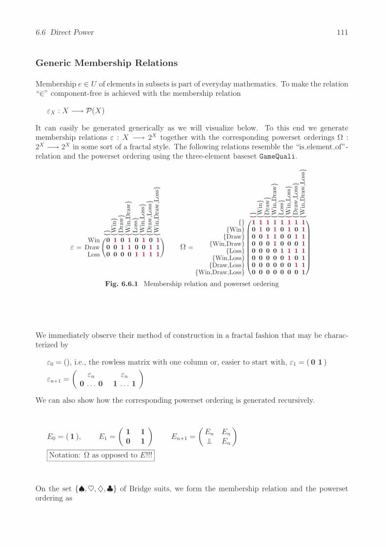
6.6 Direct Power 111
Generic Membership Relations
Membership e ∈ U of elements in subsets is part of everyday mathematics. To make the relation“∈” component-free is achieved with the membership relation
εX : X −→ P(X)
It can easily be generated generically as we will visualize below. To this end we generatemembership relations ε : X −→ 2X together with the corresponding powerset orderings Ω :2X −→ 2X in some sort of a fractal style. The following relations resemble the “is element of”-relation and the powerset ordering using the three-element baseset GameQuali.
Win
Dra
w
Win
,Dra
w
Los
sW
in,L
oss
Dra
w,L
oss
Win
,Dra
w,L
oss
ε =Win
DrawLoss
(0 1 0 1 0 1 0 10 0 1 1 0 0 1 10 0 0 0 1 1 1 1
) W
in
Dra
w
Win
,Dra
w
Los
sW
in,L
oss
Dra
w,L
oss
Win
,Dra
w,L
oss
Ω =
WinDraw
Win,DrawLoss
Win,LossDraw,Loss
Win,Draw,Loss
⎛⎜⎜⎜⎜⎜⎜⎜⎜⎝
1 1 1 1 1 1 1 10 1 0 1 0 1 0 10 0 1 1 0 0 1 10 0 0 1 0 0 0 10 0 0 0 1 1 1 10 0 0 0 0 1 0 10 0 0 0 0 0 1 10 0 0 0 0 0 0 1
⎞⎟⎟⎟⎟⎟⎟⎟⎟⎠
Fig. 6.6.1 Membership relation and powerset ordering
We immediately observe their method of construction in a fractal fashion that may be charac-terized by
ε0 = (), i.e., the rowless matrix with one column or, easier to start with, ε1 = ( 0 1 )
εn+1 =
(εn εn
0 . . . 0 1 . . . 1
)
We can also show how the corresponding powerset ordering is generated recursively.
E0 = ( 1 ), E1 =
(1 10 1
)En+1 =
(En En
En
)
Notation: Ω as opposed to E!!!
On the set ♠,♥,♦,♣ of Bridge suits, we form the membership relation and the powersetordering as

112 Chapter 6 Relational Domain Construction
♠
♥
♠,♥
♦
♠
,♦
♥,♦
♠
,♥,♦
♣
♠
,♣
♥,♣
♠
,♥,♣
♦
,♣
♠,♦
,♣
♥,♦
,♣
♠,♥
,♦,♣
ε =
♠♥♦♣
⎛⎜⎝
0 1 0 1 0 1 0 1 0 1 0 1 0 1 0 10 0 1 1 0 0 1 1 0 0 1 1 0 0 1 10 0 0 0 1 1 1 1 0 0 0 0 1 1 1 10 0 0 0 0 0 0 0 1 1 1 1 1 1 1 1
⎞⎟⎠
♠
♥
♠,♥
♦
♠
,♦
♥,♦
♠
,♥,♦
♣
♠
,♣
♥,♣
♠
,♥,♣
♦
,♣
♠,♦
,♣
♥,♦
,♣
♠,♥
,♦,♣
Ω =
♠♥
♠,♥♦
♠,♦♥,♦
♠,♥,♦♣
♠,♣♥,♣
♠,♥,♣♦,♣
♠,♦,♣♥,♦,♣
♠,♥,♦,♣
⎛⎜⎜⎜⎜⎜⎜⎜⎜⎜⎜⎜⎜⎜⎜⎜⎜⎜⎜⎜⎜⎜⎜⎝
1 1 1 1 1 1 1 1 1 1 1 1 1 1 1 10 1 0 1 0 1 0 1 0 1 0 1 0 1 0 10 0 1 1 0 0 1 1 0 0 1 1 0 0 1 10 0 0 1 0 0 0 1 0 0 0 1 0 0 0 10 0 0 0 1 1 1 1 0 0 0 0 1 1 1 10 0 0 0 0 1 0 1 0 0 0 0 0 1 0 10 0 0 0 0 0 1 1 0 0 0 0 0 0 1 10 0 0 0 0 0 0 1 0 0 0 0 0 0 0 10 0 0 0 0 0 0 0 1 1 1 1 1 1 1 10 0 0 0 0 0 0 0 0 1 0 1 0 1 0 10 0 0 0 0 0 0 0 0 0 1 1 0 0 1 10 0 0 0 0 0 0 0 0 0 0 1 0 0 0 10 0 0 0 0 0 0 0 0 0 0 0 1 1 1 10 0 0 0 0 0 0 0 0 0 0 0 0 1 0 10 0 0 0 0 0 0 0 0 0 0 0 0 0 1 10 0 0 0 0 0 0 0 0 0 0 0 0 0 0 1
⎞⎟⎟⎟⎟⎟⎟⎟⎟⎟⎟⎟⎟⎟⎟⎟⎟⎟⎟⎟⎟⎟⎟⎠
Fig. 6.6.2 Another membership relation with powerset ordering
Although quite different sets have been used in this example and the one before, one mayimmediately follow the indication for the construction principle explained above. We proceedeven further to a 5-element set as follows.
ε=
Am
eric
an
Fre
nch
Am
eric
an,F
renc
hG
erm
an
Am
eric
an,G
erm
an
Fre
nch,
Ger
man
A
mer
ican
,Fre
nch,
Ger
man
B
riti
sh
Am
eric
an,B
riti
sh
Fre
nch,
Bri
tish
Am
eric
an,F
renc
h,B
riti
sh
Ger
man
,Bri
tish
Am
eric
an,G
erm
an,B
riti
sh
Fre
nch,
Ger
man
,Bri
tish
Am
eric
an,F
renc
h,G
erm
an,B
riti
sh
Spa
nish
Am
eric
an,S
pani
sh
Fre
nch,
Span
ish
Am
eric
an,F
renc
h,Sp
anis
hG
erm
an,S
pani
sh
Am
eric
an,G
erm
an,S
pani
sh
Fre
nch,
Ger
man
,Spa
nish
Am
eric
an,F
renc
h,G
erm
an,S
pani
sh
Bri
tish
,Spa
nish
Am
eric
an,B
riti
sh,S
pani
sh
Fre
nch,
Bri
tish
,Spa
nish
Am
eric
an,F
renc
h,B
riti
sh,S
pani
sh
Ger
man
,Bri
tish
,Spa
nish
Am
eric
an,G
erm
an,B
riti
sh,S
pani
sh
Fre
nch,
Ger
man
,Bri
tish
,Spa
nish
Am
eric
an,F
renc
h,G
erm
an,B
riti
sh,S
pani
sh
AmericanFrench
GermanBritish
Spanish
⎛⎜⎜⎝
0 1 0 1 0 1 0 1 0 1 0 1 0 1 0 1 0 1 0 1 0 1 0 1 0 1 0 1 0 1 0 10 0 1 1 0 0 1 1 0 0 1 1 0 0 1 1 0 0 1 1 0 0 1 1 0 0 1 1 0 0 1 10 0 0 0 1 1 1 1 0 0 0 0 1 1 1 1 0 0 0 0 1 1 1 1 0 0 0 0 1 1 1 10 0 0 0 0 0 0 0 1 1 1 1 1 1 1 1 0 0 0 0 0 0 0 0 1 1 1 1 1 1 1 10 0 0 0 0 0 0 0 0 0 0 0 0 0 0 0 1 1 1 1 1 1 1 1 1 1 1 1 1 1 1 1
⎞⎟⎟⎠⊆V × P(V )
Fig. 6.6.3 Membership relation
Recognize again the fractal style of this presentation. This gives a basis for the intended genericconstruction. When trying to constructively generate a direct power and the correspondingmembership relation, one will need a type t, later interpreted by some set X, e.g. The languageTITUREL allows then to formulate
DirPow t, the direct power, corresponding to the powerset 2X , and

6.6 Direct Power 113
Epsi t, the membership relation, corresponding to ε : X −→ 2X .
By this generic construction, the domain of Epsi t will be t and the codomain will be DirPow
t. Fig. 6.6.3 visualizes the intended meaning. Elements, vectors, and relations will then beformulated only via this membership relation.
Elements in a direct power
To get an element in the direct power, we need the denotation vX of a subset of elements inX. Then VectToPowElem vX denotes an element in the direct power DirPow cX, in traditionalmathematics simply in the powerset P(X).
v = ε; e =
♠♥♦♣
⎛⎜⎝
0101
⎞⎟⎠
♠
♥
♠,♥
♦
♠
,♦
♥,♦
♠
,♥,♦
♣
♠
,♣
♥,♣
♠
,♥,♣
♦
,♣
♠,♦
,♣
♥,♦
,♣
♠,♥
,♦,♣
ε =
♠♥♦♣
⎛⎜⎝
0 1 0 1 0 1 0 1 0 1 0 1 0 1 0 10 0 1 1 0 0 1 1 0 0 1 1 0 0 1 10 0 0 0 1 1 1 1 0 0 0 0 1 1 1 10 0 0 0 0 0 0 0 1 1 1 1 1 1 1 1
⎞⎟⎠
eT = (0 0 0 0 0 0 0 0 0 0 1 0 0 0 0 0)
Fig. 6.6.4 A vector, the membership relation and the powerset element as row vector
It is absolutely clear how to proceed in this visualization: Take the vector v, move it horizon-tally over the relation ε, and mark the column that equals v. It is, however, more intricateto establish this as an algebraic method. “Column comparison” has been introduced as analgebraic operation in Sect. 4.4:
e = syq(v, ε)
Frequently we will, however, also have to go from an element e in DirPow o in the powerset toits corresponding subset. This is simply composition v := ε; e.
Vectors in a direct power
Expressible subsets in the direct power of X stem from finite sets (vi)i∈I of (different!) vectorsin X we have already defined somehow. The example shows the red, black, and the extreme-valued suits in the game of Skat, these then comprehended in one matrix, as well as in thecorresponding vector in the direct power, which is obtained as v := sup i∈I(syq(vi, ε))
♣♠♥♦
⎛⎜⎝
0011
⎞⎟⎠♣♠♥♦
⎛⎜⎝
1100
⎞⎟⎠♣♠♥♦
⎛⎜⎝
1001
⎞⎟⎠ R =
♣,♠
→♣
,♦→
♥,♦
→
♣♠♥♦
⎛⎜⎝
1 1 01 0 00 0 10 1 1
⎞⎟⎠ ε =
♣
♠
♣,♠
♥
♣
,♥
♠,♥
♣
,♠,♥
♦
♣
,♦
♠,♦
♣
,♠,♦
♥
,♦
♣,♥
,♦
♠,♥
,♦
♣,♠
,♥,♦
♣♠♥♦
⎛⎜⎝
0 1 0 1 0 1 0 1 0 1 0 1 0 1 0 10 0 1 1 0 0 1 1 0 0 1 1 0 0 1 10 0 0 0 1 1 1 1 0 0 0 0 1 1 1 10 0 0 0 0 0 0 0 1 1 1 1 1 1 1 1
⎞⎟⎠
vT =(0 0 0 1 0 0 0 0 0 1 0 0 1 0 0 0)
Fig. 6.6.5 Set of vectors determining a single vector (shown horizontally) in the direct power
114 Chapter 6 Relational Domain Construction
Of course, one will loose information on the sequence in which the vectors had originally beengiven. The way back is easier to a relation that is made up of the vectors vi, putting them sideaside R := ε;(Inject v)T. From this matrix, the original vectors may only be obtained selectinga column element e as R; e.
It may have become clear, that we are not trained for such operations and have no routinedenotation. Many would try to write a free-style program while there exist algebraically soundmethods. The problem is not least that we traditionally abstract over the two natures v, e of aset.
Relations starting or ending in a direct power
We demand that relations ending in a direct power be always formed using the membershiprelation εX , in programs denoted as Epsi x. This often takes a more composite form
syq(ε, R)
for some relation R. Typically, we also use two composite relations, namely the containmentordering on the powerset
Ω := εT; ε = ε\εand the complement transition in the powerset
N := syq(ε, ε). illustrate; also a, N, ε
Algebraic properties of the generic membership relation
The domain construction of the direct power is designed to give a relational analog to thesituation between a set A and its power set P(A). In particular, the “is element of” membershiprelation between A and P(A) is specified in the following definition, which has already beengiven in [BSZ86, BSZ90, BGS94] as follows.
6.6.1 Definition. A relation ε is called a direct power if it satisfies the following properties:
i) syq(ε, ε) ⊆ ,ii) syq(ε, X) is surjective for every relation X.
Instead of (ii), one may also say that syq(X, ε) shall be a mapping, i.e. univalent and total.One should bear in mind, that for all X
ε;syq(ε, X) = X
since “⊆ ” holds according to Prop. 5.7.3. Again, the direct power is defined in an essentiallyunique fashion. Whenever a second relation ε′ should be presented, one could easily constructfrom the two the bijection P := syq(ε, ε′) relating the two versions of a direct product.
illustrate
Something ignored in test edition!
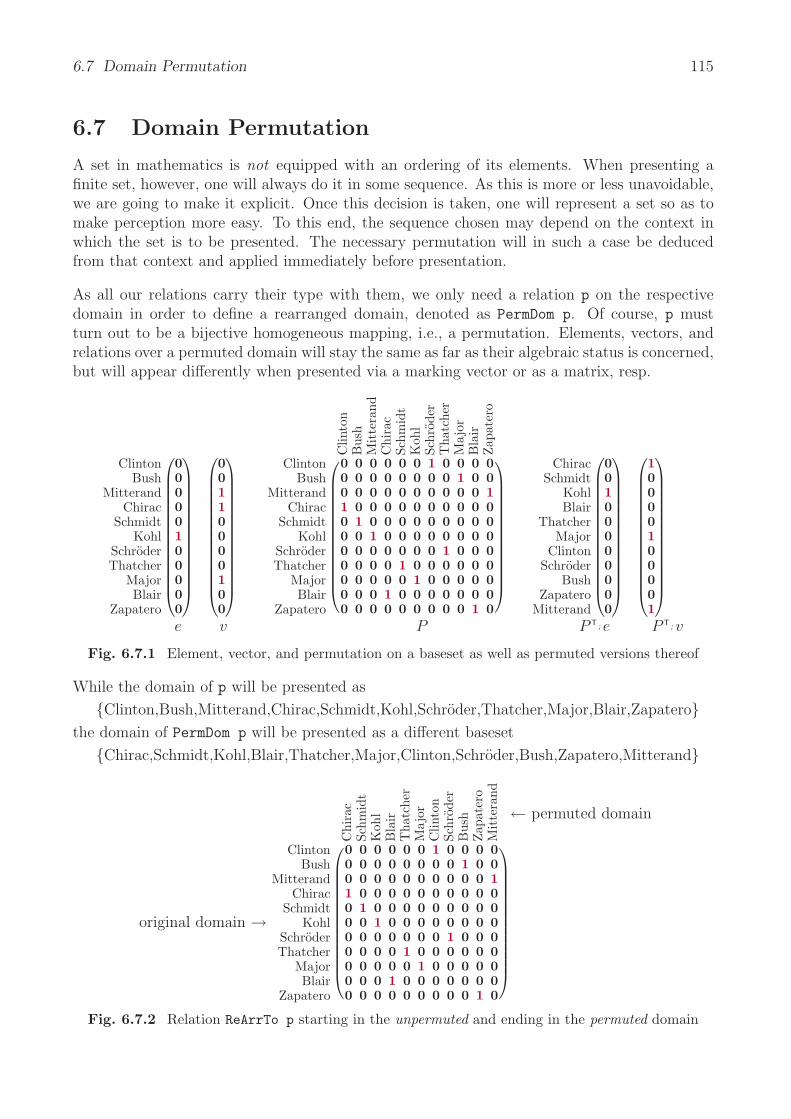
6.7 Domain Permutation 115
6.7 Domain Permutation
A set in mathematics is not equipped with an ordering of its elements. When presenting afinite set, however, one will always do it in some sequence. As this is more or less unavoidable,we are going to make it explicit. Once this decision is taken, one will represent a set so as tomake perception more easy. To this end, the sequence chosen may depend on the context inwhich the set is to be presented. The necessary permutation will in such a case be deducedfrom that context and applied immediately before presentation.
As all our relations carry their type with them, we only need a relation p on the respectivedomain in order to define a rearranged domain, denoted as PermDom p. Of course, p mustturn out to be a bijective homogeneous mapping, i.e., a permutation. Elements, vectors, andrelations over a permuted domain will stay the same as far as their algebraic status is concerned,but will appear differently when presented via a marking vector or as a matrix, resp.
ClintonBush
MitterandChirac
SchmidtKohl
SchroderThatcher
MajorBlair
Zapatero
⎛⎜⎜⎜⎜⎜⎜⎜⎜⎜⎜⎜⎜⎜⎜⎝
00000100000
⎞⎟⎟⎟⎟⎟⎟⎟⎟⎟⎟⎟⎟⎟⎟⎠
⎛⎜⎜⎜⎜⎜⎜⎜⎜⎜⎜⎜⎜⎜⎜⎝
00110000100
⎞⎟⎟⎟⎟⎟⎟⎟⎟⎟⎟⎟⎟⎟⎟⎠
Clin
ton
Bus
hM
itte
rand
Chi
rac
Schm
idt
Koh
lSc
hrod
erT
hatc
her
Maj
orB
lair
Zap
ater
o
ClintonBush
MitterandChirac
SchmidtKohl
SchroderThatcher
MajorBlair
Zapatero
⎛⎜⎜⎜⎜⎜⎜⎜⎜⎜⎜⎜⎜⎜⎝
0 0 0 0 0 0 1 0 0 0 00 0 0 0 0 0 0 0 1 0 00 0 0 0 0 0 0 0 0 0 11 0 0 0 0 0 0 0 0 0 00 1 0 0 0 0 0 0 0 0 00 0 1 0 0 0 0 0 0 0 00 0 0 0 0 0 0 1 0 0 00 0 0 0 1 0 0 0 0 0 00 0 0 0 0 1 0 0 0 0 00 0 0 1 0 0 0 0 0 0 00 0 0 0 0 0 0 0 0 1 0
⎞⎟⎟⎟⎟⎟⎟⎟⎟⎟⎟⎟⎟⎟⎠
ChiracSchmidt
KohlBlair
ThatcherMajor
ClintonSchroder
BushZapatero
Mitterand
⎛⎜⎜⎜⎜⎜⎜⎜⎜⎜⎜⎜⎜⎜⎜⎝
00100000000
⎞⎟⎟⎟⎟⎟⎟⎟⎟⎟⎟⎟⎟⎟⎟⎠
⎛⎜⎜⎜⎜⎜⎜⎜⎜⎜⎜⎜⎜⎜⎜⎝
10000100001
⎞⎟⎟⎟⎟⎟⎟⎟⎟⎟⎟⎟⎟⎟⎟⎠
e v P P T; e P T; v
Fig. 6.7.1 Element, vector, and permutation on a baseset as well as permuted versions thereof
While the domain of p will be presented as
Clinton,Bush,Mitterand,Chirac,Schmidt,Kohl,Schroder,Thatcher,Major,Blair,Zapaterothe domain of PermDom p will be presented as a different baseset
Chirac,Schmidt,Kohl,Blair,Thatcher,Major,Clinton,Schroder,Bush,Zapatero,Mitterand
original domain →
Chi
rac
Schm
idt
Koh
lB
lair
Tha
tche
rM
ajor
Clin
ton
Schr
oder
Bus
hZap
ater
oM
itte
rand
ClintonBush
MitterandChirac
SchmidtKohl
SchroderThatcher
MajorBlair
Zapatero
⎛⎜⎜⎜⎜⎜⎜⎜⎜⎜⎜⎜⎜⎜⎝
0 0 0 0 0 0 1 0 0 0 00 0 0 0 0 0 0 0 1 0 00 0 0 0 0 0 0 0 0 0 11 0 0 0 0 0 0 0 0 0 00 1 0 0 0 0 0 0 0 0 00 0 1 0 0 0 0 0 0 0 00 0 0 0 0 0 0 1 0 0 00 0 0 0 1 0 0 0 0 0 00 0 0 0 0 1 0 0 0 0 00 0 0 1 0 0 0 0 0 0 00 0 0 0 0 0 0 0 0 1 0
⎞⎟⎟⎟⎟⎟⎟⎟⎟⎟⎟⎟⎟⎟⎠
← permuted domain
Fig. 6.7.2 Relation ReArrTo p starting in the unpermuted and ending in the permuted domain
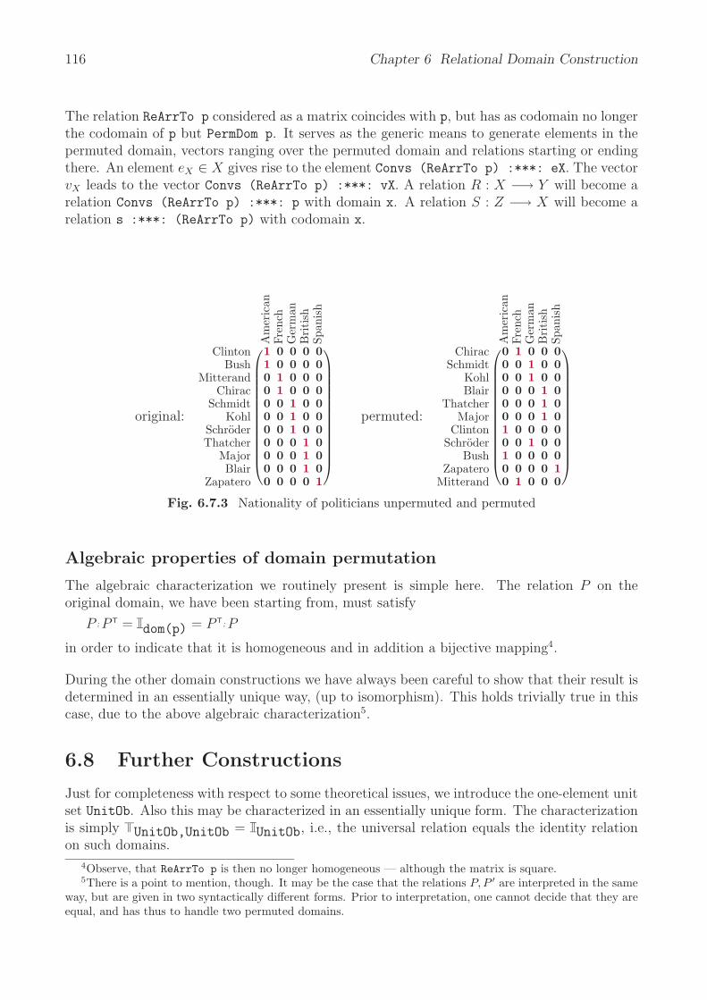
116 Chapter 6 Relational Domain Construction
The relation ReArrTo p considered as a matrix coincides with p, but has as codomain no longerthe codomain of p but PermDom p. It serves as the generic means to generate elements in thepermuted domain, vectors ranging over the permuted domain and relations starting or endingthere. An element eX ∈ X gives rise to the element Convs (ReArrTo p) :***: eX. The vectorvX leads to the vector Convs (ReArrTo p) :***: vX. A relation R : X −→ Y will become arelation Convs (ReArrTo p) :***: p with domain x. A relation S : Z −→ X will become arelation s :***: (ReArrTo p) with codomain x.
original:
Am
eric
anFr
ench
Ger
man
Bri
tish
Span
ish
ClintonBush
MitterandChirac
SchmidtKohl
SchroderThatcher
MajorBlair
Zapatero
⎛⎜⎜⎜⎜⎜⎜⎜⎜⎜⎜⎜⎜⎜⎝
1 0 0 0 01 0 0 0 00 1 0 0 00 1 0 0 00 0 1 0 00 0 1 0 00 0 1 0 00 0 0 1 00 0 0 1 00 0 0 1 00 0 0 0 1
⎞⎟⎟⎟⎟⎟⎟⎟⎟⎟⎟⎟⎟⎟⎠
permuted:
Am
eric
anFr
ench
Ger
man
Bri
tish
Span
ish
ChiracSchmidt
KohlBlair
ThatcherMajor
ClintonSchroder
BushZapatero
Mitterand
⎛⎜⎜⎜⎜⎜⎜⎜⎜⎜⎜⎜⎜⎜⎝
0 1 0 0 00 0 1 0 00 0 1 0 00 0 0 1 00 0 0 1 00 0 0 1 01 0 0 0 00 0 1 0 01 0 0 0 00 0 0 0 10 1 0 0 0
⎞⎟⎟⎟⎟⎟⎟⎟⎟⎟⎟⎟⎟⎟⎠
Fig. 6.7.3 Nationality of politicians unpermuted and permuted
Algebraic properties of domain permutation
The algebraic characterization we routinely present is simple here. The relation P on theoriginal domain, we have been starting from, must satisfy
P ; P T = dom(p) = P T; P
in order to indicate that it is homogeneous and in addition a bijective mapping4.
During the other domain constructions we have always been careful to show that their result isdetermined in an essentially unique way, (up to isomorphism). This holds trivially true in thiscase, due to the above algebraic characterization5.
6.8 Further Constructions
Just for completeness with respect to some theoretical issues, we introduce the one-element unitset UnitOb. Also this may be characterized in an essentially unique form. The characterizationis simply UnitOb,UnitOb = UnitOb, i.e., the universal relation equals the identity relationon such domains.
4Observe, that ReArrTo p is then no longer homogeneous — although the matrix is square.5There is a point to mention, though. It may be the case that the relations P, P ′ are interpreted in the same
way, but are given in two syntactically different forms. Prior to interpretation, one cannot decide that they areequal, and has thus to handle two permuted domains.

6.9 Equivalent Representations 117
More involved is the recursive construction of sets with which we may get infinite sets for thefirst time. We give here a couple of examples.
Fix, NamedBS
6.9 Equivalent Representations
It should be mentioned that we have introduced constructions in a granularity finer than theusual one. We have abandoned some abstractions and denote, thus, with some more detail.In particular will we have several possibilities to represent the same item classically abstractedover. So this approach will probably suffer from obstruction of people who traditionally useabstractions thrown away here.
We give an example using domain constructions just explained to show that concepts may berepresented in quite different ways. While it is from a certain point of view nice to abstract fromdetails of representation, one often loses intuition when abstraction is too far off. In particularwill one not immediately see in which cases a situation is a “linear” one; i.e., one offering itselfto be handled relationally.
In Fig. 6.9.1, we present representations of a relation as a matrix, as a vector along the productspace and finally as an element in the powerset of the product space. The latter concept, how-ever, will hardly ever be used. It is indicated in which way the transition between the versionsmay be managed with the generic projection relations π, ρ and the membership relation ε.

118 Chapter 6 Relational Domain Construction
X Y
2X Y
1l
t
R
e
π ρ
εX Y×
×
Win
Dra
wLos
s
malefemale
(0 1 01 0 1
)= R
(male,Win)(female,Win)(male,Draw)
(female,Draw)(male,Loss)
(female,Loss)
⎛⎜⎜⎜⎜⎜⎝
011001
⎞⎟⎟⎟⎟⎟⎠= t
R = πT; ( ∩ t; ); ρ
t = (π; R ∩ ρ);
e = syq(ε, t)
t = ε; e
(male,Win)
(female,Win)(male,Win),(female,Win)
(male,Draw)(male,Win),(male,Draw)
(female,Win),(male,Draw)(male,Win),(female,Win),(male,Draw)
(female,Draw)(male,Win),(female,Draw)
(female,Win),(female,Draw)(male,Win),(female,Win),(female,Draw)
(male,Draw),(female,Draw)(male,Win),(male,Draw),(female,Draw)
(female,Win),(male,Draw),(female,Draw)(male,Win),(female,Win),(male,Draw),(female,Draw)
(male,Loss)(male,Win),(male,Loss)
(female,Win),(male,Loss)(male,Win),(female,Win),(male,Loss)
(male,Draw),(male,Loss)(male,Win),(male,Draw),(male,Loss)
(female,Win),(male,Draw),(male,Loss)(male,Win),(female,Win),(male,Draw),(male,Loss)
(female,Draw),(male,Loss)(male,Win),(female,Draw),(male,Loss)
(female,Win),(female,Draw),(male,Loss)(male,Win),(female,Win),(female,Draw),(male,Loss)
(male,Draw),(female,Draw),(male,Loss)(male,Win),(male,Draw),(female,Draw),(male,Loss)
(female,Win),(male,Draw),(female,Draw),(male,Loss)(male,Win),(female,Win),(male,Draw),(female,Draw),(male,Loss)
(female,Loss)(male,Win),(female,Loss)
(female,Win),(female,Loss)(male,Win),(female,Win),(female,Loss)
(male,Draw),(female,Loss)(male,Win),(male,Draw),(female,Loss)
(female,Win),(male,Draw),(female,Loss)(male,Win),(female,Win),(male,Draw),(female,Loss)
(female,Draw),(female,Loss)(male,Win),(female,Draw),(female,Loss)
(female,Win),(female,Draw),(female,Loss)(male,Win),(female,Win),(female,Draw),(female,Loss)
(male,Draw),(female,Draw),(female,Loss)(male,Win),(male,Draw),(female,Draw),(female,Loss)
(female,Win),(male,Draw),(female,Draw),(female,Loss)(male,Win),(female,Win),(male,Draw),(female,Draw),(female,Loss)
(male,Loss),(female,Loss)(male,Win),(male,Loss),(female,Loss)
(female,Win),(male,Loss),(female,Loss)(male,Win),(female,Win),(male,Loss),(female,Loss)
(male,Draw),(male,Loss),(female,Loss)(male,Win),(male,Draw),(male,Loss),(female,Loss)
(female,Win),(male,Draw),(male,Loss),(female,Loss)(male,Win),(female,Win),(male,Draw),(male,Loss),(female,Loss)
(female,Draw),(male,Loss),(female,Loss)(male,Win),(female,Draw),(male,Loss),(female,Loss)
(female,Win),(female,Draw),(male,Loss),(female,Loss)(male,Win),(female,Win),(female,Draw),(male,Loss),(female,Loss)
(male,Draw),(female,Draw),(male,Loss),(female,Loss)(male,Win),(male,Draw),(female,Draw),(male,Loss),(female,Loss)
(female,Win),(male,Draw),(female,Draw),(male,Loss),(female,Loss)(male,Win),(female,Win),(male,Draw),(female,Draw),(male,Loss),(female,Loss)
⎛⎜⎜⎜⎜⎜⎜⎜⎜⎜⎜⎜⎜⎜⎜⎜⎜⎜⎜⎜⎜⎜⎜⎜⎜⎜⎜⎜⎜⎜⎜⎜⎜⎜⎜⎜⎜⎜⎜⎜⎜⎜⎜⎜⎜⎜⎜⎜⎜⎜⎜⎜⎜⎜⎜⎜⎜⎜⎜⎜⎜⎜⎜⎜⎜⎜⎜⎜⎜⎜⎜⎜⎜⎜⎜⎜⎜⎜⎜⎜⎜⎜⎜⎜⎜⎜⎜⎜⎜⎜⎜⎜⎜⎜⎜⎜⎜⎜⎜⎜⎜⎜⎜⎜⎜⎜⎜⎜⎜⎜⎜⎜⎝
0000000000000000000000000000000000000010000000000000000000000000
⎞⎟⎟⎟⎟⎟⎟⎟⎟⎟⎟⎟⎟⎟⎟⎟⎟⎟⎟⎟⎟⎟⎟⎟⎟⎟⎟⎟⎟⎟⎟⎟⎟⎟⎟⎟⎟⎟⎟⎟⎟⎟⎟⎟⎟⎟⎟⎟⎟⎟⎟⎟⎟⎟⎟⎟⎟⎟⎟⎟⎟⎟⎟⎟⎟⎟⎟⎟⎟⎟⎟⎟⎟⎟⎟⎟⎟⎟⎟⎟⎟⎟⎟⎟⎟⎟⎟⎟⎟⎟⎟⎟⎟⎟⎟⎟⎟⎟⎟⎟⎟⎟⎟⎟⎟⎟⎟⎟⎟⎟⎟⎟⎠
= e
Fig. 6.9.1 Relating representations of a relation as a matrix R, a vector t, and as an element e

Part III
How to Use the Relational Language
119


121
In this part, we reach a third step of abstraction. Recall that first relations have been observedas they occur in real life situations. We have then made a step forward using component-freealgebraic formulation; we have, however, not immediately started introducing the respectivealgebraic proofs. Instead we have visualized and tried to construct with relations. In a sense wasthis what one will always find in a book treating eigen vectors and eigen values of real-valuedmatrices, or their invariant subspaces: Usually this is heavily supported visualizing matrixsitutions. We did this in full mathematical rigor but did so far not immediately convince thereader concerning this fact. Proofs, although rather trivial in that beginning phase, have beenpostponed so as to establish an easy line of understanding first.
As gradually more advanced topics are handled, we will now switch to a fully formal style withimmediately appended proofs. The reader will, however, be in a position to refer to the firsttwo parts and to see there how the effects had been.
Formulating only in algebraic terms — or what comes close to that, formulating in the relationallanguage TITUREL —, means that we are far more restricted in expressivity. On the otherhand will this improve precision considerably. Restricting to the language will allow later thattransformations and proofs become possible.

122

7 Relation Algebra
Concerning syntax and notation, everything is now available to work with. We take thisopportunity to have a closer look at the algebraic laws of relation algebra. In particular willwe be interested in how they may be traced back to a small subset of rules which may serve asaxioms. We present them right now and discuss them immediately afterwards.
more text here!
7.1 Laws of Relation Algebra
The set of axioms for an abstract (heterogeneous) relation algebra is nowadays generally agreedupon, and it is rather short. When we use the concept of a category, this does not mean thatwe introduce a higher concept. Rather, it is here used as a mathematically acceptable way toprevent from multiplying a 7 × 5-matrix with a 4 × 6-matrix.
7.1.1 Definition. A heterogeneous relation algebra is defined as a structure that
• is a category wrt. composition “ ; ” and identities ,
• has complete atomic boolean lattices with ∪, ∩, , , , ⊆ as morphism ??? sets,
• obeys rules for transposition in connection with the latter two that may be stated ineither one of the following two ways:
Dedekind: R; S ∩ Q ⊆ (R ∩ Q; ST); (S ∩ RT; Q) orSchroder: A; B ⊆ C ⇐⇒ AT; C ⊆ B ⇐⇒ C ; BT ⊆ A.
Composition, union, etc., are thus only partial operations and one has to be careful not toviolate the composition rules. In order to avoid clumsy presentation, we shall adhere to thefollowing policy in a heterogeneous algebra with its only partially defined operations: Wheneverwe say “For every X . . . ”, we mean “For every X for which the construct in question is defined. . . ”. We are also a bit sloppy writing when A,B, e.g., would be more precise.
The Dedekind rule as well as the Schroder rule are widely unknown. They are as important asthe rule of associativity, the rule demanding distributivity, or the De Morgan rule, and thereforedeserve to be known much better.
One may ask why they are so little known. Is it since they are so complicated? Consider, e.g.,a ∗ (b + c) = a ∗ b + a ∗ c distributivitya + (b + c) = (a + b) + c associativity
123

124 Chapter 7 Relation Algebra
a ∪ b = a ∩ b De Morgan law
When comparing the Dedekind and the Schroder rule with these most commonly known math-ematical rules, they are indeed a little bit longer as text. But already the effort to checkassociativity1 is tremendous compared with the pictorial examples below, making them seemsimpler.
One should also mention that the Dedekind and Schroder rules — still without the names whichhave been attributed to them only later — have their origin in the same paper as the famousDe Morgan2 rule, namely [De 56]. People probably have not read far enough in De Morgan’spaper. Rather, they have confined themselves to using slightly simplified and restricted formsof these rules. Such versions describe functions, orderings, and equivalences. School educationfavours functions. Even today, when teaching orderings at university level it is not clear fromthe beginning that orderings need not be linear ones. Thinking in relations is mainly avoidedas people like the assignment of just one as traditionally in personal relations.
Exercises
2.3.2 Prove with relation-algebraic techniques that Q; R; S ⊆ Q; R; SandQ; R; S ⊆ Q; R; S
Solution 2.3.2 Q;R ⊆ Q;R ⇐⇒ QT;Q; R ⊆ R =⇒ QT;Q; R;S ⊆ R;S ⇐⇒ Q;R; S ⊆ Q; R; S
7.2 Visualizing the Schroder Equivalences
For an intuitive description the so-called dotted arrow convention is helpful. Consider thefollowing figures. There are normal arrows and dotted arrows. By the dotted arrow convention,a dotted arrow is conceived to be a forbidden arrow. It belongs, thus, to the negated relation.
C
BA
C
BA
C
BA
Fig. 7.2.1
A;B ⊆ C AT;C ⊆ B C ;BT ⊆ A
The dotted arrow convention in case of Schroder equivalences
To memorize and understand the Schroder rule is now easy:
• The containment A; B ⊆ C means that for consecutive arrows of A and B, there willalways exist a “shortcutting” arrow in C.
• But assuming this to hold, we have the following situation: When following A in reversedirection and then a non-existing arrow of C, there can be no shortcutting arrow in B.Of course not; it would be an arrow consecutive to one of A with the consequence of anarrow in C which is impossible.
1Who has ever checked associativity for a group table? We simply take it for granted.2He was Scottish, born in Madras (India), not French
7.2 Visualizing the Schroder Equivalences 125
• Let us consider a not existing arrow from C (i.e., an arrow from C), followed by an arrowfrom B in reverse direction. Then it cannot happen that this can be shortcut by an arrowof A as then there were consecutive arrows of A and B without shortcut in C.
also in PL1?
When thinking on this for a while, one will indeed understand Schroder’s rule. What onecannot assess at this point is that Schroder’s rule (in combination with the others mentionedin the definition of a relation algebra) is strong enough to span all our standard methods ofthinking and reasoning. The next three examples will at least illustrate this claim.
If we are about to work with a function, we mean that it must never assign two different imagesto an argument; a function F will, therefore, later be defined to be univalent, F T ; F ⊆ . So,when going back from an image to its argument and then going again forward to an image, itwill turn out that one will arrive at the same element. But one may also follow the functionto an image and then proceed to another element on the image side, which then can not beimage of the starting point: F ; ⊆ F . This transition which is difficult to formulate in spokenlanguage is again simple using Schroder’s rule.
Consider the equivalence Ξ := “plays in the same team as” defined over the set of players insome national sports league. When a and b play in the same team, and also b and c play inthe same team, we standardwise reason that a will play in the same team with c. Altogetherwe have transitivity of an equivalence relation, meaning not least Ξ; Ξ ⊆ Ξ. Using Schroder’srule, we have also ΞT ; Ξ ⊆ Ξ meaning that when a plays in the same team with b, but b doesnot play in the same team with c, then a and c cannot play in the same team.
Yet another example assumes C as a comparison of persons as to their height. If a is tallerthan b and b in turn is taller than c, it is clear for us that a is taller than c, i.e. C;C ⊆ C. Weroutinely use “is smaller than”as denotation for the converse. Probably we will also be able toreason that i.e. CT;C ⊆ C; namely when a is smaller than b and b is not taller than c, then ais not taller than c.
Nearly all of human thinking is based on such triangle situations; mankind does not seemcapable of achieving more. If everyday situations are concerned, we handle this routinely.When new relations come into play for which no standard notation has been agreed for, weoften fail to handle this properly. Big problems usually show up when not just one relation isenvisaged such as “plays in the same team as”, “is taller than”, or “is mapped to” and differentrelations are taken as in the following examples.
7.2.1 Example. Let some gentlemen H, ladies D, and flowers B be given, as well as the threerelations
• Sympathy S : H −→ D,
• Likes flowers M : D −→ B,
• Has bought K : H −→ B.

126 Chapter 7 Relation Algebra
Then the following will hold
S ; M ⊆ K ⇐⇒ ST; K ⊆ M ⇐⇒ K ; MT ⊆ S
Gentlemen Ladies
Flowers
feels sympathy for
buys likes
Fig. 7.2.2 Visualization of the Schroder rule
It need not be the case that any of these containments is true. In any case, however, eitherall three or none of them will be true. The following three propositions are, thus, logicallyequivalent:
• All gentlemen h buy at least those flowers b that are liked by some of the ladies sympa-thetic to them.
• Whenever a lady d is sympathetic to some gentleman, who does not buy flower b, thislady d is not fond of flower b.
• Whenever a gentleman h does not buy a flower that lady d likes, then h has no sympathyfor d.
As we will only in rare cases have that S ; M ⊆ K, this may seem rather artificial — butit is not. Assume, e.g., a situation where a gentleman does not buy a flower liked by oneof the ladies sympathetic to him. Then also the other two statements will not be satisfied.one example each!!
To memorize the Schroder rule, we concentrate on triangles. As indicated above, a triangle maybe formed by a cycle buys—is sympathetic—likes. Once we found out that every arrow belongsto some triangle, it is straightforward to state that over every line there exists an element in

7.2 Visualizing the Schroder Equivalences 127
the third set such that a triangle may be formed — regardless of which line has been chosen tostart with.
7.2.2 Example. Look at the situation with three relations on one set of human beings, namely
• B “is brother of”
• E “is parent of”
• P “is godfather of”
Otto A. Erika A. Emil B. Isa B. Uwe C.
is parent of is brother of is godfather of
Fig. 7.2.3 Another visualization of the Schroder equivalences
Now we have according to the Schroder rule
B ; E ⊆ P ⇐⇒ BT; P ⊆ E ⇐⇒ P ; ET ⊆ B
This is applicable to every group of human beings, stating that the following three propositionsare logically equivalent. So either all of them are true or none.
• Uncleship implies godfathership.
• A person with a brother who is not godfather of a child, will never be parent of that child.
• If someone is not the godfather of a child of some person, he will not be that personsbrother.
Now assume the leftmost godfathership arrow starting at Emil B. were not indicated. Thenobviously B;E ⊆ P is not satisfied. But then also P ;ET ⊆ B is not satisfied; namely: Take themissing arrow and follow parenthood back to Erika A. To this person a brother arrow exists,so that P ; ET ⊆ B can not be true.
Something ignored in test edition!

128 Chapter 7 Relation Algebra
7.3 Visualizing the Dedekind-Formula
Observe that the setting is a little bit different now. The Dedekind formula is satisfied for anythree-relation-configuration whatsoever. From the beginning, we assume in this case a situationwhere S ; M ⊆ K may not be satisfied.
Fig. 7.3.1 Checking the Dedekind rule
with matrix!
In an arbitrary such configuration we have:
S ; M ∩ K ⊆ (S ∩ K ; MT); (M ∩ ST; K)
Whenever a gentleman h buys a flower b, which some lady sympathetic to him likes, therewill exist a lady d sympathetic to him, liking a flower b′ he bought, and this lady d will like aflower b, that some gentleman h′ with sympathy for her has bought. Observe how fuzzily thisis formulated concerning existence of b′, h′.
One need not learn this by heart. Just consider the triangles of three arrows. Then at least thetranspositions follow immediately.
The Dedekind rule
B ; E ∩ P ⊆ (B ∩ P ; ET); (E ∩ BT; P )
says that the following holds for every configuration of human beings:
An uncle u of a child k, who is at the same time a godfather of k,
• is a brother of some person p, who is parent of one of his godchildren,
• and at the same time is parent of child k and has a brother, who is godfather of k.

7.4 Elementary Properties of Relations 129
One should emphasize that at two positions there is an ambivalence: The person p is parent ofone of his godchildren. There exists a brother of p who is godfather of k. These two are notidentified more than these descriptions allow. The very general quantifications, however, makethis precise.
Something ignored in test edition!
7.4 Elementary Properties of Relations
The following are elementary properties of operations on relations. We mention them herewithout proof as it is not the intention of this book to show how they all depend on axioms.
7.4.1 Proposition (Rules presented earlier — check! ).i) ; R = R; =ii) R ⊆ S =⇒ Q; R ⊆ Q; S, R; Q ⊆ S ; Q (monotonicity)iii) Q; (R ∩ S) ⊆ Q; R ∩ Q; S, (R ∩ S); Q ⊆ R; Q ∩ S ; Q (∩-subdistributivity)
Q; (R ∪ S) = Q; R ∪ Q; S, (R ∪ S); Q = R; Q ∪ S ; Q (∪-distributivity)v) (R; S)T = ST; RT
The following basic properties are mainly recalled from [SS89, SS93], where also proofs may befound.
7.4.2 Proposition (Row and column masks). The following formulae hold for arbitraryrelations P : V −→ W, Q : U −→ V, R : U −→ W, S : V −→ W , provided the constructs aredefined.
i) (Q ∩ R; WV ); S = Q; S ∩ R; WW ;
ii) (Q ∩ (P ; WU)T); S = Q; (S ∩ P ; WW ).
An interpretation with Q meaning “is brother of”, S meaning “is parent of”, and R; meaning“is bald” reads as follows:
(i) The result is the same when looking for bald brothers b of parents of some child c or whenfirst looking for nephewships (b, c) and afterwards selecting those with b bald.(ii) This is hard to recognize in our colloquial language: (A brother of a bald parent) of childc is a brother of (a bald parent of child c).
examples
Exercises
OK2.3.1 Prove that ( ∩ R; RT); R = R = R; ( ∩ RT; R) for every relation R.
Solution OK2.3.1 As ∩ R; RT ⊆ and composition is monotonic, we show the left equationwith Schroders equivalence R = ; R ∩ R ⊆ ( ∩ R; RT); (R ∩ T
; R) ⊆ ( ∩ R; RT); R

130 Chapter 7 Relation Algebra
2.3.3 Deduce the Dedekind formula Q;R ∩ S ⊆ (Q ∩ S;RT); (R ∩ QT;S) relation-algebraicallyfrom the Schroder equivalences. Hint: In the product Q; R, the factor Q should be split withrespect to S ; RT and its complement; (R with respect to QT; S).
Solution 2.3.3 Q; R ∩ S = [(Q ∩ S ; RT) ∪ (Q ∩ S ; RT)]; [(R ∩ QT ; S) ∪ (R ∩ QT; S)] ∩ S ⊆(Q ∩ S ; RT); (R ∩ QT; S), since, e.g., (Q ∩ S ; RT); (R ∩ QT; S) ⊆ Q; QT; S ⊆ S.
2.3.4 In 1952, R. D. Luce claimed the existence of some X with the properties
X ⊆ S, Q ⊆ ; X and Q; XT ⊆ R
to be sufficient for Q ⊆ R; S. Prove this claim using the Dedekind formula.
Solution 2.3.4 Q = ; X ∩ Q ⊆ ( ∩ Q; XT); (X ∩ T; Q) ⊆ R; S.
2.3.5 Show that in a relation algebra the Tarski rule
R =/ =⇒ ; R; = for all R
holds precisely when the following rule is satisfied
S ; = or ; S = for all S.
Solution 2.3.5 Let ∀R : R =/ → ; R ; = . Assuming R ; =/ it follows R; =/ and; R; ; = . As R; ; = R; and R; ⊆ R then also = ; R.
Fur die umgekehrte Richtung sei ein R =/ gegeben. Wir betrachten ;R. Hierfur gilt nachVoraussetzung ( ;R); = oder ;( ; R) = . Aus letzterem wurde aber wegen ; ; R = ; Rsofort folgen ; R = sowie ; R = und damit R = , im Widerspruch zur Voraussetzung.Also gilt ; R; = . check!!!
OK2.3.6 Show that the relations R, RT; R, and R; RT can only vanish simultaneously:
R =/ ⇐⇒ RT; R =/ .
Solution OK2.3.6 R = R; ∩ R ⊆ (R ∩ R;T); ( ∩ RT; R)
OK2.3.7 Show that every relation contained in the identity is idempotent:
R ⊆ =⇒ R2 = R.
Solution OK2.3.7 R ⊆ =⇒ R2 ⊆ R and RT ⊆ . Using the latter, we prove
R = R; ∩ R ⊆ (R ∩ R;T); ( ∩ RT; R) ⊆ R; RT; R ⊆ R; ; R = R2
2.3.8 Show that we have R; = R; ; for any R.
Solution 2.3.8 Wird bereits bei Beweis Ex. 2.3.5 verwendet!!!
OK2.3.9 Prove that X ⊆ P ; Y ; QT ⇐⇒ Y ⊆ P T; X ; Q
Solution OK2.3.9 ⇐⇒ (P ; Y ); QT ⊆ X ⇐⇒ Y T; P T; X ⊆ QT
⇐⇒ Y T; (P T; X) ⊆ QT ⇐⇒ QT; XT; P ⊆ Y T ⇐⇒ Y ⊆ P T; X ; Q
OK2.3.10 Prove that P ;Q ⊆ ⇐⇒ Q;P ⊆ and determine types of both diversity relations.

7.4 Elementary Properties of Relations 131
Solution OK2.3.10 P ;Q ⊆ ⇐⇒ P T; ⊆ Q ⇐⇒ ;P T ⊆ Q ⇐⇒ Q;P ⊆ . GivenP ⊆ X × Y and Q ⊆ Y × X, we have that P ; Q ⊆ X and Q; P ⊆ Y .
OK2.3.11 Prove that P ; Q ∩ R = P ; (P T; R ∩ Q) ∩ R.
Solution OK2.3.11 “ ⊇ ” is obvious. “⊆ ” requires two inclusions from which the second is againtrivial. The first follows via Schroder equivalence. Dedekind???
2.4.1 Prove R ⊆ =⇒ R; = ( ∩ R); .
Solution 2.4.1 “⊆ ”: = ; = [( ∩ R) ∪ ( ∩ R)]; = [R ∪ ( ∩ R)]; = R; ∪ ( ∩ R); .“ ⊇ ”: ( ∩ R); ⊆ R; ⇐⇒ ( ∩ R); R; ⊆ ; letzteres folgt aus
( ∩ R); R; = ( ∩ R); ( ∩ R); ⊆ [( ∩ R); ∩ ( ∩ R); R]; ⊆ ( ∩ R ∩ R); = .
2.4.2 Show that x; yT is an atomic already known ??? relation if x, y are points.
Solution 2.4.2 Der spatere Satz 2.4.2 stellt allgemeine Resultate her, wann bei einer InklusionQ ⊆ R auf Gleichheit Q = R geschlossen werden kann. Wir haben hier eine spezielle Situation:
R := x; yT Atom ⇐⇒ (i) R =/ und (ii) [ =/ Q ⊆ R =⇒ Q = R].(i) folgt aus =/ x = x; , =/ y = y; und der Tarski-Regel:
; R; = ; x; yT; = ; x; ; ; yT; = ; = =⇒ R =/ . Caution: ; = ?????(ii) folgt aus x; xT ⊆ , y; yT ⊆ und der Dedekind-Formel:Wir zeigen zunachst(1) RT; R ⊆ , (2) r; rT ⊆ und (3) r = q fur r := R; , q := Q;
durch RT; R = y; xT; x; yT ⊆ y; ; yT = y; yT ⊆ ,und r; rT ⊆ x; xT ⊆ , da r = x; yT; ⊆ x; = xsowie mittels ; r = ; q = , q ⊆ r und (2)r = ; r ∩ r = ; q ∩ r ⊆ ( ∩ r; qT); (q ∩ ; r) ⊆ r; qT; q ⊆ r; rT; q ⊆ q.Ahnlich der letzten Schlußweise, zeigen wir jetzt mit (3) und (1) die Behauptung:R = R; ∩ R = Q; ∩ R ⊆ (Q ∩ R; ); ( ∩ QT; R) ⊆ Q; QT; R ⊆ Q; RT; R ⊆ Q.
2.4.3 Show that points x, y are uniquely determined by the product term x; yT:
x; yT = u; vT ⇐⇒ x; = u; and y; = v; .
Solution 2.4.3 Fur ”=⇒” fuhrt die Annahme v =/ y mit Satz 2.4.5 zu einem Widerspruch:x; = x; yT; y = u; vT; y = u; = . Gleiches gilt fur x und u.

132 Chapter 7 Relation Algebra
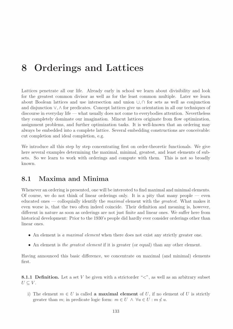
8 Orderings and Lattices
Lattices penetrate all our life. Already early in school we learn about divisibility and lookfor the greatest common divisor as well as for the least common multiple. Later we learnabout Boolean lattices and use intersection and union ∪,∩ for sets as well as conjunctionand disjunction ∨,∧ for predicates. Concept lattices give us orientation in all our techniques ofdiscourse in everyday life — what usually does not come to everybodies attention. Neverthelessthey completely dominate our imagination. Mincut lattices originate from flow optimization,assignment problems, and further optimization tasks. It is well-known that an ordering mayalways be embedded into a complete lattice. Several embedding constructions are conceivable:cut completion and ideal completion, e.g.
We introduce all this step by step concentrating first on order-theoretic functionals. We givehere several examples determining the maximal, minimal, greatest, and least elements of sub-sets. So we learn to work with orderings and compute with them. This is not so broadlyknown.
8.1 Maxima and Minima
Whenever an ordering is presented, one will be interested to find maximal and minimal elements.Of course, we do not think of linear orderings only. It is a pity that many people — eveneducated ones — colloquially identify the maximal element with the greatest. What makes iteven worse is, that the two often indeed coincide. Their definition and meaning is, however,different in nature as soon as orderings are not just finite and linear ones. We suffer here fromhistorical development: Prior to the 1930’s people did hardly ever consider orderings other thanlinear ones.
• An element is a maximal element when there does not exist any strictly greater one.
• An element is the greatest element if it is greater (or equal) than any other element.
Having announced this basic difference, we concentrate on maximal (and minimal) elementsfirst.
8.1.1 Definition. Let a set V be given with a strictorder “<”, as well as an arbitrary subsetU ⊆ V .
i) The element m ∈ U is called a maximal element of U , if no element of U is strictlygreater than m; in predicate logic form: m ∈ U ∧ ∀u ∈ U : m </ u.
133

134 Chapter 8 Orderings and Lattices
ii) Correspondingly, the element m ∈ U is called a minimal element of U , if no elementof U is strictly less than m; in predicate logic form: m ∈ U ∧ ∀u ∈ U : m >/ u.
When looking for maximal elements, one should be prepared to find as a result a set of elementswhich may thus be empty, a one-element set, or a multi-element set. The algebraic definitionuses the strictorder C instead of “<”. Then we move gradually to the componentfree form:
m ∈ U ∧ ∀u ∈ U : m </ um ∈ U ∧ ∀u : u ∈ U → m </ u proceeding to quantification over the whole domainm ∈ U ∧ ∀u : u /∈ U ∨ m </ u using that a → b = ¬a ∨ bm ∈ U ∧ ¬(∃u : u ∈ U ∧ m < u) using that ¬(∀x : p(x)) = ∃x : ¬p(x)m ∈ U ∧ ¬(∃u : m < u ∧ u ∈ U) using that a ∧ b = b ∧ aUu ∩ ¬(∃u : Cmu ∧ Uu) corresponding matrix and vector formUu ∩ C ; Uu composition of relation and vector
So we arrive at the componentfree definition
maxC(U) := U ∩ C ; U
and analagously,
minC(U) := U ∩ CT; U
People are usually heavily oriented towards predicate logic formulations. One can, however,also read the present relation-algebraic form directly: Maximal elements are elements from Ufor which it is not the case that one can go a step up according to C and reach an elementfrom U .
1 2 3 4 5
12345
⎛⎜⎜⎝
1 1 1 1 10 1 0 1 10 0 1 0 10 0 0 1 00 0 0 0 1
⎞⎟⎟⎠
1
23
45
12345
⎛⎜⎜⎜⎝
11000
⎞⎟⎟⎟⎠ →
12345
⎛⎜⎜⎜⎝
01000
⎞⎟⎟⎟⎠
12345
⎛⎜⎜⎜⎝
01011
⎞⎟⎟⎟⎠ →
12345
⎛⎜⎜⎜⎝
00011
⎞⎟⎟⎟⎠
12345
⎛⎜⎜⎜⎝
11100
⎞⎟⎟⎟⎠ →
12345
⎛⎜⎜⎜⎝
01100
⎞⎟⎟⎟⎠
Fig. 8.1.1 An ordering with three sets and their sets of maxima
Something ignored in test edition!
8.2 Bounds and Cones
An upper bound of a subset U ⊆ V is some element s that is greater or equal than all elements ofU , regardless of whether the element s itself belongs to U . A lower bound is defined accordingly.We first recall this definition in a slightly more formal way.
8.2.1 Definition. Let an ordering “≤” be given on a set V .
i) The element s ∈ V is called an upper bound (also: majorant) of the set U ⊆ Vprovided ∀u ∈ U : u ≤ s.
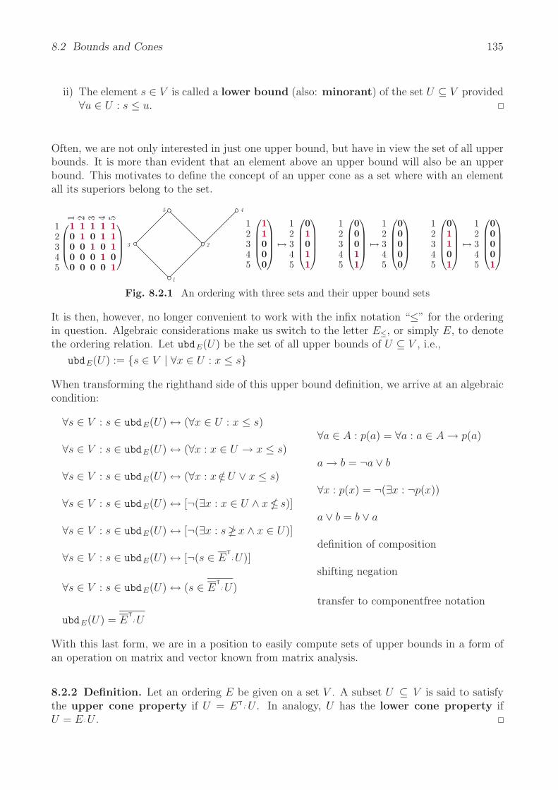
8.2 Bounds and Cones 135
ii) The element s ∈ V is called a lower bound (also: minorant) of the set U ⊆ V provided∀u ∈ U : s ≤ u.
Often, we are not only interested in just one upper bound, but have in view the set of all upperbounds. It is more than evident that an element above an upper bound will also be an upperbound. This motivates to define the concept of an upper cone as a set where with an elementall its superiors belong to the set.
1 2 3 4 5
12345
⎛⎜⎜⎝
1 1 1 1 10 1 0 1 10 0 1 0 10 0 0 1 00 0 0 0 1
⎞⎟⎟⎠
1
23
45
12345
⎛⎜⎜⎜⎝
11000
⎞⎟⎟⎟⎠ →
12345
⎛⎜⎜⎜⎝
01011
⎞⎟⎟⎟⎠
12345
⎛⎜⎜⎜⎝
00011
⎞⎟⎟⎟⎠ →
12345
⎛⎜⎜⎜⎝
00000
⎞⎟⎟⎟⎠
12345
⎛⎜⎜⎜⎝
01101
⎞⎟⎟⎟⎠ →
12345
⎛⎜⎜⎜⎝
00001
⎞⎟⎟⎟⎠
Fig. 8.2.1 An ordering with three sets and their upper bound sets
It is then, however, no longer convenient to work with the infix notation “≤” for the orderingin question. Algebraic considerations make us switch to the letter E≤, or simply E, to denotethe ordering relation. Let ubdE(U) be the set of all upper bounds of U ⊆ V , i.e.,
ubdE(U) := s ∈ V | ∀x ∈ U : x ≤ s
When transforming the righthand side of this upper bound definition, we arrive at an algebraiccondition:
∀s ∈ V : s ∈ ubdE(U) ↔ (∀x ∈ U : x ≤ s)∀a ∈ A : p(a) = ∀a : a ∈ A → p(a)
∀s ∈ V : s ∈ ubdE(U) ↔ (∀x : x ∈ U → x ≤ s)a → b = ¬a ∨ b
∀s ∈ V : s ∈ ubdE(U) ↔ (∀x : x∈/ U ∨ x ≤ s)∀x : p(x) = ¬(∃x : ¬p(x))
∀s ∈ V : s ∈ ubdE(U) ↔ [¬(∃x : x ∈ U ∧ x≤/ s)]a ∨ b = b ∨ a
∀s ∈ V : s ∈ ubdE(U) ↔ [¬(∃x : s≥/ x ∧ x ∈ U)]definition of composition
∀s ∈ V : s ∈ ubdE(U) ↔ [¬(s ∈ ET; U)]
shifting negation
∀s ∈ V : s ∈ ubdE(U) ↔ (s ∈ ET; U)
transfer to componentfree notation
ubdE(U) = ET; U
With this last form, we are in a position to easily compute sets of upper bounds in a form ofan operation on matrix and vector known from matrix analysis.
8.2.2 Definition. Let an ordering E be given on a set V . A subset U ⊆ V is said to satisfythe upper cone property if U = ET ; U . In analogy, U has the lower cone property ifU = E ; U .

136 Chapter 8 Orderings and Lattices
One can interpret U = ET;U by saying that when one has stepped down according to E endingin a point of the set U , then one has necessarily already been starting in U . That this holdstrue when U := ubdE(X) is an upper bound set can be proved algebraically:
ET; U = ET;ubdE(X) ⊇ ubdE(X) = U as E is reflexive
But also the other way round using transitivity and the Schroder rule:
ET;ET ⊆ ET ⇐⇒ E;ET ⊆ E
T=⇒ E;E
T;X ⊆ E
T;X ⇐⇒ ET;E
T; X ⊆ E
T; X
so that
ET; U = ET;ubdE(X) = ET; ET; X ⊆ E
T; X = ubdE(X) = U
Exercises
OK3.3.1 Prove the identity R; S = R; RT; R; S for arbitrary relations R, S. Relate this to lbd and
ubd .
Solution OK3.3.1 R; S ⊆ R; S ⇐⇒ RT; R; S ⊆ S ⇐⇒ S ⊆ R
T; R; S =⇒ R; S ⊆ R; R
T; R; S.
RT; R; S ⊆ R
T; R; S ⇐⇒ R; R
T; R; S ⊆ R; S.
So we have alwayslbdR(S) = lbdR(ubdR(lbdR(S)))
where R need not be an ordering.
3.3.2 Let R be an arbitrary relation which is not necessarily an ordering. Define ubdR(X) :=
RT; X and lbdR(X) := R; X, and prove
ubdR(X) = ubdR(lbdR(ubdR(X))).
Solution 3.3.2 Same as 3.3.1
3.3.5 For points x, y, the condition ubd(x) = ubd(y) implies x = y.
Solution 3.3.5 E;x = ubd(x) = ubd(y) = E;y. E ; x = ubd(x)??? Mehrmals mit (2.4.5.ii) gilt
x;yT ⊆ E;x;yT = E;y;yT ⊆ E und x;yT ⊆ x;yT;ET = x;xT;ET ⊆ ET, also x;yT ⊆ E ∩ ET = .Also erhalt man x = y.
8.3 Least and Greatest Elements
As we have already noticed, it is necessary to distinguish the maximal elements from the greatestelement of a set. If the latter exists, it is the only maximum. The predicate logic form of adefinition of a greatest element is as follows.
8.3.1 Definition. Let a set V be given that is ordered with the relation “≤”, and an arbitrarysubset U ⊆ V . The element g ∈ U is called the greatest element of U , if for all elementse ∈ U we have e ≤ g. The element l ∈ U is called the least element of U , if for all elementse ∈ U we have e ≥ l.
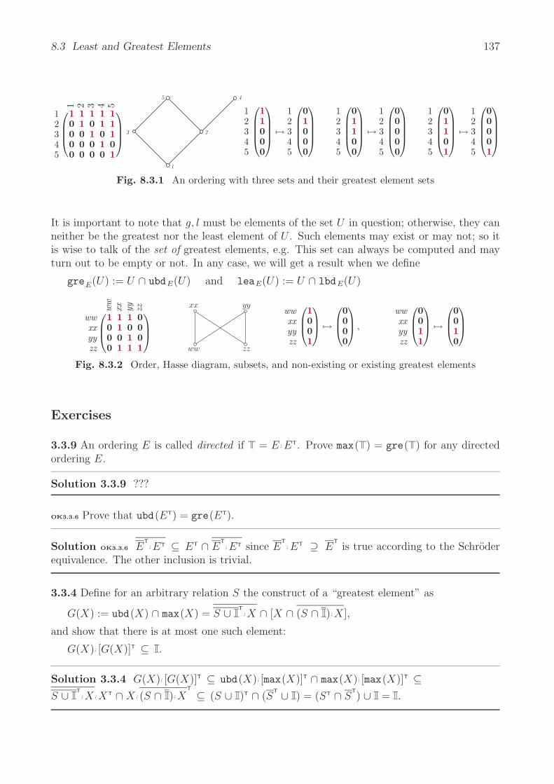
8.3 Least and Greatest Elements 137
1 2 3 4 512345
⎛⎜⎜⎝
1 1 1 1 10 1 0 1 10 0 1 0 10 0 0 1 00 0 0 0 1
⎞⎟⎟⎠
1
23
45
12345
⎛⎜⎜⎜⎝
11000
⎞⎟⎟⎟⎠ →
12345
⎛⎜⎜⎜⎝
01000
⎞⎟⎟⎟⎠
12345
⎛⎜⎜⎜⎝
01100
⎞⎟⎟⎟⎠ →
12345
⎛⎜⎜⎜⎝
00000
⎞⎟⎟⎟⎠
12345
⎛⎜⎜⎜⎝
01101
⎞⎟⎟⎟⎠ →
12345
⎛⎜⎜⎜⎝
00001
⎞⎟⎟⎟⎠
Fig. 8.3.1 An ordering with three sets and their greatest element sets
It is important to note that g, l must be elements of the set U in question; otherwise, they canneither be the greatest nor the least element of U . Such elements may exist or may not; so itis wise to talk of the set of greatest elements, e.g. This set can always be computed and mayturn out to be empty or not. In any case, we will get a result when we define
greE(U) := U ∩ ubdE(U) and leaE(U) := U ∩ lbdE(U)
ww
xx yy zz
wwxxyyzz
⎛⎜⎝
1 1 1 00 1 0 00 0 1 00 1 1 1
⎞⎟⎠
ww
xx yy
zz
wwxxyyzz
⎛⎜⎝
1001
⎞⎟⎠ →
⎛⎜⎝
0000
⎞⎟⎠ ,
wwxxyyzz
⎛⎜⎝
0011
⎞⎟⎠ →
⎛⎜⎝
0010
⎞⎟⎠
Fig. 8.3.2 Order, Hasse diagram, subsets, and non-existing or existing greatest elements
Exercises
3.3.9 An ordering E is called directed if = E ; ET. Prove max( ) = gre( ) for any directedordering E.
Solution 3.3.9 ???
OK3.3.6 Prove that ubd(ET) = gre(ET).
Solution OK3.3.6 ET; ET ⊆ ET ∩ E
T; ET since E
T; ET ⊇ E
Tis true according to the Schroder
equivalence. The other inclusion is trivial.
3.3.4 Define for an arbitrary relation S the construct of a “greatest element” as
G(X) := ubd(X) ∩ max(X) = S ∪ T; X ∩ [X ∩ (S ∩ ); X],
and show that there is at most one such element:
G(X); [G(X)]T ⊆ .
Solution 3.3.4 G(X); [G(X)]T ⊆ ubd(X); [max(X)]T ∩ max(X); [max(X)]T ⊆S ∪ T
; X ; XT ∩ X ; (S ∩ ); XT
⊆ (S ∪ )T ∩ (ST ∪ ) = (ST ∩ S
T) ∪ = .

138 Chapter 8 Orderings and Lattices
8.4 Greatest Lower and Least Upper Bounds
Among the set of upper bounds of some set, there may exists a least element in the same wayas there is a least element among all multiples of a set of natural numbers — known as leastcommon multiple. Starting herefrom, traditional functionals may be obtained, namely the leastupper bound u, (also: supremum), i.e., the at most 1-element set of least elements among theset of all upper bounds of u In contrast to our expectation that a least upper bound may existor not, it will here always exist as a vector; it may, however be the null vector resembling thatthere is none, or else a 1-element vector.
8.4.1 Definition. Let an ordered set V,≤ be given and a subset U ⊆ V . An element l iscalled the least upper bound of U if it is the least element in the set of all upper bounds.An element g is called the greatest lower bound of U if it is the greatest element in the setof all lower bounds.
Applying the definitions presented earlier, the least upper and greatest lower bounds maybe defined as
lubE(U) := ubdE(U) ∩ lbdE(ubdE(U)) := ET; U ∩ E ; E
T; U
glbE(U) := lbdE(U) ∩ ubdE(lbdE(U)) := E ; U ∩ ET; E ; U
These functionals are always defined; the results may, however, be null vectors. It is an easytask to prove that lub , glb are always injective, resembling that such bounds are uniquelydefined if they exist, see Ch. 3 of [SS89, SS93]. As an example we compute the least upper
bound of the relation E itself, employing the well-known facts ET; E = ET and E ; ET = E as
well as antisymmetry of E:
lubE(E) = ET; E ∩ E ; E
T; E = ET ∩ E ; ET = ET ∩ E = .
1 2 3 4 5
12345
⎛⎜⎜⎝
1 1 1 1 10 1 0 1 10 0 1 0 10 0 0 1 00 0 0 0 1
⎞⎟⎟⎠
1
23
45
12345
⎛⎜⎜⎜⎝
11000
⎞⎟⎟⎟⎠ →
12345
⎛⎜⎜⎜⎝
01000
⎞⎟⎟⎟⎠ ,
12345
⎛⎜⎜⎜⎝
01100
⎞⎟⎟⎟⎠ →
12345
⎛⎜⎜⎜⎝
00001
⎞⎟⎟⎟⎠ ,
12345
⎛⎜⎜⎜⎝
01110
⎞⎟⎟⎟⎠ →
12345
⎛⎜⎜⎜⎝
00000
⎞⎟⎟⎟⎠
Fig. 8.4.1 An ordering with three sets and their least upper bound sets
As a tradition, a vector is often a column vector. In many cases, however, a row vector wouldbe more convenient. We decided to introduce a variant notation for order-theoretic functionalsworking on row vectors:
lubRE(X) := [lubE(XT)]T, etc.
For convenience we introduce notation for least and greatest elements as
0E = glbE( ) = leaE( ), 1E = lubE( ) = greE( )
When using 0E, 1E it is understood that the underlying vectors are not null vectors.
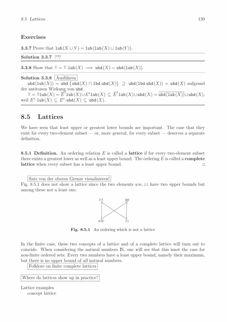
8.5 Lattices 139
Exercises
3.3.7 Prove that lub(X ∪ Y ) = lub(lub(X) ∪ lub(Y )).
Solution 3.3.7 ???
3.3.8 Show that = ;lub(X) =⇒ ubd(X) = ubd(lub(X)).
Solution 3.3.8 Ausfuhrenubd(lub(X)) = ubd
(ubd(X) ∩ lbd ubd(X)
)⊇ ubd(lbd ubd(X)) = ubd(X) aufgrund
der antitonen Wirkung von ubd .= ;lub(X) = E
T;lub(X)∪ET;lub(X) ⊆ E
T;lub(X)∪ubd(X) = ubd(lub(X))∪ubd(X),
weil ET;lub(X) ⊆ ET;ubd(X) ⊆ ubd(X).
8.5 Lattices
We have seen that least upper or greatest lower bounds are important. The case that theyexist for every two-element subset — or, more general, for every subset — deserves a separatedefinition.
8.5.1 Definition. An ordering relation E is called a lattice if for every two-element subsetthere exists a greatest lower as well as a least upper bound. The ordering E is called a completelattice when every subset has a least upper bound.
Satz von der oberen Grenze visualisieren!Fig. 8.5.1 does not show a lattice since the two elements ww, zz have two upper bounds butamong these not a least one.
ww
xx yy
zz
Fig. 8.5.1 An ordering which is not a lattice
In the finite case, these two concepts of a lattice and of a complete lattice will turn out tocoincide. When considering the natural numbers IN, one will see that this isnot the case fornon-finite ordered sets: Every two numbers have a least upper bound, namely their maximum,but there is no upper bound of all natural numbers.
Folklore on finite complete lattices
Where do lattices show up in practice?
Lattice examplesconcept lattice

140 Chapter 8 Orderings and Lattices
mincut latticeassignment lattice
8.5.2 Definition. Let an order E be given together with a nonempty subset v and its corre-sponding natural injection ιv and restricted ordering Ev := ιv ; E ; ιT
v. We then say that
v is an antichain :⇐⇒ Ev is a trivial order, i.e., Ev = .
With every chain v all its non-empty subsets are obviously antichains. There may exist differentmaximum antichains. The set of all cardinality-maximum antichains is an interesting exampleof a lattice.
8.5.3 Proposition. Given any finite order E, the set of cardinality-maximum antichains formsa lattice with order and corresponding infima and suprema defined as
v1 v2 :⇐⇒ ιTv1
; ιv2 ⊆ Ev1 v2 := max(E ; v1 ∪ E ; v2)
v1 v2 := max(E ; v1 ∩ E ; v2)
Proof : Let A := (vi)i∈J be the (finite) set of cardinality-maximum antichains for E. Thecardinalities of these sets are, of course, equal. The injections ιv corresponding to the non-emptyantichain subsets may thus be conceived as injective mappings with all the same domain.
The relation “” is reflexive as the injections are univalent. As ιv2; ιT
v2⊆ for the injection
corresponding to v2, the relation “” is obviously transitive. Antisymmetry follows from ιTv1
;ιv2∩ιTv2
;ιv1 ⊆ E ∩ET ⊆ and totality of ιv2 , from which we get v1 = ιTv1
; = ιTv1
;ιv2;ιT
v2; ⊆ ιT
v2; = v2
and vice versa.
One will verify that
ιv1v2 = (ιv1 ∩ ιv2; ET) ∪ (ιv2 ∩ ιv1
; ET)ιv1v2 = (ιv1 ∩ ιv2
; E) ∪ (ιv2 ∩ ιv1; E)
Starting herefrom we prove that they are indeed antichains.
ιv1v2; E ; ιT
v1v2=
[(ιv1 ∩ ιv2
; ET) ∪ (ιv2 ∩ ιv1; ET)
]; E ;
[(ιT
v1∩ E ; ιT
v2) ∪ (ιT
v2∩ E ; ιT
v1)]
⊆ (ιv1; E ; ιT
v1) ∪ (ιv1
; E ; E ; ιTv1
) ∪ (ιv2; E ; ιT
v1) ∪ (ιv2
; E ; E ; ιTv2
) ⊆
not yet ok
As all this is so nice, one often tries to complete an ordering so as to obtain a lattice. We willgive a short description of cut completion and ideal completion later.
8.6 Cut Completion of an Ordering
We have seen that a lattice, and in particular, a complete lattice, enjoy pleasant properties. Sothe question has arisen whether one may at least embed an ordering into a lattice in order tomake use of some of these nice properties. This runs under the names of a cut completionand an ideal completion, for which we will give some hints.

8.6 Cut Completion of an Ordering 141
With an example we try to make clear what a cut completion is like. The ordered set shall bethe 4-element set as shown in Fig. 8.5.1, but now with named elements for better identificationin Fig. 8.6.1. The matrix gives the ordering while the graph restricts to presenting the Hassediagram only as otherwise the picture would be overcrowded.
ww
xx yy zz
wwxxyyzz
⎛⎜⎝
1 1 1 00 1 0 00 0 1 00 1 1 1
⎞⎟⎠= E
ww
xx yy
zz
ε =
ww
xx
ww,x
xy
yw
w,y
yx
x,yy
ww,x
x,yy
zz
ww,zz
xx,
zz
ww,x
x,zz
yy,
zz
ww,y
y,zz
xx,
yy,zz
ww,x
x,yy
,zz
wwxxyyzz
⎛⎜⎝
0 1 0 1 0 1 0 1 0 1 0 1 0 1 0 10 0 1 1 0 0 1 1 0 0 1 1 0 0 1 10 0 0 0 1 1 1 1 0 0 0 0 1 1 1 10 0 0 0 0 0 0 0 1 1 1 1 1 1 1 1
⎞⎟⎠
ww
xx
ww,x
xy
yw
w,y
yx
x,yy
ww,x
x,yy
zz
ww,zz
xx,
zz
ww,x
x,zz
yy,
zz
ww,y
y,zz
xx,
yy,zz
ww,x
x,yy
,zz
wwxxyyzz
⎛⎜⎝
1 1 0 0 0 0 0 0 0 0 0 0 0 0 0 01 1 1 1 0 0 0 0 1 1 1 1 0 0 0 01 1 0 0 1 1 0 0 1 1 0 0 1 1 0 01 0 0 0 0 0 0 0 1 0 0 0 0 0 0 0
⎞⎟⎠
lower bounds ubd(ε)
ww
xx
ww,x
xy
yw
w,y
yx
x,yy
ww,x
x,yy
zz
ww,zz
xx,
zz
ww,x
x,zz
yy,
zz
ww,y
y,zz
xx,
yy,zz
ww,x
x,yy
,zz
wwxxyyzz
⎛⎜⎝
0 1 1 1 1 1 1 1 0 1 1 1 1 1 1 10 0 1 1 0 0 1 1 0 0 1 1 0 0 1 10 0 0 0 1 1 1 1 0 0 0 0 1 1 1 10 0 1 1 1 1 1 1 1 1 1 1 1 1 1 1
⎞⎟⎠
upper bounds of lower bounds lbd(ubd(ε))(1 1 0 0 0 0 0 0 1 1 0 1 0 1 0 1)
equal columns marked
ww
xx
ww,x
xy
yw
w,y
yx
x,yy
ww,x
x,yy
zz
ww,zz
xx,
zz
ww,x
x,zz
yy,
zz
ww,y
y,zz
xx,
yy,zz
ww,x
x,yy
,zz
→ww→zz→
ww,zz→ww,xx,zz→ww,yy,zz→
ww,xx,yy,zz→
⎛⎜⎜⎜⎜⎜⎜⎝
1 0 0 0 0 0 0 0 0 0 0 0 0 0 0 00 1 0 0 0 0 0 0 0 0 0 0 0 0 0 00 0 0 0 0 0 0 0 1 0 0 0 0 0 0 00 0 0 0 0 0 0 0 0 1 0 0 0 0 0 00 0 0 0 0 0 0 0 0 0 0 1 0 0 0 00 0 0 0 0 0 0 0 0 0 0 0 0 1 0 00 0 0 0 0 0 0 0 0 0 0 0 0 0 0 1
⎞⎟⎟⎟⎟⎟⎟⎠
Fig. 8.6.1 A cut completion
8.6.1 Example. Consider the 4-element set V = xx, yy, ww, zz related with ε to its pow-

142 Chapter 8 Orderings and Lattices
erset 2V . Using lbd(E, x), which means forming E ; x, all lower bounds of these sets are deter-mined. Following this, for all these lower bounds in addition the upper bounds ma o (mi o x)
are formed. These always form the “cone closure” of the original set.
HasseDiagE =
⎛⎜⎝
0 0 1 10 0 1 10 0 0 00 0 0 0
⎞⎟⎠ E =
⎛⎜⎝
1 0 1 10 1 1 10 0 1 00 0 0 1
⎞⎟⎠ ε =
⎛⎜⎝
0 1 0 1 0 1 0 1 0 1 0 1 0 1 0 10 0 1 1 0 0 1 1 0 0 1 1 0 0 1 10 0 0 0 1 1 1 1 0 0 0 0 1 1 1 10 0 0 0 0 0 0 0 1 1 1 1 1 1 1 1
⎞⎟⎠
lower bounds ubd (ε) =
⎛⎜⎝
1 1 0 0 1 1 0 0 1 1 0 0 1 1 0 01 0 1 0 1 0 1 0 1 0 1 0 1 0 1 01 0 0 0 1 0 0 0 0 0 0 0 0 0 0 01 0 0 0 0 0 0 0 1 0 0 0 0 0 0 0
⎞⎟⎠
upper bounds of lower bounds lbd (ubd (ε)) =
⎛⎜⎝
0 1 0 1 0 1 0 1 0 1 0 1 0 1 0 10 0 1 1 0 0 1 1 0 0 1 1 0 0 1 10 1 1 1 1 1 1 1 0 1 1 1 1 1 1 10 1 1 1 0 1 1 1 1 1 1 1 1 1 1 1
⎞⎟⎠
Fig. 8.6.2 Hasse diagram, ordering, membership, lower and upper of lower bounds
A few sets are not changed by this procedure; they are “invariant” under forming majorants ofminorants. All sets with this characteristic property are marked, then extruded and depictedwith their inclusion ordering. One will immediately recognize that precisely those sets areunchanged that are closed to the lower side as, e.g., xx, ww, zz. They are the lower cones. Itis indicated in which way every element of the original ordered set V in the right diagram maybe found as the top of some cone directed downwards. As only Hasse diagrams of the emergingordered set are presented, this does not look too similar. But indeed, xx ⊆ xx, ww, zz theold ordering is mapped isotone/homomorphic into the new one.
What might easily be considered juggling around, follows a general concept. With the techniquepresented here in the example, one may in principle “embed” every ordered set into a completelattice. Applying such a technique, one will be able to define real numbers in a precise manner!Already ancient Greeks knew, that the rational numbers are not sufficiently dense and one hadto insert
√2 or π, e.g., in between.
First the ordering is shown as a relation and a Hasse diagram. Fig. 8.6.3 shows in addition thesubset inclusion relation. (In this case, ideal completion not yet inttroduced will produce thesame result.)
Cut embedding = Ideal embedding =
→
ww→
zz→
ww,zz→
ww,x
x,zz→
ww,y
y,zz→
ww,x
x,yy
,zz→
→ww→zz→
ww,zz→ww,xx,zz→ww,yy,zz→
ww,xx,yy,zz→
⎛⎜⎜⎜⎜⎜⎜⎝
1 1 1 1 1 1 10 1 0 1 1 1 10 0 1 1 1 1 10 0 0 1 1 1 10 0 0 0 1 0 10 0 0 0 0 1 10 0 0 0 0 0 1
⎞⎟⎟⎟⎟⎟⎟⎠
Fig. 8.6.3 Inclusion of cones of Fig. 8.6.2
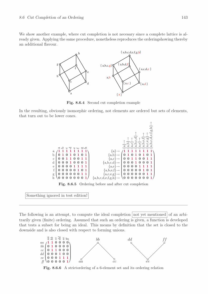
8.6 Cut Completion of an Ordering 143
We show another example, where cut completion is not necesary since a complete lattice is al-ready given. Applying the same procedure, nonetheless reproduces the orderingshowing therebyan additional flavour.
a
c
b
d
ef
g
h
a
a,b,c,g
a,d
a,c,d,e
a,b,c,d,e,f,g,h
a,c
a,b
a,b,d,f
Fig. 8.6.4 Second cut completion example
In the resulting, obviously isomorphic ordering, not elements are ordered but sets of elements,that turn out to be lower cones.
a b c d e f g h
abcdefgh
⎛⎜⎜⎜⎜⎜⎜⎜⎜⎝
1 1 1 1 1 1 1 10 1 0 1 0 1 0 10 0 1 1 0 0 1 10 0 0 1 0 0 0 10 0 0 0 1 1 1 10 0 0 0 0 1 0 10 0 0 0 0 0 1 10 0 0 0 0 0 0 1
⎞⎟⎟⎟⎟⎟⎟⎟⎟⎠
a→
a,b→
a,c→
a,b
,c,d→
a,e→
a,b
,e,f
→a
,c,e
,g→
a,b
,c,d
,e,f,
g,h
→a→
a,b→a,c→
a,b,c,d→a,e→
a,b,e,f→a,c,e,g→
a,b,c,d,e,f,g,h→
⎛⎜⎜⎜⎜⎜⎜⎜⎜⎝
1 1 1 1 1 1 1 10 1 0 1 0 1 0 10 0 1 1 0 0 1 10 0 0 1 0 0 0 10 0 0 0 1 1 1 10 0 0 0 0 1 0 10 0 0 0 0 0 1 10 0 0 0 0 0 0 1
⎞⎟⎟⎟⎟⎟⎟⎟⎟⎠
Fig. 8.6.5 Ordering before and after cut completion
Something ignored in test edition!
The following is an attempt, to compute the ideal completion not yet mentioned of an arbi-
trarily given (finite) ordering. Assumed that such an ordering is given, a function is developedthat tests a subset for being an ideal. This means by definition that the set is closed to thedownside and is also closed with respect to forming unions.
aa bb cc dd ee ff
aabbccddeeff
⎛⎜⎜⎜⎜⎝
1 1 0 0 0 00 1 0 0 0 00 1 1 0 0 00 0 0 1 0 00 0 0 1 1 10 0 0 0 0 1
⎞⎟⎟⎟⎟⎠
aa
bb
cc
dd
ee
ff
Fig. 8.6.6 A strictordering of a 6-element set and its ordering relation

144 Chapter 8 Orderings and Lattices
In this case, the cut completion is a simple one: Just a top element aa, bb, cc, dd , ee, f f and abottom element are added. One should observe that annotations are now sets of the originalvertices. For those cases where this set is a set closed to the down-side, its top element isunderlined to make clear in which way the embedding takes place.
→
aa
→c
c→
aa,
bb,cc→
ee→
dd,
ee→
ee,
ff→
aa,
bb,cc,
dd,ee,
ff→
→aa→cc→
aa,bb,cc→ee→
dd,ee→ee,ff→
aa,bb,cc,dd,ee,ff→
⎛⎜⎜⎜⎜⎜⎜⎜⎜⎝
1 1 1 1 1 1 1 10 1 0 1 0 0 0 10 0 1 1 0 0 0 10 0 0 1 0 0 0 10 0 0 0 1 1 1 10 0 0 0 0 1 0 10 0 0 0 0 0 1 10 0 0 0 0 0 0 1
⎞⎟⎟⎟⎟⎟⎟⎟⎟⎠
Fig. 8.6.7 Lattice obtained by cut completion
Something ignored in test edition!

9 Rectangles
Although not many scientists seem to be aware of this fact, an incredible amount of our rea-soning is concerned with “rectangles” in/of a relation. Rectangles are handled at various placesfrom the theoretical point of view as well as from the practical side. Among the application ar-eas are equivalences, preorders, concept lattices, clustering methods, and measuring, to mentionjust a few seemingly incoherent ones. In most cases, rectangles are treated in the respectiveapplication environment, i.e., together with certain additional properties. So it is not clearwhich results stem from their status as rectangles as such and which employ these additionalproperties. Here we try to formulate rectangle properties before going into the various applica-tions and hope, thus, to present several concepts only once, facilitating the overall amount ofwork.
9.1 Maximal Rectangles
In Def. 5.6.2 , we have already introduced rectangles on a rather phaenomenological basis. Wewill investigate them here in more detail.
9.1.1 Definition. Let a relation R be given together with subsets u, v that form a rectangleinside R, i.e., all the following are satisfied: u; vT ⊆ R ⇐⇒ R; v ⊆ u ⇐⇒ R
T; u ⊆ v.
The rectangle u, v is said to be non-enlargable if there does not exist a different rectangleu′, v′ with the respective property such that u ⊆ u′ and v ⊆ v′.
Non-enlargable rectangles are maximal, but they need not be greatest ones. The property toconstitute a maximal rectangle has an algebraic characterisation.
9.1.2 Proposition. Let u, v define a rectangle inside the relation R. Precisely when both,
R; v = u and RT; u = v,
are satisfied, there will exist no strictly greater rectangle u′, v′ inside R. A reformulation ofthese conditions using residuals is
u = R/vT and vT = u\R.
Proof : Let us assume a rectangle that does not satisfy, e.g., the first equation: R;v ⊂=/ u. Then
there will exist a point p ⊆ u∩R; v (at least in the case of finite representable relations handledhere). Then u′ := u ∪ p =/ u and v′ := v is a strictly greater rectangle as p; vT ⊆ R.
Consider for the opposite direction a rectangle u, v inside R satisfying the two equations togetherwith another rectangle u′, v′ inside R such that u ⊆ u′ and v ⊆ v′. Then we may conclude
145

146 Chapter 9 Rectangles
with monotony and an application of the Schroder rule that v′ ⊇ RT
; u′ ⊇ RT
; u = v. Thisresults in v′ = v. In a similar way it is shown that u = u′. To sum up, u′, v′ is not strictlygreater than u, v.
Note that both of the two equations R;v = u and RT;u = v are used in this proof; they are not
via Schroder’s rule equivalent with one another as their ⊆ -versions are.
Consider a pair of elements (x, y) related by some relation R. This may be expressed a littlemore algebraically as x;yT ⊆ R or, equivalently, as x ⊆ R;y due to Prop. 5.2.5. It is immediatelyclear that y may or may not be the only point related with x. With RT;x we have the set of allelements of the codomain side related with x. As we have been starting from (x, y) ∈ R, it isnonempty, i.e., =/ y ⊆ RT; x.
For reasons we will accept shortly, it is advisable to use the identity RT; x = RT; x which holds
due to Prop. 5.2.6 if x is a point. We then see, that a whole rectangle — may be one-elementonly — is contained in R, namely the one given by rows
ux := R; RT; x on the domain side together with columns
vx := RT; x on the range side.
One application of the Schroder equivalence shows that indeed ux ; vTx ⊆ R. Some preference
has here been given to x, so that we expect something similar to hold when starting with y.This is indeed the case; for the rectangle defined by
uy := R; y on the domain side
vy := RT; R; y on the range side
we have analogously uy ; vTy ⊆ R. Fig. 9.1.1 indicates how these rectangles turn out to be
non-enlargable ones.
Regarding Def. 8.4.1, one will find out that — although R has not been defined as an ordering— the construct is similar to those defining upper bound sets and lower bound sets of upperbound sets.
In both cases, we have non-enlargable rectangles inside R according to Prop. 9.1.2. Indeed,
R; vx = ux and RT; ux = vx
as well as
R; vy = uy and RT; ux = vy.
This may easily be seen as “⊆ ” is trivially satisfied and, e.g., R; RT; x ⊆ x, so that “ ⊇ ”.
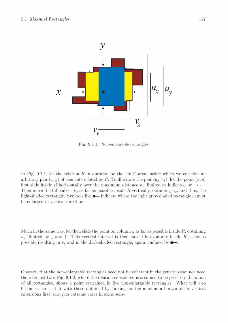
9.1 Maximal Rectangles 147
y
x ux
vxy
uy
vFig. 9.1.1 Non-enlargable rectangles
In Fig. 9.1.1, let the relation R in question be the “full” area, inside which we consider anarbitrary pair (x, y) of elements related by R. To illustrate the pair (ux, vx), let the point (x, y)first slide inside R horizontally over the maximum distance vx, limited as indicated by → ←.Then move the full subset vx as far as possible inside R vertically, obtaining ux, and thus, thelight-shaded rectangle. Symbols like indicate where the light grey-shaded rectangle cannotbe enlarged in vertical direction.
Much in the same way, let then slide the point on column y as far as possible inside R, obtaininguy, limited by ↓ and ↑. This vertical interval is then moved horizontally inside R as far aspossible resulting in vy and in the dark-shaded rectangle, again confined by .
Observe, that the non-enlargable rectangles need not be coherent in the general case; nor needthere be just two. Fig. 9.1.2, where the relation considered is assumed to be precisely the unionof all rectangles, shows a point contained in five non-enlargable rectangles. What will alsobecome clear is that with those obtained by looking for the maximum horizontal or verticalextensions first, one gets extreme cases in some sense.

148 Chapter 9 Rectangles
Fig. 9.1.2 A point contained in five non-enlargable rectangles
9.1.3 Proposition. For a pair (x, y) related by a relation R the following are equivalent:
i) (x, y) is contained in precisely one maximal rectangle.
ii) There is no other pair (u, v) of elements such that together (x, v) ∈ R, (v, u) ∈ RT, (u, y) ∈ R.
Proof : (i) =⇒ (ii): Assume such a pair (u, v) to exist. Then the constructs
lbdR(ubdR(x ∪ u)) = R; RT; (x ∪ u) and ubdR(lbdR(y ∪ v)) = RT; R; (y ∪ v)
constitute two rectangles. By construction, they are non-enlargable. According to asssumption(i) on (u, v), they coincide and so easily contradict the assumptions on (u, v).
(ii) =⇒ (i): Assume two different non-enlargable rectangles containing (x, y) to be given via
their row and column sets (ui, vi)i=1,2. Then they satisfy ui = R; vi as well as vi = RT; ui. Asthe rectangles are different and non-enlargable, certainly neither u1 = u2 nor v1 = v2.
Now points u, v may be chosen as follows
u ⊆ u2 ∩ u1 and v ⊆ v1 ∩ v2
As a consequence, u ⊆ u2 ∩ R; v1 and v ⊆ v1 ∩ RT; u2 . . .
Many important concepts concerning relations depend heavily on rectangles. This follows notleast from the following fact:
9.1.4 Proposition. Every relation R may in essentially one way be written as the union ofnon-enlargable rectangles.
Proof : For the finite case handled here, existence of a decomposition to rectangles is trivial,as we may choose one-point rectangles. To exclude trivialities, let R be different from and
assume two different decompositions in non-enlargable rectangles to be given
R = supnuvi=1 ui; v
Ti = supnab
j=1 aj ; bTj
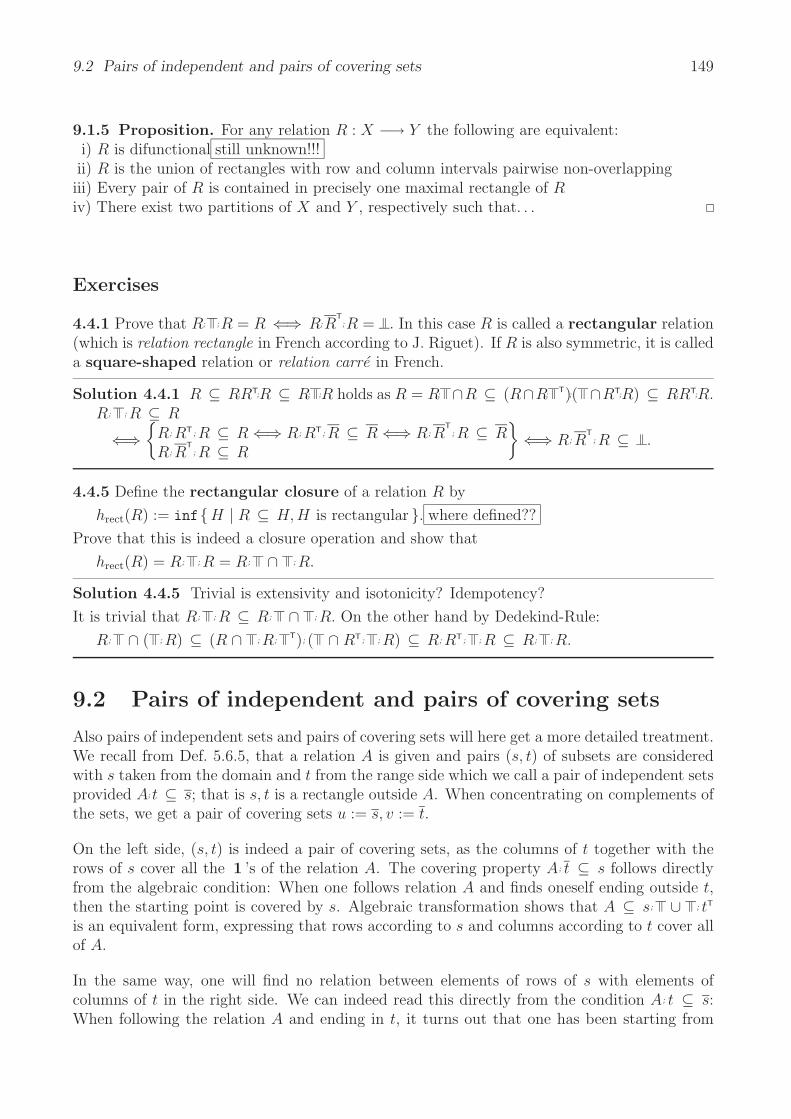
9.2 Pairs of independent and pairs of covering sets 149
9.1.5 Proposition. For any relation R : X −→ Y the following are equivalent:i) R is difunctional still unknown!!!ii) R is the union of rectangles with row and column intervals pairwise non-overlappingiii) Every pair of R is contained in precisely one maximal rectangle of Riv) There exist two partitions of X and Y , respectively such that. . .
Exercises
4.4.1 Prove that R; ;R = R ⇐⇒ R;RT;R = . In this case R is called a rectangular relation
(which is relation rectangle in French according to J. Riguet). If R is also symmetric, it is calleda square-shaped relation or relation carre in French.
Solution 4.4.1 R ⊆ R;RT;R ⊆ R; ;R holds as R = R; ∩R ⊆ (R∩R;T);( ∩RT;R) ⊆ R;RT;R.
R; ; R ⊆ R
⇐⇒
R; RT; R ⊆ R ⇐⇒ R; RT; R ⊆ R ⇐⇒ R; RT; R ⊆ R
R; RT; R ⊆ R
⇐⇒ R; R
T; R ⊆ .
4.4.5 Define the rectangular closure of a relation R by
hrect(R) := infH | R ⊆ H, H is rectangular . where defined??
Prove that this is indeed a closure operation and show that
hrect(R) = R; ; R = R; ∩ ; R.
Solution 4.4.5 Trivial is extensivity and isotonicity? Idempotency?
It is trivial that R; ; R ⊆ R; ∩ ; R. On the other hand by Dedekind-Rule:
R; ∩ ( ; R) ⊆ (R ∩ ; R;T); ( ∩ RT; ; R) ⊆ R; RT; ; R ⊆ R; ; R.
9.2 Pairs of independent and pairs of covering sets
Also pairs of independent sets and pairs of covering sets will here get a more detailed treatment.We recall from Def. 5.6.5, that a relation A is given and pairs (s, t) of subsets are consideredwith s taken from the domain and t from the range side which we call a pair of independent setsprovided A;t ⊆ s; that is s, t is a rectangle outside A. When concentrating on complements ofthe sets, we get a pair of covering sets u := s, v := t.
On the left side, (s, t) is indeed a pair of covering sets, as the columns of t together with therows of s cover all the 1 ’s of the relation A. The covering property A; t ⊆ s follows directlyfrom the algebraic condition: When one follows relation A and finds oneself ending outside t,then the starting point is covered by s. Algebraic transformation shows that A ⊆ s; ∪ ; tT
is an equivalent form, expressing that rows according to s and columns according to t cover allof A.
In the same way, one will find no relation between elements of rows of s with elements ofcolumns of t in the right side. We can indeed read this directly from the condition A; t ⊆ s:When following the relation A and ending in t, it turns out that one has been starting from

150 Chapter 9 Rectangles
outside s. With Schroder’s rule we immediately arrive at s; tT ⊆ A; this also expresses thatfrom s to t, there is no relationship according to A. prove transition
It is a trivial fact that with (s, t) a pair of independent sets and s′ ⊆ s, t′ ⊆ t, also the smaller(s′, t′) will be a pair of independent sets. In the same way, if (s, t) is a pair of covering sets ands′ ⊇ s, t′ ⊇ t, also (s′, t′) will be a pair of covering sets. For pairs of independent sets, one istherefore interested in greatest ones and for covering pairs for smallest ones.
Both concepts allow for enlarging the pair, or reducing it, corresponding to the respectiveordering, so as to arrive at an equation. We prove this for a line-covering.
folgt nun aus dem Satz fur Rechtecke!!!
9.2.1 Proposition. i) Let (s, t) be a line-covering of the relation A, i.e., A; t ⊆ s. Preciselywhen both, A; t = s and AT ; s = t, are satisfied there will be no smaller (i.e. satisfying both,x ⊆ s and y ⊆ t) pair (x, y) =/ (s, t) line-covering A.
ii) Let (s, t) be a pair of independent sets of the relation A, i.e., A;t ⊆ s. Precisely when both,A; t = s and ATs = t, are satisfied there will be no greater (i.e. satisfying both, x ⊇ s andy ⊇ t) pair of independent sets (x, y) =/ (s, t) for A.
Proof : i) Assume A; t ⊂=/ s. Then there will exist a point p ⊆ s ∩ A; t (at least in the case
of finite representable relations handled here). Then x := s ∩ p =/ s and y := t will obviouslyconstitute a strictly smaller line-covering.
If on the other hand side (x, y) is line-covering A with x ⊆ s and y ⊆ t and the two equationsare satisfied, then t = AT; s ⊆ AT; x ⊆ y.
Some relations may be decomposed in such a way, that there is a subset of row entries that iscompletely unrelated to a subset of column entries. In this context, a relation A may admitvectors x and y (with =/ x =/ or =/ y =/ to avoid degeneration), such that A;y ⊆ x or elseA ⊆ x; yT. Given appropriate permutations P of the rows, and Q of the columns, respectively,we then have
P ; A; QT =
(∗∗ ∗
)P ; x =
( )Q; y =
( ).
Given A;y ⊆ x, to enlarge the -zone is not so easy a task, which may be seen at the identityrelation : All shapes from 1 × (n − 1), 2 × (n − 2), . . . (n − 1) × 1 may be chosen. There isno easily acceptable extremality criterion. Therefore, one usually studies this effect with oneof the sets negated.
hier x, y gleichgeordnet!!
The diversity of reductions shown suggests to look for the following line-covering possibility.For the moment, call rows and columns, respectively, lines. Then together with the |x| by |y|zone of 0 ’s, we are able to cover all entries 1 by |x| vertical plus |y| horizontal lines. It isstandard, to try to minimize the number of lines to cover all 1 ’s of the relation.
9.2.2 Definition. Given a relation A, the term rank is defined as the minimum number oflines necessary to cover all entries 1 in A, i.e.

9.2 Pairs of independent and pairs of covering sets 151
min|s| + |t| | A; t ⊆ s.
Consider
(A11
A21 A22
);
( )=
( ). Hoping to arrive at fewer lines than the columns of A11
and the rows of A22 to cover, one might start a first naive attempt and try to cover with s andt but row i, e.g., omitted. If (s, t) has already been minimal, there will be an entry in row i ofA22 containing a 1 . Therefore, A22 is a total relation. In the same way, A11 turns out to besurjective.
But we may also try to get rid of a set x ⊆ s of rows and accept that a set of columns be addedinstead. It follows from minimality that regardless of how we choose x ⊆ s, there will be atleast as many columns necessary to cover what has been left out. This leads to the followingfamous definition.
9.2.3 Definition. Let a bipartitioned graph (X, Y, Q) with a left-hand point set x be given.
x satisfies the Hall condition
:⇐⇒ |z| ≤ |QT; z| for every subset z ⊆ x
⇐⇒ For every subset z ⊆ x there exist a relation ρ satisfying
ρ; ρT ⊆ , ρT; ρ ⊆ , ρ; = z, and ρT; ⊆ QT; z
x can be saturated
:⇐⇒ There exists a matching λ with λ; = x
cardinality still undefined
As we have nearly completely refrained from using natural numbers in all this text, it looks funnyto see an argument “strictly more” which is seemingly based on natural numbers. However, itis not really. It may be formulated via existence or non-existence of a permutation relation.
Compare with Hall ! After removing an arbitrary entry it will remain Hall ???
Summarized, if we have a line-covering with |s|+ |t| minimal, then AT11 as well as A22 will satisfy
the Hall-condition. We will later learn how to find minimum line-coverings and maximumindependent sets without just checking them all exhaustively. Then also a better visualizationwill become possible; see Page 287. Additional structure will be extracted employing assignmentmechanisms. We postpone this, however, until other prerequisites are at hand and concentrateon the following aspect.
Rearrange the followung figure showing diagonals as in Fig. 15.6.4
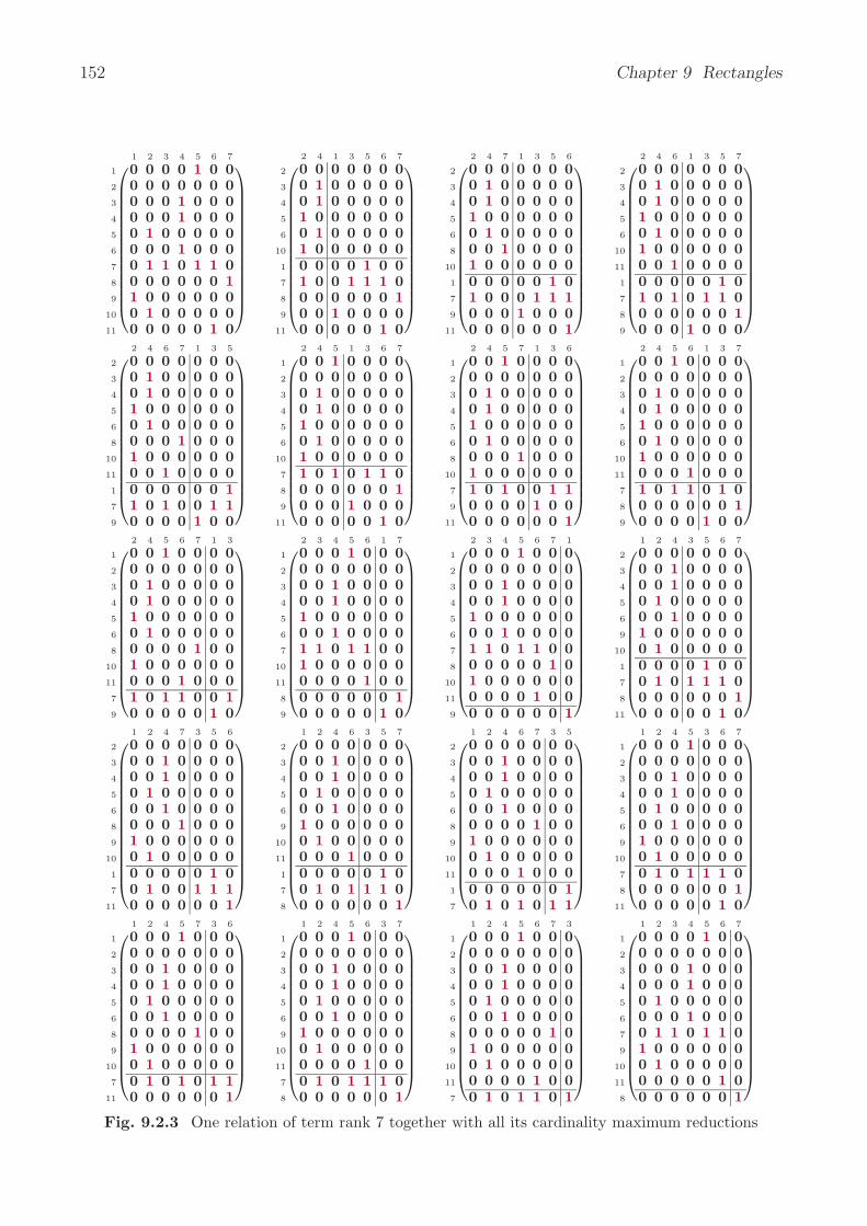
152 Chapter 9 Rectangles
1 2 3 4 5 6 7
1
2
3
4
5
6
7
8
9
10
11
⎛⎜⎜⎜⎜⎜⎜⎜⎜⎜⎜⎜⎜⎜⎝
0 0 0 0 1 0 00 0 0 0 0 0 00 0 0 1 0 0 00 0 0 1 0 0 00 1 0 0 0 0 00 0 0 1 0 0 00 1 1 0 1 1 00 0 0 0 0 0 11 0 0 0 0 0 00 1 0 0 0 0 00 0 0 0 0 1 0
⎞⎟⎟⎟⎟⎟⎟⎟⎟⎟⎟⎟⎟⎟⎠
2 4 1 3 5 6 7
2
3
4
5
6
10
1
7
8
9
11
⎛⎜⎜⎜⎜⎜⎜⎜⎜⎜⎜⎜⎜⎜⎝
0 0 0 0 0 0 00 1 0 0 0 0 00 1 0 0 0 0 01 0 0 0 0 0 00 1 0 0 0 0 01 0 0 0 0 0 00 0 0 0 1 0 01 0 0 1 1 1 00 0 0 0 0 0 10 0 1 0 0 0 00 0 0 0 0 1 0
⎞⎟⎟⎟⎟⎟⎟⎟⎟⎟⎟⎟⎟⎟⎠
2 4 7 1 3 5 6
2
3
4
5
6
8
10
1
7
9
11
⎛⎜⎜⎜⎜⎜⎜⎜⎜⎜⎜⎜⎜⎜⎝
0 0 0 0 0 0 00 1 0 0 0 0 00 1 0 0 0 0 01 0 0 0 0 0 00 1 0 0 0 0 00 0 1 0 0 0 01 0 0 0 0 0 00 0 0 0 0 1 01 0 0 0 1 1 10 0 0 1 0 0 00 0 0 0 0 0 1
⎞⎟⎟⎟⎟⎟⎟⎟⎟⎟⎟⎟⎟⎟⎠
2 4 6 1 3 5 7
2
3
4
5
6
10
11
1
7
8
9
⎛⎜⎜⎜⎜⎜⎜⎜⎜⎜⎜⎜⎜⎜⎝
0 0 0 0 0 0 00 1 0 0 0 0 00 1 0 0 0 0 01 0 0 0 0 0 00 1 0 0 0 0 01 0 0 0 0 0 00 0 1 0 0 0 00 0 0 0 0 1 01 0 1 0 1 1 00 0 0 0 0 0 10 0 0 1 0 0 0
⎞⎟⎟⎟⎟⎟⎟⎟⎟⎟⎟⎟⎟⎟⎠
2 4 6 7 1 3 5
2
3
4
5
6
8
10
11
1
7
9
⎛⎜⎜⎜⎜⎜⎜⎜⎜⎜⎜⎜⎜⎜⎝
0 0 0 0 0 0 00 1 0 0 0 0 00 1 0 0 0 0 01 0 0 0 0 0 00 1 0 0 0 0 00 0 0 1 0 0 01 0 0 0 0 0 00 0 1 0 0 0 00 0 0 0 0 0 11 0 1 0 0 1 10 0 0 0 1 0 0
⎞⎟⎟⎟⎟⎟⎟⎟⎟⎟⎟⎟⎟⎟⎠
2 4 5 1 3 6 7
1
2
3
4
5
6
10
7
8
9
11
⎛⎜⎜⎜⎜⎜⎜⎜⎜⎜⎜⎜⎜⎜⎝
0 0 1 0 0 0 00 0 0 0 0 0 00 1 0 0 0 0 00 1 0 0 0 0 01 0 0 0 0 0 00 1 0 0 0 0 01 0 0 0 0 0 01 0 1 0 1 1 00 0 0 0 0 0 10 0 0 1 0 0 00 0 0 0 0 1 0
⎞⎟⎟⎟⎟⎟⎟⎟⎟⎟⎟⎟⎟⎟⎠
2 4 5 7 1 3 6
1
2
3
4
5
6
8
10
7
9
11
⎛⎜⎜⎜⎜⎜⎜⎜⎜⎜⎜⎜⎜⎜⎝
0 0 1 0 0 0 00 0 0 0 0 0 00 1 0 0 0 0 00 1 0 0 0 0 01 0 0 0 0 0 00 1 0 0 0 0 00 0 0 1 0 0 01 0 0 0 0 0 01 0 1 0 0 1 10 0 0 0 1 0 00 0 0 0 0 0 1
⎞⎟⎟⎟⎟⎟⎟⎟⎟⎟⎟⎟⎟⎟⎠
2 4 5 6 1 3 7
1
2
3
4
5
6
10
11
7
8
9
⎛⎜⎜⎜⎜⎜⎜⎜⎜⎜⎜⎜⎜⎜⎝
0 0 1 0 0 0 00 0 0 0 0 0 00 1 0 0 0 0 00 1 0 0 0 0 01 0 0 0 0 0 00 1 0 0 0 0 01 0 0 0 0 0 00 0 0 1 0 0 01 0 1 1 0 1 00 0 0 0 0 0 10 0 0 0 1 0 0
⎞⎟⎟⎟⎟⎟⎟⎟⎟⎟⎟⎟⎟⎟⎠
2 4 5 6 7 1 3
1
2
3
4
5
6
8
10
11
7
9
⎛⎜⎜⎜⎜⎜⎜⎜⎜⎜⎜⎜⎜⎜⎝
0 0 1 0 0 0 00 0 0 0 0 0 00 1 0 0 0 0 00 1 0 0 0 0 01 0 0 0 0 0 00 1 0 0 0 0 00 0 0 0 1 0 01 0 0 0 0 0 00 0 0 1 0 0 01 0 1 1 0 0 10 0 0 0 0 1 0
⎞⎟⎟⎟⎟⎟⎟⎟⎟⎟⎟⎟⎟⎟⎠
2 3 4 5 6 1 7
1
2
3
4
5
6
7
10
11
8
9
⎛⎜⎜⎜⎜⎜⎜⎜⎜⎜⎜⎜⎜⎜⎝
0 0 0 1 0 0 00 0 0 0 0 0 00 0 1 0 0 0 00 0 1 0 0 0 01 0 0 0 0 0 00 0 1 0 0 0 01 1 0 1 1 0 01 0 0 0 0 0 00 0 0 0 1 0 00 0 0 0 0 0 10 0 0 0 0 1 0
⎞⎟⎟⎟⎟⎟⎟⎟⎟⎟⎟⎟⎟⎟⎠
2 3 4 5 6 7 1
1
2
3
4
5
6
7
8
10
11
9
⎛⎜⎜⎜⎜⎜⎜⎜⎜⎜⎜⎜⎜⎜⎝
0 0 0 1 0 0 00 0 0 0 0 0 00 0 1 0 0 0 00 0 1 0 0 0 01 0 0 0 0 0 00 0 1 0 0 0 01 1 0 1 1 0 00 0 0 0 0 1 01 0 0 0 0 0 00 0 0 0 1 0 00 0 0 0 0 0 1
⎞⎟⎟⎟⎟⎟⎟⎟⎟⎟⎟⎟⎟⎟⎠
1 2 4 3 5 6 7
2
3
4
5
6
9
10
1
7
8
11
⎛⎜⎜⎜⎜⎜⎜⎜⎜⎜⎜⎜⎜⎜⎝
0 0 0 0 0 0 00 0 1 0 0 0 00 0 1 0 0 0 00 1 0 0 0 0 00 0 1 0 0 0 01 0 0 0 0 0 00 1 0 0 0 0 00 0 0 0 1 0 00 1 0 1 1 1 00 0 0 0 0 0 10 0 0 0 0 1 0
⎞⎟⎟⎟⎟⎟⎟⎟⎟⎟⎟⎟⎟⎟⎠
1 2 4 7 3 5 6
2
3
4
5
6
8
9
10
1
7
11
⎛⎜⎜⎜⎜⎜⎜⎜⎜⎜⎜⎜⎜⎜⎝
0 0 0 0 0 0 00 0 1 0 0 0 00 0 1 0 0 0 00 1 0 0 0 0 00 0 1 0 0 0 00 0 0 1 0 0 01 0 0 0 0 0 00 1 0 0 0 0 00 0 0 0 0 1 00 1 0 0 1 1 10 0 0 0 0 0 1
⎞⎟⎟⎟⎟⎟⎟⎟⎟⎟⎟⎟⎟⎟⎠
1 2 4 6 3 5 7
2
3
4
5
6
9
10
11
1
7
8
⎛⎜⎜⎜⎜⎜⎜⎜⎜⎜⎜⎜⎜⎜⎝
0 0 0 0 0 0 00 0 1 0 0 0 00 0 1 0 0 0 00 1 0 0 0 0 00 0 1 0 0 0 01 0 0 0 0 0 00 1 0 0 0 0 00 0 0 1 0 0 00 0 0 0 0 1 00 1 0 1 1 1 00 0 0 0 0 0 1
⎞⎟⎟⎟⎟⎟⎟⎟⎟⎟⎟⎟⎟⎟⎠
1 2 4 6 7 3 5
2
3
4
5
6
8
9
10
11
1
7
⎛⎜⎜⎜⎜⎜⎜⎜⎜⎜⎜⎜⎜⎜⎝
0 0 0 0 0 0 00 0 1 0 0 0 00 0 1 0 0 0 00 1 0 0 0 0 00 0 1 0 0 0 00 0 0 0 1 0 01 0 0 0 0 0 00 1 0 0 0 0 00 0 0 1 0 0 00 0 0 0 0 0 10 1 0 1 0 1 1
⎞⎟⎟⎟⎟⎟⎟⎟⎟⎟⎟⎟⎟⎟⎠
1 2 4 5 3 6 7
1
2
3
4
5
6
9
10
7
8
11
⎛⎜⎜⎜⎜⎜⎜⎜⎜⎜⎜⎜⎜⎜⎝
0 0 0 1 0 0 00 0 0 0 0 0 00 0 1 0 0 0 00 0 1 0 0 0 00 1 0 0 0 0 00 0 1 0 0 0 01 0 0 0 0 0 00 1 0 0 0 0 00 1 0 1 1 1 00 0 0 0 0 0 10 0 0 0 0 1 0
⎞⎟⎟⎟⎟⎟⎟⎟⎟⎟⎟⎟⎟⎟⎠
1 2 4 5 7 3 6
1
2
3
4
5
6
8
9
10
7
11
⎛⎜⎜⎜⎜⎜⎜⎜⎜⎜⎜⎜⎜⎜⎝
0 0 0 1 0 0 00 0 0 0 0 0 00 0 1 0 0 0 00 0 1 0 0 0 00 1 0 0 0 0 00 0 1 0 0 0 00 0 0 0 1 0 01 0 0 0 0 0 00 1 0 0 0 0 00 1 0 1 0 1 10 0 0 0 0 0 1
⎞⎟⎟⎟⎟⎟⎟⎟⎟⎟⎟⎟⎟⎟⎠
1 2 4 5 6 3 7
1
2
3
4
5
6
9
10
11
7
8
⎛⎜⎜⎜⎜⎜⎜⎜⎜⎜⎜⎜⎜⎜⎝
0 0 0 1 0 0 00 0 0 0 0 0 00 0 1 0 0 0 00 0 1 0 0 0 00 1 0 0 0 0 00 0 1 0 0 0 01 0 0 0 0 0 00 1 0 0 0 0 00 0 0 0 1 0 00 1 0 1 1 1 00 0 0 0 0 0 1
⎞⎟⎟⎟⎟⎟⎟⎟⎟⎟⎟⎟⎟⎟⎠
1 2 4 5 6 7 3
1
2
3
4
5
6
8
9
10
11
7
⎛⎜⎜⎜⎜⎜⎜⎜⎜⎜⎜⎜⎜⎜⎝
0 0 0 1 0 0 00 0 0 0 0 0 00 0 1 0 0 0 00 0 1 0 0 0 00 1 0 0 0 0 00 0 1 0 0 0 00 0 0 0 0 1 01 0 0 0 0 0 00 1 0 0 0 0 00 0 0 0 1 0 00 1 0 1 1 0 1
⎞⎟⎟⎟⎟⎟⎟⎟⎟⎟⎟⎟⎟⎟⎠
1 2 3 4 5 6 7
1
2
3
4
5
6
7
9
10
11
8
⎛⎜⎜⎜⎜⎜⎜⎜⎜⎜⎜⎜⎜⎜⎝
0 0 0 0 1 0 00 0 0 0 0 0 00 0 0 1 0 0 00 0 0 1 0 0 00 1 0 0 0 0 00 0 0 1 0 0 00 1 1 0 1 1 01 0 0 0 0 0 00 1 0 0 0 0 00 0 0 0 0 1 00 0 0 0 0 0 1
⎞⎟⎟⎟⎟⎟⎟⎟⎟⎟⎟⎟⎟⎟⎠
Fig. 9.2.3 One relation of term rank 7 together with all its cardinality maximum reductions
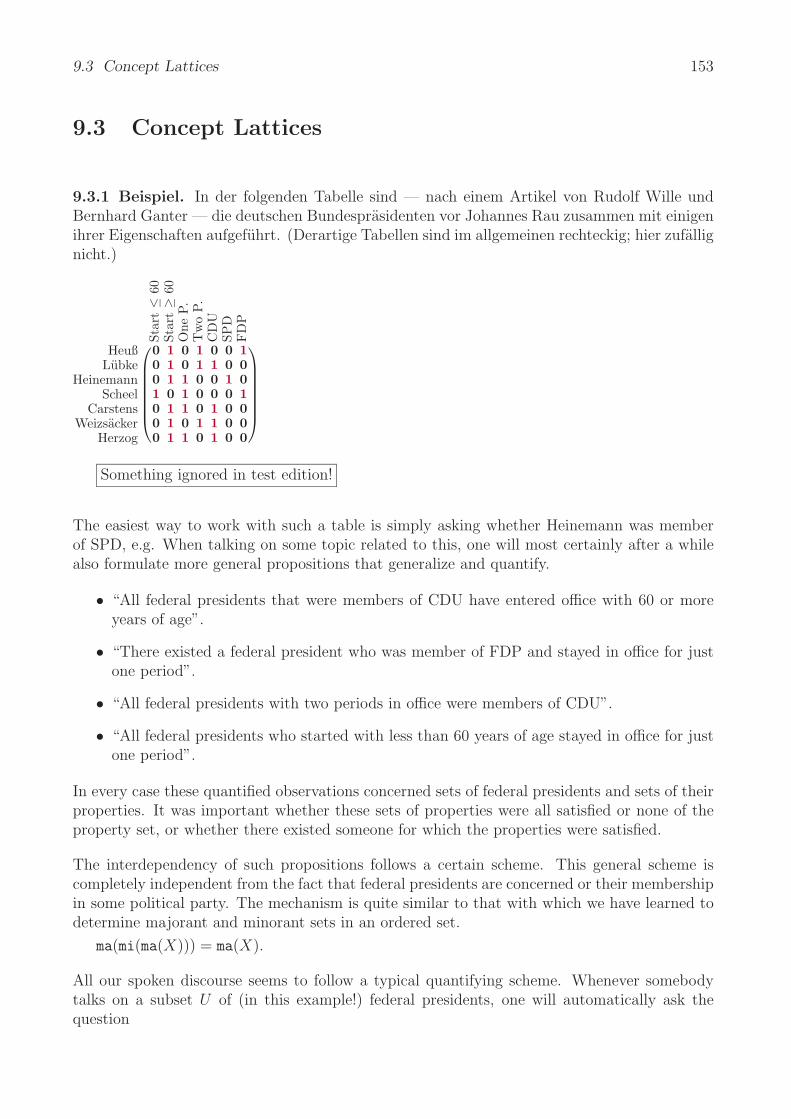
9.3 Concept Lattices 153
9.3 Concept Lattices
9.3.1 Beispiel. In der folgenden Tabelle sind — nach einem Artikel von Rudolf Wille undBernhard Ganter — die deutschen Bundesprasidenten vor Johannes Rau zusammen mit einigenihrer Eigenschaften aufgefuhrt. (Derartige Tabellen sind im allgemeinen rechteckig; hier zufallignicht.)
Star
t≤
60St
art≥
60O
neP.
Tw
oP.
CD
USP
DFD
P
HeußLubke
HeinemannScheel
CarstensWeizsacker
Herzog
⎛⎜⎜⎜⎜⎜⎜⎝
0 1 0 1 0 0 10 1 0 1 1 0 00 1 1 0 0 1 01 0 1 0 0 0 10 1 1 0 1 0 00 1 0 1 1 0 00 1 1 0 1 0 0
⎞⎟⎟⎟⎟⎟⎟⎠
Something ignored in test edition!
The easiest way to work with such a table is simply asking whether Heinemann was memberof SPD, e.g. When talking on some topic related to this, one will most certainly after a whilealso formulate more general propositions that generalize and quantify.
• “All federal presidents that were members of CDU have entered office with 60 or moreyears of age”.
• “There existed a federal president who was member of FDP and stayed in office for justone period”.
• “All federal presidents with two periods in office were members of CDU”.
• “All federal presidents who started with less than 60 years of age stayed in office for justone period”.
In every case these quantified observations concerned sets of federal presidents and sets of theirproperties. It was important whether these sets of properties were all satisfied or none of theproperty set, or whether there existed someone for which the properties were satisfied.
The interdependency of such propositions follows a certain scheme. This general scheme iscompletely independent from the fact that federal presidents are concerned or their membershipin some political party. The mechanism is quite similar to that with which we have learned todetermine majorant and minorant sets in an ordered set.
ma(mi(ma(X))) = ma(X).
All our spoken discourse seems to follow a typical quantifying scheme. Whenever somebodytalks on a subset U of (in this example!) federal presidents, one will automatically ask thequestion
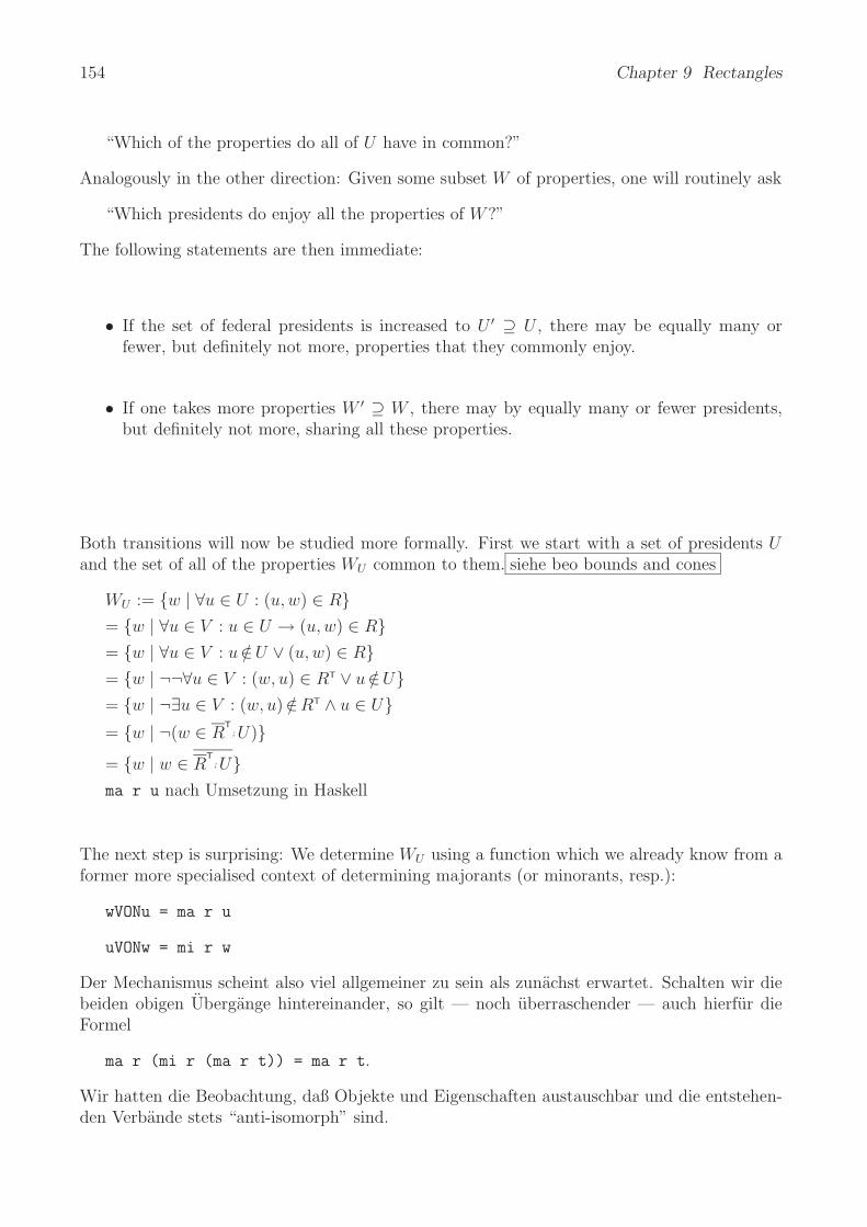
154 Chapter 9 Rectangles
“Which of the properties do all of U have in common?”
Analogously in the other direction: Given some subset W of properties, one will routinely ask
“Which presidents do enjoy all the properties of W?”
The following statements are then immediate:
• If the set of federal presidents is increased to U ′ ⊇ U , there may be equally many orfewer, but definitely not more, properties that they commonly enjoy.
• If one takes more properties W ′ ⊇ W , there may by equally many or fewer presidents,but definitely not more, sharing all these properties.
Both transitions will now be studied more formally. First we start with a set of presidents Uand the set of all of the properties WU common to them. siehe beo bounds and cones
WU := w | ∀u ∈ U : (u, w) ∈ R= w | ∀u ∈ V : u ∈ U → (u, w) ∈ R= w | ∀u ∈ V : u∈/ U ∨ (u, w) ∈ R= w | ¬¬∀u ∈ V : (w, u) ∈ RT ∨ u∈/ U= w | ¬∃u ∈ V : (w, u)∈/ RT ∧ u ∈ U= w | ¬(w ∈ R
T; U)
= w | w ∈ RT; U
ma r u nach Umsetzung in Haskell
The next step is surprising: We determine WU using a function which we already know from aformer more specialised context of determining majorants (or minorants, resp.):
wVONu = ma r u
uVONw = mi r w
Der Mechanismus scheint also viel allgemeiner zu sein als zunachst erwartet. Schalten wir diebeiden obigen Ubergange hintereinander, so gilt — noch uberraschender — auch hierfur dieFormel
ma r (mi r (ma r t)) = ma r t.
Wir hatten die Beobachtung, daß Objekte und Eigenschaften austauschbar und die entstehen-den Verbande stets “anti-isomorph” sind.

9.3 Concept Lattices 155
No. Sets of German Federal Presidents Their Properties
1 all federal presidents none2 all but Scheel ≥ 60 or CDU3 Lubke, Carstens, Weizsacker, Herzog ≥ 604 Heinemann, Scheel, Carstens Herzog one period5 Heinemann, Carstens, Herzog ≥ 60 or one period6 Carstens, Herzog ≥ 60 or one period or CDU7 Heuß, Scheel FDP8 Heuß, Lubke, Weizsacker ≥ 60 or two periods9 Heinemann ≥ 60 or one period or SPD10 Heuß ≥ 60 or two periods or FDP11 Lubke, Weizsacker ≥ 60 or two periods or CDU12 Scheel < 60 or one period or FDP13 no federal president all properties
Fig. 9.3.1 Example of a concept lattice
9.3.2 Beispiel. Von einer Wand sind einige Kacheln heruntergefallen, und es soll der Klebe-mortel zur Wiederanbringung mit einem Gerat eingestrichen werden. Dieses Gerat kann eineTraufel einer gewissen Breite entweder horiziontal (dann vertikal positioniert) oder vertikal(dann horizontal positioniert) hindurchziehen. Man stellt schnell fest, daß sich die horizontalresp. vertikal passenden Traufelbreiten und -positionen genau entsprechen. Man darf sogar
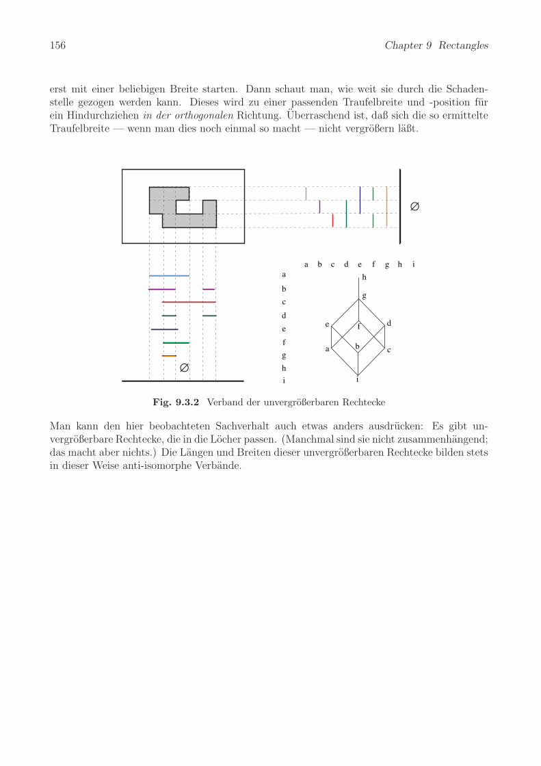
156 Chapter 9 Rectangles
erst mit einer beliebigen Breite starten. Dann schaut man, wie weit sie durch die Schaden-stelle gezogen werden kann. Dieses wird zu einer passenden Traufelbreite und -position furein Hindurchziehen in der orthogonalen Richtung. Uberraschend ist, daß sich die so ermittelteTraufelbreite — wenn man dies noch einmal so macht — nicht vergroßern laßt.
a b c d e f g h ia
b
c
e
f
g
d
h
i
a
e f
g
c
d
h
b
i
∅
∅
Fig. 9.3.2 Verband der unvergroßerbaren Rechtecke
Man kann den hier beobachteten Sachverhalt auch etwas anders ausdrucken: Es gibt un-vergroßerbare Rechtecke, die in die Locher passen. (Manchmal sind sie nicht zusammenhangend;das macht aber nichts.) Die Langen und Breiten dieser unvergroßerbaren Rechtecke bilden stetsin dieser Weise anti-isomorphe Verbande.

9.3 Concept Lattices 157
9.3.3 Beispiel. Als nachstes betrachten wir einen vielbeschaftigten Parteiredner. Von unserenPolitikern ist man es gewohnt, daß sie ihre Reden modular aus relativ wenigen Versatzstuckenaufbauen, die sie zielgenau aus einem Fundus von vorgestanzten Satzen aussuchen — leiderunter Vermeidung jeder frei geaußerten Meinung. Das folgende dient der Vorbereitung solcherVersatzstucke und ihrer Zusammenstellung fur ein bestimmtes mit einer Rede zu begluckendesFeuerwehrhaus-Einweihungsfest o.a.
Zunachst werden die relevanten Bevolkerungsgruppen und die sie betreffenden Themen tabel-larisch erfaßt. Dann wird eine Prognose erstellt fur die Teilnehmersituation der genannten Ver-anstaltung. Schließlich werden die Rede-Elemente anhand des Konzeptverbandes ausgewahlt.Geht es um positiv zu wertende Versprechungen, nimmt man lub, geht es um das Enger-schnallen des Gurtels, wird glb genommen.
Sic
her
hei
tsfr
agen
Ste
uer
Dorf
ver
schoner
ung
Weh
rpflic
ht
Sch
ulg
ebet
Leh
rlin
gsa
usb
ildung
Ren
te
Auto
bahnbau
Okolo
gie
Sta
dio
nneu
bau
Lohnru
nde
AB
M-M
aßnahm
enAltenheim
Fußballverein
Naturschutzbund
kath. Kindergarten
Schwimmverein
Elternbeirat
Handwerkskammer
Kriegsgraberfursorge
ev. Kindergarten
⎛⎜⎜⎜⎜⎜⎜⎜⎜⎝
1 1 1 0 1 0 1 0 1 0 0 10 0 0 1 0 1 0 0 0 1 0 00 0 1 0 0 0 0 1 1 0 1 11 0 0 0 1 0 0 0 0 0 0 00 0 0 1 0 1 0 0 0 0 0 01 0 0 1 1 1 0 0 1 1 0 00 1 0 1 0 1 0 1 0 1 1 00 0 1 0 0 0 1 0 0 0 0 11 0 0 0 1 0 0 0 1 0 0 0
⎞⎟⎟⎟⎟⎟⎟⎟⎟⎠
⎛⎜⎜⎜⎜⎜⎜⎜⎜⎜⎝
0 1 0 1 0 0 1 0 0 0 1 1 1 1 1 10 0 0 0 0 0 0 0 1 1 0 0 0 0 0 10 0 1 1 0 0 0 1 0 0 0 1 0 1 0 10 0 0 0 0 0 0 0 0 0 0 0 0 0 1 10 0 0 0 0 0 0 0 0 1 0 0 0 0 0 10 0 0 0 1 0 0 0 1 1 0 0 1 1 1 10 0 0 0 0 1 1 1 1 1 0 0 0 0 0 10 0 0 0 0 0 0 0 0 0 1 1 0 0 0 10 0 0 0 0 0 0 0 0 0 0 0 1 1 1 1
⎞⎟⎟⎟⎟⎟⎟⎟⎟⎟⎠
⎛⎜⎜⎜⎜⎜⎜⎜⎜⎜⎜⎜⎜⎜⎜⎜⎜⎜⎜⎜⎜⎜⎜⎝
1 1 1 1 1 1 1 1 1 1 1 1 1 1 1 10 1 0 1 0 0 1 0 0 0 1 1 1 1 1 10 0 1 1 0 0 0 1 0 0 0 1 0 1 0 10 0 0 1 0 0 0 0 0 0 0 1 0 1 0 10 0 0 0 1 0 0 0 1 1 0 0 1 1 1 10 0 0 0 0 1 1 1 1 1 0 0 0 0 0 10 0 0 0 0 0 1 0 0 0 0 0 0 0 0 10 0 0 0 0 0 0 1 0 0 0 0 0 0 0 10 0 0 0 0 0 0 0 1 1 0 0 0 0 0 10 0 0 0 0 0 0 0 0 1 0 0 0 0 0 10 0 0 0 0 0 0 0 0 0 1 1 0 0 0 10 0 0 0 0 0 0 0 0 0 0 1 0 0 0 10 0 0 0 0 0 0 0 0 0 0 0 1 1 1 10 0 0 0 0 0 0 0 0 0 0 0 0 1 0 10 0 0 0 0 0 0 0 0 0 0 0 0 0 1 10 0 0 0 0 0 0 0 0 0 0 0 0 0 0 1
⎞⎟⎟⎟⎟⎟⎟⎟⎟⎟⎟⎟⎟⎟⎟⎟⎟⎟⎟⎟⎟⎟⎟⎠
Fig. 9.3.3 Konzeptverband fur einen Parteiredner
Erstellt wurde diese Ordnung, indem alle Teilmengen u danach durchgetestet wurden, ob ma r
(mi r u) == u gilt. Fur die dabei verbleibenden Teilmengen wurde die normale Inklusionsor-dnung aufgezeichnet.

158 Chapter 9 Rectangles
Dorf + Öko + ABM Autobahn + Lohn Steuer
keines der Themen
Sicherheit + Gebet + Ökologie
ÖkologieSicherheit + Schulgebet
Dorf + Rente + ABM
Dorfverschönerung + ABM
alle Themen
Sich + Steuer + Dorf + Gebet + Rente + Öko + ABM Dorf + ... + ABM Sich + ... + Stadion Steuer + ... + Lohn
Wehrpflicht + Lehrlinge
Wehrpflicht + Lehrlinge + Stadion
Alt + Natur Natur + Handwerk Alte + Handwerk
alle Gruppen
Alte + Eltern + evKg
Alte + Natur + Eltern + evKgAlte + beideKg + Eltern
Alte + Gräber
Alte + Natur + Gräber
keine der Gruppen
Altenheim Naturschutz Elternbeirat Handwerk
Fußball + Eltern + Handwerk
Fußball + Schwimmen + Eltern + Handwerk
Fig. 9.3.4 Ordnung fur Konzeptverband
Something ignored in test edition!
Something ignored in test edition!
9.4 Difunctionality
The concept of a difunctional relation has already been formulated in a phenomenological formin Def. 5.4.5. It generalizes the concept of a (partial) equivalence relation in as far as domainand range need no longer be identical. We recall that a possibly heterogeneous relation A iscalled difunctional if A;AT;A = A, or equivalently, if A;A
T;A ⊆ A. The interpretation is that
A can be written in block diagonal form when suitably rearranging rows and columns.
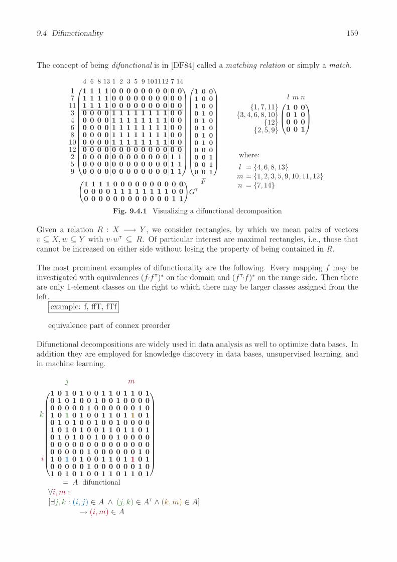
9.4 Difunctionality 159
The concept of being difunctional is in [DF84] called a matching relation or simply a match.
171134681012259
4 6 8 13 1 2 3 5 9 101112 7 14⎛⎜⎜⎜⎜⎜⎜⎜⎜⎜⎜⎜⎜⎜⎜⎝
1 1 1 1 0 0 0 0 0 0 0 0 0 01 1 1 1 0 0 0 0 0 0 0 0 0 01 1 1 1 0 0 0 0 0 0 0 0 0 00 0 0 0 1 1 1 1 1 1 1 1 0 00 0 0 0 1 1 1 1 1 1 1 1 0 00 0 0 0 1 1 1 1 1 1 1 1 0 00 0 0 0 1 1 1 1 1 1 1 1 0 00 0 0 0 1 1 1 1 1 1 1 1 0 00 0 0 0 0 0 0 0 0 0 0 0 0 00 0 0 0 0 0 0 0 0 0 0 0 1 10 0 0 0 0 0 0 0 0 0 0 0 1 10 0 0 0 0 0 0 0 0 0 0 0 1 1
⎞⎟⎟⎟⎟⎟⎟⎟⎟⎟⎟⎟⎟⎟⎟⎠
⎛⎜⎜⎜⎜⎜⎜⎜⎜⎜⎜⎜⎜⎜⎜⎜⎜⎝
1 0 01 0 01 0 00 1 00 1 00 1 00 1 00 1 00 0 00 0 10 0 10 0 1
⎞⎟⎟⎟⎟⎟⎟⎟⎟⎟⎟⎟⎟⎟⎟⎟⎟⎠
F(1 1 1 1 0 0 0 0 0 0 0 0 0 00 0 0 0 1 1 1 1 1 1 1 1 0 00 0 0 0 0 0 0 0 0 0 0 0 1 1
)GT
1, 7, 113, 4, 6, 8, 10
122, 5, 9
l m n⎛⎜⎝
1 0 00 1 00 0 00 0 1
⎞⎟⎠
where:
l = 4, 6, 8, 13m = 1, 2, 3, 5, 9, 10, 11, 12n = 7, 14
Fig. 9.4.1 Visualizing a difunctional decomposition
Given a relation R : X −→ Y , we consider rectangles, by which we mean pairs of vectorsv ⊆ X, w ⊆ Y with v ; wT ⊆ R. Of particular interest are maximal rectangles, i.e., those thatcannot be increased on either side without losing the property of being contained in R.
The most prominent examples of difunctionality are the following. Every mapping f may beinvestigated with equivalences (f;fT)∗ on the domain and (fT;f)∗ on the range side. Then thereare only 1-element classes on the right to which there may be larger classes assigned from theleft.
example: f, ffT, fTf
equivalence part of connex preorder
Difunctional decompositions are widely used in data analysis as well to optimize data bases. Inaddition they are employed for knowledge discovery in data bases, unsupervised learning, andin machine learning.
j m
k
i
⎛⎜⎜⎜⎜⎜⎜⎜⎜⎜⎜⎜⎜⎜⎝
1 0 1 0 1 0 0 1 1 0 1 1 0 10 1 0 1 0 0 1 0 0 1 0 0 0 00 0 0 0 0 1 0 0 0 0 0 0 1 01 0 1 0 1 0 0 1 1 0 1 1 0 10 1 0 1 0 0 1 0 0 1 0 0 0 01 0 1 0 1 0 0 1 1 0 1 1 0 10 1 0 1 0 0 1 0 0 1 0 0 0 00 0 0 0 0 0 0 0 0 0 0 0 0 00 0 0 0 0 1 0 0 0 0 0 0 1 01 0 1 0 1 0 0 1 1 0 1 1 0 10 0 0 0 0 1 0 0 0 0 0 0 1 01 0 1 0 1 0 0 1 1 0 1 1 0 1
⎞⎟⎟⎟⎟⎟⎟⎟⎟⎟⎟⎟⎟⎟⎠
= A difunctional∀i, m :[∃j, k : (i, j) ∈ A ∧ (j, k) ∈ AT ∧ (k, m) ∈ A]
→ (i, m) ∈ A

160 Chapter 9 Rectangles
1 2 3 4 5 6 7 8 9 10 11 12 13 14
1
2
3
4
5
6
7
8
9
10
11
12
⎛⎜⎜⎜⎜⎜⎜⎜⎜⎜⎜⎜⎜⎜⎜⎜⎜⎜⎜⎜⎜⎜⎜⎜⎜⎜⎜⎜⎝
0 0 1 0 0 0 0 1 0 0 0 0 0 00 1 0 1 0 0 0 0 0 1 0 0 0 00 0 0 0 0 0 0 0 0 0 0 0 1 01 0 0 0 1 0 0 0 1 0 1 0 0 10 0 0 0 0 0 1 0 0 0 0 0 0 01 0 1 0 0 0 0 0 0 0 0 1 0 10 0 0 1 0 0 1 0 0 0 0 0 0 00 0 0 0 0 0 0 0 0 0 0 0 0 00 0 0 0 0 1 0 0 0 0 0 0 1 00 0 0 0 0 0 0 1 0 0 1 0 0 00 0 0 0 0 0 0 0 0 0 0 0 1 00 0 0 0 0 0 0 0 1 0 0 1 0 0
⎞⎟⎟⎟⎟⎟⎟⎟⎟⎟⎟⎟⎟⎟⎟⎟⎟⎟⎟⎟⎟⎟⎟⎟⎟⎟⎟⎟⎠
1 3 5 8 9 11 12 14 2 4 7 10 6 13
1
4
6
10
12
2
5
7
3
9
11
8
⎛⎜⎜⎜⎜⎜⎜⎜⎜⎜⎜⎜⎜⎜⎜⎜⎜⎜⎜⎜⎜⎜⎜⎜⎜⎜⎜⎜⎝
0 1 0 1 0 0 0 0 0 0 0 0 0 01 0 1 0 1 1 0 1 0 0 0 0 0 01 1 0 0 0 0 1 1 0 0 0 0 0 00 0 0 1 0 1 0 0 0 0 0 0 0 00 0 0 0 1 0 1 0 0 0 0 0 0 00 0 0 0 0 0 0 0 1 1 0 1 0 00 0 0 0 0 0 0 0 0 0 1 0 0 00 0 0 0 0 0 0 0 0 1 1 0 0 00 0 0 0 0 0 0 0 0 0 0 0 0 10 0 0 0 0 0 0 0 0 0 0 0 1 10 0 0 0 0 0 0 0 0 0 0 0 0 10 0 0 0 0 0 0 0 0 0 0 0 0 0
⎞⎟⎟⎟⎟⎟⎟⎟⎟⎟⎟⎟⎟⎟⎟⎟⎟⎟⎟⎟⎟⎟⎟⎟⎟⎟⎟⎟⎠
Fig. 9.4.2 A difunctional decomposition visualized via permutation and partitioning
Meanwhile, we have some feeling how a difunctional matrix looks like. We also know thealgebraic characterization from the definition. Now we ask for the practical aspects of thisdefinition, which has long been discussed and is known among numerical analysts as chainability.
9.4.1 Definition. Let a relation R be given that is conceived as a chessboard with darksquares or white according to whether Rik is True or False. A rook shall operate on thechessboard in horizontal or vertical direction; however, it is only allowed to change direction ondark squares. Using this interpretation, a relation R is called chainable if the non-vanishingentries (i.e., the dark squares) can all be reached from one another by a sequence of “rookmoves”, or else if hdifu(R) = .
We illustrate this definition mentioning a related concept. The relation R shall for the momentbe conceived as a hypergraph-incidence between hyperedges (rows) and vertices (columns).Then K := ∩ R; RT is the so-called edge-adjacency, see e.g. [SS89, SS93].
9.4.2 Proposition. A total and surjective relation R is chainable precisely when its edge-adjacency K is strongly connected.
Proof : First we show that K∗ = (R;RT)∗, using the formula (A∪B)∗ = (A∗;B)∗;A∗, well-knownfrom regular algebra. Then
(R;RT)∗ = (( ∩R;RT)∪ ( ∩R;RT))∗ = (( ∩R;RT)∗;( ∩R;RT))∗;( ∩R;RT)∗ = ( ;K)∗; = K∗
From chainability, hdifu(R) = (R;RT)∗;R = we get immediately K∗ = (R;RT)∗ ⊇ (R;RT)+ =(R;RT)∗;R;RT = ;RT. Totality of R gives the first direction; it is necessary, since there mightexist an empty hyperedge completely unrelated to the vertices.
The other direction is hdifu(R) = (R; RT)∗ ; R = K∗ ; R = ; R, where R must be surjective, asotherwise there might exist an isolated vertex unrelated to all the edges.
It is possible to determine how far chainability reaches. This is achieved with the concept of adifunctional closure.
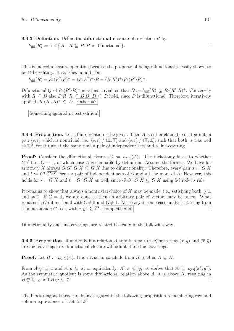
9.4 Difunctionality 161
9.4.3 Definition. Define the difunctional closure of a relation R by
hdif(R) := infH | R ⊆ H, H is difunctional .
This is indeed a closure operation because the property of being difunctional is easily shown tobe ∩-hereditary. It satisfies in addition
hdif(R) = R; (RT; R)+ = (R; RT)+; R = (R; RT)+; R; (RT; R)+.
Difunctionality of R; (RT;R)+ is rather trivial, so that D := hdif(R) ⊆ R; (RT;R)+. Converselywith R ⊆ D also D;RT;R ⊆ D;DT;D ⊆ D hold, since D is difunctional. Therefore, iterativelyapplied, R; (RT; R)+ ⊆ D. Other =?
Something ignored in test edition!
9.4.4 Proposition. Let a finite relation A be given. Then A is either chainable or it admits apair (s, t) which is nontrivial, i.e., (s, t) =/ ( , ) and (s, t) =/ ( , ), such that both, s, t as wellas s, t, constitute at the same time a pair of independent sets and a line-covering.
Proof : Consider the difunctional closure G := hdifu(A). The dichotomy is as to whetherG =/ or G = , in which case A is chainable by definition. Assume the former. We have forarbitrary X always G;GT;G; X ⊆ G; X due to difunctionality. Therefore, every pair s := G;Xand t := GT ; G; X forms a pair of independent sets of G and all the more of A. However, this
holds for s = G; X and t = GT; G; X as well, since G; GT; G; X ⊆ G; X using Schroder’s rule.
It remains to show that always a nontrivial choice of X may be made, i.e., satisfying both =/and =/ . If G = , we are done as then an arbitrary pair of vectors may be taken. Whatremains is G difunctional with G =/ and G =/ . Necessary is some case analysis starting from
a point outside G, i.e., with x; yT ⊆ G. komplettieren!
Difunctionality and line-coverings are related basically in the following way.
9.4.5 Proposition. If and only if a relation A admits a pair (x, y) such that (x, y) and (x, y)are line-coverings, its difunctional closure will admit these line-coverings.
Proof : Let H := hdifu(A). It is trivial to conclude from H to A as A ⊆ H.
From A; y ⊆ x and A; y ⊆ x, or equivalently, AT ; x ⊆ y, we derive that A ⊆ syq(xT, yT).As the symmetric quotient is some difunctional relation above A, it is above H, resulting inH ; y ⊆ x and H ; y ⊆ x.
The block-diagonal structure is investigated in the following proposition remembering row andcolumn equivalence of Def. 5.4.3.
162 Chapter 9 Rectangles
9.4.6 Proposition. Let some difunctional relation R be given together with its row equiva-lence Ξ := syq(RT, RT) and its column equivalence Θ := syq(R, R) (see Def. 5.4.3) as well aswith the corresponding natural projection mappings ηΞ, ηΘ. Then the quotient of R modulorow and column equivalence RΞ,Θ := ηT
Ξ; R ; ηΘ is a matching, i.e., a univalent and injective
relation.
Proof : The main point to prove is that
RT; R ⊆ Θ
which by definition means
RT; R ⊆ syq(R, R) = RT; R ∩ RT; R
Now the two parts of the right side are handled individually as we show for the first, e.g.
RT; R ⊆ RT; R ⇐⇒ R
T; R ⊆ RT; R ⇐⇒ RT; R; RT ⊆ RT ⇐= R difunctional
This intermediate result extends to
RT; Ξ; R ⊆ RT; R; Θ ⊆ Θ; Θ = Θ
We have used that Ξ, Θ is an R-congruence already known?? . This in turn allows us to calculate
RTΞ,Θ
; RΞ,Θ = ηTΘ
; RT; ηΞ; ηTΞ
; R; ηΘ = ηTΘ
; RT; Ξ; R; ηΘ ⊆ ηTΘ
; RT; R; Θ; ηΘ congruence
⊆ ηTΘ
; Θ; Θ; ηΘ = ηTΘ
; Θ; ηΘ = ηTΘ
; ηΘ; ηTΘ
; ηΘ = ; =
This is related to the following concepts of inverses in the context of linear algebra for numericalproblems.
9.4.7 Definition. Let some relation A be given. The relation G is called
i) a generalized inverse of A if A; G; A = A.
ii) a Moore-Penrose inverse of A if the following four conditions holdA; G; A = A, G; A; G = G, (A; G)T = A; G, (G; A)T = G; A.
We recall a well-known result on these Moore-Penrose inverses.
9.4.8 Theorem. Moore-Penrose inverses are uniquely determined provided they exist.
Proof : Assume two Moore-Penrose inverses G, H of A to be given. Then we may proceed asfollows G = G;A;G = G;GT;AT = G;GT;AT;HT;AT = G;GT;AT;A;H = G;A;G;A;H = G;A;H =G; A; H ; A; H = G; A; AT; HT; H = AT; GT; AT; HT; H = AT; HT; H = H ; A; H = H.
We now relate these concepts with permutations and difunctionality.
9.4.9 Theorem. For a relation A, the following are equivalent:
i) A has a Moore-Penrose inverse.
ii) A has AT as its Moore-Penrose inverse.

9.4 Difunctionality 163
iii) A is difunctional.
iv) Any two rows (or columns) of A are either disjoint or identical.
v) There exist permutation matrices P, Q such that P ; A; Q has block-diagonal form, i.e.
P ; A; Q =
⎛⎜⎜⎜⎜⎜⎜⎝
B1
B2
B3
B4
B5
⎞⎟⎟⎟⎟⎟⎟⎠
with not necessarily square diagonal entries Bi = .
Exercises
4.4.7 Let a symmetric difunctional relation A be partitioned A = H ∪ T , where H = A ∩ A2
is the non-transitive part and T = A ∩ A2. Show that H ; T = T ; H = and T is a transitiverelation.
Solution 4.4.7 H ; T ⊆ A ; A2 ∩ A2 ; A ⊆ A ∩ A ⊆ . Here, it was first used that A3 =A;AT;A ⊆ A by symmetry and difunctionality. Furthermore for symmetric A, we may employA; AT ⊆ A2 =⇒ A2 ; A ⊆ A. Transitivity of T follows again by symmetry and difunctionalityfrom T 2 ⊆ A3 ∩ A4 ⊆ A ∩ A2 = T .
4.4.8 Let two disjoint orthogonal relations S and U be given, i.e., S;U = U ;S = , where S issymmetric difunctional and satisfies S ⊆ S2 while U = UT = U2, i.e., U is a so-called quasi-equivalence. Then A := S∪U is a symmetric difunctional relation with disjoint decompositionS = A ∩ A2 and U = A ∩ A2.
Solution 4.4.8 A is symmetric, since S and U are. A is difunctional, since A ; AT ; A =S ; ST; S ∪ U ; UT; U by orthogonality. Now S ; ST; S ∪ U ; UT; U ⊆ S ∪ U ; U ; U ⊆ S ∪ U = A.
For the partition, we first show U ⊆ A and U = U2 ⊆ A2. Obviously, S ⊆ A and,furthermore, by disjointness S ⊆ S ∩ U ⊆ S2 ∩ U = S2 ∪ U = S2 ∪ U2 = A2.
[DF69] Let R be some difunctional relation. When one considers the direct sum of its domainand range, and thereon the relation dort weitere derartige Aussagen!
RC := ιT; R; κ ∪ ιT; ( dom ∪ R; RT); ι ∪ κT; RT; ι ∪ κT; ( ran ∪ RT; R); κthen this turns out to be an equivalence.
Solution [DF69]
[DF69] Let R be some Ferrers relation, i.e., R; RT; R ⊆ R. Show that R
T; R; R
T ⊆ RT,
R; RT ∩ R; RT = ,
RT; R ∩ RT; R =
are equivalent characterisations.

164 Chapter 9 Rectangles
Solution [DF69]
new Let R be any difunctional relation. Then the composite relation
Rc :=
(∪ R; RT RRT ∪ RT; R
)is an equivalence.
Solution new Rc is reflexive and symmetric by construction.
R2c =
(( ∪ R; RT)2 ∪ R; RT ( ∪ R; RT); R ∪ R; ( ∪ RT; R)
RT; ( ∪ R; RT) ∪ ( ∪ RT; R); RT RT; R ∪ ( ∪ RT; R)2
)= Rc
OKeig Prove that RT; R; S ⊆ S implies R; S = R; ∩ R; S (Compare to Prop. 5.1.6)
Solution OKeig “⊆ ” follows from Schroder’s rule and monotonicity. “ ⊇ ” holds as obviously= R; S ∪ R; ∪ R; S
4.4.2 A relation R is called right-invertible if there exists a relation X with R ; X = , andleft-invertible if there exists a relation Y with Y ;R = . The relations X and Y are then calledthe right and left inverse of R, respectively. Relations which are at the same time right- andleft-invertible are called invertible.i) For invertible homogeneous relations all right and left inverses coincide; the notion inverse
R−1 is used. Then R−1 = RT holds.ii) Show that for finite Boolean n × n-matrices
R invertible ⇐⇒ Rm = for some m ≥ 1.
(R is then called a permutation matrix.)
Solution 4.4.2 i) Ist R invertierbar, so existieren X, Y mit R ; X = = Y ; R. Dann giltX = Y ; R; X = Y.
ii) Es ist ”=⇒” zu beweisen: Wir betrachten alle Potenzen Ri, i ≥ 0 von R. Da es nur endlichviele boolesche n × n-Matrizen gibt, mussen mindestens zwei verschiedene Potenzen uberein-stimmen: Rt = Rs, mit t > s =⇒ Rt ; Xs = Rs ; Xs =⇒ Rm = , mit m := t − s ≥ 1.
9.5 Application in Knowledge Acquisition
There are several fields in data mining in which difunctionality is heavily used. One is predictivemodeling which means classification and regression. The next is clustering, i.e., grouping similarobjects. Finally summarization should be mentioned which means to discover from given dataassociation rules. The input to a corresponding algorithm is a single flat table — mostly ofreal numbers, but in our case of truth values. So we start from an arbitrary relation that maybe heterogeneous. Should data from several such be studied, one may subsume this under theaforementioned case introducing products, e.g.
The task is to output a pattern valid in the given data. Such a pattern is simply a propositiondescribing relationships among the facts of the given data. It is useful only, when it is simplerthan the enumeration of all the given facts.
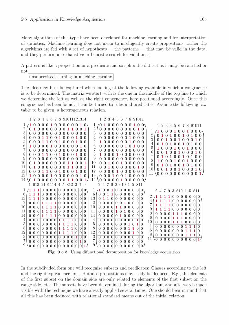
9.5 Application in Knowledge Acquisition 165
Many algorithms of this type have been developed for machine learning and for interpretationof statistics. Machine learning does not mean to intelligently create propositions; rather thealgorithms are fed with a set of hypotheses — the patterns — that may be valid in the data,and they perform an exhaustive or heuristic search for valid ones.
A pattern is like a proposition or a predicate and so splits the dataset as it may be satisfied ornot.
unsupervised learning in machine learning
The idea may best be captured when looking at the following example in which a congruenceis to be determined. The matrix we start with is the one in the middle of the top line to whichwe determine the left as well as the right congruence, here positioned accordingly. Once thiscongruence has been found, it can be turned to rules and predicates. Assume the following rawtable to be given, a heterogeneous relation.
1 2 3 4 5 6 7 8 91011121314123456789
1011121314
⎛⎜⎜⎜⎜⎜⎜⎜⎜⎜⎜⎜⎜⎜⎜⎜⎜⎜⎝
1 0 0 0 0 1 0 0 0 0 0 0 1 00 1 0 0 0 0 0 0 0 1 1 0 0 10 0 0 0 0 0 0 0 0 0 0 0 0 00 0 0 1 1 0 0 1 0 0 0 1 0 00 0 0 1 1 0 0 1 0 0 0 1 0 01 0 0 0 0 1 0 0 0 0 0 0 1 00 0 0 0 0 0 0 0 0 0 0 0 0 00 0 0 1 1 0 0 1 0 0 0 1 0 00 0 0 0 0 0 0 0 0 0 0 0 0 00 1 0 0 0 0 0 0 0 1 1 0 0 10 1 0 0 0 0 0 0 0 1 1 0 0 10 0 0 1 1 0 0 1 0 0 0 1 0 01 0 0 0 0 1 0 0 0 0 0 0 1 00 1 0 0 0 0 0 0 0 1 1 0 0 1
⎞⎟⎟⎟⎟⎟⎟⎟⎟⎟⎟⎟⎟⎟⎟⎟⎟⎟⎠
1 2 3 4 5 6 7 8 91011123456789
1011121314
⎛⎜⎜⎜⎜⎜⎜⎜⎜⎜⎜⎜⎜⎜⎜⎜⎜⎜⎝
0 1 0 0 0 0 0 0 1 0 00 0 0 0 0 0 0 0 0 1 00 0 0 0 0 0 0 0 0 0 00 0 0 0 0 0 0 1 0 0 01 0 0 0 0 0 0 1 0 0 00 0 0 0 0 0 1 0 1 0 00 0 0 0 0 0 0 0 0 0 01 0 0 0 1 0 0 0 0 0 00 0 0 0 0 0 0 0 0 0 00 0 1 0 0 1 0 0 0 0 00 0 1 0 0 0 0 0 0 1 00 0 0 0 1 0 0 0 0 0 00 0 0 1 0 0 1 0 0 0 00 0 0 0 0 1 0 0 0 0 0
⎞⎟⎟⎟⎟⎟⎟⎟⎟⎟⎟⎟⎟⎟⎟⎟⎟⎟⎠
1 2 3 4 5 6 7 8 91011123456789
1011
⎛⎜⎜⎜⎜⎜⎜⎜⎜⎜⎜⎜⎜⎝
1 0 0 0 1 0 0 1 0 0 00 1 0 1 0 0 1 0 1 0 00 0 1 0 0 1 0 0 0 1 00 1 0 1 0 0 1 0 1 0 01 0 0 0 1 0 0 1 0 0 00 0 1 0 0 1 0 0 0 1 00 1 0 1 0 0 1 0 1 0 01 0 0 0 1 0 0 1 0 0 00 1 0 1 0 0 1 0 1 0 00 0 1 0 0 1 0 0 0 1 00 0 0 0 0 0 0 0 0 0 1
⎞⎟⎟⎟⎟⎟⎟⎟⎟⎟⎟⎟⎟⎠
1 613 2101114 4 5 812 3 7 916
132
101114458
12379
⎛⎜⎜⎜⎜⎜⎜⎜⎜⎜⎜⎜⎜⎜⎜⎜⎜⎜⎜⎜⎝
1 1 1 0 0 0 0 0 0 0 0 0 0 01 1 1 0 0 0 0 0 0 0 0 0 0 01 1 1 0 0 0 0 0 0 0 0 0 0 00 0 0 1 1 1 1 0 0 0 0 0 0 00 0 0 1 1 1 1 0 0 0 0 0 0 00 0 0 1 1 1 1 0 0 0 0 0 0 00 0 0 1 1 1 1 0 0 0 0 0 0 00 0 0 0 0 0 0 1 1 1 1 0 0 00 0 0 0 0 0 0 1 1 1 1 0 0 00 0 0 0 0 0 0 1 1 1 1 0 0 00 0 0 0 0 0 0 1 1 1 1 0 0 00 0 0 0 0 0 0 0 0 0 0 1 0 00 0 0 0 0 0 0 0 0 0 0 0 1 00 0 0 0 0 0 0 0 0 0 0 0 0 1
⎞⎟⎟⎟⎟⎟⎟⎟⎟⎟⎟⎟⎟⎟⎟⎟⎟⎟⎟⎟⎠
2 4 7 9 3 610 1 5 81116
132
101114458
12379
⎛⎜⎜⎜⎜⎜⎜⎜⎜⎜⎜⎜⎜⎜⎜⎜⎜⎜⎜⎜⎝
1 0 0 1 0 0 0 0 0 0 00 0 1 1 0 0 0 0 0 0 00 1 1 0 0 0 0 0 0 0 00 0 0 0 0 0 1 0 0 0 00 0 0 0 1 1 0 0 0 0 00 0 0 0 1 0 1 0 0 0 00 0 0 0 0 1 0 0 0 0 00 0 0 0 0 0 0 0 0 1 00 0 0 0 0 0 0 1 0 1 00 0 0 0 0 0 0 1 1 0 00 0 0 0 0 0 0 0 1 0 00 0 0 0 0 0 0 0 0 0 00 0 0 0 0 0 0 0 0 0 00 0 0 0 0 0 0 0 0 0 0
⎞⎟⎟⎟⎟⎟⎟⎟⎟⎟⎟⎟⎟⎟⎟⎟⎟⎟⎟⎟⎠
2 4 7 9 3 610 1 5 811247936
10158
11
⎛⎜⎜⎜⎜⎜⎜⎜⎜⎜⎜⎜⎜⎜⎝
1 1 1 1 0 0 0 0 0 0 01 1 1 1 0 0 0 0 0 0 01 1 1 1 0 0 0 0 0 0 01 1 1 1 0 0 0 0 0 0 00 0 0 0 1 1 1 0 0 0 00 0 0 0 1 1 1 0 0 0 00 0 0 0 1 1 1 0 0 0 00 0 0 0 0 0 0 1 1 1 00 0 0 0 0 0 0 1 1 1 00 0 0 0 0 0 0 1 1 1 00 0 0 0 0 0 0 0 0 0 1
⎞⎟⎟⎟⎟⎟⎟⎟⎟⎟⎟⎟⎟⎟⎠
Fig. 9.5.3 Using difunctional decomposition for knowledge acquisition
In the subdivided form one will recognize subsets and predicates: Classes according to the leftand the right equivalence first. But also propositions may easily be deduced. E.g., the elementsof the first subset on the domain side are only related to elements of the first subset on therange side, etc. The subsets have been determined during the algorithm and afterwards madevisible with the technique we have already applied several times. One should bear in mind thatall this has been deduced with relational standard means out of the initial relation.

166 Chapter 9 Rectangles
Exercises
4.4.3 If f is univalent and Ξ is an equivalence relation, then f ; Ξ is difunctional.
Solution 4.4.3 f ; Ξ; (f ; Ξ)T;f ; Ξ = f ; Ξ; ΞT;fT;f ; Ξ ⊆ f ; Ξ; Ξ = f ; Ξ, since Ξ; ΞT = Ξ; Ξ = Ξ andfT; f ⊆ .
4.4.4 For equivalences Ξ, Θ and an arbitrary R the following implication holds:
RT; Ξ; R ⊆ Θ =⇒ Ξ; R; Θ difunctional.
Solution 4.4.4 Ξ; R; Θ; (ΘT; RT; ΞT); Ξ; R; Θ = Ξ; R; Θ; RT; Ξ; R; Θ ⊆ Ξ; R; Θ.
9.6 Fringes
Here we present a plexus of formulae that look difficult. A person not yet familiar with thefield would probably not try to prove them. Nevertheless, they are heavily interrelated andmay even be visualized and then understood.
We consider the rather artificial looking functional that identifies a “fringe” or “frontier” in agiven (possibly heterogeneous) relation
fringe(R) := R ∩ R; RT; R.
A first inspection shows that fringe(RT) = [fringe(R)]T. The fringe may also be obtainedwith the symmetric quotient from the row-contains-preorder and the relation in question.
9.6.1 Proposition. An arbitrary (possibly heterogeneous relation) R satisfies
fringe(R) = syq(R; RT, R)
Proof : We expand fringe, syq and apply trivial operations to obtain
R ∩ R; RT; R = R; R
T; R ∩ R; R
T; R
It remains, thus, to convince oneself that with Prop. 4.4.2, here R = R; RT; R, the first on the
left side turns to be equal to the second on the right.
We are, thus, allowed to make use of the cancellation formulae regulating the behaviour of thesymmetric quotient.
We have a look at the reduce in number!
• identity relation which is simply reproduced
=
1 2 3 4 5 6 7
1234567
⎛⎜⎜⎜⎜⎜⎜⎝
1 0 0 0 0 0 00 1 0 0 0 0 00 0 1 0 0 0 00 0 0 1 0 0 00 0 0 0 1 0 00 0 0 0 0 1 00 0 0 0 0 0 1
⎞⎟⎟⎟⎟⎟⎟⎠
fringe( ) =
1 2 3 4 5 6 7
1234567
⎛⎜⎜⎜⎜⎜⎜⎝
1 0 0 0 0 0 00 1 0 0 0 0 00 0 1 0 0 0 00 0 0 1 0 0 00 0 0 0 1 0 00 0 0 0 0 1 00 0 0 0 0 0 1
⎞⎟⎟⎟⎟⎟⎟⎠
Fig. 9.6.4 Fringe of an identity
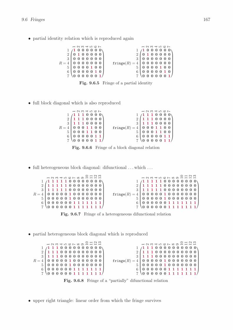
9.6 Fringes 167
• partial identity relation which is reproduced again
R =
1 2 3 4 5 6 7
1234567
⎛⎜⎜⎜⎜⎜⎜⎝
1 0 0 0 0 0 00 1 0 0 0 0 00 0 0 0 0 0 00 0 0 0 0 0 00 0 0 0 1 0 00 0 0 0 0 1 00 0 0 0 0 0 1
⎞⎟⎟⎟⎟⎟⎟⎠
fringe(R) =
1 2 3 4 5 6 7
1234567
⎛⎜⎜⎜⎜⎜⎜⎝
1 0 0 0 0 0 00 1 0 0 0 0 00 0 0 0 0 0 00 0 0 0 0 0 00 0 0 0 1 0 00 0 0 0 0 1 00 0 0 0 0 0 1
⎞⎟⎟⎟⎟⎟⎟⎠
Fig. 9.6.5 Fringe of a partial identity
• full block diagonal which is also reproduced
R =
1 2 3 4 5 6 7
1234567
⎛⎜⎜⎜⎜⎜⎜⎝
1 1 1 0 0 0 01 1 1 0 0 0 01 1 1 0 0 0 00 0 0 1 1 0 00 0 0 1 1 0 00 0 0 0 0 1 10 0 0 0 0 1 1
⎞⎟⎟⎟⎟⎟⎟⎠
fringe(R) =
1 2 3 4 5 6 7
1234567
⎛⎜⎜⎜⎜⎜⎜⎝
1 1 1 0 0 0 01 1 1 0 0 0 01 1 1 0 0 0 00 0 0 1 1 0 00 0 0 1 1 0 00 0 0 0 0 1 10 0 0 0 0 1 1
⎞⎟⎟⎟⎟⎟⎟⎠
Fig. 9.6.6 Fringe of a block diagonal relation
• full heterogeneous block diagonal: difunctional . . . which . . .
R =
1 2 3 4 5 6 7 8 9 10 11 12 13
1234567
⎛⎜⎜⎜⎜⎜⎜⎝
1 1 1 1 1 0 0 0 0 0 0 0 01 1 1 1 1 0 0 0 0 0 0 0 01 1 1 1 1 0 0 0 0 0 0 0 00 0 0 0 0 1 0 0 0 0 0 0 00 0 0 0 0 1 0 0 0 0 0 0 00 0 0 0 0 0 1 1 1 1 1 1 10 0 0 0 0 0 1 1 1 1 1 1 1
⎞⎟⎟⎟⎟⎟⎟⎠
fringe(R) =
1 2 3 4 5 6 7 8 9 10 11 12 13
1234567
⎛⎜⎜⎜⎜⎜⎜⎝
1 1 1 1 1 0 0 0 0 0 0 0 01 1 1 1 1 0 0 0 0 0 0 0 01 1 1 1 1 0 0 0 0 0 0 0 00 0 0 0 0 1 0 0 0 0 0 0 00 0 0 0 0 1 0 0 0 0 0 0 00 0 0 0 0 0 1 1 1 1 1 1 10 0 0 0 0 0 1 1 1 1 1 1 1
⎞⎟⎟⎟⎟⎟⎟⎠
Fig. 9.6.7 Fringe of a heterogeneous difunctional relation
• partial heterogeneous block diagonal which is reproduced
R =
1 2 3 4 5 6 7 8 9 10 11 12 13
1234567
⎛⎜⎜⎜⎜⎜⎜⎝
1 1 1 0 0 0 0 0 0 0 0 0 01 1 1 0 0 0 0 0 0 0 0 0 01 1 1 0 0 0 0 0 0 0 0 0 00 0 0 0 0 1 0 0 0 0 0 0 00 0 0 0 0 1 0 0 0 0 0 0 00 0 0 0 0 0 1 1 1 1 1 1 10 0 0 0 0 0 1 1 1 1 1 1 1
⎞⎟⎟⎟⎟⎟⎟⎠
fringe(R) =
1 2 3 4 5 6 7 8 9 10 11 12 13
1234567
⎛⎜⎜⎜⎜⎜⎜⎝
1 1 1 0 0 0 0 0 0 0 0 0 01 1 1 0 0 0 0 0 0 0 0 0 01 1 1 0 0 0 0 0 0 0 0 0 00 0 0 0 0 1 0 0 0 0 0 0 00 0 0 0 0 1 0 0 0 0 0 0 00 0 0 0 0 0 1 1 1 1 1 1 10 0 0 0 0 0 1 1 1 1 1 1 1
⎞⎟⎟⎟⎟⎟⎟⎠
Fig. 9.6.8 Fringe of a “partially” difunctional relation
• upper right triangle: linear order from which the fringe survives
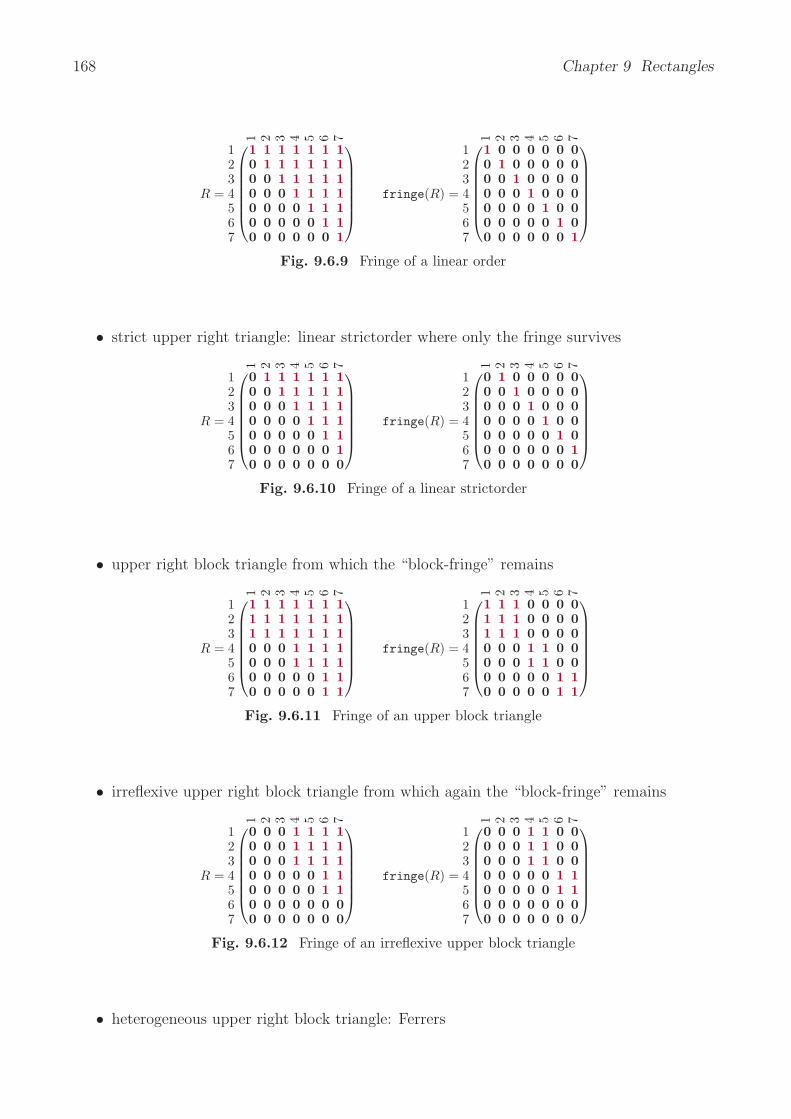
168 Chapter 9 Rectangles
R =
1 2 3 4 5 6 7
1234567
⎛⎜⎜⎜⎜⎜⎜⎝
1 1 1 1 1 1 10 1 1 1 1 1 10 0 1 1 1 1 10 0 0 1 1 1 10 0 0 0 1 1 10 0 0 0 0 1 10 0 0 0 0 0 1
⎞⎟⎟⎟⎟⎟⎟⎠
fringe(R) =
1 2 3 4 5 6 7
1234567
⎛⎜⎜⎜⎜⎜⎜⎝
1 0 0 0 0 0 00 1 0 0 0 0 00 0 1 0 0 0 00 0 0 1 0 0 00 0 0 0 1 0 00 0 0 0 0 1 00 0 0 0 0 0 1
⎞⎟⎟⎟⎟⎟⎟⎠
Fig. 9.6.9 Fringe of a linear order
• strict upper right triangle: linear strictorder where only the fringe survives
R =
1 2 3 4 5 6 7
1234567
⎛⎜⎜⎜⎜⎜⎜⎝
0 1 1 1 1 1 10 0 1 1 1 1 10 0 0 1 1 1 10 0 0 0 1 1 10 0 0 0 0 1 10 0 0 0 0 0 10 0 0 0 0 0 0
⎞⎟⎟⎟⎟⎟⎟⎠
fringe(R) =
1 2 3 4 5 6 7
1234567
⎛⎜⎜⎜⎜⎜⎜⎝
0 1 0 0 0 0 00 0 1 0 0 0 00 0 0 1 0 0 00 0 0 0 1 0 00 0 0 0 0 1 00 0 0 0 0 0 10 0 0 0 0 0 0
⎞⎟⎟⎟⎟⎟⎟⎠
Fig. 9.6.10 Fringe of a linear strictorder
• upper right block triangle from which the “block-fringe” remains
R =
1 2 3 4 5 6 7
1234567
⎛⎜⎜⎜⎜⎜⎜⎝
1 1 1 1 1 1 11 1 1 1 1 1 11 1 1 1 1 1 10 0 0 1 1 1 10 0 0 1 1 1 10 0 0 0 0 1 10 0 0 0 0 1 1
⎞⎟⎟⎟⎟⎟⎟⎠
fringe(R) =
1 2 3 4 5 6 7
1234567
⎛⎜⎜⎜⎜⎜⎜⎝
1 1 1 0 0 0 01 1 1 0 0 0 01 1 1 0 0 0 00 0 0 1 1 0 00 0 0 1 1 0 00 0 0 0 0 1 10 0 0 0 0 1 1
⎞⎟⎟⎟⎟⎟⎟⎠
Fig. 9.6.11 Fringe of an upper block triangle
• irreflexive upper right block triangle from which again the “block-fringe” remains
R =
1 2 3 4 5 6 7
1234567
⎛⎜⎜⎜⎜⎜⎜⎝
0 0 0 1 1 1 10 0 0 1 1 1 10 0 0 1 1 1 10 0 0 0 0 1 10 0 0 0 0 1 10 0 0 0 0 0 00 0 0 0 0 0 0
⎞⎟⎟⎟⎟⎟⎟⎠
fringe(R) =
1 2 3 4 5 6 7
1234567
⎛⎜⎜⎜⎜⎜⎜⎝
0 0 0 1 1 0 00 0 0 1 1 0 00 0 0 1 1 0 00 0 0 0 0 1 10 0 0 0 0 1 10 0 0 0 0 0 00 0 0 0 0 0 0
⎞⎟⎟⎟⎟⎟⎟⎠
Fig. 9.6.12 Fringe of an irreflexive upper block triangle
• heterogeneous upper right block triangle: Ferrers
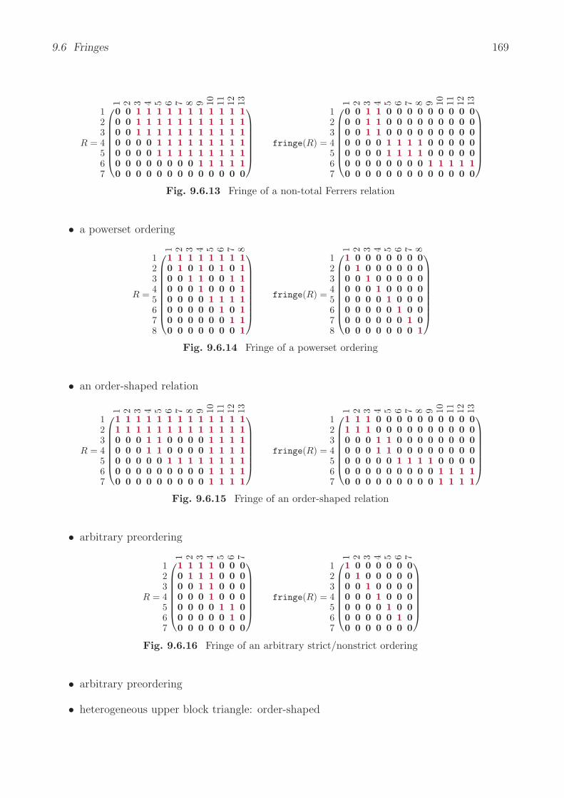
9.6 Fringes 169
R =
1 2 3 4 5 6 7 8 9 10 11 12 13
1234567
⎛⎜⎜⎜⎜⎜⎜⎝
0 0 1 1 1 1 1 1 1 1 1 1 10 0 1 1 1 1 1 1 1 1 1 1 10 0 1 1 1 1 1 1 1 1 1 1 10 0 0 0 1 1 1 1 1 1 1 1 10 0 0 0 1 1 1 1 1 1 1 1 10 0 0 0 0 0 0 0 1 1 1 1 10 0 0 0 0 0 0 0 0 0 0 0 0
⎞⎟⎟⎟⎟⎟⎟⎠
fringe(R) =
1 2 3 4 5 6 7 8 9 10 11 12 13
1234567
⎛⎜⎜⎜⎜⎜⎜⎝
0 0 1 1 0 0 0 0 0 0 0 0 00 0 1 1 0 0 0 0 0 0 0 0 00 0 1 1 0 0 0 0 0 0 0 0 00 0 0 0 1 1 1 1 0 0 0 0 00 0 0 0 1 1 1 1 0 0 0 0 00 0 0 0 0 0 0 0 1 1 1 1 10 0 0 0 0 0 0 0 0 0 0 0 0
⎞⎟⎟⎟⎟⎟⎟⎠
Fig. 9.6.13 Fringe of a non-total Ferrers relation
• a powerset ordering
R =
1 2 3 4 5 6 7 8
12345678
⎛⎜⎜⎜⎜⎜⎜⎜⎜⎝
1 1 1 1 1 1 1 10 1 0 1 0 1 0 10 0 1 1 0 0 1 10 0 0 1 0 0 0 10 0 0 0 1 1 1 10 0 0 0 0 1 0 10 0 0 0 0 0 1 10 0 0 0 0 0 0 1
⎞⎟⎟⎟⎟⎟⎟⎟⎟⎠
fringe(R) =
1 2 3 4 5 6 7 8
12345678
⎛⎜⎜⎜⎜⎜⎜⎜⎜⎝
1 0 0 0 0 0 0 00 1 0 0 0 0 0 00 0 1 0 0 0 0 00 0 0 1 0 0 0 00 0 0 0 1 0 0 00 0 0 0 0 1 0 00 0 0 0 0 0 1 00 0 0 0 0 0 0 1
⎞⎟⎟⎟⎟⎟⎟⎟⎟⎠
Fig. 9.6.14 Fringe of a powerset ordering
• an order-shaped relation
R =
1 2 3 4 5 6 7 8 9 10 11 12 13
1234567
⎛⎜⎜⎜⎜⎜⎜⎝
1 1 1 1 1 1 1 1 1 1 1 1 11 1 1 1 1 1 1 1 1 1 1 1 10 0 0 1 1 0 0 0 0 1 1 1 10 0 0 1 1 0 0 0 0 1 1 1 10 0 0 0 0 1 1 1 1 1 1 1 10 0 0 0 0 0 0 0 0 1 1 1 10 0 0 0 0 0 0 0 0 1 1 1 1
⎞⎟⎟⎟⎟⎟⎟⎠
fringe(R) =
1 2 3 4 5 6 7 8 9 10 11 12 13
1234567
⎛⎜⎜⎜⎜⎜⎜⎝
1 1 1 0 0 0 0 0 0 0 0 0 01 1 1 0 0 0 0 0 0 0 0 0 00 0 0 1 1 0 0 0 0 0 0 0 00 0 0 1 1 0 0 0 0 0 0 0 00 0 0 0 0 1 1 1 1 0 0 0 00 0 0 0 0 0 0 0 0 1 1 1 10 0 0 0 0 0 0 0 0 1 1 1 1
⎞⎟⎟⎟⎟⎟⎟⎠
Fig. 9.6.15 Fringe of an order-shaped relation
• arbitrary preordering
R =
1 2 3 4 5 6 7
1234567
⎛⎜⎜⎜⎜⎜⎜⎝
1 1 1 1 0 0 00 1 1 1 0 0 00 0 1 1 0 0 00 0 0 1 0 0 00 0 0 0 1 1 00 0 0 0 0 1 00 0 0 0 0 0 0
⎞⎟⎟⎟⎟⎟⎟⎠
fringe(R) =
1 2 3 4 5 6 7
1234567
⎛⎜⎜⎜⎜⎜⎜⎝
1 0 0 0 0 0 00 1 0 0 0 0 00 0 1 0 0 0 00 0 0 1 0 0 00 0 0 0 1 0 00 0 0 0 0 1 00 0 0 0 0 0 0
⎞⎟⎟⎟⎟⎟⎟⎠
Fig. 9.6.16 Fringe of an arbitrary strict/nonstrict ordering
• arbitrary preordering
• heterogeneous upper block triangle: order-shaped
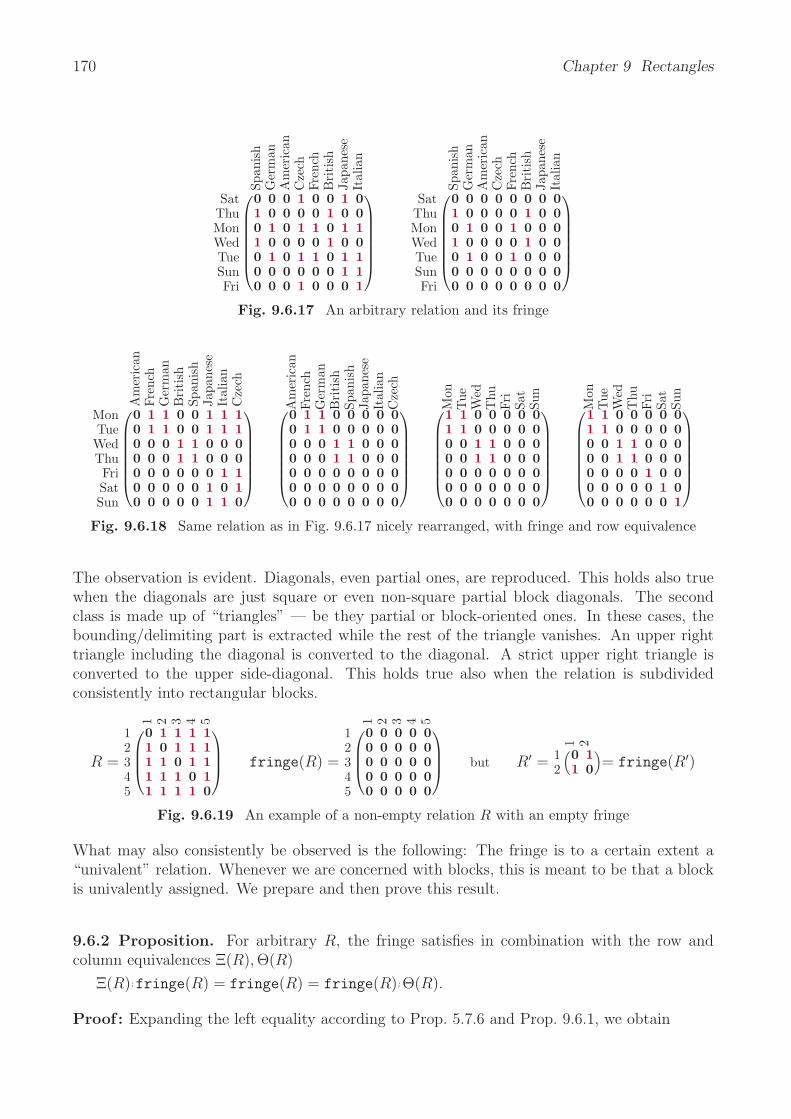
170 Chapter 9 Rectangles
Span
ish
Ger
man
Am
eric
anC
zech
Fren
chB
riti
shJa
pane
seIt
alia
n
SatThuMonWedTueSunFri
⎛⎜⎜⎜⎜⎜⎜⎝
0 0 0 1 0 0 1 01 0 0 0 0 1 0 00 1 0 1 1 0 1 11 0 0 0 0 1 0 00 1 0 1 1 0 1 10 0 0 0 0 0 1 10 0 0 1 0 0 0 1
⎞⎟⎟⎟⎟⎟⎟⎠
Span
ish
Ger
man
Am
eric
anC
zech
Fren
chB
riti
shJa
pane
seIt
alia
n
SatThuMonWedTueSunFri
⎛⎜⎜⎜⎜⎜⎜⎝
0 0 0 0 0 0 0 01 0 0 0 0 1 0 00 1 0 0 1 0 0 01 0 0 0 0 1 0 00 1 0 0 1 0 0 00 0 0 0 0 0 0 00 0 0 0 0 0 0 0
⎞⎟⎟⎟⎟⎟⎟⎠
Fig. 9.6.17 An arbitrary relation and its fringe
Am
eric
anFr
ench
Ger
man
Bri
tish
Span
ish
Japa
nese
Ital
ian
Cze
ch
MonTueWedThuFriSatSun
⎛⎜⎜⎜⎜⎜⎜⎝
0 1 1 0 0 1 1 10 1 1 0 0 1 1 10 0 0 1 1 0 0 00 0 0 1 1 0 0 00 0 0 0 0 0 1 10 0 0 0 0 1 0 10 0 0 0 0 1 1 0
⎞⎟⎟⎟⎟⎟⎟⎠
Am
eric
anFr
ench
Ger
man
Bri
tish
Span
ish
Japa
nese
Ital
ian
Cze
ch⎛⎜⎜⎜⎜⎜⎜⎝
0 1 1 0 0 0 0 00 1 1 0 0 0 0 00 0 0 1 1 0 0 00 0 0 1 1 0 0 00 0 0 0 0 0 0 00 0 0 0 0 0 0 00 0 0 0 0 0 0 0
⎞⎟⎟⎟⎟⎟⎟⎠
Mon
Tue
Wed
Thu
Fri
Sat
Sun⎛
⎜⎜⎜⎜⎜⎜⎝
1 1 0 0 0 0 01 1 0 0 0 0 00 0 1 1 0 0 00 0 1 1 0 0 00 0 0 0 0 0 00 0 0 0 0 0 00 0 0 0 0 0 0
⎞⎟⎟⎟⎟⎟⎟⎠
Mon
Tue
Wed
Thu
Fri
Sat
Sun⎛
⎜⎜⎜⎜⎜⎜⎝
1 1 0 0 0 0 01 1 0 0 0 0 00 0 1 1 0 0 00 0 1 1 0 0 00 0 0 0 1 0 00 0 0 0 0 1 00 0 0 0 0 0 1
⎞⎟⎟⎟⎟⎟⎟⎠
Fig. 9.6.18 Same relation as in Fig. 9.6.17 nicely rearranged, with fringe and row equivalence
The observation is evident. Diagonals, even partial ones, are reproduced. This holds also truewhen the diagonals are just square or even non-square partial block diagonals. The secondclass is made up of “triangles” — be they partial or block-oriented ones. In these cases, thebounding/delimiting part is extracted while the rest of the triangle vanishes. An upper righttriangle including the diagonal is converted to the diagonal. A strict upper right triangle isconverted to the upper side-diagonal. This holds true also when the relation is subdividedconsistently into rectangular blocks.
R =
1 2 3 4 5
12345
⎛⎜⎜⎝
0 1 1 1 11 0 1 1 11 1 0 1 11 1 1 0 11 1 1 1 0
⎞⎟⎟⎠ fringe(R) =
1 2 3 4 5
12345
⎛⎜⎜⎝
0 0 0 0 00 0 0 0 00 0 0 0 00 0 0 0 00 0 0 0 0
⎞⎟⎟⎠ but R′ =
1 2
12
(0 11 0
)= fringe(R′)
Fig. 9.6.19 An example of a non-empty relation R with an empty fringe
What may also consistently be observed is the following: The fringe is to a certain extent a“univalent” relation. Whenever we are concerned with blocks, this is meant to be that a blockis univalently assigned. We prepare and then prove this result.
9.6.2 Proposition. For arbitrary R, the fringe satisfies in combination with the row andcolumn equivalences Ξ(R), Θ(R)
Ξ(R);fringe(R) = fringe(R) = fringe(R); Θ(R).
Proof : Expanding the left equality according to Prop. 5.7.6 and Prop. 9.6.1, we obtain

9.6 Fringes 171
syq(R; RT, R; RT);syq(R; RT, R) = syq(R; RT, R)
due to the cancellation rule Prop. 5.7.4.ii with the first factor total according to Prop. 5.7.2.The other equality follows analogously.
visualize
9.6.3 Proposition. Consider any (possibly heterogeneous) relation R together with its rowequivalence Ξ(R) and its column equivalence Θ(R). Then the fringe satisfies
fringe(R)T; Ξ(R);fringe(R) ⊆ Θ(R)
and is, thus, “blockwisely univalent”. Equality holds whenever the fringe is surjective.
ii) R; [fringe(R)]T; R ⊆ R
Proof : In view of Prop. 9.6.2, we may simply drop the Ξ(R). With the cancellation rule forsymmetric quotients, then
[fringe(R)]T;fringe(R)
= [syq(R; RT, R)]T;syq(R; RT, R)
= syq(R, R; RT);syq(R; RT, R)⊆ syq(R, R) = Θ(R)
If the first factor is total when cancelling, i.e., if the fringe is surjective, we have in addition“=”.
ii) R; [fringe(R)]T; R
= R; [syq(R; RT, R)]T; R
= R;syq(R, R; RT); R
⊆ R; RT; R = R
For every relation, the fringe gives rise to a “partial” equivalence that closely resembles the rowequivalence as already shown with the third relation of Fig. 9.6.18.
9.6.4 Definition. For a relation R we define the fringe-partial row equivalence as wellas the fringe-partial column equivalence
ΞF (R) := fringe(R); [fringe(R)]T
ΘF (R) := [fringe(R)]T;fringe(R)
We show that to a certain extent Ξ(R) may be substituted by ΞF (R); both coincide as long asthe fringe is total. They may be different, but only in the way that a square diagonal block ofthe fringe-partial row equivalence is either equal to the other or empty:
9.6.5 Proposition. Both fringe-partial equivalences are symmetric and transitive, i.e., in-deed “partial equivalences”, and satisfy
ΞF (R) = Ξ(R) ∩ fringe(R); = Ξ(R) ∩ ;fringe(R)
as well as

172 Chapter 9 Rectangles
ΘF (R) = Θ(R) ∩ fringe(R)T; = Θ(R) ∩ ;fringe(R)T.
Furthermore
ΞF (R); Ξ(R) = ΞF (R) = Ξ(R); ΞF (R)ΘF (R); Θ(R) = ΘF (R) = Θ(R); ΘF (R)
Proof : The first formula is shown abbreviating f := fringe(R), where all containments turnout to be equalities:
f ; ∩ Ξ(R)⊆ (f ∩ Ξ(R);
T); ( ∩ fT; Ξ(R))= f ; fT; Ξ(R) due to the Dedekind rule and reflexivity of Ξ(R)
= syq(R; RT, R);syq(R, R; RT);syq(R; RT, R; RT)according to Prop. 9.6.1 and Prop. 5.7.6
⊆ syq(R; RT, R);syq(R, R; RT)= f ; fT = ΞF (R)= f ; fT ∩ f ;
⊆ syq(R; RT, R; RT) ∩ f ;
= Ξ(R) ∩ f ;
This demonstrated also the second series of formulae.
The following proposition relates the row equivalence to fringe of the row-contains-order withthe row equivalence.
9.6.6 Proposition. Provided the fringe is total or surjective, respectively, we have for every(possibly heterogeneous) relation R, that
fringe(R; RT) = syq(RT, RT) = Ξ(R).
fringe(RT; R) = syq(R, R) = Θ(R).
Proof : The first identity, e.g., requires to prove that
fringe(R; RT) = R; RT ∩ R; RT; R; RT; R; RT = R; RT ∩ R; R
T= syq(RT, RT).
The first term on the left equals the first on the right. In addition, the second terms are equal,which is not seen so easily, but also trivial according to Prop. 4.4.2.
The corollary relates the fringe with difunctionality.
9.6.7 Corollary. For arbitrary R, the fringe fringe(R) is difunctional.
Proof : For f := fringe(R) = syq(R; RT, R), we prove f ; fT; f ⊆ f .
f ; fT; f ⊆ f ; Θ(R) = syq(R; RT, R);syq(R, R) ⊆ syq(R; RT, R) = f
We are now confronted with the drawback that the existence of a non-empty fringe heavilydepends on finiteness or at least discreteness. The following proposition resembles a result of

9.7 Ferrers Property/Biorders Heterogeneous 173
Michael Winter [Win04]. Let us for a moment call C a dense relation if it satisfies C ; C = C.An example is obviously the relation “<” on the real numbers. This strictorder is, of course,transitive C ;C ⊆ C, but satisfies also C ⊆ C ;C, meaning that whatever element relationshipone chooses, e.g., 3.7 < 3.8, one will find an element in between, 3.7 < 3.75 < 3.8.
9.6.8 Proposition. A dense linear strictordering has an empty fringe.
Proof : Using the standard property Prop. 5.3.10 of a linear strictordering CT
= E = ∪ C,we have
C ; CT; C = C ; ( ∪ C); C = C ; C ∪ C ; C ; C = C,
so that fringe(C) = C ∩ C ; CT; C = .
9.7 Ferrers Property/Biorders Heterogeneous
The question arose as to whether there was a counterpart of a linear order with rectangularblock-shaped matrices. In this context, the Ferrers1 property of a relation is studied.
9.7.1 Definition. We say that a (possibly heterogeneous) relation A is Ferrers if A;AT;A ⊆ A.
Equivalent forms — easy to prove — of the condition are A;AT;A ⊆ A or AT;A;AT ⊆ AT; i.e.,with A, also A and AT are Ferrers.
The meaning of the algebraic condition just presented will now be visualized and interpreted.
1k→2
345
i→6789
101112
1 2
j↓3 4 5 6
m↓7 8 9 1011121314⎛
⎜⎜⎜⎜⎜⎜⎜⎜⎜⎜⎜⎜⎜⎜⎝
1 1 1 0 1 0 1 1 1 1 1 1 1 10 0 0 0 0 0 1 0 0 0 0 0 0 11 1 1 0 1 0 1 0 1 1 1 1 0 11 1 1 0 1 0 1 0 1 1 1 1 0 10 0 0 0 0 0 0 0 0 0 0 0 0 01 1 1 0 1 0 1 1 1 1 1 1 1 11 1 1 0 1 0 1 0 1 1 1 1 0 11 1 1 0 1 0 1 0 1 1 1 1 0 10 0 0 0 0 0 1 0 0 0 0 0 0 11 1 1 0 1 0 1 0 1 1 1 1 0 11 1 1 0 1 0 1 1 1 1 1 1 1 10 0 0 0 0 0 0 0 0 0 0 0 0 0
⎞⎟⎟⎟⎟⎟⎟⎟⎟⎟⎟⎟⎟⎟⎟⎠
1i→6
113478
10k→2
95
12
4 6 8 13 1 2
j↓3 5 9 101112
m↓7 14⎛
⎜⎜⎜⎜⎜⎜⎜⎜⎜⎜⎜⎜⎜⎜⎝
0 0 1 1 1 1 1 1 1 1 1 1 1 10 0 1 1 1 1 1 1 1 1 1 1 1 10 0 1 1 1 1 1 1 1 1 1 1 1 10 0 0 0 1 1 1 1 1 1 1 1 1 10 0 0 0 1 1 1 1 1 1 1 1 1 10 0 0 0 1 1 1 1 1 1 1 1 1 10 0 0 0 1 1 1 1 1 1 1 1 1 10 0 0 0 1 1 1 1 1 1 1 1 1 10 0 0 0 0 0 0 0 0 0 0 0 1 10 0 0 0 0 0 0 0 0 0 0 0 1 10 0 0 0 0 0 0 0 0 0 0 0 0 00 0 0 0 0 0 0 0 0 0 0 0 0 0
⎞⎟⎟⎟⎟⎟⎟⎟⎟⎟⎟⎟⎟⎟⎟⎠
Fig. 9.7.20 A Ferrers relation1From Wikipedia, the free encyclopedia:
Norman Macleod Ferrers (*1829 †1903) was a British mathematician at Cambridge’s Gonville and Caius College(vice chancellor of Cambridge University 1884) who now seems to be remembered mainly for pointing out aconjugacy in integer partition diagrams, which are accordingly called Ferrers graphs and are closely related toYoung diagrams.
— N. M. Ferrers, An Elementary Treatise on Trilinear Coordinates (London, 1861)— N. M. Ferrers (ed.), Mathematical papers of the late George Green, 1871

174 Chapter 9 Rectangles
It is at first sight not at all clear that the matrix representing R may — due to Ferrers property— be written in staircase (or echelon) block form after suitably rearranging rows and columnsindependently. The graph interpretation is as follows: Given any two arrows, there exists anarrow from one of the starting points leading to the ending point of the other arrow.
∀i, j, k, m : (i, j) ∈ A ∧ (j, k) /∈ AT ∧ (k, m) ∈ A → (i, m) ∈ A or
Or better
∀i, k ∈ X,∀j, m ∈ Y : (i, j) ∈ A ∧ (k, m) ∈ A → (i, m) ∈ A ∨ (k, j) ∈ A or
∀i, m : [∃j, k : (i, j) ∈ A ∧ (j, k) /∈ AT ∧ (k, m) ∈ A] → (i, m) ∈ A.
x
y
z
w
Fig. 9.7.21 Ferrers property represented with the dotted arrow convention
A pictorial description uses the dotted arrow convention. A dotted arrow is conceived tobe an arrow in the complement, i.e., a forbidden arrow. Another characterization is givenwith the following corollary, which says that being Ferrers is equivalent to the fact that therow-is-contained-order is connex, and, thus, a linear order.
9.7.2 Proposition. Let R be an arbitrary relation.
R Ferrers ⇐⇒ R(R) connex ⇐⇒ C(R) connex
Proof : We employ Schroder equivalences to obtain
R; RT; R ⊆ R ⇐⇒ R; RT; R ⊆ R
⇐⇒ R; RT ⊆ R; RT ⇐⇒ R/R ⊆ (R/R)T
which means that R(R) is connex. The second follows in an analogous way.
Thus, the row-contains-relation and the column-is-contained-relation of the given possibly het-erogeneous Ferrers relation turn out to be connex. It is clear that all rows, or columns resp., arein a linear order with regard to containment — up to the fact that there may exist duplicates.
Ferrers relations may, although possibly heterogeneous, in many respects be considered assimilar to a linear strictordering. To make this correspondence transparent, compare
R with C
RT
with C = ET
in case of a linear order.
ET; E = E
Twith C
Using this correlation, transitivity C ; C ⊆ C translates to the Ferrers condition.
R is of strongly Ferrers :⇐⇒ R; RT; R ⊆ Rd; RdT
; R; RdT; Rd ???
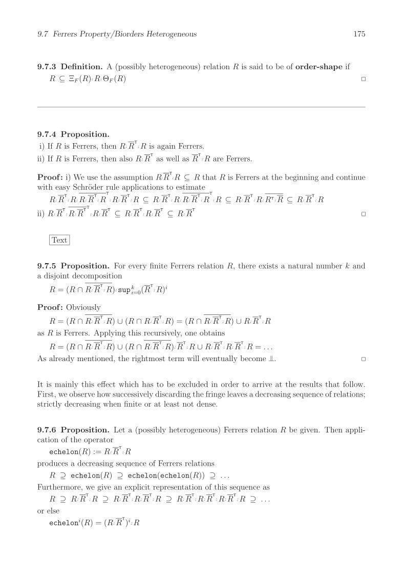
9.7 Ferrers Property/Biorders Heterogeneous 175
9.7.3 Definition. A (possibly heterogeneous) relation R is said to be of order-shape if
R ⊆ ΞF (R); R; ΘF (R)
9.7.4 Proposition.
i) If R is Ferrers, then R; RT; R is again Ferrers.
ii) If R is Ferrers, then also R; RT
as well as RT; R are Ferrers.
Proof : i) We use the assumption R;RT;R ⊆ R that R is Ferrers at the beginning and continue
with easy Schroder rule applications to estimate
R; RT; R; R; R
T; R
T
; R; RT; R ⊆ R; R
T; R; R; R
T; R
T
; R ⊆ R; RT; R; RT; R ⊆ R; R
T; R
ii) R; RT; R; R
TT
; R; RT ⊆ R; R
T; R; R
T ⊆ R; RT
Text
9.7.5 Proposition. For every finite Ferrers relation R, there exists a natural number k anda disjoint decomposition
R = (R ∩ R; RT; R);supk
i=0(RT; R)i
Proof : Obviously
R = (R ∩ R; RT; R) ∪ (R ∩ R; R
T; R) = (R ∩ R; R
T; R) ∪ R; R
T; R
as R is Ferrers. Applying this recursively, one obtains
R = (R ∩ R; RT; R) ∪ (R ∩ R; R
T; R); R
T; R ∪ R; R
T; R; R
T; R = . . .
As already mentioned, the rightmost term will eventually become .
It is mainly this effect which has to be excluded in order to arrive at the results that follow.First, we observe how successively discarding the fringe leaves a decreasing sequence of relations;strictly decreasing when finite or at least not dense.
9.7.6 Proposition. Let a (possibly heterogeneous) Ferrers relation R be given. Then appli-cation of the operator
echelon(R) := R; RT; R
produces a decreasing sequence of Ferrers relations
R ⊇ echelon(R) ⊇ echelon(echelon(R)) ⊇ . . .
Furthermore, we give an explicit representation of this sequence as
R ⊇ R; RT; R ⊇ R; R
T; R; R
T; R ⊇ R; R
T; R; R
T; R; R
T; R ⊇ . . .
or else
echeloni(R) = (R; RT)i; R

176 Chapter 9 Rectangles
Proof : The proof is easy as echelon(echelon(R))=
R; RT; R; R; R
T; R
T
; R; RT; R ⊆ R; R
T; R; RT; R; R
T; R ⊆ R; R
T; R; R
T; R
and in the other direction
R; RT; R; R
T; R ⊆ R; R
T; R; R; R
T; R
T
; R; RT; R
since ???
Es gilt offenbar, ist aber schwer zu beweisen:
R Ferrers =⇒ R; R; RT; R
T
; R = R
9.7.7 Proposition. Let a (possibly heterogeneous) Ferrers relation R =/ be given and assumea finite environment with point axiom. Then also fringe(R) =/ .
Proof : Assume the contrary, R ∩ R; RT; R = . Then R ⊆ R;R
T;R, so that together with the
Ferrers property R = R;RT;R. This, however, means that for all i ≥ 0 we have R = (R;R
T)i;R.
On the other hand, (R ; RT)i ⊆ for all i ≥ 1 due to Schroder equivalence and the Ferrers
property.
This is now a contradiction as it would follow the existence of an infinite sequence of pairs
(x0, y1) ∈ R, (y1, x1) ∈ RT, (x1, y2) ∈ R, (y2, x2) ∈ R
T, (x2, y3) ∈ R, . . .
with xi’s pairwisely different, contradicting finiteness.
The following proposition is a classic; it may not least be found in [DF69] and also with acompletely different componentfree proof in [SS93, SS89]. The proof here is a constructiveone, which means that one may write the constructs down in the language TITUREL andimmediately run this as a program. The reason is that the constructs are generic ones that areuniquely characterized, so that a standard realization for interpretation is possible.
9.7.8 Proposition. Let R : X −→ Y be a possibly heterogeneous finite relation.
R Ferrers ⇐⇒ There exist mappings f, g and a linearstrictorder C such that R = f ; C ; gT.
Proof : “⇐=” follows using several times that mappings may slip below a negation from theleft without affecting the result; see Prop. 5.2.6.
R; RT; R = f ; C ; gT; f ; C ; gT
T; f ; C ; gT by definition
= f ; C ; gT; g; CT; fT; f ; C ; gT as f, g are mappings
⊆ f ; C ; CT; C ; gT as f, g are univalent
⊆ f ; C ; gT as the linear strictorder C is Ferrers= R again by definition
At the end we have used that the linear strictorder C is according to Prop. 5.3.10 certainlyFerrers: C ; C
T; C = C ; E ; C = C ; ( ∪ C); C = C2 ∪ C3 ⊆ C
“=⇒” Let R be Ferrers. There may exist empty rows or columns in R or not. To care for thisin a general form, we enlarge the domain to X + 1l and the codomain to 1l + Y and consider

9.7 Ferrers Property/Biorders Heterogeneous 177
the relation R′ := ιTX
;R;κY . In R′, there will definitely exist at least one empty row and at leastone empty column. It is intuitively clear and easy to demonstrate that also R′ is Ferrers:
R′; R′T; R′ = ιTX
; R; κY ; ιTX
; R; κYT; ιT
X; R; κY by definition
= ιTX
; R; κY ; κTY
; RT; ιX ; ιTX
; R; κY transposing= ιT
X; R; κY ; κT
Y; RT; ιX ; ιT
X; R; κY as ιX , κY are mappings
= ιTX
; R; RT; R; κY as ιX , κY are total and injective⊆ ιT
X; R; κY as R is Ferrers
= R′ again by definition
Y
Ξ ΘX 1 1 Y+ +
1
X
λ
ηΘηΞ
R
R
C
f
gιXιY
κY
κX
Fig. 9.7.22 Constructing the Ferrers decomposition
We define row equivalence Ξ(R′) := syq(R′T, R′T) as well as its column equivalence Θ(R′) :=syq(R′, R′) of R′ together with the corresponding natural projections which we call ηΞ, ηΘ.Heavily based on the fact that R is finite and, according to new prop. , fringe(R′) is total,we define
λ := ηTΞ
;fringe(R′); ηΘ
f := ιX ; ηΞ; λ
g := κY ; ηΘ
C := λT; ηTΞ
; R′; ηΘ
The crucial point is to convince oneself that λ is a bijective mapping:
λT; λ = ηTΘ
; [fringe(R′)]T; ηΞ; ηTΞ
;fringe(R′); ηΘ
= ηTΘ
; [fringe(R′)]T; Ξ(R′);fringe(R′); ηΘ Def. 6.4.1= ηT
Θ; [fringe(R′)]T; Ξ(R′);fringe(R′); ηΘ Ξ(R′) = Ξ(R′)
= ηTΘ
; Θ(R′); ηΘ fringe(R′) is total= ηT
Θ; Θ(R′); ηΘ
= ηTΘ
; ηΘ; ηTΘ
; ηΘ
= ; =
By symmetry, λ is also surjective and injective. Thus, f, g are mappings by definition. Weshow
f ; C ; gT = ιX ; ηΞ; λ; λT; ηTΞ
; R′; ηΘ; (κY ; ηΘ)T by definition= ιX ; ηΞ; ηT
Ξ; R′; ηΘ; ηT
Θ; κT
Y see before= ιX ; Ξ(R′); R′; Θ(R′); κT
Y natural projections= ιX ; R′; κY Prop. 5.4.4= ιX ; ιT
X; R; κY ; κT
Y definition of R′
= R total and injective

178 Chapter 9 Rectangles
Using all this, we prove that C is a linear strictorder, i.e., that it is transitive, irreflexive, andsemi-connex.
C ; C = λT; ηTΞ
; R′; ηΘ; λT; ηTΞ
; R′; ηΘ by definition of C= λT; ηT
Ξ; R′; ηΘ; (ηT
Ξ;fringe(R′); ηΘ)T; ηT
Ξ; R′; ηΘ by definition of λ
⊆ λT; ηTΞ
; R′; ηΘ; (ηTΞ
; R′; ηΘ)T; ηTΞ
; R′; ηΘ by definition of fringe
= λT; ηTΞ
; R′; ηΘ; ηTΘ
; R′T; ηΞ; ηTΞ
; R′; ηΘ transposition
= λT; ηTΞ
; R′; Θ(R′); R′T; Ξ(R′); R′; ηΘ natural projection
= λT; ηTΞ
; R′; R′T; R′; ηΘ following Prop. 5.4.4⊆ λT; ηT
Ξ; R′; ηΘ = C as R′ is Ferrers
Finally, we prove that C is irreflexive and semi-connex, i.e., a linear strictorder.
Irreflexivity
C = λT; ηTΞ
; R′; ηΘ ⊆⇐⇒ R′ ⊆ ηΞ; λ; ; ηT
Θ applying Prop. 5.2.5 several times⇐⇒ R′ ⊆ ηΞ; λ; ; ηT
Θ applying Prop. 5.1.6
⇐⇒ R′ ⊆ ηΞ; ηTΞ
;fringe(R′); ηΘ; ηTΘ expanding λ
⇐⇒ R′ ⊆ Ξ(R′);fringe(R′); Θ(R′) natural projections
⇐⇒ R′ ⊆ fringe(R′) using Prop. 9.6.2
⇐= R′ ⊆ R′ ∩ R′; R′T; R′ which is obviously true
Semi-Connexity
C ∪ CT = λT; ηTΞ
; R′; ηΘ ∪(λT; ηT
Ξ; R′; ηΘ
)T
= λT; ηTΞ
; R′; ηΘ ∪ ηTΘ
; R′T; ηΞ; λ= ηT
Θ;fringe(R′)T; ηΞ; ηT
Ξ; R′; ηΘ ∪ ηT
Θ; R′T; ηΞ; ηT
Ξ;fringe(R′); ηΘ
= ηTΘ
;fringe(R′)T; Ξ(R′); R′; ηΘ ∪ ηTΘ
; R′T; Ξ(R′);fringe(R′); ηΘ
= ηTΘ
;fringe(R′)T; R′; ηΘ ∪ ηTΘ
; R′T;fringe(R′); ηΘ
= ηTΘ
;
(fringe(R′)T; R′ ∪ R′T;fringe(R′)
); ηΘ
= ηTΘ
; Θ(R′); ηΘ
= ηTΘ
; ηΘ; ηTΘ
; ηΘ
= ηTΘ
; ηΘ; ; ηTΘ
; ηΘ
=
This decomposition is essentially unique. Of course, one may choose a much bigger domainof C than necessary. But the essential part of it is uniquely determined up to isomorphism.Whenever another triple f1, g1, C1 is presented, it will be possible to define an isomorphism
ϕ := fT; f1, ψ := gT; g1
such that ϕ, ψ is an isomorphism wrt. C ∩ (fT ; ∪ gT ; ) and C1 ∩ (fT1
; ∪ gT1
; ). As we donot require f, g to be surjective as in [SS89, SS93], C may behave rather arbitrary outside theimages of f, g.
In a first proof we show with f, g surjective mappings that
fringe(R) = R ∩ R; RT; R = f ; C ; gT ∩ f ; C ; gT; g; CT; fT; f ; C ; gT

9.7 Ferrers Property/Biorders Heterogeneous 179
= f ; C ; gT ∩ f ; C ; gT; g; CT; fT; f ; C ; gT = f ; C ; gT ∩ f ; C ; ; CT; ; C ; gT
= f ; (C ∩ C ; CT; C); gT = f ;fringe(C); gT = f ; ; gT = f ; gT
We have also
R(R) = R; RT = f ; C ; gT; g; CT; fT = f ; C ; gT; g; CT; fT = f ; C ; CT; fT = f ; CT; fT = f ; E ; fT
C(R) = RT; R = f ; C ; gT
T; g; C ; fT = g; C
T; fT; f ; C ; gT = g; C
T; C ; gT = g; C ; gT = g; ET; gT
for the order E := ∪ C associated to C, so that
Ξ(R) = f ; fT and Θ(R) = g; gT.
With this, we are in a position to prove tht the structure R, f, g, C is via domR, codR, ϕ isomor-phic to the structure R, f1, C1.
ϕ; ϕT = (fT; f1)T; fT; f1 = fT
1; f ; fT; f1 = fT
1; Ξ(R); f1 = fT
1; f1; fT
1; f1 = ; =
C;ϕ = ϕ;ϕT;C;ϕ = ϕ;(fT;f1)T;C;fT;f1 = ϕ;fT
1;f;C;fT;f1 = ϕ;fT
1;R;f1 = ϕ;fT
1;f1;C1;fT
1;f1 = ϕ;C1
f ; ϕ = f ; fT; f1 = Ξ(R); f1 = f1; fT1
; f1 = f1
9.7.9 Proposition. Let R : X −→ Y be a possibly heterogeneous relation.
R of order-shape ⇐⇒ There exist mappings f, g and anorder E such that R = f ; E ; gT.
Proof : “⇐=” We observe that
f ;fringe(E); gT = f ; (E ∩ E ; ET; E); gT = f ; E ; gT ∩ f ; E ; E
T; E ; gT
= f ; E ; gT ∩ f ; E ; ET; E ; gT = f ; E ; fT ∩ f ; E ; gT; g; E
TfT; f ; E ; gT
= f ; E ; gT ∩ f ; E ; gT; f ; E ; gTT; f ; E ; gT = fringe(f ; E ; gT) = fringe(R)
from which we may conclude as follows
R = f ; E ; gT by assumption= f ; ; E ; ; gT
= f ; ΞF (E); E ; ΘF (E); gT as E itself is of order-shape= f ; ΞF (E); fT; f ; E ; gT; g; ΘF (E); gT since f, g are surjective mappings= f ;fringe(E); [fringe(E)]T; fT; f ; E ; gT; g; [fringe(E)]T;fringe(E); gT
= ΞF (f ; E ; fT); f ; E ; gT; ΘF (g; E ; gT)= ΞF (R); R; ΘF (R)
“=⇒” Let R be order-shaped. We proceed mainly in the same way as for Ferrers relations.There may exist empty rows or columns in R or not. To care for this in a general form, weenlarge the domain to X +1l and the codomain to 1l+Y and consider the relation R′ := ιT
X;R;κY .
In R′, there exists at least one empty row and at least one empty column. It is intuitively clearand easy to demonstrate that also R′ is order-shaped:
We refer to Fig. 9.7.22 and define its row equivalences Ξ(R′) := syq(R′T, R′T) as well as itscolumn equivalences Θ(R′) := syq(R′, R′) together with the corresponding natural projectionswhich we call ηΞ, ηΘ. Now define
λ := ηTΞ
;fringe(R′); ηΘ
f := ιX ; ηΞ; λg := κY ; ηΘ

180 Chapter 9 Rectangles
C := λT; ηTΞ
; R′; ηΘ
By definition, f, g are mappings. The crucial point is to convince oneself that λ is a bijectivemapping:
λT; λ = ηTΘ
; [fringe(R′)]T; ηΞ; ηTΞ
;fringe(R′); ηΘ
= ηTΘ
; [fringe(R′)]T; Ξ(R′);fringe(R′); ηΘ Prop. 9.6.3= ηT
Θ; [fringe(R′)]T; Ξ(R′);fringe(R′); ηΘ
= ηTΘ
; Θ(R′); ηΘ
= ηTΘ
; Θ(R′); ηΘ
= ηTΘ
; ηΘ; ηTΘ
; ηΘ
= ; =
By symmetry, λ is also surjective and injective. We show
f ; C ; gT = ιX ; ηΞ; λ; λT; ηTΞ
; R′; ηΘ; (κY ; ηΘ)T
= ιX ; ηΞ; ηTΞ
; R′; ηΘ; ηTΘ
; κTY
= ιX ; Ξ(R′); R′; Θ(R′); κTY
= ιX ;syq(R′T, R′T); R′;syq(R′, R′); κTY
= ιX ; R′; κY
= ιX ; ιTX
; R; κY ; κTY
= R
Using all this, we prove that C is a strictorder, i.e., that it is transitive and irreflexive.
C ; C = λT; ηTΞ
; R′; ηΘ; λT; ηTΞ
; R′; ηΘ by definition of C= λT; ηT
Ξ; R′; ηΘ; (ηT
Ξ;fringe(R′); ηΘ)T; ηT
Ξ; R′; ηΘ by definition of λ
= λT; ηTΞ
; R′; ηΘ; ηTΘ
;fringe(R′)T; ηΞ; ηTΞ
; R′; ηΘ transposed= λT; ηT
Ξ; R′; Θ(R′);fringe(R′)T; Ξ(R′); R′; ηΘ projection
= λT; ηTΞ
; R′; Θ(R′);fringe(R′)T; Ξ(R′); R′; ηΘ Θ(R′) = Θ(R′), e.g.= λT; ηT
Ξ; R′;fringe(R′)T; R′; ηΘ
= λT; ηTΞ
;R(R′); R′; ηΘ
= λT; ηTΞ
; R′; ηΘ = C
IrreflexivityC = λT; ηT
Ξ; R′; ηΘ ⊆
⇐⇒ R′ ⊆ ηΞ; λ; ; ηTΘ = ηΞ; λ; ; ηT
Θ applying Prop. 5.2.5 and then Prop. 5.1.6
⇐⇒ R′ ⊆ ηΞ; ηTΞ
;fringe(R′); ηΘ; ηTΘ
= Ξ(R);fringe(R′); Θ(R) expanding λ
⇐= R′ ⊆ Ξ(R); R′; Θ(R) = R′ using Prop. 5.4.2
Exercises
4.4.9 i) Prove that any relation R is union as well as intersection of Ferrers relations.
So the bidimension ??? is the smallest number of intersection or uniting Ferrers relations.ii) Let an arbitrary relation R be given and consider all reflexive and transitive relations Q
on dom(X) + cod(Y ) satisfying ι; Q; κT = R. Among these,

9.7 Ferrers Property/Biorders Heterogeneous 181
QM :=
(R/R R
RT; R; RT R\R
)is the greatest.
iii) Given the setting just studied, R is Ferrers precisely when QM is connex.
Solution 4.4.9 i) Any relation consisting of just one related pair (x, y) is Ferrers. ii) Use thisidea for R.

182 Chapter 9 Rectangles
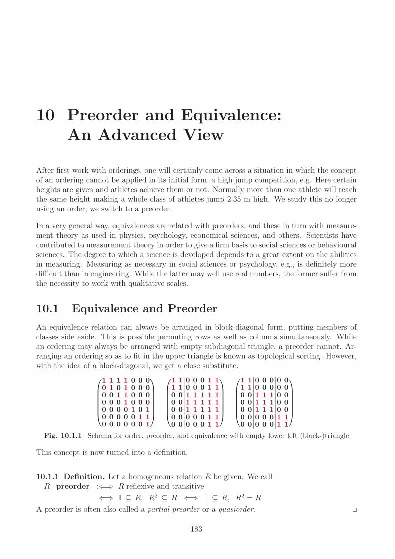
10 Preorder and Equivalence:An Advanced View
After first work with orderings, one will certainly come across a situation in which the conceptof an ordering cannot be applied in its initial form, a high jump competition, e.g. Here certainheights are given and athletes achieve them or not. Normally more than one athlete will reachthe same height making a whole class of athletes jump 2.35 m high. We study this no longerusing an order; we switch to a preorder.
In a very general way, equivalences are related with preorders, and these in turn with measure-ment theory as used in physics, psychology, economical sciences, and others. Scientists havecontributed to measurement theory in order to give a firm basis to social sciences or behaviouralsciences. The degree to which a science is developed depends to a great extent on the abilitiesin measuring. Measuring as necessary in social sciences or psychology, e.g., is definitely moredifficult than in engineering. While the latter may well use real numbers, the former suffer fromthe necessity to work with qualitative scales.
10.1 Equivalence and Preorder
An equivalence relation can always be arranged in block-diagonal form, putting members ofclasses side aside. This is possible permuting rows as well as columns simultaneously. Whilean ordering may always be arranged with empty subdiagonal triangle, a preorder cannot. Ar-ranging an ordering so as to fit in the upper triangle is known as topological sorting. However,with the idea of a block-diagonal, we get a close substitute.
⎛⎜⎜⎜⎜⎜⎝
1 1 1 1 0 0 00 1 0 1 0 0 00 0 1 1 0 0 00 0 0 1 0 0 00 0 0 0 1 0 10 0 0 0 0 1 10 0 0 0 0 0 1
⎞⎟⎟⎟⎟⎟⎠
⎛⎜⎜⎜⎜⎜⎝
1 1 0 0 0 1 11 1 0 0 0 1 10 0 1 1 1 1 10 0 1 1 1 1 10 0 1 1 1 1 10 0 0 0 0 1 10 0 0 0 0 1 1
⎞⎟⎟⎟⎟⎟⎠
⎛⎜⎜⎜⎜⎜⎝
1 1 0 0 0 0 01 1 0 0 0 0 00 0 1 1 1 0 00 0 1 1 1 0 00 0 1 1 1 0 00 0 0 0 0 1 10 0 0 0 0 1 1
⎞⎟⎟⎟⎟⎟⎠
Fig. 10.1.1 Schema for order, preorder, and equivalence with empty lower left (block-)triangle
This concept is now turned into a definition.
10.1.1 Definition. Let a homogeneous relation R be given. We callR preorder :⇐⇒ R reflexive and transitive
⇐⇒ ⊆ R, R2 ⊆ R ⇐⇒ ⊆ R, R2 = R
A preorder is often also called a partial preorder or a quasiorder.
183
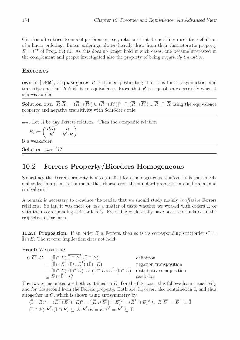
184 Chapter 10 Preorder and Equivalence: An Advanced View
One has often tried to model preferences, e.g., relations that do not fully meet the definitionof a linear ordering. Linear orderings always heavily draw from their characteristic propertyE = CT of Prop. 5.3.10. As this does no longer hold in such cases, one became interested inthe complement and people investigated also the property of being negatively transitive.
Exercises
own In [DF69], a quasi-series R is defined postulating that it is finite, asymmetric, and
transitive and that R ∩ RT
is an equivalence. Prove that R is a quasi-series precisely when itis a weakorder.
Solution own R; R = [(R ∩ RT) ∪ (R ∩ RT)]2 ⊆ (R ∩ R
T) ∪ R ⊆ R using the equivalence
property and negative transitivity with Schroder’s rule.
new-2 Let R be any Ferrers relation. Then the composite relation
Rb :=
(R; R
TR
RT
RT; R
)is a weakorder.
Solution new-2 ???
10.2 Ferrers Property/Biorders Homogeneous
Sometimes the Ferrers property is also satisfied for a homogeneous relation. It is then nicelyembedded in a plexus of formulae that characterize the standard properties around orders andequivalences.
A remark is necessary to convince the reader that we should study mainly irreflexive Ferrersrelations. So far, it was more or less a matter of taste whether we worked with orders E orwith their corresponding strictorders C. Everthing could easily have been reformulated in therespective other form.
10.2.1 Proposition. If an order E is Ferrers, then so is its corresponding strictorder C :=∩ E. The reverse implication does not hold.
Proof : We compute
C ; CT; C = ( ∩ E); ∩ E
T
; ( ∩ E) definition
= ( ∩ E); ( ∪ ET); ( ∩ E) negation transposition
= ( ∩ E); ( ∩ E) ∪ ( ∩ E); ET; ( ∩ E) distributive composition
⊆ E ∩ = C see below
The two terms united are both contained in E. For the first part, this follows from transitivityand for the second from the Ferrers property. Both are, however, also contained in , and thusaltogether in C, which is shown using antisymmetry by
( ∩ E)2 = (E ∩ ET ∩ E)2 = ([E ∪ ET] ∩ E)2 = (E
T ∩ E)2 ⊆ E ; ET
= ET ⊆
( ∩ E); ET; ( ∩ E) ⊆ E ; E
T; E = E ; E
T= E
T ⊆
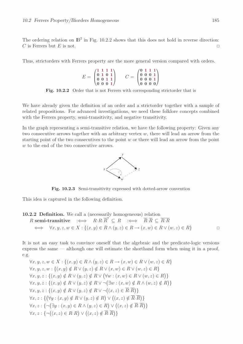
10.2 Ferrers Property/Biorders Homogeneous 185
The ordering relation on IB2 in Fig. 10.2.2 shows that this does not hold in reverse direction:C is Ferrers but E is not.
Thus, strictorders with Ferrers property are the more general version compared with orders.
E =
⎛⎜⎝
1 1 1 10 1 0 10 0 1 10 0 0 1
⎞⎟⎠ C =
⎛⎜⎝
0 1 1 10 0 0 10 0 0 10 0 0 0
⎞⎟⎠
Fig. 10.2.2 Order that is not Ferrers with corresponding strictorder that is
We have already given the definition of an order and a strictorder together with a sample ofrelated propositions. For advanced investigatiions, we need these folklore concepts combinedwith the Ferrers property, semi-transitivity, and negative transitivity.
In the graph representing a semi-transitive relation, we have the following property: Given anytwo consecutive arrows together with an arbitrary vertex w, there will lead an arrow from thestarting point of the two consecutives to the point w or there will lead an arrow from the pointw to the end of the two consecutive arrows.
x
y
z
w
Fig. 10.2.3 Semi-transitivity expressed with dotted-arrow convention
This idea is captured in the following definition.
10.2.2 Definition. We call a (necessarily homogeneous) relation
R semi-transitive :⇐⇒ R; R; RT ⊆ R :⇐⇒ R; R ⊆ R; R
⇐⇒ ∀x, y, z, w ∈ X : (x, y) ∈ R ∧ (y, z) ∈ R → (x, w) ∈ R ∨ (w, z) ∈ R
It is not an easy task to convince oneself that the algebraic and the predicate-logic versionsexpress the same — although one will estimate the shorthand form when using it in a proof,e.g.
∀x, y, z, w ∈ X : (x, y) ∈ R ∧ (y, z) ∈ R → (x, w) ∈ R ∨ (w, z) ∈ R∀x, y, z, w : (x, y) /∈ R ∨ (y, z) /∈ R ∨ (x, w) ∈ R ∨ (w, z) ∈ R∀x, y, z : (x, y) /∈ R ∨ (y, z) /∈ R ∨
(∀w : (x, w) ∈ R ∨ (w, z) ∈ R
)
∀x, y, z : (x, y) /∈ R ∨ (y, z) /∈ R ∨ ¬(∃w : (x, w) /∈ R ∧ (w, z) /∈ R
)
∀x, y, z : (x, y) /∈ R ∨ (y, z) /∈ R ∨ ¬((x, z) ∈ R; R
)
∀x, z : (∀y : (x, y) /∈ R ∨ (y, z) /∈ R
)∨
((x, z) /∈ R; R
)
∀x, z : ¬(∃y : (x, y) ∈ R ∧ (y, z) ∈ R
)∨
((x, z) /∈ R; R
)
∀x, z : ¬((x, z) ∈ R; R
)∨
((x, z) /∈ R; R
)
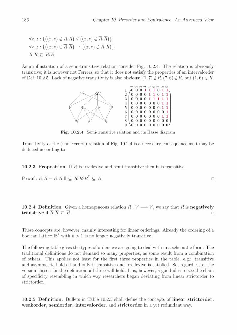
186 Chapter 10 Preorder and Equivalence: An Advanced View
∀x, z : ((x, z) /∈ R; R
)∨
((x, z) /∈ R; R
)
∀x, z : ((x, z) ∈ R; R
)→
((x, z) /∈ R; R
)
R; R ⊆ R; R
As an illustration of a semi-transitive relation consider Fig. 10.2.4. The relation is obviouslytransitive; it is however not Ferrers, so that it does not satisfy the properties of an intervalorderof Def. 10.2.5. Lack of negative transitivity is also obvious: (1, 7)∈/ R, (7, 6)∈/ R, but (1, 6) ∈ R.
1 2 3
4 5 6 7
8 9
1 2 3 4 5 6 7 8 9
123456789
⎛⎜⎜⎜⎜⎜⎜⎜⎜⎜⎝
0 0 0 1 1 1 0 1 10 0 0 0 1 1 0 1 10 0 0 0 1 1 1 1 10 0 0 0 0 0 0 1 10 0 0 0 0 0 0 1 10 0 0 0 0 0 0 0 10 0 0 0 0 0 0 1 10 0 0 0 0 0 0 0 00 0 0 0 0 0 0 0 0
⎞⎟⎟⎟⎟⎟⎟⎟⎟⎟⎠
Fig. 10.2.4 Semi-transitive relation and its Hasse diagram
Transitivity of the (non-Ferrers) relation of Fig. 10.2.4 is a necessary consequence as it may bededuced according to
10.2.3 Proposition. If R is irreflexive and semi-transitive then it is transitive.
Proof : R; R = R; R; ⊆ R; R; RT ⊆ R.
10.2.4 Definition. Given a homogeneous relation R : V −→ V , we say that R is negativelytransitive if R; R ⊆ R.
These concepts are, however, mainly interesting for linear orderings. Already the ordering of aboolean lattice IBk with k > 1 is no longer negatively transitive.
The following table gives the types of orders we are going to deal with in a schematic form. Thetraditional definitions do not demand so many properties, as some result from a combinationof others. This applies not least for the first three properties in the table, e.g.: transitiveand asymmetric holds if and only if transitive and irreflexive is satisfied. So, regardless of theversion chosen for the definition, all three will hold. It is, however, a good idea to see the chainof specificity resembling in which way researchers began deviating from linear strictorder tostrictorder.
10.2.5 Definition. Bullets in Table 10.2.5 shall define the concepts of linear strictorder,weakorder, semiorder, intervalorder, and strictorder in a yet redundant way.
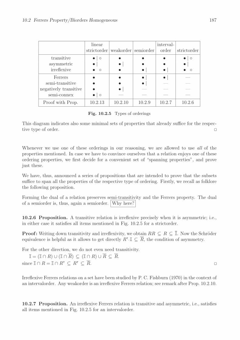
10.2 Ferrers Property/Biorders Homogeneous 187
linear interval-strictorder weakorder semiorder order strictorder
transitive • | • • • • | asymmetric • | • | • • • |irreflexive • • • | • | • Ferrers • • • | • | —
semi-transitive • • • | — —negatively transitive • • | — — —
semi-connex • | — — — —
Proof with Prop. 10.2.13 10.2.10 10.2.9 10.2.7 10.2.6
Fig. 10.2.5 Types of orderings
This diagram indicates also some minimal sets of properties that already suffice for the respec-tive type of order.
Whenever we use one of these orderings in our reasoning, we are allowed to use all of theproperties mentioned. In case we have to convince ourselves that a relation enjoys one of theseordering properties, we first decide for a convenient set of “spanning properties”, and provejust these.
We have, thus, announced a series of propositions that are intended to prove that the subsetssuffice to span all the properties of the respective type of ordering. Firstly, we recall as folklorethe following proposition.
Forming the dual of a relation preserves semi-transitivity and the Ferrers property. The dualof a semiorder is, thus, again a semiorder. Why here?
10.2.6 Proposition. A transitive relation is irreflexive precisely when it is asymmetric; i.e.,in either case it satisfies all items mentioned in Fig. 10.2.5 for a strictorder.
Proof : Writing down transitivity and irreflexivity, we obtain R;R ⊆ R ⊆ . Now the Schroderequivalence is helpful as it allows to get directly RT; ⊆ R, the condition of asymmetry.
For the other direction, we do not even need transitivity.
= ( ∩ R) ∪ ( ∩ R) ⊆ ( ∩ R) ∪ R ⊆ R.
since ∩ R = ∩ RT ⊆ RT ⊆ R.
Irreflexive Ferrers relations on a set have been studied by P. C. Fishburn (1970) in the context ofan intervalorder. Any weakorder is an irreflexive Ferrers relation; see remark after Prop. 10.2.10.
10.2.7 Proposition. An irreflexive Ferrers relation is transitive and asymmetric, i.e., satisfiesall items mentioned in Fig. 10.2.5 for an intervalorder.

188 Chapter 10 Preorder and Equivalence: An Advanced View
Proof : We have R ⊆ , or equivalently, ⊆ R. Therefore, Ferrers property specializes totransitivity:
R; R = R; ; R ⊆ R; RT; R ⊆ R.
From Prop. 10.2.6, we have also that R is asymmetric.
By the way:
10.2.8 Proposition. A reflexive Ferrers relation is connex and negatively transitive.
Proof : A Ferrers relation satisfies R ; RT
; R ⊆ R by definition, which implies RT ⊆ R in
case R is reflexive, i.e., ⊆ R. Therefore, = RT ∪ R. Negative transitivity is equivalentto R
T; R ⊆ R with Schroders equivalence; this, however follows immediately from the Ferrers
property when R is reflexive.
Semiorders have first been introduced in [Luc56] by R. Duncan Luce in 1956.
10.2.9 Proposition. An irreflexive semi-transitive Ferrers relation is transitive and asymmet-ric, i.e., satisfies all items mentioned in Fig. 10.2.5 for a semiorder.
Proof : The proof follows immediately from Prop. 10.2.7.
One has often tried to model preferences, e.g., relations that do not fully meet the definitionof a linear ordering. Linear orderings always heavily draw from their characteristic propertyE = CT of Prop. 5.3.10. As this does no longer hold in such cases, one became interested inthe complement and people investigated also the property of being negatively transitive. Thefollowing result is proved here to demonstrate in which way a subset of properties suffices todefine a weakorder.
10.2.10 Proposition. An asymmetric and negatively transitive relation is transitive, irreflex-ive, Ferrers, and semi-transitive, i.e., satisfies all items mentioned in Fig. 10.2.5 for a weakorder.
Proof : W is necessarily transitive, as
W ; W T ⊆ W ; W ⊆ W
due to asymmetry and negative transitivity. Using the Schroder equivalence, we get W;W ⊆ W .
Being negatively transitive may also be formulated as W ; WT ⊆ W . To prove that W is
semi-transitive and Ferrers, is now easy:
W ; W ; WT ⊆ W ; W ⊆ W
W ; WT; W ⊆ W ; W ⊆ W
With Prop. 10.2.6, we have finally that W is also irreflexive.

10.2 Ferrers Property/Biorders Homogeneous 189
We note in passing, that negatively transitive and irreflexive does not suffice, as the exampleW := shows. With Fig. 10.2.6, we illustrate the concept of a weakorder. In the rearrangedform as well as in the Hasse diagram, it can easily be seen how weakorder and preorder arerelated with adding an equivalence, or removing it.
Alfr
edB
arba
raC
hris
tian
Don
ald
Eug
ene
Fred
eric
kG
eorg
eAlfred
BarbaraChristian
DonaldEugene
FrederickGeorge
⎛⎜⎜⎜⎜⎜⎜⎝
0 0 0 0 0 1 01 0 1 0 1 1 11 0 0 0 0 1 01 0 1 0 1 1 11 0 0 0 0 1 00 0 0 0 0 0 01 0 0 0 0 1 0
⎞⎟⎟⎟⎟⎟⎟⎠
C
B
A
D
GE
F
Bar
bara
Don
ald
Eug
ene
Geo
rge
Chr
isti
anA
lfred
Fred
eric
k
BarbaraDonaldEugeneGeorge
ChristianAlfred
Frederick
⎛⎜⎜⎜⎜⎜⎜⎝
0 0 1 1 1 1 10 0 1 1 1 1 10 0 0 0 0 1 10 0 0 0 0 1 10 0 0 0 0 1 10 0 0 0 0 0 10 0 0 0 0 0 0
⎞⎟⎟⎟⎟⎟⎟⎠
Fig. 10.2.6 Personal assessment as weakorder with Hasse diagram and in rearranged form
There is a close relationship between weakorders and preorders which we will now exhibit intwo steps. In both cases it is an equivalence that is added, or removed, respectively. One maysay that Lemma 10.2.11 is a close analog of Prop. 5.3.10 in case the diagonal is a block-diagonalinstead of a diagonal line.
10.2.11 Lemma. If W is a weakorder and we define Θ := W ∩ WT, then
i) Θ is an equivalence
ii) WT; W = W and W ; W
T= W
iii) Θ = syq(W, W ) = syq(W T, W T) = Ξ(W ) = Θ(W )
Proof : i) Symmetry is evident by construction. From irreflexivity W ⊆ follows that Θ isreflexive. As W is negatively transitive, Θ is transitive.
ii) Direction “⊆ ” follows via the Schroder equivalence from negative transitivity. In the other
direction, we have WT; W ⊇ Θ; W ⊇ W as Θ is an equivalence. The second formula follows
analogously.
iii) syq(W, W ) = W T; W ∩WT; W , e.g., is evaluated using (ii) and the definition of Θ. According
to Def. 5.4.3, therefore, row and column equivalence coincide.
Using these intermediate results, we are in a position to establish a close relationship betweenweakorder and preorder.
10.2.12 Proposition. i) If W is a weakorder then P := WT
is a preorder.
ii) If P is a connex preorder, then W := P ∩ Ξ with Ξ := P ∩ P T is a weakorder.
Proof : i) We apply the preceding lemma. P is reflexive since P = WT ⊇ Θ and Θ is an
equivalence. It is transitive as W is negatively transitive.
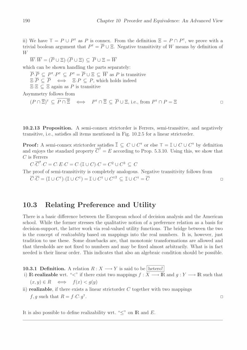
190 Chapter 10 Preorder and Equivalence: An Advanced View
ii) We have = P ∪ P T as P is connex. From the definition Ξ = P ∩ P T, we prove with atrivial boolean argument that P T = P ∪ Ξ. Negative transitivity of W means by definition ofW
W ; W = (P ∪ Ξ); (P ∪ Ξ) ⊆ P ∪ Ξ = W
which can be shown handling the parts separately:
P ; P ⊆ P T; P T ⊆ P T = P ∪ Ξ ⊆ W as P is transitiveΞ; P ⊆ P ⇐⇒ Ξ; P ⊆ P , which holds indeedΞ; Ξ ⊆ Ξ again as P is transitive
Asymmetry follows from
(P ∩ Ξ)T ⊆ P ∩ Ξ ⇐⇒ P T ∩ Ξ ⊆ P ∪ Ξ, i.e., from P T ∩ P = Ξ
10.2.13 Proposition. A semi-connex strictorder is Ferrers, semi-transitive, and negativelytransitive, i.e., satisfies all items mentioned in Fig. 10.2.5 for a linear strictorder.
Proof : A semi-connex strictorder satisfies ⊆ C ∪ CT or else = ∪ C ∪ CT by definitionand enjoys the standard property C
T= E according to Prop. 5.3.10. Using this, we show that
C is Ferrers
C ; CT; C = C ; E ; C = C ; ( ∪ C); C = C2 ∪ C3 ⊆ C
The proof of semi-transitivity is completely analogous. Negative transitivity follows from
C ; C = ( ∪ CT); ( ∪ CT) = ∪ CT ∪ CT2 ⊆ ∪ CT = C
10.3 Relating Preference and Utility
There is a basic difference between the European school of decision analysis and the Americanschool. While the former stresses the qualitative notion of a preference relation as a basis fordecision-support, the latter work via real-valued utility functions. The bridge between the twois the concept of realizability based on mappings into the real numbers. It is, however, justtradition to use these. Some drawbacks are, that monotonic transformations are allowed andthat thresholds are not fixed to numbers and may be fixed almost arbitrarily. What is in factneeded is their linear order. This indicates that also an algebraic condition should be possible.
10.3.1 Definition. A relation R : X −→ Y is said to be hetero!i) IR-realizable wrt. “<” if there exist two mappings f : X −→ IR and g : Y −→ IR such that
(x, y) ∈ R ⇐⇒ f(x) < g(y)
ii) realizable, if there exists a linear strictorder C together with two mappings
f, g such that R = f ; C ; gT.
It is also possible to define realizability wrt. “≤” on IR and E.

10.3 Relating Preference and Utility 191
In several applied sciences, one may observe the task that two or more entities shall be measuredsimultaneously; a composite or conjoint measurement has to take place. A classical exampleis to measure pure tones (identified by their frequency and their intensity) for loudness. So areduction of two (or more, of course) scales to one scale has too be executed. One soon foundout that this is not in the first place a real number problem, although frequencies, e.g., will begiven as values in IR. One has tried to find mappings f, g : IR −→ IR such that (a, b) is louder
than (a′, b′) precisely when f(a) + g(b) > f(a′) + g(b′). dies ist Ferrers!!
An application looking completely differently are Guttman scales. One considers a set A ofsubjects and a set B of questions allowing yes-no answers only. Each subject is supposed tohave answered every question. Given the result of such an interview action, one is supposed tojointly arrange subjects and questions linearly in such a way that the person has answered yesprecisely when it is greater than the question. Chapter III in [DF69].
In psychometric applications, relations that arise from practice and turn out to be realizable inthe sense now to be defined, are called a Guttman scale.
A semiorder has not least been introduced to model nontransitive indifference.
The form the problem originally occurred in is from Mathematical Psychology. Given a relationbetween two sets. Is it possible to arrange these sets by independent permutation so as to findtwo real-valued mappings with
(a, b) ∈ R ⇐⇒ f(a) = g(b).
For the relation(1 11 0
)this would lead to g(2) = f(1) = g(b) and g(2) = f(a) =/ g(b) which cannot be the case. This isat least a hint that when 3 entries of a square are 1 , then also the fourth should be 1 .
When a difunctional relation originates from some practical application, it may also run underthe name of a bi-classificatory system as in [DF69]. Hier!!!
In each of such applications, one deals with an attribute related with two interacting entities.
The start is simple and considers linear strictorders which to embed into the real axis IR israther straightforward.
10.3.2 Theorem (Birkhoff-Milgram). Let C be a linear strictorder. Then there exists amapping f from the domain into the real numbers such that
(x, y) ∈ C ⇐⇒ f(x) < f(y)
if and only if C has a countable order-dense subset.
We do not prove this here, nor do we comment order-density at this point. It is only relevantin non-finite cases. Important is that, once we have a mapping into a strictorder, we can usethis theorem to finally arrive in IR. According to our general approach, we will therefore onlystudy realizations in a strictorder.

192 Chapter 10 Preorder and Equivalence: An Advanced View
A little bit weakened in comparison with linear strictorders are weakorders. Also for these, thereexist characterisations with regard to their embeddability into IR — or into a linear strictorder.
10.3.3 Proposition. Let R be a finite? relation.
R weakorder ⇐⇒ There exists a mapping f and a linearstrictorder C such that R = f ; C ; fT.
Proof : “=⇒”: A weakorder is a Ferrers relation, so that a linear strictorder C exists togetherwith two mappings such that R = f ; C ; gT; see Prop. 9.7.8. With Prop. 10.2.11, we convinceourselves that row equivalence Ξ(R) = syq(RT, RT) and column equivalence Θ(R) = syq(R, R)coincide, so that their corresponding natural projections will also be equal: f = g.
“⇐=”: Assume a mapping f , a linear strictorder C, and consider R := f ; C ; fT:
Irreflexivity propagates from C to R:
R = f ; C ; fT definition of R⊆ f ; ; fT irreflexivity of C= f ; ; fT mapping f slipping under negation= f ; fT identity⊆ as the mapping f is total
Negatively transitive:
R; R = f ; C ; fT; f ; C ; fT definition of R= f ; C ; fT; f ; C ; fT Prop. 5.2.6⊆ f ; C ; C ; fT as f is univalent= f ; ET; ET; fT standard property of a linear strictordering= f ; ET; fT as E is transitive= f ; C ; fT standard property of a linear strictordering= f ; C ; fT Prop. 5.2.6= R
It is then also transitive according to Prop. 10.2.10, and, thus, asymmetric.
We mention in passing that in case of such a weakorder realization always f ; fT = Ξ(R) as
f ; fT = f ; ; fT = f ; (C ∩ CT); fT = f ; C ; fT ∩ f ; CT; fT = R ∩ R = Ξ(R)
Furthermore, the factorization of R into f, C is uniquely defined up to isomorphism — pro-vided that only those with f surjective are considered, a trivial condition. Should a secondfactorization R = f1 ; C1 ; fT
1 be presented, there could easily be defined an isomorphism of thestructure R, f, C into the structure R, f1, C1 with ϕ := fT ; f1 (and in addition the identity onR). Then, e.g., ϕ is total and injective and C satisfies the homomorphism condition as
ϕ; ϕT = fT1
; f ; fT; f1 = fT1
; Ξ(R); f1 = fT1
; f1; fT1
; f1 = ; =
C ; ϕ = ϕ; ϕT; C ; ϕ = ϕ; fT1
; f ; C ; fT; f1 = ϕ; fT1
; R; f1 = ϕ; C
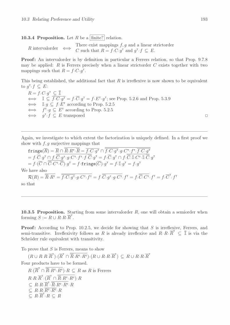
10.3 Relating Preference and Utility 193
10.3.4 Proposition. Let R be a finite? relation.
R intervalorder ⇐⇒ There exist mappings f, g and a linear strictorderC such that R = f ; C ; gT and gT; f ⊆ E.
Proof : An intervalorder is by definition in particular a Ferrers relation, so that Prop. 9.7.8may be applied: R is Ferrers precisely when a linear strictorder C exists together with twomappings such that R = f ; C ; gT.
This being established, the additional fact that R is irreflexive is now shown to be equivalentto gT; f ⊆ E:
R = f ; C ; gT ⊆⇐⇒ ⊆ f ; C ; gT = f ; C ; gT = f ; ET; gT; see Prop. 5.2.6 and Prop. 5.3.9⇐⇒ ; g ⊆ f ; ET according to Prop. 5.2.5⇐⇒ fT; g ⊆ ET according to Prop. 5.2.5⇐⇒ gT; f ⊆ E transposed
Again, we investigate to which extent the factorization is uniquely defined. In a first proof weshow with f, g surjective mappings that
fringe(R) = R ∩ R; RT; R = f ; C ; gT ∩ f ; C ; gT; g; CT; fT; f ; C ; gT
= f ; C ; gT ∩ f ; C ; gT; g; CT; fT; f ; C ; gT = f ; C ; gT ∩ f ; C ; ; CT; ; C ; gT
= f ; (C ∩ C ; CT; C); gT = f ;fringe(C); gT = f ; ; gT = f ; gT
We have also
R(R) = R; RT = f ; C ; gT; g; CT; fT = f ; C ; gT; g; CT; fT = f ; C ; CT; fT = f ; CT; fT
so that
10.3.5 Proposition. Starting from some intervalorder R, one will obtain a semiorder whenforming S := R ∪ R; R; R
T.
Proof : According to Prop. 10.2.5, we decide for showing that S is irreflexive, Ferrers, andsemi-transitive. Irreflexivity follows as R is already irreflexive and R ; R ; R
T ⊆ is via theSchroder rule equivalent with transitivity.
To prove that S is Ferrers, means to show
(R ∪ R; R; RT); (R
T ∩ R; RT; RT); (R ∪ R; R; RT) ⊆ R ∪ R; R; R
T
Four products have to be formed.
R; (RT ∩ R; RT; RT); R ⊆ R as R is Ferrers
R; R; RT; (R
T ∩ R; RT; RT); R
⊆ R; R; RT; R; RT; RT; R
⊆ R; R; RT; RT; R⊆ R; R
T; R ⊆ R

194 Chapter 10 Preorder and Equivalence: An Advanced View
R; R; RT; (R
T ∩ R; RT; RT); R; R; RT ⊆ as before, but with additional factors
⊆ R; R; RT
R; (RT ∩ R; RT; RT); R; R; R
T ⊆ R; RT; R; R; R
T ⊆ R; R; RT ⊆ R; R; R
T
Proving semi-transitivity repeats this procedure in a slightly changed fashion.
(R ∪ R; R; RT); (R ∪ R; R; R
T); (R
T ∩ R; RT; RT) ⊆ R ∪ R; R; RT
R; R; (RT ∩ R; RT; RT) ⊆ R; R; R
T
R; R; R; RT; (R
T ∩ R; RT; RT)
⊆ R; R; R; RT; R; RT; RT
⊆ R; R; R; RT; RT
⊆ R; R; RT
R; R; RT; R; (R
T ∩ R; RT; RT) ⊆ R; R; RT
R; R; RT; R; R; R
T; (R
T ∩ R; RT; RT)
⊆ R; R; RT; R; R; R
T; R; RT; RT
⊆ R; R; RT; R; R; RT; RT
⊆ R; R; RT; R; RT
⊆ R; R; RT
1 2 3 4 5 6 7 8 9 10 11 12 13
123456789
10111213
⎛⎜⎜⎜⎜⎜⎜⎜⎜⎜⎜⎜⎜⎜⎜⎜⎜⎜⎝
0 0 1 0 0 0 0 1 0 0 0 0 01 0 1 1 0 0 1 1 0 0 1 0 10 0 0 0 0 0 0 0 0 0 0 0 00 0 1 0 0 0 0 1 0 0 0 0 00 0 1 0 0 0 0 1 0 0 0 0 11 0 1 1 0 0 1 1 0 0 1 0 11 0 1 0 0 0 0 1 0 0 0 0 10 0 0 0 0 0 0 0 0 0 0 0 01 1 1 1 0 1 1 1 0 0 1 1 11 0 1 1 0 0 1 1 0 0 1 0 10 0 1 0 0 0 0 1 0 0 0 0 00 0 1 0 0 0 0 1 0 0 0 0 10 0 0 0 0 0 0 0 0 0 0 0 0
⎞⎟⎟⎟⎟⎟⎟⎟⎟⎟⎟⎟⎟⎟⎟⎟⎟⎟⎠ 9
102 6
7 4 11
512 1
1383
Fig. 10.3.1 An intervalorder that is not a semiorder
Fig. 10.3.1 shows matrix and Hasse diagram of an intervalorder which is not a semiorder. Theformer may be seen from the mappings f, g of Fig. 10.3.3, in which the f -value is never smallerthan the g-value. It cannot be a semiorder as is documented by 2 < 7 < 1, where we for 12have neither 2 < 12 nor 12 < 1.

10.3 Relating Preference and Utility 195
1 2 3 4 5 6 7 8 9 10 11 12 13
123456789
10111213
⎛⎜⎜⎜⎜⎜⎜⎜⎜⎜⎜⎜⎜⎜⎜⎜⎜⎜⎝
0 0 0 0 0 0 0 0 0 0 0 0 00 0 0 0 1 0 0 0 0 0 0 1 00 0 0 0 0 0 0 0 0 0 0 0 00 0 0 0 0 0 0 0 0 0 0 0 00 0 0 0 0 0 0 0 0 0 0 0 00 0 0 0 1 0 0 0 0 0 0 1 00 0 0 0 0 0 0 0 0 0 0 0 00 0 0 0 0 0 0 0 0 0 0 0 00 0 0 0 1 0 0 0 0 0 0 0 00 0 0 0 1 0 0 0 0 0 0 1 00 0 0 0 0 0 0 0 0 0 0 0 00 0 0 0 0 0 0 0 0 0 0 0 00 0 0 0 0 0 0 0 0 0 0 0 0
⎞⎟⎟⎟⎟⎟⎟⎟⎟⎟⎟⎟⎟⎟⎟⎟⎟⎟⎠ 9
102 6
7 4 11
512 1
1383
Fig. 10.3.2 Diagram of semiorder additions to the intervalorder
1 2 3 4 5 6 7 8 9 10 11 12 13
123456789
10111213
⎛⎜⎜⎜⎜⎜⎜⎜⎜⎜⎜⎜⎜⎜⎜⎜⎜⎜⎝
0 0 1 0 0 0 0 1 0 0 0 0 01 0 1 1 1 0 1 1 0 0 1 1 10 0 0 0 0 0 0 0 0 0 0 0 00 0 1 0 0 0 0 1 0 0 0 0 00 0 1 0 0 0 0 1 0 0 0 0 11 0 1 1 1 0 1 1 0 0 1 1 11 0 1 0 0 0 0 1 0 0 0 0 10 0 0 0 0 0 0 0 0 0 0 0 01 1 1 1 1 1 1 1 0 0 1 1 11 0 1 1 1 0 1 1 0 0 1 1 10 0 1 0 0 0 0 1 0 0 0 0 00 0 1 0 0 0 0 1 0 0 0 0 10 0 0 0 0 0 0 0 0 0 0 0 0
⎞⎟⎟⎟⎟⎟⎟⎟⎟⎟⎟⎟⎟⎟⎟⎟⎟⎟⎠
⎛⎜⎜⎜⎜⎜⎜⎜⎜⎜⎜⎜⎜⎜⎜⎜⎜⎜⎝
0 0 0 0 1 00 1 0 0 0 00 0 0 0 0 10 0 0 0 1 00 0 0 1 0 00 1 0 0 0 00 0 1 0 0 00 0 0 0 0 11 0 0 0 0 00 1 0 0 0 00 0 0 0 1 00 0 0 1 0 00 0 0 0 0 1
⎞⎟⎟⎟⎟⎟⎟⎟⎟⎟⎟⎟⎟⎟⎟⎟⎟⎟⎠
⎛⎜⎜⎜⎜⎜⎜⎜⎜⎜⎜⎜⎜⎜⎜⎜⎜⎜⎝
0 0 0 1 0 00 1 0 0 0 00 0 0 0 0 10 0 1 0 0 01 0 0 0 0 00 1 0 0 0 00 0 1 0 0 00 0 0 0 0 11 0 0 0 0 01 0 0 0 0 00 0 1 0 0 00 1 0 0 0 00 0 0 0 1 0
⎞⎟⎟⎟⎟⎟⎟⎟⎟⎟⎟⎟⎟⎟⎟⎟⎟⎟⎠
Fig. 10.3.3 Semiorder for Fig. 10.3.1 and f and g mapping it on the 6-element strictorder
The semiorder for Fig. 10.3.1 has, therefore, not least the threshold of Fig. 10.3.4 for thefactorized semiorder.
[1]
[2]
[3]
[4]
[5]
[7]
[9]
[10]
[13]
[1][2][3][4][5][7][9]
[10][13]
⎛⎜⎜⎜⎜⎜⎜⎜⎜⎜⎝
0 0 1 0 0 0 0 0 01 0 1 1 1 1 0 0 10 0 0 0 0 0 0 0 00 0 1 0 0 0 0 0 00 0 1 0 0 0 0 0 11 0 1 0 0 0 0 0 11 1 1 1 1 1 0 0 11 0 1 1 1 1 0 0 10 0 0 0 0 0 0 0 0
⎞⎟⎟⎟⎟⎟⎟⎟⎟⎟⎠
Fig. 10.3.4 Threshold
We follow the line of weakening linear strictorders one step further and proceed from weakordersto semiorders. Also for these, there exist characterizations with regard to their embeddabilityinto IR via embedding first into a strictorder. Fig. 10.3.9 shows a semiorder. Semi-transitivityhas to be checked testing all consecutive arrows, i.e., (f, d, e), (b, d, e), (c, b, d), (c, a, e), (c, g, e).The diagram does not show a weakorder as it fails to be negatively transitive; see the triangleb, a, d with (b, a)∈/ R, (a, d)∈/ R, but (b, d) ∈ R.

196 Chapter 10 Preorder and Equivalence: An Advanced View
a
b
c
d
e
f g ab
c
d
e
f
g
distancethreshold
c
e
fb
da = g
Fig. 10.3.5 Hasse diagram of a semiorder, squeezed, and linearized with threshold
The proposition we now aim at resembles what is referred to in the literature as the Scott-Suppes-Theorem; see [Sco64]. Traditionally it is formulated as a theorem on mapping asemiorder into the real numbers with a threshold: “Under what conditions on R will thereexist a real function f on dom(R) such that (x, y) ∈ R ⇐⇒ f(x) ≥ f(y) + 1”
10.3.6 Example. To find out in which way such thresholds emerge, consider a set X whichhas somehow been given a numeric valuation v : X −→ IR. The task is to arrange elements ofX linearly according to this valuation, but to consider valuations as equal when not differingby more than some threshold number t; one does not wish to make a distinction between x andy provided |v(x)− v(y)| < t. One will then get a preference relation T : X −→ X as well as anindifference relation I : X −→ X as follows.
(x, y) ∈ T ⇐⇒ v(x) > v(y) + t
(x, y) ∈ I ⇐⇒ |v(x) − v(y)| ≤ t
One will find out that then T is always a threshold in the above sense. For better reference,we take an example from [Vin]: X = a, b, c, d, e, f with valuations 13, 12, 8, 5, 4, 2, whereany difference of not more than 2 shall be considered unimportant and all values attached aredifferent. Two relations will emerge as indicated in Fig. 10.3.6.
T =
a b c d e f
abcdef
⎛⎜⎜⎜⎜⎝
0 0 1 1 1 10 0 1 1 1 10 0 0 1 1 10 0 0 0 0 10 0 0 0 0 00 0 0 0 0 0
⎞⎟⎟⎟⎟⎠
a b c d e f
abcdef
⎛⎜⎜⎜⎜⎝
0 1 0 0 0 00 0 0 0 0 00 0 0 0 0 00 0 0 0 1 00 0 0 0 0 10 0 0 0 0 0
⎞⎟⎟⎟⎟⎠ = I
Fig. 10.3.6 Preference and indifference relation stemming fromnumerical valuation with threshold
Here obviously, T ∪ I = C is the full strictorder, which is evident as it is properly arranged.One will also verify the threshold property for T . It is easily seen that the outcome T, I isinvariant when X is transformed monotonically. was ist mit t? Therefore, assertions based onT, I alone may be considered meaningful ones.
Once this is presented, authors routinely add that every positive real number other than 1 wouldalso do, and that the 1 “has no meaning”. Also they stress that addition and substraction inthese formulae do not induce any particular algebraic structure. One will not spot obviousconnections with our setting here. While proofs with real numbers are lengthy and usually

10.3 Relating Preference and Utility 197
free-hand mathematics1, we concentrate here on what is important, namely the strictorderaspect, and prove it componentfree. So the proof may be checked — or even found — withcomputer help. To go from the strictorder to the reals is in the finite case trivial — in thegeneral case regulated by the Birkhoff-Milgram Theorem.
The idea of a threshold in the real numbers shall now be transferred to a relational form. Weconsider
(x, y) ∈ T ⇐⇒ v(x) > v(y) + t
and see immediately that
(u, y) ∈ T for every (u, x) ∈ T as then by definition v(u) > v(x) + t(x, z) ∈ T for every (y, z) ∈ T as then by definition v(y) > v(z) + t
So the full cone above x as well as the full cone below y satisfy the condition. This is easy tomodel.
10.3.7 Definition. Given a linear strictorder C, we call a relation T a threshold in Cprovided that C ; T ∪ T ; C ⊆ T ⊆ C.
In other words, we demand T ⊆ C and that T considered rowwise be an upper cone withrespect to C while considered columnwise be a lower cone. Concerning such thresholds, weprove that they are necessarily Ferrers, transitive, and semi-transitive:
Bild
10.3.8 Proposition. A threshold T in a linear strictorder C is itself a semiorder.
Proof : We decide to prove that T is irreflexive, Ferrers, and semi-transitive. As T ⊆ C ⊆ ,we have that T is irreflexive. The remaining point in proving the Ferrers property with
T ; TT; T ⊆ T ; C ⊆ T
is to show that TT
; T ⊆ C. This is equivalent with C ; T T ⊆ T T, and with T ; CT ⊆ T . The
latter, however, follows from the characteristic property (Prop. 5.3.10.i) due to linearity of the
strictorder C and the cone property of T as T ; CT
= T ; E = T ; ( ∪ C) ⊆ T .
Semi-transitivity follows in a rather similar way
T ; T ; TT ⊆ T ; C ⊆ T
using that
T ; TT ⊆ C ⇐⇒ T T; C ⊆ T T ⇐⇒ C
T; T ⊆ T ,
where the latter is trivially satisfied as due to linearity of C
CT; T = E ; T = ( ∪ C); T = T
A semiorder can be closely embedded in a weakorder. The question is where to enlarge R soas to obtain the weakorder W ⊇ R. Would R itself already be negatively transitive, it wouldsatisfy R; R ⊆ R and we might take W := R. If this is not yet satisfied, we have
1“The author (Dana Scott) does not claim that the proof given here is particularly attractive.”

198 Chapter 10 Preorder and Equivalence: An Advanced View
=/ R; R ∩ R ⊆ (R ∩ R; RT); (R ∩ R
T; R),
in which none of the two factors will vanish. We add these factors to R in
W := R ∪ (R ∩ RT; R) ∪ (R ∩ R; R
T) = R ∪ R
T; R ∪ R; R
T. (10.1)
In the following, we will often abbreviate the dual of W as
X := RT ∩ RT; R ∩ R; RT = W d (10.2)
Later, we will at several occasions make use of its trivial properties
R; X ⊆ R X ; R ⊆ R X ⊆ RT
X ; RT ⊆ R
TR
T; X ⊆ R
T(10.3)
10.3.9 Proposition. Every semiorder R may be enlarged so as to obtain the weakorder
W := R ∪ RT; R ∪ R; R
T
which satisfies W ;R ⊆ R and R;W ⊆ R, as well as Ξ;R = R for the corresponding equivalenceΞ := W ∩ W
T.
Proof : We prove that T is asymmetric and negatively transitive.
W is asymmetric provided we are able to show that
W T = RT ∪ RT; R ∪ R; RT ⊆ R ∩ RT; R ∩ R; R
T= W
The first term, RT is contained in R as the semiorder R is asymmetric; it is contained in theother two terms as R is transitive. The second term, e.g., is contained in R as R is transitive,
in RT; R as R is Ferrers, and in R; R
Tsince R is semi-transitive.
W is negatively transitive:
W ; W = R ∪ RT; R ∪ R; R
T; W ⊆ R ∪ R
T; R ∪ R; R
T= W
is equivalent with
X ; (R ∪ RT; R ∪ R; R
T) ⊆ W
Now indeed
X ; R ⊆ RT; R ⊆ W and X ; R
T; R ⊆ R
T; R ⊆ W
We prove some properties in advance that are used later in the other parts of the proof.
W ; R = (R ∪ RT; R ∪ R; R
T); R = R; R ∪ R
T; R; R ∪ R; R
T; R ⊆ R
since R is transitive, semi-transitive (R ; R ⊆ R; R), and Ferrers.
W ; RT; R = (R ∪ R
T; R ∪ R; R
T); R
T; R = R; R
T; R ∪ R
T; R; R
T; R ∪ R; R
T; R
T; R
⊆ R ∪ RT; R ∪ R; R
T= W
as R is Ferrers and, as together with R also its dual RT
is semi-transitive.
R; W = R; (R ∪ RT; R ∪ R; R
T) = R; R ∪ R; R
T; R ∪ R; R; R
T ⊆ R
since R is transitive, Ferrers and semi-transitive.
R; Ξ = R; (W ∩ WT)
= R; (R ∪ RT; R ∪ R; R
T ∩ R ∪ RT; R ∪ R; R
TT
)
= R; (R ∩ RT; R ∩ R; R
T ∩ RT ∩ R
T; R
T
∩ R; RT
T
)
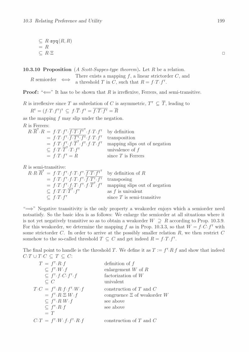
10.3 Relating Preference and Utility 199
⊆ R;syq(R, R)= R⊆ R; Ξ
10.3.10 Proposition (A Scott-Suppes-type theorem). Let R be a relation.
R semiorder ⇐⇒ There exists a mapping f , a linear strictorder C, anda threshold T in C, such that R = f ; T ; fT.
Proof : “⇐=” It has to be shown that R is irreflexive, Ferrers, and semi-transitive.
R is irreflexive since T as subrelation of C is asymmetric, T T ⊆ T , leading to
RT = (f ; T ; fT)T ⊆ f ; T ; fT = f ; T ; fT = R
as the mapping f may slip under the negation.
R is Ferrers:R; R
T; R = f ; T ; fT; f ; T ; fT
T; f ; T ; fT by definition
= f ; T ; fT; f ; T T; fT; f ; T ; fT transposition= f ; T ; fT; f ; T
T; fT; f ; T ; fT mapping slips out of negation
⊆ f ; T ; TT; T ; fT univalence of f
= f ; T ; fT = R since T is Ferrers
R is semi-transitive:R; R; R
T= f ; T ; fT; f ; T ; fT; f ; T ; fT
Tby definition of R
= f ; T ; fT; f ; T ; fT; f ; T T; fT transposing= f ; T ; fT; f ; T ; fT; f ; T
T; fT mapping slips out of negation
⊆ f ; T ; T ; TT; fT as f is univalent
⊆ f ; T ; fT since T is semi-transitive
“=⇒” Negative transitivity is the only property a weakorder enjoys which a semiorder neednotsatisfy. So the basic idea is as follows: We enlarge the semiorder at all situations where itis not yet negatively transitive so as to obtain a weakorder W ⊇ R according to Prop. 10.3.9.For this weakorder, we determine the mapping f as in Prop. 10.3.3, so that W = f ; C ; fT withsome strictorder C. In order to arrive at the possibly smaller relation R, we then restrict Csomehow to the so-called threshold T ⊆ C and get indeed R = f ; T ; fT.
The final point to handle is the threshold T . We define it as T := fT;R;f and show that indeedC ; T ∪ T ; C ⊆ T ⊆ C:
T = fT; R; f definition of f⊆ fT; W ; f enlargement W of R⊆ fT; f ; C ; fT; f factorization of W⊆ C univalent
T ; C = fT; R; f ; fT; W ; f construction of T and C= fT; R; Ξ; W ; f congruence Ξ of weakorder W⊆ fT; R; W ; f see above⊆ fT; R; f see above= T
C ; T = fT; W ; f ; fT; R; f construction of T and C

200 Chapter 10 Preorder and Equivalence: An Advanced View
= fT; W ; Ξ; R; f= fT; W ; R; f⊆ fT; R; f= T
f ; T ; fT = f ; fT; R; f ; fT definition of T= Ξ; R; Ξ natural projection f= (XT ∩ X); R; (XT ∩ X) see ??= R
Here, firstly Ξ ⊇ so that ⊇ R holds. Secondly, we remember X ; R ⊆ R, so that =.
Yet another time, we mention in passing that in case of such a semiorder realization alwaysf ; C ; fT = weakorder(R) as
f ; fT = f ; ; fT = f ; (C ∩ CT); fT = f ; C ; fT ∩ f ; C
T; fT = f ; C ; fT ∩ f ; C ; fT
T
= weakorder(R) ∩ weakorder(R)T
= Ξ(weakorder(R))
f ; C ; fT = f ; (T ∪ TT; T ∪ T T; T ); fT = f ; (T ∪ T
T; fT; f ; T ∪ T T; fT; f ; T ); fT
= f ; T ; fT ∪ f ; TT; fT; f ; T ; fT ∪ f ; T T; fT; f ; T ; fT
= f ; T ; fT ∪ f ; T T; fTT; f ; T ; fT ∪ f ; T T; fT; f ; T T; fT
= R ∪ RT; R ∪ RT; R = weakorder(R)
ϕ; ϕT = fT1
; f ; fT; f1 = fT1
; Ξ(weakorder(R)); f1 = fT1
; f1; fT1
; f1 = ; =
Furthermore, the factorization of R into f, T, C is uniquely defined up to isomorphism —provided that only those with f surjective are considered, a trivial condition. Should a secondfactorization R = f1 ; T1 ; fT
1 with T1 threshold in the linear strictorder C1 be presented, therecould easily be defined an isomorphism of the structure R, f, T, C into the structure R, f1, T1, C1
with ϕ := fT;f1 (and in addition the identity on R). Then, e.g., ϕ is total and injective and Csatisfies the homomorphism condition as
ϕ; ϕT = fT1
; f ; fT; f1 = fT1
; Ξ(R); f1 = fT1
; f1; fT1
; f1 = ; =
C ; ϕ = ϕ; ϕT; C ; ϕ = ϕ; fT1
; f ; C ; fT; f1 = ϕ; fT1
; weakorder(R); f1 = ϕ; fT1
; f1; C1; fT1
; f1 = ϕ; C1
T ; ϕ = ϕ; ϕT; T ; ϕ = ϕ; fT1
; f ; T ; fT; f1 = ϕ; fT1
; R; f1 = ϕ; fT1
; f1; T1; fT1
; f1 = ϕ; T1
R
C T C1 T1
f1f
ϕ
Fig. 10.3.7 Standard situation when studying uniqueness
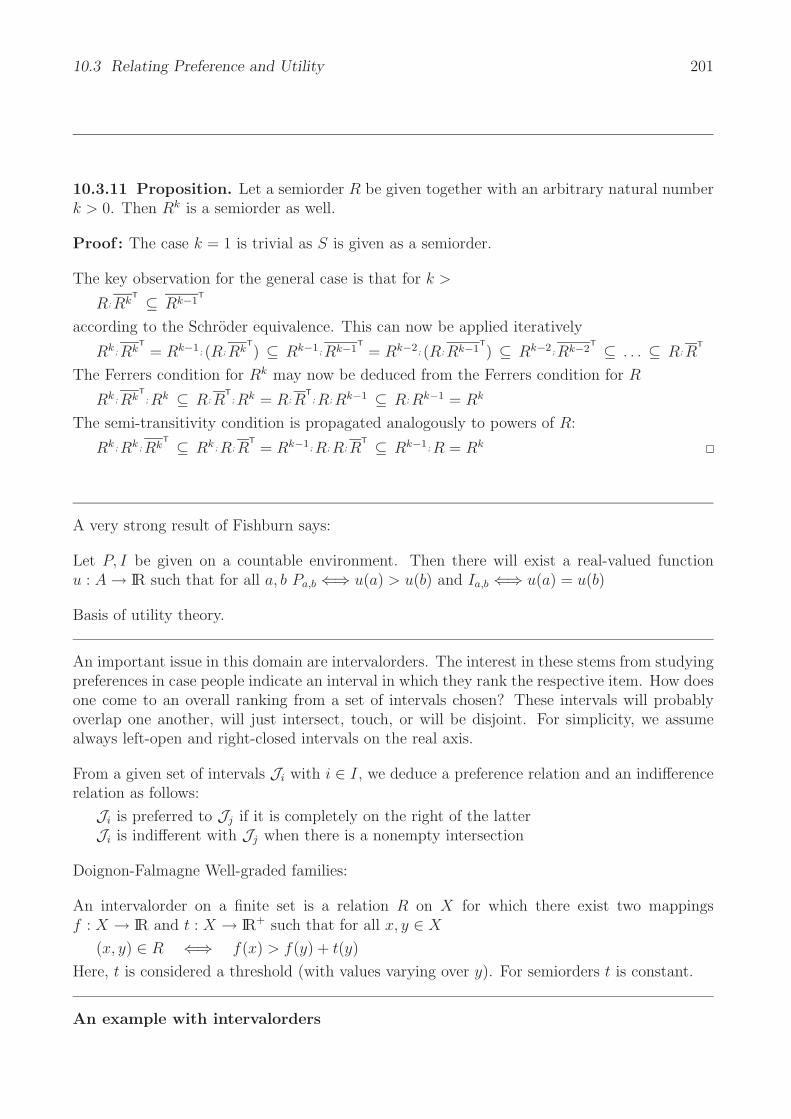
10.3 Relating Preference and Utility 201
10.3.11 Proposition. Let a semiorder R be given together with an arbitrary natural numberk > 0. Then Rk is a semiorder as well.
Proof : The case k = 1 is trivial as S is given as a semiorder.
The key observation for the general case is that for k >
R; RkT ⊆ Rk−1
T
according to the Schroder equivalence. This can now be applied iteratively
Rk ; RkT
= Rk−1; (R; RkT
) ⊆ Rk−1; Rk−1T
= Rk−2; (R; Rk−1T
) ⊆ Rk−2; Rk−2T ⊆ . . . ⊆ R; R
T
The Ferrers condition for Rk may now be deduced from the Ferrers condition for R
Rk ; RkT; Rk ⊆ R; R
T; Rk = R; R
T; R; Rk−1 ⊆ R; Rk−1 = Rk
The semi-transitivity condition is propagated analogously to powers of R:
Rk ; Rk ; RkT ⊆ Rk ; R; R
T= Rk−1; R; R; R
T ⊆ Rk−1; R = Rk
A very strong result of Fishburn says:
Let P, I be given on a countable environment. Then there will exist a real-valued functionu : A → IR such that for all a, b Pa,b ⇐⇒ u(a) > u(b) and Ia,b ⇐⇒ u(a) = u(b)
Basis of utility theory.
An important issue in this domain are intervalorders. The interest in these stems from studyingpreferences in case people indicate an interval in which they rank the respective item. How doesone come to an overall ranking from a set of intervals chosen? These intervals will probablyoverlap one another, will just intersect, touch, or will be disjoint. For simplicity, we assumealways left-open and right-closed intervals on the real axis.
From a given set of intervals Ji with i ∈ I, we deduce a preference relation and an indifferencerelation as follows:
Ji is preferred to Jj if it is completely on the right of the latterJi is indifferent with Jj when there is a nonempty intersection
Doignon-Falmagne Well-graded families:
An intervalorder on a finite set is a relation R on X for which there exist two mappingsf : X → IR and t : X → IR+ such that for all x, y ∈ X
(x, y) ∈ R ⇐⇒ f(x) > f(y) + t(y)
Here, t is considered a threshold (with values varying over y). For semiorders t is constant.
An example with intervalorders

202 Chapter 10 Preorder and Equivalence: An Advanced View
Assume an assessment activity requiring a manager to position his employees as to their abilitieson a linearly ordered scale. One is, however not interested in a linear ranking of the personal;so in the assessment the manager need not enter just one position; he is allowed to indicate arange to which he feels the person belongs to. Assume the following result of this procedure.
unac
cept
able
very
poor
poor
acce
ptab
lefa
iren
joya
ble
good
very
good
mag
nific
ent
AlfredBarbara
ChristianDonaldEugene
FrederickGeorge
⎛⎜⎜⎜⎜⎜⎜⎝
0 0 0 0 0 0 1 0 01 1 1 0 0 0 0 0 00 0 0 1 1 0 0 0 00 0 1 0 0 0 0 0 00 0 0 1 0 0 0 0 00 0 0 0 0 0 0 1 10 0 0 1 1 1 0 0 0
⎞⎟⎟⎟⎟⎟⎟⎠
C
B
A
D
GE
F
Alfr
edB
arba
raC
hris
tian
Don
ald
Eug
ene
Fred
eric
kG
eorg
e
AlfredBarbara
ChristianDonaldEugene
FrederickGeorge
⎛⎜⎜⎜⎜⎜⎜⎝
1 0 0 0 0 1 01 1 1 0 1 1 11 0 1 0 0 1 01 0 1 1 1 1 11 0 0 0 1 1 00 0 0 0 0 1 01 0 0 0 0 1 1
⎞⎟⎟⎟⎟⎟⎟⎠
Fig. 10.3.8 Interval assessment and Hasse diagram of intervalordering
too specific! it is a weakorder!!
The strict intervalorder corresponding to the intervals of this assessment is obtained as follows.It is also shown that it satisfies the Helly property and its strict version is semi-transitive.
Such an interval classification is obviously also possible with real-valued intervals. In such case,it is important whether the interval length is constant or varying over the employees.
10.3.12 Example. The relation of Fig. 10.3.9 is a semiorder. It is not a weakorder as thetriangle C, D, F , e.g., shows that it is not negatively transitive.
Alfr
edB
arba
raC
hris
tian
Don
ald
Eug
ene
Fred
eric
kG
eorg
e
AlfredBarbara
ChristianDonaldEugene
FrederickGeorge
⎛⎜⎜⎜⎜⎜⎜⎝
0 0 1 1 1 1 10 0 1 1 1 1 10 0 0 0 0 1 10 0 0 0 0 0 10 0 0 0 0 0 10 0 0 0 0 0 00 0 0 0 0 0 0
⎞⎟⎟⎟⎟⎟⎟⎠
E
A B
C D
F G
Fig. 10.3.9 A semiorder and its Hasse diagram
We follow the idea of the constructive proof of Prop. 10.3.10 and first embed this semiorder ina weakorder obtaining the left diagram and matrix of Fig. 10.3.10. The link C, E, e.g., is addedsince (C, F ) belongs to the relation R and (F, E) to its dual, so that in total (C, E) is in R;R
T.
The factorization of this weakorder according to Prop. 10.3.10 is then straightforward; see themapping f given as the second relation and the strictorder as the third relation in Fig. 10.3.10.The crucial point is to determine the threshold T ; it is shown as fourth relation in Fig. 10.3.10.
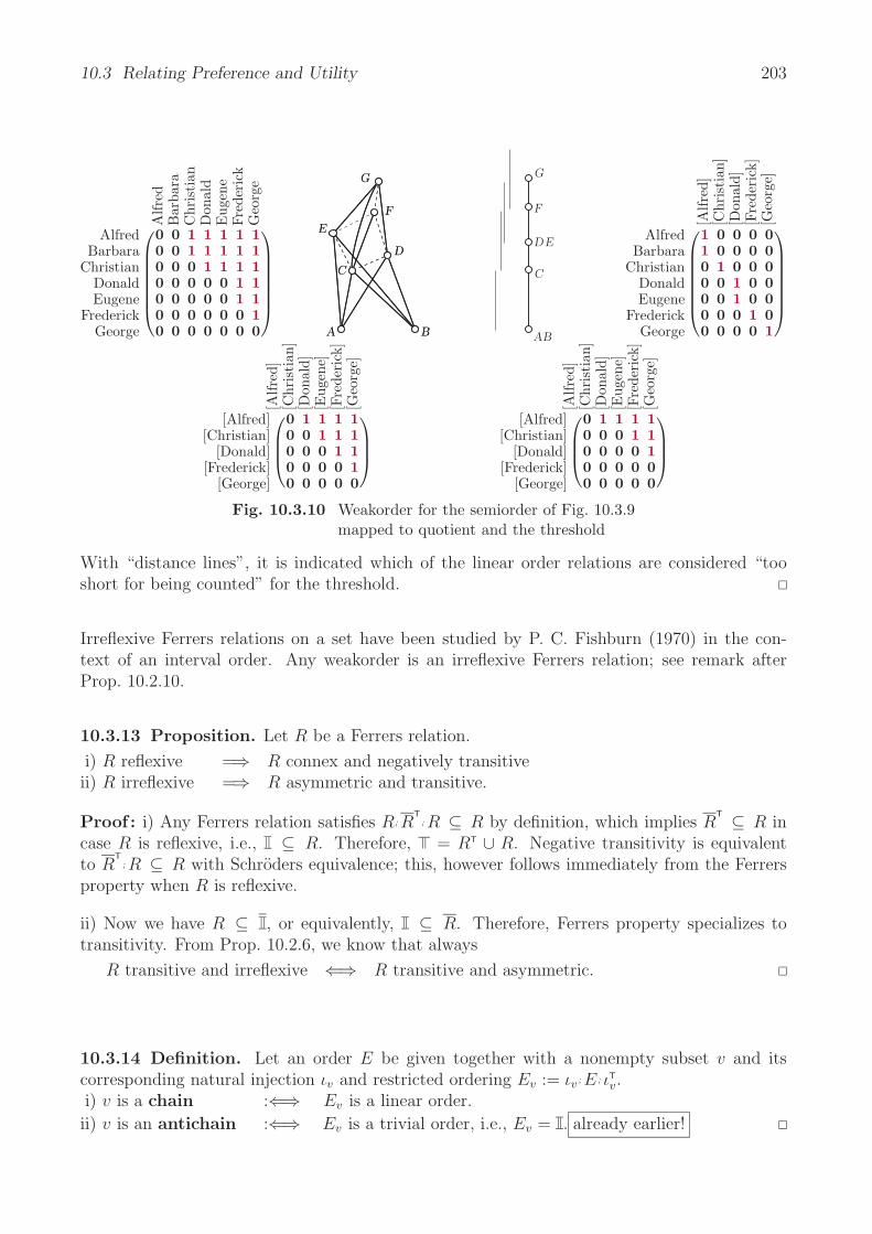
10.3 Relating Preference and Utility 203
AB
C
G
F
DE
A B
C
D
E
F
G
A B
C
D
E
F
G
Alfr
edB
arba
raC
hris
tian
Don
ald
Eug
ene
Fred
eric
kG
eorg
eAlfred
BarbaraChristian
DonaldEugene
FrederickGeorge
⎛⎜⎜⎜⎜⎜⎜⎝
0 0 1 1 1 1 10 0 1 1 1 1 10 0 0 1 1 1 10 0 0 0 0 1 10 0 0 0 0 1 10 0 0 0 0 0 10 0 0 0 0 0 0
⎞⎟⎟⎟⎟⎟⎟⎠
[Alfr
ed]
[Chr
isti
an]
[Don
ald]
[Fre
deri
ck]
[Geo
rge]
AlfredBarbara
ChristianDonaldEugene
FrederickGeorge
⎛⎜⎜⎜⎜⎜⎜⎝
1 0 0 0 01 0 0 0 00 1 0 0 00 0 1 0 00 0 1 0 00 0 0 1 00 0 0 0 1
⎞⎟⎟⎟⎟⎟⎟⎠
[Alfr
ed]
[Chr
isti
an]
[Don
ald]
[Eug
ene]
[Fre
deri
ck]
[Geo
rge]
[Alfred][Christian]
[Donald][Frederick]
[George]
⎛⎜⎜⎝
0 1 1 1 10 0 1 1 10 0 0 1 10 0 0 0 10 0 0 0 0
⎞⎟⎟⎠
[Alfr
ed]
[Chr
isti
an]
[Don
ald]
[Eug
ene]
[Fre
deri
ck]
[Geo
rge]
[Alfred][Christian]
[Donald][Frederick]
[George]
⎛⎜⎜⎝
0 1 1 1 10 0 0 1 10 0 0 0 10 0 0 0 00 0 0 0 0
⎞⎟⎟⎠
Fig. 10.3.10 Weakorder for the semiorder of Fig. 10.3.9mapped to quotient and the threshold
With “distance lines”, it is indicated which of the linear order relations are considered “tooshort for being counted” for the threshold.
Irreflexive Ferrers relations on a set have been studied by P. C. Fishburn (1970) in the con-text of an interval order. Any weakorder is an irreflexive Ferrers relation; see remark afterProp. 10.2.10.
10.3.13 Proposition. Let R be a Ferrers relation.
i) R reflexive =⇒ R connex and negatively transitiveii) R irreflexive =⇒ R asymmetric and transitive.
Proof : i) Any Ferrers relation satisfies R; RT; R ⊆ R by definition, which implies R
T ⊆ R incase R is reflexive, i.e., ⊆ R. Therefore, = RT ∪ R. Negative transitivity is equivalentto R
T; R ⊆ R with Schroders equivalence; this, however follows immediately from the Ferrers
property when R is reflexive.
ii) Now we have R ⊆ , or equivalently, ⊆ R. Therefore, Ferrers property specializes totransitivity. From Prop. 10.2.6, we know that always
R transitive and irreflexive ⇐⇒ R transitive and asymmetric.
10.3.14 Definition. Let an order E be given together with a nonempty subset v and itscorresponding natural injection ιv and restricted ordering Ev := ιv ; E ; ιT
v.i) v is a chain :⇐⇒ Ev is a linear order.
ii) v is an antichain :⇐⇒ Ev is a trivial order, i.e., Ev = . already earlier!

204 Chapter 10 Preorder and Equivalence: An Advanced View
The corresponding characterization in first-order form for a nonempty subset v to be a chainruns as follows:
∀x : x ∈ v → (∀y : (y ∈ v) → (x ≤ y ∨ y ≤ x))
We transform this stepwise into a relational form:
∀x : x ∈ v → (∀y : y ∈ v → ((x, y) ∈ E ∨ (y, x) ∈ E))∀x : x ∈ v → (∀y : y ∈ v → ((x, y) ∈ (E ∪ ET))∀x : x ∈ v → ¬(∃y : y ∈ v ∧ ((x, y) ∈ E ∪ ET))∀x : x ∈ v → ¬(x ∈ E ∪ ET; v)
∀x : x ∈ v → (x ∈ E ∪ ET; v)
v ⊆ E ∪ ET; vE ∪ ET; v ⊆ v
According to Sect. ???, v has, thus, to be stable wrt. E ∪ ET.
For several applications, it is interesting to find a characterization of all chains. This is bestachieved applying this functional to the membership relation ε.
We recall a result with proof that has already been visualized along with Prop. 5.3.11.
10.3.15 Proposition (Szpilrajn’s Theorem). For every order E there exists a linear orderESp with E ⊆ ESp.
Variant:For every order E there exists a bijective homomorphism onto a linear order ESp. This maybe expressed also in the following form: There exists a permutation such that the resultingorder resides in the upper right triangle — in which case the Szpilrajn extension is completelyobvious.
Proof : Assume E were not yet linear, i.e., E ∪ET =/ . Then there exist according to the PointAxiom [SS89, SS93]2.4.6 two points x, y with x; yT ⊆ E ∪ ET.
If we define E1 := E ∪ E;x;yT;E, it is easy to show that E1 is an order again: It is reflexive asalready E is. For proving transitivity and antisymmetry, we need the following intermediateresult:
yT; E2; x = yT; E ; x ⊆It is equivalent with y ; ⊆ E ; x = E ; x as x is a point, and with y ; xT = y ; ; xT ⊆ E whichholds according to the choice of x, y.
Now transitivity is shown as
E1; E1 = E2 ∪ E2; x; yT; E ∪ E ; x; yT; E2 ∪ E ; x; yT; E2; x; yT; E = E ∪ E ; x; yT; E = E1
Antisymmetry may be shown evaluating the additive parts of E1 ∩ ET1 separately. Because E
is an order, E ∩ ET ⊆ . Furthermore,
E ∩ ET; y; xT; ET ⊆ E ∩ ET; E ∪ ET; ET ⊆ E ∩ ET; E ; ET = E ∩ ET; E = E ∩ E =ET; y; xT; ET ∩ E ; x; yT; E ⊆ (ET; y ∩ E ; x; yT; E ; E ; x); (. . .) ⊆ (. . . ∩ ); (. . .) ⊆
In the finite case, this argument may be iterated, and En will eventually become linear.
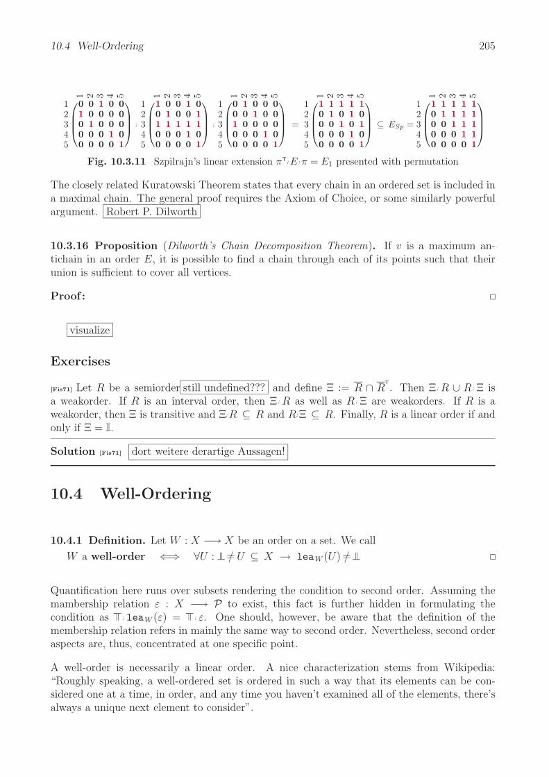
10.4 Well-Ordering 205
1 2 3 4 5
12345
⎛⎜⎜⎝
0 0 1 0 01 0 0 0 00 1 0 0 00 0 0 1 00 0 0 0 1
⎞⎟⎟⎠ ;
1 2 3 4 5
12345
⎛⎜⎜⎝
1 0 0 1 00 1 0 0 11 1 1 1 10 0 0 1 00 0 0 0 1
⎞⎟⎟⎠ ;
1 2 3 4 5
12345
⎛⎜⎜⎝
0 1 0 0 00 0 1 0 01 0 0 0 00 0 0 1 00 0 0 0 1
⎞⎟⎟⎠ =
1 2 3 4 5
12345
⎛⎜⎜⎝
1 1 1 1 10 1 0 1 00 0 1 0 10 0 0 1 00 0 0 0 1
⎞⎟⎟⎠ ⊆ ESp =
1 2 3 4 5
12345
⎛⎜⎜⎝
1 1 1 1 10 1 1 1 10 0 1 1 10 0 0 1 10 0 0 0 1
⎞⎟⎟⎠
Fig. 10.3.11 Szpilrajn’s linear extension πT;E ;π = E1 presented with permutation
The closely related Kuratowski Theorem states that every chain in an ordered set is included ina maximal chain. The general proof requires the Axiom of Choice, or some similarly powerfulargument. Robert P. Dilworth
10.3.16 Proposition (Dilworth’s Chain Decomposition Theorem). If v is a maximum an-tichain in an order E, it is possible to find a chain through each of its points such that theirunion is sufficient to cover all vertices.
Proof :
visualize
Exercises
[Fis71] Let R be a semiorder still undefined??? and define Ξ := R ∩ RT. Then Ξ ; R ∪ R ; Ξ is
a weakorder. If R is an interval order, then Ξ ; R as well as R ; Ξ are weakorders. If R is aweakorder, then Ξ is transitive and Ξ;R ⊆ R and R;Ξ ⊆ R. Finally, R is a linear order if andonly if Ξ = .
Solution [Fis71] dort weitere derartige Aussagen!
10.4 Well-Ordering
10.4.1 Definition. Let W : X −→ X be an order on a set. We call
W a well-order ⇐⇒ ∀U : =/ U ⊆ X → leaW (U) =/
Quantification here runs over subsets rendering the condition to second order. Assuming themambership relation ε : X −→ P to exist, this fact is further hidden in formulating thecondition as ; leaW (ε) = ; ε. One should, however, be aware that the definition of themembership relation refers in mainly the same way to second order. Nevertheless, second orderaspects are, thus, concentrated at one specific point.
A well-order is necessarily a linear order. A nice characterization stems from Wikipedia:“Roughly speaking, a well-ordered set is ordered in such a way that its elements can be con-sidered one at a time, in order, and any time you haven’t examined all of the elements, there’salways a unique next element to consider”.
206 Chapter 10 Preorder and Equivalence: An Advanced View
We now investigate the interrelationship between a well-ordering and the choice function. Fromfoundtions of set theory one knows that certain results can only be obtained when one assumesthat a well-ordering is available. As this well-ordering need not be in any reasonable connectionto the field discussed, one is often a bit frustrated when it is not possible to get rid of it.
10.4.2 Proposition. Let be given a direct power ε and a well-ordering W . Provided theconstruct can be formed, the relation
α := [leaW (ε)]T
enjoys the following properties
i) αT; α ⊆ii) α ⊆ εT
iii) α; = εT;
Proof : i) is satisfied as least elements are always uniquely determined; see ?
ii) follows directly from the definition of lea .
iii) A well-ordering satisfies for all relations for which the construct may be formed ; R =;leaW (R).
This result may to a certain extent be reversed.
10.4.3 Proposition. Given a direct power ε and a choice function α, namely a univalentrelation contained in εT and satisfying α; = εT; , then W := (ε; α)T will be a well-ordering.
Proof : Liegt vor mit MC 82 Text!
10.5 Data Base Congruences
There are congruences in data base theory as well as practice that go beyond difunctionalityconsiderations.
information systems
attributes and decision attributes
consistent
congruence introduced by an attribute
reduct as minimal set of attributes the intersection of congruences of which is contained inthe identity (or in the congruence belonging to the decision attribute)
key
core
indispensable attribute

10.6 Preferences and Indifference 207
10.6 Preferences and Indifference
There exists considerable literature for modeling preferences. The very first observation isthat a preference should be transitive. As it is used in an environment of financial serviceswhere optimization is omnipresent, one could easily bring a person to change its preference toa transitive one. One would namely ask the person to give an amount of Euros to which car ais preferred by him to car b, car b is preferred by him to car c, car c is preferred by him to cara. Once he has paid p(a, b) changing his car from a to b, p(b, c) changing his car from b to c,p(c, a) changing his car from c to a, he will find himself in the uncomfortable situation to havepaid an amount of money just in order to own the same car as before.
In this setting, one is traditionally unsatisfied with the concept of indifference, here defined asintersection of intervals. But indifference should not be transitive, which it turns out to behere. Transitivity of indifference has been strongly contradicted already by Luce and Tversky.
Let a relation R be given that is considered as the outcome of asking for any two alternativesa, b whether a is not worse than b. This makes R immediately a reflexive relation which is calleda weak preference relation. Any relation expressing weak preference can be separated intothree components respectively describing strict preference, indifference and incomparability.
One favourite approach is to partition the universal relation into three or four others and totry on the basis of these to find some justification for arranging the items in a linear order.
Something ignored in test edition!
Something ignored in test edition!
10.7 Scaling
Realizations of measured items on the real scale often undergo several transformations. Asimilarity transformation such as φ(x) := αx is best known for temperature on the Kelvin scale.Positive linear transformations such as φ(x) := αx + β, α > 0 concern intervals and are knownfor temperature in Fahrenheit or Reaumur and for calendar dates (Gregorian vs. Russian).Also ordinal scale transformations are used. In this case one has already an ordering as forhardness (Mohs scale), air quality (1,2,3,4,5 is as good as 100,200,300,400,500), or raw scoresof intelligence tests and undertakes a monotone transformation x ≤ y ⇐⇒ φ(x) ≤ φ(y).Measuring may also be purely nominal by attachments of linguistic variables. Sometimesphysical values are related to a psychological quantity as for loudness with logarithmic Dezibel.If one achieves to arrive at a scale where important operations enjoy pleasant properties (areadditive, e.g.), such a scale will get high acceptance.
Something ignored in test edition!
Something ignored in test edition!

208 Chapter 10 Preorder and Equivalence: An Advanced View

11 Function Properties:An Advanced View
Functions occur in all our algebraic structures, groups, fields, vector spaces, e.g. They of-ten serve the purpose of comparing structures of various forms. Several situations and alsotechniques show up over and over again. We study here, what applies in many such cases.
more text here!
11.1 Homomorphy
Let any two “structures” be given; here for simplicity assumed as a relation R1 between setsX1, Y1 and a relation R2 between sets X2, Y2. Such structures may be conceived as addition ormultiplication in a group, or as an ordering, an equivalence, or simply a graph on a set, or maydescribe multiplication of a vector with a scalar in a vector space, e.g. As a preparation, werecall isotonicity of orderings.
11.1.1 Definition. Let two ordered sets X1,≤1 und X2,≤2 be given as well as a mappingϕ : X1 −→ X2. Then we have the following equivalent possibilities to qualify the mapping asisotonic (also: monotonic):
i) ϕ is a homomorphism from “≤1” to “≤2”, i.e., E≤1; ϕ ⊆ ϕ; E≤2 .
ii) For all x, y ∈ X1 satisfying x ≤1 y we have ϕ(x) ≤2 ϕ(y).
Careful observation shows, that homomorphy holds only for the ordering, but not for leastupper or greatest lower bounds lub, glb formed therein. As an example take the two mediumelements in Fig. 11.1.1.
11.1.2 Beispiel. In einem weiteren Beispiel seien die Strukturen R1, R2 unterschiedliche Ord-nungen auf jeweils 4-elementigen Mengen, wie abgebildet. Es sei ψ die durch horizontalenUbergang skizzierte Abbildung.
209

210 Chapter 11 Function Properties: An Advanced View
Fig. 11.1.1 Homomorphism of orderings
mit Matrix
Wann immer links eine Ordnungsbeziehung besteht, besteht sie nach dem angedeuteten Uber-gang auch rechts. Daß die beiden mittleren Punkte links unvergleichbar sind, rechts aber ineiner Ordnungsbeziehung stehen, stort bei einem Ordnungshomomorphismus nicht. Auch hierhandelt es sich nicht um einen Isomorphismus, eben wegen dieser beiden mittleren Punkte derenOrdnungsbeziehung nicht durch die umgekehrte Abbildung von rechts nach links ubertragenwird.
When we strive to compare any two given such structures, we must be in a position to relatethem somehow. This means typically, that two mappings ϕ : X1 −→ X2 and ψ : Y1 −→ Y2 areprovided “mapping the first structure into the second”.
Φ
Ψ
X
Y
X
Y
1
1
2
2
R1 R2
Fig. 11.1.2 Basic concept of a homomorphism
Once such mappings ϕ, ψ are given, they are said to form a homomorphism of the first into thesecond structure if the following holds: Whenever any two elements x, y are related by the firstrelation R1, their images ϕ(x), ψ(y) are related by the second relation R2. This is captured bythe lengthy predicate logic formulation
∀x ∈ X1 : ∀y ∈ Y1 : (x, y) ∈ R1 → (ϕ(x), ψ(y)) ∈ R2
which will now be converted to a relational form.switching from R to B!
11.1.3 Definition. Let be given two “structures”, a relation R1 between the sets X1, Y1 anda relation R2 between the sets X2, Y2. Relations ϕ : X1 −→ X2 and ψ : Y1 −→ Y2 from thestructure on the left side to the structure on the right are called a homomorphism (ϕ, ψ) ofthe first into the second structure, if the following holds:
ϕT; ϕ ⊆ , ⊆ ϕ; ϕT, ψT; ψ ⊆ , ⊆ ψ; ψT, R1; ψ ⊆ ϕ; R2
i.e. if ϕ, ψ are mappings satisfying R1; ψ ⊆ ϕ; R2.

11.1 Homomorphy 211
Often one has structures “on a set”; in this case, the mappings ϕ, ψ coincide. As it would notbe appealing to talk of the homomorphism (ϕ, ϕ), one simply denotes the homomorphism as ϕ.
We explain the concept of homomorphism for relational structures that are unary: Structureand mappings shall commute, however, not as equality but just as containment. This conceptof homomorphism — solely based on inclusion R1;ψ ⊆ ϕ;R2 — is a very general one. Even incase of such a simple example as here between two graphs it is not easy to recognize. It is anextremely broadly applicable concept.
As already several times, we show how the lengthy predicate logic form translates in the shorterrelational form:
∀x1 ∈ X1 : ∀y1 ∈ Y1 : ∀x2 ∈ X2 : ∀y2 ∈ Y2 :(x1, y1) ∈ R1 ∧ (x1, x2) ∈ ϕ ∧ (y1, y2) ∈ ψ → (x2, y2) ∈ R2
∀x1 ∈ X1 : ∀y1 ∈ Y1 : ∀y2 ∈ Y2 : ∀x2 ∈ X2 :(x1, y1)∈/ R1 ∨ (y1, y2)∈/ ψ ∨ (x1, x2)∈/ ϕ ∨ (x2, y2) ∈ R2 u ∨ v = v ∨ u, a → b = ¬a ∨ b
∀x1 ∈ X1 : ∀y1 ∈ Y1 : ∀y2 ∈ Y2 : (x1, y1)∈/ R1 ∨ (y1, y2)∈/ ψ∨(∀x2 ∈ X2 : (x1, x2)∈/ ϕ ∨ (x2, y2) ∈ R2
)a ∨ (∀x : p(x)) = ∀x : (a ∨ p(x))
∀x1 ∈ X1 : ∀y2 ∈ Y2 : ∀y1 ∈ Y1 : (x1, y1)∈/ R1 ∨ (y1, y2)∈/ ψ∨¬¬
(∀x2 ∈ X2 : (x1, x2)∈/ ϕ ∨ (x2, y2) ∈ R2
)∀x1 ∈ X1 : ∀y2 ∈ Y2 :
(∀y1 ∈ Y1 : (x1, y1)∈/ R1 ∨ (y1, y2)∈/ ψ
)∨
¬(∃x2 ∈ X2 : (x1, x2) ∈ ϕ ∧ (x2, y2)∈/ R2
)∀x1 ∈ X1 : ∀y2 ∈ Y2 : ¬¬
(∀y1 ∈ Y1 : (x1, y1)∈/ R1 ∨ (y1, y2)∈/ ψ
)∨ ¬
((x1, y2) ∈ ϕ; R2
)∀x1 ∈ X1 : ∀y2 ∈ Y2 : ¬
(∃y1 ∈ Y1 : (x1, y1) ∈ R1 ∧ (y1, y2) ∈ ψ
)∨ ¬
((x1, y2) ∈ ϕ; R2
)∀x1 ∈ X1 : ∀y2 ∈ Y2 : ¬
((x1, y2) ∈ R1; ψ
)∨
((x1, y2) ∈ ϕ; R2
)∀x1 ∈ X1 : ∀y2 ∈ Y2 :
((x1, y2) ∈ R1; ψ
)→
((x1, y2) ∈ ϕ; R2
)R1; ψ ⊆ ϕ; R2
The result looks quite similar to a commutativity rule; it is, however, not an equality butcontainment: When one follows the structural relation R1 and then proceeds with ψ to the setY2, it is always possible to go to the set X2 first and then follow the structural relation R2 toreach the same element.
Assume therefore, the relations R1, R2, ϕ, ψ to be given. The test on homomorphy is then easilywritten down in TITUREL:
isHomomorphismFormula rt st phi psi =Conjunct (Conjunct (isMappingFormula phi) (isMappingFormula psi))
(RF $ rt :***: phi :<==: (psi :***: st))
The homomorphism condition proper has four variants which may be used interchangeably:
11.1.4 Proposition. If ϕ, ψ are mappings, then
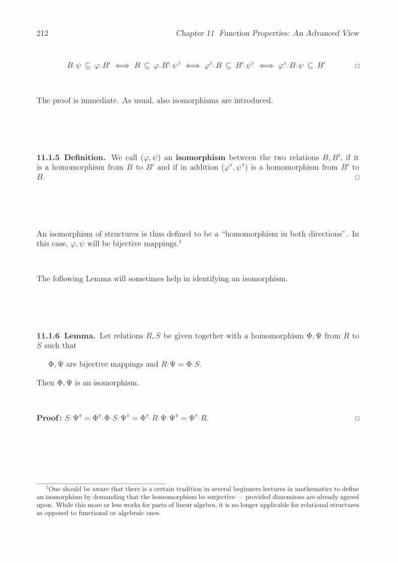
212 Chapter 11 Function Properties: An Advanced View
B ; ψ ⊆ ϕ; B′ ⇐⇒ B ⊆ ϕ; B′; ψT ⇐⇒ ϕT; B ⊆ B′; ψT ⇐⇒ ϕT; B ; ψ ⊆ B′
The proof is immediate. As usual, also isomorphisms are introduced.
11.1.5 Definition. We call (ϕ, ψ) an isomorphism between the two relations B, B′, if itis a homomorphism from B to B′ and if in addition (ϕT, ψT) is a homomorphism from B′ toB.
An isomorphism of structures is thus defined to be a “homomorphism in both directions”. Inthis case, ϕ, ψ will be bijective mappings.1
The following Lemma will sometimes help in identifying an isomorphism.
11.1.6 Lemma. Let relations R, S be given together with a homomorphism Φ, Ψ from R toS such that
Φ, Ψ are bijective mappings and R; Ψ = Φ; S.
Then Φ, Ψ is an isomorphism.
Proof : S ; ΨT = ΦT; Φ; S ; ΨT = ΦT; R; Ψ; ΨT = ΦT; R.
1One should be aware that there is a certain tradition in several beginners lectures in mathematics to definean isomorphism by demanding that the homomorphism be surjective — provided dimensions are already agreedupon. While this more or less works for parts of linear algebra, it is no longer applicable for relational structuresas opposed to functional or algebraic ones.
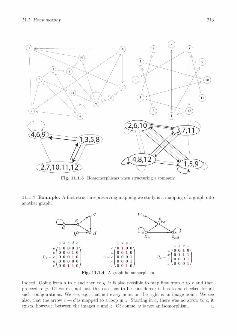
11.1 Homomorphy 213
1
2
3
4
5
6
7
8
9
10
11
12
1
2
3
4
5
67
8
9
10
11
12
4,6,91,3,5,8
2,7,10,11,12 1,5,9
2,6,103,7,11
4,8,12
Fig. 11.1.3 Homomorphisms when structuring a company
11.1.7 Example. A first structure-preserving mapping we study is a mapping of a graph intoanother graph.
ab
c
d
ew
yb,e
xa zc,d
R1 =
⎛⎜⎜⎜⎝
a b c d e
a 1 0 0 0 1b 0 0 0 1 0c 0 0 0 1 0d 0 0 0 0 0e 0 0 1 1 0
⎞⎟⎟⎟⎠ ϕ =
⎛⎜⎜⎜⎝
w x y z
a 0 1 0 0b 0 0 1 0c 0 0 0 1d 0 0 0 1e 0 0 1 0
⎞⎟⎟⎟⎠ R2 =
⎛⎜⎝
w x y z
w 0 0 1 0x 0 1 1 1y 0 0 0 1z 0 0 0 1
⎞⎟⎠
Fig. 11.1.4 A graph homomorphism
Indeed: Going from a to e and then to y, it is also possible to map first from a to x and thenproceed to y. Of course, not just this case has to be considered; it has to be checked for allsuch configurations. We see, e.g., that not every point on the right is an image point. We seealso, that the arrow c → d is mapped to a loop in z. Starting in a, there was no arrow to c; itexists, however, between the images x und z. Of course, ϕ is not an isomorphism.

214 Chapter 11 Function Properties: An Advanced View
11.1.8 Beispiel. Ein weiteres Beispiel gibt es bei der Bemuhung um den Erwerb von”Wissen“.
Man nehme eine beliebige Relation R. Wenn sie relativ dunn besetzt ist, wird die folgendeUberlegung interessant; ist die Relation dicht besetzt, bleiben die Aussagen zwar richtig, ihreNutzung lohnt sich aber weniger. Es geht darum, welche Elemente der linken Menge mit glei-chen Elementen der rechten Menge in Relation stehen, d.h. wir betrachten R;RT:
”Gehe von links
nach rechts und schaue zuruck, um herauszufinden, welche Elemente der linken Menge ebenfallsauf das dort erreichte Element abgebildet wurden“. Aus Symmetriegrunden interessieren wiruns in analoger Weise fur die Relation RT;R auf der rechten Menge. See also in which way thisgives a congruence in Example 11.2.4.
1 2 3 4 5 6 7 8 9 10 11 12 13 14
1
2
3
4
5
6
7
8
9
10
11
12
13
14
⎛⎜⎜⎜⎜⎜⎜⎜⎜⎜⎜⎜⎜⎜⎜⎜⎜⎜⎜⎜⎝
1 0 0 0 0 1 0 0 0 0 0 0 1 00 1 0 0 0 0 0 0 0 1 1 0 0 10 0 0 0 0 0 0 0 0 0 0 0 0 00 0 0 1 1 0 0 1 0 0 0 1 0 00 0 0 1 1 0 0 1 0 0 0 1 0 01 0 0 0 0 1 0 0 0 0 0 0 1 00 0 0 0 0 0 0 0 0 0 0 0 0 00 0 0 1 1 0 0 1 0 0 0 1 0 00 0 0 0 0 0 0 0 0 0 0 0 0 00 1 0 0 0 0 0 0 0 1 1 0 0 10 1 0 0 0 0 0 0 0 1 1 0 0 10 0 0 1 1 0 0 1 0 0 0 1 0 01 0 0 0 0 1 0 0 0 0 0 0 1 00 1 0 0 0 0 0 0 0 1 1 0 0 1
⎞⎟⎟⎟⎟⎟⎟⎟⎟⎟⎟⎟⎟⎟⎟⎟⎟⎟⎟⎟⎠
1 2 3 4 5 6 7 8 9 10 11
1
2
3
4
5
6
7
8
9
10
11
12
13
14
⎛⎜⎜⎜⎜⎜⎜⎜⎜⎜⎜⎜⎜⎜⎜⎜⎜⎜⎜⎜⎝
0 1 0 0 0 0 0 0 1 0 00 0 0 0 0 0 0 0 0 1 00 0 0 0 0 0 0 0 0 0 00 0 0 0 0 0 0 1 0 0 01 0 0 0 0 0 0 1 0 0 00 0 0 0 0 0 1 0 1 0 00 0 0 0 0 0 0 0 0 0 01 0 0 0 1 0 0 0 0 0 00 0 0 0 0 0 0 0 0 0 00 0 1 0 0 1 0 0 0 0 00 0 1 0 0 0 0 0 0 1 00 0 0 0 1 0 0 0 0 0 00 0 0 1 0 0 1 0 0 0 00 0 0 0 0 1 0 0 0 0 0
⎞⎟⎟⎟⎟⎟⎟⎟⎟⎟⎟⎟⎟⎟⎟⎟⎟⎟⎟⎟⎠
1 2 3 4 5 6 7 8 9 10 11
1
2
3
4
5
6
7
8
9
10
11
⎛⎜⎜⎜⎜⎜⎜⎜⎜⎜⎜⎜⎜⎜⎝
1 0 0 0 1 0 0 1 0 0 00 1 0 1 0 0 1 0 1 0 00 0 1 0 0 1 0 0 0 1 00 1 0 1 0 0 1 0 1 0 01 0 0 0 1 0 0 1 0 0 00 0 1 0 0 1 0 0 0 1 00 1 0 1 0 0 1 0 1 0 01 0 0 0 1 0 0 1 0 0 00 1 0 1 0 0 1 0 1 0 00 0 1 0 0 1 0 0 0 1 00 0 0 0 0 0 0 0 0 0 1
⎞⎟⎟⎟⎟⎟⎟⎟⎟⎟⎟⎟⎟⎟⎠
Fig. 11.1.5 Die Relation R;RT, das gegebene beliebige R, und RT;R
Something ignored in test edition!
11.2 Congruences
In a natural way, any equivalence leads to a partitioning into classes. To work with setsof classes is usually more efficient as they are less in number. We have learned to compute“modulo” a prime number; i.e., we only care to which class determined by the remainder anumber belongs. However, this is only possible in cases where the operations aimed at behavenicely with respect to the subdivision into classes. The operations addition and multiplicationin this sense behave nicely with regard to the equivalence “have same remainder modulo 5”.Would one try an arbitrary subdivision into classes, e.g., 1, 5, 99, 213, 2, 3, 4, 6 . . ., additionand multiplication would not work “properly” on classes.
We ask what it means that the equivalence and the operations intended “behave nicely” anddevelop very general algebraic characterizations. While it is a classical topic to study mappingsthat respect a certain equivalence, only recently also relations respecting equations have beenstudied in simulation and bisimulation.
Whenever some equivalences behave well with regard to some structure, we are accustomedto call them congruences. This is well-known for algebraic structures, i.e., those defined by

11.2 Congruences 215
mappings on or between sets. We define it correspondingly for the non-algebraic case, includingheterogeneous relations; i.e., relations that are possibly neither univalent nor total. While thebasic idea is known from many application fields, the following general concepts may be a newabstraction.
11.2.1 Definition. Let B be a relation and Ξ, Θ equivalences. The pair (Ξ, Θ) is called aB-congruence if Ξ; B ⊆ B ; Θ.
We are going to show in which way this containment formula describes what we mean whensaying that a “structure” B between sets X und Y is respected somehow by equivalences Ξon X and Θ on Y . To this end consider an element x having an equivalent element x′ whichis in relation B with y. In all these cases, there shall exist for x an element y′ to which itis in relation B, and which is in addition equivalent to y. This may also be written down inpredicate logic form as
∀x ∈ X : ∀y ∈ Y :
[∃x′ ∈ X : (x, x′) ∈ Ξ ∧ (x′, y) ∈ B] → [∃y′ ∈ Y : (x, y′) ∈ B ∧ (y′, y) ∈ Θ]
We will here not again show how the relational formula and the predicate logic expressioncorrespond to one another, but they do. Some examples shall illustrate what a congruence ismeant to capture.
11.2.2 Example. Consider a pairset together with the corresponding projection to the secondcomponent, ρ : X × Y −→ Y and define the equivalence Ξ as “Have common second compo-nent”. Take for the other equivalence the identity on Y . Then (Ξ, ) constitute a ρ-congruenceas shown in Fig. 11.2.1.
Ξ =
(a, 1)(a, 2)(a, 3)(a, 4)(b, 1)(b, 2)(b, 3)(b, 4)(c, 1)(c, 2)(c, 3)(c, 4)
⎛⎜⎜⎜⎜⎜⎜⎜⎜⎜⎜⎜⎜⎜⎜⎜⎝
1 0 0 0 1 0 0 0 1 0 0 00 1 0 0 0 1 0 0 0 1 0 00 0 1 0 0 0 1 0 0 0 1 00 0 0 1 0 0 0 1 0 0 0 11 0 0 0 1 0 0 0 1 0 0 00 1 0 0 0 1 0 0 0 1 0 00 0 1 0 0 0 1 0 0 0 1 00 0 0 1 0 0 0 1 0 0 0 11 0 0 0 1 0 0 0 1 0 0 00 1 0 0 0 1 0 0 0 1 0 00 0 1 0 0 0 1 0 0 0 1 00 0 0 1 0 0 0 1 0 0 0 1
⎞⎟⎟⎟⎟⎟⎟⎟⎟⎟⎟⎟⎟⎟⎟⎟⎠
, ρ =
⎛⎜⎜⎜⎜⎜⎜⎜⎜⎜⎜⎜⎜⎜⎜⎜⎝
1 0 0 00 1 0 00 0 1 00 0 0 11 0 0 00 1 0 00 0 1 00 0 0 11 0 0 00 1 0 00 0 1 00 0 0 1
⎞⎟⎟⎟⎟⎟⎟⎟⎟⎟⎟⎟⎟⎟⎟⎟⎠
, =
⎛⎜⎝
1 0 0 00 1 0 00 0 1 00 0 0 1
⎞⎟⎠
Fig. 11.2.1 Ξ, is a congruence wrt. ρ

216 Chapter 11 Function Properties: An Advanced View
Fig. 11.2.2 Binary mapping with arguments changing inside congruence classes
If B were a binary operation on a given set and we had Ξ = Θ, we would say that B “hasthe substitution property with regard to Ξ”. Fig. 11.2.2 visualizes schematically, that whenvarying the two arguments of a binary mapping inside their equivalence classes then the imagemay vary also, but is confined to its congruence class.
V
W
R S
W
VΞ
Ω
η
η
Ξ
Ω
Ξ
Ω
Fig. 11.2.3 Natural projections
11.2.3 Proposition. Sei die Relation R zwischen den Mengen V und W gegeben. Liegt mitΞ, Ω eine Kongruenz in bezug auf R vor, so betrachte man die Relation S := ηT
Ξ;R;ηΩ zwischen
den Quotientenmengen VΞ und WΩ.
Dann bildet das Paar ηΞ, ηΩ einen Homomorphismus der Struktur R in die Struktur S.
Dafur gilt sogar R; ηΩ = ηΞ; S.
Proof :R; ηΩ ⊆ ηΞ; ηT
Ξ; R; ηΩ = ηΞ; S since ηΞ is total and by definition of S
= Ξ; R; ηΩ weil Ξ = ηΞ; ηTΞ
⊆ R; Ω; ηΩ wegen Ξ; R ⊆ R; Ω= R; ηΩ; ηT
Ω; ηΩ wegen Ω = ηΩ; ηT
Ω
= R; ηΩ; WΩwegen WΩ
= ηTΩ
; ηΩ
= R; ηΩ
11.2.4 Example. Remember the knowledge acquisition in Example 11.1.8. Rearranging rowsand columns simultaneously, a procedure that does not change the relation, the equivalences
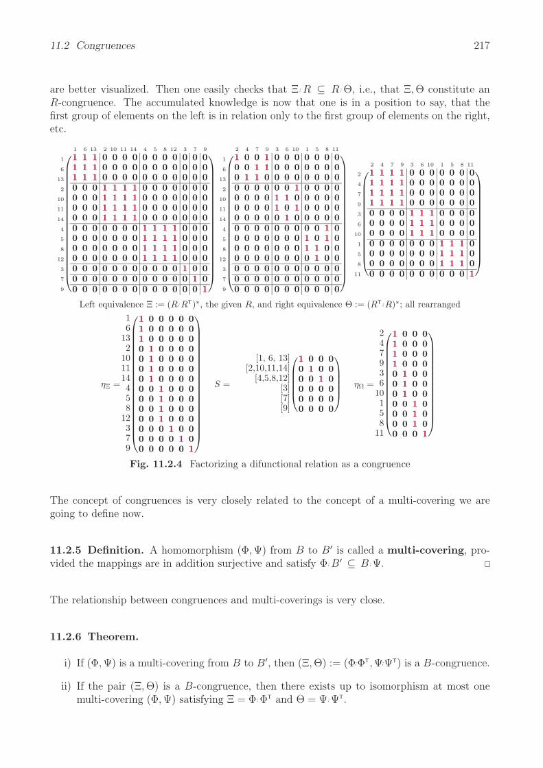
11.2 Congruences 217
are better visualized. Then one easily checks that Ξ; R ⊆ R; Θ, i.e., that Ξ, Θ constitute anR-congruence. The accumulated knowledge is now that one is in a position to say, that thefirst group of elements on the left is in relation only to the first group of elements on the right,etc.
1 6 13 2 10 11 14 4 5 8 12 3 7 9
1
6
13
2
10
11
14
4
5
8
12
3
7
9
⎛⎜⎜⎜⎜⎜⎜⎜⎜⎜⎜⎜⎜⎜⎜⎜⎜⎜⎜⎜⎝
1 1 1 0 0 0 0 0 0 0 0 0 0 01 1 1 0 0 0 0 0 0 0 0 0 0 01 1 1 0 0 0 0 0 0 0 0 0 0 00 0 0 1 1 1 1 0 0 0 0 0 0 00 0 0 1 1 1 1 0 0 0 0 0 0 00 0 0 1 1 1 1 0 0 0 0 0 0 00 0 0 1 1 1 1 0 0 0 0 0 0 00 0 0 0 0 0 0 1 1 1 1 0 0 00 0 0 0 0 0 0 1 1 1 1 0 0 00 0 0 0 0 0 0 1 1 1 1 0 0 00 0 0 0 0 0 0 1 1 1 1 0 0 00 0 0 0 0 0 0 0 0 0 0 1 0 00 0 0 0 0 0 0 0 0 0 0 0 1 00 0 0 0 0 0 0 0 0 0 0 0 0 1
⎞⎟⎟⎟⎟⎟⎟⎟⎟⎟⎟⎟⎟⎟⎟⎟⎟⎟⎟⎟⎠
2 4 7 9 3 6 10 1 5 8 11
1
6
13
2
10
11
14
4
5
8
12
3
7
9
⎛⎜⎜⎜⎜⎜⎜⎜⎜⎜⎜⎜⎜⎜⎜⎜⎜⎜⎜⎜⎝
1 0 0 1 0 0 0 0 0 0 00 0 1 1 0 0 0 0 0 0 00 1 1 0 0 0 0 0 0 0 00 0 0 0 0 0 1 0 0 0 00 0 0 0 1 1 0 0 0 0 00 0 0 0 1 0 1 0 0 0 00 0 0 0 0 1 0 0 0 0 00 0 0 0 0 0 0 0 0 1 00 0 0 0 0 0 0 1 0 1 00 0 0 0 0 0 0 1 1 0 00 0 0 0 0 0 0 0 1 0 00 0 0 0 0 0 0 0 0 0 00 0 0 0 0 0 0 0 0 0 00 0 0 0 0 0 0 0 0 0 0
⎞⎟⎟⎟⎟⎟⎟⎟⎟⎟⎟⎟⎟⎟⎟⎟⎟⎟⎟⎟⎠
2 4 7 9 3 6 10 1 5 8 11
2
4
7
9
3
6
10
1
5
8
11
⎛⎜⎜⎜⎜⎜⎜⎜⎜⎜⎜⎜⎜⎜⎝
1 1 1 1 0 0 0 0 0 0 01 1 1 1 0 0 0 0 0 0 01 1 1 1 0 0 0 0 0 0 01 1 1 1 0 0 0 0 0 0 00 0 0 0 1 1 1 0 0 0 00 0 0 0 1 1 1 0 0 0 00 0 0 0 1 1 1 0 0 0 00 0 0 0 0 0 0 1 1 1 00 0 0 0 0 0 0 1 1 1 00 0 0 0 0 0 0 1 1 1 00 0 0 0 0 0 0 0 0 0 1
⎞⎟⎟⎟⎟⎟⎟⎟⎟⎟⎟⎟⎟⎟⎠
Left equivalence Ξ := (R;RT)∗, the given R, and right equivalence Θ := (RT;R)∗; all rearranged
ηΞ =
16
132
101114458
12379
⎛⎜⎜⎜⎜⎜⎜⎜⎜⎜⎜⎜⎜⎜⎜⎜⎜⎜⎜⎜⎝
1 0 0 0 0 01 0 0 0 0 01 0 0 0 0 00 1 0 0 0 00 1 0 0 0 00 1 0 0 0 00 1 0 0 0 00 0 1 0 0 00 0 1 0 0 00 0 1 0 0 00 0 1 0 0 00 0 0 1 0 00 0 0 0 1 00 0 0 0 0 1
⎞⎟⎟⎟⎟⎟⎟⎟⎟⎟⎟⎟⎟⎟⎟⎟⎟⎟⎟⎟⎠
S =
[1, 6, 13][2,10,11,14]
[4,5,8,12][3][7][9]
⎛⎜⎜⎜⎜⎝
1 0 0 00 1 0 00 0 1 00 0 0 00 0 0 00 0 0 0
⎞⎟⎟⎟⎟⎠ ηΩ =
247936
10158
11
⎛⎜⎜⎜⎜⎜⎜⎜⎜⎜⎜⎜⎜⎜⎝
1 0 0 01 0 0 01 0 0 01 0 0 00 1 0 00 1 0 00 1 0 00 0 1 00 0 1 00 0 1 00 0 0 1
⎞⎟⎟⎟⎟⎟⎟⎟⎟⎟⎟⎟⎟⎟⎠
Fig. 11.2.4 Factorizing a difunctional relation as a congruence
The concept of congruences is very closely related to the concept of a multi-covering we aregoing to define now.
11.2.5 Definition. A homomorphism (Φ, Ψ) from B to B′ is called a multi-covering, pro-vided the mappings are in addition surjective and satisfy Φ; B′ ⊆ B ; Ψ.
The relationship between congruences and multi-coverings is very close.
11.2.6 Theorem.
i) If (Φ, Ψ) is a multi-covering from B to B′, then (Ξ, Θ) := (Φ;ΦT, Ψ;ΨT) is a B-congruence.
ii) If the pair (Ξ, Θ) is a B-congruence, then there exists up to isomorphism at most onemulti-covering (Φ, Ψ) satisfying Ξ = Φ; ΦT and Θ = Ψ; ΨT.

218 Chapter 11 Function Properties: An Advanced View
Proof : i) Ξ is certainly reflexive and transitive, as Φ is total and univalent. In the same way,Θ is reflexive and transitive. The relation Ξ = Φ;ΦT is symmetric by construction and so is Θ.Now we prove
Ξ; B = Φ; ΦT; B ⊆ Φ; B′; ΨT ⊆ B ; Ψ; ΨT = B ; Θapplying one after the other the definition of Ξ, one of the homomorphism definitions, the
multi-covering condition, and the definition of Θ.
ii) Let (Φi, Ψi) be a multi-covering from B to Bi, i = 1, 2. Then
Bi ⊆ ΦTi; Φi; Bi ⊆ ΦT
i; B ; Ψi ⊆ Bi, and therefore everywhere “=”,
applying surjectivity, the multi-covering property and one of the homomorphism conditions.
Now we show that (ξ, θ) := (ΦT1
; Φ2, ΨT1
; Ψ2) is a homomorphism from B1 onto B2 — which isthen of course also an isomorphism.
ξT; ξ = ΦT2; Φ1; ΦT
1; Φ2 = ΦT
2; Ξ; Φ2 = ΦT
2; Φ2; ΦT
2; Φ2 = ; =
B1; θ = ΦT1; B ; Ψ1; ΨT
1; Ψ2 = ΦT
1; B ; Θ; Ψ2 = ΦT
1; B ; Ψ2; ΨT
2; Ψ2 ⊆ ΦT
1; Φ2; B2; = ξ; B2
The multi-covering (Φ, Ψ) for some given congruences P, Q need not exist in the given relationalgebra. It may, however, be constructed by setting Φ, Ψ to be the quotient mappings accordingto the equivalences P, Q together with R′ := ΦT; R; Ψ.
A multi-covering is something in between relational and algebraic structures! An importantexample of a multicovering is an algebraic structure.
11.2.7 Proposition. A homomorphism between algebraic structures is necessarily a multi-covering.
Proof : Assume the homomorphism (Φ, Ψ) from the mapping B to the mapping B′, so thatB ; Φ ⊆ Ψ; B′. The relation Ψ; B′ is univalent, since Ψ and B′ are mappings. The domainsB ; Φ; = = Φ; B′ ; of B ; Φ and Ψ; B′ coincide, because all the relations are mappings and,therefore, are total. So we may use Prop. 5.1.2 and obtain B ; Φ = Ψ; B′.
The condition for homomorphy, B ; Φ ⊆ Ψ ; B′, holds for algebraic as well as for relationalstructures. The equation B ; Φ = Ψ; B′ applies to algebraic structures only.
There is another trivial standard example of a multi-covering. In an arbitrary relation it mayhappen that several rows and/or columns coincide. We are then accustomed to consider classesof rows, e.g. This is for economy of thinking, but also often for reasons of memory management.In the following proposition, we write down what holds in algebraic formulae.
11.2.8 Proposition. Consider a (possibly heterogeneous) relation R together with its
row equivalence Ξ := syq(RT, RT) and its
column equivalence Θ := syq(R, R)
according to Def. 5.4.3 as well as the corresponding natural projection mappings ηΞ, ηΘ, anddefine
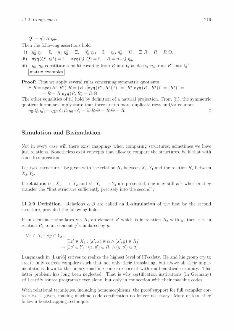
11.2 Congruences 219
Q := ηTΞ
; R; ηΘ.
Then the following assertions hold
i) ηTΞ
; ηΞ = , ηΞ; ηTΞ = Ξ, ηT
Θ; ηΘ = , ηΘ; ηT
Θ = Θ, Ξ; R = R = R; Θ.
ii) syq(QT, QT) = , syq(Q, Q) = , R = ηΞ; Q; ηTΘ
iii) ηΞ, ηΘ constitute a multi-covering from R into Q as do ηΘ, ηΞ from RT into QT.
matrix examples
Proof : First we apply several rules concerning symmetric quotientsΞ; R; = syq(RT, RT); R = (RT; [syq(RT, RT)]T)T = (RT;syq(RT, RT))T = (RT)T =
= R = R;syq(R, R) = R; ΘThe other equalities of (i) hold by definition of a natural projection. From (ii), the symmetricquotient formulae simply state that there are no more duplicate rows and/or columns.
ηΞ; Q; ηTΘ = ηΞ; ηT
Ξ; R; ηΘ; ηT
Θ = Ξ; R; Θ = R; Θ = R
Simulation and Bisimulation
Not in every case will there exist mappings when comparing structures; sometimes we havejust relations. Nonetheless exist concepts that allow to compare the structures, be it that withsome less precision.
Let two “structures” be given with the relation R1 between X1, Y1 and the relation R2 betweenX2, Y2.
If relations α : X1 −→ X2 and β : Y1 −→ Y2 are presented, one may still ask whether theytransfer the “first structure sufficiently precisely into the second”.
11.2.9 Definition. Relations α, β are called an L-simulation of the first by the secondstructure, provided the following holds:
If an element x simulates via R1 an element x′ which is in relation R2 with y, then x is inrelation R1 to an element y′ simulated by y.
∀x ∈ X1 : ∀y ∈ Y2 :[∃x′ ∈ X2 : (x′, x) ∈ α ∧ (x′, y) ∈ R2]
→ [∃y′ ∈ Y1 : (x, y′) ∈ R1 ∧ (y, y′) ∈ β]
Langmaack in [Lan95] strives to realize the highest level of IT-safety. He and his group try tocreate fully correct compilers such that not only their translating, but above all their imple-mentations down to the binary machine code are correct with mathematical certainty. Thislatter problem has long been neglected. That is why certification institutions (in Germany)still certify source programs never alone, but only in connection with their machine codes.
With relational techniques, including homomorphisms, the proof support for full compiler cor-rectness is given, making machine code certification no longer necessary. More or less, theyfollow a bootstrapping technique.

220 Chapter 11 Function Properties: An Advanced View
We have just finished studying homomorphisms. One basic aspect was that of being able to“roll” the conditions so as to have four different forms.
B B
Φ
Ψ
Fig. 11.2.5 Basic situation of a simulation
Given two relations B, B′, we called the pair Φ, Ψ of mappings a homomorphism from B toB′, if B ; Φ ⊆ Ψ; B′. Then we proved that in this context
B ; Φ ⊆ Ψ; B′ ⇐⇒ B ⊆ Ψ; B′; ΦT ⇐⇒ ΨT; B ⊆ B′; ΦT ⇐⇒ ΨT; B ; Φ ⊆ B′.
For several reasons, it turned out that one should also be interested in Φ, Ψ being arbitraryrelations, not necessarily mappings. One field of applications is that of data refinement andsimulation. There, one will often be confronted with non-total and non-univalent relations.B will in these cases be an abstract program, and B′ a concrete one. Φ, Ψ represent theinterrelationsship between these versions. Abstractly, we have, e.g., natural numbers, butconcretely only limited size numbers. So not every natural number has a counterpart. Whenstudying sets, one might for reasons of efficiency, work with bags, multisets, lists etc. Thensometimes there may be more than one representation for the abstract form.
Anyway, a considerable amount of literature has emerged dealing with these questions. Thefirst observation is, that the aforementioned “rolling” is no longer possible, since it heavilydepended on univalence and totality.
11.2.10 Definition. Given two relations Φ, Ψ, we call
• B a Φ, Ψ-U -simulation of B′ provided that ΨT; B ; Φ ⊆ B′
• B a Φ, Ψ-L-simulation of B′ provided that ΨT; B ⊆ B′; ΦT
• B a Φ, Ψ-UT-simulation of B′ provided that B ⊆ Ψ; B′; ΦT
• B a Φ, Ψ-LT-simulation of B′ provided that B ; Φ ⊆ Ψ; B′
Immediately, some technical questions arise. E.g., do these simulations compose in some wayas homomorphisms do? Does any (or do any two) of these simulations imply an other one?
11.2.11 Theorem. Let relations Φ, Ψ, Ξ be given. Then one has, under conditions on func-tionality or totality, that the simulations considered compose:

11.2 Congruences 221
i) B is a Φ, Ψ-U -simulation of B′
B′ is a Ξ, Φ-U -simulation of B′′
Ψ is total
=⇒ B is a Ξ, Ψ-U -simulation of B′′
ii) B is a Φ, Ψ-UT-simulation of B′
B′ is a Ξ, Φ-UT-simulation of B′′
Ψ is univalent
=⇒ B is a Ξ, Ψ-UT-simulation of B′′
iii) B is a Φ, Ψ-UT-simulation of B′
B′ is a Ξ, Φ-L-simulation of B′′
Ψ is univalent
=⇒ B is a Ξ, Ψ-L-simulation of B′′
iv) B is a Φ, Ψ-UT-simulation of B′
B′ is a Ξ, Φ-LT-simulation of B′′
Ψ is univalent
=⇒ B is a Ξ, Ψ-LT-simulation of B′′
Dies ist u.U. noch falsch und unvollstandig!!!!
Something ignored in test edition!

222 Chapter 11 Function Properties: An Advanced View

Part IV
Applications
223


225
So far we have concentrated on foundations. Now we switch to applications. A first areaof applications is graph theory, where several effects need relational or regular algebra for anadequate description. The area of modeling preferences with relations is relatively new. Well-known is only the fuzzy approach with matrices the coefficients of which stem from the realinterval [0, 1], which came closer and closer to relational algebra proper. Here a direct attemptis made. Also t-norms and De Morgan triples may be tackled in relational form. Then comesthe broad area of Galois mechanisms. This is long known but not often described in relationalform.
One of the application areas may not be seen as application in the first place. We use relationsalso to review parts of standard mathematics, the homomorphism and isomorphism theorems.Even additional results may be reported and deeper insights when using relations.

226
12 Relational Graph Theory
Many of the problems handled in applications are traditionally formulated in terms of graphs.This means that graphs will be drawn and pictorial reasoning takes place. On one hand, thisis nice and intuitive when executed with chalk on a blackboard. On the other hand there is aconsiderable gap from this point to treating the problem on a computer. Often ad hoc programsare written in which more time is spent for I/O handling than for precision of the algorithm.Graphs are well-suited to visualize a result, even with possibilities to generate the graph via agraph drawing program. What is nearly impossible is the input of a problem given by means ofa graph — when not using RelView’s graph input (see [BSW03], e.g.). In such cases usuallysome sort of a relational interpretation of the respective graph is generated and input in someway.
While this is often ad hoc, we have here already demonstrated how relations can be presentedand may now fully concentrate on handling the task proper. We start with a careful relation-based introduction of the typical five types of graphs. While it may seem complicated at thebeginning, we will enjoy benefits of this precision later.
12.1 Types of Graphs
Traditionally five types of graphs are distinguished, which are designed to model differentsituations appropriately:
• The 1-graph for simply modeling relations on a set.
• The directed graph for modeling relations on a set under the requirement that relation-ships between elements may be denoted directly, and that there may be several sourcesfor two elements to be related, i.e., there may exist more than one arrow from x to y andthe two shall be distinguishable.
• The hypergraph for modeling relations between two sets.
• The bipartitioned graph for forward and backward relations between two sets.
• The simple graph for modeling symmetric relations such as neighbourhood on a set.
Tests zeigen
Several aspects may be modeled in more than one type of a graph. Neglecting a single aspect,often one graph may be converted to another type. In other cases a graph has a counterpart
227

228 Chapter 12 Relational Graph Theory
with more information than the original one — which is of course only conceivable when therest is added in a schematic manner.
Something ignored in test edition!
12.2 Roots in a Graph
When reachability is studied in a graph, one will mainly use the 1-graph, the directed graph,or the bipartite graph. In all these types the reachability relation B on the vertex set V isdefined. It is then often interesting whether there exists a vertex in that graph from which allpoints may be reached. It makes, however, a difference if this is defined and named from thebeginning, or if it is determined only afterwards. Such a root may exist in a graph or may not,and it may be uniquely defined, or not.
If a really big graph is given simply as a square relation, it may be interesting to find outwhether it is in fact a rooted tree and if so, which is its root. There is an easy relation-algebraicmeans to do that. A tree is loop-free, i.e., its transitive closure is asymmetric. The transposedrelation BT is univalent and has precisely on terminal point. This root will be returned as aone element-list — or the empty list if it is not a tree.
12.2.1 Definition. Let a graph B be given together with a point a.
a root of B :⇐⇒ a; ⊆ B∗ ⇐⇒ ⊆ aT; B∗
⇐⇒ a ⊆ B∗;
⇐⇒ All points can be reached from a.
A pair W = (B, a) consisting of a graph B and a selected root a of B is called a rooted graph.
An injective and circuit-free rooted graph is called a rooted tree. Thus, a rooted graph is arooted tree, if B ; BT ⊆ and B+ ⊆ .
Exercises
5.2.2 Show that for a total graph injectivity may be expressed equivalently by the associatedrelation or the ingoing incidence, i.e.,
E ; ET ⊆ ⇐⇒ B ; BT ⊆ .
Solution 5.2.2 Aus E;ET ⊆ folgt sofort B;BT = AT;E;ET;A ⊆ AT;A ⊆ ; in umgekehrterRichtung gilt aufgrund der Totalitat E;ET ⊆ A;AT;E;ET;A;AT = A;B;BT;AT ⊆ A;AT, so daßmit Hilfe der 1-Grapheneigenschaft folgt E ; ET = A; AT ∩ E ; ET ⊆ .
5.2.3 Let A; B determine a directed graph. Prove that ∩ B = AT; (E ∩ A).
Solution 5.2.3 AT; (E ∩ A) ⊆ Anderung AT;E ∩ AT;A ⊆ B ∩ = AT;E ∩ ⊆ (AT ∩ ;ET);
(E ∩ A; ) ⊆ AT; (E ∩ A),

12.3 Reducible Relations 229
da AT; A ⊆ ⇐⇒ A; ⊆ A und A; ⊆ A ⇐⇒ AT; A ⊆ .
5.2.4 Let p and q be arcs of a graph. Show that
p; qT ⊆ A; AT ⇐⇒ AT; p = AT; q =/ .
Prove that for a total graph H := A; AT ∩ E ; ET is an equivalence relation.
Solution 5.2.4 Nach Satz 2.4.4 ist p; qT ⊆ A;AT aquivalent zu p ⊆ A;AT; q. Bei eindeutigemA folgt hieraus AT ; p ⊆ AT ; q und aus Symmetriegrunden sogar AT ; p = AT ; q. Beides kannnicht verschwinden, denn dann ware aufgrund der mittleren Inklusion p = . In umgekehrter
Richtung nutzen wir =/ aus; es folgt aus AT ; p = AT ; q sicherlich Anderungen A; AT ; p; qT =
A ; AT ; q ; qT ⊆ A ; AT. Zu zeigen ist dann nur noch, daß wegen AT ; p =/ und p = p ; gilt
= ;AT;p; = ;AT;p = A;AT;p ∪ A;AT;p =⇒ A; AT; p ⊆ A;AT;p und daher p; qT = ;p; qT ⊆A; AT; p; qT ⊆ A; AT; p; qT ⊆ A; AT; p; qT ⊆ A; AT.
Die Symmetrie von H ist klar, und fur totale Graphen auch die Reflexivitat. Zum Nachweisder Transitivitat schatzen wir ab (A;AT ∩ E;ET)2 ⊆ A;AT;A;AT ∩ E;ET;E;ET ⊆ A;AT ∩ E;ET.
12.3 Reducible Relations
Jetzt schon einfache Version als Sect. 5.6!!!
Who is about to solve a system of n linear equations with n variables is usually happy when thissystem turns out to have a special structure allowing the person to solve a system of m linearequations with m variables, m < n, first and then after resubstitution solve an n − m system.It is precisely this, what the concept of reducibility captures. When an arrow according to Aends in the set x, then it must already have started in x.
xx
Fig. 12.3.1 Schema of a reducible relation with dotted arrow convention
12.3.1 Definition. Let a homogeneous relation A be given. We call
A reducible :⇐⇒ There exists a vector =/ x =/ with A; x ⊆ x,
otherwise A is called irreducible.
A relation A on a set X is, thus, called reducible if there exists a relation =/ x =/ , whichis contracted by A, i.e. A; x ⊆ x. One may say that a relation is reducible, precisely when itcontracts (i.e. A; x ⊆ x) some non-trivial (i.e. =/ x =/ ) relation. Usually one is interestedin contracted vectors. Arrows of the graph according to A ending in the subset x will always

230 Chapter 12 Relational Graph Theory
start in x. It is easy to see that the reducing vectors x, in this case including the trivial onesx = and x = , form a lattice.
Using Schroder’s rule, a relation A contracts a set x precisely when its tranpose AT contracts xas well: A;x ⊆ x ⇐⇒ AT;x ⊆ x. Therefore, a relation is reducible precisely when its tranposeis.
The essence of the reducibility condition is much better visible after determining some permu-tation P that sends the 1 -entries of x to the end. Applying this simultaneously on rows and
columns we obtain the shape P ; A; P T =
(BC D
)as well as P ; x =
( )mentioned in the
introduction to this chapter.
The contraction condition can also be expressed as A ⊆ x; xT. If such a relation x does notexist, A is called irreducible. Irreducible means that precisely two vectors are contracted,namely x = and x = . As already discussed, a relation is irreducible precisely when itstranpose is. In particular, we have for an irreducible A that A; A∗ ⊆ A∗, so that A∗ = , asobviously A∗ =/ . Therefore, one can translate this into the language of graph theory:
A irreducible ⇐⇒ The graph of A is strongly connected.
An irreducible relation A is necessarily total. A certainly contracts A; as A;A; ⊆ A; . Fromirreducibility we obtain that A; = or A; = . The former would mean A = , so that Awould contract every relation x, and, thus, violate irreducibility. Therefore, only the latter ispossible, i.e., A is total.
For a reducible relation A and arbitrary k, also Ak is reducible as Ak ; x ⊆ Ak−1 ; x ⊆ . . . ⊆A;x ⊆ x. However, the following is an example of an irreducible relation A with A2 reducible.Therefore, the property of being irreducible is not multiplicative.
A =
⎛⎜⎝
0 0 0 10 0 0 10 0 0 11 1 1 0
⎞⎟⎠
⎛⎜⎝
1 1 1 01 1 1 01 1 1 00 0 0 1
⎞⎟⎠ = A2
Fig. 12.3.2 Irreducible relation with reducible square
Reducible Permutations
It is interesting to look for irreducibility of permutations P . We observe P ; x = x for x :=(P k ∩ ); and arbitrary k as — due to the doublesided mapping properties of P — obviouslyP ; x = P ; (P k ∩ ); = P ; (P k ∩ ); = (P ; P k ∩ P ); = (P k ∩ ); P ; = (P k ∩ ); = x. Fork = 0, e.g., this means x = and is rather trivial. Also cases with P k ∩ = resulting inx = are trivial.
⎛⎜⎜⎝
0 1 0 0 00 0 1 0 00 0 0 1 00 0 0 0 11 0 0 0 0
⎞⎟⎟⎠
⎛⎜⎜⎝
0 1 0 0 01 0 0 0 00 0 0 1 00 0 0 0 10 0 1 0 0
⎞⎟⎟⎠
Fig. 12.3.3 Irreducible and reducible permutation

12.3 Reducible Relations 231
The permutation P is reducible, namely reduced by x, when neither P k ∩ = nor P k ∩ = .In recalling permutations, every cycle of P of length c will lead to P c ∩ =/ . If k is the leastcommon multiple of all cycle lengths occurring in P , obviously P k = . If there is just one cycle— as for the cyclic successor relation for n > 1 — the permutation P is irreducible. Otherpermutations with more than one cycle are reducible.
12.3.2 Proposition. A finite =⇒ An ⊆ ( ∪ A)n−1 and ( ∪ A)n−1 = A∗.
Proof : It is trivial that Ai ⊆ A∗ for all i ≥ 0. By the pigeon hole principle always An ⊆( ∪ A)n−1 as otherwise n + 1 vertices would be needed to delimit a non-selfcrossing path oflength n while only n distinct vertices are available. (See Exercise 3.2.6 of [SS89, SS93])
Irreducible relations satisfy further important formulae; see, e.g., [BR96] 1.1.2.
12.3.3 Theorem. For any n × n-relation A
i) A irreducible ⇐⇒ ( ∪ A)n−1 = ⇐⇒ A; ( ∪ A)n−1 =ii) A irreducible =⇒ There exists an exponent k such that ⊆ Ak.
Proof : i) We start proving the first equivalence. By definition, A is irreducible, if we have forall vectors x =/ that A;x ⊆ x implies x = . Now, by the preceding proposition A;( ∪A)n−1 ⊆( ∪ A)n−1 so that indeed ( ∪ A)n−1 = .
For the other direction assume A to be reducible, so that =/ x =/ exists with A ; x ⊆ x.Then also Ak ; x ⊆ x for arbitrary k. This is a contradiction, as it would follow that also( ∪ A)n−1;x ⊆ x resulting in ;x ⊆ x and, in the case of boolean matrices, i.e., with Tarski’srule satisfied, in x = , a contradiction.
Now we prove the second equivalence. Using Prop. 12.3.2, ( ∪ A)n−1 ⊇ A;( ∪ A)n−1, so thatalso A; ( ∪ A)n−1 ⊇ A; A; ( ∪ A)n−1. Since A is irreducible, this leads to A; ( ∪ A)n−1 beingequal to or , from which only the latter is possible.
ii) Consider the irreducible n × n-relation A and its powers. According to (i), there exists forevery row number j a least power 1 ≤ pj ≤ n with position (j, j) ∈ Apj . For the least commonmultiple p of all these pj we have ⊆ Ap, and p is the smallest positive number with thisproperty.
For irreducible relations yet a further distinction can be made; see, e.g., [Var62] 2.5.
12.3.4 Definition. An irreducible relation A is called primitive if there exists some integerk ≥ 1 such that Ak = . If this is not the case, the irreducible relation may be called cyclicof order k, indicating that the (infinitely many) powers A, A2, A3 . . . reproduce cyclically andk is the greatest common divisor of all the occurring periods.
We observe first powers of primitive relations.

232 Chapter 12 Relational Graph Theory
⎛⎜⎜⎜⎜⎜⎜⎜⎜⎜⎜⎜⎜⎜⎜⎜⎜⎜⎝
0 1 1 0 0 0 0 0 0 0 0 0 00 0 0 0 1 1 0 1 0 1 0 0 00 0 0 0 0 1 0 0 0 0 0 0 00 0 0 0 0 0 1 0 0 0 1 0 10 1 0 0 1 1 0 0 0 0 0 0 01 0 0 0 0 0 0 0 0 0 0 0 01 0 0 0 0 0 0 0 0 0 0 0 00 0 0 0 1 0 0 0 0 0 0 1 00 0 0 1 0 1 0 0 1 0 0 1 00 0 0 1 0 0 1 0 1 0 0 0 00 0 0 0 0 0 0 0 0 1 0 0 00 1 0 0 0 0 0 0 0 0 0 0 00 0 0 1 0 0 0 0 1 1 0 0 0
⎞⎟⎟⎟⎟⎟⎟⎟⎟⎟⎟⎟⎟⎟⎟⎟⎟⎟⎠
⎛⎜⎜⎜⎜⎜⎜⎜⎜⎜⎜⎜⎜⎜⎜⎜⎜⎜⎝
0 0 0 0 1 1 0 1 0 1 0 0 01 1 0 1 1 1 1 0 1 0 0 1 01 0 0 0 0 0 0 0 0 0 0 0 01 0 0 1 0 0 0 0 1 1 0 0 01 1 0 0 1 1 0 1 0 1 0 0 00 1 1 0 0 0 0 0 0 0 0 0 00 1 1 0 0 0 0 0 0 0 0 0 00 1 0 0 1 1 0 0 0 0 0 0 01 1 0 1 0 1 1 0 1 0 1 1 11 0 0 1 0 1 1 0 1 0 1 1 10 0 0 1 0 0 1 0 1 0 0 0 00 0 0 0 1 1 0 1 0 1 0 0 00 0 0 1 0 1 1 0 1 0 1 1 1
⎞⎟⎟⎟⎟⎟⎟⎟⎟⎟⎟⎟⎟⎟⎟⎟⎟⎟⎠
⎛⎜⎜⎜⎜⎜⎜⎜⎜⎜⎜⎜⎜⎜⎜⎜⎜⎜⎝
1 1 0 1 1 1 1 0 1 0 0 1 01 1 1 1 1 1 1 1 1 1 1 1 10 1 1 0 0 0 0 0 0 0 0 0 00 1 1 1 0 1 1 0 1 0 1 1 11 1 1 1 1 1 1 1 1 1 0 1 00 0 0 0 1 1 0 1 0 1 0 0 00 0 0 0 1 1 0 1 0 1 0 0 01 1 0 0 1 1 0 1 0 1 0 0 01 1 1 1 1 1 1 1 1 1 1 1 11 1 1 1 0 1 1 0 1 1 1 1 11 0 0 1 0 1 1 0 1 0 1 1 11 1 0 1 1 1 1 0 1 0 0 1 01 1 0 1 0 1 1 0 1 1 1 1 1
⎞⎟⎟⎟⎟⎟⎟⎟⎟⎟⎟⎟⎟⎟⎟⎟⎟⎟⎠
⎛⎜⎜⎜⎜⎜⎜⎜⎜⎜⎜⎜⎜⎜⎜⎜⎜⎜⎝
1 1 1 1 1 1 1 1 1 1 1 1 11 1 1 1 1 1 1 1 1 1 1 1 10 0 0 0 1 1 0 1 0 1 0 0 01 1 0 1 1 1 1 1 1 1 1 1 11 1 1 1 1 1 1 1 1 1 1 1 11 1 0 1 1 1 1 0 1 0 0 1 01 1 0 1 1 1 1 0 1 0 0 1 01 1 1 1 1 1 1 1 1 1 0 1 01 1 1 1 1 1 1 1 1 1 1 1 11 1 1 1 1 1 1 1 1 1 1 1 11 1 1 1 0 1 1 0 1 1 1 1 11 1 1 1 1 1 1 1 1 1 1 1 11 1 1 1 1 1 1 1 1 1 1 1 1
⎞⎟⎟⎟⎟⎟⎟⎟⎟⎟⎟⎟⎟⎟⎟⎟⎟⎟⎠
⎛⎜⎜⎜⎜⎜⎜⎜⎜⎜⎜⎜⎜⎜⎜⎜⎜⎜⎝
1 1 1 1 1 1 1 1 1 1 1 1 11 1 1 1 1 1 1 1 1 1 1 1 11 1 0 1 1 1 1 0 1 0 0 1 01 1 1 1 1 1 1 1 1 1 1 1 11 1 1 1 1 1 1 1 1 1 1 1 11 1 1 1 1 1 1 1 1 1 1 1 11 1 1 1 1 1 1 1 1 1 1 1 11 1 1 1 1 1 1 1 1 1 1 1 11 1 1 1 1 1 1 1 1 1 1 1 11 1 1 1 1 1 1 1 1 1 1 1 11 1 1 1 1 1 1 1 1 1 1 1 11 1 1 1 1 1 1 1 1 1 1 1 11 1 1 1 1 1 1 1 1 1 1 1 1
⎞⎟⎟⎟⎟⎟⎟⎟⎟⎟⎟⎟⎟⎟⎟⎟⎟⎟⎠
⎛⎜⎜⎜⎜⎜⎜⎜⎜⎜⎜⎜⎜⎜⎜⎜⎜⎜⎝
1 1 1 1 1 1 1 1 1 1 1 1 11 1 1 1 1 1 1 1 1 1 1 1 11 1 1 1 1 1 1 1 1 1 1 1 11 1 1 1 1 1 1 1 1 1 1 1 11 1 1 1 1 1 1 1 1 1 1 1 11 1 1 1 1 1 1 1 1 1 1 1 11 1 1 1 1 1 1 1 1 1 1 1 11 1 1 1 1 1 1 1 1 1 1 1 11 1 1 1 1 1 1 1 1 1 1 1 11 1 1 1 1 1 1 1 1 1 1 1 11 1 1 1 1 1 1 1 1 1 1 1 11 1 1 1 1 1 1 1 1 1 1 1 11 1 1 1 1 1 1 1 1 1 1 1 1
⎞⎟⎟⎟⎟⎟⎟⎟⎟⎟⎟⎟⎟⎟⎟⎟⎟⎟⎠
Fig. 12.3.4 Powers of a primitive irreducible relation
12.3.5 Proposition. A relation R is primitive precisely when its powers Rk are irreduciblefor all k ≥ 1.
Proof : “=⇒”: Assume Rk ; x ⊆ x with x =/ and x =/ for some k ≥ 1. Then we have alsoRnk ; x ⊆ R(n−1)k ; x . . . ⊆ Rk ; x ⊆ x for all n ≥ 1. This contradicts primitivity of R as fromsome index on all powers of a primitive R will be .
“⇐=”: Assume R were not primitive, i.e. Rk =/ for all k. It is impossible for any Rk to havea column as this would directly show reducibility of Rk. It follows from finiteness that therewill exist identical powers Rl = Rk =/ with l > k, e.g. This results in Rl−k ; Rk = Rk. PowerRl−k, therefore, contracts all columns of Rk — and at least one column which is unequal .(See,e.g., [BR96] 1.8.2)
Now we observe how powers of a cyclic relation behave.
1 2 3 4 5 6 7 8 9123456789
⎛⎜⎜⎜⎜⎜⎜⎜⎜⎜⎝
0 0 1 1 0 0 0 0 00 0 0 0 0 1 0 0 10 0 0 0 0 0 0 1 00 0 0 0 1 0 0 0 01 0 0 0 0 0 1 0 01 0 0 0 0 0 0 0 00 1 0 0 0 0 0 0 00 0 0 0 0 0 1 0 01 0 0 0 0 0 0 0 0
⎞⎟⎟⎟⎟⎟⎟⎟⎟⎟⎠
original relation withsubdivided andrearranged version
5 6 8 9 1 7 2 3 4568917234
⎛⎜⎜⎜⎜⎜⎜⎜⎜⎜⎜⎝
0 0 0 0 1 1 0 0 00 0 0 0 1 0 0 0 00 0 0 0 0 1 0 0 00 0 0 0 1 0 0 0 00 0 0 0 0 0 0 1 10 0 0 0 0 0 1 0 00 1 0 1 0 0 0 0 00 0 1 0 0 0 0 0 01 0 0 0 0 0 0 0 0
⎞⎟⎟⎟⎟⎟⎟⎟⎟⎟⎟⎠
Fig. 12.3.5 A cyclic irreducible relation

12.4 Difunctionality and Irreducibility 233
⎛⎜⎜⎜⎜⎜⎜⎜⎜⎜⎝
0 0 1 1 0 0 0 0 00 0 0 0 0 1 0 0 10 0 0 0 0 0 0 1 00 0 0 0 1 0 0 0 01 0 0 0 0 0 1 0 01 0 0 0 0 0 0 0 00 1 0 0 0 0 0 0 00 0 0 0 0 0 1 0 01 0 0 0 0 0 0 0 0
⎞⎟⎟⎟⎟⎟⎟⎟⎟⎟⎠
⎛⎜⎜⎜⎜⎜⎜⎜⎜⎜⎝
0 0 0 0 1 0 0 1 01 0 0 0 0 0 0 0 00 0 0 0 0 0 1 0 01 0 0 0 0 0 1 0 00 1 1 1 0 0 0 0 00 0 1 1 0 0 0 0 00 0 0 0 0 1 0 0 10 1 0 0 0 0 0 0 00 0 1 1 0 0 0 0 0
⎞⎟⎟⎟⎟⎟⎟⎟⎟⎟⎠
⎛⎜⎜⎜⎜⎜⎜⎜⎜⎜⎝
1 0 0 0 0 0 1 0 00 0 1 1 0 0 0 0 00 1 0 0 0 0 0 0 00 1 1 1 0 0 0 0 00 0 0 0 1 1 0 1 10 0 0 0 1 0 0 1 01 0 0 0 0 0 0 0 00 0 0 0 0 1 0 0 10 0 0 0 1 0 0 1 0
⎞⎟⎟⎟⎟⎟⎟⎟⎟⎟⎠
⎛⎜⎜⎜⎜⎜⎜⎜⎜⎜⎝
0 1 1 1 0 0 0 0 00 0 0 0 1 0 0 1 00 0 0 0 0 1 0 0 10 0 0 0 1 1 0 1 11 0 0 0 0 0 1 0 01 0 0 0 0 0 1 0 00 0 1 1 0 0 0 0 01 0 0 0 0 0 0 0 01 0 0 0 0 0 1 0 0
⎞⎟⎟⎟⎟⎟⎟⎟⎟⎟⎠
⎛⎜⎜⎜⎜⎜⎜⎜⎜⎜⎝
0 0 0 0 1 1 0 1 11 0 0 0 0 0 1 0 01 0 0 0 0 0 0 0 01 0 0 0 0 0 1 0 00 1 1 1 0 0 0 0 00 1 1 1 0 0 0 0 00 0 0 0 1 0 0 1 00 0 1 1 0 0 0 0 00 1 1 1 0 0 0 0 0
⎞⎟⎟⎟⎟⎟⎟⎟⎟⎟⎠
⎛⎜⎜⎜⎜⎜⎜⎜⎜⎜⎝
1 0 0 0 0 0 1 0 00 1 1 1 0 0 0 0 00 0 1 1 0 0 0 0 00 1 1 1 0 0 0 0 00 0 0 0 1 1 0 1 10 0 0 0 1 1 0 1 11 0 0 0 0 0 1 0 00 0 0 0 1 0 0 1 00 0 0 0 1 1 0 1 1
⎞⎟⎟⎟⎟⎟⎟⎟⎟⎟⎠
⎛⎜⎜⎜⎜⎜⎜⎜⎜⎜⎝
0 1 1 1 0 0 0 0 00 0 0 0 1 1 0 1 10 0 0 0 1 0 0 1 00 0 0 0 1 1 0 1 11 0 0 0 0 0 1 0 01 0 0 0 0 0 1 0 00 1 1 1 0 0 0 0 01 0 0 0 0 0 1 0 01 0 0 0 0 0 1 0 0
⎞⎟⎟⎟⎟⎟⎟⎟⎟⎟⎠
⎛⎜⎜⎜⎜⎜⎜⎜⎜⎜⎝
0 0 0 0 1 1 0 1 11 0 0 0 0 0 1 0 01 0 0 0 0 0 1 0 01 0 0 0 0 0 1 0 00 1 1 1 0 0 0 0 00 1 1 1 0 0 0 0 00 0 0 0 1 1 0 1 10 1 1 1 0 0 0 0 00 1 1 1 0 0 0 0 0
⎞⎟⎟⎟⎟⎟⎟⎟⎟⎟⎠
Fig. 12.3.6 Powers of a cyclic relation
⎛⎜⎜⎜⎜⎜⎜⎜⎜⎜⎜⎝
0 0 0 0 1 1 0 0 00 0 0 0 1 0 0 0 00 0 0 0 0 1 0 0 00 0 0 0 1 0 0 0 00 0 0 0 0 0 0 1 10 0 0 0 0 0 1 0 00 1 0 1 0 0 0 0 00 0 1 0 0 0 0 0 01 0 0 0 0 0 0 0 0
⎞⎟⎟⎟⎟⎟⎟⎟⎟⎟⎟⎠
⎛⎜⎜⎜⎜⎜⎜⎜⎜⎜⎜⎝
0 0 0 0 0 0 1 1 10 0 0 0 0 0 0 1 10 0 0 0 0 0 1 0 00 0 0 0 0 0 0 1 11 0 1 0 0 0 0 0 00 1 0 1 0 0 0 0 00 0 0 0 1 0 0 0 00 0 0 0 0 1 0 0 00 0 0 0 1 1 0 0 0
⎞⎟⎟⎟⎟⎟⎟⎟⎟⎟⎟⎠
⎛⎜⎜⎜⎜⎜⎜⎜⎜⎜⎜⎝
1 1 1 1 0 0 0 0 01 0 1 0 0 0 0 0 00 1 0 1 0 0 0 0 01 0 1 0 0 0 0 0 00 0 0 0 1 1 0 0 00 0 0 0 1 0 0 0 00 0 0 0 0 0 0 1 10 0 0 0 0 0 1 0 00 0 0 0 0 0 1 1 1
⎞⎟⎟⎟⎟⎟⎟⎟⎟⎟⎟⎠
⎛⎜⎜⎜⎜⎜⎜⎜⎜⎜⎜⎝
0 0 0 0 1 1 0 0 00 0 0 0 1 1 0 0 00 0 0 0 1 0 0 0 00 0 0 0 1 1 0 0 00 0 0 0 0 0 1 1 10 0 0 0 0 0 0 1 11 0 1 0 0 0 0 0 00 1 0 1 0 0 0 0 01 1 1 1 0 0 0 0 0
⎞⎟⎟⎟⎟⎟⎟⎟⎟⎟⎟⎠
⎛⎜⎜⎜⎜⎜⎜⎜⎜⎜⎜⎝
0 0 0 0 0 0 1 1 10 0 0 0 0 0 1 1 10 0 0 0 0 0 0 1 10 0 0 0 0 0 1 1 11 1 1 1 0 0 0 0 01 0 1 0 0 0 0 0 00 0 0 0 1 1 0 0 00 0 0 0 1 0 0 0 00 0 0 0 1 1 0 0 0
⎞⎟⎟⎟⎟⎟⎟⎟⎟⎟⎟⎠
⎛⎜⎜⎜⎜⎜⎜⎜⎜⎜⎜⎝
1 1 1 1 0 0 0 0 01 1 1 1 0 0 0 0 01 0 1 0 0 0 0 0 01 1 1 1 0 0 0 0 00 0 0 0 1 1 0 0 00 0 0 0 1 1 0 0 00 0 0 0 0 0 1 1 10 0 0 0 0 0 0 1 10 0 0 0 0 0 1 1 1
⎞⎟⎟⎟⎟⎟⎟⎟⎟⎟⎟⎠
⎛⎜⎜⎜⎜⎜⎜⎜⎜⎜⎜⎝
0 0 0 0 1 1 0 0 00 0 0 0 1 1 0 0 00 0 0 0 1 1 0 0 00 0 0 0 1 1 0 0 00 0 0 0 0 0 1 1 10 0 0 0 0 0 1 1 11 1 1 1 0 0 0 0 01 0 1 0 0 0 0 0 01 1 1 1 0 0 0 0 0
⎞⎟⎟⎟⎟⎟⎟⎟⎟⎟⎟⎠
⎛⎜⎜⎜⎜⎜⎜⎜⎜⎜⎜⎝
0 0 0 0 0 0 1 1 10 0 0 0 0 0 1 1 10 0 0 0 0 0 1 1 10 0 0 0 0 0 1 1 11 1 1 1 0 0 0 0 01 1 1 1 0 0 0 0 00 0 0 0 1 1 0 0 00 0 0 0 1 1 0 0 00 0 0 0 1 1 0 0 0
⎞⎟⎟⎟⎟⎟⎟⎟⎟⎟⎟⎠
Fig. 12.3.7 Powers of a cyclic relation in nicely arranged form
More than one cycle =⇒ reducible
12.4 Difunctionality and Irreducibility
For an application of the transitive closure, we start with a rather arbitrary relation — orgraph.
Something ignored in test edition!
We now specialize our investigations concerning difunctional relations to homogeneous and,later, irreducible ones.

234 Chapter 12 Relational Graph Theory
12.4.1 Proposition. Let an arbitrary finite homogeneous relation R be given. Then inaddition to the constructs Ξ, Ξ′ of Prop. 9.4.2 also Θ := (Ξ ∪ Ξ′)∗, G := Θ; R, and G′ := R; Θmay be formed.
i) Θ is an equivalence.
ii) G; GT ⊆ Θ and G′T; G′ ⊆ Θ
iii) G as well as G′ are difunctional.
Proof : (i) is trivial. From the other statements, we prove the G-variants.(ii) G; GT = Θ; R; (Θ; R)T = Θ; R; RT; Θ ⊆ Θ; Ξ; Θ ⊆ Θ; Θ; Θ = Θ(iii) G; GT; G ⊆ Θ; G = Θ; Θ; R = Θ; R = G, using (ii).
It need not be that GT ; G ⊆ Θ; see the example R =
(0 0 00 1 11 0 0
)with G =
(0 0 01 1 11 1 1
). Nor need
the pair (Θ, Θ) be an R-congruence as this example shows, where also G =/ G′.
1 2 3 4 5 6 7 8 9 10 11 12 13
1
2
3
4
5
6
7
8
9
10
11
12
13
⎛⎜⎜⎜⎜⎜⎜⎜⎜⎜⎜⎜⎜⎜⎜⎜⎜⎜⎝
0 0 0 0 0 1 0 0 0 0 0 0 00 0 0 0 1 0 1 1 0 0 0 0 00 0 0 0 0 0 0 0 0 0 0 0 10 0 0 0 0 0 0 0 0 0 0 0 00 0 0 0 0 0 0 0 0 0 0 0 00 0 0 0 0 0 0 0 0 0 1 0 01 0 0 0 0 0 0 0 0 0 0 0 00 0 0 0 0 0 0 0 0 0 0 0 00 0 0 0 0 0 0 0 0 0 1 0 10 0 0 0 0 0 0 0 0 0 0 0 00 1 0 0 0 0 0 0 0 0 0 0 00 0 0 1 0 0 0 0 0 0 0 0 00 0 0 0 0 1 0 0 0 0 0 1 0
⎞⎟⎟⎟⎟⎟⎟⎟⎟⎟⎟⎟⎟⎟⎟⎟⎟⎟⎠
1 11 13 2 3 6 9 12 4 5 7 8 10
1
11
13
2
3
6
9
12
4
5
7
8
10
⎛⎜⎜⎜⎜⎜⎜⎜⎜⎜⎜⎜⎜⎜⎜⎜⎜⎜⎝
1 1 1 0 0 0 0 0 0 0 0 0 01 1 1 0 0 0 0 0 0 0 0 0 01 1 1 0 0 0 0 0 0 0 0 0 00 0 0 1 0 0 0 0 0 0 0 0 00 0 0 0 1 1 1 1 0 0 0 0 00 0 0 0 1 1 1 1 0 0 0 0 00 0 0 0 1 1 1 1 0 0 0 0 00 0 0 0 1 1 1 1 0 0 0 0 00 0 0 0 0 0 0 0 1 0 0 0 00 0 0 0 0 0 0 0 0 1 1 1 00 0 0 0 0 0 0 0 0 1 1 1 00 0 0 0 0 0 0 0 0 1 1 1 00 0 0 0 0 0 0 0 0 0 0 0 1
⎞⎟⎟⎟⎟⎟⎟⎟⎟⎟⎟⎟⎟⎟⎟⎟⎟⎟⎠
1 11 13 2 3 6 9 12 4 5 7 8 10
1
11
13
2
3
6
9
12
4
5
7
8
10
⎛⎜⎜⎜⎜⎜⎜⎜⎜⎜⎜⎜⎜⎜⎜⎜⎜⎜⎝
0 0 0 0 0 1 0 0 0 0 0 0 00 0 0 1 0 0 0 0 0 0 0 0 00 0 0 0 0 1 0 1 0 0 0 0 00 0 0 0 0 0 0 0 0 1 1 1 00 0 1 0 0 0 0 0 0 0 0 0 00 1 0 0 0 0 0 0 0 0 0 0 00 1 1 0 0 0 0 0 0 0 0 0 00 0 0 0 0 0 0 0 1 0 0 0 00 0 0 0 0 0 0 0 0 0 0 0 00 0 0 0 0 0 0 0 0 0 0 0 01 0 0 0 0 0 0 0 0 0 0 0 00 0 0 0 0 0 0 0 0 0 0 0 00 0 0 0 0 0 0 0 0 0 0 0 0
⎞⎟⎟⎟⎟⎟⎟⎟⎟⎟⎟⎟⎟⎟⎟⎟⎟⎟⎠
1 11 13 2 3 6 9 12 4 5 7 8 10
1
11
13
2
3
6
9
12
4
5
7
8
10
⎛⎜⎜⎜⎜⎜⎜⎜⎜⎜⎜⎜⎜⎜⎜⎜⎜⎜⎝
0 0 0 1 0 1 0 1 0 0 0 0 00 0 0 1 0 1 0 1 0 0 0 0 00 0 0 1 0 1 0 1 0 0 0 0 00 0 0 0 0 0 0 0 0 1 1 1 00 1 1 0 0 0 0 0 1 0 0 0 00 1 1 0 0 0 0 0 1 0 0 0 00 1 1 0 0 0 0 0 1 0 0 0 00 1 1 0 0 0 0 0 1 0 0 0 00 0 0 0 0 0 0 0 0 0 0 0 01 0 0 0 0 0 0 0 0 0 0 0 01 0 0 0 0 0 0 0 0 0 0 0 01 0 0 0 0 0 0 0 0 0 0 0 00 0 0 0 0 0 0 0 0 0 0 0 0
⎞⎟⎟⎟⎟⎟⎟⎟⎟⎟⎟⎟⎟⎟⎟⎟⎟⎟⎠
1 11 13 2 3 6 9 12 4 5 7 8 10
1
11
13
2
3
6
9
12
4
5
7
8
10
⎛⎜⎜⎜⎜⎜⎜⎜⎜⎜⎜⎜⎜⎜⎜⎜⎜⎜⎝
0 0 0 0 1 1 1 1 0 0 0 0 00 0 0 1 0 0 0 0 0 0 0 0 00 0 0 0 1 1 1 1 0 0 0 0 00 0 0 0 0 0 0 0 0 1 1 1 01 1 1 0 0 0 0 0 0 0 0 0 01 1 1 0 0 0 0 0 0 0 0 0 01 1 1 0 0 0 0 0 0 0 0 0 00 0 0 0 0 0 0 0 1 0 0 0 00 0 0 0 0 0 0 0 0 0 0 0 00 0 0 0 0 0 0 0 0 0 0 0 01 1 1 0 0 0 0 0 0 0 0 0 00 0 0 0 0 0 0 0 0 0 0 0 00 0 0 0 0 0 0 0 0 0 0 0 0
⎞⎟⎟⎟⎟⎟⎟⎟⎟⎟⎟⎟⎟⎟⎟⎟⎟⎟⎠
Fig. 12.4.8 A relation, its symmetrized difunctional closure, rearranged according to it, and G, G′
One easily observes, that the relation is not yet block-wisely injective, nor need it be block-wisely univalent. The blocks of G, G′ are not yet completely filled, but only filled row- orcolumnwise, respectively. So by applying the permutations simultaneously, we have lost someof the properties the relations enjoyed when permuting independently in the heterogeneouscase. In the next theorem, we define a bigger congruence where we get back what has just beenlost.
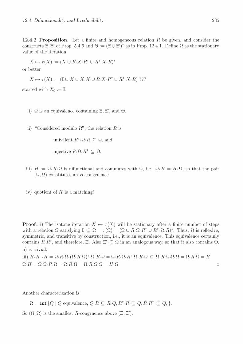
12.4 Difunctionality and Irreducibility 235
12.4.2 Proposition. Let a finite and homogeneous relation R be given, and consider theconstructs Ξ, Ξ′ of Prop. 5.4.6 and Θ := (Ξ∪Ξ′)∗ as in Prop. 12.4.1. Define Ω as the stationaryvalue of the iteration
X → τ(X) := (X ∪ R; X ; RT ∪ RT; X ; R)∗
or better
X → τ(X) := ( ∪ X ∪ X ; X ∪ R; X ; RT ∪ RT; X ; R) ???
started with X0 := .
i) Ω is an equivalence containing Ξ, Ξ′, and Θ.
ii) “Considered modulo Ω”, the relation R is
univalent RT; Ω; R ⊆ Ω, and
injective R; Ω; RT ⊆ Ω.
iii) H := Ω; R ; Ω is difunctional and commutes with Ω, i.e., Ω; H = H ; Ω, so that the pair(Ω, Ω) constitutes an H-congruence.
iv) quotient of H is a matching!
Proof : i) The isotone iteration X → τ(X) will be stationary after a finite number of stepswith a relation Ω satisfying ⊆ Ω = τ(Ω) = (Ω ∪ R; Ω; RT ∪ RT ; Ω; R)∗. Thus, Ω is reflexive,symmetric, and transitive by construction, i.e., it is an equivalence. This equivalence certainlycontains R;RT, and therefore, Ξ. Also Ξ′ ⊆ Ω in an analogous way, so that it also contains Θ.
ii) is trivial.
iii) H ; HT; H = Ω; R; Ω; (Ω; R; Ω)T; Ω; R; Ω = Ω; R; Ω; RT; Ω; R; Ω ⊆ Ω; R; Ω;;Ω; Ω = Ω; R; Ω = H
Ω; H = Ω; Ω; R; Ω = Ω; R; Ω = Ω; R; Ω; Ω = H ; Ω
Another characterization is
Ω = infQ | Q equivalence, Q; R ⊆ R; Q, RT; R ⊆ Q, R; RT ⊆ Q, .
So (Ω, Ω) is the smallest R-congruence above (Ξ, Ξ′).
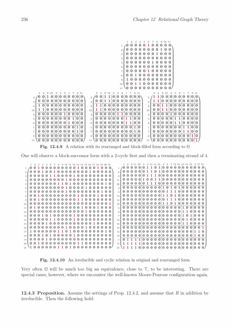
236 Chapter 12 Relational Graph Theory
1 2 3 4 5 6 7 8 9 10 11
1
2
3
4
5
6
7
8
9
10
11
⎛⎜⎜⎜⎜⎜⎜⎜⎜⎜⎜⎜⎜⎜⎝
0 0 0 0 0 1 0 0 0 0 00 0 0 0 0 0 0 0 1 0 00 0 0 0 0 0 0 1 0 0 00 0 0 0 0 0 0 0 0 0 00 0 0 0 0 0 1 0 0 0 00 0 0 0 0 0 0 0 0 0 00 0 0 0 0 1 0 0 0 0 00 0 1 0 0 0 0 0 0 0 01 0 0 0 0 0 0 0 0 0 00 0 1 1 0 0 0 0 0 0 00 0 0 0 0 0 0 0 0 0 0
⎞⎟⎟⎟⎟⎟⎟⎟⎟⎟⎟⎟⎟⎟⎠
3 4 8 10 2 5 9 1 7 6 11
3
4
8
10
2
5
9
1
7
6
11
⎛⎜⎜⎜⎜⎜⎜⎜⎜⎜⎜⎜⎜⎜⎜⎝
0 0 1 0 0 0 0 0 0 0 00 0 0 0 0 0 0 0 0 0 01 0 0 0 0 0 0 0 0 0 01 1 0 0 0 0 0 0 0 0 00 0 0 0 0 0 1 0 0 0 00 0 0 0 0 0 0 0 1 0 00 0 0 0 0 0 0 1 0 0 00 0 0 0 0 0 0 0 0 1 00 0 0 0 0 0 0 0 0 1 00 0 0 0 0 0 0 0 0 0 00 0 0 0 0 0 0 0 0 0 0
⎞⎟⎟⎟⎟⎟⎟⎟⎟⎟⎟⎟⎟⎟⎟⎠
3 4 8 10 2 5 9 1 7 6 11
3
4
8
10
2
5
9
1
7
6
11
⎛⎜⎜⎜⎜⎜⎜⎜⎜⎜⎜⎜⎜⎜⎜⎝
0 0 1 1 0 0 0 0 0 0 00 0 1 1 0 0 0 0 0 0 01 1 0 0 0 0 0 0 0 0 01 1 0 0 0 0 0 0 0 0 00 0 0 0 0 1 1 0 0 0 00 0 0 0 0 0 0 1 1 0 00 0 0 0 0 0 0 1 1 0 00 0 0 0 0 0 0 0 0 1 00 0 0 0 0 0 0 0 0 1 00 0 0 0 0 0 0 0 0 0 00 0 0 0 0 0 0 0 0 0 0
⎞⎟⎟⎟⎟⎟⎟⎟⎟⎟⎟⎟⎟⎟⎟⎠
3 4 8 10 2 5 9 1 7 6 11
3
4
8
10
2
5
9
1
7
6
11
⎛⎜⎜⎜⎜⎜⎜⎜⎜⎜⎜⎜⎜⎜⎜⎝
1 1 0 0 0 0 0 0 0 0 01 1 0 0 0 0 0 0 0 0 00 0 1 1 0 0 0 0 0 0 00 0 1 1 0 0 0 0 0 0 00 0 0 0 1 0 0 0 0 0 00 0 0 0 0 1 1 0 0 0 00 0 0 0 0 1 1 0 0 0 00 0 0 0 0 0 0 1 1 0 00 0 0 0 0 0 0 1 1 0 00 0 0 0 0 0 0 0 0 1 00 0 0 0 0 0 0 0 0 0 1
⎞⎟⎟⎟⎟⎟⎟⎟⎟⎟⎟⎟⎟⎟⎟⎠
Fig. 12.4.9 A relation with its rearranged and block-filled form according to Ω
One will observe a block-successor form with a 2-cycle first and then a terminating strand of 4.
1 2 3 4 5 6 7 8 9 10 11 12 13 14 15 16 17 18 19 20 21
1
2
3
4
5
6
7
8
9
10
11
12
13
14
15
16
17
18
19
20
21
⎛⎜⎜⎜⎜⎜⎜⎜⎜⎜⎜⎜⎜⎜⎜⎜⎜⎜⎜⎜⎜⎜⎜⎜⎜⎜⎜⎜⎜⎜⎜⎜⎝
0 0 1 0 0 0 0 0 0 0 0 0 1 0 0 0 0 1 0 0 00 0 0 1 0 0 1 0 0 0 0 0 0 0 0 1 0 0 0 0 00 0 0 0 0 1 1 0 0 0 0 1 0 0 0 0 0 0 0 0 00 0 0 0 0 0 0 0 0 1 0 0 0 0 0 0 0 0 0 0 00 0 0 0 0 0 0 1 1 0 1 0 0 0 0 0 0 0 0 1 00 0 0 0 0 0 0 0 0 1 0 0 0 0 1 0 0 0 0 0 00 0 0 0 0 0 0 0 0 1 0 0 0 0 0 0 0 0 1 0 00 0 1 0 0 0 0 0 0 0 0 0 1 0 0 0 0 1 0 0 00 0 1 0 0 0 0 0 0 0 0 0 1 1 0 0 0 0 0 0 00 0 0 0 0 0 0 0 0 0 0 0 0 0 0 0 0 0 0 0 10 1 0 0 0 0 0 0 0 0 0 0 0 1 0 0 0 1 0 0 00 0 0 0 0 0 0 0 0 0 0 0 0 0 1 0 0 0 0 0 00 0 0 1 0 1 0 0 0 0 0 1 0 0 0 0 0 0 0 0 00 0 0 0 0 1 1 0 0 0 0 1 0 0 0 0 0 0 0 0 00 0 0 0 1 0 0 0 0 0 0 0 0 0 0 0 1 0 0 0 00 0 0 0 0 0 0 0 0 1 0 0 0 0 1 0 0 0 0 0 01 0 0 0 0 0 0 1 1 0 1 0 0 0 0 0 0 0 0 1 00 0 0 1 0 1 0 0 0 0 0 1 0 0 0 0 0 0 0 0 00 0 0 0 1 0 0 0 0 0 0 0 0 0 0 0 0 0 0 0 00 0 1 0 0 0 0 0 0 0 0 0 1 1 0 0 0 0 0 0 01 0 0 0 0 0 0 1 1 0 1 0 0 0 0 0 0 0 0 0 0
⎞⎟⎟⎟⎟⎟⎟⎟⎟⎟⎟⎟⎟⎟⎟⎟⎟⎟⎟⎟⎟⎟⎟⎟⎟⎟⎟⎟⎟⎟⎟⎟⎠
1 8 9 11 20 2 3 13 14 18 4 6 7 12 16 10 15 19 5 17 21
1
8
9
11
20
2
3
13
14
18
4
6
7
12
16
10
15
19
5
17
21
⎛⎜⎜⎜⎜⎜⎜⎜⎜⎜⎜⎜⎜⎜⎜⎜⎜⎜⎜⎜⎜⎜⎜⎜⎜⎜⎜⎜⎜⎜⎜⎜⎜⎝
0 0 0 0 0 0 1 1 0 1 0 0 0 0 0 0 0 0 0 0 00 0 0 0 0 0 1 1 0 1 0 0 0 0 0 0 0 0 0 0 00 0 0 0 0 0 1 1 1 0 0 0 0 0 0 0 0 0 0 0 00 0 0 0 0 1 0 0 1 1 0 0 0 0 0 0 0 0 0 0 00 0 0 0 0 0 1 1 1 0 0 0 0 0 0 0 0 0 0 0 00 0 0 0 0 0 0 0 0 0 1 0 1 0 1 0 0 0 0 0 00 0 0 0 0 0 0 0 0 0 0 1 1 1 0 0 0 0 0 0 00 0 0 0 0 0 0 0 0 0 1 1 0 1 0 0 0 0 0 0 00 0 0 0 0 0 0 0 0 0 0 1 1 1 0 0 0 0 0 0 00 0 0 0 0 0 0 0 0 0 1 1 0 1 0 0 0 0 0 0 00 0 0 0 0 0 0 0 0 0 0 0 0 0 0 1 0 0 0 0 00 0 0 0 0 0 0 0 0 0 0 0 0 0 0 1 1 0 0 0 00 0 0 0 0 0 0 0 0 0 0 0 0 0 0 1 0 1 0 0 00 0 0 0 0 0 0 0 0 0 0 0 0 0 0 0 1 0 0 0 00 0 0 0 0 0 0 0 0 0 0 0 0 0 0 1 1 0 0 0 00 0 0 0 0 0 0 0 0 0 0 0 0 0 0 0 0 0 0 0 10 0 0 0 0 0 0 0 0 0 0 0 0 0 0 0 0 0 1 1 00 0 0 0 0 0 0 0 0 0 0 0 0 0 0 0 0 0 1 0 00 1 1 1 1 0 0 0 0 0 0 0 0 0 0 0 0 0 0 0 01 1 1 1 1 0 0 0 0 0 0 0 0 0 0 0 0 0 0 0 01 1 1 1 0 0 0 0 0 0 0 0 0 0 0 0 0 0 0 0 0
⎞⎟⎟⎟⎟⎟⎟⎟⎟⎟⎟⎟⎟⎟⎟⎟⎟⎟⎟⎟⎟⎟⎟⎟⎟⎟⎟⎟⎟⎟⎟⎟⎟⎠
Fig. 12.4.10 An irreducible and cyclic relation in original and rearranged form
Very often Ω will be much too big an equivalence, close to , to be interesting. There arespecial cases, however, where we encounter the well-known Moore-Penrose configuration again.
12.4.3 Proposition. Assume the settings of Prop. 12.4.2, and assume that R in addition beirreducible. Then the following hold:
12.5 Hammocks 237
i) H is irreducible.
ii) H is total and surjective making it a 1:1-correspondence of the classes according to Ω.
iii) HT acts as an “inverse” of H in as far as HT; H = Ω, as well as HT; H2 = H, etc.
iv) There exists a power k such that Rk = Ω and Rk+1 = H.
Proof : (i) Assumed H ; x ⊆ x to hold, then all the more R; x ⊆ x. If it were the case that=/ x =/ , we would obtain that R were reducible, i.e., a contradiction.
(ii) As proved on page shortly after Prop. 12.3.1, an irreducible relation R is total. This holdsfor Ω; R; Ω as well. Surjectivity is shown analogously.
(iii) We now easily deduce that HT; H = Ω, since with surjectivity and definition of Ω
HT; H = Ω; RT; Ω; Ω; R; Ω = Ω; RT; Ω; R; Ω = Ω; Ω; Ω = Ω.
Then also by induction
HT; Hk+1 = HT; H ; Hk = Ω; Hk = Hk.
(iv) We may prove a property we had already on page 230 for permutations proper, i.e., withall block-widths 1: The construct x := (Hk ∩ Ω); satisfies H ; x ⊆ x for all powers k.
H;x = H;(Hk ∩ Ω); = H ; (Hk ∩ Ω); = (Hk+1 ∩ H); = (Hk ∩ Ω); H ; = (Hk ∩ Ω); = x
To this end, we convince ourselves that HT; X = HT ; X proving the second equality, andH ; (Hk ∩ Ω) = Hk+1 ∩ H = (Hk ∩ Ω); H proving the others.
From totality of HT we have = HT; = HT; X ∪ HT; X so that always HT; X ⊆ HT; X. Theopposite inclusion is satisfied for arbitrary X with Ω; X = X, since H ; HT; X ⊆ Ω; X = X.
Furthermore, we have
H;(Hk ∩ Ω) ⊆ H;Hk ∩ H ⊆ (H ∩ H;HkT);(Hk ∩ HT;H) ⊆ H;(Hk ∩ HT;H) = H;(Hk ∩ Ω)
giving equality everywhere in between.
We have, after all, that R ; x ⊆ H ; x = x, regardless of how we choose k. However, R isirreducible, which means that no x unequal to , is allowed to occur. This restricts Hk to beeither Ω or to be disjoint therefrom.
12.5 Hammocks
While one usually knows what a hammock is like in everyday life, one may have problems toidentify them in graph theory or even in programming. Pictorially, however, it is the same,namely something that hangs fastened at two points.
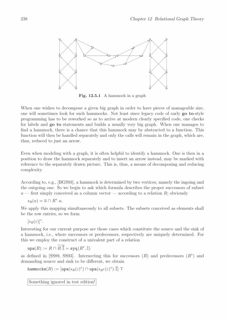
238 Chapter 12 Relational Graph Theory
Fig. 12.5.1 A hammock in a graph
When one wishes to decompose a given big graph in order to have pieces of manageable size,one will sometimes look for such hammocks. Not least since legacy code of early go to-styleprogramming has to be reworked so as to arrive at modern clearly specified code, one checksfor labels and go to statements and builds a usually very big graph. When one manages tofind a hammock, there is a chance that this hammock may by abstracted to a function. Thisfunction will then be handled separately and only the calls will remain in the graph, which are,thus, reduced to just an arrow.
Even when modeling with a graph, it is often helpful to identify a hammock. One is then in aposition to draw the hammock separately and to insert an arrow instead, may be marked withreference to the separately drawn picture. This is, thus, a means of decomposing and reducingcomplexity.
According to, e.g., [BGS93], a hammock is determined by two vertices, namely the ingoing andthe outgoing one. So we begin to ask which formula describes the proper successors of subsetu — first simply conceived as a column vector — according to a relation R; obviously
sR(u) = u ∩ RT; u.
We apply this mapping simultaneously to all subsets. The subsets conceived as elements shallbe the row entries, so we form
[sR(ε)]T.
Interesting for our current purpose are those cases which constitute the source and the sink ofa hammock, i.e., where successors or predecessors, respectively are uniquely determined. Forthis we employ the construct of a univalent part of a relation
upa(R) := R ∩ R; = syq(RT, )
as defined in [SS89, SS93]. Intersecting this for successors (R) and predecessors (RT) anddemanding source and sink to be different, we obtain
hammocks(R) := [upa(sR(ε)T) ∩ upa(sRT(ε)T); ];
Something ignored in test edition!
12.6 Feedback Vertex Sets 239
12.6 Feedback Vertex Sets
Let a directed graph be given and consider all its cycles. A feedback vertex set is defined to bea subset of the vertex set containing at least one vertex from every cycle.
Such feedback vertex sets have a diversity of important applications.Switching circuitssignal flow graphselectrical networksconstraint satisfaction problems
One is mainly interested in minimal such sets; they are, however, difficult to compute.
Something ignored in test edition!
12.7 Helly and Conformal Property
We use the mechanisms just developed for the Helly and the conformal property. We needsimply two category objects, as only one heterogeneous relation is under observation. First wepresent the formulae to be investigated.
conformalFormula rt =let vv = VarV "vv" (codRT rt)
vt = VV vvleft y = RF $ y :||--: y :<==: (Convs rt :***: rt)right y = VF $ NegaR rt :****: y :==/=: (UnivV $ domRT rt)
in VF $ QuantVectForm Univ vv [Implies (left vt) (right vt)]hellyTypeFormula rt = conformalFormula $ Convs rt
MATRRel bs12 bs13 $[[True ,True ,False,False,False,False,False],[False,True ,True ,False,False,False,False],[True ,False,True ,False,False,False,False],[True ,True ,True ,False,False,False,False],[False,False,True ,True ,False,False,False],[False,False,True ,False,False,False,True ],[False,False,True ,True ,True ,True ,True ],[False,False,False,False,False,True ,True ],[False,False,False,False,True ,True ,True ]]
MATRRel bs14 bs15[[False,False,False,True ,True ],[False,True ,True ,True ,False],[True ,True ,True ,False,False],[True ,False,True ,True ,False]]
Ablauf, Covering?
240 Chapter 12 Relational Graph Theory
Exercises
9.4.2 Prove that M ∩ M ; MT; M = M ∩ K; M for arbitrary M and K := ∩ M ; MT.
Solution 9.4.2 Es wird zerlegt M ; MT = K ∪ ( ∩ M ; MT), so daß
M ; MT; M = (K ∪ ( ∩ M ; MT)); M = K; M ∪ ( ∩ M ; MT); M = K; M ∩ ( ∩ M ; MT); M.
Letzteres ist uberflussig, wenn mit M geschnitten wird, weil ( ∩ M ; MT); M ⊇ ; M = M.
9.4.3 Prove that M ∩ [(M ∩ K; M)T;T] = M ∩ K; M if M is starlike.
Solution 9.4.3 “ ⊇ ” ist trivial. Wir beweisen ???
;(M ∩K; M)∩M ∩K;M ⊆(
∩ (M ∩K;M);(M ∩K; M)T);
((M ∩K; M)∩ ;(M ∩K;M)
)=
durch Ruckgriff auf den ersten Teil des Beweises von (9.4.3.iii).
9.4.4 Prove that M ; MT; M is univalent if the incidence M is reflexive, antisymmetric, andstarlike.
Solution 9.4.4 M ; MT; M ; ⊆ M ; MT; M ; (MT ∪ M), da M antisymmetrisch Wo geht ein
= M ; MT; M ; MT ∪ M ; MT; M ; M sternformig ?
⊆ M ; MT ∪ ; M ; M, da M reflexiv⊆ M ; ∪ M ; M, da M reflexiv⊆ M ; MT; M, da M reflexiv.
9.4.5 Prove the following identity for a reflexive, antisymmetric, and starlike incidence:
M ∩ M ; MT; M = M ∩ (M ∩ );
T
.
Solution 9.4.5 Fur “⊆ ” beweisen wir ; (MT ∩ ) ⊆ M ; MT; M, indem wir aufspalten ???= M ; MT ∪ M ; MT und zeigen
; (MT ∩ ) = ;
(MT ∩ (M ∪ M
T))
= ; (MT ∩ M), da M antisymmetrisch
= M ; MT; (MT ∩ M) ∪ M ; MT; (MT ∩ M)⊆ M ; MT; M ∪ M ; MT; MT
⊆ M ; MT; M ∪ M, da M ; M ⊆ M ; MT; M ; MT ⊆ M ; MT nach (9.4.3.ii)⊆ M ; MT; M, da M reflexiv.
“ ⊇ ” ergibt sich folgendermaßen:
M ; MT; M ∩ M ⊆ (M ∩ M ; MT; M); MT; M ∩ M, nach (9.4.3.i)
⊆((M ∩ M ; MT; M) ∩ M ; M
T; M
);
(MT; M ∩ (M ∩ M ; MT; M)T; M
)⊆ ; ( ∩ MT), weil M
T; MT ⊆ M
T; M ; MT ⊆ M
T ∪ MT; M ; MT, da M reflexiv.
Also gilt M ; MT; M ⊇ M ∩ ; ( ∩ MT).
9.4.6 Prove that M ∩ M ; MT; M = syq(M ; MT, M) ∩ M ; for every M .
Solution 9.4.6 ???
9.4.7 Prove that starlikeness of an incidence implies the Helly property, and disprove the con-verse of this implication by giving a counterexample.
Solution 9.4.7 ???
13 Modeling Preferences
Mankind has developed a multitude of concepts to reason about something that is better as oris more attractive than something else or similar to something else. Such concepts lead to anenormous bulk of formulae and interdependencies.
We start from the concept of an order and a strictorder, defined as transitive, antisymmetric,reflexive relation or as transitive and asymmetric, respectively. In earlier times it was not at allclear that orderings need not be linear orderings. But since the development of lattice theoryin the 1930s it became more and more evident that most of our reasoning with orderings wasalso possible when they failed to be linear ones. So people studied fuzziness mainly along linearorder of IR und began only later to generalize to the ordinal level: Numbers indicate the relativeposition of items, but no longer the magnitude of difference. Then they moved to the intervallevel: Numbers indicate the magnitude of difference between items, but there is no absolutezero point. Examples are attitude scales and opinion scales. We proceed even further andintroduce relational measures with values in a lattice. Measures traditionally provide a basisfor integration. Astonishingly, this holds true for these relational measures so that it becomespossible to introduce a concept of relational integration.
13.1 Modeling Preferences
Who is about to make severe decisions will usually base these on carefully selected basic infor-mation and clean lines of reasoning. It is in general not too difficult to apply just one criterionand to operate according to this criterion. If several criteria must be taken into consideration,one has also to consider the all too often occurring situation that these provide contradictoryinformation: “This car looks nicer, but it is much more expensive”. Social and economicalsciences have developed techniques to model what takes place when decisions are to be made inan environment with a multitude of diverging criteria. Preference is assumed to represent thedegree to which one alternative is preferred to another. Often it takes the form of expressingthat alternative A is considered being “not worse than” alternative B. Sometimes a linearranking of the set of alternatives is assumed, which we avoid.
So finding decisions became abstracted to a scientific task. We may observe two lines of develop-ment. The Anglo-Saxon countries, in particular, formulated utility theory, in which numericalvalues shall indicate the intensity of some preference. Mainly in continental Europe, on theother hand side, binary relations were used to model pairwise preference; see [FR94], e.g. Whilethe former idea allows to easily relate to statistics, the latter is based on evidence via directcomparison. In earlier years indeed, basic information was quite often statistical in natureand expressed in real numbers. Today we have more often fuzzy, vague, rough, etc. forms ofqualification.
241

242 Chapter 13 Modeling Preferences
13.2 Introductory Example
We first give an example of relational integration deciding for a car to be bought out of severaloffers. We intend to follow a set C of three criteria, namely color, price, and speed. Theyare, of course, not of equal importance for us; price will most certainly outweigh the color ofthe car, e.g. Nevertheless let the valuation with these criteria be given on an ordinal scale Lwith 5 linearly ordered values as indicated on the left side. (Here for simplicity, the orderingis linear, but it need not.) We name these values 1,2,3,4,5, but do not combine this with anyarithmetic; i.e., value 4 is not intended to mean two times as good as value 2. Rather they mightbe described with linguistic variables as bad, not totally bad, medium, outstanding, absolutelyoutstanding, purposefully these example qualifications have not been chosen equidistant.
colorpricespeed
(0 0 0 1 00 0 0 1 00 1 0 0 0
) 4 = lub[glb(4v(color), 4µc,p),glb(4v(price), 4µc,p),glb(2v(speed), 5µc,p,s)
] (13.1)
First we concentrate on the left side of Ex. 13.1. The task is to arrive at one overall valuationof the car out of these three. In a simple-minded approach, we might indeed conceive numbers1, 2, 3, 4, 5 ∈ IR and then evaluate in a classical way the average value as 1
3(4+4+2) = 3.3333 . . .,
which is a value not expressible in the given scale. When considering the second exampleEx. 13.2, we would arrive at the same average value although the switch from Ex. 13.1 toEx. 13.2 between price and speed would trigger most people to decide differently.
colorpricespeed
(0 0 0 1 00 1 0 0 00 0 0 1 0
) 3 = lub[glb(4v(color), 3µc,s),glb(2v(price), 5µc,p,s),glb(4v(speed), 3µc,s)
] (13.2)
With relational integration, we learn to make explicit which set of criteria to apply with whichweight. It is conceivable that criteria c1, c2 are given a low weight but the criteria set c1, c2 inconjunction a high one. This means that we introduce a relational measure assigning valuesin L to subsets of C.
µ =
colorpricecolor,pricespeedcolor,speedprice,speedcolor,price,speed
⎛⎜⎜⎜⎜⎜⎜⎜⎜⎝
1 0 0 0 01 0 0 0 00 0 1 0 00 0 0 1 00 1 0 0 00 0 1 0 00 0 1 0 00 0 0 0 1
⎞⎟⎟⎟⎟⎟⎟⎟⎟⎠
For gauging purposes we demand that the empty criteria set gets assigned the least value in Land the full criteria set the greatest. A point to stress is that we assume the criteria themselvesas well as the measuring of subsets of criteria as commensurable.
The relational measure µ should obviously be monotonic with respect to the ordering Ω on thepowerset of C and the ordering E on L. We do not demand continuity (additivity), however.The price alone is ranked of medium importance 3, higher than speed alone, while color alone isconsidered completely unimportant and ranks 1. However, color and price together are ranked4, i.e., higher than the supremum of ranks for color alone and for price alone, etc.

13.3 Relational Measures 243
As now the valuations according to the criteria as well as the valuation according to the relativemeasuring of the criteria are given, we may proceed as visualized on the right sides of (1) and(2). We run through the criteria and always look for two items: their corresponding valueand in addition for the value of that subset of criteria assigning equal or higher values. Thenwe determine the greatest lower bound for the two values. From the list thus obtained, theleast upper bound is taken. The two examples above show how by simple evaluation along thisconcept, one will arrive at the overall values 4 or 3, respectively. This results from the fact thatin the second case only such rather unimportant criteria as color and speed assign the highervalues.
The effect is counterrunning: Low values of criteria as for s in (1) are intersected with ratherhigh µ’s as many criteria give higher scores and µ is monotonic. Highest values of criteria asfor color or speed in (2) are intersected with the µ of a small or even one-element criteria set;i.e., with a rather small one. In total we find that here are two operations applied in a way wealready know from matrix multiplication: a “sum”operator, lub or ∨, following application a“product”operator, glb or ∧.
This example gave a first idea of how relational integration works and how it may be useful.Introducing a relational measure and using it for integration serves an important purpose:Concerns are now separated. One may design the criteria and the measure in a design phaseprior to polling. Only then shall the questionnaire be filled, or the voters be polled. Theprocedure of coming to an overall valuation is now just computation and should no longer leadto quarrels.
Something ignored in test edition!
13.3 Relational Measures
Assume the following basic setting with a set C of so-called criteria and a measuring lattice L.Depending on the application envisaged, the set C may also be interpreted as one of playersin a cooperative game, of attributes, of experts, or of voters in an opinion polling problem.This includes the setting with L the interval [0, 1] ⊆ IR or a linear orderings for measuring.We consider a (relational) measure generalizing the concept of a fuzzy measure (or capacite inFrench origin) assigning measures in L for subsets of C.
M E
m, X
P(C)
C
Ω
L
µε
Fig. 13.3.1 Basic situation for relational integration
The relation ε is the membership relation between C and its powerset P(C). The measuresenvisaged will be called µ, other relations as M . Valuations according to the criteria will be Xor m depending on the context.
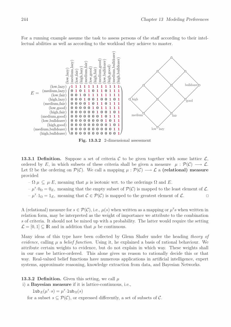
244 Chapter 13 Modeling Preferences
For a running example assume the task to assess persons of the staff according to their intel-lectual abilities as well as according to the workload they achieve to master.
E =
(low
,lazy
)(m
ediu
m,la
zy)
(low
,fair
)(h
igh,
lazy
)(m
ediu
m,fa
ir)
(low
,goo
d)(h
igh,
fair
)(m
ediu
m,g
ood)
(low
,bul
ldoz
er)
(hig
h,go
od)
(med
ium
,bul
ldoz
er)
(hig
h,bu
lldoz
er)
(low,lazy)(medium,lazy)
(low,fair)(high,lazy)
(medium,fair)(low,good)(high,fair)
(medium,good)(low,bulldozer)
(high,good)(medium,bulldozer)
(high,bulldozer)
⎛⎜⎜⎜⎜⎜⎜⎜⎜⎜⎜⎜⎜⎜⎜⎜⎝
1 1 1 1 1 1 1 1 1 1 1 10 1 0 1 1 0 1 1 0 1 1 10 0 1 0 1 1 1 1 1 1 1 10 0 0 1 0 0 1 0 0 1 0 10 0 0 0 1 0 1 1 0 1 1 10 0 0 0 0 1 0 1 1 1 1 10 0 0 0 0 0 1 0 0 1 0 10 0 0 0 0 0 0 1 0 1 1 10 0 0 0 0 0 0 0 1 0 1 10 0 0 0 0 0 0 0 0 1 0 10 0 0 0 0 0 0 0 0 0 1 10 0 0 0 0 0 0 0 0 0 0 1
⎞⎟⎟⎟⎟⎟⎟⎟⎟⎟⎟⎟⎟⎟⎟⎟⎠
high
medium
low lazy
fair
good
bulldozer
Fig. 13.3.2 2-dimensional assessment
13.3.1 Definition. Suppose a set of criteria C to be given together with some lattice L,ordered by E, in which subsets of these criteria shall be given a measure µ : P(C) −→ L.Let Ω be the ordering on P(C). We call a mapping µ : P(C) −→ L a (relational) measureprovided
– Ω;µ ⊆ µ;E, meaning that µ is isotonic wrt. to the orderings Ω and E.
– µT; 0Ω = 0E, meaning that the empty subset of P(C) is mapped to the least element of L.
– µT; 1Ω = 1E, meaning that C ∈ P(C) is mapped to the greatest element of L.
A (relational) measure for s ∈ P(C), i.e., µ(s) when written as a mapping or µT;s when written inrelation form, may be interpreted as the weight of importance we attribute to the combinations of criteria. It should not be mixed up with a probability. The latter would require the settingL = [0, 1] ⊆ IR and in addition that µ be continuous.
Many ideas of this type have been collected by Glenn Shafer under the heading theory ofevidence, calling µ a belief function. Using it, he explained a basis of rational behaviour. Weattribute certain weights to evidence, but do not explain in which way. These weights shallin our case be lattice-ordered. This alone gives us reason to rationally decide this or thatway. Real-valued belief functions have numerous applications in artificial intelligence, expertsystems, approximate reasoning, knowledge extraction from data, and Bayesian Networks.
13.3.2 Definition. Given this setting, we call µi) a Bayesian measure if it is lattice-continuous, i.e.,
lubE(µT; s) = µT;lubΩ(s)
for a subset s ⊆ P(C), or expressed differently, a set of subsets of C.

13.3 Relational Measures 245
ii) a simple support mapping focussed on U valued with v, if U is a non-empty subsetU ⊆ C and v ∈ L an element such that
µ(s) =
0E if s⊇/ Uv if C =/ s ⊇ U1E if C = s
In the real-valued environment, the condition for a Bayesian measure is: additive when non-overlapping. Lattice-continuity incorporates two concepts, namely additivity
µT; (s1 ∪ s2) = µT; s1 ∪L µT; s2
and sending 0Ω to 0E.
Concerning additivity, the example of Glenn Shafer [Sha76] is when one is wondering whethera Ming vase is a genuine one or a fake. We have to put the full amount of our belief on thedisjunction “genuine or fake” as one of the alternatives will certainly be the case. But theamount of trust we are willing to put on the alternatives may in both cases be very small as wehave only tiny hints for being genuine, but also very tiny hints for being a fake. In any case,we do not put trust on 0Ω = “at the same time genuine and fake”.
In the extreme case, we have complete ignorance expressed by the so-called vacuous beliefmapping
µ0(s) =
0E if C =/ s1E if C = s
µ0 =
(low
,lazy
)(m
ediu
m,la
zy)
(low
,fair
)(h
igh,
lazy
)(m
ediu
m,fa
ir)
(low
,goo
d)(h
igh,
fair
)(m
ediu
m,g
ood)
(low
,bul
ldoz
er)
(hig
h,go
od)
(med
ium
,bul
ldoz
er)
(hig
h,bu
lldoz
er)
AbeBob
Abe,BobCarl
Abe,CarlBob,Carl
Abe,Bob,CarlDon
Abe,DonBob,Don
Abe,Bob,DonCarl,Don
Abe,Carl,DonBob,Carl,Don
Abe,Bob,Carl,Don
⎛⎜⎜⎜⎜⎜⎜⎜⎜⎜⎜⎜⎜⎜⎜⎜⎜⎜⎜⎜⎜⎜⎜⎝
1 0 0 0 0 0 0 0 0 0 0 01 0 0 0 0 0 0 0 0 0 0 01 0 0 0 0 0 0 0 0 0 0 01 0 0 0 0 0 0 0 0 0 0 01 0 0 0 0 0 0 0 0 0 0 01 0 0 0 0 0 0 0 0 0 0 01 0 0 0 0 0 0 0 0 0 0 01 0 0 0 0 0 0 0 0 0 0 01 0 0 0 0 0 0 0 0 0 0 01 0 0 0 0 0 0 0 0 0 0 01 0 0 0 0 0 0 0 0 0 0 01 0 0 0 0 0 0 0 0 0 0 01 0 0 0 0 0 0 0 0 0 0 01 0 0 0 0 0 0 0 0 0 0 01 0 0 0 0 0 0 0 0 0 0 00 0 0 0 0 0 0 0 0 0 0 1
⎞⎟⎟⎟⎟⎟⎟⎟⎟⎟⎟⎟⎟⎟⎟⎟⎟⎟⎟⎟⎟⎟⎟⎠
Fig. 13.3.3 Vacuous belief mapping
With the idea of probability, we could not so easily cope with ignorance. Probability does notallow one to withhold belief from a proposition without according the withheld amount of beliefto the negation. When thinking on the Ming vase in terms of probability we would have toattribute p to genuine and 1 − p to fake.
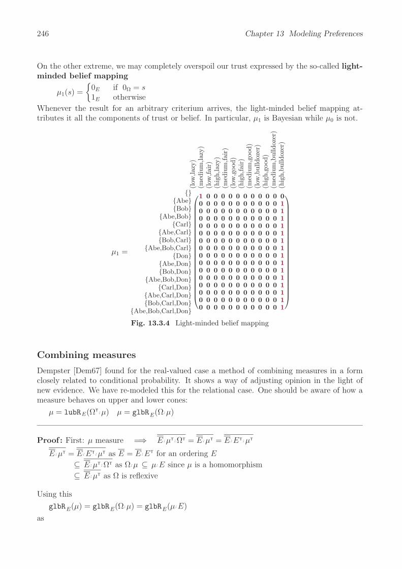
246 Chapter 13 Modeling Preferences
On the other extreme, we may completely overspoil our trust expressed by the so-called light-minded belief mapping
µ1(s) =
0E if 0Ω = s1E otherwise
Whenever the result for an arbitrary criterium arrives, the light-minded belief mapping at-tributes it all the components of trust or belief. In particular, µ1 is Bayesian while µ0 is not.
µ1 =
(low
,lazy
)(m
ediu
m,la
zy)
(low
,fair
)(h
igh,
lazy
)(m
ediu
m,fa
ir)
(low
,goo
d)(h
igh,
fair
)(m
ediu
m,g
ood)
(low
,bul
ldoz
er)
(hig
h,go
od)
(med
ium
,bul
ldoz
er)
(hig
h,bu
lldoz
er)
AbeBob
Abe,BobCarl
Abe,CarlBob,Carl
Abe,Bob,CarlDon
Abe,DonBob,Don
Abe,Bob,DonCarl,Don
Abe,Carl,DonBob,Carl,Don
Abe,Bob,Carl,Don
⎛⎜⎜⎜⎜⎜⎜⎜⎜⎜⎜⎜⎜⎜⎜⎜⎜⎜⎜⎜⎜⎜⎜⎝
1 0 0 0 0 0 0 0 0 0 0 00 0 0 0 0 0 0 0 0 0 0 10 0 0 0 0 0 0 0 0 0 0 10 0 0 0 0 0 0 0 0 0 0 10 0 0 0 0 0 0 0 0 0 0 10 0 0 0 0 0 0 0 0 0 0 10 0 0 0 0 0 0 0 0 0 0 10 0 0 0 0 0 0 0 0 0 0 10 0 0 0 0 0 0 0 0 0 0 10 0 0 0 0 0 0 0 0 0 0 10 0 0 0 0 0 0 0 0 0 0 10 0 0 0 0 0 0 0 0 0 0 10 0 0 0 0 0 0 0 0 0 0 10 0 0 0 0 0 0 0 0 0 0 10 0 0 0 0 0 0 0 0 0 0 10 0 0 0 0 0 0 0 0 0 0 1
⎞⎟⎟⎟⎟⎟⎟⎟⎟⎟⎟⎟⎟⎟⎟⎟⎟⎟⎟⎟⎟⎟⎟⎠
Fig. 13.3.4 Light-minded belief mapping
Combining measures
Dempster [Dem67] found for the real-valued case a method of combining measures in a formclosely related to conditional probability. It shows a way of adjusting opinion in the light ofnew evidence. We have re-modeled this for the relational case. One should be aware of how ameasure behaves on upper and lower cones:
µ = lubRE(ΩT; µ) µ = glbRE(Ω; µ)
Proof : First: µ measure =⇒ E ; µT; ΩT = E ; µT = E ; ET; µT
E ; µT = E ; ET; µT as E = E ; ET for an ordering E
⊆ E ; µT; ΩT as Ω; µ ⊆ µ; E since µ is a homomorphism
⊆ E ; µT as Ω is reflexive
Using this
glbRE(µ) = glbRE(Ω; µ) = glbRE(µ; E)
as
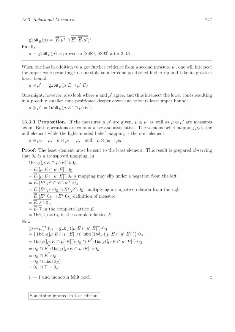
13.3 Relational Measures 247
glbRE(µ) = [E ; µT ∩ ET; E ; µT]T
Finally
µ = glbRE(µ) is proved in [SS89, SS93] after 3.3.7.
When one has in addition to µ got further evidence from a second measure µ′, one will intersectthe upper cones resulting in a possibly smaller cone positioned higher up and take its greatestlower bound:
µ ⊕ µ′ := glbRE(µ; E ∩ µ′; E)
One might, however, also look where µ and µ′ agree, and thus intersect the lower cones resultingin a possibly smaller cone positioned deeper down and take its least upper bound:
µ ⊗ µ′ := lubRE(µ; ET ∩ µ′; ET)
13.3.3 Proposition. If the measures µ, µ′ are given, µ ⊕ µ′ as well as µ ⊗ µ′ are measuresagain. Both operations are commutative and associative. The vacuous belief mapping µ0 is thenull element while the light-minded belief mapping is the unit element:
µ ⊕ µ0 = µ, µ ⊗ µ1 = µ, and µ ⊗ µ0 = µ0
Proof : The least element must be sent to the least element. This result is prepared observingthat 0Ω is a transposed mapping, in
lbdE([µ; E ∩ µ′; E]T); 0Ω
= E ; [µ; E ∩ µ′; E]T; 0Ω
= E ; [µ; E ∩ µ′; E]T; 0Ω a mapping may slip under a negation from the left
= E ; [ET; µT ∩ ET; µ′T]; 0Ω
= E ; [ET; µT; 0Ω ∩ ET; µ′T; 0Ω] multiplying an injective relation from the right
= E ; [ET; 0E ∩ ET; 0E] definition of measure
= E ; ET; 0E
= E ; in the complete lattice E= lbd( ) = 0E in the complete lattice E
Now
(µ ⊕ µ′)T; 0Ω = glbE([µ; E ∩ µ′; E]T); 0Ω
=(lbdE([µ; E ∩ µ′; E]T) ∩ ubd(lbdE([µ; E ∩ µ′; E]T)
); 0Ω
= lbdE([µ; E ∩ µ′; E]T); 0Ω ∩ ET;lbdE([µ; E ∩ µ′; E]T); 0Ω
= 0E ∩ ET;lbdE([µ; E ∩ µ′; E]T); 0Ω
= 0E ∩ ET; 0E
= 0E ∩ ubd(0E)= 0E ∩ = 0E
1 → 1 und monoton fehlt noch
Something ignored in test edition!
248 Chapter 13 Modeling Preferences
13.4 Relational Integration
Assume now that for all the criteria C a valuation has taken place resulting in a mappingX : C −→ L. The question is how to arrive at an overall valuation by rational means, for whichµ shall be the guideline.
13.4.1 Definition. Given a relational measure µ and a mapping X indicating the values givenby the criteria, we define the relational integral
(R)
∫X µ := lubRE( ; glbRE[X ∪ syq(X ; ET; XT, ε) ; µ])
The idea behind this integral is as follows: From the valuation of any criterion proceed to allhigher valuations and from these back to those criteria that assigned such higher values. WithX ; E; XT, the transition from all the criteria to the set of criteria are given. Now a symmetricquotient is needed in order to comprehend all these sets to elements of the powerset. (To thisend, the converse is needed.) Once the sets are elements of the powerset, the measure µ maybe applied. As already shown in the initial example, we have now the value of the respectivecriterion and in addition the valuation of the criteria set. From the two, we form the greatestlower bound. So in total, we have lower bounds for all the criteria. These are combined inone set multiplying the universal relation from the left side. Finally, the least upper bound istaken.
We are now in a position to understand why gauging µT;1Ω = 1E is necessary for µ, or “greatestelement is sent to greatest element”. Consider, e.g., the special case of an X with all criteriaassigning the same value. We certainly expect the relational integral to precisely deliver thisvalue regardless of the measure chosen. But this might not be the case if a measure shouldassign too small a value to the full set.

13.4 Relational Integration 249
µ =(l
ow,la
zy)
(med
ium
,lazy
)(l
ow,fa
ir)
(hig
h,la
zy)
(med
ium
,fair
)(l
ow,g
ood)
(hig
h,fa
ir)
(med
ium
,goo
d)(l
ow,b
ulld
ozer
)(h
igh,
good
)(m
ediu
m,b
ulld
ozer
)(h
igh,
bulld
ozer
)
AbeBob
Abe,BobCarl
Abe,CarlBob,Carl
Abe,Bob,CarlDon
Abe,DonBob,Don
Abe,Bob,DonCarl,Don
Abe,Carl,DonBob,Carl,Don
Abe,Bob,Carl,Don
⎛⎜⎜⎜⎜⎜⎜⎜⎜⎜⎜⎜⎜⎜⎜⎜⎜⎜⎜⎜⎜⎜⎜⎝
1 0 0 0 0 0 0 0 0 0 0 00 0 0 1 0 0 0 0 0 0 0 00 0 0 0 1 0 0 0 0 0 0 00 0 0 0 0 0 0 0 0 1 0 00 0 1 0 0 0 0 0 0 0 0 00 0 0 0 0 0 0 0 0 1 0 00 0 0 0 0 0 0 1 0 0 0 00 0 0 0 0 0 0 0 0 1 0 00 1 0 0 0 0 0 0 0 0 0 00 0 0 0 0 0 1 0 0 0 0 00 0 0 0 0 0 1 0 0 0 0 00 0 0 0 0 0 0 0 0 1 0 00 0 0 0 1 0 0 0 0 0 0 00 0 0 0 0 0 0 0 0 1 0 00 0 0 0 0 0 0 0 0 1 0 00 0 0 0 0 0 0 0 0 0 0 1
⎞⎟⎟⎟⎟⎟⎟⎟⎟⎟⎟⎟⎟⎟⎟⎟⎟⎟⎟⎟⎟⎟⎟⎠
X =
AbeBobCarlDon
⎛⎜⎝
0 0 0 1 0 0 0 0 0 0 0 00 0 0 0 0 0 1 0 0 0 0 00 1 0 0 0 0 0 0 0 0 0 00 0 0 0 1 0 0 0 0 0 0 0
⎞⎟⎠
(R)
∫X µ = (0 0 0 0 0 0 1 0 0 0 0 0)
Fig. 13.4.1 Measure, a valuation and the relational integral
As a running example, we provide the following highly non-continuous measure of Fig. 13.4.2.Here, e.g.,
µ(Abe) = (high, lazy), µ(Bob) = (medium, fair), with supremum (high, fair)
in contrast to µ(Abe, Bob) = (high, good).

250 Chapter 13 Modeling Preferences
µ =
(low
,lazy
)(m
ediu
m,la
zy)
(low
,fair
)(h
igh,
lazy
)(m
ediu
m,fa
ir)
(low
,goo
d)(h
igh,
fair
)(m
ediu
m,g
ood)
(low
,bul
ldoz
er)
(hig
h,go
od)
(med
ium
,bul
ldoz
er)
(hig
h,bu
lldoz
er)
AbeBob
Abe,BobCarl
Abe,CarlBob,Carl
Abe,Bob,CarlDon
Abe,DonBob,Don
Abe,Bob,DonCarl,Don
Abe,Carl,DonBob,Carl,Don
Abe,Bob,Carl,Don
⎛⎜⎜⎜⎜⎜⎜⎜⎜⎜⎜⎜⎜⎜⎜⎜⎜⎜⎜⎜⎜⎜⎜⎝
1 0 0 0 0 0 0 0 0 0 0 00 0 0 1 0 0 0 0 0 0 0 00 0 0 0 1 0 0 0 0 0 0 00 0 0 0 0 0 0 0 0 1 0 00 0 1 0 0 0 0 0 0 0 0 00 0 0 0 0 0 0 0 0 1 0 00 0 0 0 0 0 0 1 0 0 0 00 0 0 0 0 0 0 0 0 1 0 00 1 0 0 0 0 0 0 0 0 0 00 0 0 0 0 0 1 0 0 0 0 00 0 0 0 0 0 1 0 0 0 0 00 0 0 0 0 0 0 0 0 1 0 00 0 0 0 1 0 0 0 0 0 0 00 0 0 0 0 0 0 0 0 1 0 00 0 0 0 0 0 0 0 0 1 0 00 0 0 0 0 0 0 0 0 0 0 1
⎞⎟⎟⎟⎟⎟⎟⎟⎟⎟⎟⎟⎟⎟⎟⎟⎟⎟⎟⎟⎟⎟⎟⎠
Fig. 13.4.2 Example measure
Assume in addition valuations X1, X2
X1 =
(low
,lazy
)(m
ediu
m,la
zy)
(low
,fair
)(h
igh,
lazy
)(m
ediu
m,fa
ir)
(low
,goo
d)(h
igh,
fair
)(m
ediu
m,g
ood)
(low
,bul
ldoz
er)
(hig
h,go
od)
(med
ium
,bul
ldoz
er)
(hig
h,bu
lldoz
er)
AbeBobCarlDon
⎛⎜⎝
0 0 0 1 0 0 0 0 0 0 0 00 0 0 0 0 0 1 0 0 0 0 00 1 0 0 0 0 0 0 0 0 0 00 0 0 0 1 0 0 0 0 0 0 0
⎞⎟⎠ X2 =
(low
,lazy
)(m
ediu
m,la
zy)
(low
,fair
)(h
igh,
lazy
)(m
ediu
m,fa
ir)
(low
,goo
d)(h
igh,
fair
)(m
ediu
m,g
ood)
(low
,bul
ldoz
er)
(hig
h,go
od)
(med
ium
,bul
ldoz
er)
(hig
h,bu
lldoz
er)
AbeBobCarlDon
⎛⎜⎝
0 1 0 0 0 0 0 0 0 0 0 00 0 0 0 1 0 0 0 0 0 0 00 0 0 0 0 1 0 0 0 0 0 00 0 1 0 0 0 0 0 0 0 0 0
⎞⎟⎠
(R)
∫X1 µ = (0 0 0 0 0 0 1 0 0 0 0 0) (R)
∫X2 µ = (0 0 0 0 1 0 0 0 0 0 0 0)
Fig. 13.4.3 Two relational integrations
As already mentioned, we apply a sum operator lub after applying the product operator glb .When values are assigned with X, we look with E for those greater or equal, then with XT
for the criteria so valuated. Now comes a technically difficult step, namely proceeding to theunion of the resulting sets with the symmetric quotient syq and the membership relation ε.The µ-score of this set is then taken.
Obviously: glbRE(X) ≤ (R)
∫X µ ≤ lubR E(X)
13.5 Defining Relational Measures 251
These considerations originate from a free re-interpretation of the following concepts for workin [0, 1] ⊆ IR. The Sugeno integral operator is in the literature defined as
MS,µ(x1. . . . , xm) = (S)
∫x µ =
m∨i=1
[xi ∧ µ(Ai)]
and the Choquet integral operator as
MC,µ(x1, . . . , xm) = (C)
∫x µ =
m∑i=1
[(xi − xi−1) · µ(Ai)]
In both cases the elements of vector (x1, . . . , xm) have each time to be reordered such that0 = x0 ≤ x1 ≤ x2 ≤ · · · ≤ xm ≤ xm+1 = 1 and µ(Ai) = µ(Ci, . . . , Cm).
The concept of Choquet integral was first introduced for a real-valued context in [Cho53] andlater used by Michio Sugeno. This integral has nice properties for aggregation: It is continuous,non-decreasing, and stable under certain interval preserving transformations. Not least reducesit to the weighted arithmetic mean as soon as it becomes additive.
Something ignored in test edition!
13.5 Defining Relational Measures
Such measures may be given directly, which is, however, a costly task as a powerset is involvedall of whose elements need values. Therefore, they mainly originate in some other way.
Measures originating from direct valuation of criteria
Let a direct valuation of the criteria be given as any relation m between C and L. Althoughit is allowed to be contradictory and non-univalent, we provide for a way of defining a relationalmeasure based on it. This will happen via the following constructs
σ(m) := εT; m; E π(µ) := ε; µ; ET, (13.3)
which very obviously satisfy the Galois correspondence requirement
m ⊆ π(µ) ⇐⇒ µ ⊆ σ(m).
They satisfy σ(m;ET) = σ(m) and π(µ;E) = π(µ), so that in principle only lower, respectivelyupper, cones occur as arguments. Applying W ; E = W ; E ; ET, we get
σ(m); E = εT; m; E ; E = εT; m; E ; ET; E = εT; m; E = σ(m),
so that images of σ are always upper cones — and thus best described by their greatest lowerbound glbRE(σ(m)).
13.5.1 Proposition. Given any relation m : C → L, the construct
µm := µ0 ⊕ glbRE(σ(m))
forms a relational measure, the so-called possibility measure.

252 Chapter 13 Modeling Preferences
Addition of the vacuous belief mapping µ0 is again necessary for gauging purposes. In case mis a mapping, the situation becomes even nicer. From
π(σ(m; ET)) = π(σ(m)) = ε; εT; m; E ; ET
= m; E ; ET
as it can be shown that in general ε; εT; X = X for all X
= m; E ; ET
as m was assumed to be a mapping
= m; E ; ET
= m; ET
we see that this is an adjunction on cones. The lower cones m;ET in turn are 1 : 1 representedby their least upper bounds lubRE(m; E).
The following proposition exhibits that a Bayesian measure is a rather special case, namelymore or less directly determined as a possibility measure for a direct valuation via a mappingm. Fig. 7.1 shows an example. One may proceed from m to the measure according to Prop. 7.1or vice versa according to Prop. 7.2.
13.5.2 Proposition. Let µ be a Bayesian measure. Then mµ := lubRE(π(µ)) is that directvaluation for which µ = µmµ .
µB =
(low
,lazy
)(m
ediu
m,la
zy)
(low
,fair
)(h
igh,
lazy
)(m
ediu
m,fa
ir)
(low
,goo
d)(h
igh,
fair
)(m
ediu
m,g
ood)
(low
,bul
ldoz
er)
(hig
h,go
od)
(med
ium
,bul
ldoz
er)
(hig
h,bu
lldoz
er)
AbeBob
Abe,BobCarl
Abe,CarlBob,Carl
Abe,Bob,CarlDon
Abe,DonBob,Don
Abe,Bob,DonCarl,Don
Abe,Carl,DonBob,Carl,Don
Abe,Bob,Carl,Don
⎛⎜⎜⎜⎜⎜⎜⎜⎜⎜⎜⎜⎜⎜⎜⎜⎜⎜⎜⎜⎜⎜⎜⎝
1 0 0 0 0 0 0 0 0 0 0 00 0 0 0 1 0 0 0 0 0 0 00 0 0 0 0 0 1 0 0 0 0 00 0 0 0 0 0 1 0 0 0 0 00 0 1 0 0 0 0 0 0 0 0 00 0 0 0 1 0 0 0 0 0 0 00 0 0 0 0 0 1 0 0 0 0 00 0 0 0 0 0 1 0 0 0 0 00 0 0 0 0 1 0 0 0 0 0 00 0 0 0 0 0 0 1 0 0 0 00 0 0 0 0 0 0 0 0 1 0 00 0 0 0 0 0 0 0 0 1 0 00 0 0 0 0 1 0 0 0 0 0 00 0 0 0 0 0 0 1 0 0 0 00 0 0 0 0 0 0 0 0 1 0 00 0 0 0 0 0 0 0 0 0 0 1
⎞⎟⎟⎟⎟⎟⎟⎟⎟⎟⎟⎟⎟⎟⎟⎟⎟⎟⎟⎟⎟⎟⎟⎠
mµB=
AbeBobCarlDon
⎛⎜⎝
0 0 0 0 1 0 0 0 0 0 0 00 0 0 0 0 0 1 0 0 0 0 00 0 1 0 0 0 0 0 0 0 0 00 0 0 0 0 1 0 0 0 0 0 0
⎞⎟⎠
Fig. 13.5.1 Direct valuation with corresponding Bayesian measure
With this method just a few of the many relational measures will be found. By constructionthey are all continuous (or additive).

13.5 Defining Relational Measures 253
Measures originating from a body of evidence
We may also derive relational measures out of some relation between P(C) and L. Althoughit is allowed to be non-univalent, we provide for a way of defining two measures based on it —which may coincide.
13.5.3 Definition. Let our general setting be given.i) A body of evidence is an arbitrary relation M : P(C) −→ L, restricted by the requirementthat MT; 0Ω ⊆ 0E.ii) When the body of evidence M is in addition a mapping, we speak — following [Sha76] —of a basic probability assignment.
If I dare saying that occurrence of A ⊆ C deserves my trust to the amount M(A), thenA′ ⊆ A ⊆ C deserves at least this amount of trusting as it occurs whenever A occurs. Imight, however, not be willing to consider that A′′ ⊆ C with A ⊆ A′′ deserves to be trustedwith the same amount as there is a chance that it occurs not so often.
M :=
(low
,lazy
)(m
ediu
m,la
zy)
(low
,fair
)(h
igh,
lazy
)(m
ediu
m,fa
ir)
(low
,goo
d)(h
igh,
fair
)(m
ediu
m,g
ood)
(low
,bul
ldoz
er)
(hig
h,go
od)
(med
ium
,bul
ldoz
er)
(hig
h,bu
lldoz
er)
AbeBob
Abe,BobCarl
Abe,CarlBob,Carl
Abe,Bob,CarlDon
Abe,DonBob,Don
Abe,Bob,DonCarl,Don
Abe,Carl,DonBob,Carl,Don
Abe,Bob,Carl,Don
⎛⎜⎜⎜⎜⎜⎜⎜⎜⎜⎜⎜⎜⎜⎜⎜⎜⎜⎜⎜⎜⎜⎜⎝
0 0 0 0 0 0 0 0 0 0 0 00 0 0 0 0 0 0 0 0 0 0 00 0 1 0 0 0 0 0 0 0 0 00 0 0 0 0 0 0 0 0 0 0 00 0 0 0 0 0 0 0 0 0 0 00 0 0 0 0 0 0 0 0 0 0 00 0 0 0 0 0 0 0 0 0 0 00 0 0 0 0 0 0 0 0 0 0 00 0 0 0 0 0 0 0 0 0 0 00 0 0 0 0 0 0 0 0 0 0 00 0 0 0 0 0 0 0 0 0 0 00 0 0 0 1 0 0 0 0 0 0 00 0 0 0 0 0 0 0 0 0 0 00 0 0 0 0 0 0 0 1 0 0 00 0 0 0 0 0 0 0 0 0 0 00 0 0 0 0 0 0 0 0 0 0 0
⎞⎟⎟⎟⎟⎟⎟⎟⎟⎟⎟⎟⎟⎟⎟⎟⎟⎟⎟⎟⎟⎟⎟⎠
Fig. 13.5.2 A body of evidence
We should be aware that the basic probability assignment is meant to assign something to aset regardless of what is assigned to its proper subsets. The condition MT ; 0Ω ⊆ 0E expressesthat M either does not assign any belief to the empty set or assigns it just 0E.
Now a construction similar to that in (3) becomes possible, introducing
σ′(M) := ΩT; M ; E π′(µ) := Ω; µ; ET, (13.4)
which again satisfies the Galois correspondence requirement
M ⊆ π′(µ) ⇐⇒ µ ⊆ σ′(M).

254 Chapter 13 Modeling Preferences
Obviously σ′(M ; ET) = σ′(M) and π′(µ; E) = π′(µ), so that in principle only upper (E) andlower (ET), respectively, cones are set into relation. But again applying W ; E = W ; E ; ET, weget
σ′(M); E = ΩT; M ; E ; E = ΩT; M ; E ; ET; E = ΩT; M ; E = σ′(M),
so that images of σ′ are always upper cones — and thus best described by their greatest lowerbound glbRE(σ′(M)).
13.5.4 Proposition. Should some body of evidence M be given, there exist two relationalmeasures closely resembling M ,
i) the belief measure µbelief(M) := µ0 ⊕ lubRE(ΩT; M)
ii) the plausibility measure µplausibility(M) := µ0 ⊕ lubRE((Ω ∩ Ω; )T; Ω; M)
iii) In general, the belief measure assigns values not exceeding those of the plausibility mea-sure, i.e., µbelief(M) ⊆ µplausibility(M); ET.
(low
,lazy
)(m
ediu
m,la
zy)
(low
,fair
)(h
igh,
lazy
)(m
ediu
m,fa
ir)
(low
,goo
d)(h
igh,
fair
)(m
ediu
m,g
ood)
(low
,bul
ldoz
er)
(hig
h,go
od)
(med
ium
,bul
ldoz
er)
(hig
h,bu
lldoz
er)
AbeBob
Abe,BobCarl
Abe,CarlBob,Carl
Abe,Bob,CarlDon
Abe,DonBob,Don
Abe,Bob,DonCarl,Don
Abe,Carl,DonBob,Carl,Don
Abe,Bob,Carl,Don
⎛⎜⎜⎜⎜⎜⎜⎜⎜⎜⎜⎜⎜⎜⎜⎜⎜⎜⎜⎜⎜⎜⎜⎝
1 0 0 0 0 0 0 0 0 0 0 01 0 0 0 0 0 0 0 0 0 0 00 0 1 0 0 0 0 0 0 0 0 00 0 1 0 0 0 0 0 0 0 0 01 0 0 0 0 0 0 0 0 0 0 01 0 0 0 0 0 0 0 0 0 0 00 0 1 0 0 0 0 0 0 0 0 00 0 1 0 0 0 0 0 0 0 0 01 0 0 0 0 0 0 0 0 0 0 01 0 0 0 0 0 0 0 0 0 0 00 0 1 0 0 0 0 0 0 0 0 00 0 0 0 1 0 0 0 0 0 0 01 0 0 0 0 0 0 0 0 0 0 00 0 0 0 0 0 0 0 1 0 0 00 0 1 0 0 0 0 0 0 0 0 00 0 0 0 0 0 0 0 0 0 0 1
⎞⎟⎟⎟⎟⎟⎟⎟⎟⎟⎟⎟⎟⎟⎟⎟⎟⎟⎟⎟⎟⎟⎟⎠
(low
,lazy
)(m
ediu
m,la
zy)
(low
,fair
)(h
igh,
lazy
)(m
ediu
m,fa
ir)
(low
,goo
d)(h
igh,
fair
)(m
ediu
m,g
ood)
(low
,bul
ldoz
er)
(hig
h,go
od)
(med
ium
,bul
ldoz
er)
(hig
h,bu
lldoz
er)
⎛⎜⎜⎜⎜⎜⎜⎜⎜⎜⎜⎜⎜⎜⎜⎜⎜⎜⎜⎜⎜⎜⎜⎝
1 0 0 0 0 0 0 0 0 0 0 00 0 0 0 0 0 0 0 0 0 1 00 0 0 0 1 0 0 0 0 0 0 00 0 0 0 0 0 0 0 0 0 1 00 0 0 0 0 0 0 0 1 0 0 00 0 0 0 0 0 0 0 0 0 1 00 0 0 0 0 0 0 0 0 0 1 00 0 0 0 0 0 0 0 0 0 1 00 0 0 0 0 0 0 0 0 0 1 00 0 0 0 0 0 0 0 0 0 1 00 0 0 0 0 0 0 0 0 0 1 00 0 0 0 0 0 0 0 0 0 1 00 0 0 0 0 0 0 0 0 0 1 00 0 0 0 0 0 0 0 0 0 1 00 0 0 0 0 0 0 0 0 0 1 00 0 0 0 0 0 0 0 0 0 0 1
⎞⎟⎟⎟⎟⎟⎟⎟⎟⎟⎟⎟⎟⎟⎟⎟⎟⎟⎟⎟⎟⎟⎟⎠
µbelief(M) µplausibility(M)
Fig. 13.5.3 Belief measure and plausibility measure for M of Fig. 13.5.2
The belief measure adds information to the extent that all evidence of subsets with an evidenceattached is incorporated. Another idea is followed by the plausibility measure. One asks whichsets have a non-empty intersection with some set with an evidence attached and determinesthe least upper bound of all these.
The plausibility measure collects those pieces of evidence that do not indicate trust againstoccurrence of the event or non-void parts of it. The belief as well as the plausibility measuremore or less precisely determine their original body of evidence.

13.5 Defining Relational Measures 255
13.5.5 Proposition. Should the body of evidence be concentrated on singleton sets only, thebelief and the plausibility measure will coincide.
Proof : That M is concentrated on arguments which are singleton sets means that M = a; Mwith a the partial diagonal relation describing the atoms of the ordering Ω. For Ω and a onecan prove (Ω ∩ Ω; );a = a as the only other element less or equal to an atom, namely the leastone, has been cut out via Ω. Then
(Ω∩Ω; )T;Ω;M = (ΩT∩ ;ΩT);Ω;a;M M = a; M and transposing
= ΩT; (Ω ∩ Ω; ); a; M mask shifting= ΩT; a; M see above= ΩT; M again since M = a; M
One should compare this result with the former one assuming m to be a mapping puttingm := ε;M . One may also try to go in reverse direction, namely from a measure back to a bodyof evidence.
13.5.6 Definition. Let some measure µ be given and define strict subset containment C :=∩ Ω. We introduce two basic probability assignments, namely
i) Aµ := lubRE(CT; µ), its purely additive part,
ii) Jµ := µ1 ⊗ (µ ∩ lubRE(CT; µ)), its jump part.
As an example, the purely additive part Aµ of the µ of Fig. 13.4.1 would assign in line Abe,Bobthe value high,fair only as µ(Abe) = high,lazy and µ(Bob) = medium,fair. In excessto this, µ assigns high,good, and is, thus, not additive or Bayesian. We have for Aµ takenonly what could have been computed already by summing up the values attached to strictlysmaller subsets. In Jµ the excess of µ to Aµ is collected. In the procedure for Jµ all the valuesattached to atoms of the lattice will be saved as from an atom only one step down according toC is possible. The value for the least element is, however, the least element of L. Multiplicationwith µ1 serves the purpose that rows full of 0 ’s be converted to rows with the least element0E attached as a value.
Now some arithmetic on these parts is possible, not least providing the insight that a measuredecomposes into an additive part and a jump part.
13.5.7 Proposition. Given the present setting, we have
i) Aµ ⊕ Jµ = µ.
ii) µbelief(Jµ) = µ.
In the real-valued case, this result is not surprising at all as one may always decompose into apart continuous from the left and a jump part.
In view of these results it seems promising to investigate in which way also concepts suchas commonality, consonance, necessity measures, focal sets, and cores may be found in therelational approach. This seems particularly interesting as also the concepts of De Morgan
256 Chapter 13 Modeling Preferences
triples have been transferred to the componentfree relational side. We leave this to futureresearch.
Something ignored in test edition!
Something ignored in test edition!
13.6 Focal Sets
For the following we recall the concept of an atom a as a non-empty injective row-constantrelation, i.e., =/ a = a; and a; aT ⊆ .
13.6.1 Definition. Let a relational measure µ be given together with an atom s.i) The subset s ∈ P(C) is called a focal set if =/ MT
µ; s, or equivalently, if s ⊆ Mµ; .
ii) The core is the set of all focal sets, i.e., coreµ := Mµ;
The two equivalent formulations in (i) require detailed analysis as presented in Chapter 2.4 of[SS89, SS93].
Something ignored in test edition!
13.6.2 Proposition. A subset B satisfies µ(B) = 1E precisely whenlubRΩ(coreµ) ⊆ B ; ET.
Proof :
Shafer describes trust or belief attached to a set as acting like a mobile mass, which may movefrom point to point. Let us assume for the moment that we have a minus operation. Thenδ := Mµ−lubRE(CT;µ), i.e., the excess over that amount which results from additivity, measuresthe total portion of belief or the total mass of trust that is confined to A yet no part of whichis confined to any proper subset of A. So δ measures the probability mass that is confined toA, but can move freely to every point of A. The quantity
Q(A) := supEMµ(B) | B ⊇ Ameasures the total probability mass that can in this sense move freely to every point of A. ThisQ is called the commonality mapping. Obviously Q(1Ω) = 1E. There is also a cross relationbetween the relational measure and its commonality mapping. Commonality is antitonic, andnot a relational measure.
13.6.3 Proposition. Let µ be a relational measure and Q its commonality mapping. Thenfor all A

13.7 De Morgan Triples 257
µ(A) = supQ(B) | B ⊆ A or µ := lubRE(N ; ΩT; Q) and
Q(A) = supµ(B) | B ⊆ A. or Q := lubRE(ΩT; N ; µ)
Something ignored in test edition!
Consonance
13.6.4 Definition. Let some body of evidence M : P(C) −→ L be given.i) M will be called consonant provided that
Ω; M ∩ M ; ⊆ M ; E,i.e., M is monotonic for any two subsets carrying a value.
ii) A consonant belief measure is called a necessity measure.iii) A consonant plausibility measure is called a possibility measure.
13.6.5 Proposition. i) A belief measure is a necessity measure precisely whenµbelief(A ∩ B) = glbE(µbelief(A), µbelief(B))
ii) A plausibility measure is a possibility measure precisely whenµplausibility(A ∪ B) = lubE(µplausibility(A), µplausibility(B))
Proof :
Something ignored in test edition!
13.7 De Morgan Triples
The introduction of triangular norms in fuzzy sets has strongly influenced the fuzzy set com-munity and made it an accepted part of mathematics.
As long as the set C of criteria is comparatively small, it seems possible to work with P(C) and,thus, to take into consideration specific combinations of criteria. As the size of C increases so asto handle a voting-type or polling-type problem, one will soon handle voters on an equal basis— at least in democracies. This means that the measure applied must not attribute differentvalues to differently chosen n-element sets, e.g. That the values for an n-element set is differentfrom the value attached to an (n + 1)-element set, will probably be accepted.
As a result, the technique to define the measure will be based operations in L alone. In total:instead of a measure on P(C) we work with an operation on values of L.

258 Chapter 13 Modeling Preferences
Norms and Co-Norms
Researchers have often studied situations with fuzzy valuations in the interval [0, 1] and thenasked for methods of negation, conjunction, disjunction, and subjunction (implication). Whatthey found out in the fuzzy environment was finally the De Morgan triple, a combination ofthree, or even four, real-valued functions that resemble more or less what is known to holdunder the aforementioned concepts. We here introduce newly corresponding functions on therelational side that achieve the same. We start defining the basic situation for a De Morgantriple:
V
V2
π ρT S
E N
J
Fig. 13.7.1 Basic situation for a De Morgan triple
The set of fuzzy values is V with ordering E; it corresponds, thus, to the interval [0, 1] tradi-tionally used. With T , two values are combined to one in the sense of a conjunction, with Sas a disjunction. While N is intended to model negation, J shall be derived so as to resemblesubjunction (implication).
By now it is tradition to axiomatize what is intended as follows. If we transfer this to therelational side, we will have to give relational versions of this.
13.7.1 Definition (t-norm). Given a set L of values, lattice-ordered by E, one will ask for at-norm to work as a conjunction operator T and demand it to be
normalized T ( , x) = xcommutative T (x, y) = T (y, x)monotonic T (x, y) ≤ T (u, v) whenever ≤ x ≤ u ≤ , ≤ y ≤ v ≤associative T (x, T (y, z)) = T (T (x, y), z)
13.7.2 Definition (t-conorm). Given a set L of values, ordered by E, one will ask for at-conorm to work as a disjunction operator S and demand it to take
normalized S( , x) = xcommutative S(x, y) = S(y, x)monotone S(x, y) ≤ S(u, v) whenever ≤ x ≤ u ≤ , ≤ y ≤ v ≤associative S(x, S(y, z)) = S(S(x, y), z)
Commutativity formulated component-free:
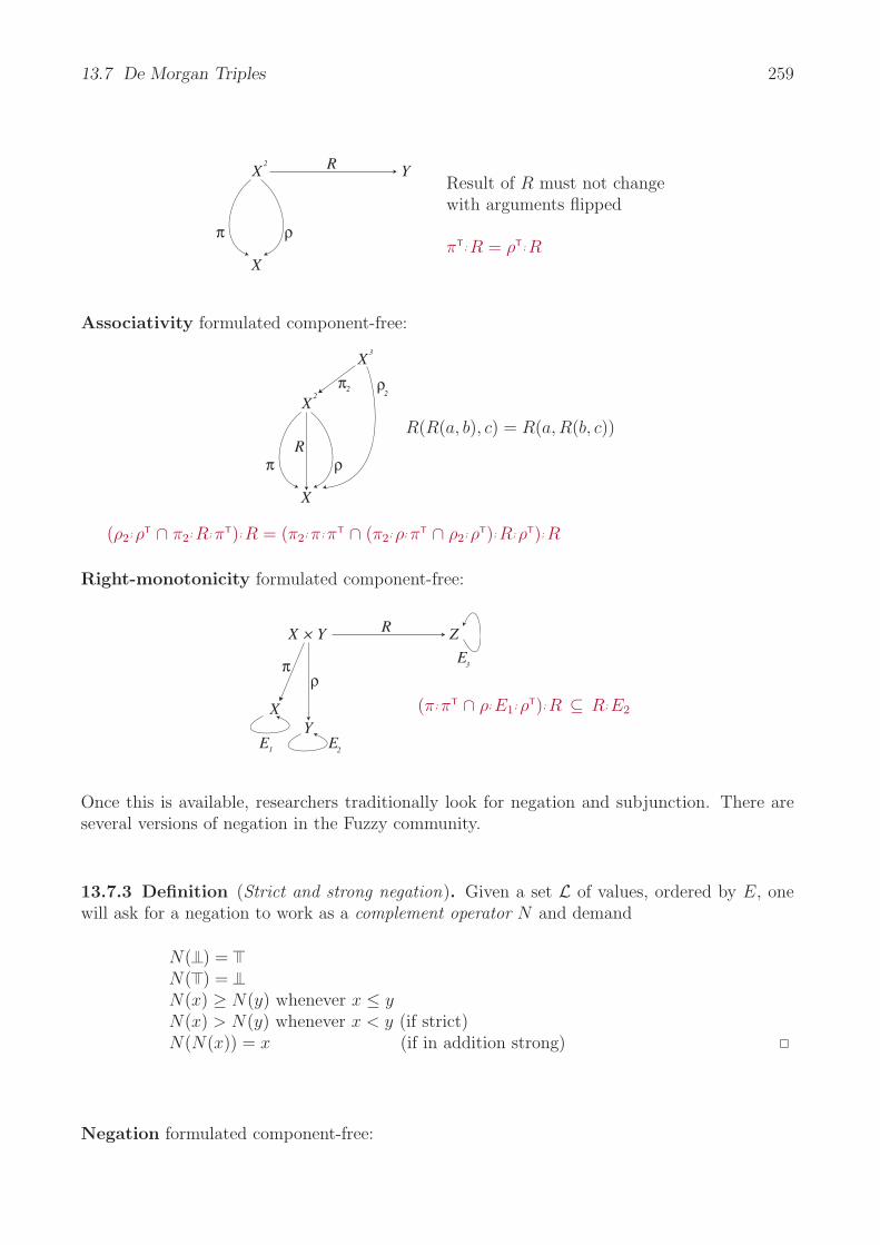
13.7 De Morgan Triples 259
X
X2
Y
π ρ
RResult of R must not changewith arguments flipped
πT; R = ρT; R
Associativity formulated component-free:
X
X2
π ρR
X3
π ρ22
R(R(a, b), c) = R(a, R(b, c))
(ρ2; ρT ∩ π2; R; πT); R = (π2; π; πT ∩ (π2; ρ; πT ∩ ρ2; ρT); R; ρT); R
Right-monotonicity formulated component-free:
X × Y ZR
3E
Y
πρ
E1
X
2E
(π; πT ∩ ρ; E1; ρT); R ⊆ R; E2
Once this is available, researchers traditionally look for negation and subjunction. There areseveral versions of negation in the Fuzzy community.
13.7.3 Definition (Strict and strong negation). Given a set L of values, ordered by E, onewill ask for a negation to work as a complement operator N and demand
N( ) =N( ) =N(x) ≥ N(y) whenever x ≤ yN(x) > N(y) whenever x < y (if strict)N(N(x)) = x (if in addition strong)
Negation formulated component-free:

260 Chapter 13 Modeling Preferences
N
E
N
E
e0; eT1 ∪ e1; eT
0 ⊆ N where e0 := lubE( ), e1 := glbE( )
E ; N ⊆ N ; ET
C ; N ⊆ N ; CT with C := ∩ E
N ; N =
Fig. 13.7.2 De Morgan negation
When we have something as disjunction and another operation as conjunction, it seems naturalto look for negation. Negation will not be available in every lattice L, but will show upsufficiently often in applications. We study the properties of a negation with the followingconsiderations.
When talking on conjunction, disjunction, negation, and subjunction, one has certain expecta-tions as to how these behave relatively to one another. We do not stay, however, in Booleanalgebra any longer, so things may have changed. Not least will we find ourselves in a situationwhere no longer just one subjunction operator is conceivable. What we can do, nonetheless, isto specify properties the subjunction operators should satisfy.
13.7.4 Definition. Given a set L of values, ordered by E, one will ask for an implicationoperator J and demand
J( , x) =J(x, ) =J( , ) =J(x, y) ≥ J(z, y) for all y whenever x ≤ zJ(x, y) ≤ J(x, t) for all x whenever y ≤ t
We will now show that two possibly different subjunctions may turn out to exist. The first isoften defined as JS,N(x, y) := S(N(x), y), which we now convert to a relational definition.
13.7.5 Proposition. Let E, S, N be given with the properties just postulated. Then, basedon a t-conorm S and a strong negation N , the relation
JS,N := (π; NπT ∩ κ; κT); S κ → ρ???
may be defined, which turns out to be a subjunction, the so-called S-implication.
Proof :
Instead of starting with a t-conorm, we could also have been starting with a t-norm. The resultmay then be a different one. The idea to follow is defining
JT (x, y) := supz | T (x, z) ≤ y

13.7 De Morgan Triples 261
13.7.6 Proposition. Let E, T be given with the properties just postulated. Then, based ona t-norm T , the relation
JR = lubRE (π; πT ∩ ρ; ET; T T); ρmay be defined, which turns out to be a subjunction, the so-called R-implication.
Proof :
With the first ρ, we proceed to y, E-below which we consider an arbitrary result T (u, z) of T .The latter is then traced back to its argument pair (u, z). Intersecting, the first component willstay x. Projecting with ρ, we pick out the result z.
(x,y)(π; πT
(x,?) ∩ ρy ; ET
T (u,z); T T
(u,z))(x,z); ρz
Therefore we consider
(π; πT ∩ ρ; ET; T T); ρ
to which we apply lub rowwise
JR = lubRE (π; πT ∩ ρ; ET; T T); ρ
In the next two examples, we try to give intuition for these propositions.
13.7.7 Example. Consider the attempt to define something as Boolean operations on thethree element qualifications low, medium,high. Based on E, one will try to define conjunctionand disjunction as well as negation. According to Prop. 13.7.5 and Prop. 13.7.6, we haveevaluated the relations so as to obtain the two forms of subjunction shown.
E =
low
med
ium
high
lowmedium
high
(1 1 10 1 10 0 1
)T =
low
med
ium
high
(low,low)(medium,low)(low,medium)
(high,low)(medium,medium)
(low,high)(high,medium)(medium,high)
(high,high)
⎛⎜⎜⎜⎜⎜⎜⎜⎜⎜⎝
1 0 01 0 01 0 01 0 00 1 01 0 00 1 00 1 00 0 1
⎞⎟⎟⎟⎟⎟⎟⎟⎟⎟⎠
S =
low
med
ium
high⎛
⎜⎜⎜⎜⎜⎜⎜⎜⎜⎝
1 0 00 1 00 1 00 0 10 1 00 0 10 0 10 0 10 0 1
⎞⎟⎟⎟⎟⎟⎟⎟⎟⎟⎠
N =
low
med
ium
high
lowmedium
high
(0 0 10 1 01 0 0
)JS,N =
low
med
ium
high
(low,low)(medium,low)(low,medium)
(high,low)(medium,medium)
(low,high)(high,medium)(medium,high)
(high,high)
⎛⎜⎜⎜⎜⎜⎜⎜⎜⎜⎝
0 0 10 1 00 0 11 0 00 1 00 0 10 1 00 0 10 0 1
⎞⎟⎟⎟⎟⎟⎟⎟⎟⎟⎠
JR =
low
med
ium
high⎛
⎜⎜⎜⎜⎜⎜⎜⎜⎜⎝
0 0 11 0 00 0 11 0 00 0 10 0 10 1 00 0 10 0 1
⎞⎟⎟⎟⎟⎟⎟⎟⎟⎟⎠
Fig. 13.7.3 Subjunctions JS,N , JR derived from E, T, S, N

262 Chapter 13 Modeling Preferences
13.7.8 Example. In the following example we use a very specific ordering, namely the pow-erset ordering of a 3-element set. It will turn out that in this case both subjunctions coincide.The powerset ordering is, of course, highly regular so that a special result could be expected.One will observe that here the result is given in a different style, namely in a table for thefunction instead of a voluminous relation.
E=
1 2 3 4 5 6 7 8
12345678
⎛⎜⎜⎜⎜⎜⎜⎜⎜⎝
1 1 1 1 1 1 1 10 1 0 1 0 1 0 10 0 1 1 0 0 1 10 0 0 1 0 0 0 10 0 0 0 1 1 1 10 0 0 0 0 1 0 10 0 0 0 0 0 1 10 0 0 0 0 0 0 1
⎞⎟⎟⎟⎟⎟⎟⎟⎟⎠
T =
[[1,1,1,1,1,1,1,1],[1,2,1,2,1,2,1,2],[1,1,3,3,1,1,3,3],[1,2,3,4,1,2,3,4],[1,1,1,1,5,5,5,5],[1,2,1,2,5,6,5,6],[1,1,3,3,5,5,7,7],[1,2,3,4,5,6,7,8]]
S =
[[1,2,3,4,5,6,7,8],[2,2,4,4,6,6,8,8],[3,4,3,4,7,8,7,8],[4,4,4,4,8,8,8,8],[5,6,7,8,5,6,7,8],[6,6,8,8,6,6,8,8],[7,8,7,8,7,8,7,8],[8,8,8,8,8,8,8,8]]
N =
1 2 3 4 5 6 7 8
12345678
⎛⎜⎜⎜⎜⎜⎜⎜⎜⎝
0 0 0 0 0 0 0 10 0 0 0 0 0 1 00 0 0 0 0 1 0 00 0 0 0 1 0 0 00 0 0 1 0 0 0 00 0 1 0 0 0 0 00 1 0 0 0 0 0 01 0 0 0 0 0 0 0
⎞⎟⎟⎟⎟⎟⎟⎟⎟⎠
JS,N =
[[8,8,8,8,8,8,8,8],[7,8,7,8,7,8,7,8],[6,6,8,8,6,6,8,8],[5,6,7,8,5,6,7,8],[4,4,4,4,8,8,8,8],[3,4,3,4,7,8,7,8],[2,2,4,4,6,6,8,8],[1,2,3,4,5,6,7,8]]
= JR
Fig. 13.7.4 Subjunctions JS,N = JR derived from E, T, S, N
Something ignored in test edition!
Something ignored in test edition!

14 Mathematical Applications
Homomorphism and isomorphism theorems shall now serve as an application area for relationalmethods. We review, thus, parts of traditional mathematics. When using relations, minorgeneralizations become possible. The traditional theorems aim at algebraic structures only;i.e., with mappings satisfying certain algebraic laws. When allowing relational structures, therewill not always exist images, nor need these be uniquely defined. In spite of this, much of thetheorems remains valid.
14.1 Homomorphism and Isomorphism Theorems
Now we study the homomorphism and isomorphism theorems1 traditionally offered in a courseon group theory or on universal algebra generalized from the relational point of view. In thecourses mentioned, R, S are often n-ary mappings such as addition and multiplication. We arehere more general allowing them to be relations, i.e., not necessarily mappings. The algebraiclaws they satisfy in the algebra are completely irrelevant. They are for a long time seen asgeneral concepts of universal algebra. We go here even further and identify them as relationalproperties which to study does not require the concept of an algebra. In addition it is shownhow the homomorphism and isomorphism theorems generalize to not necessarily algebraic andthus relational structures.
RS
Ξ
Ξ1
2
ϕ
ϕ
1
2
Θ
Θ
1
2
Fig. 14.1.1 Basic situation of the homomorphism theorem
14.1.1 Proposition (Homomorphism Theorem). Let a relation R be given with an R-congru-ence (Θ2, Θ1) as well as a relation S together with an S-congruence (Ξ2, Ξ1). Assume a multi-covering (ϕ2, ϕ1) from R to S such that at the same time Θi = ϕi ; Ξi ; ϕT
i for i = 1, 2; seeFig. 14.1.1.
1In George Gratzers Universal Algebra, e.g., reported as:Homomorphism Theorem: Let A and B be algebras, and ϕ : A → B a homomorphism of A onto B. Let
Θ denote the congruence relation induced by ϕ. Then we have that A/Θ is isomorphic to B.First Isomorphism Theorem: Let A be an algebra, B a subalgebra of A, and Θ a congruence relation of
A. Then ...Second Isomorphism Theorem: Let A be an algebra, let Θ,Φ be congruence relations of A, and assume
that Θ ⊆ Φ. Then A/Φ ≈ (A/Θ)/(Φ/Θ).
263

264 Chapter 14 Mathematical Applications
Introducing the natural projections ηi for Θi and δi for Ξi, Fig. 14.1.2, one has that ψi := ηTi;ϕi;δi,
i = 1, 2, establish an isomorphism from R′ := ηT2
; R; η1 to S ′ := δT2
; S ; δ1.
Proof : Equivalences (Θ2, Θ1) satisfy Θ2;R ⊆ R;Θ1 while (Ξ2, Ξ1) satisfy Ξ2;S ⊆ S;Ξ1. Further-more, we have that (ϕ2, ϕ1) are surjective mappings satisfying R;ϕ1 ⊆ ϕ2;S for homomorphismand R; ϕ1 ⊇ ϕ2; S for multi-covering.
RS
Ξ
Ξ1
2
ϕ
ϕ
1
2
Θ
Θ
1
2
η
η1
2δ
δ1
2 SR
ψ
ψ1
2
Fig. 14.1.2 Natural projections added to Fig. 14.1.1
The ψi are bijective mappings, which we prove omitting indices:
ψT; ψ = (ηT; ϕ; δ)T; ηT; ϕ; δ by definition= δT; ϕT; η; ηT; ϕ; δ executing transposition= δT; ϕT; Θ; ϕ; δ natural projection η= δT; ϕT; ϕ; Ξ; δ multi-covering= δT; Ξ; δ as ϕ is surjective and univalent= δT; δ; δT; δ = ; = natural projection δ
and
ψ; ψT = ηT; ϕ; δ; (ηT; ϕ; δ)T by definition= ηT; ϕ; δ; δT; ϕT; η transposing= ηT; ϕ; Ξ; ϕT; η natural projection δ= ηT; Θ; η property of ϕ wrt. Θ, Ξ= ηT; η; ηT; η = ; = natural projection η
Proof of the isomorphism property:
R′; ψ1 = ηT2
; R; η1; ηT1
; ϕ1; δ1 by definition= ηT
2; R; Θ1; ϕ1; δ1 natural projection η1
= ηT2
; R; ϕ1; Ξ1; ϕT1; ϕ1; δ1 property of ϕ1 wrt. Θ1, Ξ1
= ηT2
; R; ϕ1; Ξ1; δ1 as the multicovering ϕ1 is surjective and univalent= ηT
2; ϕ2; S ; Ξ1; δ1 multi-covering
= ηT2
; ϕ2; Ξ2; S ; Ξ1; δ1 S ; Ξ1 ⊆ Ξ2; S ; Ξ1 ⊆ S ; Ξ1; Ξ1 = S ; Ξ1
= ηT2
; ϕ2; δ2; δT2
; S ; δ1; δT1
; δ1 natural projections= ηT
2; ϕ2; δ2; S ′; δT
1; δ1 definition of S ′
= ηT2
; ϕ2; δ2; S ′ as δ1 is surjective and univalent= ψ2; S ′ definition of ψ2
According to Lemma 11.1.6, this suffices for an isomorphism.
One should bear in mind that this proposition was in several respects slightly more generalthan the classical homomorphism theorem: R, S need not be mappings, nor need they be

14.1 Homomorphism and Isomorphism Theorems 265
homogeneous relations, Ξ was not confined to be the identity congruence, and not least doesrelation algebra admit non-standard models.
14.1.2 Proposition (First Isomorphism Theorem). Let a homogeneous relation R on X begiven and consider it in connection with an equivalence Ξ and a subset U . Assume that U iscontracted by R and that Ξ is an R-congruence:
RT; U ⊆ U and Ξ; R ⊆ R; Ξ.
Now extrude both, U and its Ξ-saturation Ξ; U , so as to obtain natural injections
ι : Y −→ X and λ : Z −→ X,
universally characterized by
ιT; ι = X ∩ U ; , ι; ιT = Y ,λT; λ = X ∩ Ξ; U ; , λ; λT = Z .
On Y and Z, we consider the derived equivalences ΞY := ι;Ξ;ιT and ΞZ := λ;Ξ;λT and in additiontheir natural projections η : Y −→ YΞ and δ : Z −→ ZΞ. In a standard way, restrictions of Rmay be defined on both sides, namely
S := ηT; ι; R; ιT; η and T := δT; λ; R; λT; δ.
In this setting, ϕ := δT; λ; ιT; η gives an isomorphism (ϕ, ϕ) between S and T .
R
S
Ξ
ι λ
η
X
ZY
δ
T
ΞY ΞZ
ϕ
Fig. 14.1.3 Situation of the First Isomorphism Theorem
Proof : We prove several results in advance, namely
Ξ; ιT; ι; Ξ = Ξ; λT
; λ; Ξ, (14.1)
proved using rules for composition of equivalences:
Ξ; ιT; ι; Ξ = Ξ; ( ∩ U ; ); Ξ definition of natural injection ι= Ξ; Ξ; ( ∩ U ; ; Ξ); Ξ; Ξ Ξ surjective and an equivalence= Ξ; ( ∩ Ξ; U ; ); Ξ several applications of Prop. 5.4.2= Ξ; λT; λ; Ξ definition of natural injection λ
In a similar way followι; λT
; λ = ι ι; R; ιT; ι = ι; R (14.2)
The left identity is proved with
ι; λT; λ = ι; ιT; ι; λT; λ ι is injective and total= ι; ( ∩ U ; ); ( ∩ Ξ; U ; ) definition of natural injections= ι; ( ∩ U ; ∩ Ξ; U ; ) intersecting partial identities
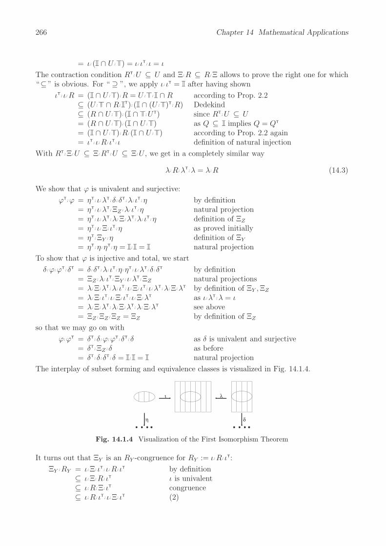
266 Chapter 14 Mathematical Applications
= ι; ( ∩ U ; ) = ι; ιT; ι = ι
The contraction condition RT;U ⊆ U and Ξ;R ⊆ R;Ξ allows to prove the right one for which“⊆ ” is obvious. For “ ⊇ ”, we apply ι; ιT = after having shown
ιT; ι; R = ( ∩ U ; ); R = U ; ; ∩ R according to Prop. 2.2⊆ (U ; ∩ R;
T); ( ∩ (U ; )T; R) Dedekind⊆ (R ∩ U ; ); ( ∩ ; UT) since RT; U ⊆ U= (R ∩ U ; ); ( ∩ U ; ) as Q ⊆ implies Q = QT
= ( ∩ U ; ); R; ( ∩ U ; ) according to Prop. 2.2 again= ιT; ι; R; ιT; ι definition of natural injection
With RT; Ξ; U ⊆ Ξ; RT; U ⊆ Ξ; U , we get in a completely similar way
λ; R; λT; λ = λ; R (14.3)
We show that ϕ is univalent and surjective:
ϕT; ϕ = ηT; ι; λT; δ; δT; λ; ιT; η by definition= ηT; ι; λT; ΞZ ; λ; ιT; η natural projection= ηT; ι; λT; λ; Ξ; λT; λ; ιT; η definition of ΞZ
= ηT; ι; Ξ; ιT; η as proved initially= ηT; ΞY ; η definition of ΞY
= ηT; η; ηT; η = ; = natural projection
To show that ϕ is injective and total, we start
δ; ϕ; ϕT; δT = δ; δT; λ; ιT; η; ηT; ι; λT; δ; δT by definition= ΞZ ; λ; ιT; ΞY ; ι; λT; ΞZ natural projections= λ; Ξ; λT; λ; ιT; ι; Ξ; ιT; ι; λT; λ; Ξ; λT by definition of ΞY , ΞZ
= λ; Ξ; ιT; ι; Ξ; ιT; ι; Ξ; λT as ι; λT; λ = ι= λ; Ξ; λT; λ; Ξ; λT; λ; Ξ; λT see above= ΞZ ; ΞZ ; ΞZ = ΞZ by definition of ΞZ
so that we may go on with
ϕ; ϕT = δT; δ; ϕ; ϕT; δT; δ as δ is univalent and surjective= δT; ΞZ ; δ as before= δT; δ; δT; δ = ; = natural projection
The interplay of subset forming and equivalence classes is visualized in Fig. 14.1.4.
ι λ
η δ
Fig. 14.1.4 Visualization of the First Isomorphism Theorem
It turns out that ΞY is an RY -congruence for RY := ι; R; ιT:
ΞY ; RY = ι; Ξ; ιT; ι; R; ιT by definition⊆ ι; Ξ; R; ιT ι is univalent⊆ ι; R; Ξ; ιT congruence⊆ ι; R; ιT; ι; Ξ; ιT (2)

14.1 Homomorphism and Isomorphism Theorems 267
⊆ RY ; ΞY definition of RY , ΞY
The construct α := ι; Ξ; λT; δ is a surjective mapping:
αT; α = δT; λ; Ξ; ιT; ι; Ξ; λT; δ by the definition just given= δT; λ; Ξ; λT; λ; Ξ; λT; δ (1)= δT; ΞZ ; ΞZ ; δ definition of ΞZ
= δT; ΞZ ; δ ΞZ is indeed an equivalence= δT; δ; δT; δ = ; = δ is natural projection for ΞZ
α; αT = ι; Ξ; λT; δ; δT; λ; Ξ; ιT by definition= ι; Ξ; λT; ΞZ ; λ; Ξ; ιT δ is natural projection for ΞZ
= ι; Ξ; λT; λ; Ξ; λT; λ; Ξ; ιT definition of ΞZ
= ι; Ξ; ιT; ι; Ξ; ιT; ι; Ξ; ιT (1)= ΞY ; ΞY ; ΞY = ΞY ⊇ definition of equivalence ΞY
With α, we may express S, T in a shorter way:αT; RY ; α = δT; λ; Ξ; ιT; RY ; ι; Ξ; λT; δ definition of α
= δT; λ; Ξ; ιT; ι; R; ιT; ι; Ξ; λT; δ definition of RY
= δT; λ; Ξ; ιT; ι; R; Ξ; λT; δ (2)= δT; λ; Ξ; ιT; ι; Ξ; R; Ξ; λT; δ Ξ; R; Ξ ⊆ R; Ξ; Ξ = R; Ξ ⊆ Ξ; R; Ξ= δT; λ; Ξ; λT; λ; Ξ; R; Ξ; λT; δ (1)= δT; ΞZ ; λ; R; Ξ; λT; δ as before, definition of ΞZ
= δT; ΞZ ; λ; R; λT; λ; Ξ; λT; δ (3)= δT; ΞZ ; λ; R; λT; ΞZ ; δ definition of ΞZ
= δT; δ; δT; λ; R; λT; δ; δT; δ δ is natural projection for ΞZ
= δT; λ; R; λT; δ = T δ is a surjective mappingηT; RY ; η = ηT; ι; R; ιT; η definition of RY
= S definition of S
Relations α and ϕ are closely related:= ι; Ξ; λT; δ; δT; λ; ιT; η definition of α, ϕ= ι; Ξ; λT; ΞZ ; λ; ιT; η δ is natural projection for ΞZ
= ι; Ξ; λT; λ; Ξ; λT; λ; ιT; η definition of ΞZ
= ι; Ξ; λT; λ; Ξ; ιT; η (2)= ι; Ξ; ιT; ι; Ξ; ιT; η (1)= ΞY ; ΞY ; η definition of ΞY
= η; ηT; η; ηT; η = η η is natural projection for ΞY
αT; η = αT; α; ϕ see before= ϕ α is univalent and surjective
This enables us already to prove the homomorphism condition:
T ; ϕ = αT; RY ; α; αT; η above results on T, ϕ= αT; RY ; ΞY ; η α; αT = ΞY , see above= αT; ΞY ; RY ; ΞY ; η ΞY is an RY -congruence= αT; η; ηT; RY ; η; ηT; η η is natural projection for ΞY
= ϕ; ηT; RY ; η η is univalent and surjective= ϕ; S see above
This was an equality, so that it suffices according to Lemma 11.1.6.

268 Chapter 14 Mathematical Applications
RS
Ξ
ΞV
Uϕ
Θ
Θ
Y
X
η
ηY
Xδ
δV
U SR
α
ψ
β
V
U
Y
X
Fig. 14.1.5 Situation of the Second Isomorphism Theorem
14.1.3 Proposition (Second Isomorphism Theorem). Let a multicovering (ϕ, ψ) between anytwo relations R : X −→ Y and S : U −→ V be given as well as an R-congruence (ΞX , ΞY ) andan S-congruence (ΘU , ΘV ). Let also the equivalences be related through ϕ, ψ as ΞY = ψ;ΘV ;ψT
and ΞX = ϕ; ΘU ; ϕT. Given this situation, introduce the natural projections ηX , ηY , δU , δV forthe equivalences and proceed to relations R′ := ηT
X;R;ηY and S ′ := δT
U;S;δV . Then α := ηT
X;ϕ;δU
and β := ηTY
; ψ; δV constitute an isomorphism from R′ to S ′.
Proof : α is univalent and surjective (β follows completely analogously)
αT; α = (ηTX
; ϕ; δU)T; ηTX
; ϕ; δU by definition= δT
U; ϕT; ηX ; ηT
X; ϕ; δU transposing
= δTU
; ϕT; ΞX ; ϕ; δU natural projection= δT
U; ϕT; ϕ; ΘU ; ϕT; ϕ; δU condition on mapping equivalences
= δTU
; ΘU ; δU as ϕ is a surjective mapping= δT
U; δU ; δT
U; δU natural projection
= ; =
We show that α is total and injective (β follows completely analogously)α; αT = ηT
X; ϕ; δU ; (ηT
X; ϕ; δU)T by definition
= ηTX
; ϕ; δU ; δTU
; ϕT; ηX transposing= ηT
X; ϕ; ΘU ; ϕT; ηX natural projection
= ηTX
; ΞX ; ηX condition on mapping equivalences= ηT
X; ηX ; ηT
X; ηX natural projection
= ; =
We show that α, β is a homomorphism:
R′; β = ηTX
; R; ηY ; ηTY
; ψ; δV by definition= ηT
X; R; ΞY ; ψ; δV natural projection
= ηTX
; R; ψ; ΘV ; ψT; ψ; δV condition on mapping equivalences= ηT
X; R; ψ; ΘV ; δV as ψ is surjective and univalent
= ηTX
; ϕ; S ; ΘV ; δV multi-covering= ηT
X; ϕ; ΘU ; S ; ΘV ; δV S ; ΘV ⊆ ΘU ; S ; ΘV ⊆ S ; ΘV ; ΘV = S ; ΘV
= ηTX
; ϕ; ΘU ; S ; δV ; δTV
; δV natural projection= ηT
X; ϕ; ΘU ; S ; δV as δ is a surjective mapping
= ηTX
; ϕ; δU ; δTU
; S ; δV natural projection= α; S ′ by definition
This was an equality, so that it suffices according to Lemma 11.1.6.
14.2 Covering of Graphs and Path Equivalence 269
14.2 Covering of Graphs and Path Equivalence
There is another point to mention here which has gained considerable interest in an algebraicor topological context, not least for Riemann surfaces.
14.2.1 Proposition (Lifting property). Let a homogeneous relation B be given together witha multi-covering (Φ, Φ) on the relation B′. Let furthermore some rooted graph B0 with roota0, i.e., satisfying and BT
0∗; a0 = , be given together with a homomorphism Φ0 that sends the
root a0 to a′ := ΦT0
; a0. If a ⊆ ΦT ; a′ is some point mapped by Φ to a′, there exists always arelation Ψ — not necessarily a mapping — satisfying the properties
ΨT; a0 = a and B0; Ψ ⊆ Ψ; B.
Idea of proof: Define Ψ := infX | a0; aT ∪ (BT0
; X ; B ∩ Φ0; ΦT) ⊆ X.
The relation Ψ enjoys the homomorphism property but fails to be a mapping in general. Inorder to make it a mapping, one will choose one of the following two possibilities:
• Firstly, one might follow the recursive definition starting from a0 and at every stage makean arbitrary choice among the relational images offered, thus choosing a fiber.
• Secondly, one may further restrict the multi-covering condition to “locally univalent” fansin Φ, requiring BT
0;Ψ;B ∩Φ0;Φ
T ⊆ to hold for it, which leads to a well-developed theory,see [Sch77, Sch81a, Sch81b].
In both cases, one will find a homomorphism from B0 to B. The effect of a flow chart diagram isparticularly easy to understand when the underlying rooted graph is also a rooted tree, so thatthe view is not blocked by nested circuits which can be traveled several times. When dealingwith a rooted graph that does contain such circuits one has to keep track of the possibly infinitenumber of ways in which the graph can be traversed from its root. To this end there exists atheory of coverings which is based on the notion of homomorphy.
The idea is to unfold circuits. We want to characterize those homomorphisms of a graph thatpreserve to a certain extent the possibilities of traversal. We shall see that such a homomorphismis surjective and that it carries the successor relation at any point onto that at the image point.
14.2.2 Definition. A surjective homomorphism Φ: G −→ G′ is called a covering, providedthat it is a multi-covering satisfying BT; B ∩ Φ; ΦT ⊆ .
The multi-covering Φ compares two relations between the points of G and of G′ and ensuresthat for any inverse image point x of some point x′ and successor y′ of x′ there is at least onesuccessor y of x which is mapped onto y′. The new condition guarantees that there is at mostone such y since it requires that the relation “have a common predecessor according to B, andhave a common image under Φ” is contained in the identity.
We have reworked mathematical basics from a relational perspective. First the step from analgebraic to a relational structure has been made. This is so serious a generalization, that onewould not expect much of the idea of homomorphism and isomorphism theorems to survive.

270 Chapter 14 Mathematical Applications
With the concept of a multi-covering, however, a new and adequate concept seems to have beenfound. Prop. 11.2.7 shows that it reduces completely to homomorphisms when going back tothe algebraic case. For relational structures, a multi-covering behaves nicely with respect toquotient forming. This relates to earlier papers (see [Sch77, Sch81a, Sch81b]) where semanticsof programs (partial correctness, total correctness, and flow equivalence, even for systems ofrecursive procedures) has first been given a componentfree relational form.
Something ignored in test edition!
Something ignored in test edition!
15 Standard Galois Mechanisms
The work in this chapter is characterized by the fact that two antitone mappings are given.In most cases they are related with one or more relations which are often heterogeneous. Aniteration leads to a fixedpoint of a Galois correspondence. Important classes of applicationslead to these investigations. Termination and initial part, games, correctness, matchings, andassignments may be studied in structurally the same way when following this idea.
15.1 Galois Iteration
When Evariste Galois in preparation of the duell around 1830, in which he expected to fall,wrote down his last notes, he could probably not imagine to which extent these would laterinfluence mathematics and also applications. What he had observed may basically be presentedwith the correspondence of permutations of a set and their fixedpoints. Consider the 5-elementsequence 1, 2, 3, 4, 5 for which there exist in total 5! = 120 permutations. The idea is now toobserve which set of permutations leaves which set of elements fixed. Demanding more elementsto be untouched by a permutation results, of course, in fewer permutations. 2, 4 fixed allowsonly 6 permutations, namely
1, 2, 3, 4, 5 1, 2, 5, 4, 3 3, 2, 1, 4, 5 3, 2, 5, 4, 1 5, 2, 1, 4, 3 5, 2, 3, 4, 1
If, e.g., 2, 3, 4 shall be fixed, only permutations 1, 2, 3, 4, 5 and 5, 2, 3, 4, 1 remain. On the otherside, when we increase the set of permutations adding a last one to obtain
1, 2, 3, 4, 5 1, 2, 5, 4, 3 3, 2, 1, 4, 5 3, 2, 5, 4, 1 5, 2, 1, 4, 3 5, 2, 3, 4, 1 5, 3, 2, 4, 1
the set of fixedpoints reduces to 4, i.e., to just one. It is this counterplay of antitone functionsthat is utilized in what follows. In our finite case, it is more or less immaterial which antitonefunctions we work with. The schema stays the same. This shall now be demonstrated with twoexamples.
15.1.1 Example. Let a set V be given and consider all of its subsets, i.e., the powerset P(V ).Then assume the following obviously antitone mappings to be given which depend on somegiven relation R : V −→ V .
σ : P(V ) → P(V ), here: v → σ(v) = R; v
π : P(V ) → P(V ), here: w → π(w) = w
In such a setting it is a standard technique to proceed as follows starting with the empty setin the upper row and the full set in the lower. Then the mappings are applied from the upperto the next lower as well as from the lower to the next upper subset as shown here.
271

272 Chapter 15 Standard Galois Mechanisms
R =
1 2 3 4 5 6 7 8 9123456789
⎛⎜⎜⎜⎜⎜⎜⎜⎜⎝
0 0 0 0 0 0 0 1 00 0 0 0 0 0 0 0 10 0 0 0 0 0 1 0 00 1 0 0 0 0 0 0 00 1 0 1 0 0 0 0 11 0 0 0 0 0 1 0 00 0 0 0 0 0 0 0 11 0 0 0 0 0 0 0 00 0 0 0 0 0 0 0 0
⎞⎟⎟⎟⎟⎟⎟⎟⎟⎠
⎛⎜⎜⎜⎜⎜⎜⎜⎜⎝
000000000
⎞⎟⎟⎟⎟⎟⎟⎟⎟⎠
⎛⎜⎜⎜⎜⎜⎜⎜⎜⎝
000000000
⎞⎟⎟⎟⎟⎟⎟⎟⎟⎠
⎛⎜⎜⎜⎜⎜⎜⎜⎜⎝
000000001
⎞⎟⎟⎟⎟⎟⎟⎟⎟⎠
⎛⎜⎜⎜⎜⎜⎜⎜⎜⎝
000000001
⎞⎟⎟⎟⎟⎟⎟⎟⎟⎠
⎛⎜⎜⎜⎜⎜⎜⎜⎜⎝
010000101
⎞⎟⎟⎟⎟⎟⎟⎟⎟⎠
⎛⎜⎜⎜⎜⎜⎜⎜⎜⎝
010000101
⎞⎟⎟⎟⎟⎟⎟⎟⎟⎠
⎛⎜⎜⎜⎜⎜⎜⎜⎜⎝
011100101
⎞⎟⎟⎟⎟⎟⎟⎟⎟⎠
⎛⎜⎜⎜⎜⎜⎜⎜⎜⎝
011100101
⎞⎟⎟⎟⎟⎟⎟⎟⎟⎠
⎛⎜⎜⎜⎜⎜⎜⎜⎜⎝
011110101
⎞⎟⎟⎟⎟⎟⎟⎟⎟⎠
. . .
⎛⎜⎜⎜⎜⎜⎜⎜⎜⎝
011110101
⎞⎟⎟⎟⎟⎟⎟⎟⎟⎠
=: a
σ
π
σ
π
σ
π
σ
π
σ
π
σ
π
σ
π
σ
π. . . σ π
⎛⎜⎜⎜⎜⎜⎜⎜⎜⎝
111111111
⎞⎟⎟⎟⎟⎟⎟⎟⎟⎠
⎛⎜⎜⎜⎜⎜⎜⎜⎜⎝
111111110
⎞⎟⎟⎟⎟⎟⎟⎟⎟⎠
⎛⎜⎜⎜⎜⎜⎜⎜⎜⎝
111111110
⎞⎟⎟⎟⎟⎟⎟⎟⎟⎠
⎛⎜⎜⎜⎜⎜⎜⎜⎜⎝
101111010
⎞⎟⎟⎟⎟⎟⎟⎟⎟⎠
⎛⎜⎜⎜⎜⎜⎜⎜⎜⎝
101111010
⎞⎟⎟⎟⎟⎟⎟⎟⎟⎠
⎛⎜⎜⎜⎜⎜⎜⎜⎜⎝
100011010
⎞⎟⎟⎟⎟⎟⎟⎟⎟⎠
⎛⎜⎜⎜⎜⎜⎜⎜⎜⎝
100011010
⎞⎟⎟⎟⎟⎟⎟⎟⎟⎠
⎛⎜⎜⎜⎜⎜⎜⎜⎜⎝
100001010
⎞⎟⎟⎟⎟⎟⎟⎟⎟⎠
⎛⎜⎜⎜⎜⎜⎜⎜⎜⎝
100001010
⎞⎟⎟⎟⎟⎟⎟⎟⎟⎠
. . .
⎛⎜⎜⎜⎜⎜⎜⎜⎜⎝
100001010
⎞⎟⎟⎟⎟⎟⎟⎟⎟⎠
=: b
Fig. 15.1.1 Example of an eventually stationary Galois iteration
The first important observation is that both sequences are monotone; the upper increasing andthe lower decreasing. They will thus become stationary in the finite case. When looking at thesequences in detail, it seems that there are two different sequences, but somehow alternatingand respecting each others order. Even more important is the second observation, namely thatthe upper and the lower stationary values a, b will satisfy
b = σ(a) = R; a and a = π(b) = b
One has, thus, a strong algebraic property for the final result of the iteration and one shouldtry to interpret and to make use of it.
15.1.2 Example. Consider now a completely different situation with two heterogeneous rela-tions Q, λ and the obviously antitone mappings
σ : P(V ) → P(W ), here: v → σ(v) = QT; v
π : P(W ) → P(V ), here: w → π(w) = λ; w
Given this setting, we again start an iteration with the two start vectors and obtain the follow-ing.

15.2 Termination 273
Q =
1 2 3 4 5
1
2
3
4
5
6
7
⎛⎜⎜⎜⎜⎜⎜⎝
1 0 0 1 00 0 0 0 01 0 0 1 00 0 0 1 00 1 1 1 11 0 0 1 00 0 1 0 1
⎞⎟⎟⎟⎟⎟⎟⎠
λ =
1 2 3 4 5
1
2
3
4
5
6
7
⎛⎜⎜⎜⎜⎜⎜⎝
1 0 0 0 00 0 0 0 00 0 0 1 00 0 0 0 00 0 0 0 10 0 0 0 00 0 1 0 0
⎞⎟⎟⎟⎟⎟⎟⎠
⎛⎜⎜⎜⎜⎜⎜⎝
0000000
⎞⎟⎟⎟⎟⎟⎟⎠
⎛⎜⎜⎜⎜⎜⎜⎝
0101010
⎞⎟⎟⎟⎟⎟⎟⎠
⎛⎜⎜⎜⎜⎜⎜⎝
0101010
⎞⎟⎟⎟⎟⎟⎟⎠
⎛⎜⎜⎜⎜⎜⎜⎝
1111010
⎞⎟⎟⎟⎟⎟⎟⎠
. . .
⎛⎜⎜⎜⎜⎜⎜⎝
1111010
⎞⎟⎟⎟⎟⎟⎟⎠
=: a
σ
π
σ
π
σ
π. . . σ π
⎛⎜⎜⎝
11111
⎞⎟⎟⎠
⎛⎜⎜⎝
11111
⎞⎟⎟⎠
⎛⎜⎜⎝
01101
⎞⎟⎟⎠
⎛⎜⎜⎝
01101
⎞⎟⎟⎠ . . .
⎛⎜⎜⎝
01101
⎞⎟⎟⎠ =: b
Fig. 15.1.2 Stationary heterogeneous Galois iteration
Again, both sequences are monotone, increasing resp. decreasing, and become stationary. Inaddition, the upper and the lower stationary values a, b satisfy
b = σ(a) = QT; b a = π(b) = λ; a,
i.e., schematically the same formulae as above.
In the sections to follow, different applications will be traced back to this type of iteration.It will turn out that several well-known problems get a (relation-)algebraic flavour. In severalcases, we will in addition be able to deduce subdivisions of the sets in question from a and b.When by permutation of the rows and columns of the matrices representing the relation thesets come together, additional visual properties will show up.
Exercises
New Execute the iterations with σ(v) =?? and π(w) =??.
Solution New
15.2 Termination
Jetzt einfaches vorne!!
The first group of considerations is usually located in graph theory, where one often looks forloops. The task arises to characterize an infinite path of a graph in an algebraic fashion. Thisis then complementary to looking for non-infinite sequences in the execution of programs, i.e.,terminating ones.
B ; y ⊆ y expresses that all predecessors of y also belong to y
y ⊆ B ; y expresses that every point of y precedes a point of y
B ; y = y characterizes y as an eigenvector similar to x in Ax = λx in matrix analysis
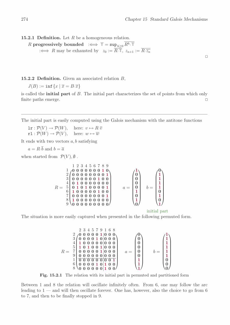
274 Chapter 15 Standard Galois Mechanisms
15.2.1 Definition. Let R be a homogeneous relation.
R progressively bounded :⇐⇒ = suph≥0 Rh;
:⇐⇒ R may be exhausted by z0 := R; , zn+1 := R; zn
15.2.2 Definition. Given an associated relation B,
J(B) := infx | x = B ; xis called the initial part of B. The initial part characterizes the set of points from which onlyfinite paths emerge.
The initial part is easily computed using the Galois mechanism with the antitone functions
lr : P(V ) → P(W ), here: v → R; vrl : P(W ) → P(V ), here: w → w
It ends with two vectors a, b satisfying
a = R; b and b = a
when started from P(V ), ∅ .
R =
1 2 3 4 5 6 7 8 9123456789
⎛⎜⎜⎜⎜⎜⎜⎜⎜⎝
0 0 0 0 0 0 0 1 00 0 0 0 0 0 0 0 10 0 0 0 0 0 1 0 00 1 0 0 0 0 0 0 00 1 0 1 0 0 0 0 11 0 0 0 0 0 1 0 00 0 0 0 0 0 0 0 11 0 0 0 0 0 0 0 00 0 0 0 0 0 0 0 0
⎞⎟⎟⎟⎟⎟⎟⎟⎟⎠
a =
⎛⎜⎜⎜⎜⎜⎜⎜⎝
100001010
⎞⎟⎟⎟⎟⎟⎟⎟⎠
b =
⎛⎜⎜⎜⎜⎜⎜⎜⎝
011110101
⎞⎟⎟⎟⎟⎟⎟⎟⎠
initial partThe situation is more easily captured when presented in the following permuted form.
R =
2 3 4 5 7 9 1 6 8234579168
⎛⎜⎜⎜⎜⎜⎜⎜⎜⎝
0 0 0 0 0 1 0 0 00 0 0 0 1 0 0 0 01 0 0 0 0 0 0 0 01 0 1 0 0 1 0 0 00 0 0 0 0 1 0 0 00 0 0 0 0 0 0 0 00 0 0 0 0 0 0 0 10 0 0 0 1 0 1 0 00 0 0 0 0 0 1 0 0
⎞⎟⎟⎟⎟⎟⎟⎟⎟⎠
a =
⎛⎜⎜⎜⎜⎜⎜⎜⎝
000000111
⎞⎟⎟⎟⎟⎟⎟⎟⎠
b =
⎛⎜⎜⎜⎜⎜⎜⎜⎝
111111000
⎞⎟⎟⎟⎟⎟⎟⎟⎠
Fig. 15.2.1 The relation with its initial part in permuted and partitioned form
Between 1 and 8 the relation will oscillate infinitely often. From 6, one may follow the arcleading to 1 — and will then oscillate forever. One has, however, also the choice to go from 6to 7, and then to be finally stopped in 9.

15.2 Termination 275
a = inf , B ; , B ; B ; , . . .,
b = sup , B ; , B ; B ; , . . .,
B ; b = a,
a = b⎛⎜⎜⎜⎜⎜⎜⎜⎜⎜⎜⎜⎜⎜⎜⎜⎜⎜⎜⎜⎜⎝
11111111111111111
⎞⎟⎟⎟⎟⎟⎟⎟⎟⎟⎟⎟⎟⎟⎟⎟⎟⎟⎟⎟⎟⎠
⎛⎜⎜⎜⎜⎜⎜⎜⎜⎜⎜⎜⎜⎜⎜⎜⎜⎜⎜⎜⎜⎝
10111010111101111
⎞⎟⎟⎟⎟⎟⎟⎟⎟⎟⎟⎟⎟⎟⎟⎟⎟⎟⎟⎟⎟⎠
⎛⎜⎜⎜⎜⎜⎜⎜⎜⎜⎜⎜⎜⎜⎜⎜⎜⎜⎜⎜⎜⎝
10111010111101111
⎞⎟⎟⎟⎟⎟⎟⎟⎟⎟⎟⎟⎟⎟⎟⎟⎟⎟⎟⎟⎟⎠
⎛⎜⎜⎜⎜⎜⎜⎜⎜⎜⎜⎜⎜⎜⎜⎜⎜⎜⎜⎜⎜⎝
00111010111100111
⎞⎟⎟⎟⎟⎟⎟⎟⎟⎟⎟⎟⎟⎟⎟⎟⎟⎟⎟⎟⎟⎠
⎛⎜⎜⎜⎜⎜⎜⎜⎜⎜⎜⎜⎜⎜⎜⎜⎜⎜⎜⎜⎜⎝
00111010111100111
⎞⎟⎟⎟⎟⎟⎟⎟⎟⎟⎟⎟⎟⎟⎟⎟⎟⎟⎟⎟⎟⎠
⎛⎜⎜⎜⎜⎜⎜⎜⎜⎜⎜⎜⎜⎜⎜⎜⎜⎜⎜⎜⎜⎝
00111010011100111
⎞⎟⎟⎟⎟⎟⎟⎟⎟⎟⎟⎟⎟⎟⎟⎟⎟⎟⎟⎟⎟⎠
⎛⎜⎜⎜⎜⎜⎜⎜⎜⎜⎜⎜⎜⎜⎜⎜⎜⎜⎜⎜⎜⎝
00111010011100111
⎞⎟⎟⎟⎟⎟⎟⎟⎟⎟⎟⎟⎟⎟⎟⎟⎟⎟⎟⎟⎟⎠
A careful reader may ask to which extend the choice to start the iteration with , wasarbitrary. When starting the other way round, i.e., with , , the result will be the initial partfor the transposed graph.
The initial part characterizes those points from which one may run into an infinite path, notfrom which one cannot avoid running into one. This latter question is also interesting.
15.2.3 Theorem (Termination Formulae).
i) suph≥0 Bh; ⊆ J(B) ⊆ B∗; B ;
ii) B univalent =⇒ suph≥0 Bh; = J(B) = B∗; B ;
iii) B progressivelybounded
=⇒ =suph≥0 Bh; = J(B) = B∗; B ;
iv) B progressivelyfinite
=⇒ suph≥0 Bh; ⊆ J(B) = B∗; B ; =
v) B finite =⇒ suph≥0 Bh; = J(B) ⊆ B∗; B ;
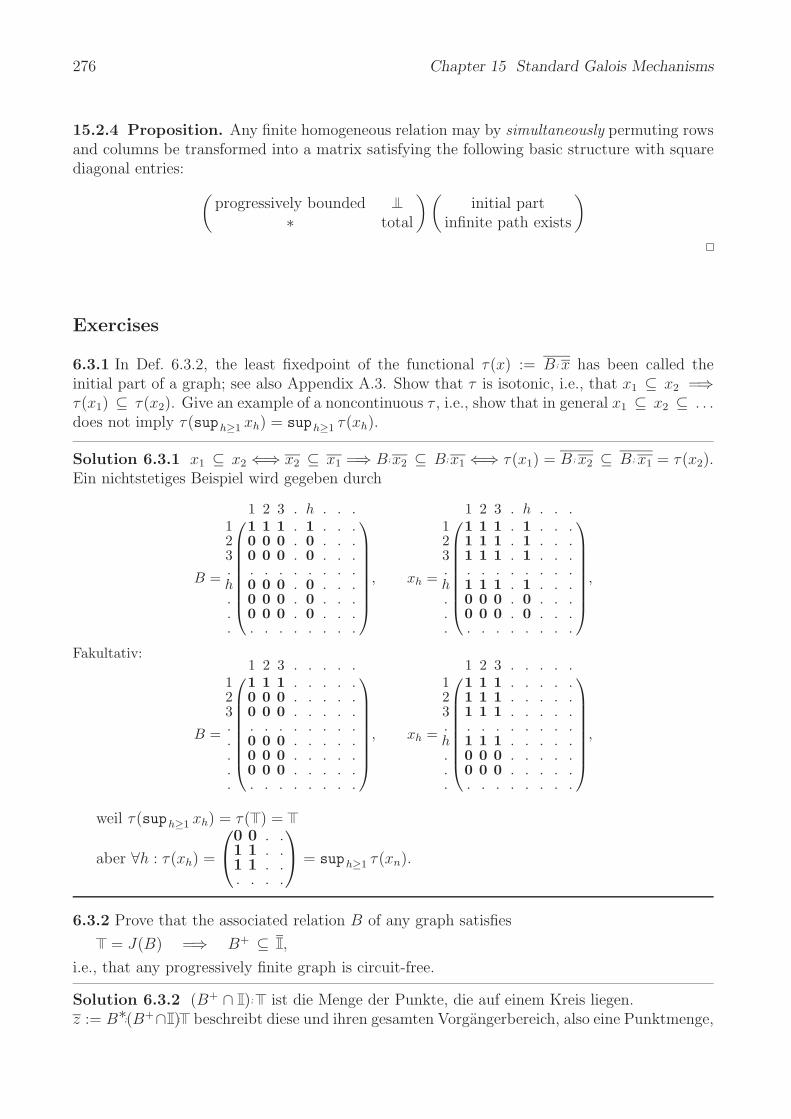
276 Chapter 15 Standard Galois Mechanisms
15.2.4 Proposition. Any finite homogeneous relation may by simultaneously permuting rowsand columns be transformed into a matrix satisfying the following basic structure with squarediagonal entries: (
progressively bounded∗ total
) (initial part
infinite path exists
)
Exercises
6.3.1 In Def. 6.3.2, the least fixedpoint of the functional τ(x) := B ; x has been called theinitial part of a graph; see also Appendix A.3. Show that τ is isotonic, i.e., that x1 ⊆ x2 =⇒τ(x1) ⊆ τ(x2). Give an example of a noncontinuous τ , i.e., show that in general x1 ⊆ x2 ⊆ . . .does not imply τ(suph≥1 xh) = suph≥1 τ(xh).
Solution 6.3.1 x1 ⊆ x2 ⇐⇒ x2 ⊆ x1 =⇒ B;x2 ⊆ B;x1 ⇐⇒ τ(x1) = B ; x2 ⊆ B ; x1 = τ(x2).Ein nichtstetiges Beispiel wird gegeben durch
B =
⎛⎜⎜⎜⎜⎜⎜⎜⎝
1 2 3 . h . . .1 1 1 1 . 1 . . .2 0 0 0 . 0 . . .3 0 0 0 . 0 . . .. . . . . . . . .h 0 0 0 . 0 . . .. 0 0 0 . 0 . . .. 0 0 0 . 0 . . .. . . . . . . . .
⎞⎟⎟⎟⎟⎟⎟⎟⎠
, xh =
⎛⎜⎜⎜⎜⎜⎜⎜⎝
1 2 3 . h . . .1 1 1 1 . 1 . . .2 1 1 1 . 1 . . .3 1 1 1 . 1 . . .. . . . . . . . .h 1 1 1 . 1 . . .. 0 0 0 . 0 . . .. 0 0 0 . 0 . . .. . . . . . . . .
⎞⎟⎟⎟⎟⎟⎟⎟⎠
,
Fakultativ:
B =
⎛⎜⎜⎜⎜⎜⎜⎜⎝
1 2 3 . . . . .1 1 1 1 . . . . .2 0 0 0 . . . . .3 0 0 0 . . . . .. . . . . . . . .. 0 0 0 . . . . .. 0 0 0 . . . . .. 0 0 0 . . . . .. . . . . . . . .
⎞⎟⎟⎟⎟⎟⎟⎟⎠
, xh =
⎛⎜⎜⎜⎜⎜⎜⎜⎝
1 2 3 . . . . .1 1 1 1 . . . . .2 1 1 1 . . . . .3 1 1 1 . . . . .. . . . . . . . .h 1 1 1 . . . . .. 0 0 0 . . . . .. 0 0 0 . . . . .. . . . . . . . .
⎞⎟⎟⎟⎟⎟⎟⎟⎠
,
weil τ(suph≥1 xh) = τ( ) =
aber ∀h : τ(xh) =
⎛⎝0 0 . .
1 1 . .1 1 . .. . . .
⎞⎠ = suph≥1 τ(xn).
6.3.2 Prove that the associated relation B of any graph satisfies
= J(B) =⇒ B+ ⊆ ,
i.e., that any progressively finite graph is circuit-free.
Solution 6.3.2 (B+ ∩ ); ist die Menge der Punkte, die auf einem Kreis liegen.z := B∗;(B+∩ ); beschreibt diese und ihren gesamten Vorgangerbereich, also eine Punktmenge,

15.3 Correctness and wp 277
von der man erwarten muß, daß dort Wege unendlicher Lange entspringen. In der Tat weistman nach
z := B∗; (B+ ∩ ); = (B+ ∩ ); ∪ B+; (B+ ∩ );
= (B+ ∩ )2; ∪ . . . ; siehe Ubung (2.3.7)⊆ B+; (B+ ∩ ); . . .= B+; (B+ ∩ ); = B ; B∗; (B+ ∩ ); = B ; z,
so daß aufgrund der Voraussetzung gilt = J(B) ⊆ z = B∗; (B+ ∩ ); ⊆ ; (B+ ∩ ); .Also ist (B+ ∩ ); = und damit B+ ∩ = .
6.3.3 If there exists a homomorphism of a graph G into a progressively bounded or progressivelyfinite graph, then G itself is progressively bounded or progressively finite, respectively.
Solution 6.3.3 Nach Kap. 7 !
Wir beweisen Φ suph≥0 B′h; ⊆ suph≥0 Bh; indem wir zeigen B;Φ ⊆ Φ;B′ =⇒ Bh;Φ ⊆Bh−1;Φ;B′ ⊆ Φ;B′h =⇒ Bh; = Bh;Φ; ⊆ Φ;B′h; ⇐⇒ Φ;B′h; = Φ; B′h; ⊆ Bh; . Ist nun
G′ progressiv-beschrankt, so gilt Φ; = ⊆ suph≥0 B′h; . AnderungAnalog fur progressiv-endlich.
6.3.4 Prove the following identities for the initial part J(B):B∗T; J(B) = J(B), B∗; J(B) = J(B).
Solution 6.3.4 ???
6.3.5 Show that in general J(B) ⊆ infx | B ; ∪B;x ⊆ x and that for a univalent relationB this may be sharpened to J(B) = infx | B ; ∪ B ; x ⊆ x .
Solution 6.3.5 Aus ??? B ; ∪ B;x ⊆ x folgt stets x ⊆ B; ∩ B ; x ⊆ B;x. Gilt BT;B ⊆ ,so folgt aus x ⊆ B ; x auch B ; ∪ B ; x ⊆ B ; x ⊆ x.
15.3 Correctness and wp
Consider a given group of several relations and assume that these have to be composed insome way. If this occurs in practice, often certain conditions have to be satisfied. Two mainconditions may be separated. One demands that when chasing with the finger around thearrows provided by the relations, one will not leave a certain prescribed “safe” area. The otherfollows an opposite idea. It is interested that a “dangerous” area will definitely be avoided. Forboth cases an easy-to-understand condition may be formulated.
Fig. 15.3.1 Self-filling funnel

278 Chapter 15 Standard Galois Mechanisms
Exercises
New Let the relation A =??? be given as well as the subset v =???. Determine the set x sothat it is impossible to reach a point outside s when terminating.
Solution New
15.4 Games
For a second application, we look at solutions of relational games. Let an arbitrary homogeneousrelation B : V ↔ V be given. Two players are supposed to make moves alternatingly accordingto B in choosing a consecutive arrow to follow. The player who has no further move, i.e., whois about to move and finds an empty row in the relation B, or a terminal vertex in the graph,has lost.
Such a game is easily visualized taking a relation B represented by a graph, on which playershave to determine a path in an alternating way. We study it for the Nim-type game startingwith 6 matches from which we are allowed to take 1 or 2.
036
1245
0 1 2 3 4 5 6
0
1
2
3
4
5
6
⎛⎜⎜⎜⎜⎜⎜⎝
0 0 0 0 0 0 01 0 0 0 0 0 01 1 0 0 0 0 00 1 1 0 0 0 00 0 1 1 0 0 00 0 0 1 1 0 00 0 0 0 1 1 0
⎞⎟⎟⎟⎟⎟⎟⎠
Fig. 15.4.1 A NIM-type game in graph- and in matrix-form
The antitone functionals based on this relation are formed in a manner quite similar to termi-nation.
antitonFctlGame b x = negaMat (b *** x)
The solution of the game is then again determined following the general scheme.
gameSolution b = untilGalois (antitonFctlGame b) (antitonFctlGame b)(startVector False b, startVector True b)
There is one further point to mention concerning the result. This time, we have a homogeneousrelation, and we easily observe, that the two sequences from page ?? reduce using monotonyto just one
⊆ π( ) ⊆ π(σ( )) ⊆ π(σ(π( ))) ⊆ . . . ⊆ . . . ⊆ σ(π(σ( ))) ⊆ σ(π( )) ⊆ σ( ) ⊆.
It is explicitly given here, and we observe equalities in an alternating pattern: ⊆ B ; =
B ; B ; ⊆ B ; B ; B ; = . . . ⊆ . . . ⊆ B ; B ; B ; = B ; B ; ⊆ B ; = .
Again, the final situation is characterised by the formulae a = π(b) and σ(a) = b, which thistime turn out to be a = B ; b and B ; a = b. In addition, we will always have a ⊆ b. The
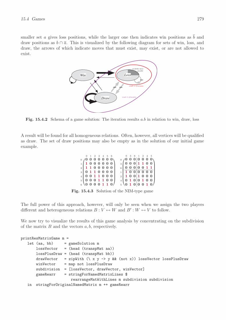
15.4 Games 279
smaller set a gives loss positions, while the larger one then indicates win positions as b anddraw positions as b ∩ a. This is visualized by the following diagram for sets of win, loss, anddraw, the arrows of which indicate moves that must exist, may exist, or are not allowed toexist.
Win Loss
Draw
no further move possible
result a of iteration
result b of iteration
Fig. 15.4.2 Schema of a game solution: The iteration results a.b in relation to win, draw, loss
A result will be found for all homogeneous relations. Often, however, all vertices will be qualifiedas draw. The set of draw positions may also be empty as in the solution of our initial gameexample.
0 1 2 3 4 5 6
0
1
2
3
4
5
6
⎛⎜⎜⎜⎜⎜⎜⎝
0 0 0 0 0 0 01 0 0 0 0 0 01 1 0 0 0 0 00 1 1 0 0 0 00 0 1 1 0 0 00 0 0 1 1 0 00 0 0 0 1 1 0
⎞⎟⎟⎟⎟⎟⎟⎠
0 3 6 1 2 4 5
0
3
6
1
2
4
5
⎛⎜⎜⎜⎜⎜⎜⎝
0 0 0 0 0 0 00 0 0 1 1 0 00 0 0 0 0 1 11 0 0 0 0 0 01 0 0 1 0 0 00 1 0 0 1 0 00 1 0 0 0 1 0
⎞⎟⎟⎟⎟⎟⎟⎠
Fig. 15.4.3 Solution of the NIM-type game
The full power of this approach, however, will only be seen when we assign the two playersdifferent and heterogeneous relations B : V ↔ W and B′ : W ↔ V to follow.
We now try to visualize the results of this game analysis by concentrating on the subdivisionof the matrix B and the vectors a, b, respectively.
printResMatrixGame m =let (aa, bb) = gameSolution m
lossVector = (head (transpMat aa))lossPlusDraw = (head (transpMat bb))drawVector = zipWith (\ x y -> y && (not x)) lossVector lossPlusDrawwinVector = map not lossPlusDrawsubdivision = [lossVector, drawVector, winVector]gameRearr = stringForNamedMatrixLines $
rearrangeMatWithLines m subdivision subdivisionin stringForOriginalNamedMatrix m ++ gameRearr

280 Chapter 15 Standard Galois Mechanisms
1 2 3 4 5 6 7 8 9 10 11 12 13 14 15 16 17 18 19 20 21
1
2
3
4
5
6
7
8
9
10
11
12
13
14
15
16
17
18
19
20
21
⎛⎜⎜⎜⎜⎜⎜⎜⎜⎜⎜⎜⎜⎜⎜⎜⎜⎜⎜⎜⎜⎜⎜⎜⎜⎜⎜⎜⎜⎜⎜⎜⎝
0 0 0 0 0 0 0 0 0 1 1 0 0 0 0 0 0 0 0 0 00 0 0 0 0 0 0 0 0 0 0 0 0 0 0 0 0 0 0 0 00 0 0 0 0 0 0 0 0 0 0 0 0 0 0 0 1 0 1 0 00 0 0 0 0 0 0 0 0 0 0 0 1 0 1 0 0 0 0 0 00 0 0 0 1 0 1 0 0 0 0 0 0 1 0 0 1 0 1 1 00 0 0 0 0 0 0 0 0 0 0 0 0 0 0 0 0 0 0 0 00 0 0 1 0 1 0 0 0 0 0 0 0 1 1 0 0 0 0 0 00 1 0 0 0 0 0 0 1 0 1 1 0 1 0 0 0 0 0 0 01 0 0 0 0 0 0 0 0 0 0 0 0 0 1 0 0 0 0 0 00 0 0 0 0 0 0 0 1 0 0 0 0 0 0 0 0 1 0 0 00 0 0 0 0 0 0 0 0 0 0 0 0 0 0 0 0 0 0 0 00 1 0 0 0 0 0 1 0 0 0 0 0 1 0 0 0 0 1 0 01 0 0 0 1 0 0 0 0 0 0 1 1 0 1 0 0 1 0 0 01 0 0 0 0 0 0 0 0 0 0 1 0 0 0 0 0 0 0 1 00 0 0 0 0 0 1 0 0 0 0 0 0 0 0 0 0 0 0 0 00 0 1 0 0 1 0 0 1 0 1 0 0 0 0 1 0 0 1 0 00 0 1 0 0 0 0 1 1 0 0 0 0 0 0 0 0 0 1 0 00 1 0 0 0 0 0 0 0 0 0 0 0 0 1 1 0 0 0 0 00 0 0 1 0 0 0 0 0 0 0 1 0 0 0 0 0 0 0 0 00 0 0 0 0 0 0 0 0 0 0 0 0 1 0 0 1 0 0 0 00 1 0 1 0 0 0 0 0 0 0 0 0 0 0 0 0 0 0 0 0
⎞⎟⎟⎟⎟⎟⎟⎟⎟⎟⎟⎟⎟⎟⎟⎟⎟⎟⎟⎟⎟⎟⎟⎟⎟⎟⎟⎟⎟⎟⎟⎟⎠
2 6 10 11 15 19 14 20 1 3 4 5 7 8 9 12 13 16 17 18 21
2
6
10
11
15
19
14
20
1
3
4
5
7
8
9
12
13
16
17
18
21
⎛⎜⎜⎜⎜⎜⎜⎜⎜⎜⎜⎜⎜⎜⎜⎜⎜⎜⎜⎜⎜⎜⎜⎜⎜⎜⎜⎜⎜⎜⎜⎜⎜⎝
0 0 0 0 0 0 0 0 0 0 0 0 0 0 0 0 0 0 0 0 00 0 0 0 0 0 0 0 0 0 0 0 0 0 0 0 0 0 0 0 00 0 0 0 0 0 0 0 0 0 0 0 0 0 1 0 0 0 0 1 00 0 0 0 0 0 0 0 0 0 0 0 0 0 0 0 0 0 0 0 00 0 0 0 0 0 0 0 0 0 0 0 1 0 0 0 0 0 0 0 00 0 0 0 0 0 0 0 0 0 1 0 0 0 0 1 0 0 0 0 00 0 0 0 0 0 0 1 1 0 0 0 0 0 0 1 0 0 0 0 00 0 0 0 0 0 1 0 0 0 0 0 0 0 0 0 0 0 1 0 00 0 1 1 0 0 0 0 0 0 0 0 0 0 0 0 0 0 0 0 00 0 0 0 0 1 0 0 0 0 0 0 0 0 0 0 0 0 1 0 00 0 0 0 1 0 0 0 0 0 0 0 0 0 0 0 1 0 0 0 00 0 0 0 0 1 1 1 0 0 0 1 1 0 0 0 0 0 1 0 00 1 0 0 1 0 1 0 0 0 1 0 0 0 0 0 0 0 0 0 01 0 0 1 0 0 1 0 0 0 0 0 0 0 1 1 0 0 0 0 00 0 0 0 1 0 0 0 1 0 0 0 0 0 0 0 0 0 0 0 01 0 0 0 0 1 1 0 0 0 0 0 0 1 0 0 0 0 0 0 00 0 0 0 1 0 0 0 1 0 0 1 0 0 0 1 1 0 0 1 00 1 0 1 0 1 0 0 0 1 0 0 0 0 1 0 0 1 0 0 00 0 0 0 0 1 0 0 0 1 0 0 0 1 1 0 0 0 0 0 01 0 0 0 1 0 0 0 0 0 0 0 0 0 0 0 0 1 0 0 01 0 0 0 0 0 0 0 0 0 1 0 0 0 0 0 0 0 0 0 0
⎞⎟⎟⎟⎟⎟⎟⎟⎟⎟⎟⎟⎟⎟⎟⎟⎟⎟⎟⎟⎟⎟⎟⎟⎟⎟⎟⎟⎟⎟⎟⎟⎟⎠
Fig. 15.4.4 A random relation and its game solution rearranged
15.4.1 Proposition (Rearranging relations with respect to a game). Every finite homoge-neous relation may by simultaneously permuting rows and columns be transformed into amatrix satisfying the following basic structure with square diagonal entries:⎛
⎝ ∗total ∗
total ∗ ∗
⎞⎠
The subdivision into groups loss/draw/win is uniquely determined, and indeed
a =
⎛⎝
⎞⎠ =
⎛⎝ ∗
total ∗total ∗ ∗
⎞⎠;
⎛⎝
⎞⎠ b =
⎛⎝
⎞⎠ =
⎛⎝ ∗
total ∗total ∗ ∗
⎞⎠;
⎛⎝
⎞⎠
It seems extremely interesting, to find out how these standard iterations behave if matrices aretaken the coefficients of which are drawn from other relation algebras. Do, e.g., matrices overan interval algebra lead to steering algorithms? Will game algorithms over matrices with pairs(interval, compass) give hints to escape games? Will there be targeting games?
Game conditions in componentfree form
Look for the pattern ∃ y : Pxy ∧ Qy
replace it by (P ; Q)x
1. ∀ x : Wx −→ (∃ y : Bxy ∧ Ly)From every position of win there exists at least one move to a losing position

15.4 Games 281
∀ x : Wx −→ (B ;L)x or W ⊆ B ;L
2. ∀ x : Dx −→ (∀ y : Bxy −→ Ly)From a draw position there cannot exist a move to a losing position
∀ x : Dx −→ ∃ y : Bxy ∧ Ly
∀ x : Dx −→ B ;Lx or D ⊆ B ;L
Vloss
Gwin
Rdraw
Fig. 15.4.5 A game with win, draw, and loss
The following is an example for use of functionals. We start with a simple theory and blow itup.
Of course, the formula that shall hold cannot be generated automatically. They have to bewritten down separately and inserted afterwards.
Now the model is generated. The first one is in simple form as follows.⎛⎜⎜⎜⎜⎜⎜⎝
0000000
⎞⎟⎟⎟⎟⎟⎟⎠
⎛⎜⎜⎜⎜⎜⎜⎝
0000010
⎞⎟⎟⎟⎟⎟⎟⎠
⎛⎜⎜⎜⎜⎜⎜⎝
0000010
⎞⎟⎟⎟⎟⎟⎟⎠
⎛⎜⎜⎜⎜⎜⎜⎝
0010010
⎞⎟⎟⎟⎟⎟⎟⎠
⎛⎜⎜⎜⎜⎜⎜⎝
0010010
⎞⎟⎟⎟⎟⎟⎟⎠
⎛⎜⎜⎜⎜⎜⎜⎝
1111111
⎞⎟⎟⎟⎟⎟⎟⎠
⎛⎜⎜⎜⎜⎜⎜⎝
1111111
⎞⎟⎟⎟⎟⎟⎟⎠
⎛⎜⎜⎜⎜⎜⎜⎝
1011111
⎞⎟⎟⎟⎟⎟⎟⎠
⎛⎜⎜⎜⎜⎜⎜⎝
1011111
⎞⎟⎟⎟⎟⎟⎟⎠
⎛⎜⎜⎜⎜⎜⎜⎝
1011011
⎞⎟⎟⎟⎟⎟⎟⎠
Now we investigate the formulae to hold.
gameFctl rt =let vv = VarV "v" (domRT rt)
vft = NegaV $ rt :****: (VV vv)in VFCT vv vft
gameSolutionTEST rt =let vv = VarV "v" (domRT rt)
vvT = VV vvvFct = VFctAppl (gameFctl rt)

282 Chapter 15 Standard Galois Mechanisms
i = InfVect $ VS vv [VF $ vFct (vFct vvT) :====: vvT]s = SupVect $ VS vv [VF $ vFct (vFct vvT) :====: vvT]
in i --
--iterateFct [] f x = x--iterateFct (h:t) f x = f (iterateFct t f x)
Exercises
New Let the matrix ??? represent the game relation. Determine the sets of win, loss, anddraw.
Solution New
15.5 Specialization to Kernels
The study of kernels in a graph has a long tradition. Even today interest in finding kernelsand computing them is alive. The interest comes from playig games and trying to win, or to atleast characterize winning positions, losing positions, and draw positions. But also in modernmulti-criteria decision analysis kernels are investigated with much intensity.
The game aspect is better studied when considering games in the next section. Here we simplygive the definition and try to visualize the effect. The main point is that we look for a subsetof points of the graph with a specific property which may be described as follows: There is noarrow leading from one vertex of the subset to any other in the subset. On the other hand side,one will from every vertex outside find an arrow leading into the subset.
15.5.1 Definition. Let a graph be given with associate relation B.
s kernel of a graph :⇐⇒ B ; s = s ⇐⇒ s stable and absorbant⇐⇒ No arrow will begin and end in s; from every
vertex outside s an arrow leads into s
Berghammer,Bisdorff,Roubens
S
S
1
2
≈
Fig. 15.5.1 Two kernels S1 and S2 of a graph in a rather independent position

15.6 Matching and Assignment 283
We will now again consider this from the point of view of triangles in two steps.
∀x : ∀y : x ∈ s ∧ y ∈ s → (x, y)∈/ B
∀x : ∀y : x∈/ s ∨ y ∈/ s ∨ (x, y)∈/ B
∀x : ¬(∃y : x ∈ s ∧ y ∈ s ∧ (x, y) ∈ B)
∀x : ¬(x ∈ s ∧ ∃y : (x, y) ∈ B ∧ y ∈ s)
∀x : ¬(x ∈ s ∧ (x ∈ B ; s))
∀x : x∈/ s ∨ (x∈/ B ; s))
∀x : x∈/ B ; s ∨ x∈/ s
∀x : x ∈ B ; s → x∈/ s
B ; s ⊆ s
∀x : ∃y : x∈/ s → [(x, y) ∈ B ∧ y ∈ s]
∀x : x∈/ s → [∃y : (x, y) ∈ B ∧ y ∈ s]
∀x : x∈/ s → [x ∈ (B ; s)]
s ⊆ B ; s
To determine a kernel in a graph requires considerable effort as it is an NP-complete task.
Something ignored in test edition!
15.6 Matching and Assignment
Zuordnungsproblem
Gegeben sei die Sympathie Q zwischen Burschen V und Madchen W im Dorf, sowie eineMassenhochzeit, d.h. λ ⊆ Q, eindeutig, injektiv, inklusionsmaximal.
Gabe es eine Anzahl-großere Massenhochzeit λ′ ⊆ Q ?
Man beachte fur jede Menge v ⊆ V bzw. w ⊆ W
• die Menge QT; v der keinem aus v symp. Madchen
• die Menge λ; w der mit keiner aus w verh. Burschen
a = λ; b
b = QT; a
From b ∩ λT; a an alternating chain may be started.

284 Chapter 15 Standard Galois Mechanisms
ba
a b
boys girls
sympathymarriage
Fig. 15.6.1 Schema of an assignment iteration
An additional antimorphism situation is known to exist in connection with matchings andassignments. Let two matrices Q, λ : V ↔ W be given where λ ⊆ Q is univalent and injective,i.e. a matching — possibly not yet of maximum cardinality, for instance
Q =
1 2 3 4 5
1
2
3
4
5
6
7
⎛⎜⎜⎜⎜⎜⎜⎝
1 0 0 1 00 0 0 0 01 0 0 1 00 0 0 1 00 1 1 1 11 0 0 1 00 0 1 0 1
⎞⎟⎟⎟⎟⎟⎟⎠
⊇ λ =
1 2 3 4 5
1
2
3
4
5
6
7
⎛⎜⎜⎜⎜⎜⎜⎝
1 0 0 0 00 0 0 0 00 0 0 1 00 0 0 0 00 0 0 0 10 0 0 0 00 0 1 0 0
⎞⎟⎟⎟⎟⎟⎟⎠
Sympathy and matching
a = inf , QT; λ; , QT; λ; QT; λ; , . . ., Vorsicht a, b vertauschen ???
b = sup , λ; QT; , λ; QT; λ; QT; , . . .,
QT; b = a,
λ; a = b
We consider Q to be a relation of sympathy between a set of boys and a set of girls and λ theset of current dating assignments, assumed only to be established if sympathy holds. We nowtry to maximize the number of dating assignments.
15.6.1 Definition. i) Given a possibly heterogeneous relation Q, we call λ a Q-matchingprovided it is a univalent and injective relation contained in Q, i.e., if
λ ⊆ Q λ; λT ⊆ , λT; λ ⊆ .ii) We say that a point set x can be saturated if there exists a matching λ with λ; = x.

15.6 Matching and Assignment 285
The current matching λ may have its origin from a procedure like the following that assignsmatchings as long as no backtracking is necessary. The second parameter serves to bookkeepingpurposes so that no matching row will afterwards contain more than one assignment.
trivialMatchAbove q lambda =trivialMatch q = trivialMatchAbove q (nullMatFor q)
Given this setting, it is again wise to design two antitone mappings. The first shall relate a setof boys to those girls not sympathetic to anyone of them, v → σ(v) = QT; v. The second shallpresent the set of boys not assigned to some set of girls, w → π(w) = λ; w. In Haskell, theymay both be formulated applying
antitoneMapAssign b x = negaMat (b *** x)
Q-λ-a-b iteration and result in TituRel, maxmatch algorithm not
Using these antitone mappings, we execute the standard Galois iteration, i.e., we apply thefollowing function, which may be started in two ways.
The iteration will end with two vectors (a, b) satisfying a = π(b) and σ(a) = b as before.Here, this means a = λ; b and b = QT ; a. In addition a = Q; b. This follows from the chaina = λ; b ⊆ Q; b ⊆ a, which implies equality at every intermediate state. Only the resultingequalities for a, b have been used together with monotony and the Schroder rule.
Remembering Prop. 9.2.1, we learn that the pair a, b is an inclusion-maximal pair of independentsets for Q, or else: a, b is an inclusion-minimal line covering.
As of yet, a, b need not be an inclusion-maximal pair of independent sets for λ, nor need a, b bean inclusion-minimal line covering for λ! This will only be the case, when in addition b = λT;a.We provide functions to test for these properties.
aBarEQUALSlamBFormula q lambda (a, b) = NegaR a :===: (lambda :***: b)bBarEQUALSqTaFormula q lambda (a, b) = NegaR b :===: ((Convs q) :***: a)aBarEQUALSQbFormula q lambda (a, b) = NegaR a :===: (q :***: b)bBarEQUALSlTaFormula q lambda (a, b) = NegaR b :===: ((Convs lambda) :***: a)
isInclMinLineCoveringForQFormula q lambda (a, b) =Conjunct (RF $ aBarEQUALSQbFormula q lambda (a, b))
(RF $ bBarEQUALSqTaFormula q lambda (a, b))isInclMinLineCoveringForLambdaFormula q lambda (a, b) =
Conjunct (RF $ aBarEQUALSlamBFormula q lambda (a, b))(RF $ bBarEQUALSlTaFormula q lambda (a, b))
tteesstt = findMaxMatchFromInitial[[True, False, False, True, False],[False, False, False, True, False],[True, False, True, False, False],[True, False, True, False, False]]

286 Chapter 15 Standard Galois Mechanisms
[[False, False, False, False, False],[False, False, False, False, False],[False, False, False, False, False],[False, False, False, False, False]]
printResMatchingNEWEST q lambda =
We now visualize the results of this matching iteration by concentrating on the subdivision ofthe matrices Q, λ initially considered by the resulting vectors a = 2, 4, 6, 1, 3 and b = 5, 3, 2.
1 4 5 3 2
2
6
4
1
3
5
7
⎛⎜⎜⎜⎜⎜⎜⎝
0 0 0 0 01 1 0 0 00 1 0 0 01 1 0 0 01 1 0 0 00 1 1 1 10 0 1 1 0
⎞⎟⎟⎟⎟⎟⎟⎠
1 4 5 3 2
2
6
4
1
3
5
7
⎛⎜⎜⎜⎜⎜⎜⎝
0 0 0 0 00 0 0 0 00 0 0 0 01 0 0 0 00 1 0 0 00 0 1 0 00 0 0 1 0
⎞⎟⎟⎟⎟⎟⎟⎠
Fig. 15.6.2 Sympathy and matching rearranged
It is questionable whether we had been right in deciding for the variant LeftRight of theiteration procedure. Assume now we had decided the other way round and had chosen to startwith RightLeft. This would obviously mean the same as starting with LeftRight for QT andλT. One will observe easily that again four conditions would be valid at the end of the iterationwith QT for Q and λT for λ as well as, say a′, b′. Then a′ corresponds to b and b′ corresponds toa. This means that the resulting decomposition of the matrices does not depend on the choiceof LeftRight/RightLeft — as long as all four equations are satisfied.
It is thus not uninteresting to concentrate on condition b = λT ; a. After having appliedtrivialMatch to some sympathy relation and applying the iteration, it may not yet be satisfied.
So let us assume b = λT; a not to hold, which means that b = QT; a⊇=/
λT; a.
We make use of the formula λ;S = λ; ∩λ; S, which holds since λ is univalent; see Prop. 5.1.2.iv.The iteration ends with b = QT; a and a = λ; b. This easily expands to
b = QT; a = QT; λ; b = QT; λ; QT; a = QT; λ; QT; λ; QT; a . . .
from which the last but one becomes
b = QT;a = QT;λ; b = QT;λ; ∩ λ; QT; a = QT;(λ; ∪ λ;QT;a) = QT;(λ; ∪ λ;QT;(λ; ∪ λ;QT;a))
indicating how to prove that
b = (QT ∪ QT; λ; QT ∪ QT; λ; QT; λ; QT ∪ . . . ); λ;
If λT;a⊆=/ b, we may thus find a point in λT; a ∩ (QT ∪ QT;λ;QT ∪ QT;λ;QT;λ;QT ∪ . . . );λ; which
leads to the following alternating chain algorithm.
When showing the result, some additional care will be taken concerning empty rows or columnsin Q. To obtain the subdivided relations neatly, these are placed at the beginning, or at theend, depending on f being assigned the value True or False, respectively,
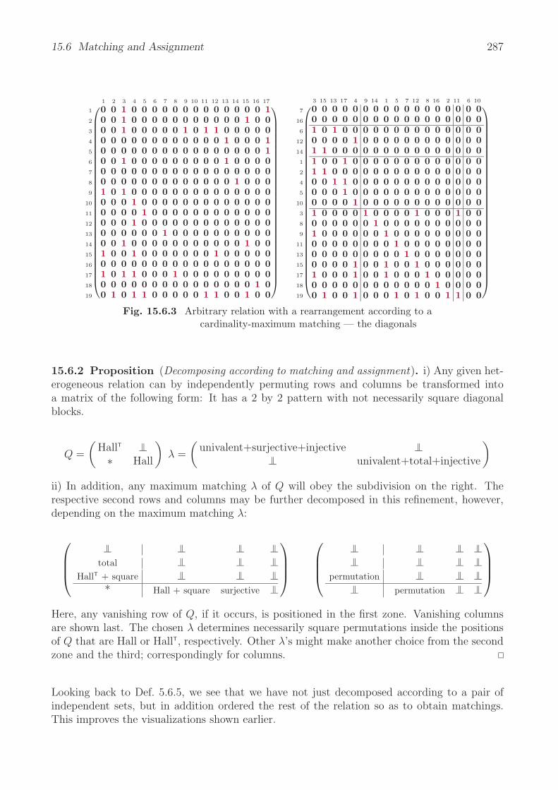
15.6 Matching and Assignment 287
1 2 3 4 5 6 7 8 9 10 11 12 13 14 15 16 17
1
2
3
4
5
6
7
8
9
10
11
12
13
14
15
16
17
18
19
⎛⎜⎜⎜⎜⎜⎜⎜⎜⎜⎜⎜⎜⎜⎜⎜⎜⎜⎜⎜⎜⎜⎜⎜⎜⎜⎜⎜⎜⎝
0 0 1 0 0 0 0 0 0 0 0 0 0 0 0 0 10 0 1 0 0 0 0 0 0 0 0 0 0 0 1 0 00 0 1 0 0 0 0 0 1 0 1 1 0 0 0 0 00 0 0 0 0 0 0 0 0 0 0 0 1 0 0 0 10 0 0 0 0 0 0 0 0 0 0 0 0 0 0 0 10 0 1 0 0 0 0 0 0 0 0 0 1 0 0 0 00 0 0 0 0 0 0 0 0 0 0 0 0 0 0 0 00 0 0 0 0 0 0 0 0 0 0 0 0 1 0 0 01 0 1 0 0 0 0 0 0 0 0 0 0 0 0 0 00 0 0 1 0 0 0 0 0 0 0 0 0 0 0 0 00 0 0 0 1 0 0 0 0 0 0 0 0 0 0 0 00 0 0 1 0 0 0 0 0 0 0 0 0 0 0 0 00 0 0 0 0 0 1 0 0 0 0 0 0 0 0 0 00 0 1 0 0 0 0 0 0 0 0 0 0 0 1 0 01 0 0 1 0 0 0 0 0 0 0 1 0 0 0 0 00 0 0 0 0 0 0 0 0 0 0 0 0 0 0 0 01 0 1 1 0 0 0 1 0 0 0 0 0 0 0 0 00 0 0 0 0 0 0 0 0 0 0 0 0 0 0 1 00 1 0 1 1 0 0 0 0 0 1 1 0 0 1 0 0
⎞⎟⎟⎟⎟⎟⎟⎟⎟⎟⎟⎟⎟⎟⎟⎟⎟⎟⎟⎟⎟⎟⎟⎟⎟⎟⎟⎟⎟⎠
3 15 13 17 4 9 14 1 5 7 12 8 16 2 11 6 10
7
16
6
12
14
1
2
4
5
10
3
8
9
11
13
15
17
18
19
⎛⎜⎜⎜⎜⎜⎜⎜⎜⎜⎜⎜⎜⎜⎜⎜⎜⎜⎜⎜⎜⎜⎜⎜⎜⎜⎜⎜⎜⎝
0 0 0 0 0 0 0 0 0 0 0 0 0 0 0 0 00 0 0 0 0 0 0 0 0 0 0 0 0 0 0 0 01 0 1 0 0 0 0 0 0 0 0 0 0 0 0 0 00 0 0 0 1 0 0 0 0 0 0 0 0 0 0 0 01 1 0 0 0 0 0 0 0 0 0 0 0 0 0 0 01 0 0 1 0 0 0 0 0 0 0 0 0 0 0 0 01 1 0 0 0 0 0 0 0 0 0 0 0 0 0 0 00 0 1 1 0 0 0 0 0 0 0 0 0 0 0 0 00 0 0 1 0 0 0 0 0 0 0 0 0 0 0 0 00 0 0 0 1 0 0 0 0 0 0 0 0 0 0 0 01 0 0 0 0 1 0 0 0 0 1 0 0 0 1 0 00 0 0 0 0 0 1 0 0 0 0 0 0 0 0 0 01 0 0 0 0 0 0 1 0 0 0 0 0 0 0 0 00 0 0 0 0 0 0 0 1 0 0 0 0 0 0 0 00 0 0 0 0 0 0 0 0 1 0 0 0 0 0 0 00 0 0 0 1 0 0 1 0 0 1 0 0 0 0 0 01 0 0 0 1 0 0 1 0 0 0 1 0 0 0 0 00 0 0 0 0 0 0 0 0 0 0 0 1 0 0 0 00 1 0 0 1 0 0 0 1 0 1 0 0 1 1 0 0
⎞⎟⎟⎟⎟⎟⎟⎟⎟⎟⎟⎟⎟⎟⎟⎟⎟⎟⎟⎟⎟⎟⎟⎟⎟⎟⎟⎟⎟⎠
Fig. 15.6.3 Arbitrary relation with a rearrangement according to acardinality-maximum matching — the diagonals
15.6.2 Proposition (Decomposing according to matching and assignment). i) Any given het-erogeneous relation can by independently permuting rows and columns be transformed intoa matrix of the following form: It has a 2 by 2 pattern with not necessarily square diagonalblocks.
Q =
(HallT
∗ Hall
)λ =
(univalent+surjective+injective
univalent+total+injective
)
ii) In addition, any maximum matching λ of Q will obey the subdivision on the right. Therespective second rows and columns may be further decomposed in this refinement, however,depending on the maximum matching λ:
⎛⎜⎜⎝ total
HallT + square* Hall + square surjective
⎞⎟⎟⎠
⎛⎜⎜⎝ permutation
permutation
⎞⎟⎟⎠
Here, any vanishing row of Q, if it occurs, is positioned in the first zone. Vanishing columnsare shown last. The chosen λ determines necessarily square permutations inside the positionsof Q that are Hall or HallT, respectively. Other λ’s might make another choice from the secondzone and the third; correspondingly for columns.
Looking back to Def. 5.6.5, we see that we have not just decomposed according to a pair ofindependent sets, but in addition ordered the rest of the relation so as to obtain matchings.This improves the visualizations shown earlier.
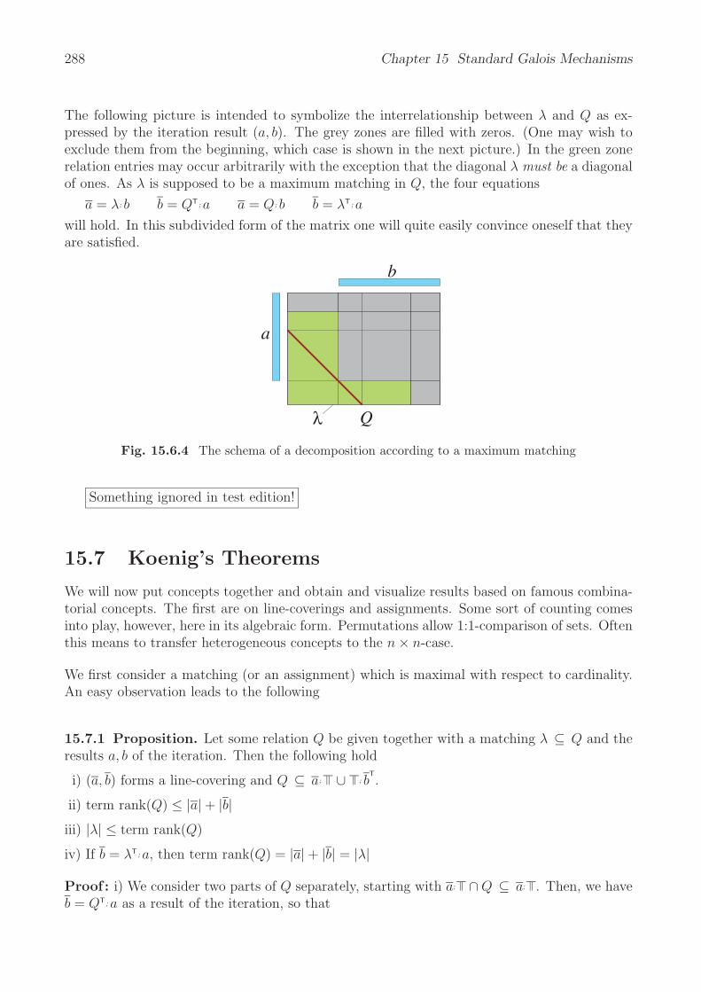
288 Chapter 15 Standard Galois Mechanisms
The following picture is intended to symbolize the interrelationship between λ and Q as ex-pressed by the iteration result (a, b). The grey zones are filled with zeros. (One may wish toexclude them from the beginning, which case is shown in the next picture.) In the green zonerelation entries may occur arbitrarily with the exception that the diagonal λ must be a diagonalof ones. As λ is supposed to be a maximum matching in Q, the four equations
a = λ; b b = QT; a a = Q; b b = λT; a
will hold. In this subdivided form of the matrix one will quite easily convince oneself that theyare satisfied.
a
b
Qλ
Fig. 15.6.4 The schema of a decomposition according to a maximum matching
Something ignored in test edition!
15.7 Koenig’s Theorems
We will now put concepts together and obtain and visualize results based on famous combina-torial concepts. The first are on line-coverings and assignments. Some sort of counting comesinto play, however, here in its algebraic form. Permutations allow 1:1-comparison of sets. Oftenthis means to transfer heterogeneous concepts to the n × n-case.
We first consider a matching (or an assignment) which is maximal with respect to cardinality.An easy observation leads to the following
15.7.1 Proposition. Let some relation Q be given together with a matching λ ⊆ Q and theresults a, b of the iteration. Then the following hold
i) (a, b) forms a line-covering and Q ⊆ a; ∪ ; bT.
ii) term rank(Q) ≤ |a| + |b|iii) |λ| ≤ term rank(Q)
iv) If b = λT; a, then term rank(Q) = |a| + |b| = |λ|
Proof : i) We consider two parts of Q separately, starting with a; ∩ Q ⊆ a; . Then, we haveb = QT; a as a result of the iteration, so that
15.7 Koenig’s Theorems 289
a; ∩ Q ⊆ (a ∩ Q;T); ( ∩ aT; Q) ⊆ ; aT; Q = ; b
T
ii) According to (i), the rows of a together with the columns of b cover all of Q, so that theterm rank cannot be strictly above the sum of the cardinalities.
iii) A line-covering of a matching λ can obviously not be achieved with less than |λ| lines. Thematching properties λT;λ ⊆ , λ;λT ⊆ of univalency and injectivity require that every entryof λ be covered by a separate line.
iv) Condition b = λT ; a together with a = λ ; b shows that |b| entries of λ are needed to endin b and |a| to start in a. According to injectivity no entry of λ will start in a and end in bas λ ; b = λ ; λT ; a ⊆ a. Therefore, |a| + |b| ≤ |λ|, which in combination with (ii,iii) leads toequality.
The following is an easy consequence which sometimes is formulated directly as a result.
15.7.2 Corollary (Konig-Egervary-Theorem). For an arbitrary heterogeneous relation wehave that the maximum cardinality of a matching equals the minimum cardinality of a line-covering.
We now specialize to the homogeneous case and investigate what happens when the term rankof a homogeneous relation is less than n.
15.7.3 Proposition (Frobenius-Konig; see [BR96] 2.1.4 ). For a finite homogeneous relationQ the following are equivalent:
i) None of all permutations P satisfies P ⊆ Q.
ii) There exists a pair of sets a, b such that a, b is a line-covering with |a| + |b| < n, orequivalently, a, b is an independent pair of sets with n < |a| + |b|, or equivalently termrank < n.
iii) There exists a vector z together with a permutation P such that QT ; z ⊂=/ P ; z. In other
words: There exists a subset z which is mapped by Q onto a set with strictly fewerelements than z.
Proof: (i) =⇒ (ii): Find a maximum cardinality matching λ ⊆ Q and execute the assignmentiteration on page 285. It will end in a, b with |a|+ |b| = |λ| < n as λ can by assumption not bea permutation.
(ii) =⇒ (iii): Take z := a, which satisfies QT ; a = b according to the iteration. Then |b| =n − |b| < |a|.(iii) =⇒ (i): When (iii) holds, Q violates the Hall condition for the subset z. If there were apermutation P contained in Q, we would have QT;z ⊇ P T;z, and thus |QT;z| ≥ |P T;z| = |z|, acontradiction.
Something ignored in test edition!

290 Chapter 15 Standard Galois Mechanisms

Part V
Advanced Topics
291


293
Beyond what has so far been shown exist further fascinating areas. Demonics assist specifi-cation. While standard relation algebra formulates what has to be related, here only an areais circumscribed within which the relation envisaged shall be confined. Implication structuresstudy long-range implications, preferably with only few alternatives. Partialities open a com-pletely new field, that possibly helps formulate net construction. With relational grammarit has been shown that the translation of relations of time, possession, or modality, e.g., innatural languages may be handled when translating to another one. Spatial reasoning has longactivated relation algebra in order to reason about relative situatedness of items.

294
16 Demonics
One line of investigation with a considerable amount of scientific publications is that concerningrefinement orderings. It deals with nondeterministic specifications as a means of freeing spec-ifications from being unnecessarily restrictive. It is intended to model the so-called demonicsemantics. Therefore specific operators are introduced.
16.1 Demonic Operators
In the context of developing provably correct software, one important approach is that ofdeveloping programs from specifications by stepwise refinement, originally proposed by NiklasWirth. The most wide-spread view of a specification is that of a relation constraining theinput-output (resp. argument-result) behaviour of the program envisaged. Relations stand fornon-deterministic programs; so one branch may terminate, while others do not. This makesthese considerations difficult. Different points of view are taken and different kinds of operationshave been classified into demonic, angelic and erratic variants.
A frequently followed idea in mathematical program construction is that of development bysuccessive refinement. One hesitates to overspecify in early stages of the programming process.So one starts with relations and only later makes them narrower and narrower so as to possiblyarrive at a function. Therefore a concept of refinement is necessary.
The demonic interpretation of non-determinism turns out to closely correspond to the conceptof under-specification, and therefore the demonic operations are used in most specification andrefinement calculi. The demonic calculus of relations views any relation R from a set A toanother set B as specifying those programs that terminate for all a ∈ A wherever R associatesany values from B with a, and then the program may only return values b for which (a, b) ∈ R.Consequently, a relation R refines another relation S precisely when the domain of definition ofS is contained in that of R, and if R restricted to the domain of definition of S is contained inS. It is intended to model demonic semantics: What may go wrong will go wrong! see above!!!
By Desharnais and his coworkers, the demonic calculus of relations has in 1995 been shownto be equivalent to the popular approach of C. A. R. Hoare and Jifeng He, where unspecifiedbehaviour is denoted by an extra bottom element. The classical relational composition as suchcorresponds to angelic what is that? non-determinism.
In comparison with the approach of Hoare, He, the demonic calculus of relations has the ad-vantage that the demonic operations are defined on top of the conventional relation algebraicoperations, and can easily and usefully be mixed with the latter, allowing application of nu-merous algebraic properties.
295

296 Chapter 16 Demonics
R• := R ∪ R; totalisationObviously, R ⊆ R• % R
16.1.1 Definition. We say that relation R refines some relation S, denoted R % S, by
R % S :⇐⇒ R ∩ S ; ⊆ S and S ; ⊆ R; :⇐⇒ R ∩ S ; ⊆ S ⊆ R;
If the domains of the two relations are equal, i.e., R; = S ; (in particular, if R and S aretotal), then refinement is equivalent to inclusion.
In other words, R % s if R terminates where S is defined, but R may have less non-determinismthatn S. Where non-termination is allowed, any result is allowed.
Using R, no possible observation shows that we are not using S. Observation means resultdelivered from some input.
R =
1 2 3 4 5 6 7 8 9 10 11
MondayTuesday
WednesdayThursday
FridaySaturday
Sunday
⎛⎜⎜⎜⎜⎜⎜⎝
0 0 0 0 0 0 1 0 0 0 00 0 0 0 1 0 0 0 0 0 01 0 1 0 0 0 1 0 0 0 00 0 0 0 0 1 0 1 0 0 00 0 0 0 0 1 0 0 0 0 00 0 0 0 0 0 0 0 0 0 00 0 0 0 1 1 0 0 0 0 1
⎞⎟⎟⎟⎟⎟⎟⎠
S =
1 2 3 4 5 6 7 8 9 10 11
MondayTuesday
WednesdayThursday
FridaySaturday
Sunday
⎛⎜⎜⎜⎜⎜⎜⎝
0 0 0 0 0 0 1 0 0 0 00 0 0 0 0 0 0 0 0 0 01 0 1 0 0 0 1 0 0 0 00 0 0 0 0 0 0 0 0 0 00 0 0 1 0 1 0 0 0 0 00 0 0 0 0 0 0 0 0 0 00 0 0 0 1 1 1 0 0 0 1
⎞⎟⎟⎟⎟⎟⎟⎠
R & S
1 2 3 4 5 6 7 8 9 10 11
MondayTuesday
WednesdayThursday
FridaySaturday
Sunday
⎛⎜⎜⎜⎜⎜⎜⎝
0 0 0 0 0 0 1 0 0 0 00 0 0 0 0 0 0 0 0 0 01 0 1 0 0 0 1 0 0 0 00 0 0 0 0 0 0 0 0 0 00 0 0 1 0 1 0 0 0 0 00 0 0 0 0 0 0 0 0 0 00 0 0 0 1 1 1 0 0 0 1
⎞⎟⎟⎟⎟⎟⎟⎠
R ' S
1 2 3 4 5 6 7 8 9 10 11
MondayTuesday
WednesdayThursday
FridaySaturday
Sunday
⎛⎜⎜⎜⎜⎜⎜⎝
0 0 0 0 0 0 1 0 0 0 00 0 0 0 1 0 0 0 0 0 01 0 1 0 0 0 1 0 0 0 00 0 0 0 0 1 0 1 0 0 00 0 0 0 0 1 0 0 0 0 00 0 0 0 0 0 0 0 0 0 00 0 0 0 1 1 0 0 0 0 1
⎞⎟⎟⎟⎟⎟⎟⎠
RT S =
1 2 3 4 5 6 7 8 9 10 11
123456789
1011
⎛⎜⎜⎜⎜⎜⎜⎜⎜⎜⎜⎜⎜⎜⎝
1 0 1 0 0 0 1 0 0 0 00 0 0 0 0 0 0 0 0 0 01 0 1 0 0 0 1 0 0 0 00 0 0 0 0 0 0 0 0 0 00 0 0 0 0 0 0 0 0 0 00 0 0 0 0 0 0 0 0 0 01 0 1 0 0 0 1 0 0 0 00 0 0 0 0 0 0 0 0 0 00 0 0 0 0 0 0 0 0 0 00 0 0 0 0 0 0 0 0 0 00 0 0 0 1 1 1 0 0 0 1
⎞⎟⎟⎟⎟⎟⎟⎟⎟⎟⎟⎟⎟⎟⎠
R ST =
Mon
day
Tue
sday
Wed
nesd
ayT
hurs
day
Frid
aySa
turd
aySu
nday
MondayTuesday
WednesdayThursday
FridaySaturday
Sunday
⎛⎜⎜⎜⎜⎜⎜⎝
1 0 1 0 0 0 10 0 0 0 0 0 11 0 1 0 0 0 10 0 0 0 0 0 00 0 0 0 1 0 10 0 0 0 0 0 00 0 0 0 1 0 1
⎞⎟⎟⎟⎟⎟⎟⎠
This refinement ordering easily turns out to be a preorder, and one can do a lot of nice math-ematics around this idea. A complete new line of operators, the demonic ones, appear:
16.1.2 Definition. Let two relations R, S be given.
i) The least upper bound of relations R and S with respect to % , denoted by R & S andcalled the demonic join, is
R & S = (R ∪ S) ∩ R; ∩ S ;
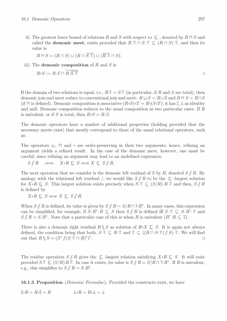
16.1 Demonic Operators 297
ii) The greatest lower bound of relations R and S with respect to % , denoted by R ' S andcalled the demonic meet, exists provided that R; ∩ S ; ⊆ (R ∩ S); , and then itsvalue is
R ' S = (R ∩ S) ∪ (R ∩ S ; ) ∪ (R; ∩ S).
iii) The demonic composition of R and S is
R S := R; S ∩ R; S ;
If the domain of two relations is equal, i.e., R; = S; (in particular, if R and S are total), thendemonic join and meet reduce to conventional join and meet: R & S = R∪S and R ' S = R∩S(if ' is defined). Demonic composition is associative (R S) T = R (S T ); it has , as identityand null. Demonic composition reduces to the usual composition in two particular cases: If Ris univalent, or if S is total, then R S = R; S.
The demonic operators have a number of additional properties (holding provided that thenecessary meets exist) that mostly correspond to those of the usual relational operators, suchas:
The operators & , ' and are order-preserving in their two arguments; hence, refining anargument yields a refined result. In the case of the demonic meet, however, one must becareful, since refining an argument may lead to an undefined expression.
S // R :⇐⇒ X R % S ⇐⇒ X % S // R.
The next operation that we consider is the demonic left residual of S by R, denoted S // R. Byanalogy with the relational left residual /, we would like S // R to be the % -largest solutionfor X R % S. This largest solution exists precisely when S ; ⊆ (S/R); R; and then, S // Ris defined by
X R % S ⇐⇒ X % S // R.
When S // R is defined, its value is given by S // R = S/R∩ ;RT. In many cases, this expressioncan be simplified; for example, if S ; RT ; R ⊆ S then S // R is defined iff S ; ⊆ S ; RT ; andS // R = S ; RT. Note that a particular case of this is when R is univalent (RT; R ⊆ ).
There is also a demonic right residual R \\S as solution of R X % S. It is again not alwaysdefined, the condition being that both, S ; ⊆ R; and ⊆ ((R ∩ S ; ) // S); . We will findout that R \\S = (ST //(S ; ∩ R)T)T.
The residue operation S // R gives the % -largest relation satisfying X R % S. It will existprovided S; % (S/R);R; . In case it exists, its value is S // R = S/R∩ ;RT. If R is univalent,e.g., this simplifies to S // R = S ; RT.
16.1.3 Proposition (Demonic Formulae). Provided the constructs exist, we have
R = R = R R = R =

298 Chapter 16 Demonics
S % T =⇒ R S % R TS % T =⇒ S R % T R
R (S & T ) = R S & R T(S & T ) R = S R & T R
R (S ' T ) % R S ' R T(S ' T ) R % S R ' T R
R '(S & T ) = (R ' S) &(R ' T )R &(S ' T ) = (R & S) '(R & T )
The following implications holdR ' S &(R ' T ) defined =⇒ R '(S & T ) definedR &(S ' T ) defined =⇒ (R & S) '(R & T ) definedR (S ' T ) defined =⇒ (R S) '(R T ) defined(S ' T ) R defined =⇒ (S R) '(T R) defined
The operators & , ' , are monotonic with respect to both of their arguments. Refining oneof the arguments will, thus, result in refinement of the result. The demonic meet offers minorproblems as one has in addition to check whether it is defined. Refining an argument may leedto an undefined result.
Demonic Residuals
Demonic residuals are formed in a way reminiscent of the normal residuals.
R % S =⇒ R // T % S // TR % S =⇒ T // S % T // R
(R // S) S % R (R // R) R = R R (R \\R) = R % (R \\R)
(R // S) // T = R //(T S)
(R ' S) // T = (R // T ) '(S // T )
R //(S & T ) = (R // S) '(R // T )
(R // S) (S // T ) % R // T
(R \\S) (S \\T ) % R \\T
(R \\R) is alqays defined
R; RT; R ⊆ R =⇒ (R \\R) = RT; R
This has been put forward so as to have also programming constructs, and coming close to aprogramming methodology. It is, however, not yet a software engineering methodology.
The following properties of left residuals hold provided that the partial operations are defined:

16.1 Demonic Operators 299
In a similar fashion, one defines the demonic right residual of S by R, denoted by R \\S, as the% -largest solution for R X % S. In other words, R X % S ⇐⇒ X % R \\S. The demonicright residual has properties dual to those given in the left residual. Like the demonic leftresidual, it is not always defined, but only if S ; % R; and % ((R ∩ S ; )\S); , and thenits value is given by R \\S = (ST //(S ; ∩ R)T)T.
In the very last days, I have read a paper on a large scale project in US aircraft industry.The task was to study requirements of a fault tolerant flight control system with sensors andactuators and flow of information between these units. They had to discuss fail operationalund fail passive situations of redundancy to guarantee safe operation whenever no more thanone item went wrong. They also discussed why other available specification tools would not becapable of executing such investigations. They had to start out from 25 years old plain-Englishspecifications.
Exercises
2.4.4 Prove that demonic composition R S = R; S ∩ R; S ; is an associative operation.
Solution 2.4.4 ???
4.2.3 Prove that F G is a mapping if F and G are.
Solution 4.2.3 ???
10.4.1 Prove for demonic composition R S = R; S ∩ R; S ; (see Exercise 2.4.4) thatwp(R, wp(S, n)) = wp(R S, n).
Solution 10.4.1 We use Prop. 2.4.2 to get wp((R S, n)
)= (R S) ∩ (R S)n =
(R; S ∩ R; S ; ); ∩ (R; S ∩ R; S ; )n = R; S ; ∩ R; S ; ∩ R; S ; n ∩ R; S ; =
R; S ; ∩ [(R; S ; ∩ R; S ; n) ∪ (R; S ; ∩ R; S ; )] = R; S ; ∩ R; S ; ∩ R; S ; n.
And, on the other hand wp(R, wp(S, n)) = R; ∩ R; (S ; ∩ S ; n) =
R; ∩ R; S ; ∪ R; S ; n = R; ∩ R; S ; ∩ R; S ; n. ?

300 Chapter 16 Demonics

17 Implication Structures
What is here called an implication structure is an abstraction of situations that occur frequently:One is given a set of conflicting alternatives and the task to choose among them as many non-conflicting ones as possible. This runs then also under names such as attribute dependencysystem. The criteria to observe include choices that forbid others to choose. Sometimes onechoice implies that another choice be taken. Situations as described occur not least whenconstructing a timetable. They describe, however, also how one tries to learn from a chunk ofraw data in machine learning.
17.1 Dependency Systems
We assume an implication situation where we have a set of items that may imply (enforce),forbid, or counterimply one another. The task is to select a subset such that all the givenpostulates are satisfied.
In order to model this, let a base set N be given. What we are looking for are subsets s ⊆ Nsatisfying whatever has been demanded as implication concerning two elements i, k ∈ N :
si → sk, si → ¬sk, ¬si → sk
Subsets s are here conceived as boolean vectors s ∈ IBN . Therefore, si is shorthand for i ∈ s.Enforcing, forbidding, and counter-enforcing are conceived to be given as relations E, F, C ⊆N × N .
An arbitrary subset may either satisfy the implicational requirements or may not. We are usu-ally not interested in all solutions, much in the same way as one timetable satisfying formulatedrequirements will suffice.For a theoretical investigation, we consider the set S ⊆ P(N) of all subsets fulfilling the givenpostulates, the possible solutions for the postulated set of implications. They satisfy, thus,
∀s ∈ S : si → sk if (i, k) ∈ E (∗)∀s ∈ S : si → ¬sk if (i, k) ∈ F (†)∀s ∈ S : ¬si → sk if (i, k) ∈ C (‡)
∀i ∈ N : ∀k ∈ N : Ei,k → (∀s ⊆ N : si → sk)a → b = a ∪ b
∀i ∈ N : ∀k ∈ N : Ei,k ∪ (∀s ⊆ N : sk ∪ si)
¬∃k ∈ N : p(k) = ∀k ∈ N : p(k)
301
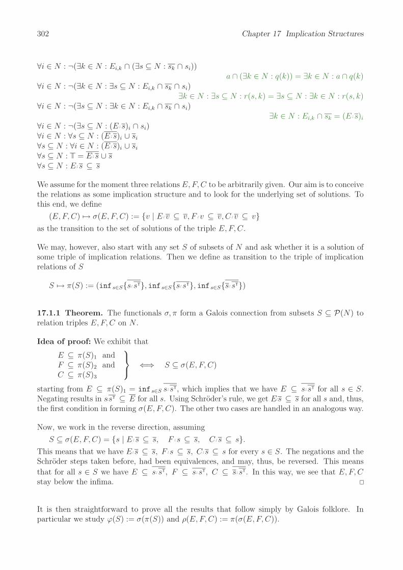
302 Chapter 17 Implication Structures
∀i ∈ N : ¬(∃k ∈ N : Ei,k ∩ (∃s ⊆ N : sk ∩ si))a ∩ (∃k ∈ N : q(k)) = ∃k ∈ N : a ∩ q(k)
∀i ∈ N : ¬(∃k ∈ N : ∃s ⊆ N : Ei,k ∩ sk ∩ si)∃k ∈ N : ∃s ⊆ N : r(s, k) = ∃s ⊆ N : ∃k ∈ N : r(s, k)
∀i ∈ N : ¬(∃s ⊆ N : ∃k ∈ N : Ei,k ∩ sk ∩ si)∃k ∈ N : Ei,k ∩ sk = (E ; s)i
∀i ∈ N : ¬(∃s ⊆ N : (E ; s)i ∩ si)∀i ∈ N : ∀s ⊆ N : (E ; s)i ∪ si
∀s ⊆ N : ∀i ∈ N : (E ; s)i ∪ si
∀s ⊆ N : = E ; s ∪ s∀s ⊆ N : E ; s ⊆ s
We assume for the moment three relations E, F, C to be arbitrarily given. Our aim is to conceivethe relations as some implication structure and to look for the underlying set of solutions. Tothis end, we define
(E, F, C) → σ(E, F, C) := v | E ; v ⊆ v, F ; v ⊆ v, C ; v ⊆ vas the transition to the set of solutions of the triple E, F, C.
We may, however, also start with any set S of subsets of N and ask whether it is a solution ofsome triple of implication relations. Then we define as transition to the triple of implicationrelations of S
S → π(S) := (inf s∈Ss; sT, inf s∈Ss; sT, inf s∈Ss; sT)
17.1.1 Theorem. The functionals σ, π form a Galois connection from subsets S ⊆ P(N) torelation triples E, F, C on N .
Idea of proof: We exhibit that
E ⊆ π(S)1 andF ⊆ π(S)2 andC ⊆ π(S)3
⎫⎬⎭ ⇐⇒ S ⊆ σ(E, F, C)
starting from E ⊆ π(S)1 = inf s∈S s; sT, which implies that we have E ⊆ s; sT for all s ∈ S.Negating results in s;sT ⊆ E for all s. Using Schroder’s rule, we get E;s ⊆ s for all s and, thus,the first condition in forming σ(E, F, C). The other two cases are handled in an analogous way.
Now, we work in the reverse direction, assuming
S ⊆ σ(E, F, C) = s | E ; s ⊆ s, F ; s ⊆ s, C ; s ⊆ s.This means that we have E;s ⊆ s, F ;s ⊆ s, C;s ⊆ s for every s ∈ S. The negations and theSchroder steps taken before, had been equivalences, and may, thus, be reversed. This means
that for all s ∈ S we have E ⊆ s; sT, F ⊆ s; sT, C ⊆ s; sT. In this way, we see that E, F, Cstay below the infima.
It is then straightforward to prove all the results that follow simply by Galois folklore. Inparticular we study ϕ(S) := σ(π(S)) and ρ(E, F, C) := π(σ(E, F, C)).

17.1 Dependency Systems 303
• ρ and ϕ are expanding, i.e.,
E ⊆ π1(σ(E, F, C)), F ⊆ π2(σ(E, F, C)), C ⊆ π3(σ(E, F, C)),
and in addition S ⊆ σ(π(S)) for all E, F, C, and S
• ρ and ϕ are idempotent, i.e., ρ(E, F, C) = ρ(ρ(E, F, C)), and in addition ϕ(S) = ϕ(ϕ(S))for all E, F, C, and S.
• ρ, ϕ are monotonic and, thus, closure operations.
• There exist fixpoints for ρ, ϕ.
• The fixpoint sets with regard to ρ, ϕ are mapped antitonely onto one another.
17.1.2 Theorem. All the fixedpoints of the Galois connection satisfy
i) F = F T, C = CT
ii) ⊆ E = E2
iii) E ; F = F, C ; E = Civ) F ; C ⊆ E
Proof: We immediately see that the second as well as the third component of π(S) are sym-
metric by definition. ⊆ E as obviously ⊆ s; sT for all s.
Transitivity of E follows as s; sT ; s; sT ⊆ s; sT and since transitivity is ∩-hereditary. Similarly,for F and C in (iii) and for (iv).
The enforcing relation E of a fixpoint is, thus, a preorder. While these properties concernednon-negated implications relations, there are others including also negated ones.
17.1.3 Corollary. The fixedpoints of the Galois connection satisfy in addition
i) E ; C = C, F ; E = Fii) C ; C ⊆ E, E ; C ⊆ Fiii) F ; F ⊆ E, F ; E ⊆ C
Now we consider closure forming
S → ϕ(S) and (E, F, C) → ρ(E, F, C)
from a computational point of view. While it seems possible to handle three n × n-matricesE, F, C for rather big numbers n in a relation-algebraic way with Relview (see [BSW03], e.g.),it will soon become extremely difficult to determine vectors of length n satisfying certain givenimplications. While we do not see enough mathematical structure on the S-side, the formulaejust proved on the (E, F, C)-side may be helpful.

304 Chapter 17 Implication Structures
Therefore, we try to determine for given elementary implication matrices (E, F, C) their impli-cation closure ρ(E, F, C). In case there exist very long chains of implications, it may well bethe case that the closure ρ(E, F, C) makes it easier to determine a solution S by applying thefollowing concepts.
The structure of the definition of implication relations leads us to call i ∈ N
a tight element with respect to S if CS(i, i) = 1 ,
a pseudo element if FS(i, i) = 1 ,
otherwise it is called a flexible element.
The names are derived from the instantiations of (†, ‡) for k := i:
∀s ∈ S : si → ¬si if (i, i) ∈ FS, meaning ∀s ∈ S : ¬si
∀s ∈ S : ¬si → si if (i, i) ∈ CS, meaning ∀s ∈ S : si
So, for every 1 in the diagonal of C, the corresponding element must and for every 1 in thediagonal of F , it must not belong to any solution s ∈ S. These facts together with all theirimplications according to E, F, C may be helpful in looking for solutions S.
Implication matrices are only interesting modulo the equivalence E ∩ ET derived from thepreorder E. It is an easy consequence that by simultaneous permutation of rows and columnsevery triple of implication matrices may be arranged in the following standard form of row andcolumn groups. An example may be found in the illustrating closure matrices of Sect. 3, whichare here given in reordered form.
E =
⎛⎝ E0
⎞⎠ , F =
⎛⎝ F0
⎞⎠ , C =
⎛⎝ C0
⎞⎠
All rows corresponding to tight elements are positioned as the first group of rows, followed bythe group of rows corresponding to flexible elements, and those for pseudo elements. E0, F0, C0
satisfy some additional rules.
1 2 3 4 5 6 71234567
⎛⎜⎜⎜⎜⎜⎜⎝
1 1 1 1 1 1 11 1 1 1 1 1 10 0 1 0 0 1 10 0 0 1 0 1 10 0 0 0 1 1 10 0 0 0 0 1 10 0 0 0 0 1 1
⎞⎟⎟⎟⎟⎟⎟⎠
1 2 3 4 5 6 71234567
⎛⎜⎜⎜⎜⎜⎜⎝
1 1 1 1 1 1 11 1 1 1 1 1 11 1 0 1 0 0 01 1 1 0 0 0 01 1 0 0 0 0 01 1 0 0 0 0 01 1 0 0 0 0 0
⎞⎟⎟⎟⎟⎟⎟⎠
1 2 3 4 5 6 71234567
⎛⎜⎜⎜⎜⎜⎜⎝
0 0 0 0 0 1 10 0 0 0 0 1 10 0 0 0 1 1 10 0 0 0 0 1 10 0 1 0 0 1 11 1 1 1 1 1 11 1 1 1 1 1 1
⎞⎟⎟⎟⎟⎟⎟⎠
There is one further idea. E is a preorder according to Thm. 17.1.2. One may ask which influ-ence it has for the necessarily heuristic algorithm when one chooses minimal/maximal elementsto be handled first. Selecting minimal elements with regard to E first, makes fundamentaldecisions early in a backtracking algorithm. It may, however, also be wise, to assign maximalelements first. Then some freedom is still left to assign the others — and to fit to criteria notyet formalized.
Considering Thm. 17.1.2, one will easily suggest to apply round-robinwise the following stepsuntil a stable situation is reached:
• determine the reflexive-transive closure of E

17.1 Dependency Systems 305
• determine the symmetric closure of F and C
• expand F to E ; F and C to C ; E
• add F ; C to E
17.1.4 Example. A nice example of an implication structure is given by one of the popu-lar Sudoku puzzles. A table of 9 × 9 squares is given, partially filled with natural numbers1, 2, 3, 4, 5, 6, 7, 8, 9, that shall be completely filled. The problem is that one is neither allowedto enter the same number twice in a row or column nor that one is allowed to enter duplicatesin the nine 3 × 3 subsquares.
Sudokus published in a newspaper typically allow for just one solution. In general, there maybe none or many. Often the first steps are rather trivial; looking from position i, k to row i andalso column k as well as to subsquare s, one may find out that already 8 of the nine numbershave been used. It is then obvious that the nineth has to be entered in square i, k.
3 98 2 4
4 7 6 3
3 2 7 46 7
7 5 8 9
8 3 5 46 4 2
7 1
3 7 98 2 4
4 7 6 3
3 2 7 46 7
7 5 8 9
8 3 5 46 4 2
7 2 1
Fig. 17.1.1 A Sudoku puzzle and two immediate insertions
Something ignored in test edition!
Something ignored in test edition!

306 Chapter 17 Implication Structures

18 Partiality Structures
[Sch06]
Naiv konnte man meinen, die Realitat lasse sich bei genugend sorgfaltiger Beobachtung stetsvollkommen prazise erfassen. Aus der Physik wissen wir aber, daß eine solche Auffassungprinzipiell falsch ist. Bei sehr hohen Geschwindigkeiten entstehen relativistische Effekte. Beisehr kleinen Strukturen Quanteneffekte.
Eine besonders alltagliche Situation ergibt sich beim Versuch, ein Panorama großer Breite zufotografieren. Man bekommt es nicht auf ein Bild und knipst deshalb mehrere. Leider passensie dann niemals hundertprozentig zusammen. Auch Fotos von unserer Erde verhalten sichahnlich. Ein einziges kann nicht alles abbilden. Also fertigt man viele (Land-)Karten; diesebilden eventuelle Uberschneidungsgebiete verformt ab.
Wir akzeptieren als Standardsituation, daß sich Realitat (meist) nicht in voller Perfektionreprasentieren laßt, sondern nur in sich vielfaltig uberschneidenden Teil-Sichten. Wir habenfolglich das Schema zu lernen, wie die in mehreren Sichten auftretenden Details aufeinander zubeziehen sind. Man denke an uberlappende Landkarten mit unterschiedlichem Maßstab undunterschiedlicher Projektionsmethode.
see papers I and II
Product definitions have long been investigated by relation algebraists and computer scientists.A considerable part of [TG87] is devoted to various aspects of that. The concept of a productshould cover both aspects, Cartesian product as product of types or sets combined with tupeling(sometimes called construction) as product of operations. The following definition of a directproduct may be found, e.g., in [SS89, SS93]. It has been compared with other approaches toproducts in [BHSV94].It would even suffice to require only πT ; π ⊆ . Interpreting the condition π; πT ∩ ρ; ρT ⊆ inthe case of two sets A, B and their Cartesian product A × B, it ensures that there is at mostone pair with given images in A and B. In addition, “= ” means that π, ρ are total, i.e., thatthere are no “unprojected pairs”. Finally, the condition πT;ρ = implies that for every elementin A and every element in B there exists a pair in A × B.
It has always been felt that there is a specific problem when working with relations if productsare studied. This problem shows up in case of non-strictness. On one hand, the Cartesianproduct of sets is available. Considered from the viewpoint of semantics, it provides pairs ortuples which are needed for giving semantics. However, there is the drawback that forming theCartesian product of sets doesn’t result in a Cartesian product in the categorical sense becauseof some sort of a strict behaviour. For two relations R ⊆ A × B and S ⊆ A × C, we can formR; πT ∩ S ; ρT ⊆ A × (B × C), but (R; πT ∩ S ; ρT); π = R ∩ S ; .
307

308 Chapter 18 Partiality Structures
This means that the classical construction of the Cartesian product of two sets A, B andconsidering the relations between A, B, A × B does not lead to the situation that this is acategorical product. The concept of being categorical describes what is definitely needed fromthe various application sides and even from the purely mathematical point of view. For everypair R, S of relations from a set C to A and B, respectively, there shall exist precisely onerelation Q from C to A × B such that it factorizes to R, S, respectively, over the projections.
Something ignored in test edition!
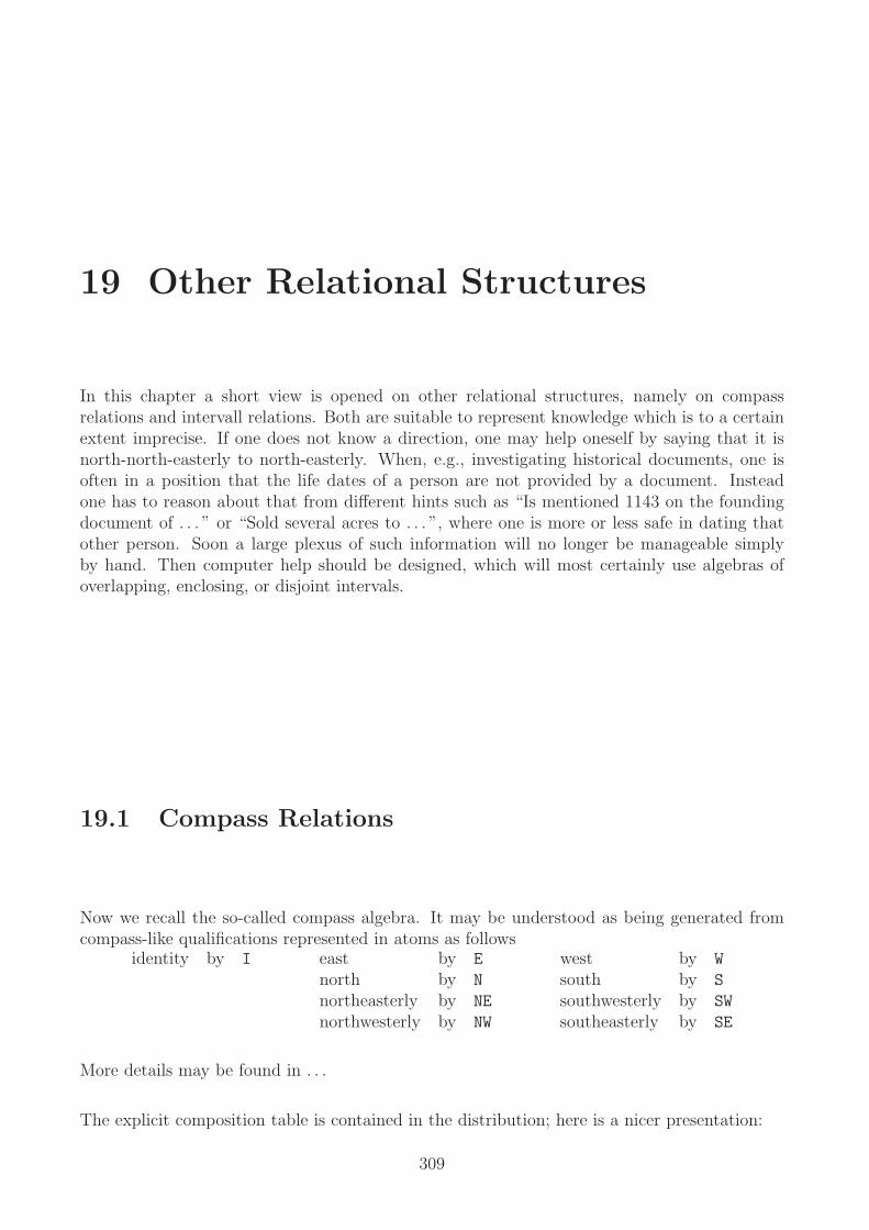
19 Other Relational Structures
In this chapter a short view is opened on other relational structures, namely on compassrelations and intervall relations. Both are suitable to represent knowledge which is to a certainextent imprecise. If one does not know a direction, one may help oneself by saying that it isnorth-north-easterly to north-easterly. When, e.g., investigating historical documents, one isoften in a position that the life dates of a person are not provided by a document. Insteadone has to reason about that from different hints such as “Is mentioned 1143 on the foundingdocument of . . . ” or “Sold several acres to . . . ”, where one is more or less safe in dating thatother person. Soon a large plexus of such information will no longer be manageable simplyby hand. Then computer help should be designed, which will most certainly use algebras ofoverlapping, enclosing, or disjoint intervals.
19.1 Compass Relations
Now we recall the so-called compass algebra. It may be understood as being generated fromcompass-like qualifications represented in atoms as follows
identity by I east by E west by W
north by N south by S
northeasterly by NE southwesterly by SW
northwesterly by NW southeasterly by SE
More details may be found in . . .
The explicit composition table is contained in the distribution; here is a nicer presentation:
309
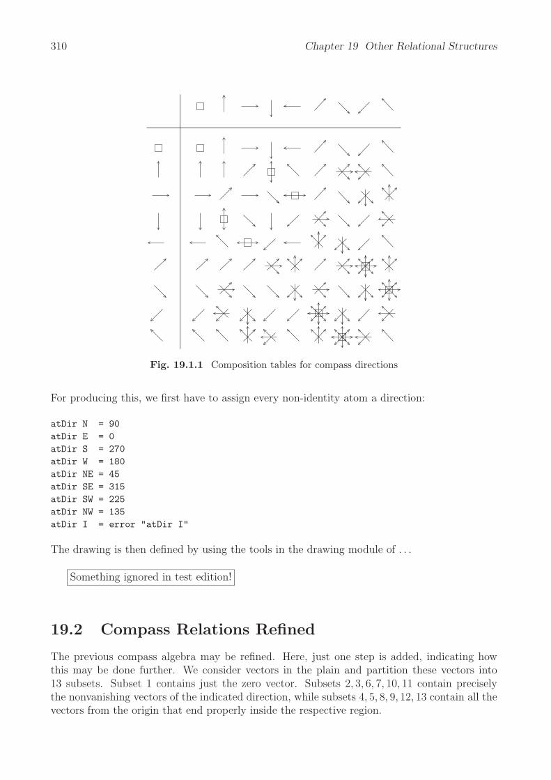
310 Chapter 19 Other Relational Structures
Fig. 19.1.1 Composition tables for compass directions
For producing this, we first have to assign every non-identity atom a direction:
atDir N = 90atDir E = 0atDir S = 270atDir W = 180atDir NE = 45atDir SE = 315atDir SW = 225atDir NW = 135atDir I = error "atDir I"
The drawing is then defined by using the tools in the drawing module of . . .
Something ignored in test edition!
19.2 Compass Relations Refined
The previous compass algebra may be refined. Here, just one step is added, indicating howthis may be done further. We consider vectors in the plain and partition these vectors into13 subsets. Subset 1 contains just the zero vector. Subsets 2, 3, 6, 7, 10, 11 contain preciselythe nonvanishing vectors of the indicated direction, while subsets 4, 5, 8, 9, 12, 13 contain all thevectors from the origin that end properly inside the respective region.

19.3 Interval Relations 311
106
2
117
5
9 13
13
12 8
4
Fig. 19.2.1 Compass directions refined
It may be understood as being generated from compass-like qualifications represented in atomsas follows:
As in the last example, we only show a graphical presentation of the composition table:
Fig. 19.2.2 Compass directions
Something ignored in test edition!
19.3 Interval Relations
The following algebra is well-known to specialists. A description may be found in the AMAST1993 invited talk of Roger Maddux.
For the interpretation of the algebra IA consider nonempty intervals on the real axis. Theymay be described by a pair of two different real numbers which we assume to be in ascending

312 Chapter 19 Other Relational Structures
order. The first gives the starting time of the interval and the second the ending time. Forsimplicity, we assume only intervals (x, y], i.e., left-open and right-closed.
On any given set of such intervals, we now consider the following relations together with theirconverses, if this is a different relation. Let the first interval be given by the pair (x, x′] andthe second by (y, y′].
1′ ≡ x = y and x′ = y′ ≡ “identity of intervals”p ≡ x′ < y ≡ “first interval stricly precedes the second”d ≡ y < x < x′ < y′ ≡ “first interval is bi-strictly contained in the second”o ≡ x < y < x′ < y′ ≡ “first interval is partly overlapped by the second”m ≡ x < x′ = y < y′ ≡ “first interval touches the second from the left”s ≡ x = y < x′ < y′ ≡ “first interval is strict initial part of the second”f ≡ y < x < x′ = y′ ≡ “first interval is strict terminal part of the second”
The interrelationship is then investigated by constructing a homogeneous relation algebra froma set of thirteen atoms induced by the above relations, using the following names:
data Atomset = I | P | Pc | D | Dc | O | Oc | M | Mc | S | Sc | F | Fcderiving (Eq, Ord, Show)
atoms = [I, P, Pc, D, Dc, O, Oc, M, Mc, S, Sc, F, Fc]
Exercises
19.4 Relational Grammar
The relational calculus is often termed as being “component-free”. Not least this propertymakes it suitable for application in linugistics.
We will here give a very limited account of this broad field. And even in this case it is difficultto convince others that it is useful to apply relations. Our test method will be whether itis possible to apply certain operators to the construct and obtain acceptable results. Suchoperators are, e.g., negation of sentences.
We will try to define some basic constructs and qualifications so that sevaral intuisticallyacceptable transformations of sentences result. More detailed explanations may be found inthe book [Bot99]
Something ignored in test edition!
Something ignored in test edition!

19.5 Mereology 313
19.5 Mereology
The first approach to mereology will now be refined by taking into account also that there maybe external contact (ec) between two items. So a fifth atom is added. Much of the compositionstables stays the same. One may say that a row and a column have to be added.
Something ignored in test edition!
Something ignored in test edition!

314 Chapter 19 Other Relational Structures
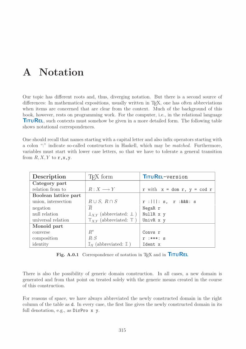
A Notation
Our topic has different roots and, thus, diverging notation. But there is a second source ofdifferences: In mathematical expositions, usually written in TEX, one has often abbreviationswhen items are concerned that are clear from the context. Much of the background of thisbook, however, rests on programming work. For the computer, i.e., in the relational languageTITUREL, such contexts must somehow be given in a more detailed form. The following tableshows notational correspondences.
One should recall that names starting with a capital letter and also infix operators starting witha colon “:” indicate so-called constructors in Haskell, which may be matched. Furthermore,variables must start with lower case letters, so that we have to tolerate a general transitionfrom R, X, Y to r,x,y.
Description TEX form TITUREL-versionCategory partrelation from to R : X −→ Y r with x = dom r, y = cod r
Boolean lattice partunion, intersection R ∪ S, R ∩ S r :|||: s, r :&&&: s
negation R NegaR r
null relation X,Y (abbreviated: ) NullR x y
universal relation X,Y (abbreviated: ) UnivR x y
Monoid partconverse RT Convs r
composition R; S r :***: s
identity X (abbreviated: ) Ident x
Fig. A.0.1 Correspondence of notation in TEX and in TITUREL
There is also the possibility of generic domain construction. In all cases, a new domain isgenerated and from that point on treated solely with the generic means created in the courseof this construction.
For reasons of space, we have always abbreviated the newly constructed domain in the rightcolumn of the table as d. In every case, the first line gives the newly constructed domain in itsfull denotation, e.g., as DirPro x y.
315
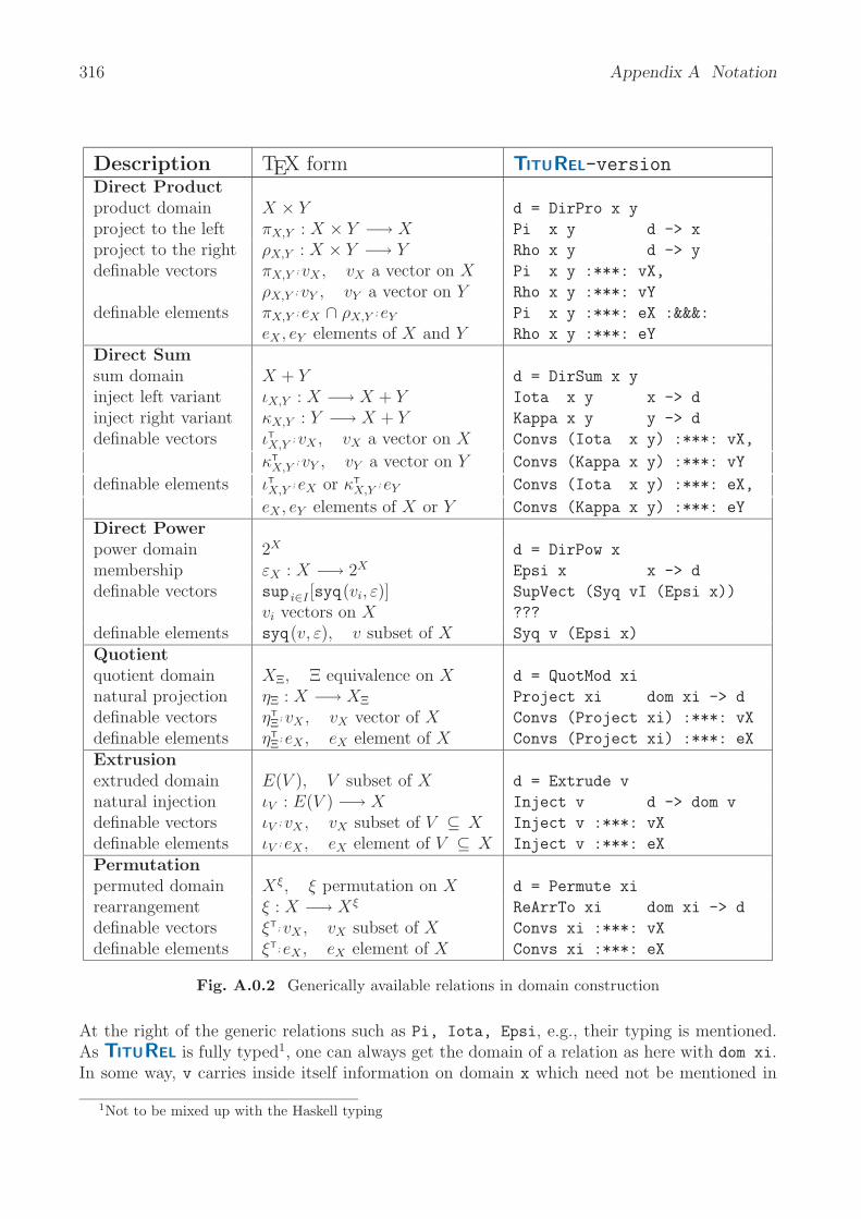
316 Appendix A Notation
Description TEX form TITUREL-versionDirect Productproduct domain X × Y d = DirPro x y
project to the left πX,Y : X × Y −→ X Pi x y d -> x
project to the right ρX,Y : X × Y −→ Y Rho x y d -> y
definable vectors πX,Y ; vX , vX a vector on X Pi x y :***: vX,
ρX,Y ; vY , vY a vector on Y Rho x y :***: vY
definable elements πX,Y ; eX ∩ ρX,Y ; eY Pi x y :***: eX :&&&:
eX , eY elements of X and Y Rho x y :***: eY
Direct Sumsum domain X + Y d = DirSum x y
inject left variant ιX,Y : X −→ X + Y Iota x y x -> d
inject right variant κX,Y : Y −→ X + Y Kappa x y y -> d
definable vectors ιTX,Y
; vX , vX a vector on X Convs (Iota x y) :***: vX,
κTX,Y
; vY , vY a vector on Y Convs (Kappa x y) :***: vY
definable elements ιTX,Y
; eX or κTX,Y
; eY Convs (Iota x y) :***: eX,
eX , eY elements of X or Y Convs (Kappa x y) :***: eY
Direct Powerpower domain 2X d = DirPow x
membership εX : X −→ 2X Epsi x x -> d
definable vectors sup i∈I [syq(vi, ε)] SupVect (Syq vI (Epsi x))
vi vectors on X ???
definable elements syq(v, ε), v subset of X Syq v (Epsi x)
Quotientquotient domain XΞ, Ξ equivalence on X d = QuotMod xi
natural projection ηΞ : X −→ XΞ Project xi dom xi -> d
definable vectors ηTΞ
; vX , vX vector of X Convs (Project xi) :***: vX
definable elements ηTΞ
; eX , eX element of X Convs (Project xi) :***: eX
Extrusionextruded domain E(V ), V subset of X d = Extrude v
natural injection ιV : E(V ) −→ X Inject v d -> dom v
definable vectors ιV ; vX , vX subset of V ⊆ X Inject v :***: vX
definable elements ιV ; eX , eX element of V ⊆ X Inject v :***: eX
Permutationpermuted domain Xξ, ξ permutation on X d = Permute xi
rearrangement ξ : X −→ Xξ ReArrTo xi dom xi -> d
definable vectors ξT; vX , vX subset of X Convs xi :***: vX
definable elements ξT; eX , eX element of X Convs xi :***: eX
Fig. A.0.2 Generically available relations in domain construction
At the right of the generic relations such as Pi, Iota, Epsi, e.g., their typing is mentioned.As TITUREL is fully typed1, one can always get the domain of a relation as here with dom xi.In some way, v carries inside itself information on domain x which need not be mentioned in
1Not to be mixed up with the Haskell typing

317
the term.
It might seem overly restrictive to consider only definable relations as mentioned before (whileadmitting all vectors and elements), but is is not. Other relations are by no means excluded;it is left to those who are longing for them to introduce them. They will then have to go backto the enumeration of pairs of elements, e.g., to get a relation.

318 Appendix A Notation
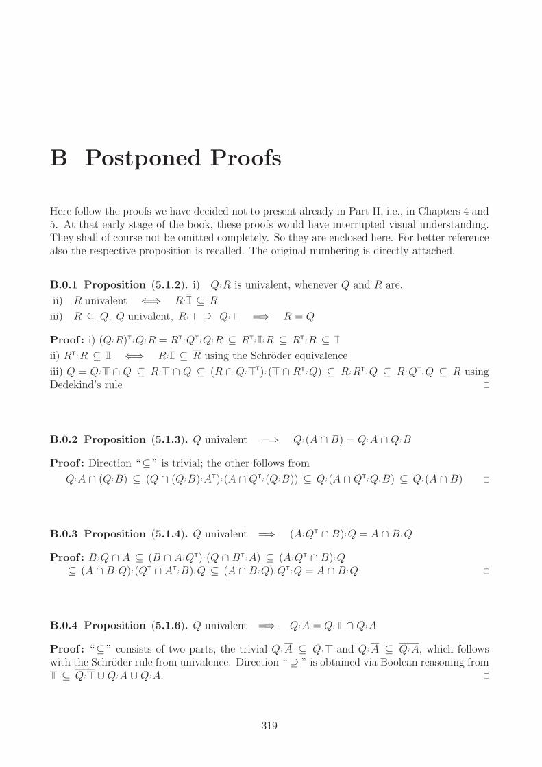
B Postponed Proofs
Here follow the proofs we have decided not to present already in Part II, i.e., in Chapters 4 and5. At that early stage of the book, these proofs would have interrupted visual understanding.They shall of course not be omitted completely. So they are enclosed here. For better referencealso the respective proposition is recalled. The original numbering is directly attached.
B.0.1 Proposition (5.1.2). i) Q; R is univalent, whenever Q and R are.
ii) R univalent ⇐⇒ R; ⊆ R
iii) R ⊆ Q, Q univalent, R; ⊇ Q; =⇒ R = Q
Proof : i) (Q; R)T; Q; R = RT; QT; Q; R ⊆ RT; ; R ⊆ RT; R ⊆ii) RT; R ⊆ ⇐⇒ R; ⊆ R using the Schroder equivalence
iii) Q = Q; ∩ Q ⊆ R; ∩ Q ⊆ (R ∩ Q;T); ( ∩ RT ; Q) ⊆ R; RT ; Q ⊆ R; QT ; Q ⊆ R using
Dedekind’s rule
B.0.2 Proposition (5.1.3). Q univalent =⇒ Q; (A ∩ B) = Q; A ∩ Q; B
Proof : Direction “⊆ ” is trivial; the other follows from
Q;A ∩ (Q;B) ⊆ (Q ∩ (Q;B);AT); (A ∩ QT; (Q;B)) ⊆ Q; (A ∩ QT;Q;B) ⊆ Q; (A ∩ B)
B.0.3 Proposition (5.1.4). Q univalent =⇒ (A; QT ∩ B); Q = A ∩ B ; Q
Proof : B ; Q ∩ A ⊆ (B ∩ A; QT); (Q ∩ BT; A) ⊆ (A; QT ∩ B); Q⊆ (A ∩ B ; Q); (QT ∩ AT; B); Q ⊆ (A ∩ B ; Q); QT; Q = A ∩ B ; Q
B.0.4 Proposition (5.1.6). Q univalent =⇒ Q; A = Q; ∩ Q; A
Proof : “⊆ ” consists of two parts, the trivial Q; A ⊆ Q; and Q; A ⊆ Q; A, which followswith the Schroder rule from univalence. Direction “ ⊇ ” is obtained via Boolean reasoning from
⊆ Q; ∪ Q; A ∪ Q; A.
319
320 Appendix B Postponed Proofs
B.0.5 Proposition (5.3.10). i) A linear order E and its associated strictorder C satisfy
ET
= C.
ii) A linear order E satisfies E ; ET; E = C ⊆ E.
iii) A linear strictorder C satisfies C ; CT; C = C2 ⊆ C.
iv) E is a linear order precisely when Ed is a linear strictorder.
v) C is a linear strictorder precisely when Cd is a linear order.
Proof : i) By definition, a linear order is connex, i.e., satisfies = E ∪ ET, so that ET ⊆ E.
We have in addition ET ⊆ from reflexivity. Both together result in E
T ⊆ C. The reversecontainment C = ∩ E ⊆ E
Tfollows from antisymmetry.
ii) E ; ET
= E ; C = C
iii)–v) These proofs are immediate.
B.0.6 Proposition (5.2.5). Let R, S be arbitrary relations for which the following constructsin connection with x, y and f exist.
i) If f is a mapping, R ⊆ S ; fT ⇐⇒ R; f ⊆ Sii) If x is a point, R ⊆ S ; x ⇐⇒ R; xT ⊆ Siii) If x, y are points, y ⊆ S ; x ⇐⇒ x ⊆ ST; y
Proof : i) “=⇒” is immediate multiplying f from the right and using fT; f ⊆ .
“⇐=”: For the other direction, we start from = ;fT = S;fT ∪ S;fT ⊆ R ∪ S;fT making useof totality of f and of R; f ⊆ S ⇐⇒ S ; fT ⊆ R.
ii) We apply (i) remembering that by definition the converse of a point is always a mapping.
iii) From (ii) we have y ⊆ S;x ⇐⇒ y;xT ⊆ S, which, transposed, gives x;yT ⊆ ST. The proofis completed by employing (ii) again.
B.0.7 Proposition (6.4.1). The natural projection η onto the quotient domain modulo anequivalence Ξ is defined in an essentially unique way.
Proof : The natural projection η is uniquely determined up to isomorphism: should a secondnatural projection ξ be presented, i.e., we assume two such projections VΞ
η←− Vχ−→ WΞ, for
which therefore
Ξ = η; ηT, ηT; η = VΞ, but also
Ξ = χ; χT, χT; χ = WΞ.
the isomorphism is ( , ηT ; ξ). Looking at this setting, the only way to relate VΞ with WΞ is todefine Φ := ηT; χ and proceed showing
ΦT; Φ = (χT; η); (ηT; χ) by definition of Φ= χT; (η; ηT); χ associative= χT; Ξ; χ as Ξ = η; ηT
= χT; (χ; χT); χ as Ξ = χ; χT
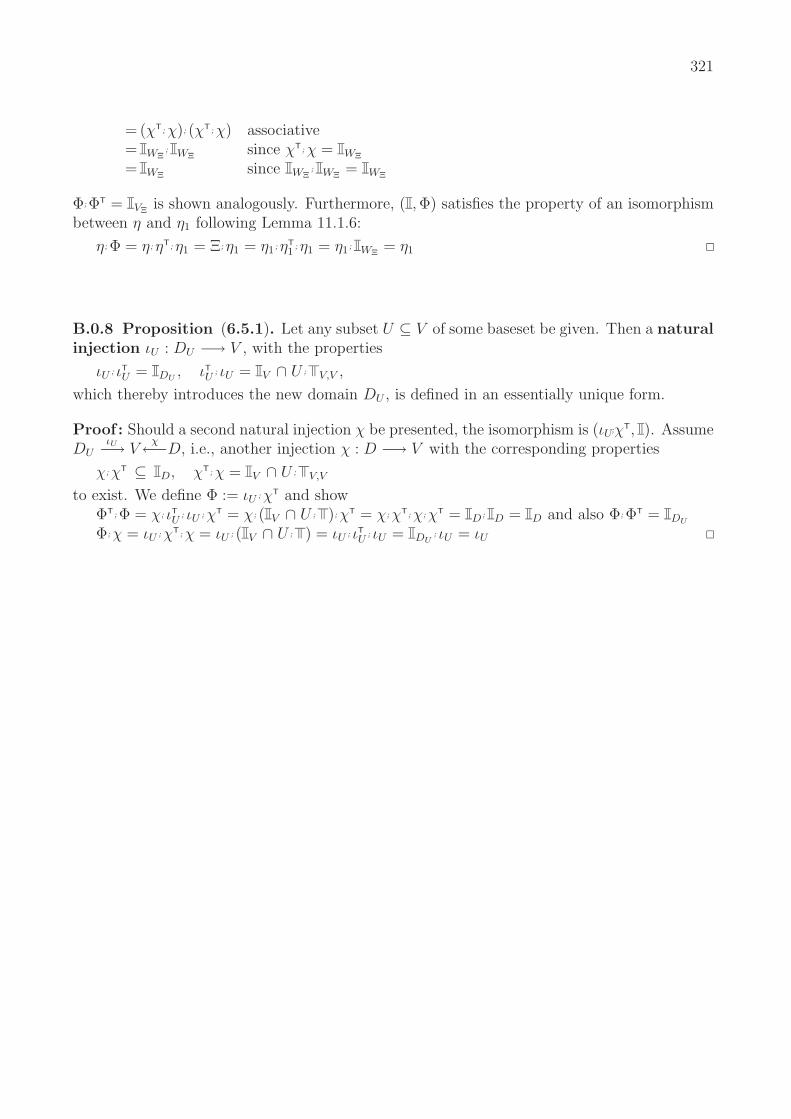
321
= (χT; χ); (χT; χ) associative= WΞ
; WΞsince χT; χ = WΞ
= WΞsince WΞ
; WΞ= WΞ
Φ;ΦT = VΞis shown analogously. Furthermore, ( , Φ) satisfies the property of an isomorphism
between η and η1 following Lemma 11.1.6:
η; Φ = η; ηT; η1 = Ξ; η1 = η1; ηT1
; η1 = η1; WΞ= η1
B.0.8 Proposition (6.5.1). Let any subset U ⊆ V of some baseset be given. Then a naturalinjection ιU : DU −→ V , with the properties
ιU ; ιTU = DU
, ιTU
; ιU = V ∩ U ; V,V ,
which thereby introduces the new domain DU , is defined in an essentially unique form.
Proof : Should a second natural injection χ be presented, the isomorphism is (ιU;χT, ). AssumeDU
ιU−→ Vχ←−D, i.e., another injection χ : D −→ V with the corresponding properties
χ; χT ⊆ D, χT; χ = V ∩ U ; V,V
to exist. We define Φ := ιU ; χT and showΦT; Φ = χ; ιT
U; ιU ; χT = χ; ( V ∩ U ; ); χT = χ; χT; χ; χT = D ; D = D and also Φ; ΦT = DU
Φ; χ = ιU ; χT; χ = ιU ; ( V ∩ U ; ) = ιU ; ιTU
; ιU = DU; ιU = ιU

322 Appendix B Postponed Proofs

C History
Matrices have been invented by Arthur Cayley in 1858 [Cay58] for rectangular array of elements
of a field, Sir William Rowan Hamilton wann? and later been intensively studied by OttoToeplitz. So we can fix the fact, that the concept of a matrix was not yet available whenrelations have first been studied!
• 1646–1716 Gottfried Wilhelm Leibniz already calculated with bit values as can be seenfrom one of his manuscripts
Fig. C.0.1 Gottfried Wilhelm Leibniz (1646–1716)
• 1847 George Boole: The mathematical analysis of logic, being an essay towards a calculusof deductive reasoning
323

324 Appendix C History
Fig. C.0.2 George Boole (1815–1864)
• 1859 Augustus De Morgan: On the syllogisms: IV and on the logic of relatives
a ∨ b = a ∧ b, “Theorem K”
Fig. C.0.3 Augustus De Morgan (1806–1871)
• 1870 Charles S. Peirce: . . . looking for a good general algebra of logic
He was initially unaware of Cayley’s matrix concept, but when getting informed on it,immediately realized that this is also useful for relations.[Cop48]

325
Fig. C.0.4 Charles Sanders Peirce (1839–1914)
• 1895 Ernst Schroder
Fig. C.0.5 Ernst Schroder (1841–1902)
• 1915 Leopold Lowenheim: “Schroderize” all of mathematics !
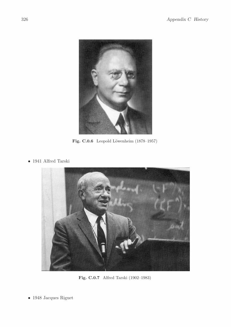
326 Appendix C History
Fig. C.0.6 Leopold Lowenheim (1878–1957)
• 1941 Alfred Tarski
Fig. C.0.7 Alfred Tarski (1902–1983)
• 1948 Jacques Riguet

327
Fig. C.0.8 Jacques Riguet
jeweils den Bezug zu einer wichtigen Arbeit herstellen!

328 Appendix C History

Bibliography
[BGK+96] Arne Bayer, Bernd Grobauer, Wolfram Kahl, Franz Schmalhofer, Gunther Schmidt,and Michael Winter. HOPS-Report, 1996. Fakultat fur Informatik, Universitat derBundeswehr Munchen, 200 p.
[BGS93] Rudolf Berghammer, Thomas Gritzner, and Gunther Schmidt. Prototyping relationalspecifications using higher-order objects. Technical Report 1993/04, Fakultat fur In-formatik, Universitat der Bundeswehr Munchen, 33 p., 1993.
[BGS94] Rudolf Berghammer, Thomas Gritzner, and Gunther Schmidt. Prototyping relationalspecifications using higher-order objects. In Jan Heering, Kurt Meinke, BernhardMoller, and Tobias Nipkow, editors, Higher-Order Algebra, Logic, and Term Rewriting,volume 816 of Lect. Notes in Comput. Sci., pages 56–75. Springer-Verlag, 1994. 1st Int’lWorkshop, HOA ’93 in Amsterdam.
[BHLM03] Rudolf Berghammer, Thorsten Hoffmann, Barbara Leoniuk, and Ulf Milanese. Pro-totyping and Programming With Relations. Electronic Notes in Theoretical ComputerScience, 44(3):24 pages, 2003.
[BHSV94] Rudolf Berghammer, Armando Martın Haeberer, Gunther Schmidt, and Paulo A. S.Veloso. Comparing two different approaches to products in abstract relation algebra.In Nivat et al. [NRRS94a], pages 167–176.
[BR96] R. B. Bapat and T. E. S. Raghavan. Nonnegative Matrices and Applications, volume 64of Encyclopaedia of Mathematics and its Applications. Cambridge University Press,1996.
[BS79] I. N. Bronstein and K. A. Semendjajew. Taschenbuch der Mathematik. Verlag HarriDeutsch, Thun und Frankfurt/Main, 1979. ISBN 3871444928.
[BS83] Rudolf Berghammer and Gunther Schmidt. Discrete ordering relations. Discrete Math.,43:1–7, 1983.
[BSW03] Rudolf Berghammer, Gunther Schmidt, and Michael Winter. RelView and Rath— Two Systems for Dealing with Relations. In de Swart et al. [dSOSR03], pages 1–16.ISBN 3-540-20780-5.
[BSZ86] Rudolf Berghammer, Gunther Schmidt, and Hans Zierer. Symmetric quotients. Tech-nical Report TUM-INFO 8620, Technische Universitat Munchen, Institut fur Infor-matik, 1986.
[BSZ90] Rudolf Berghammer, Gunther Schmidt, and Hans Zierer. Symmetric quotients anddomain constructions. Information Processing Letters, 33(3):163–168, 1989/90.
329

330 Bibliography
[Bot99] Michael Bottner. Relationale Grammatik. Number 402 in Linguistische Arbeiten. MaxNiemeyer Velag, Tubingen, 1999.
[Cay58] Arthur Cayley. Memoir on matrices. Philosophical Transactions of the Royal Societyof London, 148-1:17–37, 1858.
[Cho53] G. Choquet. Theory of capacities. Annales de l’Institut Fourier, 5:131–295, 1953.
[Cop48] Irving M. Copilowish. Matrix development of the calculus of relations. Journal ofSymbolic Logic, 13-4:193203–262, 1948.
[De 56] Augustus De Morgan. On the symbols of logic, the theory of the syllogism, and inparticular of the copula, and the application of the theory of probabilities to somequestions theory of evidence. Transactions of the Cambridge Philosophical Society,9:79–127, 1856. Reprinted in 1966.
[Dem67] A. P. Dempster. Upper and lower probabilities induced by a multivalued mapping.Annals of Math. Statistics, 38:325–339, 1967.
[DF69] A. Ducamp and Jean-Claude Falmagne. Composite Measurement. J. Math. Psychology,6:359–390, 1969.
[DF84] Jean-Paul Doignon and Jean-Claude Falmagne. Matching Relations and the Dimen-sional Structure of Social Sciences. Math. Soc. Sciences, 7:211–229, 1984.
[dSOSR03] Harrie de Swart, Ewa S. Orlowska, Gunther Schmidt, and Marc Roubens, editors.Theory and Applications of Relational Structures as Knowledge Instruments. COST
Action 274: TARSKI. ISBN 3-540-20780-5, number 2929 in Lect. Notes in Comput.Sci. Springer-Verlag, 2003. ISBN 3-540-20780-5.
[Fis71] Peter C. Fishburn. Betweenness, Orders and Interval Graphs. J. Pure and Appl.Algebra, 1:159–178, 1971.
[FR94] Janos Fodor and Marc Roubens. Fuzzy Preference Modelling and Multicriteria Deci-sion Support, volume 14 of Theory and Decision Library, Series D: System Theory,Knowledge Engineering and Problem Solving. Kluwer Academic Publishers, 1994.
[FS90] Peter J. Freyd and Andre Scedrov. Categories, Allegories, volume 39 of North-HollandMathematical Library. North-Holland, Amsterdam, 1990.
[Har74] Robert M. Haralick. The diclique representation and decomposition of binary relations.J. ACM, 21:356–366, 1974.
[HBS94a] Claudia Hattensperger, Rudolf Berghammer, and Gunther Schmidt. Ralf — Arelation-algebraic formula manipulation system and proof checker (Notes to a systemdemonstration). In Nivat et al. [NRRS94a], pages 405–406.
[HBS94b] Claudia Hattensperger, Rudolf Berghammer, and Gunther Schmidt. Ralf — Arelation-algebraic formula manipulation system and proof checker (Notes to a systemdemonstration). In Nivat et al. [NRRS94b], pages 405–406. Proc. 3rd Int’l Conf. Alge-braic Methodology and Software Technology (AMAST ’93), University of Twente, En-schede, The Netherlands, Jun 21–25, 1993. Only included for references from [HBS94b].

Bibliography 331
[Kah02] Wolfram Kahl. A Relation-Algebraic Approach to Graph Structure Transforma-tion. Technical Report 2002/03, Fakultat fur Informatik, Universitat der Bun-deswehr Munchen, June 2002. http://ist.unibw-muenchen.de/Publications/TR/
2002-03/.
[KK06] Volker Kaibel and Thorsten Koch. Mathematik fur den volkssport. Mitteilungen derDeutschen Mathematiker-Vereinigung, 14(2):93–96, 2006.
[Lan95] Hans Langmaack. Langmaackitsafety. ca 1995.
[Leo01] Barbara Leoniuk. ROBDD-basierte Implementierung von Relationen und relationalenOperationen mit Anwendungen. PhD thesis, Christian-Albrechts-Universitat zu Kiel,2001.
[Luc56] R. Duncan Luce. Semi-orders and a theory of utility discrimination. Econometrica,24:178–191, 1956.
[NRRS94a] Maurice Nivat, Charles Rattray, Teodore Rus, and Giuseppe Scollo, editors. Al-gebraic Methodology and Software Technology, Proc. 3rd Int’l Conf. (AMAST ’93),University of Twente, Enschede, The Netherlands, Jun 21–25, 1993, Workshops inComputing. Springer-Verlag, 1994.
[NRRS94b] Maurice Nivat, Charles Rattray, Teodore Rus, and Giuseppe Scollo, editors. Al-gebraic Methodology and Software Technology, Workshops in Computing. Springer-Verlag, 1994. Proc. 3rd Int’l Conf. Algebraic Methodology and Software Technology(AMAST ’93), University of Twente, Enschede, The Netherlands, Jun 21–25, 1993.Only included for references from [HBS94b].
[SBK90] Gunther Schmidt, Ludwig Bayer, and Peter Kempf. Hinweise zur interaktiven Kon-struktion von Bereichen, Objekten und Programmtexten im HOPS-System. TechnicalReport 1990/04, Fakultat fur Informatik, Universitat der Bundeswehr Munchen, May1990.
[Sch77] Gunther Schmidt. Programme als partielle Graphen. Habil. Thesis 1977 und Bericht7813, Fachbereich Mathematik der Techn. Univ. Munchen, 1977. English as [Sch81a,Sch81b].
[Sch81a] Gunther Schmidt. Programs as partial graphs I: Flow equivalence and correctness.Theoret. Comput. Sci., 15:1–25, 1981.
[Sch81b] Gunther Schmidt. Programs as partial graphs II: Recursion. Theoret. Comput. Sci.,15:159–179, 1981.
[Sch03] Gunther Schmidt. Relational Language. Technical Report 2003-05, Fakultat fur In-formatik, Universitat der Bundeswehr Munchen, 2003. 101 pages, http://homepage.mac.com/titurel/Papers/LanguageProposal.html.
[Sch04] Gunther Schmidt. A Proposal for a Multilevel Relational Reference Language. Elec-tronic J. on Relational Methods in Comput. Sci., 1:314–338, 2004.

332 Bibliography
[Sch05] Gunther Schmidt. The Relational Language TituRel: Revised Version,2005. In preparation; see http://homepage.mac.com/titurel/TituRel/
LanguageProposal2.pdf.
[Sch06] Gunther Schmidt. Partiality I: Embedding Relation Algebras. Journal of Logic andAlgebraic Programming, 66(2):212–238, 2006. Special Issue edited by Bernhard Moller.
[Sco64] Dana Scott. Measurement Structures and Linear Inequalities. Journal of MathematicalPsychology, 1:233–247, 1964.
[Sha76] Glenn Shafer. A Mathematical Theory of Evidence. Princeton University Press, 1976.
[SS89] Gunther Schmidt and Thomas Strohlein. Relationen und Graphen. Mathematik furInformatiker. Springer-Verlag, 1989. ISBN 3-540-50304-8, ISBN 0-387-50304-8.
[SS93] Gunther Schmidt and Thomas Strohlein. Relations and Graphs — Discrete Mathemat-ics for Computer Scientists. EATCS Monographs on Theoretical Computer Science.Springer-Verlag, 1993. ISBN 3-540-56254-0, ISBN 0-387-56254-0.
[TG87] Alfred Tarski and Steven R. Givant. A Formalization of Set Theory without Variables,volume 41 of Colloquium Publications. American Mathematical Society, 1987.
[Var62] Richard S. Varga. Matrix Iterative Analysis. Prentice-Hall, Englewood Cliffs, NJ, USA,1962.
[Vin] Philippe Vincke. Preferences and numbers, ???
[Win04] Michael Winter. Decomposing Relations Into Orderings. In Rudolf Berghammer,Bernhard Moller, and Georg Struth, editors, Proc. of the Internat. Workshop RelMiCS’7 and 2nd Internat. Workshop on Applications of Kleene Algebra, in combinationwith a workshop of the COST Action 274: TARSKI. Revised Selected Papers; ISBN3-540-22145-X, 279 pages, number 3051 in Lect. Notes in Comput. Sci., pages 261–272.Springer-Verlag, 2004.

Index
1-graph, 227
aBarEQUALSlamB, 285aBarEQUALSQb, 285antichain, 140, 204antisymmetric, 67antitoneMapAssign, 285antitonFctlGame, 278assignment, 283associated ordering, 70, 72associated strictorder, 70, 72association rule, 164asymmetric, 67, 73, 188, 203atom, 131attribute dependency system, 301
baseset, 11, 19ground, 21
Bayesian measure, 244bBarEQUALSlTa, 285bBarEQUALSqTa, 285BDD, 29belief
light-minded, 246mapping, 244vacuous, 245
bi-classificatory system, 191bijective, 62binary decision diagram, 29biorder, 173bipartitioned graph, 227Birkhoff-Milgram Theorem, 191bisimulation, 220block diagonal form, 55Boole, George, 323, 324bound
greatest lower, 138least upper, 138lower, 134upper, 134
BridgeColors, 20
Cantor’s diagonal enumeration, 96CardValues, 20carre (French), 149Cayley, Arthur, 323chain, 204chainable, 160, 161Choquet integral, 251closure
difunctional, 161rectangular, 149transitive, 77
column equivalence, 74, 161, 177, 180, 192column mask, 129commonality, 256compass relation, 309complement, 114, 259complete, 67
strongly, 67complete order, 71completion
by cuts, 140by ideals, 140
componentstrongly connected, 78
composite measurement, 191composition, 51
demonic, 297concept lattice, 153, 155, 157cone, 134
lower, 136upper, 136
conformal property, 239congruence, 165, 214conjoint measurement, 191connex, 67, 174, 181, 188, 203conorm, t-, 258consonant, 257Continents, 20continuous functional, 276contraction, 84, 230converse, 50
333

334 Index
coproduct, 103core, 256correctness, 277covering set, 82, 149cut, 34cut completion, 140cyclic, 229cyclic permutation, 232
De Morgancomplement, 259triples, 257
De Morgan, Augustus, 324decision diagram, 29Dedekind rule, 52, 123defined zone, 80demonic
composition, 297operator, 295residuals, 298
dense, 173, 191diagonal enumeration, 96difunctional, 36, 76, 173
closure, 161difunctional relation, 149, 158–161, 163–166,
184Dilworth Theorem, 205direct
power, 114product, 92, 99sum, 100, 103
directed graph, 227disjoint union, 100dotted arrow convention, 59, 124, 174dotted-arrow convention, 185draw, 278dual, 71
elemAs. . . , 22element
greatest, 137in powerset, 24least, 137
equivalence, 21, 69, 73, 76, 104, 105, 183of columns, 74, 161, 177, 180, 192of rows, 74, 161, 177, 180, 192quasi-, 163
equivalence (relation), 88
extruded subset, 107extrusion, 21, 107, 109, 317, 321
Ferrers, 188Ferrers relation, 72, 163, 165, 168, 169, 173–
176, 180, 181, 184, 187, 188, 191,200, 203
Ferrers, Norman Macleod, 173Fishburn, P. C., 187, 201, 203, 205focal, 256fork operator, 99fringe, 166–170Frobenius-Konig Theorem, 289function, 37, 57
set-valued, 29functional
continuous, 276isotone, 276monotone, 276
fuzzy measure, 244
Galois iteration, 271games, 278gameSolution, 278generalized inverse, 162GermPres, 20GermSocc, 20glb, 138glbR, 138grammar, relational, 312graph
1-, 227bipartitioned, 227directed, 227rooted, 228simple, 227
gre, 137gre, 137greatest
element, 137lower bound, 138
ground, 22baseset, 21set, 20
ground setordering of, 20
Guttman scale, 191

Index 335
Hall condition, 151, 287hammock, 237Hasse
diagram, 70relation, 70
Helly property, 202, 239, 240higherBound, 36homomorphism, 209hypergraph, 227
ideal completion, 140identity, 51immediate predecessor, 71immediate successor, 71implication
R-, 259S-, 259
implication structure, 301independent set, 82, 149indifference, 207infimum, 138initial part, 274injection, 103, 107
natural, 109, 321injective, 57, 62integral
Choquet, 251relational, 248Sugeno, 243, 248, 251
interval(strict)order, 187, 203order, 65, 187, 193, 201, 203, 205relation, 311
IntSocc, 20inverse, 149invertible, 149irreducible, 229, 230irreflexive, 73, 188, 203isInclMinLineCoveringForLambda, 285isInclMinLineCoveringForQ, 285isIrreducible, 230isotone
functional, 276
kernel, 282Klein-4-Group, 37knowledge acquisition, 164, 165Konig-Egervary Theorem, 289
Kuratowski Theorem, 205
L-simulation, 220lattice, 133, 139lbd, 136lbd, 135lea, 137least
element, 137upper bound, 138
least upper bound, 138left
-invertible, 149identity, 51residual, 53
Leibniz, Gottfried Wilhelm, 323light-minded belief, 246linear
order, 71strictorder, 71
linear extension, 205LISTFunc, 37Lowenheim, Leopold, 325, 326loss, 278lower bound, 134
greatest, 138lower cone, 136lowerBound, 36lub, 137lub, 138lubR, 138Luce, R. Duncan, 130, 207
machine learning, 159, 165Maddux, Roger Duncan, 311majorant, 134mapping, 57, 62, 63Marczewski, Edward, 72mask, 129matching, 76, 159, 283, 284MATRFct2, 37MATRFunc, 37MATRRel, 30max, 134measure
Bayesian, 244fuzzy, 244necessity, 257

336 Index
plausibility, 257possibility, 257relational, 243, 244, 248
measurement, 191composite, 191conjoint, 191
membership relation, 111min, 134minorant, 134monotone functional, 276Months, 20MonthsS, 20Moore-Penrose, 162, 236Morgan triples, 257Morgan, Augustus De, 324multi-covering, 217–219multiplication, 51
Nations, 20natural injection, 109, 321natural projection, 104, 105necessity measure, 257negation, 259
strict, 259strong, 259
negatively transitive, 186, 188, 203non-enlargable rectangle, 145nonvalue zone, 80norm, t-, 258
operator, demonic, 295order, 65, 69, 183
interval, 65, 187, 193, 201, 203, 205linear, 71semi-, 65, 200–202, 205strict-, 69total, 71weak-, 65, 186
order-dense, 191order-shaped, 179order-shaped relation, 169ordering
associated, 70, 72orthogonal, 163
pair of covering sets, 82, 149pair of independent sets, 82, 149PALIRel, 30
partunivalent, 238
partial preorder, 69, 183partition, 42Peirce, Charles Sanders, 324, 325percentage, 36permutation, 39, 115, 149
cyclic, 232primitive, 232relation, 32subset, 26
plausibility measure, 257point, 63, 131Politicians, 20, 23possibility measure, 257power ordering, 114power, direct, 114POWERel, 30powerset element, 24precondition
weakest, 278predecessor, immediate, 71predictive modeling, 164PREDRel, 30preference, 207preorder, 69, 183, 189primitive
permutation, 232relation, 229
printHeteroReducible, 231printLeftRightIterated, 236printResMatrixGame, 279, 280printResReducible, 231product, direct, 92progressively
bounded, 274projection, 99
quasi-equivalence, 163quasi-series, 184quasiorder, 69, 183quotient
set, 104, 105symmetric, 54
quotient, symmetric, 87
R-implication, 259random relation, 36

Index 337
randomly generated relation, 36randomMatrix, 36randomPermutation, 36randomUnivAndInject, 36rank, 151realizable, 190rectangle, 80, 82, 145, 149
non-enlargable, 145rectangle inside a relation, 81rectangle inside a relation, 145rectangle outside a relation, 81rectangular, 149
closure, 149relation, 80, 91, 149
reducible, 84, 229, 230reducing vector, 84refines, 296reflexive, 76, 188, 203relation
boolean operation on, 48composition of, 51converse of, 50cyclic, 229difunctional, 149, 158–161, 163–166, 184dual, 71Ferrers, 72, 163, 165, 168, 169, 173–176,
180, 181, 184, 187, 188, 191, 200, 203irreducible, 229membership-, 111multiplication of, 51order-shaped, 169, 179primitive, 229randomly generated, 36rectangular, 80, 91, 149reducible, 84, 229transposition of, 50type of, 47
relationalgrammar, 312integral, 248measure, 243, 244, 248
RelView, 29representation
basesets, 19element, 21relation, 29, 32subset, 22
residual, 69, 297demonic, 298left, 53right, 53
right-invertible, 149identity, 51residual, 53
Riguet, Jacques, 149, 326ROBDD, 29root of a graph, 228rooted
graph, 228tree, 228
row equivalence, 74, 161, 177, 180, 192row mask, 129rowSplit, 36rule
Tarski, 81
S-implication, 259saturated, 284scale, Guttman, 191scaling, 207Schroder, Ernst, 325Schroder equivalences, 52, 123Scott-Suppes Theorem, 200semi-connex, 67semi-transitive, 185, 200, 202semiorder, 65, 200–202, 205set
covering, 82, 149focal, 256independent, 82, 149
set-valued function, 29setAs. . . , 23SETFRel, 30simple graph, 227simple support mapping, 245simulation, 220SkatColors, 20MATRRel, 30sorting
topological, 78square-shaped, 149staircase, 173strict

338 Index
complete order, 71negation, 259total order, 71
strict-, 69strictorder, 65, 183
associated, 70, 72linear, 71
strong negation, 259strongly complete, 67strongly connected, 78, 230subset, 11, 19, 107
boolean operations on, 24, 25permutation, 26
subset extrusion, 21, 107, 109, 317, 321successor, immediate, 71Sudoku, 305Sugeno integral, 243, 248, 251sum, direct, 100summarization, 164support mapping, 245supremum, 138surjective, 62, 63symmetric, 67, 73symmetric quotient, 54, 87syq, 54Szpilrajn
Edward, 72extension, 78Theorem, 72, 204
t-conorm, 258t-norm, 258TABUFct2, 37tabulation, 110Tarski
Alfred, 326rule, 63, 81
term rank, 151, 288termination, 273Theorem
Birkhoff-Milgram, 191Dilworth, 205Frobenius-Konig, 289Kuratowski, 205Konig-Egervary, 289Scott-Suppes, 200Szpilrajn, 72, 204
threshold, 196, 197, 199, 201–203TITUREL, 6, 29, 45TITUREL, 58TITUREL, 121, 315, 316topological sorting, 72, 78, 183, 205total, 62, 63total order, 71totalisation, 295tournament, 67transitive, 68
negatively, 186semi-, 185, 200, 202
transitive closure, 77transposition, 50tree, rooted, 228triples, De Morgan, 257trivialMatch, 285trivialMatchAbove, 285tupeling, 99type of a relation, 47
U -simulation, 220ubd, 136, 137ubd, 135undefined zone, 80union
disjoint, 100univalent, 57, 59, 319univalent part, 238unsupervised learning, 159, 165upper bound, 134
least, 138upper cone, 136utility, 190, 201, 241
vacuous belief, 245value zone, 80vector, 80
reducing, 84VECTRel, 30
weak preference, 207weakest precondition, 278weakorder, 65, 69, 186–189, 203well-ordering, 206win, 278