i

Final Report

Rejection of Pharmaceuticals by Reverse Osmosis Membranes: Quantitative Structure Activity Relationship (QSAR) Analysis

Submitted by:

Grisel Rodriguez, Sarah Buonora, Tom Knoell, Don Phipps, Jr. Orange County Water District

Dr. Harry Ridgway

AquaMem

Submitted to:

The National Water Research Institute (NWRI)

West Basin Municipal Water District (WBMWD)

Orange County Water District (OCWD)

Orange County Sanitation District (OCSD)

U.S. Bureau of Reclamation

NWRI Project 01-EC-002

October 2004

ii

Acknowledgements

The authors of this report wish to thank the National Water Research Institute (NWRI), the West Basin Municipal Water District (WBMWD), the Orange County Sanitation District (OCSD) and the Unites States Bureau of Reclamation (US BuREC) for providing funding for this research project. Furthermore, the authors would like to thank the management and Board of Directors of the Orange County Water District (OCWD) for supporting this research effort. Special thanks are also extended to Dr. Harry F. Ridgway of AquaMem for his contributions to this study.

iii

Table of Contents

EXECUTIVE SUMMARY xv ABSTRACT xviii 1. INTRODUCTION 1

1.1. Background 1 1.2. Project Objective 8

2. TECHNICAL DESCRIPTION 10

2.1. Creation of Empirical (QSAR) Models Describing Organic Compound Rejection 10

2.1.1. Organic Compound Master List 10 2.1.2. Selection of QSAR Molecular Descriptors 10 2.1.3. Clustering Compounds by Similar QSAR Descriptor Properties 11 2.1.4. Selection of Surrogate Compounds for Analysis 12 2.1.5. Membranes Used in Study 13 2.1.6. Membrane Preparation and Coupon Fabrication 13 2.1.7. Determination of Membrane-Compound Interactions 13

2.1.7.1. Radiometric Membrane Performance (RMP) Assay 13 2.1.7.2. Membrane-Compound Interactions: Relative Solute Fluxes 17 2.1.7.3.Determining Relative P-, M- and R-Fluxes from the RMP

Assay Results 17 2.1.8. Comparison of RMP Assay Results to Crossflow Membrane

Test Unit 18 2.1.9. Construction of Artificial Neural Network Models Describing

Association of Organic Compounds with RO Membranes 20 2.1.9.1. Selection of QSAR Descriptors Best Correlating with Organic

Compound Membrane Association 21 2.1.9.1.1. Choice of Exemplars and Randomization of Order 21 2.1.9.1.2. Identification of Subsets of Influential Descriptors

Using a Genetic Algorithm (GA) 22 2.1.9.1.3. Identification of Most Common Influential Descriptors 23

2.1.9.2. Construction of Artificial Neural Network (ANN) Models 24 2.1.9.2.1. Randomization of Exemplars Prior to Model

Construction 25 2.1.9.2.2. Construction of ANN Models 25

2.1.9.2.2.1. Assigning a Data Noise Level 25 2.1.9.2.2.2. Assignment of I/O Transformation Functions 26 2.1.9.2.2.3. Selection of Model Inputs using the GA 26

iv

2.1.9.2.2.4. Selecting Training and Test Exemplar Pools 26 2.1.9.2.2.5. Training and Selecting the Best ANN Model 27 2.1.9.2.2.6. Testing the Selected Network 27

2.1.9.2.3. Using Sensitivity Analysis to Eliminate Non-Influential ANN Inputs 27

2.1.9.3. Characterization and Validation of the ANN models 28 2.1.9.3.1. Determining Basic Model Attributes 28 2.1.9.3.2. Determining the Overall Iinfluence of Model Inputs

on Organic Compound Fluxes 28 2.1.9.3.3. Predicting Behavior of the Remaining Compounds

in the Database 28 2.1.10. Validating the ANN Models 29

2.1.10.1. “Virtual Mass Balance” Method 29 2.1.10.2. Comparison of Model Results with Rejection Values

Reported for Organic Compounds in the Literature 29 2.1.11. Producing Excel-Enabled Exportable ANN Models Describing

Organic Compound Interactions With RO Membranes 30 2.2. Molecular Modeling Method Simulation of Compound-Membrane

Interactions 31 2.2.1. PA Modeling Methods and Simulation Conditions 31 2.2.2. Building the Membrane Models 31 2.2.3. Modeling the Organic Solutes 33 2.2.4. MD Simulation Setup and Run Conditions 33

3. PROJECT RESULTS 36

3.1. QSAR ANN Modeling Results 36 3.1.1. Comparison of RMP Assay with a Crossflow RO System 36 3.1.2. Determination of Compound-Membrane Interactions 36 3.1.3. ANN Models Describing Organic Compound-Membrane

Interactions 38 3.1.3.1. Overall Performance of ANN Membrane Models 38

3.1.3.1.1. ANN Model Sensitivity Analysis Results 39 3.1.3.1.1.1. Relative P-Flux Sensitivity Index Analysis:

Molecular Descriptors Associated with Penetration of Organic Compounds Through the RO Membranes 41

3.1.3.1.1.2. Relative M-Flux Sensitivity Index Analysis: Molecular Descriptors Associated with the Adsorbtion/ Absorption of Organic Compounds to the RO Membranes 43

3.1.3.1.1.3. Relative R-Flux Sensitivity Index Analysis: Molecular Descriptors Associated with the Ability of RO Membranes to Repel Compounds at the Membrane Surface 45

3.1.3.2. Validation of the “Universal” PA ANN Models – Comparison with the Individual PA Models 47

3.1.4. Application of the ANN Models to the Master Compound List – Prediction of Compound Interactions with RO Membranes 48

v

3.1.4.1. Prediction of Compound-Membrane Interactions; Determination of Prediction Success using the “Virtual Mass Balance” Method 48

3.1.4.2. Interpretation of the Relative Flux Table Data 49 3.1.4.3.Estimation of Membrane Percent Rejection From the Relative

Compound Flux Data 50 3.1.5. Comparison of Rejection Predicted by the ANN Model to

Rejection Reported in the Literature and Field 51 3.1.6. Instances where Models failed to predict Compound Behavior:

Gap Analysis and Suggestion for Further Study 51 3.2. Analysis of MD Simulations 54

3.2.1. System Energies 54 3.2.2. Diffusion Behaviors of NDMA and TCE 54 3.2.3. Calculation of Water and Solute Diffusivities and

Theoretical Fluxes 56 3.2.4. Water and Membrane Interactions with the Organics 57 3.2.5. Idealized PA Membrane Pore Model to Estimate Solute-

Membrane Interactions 59

4. CONCLUSIONS AND RECOMMENDATIONS 61

4.1. QSAR ANN Model Predictions of Compound-Membrane Interactions 61 4.1.1. Interacion of Organic Compounds with RO Membranes 61 4.1.2. Use of QSAR Molecular Descriptors to Explain Compound

Behavior 63 4.1.3. Use of Radiolabeled Tracers and the RMP Assay as a Rapid

Method to Evaluate Compound Fate 64 4.1.4. Application of ANN Modeling to Determine Salient Parameters

Related to Compound Interactions with RO Membranes 66 4.1.5. Successful Construction of ANN Models describing Compound-

Membrane Interactions 67 4.1.6. QSAR analysis – Relating Descriptors to Compound-Membrane

Interactions 69 4.1.7. Prediction of Compound-Membrane Interactions for

Compounds in the Master Compound List 71 4.1.8. Improving the ANN QSAR Models 74 4.1.9. Extending QSAR ANN Model Results to the Real World 74

4.2. Description of Compound-Membrane Interactions Using Molecular Dynamics (MD) Simulation 75

vi

5. LITERATURE CITED 78 APPENDIX Appendix 1. Glossary of QSAR terms Used in Models 220 Appendix 2. Structures and QSAR Molecular Descriptors of the Surrogate

Compounds 227 Appendix 3. All Compound QSAR Molecular Descriptors and Molecular

Properties 278 Appendix 4. Instructions on Use of Distributed EXCEL Models 294

vii

List of Figures

Figure 1. Interaction of a Compound (Solute) with a Membrane 82 Figure 2. RMP Assay Diagram and Flux Determinations 83 Figure 3. Apparatus used for the RMP Assay Method 84 Figure 4. Cross-Flow Membrane Test Unit 85 Figure 5. Comparison of RMP Assay to Crossflow Block Tester Performance 86 Figure 6. Selection of Molecular Descriptor Inputs and Construction of Artificial Neural Network (ANN) Models 87 Figure 7. Selection of QSAR Molecular Descriptors and Surrogate Compounds 88 Figure 8a. Surrogate Compound Fate in BW-30 Membrane 89 Figure 8b. Surrogate Compound Fate in BW-30 Membrane 90 Figure 8c. Surrogate Compound Fate in BW-30 Membrane 91 Figure 9a. Surrogate Compound Fate in ESPA-2 Membrane 92 Figure 9b. Surrogate Compound Fate in ESPA-2 Membrane 93 Figure 9c. Surrogate Compound Fate in ESPA-2 Membrane 94 Figure 10a. Surrogate Compound Fate in LFC-1 Membrane 95 Figure 10b. Surrogate Compound Fate in LFC-1 Membrane 96 Figure 10c. Surrogate Compound Fate in LFC-1 Membrane 97 Figure 11a. Surrogate Compound Fate in TFC-HR Membrane 98 Figure 11b. Surrogate Compound Fate in TFC-HR Membrane 99 Figure 11c. Surrogate Compound Fate in TFC-HR Membrane 100 Figure 12a. Surrogate Compound Fate in “Universal” PA Membrane 101 Figure 12b. Surrogate Compound Fate in “Universal” PA Membrane 102

viii

Figure 12c. Surrogate Compound Fate in “Universal” PA Membrane 103 Figure 13a. Surrogate Compound Fate in CA Membrane 104 Figure 13b. Surrogate Compound Fate in CA Membrane 105 Figure 13c. Surrogate Compound Fate in CA Membrane 106 Figure 14a. ANN Model Results for BW-30 – P-Flux 107 Figure 14b. ANN Model Results for BW-30 – M-Flux 108 Figure 14c. ANN Model Results for BW-30 – R-Flux 109 Figure 15a. ANN Model Results for ESPA-2 – P-Flux 110 Figure 15b. ANN Model Results for ESPA-2 – M-Flux 111 Figure 15c. ANN Model Results for ESPA-2 – R-Flux 112 Figure 16a. ANN Model Results for LFC-1 – P-Flux 113 Figure 16b. ANN Model Results for LFC-1 – M-Flux 114 Figure 16c. ANN Model Results for LFC-1 – R-Flux 115 Figure 17a. ANN Model Results for TFC-HR – P-Flux 116 Figure 17b. ANN Model Results for TFC-HR – M-Flux 117 Figure 17c. ANN Model Results for TFC-HR – R-Flux 118 Figure 18a. ANN Model Results for CA – P-Flux 119 Figure 18b. ANN Model Results for CA – M-Flux 120 Figure 18c. ANN Model Results for CA – R-Flux 121 Figure 19a. ANN Model Results for “Universal” PA – P-Flux 122 Figure 19b. ANN Model Results for “Universal” PA – M-Flux 123 Figure 19c. ANN Model Results for “Universal” PA – R-Flux 124 Figure 20a. Comparison of “Universal” PA Model Output to BW-30 – P-Flux 125

ix

Figure 20b. Comparison of “Universal” PA Model Output to BW-30 – M-Flux 126 Figure 20c. Comparison of “Universal” PA Model Output to BW-30 – R-Flux 127 Figure 21a. Comparison of “Universal” PA Model Output to ESPA-2 – P-Flux 128 Figure 21b. Comparison of “Universal” PA Model Output to ESPA-2 – M-Flux 129 Figure 21c. Comparison of “Universal” PA Model Output to ESPA-2 – R-Flux 130 Figure 22a. Comparison of “Universal” PA Model Output to LFC-1 – P-Flux 131 Figure 22b. Comparison of “Universal” PA Model Output to LFC-1 – M-Flux 132 Figure 22c. Comparison of “Universal” PA Model Output to LFC-1 – R-Flux 133 Figure 23a. Comparison of “Universal” PA Model Output to TFC-HR – P-Flux 134 Figure 23b. Comparison of “Universal” PA Model Output to TFC-HR – M-Flux 135 Figure 23c. Comparison of “Universal” PA Model Output to TFC-HR – R-Flux 136 Figure 24. Model Failure vs Representation of Surrogates in QSAR Descriptor Clusters 137 Figure 25. Dendrogram illustrating compounds that 75% or more of the PA Models Failed to Predict 138 Figure 26. QSAR Molecular Descriptors Relating to Compound Transport 139 Figure 27. Atomic Microscope Image of a Polyamide TFC Membrane 140 Figure 28. Transmission Electron Micrograph of a Polyamide TFC Membrane 141 Figure 29. Screen Capture of Membrane Build Software 142

x

Figure 30. Steps Used in Building Crosslinked PA Membrane Models 143 Figure 31. Schematic illustrating the role of internal crosslinks in establishing membrane “pores” or void spaces 144 Figure 32. PA Membrane Model before and after Geometry Optimization using the AMBER force field 145 Figure 33. Model properties and atom partial changes for NDMA and TCE 146 Figure 34. Structure of the FT-30 Membrane Model before and after imposing periodic boundary conditions 147 Figure 35. Compacted membrane with water removed 148 Figure 36. System potential energy and temperature for the NDMA simulation 149 Figure 37. Three-axis plot showing trajectory of NDMA in membrane system between 15 and 35 ps. 150 Figure 38. COM distances from the origin at t=0 ps for NDMA and TCE 151 Figure 39. Schematic illustrating the concept of diffusional jumps or hops 152 Figure 40. Calculated diffusion coefficients for five randomly chosen water molecules and NDMA 153 Figure 41. Schematic showing method for estimating the energy of association (interaction energy) of the organic solute with the membrane-water complex 154 Figure 42. Estimated energies of interaction (binding energies) of NDMA and TCE within the hydrated membrane system 155 Figure 43. NDMA and TCE interactions with water and membrane atoms 156 Figure 44. Idealized model PA membrane pores 157 Figure 45. Solute-membrane interaction potentials as a function of compound type and measured solute-membrane binding activity 158

xi

List of Tables

Table 1a. Description of Compounds Considered in the Study 159 Table 1b. Description of Compounds Considered in the Study 160 Table 1c. Description of Compounds Considered in the Study 161 Table 1d. Description of Compounds Considered in the Study 162 Table 1e. Description of Compounds Considered in the Study 163 Table 2. Molecular Descriptors Used in Models 164 Table 3. Polyamide (PA) Reverse Osmosis Membrane Properties 165 Table 4. Surrogate Compounds Chosen for the Study 166 Table 5. Membranes Used in the Study 167 Table 6. Comparison of Membrane Performance – Relative P-Flux 168 Table 7. Comparison of Membrane Performance – Relative M-Flux 169 Table 8. Comparison of Membrane Performance – Relative R-Flux 170 Table 9a. BW-30 Performance Based on Individual Compounds – Relative P-Flux 171 Table 9b. BW-30 Performance Based on Individual Compounds – Relative M-Flux 172 Table 9c. BW-30 Performance Based on Individual Compounds – Relative R-Flux 173 Table 10a. ESPA-2 Performance Based on Individual Compounds – Relative P-Flux 174 Table 10b. ESPA-2 Performance Based on Individual Compounds – Relative M-Flux 175 Table 10c. ESPA-2 Performance Based on Individual Compounds – Relative R-Flux 176

xii

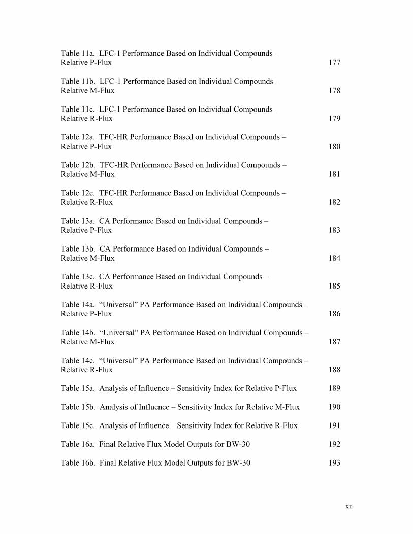
Table 11a. LFC-1 Performance Based on Individual Compounds – Relative P-Flux 177 Table 11b. LFC-1 Performance Based on Individual Compounds – Relative M-Flux 178 Table 11c. LFC-1 Performance Based on Individual Compounds – Relative R-Flux 179 Table 12a. TFC-HR Performance Based on Individual Compounds – Relative P-Flux 180 Table 12b. TFC-HR Performance Based on Individual Compounds – Relative M-Flux 181 Table 12c. TFC-HR Performance Based on Individual Compounds – Relative R-Flux 182 Table 13a. CA Performance Based on Individual Compounds – Relative P-Flux 183 Table 13b. CA Performance Based on Individual Compounds – Relative M-Flux 184 Table 13c. CA Performance Based on Individual Compounds – Relative R-Flux 185 Table 14a. “Universal” PA Performance Based on Individual Compounds – Relative P-Flux 186 Table 14b. “Universal” PA Performance Based on Individual Compounds – Relative M-Flux 187 Table 14c. “Universal” PA Performance Based on Individual Compounds – Relative R-Flux 188 Table 15a. Analysis of Influence – Sensitivity Index for Relative P-Flux 189 Table 15b. Analysis of Influence – Sensitivity Index for Relative M-Flux 190 Table 15c. Analysis of Influence – Sensitivity Index for Relative R-Flux 191 Table 16a. Final Relative Flux Model Outputs for BW-30 192 Table 16b. Final Relative Flux Model Outputs for BW-30 193

xiii

Table 16c. Final Relative Flux Model Outputs for BW-30 194 Table 17a. Final Model Output for ESPA-2 195 Table 17b. Final Model Output for ESPA-2 196 Table 17c. Final Model Output for ESPA-2 197 Table 18a. Final Model Output for LFC-1 198 Table 18b. Final Model Output for LFC-1 199 Table 18c. Final Model Output for LFC-1 200 Table 19a. Final Model Output for TFC-HR 201 Table 19b. Final Model Output for TFC-HR 202 Table 19c. Final Model Output for TFC-HR 203 Table 20a. Final Model Output for CA 204 Table 20b. Final Model Output for CA 205 Table 20c. Final Model Output for CA 206 Table 21a. Final Model Output for “Universal” PA 207 Table 21b. Final Model Output for “Universal” PA 208 Table 21c. Final Model Output for “Universal” PA 209 Table 22a. Estimated Percent Rejection based on mass of compound passing through the membrane (P-Flux) and on mass of compound not interacting with the membrane (R-Flux). 210 Table 22b. Estimated Percent Rejection based on mass of compound passing through the membrane (P-Flux) and on mass of compound not interacting with the membrane (R-Flux). 211 Table 22c. Estimated Percent Rejection based on mass of compound passing through the membrane (P-Flux) and on mass of compound not interacting with the membrane (R-Flux). 212

xiv

Table 22d. Estimated Percent Rejection based on mass of compound passing through the membrane (P-Flux) and on mass of compound not interacting with the membrane (R-Flux). 213 Table 22e. Estimated Percent Rejection based on mass of compound passing through the membrane (P-Flux) and on mass of compound not interacting with the membrane (R-Flux). 214 Table 23. Comparison between predicted rejection and reported values. 215 Table 24. Compounds that 75% or more of the PA Models Fail to Predict 216 Table 25. Conditions used for MD simulations of NDMA and TCE transport 217 Table 26. Modeled compound diffusivities and flux calculation results 218 Table 27. Summary of NDMA and TCE interactions with pure water 219

xv

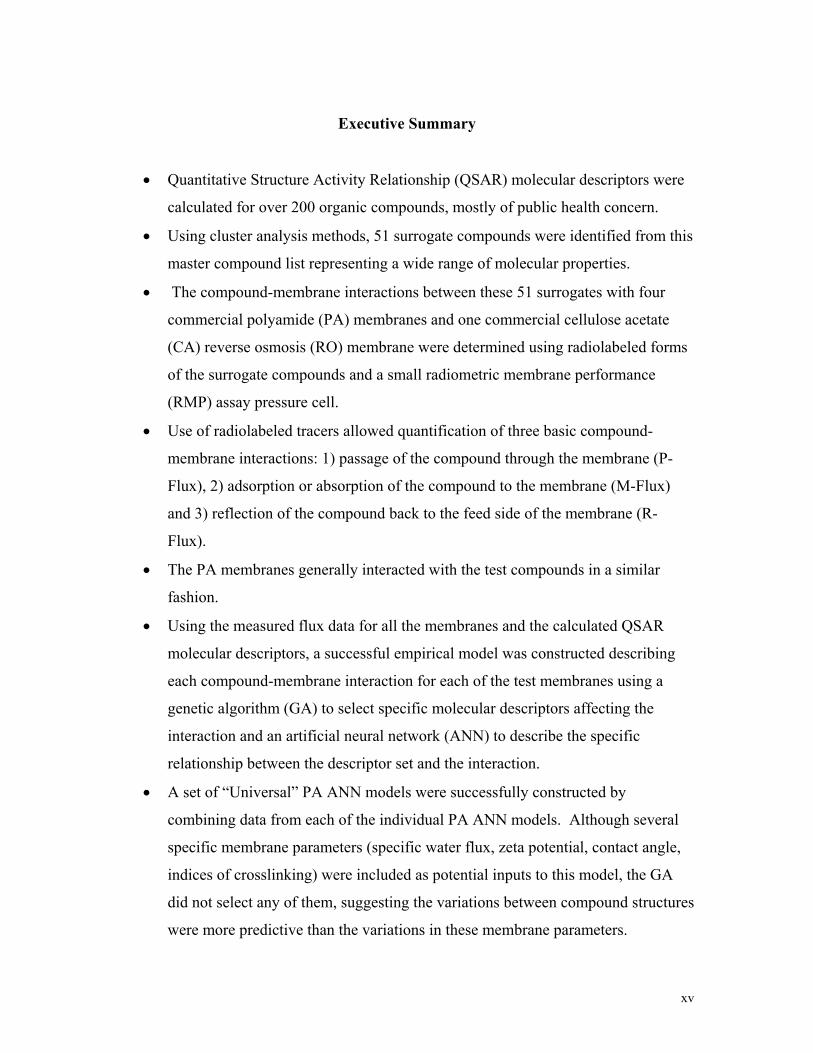
Executive Summary

Quantitative Structure Activity Relationship (QSAR) molecular descriptors were

calculated for over 200 organic compounds, mostly of public health concern.

Using cluster analysis methods, 51 surrogate compounds were identified from this

master compound list representing a wide range of molecular properties.

The compound-membrane interactions between these 51 surrogates with four

commercial polyamide (PA) membranes and one commercial cellulose acetate

(CA) reverse osmosis (RO) membrane were determined using radiolabeled forms

of the surrogate compounds and a small radiometric membrane performance

(RMP) assay pressure cell.

Use of radiolabeled tracers allowed quantification of three basic compound-

membrane interactions: 1) passage of the compound through the membrane (P-

Flux), 2) adsorption or absorption of the compound to the membrane (M-Flux)

and 3) reflection of the compound back to the feed side of the membrane (R-

Flux).

The PA membranes generally interacted with the test compounds in a similar

fashion.

Using the measured flux data for all the membranes and the calculated QSAR

molecular descriptors, a successful empirical model was constructed describing

each compound-membrane interaction for each of the test membranes using a

genetic algorithm (GA) to select specific molecular descriptors affecting the

interaction and an artificial neural network (ANN) to describe the specific

relationship between the descriptor set and the interaction.

A set of “Universal” PA ANN models were successfully constructed by

combining data from each of the individual PA ANN models. Although several

specific membrane parameters (specific water flux, zeta potential, contact angle,

indices of crosslinking) were included as potential inputs to this model, the GA

did not select any of them, suggesting the variations between compound structures

were more predictive than the variations in these membrane parameters.

xvi

Behavior of the “Universal” PA models in general mirrored the behavior of the

individual PA membrane models.

Molecular descriptors included by the ANN models included those describing

molecular charge/polarity, molecular complexity, hydrogen bonding and

hydrophobicity.

There was variation in the exact descriptors included in each of the models across

membrane types; CA differed from PA, and within the four PA membranes (and

with the “Universal” models), inputs differed.

However, there were some commonly included descriptors in the models between

membranes and between interactions. Notably, descriptors related to electrophilic

interactions (Gmin), molecular dipole and quadripole moments (P, Py and Q),

hydrogen bonding (numHBa) and hydrophobicity (LogP) were used by multiple

models.

Behavior of all 202 compounds in the master compound list was modeled;

predictions passing a “virtual mass balance” criterion based on the summation of

mass fluxes achieving ±25% of the original feed flux was used to validate

predictions. Based on this criterion, behavior of between 57% and 70% of the

master list compounds were successfully predicted by the ANN models.

The “Universal” PA models were able to describe ~76% of the compounds within

this criterion.

Percent rejection was estimated based on the predicted P-Flux and R-Flux values.

Many pharmaceutically active compounds (PhACs) and disinfection byproducts

(DBPs) were predicted to be highly rejected, especially by PA membranes.

However, in many cases, a significant component of rejection involved

adsorption/absorption to the RO membrane material. Tables of rejection data are

presented for each membrane, and for the “Universal” PA models.

Percent rejection determined from the P-Flux predictions of theANN models

agreed favorably with values published in the literature or observed in the field.

Failures of the models were associated with specific compounds; an iterative gap

analysis process was suggested that could converge on a more robust set of

models by choosing additional surrogates from the failed compounds

xvii

A computer program was written to automatically build fully-atomistic,

geometry-optimized models of a polyamide (PA) reverse osmosis membrane

useful for molecular dynamics (MD) simulation of the free diffusion behavior of

1,1,2,2-tetrachloroethylene (TCE) and nitrosodimethylamine (NDMA).

Although the simulations were of relatively short duration, typically 200

picoseconds (ps), differences were evident in the behavior of the two organics;

NDMA exhibited two “jump” events involving rapid long-range (~7Å) excursions

from the origin at t = 0 ps whereas TCE did not in the time period.

Calculated solute fluxes based on root mean square (RMS) displacements of local

diffusion were much greater than experimental values, although calculated water

fluxes agreed with those expected for PA membranes.

Two factors contributed to overestimation of organic fluxes: (i) inability to

account for solute jump frequencies in the short duration simulations, and (ii)

likely overestimation of solute partition coefficients.

Although NDMA and TCE diffusivities were nearly identical in pure-water

simulations, there was a 4-fold reduction of TCE diffusion in the membrane

system relative to NDMA, suggesting greater interaction of TCE with the

membrane. The results agreed relatively with the laboratory observations in this

study for these two compounds and PA membranes.

Analysis of simulation playbacks revealed NDMA associated more with water

and polymer atoms than did TCE. The relative lack of a hydration field around

TCE may contribute to stronger long-range electrostatic interactions with

membrane atoms resulting in lower diffusivity and higher rejection for this

compound.

An idealized PA membrane pore model is proposed that may be able to rapidly

estimate and compare solute-membrane interaction potentials.

xviii

Abstract

In this study, 51 radiolabeled surrogate compounds selected from an initial compound list

of over 200 organic compounds, mostly of public health concern, were used to construct

a series of quantitative structure activity relationship (QSAR) based empirical

multivariate models describing the interaction of the compounds with several commercial

polyamide (PA) and cellulose acetate (CA) reverse osmosis (RO) membranes. Models

were constructed using artificial neural networks (ANNs) based on data obtained from

calculated QSAR molecular descriptors and direct measurements of compound-

membrane associations. The penetration of molecules through the membranes, the

adsorption/absorption of molecules on/in the membranes and the rejection of molecules

at the feed/membrane interface were associated with molecular properties that included

charge/polarity, structural complexity, hydrogen bonding and hydrophobicity. Percent

rejection, calculated from the ANN model predictions, compared favorably with

published values. Models developed in this study were capable of predicting the

compound-membrane interactions of 57% to 70% of the organics in the initial compound

list. In addition to the individual membrane models, a “Universal” PA model was

constructed from individual PA membrane performance data capable of predicting the

compound-membrane interactions for 76% of the compounds. A gap analysis that could

improve model performance was discussed. A fully-atomistic geometry-optimized model

of a PA membrane was created and used to study the free diffusion behavior of 1,1,2,2-

tetrachloroethylene (TCE) and N-nitrosodimethylabine (NDMA). Predicted TCE

diffusion was 4-fold less than NDMA. This result agreed in general with the relationship

between TCE and NDMA relative membrane fluxes; however, absolute values were

much overestimated compared to laboratory results, although water flux measurements

were not. Movement of compounds through the membrane by low-frequency, longer-

range “jumps” as opposed to local diffusion and underestimation of the solute partition

coefficients may account for the discrepancies. A simplified membrane model system

using a single PA membrane “pore” to speed investigation of compound-membrane

interactions is proposed.

1

1 INTRODUCTION 1.1 Background Ultra-low-pressure reverse osmosis (RO) and nanofiltration (NF) membrane processes

are arguably the most cost-effective modern technologies for removing trace organic and

inorganic constituents from water. Because of their favorable energy efficiencies,

flexible engineering design and scale-up, and ability to remove a wide range of low-

molecular-weight (LMW) organics, membrane processes are increasingly being

employed in drinking water purification and water reuse applications worldwide.

Whereas their overall performance can be modeled with considerable precision, the

mechanisms by which organics and other substances are transported across or rejected by

these semi-permeable membranes are still incompletely understood (Weisner and

Buckley, 1996).

The ability of RO membranes to remove organic contaminants such as pharmaceutically

active compounds (PhACs) and endocrine disrupting compounds (EDCs) from drinking

water supplies is very desirable because of the potential health risk posed by these

substances. This issue has been widely reported in the literature (Drewes et al., 2002;

Hileman, 2001; Kolpin et al., 2002; Schafer et al., 2003). It is currently recognized that

molecular mass and size of organic compounds are perhaps among the most significant

factors in determining how well they are rejected by any given RO membrane. In

general, compounds exceeding a molecular-weight cutoff (MWCO) value of about 300

Daltons are rejected well by most RO membranes regardless of their other inherent

molecular properties. Almost all of the compounds categorized as EDCs or PhACs have

molecular weights of >200 Da. (Kimura et al., 2003), although some EDCs with

molecular weight near 300 such as 17β-estradiol (MW = 279g/mol) may be detected in

RO permeate at very low concentrations (Salveson et al., 2000). For compounds that lie

below the MWCO value for a particular membrane type, rejection and transport

behaviors are based on a host of other compound molecular properties. Together, these

molecular properties determine the nature of the compound’s interaction with the solvent

phase (typically water), dissolved salts and other organics, and the polymer membrane

2

matrix, which in turn determines the diffusion rate and transport behavior of the organic

compound. Some of the molecular properties (also referred to as attributes or

descriptors) that may affect a compound’s transport across RO or NF membranes include

shape, hydrophobicity, partial atomic charges and their distribution, molecular orbital

shapes, reactive centers and locations of electron and recipient donor atoms, bonding

arrangements, atom types, dipole moment, ionization potentials, etc.

A few efforts have been made to identify relationships between molecular structure and

the ability of an organic compound to pass through modern RO or NF membrane

materials. Huang and Negishi (1993) examined the transport behaviors of aliphatic acids,

alcohols, and amines for a series of experimental cellulose acetate derivative RO

membrane materials. It was found that for n-alkyl organics, solute rejections firstly

increased with alkyl chain length, reaching a maximum at about three carbons atoms, and

then decreased thereafter or remained stable. Branched compounds were rejected best,

presumably due to steric hindrances as they interacted with the polymer matrix.

According to Matsuura and Sourirajan (1971) for a given membrane material and

structure, polar effects constitute one of the most important physicochemical criteria

governing reverse osmosis separation of organic solutes. They developed and confirmed

a method for estimating Taft numbers for polyhydric alcohols, and used this technique to

predict solute transport of alcohols, aldehydes, and carbohydrates in porous cellulose

acetate membranes. Several investigators have reported that organic removal from

membranes depends highly on the degree of compound ionization. It has been found that

formic acid removal by the NS-100 membrane varied from ~ 6% when partially

undissociated to 98% when dissociated completely (Fang and Chian, 1975).

The nature of the membrane material itself greatly influences the types and the degree to

which organic compounds are rejected. For example, Reinhard and coworkers (1986)

reported that both polyamide thin-film composite (TFC) membranes as well as blend

cellulose acetate membranes tended to reject branched complex organic molecules

including neutrals, bases, acids, and phenols. However, various halogenated DBPs and

chlorinated solvents were only rejected significantly by the TFC membranes. Membrane

3

properties that affect compound rejection include surface charge and charge distribution,

degree of polymer crosslinking and polymer mobility, overall thickness, hydrophobicity,

density, surface morphology, hydration energy, and other factors. The trend in recent

years to make membranes with lower operating pressures has generally resulted in

somewhat poorer organics rejection. Lipp et al. (1994) showed that when using FT-30

membranes, the transmembrane pressure drop, ion composition, ion concentration and

pH have an influence on the solute and salt rejection. An increase in pH increases the

solute rejection and an increase in the ion concentration decreases the solute rejection.

The rejection exhibited by membranes is also strongly influenced by the nature of the

fouling layer that develops. Schafer and coworkers (2000) recently reported that the

rejection of LMW organic acids by a series of microfiltration, ultrafiltration, and NF

membranes was dependent on the type of deposit on the membrane surface. Positively

charged ferric chloride precipitates on the membrane surfaces were found to improve the

rejection of cationic species but reduced the rejection of LMW organic acids present in

natural organic matter (NOM).

Given the effects of natural fouling layers on rejection, it is not surprising that purposeful

modification of membrane surfaces also has met with some success in terms of

improving the rejection of organics. For example, Kilduff et al. (2000) reported recently

that ultraviolet (UV)-assisted graft polymerization of N-vinyl-2-pyrrolidinone onto

sulfonated polyethersulfone NF membranes not only helped to mitigate NOM fouling,

but also could under certain circumstances leave NOM rejection and water flux relatively

unaffected. On the other hand, when the same membranes were simply UV irradiated in

the absence of graft polymerization to increase surface hydrophilicity and wettability, the

degree of NOM rejection was diminished significantly.

The foregoing examples suggest it is theoretically possible to predict the membrane

transport or rejection behavior of organic compounds from a knowledge of their

fundamental molecular attributes. However, since more than one molecular attribute may

influence a compound’s ability to penetrate a semi-permeable membrane barrier and

4

diffuse through it, multivariate statistical procedures such as multiple linear regression

analyses or artificial neural network (ANN) analyses are required to accurately model the

phenomenon. Such a multivariate statistical approach which seeks to correlate some

minimum set of independent molecular descriptors with molecular activity or function

(i.e., membrane transport or rejection) is referred to as quantitative structure-activity

relationship (QSAR) analysis. The predictive statistical model developed from this

analytical approach is referred to as a QSAR model. Because of the multitude of

interacting solute-membrane factors, QSAR models describing organics rejection by

membranes will very likely turn out to be specific to a particular membrane type. Thus,

multiple models will be needed for a series of membrane materials.

In recent years, QSAR models have been successfully developed for a variety of

experimental systems involving complex bio-organic interactions. For example, Carroll

et al. (1994) developed QSAR models for predicting the potency of dopamine binding

inhibitors by various natural cocaine derivatives (e.g., 3B-(substituted phenyl)tropane-2B-

carboxylic acids). Many physical and chemical material properties of natural and

synthetic polymers can be predicted with reasonable accuracy (typically >85%) using

QSAR type models based on molecular group contribution and topological (graph theory)

techniques (Bicerano, 1996). More recently, Campbell et al. (1999) working at OCWD’s

Water Factory 21, developed regression-based QSAR models to predict the effectiveness

of charged and neutral surfactants for inhibiting the attachment of fouling bacteria to TFC

and cellulose acetate RO membranes. Because the surfactants examined interacted

differently with each membrane chemistry, separate QSAR models were developed for

polyamide TFC and cellulose acetate membranes.

We proposed to apply multivariate (ANN-based) techniques to create QSAR models that

could accurately describe and predict the rejection of organic compounds by several

modern commercial TFC membranes. The project focused on those compounds that

exhibit a potential for negatively impacting human health or the environment. The

compounds of most interest include a host of endocrine disruptors, human and animal

antibiotics, DBPs, insecticides and herbicides, and various neuroactive drugs (e.g.,

5

aspirin, anticancer agents, etc.). Many of these compounds have been found in recent

years to enter natural ecosystems at still bioactive concentrations by way of sewage

outfalls and urban runoff.

Although research on RO membrane performance is extensive, the majority of studies

have relied upon empirical observations to formulate and bolster theoretical precepts of

membrane structure and function. Indeed, until very recently, membranes were treated as

structurally and chemically homogeneous “black boxes.” However, recent ultrastructural

studies of PA membranes have revealed that they are chemically and structurally

asymmetric (Figs. 27 and 28; Freger, 2003). The observed chemical and structural

asymmetry of PA membranes is believed to result from differential rates of diffusion of

the reactive monomers into the incipient membrane during the interfacial polymerization

reaction. Because of the morphological complexity of TFC membranes, compelling

ultrastructural or experimental evidence is lacking as to the exact location of the solute-

water separation layer. Other unknowns concerning the PA membranes include the

surface and bulk charge distribution, polymer density as a function of membrane depth,

and water content. Such uncertainties have hindered our efforts to fully validate

atomistic models of PA membrane materials and underscore a strong need to better

characterize the membranes experimentally. Unfortunately, apart from microscopy, there

are few analytic techniques able to effectively probe PA membrane substructure at the

nanoscale, a consideration that has in recent years prompted efforts to model the structure

and functionality of the PA separation layer.

Atomistic modeling of small-molecule sorption and diffusion in the PA layer is complex.

In contrast to simulations of simple gas solutes where solute-solute and polymer-solute

interactions can be often neglected, RO simulations must account for specific

interactions, such as water-water, water-solute, water-polymer and solute-polymer

interactions (Kotelyanskii et al., 1998). In addition, models need to accurately describe

the physical and chemical characteristics of the aromatic crosslinked PA thin film of

current RO membranes. Key properties include density, hydrogen bonding and water

sorption capacities, and concentrations of crosslinks and functional groups (e.g.,

6

unreacted free amine and carboxylic acid). Due to insufficient experimental data, it is not

surprising that the literature on atomistic modeling of RO membranes and water sorption

in polyamides is limited. Important studies in this field are those by Knopp and Suter

(1997a, 1997b) and by Kotelyanskii et al. (1998, 1999).

Knopp and Suter (1997a) developed a method based on atomistic models to calculate the

excess chemical potential of a solute in dense polymer microstructures. The technique

consists of combining two well-established procedures for determining excess chemical

potentials such that the shortcomings associated with each individual method are

minimized. Consequently, the technique can then be applied to a wider range of solute-

polymer systems. This hybrid method was successfully tested in separate studies using

water as the solute and polyamides (Knopp and Suter, 1997b), bisphenol-A-

polycarbonate and polyvinyl alcohol (Nick and Suter, 2001), as the polymers. The

difference between the calculated excess chemical potential of water in a given polymer

and the excess value of pure water can be used to give an initial prediction of the

equilibrium water sorption capability of that polymer.

In simulations of PA films, information on the water content within the polymeric matrix

is crucial for the success of the atomistic model. Although Knopp and Suter (1997a,

1997b) evaluated their method on PAs unlike the typical crosslinked aromatic PA used in

RO membranes, valuable insight can be still obtained about the accuracy of the technique

and its potential in simulations of RO systems. In comparison to experimental data, this

method was able to reasonably predict the variation in sorption values between two linear

PAs that differ from each other only in the number of amide bonds. However, it failed to

recognize sorption differences between two PAs with the same number of amide bonds,

but different chemical structure. The authors concluded that the force field used in the

simulation must correctly model chemical structure differences such that they will be

reflected in the estimated sorption values. It was also found that equilibrium sorption of

water cannot be described by a simple function of the concentration of amide groups.

7

Kotelyanskii et al. (1998, 1999) performed atomistic simulations of water and salt

transport in the aromatic polyamide film of an FT-30 RO membrane in order to obtain

information about diffusion and rejection mechanisms. Specific objectives of these

studies included the investigation of crosslinking effects on density and solute transport,

ion mobility (Na+ and Cl–), estimation of water diffusion coefficients and water structure

and interactions within the polyamide. The polyamide structure modeled was designed

based on data for density, equilibrium water content and number of crosslinks obtained

from the industry, but not available elsewhere (Kotelyanskii et al., 1998). These

properties are essential to the outcome of the simulations, and it is therefore critical to

generate more accurate and reliable experimental data to support the models.

Simulation results show, as expected, that a higher concentration of crosslinks increased

the density of the polyamide and reduced the mobility of water molecules. The authors

found that water diffusion in the hydrated polyamide occurred by “jumps” between

localized sites (Kotelyanskii et al., 1998). These sites may be described as void spaces

arising from the dynamic structure of the polymer chains. Water molecules oscillate in

these sites until thermal fluctuations or local structure rearrangements of the polymer

permit another “jump”. The estimated “jump” length was approximately 3Å, which was

independent of the simulation conditions. The frequency of these “jump” events, on the

other hand, decreased with higher polymer densities. In other words, the mobility of

water molecules was reduced due to the decrease in the dynamics of the polymer chain

caused by more crosslinks (i.e., higher density; Kotelyanskii et al., 1999). The authors

concluded that about 90% of the water molecules within the polymer matrix are

interconnected by hydrogen bonds, forming a large network. Water mobility (i.e.,

“jump” frequency) decreased as the concentration of hydrogen bonds increased. With

respect to salt transport in the polyamide, it was found that salt ions were partially

hydrated with some water interactions replaced by ion-polymer interactions. The

mobility of the salt molecule was significantly lower than that of water and was limited

by the chloride ion, which is consistent with the observed permselectivity of PA

membranes.

8

Although atomistic simulations may be powerful tools for the investigation of transport

and rejection mechanisms within the PA film of RO membranes, modeling predictions

must be verified by experimental data since simulation results may be strongly influenced

by PA characteristics. Experimental data will allow the construction of more consistent

PA models and help validate conclusions extracted from simulations.

1.2 Project Objective The primary goal of this project was to develop robust solute rejection QSAR models for

a series of commercial RO membranes challenged with a structurally diverse suite of

organic compounds of immediate interest to water utilities and regulatory agencies.

Compounds of special interest included endocrine disruptors, antibiotic agents,

neuroactive drugs, insecticides, and DBPs. To accomplish this goal, a radiometric

membrane performance (RMP) assay was developed which permited rapid determination

of the interactions of radiolabeled organic substances (rejection, association) with RO

membrane materials. QSAR models enabling prediction of compound rejection for each

membrane type evaluated were developed using the RMP assay dataset and calculated

compound molecular properties (descriptors).

Specific project objectives included (1) validation and calibration of the RMP assay

(described in further detail below), (2) use of the RMP assay to quantify the rejection

behaviors of a wide range of endocrine disruptors, antibiotics, and DBPs by commercial

low-pressure TFC membranes, and (3) development of QSAR models (one model for

each membrane type investigated) based on the mass transport/rejection data for the

compounds examined. Compound transport data derived from RMP experiments were

also compared with the results of molecular dynamics (MD) simulations.

A second objective of this study was to evaluate the usefulness and accuracy of MD

simulations for determining RO membrane fluxes and rejections of trace organic

compounds of public health concern. Examples of compounds of particular interest

include disinfection by-products such as N-nitrosodimethylamine (NDMA) and 1,1,2,2-

tetrachloroethylene (TCE), as well as the endocrine disruptor 17a estradiol. The initial

9

focus was on polyamide RO membranes since they are widely used in water treatment

and organic compound rejections are generally superior for this class of membranes. If

successful, MD simulations could provide an approach that may be generalized for

predicting the organic rejection properties of any membrane material that can be

modeled.

10

2 TECHNICAL DESCRIPTION 2.1 Creation of Empirical (QSAR) Models Describing Organic Compound

Rejection The experimental approach involved application of the RMP assay to build a database of

membrane interactions between the test membranes and organic compounds which have

special relevance for water utilities and regulatory agencies, and then to relate the

membrane interactions with molecular properties (defined by QSAR molecular

descriptors).

2.1.1 Organic Compound Master List A master list of 190 compounds was compiled based on a search of the following

governmental databases: U.S. Geological Survey Toxic Substances Hydrology Program,

U.S. Environmental Protection Agency Unregulated Contaminant Monitoring Rule and

Drinking Water Contaminant Candidate List, April, 1999 and the California Department

of Health Services Unregulated Chemicals Requiring Monitoring, May, 2001. The

compound list included many endocrine disruptors, antibiotics, neuroactive drugs,

insecticides, and DBPs. Additional compounds (amino acids, marine toxins) were added

to increase the breadth of molecular properties variations. The final master list of 202

compounds with brief descriptions of their regulatory or environmental relevance is

shown in Tables 1a-1e.

2.1.2 Selection of QSAR Molecular Descriptors Compounds were constructed using molecular modeling computer software and initially

more than 370 molecular descriptors were calculated for each of the compounds in the

master list using QSARis software ( SciVision, Inc., Lexington, MA). The descriptors

were organized into eight general categories, each of which contained numerous sub-

categories, as indicated below:

Molecular Connectivity Chi indices (3 descriptors total)

Kappa Shape indices (2 descriptors total)

Electrotopological State (E-State) indices (6 descriptors total)

11

Information indices (7 descriptors total)

Subgraph Count indices (22 descriptors total)

Total Topological descriptors (11 descriptors total)

Molecular Properties (17 descriptors total)

Other descriptors (4 descriptors total)

Due to software limitations that restricted the total number of independent-variable

(descriptor) inputs that could be used for the development of QSAR models, a strategy

was devised to reduce the total number of descriptors to be used in model development.

This approach involved performing a series of cluster analyses (nearest neighbor, squared

Euclidian method) on each major descriptor category using a statistical analysis package

(Statgraphics, Manugistics, Rockville, MD) to reveal any highly cross-correlated

descriptors in that particular group. For example, the seven descriptors in the information

indices category were observed to form four independent clusters (i.e., non-correlated

subgroups). One or more information index from each of the four subgroups was

subsequently selected for candidate membership in the final (master) descriptor list.

Selection of descriptors from within cluster subgroups was based on the perceived

relevance of the descriptor based on its definition (e.g., simple descriptors were generally

favored over more complex derivative descriptors) and done in a conservative manner,

i.e., often more than one member of a subgroup was chosen for inclusion in the master

descriptor list. Following this protocol for each of the eight major descriptor categories

resulted in a master list of 73 molecular descriptors for each organic compound used in

the study (Table 2).

2.1.3 Clustering Compounds by Similar QSAR Descriptor Properties Cluster analyses were similarly employed to break the list of compounds of interest into

subgroups of compounds having similar descriptor values. Such statistically-based

grouping was necessary because most of the compounds were known to be unavailable in

a radiolabeled form. Therefore, the simplifying assumption was made that compounds

having similar descriptor-set values would exhibit similar rejection behaviors across the

12

different RO membranes used in the study, and vice versa. A single cluster analysis was

performed using Statgraphics (Ward’s squared Euclidian method). In this case,

truncation of the master descriptor list was necessary in this step since Statgraphics

would accept a maximum of 64 independent variables as inputs for clustering analyses.

In this case, a Pearson’s R correlation matrix was used to eliminate the most highly cross-

correlated descriptors. A subsequent dendritic analysis of the remaining descriptors

resulted in creation of 20 subgroups (QSAR molecular property clusters) (Fig. 7). A

complete listing of all master database compounds with their properties, QSAR

descriptor values and QSAR descriptor clusters is presented in Appendix 3.

2.1.4 Selection of Surrogate Compounds for Analysis From the contents of each of these 20 clusters, one or more compounds were identified as

surrogates to represent the molecular behavior of the members of the cluster for

determination of actual compound interactions with the five different RO membranes. A

total of 51 compounds were obtained as surrogates for this study (Table 4). Not all

clusters were represented, but in many cases more than one member of a cluster was

included in the surrogate list. Compounds used in the study were obtained from

American Radiolabeled Chemicals, Inc., St. Louis, MO; Amersham, Piscataway, NJ;

ICN, Irvine, CA; Perkin Elmer Life Sciences, Inc., Boston, MA; Moravek Biochemicals,

Inc., Brea, CA and Sigma, St. Louis, MO. Purity of the compounds was >99% and all

compounds were stored either at 4 C or –20 C (depending on the compound) for a

minimal period of time (typically less than one week) prior to assay to lessen the

opportunity for post-manufacture chemical changes. Compounds labeled with 14C were

chosen preferentially over compounds labeled with 3H to reduce the possibility of

radiolysis during storage and to avoid the possibility of the 3H proton exchanging with

water during interaction with the membrane (Riley et. al., 1988). Only four compounds

labeled with 3H were used in the study. Complete surrogate compound information is

presented in Appendix 2.

13

2.1.5 Membranes Used In Study

Four commercial polyamide (PA) RO membranes and one cellulose acetate (CA) RO

membrane were selected for this project (Table 5). Due to the high solute rejection and

throughput, PA membranes have become the commercial membranes of choice utilized

in the water and wastewater treatment industry today. However, CA membranes are still

extensively used in the industry and one was included for comparative purposes.

2.1.6 Membrane Preparation and Coupon Fabrication Swatches (4” x 6’) were randomly obtained from sheets of each of the membranes (to

avoid the potential for regional variations in the membrane material) and preconditioned

under crossflow conditions in a stainless steel cell designed at OCWD (Fig. 4) at a

pressure of 150 PSIG for 16 hrs using 1 μohm-cm deionized water. This process was

necessary to hydrate the membrane material and to extract unreacted monomers (e.g.,

trimesoyl chloride and m-phenylenediamine) or other chemical substances (e.g., certain

surfactants and possibly biocides) that could remain associated with the membranes

following their manufacture.

Following preconditioning, circular 12.5-mm diameter coupons of membrane were cut

from the swatches using a circular punch. As with the swatches, coupons were randomly

harvested from the swatch surface to help eliminate effects of short order

inhomogenieties in the membrane material. The coupons thus obtained were stored in 17

Mohm-cm ASTM I ultrapure water at 4 C for no more than one week before use.

2.1.7 Determination of Membrane-Compound Interactions

2.1.7.1 Radiometric Membrane Performance (RMP) Assay The Radiometric Membrane Performance (RMP) assay (Figs. 2 and 3) was performed

using a small stainless-steel/Teflon pressure cell (VWR, Bristol, CN), which supported

the membrane coupon on a perforated stainless steel disk with the feed surface gasketed

14

with a Teflon O-ring. The pressure cell was screwed together to a constant torque of 15

inch-lb with a torque wrench. Care was taken to apply sufficient torque to avoid leaks,

but not so much as to crush or damage the permselective membrane surface.

The feed side of the pressure cell was filled with a feed solution consisting of 17 Mohm-

cm ASTM I ultrapure water containing typically 100,000 – 1,000,000 disintegrations per

minute (DPM) of radiolabeled (14C or 3H) test compound (typically approximately 9 μM

concentration of feed compound) adjusted to pH 7 as needed (using extremely small

amounts of HCl or NaOH). At this concentration, the effects of concentration

polarization was expected to be relatively low in spite of a lack of cross-flow.

A 10 μL sample of the feed solution was recovered and placed in 10 mL of scintillation

cocktail (Optifluor, Packard Instrument Company, Meriden, CT) prior to filling a 5 mL

glass and Teflon gas-tight syringe (Hamilton Company, Reno, NV) with 2 mL of feed

solution. The pressure cell was connected to the syringe such that all air bubbles were

excluded. The pressure cell and syringe were then placed in a polyvinyl chloride (PVC)

housing equipped with a 50 mL glass and Teflon Hamilton syringe designed such that the

plungers of both, it and the feed syringe, were brought into contact. When regulated 15

PSI compressed air was supplied to the larger syringe, the 10:1 area ratio of the pistons

generated 150 PSI of hydraulic pressure at 24 C in the smaller feed solution syringe.

Product expressed through the membrane coupon under pressure was collected through a

18 gauge (GA) hypodermic needle attached to the pressure cell product side. As soon as

product was observed at the needle tip, the tip was submerged below the surface of 10

mL of scintillation cocktail in a 22 mm scintillation vial and a stopwatch was started to

record the time required for collection of the product sample. Collection of the product in

this manner avoided significant loss of the more volatile surrogate compounds during

product collection.

A product volume of approximately 0.5 mL was collected; the volume was

gravimetrically determined using a 2-place digital balance (Sartorius Model PT-120,

15

Sartorius Corp., Bohemia, NY; error ±-0.005 g). The time required for collection of the

product was noted during each assay and varied from 10 to 40 min depending on the

membrane in use.

After product collection, the pressure cell was recovered and detached from the pressure

apparatus. A second 10 μL feed sample was obtained from the chamber reservoir and

placed in 10 mL of scintillation cocktail as was previously described. This second

sample was used to determine whether or not significant loss of feed concentration

occurred (by adsorption to the apparatus, e.g.) during the course of the experiment. No

significant differences were observed between the initial and final feed samples during

the study.

Following sampling, the residual feed and product solutions remaining in the pressure

cell were removed using a thin pipette tip (Ranin Instrument Corporation, Woburn, MA).

The pressure cell was carefully unscrewed and the membrane coupon recovered using

clean forceps. The coupon was rinsed by sequentially dipping and swishing six times in

three 400-mL beakers containing 350 mL of 17 Mohm ASTM I grade ultrapure water.

The coupon was then blotted by gently touching the front and back surfaces to adsorbent

paper to wick away any adhering water and placed into 10 mL of scintillation cocktail in

a 22 mL scintillation vial. Membrane coupons in scintillation cocktail were incubated

overnight (roughly 12 hr) in order to facilitate permeation of the cocktail into the

membrane material. Tests performed in the laboratory indicated that this procedure

yielded the most complete recovery of membrane-associated compound.

Scintillation vials containing feed samples, product samples and membrane coupons were

placed in a scintillation counter (Wallac LKB 1219 Rackbeta Liquid Scintillation

Counter, Perkin-Elmer, Shelton, CT) and counted for 1min. Quench and counting

efficiency were corrected using the external sample channel ratio method with 226Ra as

the external standard to yield a measurement of DPM. Background correction was

applied by subtracting DPM obtained by counting 10 mL of scintillation cocktail with no

sample.

16

A minimum of 5 replicate measurements were performed with each combination of

membrane and solute compound in order to define noise due to variations in the

membrane coupons, counting error, assay errors (pippetting errors), etc. The numbers of

replicates were occasionally greater for certain compounds or membrane materials.

Statistical outliers were defined as having values >3 interquartile ranges below the first or

above the third quartile, and may have been caused by defective membrane coupons or

leaky seals in the RMP assay apparatus. Outliers were detected in sets of 5 or more

replicates using Statgraphics and eliminated from the data set if discovered. In cases

where outliers were eliminated, additional replicates were acquired to replace them such

that the total number of replicates remained consistent.

All pressure cell components, needles and glass syringes were thoroughly

decontaminated by placing in a stainless steel tray and spraying with a

radiodecontamination solution (Radiacwash #005-400, Biodex Medical Systems, Inc.,

Shirley, MA) followed by laboratory detergent to remove organic contaminants (Micro-

90, International Products Corporation, Burlington, NJ). After spraying, deionized water

(1 μohm-cm deionized water) was added to cover the treated parts and they were soaked

for a minimum of one hr. Parts were then scrubbed thoroughly with a nylon bristle brush

and rinsed with deionized water followed by 70% laboratory grade denatured ethanol

(squirt bottles were used to insure chamber and needle lumens were thoroughly cleaned).

Following a final thorough rinsing with deionized water, components were air-dried on

the bench. Experiments performed in the laboratory demonstrated that this procedure

reduced background activity (contamination) by the apparatus to below 50 DPM in the

product.

As 100,000 to 1,000,000 DPM were typically used in experiments, the RMP assay

dynamic range of measurable attenuation was typically on the order of 3 to 4 logs

removal (99.9% to 99.99% rejection).

17

2.1.7.2 Membrane-Compound Interactions: Relative Solute Fluxes There are three basic mechanisms by which the incoming flux of solute in the feed may

interact with a membrane. The solute can be rejected at the membrane surface, showing

no interaction with the membrane and remaining feed. For purposes of this study we

term this flux of mass the “R-Flux”, where “R” indicates rejection at the membrane

surface (the membrane acts as a mechanical barrier). The solute can be adsorbed onto or

absorbed into the membrane, which we define in this study as the “M-Flux”, where “M”

indicates “membrane”. Finally, the solute mass can pass through the membrane and into

the product, an interaction we term the “P-Flux”, where “P” means “product”). These

fluxes may be normalized by considering the flux of solute impinging on the membrane

(“F-Flux”) as 100 (%); thus the other values represent a mass distribution amongst the

three membrane interactions (Fig. 1).

2.1.7.3 Determining Relative P-, M- and R-Fluxes from the RMP Assay Results

Using the RMP assay, the solute mass entering the product and the membrane were

directly determined by measuring the amount of radioactivity accumulated in the total

recovered product volume and in the membrane coupon. From the concentration of

radioactivity in the feed solution and knowledge of the total feed volume recovered,

relative values for the P-Flux and M-Flux may be obtained using the following

expressions:

Relative P-Flux = [Total DPMProduct/((DMPFeed/ml)(VolumeProduct))] x 100

Relative M-Flux = [DPMMembrane/((DMPFeed/ml)(VolumeProduct))] x 100

The relative F-Flux = 100 by definition; therefore the relative R-Flux could be calculated

from the following expression:

Relative R-Flux = F-Flux – (P-Flux + M-Flux)

18

These expressions represent the distribution of solute mass during membrane interactions

such that the sum of the relative P-, M- and R-Fluxes should equal 100 (which affords a

simple means to evaluate the results of predictions of the models created independently

from these data as described below). Actual fluxes of compounds (in terms of mass per

unit area per unit time) may be calculated from the relative fluxes by treating them as a

proportion of the actual feed flux. Actual specific feed flux may be obtained by

calculating the mass of solute per unit area per unit time impinging on the membrane

based on a knowledge of the recovered product volume, the area of the membrane

coupon, and the concentration of solute in the feed. At 9 μM solute concentration, an

average water flux of 28.11 GFD for PA membranes and a coupon area of 6.58x10-5 m2,

the average specific feed flux observed in RMP assay experiments typically was on the

order of 0.54 μM of compound • m-2 membrane • min-1 per μM solute in the feed.

2.1.8 Comparison of RMP Assay Results to Crossflow Membrane Test Unit The RMP assay lacked the crossflow component present in RO systems, which is

required for prevention of significant formation of a polarization layer on the membrane.

Formation of this layer seriously degrades RO performance by increasing osmotic

backpressure and by increasing compound concentration at the membrane surface, which

increases overall mass flux of compound through to the product side. The concentration

of substances capable of influencing the osmotic pressure of an aqueous solution was far

lower in the experimental feedstock that would be typically present in an operational RO

system; nonetheless, it was desired to compare the behavior of the RMP assay with that

of a standard crossflow RO unit to determine the similarity in performance, and to

confirm that behavior of the assay was at least reasonably consistent with what could be

expected of membrane performance under nominal operating conditions.

Four test compounds, urea, N-nitrosodimethylamine, caffeine, and sulfate, were chosen

for this comparison based on their disparate rejection behavior and their relative ease of

analysis by traditional methods. The test compounds were obtained in both radiolabeled

(14C for the organic compounds and 35S for sulfate) and cold forms.

19

For the RMP assay, the test compounds were present in the feedstock at approximately 9

μM for NDMA and caffeine, 20 μM for urea and 10-5 μM for sulfate. Relative P-Fluxes

for each of these compounds were determined for each of the test membranes (n = 5)

using the RMP assay methods described above, and from this value a percent rejection

was calculated for these test compounds from:

% Rejection = 100 – P-Flux.

Rejection for each of the test compounds by each of the test membranes (n = 2 to 3) was

also determined using a 4” x 6” rectangular crossflow block tester unit (Fig. 4). For this

assay, the membranes were conditioned with 1 μohm-cm deionized water as previously

described. Following conditioning, a feedstock was introduced containing either 9 μM

caffeine, 2,800 μM sulfate, 10,000 μM urea or 0.0054 μM NDMA. The block tester was

operated with a crossflow velocity of 0.3 m/sec at 150 PSI (approximating nominal RO

operating conditions). Operating temperature was 22 – 27 C, (rejection was corrected to

25 C), and membranes were operated for 5 to 7 hrs before the product stream and

feedstock were sampled. Concentration of solute in the feed and product was

immediately analyzed by the following protocols:

Sulfate: Concentration in the feed and product was estimated by conductivity

using a field conductivity meter (Model 115A + Orion Research Inc. Beverly,

MA). Two meters were used; one to measure the higher feed conductivity and the

other to measure the lower product conductivity to enhance accuracy. Meter was

temperature-compensated.

Urea: Concentration was analyzed spectrophotometrically (OD200) (Spectral

Instruments, Inc., Tuscon, AZ). Concentration of urea was determined by

correlation with a standard curve generated using duplicate standards prepared in

17 Mohm ASTM I ultrapure water.

20

NDMA: Concentration was determined by gas chromatography (3800 Varian gas

chromatograph with DB-VRX column, Varian Corp., Walnut Creek, CA).

Caffeine: Concentration was determined using EPA Method 507 (Varian 3500

gas chromatograph with dual columns and an NPD detector, Varian Corp.,

Walnut Creek, CA).

Rejection was determined using the following expression:

(([Solute feed] – [Solute Product])/[Solute feed]) x 100

The performance of the crossflow block tester and RMP assay were compared using a

standard linear regression model for each of the RO membranes used in the study

(Fig. 5).

2.1.9 Construction of Artificial Neural Network Models Describing

Association of Organic Compounds with RO Membranes

Figure 6 presents a schematic illustrating the methods used to select molecular descriptor

input parameters using a genetic algorithm (GA) and to construct artificial neural network

(ANN) models of compound/membrane interactions.

21

2.1.9.1 Selection of QSAR Descriptors Best Correlating with Organic

Compound Membrane Association

The three compound-membrane interactions (the relative P-Flux, M-Flux and R-Flux)

described above were modeled in this study for each of the five study membranes. In

addition, data were pooled for the PA membranes and used to construct “'Universal” PA

models for P- M- and R-Flux (a total of 18 models in all).

The initial set of 73 QSAR molecular descriptors originally identified (Table 2) was

chosen without regard for their relationship to specific organic compound/membrane

interactions. Thus, for each membrane and for each interaction, an initial selection

process was required to identify the subset of molecular descriptors best correlated with

each compound-membrane interaction prior to model construction.

2.1.9.1.1 Choice of Exemplars and Randomization of Order.

All numerical operations were carried out using Microsoft Excel (Microsoft Corp.,

Redmond, WA). For all the individual membrane models, data spreadsheets were created

containing a line of data for each individual exemplar. Exemplars were constructed for

each surrogate compound by combining the originally identified 73 molecular descriptors

(independent input parameters) with the measured relative compound flux (either P, M,

or R; dependent output parameter). The original laboratory replicates were used in this

process rather than averages of the data. Each of the 51 surrogate compounds was

typically represented by 5 or more laboratory replicates, raising the total number of

exemplars used in the individual models to 255 or more. This was done because there

was a relatively small number of surrogates for multivariate analysis, and this approach

increased the number of available exemplars for modeling as well as captured the full

range of statistical variation present in the laboratory measurements which otherwise

would have been lost in the averaging process.

For the “Universal” PA membrane models, in addition to the molecular descriptors,

numerical measurements related to specific PA membrane properties (Table 3) were also

included in the input parameter set, the a priori assumption being that one or more of

22

these membrane properties could prove as influential on compound-membrane

interactions as the QSAR molecular descriptors.

In all cases, the order of the exemplars was randomized prior to any input winnowing or

modeling efforts. This was achieved by first creating random numbers using the Excel

randomization function and assigning these numbers to each of line of exemplar data,

then sorting the exemplars using these random numbers. This resulted in a complete

randomization of the order of the exemplars in the data spreadsheet. Randomization of

the order of the exemplars was performed before each input selection or modeling effort

as an additional precaution to insure that the order in which data were presented did not

influence the final results.

2.1.9.1.2 Identification of Subsets of Influential Descriptors Using a Genetic

Algorithm (GA)

Reduction of input data by determination of inputs salient to the process being modeled is

the first step in any modeling process. There are a number of possible methods by which

this may be achieved, but with the advent of more powerful desktop computer systems,

genetic algorithms (GA) are now commonly being used to find a set of parameters that

optimize a complex multiparameter function (Mitchell, 1998), especially when there is a

large number of potential input parameters and a restricted number of exemplars to

analyze. Evolutionary computation theory is too complex to thoroughly explain in this

report; however, in a simple sense genetic algorithms operate by using the rules of

genetic recombination and evolution to select the “fittest” set of input parameters to

describe the behavior of a chosen output parameter. They all have in common

populations of “chromosomes”, “crossover” to produce new "offspring", and "random

mutation" (Mitchell, 1998). In this case, “chromosomes” refer to a set of input

parameters (initially randomly chosen), “crossover” is the process of randomly

exchanging inputs between “chromosomes”, and “mutation” refers to the occasional

random inclusion of lost inputs back into the population. The algorithm operates by

sequentially performing “crossover” functions and “mutation” functions to produce a new

combination of input variables, and then tests this new combination to determine whether

23

or not it better describes observed variations in the output parameter (using some testing

protocol such as linear regression) than the original combinations. If so, net new

combination becomes the “parent” for a subsequent “generation”. Thus, by iterative

processing using evolutionary theory, the algorithm converges upon a “fittest” subset of

input parameters.

Selection of input parameters for this study was achieved using a GA provided as part of

the NeuralWorks Predict package (NeuralWorks Predict, Neuralware, Carnegie, PA).

This program utilized a logistic multiple linear regression fitness evaluation. In addition

to the normal GA selection criteria, an additional “Cascaded Variable Selection” was

employed to rapidly eliminate inputs with a low probability of inclusion in the optimum

input set (a function especially useful with large input arrays). Inclusion of inputs by the

GA was detected by construction of a single neural network and performing a sensitivity

analysis to detect influential inputs (methods described below). The GA eliminated

descriptors that did not predict compound-membrane interactions, and typically reduced

the initial 73 molecular descriptor set down to subsets of from 7 to 21 descriptors each.

2.1.9.1.3 Identification of Most Common Influential Descriptors.

The GA converges on an optimum fit between the input parameters and the output

parameter, but it does not necessarily predict a globally optimum input set. More than

one combination of inputs may lead to an acceptable solution, especially if the inputs are

partially intercorrelated, as are many of the molecular descriptors (even though efforts

were taken to reduce intercorrelation, some still persisted). Therefore, some randomness

exists in the selection of inputs by the GA. However, it was expected that statistically the

GA should choose the most highly influential inputs most frequently. Thus, a histogram

constructed from multiple, independent GA selections should reveal the most influential

input parameters for subsequent modeling. This histogram was constructed for each

model by operating the GA on each data set for 10 iterations. For each iteration, the

order of exemplars in the data spreadsheet was re-randomized, ensuring that the GA

started with a completely different and randomized seed population each time. Inputs

selected by the GA were detected as described above and recorded to produce a

24

histogram. “Influential” inputs were retained using a simple filter based on inclusion of

the input in ≥ 50% of the input sets by the GA. This method typically resulted in

selection of from 4 to 10 of the inputs per spreadsheet for inclusion in the artificial neural

network (ANN) models.

2.1.9.2 Construction of Artificial Neural Network (ANN) Models

Multivariate analysis methods based on standard statistical approaches are capable of

predicting the behavior of reasonably complex systems provided the systems are well-

behaved and that the input functions describing the system are statistically independent of

each other. In the case of organic compound interactions with RO membranes, the

literature suggests that there may be reasonably smooth relationships within the scope of

the interactions that could model well by traditional techniques. However, the molecular

descriptors are by nature not entirely independent of one another. For example, it is

difficult to design a molecule in which the molecular weight increases very much without

a concomitant increase in molecular complexity. Thus, existence of intercorrelations

between molecular descriptor inputs makes modeling compound-membrane interactions

more difficult. However, neural network computing is less susceptible to these issues

than are more traditional modeling methods. Moreover, neural computing methods are

capable of describing the behavior of highly complex, nonlinear systems in which the

exclusive rules of the interaction are either unknown or difficult to quantify. Although,

as with GAs, the details regarding how ANNs are designed and constructed is outside the

scope of this report (Bharath and Drosen, 1994, provides a good review), ANNs may be

simply described as virtual models of biological brains.

An ANN is composed of a network of virtual neurons (“perceptrons”). Information

enters each perceptron via “synapses”; each feeding a simple function with a weighting

factor that can emphasize or de-emphasize the overall influence of the function. The

effects of all the input functions are summed in the perceptron, then fed to an output

function (often sigmoidal) by which the perceptron passes information to units further

down in the network. The neural net is constructed by interconnecting layers of these

perceptrons. Although highly complex multlayered networks are possible, the design

25

adopted for this study was a three-layered network consisting of an input layer, a

“hidden” processing layer and an output layer (a single output perceptron in this case).

The relationship between inputs and the outputs of a complex system are embossed upon

the network by “training” it using concrete exemplars from the real world. During the

training process, perceptrons are added and the values of the weighting factors are

adjusted until the behavior of the network converges on the behavior of the real system as

determined by one or more correlative comparisons. At this point, the network has

"learned" to recognize patterns in the input data that predict the output data. As with any

empirical mathematical modeling method, challenging the network with a “test” set of

exemplars evaluates the predictive ability of the network. Test data typically consist of

10% to 20% of the exemplars that were not present during training. A well-trained

network will predict behavior of the test exemplars as well as it did the training

exemplars.

2.1.9.2.1 Randomization of Exemplars Prior to Model Construction

As before, the order of exemplars was randomized prior to GA selection and ANN model

construction. This ensured that any ordering of the exemplars would not influence

selection of inputs by the GA or training of the ANN.

2.1.9.2.2 Construction of ANN Models

ANN models were constructed from the surviving input parameters using NeuralWorks

Predict v2.41 (Neuralware, Carnegie, PA).

2.1.9.2.2.1 Assigning a Data Noise Level

Although the input data were theoretically “clean”, the output data were considered to be

“moderately noisy”. The software settings were was adjusted accordingly to help prevent

model over fitting (modeling variations caused by noise).

26

2.1.9.2.2.2 Assignment of I/O Transformation Functions

Input data entering and leaving the network had to be transformed from real world values

to the relative input values required by the ANN. This was accomplished by use of one

or more transformation functions. Whereas during selection of salient inputs the choice

of transforms was limited to one, in this case up to three transforms could be assigned per

input (thus, there could be up to three input perceptrons per descriptor in the ANN).

Transformation functions could either be linear (scaling only), or nonlinear (log, ln,

exponential, power, inverse, inverse power or hyperbolic tangent) expressions. The

software automatically optimized the choice of functions by regression analysis.

2.1.9.2.2.3 Selection of Model Inputs Using the GA

The method used was more extensive than that for identification of salient input

parameters described above in an attempt to further reduce the number of input

parameters per ANN model. Once again a multiple logistic linear regression routine was

employed with the cascade variable selection activated.

2.1.9.2.2.4 Selecting Training and Test Exemplar Pools

Input data were divided into two sets using a round robin selection criterion that

eliminated every fifth exemplar from the training pool and used these eliminated

exemplars to create a testing pool. As the data were previously randomized, this process

yielded a random selection of 20% of the exemplars for testing. This process did not

specifically remove entire surrogate compounds from the training pool. The number of

surrogates was so small and the variation in chemical structures so great that elimination

of any compound from the exemplar database would have seriously affected the

experience of the ANN. Thus, the model was tested for its ability to predict around noise

variations in the exemplar data, and an approach combining the behavior of all three

models describing compound-membrane interactions (P-, M- and R-Flux models) was

employed to evaluate the overall prediction performance of the ANN models (see below).

27

2.1.9.2.2.5 Training and Selecting the Best ANN Model

Three networks were constructed using the training data. Construction and training the

networks proceeded using an adaptive gradient learning rule in which back-propagated

gradient information was used to guide an iterative search algorithm. Back-propagation

involves determining the difference between the desired output (the actual laboratory

result) and the network prediction, then adjusting the output layer (perceptron) weighting

factors in proportion to the difference. The calculations involved in this correction are

then used as a basis for making correction to weights in the hidden layer and finally in the

input layer (Bharath and Drosen, 1994).

Performance of the networks was evaluated by comparison of the linear correlation (R)

between the predicted outputs and the actual laboratory flux data, and the best of the three

ANNs chosen. Correlation values were found to be in excess of 0.95 in most cases for

these models.

2.1.9.2.2.6 Testing the Selected Network

The test exemplar set previously described was used to determine the ability of the

network to model behavior of the surrogates. Comparison of the correlation coefficient

was used as a measure of overall performance. Close matches between training and test

data sets were taken as an indication of a good model. Typically, training and test R

values were within 0.05 - 0.07 for these models. Additional measures of good model

behavior included tight predicted 95% confidence limits. The number of molecular

descriptors per model at this point was 4 to 10.

2.1.9.2.3 Using Sensitivity Analysis to Eliminate Non-Influential ANN Inputs

Due to the more stringent GA settings and the ability to employ more than one

transformation function during ANN model construction, the possibility existed that not

all of the descriptors provided to the model would be chosen for inclusion in the model.

In order to eliminate inputs that had been rejected by the ANN, a sensitivity analysis was

28

performed on the entire data set. This analysis generally indicates the degree and

direction of influence that each input in the ANN model has on the model output. If the

sensitivity analysis is zero, the input likely has no significant effect on the model and may

be eliminated without a significant change in model fitness.

Inputs discovered with null sensitivity indices were eliminated from the input data set and

a new ANN model was then constructed using the above methods. This process was

continued until all inputs demonstrated influence in the model. It typically took 2 to 3

iterations to achieve this. This served to simplify each flux model by eliminating one or

two inputs without significantly sacrificing model predictability. The final ANN models

contained from 4 to 10 input descriptors.

2.1.9.3 Characterization and Validation of the ANN Models

2.1.9.3.1 Determining Basic Model Attributes

For each ANN model, the predicted output was graphically compared with the actual

measured flux data, the correlation coefficients between predicted and actual flux data

were determined, and the 95% confidence intervals were calculated (Figs 14a through

19c; Tables 9a through 14c).

2.1.9.3.2 Determining the Overall Influence of Model Inputs on Organic

Compound Fluxes

A final sensitivity analysis was performed to evaluate the relative influence of each of the

molecular descriptors included in the model on compound P-, M- and R-Fluxes (Tables

15a through 15c).

2.1.9.3.3 Predicting Behavior of the Remaining Compounds in the Database

The P-, M- and R-Fluxes of all 202 compounds in the organic compound database were

predicted for each membrane and for the “Universal” PA model.

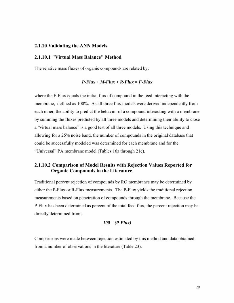
29

2.1.10 Validating the ANN Models

2.1.10.1 "Virtual Mass Balance" Method

The relative mass fluxes of organic compounds are related by:

P-Flux + M-Flux + R-Flux = F-Flux

where the F-Flux equals the initial flux of compound in the feed interacting with the

membrane, defined as 100%. As all three flux models were derived independently from

each other, the ability to predict the behavior of a compound interacting with a membrane

by summing the fluxes predicted by all three models and determining their ability to close

a “virtual mass balance” is a good test of all three models. Using this technique and

allowing for a 25% noise band, the number of compounds in the original database that

could be successfully modeled was determined for each membrane and for the

“Universal” PA membrane model (Tables 16a through 21c).

2.1.10.2 Comparison of Model Results with Rejection Values Reported for Organic Compounds in the Literature

Traditional percent rejection of compounds by RO membranes may be determined by

either the P-Flux or R-Flux measurements. The P-Flux yields the traditional rejection

measurements based on penetration of compounds through the membrane. Because the

P-Flux has been determined as percent of the total feed flux, the percent rejection may be

directly determined from:

100 – (P-Flux)

Comparisons were made between rejection estimated by this method and data obtained

from a number of observations in the literature (Table 23).

30

2.1.11 Producing Excel-Enabled Exportable ANN Models Describing Organic Compound Interactions with RO Membranes

Each of the ANN compound flux models were converted to Visual Basic (VB) source

code using a Visual Basic compiler provided with NeuralWorks Predict. For each of the

test membranes and for the “Universal” PA model, the relevant P-, M- and R-Flux

models were imported as macro functions into an Excel spreadsheet. This spreadsheet

was designed to include input cells allowing the user to manually enter relevant

molecular descriptor data for any compound of interest, after which the embedded ANN

VB programs calculate the predicted P-, M- and R-Fluxes, and percent rejection based on

both P- and R-Fluxes. Further user inputs regarding compound feed concentration and

membrane water flux are provided so that the user may project absolute compound fluxes

as well as concentration of compound expected in the RO product. An F-Flux calculator

and a residual comparator allows testing of the prediction results using the “virtual mass

balance” method so that the user may determine whether or not the model predictions are

acceptable for the particular test compound.

These exportable models are capable of running under Windows on any PC computer

running a macro enabled version of Excel (version for Office 2000 or later) and are

available upon request.

31

2.2 Molecular Modeling Method Simulation of Compound-Membrane

Interactions

2.2.1 PA Modeling Methods and Simulation Conditions

The steps carried out to achieve the above objective included (i) preparation and

optimization of fully atomistic molecular models of PA membranes, (ii) preparation of

specific compound molecular models, (iii) introduction of a selected compound into the

hydrated PA membrane system, (iv) running the MD simulation, and (v) analysis of the

results.

2.2.2 Building the Membrane Models

The membrane modeling (MM) software used to build the PA membrane models has

evolved steadily over the past several years. It is custom written in the Tool Command

and Tool Kit (Tcl/Tk) language, a freeware, string-based, cross-platform dialect similar to

Javascript. Tcl/Tk has been ported to HyperChem, a commercial molecular modeling

package containing more than 600 commands and state variables that can be addressed

and logically controlled by Tcl. A complete description of Tcl/Tk may be found at

www.scriptics.com. The version of software available before this project began had a

number of limitations and bugs that needed to be overcome at the project inception.

A screen capture of the variable setup page for the MM program is shown in Fig 29. The

software automatically constructs models of randomly crosslinked PA membranes using

optimized models of meta-phenylenediamine (MPD) and trimesoyl chloride (TMC) as

monomer building blocks. This program involves several key steps which are outlined in

Fig. 30, including:

Step1. Laying down non-bonded alternating MPD and TMC monomers at the

vertices of a 3D cubic lattice.

32

Step 2. Bonding of the monomers into a nascent linear “backbone” chain by

creating an amide bond at each step of a “random walk” through the 3D lattice.

This method ensures a randomly folded chain is produced, which is in accordance

with X-ray crystallographic data indicating a chaotic polymer arrangement in PA

membranes.

Step 3. Initiation of random crosslinking between TMC residues in adjacent

regions of the folded backbone structure. This is carried out by forming amide

bonds from the two TMC residues to a mutually-shared and neighboring MPD

monomer. Crosslinking effectively establishes membrane “pores”, as illustrated

in Figs. 31 and 32. The size, number, location, and dynamic behavior of such

pores is a factor in controlling water and solute transport in the membrane.

Step 4. Elimination of remaining non-bonded MPD and TMC monomers

followed by proportional scaling of partial atom charges to achieve the correct net

membrane charge. Charge is based on the number of free non-protonated

carboxylate groups. The membrane concentration of these groups can exceed

1 M.

Step 5. Geometry optimization of the model followed by iteration of the program

to build additional models. At each iteration cycle, certain variables, such as the

probability of crosslinking, can be incremented by some amount or randomly

varied across a predetermined range. In this way, a diverse population of

membrane models can be prepared. Models having the most suitable properties

(e.g., globular shape, higher charge, etc.) can then be selected for a particular

modeling task.

The nascent membranes constitute a latticework of alternating TMC and MPD monomers

connected by a random series of elongated amide bonds (Fig. 32). The bonds rapidly

shorten to realistic lengths and angles when the system is geometry optimized using a

suitable classical force field, such as AMBER. The “pores” remain distinctly visible,

33

however, as void spaces even in the final geometry-optimized structures. The software

monitors the number and location along the initial chain of crosslinks. It should therefore

be possible to calculate the number of pores in a membrane based on this information, but

the relationship between crosslink number and location is not simple due to the

occurrence of nested and overlapping crosslinks. Efforts to resolve this relationship are

underway.

2.2.3 Modeling the Organic Solutes

Software was developed to automatically call up and geometry-optimize any set of

organic compounds using tandem classical and semi-empirical force fields. This

software was used to create the master compound list used for this study (previously

described). Final molecular structure optimizations were carried out using the PM3 semi-

empirical force field.

Based on the results of the RMP assay (previously described), two compounds were

chosen as surrogates for this modeling subtask; NDMA, which is poorly rejected by PA

membranes (~50%) and 1,1,2,2-tetrachloroethylene (TCE) which is well rejected

(>99.9%). The disinfection by-products NDMA and TCE are of particular interest

because they both are uncharged, low-molecular-weight organics, yet one passes through

the PA membrane well while the other is retarded. The orbital structures and electrostatic

configurations of NDMA and TCE are presented in Fig. 33.

2.2.4 MD Simulation Setup & Run Conditions

The basic conditions of the MD simulations are given in Table 25. Four relatively short

duration (~200 ps) simulations have been conducted, two each for NDMA and TCE in

either a hydrated membrane system of in water. The simulations are preliminary in

nature because of the brief simulation times and the need to explore the effects of key

variables in future simulations, e.g., membrane charge, density, crosslinking, pressure,

etc.

34

The densities of the initial optimized model membranes are generally about 0.1 g/cm3,

i.e., more than 10-fold less than the value of 1.3 g/cm3 for actual PA membranes that has

been reported in the literature (Kotelyanskii et al., 1998). The membranes do not

spontaneously undergo contraction and densification on their own in MD simulations due

to strong electrostatic charge repulsion between the non-protonated carboxylate groups.

Because pKa values for organic acid carboxyl groups generally range from about 3-4,

these groups were left non-protonated in the membrane models. This assumption seems

reasonable given that many water treatment membranes are operated at ~pH 6-7 and

sometimes higher. However, this point may be contested and therefore should be

explored more carefully in future work.

The membranes undergo spontaneous contraction (“densification”) if monovalent or

divalent cations (e.g., Na+ or Ca++) are placed in the system (data not shown) resulting

in shielding and neutralization of the carboxylate charges by the cations. However, this

was not done in this study because the ion concentrations needed to achieve significant

membrane contraction were unrealistically high (>1M). Instead, densification was

accomplished by “packing” the hydrated membrane into a cubic periodic cell of

appropriate volume (30 Å per side), as illustrated in Fig. 34. Packing occurs by

shortening and bending bonds resulting in a strained molecular conformation with some

bad contacts and increased potential energy. However, much of the strain is relieved by

geometry optimizations and by running 100 ps of MD prior to introduction of the organic

solute. It is unknown whether real PA membranes are as highly packed and strained as

the models seem to indicate, but this possibility is plausible in view of the extremely

rapid nature of the interfacial polycondensation reaction between MPD and TMC. The

insoluble polymer network could rapidly precipitate in a strained conformation before it

had time to fully relax. Reliable surface energy measurements of PA membranes might

shed light on the conformational stability of this polymer and such data could be useful in

model verification and refinement of model structural details.

Membrane hydration was performed by random addition of 200 TIP3P water models to

the membrane prior to packing, yielding a water concentration of about 19 wt%. These

35

are flexible water molecules with partial charges of -0.834e on oxygen and +0.417e on

hydrogens. The “packed” hydrated membrane system (with a density of ~1.19 g/cm3)

was relaxed for 100 ps of MD simulation (300oK) before adding either NDMA or TCE to

the system’s center. The resulting system for NDMA is shown in Fig. 35, but water

molecules have been removed to facilitate visual localization of the organic molecule.

Note that membrane void spaces resembling membrane “pores” can still be observed

even at the higher system density.

36

3 PROJECT RESULTS 3.1 QSAR ANN Modeling Results

3.1.1 Comparison of RMP Assay with a Crossflow RO System Although the absolute value of rejection determined by the RMP assay and the block

tester were not equal (Fig. 5), there was an overall agreement in the comparative behavior

of the two systems (e.g., compounds rejecting well in the RMP assay were observed to

reject well with the crossflow block tester and vice-versa.). The lack of the crossflow in

the RMP assay, and subsequent increase in membrane concentration of solute at the

membrane surface likely explains the reason why the rejection results deviate from ideal

values (the dotted line in the figure). However, the difference between the RMP assay

and the cross-flow block tester is greatest where rejection is poor, and the results tend to

converge as rejection improves (with the exception of the CA membrane). Thus, for the

most part, predictions of high rejection by the RMP assay (at least for PA membranes)

should tend to reflect high rejection values observed in a standard RO unit.

3.1.2 Determination of Compound-Membrane Interactions In the RMP assay, use of radioactively tagged compounds allows the mass of compound

in the product, the feed, and in the membrane to be directly measured, and fluxes of

compound through the membrane (P-Flux) and into the membrane (M-Flux) to be

directly determined. By difference, it was possible to estimate the flux of compound that

remained in the feed. Thus, the fate of surrogate compounds could be accurately tracked

and their behavior could be determined.

Figures 8a, 9a, 10a, 11a, 12a and 13a represent performance diagrams that illustrate

compound behaviors determined for each membrane. In these representations, the X-axis

shows the relative M-Flux (values 0 – 100) representing increasing membrane association

from the left to the right of the graph. The Y-axis shows the relative P-Flux (values 100

– 0) decreasing membrane penetration (increasing rejection) from bottom to top of the

graph. Each of the numbers on the graphs represent the identity of a surrogate

37

compound. A list of these compounds with their respective ID numbers and relative

compound fluxes (P-, M- and R-Fluxes) are presented in Figs. 8b, 8c, 9b, 9c, 10b, 10c,

11b, 11c, 12b, 12c, 13b and 13c. The QSAR descriptor cluster numbers correspond to

the compounds’ molecular properties categories.

The graphs representing compound fate are divided into four quadrants. Compounds in

quadrant “A” interact poorly with the membrane; they neither associate with the

membrane nor do they pass through it. This can be confirmed by their relatively low P-

Flux and M-Flux values, but relatively high R-Flux values (high rejection at the

membrane surface). Compounds in quadrant “A” are well rejected by the membrane

acting as a mechanical barrier. Some examples of compounds in this category include

the pharmaceuticals ibuprofen, ciprofloxacin, the endocrine disruptor bisphenol, and the

herbicide alachlor. These compounds are very well rejected by all the PA membranes.

Compounds in quadrant “B” do not associate with the membrane well, but pass through it

relatively easily. These compounds are poorly rejected, as the membrane provides a poor

barrier to them. Urea and NDMA are the only two surrogate compounds that fell in this

category in for the PA membranes, while the CA membrane had several others, including

caffeine and t-butyl alcohol.

Compounds in quadrant “C” pass through the membrane poorly; however, they strongly

associate with the membrane so their apparently high rejection is largely due to

membrane absorption or adsorption. In this case the membrane acts as an affinity filter.

Although these compounds are initially well rejected, if the membrane reaches saturation

(may occur if compound is constantly in the feed), these compounds may eventually

break through, especially if they are absorbed into the membrane and not adsorbed on the

membrane surface. Examples of compounds that fall in this category for all the PA

membranes are the endocrine hormones 17a-estradiol and estrone, the aromatic

hydrocarbons toluene, benzene and the aromatic alcohol phenol.

38

The CA membrane behaved somewhat differently than PA membranes. In general, there

were less surrogate compounds associated with quadrant “A” and there were more

compounds that fell in quadrant “B”, indicating that the CA membrane was not as

successful as the PA membranes in rejecting organic compounds.

A direct performance comparison between membranes for P-, M- and R-Flux for each

surrogate compound is presented in Tables 6, 7 and 8.

3.1.3 ANN Models Describing Organic Compound-Membrane Interactions

3.1.3.1 Overall Performance of ANN Membrane Models

Results of ANN modeling for P-, M- and R-Fluxes for all membranes (and for the

“Universal” PA model) are summarized in Figs. 14a through 19c and Tables 9a through

14c. In each of Figs. 14a through 19c, a scatter plot comparing actual surrogate

compound behavior with that predicted by the ANN model visually indicates model

performance. The diagonal line in this plot indicates perfect agreement between the

model and real world values. Error bars represent one standard deviation about the mean

for the actual behavior data (n = 4 to 7). ANN model statistics are presented beneath the

scatter plot, including the R correlation values (linear correlation between predicted and

actual values), the average absolute error values (average absolute error between the

predicted and actual values) the root mean squared (RMS) error values (root mean square

error between the predicted and actual values), the 95% confidence interval for the model

and the number of exemplar records used to create the model. The identity of the QSAR

molecular descriptors used in model construction is indicated below the statistics panel.

For each input, a value representing a sensitivity index calculation relating the direction

and degree of influence of each of the input parameters to the model is presented

(explained in more detail below). Tables 9a through 14c present the predicted and actual

behavior results for P-, M- and R-Fluxes for each of the surrogate compounds for all the

membrane models (in the case of the “Universal” PA membrane, the actual values

reported are the averages of results for all the PA membranes combined).

39

Performance of the ANN models was evaluated by comparing the linear correlation (R)

coefficients between the predicted model outputs and the actual laboratory flux data.

Correlation values were typically in excess of 0.95 in most cases. Moreover, the

closeness of matching between training and test data sets indicated a predictive model.

Reasonably close ranges for the predicted 95% confidence limits also indicated good

model behavior. The P- and M-Fluxes tended to model better than the R-Flux, primarily

due to the fact that the R-Flux was a calculated value made up of data from the other

fluxes, and therefore contained the sum of their statistical noise. For a like reason, the

“Universal” PA membrane model was also noisier than the individual PA membrane

models (but still possesse a relatively high R value). Because of an increase in internal

noise, this model is more flexible than the individual PA models, and tended to be

somewhat more applicable to compound behavior prediction (see below).

3.1.3.1.1 ANN Model Sensitivity Analysis Results

Because the models in this study were constructed using QSAR molecular descriptors

(for a detailed listing see Appendix 1) linked to fundamental molecular properties, it was

hoped that the nature of the individual inputs to the models and the degree to which they

influenced the predicted behavior of the surrogate compounds would provide insights as

to the molecular mechanisms defining compound-membrane interactions. One goal of

the study was, therefore, a search for “universal behaviors” in a broad sense between

membrane models with regard to the basic molecular properties.

By considering the inputs selected by the GA during model construction, it was possible

to gain insight as to which input parameter proved influential in a given compound-

membrane interaction. However, the direction and magnitude of that influence was not

revealed. In the case of multivariate linear models, it is possible to gain this insight by

analysis of the magnitude and direction of the slopes of the individual linear equations

from which the model was assembled. In the case of the ANN models, this is not

possible. However, it is possible with the ANN models to compute a “sensitivity index”

for each of the input parameters. The sensitivity index is a measure of the overall

magnitude and direction of influence that each of the model input parameters has on the

40

model output. If this index is calculated over the entire range of the input data set (for all

the surrogate compounds), then it tends to represent the overall strength and direction the

input parameter has on the model output. However, it may not entirely indicate a long-

range output response. For example, the sensitivity index for a constantly increasing

function would be positive and one for a constantly decreasing function would be

negative, and the magnitude of the index would be a relative index of slope. If, on the

other hand, the function contained a number of hills and valleys (a sine wave parallel to

the X-axis would be an extreme example of this), the sensitivity index could be large

because of short-range influences, but would not well indicate the long-range

relationships in the function.

A summary of the sensitivity indices for all the membranes with regard to each of the

compound-membrane interactions (P-, M- and R-Fluxes) is presented in Tables 15a

through 15c. Of the original 73 molecular descriptors used in the modeling, a total of 33

survived as inputs used in the ANN models (See Appendix 2). In these tables, the

molecular descriptors were broadly grouped into five categories to aid comparison. The

five groupings include descriptors related to molecular charge or polarity (ABSQ,

MaxQp, MaxNeg, P, Py, Pz, Q, SsCH3, SdssC, SaaCH, SdO, Gmax, Gmin, Hmin),

descriptors related to molecular size or complexity (Ovality, Surface, xpc4, xv1, xvpc4,

nxp5, nxch6, k1, k2, k3, Iy, fw, idcbar, sumdelI, Wt), descriptors related to molecular

hydrophobicity (Log P), descriptors related to hydrophobicity/charge (Qs, Qsv), and

descriptors related to the extent of molecular hydrogen bonding (numHBa ). (For a

detailed explanation of these descriptors, see Appendix 1.)

41

3.1.3.1.1.1 Relative P-Flux Sensitivity Index Analysis: Molecular Descriptors

Associated with Penetration of Organic Compounds through the

RO Membranes

In the case of the relative P-Flux (solute passing through the membrane, Table 15a), it

was observed that, depending on the membrane, this compound-membrane interaction

was associated with all five molecular descriptor groups, although models contained

varying numbers of inputs (a minimum of 4 inputs for LFC1 to a maximum of 8 inputs

for ESPA-2 and for the CA model). Thus, ability of compounds to pass through the

membranes were related to molecular charge and charge distribution, molecular size and

complexity, hydrophobicity and to the hydrogen bonding. However, the magnitude and

direction of influence for many of these properties varied from membrane to membrane.

In general, for the polyamide membranes, influential molecular descriptors included

MaxQp (the largest positive charge over the atoms in the compound), Py (the magnitude

of charge separation along the compound’s inertial Y-axis), P (the magnitude of the

compound’s dipole moment), SsCH3 (the sum of the E-state values for all the methyl

groups in the compound), SdssC (the sum of the E-states for all the aromatic carbon

atoms in the molecule), and Hmin (the smallest hydrogen atom E-state in the compound).

The CA membrane model included the same descriptors as the PA models (P and SdssC).

There was a general variation in the direction and magnitude of the influences of the

inputs related to molecular charge and polarity. However, in general, Py (component of

the dipole moment along the inertial Y-axis) tended to show agreement across three of

the four PA models. An increase in this descriptor was related to an increase in P-Flux.

The CA model did not contain unique charge/polarity related inputs (some were also

shared by one more PA models).

Molecular complexity descriptors included in the models were Ovality (the deviation of

the compound’s shape from a perfect sphere), Surface (the molecular surface area), the

chi indices xpc4 (5 atom chi index encoding patterns of adjacency), xv1 (2 atom chi

index encoding degree of branching) and xvpc4 (5 atom chi index encoding patterns of

42

adjacency), nxp5 (the number of paths in the molecule with 5 edges), Iy (the principal

moment of inertia along the compound’s Y-axis), and fw (the compound’s molecular

weight). The relationship between molecular complexity and P-Flux was also mixed. It

would be generally expected that as molecular size and complexity increased that P-Flux

should decrease. In many cases (9 of 13 involving molecular complexity parameters),

this was observed. The CA membrane model emphasized the chi indices more than did

the PA models, but the chi index descriptor xvpc4, though not included in the CA model,

occurred in 3 out of 4 PA models. Sensitivity indices for the chi indices tended to be

negative, suggesting that ability to transverse the RO membrane matrix was in general

inversely proportional to molecular complexity.

Qsv (the average molecular group polarity descriptor) was only included in the CA

model, and was positively associated with P-Flux.

Hydrophobicity was almost universally important in models predicting P-Flux, evident

by the nearly universal inclusion of LogP in both PA and CA models (with the exception

of the TFC-HR model). This input universally exhibited a negative relationship with the

P-Flux. As LogP increases, compound hydrophobicity increases. This means that as

compound hydrophobicity increased, there was a fairly universal tendency for the

compound to be retained by the membrane.

There was also a generally positive relationship between numHBa (the number of

hydrogen bond acceptors in the compound) and the P-Flux (in three of the four PA

membranes). This indicates that as the number of hydrogen bond acceptors on the

molecule increase, there is a greater tendency for the molecule to pass through the

membrane.

The “Universal” PA model exhibited general overall agreement with the nature and

direction of influence of the parameters included in the other models. More interesting

was the fact that, although the membrane properties (Table 3) were included in

construction of the P-Flux model, none of them survived during the evolution of the

43

inputs by the GA. This suggests that compound molecular properties were more

influential than the measured membrane properties with regard to penetration of

compounds through the PA membranes.

The CA membrane model included many of the same descriptors appearing in the PA

models, although there were some unique inputs (Qsv, xv1, xpc4) which did not appear

in any of the PA models.

3.1.3.1.1.2 Relative M-Flux Sensitivity Index Analysis: Molecular Descriptors

Associated with the Adsorbtion/Absorption of Organic Compounds

to the RO Membranes

ANN models describing the interaction of the compounds with the membranes (M-Flux)

once again included representative molecular descriptors from all the five basic

descriptor groups, and as with the P-Flux models there were differences in the descriptors

emphasized by each membrane model (Table 15b). Some descriptors included in the P-

Flux models also appeared in the M-Flux models (specifically MaxQp, P, SdssC, nxch6,

LogP and NumHBa). Once again, there was a range in the number of descriptors

included in each membrane model (from as few as 4 with BW-30 and CA to as many as

10 with LFC-1).

With regard to the charge/polarity-related descriptors, besides MaxQp, P and SdssC, the

M-Flux models included Q (the magnitude of the principal quadripole moment), SaaCH

(the average E-state value for all aromatic carbon-hydride groups in the compound),

Gmax (the largest atom E-state in the compound) and Gmin (the smallest atom E-state in

the compound). Once again, there was variation in the direction and magnitude of

influence amongst the various membrane models for these inputs, though all of the

models did include an input indicating that molecular charge and/or polarity played an

important role in the association of the compounds with the membranes. Gmin (the

smallest atom E-state in the molecule (the most electrophilic atom in the molecule) was

universally included in this category, and its sensitivity index was universally positive

44

and relatively strong. This suggested that the association of compounds with the

membranes might involve electrophilic interactions. Likewise, P (the magnitude of

charge separation along the whole molecule) was universally included in all models. In

the case of 3 of the 4 PA models (and in the case of the “Universal” PA model), the

sensitivity indices for P were negative, indicating that as the magnitude of the charge

separation decreased, the association of the compound with the membrane increased.

This relationship reversed in the case of CA and TFC-HR, however, but remained a

strong relationship.

Of the indices related to molecular complexity, only fw (formula weight) appeared in the

P-Flux models. Additional complexity descriptors related to M-Flux included nxch6 (the

number of 6-membered rings in the compound), k1 (kappa shape index related to the

degree of cyclicity in the compound) and idcbar (the Bonchev-Trinajsti mean information

content). The contribution of molecular descriptors related to molecular complexity to

the M-Flux varied. In some cases, (BW-30, TFC-HR and CA), complexity did not seem

to be important in the models at all, and in the case of LFC-1 and ESPA-2, the models

exhibited strong but inconsistent directions of influence with regards to formula weight

(mass) and indicators related to molecular structural complexity (idcbar and k1).

The number of hydrogen bond acceptors (numHBa) was once again included in the M-

Flux models, at least in 3 of the 4 PA models as well as in the “Universal” PA model. It

is universally positive, indicating that the presence of more hydrogen bonding acceptors

in the compound is associated with increased tendencies to associate with the membrane

(either adsorption or absorption).

Log P is not as prevalent with regard to membrane association, (it was included in just

two of the PA membrane models, the “Universal” membrane model and the CA model).

It also exhibits some variation in response, but in the case of BW-30, the “Universal” PA

and CA, it was positively associated with M-Flux, suggesting that in these cases

increasing hydrophobicity may increase compound association with the membranes.

45

As with P-Flux, there was general agreement between the “Universal” PA model inputs

and direction of influence as the individual PA models. Once again, none of the

membrane parameters were included in the final model, although they were present

during model construction. As with the P-Flux, this indicates that none of the membrane

parameters included in the modeling were more influential than the compound molecular

descriptors in predicting the interaction of the compounds with PA membranes.

The CA model describing M-Flux differed from the PA models in the direction of

influence the charge/polarity-related descriptors, possibly indicating a difference in

mechanism of interaction between the compounds and the CA membrane.

3.1.3.1.1.3 Relative R-Flux Sensitivity Index Analysis: Molecular Descriptors

Associated with the Ability of RO Membranes to Repel

Compounds at the Membrane Surface

Molecular descriptors and their sensitivity indices are shown for the R-Flux models in

Table 15c. There are molecular descriptors in these models which appear in both the P-

Flux and/or M-Flux models, including Py, Q, SaaCH, SdssC, Gmax, Gmin, nxch6,

idcbar, LogP and numHBa. Again, as with the other compound flux models, responses of

the individual membrane models varied with respect to the individual molecular

descriptors included in the R-Flux models. Also, as with the other compound flux

models, the molecular descriptors are related to charge/polarity, molecular complexity,

hydrophobicity or hydrogen bonding, although not all membrane models contain

descriptors from all of these groups. The complexity of the models covers a range similar

to that seen with the other flux models (from 4 inputs for BW-30 to 10 inputs for TFC-

HR). There was a general tendency for the sensitivity indices for R-Flux to be opposite

those noted for the M-Flux, and as R-Flux is a measure of the tendency of compounds not

to associate with the membranes, this is not a wholly unexpected result.

Charge/polarity descriptors serving as inputs for the R-Flux models that were not

included in other flux models include ABSQ (the sum of the absolute value of the

46

charges on all atoms in the compound), MaxNeg (the largest negative charge over the

atoms in the compound), Pz (the component of the dipole moment along the compound’s

inertial Z-axis) and SdO (the sum of all E-state values for the doubly bonded oxygen

atom in the compound). There was in general a negative relationship noted between

charge-related inputs and R-Flux in most of the models. The most commonly represented

molecular descriptor related to compound charge was Gmin, which was also strongly

represented here as it was in the M-Flux models, except that its direction of influence is

reversed. Q (the magnitude of the principal quadripole moment) was contained in three

of four PA models and Gmin was contained in all PA models.

Regarding molecular complexity, nxch6 and idcbar were shared with other flux models,

but sumdelI (the sum of the delta intrinsic states of atoms in the compound), Wt (the total

Weiner number) and the kappa shape indices k2 (encoding the degree of central

branching in the compound) and k3 (encoding the degree of separated branching in the

compound) were unique to the R-Flux models. The direction of influence of molecular

complexity indices tended to vary; however, they were on the overall positive, indicating

that for the most part, R-Flux tended to increase with increases in molecular complexity.

Where models included LogP (BW-30 and TFC-HR), as an input parameter, its

sensitivity index was negative, indicating that compounds with lower hydrophobicity

tended to remain unassociated with the membrane. In the case of BW-30, this effect was

opposite that for M-Flux and similar to that for P-Flux, consistent with a model in which

hydrophobic association with the membrane removed compounds from solution on the

feed side and also prevented them from passing to the product side.

The number of hydrogen bond acceptors (numHBa) was again included in three of the

four PA models, as well as in the “Universal” PA model. In this case, the sensitivity

analysis indicated a negative relationship between the number of hydrogen bond

acceptors in the solute molecules and the ability of the molecule to remain free in the

feed. This is consistent with the results for the M-Flux, which indicated an opposite role

for this parameter, and for the P-Flux models as well. This suggests that hydrogen

47

bonding may facilitate the attachment of compounds to the membrane as well as facilitate

their transport through the membrane matrix.

Once again, there was general agreement between the “Universal” PA model and the

individual PA models with regard to the inputs emphasized and the direction of their

influence. In this case, as with the other “Universal” PA models, no membrane input

parameters survived in the final evolution of input parameters, indicating that the

measured membrane parameters were far less predictive of the ability of the membranes

to reject compounds at membrane-feedwater surface than were the molecular descriptors.

The CA model was also in general agreement with respect to the type and direction of

influence of the molecular descriptors. The CA model tended to emphasize the

charge/polarity descriptors, and included the absolute molecular charge (ABSQ) as one of

the more influential inputs. The sensitivity index suggested that the R-Flux was

positively related to compound absolute charge.

3.1.3.2 Validation of the “Universal” PA ANN Models – Comparison with the

Individual PA Models

The success of prediction of the “Universal” PA ANN model was evaluated by

comparing it to the outputs of each individual PA membrane models. These comparisons

were determined for P-, M- and R-Fluxes (Figs. 20a through 23c). In these figures, the

closed circles represent the specific PA membrane models while open circles represent

the “Universal” PA model. All the “Universal” models agreed reasonably well with the

individual membrane models. The “Universal” PA models generally exhibited more

noise, which is an expected result of them containing the combined statistical noise of all

of the other PA membrane models. It was also noted that, as with the individual

membrane models, the R-Flux model was the noisiest.

48

3.1.4 Application of the ANN Models to the Master Compound List –

Prediction of Compound Interactions with RO Membranes

3.1.4.1 Prediction of Compound-Membrane Interactions; Determination of

Prediction Success Using the “Virtual Mass Balance” Method

The ANN models were applied to all 202 compounds in the master compound list to

predict relative P, M and R-Fluxes for each of the 5 membranes used in the study as well

as for the “Universal” PA model. Following prediction of relative fluxes, the F-Flux was

calculated from the predicted values by summation of the individual relative mass fluxes.

This F-Flux represents the estimated total relative compound flux impinging on the

membrane in the RMP assay, and by definition should have equaled 100 in all cases. As

each of the ANN models was developed independently of the other, this combination of

their data to provide a “virtual mass balance” should have amounted to a conservative

performance evaluation. Based in the confidence intervals observed in the individual

models, a somewhat subjective criterion was used to establish a noise band of ± 25% as

the cutoff for the study. Compounds whose predicted F-Flux values were outside this

range were culled from the database for each membrane

The final list of compounds, in alphabetical order, that were successfully modeled in the

study is presented, for each membrane used in Tables 16a through 21c. In these tables,

the compounds appearing in boldfaced type represent the surrogates that were used to

construct the predictive models. The predicted values for the relative P-Flux, the relative

M-Flux, the relative R-Flux and the summation of these values (the F-Flux) are presented

to the right of each of the compounds..

Based on the above criterion, success in prediction of the interactions between the

organic compounds with the test membranes varied with membrane type. With CA, the

ANN models were capable of predicting the behavior of 58% of the compounds. The PA

models could describe the behavior of between 57% and 70% of the compounds. The

49

“Universal” PA model was the most flexible, and was able to predict the behavior of 76%

of the compounds in the master compound list.

3.1.4.2 Interpretation of the Relative Flux Table Data

The relative fluxes presented in Tables 16a through 21c may be used to gain insight as to

the expected performance of the membranes on a given compound. In general,

compounds exhibiting a low relative P-Flux and a low relative M-Flux (and a

concomitantly high relative R-Flux) will be rejected well by the membrane in question

(they would fall in quadrant “A” in a quadrant diagram such that presented in Figure 8a).

Because the membrane interaction is predicted as being low, rejection should be

relatively insensitive to mechanisms such as compound binding and saturation of the

membrane material.

If a compound presents a high value for the relative P-Flux and a low value for the

relative M-Flux (also a low value for the relative R-Flux), then the compound is passing

through the membrane with little interaction. The membrane is providing neither a

mechanical or adsorptive/absorptive barrier to the compound in this case. Compounds in

this category are not well susceptible to removal from the feed by reverse osmosis using

the particular membrane in question.

Finally, in situations where the P-Flux is high and the M-Flux is high (but the R-Flux is

low), the compound is being removed by the membrane by a largely

adsorbtive/absorptive mechanism. Compounds exhibiting this behavior are initially

blocked from the product water effectively, but as the membrane begins loading with

bound material, removal may begin to suffer, especially should the compound be

removed by absorption into the membrane structure (or the support materials).

Compounds exhibiting this sort of behavior could eventually prove problematic if

provided to the RO system in low concentrations over long time periods as opposed to

spikes with long periods in between.

50

3.1.4.3 Estimation of Membrane Percent Rejection from the Relative

Compound Flux Data

It is possible to convert the relative flux data provided by the RMP assay into a percent

rejection value. Two mass fluxes can provide the basis for this sort of conversion; the

relative P-Flux or the relative R-Flux (as described in the methods section).

Rejection calculated by relative P-Flux is based on two principal mechanisms:

mechanical exclusion and adsorptive/adsorptive compound-membrane interactions. This

is the “classical” method of determining RO membrane rejection. In the field, as with

the RMP assay, rejection does not take into account association of the compound with the

membrane at all (e.g., a high rejection doesn’t indicate a priori that the compound is

being physically rejected at the feed/membrane interface).

On the other hand, percent rejection determined by the relative R-Flux value is based

solely on the interaction (or lack of interaction) at the membrane surface. It is indeed

“rejection” directly into the feed; thus the relative R-Flux value (as defined in this study)

directly represents a “percent rejection.”

Percent rejection values predicted by all of the ANN models, determined by both P-Flux

and R-Flux methods, are presented for each membrane used in the study as well as for the

“Universal” PA membrane model in Tables 22a through 22e. All of the compounds used

in the study were included in these tables in alphabetical order. Blank cells in these

tables indicate compounds whose behavior could not be predicted by a particular

membrane model.

Compounds exhibiting large percent rejection values determined by both P-Flux and

R-Flux (such as Diazinon, Disulfoton, Lincomycin, Mestranol, and Triphenyl Phosphate)

suggest very good rejection, as the compounds are not only poorly able to pass through

the membrane but are also poorly able to associate with the membrane material (similar

to the situation of compounds in the “A” quadrant of Fig. 8a). In the case of compounds

51

in which the rejection as determined by P-Flux and R-Flux is both nearly equal and

moderate to low (such as Bromochloromethane, NDMA, and Urea), the compound passes

through the membrane without interacting with it. RO in this instance provides a

relatively poor barrier to the compound (similar to the situation with compounds in the

“B” quadrant of Fig. 8a). Finally, when the rejection based on P-Flux is high but

rejection based on the R-Flux is low, (such as with TCE, PCE, 4,6 Dichlorophenol,

Acetaminophen, Benzene, Dibromoacetonitrile, 17a Estradiol, and Estrone), the

compound is being removed mainly by adsorption/absorption to the membrane. In this

case, the compound’s rejection may initially be very good, and remain good so long as

the compound is present in short spikes. However, if the compound is chronically

present in the feed, as the membrane begins to saturate with the compound, rejection may

significantly degrade. Therefore, compounds with high P-Flux rejection but poor R-Flux

should be regarded as potentially problematic.

3.1.5 Comparison of Rejection Predicted by the ANN Model to Rejection

Reported in the Literature and Field

The rejection results predicted by the RMP assay data and the ANN models for P-Flux

were compared to results reported in the literature and from the field (Table 23). Data

were compiled for 18 compounds, including pharmaceuticals, disinfection byproducts,

pesticides, endocrine disruptors, low molecular weight aromatic hydrocarbons, and

others. In general, rejection predicted by the ANN models for PA and CA membranes

exhibit very good agreement with that reported in the literature or from the field.

3.1.6 Instances where Models Failed to Predict Compound Behavior: Gap

Analysis and Suggestion for Further Study

Even though a reasonably large proportion of the master compound list (~25%) was

included as surrogates for model construction and some care was taken to insure that the

molecular properties of the surrogates were diverse, the resultant ANN models were still

52

unable to predict the behavior of many compounds. The failure rate varied somewhat

depending on the membrane being modeled; however, in a many cases the same

compounds were observed to fail prediction in multiple membrane models.

Table 24 shows a listing of compounds that failed in 75% or more (3 or more) of the

polyamide models, and includes 45 compounds (slightly less than 25% of the total

number of compounds examined). These compounds possessed molecular properties

outside of the experience of the ANN models, and thus the models were unable to predict

their behavior.

Failure of the models could be due to two reasons: either there were insufficient

surrogates chosen to define one or more of the original QSAR molecular descriptor

groups initially identified in the study, resulting in too narrow a variation of molecular

properties, or else the original QSAR molecular descriptor groupings were not

appropriately related to the compound-membrane interactions that were modeled. The

very small number of total exemplars used in ANN model construction may have been

problematic; only 51 surrogates were used in the study whereas often hundreds or

thousands of exemplars are typically employed in constructing ANN models. For a

small number of surrogates as was employed in this study to yield a highly predictive

model requires the system under study to be very well-behaved and relatively simple so

that it may be adequately defined with a limited number of points scattered in

n-dimensional space. Clearly, the failures observed in this case indicate that this system

is more complex than can be adequately defined by only 51 different input patterns.

Figure 24 shows the fraction of compounds in the QSAR descriptor clusters that were

represented by surrogates (the density of information defining the cluster) plotted against

the percent of cluster compounds failing to model (compound failure defined as the

F-Flux failing to be predicted by at least 3 of the 4 PA ANN models within ± 25%). The

numbers on the chart represent each of the QSAR descriptor clusters identified in the

study. The general expectation is that failure of the ANN models will be inversely

proportional to model experience; that is, the greater the representation of a cluster by

53

surrogates, the greater the ability to predict behavior of the cluster compounds. Where

surrogates representing a cluster were sparse (clusters 11, 17, 9 10, 2) model failure rates

were relatively high and generally increased in proportion to lack of exemplars. In this

case, clearly the model experience is lacking, creating significant information gaps.

More surrogate compounds representing these clusters should materially improve

prediction of the models. The negative slope of the trend line supports this general

hypothesis, but the trend is relatively weak, indicating that other factors influence failure

other than simply the absence of sufficient exemplars for each cluster.

The original QSAR molecular descriptor clusters were chosen based on a suite of

molecular descriptors not necessarily related to compound-membrane interactions. Thus,

compounds may have been grouped on the basis of properties not germane to these

interactions. The data presented in Fig. 24 suggest this might have been the case. For

example, compounds in clusters 3, 4, 16 and especially 6, 15, 18, 19 and 20 could be

adequately predicted by the ANN models (“adequate” meaning failure rate ≤ ~15%)

using data provided by the surrogate compounds chosen for the study in spite of

relatively poor surrogate representation. On the other hand, compounds in clusters 1, 5,

12, 13 and especially 8 failed to model even when they were relatively well represented

by surrogates.

In order to close the “gaps” in the ANN models, additional surrogates are needed that

address the lack of information currently limiting predictive ability of the models.

Moreover, the choice of compounds for this purpose may now be based on a smaller

universe of molecular descriptors known to be related to compound-membrane

interactions, as these descriptors were identified in the current study.

Figure 25 represents a dendritic analysis of the 45 poorly modeled compounds. As

before, the intent of this analysis was to identify compounds with similar properties so

that they may be clustered for purposes of surrogate identification. A somewhat arbitrary

criterion was adopted for separating clusters; a distance of 300 was chosen because, in

general, it isolated like compounds well. In addition to this criterion, a fine-tuning was

54

performed to separate clusters that appeared to have larger numbers of compounds, so

that cluster size was reduced to no more than 7 compounds. A total of 16 clusters were

identified containing from 1 to 7 compounds.

Addition of surrogate compounds chosen from these clusters should substantially

improve predictability of the current models. This approach should be considered as a

future area of study.

3.2 Analysis of MD Simulations

3.2.1 System Energies

Data presented in Fig. 36 indicates system potential energy fluctuations for the NDMA

membrane simulation. TCE data (not shown) were similar and, in each case, system

potential energies initially increased, followed by a gradual decline to steady state. The

initial increase in potential energy was due to early interactions as the system temperature

was raised from 0oK to 300oK in the first 0.1 ps of simulation. Once the specified

simulation temperature was reached, both systems drifted toward more relaxed

conformations with lower overall potential energies.

3.2.2 Diffusion Behaviors of NDMA and TCE

Using center-of-mass (COM) positional data to dampen the effects of single-atom

motions, NDMA and TCE trajectories were monitored over the course of the membrane

simulations. The data revealed that both compounds exhibited continuous, small-scale

translocations (usually on the order of ~1Å) primarily centered in the local region of the

membrane into which the compound had been first introduced. Preliminary efforts to

compute diffusion coefficients for NDMA and TCE were based on these small-scale

translations (see below), but other types of longer-range excursions were also observed,

particularly for NDMA. It is these irregular long-range translocations that must be more

fully documented and statistically described in terms of their magnitudes and frequencies

of occurrence before accurate diffusion kinetics can be obtained. For example, NDMA

was observed to make two abrupt translocations beginning at about 20 ps of elapsed

55

simulation time. These translocations can be observed in the COM trajectory paths

shown in Fig. 37. In the first “outbound” translocation, occurring at about 20 ps, NDMA

traveled nearly 7Å away from its point of origin at t = 0 ps. This was followed

approximately 8-10 ps later by an equally abrupt “inbound” translocation and return to

the immediate vicinity of the molecule origin (Fig. 38). Following the inbound

movement, NDMA was observed to resume small-scale excursions, but superimposed on

this was a gradual drift away from the origin over the next 60 ps. In contrast, TCE did

not exhibit any large-scale translocations of the magnitude exhibited by NDMA.

Moreover, TCE tended to reside within a fairly restricted region, traveling not more than

~1-2 Å from its point of origin for the duration of the 200-ps simulation. However,

larger-scale movements of TCE might have been observed if simulation times were

extended.

The type of rapid translocation behavior in which a solute such as NDMA moves from

one “vacancy” or void space in the polymer matrix to an adjoining void is referred to as a

“jump” or “hop” (Fig. 39). This motif of solute transport has been well documented for

dilute gas molecules diffusing in amorphous polymers, such as carbon dioxide or

methane in polyethylene or polypropylene (Takeuchi, 1990; Gusev et al., 1994; Takeuchi

and Okazaki, 1996; Mueller-Plathe, 1994). Such a jump mechanism has also been

recently reported for water diffusion in PA membrane networks (Kotelyanskii et al.,

1998); and, in that study, it was demonstrated that the accuracy of water diffusion

coefficients were critically dependent on the jump frequencies. The jumps occur when

the solute and membrane undergo conformational changes such that the solute can

suddenly squeeze into and through a passage or channel that is temporarily formed

between two adjoining void spaces in the membrane. The probability of this happening

depends on numerous variables including (i) the flexibility of the membrane and solute,

i.e., how readily they can undergo conformational rearrangements by overcoming

torsional barriers, (ii) the solute size and shape, and (iii) short- and long-range

interactions with water and membrane atoms (i.e., electrostatic and van der Waals

interactions).

56

Conventional calculation methods for solute diffusion coefficients (D) based on root-

mean-square (RMS) molecule displacements (<x2> = qiDt, where <x2> is RMS

displacement, qi is the dimensionality factor, t is the displacement time step) are

generally suitable for substances that demonstrate continuous localized diffusion

behavior, i.e., diffusion that is unmarked by jumps. However, as illustrated in Fig. 39, if

abrupt and large translocations occur, it is necessary to compute diffusion coefficients

based on the magnitude and frequency of such translocations.

3.2.3 Calculation of Water and Solute Diffusivities and Theoretical Fluxes

In spite of the limitations discussed above regarding the lack of information on solute

jump frequencies, apparent diffusion coefficients for water (DBM) and the organic solutes

(DAM) were nevertheless computed from the time-resolved RMS displacements of the

compounds during selected periods of the MD simulations. The RMS displacements

were computed from molecule COM coordinates to dampen the effects of single atom

motions. The results of a typical diffusion coefficient calculation for five randomly

selected water molecules and the NDMA solute are given in Fig. 40. Diffusion

coefficients and theoretical solute fluxes are presented in Table 26. At this stage, the

diffusion coefficients should be regarded as providing only relative indications of

transport kinetics. As expected, the organics diffused relatively more slowly than water

within the membrane matrix. It should be noted that whereas the diffusion coefficients for

NDMA and TCE were nearly indistinguishable in pure water simulations (~7.82x10-6

cm2/s), TCE diffusion in the hydrated membrane system (1.92x10-6 cm2/s) was nearly

four-fold less than that of NDMA (7.25x10-6 cm2/s). The similarity of NDMA

diffusivities in the water and membrane systems reflects the fact that calculations for DAM

were based on local molecule excursions rather than on discontinuous jump frequencies.

Theoretical fluxes (JA) for NDMA and TCE were calculated based on the modeled

diffusivities (DAM) and experimental values for KA, the water-membrane equilibrium

partition coefficient: JA = -DAMKA(∆CA/ σ), where ΔCA is the solute concentration

gradient and σ is the thickness of the PA discriminating layer (~10-5 cm). Water flux, JB,

57

was calculated from the expression: JB = -CBMDBMVBM(∆P - ∆π)/(RTσ), where CBM is

the membrane solvent concentration (12.3 M), DBM is the modeled diffusivity (Table

26), VBM is the solvent molar volume, ∆P - ∆π is the net pressure, R is the gas constant,

and T is the temperature (300oK). The solute partition coefficient, KA, is perhaps the

most critical factor and at this time can only be crudely estimated from experiment.

Values for KA were determined by rinsing membranes in ultrapure water following

laboratory rejection tests using radiolabeled compounds. It was assumed that the 30-

minute rejection test provided sufficient time for equilibration between feed and

membrane solute concentrations, although this has not been experimentally verified. It

was also assumed that the water rinse was adequate to extract unbound compound from

the fabric backing and that remaining label was evenly distributed throughout the

polysulfone support and the much thinner PA layer. Given the inherent weaknesses of

the method and underlying assumptions, the KA values must be viewed as conservative

and very likely too high, possibly by orders of magnitude. It is perhaps noteworthy that

KA for TCE was ~24-fold higher than NDMA which is consistent with the lower water

solubility (higher LogP) of TCE. Actual feed and permeate solute concentrations were

used to calculate the solute gradient, ΔCA, and a net driving pressure of 100 psi was

assumed. Poor agreement was observed between theoretical and experimental fluxes,

with modeled fluxes for NDMA and TCE ranging from ~4-6 logs higher than

experimental values (Table 26). However, good agreement was observed between

calculated water flux and that expected for a PA membrane. The principal reasons for

overestimation of the solute fluxes are likely that (i) the modeled diffusion coefficients

for the organics were too large since jump frequencies have not yet been determined, (ii)

the KA values were grossly overestimated, or (iii) both of the above.

3.2.4 Water and Membrane Interactions with the Organics

Although the mass of TCE (~165 amu) is greater than that of NDMA (~74 amu), this

difference alone is insufficient to explain the discrepancy in their relative motilities in the

PA membrane. Perhaps the simplest explanation for retarded TCE transport is that it

interacts more with the membrane polymer. In order to determine if TCE was interacting

58

more strongly than NDMA with the membrane, a Tcl script was developed to extract the

energy of interaction (i.e., “energy of association” or “binding energy”) of the organic

species with the hydrated membrane, i.e., with the water-membrane complex, at each

step of the simulation playback. As illustrated in Fig. 41, the binding energies were

computed by subtracting the component energies for (i) the water-membrane complex

and (ii) the organic species from the geometry-optimized total system energy at specified

simulation intervals (e.g., every 10 ps). The results, which are shown in Fig. 42, indicate

that on average TCE was more strongly associated with the hydrated membrane complex

than was NDMA, i.e., the association of TCE with the membrane-water complex was

energetically more favorable. The greater binding of TCE to PA membranes observed in

the laboratory RMP assay lends support to this hypothesis.

Based on these data, it was hypothesized that TCE should spend a larger proportion of

time in closer proximity to PA membrane atoms than NDMA. Moreover, simulation

playbacks suggested water molecules tended to associate more closely with NDMA than

TCE, an observation that was not entirely unexpected given the ability of NDMA to

hydrogen bond with water. To confirm this observation, a Tcl script was written to

monitor the association of NDMA and TCE with nearby water molecules, as well as with

membrane atoms. The method invoked a virtual sphere or “shell” around the organic

solute. The shell radius was set at 4.0Å because it was felt this distance was a reasonable

compromise between too few water molecules or membrane atoms to analyze and so

many that subtle proximity effects (such as hydrogen bonding) would be averaged out by

more distant molecules or atoms. Water molecules (COM coordinates) or polymer atoms

(point coordinates) that penetrated the shell at each step of the simulation were monitored

during playbacks. Data were collected for both of the membrane simulations discussed

above, as well as for MD simulations in which the organic solutes were immersed in pure

water (no membrane). The results of these analyses are summarized in Fig. 43 and Table

27, respectively. On average, over the course of the 200 ps membrane simulations, more

than four times (4X) the number of water molecules entered the 4Å NDMA shell

(ave=1.68±0.80, N=200) as compared to the TCE shell (ave=0.40±0.62, N=200). The

mean distances to shell water molecules was nearly equal for both organic solutes.

59

Because the association energy of TCE for the hydrated membrane was lower than for

NDMA (Fig. 40), it was anticipated that a correspondingly greater number of membrane

atoms should be found within the TCE shell. However, the opposite situation was

observed with >6X membrane atoms falling within the NDMA shell than the TCE shell.

Compared to the membrane systems, greater numbers of water molecules associated with

both NDMA and TCE in the pure-water simulations, presumably a result of higher water

concentrations (55 M vs.12.3 M). However, in the pure-water simulations, there was a

disproportionate increase in the number of water molecules associating with TCE (Table

27). Evidently both organic solutes compete for water and membrane interactions;

however, the disproportionate increase in water association with TCE in the pure-water

simulations argues for a greater interaction of TCE with membrane atoms. The relative

lack of a hydration field around TCE might contribute to stronger long-range electrostatic

interactions with membrane atoms. Since the membrane is essentially a condensed

immobile phase, an increase in reactivity or affinity of an organic with the membrane

would result in reduced transmigration (and thus higher observed rejection).

3.2.5 Idealized PA Membrane Pore Model to Estimate Solute-Membrane

Interactions

According to the solution-diffusion theory (Lonsdale et. al., 1965), a first-principals

calculation of organic solute fluxes requires knowledge of the solute diffusion (D) and

membrane partition coefficients (Ka). The diffusion coefficient can be directly obtained

from MD simulations from RMS displacement measurements of solute motions.

However, computing the partition coefficient Ka is more problematic. A useful

hypothesis is that solute partitioning into the PA film depends on the interaction potential

of the solute with membrane and water atoms. Thus, stronger solute-membrane and

weaker solute-water interactions should result in greater membrane partitioning. An

idealized PA membrane pore model (as illustrated in Fig. 44) should allow rapid

estimation and comparison of relative solute-membrane interaction potentials. The

solute-membrane potential may be computed for different solutes introduced into the

60

hydrated pore space. Using this approach, modeled potentials were compared to

experimental measurements of solute-membrane associations obtained by the RMP assay

for NDMA, TCE and 17a-Estradiol (Fig. 45). Although these are limited results, they

suggest a possible correlation between modeled compound-membrane potentials and

experimental determinations of solute-membrane association. The database developed

from the RMP assay and ANN modeling could provide a significant database of low

molecular weight compounds with which to further test this approach.

.

61

4 CONCLUSIONS AND RECOMMENDATIONS

4.1 QSAR ANN Model Predictions of Compound-Membrane Interactions

4.1.1 Interaction of Organic Compounds with RO Membranes

According to the solution-diffusion theory (Wiesner et. al., 1996) solutes passing through

RO membranes do so by entering the membrane matrix from the feed side, then driven by

diffusive forces pass through the membrane matrix to the product side, and finally enter

the product. The primary association with the membrane surface, the rate of passage

through the membrane and final release from the product side of the membrane is

governed by the intrinsic rate of diffusion of the solute through the membrane, plus the

kinetics of adsorption and desorption to and from the membrane surfaces. These factors

are in turn dependent on the nature of the solute and membrane chemistry; specifically on

the molecular skeletal structure, distribution of electron density, nature of chemical

constituents, chemical reactivity, and other physicochemical parameters.

The nature of solute chemistry is for the most part well understood; however, the nature

of the membrane chemistry is more of a mystery. Although the basic composition of

both CA and PA membrane polymers are known, fine details of molecular structure

(degree of internal cross-linking, ionization, etc.) of membrane polymers in situ still are

elusive. Measurements of zeta potential indicate that both PA and CA membranes

surfaces carry negative charges at lightly acidic to neutral pH (5.5 – 7.5). Some of these

negative charges are due to the presence of deprotonated carboxylate groups. However,

because commercial RO membranes are often surface-modified by proprietary means, the

precise nature of the surface chemistry of these negative groups remains largely

unknown. These groups may significantly affect solute adsorption. Moreover, the

precise chemical structure of the internal membrane matrix is almost a complete mystery.

PA membranes are perhaps more enigmatic than CA membranes. The location of the

permselective layer in the PA membranes remains controversial. These membranes

62

typically present a blebbed and convoluted surface in cross-section by electron

microscopy (Fig. 28), and whether or not the thin (often <20 nanometer) membrane

surface of the blebs or the PA-polysulfone interface is principally responsible for

permselectivity is not known. The density of the permselective layer, therefore, is

unclear. Also, the nature of the internal membrane chemistry is also largely unknown. In

the case of PA membranes, the free carboxylate groups (those not involved in

crosslinking) may or may not be protonated, a condition that materially affects the

internal chemical milieu of the membrane.

Lack of complete understanding of the nature of the chemistry of RO membranes makes

prediction of compound-membrane interactions by first principals difficult. For this

reason, an empirical approach was undertaken in this study. In this project, organic

compounds with disparate molecular properties served as “probes” to delineate the nature

and extent of organic compound-membrane interactions. The results of these interactions

served as exemplars that were used to train a neural network, which then could act as a

silicon analog of the membrane system. From this model, compound chemical properties

affecting compound-membrane interactions could be elucidated, and the behavior of

other organic compounds predicted.

During membrane operations, compounds are transported to the feed side of the

membrane by a combination of convective transport and diffusion. The vector of

convective transport into the membrane, at 28 GFD water flux (nominal for PA

membranes at 150 PSI in the study), was on the order of 13 microns sec-1. It was

presumed that convective flux was the dominant transport mechanism conveying solute

molecules to the membrane surface during RO membrane operation.

The mass of solute compound transported to the membrane per unit area per unit time

was defined as the feed flux (F-Flux). Molecules comprising the F-Flux were presumed

to interact with the membrane in one of three ways (Fig. 1): they could fail to interact

with the membrane and remain in the feed solution (R-Flux), they could bind onto or into

the membrane (M-Flux), or they could pass completely through the membrane and enter

63

the product (P-Flux). The three membrane solute fluxes may be expressed as percentages

of the feed flux. In this case, they represent the proportions of compound that interact

with the membrane.

Rejection, in the classical sense, may be expressed as the difference between the relative

mass of compound impinging on the membrane and that passing through the membrane,

divided by the mass impinging on the membrane. This expression represents a

combination of compound removal by rejection at the membrane surface and compound

removal as a function of interaction with the membrane matrix, either by adsorption or

absorption. Although initially nearly constant, rate of removal by adsorption or

absorption mechanisms are expected to exhibit decay, such that as the membrane

saturates it eventually offers no significant compound retardation. Thus, spike studies

may show large percent rejections (based on P-Flux or traditional means of determining

solute rejection), but tests involving longer exposures of the membrane that allow

equilibration with the solute may ultimately result in poorer membrane performance.

Rejection estimated by R-Flux, on the other hand, measures direct interaction of solutes

with the membrane-water interface, and is expressed in relative proportion to the feed

flux as described above. This is another means by which percent rejection may be

estimated. In this case, a large value for rejection is indicative of poor interaction with or

penetration through the membrane material, and likely provides a good indication of

longer term membrane performance (apart from properties of the membrane surface or

internal matrix changing significantly with time).

4.1.2 Use of QSAR Molecular Descriptors to Explain Compound Behavior A QSAR analysis using basic molecular descriptors defining basic molecular structural

and electronic features forms a powerful basis for predictive modeling because the

fundamental nature of these numerical factors tends to reflect simpler molecular issues.

Physicochemical properties of molecules (solubility, vapor pressure, melting point,

solubility, etc.) are based on combinations of these more basic descriptors. Models using

descriptors of molecular structure as a basis for predicting RO membrane performance

64

provide a means of analyzing the compound-membrane interactions in terms of

fundamental molecular interactions. Such QSAR molecular descriptors have recently

been used to evaluate molecular chemistry responsible for compound toxicity (Votano et.

al., 2004 in press).

4.1.3 Use of Radiolabeled Tracers and the RMP Assay as a Rapid Method to Evaluate Compound Fate

The use of radiolabeled compounds in this study provided a means by which solutes

could be traced as they interacted with RO membrane materials, and has been

successfully been used by others to examine the fate of organic compounds interacting

with RO and NF membranes (Schaffer et. al., 2003). Detection of the label is simple

using liquid scintillation counting. Evaluation of organic compound mass in the product

was completely straightforward, involving direct counting of recovered product.

Determination of mass in the membrane was more challenging, but was achievable.

Measuring uptake of compounds by the membrane materials was complicated by the fact

that it was impossible to determine the location of bound compound. RO membranes

used in the study were commercial membranes, and therefore consisted of several

different layers of dissimilar materials. In the case of the CA membrane, in addition to

the permselective layer there was the support backing. The PA membrane consisted of a

more complex sandwich, with the permselective PA layer resting on a microporous

polysulfone layer, which in turn was supported on a polyester backing. Labeled

compound could have bound entirely on the feed surface of the membrane, entirely inside

the permselective PA layer, or if it penetrated this layer could have bound up in the

polysulfone layer or the backing material. Therefore, for purposes of this study, the term

“membrane” actually refers to the whole commercial product and not solely to the

permselective layer.

Holdup of labeled compound in the bulk product water contained in the interstices of the

polysulfone and backing layer was another potential source of experimental error. The

thorough washing steps were meant to address at least some of this potential error.

65

Although it was not possible to directly evaluate the degree of holdup for all compounds,

it was possible, (using urea) to indirectly determine that for the most part holdup error

was probably small. This compound exhibited poor binding to the membrane even

though a large amount passed into the product, and presumably would have filled the

interstices along with the bulk water. In the case of the ESPA-2 membrane sample, the

pore volume of the entire membrane coupon was estimated at ~3.9 μL (by gravimetric

determination of dry and hydrated coupons). In this case, the product contained

~2,479,000 DPM/mL. If the washing steps removed none of this activity from the pore

water in the coupon, the total counts remaining in the coupon due to product in the pore

space would have amounted to ~9,700 DPM. The membrane activity recorded for

ESPA-2 and urea was actually ~25,800 DPM, therefore the pore water holdup could only

have accounted for ~38% or less of the observed mass in the membrane. As urea bound

poorly to the membrane and was present at the highest concentration in the feed, this

would have been a worst-case scenario. For compounds with far lower product

concentrations and far higher membrane binding, the error due to pore water holdup was

likely negligible.

The RMP pressure cell provided a convenient means for determination of compound-

membrane interactions. The cell was easy to assemble, operate and clean, and up to 10

units could be set up on the bench in parallel. The small size of the test coupon presented

a potential challenge, but randomization applied during swatch and coupon harvesting,

replicate assay measurements and statistical filtering of results sufficiently addressed this

issue. The study was somewhat hampered, however, by lack of availability of many of

the organic compounds in radiolabeled form, and especially in 14C radiolabeled form.

Lack of the crossflow component typically resulted in underestimation of rejection

compared with an RO block test unit, especially with the CA membrane, but the

membrane performance with respect to the order of rejection (poor to good) of

compounds observed in the block tester was paralleled by the RMP assay.

66

4.1.4 Application of ANN Modeling to Determine Salient Parameters

Related to Compound Interactions with RO Membranes

Artificial neural networks (ANNs) are useful for providing explanatory models for

myriad and diverse systems, from industrial processes control to stock market

forecasting. Quite recently, ANN models have been constructed capable of successfully

predicting organic compound toxicity (Votano et.al., 2004, in press).

In the last few years, commercial software packages combining ANN construction kits

with GAs and providing a highly user-friendly interface (such as Neuralware’s

Neuralworks Predict) have been made available to the scientific community. The advent

of faster algorithms and faster computer platforms have greatly facilitated application of

these advanced mathematical tools to perform data mining and to model complex

processes.

For their usefulness, ANN models do have some shortcomings. They depend, for

accuracy, on sufficient exemplars being provided to adequately define the nature of the

system being modeled. When the system being explained is relatively simple (may be

explained by a small collection of continuous functions, e.g.), a small number of

exemplars may be used to construct an adequate model, provided the exemplars represent

well the vertices of the system. Often this is not the case; it is typical to employ hundreds

to thousands of exemplars to construct ANN models describing natural systems. ANN

models, while they may predict behavior of the system very well within the range of

input parameters provided by the exemplars used in their construction, often are poorly

able to extrapolate beyond the range of the exemplars (especially in complex systems).

Therefore, it is important to define the input data well before attempting to construct

predictive models using this technique.

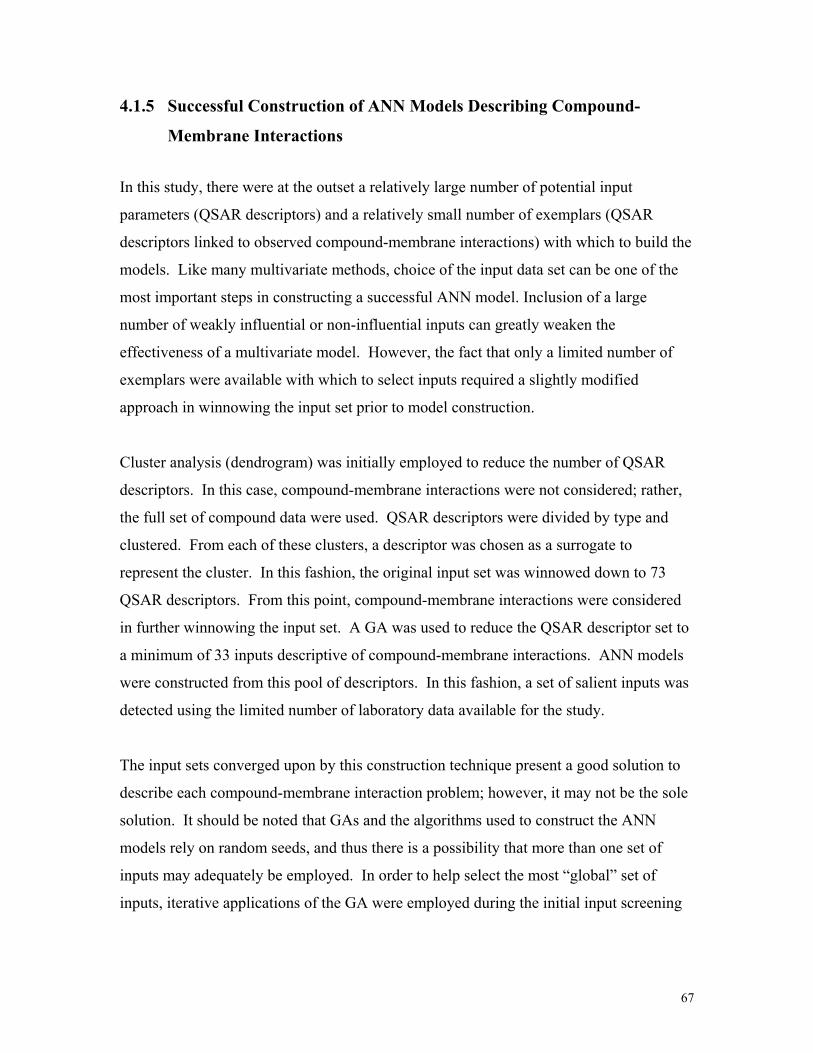
67

4.1.5 Successful Construction of ANN Models Describing Compound-

Membrane Interactions

In this study, there were at the outset a relatively large number of potential input

parameters (QSAR descriptors) and a relatively small number of exemplars (QSAR

descriptors linked to observed compound-membrane interactions) with which to build the

models. Like many multivariate methods, choice of the input data set can be one of the

most important steps in constructing a successful ANN model. Inclusion of a large

number of weakly influential or non-influential inputs can greatly weaken the

effectiveness of a multivariate model. However, the fact that only a limited number of

exemplars were available with which to select inputs required a slightly modified

approach in winnowing the input set prior to model construction.

Cluster analysis (dendrogram) was initially employed to reduce the number of QSAR

descriptors. In this case, compound-membrane interactions were not considered; rather,

the full set of compound data were used. QSAR descriptors were divided by type and

clustered. From each of these clusters, a descriptor was chosen as a surrogate to

represent the cluster. In this fashion, the original input set was winnowed down to 73

QSAR descriptors. From this point, compound-membrane interactions were considered

in further winnowing the input set. A GA was used to reduce the QSAR descriptor set to

a minimum of 33 inputs descriptive of compound-membrane interactions. ANN models

were constructed from this pool of descriptors. In this fashion, a set of salient inputs was

detected using the limited number of laboratory data available for the study.

The input sets converged upon by this construction technique present a good solution to

describe each compound-membrane interaction problem; however, it may not be the sole

solution. It should be noted that GAs and the algorithms used to construct the ANN

models rely on random seeds, and thus there is a possibility that more than one set of

inputs may adequately be employed. In order to help select the most “global” set of

inputs, iterative applications of the GA were employed during the initial input screening

68

to identify and select the most commonly influential input parameters prior to ANN

model construction.

The ANN models constructed in the study to describe P-, M- and R-Flux values

determined by the RMP assay were in general fairly robust. They were able to explain

with reasonable accuracy the variations in behavior observed amongst the surrogate

compounds selected for the study.

It was possible to construct a reasonable “Universal” PA model by incorporating all of

the data for each of the 4 PA membranes and adding PA membrane parameters to the

potential input list. This model exhibited more noise than did the individual PA models,

which is not unexpected as it represents the sum of the experimental noise in all 4 PA

membrane models as well as incorporates the intrinsic differences in performance that

occurred between membranes. It is notable that, for many compounds, it predicts the

nature of compound-membrane interactions nearly as well as the individual PA models,

and thus may at least serve as a “first cut” prediction of general PA membrane

performance.

Interestingly, none of the membrane parameters survived in the final “Universal” PA

models for P-Flux, M-Flux or R-Flux, even though some of these parameters represented

several fold changes in value between membranes (Table 3). This does not at all indicate

that membrane differences do not play a role in the variations observed in membrane

performance; indeed, all of the individual PA membrane models exhibit differences in

inclusion of molecular descriptors. However, it does indicate that the particular

membrane properties selected for inclusion in the models were not nearly as influential as

the compound molecular descriptors in predicting compound-membrane interactions.

69

4.1.6 QSAR Analysis – Relating Descriptors to Compound-Membrane

Interactions

Figure 26 shows a composite of the QSAR molecular descriptors that the ANN models

associated with each of the basic compound-membrane interactions (P-Flux, M-Flux and

R-Flux) defined in the study.

Analysis of the parameters included in each of the models and the direction and

magnitude of their influence (sensitivity analysis) gives some general insight as to the

possible molecular mechanisms involved in the compound-membrane interactions

observed in the study. It would be expected that differences would be seen between

membrane types with completely disparate chemistries (PA vs CA), and indeed this was

observed. Although none of the PA membrane models utilized exactly the same QSAR

descriptor input set, some themes could be noted amongst the descriptors associated with

each type of compound-membrane interaction (P-, M- or R-Flux).

If the molecular descriptors are considered in broader categories related to

charge/polarity issues, molecular complexity, hydrophobicity and hydrogen bonding,

then some similarities may be noted amongst the different membrane models. In many

cases, the direction of relationships commonly occurring in the R-Flux and M-Flux

models show reversed signs, indicating the inverse relationship possible between these

interactions (molecular mechanisms favoring strong membrane surface binding, for

example, would also favor reduced release of compounds from the membrane surface to

the feed).

Charge and polarity descriptors were very much represented as inputs in all of the

models, indicating that these molecular parameters were very much involved in

compound-membrane interactions. This is not at all an unexpected result, as the

literature already suggests that this should indeed be the case (Kosutic et. al., 2002; Fang

et. al., 1976; Koyama et. al., 1982; Schafer et. al., 2003). In the case of the M-Flux and

R-Flux, the Gmin was commonly selected as by the PA membranes (and the “Universal”

70

PA models). This molecular descriptor indicates the minimum atom E-state in the

compounds. This value is related to how electrophilic the atom is. Electrophilic atoms

participate in chemical bonding interactions, including hydrogen bonding. In this case,

the M-Flux (membrane association) was relatively strongly positively associated with

Gmin values, while the R-Flux was strongly negatively associated with Gmin. This

suggests that compounds bearing more reactive atoms tended to interact more strongly

with PA membranes (were less likely to be rejected into the feed).

Descriptors of electrical dipole magnitude (P, Py and Q) were observed in several of the

PA models. In general, indications were that the greater the separation of charge across

the molecule, the less likely the compound was found to associate with the PA

membranes (and found to remain in the feed). Compounds passing through the PA

membranes were favored by increased dipole separation in the direction of the molecular

Y-axis. The CA membrane model presented a more confusing relationship, however.

The Q sensitivity index was negative for R-Flux (increased charge separation, increased

R-Flux), but P was strongly positive for the M-Flux, indicating that as dipole magnitude

increased, the compounds associated more strongly with CA (which indicates increased

polarity should favor decreased R-Flux).

Hydrogen bonding acceptor density (numHBa) was also commonly related to compound-

membrane interactions in the PA membranes (included in 3 of 4 models). The number of

hydrogen bond acceptors in compounds was typically positively associated with M-Flux

(and inversely associated with R-Flux) in the PA membranes. The “Universal” PA

models also shared this relationship. In addition, this descriptor also appeared as an input

in the P-Flux models for PA. Hydrogen bonding may well facilitate interactions between

compounds and the membrane (at least with PA), and in addition, facilitate transport

through the membrane as well.

Hydrophobic/hydrophilic interactions (LogP) appeared to be important in determining

P-Flux for compounds (noted both for PA and CA membranes, but stronger with CA),

but was only included in a few of the M-Flux models. The direction of the sensitivity

71

index suggests that overall the more hydrophilic the compound, the more likely it will

traverse the membrane. It may be that the hydrophobic compounds interact with the

membrane, but the interaction is swamped by the magnitude of the charge interactions,

and thus didn’t appear in many of the M-Flux models. Where it does appear most

strongly (the BW-30 model and “Universal PA” model), the sensitivity index is positive,

suggesting PA membranes favor binding of the more hydrophobic compounds.

Molecular complexity, especially formula weight (fw) has been suggested as a key factor

in determining rejection by RO membranes, and may be expected to be a major factor in

determining membrane permeability (Schutte, 2003; Fang et. al., 1976; Kosutic et. al.,

2002; Wiesner et. al., 1996; Ozaki et. al., 2002; Slater et. al., 1983). Complexity

descriptors indeed appeared more often in the P-Flux models, but as a rule were not as

universally represented as were the charge/polarity descriptors in the M- and R-Flux

models. Most notably, the chi index xvpc4 appeared in 3 of the 4 PA models, as well as

in the “Universal” PA model, and the sensitivity index analysis indicated moderate to

strong (but variable) influence. With BW-30, ESPA-2 and the “Universal” PA models

there was an overall negative influence between this descriptor and P-Flux, suggesting

that as the complexity of the compounds increased (measured by patterns of adjacently

amongst 5 atom groups, sensitive to heteroatom type), they were less able to pass through

these membranes. However, effects of other descriptors related to molecular complexity

were more variable. In general, though, it was suggested that the more complex

molecules were less likely to pass through both PA and CA membranes. Formula weight

did appear in the P-Flux model for the TFC-HR membrane; in this case, as expected, flux

through the membrane was favored by less massive molecules.

4.1.7 Prediction of Compound-Membrane Interactions for Compounds in

the Master Compound List

Outputs of the ANN models of P-, M- and R-Flux values for each of the 5 membranes

and for the “Universal” PA model (Tables 16a through 21c) suggest that predictions of

compound behavior were possible in over half to three-quarters of the cases (depending

72

on the membrane). Given the relatively small number of surrogate compounds available

as exemplars, and the wide range of potential compound structures represented in the

master compound list, this result is very encouraging. That the sum of the membrane

fluxes in these cases closes a “virtual mass balance” and the ability to match rejection

with at least a handful of laboratory experiments and field observations (Table 23) is also

very encouraging. However, as the matrix employed in this study was relatively simple

compared to field applications, much more data from the field will be needed to

determine just how much the compound-membrane interactions elucidated in this study

may be extrapolated to the field.

It is possible, within the context of the conditions established in the study, to make

comparisons between performance of the RO membranes and to assess the relative ability

of the membranes to deal with classes of organic compounds of public health concern

presented in the master compound list (Tables 22a through 22e). The differences in

rejection values based on the P-Flux and the R-Flux are especially illuminating, as

instances where the R-Flux predictions of rejection are significantly lower than P-Flux

predictions of rejection may signify compound removal by association with the

membrane materials as opposed to a barrier mechanism. It should be noted that the ANN

models may predict negative values of rejection based on R-Flux as a consequence of

noise in the models; in these instances extremely strong association between the

compound and the membrane may be inferred, and observed removal based on P-Flux is

predicted to almost entirely be due to adsorptive or absorptive mechanisms.

The ANN predictions indicate that PA membranes, for the most part, appear to perform

nearly equally well with respect to compound removal, although some exceptions may be

found (dichloroacetic acid, molinate, methylene bromide, e.g.). Most of the

pharmaceutical compounds were predicted to be very well rejected by P-Flux; however in

many cases a part of compound removal may be attributed to membrane association

(rejection based on R-Flux < rejection based on P-Flux). The steroid hormones (estrone

and the estradiols, e.g.) are examples. The ANN models also predicted that many of the

disinfection byproducts (DBPs) should be removed well based on P-Flux rejection;

73

however, as with the pharmaceuticals, in many cases a large part of their removal may be

due to membrane association (dibromoacetonitrile, bromochloroacetonitrile, 1,1,

dichloropropanone, e.g.). Metformin was predicted to be the most poorly rejected of the

pharmaceuticals, and amongst the DBPs, bromochloromethane was predicted to be most

poorly rejected.

Compounds associating strongly with the RO membranes may bind to the membrane

surface, enter into and bind within the polymer matrix, or pass through to the product side

of the permselective layer and bind to the polysulfone or to the nonwoven support layer.

The location and intrinsic ability of the molecule to penetrate the membrane is unclear

based solely on data provided by the RMP assay. For compounds poorly able to

penetrate the membrane polymer matrix, surface binding may not lead to a serious

deterioration in longer term rejection providing the compound does not significantly alter

rejection properties of the permselective layer . Desorption and penetration of such a

compound would be expected to be relatively slow. On the other hand, for compounds

able to absorb into the membrane polymer matrix with facility, once the membrane

concentration increases to saturation, desorption and subsequent penetration may result in

a significant release of material into the product. Thus, although it is unclear from this

study which specific mechanism is responsible for compound binding, any organics the

study revealed were exhibiting rejection based largely on affinity to the RO membrane

should be treated with some caution with regard to the ability of the membranes to

exclude them over longer periods of time (Schafer et. al., 2003).

That “Universal” PA ANN flux models generally mirror performance of the individual

PA models for a wide variety of compounds, may suggest commonness of mechanism

with respect to compound-membrane interactions. Providing the PA membranes selected

for this study are fairly representative of the range of membrane chemistries defining the

commercial market, the “Universal” models can serve as generic surrogates to predict the

gross ability of a PA RO membrane to reject specific organic compounds.

74

It was noted that the CA models generally predicted poorer rejection performance than

the PA models; however, this result may have been somewhat artifactual, as comparisons

between the performance of the RMP assay and actual membrane performance in the

block tester indicated that the RMP assay may have significantly underestimated CA

rejection. However, compounds exhibiting high rejection in the RMP assay are expected,

for the most part, also to be rejected well in the field.

4.1.8 Improving the ANN QSAR Models

A number of gaps exist in the ANN models, presumably due to a lack of exemplars

covering specific novel patterns of molecular properties that affect interactions between

the compounds and RO membranes. Although model failure frequency was somewhat

dependent on the membrane being emulated, the ANN models were completely unable to

predict 15 compounds, most notably many of the N-nitroso compounds. In this case, the

mechanism responsible for compound-membrane interactions were most likely

significantly different from those exemplified by the surrogate compounds chosen for the

study.

One way to improve the predictive ability of the ANN models would be to include one or

more of these compounds in the surrogate database and reconstruct the models de novo.

The use of QSAR descriptors known to be related to compound-membrane interactions

may greatly enhance the ability to detect appropriate surrogates in this case. By taking an

iterative approach from this point, the models may be developed in an “evolutionary”

fashion, converging on a broadly predictive solution using a minimal set of exemplars.

Future work would proceed in this direction.

4.1.9 Extending QSAR ANN Model Results to the Real World

Although some comparisons with laboratory and field data suggest that the predictions of

these ANN models may have a good deal of merit, validation by more widespread

comparisons between the model predictions and experience under field conditions is

desirable. It is hoped that dissemination of the ANN models as well as data presented in

75

this study (tables of predicted performance data for the 5 membranes used in the study,

and also of the “Universal” models for PA) to agencies possessing or collecting specific

information regarding removal of these compounds by RO membranes will aid in model

validation.

This study focused on fundamental relationships between several organic compounds of

public health concern and several commercial RO membranes within the context of a

simple experimental matrix. Actual matrices defining commercial RO feed water are far

more complex, and certainly are capable of modifying the behavior of organic

compounds and RO membranes (Chen et. al., 1997; Koops et. al., 2001). The

temperature, pH, salinity and nature of the organic constituents in the feed may vary

considerably from one plant location to another. Moreover, throughout the length of an

RO purification plant from the feed inlet to the brine outlet, concentration of salts and

organics may increase as much as 5-fold, so that membranes in different locations of the

plant are exposed to different feed conditions. An understanding of how these changing

conditions may modulate the interaction of organic compounds with the membranes

would be a valuable modulation factor to include in membrane performance models.

Future work is planned to help achieve this goal.

4.2 Description of Compound-Membrane Interactions Using Molecular

Dynamics (MD) Simulations

Software has been successfully developed that automatically builds, geometry optimizes,

analyzes, and stores fully-atomistic models of randomly crosslinked PA membranes

using MPD and TMC monomers as building blocks. The program allows control over all

membrane structural parameters including the membrane mass, degree of intra-chain

crosslinking, and the net membrane charge. The program also provides the ability to

automatically create a diverse population of PA membrane models whose properties vary

incrementally or randomly over user-specified ranges. The models can be used in studies

of membrane structure and dynamics and to gain insight into theoretical motifs of solute

transport and surface biomolecular fouling.

76

Compared to experimental data, the calculated fluxes of NDMA and TCE through a

model PA membrane proportionally represented laboratory observations (NDMA >

TCE), though absolute values were overestimated by several logs. Short simulation times

(200 ps) resulting in the inability to account for low-frequency solute jumps is likely to

have contributed to the overestimation of compound diffusivities and fluxes. In addition,

the water-membrane partition coefficients for the organics, KA, which were derived from

experimental data, were likely to have been overestimated as well, further compounding

errors in the modeled diffusivities.

In spite of the problems outlined above regarding calculations of absolute solute fluxes, a

comparison of the relative diffusivities of the organic solutes in the pure-water and

membrane simulations suggested that TCE interacts more strongly than NDMA with the

hydrated PA membrane, a factor which should retard its mobility in the membrane and

increase its rejection compared to NDMA. In addition, both water and membrane atoms

were found to generally associate more with NDMA than TCE. The reduced hydration

sphere around TCE may result in less shielding of long-range electrostatic interactions

with membrane atoms leading to diminished mobility compared to NDMA.

Future work, which may be carried out in collaboration with the recently established NSF

“Center for Advanced Materials for Water Purification with Systems” at UIUC, could

pursue several key issues that were not possible to address in this project. Key objectives

undertaken in such future work would include:

1. Implementation of MD simulations up to 10 nanoseconds (ns) with larger

membrane systems to better document and quantify solute diffusion behaviors,

such as jump frequencies and magnitudes, under a variety of conditions. It is

anticipated that a range of organic solutes would be explored in these studies

along with a host of other variables, including the membrane density, degree of

hydration, ion and pH effects, temperature, and pressure.

77

2. Establishment of a predictive relationship between one or more organic

molecular descriptors and KA, the equilibrium water-membrane partition

coefficient. Reliable estimates of KA are required to calculate solute fluxes in RO

membranes from first principles. An attempt could be made to correlate a limited

number of experimental KA values with one or more easily determined molecular

descriptors, such as LogP, solvation energies, or other parameters that can be

readily computed from molecular simulations.

3. More detailed simulations and analyses of water interactions with the organic

solutes and membrane atoms could be performed. Similarly, more in-depth

analyses of organic compound interactions with membrane atoms are also

required. Such interactions are critical to an explanation of differences in organic

compound flux (and rejection) by RO membranes. Moreover, greater insights

into these processes will enable more accurate and reliable predictions of the

transport behaviors of unknown trace organic compounds and facilitate the design

of novel molecular architectures to enhance rejection.

78

5 LITERATURE CITED Bharath, R.and Drosen, J. 1994. Neural Network Computing. Windcrest/McGraw-Hill, New York, New York. Bicerano, J. 1996. Prediction of Polymer Properties. 528 pp. Marcel Dekker, Inc., New York. Campbell, P., Srinivasan, R., Knoell, T., Phipps, D., Ishida, K., Safarik, J., Cormack, T. and H. Ridgway. 1999. Quantitative structure activity relationship (QSAR) analysis of surfactants influencing attachment of a Mycobacterium species to cellulose acetate and aromatic polyamide reverse osmosis membranes. Biotechnology and Bioengineering 64, 527-544. Carroll, F. I., Mascarella, S.W., Kuzemko, M.A., Gao, Y., Abraham, P., Lewin, A.H., Boja, J.W. and M.J. Kuhar. 1994. Synthesis, ligand binding, and QSAR (CoMFA and Classical) study of 3.beta.-(3’-substituted phenyl) tropane-2.beta.-carboxylic acid methyl esters. Journal of Medicinal Chemistry. 37: 2865-2873. Chen, S-S, Taylor, J.S., Norris, C.D. and J.A.M.H. Hofman. Flat sheet for pesticide removal by varying RO/NF membrane. Membrane Technology Conference Proceedings, American Water Works Association, New Orleans, LA. 1997. Drewes, J.E., Heberer, T. and K. Reddersen. 2002. Removal of pharmaceuticals during conventional wastewater treatment, advanced membrane treatment and soil-aquifer treatment. ACWA Xenobiotics Workshop. Sept. 19, 2002. Fang, H.H.P. and E.S.K. Chian. 1975. Removal of alcohols, amines and aliphatic acids in aqueous solution by NS-100 membrane. Journal of Applied Polymer Science. 19(5):1347-1358. Fang, H.H.P. and E.S.K. Chian. 1976. Reverse Osmosis Separation of Polar Organic Compounds in Aqueous Solution. Environmental Science and Technology. 10(4):364-369. Freger, V. 2003. Nano-scale heterogeneity of polyamide membrane formed by interfacial polymerization. Langmuir 19:4791-4797. Gusev, A.A., Mueller-Plathe, F., van Gunsteren, W.F. and U.W. Suter. 1994. Dynamics of small molecules in bulk polymers. Advances in Polymer Science. 209-246. Hileman, B. 2001. Troubled Waters: EPA, USGS try to quantify prevalence, risks of compounds from drugs, personal care products. Chemical and Engineering Technology. 79:31-33.

79

Huang, J., Haruhiko, O., and Y. Negishi. 1993. Studies on reverse osmosis separation of aqueous solutions of low molecular weight organics by cellulose acetate derivative membranes. Membrane 18:285-292. Kilduff, J. E., Mattaraj, S., Pieracci, J. P. and G. Belfort. 2000. Photochemical modification of poly(ether sulfone) and sulfonated poly(sulfone) nanofiltration membranes for control of fouling by natural organic matter. Desalination 132:133-142. Kimura, K., Amy, G., Drewes, J. and Y. Watanabe. 2003. Adsorption of hydrophobic compounds onto NF/RO membranes: an artifact leading to overestimation of rejection. Journal of Membrane Science. 221:89-101.

Knopp, B. and U.W. Suter. 1997a. Atomistically modeling the chemical potential of small molecules in dense polymer microstructures. 1. Method. Macromolecules. 30:6107-6113.

Knopp, B. and U.W. Suter. 1997b. Atomistically modeling the chemical potential of small molecules in dense polymer microstructures. 2. Water sorption by polyamides. Macromolecules. 30:6114-6119.

Kolpin, D.W., Furlong, E.T., Meyer, M.T., Thurman, E.M., Zaugg, S.D., Barber, L.B. and H.T. Buxton. 2002. Pharmaceuticals, hormones, and other organic wastewater contaminants in U.S. streams, 1999-2000: A National Reconnaissance. Environmental Science and Technology. 36:1202-1211. Koops, G.H., Yamada, S. and S.-I. Nakao. 2001. Separation of linear hydrocarbons and carboxylic acids from ethanol and hexane solutions by RO. Journal of Membrane Science. 189:241-254. Kosutic, K. and B. Kunst. 2002. Removal of organics from aqueous solutions by commercial RO and NF membranes of characterized porosities. Desalination. 142:47-56. Kotelyanskii, M.J., Wagner, N.J. and M.E. Paulaitis. 1998. Atomistic simulation of water and salt transport in the reverse osmosis membrane FT-30. Journal of Membrane Science 139:1-16.

Kotelyanskii, M. J., Wagner, N. J. and M.E. Paulaitis. 1999. Molecular dynamics simulation study of the mechanisms of water diffusion in a hydrated, amorphous polyamide. Computational and Theoretical Polymer Science. 9:301-306.

Koyama, K., Nishi, T., Hashida, I. and M. Nishimura. 1982. The rejection of polar organic solutes in aqueous solution by an interpolymer anionic composite RO membrane. Journal of Applied Polymer Science. 27:2845-2855.

80

Lipp, P., Gimbel, R. and F.H. Frimmel. 1994. Parameters influencing the rejection properties of FT30 membranes. Journal of Membrane Science. 95:185-197.

Lonsdale, H., Merten, U. and R. Riley. 1965. Journal of Applied Polymer Science. 9:1341-1362.

Matsuura, T. and S. Sourirajan. 1971. Physicochemical criteria for reverse osmosis separation of alcohols, phenols, and monocarboxylic acid in aqueous solutions using porous cellulose acetate membranes. Journal of Applied Polymer Science. 15(12):2905-2927. Mitchell, M. 1998. An Introduction to Genetic Algorithms. The MIT Press, Cambridge, Massachusetts. Mueller-Plathe, F. 1994. Permeation of polymers – a computational approach. Acta Polymerica. 45:259-293.

Nick, B. and U.W. Suter. 2001. Solubility of water in polymers - atomistic simulations. Computational and Theoretical Polymer Science. 11:49-55.

Ozaki, H. and L. Huafang. 2002. Rejection of organic compounds by ultra-low pressure reverse osmosis membrane. Water Research. 36:123-130. Reinhard, M., Goodman, N. L., McCarty, P., and D. G. Argo. 1986. Removing trace organics by reverse osmosis using cellulose acetate and polyamide membranes. Journal of the American Water Works Association 78:163-174. Riley, R.T., Kemppainen, B.W. and W.P. Norred. 1988. Quantitative tritium exchange of (/sup 3/H) aflatoxin B1 during penetration through isolated human skin. Biochemical and Biophysical Research Communications. 153(1). Salveson, A.T., Requa, D.A., Whitley, R.D. and G. Tchobanoglous. 2000. Potable versus reclaimed water quality, regulatory issues, emerging concerns, in: Proceedings of the Annual Conference of Water Environment Federation, WEFTEC, Anaheim, CA Schafer, A., Fane, A. G. and T. D. Waite. 2000. Fouling effects on rejection in the membrane filtration of natural waters. Desalination 131, 215-224. Schafer, A.I., Nghiem, L.D. and T.D. Waite. 2003. Removal of the natural hormone estrone from aqueous solutions using nanofiltration and reverse osmosis. Environmental Science and Technology. 37:182-188. Schutte, C.F. 2003. The rejection of specific organic compounds by reverse osmosis membranes. Desalination. 158:285-294.

81

Slater, C.S., Ahlert, R.C. and C.G. Uchrin. 1983. Applications of RO to complex industrial wastewater treatment. Desalination. 48:171-187. Takeuchi, H. 1990. A jump motion of small molecules in glassy polymers: a molecular dynamics simulation. Journal of Chemical Physics. 93:2062-2067. Takeuchi, H. and K. Okazaki. 1996. Dynamics of small molecules in a dense polymer matrix: molecular dynamics studies. Molecular Simulations 16:59-74. Votano, J.R., Parham, M., Hall, L.H., Kier, L.B., Oloff, S., Tropsha, A., Xie, Q. and W. Tong. Three New Consensus QSAR Models for the Prediction of Ames Genotoxicity. Reprint Submitted to Mutagenesis, 2004. Weisner, M. R. and C. A. Buckley. 1996. Principles of rejection in pressure-driven membrane processes. In Mallevialle, J., Odendaal, P. E. and M. R. Weisner (Eds.), Water Treatment Membrane Processes. pp. 5.1-5.17. McGraw-Hill, New York.

82

Solute in Feed (F)

Membrane

Feed Product

Solute Passes Membrane

Into Product (P)

Solute Adsorbed/Absorbed

by Membrane (M)

Solute Rejected Without Interaction

F- (P+M) = (R)

Figure 1. Interaction of a Compound (Solute) with a Membrane A compound transported from the membrane surface from the feed can interact with the membrane in three different ways: it can adsorb or absorb into the membrane (M-Flux), it can pass entirely through the membrane into the product (P-Flux), or it can fail to interact with the membrane and remain in the feed (R-Flux).

83

150 PSI150 PSI Collect Collect ProductProduct

Determine Determine Volume Volume

(Gravimetrically) (Gravimetrically) after Timeafter Time

RO Memb.RO Memb.

9 uM *Solute in9 uM *Solute in17 MOhm dH17 MOhm dH2200

Measure Product Measure Product Radioactivity, Radioactivity,

Calculate Product Calculate Product Flux (P)Flux (P)

Measure Feed Measure Feed Radioactivity, Radioactivity,

Calculate Feed Calculate Feed Flux (F)Flux (F)

Measure Membrane Measure Membrane Radioactivity, Radioactivity,

Calculate Flux into Calculate Flux into Membrane (M)Membrane (M)

Determine Flux Into Membrane (Adsorption/Absorption)(M) Determine Flux Into Membrane (Adsorption/Absorption)(M)

Calculate Flux Rejected at Membrane Surface (R = F Calculate Flux Rejected at Membrane Surface (R = F -- (P+M) ) (P+M) )

Determine Flux Through Membrane (P) Determine Flux Through Membrane (P)

Figure 2. RMP Assay Diagram and Flux Determinations The radiolabeled compound consisted of either 14C or 3H isotope. Radioactivity was measured using a scintillation counter. Feed activity of 100,000 to 1,000,000 DPM provided 2-4 logs of dynamic range (99 – 99.99% rejection).

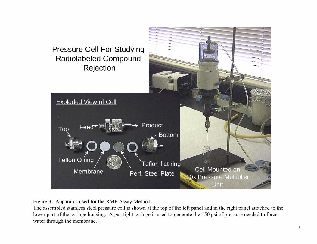
84

Pressure Cell For StudyingRadiolabeled Compound

Rejection

Exploded View of Cell

Cell Mounted on10x Pressure Multiplier

Unit

Top

Teflon O ring

Membrane Perf. Steel Plate

Teflon flat ring

BottomFeed Product

Figure 3. Apparatus used for the RMP Assay MethodThe assembled stainless steel pressure cell is shown at the top of the left panel and in the right panel attached to the lower part of the syringe housing. A gas-tight syringe is used to generate the 150 psi of pressure needed to force water through the membrane.

85

B

3

2

4

1

A

5 1

2

3

4

5

Figure 4. Cross-Flow Membrane Test Unit This unit is used for membrane preparation (hydration under pressure) and validation of the RMP Assay. The assembled test unit is illustrated in (A) above and consists of a top plate (A1), bottom plate (A2), permeate tube with attached flexible tubing (A3), pressure gauge (A4) and a concentrate flow valve (A5). The disassembled test unit is illustrated in (B) and consists of a stainless steel permeate carrier (B1), membrane material (B2), feed spacer (B3), feed flow channel (B4) and teflon shim/gasket (B5).

86

0

10

20

30

40

50

60

70

80

90

100

0 10 20 30 40 50 60 70 80 90 100

RMP Assay, % Rejection (P-Flux)

Cro

ssfl

ow

, %

Rej

ecti

on

BW-30

ESPA-2

CA

LFC-1

TFC-HR

Ideal

Figure 5. Comparison of RMP Assay to Crossflow Block Tester PerformanceA standard linear regression model was performed for each RO membrane used in the study. There was an overall agreement in the comparative behavior of the two systems.

87

Full (73) Descriptor Input Set

Randomize Order ofExemplars

Iterate 10x

Use Genetic Algorithm (GA) to Select “Fittest” Subset of Descriptors

Retain Descriptors Selected =>50% of GA

Selections(~10)

Test Descriptors for Influence

Non-Influential Descriptors in

Model?

Finished ANN Model (7-8

Descriptors)

No

Yes

Remove Non-Influential Inputs

Build Artificial Neural Network (ANN) Model

6 M-Flux Models+6 P-Flux Models+6 R-Flux Models18 Models Total

Figure 6. Selection of Molecular Descriptor Inputs and Construction of Artificial Neural Network (ANN) Models

88

>370 Molecular Descriptors Calculated

190 Organic Compounds Constructed using Molecular

Modeling Software

Molecular Connectivity (Chi) Indices

Kappa Shape Indices

Electrotopological State (E-State)

Indices

Information Indices

Subgraph Count

Indices

Total Topological Descriptors

Molecular Properties

Other Descriptor

73 QSAR Molecular Descriptors Identified

For Use in Study

Pearson’s R to Detect

Crosscorrelated Descriptors

Set of 41 Descriptors Identified with minimal

Crosscorrelations

Dendrogram Cluster Analysis to Group

Compounds

20 Groups (Clusters) Identified containing Compounds with Similar

QSAR Descriptor Properties

51 Surrogate Compounds Selected from the 20 Groups

Dendrogram Cluster Analysis Performed to Reduce Number of Descriptors

Figure 7. Selection of QSAR Molecular Descriptors and Surrogate Compounds

89

BW-30 Membrane Compound Fate

2720

38

19243914

51

14613548

1849

47 4810

6

3 2 34

2332

292522404341

9

7

42 31441745

26213035

50

15 2811 123736160

50

100

0 50 100

Relative Membrane Flux (M)

Rel

ativ

e P

rod

uct

Flu

x (P

)

A C

B

Increasing Membrane AssociationIn

crea

sing

Rej

ecti

on

Figure 8a. Surrogate Compound Fate in BW-30 MembraneCompounds in Quadrant “A” are well rejected; they neither associate with the membrane nor they pass through it. Compounds in Quadrant “B” are poorly rejected and do not interact well with the membrane. Compounds in Quadrant “C” are initially well rejected; however, they strongly associate with the membrane, so their rejection is largely due to membrane uptake. Numbers in the graph correspond to compounds listed in Figs. 8b and 8c.

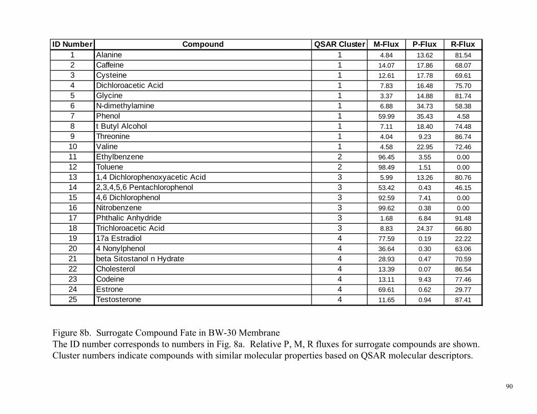
90

ID Number Compound QSAR Cluster M-Flux P-Flux R-Flux1 Alanine 1 4.84 13.62 81.54

2 Caffeine 1 14.07 17.86 68.07

3 Cysteine 1 12.61 17.78 69.61

4 Dichloroacetic Acid 1 7.83 16.48 75.70

5 Glycine 1 3.37 14.88 81.74

6 N-dimethylamine 1 6.88 34.73 58.38

7 Phenol 1 59.99 35.43 4.58

8 t Butyl Alcohol 1 7.11 18.40 74.48

9 Threonine 1 4.04 9.23 86.74

10 Valine 1 4.58 22.95 72.46

11 Ethylbenzene 2 96.45 3.55 0.00

12 Toluene 2 98.49 1.51 0.00

13 1,4 Dichlorophenoxyacetic Acid 3 5.99 13.26 80.76

14 2,3,4,5,6 Pentachlorophenol 3 53.42 0.43 46.15

15 4,6 Dichlorophenol 3 92.59 7.41 0.00

16 Nitrobenzene 3 99.62 0.38 0.00

17 Phthalic Anhydride 3 1.68 6.84 91.48

18 Trichloroacetic Acid 3 8.83 24.37 66.80

19 17a Estradiol 4 77.59 0.19 22.22

20 4 Nonylphenol 4 36.64 0.30 63.06

21 beta Sitostanol n Hydrate 4 28.93 0.47 70.59

22 Cholesterol 4 13.39 0.07 86.54

23 Codeine 4 13.11 9.43 77.46

24 Estrone 4 69.61 0.62 29.77

25 Testosterone 4 11.65 0.94 87.41

Figure 8b. Surrogate Compound Fate in BW-30 MembraneThe ID number corresponds to numbers in Fig. 8a. Relative P, M, R fluxes for surrogate compounds are shown. Cluster numbers indicate compounds with similar molecular properties based on QSAR molecular descriptors.

91

ID Number Compound QSAR Cluster M-Flux P-Flux R-Flux26 Bisphenol 5 28.34 3.11 68.55

27 Diethylstilbestrol 5 37.33 0.09 62.58

28 2,4 Dinitrotoluene 6 94.94 5.06 0.00

29 methyl parathion 8 12.00 0.97 87.03

30 Progesterone 8 25.33 0.04 74.64

31 2-chloro-2'-6'-diethyl-N-methoxymethyl-acetanilide (Alachlor) 9 5.20 0.42 94.38

32 Cimetidine 9 13.37 7.75 78.88

33 Diethylphthalate 9 37.02 6.81 56.16

34 Ibuprofen 9 18.36 16.15 65.49

35 Chlorpyrifos 10 25.68 0.81 73.50

36 Phenanthrene 12 99.71 0.28 0.00

37 1,1,2,2, Tetrachloroethylene (PCE) 13 99.95 0.05 0.00

38 Benzene 13 74.01 25.99 0.00

39 Lindane 13 66.26 2.36 31.38

40 Doxycycline 15 10.54 3.26 86.21

41 Tetracycline 15 7.69 3.43 88.88

42 Ciprofloxacin 16 2.67 2.08 95.24

43 Erythromycin 16 7.66 3.77 88.56

44 Ethylenediaminetetraacetic Acid (EDTA) 18 2.98 5.31 91.72

45 Asparagine N/A 2.37 6.93 90.70

46 Aspartic Acid N/A 5.54 12.60 81.86

47 Histidine N/A 6.22 16.17 77.61

48 Lysine N/A 3.11 14.04 82.85

49 Methionine N/A 7.93 24.13 67.94

50 N-nitroso dimethyl amine (NDMA) N/A 17.66 82.34 0.00

51 Urea N/A 1.40 89.37 9.23

Figure 8c. Surrogate Compound Fate in BW-30 Membrane. (Continued – See Fig. 8b)

92

ESPA-2 Membrane Compound Fate

5150

45

371624152811

12

3619

38

1734

3946 18 444781

104518

4340

132

4142

2231

6

49

262720 3033

2529

32

14

23

21

7

39350

50

100

0 50 100

Relative Membrane Flux (M)

Rel

ativ

e P

rod

uct

Flu

x (P

)

Increasing Membrane Association

Incr

easi

ng R

ejec

tion A

B

C

Figure 9a. Surrogate Compound Fate in ESPA-2 MembraneCompounds in Quadrant “A” are well rejected; they neither associate with the membrane nor they pass through it. Compounds in Quadrant “B” are poorly rejected and do not interact well with the membrane. Compounds in Quadrant “C” are initially well rejected; however, they strongly associate with the membrane, so their rejection is largely due to membrane uptake. Numbers in the graph correspond to compounds listed in Figs. 9b and 9c.

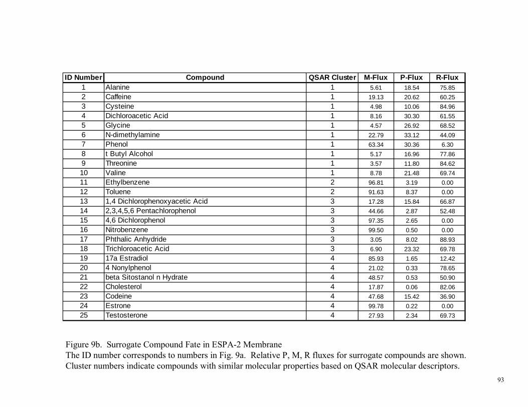
93

ID Number Compound QSAR Cluster M-Flux P-Flux R-Flux1 Alanine 1 5.61 18.54 75.85

2 Caffeine 1 19.13 20.62 60.25

3 Cysteine 1 4.98 10.06 84.96

4 Dichloroacetic Acid 1 8.16 30.30 61.55

5 Glycine 1 4.57 26.92 68.52

6 N-dimethylamine 1 22.79 33.12 44.09

7 Phenol 1 63.34 30.36 6.30

8 t Butyl Alcohol 1 5.17 16.96 77.86

9 Threonine 1 3.57 11.80 84.62

10 Valine 1 8.78 21.48 69.74

11 Ethylbenzene 2 96.81 3.19 0.00

12 Toluene 2 91.63 8.37 0.00

13 1,4 Dichlorophenoxyacetic Acid 3 17.28 15.84 66.87

14 2,3,4,5,6 Pentachlorophenol 3 44.66 2.87 52.48

15 4,6 Dichlorophenol 3 97.35 2.65 0.00

16 Nitrobenzene 3 99.50 0.50 0.00

17 Phthalic Anhydride 3 3.05 8.02 88.93

18 Trichloroacetic Acid 3 6.90 23.32 69.78

19 17a Estradiol 4 85.93 1.65 12.42

20 4 Nonylphenol 4 21.02 0.33 78.65

21 beta Sitostanol n Hydrate 4 48.57 0.53 50.90

22 Cholesterol 4 17.87 0.06 82.06

23 Codeine 4 47.68 15.42 36.90

24 Estrone 4 99.78 0.22 0.00

25 Testosterone 4 27.93 2.34 69.73

Figure 9b. Surrogate Compound Fate in ESPA-2 MembraneThe ID number corresponds to numbers in Fig. 9a. Relative P, M, R fluxes for surrogate compounds are shown. Cluster numbers indicate compounds with similar molecular properties based on QSAR molecular descriptors.

94

ID Number Compound QSAR Cluster M-Flux P-Flux R-Flux26 Bisphenol 5 25.50 1.88 72.62

27 Diethylstilbestrol 5 21.66 0.09 78.25

28 2,4 Dinitrotoluene 6 96.55 3.45 0.00

29 methyl parathion 8 28.17 1.54 70.29

30 Progesterone 8 34.21 0.25 65.54

31 2-chloro-2'-6'-diethyl-N-methoxymethyl-acetanilide (Alachlor) 9 19.99 2.33 77.67

32 Cimetidine 9 34.06 19.61 46.33

33 Diethylphthalate 9 31.46 4.93 63.62

34 Ibuprofen 9 8.89 4.45 86.66

35 Chlorpyrifos 10 59.64 0.66 39.70

36 Phenanthrene 12 85.27 0.45 14.28

37 1,1,2,2, Tetrachloroethylene (PCE) 13 99.67 0.33 0.00

38 Benzene 13 76.68 23.32 0.00

39 Lindane 13 58.30 2.13 39.57

40 Doxycycline 15 14.46 4.37 81.17

41 Tetracycline 15 18.89 7.08 74.02

42 Ciprofloxacin 16 18.68 10.57 70.76

43 Erythromycin 16 13.32 3.86 82.82

44 Ethylenediaminetetraacetic Acid (EDTA) 18 9.07 14.29 76.64

45 Asparagine N/A 6.72 22.01 71.27

46 Aspartic Acid N/A 3.54 15.69 80.77

47 Histidine N/A 7.91 16.02 76.07

48 Lysine N/A 6.90 14.23 78.87

49 Methionine N/A 25.10 16.74 58.17

50 N-nitroso dimethyl amine (NDMA) N/A 14.08 80.76 5.16

51 Urea N/A 8.29 85.11 6.59

Figure 9c. Surrogate Compound Fate in ESPA-2 Membrane. (Continued – See Fig. 9b)

95

LFC-1 Membrane Compound Fate

283716361115

51

50

24

12

7

38

1914

47

203029

4649910

174448

1813

45

344313

854

222126 274140

35

2

6

423332

23

39 250

50

100

0 50 100

Relative Membrane Flux (M)

Rel

ativ

e P

rod

uct

Flu

x (P

)

Increasing Membrane Association

Incr

easi

ng R

ejec

tion

A

B

C

Figure 10a. Surrogate Compound Fate in LFC-1 MembraneCompounds in Quadrant “A” are well rejected; they neither associate with the membrane nor they pass through it. Compounds in Quadrant “B” are poorly rejected and do not interact well with the membrane. Compounds in Quadrant “C” are initially well rejected; however, they strongly associate with the membrane, so their rejection is largely due to membrane uptake. Numbers in the graph correspond to compounds listed in Figs. 10b and 10c.

96

ID Number Compound QSAR Cluster M-Flux P-Flux R-Flux1 Alanine 1 5.77 15.45 78.77

2 Caffeine 1 21.78 14.62 63.61

3 Cysteine 1 5.77 15.45 78.77

4 Dichloroacetic Acid 1 7.12 23.43 69.45

5 Glycine 1 6.45 22.85 70.70

6 N-dimethylamine 1 28.80 31.30 39.90

7 Phenol 1 65.33 34.67 0.00

8 t Butyl Alcohol 1 6.18 25.89 67.93

9 Threonine 1 3.88 12.00 84.12

10 Valine 1 4.89 12.18 82.92

11 Ethylbenzene 2 98.09 1.91 0.00

12 Toluene 2 80.97 19.03 0.00

13 1,4 Dichlorophenoxyacetic Acid 3 3.92 4.76 91.32

14 2,3,4,5,6 Pentachlorophenol 3 60.72 0.69 38.59

15 4,6 Dichlorophenol 3 97.65 2.35 0.00

16 Nitrobenzene 3 99.71 0.29 0.00

17 Phthalic Anhydride 3 3.06 6.06 90.88

18 Trichloroacetic Acid 3 1.99 12.80 85.21

19 17a Estradiol 4 67.29 0.67 32.04

20 4 Nonylphenol 4 23.36 0.31 76.32

21 beta Sitostanol n Hydrate 4 14.30 0.47 85.23

22 Cholesterol 4 12.56 0.27 87.17

23 Codeine 4 38.88 12.07 49.06

24 Estrone 4 83.66 0.92 15.42

25 Testosterone 4 41.21 1.65 57.14

Figure 10b. Surrogate Compound Fate in LFC-1 MembraneThe ID number corresponds to numbers in Fig. 10a. Relative P, M, R fluxes for surrogate compounds are shown. Cluster numbers indicate compounds with similar molecular properties based on QSAR molecular descriptors.

97

ID Number Compound QSAR Cluster M-Flux P-Flux R-Flux26 Bisphenol 5 16.12 1.08 82.80

27 Diethylstilbestrol 5 18.39 0.19 81.42

28 2,4 Dinitrotoluene 6 98.31 1.69 0.00

29 methyl parathion 8 23.85 1.32 74.82

30 Progesterone 8 23.25 0.03 76.73

32 Cimetidine 9 28.99 5.19 65.82

33 Diethylphthalate 9 29.88 5.48 64.65

34 Ibuprofen 9 8.62 5.20 86.18

35 Chlorpyrifos 10 21.23 1.08 77.70

36 Phenanthrene 12 99.34 0.66 0.00

37 1,1,2,2, Tetrachloroethylene (PCE) 13 99.93 0.07 0.00

38 Benzene 13 64.01 19.46 16.54

39 Lindane 13 37.32 1.07 61.61

40 Doxycycline 15 15.95 5.33 78.71

41 Tetracycline 15 17.59 3.52 78.89

42 Ciprofloxacin 16 30.45 7.61 61.94

43 Erythromycin 16 7.58 2.99 89.43

44 Ethylenediaminetetraacetic Acid (EDTA) 18 2.12 6.69 91.20

45 Asparagine N/A 7.41 12.01 80.58

46 Aspartic Acid N/A 2.81 9.68 87.52

47 Histidine N/A 7.98 17.34 74.68

48 Lysine N/A 2.35 6.21 91.44

49 Methionine N/A 4.14 10.25 85.60

50 N-nitroso dimethyl amine (NDMA) N/A 0.53 84.23 15.25

51 Urea N/A 1.66 95.48 2.86

Figure 10c. Surrogate Compound Fate in LFC-1 Membrane. (Continued – See Fig. 10b)

98

TFC-HR Membrane Compound Fate

147

2126312340

2

29

32

30 33 2415281136

31744

46549

84618

45

13344342

412225

109

27 35 3914

7

20

38

19

12

50

51

37160

50

100

0 50 100

Relative Membrane Flux (M)

Rel

ativ

e P

rod

uct

Flu

x (P

)Increasing Membrane Association

Incr

easi

ng R

ejec

tion

A

B

C

Figure 11a. Surrogate Compound Fate in TFC-HR MembraneCompounds in Quadrant “A” are well rejected; they neither associate with the membrane nor they pass through it. Compounds in Quadrant “B” are poorly rejected and do not interact well with the membrane. Compounds in Quadrant “C” are initially well rejected; however, they strongly associate with the membrane, so their rejection is largely due to membrane uptake. Numbers in the graph correspond to compounds listed in Figs. 11b and 11c.

99

ID Number Compound QSAR Cluster M-Flux P-Flux R-Flux1 Alanine 1 4.16 10.20 85.64

2 Caffeine 1 17.38 14.78 67.84

3 Cysteine 1 5.68 7.02 87.30

4 Dichloroacetic Acid 1 8.78 25.82 65.41

5 Glycine 1 5.36 18.03 76.61

6 N-dimethylamine 1 7.89 28.58 63.53

7 Phenol 1 64.67 35.10 0.23

8 t Butyl Alcohol 1 10.10 23.94 65.95

9 Threonine 1 4.89 10.63 84.48

10 Valine 1 5.07 11.10 83.82

11 Ethylbenzene 2 98.39 1.61 0.00

12 Toluene 2 88.09 11.91 0.00

13 1,4 Dichlorophenoxyacetic Acid 3 9.60 5.97 84.43

14 2,3,4,5,6 Pentachlorophenol 3 68.69 5.08 26.23

15 4,6 Dichlorophenol 3 97.98 2.02 0.00

16 Nitrobenzene 3 99.64 0.36 0.00

17 Phthalic Anhydride 3 3.45 8.14 88.41

18 Trichloroacetic Acid 3 6.50 29.05 64.46

19 17a Estradiol 4 84.92 0.46 14.61

20 4 Nonylphenol 4 69.90 0.29 29.81

21 beta Sitostanol n Hydrate 4 24.75 0.43 74.82

22 Cholesterol 4 13.33 0.38 86.30

23 Codeine 4 16.76 7.66 75.59

24 Estrone 4 99.84 0.16 0.00

25 Testosterone 4 14.54 0.51 84.95

Figure 11b. Surrogate Compound Fate in TFC-HR MembraneThe ID number corresponds to numbers in Fig. 11a. Relative P, M, R fluxes for surrogate compounds are shown. Cluster numbers indicate compounds with similar molecular properties based on QSAR molecular descriptors.

100

ID Number Compound QSAR Cluster M-Flux P-Flux R-Flux26 Bisphenol 5 24.01 0.60 75.39

27 Diethylstilbestrol 5 47.75 0.12 52.14

28 2,4 Dinitrotoluene 6 98.06 1.94 0.00

29 methyl parathion 8 25.57 3.52 70.91

30 Progesterone 8 33.90 0.04 66.06

31 2-chloro-2'-6'-diethyl-N-methoxymethyl-acetanilide (Alachlor) 9 21.19 2.43 76.39

32 Cimetidine 9 26.06 13.96 59.98

33 Diethylphthalate 9 41.18 1.47 57.35

34 Ibuprofen 9 10.36 3.97 85.67

35 Chlorpyrifos 10 52.56 0.73 46.71

36 Phenanthrene 12 98.28 0.46 1.26

37 1,1,2,2, Tetrachloroethylene (PCE) 13 99.98 0.02 0.00

38 Benzene 13 78.59 21.41 0.00

39 Lindane 13 66.34 0.94 32.72

40 Doxycycline 15 16.74 10.24 73.03

41 Tetracycline 15 14.45 2.93 82.62

42 Ciprofloxacin 16 12.11 6.61 81.28

43 Erythromycin 16 9.85 2.53 87.61

44 Ethylenediaminetetraacetic Acid (EDTA) 18 2.03 11.10 86.87

45 Asparagine N/A 6.59 31.86 61.55

46 Aspartic Acid N/A 5.54 14.67 79.79

47 Histidine N/A 4.57 11.68 83.76

48 Lysine N/A 3.82 10.72 85.46

49 Methionine N/A 6.49 19.96 73.55

50 N-nitroso dimethyl amine (NDMA) N/A 21.33 78.67 0.00

51 Urea N/A 1.74 90.01 8.25

Figure 11c. Surrogate Compound Fate in TFC-HR Membrane. (Continued – See Fig. 11b)

101

"Universal" PA Membrane Compound Fate

3637 1611 1528

51

50

121924

38

7

143942

5

2135292526 2730 2033

2223

6

2818 4

314140433432133

1 1047464548949

4417

0

50

100

0 50 100

Relative Membrane Flux (M)

Rel

ativ

e P

rod

uct

Flu

x (P

)Increasing Membrane Association

Incr

easi

ng R

ejec

tion A

B

C

Figure 12a. Surrogate Compound Fate in “Universal” PA MembraneCompounds in Quadrant “A” are well rejected; they neither associate with the membrane nor they pass through it. Compounds in Quadrant “B” are poorly rejected and do not interact well with the membrane. Compounds in Quadrant “C” are initially well rejected; however, they strongly associate with the membrane, so their rejection is largely due to membrane uptake. Numbers in the graph correspond to compounds listed in Figs. 12b and 12c.

102

ID Number Compound QSAR Cluster M-Flux P-Flux R-Flux1 Alanine 1 4.40 16.43 80.97

2 Caffeine 1 16.70 20.08 64.92

3 Cysteine 1 6.06 9.99 82.35

4 Dichloroacetic Acid 1 7.46 23.83 66.72

5 Glycine 1 3.93 33.98 86.59

6 N-dimethylamine 1 14.10 35.30 51.93

7 Phenol 1 65.52 31.55 3.93

8 t Butyl Alcohol 1 7.08 20.79 71.30

9 Threonine 1 4.86 10.38 82.90

10 Valine 1 6.39 16.93 76.44

11 Ethylbenzene 2 95.58 2.61 -4.95

12 Toluene 2 90.38 5.76 -4.88

13 1,4 Dichlorophenoxyacetic Acid 3 7.65 7.33 80.77

14 2,3,4,5,6 Pentachlorophenol 3 55.61 1.72 39.53

15 4,6 Dichlorophenol 3 97.88 3.30 -3.38

16 Nitrobenzene 3 97.53 0.37 -6.95

17 Phthalic Anhydride 3 2.90 7.53 89.95

18 Trichloroacetic Acid 3 5.51 22.09 73.92

19 17a Estradiol 4 88.30 0.58 24.93

20 4 Nonylphenol 4 33.54 0.45 68.02

21 beta Sitostanol n Hydrate 4 18.84 0.54 70.10

22 Cholesterol 4 25.86 9.39 85.63

23 Codeine 4 28.03 11.13 61.67

24 Estrone 4 77.69 0.42 32.56

25 Testosterone 4 20.57 1.04 75.39

Figure 12b. Surrogate Compound Fate in “Universal” PA MembraneThe ID number corresponds to numbers in Fig. 12a. Relative P, M, R fluxes for surrogate compounds are shown. Cluster numbers indicate compounds with similar molecular properties based on QSAR molecular descriptors.

103

ID Number Compound QSAR Cluster M-Flux P-Flux R-Flux26 Bisphenol 5 21.31 1.18 74.46

27 Diethylstilbestrol 5 27.74 0.14 69.13

28 2,4 Dinitrotoluene 6 98.89 2.76 -2.48

29 methyl parathion 8 20.55 1.45 78.87

30 Progesterone 8 28.97 0.21 70.12

31 2-chloro-2'-6'-diethyl-N-methoxymethyl-acetanilide (Alachlor) 9 14.15 1.51 85.37

32 Cimetidine 9 11.68 6.24 67.54

33 Diethylphthalate 9 32.62 4.88 61.30

34 Ibuprofen 9 9.92 5.07 82.17

35 Chlorpyrifos 10 19.07 0.21 62.81

36 Phenanthrene 12 94.79 0.47 7.52

37 1,1,2,2, Tetrachloroethylene (PCE) 13 95.55 0.12 -3.28

38 Benzene 13 74.11 20.79 8.13

39 Lindane 13 49.52 1.51 47.32

40 Doxycycline 15 14.48 5.08 78.59

41 Tetracycline 15 14.16 3.40 83.29

42 Ciprofloxacin 16 41.47 0.71 80.62

43 Erythromycin 16 9.15 3.33 88.25

44 Ethylenediaminetetraacetic Acid (EDTA) 18 3.56 8.77 85.89

45 Asparagine N/A 3.78 12.98 79.02

46 Aspartic Acid N/A 5.04 13.22 80.64

47 Histidine N/A 6.98 14.13 78.75

48 Lysine N/A 3.88 10.41 84.69

49 Methionine N/A 6.01 12.22 75.75

50 N-nitroso dimethyl amine (NDMA) N/A 12.02 67.55 3.63

51 Urea N/A 2.21 75.25 4.50

Figure 12c. Surrogate Compound Fate in “Universal” PA Membrane. (Continued – See Fig. 12b)

104

CA Membrane Compound Fate

97.5297.7797.5699.1198.4835242930362720

28

3325

1637

11

12

5051

8

38

7

233234

2

4510

1851 6

48

21

40

42

4749449

1743

46

413

41

22

3

0

50

100

0 50 100

Relative Membrane Flux (M)

Rel

ativ

e P

rod

uct

Flu

x (P

)Increasing Membrane Association

Incr

easi

ng R

ejec

tion A

B

C

Figure 13a. Surrogate Compound Fate in CA MembraneCompounds in Quadrant “A” are well rejected; they neither associate with the membrane nor they pass through it. Compounds in Quadrant “B” are poorly rejected and do not interact well with the membrane. Compounds in Quadrant “C” are initially well rejected; however, they strongly associate with the membrane, so their rejection is largely due to membrane uptake. Numbers in the graph correspond to compounds listed in Figs. 13b and 13c.

105

ID Number Compound QSAR Cluster M-Flux P-Flux R-Flux1 Alanine 1 6.78 53.89 39.33

2 Caffeine 1 10.09 75.53 14.37

3 Cysteine 1 9.37 43.88 46.75

4 Dichloroacetic Acid 1 6.23 41.26 52.51

5 Glycine 1 6.72 56.36 36.92

6 N-dimethylamine 1 13.25 54.91 31.84

7 Phenol 1 28.33 71.67 0.00

8 t Butyl Alcohol 1 4.04 87.42 8.53

9 Threonine 1 7.52 45.73 46.75

10 Valine 1 5.64 62.72 31.64

11 Ethylbenzene 2 66.72 24.15 9.13

12 Toluene 2 52.21 47.79 0.00

13 1,4 Dichlorophenoxyacetic Acid 3 5.30 43.74 50.96

14 2,3,4,5,6 Pentachlorophenol 3 97.77 2.23 0.00

15 4,6 Dichlorophenol 3 97.56 2.44 0.00

16 Nitrobenzene 3 65.54 34.46 0.00

17 Phthalic Anhydride 3 6.22 29.08 64.70

18 Trichloroacetic Acid 3 4.19 60.12 35.70

19 17a Estradiol 4 97.52 2.48 0.00

20 4 Nonylphenol 4 95.98 0.73 3.29

21 beta Sitostanol n Hydrate 4 28.23 0.67 71.10

22 Cholesterol 4 16.48 0.25 83.27

23 Codeine 4 26.16 57.34 16.50

24 Estrone 4 97.32 2.68 0.00

25 Testosterone 4 74.38 20.97 4.65

Figure 13b. Surrogate Compound Fate in CA MembraneThe ID number corresponds to numbers in Fig. 13a. Relative P, M, R fluxes for surrogate compounds are shown. Cluster numbers indicate compounds with similar molecular properties based on QSAR molecular descriptors.

106

ID Number Compound QSAR Cluster M-Flux P-Flux R-Flux26 Bisphenol 5 99.11 0.89 0.00

27 Diethylstilbestrol 5 99.74 0.26 0.00

28 2,4 Dinitrotoluene 6 92.94 7.06 0.00

29 methyl parathion 8 97.82 2.18 0.00

30 Progesterone 8 98.51 1.49 0.00

32 Cimetidine 9 21.67 59.89 18.44

33 Diethylphthalate 9 83.52 16.48 0.00

34 Ibuprofen 9 20.45 57.98 21.57

35 Chlorpyrifos 10 97.09 2.91 0.00

36 Phenanthrene 12 99.57 0.43 0.00

37 1,1,2,2, Tetrachloroethylene (PCE) 13 67.77 30.80 1.44

38 Benzene 13 43.42 56.58 0.00

39 Lindane 13 98.48 1.52 0.00

40 Doxycycline 15 30.61 18.03 51.36

41 Tetracycline 15 14.42 32.26 53.32

42 Ciprofloxacin 16 27.03 35.12 37.85

43 Erythromycin 16 8.28 28.32 63.41

44 Ethylenediaminetetraacetic Acid (EDTA) 18 7.52 48.06 44.42

45 Asparagine N/A 0.73 64.97 34.30

46 Aspartic Acid N/A 8.48 34.23 57.29

47 Histidine N/A 8.82 45.29 45.89

48 Lysine N/A 9.30 51.85 38.85

49 Methionine N/A 8.58 46.93 44.49

50 N-nitroso dimethyl amine (NDMA) N/A 3.51 94.06 2.44

51 Urea N/A 3.08 90.58 6.34

Figure 13c. Surrogate Compound Fate in CA Membrane. (Continued – See Fig. 13b)

107

Norm P Flux (%) R Avg. Abs. RMS Conf. Interval (95%) RecordsAll 0.9821 2.3256 4.0927 8.0013 255

Train 0.9829 2.3317 4.1521 8.1379 178

Test 0.9805 2.3114 3.9518 7.8298 77

Sensitivity IndexOvality xvpc4 Py LogP SsCH3 numHBa-0.1699 -0.7242 0.2610 -0.0119 0.6658 1.3186

BW30 P-Flux ANN Model

-20

0

20

40

60

80

100

0 20 40 60 80 100

Predicted

Act

ual

Figure 14a. ANN Model Results for BW-30 – P-FluxThe graph shows the accuracy of prediction. The overall R values are high and there is a good agreement between the test and the train values. The line indicates a perfect model. The bar represents one standard deviation above the mean based on n=4-7. R=Linear correlation between predicted and actual, Avg.Abs.=Average absolute error between predicted and actual, RMS=mean root square error between predicted and actual, Conf.Interval (95%)=Represents 95% confidence interval, Records=Represents number of exemplars used. The sensitivity index lists the inputs to the model and indicates how sensitive the model output is to small changes in each input.

108

Norm. M Flux (%) R Avg. Abs. RMS Conf. Interval (95%) RecordsAll 0.9839 3.6830 5.9178 11.5696 255

Train 0.9860 3.4998 5.5314 10.8412 178

Test 0.9793 4.1064 6.7266 13.3277 77

BW30 M-Flux ANN Model

-20

0

20

40

60

80

100

0 20 40 60 80 100

Predicted

Act

ual

Sensitivity IndexP LogP Gmax Gmin

-0.6355 0.3669 0.0131 0.7941

Figure 14b. ANN Model Results for BW-30 – M-FluxThe graph shows the accuracy of prediction. The overall R values are high and there is a good agreement between the test and the train values. The line indicates a perfect model. The bar represents one standard deviation above the mean based on n=4-7. R=Linear correlation between predicted and actual, Avg.Abs.=Average absolute error between predicted and actual, RMS=mean root square error between predicted and actual, Conf.Interval (95%)=Represents 95% confidence interval, Records=Represents number of exemplars used. The sensitivity index lists the inputs to the model and indicates how sensitive the model output is to small changes in each input.

109

Norm R Flux (%) R Avg. Abs. RMS Conf. Interval (95%) RecordsAll 0.9608 6.0026 9.4015 18.3803 255

Train 0.9569 6.2819 9.9020 19.4073 178

Test 0.9705 5.3567 8.1272 16.1028 77

Sensitivity IndexPz Wt LogP Gmin

-0.4680 -6.1063 -1.0190 -2.1272

BW30 R-Flux ANN Model

-20

0

20

40

60

80

100

0 20 40 60 80 100

Predicted

Act

ual

Figure 14c. ANN Model Results for BW-30 – R-FluxThe graph shows the accuracy of prediction. The overall R values are high and there is a good agreement between the test and the train values. The line indicates a perfect model. The bar represents one standard deviation above the mean based on n=4-7. R=Linear correlation between predicted and actual, Avg.Abs.=Average absolute error between predicted and actual, RMS=mean root square error between predicted and actual, Conf.Interval (95%)=Represents 95% confidence interval, Records=Represents number of exemplars used. The sensitivity index lists the inputs to the model and indicates how sensitive the model output is to small changes in each input.

110

Norm P Flux (%) R Avg. Abs. RMS Conf. Interval (95%) RecordsAll 0.9644 2.8041 4.7706 9.3254 261

Train 0.9704 2.6084 4.3232 8.4717 182

Test 0.9521 3.2551 5.6683 11.2254 79

ESPA2 P-Flux ANN Model

0

20

40

60

80

100

0 20 40 60 80 100

Predicted

Act

ual

Sensitivity IndexMaxQp xvpc4 Iy Py LogP SsCH3 Hmin numHBa-0.3767 -0.4996 -1.0265 0.1432 -0.3241 0.1174 0.3817 0.3934

Figure 15a. ANN Model Results for ESPA-2 – P-FluxThe graph shows the accuracy of prediction. The overall R values are high and there is a good agreement between the test and the train values. The line indicates a perfect model. The bar represents one standard deviation above the mean based on n=4-7. R=Linear correlation between predicted and actual, Avg.Abs.=Average absolute error between predicted and actual, RMS=mean root square error between predicted and actual, Conf.Interval (95%)=Represents 95% confidence interval, Records=Represents number of exemplars used. The sensitivity index lists the inputs to the model and indicates how sensitive the model output is to small changes in each input.

111

Norm. M Flux (%) R Avg. Abs. RMS Conf. Interval (95%) RecordsAll 0.9853 3.8561 5.5805 10.9087 261

Train 0.9860 3.8111 5.4474 10.6747 182

Test 0.9838 3.9597 5.8756 11.6360 79

ESPA2 M-Flux ANN Model

-20

0

20

40

60

80

100

0 20 40 60 80 100

Prediction

Act

ual

Sensitivity IndexP k1 SdssC Gmin fw numHBa Qs

-0.2011 -1.6738 -0.3071 0.5616 1.2028 0.2102 1.3982

Figure 15b. ANN Model Results for ESPA-2 – M-FluxThe graph shows the accuracy of prediction. The overall R values are high and there is a good agreement between the test and the train values. The line indicates a perfect model. The bar represents one standard deviation above the mean based on n=4-7. R=Linear correlation between predicted and actual, Avg.Abs.=Average absolute error between predicted and actual, RMS=mean root square error between predicted and actual, Conf.Interval (95%)=Represents 95% confidence interval, Records=Represents number of exemplars used. The sensitivity index lists the inputs to the model and indicates how sensitive the model output is to small changes in each input.

112

Norm R Flux (%) R Avg. Abs. RMS Conf. Interval (95%) RecordsAll 0.9791 4.9779 6.3888 12.4887 261

Train 0.9824 4.5969 5.8686 11.4999 182

Test 0.9729 5.8556 7.4503 14.7544 79

Sensitivity IndexMaxNeg nxch6 Q k2 Gmax Gmin numHBa0.0384 0.2095 -1.6123 0.3314 -0.5237 -2.1458 -1.4751

ESPA2 R-Flux ANN Model

-20

0

20

40

60

80

100

0 20 40 60 80 100

Predicted

Act

ual

Figure 15c. ANN Model Results for ESPA-2 – R-FluxThe graph shows the accuracy of prediction. The overall R values are high and there is a good agreement between the test and the train values. The line indicates a perfect model. The bar represents one standard deviation above the mean based on n=4-7. R=Linear correlation between predicted and actual, Avg.Abs.=Average absolute error between predicted and actual, RMS=mean root square error between predicted and actual, Conf.Interval (95%)=Represents 95% confidence interval, Records=Represents number of exemplars used. The sensitivity index lists the inputs to the model and indicates how sensitive the model output is to small changes in each input.

113

Norm P Flux (%) R Avg. Abs. RMS Conf. Interval (95%) RecordsAll 0.9914 1.7375 2.9206 5.7102 252

Train 0.9913 1.7245 2.9384 5.7596 176

Test 0.9918 1.7675 2.8789 5.7055 76

Sensitivity IndexIy Py LogP SdssC

0.4935 0.7729 -0.3455 -0.0801

LFC1 P-Flux ANN Model

0

20

40

60

80

100

0 20 40 60 80 100

Predicted

Act

ual

Figure 16a. ANN Model Results for LFC-1 – P-FluxThe graph shows the accuracy of prediction. The overall R values are high and there is a good agreement between the test and the train values. The line indicates a perfect model. The bar represents one standard deviation above the mean based on n=4-7. R=Linear correlation between predicted and actual, Avg.Abs.=Average absolute error between predicted and actual, RMS=mean root square error between predicted and actual, Conf.Interval (95%)=Represents 95% confidence interval, Records=Represents number of exemplars used. The sensitivity index lists the inputs to the model and indicates how sensitive the model output is to small changes in each input.

114

Norm. M Flux (%) R Avg. Abs. RMS Conf. Interval (95%) RecordsAll 0.9887 3.0407 4.9548 9.6876 252

Train 0.9926 2.7627 4.1714 8.1765 176

Test 0.9807 3.6845 6.4115 12.7066 76

LFC1 M-Flux ANN Model

0

20

40

60

80

100

0 20 40 60 80 100

Predicted

Act

ual

Sensitivity IndexMaxQp P Q SaaCH SdssC Gmin idcbar fw numHBa Qs2.1870 -0.6448 0.4650 0.4792 -0.3696 1.3010 -1.2797 0.6555 0.7628 1.9183

Figure 16b. ANN Model Results for LFC-1 – M-FluxThe graph shows the accuracy of prediction. The overall R values are high and there is a good agreement between the test and the train values. The line indicates a perfect model. The bar represents one standard deviation above the mean based on n=4-7. R=Linear correlation between predicted and actual, Avg.Abs.=Average absolute error between predicted and actual, RMS=mean root square error between predicted and actual, Conf.Interval (95%)=Represents 95% confidence interval, Records=Represents number of exemplars used. The sensitivity index lists the inputs to the model and indicates how sensitive the model output is to small changes in each input.

115

Norm R Flux (%) R Avg. Abs. RMS Conf. Interval (95%) RecordsAll 0.9879 3.5841 5.1401 10.0498 252

Train 0.9897 3.5236 4.7465 9.3037 176

Test 0.9841 3.7242 5.9525 11.7969 76

LFC1 R-Flux ANN Model

-20

0

20

40

60

80

100

0 20 40 60 80 100

Prediction

Act

ual

Sensitivity Indexnxch6 Q sumdelI k2 SdssC Gmin numHBa0.8560 -0.3335 -0.3209 1.5810 -3.1102 -0.3399 -0.6827

Figure 16c. ANN Model Results for LFC-1 – R-FluxThe graph shows the accuracy of prediction. The overall R values are high and there is a good agreement between the test and the train values. The line indicates a perfect model. The bar represents one standard deviation above the mean based on n=4-7. R=Linear correlation between predicted and actual, Avg.Abs.=Average absolute error between predicted and actual, RMS=mean root square error between predicted and actual, Conf.Interval (95%)=Represents 95% confidence interval, Records=Represents number of exemplars used. The sensitivity index lists the inputs to the model and indicates how sensitive the model output is to small changes in each input.

116

Norm P Flux (%) R Avg. Abs. RMS Conf. Interval (95%) RecordsAll 0.9691 2.6487 4.4316 8.6630 260

Train 0.9713 2.5938 4.4266 8.6746 181

Test 0.9667 2.7745 4.4430 8.7989 79

TFC-HR P-Flux ANN Model

-20

0

20

40

60

80

100

0 20 40 60 80 100

Predicted

Act

ual

Sensitivity IndexMaxQp xvpc4 nxp5 P Hmin fw numHBa-1.5199 0.3931 0.0100 0.6744 0.2301 -0.5962 0.2296

Figure 17a. ANN Model Results for TFC-HR – P-FluxThe graph shows the accuracy of prediction. The overall R values are high and there is a good agreement between the test and the train values. The line indicates a perfect model. The bar represents one standard deviation above the mean based on n=4-7. R=Linear correlation between predicted and actual, Avg.Abs.=Average absolute error between predicted and actual, RMS=mean root square error between predicted and actual, Conf.Interval (95%)=Represents 95% confidence interval, Records=Represents number of exemplars used. The sensitivity index lists the inputs to the model and indicates how sensitive the model output is to small changes in each input.

117

Norm. M Flux (%) R Avg. Abs. RMS Conf. Interval (95%) RecordsAll 0.9844 3.7152 6.0456 11.8181 260

Train 0.9891 3.3200 5.0634 9.9226 181

Test 0.9736 4.6208 7.8452 15.5365 79

TFCHR M-Flux ANN Model

0

20

40

60

80

100

0 20 40 60 80 100

Predicted

Act

ual

Sensitivity IndexP LogP SaaCH Gmin numHBa

0.4421 -0.1036 3.3047 1.5067 0.1772

Figure 17b. ANN Model Results for TFC-HR – M-FluxThe graph shows the accuracy of prediction. The overall R values are high and there is a good agreement between the test and the train values. The line indicates a perfect model. The bar represents one standard deviation above the mean based on n=4-7. R=Linear correlation between predicted and actual, Avg.Abs.=Average absolute error between predicted and actual, RMS=mean root square error between predicted and actual, Conf.Interval (95%)=Represents 95% confidence interval, Records=Represents number of exemplars used. The sensitivity index lists the inputs to the model and indicates how sensitive the model output is to small changes in each input.

118

Norm R Flux (%) R Avg. Abs. RMS Conf. Interval (95%) RecordsAll 0.9803 4.5211 6.5732 12.8495 260

Train 0.9818 4.2638 6.3169 12.3789 181

Test 0.9769 5.1107 7.1259 14.1121 79

TFC-HR R-Flux ANN Model

-20

0

20

40

60

80

100

0 20 40 60 80 100

Predicted

Act

ual

Sensitivity IndexPy Q LogP SaaCH SdssC SdO Gmax Gmin idcbar numHBa

-0.8254 -1.6494 -0.5547 -2.7032 -0.4940 0.0280 0.0117 -1.3812 1.3378 -1.4252

Figure 17c. ANN Model Results for TFC-HR – R-FluxThe graph shows the accuracy of prediction. The overall R values are high and there is a good agreement between the test and the train values. The line indicates a perfect model. The bar represents one standard deviation above the mean based on n=4-7. R=Linear correlation between predicted and actual, Avg.Abs.=Average absolute error between predicted and actual, RMS=mean root square error between predicted and actual, Conf.Interval (95%)=Represents 95% confidence interval, Records=Represents number of exemplars used. The sensitivity index lists the inputs to the model and indicates how sensitive the model output is to small changes in each input.

119

Norm P Flux (%) R Avg. Abs. RMS Conf. Interval (95%) RecordsAll 0.9853 3.0996 4.6515 9.0943 253

Train 0.9858 3.0948 4.5760 8.9690 177

Test 0.9842 3.1107 4.8229 9.5582 76

Sensitivity IndexSurface xpc4 xv1 P LogP SdssC numHBa Qsv-0.6895 0.4585 -1.4028 1.0620 -0.9874 -0.6083 0.0015 0.7710

CA P-Flux ANN Model

0

20

40

60

80

100

0 20 40 60 80 100

PredictedA

ctu

al

Figure 18a. ANN Model Results for CA – P-FluxThe graph shows the accuracy of prediction. The overall R values are high and there is a good agreement between the test and the train values. The line indicates a perfect model. The bar represents one standard deviation above the mean based on n=4-7. R=Linear correlation between predicted and actual, Avg.Abs.=Average absolute error between predicted and actual, RMS=mean root square error between predicted and actual, Conf.Interval (95%)=Represents 95% confidence interval, Records=Represents number of exemplars used. The sensitivity index lists the inputs to the model and indicates how sensitive the model output is to small changes in each input.

120

Norm. M Flux (%) R Avg. Abs. RMS Conf. Interval (95%) RecordsAll 0.9900 2.4784 5.4600 10.6748 254

Train 0.9883 2.5333 5.9050 11.5740 177

Test 0.9939 2.3520 4.2644 8.4493 77

CA M-Flux ANN Model

0

20

40

60

80

100

0 20 40 60 80 100

PredictedA

ctu

al

Sensitivity IndexP Q LogP SdssC

2.0098 0.9829 1.2532 1.2304

Figure 18b. ANN Model Results for CA – M-FluxThe graph shows the accuracy of prediction. The overall R values are high and there is a good agreement between the test and the train values. The line indicates a perfect model. The bar represents one standard deviation above the mean based on n=4-7. R=Linear correlation between predicted and actual, Avg.Abs.=Average absolute error between predicted and actual, RMS=mean root square error between predicted and actual, Conf.Interval (95%)=Represents 95% confidence interval, Records=Represents number of exemplars used. The sensitivity index lists the inputs to the model and indicates how sensitive the model output is to small changes in each input.

121

Norm R Flux (%) R Avg. Abs. RMS Conf. Interval (95%) RecordsAll 0.9435 5.4438 8.2063 16.0441 254

Train 0.9427 5.4063 8.2350 16.1408 177

Test 0.9464 5.5302 8.1400 16.1282 77

CA R-Flux ANN Model

-20

0

20

40

60

80

100

0 20 40 60 80 100

PredictedA

ctu

al

Sensitivity IndexABSQ Q sumdelI SaaCH SdssC0.7603 -0.8255 -0.2971 -0.3784 -0.7532

Figure 18c. ANN Model Results for CA – R-FluxThe graph shows the accuracy of prediction. The overall R values are high and there is a good agreement between the test and the train values. The line indicates a perfect model. The bar represents one standard deviation above the mean based on n=4-7. R=Linear correlation between predicted and actual, Avg.Abs.=Average absolute error between predicted and actual, RMS=mean root square error between predicted and actual, Conf.Interval (95%)=Represents 95% confidence interval, Records=Represents number of exemplars used. The sensitivity index lists the inputs to the model and indicates how sensitive the model output is to small changes in each input.

122

Norm P Flux (%) R Avg. Abs. RMS Conf. Interval (95%) RecordsAll 0.9617 3.3033 5.6340 10.9670 1028

Train 0.9644 3.1853 5.5692 10.8476 719

Test 0.9559 3.5779 5.7818 11.2923 309

"Universal" PA P-Flux ANN Model

-20

0

20

40

60

80

100

0 20 40 60 80 100

Predicted

Act

ual

Sensitivity IndexAverage Surface xvpc4 Py LogP SsCH3 SdssC HminNetOut01 -0.1755 -0.6933 -0.0110 -0.2393 0.1387 -0.0178 0.2539

Figure 19a. ANN Model Results for “Universal” PA – P-FluxThe graph shows the accuracy of prediction. The overall R values are high and there is a good agreement between the test and the train values. The line indicates a perfect model. The bar represents one standard deviation above the mean based on n=4-7. R=Linear correlation between predicted and actual, Avg.Abs.=Average absolute error between predicted and actual, RMS=mean root square error between predicted and actual, Conf.Interval (95%)=Represents 95% confidence interval, Records=Represents number of exemplars used. The sensitivity index lists the inputs to the model and indicates how sensitive the model output is to small changes in each input.

123

Norm. M Flux (%) R Avg. Abs. RMS Conf. Interval (95%) RecordsAll 0.9646 5.6114 8.8493 17.2259 1027

Train 0.9634 5.6258 8.9931 17.5167 718

Test 0.9674 5.5779 8.5057 16.6123 309

"Universal" PA M-Flux ANN Model

-20

0

20

40

60

80

100

0 20 40 60 80 100

PredictedA

ctu

al

Sensitivity IndexAverage Surface xvpc4 Py LogP SsCH3 SdssC HminNetOut01 -0.1755 -0.6933 -0.0110 -0.2393 0.1387 -0.0178 0.2539

Figure 19b. ANN Model Results for “Universal” PA – M-FluxThe graph shows the accuracy of prediction. The overall R values are high and there is a good agreement between the test and the train values. The line indicates a perfect model. The bar represents one standard deviation above the mean based on n=4-7. R=Linear correlation between predicted and actual, Avg.Abs.=Average absolute error between predicted and actual, RMS=mean root square error between predicted and actual, Conf.Interval (95%)=Represents 95% confidence interval, Records=Represents number of exemplars used. The sensitivity index lists the inputs to the model and indicates how sensitive the model output is to small changes in each input.

124

Norm R Flux (%) R Avg. Abs. RMS Conf. Interval (95%) RecordsAll 0.9487 7.7847 10.4720 20.3846 1029

Train 0.9463 7.8690 10.7083 20.8573 720

Test 0.9543 7.5883 9.8997 19.3348 309

"Universal" PA R-Flux ANN Model

-20

0

20

40

60

80

100

0 20 40 60 80 100

PredictedA

ctu

al

Sensitivity IndexQ Wt k3 LogP Gmax Gmin numHBa

-1.2360 22.6983 -0.0397 -0.6264 -0.4501 -0.0899 -0.8011

Figure 19c. ANN Model Results for “Universal” PA – R-FluxThe graph shows the accuracy of prediction. The overall R values are high and there is a good agreement between the test and the train values. The line indicates a perfect model. The bar represents one standard deviation above the mean based on n=4-7. R=Linear correlation between predicted and actual, Avg.Abs.=Average absolute error between predicted and actual, RMS=mean root square error between predicted and actual, Conf.Interval (95%)=Represents 95% confidence interval, Records=Represents number of exemplars used. The sensitivity index lists the inputs to the model and indicates how sensitive the model output is to small changes in each input.

125

“Universal” PA and BW-30 Model Comparison

P-Flux

0

20

40

60

80

100

120

-20 0 20 40 60 80 100 120

Actual

Pre

dic

ted

Universal

BW-30

Figure 20a. Comparison of “Universal” PA Model Output to BW-30 – P-FluxThe closed circles represent the specific PA membrane model and the opened circles represent the “Universal”PA model. The “Universal” PA model agrees reasonably well with the BW-30 model.

126

“Universal” PA and BW-30 Model Comparison

M-flux

0

20

40

60

80

100

120

-20 0 20 40 60 80 100 120

Actual

Pre

dic

ted

Universal

BW-30

Figure 20b. Comparison of “Universal” PA Model Output to BW-30 – M-FluxThe closed circles represent the specific PA membrane model and the opened circles represent the “Universal”PA model. The “Universal” PA model agrees reasonably well with the BW-30 model.

127

“Universal” PA and BW-30 Model Comparison

R-Flux

-20

0

20

40

60

80

100

120

-20 0 20 40 60 80 100 120

Actual

Pre

dic

ted

Universal

BW-30

Figure 20c. Comparison of “Universal” PA Model Output to BW-30 – R-FluxThe closed circles represent the specific PA membrane model and the opened circles represent the “Universal”PA model. The “Universal” PA model agrees reasonably well with the BW-30 model.

128

“Universal” PA and ESPA-2 Model ComparisonP-Flux

0

20

40

60

80

100

120

-20 0 20 40 60 80 100 120

Actual

Pre

dic

ted

Universal

ESPA-2

Figure 21a. Comparison of “Universal” PA Model Output to ESPA-2 – P-FluxThe closed circles represent the specific PA membrane model and the opened circles represent the “Universal”PA model. The “Universal” PA model agrees reasonably well with the ESPA-2 model.

129

“Universal” PA and ESPA-2 Model Comparison M-Flux

Figure 21b. Comparison of “Universal” PA Model Output to ESPA-2 – M-Flux The closed circles represent the specific PA membrane model and the opened circles represent the “Universal” PA model. The “Universal” PA model agrees reasonably well with the ESPA-2 model.

0

20

40

60

80

100

120

-20 0 20 40 60 80 100 120

Actual

Pre

dic

ted

Universal

ESPA-2

130

“Universal” PA and ESPA-2 Model ComparisonR-Flux

-20

0

20

40

60

80

100

120

-20 0 20 40 60 80 100 120

Actual

Pre

dic

ted

Universal

ESPA-2

Figure 21c. Comparison of “Universal” PA Model Output to ESPA-2 – R-FluxThe closed circles represent the specific PA membrane model and the opened circles represent the “Universal”PA model. The “Universal” PA model agrees reasonably well with the ESPA-2 model.

131

“Universal” PA and LFC-1 Model ComparisonP-Flux

0

20

40

60

80

100

120

0 20 40 60 80 100 120

Actual

Pre

dic

ted

Universal

LFC-1

Figure 22a. Comparison of “Universal” PA Model Output to LFC-1 – P-FluxThe closed circles represent the specific PA membrane model and the opened circles represent the “Universal”PA model. The “Universal” PA model agrees reasonably well with the LFC-1 model.

132

“Universal” PA and LFC-1 Model ComparisonM-Flux

0

20

40

60

80

100

120

-20 0 20 40 60 80 100 120

Actual

Pre

dic

ted

Universal

LFC-1

Figure 22b. Comparison of “Universal” PA Model Output to LFC-1 – M-FluxThe closed circles represent the specific PA membrane model and the opened circles represent the “Universal”PA model. The “Universal” PA model agrees reasonably well with the LFC-1 model.

133

“Universal” PA and LFC-1 Model ComparisonR-Flux

-20

0

20

40

60

80

100

120

-20 0 20 40 60 80 100 120

Actual

Pre

dic

ted

Universal

LFC-1

Figure 22c. Comparison of “Universal” PA Model Output to LFC-1 – R-FluxThe closed circles represent the specific PA membrane model and the opened circles represent the “Universal”PA model. The “Universal” PA model agrees reasonably well with the LFC-1 model.

134

“Universal” PA and TFC-HR Model ComparisonP-Flux

0

20

40

60

80

100

120

-20 0 20 40 60 80 100 120

Actual

Pre

dic

ted

Universal

TFC-HR

Figure 23a. Comparison of “Universal” PA Model Output to TFC-HR – P-FluxThe closed circles represent the specific PA membrane model and the opened circles represent the “Universal”PA model. The “Universal” PA model agrees reasonably well with the TFC-HR model.

135

“Universal” PA and TFC-HR Model ComparisonM-Flux

0

20

40

60

80

100

120

0 20 40 60 80 100 120

Actual

Pre

dic

ted

Universal

TFC-HR

Figure 23b. Comparison of “Universal” PA Model Output to TFC-HR – M-FluxThe closed circles represent the specific PA membrane model and the opened circles represent the “Universal”PA model. The “Universal” PA model agrees reasonably well with the TFC-HR model.

136

“Universal” PA and TFC-HR Model ComparisonR-Flux

-20

0

20

40

60

80

100

120

-20 0 20 40 60 80 100 120

Actual

Pre

dic

ted

Universal

TFC-HR

Figure 23c. Comparison of “Universal” PA Model Output to TFC-HR – R-FluxThe closed circles represent the specific PA membrane model and the opened circles represent the “Universal”PA model. The “Universal” PA model agrees reasonably well with the TFC-HR model.

137

Model Failure vs Representation of Surrogates in QSAR Descriptor Clusters

0

10

20

30

40

50

60

70

0 10 20 30 40 50 60 70

% of Cluster Compounds Represented by Surrogates

% o

f C

lus

ter

Co

mp

oun

ds F

aili

ng

Pre

dic

tion

None

11

17

95 8

10

21

13

1216 4

319,20 6 18 15

Clusters Modeled Well based on Chosen Surrogates

Surrogate Representation Inadequate

Chosen Surrogates More PoorlyRepresent Cluster Behavior

Figure 24. Model Failure vs Representation of Surrogates in QSAR Descriptor ClustersThis figure shows the relationship between the percentage of the cluster compounds represented by surrogate compounds and the percentage of compounds in each QSAR descriptor cluster that failed model prediction. Each QSAR descriptor cluster is indicated on the chart by numbers.

138

Compounds 75%+ of PA Models Failed to PredictWard's Method,Squared Euclidean

Dis

tanc

e

0

300

600

900

1200

1500

2,6

Din

itro

tolu

ene

Atr

azin

e

cis-

Chl

orda

ne

Hex

achl

orop

enta

dien

e

Met

olac

hlor

N-n

itro

sodi

-n-p

ropy

lam

ine

N-n

itro

sopi

peri

dine

N-n

itro

sopy

rrol

idin

e

Nit

roso

diet

hyla

min

e

N N

die

thyl

3 m

ethy

lben

zam

ide

Pram

itol

Ran

itid

ine

Sim

azin

e

Ana

toxi

n a

2,2

bis-

p-C

hlor

ophe

nyl 1

,1,1

Tri

chlo

roet

hane

2,2-

bis-

p-C

hlor

ophe

nyl 1

,1 D

ichl

oroe

than

e

2,4

Dic

hlor

o-4'

-nit

rodi

phen

yl E

ther

2,6

bis-

1,1

Dim

ethy

leth

yl 2

,5 C

yclo

hexa

dien

e 1,

4 di

one

3,4,

5,6,

7,8,

8a-H

epta

chlo

rodi

cycl

open

tadi

ene

4-am

ino-

6-te

rt-b

utyl

-3-m

ethy

lthi

o-as

-tri

azin

-5,4

H-o

ne

5-m

ethy

l-1H

-Ben

zotr

iazo

le

Ace

toch

lor

And

rost

eron

e

benz

o-a-

Pyre

ne

Bro

mof

orm

Cyc

lotr

imet

hyle

netr

init

ram

ine

Dia

zino

n

Dib

rom

ochl

orom

etha

ne

Dic

hlor

odif

luor

omet

hane

Die

ldri

n

Dig

oxin

End

osul

fans

ulfa

te

Equ

ilin

ethy

l-te

rt-B

utyl

Eth

erex

o-D

imet

hano

naph

thal

ene

Hex

achl

orob

enze

ne

Hex

achl

oroc

yclo

hexa

ne

Met

form

in

Met

ribu

zin

met

hyl-

tert

-but

yl E

ther

(M

TB

E)

N-n

itro

sodi

-n-b

utyl

amin

e

N-n

itro

som

orph

olin

e

Oct

achl

oroe

poxi

de

s-1-

Met

hyl-

5-3-

Pyri

diny

l-2-

Pyrr

olid

inon

e

Ter

baci

lA

B

C

D

E

F

G

H

I

J

KL

MN

O

P

16 New QSAR Descriptor

Clusters Proposed to Cover

Deficiencies in Current Models

(Dendrogram based on 33 descriptors chosen in

ANN Models)

Figure 25. Dendrogram illustrating compounds that 75% or more of the PA Models Failed to PredictThe compounds that were identified in Fig. 24 are in this figure, clustered by similar QSAR molecular descriptor properties using dendritic analysis. The identified clusters are shown in the figure in boxes. These clusters represent compounds whose properties were in general poorly represented in the original models. Inclusion of one or more surrogates from these clusters in the surrogate list should substantially improve predictability of the current models.

139

MembraneFeed Product

R-Flux

Solute in Feed (F-Flux)

Figure 26. QSAR Molecular Descriptors Relating to Compound Transport Bolded QSAR molecular descriptors indicate those that were common and most influential amongst the PA membranes

P-Flux

MaxQpPyP

SsCH3SdssCHmin

Charge

OvalitySurface

xpc4xv1

xvpc4nxp5Iyfw

MolecularComplexity

LogP

HPBQsv

HPB/Chge

numHBaH-Bond

M-Flux

MaxQpPQ

SaaCHSdssCGmaxGmin

Charge

nxch6k1

idcbarfw

MolecularComplexity

LogP

HPB

numHBaH-Bond

QsHPB/Chge

ABSQ

PyMaxNeg

Pz

QSaaCHSdssC

SdOGmaxGmin

Charge

nxch6sumdell

Wt

k2k3

idcbar

Molecular Complexity

LogP

HPB

numHBaH-Bond

140

Figure 27. Atomic force microscope image of a polyamide TFC membrane showing rough feedwater surface. (Image courtesy of J Safarik, Orange County Water District).

141

Figure 28. Transmission electron micrograph of an experimental polyamide TFC membrane showing spatial asymmetry and structural heterogeneity. Image courtesy of R. Riley, Separation Systems Technology.

142Figure 29. Screen capture of membrane build software. Note provisions for setting the degree of membrane crosslinking.

143

Figure 30. Main steps used in building crosslinked PA membrane models. NN = nearest neighbor.

144

Figure 31 . Schematic illustrating the role of internal crosslinks in establishing membrane "pores" or void spaces.

145Figure 32. A PA membrane model before and after geometry optimization using the AMBER force field.

146

Figure 33. Model properties and atom partial charges for NDMA and TCE.

147

Figure 34. Structure of the FT30 membrane model before and after imposing periodic boundary conditions.

148Figure 35. Compacted membrane with water removed. NDMA=dark gray; polymer=light gray.

149

Figure 36. System potential energy and temperature for the NDMA simulation.

150

Figure 37. Three-axis plot showing trajectory of NDMA in membrane system between 15 and 35 ps.

151

Figure 38. COM distances from the origin at t=0 ps for NDMA and TCE. Note that NDMA underwent two “jumps”, a outbound jump beginning at about 20 ps and a return (inbound) jump at about 30 ps.

152

Figure 39. Schematic illustrating the concept of diffusinal jumps or hops. A separate "diffusion coefficient" may be computed based on jump magnitude and frequency while ignoring local free diffusion.

153Figure 40. Calculated diffusion coefficients for five randomly chosen water molecules and NDMA.

154

Figure 41. Schematic showing method for estimating the energy of association ("interaction energy") of the organic solute with the membrane-water complex.

155

Figure 42. Estimated energies of interaction (binding energies) of NDMA and TCE within the hydrated membrane system.

156Figure 43. NDMA and TCE interactions with water and membrane atoms. Distances are in Å.

157

Figure 44. Idealized model PA membrane pores.

158

0

20

40

60

80

100

120

NDM A PCE Estradiol

Me

as

ure

d M

-Flu

x(m

em

bra

ne

bin

din

g,

% o

f fe

ed

)

0

1

2

3

4

5

6

7

Re

lati

ve

Bo

ltzm

an

Fa

cto

r

M-Flux (expt)

Relative Boltzman Factor

Figure 45. Solute-membrane interaction potentials (Relative Boltzman Factors) as a function of compound type and measured solute-membrane binding activity.

159

QSAR Cluster Compound Compound Properties1 1,1 Dichloropropanone Disinfection Byproduct1 3-amino-1H-1,2,4 Triazole Endocrine Disruptor1 Alanine Amino Acid1 benzo-e-1,3,2 Dioxathiepin-3-oxide Endocrine Disruptor1 Bromochloroacetic Acid Disinfection Byproduct1 Bromochloroacetonitrile Disinfection Byproduct1 Caffeine Pharmaceutical-Human Drug1 Chloralhydrate Disinfection Byproduct1 Cyclotrimethylenetrinitramine Carcinogen1 Cysteine Amino Acid1 Dibromoacetatic Acid Disinfection Byproduct1 Dibromoacetonitrile Disinfection Byproduct1 Dichloroacetic Acid Disinfection Byproduct1 Dichloroacetonitrile Disinfection Byproduct1 Dichlorodif luoromethane Refrigerant Gas1 Dichloropropane Chemical intermediate of perchloroethylene and other chlorinated chemicals1 Glycine Amino Acid1 Leucine Amino Acid1 Metformin Pharmaceutical-Human Drug1 N-Dimethylamine used as a raw material of solvent /used to make organic chemicals1 Nitrosodiethylamine Carcinogen1 N-nitrosomorpholine Carcinogen1 N-nitrosopiperidine Carcinogen1 N-nitrosopyrrolidine Carcinogen1 o-Cresol Intermediate for production of pesticides, pharmaceuticals1 Paraxanthine Caffeine metabolite1 p-Cresol Wood preservative-Industrial/Household w astew ater product1 Phenol Disinfectant-Industrial/Household w astew ater product1 s-1-Methyl-5-3-Pyridinyl-2-Pyrrolidinone1 Serine Amino Acid1 t Butyl Alcohol Alcohol1 Threonine Amino Acid1 Valine Amino Acid2 1,1,2 Trichloroethene (TCE) Solvent/Carcinogen2 1,2 Dichlorobenzene Fumigant2 1,2 Dimethylbenzene Fuel Hydrocarbon-Carcinogen

Table 1a. Description of Compounds Considered in the StudyThe table shows a comprehensive list of 202 compounds, mostly obtained from the USGS Toxic Substances Hydrology (Toxics) Program, USEPA Drinking Water Contaminant Candidate List (March, 1995), USEPA Unregulated Contaminant Monitoring Rule (April, 1999), California Department of Health Services (May, 2001). “QSAR clusters” represent grouping of compounds based on their molecular descriptors.

160

QSAR Cluster Compound Compound Properties2 1,2,4 Trimethylbenzene Fuel Hydrocarbon2 1,3,5 Trimethylbenzene Fuel Hydrocarbon2 1,4 Dichlorobenzene Fumigant-Carcinogen/Industrial-Household w astew ater product2 3,4,5,6,7,8,8a-Heptachlorodicyclopentadiene Endocrine Disruptor2 5-methyl-1H-Benzotriazole Antioxidant-Industrial/Household w astew ater product2 Bromochloromethane Disinfection Byproduct2 Bromodichloromethane Disinfection Byproduct2 Bromoform Disinfection Byproduct-Carcinogen2 Bromomethane Fumigant/Solvent2 Chloroform Disinfection Byproduct-Carcinogen2 Cymene Manufacture of synthetic resins2 Dibromochloromethane Disinfection Byproduct2 Dibromochloropropane Carcinogen2 Ethylbenzene Fuel Hydrocarbon2 exo-Dimethanonaphthalene Endocrine Disruptor2 Methylene Bromide Solvent; intermediate in production of herbicides2 Methylene Chloride Solvent/found in aerosol and pesticide products, photographic f ilm2 Monobromobenzene Solvent2 p-Dichlorobenzene Carcinogen2 Toluene Fuel Hydrocarbon-Carcinogen3 1,4 Dichlorophenoxyacetic Acid Endocrine Disruptor3 2,3 Naphthalenedicarboxylic Acid Plasticizer3 2,3,4,5,6 Pentachlorophenol Endocrine Disruptor3 2,3,5,6 Tetrachloroterephthalic Acid Herbicide 3 2,4 Dichloro-4'-nitrodiphenyl Ether Endocrine Disruptor3 2,4 Dinitrophenol Released from mines, metals, petroleum and dye plants3 2,4,5 Trichlorophenoxyacetic Acid Endocrine Disruptor3 2,6 Naphthalenedicarboxylic Acid Manufacture polyethylenenaphthalate and polyethylenephthalate polymers3 4,6 Dichlorophenol Algicide, antihelmintic, bactericide, agricultural fungicide3 Acetaminophen Pharmaceutical-Analgesic-Human Drug3 Dichlorodiphenyldichloroethylene Pesticide-Carcinogen3 Nitrobenzene production of aniline, used to make drugs, dyes, herbicides3 Phthalic Anhydride Plasticizer-Industrial/Household w astew ater product3 Trichloroacetic Acid Disinfection Byproduct3 Triclosan Antimicrobial-Industrial/Household w astew ater product4 17a Estradiol Pharmaceutical-Estrogen-Sex/Steroid hormone4 4 Nonylphenol Surfactant/Wastew ater product-Endocrine Disruptor4 Androsterone Pharmaceutical-Sex/Steroid hormone4 beta Sitostanol n Hydrate Plant Sterol-Endocrine Disruptor4 beta-Estradiol Pharmaceutical-Estrogen-Sex/Steroid hormone4 Cholesterol Pharmaceutical-Sex/Steroid hormone-Fecal indicator

Table 1b. Description of Compounds Considered in the Study(Continued – See Table 1a)

161

QSAR Cluster Compound Compound Properties4 Codeine Pharmaceutical-Human Drug4 Digoxigenin Pharmaceutical-Human Drug4 Equilenin Pharmaceutical-Sex/Steroid hormone4 Equilin Pharmaceutical-Sex/Steroid hormone4 Estrone Pharmaceutical-Sex/Steroid hormone4 Mestranol Pharmaceutical-Sex/Steroid hormone4 Norethindrone Form of progesterone4 Testosterone Pharmaceutical-Sex/Steroid hormone5 2,2 bis-p-Chlorophenyl 1,1,1 Trichloroethane Endocrine Disruptor5 2,2 bis-p-Methoxyphenyl 1,1,1 Trichloroethane Endocrine Disruptor5 2,2,2 Trichloro 1,1-bis-4-chlorophenyl Ethanol Endocrine Disruptor5 2,2-bis-p-Chlorophenyl 1,1 Dichloroethane Endocrine Disruptor5 Bisphenol Oestrogenic/Antiandrogen-Household/Wastew ater product5 Diethylstilbestrol Pharmaceutical-Estrogen-Carcinogen6 2,4 Dinitrotoluene Production of isocyanate and explosives-Carcinogen6 d--n-Butylphthalate Plasticizer6 Estriol Pharmaceutical-Sex/Steroid hormone6 Thio-N-methyl-carbamoyl-oxy-methylester Endocrine Disruptor7 2,6 bis-1,1 Dimethylethyl 2,5 Cyclohexadiene 1,4 dione7 2,6 bis-1,1 Dimethylethyl Phenol Intermediate for preparation of antioxidants and UV stabilizers7 2,6 di-tert-butyl-p-Cresol Antioxidant/Antiskimming agent7 ethyl-tert-Butyl Ether Fuel oxygenate-Carcinogen7 methyl-tert-butyl Ether (MTBE) Fuel Hydrocarbon-Carcinogen7 tert amyl methyl Ether Solvent8 2,6 Dinitrotoluene Production of polyurethane foams; ammunition and explosives8 methyl Parathion Insecticide8 Progesterone Pharmaceutical-Sex/Steroid hormone9 2-chloro-2'-6'-diethyl-N-methoxymethyl-acetanilide (Alachlor) Endocrine Disruptor9 3-Hydroxycarbofuran Pesticide9 4-amino-6-tert-butyl-3-methylthio-as-triazin-5,4H-one Endocrine Disruptor9 6-chloro-N-ethyl-N'-isopropyl-1,3,5 Triazine-2,4-diamine Endocrine Disruptor9 Acetochlor Herbicide9 alpha-naphthyl-N-Methylcarbamate Endocrine Disruptor9 Atrazine Carcinogen9 Butylated-Hydroxyanisole Antioxidant-Industrial/Household w astew ater product9 Carbadox Pharmaceutical-Human/Veterinary Antibiotic9 Cimetidine Pharmaceutical-Human Drug9 Diethylphthalate Plasticizer-Industrial/Household w astew ater product9 Dipropylthiocarbamic Acid-s-ethylester9 Diuron Herbicide9 Fluoxetine Pharmaceutical-Human Drug

Table 1c. Description of Compounds Considered in the Study(Continued – See Table 1b)

162

QSAR Cluster Compound Compound Properties9 Fonofos Insecticide9 Gemfibrozil Pharmaceutical-Human Drug9 Ibuprofen Pharmaceutical-Human Drug9 Linuron Herbicide9 Metolachlor Pesticide9 Metribuzin Pesticide9 Molinate Herbicide9 N N diethyl 3 methylbenzamide Insecticide9 Nitrosodibutylamine Carcinogen9 N-nitrosodi-n-butylamine Carcinogen9 N-nitrosodi-n-propylamine Carcinogen9 Paroxetine Pharmaceutical-Human Drug9 Pramitol Herbicide9 Salbutamol Pharmaceutical-Human Drug9 Simazine Carcinogen9 Terbacil Herbicide9 Trimethoprim Pharmaceutical-Human/Veterinary Antibiotic10 Aldicarbsulfone Agricultural product residue10 Clorpyrifos Insecticide-Industrial/Household w astew ater product10 Diazinon Insecticide10 Disulfoton Insecticide10 Endosulfansulfate Pesticide10 Terbufos Insecticide10 triphenyl Phosphate Plasticizer-Industrial/Household w astew ater product10 tris 2 Chloroethyl Phosphate Plasticizer/Flame retardant-Industrial/Household w astew ater product11 Aldrin Insecticide11 cis-Chlordane Insecticide11 Dieldrin Insecticide-Industrial/Household w astew ater product11 Hexachloropentadiene Endocrine Disruptor11 Octachloro-4-7-methanotetrahydroindane Endocrine Disruptor11 Octachloroepoxide Endocrine Disruptor12 Anthracene Polycyclic aromatic Hydrocarbon12 benzo-a-Pyrene Polycyclic aromatic Hydrocarbon12 Fluoranthrene Polycyclic aromatic Hydrocarbon12 Phenanthrene Polycyclic aromatic Hydrocarbon12 Pyrene Polycyclic aromatic Hydrocarbon13 1,1,2,2 Tetrachloroethane Solvent13 1,1,2,2, Tetrachloroethylene (PCE) Industrial Solvent13 Benzene Fuel Hydrocarbon-Carcinogen13 Hexachlorobenzene Endocrine Disruptor13 Hexachlorobutadiene Used to make rubber compounds/solvent13 Hexachlorocyclohexane Carcinogen

Table 1d. Description of Compounds Considered in the Study(Continued – See Table 1c)

163

QSAR Cluster Compound Compound Properties13 Lindane Insecticide-Industrial/Household w astew ater product14 bis-2-Ethylhexyl-adipate Plasticizer-Industrial/Household w astew ater product14 di-sec-Octylphthalate Carcinogen14 d--n-Octylphthalate Plasticizer15 Chlorotetracycline Pharmaceutical-Human/Veterinary Antibiotic15 Doxycycline Pharmaceutical-Human/Veterinary Antibiotic15 Terramycin Antibiotic15 Tetracycline Pharmaceutical-Human/Veterinary Antibiotic16 Ciprofloxacin Pharmaceutical-Human/Veterinary Antibiotic16 Diltiazem Pharmaceutical-Human Drug16 Enalaprilat Pharmaceutical-Human Drug16 Enrofloxacin Antibiotic-Industrial/Household w astew ater product16 Erythromycin Pharmaceutical-Human/Veterinary Antibiotic16 Lincomycin Pharmaceutical-Human/Veterinary Antibiotic16 Norf loxacin Pharmaceutical-Human/Veterinary Antibiotic16 Ranitidine Pharmaceutical-Human Drug17 Digoxin Pharmaceutical-Human Drug17 Tylosin Pharmaceutical-Human/Veterinary Antibiotic18 Ethylenediaminetetraacetic Acid (EDTA) Chelating agent18 Nitrilotriacetic Acid Carcinogen18 N-triacetic Acid19 Perchloric Acid Used to prepare perchlorate, produce films, oxidant-Carcinogen19 Sulfachlorpyridazine Pharmaceutical-Human/Veterinary Antibiotic19 Sulfadimethoxine Pharmaceutical-Human/Veterinary Antibiotic19 Sulfamerazine Pharmaceutical-Human/Veterinary Antibiotic19 Sulfamethazine Pharmaceutical-Human/Veterinary Antibiotic19 Sulfamethizole Pharmaceutical-Human/Veterinary Antibiotic19 Sulfamethoxazole Pharmaceutical-Human/Veterinary Antibiotic19 Sulfathiazole Pharmaceutical-Human/Veterinary Antibiotic20 Tributyl Tin EstrogenN/A Anatoxin a Algal toxinN/A Asparagine Amino AcidN/A Aspartic Acid Amino AcidN/A Cylindrospermopsin Algal toxinN/A Histidine Amino AcidN/A Lysine Amino AcidN/A Methionine Amino AcidN/A Microcystin LR Algal toxinN/A N-nitroso dimethyl amine (NDMA) CarcinogenN/A Phenylalanine Amino AcidN/A Saxitoxin Algal toxinN/A Urea Fertilizer

Table 1e. Description of Compounds Considered in the Study(Continued – See Table 1d)

164

Table 2. Molecular Descriptors Used in Models (For detailed description refer to Appendix 1)

Charge/Polarity Properties Molecular Complexity Properties3D Descriptors of Entire Molecule 3D Descriptors of Entire Molecule

ABSQ OvalityDipole Surface

MaxHp Chi IndicesMaxNeg x1MaxQp xp4

Polarizability xc33D Descriptors for CoMMA xpc4

Py xv1Pz xvp4P xvp7Q xvp10

Dx xvc3Dy xvpc4Dz xvch6Qxx Subgraph Count IndicesQyy nxp5

Atom Type E-State Descriptors nxc3SsCH3 nxch6SssCH2 3D Descriptors for CoMMASaaCH IxSdssC IySdO Total Topological DescriptorsSsCl W

Hydrogen Atom Type E-State Descriptors PfSssOH sumdellShother tets2Hmax totopGmax WtHmin nclassGmin Traditional Kappa Shape Indices

Molecular Properties k0Qs k1Qsv k2

k3Information Indices

Hydrogen Bonding Properties si

Molecular Properties ICnumHBa RSHHbd idc

idcbarMolecular Properties

Hydrophobicity Properties fwLogP nelem

nringsncirc

Other phiaLD50 knotp

165

Membrane Properties BW-30 ESPA-2 LFC-1 TFC-HR

Contact Angle (degrees) 61.48 61.33 61.68 61.47

Zeta Potential (mV) -12.82 -26.03 -17.33 -16.27

Zeta Potential Slope (pH 5-7) -2.67 -5.00 -1.03 -1.61

COO/Amide I Ratio 0.46 0.31 0.43 0.33

COO/Amide II Ratio 0.42 0.27 0.42 0.33

OH/Amide I Ratio 2.09 0.53 1.37 0.80

Polyamide Thickness 1.30 1.31 1.19 0.69

Roughness (nm) 82.90 90.86 111.50 48.64

Specific Water Flux (GFD/PSI) 0.15 0.21 0.21 0.18

Table 3. Polyamide (PA) Reverse Osmosis Membrane PropertiesThese were used as inputs in development of the “Universal” PA model. BW-30 shows a higher OH/Amide I Ratio, meaning it is a less cross-linked membrane. Largest differences were observed with OH/Amide I Ratio (measure of cross-linking), Roughness, relative Polyamide Thickness and Zeta Potential. Other properties exhibited less variation. (For detailed definitions refer to Appendix 1)

166

QSAR Cluster Compound Commercial Source Isotope1 Alanine American Radiolabeled Chemicals 14C1 Caffeine American Radiolabeled Chemicals 14C1 Cysteine American Radiolabeled Chemicals 14C1 Dichloroacetic Acid American Radiolabeled Chemicals 14C1 Glycine American Radiolabeled Chemicals 14C1 N-dimethylamine American Radiolabeled Chemicals 14C1 Phenol Moravek 14C1 t Butyl Alcohol Moravek 14C1 Threonine American Radiolabeled Chemicals 14C1 Valine American Radiolabeled Chemicals 14C2 Ethylbenzene Sigma 14C2 Toluene Sigma 14C3 1,4 Dichlorophenoxyacetic Acid American Radiolabeled Chemicals 14C3 2,3,4,5,6 Pentachlorophenol American Radiolabeled Chemicals 14C3 4,6 Dichlorophenol American Radiolabeled Chemicals 14C3 Nitrobenzene American Radiolabeled Chemicals 14C3 Phthalic Anhydride American Radiolabeled Chemicals 14C3 Trichloroacetic Acid American Radiolabeled Chemicals 14C4 17a Estradiol American Radiolabeled Chemicals 14C4 4 Nonylphenol American Radiolabeled Chemicals 14C4 beta Sitostanol n Hydrate American Radiolabeled Chemicals 3H4 Cholesterol American Radiolabeled Chemicals 14C4 Codeine American Radiolabeled Chemicals 14C4 Estrone American Radiolabeled Chemicals 14C4 Testosterone American Radiolabeled Chemicals 14C5 Bisphenol Moravek 14C5 Diethylstilbestrol American Radiolabeled Chemicals 14C6 2,4 Dinitrotoluene American Radiolabeled Chemicals 14C8 methyl parathion American Radiolabeled Chemicals 14C8 Progesterone American Radiolabeled Chemicals 14C9 2-chloro-2'-6'-diethyl-N-methoxymethyl-acetanilide (Alachlor) Sigma 14C9 Cimetidine Amersham 3H9 Diethylphthalate American Radiolabeled Chemicals 14C9 Ibuprofen American Radiolabeled Chemicals 14C10 Chlorpyrifos American Radiolabeled Chemicals 14C12 Phenanthrene Moravek 14C13 1,1,2,2, Tetrachloroethylene (PCE) American Radiolabeled Chemicals 14C13 Benzene Moravek 14C13 Lindane American Radiolabeled Chemicals 14C15 Doxycycline American Radiolabeled Chemicals 3H15 Tetracycline Moravek 3H16 Ciprofloxacin Moravek 14C16 Erythromycin American Radiolabeled Chemicals 14C18 Ethylenediaminetetraacetic Acid (EDTA) Sigma 14CN/A Asparaginine American Radiolabeled Chemicals 14CN/A Aspartic Acid American Radiolabeled Chemicals 14CN/A Histidine American Radiolabeled Chemicals 14CN/A Lysine American Radiolabeled Chemicals 14CN/A Methionine American Radiolabeled Chemicals 14CN/A N-nitroso dimethyl amine (NDMA) American Radiolabeled Chemicals 14CN/A Urea American Radiolabeled Chemicals 14C

Table 4. Surrogate Compounds Chosen for the Study The table shows that QSAR cluster the compounds fall into, the commercial source and the radioisotope used in the study.

167

Membranes Used in the Study

Membrane Manufacturer Classification

BW-30 DOW / Filmtec TFC Brackish Water RO

TFC-HR Koch / Fluid Systems TFC High Rejectin RO

ESPA-2 Hydranautics TFC Brackish Water RO

LFC-1 Hydranautics TFC Low Fouling Brackish Water RO

CA Osmonics CA Brackish Water RO

Table 5. Membranes Used in the StudyThe table shows the membranes source and their fundamental classification.

168

Compound BW-30 ESPA-2 LFC-1 TFC-HR CA1,1,2,2-Tetrachloroethylene 0.05 0.33 0.07 0.02 30.8017a Estradiol 0.19 1.65 0.67 0.46 2.482,3,4,5,6 Pentachlorophenol 0.43 2.87 0.69 5.08 2.232,4-Dichlorophenol 7.41 2.65 2.35 2.02 2.442,4-Dichlorophenoxyacetic Acid 13.26 15.84 4.76 5.97 43.742,4-Dinitrotoluene 5.06 3.45 1.69 1.94 7.062-chloro-2'-6'-diethyl-N-methoxymethyl-acetanilide (Alachlor) 0.42 2.33 N/A 2.43 N/A4-Nonylphenol 0.30 0.33 0.31 0.29 0.73Alanine 13.62 18.54 15.45 10.20 53.89Asparagine 6.93 22.01 12.01 31.86 64.97Aspartic Acid 12.60 15.69 9.68 14.67 34.23Benzene 25.99 23.32 19.46 21.41 56.58beta Sitostanol n Hydrate 0.47 0.53 0.47 0.43 0.67Bisphenol-A 3.11 1.88 1.08 0.60 0.89Caffeine 17.86 20.62 14.62 14.78 75.53Chlorpyrifos 0.81 0.66 1.08 0.73 2.91Cholesterol 0.07 0.06 0.27 0.38 0.25Cimetidine 7.75 19.61 5.19 13.96 59.89Ciprofloxacin 2.08 10.57 7.61 6.61 35.12Codeine 9.43 15.42 12.07 7.66 57.34Cysteine 17.78 10.06 15.45 7.02 43.88Dichloroacetic Acid 16.48 30.30 23.43 25.82 41.26Diethylphthalate 6.81 4.93 5.48 1.47 16.48Diethylstilbestrol 0.09 0.09 0.19 0.12 0.26Doxycycline 3.26 4.37 5.33 10.24 18.03Erythromycin 3.77 3.86 2.99 2.53 28.32Estrone 0.62 0.22 0.92 0.16 2.68Ethylbenzene 3.55 3.19 1.91 1.61 24.15Ethylenediaminetetraacetic Acid (EDTA) 5.31 14.29 6.69 11.10 48.06Glycine 14.88 26.92 22.85 18.03 56.36Histidine 16.17 16.02 17.34 11.68 45.29Ibuprofen 16.15 4.45 5.20 3.97 57.98Lindane 2.36 2.13 1.07 0.94 1.52Lysine 14.04 14.23 6.21 10.72 51.85Methionine 24.13 16.74 10.25 19.96 46.93methyl Parathion 0.97 1.54 1.32 3.52 2.18N-dimethylamine 34.73 33.12 31.30 28.58 54.91Nitrobenzene 0.38 0.50 0.29 0.36 34.46N-nitroso dimethyl amine (NDMA) 82.34 80.76 84.23 78.67 94.06Phenanthrene 0.28 0.45 0.66 0.46 0.43Phenol 35.43 30.36 34.67 35.10 71.67Phthalic Anhydride 6.84 8.02 6.06 8.14 29.08Progesterone 0.04 0.25 0.03 0.04 1.49t Butyl Alcohol 18.40 16.96 25.89 23.94 87.42Testosterone 0.94 2.34 1.65 0.51 20.97Tetracycline 3.43 7.08 3.52 2.93 32.26Threonine 9.23 11.80 12.00 10.63 45.73Toluene 1.51 8.37 19.03 11.91 47.79Trichloroacetic Acid 24.37 23.32 12.80 29.05 60.12Urea 89.37 85.11 95.48 90.01 90.58Valine 22.95 21.48 12.18 11.10 62.72

Table 6. Comparison of Membrane Performance – Relative P-Flux Measured results (raw data) from RMP assay. Averaged Relative fluxes are based on F-Flux of 100% and mean based on n = 4-7. For the most part the values are very similar among the PA membranes.

169

Compound BW-30 ESPA-2 LFC-1 TFC-HR CA1,1,2,2-Tetrachloroethylene 99.95 99.67 99.93 99.98 67.7717a Estradiol 77.59 85.93 67.29 84.92 97.522,3,4,5,6 Pentachlorophenol 53.42 44.66 60.72 68.69 97.772,4-Dichlorophenol 92.59 97.35 97.65 97.98 97.562,4-Dichlorophenoxyacetic Acid 5.99 17.28 3.92 9.60 5.302,4-Dinitrotoluene 94.94 96.55 98.31 98.06 92.942-chloro-2'-6'-diethyl-N-methoxymethyl-acetanilide (Alachlor) 5.20 19.99 N/A 21.19 N/A4-Nonylphenol 36.64 21.02 23.36 69.90 95.98Alanine 4.84 5.61 5.77 4.16 6.78Asparagine 2.37 6.72 7.41 6.59 0.73Aspartic Acid 5.54 3.54 2.81 5.54 8.48Benzene 74.01 76.68 64.01 78.59 43.42beta Sitostanol n Hydrate 28.93 48.57 14.30 24.75 28.23Bisphenol-A 28.34 25.50 16.12 24.01 99.11Caffeine 14.07 19.13 21.78 17.38 10.09Chlorpyrifos 25.68 59.64 21.23 52.56 97.09Cholesterol 13.39 17.87 12.56 13.33 16.48Cimetidine 13.37 34.06 28.99 26.06 21.67Ciprofloxacin 2.67 18.68 30.45 12.11 27.03Codeine 13.11 47.68 38.88 16.76 26.16Cysteine 12.61 4.98 5.77 5.68 9.37Dichloroacetic Acid 7.83 8.16 7.12 8.78 6.23Diethylphthalate 37.02 31.46 29.88 41.18 83.52Diethylstilbestrol 37.33 21.66 18.39 47.75 99.74Doxycycline 10.54 14.46 15.95 16.74 30.61Erythromycin 7.66 13.32 7.58 9.85 8.28Estrone 69.61 99.78 83.66 99.84 97.32Ethylbenzene 96.45 96.81 98.09 98.39 66.72Ethylenediaminetetraacetic Acid (EDTA) 2.98 9.07 2.12 2.03 7.52Glycine 3.37 4.57 6.45 5.36 6.72Histidine 6.22 7.91 7.98 4.57 8.82Ibuprofen 18.36 8.89 8.62 10.36 20.45Lindane 66.26 58.30 37.32 66.34 98.48Lysine 3.11 6.90 2.35 3.82 9.30Methionine 7.93 25.10 4.14 6.49 8.58methyl Parathion 12.00 28.17 23.85 25.57 97.82N-dimethylamine 6.88 22.79 28.80 7.89 13.25Nitrobenzene 99.62 99.50 99.71 99.64 65.54N-nitroso dimethyl amine (NDMA) 17.66 14.08 0.53 21.33 3.51Phenanthrene 99.71 85.27 99.34 98.28 99.57Phenol 59.99 63.34 65.33 64.67 28.33Phthalic Anhydride 1.68 3.05 3.06 3.45 6.22Progesterone 25.33 34.21 23.25 33.90 98.51t Butyl Alcohol 7.11 5.17 6.18 10.10 4.04Testosterone 11.65 27.93 41.21 14.54 74.38Tetracycline 7.69 18.89 17.59 14.45 14.42Threonine 4.04 3.57 3.88 4.89 7.52Toluene 98.49 91.63 80.97 88.09 52.21Trichloroacetic Acid 8.83 6.90 1.99 6.50 4.19Urea 1.40 8.29 1.66 1.74 3.08Valine 4.58 8.78 4.89 5.07 5.64

Table 7. Comparison of Membrane Performance – Relative M-Flux Measured results (raw data) from RMP assay. Averaged Relative fluxes are based on F-Flux of 100% and mean based on n = 4-7. For the most part the values are very similar among the PA membranes.

170

Compound BW-30 ESPA-2 LFC-1 TFC-HR CA1,1,2,2-Tetrachloroethylene 0.00 0.00 0.00 0.00 1.4417a Estradiol 22.22 12.42 32.04 14.61 0.002,3,4,5,6 Pentachlorophenol 46.15 52.48 38.59 26.23 0.002,4-Dichlorophenol 0.00 0.00 0.00 0.00 0.002,4-Dichlorophenoxyacetic Acid 80.76 66.87 91.32 84.43 50.962,4-Dinitrotoluene 0.00 0.00 0.00 0.00 0.002-chloro-2'-6'-diethyl-N-methoxymethyl-acetanilide (Alachlor) 94.38 77.67 N/A 76.39 N/A4-Nonylphenol 63.06 78.65 76.32 29.81 3.29Alanine 81.54 75.85 78.77 85.64 39.33Asparagine 90.70 71.27 80.58 61.55 34.30Aspartic Acid 81.86 80.77 87.52 79.79 57.29Benzene 0.00 0.00 16.54 0.00 0.00beta Sitostanol n Hydrate 70.59 50.90 85.23 74.82 71.10Bisphenol-A 68.55 72.62 82.80 75.39 0.00Caffeine 68.07 60.25 63.61 67.84 14.37Chlorpyrifos 73.50 39.70 77.70 46.71 0.00Cholesterol 86.54 82.06 87.17 86.30 83.27Cimetidine 78.88 46.33 65.82 59.98 18.44Ciprofloxacin 95.24 70.76 61.94 81.28 37.85Codeine 77.46 36.90 49.06 75.59 16.50Cysteine 69.61 84.96 78.77 87.30 46.75Dichloroacetic Acid 75.70 61.55 69.45 65.41 52.51Diethylphthalate 56.16 63.62 64.65 57.35 0.00Diethylstilbestrol 62.58 78.25 81.42 52.14 0.00Doxycycline 86.21 81.17 78.71 73.03 51.36Erythromycin 88.56 82.82 89.43 87.61 63.41Estrone 29.77 0.00 15.42 0.00 0.00Ethylbenzene 0.00 0.00 0.00 0.00 9.13Ethylenediaminetetraacetic Acid (EDTA) 91.72 76.64 91.20 86.87 44.42Glycine 81.74 68.52 70.70 76.61 36.92Histidine 77.61 76.07 74.68 83.76 45.89Ibuprofen 65.49 86.66 86.18 85.67 21.57Lindane 31.38 39.57 61.61 32.72 0.00Lysine 82.85 78.87 91.44 85.46 38.85Methionine 67.94 58.17 85.60 73.55 44.49methyl Parathion 87.03 70.29 74.82 70.91 0.00N-dimethylamine 58.38 44.09 39.90 63.53 31.84Nitrobenzene 0.00 0.00 0.00 0.00 0.00N-nitroso dimethyl amine (NDMA) 0.00 5.16 15.25 0.00 2.44Phenanthrene 0.00 14.28 0.00 1.26 0.00Phenol 4.58 6.30 0.00 0.23 0.00Phthalic Anhydride 91.48 88.93 90.88 88.41 64.70Progesterone 74.64 65.54 76.73 66.06 0.00t Butyl Alcohol 74.48 77.86 67.93 65.95 8.53Testosterone 87.41 69.73 57.14 84.95 4.65Tetracycline 88.88 74.02 78.89 82.62 53.32Threonine 86.74 84.62 84.12 84.48 46.75Toluene 0.00 0.00 0.00 0.00 0.00Trichloroacetic Acid 66.80 69.78 85.21 64.46 35.70Urea 9.23 6.59 2.86 8.25 6.34Valine 72.46 69.74 82.92 83.82 31.64

Table 8. Comparison of Membrane Performance – Relative R-Flux Measured results (raw data) from RMP assay. Averaged Relative fluxes are based on F-Flux of 100% and mean based on n = 4-7. For the most part the values are very similar among the PA membranes.

171

Actual PredictedCompound (Avg) (StDev)

1,1,2,2, Tetrachloroethylene (PCE) 0.05 0.03 0.091,4 Dichlorophenoxyacetic Acid 13.26 7.08 11.1217a Estradiol 0.19 0.06 0.182,3,4,5,6 Pentachlorophenol 0.43 0.15 0.372,4 Dinitrotoluene 5.06 1.52 4.062-chloro-2'-6'-diethyl-N-methoxymethyl-acetanilide (A lachlor) 0.42 0.10 0.444 Nonylphenol 0.30 0.08 0.254,6 Dichlorophenol 7.41 1.27 7.63A lanine 13.62 3.53 12.74Asparagine 6.93 2.61 9.47Aspartic Acid 12.60 2.52 14.32Benzene 25.99 5.45 24.97beta Sitostanol n Hydrate 0.47 0.06 0.45Bisphenol 3.11 1.95 2.69Caf feine 17.86 2.91 17.61Cholesterol 0.07 0.01 0.09Cimetidine 7.75 3.26 7.80Ciprof loxacin 2.08 1.98 1.51Clorpyrifos 0.81 0.05 0.80Codeine 9.43 4.74 7.15Cysteine 17.78 6.42 16.20Dichloroacetic Acid 16.48 4.42 14.65Diethylphthalate 6.81 4.04 5.76Diethylstilbestrol 0.09 0.11 0.10Doxycycline 3.26 0.84 4.14Erythromycin 3.77 0.38 3.72Estrone 0.62 0.16 0.59Ethylbenzene 3.55 0.36 4.50Ethylenediaminetetraacetic Acid (EDTA) 5.31 1.49 5.09Glycine 14.88 4.37 6.12Histidine 16.17 1.01 15.61Ibuprofen 16.15 2.48 15.83Lindane 2.36 0.89 1.93Lysine 14.04 3.25 13.88Methionine 24.13 5.48 25.39methyl Parathion 0.97 0.15 1.19N-Dimethylamine 34.73 4.38 31.62Nitrobenzene 0.38 0.10 0.39N-nitroso dimethyl amine (NDMA) 82.34 1.87 101.35Phenanthrene 0.28 0.01 0.27Phenol 35.43 5.68 33.46Phthalic Anhydride 6.84 2.73 5.58Progesterone 0.04 0.01 0.06t Butyl A lcohol 18.40 3.76 19.63Testosterone 0.94 0.50 0.87Tetracycline 3.43 1.48 3.32Threonine 9.23 2.48 9.01Toluene 1.51 0.04 1.41Trichloroacetic Acid 24.37 5.41 22.80Urea 89.37 2.10 96.32Valine 22.95 6.43 21.39

P-Flux

Table 9a. BW-30 Performance Based on Individual Compounds – Relative P-Flux The table shows how well compound behavior could be predicted by the ANN model. In most cases, the model accurately predicted behavior. Actual = laboratory determination Predicted = ANN model prediction

172

Actual PredictedCompound (Avg) (StDev)

1,1,2,2, Tetrachloroethylene (PCE) 99.95 0.03 93.761,4 Dichlorophenoxyacetic Acid 5.99 1.51 6.0717a Estradiol 77.59 12.82 77.022,3,4,5,6 Pentachlorophenol 53.42 5.33 53.232,4 Dinitrotoluene 94.94 1.52 95.972-chloro-2'-6'-diethyl-N-methoxymethyl-acetanilide (Alachlor) 5.20 1.87 4.474 Nonylphenol 36.64 5.83 35.994,6 Dichlorophenol 92.59 1.27 96.83Alanine 4.84 0.73 5.57Asparagine 2.37 0.72 2.66Aspartic Acid 5.54 2.61 4.90Benzene 74.01 5.45 79.34beta Sitostanol n Hydrate 28.93 9.38 16.59Bisphenol 28.34 8.87 28.63Caffeine 14.07 6.54 13.06Cholesterol 13.39 1.26 20.17Cimetidine 13.37 2.91 14.46Ciprofloxacin 2.67 1.36 2.41Clorpyrifos 25.68 13.53 20.83Codeine 13.11 4.08 10.35Cysteine 12.61 1.31 7.82Dichloroacetic Acid 7.83 1.06 8.62Diethylphthalate 37.02 17.76 28.67Diethylstilbestrol 37.33 8.08 33.85Doxycycline 10.54 2.52 10.67Erythromycin 7.66 1.69 5.36Estrone 69.61 23.30 68.57Ethylbenzene 96.45 0.36 98.43Ethylenediaminetetraacetic Acid (EDTA) 2.98 0.94 2.46Glycine 3.37 0.81 4.19Histidine 6.22 1.75 7.29Ibuprofen 18.36 0.69 19.16Lindane 66.26 5.63 62.01Lysine 3.11 0.78 2.96Methionine 7.93 2.68 5.60methyl Parathion 12.00 1.86 18.28N-Dimethylamine 6.88 1.79 5.49Nitrobenzene 99.62 0.10 97.42N-nitroso dimethyl amine (NDMA) 17.66 1.87 18.90Phenanthrene 99.71 0.02 100.45Phenol 59.99 5.06 60.66Phthalic Anhydride 1.68 0.99 1.96Progesterone 25.33 2.14 28.41t Butyl Alcohol 7.11 1.80 6.80Testosterone 11.65 3.45 13.49Tetracycline 7.69 0.94 8.63Threonine 4.04 0.62 5.92Toluene 98.49 0.04 94.23Trichloroacetic Acid 8.83 1.23 7.05Urea 1.40 0.06 1.68Valine 4.58 1.41 8.57

M-Flux

Table 9b. BW-30 Performance Based on Individual Compounds – Relative M-Flux The table shows how well compound behavior could be predicted by the ANN model. In most cases, the model accurately predicted behavior. Actual = laboratory determination Predicted = ANN model prediction

173

Actual PredictedCompound (Avg) (StDev)

1,1,2,2, Tetrachloroethylene (PCE) 0.00 0.00 0.001,4 Dichlorophenoxyacetic Acid 80.76 7.08 81.0817a Estradiol 22.22 12.81 29.322,3,4,5,6 Pentachlorophenol 46.15 5.30 53.522,4 Dinitrotoluene 0.00 0.00 8.412-chloro-2'-6'-diethyl-N-methoxymethyl-acetanilide (Alachlor) 94.38 1.95 94.034 Nonylphenol 63.06 5.88 63.884,6 Dichlorophenol 0.00 0.00 0.00Alanine 81.54 3.84 79.84Asparagine 90.70 3.26 91.74Aspartic Acid 81.86 4.84 82.57Benzene 0.00 0.00 0.00beta Sitostanol n Hydrate 70.59 9.41 73.77Bisphenol 68.55 10.53 65.81Caffeine 68.07 9.29 69.59Cholesterol 86.54 1.25 87.46Cimetidine 78.88 5.83 79.85Ciprof loxacin 95.24 3.15 92.20Clorpyrifos 73.50 13.49 71.33Codeine 77.46 8.49 77.34Cysteine 69.61 6.37 76.79Dichloroacetic Acid 75.70 5.45 75.43Diethylphthalate 56.16 21.24 59.64Diethylstilbestrol 62.58 8.14 67.32Doxycycline 86.21 2.96 85.33Erythromycin 88.56 1.33 91.16Estrone 29.77 23.40 28.69Ethylbenzene 0.00 0.00 0.00Ethylenediaminetetraacetic Acid (EDTA) 91.72 2.07 91.11Glycine 81.74 5.07 87.92Histidine 77.61 2.19 76.70Ibuprofen 65.49 2.77 65.88Lindane 31.38 5.85 24.78Lysine 82.85 3.88 82.97Methionine 67.94 7.21 64.32methyl Parathion 87.03 1.95 86.03N-Dimethylamine 58.38 3.73 31.81Nitrobenzene 0.00 0.00 0.00N-nitroso dimethyl amine (NDMA) 0.00 0.00 31.79Phenanthrene 0.00 0.00 12.63Phenol 4.58 4.66 2.68Phthalic Anhydride 91.48 3.59 91.30Progesterone 74.64 2.15 77.15t Butyl Alcohol 74.48 4.76 78.13Testosterone 87.41 3.72 87.55Tetracycline 88.88 1.63 86.62Threonine 86.74 2.64 83.13Toluene 0.00 0.00 0.00Trichloroacetic Acid 66.80 5.79 63.68Urea 9.23 2.16 4.12Valine 72.46 6.12 70.71

R-Flux

Table 9c. BW-30 Performance Based on Individual Compounds – Relative R-Flux The table shows how well compound behavior could be predicted by the ANN model. In most cases, the model accurately predicted behavior. Actual = laboratory determination Predicted = ANN model prediction

174

Actual PredictedCompound (Avg) (StDev)

1,1,2,2, Tetrachloroethylene (PCE) 0.33 0.22 0.291,4 Dichlorophenoxyacetic Acid 15.84 6.32 14.6417a Estradiol 1.65 0.62 1.842,3,4,5,6 Pentachlorophenol 2.87 1.55 2.602,4 Dinitrotoluene 3.45 0.83 3.442-chloro-2'-6'-diethyl-N-methoxymethyl-acetanilide (Alachlor) 2.33 0.64 2.554 Nonylphenol 0.33 0.13 0.134,6 Dichlorophenol 2.65 0.59 3.31Alanine 18.54 6.46 14.96Asparagine 22.01 2.99 22.17Aspartic Acid 15.69 1.87 18.82Benzene 23.32 4.14 30.72beta Sitostanol n Hydrate 0.53 0.02 0.47Bisphenol 1.88 0.69 2.00Caffeine 20.62 4.20 19.64Cholesterol 0.06 0.01 0.03Cimetidine 19.61 6.43 16.21Ciprofloxacin 10.57 5.74 11.67Clorpyrifos 0.66 0.05 0.71Codeine 15.42 5.20 15.88Cysteine 10.06 2.99 8.36Dichloroacetic Acid 30.30 6.42 30.56Diethylphthalate 4.93 1.62 5.91Diethylstilbestrol 0.09 0.10 0.15Doxycycline 4.37 2.02 4.09Erythromycin 3.86 0.53 4.24Estrone 0.22 0.11 0.28Ethylbenzene 3.19 0.15 2.63Ethylenediaminetetraacetic Acid (EDTA) 14.29 5.34 13.69Glycine 26.92 2.75 25.22Histidine 16.02 2.53 13.00Ibuprofen 4.45 1.60 4.51Lindane 2.13 0.48 2.34Lysine 14.23 3.33 14.75Methionine 16.74 7.04 16.95methyl Parathion 1.54 0.18 1.54N-Dimethylamine 33.12 8.90 34.94Nitrobenzene 0.50 0.06 0.47N-nitroso dimethyl amine (NDMA) 80.76 8.57 71.97Phenanthrene 0.45 0.06 0.55Phenol 30.36 7.40 27.89Phthalic Anhydride 8.02 4.82 7.08Progesterone 0.25 0.13 0.21t Butyl Alcohol 16.96 2.64 17.89Testosterone 2.34 1.22 2.31Tetracycline 7.08 2.56 5.82Threonine 11.80 2.29 11.59Toluene 8.37 0.88 6.60Trichloroacetic Acid 23.32 6.68 20.20Urea 85.11 10.20 84.52Valine 21.48 8.84 17.16

P-Flux

Table 10a. ESPA-2 Performance Based on Individual Compounds – Relative P-Flux The table shows how well compound behavior could be predicted by the ANN model. In most cases, the model accurately predicted behavior. Actual = laboratory determination Predicted = ANN model prediction

175

Actual PredictedCompound (Avg) (StDev)

1,1,2,2, Tetrachloroethylene (PCE) 99.67 0.22 96.261,4 Dichlorophenoxyacetic Acid 17.28 2.14 18.0617a Estradiol 85.93 8.50 90.122,3,4,5,6 Pentachlorophenol 44.66 6.42 47.442,4 Dinitrotoluene 96.55 0.83 103.202-chloro-2'-6'-diethyl-N-methoxymethyl-acetanilide (Alachlor) 19.99 3.86 19.664 Nonylphenol 21.02 3.14 20.794,6 Dichlorophenol 97.35 0.59 97.69Alanine 5.61 2.38 5.69Asparagine 6.72 1.02 7.64Aspartic Acid 3.54 0.56 3.05Benzene 76.68 4.14 78.22beta Sitostanol n Hydrate 48.57 4.34 49.82Bisphenol 25.50 7.50 24.05Caffeine 19.13 4.41 17.74Cholesterol 17.87 3.42 21.43Cimetidine 34.06 2.06 40.06Ciprofloxacin 18.68 3.78 18.84Clorpyrifos 59.64 11.05 61.97Codeine 47.68 6.58 48.31Cysteine 4.98 0.86 6.21Dichloroacetic Acid 8.16 1.21 7.60Diethylphthalate 31.46 8.92 31.95Diethylstilbestrol 21.66 5.69 16.59Doxycycline 14.46 1.48 15.10Erythromycin 13.32 2.50 13.02Estrone 99.78 0.11 93.84Ethylbenzene 96.81 0.15 88.96Ethylenediaminetetraacetic Acid (EDTA) 9.07 3.78 8.02Glycine 4.57 1.59 4.69Histidine 7.91 0.71 8.12Ibuprofen 8.89 2.87 8.84Lindane 58.30 10.23 56.03Lysine 6.90 2.10 9.25Methionine 25.10 9.80 18.83methyl Parathion 28.17 6.83 25.00N-Dimethylamine 22.79 12.44 21.84Nitrobenzene 99.50 0.06 97.58N-nitroso dimethyl amine (NDMA) 14.08 1.78 13.32Phenanthrene 85.27 8.74 84.54Phenol 63.34 5.43 63.55Phthalic Anhydride 3.05 1.23 3.11Progesterone 34.21 6.30 32.75t Butyl Alcohol 5.17 1.23 5.50Testosterone 27.93 10.07 28.66Tetracycline 18.89 1.65 17.15Threonine 3.57 0.50 4.77Toluene 91.63 0.88 84.41Trichloroacetic Acid 6.90 2.31 7.78Urea 8.29 13.68 3.22Valine 8.78 2.44 7.46

M-Flux

Table 10b. ESPA-2 Performance Based on Individual Compounds – Relative M-Flux The table shows how well compound behavior could be predicted by the ANN model. In most cases, the model accurately predicted behavior. Actual = laboratory determination Predicted = ANN model prediction

176

Actual PredictedCompound (Avg) (StDev)

1,1,2,2, Tetrachloroethylene (PCE) 99.67 0.22 96.261,4 Dichlorophenoxyacetic Acid 17.28 2.14 18.0617a Estradiol 85.93 8.50 90.122,3,4,5,6 Pentachlorophenol 44.66 6.42 47.442,4 Dinitrotoluene 96.55 0.83 103.202-chloro-2'-6'-diethyl-N-methoxymethyl-acetanilide (Alachlor) 19.99 3.86 19.664 Nonylphenol 21.02 3.14 20.794,6 Dichlorophenol 97.35 0.59 97.69Alanine 5.61 2.38 5.69Asparagine 6.72 1.02 7.64Aspartic Acid 3.54 0.56 3.05Benzene 76.68 4.14 78.22beta Sitostanol n Hydrate 48.57 4.34 49.82Bisphenol 25.50 7.50 24.05Caffeine 19.13 4.41 17.74Cholesterol 17.87 3.42 21.43Cimetidine 34.06 2.06 40.06Ciprofloxacin 18.68 3.78 18.84Clorpyrifos 59.64 11.05 61.97Codeine 47.68 6.58 48.31Cysteine 4.98 0.86 6.21Dichloroacetic Acid 8.16 1.21 7.60Diethylphthalate 31.46 8.92 31.95Diethylstilbestrol 21.66 5.69 16.59Doxycycline 14.46 1.48 15.10Erythromycin 13.32 2.50 13.02Estrone 99.78 0.11 93.84Ethylbenzene 96.81 0.15 88.96Ethylenediaminetetraacetic Acid (EDTA) 9.07 3.78 8.02Glycine 4.57 1.59 4.69Histidine 7.91 0.71 8.12Ibuprofen 8.89 2.87 8.84Lindane 58.30 10.23 56.03Lysine 6.90 2.10 9.25Methionine 25.10 9.80 18.83methyl Parathion 28.17 6.83 25.00N-Dimethylamine 22.79 12.44 21.84Nitrobenzene 99.50 0.06 97.58N-nitroso dimethyl amine (NDMA) 14.08 1.78 13.32Phenanthrene 85.27 8.74 84.54Phenol 63.34 5.43 63.55Phthalic Anhydride 3.05 1.23 3.11Progesterone 34.21 6.30 32.75t Butyl Alcohol 5.17 1.23 5.50Testosterone 27.93 10.07 28.66Tetracycline 18.89 1.65 17.15Threonine 3.57 0.50 4.77Toluene 91.63 0.88 84.41Trichloroacetic Acid 6.90 2.31 7.78Urea 8.29 13.68 3.22Valine 8.78 2.44 7.46

M-Flux

Table 10b. ESPA-2 Performance Based on Individual Compounds – Relative M-Flux The table shows how well compound behavior could be predicted by the ANN model. In most cases, the model accurately predicted behavior. Actual = laboratory determination Predicted = ANN model prediction

177

Actual PredictedCompound (Avg) (StDev)

1,1,2,2, Tetrachloroethylene (PCE) 0.07 0.02 0.111,4 Dichlorophenoxyacetic Acid 4.76 1.02 4.5217a Estradiol 0.67 0.14 0.892,3,4,5,6 Pentachlorophenol 0.69 0.11 0.822,4 Dinitrotoluene 1.69 0.27 1.892-chloro-2'-6'-diethyl-N-methoxymethyl-acetanilide (Alachlor) N/A N/A N/A4 Nonylphenol 0.31 0.03 0.374,6 Dichlorophenol 2.35 1.01 1.72Alanine 15.45 3.00 15.11Asparagine 12.01 2.70 12.06Aspartic Acid 9.68 2.24 8.31Benzene 19.46 5.64 16.21beta Sitostanol n Hydrate 0.47 0.20 0.31Bisphenol 1.08 0.52 0.96Caffeine 14.62 4.08 17.01Cholesterol 0.27 0.08 0.24Cimetidine 5.19 1.70 4.78Ciprofloxacin 7.61 2.33 7.97Clorpyrifos 1.08 0.13 1.12Codeine 12.07 2.56 10.85Cysteine 15.45 3.00 15.33Dichloroacetic Acid 23.43 1.51 26.75Diethylphthalate 5.48 1.21 5.50Diethylstilbestrol 0.19 0.07 0.15Doxycycline 5.33 0.38 5.74Erythromycin 2.99 1.23 2.78Estrone 0.92 0.13 0.90Ethylbenzene 1.91 0.12 1.95Ethylenediaminetetraacetic Acid (EDTA) 6.69 2.28 7.21Glycine 22.85 4.86 26.60Histidine 17.34 2.30 19.26Ibuprofen 5.20 2.16 5.25Lindane 1.07 0.29 1.09Lysine 6.21 1.84 5.85Methionine 10.25 1.63 10.56methyl Parathion 1.32 0.21 1.14N-Dimethylamine 31.30 3.35 28.76Nitrobenzene 0.29 0.06 0.29N-nitroso dimethyl amine (NDMA) 84.23 1.81 80.37Phenanthrene 0.66 0.17 0.72Phenol 34.67 2.19 39.54Phthalic Anhydride 6.06 1.29 5.59Progesterone 0.03 0.00 0.01t Butyl Alcohol 25.89 4.19 22.32Testosterone 1.65 0.94 1.77Tetracycline 3.52 1.45 3.33Threonine 12.00 1.84 11.86Toluene 19.03 4.79 19.51Trichloroacetic Acid 12.80 2.73 12.65Urea 95.48 2.81 85.33Valine 12.18 1.96 12.29

P-Flux

Table 11a. LFC-1 Performance Based on Individual Compounds – Relative P-Flux The table shows how well compound behavior could be predicted by the ANN model. In most cases, the model accurately predicted behavior. Actual = laboratory determination Predicted = ANN model prediction

178

Actual PredictedCompound (Avg) (StDev)

1,1,2,2, Tetrachloroethylene (PCE) 99.93 0.02 96.991,4 Dichlorophenoxyacetic Acid 3.92 0.40 3.6817a Estradiol 67.29 6.49 72.512,3,4,5,6 Pentachlorophenol 60.72 3.58 56.122,4 Dinitrotoluene 98.31 0.27 100.872-chloro-2'-6'-diethyl-N-methoxymethyl-acetanilide (Alachlor) N/A N/A N/A4 Nonylphenol 23.36 0.75 24.074,6 Dichlorophenol 97.65 1.01 97.84Alanine 5.77 1.15 6.50Asparagine 7.41 3.29 5.73Aspartic Acid 2.81 1.19 4.63Benzene 64.01 11.87 69.75beta Sitostanol n Hydrate 14.30 5.73 13.78Bisphenol 16.12 3.63 15.61Caffeine 21.78 4.86 22.36Cholesterol 12.56 2.75 12.00Cimetidine 28.99 2.69 26.25Ciprofloxacin 30.45 3.94 32.59Clorpyrifos 21.23 3.31 18.88Codeine 38.88 2.76 37.98Cysteine 5.77 1.15 6.74Dichloroacetic Acid 7.12 0.71 7.57Diethylphthalate 29.88 3.73 29.19Diethylstilbestrol 18.39 6.18 18.62Doxycycline 15.95 1.44 16.43Erythromycin 7.58 2.07 8.30Estrone 83.66 4.56 74.58Ethylbenzene 98.09 0.12 85.79Ethylenediaminetetraacetic Acid (EDTA) 2.12 0.20 2.12Glycine 6.45 0.63 4.91Histidine 7.98 1.38 7.09Ibuprofen 8.62 1.85 8.78Lindane 37.32 5.83 40.88Lysine 2.35 0.29 1.40Methionine 4.14 0.78 4.53methyl Parathion 23.85 6.68 25.75N-Dimethylamine 28.80 2.96 29.10Nitrobenzene 99.71 0.06 90.41N-nitroso dimethyl amine (NDMA) 0.53 0.72 0.46Phenanthrene 99.34 0.17 97.55Phenol 65.33 2.19 61.98Phthalic Anhydride 3.06 0.36 3.16Progesterone 23.25 7.77 22.68t Butyl Alcohol 6.18 0.64 5.96Testosterone 41.21 16.05 46.42Tetracycline 17.59 3.78 16.99Threonine 3.88 0.43 3.54Toluene 80.97 4.79 89.27Trichloroacetic Acid 1.99 0.48 1.68Urea 1.66 0.32 1.70Valine 4.89 1.67 4.21

M-Flux

Table 11b. LFC-1 Performance Based on Individual Compounds – Relative M-Flux The table shows how well compound behavior could be predicted by the ANN model. In most cases, the model accurately predicted behavior. Actual = laboratory determination Predicted = ANN model prediction

179

Actual PredictedCompound (Avg) (StDev)

1,1,2,2, Tetrachloroethylene (PCE) 0.00 0.00 -2.581,4 Dichlorophenoxyacetic Acid 91.32 1.28 90.2817a Estradiol 32.04 6.62 32.612,3,4,5,6 Pentachlorophenol 38.59 3.47 37.652,4 Dinitrotoluene 0.00 0.00 1.752-chloro-2'-6'-diethyl-N-methoxymethyl-acetanilide (Alachlor) N/A N/A N/A4 Nonylphenol 76.32 0.74 76.994,6 Dichlorophenol 0.00 0.00 6.22Alanine 78.77 3.45 76.08Asparagine 80.58 5.15 83.17Aspartic Acid 87.52 3.12 87.17Benzene 16.54 17.15 12.98beta Sitostanol n Hydrate 85.23 5.90 85.52Bisphenol 82.80 3.87 84.03Caffeine 63.61 7.55 72.39Cholesterol 87.17 2.70 87.83Cimetidine 65.82 3.99 63.65Ciprofloxacin 61.94 4.99 62.14Clorpyrifos 77.70 3.34 76.80Codeine 49.06 2.68 46.74Cysteine 78.77 3.45 80.05Dichloroacetic Acid 69.45 1.88 75.94Diethylphthalate 64.65 4.23 64.57Diethylstilbestrol 81.42 6.14 80.44Doxycycline 78.71 1.51 79.40Erythromycin 89.43 3.19 90.00Estrone 15.42 4.62 18.65Ethylbenzene 0.00 0.00 -2.06Ethylenediaminetetraacetic Acid (EDTA) 91.20 2.34 92.16Glycine 70.70 4.57 76.65Histidine 74.68 3.51 75.48Ibuprofen 86.18 3.37 85.14Lindane 61.61 5.90 61.22Lysine 91.44 1.83 91.00Methionine 85.60 1.85 84.79methyl Parathion 74.82 6.87 75.01N-Dimethylamine 39.90 3.06 39.43Nitrobenzene 0.00 0.00 -2.69N-nitroso dimethyl amine (NDMA) 15.25 2.23 18.60Phenanthrene 0.00 0.00 -4.09Phenol 0.00 0.00 -1.45Phthalic Anhydride 90.88 1.60 90.03Progesterone 76.73 7.78 80.95t Butyl Alcohol 67.93 4.71 66.91Testosterone 57.14 16.70 61.03Tetracycline 78.89 4.60 78.49Threonine 84.12 2.09 80.51Toluene 0.00 0.00 0.23Trichloroacetic Acid 85.21 2.86 82.86Urea 2.86 2.58 4.38Valine 82.92 3.18 83.59

R-Flux

Table 11c. LFC-1 Performance Based on Individual Compounds – Relative R-Flux The table shows how well compound behavior could be predicted by the ANN model. In most cases, the model accurately predicted behavior. Actual = laboratory determination Predicted = ANN model prediction

180

Table 12a. TFC-HR Performance Based on Individual Compounds – Relative P-Flux The table shows how well compound behavior could be predicted by the ANN model. In most cases, the model accurately predicted behavior. Actual = laboratory determination Predicted = ANN model prediction

Actual Predicted

Compound (Avg) (StDev)1,1,2,2, Tetrachloroethylene (PCE) 0.02 0.01 0.081,4 Dichlorophenoxyacetic Acid 5.97 2.93 5.0417a Estradiol 0.46 0.15 0.372,3,4,5,6 Pentachlorophenol 5.08 1.82 5.742,4 Dinitrotoluene 1.94 0.54 1.962-chloro-2'-6'-diethyl-N-methoxymethyl-acetanilide (Alachlor) 2.43 0.79 2.654 Nonylphenol 0.29 0.08 0.224,6 Dichlorophenol 2.02 0.65 2.18Alanine 10.20 4.43 9.73Asparagine 31.86 4.44 34.91Aspartic Acid 14.67 3.69 12.00Benzene 21.41 3.41 22.21beta Sitostanol n Hydrate 0.43 0.03 0.40Bisphenol 0.60 0.21 0.24Caffeine 14.78 3.54 17.20Cholesterol 0.38 0.05 0.34Cimetidine 13.96 9.19 13.54Ciprofloxacin 6.61 2.60 4.89Clorpyrifos 0.73 0.24 0.75Codeine 7.66 2.93 7.39Cysteine 7.02 1.85 7.75Dichloroacetic Acid 25.82 4.86 20.67Diethylphthalate 1.47 0.32 1.42Diethylstilbestrol 0.12 0.03 0.15Doxycycline 10.24 7.79 8.58Erythromycin 2.53 0.50 2.54Estrone 0.16 0.02 0.20Ethylbenzene 1.61 0.23 2.83Ethylenediaminetetraacetic Acid (EDTA) 11.10 3.67 11.30Glycine 18.03 3.90 2.68Histidine 11.68 3.38 9.64Ibuprofen 3.97 1.12 3.91Lindane 0.94 0.22 1.00Lysine 10.72 2.79 16.85Methionine 19.96 5.59 17.45methyl Parathion 3.52 4.74 3.28N-Dimethylamine 28.58 4.20 35.24Nitrobenzene 0.36 0.08 0.34N-nitroso dimethyl amine (NDMA) 78.67 2.07 74.72Phenanthrene 0.46 0.04 0.51Phenol 35.10 2.99 32.48Phthalic Anhydride 8.14 2.18 8.20Progesterone 0.04 0.02 0.17t Butyl Alcohol 23.94 3.32 19.14Testosterone 0.51 0.22 0.33Tetracycline 2.93 0.93 2.98Threonine 10.63 0.98 8.68Toluene 11.91 0.64 7.12Trichloroacetic Acid 29.05 8.69 28.16Urea 90.01 1.84 72.31Valine 11.10 5.00 9.41

P-Flux

181

Table 12b. TFC-HR Performance Based on Individual Compounds – Relative M-Flux The table shows how well compound behavior could be predicted by the ANN model. In most cases, the model accurately predicted behavior. Actual = laboratory determination Predicted = ANN model prediction

Actual Predicted

Compound (Avg) (StDev)1,1,2,2, Tetrachloroethylene (PCE) 99.98 0.01 103.081,4 Dichlorophenoxyacetic Acid 9.60 2.96 8.5817a Estradiol 84.92 12.73 75.072,3,4,5,6 Pentachlorophenol 68.69 7.92 73.842,4 Dinitrotoluene 98.06 0.54 96.012-chloro-2'-6'-diethyl-N-methoxymethyl-acetanilide (Alachlor) 21.19 6.62 24.664 Nonylphenol 69.90 16.95 70.734,6 Dichlorophenol 97.98 0.65 94.19Alanine 4.16 0.60 5.41Asparagine 6.59 1.40 5.26Aspartic Acid 5.54 0.49 5.32Benzene 78.59 3.41 81.24beta Sitostanol n Hydrate 24.75 4.01 21.71Bisphenol 24.01 4.96 25.91Caffeine 17.38 4.49 17.06Cholesterol 13.33 4.58 14.79Cimetidine 26.06 3.97 25.32Ciprofloxacin 12.11 4.52 11.23Clorpyrifos 52.56 6.78 55.86Codeine 16.76 5.82 20.50Cysteine 5.68 1.21 5.58Dichloroacetic Acid 8.78 1.06 8.61Diethylphthalate 41.18 12.30 40.75Diethylstilbestrol 47.75 10.61 54.06Doxycycline 16.74 4.68 15.54Erythromycin 9.85 0.53 10.48Estrone 99.84 0.02 103.33Ethylbenzene 98.39 0.23 94.23Ethylenediaminetetraacetic Acid (EDTA) 2.03 0.79 2.28Glycine 5.36 0.46 5.51Histidine 4.57 1.24 4.59Ibuprofen 10.36 1.54 11.54Lindane 66.34 10.00 66.21Lysine 3.82 0.98 3.48Methionine 6.49 0.69 5.07methyl Parathion 25.57 6.43 22.48N-Dimethylamine 7.89 1.18 7.62Nitrobenzene 99.64 0.08 100.87N-nitroso dimethyl amine (NDMA) 21.33 2.07 20.80Phenanthrene 98.28 2.07 88.47Phenol 64.67 2.85 61.87Phthalic Anhydride 3.45 0.86 3.06Progesterone 33.90 21.76 26.30t Butyl Alcohol 10.10 1.59 8.47Testosterone 14.54 4.44 14.39Tetracycline 14.45 4.32 15.89Threonine 4.89 1.02 5.22Toluene 88.09 0.64 93.08Trichloroacetic Acid 6.50 2.51 6.18Urea 1.74 0.13 1.76Valine 5.07 1.05 6.05

M-Flux

182

Table 12c. TFC-HR Performance Based on Individual Compounds – Relative R-Flux The table shows how well compound behavior could be predicted by the ANN model. In most cases, the model accurately predicted behavior. Actual = laboratory determination Predicted = ANN model prediction

Actual Predicted

Compound (Avg) (StDev)1,1,2,2, Tetrachloroethylene (PCE) 0.00 0.00 -2.441,4 Dichlorophenoxyacetic Acid 84.43 5.57 83.4917a Estradiol 14.61 12.71 16.912,3,4,5,6 Pentachlorophenol 26.23 8.79 23.232,4 Dinitrotoluene 0.00 0.00 1.682-chloro-2'-6'-diethyl-N-methoxymethyl-acetanilide (Alachlor) 76.39 7.29 77.774 Nonylphenol 29.81 16.92 26.834,6 Dichlorophenol 0.00 0.00 4.68Alanine 85.64 4.72 82.22Asparagine 61.55 4.97 64.01Aspartic Acid 79.79 3.38 80.79Benzene 0.00 0.00 2.46beta Sitostanol n Hydrate 74.82 4.03 74.20Bisphenol 75.39 5.14 74.45Caffeine 67.84 2.79 68.49Cholesterol 86.30 4.57 88.03Cimetidine 59.98 11.52 62.29Ciprofloxacin 81.28 6.81 82.21Clorpyrifos 46.71 6.91 46.84Codeine 75.59 7.17 76.11Cysteine 87.30 2.36 86.50Dichloroacetic Acid 65.41 5.54 67.59Diethylphthalate 57.35 12.37 62.42Diethylstilbestrol 52.14 10.64 50.95Doxycycline 73.03 8.00 77.12Erythromycin 87.61 0.82 87.94Estrone 0.00 0.00 -1.54Ethylbenzene 0.00 0.00 -4.96Ethylenediaminetetraacetic Acid (EDTA) 86.87 4.09 88.17Glycine 76.61 3.98 87.17Histidine 83.76 2.77 83.38Ibuprofen 85.67 1.55 86.27Lindane 32.72 10.06 35.69Lysine 85.46 2.94 84.53Methionine 73.55 5.68 73.18methyl Parathion 70.91 6.40 67.29N-Dimethylamine 63.53 3.66 62.76Nitrobenzene 0.00 0.00 -2.19N-nitroso dimethyl amine (NDMA) 0.00 0.00 2.72Phenanthrene 1.26 2.05 5.46Phenol 0.23 0.51 -1.19Phthalic Anhydride 88.41 2.09 88.36Progesterone 66.06 21.78 69.81t Butyl Alcohol 65.95 3.88 66.84Testosterone 84.95 4.49 85.55Tetracycline 82.62 5.08 83.45Threonine 84.48 1.80 84.04Toluene 0.00 0.00 -1.25Trichloroacetic Acid 64.46 9.81 67.17Urea 8.25 1.87 7.26Valine 83.82 5.94 82.94

R-Flux

183

Actual PredictedCompound (Avg) (StDev)

1,1,2,2, Tetrachloroethylene (PCE) 0.12 0.16 0.121,4 Dichlorophenoxyacetic Acid 9.96 6.65 7.3317a Estradiol 0.77 0.65 0.582,3,4,5,6 Pentachlorophenol 2.27 2.22 1.722,4 Dinitrotoluene 3.03 1.62 2.762-chloro-2'-6'-diethyl-N-methoxymethyl-acetanilide (Alachlor) 1.77 1.09 1.514 Nonylphenol 0.31 0.08 0.454,6 Dichlorophenol 3.61 2.42 3.30Alanine 14.25 5.25 16.43Asparagine 18.20 10.27 12.98Aspartic Acid 13.23 3.43 13.22Benzene 22.60 5.08 20.79beta Sitostanol n Hydrate 0.48 0.11 0.54Bisphenol 1.67 1.39 1.18Caffeine 16.97 4.25 20.08Cholesterol 0.20 0.14 0.21Cimetidine 11.84 8.06 9.39Ciprofloxacin 6.72 4.48 6.24Clorpyrifos 0.82 0.21 0.71Codeine 10.98 4.74 11.13Cysteine 12.83 5.83 9.99Dichloroacetic Acid 24.44 6.66 23.83Diethylphthalate 6.23 7.42 4.88Diethylstilbestrol 0.12 0.09 0.14Doxycycline 5.80 4.61 5.08Erythromycin 3.29 0.92 3.33Estrone 0.48 0.35 0.42Ethylbenzene 2.57 0.87 2.61Ethylenediaminetetraacetic Acid (EDTA) 9.35 4.88 8.77Glycine 20.39 6.06 33.98Histidine 15.30 3.16 14.13Ibuprofen 6.78 4.99 5.07Lindane 1.62 0.81 1.51Lysine 11.43 4.25 10.41Methionine 18.16 7.14 12.22methyl Parathion 1.84 2.41 1.45N-Dimethylamine 31.93 5.68 35.30Nitrobenzene 0.38 0.10 0.37N-nitroso dimethyl amine (NDMA) 81.54 4.79 67.55Phenanthrene 0.46 0.16 0.47Phenol 33.89 5.07 31.55Phthalic Anhydride 7.27 2.93 7.53Progesterone 0.09 0.11 0.21t Butyl Alcohol 21.30 5.00 20.79Testosterone 1.36 1.03 1.04Tetracycline 4.24 2.31 3.40Threonine 10.91 2.15 10.38Toluene 9.62 6.58 5.76Trichloroacetic Acid 23.30 8.47 22.09Urea 90.57 6.53 75.25Valine 16.93 7.82 16.93

P-Flux

Table 13a. CA Performance Based on Individual Compounds – Relative P-Flux The table shows how well compound behavior could be predicted by the ANN model. In most cases, the model accurately predicted behavior. Actual = laboratory determination Predicted = ANN model prediction

184

Actual PredictedCompound (Avg) (StDev)

1,1,2,2, Tetrachloroethylene (PCE) 67.77 5.49 66.341,4 Dichlorophenoxyacetic Acid 5.30 1.07 6.4017a Estradiol 97.52 0.53 97.452,3,4,5,6 Pentachlorophenol 97.77 0.30 97.692,4 Dinitrotoluene 92.94 0.85 93.282-chloro-2'-6'-diethyl-N-methoxymethyl-acetanilide (Alachlor) N/A N/A N/A4 Nonylphenol 95.98 3.64 98.574,6 Dichlorophenol 97.56 0.36 97.54Alanine 6.78 1.42 8.33Asparagine 0.73 0.19 0.64Aspartic Acid 8.48 2.33 9.24Benzene 43.42 3.24 44.79beta Sitostanol n Hydrate 28.23 8.99 24.04Bisphenol 99.11 0.07 97.96Caffeine 10.09 0.58 11.46Cholesterol 16.48 14.86 20.11Cimetidine 21.67 2.42 21.54Ciprofloxacin 27.03 5.33 24.20Clorpyrifos 97.09 0.48 97.63Codeine 26.16 3.05 27.10Cysteine 9.37 2.37 6.61Dichloroacetic Acid 6.23 1.02 5.87Diethylphthalate 83.52 0.56 82.97Diethylstilbestrol 99.74 0.06 99.37Doxycycline 30.61 5.57 29.48Erythromycin 8.28 1.56 6.06Estrone 97.32 0.33 97.30Ethylbenzene 66.72 8.20 68.70Ethylenediaminetetraacetic Acid (EDTA) 7.52 1.90 7.05Glycine 6.72 1.67 9.95Histidine 8.82 0.95 8.06Ibuprofen 20.45 2.15 23.00Lindane 98.48 0.42 98.80Lysine 9.30 1.02 9.55Methionine 8.58 1.95 8.93methyl Parathion 97.82 0.18 97.86N-Dimethylamine 13.25 1.31 12.92Nitrobenzene 73.09 3.84 63.65N-nitroso dimethyl amine (NDMA) 3.51 0.11 3.67Phenanthrene 99.57 0.05 99.65Phenol 28.33 1.84 31.30Phthalic Anhydride 6.22 1.19 5.34Progesterone 98.51 0.21 98.63t Butyl Alcohol 4.04 0.43 3.69Testosterone 74.38 5.94 55.06Tetracycline 14.42 2.76 15.49Threonine 7.52 2.55 7.53Toluene 52.21 3.16 48.83Trichloroacetic Acid 4.19 0.43 4.60Urea 3.08 0.35 4.59Valine 5.64 1.67 4.93

M-Flux

Table 13b. CA Performance Based on Individual Compounds – Relative M-Flux The table shows how well compound behavior could be predicted by the ANN model. In most cases, the model accurately predicted behavior. Actual = laboratory determination Predicted = ANN model prediction

185

Actual PredictedCompound (Avg) (StDev)

1,1,2,2, Tetrachloroethylene (PCE) 1.44 1.99 6.041,4 Dichlorophenoxyacetic Acid 50.96 10.26 46.6117a Estradiol 0.00 0.00 0.842,3,4,5,6 Pentachlorophenol 0.00 0.00 0.352,4 Dinitrotoluene 0.00 0.00 0.472-chloro-2'-6'-diethyl-N-methoxymethyl-acetanilide (Alachlor) N/A N/A N/A4 Nonylphenol 3.29 3.71 1.884,6 Dichlorophenol 0.00 0.00 -0.80Alanine 39.33 7.76 40.05Asparagine 34.30 4.39 42.86Aspartic Acid 57.29 4.94 61.70Benzene 0.00 0.00 1.48beta Sitostanol n Hydrate 71.10 8.98 75.84Bisphenol 0.00 0.00 0.21Caffeine 14.37 3.17 15.14Cholesterol 83.27 14.80 70.30Cimetidine 18.44 6.38 22.86Ciprofloxacin 37.85 7.65 24.76Clorpyrifos 0.00 0.00 -0.19Codeine 16.50 6.97 10.66Cysteine 46.75 4.94 42.02Dichloroacetic Acid 52.51 4.75 37.16Diethylphthalate 0.00 0.00 0.22Diethylstilbestrol 0.00 0.00 0.43Doxycycline 51.36 6.91 53.97Erythromycin 63.41 6.88 70.00Estrone 0.00 0.00 -0.39Ethylbenzene 9.13 10.19 1.42Ethylenediaminetetraacetic Acid (EDTA) 44.42 6.49 45.09Glycine 36.92 3.71 38.56Histidine 45.89 3.20 44.55Ibuprofen 21.57 7.70 22.96Lindane 0.00 0.00 -0.22Lysine 38.85 4.23 27.34Methionine 44.49 4.88 39.66methyl Parathion 0.00 0.00 -0.10N-Dimethylamine 31.84 2.92 10.38Nitrobenzene 0.00 0.00 0.80N-nitroso dimethyl amine (NDMA) 2.44 4.67 3.67Phenanthrene 0.00 0.00 0.97Phenol 0.00 0.00 -0.34Phthalic Anhydride 64.70 8.85 64.35Progesterone 0.00 0.00 -0.28t Butyl Alcohol 8.53 4.42 12.52Testosterone 4.65 5.50 2.77Tetracycline 53.32 8.11 57.31Threonine 46.75 1.96 35.08Toluene 0.00 0.00 2.04Trichloroacetic Acid 35.70 5.25 39.79Urea 6.34 2.36 28.21Valine 31.64 6.68 34.09

R-Flux

Table 13c. CA Performance Based on Individual Compounds – Relative R-Flux The table shows how well compound behavior could be predicted by the ANN model. In most cases, the model accurately predicted behavior. Actual = laboratory determination Predicted = ANN model prediction

186

Actual PredictedCompound (Avg) (StDev)

1,1,2,2, Tetrachloroethylene (PCE) 0.12 0.16 0.121,4 Dichlorophenoxyacetic Acid 9.96 6.65 7.3317a Estradiol 0.77 0.65 0.582,3,4,5,6 Pentachlorophenol 2.27 2.22 1.722,4 Dinitrotoluene 3.03 1.62 2.762-chloro-2'-6'-diethyl-N-methoxymethyl-acetanilide (Alachlor) 1.77 1.09 1.514 Nonylphenol 0.31 0.08 0.454,6 Dichlorophenol 3.61 2.42 3.30Alanine 14.25 5.25 16.43Asparagine 18.20 10.27 12.98Aspartic Acid 13.23 3.43 13.22Benzene 22.60 5.08 20.79beta Sitostanol n Hydrate 0.48 0.11 0.54Bisphenol 1.67 1.39 1.18Caffeine 16.97 4.25 20.08Cholesterol 0.20 0.14 0.21Cimetidine 11.84 8.06 9.39Ciprofloxacin 6.72 4.48 6.24Clorpyrifos 0.82 0.21 0.71Codeine 10.98 4.74 11.13Cysteine 12.83 5.83 9.99Dichloroacetic Acid 24.44 6.66 23.83Diethylphthalate 6.23 7.42 4.88Diethylstilbestrol 0.12 0.09 0.14Doxycycline 5.80 4.61 5.08Erythromycin 3.29 0.92 3.33Estrone 0.48 0.35 0.42Ethylbenzene 2.57 0.87 2.61Ethylenediaminetetraacetic Acid (EDTA) 9.35 4.88 8.77Glycine 20.39 6.06 33.98Histidine 15.30 3.16 14.13Ibuprofen 6.78 4.99 5.07Lindane 1.62 0.81 1.51Lysine 11.43 4.25 10.41Methionine 18.16 7.14 12.22methyl Parathion 1.84 2.41 1.45N-Dimethylamine 31.93 5.68 35.30Nitrobenzene 0.38 0.10 0.37N-nitroso dimethyl amine (NDMA) 81.54 4.79 67.55Phenanthrene 0.46 0.16 0.47Phenol 33.89 5.07 31.55Phthalic Anhydride 7.27 2.93 7.53Progesterone 0.09 0.11 0.21t Butyl Alcohol 21.30 5.00 20.79Testosterone 1.36 1.03 1.04Tetracycline 4.24 2.31 3.40Threonine 10.91 2.15 10.38Toluene 9.62 6.58 5.76Trichloroacetic Acid 23.30 8.47 22.09Urea 90.57 6.53 75.25Valine 16.93 7.82 16.93

P-Flux

Table 14a. “Universal” PA Performance Based on Individual Compounds – Relative P-Flux The table shows how well compound behavior could be predicted by the ANN model. In most cases, the model accurately predicted behavior. Actual = laboratory determination Predicted = ANN model prediction

187

Actual PredictedCompound (Avg) (StDev)

1,1,2,2, Tetrachloroethylene (PCE) 99.88 0.16 95.551,4 Dichlorophenoxyacetic Acid 9.20 5.53 7.6517a Estradiol 79.01 12.26 88.302,3,4,5,6 Pentachlorophenol 56.87 10.66 55.612,4 Dinitrotoluene 96.97 1.62 98.892-chloro-2'-6'-diethyl-N-methoxymethyl-acetanilide (Alachlor) 15.81 8.44 14.154 Nonylphenol 37.73 21.69 33.544,6 Dichlorophenol 96.39 2.42 97.88Alanine 5.05 1.43 4.40Asparagine 4.62 2.33 3.78Aspartic Acid 4.41 1.82 5.04Benzene 73.05 8.78 74.11beta Sitostanol n Hydrate 29.14 13.97 18.84Bisphenol 23.49 7.61 21.31Caffeine 18.09 5.53 16.70Cholesterol 14.29 3.66 19.07Cimetidine 25.66 7.99 25.86Ciprofloxacin 15.98 10.89 11.68Clorpyrifos 39.78 19.13 41.47Codeine 28.52 15.54 28.03Cysteine 7.52 3.48 6.06Dichloroacetic Acid 8.05 1.15 7.46Diethylphthalate 34.99 12.18 32.62Diethylstilbestrol 31.28 14.19 27.74Doxycycline 14.42 3.59 14.48Erythromycin 9.59 3.02 9.15Estrone 89.73 14.75 77.69Ethylbenzene 97.43 0.87 95.58Ethylenediaminetetraacetic Acid (EDTA) 4.05 3.51 3.56Glycine 4.86 1.47 3.93Histidine 6.67 1.88 6.98Ibuprofen 10.97 4.17 9.92Lindane 57.06 14.31 49.52Lysine 4.00 2.07 3.88Methionine 6.34 2.00 6.01methyl Parathion 22.40 8.31 20.55N-Dimethylamine 16.27 11.18 14.10Nitrobenzene 99.62 0.10 97.53N-nitroso dimethyl amine (NDMA) 13.80 7.76 12.02Phenanthrene 95.65 7.42 94.79Phenol 63.33 4.33 65.52Phthalic Anhydride 2.81 1.09 2.90Progesterone 29.83 12.10 28.97t Butyl Alcohol 7.14 2.28 7.08Testosterone 23.83 15.10 20.57Tetracycline 14.66 5.24 14.16Threonine 4.10 0.80 4.86Toluene 90.38 6.58 90.38Trichloroacetic Acid 6.28 2.96 5.51Urea 3.28 6.95 2.21Valine 5.83 2.36 6.39

M-Flux

Table 14b. “Universal” PA Performance Based on Individual Compounds – Relative M-Flux The table shows how well compound behavior could be predicted by the ANN model. In most cases, the model accurately predicted behavior. Actual = laboratory determination Predicted = ANN model prediction

188

Actual PredictedCompound (Avg) (StDev)

1,1,2,2, Tetrachloroethylene (PCE) 0.00 0.00 -3.281,4 Dichlorophenoxyacetic Acid 80.84 10.71 80.7717a Estradiol 20.22 12.40 24.932,3,4,5,6 Pentachlorophenol 40.86 11.62 39.532,4 Dinitrotoluene 0.00 0.00 -2.482-chloro-2'-6'-diethyl-N-methoxymethyl-acetanilide (Alachlor) 83.40 9.75 85.374 Nonylphenol 61.96 21.67 68.024,6 Dichlorophenol 0.00 0.00 -3.38Alanine 80.70 5.98 80.97Asparagine 76.02 11.75 79.02Aspartic Acid 82.35 4.43 80.64Benzene 4.35 11.02 8.13beta Sitostanol n Hydrate 70.39 14.02 70.10Bisphenol 74.84 8.62 74.46Caffeine 64.94 7.09 64.92Cholesterol 85.52 3.61 85.63Cimetidine 62.50 13.58 67.54Ciprofloxacin 77.30 13.89 80.62Clorpyrifos 59.40 19.01 62.81Codeine 60.51 19.16 61.67Cysteine 79.66 8.28 82.35Dichloroacetic Acid 67.52 7.11 66.72Diethylphthalate 59.93 13.26 61.30Diethylstilbestrol 68.59 14.18 69.13Doxycycline 79.78 6.37 78.59Erythromycin 87.13 3.47 88.25Estrone 9.79 14.57 32.56Ethylbenzene 0.00 0.00 -4.95Ethylenediaminetetraacetic Acid (EDTA) 86.60 7.35 85.89Glycine 74.74 6.71 86.59Histidine 78.03 4.39 78.75Ibuprofen 82.25 8.85 82.17Lindane 41.32 14.54 47.32Lysine 84.57 5.68 84.69Methionine 75.50 8.61 75.75methyl Parathion 75.76 8.77 78.87N-Dimethylamine 51.48 11.21 51.93Nitrobenzene 0.00 0.00 -6.95N-nitroso dimethyl amine (NDMA) 4.66 7.87 3.63Phenanthrene 3.88 7.42 7.52Phenol 2.78 4.75 3.93Phthalic Anhydride 89.92 3.52 89.95Progesterone 70.74 12.19 70.12t Butyl Alcohol 71.56 6.33 71.30Testosterone 74.81 15.77 75.39Tetracycline 81.10 6.69 83.29Threonine 84.99 2.32 82.90Toluene 0.00 0.00 -4.88Trichloroacetic Acid 70.42 10.12 73.92Urea 6.15 3.74 4.50Valine 77.24 9.08 76.44

R-Flux

Table 14c. “Universal” PA Performance Based on Individual Compounds – Relative R-Flux The table shows how well compound behavior could be predicted by the ANN model. In most cases, the model accurately predicted behavior. Actual = laboratory determination Predicted = ANN model prediction

189

HPB/CHGE = Hydrophobicity/Charge

HPB = HydrophobicityH-Bond = Hydrogen Bonding

Sensitivity Index P-Flux

BW-30 ESPA-2 LFC-1 TFC-HR "Univ" PA CAMaxQp -0.38 -1.52

Py 0.26 0.14 0.77 -0.01

P 0.67 1.06

SsCH3 0.67 0.12 0.14

SdssC -0.08 -0.02 -0.61

Hmin 0.38 0.23 0.25

Ovality -0.17

Surface -0.18 -0.69

xpc4 0.46

xv1 -1.40

xvpc4 -0.72 -0.50 0.39 -0.69

nxp5 0.01

Iy -1.03 0.49

fw -0.60

HPB/CHGE Qsv 0.77

HPB LogP -0.01 -0.32 -0.35 -0.24 -0.99

H-Bond numHBa 1.32 0.39 0.23 0.00

Ch

arg

eM

ole

cula

r C

om

ple

xity

Table 15a. Analysis of Influence – Sensitivity Index for Relative P-FluxThe table represents a summary of input parameters that were influential in the model. The index represents the magnitude and direction of strength of influence of each input on the model output.

190

Sensitivity Index M-Flux

BW-30 ESPA-2 LFC-1 TFC-HR "Univ" PA CAMaxQp 2.19

P -0.64 -0.20 -0.64 0.44 -0.24 2.01

Q 0.47 0.98

SaaCH 0.48 3.30

SdssC -0.31 -0.37 1.23

Gmax 0.01

Gmin 0.79 0.56 1.30 1.51 0.52

nxch6 0.76

k1 -1.67

idcbar -1.28

fw 1.20 0.66 -0.65

HPB/CHGE Qs 1.40 1.92

HPB LogP 0.37 -0.10 0.70 1.25

H-Bond numHBa 0.21 0.76 0.18 1.20

Ch

arg

eM

ole

cula

r C

om

ple

xity

HPB/CHGE = Hydrophobicity/Charge

HPB = Hydrophobicity

H-Bond = Hydrogen Bonding

Table 15b. Analysis of Influence – Sensitivity Index for Relative M-FluxThe table represents a summary of input parameters that were influential in the model. The index represents the magnitude and direction of strength of influence of each input on the model output.

191

HPB/CHGE = Hydrophobicity/ChargeHPB = HydrophobicityH-Bond = Hydrogen Bonding

Sensitivity Index R-Flux

BW-30 ESPA-2 LFC-1 TFC-HR "Univ" PA CAABSQ 0.76

MaxNeg 0.04

Py -0.83

Pz -0.47

Q -1.61 -0.33 -1.65 -1.24 -0.83

SaaCH -2.70 -0.38

SdssC -3.11 -0.49 -0.75

SdO 0.03

Gmax -0.52 0.01 -0.45

Gmin -2.13 -2.15 -0.34 -1.38 -0.09

nxch6 0.21 0.86

sumdelI -0.32 -0.30

Wt -6.11 22.70

k2 0.33 1.58

k3 -0.04

idcbar 1.34

HPB LogP -1.02 -0.55 -0.63

H-Bond numHBa -1.48 -0.68 -1.43 -0.80

Ch

arg

eM

ole

cula

r C

om

ple

xity

Table 15c. Analysis of Influence – Sensitivity Index for Relative R-FluxThe table represents a summary of input parameters that were influential in the model. The index represents the magnitude and direction of strength of influence of each input on the model output.

192

Compound Name P-Flux M-Flux R-Flux F-Flux1,1,2 Trichloroethene (TCE) 4.04 92.54 21.20 117.781,1,2,2 Tetrachloroethane 0.09 92.35 0.00 92.44

1,1,2,2, Tetrachloroethylene (PCE) 0.09 93.76 0.00 93.851,2 Dichlorobenzene 1.23 94.17 2.00 97.411,2 Dimethylbenzene 3.96 97.75 0.00 101.701,2,4 Trimethylbenzene 0.12 100.84 0.00 100.961,3,5 Trimethylbenzene 1.00 100.27 0.00 101.281,4 Dichlorobenzene 1.93 100.11 0.52 102.56

1,4 Dichlorophenoxyacetic Acid 11.12 6.07 81.08 98.2717a Estradiol 0.18 77.02 29.32 106.522,2 bis-p-Chlorophenyl 1,1 Dichloroethane 0.51 21.66 71.86 94.032,2 bis-p-Chlorophenyl 1,1,1 Trichloroethane 3.26 45.96 72.46 121.692,2 bis-p-Methoxyphenyl 1,1,1 Trichloroethane 9.64 34.09 72.19 115.922,2,2 Trichloro 1,1-bis-4-chlorophenyl Ethanol 0.85 37.13 71.60 109.582,3 Naphthalenedicarboxylic Acid 15.65 9.68 90.42 115.74

2,3,4,5,6 Pentachlorophenol 0.37 53.23 53.52 107.132,3,5,6 Tetrachloroterephthalic Acid 0.92 17.68 68.40 87.002,4 Dichloro-4'-nitrodiphenyl Ether 10.54 37.38 75.16 123.08

2,4 Dinitrotoluene 4.06 95.97 8.41 108.442,4,5 Trichlorophenoxyacetic Acid 6.57 16.63 73.24 96.442,6 bis-1,1 Dimethylethyl 2,5 Cyclohexadiene 1,4 dione 22.48 21.72 54.10 98.292,6 bis-1,1 Dimethylethyl Phenol 0.42 31.03 70.31 101.762,6 di-tert-butyl-p-Cresol 1.84 30.17 74.91 106.91

2-chloro-2'-6'-diethyl-N-methoxymethyl-acetanilide (Alachlor) 0.44 4.47 94.03 98.933 Hydroxycarbofuran 0.77 95.32 94.98 113.403,4,5,6,7,8,8a-Heptachlorodicyclopentadiene 0.30 2.69 19.81 115.433-amino-1H-1,2,4 Triazole 6.97 17.65 81.25 90.91

4 Nonylphenol 0.25 35.99 63.88 100.124,6 Dichlorophenol 7.63 96.83 0.00 104.465-methyl-1H-Benzotriazole 6.29 71.15 33.56 111.01Acetaminophen 6.44 66.99 3.34 76.78

Alanine 12.74 5.57 79.84 98.15Aldicarbsulfone 21.63 8.85 86.28 116.76alpha-naphthyl-N-Methylcarbamate 8.14 4.99 81.67 94.80Androsterone 0.24 18.06 95.88 114.18Anthracene 0.09 99.68 12.48 112.25

Asparagine 9.47 2.66 91.74 103.87Aspartic Acid 14.32 4.90 82.57 101.80Atrazine 3.59 110.61 34.50 148.70Benzene 24.97 79.34 0.00 104.32

benzo-e-1,3,2 Dioxathiepin-3-oxide 4.45 4.47 94.70 103.61

beta Sitostanol n Hydrate 0.45 16.59 73.77 90.80beta-Estradiol 0.24 72.30 33.22 105.76bis-2-Ethylhexyl-adipate 53.38 49.91 0.00 103.29

Bisphenol 2.69 28.63 65.81 97.14Bromochloroacetic Acid 5.26 15.70 87.76 108.72Bromochloromethane 89.81 10.36 15.85 116.02

Caffeine 17.61 13.06 69.59 100.26Chloralhydrate 0.53 6.99 71.24 78.76

Table 16a. Final Relative Flux Model Outputs for BW-30 The predicted values represent a 25% noise-band criteria. Bolded compounds represent surrogates used to build the models

193

Compound Name P-Flux M-Flux R-Flux F-FluxChlorotetracycline 0.46 4.76 86.21 91.44Chlorpyrifos 0.80 20.17 71.33 92.96Cholesterol 0.09 14.46 87.46 107.72Cimetidine 7.80 2.41 79.85 102.11Ciprofloxacin 1.51 52.82 92.20 96.12Codeine 7.15 10.35 77.34 94.83Cylindrospermopsin 6.63 3.83 91.02 101.48Cymene 0.68 102.20 0.00 102.88Cysteine 16.20 7.82 76.79 100.81Diazinon 4.40 20.69 96.52 121.60Dibromoacetatic Acid 1.72 10.36 78.09 90.17Dibromoacetonitrile 9.57 96.12 0.00 105.69Dibromochloropropane 0.43 113.67 0.00 114.10Dichloroacetic Acid 14.65 8.62 75.43 98.71Dichlorodiphenyldichloroethylene 2.55 15.64 79.24 97.43Dieldrin 0.04 11.34 94.96 106.34Diethylphthalate 5.76 28.67 59.64 94.07Diethylstilbestrol 0.10 33.85 67.32 101.27Digoxigenin 0.91 2.58 81.64 85.14Digoxin 4.00 2.15 73.73 79.88Disulfoton 0.19 3.89 96.58 100.66Diuron 63.78 14.05 2.64 80.48d--n-Butylphthalate 0.40 42.25 67.47 110.13d--n-Octylphthalate

Doxycycline 4.14 10.67 85.33 100.14Enalaprilat 0.44 8.32 92.11 100.86Endosulfansulfate 0.06 29.66 93.66 123.37Enrofloxacin 3.18 3.81 89.40 96.39Equilenin 0.23 37.29 42.95 80.48

Erythromycin 3.72 5.36 91.16 100.24Estriol 0.03 23.38 94.26 117.68Estrone 0.59 68.57 28.69 97.85Ethylbenzene 4.50 98.43 0.00 102.94Ethylenediaminetetraacetic Acid (EDTA) 5.09 2.46 91.11 98.66Fluoranthrene 0.08 67.44 19.06 86.58Fluoxetine 0.37 30.42 90.00 120.78Fonofos 0.22 8.93 72.71 81.86Gemfibrozil 14.06 24.82 72.36 111.25

Glycine 6.12 4.19 87.92 98.23Hexachlorobutadiene 10.41 70.90 39.32 120.63Histidine 15.61 7.29 76.70 99.60Ibuprofen 15.83 19.16 65.88 100.87Lincomycin 3.13 3.87 91.88 98.89

Lindane 1.93 62.01 24.78 88.72Linuron 42.07 16.36 26.34 84.76Lysine 13.88 2.96 82.97 99.82Mestranol 0.18 21.97 83.41 105.56

Methionine 25.39 5.60 64.32 95.32methyl Parathion 1.19 18.28 86.03 105.49

Table 16b. Final Relative Flux Model Outputs for BW-30 (Continued – See Table 16a)

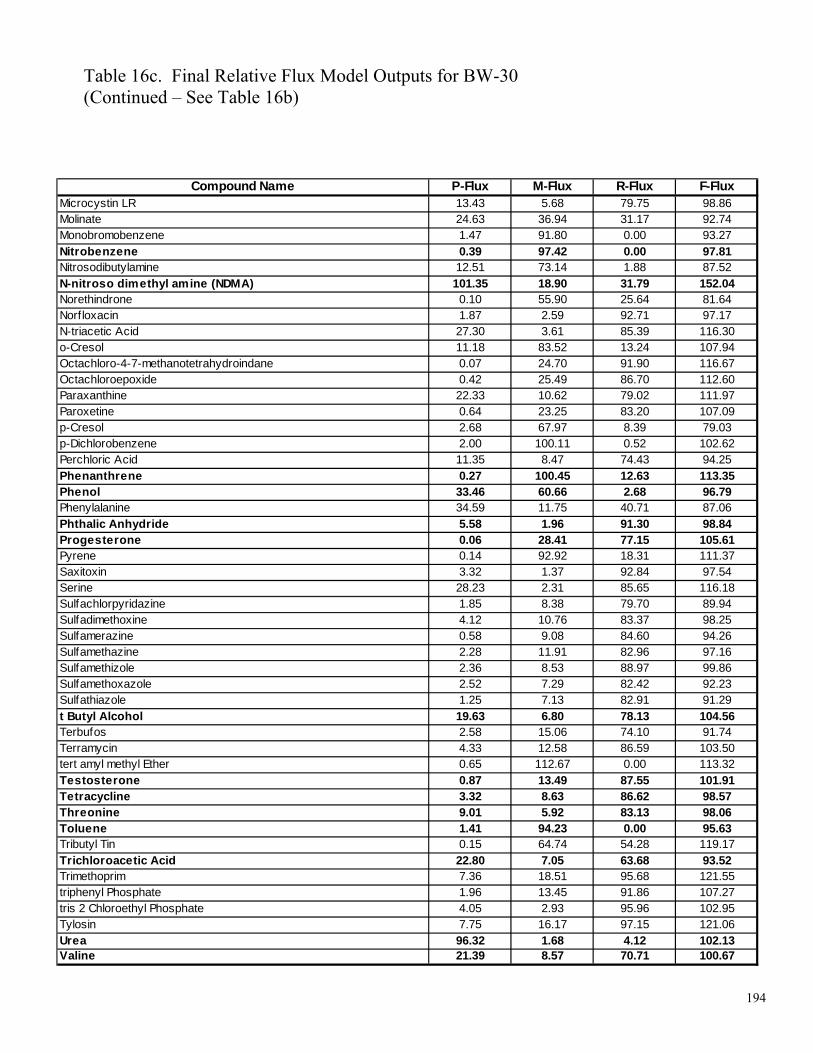
194

Compound Name P-Flux M-Flux R-Flux F-FluxMicrocystin LR 13.43 5.68 79.75 98.86Molinate 24.63 36.94 31.17 92.74Monobromobenzene 1.47 91.80 0.00 93.27Nitrobenzene 0.39 97.42 0.00 97.81Nitrosodibutylamine 12.51 73.14 1.88 87.52N-nitroso dimethyl amine (NDMA) 101.35 18.90 31.79 152.04Norethindrone 0.10 55.90 25.64 81.64Norfloxacin 1.87 2.59 92.71 97.17N-triacetic Acid 27.30 3.61 85.39 116.30o-Cresol 11.18 83.52 13.24 107.94Octachloro-4-7-methanotetrahydroindane 0.07 24.70 91.90 116.67Octachloroepoxide 0.42 25.49 86.70 112.60Paraxanthine 22.33 10.62 79.02 111.97Paroxetine 0.64 23.25 83.20 107.09p-Cresol 2.68 67.97 8.39 79.03p-Dichlorobenzene 2.00 100.11 0.52 102.62Perchloric Acid 11.35 8.47 74.43 94.25Phenanthrene 0.27 100.45 12.63 113.35Phenol 33.46 60.66 2.68 96.79Phenylalanine 34.59 11.75 40.71 87.06Phthalic Anhydride 5.58 1.96 91.30 98.84Progesterone 0.06 28.41 77.15 105.61Pyrene 0.14 92.92 18.31 111.37Saxitoxin 3.32 1.37 92.84 97.54Serine 28.23 2.31 85.65 116.18Sulfachlorpyridazine 1.85 8.38 79.70 89.94Sulfadimethoxine 4.12 10.76 83.37 98.25Sulfamerazine 0.58 9.08 84.60 94.26Sulfamethazine 2.28 11.91 82.96 97.16Sulfamethizole 2.36 8.53 88.97 99.86Sulfamethoxazole 2.52 7.29 82.42 92.23Sulfathiazole 1.25 7.13 82.91 91.29t Butyl Alcohol 19.63 6.80 78.13 104.56Terbufos 2.58 15.06 74.10 91.74Terramycin 4.33 12.58 86.59 103.50tert amyl methyl Ether 0.65 112.67 0.00 113.32Testosterone 0.87 13.49 87.55 101.91Tetracycline 3.32 8.63 86.62 98.57Threonine 9.01 5.92 83.13 98.06Toluene 1.41 94.23 0.00 95.63Tributyl Tin 0.15 64.74 54.28 119.17Trichloroacetic Acid 22.80 7.05 63.68 93.52Trimethoprim 7.36 18.51 95.68 121.55triphenyl Phosphate 1.96 13.45 91.86 107.27tris 2 Chloroethyl Phosphate 4.05 2.93 95.96 102.95Tylosin 7.75 16.17 97.15 121.06Urea 96.32 1.68 4.12 102.13Valine 21.39 8.57 70.71 100.67

Table 16c. Final Relative Flux Model Outputs for BW-30 (Continued – See Table 16b)

195

Compound Name P-Flux M-Flux R-Flux F-Flux1,1 Dichloropropanone 14.82 42.67 33.24 90.731,1,2 Trichloroethene (TCE) 19.57 93.57 11.14 124.28

1,1,2,2, Tetrachloroethylene (PCE) 0.29 96.26 -2.36 94.191,2 Dichlorobenzene 6.24 89.24 -1.78 93.701,2 Dimethylbenzene 2.98 87.66 -5.39 85.251,2,4 Trimethylbenzene 0.86 92.70 -6.13 87.431,3,5 Trimethylbenzene 1.63 95.86 -5.02 92.471,4 Dichlorobenzene 5.38 90.75 -4.85 91.28

1,4 Dichlorophenoxyacetic Acid 14.64 18.06 66.00 98.6917a Estradiol 1.84 90.12 15.35 107.312,3 Naphthalenedicarboxylic Acid 2.93 2.68 79.80 85.40

2,3,4,5,6 Pentachlorophenol 2.60 47.44 52.89 102.932,3,5,6 Tetrachloroterephthalic Acid 3.24 14.28 75.26 92.78

2,4 Dinitrotoluene 3.44 103.20 3.88 110.522,4,5 Trichlorophenoxyacetic Acid 10.13 13.95 56.28 80.362,6 Naphthalenedicarboxylic Acid 2.20 3.68 74.88 80.76

2-chloro-2'-6'-diethyl-N-methoxymethyl-acetanilide (Alachlor) 2.55 19.66 77.40 99.623 Hydroxycarbofuran 1.57 102.82 60.74 77.06

4 Nonylphenol 0.13 20.79 78.85 99.774,6 Dichlorophenol 3.31 97.69 0.07 101.064-amino-6-tert-butyl-3-methylthio-as-triazin-5,4H-one 20.88 6.13 70.65 97.66

Acetochlor 8.09 12.85 80.83 101.77

Alanine 14.96 5.69 76.28 96.93Aldicarbsulfone 2.74 5.16 69.22 77.12alpha-naphthyl-N-Methylcarbamate 0.84 27.61 77.57 106.01Anthracene 0.45 86.36 14.71 101.52

Asparagine 22.17 7.64 73.00 102.81Aspartic Acid 18.82 3.05 76.75 98.62Benzene 30.72 78.22 -2.55 106.39benzo-a-Pyrene 0.01 74.12 18.06 92.20benzo-e-1,3,2 Dioxathiepin-3-oxide 18.74 9.10 81.43 109.28

beta Sitostanol n Hydrate 0.47 49.82 59.95 110.24beta-Estradiol 1.99 88.94 30.65 121.58bis-2-Ethylhexyl-adipate 3.55 6.77 79.05 89.37

Bisphenol 2.00 24.05 69.88 95.93Bromochloroacetonitrile 24.65 63.98 32.48 121.10Bromochloromethane 11.43 27.47 63.48 102.38Bromomethane 17.41 9.35 49.51 76.27Butylated-Hydroxyanisole 0.25 50.09 31.89 82.24

Caffeine 19.64 17.74 59.49 96.87Chloralhydrate 6.97 8.47 89.52 104.96

Chlorpyrifos 0.71 21.43 43.86 106.55Cholesterol 0.03 40.06 76.24 97.70

Table 17a. Final Model Output for ESPA-2 The predicted values represent a 25% noise-band criteria. Bolded compounds represent surrogates used to build the models

196

Compound Name P-Flux M-Flux R-Flux F-FluxCimetidine 16.21 18.84 44.47 100.74Ciprofloxacin 11.67 96.98 69.51 100.02Codeine 15.88 48.31 36.50 100.70Cymene 0.24 96.65 14.69 111.58Cysteine 8.36 6.21 83.09 97.66Dibromoacetatic Acid 32.76 8.99 66.79 108.54Dichloroacetic Acid 30.56 7.60 58.63 96.78Dichloroacetonitrile 19.15 42.16 39.77 101.08Dichlorodiphenyldichloroethylene 0.61 38.09 78.66 117.36Dichloropropane 4.02 47.19 33.88 85.09

Diethylphthalate 5.91 31.95 63.20 101.06Diethylstilbestrol 0.15 16.59 81.93 98.68Digoxigenin 1.35 29.53 89.12 120.00Diltiazem 7.35 13.54 72.69 93.58Dipropylthiocarbamic Acid-s-ethylester 5.68 11.30 91.28 108.25di-sec-Octylphthalate 1.54 8.82 70.20 80.56Diuron 3.96 16.08 60.35 80.39d--n-Butylphthalate 3.70 33.82 71.57 109.08d--n-Octylphthalate 0.06 9.29 74.83 84.17Doxycycline 4.09 15.10 82.58 101.77Enrofloxacin 2.61 18.73 69.09 90.44Erythromycin 4.24 13.02 82.74 100.00Estriol 8.38 68.32 26.36 103.06

Estrone 0.28 93.84 1.39 95.50Ethylbenzene 2.63 88.96 -2.72 88.87Ethylenediaminetetraacetic Acid (EDTA) 13.69 8.02 74.29 96.01Fluoranthrene 0.15 87.71 13.32 101.17Fonofos 0.16 10.20 108.88 119.24Gemfibrozil 6.21 11.45 83.44 101.09Glycine 25.22 4.69 79.11 109.01Hexachlorobenzene 0.01 89.30 18.07 107.38Histidine 13.00 8.12 77.22 98.33Ibuprofen 4.51 8.84 82.48 95.83Leucine 4.53 7.56 77.42 89.52Lindane 2.34 56.03 40.32 98.68Lysine 14.75 9.25 81.25 105.25Mestranol 0.82 16.83 106.34 123.99Methionine 16.95 18.83 55.26 91.04methyl Parathion 1.54 25.00 69.41 95.94Methylene Bromide 6.78 72.64 45.07 124.48Metribuzin 20.87 6.12 70.58 97.58Molinate 1.31 47.26 71.99 120.55

Table 17b. Final Model Output for ESPA-2 (Continued – See Table 17a)

197

Compound Name P-Flux M-Flux R-Flux F-FluxMonobromobenzene 6.24 76.75 11.34 94.32N-Dimethylamine 34.94 21.84 42.84 99.62Nitrobenzene 0.47 97.58 -3.05 95.00Nitrosodibutylamine 2.73 36.12 63.27 102.12N-nitroso dimethyl amine (NDMA) 71.97 13.32 6.45 91.73N-nitrosodi-n-butylamine 3.81 41.82 59.18 104.81Norfloxacin 6.39 11.60 67.80 85.79o-Cresol 5.70 75.39 10.57 91.66Paraxanthine 17.18 12.20 60.94 90.32p-Cresol 4.92 71.71 7.43 84.06p-Dichlorobenzene 5.38 90.75 -4.85 91.28Phenanthrene 0.55 84.54 14.04 99.12Phenol 27.89 63.55 10.55 102.00Phthalic Anhydride 7.08 3.11 90.53 100.72Progesterone 0.21 32.75 65.15 98.11Pyrene 0.27 89.48 22.23 111.98s-1-Methyl-5-3-Pyridinyl-2-Pyrrolidinone 3.96 39.80 62.09 105.85Salbutamol 10.84 5.46 68.81 85.12Saxitoxin 8.25 48.12 65.29 121.66Serine 21.86 5.80 85.84 113.50Sulfachlorpyridazine 2.11 42.31 70.01 114.43Sulfadimethoxine 2.89 46.65 58.41 107.95Sulfamerazine 1.37 26.22 74.61 102.20Sulfamethazine 2.60 26.69 77.32 106.62Sulfamethoxazole 1.35 31.30 73.11 105.76Sulfathiazole 2.42 35.22 74.96 112.60t Butyl Alcohol 17.89 5.50 79.67 103.06Terbufos 1.40 18.53 73.79 93.71Terramycin 8.95 18.08 74.69 101.72Testosterone 2.31 28.66 70.40 101.37Tetracycline 5.82 17.15 75.41 98.39Thio-N-methyl-carbamoyl-oxy-methylester 18.75 4.64 66.30 89.68Threonine 11.59 4.77 83.70 100.06Toluene 6.60 84.41 7.43 98.44Trichloroacetic Acid 20.20 7.78 71.78 99.77Triclosan 1.00 25.09 72.65 98.74Trimethoprim 5.57 50.05 56.41 112.03triphenyl Phosphate 0.78 10.68 90.90 102.35tris 2 Chloroethyl Phosphate 1.24 33.95 53.03 88.21Tylosin 5.45 11.28 72.09 88.82

Urea 84.52 3.22 5.69 93.44Valine 17.16 7.46 79.31 103.93

Table 17c. Final Model Output for ESPA-2 (Continued – See Table 17b)

198

Compound Name P-Flux M-Flux R-Flux F-Flux1,1 Dichloropropanone 19.68 21.24 61.57 102.491,1,2 Trichloroethene (TCE) 6.54 69.36 34.08 109.981,1,2,2 Tetrachloroethane 0.11 92.52 16.02 108.651,1,2,2, Tetrachloroethylene (PCE) 0.11 96.99 -2.58 94.521,2 Dimethylbenzene 1.46 93.81 -19.89 75.371,2,4 Trimethylbenzene 1.04 102.38 -16.39 87.041,3,5 Trimethylbenzene 0.24 105.35 -19.54 86.061,4 Dichlorophenoxyacetic Acid 4.52 3.68 90.28 98.4817a Estradiol 0.89 72.51 32.61 106.012,3 Naphthalenedicarboxylic Acid 11.25 4.01 81.66 96.932,3,4,5,6 Pentachlorophenol 0.82 56.12 37.65 94.592,3,5,6 Tetrachloroterephthalic Acid 13.53 6.07 99.68 119.282,4 Dinitrophenol 2.46 56.64 44.18 103.282,4 Dinitrotoluene 1.89 100.87 1.75 104.512,4,5 Trichlorophenoxyacetic Acid 3.27 3.47 82.31 89.052,6 Naphthalenedicarboxylic Acid 3.89 5.49 82.51 91.893 Hydroxycarbofuran 5.37 101.27 74.71 94.323-amino-1H-1,2,4 Triazole 23.60 14.25 0.29 120.034 Nonylphenol 0.37 24.07 76.99 101.444,6 Dichlorophenol 1.72 97.84 6.22 105.77Alanine 15.11 6.50 76.08 97.69Aldicarbsulfone 12.54 1.53 75.89 89.97Aldrin 0.98 6.86 67.59 75.43Anthracene 0.55 96.14 -10.69 85.99Asparagine 12.06 5.73 83.17 100.97Aspartic Acid 8.31 4.63 87.17 100.11Benzene 16.21 69.75 12.98 98.95benzo-e-1,3,2 Dioxathiepin-3-oxide 0.11 24.62 81.18 105.90beta Sitostanol n Hydrate 0.31 13.78 85.52 99.61Bisphenol 0.96 15.61 84.03 100.60Bromochloroacetonitrile 46.44 10.58 67.87 124.90Bromodichloromethane 5.39 26.54 72.32 104.25Bromomethane 13.86 5.33 75.90 95.10Caffeine 17.01 22.36 72.39 111.75Carbadox 1.87 29.58 73.90 105.36Chloroform 11.08 30.80 56.31 98.19Chlorotetracycline 0.96 19.34 100.87 121.17Chlorpyrifos 1.12 12.00 76.80 96.80Cholesterol 0.24 26.25 87.83 100.07

Table 18a. Final Model Output for LFC-1 The predicted values represent a 25% noise-band criteria. Bolded compounds represent surrogates used to build the models

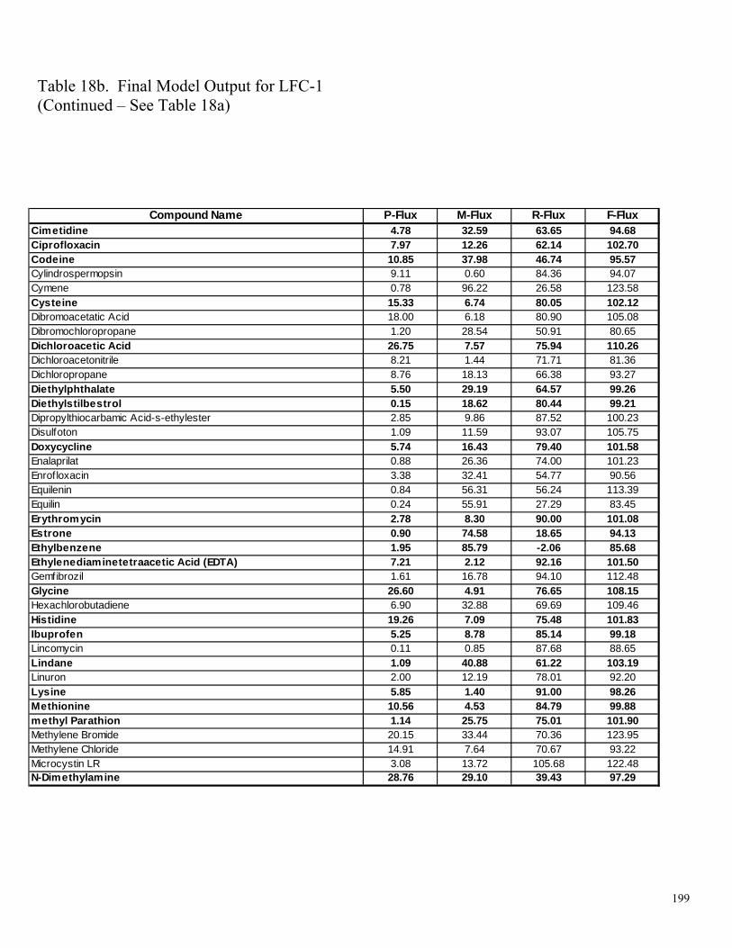
199

Compound Name P-Flux M-Flux R-Flux F-FluxCimetidine 4.78 32.59 63.65 94.68Ciprofloxacin 7.97 12.26 62.14 102.70Codeine 10.85 37.98 46.74 95.57Cylindrospermopsin 9.11 0.60 84.36 94.07Cymene 0.78 96.22 26.58 123.58Cysteine 15.33 6.74 80.05 102.12Dibromoacetatic Acid 18.00 6.18 80.90 105.08Dibromochloropropane 1.20 28.54 50.91 80.65Dichloroacetic Acid 26.75 7.57 75.94 110.26Dichloroacetonitrile 8.21 1.44 71.71 81.36Dichloropropane 8.76 18.13 66.38 93.27Diethylphthalate 5.50 29.19 64.57 99.26Diethylstilbestrol 0.15 18.62 80.44 99.21Dipropylthiocarbamic Acid-s-ethylester 2.85 9.86 87.52 100.23Disulfoton 1.09 11.59 93.07 105.75Doxycycline 5.74 16.43 79.40 101.58Enalaprilat 0.88 26.36 74.00 101.23Enrofloxacin 3.38 32.41 54.77 90.56Equilenin 0.84 56.31 56.24 113.39Equilin 0.24 55.91 27.29 83.45Erythromycin 2.78 8.30 90.00 101.08Estrone 0.90 74.58 18.65 94.13Ethylbenzene 1.95 85.79 -2.06 85.68Ethylenediaminetetraacetic Acid (EDTA) 7.21 2.12 92.16 101.50Gemfibrozil 1.61 16.78 94.10 112.48Glycine 26.60 4.91 76.65 108.15Hexachlorobutadiene 6.90 32.88 69.69 109.46Histidine 19.26 7.09 75.48 101.83Ibuprofen 5.25 8.78 85.14 99.18Lincomycin 0.11 0.85 87.68 88.65Lindane 1.09 40.88 61.22 103.19Linuron 2.00 12.19 78.01 92.20Lysine 5.85 1.40 91.00 98.26Methionine 10.56 4.53 84.79 99.88methyl Parathion 1.14 25.75 75.01 101.90Methylene Bromide 20.15 33.44 70.36 123.95Methylene Chloride 14.91 7.64 70.67 93.22Microcystin LR 3.08 13.72 105.68 122.48N-Dimethylamine 28.76 29.10 39.43 97.29

Table 18b. Final Model Output for LFC-1 (Continued – See Table 18a)

200

Compound Name P-Flux M-Flux R-Flux F-FluxNitrilotriacetic Acid 3.44 6.34 102.92 112.70Nitrobenzene 0.29 90.41 -2.69 88.00N-nitroso dimethyl amine (NDMA) 80.37 0.46 18.60 99.43Norethindrone 0.17 53.32 63.79 117.28Norf loxacin 8.38 25.64 51.13 85.15N-triacetic Acid 0.43 5.85 96.32 102.61o-Cresol 14.48 95.55 -0.03 110.00Paraxanthine 10.37 17.39 77.01 104.77Paroxetine 0.64 17.64 78.53 96.81p-Cresol 34.87 72.70 -3.43 104.14Phenanthrene 0.72 97.55 -4.09 94.18Phenol 39.54 61.98 -1.45 100.07Phenylalanine 34.30 3.56 58.11 95.97Phthalic Anhydride 5.59 3.16 90.03 98.78Progesterone 0.01 22.68 80.95 103.63Pyrene 0.57 102.02 -26.66 75.92Saxitoxin 2.09 9.52 82.08 93.69Serine 34.22 2.72 80.40 117.35Sulfachlorpyridazine 3.51 17.56 51.27 72.33Sulfadimethoxine 3.42 26.49 62.32 92.23Sulfamethazine 2.35 28.12 48.85 79.31Sulfamethizole 15.24 13.65 84.93 113.82Sulfamethoxazole 6.40 18.53 60.94 85.86Sulfathiazole 4.56 20.90 80.74 106.19t Butyl Alcohol 22.32 5.96 66.91 95.19Terbacil 1.56 25.49 65.34 92.38Terbufos 0.63 51.00 70.40 122.04Terramycin 4.58 18.67 80.61 103.86Testosterone 1.77 46.42 61.03 109.22Tetracycline 3.33 16.99 78.49 98.81Thio-N-methyl-carbamoyl-oxy-methylester 1.55 0.68 75.62 77.85Threonine 11.86 3.54 80.51 95.91Toluene 19.51 89.27 0.23 109.01Tributyl Tin 0.78 2.31 96.50 99.59Trichloroacetic Acid 12.65 1.68 82.86 97.20tris 2 Chloroethyl Phosphate 2.52 19.73 92.71 114.96Tylosin 0.71 38.11 68.20 107.02Urea 85.33 1.70 4.38 91.41Valine 12.29 4.21 83.59 100.09

Table 18c. Final Model Output for LFC-1 (Continued – See Table 18b)

201

Compound Name P-Flux M-Flux R-Flux F-Flux1,1 Dichloropropanone 15.34 32.71 58.21 106.261,1,2,2 Tetrachloroethane 0.09 102.96 0.12 103.171,1,2,2, Tetrachloroethylene (PCE) 0.08 103.08 -2.44 100.721,3,5 Trimethylbenzene 0.10 86.66 -7.06 79.701,4 Dichlorophenoxyacetic Acid 5.04 8.58 83.49 97.1117a Estradiol 0.37 75.07 16.91 92.352,2 bis-p-Chlorophenyl 1,1,1 Trichloroethane 0.48 9.53 77.47 87.482,2 bis-p-Methoxyphenyl 1,1,1 Trichloroethane 1.20 13.39 98.03 112.622,2,2 Trichloro 1,1-bis-4-chlorophenyl Ethanol 0.37 14.88 58.85 74.102,3 Naphthalenedicarboxylic Acid 2.52 4.00 78.47 85.002,3,4,5,6 Pentachlorophenol 5.74 73.84 23.23 102.822,4 Dinitrophenol 10.10 39.33 36.53 85.972,4 Dinitrotoluene 1.96 96.01 1.68 99.652,4,5 Trichlorophenoxyacetic Acid 9.33 9.15 74.91 93.392,6 bis-1,1 Dimethylethyl Phenol 0.09 26.31 52.45 78.852,6 di-tert-butyl-p-Cresol 0.12 35.36 40.35 75.822,6 Naphthalenedicarboxylic Acid 3.19 8.30 76.20 87.692-chloro-2'-6'-diethyl-N-methoxymethyl-acetanilide (Alachlor) 2.65 24.66 77.77 105.083 Hydroxycarbofuran 0.22 87.93 42.92 121.723-amino-1H-1,2,4 Triazole 12.35 78.57 1.20 119.604 Nonylphenol 0.22 70.73 26.83 97.784,6 Dichlorophenol 2.18 94.19 4.68 101.05Acetaminophen 21.02 36.51 31.71 89.24Alanine 9.73 5.41 82.22 97.35Aldicarbsulfone 1.42 3.29 77.50 82.21Aldrin 8.01 29.67 84.69 122.37Anthracene 0.49 87.50 16.93 104.92Asparagine 34.91 5.26 64.01 104.17Aspartic Acid 12.00 5.32 80.79 98.11Benzene 22.21 81.24 2.46 105.92benzo-e-1,3,2 Dioxathiepin-3-oxide 9.17 24.11 83.96 117.23beta Sitostanol n Hydrate 0.40 21.71 74.20 96.31beta-Estradiol 0.38 62.55 17.25 80.19Bisphenol 0.24 25.91 74.45 100.59Bromochloroacetic Acid 9.97 14.08 69.30 93.35Bromochloroacetonitrile 26.04 12.94 74.57 113.55Bromochloromethane 21.17 11.48 62.77 95.42Bromodichloromethane 18.55 9.18 59.89 87.61Bromoform 0.28 45.88 51.00 97.17Bromomethane 19.70 11.08 52.96 83.74Butylated-Hydroxyanisole 0.19 37.37 39.50 77.06Caffeine 17.20 17.06 68.49 102.75Carbadox 9.71 40.91 71.49 122.11

Chloroform 26.18 19.04 56.20 101.42Chlorpyrifos 0.75 14.79 46.84 103.46

Table 19a. Final Model Output for TFC-HR The predicted values represent a 25% noise-band criteria. Bolded compounds represent surrogates used to build the models

202

Compound Name P-Flux M-Flux R-Flux F-FluxCholesterol 0.34 25.32 88.03 103.17Cimetidine 13.54 11.23 62.29 101.15Ciprofloxacin 4.89 82.57 82.21 98.33Codeine 7.39 20.50 76.11 104.00Cyclotrimethylenetrinitramine 70.17 97.78 -54.30 113.65Cylindrospermopsin 13.00 2.71 73.06 88.78Cymene 0.08 74.55 35.94 110.57Cysteine 7.75 5.58 86.50 99.83Dibromoacetatic Acid 3.15 18.59 80.56 102.29Dibromoacetonitrile 9.10 6.43 75.88 91.40Dibromochloromethane 7.53 6.72 67.86 82.11Dichloroacetic Acid 20.67 8.61 67.59 96.87Dichlorodif luoromethane 21.72 13.90 61.43 97.06Dichlorodiphenyldichloroethylene 16.63 58.94 36.15 111.71Dichloropropane 15.01 28.69 76.99 120.69Diethylphthalate 1.42 40.75 62.42 104.58Diethylstilbestrol 0.15 54.06 50.95 105.16Digoxigenin 0.57 47.26 58.85 106.68Diltiazem 0.28 20.93 73.85 95.06di-sec-Octylphthalate 0.18 23.09 82.66 105.93Disulfoton 0.22 12.58 103.16 115.96d--n-Octylphthalate 0.04 22.76 93.84 116.64Doxycycline 8.58 15.54 77.12 101.24Enalaprilat 0.33 15.50 76.88 92.70Enrofloxacin 8.75 4.70 81.74 95.19Erythromycin 2.54 10.48 87.94 100.95Estrone 0.20 103.33 -1.54 101.99Ethylbenzene 2.83 94.23 -4.96 92.10Ethylenediaminetetraacetic Acid (EDTA) 11.30 2.28 88.17 101.76ethyl-tert-Butyl Ether 18.66 10.21 84.91 113.77exo-Dimethanonaphthalene 1.27 54.06 57.89 113.22Fluoranthrene 1.85 87.29 -0.87 88.26Fluoxetine 4.52 4.43 66.67 75.62Fonofos 0.11 4.29 75.24 79.64Gemfibrozil 4.17 9.43 84.61 98.21Glycine 2.68 5.51 87.17 95.36Hexachlorocyclohexane 0.40 77.22 10.65 88.27Histidine 9.64 4.59 83.38 97.62Ibuprofen 3.91 11.54 86.27 101.72Leucine 6.54 7.22 94.32 108.07Lincomycin 0.97 21.24 98.72 120.93Lindane 1.00 66.21 35.69 102.91Lysine 16.85 3.48 84.53 104.86Metformin 63.82 31.44 13.44 108.71

Table 19b. Final Model Output for TFC-HR (Continued – See Table 19a)

203

Compound Name P-Flux M-Flux R-Flux F-FluxMethionine 17.45 5.07 73.18 95.70methyl Parathion 3.28 22.48 67.29 93.05Methylene Bromide 6.94 34.66 77.58 119.18Methylene Chloride 39.50 19.71 44.93 104.15methyl-tert-butyl Ether (MTBE) 21.96 8.90 76.90 107.76Monobromobenzene 23.31 107.52 -54.30 76.53N-Dimethylamine 35.24 7.62 62.76 105.62Nitrilotriacetic Acid 3.27 5.57 78.56 87.39Nitrobenzene 0.34 100.87 -2.19 99.02N-nitroso dimethyl amine (NDMA) 74.72 20.80 2.72 98.24N-nitrosomorpholine 17.18 28.14 30.68 76.00Norethindrone 0.36 48.40 68.08 116.85Norfloxacin 3.75 16.06 83.01 102.82N-triacetic Acid 2.48 3.55 76.47 82.50Octachloro-4-7-methanotetrahydroindane 4.71 49.51 70.66 124.88Paraxanthine 5.69 13.90 58.57 78.16Perchloric Acid 7.16 1.98 99.37 108.51Phenanthrene 0.51 88.47 5.46 94.45Phenol 32.48 61.87 -1.19 93.15Phenylalanine 16.24 3.15 90.21 109.59Phthalic Anhydride 8.20 3.06 88.36 99.62Progesterone 0.17 26.30 69.81 96.28Pyrene 1.29 87.34 -1.56 87.07Salbutamol 14.32 8.40 80.01 102.73Serine 7.00 5.68 80.18 92.87Sulfachlorpyridazine 0.80 41.79 81.89 124.48Sulfadimethoxine 1.19 12.36 85.35 98.89Sulfamerazine 0.54 9.60 83.61 93.75Sulfamethazine 0.80 9.80 86.30 96.90Sulfathiazole 0.66 10.41 71.33 82.41t Butyl Alcohol 19.14 8.47 66.84 94.46Terramycin 2.26 23.38 80.83 106.47tert amyl methyl Ether 7.73 9.28 76.61 93.62Testosterone 0.33 14.39 85.55 100.27Tetracycline 2.98 15.89 83.45 102.32Thio-N-methyl-carbamoyl-oxy-methylester 8.26 18.42 80.19 106.88Threonine 8.68 5.22 84.04 97.94Toluene 7.12 93.08 -1.25 98.95Tributyl Tin 0.08 2.31 98.08 100.47Trichloroacetic Acid 28.16 6.18 67.17 101.51Triclosan 18.33 32.78 61.95 113.06triphenyl Phosphate 0.15 17.48 99.44 117.07Urea 72.31 1.76 7.26 81.33Valine 9.41 6.05 82.94 98.40

Table 19c. Final Model Output for TFC-HR (Continued – See Table 19b)

204

Compound Name P-Flux M-Flux R-Flux F-Flux1,1,2,2 Tetrachloroethane 32.88 64.71 5.31 102.89

1,1,2,2, Tetrachloroethylene (PCE) 30.91 66.34 6.04 103.291,2 Dichlorobenzene 13.09 86.00 -0.73 98.361,2,4 Trimethylbenzene 24.52 96.41 1.94 122.871,3,5 Trimethylbenzene 17.79 98.96 3.46 120.221,4 Dichlorobenzene 6.32 90.95 -0.57 96.71

1,4 Dichlorophenoxyacetic Acid 43.90 6.40 46.61 96.9117a Estradiol 3.03 97.45 0.84 101.322,2 bis-p-Chlorophenyl 1,1,1 Trichloroethane 2.44 98.53 -2.07 98.902,3 Naphthalenedicarboxylic Acid 8.98 85.75 0.62 95.35

2,3,4,5,6 Pentachlorophenol 2.06 97.69 0.35 100.102,4 Dichloro-4'-nitrodiphenyl Ether 2.79 98.01 -1.18 99.62

2,4 Dinitrotoluene 7.90 93.28 0.47 101.642,6 bis-1,1 Dimethylethyl 2,5 Cyclohexadiene 1,4 dione 4.93 98.87 6.33 110.132,6 bis-1,1 Dimethylethyl Phenol 9.66 98.33 0.88 108.872,6 di-tert-butyl-p-Cresol 7.26 98.49 2.08 107.83

2-chloro-2'-6'-diethyl-N-methoxymethyl-acetanilide (Alachlor) 5.73 86.29 4.95 96.973-amino-1H-1,2,4 Triazole 77.12 54.36 9.79 90.23

4 Nonylphenol 0.54 98.57 1.88 100.994,6 Dichlorophenol 2.18 97.54 -0.80 98.914-amino-6-tert-butyl-3-methylthio-as-triazin-5,4H-one 50.52 62.28 0.23 113.03Acetaminophen 88.96 28.10 0.76 117.82

Alanine 58.64 8.33 40.05 107.01Aldicarbsulfone 73.16 31.81 12.56 117.53Aldrin 14.72 93.59 2.07 110.38alpha-naphthyl-N-Methylcarbamate 4.59 98.04 9.85 112.48Androsterone 3.95 87.95 0.55 92.45Anthracene 0.45 99.66 0.97 101.08

Asparagine 66.08 0.64 42.86 109.59Aspartic Acid 35.62 9.24 61.70 106.55Benzene 57.21 44.79 1.48 103.48benzo-a-Pyrene 0.23 99.40 4.16 103.79

beta Sitostanol n Hydrate 0.53 24.04 75.84 100.42bis-2-Ethylhexyl-adipate 5.10 97.77 0.87 103.74

Bisphenol 0.84 97.96 0.21 99.01Butylated-Hydroxyanisole 11.79 98.90 2.30 113.00

Caffeine 70.35 11.46 15.14 96.96Carbadox 2.17 82.21 1.58 85.96Chloralhydrate 38.42 51.35 1.57 91.34Chlorpyrifos 3.32 20.11 -0.19 100.76Cholesterol 0.27 21.54 70.30 90.68

Table 20a. Final Model Output for CA The predicted values represent a 25% noise-band criteria. Bolded compounds represent surrogates used to build the models

205

Compound Name P-Flux M-Flux R-Flux F-FluxCimetidine 62.08 24.20 22.86 106.48Ciprofloxacin 34.38 98.23 24.76 83.35Codeine 55.86 27.10 10.66 93.62Cymene 12.32 99.49 1.63 113.44Cysteine 42.90 6.61 42.02 91.54Diazinon 7.65 97.52 -1.34 103.83Dibromoacetonitrile 58.43 33.98 16.00 108.42Dichloroacetic Acid 44.11 5.87 37.16 87.13Dichlorodif luoromethane 2.57 95.58 1.75 99.90Dichlorodiphenyldichloroethylene 7.58 98.63 13.22 119.43

Diethylphthalate 15.81 82.97 0.22 99.00Diethylstilbestrol 0.28 99.37 0.43 100.08Diltiazem 5.25 95.30 -0.32 100.22Dipropylthiocarbamic Acid-s-ethylester 13.74 89.44 7.33 110.51di-sec-Octylphthalate 2.59 98.78 9.08 110.44Diuron 30.36 69.47 7.30 107.12d--n-Butylphthalate 0.36 69.10 12.77 82.23d--n-Octylphthalate 0.24 87.88 22.22 110.34Doxycycline 17.04 29.48 53.97 100.49Enalaprilat 79.49 4.62 6.42 90.52Endosulfansulfate 7.82 97.87 5.86 111.55Enrofloxacin 13.30 43.41 28.45 85.16Equilenin 1.42 97.55 4.97 103.95Equilin 1.63 87.53 0.13 89.29Erythromycin 29.37 6.06 70.00 105.43Estriol 1.15 87.31 3.31 91.76Estrone 2.56 97.30 -0.39 99.47Ethylbenzene 25.86 68.70 1.42 95.98Ethylenediaminetetraacetic Acid (EDTA) 47.11 7.05 45.09 99.26Fluoranthrene 0.36 99.43 1.48 101.27Fluoxetine 1.35 97.92 -1.93 97.34Fonofos 5.03 97.71 0.44 103.17

Glycine 62.73 9.95 38.56 111.24Hexachlorobenzene 2.74 99.67 -0.85 101.55

Histidine 44.17 8.06 44.55 96.78Ibuprofen 57.58 23.00 22.96 103.54Leucine 60.64 2.21 37.79 100.64Lincomycin 51.04 23.24 12.59 86.86Lindane 1.53 98.80 -0.22 100.11Lysine 53.44 9.55 27.34 90.34

Table 20b. Final Model Output for CA (Continued – See Table 20a)

206

Compound Name P-Flux M-Flux R-Flux F-FluxMestranol 1.68 98.14 0.24 100.07Metformin 69.85 32.89 2.30 105.04

Methionine 48.80 8.93 39.66 97.40methyl Parathion 1.86 97.86 -0.10 99.61Metribuzin 50.49 62.26 0.22 112.97N N diethyl 3 methylbenzamide 25.38 91.94 0.29 117.61

N-Dimethylamine 55.85 12.92 10.38 79.16Nitrilotriacetic Acid 50.70 4.55 49.24 104.49

Nitrobenzene 35.98 63.65 0.80 100.43Nitrosodiethylamine 57.49 19.87 8.70 86.07

N-nitroso dimethyl amine (NDMA) 90.16 3.67 3.67 97.50N-nitrosomorpholine 29.62 33.98 9.73 73.33N-nitrosopiperidine 39.06 20.47 12.29 71.81Norfloxacin 34.01 67.82 11.89 113.71N-triacetic Acid 66.99 4.26 33.92 105.17o-Cresol 23.12 93.78 0.05 116.96Paraxanthine 53.15 13.62 16.16 82.93Paroxetine 1.39 98.99 0.49 100.88p-Dichlorobenzene 6.32 90.95 -0.57 96.71

Phenanthrene 0.50 99.65 0.97 101.12Phenol 71.96 31.30 -0.34 102.93Phthalic Anhydride 28.58 5.34 64.35 98.27Progesterone 1.68 98.63 -0.28 100.03Pyrene 0.33 99.68 1.71 101.72Salbutamol 75.08 31.51 3.65 110.25Saxitoxin 39.84 54.89 7.91 102.64Sulfamerazine 70.15 7.32 0.68 78.15Sulfamethazine 49.20 22.93 2.80 74.93

t Butyl Alcohol 86.51 3.69 12.52 102.72Terbufos 20.24 99.14 4.87 124.25

Testosterone 19.64 55.06 2.77 77.46Tetracycline 37.95 15.49 57.31 110.75Threonine 49.43 7.53 35.08 92.04Toluene 46.90 48.83 2.04 97.76Trichloroacetic Acid 55.91 4.60 39.79 100.31Trimethoprim 12.12 66.48 41.94 120.54triphenyl Phosphate 0.50 98.14 -1.50 97.13tris 2 Chloroethyl Phosphate 2.23 96.31 1.67 100.20

Urea 91.95 4.59 28.21 124.75Valine 61.69 4.93 34.09 100.71

Table 20c. Final Model Output for CA (Continued – See Table 20b)

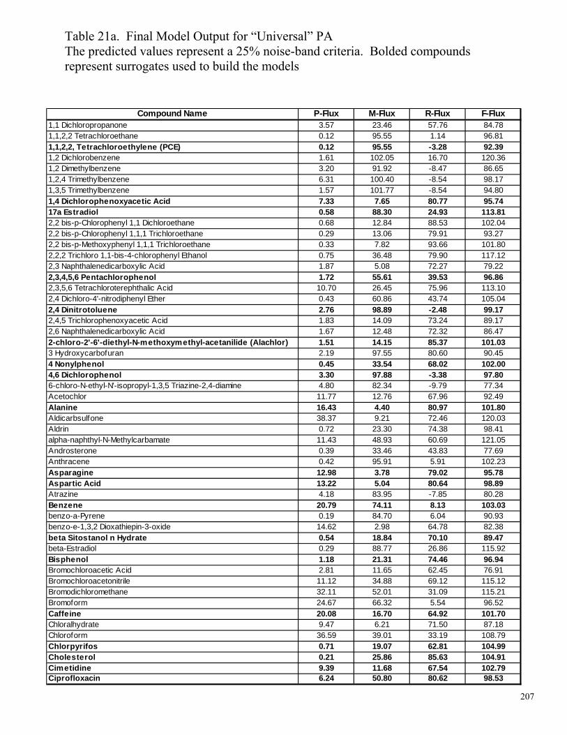
207

Compound Name P-Flux M-Flux R-Flux F-Flux1,1 Dichloropropanone 3.57 23.46 57.76 84.781,1,2,2 Tetrachloroethane 0.12 95.55 1.14 96.811,1,2,2, Tetrachloroethylene (PCE) 0.12 95.55 -3.28 92.391,2 Dichlorobenzene 1.61 102.05 16.70 120.361,2 Dimethylbenzene 3.20 91.92 -8.47 86.651,2,4 Trimethylbenzene 6.31 100.40 -8.54 98.171,3,5 Trimethylbenzene 1.57 101.77 -8.54 94.801,4 Dichlorophenoxyacetic Acid 7.33 7.65 80.77 95.7417a Estradiol 0.58 88.30 24.93 113.812,2 bis-p-Chlorophenyl 1,1 Dichloroethane 0.68 12.84 88.53 102.042,2 bis-p-Chlorophenyl 1,1,1 Trichloroethane 0.29 13.06 79.91 93.272,2 bis-p-Methoxyphenyl 1,1,1 Trichloroethane 0.33 7.82 93.66 101.802,2,2 Trichloro 1,1-bis-4-chlorophenyl Ethanol 0.75 36.48 79.90 117.122,3 Naphthalenedicarboxylic Acid 1.87 5.08 72.27 79.222,3,4,5,6 Pentachlorophenol 1.72 55.61 39.53 96.862,3,5,6 Tetrachloroterephthalic Acid 10.70 26.45 75.96 113.102,4 Dichloro-4'-nitrodiphenyl Ether 0.43 60.86 43.74 105.042,4 Dinitrotoluene 2.76 98.89 -2.48 99.172,4,5 Trichlorophenoxyacetic Acid 1.83 14.09 73.24 89.172,6 Naphthalenedicarboxylic Acid 1.67 12.48 72.32 86.472-chloro-2'-6'-diethyl-N-methoxymethyl-acetanilide (Alachlor) 1.51 14.15 85.37 101.033 Hydroxycarbofuran 2.19 97.55 80.60 90.454 Nonylphenol 0.45 33.54 68.02 102.004,6 Dichlorophenol 3.30 97.88 -3.38 97.806-chloro-N-ethyl-N'-isopropyl-1,3,5 Triazine-2,4-diamine 4.80 82.34 -9.79 77.34Acetochlor 11.77 12.76 67.96 92.49Alanine 16.43 4.40 80.97 101.80Aldicarbsulfone 38.37 9.21 72.46 120.03Aldrin 0.72 23.30 74.38 98.41alpha-naphthyl-N-Methylcarbamate 11.43 48.93 60.69 121.05Androsterone 0.39 33.46 43.83 77.69Anthracene 0.42 95.91 5.91 102.23Asparagine 12.98 3.78 79.02 95.78Aspartic Acid 13.22 5.04 80.64 98.89Atrazine 4.18 83.95 -7.85 80.28Benzene 20.79 74.11 8.13 103.03benzo-a-Pyrene 0.19 84.70 6.04 90.93benzo-e-1,3,2 Dioxathiepin-3-oxide 14.62 2.98 64.78 82.38beta Sitostanol n Hydrate 0.54 18.84 70.10 89.47beta-Estradiol 0.29 88.77 26.86 115.92Bisphenol 1.18 21.31 74.46 96.94Bromochloroacetic Acid 2.81 11.65 62.45 76.91Bromochloroacetonitrile 11.12 34.88 69.12 115.12Bromodichloromethane 32.11 52.01 31.09 115.21Bromoform 24.67 66.32 5.54 96.52Caffeine 20.08 16.70 64.92 101.70Chloralhydrate 9.47 6.21 71.50 87.18Chloroform 36.59 39.01 33.19 108.79Chlorpyrifos 0.71 19.07 62.81 104.99Cholesterol 0.21 25.86 85.63 104.91Cimetidine 9.39 11.68 67.54 102.79Ciprofloxacin 6.24 50.80 80.62 98.53

Table 21a. Final Model Output for “Universal” PA The predicted values represent a 25% noise-band criteria. Bolded compounds represent surrogates used to build the models

208

Compound Name P-Flux M-Flux R-Flux F-FluxCodeine 11.13 28.03 61.67 100.83Cylindrospermopsin 2.96 15.48 84.32 102.77Cymene 1.64 93.46 -10.39 84.72Cysteine 9.99 6.06 82.35 98.39Dibromoacetatic Acid 5.28 4.32 69.17 78.77Dibromoacetonitrile 4.49 42.01 69.65 116.15Dibromochloromethane 12.15 61.68 29.28 103.11

Dichloroacetic Acid 23.83 7.46 66.72 98.01Dichloroacetonitrile 3.17 25.19 71.90 100.26Dichloropropane 11.06 27.63 56.84 95.53Dieldrin 0.86 9.21 91.26 101.33Diethylphthalate 4.88 32.62 61.30 98.79Diethylstilbestrol 0.14 27.74 69.13 97.00Digoxigenin 1.80 2.70 72.19 76.69Digoxin 3.26 28.42 79.32 111.00Diltiazem 7.77 12.15 75.54 95.46Disulfoton 1.81 13.67 85.98 101.47Diuron 12.47 16.17 70.19 98.84d--n-Butylphthalate 2.58 19.39 80.70 102.67Doxycycline 5.08 14.48 78.59 98.15Enalaprilat 8.74 1.90 83.14 93.78Endosulfansulfate 0.73 59.18 46.75 106.65Enrofloxacin 2.60 4.55 74.79 81.95Equilenin 0.41 79.33 0.77 80.50Erythromycin 3.33 9.15 88.25 100.73Estriol 3.35 27.98 87.63 118.96

Estrone 0.42 77.69 32.56 110.67Ethylbenzene 2.61 95.58 -4.95 93.24Ethylenediaminetetraacetic Acid (EDTA) 8.77 3.56 85.89 98.22ethyl-tert-Butyl Ether 46.45 63.46 -0.39 109.52exo-Dimethanonaphthalene 7.28 24.45 88.09 119.83Fluoranthrene 0.28 99.17 7.01 106.45Fluoxetine 0.56 9.98 77.75 88.29Fonofos 1.43 3.64 85.06 90.14Glycine 33.98 3.93 86.59 124.50Hexachlorobutadiene 0.21 103.90 -3.00 101.11Hexachlorocyclohexane 7.29 98.91 -4.50 101.70Histidine 14.13 6.98 78.75 99.86Ibuprofen 5.07 9.92 82.17 97.15Leucine 16.80 8.40 86.31 111.51Lincomycin 7.41 14.33 85.48 107.22Lindane 1.51 49.52 47.32 98.35Linuron 4.93 29.94 65.54 100.41Lysine 10.41 3.88 84.69 98.99Mestranol 0.89 7.39 81.69 89.97Methionine 12.22 6.01 75.75 93.97methyl Parathion 1.45 20.55 78.87 100.88Methylene Chloride 31.93 59.43 23.26 114.63methyl-tert-butyl Ether (MTBE) 48.05 50.92 -0.47 98.50Metolachlor 27.61 21.75 61.32 110.69

Table 21b. Final Model Output for “Universal” PA (Continued – See Table 21a)

209

Compound Name P-Flux M-Flux R-Flux F-FluxN N diethyl 3 methylbenzamide 37.29 6.06 48.87 92.21N-Dimethylamine 35.30 14.10 51.93 101.33Nitrilotriacetic Acid 11.20 6.53 88.64 106.37Nitrobenzene 0.37 97.53 -6.95 90.95Nitrosodibutylamine 34.40 64.15 -9.03 89.52N-nitroso dimethyl amine (NDMA) 67.55 12.02 3.63 83.20N-nitrosodi-n-butylamine 29.66 59.69 -3.09 86.25N-nitrosopyrrolidine 25.28 4.74 83.64 113.66Norethindrone 0.28 23.12 63.34 86.75Norfloxacin 7.62 12.85 83.52 103.99N-triacetic Acid 14.58 6.07 82.21 102.85o-Cresol 5.87 82.85 3.55 92.26Octachloro-4-7-methanotetrahydroindane 0.39 48.15 75.90 124.44Octachloroepoxide 0.77 28.00 78.59 107.36Paraxanthine 12.22 15.03 56.47 83.71p-Cresol 15.07 76.90 -0.29 91.69Perchloric Acid 12.02 10.77 60.07 82.87Phenanthrene 0.47 94.79 7.52 102.77Phenol 31.55 65.52 3.93 101.00Phenylalanine 5.84 1.62 86.01 93.47Phthalic Anhydride 7.53 2.90 89.95 100.38Pramitol 10.61 87.08 -10.85 86.84Progesterone 0.21 28.97 70.12 99.29Pyrene 0.33 90.93 10.05 101.31Ranitidine 12.61 34.88 69.39 116.89s-1-Methyl-5-3-Pyridinyl-2-Pyrrolidinone 1.55 36.32 38.95 76.82Salbutamol 23.10 3.29 85.57 111.95Saxitoxin 5.28 8.52 86.56 100.37Serine 15.56 3.13 77.26 95.95Sulfachlorpyridazine 1.48 9.09 82.49 93.05Sulfadimethoxine 1.52 10.30 85.40 97.22Sulfamerazine 1.64 5.60 84.19 91.43Sulfamethazine 1.77 5.99 85.23 93.00Sulfamethizole 4.18 6.24 86.92 97.34Sulfamethoxazole 1.43 8.86 81.01 91.30Sulfathiazole 2.94 8.99 84.23 96.17t Butyl Alcohol 20.79 7.08 71.30 99.17Terbacil 6.98 5.90 69.12 82.00Terramycin 3.76 27.89 83.81 115.47tert amyl methyl Ether 21.30 66.97 -0.77 87.49Testosterone 1.04 20.57 75.39 97.01Tetracycline 3.40 14.16 83.29 100.85Thio-N-methyl-carbamoyl-oxy-methylester 15.94 19.09 74.25 109.29Threonine 10.38 4.86 82.90 98.14Toluene 5.76 90.38 -4.88 91.26Trichloroacetic Acid 22.09 5.51 73.92 101.52Trimethoprim 2.13 87.68 2.16 91.97triphenyl Phosphate 0.33 17.03 74.74 92.10Urea 75.25 2.21 4.50 81.95Valine 16.93 6.39 76.44 99.76

Table 21c. Final Model Output for “Universal” PA (Continued – See Table 21b)

210

Compound Name P-Flux R-Flux P-Flux R-Flux P-Flux R-Flux P-Flux R-Flux P-Flux R-Flux P-Flux R-Flux

1,1 Dichloropropanone 85.18 33.24 80.32 61.57 84.66 58.21 96.43 57.761,1,2 Trichloroethene (TCE) 95.96 21.20 80.43 11.14 93.46 34.081,1,2,2 Tetrachloroethane 99.91 0.00 99.68 -33.49 99.89 16.02 99.91 0.12 99.88 1.14 67.12 5.311,1,2,2, Tetrachloroethylene (PCE) 99.91 0.00 99.71 -2.36 99.89 -2.58 99.92 -2.44 99.88 -3.28 69.09 6.041,2 Dichlorobenzene 98.77 2.00 93.76 -1.78 98.39 16.70 86.91 -0.731,2 Dimethylbenzene 96.04 0.00 97.02 -5.39 98.54 -19.89 96.80 -8.471,2,4 Trimethylbenzene 99.88 0.00 99.14 -6.13 98.96 -16.39 93.69 -8.54 75.48 1.941,3,5 Trimethylbenzene 99.00 0.00 98.37 -5.02 99.76 -19.54 99.90 -7.06 98.43 -8.54 82.21 3.461,4 Dichlorobenzene 98.07 0.52 94.62 -4.85 93.68 -0.571,4 Dichlorophenoxyacetic Acid 88.88 81.08 85.36 66.00 95.48 90.28 94.96 83.49 92.67 80.77 56.10 46.6117a Estradiol 99.82 29.32 98.16 15.35 99.11 32.61 99.63 16.91 99.42 24.93 96.97 0.842,2 bis-p-Chlorophenyl 1,1 Dichloroethane 99.49 71.86 99.32 88.532,2 bis-p-Chlorophenyl 1,1,1 Trichloroethane 96.74 72.46 99.52 77.47 99.71 79.91 97.56 -2.072,2 bis-p-Methoxyphenyl 1,1,1 Trichloroethane 90.36 72.19 98.80 98.03 99.67 93.662,2,2 Trichloro 1,1-bis-4-chlorophenyl Ethanol 99.15 71.60 99.25 79.902,3 Naphthalenedicarboxylic Acid 84.35 90.42 97.07 79.80 88.75 81.66 97.48 78.47 98.13 72.27 91.02 0.622,3,4,5,6 Pentachlorophenol 99.63 53.52 97.40 52.89 99.18 37.65 94.26 23.23 98.28 39.53 97.94 0.352,3,5,6 Tetrachloroterephthalic Acid 99.08 68.40 96.76 75.26 86.47 99.68 89.30 75.962,4 Dichloro-4'-nitrodiphenyl Ether 89.46 75.16 99.57 43.74 97.21 -1.182,4 Dinitrophenol 97.54 44.18 89.90 36.532,4 Dinitrotoluene 95.94 8.41 96.56 3.88 98.11 1.75 98.04 1.68 97.24 -2.48 92.10 0.472,4,5 Trichlorophenoxyacetic Acid 93.43 73.24 89.87 56.28 96.73 82.31 90.67 74.91 98.17 73.242,6 bis-1,1 Dimethylethyl 2,5 Cyclohexadiene 1,4 dione 77.52 54.10 95.07 6.332,6 bis-1,1 Dimethylethyl Phenol 99.58 70.31 99.91 52.45 90.34 0.882,6 Dinitrotoluene2,6 di-tert-butyl-p-Cresol 98.16 74.91 99.88 40.35 92.74 2.082,6 Naphthalenedicarboxylic Acid 97.80 74.88 96.11 82.51 96.81 76.20 98.33 72.322-chloro-2'-6'-diethyl-N-methoxymethyl-acetanilide (Alachl 99.56 94.03 97.45 77.40 97.35 77.77 98.49 85.37 94.27 4.953 Hydroxycarbofuran 99.23 94.983,4,5,6,7,8,8a-Heptachlorodicyclopentadiene 99.70 19.81 96.25 55.84 99.82 47.92 76.45 28.833-amino-1H-1,2,4 Triazole 93.03 81.25 69.84 49.65 76.40 0.29 87.65 1.20 95.40 24.454 Nonylphenol 99.75 63.88 99.87 78.85 99.63 76.99 99.78 26.83 99.55 68.02 99.46 1.884,6 Dichlorophenol 92.37 0.00 96.69 0.07 98.28 6.22 97.82 4.68 96.70 -3.38 97.82 -0.804-amino-6-tert-butyl-3-methylthio-as-triazin-5,4H-one 79.12 70.65 49.48 0.235-methyl-1H-Benzotriazole 93.71 33.56 72.13 -12.38

"Univ" PA CA BW-30 ESPA-2 LFC-1 TFC-HR

Table 22a. Estimated Percent Rejection based on mass of compound passing through the membrane (P-Flux) and on mass of compound not interacting with the membrane (R-Flux). P-Flux represents the classical method of determining rejection, which does not take into account association with the membrane. Bolded compounds represent surrogates used to build the models. Blank spaces indicate model failure.

211

Compound Name P-Flux R-Flux P-Flux R-Flux P-Flux R-Flux P-Flux R-Flux P-Flux R-Flux P-Flux R-Flux

6-chloro-N-ethyl-N'-isopropyl-1,3,5 Triazine-2,4-diamine 95.20 -9.79Acetaminophen 93.56 3.34 78.98 31.71 11.04 0.76Acetochlor 91.91 80.83 88.23 67.96Alanine 87.26 79.84 85.04 76.28 84.89 76.08 90.27 82.22 83.57 80.97 41.36 40.05Aldicarbsulfone 78.37 86.28 97.26 69.22 87.46 75.89 98.58 77.50 61.63 72.46 26.84 12.56Aldrin 99.02 67.59 91.99 84.69 99.28 74.38 85.28 2.07alpha-naphthyl-N-Methylcarbamate 91.86 81.67 99.16 77.57 88.57 60.69 95.41 9.85Anatoxin aAndrosterone 99.76 95.88 99.61 43.83 96.05 0.55Anthracene 99.91 12.48 99.55 14.71 99.45 -10.69 99.51 16.93 99.58 5.91 99.55 0.97

Asparagine 90.53 91.74 77.83 73.00 87.94 83.17 65.09 64.01 87.02 79.02 33.92 42.86Aspartic Acid 85.68 82.57 81.18 76.75 91.69 87.17 88.00 80.79 86.78 80.64 64.38 61.70Atrazine 95.82 -7.85

Benzene 75.03 0.00 69.28 -2.55 83.79 12.98 77.79 2.46 79.21 8.13 42.79 1.48benzo-a-Pyrene 99.99 18.06 99.37 58.99 99.81 6.04 99.77 4.16benzo-e-1,3,2 Dioxathiepin-3-oxide 95.55 94.70 81.26 81.43 99.89 81.18 90.83 83.96 85.38 64.78beta Sitostanol n Hydrate 99.55 73.77 99.53 59.95 99.69 85.52 99.60 74.20 99.46 70.10 99.47 75.84beta-Estradiol 99.76 33.22 98.01 30.65 99.62 17.25 99.71 26.86bis-2-Ethylhexyl-adipate 46.62 0.00 96.45 79.05 94.90 0.87Bisphenol 97.31 65.81 98.00 69.88 99.04 84.03 99.76 74.45 98.82 74.46 99.16 0.21Bromochloroacetic Acid 94.74 87.76 90.03 69.30 97.19 62.45Bromochloroacetonitrile 75.35 32.48 53.56 67.87 73.96 74.57 88.88 69.12Bromochloromethane 10.19 15.85 88.57 63.48 78.83 62.77Bromodichloromethane 94.61 72.32 81.45 59.89 67.89 31.09Bromoform 99.72 51.00 75.33 5.54Bromomethane 82.59 49.51 86.14 75.90 80.30 52.96Butylated-Hydroxyanisole 99.75 31.89 99.81 39.50 88.21 2.30Caffeine 82.39 69.59 80.36 59.49 82.99 72.39 82.80 68.49 79.92 64.92 29.65 15.14Carbadox 98.13 73.90 90.29 71.49 97.83 1.58Chloralhydrate 99.47 71.24 93.03 89.52 90.53 71.50 61.58 1.57Chloroform 88.92 56.31 73.82 56.20 63.41 33.19Chlorotetracycline 99.54 86.21 99.04 100.87Chlorpyrifos 99.20 71.33 99.29 43.86 98.88 76.80 99.25 46.84 99.29 62.81 96.68 -0.19Cholesterol 99.91 87.46 99.97 76.24 99.76 87.83 99.66 88.03 99.79 85.63 99.73 70.30Cimetidine 92.20 79.85 83.79 44.47 95.22 63.65 86.46 62.29 90.61 67.54 37.92 22.86Ciprofloxacincis-Chlordane 99.31 86.35 98.28 103.47 98.98 46.42 98.06 -54.30 99.42 79.64 91.73 48.52Codeine 92.85 77.34 84.12 36.50 89.15 46.74 92.61 76.11 88.87 61.67 44.14 10.66Cyclotrimethylenetrinitramine 29.83 -54.30Cylindrospermopsin 93.37 91.02 90.89 84.36 87.00 73.06 97.04 84.32Cymene 99.32 0.00 99.76 14.69 99.22 26.58 99.92 35.94 98.36 -10.39 87.68 1.63Cysteine 83.80 76.79 91.64 83.09 84.67 80.05 92.25 86.50 90.01 82.35 57.10 42.02

"Univ" PA CA BW-30 ESPA-2 LFC-1 TFC-HR

Table 22b. Estimated Percent Rejection based on mass of compound passing through the membrane (P-Flux) and on mass of compound not interacting with the membrane (R-Flux).(Continued – See Table 22a)

212

Compound Name P-Flux R-Flux P-Flux R-Flux P-Flux R-Flux P-Flux R-Flux P-Flux R-Flux P-Flux R-Flux

Diazinon 95.60 96.52 92.35 -1.34Dibromoacetatic Acid 98.28 78.09 67.24 66.79 82.00 80.90 96.85 80.56 94.72 69.17Dibromoacetonitrile 90.43 0.00 90.90 75.88 95.51 69.65 41.57 16.00Dibromochloromethane 92.47 67.86 87.85 29.28Dibromochloropropane 99.57 0.00 98.80 50.91Dichloroacetic Acid 85.35 75.43 69.44 58.63 73.25 75.94 79.33 67.59 76.17 66.72 55.89 37.16Dichloroacetonitrile 80.85 39.77 91.79 71.71 96.83 71.90Dichlorodif luoromethane 78.28 61.43 97.43 1.75Dichlorodiphenyldichloroethylene 97.45 79.24 99.39 78.66 83.37 36.15 92.42 13.22Dichloropropane 95.98 33.88 91.24 66.38 84.99 76.99 88.94 56.84Dieldrin 99.96 94.96 99.14 91.26Diethylphthalate 94.24 59.64 94.09 63.20 94.50 64.57 98.58 62.42 95.12 61.30 84.19 0.22Diethylstilbestrol 99.90 67.32 99.85 81.93 99.85 80.44 99.85 50.95 99.86 69.13 99.72 0.43Digoxigenin 99.09 81.64 98.65 89.12 99.43 58.85 98.20 72.19Digoxin 96.00 73.73 96.74 79.32Diltiazem 92.65 72.69 99.72 73.85 92.23 75.54 94.75 -0.32Dipropylthiocarbamic Acid-s-ethylester 94.32 91.28 97.15 87.52 86.26 7.33di-sec-Octylphthalate 98.46 70.20 99.82 82.66 97.41 9.08Disulfoton 99.81 96.58 98.91 93.07 99.78 103.16 98.19 85.98Diuron 36.22 2.64 96.04 60.35 87.53 70.19 69.64 7.30d--n-Butylphthalate 99.60 67.47 96.30 71.57 97.42 80.70 99.64 12.77d--n-Octylphthalate 99.94 74.83 99.96 93.84 99.76 22.22Doxycycline 95.86 85.33 95.91 82.58 94.26 79.40 91.42 77.12 94.92 78.59 82.96 53.97Enalaprilat 99.56 92.11 99.12 74.00 99.67 76.88 91.26 83.14 20.51 6.42Endosulfansulfate 99.94 93.66 99.27 46.75 92.18 5.86Enrofloxacin 96.82 89.40 97.39 69.09 96.62 54.77 91.25 81.74 97.40 74.79 86.70 28.45Equilenin 99.77 42.95 99.16 56.24 99.59 0.77 98.58 4.97Equilin 99.76 27.29 98.37 0.13Erythromycin 96.28 91.16 95.76 82.74 97.22 90.00 97.46 87.94 96.67 88.25 70.63 70.00Estriol 99.97 94.26 91.62 26.36 96.65 87.63 98.85 3.31Estrone 99.41 28.69 99.72 1.39 99.10 18.65 99.80 -1.54 99.58 32.56 97.44 -0.39Ethylbenzene 95.50 0.00 97.37 -2.72 98.05 -2.06 97.17 -4.96 97.39 -4.95 74.14 1.42Ethylenediaminetetraacetic Acid (EDTA) 94.91 91.11 86.31 74.29 92.79 92.16 88.70 88.17 91.23 85.89 52.89 45.09ethyl-tert-Butyl Ether 81.34 84.91 53.55 -0.39exo-Dimethanonaphthalene 98.73 57.89 92.72 88.09Fluoranthrene 99.92 19.06 99.85 13.32 98.15 -0.87 99.72 7.01 99.64 1.48Fluoxetine 99.63 90.00 95.48 66.67 99.44 77.75 98.65 -1.93Fonofos 99.78 72.71 99.84 108.88 99.89 75.24 98.57 85.06 94.97 0.44Gemfibrozil 85.94 72.36 93.79 83.44 98.39 94.10 95.83 84.61Glycine 93.88 87.92 74.78 79.11 73.40 76.65 97.32 87.17 66.02 86.59 37.27 38.56Hexachlorobenzene 99.99 18.07 97.26 -0.85Hexachlorobutadiene 89.59 39.32 93.10 69.69 99.79 -3.00

"Univ" PA CA BW-30 ESPA-2 LFC-1 TFC-HR

Table 22c. Estimated Percent Rejection based on mass of compound passing through the membrane (P-Flux) and on mass of compound not interacting with the membrane (R-Flux).(Continued – See Table 22b)

213

Compound Name P-Flux R-Flux P-Flux R-Flux P-Flux R-Flux P-Flux R-Flux P-Flux R-Flux P-Flux R-Flux

Hexachlorocyclohexane 99.60 10.65 92.71 -4.50HexachloropentadieneHistidine 84.39 76.70 87.00 77.22 80.74 75.48 90.36 83.38 85.87 78.75 55.83 44.55Ibuprofen 84.17 65.88 95.49 82.48 94.75 85.14 96.09 86.27 94.93 82.17 42.42 22.96Leucine 95.47 77.42 93.46 94.32 83.20 86.31 39.36 37.79Lincomycin 96.87 91.88 99.89 87.68 99.03 98.72 92.59 85.48 48.96 12.59Lindane 98.07 24.78 97.66 40.32 98.91 61.22 99.00 35.69 98.49 47.32 98.47 -0.22Linuron 57.93 26.34 98.00 78.01 95.07 65.54Lysine 86.12 82.97 85.25 81.25 94.15 91.00 83.15 84.53 89.59 84.69 46.56 27.34Mestranol 99.82 83.41 99.18 106.34 99.11 81.69 98.32 0.24Metformin 36.18 13.44 30.15 2.30Methionine 74.61 64.32 83.05 55.26 89.44 84.79 82.55 73.18 87.78 75.75 51.20 39.66methyl Parathion 98.81 86.03 98.46 69.41 98.86 75.01 96.72 67.29 98.55 78.87 98.14 -0.10Methylene Bromide 93.22 45.07 79.85 70.36 93.06 77.58Methylene Chloride 85.09 70.67 60.50 44.93 68.07 23.26methyl-tert-butyl Ether (MTBE) 78.04 76.90 51.95 -0.47Metolachlor 72.39 61.32Metribuzin 79.13 70.58 49.51 0.22Microcystin LR 86.57 79.75 96.92 105.68Molinate 75.37 31.17 98.69 71.99Monobromobenzene 98.53 0.00 93.76 11.34 76.69 -54.30N N diethyl 3 methylbenzamide 62.71 48.87 74.62 0.29N-Dimethylamine 65.06 42.84 71.24 39.43 64.76 62.76 64.70 51.93 44.15 10.38Nitrilotriacetic Acid 96.56 102.92 96.73 78.56 88.80 88.64 49.30 49.24Nitrobenzene 99.61 0.00 99.53 -3.05 99.71 -2.69 99.66 -2.19 99.63 -6.95 64.02 0.80Nitrosodibutylamine 87.49 1.88 97.27 63.27 65.60 -9.03Nitrosodiethylamine 42.51 8.70N-nitroso dimethyl amine (NDMA) 28.03 6.45 19.63 18.60 25.28 2.72 32.45 3.63 9.84 3.67N-nitrosodi-n-butylamine 96.19 59.18 70.34 -3.09N-nitrosodi-n-propylamineN-nitrosomorpholine 82.82 30.68N-nitrosopiperidineN-nitrosopyrrolidine 74.72 83.64Norethindrone 99.90 25.64 99.83 63.79 99.64 68.08 99.72 63.34Norfloxacin 98.13 92.71 93.61 67.80 91.62 51.13 96.25 83.01 92.38 83.52 65.99 11.89N-triacetic Acid 72.70 85.39 99.57 96.32 97.52 76.47 85.42 82.21 33.01 33.92o-Cresol 88.82 13.24 94.30 10.57 85.52 -0.03 94.13 3.55 76.88 0.05Octachloro-4-7-methanotetrahydroindane 99.93 91.90 95.29 70.66 99.61 75.90Octachloroepoxide 99.58 86.70 99.23 78.59Paraxanthine 77.67 79.02 82.82 60.94 89.63 77.01 94.31 58.57 87.78 56.47 46.85 16.16Paroxetine 99.36 83.20 99.36 78.53 98.61 0.49

"Univ" PA CA BW-30 ESPA-2 LFC-1 TFC-HR

Table 22d. Estimated Percent Rejection based on mass of compound passing through the membrane (P-Flux) and on mass of compound not interacting with the membrane (R-Flux).(Continued – See Table 22c)

214

Compound Name P-Flux R-Flux P-Flux R-Flux P-Flux R-Flux P-Flux R-Flux P-Flux R-Flux P-Flux R-Flux

p-Cresol 97.32 8.39 95.08 7.43 65.13 -3.43 84.93 -0.29p-Dichlorobenzene 98.00 0.52 94.62 -4.85 93.68 -0.57Perchloric Acid 88.65 74.43 92.84 99.37 87.98 60.07

Phenanthrene 99.73 12.63 99.45 14.04 99.28 -4.09 99.49 5.46 99.53 7.52 99.50 0.97Phenol 66.54 2.68 72.11 10.55 60.46 -1.45 67.52 -1.19 68.45 3.93 28.04 -0.34Phthalic Anhydride 94.42 91.30 92.92 90.53 94.41 90.03 91.80 88.36 92.47 89.95 71.42 64.35Progesterone 99.94 77.15 99.79 65.15 99.99 80.95 99.83 69.81 99.79 70.12 98.32 -0.28Pyrene 99.86 18.31 99.73 22.23 99.43 -26.66 98.71 -1.56 99.67 10.05 99.67 1.71Ranitidine 87.39 69.39s-1-Methyl-5-3-Pyridinyl-2-Pyrrolidinone 96.04 62.09 98.45 38.95Salbutamol 89.16 68.81 85.68 80.01 76.90 85.57 24.92 3.65Saxitoxin 96.68 92.84 91.75 65.29 97.91 82.08 94.72 86.56 60.16 7.91Serine 71.77 85.65 78.14 85.84 65.78 80.40 93.00 80.18 84.44 77.26SimazineSulfachlorpyridazine 98.15 79.70 97.89 70.01 99.20 81.89 98.52 82.49Sulfadimethoxine 95.88 83.37 97.11 58.41 96.58 62.32 98.81 85.35 98.48 85.40Sulfamerazine 99.42 84.60 98.63 74.61 99.46 83.61 98.36 84.19 29.85 0.68Sulfamethazine 97.72 82.96 97.40 77.32 97.65 48.85 99.20 86.30 98.23 85.23Sulfamethizole 97.64 88.97 84.76 84.93 95.82 86.92Sulfamethoxazole 97.48 82.42 98.65 73.11 93.60 60.94 98.57 81.01Sulfathiazole 98.75 82.91 97.58 74.96 95.44 80.74 99.34 71.33 97.06 84.23

t Butyl Alcohol 80.37 78.13 82.11 79.67 77.68 66.91 80.86 66.84 79.21 71.30 13.49 12.52Terbacil 98.44 65.34 93.02 69.12Terbufos 97.42 74.10 98.60 73.79 99.37 70.40 79.76 4.87Terramycin 95.67 86.59 91.05 74.69 95.42 80.61 97.74 80.83 96.24 83.81tert amyl methyl Ether 99.35 0.00 92.27 76.61 78.70 -0.77

Testosterone 99.13 87.55 97.69 70.40 98.23 61.03 99.67 85.55 98.96 75.39 80.36 2.77Tetracycline 96.68 86.62 94.18 75.41 96.67 78.49 97.02 83.45 96.60 83.29 62.05 57.31Thio-N-methyl-carbamoyl-oxy-methylester 81.25 66.30 98.45 75.62 91.74 80.19 84.06 74.25

Threonine 90.99 83.13 88.41 83.70 88.14 80.51 91.32 84.04 89.62 82.90 50.57 35.08Toluene 98.59 0.00 93.40 7.43 80.49 0.23 92.88 -1.25 94.24 -4.88 53.10 2.04Tributyl Tin 99.85 54.28 99.22 96.50 99.92 98.08

Trichloroacetic Acid 77.20 63.68 79.80 71.78 87.35 82.86 71.84 67.17 77.91 73.92 44.09 39.79Triclosan 99.00 72.65 81.67 61.95Trimethoprim 92.64 95.68 94.43 56.41 97.87 2.16 87.88 41.94triphenyl Phosphate 98.04 91.86 99.22 90.90 99.85 99.44 99.67 74.74 99.50 -1.50tris 2 Chloroethyl Phosphate 95.95 95.96 98.76 53.03 97.48 92.71 97.77 1.67Tylosin 92.25 97.15 94.55 72.09 99.29 68.20

Urea 3.68 4.12 15.48 5.69 14.67 4.38 27.69 7.26 24.75 4.50 8.05 28.21Valine 78.61 70.71 82.84 79.31 87.71 83.59 90.59 82.94 83.07 76.44 38.31 34.09

"Univ" PA CA BW-30 ESPA-2 LFC-1 TFC-HR

Table 22e. Estimated Percent Rejection based on mass of compound passing through the membrane (P-Flux) and on mass of compound not interacting with the membrane (R-Flux).(Continued – See Table 22d)

215

Test Compounds BW-30 ESPA-2 LFC-1 TFC-HR "Univ" PA CA References1-2 Dichlorobenzene 98.77 93.76 99.84 91.63 98.39 86.91 70-92% (PA) DOW-Filmtec

2,3,4,5,6 Pentachlorophenol 99.63 97.40 99.18 94.26 98.28 97.94 >86% (PA) DOW-Filmtec; >95% (PA) Ozaki et al.

2,4 Dinitrophenol 33.56 94.71 97.54 89.90 97.73 92.63 ~95% (PA) Ozaki et al.

Bromodichloromethane 45.93 81.58 94.61 81.45 67.89 8.31 79% (PA) DOW-Filmtec

Caffeine 82.39 80.40 82.99 82.80 79.92 29.65 92% (PA) Reinhard et al.

Ciprofloxacin 98.49 88.33 92.03 95.11 93.76 65.62 >91% WBMWD

Dieldrin 99.96 99.18 98.59 78.91 99.14 83.15 95.4% (CA) Chian et al.

Estrone 99.41 99.72 99.10 99.80 99.58 97.44 93-98% Schafer et al.

Gemfibrozil 85.94 93.79 98.39 95.83 69.07 91.43 >99% WBMWD

Glycine 93.88 74.78 73.40 97.32 66.02 37.27 78% (PA) DOW-Filmtec

Ibuprofen 84.17 95.49 94.75 96.09 94.93 41.30 >89% WBMWD

Lindane 98.07 97.66 98.91 99.00 98.49 98.47 99.5% (CA) Chian et al.

Methyl parathion 98.81 98.46 98.86 96.72 98.55 98.14 99.6% (CA) Chian et al.

Phenol 66.54 72.11 60.46 67.52 68.45 28.04 65% (PA) DOW-Filmtec; 67-85% (PA) Koyama et al.

Sulfamethoxazole 97.48 98.65 93.60 99.26 98.57 86.36 >90% WBMWD

t butyl alcohol 80.37 82.11 77.68 80.86 79.21 13.49 81-83% (PA) Koyama et al.; 87% (PA) Dickson et al.

Toluene 98.59 93.40 80.49 92.88 94.24 53.10 84-94% (PA) Schutte et al.

Urea 3.68 15.48 14.67 27.69 24.75 8.05 30% (PA) Ozaki et al.

WBMWD = West Basin Municipal Water District

PA = Polyamide

CA = Cellulose Acetate

Percent Rejection by P-Flux

Table 23. Comparison between predicted rejection and reported values. Generally, rejection of compounds predicted by the ANN models were in accord with results obtained from the literature. Bolded compounds indicate surrogate compounds used in the study.

216

QSAR Cluster Compound Name Notes1 Cyclotrimethylenetrinitramine Carcinogen1 Dichlorodifluoromethane Refrigerant Gas1 Metformin Pharmaceutical1 Nitrosodiethylamine Carcinogen1 N-nitrosomorpholine Carcinogen1 N-nitrosopiperidine Carcinogen1 N-nitrosopyrrolidine Carcinogen1 s-1-Methyl-5-3-Pyridinyl-2-Pyrrolidinone2 3,4,5,6,7,8,8a-Heptachlorodicyclopentadiene Endocrine Disruptor2 5-methyl-1H-Benzotriazole Antioxidant-Wastewater Product2 Bromoform Disinfection Byproduct2 Dibromochloromethane Disinfection Byproduct2 exo-Dimethanonaphthalene Endocrine Disruptor3 2,4 Dichloro-4'-nitrodiphenyl Ether Endocrine Disruptor4 Androsterone Pharmaceutical4 Equilin Pharmaceutical5 2,2 bis-p-Chlorophenyl 1,1,1 Trichloroethane Endocrine Disruptor5 2,2-bis-p-Chlorophenyl 1,1 Dichloroethane Endocrine Disruptor7 2,6 bis-1,1 Dimethylethyl 2,5 Cyclohexadiene 1,4 dione7 ethyl-tert-Butyl Ether Fuel Oxygenate-Carcinogen7 methyl-tert-butyl Ether (MTBE) Fuel Hydrocarbon-Carcinogen8 2,6 Dinitrotoluene Ammuntion/Explosives/Foams Manuf9 4-amino-6-tert-butyl-3-methylthio-as-triazin-5,4H-one Endocrine Disruptor9 Acetochlor Herbicide9 Atrazine Carcinogen9 Metolachlor Pesticide9 Metribuzin Pesticide9 N N diethyl 3 methylbenzamide Insecticide9 N-nitrosodi-n-butylamine Carcinogen9 N-nitrosodi-n-propylamine Carcinogen9 Pramitol Herbicide9 Simazine Carcinogen9 Terbacil Herbicide10 Diazinon Pesticide10 Endosulfansulfate Pesticide11 cis-Chlordane Pesticide11 Dieldrin Pesticide11 Hexachloropentadiene Endocrine Disruptor11 Octachloroepoxide Endocrine Disruptor12 benzo-a-Pyrene Polycyclic Aromatic Hydrocarbon13 Hexachlorobenzene Endocrine Disruptor13 Hexachlorocyclohexane Carcinogen16 Ranitidine Pharmaceutical17 Digoxin Pharmaceutical

Anatoxin a Marine Toxin

Compounds 75%+ of the PA Models Failed to Predict

Table 24. Compounds that 75% or more of the PA Models Fail to Predict Compounds that failed or didn’t model well were identified and it is suggested to use them to build future models.

217

Table 25. Conditions used for MD simulations of NDMA and TCE transport.

Parameter Value Comment

Temperature 300oK 27oC

Time Step Size 1 fs 0.001 ps (data analysis at 0.01 ps intervals)

Simulation Duration 200 ps 0.2 ns

Boundary Conditions Yes cubic, 30Å per side

System Density 1.19 g/cc membrane + water + solute

Water Content 18.96 Wt% TIP3P water models added randomly

Membrane Charge -24 -1.0 for each free COO- group

Membrane Mass 15398 amu 1724 atoms

Total Monomers 116 MPD + TMC

Crosslink Probability 1.0 all possible crosslinks formed

Number of Crosslinks 14 28 crosslink bonds

COO-/Amide Bond Ratio 0.186 experimental ratios from IR ~0.2-0.5

Number Solute Molecules 1 either NDMA or TCE

Solute Concentration 0.062 M concentration in membrane

218

Table 26. Modeled compound diffusivities and flux calculation results.

Diffusion Coefficient,

Membrane System (cm2/s)

Diffusion Coefficient, Pure

Water System (cm2/s)

Partition Coefficient (KA) from Experiment

(OCWD data)

Flux - Expt.

(M/cm2-s)

Flux - Model

(M/cm2-s)Rejection -

Expt. Rejection -

Model NDMA 7.25E-06 7.82E-06 2.10E+01 6.70E-12 6.08E-08 0.44 NC** TCE 1.92E-06 7.82E-06 5.06E+02 1.54E-14 8.73E-07 0.99 NC

Water 1.62E-05 1.56E-05 NA 2-20E-05 9.83E-05* NA NA

*Corresponds to 37.4 gallons/ft2/day **NC = not calculated

219

Table 27. Summary of NDMA and TCE interactions with pure water. No membrane present (data from 200 ps simulations) .

NDMA SD N

TCE SD N

Ave. Shell Water Count 4.34 1.10 200

2.06 0.66 200

Ave. Distance To Shell Water (Å) 3.73 0.09 200

3.52 0.16 200

Ave. H-Bonded Water Count 1.59 1.00 200

0.00 0.00 200

220

Appendix 1

Definitions of ANN Model Inputs 1. QSAR Molecular Descriptors used in modeling (* Indicates inclusion

in one or more of the final ANN models) General 3D Descriptors: These molecular descriptors describe the 3D properties of the entire molecule.

ABSQ* - The sum of the absolute value of the charges on each atom of a molecule, expressed as electrons. Dipole - The dipole moment of the molecule expressed in Debyes. MaxHp - The largest positive charge on a hydrogen atom in the molecule. MaxNeg* – The largest negative charge over the atoms in the molecule. MaxQp* – The largest positive charge over the atoms in the molecule. Ovality* – The ovality of the molecule, expressed as the ratio of the surface of the molecule to that of a perfect sphere (larger values indicate increasingly elongated molecules. Polarizability – Molecular polarizability calculated on the base of the additive approach. Polarizability is the relative tendency of the electron cloud of the molecule to be distorted from its normal shape by the presence of a nearby external electric field. Surface* – The surface area of the molecule.

2D Descriptors – These descriptors quantify properties such as bond properties, shape, information content, connectivity topological information and other properties. Molecular Connectivity Chi Indices – A chi index is a weighted count of values computed for a function of the delta values of the constituent atoms in a given type of subgraph (portion of the molecular skeleton - delta values refer to the count of neighboring atoms bonded to an atom in a hydrogen-suppressed molecule and also corresponds to the count of sigma electrons contributed by that atom to bonded, non-hydrogen atoms). There are two classes of chi indices. Simple chi indices, in which all atoms are treated as carbon atoms and valence chi indices, in which the value for heteroatoms (non-carbon atoms) are computed differently than for the values of carbon atoms according to their electron characteristics. Chi indices have two attributes, order (the number of bonds in the molecule fragment being described) and type (the type of molecular fragment). There are four characteristic types – path (p), cluster (c), pathcluster (pc) and chain (ring) (ch). The molecular connectivity chi indices represent molecular structure by encoding significant features of whole molecules. Five general categories of molecular information are encoded by these indices: degree of branching (low order indices 0 – 2), variable branching patterns (high order path chi indices 3 – 10), position and influence of heteroatoms (valence chi indices), patterns of adjacency (chi cluster and path/cluster indices) and degree of cyclicity (chi chain indices).

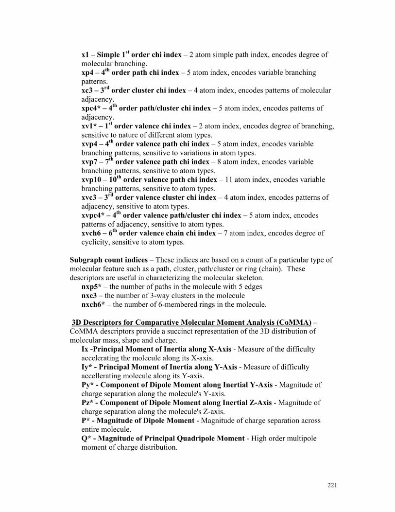
221

x1 – Simple 1st order chi index – 2 atom simple path index, encodes degree of molecular branching. xp4 – 4th order path chi index – 5 atom index, encodes variable branching patterns. xc3 – 3rd order cluster chi index – 4 atom index, encodes patterns of molecular adjacency. xpc4* – 4th order path/cluster chi index – 5 atom index, encodes patterns of adjacency. xv1* – 1st order valence chi index – 2 atom index, encodes degree of branching, sensitive to nature of different atom types. xvp4 – 4th order valence path chi index – 5 atom index, encodes variable branching patterns, sensitive to variations in atom types. xvp7 – 7th order valence path chi index – 8 atom index, encodes variable branching patterns, sensitive to atom types. xvp10 – 10th order valence path chi index – 11 atom index, encodes variable branching patterns, sensitive to atom types. xvc3 – 3rd order valence cluster chi index – 4 atom index, encodes patterns of adjacency, sensitive to atom types. xvpc4* – 4th order valence path/cluster chi index – 5 atom index, encodes patterns of adjacency, sensitive to atom types. xvch6 – 6th order valence chain chi index – 7 atom index, encodes degree of cyclicity, sensitive to atom types.

Subgraph count indices – These indices are based on a count of a particular type of molecular feature such as a path, cluster, path/cluster or ring (chain). These descriptors are useful in characterizing the molecular skeleton.

nxp5* – the number of paths in the molecule with 5 edges nxc3 – the number of 3-way clusters in the molecule nxch6* – the number of 6-membered rings in the molecule.

3D Descriptors for Comparative Molecular Moment Analysis (CoMMA) – CoMMA descriptors provide a succinct representation of the 3D distribution of molecular mass, shape and charge.

Ix -Principal Moment of Inertia along X-Axis - Measure of the difficulty accelerating the molecule along its X-axis. Iy* - Principal Moment of Inertia along Y-Axis - Measure of difficulty accellerating molecule along its Y-axis. Py* - Component of Dipole Moment along Inertial Y-Axis - Magnitude of charge separation along the molecule's Y-axis. Pz* - Component of Dipole Moment along Inertial Z-Axis - Magnitude of charge separation along the molecule's Z-axis. P* - Magnitude of Dipole Moment - Magnitude of charge separation across entire molecule. Q* - Magnitude of Principal Quadripole Moment - High order multipole moment of charge distribution.

222

Dx - Displacement between Center of Mass and Center of Dipole Moment along X-Axis - Difference between center of mass in the X-axis and point along X-axis where charge is zero. Dy - Displacement between Center of Mass and Center of Dipole Moment along Y-Axis - Difference between center of mass in the Y-axis and point along Y-axis where charge is zero. Dz - Displacement between Center of Mass and Center of Dipole Moment along Z-Axis - Difference between center of mass in the Z-axis and point along Z-axis where charge is zero. Qxx - The xx Component of Second Rank Tensor Translated so Origin Coincides With Center of Dipole. Qyy - The yy Component of Second Rank Tensor Translated so Origin Coincides With Center of Dipole.

Total Topological Descriptors - These are descriptors related to the geometrical structure of molecules (including the geometry of electron distribution about the molecule).

W - Weiner Index - The number of bonds between all pairs of atoms (based on shortest path around the molecule). Pf - Platt f Index - Total sum of degrees of edges in the molecular graph; the degree of an edge in the number of adjacent edges. sumdelI* - Sum of Delta Intrinsic States of atoms - Sum of degree of perturbation of the intrinsic state of all atoms in the molecule caused by the presence of the adjacent atoms. tets2 - Total Electrotopological Index - Sum of E-States values of all atoms in the molecule. E-State is the sum of the intrinsic state of an atom (group) plus the sum of the perturbations of the intrinsic state caused by all the other atoms in the molecule. totop - Total Topological Index – The total topological index, based on molecular connectivity formalism. Wt* - Total Weiner Number - Same as W, but pairs of atoms are counted with respect to all paths in the molecule, not just the shortest path. This makes Wt > W for cyclic molecules. nclass - # Symmetry Classes in Molecule - Number of classes of topologically similar molecular vertices.

Traditional Kappa Shape Indices – Kappa shape indices represent a method of molecular structure quantification in which attributes of molecular shape are encoded into three indices derived from counts of one, two and three bond fragments.

k0 – Kappa 0 – Encodes the number of vertex symmetry classes in the molecule; the value decreases with increasing molecular symmetry. k1* - Kappa 1 – Encodes the degree of cyclicity in the molecule; the value decreases as the degree of cyclicity increases. Long, straight chain molecules have the highest value. k2* - Kappa 2 – Encodes the degree of central branching in the molecule; the value decreases as the degree of central branching increases.

223

k3* - Kappa 3 – Encodes the degree of separated branching in the molecule. (far it is between branches along the molecular backbone); the index increases as the degree of branch separation increases (as the distance between branch points increases along the molecular backbone).

Other 2D Descriptors LogP* - The octanol/water partition coefficient. A measure of hydrophobicity, this represents the log of the ratio of the solubility of the molecule in octanol over the solubility in water. The index increases as molecules become more hydrophobic and decreases as they become more hydrophilic. LD50 - The mouse oral LD50 for the molecule, a measure of toxicity.

Atom Type E-State Descriptors – These descriptors describe the electronic environment (the accessibility of the electrons) of each atom in the molecule that arise due to a combination of the intrinsic properties of the of the atom and the influence of the neighboring atoms in the molecule. These descriptors parameterize such properties as hydrogen bonds, molecular polarity, etc. Atom type and group type E-state descriptors are computed for a number of atoms and functional groups. Large E-state values may indicate the molecule is more apt to participate in intermolecular interactions.

SsCH3* - Describes the sum of the E-state values for all -CH3 groups in the molecule. SssCH2 - Describes the sum of the E-state values for all –CH2- groups in the molecule. SaaCH* - Describes the sum of the E-state values for all aromatic carbon-hydride (=CH-) groups in the molecule (the aromatic ring CH). SdssC* - Describes the sum of the E-state values for all =C< carbon in molecule. SdO* - Describes the sum of E-state values for all =O oxygen in the molecule. SsCl – Describes the sum of E-state values for all –Cl chlorine in the molecule.

Hydrogen Atom Type E-State Descriptors – These descriptors describe the sum of the hydrogen E-states (electron accessibility at the hydrogen atoms) for all polar or non-polar hydride groups of a given type in the molecule. These descriptors relate to such molecular properties as hydrogen bonding. As with E-state descriptors, large values indicate an increased ability of the molecule to participate in intermolecular interactions.

SssOH – Sum of the hydrogen E-states for the –OH groups in the molecule. Shother – Sum of the hydrogen E-states for non-polar hydrogens (CH hydrogen) in the molecule Hmax – The largest atom hydrogen E-state in the molecule – the largest polarity on a hydrogen atom in the molecule (also correlates with partial charge). Gmax* - The largest atom E-state in the molecule (the most electronegative atom in the molecule). Hmin* - The smallest atom hydrogen E-state in the molecule. Gmin* - The smallest atom E-state in the molecule (also, the most electrophilic atom in the molecule).

224

Information Indices – These molecular descriptors are related to the information content of the molecule, and are derived from information theory.

si - Shannon Information Index – A measure of molecular complexity accounting for both diversity and concentration of features. IC - Information Content - Based on the total number of molecular vertices, hydride groups or non-polar hydrogen atoms. R - Molecular Redundancy – A measure of structural repetition within the molecule (is highest in highly internally symmetrical molecules like benzene and lowest in internally diverse molecules such as tetracycline). idc - Bonchev-Trinajsti Information Content – Index is based on 2-path counts. Value increases with increasing molecular complexity. idcbar* - Bonchev-Trinajsti Mean Information Content – Index is based on 2-path counts. Index increases with molecular complexity.

Molecular Properties – These descriptors include some fundamental properties of the entire molecule.

fw* – Formula weight – the molecular weight of the molecule in Daltons. nelem – Number of elements – The total number of different elements in the molecule. nrings – Number of rings – The number of rings in the molecule (also known as the cyclomatic number). ncirc – Number of circuits – The total number of all cycles in the molecule. Includes ring structures as well as path circuits. Example: biphenyl = 2, but naphthalene = 3 because in addition to the aromatic rings, a circuit can be made about the periphery of the naphthalene molecule. phia - Kappa Flexibility Index (# Bonds in normal graph for alkanes) – Inversely proportional to molecular complexity; increases with homolgation and decreases with increased branching or cyclicity. knotp - Difference Between Chi cluster-3 and chi path/cluster-4 – Decreases with increasing molecular complexity. numHBa* – The number of hydrogen bond acceptors in the molecule. SHHbd – The number of hydrogen bond donors in the molecule. Qs* – Specific Molecular and Group Polarity Descriptor – This descriptor is inversely proportional to molecular polarity and hydrophibicity. Qsv* – Average Molecular and Group Polarity Descriptor – This descriptor is inversely proportional to molecular polarity and hydrophibicity.

2. Polyamide (PA) reverse osmosis membrane properties used as inputs

in development of the “Universal” PA model. Contact Angle (degrees) – The air bubble contact angle of the membrane, measured as the outside angle between the membrane surface and a line tangential to an air bubble trapped against the membrane surface (in 17 MOhm deionized water at 24oC). The contact angle represents a measure of surface hydrophibicity; the smaller the angle, the greater the surface hydrophibicity.

225

COO-/Amide I Ratio - A unitless relative index of membrane cross-link frequency derived from attenuated total internal reflection Fourier transform infra-red (ATR-FTIR) spectroscopic measurements based on the ratio of the absorption at 1415 cm-1 corresponding to the presence of free carboxylate groups and the absorption 1665 cm-1 corresponding to the amide I bonds in the membrane. The larger the ration, the less cross-linked the membrane. COO-/Amide II Ratio - A unitless relative index of membrane cross-link frequency derived from ATR-FTIR spectroscopic measurements based on the ratio of the absorption at 1415 cm-1 corresponding to the presence of free carboxylate groups and the absorption at 1542 cm-1 corresponding to the amide II bonds in the membrane. The larger the ration, the less cross-linked the membrane. OH-/Amide I Ratio - A unitless relative index of membrane cross-link frequency derived from ATR-FTIR spectroscopic measurements based on the ratio of the absorption at 3400 cm-1 corresponding to the presence of hydroxyl groups and the absorption at 1665 cm-1 corresponding to the amide I bonds in the membrane. The larger the ratio, the less cross-linked the membrane. Polyamide Thickness – A unitless relative index derived from ATR-FTIR spectroscopic measurements based on the ratio of the strength of the 1665 cm-1 amide I absorption band of the polyamide layer and the 874 cm-1 absorption band of the polysulfone membrane support layer. The greater the ratio, the thicker the polyamide layer. Roughness (nm) – A direct measurement by atomic force microscopy (AFM) of the rugosity of the membrane surface defined as the standard deviation of the height of features on the membrane, expressed in nanometers. The roughness of the membrane may reflect subtle differences in internal physicochemical properties. Interactions of nanoparticles with membrane surfaces are often positively related to surface roughness. Specific Water Flux (GFD/PSI) – Measurement of the membrane water flux per unit water pressure. Many membrane properties are represented by the specific water flux, including membrane density and intrinsic porosity, hydraulic conductivity, hydrogen bonding, charge interactions and many others. Zeta Potential (mV, pH 7) – The Zeta potential of the membrane, in millivolts. Zeta , was determined at pH 7.0 at 20oC in 1000 mg/L NaCl using measurement of streaming potential obtained with a streaming potential analyzer (ZetaCAD, CAD Instrumentation, Les Essarts Le Roi, France) and applying the Helmholtz-Smoluchowski equation:

226

RA

L

P

Us 1

0

where is the zeta potential; Us is the streaming potential; P is the applied pressure, Us/P is the slope of the streaming potential versus applied pressure curve; is the dynamic viscosity of the solution; is the permittivity of the test solution; 0 is the permittivity of free space; L is the channel length of the membrane test cell; A is the test cell channel cross-sectional area; and R is the test cell channel resistance. Zeta Potential Slope (pH 5-7) - This is rate of change of the Zeta potential as the pH is shifted from 5 to 7. This index is inversely proportional to the ease with which membrane protons may be introduced or removed as a function of pH; the more negative the index, the more easily the membrane may be protonated or deprotonated.

227

Appendix 2

Structures and QSAR Molecular Descriptors of the Surrogate Molecules Used for Modeling Compound Interactions

with Reverse Osmosis Membranes

228

ABSQ MaxNeg MaxQp Ovality Surface xpc4 xv1 xvpc4 nxp5 nxch62.0688 -0.4507 0.2383 1.2151 86.1161 0.0000 0.7815 0.0000 0.0000 0.0000

Iy Py Pz P Q sumdelI Wt k1 k2 k348.1178 0.9057 0.0000 0.9057 2.0820 3.1667 9.0000 4.0000 1.3333 0.0000

LogP SsCH3 SaaCH SdssC SdO Gmax Hmin Gmin idcbar fw-1.8420 0.0000 0.0000 -0.8333 9.0000 9.0000 1.5514 -0.8333 1.0000 60.0556

numHBa Qs Qsv3.0000 0.4224 0.4400

Urea

229

ABSQ MaxNeg MaxQp Ovality Surface xpc4 xv1 xvpc4 nxp5 nxch60.8702 -0.3118 0.1834 1.2193 82.6823 0.0000 1.0233 0.0000 0.0000 0.0000

Iy Py Pz P Q sumdelI Wt k1 k2 k353.6047 0.1875 0.0000 0.1951 0.6462 1.6944 4.0000 3.0000 2.0000 0.0000

LogP SsCH3 SaaCH SdssC SdO Gmax Hmin Gmin idcbar fw-0.0314 1.6806 0.0000 0.0000 0.0000 7.5694 0.3833 0.2500 0.9183 46.0690

numHBa Qs Qsv1.0000 0.5485 0.7618

t Butyl Alcohol

230

ABSQ MaxNeg MaxQp Ovality Surface xpc4 xv1 xvpc4 nxp5 nxch61.1210 -0.3578 0.2604 1.3094 112.1383 0.4082 1.2770 0.0816 0.0000 0.0000

Iy Py Pz P Q sumdelI Wt k1 k2 k3114.3784 0.0749 0.0000 0.6665 0.7723 2.6528 18.0000 5.0000 2.2500 4.0000

LogP SsCH3 SaaCH SdssC SdO Gmax Hmin Gmin idcbar fw-0.2035 3.1528 0.0000 0.0000 9.1806 9.1806 0.5934 1.1944 1.5219 74.0824

numHBa Qs Qsv3.0000 0.8626 0.6614

N-dimethylamine

231

ABSQ MaxNeg MaxQp Ovality Surface xpc4 xv1 xvpc4 nxp5 nxch60.9623 -0.2788 0.0604 1.2497 102.4022 0.4082 1.2770 0.0816 0.0000 0.0000

Iy Py Pz P Q sumdelI Wt k1 k2 k3123.8753 0.2195 0.0001 1.0488 1.2847 2.6528 18.0000 5.0000 2.2500 4.0000

LogP SsCH3 SaaCH SdssC SdO Gmax Hmin Gmin idcbar fw-0.2035 3.1528 0.0000 0.0000 9.1806 9.1806 0.5934 1.1944 1.5219 74.0824

numHBa Qs Qsv3.0000 0.8626 0.6614

N-Nitroso Dimethylamine (NDMA)

232

ABSQ MaxNeg MaxQp Ovality Surface xpc4 xv1 xvpc4 nxp5 nxch61.6402 -0.3897 0.3436 1.2919 105.8707 0.4082 1.1895 0.0373 0.0000 0.0000

Iy Py Pz P Q sumdelI Wt k1 k2 k3130.0206 0.0537 0.0000 0.4736 0.3324 4.8773 18.0000 5.0000 2.2500 4.0000

LogP SsCH3 SaaCH SdssC SdO Gmax Hmin Gmin idcbar fw-2.6129 0.0000 0.0000 -0.9676 9.2431 9.2431 0.7819 -0.9676 1.5219 75.0672

numHBa Qs Qsv3.0000 0.5430 0.4163

Glycine

233

ABSQ MaxNeg MaxQp Ovality Surface xpc4 xv1 xvpc4 nxp5 nxch61.4882 -0.2795 0.3350 1.2436 109.0973 2.5981 2.3786 0.9802 0.0000 0.0000

Iy Py Pz P Q sumdelI Wt k1 k2 k3369.6898 0.3927 0.0000 0.5364 0.5998 7.6551 42.0000 7.0000 1.8519 2.6667

LogP SsCH3 SaaCH SdssC SdO Gmax Hmin Gmin idcbar fw1.0930 0.0000 0.0000 -1.4606 9.6250 9.6250 2.6583 -2.1667 1.5567 163.3877

numHBa Qs Qsv5.0000 0.7726 0.4435

Trichloroacetic Acid

234

ABSQ MaxNeg MaxQp Ovality Surface xpc4 xv1 xvpc4 nxp5 nxch61.4396 -0.3014 0.3345 1.2345 107.6139 1.3333 2.0257 0.4370 0.0000 0.0000

Iy Py Pz P Q sumdelI Wt k1 k2 k3226.5332 0.3679 0.1487 0.5628 0.3662 6.2886 29.0000 6.0000 2.2222 3.0000

LogP SsCH3 SaaCH SdssC SdO Gmax Hmin Gmin idcbar fw0.3708 0.0000 0.0000 -1.2099 9.4352 9.4352 1.0402 -1.2870 1.5656 128.9427

numHBa Qs Qsv4.0000 0.6545 0.4242

Dichloroacetic Acid

235

Alanine

ABSQ MaxNeg MaxQp Ovality Surface xpc4 xv1 xvpc4 nxp5 nxch61.8023 -0.3998 0.3431 1.3117 122.2123 1.3333 1.6271 0.2257 0.0000 0.0000

Iy Py Pz P Q sumdelI Wt k1 k2 k3171.8076 0.3392 0.1935 0.5073 0.3040 5.9861 29.0000 6.0000 2.2222 3.0000

LogP SsCH3 SaaCH SdssC SdO Gmax Hmin Gmin idcbar fw-2.3284 1.4190 0.0000 -0.9630 9.5741 9.5741 0.5434 -0.9630 1.5656 89.0941

numHBa Qs Qsv3.0000 0.7934 0.5142

236

ABSQ MaxNeg MaxQp Ovality Surface xpc4 xv1 xvpc4 nxp5 nxch61.1008 -0.2752 0.1376 1.3233 143.6209 1.3333 2.5178 1.4579 0.0000 0.0000

Iy Py Pz P Q sumdelI Wt k1 k2 k3353.5459 0.0000 0.0000 0.0000 1.1329 3.5309 29.0000 6.0000 2.2222 3.0000

LogP SsCH3 SaaCH SdssC SdO Gmax Hmin Gmin idcbar fw3.3964 0.0000 0.0000 -0.1975 0.0000 4.9938 0.0000 -0.0988 1.5656 165.8340

numHBa Qs Qsv4.0000 0.9817 0.6363

1,1,2,2 Tetrachloroethylene

237

ABSQ MaxNeg MaxQp Ovality Surface xpc4 xv1 xvpc4 nxp5 nxch61.8902 -0.3693 0.3405 1.3337 131.8441 1.2761 2.4067 0.3266 0.0000 0.0000

Iy Py Pz P Q sumdelI Wt k1 k2 k3356.3286 0.4084 0.1650 0.4639 0.7559 7.0091 46.0000 7.0000 3.0612 2.6667

LogP SsCH3 SaaCH SdssC SdO Gmax Hmin Gmin idcbar fw-2.1330 0.0000 0.0000 -1.0046 9.7564 9.7564 0.7045 -1.0046 1.8842 121.1601

numHBa Qs Qsv3.0000 0.9754 0.5143

Cysteine

238

ABSQ MaxNeg MaxQp Ovality Surface xpc4 xv1 xvpc4 nxp5 nxch62.1810 -0.3839 0.3404 1.3733 147.1524 1.8214 2.5378 0.6947 0.0000 0.0000

Iy Py Pz P Q sumdelI Wt k1 k2 k3334.4675 0.2137 0.1685 0.5063 0.0934 7.4700 65.0000 8.0000 3.1111 2.8125

LogP SsCH3 SaaCH SdssC SdO Gmax Hmin Gmin idcbar fw-1.6909 3.5531 0.0000 -0.9306 10.0157 10.0157 0.4723 -0.9306 1.9438 117.1478

numHBa Qs Qsv3.0000 1.3961 0.6544

Valine

239

ABSQ MaxNeg MaxQp Ovality Surface xpc4 xv1 xvpc4 nxp5 nxch62.4695 -0.3804 0.3381 1.3550 139.1301 1.8214 2.2186 0.4430 0.0000 0.0000

Iy Py Pz P Q sumdelI Wt k1 k2 k3330.7648 0.0731 0.2824 0.4321 0.5552 9.2889 65.0000 8.0000 3.1111 2.8125

LogP SsCH3 SaaCH SdssC SdO Gmax Hmin Gmin idcbar fw-2.7039 1.3321 0.0000 -1.1806 9.8557 9.8557 0.5834 -1.1806 1.9438 119.1204

numHBa Qs Qsv4.0000 1.0413 0.4881

Threonine

240

ABSQ MaxNeg MaxQp Ovality Surface xpc4 xv1 xvpc4 nxp5 nxch62.7808 -0.3300 0.2614 1.5190 198.2787 1.2071 3.3662 0.2518 5.0000 0.0000

Iy Py Pz P Q sumdelI Wt k1 k2 k31187.2531 0.0914 0.5505 0.5782 1.1690 8.5844 143.0000 10.0000 5.7600 5.5309

LogP SsCH3 SaaCH SdssC SdO Gmax Hmin Gmin idcbar fw-3.3935 0.0000 0.0000 -0.9333 10.1372 10.1372 0.5321 -0.9333 2.6608 146.1894

numHBa Qs Qsv4.0000 1.8519 0.6173

Lysine

241

ABSQ MaxNeg MaxQp Ovality Surface xpc4 xv1 xvpc4 nxp5 nxch63.3170 -0.4237 0.2621 1.4623 175.5508 1.4122 2.3043 0.2756 4.0000 0.0000

Iy Py Pz P Q sumdelI Wt k1 k2 k3551.9764 0.4996 0.0595 0.5835 1.5535 10.8249 96.0000 9.0000 3.9200 4.5000

LogP SsCH3 SaaCH SdssC SdO Gmax Hmin Gmin idcbar fw-3.2338 0.0000 0.0000 -1.9179 19.8950 9.9931 0.8948 -1.2141 2.2608 132.1191

numHBa Qs Qsv5.0000 1.0755 0.4315

Asparagine

242

ABSQ MaxNeg MaxQp Ovality Surface xpc4 xv1 xvpc4 nxp5 nxch63.1448 -0.3271 0.2626 1.4108 158.6067 1.4122 2.2393 0.2647 4.0000 0.0000

Iy Py Pz P Q sumdelI Wt k1 k2 k3585.1631 0.1482 0.2765 0.3165 2.3017 11.4988 96.0000 9.0000 3.9200 4.5000

LogP SsCH3 SaaCH SdssC SdO Gmax Hmin Gmin idcbar fw-2.5518 0.0000 0.0000 -2.4979 19.6173 9.8464 0.9503 -1.2941 2.2608 133.1039

numHBa Qs Qsv5.0000 0.9598 0.3851

Aspartic Acid

243

ABSQ MaxNeg MaxQp Ovality Surface xpc4 xv1 xvpc4 nxp5 nxch62.2816 -0.3254 0.2614 1.4852 185.9375 1.2071 3.7686 0.2518 4.0000 0.0000

Iy Py Pz P Q sumdelI Wt k1 k2 k31008.2385 0.2751 0.5057 0.6133 1.7373 7.4537 102.0000 9.0000 4.8395 4.5000

LogP SsCH3 SaaCH SdssC SdO Gmax Hmin Gmin idcbar fw-1.5630 1.9252 0.0000 -0.9129 10.0709 10.0709 0.4899 -0.9129 2.4438 149.2138

numHBa Qs Qsv4.0000 1.7062 0.6495

Methionine

244

ABSQ MaxNeg MaxQp Ovality Surface xpc4 xv1 xvpc4 nxp5 nxch62.9463 -0.3254 0.2619 1.4658 192.9965 1.5830 3.1553 0.3909 12.0000 0.0000

Iy Py Pz P Q sumdelI Wt k1 k2 k3921.0010 0.2561 0.0406 0.3223 4.2728 9.3994 352.0000 9.0909 4.1327 2.8444

LogP SsCH3 SaaCH SdssC SdO Gmax Hmin Gmin idcbar fw-2.4299 0.0000 3.0483 -1.0004 10.2662 10.2662 0.8712 -1.0004 2.4982 155.1564

numHBa Qs Qsv4.0000 1.9843 0.5330

Histidine

245

ABSQ MaxNeg MaxQp Ovality Surface xpc4 xv1 xvpc4 nxp5 nxch61.2254 -0.1025 0.1021 1.2646 133.7207 0.0000 2.0000 0.0000 6.0000 1.0000

Iy Py Pz P Q sumdelI Wt k1 k2 k388.4166 0.0000 0.0000 0.0000 1.3002 0.0000 90.0000 4.1667 2.2222 1.3333

LogP SsCH3 SaaCH SdssC SdO Gmax Hmin Gmin idcbar fw1.9516 0.0000 12.0000 0.0000 0.0000 2.0000 1.0531 2.0000 1.5219 78.1136

numHBa Qs Qsv0.0000 2.2500 0.9375

Benzene

246

ABSQ MaxNeg MaxQp Ovality Surface xpc4 xv1 xvpc4 nxp5 nxch61.3028 -0.1090 0.1052 1.3300 154.5761 0.4082 2.4107 0.1925 8.0000 1.0000

Iy Py Pz P Q sumdelI Wt k1 k2 k3197.2618 0.0017 0.0000 0.0529 1.4244 0.3449 131.0000 5.1429 2.3438 1.5000

LogP SsCH3 SaaCH SdssC SdO Gmax Hmin Gmin idcbar fw2.6571 2.0833 10.2616 0.0000 0.0000 2.0833 0.4868 1.3218 1.7608 92.1405

numHBa Qs Qsv0.0000 2.8421 1.1117

Toluene

247

ABSQ MaxNeg MaxQp Ovality Surface xpc4 xv1 xvpc4 nxp5 nxch61.6683 -0.2276 0.1962 1.3246 149.2555 0.4082 2.1343 0.0861 8.0000 1.0000

Iy Py Pz P Q sumdelI Wt k1 k2 k3191.5561 0.0921 0.0000 0.1106 2.5196 2.8938 131.0000 5.1429 2.3438 1.5000

LogP SsCH3 SaaCH SdssC SdO Gmax Hmin Gmin idcbar fw1.2356 0.0000 8.7127 0.0000 0.0000 8.6322 1.1011 0.3218 1.7608 94.1130

numHBa Qs Qsv1.0000 1.7008 0.6653

Phenol

248

ABSQ MaxNeg MaxQp Ovality Surface xpc4 xv1 xvpc4 nxp5 nxch61.5028 -0.1117 0.1095 1.4038 176.7742 0.4928 2.9713 0.2539 10.0000 1.0000

Iy Py Pz P Q sumdelI Wt k1 k2 k3339.1219 0.0082 0.0000 0.0719 1.7560 0.6589 184.0000 6.1250 3.1111 1.8000

LogP SsCH3 SaaCH SdssC SdO Gmax Hmin Gmin idcbar fw3.1435 2.1620 10.4552 0.0000 0.0000 2.1620 0.4047 1.1397 2.0597 106.1674

numHBa Qs Qsv0.0000 3.4315 1.1617

Ethylbenzene

249

ABSQ MaxNeg MaxQp Ovality Surface xpc4 xv1 xvpc4 nxp5 nxch61.6713 -0.2176 0.2041 1.3835 183.1283 1.4783 3.0955 0.6008 14.0000 1.0000

Iy Py Pz P Q sumdelI Wt k1 k2 k3675.1678 0.0302 0.0000 0.0327 2.6672 6.3046 243.0000 7.1111 2.7222 1.7041

LogP SsCH3 SaaCH SdssC SdO Gmax Hmin Gmin idcbar fw2.8589 0.0000 4.5058 0.0000 0.0000 8.8531 1.2591 0.0565 2.0375 163.0032

numHBa Qs Qsv3.0000 1.8462 0.6268

4,6 Dichlorophenol

250

ABSQ MaxNeg MaxQp Ovality Surface xpc4 xv1 xvpc4 nxp5 nxch61.9400 -0.2120 0.2078 1.4810 230.9885 3.6427 4.5583 2.3038 24.0000 1.0000

Iy Py Pz P Q sumdelI Wt k1 k2 k31081.9465 0.0544 0.0000 0.0830 4.4959 10.9893 486.0000 10.0833 3.3951 1.5625

LogP SsCH3 SaaCH SdssC SdO Gmax Hmin Gmin idcbar fw4.9449 0.0000 0.0000 0.0000 0.0000 9.2010 2.6885 -0.3632 2.1339 266.3383

numHBa Qs Qsv6.0000 2.1552 0.5987

2,3,4,5,6 Pentachlorophenol

251

ABSQ MaxNeg MaxQp Ovality Surface xpc4 xv1 xvpc4 nxp5 nxch62.7005 -0.4222 0.5951 1.4377 183.7826 1.0404 2.5169 0.1970 12.0000 1.0000

Iy Py Pz P Q sumdelI Wt k1 k2 k3437.7393 0.0286 0.0000 0.5942 1.1659 5.8751 239.0000 7.1111 3.2397 2.0000

LogP SsCH3 SaaCH SdssC SdO Gmax Hmin Gmin idcbar fw1.4691 0.0000 8.1666 0.0000 10.1176 10.1176 1.1547 -0.1667 2.1499 124.1191

numHBa Qs Qsv3.0000 1.6137 0.5146

Nitrobenzene

252

2,4 Dinitrotoluene

ABSQ MaxNeg MaxQp Ovality Surface xpc4 xv1 xvpc4 nxp5 nxch65.0709 -0.5651 0.7838 1.5199 231.2349 2.4994 3.4504 0.6557 26.0000 1.0000

Iy Py Pz P Q sumdelI Wt k1 k2 k31000.4230 0.0792 0.0493 0.1519 0.7408 13.1531 611.0000 11.0769 4.4815 2.7211

LogP SsCH3 SaaCH SdssC SdO Gmax Hmin Gmin idcbar fw1.5672 1.5900 3.8448 0.0000 20.9126 10.5111 0.7100 -0.3825 2.4961 184.1515

numHBa Qs Qsv6.0000 1.9346 0.4674

253

ABSQ MaxNeg MaxQp Ovality Surface xpc4 xv1 xvpc4 nxp5 nxch63.4563 -0.3994 0.3780 1.4646 231.4523 2.3237 5.3203 1.0329 26.0000 1.0000

Iy Py Pz P Q sumdelI Wt k1 k2 k31910.8380 0.4130 0.1644 0.5162 1.4364 8.9442 905.0000 13.0667 5.9150 4.1653

LogP SsCH3 SaaCH SdssC SdO Gmax Hmin Gmin idcbar fw3.7567 6.0569 7.8716 -0.7717 10.7624 10.7624 0.4304 -0.7717 2.9862 206.2847

numHBa Qs Qsv2.0000 4.1570 0.8468

Ibuprofen

254

ABSQ MaxNeg MaxQp Ovality Surface xpc4 xv1 xvpc4 nxp5 nxch67.8037 -0.6714 1.8239 1.6067 273.6969 3.1755 6.7345 1.9643 28.0000 1.0000

Iy Py Pz P Q sumdelI Wt k1 k2 k32651.7883 0.1304 0.5221 0.6457 9.9741 13.9112 1029.0000 14.0625 6.0744 4.0768

LogP SsCH3 SaaCH SdssC SdO Gmax Hmin Gmin idcbar fw2.2530 2.7892 5.7279 0.0000 10.5226 10.5226 0.8433 -2.7628 3.0079 264.2188

numHBa Qs Qsv7.0000 3.2115 0.6142

Methyl Parathion

255

4 - Nonylphenol

ABSQ MaxNeg MaxQp Ovality Surface xpc4 xv1 xvpc4 nxp5 nxch63.3373 -0.2271 0.1956 1.7495 337.1841 0.8413 6.6056 0.3055 23.0000 1.0000

Iy Py Pz P Q sumdelI Wt k1 k2 k35120.7363 0.0529 0.0000 0.1665 3.2246 4.5156 1178.0000 14.0625 9.0741 7.0582

LogP SsCH3 SaaCH SdssC SdO Gmax Hmin Gmin idcbar fw6.0608 2.2548 7.5893 0.0000 0.0000 9.1487 0.3349 0.3642 3.4482 220.3549

numHBa Qs Qsv1.0000 6.4319 1.0887

256

ABSQ MaxNeg MaxQp Ovality Surface xpc4 xv1 xvpc4 nxp5 nxch66.4551 -0.6716 1.8678 1.6867 298.2288 3.3582 8.7074 2.2281 38.0000 1.0000

Iy Py Pz P Q sumdelI Wt k1 k2 k32999.8074 0.7388 0.0000 0.7394 1.5261 14.9426 1335.0000 16.0556 6.9632 4.5660

LogP SsCH3 SaaCH SdssC SdO Gmax Hmin Gmin idcbar fw4.7570 3.5701 1.4220 0.0000 0.0000 5.9377 0.6322 -2.9185 2.9677 350.5900

numHBa Qs Qsv8.0000 4.4586 0.7655

Clorpyrifos

257

Bisphenol A

ABSQ MaxNeg MaxQp Ovality Surface xpc4 xv1 xvpc4 nxp5 nxch63.7346 -0.2257 0.1963 1.5936 296.2599 3.7281 5.5899 1.9360 44.0000 2.0000

Iy Py Pz P Q sumdelI Wt k1 k2 k32245.0769 0.1135 0.0000 0.1298 1.6861 9.0630 1950.0000 13.4321 5.3254 3.0625

LogP SsCH3 SaaCH SdssC SdO Gmax Hmin Gmin idcbar fw3.6500 4.2337 14.4432 0.0000 0.0000 9.2963 0.6307 -0.1514 2.9637 228.2908

numHBa Qs Qsv2.0000 4.8217 0.8029

258

ABSQ MaxNeg MaxQp Ovality Surface xpc4 xv1 xvpc4 nxp5 nxch64.1083 -0.2197 0.1958 1.7229 378.1116 2.7227 6.9613 1.1601 53.0000 2.0000

Iy Py Pz P Q sumdelI Wt k1 k2 k33323.4529 0.1687 0.0000 0.1801 3.0729 9.3131 2638.0000 16.3719 7.8520 4.2500

LogP SsCH3 SaaCH SdssC SdO Gmax Hmin Gmin idcbar fw3.9051 4.2743 14.6640 2.5522 0.0000 9.4107 0.5420 0.2842 3.1174 268.3556

numHBa Qs Qsv2.0000 6.1235 0.8420

Diethylstilbestrol

259

ABSQ MaxNeg MaxQp Ovality Surface xpc4 xv1 xvpc4 nxp5 nxch62.1113 -0.1014 0.1108 1.4586 251.9400 1.8265 4.8154 0.7775 55.0000 3.0000

Iy Py Pz P Q sumdelI Wt k1 k2 k3903.6428 0.0095 0.0000 0.0095 3.6724 1.3670 3511.0000 9.2422 3.8678 1.6483

LogP SsCH3 SaaCH SdssC SdO Gmax Hmin Gmin idcbar fw4.6080 0.0000 21.3670 0.0000 0.0000 2.1782 1.1676 1.3113 2.4920 178.2334

numHBa Qs Qsv0.0000 5.6044 0.9055

Phenanthrene

260

ABSQ MaxNeg MaxQp Ovality Surface xpc4 xv1 xvpc4 nxp5 nxch62.6157 -0.2819 0.4169 1.3867 186.6669 1.8843 3.1438 0.4881 31.0000 1.0000

Iy Py Pz P Q sumdelI Wt k1 k2 k3440.7403 0.0001 0.0000 1.0915 0.0243 9.8379 874.0000 7.6389 2.8028 1.2098

LogP SsCH3 SaaCH SdssC SdO Gmax Hmin Gmin idcbar fw1.3456 0.0000 6.5303 -1.1007 21.6657 10.8329 1.2455 -0.5504 2.1152 148.1180

numHBa Qs Qsv3.0000 1.9685 0.4745

Phthalic Anhydride

261

ABSQ MaxNeg MaxQp Ovality Surface xpc4 xv1 xvpc4 nxp5 nxch63.8160 -0.4001 0.4072 1.6739 304.4620 1.9455 5.1354 0.5054 32.0000 1.0000

Iy Py Pz P Q sumdelI Wt k1 k2 k31063.6456 0.3112 0.0000 0.6795 4.6372 13.8608 1084.0000 14.0625 7.3500 4.0768

LogP SsCH3 SaaCH SdssC SdO Gmax Hmin Gmin idcbar fw2.6343 3.4263 6.4429 -1.0164 23.0884 11.5442 0.5929 -0.5082 2.8537 222.2408

numHBa Qs Qsv4.0000 3.5625 0.6494

Diethylphthalate

262

ABSQ MaxNeg MaxQp Ovality Surface xpc4 xv1 xvpc4 nxp5 nxch61.3832 -0.1215 0.1260 1.3847 188.1796 3.6427 5.9279 4.4811 24.0000 1.0000

Iy Py Pz P Q sumdelI Wt k1 k2 k31161.5708 0.1611 0.0920 0.1855 0.1916 10.6204 486.0000 10.0833 3.3951 1.5625

LogP SsCH3 SaaCH SdssC SdO Gmax Hmin Gmin idcbar fw3.5566 0.0000 0.0000 0.0000 0.0000 5.8812 0.9092 -0.4367 2.1339 290.8316

numHBa Qs Qsv6.0000 2.6989 0.7497

Lindane

263

Caffeine

ABSQ MaxNeg MaxQp Ovality Surface xpc4 xv1 xvpc4 nxp5 nxch63.7109 -0.4136 0.3720 1.5417 247.7542 3.7053 4.1079 1.1570 47.0000 1.0000

Iy Py Pz P Q sumdelI Wt k1 k2 k3737.9059 0.1687 0.0906 0.7400 0.4252 11.5069 1538.0000 10.5156 3.5388 1.4545

LogP SsCH3 SaaCH SdssC SdO Gmax Hmin Gmin idcbar fw-0.5099 4.7732 1.5194 -0.6766 23.1613 11.6720 0.7578 -0.3600 2.2940 194.1930

numHBa Qs Qsv5.0000 3.0853 0.6559

264

ABSQ MaxNeg MaxQp Ovality Surface xpc4 xv1 xvpc4 nxp5 nxch63.2615 -0.2860 0.2630 1.5516 291.5823 2.4350 6.6852 1.0770 45.0000 1.0000

Iy Py Pz P Q sumdelI Wt k1 k2 k31733.9794 0.0377 0.4024 0.4135 1.2547 10.5848 1348.0000 16.0556 8.2268 3.9958

LogP SsCH3 SaaCH SdssC SdO Gmax Hmin Gmin idcbar fw2.9333 5.7337 6.1058 -0.1304 11.9527 11.9527 0.5353 -0.1304 2.6952 269.7713

numHBa Qs Qsv4.0000 5.4512 0.8973

2-chloro-2'-6'-diethyl-N-methoxymethyl-acetanilide (Alachlor)

265

ABSQ MaxNeg MaxQp Ovality Surface xpc4 xv1 xvpc4 nxp5 nxch63.0799 -0.2586 0.3129 1.7141 314.0870 1.5130 6.1484 0.5879 19.0000 0.0000

Iy Py Pz P Q sumdelI Wt k1 k2 k34073.7322 0.4029 0.1934 0.7591 10.2766 7.4392 1226 15.0588 9 5.9282

LogP SsCH3 SaaCH SdssC SdO Gmax Hmin Gmin idcbar fw0.646 3.7393 1.7105 0.5038 0 8.3916 0.6245 0.5038 3.3449 252.3432

numHBa Qs Qsv6 4.9502 0.8136

Cimetidine

266

ABSQ MaxNeg MaxQp Ovality Surface xpc4 xv1 xvpc4 nxp5 nxch66.6799 -0.3979 0.3655 1.6594 317.7363 1.7029 5.2398 0.5227 24.0000 0.0000

Iy Py Pz P Q sumdelI Wt k1 k2 k33381.7441 0.0017 0.7572 0.7572 9.8344 26.5053 910.0000 20.0000 10.6875 12.4898

LogP SsCH3 SaaCH SdssC SdO Gmax Hmin Gmin idcbar fw-2.9415 0.0000 0.0000 -5.1151 42.0844 10.5211 1.1567 -1.2788 3.1503 290.2298

numHBa Qs Qsv10.0000 2.4998 0.4062

Ethylenediaminetetraacetic Acid

267

17 a EstradiolABSQ MaxNeg MaxQp Ovality Surface xpc4 xv1 xvpc4 nxp5 nxch6

3.8151 -0.3052 0.1949 1.4357 226.2367 3.5726 7.7366 2.4643 90.0000 3.0000

Iy Py Pz P Q sumdelI Wt k1 k2 k32622.6062 0.1989 0.1080 0.3222 3.0584 10.0301 13763.0000 12.7190 4.7769 2.0000

LogP SsCH3 SaaCH SdssC SdO Gmax Hmin Gmin idcbar fw3.4696 0.0000 5.9495 0.0000 0.0000 10.1132 0.5784 -0.0350 2.9420 258.3605

numHBa Qs Qsv2.0000 6.8009 0.8635

268

ABSQ MaxNeg MaxQp Ovality Surface xpc4 xv1 xvpc4 nxp5 nxch64.1119 -0.3024 0.2905 1.5212 292.9848 5.0919 7.9452 3.4729 97.0000 3.0000

Iy Py Pz P Q sumdelI Wt k1 k2 k32765.3069 0.4227 0.0913 0.4833 1.2049 12.0300 15139.0000 13.6484 4.7500 1.9608

LogP SsCH3 SaaCH SdssC SdO Gmax Hmin Gmin idcbar fw3.6617 2.2178 5.8977 0.5115 12.2620 12.2620 0.5691 -0.0322 2.9579 270.3715

numHBa Qs Qsv2.0000 6.8488 0.8668

Estrone

269

ABSQ MaxNeg MaxQp Ovality Surface xpc4 xv1 xvpc4 nxp5 nxch64.1977 -0.3194 0.3163 1.4550 185.2442 3.5726 8.1516 2.7452 90.0000 3.0000

Iy Py Pz P Q sumdelI Wt k1 k2 k32680.8655 0.0469 0.0522 0.6833 1.2642 10.4973 13763.0000 12.7190 4.7769 2.0000

LogP SsCH3 SaaCH SdssC SdO Gmax Hmin Gmin idcbar fw2.6015 0.0000 0.0000 1.8233 11.5941 11.5941 0.5594 -0.0178 2.9420 260.3763

numHBa Qs Qsv2.0000 6.9197 0.8785

Testosterone

270

ABSQ MaxNeg MaxQp Ovality Surface xpc4 xv1 xvpc4 nxp5 nxch64.7039 -0.3173 0.3155 1.5482 294.9027 4.0170 8.8862 3.0945 98.0000 3.0000

Iy Py Pz P Q sumdelI Wt k1 k2 k33542.6272 0.1935 0.4017 0.5362 12.7234 11.9352 17841.0000 14.5833 5.5710 2.3965

LogP SsCH3 SaaCH SdssC SdO Gmax Hmin Gmin idcbar fw2.7916 1.7992 0.0000 2.2487 23.5431 11.8785 0.5785 0.3527 3.1115 286.4142

numHBa Qs Qsv2.0000 7.5130 0.8944

Progesterone

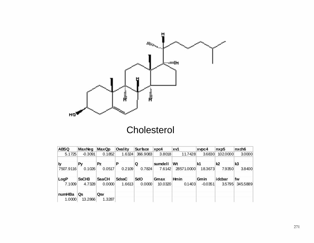
271

ABSQ MaxNeg MaxQp Ovality Surface xpc4 xv1 xvpc4 nxp5 nxch65.1725 -0.3091 0.1852 1.6324 366.9083 3.8018 11.7428 3.6830 102.0000 3.0000

Iy Py Pz P Q sumdelI Wt k1 k2 k37507.9116 0.1026 0.0517 0.2109 0.7824 7.6142 28571.0000 18.3673 7.9350 3.8400

LogP SsCH3 SaaCH SdssC SdO Gmax Hmin Gmin idcbar fw7.1009 4.7328 0.0000 1.6613 0.0000 10.0320 0.1403 -0.0351 3.5795 345.5889

numHBa Qs Qsv1.0000 13.2866 1.3287

Cholesterol

272

ABSQ MaxNeg MaxQp Ovality Surface xpc4 xv1 xvpc4 nxp5 nxch65.5836 -0.3127 0.1859 1.6526 370.1698 4.6023 12.7606 4.3974 104.0000 3.0000

Iy Py Pz P Q sumdelI Wt k1 k2 k37152.4863 0.0637 0.1380 0.2319 0.6953 6.8588 33956.0000 20.2800 8.7885 4.1600

LogP SsCH3 SaaCH SdssC SdO Gmax Hmin Gmin idcbar fw7.5768 7.2236 0.0000 0.0000 0.0000 10.1025 0.3646 0.0211 3.6533 374.6506

numHBa Qs Qsv1.0000 14.8095 1.4051

beta Sitostanol-n-hydrate

273

ABSQ MaxNeg MaxQp Ovality Surface xpc4 xv1 xvpc4 nxp5 nxch65.6687 -0.3800 0.4588 1.5852 311.2392 4.4359 8.1339 1.5796 101.0000 3.0000

Iy Py Pz P Q sumdelI Wt k1 k2 k33400.7456 1.2467 0.1828 1.4960 3.8252 23.6997 11660.0000 17.4156 6.9575 3.4856

LogP SsCH3 SaaCH SdssC SdO Gmax Hmin Gmin idcbar fw-0.5653 0.0000 2.8906 -2.2021 23.7581 14.6077 0.6899 -1.2751 3.1701 331.3466

numHBa Qs Qsv7.0000 5.3576 0.5736

Ciprofloxacin

274

ABSQ MaxNeg MaxQp Ovality Surface xpc4 xv1 xvpc4 nxp5 nxch68.5480 -0.4552 0.4188 1.6843 399.9212 9.0664 9.5882 3.5123 168.0000 4.0000

Iy Py Pz P Q sumdelI Wt k1 k2 k35550.8569 0.5439 0.1154 0.7765 7.7079 47.3737 42500 24.1349 8.3405 3.3333

LogP SsCH3 SaaCH SdssC SdO Gmax Hmin Gmin idcbar fw-0.3782 3.0591 4.1574 -6.4174 38.1444 13.1715 0.8141 -2.7275 3.1951 430.4143

numHBa Qs Qsv10 5.6223 0.5351

Tetracycline

275

ABSQ MaxNeg MaxQp Ovality Surface xpc4 xv1 xvpc4 nxp5 nxch63.7291 -0.2989 0.1963 1.4480 243.4733 5.5732 8.1021 3.3159 162.0000 4.0000

Iy Py Pz P Q sumdelI Wt k1 k2 k31856.4359 0.1326 0.0280 0.4259 1.9912 13.6669 40612.0000 14.3521 4.7619 1.6436

LogP SsCH3 SaaCH SdssC SdO Gmax Hmin Gmin idcbar fw1.5614 3.9071 4.2046 0.0000 0.0000 10.5542 0.6335 -0.5386 2.7299 299.3696

numHBa Qs Qsv4.0000 7.9154 0.8824

Codeine

276

ABSQ MaxNeg MaxQp Ovality Surface xpc4 xv1 xvpc4 nxp5 nxch68.3023 -0.3723 0.3991 1.7216 422.4388 9.4271 10.0157 3.9079 182.0000 4.0000

Iy Py Pz P Q sumdelI Wt k1 k2 k35809.5972 1.3701 0.6225 1.5197 4.7566 49.0391 45143 25.1037 8.5873 3.3704

LogP SsCH3 SaaCH SdssC SdO Gmax Hmin Gmin idcbar fw0.6689 4.6519 4.438 -6.6737 38.446 13.317 0.8165 -2.8948 3.1767 444.4412

numHBa Qs Qsv10 5.9729 0.5578

Doxycycline

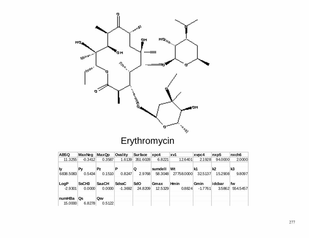
277

ABSQ MaxNeg MaxQp Ovality Surface xpc4 xv1 xvpc4 nxp5 nxch611.3255 -0.3412 0.3587 1.6139 351.6028 6.8221 12.6401 2.1928 94.0000 2.0000

Iy Py Pz P Q sumdelI Wt k1 k2 k36838.5083 0.5434 0.1510 0.8247 2.9768 58.3048 27758.0000 32.5137 15.2908 9.8097

LogP SsCH3 SaaCH SdssC SdO Gmax Hmin Gmin idcbar fw-2.9301 0.0000 0.0000 -1.3692 24.8209 12.5329 0.8824 -1.7761 3.5862 554.5457

numHBa Qs Qsv15.0000 6.8278 0.5122

Erythromycin

278

Appendix 3. All Compound QSAR Molecular Descriptors and Molecular Properties

279

280

281

282

283

284

285

286

287

288

289

290

291

292

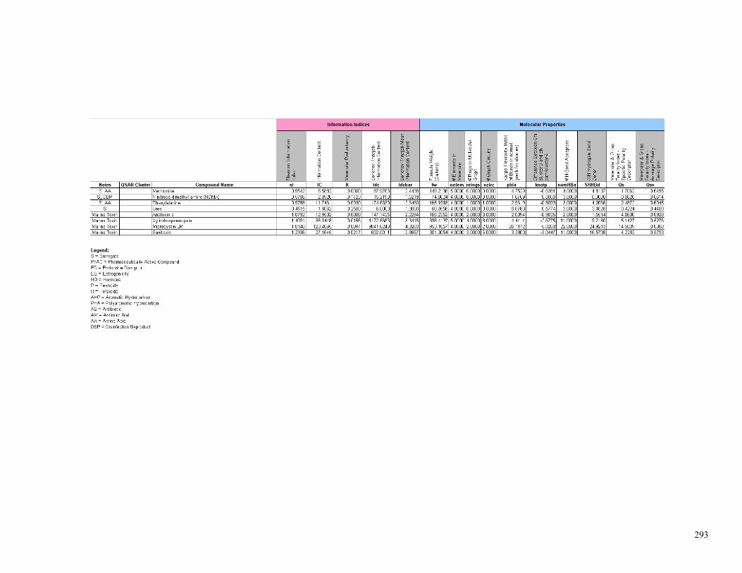
293

294

Appendix 4

General Instructions for Operating QSAR Descriptor ANN Models Describing Compound Interactions with RO Membranes Introduction: The models described in this study have been embedded as macros in Excel workbooks on a CD-ROM, and as such are being made available for experimentation. There are six workbooks altogether; one each for CA and four PA membranes used in the study, and one for the “Universal” PA model. In order to operate these models, the user must have Excel 2000 or later installed, and macros enabled. Each of the workbooks consists of two sheets. The first spreadsheet is for data I/O, and is where the user enters information regarding the specific molecule being tested, its salient QSAR molecular descriptors, and information regarding operating conditions that will be used to predict membrane performance based on the results of this study (due to the complexity of parameters involved with field performance, these specific predictions may vary from a specific field site; however, they may be used in a comparative sense to examine the behavior of a series of compounds relative to each other). The second sheet is a graphic representation of the interaction of the compound with the membrane, and plots relative solute flux (P-flux) against membrane association flux (M-Flux). This diagram provides the user with a visual representation of the predicted interaction of the compound with the membrane. Entering Data in the data spreadsheet: The used inputs information required by the model by filling in the gray boxes. Care should be taken to only modify the values in these boxes and not to change the

295

values or formulae in any of the other cells in the sheet, or the model will not work correctly. Limitations to the range of values for the QSAR molecular descriptors: The QSAR molecular descriptors used in the models must be constrained within the limits used to train the artificial neural networks. If values outside thee limits are used, predictability of the models may be severely compromised. These limits, for all the models, are shown below:

ABSQ MaxNeg MaxQp Ovality Surface xpc4 xv1 xvpc4 Minimum 0.870199 -0.67159 0.060379 1.215067 82.68226 0 0.781474 0 Maximum 11.3255 -0.10137 1.867779 1.749453 422.4388 9.427053 12.76057 4.481088 nxp5 nxch6 Iy Py Pz P Q sumdelI Minimum 0 0 48.11783 0 0 0 0.0243 0 Maximum 182 4 7507.912 1.370073 0.757215 1.519661 12.72342 58.3048 Wt k1 k2 k3 LogP SsCH3 SaaCH SdssC Minimum 4 3 1.333333 0 -3.39353 0 0 -6.6737 Maximum 45143 32.5137 15.2908 12.4898 7.5768 7.2236 21.367 2.5522 SdO Gmax Hmin Gmin idcbar fw numHBa Qs Minimum 0 2 0 -2.9185 0.9183 46.069 0 0.4224 Maximum 42.0844 14.6077 2.6885 2 3.6533 554.5457 15 14.8095 Qsv Minimum 0.385122 Maximum 1.4051

Model Output: As data are entered, the embedded macros will determine the predicted relative P, M and R Fluxes for the compound being evaluated, and will display them on the sheet (below).

296

Explanation of Output Data: The solute feed flux represents the estimated actual specific feed flux (actual F-Flux) of the solute (in micromoles of solute/m2 membrane*min per micromolar solute concentration in the feed the feed) to the membrane based on user-defined values of solute concentration and membrane water flux. The relative solute feed flux (F-Flux) is, by definition, always defined as 100 (% of the feed flux). The modeled relative solute fluxes represent the predicted values from the ANN models describing the relative P-Flux (the proportion of the mass interacting with the membrane that passes into the product), the relative M-Flux (the proportion of the solute interacting with the membrane that remains bound on or in the membrane) and the relative R-Flux (the proportion of the solute that fails to interact with the membrane and remains unassociated in the feed). For each of these fluxes, the spreadsheet calculates specific P, M and R solute fluxes (in micromoles/m2*min per micromolar solute in the feed) using the relative flux data and user-specified values for feed solute concentration and water flux. The spreadsheed also estimates the modeled concentration of solute in the product, in micromoles/liter. The modeled solute F-Flux represents a “virtual mass balance” obtained by summing the values of the relative P, M and R-Fluxes. Theoretically, the sum of these relative fluxes should total 100 (the value of the relative F-Flux). The model residual error represents the difference between the theoretical relative F-Flux and the value obtained from summation of the modeled flux outputs. This value reflects the deviation of the membrane models from an ideal response, and may be used as an evaluation criterion to determine whether or not the models have provided a reasonable prediction of the various solute-membrane interactions. Estimated Percent rejection of the solute by the membrane is estimated based on two criteria. The percent rejection based on the relative solute P-Flux represents rejection calculated based on the P-Flux. This is the “traditional” expression of RO membrane rejection, determined by the mass of solute passing through the membrane into the product. This value represents the sum of two compound-membrane interactions; the ability of the membrane to act as a mechanical shield against the compound and the removal of the compound by binding on or in the membrane. This, a high percent rejection determined by P-Flux may be due to strong rejection at the membrane surface or strong interaction of the compound with the membrane. However, the percent rejection based on the relative solute R-Flux only describes rejection at the membrane surface, in which the membrane acts as a mechanical shield. This result is significant, because compounds exhibiting a high rejection by this criterion are likely to be excluded from the RO product for extended periods of time, whereas, those compounds that are principally removed by interactions with the membrane may, in time as the membrane saturates, begin to break through significantly into the product. Evaluating Model Results: The Modeled Solute F-Flux should approach 100% if all models are working correctly. A practical model residual error is +/-25. (a 25% model noise band). Values outside this range should be treated with suspicion, as this indicates a significant failure

297

of the “virtual mass balance” technique. Furthermore, instances where solute rejection evaluated by the P-Flux significantly less than that evaluated by the R-Flux should be treated with suspicion, as in order for this to occur the M-Flux needs to be seriously below zero. Because these results are predicted, it is possible to have relative fluxes in excess of 100 or less than zero. Within error, this is acceptable; however, a value far outside these limits should be treated with suspicion.