Universität Potsdam Institut für Informatik

Lehrstuhl Maschinelles Lernen

Reinforcement Learning

Uwe Dick

Inte

lligent D

ata

Analy

sis

II

Overview

Problem Statements

Examples

Markov Decision Processes

Planning – Fully defined MDPs

Learning – Partly defined MDPs

Monte-Carlo

Temporal Difference

Inte

lligent D

ata

Analy

sis

II

Problem Statements in Machine Learning

Supervised Learning: Learn a decision function from examples of correct decisions.

Unsupervised Learning: Learn e.g. how to partition a data set (clustering) without knowledge of a correct partitioning.

Reinforcement Learning: Learn how to make a sequence of decisions. The quality of each decision may depend on the complete decision sequence. Temporal Credit Assignment Problem.

Inte

lligent D

ata

Analy

sis

II

Examples

Backgammon: How much does one move influence

the outcome of a game?

Robot Football: We want to score a goal. But which

sequence of moves gives highest chance to do so?

Helicopter Flight: What do we have to do to fly a

maneuver without crashing in unknown

environments?

Inte

lligent D

ata

Analy

sis

II

Learning from Interactions

Environment

Agent

Controller

Action •Reward

•Observation

Inte

lligent D

ata

Analy

sis

II

When Reinforcement Learning?

Delayed reward for actions.

(Temporal credit assignment problem)

Control problems.

Agents – The full AI problem.

Inte

lligent D

ata

Analy

sis

II

What is Reinforcement Learning?

RL methods are „Sampling based methods to solve

optimal control problems “ (Richard Sutton)

Search for an optimal policy (function from states to

actions).

Optimality: Policy with highest expected reward.

Other definitions for optimal learning: Fast learning

without making too many mistakes.

Inte

lligent D

ata

Analy

sis

II

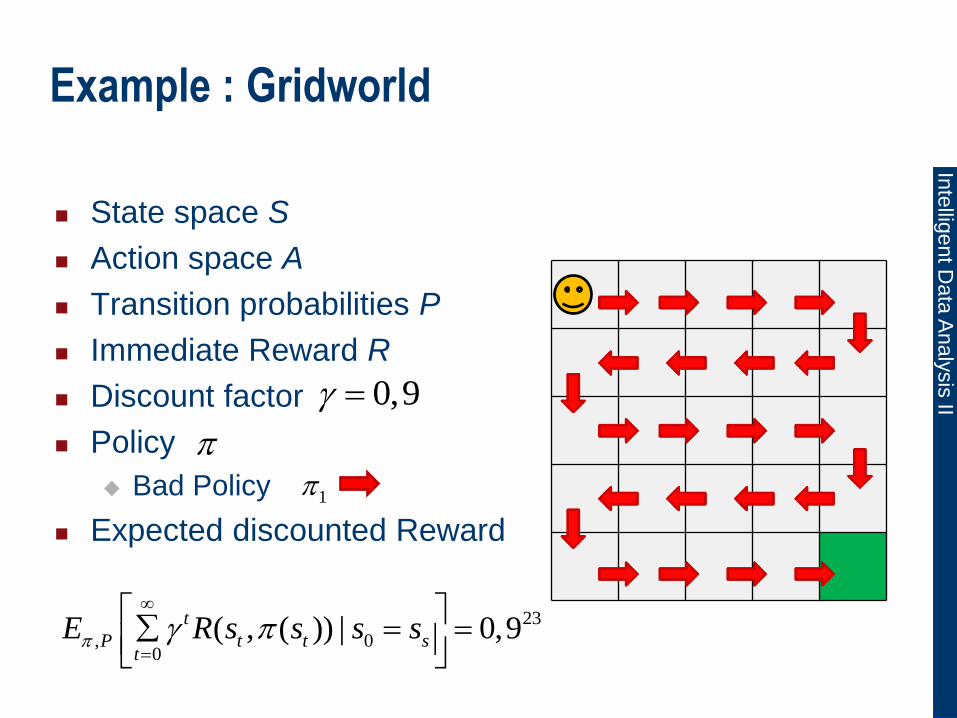
Example: Gridworld

Inte

lligent D

ata

Analy

sis

II

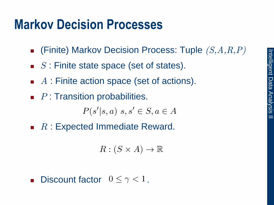
Markov Decision Processes

(Finite) Markov Decision Process: Tuple (S,A,R,P)

S : Finite state space (set of states).

A : Finite action space (set of actions).

P : Transition probabilities.

R : Expected Immediate Reward.

Discount factor .

Inte

lligent D

ata

Analy

sis

II

State space S

Start state

Target state

Example: Gridworld

ss S

zs S

Inte

lligent D

ata

Analy

sis

II

State space S

Action space A

A=(left, right, up, down)

Example : Gridworld

Inte

lligent D

ata

Analy

sis

II

State space S

Action space A

Transition probabilities P

P((1,2)|(1,1), right) = 1

Example: Gridworld

Inte

lligent D

ata

Analy

sis

II

State space S

Action space A

Transition probabilities P

Immediate Reward R

R((1,1),right) = 0

Example: Gridworld

Inte

lligent D

ata

Analy

sis

II

State space S

Action space A

Transition probabilities P

Immediate Reward R

R((4,5),down) = 1

Example: Gridworld

Inte

lligent D

ata

Analy

sis

II

Markov Decision Processes

(Finite) Markov Decision Process: Tuple (S,A,R,P)

S : Finite state space (set of states).

A : Finite action space (set of actions).

P : Transition probabilities.

R : Expected Immediate Reward.

Discount factor .

Inte

lligent D

ata

Analy

sis

II

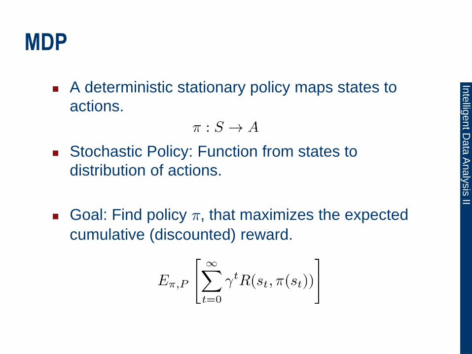
MDP

A deterministic stationary policy maps states to

actions.

Stochastic Policy: Function from states to

distribution of actions.

Goal: Find policy ¼, that maximizes the expected

cumulative (discounted) reward.

Inte

lligent D

ata

Analy

sis

II

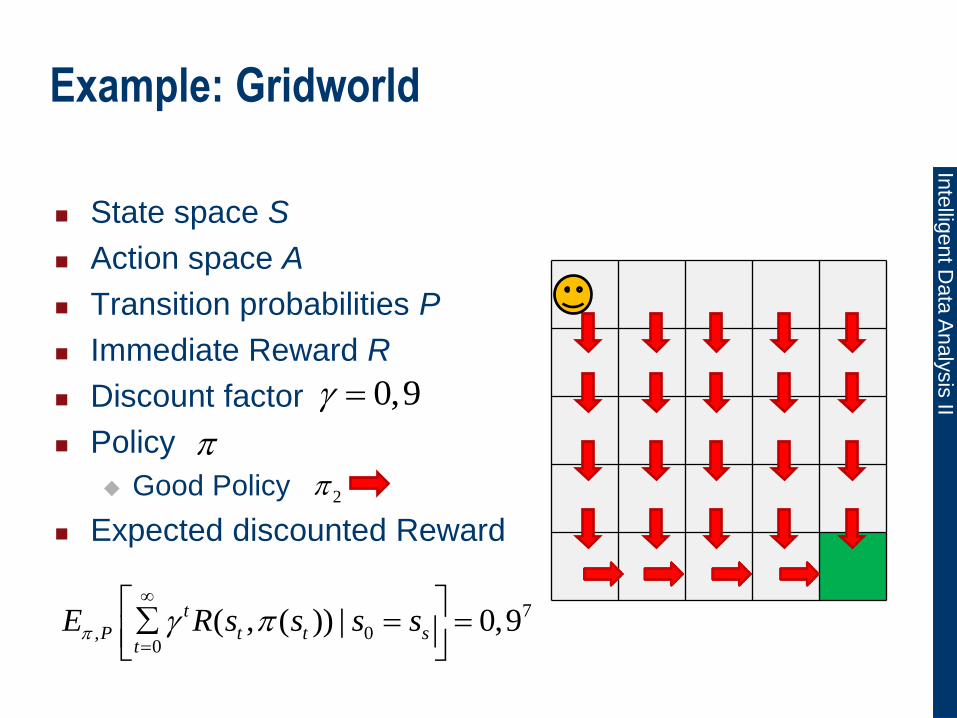
State space S

Action space A

Transition probabilities P

Immediate Reward R

Discount factor

Policy

Good Policy

Expected discounted Reward

Example: Gridworld

2

0,9

7

, 00

( , ( )) | 0,9t

P t t st

E R s s s s

Inte

lligent D

ata

Analy

sis

II

Example : Gridworld

1

0,9

23

, 00

( , ( )) | 0,9t

P t t st

E R s s s s

State space S

Action space A

Transition probabilities P

Immediate Reward R

Discount factor

Policy

Bad Policy

Expected discounted Reward

Inte

lligent D

ata

Analy

sis

II

Markov Property

Markov Property:

In order to model real world scenarios as MDPs,

sequences of observations and actions have to be

aggregated into states.

Markov property rarely fulfilled in reality.

Inte

lligent D

ata

Analy

sis

II

Value Functions

Value function V¼(s) for a state s and policy ¼

describes the expected discounted cumulative reward that will be observed when starting in s and performing

actions according to. ¼.

There always exists an optimal deterministic stationary policy ¼*, which maximizes the value function.

Inte

lligent D

ata

Analy

sis

II

State space S

Action space A

Transition probabilities P

Immediate Reward R

Discount factor

Policy

Good Policy

Expected discounted Reward

Example: Gridworld

2

0,9

1 3

,0

( ) ( , ( )) 0,9k

t P t k t kk

V s E R s s

Inte

lligent D

ata

Analy

sis

II

Value Functions

Value function for state action pair:

Optimal value function:

Assumption: Value function can be stored in (large)

table (One entry for each state-action pair).

Inte

lligent D

ata

Analy

sis

II

Continuous State Spaces

In the real world state spaces are (often) continuous

or very large.

The same can hold for action spaces.

Representation of value function and/or policy via

function approximation methods.

E.g. representation of value function as parametric function with parameter vector µ and features (basis

functions) :

1

ˆ ( , ; ) ( , )N

i i

i

Q s a s a

:i S A

Inte

lligent D

ata

Analy

sis

II

Continuous State Spaces

Alternatively, use representation of policy as

parametric function of state-dependent features

Such problems will be covered next week!

Today: „Idealized“ problems with small and discrete

state and action spaces.

1

( ; ) ( )N

i i

i

s s

Inte

lligent D

ata

Analy

sis

II

Bellman Equations

Bellman equations describe a recursive property of

value functions. (Because of Markov property)

Inte

lligent D

ata

Analy

sis

II

Bellman Equations

State action value functions:

The Bellman equations constitute a system of linear

equations.

Inte

lligent D

ata

Analy

sis

II

Bellman Operators

Notation using (linear) operators:

with linear operator T¼:

V¼ is a fixed point of the Bellman operator T¼.

Inte

lligent D

ata

Analy

sis

II

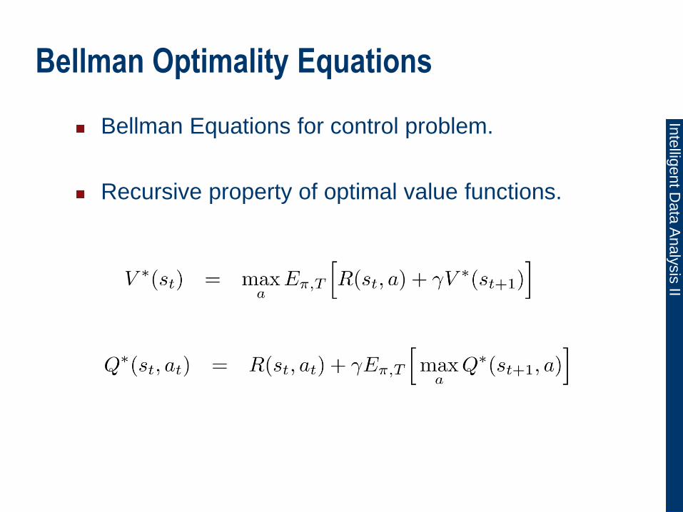
Bellman Optimality Equations

Bellman Equations for control problem.

Recursive property of optimal value functions.

Inte

lligent D

ata

Analy

sis

II

Model Knowledge

Different problem formulations for differing

knowledge about MDPs.

MDP fully defined.

Planning.

MDP only partly defined.

We can gather experience by interacting with the

environment.

Reinforcement Learning.

Inte

lligent D

ata

Analy

sis

II

Types of Reinforcement Learning

Reinforcement Learning methods can be

distinguished w.r.t. their usage of those interactions.

Indirect methods:

Model learning.

Direct methods:

Direct policy search.

Value function estimation

Policy Iteration.

Value Iteration.

Inte

lligent D

ata

Analy

sis

II

MDP Fully Defined – Planning with Policy Iteration

Both reward function R and transition probabilities

P are defined.

Policy Iteration is a general algorithm for

computing the optimal policy.

Iterate the following 2 Steps for computation of optimal policy for k=0,1,… Initialize ¼0 randomly.

Policy Evaluation: Compute Q¼ for fixed ¼k.

Policy Improvement: Determine next ¼k+1.

(Policy Improvement Theorem)

Inte

lligent D

ata

Analy

sis

II

Policy Evaluation

First step in each iteration: Evaluate quality of

current (approximation of optimal) policy.

Policy Evaluation computes value function V¼’ or Q¼’

for fixed ¼‘.

Bellman Equations constitute system of linear

equations.

However, state space is usually too large to solve

system of linear equations with standard solvers.

Inte

lligent D

ata

Analy

sis

II

Policy Evaluation with Value Iteration

Value Iteration for policy evaluation is an iterative algorithm that computes value function for

current policy as the limit of a sequence of approximations Qi.

1 ,

'

( , ) ( , ) ( ', ( '))

( , ) ( ' | , ) ( ', ( '))

i P i k

i k

s

Q s a E R s a Q s s

R s a P s s a Q s s

kQ

k

, : s S a A

Inte

lligent D

ata

Analy

sis

II

Policy Evaluation with Value Iteration

Value Iteration for policy evaluation is an iterative algorithm that computes value function for

current policy as the limit of a sequence of

approximations:

kV

k

: s S

1 ,

'

( ) ( , ( )) ( ')

( , ( )) ( ' | , ( )) ( ')

i P k i

k k i

s

V s E R s s V s

R s s P s s s V s

Inte

lligent D

ata

Analy

sis

II

Policy Iteration

k=0. Repeat until :

Evaluate current policy, e.g. using Value Iteration.

Greedy Policy Improvement:

1: ( ) ( ) k ks S s s

: s S

1 ,

'

( , ) ( , ) ( ', ( '))

( , ) ( ' | , ) ( ', ( '))

i P i k

i k

s

Q s a E R s a Q s s

R s a P s s a Q s s

, : s S a A

for 1... :i

Inte

lligent D

ata

Analy

sis

II

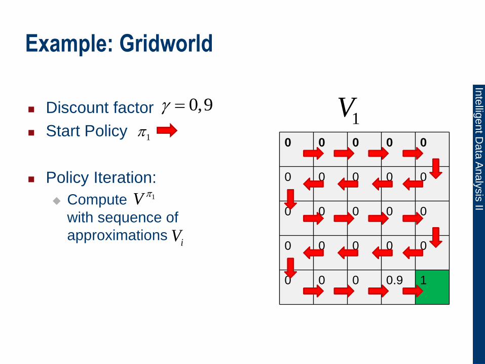
Example: Gridworld

1

0,9 Discount factor

Start Policy

Policy Iteration:

Compute

with sequence of

approximations

1V

iV

Inte

lligent D

ata

Analy

sis

II

Example: Gridworld

0 0 0 0 0

0 0 0 0 0

0 0 0 0 0

0 0 0 0 0

0 0 0 0 0

1

0,9 Discount factor

Start Policy

Policy Iteration:

Compute

with sequence of

approximations

1V

iV

0V

Inte

lligent D

ata

Analy

sis

II

Example: Gridworld

0 0 0 0 0

0 0 0 0 0

0 0 0 0 0

0 0 0 0 0

0 0 0 0.9 1

1

0,9 Discount factor

Start Policy

Policy Iteration:

Compute

with sequence of

approximations

1V

iV

1V

Inte

lligent D

ata

Analy

sis

II

Example: Gridworld

0 0 0 0 0

0 0 0 0 0

0 0 0 0 0

0 0 0 0 0

0 0 0.81 0.9 1

2V1

0,9 Discount factor

Start Policy

Policy Iteration:

Compute

with sequence of

approximations

1V

iV

Inte

lligent D

ata

Analy

sis

II

Example: Gridworld

0 0 0 0 0

0 0 0 0 0

0.. 0.. 0.. 0.. 0..

0.59 0.53 0.48 0.43 0…

0.66 0.73 0.81 0.9 1

nV1

0,9 Discount factor

Start Policy

Policy Iteration:

Compute

with sequence of

approximations

1V

iV

Inte

lligent D

ata

Analy

sis

II

Example: Gridworld

0 0 0 0 0

0 0 0 0 0

0.. 0.. 0.. 0.. 0..

0.59 0.53 0.48 0.43 0…

0.66 0.73 0.81 0.9 1

1

0,9 Discount factor

Start Policy

Policy Iteration:

Compute

with sequence of

approximations

Policy Improvement:

Compute greedy Policy

( )

1V

1V

2( , ) ( , ) [ ( ')]k kQ s a R s a E V s

iV

Inte

lligent D

ata

Analy

sis

II

Policy Evaluation

In the limit k1, Vk converges to V¼.

Rate of convergence O(°k): ||Vk – V¼|| = O(°k)

Proof e.g. using Banach fixed-point theorem.

Let B=(B,||.||) be a Banach space.

Let T be an operator T:BB, such that

||TU – TV|| · ° ||U – V|| with °<1.

T is a °-contraction mapping.

Then T admits a unique fixed-point V . Furthermore,

for all V0 2 B, the sequence Vk+1=T Vk, k 1

converges to V. Also, ||Vk – V|| = O(°k)

Inte

lligent D

ata

Analy

sis

II

Policy Evaluation

The Bellman operator T¼

is a contraction mapping with contraction constant

°. It follows that the sequence that results from

iteratively applying the operator

converges to V¼.

Inte

lligent D

ata

Analy

sis

II

Policy Evaluation: Contraction Mapping

What is a contraction mapping?

According to the algorithm:

Distance to the real value function reduces per iteration by a factor ° (using sup norm).

Inte

lligent D

ata

Analy

sis

II

Policy Improvement

Greedy Policy Improvement

Policy Improvement Theorem:

Let ¼‘ and ¼ be deterministic policies with: For all

s2S: Q¼(s,¼‘(s)) ¸ V¼(s).

Then V¼‘(s) ¸ V¼(s)

Inte

lligent D

ata

Analy

sis

II

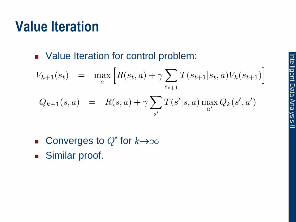
Value Iteration

Value Iteration for control problem:

Converges to Q* for k1

Similar proof.

Inte

lligent D

ata

Analy

sis

II

Value Iteration

Algorithm:

Initialize Q, e.g. Q = 0

for k=0,1,2,…:

foreach (s,a) in (S x A):

until

Alternative convergence criterion:

Max distance to optimal Q* smaller than .

Conservative Choice:

1k kQ Q

2(1 )log

2K

R

Inte

lligent D

ata

Analy

sis

II

MDP Partially Undefined— Reinforcement Learning

Indirect Reinforcement Learning: Model based.

Learn Modell of MDP:

Reward function R

Transition probabilities P

Apply planning algorithm as before, e.g. Policy

Iteration.

Inte

lligent D

ata

Analy

sis

II

Policy Iteration (Again)

Even without learning a model of the MDP, we can

apply the same principles.

As before: Iterate the following 2 Steps for

computation of optimal policy:

Policy Evaluation: Compute Q¼ for fixed ¼k.

Policy Improvement: Determine next ¼k+1.

Policy Evaluation step changes for partly defined

MDPs.

Inte

lligent D

ata

Analy

sis

II

Policy Evaluation: Monte-Carlo Methods

Learn from episodic interactions with the

environment.

Goal: Learn Q¼(s,a).

Monte-Carlo Estimation of Q¼(s,a): Compute mean

of sampled cumulative rewards.

Unbiased Estimation of real rewards. Variance reduces with 1/n.

Inte

lligent D

ata

Analy

sis

II

Policy Evaluation: Monte-Carlo Methods

Computation time of estimation is independent from

size of state space.

Problem: If ¼ is deterministic, many state action

pairs Q(s,a) will never be observed.

Problems in Policy Improvement step.

Solution: stochastic policies, e.g. ²-greedy policies.

Inte

lligent D

ata

Analy

sis

II

Greedy and ²-Greedy Policies

Greedy:

²-greedy:

Notation as distribution:

²-greedy allows for exploration.

( ) arg max ( , )a

s Q s a

arg max ( , ) with probability ( )

random action with probability 1

aQ s a

s

' if arg max ( , ')

( , ) 1 otherwise

1

aa Q s a

s a

A

Inte

lligent D

ata

Analy

sis

II

Stochastic Policy: Softmax

Current estimation of value function should have

influence on probabilities.

soft max

Example: Gibbs distribution:

¿t is also called the temperature parameter.

Inte

lligent D

ata

Analy

sis

II

Temporal Difference Learning

Idea: Update states based on estimates of other

states. Natural formulation as online learning

method.

Also applicable to incomplete episodes.

Disadvantage compared to Monte-Carlo:

Stronger influence (more damage) if Markov property

violated.

Inte

lligent D

ata

Analy

sis

II

Policy Evaluation: Value Iteration

Idea: Update states based on estimates of other

states. Natural formulation as online learning

method.

Same idea as before in fully defined case.

Value Iteration for Policy Evaluation. Iteratively sample action at and observe next state

st+1. Update Q according to:

1 '~ 1

1

'

( , ) ( , ) ( , ')

( , ) ( , ') ( , ')

k k

k

t t t a t t t t

t t t t

a

Q s a E R s a Q s a

R s a s a Q s a

Inte

lligent D

ata

Analy

sis

II

Policy Evaluation: Value Iteration

Exploration / exploitation problem. Same as for

Monte-Carlo methods.

If policy stochastic: Sample state-action sequence

on-policy according to .

Or sample off-policy according to

stochastic off-policy .

1 1 2 2 3 3 4 4...s a s a s a s a ~ ( )t ta s

1 1 2 2 3 3 4 4...s a s a s a s a

~ ( )t b ta s

Inte

lligent D

ata

Analy

sis

II

Policy Iteration (Again)

As before: Iterate the following 2 Steps for

computation of optimal policy:

Policy Evaluation: Compute Q¼ for fixed ¼k.

Policy Improvement: Determine next ¼k+1.

Policy Evaluation either with Monte-Carlo sampling

or value iteration.

Inte

lligent D

ata

Analy

sis

II

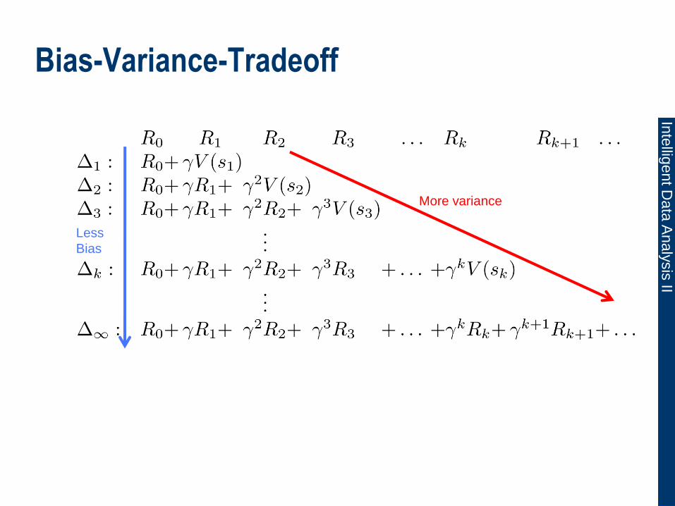
N-step Returns

General update rule:

Temporal difference methods perform 1-step

updates:

Monte-Carlo methods make updates, that are

based on complete episodes:

N-Step Updates:

Inte

lligent D

ata

Analy

sis

II

TD(¸)

Inte

lligent D

ata

Analy

sis

II

TD(¸)

Idea: Weighted sum over all n-step returns.

Inte

lligent D

ata

Analy

sis

II

TD(¸)

TD(¸) Update:

0·¸·1 interpolates between 1-step and MC.

Inte

lligent D

ata

Analy

sis

II

Bias-Variance-Tradeoff

Less

Bias

More variance

Inte

lligent D

ata

Analy

sis

II

Eligibility Traces

Algorithmic view on TD(¸)

Use additional variable e(s) for every state s2S.

After observation <st,at,Rt,st+1>, compute

Update for all states

Inte

lligent D

ata

Analy

sis

II

Q-Learning

Q-Learning Update:

Converges to Q* if

Every state will be observed infinitely often.

Step size parameters follow:

Inte

lligent D

ata

Analy

sis

II

Q-Learning

Off-Policy method. No exploration / exploitation

problem.

Learn optimal policy ¼* while following another

behavior policy ¼‘.

Policy ¼‘ could e.g. be a stochastic policy with

¼(s,a)>0 for all s and a to guarantee convergence

of Q.

Inte

lligent D

ata

Analy

sis

II

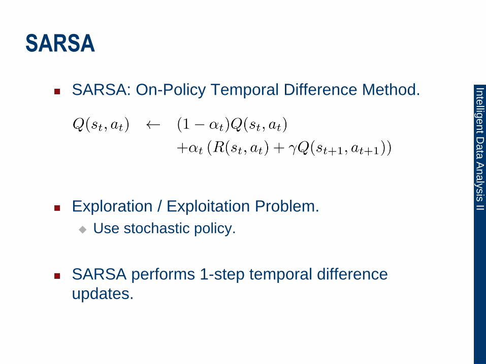
SARSA

SARSA: On-Policy Temporal Difference Method.

Exploration / Exploitation Problem.

Use stochastic policy.

SARSA performs 1-step temporal difference

updates.

Inte

lligent D

ata

Analy

sis

II

Problem Formulations

Learn optimal policy.

Or best possible approximation.

Optimal Learning: Make as few as possible

mistakes during learning.

Exploration / exploitation problem.

Inte

lligent D

ata

Analy

sis

II

Exploration / Exploitation Problem

Tradeoff between

using the current best policy to maximize (greedy)

reward.

(Exploitation)

and exploring currently suboptimal actions whose

values are still uncertain in order to find a potentially

better policy.

(Exploration)

Inte

lligent D

ata

Analy

sis

II

Bandit Problem

n-armed bandit problem:

n actions (arms / slot machines) .

Each action has different expected reward.

Expected reward unknown.

Problem: find best action without losing too much on

the way.

Expected reward for action a is Q*(a).

Estimated expected reward after t trials:

Inte

lligent D

ata

Analy

sis

II

Greedy and ²-Greedy Policies

Greedy:

²-greedy

²-greedy allows for random exploration.

Inte

lligent D

ata

Analy

sis

II

²-Greedy Policies

10-armed bandit

2000 experiments

For each experiment draw Q*(a) for all a:

Rewards are drawn

from

Inte

lligent D

ata

Analy

sis

II

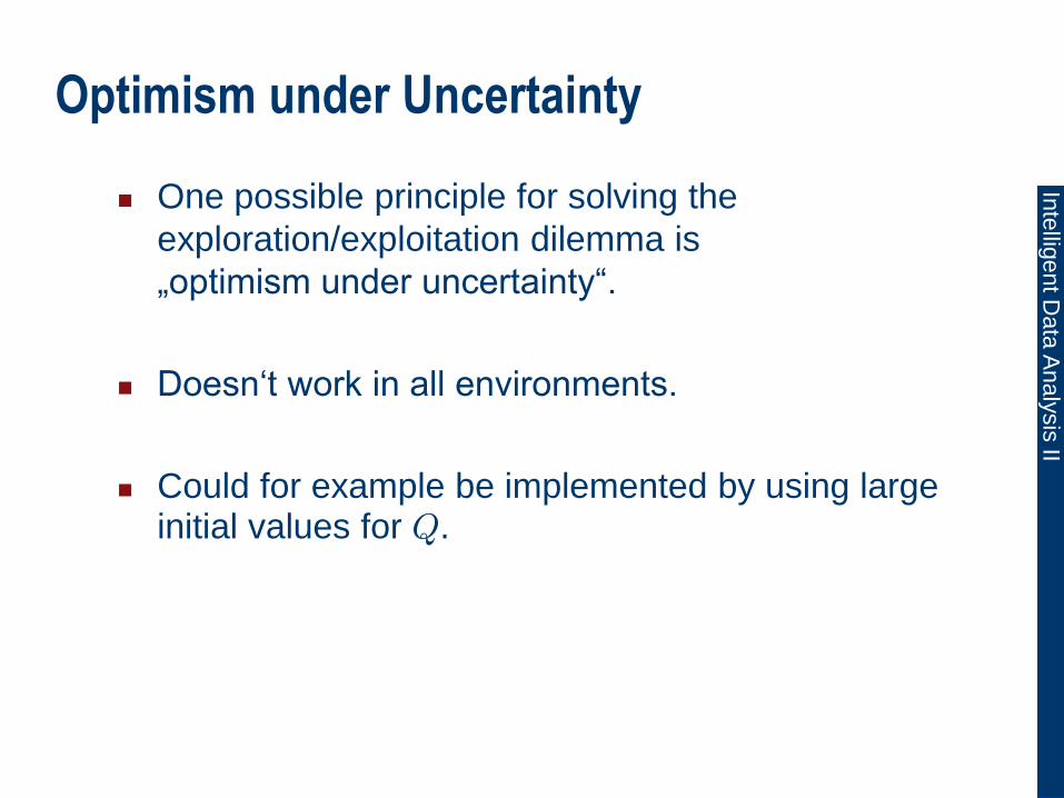
Optimism under Uncertainty

One possible principle for solving the

exploration/exploitation dilemma is

„optimism under uncertainty“.

Doesn‘t work in all environments.

Could for example be implemented by using large initial values for Q.

Inte

lligent D

ata

Analy

sis

II

Optimism under Uncertainty

Upper Confidence Bound (UCB): [Auer et al. 02 ]

Assume that rewards are bounded by [0,1].

Good results for stationary environments and i.i.d.

rewards.

Inte

lligent D

ata

Analy

sis

II

Problem Formulations

P,R known. P(s‘|s,a) can be queried.

P,R not explicitly known. But we can sample from

the distributions P(s‘|s,a). Assumption: Generative

model of P and R.

P,R not or only partly known. We can gain

experience by interacting with the environment.

Reinforcement Learning.

Batch Reinforcement Learning: We have to learn

from a fixed set of episodes.

Inte

lligent D

ata

Analy

sis

II

Large and Infinite State Spaces

In realistic applications state spaces are usually

very large or continuous.

So far: Assumption that value function could be

stored as a table.

Different approaches:

Planning:

Monte-Carlo Sampling

Discretization with subsequent Value Iteration (or PI)

Approximation of value function with function

approximation methods.

Direct learning of policy.

Inte

lligent D

ata

Analy

sis

II

Approximation

Types of approximations

Representation, e.g.

Value function

Policy

Sampling

Online learning via interactions.

Sample from generative model of environment.

Maximization

Find the good action instead of best action for current

state.

ˆ ( , ; ) ( , )TQ s a s a

( , ; ) ( ( , ) )Ts a h s a

Inte

lligent D

ata

Analy

sis

II

Monte-Carlo Sampling

Assume that S is very large

Goal: Find Q, s.t. ||Q-Q*||1<².

Sparse Lookahead Trees:

[Kearns et al. 02]

Monte-Carlo: Sample sparse action-

state tree.

Depth of tree: Effective horizon H(²) =

O( 1/(1-°) log(1/²(1-°)) )

MC independent of |S|

But exponential in H(²):

minimal size of tree.

Inte

lligent D

ata

Analy

sis

II

Sparse Lookahead Trees

Inte

lligent D

ata

Analy

sis

II

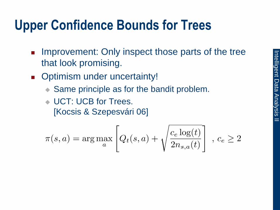
Upper Confidence Bounds for Trees

Improvement: Only inspect those parts of the tree

that look promising.

Optimism under uncertainty!

Same principle as for the bandit problem.

UCT: UCB for Trees.

[Kocsis & Szepesvári 06]

Inte

lligent D

ata

Analy

sis

II

UCT Performance: Go

Very good results in Go.

9x9 & 19x19

Computer Olympics 2007 - 2009:

2007 & 2008: 1st to 3rd places employed variants of

UCT.

More general: Monte-Carlo Search Trees (MCST).

2009: At least 2nd and 3rd employed variants of

UCT.

Inte

lligent D

ata

Analy

sis

II

Discretization

Continuous state space S.

Random Discretization Method: [Rust 97]

Sample states S‘ according to uniform distribution

over state space.

Value iteration.

Continuous value iteration:

Discretization: Weighted Importance Sampling

Inte

lligent D

ata

Analy

sis

II

Discretization

Compute value function V(s) for states that are not

in sample set S‘:

Bellman update step:

Guaranteed performance: [Rust97] Assumption: S=[0,1]d