Reinforcement Learning for Cyber-Physical Systems

Reinforcement Learning for Cyber-Physical Systems

Anand Balakrishnan Jyo Deshmukh

Spring 2019 CSCI 599: Autonomous Cyber-Physical Systems

March 25, 2019

Anand Balakrishnan (CSCI599) Reinforcement Learning March 25 1 / 73

Outline

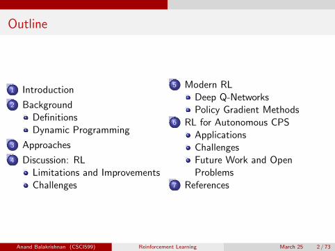
1 Introduction

2 BackgroundDefinitionsDynamic Programming

3 Approaches

4 Discussion: RLLimitations and ImprovementsChallenges

5 Modern RLDeep Q-NetworksPolicy Gradient Methods

6 RL for Autonomous CPSApplicationsChallengesFuture Work and OpenProblems

7 References


Introduction

Outline

1 Introduction


3 Approaches




7 References


Introduction

What is Reinforcement Learning?

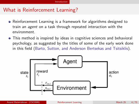
Reinforcement Learning is a framework for algorithms designed totrain an agent on a task through repeated interaction with theenvironment.

This method is inspired by ideas in cognitive sciences and behavioralpsychology, as suggested by the titles of some of the early work donein this field (Barto, Sutton, and Anderson Bertsekas and Tsitsiklis).


Introduction

What is Reinforcement Learning?

RL is more related to Optimal Control Theory than it is to MachineLearning.

It was initially developed as a method to learn controllers (or policies)for stochastic systems1 (Kumar and Varaiya).

In RL, we typically model the environment as a Markov DecisionProcess (MDP) and say that the goal is to learn a policy, π, thatlearns to “solve” the MDP.

1systems modeled with random noise in their observations and their control vectorsAnand Balakrishnan (CSCI599) Reinforcement Learning March 25 5 / 73

Background

Outline

1 Introduction


3 Approaches




7 References


Background Definitions

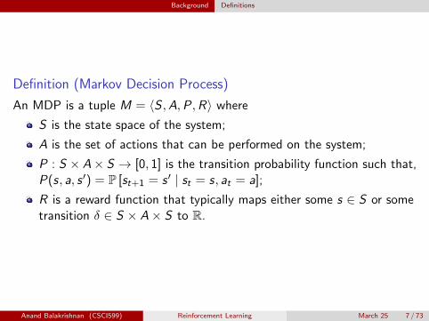
Definition (Markov Decision Process)

An MDP is a tuple M = 〈S ,A,P,R〉 where

S is the state space of the system;

A is the set of actions that can be performed on the system;

P : S × A× S → [0, 1] is the transition probability function such that,P(s, a, s ′) = P [st+1 = s ′ | st = s, at = a];

R is a reward function that typically maps either some s ∈ S or sometransition δ ∈ S × A× S to R.



In the standard RL problem (Sutton and Barto), a learning agentinteracts with a MDP.

The state, action, and reward at each time t ∈ 0, 1, 2, . . . aredenoted st ∈ S , at ∈ A, and rt ∈ R respectively.

We also denote the expected reward received from taking an actiona ∈ A in state s ∈ S to be

R(s, a) = E[rt+1 | st = s, at = a]



Example: MDP

0 1 2 3

0

1

2

3 +1

−1

S = (i , j)|i , j ∈ [0, 3],i.e., each cell in the above grid.

A = UP, DOWN, LEFT, RIGHT.2

P(success) = 0.8, else choose an orthogonal direction;

R: +1 for goal (green) and −1 for fail (red), else 0.

We will use this MDP as a running example.

2if agent is trying to move into an obstacle, the agent shouldn’t be allowed to moveAnand Balakrishnan (CSCI599) Reinforcement Learning March 25 9 / 73


Definition (Policy)

π : S → A is a function that outputs an action a given a state s.

We can also denote the policy to be a probability distributionπ : S × A→ [0, 1] such that π(s, a) = P [at = a | st = s]

Thus, in the deterministic case, the chosen action will be the mode ofthe probability distribution represented by π.



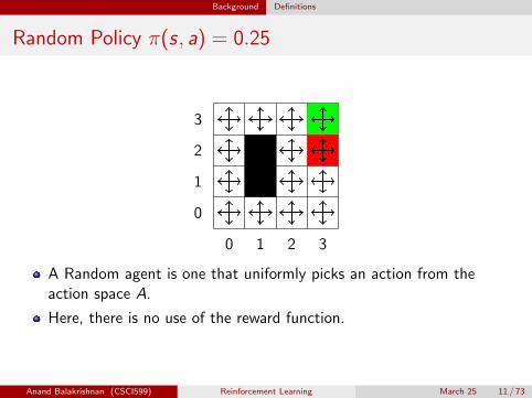
Random Policy π(s, a) = 0.25

0 1 2 3

0

1

2

3

A Random agent is one that uniformly picks an action from theaction space A.

Here, there is no use of the reward function.



Policy under deterministic MDP (P(success) = 1)

0 1 2 3

0

1

2

3 +1

−1

In the deterministic MDP case, you can use your favorite pathplanning algorithm (Dijkstras, A*, D*, Bellman-Ford, etc.) to find athe optimal policy.

We learn a policy π such that π(s, a) = 1 for correct action, 0otherwise.



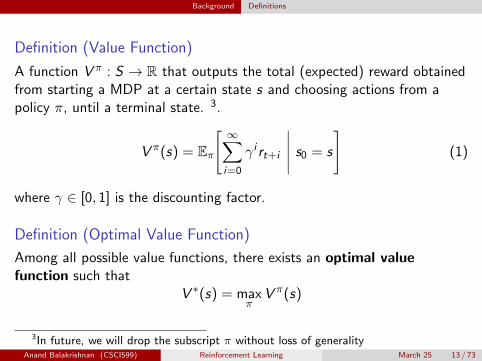
Definition (Value Function)

A function V π : S → R that outputs the total (expected) reward obtainedfrom starting a MDP at a certain state s and choosing actions from apolicy π, until a terminal state. 3.

V π(s) = Eπ

[ ∞∑i=0

γ i rt+i

∣∣∣∣∣ s0 = s

](1)

where γ ∈ [0, 1] is the discounting factor.

Definition (Optimal Value Function)

Among all possible value functions, there exists an optimal valuefunction such that

V ∗(s) = maxπ

V π(s)

3In future, we will drop the subscript π without loss of generalityAnand Balakrishnan (CSCI599) Reinforcement Learning March 25 13 / 73


Definition (Action-Value or Q Function)

A function Qπ : S × A→ R that outputs the expected value of the givenstate s, if we take action a.

Qπ(s, a) = Eπ[R(s, a) + V π(st+1) | st = s, at = a] (2)

where R(s, a) is the expected random reward associated with thestate-action pair (s, a).

The Q-function is a measure of how good it is for an agent to pick anaction a in state s so as to maximize V (s).

The optimal Q-function Q∗(s, a) means the expected total rewardreceived by an agent starting in sand picks action a, then will behaveoptimally afterwards.


Background Dynamic Programming

Bellman Equation

Richard Bellman showed that a dynamic optimization problem indiscrete time can be stated in a recursive, step-by-step form known asbackward induction by writing down the relationship between thevalue function in one period and the value function in the next period.

This recursive relationship is called a Bellman equation.

In dynamic programming, the existence of a Bellman equation is anecessary condition to learn an optimal solution to a problem.


Background Dynamic Programming

Bellman equation for Value functions

We can provide a Bellman equation for the optimal Q-function by thefollowing relation:

Q∗ (s, a) = R(s, a) + γEs′[V ∗(s ′)]

= R(s, a) + γ∑s′∈S

P[s ′ | s, a

]V ∗(s ′) (3)

Since,

V ∗ (s) = maxa

Q∗ (s, a)

= maxa

[R(s, a) + γ

∑s′∈S

P[s ′ | s, a

]V ∗(s ′)] (4)

The above relation is very important for classical RL methods, and lay afoundation for designing objective functions modern RL.


Approaches

Outline

1 Introduction


3 Approaches




7 References


Approaches

Objective of an RL Agent

Since V ∗ (s) is the maximum expected total reward when startingfrom state s,

V ∗ (s) = maxa

Q∗ (s, a) ∀s ∈ S

And since the policy attempts to maximize V (s), the optimal policyπ∗ is

π∗(s) = arg maxa

Q∗ (s, a)

Thus, the goal of a reinforcement learning agent is to learn a policyπ ≈ π∗.


Approaches

Approaches to learning an Optimal Policy

We will go through the following algorithms for Finite-state MDPs withfinite action space:

Linear Programming formulation

Value Iteration

Policy Iteration

Q-Learning


Approaches

Linear Programming

From (3) and (4), we can see that for finite-state MDPs, we can write|S | linear equations for each state s ∈ S , with unknown V ∗ (s).

Thus, this linear programming formulation can easily be used to learna optimal Q∗ (s, a) for all (s, a) ∈ S × A for the given MDP.


Approaches

Value Iteration

Value iteration computes the optimal state value function by iterativelyimproving the estimate of V (s).

Algorithm 1 Value Iteration

1: Initialize V (s) = 0∀s ∈ S2: repeat3: for all s ∈ S do4: for all a ∈ A do5: Q (s, a)← E[r | s, a] + γEs′[V (s ′) | s, a]6: end for7: V (s)← maxa Q (s, a)8: end for9: until V (s) converges

It can be shown that V converges to V ∗ in a finite number of iterations.


Approaches

Value Iteration in Gridworldnoise = 0.2, γ = 0.9

0 1 2 3

0

1

2

3

0

0

0

0

0.37

0

0

0.520.66

0

0

0.31

0

0.430.51

0

0.720.780.83

0

0

+1

−1

Values after 1 iteration.

Run for about 100 iterations to be sure of convergence.


Approaches


0 1 2 3

0

1

2

3

0

0

0

0

0.37

0

0

0.520.66

0

0

0.31

0

0.430.51

0

0.72

0.780.83

0

0

+1

−1

Values after 2 iterations.



Approaches


0 1 2 3

0

1

2

3

0

0

0

0

0.37

0

0

0.52

0.66

0

0

0.31

0

0.43

0.51

00.72

0.78

0.83

0

0

+1

−1




Approaches


0 1 2 3

0

1

2

3

0

0

0

0

0.37

0

00.52

0.66

0

0

0.31

00.43

0.51

00.720.78

0.83

0

0

+1

−1




Approaches


0 1 2 3

0

1

2

3

0

0

0

0

0.37

0

00.52

0.66

0

0

0.31

00.43

0.51

00.720.78

0.83

0

0

+1

−1

Values after iterations.



Approaches

Value Iteration: Effect of noise and γ

Noise (∈ [0, 0.5])4 γ ∈ [0, 1] Effect

Low High Prefer to find the closest positive exit,while avoiding negative exits.

High High Prefer distant positive; Risk being closeto negative.

Low Low Prefer distant positive; Avoid negative.

High Low Prefer close exit; Risk negative.

4Too much noise implies a bad modelAnand Balakrishnan (CSCI599) Reinforcement Learning March 25 23 / 73

Approaches

Policy Iteration I

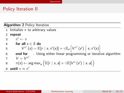
In Value Iteration, we care about the convergence of the valuefunction, but it is possibly for us to reach an optimal policy before thevalue function converges.

In Policy Iteration, we update the policy at each iteration, rather thanthe value function.


Approaches

Policy Iteration II

Algorithm 2 Policy Iteration

1: Initialize π to arbitrary values2: repeat3: π′ ← π4: for all s ∈ S do5: V π′

(s) = E[r | s, π′(s)] + γEs′

[V π′

(s ′)∣∣∣ s, π′(s)

]6: end for . Using either linear programming or iterative algorithm7: V = V π′

8: π(s)← arg maxa

(E[r | s, a] + γE[V π (s ′) | s, a]

)9: until π ≈ π′


Approaches

Model-based vs. Model-free Learning

Model-based In model-based learning, the agent is assumed to have priorknowledge about the effects of its actions on theenvironment, that is, the transition probability function P ofthe MDP is known.

Model-free In model-free learning, the agent will not try to learn explicitmodels of the environment state transition and rewardfunctions. However, it directly derives an optimal policy fromthe interactions with the environment.

Policy iteration and Value iteration are model-based methods as it isnecessary to have knowledge of the probability of transitions in the MDPto compute the expected V (s) at any given iteration of the algorithm.


Approaches

Q-Learning (Watkins) I

Q-Learning is an example of model-free learning algorithm. It does notassume that agent knows anything about the state-transitionand reward models. However, the agent will discover whatare the good and bad actions by trial and error.

The basic idea behind Q-learning is is to approximate the state-actionpairs Q-function from the samples of Q (s, a) that we observe duringinteraction with the environment.

This approach is known as Temporal-Difference (TD) Learning.

We combine this idea with bootstrapping, where TD learningmethods update targets with regard to existing estimates rather thanexclusively relying on actual rewards and complete returns as inMonte-Carlo methods.


Approaches

Q-Learning (Watkins) II

The update equation for the Q-function is:

Q (s, a)← (1− α)Q (s, a) + α

(R(s, a) + γmax

a′Q(s ′, a′

))(5)

where,I α ∈ [0, 1] is the learning rate, such that if α ≈ 0 the Q value is

updated very slowly and α ≈ 1 simply replaces the old Q with the newQ without any TD-learning taking place.

I maxa′ Q (s ′, a′) is the estimate of the optimal state-value function.

In Q-learning, we initialize the Q function as a table mapping allstates s ∈ S to the expected value for all actions a ∈ A.

We then update this Q-table in an iterative (episodic) manner.


Discussion: RL

Outline

1 Introduction


3 Approaches




7 References


Discussion: RL Limitations and Improvements

Limitations

In the algorithms discussed up to this point, we have a generalassumption that the environment we are acting upon has finite actionand state spaces.

This is (in general) a really bad assumption as most problems we seein the real world (especially in control theory) have either continuousaction space or continuous state space or both.



Approachs: Continuous or Large State Space

Discretize the state spaceI Here, we convert the continuous state space to a discrete grid or bins

and use our favorite discrete state space RL agent.I But this leads to the curse of dimensionality! This refers to the

explosion in state space with increase in the number of dimensions inthe state space.

Use Function approximatorsI We can define Q and value functions as functions that act upon a

vector ~s ∈ S .I Thus, the learning problem is that of optimizing the function using

function approximation methods (convex optimization, etc.).



Approachs: Continuous Action Space I

To operate on continuous action spaces, we build on functionapproximators that map to a action vector. The following are a generalclass of algorithms used to learn a policy that operates in continuousaction spaces:

Policy gradient (Sutton et al.) methods target at modeling andoptimizing the policy directly. The policy is usually modeled with aparameterized function respect to θ, πθ(s). The value of the reward(objective) function depends on this policy and then variousalgorithms can be applied to optimize θ for the best reward.



Approachs: Continuous Action Space II

Actor-critic (Konda and Tsitsiklis) methods contain two separateapproximators defined as follows:I Critic updates the estimate of the value function (parametrized by w),

and can either represent Qw (s, a) or Vw (s, a)I Actor outputs the direct action a and models the (stochastic) policy

πθ(s).

Note

Actor-critic methods typically use policy gradient methods to update theactor and TD-learning methods to update the critic.



Aside: On-policy and Off-policy Methods

On-policy These methods use deterministic actions (or samples) fromthe target policy to train the algorithm. Examples of this areMonte-Carlo methods that compute V π for the episode toupdate π.

Off-policy They train on a distribution of transitions or episodesproduced by a different behavior policy rather than thatproduced by the target policy. Example of this is Q-Learning,where the TD error is computed against an existing (possiblyolder) Q(s ′, a′) to update the current Q(s, a).


Discussion: RL Challenges

Exploration vs. Exploitation I

Example

Say there is a sheep grazing in a very patchy and large plot of land. Thesheep can either approach a patch of grass that is somewhat small, andexploit this patch of grass until it is depleted, and then have no idea whatto do. Otherwise, the sheep could explore the plot of land for a bit andthen come back to the largest patch of grass it finds. Who knows, it couldfind some magical never-ending patch of grass! But too much explorationend up in the sheep going too far from any patch of grass and starvebefore it gets back to a known patch!

This is referred to as the exploration vs. exploitation problem.

In the context of RL, we should train the learning agent to do bothexploration and exploitation without being either too explorative ortoo greedy.



Exploration vs. Exploitation II

This is typically done by performing ε−greedy exploration, orsampling actions from a Boltzmann distribution.

In ε−greedy exploration, a decaying ε value is used as the probabilityof choosing a deterministic action (vs. a uniformly sampled actionfrom A).

In the Boltzmann distribution case, the action is sampled from adistribution

P [a | s] =eQ(s,a)/k∑

a′∈A eQ(s,a′)/k,

where k is the temperature of the distribution. A large k impliesuniform sampling of actions (explore) and a small k chooses thegreedy strategy.



The Deadly Triad

TD-learning + bootstrapping methods are a very efficient and flexibleclass of learning algorithms. But, when we combine Off-policy,bootstrapping methods with non-linear function approximation, thetraining could be (and is most likely) unstable and hard to converge.

To tackle this, many architectures using deep learning models wereproposed to resolve the problem, including DQN to stabilize thetraining with experience replay and occasionally frozen target network.


Modern RL

Outline

1 Introduction


3 Approaches




7 References


Modern RL

Deep Reinforcement Learning

Deep RL = Deep Learning + RL.

As mentioned in the previous section, deep RL architectures weredeveloped to combat the so-called deadly triad, issue.

Frameworks like AlphaZero (Silver et al.) and DQN (Mnih et al.)proposed the use of Convolutional Neural Networks to observe thestate of games (Go and Atari games respectively) from raw pixelvalues and map them to discrete actions corresponding to eithermoves on a board or buttons on a video game controller.

Both the above methods are off-policy methods that build off ofTD-learning and bootstrapping methods like Q-learning.

Many other works have also proposed the use of Deep RL in thecontext of continuous action and state spaces, like (Mnih et al.Schulman et al. Levine et al. Schulman et al.).


Modern RL Deep Q-Networks

Deep Q Networks (Mnih et al.) I

When using the DQN framework, we model the Q-function as afunction approximator (deep neural network) Q (s, a; θ), where θ isthe parameters for the NN.

In the original Nature paper, the authors use a CNN that observesAtari games using their raw pixel values, and outputs the expectedvalue of taking an action a at that state.



Deep Q Networks (Mnih et al.) II

Moreover, to stabilize the problem of instability due to usingTD-learning + bootstrapping with non-linear function approximators,the authors propose the following improvements to the vanillaQ-learning algorithm:I Experience Replay: All previous state transitions and their associated

rewards et = (st , at , rt , st+1) are stored in one replay memoryD = e1, . . . , et. During update, a batch of experiences are sampledfrom this memory and used to compute the loss gradient for the NN.

I Periodically Update Targets: The target for the loss is computedagainst a fixed (older) Q function, which is updated periodically.Essentially, The Q network is cloned and kept frozen as theoptimization target every C steps (C is a hyperparameter). Thismodification makes the training more stable as it overcomes theshort-term oscillations.



Deep Q Networks (Mnih et al.) III

The loss function is computed as follows:

L(θ) = E(s,a,r ,s′)∼U(D)

[(r + γmax

a′Q(s ′, a′; θ−

)− Q (s, a; θ)

)2](6)

where, U(D) is a uniform distribution over the replay memory D; θ−

is the parameters of the frozen target Q-network.

Equation (6) is essentially computing the Mean-Squared Error (MSE)over a sampled batch of experiences, thus can be easily optimized(minimized) using Stochastic Gradient Descent (SGD).



Extensions to DQN

Several extensions to DQN have been proposed, including(van Hasselt, Guez, and Silver Schaul et al. Z. Wang et al. Pritzelet al.).

These build mainly on either the experience replay memory of the RLagent (with better, more intuitive sampling as opposed to uniformsampling) or they improve on the way the frozen target behaves inthe update stage.


Modern RL Policy Gradient Methods

Policy Gradients I(Sutton et al.)

The general idea is that, instead of parameterizing the value function(as in the case of DQN) and doing policy improvement by greedilymaximizing the expected value function, we parameterize the policyand do gradient decent along the direction that improves the policy.

The intuition is that, sometimes, the policy is easier to approximatethan the value function.

The technique of policy gradients is a relatively old idea, but onlyrecently has it been used along with non-linear function approximators(deep Neural Networks), like in (Mnih et al. Silver et al. Schulmanet al. Schulman et al. Z. Wang et al. Lillicrap et al.) to name a few.



Policy Gradients II(Sutton et al.)

The problem is generally formulated as so:

Let πθ(a | s) be a stochastic policy that outputs the probabilitydistribution on the action space for a given state s, where θ parameterizesthe policy. Thus, the objective function for the optimization problem canbe written as:

J(θ) =∑s∈S

dπ(s)V π (s) =∑s∈S

dπ(s)∑a∈A

πθ(a | s)Qπ (s, a) , (7)

where dπ(s) is the (on-policy )stationary distribution of the Markov chaininduced under the policy πθ.5

5For simplicity, we will omit θ under π when it is used in subscripts and superscripts(like in dπ,Qπ,V π above).



Policy Gradient Theorem(Sutton et al.)

Theorem (Policy Gradient Theorem)

The gradient of the objective function ∇θJ(θ) can be simplified as follows:

∇θJ(θ) = ∇θ∑s∈S

dπ(s)∑a∈A

Qπ (s, a)πθ(a | s) (8)

∝∑s∈S

dπ(s)∑a∈A

Qπ (s, a)πθ(a | s)d (9)

This reduces the amount of computation required for the gradientsignificantly! But the approximation of dπ and Qπ (s, a) still remains anissue. . .



Generalized Policy Gradients(Schulman et al.)

Policy gradient methods maximize the objective function J(θ) byrepeatedly estimating the gradient g := ∇θJ(θ), which have the followinggeneral form:

g = E

[ ∞∑t=0

Ψt∇θ log πθ(at | st)

], (10)

where Ψ denotes the target returns, and may be one of:

1∑∞

t=0 rt : Total Reward;2∑∞

t′=t rt′ : Reward followingaction at ;

3∑∞

t′=t rt′ − b(st): baselinedversion of the previous form;

4 Qπ (st , at);

5 Aπ(st , at) :=Qπ (st , at)− V π (st):Advantage function;

6 rt + V π (st+1)− V π (st): TDresidual.



Actor-Critic Models I(Sutton and Barto)

Two main components in PG are the policy model and the valuefunction.

It makes sense to learn the value function in addition to the policy,since knowing the value function can assist in the policy update.I This is mainly to reduce the gradient variance in vanilla policy

gradients like REINFORCE (Williams).

As mentioned earlier, an actor-critic model consists of two parts:I Critic updates the estimate of the value function (parametrized by w),

and can either represent Qw (s, a) or Vw (s, a)I Actor outputs the direct action a and models the (stochastic) policy

πθ(a | s).



Actor-Critic Models II(Sutton and Barto)

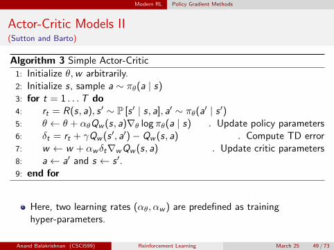
Algorithm 3 Simple Actor-Critic

1: Initialize θ,w arbitrarily.2: Initialize s, sample a ∼ πθ(a | s)3: for t = 1 . . .T do4: rt = R(s, a), s ′ ∼ P [s ′ | s, a], a′ ∼ πθ(a′ | s ′)5: θ ← θ + αθQw (s, a)∇θ log πθ(a | s) . Update policy parameters6: δt = rt + γQw (s ′, a′)− Qw (s, a) . Compute TD error7: w ← w + αwδt∇wQw (s, a) . Update critic parameters8: a← a′ and s ← s ′.9: end for

Here, two learning rates (αθ, αw ) are predefined as traininghyper-parameters.



Advantage Actor Critic (A2C) I(Mnih et al.)

Figure: This algorithm is the same as Asynchronous Advantage Actor Critic(A3C) with the exception that A2C runs in a synchronous fashion. It is shownthat A2C is generally better than A3C.



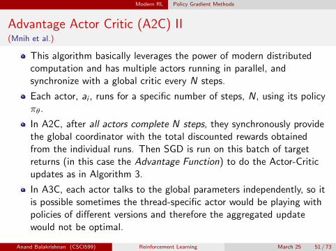
Advantage Actor Critic (A2C) II(Mnih et al.)

This algorithm basically leverages the power of modern distributedcomputation and has multiple actors running in parallel, andsynchronize with a global critic every N steps.

Each actor, ai , runs for a specific number of steps, N, using its policyπθ.

In A2C, after all actors complete N steps, they synchronously providethe global coordinator with the total discounted rewards obtainedfrom the individual runs. Then SGD is run on this batch of targetreturns (in this case the Advantage Function) to do the Actor-Criticupdates as in Algorithm 3.

In A3C, each actor talks to the global parameters independently, so itis possible sometimes the thread-specific actor would be playing withpolicies of different versions and therefore the aggregated updatewould not be optimal.



Other Extensions

Deterministic Policy Gradient (DPG) (Silver et al.) extends the PGalgorithm to deterministic policies (as opposed to stochastic).

DDPG (Lillicrap et al.) extends the DPG algorithm with ideas fromDQN, and thus extends DQN to the continuous domain.

Trust Region Policy Optimization (Schulman et al. TRPO), ProximalPolicy Optimization (Schulman et al. PPO) and ACKTR (Wu et al.)further improve on the PG algorithm by using so-called naturalgradients that provide better approximation of the gradient direction.

ACER (Z. Wang et al.) and Soft Actor-Critic (Haarnoja et al. SAC)both improve on the Actor-Critic algorithm by incorporating off-policyexperience replay.

SAC also incorporates the entropy measure of the stochastic policyinto the returns to encourage exploration.


RL for Autonomous CPS

Outline

1 Introduction


3 Approaches




7 References


RL for Autonomous CPS Applications

Applications of RL in CPSCPS + Formal Methods Community

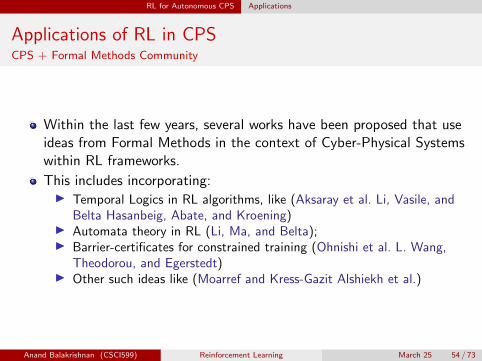
Within the last few years, several works have been proposed that useideas from Formal Methods in the context of Cyber-Physical Systemswithin RL frameworks.

This includes incorporating:I Temporal Logics in RL algorithms, like (Aksaray et al. Li, Vasile, and

Belta Hasanbeig, Abate, and Kroening)I Automata theory in RL (Li, Ma, and Belta);I Barrier-certificates for constrained training (Ohnishi et al. L. Wang,

Theodorou, and Egerstedt)I Other such ideas like (Moarref and Kress-Gazit Alshiekh et al.)


RL for Autonomous CPS Applications

Applications of RL in CPSRL Community

Inverse Reinforcement Learning:I Given policy π or behavior history sampled using a given policy, find a

reward function for which the behavior is optimal.I The goal is to essentially derive a model that discriminates good

behavior from bad, by looking at the demonstrations given by a“expert” (human or otherwise).

I Some key works are:

“Algorithms for Inverse Reinforcement Learning”“Apprenticeship Learning via Inverse Reinforcement Learning”“Maximum Entropy Inverse Reinforcement Learning.”

Learning from Demonstrations/Apprenticeship Learning/ImitationLearning:I Goal is to learn a policy from demonstrations, using either direct

mapping (deep learning) techniques or IRL.


RL for Autonomous CPS Challenges

Challenges: RL in Autonomous CPS

Although many deep RL algorithms perform very well, they are verysensitive to hyperparameters and design of reward functions.I This introduces a lot of uncertainty in the training of the controller!

Moreover, the RL algorithms we have discussed work on MDPs, thatis, the environment is fully observable.I This is, in general, not true.I In CPS examples, there is uncertainty in states (sensor/actuation noise,

state may be observable only by estimates, etc).I The approach to model this is by using Partially Observable MDPs

(POMDPs).



POMDPs I

POMDPs are incredibly powerful mathematical abstractions.

They have been used in recent works for various tasks:I Navigating an office: (Astrom).I Grasping with a robot arm: (Hsiao, Kaelbling, and Lozano-Perez).I Wind Farm Management: (Memarzadeh Milad, Pozzi Matteo, and Zico

Kolter J.).I Aircraft collision avoidance: (Mueller and Kochenderfer).



POMDPs II

Definition (POMDP)

It is a tuple 〈S ,A,P,R,Ω,O〉 where:

S ,A,P,R are the same as in and MDP;

Ω is a set of observations;

O : S × A× Ω→ [0, 1] is the observation function, which is aprobability distribution such that O(s, a, o) = P [o | s, a], ∀o ∈ Ω (theprobability of observing o if action a is taken in state s).

POMDPs model the information available to the agent by specifying afunction from the hidden state to the observables.



Planning for POMDPs

Unfortunately, the observations are not Markov (because two differentstates might look the same), which invalidates all of the MDPsolution techniques.

The optimal solution to this problem is to construct a belief stateMDP, where a belief state is a probability distribution over states.

Control theory is concerned with solving POMDPs, but in practice,control theorists make strong assumptions about the nature of themodel (typically linear-Gaussian) and reward function (typicallynegative quadratic loss) in order to be able to make theoreticalguarantees of optimality, etc.

By contrast, optimally solving a generic discrete POMDP is wildlyintractable. Finding tractable special cases (e.g., structured models)is a hot research topic.



Approachs to solve POMDPs

Research has been done since the 1960’s!

POMDPs are MDPs if they are properly updated over belief states(Astrom).

Belief states can be computed with the following general idea:I Start in some initial belied b prior to any observationsI Compute new belief state b′ based on current belief state b, action a,

and observation o.

This is a very common approach used in popular algorithms inrobotics, like:I Bayes Filters, Kalman Filters, and Particle Filters.



RL for POMDPsAdapted Policies (Singh, Jaakkola, and Jordan)

Definition (Adapted Policy)

is a mapping π : Ω× A→ [0, 1]. That is, π is a stochastic policy thatoperates on the observation space Ω as opposed to the state space S .

Moreover, the value function of the POMDP is associated with adistribution on states as opposed to a single state.This problem is then solved for relatively small, discrete, andlow-dimensional state-spaces using a modified Q-learning algorithm.



RL for POMDPsPoint-based Value Iteration (Porta, Spaan, and Vlassis)

In this approach,

A small set of reachable belief points is selected.

A Bellman equation is defined for those points, keeping value andgradient.

This approach is shown to be generalized to continuous state spaces,but not to continuous action and observation spaces.



RL for POMDPsDeep RL Methods

1 Use tracking techniques for Deep Learning data:I Deep Variational Bayes Filter (Karl et al.) uses variational inference

during batch updates to learn temporal and spatial dependencies.

2 Throw an Recurrent NN (LSTM/GRU) / Forget the math!:I DRQN (Hausknecht and Stone), RDPG (Heess et al.).I Recurrent Predictive State Policy (Hefny et al.).

3 Use human-like differentiable memory:I Neural Map (Parisotto and Salakhutdinov), MERLIN (Wayne et al.).


RL for Autonomous CPS Future Work and Open Problems

Future Work and Open Problems I

Verifiable Robotics and RL:I There are several challenges in modern RL and AI, some of which are

summarized in (Amodei et al. Leike et al.).I Most Deep RL systems are very sensitive to hyperparameter tuning,

this a lot of empirical results are hard to reproduce in environmentsthat differ from the environments used in a paper.

I Interpretability of policies learned by Deep RL algorithms is anotherkey issue, along with the interpretability of Deep Learning systems ingeneral.


RL for Autonomous CPS Future Work and Open Problems

Future Work and Open Problems II

Safety in CPS + Deep Learning systems:I This is a relatively new topic, where there have been attempts to use

Formal Methods to prove the safety of systems that use deep learningcontrollers.

This is not an easy task even in standard cyber-physical systems andhybrid systems.

The addition of a non-linear, “black-box” component just compoundsthis problem.

I There have also been attempts to incorporate ideas like TemporalLogic, Barrier Certificates, and Shields during the training of RLsystems.

I See: (Tian et al. Pei et al. S. Wang et al. Tuncali et al.)


References

Outline

1 Introduction


3 Approaches




7 References


References

References I

Abbeel, Pieter and Andrew Y. Ng. “Apprenticeship Learning via Inverse ReinforcementLearning”. Proceedings of the Twenty-First International Conference on Machine Learning.New York, NY, USA: ACM, 2004. 1–. Web. ICML ’04.

Aksaray, D., et al. “Q-Learning for Robust Satisfaction of Signal Temporal Logic Specifications”.2016 IEEE 55th Conference on Decision and Control (CDC). 2016. 6565–6570. Print.

Alshiekh, Mohammed, et al. “Safe Reinforcement Learning via Shielding”. (2017). Print.

Amodei, Dario, et al. “Concrete Problems in AI Safety”. (21 June 2016). arXiv: 1606.06565[cs]. Web.

Astrom, K. J. “Optimal Control of Markov Processes with Incomplete State Information”.Journal of Mathematical Analysis and Applications 10.1 (1965): 174–205. Print.

Barto, A. G., R. S. Sutton, and C. W. Anderson. “Neuronlike Adaptive Elements That CanSolve Difficult Learning Control Problems”. IEEE Transactions on Systems, Man, andCybernetics SMC-13.5 (Sept. 1983): 834–846. Print.

Bertsekas, Dimitri P. and John N. Tsitsiklis. Neuro-Dynamic Programming. Belmont, Mass:Athena Scientific, 1996. Print. Optimization and Neural Computation Series.

Haarnoja, Tuomas, et al. “Soft Actor-Critic: Off-Policy Maximum Entropy Deep ReinforcementLearning with a Stochastic Actor”. (4 Jan. 2018). arXiv: 1801.01290 [cs, stat]. Web.


http://doi.acm.org/10.1145/1015330.1015430

http://arxiv.org/abs/1606.06565





References

References II

Hasanbeig, Mohammadhosein, Alessandro Abate, and Daniel Kroening. “Logically-ConstrainedReinforcement Learning”. arXiv:1801.08099 [cs] (2018). arXiv: 1801.08099 [cs].

Hausknecht, Matthew and Peter Stone. “Deep Recurrent Q-Learning for Partially ObservableMDPs”. (23 July 2015). arXiv: 1507.06527 [cs]. Web.

Heess, Nicolas, et al. “Memory-Based Control with Recurrent Neural Networks”. (14 Dec.2015). Web.

Hefny, Ahmed, et al. “Recurrent Predictive State Policy Networks”. (5 Mar. 2018). Web.

Hsiao, Kaijen, Leslie Pack Kaelbling, and Tomas Lozano-Perez. “Robust Grasping under ObjectPose Uncertainty”. Autonomous Robots 31.2 (2011): 253. Print.

Karl, Maximilian, et al. “Deep Variational Bayes Filters: Unsupervised Learning of State SpaceModels from Raw Data”. (20 May 2016). Web.

Konda, Vijay R. and John N. Tsitsiklis. “Actor-Critic Algorithms”. Advances in NeuralInformation Processing Systems 12. Edited by S. A. Solla, T. K. Leen, and K. Muller. MITPress, 2000. 1008–1014. Print.

Kumar, P. R. and P. P. Varaiya. Stochastic Systems: Estimation, Identification, and AdaptiveControl. Philadelphia: Society for Industrial and Applied Mathematics, 2016. Print. Classicsin Applied Mathematics 75.

Leike, Jan, et al. “AI Safety Gridworlds”. (27 Nov. 2017). arXiv: 1711.09883 [cs]. Web.





https://arxiv.org/abs/1512.04455v1





References

References III

Levine, Sergey, et al. “End-to-End Training of Deep Visuomotor Policies”. (2 Apr. 2015). arXiv:1504.00702 [cs]. Web.

Li, X., C. Vasile, and C. Belta. “Reinforcement Learning with Temporal Logic Rewards”. 2017IEEE/RSJ International Conference on Intelligent Robots and Systems (IROS). 2017.3834–3839. Print.

Li, Xiao, Yao Ma, and Calin Belta. “Automata-Guided Hierarchical Reinforcement Learning forSkill Composition”. arXiv:1711.00129 [cs] (2017). arXiv: 1711.00129 [cs].

Lillicrap, Timothy P., et al. “Continuous Control with Deep Reinforcement Learning”. (9 Sept.2015). arXiv: 1509.02971 [cs, stat]. Web.

Memarzadeh Milad, Pozzi Matteo, and Zico Kolter J. “Optimal Planning and Learning inUncertain Environments for the Management of Wind Farms”. Journal of Computing in CivilEngineering 29.5 (2015): 04014076. Print.

Mnih, Volodymyr, et al. “Asynchronous Methods for Deep Reinforcement Learning”. (4 Feb.2016). arXiv: 1602.01783 [cs]. Web.

Mnih, Volodymyr, et al. “Human-Level Control through Deep Reinforcement Learning”. Nature518.7540 (Feb. 2015): 529–533. Web.

Moarref, S. and H. Kress-Gazit. “Decentralized Control of Robotic Swarms from High-LevelTemporal Logic Specifications”. 2017 International Symposium on Multi-Robot andMulti-Agent Systems (MRS). 2017. 17–23. Print.









http://www-nature-com/articles/nature14236

References

References IV

Mueller, Eric R. and Mykel Kochenderfer. “Multi-Rotor Aircraft Collision Avoidance UsingPartially Observable Markov Decision Processes”. AIAA Modeling and SimulationTechnologies Conference. American Institute of Aeronautics and Astronautics, 2016. Print.AIAA AVIATION Forum.

Ng, Andrew Y. and Stuart Russell. “Algorithms for Inverse Reinforcement Learning”. In Proc.17th International Conf. on Machine Learning. Morgan Kaufmann, 2000. 663–670. Print.

Ohnishi, Motoya, et al. “Barrier-Certified Adaptive Reinforcement Learning with Applications toBrushbot Navigation”. arXiv:1801.09627 [cs] (2018). arXiv: 1801.09627 [cs].

Parisotto, Emilio and Ruslan Salakhutdinov. “Neural Map: Structured Memory for DeepReinforcement Learning”. (27 Feb. 2017). Web.

Pei, Kexin, et al. “DeepXplore: Automated Whitebox Testing of Deep Learning Systems”.Proceedings of the 26th Symposium on Operating Systems Principles - SOSP ’17 (2017):1–18. arXiv: 1705.06640.

Porta, Josep M., Matthijs T. J. Spaan, and Nikos A. Vlassis. “Robot Planning in PartiallyObservable Continuous Domains”. Robotics: Science and Systems. 2005. Print.

Pritzel, Alexander, et al. “Neural Episodic Control”. (6 Mar. 2017). arXiv: 1703.01988 [cs,

stat]. Web.

Schaul, Tom, et al. “Prioritized Experience Replay”. (18 Nov. 2015). arXiv: 1511.05952 [cs].Web.










References

References V

Schulman, John, et al. “High-Dimensional Continuous Control Using Generalized AdvantageEstimation”. (8 June 2015). arXiv: 1506.02438 [cs]. Web.

Schulman, John, et al. “Proximal Policy Optimization Algorithms”. (19 July 2017). arXiv:1707.06347 [cs]. Web.

Schulman, John, et al. “Trust Region Policy Optimization”. (19 Feb. 2015). arXiv: 1502.05477[cs]. Web.

Silver, David, et al. “Deterministic Policy Gradient Algorithms”. ICML. 2014. Print.

Silver, David, et al. “Mastering the Game of Go with Deep Neural Networks and Tree Search”.Nature 529.7587 (Jan. 2016): 484–489. Web.

Singh, Satinder P., Tommi Jaakkola, and Michael I. Jordan. “Learning WithoutState-Estimation in Partially Observable Markovian Decision Processes”. Machine LearningProceedings 1994. Edited by William W. Cohen and Haym Hirsh. San Francisco (CA):Morgan Kaufmann, 1994. 284–292. Print.

Sutton, Richard S. and Andrew G. Barto. Reinforcement Learning: An Introduction. Secondedition. Cambridge, MA: The MIT Press, 2018. Print. Adaptive Computation and MachineLearning Series.









https://www.nature.com/articles/nature16961

References

References VI

Sutton, Richard S., et al. “Policy Gradient Methods for Reinforcement Learning with FunctionApproximation”. Advances in Neural Information Processing Systems. 2000. 1057–1063.Print.

Tian, Yuchi, et al. “DeepTest: Automated Testing of Deep-Neural-Network-Driven AutonomousCars”. arXiv:1708.08559 [cs] (2017). arXiv: 1708.08559 [cs].

Tuncali, Cumhur Erkan, et al. “Reasoning about Safety of Learning-Enabled Components inAutonomous Cyber-Physical Systems”. arXiv:1804.03973 [cs] (2018). arXiv: 1804.03973[cs].

Van Hasselt, Hado, Arthur Guez, and David Silver. “Deep Reinforcement Learning with DoubleQ-Learning”. (22 Sept. 2015). arXiv: 1509.06461 [cs]. Web.

Wang, L., E. A. Theodorou, and M. Egerstedt. “Safe Learning of Quadrotor Dynamics UsingBarrier Certificates”. 2018 IEEE International Conference on Robotics and Automation(ICRA). 2018. 2460–2465. Print.

Wang, Shiqi, et al. “Efficient Formal Safety Analysis of Neural Networks”. arXiv:1809.08098 [cs,stat] (2018). arXiv: 1809.08098 [cs, stat].

Wang, Ziyu, et al. “Dueling Network Architectures for Deep Reinforcement Learning”. (20 Nov.2015). arXiv: 1511.06581 [cs]. Web.

Wang, Ziyu, et al. “Sample Efficient Actor-Critic with Experience Replay”. (3 Nov. 2016). arXiv:1611.01224 [cs]. Web.












References

References VII

Watkins, Christopher John Cornish Hellaby. “Learning from Delayed Rewards”. Diss. King’sCollege, Cambridge, 1989. Print.

Wayne, Greg, et al. “Unsupervised Predictive Memory in a Goal-Directed Agent”. (28 Mar.2018). Web.

Williams, Ronald J. “Simple Statistical Gradient-Following Algorithms for ConnectionistReinforcement Learning”. Machine Learning 8.3 (May 1992): 229–256. Print.

Wu, Yuhuai, et al. “Scalable Trust-Region Method for Deep Reinforcement Learning UsingKronecker-Factored Approximation”. (17 Aug. 2017). arXiv: 1708.05144 [cs]. Web.

Ziebart, Brian D., et al. “Maximum Entropy Inverse Reinforcement Learning.” Aaai. Chicago,IL, USA, 2008. 1433–1438. Print.





Reinforcement Learning for Cyber-Physical Systems

Documents

Transcript of Reinforcement Learning for Cyber-Physical Systems