REIMBURSABLE ADVISORY SERVICES (RAS): CONSTRUCTION OF ...
274
E3-Modelling | Athens, July 2018 REIMBURSABLE ADVISORY SERVICES (RAS): CONSTRUCTION OF ECONOMIC MODELING TOOLS AND BUILDING CAPACITY IN MODELING FOR SUSTAINED GROWTH IN THE SLOVAK REPUBLIC USER’S GUIDE TO THE CPS MODEL
Transcript of REIMBURSABLE ADVISORY SERVICES (RAS): CONSTRUCTION OF ...

Page | 1
E3-Modelling | Athens, July 2018
REIMBURSABLE ADVISORY SERVICES (RAS): CONSTRUCTION OF ECONOMIC MODELING TOOLS AND BUILDING CAPACITY IN MODELING FOR SUSTAINED GROWTH IN THE SLOVAK REPUBLIC
USER’S GUIDE TO THE CPS MODEL

REIMBURSABLE ADVISORY SERVICES (RAS): CONSTRUCTION OF ECONOMIC MODELING TOOLS AND BUILDING CAPACITY IN MODELING FOR
SUSTAINED GROWTH IN THE SLOVAK REPUBLIC
Page | 2
Authors
Panagiotis Karkatsoulis, Maria Kannavou, Pantelis Capros and Stavroula
Evangelopoulou.
With contributions from
Nikos Tasios, Katerina Sardi and Leonidas Paroussos

REIMBURSABLE ADVISORY SERVICES (RAS): CONSTRUCTION OF ECONOMIC MODELING TOOLS AND BUILDING CAPACITY IN MODELING FOR
SUSTAINED GROWTH IN THE SLOVAK REPUBLIC
Page | 3
This User Manual and the CPS Model described within, are products of E3 Modelling prepared under Contract No. 7182219/2017
between the World Bank Group and E3 Modelling. The User Manual is solely intended for the members of the World Bank Group
and Slovakian CMT which are involved in this Contract. Distribution of the User Manual and the CPS Model to others outside the
above group is strictly forbidden.

REIMBURSABLE ADVISORY SERVICES (RAS): CONSTRUCTION OF ECONOMIC MODELING TOOLS AND BUILDING CAPACITY IN MODELING FOR
SUSTAINED GROWTH IN THE SLOVAK REPUBLIC
Page | 4
Contents
1. Introduction ....................................................................................................................... 7
2. Starting and Executing the CPS model ..........................................................................11
2.1 Starting the CPS GUI ..................................................................................................11
2.2 The CPS GUI features ................................................................................................11
Preparing a Scenario with the CPS GUI ...............................................................12
Defining a Scenario Type and a new Scenario with the CPS GUI ........................14
Running a CPS scenario ......................................................................................17
Checking for runtime errors ..................................................................................18
Reporting .............................................................................................................20
Resetting Scenario Inputs ....................................................................................21
Exiting the GUI CPS Model ..................................................................................22
2.3 Locating the CPS Model Subfolders and the respective GAMS Files ..........................23
2.4 The structure of the Scenario name subfolder .............................................................25
3. Input and Output Data .....................................................................................................26
3.1 Common Input Data ....................................................................................................26
Definitions ............................................................................................................26
Sets_CPS.xlsm ....................................................................................................27
Exogdata.xlsx ......................................................................................................28
3.2 Output Data ................................................................................................................29
Final Report file ....................................................................................................29
Database file ........................................................................................................34
Approaches used in Energy Balances Reporting .................................................35
4. Overview of the CPS Demand Module ............................................................................37
4.1 Basic concepts in the CPS Demand Module ...............................................................37
4.2 Mathematical structure, unknown variables and exogenous parameters .....................39
Mathematical structure .........................................................................................39
Unknown variables ..............................................................................................60
Exogenous Parameters .......................................................................................61
4.3 Model features, considerations and assumptions ........................................................62
Sectoral coverage of the CPS Demand Module ...................................................63
4.4 Policy Focus – Demand ..............................................................................................68

REIMBURSABLE ADVISORY SERVICES (RAS): CONSTRUCTION OF ECONOMIC MODELING TOOLS AND BUILDING CAPACITY IN MODELING FOR
SUSTAINED GROWTH IN THE SLOVAK REPUBLIC
Page | 5
Policy drivers of Demand Module .........................................................................69
4.5 Explaining the demand-related scenario input file .......................................................71
Macro_data ..........................................................................................................73
Drivers_data ........................................................................................................74
Prices_data ..........................................................................................................75
Techdata_sf .........................................................................................................77
Techdata_ep ........................................................................................................79
Policy_dem_data .................................................................................................80
EquipmentSubsidy ...............................................................................................81
Perceived Costs sheets .......................................................................................82
Potential ...............................................................................................................84
LBD ..................................................................................................................85
ThetaOptimum .................................................................................................86
Exo_effi_ORD ..................................................................................................86
HER_logit .........................................................................................................87
Sheets dACTSBC_inert to dACTSEF_AG_ST_inert .........................................88
dSW_F_inert_av ..............................................................................................90
Options for changing parameters’ values exogenously .....................................90
5. Overview of the CPS Power Module ...............................................................................96
5.1 Basic concepts in the CPS Power Module ..................................................................96
5.2 Mathematical Structure, unknown variables and exogenous parameters .................. 100
Mathematical Structure ...................................................................................... 100
Unknown variables ............................................................................................ 110
Exogenous Parameters ..................................................................................... 111
5.3 Model features, considerations and assumptions ...................................................... 111
Representation of Plants .................................................................................... 112
5.4 Principles of the pricing model .................................................................................. 124
5.5 Policy Focus – Power ............................................................................................... 126
Targets .............................................................................................................. 126
Policy drivers of the CPS Power Module ............................................................ 127
5.6 Explaining the supply-related scenario input file ........................................................ 128
Techdata_plants ................................................................................................ 129
Fuelswitch .......................................................................................................... 131
Fuelblend ........................................................................................................... 132

REIMBURSABLE ADVISORY SERVICES (RAS): CONSTRUCTION OF ECONOMIC MODELING TOOLS AND BUILDING CAPACITY IN MODELING FOR
SUSTAINED GROWTH IN THE SLOVAK REPUBLIC
Page | 6
Policy_power_data ............................................................................................ 133
Level_struct (non – linear curves) ...................................................................... 135
Options for changing parameters’ values exogenously ...................................... 136
6. Overview of the CPS Biomass Module ......................................................................... 147
6.1 Basic concepts in the CPS Biomass Module ............................................................. 147
6.2 Mathematical structure, unknown variables and exogenous parameters ................... 149
Mathematical structure ....................................................................................... 149
Unknown variables ............................................................................................ 152
Exogenous Parameters ..................................................................................... 153
Model features, considerations and assumptions Feedstock ............................. 153
6.3 Policy Focus - Biomass ............................................................................................. 156
6.4 Explaining the biomass-related scenario input sheets ............................................... 157
Techdata_bio ..................................................................................................... 157
Policy_biofuels ................................................................................................... 160
Options for changing parameters’ values exogenously ...................................... 161
Appendix I CPS Model’s Sets ............................................................................................... 164
Appendix II Sectoral structure of the CPS demand sectors .............................................. 170
Appendix III Mathematical formulation of the CPS Demand Module ................................. 189
Appendix IV Mathematical formulation of the CPS Power Module .................................... 190
Appendix V Mathematical formulation of the CPS Biomass Module ................................. 191

REIMBURSABLE ADVISORY SERVICES (RAS): CONSTRUCTION OF ECONOMIC MODELING TOOLS AND BUILDING CAPACITY IN MODELING FOR
SUSTAINED GROWTH IN THE SLOVAK REPUBLIC
Page | 7
1. Introduction
The CPS Model has been developed by E3-Modelling in the context of Contract 7182219/15.02.2017
between E3-Modelling and the World Bank.
This document is the User’s Manual to the CPS Model (Compact-PRIMES Single Country model). It aims
to serve as a methodological and technical guide to users so that they become fully equipped to utilize
the CPS, appreciate its’ unique features and comprehend the mathematical approach implemented
within.
The model, developed in the General Algebraic Modelling System (GAMS)1, is a fully-fledged energy
demand and supply model, designed as a single-country compact tool.
The model allows users to assess the impact of European and national climate and energy policy decisions
with a horizon up to 2050. The model includes key energy sector metrics at a detailed level: demand of
energy by sector, modelling of energy efficiency possibilities, energy and electricity use, technology
capacities, power generation, cogeneration, energy supply technology and energy form mix, fuel prices
and system costs from an end-user perspective, investments by sector and energy-related CO2 emissions.
The CPS model runs up to 2050 and the electricity model performs hourly simulations. The model
structure permits linkages with the external (outside the country) markets, to get international fuel prices,
carbon prices of ETS etc. It allows for a flexible definition of technological parameters and technological
learning, overall efficiencies, and specific investment lead times for technologies.
The model is actor and market oriented, and so it represents individual actors’ decisions in supply and
demand of energy and the balancing of their decisions in simultaneous markets cleared by prices. In this
way, the model explicitly projects energy forms’ prices into the future as derived from cost minimization
in the supply side and the price-elastic behaviors of demanders for energy. In this sense the model has no
overall objective function, but as economic theory suggests, the simultaneous market clearing under
perfect competition conditions leads to an overall optimum of economic welfare, which coincides with
minimum cost of energy for the end-users. In the energy supply sectors, the model performs a detailed
breakdown of cost categories, such as capital, operational, emission-related and maintenance costs. All
external assumptions, including fossil fuel prices, price elasticities, technological or policy constraints are
presented in a transparent manner and can be tested in sensitivity analysis.
A substantial part of the mathematics of CPS are derived from the well-known PRIMES2 model, a large-
scale modular system of sub-models, covering multiple countries also developed within our group.
1 https://www.gams.com/ 2 PRIMES (Price-Induced Market Equilibrium System) energy system model is a development of the Energy-Economy Environment
Modelling Laboratory at National Technical University of Athens (http://www.e3mlab.eu/e3mlab/PRIMES%20Manual/The%20PRIMES%20MODEL%202016-7.pdf).

REIMBURSABLE ADVISORY SERVICES (RAS): CONSTRUCTION OF ECONOMIC MODELING TOOLS AND BUILDING CAPACITY IN MODELING FOR
SUSTAINED GROWTH IN THE SLOVAK REPUBLIC
Page | 8
Figure 1 Schematic of the CPS model structure
The CPS comprises four Modules:
Demand Module: The Demand Module projects energy demand and investments in the
industrial, domestic and transport sectors, as well as refineries.
Power Module: The Power Module includes all necessary mathematical formulations for
projecting energy supply. It includes detailed and distinct representations of the Slovak power
system, including district heating plants (boilers and CHP plants). The Power Module also
accounts for the steam and power produced in the industrial sector (industrial boilers and
CHP).
Biomass Module: The Biomass Module projects the primary energy-feedstock consumption
required to satisfy the demand for bioenergy from all demand sectors, as well as the power-
heat generation system.
Balance Module: The Balance Module receives the results of energy consumption from the
CPS Demand, Power and Biomass Modules and produces the annual energy balances.
The four modules communicate as shown in Figure 1, and iterate in order to reach a market equilibrium.
The following paragraphs provide further details on the outputs of each Module:
Demand Module:
Energy Demand by sector and fuel

REIMBURSABLE ADVISORY SERVICES (RAS): CONSTRUCTION OF ECONOMIC MODELING TOOLS AND BUILDING CAPACITY IN MODELING FOR
SUSTAINED GROWTH IN THE SLOVAK REPUBLIC
Page | 9
CO2 emissions by sector
Energy Savings, Energy and Carbon Intensity
Costs (capital, fuel, non-fuel, emissions & taxation costs)
Investments & Investment Expenditures
Power Module:
Power & Heat Generation by plant type
Fuel Consumption by plant type and fuel
CO2 emissions & Carbon Intensity by plant type
Costs of electricity & heat supply (capital, fuel, non-fuel, emission & taxation, grid costs)
Capacity Expansion & Investment Expenditures by plant type
Biomass Module:
Production of Bioenergy per fuel
Price of Bioenergy per fuel
Net Imports of Biomass Feedstock & Bioenergy
Domestic Production of Biomass Feedstock
Capacity Expansion per Biomass Technology
Balance Module:
Energy balance for each projection year (End-use approach)
The simulation results are dynamic over time and are influenced by factors which are exogenously
specified. The user can easily build multiple scenarios to assess a variety of parameters. Input data for
each scenario include the following:
GDP, Income per capita, population
Fuel availability constraints (e.g. renewables potential, domestic reserves for fossil fuels,
import limitations)
Technology characteristics (energy conversion rates, CAPEX, OPEX)
Taxes and subsidies
Discount rates
Technology standards
Emission, renewables and energy efficiency regulations
Targets for emissions, renewables and energy efficiency
Perceived or hidden costs
Exogenous investments, decommissioning or retrofitting of power and heat plants.
The next Chapters highlight the features of the CPS Model.
A brief description of each Chapter is listed below. Appendices III, IV and V offer a detailed listing of the
mathematical formulation of Demand, Power and Biomass Modules.

REIMBURSABLE ADVISORY SERVICES (RAS): CONSTRUCTION OF ECONOMIC MODELING TOOLS AND BUILDING CAPACITY IN MODELING FOR
SUSTAINED GROWTH IN THE SLOVAK REPUBLIC
Page | 10
Chapter 2 Starting and Executing the CPS model describes the mechanics of using the graphical
user interface in order to run an existing scenario, create a new scenario, check for possible errors
in the model run and view scenario results.
Chapter 3 Input and Output Data describes the information inserted in the Model and the form
and content of the results’ files.
Chapter 4 Overview of the CPS Demand Module describes the main principles of the CPS Demand
Module and guides the user towards the formulation of alternative scenarios related to
influencing and projecting energy demand.
Chapter 5 Overview of the CPS Power Module describes the main principles of the CPS Power
Module and guides the user towards the formulation of alternative scenarios related to power
supply.
Chapter 6 Overview of the CPS Biomass Module describes the main principles of the CPS Biomass
Module and guides the user towards the formulation of alternative scenarios related to biomass
supply.
Appendix I CPS Model’s Sets
Appendix II Sectoral structure of the demand sectors
Appendix III Mathematical formulation of the Demand Module
Appendix IV Mathematical formulation of the Power Module
Appendix V Mathematical formulation of the Biomass Module

REIMBURSABLE ADVISORY SERVICES (RAS): CONSTRUCTION OF ECONOMIC MODELING TOOLS AND BUILDING CAPACITY IN MODELING FOR
SUSTAINED GROWTH IN THE SLOVAK REPUBLIC
Page | 11
2. Starting and Executing the CPS model
This Chapter provides instructions for starting and executing the CPS Model through the custom-made
CPS Graphical User Interface (hereinafter CPS GUI). The Chapter is structured as follows:
Section 2.1: Starting the CPS GUI
Section 2.2: The CPS GUI Features
Section 2.3: Locating the CPS Model Subfolders and the respective Gams Files
Section 2.4: The structure of the Scenario name subfolder
Note that the CPS user may alternatively omit the GUI and run directly the model through GAMS interface.
2.1 Starting the CPS GUI
Before running the CPS GUI for the first time, the user needs to install the CPS Model and all its’ Modules
(including the CPS GUI) in drive C or D, in a predefined directory named CPS_SK_2018_new.
The CPS GUI runs by double clicking upon the CPS_GUI application located in the path
CPS_SK_2018_new\GUI, see Figure 2.
Figure 2 Location of the CPS_GUI Application file
Alternatively, the CPS user can access the CPS GUI through a shortcut created on the desktop (or in any
other location that the CPS user is comfortable with)
2.2 The CPS GUI features
The CPS GUI is a facilitator, which allows the user to access and interact with the CPS Model in a simple
and user friendly way, through a variety of graphical icons.
The CPS GUI allows the CPS user to perform the following:
Create a new CPS Scenario
Run a CPS Scenario
Perform an error checking analysis. The error check functionality reports on any errors that may
have prohibited the successful conclusion of a scenario’s run
Create the final reporting files and view the final results
The next paragraphs provide further details.

REIMBURSABLE ADVISORY SERVICES (RAS): CONSTRUCTION OF ECONOMIC MODELING TOOLS AND BUILDING CAPACITY IN MODELING FOR
SUSTAINED GROWTH IN THE SLOVAK REPUBLIC
Page | 12
For the purposes of the next paragraphs it is assumed that the CPS user has already loaded the CPS GUI
as described in Section 2.1 Starting the CPS GUI.
Figure 3 Starting with CPS GUI, step 1, choose folder directory
Preparing a Scenario with the CPS GUI
To run a Scenario with the CPS GUI, the CPS user should do the following:
Press the “Choose Folder Directory” pushbutton. Select the corresponding folder from the
browsing window that will appear. Eligible folder directories are named “CPS_SK_2018_new” (e.g. C:\
CPS_SK_2018_new or D:\ CPS_SK_2018_new), see Figure 3;
Press the “Click here to set the options to run a CPS Scenario” pushbutton, see Figure 4.
Select the type of scenario to be run by selecting from the “Choose a scenario type” list from the
two available options (see Figure 5):
Reference
Scenario

REIMBURSABLE ADVISORY SERVICES (RAS): CONSTRUCTION OF ECONOMIC MODELING TOOLS AND BUILDING CAPACITY IN MODELING FOR
SUSTAINED GROWTH IN THE SLOVAK REPUBLIC
Page | 13
Figure 4 Starting with CPS GUI, step 2
Figure 5 Starting with CPS GUI, step 3, choose a scenario type

REIMBURSABLE ADVISORY SERVICES (RAS): CONSTRUCTION OF ECONOMIC MODELING TOOLS AND BUILDING CAPACITY IN MODELING FOR
SUSTAINED GROWTH IN THE SLOVAK REPUBLIC
Page | 14
Figure 6 Starting with CPS GUI, running a reference scenario
Defining a Scenario Type and a new Scenario with the CPS GUI
The CPS GUI allows the user to select between the following Scenario Types:
Reference: A Reference Scenario represents a current situation scenario (for example a
Reference Scenario is a scenario that includes all adopted national and EU policies up to 2020)
Scenario: Other (decarbonization) Scenario
To run a Reference Scenario, the CPS user needs to select the “Reference” from the list, as shown in Figure
6.
To run a decarbonization scenario, the CPS user needs to select the “Scenario” type, as shown in Figure 7.
Upon this specific selection, further options regarding the run of a decarbonization scenario will appear.
These options are explained below.

REIMBURSABLE ADVISORY SERVICES (RAS): CONSTRUCTION OF ECONOMIC MODELING TOOLS AND BUILDING CAPACITY IN MODELING FOR
SUSTAINED GROWTH IN THE SLOVAK REPUBLIC
Page | 15
Figure 7 Starting with CPS GUI, running a decarbonization scenario
To create a new Scenario, the CPS user takes the following actions as shown in Figure 8:
Types the name of the Scenario basis in the Scenario basis text box.
Types the Scenario Name in the Scenario Name text box.
Clicks the “Check scenario name” pushbutton.
Figure 8 Creating a new scenario

REIMBURSABLE ADVISORY SERVICES (RAS): CONSTRUCTION OF ECONOMIC MODELING TOOLS AND BUILDING CAPACITY IN MODELING FOR
SUSTAINED GROWTH IN THE SLOVAK REPUBLIC
Page | 16
By pressing the “Check scenario name” pushbutton the CPS user instructs the GUI to search
for a subfolder named after the Scenario name (hereinafter Scenario name subfolder). In case that
a Scenario name subfolder is found in the “Scenarios” folder of the CPS directory then a
notification message will appear on the screen, as shown in Figure 9.
Figure 9 Message confirming that the decarbonization scenario typed by the CPS user in the Scenario name text box exists
In case that a Scenario name subfolder does not exist in the “Scenarios” folder, a message
prompting the CPS user to create a new scenario will appear, Figure 10.

REIMBURSABLE ADVISORY SERVICES (RAS): CONSTRUCTION OF ECONOMIC MODELING TOOLS AND BUILDING CAPACITY IN MODELING FOR
SUSTAINED GROWTH IN THE SLOVAK REPUBLIC
Page | 17
Figure 10 Message confirming that the decarbonization scenario typed by the CPS user in the Scenario name text box does not exist
If the Scenario name subfolder does not exist, the CPS user presses the “Create a new
scenario” pushbutton, Figure 11. This action generates the required new subfolder. Further
subfolders are also created within the Scenario name Folder. The “Create a new scenario”
action also copies the Input excel files of the Scenario Basis in the Scenario Folder. All input
files are placed in the “Inputxlsx” subfolder.
The user can access the input files, by pressing the “Open the scenario name input excel file”
pushbutton, which opens the relevant input files in Excel.
Figure 11 CPS GUI, creating a new scenario
Running a CPS scenario
To run a CPS scenario, the CPS user clicks the “Run a CPS Scenario” pushbutton, Figure 12.

REIMBURSABLE ADVISORY SERVICES (RAS): CONSTRUCTION OF ECONOMIC MODELING TOOLS AND BUILDING CAPACITY IN MODELING FOR
SUSTAINED GROWTH IN THE SLOVAK REPUBLIC
Page | 18
Figure 12 CPS GUI, running a CPS scenario
Checking for runtime errors
The CPS user should always check for any runtime errors. The CPS GUI has been purposely designed to
allow such a check through a very straightforward process.
Following the end of a GUI CPS run, the CPS user selects the “Errors Check” checkbox. Upon checkbox
selection, the “Check logs in Scenario” option will appear, as shown in Figure 13.
Figure 13 CPS GUI, error check

REIMBURSABLE ADVISORY SERVICES (RAS): CONSTRUCTION OF ECONOMIC MODELING TOOLS AND BUILDING CAPACITY IN MODELING FOR
SUSTAINED GROWTH IN THE SLOVAK REPUBLIC
Page | 19
The user can either type the Scenario name to be checked or press the “Help” pushbutton, to select a
Scenario by selecting the Scenario name subfolder from a browser window.
Then, the CPS user must press the “Errors Check” pushbutton. The CPS GUI proceeds in a detailed
check of the status files of Demand Module for all iterations. The status files are output text files that are
created by the Demand Module after completion of every iteration of the model run, indicating whether
the module has or has not solved. It also checks all the log files of Power, Biomass and Balance Module,
in order to trace possible error notifications. In case the scenario has run without errors a verification
message appears on the screen, as shown in Figure 14 (e.g. for the 1st iteration) and Figure 15. In case
error notifications are found in the log files, then an appropriate message informs the user on the type of
the errors that have occurred.
Figure 14 CPS GUI, Message informing the user of normal completion of the Demand Module

REIMBURSABLE ADVISORY SERVICES (RAS): CONSTRUCTION OF ECONOMIC MODELING TOOLS AND BUILDING CAPACITY IN MODELING FOR
SUSTAINED GROWTH IN THE SLOVAK REPUBLIC
Page | 20
Figure 15 CPS GUI, Message informing the user of no encountered errors in the Power Module
Reporting
The “Enable Reporting” checkbox allows the user to access the Final Results Excel Files, see Figure 16.
The procedure is completed in three simple steps as follows:
1) After clicking the “Enable Reporting” check box, the user types the name of the Scenario to
be processed in the corresponding field. Alternatively, the user may click the help pushbutton and select
the Scenario name subfolder.
2) Then, the user clicks the “Run Final Report for Scenario” pushbutton. Two messages
informing the user that the “the final report/database report file has been created” will appear on the
screen, see Figure 16.
3) The user can then press the “Open Final Results Excel File” pushbutton to gain access to
the report excel files.

REIMBURSABLE ADVISORY SERVICES (RAS): CONSTRUCTION OF ECONOMIC MODELING TOOLS AND BUILDING CAPACITY IN MODELING FOR
SUSTAINED GROWTH IN THE SLOVAK REPUBLIC
Page | 21
Figure 16 CPS GUI, Creation of results files
Resetting Scenario Inputs
The CPS GUI also provides a reset inputs option, see Figure 17.
By clicking on the “Reset Scenario inputs” pushbutton, the user resets all parameters included in the
input excel files to the values of the Scenario basis. This is a very useful functionality provided by the GPS
GUI, as it allows the user to quickly reset all changes (including potential errors) and start again the
Scenario definition.

REIMBURSABLE ADVISORY SERVICES (RAS): CONSTRUCTION OF ECONOMIC MODELING TOOLS AND BUILDING CAPACITY IN MODELING FOR
SUSTAINED GROWTH IN THE SLOVAK REPUBLIC
Page | 22
Figure 17 CPS GUI, Resetting the Scenario input file
Exiting the GUI CPS Model
The user may exit the GUI by clicking the “Exit” pushbutton.
Figure 18 Exiting the CPS GUI

REIMBURSABLE ADVISORY SERVICES (RAS): CONSTRUCTION OF ECONOMIC MODELING TOOLS AND BUILDING CAPACITY IN MODELING FOR
SUSTAINED GROWTH IN THE SLOVAK REPUBLIC
Page | 23
2.3 Locating the CPS Model Subfolders and the respective GAMS Files
The CPS Model folder structure comprises 5 subfolders:
1. The CommonData subfolder which includes the excel input files that are common between
scenarios. These are the Sets_CPS and Exogdata excel files, described further in section 3.1
Common Input Data.
2. The GUI subfolder which includes the GUI application file.
3. The Model subfolder which includes all gams (.gms) files of the model, the corresponding gams
project and the solver option files that are used by the CPS model. The overview of the gams files
comprising the model, as well as the way the CPS Modules are linked with each other are shown
in Figure 19.
4. The Scenarios subfolder which contains the Scenario name subfolders (i.e. subfolders for
every scenario that has been created, e.g. Reference, DCarb1, DCarb2 subfolders). The structure
of the Scenario name subfolder is explained below, in Section 2.4 The structure of the Scenario
name subfolder.
5. The Templates subfolder which includes the excel template files for the Final Report and
Database excel files, which include the results of a scenario’s run.

REIMBURSABLE ADVISORY SERVICES (RAS): CONSTRUCTION OF ECONOMIC MODELING TOOLS AND BUILDING CAPACITY IN MODELING FOR
SUSTAINED GROWTH IN THE SLOVAK REPUBLIC
Page | 24
Figure 19 Overview of CPS gams files and linkage

REIMBURSABLE ADVISORY SERVICES (RAS): CONSTRUCTION OF ECONOMIC MODELING TOOLS AND BUILDING CAPACITY IN MODELING FOR
SUSTAINED GROWTH IN THE SLOVAK REPUBLIC
Page | 25
2.4 The structure of the Scenario name subfolder
The Scenario name subfolder includes 7 subfolders:
1. Inputxlsx: containing the input excel files of the scenario
2. Inputgdx: containing the input data that are relevant to the scenario in gdx format. The input
gdx files are created by the model during runtime
3. Outputxlsx: containing the results of the model run in excel format
4. Outputgdx: containing the results of the model run in gdx format
5. Lst: containing the lst files of the model run. Lst files are created at every iteration of the model
run, hence the corresponding numbers at the end of the files’ names
6. Log: containing the log files of the model run. Log files are created at every iteration of the model
run, hence the corresponding numbers at the end of the files’ names
7. Save: containing intermediate work files

REIMBURSABLE ADVISORY SERVICES (RAS): CONSTRUCTION OF ECONOMIC MODELING TOOLS AND BUILDING CAPACITY IN MODELING FOR
SUSTAINED GROWTH IN THE SLOVAK REPUBLIC
Page | 26
3. Input and Output Data
3.1 Common Input Data
As described in Section 2.3 Locating the CPS Model Subfolders and the respective Gams Files, the
CommonData subfolder contains two excel files, Sets_CPS and Exogdata. Both files are essential
for the CPS Model to run.
These files contain information which are common between scenarios. The data types included in these
files are sets and parameters. Before proceeding it is useful to clarify the meaning of sets and parameters
in GAMS.
Definitions
The definition of sets as mentioned in GAMS User’s Guide3 is presented in Box 1 Definition of sets in GAMS.
Box 1 Definition of sets in GAMS
Sets: Sets are the basic building blocks of a GAMS model, corresponding exactly to the indices in the
algebraic representations of Models
For example, the set “SW” is the set of technology categories incorporated in the CPS Model and includes
the technology types shown in Table 1.
Table 1 Elements of set SW
Technology type Description
ORD Ordinary
ORI Ordinary-Improved Intermediate
IMR Improved
IMA Improved-Advanced Intermediate
ADV Advanced
ADF Advanced-Future Intermediate
FUT Future
A parameter is a data type, which enables the data entry of list oriented data. The dimensions (or indices)
of a parameter are sets. For example, the capital cost of an equipment is inserted in the Model in the form
of a parameter. The values of this parameter depend on the equipment (e.g. blast furnace, appliance for
material preparation, electric arc), the technology category of the equipment (ordinary, improved,
advanced) and the running year. Thus, capital cost is a parameter defined upon the sets of processes,
technology categories and years.
3 https://www.gams.com/24.8/docs/userguides/GAMSUsersGuide.pdf

REIMBURSABLE ADVISORY SERVICES (RAS): CONSTRUCTION OF ECONOMIC MODELING TOOLS AND BUILDING CAPACITY IN MODELING FOR
SUSTAINED GROWTH IN THE SLOVAK REPUBLIC
Page | 27
Sets_CPS.xlsm
The excel file Sets_CPS includes sets and parameters that constitute the core of the CPS Model. Table
2 below presents a selected/indicative list of the sets included in the Sets_CPS file, in order to familiarize
the user. All sets included in Sets_CPS.xlsm can be found in Appendix I.
Table 2 Sets included in Sets_CPS.xlsm
Universal CPS Sets Description
Year_all Set of all years that may be used in the Model: from 1960 to 2050 in 5-year steps
Year Set including the basis year 2015 (year of calibration) and projection years 2020 to 2050
Fuel_all Set of all fuels used in the Model
Demand Module Sets Description
SA Set of demand sectors upper level
SB Set of demand sectors second level
SC Set of demand sectors third level
SD Set of demand sectors fourth level
SE Set of supply of demand sectors upper level
SF Set of supply of demand sectors second level - supply processes
EP Set of self-producing equipment/cokery
AG Set of representative agents
SW Set of technology categories
TC Set of equipment vintages in 5-year steps
Stndrds Set of types of standards
SF_F Mapping of input fuels used in supply processes of demand sectors (ex. heat recovery)
SA_SF Mapping of supply processes SF and demand sectors SA
foutprimary Set of fuels that are primary outputs of self-producing equipment
foutsecondary Set of fuels that are secondary outputs of self-producing equipment
lifecat Set of lifetime categories
SF_HER Mapping of supply processes SF eligible for heat recovery and HER fuel
Power Module Sets Description
hour Set of typical hours
day Set of typical days
plant Set of all plants of Power Module
cluster Set of labels of unit clusters
unit Set of power plants
unit_region Set of locations of units
unit_limit Set of power plants with operation constraints in unit commitment
indCHP Set of onsite CHP power plants
storage Set of storage facilities
PtoX Set of power to X plants
dhh Set of district heating plants producing heat
CCS Set of plants with a carbon capture and storage possibility
ancillary_all Set of ancillary services
ancillary_up Set of upward ancillary services
ancillary_down Set of downward ancillary services
load_type Set of types of load
hour_day Mapping of hours belonging to the same day
fuel_dhh Subset of fuels used in district heating plants
fuel_limit Subset of fuels with a nonlinear cost supply curve
cleanfuel Subset of clean fuels
type_dhh Set of types of district heating plants

REIMBURSABLE ADVISORY SERVICES (RAS): CONSTRUCTION OF ECONOMIC MODELING TOOLS AND BUILDING CAPACITY IN MODELING FOR
SUSTAINED GROWTH IN THE SLOVAK REPUBLIC
Page | 28
type_limit Set of types of plants with nonlinear cost supply curves
type_storage Set of types of storage power plants with nonlinear cost supply curves
level Set of levels in the cost supply curves
mapday Mapping of hours in days
hour_seq Mapping indicating the sequence of hours
fuelplant_init Mapping of fuels used by a plant
For example, set Fuel_all includes, among others, the following fuels:
Table 3 Elements of Fuel_all set
Fuel Fuel description Fuel Fuel description Fuel Fuel description
GSL Gasoline BMS Biomass Solids H2F Hydrogen
GDO Diesel WSD Waste Solids HER Self-produced heat recovery
KRS Kerosene BGS Biogas NUC Nuclear
LPG LPG WSG Waste Gas HYDR Hydro
RFO Fuel Oil BFC Biofuel conventional WON Wind onshore
CRO Crude oil BFA Biofuel advanced WOF Wind offshore
NGS Natural Gas SOL Solar TID Tidal
HCL Hard Coal GEO Geothermal WSLD Waste solid
CKE Coke ELC Electricity WLQD Waste liquid
CKE_self Self-produced Coke HET Heat WGAS Waste gas
LGN Lignite STM Self-produced Steam FDS Feedstock
The parameters included in Sets_CPS.xlsm are presented in Table 4:
Table 4 Parameters of Sets_CPS.xlsm
Demand Module Parameters Description
TcHist Histogram/mapping between vintages and lifetime categories
Stock Stock of vehicles in thousand vehicles in 2015
Occupancy Occupancy factor in passengers or tons per vehicle-trip
fopportunity Ratio denoting fraction of price of marketed fuel saved due to self-production of fuels
Power Module Parameters Description
ImpExp Net Imports product pattern [%]
respattern Hourly pattern for variables RES generation [%]
elecpattern Hourly pattern for electricity demand [%]
heatpattern Hourly pattern for heat demand [%]
netimportspattern Net Imports pattern [%]
onsitechpelecpattern Electricity generation pattern from onsite CHP plants [%]
sectors_alloc Mapping of sectors and voltage type [%]
first Mapping between days and first hour of each day
last Mapping between days and last hour of each day
freq_hour Annual frequency of a typical hour
freq_day Annual frequency of a typical day
sectors_load_type Mapping of demand sectors and load types [%]
Exogdata.xlsx
The Exogdata input file includes exogenous data inserted in the CPS Model in the form of parameters.
Exogdata includes consumption data of previous years by demand sector and process, as well as

REIMBURSABLE ADVISORY SERVICES (RAS): CONSTRUCTION OF ECONOMIC MODELING TOOLS AND BUILDING CAPACITY IN MODELING FOR
SUSTAINED GROWTH IN THE SLOVAK REPUBLIC
Page | 29
exogenous parameters used in the Balance Module and the fuel blend of industrial plants. A detailed
description of the parameters included in Exogdata.xlsx can be found in Table 5.
Table 5 Parameters of Exogdata.xlsx
Parameters Description
Exogdata Fuel consumption of all processes of demand sectors for years 2015 to 2050. 2015 values are used for calibration purposes, while future years’ values are used for initialization purposes
Blend Predefined fuel shares for fuels consumed in industrial CHP plants and boilers
Balance_rep_exog Projection of Energy Consumption in Mines & Patent Fuel/Briquetting plants, in Oil and Gas Extraction and Non specified Transport balance sectors used for the first iteration of the Power Module
BAL_PAR Exogenous trends used for the calculation of the energy balances in Balance Module
Balance_rep_Exog2015 Consumption of purchased (not produced by industrial plants) steam in certain industrial sectors for year 2015
The values of the above parameters are derived from Eurostat balances for past years, and PRIMES’
projections for future years, using the results of the Reference Scenario 2016
(https://ec.europa.eu/energy/sites/ener/files/documents/20160713%20draft_publication_REF2016_v1
3.pdf).
The information existing in the input excel files Sets_CPS and Exogdata are not to be changed by
the user and should remain as provided by E3Modelling for every existing or to be created scenario.
3.2 Output Data
The results files of the CPS Model are created by pressing the “Run Final Report for Scenario”
pushbutton, as mentioned in section 2.2.5 Reporting, and are placed in the outputxlsx subfolder of the
corresponding scenario folder (e.g. D:\CPS_SK_2018_new\Scenarios\DCarb1\outputxlsx). The results are
presented in two excel files, each one having a different form:
Final Report: Results presented in a Report Form, suitable for a printed version of the CPS
outputs (e.g. file name: FinalReport_DCarb1.xlsx)
Database: Results presented in a Database Form (e.g. file name: DCarb1_db.xlsm)
Final Report file
The Final Report excel file consists of 23 sheets. Each sheet’s name and contents is described below:
Scenario_Assumptions
Macroeconomic drivers (GDP, Population, GDP per capita)
International fuel prices of hard coal, crude oil and natural gas
Sectoral Value Added for all sectors
Key policy drivers

REIMBURSABLE ADVISORY SERVICES (RAS): CONSTRUCTION OF ECONOMIC MODELING TOOLS AND BUILDING CAPACITY IN MODELING FOR
SUSTAINED GROWTH IN THE SLOVAK REPUBLIC
Page | 30
Carbon price for ETS sectors
Carbon value for non-ETS sectors
Average renewable value
Average energy efficiency value
Summary&Indicators
Key Policy indicators
Total CO2 emissions from energy combustion (% change w.r.t. 2005)
CO2 emissions of ETS sectors (% change w.r.t. 2005)
CO2 emissions of non-ETS sectors (% change w.r.t. 2005)
Overall RES share (%)
RES-H&C share (RES share in heating and cooling)
RES-E share (RES share in electricity generation)
RES-T share (RES share in transport)
Primary energy savings w.r.t. the respective year value of PRIMES 2007 baseline
projection (%) for years 2020-2030
Energy Intensity of GDP (in MWh/M€)
Carbon Intensity of GDP (in tnCO2/M€)
Import Dependency %
Key energy results
Primary energy production per fuel type
Net imports for electricity and fuels
Gross inland consumption for electricity and fuels
Final energy demand in Non Energy sector
Total final energy consumption per fuel
Power generation per fuel type
CO2 emissions per sector
Average electricity price
Key economic results for Industry, Households, Tertiary and Transport
Capital, non-fuel and fuel costs
Emission and energy taxation costs
Subsidies
Fuel_Prices
Pre-tax price
Excise tax
VAT
End user price
per fuel and sector
Industry
Sectoral Value Added per industrial sector

REIMBURSABLE ADVISORY SERVICES (RAS): CONSTRUCTION OF ECONOMIC MODELING TOOLS AND BUILDING CAPACITY IN MODELING FOR
SUSTAINED GROWTH IN THE SLOVAK REPUBLIC
Page | 31
Physical output indicator (for certain sectors)
Fuel consumption per sector and fuel
CO2 emissions per sector
Energy intensity per sector
Carbon intensity per sector
For industrial CHP plants and boilers:
Fuel consumption per sector and fuel
Gross electricity production
Steam production
CO2 emissions per sector
Sheets of industrial sectors: Iron&Steel to Other_Industries
Sectoral Value Added
Direct use of fuels per fuel
CO2 emissions
For industrial CHP and boilers:
Installed capacity
Investments
Electricity production (for industrial CHP only)
Steam production
Fuel consumption per fuel type
Total CO2 emissions of industrial plants
Energy savings
Carbon Intensity
System costs
Investment expenditures
For Iron & Steel, Non Ferrous, Chemicals, Building Materials and Paper & Pulp sectors the
physical output indicator is also being reported
Non_energy
Sectoral Value Added
Final energy demand by fuel
Residential & Tertiary
Private consumption
Population
Final energy demand (per use and fuel)
CO2 emissions
Energy savings
Energy efficiency indicator (Useful energy over Final energy demand)
Energy intensity
Carbon intensity

REIMBURSABLE ADVISORY SERVICES (RAS): CONSTRUCTION OF ECONOMIC MODELING TOOLS AND BUILDING CAPACITY IN MODELING FOR
SUSTAINED GROWTH IN THE SLOVAK REPUBLIC
Page | 32
System costs
Investment expenditures
Transport
Transport activity separated in passenger and freight transport
Final energy demand per transport activity and fuel
CO2 emissions
Specific energy consumption per transport activity
System costs
Investment expenditures per transport activity
Stock of vehicles per type of vehicle and fuel consumed
Power_Generation
Domestic consumption of electricity per demand sector
Transmission and Distribution Losses
Storage and Demand Response Losses
Self-Consumption of power plants
Consumption of electricity in Power to X units
Exports of electricity
Total Gross Demand for electricity
Total Gross Domestic Power Generation
Total Supply of electricity
Gross Electricity Generation per plant type
Net Electricity Generation per plant type
Net Installed Capacity per plant type
Capacity Expansion per plant type
Fuel Consumption per fuel (for thermal power plants)
Heat_Generation
Domestic Consumption of heat
District Heating Losses
Total Gross Demand for Heat
Total Gross Domestic Heat Generation
Total Supply of Heat
Heat Generation per plant type
Net Installed Capacity per plant type
Capacity Expansion per plant type
Fuel Consumption per fuel
PowerGeneration-Costs
Costs of electricity and heat supply
Capital, non-fuel and fuel costs
Emission and energy taxation costs

REIMBURSABLE ADVISORY SERVICES (RAS): CONSTRUCTION OF ECONOMIC MODELING TOOLS AND BUILDING CAPACITY IN MODELING FOR
SUSTAINED GROWTH IN THE SLOVAK REPUBLIC
Page | 33
Other costs/revenues
Transmission and distribution costs
Fees related to RES support
Investment Expenditures in Electricity, CHP & Heating Plants per plant type
Investment Expenditures for Storage per storage type
Investment Expenditures for Power to X plants
Average cost of electricity generation
Additional supply costs
Pre-tax average price of electricity
Excise tax and VAT on electricity
After-tax average price of electricity
PowerGeneration-Indicators
Ratio of provided ancillary services over domestic electricity consumption including
transmission and distribution losses
Shares of various plant types (Carbon free generation, Renewables, Variable renewables,
CHP, CCS) in net electricity generation
CO2 emissions
CO2 emissions captured
Carbon Intensity per plant type (e.g. Thermal power plants, Industrial Boilers, District
Heating heat plants and Total power generation)
Biomass_Supply_Model
Demand of bioenergy per fuel
Domestic production of Biomass Feedstock
Net Imports of Biomass Feedstock
Net imports of Bioenergy
Bioenergy Production
Installed Capacity of Biomass Technologies
Capacity Expansion of Biomass Technologies
Fuel Consumption
Total Cost of Biomass Supply
Commodity Price per fuel type
TransformationP_EnBR
For cokery and refineries
Capacity
Investments
Input Fuel
Output Fuel
Energy consumption of Energy branch
Self-consumption in Electricity, CHP and Heat plants

REIMBURSABLE ADVISORY SERVICES (RAS): CONSTRUCTION OF ECONOMIC MODELING TOOLS AND BUILDING CAPACITY IN MODELING FOR
SUSTAINED GROWTH IN THE SLOVAK REPUBLIC
Page | 34
Self-consumption in Storage plants (losses)
Direct Fuel Consumption in Refineries
Fuel Consumption in Coke-Oven and Gas-Works Plants
Fuel Consumption in Mines and Patent Fuel\Briquetting Plants
Fuel Consumption in Oil and Gas Extraction
For CHP plants and boilers of Refineries
Installed capacity
Steam production
Fuel consumption per fuel
Gross Electricity Production (CHP only)
Energy Savings
Energy intensity production related (GWh consumed over GWhfuel produced)
CO2 emissions of the Energy Branch
CO2 emissions of CHP Plants and boilers of Refineries
Database file
The database file includes all information presented in the Final Report file in database form, plus two
additional sheets: Balance_db and Baldat_2015_db. The former presents the energy balances for each
year as calculated by the CPS Balance Module, through the application of the End Use approach. The latter
presents the energy balance of 2015, as calculated by the CPS Balance Module using the so called Baldat
approach. Both the End-Use and the Baldat approach are further explained at the end of this section.
Scenario_Inputs
Includes the information in Scenario_Assumptions sheet of Final Report
Summary_db
Includes the information in Summary&Indicators sheet of Final Report
Fuel_Prices
Includes pre-tax prices, excise tax, VAT and end user prices per fuel & sector
Demand_db
Includes the results of the Demand Module for all demand sectors, existing also in sheets
Iron&Steel to Transport of Final Report
PowerHeat_db
Includes the results of the Power Module, existing also in sheets Power_Generation to
PowerGeneration-Indicators of Final Report
Biomass_Supply_db
Includes the results of the Biomass Module, similar to Biomass_Supply_Model sheet of
Final Report
Balance_db

REIMBURSABLE ADVISORY SERVICES (RAS): CONSTRUCTION OF ECONOMIC MODELING TOOLS AND BUILDING CAPACITY IN MODELING FOR
SUSTAINED GROWTH IN THE SLOVAK REPUBLIC
Page | 35
Includes the Energy Balances of every projection year following the End Use approach.
The assumptions of the End Use balancing approach are explained below.
Baldat_2015_db
Includes the calculated energy balance of 2015 following the Baldat approach of Eurostat.
The assumptions of the Baldat balancing approach are explained below.
TransProcesses_db
Includes results regarding transformation processes (cokery, refineries, energy branch),
similar to TransformationP_EnNR sheet of Final Report.
Approaches used in Energy Balances Reporting
Energy Balances reported in sheets Balance_db and Baldat_2015_db have been calculated by the
implementation of two approaches: the End Use approach (sheet Balance_db ) and the Baldat approach
(sheet Baldat_2015_db).
Details of each approach and additional information concerning the structure of each Excel sheet are
provided below:
End Use approach (sheet Balance_db):
Fuel consumption for the production of electricity and steam in industrial CHP and boilers
are reported in columns labelled “Transformation input – Industrial CHP” and
“Transformation input – Industrial Boilers” respectively
Steam and electricity output from industrial plants (meaning the steam and electricity
produced in the industrial plants) are reported in columns labelled “Transformation
output – Industrial CHP” and “Transformation output – Industrial Boilers”
The column labelled “Energy Consumption” represents fuel consumption and includes
only the fuels directly consumed in industrial sectors (including refineries) by the
processes of these sectors, including the entire amount of steam and electricity
consumed, which could be either steam and electricity produced by the industrial plants
or purchased from the market
Label “Energy Consumption” of industrial sectors does not include the fuel
consumption for the production of electricity and steam in industrial plants
The End Use accounting approach is appropriate for modelling self-production of energy, but End
Use data are not fully available. Therefore the required process of calibration of the model in the
basis year (2015) has been done via the use of the available energy balances of 2015 in Baldat
approach, and the results of the calibration are available in the sheet Baldat_2015_db of the
database file.
Baldat approach (sheet Baldat_2015_db, official EUROSTAT approach):
Industrial Boilers
Fuel consumption for the production of steam is reported in the column labelled
“Energy Consumption” of each industrial sector

REIMBURSABLE ADVISORY SERVICES (RAS): CONSTRUCTION OF ECONOMIC MODELING TOOLS AND BUILDING CAPACITY IN MODELING FOR
SUSTAINED GROWTH IN THE SLOVAK REPUBLIC
Page | 36
The steam output of industrial boilers is not reported
Industrial CHP plants
Fuel consumption in industrial CHP plants is split into fuel consumption for the
production of steam and fuel consumption for the production of electricity
Fuel consumption for the production of steam from industrial CHP is reported,
for each industrial sector, in the column labelled “Energy Consumption”
The steam output of industrial CHP plants is not reported
Fuel consumption for self-production of electricity is reported in the column
labelled “Transformation input – Industrial CHP” and is not included in “Energy
Consumption” label of industrial sectors
Electricity output of industrial CHP appears in label “Transformation output –
Industrial CHP” and is also included in “Energy Consumption” label of industrial
sectors
Thus, label “Energy Consumption” for industrial sectors includes fuels consumed for the production
of steam in industrial plants, but not fuel consumption for the self-production of electricity. Moreover,
“Energy Consumption” label includes only the amount of steam distributed (purchased from third
parties), and not the amount of steam produced from industrial CHP and boilers, as well as the total
amount of electricity consumed (self-produced and purchased).

REIMBURSABLE ADVISORY SERVICES (RAS): CONSTRUCTION OF ECONOMIC MODELING TOOLS AND BUILDING CAPACITY IN MODELING FOR
SUSTAINED GROWTH IN THE SLOVAK REPUBLIC
Page | 37
4. Overview of the CPS Demand Module
This chapter provides an overview of the main principles of the CPS Demand Module.
Section 4.1: Basic concepts in the CPS Demand Module
Section 4.2: Mathematical Structure, unknown variables and exogenous parameters
Section 4.3: Model features, considerations and assumptions
Section 4.4: Policy Focus – Demand
Section 4.5: Explaining the demand-related scenario input file
4.1 Basic concepts in the CPS Demand Module
The CPS Demand Module includes all necessary mathematical formulations for projecting energy demand
in the industrial, transport, residential and tertiary sectors, as well as refineries. For each energy demand
sector, a representative decision-making agent (or numerous agents for certain sectors) is considered to
operate.
In general, demand is modelled in terms of useful energy services (such as heating, electric appliances,
mobility, raw material preparation, metal melting etc.) and in terms of final energy commodities, ensuring
energy balance between useful and final energy. Figure 20 provides a very simple illustrative example
relating useful energy to the energy input in a process. In the example, energy input reflects final energy
demand (here electricity), which is converted to useful energy (here light).
Box 2 Definition of useful energy
Useful energy: The portion of final energy which is actually available to the consumer for the respective
use after the energy conversion. In final energy conversion, electricity becomes for instance light,
mechanical energy or heat.
Figure 20 Illustrative example of the conversion of energy input to useful energy. For all cases (a) – (c), useful energy is equal to 0.8 J. The more efficient the conversion of energy input to useful energy, the less energy input is needed

REIMBURSABLE ADVISORY SERVICES (RAS): CONSTRUCTION OF ECONOMIC MODELING TOOLS AND BUILDING CAPACITY IN MODELING FOR
SUSTAINED GROWTH IN THE SLOVAK REPUBLIC
Page | 38
Energy efficiency investments may reduce demand for useful energy, as simplistically shown in Figure 20.
The costs of such energy efficiency investments are included in the investment expenditures and annuity
payments accounting of the CPS Demand Module.
The calculation sequence of the CPS Demand Module is:
a) Macroeconomic drivers are inserted as input
b) Activity-useful energy per demand subsector is then computed
c) Technology equipment is employed to meet useful energy demand. Final energy demand, in the
form of purchased fuels or self-produced energy forms, is calculated in order to meet the demand
for useful energy
d) The need for new investments is derived from the demand for useful energy and the capacity of
the existing equipment. The choice of the investments’ characteristics is based on cost minimization
criteria.
The reader is referred to Appendix III for a detailed mathematical representation. The Demand Module’s
mathematical formulation is a mixed complementarity problem, which concatenates the individual
optimization problems, written in the form of Kuhn-Tucker conditions.
Figure 21 shows the basics of the CPS Demand Module. The Module is based on concluding a number of
choices, such as choice of technology, fuel, investment and premature replacement.
Figure 21 CPS Demand Module basics

REIMBURSABLE ADVISORY SERVICES (RAS): CONSTRUCTION OF ECONOMIC MODELING TOOLS AND BUILDING CAPACITY IN MODELING FOR
SUSTAINED GROWTH IN THE SLOVAK REPUBLIC
Page | 39
4.2 Mathematical structure, unknown variables and exogenous parameters
Mathematical structure
The basic mathematical problem of the Demand Module is to calculate the final energy that needs to be
consumed by the demand sectors in order to satisfy the sectors’ activity, whether that corresponds to
physical output, e.g for some industrial sectors, or energy services, as in the case of
heating/cooking/appliances etc. for the domestic sector, or demand for passenger/tonne-kilometers in
the transport sector. In order to project final energy demand/consumption, the CPS Demand Module
decomposes each sector in subsectors (sets 𝑆𝐴 to 𝑆𝐹 of Table 2), following the structure of a nesting tree:
Initially, macroeconomic drivers, such as GDP per capita and Income per capita are inserted in the
Demand Module as an input defined exogenously.
The first level of the nesting tree, corresponding to set 𝑆𝐴, represents the most aggregated form
of the demand sectors.
It must be noted that level SA is used in the Demand Module solely as a modelling tool for the
avoidance of scaling problems during the model run. Set SA is incorporated in the model in order
for the demand sectors to run sequentially (separately) and not simultaneously.
In the second level 𝑆𝐵 of the nesting tree, sectors of level 𝑆𝐴 are split in subsectors representing
a more detailed categorization, e.g. Iron & Steel splits in Integrated Steelworks and Electric Arc,
Chemicals are decomposed in Fertilizers & Petrochemicals and Pharmaceuticals & Cosmetics and
Tertiary splits in Services and Agriculture. At this level, the macroeconomic drivers are converted
to demand for activity-useful energy for each subsector of level SB, through the use of an
econometric function.
At the third 𝑆𝐶 and fourth 𝑆𝐷 level of the tree, activities are allocated in further subsectors, which
may be complementary or substitutable. For example, Services subsector consists of 5 subsectors,
which are: Electric Uses, Lighting, Heating, Air Cooling and Water heating & Cooking. In the case
of Services, the subsectors are complementary to each other. However, in the case of Land/Water
passenger transport, the demand for passenger-kilometers can be satisfied by inland navigation,
private passenger transport, public passenger transport or rail, which are substitutable subsectors
belonging to the third level 𝑆𝐶. In fourth level 𝑆𝐷, the subsector of private transport is further
split in cars and 2 wheelers, whilst public transport is split in metro/tram and road transport,
where substitutability also applies.

REIMBURSABLE ADVISORY SERVICES (RAS): CONSTRUCTION OF ECONOMIC MODELING TOOLS AND BUILDING CAPACITY IN MODELING FOR
SUSTAINED GROWTH IN THE SLOVAK REPUBLIC
Page | 40
Figure 22 depicts the whole structure of Land/Water passenger transport sector from level 𝑆𝐴
to 𝑆𝐷.

REIMBURSABLE ADVISORY SERVICES (RAS): CONSTRUCTION OF ECONOMIC MODELING TOOLS AND BUILDING CAPACITY IN MODELING FOR
SUSTAINED GROWTH IN THE SLOVAK REPUBLIC
Page | 41
Figure 22 Structure of Land/Water Passenger Transport sector for levels SA to SD
The last two levels of the nesting tree (5th and 6th level, corresponding to sets 𝑆𝐸 and 𝑆𝐹
respectively) no longer represent a further categorization of subsectors of level 𝑆𝐷, but rather
the processes or uses of every subsector that are meant to provide the useful energy needed to
satisfy the energy demand for the calculated activity-useful energy of the 4th level 𝑆𝐷, and are
thus called supply processes. Every process/use is considered to correspond to a relevant
equipment category. In the previous example, the processes/equipment of the 5th level that
correspond to Private cars subsector of the 4th level are: Internal Combustion Engine (ICE) cars,
Electric cars and Hydrogen-consuming cars. At the lowest level 𝑆𝐹 of the nesting tree, the most
detailed categorization of processes/equipment is presented, e.g. ICE cars are comprised of
Diesel, Gasoline and Gas consuming cars, as shown in Figure 23. To provide another example from
the industrial sectors, the Basic Oxygen Furnace subsector of Iron & Steel is comprised of 4
processes/uses: horizontal energy uses, raw material preparation, thermal & electric processing
and product finishing. The detailed structure of every demand sector is presented in Appendix II.
The calculated activity-useful energy of the subsectors of level 𝑆𝐷 is translated into useful energy
needed to be produced by the supply processes of level 𝑆𝐸. Similarly, useful energy produced by
the supply processes level 𝑆𝐸 defines the need for useful energy production from the supply
processes of level 𝑆𝐹.

REIMBURSABLE ADVISORY SERVICES (RAS): CONSTRUCTION OF ECONOMIC MODELING TOOLS AND BUILDING CAPACITY IN MODELING FOR
SUSTAINED GROWTH IN THE SLOVAK REPUBLIC
Page | 42
Figure 23 Supply processes/equipment of land/water passenger transport
The final level 𝑆𝐹 of the nesting tree, is the level in which useful energy produced can be
translated to final energy consumption, as this is the level of the most detailed equipment
categorization. All technical characteristics of equipment, including specific energy consumption,
utilization rates, investment/fixed costs etc. are defined for the equipment of level 𝑆𝐹. At this
level, the choices that have to be considered are of two categories:
o Choice of the equipment type mix: the equipment type is defined by two parameters: the
technology advancement level, as this has been described in Section 3.1.1. Definitions
(ordinary, improved, advanced etc.), and the vintage of the equipment. Thus, in level 𝑆𝐹,
the combination of the equipment types that will operate needs to be defined.
o Choice of the fuel mix: meaning the share of each fuel in the total final energy
consumption of every equipment type.
Having defined the decomposition of demand sectors in subsectors and processes/equipment, the
remaining problem to be solved is the calculation of the percentage to which every process/equipment
or subsector of a lower level contributes to the satisfaction of the demand for activity-useful energy of
the corresponding upper level process/equipment or subsector.

REIMBURSABLE ADVISORY SERVICES (RAS): CONSTRUCTION OF ECONOMIC MODELING TOOLS AND BUILDING CAPACITY IN MODELING FOR
SUSTAINED GROWTH IN THE SLOVAK REPUBLIC
Page | 43
In economics, discrete choice models or qualitative choice models describe, explain and predict choices
between two or more discrete alternatives, such as choosing between modes of transport, choosing
amongst different processes or fuels, through the use of logit functions.
Consequently, in the CPS Demand Module the allocation of the activity of an upper level between the
subsectors or processes of the lower level is defined through the use of logit functions. The decisive
variable that is inserted in the logit function in order to calculate the shares of the lower level subsectors
or processes is the cost. The logit function compares the costs of the available choices of the lower level
subsectors or processes and defines the share of every subsector or process in the composition of the
activity-useful energy of the upper level. Logit functions are applied also for the choice of the equipment
type mix and fuel mix. The above description of the mathematical structure of the CPS Demand Module
is summarized in Table 6.
Table 6 The nesting tree structure of the CPS Demand Module
Level Description Mathematical Formulation
SA Top level of the nesting tree -
SB Conversion of macroeconomic driver to activity-useful energy of subsectors of level SB
Econometric function
SC Allocation of activity-useful energy of subsectors of level SB to subsectors of level SC
Logit functions
SD Allocation of activity-useful energy of subsectors of level SC to subsectors of level SD
Logit functions
SE Allocation of activity-useful energy of subsectors of level SD to processes/equipment of level SE
Logit functions
SF Allocation of useful energy of processes/equipment of level SE to processes/equipment of level SF
Logit functions
SF Calculation of equipment type mix and fuel mix in a process SF
Logit functions
Before the extended review of the mathematical formulation of the Module it is useful to present the two
types of economic behaviors of the representative decision-making agents considered in the Module: the
short term behavior and the long term behavior. The notions of the two behaviors are presented in Table
7.
Table 7 Details on the modelling of long term and short term behavior
Long Term behavior Short Term behavior
• Focuses on actions with a long-term effect • Involves decision making related to the operation of
existing equipment with fixed capital vintage
• Takes into account annuity payments • Defines the fuel mix used in operating equipment
• Determines the volume of investments needed • Does not take into account annuity payments
• Determines the technology type and fuel of investments

REIMBURSABLE ADVISORY SERVICES (RAS): CONSTRUCTION OF ECONOMIC MODELING TOOLS AND BUILDING CAPACITY IN MODELING FOR
SUSTAINED GROWTH IN THE SLOVAK REPUBLIC
Page | 44
Long term behavior is reflected in the calculation of long term marginal costs, while short term behavior is
represented through short term marginal costs. For example, an industry may differentiate fuel usage (e.g.
a cement industry may decide to use a combination of waste and coal as fuel, rather than 100% coal) by
comparing short term marginal costs between the fuel options. On the other hand, the decision regarding
the upgrade or renewal of equipment involves the consideration of capital costs embedded within. In this
decision making process, the comparison of long term marginal costs will determine the technology type of
the new investment, as well as the capacity of the new equipment and the fuel it will consume.
Equipment of levels 𝑆𝐸 and 𝑆𝐹 have both short and long term costs, as mentioned previously. In order to
calculate the investments in new equipment, the model projects the optimum technology mix, via the use
of long term costs assuming no existing capacity of equipment and calculates the capacity of new
investments as:
Capacity of new investments
𝐼𝑛𝑣 = 𝑚𝑎𝑥(0, (𝑜𝑝𝑡𝑖𝑚𝑢𝑚 𝑡𝑒𝑐ℎ𝑛𝑜𝑙𝑜𝑔𝑦 𝑚𝑖𝑥 − 𝑒𝑥𝑖𝑠𝑡𝑖𝑛𝑔 𝑐𝑎𝑝𝑎𝑐𝑖𝑡𝑦))
4.2.1.1 Calculation of sectoral activity of level 𝑆𝐵
At the second level of nesting 𝑆𝐵, activity is derived from macroeconomic drivers, such as GDP, income and
population. The projection of macroeconomic drivers is exogenous to the model.
For the projection of second level activity-useful energy 𝐴𝐶𝑇𝑆𝐵,𝑡 an econometric-type equation is used,
which involves elasticity 𝑏𝑎𝑐𝑡𝑆𝐵,𝑡 regarding the macroeconomic drivers 𝑚𝑎𝑐𝑟𝑜𝑆𝐵,𝑡. The elasticity 𝑏𝑎𝑐𝑡𝑆𝐵,𝑡
is changing over time, depending on the distance of the macroeconomic driver of the previous period
𝑚𝑎𝑐𝑟𝑜𝑆𝐵,𝑡−1 from the value of the macroeconomic driver at the inflection point 𝑚𝑎𝑐𝑟𝑜𝑆𝐵,𝑡𝑖𝑝
, divided by the
benchmark value of the macroeconomic driver 𝑚𝑎𝑐𝑟𝑜̅̅ ̅̅ ̅̅ ̅̅ �̅�𝐵,𝑡. For the calculation of elasticity 𝑏𝑎𝑐𝑡𝑆𝐵,𝑡 a logit
function is used.
The econometric equation for the calculation of sectoral activity
𝑙𝑜𝑔(𝐴𝐶𝑇𝑆𝐵,𝑡) = 𝑎𝑎𝑐𝑡𝑆𝐵,𝑡 + 𝑏𝑎𝑐𝑡𝑆𝐵,𝑡 ⋅ 𝑙𝑜𝑔(𝑚𝑎𝑐𝑟𝑜𝑆𝐵,𝑡)
Where
𝑎𝑎𝑐𝑡𝑆𝐵,𝑡: Additive parameter of the econometric equation
The logit function for elasticity 𝑏𝑎𝑐𝑡𝑆𝐵,𝑡
𝑏𝑎𝑐𝑡𝑆𝐵,𝑡 = 𝑏𝑎𝑐𝑡̅̅ ̅̅ ̅̅𝑆𝐵,𝑡 + 𝑐𝑎𝑙𝑆𝐵,𝑡 ⋅
𝑏𝑎𝑐𝑡𝑆𝐵𝑚𝑎𝑥 − 𝑏𝑎𝑐𝑡̅̅ ̅̅ ̅̅
𝑆𝐵,𝑡
1 + 𝑒
𝑏𝑠𝑝𝑒𝑒𝑑𝑆𝐵,𝑡⋅(𝑚𝑎𝑐𝑟𝑜𝑆𝐵,𝑡−1−𝑚𝑎𝑐𝑟𝑜𝑆𝐵,𝑡
𝑖𝑝
𝑚𝑎𝑐𝑟𝑜̅̅ ̅̅ ̅̅ ̅̅ ̅̅ 𝑆𝐵,𝑡)
𝑐𝑎𝑙𝑆𝐵,𝑡: = 1 + 𝑒−𝑏𝑠𝑝𝑒𝑒𝑑𝑆𝐵,𝑡⋅(
𝑚𝑎𝑐𝑟𝑜𝑆𝐵,𝑡𝑖𝑝
𝑚𝑎𝑐𝑟𝑜̅̅ ̅̅ ̅̅ ̅̅ ̅̅ 𝑆𝐵,𝑡)

REIMBURSABLE ADVISORY SERVICES (RAS): CONSTRUCTION OF ECONOMIC MODELING TOOLS AND BUILDING CAPACITY IN MODELING FOR
SUSTAINED GROWTH IN THE SLOVAK REPUBLIC
Page | 45
Where
𝑡: Year
𝑏𝑎𝑐𝑡𝑆𝐵𝑚𝑎𝑥: Maximum value of elasticity
𝑏𝑎𝑐𝑡̅̅ ̅̅ ̅̅𝑆𝐵,𝑡: Benchmark value of elasticity
𝑏𝑠𝑝𝑒𝑒𝑑𝑆𝐵,𝑡: Speed of convergence
𝑚𝑎𝑐𝑟𝑜𝑆𝐵,𝑡𝑖𝑝
: Macroeconomic driver equal to activity level at the inflection point
𝑚𝑎𝑐𝑟𝑜̅̅ ̅̅ ̅̅ ̅̅ �̅�𝐵,𝑡: Benchamrk value of macroeconomic driver
4.2.1.2 Allocation of activity-useful energy along the subsectors’ levels 𝑆𝐵 to 𝑆𝐷
The allocation of activity-useful energy 𝐴𝐶𝑇𝑆𝑈,𝑡 of an upper level 𝑆𝑈 between the subsectors of a lower
level 𝑆𝐿 is calculated through the use of two generalized logit functions: the Inertia Share and the
Optimum Share logit function. The Inertia Share logit function 𝑆𝐻𝑆𝑈,𝑆𝐿,𝑡𝐼𝑛𝑒𝑟𝑡 projects the shares of subsectors,
as these would be defined influenced by the current observed preferences, while the Optimum Share logit
function 𝑆𝐻𝑆𝑈,𝑆𝐿,𝑡𝑂𝑝𝑡
projects the shares of subsectors defined solely by their costs, deprived of market
preferences.
The mathematical formulations of the Inertia and Optimum share logit functions are:
The Inertia Share logit function
𝑆𝐻𝑆𝑈,𝑆𝐿,𝑡𝐼𝑛𝑒𝑟𝑡 = 𝑚𝑢𝑙𝑡𝑖𝑆𝑈,𝑡 ⋅
𝛿𝑆𝑈,𝑆𝐿,𝑡 ⋅ 𝑒−𝑔𝑆𝑈,𝑡⋅(𝑝𝑆𝐿,𝑡)
∑ 𝛿𝑆𝑈,𝑆𝐿,𝑡 ⋅ 𝑒−𝑔𝑆𝑈,𝑡⋅(𝑝𝑆𝐿,𝑡)
𝑆𝐿
The Optimum Share logit function
𝑆𝐻𝑆𝑈,𝑆𝐿,𝑡𝑂𝑝𝑡
= 𝑚𝑢𝑙𝑡𝑖𝑆𝑈,𝑡 ⋅𝛿𝑆𝑈,𝑆𝐿,𝑡𝑂𝑝𝑡
⋅ 𝑒−𝑔𝑆𝑈,𝑡𝑂𝑝𝑡
⋅(𝑝𝑆𝐿,𝑡)
∑ 𝛿𝑆𝑈,𝑆𝐿,𝑡𝑂𝑝𝑡
⋅ 𝑒−𝑔𝑆𝑈,𝑡𝑂𝑝𝑡
⋅(𝑝𝑆𝐿,𝑡)𝑆𝐿
Where
𝑡: Year
𝑚𝑢𝑙𝑡𝑖𝑆𝑈,𝑡: Parameter distinguishing between substitutability and complementarity of subsectors 𝑆𝐿 (equal
to 1 for substitutable subsectors or equal to the number of relevant choices of level 𝑆𝐿 for complementary
subsectors)
𝛿𝑆𝑈,𝑆𝐿,𝑡: Scale parameter of inertia logit function of level 𝑆𝐿 depicting preferences between subsectors
𝑔𝑆𝑈,𝑡: Exponent of inertia logit function of level 𝑆𝑈
𝑝𝑆𝐿,𝑡: Cost per unit of activity of subsector 𝑆𝐿

REIMBURSABLE ADVISORY SERVICES (RAS): CONSTRUCTION OF ECONOMIC MODELING TOOLS AND BUILDING CAPACITY IN MODELING FOR
SUSTAINED GROWTH IN THE SLOVAK REPUBLIC
Page | 46
𝛿𝑆𝑈,𝑆𝐿,𝑡𝑂𝑝𝑡
: Scale parameter of optimum logit function of level 𝑆𝐿 (equal to the inverse of the number of
relevant choices of level 𝑆𝐿, used for scaling purposes)
𝑔𝑆𝑈,𝑡𝑂𝑝𝑡
: Exponent of optimum logit function of level 𝑆𝑈
The above generalized logit functions have to the ability to represent both substitutability and
complementarity cases in one compact formula. This is established via the application of proper values for
the functions’ parameters: 𝑚𝑢𝑙𝑡𝑖 and 𝑔.
The share 𝑆𝐻𝑆𝑈,𝑆𝐿,𝑡 of each subsector of level 𝑆𝐿 which belongs to a corresponding subsector of level 𝑆𝑈,
is calculated as the weighted average of the two generalized logit functions 𝑆𝐻𝑆𝑈,𝑆𝐿,𝑡𝐼𝑛𝑒𝑟𝑡 and 𝑆𝐻𝑆𝑈,𝑆𝐿,𝑡
𝑂𝑝𝑡:
The share of a subsector/process 𝑆𝐿 in the activity of level 𝑆𝑈 as the weighted average
𝑆𝐻𝑆𝑈,𝑆𝐿,𝑡 = (1 − 𝜃𝑆𝑈) ⋅ 𝑆𝐻𝑆𝑈,𝑆𝐿,𝑡𝐼𝑛𝑒𝑟𝑡 + 𝜃𝑆𝑈 ⋅ 𝑆𝐻𝑆𝑈,𝑆𝐿,𝑡
𝑂𝑝𝑡
The generalized unit cost of level 𝑆𝑈
𝑝𝑆𝑈,𝑡 =∑𝑆𝐻𝑆𝑈,𝑆𝐿,𝑡 ⋅ 𝑝𝑆𝐿,𝑡𝑆𝐿
The activity-useful energy of lower level 𝑆𝐿
𝐴𝐶𝑇𝑆𝐿,𝑡 = 𝑆𝐻𝑆𝑈,𝑆𝐿,𝑡 ⋅ 𝐴𝐶𝑇𝑆𝑈,𝑡
Where
𝜃𝑆𝑈: Parameter depicting the degree of tendency towards the optimum share of level 𝑆𝑈
𝑝𝑆𝑈,𝑡: Cost per unit of activity of subsector 𝑆𝑈
𝐴𝐶𝑇𝑆𝐿,𝑡: Activity of subsector 𝑆𝐿
Through this mathematical mechanism, the exogenous macroeconomic drivers have now been translated
to activity volumes per subsector of levels 𝑆𝐶 and 𝑆𝐷.
The energy demand corresponding to the calculated activity of level SD must be satisfied by the production of useful energy by the supply processes of final levels SE and SF. Once more, the variable which defines the useful energy produced by each supply process is the cost/price. In order to depict the way the model calculates the cost of each supply process, a bottom-up approach will be used below for the description of the decision making included in the last two levels.
4.2.1.3 Choice of fuel mix
At the level of each equipment type of a process 𝑆𝐹 - technology 𝑡𝑒 and vintage 𝑣 - the model applies the
same logit mechanism to select the fuel mix of each equipment type. For the choice of the fuel mix, the
allocation of equipment types is considered known and only fuel-related short term costs (𝑆𝑇𝐶𝑆𝐹,𝑡𝑒,𝑣,𝑓,𝑡)
apply in the logit functions. At this level of decision making, the goal is to minimize the operational/short

REIMBURSABLE ADVISORY SERVICES (RAS): CONSTRUCTION OF ECONOMIC MODELING TOOLS AND BUILDING CAPACITY IN MODELING FOR
SUSTAINED GROWTH IN THE SLOVAK REPUBLIC
Page | 47
term cost of each equipment type (𝑆𝑇𝐶𝑆𝐹,𝑡𝑒,𝑣,𝑡). It should be noted that, at the point of the definition of the
fuel mix, only fuels purchased from the market compete with each other. The share of heat recovery/energy
savings in the fuel mix of a process 𝑆𝐹 is calculated separately, as described in Section 4.2.1.4 Modelling of
heat recovery.
Some of the fuels may have a limited availability potential, e.g. biomass, waste, solar or geothermal,
meaning a significant risk of exhaustion exists. The model applies asymptotic cost-supply curves of
ascending slope to represent the cost impact of potential exhaustion (𝑀𝑃𝑜𝑡𝑆𝐷,𝑓,𝑡), through the use of a
polynomial function of 6th degree. The amount of availability potential (maximum available volume of a
fuel) relates to the nature of the use or process and is defined at the last level of subsectors 𝑆𝐷. Promotion
of renewable fuels (𝑅𝐸𝑆𝑣𝑎𝑙𝑢𝑒𝑓,𝑆𝐹,𝑡) and carbon pricing (𝑝𝑜𝑝𝑟𝑖𝑐𝑒𝑝𝑜,𝑆𝐹,𝑡 for ETS sectors and 𝑝𝑜𝑣𝑎𝑙𝑢𝑒𝑝𝑜,𝑆𝐹,𝑡
for non-ETS sectors) are also inserted in the calculation of fuel-related short term costs and thus influence
the choice of the fuel mix.
Fuel related short term cost
𝑆𝑇𝐶𝑆𝐹,𝑡𝑒,𝑣,𝑓,𝑡 = ℎ𝑓,𝑆𝐹,𝑡𝑒,𝑣,𝑡
⋅ (𝑝𝑐𝑆𝐹,𝑓,𝑡 + [𝑝𝑟𝑖𝑐𝑒𝑆𝐹,𝑓,𝑡][𝑖𝑓 𝑓∈𝑓𝑚𝑎𝑟𝑘𝑒𝑡𝑓]+ [ ∑ 𝑀𝑃𝑜𝑡𝑆𝐷,𝑓,𝑡
𝑆𝐷_𝑆𝐹(𝑆𝐷,𝑆𝐹)
]
[𝑖𝑓 𝑓∈𝑓𝑝𝑜𝑡𝑆𝐷,𝑓,𝑡]
− [𝑅𝐸𝑆𝑣𝑎𝑙𝑢𝑒𝑓,𝑆𝐹,𝑡][𝑖𝑓 𝑓∈𝑓𝑟𝑒𝑠𝑓]+ [∑𝑝𝑜𝑣𝑎𝑙𝑢𝑒𝑝𝑜,𝑆𝐹,𝑡 ⋅ 𝑒𝑚𝑓𝑝𝑜,𝑓,𝑡
𝑝𝑜
]
[𝑖𝑓 𝑆𝐹 ∈ 𝑛𝑜𝑛−𝐸𝑇𝑆]
+ [∑𝑝𝑜𝑝𝑟𝑖𝑐𝑒𝑝𝑜,𝑆𝐹,𝑡 ⋅ 𝑒𝑚𝑓𝑝𝑜,𝑓,𝑡𝑝𝑜
]
[𝑖𝑓 𝑆𝐹 ∈ 𝐸𝑇𝑆]
)
Cost impact of potential exhaustion
𝑀𝑝𝑜𝑡𝑆𝐷,𝑓,𝑡 = ∑𝑎𝑝𝑆𝐷,𝑓,𝑡𝜇
⋅ (∑ 𝐹𝐸𝑆𝐹,𝑓,𝑡𝑆𝐷_𝑆𝐹(𝑆𝐷,𝑆𝐹)
𝑝𝑜𝑡𝑆𝐷,𝑓,𝑡)
𝜇6
𝜇=1
Where
𝑡𝑒: Technology advancement level
𝑣: Vintage
𝑓: Fuel
ℎ𝑓,𝑆𝐹,𝑡𝑒,𝑣,𝑡: Heatrate of fuel 𝑓, process 𝑆𝐹, technology 𝑡𝑒 and vintage 𝑣
𝑝𝑐𝑆𝐹,𝑓,𝑡: Perceived cost of process 𝑆𝐹 and fuel 𝑓

REIMBURSABLE ADVISORY SERVICES (RAS): CONSTRUCTION OF ECONOMIC MODELING TOOLS AND BUILDING CAPACITY IN MODELING FOR
SUSTAINED GROWTH IN THE SLOVAK REPUBLIC
Page | 48
𝑝𝑟𝑖𝑐𝑒𝑆𝐹,𝑓,𝑡: Market price of fuel 𝑓 for process 𝑆𝐹
𝑒𝑚𝑓𝑝𝑜,𝑓,𝑡: Emission factor of fuel 𝑓 for pollutant 𝑝𝑜
𝜇: Degree of polynomial function
𝑎𝑝𝑆𝐷,𝑓,𝑡𝜇
: Coefficient of polynomial function (cost-supply curve of fuel 𝑓) of degree 𝜇
𝐹𝐸𝑆𝐹,𝑓,𝑡: Final energy consumption of process 𝑆𝐹 and fuel 𝑓
𝑝𝑜𝑡𝑆𝐷,𝑓,𝑡: Availability potential of fuel in 𝑆𝐷 level
The share 𝑆𝐻𝑆𝐹,𝑡𝑒,𝑣,𝑓,𝑡 of each fuel 𝑓 for an equipment type of a process 𝑆𝐹, technology 𝑡𝑒 and vintage 𝑣 is
calculated as the weighted average of the two generalized logit functions (𝑆𝐻𝑆𝐹,𝑡𝑒,𝑣,𝑓,𝑡𝐼𝑛𝑒𝑟𝑡 ,𝑆𝐻𝑆𝐹,𝑡𝑒,𝑣,𝑓,𝑡
𝑂𝑝𝑡):
The Inertia Share logit function
𝑆𝐻𝑆𝐹,𝑡𝑒,𝑣,𝑓,𝑡𝐼𝑛𝑒𝑟𝑡 =
𝛿𝑆𝐹,𝑡𝑒,𝑣,𝑓,𝑡 ⋅ 𝑒−𝑔𝑆𝐹,𝑡𝑒,𝑣,𝑓,𝑡⋅(𝑆𝑇𝐶𝑆𝐹,𝑡𝑒,𝑣,𝑓,𝑡)
∑ 𝛿𝑆𝐹,𝑡𝑒,𝑣,𝑓,𝑡 ⋅ 𝑒−𝑔𝑆𝐹,𝑡𝑒,𝑣,𝑓,𝑡⋅(𝑆𝑇𝐶𝑆𝐹,𝑡𝑒,𝑣,𝑓,𝑡)
𝑓
The Optimum Share logit function
𝑆𝐻𝑆𝐹,𝑡𝑒,𝑣,𝑓,𝑡𝑂𝑝𝑡
=𝑒−𝑔𝑆𝐹,𝑡𝑒,𝑣,𝑓,𝑡
𝑂𝑝𝑡⋅(𝑆𝑇𝐶𝑆𝐹,𝑡𝑒,𝑣,𝑓,𝑡)
∑ 𝑒−𝑔
𝑆𝐹,𝑡𝑒,𝑣,𝑓,𝑡𝑂𝑝𝑡
⋅(𝑆𝑇𝐶𝑆𝐹,𝑡𝑒,𝑣,𝑓,𝑡)𝑓
The share of fuel 𝑓 calculated as the weighted average
𝑆𝐻𝑆𝐹,𝑡𝑒,𝑣,𝑓,𝑡 = (1 − 𝜃𝑆𝐹,𝑡) ⋅ 𝑆𝐻𝑆𝐹,𝑡𝑒,𝑣,𝑓,𝑡𝐼𝑛𝑒𝑟𝑡 + 𝜃𝑆𝐹,𝑡 ⋅ 𝑆𝐻𝑆𝐹,𝑡𝑒,𝑣,𝑓,𝑡
𝑂𝑝𝑡
Where
𝛿𝑆𝐹,𝑡𝑒,𝑣,𝑓,𝑡: Scale parameter of inertia logit function of fuel 𝑓, process 𝑆𝐹, technology 𝑡𝑒 and vintage 𝑣
depicting preferences
𝑔𝑆𝐹,𝑡𝑒,𝑣,𝑓,𝑡: Exponent of inertia logit function of fuel 𝑓, process 𝑆𝐹, technology 𝑡𝑒 and vintage 𝑣
𝑔𝑆𝐹,𝑡𝑒,𝑣,𝑓,𝑡𝑂𝑝𝑡
: Exponent of optimum logit function of fuel 𝑓, process 𝑆𝐹, technology 𝑡𝑒 and vintage 𝑣
𝜃𝑆𝐹,𝑡: Parameter depicting the degree of tendency towards the optimum share for process 𝑆𝐹
4.2.1.4 Modelling of heat recovery
This section addresses the specific topic of modelling heat recovery/energy savings. In industrial sectors,
heat recovery represents the equipment that take advantage of waste heat derived from the industrial
processes and redirect it back to the system in order to be reused. In buildings, investments concern
renovation of structures using insulation and other materials, thus heat recovery investments aim at the

REIMBURSABLE ADVISORY SERVICES (RAS): CONSTRUCTION OF ECONOMIC MODELING TOOLS AND BUILDING CAPACITY IN MODELING FOR
SUSTAINED GROWTH IN THE SLOVAK REPUBLIC
Page | 49
reduction of heat losses in the building. Heat recovery can also derive from energy management and control
systems.
The objective is to define the share of recovered heat in the final fuel consumption of a process 𝑆𝐹. The
share of heat recovered (𝑆𝐻_𝐻𝐸𝑅𝑆𝐹,𝑡𝑒,𝑣,𝑡) in a process 𝑆𝐹 is calculated as the share of the previous year
(𝑆𝐻_𝐻𝐸𝑅𝑆𝐹,𝑡𝑒,𝑣,𝑡−1) plus the additional share (𝑆𝐻_𝐻𝐸𝑅_𝐴𝐷𝑆𝐹,𝑡𝑒,𝑣,𝑡) of the current year:
Share of heat recovered
𝑆𝐻_𝐻𝐸𝑅𝑆𝐹,𝑡𝑒,𝑣,𝑡 = 𝑆𝐻_𝐻𝐸𝑅_𝐴𝐷𝑆𝐹,𝑡𝑒,𝑣,𝑡 + 𝑆𝐻_𝐻𝐸𝑅𝑆𝐹,𝑡𝑒,𝑣,𝑡−1
In order to assess the additional share of heat recovery for the current year, the model compares the long
term cost of heat recovery (including heat recovery investments of current year) for a process 𝑆𝐹,
technology 𝑡𝑒 and vintage 𝑣 (𝐿𝑇𝐶_𝐻𝐸𝑅𝑆𝐹,𝑡𝑒,𝑣,𝑡) and the short term cost of the process 𝑆𝐹, technology 𝑡𝑒
and vintage 𝑣 (𝑆𝑇𝐶_𝑁𝑜𝐻𝐸𝑅𝑆𝐹,𝑡𝑒,𝑣,𝑡 ) assuming no new investments are made.
Additional share of heat recovery
𝑆𝐻_𝐻𝐸𝑅_𝐴𝐷𝑆𝐹,𝑡𝑒,𝑣,𝑡 =𝑒−𝑔𝐻𝐸𝑅,𝑆𝐹,𝑡⋅(𝐿𝑇𝐶_𝐻𝐸𝑅𝑆𝐹,𝑡𝑒,𝑣,𝑡+𝑝𝑐𝐻𝐸𝑅,𝑆𝐹,𝑡𝑒,𝑣,𝑡)
𝑒−𝑔𝐻𝐸𝑅,𝑆𝐹,𝑡⋅(𝐿𝑇𝐶_𝐻𝐸𝑅𝑆𝐹,𝑡𝑒,𝑣,𝑡+𝑝𝑐𝑆𝐹,𝑡𝑒,𝑣,𝑡) + 𝑒−𝑔𝐻𝐸𝑅,𝑆𝐹,𝑡⋅𝑆𝑇𝐶_𝑁𝑜𝐻𝐸𝑅𝑆𝐹,𝑡𝑒,𝑣,𝑡
Where
𝑔𝐻𝐸𝑅,𝑆𝐹,𝑡: Exponent of heat recovery for process 𝑆𝐹
𝑝𝑐𝐻𝐸𝑅,𝑆𝐹,𝑡𝑒,𝑣,𝑡: Perceived cost of heat recovery for process 𝑆𝐹, technology 𝑡𝑒 and vintage 𝑣
For the calculation of the long term cost of heat recovery, the availability potential has to be taken into
account. Availability potential of heat recovery, or energy savings, is limited (𝑆𝐻_𝐻𝐸𝑅_𝑃𝑜𝑡𝑆𝐹,𝑡 represents
maximum share of energy savings that can be achieved in a process 𝑆𝐹). The model applies the same
asymptotic curve of ascending slope to represent the cost impact of potential exhaustion
(𝑀_𝐻𝐸𝑅_𝑃𝑜𝑡𝑆𝐹,𝑡𝑒,𝑣,𝑡), through the use of a polynomial function of 6th degree.
The capital cost of heat recovery investments (𝑐𝑎𝑝𝑐𝐻𝐸𝑅,𝑆𝐹,𝑡) is thus increased by the cost impact of
potential exhaustion (𝑀_𝐻𝐸𝑅_𝑃𝑜𝑡𝑆𝐹,𝑡𝑒,𝑣,𝑡), which tends to infinity when the share of heat recovery
approaches the maximum potential. The long term cost of heat recovery is calculated via:
Long term cost of heat recovery
𝐿𝑇𝐶_𝐻𝐸𝑅𝑆𝐹,𝑡𝑒,𝑣,𝑡 =
(
𝑐𝑎𝑝𝑐𝐻𝐸𝑅,𝑆𝐹,𝑡 ⋅ (1 − 𝑠𝑢𝑏𝑠𝐻𝐸𝑅,𝑆𝐹,𝑡) ⋅ 𝑎𝑛𝑛𝑓𝑎𝑐𝑡𝑜𝑟𝐻𝐸𝑅,𝑆𝐹,𝑡
𝑢𝑡𝑖𝑙𝑆𝐹,𝑡 ⋅ 8760⋅ (1 + 𝑀_𝐻𝐸𝑅_𝑃𝑜𝑡𝑆𝐹,𝑡𝑒,𝑣,𝑡)
+𝑜𝑚𝑐𝐻𝐸𝑅,𝑆𝐹,𝑡𝑢𝑡𝑖𝑙𝑆𝐹,𝑡 ⋅ 8760
− 𝐸𝐸𝑣𝑎𝑙𝑢𝑒𝐻𝐸𝑅,𝑆𝐹,𝑡)
⋅ ℎ𝐻𝐸𝑅,𝑆𝐹,𝑡𝑒,𝑣,𝑡
Where
𝑐𝑎𝑝𝑐𝐻𝐸𝑅,𝑆𝐹,𝑡: Capital cost of heat recovery equipment for process 𝑆𝐹

REIMBURSABLE ADVISORY SERVICES (RAS): CONSTRUCTION OF ECONOMIC MODELING TOOLS AND BUILDING CAPACITY IN MODELING FOR
SUSTAINED GROWTH IN THE SLOVAK REPUBLIC
Page | 50
𝑠𝑢𝑏𝑠𝐻𝐸𝑅,𝑆𝐹,𝑡: Subsidy for heat recovery equipment for process 𝑆𝐹
𝑎𝑛𝑛𝑓𝑎𝑐𝑡𝑜𝑟𝐻𝐸𝑅,𝑆𝐹,𝑡: Annuity factor for heat recovery investments in equipment of process 𝑆𝐹
𝑢𝑡𝑖𝑙𝑆𝐹,𝑡: Utilization rate of equipment of process 𝑆𝐹
𝑜𝑚𝑐𝐻𝐸𝑅,𝑆𝐹,𝑡: Operation and maintenance cost of heat recovery for process 𝑆𝐹
𝐸𝐸𝑣𝑎𝑙𝑢𝑒𝐻𝐸𝑅,𝑆𝐹,𝑡: Energy efficiency value of heat recovery for process 𝑆𝐹
ℎ𝐻𝐸𝑅,𝑆𝐹,𝑡𝑒,𝑣,𝑡: Heatrate of heat recovery equipment for process 𝑆𝐹, technology 𝑡𝑒 and vintage 𝑣
Cost impact of the heat recovery potential exhaustion
𝑀_𝐻𝐸𝑅_𝑃𝑜𝑡𝑆𝐹,𝑡𝑒,𝑣,𝑡 = ∑𝑎𝑝𝐻𝐸𝑅,𝑆𝐹,𝑡𝑒,𝑣,𝑡𝜇
(𝑆𝐻_𝐻𝐸𝑅_𝐴𝐷𝑆𝐹,𝑡𝑒,𝑣,𝑡 + 𝑆𝐻_𝐻𝐸𝑅𝑆𝐹,𝑡𝑒,𝑣,𝑡−1
𝑆𝐻_𝐻𝐸𝑅_𝑃𝑜𝑡𝑆𝐹,𝑡)
𝜇6
𝜇=1
Where
𝑎𝑝𝐻𝐸𝑅,𝑆𝐹,𝑡𝑒,𝑣,𝑡𝜇
: Coefficient of polynomial function (cost-supply curve of heat recovery for process 𝑆𝐹,
technology 𝑡𝑒 and vintage 𝑣) of degree 𝜇
In case no investments in heat recovery equipment are made at the current year, the share of heat
recovered remains the same as the previous year (𝑆𝐻_𝐻𝐸𝑅𝑆𝐹,𝑡𝑒,𝑣,𝑡−1) and the short term cost of
process 𝑆𝐹, technology 𝑡𝑒 and vintage 𝑣 (𝑆𝑇𝐶_𝑁𝑜𝐻𝐸𝑅𝑆𝐹,𝑡𝑒,𝑣,𝑡 ) is calculated as:
Short term cost of process 𝑆𝐹 excluding new investments in heat recovery
𝑆𝑇𝐶_𝑁𝑜𝐻𝐸𝑅𝑆𝐹,𝑡𝑒,𝑣,𝑡 = (1 − 𝑆𝐻_𝐻𝐸𝑅𝑆𝐹,𝑡𝑒,𝑣,𝑡−1) ⋅∑𝑆𝐻𝑆𝐹,𝑡𝑒,𝑣,𝑓,𝑡 ⋅ 𝑆𝑇𝐶𝑆𝐹,𝑡𝑒,𝑣,𝑓,𝑡𝑓
+𝑣𝑐𝑆𝐹,𝑡 ⋅ ℎ̅𝑆𝐹 +𝑜𝑚𝑐𝑆𝐹,𝑡
𝑢𝑡𝑖𝑙𝑆𝐹,𝑡 ⋅ 8760
ℎ̅𝑆𝐹
⋅ (1 + 𝑜𝑚𝑔𝑆𝐹,𝑡)𝑣
Where
𝑣𝑐𝑆𝐹,𝑡: Variable cost of process 𝑆𝐹
ℎ̅𝑆𝐹: Average heatrate of process 𝑆𝐹
𝑜𝑚𝑐𝑆𝐹,𝑡: Operation & Maintenance cost of process 𝑆𝐹
𝑜𝑚𝑔𝑆𝐹,𝑡: Growth rate of operation and maintenance cost of process 𝑆𝐹
Investments in heat recovery are derived from the calculated additional share of heat recovered:
Heat recovery investments

REIMBURSABLE ADVISORY SERVICES (RAS): CONSTRUCTION OF ECONOMIC MODELING TOOLS AND BUILDING CAPACITY IN MODELING FOR
SUSTAINED GROWTH IN THE SLOVAK REPUBLIC
Page | 51
𝐼𝑁𝑉_𝐻𝐸𝑅𝑆𝐹,𝑡𝑒,𝑣,𝑡 =ℎ𝑆𝐹,𝑡𝑒,𝑣,𝑡 ⋅ 𝑆𝐻_𝐻𝐸𝑅_𝐴𝐷𝑆𝐹,𝑡𝑒,𝑣,𝑡 ⋅ 𝑈𝐸𝑆𝐹,𝑡𝑒,𝑣,𝑡
𝑢𝑡𝑖𝑙𝑆𝐹,𝑡 ⋅ 8760
Where
𝐼𝑁𝑉_𝐻𝐸𝑅𝑆𝐹,𝑡𝑒,𝑣,𝑡: Investments in heat recovery equipment for process 𝑆𝐹 of technology 𝑡𝑒 and vintage 𝑣
ℎ𝑆𝐹,𝑡𝑒,𝑣,𝑡: Heatrate of process 𝑆𝐹 of technology 𝑡𝑒 and vintage 𝑣
𝑈𝐸𝑆𝐹,𝑡𝑒,𝑣,𝑡: Useful energy of process 𝑆𝐹, technology 𝑡𝑒 and vintage 𝑣
Operational capacity of heat recovery equipment is derived from the capacity of the previous year
(𝐶𝐴𝑃_𝐻𝐸𝑅𝑆𝐹,𝑡𝑒,𝑣,𝑡−1), multiplied by a probability of survival factor (𝑝𝑟𝑜𝑏_𝑠𝑢𝑟𝑣_𝐻𝐸𝑅𝑆𝐹,𝑡𝑒,𝑣,𝑡), and
increased by the new investments (𝐼𝑁𝑉_𝐻𝐸𝑅𝑆𝐹,𝑡𝑒,𝑣,𝑡):
Operational capacity of heat recovery equipment
𝐶𝐴𝑃_𝐻𝐸𝑅𝑆𝐹,𝑡𝑒,𝑣,𝑡 = 𝐶𝐴𝑃_𝐻𝐸𝑅𝑆𝐹,𝑡𝑒,𝑣,𝑡−1 ⋅ 𝑝𝑟𝑜𝑏_𝑠𝑢𝑟𝑣_𝐻𝐸𝑅𝑆𝐹,𝑡𝑒,𝑣,𝑡 + 𝐼𝑁𝑉_𝐻𝐸𝑅𝑆𝐹,𝑡𝑒,𝑣,𝑡
4.2.1.5 Choice of equipment type mix
Having defined the fuel mix, as well as the share of recovered heat for each equipment type of process 𝑆𝐹,
technology 𝑡𝑒 and vintage 𝑣, the next decision to be taken is the combination of equipment types,
regarding both the operation of existing equipment, as well as investments in new equipment.
Choice of existing equipment type mix in operation The decision regarding which of the existing equipment will operate is made from a short term behavior
perspective, taking into account short term marginal costs (operational costs). The short term cost
𝑆𝑇𝐶𝑆𝐹,𝑡𝑒,𝑣,𝑡 of an equipment type of a process 𝑆𝐹, technology 𝑡𝑒 and vintage 𝑣 is:
Short term cost of equipment type
𝑆𝑇𝐶𝑆𝐹,𝑡𝑒,𝑣,𝑡 = (1 − 𝑆𝐻_𝐻𝐸𝑅𝑆𝐹,𝑡𝑒,𝑣,𝑡) ⋅∑𝑆𝐻𝑆𝐹,𝑡𝑒,𝑣,𝑓,𝑡 ⋅ 𝑆𝑇𝐶𝑆𝐹,𝑡𝑒,𝑣,𝑓,𝑡𝑓
+ 𝑣𝑐𝑆𝐹,𝑡 ⋅ ℎ̅𝑆𝐹 +𝑀𝐶𝐴𝑃𝑆𝐹,𝑡𝑒,𝑣,𝑡𝑢𝑡𝑖𝑙𝑆𝐹,𝑡 ⋅ 8760
Where:
𝑆𝐻_𝐻𝐸𝑅𝑆𝐹,𝑡𝑒,𝑣,𝑡: Share of heat recovered in process 𝑆𝐹, technology 𝑡𝑒 and vintage 𝑣
𝑆𝐻𝑆𝐹,𝑡𝑒,𝑣,𝑓,𝑡: Share of fue𝑙 𝑓 in fuel consumption of process 𝑆𝐹, technology 𝑡𝑒 and vintage 𝑣
𝑆𝑇𝐶𝑆𝐹,𝑡𝑒,𝑣,𝑓,𝑡: Fuel-related short term cost of fue𝑙 𝑓, process 𝑆𝐹, technology 𝑡𝑒 and vintage 𝑣
𝑣𝑐𝑆𝐹,𝑡: Variable cost of process 𝑆𝐹 (mentioned above)
ℎ̅𝑆𝐹: Average heatrate of process 𝑆𝐹
𝑀𝐶𝐴𝑃𝑆𝐹,𝑡𝑒,𝑣,𝑡: Marginal-shadow value of existing capacity constraints for process 𝑆𝐹, technology 𝑡𝑒 and vintage 𝑣

REIMBURSABLE ADVISORY SERVICES (RAS): CONSTRUCTION OF ECONOMIC MODELING TOOLS AND BUILDING CAPACITY IN MODELING FOR
SUSTAINED GROWTH IN THE SLOVAK REPUBLIC
Page | 52
𝑢𝑡𝑖𝑙𝑆𝐹,𝑡: Utilization rate or mileage of process 𝑆𝐹
The share of heat recovered is subtracted from fuel cost as it represents the percentage of energy savings.
As mentioned in Section 3.1 Common Input Data, the model considers several equipment types for each
use/process. The CPS Demand Module supports 7 levels of technology progress, shown in Table 1 of Section
3 Definitions, and 9 possible vintages: from 0 to 40 years of age, in 5-year steps.
The share (𝑆𝐻𝑆𝐹,𝑡𝑒,𝑣,𝑡) of an equipment type of a process 𝑆𝐹, technology 𝑡𝑒 and vintage 𝑣 is calculated once
more as the weighted average of two generalized logit functions (𝑆𝐻𝑆𝐹,𝑡𝑒,𝑣,𝑡𝐼𝑛𝑒𝑟𝑡 ,𝑆𝐻𝑆𝐹,𝑡𝑒,𝑣,𝑡
𝑂𝑝𝑡). The marginal-
shadow value of the capacity constraints (𝑀𝐶𝐴𝑃𝑆𝐹,𝑡𝑒,𝑣,𝑡) influences the choice of existing equipment in
operation.
The Inertia Share logit function
𝑆𝐻𝑆𝐹,𝑡𝑒,𝑣,𝑡𝐼𝑛𝑒𝑟𝑡 =
𝛿𝑆𝐹,𝑡𝑒,𝑣,𝑡 ⋅ 𝑒−𝑔𝑆𝐹,𝑡𝑒,𝑣,𝑡⋅(𝑆𝑇𝐶𝑆𝐹,𝑡𝑒,𝑣,𝑡)
∑ 𝛿𝑆𝐹,𝑡𝑒,𝑣,𝑡 ⋅ 𝑒−𝑔𝑆𝐹,𝑡𝑒,𝑣,𝑡⋅(𝑆𝑇𝐶𝑆𝐹,𝑡𝑒,𝑣,𝑡)
𝑓
The Optimum Share logit function
𝑆𝐻𝑆𝐹,𝑡𝑒,𝑣,𝑡𝑂𝑝𝑡
=𝑒−𝑔𝑆𝐹,𝑡𝑒,𝑣,𝑡
𝑂𝑝𝑡⋅(𝑆𝑇𝐶𝑆𝐹,𝑡𝑒,𝑣,𝑡)
∑ 𝑒−𝑔𝑆𝐹,𝑡𝑒,𝑣,𝑡𝑂𝑝𝑡
⋅(𝑆𝑇𝐶𝑆𝐹,𝑡𝑒,𝑣,𝑡)𝑓
The share of equipment type calculated as the weighted average
𝑆𝐻𝑆𝐹,𝑡𝑒,𝑣,𝑡 = (1 − 𝜃𝑆𝐹,𝑡) ⋅ 𝑆𝐻𝑆𝐹,𝑡𝑒,𝑣,𝑡𝐼𝑛𝑒𝑟𝑡 + 𝜃𝑆𝐹,𝑡 ⋅ 𝑆𝐻𝑆𝐹,𝑡𝑒,𝑣,𝑡
𝑂𝑝𝑡
Where
𝛿𝑆𝐹,𝑡𝑒,𝑣,𝑡: Scale parameter of inertia logit function of process 𝑆𝐹, technology 𝑡𝑒 and vintage 𝑣
𝑔𝑆𝐹,𝑡𝑒,𝑣,𝑡: Exponent of inertia logit function of process 𝑆𝐹, technology 𝑡𝑒 and vintage 𝑣
𝑔𝑆𝐹,𝑡𝑒,𝑣,𝑡𝑂𝑝𝑡
: Exponent of optimum logit function of process 𝑆𝐹, technology 𝑡𝑒 and vintage 𝑣
𝜃𝑆𝐹,𝑡: Parameter depicting the degree of tendency towards the optimum share for process 𝑆𝐹
After the calculation of the shares of each equipment type (𝑡𝑒, 𝑣) in the equipment mix of process 𝑆𝐹, the
short term unit cost of each process is defined as:
Short term unit cost of a process 𝑆𝐹
𝑆𝑇𝐶𝑆𝐹,𝑡 =∑𝑆𝐻𝑆𝐹,𝑡𝑒,𝑣,𝑡 ⋅ 𝑆𝑇𝐶𝑆𝐹,𝑡𝑒,𝑣,𝑡𝑡𝑒,𝑣

REIMBURSABLE ADVISORY SERVICES (RAS): CONSTRUCTION OF ECONOMIC MODELING TOOLS AND BUILDING CAPACITY IN MODELING FOR
SUSTAINED GROWTH IN THE SLOVAK REPUBLIC
Page | 53
Choice of equipment type mix in investments Planning for investments in new equipment is made from a long term behavior perspective, taking into
account long term costs. The long term cost 𝐿𝑇𝐶𝑆𝐹,𝑡𝑒,𝑡 of an equipment type of a process 𝑆𝐹 and technology
𝑡𝑒 is:
Long term cost of equipment type
𝐿𝑇𝐶𝑆𝐹,𝑡𝑒,𝑡 =
(
𝑐𝑎𝑝𝑐𝑆𝐹,𝑡𝑒,𝑡 ⋅ (1 − 𝑠𝑢𝑏𝑠𝑆𝐹,𝑡𝑒,𝑡) ⋅ 𝑎𝑛𝑛𝑓𝑎𝑐𝑡𝑜𝑟𝑆𝐹,𝑡
𝑢𝑡𝑖𝑙𝑆𝐹,𝑡 ⋅ 8760
ℎ̅𝑆𝐹
+ (1 − 𝑆𝐻_𝐻𝐸𝑅𝑆𝐹,𝑡𝑒,0,𝑡)
⋅∑𝑆𝐻𝑆𝐹,𝑡𝑒,0,𝑓,𝑡 ⋅ 𝑆𝑇𝐶𝑆𝐹,𝑡𝑒,0,𝑓,𝑡 ⋅ (1 + 𝑝𝑐𝑓,𝑆𝐹,𝑡)
𝑓
+ 𝑣𝑐𝑆𝐹,𝑡 ⋅ ℎ̅𝑆𝐹 +𝑜𝑚𝑐𝑆𝐹,𝑡
𝑢𝑡𝑖𝑙𝑆𝐹,𝑡 ⋅ 8760
ℎ̅𝑆𝐹 )
⋅ (1 + 𝑝𝑐𝑆𝐹,𝑡𝑒,𝑡)
Where
𝑐𝑎𝑝𝑐𝑆𝐹,𝑡𝑒,𝑡: Capital cost of equipment of process 𝑆𝐹 and technology 𝑡𝑒
𝑠𝑢𝑏𝑠𝑆𝐹,𝑡𝑒,𝑡: Subsidy of equipment of process 𝑆𝐹 and technology 𝑡𝑒
𝑎𝑛𝑛𝑓𝑎𝑐𝑡𝑜𝑟𝑆𝐹,𝑡: Annuity factor of investment in equipment of process 𝑆𝐹
𝑝𝑐𝑓,𝑆𝐹,𝑡: Fuel related perceived/hidden costs of equipment of process 𝑆𝐹 and fuel 𝑓
𝑜𝑚𝑐𝑆𝐹,𝑡: Operation and maintenance cost of equipment of process 𝑆𝐹
𝑝𝑐𝑆𝐹,𝑡𝑒,𝑡: Technology related perceived/hidden costs of equipment of process 𝑆𝐹 and technology 𝑡𝑒
Vintage values in the above equation are set equal to zero, as investments in new equipment are only of
vintage/age 0.
The long term share (𝑆𝐻𝑆𝐹,𝑡𝑒,𝑡𝐿𝑇 ) of an equipment type of a process 𝑆𝐹 and technology 𝑡𝑒 in new investments
is calculated in the same way as in the choice of existing equipment type mix, as the weighted average of
the inertia and the optimum share, via the use of corresponding long term parameters and long terms costs.
After the calculation of the shares of each equipment type in the investments of process/equipment 𝑆𝐹,
the long term unit cost of each process is defined as:
Long term unit cost of a process 𝑆𝐹
𝐿𝑇𝐶𝑆𝐹,𝑡 =∑𝑆𝐻𝑆𝐹,𝑡𝑒,𝑡𝐿𝑇 ⋅ 𝐿𝑇𝐶𝑆𝐹,𝑡𝑒,𝑡
𝑡𝑒

REIMBURSABLE ADVISORY SERVICES (RAS): CONSTRUCTION OF ECONOMIC MODELING TOOLS AND BUILDING CAPACITY IN MODELING FOR
SUSTAINED GROWTH IN THE SLOVAK REPUBLIC
Page | 54
4.2.1.6 Allocation of activity-useful energy of level 𝑆𝐸 in level 𝑆𝐹
Having defined the short term and long term unit cost of the lowest level 𝑆𝐹, it is now possible to apply the
same mathematical mechanism in order to calculate the extent/share to which each process 𝑆𝐹 contributes
to the production of useful energy of the upper level 𝑆𝐸, both in short term and long term decision making.
The short term share 𝑆𝐻𝑆𝐸,𝑆𝐹,𝑡 of a process 𝑆𝐹 in the composition of the activity-useful energy of level 𝑆𝐸
is calculated via:
The Inertia Share logit function
𝑆𝐻𝑆𝐸,𝑆𝐹,𝑡𝐼𝑛𝑒𝑟𝑡 = 𝑚𝑢𝑙𝑡𝑖𝑆𝐸,𝑡 ⋅
𝛿𝑆𝐸,𝑆𝐹,𝑡 ⋅ 𝑒−𝑔𝑆𝐸,𝑡⋅(𝑆𝑇𝐶𝑆𝐹,𝑡)
∑ 𝛿𝑆𝐸,𝑆𝐹,𝑡 ⋅ 𝑒−𝑔𝑆𝐸,𝑡⋅(𝑆𝑇𝐶𝑆𝐹,𝑡)
𝑆𝐹
The Optimum Share logit function
𝑆𝐻𝑆𝐸,𝑆𝐹,𝑡𝑂𝑝𝑡
= 𝑚𝑢𝑙𝑡𝑖𝑆𝐸,𝑡 ⋅𝛿𝑆𝐸,𝑆𝐹,𝑡𝑂𝑝𝑡
⋅ 𝑒−𝑔𝑆𝐸,𝑡𝑂𝑝𝑡
⋅(𝑆𝑇𝐶𝑆𝐹,𝑡)
∑ 𝛿𝑆𝐸,𝑆𝐹,𝑡𝑂𝑝𝑡
⋅ 𝑒−𝑔𝑆𝐸,𝑡𝑂𝑝𝑡
⋅(𝑆𝑇𝐶𝑆𝐹,𝑡)𝑆𝐹
The share of a process 𝑆𝐹 in the activity of level 𝑆𝐸 as the weighted average
𝑆𝐻𝑆𝐸,𝑆𝐹,𝑡 = (1 − 𝜃𝑆𝐸) ⋅ 𝑆𝐻𝑆𝐸,𝑆𝐹,𝑡𝐼𝑛𝑒𝑟𝑡 + 𝜃𝑆𝐸 ⋅ 𝑆𝐻𝑆𝐸,𝑆𝐹,𝑡
𝑂𝑝𝑡
Where
𝑚𝑢𝑙𝑡𝑖𝑆𝐸,𝑡: Parameter distinguishing between substitutability and complementarity of processes 𝑆𝐹 (equal
to 1 for substitutable processes or equal to the number of relevant choices of processes 𝑆𝐹 for
complementary processes)
The short term cost of a process of level 𝑆𝐸 is thus equal to:
Short term unit cost of a process 𝑆𝐸
𝑆𝑇𝐶𝑆𝐸,𝑡 =∑𝑆𝐻𝑆𝐸,𝑆𝐹,𝑡 ⋅ 𝑆𝑇𝐶𝑆𝐹,𝑡𝑆𝐹
The same equations apply also for the calculation of the long term share of a process 𝑆𝐹.
For the levels 𝑆𝐸 and 𝑆𝐹 of the nesting tree, the calculated costs of processes/equipment and the
consequential shares are differentiated between short and long term, as these levels have the notion of
equipment. Thus, long term shares of equipment types in the investments’ composition, defined by the
long term costs, have a meaning only for levels 𝑆𝐸 and 𝑆𝐹. For the rest levels of the nesting tree 𝑆𝐷 to
𝑆𝐵, the costs as well as the shares are not differentiated between short term and long term and only a
generalized unit cost is calculated.

REIMBURSABLE ADVISORY SERVICES (RAS): CONSTRUCTION OF ECONOMIC MODELING TOOLS AND BUILDING CAPACITY IN MODELING FOR
SUSTAINED GROWTH IN THE SLOVAK REPUBLIC
Page | 55
4.2.1.7 Agent heterogeneity
The logit functions represent heterogeneity of preferences of individual consumers. The CPS Demand
Module involves further heterogeneity by distinguishing agents with different preferences in the choice of
private cars and the choice of space heating for residential sector. There are five agent classes considered
in the CPS Demand Module, shown in Table 8.
Table 8 Agent classes of CPS Demand Module
Agent classes (𝒂)
High income or consumption class
Medium High intermediate income or consumption class
Medium income or consumption class
Low Medium intermediate income or consumption class
Low income or consumption class
Once more, agent heterogeneity exists only in the last two levels of processes/equipment 𝑆𝐸 and 𝑆𝐹. An
assumed histogram (ℎ𝑖𝑠𝑡𝑎,𝑡) denotes the distribution of activity between the agent classes. Also, values for
certain characteristics are differentiated across the agent classes such as: discount rate, utilization rate or
mileage, perceived costs and parameters of the logit function. The generalized logit functions apply to each
agent, with agent specific corresponding parameters, and then aggregate to the share 𝑆𝐻𝑆𝑈,𝑆𝐿,𝑡:
The Inertia Share logit function
𝑆𝐻𝑎,𝑆𝑈,𝑆𝐿,𝑡𝐼𝑛𝑒𝑟𝑡 = 𝑚𝑢𝑙𝑡𝑖𝑆𝑈,𝑡 ⋅
𝛿𝑎,𝑆𝑈,𝑆𝐿,𝑡 ⋅ 𝑒−𝑔𝑎,𝑆𝑈,𝑡⋅(𝑝𝑎,𝑆𝐿,𝑡)
∑ 𝛿𝑎,𝑆𝑈,𝑆𝐿,𝑡 ⋅ 𝑒−𝑔𝑎,𝑆𝑈,𝑡⋅(𝑝𝑎,𝑆𝐿,𝑡)
𝑆𝐿
The Optimum Share logit function
𝑆𝐻𝑎,𝑆𝑈,𝑆𝐿,𝑡𝑂𝑝𝑡
= 𝑚𝑢𝑙𝑡𝑖𝑆𝑈,𝑡 ⋅𝛿𝑎,𝑆𝑈,𝑆𝐿,𝑡𝑂𝑝𝑡
⋅ 𝑒−𝑔𝑎,𝑆𝑈,𝑡𝑂𝑝𝑡
⋅(𝑝𝑎,𝑆𝐿,𝑡)
∑ 𝛿𝑎,𝑆𝑈,𝑆𝐿,𝑡𝑂𝑝𝑡
⋅ 𝑒−𝑔𝑎,𝑆𝑈,𝑡𝑂𝑝𝑡
⋅(𝑝𝑎,𝑆𝐿,𝑡)𝑆𝐿
The share of a process 𝑆𝐿 in the activity/useful energy of level 𝑆𝑈 as the weighted
average
𝑆𝐻𝑎,𝑆𝑈,𝑆𝐿,𝑡 = (1 − 𝜃𝑎,𝑆𝑈) ⋅ 𝑆𝐻𝑎,𝑆𝑈,𝑆𝐿,𝑡𝐼𝑛𝑒𝑟𝑡 + 𝜃𝑎,𝑆𝑈 ⋅ 𝑆𝐻𝑎,𝑆𝑈,𝑆𝐿,𝑡
𝑂𝑝𝑡
𝑆𝐻𝑆𝑈,𝑆𝐿,𝑡 =∑ℎ𝑖𝑠𝑡𝑎,𝑡 ⋅ 𝑆𝐻𝑎,𝑆𝑈,𝑆𝐿,𝑡𝑎
The generalized unit cost of level 𝑆𝐿 for agent 𝑎
𝑃𝑎,𝑆𝐿,𝑡 = 𝑓(𝐶𝑆𝐿,𝑡, 𝑝𝑐𝑎,𝑆𝐹,𝑡 , 𝑢𝑡𝑖𝑙𝑎,𝑆𝐹,𝑡 , 𝑟𝑎,𝑡)
Where

REIMBURSABLE ADVISORY SERVICES (RAS): CONSTRUCTION OF ECONOMIC MODELING TOOLS AND BUILDING CAPACITY IN MODELING FOR
SUSTAINED GROWTH IN THE SLOVAK REPUBLIC
Page | 56
𝑃𝑎,𝑆𝐿,𝑡: Generalized cost of process 𝑆𝐿 for agent 𝑎 used for the decision
𝐶𝑆𝐿,𝑡: Short term or long term cost of level 𝑆𝐿
𝑝𝑐𝑎,𝑆𝐹,𝑡: Perceived cost of process 𝑆𝐹 for agent 𝑎
𝑢𝑡𝑖𝑙𝑎,𝑆𝐹,𝑡: Utilization rate or mileage of process 𝑆𝐹 for agent 𝑎
𝑟𝑎,𝑡: Discount rate for agent 𝑎
4.2.1.8 Technology standards
At the point of choice for the equipment type mix in new investments – level 𝑆𝐹 – another policy instrument
which influences the decision (apart from promotion of RES and carbon pricing mentioned above) is the
technology standards. The technology standards/targets (𝑠𝑡𝑛_𝑡𝑎𝑟𝑔𝑒𝑡𝑆𝑡𝑛,𝑆𝐷,𝑡) are carbon emissions and
energy efficiency standards, defined per unit of output in level 𝑆𝐷. These standards influence the decision
for the equipment type mix in new investments, through the following mechanism:
every equipment type has a label - nominal performance (𝑙𝑏𝑙𝑆𝑡𝑛,𝑆𝐹,𝑡𝑒,𝑡) corresponding to a standard
type (carbon emissions or energy efficiency)
the model calculates the weighted average label (performance) of the equipment type mix of new
investments at the last level of subsectors 𝑆𝐷
in case the weighted average performance of level 𝑆𝐷 is higher than the targeted value of the
standard (𝑠𝑡𝑛_𝑡𝑎𝑟𝑔𝑒𝑡𝑆𝑡𝑛,𝑆𝐷,𝑡) then a penalty (𝑃𝑠𝑡𝑛𝑆𝐹,𝑡𝑒,𝑡) applies to the non-compliant equipment
types
hence the model modifies the equipment type mix until the average performance of level 𝑆𝐷
complies with the targeted value of the standard
Technology Standards Constraint
𝑠𝑡𝑛_𝑡𝑎𝑟𝑔𝑒𝑡𝑆𝑡𝑛,𝑆𝐷,𝑡 ⋅ ∑ 𝐼𝑁𝑉𝑆𝐹,𝑡𝑒,𝑡𝑆𝐷_𝑆𝐹(𝑆𝐷,𝑆𝐹)
≥ ∑ 𝑙𝑏𝑙𝑆𝑡𝑛,𝑆𝐹,𝑡𝑒,𝑡 ⋅ 𝐼𝑁𝑉𝑆𝐹,𝑡𝑒,𝑡𝑆𝐷_𝑆𝐹(𝑆𝐷,𝑆𝐹)
⊥ 𝑀_𝑠𝑡𝑛𝑆𝑡𝑛,𝑆𝐷,𝑡 ≥ 0
Penalty of non-compliance
𝑃𝑠𝑡𝑛𝑆𝐹,𝑡𝑒,𝑡 = 𝑀_𝑠𝑡𝑛𝑆𝑡𝑛,𝑆𝐷,𝑡 ⋅ max(𝑙𝑏𝑙𝑆𝑡𝑛,𝑆𝐹,𝑡𝑒,𝑡 − 𝑠𝑡𝑛_𝑡𝑎𝑟𝑔𝑒𝑡𝑆𝑡𝑛,𝑆𝐷,𝑡 , 0)
Where
𝑆𝑡𝑛: Type of standard - carbon emissions or energy efficiency
𝐼𝑁𝑉𝑆𝐹,𝑡𝑒,𝑡: Investments in equipment of process 𝑆𝐹 of technology 𝑡𝑒
𝑀_𝑠𝑡𝑛𝑆𝑡𝑛,𝑆𝐷,𝑡: Marginal/shadow value of the technology standards constraint for standard 𝑆𝑡𝑛 defined in
level 𝑆𝐷.

REIMBURSABLE ADVISORY SERVICES (RAS): CONSTRUCTION OF ECONOMIC MODELING TOOLS AND BUILDING CAPACITY IN MODELING FOR
SUSTAINED GROWTH IN THE SLOVAK REPUBLIC
Page | 57
4.2.1.9 Cokery
In Iron & Steel sector specifically, fuels from the market, including purchased coke, compete with coke and
derived gasses (DGS) produced from cokery. The fuel mix of the relevant processes is calculated by
comparing the price of market fuels with the unit cost of coke or derived gasses production, via the use of
inertia and optimum shares, as described in Section 4.2.1.3 Choice of fuel mix. Derived gasses are a by-
product of coke production and thus have no real cost of production. However, in the CPS Demand Module,
the unit cost of derived gasses is set equal to the marginal value of the constraint of DGS demand
satisfaction.
Calculation of unit cost of coke production
In order to calculate the unit cost of coke production, the combination of fuels consumed in the production
of coke (fuel mix of cokery) has to be defined. At the level of choice of cokery’s fuel mix, the fuels’ shares
(𝑆𝐻_𝐶𝑜𝑘𝑒𝑡𝑒,𝑣,𝑓,𝑡) are calculated through the same logit mechanism mentioned in Section 4.2.1.3 Choice of
fuel mix.
The same mathematical method applies also for the choice of the equipment type mix that will be used
both in short term - operation (𝑆𝐻_𝐶𝑜𝑘𝑒𝑡𝑒,𝑡) and long term - planning (𝑆𝐻_𝐶𝑜𝑘𝑒_𝐿𝑇𝑡𝑒,𝑡) of cokery, as
described in Section 4.2.1.5 Choice of equipment type mix.
Once the above shares are calculated, the costs of coke production are calculated as:
Fuel-related short term cost of cokery for fuel 𝑓, technology 𝑡𝑒 and vintage 𝑣
𝑆𝑇𝐶_𝐶𝑜𝑘𝑒𝑡𝑒,𝑣,𝑓,𝑡
= ℎ𝐶𝑜𝑘𝑒,𝑓,𝑡𝑒,𝑣,𝑡
⋅ (𝑝𝑐_𝐶𝑜𝑘𝑒𝑓,𝑡 + [𝑝𝑟𝑖𝑐𝑒𝐶𝑜𝑘𝑒,𝑓,𝑡][𝑖𝑓 𝑓∈𝑓𝑚𝑎𝑟𝑘𝑒𝑡𝑓]− [𝑅𝐸𝑆𝑣𝑎𝑙𝑢𝑒𝐶𝑜𝑘𝑒,𝑓,𝑡][𝑖𝑓 𝑓∈𝑓𝑟𝑒𝑠𝑓]
+ [∑𝑝𝑜𝑝𝑟𝑖𝑐𝑒_𝐶𝑜𝑘𝑒𝑝𝑜,𝑡 ⋅ 𝑒𝑚𝑓_𝐶𝑜𝑘𝑒𝑝𝑜,𝑓,𝑡𝑝𝑜
]
[𝑖𝑓 𝑓∈𝑝𝑜𝑙𝑙𝑝𝑟𝑖𝑐𝑒𝑆𝐹,𝑡]
)
Where
ℎ𝐶𝑜𝑘𝑒,𝑓,𝑡𝑒,𝑣,𝑡: Heatrate of cokery equipment for fuel 𝑓, technology 𝑡𝑒 and vintage 𝑣
𝑝𝑐_𝐶𝑜𝑘𝑒𝑓,𝑡: Fuel-related perceived cost of coke production for fuel 𝑓
𝑝𝑟𝑖𝑐𝑒𝐶𝑜𝑘𝑒,𝑓,𝑡: Market price of fuel 𝑓 for cokery
𝑅𝐸𝑆𝑣𝑎𝑙𝑢𝑒𝐶𝑜𝑘𝑒,𝑓,𝑡: Renewable value of fuel 𝑓 for cokery
𝑝𝑜𝑝𝑟𝑖𝑐𝑒_𝐶𝑜𝑘𝑒𝑝𝑜,𝑡: Price of pollutant 𝑝𝑜 for cokery
𝑒𝑚𝑓_𝐶𝑜𝑘𝑒𝑝𝑜,𝑓,𝑡: Emission factor of cokery for fuel 𝑓 and pollutant 𝑝𝑜,

REIMBURSABLE ADVISORY SERVICES (RAS): CONSTRUCTION OF ECONOMIC MODELING TOOLS AND BUILDING CAPACITY IN MODELING FOR
SUSTAINED GROWTH IN THE SLOVAK REPUBLIC
Page | 58
Short term cost of coke production for technology 𝑡𝑒 and vintage 𝑣
𝑆𝑇𝐶_𝐶𝑜𝑘𝑒𝑡𝑒,𝑣,𝑡 =∑𝑆𝐻_𝐶𝑜𝑘𝑒𝑡𝑒,𝑣,𝑓,𝑡 ⋅ 𝑆𝑇𝐶_𝐶𝑜𝑘𝑒𝑡𝑒,𝑣,𝑓,𝑡𝑓
+ 𝑣𝑐_𝐶𝑜𝑘𝑒𝑡 +𝑀𝐶𝐴𝑃𝐶𝑜𝑘𝑒,𝑡𝑒,𝑣,𝑡
Where:
𝑆𝐻_𝐶𝑜𝑘𝑒𝑡𝑒,𝑣,𝑓,𝑡: Share of fuel 𝑓 in the fuel mix of coke production for technology 𝑡𝑒 and vintage 𝑣
𝑣𝑐_𝐶𝑜𝑘𝑒𝑡: Variable cost of cokery equipment
𝑀𝐶𝐴𝑃𝐶𝑜𝑘𝑒,𝑡𝑒,𝑣,𝑡: Marginal-shadow value of existing equipment capacity constraint for technology 𝑡𝑒 and
vintage 𝑣
Long term cost of coke production for technology 𝑡𝑒
𝐿𝑇𝐶_𝐶𝑜𝑘𝑒𝑡𝑒,𝑡 = (𝑐𝑎𝑝𝑐_𝐶𝑜𝑘𝑒𝑡𝑒,𝑡 ⋅ (1 − 𝑠𝑢𝑏𝑠_𝐶𝑜𝑘𝑒𝑡𝑒,𝑡) ⋅ 𝑎𝑛𝑛𝑓𝑎𝑐𝑡𝑜𝑟_𝐶𝑜𝑘𝑒𝑡
𝑢𝑡𝑖𝑙_𝐶𝑜𝑘𝑒𝑡 ⋅ 8760
+∑𝑆𝐻_𝐶𝑜𝑘𝑒𝑡𝑒,0,𝑓,𝑡 ⋅ 𝑆𝑇𝐶_𝐶𝑜𝑘𝑒𝑡𝑒,0,𝑓,𝑡 ⋅ (1 + 𝑝𝑐_𝐶𝑜𝑘𝑒𝑓,𝑡)
𝑓
+ 𝑣𝑐_𝐶𝑜𝑘𝑒𝑡
⋅ +𝑜𝑚𝑐_𝐶𝑜𝑘𝑒𝑡
𝑢𝑡𝑖𝑙_𝐶𝑜𝑘𝑒𝑡 ⋅ 8760) ⋅ (1 + 𝑝𝑐_𝐶𝑜𝑘𝑒𝑡𝑒,𝑡)
Where
𝑐𝑎𝑝𝑐_𝐶𝑜𝑘𝑒𝑡𝑒,𝑡: Capital cost of cokery equipment of technology 𝑡𝑒
𝑠𝑢𝑏𝑠_𝐶𝑜𝑘𝑒𝑡𝑒,𝑡: Subsidy of cokery equipment of technology 𝑡𝑒
𝑎𝑛𝑛𝑓𝑎𝑐𝑡𝑜𝑟_𝐶𝑜𝑘𝑒𝑡: Annuity factor of cokery investments
𝑆𝐻_𝐶𝑜𝑘𝑒𝑡𝑒,0,𝑓,𝑡: Share of fuel 𝑓 in the fuel mix of coke production for technology 𝑡𝑒 and vintage 0
𝑆𝑇𝐶_𝐶𝑜𝑘𝑒𝑡𝑒,0,𝑓,𝑡: Fuel-related short term cost of coke production for fuel 𝑓, technology 𝑡𝑒 and vintage 0
𝑝𝑐𝐶𝑜𝑘𝑒,𝑓,𝑡: Fuel-related perceived/hidden cost of cokery for fuel 𝑓
𝑢𝑡𝑖𝑙_𝐶𝑜𝑘𝑒𝑡: Utilization rate of cokery equipment
𝑜𝑚𝑐_𝐶𝑜𝑘𝑒𝑡: Operation and maintenance cost of cokery equipment
𝑝𝑐_𝐶𝑜𝑘𝑒𝑡𝑒,𝑡: Technology-related perceived/hidden costs of cokery equipment for technology 𝑡𝑒
Long term cost of coke production
𝐿𝑇𝐶_𝐶𝑜𝑘𝑒𝑡 =∑𝑆𝐻_𝐶𝑜𝑘𝑒_𝐿𝑇𝑡𝑒,𝑡 ⋅ 𝐿𝑇𝐶_𝐶𝑜𝑘𝑒𝑡𝑒,𝑡𝑡𝑒
Where

REIMBURSABLE ADVISORY SERVICES (RAS): CONSTRUCTION OF ECONOMIC MODELING TOOLS AND BUILDING CAPACITY IN MODELING FOR
SUSTAINED GROWTH IN THE SLOVAK REPUBLIC
Page | 59
𝑆𝐻_𝐶𝑜𝑘𝑒_𝐿𝑇𝑡𝑒,𝑡: Long term share of technology 𝑡𝑒 in coke production
Finally, the unit cost of self-produced coke (𝑈𝐶𝑎𝑢𝑡𝑜𝐶𝑜𝑘𝑒,𝑡) is calculated as the long term cost of coke
production (𝐿𝑇𝐶_𝐶𝑜𝑘𝑒𝑡), reduced by the opportunity cost (𝑂𝑝𝐶𝑜𝑠𝑡𝑡) – cost avoided due to not purchasing
fuels from the market – plus the additional emissions cost (𝐴𝑑_𝐸𝑚𝐶𝑜𝑠𝑡𝑡).
Unit cost of self-produced coke
𝑈𝐶𝑎𝑢𝑡𝑜𝐶𝑜𝑘𝑒,𝑡 = 𝐿𝑇𝐶_𝐶𝑜𝑘𝑒𝑡 − 𝑂𝑝𝐶𝑜𝑠𝑡𝑡 + 𝐴𝑑_𝐸𝑚𝐶𝑜𝑠𝑡𝑡
Opportunity cost of self-production of coke
𝑂𝑝𝐶𝑜𝑠𝑡𝑡 = 1
𝑜𝑢𝑡𝑝𝑢𝑡𝑟𝑎𝑡𝑖𝑜𝐶𝑜𝑘𝑒,𝐷𝐺𝑆⋅ 𝑜𝑝_𝑟𝑎𝑡𝑖𝑜𝐷𝐺𝑆,𝑁𝐺𝑆 ⋅ 𝑝𝑟𝑖𝑐𝑒𝑁𝐺𝑆,𝑡
Additional emissions cost of self-production of coke
𝐴𝑑_𝐸𝑚𝐶𝑜𝑠𝑡𝑡 =1
𝑜𝑢𝑡𝑝𝑢𝑡𝑟𝑎𝑡𝑖𝑜𝐶𝑜𝑘𝑒,𝐷𝐺𝑆⋅∑𝑝𝑜𝑝𝑟𝑖𝑐𝑒𝑝𝑜,𝑡 ⋅ (𝑒𝑚𝑓𝑝𝑜,𝐷𝐺𝑆,𝑡 − 𝑒𝑚𝑓𝑝𝑜,𝑁𝐺𝑆,𝑡)
𝑝𝑜
Where
𝑜𝑢𝑡𝑝𝑢𝑡𝑟𝑎𝑡𝑖𝑜𝑐𝑜𝑘𝑒,𝐷𝐺𝑆: Ratio of coke output over the derived gasses output in cokery
𝑜𝑝_𝑟𝑎𝑡𝑖𝑜𝐷𝐺𝑆,𝑁𝐺𝑆: Ratio denoting fraction of price of marketed natural gas not paid due to consumption of
derived gasses from cokery
𝑝𝑟𝑖𝑐𝑒𝑁𝐺𝑆,𝑡: Market price of natural gas
Output fuels of cokery
The coke volume needed to be produced is derived by the total final consumption of coke for all demand
processes:
Coke output needed to be produced
𝑂𝑢𝑡𝑝𝑢𝑡_𝑃𝑟𝑖𝑚𝐶𝑜𝑘𝑒,𝑡 = ∑𝐹𝐸𝐶𝑜𝑘𝑒,𝑆𝐹,𝑡
𝑆𝐹
Where
𝐹𝐸𝐶𝑜𝑘𝑒,𝑆𝐹,𝑡: Final energy consumption of coke in process 𝑆𝐹
During the production of coke, derived gasses are produced as a secondary output fuel. The volume of
derived gasses (𝑂𝑢𝑡𝑝𝑢𝑡_𝑆𝑒𝑐𝐷𝐺𝑆,𝑡) is directly linked to the volume of produced coke via the output ratio
(𝑜𝑢𝑡𝑝𝑢𝑡𝑟𝑎𝑡𝑖𝑜𝐶𝑜𝑘𝑒,𝐷𝐺𝑆):
Output of derived gasses from self-production of coke

REIMBURSABLE ADVISORY SERVICES (RAS): CONSTRUCTION OF ECONOMIC MODELING TOOLS AND BUILDING CAPACITY IN MODELING FOR
SUSTAINED GROWTH IN THE SLOVAK REPUBLIC
Page | 60
𝑂𝑢𝑡𝑝𝑢𝑡_𝑆𝑒𝑐𝐷𝐺𝑆,𝑡 = 1
𝑜𝑢𝑡𝑝𝑢𝑡𝑟𝑎𝑡𝑖𝑜𝐶𝑜𝑘𝑒,𝐷𝐺𝑆⋅ 𝑂𝑢𝑡𝑝𝑢𝑡_𝑃𝑟𝑖𝑚𝐶𝑜𝑘𝑒,𝑡
The produced volume of derived gasses from cokery (𝑂𝑢𝑡𝑝𝑢𝑡_𝑆𝑒𝑐𝐷𝐺𝑆,𝑡) must be greater or equal to the
final demand for derived gasses (𝐹𝐸𝐷𝐺𝑆,𝑆𝐹,𝑡). The marginal-shadow value of this constraint
is 𝑀_𝑂𝑈𝑇𝑆𝐸𝐶𝐷𝐺𝑆,𝑡, which is equal to zero when production of derived gasses from cokery is greater than
demand for DGS and equal or greater than zero when the equality is met. The price of derived gasses
𝑈𝐶𝑎𝑢𝑡𝑜𝐷𝐺𝑆,𝑡 is set equal to 𝑀_𝑂𝑈𝑇𝑆𝐸𝐶𝐷𝐺𝑆,𝑡. In case of excess production of DGS, the remaining volume
(𝐹𝐷𝐺𝑆,𝑡𝐸𝑙𝑒𝑆𝑢𝑝𝑝𝑙𝑦
) is consumed by the power generation plants, in the Supply Module.
Output of derived gasses constraint
𝑂𝑢𝑡𝑝𝑢𝑡_𝑆𝑒𝑐𝐷𝐺𝑆,𝑡 ≥ ∑𝐹𝐸𝐷𝐺𝑆,𝑆𝐹,𝑡𝑆𝐹
⊥ 𝑀_𝑂𝑈𝑇𝑆𝐸𝐶𝐷𝐺𝑆,𝑡 ≥ 0
Remaining volume of derived gasses
𝐹𝐸𝐷𝐺𝑆,𝑡𝐸𝑙𝑒𝑆𝑢𝑝𝑝𝑙𝑦
= 𝑂𝑢𝑡𝑝𝑢𝑡_𝑆𝑒𝑐𝐷𝐺𝑆,𝑡 − ∑𝐹𝐸𝐷𝐺𝑆,𝑆𝐹,𝑡𝑆𝐹
Price of derived gasses
𝑈𝐶𝑎𝑢𝑡𝑜𝐷𝐺𝑆,𝑡 = 𝑀_𝑂𝑈𝑇𝑆𝐸𝐶𝐷𝐺𝑆,𝑡
Investments in cokery are calculated through the estimation of desired capacity, reduced by the survived
capacity of each year, as in the case of investments in supply processes of demand.
Operational capacity of cokery (𝐶𝐴𝑃_𝐶𝑜𝑘𝑒𝑡𝑒,𝑣,𝑡) is derived from the capacity of the previous year, multiplied
by a probability of survival factor (𝑝𝑟𝑜𝑏_𝑠𝑢𝑟𝑣_𝐶𝑜𝑘𝑒𝑡𝑒,𝑣,𝑡) and a probability of premature replacement factor
(1 − 𝑝𝑟𝑜𝑏_𝑝𝑟𝑒𝑚𝑟_𝐶𝑜𝑘𝑒𝑡𝑒,𝑣,𝑡) and increased by the capacity of new investments (𝐼𝑁𝑉_𝐶𝑜𝑘𝑒𝑡𝑒,0,𝑡).
Operational capacity of cokery equipment
𝐶𝐴𝑃_𝐶𝑜𝑘𝑒𝑡𝑒,𝑣,𝑡= (𝐶𝐴𝑃_𝐶𝑜𝑘𝑒𝑡𝑒,𝑣,𝑡−1 ⋅ 𝑝𝑟𝑜𝑏_𝑠𝑢𝑟𝑣_𝐶𝑜𝑘𝑒𝑡𝑒,𝑣,𝑡) ⋅ (1 − 𝑝𝑟𝑜𝑏_𝑝𝑟𝑒𝑚𝑟_𝐶𝑜𝑘𝑒𝑡𝑒,𝑣,𝑡) + 𝐼𝑁𝑉_𝐶𝑜𝑘𝑒𝑡𝑒,0,𝑡
Unknown variables
The unknown variables of the CPS Demand Module include at least the following:
Activity-useful energy for subsectors/processes of all nesting levels apart from the top level (𝑆𝐴)
Useful energy of each supply process 𝑆𝐹 by technology category 𝑡𝑒 and vintage 𝑣
Generalized unit cost for levels 𝑆𝐵 to 𝑆𝐷

REIMBURSABLE ADVISORY SERVICES (RAS): CONSTRUCTION OF ECONOMIC MODELING TOOLS AND BUILDING CAPACITY IN MODELING FOR
SUSTAINED GROWTH IN THE SLOVAK REPUBLIC
Page | 61
Short term and long term unit cost for levels 𝑆𝐸 and 𝑆𝐹 (and per agent, where agent heterogeneity
applies)
Share of fuel 𝑓 in final energy consumption of supply process 𝑆𝐹 by technology category 𝑡𝑒 and
vintage 𝑣
Share of heat recovery in final energy consumption of supply process 𝑆𝐹 by technology category 𝑡𝑒
and vintage 𝑣
Final Energy Consumption of supply process 𝑆𝐹 by fuel 𝑓
Short term and long term marginal cost of supply process 𝑆𝐹 by technology category 𝑡𝑒 and vintage
𝑣 (and per agent, where agent heterogeneity applies)
Unit cost of self-produced coke
Volume of self-produced coke and derived gasses from cokery
Survived and operational capacity of supply process 𝑆𝐹 by technology category 𝑡𝑒 and vintage 𝑣
Investments in supply process 𝑆𝐹 by technology category 𝑡𝑒
Investments in equipment for cokery by technology category 𝑡𝑒.
Exogenous Parameters
The parameters provided by the user include:
Macroeconomic drivers/data for the calculation of activity
Fuel prices for fuels purchased from the market
Parameters for the calculation of elasticity 𝑏𝑎𝑐𝑡𝑆,𝑡: maximum value 𝑏𝑎𝑐𝑡𝑆𝑚𝑎𝑥, minimum value
𝑏𝑎𝑐𝑡̅̅ ̅̅ ̅̅𝑆,𝑡, speed of convergence 𝑏𝑠𝑝𝑒𝑒𝑑𝑆,𝑡
Carbon price (ETS) and carbon value (non ETS)
Renewable (RES) and Energy Efficiency (EE) value
Carbon and efficiency Standards
Parameters for the calculation of learning-by-doing index, floor cost, inflection year and speed of
learning
Technical characteristics of processes - specific energy consumption (SEC) of ordinary technology,
lifetime, capacity factor (utilization rate), efficiency of technology category (normalized, efficiency
of ordinary technology equal to 1), heat recovery potential, range of penalty, mileage, occupancy
and specific electricity consumption for all processes of level 𝑆𝐹
Variable cost, operation & maintenance cost and growth rate of operation & maintenance cost of
processes
Investment cost of processes and subsidies
Perceived costs
Availability potential limitation of fuels
Technical characteristics and costs for heat recovery - heat recovery potential, investment cost,
perceived cost, subsidies, lifetime of equipment and operation & maintenance cost

REIMBURSABLE ADVISORY SERVICES (RAS): CONSTRUCTION OF ECONOMIC MODELING TOOLS AND BUILDING CAPACITY IN MODELING FOR
SUSTAINED GROWTH IN THE SLOVAK REPUBLIC
Page | 62
Technical characteristics and costs for cokery – heatrate, variable cost, operation & maintenance
cost, growth rate of operation & maintenance cost, lifetime, capacity factor (utilization rate),
investment cost, heatrate of technology category (normalized, efficiency of ordinary technology
equal to 1), output ratio
Agent specific characteristics, such as discount rate, utilization factor and population share
Existing capacity of supply processes for year 2015
Parameters for the calculation of probability of survival of equipment for each process
Exogenous improvement of efficiency for ordinary technology of processes
ETS parameters, such as percentage of free allocation of allowances and partial exemption of
processes from the EU ETS.
The location of the above parameters in the demand-related input file is mentioned in Section 4.5 Explaining
the demand-related scenario input file, and the way their values can be changed is explained in Section
4.5.16 Options for changing parameters’ values exogenously.
4.3 Model features, considerations and assumptions
Apart from the attributes of the CPS Demand Module described in the previous sections, the Module
includes also the following features:
The model solves the short term (operation) and long term (investment) problems simultaneously
and for each projection year separately, meaning there is no foresight in the decision of new
investments
The model keeps track of stock of equipment by technology type 𝑡𝑒 and vintage 𝑣, by dynamically
applying rotating vintages. This means that previous year’s vintages become five years older in the
next projection year, and all invested technologies of previous year aggregate to the “ordinary”
technology category for the next year’s run
Probability of survival of equipment follows a Gompertz survival probability function. The
Gompertz survival probability function uses 3 parameters which are defined exogenously and are:
o the scale parameter of survival function of equipment
o the survival rate of equipment at the end of lifetime
o the survival rate of equipment at 80% of lifetime
Premature replacement of equipment is possible for certain processes and is calculated
endogenously. The processes for which premature replacement is allowed is defined by the user
in the demand-related input excel file. During the Module run, premature replacement takes place
when the operation costs of the existing equipment exceed the total cost of new equipment
The technical-economic characteristics of equipment types are fixed over the entire projection
horizon. However, the choice of the equipment mix is influenced by additional parameters
representing perceived and hidden costs, as well as learning by doing factors. The latter parameters
change over time and may vary by scenario

REIMBURSABLE ADVISORY SERVICES (RAS): CONSTRUCTION OF ECONOMIC MODELING TOOLS AND BUILDING CAPACITY IN MODELING FOR
SUSTAINED GROWTH IN THE SLOVAK REPUBLIC
Page | 63
Naturally, the choice of the equipment type mix influences the degree of energy efficiency
improvement.
Sectoral coverage of the CPS Demand Module
This section describes the sectoral coverage of the CPS Demand Module.
4.3.1.1 Industrial Sector
Industry splits in 10 sectors: Iron & Steel, Non Ferrous, Chemicals, Building Materials, Paper & Pulp, Food,
Drink &Tobacco, Engineering, Textiles, Other Industries and Non Energy. Sectors Iron & Steel, Non Ferrous,
Chemicals, Building Materials are further split in two subsectors, as shown in Figure 24.
Figure 24 Industrial sectors' structure
The supply processes are sector-specific and include: heat uses, raw material preparation, thermal
processing, product finishing, electric processing, blast furnace, electric arc, smelting, kilns and specific
electricity uses. Figure 25 presents the processes of Iron & Steel sector.

REIMBURSABLE ADVISORY SERVICES (RAS): CONSTRUCTION OF ECONOMIC MODELING TOOLS AND BUILDING CAPACITY IN MODELING FOR
SUSTAINED GROWTH IN THE SLOVAK REPUBLIC
Page | 64
Figure 25 Iron & Steel supply processes
4.3.1.2 Residential Sector
Residential sector represents the energy demand in households. The energy services include thermal uses
– space heating, air cooling, cooking and water heating – lighting and appliances, split in black and white
appliances. White appliances include laundry equipment, refrigerators, freezers and dishwashers, while
black appliances are ICT-related appliances. The equipment for space heating, water heating and cooking
are distinguished by fuel type in: boilers (consuming LPG, gasoline or NGS), stoves (consuming solids
including biomass), renewables (using solar and geothermal energy), electricity and district heating, as
shown in Figure 26. For lighting and appliances there is no such distinction, as they both use solely
electricity, thus processes of levels 𝑆𝐸 and 𝑆𝐹 are identical to the subsectors of level 𝑆𝐷 for these uses.

REIMBURSABLE ADVISORY SERVICES (RAS): CONSTRUCTION OF ECONOMIC MODELING TOOLS AND BUILDING CAPACITY IN MODELING FOR
SUSTAINED GROWTH IN THE SLOVAK REPUBLIC
Page | 65
Figure 26 Residential sector structure and supply processes
4.3.1.3 Tertiary Sector
Tertiary sector splits in services and agriculture. The energy services include thermal uses – space heating,
air cooling, cooking and water heating – lighting and pumping & motors for agriculture subsector. The
equipment classification for space and water heating is the same as in the residential sector. Pumping &
motors processes may consume diesel or electricity, while for lighting and electric uses there is no further
distinction in level 𝑆𝐹, as in the residential sector.

REIMBURSABLE ADVISORY SERVICES (RAS): CONSTRUCTION OF ECONOMIC MODELING TOOLS AND BUILDING CAPACITY IN MODELING FOR
SUSTAINED GROWTH IN THE SLOVAK REPUBLIC
Page | 66
Figure 27 Tertiary sector energy structure and supply processes
4.3.1.4 Transport Sector
The transport sector is distinguished between Land/Water Passenger transport, Freight transport and
Aviation. The modes for passenger and freight transport, such as public or private passenger transport, rail,
inland navigation and road transport, are shown in Figure 28 and Figure 29 below.

REIMBURSABLE ADVISORY SERVICES (RAS): CONSTRUCTION OF ECONOMIC MODELING TOOLS AND BUILDING CAPACITY IN MODELING FOR
SUSTAINED GROWTH IN THE SLOVAK REPUBLIC
Page | 67
Figure 28 Land/Water passenger transport structure
Figure 29 Freight transport structure

REIMBURSABLE ADVISORY SERVICES (RAS): CONSTRUCTION OF ECONOMIC MODELING TOOLS AND BUILDING CAPACITY IN MODELING FOR
SUSTAINED GROWTH IN THE SLOVAK REPUBLIC
Page | 68
Further classification of transport processes for levels 𝑆𝐸 and 𝑆𝐹 is based on the type of fuels consumed by
each mode of transport. Figure 30 presents the structure of passenger inland navigation, private cars and 2
wheelers for levels 𝑆𝐸 and 𝑆𝐹.
Figure 30 SD to SF structure of certain land/water passenger transport modes
4.4 Policy Focus – Demand
The CPS Demand Module has inherited PRIMES’ rich representation of policy instruments and measures.
All drivers are available in the input file as described in the next section and can be modified by the user.
This section outlines the variety of instruments and policy actions available in the Demand Module to meet
specific targets set either by the EU or at national level. Table 9 relates policy instruments to the
corresponding CPS drivers incorporated in the Demand Module.
Table 9 Policy Instruments and corresponding CSP drivers
Policy Instrument CPS driver
EU ETS Carbon price
Emissions taxation (non ETS) Carbon value
Promotion of Renewables RES value
Promotion of energy efficiency improvement EE value
Perceived costs

REIMBURSABLE ADVISORY SERVICES (RAS): CONSTRUCTION OF ECONOMIC MODELING TOOLS AND BUILDING CAPACITY IN MODELING FOR
SUSTAINED GROWTH IN THE SLOVAK REPUBLIC
Page | 69
Removal of uncertainties and non-price barriers – Enabling Conditions
LBD index
Optimum share coefficient
Taxes & Subsidies Taxes & Subsidies
Discount rates Discount rates
Promotion of fuel switch Fuel potential
Fuel restrictions Fuel ban in a certain use/process
Promotion of advanced biofuels in transport sector Biofuel share
Technology Standards Technology Standards/targets
Policy drivers of Demand Module
A detailed description of the Demand Module’s drivers is presented below. All drivers are available in the
demand-related input file and can be modified by the user, as described in Section 4.5.16 Options for
changing parameters’ values exogenously.
Carbon Price (EU ETS): The European Emissions Trading System is included in the model and affects
all sectors included in the EU ETS. Users can specify the price of the European Union Allowances for
each projected year. Note that the ETS price is an important driver for the reduction of fossil fuels’
consumption and RES deployment
Carbon value (non ETS): Carbon value represents carbon emissions taxation and other emissions
reduction policies and is taken into account to determine fuel mix, but is not finally paid. Carbon
value applies to sectors not included in the EU ETS
RES value: RES value is a sector-specific driver that represents non – identified policies aiming at the
increase of RES use. In the model’s formulation RES value reflects the shadow cost (marginal benefit)
of the implicit RES target by sector. RES value is inserted in the calculation of short term (operation)
costs with a negative sign, thus decreasing short term costs when the consumed fuel is RES. The
lower short term costs for RES fuels enable RES penetration. RES value is a non-materialized benefit,
meaning it does not represent subsidies for the use of renewables
EE value: EE value is also defined by sector and represents non – identified energy efficiency
promoting policies. EE value reflects the shadow value of an energy efficiency target per sector and
is inserted in the calculation of long term costs of heat recovery equipment with a negative sign,
thus decreasing the capital costs of heat recovery investments in industry. The same applies in the
calculation of capital costs for renovation in buildings, regarding the residential and tertiary sectors.
In this manner, EE value enhances investments in heat recovery and energy savings measures.
Similar to RES value, EE value is a non-materialized benefit and does not represent subsidies for
energy savings investments
Enabling Conditions: Enabling conditions represent a set of policies aiming at the removal of
uncertainties or non-price barriers associated with the use of new technologies or fuels. There are
several drivers belonging in this category of drivers:
Perceived costs: Perceived or hidden costs are a main driver used in the CPS Demand
Module to control the emergence of enabling conditions. Perceived costs can be
associated with both processes – parameter AgentPerceivedCost – and fuels –

REIMBURSABLE ADVISORY SERVICES (RAS): CONSTRUCTION OF ECONOMIC MODELING TOOLS AND BUILDING CAPACITY IN MODELING FOR
SUSTAINED GROWTH IN THE SLOVAK REPUBLIC
Page | 70
parameter FuelPerceivedCost. AgentPerceivedCost parameter represents the perceived
costs of equipment by process 𝑆𝐹 and agent and is used in the calculation of long term
costs. FuelPerceivedCost parameter represents the perceived cost of a fuel’s
consumption and is inserted in the calculation of long term costs also. By reducing the
perceived costs of equipment or fuels in time the user has the ability to promote
investments in new technologies or the consumption of emerging fuels respectively.
LBD index: Learning-by-doing index represents the removal of uncertainties regarding
the use of new technologies, via a learning-by-doing process. In CPS Demand Module,
LBD parameter is directly multiplied with the capital cost of equipment, thus reducing
investment costs and assisting the increase of investments in new technologies
ThetaOptimum: ThetaOptimum parameter is defined upon all nesting levels of the
demand sectors and corresponds to the coefficient 𝜃𝑖 of the optimum share in the
calculation of the final share:
𝑆𝐻𝑖,𝑗,𝑡 = (1 − 𝜃𝑖) ⋅ 𝑆𝐻𝑖,𝑗,𝑡𝐼𝑛𝑒𝑟𝑡 + 𝜃𝑖 ⋅ 𝑆𝐻𝑖,𝑗,𝑡
𝑂𝑝𝑡
By increasing ThetaOptimum, optimum shares receive an increased weight, shifting final
shares towards the optimum mix, as this is defined by marginal costs
Taxes & Subsidies: Fuel taxes – excise tax and VAT – are exogenous in the CPS Model and follow the
level of detail of regulations. The CPS Demand Module allows users to assess in detail the impact of
taxation imposed on specific fuels and sectors
Discount rates: The CPS Demand Module takes into account the level of the discount rate for
investments. To reflect uncertainty surrounding a certain investment, the user can use the discount
rate to introduce in the model a specific risk premium, which affects the weighted average cost of
capital (WACC) of an investment. Discount rates are differentiated by sector and by agent, where
agent heterogeneity exists
Potential: Availability potential parameter represents the maximum potential of a fuel’s
consumption per year and can be used to assist fuel shifting towards biomass & waste fuels versus
the consumption of fossil fuels
Doff_f: Doff_f parameter is used in the CPS Model to represent the ban of a fuel in a certain process.
If activated (value equal to 1) doff_f implies the restriction of a fuel’s consumption in the
corresponding process
BiofuelShare: BiofuelShare parameter corresponds to the blend of conventional and advanced
biofuels in transport sector. Increasing the share of advanced biofuels in this parameter results in
the increase of advanced biofuel consumption versus conventional biofuels
Standards: As mentioned in Section 4.2.1.8. Technology standards, technology standards, such as
carbon emissions and efficiency targets, are included in the model in the form of constraints that
have to be met by the equipment type mix in investments.

REIMBURSABLE ADVISORY SERVICES (RAS): CONSTRUCTION OF ECONOMIC MODELING TOOLS AND BUILDING CAPACITY IN MODELING FOR
SUSTAINED GROWTH IN THE SLOVAK REPUBLIC
Page | 71
4.5 Explaining the demand-related scenario input file
To run alternative scenarios the user would need to modify accordingly the demand-related scenario input
file located in the Scenarios\”Scenario name”\Inputxlsx\ folder (see section 2.4 The structure of the Scenario
name subfolder) and named “Scenario name”_Input_Demand.xlsb.
The main sheets from where the user can affect parameters of the Demand Module and assess the impact
of alternative policy options are:
1) Macro_data: The sheet includes macroeconomic input data such as population, GDP, GDP per
Capita and Income per capita, used for the calculation of activity-useful energy of level 𝑆𝐵. Also,
Macro_data sheet includes activity values for years 2015 to 2050 for nesting levels 𝑆𝐵 to 𝑆𝐹, as well
as capacity of equipment/stock figures per process 𝑆𝐹. Activity and stock values for 2015 are used
for calibration purposes, while future years’ values are used for initialization purposes
2) Vintages: The sheet includes the distribution (shares) of vintages for the stock of equipment in 2015
per process 𝑆𝐹
3) Drivers_data: This sheet includes several policy drivers such as the carbon price (for the ETS
sectors) and carbon value (for the non-ETS sectors), renewable (RES) value and energy efficiency (EE)
value and parameters for the calculation of the macroeconomic drivers’ elasticity
4) Doff_f: This sheet lists the values of the parameter doff_f which represents the ban of a fuel in a
certain process (value 1 means the fuel is forbidden as input for the corresponding process)
5) Prob_premat_poss: This sheet allows the user to denote if premature replacement of equipment
per process 𝑆𝐹 is allowed (value 1 for existing possibility, value 0 for no possibility of premature
replacement)
6) Prices_data: This sheet includes pre-tax prices of imported or domestically produced fuels,
transport costs, markups, additional costs for biomass and hydrogen, excise tax and VAT in %
7) Techdata_sf: This sheet summarises all technical characteristics of the CPS Demand Module
processes, such as specific energy consumption (SEC) of ordinary technology, variable cost, operation
& maintenance cost, growth rate of operation & maintenance cost, lifetime, capacity factor
(utilization rate), investment cost, efficiency of technology category, heat recovery potential, range
of penalty, mileage, occupancy and specific electricity consumption for all processes of the Module
8) Techdata_ep: This sheet summarises the specific technical characteristics of coal gasification units
for the production of coke (cokery) – heatrate, variable cost, operation & maintenance cost, growth
rate of operation & maintenance cost, lifetime, capacity factor (utilization rate), investment cost,
heatrate per technology category, output ratio
9) Policy_dem_data: This sheet includes discount factors (rates), utilization factors and population
shares per agent. It also includes carbon and efficiency standards for cars and freight duty vehicles
and the elasticity parameter of deviation of the share of a subsector from the benchmark value

REIMBURSABLE ADVISORY SERVICES (RAS): CONSTRUCTION OF ECONOMIC MODELING TOOLS AND BUILDING CAPACITY IN MODELING FOR
SUSTAINED GROWTH IN THE SLOVAK REPUBLIC
Page | 72
10) Carbonpricing: This sheet is related to the Emissions Trading Scheme. It includes the percentage
of free allocation of allowances to the industrial sectors that participate in the EU ETS per process
𝑆𝐹, as compensation for the risk of carbon leakage
11) ETSsplit: This sheet is also related to the Emissions Trading Scheme. Values between 0 and 1 denote
the proportion of CO2 emissions of a process 𝑆𝐹 that are not included in the EU ETS
12) EquipmentSubsidy: This sheet allows the user to include subsidies for equipment of processes
per technology type
13) EquipmentPerceivedCost: This sheet includes the cokery perceived cost 𝑝𝑐_𝐶𝑜𝑘𝑒𝑡𝑒,𝑡 by
technology 𝑡𝑒
14) AgentPerceivedCost: This sheet includes equipment perceived cost 𝑝𝑐𝑆𝐹,𝑎,𝑡𝑒,𝑡 by process 𝑆𝐹,
agent 𝑎 and technology 𝑡𝑒
15) FuelPerceivedCost: This sheet includes fuel perceived cost 𝑝𝑐𝑆𝐹,𝑓,𝑡 of fuel 𝑓 per process 𝑆𝐹
16) Potential: This sheet includes potential limitation of fuels for every projection year
17) LBD: This sheet includes the learning-by-doing parameters – floor cost, inflection year and speed of
learning
18) ThetaOptimum: This sheet includes the coefficient 𝜃𝑙 of the optimum share, for all nesting levels,
for both short term and long term operation and per agent, for processes where agent heterogeneity
applies
19) Exo_effi_ORD: This sheet includes the trend of improvement of the efficiency of ordinary
technology, which is defined exogenously. The value of Exo_effi_ORD is applied in all other
technology categories in the Module during runtime
20) HER_logit: This sheet includes the parameters of heat recovery – coefficients 𝑎𝑝𝐻𝐸𝑅𝜇
of the
polynomial function of heat recovery potential, investment cost, perceived cost, subsidies, lifetime
of equipment and operation & maintenance cost
21) Sheets dACTSBC_inert to dACTSEF_AG_ST_inert: These sheets include the scale parameter
𝛿𝑆𝑈,𝑆𝐿,𝑡 of the inertia logit function
22) dSW_F_inert_av: The sheet includes the scale parameter 𝛿𝑆𝐹,𝑡𝑒,𝑣,𝑓,𝑡 used for the calculation of
the inertia share of fuel 𝑓 in a process/equipment 𝑆𝐹 of technology 𝑡𝑒 and vintage 𝑣
23) Sheets da1_POT_SD to da6_POT_SD include coefficients 𝑎𝑝𝜇 of the polynomial function of
the fuel potential
SVA: This sheet includes the Sectoral Value Added for Iron & Steel, Non Ferrous Metals, Chemicals, Building
Materials, Paper & Pulp and Tertiary (split in Services and Agriculture) sectors. The specific sheet is used for
reporting reasons only.
A more detailed presentation of the most important sheets is cited in the following paragraphs. For
simplicity reasons, figures do not depict the real version of the corresponding sheet, but a selection of rows
and columns.

REIMBURSABLE ADVISORY SERVICES (RAS): CONSTRUCTION OF ECONOMIC MODELING TOOLS AND BUILDING CAPACITY IN MODELING FOR
SUSTAINED GROWTH IN THE SLOVAK REPUBLIC
Page | 73
Macro_data
Population: Projection of population in million inhabitants
GDP, Total: Projection of GDP in billion €’13
GDP, Per Capita, Dummy: Projection of GDP per capita in €/capita
GDP, Per Capita, Benchmark: Projection of GDP per capita benchmark value in
€/capita
GDP, Per Capita, Inflection Point: Projection of GDP per capita inflection point in
€/capita
Income, Per Capita, Dummy: Projection of Income per capita in €/capita
Income, Per Capita, Benchmark: Projection of Income per capita benchmark value in
€/capita
Income, Per Capita, Inflection Point: Projection of Income per capita inflection point in
€/capita
Activity: Activity per nesting level 𝑆𝐵 to 𝑆𝐹 for calibration and
initialization purposes, as described above. Units of activity differ from one sector to
another, or between the uses of a sector, as shown in Table 10.
Stock: Capacity per supply process SF in GW or thousand
vehicles for transport sector – for calibration and initialization purposes, as described
above.
Table 10 Units of activity per sector/process
Sector/Use Unit of activity
Iron & Steel, Non Ferrous, Chemicals, Building Materials, Paper & Pulp ktons product
Food, Drink & Tobacco, Engineering, Textiles and Other Industries MEUR value added
Refineries GWh throughput (crude oil refined)
Space heating, air cooling, water heating and electric uses GWh useful energy
Lighting lighting units
Black and white appliances 000 Appliances
Passenger transport Mpkm
Freight transport Mtkm

REIMBURSABLE ADVISORY SERVICES (RAS): CONSTRUCTION OF ECONOMIC MODELING TOOLS AND BUILDING CAPACITY IN MODELING FOR
SUSTAINED GROWTH IN THE SLOVAK REPUBLIC
Page | 74
Figure 31 CPS demand input file: Macro_data sheet
Drivers_data
CarbonPriceETS: Carbon price of EU ETS in €/tnCO2
CarbonPriceDHH: Carbon price of EU ETS for District Heating in €/tnCO2
CarbonPricePower: Carbon price of EU ETS for Power sector in €/tnCO2
CarbonPriceInd: Carbon price of EU ETS for Industrial Sector in €/tnCO2
CarbonValueNETS: Carbon value for non EU ETS sectors in €/tnCO2
CarbonLeakage: Percentage of free allocation of allowances per industrial
sector
CHPValue: Virtual subsidy for investments in CHP plants used in the
CPS Power Module in €/kWhe
RenewableValue, Demand: RES value per demand sector in €/kWh
RenewableValue, Power: RES value for power sector in €/kWh
RenewableValue, Transport: RES value for transport in €/kpkm
EfficiencyValue: Efficiency value per demand sector in €/kWh
GasBlend: Percentage of clean gas and hydrogen in distributed natural
gas
Elasticity, Maximum: Maximum possible value of income or GDP elasticity
Elasticity, Benchmark: Income or GDP elasticity of a mature economy (lower than
maximum)
Elasticity, Speed: Speed of convergence of income or GDP elasticity to the
benchmark

REIMBURSABLE ADVISORY SERVICES (RAS): CONSTRUCTION OF ECONOMIC MODELING TOOLS AND BUILDING CAPACITY IN MODELING FOR
SUSTAINED GROWTH IN THE SLOVAK REPUBLIC
Page | 75
Figure 32 CPS demand input file: Drivers_data sheet
Prices_data
Fuel prices for imports and domestic production for crude oil, natural gas, lignite, coke
and hard coal in €/Mwhfuel
Transport fee for natural gas by high pressure, medium pressure and low pressure
pipelines in €/Mwhfuel
Markup (%) of natural gas sales per sector
Transport cost of hard coal for bulk transport, medium size transport and retail
distribution in €/Mwhfuel
Markup (%) of hard coal sales per sector
Transport cost of coke for bulk transport, medium size transport and retail distribution in
€/Mwhfuel
Markup (%) of coke sales per sector
Transport cost of lignite for bulk transport, medium size transport and retail distribution
in €/Mwhfuel
Markup (%) of lignite sales per sector
Additive coefficient of constant elasticity function relating to crude oil prices for diesel in
heating, diesel in transport, gasoline, kerosene, fuel oil, LPG and naphtha
Multiplicative coefficient of constant elasticity function relating to crude oil prices diesel
in heating, diesel in transport, gasoline, kerosene, fuel oil, LPG and naphtha
Exponent of constant elasticity function relating to crude oil prices for diesel in heating,
diesel in transport, gasoline, kerosene, fuel oil, LPG and naphtha

REIMBURSABLE ADVISORY SERVICES (RAS): CONSTRUCTION OF ECONOMIC MODELING TOOLS AND BUILDING CAPACITY IN MODELING FOR
SUSTAINED GROWTH IN THE SLOVAK REPUBLIC
Page | 76
Prices in power generation or wholesale supply in €/Mwhfuel for biomass solids, biogas,
waste solids, waste gas and H2 used for heating
Prices of nuclear fuel in €/Mwhfuel used in power generation
Prices of new transport fuels in €/Mwhfuel for biofuel advanced, biofuel conventional,
biogas, H2 and biomass solids
Additional cost for industrial use in €/Mwhfuel for biomass solids, biogas, waste solids,
waste gas and H2
Additional cost for domestic use in €/Mwhfuel for biomass solids, biogas, waste solids, H2
for heating and H2 for transport
Average Electricity Prices in €/Mwhe per demand sector
Average Heat Prices in €/MWhth per aggregate demand sector: Industry, Households,
Services and Agriculture
Excise taxes in €/Mwhfuel per fuel and aggregate sector
VAT Tax in % applicable to prices for Households and Transport
Figure 33 CPS demand input file: Prices_data sheet (first part)

REIMBURSABLE ADVISORY SERVICES (RAS): CONSTRUCTION OF ECONOMIC MODELING TOOLS AND BUILDING CAPACITY IN MODELING FOR
SUSTAINED GROWTH IN THE SLOVAK REPUBLIC
Page | 77
Figure 34 CPS demand input file: Prices_data sheet (second part)
Techdata_sf
SEC: Specific Energy consumption – heatrate in GWh per unit of
activity
Var_cost: Variable cost per in €/kW
OM_cost: Operation & Maintenance cost in €/kW annually
GOM_cost: Growth rate of operation & maintenance cost %
Lifetime: Lifetime of equipment in years
CAPFAC: Utilization rate of equipment
Inv_cost: Investment cost of equipment in €/kW
Effte: Normalized efficiency of technology categories (equal to 1
for ordinary technology)
Sva: Scale parameter of survival function of equipment
Svt: Survival rate of equipment at the end of lifetime
sv80: Survival rate of equipment at 80% of lifetime
HERpotential: Heat recovery potential of processes %

REIMBURSABLE ADVISORY SERVICES (RAS): CONSTRUCTION OF ECONOMIC MODELING TOOLS AND BUILDING CAPACITY IN MODELING FOR
SUSTAINED GROWTH IN THE SLOVAK REPUBLIC
Page | 78
Range_penalty: Penalty index per technology category, multiplied with
capital cost of a vehicle due to range limitations (e.g. electric, hydrogen or plug-in hybrid
vehicles)
Mileage: Mileage per type of vehicle in thousand vehicle-km per year
Occupancy: Occupancy per type of vehicle in persons or tons per
vehicle-trip
SEC_Elc: Specific electricity consumption – heatrate in GWh per unit
of activity
Figure 35 CPS demand input file: Techdata_sf sheet (first part)

REIMBURSABLE ADVISORY SERVICES (RAS): CONSTRUCTION OF ECONOMIC MODELING TOOLS AND BUILDING CAPACITY IN MODELING FOR
SUSTAINED GROWTH IN THE SLOVAK REPUBLIC
Page | 79
Figure 36 CPS demand input file: Techdata_sf sheet (second part)
Techdata_ep
Heatrate: Heatrate of cokery equipment (GWh consumed per GWh
output)
Helratio: Heat to electricity ratio of cokery equipment
Lifetime: Lifetime of cokery equipment in years
Var_cost: Variable cost of cokery equipment in €/kW

REIMBURSABLE ADVISORY SERVICES (RAS): CONSTRUCTION OF ECONOMIC MODELING TOOLS AND BUILDING CAPACITY IN MODELING FOR
SUSTAINED GROWTH IN THE SLOVAK REPUBLIC
Page | 80
OM_cost: Operation & maintenance cost of cokery equipment in
€/kW annually
GOM_cost: Growth rate of O&M cost of cokery equipment
CAPFAC: Utilization rate of cokery equipment
Inv_cost: Investment cost of cokery equipment in €/kW
Heatte: Normalized heatrate of technology categories (equal to 1
for ordinary technology)
Capexog: Capacity of cokery equipment per vintage for year 2015 in
GW
Sva: Scale parameter of survival function of cokery equipment
Svt: Survival rate of cokery equipment at the end of lifetime
Sv80: Survival rate of cokery equipment in 80% of lifetime
Outputratio: Ratio of coke output over DGS output
OUTPRIM_EP: Coke output of cokery for 2015 in GWh
OUTSEC_EP: DGS output of cokery for 2015 in GWh
Figure 37 CPS demand input file: Techdata_ep sheet (first part)
Figure 38 CPS Demand input file: Techdata_ep sheet (second part)
Policy_dem_data
Discountfactor: Discount rates per agent class, as well as the uniform
discount rate used for cost reporting
Standards: Technology standards (targets) for efficiency and carbon
emissions of vehicles in grCO2/km
elas_deviation_bn_ACTSC: Elasticity parameter of deviation of the share of a subsector
from the benchmark value
UtilizationFactor: Utilization rate by agent class. In the CPS Demand Module
this factor is multiplied with the capacity factor of each process

REIMBURSABLE ADVISORY SERVICES (RAS): CONSTRUCTION OF ECONOMIC MODELING TOOLS AND BUILDING CAPACITY IN MODELING FOR
SUSTAINED GROWTH IN THE SLOVAK REPUBLIC
Page | 81
PopulationShare: Population share of each agent class
BiofuelShare: Shares (%) of conventional and advanced biofuels in
transport sector
Figure 39 CPS Demand input file: Policy_dem_data sheet
EquipmentSubsidy
EquipmentSubsidy: Subsidy for the purchase of equipment of cokery per
technology category as percentage (%) of the investment cost
ProcessSubsidy: Subsidy for the purchase of equipment per process and
technology category as percentage (%) of the investment cost

REIMBURSABLE ADVISORY SERVICES (RAS): CONSTRUCTION OF ECONOMIC MODELING TOOLS AND BUILDING CAPACITY IN MODELING FOR
SUSTAINED GROWTH IN THE SLOVAK REPUBLIC
Page | 82
Figure 40 CPS Demand input file: EquipmentSubsidy sheet
Perceived Costs sheets
AgentPerceivedCost: Perceived cost (%) of process per technology category and
agent class

REIMBURSABLE ADVISORY SERVICES (RAS): CONSTRUCTION OF ECONOMIC MODELING TOOLS AND BUILDING CAPACITY IN MODELING FOR
SUSTAINED GROWTH IN THE SLOVAK REPUBLIC
Page | 83
Figure 41 CPS Demand input file: AgentPerceivedCost sheet
FuelPerceivedCost: Perceived cost (%) of fuel per process

REIMBURSABLE ADVISORY SERVICES (RAS): CONSTRUCTION OF ECONOMIC MODELING TOOLS AND BUILDING CAPACITY IN MODELING FOR
SUSTAINED GROWTH IN THE SLOVAK REPUBLIC
Page | 84
Figure 42 CPS Demand input file: FuelPerceivedCost sheet
EquipmentPerceivedCost: Perceived cost (%) of cokery equipment per technology
category
Figure 43 CPS Demand input file: EquipmentPerceivedCost sheet
Potential
Potential: Potential limitation of fuels per subsector 𝑆𝐷 and year in
Gwhfuel

REIMBURSABLE ADVISORY SERVICES (RAS): CONSTRUCTION OF ECONOMIC MODELING TOOLS AND BUILDING CAPACITY IN MODELING FOR
SUSTAINED GROWTH IN THE SLOVAK REPUBLIC
Page | 85
Figure 44 CPS Demand input file: Potential sheet
LBD
year_inflection: Number of years after 2015 required to reach the inflection
point of the LBD logistic curve per process, technology category and year
floor_cost: Floor value of the LBD (lowest possible reduction of capital
cost relative to the ordinary technology, considered as a technology potential) per
process, technology category and year
speed_of_learning: Parameter denoting speed of LBD towards the floor value
per process, technology category and year

REIMBURSABLE ADVISORY SERVICES (RAS): CONSTRUCTION OF ECONOMIC MODELING TOOLS AND BUILDING CAPACITY IN MODELING FOR
SUSTAINED GROWTH IN THE SLOVAK REPUBLIC
Page | 86
Figure 45 CPS Demand input file: LBD sheet
ThetaOptimum
ThetaOptimum: ThetaOptimum parameter per nesting, per short term and
long term operation and per agent class
Figure 46 CPS Demand input file: ThetaOptimum sheet
Exo_effi_ORD
Exo_effi_ORD: Exogenous improvement of efficiency (%) for ordinary
technology per process and year. The percentage of efficiency improvement is applied in
the Demand Module during runtime in all technology categories
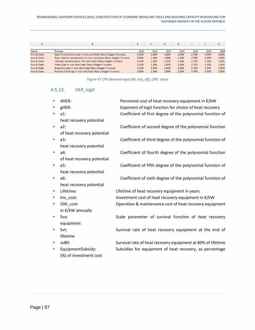
REIMBURSABLE ADVISORY SERVICES (RAS): CONSTRUCTION OF ECONOMIC MODELING TOOLS AND BUILDING CAPACITY IN MODELING FOR
SUSTAINED GROWTH IN THE SLOVAK REPUBLIC
Page | 87
Figure 47 CPS Demand input file: Exo_effi_ORD sheet
HER_logit
dHER: Perceived cost of heat recovery equipment in €/kW
gHER: Exponent of logit function for choice of heat recovery
a1: Coefficient of first degree of the polynomial function of
heat recovery potential
a2: Coefficient of second degree of the polynomial function
of heat recovery potential
a3: Coefficient of third degree of the polynomial function of
heat recovery potential
a4: Coefficient of fourth degree of the polynomial function
of heat recovery potential
a5: Coefficient of fifth degree of the polynomial function of
heat recovery potential
a6: Coefficient of sixth degree of the polynomial function of
heat recovery potential
Lifetime: Lifetime of heat recovery equipment in years
Inv_cost: Investment cost of heat recovery equipment in €/kW
OM_cost: Operation & maintenance cost of heat recovery equipment
in €/kW annually
Sva: Scale parameter of survival function of heat recovery
equipment
Svt: Survival rate of heat recovery equipment at the end of
lifetime
sv80: Survival rate of heat recovery equipment at 80% of lifetime
EquipmentSubsidy: Subsidies for equipment of heat recovery, as percentage
(%) of investment cost

REIMBURSABLE ADVISORY SERVICES (RAS): CONSTRUCTION OF ECONOMIC MODELING TOOLS AND BUILDING CAPACITY IN MODELING FOR
SUSTAINED GROWTH IN THE SLOVAK REPUBLIC
Page | 88
Figure 48 CPS Demand input file: HER_logit sheet
Sheets dACTSBC_inert to dACTSEF_AG_ST_inert
dACTSBC_inert: Scale parameter of the inertia logit function for the
calculation of the inertia share of lower nesting level (set 𝑆𝐶) in the activity of the upper
nesting level (set 𝑆𝐵). This parameter is defined upon the sets (𝑆𝐵,𝑆𝐶,𝑦𝑒𝑎𝑟_𝑎𝑙𝑙)
dACTSCD_inert: Scale parameter of the inertia logit function for the
calculation of the inertia share of lower nesting level (set 𝑆𝐷) in the activity of the upper
nesting level (set 𝑆𝐶). This parameter is defined upon the sets (𝑆𝐶,𝑆𝐷,𝑦𝑒𝑎𝑟_𝑎𝑙𝑙)
dACTSEF_AG_LT_inert: Scale parameter of the inertia logit function for the
calculation of the choice of equipment type mix of level 𝑆𝐹 in the aggregate supply
processes of level 𝑆𝐸, used for decision making of investments. The latter meaning that
this parameter is used in the logit function of unit levelized total costs (long term costs).
This parameter is agent-specific, and thus defined upon the sets (𝐴𝐺, 𝑆𝐸,𝑆𝐹,𝑦𝑒𝑎𝑟_𝑎𝑙𝑙)
dACTSEF_AG_ST_inert: Scale parameter of the inertia logit function for the
calculation of the choice of equipment type mix in operation of level 𝑆𝐹 in the aggregate
supply processes of level 𝑆𝐸. The latter meaning that this parameter is used in the logit
function of short-term marginal operation costs. This parameter is also agent-specific,
and thus defined upon the sets (𝐴𝐺, 𝑆𝐸,𝑆𝐹,𝑦𝑒𝑎𝑟_𝑎𝑙𝑙)

REIMBURSABLE ADVISORY SERVICES (RAS): CONSTRUCTION OF ECONOMIC MODELING TOOLS AND BUILDING CAPACITY IN MODELING FOR
SUSTAINED GROWTH IN THE SLOVAK REPUBLIC
Page | 89
Figure 49 CPS Demand input file: dACTSBC_inert sheet

REIMBURSABLE ADVISORY SERVICES (RAS): CONSTRUCTION OF ECONOMIC MODELING TOOLS AND BUILDING CAPACITY IN MODELING FOR
SUSTAINED GROWTH IN THE SLOVAK REPUBLIC
Page | 90
dSW_F_inert_av
dSW_F_inert_av: Scale parameter of the inertia logit function for a fuel’s
share per process and year, applied to all technology categories and vintages.
Figure 50 CPS Demand input file: dSW_F_inert_av sheet
Options for changing parameters’ values exogenously
1) How to change the macroeconomic drivers – Macro_data sheet
The user has the ability to change the macroeconomic drivers such as GDP per capita and income per
capita, by changing the content of the relevant cells in columns G to N, as shown in Figure 51.
Figure 51 How to change the macroeconomic drivers
2) How to change the policy drivers – Drivers_data sheet
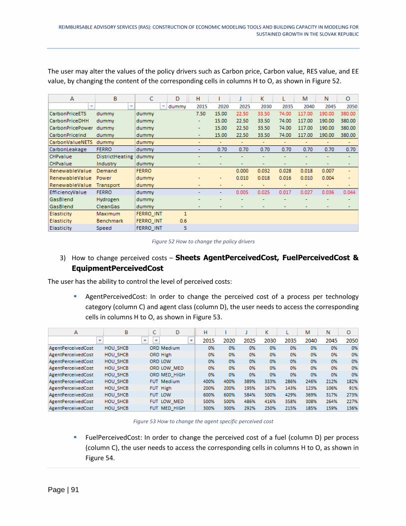
REIMBURSABLE ADVISORY SERVICES (RAS): CONSTRUCTION OF ECONOMIC MODELING TOOLS AND BUILDING CAPACITY IN MODELING FOR
SUSTAINED GROWTH IN THE SLOVAK REPUBLIC
Page | 91
The user may alter the values of the policy drivers such as Carbon price, Carbon value, RES value, and EE
value, by changing the content of the corresponding cells in columns H to O, as shown in Figure 52.
Figure 52 How to change the policy drivers
3) How to change perceived costs – Sheets AgentPerceivedCost, FuelPerceivedCost &
EquipmentPerceivedCost
The user has the ability to control the level of perceived costs:
AgentPerceivedCost: In order to change the perceived cost of a process per technology
category (column C) and agent class (column D), the user needs to access the corresponding
cells in columns H to O, as shown in Figure 53.
Figure 53 How to change the agent specific perceived cost
FuelPerceivedCost: In order to change the perceived cost of a fuel (column D) per process
(column C), the user needs to access the corresponding cells in columns H to O, as shown in
Figure 54.

REIMBURSABLE ADVISORY SERVICES (RAS): CONSTRUCTION OF ECONOMIC MODELING TOOLS AND BUILDING CAPACITY IN MODELING FOR
SUSTAINED GROWTH IN THE SLOVAK REPUBLIC
Page | 92
Figure 54 How to change the fuel specific perceived cost
EquipmentPerceivedCost: In order to change the perceived cost of cokery equipment per
technology category (column C), the user needs to access the corresponding cells in columns
H to O, as shown in Figure 55.
Figure 55 How to change the cokery equipment perceived cost
4) How to change the theta parameter – ThetaOptimum sheet
The user has the ability to change the theta parameter per nesting level (column B), per short term and
long term operation (column B) and per agent class (column D), by changing the content of the relevant
cells in columns I to O, as shown in Figure 56.

REIMBURSABLE ADVISORY SERVICES (RAS): CONSTRUCTION OF ECONOMIC MODELING TOOLS AND BUILDING CAPACITY IN MODELING FOR
SUSTAINED GROWTH IN THE SLOVAK REPUBLIC
Page | 93
Figure 56 How to change the theta parameter
5) How to change taxes’ values – Prices_data sheet
The user has the ability to change the excise tax per fuel (column B) and sector (column E), as well as the
VAT value for households and transport (column B & E), by changing the content of the relevant cells in
columns I to P, as shown in Figure 57.
Figure 57 How to change the excise and VAT taxes
6) How to change subsidies’ values – EquipmentSubsidy sheet
The user has the ability to change the subsidy for the purchase of cokery equipment (FERRO_COK) per
technology category (column C), as well as subsidies for the purchase of equipment per supply process
(column B) and technology category (column C), by changing the content of the relevant cells in columns
H to O, as shown in Figure 58.

REIMBURSABLE ADVISORY SERVICES (RAS): CONSTRUCTION OF ECONOMIC MODELING TOOLS AND BUILDING CAPACITY IN MODELING FOR
SUSTAINED GROWTH IN THE SLOVAK REPUBLIC
Page | 94
Figure 58 How to change the cokery and process equipment subsidies
7) How to change the discount rates – Policy_dem_data sheet
The user has the ability to change the discount rate per agent class (column C), by changing the content
of the relevant cells in columns I to O, as shown in Figure 59.
Figure 59 How to change the discount rate

REIMBURSABLE ADVISORY SERVICES (RAS): CONSTRUCTION OF ECONOMIC MODELING TOOLS AND BUILDING CAPACITY IN MODELING FOR
SUSTAINED GROWTH IN THE SLOVAK REPUBLIC
Page | 95
8) How to change biofuel shares – Policy_dem_data sheet
The user has the ability to change the share of conventional and advanced biofuels (column C) in transport
processes/vehicles (column B), by changing the content of the relevant cells in columns H to O, as shown
Figure 60.
Figure 60 How to change the biofuel shares
9) How to change the availability potential – Potential sheet
The user has the ability to change the potential limitation per fuel (column C) and subsector 𝑆𝐷 (column
B), by changing the content of the relevant cells in columns D to K, as shown in Figure 61.
Figure 61 How to change the availability potential

REIMBURSABLE ADVISORY SERVICES (RAS): CONSTRUCTION OF ECONOMIC MODELING TOOLS AND BUILDING CAPACITY IN MODELING FOR
SUSTAINED GROWTH IN THE SLOVAK REPUBLIC
Page | 96
5. Overview of the CPS Power Module
This chapter provides an overview of the main principles of the CPS Power Module.
Section 5.1: Basic concepts in the CPS Power Module
Section 5.2: Mathematical Structure, unknown variables and exogenous parameters
Section 5.3: Model features, considerations and assumptions
Section 5.4: Principles of the pricing model
Section 5.5: Policy Focus - Power
Section 5.6: Explaining the supply-related scenario input file
5.1 Basic concepts in the CPS Power Module
The CPS Power Module includes all necessary mathematical formulations for projecting energy supply
with distinct representations for the power system, district heating and CHP, both utilities and industrial.
The reader is referred to Section 5.3.1 Representation of Plants for a detailed analysis regarding the
representation of plants.
Figure 62 Overview of the CPS Power Module showing how the model accounts for electricity, steam and heat demand and serves electricity demand in High/Medium and Low Voltages
The power and heat/steam production model solves simultaneously the optimum capacity expansion of
power plants, district heating units and industrial plants, as further described below, along with the
dispatching of plants (Unit Commitment Dispatching Algorithm), simulating a wholesale market. The
simultaneous simulation of power market along with the steam/heat simulation enables the capture of
trade-offs between the choice of investing in cogeneration and boilers and between CHP and pure-electric

REIMBURSABLE ADVISORY SERVICES (RAS): CONSTRUCTION OF ECONOMIC MODELING TOOLS AND BUILDING CAPACITY IN MODELING FOR
SUSTAINED GROWTH IN THE SLOVAK REPUBLIC
Page | 97
plants. The choice of investing in new plants is endogenous in the model, while the optimisation is inter-
temporal (perfect foresight). Thus, investments are driven by the long term marginal costs, subject to
operational constraints, fuel limitations and demand for energy and ancillary services.
The co – optimisation of the system takes into account the hourly profiles of demand, for electricity, heat
and steam decomposed by sector and energy use of origin, and similarly the hourly production
possibilities of resources that are variable such as the renewables. The CPS model distinguishes between
heat consumed in residential, services and agriculture sectors via the district heating network, and steam
consumed in the industrial sectors and the refineries. The model also treats distinctly steam production
and demand by industrial sector.
The production of heat and steam is possible from cogeneration power plants, boilers and heat pumps.
The calibration data assume that the cogeneration plants operated by power utilities supply heat to the
district heating sector and that industrial cogeneration plants specified by industrial sector produce the
industrial steam. The latter are specific to the sectors and are not operated by utilities. Similarly, the
boilers for heat are operated by the district heating and the boilers for steam distinct by sector are
operated by the industries. In other words, the cogeneration plants and the industrial boilers are located
on the industrial sites and can only supply steam to the industrial sector they belong. The model does not
consider trading of steam among the industrial sectors. The model considers endogenously the possibility
of industries to purchase electricity from the grid or to self-generate. In the former case, the industry may
enjoy low supply tariffs but in the latter case the industry reduces total energy costs by cogenerating
industrial steam together with the self-produced electricity. In some sectors, there is also possibility to
use industrial by-products, such as gases in iron and steel, refinery gas in refineries or waste in pulp
industry, which are not tradable commodities.
Also, a variety of electricity storage facilities are represented in the model, including hydroelectric
pumping, batteries, and power-to-hydrogen, power-to-gas and power-to liquid technologies. The power-
to-X technologies are providing the so-called chemical storage of electricity, endogenously in the model,
as they can produce electricity when the resources are in excess of demand and use the outputs of power-
to-X to produce electricity when demand is in excess of resources. In addition, the power-to-X facilities
can produce endogenously in the model methane, hydrogen and liquid hydrocarbons from a synthesis of
CO2 and hydrogen to supply demand for such fuels, which may arise in the final demand sectors. Such a
demand may emerge in the context of scenarios, which aim at replacing fossil fuels with synthetic fuels
to reduce greenhouse gas emissions or to achieve petroleum or natural gas independence. The unit
commitment sub-model performs a high hourly resolution optimization of system operation, taking into
account all kinds of ancillary services and reserve, which ensure power supply reliability. The CPS model
simulates the operation and expansion of power plants on an individual plant basis and takes into account
the eventual technical operating restrictions, such as the minimum stable power generation, ramp rates,
minimum up and down times and resource constraints. The latter applies to hydroelectric plants with
reservoir, which are subject to water availability and storage limitations.
Once the system is optimally operated and expanded in the future, the model calculates costs and on this
basis it calculates the tariffs of electricity per sector of final demand, as well as the tariffs for synthetically

REIMBURSABLE ADVISORY SERVICES (RAS): CONSTRUCTION OF ECONOMIC MODELING TOOLS AND BUILDING CAPACITY IN MODELING FOR
SUSTAINED GROWTH IN THE SLOVAK REPUBLIC
Page | 98
produced fuels. The tariffs distinguish between energy supply and the provision of grid services, the latter
being under a regulated monopoly regime. The model calculates tariffs also for industrial steam by sector
and for district heating. All these prices by sector feed the closed loop of the entire model and return to
the demand sectors for further adjustment of demand in the next model iteration. Thus, the demand for
electricity is price-elastic, as the model performs adjustment of demand driven by electricity prices per
sector. After the optimization two additional steps are included in the model, pricing and reporting as
shown Figure 63.
Figure 63 Sequence of CPS Power Module
Through pricing, the Power Module is linked to the Demand Module (Chapter 4 Overview of the CPS
Demand Module) and solved as a mixed complementarity problem that concatenates the individual
problems of energy consumers and producers via endogenous calculation of energy prices. CPS simulates
a well-functioning market, where total costs (capital and operating) are recovered, including also possible
stranded investment costs. The pricing of electricity commodity is explicit and is based on the Ramsey-
Boiteux methodology. Marginal cost pricing is used, so as to calculate the price in a virtual wholesale
market; then a fixed mark-up is added according to Ramsey pricing, allocating the not yet allocated system
costs using the marginal cost pricing. A detailed description of the pricing model is included in the Section
5.4 Principles of the pricing model.

REIMBURSABLE ADVISORY SERVICES (RAS): CONSTRUCTION OF ECONOMIC MODELING TOOLS AND BUILDING CAPACITY IN MODELING FOR
SUSTAINED GROWTH IN THE SLOVAK REPUBLIC
Page | 99
Table 11 Overview of the CPS Power Module
Optimisation Considerations
The system minimizes total generation costs including annualized capital cost of new investment and all variable and fixed costs of generation to meet given demand increased by distribution losses
Demand is price-elastic, i.e. it responds to electricity/heat prices
The optimization is subject to constraints regarding capacity expansion and potential limitations by plant type.
Total generation costs include fuel costs and other variable costs. Therefore, the optimisation of capacity expansion includes the estimation of the merit order dispatching and takes account in full the provision of system reserves
Detailed representation of the system and plant characteristics
The integration of a Unit Commitment Problem (UC) allows for a detailed representation of the system operation taking into account also the use of parts of the capacities of plants to meet the system reserves (ancillary services)
The CPS Power Module takes into account the technical restrictions of plant operation and system services and simulates the operation of the Slovakian power system on an hourly basis (Unit-Commitment Problem)
Investment decision
RES investments are decided under a separate support mechanism
Old plants are decommissioned due to their age
The user can define exogenously the extension of lifetime for each existing power plant, as well as fuel switching and fuel blending
Capacity expansion to meet system reserve requirements is part of the optimization, considering given levels of reserves
Clean Energy Policies
EU and national policies may impose a system-wide clean energy obligation (e.g. RES obligation) or an emissions reduction obligation or an energy efficiency saving obligation. These obligations are also taken into account by the CPS Power Module in the determination of the endogenous capacity expansion

REIMBURSABLE ADVISORY SERVICES (RAS): CONSTRUCTION OF ECONOMIC MODELING TOOLS AND BUILDING CAPACITY IN MODELING FOR
SUSTAINED GROWTH IN THE SLOVAK REPUBLIC
Page | 100
5.2 Mathematical Structure, unknown variables and exogenous parameters
Mathematical Structure
The mathematical structure of the CPS Power Module is a mixed integer linear problem (MILP), the
optimisation is inter-temporal (perfect foresight) and solves simultaneously:
A capacity expansion problem and A unit commitment-dispatching algorithm
The model determines the optimal capacity mix and dispatching schedule of plants, so as to meet the
demand for electricity and heat/steam, subject to several constraints, aiming to minimize the total system
costs. The total system costs include:
Annualized capital costs of new investments based on WACC for discounting over time Fixed costs (Operation and Maintenance) Variable (non-fuel) costs Fuel costs and Taxes and environmental policies costs/subsidies (e.g. ETS costs, FIT equivalent policies).
Optimisation constraints can be grouped under the following categories:
1) Energy equilibrium constraints (electricity, heat, steam) 2) System – related technical constraints (reserve requirements) 3) Investment constraints (limited potential of investing in some plant types, i.e. nuclear plants, RES) 4) Plant – related technical constraints (e.g. max capacity, minimum power level, ramp up and ramp
down constraints etc.) 5) Fuel Consumption and resource availability constraints 6) Storage and Power-to-X constraints (e.g. capacity of storage facilities, maximum daily stored
energy, balance of stored energy etc.) 7) CCS – related constraints 8) Policies and Emissions constraints 9) Additional Constraints for heat and steam supply
Figure 64 depicts the Optimisation constraints of the CPS Power Module.
The next paragraphs provide further details in relation to the mathematical representation of each constraint in the CPS Power Module.

REIMBURSABLE ADVISORY SERVICES (RAS): CONSTRUCTION OF ECONOMIC MODELING TOOLS AND BUILDING CAPACITY IN MODELING FOR
SUSTAINED GROWTH IN THE SLOVAK REPUBLIC
Page | 101
Figure 64 Optimisation Constraints
5.2.1.1 Energy Equilibrium constraints
The energy equilibrium constraints ensure that the given demand4 for each form of energy is met by the
supply. The energy forms simulated in the CPS Power Module are electricity, heat, steam and hydrogen.
Although heat and steam are the same form of energy, we have chosen to include both in the CPS Power
Module as in principle households and tertiary sectors use heat for heating purposes, while industrial
sectors use steam as input to several industrial processes. The energy equilibrium constraints are included
in the model as following:
4 The demand for electricity, steam/heat and clean fuels is endogenous within the CPS model. The CPS Power Module is linked with the CPS Demand Module via prices for each energy form, representing a perfect equilibrium.
Energy equilibrium constraints (electricity, heat,
steam)
System – related technical constraints (reserve
requirements)
Investment constraints
Plant – related technical constraints
Fuel Consumption and resource availability
constraints
Storage and Power to X constraints
CCS – related constraints
Policies and Emissions constraints
Additional Constraints for heat and steam supply

REIMBURSABLE ADVISORY SERVICES (RAS): CONSTRUCTION OF ECONOMIC MODELING TOOLS AND BUILDING CAPACITY IN MODELING FOR
SUSTAINED GROWTH IN THE SLOVAK REPUBLIC
Page | 102
Energy equilibrium constraint
∑𝐺𝑝,ℎ,𝑒𝑓,𝑡𝑝
+ {∑𝑆𝑇𝑂𝑜𝑢𝑡𝑠𝑡𝑜,ℎ,𝑡𝑠𝑡𝑜
+ 𝐼𝑚𝑝𝑜𝑟𝑡𝑠ℎ,𝑡, 𝑖𝑓 𝑒𝑓 ∈ 𝑒𝑙𝑒𝑐
0, 𝑖𝑓 𝑒𝑓 ∈ (ℎ𝑒𝑎𝑡 ∪ 𝑠𝑡𝑒𝑎𝑚)
=∑𝐷𝑠,ℎ,𝑒𝑓,𝑡𝑠
+{∑𝑆𝑇𝑂𝑖𝑛𝑠𝑡𝑜,ℎ,𝑡𝑠𝑡𝑜
+∑𝑃2𝑋𝑖𝑛𝑝2𝑥,ℎ,𝑡𝑝2𝑥
+ 𝐸𝑥𝑝𝑜𝑟𝑡𝑠ℎ,𝑡 , 𝑖𝑓 𝑒𝑓 ∈ 𝑒𝑙𝑒𝑐
0, 𝑖𝑓 𝑒𝑓 ∈ (ℎ𝑒𝑎𝑡 ∪ 𝑠𝑡𝑒𝑎𝑚)
, ∀ 𝑒𝑓, ℎ, 𝑡
Where
𝑝: Plant
ℎ: Typical hour
𝑡: Year
𝑒𝑙𝑒𝑐: Electricity
𝑠: Demand sector
𝑒𝑓: Energy form
𝑠𝑡𝑜: Storage facility
𝑝2𝑥: Type of power to X facility
𝐺𝑝,ℎ,𝑒𝑓,𝑡: Generated power for plant 𝑝, typical hour ℎ, energy form 𝑒𝑓 and year 𝑡
𝐷𝑠,ℎ,𝑒𝑓,𝑡: Demand of power for demand sector 𝑠, typical hour ℎ, energy form 𝑒𝑓 and year 𝑡
𝑆𝑇𝑂𝑖𝑛𝑠𝑡𝑜,ℎ,𝑡: Charge of storage facility 𝑠𝑡𝑜 via electricity for typical hour ℎ and year 𝑡
𝑆𝑇𝑂𝑜𝑢𝑡𝑠𝑡𝑜,ℎ,𝑡: Discharge of storage facility 𝑠𝑡𝑜 via electricity for typical hour ℎ and year 𝑡
𝑃2𝑋𝑖𝑛𝑝2𝑥,ℎ,𝑡: Input of type of power to X facility 𝑝2𝑥 for typical hour ℎ
𝐼𝑚𝑝𝑜𝑟𝑡𝑠ℎ,𝑡: Imports of electricity to Slovakia for typical hour ℎ and year 𝑡
𝐸𝑥𝑝𝑜𝑟𝑡𝑠ℎ,𝑡: Exports of electricity from Slovakia for typical hour ℎ and year 𝑡
Energy demand is calculated by the CPS Demand Module annually and for each sector. The Power Module
receives energy demand results from the Demand Module and calculates an hourly demand load curve
via the use of individual load patterns decomposed by demand sector. The hourly patterns of each
demand sector and the aggregated hourly demand load curve have been calibrated in the base year
(2015), so as to reproduce the demand load curve based on the ENTSO – E data.

REIMBURSABLE ADVISORY SERVICES (RAS): CONSTRUCTION OF ECONOMIC MODELING TOOLS AND BUILDING CAPACITY IN MODELING FOR
SUSTAINED GROWTH IN THE SLOVAK REPUBLIC
Page | 103
Electricity demand is increased by transmission and distribution losses, for each voltage type, while heat
demand is increased due to losses in the district heating network. For steam demand no losses are
assumed, as the generation of steam is met by industrial onsite plants. The reader is referred to Section
5.3.1.2 Network grids for a more detailed description of the network assumptions.
It must be noted that since the CPS is a single-country model, possible network constraints are not accounted for. 𝐼𝑚𝑝𝑜𝑟𝑡𝑠 and 𝐸𝑥𝑝𝑜𝑟𝑡𝑠 are input parameters, applicable only to electricity.
5.2.1.2 System-related technical constraints
The system-related technical constraints refer to the minimum hourly quantities of operating reserves.
The CPS Power Module includes all three types of reserves, as defined by the pan-European harmonized
terminology of ENTSO-E5:
1) FCR: Frequency Containment Reserve 2) aFRR: automatic Frequency Restoration Reserve (upwards and downwards) 3) mFRR/RR: manual Frequency Restoration Reserve and Replacement Reserve
The following mathematical formulation describes the inclusion of the system-related technical constraints in the CPS Power Module:
System-related technical constraint
∑𝑅𝑝,𝑟,ℎ,𝑡 ≥
𝑝
𝑆𝑦𝑠𝑅𝑒𝑞𝑟,𝑡 , ∀ 𝑟, ℎ, 𝑡
Where
𝑟: Reserve type (FCR, aFRR or mFRR/RR),
𝑅𝑝,𝑟,ℎ,𝑡: Delivery of plant 𝑝 of reserve type 𝑟 for typical hour ℎ
𝑆𝑦𝑠𝑅𝑒𝑞𝑟,𝑡: System reserve requirements of reserve type 𝑟
5
https://ec.europa.eu/energy/sites/ener/files/documents/SystemOperationGuideline%20final%28provisional%2904052016.pdf

REIMBURSABLE ADVISORY SERVICES (RAS): CONSTRUCTION OF ECONOMIC MODELING TOOLS AND BUILDING CAPACITY IN MODELING FOR
SUSTAINED GROWTH IN THE SLOVAK REPUBLIC
Page | 104
Figure 65 Specific constraints for reserves
It must be noted that since CPS is a single country model, no sharing of reserves is taken into account. This means that in the CPS Power Module’s approach the TSO cannot access reserve capacity in another synchronous area to fulfill its’ reserve requirements. Thus reserve requirements are solely met by providers located in the same balancing area (i.e. in Slovakia).
5.2.1.3 Investment Constraints
Investment constraints reflect a possibly limited potential of investing in some plant types (i.e. nuclear
plants, RES). Investment constraints are exogenous to the model and the user can change the maximum
potential level. The investment constraint is the following:
Investment constraint
∑𝑃𝑚𝑎𝑥𝑝 ∗ 𝐼𝑁𝑆𝑇𝑝,𝑡 ≤ 𝑚𝑎𝑥𝑝𝑜𝑡𝑝,𝑡 , ∀ 𝑝, 𝑡
𝑝
Where
𝑃𝑚𝑎𝑥𝑝: Maximum installed capacity of plant 𝑝
𝐼𝑁𝑆𝑇𝑝,𝑡: Number of installed units of plant 𝑝
𝑚𝑎𝑥𝑝𝑜𝑡𝑝,𝑡: Maximum potential of installed units of plant 𝑝

REIMBURSABLE ADVISORY SERVICES (RAS): CONSTRUCTION OF ECONOMIC MODELING TOOLS AND BUILDING CAPACITY IN MODELING FOR
SUSTAINED GROWTH IN THE SLOVAK REPUBLIC
Page | 105
Investment constraints also include the non-linear cost supply curves with ascending slope (stepwise
linearized), representing potential resource exhaustion. The user is referred to Section 5.3.1.5 Non-linear
cost curves for a detailed description.
5.2.1.4 Plant-related technical constraints
A unit commitment algorithm (UC) has been incorporated into the CPS Power Module. The UC approach
allows for detailed representation of technical constraints for plants.
The following mathematical formulations describe the plant-related technical constraints included in the
CPS Power Module:
Maximum installed capacity
𝐺𝑝,ℎ,𝑒𝑙𝑒𝑐,𝑡 + ∑ 𝑅𝑝,𝑟,ℎ,𝑡𝑟∈𝑢𝑝
≤ 𝑃𝑚𝑎𝑥𝑝 ∗ 𝑈𝐶𝑝,ℎ,𝑡 , ∀ 𝑝, ℎ, 𝑡
Where
𝑈𝐶𝑝,ℎ,𝑡: Number of committed units of plant 𝑝 for typical hour ℎ
Minimum stable power generation level
𝐺𝑝,ℎ,𝑒𝑙𝑒𝑐,𝑡 − ∑ 𝑅𝑝,𝑟,ℎ,𝑡𝑟∈𝑑𝑜𝑤𝑛
≥ 𝑃𝑚𝑖𝑛𝑝 ∗ 𝑈𝐶𝑝,ℎ,𝑡 , ∀ 𝑝, ℎ, 𝑡
Where
𝑃𝑚𝑖𝑛𝑝: Minimum generation level (capacity) of plant 𝑝
Minimum up time
𝑈𝐶𝑝,ℎ,𝑡 ≥ ∑ 𝑆𝑈𝑝,ℎ′,𝑡ℎ′∈[(ℎ′≤ℎ)∩(ℎ−𝑚𝑖𝑛𝑢𝑝𝑡𝑖𝑚𝑒𝑝≤ℎℎ)]
, ∀ 𝑝, ℎ, 𝑡
Where
𝑆𝑈𝑝,ℎ′,𝑡: Number of starting up units of plant 𝑝 for typical hour ℎ′
Minimum down time
𝐼𝑁𝑆𝑇𝑝,𝑡 − 𝑈𝐶𝑝,ℎ,𝑡 ≥ ∑ 𝑆𝐷𝑝,ℎ′,𝑡ℎ′∈[(ℎ′≤ℎ)∩(ℎ−𝑚𝑖𝑛𝑑𝑜𝑤𝑛𝑡𝑖𝑚𝑒𝑝≤ℎℎ)]
, ∀ 𝑝, ℎ, 𝑡
Where
𝑆𝐷𝑝,ℎ′,𝑡: Number of shutting down units of plant 𝑝 for typical hour ℎ′
Maximum upward ramping rates
𝐺𝑝,ℎ,𝑒𝑙𝑒𝑐,𝑡 − 𝐺𝑝,ℎ−1,𝑒𝑙𝑒𝑐,𝑡 ≤ 𝑈𝐶𝑝,ℎ−1,𝑡 ∗ 𝑟𝑎𝑚𝑝𝑢𝑝𝑝 ∗ 60 + 𝑆𝑈𝑝,ℎ,𝑡 ∗ 𝑃𝑚𝑎𝑥𝑝 , ∀ 𝑝, ℎ, 𝑡

REIMBURSABLE ADVISORY SERVICES (RAS): CONSTRUCTION OF ECONOMIC MODELING TOOLS AND BUILDING CAPACITY IN MODELING FOR
SUSTAINED GROWTH IN THE SLOVAK REPUBLIC
Page | 106
Where
𝑟𝑎𝑚𝑝𝑢𝑝𝑝: Upward ramping rate of plant 𝑝
Maximum downward ramping rates (up & down)
𝐺𝑝,ℎ−1,𝑒𝑙𝑒𝑐,𝑡 − 𝐺𝑝,ℎ,𝑒𝑙𝑒𝑐,𝑡 ≤ 𝑈𝐶𝑝,ℎ−1,𝑡 ∗ 𝑟𝑎𝑚𝑝𝑑𝑛𝑝 ∗ 60 + 𝑆𝐷𝑝,ℎ,𝑡 ∗ 𝑃𝑚𝑎𝑥𝑝 , ∀ 𝑝, ℎ, 𝑡
Where
𝑟𝑎𝑚𝑝𝑑𝑜𝑤𝑛𝑝: Downward ramping rate of plant 𝑝
Maximum operating hours
∑𝐺𝑝,ℎ,𝑒𝑙𝑒𝑐,𝑡 ∗ 𝑓𝑟𝑒𝑞ℎ ≤ 𝑚𝑎𝑥𝑜𝑝𝑒𝑟𝑝 ∗ 𝑃𝑚𝑎𝑥𝑝 ∗ 𝐼𝑁𝑆𝑇𝑝,𝑡ℎ
, ∀ 𝑝, 𝑡
Where
𝑓𝑟𝑒𝑞ℎ: Annual frequency of typical hour ℎ
𝑚𝑎𝑥𝑜𝑝𝑒𝑟𝑝: Maximum operating hours of plant 𝑝
Maximum contribution to each type of reserve per plant
𝑅𝑝,𝑟,ℎ,𝑡 ≤ 𝑚𝑎𝑥𝑟𝑒𝑠𝑝,𝑟 , ∀ 𝑝, 𝑟, ℎ, 𝑡
Where
𝑚𝑎𝑥𝑟𝑒𝑠𝑝,𝑟: Maximum contribution of plant 𝑝 of reserve type 𝑟
CHP – related constraints
𝐺𝑝,ℎ,𝑒𝑙𝑒𝑐,𝑡 + 𝑠𝑙𝑜𝑝𝑒𝑝 ∗ 𝐺𝑝,ℎ,𝑠𝑡𝑒𝑎𝑚,𝑡 ≤ 𝑃𝑚𝑎𝑥𝑝 ∗ 𝑈𝐶𝑝,ℎ,𝑡 , ∀ 𝑝 ∈ 𝑐ℎ𝑝, ℎ, 𝑡
𝑆𝑝,ℎ,𝑡 ≤ ℎ𝑒𝑙𝑟𝑎𝑡𝑖𝑜𝑝 ∗ 𝐺𝑝,ℎ,𝑒𝑙,𝑡 , ∀ 𝑝 ∈ 𝑐ℎ𝑝, ℎ, 𝑡
Where
𝑠𝑙𝑜𝑝𝑒𝑝: Iso-fuel curve of CHP plant 𝑝
𝐺𝑝,ℎ,𝑠𝑡𝑒𝑎𝑚,𝑡: Steam generation of plant 𝑝 for typical hour ℎ
𝑆𝑝,ℎ,𝑡: Steam generation of plant 𝑝 for typical hour ℎ
ℎ𝑒𝑙𝑟𝑎𝑡𝑖𝑜𝑝: Heat to electricity ratio of plant 𝑝
5.2.1.5 Fuel Consumption and resource availability constraints
Fuel Consumption in each power plant is a linear function of the electricity generation, depending on a
heatrate value defined exogenously by fuel and plant type. The choice of fuels derives from the
simultaneous optimisation of investments and operation, performed inter-temporally.
The following mathematical formulations describe the fuel consumption and resource availability
constraints included in the CPS Power Module:

REIMBURSABLE ADVISORY SERVICES (RAS): CONSTRUCTION OF ECONOMIC MODELING TOOLS AND BUILDING CAPACITY IN MODELING FOR
SUSTAINED GROWTH IN THE SLOVAK REPUBLIC
Page | 107
Fuel Consumption Constraint
𝐹𝐶𝑝,𝑓,𝑡 = ℎ𝑒𝑎𝑡𝑟𝑎𝑡𝑒𝑝 ∗∑𝑓𝑟𝑒𝑞ℎ ∗ {𝐺𝑝,ℎ,𝑒𝑙,𝑡 , ∀ 𝑝 ∉ 𝑐ℎ𝑝, 𝑡
𝐺𝑝,ℎ,𝑒𝑙,𝑡 + 𝑠𝑙𝑜𝑝𝑒𝑝 ∗ 𝐺𝑝,ℎ,𝑠𝑡𝑒𝑎𝑚,𝑡 , ∀ 𝑝 ∈ 𝑐ℎ𝑝, 𝑡ℎ
Where
𝑓: Fuel consumed
𝑐ℎ𝑝: CHP power plants
𝐹𝐶𝑝,𝑓,𝑡: Fuel consumption of plant 𝑝 and fuel 𝑓
Fuel blending Constraint
𝑏𝑙𝑒𝑛𝑑𝑝,𝑓 ∗ 𝐹𝐶𝑝,𝑓,𝑡 = ∑𝐹𝐶𝑝,𝑓′,𝑡𝑓′
, ∀ 𝑝, 𝑓, 𝑡
Where
𝑏𝑙𝑒𝑛𝑑𝑝,𝑓: Blending ratio of plant 𝑝 for fuel 𝑓, denoting the ratio of each fuel to the total fuel
consumption
Maximum resource availability constraint
∑𝐹𝐶𝑝,𝑓,𝑡 ≤ 𝑚𝑎𝑥𝑟𝑒𝑠𝑜𝑢𝑟𝑐𝑒𝑓,𝑡𝑝
, ∀ 𝑓, 𝑡
𝑚𝑎𝑥𝑟𝑒𝑠𝑜𝑢𝑟𝑐𝑒𝑓,𝑡: Maximum available energy of fuel 𝑓
5.2.1.6 Storage and Power to X constraints
The CPS Power Module determines charging and discharging of the storage units endogenously. Typically,
storage units are charged during times of low marginal cost and discharge electricity at times of high
marginal cost. The investment and operation of the various storage and Power to X options are
determined simultaneously with the capacity expansion and dispatching of the power system.
The following mathematical formulations describe the Storage and Power to X constraints included in the
CPS Power Module:
Capacity constraint of storage
𝑆𝑇𝑂𝑖𝑛𝑠𝑡𝑜,ℎ,𝑡 + 𝑆𝑇𝑂𝑜𝑢𝑡𝑠𝑡𝑜,ℎ,𝑡 ≤ 𝑃𝑠𝑡𝑜𝑠𝑡𝑜,𝑡 , ∀ 𝑠𝑡𝑜, ℎ, 𝑡
Where
𝑃𝑠𝑡𝑜𝑠𝑡𝑜: Capacity of storage facility 𝑠𝑡𝑜
Maximum daily stored energy

REIMBURSABLE ADVISORY SERVICES (RAS): CONSTRUCTION OF ECONOMIC MODELING TOOLS AND BUILDING CAPACITY IN MODELING FOR
SUSTAINED GROWTH IN THE SLOVAK REPUBLIC
Page | 108
∑ 𝑆𝑇𝑂𝑜𝑢𝑡𝑠𝑡𝑜,ℎ,𝑡 ≤ 𝑑𝑠𝑡𝑜𝑟𝑠𝑡𝑜 ∗ 𝑃𝑠𝑡𝑜𝑠𝑡𝑜, ∀ 𝑠𝑡𝑜, 𝑑𝑎𝑦, 𝑡
ℎ∈𝑑𝑎𝑦
Where
𝑑𝑎𝑦: Typical day
𝑑𝑠𝑡𝑜𝑟𝑠𝑡𝑜: Maximum daily storage capability of storage facility 𝑠𝑡𝑜
Balance of stored energy
∑ 𝑆𝑇𝑂𝑖𝑛𝑠𝑡𝑜,ℎ,𝑡 = ℎ𝑒𝑎𝑡𝑟𝑎𝑡𝑒𝑠𝑡𝑜 ∗ ∑ 𝑆𝑇𝑂𝑜𝑢𝑡𝑠𝑡𝑜,ℎ,𝑡 , ∀ 𝑠𝑡𝑜 , 𝑑𝑎𝑦, 𝑡
ℎ∈𝑑𝑎𝑦ℎ∈𝑑𝑎𝑦
Where
ℎ𝑒𝑎𝑡𝑟𝑎𝑡𝑒𝑠𝑡𝑜: Heatrate of storage facility 𝑠𝑡𝑜
Capacity constraint for clean fuel production
𝑃2𝑋𝑜𝑢𝑡𝑝2𝑥,ℎ,𝑡 ≤ 𝑃𝑃2𝑋𝑝2𝑥,𝑡 , ∀ 𝑝2𝑥, 𝑡
Where
𝑃2𝑋𝑜𝑢𝑡𝑝2𝑥,ℎ,𝑡: Output of type of power to X facility 𝑝2𝑥 for typical hour ℎ
𝑃𝑃2𝑋𝑝2𝑥,𝑡: Capacity of type of power to X facility 𝑝2𝑥
Balance constraint for clean fuel
∑ 𝑃2𝑋𝑖𝑛𝑝2𝑥,ℎ,𝑡 = ℎ𝑒𝑎𝑡𝑟𝑎𝑡𝑒𝑝2𝑥 ∗ ∑ 𝑃2𝑋𝑜𝑢𝑡𝑝2𝑥,ℎ,𝑡 , ∀ 𝑝2𝑥, ℎ, 𝑡
ℎ∈𝑑𝑎𝑦ℎ∈𝑑𝑎𝑦
Where
ℎ𝑒𝑎𝑡𝑟𝑎𝑡𝑒𝑝2𝑥: Heatrate of power to X facility 𝑝2𝑥
Balance constraint for demand and supply of clean fuels
∑𝑓𝑟𝑒𝑞ℎ ∗ 𝑃2𝑋𝑜𝑢𝑡𝑝2𝑥,ℎ,𝑡 = 𝐷𝑐𝑙𝑓𝑝2𝑥,𝑡 , ∀ 𝑝2𝑥, 𝑡
ℎ
Where
𝐷𝑐𝑙𝑓𝑝2𝑥,𝑡: Demand of clean fuel of type of power to X facility 𝑝2𝑥
The reader is referred to Section 5.3.1.1 Representation of Plants for a more detailed explanation of the
modelling approach used for storage and power to x facilities.
5.2.1.7 CCS – related constraints
Power plants with the technology option of Carbon Capture and Storage (CCS) are among the list of plant
types incorporated in the CPS Power Module. In a CCS power plant system, part of the emitted CO2 is

REIMBURSABLE ADVISORY SERVICES (RAS): CONSTRUCTION OF ECONOMIC MODELING TOOLS AND BUILDING CAPACITY IN MODELING FOR
SUSTAINED GROWTH IN THE SLOVAK REPUBLIC
Page | 109
captured, transported and deposited to a storage site (a geological underground formation), instead of
being released in the atmosphere, as in the case of conventional plants.
The cost of underground storage of CO2 is taken into account through a cost-supply curve (defined
exogenously), representing cost versus potential of storage. The cost of underground CO2 storage is
included as a cost item in the total cost of CCS power plants.
The following mathematical formulations describe the CCS – related constraints included in the CPS Power
Module:
Annually captured CO2 in CCS power plants
∑ 𝑒𝑚𝑓𝑠𝑡𝑜𝑟𝑝 ∗ 𝐹𝐶𝑝,𝑓,𝑡 = 𝐶𝑂2𝑐𝑎𝑝𝑡𝑡 , ∀ 𝑡
𝑝∈𝑐𝑐𝑠,𝑓
Where
𝑒𝑚𝑓𝑠𝑡𝑜𝑟𝑝: Fraction of emissions of plant 𝑝 that is being stored
𝐶𝑂2𝑐𝑎𝑝𝑡𝑡: Captured CO2 emissions from CCS power plants
Cumulatively maximum quantity for captured CO2 in CCS power plants
∑𝐶𝑂2𝑐𝑎𝑝𝑡𝑡′ ≤ 𝑚𝑎𝑥𝐶𝑂2𝑐𝑎𝑝𝑡𝑡 , ∀ 𝑡
𝑡′≤𝑡
Where
𝑚𝑎𝑥𝐶𝑂2𝑐𝑎𝑝𝑡𝑡: Maximum possible cumulative CO2 stored
5.2.1.8 Policies and Emission constraints
Promotion of renewables is represented in the form of an equivalent feed-in-tariff. The equivalent feed-
in-tariff is a virtual subsidy that is taken into account by the CPS Power Module when deciding on
investments. The equivalent feed-in-tariff for each type of renewable technology and the total budget
available for the support of RES are exogenous.
The CPS Power Module has been designed so as to allow the user to include additional support
mechanisms which are made available under a given budget.
The following mathematical formulations describe the Policies and Emission constraints included in the
CPS Power Module:
Annual maximum budget for Feed-In-Tariff equivalent policies
∑𝑓𝑟𝑒𝑞ℎ ∗ 𝐺𝑝,ℎ,𝑒𝑙𝑒𝑐,𝑡 ∗ 𝐹𝐼𝑇𝑒𝑞𝑝,𝑡 ≤ 𝑓𝑖𝑡𝑏𝑢𝑑𝑔𝑒𝑡𝑡 , ∀ 𝑡
𝑝,ℎ

REIMBURSABLE ADVISORY SERVICES (RAS): CONSTRUCTION OF ECONOMIC MODELING TOOLS AND BUILDING CAPACITY IN MODELING FOR
SUSTAINED GROWTH IN THE SLOVAK REPUBLIC
Page | 110
Where
𝐹𝐼𝑇𝑒𝑞𝑝,𝑡: Equivalent feed-in-tariff for plant 𝑝
𝑓𝑖𝑡𝑏𝑢𝑑𝑔𝑒𝑡𝑡: Maximum budget available for the implementation of a RES FIT support policy
Additional promoting policies
∑𝑓𝑟𝑒𝑞ℎ ∗ 𝐺𝑝,ℎ,𝑓,𝑡 ∗ 𝑝𝑜𝑙𝑖𝑐𝑦𝑝,𝑓,𝑡 = 𝑃𝑠𝑢𝑝𝑝𝑜𝑟𝑡𝑡 , ∀ 𝑡
𝑝.ℎ
Where
𝑝𝑜𝑙𝑖𝑐𝑦𝑝,𝑓,𝑡: Additional policy tariff for plant 𝑝 and fuel 𝑓
𝑃𝑠𝑢𝑝𝑝𝑜𝑟𝑡𝑡: Maximum budget available for the implementation of the additional policy
Emissions constraint
∑𝑒𝑚𝑓𝑝,𝑓 ∗ 𝐹𝐶𝑝,𝑓,𝑡 = 𝐸𝑀𝐼𝑆𝑡 , ∀ 𝑡
𝑝,𝑓
Where
𝑒𝑚𝑓𝑝,𝑓: CO2 emission factor of plant 𝑝 for fuel 𝑓
𝐸𝑀𝐼𝑆𝑡: Total system’s emissions
Unknown variables
The unknown variables of the CPS Power Module include the following:
Capacity additions by plant type (several types of capacity investment)
Electricity generation by plant
Steam or heat generation by plant
Fuel consumption by type of fuel and plant
CO2 emissions
Storage and Power to X plants: injection or extraction from storage facilities and investments in
storage equipment
Capacity reserved for the provision of upward and downward ancillary services by plant
Curtailment of renewable generation
The integer variables included in the CPS Power Module are the following:
Number of installed plants
Number of plant in operation in typical hour ℎ

REIMBURSABLE ADVISORY SERVICES (RAS): CONSTRUCTION OF ECONOMIC MODELING TOOLS AND BUILDING CAPACITY IN MODELING FOR
SUSTAINED GROWTH IN THE SLOVAK REPUBLIC
Page | 111
Number of plant shut down in typical hour ℎ
Number of plant started up in typical hour ℎ
It must be noted that the integer variables apply only for the power plants that are assumed to have
technical limitations (i.e. nuclear, solids – fired, CCGT, large biomass plants).
The reader is referred to Section 5.3.1 Representation of Plants for a detailed analysis regarding the
representation of plants.
Exogenous Parameters
The parameters provided by the user are:
Installed capacity of existing plants in the beginning of the projection period
Decommissioning plans related to the existing plants (if any)
Capacities of plants under construction in the beginning of the projection period
Grid loss rates
Technical characteristics of plants by technology (commissioning/decommissioning year,
technical lifetime, size, heatrate, self-consumption rate, technical minimum output, ramping
rates, maximum contribution to each type of reserve, minimum up and down time, heat to
electricity ratio and the slope of the iso-fuel curve for CHP plants)
Economic characteristics of plants by technology (capital, fixed O&M and variable cost, economic
lifetime, growth factor of fixed costs, capital cost incurred for extending the lifetime of plant, for
fuel blending and for fuel switching, additional capital and fixed cost for CHP plants)
Fuel prices
Taxes & subsidies
Carbon price in the context of the EU Emissions Trading System - EU ETS (i.e. the price of the
European Union Allowance)
Feed-in tariffs and other support schemes for RES (FIT equivalent)
Costs and availability potential parameters for transportation and storage of captured CO2
Costs and availability potential parameters of storage technologies
Parameters reflecting policy instruments and restrictions (nuclear, CCS, environmental, efficiency,
CHP, etc.)
Parameters used in the non-linear cost-supply curves
Transmission grid, distribution grid and district heating network tariffs for the basis year
5.3 Model features, considerations and assumptions
This section presents the main features of the CPS Power Module, comprised of the following subsections:

REIMBURSABLE ADVISORY SERVICES (RAS): CONSTRUCTION OF ECONOMIC MODELING TOOLS AND BUILDING CAPACITY IN MODELING FOR
SUSTAINED GROWTH IN THE SLOVAK REPUBLIC
Page | 112
Representation of Plants: this section describes the different types of plants considered by the
model (Utility, District Heating, electricity/steam production by the industrial sector, storage and
power to X plants). This description includes detailed information on technologies, technical
characteristics and main assumptions included in the CPS Power Module
Fuels and Fuel Consumption: this section outlines the basic considerations in relation to fuel
consumption
Network Grids: this section discusses the CPS Power Module approach in relation to the power
grid
Imports and Exports: this section presents the modelling approach to electricity imports and
exports to and from Slovakia
Time resolution: the model represents demand variability for electricity and steam/heat by
introducing an hourly fluctuation of load in typical days. This section describes the main principles
of this approach
Non-linear cost curves: including detailed description of cost optimization, taking into account
current and future exploitation of resources and technological progress (including learning by
doing)
Investment decisions: this section outlines the basic considerations for the promotion of
investments in specific technologies (e.g. RES, nuclear, CHP etc.)
CHP operation: this section provides information on the modelling approach used for the
simulation of CHP operation
CCS and CO2 capture: this section outlines the basic considerations of the CPS Power Module for
the modelling of plants with the availability of carbon capture and storage (CCS)
Representation of Plants
The CPS Power Module includes all plants currently installed in Slovakia providing electricity and
steam/heat for district heating or industrial purposes. It also provides for a wide range of technologies
that may be installed in the future.
For the sake of simplicity, as well as to ensure a speedy execution, small existing plants have been grouped
into larger plants (hereinafter Plant Groupings). Plant Grouping has been done by fuel type, technology
(including CHP) and use (utility or industrial)6. The main categorization of the plants as taken into account
by the CPS Power Module is summarized in Figure 66 and described below:
6 See for example all plants referred to as Small_CHP_Waste, Small_CHP_Biomass, Small_CHP_Coal, Small_IC_1, Small_IC_2, Small_IC_3, in the input data file under the Techdata_plants SHEET.

REIMBURSABLE ADVISORY SERVICES (RAS): CONSTRUCTION OF ECONOMIC MODELING TOOLS AND BUILDING CAPACITY IN MODELING FOR
SUSTAINED GROWTH IN THE SLOVAK REPUBLIC
Page | 113
Figure 66 CPS Plant types
1) Utility power plants: a. Electricity only: power plants generating only electricity b. Cogeneration utility power plants: CHP power plants with main purpose of generating
electricity, or CHP power plants used for district heating purposes (i.e. connected to district heating network or individual tertiary facilities)
The following paragraphs highlight the CPS Power Module approach on the treatment of Utility power plants. Attention is drawn on special topics, such as new capacity, cogeneration, decommissioning and retrofitting. Note that in the below paragraphs, the phrase “plant type” refers to different technologies.
The model treats existing power plants (including Plant Groupings) individually
New Capacity
o The model projects investment in individual new power plants at a fixed (standardized) capacity per plant type, by the use of integer variable for the operation of all power plants (existing and new) and the investments in new units. As some plant types entail severe technical limitations7, only specific technologies are considered to have a fixed size in the CPS
7 Plant types considered to have strict technical limitations are the following: nuclear, solids-fired, gas-fired steam turbines, CCS, CCGT and biomass-fired steam turbine

REIMBURSABLE ADVISORY SERVICES (RAS): CONSTRUCTION OF ECONOMIC MODELING TOOLS AND BUILDING CAPACITY IN MODELING FOR
SUSTAINED GROWTH IN THE SLOVAK REPUBLIC
Page | 114
Power Module. For example, the fixed size of an investment in CCGT is 422MW. The variable of investment can take an integer value (e.g. 1,2 etc.) denoting the number of units that are being commissioned; if the investment variable takes the value of two, this mean that 2 x 422MW CCGT are being invested.
o Investments in the rest of technologies (i.e. RES, gas turbines, peak devices using gas, oil, biogas etc.) do not have a fixed size per plant type and are represented as a continuous variable.
Cogeneration (CHP)
o The user indicates which of the existing plants have a cogeneration possibility.
o For new investments, different plant types (electricity only or CHP plants) are eligible. The model chooses endogenously the most cost-effective plant type.
Decommissioning and retrofitting o Decommissioning or retrofitting (i.e. the extension of a power plant’s lifetime) is exogenously
defined by the user, while the decisions regarding the investment in new power plant are fully endogenous.
Ancillary services
o Since the Power Module co-optimizes the fulfillment of electricity and ancillary services demand, the power reserved for ancillary services in each power plant is an endogenous decision; thus some power plants result in withdrawing a part of their capacity from energy production, so as to provide ancillary services.
As summarized in Table 12, the following technologies are available for utility power plants: coal-firing
(conventional) plants, coal-firing plants with carbon capture and storage (CCS), lignite-firing
(conventional) plants, lignite-firing plants with carbon capture and storage (CCS), open cycle oil fired gas
turbines and oil fired steam cycles, open cycle gas fired gas turbines, combined cycle gas turbines (CCGT,
gas fired), nuclear plants, CCS-gas, biomass-firing, waste-firing, solar photovoltaic, wind onshore and
geothermal.
The model represents hydro (in run river and lakes), and includes storage systems such as hydro-pumping,
batteries and chemical storage (production of hydrogen and clean gas from renewables).
A power plant is characterized by the following attributes:
Thermal (fuel and fuel consumption)
Operational (gross and net capacity, ramping rates, technical minimum, minimum up and down
time, maximum contribution to each type of ancillary service)
Age (commissioning date, date of planned decommissioning)
Cost (capital cost, fixed O&M cost, variable operating cost)
Environmental (emissions).

REIMBURSABLE ADVISORY SERVICES (RAS): CONSTRUCTION OF ECONOMIC MODELING TOOLS AND BUILDING CAPACITY IN MODELING FOR
SUSTAINED GROWTH IN THE SLOVAK REPUBLIC
Page | 115
These characteristics are known for plants already existing in the beginning of the projection period, as
well as for plants under construction and for which the commissioning date is known. The user may
change these data, as explained in Section 5.6.6 Options for changing parameters’ values exogenously.
Regarding future plants, to be endogenously decided by the CPS Power Module, the respective
characteristics have been drawn from our experience with PRIMES and many other projection data by
various stakeholders. Also for these plants the user may change their data.
Table 12 Available plant technologies for utility power plants
Utility Plants types
Nuclear PPs firing biosolid CCS (Electricity only or CHP)
Coal (Electricity only or CHP) PPs firing waste
Lignite (Electricity only or CHP) PPs firing biogas (Electricity only or CHP)
Gas open cycle (Electricity only or CHP) Hydro power plants - Run of river
Combined cycle gas turbines (CCGT) (Electricity only or CHP) Hydro power plants - With Dam
Gas Turbines or ICE Solar Photovoltaic
Coal CCS (Electricity only or CHP) Wind turbines (Onshore and Offshore)
Lignite CCS (Electricity only or CHP) Geothermal power
CCGT CCS (Electricity only or CHP) Solar thermal
PPs firing biosolids (Electricity only or CHP)
2) District Heating plants: heating only plants providing heat in the residential and tertiary sectors via the use of district heating network.
The model tracks DH units in vintages both for existing and new plants and includes exogenous technical
and economic characteristics per vintage. These characteristics may improve in the future for technologies
candidate for investment due to technical progress. The user may change these assumptions, as explained
in Section 5.6.6 Options for changing parameters’ values exogenously. Table 13 presents the DH
technologies that are available in the CPS Power Module:
Table 13 Available plant technologies for District Heating plants
District Heating Plants types
Biomass Fired District Heating Plants
Gas Fired District Heating Plants
Solids (Coal/Lignite) District Heating Heat Plants
Oil Fired District Heating Plants
Geothermal District Heating Plants
Solar Thermal District Heating Boilers
Electric District Heating Boilers
3) Industrial plants: these plants are specific for each industrial sector and can be distinguished to: a. Industrial CHP plants: CHP plants providing electricity and steam, located onsite the
corresponding industry with main purpose to provide steam for the industrial processes b. Industrial boilers: providing only steam and located onsite the corresponding industry

REIMBURSABLE ADVISORY SERVICES (RAS): CONSTRUCTION OF ECONOMIC MODELING TOOLS AND BUILDING CAPACITY IN MODELING FOR
SUSTAINED GROWTH IN THE SLOVAK REPUBLIC
Page | 116
Figure 67 Industrial Plants types
The main purpose of industrial plants is the auto-production of steam to meet the requirements of various
industrial processes. Steam is produced either by CHP or boilers. The CPS Power Module accounts for the
fact that cogeneration plants produce electricity. Auto-produced electricity reduces the electricity that
the industrial sectors would otherwise need to purchase from the market.
In the CPS model it is assumed that each industrial sector is never an overall net seller of electricity or steam. This means that the amounts of electricity and steam produced by the industrial plants of the corresponding industrial sector has as an upper bound the electricity and steam demand of the sector.
4) Storage plants: The following types of storage plants are included in the CPS Power Module:
a. Pure pumped storage plants b. Batteries c. Demand Response: demand response acts as demand shifting and not as demand
shedding (e.g. shifting the use of washing machines from late afternoon to late at night, so as to smooth the daily peak)
The model determines the investment and operation of the various storage options simultaneously with the capacity expansion and operation of power and heat plants. The operation of storage plants is the charging times, when the storage unit consumes electricity thus increase the electricity demand; and discharging times, when the storage unit provides electricity to the grid. Typically the storage units charge at low marginal cost times and discharge at high marginal cost times of the system. The balancing cycle of storage is daily for hydro-pumping and batteries. The balancing involves loss of electricity with a different rate for each storage option. Also, demand response is included in the model and treated as a daily balancing storage. The demand response has a linear stepwise cost function with ascending slope and a fixed potential.

REIMBURSABLE ADVISORY SERVICES (RAS): CONSTRUCTION OF ECONOMIC MODELING TOOLS AND BUILDING CAPACITY IN MODELING FOR
SUSTAINED GROWTH IN THE SLOVAK REPUBLIC
Page | 117
5) Power to X plants:
The following types of Power to X plants are included in the CPS Power Module: a. Power to Hydrogen: plants performing electrolysis, using electricity as input, so as to
produce hydrogen as output b. Power to Clean Gas: plants performing a series of processes such as electrolysis,
methanation and capture of CO2 from air, so as to transform electricity (input) to synthetic gas (clean gas)
c. Power to Synthetic Liquids: plants performing a series of processes, so as to transform electricity (input) to synthetic liquids
The power-to-X plants produce indistinguishably fuels addressing demand of other sectors, taken as given from the projections of the rest of modules, and fuels used to perform chemical storage within the power system. To perform chemical storage, the power-to-X fuels are used to produce electricity (discharging) and use electricity produced (charging) at different times. The balancing cycle for the power-to-X technologies is seasonal.
5.3.1.1 Fuels and Fuel Consumption
The CPS includes a wide variety of fuel used as input to the plants. A detailed list of fuels taken into account
in CPS is shown in Table 3. The choice of fuels derives from simultaneous optimisation of operation and
investment, performed intertemporally. For the fuels purchased from the market8, the sectors are price
takers, meaning they cannot affect the fuel costs. The costs of the fuels may include carbon pricing,
subsidies and hidden costs. All of these can be determined exogenously by the user. All fuels that are
being produced in the power sector9 have endogenous pricing mechanisms, reflecting production costs.
For all plants, fuel consumption is endogenously calculated in the CPS Power Module; it is represented as
a linear variable, depending on an exogenous heatrate value different for each plant category.
The CPS Power Module assumes that each utility power plant may use as input one or more fuels. The
new utility plants use only one fuel (e.g. CCGT_2020 uses natural gas, Nuclear_2020 uses nuclear fuel),
while for the existing plants the possibility of fuel switch or fuel blend exists. The user may choose,
whether an existing plant will switch its input fuel or whether this plant blends more than one fuels (e.g.
Vojany coal plant co – blends coal and biomass) and to what extent (co-blending rates). These two
mechanisms have been designed for the purposes of the CPS Power Module, so that users can assess the
economics of potential fuel switching policies. Such assessments are well relevant given the current
European trend where solids-fired plants are being converted to biomass plants. The reader is referred to
Section 5.6 Explaining the supply-related scenario input file for more information.
Industrial onsite CHP and heat plants are represented in a more aggregate approach, compared to utility
plants; thus it is assumed that multiple fuels are used as input. For the existing fleet the co – blending
shares are fixed, meaning that they are not endogenously decided and are a result of the calibration to
8 The fuels that are not purchased from the market, are being auto-produced within the CPS Power Module. These fuels are electricity, clean fuels (e.g. clean gas, hydrogen) and heat/steam. 9 These fuels are electricity, heat/steam, hydrogen and clean gas from Power to X technologies

REIMBURSABLE ADVISORY SERVICES (RAS): CONSTRUCTION OF ECONOMIC MODELING TOOLS AND BUILDING CAPACITY IN MODELING FOR
SUSTAINED GROWTH IN THE SLOVAK REPUBLIC
Page | 118
the data of past years. For the new investments in industrial CHP and heat plants, the co – blending of
fuels is an endogenous option of the CPS model. For example, plant “FERRO_BOIOILGAS_2020” represents
an industrial boiler in the Iron & Steel industry, built in 2020 and has the option of using either natural gas
or oil.
5.3.1.2 Network grids
Power Grid After consultation with the Slovakian experts, two types of power grid are considered to CPS. The first is
the transmission grid (high voltage) and the second is the distribution grid (Medium/Low voltage). Each
demand sector (customer) is connected to the high or/and medium/low voltage either fully or partially
(e.g. some small industries are connected to the medium voltage). For each type of power grid a power
grid loss rate is applied aiming to represent the electricity losses. The user is able to change these loss
rates, as explained in Section 5.6.6 Options for changing parameters’ values exogenously.
District Heating Network The CPS Power Module distinguishes between heat consumed in residential, services and agriculture
sectors via the district heating network, and steam consumed in the industrial sectors and the refineries.
Grid losses for the district heating network are considered in the modelling, while for the steam
generation no grid losses apply as the production of steam is assumed to be located onsite the industry.
5.3.1.3 Imports and Exports
The CPS Model is a single country model and cannot handle the simulation of the EU electricity internal
market endogenously. The imports and exports of electricity are exogenous parameters, which are
specific to each scenario depending on the development of the power mix in Slovakia and the relative cost
of power generation. Possible network constraints are ignored, as the whole country is represented as a
single node. Nevertheless, the level of imports and exports are modelled in the form of bilateral contracts,
accompanied with a load profile (i.e. base, medium, high). The user may choose the quantity of imports
and exports for every load profile.
The reader is referred to Section 5.6.6 Options for changing parameters’ values exogenously for a detailed
explanation on how to affect import/export quantities and profiles.
5.3.1.4 Time resolution
The model represents demand variability for electricity and steam/heat by introducing an hourly
fluctuation of load in typical days. The operation of power plants and the use of energy input resources
are also calculated on an hourly basis for each typical day (load segments). Hourly profiles of intermittent
renewable sources are further considered and load segment synchronisation also applies for electricity
and steam/heat. The latter is important for capturing the operation of CHP plants and competition
between cogeneration, boilers and distribution of heat.
For a better representation of the system’s operation, each year (8760 hours) is represented by 4 typical
days covering the following periods:

REIMBURSABLE ADVISORY SERVICES (RAS): CONSTRUCTION OF ECONOMIC MODELING TOOLS AND BUILDING CAPACITY IN MODELING FOR
SUSTAINED GROWTH IN THE SLOVAK REPUBLIC
Page | 119
From 1st of November to 30th of April, considering only working days
From 1st of November to 30th of April, considering only holidays
From 1st of May to 30th of October, considering only working days
From 1st of May to 30th of October, considering only holidays
Each day is represented by 24 hours, thus each year is represented by 96 segments.
Note that the load profile is endogenously calculated in the model as a result of a bottom-up accounting
of load profiles of individual energy uses in the various sectors. The latter are provided by the CPS Demand
Module.
Figure 68 Time resolution of the CPS Power Module
5.3.1.5 Non-linear cost curves
(a) Increased cost due to resource exploitation
The CPS Power Module is using an elegant approach to account for the relative difficulty in developing
incremental capacity due to potential fuel exhaustion, site availability restrictions and RES limitations, due
to resource exploitation. This difficulty is modelled through non-linear cost-quantity curves representing
the cost-supply locus of a resource (fuel supply, renewable potentials and limitations on development of
new power plant sites, where applicable e.g. nuclear plant sites, wind sites, etc.). Cost-supply curves are
numerically estimated functions with increasing slopes serving to capture take-or-pay contracts for fuels,
possible promotion of domestically produced fuels, fuel supply response (increasing prices) to increased
fuel demand by the power sector, exhaustion of renewable energy potential, difficulties to develop CO2
storage areas, acceptability and policies regarding nuclear site development, etc. The non-linear cost-

REIMBURSABLE ADVISORY SERVICES (RAS): CONSTRUCTION OF ECONOMIC MODELING TOOLS AND BUILDING CAPACITY IN MODELING FOR
SUSTAINED GROWTH IN THE SLOVAK REPUBLIC
Page | 120
supply curves are a unique feature of the PRIMES Model and have been fully included in the power
investment and plant operation optimisation of the CPS Power Module10.
Box 3 An example of increased cost due to resource exploitation
To better understand this feature of the model consider the following example. Assume that a certain capacity of biomass plants has already been built. To build a new plant this would require for the investor to acquire a new site that may potentially be far away from the fuel resource. The cost of building a new plant in a new site is naturally increased e.g. due to the increased cost of site preparation and fuel transportation.
(b) Reduced cost due to technological maturity
Figure 69 Cost reduction of new technologies driven by technology progress
The technical-economic characteristics of technologies are assumed to change over time (as a result of
R&D and eventually economies of scale in mass production). The model evaluates consistently the
potential of new technologies, by considering endogenous technology learning and commercial maturity,
so that the unit cost of a technology decreases over time and also due to economies of scale, as shown in
Figure 69.
The rate of change of technical-economic characteristics over time is an assumption of the modelling
which may be altered depending on the scenario. For more information on how the user can specify
10 Data on potentials from various sources including: ECN (Admire-Rebus database), DLR (database), Green-X, RES-2020, Observer, national sources, various studies and a special data collection for biomass resources.

REIMBURSABLE ADVISORY SERVICES (RAS): CONSTRUCTION OF ECONOMIC MODELING TOOLS AND BUILDING CAPACITY IN MODELING FOR
SUSTAINED GROWTH IN THE SLOVAK REPUBLIC
Page | 121
technological maturity as an input to the model see Section 5.6.6 Options for changing parameters’ values
exogenously.
5.3.1.6 Investment decisions
Targets for renewables, cogeneration of heat and power, and emissions are reflected as shadow values,
influencing dispatching and choices in investment decision making11.
(a) Investment in RES and storages
In case of large development of variable RES, the model determines investment in low capital-
intensive thermal power plants (back-up) in order to meet reliability and reserve power
constraints. Flexibility of the power system to balance fluctuating RES is endogenously built and
reflected on investments, as ramping possibilities differ by plant technology. As a result, costs
increase and the competitiveness of variable RES decreases.
The hydro resources are considered dispatchable but constrained by yearly available water flows:
the model shows that they are used at peak hours until the water constraint is met. Large-scale
storage is endogenous in the model (hydro-based pumped storage, power to X). Depending on
economics, storage smooths load fluctuations and accommodates transfer of RES energy from
times when RES availability exceeds load to times when RES production is scarce.
Investment in RES is projected on economic grounds as for any other technology. The relative
competitiveness of RES depends on technology progress (change of technical-economic
characteristics over time, as discussed in the context of Figure 69) and on policies supporting RES
directly or indirectly.
Table 14 summarizes the mechanisms available in the CPS Power Module to directly affect RES
penetration. As stated above, RES penetration may also be increased by modifying the non-linear
cost curves reflecting increased cost due to resource exploitation and reduced cost due to
technological maturity. Nevertheless caution is needed when changing the values of the non-
11 Shadow values are essentially dual variables that are calculated endogenously in the model so as to meet certain constraints (e.g. RES share or emissions reduction). These values should influence all energy-related decisions of energy system actors, i.e. power producers, individual consumers, manufacturers, and technology and infrastructure providers. The introduction of “shadow values” (carbon values, Efficiency values and RES values) increases the perceived costs of energy consumers, while ETS prices incur direct carbon payments for power plants and heavy industries; thus as climate constraints become more ambitious they influence decisions of energy consumers and producers away from fossil fuels and towards low-carbon energy forms and energy efficiency improvements. The consistent calculation of “shadow values” requires a simultaneous solution of the overall model taking into account the complex interactions via the whole energy system (including operation of the power system) and the costs of all energy sources so as to determine simultaneous market equilibrium of demand and supply in all energy markets, while at the same time meeting overall system-wide constraints (e.g. on energy savings). This is the reason we propose to use this modelling framework instead of simply increasing costs with increasing RES shares.

REIMBURSABLE ADVISORY SERVICES (RAS): CONSTRUCTION OF ECONOMIC MODELING TOOLS AND BUILDING CAPACITY IN MODELING FOR
SUSTAINED GROWTH IN THE SLOVAK REPUBLIC
Page | 122
linear curves so that these remain realistic and are supported by literature or well substantiated
data.
Table 14 Mechanisms to increase RES penetration
Mechanism Description Details
Equivalent RES Feed-in tariffs
Equivalent RES Feed-in tariffs reflect power purchase agreements between producers and suppliers (or the TSO/Market operator) obliged to absorb RES produced electricity.
The RES supporting schemes are represented in the model as equivalent feed-in tariff schemes (FiT), although in reality the adopted mechanism may be different (e.g. feed in premiums). Note that a scheme of feed-in premium which uses a strike price to define the premium relative to average wholesale market prices can be approximately modelled as an equivalent contract for difference (CfD) with the same strike price. In terms of modelling this does not differ from an equivalent FiT.
Other RES facilitation policies
These are reflected as unknown renewable support schemes and also by introducing modifications in the non-linear curves
Unknown support schemes may include other schemes to mitigate risks (in addition or in replacement of the equivalent FiT). Such schemes may for example include sovereign guarantees on investment or other types of subsidies. Scenario-specific policies, which may increase RES potential and make cheaper the access to potential can also be reflected in the parameters of the cost-potential curves.
Renewable values
These are reflected as unknown renewable support schemes by introducing a virtual subsidy of renewable generation.
Policy measures regarding the penetration of renewable energy sources are modelled via the use of renewable values. Renewable values are shadow values of a virtual RES constraint considered by the actors as a virtual subsidy. However this subsidy is not provided neither in reality nor in the model. The renewable values reflect policies facilitating renewables, as for example legislation and infrastructure easing site access and connections, quicker licensing and other.
(b) Investments in nuclear plants and other conventional plants using fossil fuels
Investments in nuclear power and other plants using fossil fuels are treated as economic decisions.
Deployment depends on electricity demand, load profiles, economic features of competing
technologies and the cost of the European Union Allowance (EUA) in the context of the EU ETS
emissions trading system. Actually, the cost of the EUA (referred herein as carbon price, as already
mentioned in the overview of the CPS Demand Module) is an important driver to investment decisions
in nuclear, RES and conventional technologies. Investment decisions fit within the least cost capacity
expansion to a long-term horizon (under perfect foresight).
Regulations such as the Integrated Pollution Prevention and Control Directive (2010/75/EC) Directive,
other emission performance standards, as well as the best available techniques standards are fully
supported by the CPS Power Module and can be easily introduced. Also note that the CPS Power
Module supports CCS fitted solid and gas fired plants, as discussed in Section 5.2.1.7 CCS – related
constraints.

REIMBURSABLE ADVISORY SERVICES (RAS): CONSTRUCTION OF ECONOMIC MODELING TOOLS AND BUILDING CAPACITY IN MODELING FOR
SUSTAINED GROWTH IN THE SLOVAK REPUBLIC
Page | 123
Box 4 Introducing the requirements of Directive 2010/75/EC in the CPS
Directive 2010/75/EC foresees that, during the period from 1 January 2016 to 31 December 2023, combustion plants with operation hours less than 17,500 during the aforementioned period may be exempted from compliance with the emission limit values set by the same Directive. To include such a provision in the CPS Power Module, the user simply needs to set a maximum threshold in the plants’ operating hours (set through the input file, see Section 5.6 Explaining the supply-related scenario input file). A fully compliant plant may be introduced in the CPS through e.g. an increase in the capital cost to reflect plant modernization and the addition of anti-pollution technologies (e.g. DeNOx and DeSOx devices and particle filters).
5.3.1.7 CHP Operation – balancing electricity and heat/steam production
The choice of CHP technologies and the operation mode (mix of electricity and heat/steam production)
are endogenous in the CPS Power Module. The operation possibilities are constrained by the heat/steam
requirements. The operation possibilities are constrained by the feasible combination of electricity and
heat output. Each plant technology has a different feasible combination, which is illustrated in Figure 70.
The CHP operational constraints delimit maximum electric power and minimum steam combinations as a
locus of an iso – fuel line.
Figure 70 Basic concept of cogeneration of electricity and heat. The figure shows as an example the realisation of CHP through a conventional combustor/boiler/steam turbine and electricity generator.
The above mentioned approach is the one used for the utility CHP power plants providing heat to the
demand sectors, while for the industrial onsite CHP power plants a different approach has been used. The
demand for steam is the large majority of industry, mostly the most energy intensive, follows a base load,
and thus steam generation follows the same pattern. As the main purpose of these plants is to provide
steam to industry, they generate at stable level steam and electricity. Thus the electricity to steam ratio
is considered as constant (fixed) and has been exogenously calculated based on several statistics and
studies. The user is able to change all the technical characteristics for the CHP plants, as explained in
Section 5.6.6 Options for changing parameters’ values exogenously.
Also, the reader is referred to Appendix IV for the analytical mathematical formulations.

REIMBURSABLE ADVISORY SERVICES (RAS): CONSTRUCTION OF ECONOMIC MODELING TOOLS AND BUILDING CAPACITY IN MODELING FOR
SUSTAINED GROWTH IN THE SLOVAK REPUBLIC
Page | 124
5.3.1.8 CCS and CO2 capture
CPS model includes eight plant types with the carbon capture and storage (CCS) add – on, as candidate
options for investment. The model takes into account the costs transportation and underground storage
of the captured CO2 and the stored CO2 emissions are represented with the use of linear variables. The
user may choose is each scenario, whether the underground storage of CO2 emissions is permitted. In
cases, where the carbon dioxide storage is prohibited, no CCS investments will take place. The reader is
referred to Section 5.6.6 Options for changing parameters’ values exogenously, for an illustrative example
on how to affect the policies regarding CCS.
5.4 Principles of the pricing model
Once the system is optimally operated and expanded in the future, the model calculates costs and on this
basis it calculates the tariffs of electricity per sector of final demand, as well as the tariffs for synthetically
produced fuels. The tariffs distinguish between energy supply and the provision of grid services, the latter
being under a regulated monopoly regime. The model calculates tariffs also for industrial steam by sector
and for district heating. All these prices by sector feed the closed loop of the entire model and return to
the demand sectors for further adjustment of demand in the next model iteration. Thus, the demand for
electricity is price-elastic, as the model performs adjustment of demand driven by electricity prices per
sector. After the optimization two additional steps are included in the model, pricing and reporting as
shown in Figure 63.
Through pricing the Power Module is linked to the Demand Module and solved as a mixed
complementarity problem that concatenates the individual problems of energy consumers and producers
via endogenous calculation of energy prices. CPS simulates a well-functioning market, where total costs
(capital and operating) are recovered, including also possible stranded investment costs. The pricing of
electricity commodity is explicit and is based on the Ramsey-Boiteux methodology. Marginal cost pricing
is used, so as to calculate the price in a virtual wholesale market; then a fixed mark-up is added according
to Ramsey pricing, allocating the not yet allocated system costs using the marginal cost pricing.
Electricity prices in the CPS Power Module (as in the PRIMES model) are calculated in order to recuperate
all system costs. These costs are the following:
Capital investment costs: annuity payments of installed power plants (and also possible stranded
investment costs)
Fixed costs: fixed costs of installed plants
Variable costs: variable operating, fixed maintenance, fuel costs and payments for fuel taxes
Emission costs: emission taxes and ETS auction payments.
Costs related to schemes supporting renewables: feed-in tariffs equivalent scheme for renewable
plants
Grid costs, separately by grid type, calculated according to a regulated asset basis methodology,
which includes capital costs of old infrastructure, cost of new investment and
operating/maintenance costs (this calculation is essentially the output of the CPEX/UC problems)

REIMBURSABLE ADVISORY SERVICES (RAS): CONSTRUCTION OF ECONOMIC MODELING TOOLS AND BUILDING CAPACITY IN MODELING FOR
SUSTAINED GROWTH IN THE SLOVAK REPUBLIC
Page | 125
Costs/Revenues from cross border trade (applicable only for electricity prices): electricity imports
and exports are priced using the System Marginal Price (SMP), as this is the current pricing method
in all market coupling power exchanges.
Electricity (and steam/heat) prices are determined by category of customer (sectors and sub-sectors of
demand). Each customer type has a load profile, which is calculated in the CPS Demand Module (the
model also provides for self-supply). The aim is to allocate variable, fixed, and capital costs as well as grid
and other costs to each category of customers as would be the case in a well-functioning market in which
suppliers would conclude efficient and stable bilateral contracts with each customer category, based on
the specific load profile of the customer. To do this, the following calculation steps are performed:
a) The tariffs per consumer type are calculated to reflect the marginal costs of the generation system for the corresponding load profile (this is the Boiteux part of the tariffs)
b) As the revenues based on marginal costs do not recover the entire generation budget, all fixed and capital costs, fees and levies (e.g. RES support recovery and others) also need to be included. Thus at a second stage, the non-recovered part (mainly fixed and non-recovered capital costs) are allocated to consumer types using the reverse of consumer’s price elasticity (this is the Ramsey part of the tariffs)
c) The resulting electricity tariffs recover the entire generation cost.
Grid tariffs are also included in the generation costs. Tariffs for the base year are exogenous to the
Module, see Section 5.2.3 Exogenous Parameters. Any tariff modifications due to new investments are
endogenous to the model and are calculated based on current regulatory practices across Europe:
a) Firstly, the regulated asset base (RAB) is determined as inclusive of capital costs and new investment costs of the grids (by voltage type), including possible investment for smart systems, recharging networks, etc.
b) Secondly, a regulated weight average cost of capital is used to calculate annualized asset basis.
c) Thirdly, the RAB is equally distributed to the consumer types depending on the voltage type by which they are served.
d) Regulated tariffs are applied for recovering grid costs.
Note that overall, consumer prices are derived from wholesale market prices and grid tariffs as described
above, as well as taxation, including carbon emission pricing.

REIMBURSABLE ADVISORY SERVICES (RAS): CONSTRUCTION OF ECONOMIC MODELING TOOLS AND BUILDING CAPACITY IN MODELING FOR
SUSTAINED GROWTH IN THE SLOVAK REPUBLIC
Page | 126
Figure 71 Illustrative example for electricity prices by consumer category
As noted above, the electricity prices differ per consumer category. This difference is related to the load
profile of each category; most industrial sectors are associated with an almost continuous annual
operation, without demand peaks. On the other hand, households, services and agriculture are associated
with a less smooth load profile with occasional peaks. Demand of the former (industrial sector) is met by
the (cheaper) power plants operating at base load while the demand of the remaining sectors may be met
by a combination of load and peaking (more expensive) plants.
5.5 Policy Focus – Power
The CPS Power Module has inherited PRIMES’ rich representation of policy instruments and measures.
Based on the long experience of our group with developing and using PRIMES in major policy analysis and
impact assessment studies of the European Commission, national governments and industrial institutions,
extensive detailed mechanisms have been built in the CPS Power Module to represent a large variety of
policy measures and regulations.
Targets
It is important to understand that targets such as specific reductions in CO2 emissions, penetration level of renewable energy sources and energy efficiency savings as prescribed in existing and future European policy (e.g. the 20-20-20 targets of the EU 2020 package and the 40-32-32.5 reflected in the 2016 winter package, as updated through the 2018 negotiations12) can be met through certain policy actions. For
12 https://ec.europa.eu/energy/en/news/commission-proposes-new-rules-consumer-centred-clean-energy-transition , Energy Efficiency target update see http://europa.eu/rapid/press-release_STATEMENT-18-3997_en.htm, RES target update see http://europa.eu/rapid/press-release_STATEMENT-18-4155_en.htm

REIMBURSABLE ADVISORY SERVICES (RAS): CONSTRUCTION OF ECONOMIC MODELING TOOLS AND BUILDING CAPACITY IN MODELING FOR
SUSTAINED GROWTH IN THE SLOVAK REPUBLIC
Page | 127
example, RES targets can be achieved by application of favourable support schemes or increased carbon pricing in the European Emissions Trading system. The CPS Power Module has been designed so that the user can assess, through multiple scenarios, the
effect of alternative or complementary policy actions to meet one or more policy targets. Note that policy
targets are not necessarily (or exclusively) related to the EU targets outlined above, but can also be
additional or supplementary actions, under consideration by Slovakian policy makers at national level.
For example, a policy in this direction can well be a strategic decision for non-coal generation from 2025
or 2030.
For users to achieve and assess the effect of a certain level of reduction in CO2 emissions or increased
penetration in RES or increase in EE, a trial-and-error process of multiple runs of the CPS Model is required,
introducing consecutive changes (new and/or additional to previous runs) in order to reach a specified
target.
Policy drivers of the CPS Power Module
Table 15 provides a summary of the various drivers available in the CPS Power Module that can be
employed by users to either investigate the effect of certain policies or to achieve a certain pathway
towards a predetermined target (e.g. a possible national contribution towards the proposed EU 2030
targets).
Table 15 Drivers available in the CPS Power Module for the impact assessment of climate and environmental policies
Policy/Mechanism CPS driver
Taxation Taxes
Feed-in-Tariff (FiT) Feed-in-Tariff equivalent
Other non-specified forms of support Support for power to X, Support for electricity storage, Support for electricity generation
Emissions Trading System (EU ETS) Carbon price
Environmental Policies for airborne emissions and permitting policies
Maximum operating hours, possibility of CCS investments, maximum capacity of new investments per plant type
Policies related to lifetime extension of plants, retrofitting and early retirement
Extension of lifetime of plants
Technology progress and market failures Non-linear curves
A detailed description of the CPS Power Module drivers is presented below. All drivers are available in the
supply-related input file and can be modified by the user, as described Section 5.6.6 Options for changing
parameters’ values exogenously.
Taxation: Taxation is exogenous and follows the level of detail of regulations. The CPS Power Module
allows users to assess in detail the impact of taxation imposed on specific for fuels and sectors.

REIMBURSABLE ADVISORY SERVICES (RAS): CONSTRUCTION OF ECONOMIC MODELING TOOLS AND BUILDING CAPACITY IN MODELING FOR
SUSTAINED GROWTH IN THE SLOVAK REPUBLIC
Page | 128
Feed-in-Tariff (FiT), other forms of RES support: Feed-in tariffs and other renewable support schemes
are treated in great detail in the CPS Power Module. Users can specify FiT levels per technology and
year. The module also allows for other (additional type of support) to be also included (parameter
named “unknown renewable support schemes in EUR/kWh“). See also Table 14.
Carbon Price (EU ETS): The CPS Power Module takes into account the European emissions trading
system. Users can specify the price of the European Union Allowance for each projected year,
referred to as carbon price in the CPS. Note that the ETS price is an important driver to RES
deployment and the reduction of coal/lignite plant operation.
Environmental Policies for airborne emissions and permitting policies: The CPS Power Module
accounts for Best Available Technology regulations, energy performance standards and the
provisions of Directive 2010/75/EC, which imposes conditions that plants not satisfying certain
emission levels are obliged to shut down after reaching a certain amount of hours of operation per
year. As already described in Box 3, it is comparatively straight forward to impose limits in the
operating hours of any plant, here due to environmental issues. Policies regarding the permission of
investments in certain power plant technologies at national level, for example regarding nuclear,
CCS etc., or including constraints applicable to new site development or expansion in existing sites
are also supported by the module.
Policies related to lifetime extension of plants, retrofitting and early retirement: The CPS Power
Module has been designed to account for policies allowing for the lifetime extension of power plants
(e.g. nuclear) and retrofitting (e.g. to comply with a certain emission regulation and early retirement
due to increased operating/maintenance costs), see section 5.3.1.1 Representation of Plants.
Technology progress and market failures: The CPS Power Module can further account for regulations
and policies that address market failures and/or enable tapping on positive externalities (e.g.
technology progress) which induce reduction of cost elements (technology costs) and improve the
perception of consumers, leading to lower subjective cost components. Expansion to remote areas
for RES development purposes, and different options about management and allocation of
capacities can also be taken into account through the Cost Curves described in the previous sections.
5.6 Explaining the supply-related scenario input file
To run alternative scenarios the user would need to modify accordingly the supply-related scenario input
file located in the Scenarios\”Scenario name”\Inputxlsx\ folder (see section 2.4 The structure of the
Scenario name subfolder).
The main sheets from where you can affect the CPS Power Module are:
1) Techdata_plants: This sheet includes the full techno-economic data of existing and new plants
(the latter to be decided endogenously by the CPS Power Module)
2) Fuelswitch: This sheet includes the data regarding fuel switching of existing power plants
3) Fuelblend: This sheet includes data related to fuel blending of existing power plants

REIMBURSABLE ADVISORY SERVICES (RAS): CONSTRUCTION OF ECONOMIC MODELING TOOLS AND BUILDING CAPACITY IN MODELING FOR
SUSTAINED GROWTH IN THE SLOVAK REPUBLIC
Page | 129
4) Policy_power_data: This sheet allows the user to modify various parameters in order to
assess the effect of policies, as discussed in the previous session
5) Level_struct: This sheet includes the non-linear cost curves for each investment type and fuel,
as per Section 5.3.1.5 Non-linear cost curves.
Sheets Techdata_bio and Policy_biofuels include parameters of the CPS Biomass Module and will
be described in Section 6.4 Explaining the biomass-related scenario input sheets.
Techdata_plants
As shown in Figure 72 and Figure 73, the techdata_plants sheet includes the following data for both
existing and new plants across columns C-AL:
Commissioning: Commissioning year of each plant
Extension Year: Year of life extension of each plant
Decommissioning: Decommissioning year of each plant (in this year the plant will not
operate)
Econ_lifetime: Economic lifetime in years
Tech_lifetime: Technical lifetime in years
Amort: Share of capital costs that have already been recuperated
Gross_size: Gross installed capacity (including self-consumption) in GW
Size: Net installed capacity (excluding self-consumption) in GW
No.Units: Number of units
CHP: Indicator of CHP [1 if plant is CHP, 0 else]
CCS: Indicator of CCS [1 if plant is CCS, 0 else]
Capital: Overnight capital cost in €/kW
Capital_extension: Capital cost incurred for extending the lifetime of plant in €/kW
FixedOMCost: Fixed operation and maintenance costs in €/kW
VariableNonFuelCost: Variable non fuel cost in €/kWh
Heatrate: Heatrate
SelfConsumption: Self-consumption
Slope1_CHP: Iso-fuel curve for CHP
Helratio_CHP: Heat to electricity ratio for CHP
Minheatrate_CHP: Minimum heatrate for CHP
Techn_min: Technical minimum output level at which a plant can operate in GW
Ramp_up: Ramp up rate in GW/min
Ramp_down: Ramp down rate in GW/min
Uptime: Minimum uptime – minimum hours for which a plant has to operate above
technical minimum after a start-up in hours

REIMBURSABLE ADVISORY SERVICES (RAS): CONSTRUCTION OF ECONOMIC MODELING TOOLS AND BUILDING CAPACITY IN MODELING FOR
SUSTAINED GROWTH IN THE SLOVAK REPUBLIC
Page | 130
Downtime: Minimum downtime – minimum hours for which a plant has remain offline
after a shut-down in hours
Capacity_factor: Capacity factor % of installed capacity
EmissionFactor: Emission factor in Mtn CO2/GWhfuel
EmissionFactor_noCCS: Emission factor for non CCS power plants in Mtn CO2/GWhfuel
FCR: Maximum contribution of each plant to frequency containment reserve in GW per
hour
aFRRup: Maximum contribution of each plant to automatic frequency restoration reserve
up in GW per hour
aFRRdn: Maximum contribution of each plant to automatic frequency restoration reserve
down in GW per hour
mFRRup: Maximum contribution of each plant to manual frequency restoration reserve
up in GW per hour
mFRRdn: Maximum contribution of each plant to manual frequency restoration reserve
down in GW per hour
RR: Maximum contribution to replacement reserve in GW per hour
AdditionalCHPCapCost: Additional capital cost in case a unit is CHP % of capital cost
AdditionalCHPFixCost: Additional fixed cost in case a unit is CHP % of fixed cost
The user is able to change the above mentioned list of techno – economic characteristic for all plants
considered in the CPS, both existing and new plants.
Figure 72 CPS supply input file: techdata_plants sheet (first part)

REIMBURSABLE ADVISORY SERVICES (RAS): CONSTRUCTION OF ECONOMIC MODELING TOOLS AND BUILDING CAPACITY IN MODELING FOR
SUSTAINED GROWTH IN THE SLOVAK REPUBLIC
Page | 131
Figure 73 CPS supply input file: techdata_plants sheet (second part)
Fuelswitch
In “Fuelswitch” sheet, the user can exogenously define which existing plants have the possibility of fuel
switching. This mechanism has been designed for the purposes of the CPS Power Module, so that the user
can assess the economics of potential fuel switching policies. Such assessments are well relevant given
the current European trend where solids-fired plants are being converted to biomass plants.
The columns B – AC of the fuelswitch sheet are explained below:
Type of input fuel: Type of original fuel
Type of fuel switch: Type of fuel switch
Commissioning: Year of power plant commissioning
ExtensionYear: Year of life extension of the power plant
Year of Fuel Switch: Year of fuel switch
Decommissioning: Year of power plant decommissioning
Cost of Fuel Switch: Cost of fuel switch in €/kW
HCL: Hard Coal
LGN: Lignite
NGS: Natural Gas
GDO: Diesel
RFO: Fuel Oil
BMS: Biomass solids
WSD: Waste solids
BGS: Biogas
HCL_DH: Hard Coal District-Heating

REIMBURSABLE ADVISORY SERVICES (RAS): CONSTRUCTION OF ECONOMIC MODELING TOOLS AND BUILDING CAPACITY IN MODELING FOR
SUSTAINED GROWTH IN THE SLOVAK REPUBLIC
Page | 132
LGN_DH: Lignite District Heating
NGS_DH: Natural Gas District Heating
NGSCL_DH: Clean Gas District Heating
GDO_DH: Diesel District Heating
RFO_DH: Fuel Oil District Heating
BMS_DH: Biomass District Heating
WSD_DH: Waste Solids District Heating
BGS_DH: Biogas District Heating
Figure 74 CPS supply input file: Fuelswitch sheet
The reader is referred to Section 5.6.6 Options for changing parameters’ values exogenously, for a detailed
description on how to affect policies regarding fuel switching in power plants.
Fuelblend
In “Fuelblend” sheet, the user can exogenously define the existing plants which have a fuel blending
opportunity (e.g. cofiring coal/biomass plants).
The columns B – S of the fuelblend sheet are explained below:
Type of main input fuel: Type of main input fuel
Type of fuel blend: Type of fuel blend
% of fuel blend: Percentage of fuel blend
Commissioning: Year of commissioning of the power plant
ExtensionYear: Year of life extension of the power plant

REIMBURSABLE ADVISORY SERVICES (RAS): CONSTRUCTION OF ECONOMIC MODELING TOOLS AND BUILDING CAPACITY IN MODELING FOR
SUSTAINED GROWTH IN THE SLOVAK REPUBLIC
Page | 133
Year of Fuel Blend: Year of fuel blend
Decommissioning: Year of decommissioning of the power plant
HCL: Hard Coal
LGN: Lignite
NGS: Natural Gas
GDO: Diesel
RFO: Fuel Oil
BMS: Biomass Solids
WSD: Waste solids
BGS: Biogas
Figure 75 CPS supply input file: Fuelblend sheet
Policy_power_data
In the policy_power_data sheet, the user can exogenously change different parameters to simulate
various policies. These parameters are:
Ancil_coef: Level of each type of reserve % of demand
Capitalcost: Overnight capital cost by plant type in €/kW
CCSinvestment: Indicator of whether CCS is permitted [0,1]
CCSstoragePrice: Price of CCS storage in €/tnCO2 captured
CurtailmentCost: Curtailment cost in €/kWhelec
Daily: Maximum charging hours per day for storage power plants in hours

REIMBURSABLE ADVISORY SERVICES (RAS): CONSTRUCTION OF ECONOMIC MODELING TOOLS AND BUILDING CAPACITY IN MODELING FOR
SUSTAINED GROWTH IN THE SLOVAK REPUBLIC
Page | 134
DHHGeneration, Max: Maximum District Heating Generation %
DHHGeneration, Min: Minimum District Heating Generation %
DHHGenTypeMax: District Heating max generation per plant type %
DHHGenTypeMin: District Heating min generation per plant type %
INDCHPGeneration, Max: Maximum share of steam generation from Industrial CHP plants
%
INDCHPGeneration, Min: Minimum share of steam generation from Industrial CHP plants
%
FITsupport, MaxBudget: Maximum budget of FiT support in M€
FITsupport: Indicator of FIT existence [0,1]
FITtariff: Feed-in-Tariff price in €/kWhelec
FITyears: Duration of FIT in years
Max_fuel: Maximum quantity of fuel in GWhfuel
Max_resource: Maximum water resource for hydro in GWhelec per year
Max_new_capacity: Maximum capacity of new investments per plant type in GW
Max_oper: Maximum operational hours per power plant type in hours
MaxCO2capt: Maximum quantity of CO2 captured in Mtn CO2
NetImports: Net imports per type of load (Base, medium, high and Annual) in GWh
Imports: Imports per type of load (Base, medium, high) in GWh
Exports: Exports per type of load (Base, medium, high) in GWh
PtoXaddSupport: Support for power to X in €/kWhelec
SocialDiscount: Social discount rate %
PrivateDiscount: Private discount rate %
StorageaddSupport: Support for electricity storage in €/kWhelec
Losses: Grid losses % final demand
AddCapitalCost: Additional capital cost per plant type in €/kW
MinimumCHPheat: Minimum heat output for CHP power plants %
HeatShare: Heat share % total heat demand
LoadFactor: Load factor %
Elec_elasticity: Electricity elasticity [#]
ProfitRate: Profit rate %
Expected_OpHours: Expected operational hours in hours
Transmission Grid, Benchmark Tariff: Benchmark Tariff of transmission grid in €/kWhelec
Transmission Grid, Replacement: Percentage of the transmission grid that needs to be
replaced % of installed GWelec
Transmission Grid, Extension: Extension of the transmission grid % of installed GWelec
Transmission Grid, Exogenous Investment: Exogenous Investment in transmission grid
infrastructure % of installed GWelec
Distribution Grid, Benchmark Tariff: Benchmark Tariff of distribution grid in €/kWhelec

REIMBURSABLE ADVISORY SERVICES (RAS): CONSTRUCTION OF ECONOMIC MODELING TOOLS AND BUILDING CAPACITY IN MODELING FOR
SUSTAINED GROWTH IN THE SLOVAK REPUBLIC
Page | 135
Distribution Grid, Replacement: Percentage of the distribution grid that needs to be
replaced % of installed GWelec
Distribution Grid, Extension: Extension of the distribution grid % of installed GWelec
Distribution Grid, Exogenous Investment: Exogenous Investment in distribution grid
infrastructure % of installed GWelec
DH Network, Benchmark Tariff: Benchmark Tariff of district heating network in €/kWhth
DH Network, Replacement : Percentage of the district heating network that needs to be
replaced % of installed GWth
DH Network, Extension: Extension of the district heating network % of installed GWth
DH Network, Exogenous Investment: Exogenous Investment in district heating network %
of installed GWth
ElecAddSupport: Support for electricity generation in €/kWhelec
CleanFuel, Storage: Use of clean fuel production as an energy storage mean [0,1]
Figure 76 CPS supply input file: Sample of the Policy_Power_data sheet
The reader is referred to Section 5.6.6. Options for changing parameters’ values exogenously for detailed
examples on the use of this sheet.
Level_struct (non – linear curves)
As mentioned in Section 5.3.1.5 Non-linear cost curves, the CPS Power Module is using an elegant
approach to account for the relative difficulty in developing incremental capacity due to potential fuel
exhaustion, site availability restrictions and RES limitations, due to resource exploitation. This difficulty is
modelled through non-linear cost-quantity curves representing the cost-supply locus of a resource (fuel
supply, renewable potentials and limitations on development of new power plant sites, where applicable
e.g. nuclear plant sites, wind sites, etc.).
This sheet includes these non – linear cost curves. The columns C-J represent the quantity, while column
K-R the price at each level (step) of the stepwise linearized curve. The values regarding quantity are shares
over the total potential of each resource (capacity for the investments and fuel quantity for fuels). The
values regarding price are multiplier of the price. For example, as shown in the figure below, the first step
of the curve for geothermal investment reflect that 8% of the potential investment can be realized with

REIMBURSABLE ADVISORY SERVICES (RAS): CONSTRUCTION OF ECONOMIC MODELING TOOLS AND BUILDING CAPACITY IN MODELING FOR
SUSTAINED GROWTH IN THE SLOVAK REPUBLIC
Page | 136
an investment cost multiplied by the factor of 1, at the second step an additional 18% of the geothermal
investment has higher costs (multiplied by factor 1.05). The user is able to change these curves, so as to
facilitate or creating difficulties due to resource exploitation or other reasons for the renewable
investment. Similarly, this mechanisms applies to fuel resources.
Figure 77 CPS supply input file: Level_struct sheet
Options for changing parameters’ values exogenously
The input file gives the user the ability to change a wide variety of parameters in order to represent
different policy assumptions across different scenarios. The reader may find below some of the main
options.
1) How to change of the capacity of an existing plant or the fixed (standardized) size of a new
investment - Techdata_plants sheet
The user has the ability to change the capacity of a power plant (both existing as well as future plants)
exogenously, by changing the content of the cells in column I as shown in Figure 78.

REIMBURSABLE ADVISORY SERVICES (RAS): CONSTRUCTION OF ECONOMIC MODELING TOOLS AND BUILDING CAPACITY IN MODELING FOR
SUSTAINED GROWTH IN THE SLOVAK REPUBLIC
Page | 137
Figure 78 How to change capacity and extension date exogenously
2) How to introduce an exogenous investment - Techdata_plants sheet
In case a project is known, the user can introduce this investment exogenously in the CPS. Column K
represent the number of installed units for each plant type. For new investments this column is blank. For
example: if a CHP coal plant of 334MW is expected to be commissioned in 2020, the user has to apply the
value of 1 to column K and the corresponding row; in case two coal plants are expected to be
commissioned the value of 2 etc. It must be noted that the user must fill column K, if needed, only with
integer values.
Figure 79 How to introduce an exogenous investment
Capacity
0
Extension
date
Exogenous
investments

REIMBURSABLE ADVISORY SERVICES (RAS): CONSTRUCTION OF ECONOMIC MODELING TOOLS AND BUILDING CAPACITY IN MODELING FOR
SUSTAINED GROWTH IN THE SLOVAK REPUBLIC
Page | 138
3) How to change the year of lifetime extension for a power plant - Techdata_plants sheet
The user has the ability to change the extension date of a power plant exogenously, by changing the
content of the cells in column D as shown in Figure 78.
4) How to introduce fuel blend for a power plant– Fuelblend sheet
The user can choose the type and the year of fuel blend from the dropdown lists of columns C and J as
shown in Figure 80 and Figure 81. The user can also decide the share of the fuel blend (column D).
Figure 80 How to change type of fuel

REIMBURSABLE ADVISORY SERVICES (RAS): CONSTRUCTION OF ECONOMIC MODELING TOOLS AND BUILDING CAPACITY IN MODELING FOR
SUSTAINED GROWTH IN THE SLOVAK REPUBLIC
Page | 139
Figure 81 How to change year of fuel blend
5) How to introduce fuel switching for a power plant - Fuelswitch sheet
As shown in Figure 82, the user can choose the type of the fuel switch from the dropdown list of column
C. After choosing the type of fuel switch, the cell indicating the fuel type (columns L to AB) is automatically
filled with 1. The user can also choose the year of the fuel switch from the dropdown list of column I as
shown in Figure 83.

REIMBURSABLE ADVISORY SERVICES (RAS): CONSTRUCTION OF ECONOMIC MODELING TOOLS AND BUILDING CAPACITY IN MODELING FOR
SUSTAINED GROWTH IN THE SLOVAK REPUBLIC
Page | 140
Figure 82 How to change type of fuel switch
Figure 83 How to change year of fuel switch

REIMBURSABLE ADVISORY SERVICES (RAS): CONSTRUCTION OF ECONOMIC MODELING TOOLS AND BUILDING CAPACITY IN MODELING FOR
SUSTAINED GROWTH IN THE SLOVAK REPUBLIC
Page | 141
6) How to introduce a Feed-In-Tariff equivalent policy - Policy_power_data sheet
In order to add FIT mechanism the user has to follow the next steps:
Step 1: At Policy_power_data sheet, rows 127-211, select the types of plant eligible
for FIT and fill the cells with 1 for the period (years), during which the FIT mechanism will
exist.
Figure 84 Add FIT support
Step 2: At Policy_power_data sheet, rows 212-295, fill the cells with the FIT price for
the type of generation and the years that the FIT mechanism will exist.
Figure 85 Add FIT tariff
Step 3: At Policy_power_data, rows 296-379, fill the cells with the duration of the FIT
years for the type of generation and the years that the FIT mechanism will exist.

REIMBURSABLE ADVISORY SERVICES (RAS): CONSTRUCTION OF ECONOMIC MODELING TOOLS AND BUILDING CAPACITY IN MODELING FOR
SUSTAINED GROWTH IN THE SLOVAK REPUBLIC
Page | 142
Figure 86 Add FiT years
6) How to add a new policy promoting the electricity generation of a plant - Policy_power_data
sheet
The user has the ability to introduce policies promoting the electricity generation of certain plant types.
These policies are reflected with the use of “shadow values” – virtual subsidies. The user selects the
eligible plants (rows) and the years for which this policy will be introduced (columns D-K) and enter the
values (€/MWhe). It must be noted that these virtual subsidies are not real subsidies and are not taken
into account in the pricing calculations.
Figure 87 How to introduce policies promoting electricity generation from a plant
7) How to add a new policy promoting the use of energy storage systems - Policy_power_data
sheet
Similarly with the above, the user is able to introduce policies supporting the use of energy storage
systems. The user selects the eligible storage type (rows) and the years for which this policy will be
introduced (columns D-K) and enter the values (€/MWhelec). It must be noted that these virtual subsidies
are not real subsidies and are not taken into account in the pricing calculations.

REIMBURSABLE ADVISORY SERVICES (RAS): CONSTRUCTION OF ECONOMIC MODELING TOOLS AND BUILDING CAPACITY IN MODELING FOR
SUSTAINED GROWTH IN THE SLOVAK REPUBLIC
Page | 143
Figure 88 How to introduce policies promoting the use of energy storage systems
8) How to add a new policy promoting the use of Power-to-X technologies - Policy_power_data
sheet
The user is able to introduce policies supporting the use of Power-to-X technologies in the power sector.
The user selects the eligible storage type (rows) and the years for which this policy will be introduced
(columns D-K) and enter the values (€/MWhfuel). It must be noted that these virtual subsidies are not real
subsidies and are not taken into account in the pricing calculations.
Figure 89 How to introduce policies promoting the use of Power-to-X technologies
9) How to change the maximum and minimum shares for heat/steam generation -
Policy_power_data sheet

REIMBURSABLE ADVISORY SERVICES (RAS): CONSTRUCTION OF ECONOMIC MODELING TOOLS AND BUILDING CAPACITY IN MODELING FOR
SUSTAINED GROWTH IN THE SLOVAK REPUBLIC
Page | 144
The user can change the minimum and maximum shares of District heating per generation type as shown
in Figure 90. The production of heat is possible from cogeneration power plants (CHP plants) and heat
plants. The first two rows represent the maximum and minimum share of heat produced by heat plants
(ratio of heat generated from heat plants to total heat demand). The next rows represent the maximum
and minimum share of heat produced by each heat plant type.
Figure 90 How to change District Heating shares
Following the same philosophy, the user can change the minimum and maximum shares of industrial CHP
plants. Steam can be generated from CHP plants or industrial boilers. These shares represent the
maximum and minimum ratio of steam produced by CHP plant to the total steam demand in each
industrial sector.
Figure 91 How to change Industrial CHP shares
10) How to change the level of reserve requirements - Policy_power_data sheet
The user can change the level of reserve requirements for each reserve type, by increasing or decreasing
the values in rows 2-7, as shown in Figure 92. The level of reserve requirements is calculated as a
percentage of the peak demand for each projection year.

REIMBURSABLE ADVISORY SERVICES (RAS): CONSTRUCTION OF ECONOMIC MODELING TOOLS AND BUILDING CAPACITY IN MODELING FOR
SUSTAINED GROWTH IN THE SLOVAK REPUBLIC
Page | 145
Figure 92 How to change the level of system requirements
11) How to change net imports - Policy_power_data sheet
The user can control the level of imports from rows 800-802 at Policy_power_data sheet and the
level of exports from rows 803-805.
Note that imports have positive values while exports have negative values, see Figure 93.
Figure 93 How to change the level of net imports
12) How to change the potential for RES - Policy_power_data sheet
The user has the ability to change the potential for the Renewable Energy Sources, by increasing or
decreasing the value of the corresponding cell of rows 427-434 (max_new_capcity), as shown in Figure
94. Unlike all other RES, in order to change the potential for Hydro lakes the user has to change also the
corresponding cell of row 426 (max_resource), which represents the energy stored in the lake.
Figure 94 Change RES potential
13) How to change CCS assumptions - Policy_power_data sheet
The user can change the assumptions for CCS. The CCSinvestment row (row 16) is filled only with 1 or 0.
By having 1 in the CCSinvesment row means that CCS is not permitted while having 0 means that CCS is
permitted. In the CCSstoragePrice row (row 17) the user can control the price (€/tnCO2 captured).
Figure 95 Change CCS assumptions

REIMBURSABLE ADVISORY SERVICES (RAS): CONSTRUCTION OF ECONOMIC MODELING TOOLS AND BUILDING CAPACITY IN MODELING FOR
SUSTAINED GROWTH IN THE SLOVAK REPUBLIC
Page | 146
14) How to change network losses - Policy_power_data sheet
The user can affect the level of network losses by changing the values of the loss rate. As shown in Figure
96, the user may change the loss rates of High voltage, Medium/Low voltage and/or the losses of the
district heating network. It must be noted that the loss rates are ratio of the total final demand.
Figure 96 How to change network losses
15) How to change the maximum operating hours of a power plant - Policy_power_data sheet
The user is able to change the maximum operating hours of a power plant for each year of projection. This
feature enables the user to reflect policies limiting the operation of power plants or some limitation due
to technical reasons.
Figure 97 How to change maximum operating hours of a power plant

REIMBURSABLE ADVISORY SERVICES (RAS): CONSTRUCTION OF ECONOMIC MODELING TOOLS AND BUILDING CAPACITY IN MODELING FOR
SUSTAINED GROWTH IN THE SLOVAK REPUBLIC
Page | 147
6. Overview of the CPS Biomass Module
This chapter provides an overview of the main principles of the CPS Biomass Module.
Section 6.1: Basic concepts in the CPS Biomass Module
Section 6.2: Mathematical Structure, unknown variables and exogenous parameters
Section 6.3: Model features, considerations and assumptions
Section 6.4: Policy Focus – Biomass
Section 6.5: Explaining the biomass-related scenario input sheets
6.1 Basic concepts in the CPS Biomass Module
The CPS Biomass Module projects the primary energy/feedstock consumption required to satisfy the
demand for bioenergy from all demand sectors, as well as the power and heat generation system.
The CPS Biomass Module simulates the economics of supply of biomass and waste consumed for energy
purposes and decides on the optimal use of the available resources (feedstock) and the optimum
technology type mix of investments required to meet the given demand of final biomass energy products.
The model decides endogenously the required investments for the biomass transformation technologies,
projects the primary energy/feedstock consumption, decides the imported amounts of biomass feedstock
and biofuels and also calculates the biofuel prices, as the total average of production costs.
The structure of the CPS Biomass Module and its’ linkage to the other CPS Modules is presented in Figure
98.

REIMBURSABLE ADVISORY SERVICES (RAS): CONSTRUCTION OF ECONOMIC MODELING TOOLS AND BUILDING CAPACITY IN MODELING FOR
SUSTAINED GROWTH IN THE SLOVAK REPUBLIC
Page | 148
Figure 98 CPS Biomass Module linkage
The calculation sequence of the CPS Biomass Module is:
Initially, biomass, biogas and waste demand consumed in power plants, district heating, industry,
households, services and agriculture is inserted as input in the Biomass Module. Demand of biogas
and biofuel (conventional- first generation and advanced- second generation) consumed in the
transport sector is also included in the calculation of total bioenergy demand
The CPS Biomass Module solves an optimization problem: the satisfaction of biomass energy system
demand with simultaneous minimization of total biomass supply costs for the whole projection
period (2020 to 2050). In this optimization problem constraints of technology capacity as well as
limited availability of feedstock apply
Pricing at total average cost takes place at the end of each iteration based on the CPS Biomass
Module’s results. Bioenergy prices are subsequently provided to the CPS Demand and Power
Modules as input for the next iteration.
In the CPS Biomass Module primary energy-feedstock is transformed into final form bioenergy
commodities, through the application of biomass technologies. A wide variety of different, mature and
non-mature technologies producing biofuels (conventional and advanced), biogas, biomass and waste are
incorporated in the Module. A detailed description of the CPS biomass technologies is presented in
Section 6.2.4.2 Biomass Production Technologies.
Biomass technologies compete with each other based on their techno-economic characteristics, in order

REIMBURSABLE ADVISORY SERVICES (RAS): CONSTRUCTION OF ECONOMIC MODELING TOOLS AND BUILDING CAPACITY IN MODELING FOR
SUSTAINED GROWTH IN THE SLOVAK REPUBLIC
Page | 149
to enter into the market. In this decision making process, the model takes into account:
o cost and availability of primary energy feedstock of biomass and waste (domestic production)
o cost and availability of imported feedstock
o cost of imported final energy commodities - bioenergy
o required investments in biomass technologies.
The definition of biomass technologies which will enter the market, as well as the volume of imported
biofuels, is based on the minimization of the cumulative cost throughout the whole projection period.
Thus the model solves the optimization problem intertemporally.
Once again, cost supply curves of ascending slope are used to calculate the cost impact of potential
resources exhaustion, which is included in the cost of primary energy feedstock.
6.2 Mathematical structure, unknown variables and exogenous parameters
The CPS Biomass Module solves intertemporally the optimization problem of minimizing the total biomass
supply costs under certain constraints.
Mathematical structure
6.2.1.1 Least cost objective function
The objective function of the optimization problem is given by the below formula. It must be noted that,
in the Biomass Module the vintage is the construction year of the equipment (e.g. 2000, 2005, 2010 etc):
Objective function of CPS Biomass Module
𝑚𝑖𝑛 𝑜𝑏𝑗 = ∑∑ ∑ (𝑖𝑛𝑣𝑐𝑜𝑠𝑡𝑆𝐹𝑏𝑖𝑜,𝑣 ⋅ anfact𝑆𝐹𝑏𝑖𝑜,𝑣 ⋅ 𝐼𝑁𝑉𝑆𝐹𝑏𝑖𝑜,𝑣 ⋅ 𝑒_𝑠𝑢𝑟𝑣𝑆𝐹𝑏𝑖𝑜,𝑣,𝑡 + 𝑜𝑚𝑐𝑜𝑠𝑡𝑆𝐹𝑏𝑖𝑜,𝑣𝑆𝐹𝑏𝑖𝑜𝑣≤𝑡𝑡
⋅ (1 + 𝑜𝑚𝑔𝑟𝑆𝐹𝑏𝑖𝑜,𝑣)𝑡−𝑣
⋅ 𝐶𝐴𝑃𝑆𝐹𝑏𝑖𝑜,𝑣,𝑡 ⋅ 𝑡_𝑠𝑢𝑟𝑣𝑆𝐹𝑏𝑖𝑜,𝑣,𝑡 + 𝑣𝑎𝑟𝑐𝑜𝑠𝑡𝑆𝐹𝑏𝑖𝑜,𝑣
⋅ ∑ 𝐵𝐼𝑂𝑃𝑅𝑂𝐷𝑆𝐹𝑏𝑖𝑜,𝑣,𝑓𝑜𝑢𝑡,𝑡𝑓𝑜𝑢𝑡,𝑡
+ ∑ 𝐹𝐸𝐸𝐷𝑆𝑇𝑂𝐶𝐾𝑆𝐹𝑏𝑖𝑜,𝑣,𝑓𝑓𝑒𝑒𝑑,𝑡 ⋅ 𝐹𝐸𝐸𝐷𝐶𝑂𝑆𝑇𝑆𝐹𝑏𝑖𝑜,𝑣,𝑓𝑓𝑒𝑒𝑑,𝑡𝑓𝑓𝑒𝑒𝑑
+∑𝐵𝐹𝑈𝐸𝐿𝑆𝐹𝑏𝑖𝑜,𝑣,𝑓,𝑡 ⋅ (𝑝𝑟𝑖𝑏𝑓𝑢𝑒𝑙𝑆𝐹𝑏𝑖𝑜,𝑓,𝑡 + 𝑒𝑚𝑓𝑓 ⋅ 𝑐𝑎𝑟𝑏𝑜𝑛𝑝𝑟𝑖𝑐𝑒𝑡)
𝑓
− 𝐿𝐵𝐷_𝑏𝑖𝑜𝑆𝐹𝑏𝑖𝑜,𝑣,𝑡 ∑ 𝐵𝐼𝑂𝑃𝑅𝑂𝐷𝑆𝐹𝑏𝑖𝑜,𝑣,𝑓𝑜𝑢𝑡,𝑡𝑓𝑜𝑢𝑡
− ∑ 𝑟𝑒𝑠𝑣𝑎𝑙𝑢𝑒𝑓𝑜𝑢𝑡,𝑡 ⋅ 𝐵𝐼𝑂𝑃𝑅𝑂𝐷𝑆𝐹𝑏𝑖𝑜,𝑣,𝑓𝑜𝑢𝑡,𝑡𝑓𝑜𝑢𝑡
)
Where

REIMBURSABLE ADVISORY SERVICES (RAS): CONSTRUCTION OF ECONOMIC MODELING TOOLS AND BUILDING CAPACITY IN MODELING FOR
SUSTAINED GROWTH IN THE SLOVAK REPUBLIC
Page | 150
𝑓𝑜𝑢𝑡: Output fuel of biomass technologies
𝑓𝑓𝑒𝑒𝑑: Feedstock fuel for biomass technologies
𝑆𝐹𝑏𝑖𝑜: Biomass technologies
𝑣: Vintage
𝑡: Year
𝑓: Fuel consumed for self-consumption of biomass technologies
𝑖𝑛𝑣𝑐𝑜𝑠𝑡𝑆𝐹𝑏𝑖𝑜,𝑣: Investment cost of technology 𝑆𝐹𝑏𝑖𝑜 of vintage 𝑣
anfact𝑆𝐹𝑏𝑖𝑜,𝑣: Annuity factor of investment cost of technology 𝑆𝐹𝑏𝑖𝑜 of vintage 𝑣
𝑒_𝑠𝑢𝑟𝑣𝑆𝐹𝑏𝑖𝑜,𝑣,𝑡: Economic survival of technology 𝑆𝐹𝑏𝑖𝑜 of vintage 𝑣 (0 or 1)
𝐼𝑁𝑉𝑆𝐹𝑏𝑖𝑜,𝑣: Investment in biomass technology 𝑆𝐹𝑏𝑖𝑜 of vintage 𝑣
𝑜𝑚𝑐𝑜𝑠𝑡𝑆𝐹𝑏𝑖𝑜,𝑣: O&M cost of technology 𝑆𝐹𝑏𝑖𝑜 of vintage 𝑣
𝑜𝑚𝑔𝑟𝑆𝐹𝑏𝑖𝑜,𝑣: O&M cost growth rate of technology 𝑆𝐹𝑏𝑖𝑜 of vintage 𝑣
𝑡_𝑠𝑢𝑟𝑣𝑆𝐹𝑏𝑖𝑜,𝑣,𝑡: Technical survival of technology 𝑆𝐹𝑏𝑖𝑜 of vintage 𝑣 (0 or 1)
𝐶𝐴𝑃𝑆𝐹𝑏𝑖𝑜,𝑣,𝑡: Capacity of biomass technology 𝑆𝐹𝑏𝑖𝑜 of vintage 𝑣 in year 𝑡
𝐶𝐴𝑃𝑆𝐹𝑏𝑖𝑜,𝑣,𝑡 ≔ 𝐼𝑁𝑉𝑆𝐹𝑏𝑖𝑜,𝑡 + 𝑝𝑟𝑜𝑏_𝑠𝑢𝑟𝑣𝑆𝐹𝑏𝑖𝑜,𝑣,𝑡 ⋅ 𝐶𝐴𝑃𝑆𝐹𝑏𝑖𝑜,𝑣,𝑡−1
𝑝𝑟𝑜𝑏_𝑠𝑢𝑟𝑣𝑆𝐹𝑏𝑖𝑜,𝑣,𝑡: Probability of survival of an equipment of technology 𝑆𝐹𝑏𝑖𝑜 of vintage 𝑣
𝑣𝑎𝑟𝑐𝑜𝑠𝑡𝑆𝐹𝑏𝑖𝑜,𝑣: Variable cost of technology 𝑆𝐹𝑏𝑖𝑜 of vintage 𝑣
𝐵𝐼𝑂𝑃𝑅𝑂𝐷𝑆𝐹𝑏𝑖𝑜,𝑣,𝑓𝑜𝑢𝑡,𝑡: Production of bioenergy 𝑓𝑜𝑢𝑡 of technology 𝑆𝐹𝑏𝑖𝑜 of vintage 𝑣
𝐹𝐸𝐸𝐷𝑆𝑇𝑂𝐶𝐾𝑆𝐹𝑏𝑖𝑜,𝑣,𝑓𝑓𝑒𝑒𝑑,𝑡: Consumption of feedstock 𝑓𝑓𝑒𝑒𝑑 of technology 𝑆𝐹𝑏𝑖𝑜 of vintage 𝑣
𝐹𝐸𝐸𝐷𝐶𝑂𝑆𝑇𝑆𝐹𝑏𝑖𝑜,𝑣,𝑓𝑓𝑒𝑒𝑑,𝑡: Cost of feedstock 𝑓𝑓𝑒𝑒𝑑 including the cost impact of potential exhaustion
𝐹𝐸𝐸𝐷𝐶𝑂𝑆𝑇𝑆𝐹𝑏𝑖𝑜,𝑣,𝑓𝑓𝑒𝑒𝑑,𝑡 ≔ 𝑚𝑐_𝑓𝑒𝑒𝑑𝑓𝑓𝑒𝑒𝑑,𝑡 − 𝑛𝑐_𝑓𝑒𝑒𝑑𝑓𝑓𝑒𝑒𝑑,𝑡 ⋅ log (1 −𝑅𝐸𝑆𝐶𝑂𝑁𝑆𝑓𝑓𝑒𝑒𝑑,𝑡
𝑟𝑒𝑠𝑝𝑜𝑡𝑓𝑓𝑒𝑒𝑑,𝑡)
𝑚𝑐_𝑓𝑒𝑒𝑑𝑓𝑓𝑒𝑒𝑑,𝑡: Cost of feedstock 𝑓𝑓𝑒𝑒𝑑 excluding the cost impact potential exhaustion
𝑛𝑐_𝑓𝑒𝑒𝑑𝑓𝑓𝑒𝑒𝑑,𝑡: Nonlinear parameter of cost supply curve of feedstock 𝑓𝑓𝑒𝑒𝑑
𝑅𝐸𝑆𝐶𝑂𝑁𝑆𝑓𝑓𝑒𝑒𝑑,𝑡: Consumption of resources/feedstock 𝑓𝑓𝑒𝑒𝑑
𝑟𝑒𝑠𝑝𝑜𝑡𝑓𝑓𝑒𝑒𝑑,𝑡: Availability potential of feedstock 𝑓𝑓𝑒𝑒𝑑

REIMBURSABLE ADVISORY SERVICES (RAS): CONSTRUCTION OF ECONOMIC MODELING TOOLS AND BUILDING CAPACITY IN MODELING FOR
SUSTAINED GROWTH IN THE SLOVAK REPUBLIC
Page | 151
𝑅𝐸𝑆𝐶𝑂𝑁𝑆𝑓𝑓𝑒𝑒𝑑,𝑡 ≔ ∑ ∑𝐹𝐸𝐸𝐷𝑆𝑇𝑂𝐶𝐾𝑆𝐹𝑏𝑖𝑜,𝑣,𝑓𝑓𝑒𝑒𝑑,𝑡𝑣≤𝑡𝑆𝐹𝑏𝑖𝑜
𝐵𝐹𝑈𝐸𝐿𝑆𝐹𝑏𝑖𝑜,𝑣,𝑓,𝑡: Fuel consumption of fuel 𝑓 of technology 𝑆𝐹𝑏𝑖𝑜 of vintage 𝑣
𝑝𝑟𝑖𝑏𝑓𝑢𝑒𝑙𝑆𝐹𝑏𝑖𝑜,𝑓,𝑡: Price of fuel 𝑓 of technology 𝑆𝐹𝑏𝑖𝑜 of vintage 𝑣
𝑒𝑚𝑓𝑓: CO2 emission factor of fuel 𝑓
𝑐𝑎𝑟𝑏𝑜𝑛𝑝𝑟𝑖𝑐𝑒𝑡: Carbon price for year 𝑡
𝐿𝐵𝐷_𝑏𝑖𝑜𝑆𝐹𝑏𝑖𝑜,𝑣,𝑡: Learning-by-doing parameter for technology 𝑆𝐹𝑏𝑖𝑜 of vintage 𝑣
𝑟𝑒𝑠𝑣𝑎𝑙𝑢𝑒𝑓𝑜𝑢𝑡,𝑡: Renewable value of bioenergy fuel 𝑓𝑜𝑢𝑡
6.2.1.2 Constraints
The constraints applied in the CPS Biomass Module are:
Biomass production constraint (market clearance)
∑ ∑𝐵𝐼𝑂𝑃𝑅𝑂𝐷𝑆𝐹𝑏𝑖𝑜,𝑣,𝑓𝑜𝑢𝑡,𝑡𝑣≤𝑡𝑆𝐹𝑏𝑖𝑜
≥ 𝑏𝑖𝑜𝑑𝑒𝑚𝑎𝑛𝑑𝑓𝑜𝑢𝑡,𝑡
𝑏𝑖𝑜𝑑𝑒𝑚𝑎𝑛𝑑𝑓𝑜𝑢𝑡,𝑡: Biomass demand of output fuel 𝑓𝑜𝑢𝑡
Upper bound of biomass production (feedstock related)
∑ 𝐹𝐸𝐸𝐷𝑆𝑇𝑂𝐶𝐾𝑆𝐹𝑏𝑖𝑜,𝑣,𝑓𝑓𝑒𝑒𝑑,𝑡,𝑓𝑓𝑒𝑒𝑑
ℎ𝑒𝑎𝑡𝑟𝑎𝑡𝑒𝑆𝐹𝑏𝑖𝑜,𝑣≥ ∑ 𝐵𝐼𝑂𝑃𝑅𝑂𝐷𝑆𝐹𝑏𝑖𝑜,𝑣,𝑓𝑜𝑢𝑡,𝑡𝑓𝑜𝑢𝑡
ℎ𝑒𝑎𝑡𝑟𝑎𝑡𝑒𝑆𝐹𝑏𝑖𝑜,𝑣: Heatrate of technologies 𝑆𝐹𝑏𝑖𝑜 of vintage 𝑣
Upper bound of biomass production (capacity related)
𝐶𝐴𝑃𝑆𝐹𝑏𝑖𝑜,𝑣,𝑡 ⋅ 𝑢𝑡𝑖𝑙𝑆𝐹𝑏𝑖𝑜 ⋅ 8760 ≥ ∑ 𝐵𝐼𝑂𝑃𝑅𝑂𝐷𝑆𝐹𝑏𝑖𝑜,𝑣,𝑓𝑜𝑢𝑡,𝑡𝑓𝑜𝑢𝑡
𝑢𝑡𝑖𝑙𝑆𝐹𝑏𝑖𝑜: Utilization rate of biomass technology 𝑆𝐹𝑏𝑖𝑜
Availability potential constraint
𝑟𝑒𝑠𝑝𝑜𝑡𝑓𝑓𝑒𝑒𝑑,𝑡 ≥ 𝑅𝐸𝑆𝐶𝑂𝑁𝑆𝑓𝑓𝑒𝑒𝑑,𝑡
Upper bound of biomass production (fuel consumption related excluding electricity)
∑ 𝐵𝐹𝑈𝐸𝐿𝑆𝐹𝑏𝑖𝑜,𝑣,𝑓,𝑡𝑓 𝑛𝑜𝑡 𝑒𝑙𝑒𝑐
ℎ𝑒𝑎𝑡𝑟𝑎𝑡𝑒𝑆𝐹𝑏𝑖𝑜,𝑣,𝑡𝑓𝑢𝑒𝑙
≥ ∑ 𝐵𝐼𝑂𝑃𝑅𝑂𝐷𝑆𝐹𝑏𝑖𝑜,𝑣,𝑓𝑜𝑢𝑡,𝑡𝑓𝑜𝑢𝑡

REIMBURSABLE ADVISORY SERVICES (RAS): CONSTRUCTION OF ECONOMIC MODELING TOOLS AND BUILDING CAPACITY IN MODELING FOR
SUSTAINED GROWTH IN THE SLOVAK REPUBLIC
Page | 152
ℎ𝑒𝑎𝑡𝑟𝑎𝑡𝑒𝑆𝐹𝑏𝑖𝑜,𝑣,𝑡𝑓𝑢𝑒𝑙
: Heatrate of fuel consumption of biomass technology 𝑆𝐹𝑏𝑖𝑜 of vintage 𝑣
Upper bound of biomass production (electricity consumption related)
𝐵𝐹𝑈𝐸𝐿𝑆𝐹𝑏𝑖𝑜,𝑣,𝑒𝑙𝑒𝑐,𝑡
ℎ𝑒𝑎𝑡𝑟𝑎𝑡𝑒𝑆𝐹𝑏𝑖𝑜,𝑣,𝑡𝑒𝑙𝑒𝑐 ≥ ∑ 𝐵𝐼𝑂𝑃𝑅𝑂𝐷𝑆𝐹𝑏𝑖𝑜,𝑣,𝑓𝑜𝑢𝑡,𝑡
𝑓𝑜𝑢𝑡
ℎ𝑒𝑎𝑡𝑟𝑎𝑡𝑒𝑆𝐹𝑏𝑖𝑜,𝑣,𝑡𝑒𝑙𝑒𝑐 : Heatrate of electricity consumption of biomass technology 𝑆𝐹𝑏𝑖𝑜 of vintage 𝑣
6.2.1.3 Commodity pricing
Biofuel prices are calculated as the total average price of the production costs and are provided as input
to the Demand and Power Module, through the described linkage of the CPS Modules.
Price of biomass technologies
𝑝𝑟𝑖𝑐𝑒𝑆𝐹𝑏𝑖𝑜𝑆𝐹𝑏𝑖𝑜,𝑡 =𝐶𝑜𝑠𝑡𝑆𝐹𝑏𝑖𝑜𝑆𝐹𝑏𝑖𝑜,𝑡
∑ ∑ 𝐵𝐼𝑂𝑃𝑅𝑂𝐷𝑆𝐹𝑏𝑖𝑜,𝑣,𝑓𝑜𝑢𝑡,𝑡𝑓𝑜𝑢𝑡𝑣≤𝑡
Cost of biomass technologies
𝐶𝑜𝑠𝑡𝑆𝐹𝑏𝑖𝑜𝑆𝐹𝑏𝑖𝑜,𝑡
=∑(𝑖𝑛𝑣𝑐𝑜𝑠𝑡𝑆𝐹𝑏𝑖𝑜,𝑣 ⋅ anfact𝑆𝐹𝑏𝑖𝑜,𝑣 ⋅ 𝐼𝑁𝑉𝑆𝐹𝑏𝑖𝑜,𝑣 ⋅ 𝑒_𝑠𝑢𝑟𝑣𝑆𝐹𝑏𝑖𝑜,𝑣,𝑡 + 𝑜𝑚𝑐𝑜𝑠𝑡𝑆𝐹𝑏𝑖𝑜,𝑣𝑣≤𝑡
⋅ (1 + 𝑜𝑚𝑔𝑟𝑆𝐹𝑏𝑖𝑜,𝑣)𝑡−𝑣
⋅ 𝐶𝐴𝑃𝑆𝐹𝑏𝑖𝑜,𝑣,𝑡 ⋅ 𝑡_𝑠𝑢𝑟𝑣𝑆𝐹𝑏𝑖𝑜,𝑣,𝑡 + 𝑣𝑎𝑟𝑐𝑜𝑠𝑡𝑆𝐹𝑏𝑖𝑜,𝑣
⋅ ∑ 𝐵𝐼𝑂𝑃𝑅𝑂𝐷𝑆𝐹𝑏𝑖𝑜,𝑣,𝑓𝑜𝑢𝑡,𝑡𝑓𝑜𝑢𝑡,𝑡
+ ∑ 𝐹𝐸𝐸𝐷𝑆𝑇𝑂𝐶𝐾𝑆𝐹𝑏𝑖𝑜,𝑣,𝑓𝑓𝑒𝑒𝑑,𝑡 ⋅ 𝑚𝑐_𝑓𝑒𝑒𝑑𝑓𝑓𝑒𝑒𝑑,𝑡𝑓𝑓𝑒𝑒𝑑
+∑𝐵𝐹𝑈𝐸𝐿𝑆𝐹𝑏𝑖𝑜,𝑣,𝑓,𝑡 ⋅ (𝑝𝑟𝑖𝑏𝑓𝑢𝑒𝑙𝑆𝐹𝑏𝑖𝑜,𝑓,𝑡 + 𝑒𝑚𝑓𝑓 ⋅ 𝑐𝑎𝑟𝑏𝑜𝑛𝑝𝑟𝑖𝑐𝑒𝑡)
𝑓
− 𝐿𝐵𝐷_𝑏𝑖𝑜𝑆𝐹𝑏𝑖𝑜,𝑣,𝑡 ∑ 𝐵𝐼𝑂𝑃𝑅𝑂𝐷𝑆𝐹𝑏𝑖𝑜,𝑣,𝑓𝑜𝑢𝑡,𝑡𝑓𝑜𝑢𝑡
)
Commodity price of bioenergy
𝑝𝑟𝑖𝑐𝑒𝑏𝑖𝑜𝑓𝑜𝑢𝑡,𝑡 =∑ 𝑝𝑟𝑖𝑐𝑒𝑆𝐹𝑏𝑖𝑜𝑆𝐹𝑏𝑖𝑜,𝑡 ⋅ ∑ 𝐵𝐼𝑂𝑃𝑅𝑂𝐷𝑆𝐹𝑏𝑖𝑜,𝑣,𝑓𝑜𝑢𝑡,𝑡𝑣≤𝑡𝑆𝐹𝑏𝑖𝑜
∑ ∑ 𝐵𝐼𝑂𝑃𝑅𝑂𝐷𝑆𝐹𝑏𝑖𝑜,𝑣,𝑓𝑜𝑢𝑡,𝑡𝑆𝐹𝑏𝑖𝑜𝑣≤𝑡
Unknown variables
The unknown variables of the CPS Biomass Module include at least the following;
Production of bioenergy per output fuel 𝑓𝑜𝑢𝑡, technology 𝑆𝐹𝑏𝑖𝑜 and vintage 𝑣
Capacity of biomass technology 𝑆𝐹𝑏𝑖𝑜 of vintage 𝑣

REIMBURSABLE ADVISORY SERVICES (RAS): CONSTRUCTION OF ECONOMIC MODELING TOOLS AND BUILDING CAPACITY IN MODELING FOR
SUSTAINED GROWTH IN THE SLOVAK REPUBLIC
Page | 153
Investment in biomass technology 𝑆𝐹𝑏𝑖𝑜 of vintage 𝑣
Consumption of input fuel 𝑓𝑓𝑒𝑒𝑑 of biomass technology 𝑆𝐹𝑏𝑖𝑜 of vintage 𝑣
Consumption of fuel 𝑓 of biomass technology 𝑆𝐹𝑏𝑖𝑜 of vintage 𝑣
Total consumption of feedstock per input fuel 𝑓𝑓𝑒𝑒𝑑
Exogenous Parameters
The parameters provided by the user include:
Probability of survival of an equipment of technology 𝑆𝐹𝑏𝑖𝑜 of vintage 𝑣
Lifetime of equipment of technology 𝑆𝐹𝑏𝑖𝑜
Economic survival of technology 𝑆𝐹𝑏𝑖𝑜 of vintage 𝑣
Technical survival of technology 𝑆𝐹𝑏𝑖𝑜 of vintage 𝑣
Scale parameter of survival function of equipment per technology 𝑆𝐹𝑏𝑖𝑜
Survival rate of equipment at the end of lifetime per technology 𝑆𝐹𝑏𝑖𝑜
Survival rate of equipment at 80% of lifetime per technology 𝑆𝐹𝑏𝑖𝑜
Annuity factor of investment cost of technology 𝑆𝐹𝑏𝑖𝑜 of vintage 𝑣
Discount rate per vintage 𝑣
Heatrate of equipment of technology 𝑆𝐹𝑏𝑖𝑜
Heatrate of fuel consumption of biomass technology 𝑆𝐹𝑏𝑖𝑜 of vintage 𝑣
Heatrate of electricity consumption of biomass technology 𝑆𝐹𝑏𝑖𝑜 of vintage 𝑣
Availability potential of feedstock 𝑓𝑓𝑒𝑒𝑑
Investment cost of technology 𝑆𝐹𝑏𝑖𝑜 of vintage 𝑣
O&M cost of technology 𝑆𝐹𝑏𝑖𝑜 of vintage 𝑣
O&M cost growth rate of technology 𝑆𝐹𝑏𝑖𝑜 of vintage 𝑣
Variable cost of technology 𝑆𝐹𝑏𝑖𝑜 of vintage 𝑣
Cost of feedstock 𝑓𝑓𝑒𝑒𝑑 excluding the cost impact potential exhaustion
Nonlinear parameter of cost supply curve of feedstock 𝑓𝑓𝑒𝑒𝑑
Learning-by-doing parameter for technology 𝑆𝐹𝑏𝑖𝑜 of vintage 𝑣
Renewable value of bioenergy fuel 𝑓𝑜𝑢𝑡
Model features, considerations and assumptions Feedstock
6.2.4.1 Feedstock
The feedstock/input fuels of biomass technologies included in the CPS Biomass Module are:
Food crops
Food crops sun flower
Lignocellulosic crops
Wood and wood waste

REIMBURSABLE ADVISORY SERVICES (RAS): CONSTRUCTION OF ECONOMIC MODELING TOOLS AND BUILDING CAPACITY IN MODELING FOR
SUSTAINED GROWTH IN THE SLOVAK REPUBLIC
Page | 154
Waste solid
Waste liquid
Waste gas
Agricultural and animal waste
Algae
6.2.4.2 Biomass Production Technologies
The biomass technologies incorporated in the CPS Biomass Module are shown in Table 16.
Table 16 CPS Biomass Module technologies
Feedstock Technology Final Product
Lignocellulosic crops Wood and wood waste Imported wood
Enzymatic hydrolysis of lignocellulose Advanced Biofuels
Lignocellulosic crops Wood and wood waste Imported wood
Hydro Thermal Upgrading Advanced Biofuels
Lignocellulosic crops Wood and wood waste Imported wood
Gasification and Fischer-Tropsch conversion Advanced Biofuels
Lignocellulosic crops Wood and wood waste Imported wood
Catalytic Pyrolysis Advanced Biofuels
Food crops Fermentation of crops Conventional Biofuels
Food crops sun flower
Transesterefication of crops Conventional Biofuels
Agricultural and animal waste
Anaerobic digestion of organic waste to biogas Biogas
Algae Advanced processes, aquatic, microbial, photosynthesis
Biogas
Wood and wood waste Imported wood
Biomass solids processing Biomass Solids
Waste solid Waste liquid
Waste solids and liquid collection and processing Waste Solids, Black Liquor
Waste gas Waste gas collection and processing Waste Gas
As indicated in Table 16 there are several biomass conversion technologies producing a variety of final
biofuels. Some of them, such as fermentation and transesterification of crops for the production of
conventional biofuels, are technologically and economically mature processes and are already well
established in Europe for the production of biofuels. Other technologies, such as pyrolysis of
REIMBURSABLE ADVISORY SERVICES (RAS): CONSTRUCTION OF ECONOMIC MODELING TOOLS AND BUILDING CAPACITY IN MODELING FOR
SUSTAINED GROWTH IN THE SLOVAK REPUBLIC
Page | 155
lignocellulosic crops, offer significant benefits, regarding mainly the utilisation of cheaper and abundant
feedstock, but need further research in order to become economically competitive. The choice of the
technologies that are finally selected to be included in the Biomass Module was based on the current
status of technical and economic development, research efforts and possibilities for future improvements,
type of feedstock and type and characteristics of final products. The biomass technologies that are
incorporated in the CPS Biomass Module are based on different conversion chains and are presented
below:
Conventional Biofuel production – Fermentation and Transesterification of Crops
Conventional biofuels, such as bio‐diesel, are merely produced from vegetable oils by catalytic
transesterification with methanol. The bio‐diesel produced has similar properties with fossil diesel and
may be used to conventional engines blended up to a proportion of 20% with fossil diesel or to modified
engines in higher proportions. Vegetable oils may be produced from several biomass sources. In Europe
the most common feedstock for the production of vegetable oil as feedstock for further conversion into
biodiesel is rapeseed. Other vegetable and animal fats as well as used oils may also be used as feedstock
to the transesterification process. Transesterification is a well-established technology and is largely
deployed in Europe. Bioethanol is used in spark ignition vehicle engines either blended with gasoline or in
pure form, if the engines are properly modified. At present bio‐ethanol is mainly produced from sugar
crops via fermentation. In Europe, sugar beet and sweet sorghum are mainly used as feedstock. Starch
crops are also used as feedstock, although in that case more extensive preprocessing is needed.
Advanced Biofuel production – Enzymatic hydrolysis, Hydro thermal Upgrading (HTU), Gasification and FT Catalytic Pyrolysis
Lignocellulosic biomass constitutes the main feedstock for the production of advanced biofuels. Four
different technologies for the production of advanced bio-ethanol, bio-diesel and bio-kerosene have been
incorporated in the CPS Model:
o Enzymatic hydrolysis of lignocellulose
Enzymatic hydrolysis and consequent fermentation of lignocellulosic crops is currently the most mature
technology for the production of advanced biofuels, compared to competing technologies for advanced
biofuels. However, enzymatic hydrolysis is still under development, though a lot of research is taking place
both in Europe and in the USA, implying significant future development potential.
o Biomass Gasification - Fischer-Tropsch diesel
Conversion of biomass into synthesis gas (or syngas) is done by means of a gasification process. The
resulting syngas can be used as fuel in gas engines and power & steam generation units. It is also possible
to be further cleaned and upgraded to natural gas quality so as to be mixed in the natural gas supply
network. Furthermore, syngas may be converted into liquid fuel by processes such as Fischer‐Tropsch.
The production of diesel from coal via the Fischer‐Tropsch process is a well-established technology with
long history. Recently the utilisation of biomass derived syngas is proposed for the production of Fischer‐

REIMBURSABLE ADVISORY SERVICES (RAS): CONSTRUCTION OF ECONOMIC MODELING TOOLS AND BUILDING CAPACITY IN MODELING FOR
SUSTAINED GROWTH IN THE SLOVAK REPUBLIC
Page | 156
Tropsch bio‐diesel. However, the production of Fischer‐Tropsch diesel requires thorough cleaning and
conditioning of the biomass derived syngas, which currently bears a lot of technical difficulties, which
challenge and deteriorate the economics of the technology. However, the combination of the multiple
feedstock gasification with the synthesis of Fischer‐Tropsch diesel is an attractive alternative for the
production of a fossil diesel substitute.
o Hydro Thermal Upgrading
Another substitute of fossil diesel is proposed by converting almost all types of biomass into liquid bio‐
fuel via a process called hydro thermal upgrading (HTU). During HTU process, the biomass is decomposed
in water to produce a crude oil-like liquid called ‘bio-crude’. The resulting ‘bio‐crude’ is further upgraded
through hydrogenation methods to achieve fossil diesel quality and may be blended in any proportion
with conventional fossil diesel. The technological status of the HTU process has not reached technological
maturity yet. Furthermore, it is a highly energy intensive process which further reduces its economic
performance. Nevertheless, the utilisation of a wide variety of feedstock ranks HTU as a candidate
technology for future production of bio‐diesel.
o Catalytic Pyrolysis
Pyrolytic oil is produced by a thermo‐chemical conversion process called flash pyrolysis. In order to be
used as transport fuel, pyrolytic oil has to be upgraded and stabilised to reach specific quality
requirements. Since it is not mixable with fossil diesel, the resulting fuel may only be used directly in
modified diesel engines. Pyrolytic oil can also be used for co‐firing in power & steam generating units, or
may be gasified for the production of syngas. The technology has not reached to a maturity status yet and
there are significant difficulties that have to be overcome. However, since almost any type of biomass can
be used in flash pyrolysis, including lignocellulosic biomass, the technology is attractive and bears
significant potential for future deployment.
6.3 Policy Focus - Biomass
The model is designed in order to assist on the analysis of policies in terms of sustainability issues related
with the development of the biomass sector. Biomass supply and final production cost may be influenced
by technology progress, volume of demand, taxes or subsidies, environmental policies, as well as
agricultural and waste management policies. Further analysis regarding sustainability issues is facilitated
by the endogenous or ex‐post calculation of indicators such as:
Total cost of biomass
Production cost of end use biomass and biofuels
Energy requirements and emissions related to the production and delivery of biomass and biofuels
The policy drivers included in the CPS Biomass Module are presented below. All drivers are available in
the supply-related input file and can be modified by the user, as described in Section 6.4.3 Options for
changing parameters’ values exogenously.

REIMBURSABLE ADVISORY SERVICES (RAS): CONSTRUCTION OF ECONOMIC MODELING TOOLS AND BUILDING CAPACITY IN MODELING FOR
SUSTAINED GROWTH IN THE SLOVAK REPUBLIC
Page | 157
Carbon Price (EU ETS): The price of the EU ETS Emission Allowances, as defined for the demand
and power sectors, affects also the choice of fuel consumption in the biomass technologies. The
user can specify the price of the European Union Allowances for each projected year.
RES value: RES value in the CPS Biomass Module represents non – identified policies aiming at the
increase of RES use, as in the Demand and Power Module, reflecting the shadow cost (marginal
benefit) of the implicit RES target. RES value is defined by output fuel.
LBD: Learning-by-doing parameter represents the reduction of total biomass production costs of
a new technology, via a learning-by-doing process. In CPS Biomass Module, the LBD parameter of
a technology 𝑆𝐹𝑏𝑖𝑜 is multiplied with the bioenergy production of this technology, implying that
increased use of a biomass technology for bioenergy production reduces the cost of production
of the specific technology.
6.4 Explaining the biomass-related scenario input sheets
To run alternative scenarios the user would need to modify accordingly the sheets that include the
parameters of the Biomass Module, in the supply-related scenario input file located in the
Scenarios\”Scenario name”\Inputxlsx\ folder (see section 2.4 The structure of the Scenario name subfolder)
and named “Scenario name”_Input_Supply.xlsb.
The two sheets from where the user can affect parameters of the Biomass Module and assess the impact
of alternative policy options are:
1) Techdata_bio: This sheet summarises all technical characteristics of the Biomass Module
technologies, such as utilization rate, economic lifetime, technical lifetime, parameters for the
calculation of probability of survival function, investment cost, variable cost, operation &
maintenance cost, growth rate of operation & maintenance cost, heatrate, heatrate of fuel
consumption, heatrate of electricity consumption, availability potential of feedstock, cost of
feedstock and discount rate
2) Policy_biofuels: This sheet includes RES value per output fuel and LBD parameter per biomass
technology and vintage.
A more detailed presentation of the Biomass Module sheets is cited below:
Techdata_bio
PrivateDiscount: Discount rate for investments - uniform for all biomass
technologies – per vintage
Utilisation_rate: Utilisation rate per biomass technology
Econ_lifetime: Economic lifetime per biomass technology in years
Tech_lifetime: Technical lifetime per biomass technology in years
sva_bio: Scale parameter of survival function of equipment per biomass
technology

REIMBURSABLE ADVISORY SERVICES (RAS): CONSTRUCTION OF ECONOMIC MODELING TOOLS AND BUILDING CAPACITY IN MODELING FOR
SUSTAINED GROWTH IN THE SLOVAK REPUBLIC
Page | 158
svt_bio: Survival rate of equipment at the end of lifetime per biomass
technology
sv80_bio: Survival rate of equipment at 80% of lifetime per biomass
technology
Capital: Investment cost per biomass technology and vintage in €/kW
FixedOMCost: O&M cost per biomass technology and vintage in €/kW
VariableNonFuelCost: Variable cost per biomass technology and vintage in €/kWh
heatrate: Heatrate per biomass technology and vintage in toe input/toe
output
Self_Cons_Diesel: Heatrate of diesel consumption per biomass technology and
vintage in GWhfuel/GWh of output fuel
Self_Cons_Electricity: Heatrate of electricity consumption per biomass technology and
vintage in GWhfuel/GWh of output fuel
Self_Cons_Gas: Heatrate of gas consumption per biomass technology and
vintage in GWhfuel/GWh of output fuel
bio_omgr: O&M cost growth rate per biomass technology and vintage
bio_respotential: Availability potential of feedstock per feedstock/input fuel and
year in GWh
mc_resourcebio: Cost of feedstock excluding the cost impact of potential
exhaustion per feedstock/input fuel and year in €/kWh
nc_resourcebio: Nonlinear parameter of cost supply curve per feedstock/input
fuel and year in €/kWh
incr_mc_cost: Index denoting the increase of feedstock cost at 80% of
availability potential per biomass feedstock/input fuel and year

REIMBURSABLE ADVISORY SERVICES (RAS): CONSTRUCTION OF ECONOMIC MODELING TOOLS AND BUILDING CAPACITY IN MODELING FOR
SUSTAINED GROWTH IN THE SLOVAK REPUBLIC
Page | 159
Figure 99 CPS supply input file: Techdata_bio sheet (first part)

REIMBURSABLE ADVISORY SERVICES (RAS): CONSTRUCTION OF ECONOMIC MODELING TOOLS AND BUILDING CAPACITY IN MODELING FOR
SUSTAINED GROWTH IN THE SLOVAK REPUBLIC
Page | 160
Figure 100 CPS supply input file: Techdata_bio sheet (second part)
Policy_biofuels
Renewable value – Biofuels: RES value per output fuel and year in €/kWh
Subsidies - Biomass Technologies: LBD parameter per biomass technology, vintage
and year in €/kWh

REIMBURSABLE ADVISORY SERVICES (RAS): CONSTRUCTION OF ECONOMIC MODELING TOOLS AND BUILDING CAPACITY IN MODELING FOR
SUSTAINED GROWTH IN THE SLOVAK REPUBLIC
Page | 161
Figure 101 CPS supply input file: Policy_biofuels sheet
Options for changing parameters’ values exogenously
The user has the ability to change the parameters of the Biomass Module in order to simulate different
scenarios or policies:
1) How to change the discount rate - Techdata_bio sheet
The user has the ability to change the discount rate (PrivateDiscount) used in the calculation of the annuity
factor for investments in biomass technologies, by changing the content of the cells in the corresponding
row, in columns J to Q, as shown in Figure 102.
Figure 102 How to change the discount rate and the utilisation rate
2) How to change the utilisation rate - Techdata_bio sheet

REIMBURSABLE ADVISORY SERVICES (RAS): CONSTRUCTION OF ECONOMIC MODELING TOOLS AND BUILDING CAPACITY IN MODELING FOR
SUSTAINED GROWTH IN THE SLOVAK REPUBLIC
Page | 162
The user has the ability to change the utilisation rate of each biomass technologies (column A), by
changing the content of the relevant cells in column E, as shown in Figure 102.
3) How to change the lifetime and survival rate parameters - Techdata_bio sheet
The user can control the input values of economic and technical lifetime, as well as the parameters
sva_bio, svt_bio and sv80_bio of the survival rate function, per biomass technology (column A), in the
corresponding rows of column E, as shown in Figure 103.
Figure 103 How to change the lifetime and survival rate parameters
4) How to change the cost and heatrate parameters - Techdata_bio sheet
The user has the ability to change the investment cost (Capital), variable cost (VariableNonFuel), operation
& maintenance cost (FixedOMcost) and growth rate of operation & maintenance cost (bio_omgr) per
biomass technology (column A), by changing the values of the corresponding cells in columns J to Q, as
shown in Figure 103. Further down in the same columns, the values of heatrate, heatrate of fuel
consumption, heatrate of electricity consumption and heatrate of gas consumption can be changed, as
shown also in Figure 103.
5) How to change the availability potential and cost impact of potential exhaustion parameters -
Techdata_bio sheet
The user may alter the availability potential (bio_respotential), the cost of feedstock (mc_resourcebio),
the nonlinear parameter of cost-supply curve per feedstock/input fuel (nc_resourcebio) and the index
denoting the increase of feedstock cost at 80% of availability potential (incr_mc_cost) values for each
feedstock/input fuel (column A), by changing the cells of the corresponding rows, from columns J to Q, as
shown in Figure 104.

REIMBURSABLE ADVISORY SERVICES (RAS): CONSTRUCTION OF ECONOMIC MODELING TOOLS AND BUILDING CAPACITY IN MODELING FOR
SUSTAINED GROWTH IN THE SLOVAK REPUBLIC
Page | 163
Figure 104 How to change availability potential and cost impact parameters
6) How to change policy drivers – Policy_biofuels sheet
The user has the ability to change the RES value per output fuel (column B) and the LBD value per biomass
technology (column B) and vintage (column C), by changing the values of the corresponding cells in
columns D to K, as shown in Figure 105.
Figure 105 How to change the policy drivers

REIMBURSABLE ADVISORY SERVICES (RAS): CONSTRUCTION OF ECONOMIC MODELING TOOLS AND BUILDING CAPACITY IN MODELING FOR
SUSTAINED GROWTH IN THE SLOVAK REPUBLIC
Page | 164
Appendix I CPS Model’s Sets
Table 17 Sets of the CPS Model
# Set Description
1 labels Superset of labels
2 balreplabels Set of labels of Balance and Report Modules
3 voltage Set of voltage types
4 sectors_all Superset of Demand Module sectors
5 sectors Demand sectors considered in the Power Module
6 year_all Superset of years
7 region Regions
8 year Set of basis and projection years
9 hour Set of hours
10 day Set of days
11 hour_day Mapping of hours belonging to the same day
12 plant Superset of all plants of Power Module
13 cluster Labels of unit clusters
14 unit Set of power plants
15 unit_region Locations for units
16 unit_limit Power plants with operation constraints in unit commitment
17 indCHP Onsite CHP power plants
18 storage Storage facilities
19 PtoX Power to X plants
20 dhh District heating plants producing heat
21 CCS Plants with a carbon capture and storage possibility
22 ancillary_all Ancillary services
23 ancillary_up Upward ancillary services
24 ancillary_down Downward ancillary services
25 fuel_all Superset of fuels
26 f Fuels used in the demand\refinery&biomass sectors
27 f_bioout Output fuels of biomass submodel
28 f_biofeed Feedstock fuels used in biomass submodel
29 bioout Mapping of supply chains and output fuels
30 bioinp Mapping of feedstock fuels used in supply chains
31 fself Self-Produced fuels
32 fuel Fuels used in the power and the district heating plants including clean fuels
33 fuel_dhh Fuels used in district heating plants
34 fuel_limit Fuels with a nonlinear cost supply curve
35 cleanfuel Clean fuels

REIMBURSABLE ADVISORY SERVICES (RAS): CONSTRUCTION OF ECONOMIC MODELING TOOLS AND BUILDING CAPACITY IN MODELING FOR
SUSTAINED GROWTH IN THE SLOVAK REPUBLIC
Page | 165
36 cleanfuel_dhh Clean fuels used in district heating plants
37 resource Resources of biomass model
38 type Types of plants
39 report_type Reporting types of plants
40 report_elec Power plant types
41 report_heat Heat plant types
42 report_storage Storage types
43 report_PtoX Power to X types
44 type_dhh Types of district heating plants
45 type_limit Types of plants with nonlinear cost supply curves
46 type_storage Types of storage power plants with nonlinear cost supply curves
47 level Levels in the cost supply curves
48 mapday Mapping of hours in days
49 resourcemap Resources used by a plant
50 hour_seq Map indicating the sequence of hours
51 fuelplant_init Fuels used by a plant
52 PtoXmap Cleanfuels produced by a power to X plant
53 planttype Categorization of plants in types
54 reportplanttype Mapping of plants and report types
55 unit_cluster Mapping of units and clusters
56 load_type Types of load
57 SA_all Superset of demand sectors upper level
58 SB_all Superset of demand sectors second level
59 SC_all Superset of demand sectors third level
60 SD_all Superset of demand sectors fourth level
61 SE_all Superset of supply of demand sectors upper level
62 SF_all Superset of supply of demand sectors second level - supply processes
63 SA Demand sectors upper level
64 SB Demand sectors second level
65 SC Demand sectors third level
66 SD Demand sectors fourth level
67 SE Supply of demand sectors upper level
68 SF Supply of demand sectors second level - supply process
69 Sftra Processes belonging to the transport sector
70 SA_SB Mapping SA to SB
71 SB_SC Mapping SB to SC
72 SC_SD Mapping SC to SD
73 SD_SE Mapping SD to SE

REIMBURSABLE ADVISORY SERVICES (RAS): CONSTRUCTION OF ECONOMIC MODELING TOOLS AND BUILDING CAPACITY IN MODELING FOR
SUSTAINED GROWTH IN THE SLOVAK REPUBLIC
Page | 166
74 SE_SF Mapping SE to SF
75 SA_EP Mapping SA to EP
76 EP Self-Producing equipment/cokery
77 EP_F Input fuels used in self-producing equipments
78 AG Representative agent
79 SD_AG Mapping of subsectors SD and corresponding agents
80 SFbio Supply chains used in biomass submodels
81 resourcebio Resources used in biomass model
82 fuel_bio Fuels consumed for self consumption in supply chains of biomass submodel
83 SW Technology categories
84 SWord Ordinary technology subset
85 TC Equipement\Technology\Buildings vintages
86 tc_SW Mapping of equipment vintage and technology categories
87 basic_prices Basic prices from macroeconomic projection
88 fuel_cat1 Fuel category 1
89 fuel_cat2 Fuel category 2
90 fuel_cat3 Fuel category 3
91 PRI_DRIV Prices driver
92 SE_CAT Mapping of sectors and sector categories
93 SE_CAT_MAP Mapping of sectors and sector categories
94 Fuel_SE_CAT Mapping of fuels and sector categories
95 DIS_CAT Categories of fuel transport infrastructure used to set the transport cost of fuels
96 map_fuel_main Mapping of fuels and fuels used in district heating or industrial plants
97 map_sectors_all_sd Mapping of sectors and subsectors
98 Stndrds Types of standards
99 SF_F Input fuels used in processes (except heat recovery)
100 SF_FMain Main input fuels used in processes
101 SA_SF Mapping SA to SF
102 fres Subset of fuels considered as RES for RES value calculations
103 pollprice Flag to force pollutant marginal price for processes
104 pollvalue Flag to force pollutant marginal value for processes
105 pollprice_EP Flag to force pollutant marginal price for self-producing equipments
106 pollvalue_EP Flag to force pollutant marginal value for self-producing equipments
107 stndrds_SD Enforcement of a standard on an enrgy use at a level SD
108 foutprimary Fuels that are primary outputs of self-producing equipments
109 foutsecondary Fuels that are secondary outputs of self-producing equipments
110 fpot_SD Fuel subset for SD for which a potential constraint applies
111 yearlag Association to define the lagged year

REIMBURSABLE ADVISORY SERVICES (RAS): CONSTRUCTION OF ECONOMIC MODELING TOOLS AND BUILDING CAPACITY IN MODELING FOR
SUSTAINED GROWTH IN THE SLOVAK REPUBLIC
Page | 167
112 po Pollutants
113 sectors_EP Mapping of self-producing equipments and sectors
114 sectors_SF Mapping of self-producing equipments and sectors
115 lifecat Categories of lifetime
116 cok_EP Eligibility of an self-producing equipment to coke production
117 Indboil Industrial boiler
118 fuel_ind Fuels used in industrial plants
119 cleanfuel_ind Clean fuels used in district heating plants
120 report_steam Steam types
121 type_indboil Types of industrial boiler
122 INDmapsectors Mapping of industrial plants and sectors
123 type_indCHP Types of industrial CHP units
124 fueltypeind Categorization of fuel used in industrial plants in types
125 map_day Mapping of hours belonging to the same day
126 demtype Aggregate demand sectors
127 mapdemtype Mapping
128 SA_hide_f Sectors with hidden costs
129 year_rep Reporting years
130 SF_HER Sf to HER
131 report_res Res types
132 sectors_all_bal Set of the sectors for the balancing program
133 sectors_bal_SF Mapping of supply process and sectors of the balancing program
134 sectors_bal_EP Mapping of self-producing equipments and sectors of the balancing program
135 mapbasepri Mapping of labels for prices
136 f_bioDHIND Set of biofuels for industrial power plants and district heating
137 map_sectors_bal Mapping of balance sectors and labels
138 sectors_labels Labels of demand sectors
139 sectors_ind Industrial sectors
140 rep_labels Labels for reporting of demand results
141 plants_labels Labels for reporting of supply results
142 dem_report_labels Superset of labels for reporting
143 SAind Industrial sectors SA
144 namesSAind Labels of industrial sectors SA excluding non-energy
145 namesSAindnonen Labels of industrial sectors SA including non-energy
146 namesSBind Labels of industrial subsectors SB
147 namesphysoutSA Labels of industrial sectors SA, whose activity is based on their physical output
148 namesphysoutSB Labels of industrial subsectors SB, whose activity is based on their physical output
149 names_SA Mapping between sectors SA and corresponding labels

REIMBURSABLE ADVISORY SERVICES (RAS): CONSTRUCTION OF ECONOMIC MODELING TOOLS AND BUILDING CAPACITY IN MODELING FOR
SUSTAINED GROWTH IN THE SLOVAK REPUBLIC
Page | 168
150 names_SB Mapping between subsectors SB and corresponding labels
151 names_SD Mapping between subsectors SD and corresponding labels
152 namesSA_SB Mapping between labels of SA and SB
153 namesSA_SD Mapping between labels of SA and SD
154 names_fuels Mapping between fuels and corresponding labels
155 names_biofeed Mapping between fuels and corresponding labels for biomass model
156 fuelcat Fuel categories
157 map_fuels Mapping between fuels and fuel categories
158 Domestic_uses Uses in domestic sector
159 map_HOU_uses Mapping between processes SF for households and domestic uses
160 map_TER_uses Mapping between processes SF for tertiary and domestic uses
161 PUBRDP Subset of public road transport
162 PRIVRDP Private Road Transport
163 RAILP Rail Passenger
164 NAVP Passenger Inland Navigation
165 AVIAP Aviation
166 BUNK Bunkers
167 VEHRDF Road Tarnsport Freight
168 RAILF Rail Freight
169 NAVF Freight Inland Navigation
170 HDVFR Heavy duty vehicles - Freight
171 LDVFR Light duty vehicles - Freight
172 PASSTOT Subsectors SD of Passenger transport
173 FREITOT Subsectors SD of Freight transport
174 ROAD Subsectors SD of Road transport
175 names_fuels_TRA Mapping between fuels and corresponding labels for transport
176 label_f_TRA Labels of transport fuels
177 map_year_tc Mapping between year, vintage and age of equiment
178 map_tc_rep Mapping between vintage, year of investment, year of reporting and age of equiment
179 resTdenom Res fuels for RES-T denominator
180 resfuels Res fuels
181 resSTEAMSUP Res Plants generating steam
182 setHCDEM Res fuels for RES-HC
183 heatuses Heat uses
184 namesDOMTRA Labels of domestic and transport sector
185 bioimp1 Imported fuels of biomass model - 1st set
186 bioimp2 Imported fuels of biomass model - 2nd set
187 bioproc Processes of biomass model

REIMBURSABLE ADVISORY SERVICES (RAS): CONSTRUCTION OF ECONOMIC MODELING TOOLS AND BUILDING CAPACITY IN MODELING FOR
SUSTAINED GROWTH IN THE SLOVAK REPUBLIC
Page | 169
188 namesbioproc Labels of biomass processes
189 label_stock1 Labels of vehicles - 1st set
190 label_stock2 Labels of vehicles -2nd set
191 map_stock Mapping between labels of vehicles and processes SF
192 baldat_fuels Labels of fuels for balance reporting
193 baldat_names_fuels Mapping between fuels and corresponding labels for balance reporting

REIMBURSABLE ADVISORY SERVICES (RAS): CONSTRUCTION OF ECONOMIC MODELING TOOLS AND BUILDING CAPACITY IN MODELING FOR SUSTAINED GROWTH IN THE SLOVAK REPUBLIC
Page | 170
Appendix II Sectoral structure of the CPS demand sectors
Sector Subsectors of activity Supply processes
SA SB SC SD SE SF
Iron & Steel
I&S Electric Arc I&S Electric Arc Electric Arc
Raw material preparation
Raw material preparation
Product finishing Product finishing
Horizontal energy uses
Specific electricity uses
Heat uses
Thermal and electric processing
Thermal processing
Electric arc
I&S Integrated I&S Integrated
Basic Oxygen Furnace
Raw material preparation
Raw material preparation
Product finishing Product finishing
Horizontal energy uses
Specific electricity uses
Heat uses
Thermal and electric processing
Thermal processing
Blast Furnace
Direct Reduction of Ore
Raw material preparation
Raw material preparation
Product finishing Product finishing
Horizontal energy uses
Specific electricity uses
Heat uses
Thermal and electric processing
Direct Reduction Furnace
Electric arc

REIMBURSABLE ADVISORY SERVICES (RAS): CONSTRUCTION OF ECONOMIC MODELING TOOLS AND BUILDING CAPACITY IN MODELING FOR SUSTAINED GROWTH IN THE SLOVAK REPUBLIC
Page | 171
Non Ferrous Metals
NFM Primary processing
NFM Primary processing
NFM Primary processing
Raw material preparation
Raw material preparation
Product finishing Product finishing
Horizontal energy uses
Specific electricity uses
Heat uses
Thermal and electric processing
Thermal processing
Electric processing
Smelting
NFM Secondary processing
NFM Secondary processing
NFM Secondary processing
Product finishing Product finishing
Horizontal energy uses
Specific electricity uses
Heat uses
Thermal and electric processing
Raw material preparation
Thermal processing
Electric processing
Chemicals
Fertilisers & Petrochemicals
Fertilisers & Petrochemicals
Fertilisers & Petrochemicals
Horizontal energy uses
Specific electricity uses
Heat uses
Thermal and electric processing
Thermal processing
Electric processing
Basic Chemistry Pharmaceuticals & Cosmetics
Basic Chemistry Pharmaceuticals & Cosmetics
Basic Chemistry Pharmaceuticals & Cosmetics
Horizontal energy uses
Specific electricity uses
Heat uses
Thermal and electric processing
Thermal processing
Electric processing
Non Metallic Minerals
Cement and Others Cement and Others Cement and Others Raw material preparation
Raw material preparation

REIMBURSABLE ADVISORY SERVICES (RAS): CONSTRUCTION OF ECONOMIC MODELING TOOLS AND BUILDING CAPACITY IN MODELING FOR SUSTAINED GROWTH IN THE SLOVAK REPUBLIC
Page | 172
Kilns Kilns
Product finishing Product finishing
Horizontal energy uses
Specific electricity uses
Heat uses
Glass and Ceramics Glass and Ceramics Glass and Ceramics
Raw material preparation
Raw material preparation
Thermal processing Thermal processing
Kilns Kilns
Horizontal energy uses
Specific electricity uses
Heat uses
Product finishing Product finishing
Paper Pulp & Printing
Paper Pulp & Printing Paper Pulp & Printing Paper Pulp & Printing
Thermal processing Thermal processing
Product finishing Product finishing
Horizontal energy uses
Specific electricity uses
Heat uses
Food,Drink & Tobacco
Food,Drink & Tobacco Food,Drink & Tobacco Food,Drink & Tobacco
Thermal processing Thermal processing
Horizontal energy uses
Specific electricity uses
Heat uses
Engineering Engineering Engineering Engineering
Thermal processing Thermal processing
Horizontal energy uses
Specific electricity uses
Heat uses
Textiles Textiles Textiles Textiles Product finishing Product finishing

REIMBURSABLE ADVISORY SERVICES (RAS): CONSTRUCTION OF ECONOMIC MODELING TOOLS AND BUILDING CAPACITY IN MODELING FOR SUSTAINED GROWTH IN THE SLOVAK REPUBLIC
Page | 173
Horizontal energy uses
Specific electricity uses
Heat uses
Other Industries Other Industries Other Industries Other Industries
Thermal processing Thermal processing
Horizontal energy uses
Specific electricity uses
Heat uses
Non energy sector
Non energy sector Non energy sector Non energy sector Non energy uses Non energy uses
Refineries Refineries Refineries Refineries Thermal processing Thermal processing
Sector Subsectors of activity Supply processes
SA SB SC SD SE SF
Households
Lighting Lighting Lighting Lighting Lighting
Black Appliances Black Appliances Black Appliances Black Appliances Black Appliances
White Appliances White Appliances White Appliances White Appliances White Appliances
Thermal uses Thermal uses
Air Conditioning Air Conditioning Air Conditioning
Space Heating Space Heating
Space Heating Boilers
Space Heating Stoves
Space Heating RES
Space Heating Electricity
Space Heating Disctrict Heating
Cooking Cooking
Cooking Electricity
Cooking Gas
Cooking Stove
Water Heating Water Heating Water Heating Boilers
Water Heating Stoves

REIMBURSABLE ADVISORY SERVICES (RAS): CONSTRUCTION OF ECONOMIC MODELING TOOLS AND BUILDING CAPACITY IN MODELING FOR SUSTAINED GROWTH IN THE SLOVAK REPUBLIC
Page | 174
Water Heating RES
Water Heating Electricity
Water Heating Disctrict Heating
Tertiary
Services
Air cooling Air cooling Air cooling Air cooling
Electric uses Electric uses Electric uses Electric uses
Lighting Lighting Lighting Lighting
Space Heating Space Heating Space Heating
Space Heating Boilers
Space Heating Stoves
Space Heating RES
Space Heating Electricity
Space Heating Disctrict Heating
Water Heating Water Heating Water Heating
Water Heating Boilers
Water Heating Stoves
Water Heating RES
Water Heating Electricity
Water Heating Disctrict Heating
Agriculture
Lighting Lighting Lighting Lighting
Electric uses Electric uses Electric uses Electric uses
Heating Heating Heating
Heating Boilers
Heating Electric
Heating Disctrict Heating
Heating Stoves
Pumping & Motors Pumping & Motors Pumping & Motors Pumping & motors Diesel
Pumping & motors Electricity

REIMBURSABLE ADVISORY SERVICES (RAS): CONSTRUCTION OF ECONOMIC MODELING TOOLS AND BUILDING CAPACITY IN MODELING FOR SUSTAINED GROWTH IN THE SLOVAK REPUBLIC
Page | 175
Sector Subsectors of activity Supply processes
SA SB SC SD SE SF
Land/Water Passenger transport
Land/Water Passenger transport
Passenger Inland navigation
Passenger Inland navigation
Passenger Oil Inland navigation
Oil Inland navigation
Passenger Gas Inland navigation
Gas Inland navigation
Passenger Electric Inland navigation
Electric Inland navigation
Fuel cell Inland navigation
Private passenger transport
Private cars
Electric Private cars Electric cars
H2 Private cars H2 cars
ICE Private cars
Diesel cars
Gasoline cars
Gas cars
Plug-in Hybrid Private cars
Plug-in Hybrid Diesel cars
Plug-in Hybrid Gasoline cars
2 wheelers Gasoline 2wheelers Gasoline 2wheelers
Eletric 2wheelers Eletric 2wheelers
Public passenger transport
Metro Tram Rail Metro Tram Rail Public road transport
Electric Metro Tram Rail
Public road transport
Electric Public road transport
Electric Public road transport
H2 Public road transport H2 Public road transport
ICE Public road transport Diesel Public road transport

REIMBURSABLE ADVISORY SERVICES (RAS): CONSTRUCTION OF ECONOMIC MODELING TOOLS AND BUILDING CAPACITY IN MODELING FOR SUSTAINED GROWTH IN THE SLOVAK REPUBLIC
Page | 176
Gas Public road transport
Rail passenger transport
Slow Rail passenger transport
Slow Rail passenger transport
Diesel Slow Rail passenger transport
Electric Slow Rail passenger transport
Fuel cell Rail passenger transport
Fast Rail passenger transport
Fast Rail passenger transport
Electric Fast Rail passenger transport
Freight transport Freight transport
Rail Freight transport Rail Freight transport
Diesel Rail Freight transport
Diesel Rail Freight transport
Electric Rail Freight transport
Electric Rail Freight transport
Fuel Cell Rail Freight transport
Freight Inland navigation
Freight Inland navigation
Oil Inland waterway navigation freight transport
Oil Inland navigation
Gas Inland waterway navigation freight transport
Gas Inland navigation
Electric Inland waterway navigation freight transport
Electric Inland navigation
Fuel cell Inland navigation
Trucks Freight Heavy duty vehicles
Electric Heavy duty vehicles
Electric Heavy duty vehicles
H2 Heavy duty vehicles H2 Heavy duty vehicles

REIMBURSABLE ADVISORY SERVICES (RAS): CONSTRUCTION OF ECONOMIC MODELING TOOLS AND BUILDING CAPACITY IN MODELING FOR SUSTAINED GROWTH IN THE SLOVAK REPUBLIC
Page | 177
ICE Heavy duty vehicles
Diesel Heavy duty vehicles
Gas Heavy duty vehicles
Freight light duty vehicles
Electric Light duty vehicles
Electric Light duty vehicles
H2 Light duty vehicles H2 Light duty vehicles
ICE Light duty vehicles
Diesel Light duty vehicles
Gasoline Light duty vehicles
Gas Light duty vehicles
Plug-in Hybrid Light duty vehicles
Plug-in Hybrid Diesel Light duty vehicles
Plug-in Hybrid Gasoline Light duty vehicles
Aviation Aviation Aviation Aviation
Kerosene Aviation Kerosene Aviation
Electric Aviation Hybrid Electric aviation
Electric Aviation

REIMBURSABLE ADVISORY SERVICES (RAS): CONSTRUCTION OF ECONOMIC MODELING TOOLS AND BUILDING CAPACITY IN MODELING FOR SUSTAINED GROWTH IN THE SLOVAK REPUBLIC
Page | 178
Figure 106 Iron & Steel Sector structure

REIMBURSABLE ADVISORY SERVICES (RAS): CONSTRUCTION OF ECONOMIC MODELING TOOLS AND BUILDING CAPACITY IN MODELING FOR SUSTAINED GROWTH IN THE SLOVAK REPUBLIC
Page | 179
Figure 107 Non Ferrous Sector structure

REIMBURSABLE ADVISORY SERVICES (RAS): CONSTRUCTION OF ECONOMIC MODELING TOOLS AND BUILDING CAPACITY IN MODELING FOR SUSTAINED GROWTH IN THE SLOVAK REPUBLIC
Page | 180
Figure 108 Chemicals Sector structure

REIMBURSABLE ADVISORY SERVICES (RAS): CONSTRUCTION OF ECONOMIC MODELING TOOLS AND BUILDING CAPACITY IN MODELING FOR SUSTAINED GROWTH IN THE SLOVAK REPUBLIC
Page | 181
Figure 109 Building Materials Sector structure

REIMBURSABLE ADVISORY SERVICES (RAS): CONSTRUCTION OF ECONOMIC MODELING TOOLS AND BUILDING CAPACITY IN MODELING FOR SUSTAINED GROWTH IN THE SLOVAK REPUBLIC
Page | 182
Figure 110 Paper & Pulp Sector structure

REIMBURSABLE ADVISORY SERVICES (RAS): CONSTRUCTION OF ECONOMIC MODELING TOOLS AND BUILDING CAPACITY IN MODELING FOR SUSTAINED GROWTH IN THE SLOVAK REPUBLIC
Page | 183
Figure 111 Other Sectors structure

REIMBURSABLE ADVISORY SERVICES (RAS): CONSTRUCTION OF ECONOMIC MODELING TOOLS AND BUILDING CAPACITY IN MODELING FOR SUSTAINED GROWTH IN THE SLOVAK REPUBLIC
Page | 184
Figure 112 Residential Sector structure

REIMBURSABLE ADVISORY SERVICES (RAS): CONSTRUCTION OF ECONOMIC MODELING TOOLS AND BUILDING CAPACITY IN MODELING FOR SUSTAINED GROWTH IN THE SLOVAK REPUBLIC
Page | 185
Figure 113 Supply processes of residential sector

REIMBURSABLE ADVISORY SERVICES (RAS): CONSTRUCTION OF ECONOMIC MODELING TOOLS AND BUILDING CAPACITY IN MODELING FOR SUSTAINED GROWTH IN THE SLOVAK REPUBLIC
Page | 186
Figure 114 Tertiary Sector structure
Figure 115 Supply processes of tertiary sector

REIMBURSABLE ADVISORY SERVICES (RAS): CONSTRUCTION OF ECONOMIC MODELING TOOLS AND BUILDING CAPACITY IN MODELING FOR SUSTAINED GROWTH IN THE SLOVAK REPUBLIC
Page | 187
Figure 116 Land/Water Passenger Transport Sector structure

REIMBURSABLE ADVISORY SERVICES (RAS): CONSTRUCTION OF ECONOMIC MODELING TOOLS AND BUILDING CAPACITY IN MODELING FOR SUSTAINED GROWTH IN THE SLOVAK REPUBLIC
Page | 188
Figure 117 Freight Transport Sector structure

REIMBURSABLE ADVISORY SERVICES (RAS): CONSTRUCTION OF ECONOMIC MODELING TOOLS AND BUILDING CAPACITY IN MODELING FOR SUSTAINED GROWTH IN THE SLOVAK REPUBLIC
Page | 189
Appendix III Mathematical formulation of the CPS Demand Module

Symbols
Sets
Name Domains Description
labels *year all labels yearsyear year all projection yearsSA all labels demand sectors upper levelSA SA all demand sectors upper levelSAr SA running demand sectors upper levelSB all labels demand sectors second levelSB SB all demand sectors second levelSBr SB running demand sectors second levelSC all labels demand sectors third levelSC, SCC SC all demand sectors third levelSCr SC running demand sectors third levelSD all labels demand sectors fourth levelSD, SDD SD all demand sectors fourth levelSDr SD demand sectors fourth levelSE all labels supply of demand sectors upper levelSE, SEE SE all supply of demand sectors upper levelSEr SE supply of running demand sectors upper levelSF all labels supply of demand sectors second level - supply processSF, SFF SF all supply of demand sectors second level - supply processSFr SF supply of running demand sectors second level - supply processSFtra SF processes belonging to the transport sectorEP, EPP labels self-producing equipmentEPr EP self-producing equipmentAG labels representative agentSW, SWW labels technology categoriestc, tcc labels equipementvintage
1

Name Domains Description
tc SW tc, SW mapping of equipment vintage and technology categoriespo labels pollutantsSB SC SB, SC mapping SB to SCSC SD SC, SD mapping SC to SDSD SE SD, SE mapping SD to SESE SF SE, SF mapping SE to SFSA SF SA, SF mapping SA to SFSD SF SD, SF mapping SD to SFSA EP SA, EP mapping SA to EPSD AG SD, AG mapping of subsectors SD and corresponding agentsSE AG SE, AG mapping of subsectors SE and corresponding agentsSF AG SF, AG mapping of subsectors SF and corresponding agentsStndrds labels types of standardsfuel all labels set of fuelsf, ff, fff fuel all fuels used in the demand&biomass sectorsfself fuel all self produced fuelsfmarket fuel all fuels purchased from the marketSF fr SF, fuel all, year all input fuels used in processes (except HER)SF HER SF, fuel all SF to HEREP f EP, fuel all input fuels used in self-producing equipmentsfres fuel all subset of fuels considered as RES for the RES valuepollvalue SF, year all flag to force pollutant marginal value for processespollprice SF, year all flag to force pollutant marginal price for processespollprice EP EP, year all flag to force pollutant marginal price for self-producing equipmentsStndrds SD SD, Stndrds enforcement of a standard on an enrgy use at a level SDfoutprimary fuel all, EP fuels that are primary outputs of self-producing equipmentsfoutsecondary fuel all, EP fuels that are secondary outputs of self-producing equipmentsfpoteff SD SD, fuel all, year all fuel subset for SD for which effectively a potential constraint appliesSWord [Singleton] SW ordinary technology subsetyearbasis [Singleton] year all
2

Name Domains Description
SameAs *, * Set Element Comparison Without Checking
Parameters
Name Domains Description
Heatrate AVRG SFCAP EFFEC EP0 EP, SW, tcCAP EFFEC SF0 SF, SW, tcsubs EP EP, SW, year all subsidy of self-producing equipment EP by technology category SW in EUR per kWsubs SW SF, SW, year all subsidy of supply process SF by technology category SW in EUR per kW ??????RESvalue SF fuel all, SF, year all renewable value for supply process SF by fuel fRESvalue EP fuel all, EP, year all renewable value for self-producing equipment EPPOvalue po, SF, year all pollutant value for supply process SF (non-ETS)POprice po, SF, year all pollutant price for supply process SF in EUR per kWh (ETS)POprice EP po, EP, year all pollutant price for self-producing equipment EP by fuel f [2eq]HIDE F fuel all, SF, year all perceived or hidden cost of fuel f in supply process SF in EUR per kWhHIDE EP f fuel all, EP, year all perceived or hidden cost of fuel f in self-producing equipment EP in EUR per kWhHIDE SW AG, SF, SW, year all perceived or hidden cost of supply process SF by technology category SW and agent AG in EUR per kWhHIDE EP EP, SW, year all perceived or hidden cost of self-producing equipment EP by technology category SW in EUR per kWhannfactor AG, SF, year all annuity factor for supply process SF and agent AGannfactor EP EP, year all annuity factor for self-producing equipment EPPRIF TAX EP fuel all, EP, year all end user fuel price by self-producing equipment EP in EUR per kWhPRIF TAX SF fuel all, SF, year all end user fuel prices [fuel]fopportunity fuel all, fuel all ratio denoting fraction of price of marketed fuel saved due to the output of self-producing equipment - to calculate
opportunity costsHistAG ACT SE AG, SE, year all activity historgramm of agent AG for sector SEHistAG ACT SD AG, SD, year all activity histogramm of subsectors SDHistAG ACT SF AG, SF, year all activity histogrammaactsb SB, year all additive parameter of power function activitybspeed SB parameter denoting speed of convergence
3

Name Domains Description
macro SB, year all macroeconomic drivermacro IP SB, year all macroeconomic driver equal to activity level at the inflection pointmacro BN SB, year all benchmark value of macroeconomic driverbactsb BN SB benchmark elasticitybactsb MX SB maximum elasticityHeatrate fuel all, SF, SW, tc, year all heat rate of supply process SF by fuel f technology category sw vintage tcvqc f SF, fuel all, year all variable cost of supply process SF by fuel f in EUR per kWhvqc SF SF, year all variable cost of supply process SF in EUR per kWomq SF SF, year all fixed O&M cost of supply process SF in EUR per kW annuallyosmg SF SF, year all growth factor of fixed O&M cost of supply process SFutil AG SF AG, SF, year all utilization rate of supply process SF and agent AGcapc SW SF, SW, year all capital cost of supply process SF by technology category SW in EUR per kWvqc ep f EP, fuel all, year all variable cost of self-producing equipment EP by fuel f in EUR per kWhHeatrate EP fuel all, EP, SW, tc, year all heat rate of self-producing equipment EP by fuel f technology category sw vintage tcvqc ep EP, year all variable cost of self-producing equipment EP in EUR per kWhomq ep EP, year all fixed O&M cost of self-producing equipment EP in EUR per kW annuallyutil EP EP, year all utilization rate of self-producing equipment EPosmg EP EP, year all growth factor of fixed O&M cost of self-producing equipment EPcapc EP EP, SW, year all capital cost of self-producing equipment EP by technology category SW in EUR per kWoutputratio EP, fuel all, fuel all ratio of primary fuel output over the secondary fuel both output from an self-producing equipment EPEmfactor po, fuel all, year all emission factor of fuel fmileage AG, SF, year all Average travelling mileage of a vehicle per year in thousand vehicle km per yearoccupancy SF, year all Average number of persons or amount of tons per vehicle - trip in persons or tons per vehicle-triprange penalty SF, SW Penalty index multiplying capital cost of a technology relative to ordinary technology due to range limitationsprob surv SF SF, SW, tc, year all probability of survival of supply process SF by technology category SW and vintage tcprob surv EP EP, SW, tc, year all probability of survival of self-producing equipment EP by technology category SW and vintage tcaPROB PREMR SF SF, SW, tc, year all multiplicative parameter of probability function for premature replacement of SFePROB PREMR SF SF, SW, tc, year all additive parameter of probability function for premature replacement of SFcPROB PREMR SF SF, SW, tc, year all exponent parameter of probability function for premature replacement of SFaPROB PREMR EP EP, SW, tc, year all multiplicative parameter of probability function for self-producing equipment EP
4

Name Domains Description
ePROB PREMR EP EP, SW, tc, year all additive parameter of probability function for self-producing equipment EPcPROB PREMR EP EP, SW, tc, year all exponent parameter of probability function for self-producing equipment EPdACTSBC SB, SC, year all scale parameter of nested logit 3d leveldACTSCD SC, SD, year all scale parameter of nested logit 4th leveldACTSCD Optimum SC, SD, year all scale parameter of nested logit 4th level - OptimumdACTSDE AG ST AG, SD, SE, year all scale parameter of nested logit 5th level by agent - short-termdACTSDE AG ST Optimum AG, SD, SE, year all scale parameter of nested logit 5th level by agent - short-term - OptimumdACTSEF AG ST AG, SE, SF, year all scale parameter of nested logit 6th level by agent - short-termdACTSEF AG ST Optimum AG, SE, SF, year all scale parameter of nested logit 6th level by agent - short-term - OptimumdACTSDE AG LT AG, SD, SE, year all scale parameter of nested logit 5th level - long-termdACTSDE AG LT Optimum AG, SD, SE, year all scale parameter of nested logit 5th level - long-term - optimumdACTSEF AG LT AG, SE, SF, year all scale parameter of nested logit 6th level - long-termdACTSEF AG LT Optimum AG, SE, SF, year all scale parameter of nested logit 6th level - long-term - OptimumdSW F SF, SW, tc, fuel all, year all scale parameter of logit for fuel’s share in a supply process SF by technology category sw vintage tcdSF SW AG ST AG, SF, SW, tc, year all scale parameter of logit for technology category SW share in supply process SF by agent and vintage tc - short-termdSF SW AG LT AG, SF, SW, year all scale parameter of logit for technology category SW share in supply process SF by agent and vintage tc - long-termdEP F EP, SW, tc, fuel all, year all scale parameter of logit for fuel’s share in self-producing equipment EP by technology category sw vintage tcdEP SW ST EP, SW, tc, year all scale parameter of logit for technology category SW share in self-producing equipment EP by vintage tc - short-
termdEP SW LT EP, SW, year all scale parameter of logit for technology category SW share in self-producing equipment EP by vintage tc - long-termdEP ST SA, EP, fuel all, year all scale parameter of logit for choice of type of self-producing equipment - short-termdEP LT SA, EP, fuel all, year all scale parameter of logit for choice of type of self-producing equipment - long-termdoff SC SC, year all off technology choicedoff SB SC SB, SC, year all off technology choicedoff SD SD, year all off technology choicedoff SC SD SC, SD, year all off technology choicedoff SE SE, year all off technology choicedoff SD SE SD, SE, year all off technology choicedoff SF SF, year all off technology choicedoff SE SF SE, SF, year all off technology choice
5

Name Domains Description
doff SF SW SF, SW, year all off technology choicedoff SF tc SF, SW, tc, year all off technology choicedoff EP tc EP, SW, tc, year all off technology choiceProb premat poss SF, SW, tc, year all possibility of premature replacementgACTSB SB, year all exponent of nested logit 3d levelgACTSC SC, year all exponent of nested logit 4th levelgACTSD AG ST AG, SD, year all exponent of nested logit 5th level by agent - short-termgACTSE AG ST AG, SE, year all exponent of nested logit 6th level by agent - short-termgACTSD AG LT AG, SD, year all exponent of nested logit 5th level - long-termgACTSE AG LT AG, SE, year all exponent of nested logit 6th level - long-termgSW F SF, year all exponent of logit for fuel’s share in a supply process SF by technology category sw vintage tcgSF SW AG ST AG, SF, year all exponent of logit for technology category SW share in supply process SF by agent and vintage tc - short-termgSF SW AG LT AG, SF, year all exponent of logit for technology category SW share in supply process SF by agent and vintage tc - long-termgEP F EP, year all exponent of logit for fuel’s share in self-producing equipment EP by technology category sw vintage tcgEP SW ST EP, year all exponent of logit for technology category SW share in self-producing equipment EP by vintage tc - short-termgEP SW LT EP, year all exponent of logit for technology category SW share in self-producing equipment EP by vintage tc - long-termgEP ST SA, year all exponent of logit for choice of type of self-producing equipment - short-termgEP LT SA, year all exponent of logit for choice of type of self-producing equipment - long-termgOptimumACTSC SC, year all exponent of nested logit 4th levelgOptimumACTSD AG ST AG, SD, year all exponent of nested logit 5th level by agent - short-termgOptimumACTSE AG ST AG, SE, year all exponent of nested logit 6th level by agent - short-termgOptimumACTSD AG LT AG, SD, year all exponent of nested logit 5th level - long-termgOptimumACTSE AG LT AG, SE, year all exponent of nested logit 6th level - long-termgOptimumSW F SF, year all exponent of logit for fuel’s share in a supply process SF by technology category sw vintage tcgOptimumSF SW AG ST AG, SF, year all exponent of logit for technology category SW share in supply process SF by agent and vintage tc - short-termgOptimumSF SW AG LT AG, SF, year all exponent of logit for technology category SW share in supply process SF by agent and vintage tc - long-termgOptimumEP F EP, year all exponent of logit for fuel’s share in self-producing equipment EP by technology category sw vintage tcgOptimumEP SW ST EP, year all exponent of logit for technology category SW share in self-producing equipment EP by vintage tc - short-termgOptimumEP SW LT EP, year all exponent of logit for technology category SW share in self-producing equipment EP by vintage tc - long-termgOptimumEP ST SA, year all exponent of logit for type of self-producing equipment EP by vintage tc - short-term
6

Name Domains Description
gOptimumEP LT SA, year all exponent of logit for type of self-producing equipment EP by vintage tc - long-term (define by user)SH ACTSBC conv lag SB, SC, year allSH ACTSCD optimum conv lag SC, SD, year allSH ACTSDE AG ST Optimum conv lag AG, SD, SE, year allSH ACTSDE AG LT Optimum conv lag AG, SD, SE, year allSH ACTSEF AG ST Optimum conv lag AG, SE, SF, year allSH ACTSEF AG LT Optimum conv lag AG, SE, SF, year allSUBS P ACTSE SE, year all subsidy in sector SE []SUBS P ACTSF SF, year all subsidy in sector SF []EL SB CARD SB, year all for SBEL SC CARD SC, year all for SCEL SD CARD SD, year all for SDEL SE CARD SE, year all for SETH SH ACTSCD SC, year all theta function in subsector SCTH SH ACTSDE AG ST AG, SD, year all theta function for activity in subsector SD by agent AG short termTH SH ACTSDE AG LT AG, SD, year all theta function for activity in subsector SD by agent AG long termTH SH ACTSEF AG ST AG, SE, year all theta function for activity in subsector SE by agent AG short termTH SH ACTSEF AG LT AG, SE, year all theta function for activity in subsector SE by agent AG long termTH SH SW F SF, year all theta function for fuel share in supply process SF by technology category SW and vintage tcTH SH SF SW AG ST AG, SF, year all theta function for share of technology category SW in supply process SF by agent and vintage tc - short-termTH SH SF SW AG LT AG, SF, year all theta function for share of technology category SW in supply process SF by agent - long-termTH SHINPUT EP F EP, year all theta function for fuel share in self-producing equipment EP by technology category SW and vintage tcTH SH EP SW ST EP, year all theta function for share of technology category SW in self-producing equipment EP by vintage tc - short-termTH SH EP SW LT EP, year all theta function for share of technology category SW in self-producing equipment EP - long-termTH SH EP ST SA, year all theta function for share of the type of self-producing equipment EP - short-termTH SH EP LT SA, year all theta function for share of the type of self-producing equipment EP - long-termPOT SD SD, fuel all, year all potential amounta6 POT SD SD, fuel all, year alla5 POT SD SD, fuel all, year alla4 POT SD SD, fuel all, year all
7

Name Domains Description
a3 POT SD SD, fuel all, year alla2 POT SD SD, fuel all, year alla1 POT SD SD, fuel all, year alla6 POT HER SF, SW, tc, year alla5 POT HER SF, SW, tc, year alla4 POT HER SF, SW, tc, year alla3 POT HER SF, SW, tc, year alla2 POT HER SF, SW, tc, year alla1 POT HER SF, SW, tc, year allSH HER lag SF, SW, tc, year all survived share of total heat recoverySH POT HER SF, year all potential as sharecapc HER SF, year all capital cost of equipment of heat recovery in EUR per kWsubs HER SF, year all subsidy of heat recovery equipment HER in EUR per kWannfactor HER SF, year all annuity factor for heat recovery equipment HERomq HER SF, year all fixed O&M cost of heatracovery equipment HER in EUR per kW annuallyEEvalue HER SF, year all energy efficiency value of HEAT RECOVERY EUR per MWh savedgHER SF, year all exponent of logit for choice of heat recoverydHER SF, SW, tc, year all perceived cost of heat recoveryCAP EFFEC HER lag SF, SW, tc, year all effectively operational capacity of equipment of heat recovery in previous period in GWprob surv HER SF, SW, tc, year all probability of survival of capacity of equipment of heat recoverystnd SD target Stndrds, SD, year all value of targetlblstnd SF Stndrds, SF, SW, year all label of an equipment regarding a certain standardmacro lag SB, year all macroeconomic driver of the previous yearCAP EFFEC SF lag SF, SW, tc, year all effective capacity of supply process SF by technology category SW of the previous year in kWCAP EFFEC EP lag EP, SW, tc, year all effective capacity of self-producing equipment EP by technology category SW of the previous year in kWPrem SF flag SF, year all if 1 premature replacement is possible if 0 notPrem EP flag EP, year all if 1 premature replacement is possible if 0 not
Variables
8

Name Domains Description
ACTSB SB, year all activity of subsector SBACTSC SC, year all activity of subsector SCACTSD SD, year all activity of subsector SDACTSE AG AG, SE, year all activity of subsector SE by agentACTSE SE, year all activity of subsector totalACTSF AG AG, SF, year all activity of supply process SF by agentACTSF SF, year all activity of supply process SF totalACTSE AG LT AG, SE, year all activity of subsector SE by agent - long-termACTSF AG LT AG, SF, year all activity of supply process SF by agent - long-termP ACTSB SB, year all unit cost of services provided to subsector SB [of activity]P ACTSC SC, year all unit cost of services provided to subsector SC [of activity]P ACTSD SD, year all unit cost of services provided to subsector SD [of activity]P ACTSE AG ST AG, SE, year all short term unit cost of services SE provided to agent AG [of activity]P ACTSF AG ST AG, SF, year all short term unit cost of supply process SF providing services to agent AG [of activity]P ACTSE AG LT AG, SE, year all long term unit cost of services SE provided to agent AG [of activity]P ACTSE AG LT Stndrds AG, SE, year all penalty for car standards applying on the long term unit cost of services SE provided to agent AG [of activity]P ACTSF AG LT AG, SF, year all long term unit cost of supply process SF providing services to agent AG [of activity]P ACTSF AG LT Stndrds AG, SF, year all penalty for car standards applying on the long term unit cost of supply process SF providing services to agent AG [of
activity]P EXCESSSEC EP fuel all, EP, year all penalty for polluting fuel produced and not fully used []P ACTSE ST SE, year all unit cost at the level of SE short termP ACTSE LT SE, year all unit cost at the level of SE long termP ACTSF ST SF, year all unit cost at the level of SF short termP ACTSF LT SF, year all unit cost at the level of SE long termSH HER SF, SW, tc, year all share of total heat recoverySH SW F SF, SW, tc, fuel all, year all share of fuel f in consumption of a supply process SF by technology category SW vintage tcFE SF SF, fuel all, year all final energy consumption of supply process SF by fuel f in GWhSH ACTSBC SB, SC, year all share of activity of subsector SC in top-level subsector SBSH ACTSCD Inert SC, SD, year all share of activity of of subsector SD in top-level subsector SC - subject to inertia from previous yearSH ACTSCD Optimum SC, SD, year all share of activity of of subsector SD in top-level subsector SC - optimum without inertia from previous year
9

Name Domains Description
SH ACTSCD SC, SD, year all share of activity of of subsector SD in top-level subsector SCSH ACTSDE AG ST Inert AG, SD, SE, year all share of activity of of subsector SE in top-level subsector SD for each agent AG - subject to inertia from previous yearSH ACTSDE AG ST Optimum AG, SD, SE, year all share of activity of of subsector SE in top-level subsector SD for each agent AG - optimum without inertia from previous
yearSH ACTSDE AG ST AG, SD, SE, year all share of activity of of subsector SE in top-level subsector SD for each agent AGSH ACTSEF AG ST Inert AG, SE, SF, year all share of activity of of supply process SF in top-level subsector SE for each agent AG - subject to inertia from previous
yearSH ACTSEF AG ST Optimum AG, SE, SF, year all share of activity of of supply process SF in top-level subsector SE for each agent AG - optimum without inertia from
previous yearSH ACTSEF AG ST AG, SE, SF, year all share of activity of of supply process SF in top-level subsector SE for each agent AGSH ACTSDE AG LT Inert AG, SD, SE, year all share of SE in SD - long term - subject to inertia from previous yearSH ACTSDE AG LT Optimum AG, SD, SE, year all share of SE in SD - long term - optimum without inertia from previous yearSH ACTSDE AG LT AG, SD, SE, year all share of SE in SD - long termSH ACTSEF AG LT Inert AG, SE, SF, year all share of SF in SE - long term - subject to inertia from previous yearSH ACTSEF AG LT Optimum AG, SE, SF, year all share of SF in SE - long term - optimum without inertia from previous yearSH ACTSEF AG LT AG, SE, SF, year all share of SF in SE - long termX SH ACTSBC SB, SC, year all utility from the share of activity of subsector SC in top-level subsector SBX SH ACTSCD Inert SC, SD, year all utility from the share of activity of of subsector SD in top-level subsector SC - subject to inertia from previous yearX SH ACTSCD Optimum SC, SD, year all utility from the share of activity of of subsector SD in top-level subsector SC - optimum without inertia from previous
yearX SH ACTSDE AG ST Inert AG, SD, SE, year all utility from the share of activity of of subsector SE in top-level subsector SD for each agent AG - subject to inertia from
previous yearX SH ACTSDE AG ST Optimum AG, SD, SE, year all utility from the share of activity of of subsector SE in top-level subsector SD for each agent AG - optimum without
inertia from previous yearX SH ACTSEF AG ST Inert AG, SE, SF, year all utility from the share of activity of of supply process SF in top-level subsector SE for each agent AG - subject to inertia
from previous yearX SH ACTSEF AG ST Optimum AG, SE, SF, year all utility from the share of activity of of supply process SF in top-level subsector SE for each agent AG - optimum without
inertia from previous yearX SH ACTSDE AG LT Inert AG, SD, SE, year all utility from the share of SE in SD - long term - subject to inertia from previous yearX SH ACTSDE AG LT Optimum AG, SD, SE, year all utility from the share of SE in SD - long term - optimum without inertia from previous year
10

Name Domains Description
X SH ACTSEF AG LT Inert AG, SE, SF, year all utility from the share of SF in SE - long term - subject to inertia from previous yearX SH ACTSEF AG LT Optimum AG, SE, SF, year all utility from the share of SF in SE - long term - optimum without inertia from previous yearSH SW F Inert SF, SW, tc, fuel all, year all share of fuel f in consumption of a supply process SF by technology category SW vintage tc - subject to inertia from
previous yearSH SW F Optimum SF, SW, tc, fuel all, year all share of fuel f in consumption of a supply process SF by technology category SW vintage tc - optimum without inertia
from previous yearSH SF SW AG ST Inert AG, SF, SW, tc, year all share of technology category SW and vintage tc in consumption of a supply process SF by agent - short-term - subject
to inertia from previous yearSH SF SW AG ST Optimum AG, SF, SW, tc, year all share of technology category SW and vintage tc in consumption of a supply process SF by agent - short-term - optimum
without inertia from previous yearSH SF SW AG ST AG, SF, SW, tc, year all share of technology category SW and vintage tc in consumption of a supply process SF by agent - short-termSH SF SW AG LT Inert AG, SF, SW, year all share of technology category SW in consumption of a supply process SF by agent - long-term - subject to inertia from
previous yearSH SF SW AG LT Optimum AG, SF, SW, year all share of technology category SW in consumption of a supply process SF by agent - long-term - optimum without inertia
from previous yearSH SF SW AG LT AG, SF, SW, year all share of technology category SW in consumption of a supply process SF by agent - long-termSH INV SF SF, SW, year all share of technology category SW in new investmentX SH SW F Inert SF, SW, tc, fuel all, year all utility from the share of fuel f in consumption of a supply process SF by technology category SW vintage tc - subject to
inertia from previous yearX SH SW F Optimum SF, SW, tc, fuel all, year all utility from the share of fuel f in consumption of a supply process SF by technology category SW vintage tc - optimum
without inertia from previous yearX SH SF SW AG ST Inert AG, SF, SW, tc, year all utility from the share of technology category SW and vintage tc in consumption of a supply process SF by agent -
short-term - subject to inertia from previous yearX SH SF SW AG ST Optimum AG, SF, SW, tc, year all utility from the share of technology category SW and vintage tc in consumption of a supply process SF by agent -
short-term - optimum without inertia from previous yearX SH SF SW AG LT Inert AG, SF, SW, year all utility from the share of technology category SW in consumption of a supply process SF by agent - long-term - subject
to inertia from previous yearX SH SF SW AG LT Optimum AG, SF, SW, year all utility from the share of technology category SW in consumption of a supply process SF by agent - long-term - optimum
without inertia from previous year
11

Name Domains Description
SHINPUT EP F Inert EP, SW, tc, fuel all, year all share of input fuel f in consumption of an self-producing equipment EP of technology category SW and vintage tc -subject to inertia from previous year
SHINPUT EP F Optimum EP, SW, tc, fuel all, year all share of input fuel f in consumption of an self-producing equipment EP of technology category SW and vintage tc -optimum without inertia from previous year
SHINPUT EP F EP, SW, tc, fuel all, year all share of input fuel f in consumption of an self-producing equipment EP of technology category SW and vintage tcSH EP SW ST Inert EP, SW, tc, year all share of technology category SW of vintage tc in consumption of self-producing equipment EP - short-term - subject to
inertia from previous yearSH EP SW ST Optimum EP, SW, tc, year all share of technology category SW of vintage tc in consumption of self-producing equipment EP - short-term - optimum
without inertia from previous yearSH EP SW ST EP, SW, tc, year all share of technology category SW of vintage tc in consumption of self-producing equipment EP - short-termSH EP ST Inert SA, EP, fuel all, year all share of an EP type in the demand for the primary output that the EP type primarily produces based on short term
costs - subject to inertia from previous yearSH EP ST Optimum SA, EP, fuel all, year all share of an EP type in the demand for the primary output that the EP type primarily produces based on short term
costs - optimum without inertia from previous yearSH EP ST SA, EP, fuel all, year all share of an EP type in the demand for the primary output that the EP type primarily produces based on short term
costsSH EP SW LT Inert EP, SW, year all share of technology category SW in production of self-producing equipment EP - long-term - subject to inertia from
previous yearSH EP SW LT Optimum EP, SW, year all share of technology category SW in production of self-producing equipment EP - long-term - optimum without inertia
from previous yearSH EP SW LT EP, SW, year all share of technology category SW in production of self-producing equipment EP - long-termSH EP LT Inert SA, EP, fuel all, year all share of an EP type in the demand for the primary output that the EP type produces as primary output based on long
term costs - subject to inertia from previous yearSH EP LT Optimum SA, EP, fuel all, year all share of an EP type in the demand for the primary output that the EP type produces as primary output based on long
term costs - optimum without inertia from previous yearSH EP LT SA, EP, fuel all, year all share of an EP type in the demand for the primary output that the EP type produces as primary output based on long
term costsSTC SW F SF, SW, tc, fuel all, year all short-term marginal cost of supply process SF by technology category SW vintage tc and fuel f in EUR per kWh or EUR
per vehicle kmUCAUTO SA fuel all, SA, year all unit cost of self supply of a fuel f in a sector SA in EUR per kWh
12

Name Domains Description
STC SF SW SF, SW, tc, year all short-term marginal cost of supply process SF by technology category sw and vintage tc in EUR per kWh or EUR pervehicle km
LTC SF SW SF, SW, year all long-term marginal cost of supply process SF by technology category sw in EUR per kWh or EUR per vehicle kmSTC SF SW AG AG, SF, SW, tc, year all short-term marginal cost of supply process SF by technology category sw agent AG and vintage tc in EUR per kWh or
EUR per vehicle kmM STC SF SW AG AG, SF, SW, tc, year all short-term marginal cost of supply process SF by technology category sw agent AG and vintage tc in EUR per kWh or
EUR per vehicle km (include capacity constraint)LTC SF SW AG AG, SF, SW, year all long-term marginal cost of supply process SF by technology category sw and agent AG in EUR per kWh or EUR per
vehicle kmLTC SF SW AG Stndrds AG, SF, SW, year all penalty for car standards applying on the long-term marginal cost of supply process SF by technology category sw and
agent AG in EUR per kWh or EUR per vehicle kmSTC EP F EP, SW, tc, fuel all, year all short-term marginal cost of self-producing equipment EP by technology category SW vintage tc and fuel f in EUR per
kWhUCSUP EP fuel all, EP, year all unit cost of self production of a fuel f from an self-producing equipment EP in EUR per kWhSTC EP SW EP, SW, tc, year all short-term marginal cost of self-producing equipment EP by technology category SW and vintage tc in EUR per kWhSTC EP EP, year all short-term marginal cost of self-producing equipment EP after aggregating the optimal technology choice in EUR per
kWh (include dual price of capacity constraint)M STC EP SW EP, SW, tc, year all short-term marginal cost of self-producing equipment EP by technology category SW and vintage tc in EUR per kWh
(include capacity constraint)LTC EP SW EP, SW, year all long-term marginal cost of self-producing equipment EP by technology category SW in EUR per kWhLTC EP EP, year all long-term marginal cost of self-producing equipment EP after aggregating the optimal technology choice in EUR per
kWhLTC EP PRICE EP, year all average long-term marginal cost of self-producing equipment EP used for pricing the output in EUR per kWhOUTPRIM EP fuel all, EP, year all primary output fuel from self-producing equipment EPOUTSEC EP fuel all, EP, year all secondary output fuel from self-producing equipment EPUE SF SW SF, SW, tc, year all useful energy of supply process SF by technology category SW and vintage tc in GWhUE SF SF, year all useful energy of supply process SF in GWhFE SF SW f SF, SW, tc, fuel all, year all final energy consumption of supply process SF by fuel f technology category SW and vintage tc in GWhFE EP SW f EP, SW, tc, fuel all, year all final energy consumption of self-producing equipment EP by fuel f technology category SW and vintage tc in GWhFE EP EP, fuel all, year all final energy consumption of self-producing equipment EP by fuel f in GWh
13

Name Domains Description
PROB PREMR SF SF, SW, tc, year all probability of premature replacement of supply process SF of technology category SW and vintage tcPROB PREMR EP EP, SW, tc, year all probability of premature replacement of self-producing equipment EP of technology category SW and vintage tcCAP SURV SF SF, SW, tc, year all survived capacity of supply process SF of technology category SW and vintage tc in GWCAP SURV SF TOT SF, year all total survived capacity of supply process SF of technology category SW and vintage tc in GWCAP SURV EP EP, SW, tc, year all survived capacity of self-producing equipment EP of technology category SW and vintage tc in GWCAP DESIRED SF SF, SW, year all desired capacity of supply process SF of technology category SW in GWCAP DESIRED SF TOT SF, year all total desired capacity of supply process SF of technology category SW in GWCAP DESIRED EP EP, SW, year all desired capacity of self-producing equipment EP of technology category SW in GWCAP EFFEC SF SF, SW, tc, year all effectively operational capacity of supply process SF of technology category SW in GWCAP EFFEC EP EP, SW, tc, year all effectively operational capacity of self-producing equipment EP of technology category SW in GWM POT HER SF, SW, tc, year all marginal cost of heat recovery to potential limitation in addition to investment price as used in a processLTC HER SF, SW, tc, year all long-term marginal cost of equipment of heat recoverySTC SF SW NoHER SF, SW, tc, year all short-term marginal cost of supply process SF by technology category sw and vintage tc in EUR per kWh or EUR per
vehicle km (Non new HER)X SH HER LT SF, SW, tc, year all utility from the new share of heat recoveryX SH NoHER SF, SW, tc, year all utility from the share of no new heat recoverySH HER LT SF, SW, tc, year all share of new heat recoveryCAP SURV HER SF, SW, tc, year all survived capacity of equipment of heat recovery in GWCAP EFFEC HER SF, SW, tc, year all effectively operational capacity of equipment of heat recovery in GWINV HER SF, SW, tc, year all investment in equipment of heat recovery in GWINV SF SF, SW, year all investment in supply process SF of technology category SW in GWINV EP EP, SW, year all investment in self-producing equipment EP of technology category SW in GWM POT SD SD, fuel all, year all marginal cost of a fuel due to potential limitation in addition to its price as used in a processM STND SD Stndrds, SD, year all marginal cost of a standard constraint at a level SDM CAP SF SF, SW, tc, year all marginal cost of capacity constraints for processes by technology category SW vintage tc in EUR per kWhM CAP EP EP, SW, tc, year all marginal cost of capacity constraints for self-producing equipment EP by technology category SW vintage tc in EUR per
kWhM OUTSEC EP f, EP, year all
Equations
14

Name Domains Description
QACTSB SB, year allQACTSC SC, year allQACTSD SD, year allQACTSE AG AG, SE, year allQACTSE SE, year allQACTSE AG LT AG, SE, year allQACTSF AG AG, SF, year allQACTSF SF, year allQACTSF AG LT AG, SF, year allQP ACTSB SB, year allQP ACTSC SC, year allQP ACTSD SD, year allQP ACTSE AG ST AG, SE, year allQP ACTSE AG LT AG, SE, year allQP ACTSE AG LT Stndrds AG, SE, year allQP ACTSF AG ST AG, SF, year allQP ACTSF AG LT AG, SF, year allQP ACTSF AG LT Stndrds AG, SF, year allQP ACTSE ST SE, year allQP ACTSE LT SE, year allQP ACTSF ST SF, year allQP ACTSF LT SF, year allQX SH ACTSBC SB, SC, year allQSH ACTSBC SB, SC, year allQX SH ACTSCD Inert SC, SD, year allQX SH ACTSCD Optimum SC, SD, year allQSH ACTSCD Inert SC, SD, year allQSH ACTSCD Optimum SC, SD, year allQSH ACTSCD SC, SD, year allQX SH ACTSDE AG ST Inert AG, SD, SE, year all
15

Name Domains Description
QX SH ACTSDE AG ST Optimum AG, SD, SE, year allQSH ACTSDE AG ST Inert AG, SD, SE, year allQSH ACTSDE AG ST Optimum AG, SD, SE, year allQSH ACTSDE AG ST AG, SD, SE, year allQX SH ACTSEF AG ST Inert AG, SE, SF, year allQX SH ACTSEF AG ST Optimum AG, SE, SF, year allQSH ACTSEF AG ST Inert AG, SE, SF, year allQSH ACTSEF AG ST Optimum AG, SE, SF, year allQSH ACTSEF AG ST AG, SE, SF, year allQX SH ACTSDE AG LT Inert AG, SD, SE, year allQX SH ACTSDE AG LT Optimum AG, SD, SE, year allQSH ACTSDE AG LT Inert AG, SD, SE, year allQSH ACTSDE AG LT Optimum AG, SD, SE, year allQSH ACTSDE AG LT AG, SD, SE, year allQX SH ACTSEF AG LT Inert AG, SE, SF, year allQX SH ACTSEF AG LT Optimum AG, SE, SF, year allQSH ACTSEF AG LT Inert AG, SE, SF, year allQSH ACTSEF AG LT Optimum AG, SE, SF, year allQSH ACTSEF AG LT AG, SE, SF, year allQSTC SW F SF, SW, tc, f, year allQUCAUTO SA f, SA, year allQSTC SF SW AG AG, SF, SW, tc, year allQM STC SF SW AG AG, SF, SW, tc, year allQLTC SF SW AG AG, SF, SW, year allQLTC SF SW AG Stndrds AG, SF, SW, year allQSTC SF SW SF, SW, tc, year allQLTC SF SW SF, SW, year allQX SH SW F Inert SF, SW, tc, f, year allQX SH SW F Optimum SF, SW, tc, f, year allQSH SW F Inert SF, SW, tc, f, year all
16

Name Domains Description
QSH SW F Optimum SF, SW, tc, f, year allQSH SW F SF, SW, tc, f, year allQX SH SF SW AG ST Inert AG, SF, SW, tc, year allQX SH SF SW AG ST Optimum AG, SF, SW, tc, year allQSH SF SW AG ST Inert AG, SF, SW, tc, year allQSH SF SW AG ST Optimum AG, SF, SW, tc, year allQSH SF SW AG ST AG, SF, SW, tc, year allQX SH SF SW AG LT Inert AG, SF, SW, year allQX SH SF SW AG LT Optimum AG, SF, SW, year allQSH SF SW AG LT Inert AG, SF, SW, year allQSH SF SW AG LT Optimum AG, SF, SW, year allQSH SF SW AG LT AG, SF, SW, year allQUE SF SW SF, SW, tc, year allQUE SF SF, year allQFE SF SW f SF, SW, tc, f, year allQFE SF SF, f, year allQPROB PREMR SF SF, SW, tc, year allQCAP SURV SF SF, SW, tc, year allQCAP DESIRED SF SF, SW, year allQCAP DESIRED SF TOT SF, year allQCAP SURV SF TOT SF, year allQSH INV SF SF, SW, year allQINV SF SF, SW, year allQCAP EFFEC SF SF, SW, tc, year allQM CAP SF SF, SW, tc, year allQM POT SD SD, f, year allQM STND SD Stndrds, SD, year allQSTC EP F EP, SW, tc, f, year allQSTC EP SW EP, SW, tc, year allQM STC EP SW EP, SW, tc, year all
17
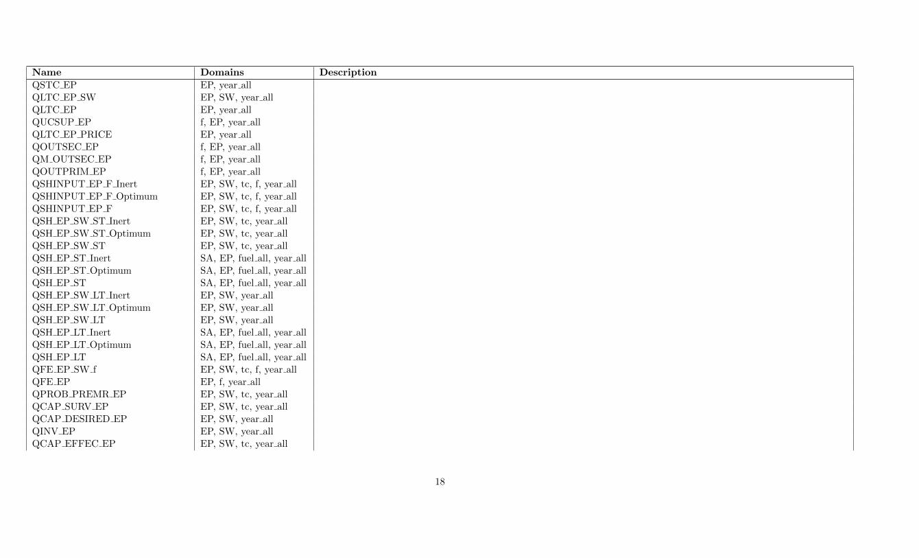
Name Domains Description
QSTC EP EP, year allQLTC EP SW EP, SW, year allQLTC EP EP, year allQUCSUP EP f, EP, year allQLTC EP PRICE EP, year allQOUTSEC EP f, EP, year allQM OUTSEC EP f, EP, year allQOUTPRIM EP f, EP, year allQSHINPUT EP F Inert EP, SW, tc, f, year allQSHINPUT EP F Optimum EP, SW, tc, f, year allQSHINPUT EP F EP, SW, tc, f, year allQSH EP SW ST Inert EP, SW, tc, year allQSH EP SW ST Optimum EP, SW, tc, year allQSH EP SW ST EP, SW, tc, year allQSH EP ST Inert SA, EP, fuel all, year allQSH EP ST Optimum SA, EP, fuel all, year allQSH EP ST SA, EP, fuel all, year allQSH EP SW LT Inert EP, SW, year allQSH EP SW LT Optimum EP, SW, year allQSH EP SW LT EP, SW, year allQSH EP LT Inert SA, EP, fuel all, year allQSH EP LT Optimum SA, EP, fuel all, year allQSH EP LT SA, EP, fuel all, year allQFE EP SW f EP, SW, tc, f, year allQFE EP EP, f, year allQPROB PREMR EP EP, SW, tc, year allQCAP SURV EP EP, SW, tc, year allQCAP DESIRED EP EP, SW, year allQINV EP EP, SW, year allQCAP EFFEC EP EP, SW, tc, year all
18

Name Domains Description
QM CAP EP EP, SW, tc, year allQM POT HER SF, SW, tc, year allQLTC HER SF, SW, tc, year allQSTC SF SW NoHER SF, SW, tc, year allQX SH HER LT SF, SW, tc, year allQX SH NoHER SF, SW, tc, year allQSH HER SF, SW, tc, year allQSH HER LT SF, SW, tc, year allQCAP SURV HER SF, SW, tc, year allQCAP EFFEC HER SF, SW, tc, year allQINV HER SF, SW, tc, year all
Equation Definitions
QACTSBSBrSB ,year
log((ACTSBSB,year + 1e− 05)) =
aactsbSB,year + (bactsb BNSB + ( bactsb MXSB−bactsb BNSB
1+exp((bspeedSB ·(macro lagSB,yearmacro BNSB,year
−macro IPSB,yearmacro BNSB,year
)))· (1 + exp(−(
bspeedSB ·macro IPSB,year
macro BNSB,year))))[aactsbSB,year]) · log((macroSB,year + 1e− 05)) ∀SBrSB, year
QACTSCSCrSC ,year
ACTSCSC,year = (1− doff SCSC,year) ·∑
SB|(SBrSB∧SB SCSB,SC)
(SH ACTSBCSB,SC,year ·ACTSBSB,year) ∀SCrSC , year
QACTSDSDrSD,year
ACTSDSD,year = (1− doff SDSD,year) ·∑
SC|(SCrSC∧SC SDSC,SD)
(SH ACTSCDSC,SD,year ·ACTSCSC,year) ∀SDrSD, year | ((1− doff SDSD,year) = 1)
19

QACTSE AGAG,SErSE ,year
ACTSE AGAG,SE,year = (1− doff SESE,year) ·∑
SD|(SDrSD∧SD SESD,SE∧SD AGSD,AG)
(SH ACTSDE AG STAG,SD,SE,year ·HistAG ACT SDAG,SD,year ·ACTSDSD,year)
∀AG,SErSE , year | (SE AGSE,AG ∧ ((1− doff SESE,year) = 1))
QACTSESErSE ,year
ACTSESE,year = (1− doff SESE,year) ·∑
AG|SE AGSE,AG
ACTSE AGAG,SE,year ∀SErSE , year | ((1− doff SESE,year) = 1)
QACTSE AG LTAG,SErSE ,year
ACTSE AG LTAG,SE,year = (1− doff SESE,year) ·∑
SD|(SDrSD∧SD SESD,SE∧SD AGSD,AG)
(SH ACTSDE AG LTAG,SD,SE,year ·HistAG ACT SDAG,SD,year ·ACTSDSD,year)
∀AG,SErSE , year | (SE AGSE,AG ∧ ((1− doff SESE,year) = 1))
QACTSF AGAG,SFrSF ,year
ACTSF AGAG,SF,year = (1− doff SFSF,year) ·∑
SE|(SErSE∧SE SFSE,SF∧SE AGSE,AG)
(SH ACTSEF AG STAG,SE,SF,year ·ACTSE AGAG,SE,year)
∀AG,SFrSF , year | (SF AGSF,AG ∧ ((1− doff SFSF,year) = 1))
QACTSFSFrSF ,year
ACTSFSF,year = (1− doff SFSF,year) ·∑
AG|SF AGSF,AG
ACTSF AGAG,SF,year ∀SFrSF , year | ((1− doff SFSF,year) = 1)
20

QACTSF AG LTAG,SFrSF ,year
ACTSF AG LTAG,SF,year = (1− doff SFSF,year) ·∑
SE|(SErSE∧SE SFSE,SF∧SE AGSE,AG)
(SH ACTSEF AG LTAG,SE,SF,year ·ACTSE AG LTAG,SE,year)
∀AG,SFrSF , year | (SF AGSF,AG ∧ ((1− doff SFSF,year) = 1))
QP ACTSBSBrSB ,year
P ACTSBSB,year ≥∑
SC|(SCrSC∧SB SCSB,SC)
(SH ACTSBCSB,SC,year · P ACTSCSC,year) ∀SBrSB, year
QP ACTSCSCrSC ,year
P ACTSCSC,year ≥ (1− doff SCSC,year) ·∑
SD|(SDrSD∧SC SDSC,SD)
(SH ACTSCDSC,SD,year · P ACTSDSD,year) ∀SCrSC , year | ((1− doff SCSC,year) = 1)
QP ACTSDSDrSD,year
P ACTSDSD,year ≥ (1− doff SDSD,year) ·∑
SE|(SErSE∧SD SESD,SE)
(∑
AG|(SD AGSD,AG∧SE AGSE,AG)
(HistAG ACT SDAG,SD,year · SH ACTSDE AG LTAG,SD,SE,year ·P ACTSE AG LTAG,SE,year · (1−
SUBS P ACTSESE,year))) ∀SDrSD, year | ((1− doff SDSD,year) = 1)
QP ACTSE AG STAG,SErSE ,year
P ACTSE AG STAG,SE,year ≥ (1− doff SESE,year) ·∑
SF |(SFrSF∧SE SFSE,SF∧SF AGSF,AG)
(SH ACTSEF AG STAG,SE,SF,year · P ACTSF AG STAG,SF,year · (1− SUBS P ACTSFSF,year))
∀AG,SErSE , year | (SE AGSE,AG ∧ ((1− doff SESE,year) = 1))
21

QP ACTSE AG LTAG,SErSE ,year
P ACTSE AG LTAG,SE,year ≥ (1− doff SESE,year) · (∑
SF |(SFrSF∧SE SFSE,SF∧SF AGSF,AG)
(SH ACTSEF AG LTAG,SE,SF,year · P ACTSF AG LTAG,SF,year · (1− SUBS P ACTSFSF,year))
+ P ACTSE AG LT StndrdsAG,SE,year) ∀AG,SErSE , year | (SE AGSE,AG ∧ ((1− doff SESE,year) = 1))
QP ACTSE AG LT StndrdsAG,SErSE ,year
P ACTSE AG LT StndrdsAG,SE,year ≥ (1− doff SESE,year) · (0.85 ·∑SD|A
(∑
Stndrds|B
(
∑SF |(SFrSF∧SE SFSE,SF )
(C)− stnd SD targetStndrds,SD,year
stnd SD targetStndrds,SD,year·M STND SDStndrds,SD,year)))
∀AG,SErSE , year | (SE AGSE,AG ∧ ((1− doff SESE,year) = 1))
WhereA=( SDrSD ∧ SD AGSD,AG ∧ SD SESD,SE)
B = (Stndrds SDSD,Stndrds ∧ stnd SD targetStndrds,SD,year ∧ (min{lblstnd SFStndrds,SF,FUT,year
∣∣SF |(SFrSF ∧ SE SFSE,SF )} > stnd SD targetStndrds,SD,year))
C = (SH ACTSEF AG LTAG,SE,SF,year ·∑SW
(SH SF SW AG LTAG,SF,SW,year · lblstnd SFStndrds,SF,SW,year))
QP ACTSF AG STAG,SFrSF ,year
P ACTSF AG STAG,SF,year ≥ (1− doff SFSF,year) ·∑
SW,tc|tc SWtc,SW
(SH SF SW AG STAG,SF,SW,tc,year ·M STC SF SW AGAG,SF,SW,tc,year)
∀AG,SFrSF , year | (SF AGSF,AG ∧ ((1− doff SFSF,year) = 1))
QP ACTSF AG LTAG,SFrSF ,year
P ACTSF AG LTAG,SF,year ≥ (1− doff SFSF,year) · (∑SW
(SH SF SW AG LTAG,SF,SW,year · LTC SF SW AGAG,SF,SW,year) + P ACTSF AG LT StndrdsAG,SF,year)
∀AG,SFrSF , year | (SF AGSF,AG ∧ ((1− doff SFSF,year) = 1))
22

QP ACTSF AG LT StndrdsAG,SFrSF ,year
P ACTSF AG LT StndrdsAG,SF,year ≥ (1− doff SFSF,year) ·∀AG,SFrSF , year | (SF AGSF,AG ∧ ((1− doff SFSF,year) = 1))
QP ACTSE STSErSE ,year
P ACTSE STSE,year ≥ (1− doff SESE,year) ·∑
AG|SE AGSE,AG
(∑
SF |(SFrSF∧SE SFSE,SF∧SF AGSF,AG)
(HistAG ACT SEAG,SE,year · SH ACTSEF AG STAG,SE,SF,year ·P ACTSF AG STAG,SF,year · (1−
SUBS P ACTSFSF,year))) ∀SErSE , year | ((1− doff SESE,year) = 1)
QP ACTSE LTSErSE ,year
P ACTSE LTSE,year ≥ (1− doff SESE,year) ·∑
AG|SE AGSE,AG
(∑
SF |(SFrSF∧SE SFSE,SF∧SF AGSF,AG)
(HistAG ACT SEAG,SE,year · SH ACTSEF AG LTAG,SE,SF,year ·P ACTSF AG LTAG,SF,year · (1−
SUBS P ACTSFSF,year)) + P ACTSE AG LT StndrdsAG,SE,year) ∀SErSE , year | ((1− doff SESE,year) = 1)
QP ACTSF STSFrSF ,year
P ACTSF STSF,year ≥ (1− doff SFSF,year) ·∑
AG|SF AGSF,AG
(HistAG ACT SFAG,SF,year · P ACTSF AG STAG,SF,year · (1− SUBS P ACTSFSF,year)) ∀SFrSF , year | ((1− doff SFSF,year) = 1)
QP ACTSF LTSFrSF ,year
P ACTSF LTSF,year ≥ (1− doff SFSF,year) ·∑
AG|SF AGSF,AG
(HistAG ACT SFAG,SF,year · P ACTSF AG LTAG,SF,year · (1− SUBS P ACTSFSF,year)) ∀SFrSF , year | ((1− doff SFSF,year) = 1)
QX SH ACTSBCSBrSB ,SCrSC ,year
X SH ACTSBCSB,SC,year = exp(−((gACTSBSB,year · P ACTSCSC,year · SH ACTSBC conv lagSB,SC,year))) ∀SBrSB, SCrSC , year | (SB SCSB,SC ∧ ((1− doff SB SCSB,SC,year) = 1))
23

QSH ACTSBCSBrSB ,SCrSC ,year
SH ACTSBCSB,SC,year = (
∑SCC|(SCrSCC∧SB SCSB,SCC)
1EL SB CARDSB,year
·(1−doff SB SCSB,SC,year)·dACTSBCSB,SC,year·exp(−((gACTSBSB,year·P ACTSCSC,year·SH ACTSBC conv lagSB,SC,year)))∑SCC|(SCrSCC∧SB SCSB,SCC)
((1− doff SB SCSB,SCC,year) · dACTSBCSB,SCC,year · exp(−((gACTSBSB,year · P ACTSCSCC,year · SH ACTSBC conv lagSB,SCC,year))))[(
∑SCC|(SCrSCC∧SB SCSB,SCC)
(1− doff SB SCSB,SCC,year) > 1)] + (1− doff SB SCSB,SC,year)[(∑
SCC|(SCrSCC∧SB SCSB,SCC)
(1− doff SB SCSB,SCC,year) ≤ 1)])[gACTSBSB,year] + (
∑SCC|(SCrSCC∧SB SCSB,SCC)
1EL SB CARDSB,year · (1− doff SB SCSB,SC,year) · dACTSBCSB,SC,year)[(¬gACTSBSB,year)] ∀SBrSB, SCrSC , year | (SB SCSB,SC ∧ ((1− doff SB SCSB,SC,year) = 1))
QX SH ACTSCD InertSCrSC ,SDrSD,year
X SH ACTSCD InertSC,SD,year = exp(−((gACTSCSC,year ·P ACTSDSD,year ·SH ACTSCD optimum conv lagSC,SD,year))) ∀SCrSC , SDrSD, year | (SC SDSC,SD∧((1−doff SC SDSC,SD,year) =1))
QX SH ACTSCD OptimumSCrSC ,SDrSD,year
X SH ACTSCD OptimumSC,SD,year = exp(−((gOptimumACTSCSC,year · P ACTSDSD,year · SH ACTSCD optimum conv lagSC,SD,year))) ∀SCrSC , SDrSD, year | (SC SDSC,SD ∧ ((1−doff SC SDSC,SD,year) = 1))
QSH ACTSCD InertSCrSC ,SDrSD,year
SH ACTSCD InertSC,SD,year = (∑SDD|(SDrSDD∧SC SDSC,SDD)
1EL SC CARDSC,year
·(1−doff SC SDSC,SD,year)·dACTSCDSC,SD,year·exp(−((gACTSCSC,year·P ACTSDSD,year·SH ACTSCD optimum conv lagSC,SD,year)))∑SDD|(SDrSDD∧SC SDSC,SDD)
((1− doff SC SDSC,SDD,year) · dACTSCDSC,SDD,year · exp(−((gACTSCSC,year · P ACTSDSDD,year · SH ACTSCD optimum conv lagSC,SDD,year))))[(
∑SDD|(SDrSDD∧SC SDSC,SDD)
(1− doff SC SDSC,SDD,year) > 1)] + (1− doff SC SDSC,SD,year)[(∑
SDD|(SDrSDD∧SC SDSC,SDD)
(1− doff SC SDSC,SDD,year) ≤ 1)])[gACTSCSC,year] + (
24

∑SDD|SC SDSC,SDD
1EL SC CARDSC,year · (1− doff SC SDSC,SD,year) · dACTSCDSC,SD,year)[(¬gACTSCSC,year)] ∀SCrSC , SDrSD, year | (SC SDSC,SD ∧ ((1− doff SC SDSC,SD,year) = 1))
QSH ACTSCD OptimumSCrSC ,SDrSD,year
SH ACTSCD OptimumSC,SD,year = (∑SDD|(SDrSDD∧SC SDSC,SDD)
1EL SC CARDSC,year
·(1−doff SC SDSC,SD,year)·dACTSCD OptimumSC,SD,year·exp(−((gOptimumACTSCSC,year·P ACTSDSD,year·SH ACTSCD optimum conv lagSC,SD,year)))∑SDD|(SDrSDD∧SC SDSC,SDD)
((1− doff SC SDSC,SDD,year) · dACTSCD OptimumSC,SDD,year · exp(−((gOptimumACTSCSC,year · P ACTSDSDD,year · SH ACTSCD optimum conv lagSC,SDD,year))))[(
∑SDD|(SDrSDD∧SC SDSC,SDD)
(1− doff SC SDSC,SDD,year) > 1)] + (1− doff SC SDSC,SD,year)[(∑
SDD|(SDrSDD∧SC SDSC,SDD)
(1− doff SC SDSC,SDD,year) ≤ 1)])[gOptimumACTSCSC,year] + (
∑SDD|SC SDSC,SDD
1EL SC CARDSC,year · (1− doff SC SDSC,SD,year) · dACTSCD OptimumSC,SD,year)[(¬gOptimumACTSCSC,year)] ∀SCrSC , SDrSD, year | (SC SDSC,SD ∧ ((1−
doff SC SDSC,SD,year) = 1))
QSH ACTSCDSCrSC ,SDrSD,year
SH ACTSCDSC,SD,year = (1− doff SC SDSC,SD,year) · ((1− TH SH ACTSCDSC,year) · SH ACTSCD InertSC,SD,year + TH SH ACTSCDSC,year · SH ACTSCD OptimumSC,SD,year)
∀SCrSC , SDrSD, year | (SC SDSC,SD ∧ ((1− doff SC SDSC,SD,year) = 1))
QX SH ACTSDE AG ST InertAG,SDrSD,SErSE ,year
X SH ACTSDE AG ST InertAG,SD,SE,year = exp(−((gACTSD AG STAG,SD,year · P ACTSE AG STAG,SE,year · SH ACTSDE AG ST Optimum conv lagAG,SD,SE,year)))
∀AG,SDrSD, SErSE , year | (SD SESD,SE ∧ SD AGSD,AG ∧ SE AGSE,AG ∧ ((1− doff SD SESD,SE,year) = 1))
QX SH ACTSDE AG ST OptimumAG,SDrSD,SErSE ,year
X SH ACTSDE AG ST OptimumAG,SD,SE,year = exp(−((gOptimumACTSD AG STAG,SD,year · P ACTSE AG STAG,SE,year · SH ACTSDE AG ST Optimum conv lagAG,SD,SE,year)))
∀AG,SDrSD, SErSE , year | (SD SESD,SE ∧ SD AGSD,AG ∧ SE AGSE,AG ∧ ((1− doff SD SESD,SE,year) = 1))
25

QSH ACTSDE AG ST InertAG,SDrSD,SErSE ,year
SH ACTSDE AG ST InertAG,SD,SE,year =
(
∑SEE|(SErSEE∧SD SESD,SEE∧SE AGSEE,AG)
1EL SD CARDSD,year
·(1−doff SD SESD,SE,year)·dACTSDE AG STAG,SD,SE,year·(A)∑SEE|(SErSEE∧SD SESD,SEE∧SE AGSEE,AG)
((1− doff SD SESD,SEE,year) · dACTSDE AG STAG,SD,SEE,year · (B))
[(∑
SEE|(SErSEE∧SD SESD,SEE∧SE AGSEE,AG)
(1− doff SD SESD,SEE,year) > 1)] +
(1− doff SD SESD,SE,year)[(∑
SEE|(SErSEE∧SD SESD,SEE∧SE AGSEE,AG)
(1− doff SD SESD,SEE,year) ≤ 1)])[gACTSD AG STAG,SD,year] +
(∑
SEE|(SErSEE∧SD SESD,SEE∧SE AGSEE,AG)
1EL SD CARDSD,year ·(1−doff SD SESD,SE,year)·dACTSDE AG STAG,SD,SE,year)[(¬gACTSD AG STAG,SD,year)] ∀AG,SDrSD, SErSE , year | (SD SESD,SE∧
SD AGSD,AG ∧ SE AGSE,AG ∧ ((1− doff SD SESD,SE,year) = 1))WhereA = exp ( - ( ( gACTSD AG STAG,SD,year · P ACTSE AG STAG,SE,year · SH ACTSDE AG ST Optimum conv lagAG,SD,SE,year)))B = exp(−((gACTSD AG STAG,SD,year · P ACTSE AG STAG,SEE,year · SH ACTSDE AG ST Optimum conv lagAG,SD,SEE,year)))
QSH ACTSDE AG ST OptimumAG,SDrSD,SErSE ,year
SH ACTSDE AG ST OptimumAG,SD,SE,year =
(
∑SEE|(SErSEE∧SD SESD,SEE∧SE AGSEE,AG)
1EL SD CARDSD,year
·(1−doff SD SESD,SE,year)·dACTSDE AG ST OptimumAG,SD,SE,year·(A)∑SEE|(SErSEE∧SD SESD,SEE∧SE AGSEE,AG)
((1− doff SD SESD,SEE,year) · dACTSDE AG ST OptimumAG,SD,SEE,year · (B))[(
∑SEE|(SErSEE∧SD SESD,SEE∧SE AGSEE,AG)
(1 − doff SD SESD,SEE,year) >
1)] + (1− doff SD SESD,SE,year)[(∑
SEE|(SErSEE∧SD SESD,SEE∧SE AGSEE,AG)
(1− doff SD SESD,SEE,year) ≤ 1)])[gOptimumACTSD AG STAG,SD,year] +
26

(∑
SEE|(SErSEE∧SD SESD,SEE∧SE AGSEE,AG)
1EL SD CARDSD,year · (1− doff SD SESD,SE,year) · dACTSDE AG ST OptimumAG,SD,SE,year)[(¬gOptimumACTSD AG STAG,SD,year)]
∀AG,SDrSD, SErSE , year | (SD SESD,SE ∧ SD AGSD,AG ∧ SE AGSE,AG ∧ ((1− doff SD SESD,SE,year) = 1))WhereA = exp(−((gOptimumACTSD AG STAG,SD,year · P ACTSE AG STAG,SE,year · SH ACTSDE AG ST Optimum conv lagAG,SD,SE,year)))B = exp(−((gOptimumACTSD AG STAG,SD,year · P ACTSE AG STAG,SEE,year · SH ACTSDE AG ST Optimum conv lagAG,SD,SEE,year)))
QSH ACTSDE AG STAG,SDrSD,SErSE ,year
SH ACTSDE AG STAG,SD,SE,year = (1 − doff SD SESD,SE,year) · ((1 − TH SH ACTSDE AG STAG,SD,year) · SH ACTSDE AG ST InertAG,SD,SE,year + TH SH ACTSDE AG STAG,SD,year ·SH ACTSDE AG ST OptimumAG,SD,SE,year) ∀AG,SDrSD, SErSE , year | (SD SESD,SE ∧ SD AGSD,AG ∧ SE AGSE,AG ∧ ((1− doff SD SESD,SE,year) = 1))
QX SH ACTSEF AG ST InertAG,SErSE ,SFrSF ,year
X SH ACTSEF AG ST InertAG,SE,SF,year = exp(−((gACTSE AG STAG,SE,year · P ACTSF AG STAG,SF,year · SH ACTSEF AG ST Optimum conv lagAG,SE,SF,year)))
∀AG,SErSE , SFrSF , year | (SE SFSE,SF ∧ SF AGSF,AG ∧ SE AGSE,AG ∧ ((1− doff SE SFSE,SF,year) = 1))
QX SH ACTSEF AG ST OptimumAG,SErSE ,SFrSF ,year
X SH ACTSEF AG ST OptimumAG,SE,SF,year = exp(−((gOptimumACTSE AG STAG,SE,year · P ACTSF AG STAG,SF,year · SH ACTSEF AG ST Optimum conv lagAG,SE,SF,year)))
∀AG,SErSE , SFrSF , year | (SE SFSE,SF ∧ SF AGSF,AG ∧ SE AGSE,AG ∧ ((1− doff SE SFSE,SF,year) = 1))
QSH ACTSEF AG ST InertAG,SErSE ,SFrSF ,year
SH ACTSEF AG ST InertAG,SE,SF,year =
(
∑SFF |(SFrSFF∧SE SFSE,SFF∧SF AGSFF,AG)
1EL SE CARDSE,year
·(1−doff SE SFSE,SF,year)·dACTSEF AG STAG,SE,SF,year·(A)∑SFF |(SFrSFF∧SE SFSE,SFF∧SF AGSFF,AG)
((1− doff SE SFSE,SFF,year) · dACTSEF AG STAG,SE,SFF,year · (B))[
(∑
SFF |(SFrSFF∧SE SFSE,SFF∧SF AGSFF,AG)
(1− doff SE SFSE,SFF,year) > 1)] +
27

(1− doff SE SFSE,SF,year)[(∑
SFF |(SFrSFF∧SE SFSE,SFF∧SF AGSFF,AG)
(1− doff SE SFSE,SFF,year) ≤ 1)])[gACTSE AG STAG,SE,year] +
(∑
SFF |(SFrSFF∧SE SFSE,SFF∧SF AGSFF,AG)
1EL SE CARDSE,year ·(1−doff SE SFSE,SF,year)·dACTSEF AG STAG,SE,SF,year)[(¬gACTSE AG STAG,SE,year)] ∀AG,SErSE , SFrSF , year | (SE SFSE,SF∧
SF AGSF,AG ∧ SE AGSE,AG ∧ ((1− doff SE SFSE,SF,year) = 1))WhereA = exp(−((gACTSE AG STAG,SE,year · P ACTSF AG STAG,SF,year · SH ACTSEF AG ST Optimum conv lagAG,SE,SF,year)))B = exp(−((gACTSE AG STAG,SE,year · P ACTSF AG STAG,SFF,year · SH ACTSEF AG ST Optimum conv lagAG,SE,SFF,year)))
QSH ACTSEF AG ST OptimumAG,SErSE ,SFrSF ,year
SH ACTSEF AG ST OptimumAG,SE,SF,year = (
∑SFF |(SFrSFF∧SE SFSE,SFF∧SF AGSFF,AG)
1EL SE CARDSE,year
·(1−doff SE SFSE,SF,year)·dACTSEF AG ST OptimumAG,SE,SF,year·(A)∑SFF |(SFrSFF∧SE SFSE,SFF∧SF AGSFF,AG)
((1− doff SE SFSE,SFF,year) · dACTSEF AG ST OptimumAG,SE,SFF,year · (B))[
(∑
SFF |(SFrSFF∧SE SFSE,SFF∧SF AGSFF,AG)
(1− doff SE SFSE,SFF,year) > 1)] +
(1− doff SE SFSE,SF,year)[(∑
SFF |(SFrSFF∧SE SFSE,SFF∧SF AGSFF,AG)
(1− doff SE SFSE,SFF,year) ≤ 1)])[gOptimumACTSE AG STAG,SE,year] +
(∑
SFF |(SFrSFF∧SE SFSE,SFF∧SF AGSFF,AG)
1EL SE CARDSE,year · (1− doff SE SFSE,SF,year) · dACTSEF AG ST OptimumAG,SE,SF,year)[(¬gOptimumACTSE AG STAG,SE,year)]
∀AG,SErSE , SFrSF , year | (SE SFSE,SF ∧ SF AGSF,AG ∧ SE AGSE,AG ∧ ((1− doff SE SFSE,SF,year) = 1))WhereA = exp(−((gOptimumACTSE AG STAG,SE,year · P ACTSF AG STAG,SF,year · SH ACTSEF AG ST Optimum conv lagAG,SE,SF,year)))B = exp(−((gOptimumACTSE AG STAG,SE,year · P ACTSF AG STAG,SFF,year · SH ACTSEF AG ST Optimum conv lagAG,SE,SFF,year)))
28

QSH ACTSEF AG STAG,SErSE ,SFrSF ,year
SH ACTSEF AG STAG,SE,SF,year = (1 − doff SE SFSE,SF,year) · ((1 − TH SH ACTSEF AG STAG,SE,year) · SH ACTSEF AG ST InertAG,SE,SF,year + TH SH ACTSEF AG STAG,SE,year ·SH ACTSEF AG ST OptimumAG,SE,SF,year) ∀AG,SErSE , SFrSF , year | (SE SFSE,SF ∧ SF AGSF,AG ∧ SE AGSE,AG ∧ ((1− doff SE SFSE,SF,year) = 1))
QX SH ACTSDE AG LT InertAG,SDrSD,SErSE ,year
X SH ACTSDE AG LT InertAG,SD,SE,year = exp(−((gACTSD AG LTAG,SD,year · P ACTSE AG LTAG,SE,year · SH ACTSDE AG LT Optimum conv lagAG,SD,SE,year)))
∀AG,SDrSD, SErSE , year | (SD SESD,SE ∧ SD AGSD,AG ∧ SE AGSE,AG ∧ ((1− doff SD SESD,SE,year) = 1))
QX SH ACTSDE AG LT OptimumAG,SDrSD,SErSE ,year
X SH ACTSDE AG LT OptimumAG,SD,SE,year = exp(−((gOptimumACTSD AG LTAG,SD,year · P ACTSE AG LTAG,SE,year · SH ACTSDE AG LT Optimum conv lagAG,SD,SE,year)))
∀AG,SDrSD, SErSE , year | (SD SESD,SE ∧ SD AGSD,AG ∧ SE AGSE,AG ∧ ((1− doff SD SESD,SE,year) = 1))
QSH ACTSDE AG LT InertAG,SDrSD,SErSE ,year
SH ACTSDE AG LT InertAG,SD,SE,year = (
∑SEE|(SErSEE∧SD SESD,SEE∧SE AGSEE,AG)
1EL SD CARDSD,year
·(1−doff SD SESD,SE,year)·dACTSDE AG LTAG,SD,SE,year·(A)∑SEE|(SErSEE∧SD SESD,SEE∧SE AGSEE,AG)
((1− doff SD SESD,SEE,year) · dACTSDE AG LTAG,SD,SEE,year · (B))[
(∑
SEE|(SErSEE∧SD SESD,SEE∧SE AGSEE,AG)
(1− doff SD SESD,SEE,year) > 1)] +
(1− doff SD SESD,SE,year)[(∑
SEE|(SErSEE∧SD SESD,SEE∧SE AGSEE,AG)
(1− doff SD SESD,SEE,year) ≤ 1)])[gACTSD AG LTAG,SD,year] +
(∑
SEE|(SErSEE∧SD SESD,SEE∧SE AGSEE,AG)
1EL SD CARDSD,year · (1− doff SD SESD,SE,year) · dACTSDE AG LTAG,SD,SE,year)[(¬gACTSD AG LTAG,SD,year)]
∀AG,SDrSD, SErSE , year | (SD SESD,SE ∧ SD AGSD,AG ∧ SE AGSE,AG ∧ ((1− doff SD SESD,SE,year) = 1))Where
29

A = exp(−((gACTSD AG LTAG,SD,year · P ACTSE AG LTAG,SE,year · SH ACTSDE AG LT Optimum conv lagAG,SD,SE,year)))B = exp(−((gACTSD AG LTAG,SD,year · P ACTSE AG LTAG,SEE,year · SH ACTSDE AG LT Optimum conv lagAG,SD,SEE,year)))
QSH ACTSDE AG LT OptimumAG,SDrSD,SErSE ,year
SH ACTSDE AG LT OptimumAG,SD,SE,year = (
∑SEE|(SErSEE∧SD SESD,SEE∧SE AGSEE,AG)
1EL SD CARDSD,year
·(1−doff SD SESD,SE,year)·dACTSDE AG LT OptimumAG,SD,SE,year·(A)∑SEE|(SErSEE∧SD SESD,SEE∧SE AGSEE,AG)
((1− doff SD SESD,SEE,year) · dACTSDE AG LT OptimumAG,SD,SEE,year · (B))[
(∑
SEE|(SErSEE∧SD SESD,SEE∧SE AGSEE,AG)
(1− doff SD SESD,SEE,year) > 1)] +
(1− doff SD SESD,SE,year)[(∑
SEE|(SErSEE∧SD SESD,SEE∧SE AGSEE,AG)
(1− doff SD SESD,SEE,year) ≤ 1)])[gOptimumACTSD AG LTAG,SD,year] +
(∑
SEE|(SErSEE∧SD SESD,SEE∧SE AGSEE,AG)
1EL SD CARDSD,year · (1− doff SD SESD,SE,year) · dACTSDE AG LT OptimumAG,SD,SE,year)[(¬gOptimumACTSD AG LTAG,SD,year)]
∀AG,SDrSD, SErSE , year | (SD SESD,SE ∧ SD AGSD,AG ∧ SE AGSE,AG ∧ ((1− doff SD SESD,SE,year) = 1))WhereA = exp(−((gOptimumACTSD AG LTAG,SD,year · P ACTSE AG LTAG,SE,year · SH ACTSDE AG LT Optimum conv lagAG,SD,SE,year)))B = exp(−((gOptimumACTSD AG LTAG,SD,year · P ACTSE AG LTAG,SEE,year · SH ACTSDE AG LT Optimum conv lagAG,SD,SEE,year)))
QSH ACTSDE AG LTAG,SDrSD,SErSE ,year
SH ACTSDE AG LTAG,SD,SE,year = (1 − doff SD SESD,SE,year) · ((1 − TH SH ACTSDE AG LTAG,SD,year) · SH ACTSDE AG LT InertAG,SD,SE,year + TH SH ACTSDE AG LTAG,SD,year ·SH ACTSDE AG LT OptimumAG,SD,SE,year) ∀AG,SDrSD, SErSE , year | (SD SESD,SE ∧ SD AGSD,AG ∧ SE AGSE,AG ∧ ((1− doff SD SESD,SE,year) = 1))
QX SH ACTSEF AG LT InertAG,SErSE ,SFrSF ,year
X SH ACTSEF AG LT InertAG,SE,SF,year = exp(−((gACTSE AG LTAG,SE,year · P ACTSF AG LTAG,SF,year · SH ACTSEF AG LT Optimum conv lagAG,SE,SF,year)))
∀AG,SErSE , SFrSF , year | (SE SFSE,SF ∧ SF AGSF,AG ∧ SE AGSE,AG ∧ ((1− doff SE SFSE,SF,year) = 1))
30

QX SH ACTSEF AG LT OptimumAG,SErSE ,SFrSF ,year
X SH ACTSEF AG LT OptimumAG,SE,SF,year = exp(−((gOptimumACTSE AG LTAG,SE,year · P ACTSF AG LTAG,SF,year · SH ACTSEF AG LT Optimum conv lagAG,SE,SF,year)))
∀AG,SErSE , SFrSF , year | (SE SFSE,SF ∧ SF AGSF,AG ∧ SE AGSE,AG ∧ ((1− doff SE SFSE,SF,year) = 1))
QSH ACTSEF AG LT InertAG,SErSE ,SFrSF ,year
SH ACTSEF AG LT InertAG,SE,SF,year = (
∑SFF |(SFrSFF∧SE SFSE,SFF∧SF AGSFF,AG)
1EL SE CARDSE,year
·(1−doff SE SFSE,SF,year)·dACTSEF AG LTAG,SE,SF,year·(A)∑SFF |(SFrSFF∧SE SFSE,SFF∧SF AGSFF,AG)
((1− doff SE SFSE,SFF,year) · dACTSEF AG LTAG,SE,SFF,year · (B))[
(∑
SFF |(SFrSFF∧SE SFSE,SFF∧SF AGSFF,AG)
(1− doff SE SFSE,SFF,year) > 1)] +
(1− doff SE SFSE,SF,year)[(∑
SFF |(SFrSFF∧SE SFSE,SFF∧SF AGSFF,AG)
(1− doff SE SFSE,SFF,year) ≤ 1)])[gACTSE AG LTAG,SE,year] +
(∑
SFF |(SFrSFF∧SE SFSE,SFF∧SF AGSFF,AG)
1EL SE CARDSE,year · (1− doff SE SFSE,SF,year) · dACTSEF AG LTAG,SE,SF,year)[(¬gACTSE AG LTAG,SE,year)]
∀AG,SErSE , SFrSF , year | (SE SFSE,SF ∧ SF AGSF,AG ∧ SE AGSE,AG ∧ ((1− doff SE SFSE,SF,year) = 1))WhereA = exp(−((gACTSE AG LTAG,SE,year · P ACTSF AG LTAG,SF,year · SH ACTSEF AG LT Optimum conv lagAG,SE,SF,year)))B = exp(−((gACTSE AG LTAG,SE,year · P ACTSF AG LTAG,SFF,year · SH ACTSEF AG LT Optimum conv lagAG,SE,SFF,year)))
31

QSH ACTSEF AG LT OptimumAG,SErSE ,SFrSF ,year
SH ACTSEF AG LT OptimumAG,SE,SF,year = (
∑SFF |(SFrSFF∧SE SFSE,SFF∧SF AGSFF,AG)
1EL SE CARDSE,year
·(1−doff SE SFSE,SF,year)·dACTSEF AG LT OptimumAG,SE,SF,year·(A)∑SFF |(SFrSFF∧SE SFSE,SFF∧SF AGSFF,AG)
((1− doff SE SFSE,SFF,year) · dACTSEF AG LT OptimumAG,SE,SFF,year · (B))[
(∑
SFF |(SFrSFF∧SE SFSE,SFF∧SF AGSFF,AG)
(1− doff SE SFSE,SFF,year) > 1)] +
(1− doff SE SFSE,SF,year)[(∑
SFF |(SFrSFF∧SE SFSE,SFF∧SF AGSFF,AG)
(1− doff SE SFSE,SFF,year) ≤ 1)])[gOptimumACTSE AG LTAG,SE,year] +
(∑
SFF |(SFrSFF∧SE SFSE,SFF∧SF AGSFF,AG)
1EL SE CARDSE,year · (1− doff SE SFSE,SF,year) · dACTSEF AG LT OptimumAG,SE,SF,year)[(¬gOptimumACTSE AG LTAG,SE,year)]
∀AG,SErSE , SFrSF , year | (SE SFSE,SF ∧ SF AGSF,AG ∧ SE AGSE,AG ∧ ((1− doff SE SFSE,SF,year) = 1))WhereA = exp(−((gOptimumACTSE AG LTAG,SE,year · P ACTSF AG LTAG,SF,year · SH ACTSEF AG LT Optimum conv lagAG,SE,SF,year)))B = exp(−((gOptimumACTSE AG LTAG,SE,year · P ACTSF AG LTAG,SFF,year · SH ACTSEF AG LT Optimum conv lagAG,SE,SFF,year)))
QSH ACTSEF AG LTAG,SErSE ,SFrSF ,year
SH ACTSEF AG LTAG,SE,SF,year = (1 − doff SE SFSE,SF,year) · ((1 − TH SH ACTSEF AG LTAG,SE,year) · SH ACTSEF AG LT InertAG,SE,SF,year + TH SH ACTSEF AG LTAG,SE,year ·SH ACTSEF AG LT OptimumAG,SE,SF,year) ∀AG,SErSE , SFrSF , year | (SE SFSE,SF ∧ SF AGSF,AG ∧ SE AGSE,AG ∧ ((1− doff SE SFSE,SF,year) = 1))
QSTC SW FSFrSF ,SW,tc,f,year
STC SW FSF,SW,tc,f,year = (1− doff SF tcSF,SW,tc,year) · (vqc fSF,f,year + PRIF TAX SFf,SF,year[fmarketf ] +∑SA|(SArSA∧SA SFSA,SF∧fselff∧(¬fmarketf ))
UCAUTO SAf,SA,year +∑
SD|(SDrSD∧SD SFSD,SF∧fpoteff SDSD,f,year)
M POT SDSD,f,year − RESvalue SFf,SF,year[fresf ] +∑po
((POvaluepo,SF,year · Emfactorpo,f,year)[pollvalueSF,year] + (POpricepo,SF,year · Emfactorpo,f,year)[pollpriceSF,year])) ·Heatratef,SF,SW,tc,year
∀SFrSF , SW, tc, f, year | (((1− doff SF tcSF,SW,tc,year) = 1) ∧ tc SWtc,SW ∧ (SF frSF,f,year ∨ SF HERSF,f ))
32

QUCAUTO SAf,SArSA,year
UCAUTO SAf,SA,year =∑
EP |(EPrEP∧SA EPSA,EP∧(foutprimaryf,EP∨foutsecondaryf,EP ))
(SH EP STSA,EP,f,year ·UCSUP EPf,EP,year)
∀f, SArSA, year | (fselff ∧ (∑
SF,SFrSF |(((1−doff SFSF,year)=1)∧SA SFSA,SF )
(SF frSF,f,year ∨ SF HERSF,f ) ∨∑
EP |(EPrEP∧SA EPSA,EP )
EP fEP,f ))
QSTC SF SW AGAG,SFrSF ,SW,tc,year
STC SF SW AGAG,SF,SW,tc,year = (1− doff SF tcSF,SW,tc,year) · ((∑
f |SF frSF,f,year
(SH SW FSF,SW,tc,f,year · STC SW FSF,SW,tc,f,year) · (1− SH HERSF,SW,tc,year[∑
ff,SF HERSF,ff
1]) +
vqc SFSF,year ·Heatrate AVRGSF +omq SFSF,year
util AG SFAG,SF,year·8760Heatrate AVRGSF
· (1 + osmg SFSF,year)tc.val)[(¬SFtraSF )] +
∑f |SF frSF,f,year
(SH SW FSF,SW,tc,f,year · STC SW FSF,SW,tc,f,year) + vqc SFSF,year +omq SFSF,year
mileageAG,SF,year · 1000· (1 + osmg SFSF,year)
tc.val
occupancySF,year[SFtraSF ])
∀AG,SFrSF , SW, tc, year | (tc SWtc,SW ∧ SF AGSF,AG ∧ ((1− doff SF tcSF,SW,tc,year) = 1))
QM STC SF SW AGAG,SFrSF ,SW,tc,year
M STC SF SW AGAG,SF,SW,tc,year = (1−doff SF tcSF,SW,tc,year) ·((∑
f |SF frSF,f,year
(SH SW FSF,SW,tc,f,year ·STC SW FSF,SW,tc,f,year) ·(1−SH HERSF,SW,tc,year[∑
ff |SF HERSF,ff
1])+vqc SFSF,year ·
Heatrate AVRGSF +M CAP SFSF,SW,tc,year
util AG SFAG,SF,year · 8760)[(¬SFtraSF )] +∑
f |SF frSF,f,year
(SH SW FSF,SW,tc,f,year · STC SW FSF,SW,tc,f,year) + vqc SFSF,year +M CAP SFSF,SW,tc,year
mileageAG,SF,year · 1000
occupancySF,year[SFtraSF ]) ∀AG,SFrSF , SW, tc, year | (tc SWtc,SW ∧ SF AGSF,AG ∧ ((1−
doff SF tcSF,SW,tc,year) = 1))
33
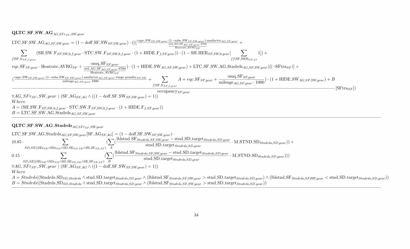
QLTC SF SW AGAG,SFrSF ,SW,year
LTC SF SW AGAG,SF,SW,year = (1− doff SF SWSF,SW,year) · (((capc SWSF,SW,year·(1−subs SWSF,SW,year)·annfactorAG,SF,year
util AG SFAG,SF,year ·8760Heatrate AVRGSF
+∑f |SF frSF,f,year
(SH SW FSF,SW,0,f,year · STC SW FSF,SW,0,f,year · (1 + HIDE Ff,SF,year)) · (1− SH HERSF,SW,0,year[∑
ff |SF HERSF,ff
1]) +
vqc SFSF,year ·Heatrate AVRGSF +omq SFSF,year
util AG SFAG,SF,year·8760Heatrate AVRGSF
) · (1 + HIDE SWAG,SF,SW,year) + LTC SF SW AG StndrdsAG,SF,SW,year)[(¬SFtraSF )] +
(capc SWSF,SW,year·(1−subs SWSF,SW,year)·annfactorAG,SF,year·range penaltySF,SW
mileageAG,SF,year·1000 +∑
f |SF frSF,f,year
A + vqc SFSF,year +omq SFSF,year
mileageAG,SF,year · 1000) · (1 + HIDE SWAG,SF,SW,year) + B
occupancySF,year[SFtraSF ])
∀AG,SFrSF , SW, year | (SF AGSF,AG ∧ ((1− doff SF SWSF,SW,year) = 1))WhereA = (SH SW FSF,SW,0,f,year · STC SW FSF,SW,0,f,year · (1 + HIDE Ff,SF,year))B = LTC SF SW AG StndrdsAG,SF,SW,year
QLTC SF SW AG StndrdsAG,SFrSF ,SW,year
LTC SF SW AG StndrdsAG,SF,SW,year[SF AGSF,AG] = (1− doff SF SWSF,SW,year) ·
(0.85 ·∑
SD,SE|(SErSE∧SDrSD∧SD SESD,SE∧SE SFSE,SF )
(∑A
(lblstnd SFStndrds,SF,SW,year − stnd SD targetStndrds,SD,year
stnd SD targetStndrds,SD,year·M STND SDStndrds,SD,year)) +
0.15 ·∑
SD,SE|(SErSE∧SDrSD∧SD SESD,SE∧SE SFSE,SF )
(∑B
(lblstnd SFStndrds,SF,SW,year − stnd SD targetStndrds,SD,year
stnd SD targetStndrds,SD,year·M STND SDStndrds,SD,year)))
∀AG,SFrSF , SW, year | (SF AGSF,AG ∧ ((1− doff SF SWSF,SW,year) = 1))WhereA = Stndrds|(Stndrds SDSD,Stndrds ∧ stnd SD targetStndrds,SD,year ∧ (lblstnd SFStndrds,SF,SW,year > stnd SD targetStndrds,SD,year) ∧ (lblstnd SFStndrds,SF,FUT,year < stnd SD targetStndrds,SD,year))B = Stndrds|(Stndrds SDSD,Stndrds ∧ stnd SD targetStndrds,SD,year ∧ (lblstnd SFStndrds,SF,SW,year > stnd SD targetStndrds,SD,year))
34

QSTC SF SWSFrSF ,SW,tc,year
STC SF SWSF,SW,tc,year = (1− doff SF tcSF,SW,tc,year) ·∑
AG|SF AGSF,AG
(HistAG ACT SFAG,SF,year · STC SF SW AGAG,SF,SW,tc,year)
∀SFrSF , SW, tc, year | (tc SWtc,SW ∧ ((1− doff SF tcSF,SW,tc,year) = 1))
QLTC SF SWSFrSF ,SW,year
LTC SF SWSF,SW,year = (1− doff SF SWSF,SW,year) ·∑
AG|SF AGSF,AG
(HistAG ACT SFAG,SF,year · LTC SF SW AGAG,SF,SW,year) ∀SFrSF , SW, year | ((1− doff SF SWSF,SW,year) = 1)
QX SH SW F InertSFrSF ,SW,tc,f,year
X SH SW F InertSF,SW,tc,f,year = exp(−((gSW FSF,year · STC SW FSF,SW,tc,f,year))) ∀SFrSF , SW, tc, f, year | (tc SWtc,SW ∧ SF frSF,f,year ∧ ((1− doff SF tcSF,SW,tc,year) = 1))
QX SH SW F OptimumSFrSF ,SW,tc,f,year
X SH SW F OptimumSF,SW,tc,f,year = exp(−((gOptimumSW FSF,year · STC SW FSF,SW,tc,f,year))) ∀SFrSF , SW, tc, f, year | (tc SWtc,SW ∧ SF frSF,f,year ∧ ((1− doff SF tcSF,SW,tc,year) = 1))
QSH SW F InertSFrSF ,SW,tc,f,year
SH SW F InertSF,SW,tc,f,year = (1− doff SF tcSF,SW,tc,year) · ((dSW FSF,SW,tc,f,year·exp(−((gSW FSF,year·STC SW FSF,SW,tc,f,year)))∑
ff |(tc SWtc,SW∧SF frSF,ff,year)
(dSW FSF,SW,tc,ff,year · exp(−((gSW FSF,year · STC SW FSF,SW,tc,ff,year))))[
∑ff |(tc SWtc,SW∧SF frSF,ff,year)
dSW FSF,SW,tc,ff,year[(∑
ff |(tc SWtc,SW∧SF frSF,ff,year)
1 > 1)]] + 1[(∑
ff |(tc SWtc,SW∧SF frSF,ff,year)
1 ≤ 1)])[gSW FSF,year] + dSW FSF,SW,tc,f,year[(¬gSW FSF,year)])
∀SFrSF , SW, tc, f, year | (tc SWtc,SW ∧ SF frSF,f,year ∧ ((1− doff SF tcSF,SW,tc,year) = 1))
35

QSH SW F OptimumSFrSF ,SW,tc,f,year
SH SW F OptimumSF,SW,tc,f,year = (1 − doff SF tcSF,SW,tc,year) · ((exp(−((gOptimumSW FSF,year·STC SW FSF,SW,tc,f,year)))∑
ff |(tc SWtc,SW∧SF frSF,ff,year)
(exp(−((gOptimumSW FSF,year · STC SW FSF,SW,tc,ff,year))))[(
∑ff |(tc SWtc,SW∧SF frSF,ff,year)
1 >
1)] + 1[(∑
ff |(tc SWtc,SW∧SF frSF,ff,year)
1 ≤ 1)])[gOptimumSW FSF,year] + SH SW F InertSF,SW,tc,f,year[(¬gOptimumSW FSF,year)]) ∀SFrSF , SW, tc, f, year | (tc SWtc,SW ∧ SF frSF,f,year ∧ ((1−
doff SF tcSF,SW,tc,year) = 1))
QSH SW FSFrSF ,SW,tc,f,year
SH SW FSF,SW,tc,f,year ≥ (1− doff SF tcSF,SW,tc,year) · ((1− TH SH SW FSF,year) · SH SW F InertSF,SW,tc,f,year + TH SH SW FSF,year · SH SW F OptimumSF,SW,tc,f,year)
∀SFrSF , SW, tc, f, year | (tc SWtc,SW ∧ SF frSF,f,year ∧ ((1− doff SF tcSF,SW,tc,year) = 1))
QX SH SF SW AG ST InertAG,SFrSF ,SW,tc,year
X SH SF SW AG ST InertAG,SF,SW,tc,year = exp(−((gSF SW AG STAG,SF,year ·M STC SF SW AGAG,SF,SW,tc,year))) ∀AG,SFrSF , SW, tc, year | (tc SWtc,SW ∧ SF AGSF,AG ∧ ((1−doff SF tcSF,SW,tc,year) = 1))
QX SH SF SW AG ST OptimumAG,SFrSF ,SW,tc,year
X SH SF SW AG ST OptimumAG,SF,SW,tc,year = exp(−((gOptimumSF SW AG STAG,SF,year ·M STC SF SW AGAG,SF,SW,tc,year))) ∀AG,SFrSF , SW, tc, year | (tc SWtc,SW ∧SF AGSF,AG ∧ ((1− doff SF tcSF,SW,tc,year) = 1))
QSH SF SW AG ST InertAG,SFrSF ,SW,tc,year
SH SF SW AG ST InertAG,SF,SW,tc,year =(1−doff SF tcSF,SW,tc,year)·dSF SW AG STAG,SF,SW,tc,year·exp(−((gSF SW AG STAG,SF,year·M STC SF SW AGAG,SF,SW,tc,year)))∑
tcc,SWW |tc SWtcc,SWW
((1− doff SF tcSF,SWW,tcc,year) · dSF SW AG STAG,SF,SWW,tcc,year · (A))[gSF SW AG STAG,SF,year]
[∑
tcc,SWW |tc SWtcc,SWW
((1− doff SF tcSF,SWW,tcc,year) · dSF SW AG STAG,SF,SWW,tcc,year)] + ((1− doff SF tcSF,SW,tc,year) · dSF SW AG STAG,SF,SW,tc,year)[(¬gSF SW AG STAG,SF,year)]
∀AG,SFrSF , SW, tc, year | (tc SWtc,SW ∧ SF AGSF,AG ∧ ((1− doff SF tcSF,SW,tc,year) = 1))
36

WhereA = exp(−((gSF SW AG STAG,SF,year ·M STC SF SW AGAG,SF,SWW,tcc,year)))
QSH SF SW AG ST OptimumAG,SFrSF ,SW,tc,year
SH SF SW AG ST OptimumAG,SF,SW,tc,year =(1−doff SF tcSF,SW,tc,year)·exp(−((gOptimumSF SW AG STAG,SF,year·M STC SF SW AGAG,SF,SW,tc,year)))∑
tcc,SWW |tc SWtcc,SWW
((1− doff SF tcSF,SWW,tcc,year) · exp(−((gOptimumSF SW AG STAG,SF,year ·M STC SF SW AGAG,SF,SWW,tcc,year))))
[gOptimumSF SW AG STAG,SF,year][∑
tcc,SWW |tc SWtcc,SWW
(1−doff SF tcSF,SWW,tcc,year)]+((1−doff SF tcSF,SW,tc,year)·SH SF SW AG ST InertAG,SF,SW,tc,year)[(¬gOptimumSF SW AG STAG,SF,year)]
∀AG,SFrSF , SW, tc, year | (tc SWtc,SW ∧ SF AGSF,AG ∧ ((1− doff SF tcSF,SW,tc,year) = 1))
QSH SF SW AG STAG,SFrSF ,SW,tc,year
SH SF SW AG STAG,SF,SW,tc,year = (1− doff SF tcSF,SW,tc,year) · ((1− TH SH SF SW AG STAG,SF,year) · SH SF SW AG ST InertAG,SF,SW,tc,year +TH SH SF SW AG STAG,SF,year · SH SF SW AG ST OptimumAG,SF,SW,tc,year) ∀AG,SFrSF , SW, tc, year | (tc SWtc,SW ∧ SF AGSF,AG ∧ ((1− doff SF tcSF,SW,tc,year) = 1))
QX SH SF SW AG LT InertAG,SFrSF ,SW,year
X SH SF SW AG LT InertAG,SF,SW,year = exp(−((gSF SW AG LTAG,SF,year · LTC SF SW AGAG,SF,SW,year))) ∀AG,SFrSF , SW, year | (SF AGSF,AG ∧ ((1− doff SF tcSF,SW,0,year) = 1))
QX SH SF SW AG LT OptimumAG,SFrSF ,SW,year
X SH SF SW AG LT OptimumAG,SF,SW,year = exp(−((gOptimumSF SW AG LTAG,SF,year · LTC SF SW AGAG,SF,SW,year))) ∀AG,SFrSF , SW, year | (SF AGSF,AG ∧ ((1−doff SF tcSF,SW,0,year) = 1))
37

QSH SF SW AG LT InertAG,SFrSF ,SW,year
SH SF SW AG LT InertAG,SF,SW,year =(1−doff SF tcSF,SW,0,year)·dSF SW AG LTAG,SF,SW,year·exp(−((gSF SW AG LTAG,SF,year·LTC SF SW AGAG,SF,SW,year)))∑
SWW
((1− doff SF tcSF,SWW,0,year) · dSF SW AG LTAG,SF,SWW,year · exp(−((gSF SW AG LTAG,SF,year · LTC SF SW AGAG,SF,SWW,year))))
[gSF SW AG LTAG,SF,year][∑
SWW
((1− doff SF tcSF,SWW,0,year) · dSF SW AG LTAG,SF,SWW,year)] + ((1− doff SF tcSF,SW,0,year) · dSF SW AG LTAG,SF,SW,year)[(¬gSF SW AG LTAG,SF,year)]
∀AG,SFrSF , SW, year | (SF AGSF,AG ∧ ((1− doff SF tcSF,SW,0,year) = 1))
QSH SF SW AG LT OptimumAG,SFrSF ,SW,year
SH SF SW AG LT OptimumAG,SF,SW,year =(1−doff SF tcSF,SW,0,year)·exp(−((gOptimumSF SW AG LTAG,SF,year·LTC SF SW AGAG,SF,SW,year)))∑
SWW
((1− doff SF tcSF,SWW,0,year) · exp(−((gOptimumSF SW AG LTAG,SF,year · LTC SF SW AGAG,SF,SWW,year))))
[gOptimumSF SW AG LTAG,SF,year][∑
tcc,SWW |tc SWtcc,SWW
(1−doff SF tcSF,SWW,tcc,year)]+((1−doff SF tcSF,SW,0,year)·SH SF SW AG LT InertAG,SF,SW,year)[(¬gOptimumSF SW AG LTAG,SF,year)]
∀AG,SFrSF , SW, year | (SF AGSF,AG ∧ ((1− doff SF tcSF,SW,0,year) = 1))
QSH SF SW AG LTAG,SFrSF ,SW,year
SH SF SW AG LTAG,SF,SW,year = (1− doff SF tcSF,SW,0,year) · ((1− TH SH SF SW AG LTAG,SF,year) · SH SF SW AG LT InertAG,SF,SW,year +TH SH SF SW AG LTAG,SF,year · SH SF SW AG LT OptimumAG,SF,SW,year)∀AG,SFrSF , SW, year | (SF AGSF,AG ∧ ((1− doff SF tcSF,SW,0,year) = 1))
QUE SF SWSFrSF ,SW,tc,year
UE SF SWSF,SW,tc,year = (1− doff SF tcSF,SW,tc,year) ·∑
AG|SF AGSF,AG
(SH SF SW AG STAG,SF,SW,tc,year ·ACTSF AGAG,SF,year)
∀SFrSF , SW, tc, year | (tc SWtc,SW ∧ ((1− doff SF tcSF,SW,tc,year) = 1))
38

QUE SFSFrSF ,year
UE SFSF,year = (1− doff SFSF,year) ·∑
SW,tc|tc SWtc,SW
UE SF SWSF,SW,tc,year
∀SFrSF , year
QFE SF SW fSFrSF ,SW,tc,f,year
FE SF SW fSF,SW,tc,f,year = (1− doff SF tcSF,SW,tc,year) · ((Heatratef,SF,SW,tc,year · SH SW FSF,SW,tc,f,year ·UE SF SWSF,SW,tc,year · (1− SH HERSF,SW,tc,year[∑
ff,SF HERSF,ff
1]))[(¬SFtraSF )] +
Heatratef,SF,SW,tc,year · SH SW FSF,SW,tc,f,year ·UE SF SWSF,SW,tc,year
occupancySF,year[SFtraSF ])
∀SFrSF , SW, tc, f, year | (tc SWtc,SW ∧ SF frSF,f,year ∧ ((1− doff SF tcSF,SW,tc,year) = 1))
QFE SFSFrSF ,f,year
FE SFSF,f,year ≥ (1− doff SFSF,year) ·∑
SW,tc|tc SWtc,SW
FE SF SW fSF,SW,tc,f,year ∀SFrSF , f, year | (SF frSF,f,year ∧ ((1− doff SFSF,year) = 1))
QPROB PREMR SFSFrSF ,SW,tc,year
PROB PREMR SFSF,SW,tc,year = ((exp(−((aPROB PREMR SFSF,SW,tc,year·
P ACTSF LTSF,year−0.75·STC SF SWSF,FUT,0,yearSTC SF SWSF,FUT,0,year
)))
A
cPROB PREMR SFSF,SW,tc,year
)[(¬yearbasisyear)] +0[yearbasisyear])[Prob premat possSF,SW,tc,year]∀SFrSF , SW, tc, year | (tc SWtc,SW ∧ SWordSW ∧ (¬(tc = 0)) ∧ ((1− doff SF tcSF,SW,tc,year) = 1) ∧ Prem SF flagSF,year)WhereA = exp(−((aPROB PREMR SFSF,SW,tc,year ·
P ACTSF LTSF,year−0.75·STC SF SWSF,FUT,0,year
STC SF SWSF,FUT,0,year))) + ePROB PREMR SFSF,SW,tc,year · (B)
B = exp(−((aPROB PREMR SFSF,SW,tc,year ·STC SF SWSF,SW,tc,year−0.75·STC SF SWSF,FUT,0,year
STC SF SWSF,FUT,0,year)))
39

QCAP SURV SFSFrSF ,SW,tc,year
CAP SURV SFSF,SW,tc,year = (1−doff SF tcSF,SW,tc,year) · ((CAP EFFEC SF lagSF,SW,tc,year ·prob surv SFSF,SW,tc,year · (1−PROB PREMR SFSF,SW,tc,year[(¬(tc = 0))]))[(¬yearbasisyear)] +CAP EFFEC SFSF,SW,tc,year[(yearbasisyear ∧ (¬(tc = 0)))]) ∀SFrSF , SW, tc, year | (tc SWtc,SW ∧ SWordSW ∧ ((1− doff SF tcSF,SW,tc,year) = 1))
QCAP DESIRED SFSFrSF ,SW,year
CAP DESIRED SFSF,SW,year = (1− doff SF SWSF,SW,year) · ((∑
AG|SF AGSF,AG
(SH SF SW AG LTAG,SF,SW,year ·ACTSF AG LTAG,SF,year
util AG SFAG,SF,year·8760Heatrate AVRGSF
)[(¬yearbasisyear)] +
∑tc|tc SWtc,SW
CAP EFFEC SFSF,SW,tc,year[yearbasisyear])[(¬SFtraSF )] + (∑
AG|SF AGSF,AG
(SH SF SW AG LTAG,SF,SW,year ·ACTSF AG LTAG,SF,year
mileageAG,SF,year · occupancySF,year)[(¬yearbasisyear)] +∑
tc|tc SWtc,SW
CAP EFFEC SFSF,SW,tc,year[yearbasisyear])[SFtraSF ]) ∀SFrSF , SW, year | ((1− doff SF SWSF,SW,year) = 1)
QCAP DESIRED SF TOTSFrSF ,year
CAP DESIRED SF TOTSF,year =∑SW
CAP DESIRED SFSF,SW,year ∀SFrSF , year |∑
SW |(1−doff SF SWSF,SW,year)
1
QCAP SURV SF TOTSFrSF ,year
CAP SURV SF TOTSF,year =∑
SW,tc|(tc SWtc,SW∧SWordSW∧(¬(tc=0)))
CAP SURV SFSF,SW,tc,year ∀SFrSF , year |∑
SW,tc|(tc SWtc,SW∧SWordSW∧((1−doff SF tcSF,SW,tc,year)=1))
1
QSH INV SFSFrSF ,SW,year
SH INV SFSF,SW,year ·∑
SWW
CAP DESIRED SFSF,SWW,year = CAP DESIRED SFSF,SW,year ∀SFrSF , SW, year | ((1− doff SF SWSF,SW,year) = 1)
40

QINV SFSFrSF ,SW,year
INV SFSF,SW,year = (1− doff SF SWSF,SW,year) · ((0.5 · (CAP DESIRED SF TOTSF,year − CAP SURV SF TOTSF,year +((CAP DESIRED SF TOTSF,year − CAP SURV SF TOTSF,year) · (CAP DESIRED SF TOTSF,year − CAP SURV SF TOTSF,year) + 1e− 06)0.5) · SH INV SFSF,SW,year)[(¬yearbasisyear)] +CAP EFFEC SFSF,SW,0,year[yearbasisyear]) ∀SFrSF , SW, year | ((1− doff SF SWSF,SW,year) = 1)
QCAP EFFEC SFSFrSF ,SW,tc,year
CAP EFFEC SFSF,SW,tc,year = (1−doff SF tcSF,SW,tc,year)·((CAP SURV SFSF,SW,tc,year[(¬(tc = 0))]+INV SFSF,SW,year[(tc = 0)])[(¬yearbasisyear)]+CAP EFFEC SF0SF,SW,tc[yearbasisyear])∀SFrSF , SW, tc, year | (tc SWtc,SW ∧ ((1− doff SF tcSF,SW,tc,year) = 1))
QM CAP SFSFrSF ,SW,tc,year
CAP EFFEC SFSF,SW,tc,year ≥ (1− doff SF tcSF,SW,tc,year) · (∑
AG|SF AGSF,AG
(SH SF SW AG STAG,SF,SW,tc,year ·ACTSF AGAG,SF,year
util AG SFAG,SF,year·8760Heatrate AVRGSF
)[(¬SFtraSF )] +
∑AG|SF AGSF,AG
(SH SF SW AG STAG,SF,SW,tc,year ·ACTSF AGAG,SF,year
mileageAG,SF,year · occupancySF,year)[SFtraSF ]) ∀SFrSF , SW, tc, year | (tc SWtc,SW ∧ ((1− doff SF tcSF,SW,tc,year) = 1))
QM POT SDSDrSD,f,year
M POT SDSD,f,year = (1−doff SDSD,year) ·(a6 POT SDSD,f,year ·
∑SF,SFrSF |(SD SFSD,SF∧SF frSF,f,year)
FE SFSF,f,year
POT SDSD,f,year+1e−06
6
+a5 POT SDSD,f,year ·
∑SF,SFrSF |(SD SFSD,SF∧SF frSF,f,year)
FE SFSF,f,year
POT SDSD,f,year+1e−06
5
+
a4 POT SDSD,f,year ·
∑SF,SFrSF |(SD SFSD,SF∧SF frSF,f,year)
FE SFSF,f,year
POT SDSD,f,year+1e−06
4
+ a3 POT SDSD,f,year ·
∑SF,SFrSF |(SD SFSD,SF∧SF frSF,f,year)
FE SFSF,f,year
POT SDSD,f,year+1e−06
3
+
a2 POT SDSD,f,year ·
∑SF,SFrSF |(SD SFSD,SF∧SF frSF,f,year)
FE SFSF,f,year
POT SDSD,f,year+1e−06
2
+ a1 POT SDSD,f,year ·
∑SF,SFrSF |(SD SFSD,SF∧SF frSF,f,year)
FE SFSF,f,year
POT SDSD,f,year+1e−06
1
)
∀SDrSD, f, year | (fpoteff SDSD,f,year ∧ ((1− doff SDSD,year) = 1))
41

QM STND SDStndrds,SDrSD,year
stnd SD targetStndrds,SD,year ·∑
SE,SF |(((1−doff SE SFSE,SF,year)=1)∧SErSE∧SFrSF∧SD SESD,SE∧SE SFSE,SF )
(∑SW
INV SFSF,SW,year) ≥∑SE,SF |(((1−doff SE SFSE,SF,year)=1)∧SD SESD,SE∧SE SFSE,SF )
(∑SW
(lblstnd SFStndrds,SF,SW,year · INV SFSF,SW,year))
∀Stndrds, SDrSD, year | (Stndrds SDSD,Stndrds ∧ stnd SD targetStndrds,SD,year ∧ (doff SDSD,year = 0))
QSTC EP FEPrEP ,SW,tc,f,year
STC EP FEP,SW,tc,f,year = (vqc ep fEP,f,year + PRIF TAX EPf,EP,year[fmarketf ] +∑
SA|(SArSA∧SA EPSA,EP∧fselff∧(¬fmarketf ))
UCAUTO SAf,SA,year − RESvalue EPf,EP,year[fresf ] +∑po
((POprice EPpo,EP,year · Emfactorpo,f,year)[pollprice EPEP,year])) ·Heatrate EPf,EP,SW,tc,year
∀EPrEP , SW, tc, f, year | (tc SWtc,SW ∧ EP fEP,f )
QSTC EP SWEPrEP ,SW,tc,year
STC EP SWEP,SW,tc,year =∑
f |EP fEP,f
(SHINPUT EP FEP,SW,tc,f,year · STC EP FEP,SW,tc,f,year) + vqc epEP,year +omq epEP,year
util EPEP,year · 8760· (1 + osmg EPEP,year)
tc.val
∀EPrEP , SW, tc, year | tc SWtc,SW
QM STC EP SWEPrEP ,SW,tc,year
M STC EP SWEP,SW,tc,year =∑
f |EP fEP,f
(SHINPUT EP FEP,SW,tc,f,year · STC EP FEP,SW,tc,f,year) + vqc epEP,year + M CAP EPEP,SW,tc,year ∀EPrEP , SW, tc, year | tc SWtc,SW
42

QSTC EPEPrEP ,year
STC EPEP,year =∑
SW,tc|tc SWtc,SW
(M STC EP SWEP,SW,tc,year · SH EP SW STEP,SW,tc,year)−
∑f,ff |(foutprimaryf,EP∧foutsecondaryff,EP∧outputratioEP,f,ff )
(1
outputratioEP,f,ff·
∑fff |fopportunityff,fff
(fopportunityff,fff · (PRIF TAX EPfff,EP,year +∑po
((POprice EPpo,EP,year · (Emfactorpo,fff,year −
Emfactorpo,ff,year))[pollprice EPEP,year])))) ∀EPrEP , year
QLTC EP SWEPrEP ,SW,year
LTC EP SWEP,SW,year = (capc EPEP,SW,year·(1−subs EPEP,SW,year)·annfactor EPEP,year
util EPEP,year·8760 +∑
f |EP fEP,f
(SHINPUT EP FEP,SW,0,f,year ·STC EP FEP,SW,0,f,year · (1+HIDE EP ff,EP,year))+vqc epEP,year +
omq epEP,year
util EPEP,year · 8760) · (1 + HIDE EPEP,SW,year) ∀EPrEP , SW, year
QLTC EPEPrEP ,year
LTC EPEP,year =∑SW
(SH EP SW LTEP,SW,year · LTC EP SWEP,SW,year) −∑
f,ff |(foutprimaryf,EP∧foutsecondaryff,EP∧outputratioEP,f,ff )
(1
outputratioEP,f,ff·
∑fff |fopportunityff,fff
(fopportunityff,fff ·
(PRIF TAX EPfff,EP,year +∑po
((POprice EPpo,EP,year · (Emfactorpo,fff,year − Emfactorpo,ff,year))[pollprice EPEP,year])))) ∀EPrEP , year
QUCSUP EPf,EPrEP ,year
UCSUP EPf,EP,year =
(LTC EP PRICEEP,year −∑
ff |(foutsecondaryff,EP∧outputratioEP,f,ff )
(1
outputratioEP,f,ff·
∑fff |fopportunityff,fff
(fopportunityff,fff · (PRIF TAX EPfff,EP,year +
∑po
((POprice EPpo,EP,year · (Emfactorpo,fff,year − Emfactorpo,ff,year))[pollprice EPEP,year])))) + 0 ·∑
ff |outputratioEP,f,ff
(1
outputratioEP,f,ff· P EXCESSSEC EPff,EP,year) +
43

0 ·∑
ff |outputratioEP,f,ff
(1
outputratioEP,f,ff·M OUTSEC EPff,EP,year))[foutprimaryf,EP ] + (M OUTSEC EPf,EP,year − 0 · P EXCESSSEC EPf,EP,year)[foutsecondaryf,EP ]
∀f,EPrEP , year | (fselff ∧ (foutprimaryf,EP ∨ foutsecondaryf,EP ))
QLTC EP PRICEEPrEP ,year
LTC EP PRICEEP,year =∑SW
(SH EP SW LTEP,SW,year · LTC EP SWEP,SW,year) ∀EPrEP , year
QOUTSEC EPff,EPrEP ,year
OUTSEC EPff,EP,year =∑
f |foutprimaryf,EP
(1
outputratioEP,f,ff·OUTPRIM EPf,EP,year) ∀ff,EPrEP , year | (foutsecondaryff,EP ∧ fselfff )
QM OUTSEC EPff,EPrEP ,year
OUTSEC EPff,EP,year ≥∑
SA|(SArSA∧SA EPSA,EP )
(SH EP STSA,EP,ff,year ·∑
SF |(((1−doff SFSF,year)=1)∧SF frSF,ff,year∧SA SFSA,SF )
FE SFSF,ff,year +
SH EP STSA,EP,ff,year ·∑
EPP |(EP fEPP,ff∧SA EPSA,EPP )
FE EPEPP,ff,year) ∀ff,EPrEP , year | (foutsecondaryff,EP ∧ fselfff )
QOUTPRIM EPf,EPrEP ,year
OUTPRIM EPf,EP,year =∑
SA|(SArSA∧SA EPSA,EP )
(SH EP STSA,EP,f,year · (∑
SF |(((1−doff SFSF,year)=1)∧SFrSF∧SF frSF,f,year∧SA SFSA,SF )
FE SFSF,f,year +∑SF |(((1−doff SFSF,year)=1)∧SFrSF∧SF HERSF,f∧SA SFSA,SF )
(∑
SW,tc|tc SWtc,SW
(Heatratef,SF,SW,tc,year·SH HERSF,SW,tc,year·UE SF SWSF,SW,tc,year))+∑
EPP |(EP fEPP,f∧SA EPSA,EPP∧SArSA)
FE EPEPP,f,year))
∀f,EPrEP , year | (foutprimaryf,EP ∧ fselff )
44

QSHINPUT EP F InertEPrEP ,SW,tc,f,year
SHINPUT EP F InertEP,SW,tc,f,year = (dEP FEP,SW,tc,f,year·exp(−((gEP FEP,year·STC EP FEP,SW,tc,f,year)))∑
ff |(tc SWtc,SW∧EP fEP,ff )
(dEP FEP,SW,tc,ff,year · exp(−((gEP FEP,year · STC EP FEP,SW,tc,ff,year))))
[∑
ff |(tc SWtc,SW∧EP fEP,ff )
dEP FEP,SW,tc,ff,year[(∑
ff |(tc SWtc,SW∧EP fEP,ff )
1 > 1)]] + 1[(∑
ff |(tc SWtc,SW∧EP fEP,ff )
1 ≤ 1)])[gEP FEP,year] + dEP FEP,SW,tc,f,year[(¬gEP FEP,year)]
∀EPrEP , SW, tc, f, year | (tc SWtc,SW ∧ EP fEP,f )
QSHINPUT EP F OptimumEPrEP ,SW,tc,f,year
SHINPUT EP F OptimumEP,SW,tc,f,year = (exp(−((gOptimumEP FEP,year·STC EP FEP,SW,tc,f,year)))∑
ff |(tc SWtc,SW∧EP fEP,ff )
(exp(−((gOptimumEP FEP,year · STC EP FEP,SW,tc,ff,year))))[(
∑ff |(tc SWtc,SW∧EP fEP,ff )
1 > 1)]+1[(∑
ff |(tc SWtc,SW∧EP fEP,ff )
1 ≤
1)])[gOptimumEP FEP,year] + SHINPUT EP F InertEP,SW,tc,f,year[(¬gOptimumEP FEP,year)] ∀EPrEP , SW, tc, f, year | (tc SWtc,SW ∧ EP fEP,f )
QSHINPUT EP FEPrEP ,SW,tc,f,year
SHINPUT EP FEP,SW,tc,f,year = (1− TH SHINPUT EP FEP,year) · SHINPUT EP F InertEP,SW,tc,f,year + TH SHINPUT EP FEP,year · SHINPUT EP F OptimumEP,SW,tc,f,year
∀EPrEP , SW, tc, f, year | (tc SWtc,SW ∧ EP fEP,f )
QSH EP SW ST InertEPrEP ,SW,tc,year
SH EP SW ST InertEP,SW,tc,year =dEP SW STEP,SW,tc,year·exp(−((gEP SW STEP,year·M STC EP SWEP,SW,tc,year)))∑
tcc,SWW |tc SWtcc,SWW
(dEP SW STEP,SWW,tcc,year · exp(−((gEP SW STEP,year ·M STC EP SWEP,SWW,tcc,year))))[gEP SW STEP,year]
[∑
tcc,SWW |tc SWtcc,SWW
dEP SW STEP,SWW,tcc,year] + dEP SW STEP,SW,tc,year[(¬gEP SW STEP,year)] ∀EPrEP , SW, tc, year | tc SWtc,SW
45

QSH EP SW ST OptimumEPrEP ,SW,tc,year
SH EP SW ST OptimumEP,SW,tc,year =(1−doff EP tcEP,SW,tc,year)·exp(−((gOptimumEP SW STEP,year·M STC EP SWEP,SW,tc,year)))∑
tcc,SWW |tc SWtcc,SWW
((1− doff EP tcEP,SWW,tcc,year) · exp(−((gOptimumEP SW STEP,year ·M STC EP SWEP,SWW,tcc,year))))
[gOptimumEP SW STEP,year][∑
tcc,SWW |tc SWtcc,SWW
(1− doff EP tcEP,SWW,tcc,year)] + SH EP SW ST InertEP,SW,tc,year[(¬gOptimumEP SW STEP,year)]
∀EPrEP , SW, tc, year | tc SWtc,SW
QSH EP SW STEPrEP ,SW,tc,year
SH EP SW STEP,SW,tc,year = (1− TH SH EP SW STEP,year) · SH EP SW ST InertEP,SW,tc,year + TH SH EP SW STEP,year · SH EP SW ST OptimumEP,SW,tc,year
∀EPrEP , SW, tc, year | tc SWtc,SW
QSH EP ST InertSArSA,EPrEP ,f,year
SH EP ST InertSA,EP,f,year =dEP STSA,EP,f,year·exp(−((gEP STSA,year·STC EPEP,year)))∑
EPP |SA EPSA,EPP
(dEP STSA,EPP,f,year · exp(−((gEP STSA,year · STC EPEPP,year))))[gEP STSA,year]
[∑
EPP |SA EPSA,EPP
dEP STSA,EPP,f,year] + dEP STSA,EP,f,year[(¬gEP STSA,year)]
∀SArSA, EPrEP , f, year | (SA EPSA,EP ∧ fselff ∧ (foutprimaryf,EP ∨ foutsecondaryf,EP ))
QSH EP ST OptimumSArSA,EPrEP ,f,year
SH EP ST OptimumSA,EP,f,year =exp(−((gOptimumEP STSA,year·STC EPEP,year)))∑
EPP |SA EPSA,EPP
(exp(−((gOptimumEP STSA,year · STC EPEPP,year))))[gOptimumEP STSA,year]+SH EP ST InertSA,EP,f,year[(¬gOptimumEP STSA,year)]
∀SArSA, EPrEP , f, year | (SA EPSA,EP ∧ fselff ∧ (foutprimaryf,EP ∨ foutsecondaryf,EP ))
46

QSH EP STSArSA,EPrEP ,f,year
SH EP STSA,EP,f,year = (1− TH SH EP STSA,year) · SH EP ST InertSA,EP,f,year + TH SH EP STSA,year · SH EP ST OptimumSA,EP,f,year
∀SArSA, EPrEP , f, year | (SA EPSA,EP ∧ fselff ∧ (foutprimaryf,EP ∨ foutsecondaryf,EP ))
QSH EP SW LT InertEPrEP ,SW,year
SH EP SW LT InertEP,SW,year =dEP SW LTEP,SW,year·exp(−((gEP SW LTEP,year·LTC EP SWEP,SW,year)))∑
SWW
(dEP SW LTEP,SWW,year · exp(−((gEP SW LTEP,year · LTC EP SWEP,SWW,year))))[gEP SW LTEP,year]
[∑
SWW
dEP SW LTEP,SWW,year] + dEP SW LTEP,SW,year[(¬gEP SW LTEP,year)]
∀EPrEP , SW, year
QSH EP SW LT OptimumEPrEP ,SW,year
SH EP SW LT OptimumEP,SW,year =exp(−((gOptimumEP SW LTEP,year·LTC EP SWEP,SW,year)))∑
SWW
(exp(−((gOptimumEP SW LTEP,year · LTC EP SWEP,SWW,year))))[gOptimumEP SW LTEP,year] +
SH EP SW LT InertEP,SW,year[(¬gOptimumEP SW LTEP,year)]∀EPrEP , SW, year
QSH EP SW LTEPrEP ,SW,year
SH EP SW LTEP,SW,year = (1− TH SH EP SW LTEP,year) · SH EP SW LT InertEP,SW,year + TH SH EP SW LTEP,year · SH EP SW LT OptimumEP,SW,year ∀EPrEP , SW, year
QSH EP LT InertSArSA,EPrEP ,f,year
SH EP LT InertSA,EP,f,year =dEP LTSA,EP,f,year·exp(−((gEP LTSA,year·LTC EPEP,year)))∑
EPP |SA EPSA,EPP
(dEP LTSA,EPP,f,year · exp(−((gEP LTSA,year · LTC EPEPP,year))))[gEP LTSA,year]
[∑
EPP |SA EPSA,EPP
dEP LTSA,EPP,f,year] + dEP LTSA,EP,f,year[(¬gEP LTSA,year)]
47

∀SArSA, EPrEP , f, year | (SA EPSA,EP ∧ fselff ∧ (foutprimaryf,EP ∨ foutsecondaryf,EP ))
QSH EP LT OptimumSArSA,EPrEP ,f,year
SH EP LT OptimumSA,EP,f,year =exp(−((gOptimumEP LTSA,year·LTC EPEP,year)))∑
EPP |SA EPSA,EPP
(exp(−((gOptimumEP LTSA,year · LTC EPEPP,year))))[gOptimumEP LTSA,year]+SH EP LT InertSA,EP,f,year[(¬gOptimumEP LTSA,year)]
∀SArSA, EPrEP , f, year | (SA EPSA,EP ∧ fselff ∧ (foutprimaryf,EP ∨ foutsecondaryf,EP ))
QSH EP LTSArSA,EPrEP ,f,year
SH EP LTSA,EP,f,year = (1− TH SH EP LTSA,year) · SH EP LT InertSA,EP,f,year + TH SH EP LTSA,year · SH EP LT OptimumSA,EP,f,year ∀SArSA, EPrEP , f, year | (SA EPSA,EP ∧ fselff ∧(foutprimaryf,EP ∨ foutsecondaryf,EP ))
QFE EP SW fEPrEP ,SW,tc,f,year
FE EP SW fEP,SW,tc,f,year = SHINPUT EP FEP,SW,tc,f,year ·Heatrate EPf,EP,SW,tc,year · (∑
ff |foutprimaryff,EP
(SH EP SW STEP,SW,tc,year ·OUTPRIM EPff,EP,year) +∑ff |foutsecondaryff,EP
(SH EP SW STEP,SW,tc,year ·OUTSEC EPff,EP,year))
∀EPrEP , SW, tc, f, year | (tc SWtc,SW ∧ EP fEP,f )
QFE EPEPrEP ,f,year
FE EPEP,f,year =∑
SW,tc|tc SWtc,SW
FE EP SW fEP,SW,tc,f,year ∀EPrEP , f, year | EP fEP,f
48

QPROB PREMR EPEPrEP ,SW,tc,year
PROB PREMR EPEP,SW,tc,year = (exp(−((aPROB PREMR EPEP,SW,tc,year·
LTC EP PRICEEP,year−0.75·STC EP SWEP,FUT,0,yearSTC EP SWEP,FUT,0,year
)))
exp(−((aPROB PREMR EPEP,SW,tc,year·LTC EP PRICEEP,year−0.75·STC EP SWEP,FUT,0,year
STC EP SWEP,FUT,0,year)))+ePROB PREMR EPEP,SW,tc,year·(A)
cPROB PREMR EPEP,SW,tc,year
)[(¬yearbasisyear)]+
0[yearbasisyear]∀EPrEP , SW, tc, year | (tc SWtc,SW ∧ SWordSW ∧ (¬(tc = 0)) ∧ Prem EP flagEP,year)WhereA = exp(−((aPROB PREMR EPEP,SW,tc,year ·
STC EP SWEP,SW,tc,year−0.75·STC EP SWEP,FUT,0,year
STC EP SWEP,FUT,0,year)))
QCAP SURV EPEPrEP ,SW,tc,year
CAP SURV EPEP,SW,tc,year = (CAP EFFEC EP lagEP,SW,tc,year · prob surv EPEP,SW,tc,year · (1− PROB PREMR EPEP,SW,tc,year[(¬(tc = 0))]))[(¬yearbasisyear)] +CAP EFFEC EPEP,SW,tc,year[yearbasisyear] ∀EPrEP , SW, tc, year | (tc SWtc,SW ∧ SWordSW )
QCAP DESIRED EPEPrEP ,SW,year
CAP DESIRED EPEP,SW,year =
SH EP SW LTEP,SW,year·∑
f |(foutprimaryf,EP∧fselff )
(∑
SA|(SArSA∧SA EPSA,EP )
(SH EP LTSA,EP,f,year · (A)))
util EPEP,year·8760 [(¬yearbasisyear)]+∑
tc|tc SWtc,SW
CAP EFFEC EPEP,SW,tc,year[yearbasisyear]
∀EPrEP , SW, yearWhereA = (
∑SF |(((1−doff SFSF,year)=1)∧SFrSF∧SF frSF,f,year∧SA SFSA,SF )
FE SFSF,f,year+∑
SF |(((1−doff SFSF,year)=1)∧SFrSF∧SF HERSF,f∧SA SFSA,SF )
(∑
SWW,tcc|tc SWtcc,SWW
(Heatratef,SF,SWW,tcc,year·SH HERSF,SWW,tcc,year·
UE SF SWSF,SWW,tcc,year)) +∑
EPP |(EP fEPP,f∧SA EPSA,EPP )
FE EPEPP,f,year)
49

QINV EPEPrEP ,SW,year
INV EPEP,SW,year = (0.5 · (CAP DESIRED EPEP,SW,year −∑
tc|(tc SWtc,SW∧(¬(tc=0)))
CAP SURV EPEP,SW,tc,year +
((CAP DESIRED EPEP,SW,year −∑
tc|(tc SWtc,SW∧(¬(tc=0)))
CAP SURV EPEP,SW,tc,year) · (CAP DESIRED EPEP,SW,year −∑
tc|(tc SWtc,SW∧(¬(tc=0)))
CAP SURV EPEP,SW,tc,year) + 1e− 06)0.5
))
[(¬yearbasisyear)] + CAP EFFEC EPEP,SW,0,year[yearbasisyear]∀EPrEP , SW, year
QCAP EFFEC EPEPrEP ,SW,tc,year
CAP EFFEC EPEP,SW,tc,year = (CAP SURV EPEP,SW,tc,year[(¬(tc = 0))] + INV EPEP,SW,year[(tc = 0)])[(¬yearbasisyear)] + CAP EFFEC EP0EP,SW,tc[yearbasisyear]∀EPrEP , SW, tc, year | tc SWtc,SW
QM CAP EPEPrEP ,SW,tc,year
CAP EFFEC EPEP,SW,tc,year ≥SH EP SW STEP,SW,tc,year·
∑f |(foutprimaryf,EP∧fselff )
(∑
SA|SA EPSA,EP
(SH EP STSA,EP,f,year · (A)))
util EPEP,year·8760 [(¬yearbasisyear)] + CAP EFFEC EP0EP,SW,tc[yearbasisyear]
∀EPrEP , SW, tc, year | tc SWtc,SW
WhereA = (
∑SF |(((1−doff SFSF,year)=1)∧SF frSF,f,year∧SA SFSA,SF )
FE SFSF,f,year +∑
SF |(((1−doff SFSF,year)=1)∧SF HERSF,f∧SA SFSA,SF )
(∑
SWW,tcc|tc SWtcc,SWW
(Heatratef,SF,SWW,tcc,year · SH HERSF,SWW,tcc,year ·
UE SF SWSF,SWW,tcc,year)) +∑
EPP |(EP fEPP,f∧SA EPSA,EPP )
FE EPEPP,f,year)
QM POT HERSFrSF ,SW,tc,year
M POT HERSF,SW,tc,year = (1− doff SF tcSF,SW,tc,year) · (a6 POT HERSF,SW,tc,year · power(SH HER LTSF,SW,tc,year+SH HER lagSF,SW,tc,year
SH POT HERSF,year+1e−06 , 6) +
a5 POT HERSF,SW,tc,year · power(SH HER LTSF,SW,tc,year+SH HER lagSF,SW,tc,year
SH POT HERSF,year+1e−06 , 5) + a4 POT HERSF,SW,tc,year · power(SH HER LTSF,SW,tc,year+SH HER lagSF,SW,tc,year
SH POT HERSF,year+1e−06 , 4) +
50

a3 POT HERSF,SW,tc,year · power(SH HER LTSF,SW,tc,year+SH HER lagSF,SW,tc,year
SH POT HERSF,year+1e−06 , 3) + a2 POT HERSF,SW,tc,year · power(SH HER LTSF,SW,tc,year+SH HER lagSF,SW,tc,year
SH POT HERSF,year+1e−06 , 2) + a1 POT HERSF,SW,tc,year ·
power(SH HER LTSF,SW,tc,year+SH HER lagSF,SW,tc,year
SH POT HERSF,year+1e−06 , 1))
∀SFrSF , SW, tc, year | (SF HERSF,HER ∧ tc SWtc,SW ∧ ((1− doff SF tcSF,SW,tc,year) = 1))
QLTC HERSFrSF ,SW,tc,year
LTC HERSF,SW,tc,year = (capc HERSF,year·(1−subs HERSF,year)·annfactor HERSF,year
util AG SFMedium,SF,year·8760 · (1 + M POT HERSF,SW,tc,year) +omq HERSF,year
util AG SFMedium,SF,year·8760 − EEvalue HERSF,year) ·HeatrateHER,SF,SW,tc,year
∀SFrSF , SW, tc, year | (SF HERSF,HER ∧ tc SWtc,SW ∧ ((1− doff SF tcSF,SW,tc,year) = 1))
QSTC SF SW NoHERSFrSF ,SW,tc,year
STC SF SW NoHERSF,SW,tc,year = (1− doff SF tcSF,SW,tc,year) ·(
∑AG|SF AGSF,AG
(HistAG ACT SFAG,SF,year ·(∑
f |SF frSF,f,year
(SH SW FSF,SW,tc,f,year ·STC SW FSF,SW,tc,f,year)·(1−SH HER lagSF,SW,tc,year[∑
ff,SF HERSF,ff
1])+vqc SFSF,year ·Heatrate AVRGSF +
omq SFSF,year
util AG SFAG,SF,year·8760Heatrate AVRGSF
· (1 + osmg SFSF,year)tc.val))[(¬SFtraSF )] +
∑AG|SF AGSF,AG
(HistAG ACT SFAG,SF,year ·
∑f |SF frSF,f,year
(SH SW FSF,SW,tc,f,year · STC SW FSF,SW,tc,f,year) + vqc SFSF,year +omq SFSF,year
mileageAG,SF,year · 1000· (1 + osmg SFSF,year)
tc.val
occupancySF,year)[SFtraSF ])
∀SFrSF , SW, tc, year | (tc SWtc,SW ∧ ((1− doff SF tcSF,SW,tc,year) = 1))
QX SH HER LTSFrSF ,SW,tc,year
X SH HER LTSF,SW,tc,year = exp(−((gHERSF,year · LTC HERSF,SW,tc,year))) ∀SFrSF , SW, tc, year | (tc SWtc,SW ∧∑
f |SF HERSF,f
1 ∧ ((1− doff SF tcSF,SW,tc,year) = 1))
51

QX SH NoHERSFrSF ,SW,tc,year
X SH NoHERSF,SW,tc,year = exp(−((gHERSF,year · STC SF SW NoHERSF,SW,tc,year))) ∀SFrSF , SW, tc, year | (tc SWtc,SW ∧∑
f |SF HERSF,f
1 ∧ ((1− doff SF tcSF,SW,tc,year) = 1))
QSH HERSFrSF ,SW,tc,year
SH HERSF,SW,tc,year ≥ SH HER LTSF,SW,tc,year + SH HER lagSF,SW,tc,year ∀SFrSF , SW, tc, year | (tc SWtc,SW ∧∑
f |SF HERSF,f
1 ∧ ((1− doff SF tcSF,SW,tc,year) = 1))
QSH HER LTSFrSF ,SW,tc,year
SH HER LTSF,SW,tc,year = (1− doff SF tcSF,SW,tc,year) ·exp(−((gHERSF,year·(LTC HERSF,SW,tc,year+dHERSF,SW,tc,year))))
exp(−((gHERSF,year·(LTC HERSF,SW,tc,year+dHERSF,SW,tc,year))))+exp(−((gHERSF,year·STC SF SW NoHERSF,SW,tc,year))) [gHERSF,year]
∀SFrSF , SW, tc, year | (tc SWtc,SW ∧∑
f |SF HERSF,f
1 ∧ ((1− doff SF tcSF,SW,tc,year) = 1))
QCAP SURV HERSFrSF ,SW,tc,year
CAP SURV HERSF,SW,tc,year = CAP EFFEC HER lagSF,SW,tc,year · prob surv HERSF,SW,tc,year ∀SFrSF , SW, tc, year | (SF HERSF,HER ∧ tc SWtc,SW ∧ ((1− doff SF tcSF,SW,tc,year) = 1))
QCAP EFFEC HERSFrSF ,SW,tc,year
CAP EFFEC HERSF,SW,tc,year = (CAP SURV HERSF,SW,tc,year + INV HERSF,SW,tc,year)[(¬yearbasisyear)] + 0[yearbasisyear] ∀SFrSF , SW, tc, year | (SF HERSF,HER ∧ tc SWtc,SW ∧ ((1−doff SF tcSF,SW,tc,year) = 1))
QINV HERSFrSF ,SW,tc,year
INV HERSF,SW,tc,year =HeatrateHER,SF,SW,tc,year·SH HER LTSF,SW,tc,year·UE SF SWSF,SW,tc,year
util AG SFMedium,SF,year·8760 [(¬yearbasisyear)] + 0[yearbasisyear] ∀SFrSF , SW, tc, year | (SF HERSF,HER ∧ tc SWtc,SW ∧ ((1−doff SF tcSF,SW,tc,year) = 1))
52

P ACTSBSB,year all ≥ 0 ∀SB, year allP ACTSCSC,year all ≥ 0 ∀SC, year allP ACTSDSD,year all ≥ 0 ∀SD, year allP ACTSE AG LTAG,SE,year all ≥ 0 ∀AG,SE, year allP ACTSE AG STAG,SE,year all ≥ 0 ∀AG,SE, year allP ACTSF AG STAG,SF,year all ≥ 0 ∀AG,SF, year allP ACTSF AG LTAG,SF,year all ≥ 0 ∀AG,SF, year allP ACTSE AG LT StndrdsAG,SE,year all ≥ 0 ∀AG,SE, year allM STND SDStndrds,SD,year all ≥ 0 ∀Stndrds, SD, year allP ACTSF AG LT StndrdsAG,SF,year all ≥ 0 ∀AG,SF, year allP ACTSE STSE,year all ≥ 0 ∀SE, year allP ACTSE LTSE,year all ≥ 0 ∀SE, year allP ACTSF STSF,year all ≥ 0 ∀SF, year allP ACTSF LTSF,year all ≥ 0 ∀SF, year allM POT SDSD,fuel all,year all ≥ 0 ∀SD, fuel all, year allSH SW FSF,SW,tc,fuel all,year all ≥ 0 ∀SF, SW, tc, fuel all, year allSH HERSF,SW,tc,year all ≥ 0 ∀SF, SW, tc, year allM CAP SFSF,SW,tc,year all ≥ 0 ∀SF, SW, tc, year allFE SFSF,fuel all,year all ≥ 0 ∀SF, fuel all, year allINV SFSF,SW,year all ≥ 0 ∀SF, SW, year allM CAP EPEP,SW,tc,year all ≥ 0 ∀EP, SW, tc, year allP EXCESSSEC EPfuel all,EP,year all ≥ 0 ∀fuel all, EP, year allM OUTSEC EPf,EP,year all ≥ 0 ∀f,EP, year allINV EPEP,SW,year all ≥ 0 ∀EP, SW, year allQACTSB⊥ACTSB, QACTSC⊥ACTSC, QACTSD⊥ACTSD, QACTSE AG⊥ACTSE AG, QACTSE⊥ACTSE, QACTSE AG LT⊥ACTSE AG LT, QACTSF AG⊥ACTSF AG, QACTSF⊥ACTSF,
QACTSF AG LT⊥ACTSF AG LT, QP ACTSB⊥P ACTSB, QP ACTSC⊥P ACTSC, QP ACTSD⊥P ACTSD, QP ACTSE AG ST⊥P ACTSE AG ST, QP ACTSE AG LT⊥P ACTSE AG LT,QP ACTSE AG LT Stndrds⊥P ACTSE AG LT Stndrds, QP ACTSF AG ST⊥P ACTSF AG ST, QP ACTSF AG LT⊥P ACTSF AG LT, QP ACTSF AG LT Stndrds⊥P ACTSF AG LT Stndrds,QP ACTSE ST⊥P ACTSE ST, QP ACTSE LT⊥P ACTSE LT, QP ACTSF ST⊥P ACTSF ST, QP ACTSF LT⊥P ACTSF LT, QX SH ACTSBC⊥X SH ACTSBC, QSH ACTSBC⊥SH ACTSBC,QX SH ACTSCD Inert⊥X SH ACTSCD Inert, QSH ACTSCD Inert⊥SH ACTSCD Inert, QX SH ACTSCD Optimum⊥X SH ACTSCD Optimum, QSH ACTSCD Optimum⊥SH ACTSCD Optimum,QSH ACTSCD⊥SH ACTSCD, QX SH ACTSDE AG ST Inert⊥X SH ACTSDE AG ST Inert, QSH ACTSDE AG ST Inert⊥SH ACTSDE AG ST Inert, QX SH ACTSDE AG ST Optimum⊥X SH ACTSDE AG ST Optimum,QSH ACTSDE AG ST Optimum⊥SH ACTSDE AG ST Optimum, QSH ACTSDE AG ST⊥SH ACTSDE AG ST, QX SH ACTSEF AG ST Inert⊥X SH ACTSEF AG ST Inert, QSH ACTSEF AG ST Inert⊥SH ACTSEF AG ST Inert,
53

QX SH ACTSEF AG ST Optimum⊥X SH ACTSEF AG ST Optimum, QSH ACTSEF AG ST Optimum⊥SH ACTSEF AG ST Optimum, QSH ACTSEF AG ST⊥SH ACTSEF AG ST, QX SH ACTSDE AG LT Inert⊥X SH ACTSDE AG LT Inert,QSH ACTSDE AG LT Inert⊥SH ACTSDE AG LT Inert, QX SH ACTSDE AG LT Optimum⊥X SH ACTSDE AG LT Optimum, QSH ACTSDE AG LT Optimum⊥SH ACTSDE AG LT Optimum,QSH ACTSDE AG LT⊥SH ACTSDE AG LT, QX SH ACTSEF AG LT Inert⊥X SH ACTSEF AG LT Inert, QSH ACTSEF AG LT Inert⊥SH ACTSEF AG LT Inert, QX SH ACTSEF AG LT Optimum⊥X SH ACTSEF AG LT Optimum,QSH ACTSEF AG LT Optimum⊥SH ACTSEF AG LT Optimum, QSH ACTSEF AG LT⊥SH ACTSEF AG LT, QSTC SW F⊥STC SW F, QSTC SF SW AG⊥STC SF SW AG, QM STC SF SW AG⊥M STC SF SW AG,QLTC SF SW AG⊥LTC SF SW AG, QLTC SF SW AG Stndrds⊥LTC SF SW AG Stndrds, QSTC SF SW⊥STC SF SW, QLTC SF SW⊥LTC SF SW, QX SH SW F Inert⊥X SH SW F Inert,QSH SW F Inert⊥SH SW F Inert, QX SH SW F Optimum⊥X SH SW F Optimum, QSH SW F Optimum⊥SH SW F Optimum, QSH SW F⊥SH SW F, QX SH SF SW AG ST Inert⊥X SH SF SW AG ST Inert,QSH SF SW AG ST Inert⊥SH SF SW AG ST Inert, QX SH SF SW AG ST Optimum⊥X SH SF SW AG ST Optimum, QSH SF SW AG ST Optimum⊥SH SF SW AG ST Optimum, QSH SF SW AG ST⊥SH SF SW AG ST,QX SH SF SW AG LT Inert⊥X SH SF SW AG LT Inert, QSH SF SW AG LT Inert⊥SH SF SW AG LT Inert, QX SH SF SW AG LT Optimum⊥X SH SF SW AG LT Optimum, QSH SF SW AG LT Optimum⊥SH SF SW AG LT Optimum,QSH SF SW AG LT⊥SH SF SW AG LT, QUE SF SW⊥UE SF SW, QUE SF⊥UE SF, QFE SF SW f⊥FE SF SW f, QFE SF⊥FE SF, QPROB PREMR SF⊥PROB PREMR SF, QCAP SURV SF⊥CAP SURV SF,QCAP SURV SF TOT⊥CAP SURV SF TOT, QCAP DESIRED SF⊥CAP DESIRED SF, QCAP DESIRED SF TOT⊥CAP DESIRED SF TOT, QINV SF⊥INV SF, QSH INV SF⊥SH INV SF,QCAP EFFEC SF⊥CAP EFFEC SF, QM CAP SF⊥M CAP SF, QM POT SD⊥M POT SD, QM STND SD⊥M STND SD, QUCAUTO SA⊥UCAUTO SA, QSTC EP F⊥STC EP F, QSTC EP SW⊥STC EP SW,QM STC EP SW⊥M STC EP SW, QSTC EP⊥STC EP, QLTC EP SW⊥LTC EP SW, QLTC EP⊥LTC EP, QUCSUP EP⊥UCSUP EP, QLTC EP PRICE⊥LTC EP PRICE, QOUTSEC EP⊥OUTSEC EP,QM OUTSEC EP⊥M OUTSEC EP, QOUTPRIM EP⊥OUTPRIM EP, QSHINPUT EP F Inert⊥SHINPUT EP F Inert, QSHINPUT EP F Optimum⊥SHINPUT EP F Optimum, QSHINPUT EP F⊥SHINPUT EP F,QSH EP SW ST Inert⊥SH EP SW ST Inert, QSH EP SW ST Optimum⊥SH EP SW ST Optimum, QSH EP SW ST⊥SH EP SW ST, QSH EP ST Inert⊥SH EP ST Inert, QSH EP ST Optimum⊥SH EP ST Optimum,QSH EP ST⊥SH EP ST, QSH EP SW LT Inert⊥SH EP SW LT Inert, QSH EP SW LT Optimum⊥SH EP SW LT Optimum, QSH EP SW LT⊥SH EP SW LT, QSH EP LT Inert⊥SH EP LT Inert,QSH EP LT Optimum⊥SH EP LT Optimum, QSH EP LT⊥SH EP LT, QFE EP SW f⊥FE EP SW f, QFE EP⊥FE EP, QPROB PREMR EP⊥PROB PREMR EP, QCAP SURV EP⊥CAP SURV EP,QCAP DESIRED EP⊥CAP DESIRED EP, QINV EP⊥INV EP, QCAP EFFEC EP⊥CAP EFFEC EP, QM CAP EP⊥M CAP EP, QM POT HER⊥M POT HER, QLTC HER⊥LTC HER,QSTC SF SW NoHER⊥STC SF SW NoHER, QX SH HER LT⊥X SH HER LT, QX SH NoHER⊥X SH NoHER, QSH HER⊥SH HER, QSH HER LT⊥SH HER LT, QCAP SURV HER⊥CAP SURV HER,QCAP EFFEC HER⊥CAP EFFEC HER, QINV HER⊥INV HER
54

REIMBURSABLE ADVISORY SERVICES (RAS): CONSTRUCTION OF ECONOMIC MODELING TOOLS AND BUILDING CAPACITY IN MODELING FOR SUSTAINED GROWTH IN THE SLOVAK REPUBLIC
Page | 190
Appendix IV Mathematical formulation of the CPS Power Module

Symbols
Sets
Name Domains Descriptionlabels *sectors all labels superset of the demand sectorsyear all, year1, vint labels yearsyear year all projection yearsregion labels regionshour, hour1 labels hoursday labels daysSA all labels demand sectors upper levelSA SA all demand sectors upper levelplant labels all pantsunit plant power plantsunit limit unit power plants with operation constraints in unit commitmentno unit limit unit power plants with operation constraints in unit commitmentunit region unit, region location of a unitunit chp unit CHP unitsstorage plant storage facilitiesPtoX plant power to X plantsdhh plant district heating plants producing heatind plant industrial plantsindboil plant industrial boilerindCHP plant onsiteCHP power plantsCCS plant plants with a carbon capture and storage possibilityancillary all labels ancillary servicesancillary up ancillary all upward ancillary servicesancillary down ancillary all downward ancillary servicesfuel all labels set of fuelsfuel, fuel1 fuel all fuels used in the power and the district heating plants including clean fuelsfuel limit fuel all fuels with a nonlinear cost supply curvefuel ind fuel all fuels used in industrial plantscleanfuel fuel all clean fuelscleanfuel dhh fuel all clean fuels used in district heating plants
1

Name Domains Descriptioncleanfuel ind fuel all clean fuels used in district heating plantsmap fuel main fuel all, fuel all mapping of fuels and fuels used in district heating or industrial plantsresource labels resourcestype labels types of plantstype dhh type types of district heating plantstype limit type types of plants with nonlinear cost supply curvestype storage type types of storage power plants with nonlinear cost supply curveslevel labels levels in the cost supply curvesmapday hour, day mapping of hours in daysresourcemap plant, resource resources used by a planthour seq hour, hour map indicating the sequence of hoursfuelplant plant, fuel all, year all fuels used by a plantPtoXmap PtoX, fuel all cleanfuels produced by a power to X plantplanttype plant, type categorization of plants in typessectors sectors all demand sectors considered in the power sectorreport type report type reporting types of plantsreport res report type res typesreportplanttype plant, report type mapping of plants and report typesINDmapsectors sectors all, plant mapping of industrial plants and sectorsSameAs *, * Set Element Comparison Without Checking
Parameters
Name Domains Descriptiondrivers data labels, labels, labels, labels drivers datatechdata plants labels, labels, labels technical datafuelswitch labels, labels data for power plant fuel switchingfuelblend labels, labels data for power plant fuel blendingpolicy power data labels, labels, labels, labels policy and system datalevel struct labels, labels, labels, labels data for the levels of the cost supply curvesblend labels, labels fuel blending for industrial plantsDemand CHPBOI DGS SA, fuel all, year all derived gasses quantity consumed in industrial plantsfirst hour first hour of each daylast hour last hour of each day
2

Name Domains Descriptionelec load hour, year all demand of electricity net of production by auto-producersloss load hour, year all transmission and distribution losses of the distributed electricityheatdemand hour, year all demand for distributed heatfreq hour hour annual frequency of an hourfreq day day annual frequency of a dayelec demand sectors, year all sectoral electricity demand [GWh]steam demand sectors, year all sectoral heat demand [GWh]DemCleanfuel fuel all, year all demand of clean fuels from demand sectors [GWh]netimportsexog hour, year all Net imports [GW]annuity factor labels, year all annual equivalent of a unit of investment using a WACC rate [%]annuity factor type labels, year all, year all annual equivalent of a unit of investment using a WACC rate [%]annuity factor ext labels, year all annual equivalent of a unit of investment for refurbishment using a WACC rate [%]annuity factor fs labels, year all annual equivalent of a unit of investment for refurbishment using a WACC rate [%]avail plant plant, year all existence or permission for a plantfuelprice fuel all, year all fuel prices used in power sectors [fuel]fuelpricedgs sectors, fuel all, year all fuel prices for derived gas used in power sectors [fuel]surv plant plant, year all technical survival of a plant in a year [0 or 1]surve plant plant, year all duration of capital costs in annual installments for a plant [0 or 1]survext plant plant, year all duration of capital costs of plant refurbishment in annual installments for a plant [0 or 1]survfs plant plant, year all duration of capital costs of plant fuel switch process in annual installments for a plant [0 or 1]INDpattern plant, hour generation pattern from onsiteCHP plants [%]capacity factor plant, hour hourly capacity factor [%]emission factor plant, fuel all, year all emission factor [MtCO2]Tper
Variables
Name Domains DescriptionELEC CUT hour, year all electricity cuts [GW elec per hour]HEAT CUT hour, year all cut of heat demand [GW thermal per hour]STEAM CUT sectors all, year all cut of steam demand [GW thermal per hour]DHH ADD type, year all additional dhh heat production [GW thermal per hour]DHH CUT type, year all cut of dhh heat production [GW thermal per hour]CHP CUT sectors all, year all cut of dhh heat production [GW thermal per hour]
3

Name Domains DescriptionCHP ADD sectors all, year all cut of dhh heat production [GW thermal per hour]DGASCUT year all cut of mandatory derived gas use [GWh fuel]ELEC OUTPUT plant, hour, year all electricity generation by plants [GW elec per hour]ELEC OUTPUT IND plant, year all electricity generation by plants [GWh elec ]STEAM OUTPUT plant, hour, year all steam production by plants [GWh thermal]STEAM OUTPUT IND plant, year all steam production by plants [GWh thermal]PtoX OUTPUT PtoX, hour, year all clean fuel output of a power to X plant [GW fuel per hour]PToX INPUT PtoX, hour, year all consumption of electricity in a power to X facility [GW elec per hour]STOR DISCHARGE storage, hour, year all discharging of a storage facility [GW elec per hour]STOR CHARGE storage, hour, year all charging a storage facility [GW elec per hour]UNIT CUT plant, hour, year all cut of production of a power plant [GW elec per hour]ANCIL UP ancillary all, unit, hour, year all delivery of upward ancillary services by a production plant [GW elec per hour]ANCIL DOWN ancillary all, unit, hour, year all delivery of downward ancillary services by a production plant [GW elec per hour]ANCIL CUT ancillary all, hour, year all cut of ancillary services [GW elec per hour]COMM STOR plant commissioning of GW capacity of a storage facility [GW]COMM PtoX plant commissioning of GW capacity of power to X plants [GW]COMM DHH plant commissioning of GW capacity of district heating heat plants [GWth]COMM IND plant commissioning of GW capacity of district heating heat plants [GWth]FUEL CONS plant, fuel all, year all fuel consumption in a power plant [GW fuel per hour]LEV UNITS type, level, year all number of units of a certain type for commissioning categorized in a level of the cost supply curveLEV FUEL fuel all, level, year all fuel consumption categorized by level in the cost supply curveLEV STORAGE type, level, year all storage capacities categorized by level in the cost supply curveCO2 EMISSIONpower year all tons of CO2 emissions in power generationCO2 EMISSIONdhh year all tons of CO2 emissions in district heating heat plantsCO2 EMISSIONind sectors all, year all tons of CO2 emissions in district heating heat plantsCO2 CAPTURE year all tons of CO2 emissions captured in CCS plantsFITPAYMENT year all payment in MEUR for feed in tariff or similar aupportFIT ELEC OUTPUT unit, year all electricity produced by plants supported by feed in tariff or similar [GWh]ADDPOLICY year all payment to support electricity or steam output of certain unitsNETIMPORTSCUTP hour, year all positive deviation of net importsNETIMPORTSCUTM hour, year all negative deviation of net importsINVESTMENT plant, year all investment in GWDECOMMISSIONING plant, year all decomissioning in GWCAPA UNITS unit, year all power of installed unit in GWINVE UNITS plant power of units of a certain technology and vintage commissioned in GW
4

Name Domains DescriptionADD FITBUDGET year all slack variable for FIT budgetREGIONCUT region, year all slack variable for heat CHP per region [GWth]ADDFUEL fuel all, year all slack variable for fuel consumption [GWhfuel]ADDHOURS plant, year all slack variable for maximum operating hours [hours]NETIMPORTS hour, year all net imports [GW]Z total system costs [MEuros]INST UNITS unit, year all number of installed unit - integerOP UNITS unit, hour, year all number of units in operation in an hour - integerShutDown unit, hour, year all number of units shut down in an hourStartUp unit, hour, year all number of units started up in an hourCOMM UNITS plant number of units of a certain technology and vintage commissioned - integer
Equations
Name Domains DescriptionQElcBal hour, year all electricity balanceQAncBal ancillary all, hour, year all balance the ancillary servicesQAncilCap unit, ancillary all, hour, year all maximum capacity constraint to offer ancillary servicesQunitMax unit, hour, year all maximum capacity constraintQunitMin unit, hour, year all minimum stable generation capacity constraintQMaxOper unit, year all maximum operating hours per yearQMaxProd resource, year all maximum energy production per year due to resource constraintQRampDo unit, hour, year all ramping down constraintQRampUp unit, hour, year all ramping up constraintQStartup unit, hour, year all start up operation conditionQStartShut unit, hour, year all start up and shut down operation conditionQMinUp unit, hour, year all minimum up time technical operation conditionQMinDown unit, hour, year all minimum down time technical operation conditionQOpInst unit, hour, year all condition linking units in operation and installedQInstall unit, year all installed power plants from commissionings and decommissioningsQINVESTMENT plant, year all accounting for investment in GWQDECOMMISSIONING plant, year all accounting for decommissioning in GWQDECOMMISSIONING unit unit, year all accounting for decommissioning in GWQCommLev type, year all commissionings constrained by the cost supply curve by type of unit
5

Name Domains DescriptionQCommLevels type, level, year all commissionings lower than the levels of the cost supply curve by type of unitQMaxCapac type, year all maximum limits to new capacitiesQFuelCons unit, year all fuel consumption per power plantQFuelBlend unit, fuel all, year all fuel blending per power plantQFuelLev fuel all, year all fuel consumption constrained by the cost supply curveQFuelLevels fuel all, level, year all fuel consumption lower than the levels of the cost supply curveQCHPslope1 unit, hour, year all operation constraint for CHP slope 1QCHPslope2 unit, hour, year all operation constraint for CHP slope 2QCHPeffic unit, year all overall efficiency constraint for CHPQSTORCAP storage, hour, year all capacity of discharge of storageQSTORBAL storage, day, year all balance of storageQSTORMAXPOT storage, day, year all maximum stored energyQStorLev type, year all constraint of storage for the the cost supply curveQStorLevels type, level, year all storage lower than the levels of the cost supply curveQEMISSIONpower year all CO2 emissions of power plantsQEMISSIONdhh year all CO2 emissions of power plantsQEMISSIONind sectors, year all CO2 emissions of power plantsQCCSCapt year all annually captured CO2 in CCS power plantsQCCSmax year all cumulatively maximum quantity of capured CO2 in CCSQCLeanCap PtoX, hour, year all capacity constraint for clean fuel productionQCLeanBal PtoX, day, year all balance constraint for clean fuelQCLeanDemBal fuel all, year all balance constraint for demand and supply of clean fuelsQFITPAYMENT year all projected payment for FIT policies supported generationQFITPOLICYBUDGET year all annually maximum budget for FIT policiesQMAXFITGENERATION1 unit, year all upper limit for FIT supported generationQUniformFIT unit, year all minimum FIT supported generation for the whole contracted periodQADDPOLICY year all additional renewable policyQNETIMPORTS hour, year all net imports constraintQHeatBal hour, year all balance of demand and supply of heatQCHPRegion region, year all minimum share of CHP heat by regionQDHHMax dhh, hour, year all maximum capacity constraint of district heating unitsQMaxOperDHH dhh, year all maximum operating hours per year of district heating unitsQFuelConsDHH dhh, year all fuel consumption of district heating unitsQMinDHHGen year all minimum share of heat produced by district heating unitsQMaxDHHGen year all maximum share of heat produced by district heating units
6
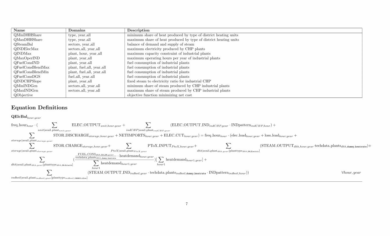
Name Domains DescriptionQMinDHHShare type, year all minimum share of heat produced by type of district heating unitsQMaxDHHShare type, year all maximum share of heat produced by type of district heating unitsQSteamBal sectors, year all balance of demand and supply of steamQINDElecMax sectors all, year all maximum electricity produced by CHP plantsQINDMax plant, hour, year all maximum capacity constraint of industrial plantsQMaxOperIND plant, year all maximum operating hours per year of industrial plantsQFuelConsIND plant, year all fuel consumption of industrial plantsQFuelConsBlendMax plant, fuel all, year all fuel consumption of industrial plantsQFuelConsBlendMin plant, fuel all, year all fuel consumption of industrial plantsQFuelConsDGS fuel all, year all fuel consumption of industrial plantsQINDCHPSlope plant, year all fixed steam to electricity ratio for industrial CHPQMinINDGen sectors all, year all minimum share of steam produced by CHP industrial plantsQMaxINDGen sectors all, year all maximum share of steam produced by CHP industrial plantsQObjective objective function minimizing net cost
Equation Definitions
QElcBalhour,year
freq hourhour · (∑
unit|avail plantunit,year
ELEC OUTPUTunit,hour,year +∑
indCHP |avail plantindCHP,year
(ELEC OUTPUT INDindCHP,year · INDpatternindCHP,hour) +∑storage|avail plantstorage,year
STOR DISCHARGEstorage,hour,year + NETIMPORTShour,year + ELEC CUThour,year) = freq hourhour · (elec loadhour,year + loss loadhour,year +∑storage|avail plantstorage,year
STOR CHARGEstorage,hour,year+∑
PtoX|avail plantPtoX,year
PToX INPUTPtoX,hour,year+∑
dhh|avail plantdhh,year[planttypedhh,DH Electric]
(STEAM OUTPUTdhh,hour,year·techdata plantsdhh,dummy,heatrate)+
∑dhh|avail plantdhh,year[planttypedhh,DH Solarth]
(
FUEL CONSdhh,ELC DH,year
techdata plantsdhh,dummy,heatrate· heatdemandhour,year∑
hour1
heatdemandhour1,year
)[∑hour1
heatdemandhour1,year] +
∑indboil|avail plantindboil,year[planttypeindboil,INDBOIL Elec]
(STEAM OUTPUT INDindboil,year · techdata plantsindboil,dummy,heatrate · INDpatternindboil,hour)) ∀hour, year
7

QAncBalancillary all,hour,year
freq hourhour · (∑
unit|avail plantunit,year
(ANCIL UPancillary all,unit,hour,year + ANCIL DOWNancillary all,unit,hour,year) + ANCIL CUTancillary all,hour,year) ≥
freq hourhour · policy power dataancill coef,ancillary all,dummy,year · (elec loadhour,year + loss loadhour,year − ELEC CUThour,year +∑dhh|(avail plantdhh,year∧fuelplantdhh,ELC DH,year)
(STEAM OUTPUTdhh,hour,year · techdata plantsdhh,dummy,heatrate) +∑indboil|(avail plantindboil,year∧fuelplantindboil,ELC IND,year)
(STEAM OUTPUT INDindboil,year · techdata plantsindboil,dummy,heatrate · INDpatternindboil,hour)) ∀ancillary all, hour, year
QAncilCapunit,ancillary all,hour,year
freq hourhour · ((INST UNITSunit,year · techdata plantsunit,dummy,ancillary all)[unit limitunit] +CAPA UNITSunit,year·techdata plantsunit,dummy,ancillary all
techdata plantsunit,dummy,size[no unit limitunit]) ≥
freq hourhour · (ANCIL UPancillary all,unit,hour,year + ANCIL DOWNancillary all,unit,hour,year) ∀unit, ancillary all, hour, year | avail plantunit,year
QunitMaxunit,hour,year
freq hourhour · ((OP UNITSunit,hour,year · techdata plantsunit,dummy,size · capacity factorunit,hour)[unit limitunit] + (CAPA UNITSunit,year · capacity factorunit,hour)[no unit limitunit]) =
freq hourhour · (ELEC OUTPUTunit,hour,year +∑
ancillary up
ANCIL UPancillary up,unit,hour,year + UNIT CUTunit,hour,year) ∀unit, hour, year | avail plantunit,year
QunitMinunit,hour,year
freq hourhour · (ELEC OUTPUTunit,hour,year −∑
ancillary down
ANCIL DOWNancillary down,unit,hour,year) ≥
freq hourhour · (OP UNITSunit,hour,year · techdata plantsunit,dummy,size · techdata plantsunit,dummy,techn min)[unit limitunit] ∀unit, hour, year | avail plantunit,year
QMaxOperunit,year
(INST UNITSunit,year · techdata plantsunit,dummy,size · policy power datamax oper,unit,dummy,year)[unit limitunit] + (CAPA UNITSunit,year · policy power datamax oper,unit,dummy,year)[no unit limitunit] ≥∑hour
(freq hourhour · ELEC OUTPUTunit,hour,year) ∀unit, year | avail plantunit,year
8

QMaxProdresource,year
policy power datamax resource,resource,dummy,year ≥∑
unit|(resourcemapunit,resource∧avail plantunit,year)
(∑hour
(freq hourhour · ELEC OUTPUTunit,hour,year)) ∀resource, year
QRampDounit limitunit,hour,year∑hour1,hour seqhour1,hour
(OP UNITSunit,hour1,year · techdata plantsunit,dummy,ramp down · 60) + ShutDownunit,hour,year · techdata plantsunit,dummy,size ≥∑hour1,hour seqhour1,hour
ELEC OUTPUTunit,hour1,year − ELEC OUTPUTunit,hour,year ∀unit limitunit, hour, year | avail plantunit,year
QRampUpunit limitunit,hour,year∑hour1,hour seqhour1,hour
(OP UNITSunit,hour1,year · techdata plantsunit,dummy,ramp up · 60) + StartUpunit,hour,year · techdata plantsunit,dummy,size ≥
ELEC OUTPUTunit,hour,year −∑
hour1,hour seqhour1,hour
ELEC OUTPUTunit,hour1,year ∀unit limitunit, hour, year | avail plantunit,year
QStartupunit limitunit,hour,year
OP UNITSunit,hour,year −∑
hour1,hour seqhour1,hour
OP UNITSunit,hour1,year = StartUpunit,hour,year − ShutDownunit,hour,year ∀unit limitunit, hour, year | avail plantunit,year
QStartShutunit limitunit,hour,year
INST UNITSunit,year ≥ StartUpunit,hour,year + ShutDownunit,hour,year ∀unit limitunit, hour, year | avail plantunit,year
QMinUpunit limitunit,hour,year
OP UNITSunit,hour,year ≥∑
hour1|A
StartUpunit,hour1,year ∀unit limitunit, hour, year | avail plantunit,year
Where
9

A=( ( ( ord( hour ) - techdata plantsunit,dummy,uptime) ≤ ord(hour1)) ∧ (ord(hour1) ≤ ord(hour)) ∧ (ord(hour1) ≤ lasthour) ∧ (ord(hour1) ≥ firsthour) ∨ (ord(hour1) ≥(lasthour + ord(hour)− techdata plantsunit,dummy,uptime)) ∧ (ord(hour1) ≥ ord(hour)))
QMinDownunit limitunit,hour,year
INST UNITSunit,year −OP UNITSunit,hour,year ≥∑
hour1|A
ShutDownunit,hour1,year
∀unit limitunit, hour, year | avail plantunit,year
WhereA=( ( ( ord( hour ) - techdata plantsunit,dummy,downtime) ≤ ord(hour1)) ∧ (ord(hour1) ≤ ord(hour)) ∧ (ord(hour1) ≤ lasthour) ∧ (ord(hour1) ≥ firsthour) ∨ (ord(hour1) ≥(lasthour + ord(hour)− techdata plantsunit,dummy,downtime)) ∧ (ord(hour1) ≥ ord(hour)))
QOpInstunit limitunit,hour,year
INST UNITSunit,year ≥ OP UNITSunit,hour,year ∀unit limitunit, hour, year | avail plantunit,year
QInstallunit,year
(COMM UNITSunit · surv plantunit,year)[unit limitunit] + (INVE UNITSunit · surv plantunit,year)[no unit limitunit] =INST UNITSunit,year[unit limitunit] + CAPA UNITSunit,year[no unit limitunit] ∀unit, year | avail plantunit,year
QINVESTMENTplant,year
INVESTMENTplant,year =∑
unit|((unit=plant)∧unit limitunit)
(techdata plantsplant,dummy,size · COMM UNITSunit) +∑unit|((unit=plant)∧no unit limitunit)
INVE UNITSunit + COMM DHHplant[dhhplant] + COMM INDplant[indplant] + COMM STORplant[storageplant] + COMM PtoXplant[PtoXplant]
∀plant, year | (year.val = techdata plantsplant,dummy,commissioning)
QDECOMMISSIONINGplant,year
DECOMMISSIONINGplant,year = (COMM DHHplant[dhhplant] + COMM INDplant[indplant] + COMM STORplant[storageplant] +
COMM PtoXplant[PtoXplant])[((surv plantplant,year −∑
year1|(year1.val=(year.val−Tper))
surv plantplant,year1) = −(1))]
∀plant, year | ((year.val > techdata plantsplant,dummy,commissioning) ∧ (¬unitplant))
10

QDECOMMISSIONING unitunit,year
DECOMMISSIONINGunit,year =
((COMM UNITSunit · techdata plantsunit,dummy,size)[unit limitunit] + INVE UNITSunit[no unit limitunit])[((surv plantunit,year −∑
year1|(year1.val=(year.val−Tper))
surv plantunit,year1) = −(1))]
∀unit, year | (year.val > techdata plantsunit,dummy,commissioning)
QCommLevtype limittype,year ∑unit|(planttypeunit,type∧(techdata plantsunit,dummy,commissioning≤year.val)∧(techdata plantsunit,dummy,commissioning>2015)∧avail plantunit,year∧unit limitunit)
(COMM UNITSunit · techdata plantsunit,dummy,size · surv plantunit,year) +∑unit|(planttypeunit,type∧(techdata plantsunit,dummy,commissioning≤year.val)∧(techdata plantsunit,dummy,commissioning>2015)∧avail plantunit,year∧no unit limitunit)
(INVE UNITSunit · surv plantunit,year) =∑level
LEV UNITStype,level,year
∀type limittype, year
QCommLevelstype limittype,level,year
policy power datamax new capacity,type,dummy,year · level structtype,level,Quantity,year +∑
unit|(planttypeunit,type∧(techdata plantsunit,dummy,commissioning≤2015))
DECOMMISSIONINGunit,year ≥ LEV UNITStype,level,year
∀type limittype, level, year
QMaxCapactype,year
policy power datamax new capacity,type,dummy,year ≥∑
plant|planttypeplant,type
(INVESTMENTplant,year −DECOMMISSIONINGplant,year) ∀type, year | (¬type limittype)
QFuelConsunit,year∑fuel|fuelplantunit,fuel,year
FUEL CONSunit,fuel,year =∑hour
(freq hourhour · (ELEC OUTPUTunit,hour,year + (STEAM OUTPUTunit,hour,year · techdata plantsunit,dummy,slope1 CHP)[unit chpunit]) · techdata plantsunit,dummy,heatrate) ∀unit, year | avail plantunit,year
11

QFuelBlendunit,fuel,year
fuelblendunit,fuel ·∑
fuel1|fuelplantunit,fuel1,year
FUEL CONSunit,fuel1,year = FUEL CONSunit,fuel,year ∀unit, fuel, year | (avail plantunit,year ∧ fuelblendunit,fuel)
QFuelLevfuel limitfuel all,year∑unit|(avail plantunit,year∧fuelplantunit,fuel all,year)
FUEL CONSunit,fuel all,year +∑
dhh|(avail plantdhh,year∧fuelplantdhh,fuel all,year)
FUEL CONSdhh,fuel all,year +∑ind|(avail plantind,year∧fuelplantind,fuel all,year)
FUEL CONSind,fuel all,year =∑level
LEV FUELfuel all,level,year ∀fuel limitfuel all, year
QFuelLevelsfuel limitfuel all,level,year
policy power datamax fuel,fuel all,dummy,year · level structfuel all,level,Quantity,year +ADDFUELfuel all,year[((level = level5) ∧ (¬fuel indfuel all) ∧ policy power datamax fuel,fuel all,dummy,year · level structfuel all,level,Quantity,year)]+ ADDFUELfuel all,year[((level = level1) ∧ fuel indfuel all ∧ policy power datamax fuel,fuel all,dummy,year · level structfuel all,level,Quantity,year)] ≥ LEV FUELfuel all,level,year
∀fuel limitfuel all, level, year
QCHPslope1unit chpunit,hour,year
(freq hourhour ·OP UNITSunit,hour,year · techdata plantsunit,dummy,size · capacity factorunit,hour)[unit limitunit] + (freq hourhour · CAPA UNITSunit,year · capacity factorunit,hour)[no unit limitunit] ≥freq hourhour · (ELEC OUTPUTunit,hour,year + STEAM OUTPUTunit,hour,year · techdata plantsunit,dummy,slope1 CHP) ∀unit chpunit, hour, year | avail plantunit,year
QCHPslope2unit chpunit,hour,year
freq hourhour · techdata plantsunit,dummy,helratio CHP · ELEC OUTPUTunit,hour,year ≥ freq hourhour · STEAM OUTPUTunit,hour,year ∀unit chpunit, hour, year | avail plantunit,year
QCHPefficunit chpunit,year∑fuel|fuelplantunit,fuel,year
FUEL CONSunit,fuel,year ≥∑hour
(freq hourhour · techdata plantsunit,dummy,minheatrate CHP · (ELEC OUTPUTunit,hour,year + STEAM OUTPUTunit,hour,year))
∀unit chpunit, year | avail plantunit,year
12

QSTORCAPstorage,hour,year
freq hourhour · COMM STORstorage · surv plantstorage,year ≥ freq hourhour · (STOR CHARGEstorage,hour,year + STOR DISCHARGEstorage,hour,year) ∀storage, hour, year | avail plantstorage,year
QSTORBALstorage,day,year
freq dayday ·∑
hour|mapdayhour,day
STOR CHARGEstorage,hour,year = freq dayday ·∑
hour|mapdayhour,day
STOR DISCHARGEstorage,hour,year · techdata plantsstorage,dummy,heatrate
∀storage, day, year | avail plantstorage,year
QSTORMAXPOTstorage,day,year
freq dayday · policy power datadaily,storage,dummy,year · COMM STORstorage · surv plantstorage,year ≥ freq dayday ·∑
hour|mapdayhour,day
STOR DISCHARGEstorage,hour,year
∀storage, day, year | avail plantstorage,year
QStorLevtype storagetype,year ∑storage|(planttypestorage,type∧((techdata plantsstorage,dummy,commissioning≤year.val)∧(techdata plantsstorage,dummy,commissioning>2015)))
(COMM STORstorage · surv plantstorage,year) =∑level
LEV STORAGEtype,level,year ∀type storagetype, year
QStorLevelstype storagetype,level,year
policy power datamax new capacity,type,dummy,year · level structtype,level,Quantity,year +∑
storage|A
(COMM STORstorage[((surv plantstorage,year −∑
year1|(year1.val=(year.val−Tper))
surv plantstorage,year1) = −(1))]) ≥
LEV STORAGEtype,level,year
∀type storagetype, level, yearWhereA = (planttypestorage,type ∧ ((techdata plantsstorage,dummy,commissioning ≤ year.val) ∧ (techdata plantsstorage,dummy,commissioning ≤ 2015)))
13

QEMISSIONpoweryear
CO2 EMISSIONpoweryear =∑
unit,fuel|(avail plantunit,year∧fuelplantunit,fuel,year)
(FUEL CONSunit,fuel,year · emission factorunit,fuel,year[(emission factorunit,fuel,year ≥ 0)]) ∀year
QEMISSIONdhhyear
CO2 EMISSIONdhhyear =∑
dhh,fuel|(avail plantdhh,year∧fuelplantdhh,fuel,year)
(emission factordhh,fuel,year · FUEL CONSdhh,fuel,year) ∀year
QEMISSIONindsectors,year
CO2 EMISSIONindsectors,year =∑
ind,fuel|(avail plantind,year∧fuelplantind,fuel,year∧INDmapsectorssectors,ind)
(emission factorind,fuel,year · FUEL CONSind,fuel,year) ∀sectors, year
QCCSCaptyear
CO2 CAPTUREyear =∑
unit,fuel|(avail plantunit,year∧CCSunit∧fuelplantunit,fuel,year)
(FUEL CONSunit,fuel,year · (techdata plantsunit,dummy,EmissionFactor noCCS − emission factorunit,fuel,year)) ∀year
QCCSmaxyear
policy power dataMaxCO2capt,dummy,dummy,year ≥∑
year1|(ord(year1)≤ord(year))
CO2 CAPTUREyear1 ∀year
QCLeanCapPtoX,hour,year
COMM PtoXPtoX · surv plantPtoX,year ≥ PtoX OUTPUTPtoX,hour,year ∀PtoX, hour, year | avail plantPtoX,year
QCLeanBalPtoX,day,year
freq dayday ·∑
hour|mapdayhour,day
PToX INPUTPtoX,hour,year = freq dayday ·∑
hour|mapdayhour,day
(techdata plantsPtoX,dummy,heatrate · PtoX OUTPUTPtoX,hour,year) ∀PtoX, day, year | avail plantPtoX,year
14

QCLeanDemBalcleanfuel,year∑hour
(∑
PtoX|(avail plantPtoX,year∧PtoXmapPtoX,cleanfuel)
(freq hourhour · PtoX OUTPUTPtoX,hour,year)) = DemCleanfuelcleanfuel,year +∑
unit|(avail plantunit,year∧fuelplantunit,cleanfuel,year)
FUEL CONSunit,cleanfuel,year +∑dhh,cleanfuel dhh|(avail plantdhh,year∧fuelplantdhh,cleanfuel dhh,year∧map fuel maincleanfuel,cleanfuel dhh)
FUEL CONSdhh,cleanfuel dhh,year +∑ind,cleanfuel ind|(avail plantind,year∧fuelplantind,cleanfuel ind,year∧map fuel maincleanfuel,cleanfuel ind)
FUEL CONSind,cleanfuel ind,year ∀cleanfuel, year
QFITPAYMENTyearyear all
FITPAYMENTyear all =∑
unit|A
(∑
year1|(year1.val=techdata plantsunit,dummy,commissioning)
policy power dataFITtariff,unit,dummy,year1 · FIT ELEC OUTPUTunit,year all) +∑unit|(policy power dataFITsupport,unit,dummy,year all∧(techdata plantsunit,dummy,commissioning<2015))
(policy power dataFITtariff,unit,dummy,2015 · FIT ELEC OUTPUTunit,year all) ∀yearyear all
WhereA =
∑year1|(year1.val=techdata plantsunit,dummy,commissioning)
policy power dataFITsupport,unit,dummy,year1 ∧ (techdata plantsunit,dummy,commissioning ≥ 2015) ∧ policy power dataFITsupport,unit,dummy,year all)
QFITPOLICYBUDGETyearyear all
policy power dataFITsupport,MaxBudget,dummy,year all + ADD FITBUDGETyear all ≥ FITPAYMENTyear all ∀yearyear all
QMAXFITGENERATION1unit,yearyear all∑hour
(freq hourhour · ELEC OUTPUTunit,hour,year all)[(∑
year1|(year1.val=techdata plantsunit,dummy,commissioning)
(A) ≤∑
year1|(year1.val=techdata plantsunit,dummy,commissioning)
(B))] +∑hour
(freq hourhour · ELEC OUTPUTunit,hour,year all)[((techdata plantsunit,dummy,commissioning < 2015) ∧ policy power dataFITsupport,unit,dummy,year all ∧ ((year all.val− techdata plantsunit,dummy,commissioning) ≤
policy power dataFITyears,unit,dummy,year all) ∧ (year all.val ≥ techdata plantsunit,dummy,commissioning))] ≥ FIT ELEC OUTPUTunit,year all ∀unit, yearyear all | avail plantunit,year all
WhereA = policy power dataFITsupport,unit,dummy,year1 ∧ policy power dataFITsupport,unit,dummy,year all ∧ ((year all.val− techdata plantsunit,dummy,commissioning)B = policy power dataFITyears,unit,dummy,year1) ∧ (year all.val ≥ techdata plantsunit,dummy,commissioning)
15

QUniformFITunit,yearyear all
FIT ELEC OUTPUTunit,year all =∑
year1|A
FIT ELEC OUTPUTunit,year1
∀unit, yearyear all | (avail plantunit,year all ∧ (techdata plantsunit,dummy,commissioning ≥ 2015))WhereA=( policy power dataFITsupport,unit,dummy,year all ∧ ((year1.val = techdata plantsunit,dummy,commissioning) ∧ (year1.val ≤ year all.val) ∧ ((year all.val− techdata plantsunit,dummy,commissioning) ≤policy power dataFITyears,unit,dummy,year1) ∧ (year all.val ≥ techdata plantsunit,dummy,commissioning)))
QADDPOLICYyear
ADDPOLICYyear =∑
unit,hour|avail plantunit,year
(freq hourhour · ELEC OUTPUTunit,hour,year · policy power dataElecaddSupport,unit,dummy,year) +∑unit|(avail plantunit,year∧
∑report res
reportplanttypeunit,report res)
((∑hour
(freq hourhour · ELEC OUTPUTunit,hour,year)− FIT ELEC OUTPUTunit,year) · drivers dataRenewableValue,Power,dummy,year) +
∑unit,unit chpunit|(avail plantunit,year∧
∑report res
reportplanttypeunit,report res)
(∑hour
(freq hourhour · STEAM OUTPUTunit,hour,year · drivers dataRenewableValue,Demand,dummy,year)) +
∑dhh|(avail plantdhh,year∧
∑report res
reportplanttypedhh,report res)
(∑hour
(freq hourhour · STEAM OUTPUTdhh,hour,year · drivers dataRenewableValue,Demand,dummy,year)) +
∑ind|(avail plantind,year∧
∑report res
reportplanttypeind,report res)
(STEAM OUTPUT INDind,year · drivers dataRenewableValue,Demand,dummy,year) +
∑unit,hour,unit chpunit|avail plantunit,year
(freq hourhour · drivers dataCHPvalue,DistrictHeating,dummy,year · STEAM OUTPUTunit,hour,year) +∑ind,indCHPind|avail plantind,year
(drivers dataCHPvalue,Industry,dummy,year · STEAM OUTPUT INDind,year) +∑PtoX,hour|avail plantPtoX,year
(freq hourhour · policy power dataPtoXaddSupport,P toX,dummy,year · PtoX OUTPUTPtoX,hour,year) +
16

∑storage,hour|avail plantstorage,year
(freq hourhour · policy power dataStorageaddSupport,storage,dummy,year · STOR DISCHARGEstorage,hour,year) ∀year
QNETIMPORTShour,year
freq hourhour · (netimportsexoghour,year + NETIMPORTSCUTPhour,year −NETIMPORTSCUTMhour,year) = freq hourhour ·NETIMPORTShour,year ∀hour, year
QHeatBalhour,year
freq hourhour · (∑
dhh|avail plantdhh,year
STEAM OUTPUTdhh,hour,year +∑
unit,unit chpunit|avail plantunit,year
STEAM OUTPUTunit,hour,year) = freq hourhour · (heatdemandhour,year −HEAT CUThour,year)
∀hour, year
QCHPRegionregion,year ∑unit,hour|(avail plantunit,year∧unit regionunit,region∧unit chpunit)
(freq hourhour · STEAM OUTPUTunit,hour,year) + REGIONCUTregion,year ≥
policy power dataMinimumCHPheat,region,dummy,year · policy power dataHeatShare,region,dummy,year ·∑hour
(freq hourhour · (heatdemandhour,year −HEAT CUThour,year)) ∀region, year
QDHHMaxdhh,hour,year
freq hourhour · COMM DHHdhh · techdata plantsdhh,dummy,capacity factor · surv plantdhh,year ≥ freq hourhour · STEAM OUTPUTdhh,hour,year ∀dhh, hour, year | avail plantdhh,year
QMaxOperDHHdhh,year
COMM DHHdhh · policy power datamax oper,dhh,dummy,year · surv plantdhh,year + ADDHOURSdhh,year · surv plantdhh,year ≥∑hour
(freq hourhour · STEAM OUTPUTdhh,hour,year) ∀dhh, year | avail plantdhh,year
QFuelConsDHHdhh,year∑fuel|fuelplantdhh,fuel,year
FUEL CONSdhh,fuel,year =∑hour
(freq hourhour · STEAM OUTPUTdhh,hour,year · techdata plantsdhh,dummy,heatrate) ∀dhh, year | avail plantdhh,year
17

QMinDHHGenyear∑dhh,hour|avail plantdhh,year
(freq hourhour · STEAM OUTPUTdhh,hour,year) ≥ policy power dataDHHGeneration,Min,dummy,year ·∑hour
(freq hourhour · heatdemandhour,year)−∑
type,type dhhtype
DHH CUTtype,year ∀year
QMaxDHHGenyear
policy power dataDHHGeneration,Max,dummy,year ·∑hour
(freq hourhour · heatdemandhour,year) +∑
type,type dhhtype
DHH ADDtype,year ≥∑
dhh,hour|avail plantdhh,year
(freq hourhour · STEAM OUTPUTdhh,hour,year) ∀year
QMinDHHSharetype dhhtype,year∑dhh,hour|avail plantdhh,year[planttypedhh,type]
(freq hourhour · STEAM OUTPUTdhh,hour,year) ≥
policy power dataDHHGenTypeMin,type,dummy,year ·∑
dhh,hour|avail plantdhh,year
(freq hourhour · STEAM OUTPUTdhh,hour,year)−DHH CUTtype,year ∀type dhhtype, year
QMaxDHHSharetype dhhtype,year
policy power dataDHHGenTypeMax,type,dummy,year ·∑
dhh,hour|avail plantdhh,year
(freq hourhour · STEAM OUTPUTdhh,hour,year) + DHH ADDtype,year ≥∑dhh,hour|avail plantdhh,year[planttypedhh,type]
(freq hourhour · STEAM OUTPUTdhh,hour,year) ∀type dhhtype, year
QSteamBalsectors,year∑ind|(avail plantind,year∧INDmapsectorssectors,ind)
STEAM OUTPUT INDind,year = steam demandsectors,year − STEAM CUTsectors,year ∀sectors, year
QINDElecMaxsectors,year
elec demandsectors,year ≥∑
indCHP |(avail plantindCHP,year∧INDmapsectorssectors,indCHP )
ELEC OUTPUT INDindCHP,year ∀sectors, year
18

QINDMaxind,hour,year
freq hourhour · COMM INDind · surv plantind,year ≥ freq hourhour · (ELEC OUTPUT INDind,year[indCHPind] +STEAM OUTPUT INDind,year[indboilind]) · INDpatternind,hour ∀ind, hour, year | avail plantind,year
QMaxOperINDind,year
COMM INDind · 8760 · techdata plantsind,dummy,capacity factor · surv plantind,year + (ADDHOURSind,year + 250[(year.val = 2015)]) · surv plantind,year ≥ELEC OUTPUT INDind,year[indCHPind] + STEAM OUTPUT INDind,year[indboilind] ∀ind, year | avail plantind,year
QFuelConsINDind,year∑fuel|fuelplantind,fuel,year
FUEL CONSind,fuel,year = techdata plantsind,dummy,heatrate · (ELEC OUTPUT INDind,year[indCHPind] + STEAM OUTPUT INDind,year) ∀ind, year | avail plantind,year
QFuelConsBlendMaxind,fuel,year
1.1 · blendind,fuel ·∑
fuel1|fuelplantind,fuel1,year
FUEL CONSind,fuel1,year ≥ FUEL CONSind,fuel,year
∀ind, fuel, year | (avail plantind,year ∧ fuelplantind,fuel,year ∧ fuel indfuel ∧ (techdata plantsind,dummy,commissioning ≤ 2015))
QFuelConsBlendMinind,fuel,year
0.9 · blendind,fuel ·∑
fuel1|fuelplantind,fuel1,year
FUEL CONSind,fuel1,year ≤ FUEL CONSind,fuel,year
∀ind, fuel, year | (avail plantind,year ∧ fuelplantind,fuel,year ∧ fuel indfuel ∧ (techdata plantsind,dummy,commissioning ≤ 2015))
QFuelConsDGSfuel,year∑ind|(avail plantind,year∧fuelplantind,fuel,year)
FUEL CONSind,fuel,year = Demand CHPBOI DGSFERRO,DGS,year −DGASCUTyear ∀fuel, year | (fuel = DGS IND)
QINDCHPSlopeindCHP,year
ELEC OUTPUT INDindCHP,year · techdata plantsindCHP,dummy,helratio CHP = STEAM OUTPUT INDindCHP,year ∀indCHP, year | avail plantindCHP,year
19

QMinINDGensectors,year∑indCHP |(avail plantindCHP,year∧INDmapsectorssectors,indCHP )
STEAM OUTPUT INDindCHP,year ≥ policy power dataINDCHPGeneration,Min,sectors,year · steam demandsectors,year − CHP CUTsectors,year ∀sectors, year
QMaxINDGensectors,year
policy power dataINDCHPGeneration,Max,sectors,year · steam demandsectors,year + CHP ADDsectors,year ≥∑
indCHP |(avail plantindCHP,year∧INDmapsectorssectors,indCHP )
STEAM OUTPUT INDindCHP,year ∀sectors, year
QObjective
Z =∑year
((1 + policy power dataSocialDiscount,dummy,dummy,year)(−year.val+2015) ·
(∑
unit|avail plantunit,year[unit limitunit]
(COMM UNITSunit · surve plantunit,year · techdata plantsunit,dummy,size · techdata plantsunit,dummy,Capital · annuity factorunit,year · (1− techdata plantsunit,dummy,Amort)) +∑unit|avail plantunit,year[no unit limitunit]
(INVE UNITSunit · surve plantunit,year · techdata plantsunit,dummy,Capital · annuity factorunit,year · (1− techdata plantsunit,dummy,Amort)) +∑ind|avail plantind,year
(COMM INDind · surve plantind,year · techdata plantsind,dummy,Capital · annuity factorind,year · (1− techdata plantsind,dummy,Amort)) +∑dhh|avail plantdhh,year
(COMM DHHdhh · surve plantdhh,year · techdata plantsdhh,dummy,Capital · annuity factordhh,year · (1− techdata plantsdhh,dummy,Amort)) +∑storage|avail plantstorage,year
(COMM STORstorage · surve plantstorage,year · techdata plantsstorage,dummy,Capital · annuity factorstorage,year · (1− techdata plantsstorage,dummy,Amort)) +∑PtoX|avail plantPtoX,year
(COMM PtoXPtoX · surve plantPtoX,year · techdata plantsPtoX,dummy,Capital · annuity factorPtoX,year · (1− techdata plantsPtoX,dummy,Amort)) +∑unit|avail plantunit,year[unit limitunit]
(COMM UNITSunit · survext plantunit,year · techdata plantsunit,dummy,size · techdata plantsunit,dummy,Capital extension · annuity factor extunit,year) +∑unit|avail plantunit,year[no unit limitunit]
(INVE UNITSunit · survext plantunit,year · techdata plantsunit,dummy,Capital extension · annuity factor extunit,year) +∑unit|avail plantunit,year[unit limitunit]
(COMM UNITSunit · survfs plantunit,year · techdata plantsunit,dummy,size · fuelswitchunit,Cost of Fuel Switch · annuity factor fsunit,year) +
20

∑unit|avail plantunit,year[no unit limitunit]
(INVE UNITSunit · survfs plantunit,year · fuelswitchunit,Cost of Fuel Switch · annuity factor fsunit,year) +∑dhh|avail plantdhh,year
(COMM DHHdhh · survfs plantdhh,year · fuelswitchdhh,Cost of Fuel Switch · annuity factor fsdhh,year) +∑ind|avail plantind,year
(COMM INDind · survfs plantind,year · fuelswitchind,Cost of Fuel Switch · annuity factor fsind,year) +∑unit|avail plantunit,year[unit limitunit]
(INST UNITSunit,year · techdata plantsunit,dummy,size · techdata plantsunit,dummy,FixedOMCost) +∑unit|avail plantunit,year[no unit limitunit]
(CAPA UNITSunit,year · techdata plantsunit,dummy,FixedOMCost) +∑dhh|avail plantdhh,year
(COMM DHHdhh · surv plantdhh,year · techdata plantsdhh,dummy,FixedOMCost) +∑ind|avail plantind,year
(COMM INDind · surv plantind,year · techdata plantsind,dummy,FixedOMCost) +∑storage|avail plantstorage,year
(COMM STORstorage · surv plantstorage,year · techdata plantsstorage,dummy,FixedOMCost) +∑PtoX|avail plantPtoX,year
(COMM PtoXPtoX · surv plantPtoX,year · techdata plantsPtoX,dummy,FixedOMCost) +∑fuel,fuel limitfuel
(fuelpricefuel,year ·∑level
(level structfuel,level,Price,year · LEV FUELfuel,level,year)) +∑plant|avail plantplant,year
(∑
fuel|(¬fuel limitfuel)[fuelplantplant,fuel,year]
(fuelpricefuel,year · FUEL CONSplant,fuel,year)) +∑ind|avail plantind,year
(∑
fuel|(avail plantind,year∧fuelplantind,fuel,year)
(∑
sectors|INDmapsectorssectors,ind
fuelpricedgssectors,fuel,year · FUEL CONSind,fuel,year)) +
CO2 EMISSIONpoweryear · drivers dataCarbonPricePower,dummy,dummy,year + CO2 EMISSIONdhhyear · drivers dataCarbonPriceDHH,dummy,dummy,year +∑sectors
(CO2 EMISSIONindsectors,year · drivers dataCarbonPriceInd,dummy,dummy,year · drivers dataCarbonLeakage,sectors,dummy,year) +
CO2 CAPTUREyear · policy power dataCCSstoragePrice,dummy,dummy,year +∑unit,hour|avail plantunit,year
(freq hourhour · ELEC OUTPUTunit,hour,year · techdata plantsunit,dummy,VariableNonFuelCost) +∑dhh,hour|avail plantdhh,year
(freq hourhour · STEAM OUTPUTdhh,hour,year · techdata plantsdhh,dummy,VariableNonFuelCost) +
21

∑indCHP |avail plantindCHP,year
(ELEC OUTPUT INDindCHP,year · techdata plantsindCHP,dummy,VariableNonFuelCost) +∑indboil|avail plantindboil,year
(STEAM OUTPUT INDindboil,year · techdata plantsindboil,dummy,VariableNonFuelCost) +∑storage,hour|avail plantstorage,year
(freq hourhour · STOR CHARGEstorage,hour,year · techdata plantsstorage,dummy,VariableNonFuelCost) +∑PtoX,hour|avail plantPtoX,year
(freq hourhour · PtoX OUTPUTPtoX,hour,year · techdata plantsPtoX,dummy,VariableNonFuelCost)− FITPAYMENTyear −ADDPOLICYyear +∑type,type limittype
(∑
vint|((vint.val≤year.val)∧(vint.val>2015))
(policy power dataAddCapitalCost,type,dummy,vint ·∑level
((level structtype,level,Price,vint − 1) · LEV UNITStype,level,vint) · annuity factor typetype,vint,year)) +∑type,type storagetype
(∑
vint|((vint.val≤year.val)∧(vint.val>2015))
(policy power dataAddCapitalCost,type,dummy,vint ·∑level
((level structtype,level,Price,vint − 1) · LEV STORAGEtype,level,vint) · annuity factor typetype,vint,year)) +∑unit,hour|policy power dataCurtailmentCost,unit,dummy,year
(policy power dataCurtailmentCost,unit,dummy,year · freq hourhour ·UNIT CUTunit,hour,year) +∑hour|policy power dataCurtailmentCost,Electricity,dummy,year
(policy power dataCurtailmentCost,Electricity,dummy,year · freq hourhour · ELEC CUThour,year) +∑hour|policy power dataCurtailmentCost,Heat,dummy,year
(policy power dataCurtailmentCost,Heat,dummy,year · freq hourhour ·HEAT CUThour,year) +∑sectors|policy power dataCurtailmentCost,Steam,dummy,year
(policy power dataCurtailmentCost,Steam,dummy,year · 1000 · STEAM CUTsectors,year) +
∑ancillary all,hour|policy power dataCurtailmentCost,ancillary all,dummy,year
(policy power dataCurtailmentCost,ancillary all,dummy,year
1000· freq hourhour ·ANCIL CUTancillary all,hour,year) +∑
ancillary all,hour|policy power dataCurtailmentCost,NetImports,dummy,year
(policy power dataCurtailmentCost,NetImports,dummy,year · freq hourhour · (NETIMPORTSCUTPhour,year + NETIMPORTSCUTMhour,year)) +∑type,type dhhtype
(DHH ADDtype,year + DHH CUTtype,year) · policy power dataCurtailmentCost,Heat,dummy,year +∑sectors
(CHP ADDsectors,year + CHP CUTsectors,year) · policy power dataCurtailmentCost,Steam,dummy,year +∑fuel|((¬(year.val=2015))∧(¬fuel indfuel))
(1000 ·ADDFUELfuel,year) +∑plant
(1000 ·ADDHOURSplant,year) + ADD FITBUDGETyear · 100))
22

ELEC OUTPUTplant,hour,year all ≥ 0 ∀plant, hour, year allELEC OUTPUT INDplant,year all ≥ 0 ∀plant, year allSTOR DISCHARGEstorage,hour,year all ≥ 0 ∀storage, hour, year allELEC CUThour,year all ≥ 0 ∀hour, year allSTOR CHARGEstorage,hour,year all ≥ 0 ∀storage, hour, year allPToX INPUTPtoX,hour,year all ≥ 0 ∀PtoX, hour, year allSTEAM OUTPUTplant,hour,year all ≥ 0 ∀plant, hour, year allFUEL CONSplant,fuel all,year all ≥ 0 ∀plant, fuel all, year allSTEAM OUTPUT INDplant,year all ≥ 0 ∀plant, year allANCIL UPancillary all,unit,hour,year all ≥ 0 ∀ancillary all, unit, hour, year allANCIL DOWNancillary all,unit,hour,year all ≥ 0 ∀ancillary all, unit, hour, year allANCIL CUTancillary all,hour,year all ≥ 0 ∀ancillary all, hour, year allINST UNITSunit,year all ∈ Z+∀unit, year allCAPA UNITSunit,year all ≥ 0 ∀unit, year allOP UNITSunit,hour,year all ∈ Z+∀unit, hour, year allUNIT CUTplant,hour,year all ≥ 0 ∀plant, hour, year allShutDownunit,hour,year all ∈ Z+∀unit, hour, year allStartUpunit,hour,year all ∈ Z+∀unit, hour, year allCOMM UNITSplant ∈ Z+∀plantINVE UNITSplant ≥ 0 ∀plantINVESTMENTplant,year all ≥ 0 ∀plant, year allCOMM DHHplant ≥ 0 ∀plantCOMM INDplant ≥ 0 ∀plantCOMM STORplant ≥ 0 ∀plantCOMM PtoXplant ≥ 0 ∀plantDECOMMISSIONINGplant,year all ≥ 0 ∀plant, year allLEV UNITStype,level,year all ≥ 0 ∀type, level, year allLEV FUELfuel all,level,year all ≥ 0 ∀fuel all, level, year allADDFUELfuel all,year all ≥ 0 ∀fuel all, year allLEV STORAGEtype,level,year all ≥ 0 ∀type, level, year allCO2 EMISSIONpoweryear all ≥ 0 ∀year allCO2 EMISSIONdhhyear all ≥ 0 ∀year allCO2 EMISSIONindsectors all,year all ≥ 0 ∀sectors all, year allCO2 CAPTUREyear all ≥ 0 ∀year all
23

PtoX OUTPUTPtoX,hour,year all ≥ 0 ∀PtoX, hour, year allFITPAYMENTyear all ≥ 0 ∀year allFIT ELEC OUTPUTunit,year all ≥ 0 ∀unit, year allADD FITBUDGETyear all ≥ 0 ∀year allADDPOLICYyear all ≥ 0 ∀year allNETIMPORTSCUTPhour,year all ≥ 0 ∀hour, year allNETIMPORTSCUTMhour,year all ≥ 0 ∀hour, year allHEAT CUThour,year all ≥ 0 ∀hour, year allREGIONCUTregion,year all ≥ 0 ∀region, year allADDHOURSplant,year all ≥ 0 ∀plant, year allDHH CUTtype,year all ≥ 0 ∀type, year allDHH ADDtype,year all ≥ 0 ∀type, year allSTEAM CUTsectors all,year all ≥ 0 ∀sectors all, year allDGASCUTyear all ≥ 0 ∀year allCHP CUTsectors all,year all ≥ 0 ∀sectors all, year allCHP ADDsectors all,year all ≥ 0 ∀sectors all, year all
24

REIMBURSABLE ADVISORY SERVICES (RAS): CONSTRUCTION OF ECONOMIC MODELING TOOLS AND BUILDING CAPACITY IN MODELING FOR SUSTAINED GROWTH IN THE SLOVAK REPUBLIC
Page | 191
Appendix V Mathematical formulation of the CPS Biomass Module

Symbols
Sets
Name Domains Description
labels *year all, year lag labels yearsyear year all projection yearsSFbio labels supply chains used in biomass submodelsfuel all labels set of fuelsf bioout fuel all output fuels of biomass submodelf biofeed fuel all feedstock fuels used in biomass submodelbioout SFbio, fuel all mapping of supply chains and output fuelsbioinp fuel all, SFbio mapping of feedstock fuels used in supply chainsfuel bio fuel all fuels consumed for self consumption in supply chains of biomass submodelresource labels resourcesresourcebio resource resources used in biomass modelyearlag year all, year all association to define the lagged yearvintbio year allSameAs *, * Set Element Comparison Without Checking
Parameters
Name Domains Description
drivers data labels, labels, labels, labels drivers dataEmissionFactors labels, labels emission factorsPRIF TAX SFbio fuel all, SFbio, year all end user fuel prices [fuel]prob surv bio SFbio, year all, year all probability of survival of an equipmentbio esurv SFbio, year all, year all economic survival for amortizationbio tsurv SFbio, year all, year all technical survivalbio ann SFbio, year all annuity factor for capital cost
1

Name Domains Description
bio demand f bioout, year all demand for bio self-productsbio heatrate SFbio, year all heatrates of equipmentbio self fuel SFbio, year all, year all rate of consumption of fuelsbio self elec SFbio, year all, year all rate of consumption of electricitybio respotential resourcebio, year all potgential of feedstockbio invcost SFbio, year all investment costbio omcost SFbio, year all O&M costbio omgr SFbio, year all growth of O&M cost with agebio varcost SFbio, year all variable non fuel costmc resourcebio resourcebio, year all margincal cost of potential cost curve for feedstocknc resourcebio resourcebio, year all nonlinear parameter of potential cost curve for feedstocklbd bio SFbio, year all, year all learning by doing of bioenergy equipmentRESvalue bio fuel all, labels, year all RES value for bioenergy equipmentCAP SUPP L2 SFbio, year all, year all exogenous capacityutilSFbio SFbio, year all Utilization rate of biomass technology SFbio
Variables
Name Domains Description
BIO SUPP SFbio, year all, fuel all, year all supply of a biomass product in GWhCAP SUPP SFbio, year all, year all capacity of a bioenergy transformation process in GWINV SUPP SFbio, year all capacity in a bioenergy transformation process in GWBIO FEEDSTOCK SFbio, year all, fuel all, year all consumption of feedstock in a bioenergy transformation process in GWhBIO FUEL SFbio, year all, fuel all, year all consumption of fuels in a bioenergy transformation process in GwhBIO RESCONS resourcebio, year all total use of a feedstock subject to potential constraints in GWhBIO Obj value of objective function of the biomass model
Equations
2

Name Domains Description
QB demand fuel all, year allQB capacity SFbio, vintbio, year allQB capital SFbio, vintbio, year allQB FEEDSTOCK SFbio, vintbio, year allQB FUEL SFbio, vintbio, year allQB ELEC SFbio, vintbio, year allQB RESCONS resourcebio, year allQB Resource resourcebio, year allQB Obj
Equation Definitions
QB demandf bioout,year∑SFbio,vintbio|(vintbio.val≤year.val)[biooutSFbio,f bioout]
BIO SUPPSFbio,vintbio,f bioout,year ≥ bio demandf bioout,year ∀f bioout, year
QB capacitySFbio,vintbio,year
CAP SUPPSFbio,vintbio,year · utilSFbioSFbio,year · 8760 ≥∑
f bioout|biooutSFbio,f bioout
BIO SUPPSFbio,vintbio,f bioout,year ∀SFbio, vintbio, year | (vintbio.val ≤ year.val)
QB capitalSFbio,vintbio,year
CAP SUPPSFbio,vintbio,year =INV SUPPSFbio,year[(vintbio.val = year.val)] +
prob surv bioSFbio,vintbio,year ·∑
year lag|yearlagyear,year lag
((CAP SUPPSFbio,vintbio,year lag + CAP SUPP L2SFbio,vintbio,year lag) · bio tsurvSFbio,vintbio,year[(vintbio.val ≤ (year.val− 5))])
∀SFbio, vintbio, year | (vintbio.val ≤ year.val)
3

QB FEEDSTOCKSFbio,vintbio,year∑f biofeed|bioinpf biofeed,SFbio
BIO FEEDSTOCKSFbio,vintbio,f biofeed,year
bio heatrateSFbio,vintbio≥
∑f bioout|biooutSFbio,f bioout
BIO SUPPSFbio,vintbio,f bioout,year ∀SFbio, vintbio, year | (vintbio.val ≤ year.val)
QB FUELSFbio,vintbio,year∑fuel bio|(¬(fuelbio=ELC))
BIO FUELSFbio,vintbio,fuel bio,year ≥ bio self fuelSFbio,vintbio,year ·∑
f bioout|biooutSFbio,f bioout
BIO SUPPSFbio,vintbio,f bioout,year ∀SFbio, vintbio, year | (vintbio.val ≤ year.val)
QB ELECSFbio,vintbio,year∑fuel bio|(fuelbio=ELC)
BIO FUELSFbio,vintbio,fuel bio,year ≥ bio self elecSFbio,vintbio,year ·∑
f bioout|biooutSFbio,f bioout
BIO SUPPSFbio,vintbio,f bioout,year ∀SFbio, vintbio, year | (vintbio.val ≤ year.val)
QB RESCONSresourcebio,year
BIO RESCONSresourcebio,year =∑
f biofeed|(fbiofeed=resourcebio)
(∑
SFbio,vintbio|(vintbio.val≤year.val)[bioinpf biofeed,SFbio]
BIO FEEDSTOCKSFbio,vintbio,f biofeed,year) ∀resourcebio, year
QB Resourceresourcebio,year
bio respotentialresourcebio,year ≥ BIO RESCONSresourcebio,year ∀resourcebio, year
QB Obj
BIO Obj =∑year
(∑
vintbio|(vintbio.val≤year.val)
(∑SFbio
(bio invcostSFbio,vintbio ·bio annSFbio,vintbio ·INV SUPPSFbio,vintbio ·bio esurvSFbio,vintbio,year+bio omcostSFbio,vintbio ·(1 + bio omgrSFbio,vintbio)(year.val−vintbio.val) ·
4

CAP SUPPSFbio,vintbio,year · bio tsurvSFbio,vintbio,year + bio varcostSFbio,vintbio ·∑
f bioout|biooutSFbio,f bioout
BIO SUPPSFbio,vintbio,f bioout,year +∑f biofeed|bioinpf biofeed,SFbio
(BIO FEEDSTOCKSFbio,vintbio,f biofeed,year ·
∑resourcebio|(fbiofeed=resourcebio)
(mc resourcebioresourcebio,year − nc resourcebioresourcebio,year · log((1−BIO RESCONSresourcebio,year
bio respotentialresourcebio,year + 1e− 06)))) +∑
fuel bio
(BIO FUELSFbio,vintbio,fuel bio,year · (PRIF TAX SFbiofuel bio,SFbio,year + EmissionFactorsCO2,fuel bio · drivers dataCarbonPriceETS,dummy,dummy,year))−
lbd bioSFbio,vintbio,year ·∑
f bioout|biooutSFbio,f bioout
BIO SUPPSFbio,vintbio,f bioout,year −∑
f bioout|biooutSFbio,f bioout
(RESvalue biof bioout,dummy,year · BIO SUPPSFbio,vintbio,f bioout,year))))
BIO SUPPSFbio,year all,fuel all,year all ≥ 0 ∀SFbio, year all, fuel all, year allCAP SUPPSFbio,year all,year all ≥ 0 ∀SFbio, year all, year allINV SUPPSFbio,year all ≥ 0 ∀SFbio, year allBIO FEEDSTOCKSFbio,year all,fuel all,year all ≥ 0 ∀SFbio, year all, fuel all, year allBIO FUELSFbio,year all,fuel all,year all ≥ 0 ∀SFbio, year all, fuel all, year allBIO RESCONSresourcebio,year all ≥ 0 ∀resourcebio, year all
5