Regularized Model of Post-Touchdown Configurations inElectrostatic MEMS: Equilibrium Analysis

A. E. Lindsay

Department of Applied and Computational Mathematics and Statistics,

University of Notre Dame, South Bend, Indiana, 46556, USA.

J. Lega

Department of Mathematics, University of Arizona, Tucson, Arizona, 85721, USA.

K. B. Glasner

Department of Mathematics, University of Arizona, Tucson, Arizona, 85721, USA.

Abstract

In canonical models of Micro-Electro Mechanical Systems (MEMS), an event called touch-down whereby the electrical components of the device come into contact, is characterizedby a blow up in the governing equations and a non-physical divergence of the electric field.In the present work, we propose novel regularized governing equations whose solutions re-main finite at touchdown and exhibit additional dynamics beyond this initial event beforeeventually relaxing to new stable equilibria. We employ techniques from variational calculus,dynamical systems and singular perturbation theory to obtain a detailed understanding ofthe properties and equilibrium solutions of the regularized family of equations.

Keywords: Singular perturbation techniques, Nano-technology, Regularization, Blow up,Higher order partial differential equations.

1. Introduction and statement of main results.

Micro-Electro Mechanical Systems (MEMS) are a large collection of miniaturized integratedcircuits and moving mechanical components that can be fabricated together to perform amultitude of tasks. MEMS practitioners aim to manipulate the interaction between electro-static forces and elastic surfaces to design a variety of complex devices with applications indrug-delivery [1, 45], micro pumps [23], optics [8], micro-scale actuators [46]. In such interac-tions, the elastic structures of the MEMS device may be overwhelmed if the magnitude of theelectrostatic forces acting on them exceeds a critical threshold. Such a failure is manifestedby an instability, known as the pull-in instability.

Email addresses: a.lindsay@nd.edu (A. E. Lindsay), lega@math.arizona.edu (J. Lega),kglasner@math.arizona.edu (K. B. Glasner)

Preprint submitted to Elsevier May 14, 2014

In a capacitor type MEMS device, an elastic membrane is held fixed along its boundaryabove a rigid substrate. When an electric potential V is applied between these surfaces,the upper elastic surface deflects downwards towards the substrate. If V is small enough,the deflection will reach an equilibrium, however, if V exceeds the pull-in voltage V ∗, noequilibrium configuration is attainable and the top plate will touch down on the substrate.Figure 1 contains a schematic representation of the device.

Touchdown is a very rapid event whereby large quantities of energy are focused on smallspatial regions of the MEMS device over short time scales. Consequently this process developslarge forces at specific areas which can either be useful to the operation of the device or bedestructive. In many mathematical models of MEMS, touchdown is described by finite timequenching, e.g. blow-up of solution derivative and energy. Accordingly, many importantoperational aspects of MEMS, such as the time and location of touchdown, can be investigatedby studying this quenching event.

However, a loss of existence to model solutions results in no information regarding configu-rations of MEMS after a primary touchdown event. This paper presents an initial attemptto describe behavior of MEMS after touchdown. To this end, we derive the second orderequation

ut = ∆u− λ

(1 + u)2+

λεm−2

(1 + u)m, x ∈ Ω; u = 0, x ∈ ∂Ω, (1.1a)

which models the dimensionless deflection u(x, t) as that of a membrane, and the fourth orderproblem

ut = −∆2u− λ

(1 + u)2+

λεm−2

(1 + u)m, x ∈ Ω; u = ∂nu = 0, x ∈ ∂Ω, (1.1b)

which is a beam description of the deflecting surface. The modeling literature on MEMShas involved second (cf. [15, 16, 19, 25, 43, 7]) and fourth order (cf. [38, 34, 33, 17, 29])descriptions of the elastic nature of the deflecting surface and so we aim to investigate theeffects of regularization on both. In both cases, Ω is a bounded region of Rn and λ ∝ V 2 is aparameter quantifying the relative importance of electrostatic to elastic forces. The physicallyrelevant dimensions are n = 1, 2. The small parameter ε in (1.1) mimics the effect of a smallinsulating layer placed on top of the substrate to prevent a short circuit of the device as thegap spacing 1 + u, u < 0, locally shrinks to zero. The regularizing term λεm−2(1 + u)−m form > 2 can also account for a variety of physical effects which become important when u ≈ −1.For example m = 4 accounts for the Casimir effect (with sign of regularizing term reversed)while m = 3 models Van der Waals forces [2, 20]. A recent mathematical study has analyzedthe existence and stability of equilibria to (1.1a) in the case m = 4 [28]. Similar quenchingevents and their regularizations have been investigated in studies of thin film dynamics onsolid substrates [3, 4, 6].

For the case ε = 0, equations (1.1) reduce to canonical models originally introduced by Pelesko(cf. [42, 43]), the salient properties of which are now well known. Of particular importanceamongst the many results, is the existence of a pull-in voltage λ∗ such that if λ < λ∗, thenu(x, t) approaches a unique and stable equilibrium as t→∞, while for λ > λ∗ no equilibriumsolutions are possible and u(x, t) reaches −1 in some finite time, tc [14, 19, 11]. In the 1Dsetting, the equilibrium structure consists of one stable and one unstable branch that meetat λ∗ (cf. dashed curve of Fig. 4). In the case where λ > λ∗, there have been many studies

2

Free or supportedboundary

d

L

Fixedground plate

h

Insulatinglayer

d

L

Insulatlayer

Deflectingmembrane

Ωx

y

z

Figure 1: Schematic diagram of a MEMS capacitor with insulating layer of thick-ness h.

centered on describing the local properties of the device near touchdown. For example, inthe second order equation,

ut = ∆u− λ

(1 + u)2, x ∈ Ω, (1.2)

a detailed analysis [19, 13, 3, 18] of solutions near touchdown reveals the local behavior

u→ −1 + [3λ(tc − t)]1/3(

1− 1

2| log(tc − t)|+

(x− xc)2

4(tc − t)| log(tc − t)|+ · · ·

), (1.3)

in the vicinity of the touchdown point xc, for t→ t−c . Detailed scaling laws for tc in the limitsλ→∞ and λ− λ∗ → 0+ have also been established in [15, 16]. In the fourth order problem,

ut = −∆2u− λ

(1 + u)2, x ∈ Ω, (1.4)

less is known about equilibrium configurations and about the dynamics of touchdown whenequilibrium solutions do not exist. In the special cases where Ω is the unit strip [−1, 1]or the unit disc x ∈ R2 | |x| ≤ 1, the existence of the pull-in voltage λ∗ was shownin [39, 22]. It was shown in [29] that there are at least two radially symmetric solutionsfor each λ < λ∗. Similar results were obtained in [17] for the case where pinned boundaryconditions u = ∆u = 0 were used. For λ > λ∗ and for Ω the unit strip [−1, 1] or the unitdisc x ∈ R2 | |x| ≤ 1, it was shown in [34] that the device touches down in finite time tc.A detailed numerical and asymptotic study established the local behavior

u(x, t)→ −1 + (tc − t)1/3v(y), y =x− xc

(tc − t)14

λ1/4, t→ t−c , (1.5)

where v(y) is a self-similar profile satisfying an associated ordinary differential equation. Inaddition to the local behavior of solutions as t → t−c , the fourth order problems (1.4) haveadditional interesting dynamical features whereby touchdown can occur simultaneously at

3

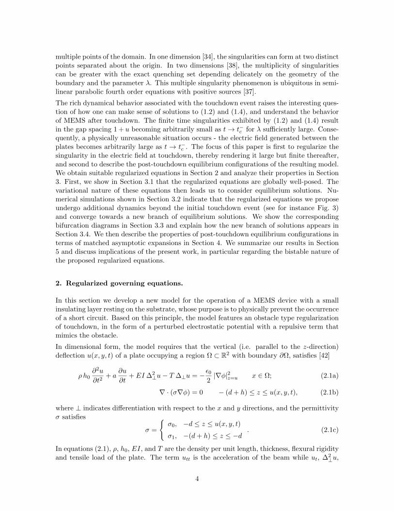
multiple points of the domain. In one dimension [34], the singularities can form at two distinctpoints separated about the origin. In two dimensions [38], the multiplicity of singularitiescan be greater with the exact quenching set depending delicately on the geometry of theboundary and the parameter λ. This multiple singularity phenomenon is ubiquitous in semi-linear parabolic fourth order equations with positive sources [37].

The rich dynamical behavior associated with the touchdown event raises the interesting ques-tion of how one can make sense of solutions to (1.2) and (1.4), and understand the behaviorof MEMS after touchdown. The finite time singularities exhibited by (1.2) and (1.4) resultin the gap spacing 1 + u becoming arbitrarily small as t→ t−c for λ sufficiently large. Conse-quently, a physically unreasonable situation occurs - the electric field generated between theplates becomes arbitrarily large as t → t−c . The focus of this paper is first to regularize thesingularity in the electric field at touchdown, thereby rendering it large but finite thereafter,and second to describe the post-touchdown equilibrium configurations of the resulting model.We obtain suitable regularized equations in Section 2 and analyze their properties in Section3. First, we show in Section 3.1 that the regularized equations are globally well-posed. Thevariational nature of these equations then leads us to consider equilibrium solutions. Nu-merical simulations shown in Section 3.2 indicate that the regularized equations we proposeundergo additional dynamics beyond the initial touchdown event (see for instance Fig. 3)and converge towards a new branch of equilibrium solutions. We show the correspondingbifurcation diagrams in Section 3.3 and explain how the new branch of solutions appears inSection 3.4. We then describe the properties of post-touchdown equilibrium configurations interms of matched asymptotic expansions in Section 4. We summarize our results in Section5 and discuss implications of the present work, in particular regarding the bistable nature ofthe proposed regularized equations.

2. Regularized governing equations.

In this section we develop a new model for the operation of a MEMS device with a smallinsulating layer resting on the substrate, whose purpose is to physically prevent the occurrenceof a short circuit. Based on this principle, the model features an obstacle type regularizationof touchdown, in the form of a perturbed electrostatic potential with a repulsive term thatmimics the obstacle.

In dimensional form, the model requires that the vertical (i.e. parallel to the z-direction)deflection u(x, y, t) of a plate occupying a region Ω ⊂ R2 with boundary ∂Ω, satisfies [42]

ρ h0∂2u

∂t2+ a

∂u

∂t+ EI ∆2

⊥u− T ∆⊥u = −ε02|∇φ|2z=u x ∈ Ω; (2.1a)

∇ · (σ∇φ) = 0 − (d+ h) ≤ z ≤ u(x, y, t), (2.1b)

where ⊥ indicates differentiation with respect to the x and y directions, and the permittivityσ satisfies

σ =

σ0, −d ≤ z ≤ u(x, y, t)

σ1, −(d+ h) ≤ z ≤ −d. (2.1c)

In equations (2.1), ρ, h0, EI, and T are the density per unit length, thickness, flexural rigidityand tensile load of the plate. The term utt is the acceleration of the beam while ut, ∆2

⊥u,

4

∆⊥u and |∇φ|2z=u represent forces on the beam due to damping, bending, stretching, and theelectric field. The parameter a represents the strength of damping forces on the system, ε0 isthe permittivity of free space and d is the undeflected gap spacing. As shown in Figure 1, athin insulating layer of thickness h and permittivity σ1 is attached to the ground plate. Theelectric potential φ, satisfying equation (2.1b), is zero on the ground plate and at voltage Von the deflecting membrane so that

φ(−(d+ h)) = 0, φ(u) = V. (2.1d)

The problem is now reduced by recasting equations (2.1) in the dimensionless variables

x′ =x

Ly′ =

y

Lz′ =

z

d, u′ =

u

d, φ′ =

φ

V, σ′ =

σ

σ0

and assuming a small aspect ratio configuration, so that δ ≡ d/L 1, where L is a char-acteristic linear dimension of the domain Ω. Concentrating first on the potential equation(2.1b), the non-dimensional equation for φ′ satisfies

∇′ · (σ′∇′φ′) = 0, −(1 + h/d) ≤ z′ ≤ u′(x′, y′, t); (2.2a)

σ′ =

1, −1 ≤ z′ ≤ u′(x′, y′, t);σ1

σ0, −(1 + h/d) ≤ z′ ≤ −1

(2.2b)

φ′(−(1 + h/d)) = 0, φ′(u′) = 1. (2.2c)

In non-dimensional coordinates, we have that

∇′ ≡(

1

L

∂

∂x′,

1

L

∂

∂y′,

1

d

∂

∂z′

)and therefore problem (2.2) reduces to

∂2φ′+

∂z′2+ δ2

(∂2φ

′+

∂x′2+∂2φ

′+

∂y′2

)= 0, −1 ≤ z′ ≤ u′; (2.3a)

∂2φ′−

∂z′2+ δ2

(∂2φ

′−

∂x′2+∂2φ

′−

∂y′2

)= 0, −1− h

d≤ z′ ≤ −1; (2.3b)

φ′+(u′) = 1, φ

′+(−1) = φ

′−(−1),

∂

∂z′φ

′+(−1) =

σ1

σ0

∂

∂z′φ

′−(−1), φ

′−(−1− d/h) = 0.

(2.3c)

In the limit where the small aspect ratio δ → 0, the leading order solution to (2.3) is

φ′ =

1 +z′ − u′

(1 + u′) +dσ0

hσ1

−1 ≤ z′ ≤ u′;

z′ + 1 +d

hσ1

σ0(1 + u′) +

d

h

−1− h

d≤ z′ ≤ −1

(2.4)

5

The explicit solution (2.4) which arises in this small aspect ratio limit affords a significantreduction in the complexity of the governing equations. If the limit δ → 0 is not exercised,the system for the potential (2.3) and the non-dimensionalized form of (2.1a) constitute afree boundary problem for the deflection u(x, y, t) of the device. With the exclusion of theinsulating layer introduced here in (2.1c), the qualitative properties of dynamic and steadysolutions of this free boundary problem have been studied in [30, 9, 10, 27, 31, 32]. Thesestudies have established the well-posedness theory for the system of evolution equations (2.1),the existence of a pull in voltage and also the convergence of equilibrium solutions of the freeboundary problem to those of the small aspect ratio limit as δ → 0. Accordingly, there isgood reason to believe that the small aspect ratio approximation is justified. In light of thesignificant simplifications it affords, we proceed by calculating from (2.4) that the forcing onthe surface z′ = u′(x′, y′) is given by

ε02|∇φ|2 = V 2 ε0

2d2

[(∂φ′

∂z′

)2

+O(δ2)

]= V 2 ε0

2d2

1(1 + u′ +

dσ0

hσ1

)2. (2.5)

After selecting the time scale t = (L2a/T )t′ in (2.1) and substituting the reduced term arrivedat in (2.5), the equation

Q2 ∂2u′

∂t′2+∂u′

∂t′+ β∆

′2⊥u′ − ∆

′⊥u′ = − λ

(1 + u′ + ε)2(2.6a)

is obtained, where the dimensionless groups are

β =EI

L2T, Q =

√Tρh0

aL, ε =

dσ0

hσ1, λ =

ε0L2V 2

2d3T. (2.6b)

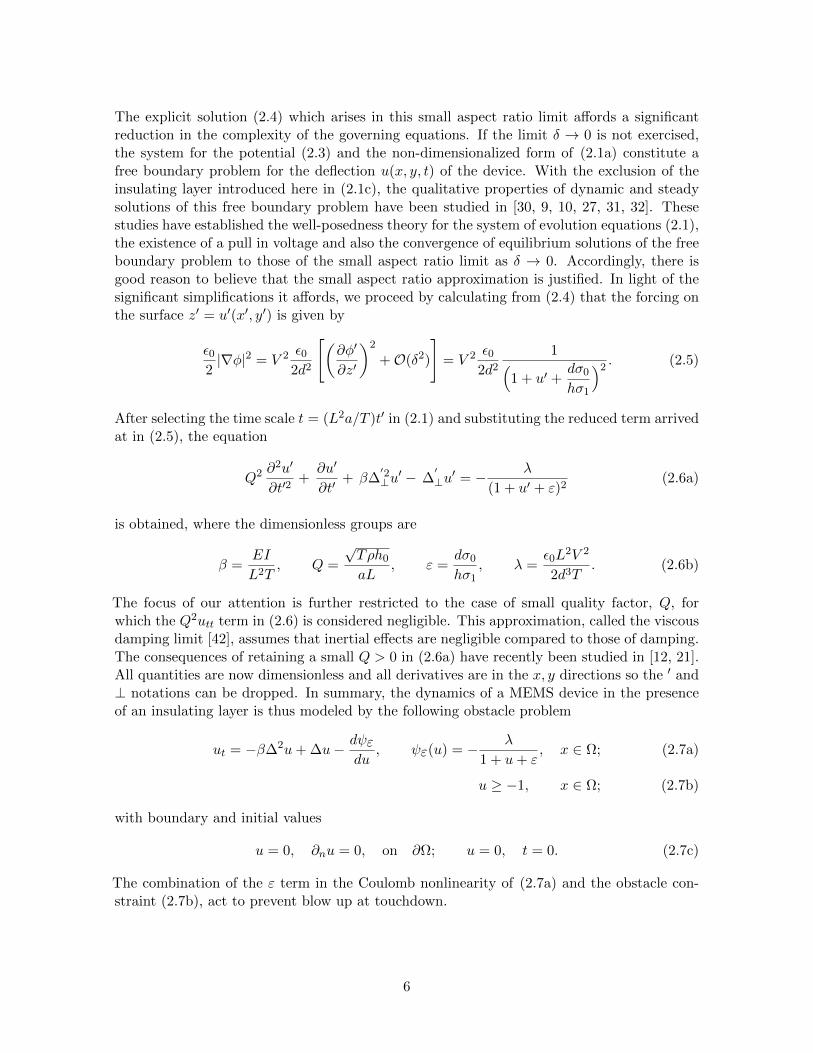
The focus of our attention is further restricted to the case of small quality factor, Q, forwhich the Q2utt term in (2.6) is considered negligible. This approximation, called the viscousdamping limit [42], assumes that inertial effects are negligible compared to those of damping.The consequences of retaining a small Q > 0 in (2.6a) have recently been studied in [12, 21].All quantities are now dimensionless and all derivatives are in the x, y directions so the ′ and⊥ notations can be dropped. In summary, the dynamics of a MEMS device in the presenceof an insulating layer is thus modeled by the following obstacle problem

ut = −β∆2u+ ∆u− dψεdu

, ψε(u) = − λ

1 + u+ ε, x ∈ Ω; (2.7a)

u ≥ −1, x ∈ Ω; (2.7b)

with boundary and initial values

u = 0, ∂nu = 0, on ∂Ω; u = 0, t = 0. (2.7c)

The combination of the ε term in the Coulomb nonlinearity of (2.7a) and the obstacle con-straint (2.7b), act to prevent blow up at touchdown.

6

2.1. Variational nature of the obstacle problem and a regularization

Obstacle problems like (2.7) often arise in mechanics when constraints are present [26]. Froma variational point of view, constraints are typically encoded by assigning infinite energy tothe set of disallowed configurations. Our model could be written formally as the L2-gradientflow of the energy functional E : H2(Ω)→ R ∪ +∞ given by

E =

∫Ω

(β

2(∆u)2 +

1

2|∇u|2 + ψ(u; ε)

)dx dy, (2.8)

where

ψ(u; ε) =

−λ

1 + u+ εu ≥ −1,

+∞ u < −1,(2.9)

is an extension of ψε in (2.7a) to u ∈ R.

For practical purposes, it is often useful to work with a regularized version of the obstacleproblem which has smooth solutions (e.g. [41, 44]). This typically involves, in essence,replacing an energy functional like (2.8) with one which is smooth but otherwise mimics thepenalization associated with the obstacle.

For our problem, we will replace the potential (2.9) with one which has the same qualitativestructure. Specifically, the new potential φε will behave like ψ in the following ways:

1. For fixed values of u > −1, φε(u) ∼ ψ(u; ε) as ε→ 0.

2. limu→−1+ φε(u) = +∞3. The value of ψ which occurs at the obstacle value u = −1 is the same as the minimum

of φε(u).

A class of potentials which fulfills these criteria is

φε(u) = − λ

(1 + u)+

λ(ζε)m−2

(m− 1)(1 + u)m−1, λ > 0, 0 < ε < 1, (2.10)

for integer exponents m > 2, and ζ = (m− 2)/(m− 1). We set ε′ = ζε, i.e. the regularizingparameter ε′ associated with the potential φε′(u) is a non-dimensional rescaling of the originalphysical ε, defined in (2.6b). Hereafter we drop the prime notation. A schematic diagram ofthe graph of φε is shown in Fig. 2.

7

−1 0u

φ(u)

−1 + ε

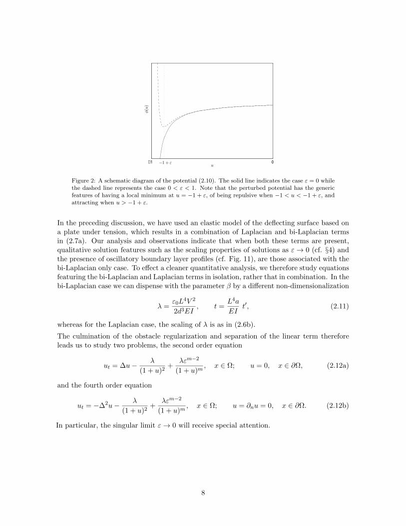
Figure 2: A schematic diagram of the potential (2.10). The solid line indicates the case ε = 0 whilethe dashed line represents the case 0 < ε < 1. Note that the perturbed potential has the genericfeatures of having a local minimum at u = −1 + ε, of being repulsive when −1 < u < −1 + ε, andattracting when u > −1 + ε.

In the preceding discussion, we have used an elastic model of the deflecting surface based ona plate under tension, which results in a combination of Laplacian and bi-Laplacian termsin (2.7a). Our analysis and observations indicate that when both these terms are present,qualitative solution features such as the scaling properties of solutions as ε→ 0 (cf. §4) andthe presence of oscillatory boundary layer profiles (cf. Fig. 11), are those associated with thebi-Laplacian only case. To effect a cleaner quantitative analysis, we therefore study equationsfeaturing the bi-Laplacian and Laplacian terms in isolation, rather that in combination. In thebi-Laplacian case we can dispense with the parameter β by a different non-dimensionalization

λ =ε0L

4V 2

2d3EI, t =

L4a

EIt′, (2.11)

whereas for the Laplacian case, the scaling of λ is as in (2.6b).

The culmination of the obstacle regularization and separation of the linear term thereforeleads us to study two problems, the second order equation

ut = ∆u− λ

(1 + u)2+

λεm−2

(1 + u)m, x ∈ Ω; u = 0, x ∈ ∂Ω, (2.12a)

and the fourth order equation

ut = −∆2u− λ

(1 + u)2+

λεm−2

(1 + u)m, x ∈ Ω; u = ∂nu = 0, x ∈ ∂Ω. (2.12b)

In particular, the singular limit ε→ 0 will receive special attention.

8

3. Properties of the regularized equations

3.1. Well-posedness

In this section we detail the existence theory for both the Laplacian and bi-Laplacian prob-lems, which we write as

ut = ∆u− φ′ε(u), x ∈ Ω; u = 0, x ∈ ∂Ω; (3.1a)

ut = −∆2u− φ′ε(u) x ∈ Ω; u = ∂nu = 0, x ∈ ∂Ω, (3.1b)

together with the initial condition u(x, 0) = u0(x). The spatial domain Ω ⊂ Rn is assumedcompact with a sufficiently smooth boundary. We note that the evolution equations are L2

gradient flows. In particular, if

EL(t) =

∫Ω

(1

2|∇u|2 + φε(u)

)dx dy, (3.2a)

EB(t) =

∫Ω

(1

2|∆u|2 + φε(u)

)dx dy, (3.2b)

it is easily shown that dEL/dt ≤ 0 and dEB/dt ≤ 0. The following results are proved fora class of potentials φ which is fairly general and for which (2.10) is a subset. For bothequations we suppose

φε(u) ∈ C1, φε(u) ≥ φmin for u ∈ (−1,∞), φε(u) < φmax for u ∈ (−1 + ε,∞) . (3.3)

Additional restrictions for each equation are

φ′ε(u) < 0 if u ∈ (−1,−1 + ε), for equation (3.1a), (3.4a)

φε(u) ∼ c(ε)(1 + u)−m+1 u→ −1, for equation (3.1b). (3.4b)

for constant c(ε).

Theorem 3.1 (Global Existence - Laplacian Case). Suppose that the initial conditionsatisfies u0 ∈ C0(Ω) and u0 > −1. Then the solution for (3.1a) exists for all t > 0 andu(x, t) > min(inf u0,−1 + ε).

Proof: Let u±(t) solve the initial value problems

du±dt

= −φ′ε(u±), u−(0) = inf u0, u+(0) = supu0. (3.5)

Conditions (3.3,3.4a) ensure that u± will exist for all t > 0 and u± > −1. Furthermore,u− > min(inf u0,−1 + ε). Standard comparison methods for parabolic equations yield the apriori bounds u−(t) ≤ u(x, t) ≤ u+(t). This guarantees that the solution will exist globally.

Theorem 3.2 (Global Existence - bi-Laplacian Case). Suppose that the initial condi-tion satisfies u0 ∈ H2(Ω) ∩ C0(Ω) and u0 > −1. Then the solution u(x, t) of (3.1b) existsfor all t > 0, provided m ≥ 3 in dimension n = 1 and m > 3 in dimension n = 2.

9

Proof: Following [5], it suffices to derive a priori pointwise bounds on the solution. Thisguarantees that the equation is uniformly parabolic and existence follows from standardarguments. The gradient flow structure and dEB/dt ≤ 0 implies that EB(T )−EB(0) ≤ 0 forany T > 0, and so∫

Ω

1

2(∆u(T ))2dx dy ≤

∫Ω

1

2(∆u0)2dx dy +

∫Ωφε(u0)dx dy −

∫Ωφε(u(T ))dx dy. (3.6)

Since φ(·) has a lower bound, it follows that u ∈ H2(Ω) a priori. The Sobolev imbeddingtheorem then gives u ∈ C1(Ω) in dimension n = 1 and u ∈ C0,α(Ω) in dimension n = 2where 0 < α < 1. In particular there are constants K1 and K2, depending only on the initialcondition, so that

‖u‖C1 < K1, n = 1; (3.7)

‖u‖C0,α < K2(α), n = 2. (3.8)

Now let umin = minu(T ) be the minimum attained at a point x0. Note that inequality (3.6)implies an upper bound for

∫Ω φε(u(T ))dx dy. In dimension n = 1 it follows that there exist

generic constants K so that

C >

∫Ωφε(u(T ))dx dy ≥ K(ε)

∫Ω

(umin + 1 +K1|x− x0|)−m+1dx dy ≥ µ(umin + 1), (3.9)

where

µ(umin + 1) = K(ε)

− ln(umin + 1) m = 3,

(umin + 1)−m+3 m > 3.(3.10)

In dimension n = 2 one similarly has

C > K(ε)

∫Ω

(umin + 1 +K2|x− x0|α)−m+1dx dy ≥ µ(umin + 1), (3.11)

where

µ(umin + 1) = K(α, ε)

− ln(umin + 1) m = 1 + 2/α,

(umin + 1)3−m m > 1 + 2/α.(3.12)

In both cases, this establishes, for ε > 0, the lower bound u > −1 for all t > 0.

The two preceding results capture two important features of the perturbed potential system.First, for a wide range of potentials, equations (3.1) mimic the effect of the obstacle constraintu > −1, established in (2.7b). This provides confidence that the perturbed potential systemqualitatively reflects the behavior of the obstacle problem (2.7). Second, in contrast to theε = 0 case, the system is now well-posed for all t > 0 and ε > 0 and no finite time singularityoccurs. It is therefore relevant to investigate the limiting behavior of equations (3.1) in thelimit t → ∞. This long term behavior of equations (3.1) is related to the minimizers of thefunctionals given in (3.2).

3.2. Variational dynamics

The dynamics of Equations (2.12) is variational and leads to relaxation of the system towardsequilibrium solutions. For values of λ such that touchdown would not occur when ε = 0,

10

−1 −0.5 0 0.5 1

−1

−0.8

−0.6

−0.4

−0.2

0

x

u

(a) Initial touchdown.

−1 −0.5 0 0.5 1

−1

−0.8

−0.6

−0.4

−0.2

0

x

u

xc−xc

(b) Spreading of touchdown region.

−1 −0.5 0 0.5 1

−1

−0.8

−0.6

−0.4

−0.2

0

x

u

−xc xc

(c) Boundary pinning.

Figure 3: One-dimensional solutions of (2.12a) initialized with zero initial data and parametervalues ε = 0.01, λ = 5. The left panel shows the initial touchdown event at x = 0. The center panelshows the spread of the touchdown region towards the boundary. Right panel: An equilibriumstate is reached after the moving front is pinned by its interaction with the boundary.

the regularization term in (2.12) remains of order εm−2 since 1 + u remains finite, and thedynamics in the presence of regularization is therefore a regular perturbation of the dynamicswithout regularization. For larger values of λ however, the non linear term is prevented fromdiverging by the regularization term and the dynamics evolve towards a solution for whichmost of the membrane is in near contact with the dielectric layer covering the substrate. Thisis illustrated in Figure 3, in the Laplacian case, for a one-dimensional domain, Ω = [−1, 1].As an initially flat membrane deforms under the effect of the applied electric field, it firsttouches down at one point in the middle of the domain Ω. A region where u ' −1 + εthen grows from the initial touchdown location towards the boundary of the domain. Thespreading of the contact set slows down as its periphery approaches the edge of the domainbefore eventually being arrested at distances ±(1 − xc) from the x = ±1 boundary points.Qualitatively similar behavior is observed in the bi-Laplacian case. A forthcoming paper [35]will concentrate on quantitative descriptions of the dynamical spreading of the contact set.

This dynamics is markedly different from the ε = 0 case, for which no equilibrium solutionsexist above a given threshold λ > λ∗. As we will see below, this is due to the appearanceof a new maximal branch of equilibrium solutions when ε 6= 0. Here we define the maximalsolution as the one attaining the greatest L2 norm for any particular λ.

3.3. One-dimensional equilibrium solutions and bifurcation diagrams

One-dimensional equilibrium solutions satisfy the second order elliptic equation

uxx =λ

(1 + u)2− λεm−2

(1 + u)m, x ∈ (−1, 1); u(±1) = 0, (3.13a)

and its fourth order equivalent

−uxxxx =λ

(1 + u)2− λεm−2

(1 + u)m, x ∈ (−1, 1); u(±1) = u′(±1) = 0. (3.13b)

Figure 4 shows bifurcation diagrams obtained by numerically solving the relevant boundaryvalue problem at fixed values of ‖u‖22. Starting from ‖u‖22 = 0, and λ = 0, a continuation

11

method is employed to trace out each solution branch of the bifurcation diagram by identifyinga value of λ and a solution u(x) for each incremental value of the L2 norm of the solution.

0 0.1 0.2 0.3 0.4 0.5 0.60

0.1

0.2

0.3

0.4

0.5

0.6

0.7

0.8

0.9

1

λ

‖u‖22

ε = 0.2724

ε = 0.1

ε = 0.5

ε = 0

λ∗(ε) λ∗(ε)

(a) Laplacian bifurcation diagram

0 1 2 3 4 5 6 7 80

0.1

0.2

0.3

0.4

0.5

0.6

0.7

0.8

λ

‖u‖22

ε = 0.5

ε = 0.2724

ε = 0ε = 0.1

λ∗(ε) λ∗(ε)

(b) Bi-Laplacian bifurcation diagram

Figure 4: Numerically obtained bifurcation diagrams showing equilibrium solutions of (2.12) form = 4. Left panel: Laplacian case; right panel: bi-Laplacian case. In each of the above, solutioncurves are plotted for ε < εc, ε ≈ εc and ε > εc to highlight the threshold of bistability. Whenε = 0, only two branches of solutions exist (dashed curves).

The bifurcation diagrams shown in Fig. 4 exhibit two remarkable deviations from the standardε = 0 bifurcation diagram, displayed as a dashed curve on both panels. The first is that forλ arbitrarily close to 0 and ε finite, equations (2.12) appear to have a unique equilibriumsolution - the minimal solution branch. Secondly, there exists a parameter range where thesystem exhibits bistability, and thus also possesses a stable maximal branch of equilibriumsolutions. More precisely, there is a critical value εc such that for ε < εc, equations (2.12)are bistable over a parameter range 0 < λ∗(ε) < λ < λ∗(ε) while for ε ≥ εc, a unique solutionis present for each λ, including for large values of λ. As ε → 0, the bistable region extendstowards smaller values of λ, that is λ∗(ε)→ 0, as is further discussed below and in §4.3.

3.4. Existence of a new branch of equilibrium solutions

To understand the existence of the saddle-node bifurcation at λ = λ∗(ε) when ε 6= 0, weconsider the dynamical system describing equilibrium solutions of Equation (2.12a), withand without regularization. Equilibrium solutions of (2.12a) satisfy (3.13a), which in termsof the rescaled independent variable y =

√λx reads

uyy =1

(1 + u)2− εm−2

(1 + u)m, y ∈ [−

√λ,√λ], u(±

√λ) = 0.

The above ordinary differential equation is equivalent to the first-order systemuy = w

wy =1

(1 + u)2− εm−2

(1 + u)m

. (3.14)

When ε = 0, this system has a line of singularities at u = −1. When ε 6= 0, this linestill persists, but trajectories originating near u = 0 cannot get close to u = −1, due to

12

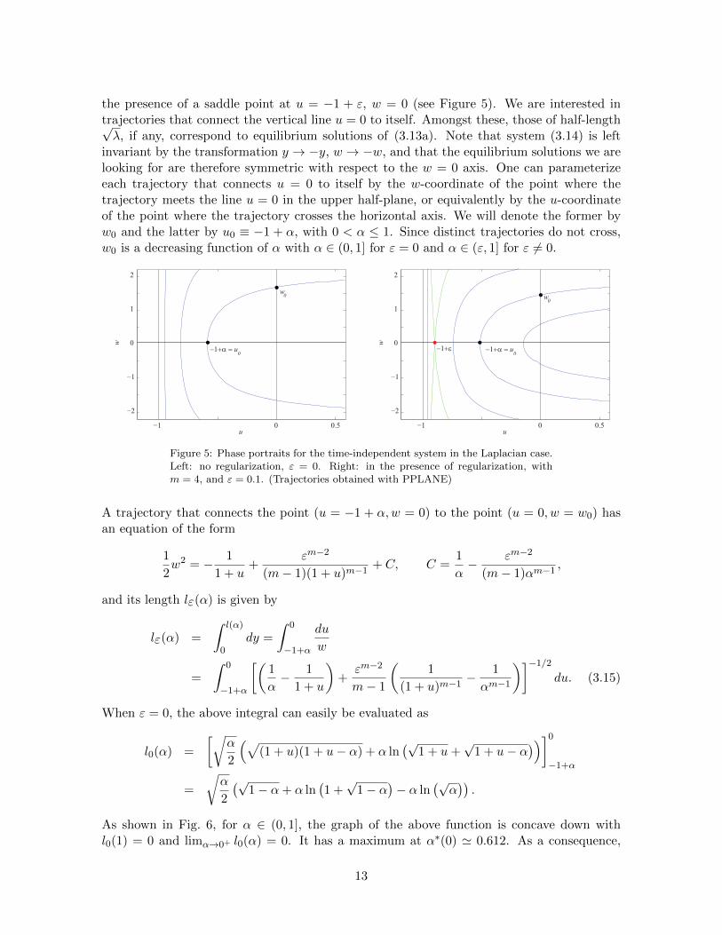
the presence of a saddle point at u = −1 + ε, w = 0 (see Figure 5). We are interested intrajectories that connect the vertical line u = 0 to itself. Amongst these, those of half-length√λ, if any, correspond to equilibrium solutions of (3.13a). Note that system (3.14) is left

invariant by the transformation y → −y, w → −w, and that the equilibrium solutions we arelooking for are therefore symmetric with respect to the w = 0 axis. One can parameterizeeach trajectory that connects u = 0 to itself by the w-coordinate of the point where thetrajectory meets the line u = 0 in the upper half-plane, or equivalently by the u-coordinateof the point where the trajectory crosses the horizontal axis. We will denote the former byw0 and the latter by u0 ≡ −1 + α, with 0 < α ≤ 1. Since distinct trajectories do not cross,w0 is a decreasing function of α with α ∈ (0, 1] for ε = 0 and α ∈ (ε, 1] for ε 6= 0.

−1 0 0.5u

−2

−1

0

1

2

w

u−1+α = 0

w0

−1 0 0.5u

−2

−1

0

1

2

w

u−1+α = 0

−1+ε

w0

Figure 5: Phase portraits for the time-independent system in the Laplacian case.Left: no regularization, ε = 0. Right: in the presence of regularization, withm = 4, and ε = 0.1. (Trajectories obtained with PPLANE)

A trajectory that connects the point (u = −1 + α,w = 0) to the point (u = 0, w = w0) hasan equation of the form

1

2w2 = − 1

1 + u+

εm−2

(m− 1)(1 + u)m−1+ C, C =

1

α− εm−2

(m− 1)αm−1,

and its length lε(α) is given by

lε(α) =

∫ l(α)

0dy =

∫ 0

−1+α

du

w

=

∫ 0

−1+α

[(1

α− 1

1 + u

)+

εm−2

m− 1

(1

(1 + u)m−1− 1

αm−1

)]−1/2

du. (3.15)

When ε = 0, the above integral can easily be evaluated as

l0(α) =

[√α

2

(√(1 + u)(1 + u− α) + α ln

(√1 + u+

√1 + u− α

))]0

−1+α

=

√α

2

(√1− α+ α ln

(1 +√

1− α)− α ln

(√α)).

As shown in Fig. 6, for α ∈ (0, 1], the graph of the above function is concave down withl0(1) = 0 and limα→0+ l0(α) = 0. It has a maximum at α∗(0) ' 0.612. As a consequence,

13

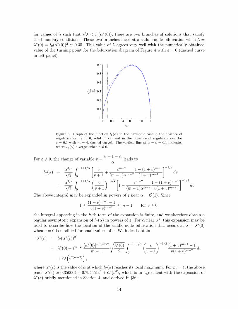
for values of λ such that√λ < l0(α∗(0)), there are two branches of solutions that satisfy

the boundary conditions. These two branches meet at a saddle-node bifurcation when λ =λ∗(0) = l0(α∗(0))2 ' 0.35. This value of λ agrees very well with the numerically obtainedvalue of the turning point for the bifurcation diagram of Figure 4 with ε = 0 (dashed curvein left panel).

Figure 6: Graph of the function lε(α) in the harmonic case in the absence ofregularization (ε = 0, solid curve) and in the presence of regularization (forε = 0.1 with m = 4, dashed curve). The vertical line at α = ε = 0.1 indicateswhere lε(α) diverges when ε 6= 0.

For ε 6= 0, the change of variable v =u+ 1− α

αleads to

lε(α) =α3/2

√2

∫ −1+1/α

0

[v

v + 1+

εm−2

(m− 1)αm−2

1− (1 + v)m−1

(1 + v)m−1

]−1/2

dv

=α3/2

√2

∫ −1+1/α

0

(v

v + 1

)−1/2 [1 +

εm−2

(m− 1)αm−2

1− (1 + v)m−1

v(1 + v)m−2

]−1/2

dv

The above integral may be expanded in powers of ε near α = O(1). Since

1 ≤ (1 + v)m−1 − 1

v(1 + v)m−2≤ m− 1 for v ≥ 0,

the integral appearing in the k-th term of the expansion is finite, and we therefore obtain aregular asymptotic expansion of lε(α) in powers of ε. For α near α∗, this expansion may beused to describe how the location of the saddle node bifurcation that occurs at λ = λ∗(0)when ε = 0 is modified for small values of ε. We indeed obtain

λ∗(ε) = lε(α∗(ε))2

= λ∗(0) + εm−2 [α∗(0)]−m+7/2

m− 1

√λ∗(0)

2

∫ −1+1/α

0

(v

v + 1

)−1/2 (1 + v)m−1 − 1

v(1 + v)m−2dv

+ O(ε2(m−2)

),

where α∗(ε) is the value of α at which lε(α) reaches its local maximum. For m = 4, the abovereads λ∗(ε) ' 0.350004 + 0.794451ε2 + O

(ε4), which is in agreement with the expansion of

λ∗(ε) briefly mentioned in Section 4, and derived in [36].

14

As α→ ε+, lε(α) is expected to diverge for all values of ε 6= 0, since the trajectory approachesthe fixed point at u = −1+ε, w = 0. To analyze this divergence, we set α = κε, with κ = 1+ηand η small, and obtain

lε(α) =α3/2

√2

∫ −1+1/α

0

(v

v + 1

)−1/2 [g(η) +

v p(v)

(1 + v)m−2

]−1/2

dv,

where

g(η) =1

(1 + η)m−2

m−2∑k=1

(m− 2

k

)ηk

v p(v) =1

(1 + η)m−2

m−2∑k=1

(m− 2

k

)k

k + 1vk.

The function H(v) =v p(v)

(1 + v)m−2is such that H(0) = 0 and

limv→∞

H(v) =1

(1 + η)m−2

m− 2

m− 1.

Moreover, H is strictly increasing for 0 ≤ v ≤ L, with L = −1 + 1/α; a simple calculationindeed shows that its derivative is given by

dH

dv=

1

(1 + η)m−2

1

(1 + v)m−1

[m− 2

2+

m−3∑k=1

(m− 2

k + 1

)vk

k + 2

]≥ m− 2

2(1 + η)m−2.

As a consequence, on the interval [0, L], H is bounded above by the line tangent to its graphat the origin, and bounded below by the straight line that goes through the origin and thepoint of coordinates (L,H(L)). In other words,

p(L)v

(1 + L)m−2≤ H(v) ≤ (m− 2)v

2(1 + η)m−2, 0 ≤ v ≤ L.

This, together with 1 ≤ v + 1 ≤ L + 1 for v ∈ [0, L], allows us to bound the term[g(η) +

v p(v)

(1 + v)m−2

]−1/2

that appears in the expression for lε(α), and therefore bound lε(α).

Noting that ∫dv√

v(v + s(η))= 2 ln

(√v +

√v + s(η)

),

we obtain l<(η) ≤ lε(α) ≤ l>(η), where η =α

ε− 1 and

l<(η) =ε3/2

√m− 2

(1 +

m+ 1

2η +O(η2)

)ln

(2(1− ε)εη

+m− 3

2η +O(η2)

)l>(η) = −ε

1/2

√2

√m− 1

m− 2ln(g(η)) +O ((η + ε)(ln(η) + ln(ε))) .

For ε fixed but small and η → 0, we thus have

− ε3/2

√m− 2

ln(η) +O (η ln(η)) ≤ lε(α) ≤ −ε1/2

√2

√m− 1

m− 2ln(η) +O (η ln(η)) . (3.16)

15

This indicates that the graph of lε(α) initially follows that of l0(α) as α decreases towards ε,and then diverges likes − ln(η) = − ln(−1 + α/ε), as shown in Fig. 6. The dashed curve is anumerical evaluation of lε(α) for ε = 0.1 and m = 4. This divergence as α→ ε+ implies theexistence of a third branch of solutions for λ ≥ λ∗(ε), where

√λ∗(ε) is the local minimum of

lε(α). The bounds in Equation (3.16) show that√λ∗(ε)→ 0 as ε→ 0+. As ε increases, the

minimum of the graph of lε(α) merges with its maximum, and only one branch of solutionsexists beyond that point. This is illustrated in the numerically obtained bifurcation diagramsshown in Fig. 4 with ε 6= 0 (solid curves in the left panel). The right panel of Fig. 4 showsthat a similar behavior is observed in the bi-Laplacian case.

3.5. Nature of the new branch of solutions

−1 −0.5 0 0.5 1−1

−0.9

−0.8

−0.7

−0.6

−0.5

−0.4

−0.3

−0.2

−0.1

0

x

u−0.6 −0.4 −0.2

−0.96

−0.95

−0.94

−0.93

x

u

x c

(a) Second order, ε = 0.05, λ = 0.63.

−1 −0.5 0 0.5 1−1

−0.9

−0.8

−0.7

−0.6

−0.5

−0.4

−0.3

−0.2

−0.1

0

x

u−0.6 −0.4 −0.2 0

−0.98

−0.96

−0.94

−0.92

−0.9

x

u

x c

(b) Fourth order, ε = 0.05, λ = 24.82.

Figure 7: Typical solutions of (3.13) on the stable upper branch for m = 4. Panels (a) and (b)represent solutions of (3.13a) and (3.13b) respectively. In each of the two panels, the inset panelsshow an enlargement of the sharp interface and touchdown region.

The newly present maximal branch of stable equilibria can be interpreted as a post touchdownequilibrium state. These additional solutions have three characteristic features, as illustratedin Fig. 7 for values of λ > λ∗. First, in a large central portion of the domain, the solution isflat and takes on values near −1 + ε. Second, a sharp transition layer links the flat region toa profile satisfying the boundary conditions. For the Laplacian problem (3.13a), this sharpinterface is monotone while in the bi-Laplacian case, the profile is non-monotone. Therefore,in the Laplacian case the region where u ' −1+ε is spread over a finite interval while in the bi-Laplacian case, u attains its minimum only at two discrete points. The third characteristicfeature of this branch of equilibrium solutions is the nature of the profile connecting theboundary to the transition layer and in particular the size of the boundary layer. In whatfollows, we use matched asymptotic expansions to characterize these properties in the limitas ε→ 0.

4. Scaling properties of equilibrium solutions.

In this section, we construct 1D post-touchdown equilibrium configurations of (3.13) in thelimit as ε → 0. As seen in Fig. 7, these solutions have interfaces located at ±xc, around

16

which a narrow transition layer is centered. This transition layer separates an interior regionof finite extent (−xc, xc), from a sharp boundary profile. As explained above, the deflectionprofile u satisfies u(x) = −1 + O(ε) in the entire interior region, is monotonic on [0, 1] inthe Laplacian case, and has a local minimum at the discrete points ±xc in the bi-Laplaciancase. In both cases, it is necessary to calculate the extent of the interior region (−xc, xc).From numerical simulations, it appears that xc approaches the boundary as ε → 0. In thecalculations below, we impose this condition, determine the scaling laws that ensue, and findthe equilibrium solutions in terms of matched asymptotic expansions.

4.1. Laplacian Case

We consider Equation (3.13a) in the limit ε→ 0 and look for solutions to

uxx =λ

(1 + u)2− εm−2λ

(1 + u)m, x ∈ [−1, 1]; (4.1a)

u(±1) = 0, (4.1b)

that satisfy the following properties: (i) u(x) = −1 + ε + O(ε) for x ∈ [−xc, xc], (ii) u(x)goes from its interior value of −1 + ε+ O(ε) to the value 1 in the boundary layers [−1,−xc]and [xc, 1], and (iii) there are two transition regions, centered at ±xc. From a dynamicalsystem point of view, the particular trajectory we are interested in crosses the horizontal axisw = ux = 0 of the associated phase plane near but to the right of the fixed point (−1 + ε, 0).As the trajectory gets closer to the fixed point (−1 + ε, 0), the corresponding solution u(x)“spends more time” near u = −1 + ε and therefore xc → 1. To make the scaling explicit,we write xc = 1− εpxc for some xc and p to be determined. From symmetry considerations,since Ω = [−1, 1], we need only study the equations on the interval [0, 1].

To analyze the solution in the boundary layer interval [1− εpxc, 1], it is convenient to use thevariables

u(x) = w(η), η =x− xc1− xc

=x− (1− εpxc)

εpxc, (4.2)

which transforms (4.1) and the boundary condition u(1− εpxc) = −1+O(ε) into

wηη = ε2pλc

[1

(1 + w)2− εm−2

(1 + w)m

], η ∈ [0, 1]; w(0) = −1+O(ε), w(1) = 0, (4.3a)

where we have definedλc = λx2

c . (4.3b)

In light of Equation (4.4b) below, the introduction of λc should be viewed as equivalent toexpanding xc in powers of ε and ε log ε. We now develop the asymptotic expansion

w = w0 + ε2p log εw1/2 + ε2pw1 + O(ε2p) (4.4a)

λc = λ0c + ε2p log ε λ1c + ε2pλ2c + O(ε2p) (4.4b)

for solutions to (4.3a). The O(ε log ε) terms are known as logarithmic switchback termsand have previously appeared in the asymptotic construction of singular solutions to non-regularized MEMS problems [40]. Their necessity in obtaining a consistent expansion isdue to a logarithmic singularity in w1 and will become apparent in the process of matching

17

to a local solution valid in the vicinity of η = 0. At leading order, the solution is given byw0(η) = −1+η while the switchback term satisfies w1/2 = a1/2(η−1) where a1/2 is a constantto be determined in the matching process. The problem for w1 is

w1ηη =λ0c

(1 + w0)2, 0 < η ≤ 1; w1(1) = 0, (4.5a)

and its solution readsw1 = −λ0c log η + a1(η − 1). (4.5b)

In the transition layer near η = 0, i.e. for x ' xc, we introduce the local variables

w(η) = −1 + ενv(ξ), ξ =x− xcεq

, (4.6)

and set the values ν = 1 and q = 3/2. This transforms equation (4.3a) to

vξξ = ε2p−1λ

[1

v2− 1

vm

], −∞ < ξ <∞. (4.7)

To balance the left and right hand sides of (4.7) as ε→ 0, the value p = 1/2 is required. Inorder to match with the far-field solutions, we need to impose

limξ→−∞

v(ξ) = 1 + O(1); −1 + εv(ηxcε

)∼ w(η) as ξ =

ηxcε→∞.

Since the associated dynamical system has only one fixed point at (1,0) in the (v,vξ) phaseplane, there is no trajectory that exactly meets these conditions. However, the unstablemanifold of the above fixed point satisfies the zeroth order equation and boundary conditions.We then look for approximate solutions that solve the differential equation to a given orderin ε and also have the correct behavior as ξ → −∞, to the same order in ε. In particular, ifthe O(ε) term that appears in the boundary condition is small beyond all orders in ε, we willhave v(ξ) = v0(ξ) + O(εk), for all integers k ≥ 1. The leading order problem for v0(ξ) reads

v0ξξ = λ

[1

v20

− 1

vm0

], −∞ < ξ <∞, (4.8a)

v0(ξ)→ 1, v0ξ(ξ)→ 0, as ξ → −∞. (4.8b)

As mentioned above, its solution corresponds to the positive branch of the unstable manifoldof the fixed point (v0 = 1, v0ξ = 0) in the (v0,v0ξ) phase plane of the associated dynamicalsystem. The above equation may be integrated once to give

1

2v2

0ξ = λ

[− 1

v0+

1

(m− 1)vm−10

]+ C0, C0 = λ

m− 2

m− 1,

where the value of C0 was obtained from the condition as ξ → −∞. From this equation, wecan infer the behavior of the unstable manifold as ξ →∞: setting v0(ξ) = αξ+β log ξ+O(1)and equating the constant terms and the terms in 1/ξ, we find

v0(ξ) =

√2λ(m− 2)

m− 1ξ − m− 1

2(m− 2)log ξ + γ +O

( log ξ

ξ

)as ξ →∞.

18

To match with the boundary layer expansion, we re-write −1 + εv0(ξ) + O(ε) in terms ofη = εξ/xc and obtain, after making use of

xc =

√λcλ

=

√λ0c

λ

[1 +

λ1c

λ0cε log ε+

λ2c

λ0cε+ O(ε)

]1/2

,

the following expansion, as ξ →∞:

−1 + εv0(ξ) ' −1 + η

√2λ0c(m− 2)

m− 1+ η

√2λ0c(m− 2)

m− 1

λ1c

2λ0cε log ε+

m− 1

2(m− 2)ε log ε

− m− 1

2(m− 2)ε log η + ε

(√2λ0c(m− 2)

m− 1

λ2c

2λ0cη + γ − m− 1

4(m− 2)log(λ0c

λ

))+O(ε).

To match with

w(η) = −1 + η + ε log ε a1/2(η − 1)− λ0cε log η + εa1(η − 1) + O(ε),

we need to impose

λ0c =m− 1

2(m− 2). (4.9)

We then have

−1+εv0(ξ) ' −1+η+ε log ε(ηλ1c

2λ0c+λ0c

)−λ0cε log η+ε

( λ2c

2λ0cη + γ − λ0c

2log(λ0c

λ

))+ O(ε),

which also requires that

a1/2 = −λ0c, λ1c = −2λ20c, λ2c = 2a1λ0c, and a1 =

λ0c

2log(λ0c

λ

)− γ.

From (4.3b), the two term expansion of xc is then

xc =

[λ0c

λ− 2ε log ε

λ20c

λ+

2a1λ0c

λε+ O(ε)

]1/2

=

√λ0c

λ

[1− λ0cε log ε+ a1ε+ O(ε)

]. (4.10)

To summarize, we expect the equilibrium solution u of (3.13a) to satisfy the followingproperties in the limit ε→ 0:

• u(x) = −1 + ε+O(εk), k > 2 in the interior region x ∈ [0, xc], with xc = 1− ε1/2xc andxc given by (4.10);

• u(x) = −1 + ε v0(ξ) + O(ε) in the transition layer near xc, with ξ =x− xcε3/2

.

• u(x) = −1 + η− ε log ελ0c(η− 1)− λ0cε log η+ εa1(η− 1) + O(ε) in the boundary layer

x ∈ (xc, 1], with η =x− xcε1/2xc

and xc given by (4.10).

19

Figure 8 shows a comparison between the above composite asymptotic expansion and anumerical solution of the full problem, indicating very good agreement. In order to plot thesolution obtained with matched asymptotic expansions, we have assumed that the contactpoint xc coincides with the maximum of the second derivative of u(x), i.e.,

xc = arg maxx∈[0,1]

u′′(x) = (x ∈ [0, 1] | u′′(x) = maxy∈Ω

u′′(y)),

and calculated numerically the value of γ in (4.10) accordingly.

−1 −0.5 0 0.5 1−1

−0.9

−0.8

−0.7

−0.6

−0.5

−0.4

−0.3

−0.2

−0.1

0

x

u

0.92 0.93 0.94 0.95 0.96

−0.9

−0.8

−0.7

x

u

Figure 8: Composite asymptotic expansion of equilibrium solutions to (4.1) for values m = 4,λ = 10, ε = 0.05. The solid line is the numerical solution and the dashed line is the compositeasymptotic expansion.

For comparison to the bifurcation diagrams, the squared L2 norm of the equilibrium solutionto (3.13a) is computed to be, in the limit ε→ 0,∫ 1

−1u(x)2 dx = 2

[∫ 1−ε1/2xc

0u(x)2 dx+

∫ 1

1−ε1/2xcu(x)2 dx

]

= 2

[1− 2ε+ O(ε)− 2

3ε1/2

√λ0c

λ+ O(ε3/2 log ε)

].

If we replace λ0c by its expression given in (4.9), the above equation reads

‖u‖22 = 2

[1− 2

3

√m− 1

2λ(m− 2)ε1/2 − 2ε+O(ε3/2 log ε)

]. (4.11)

The dashed curve in the left panel of Fig. 9 shows the above quantity as a function of λ form = 4 and ε = 0.01, and matches the upper branch of the bifurcation diagram very well.The right panel of Figure 9 is a numerical confirmation of the p = 1/2 scaling.

20

0 0.1 0.2 0.3 0.4 0.50

0.2

0.4

0.6

0.8

1

1.2

1.4

1.6

1.8

λ

‖u‖22

0 0.01 0.02 0.03 0.04 0.050.93

0.94

0.95

0.96

0.97

0.98

0.99

1

ε

xc

Figure 9: Numerical verification of (4.11) and p = 1/2 for m = 4. The left panel displays thebifurcation diagram for ε = 0.01. The solid line represents the numerically obtained branches ofsolutions, while the dashed line is the asymptotic formula for the solution, as derived in (4.11). Theright panel displays a comparison of the predictions for the equilibrium contact point xc= 1−

√εxc

with xc given by (4.10), for fixed λ = 10 and a range of ε. The dashed line is the leading orderexpansion while the dotted is the three term.

4.2. Bi-Laplacian Case

We now turn to 1D equilibrium profiles of (3.13b) in the limit xc → 1 as ε → 0. As in theLaplacian case, we write xc = 1− εpxc where p and xc are parameters to be determined. Forthis particular case, a balancing argument will provide the value p = 1/4. We consider theouter solution in the interval [1− εpxc, 1] and employ the rescaling

u(x) = w(η), η =x− (1− εpxc)

εpxc, (4.12)

which results in

−wηηηη = ε4pλc

[1

(1 + w)2− εm−2

(1 + w)m

], η ∈ [0, 1]; (4.13a)

w(0) = −1, w′(0) = 0, w(1) = w′(1) = 0, (4.13b)

where in addition, the parameter λc is defined by

λc = λx4c . (4.13c)

A logarithmic singularity also arises in the fourth order case, and as before, switchback termsare required in the expansion of (4.13). In addition there is a term at O(ε1/2) which arisesfrom the translation invariance of the inner problem. In the end, the expansions

w = w0 + ε1/2w1/4 + ε4p log εw1/2 + ε4pw1 + O(ε4p); (4.14a)

λc = λ0c + ε1/2λ1c + ε4p log ε λ2c +O(ε4p) (4.14b)

are applied to (4.13). At leading order w0ηηηη = 0 and, with boundary conditions applied,reduces to w0 = −1 + 3η2 − 2η3. The switchback term w1/2 solves the problem

w1/2ηηηη = 0, η ∈ (0, 1); w1/2(1) = w1/2η(1) = 0 (4.15a)

21

and is given byw1/2(η) = α1 + α2η − (3α1 + 2α2)η2 + (2α1 + α2)η3 (4.15b)

where α1 and α2 are constants to be determined by matching. The term ε1/2w1/4, not presentin the Laplacian analysis of §4.1, satisfies

w1/4ηηηη = 0, η ∈ (0, 1); w1/4(0) = w1/4(1) = w1/4η(1) = 0 (4.16a)

w1/4(η) = ξ0(η − 2η2 + η3), (4.16b)

where ξ0 is a constant to be fixed in the matching procedure. The correction term at O(ε4p)solves

−w1ηηηη =λ0c

(1 + w0)2, η ∈ (0, 1); w1(1) = w1η(1) = 0 (4.17)

and includes terms in log η. The full solution is given by

w1(η) =(

2β1 + β2 +5

486

)η3 −

(3β1 + 2β2 +

5

486

)η2 + β2η + β1

+

(16

729η3 − 2

27η2 +

2

27η − 1

54

)(log(3− 2η)− log η

),

where the constants β1 and β2 are arbitrary. In the transition layer near x = xc, we definethe local variables

u(x) = −1 + ενv(ξ), ξ =x− xcεq

, (4.18)

and set the values ν = 1 and q = p+ 1/2. This transforms equation (3.13b) to

−vξξξξ = λε4p−1

(1

v2− 1

vm

), −∞ < ξ <∞. (4.19)

To make this equation independent of ε, we set p = 1/4. The far-field requirements are givenby

limξ→−∞

v(ξ) = 1 + O(1); −1 + εv(η xcε1/2

)∼ w(η) as ξ =

η xc

ε1/2→∞.

As in the Laplacian case, we will assume that the O(ε) term that appears in the far fieldcondition as ξ → −∞ is of order εk with k large, or that it is small beyond all orders inε, so that v approximately lies on the two-dimensional unstable manifold of the fixed point(v = 1, vξ = 0, vξξ = 0, vξξξ = 0) of the four-dimensional phase space associated to the abovedifferential equation. We thus seek an expression for v that solves (4.19) to a given order in εand satisfies the far-field conditions to that order as well. Equation (4.19) may be integratedonce to give

−vξξξ vξ +1

2

(vξξ)2

+λ

v− λ

(m− 1)vm−1= C, (4.20)

where the constant of integration C = λm− 2

m− 1is determined by the value of the left-hand-side

of (4.20) at the fixed point (v = 1, vξ = 0, vξξ = 0, vξξξ = 0). We set

v(ξ) = v0(ξ) + ε1/2v1(ξ) + εv2(ξ) +O(ε3/2),

22

in (4.20) and solve the resulting equations at each order in half-integer powers of ε. Since thedominant term of w(η) as η → 0 is in η2, the zeroth order solution v0(ξ) must behave like ξ2

as ξ →∞. By substituting

v0 (ξ) = b0ξ2 + c0ξ + d0 + η0 log ξ + γ0

log ξ

ξ2+ φ0

log ξ

ξ+f0

ξ+g0

ξ2+O

( log ξ

ξ3

)into the leading order equation and equating similar terms in ξ, we find

v0 (ξ) = b0ξ2 + c0ξ + d0 +

λ

6 b02 log ξ +

λ2

360 b05

log ξ

ξ2+

λ c0

12 b03

1

ξ

+λ(77λ− 540 c0

2b0 + 180 δ3b02 + 360 b0

2d0

)21600 b0

5

1

ξ2+O

( log ξ

ξ3

),

where 2b20 = C and δ3 ≡ δ(m − 3) is equal to 1 if m = 3 and to 0 otherwise. Similarexpressions for v1 and v2 are obtained and provided in Appendix A. We can then evaluate−1 + εv(ξ) as ξ →∞, write the resulting expression as a function of η =

√ε ξ/xc, and match

with the expressions for wi(η) found for the boundary layer expansion. Note that xc dependson λc (see (4.13c)), which itself depends on ε through Equation (4.14b). At lowest order, weobtain

w0(η) = −1 + b0η2

√λ0c

λ+ a1η

3(λ0c

λ

)3/4

which must also be equal to −1 + 3η2−2η3. This fixes the values of b0 and a1 (the coefficientof ξ3 in v1(ξ)) to

b0 = 3

√λ

λ0c, a1 = −2

( λ

λ0c

)3/4.

With 2b20 = C = λ(m− 2)/(m− 1), we obtain

λ0c =18(m− 1)

(m− 2). (4.21)

Matching the expression for w1/4 gives

a2 = 0, c0 = ξ0

(λ

λ0c

)1/4

λ1c = −2

3ξ0λ0c,

so that

λ1c = −12(m− 1)

m− 2ξ0. (4.22)

The value of ξ0 will be numerically estimated to be ξ0 ≈ −3.77 by imposing

v0(0) = minξ∈R

v0(ξ). (4.23)

This condition removes the translation invariance of (4.19) and therefore uniquely specifiesthe contact point. The expression for w1/2 reads

w1/2 (η) =3

2

λ2c

λ0cη2 +

1

27λ0cη −

1

27λ0cη

2 − 1

108λ0c +O(η3)

23

and gives

α1 = − λ0c

108, α2 =

λ0c

27, λ2c = − λ

20c

162. (4.24)

The w1 term picks up the logarithmic singularity and reads

w1 (η) =

(O(η3) +

2

27λ0cη

2 − 2

27λ0cη +

1

54λ0c

)log

(η

4

√λ0c

λ

)

+

(−3

2

λ3c

λ0c+

1

12ξ2

0

)η3 +

(− 7

81λ0c − c1

4

√λ0c

λ+

3

2

λ3c

λ0c

)η2

+

(−1

6ξ0

2 + c14

√λ0c

λ

)η + d0,

leading to

d0 = β1 =7

81λ0c +

1

12ξ0

2, β2 = −1

6ξ0

2 +4

√λ0c

λc1,

and

λ3c = − 28

243λ0c

2 +1

18λ0c ξ0

2 − 5

729λ0c − 2/3

4

√λ0c

λλ0c c1.

Combining (4.22), (4.21), and (4.13c), the two term expansions for the contact points are

xc = ±[

1−[

18(m− 1)

λ(m− 2)

]1/4(ε1/4 − ξ0

6ε3/4 − λ0c

648ε5/4 log ε+O(ε5/4)

)].

where ξ0 ≈ −3.77.

To summarize, we expect the equilibrium solution u of (3.13b) to satisfy the following prop-erties in the limit ε→ 0:

• u(x) = −1 + ε+O(εk), k > 2 in the interior region x ∈ [0, xc], with xc = 1− ε1/4xc;

• u(x) = −1 + ε v0(ξ) + ε3/2v1(ξ) + ε2v2(ξ) +O(ε5/2) in the transition layer near xc, with

ξ =x− xcε3/4

.

• u(x) = −1 + 3η2 − 2η3 + ξ0 η (η− 1)2ε1/2 +O(ε log ε) in the boundary layer x ∈ (xc, 1],

with η =x− xcε1/4xc

.

For comparison with the numerical bifurcation diagram, the squared L2 norm of the compositeasymptotic expansion is calculated to be

‖u‖22 = 2

[∫ 1−ε1/4xc

0u(x)2 dx+

∫ 1

1−ε1/4xcu(x)2 dx

]

= 2

[(−1 + ε+O(ε))2

(1− ε1/4xc

)+ ε1/4xc

∫ 1

0w2

0+2ε1/2w0w1/4 dη+O(ε3/4)

]

24

To simplify this expression, we calculate that∫ 1

0w2

0 dη =13

35,

∫ 1

0w0w1/4 dη = −11ξ0

210,

and apply the expansion

xc =

[18(m− 1)

λ(m− 2)

]1/4(1− ξ0

6ε1/2 +O(ε log ε)

), (4.25)

which finally results in the value

‖u(x; ε)‖22 = 2

[1− 22

35

(18(m− 1)

λ(m− 2)

)1/4

ε1/4+O(ε3/4)

]. (4.26)

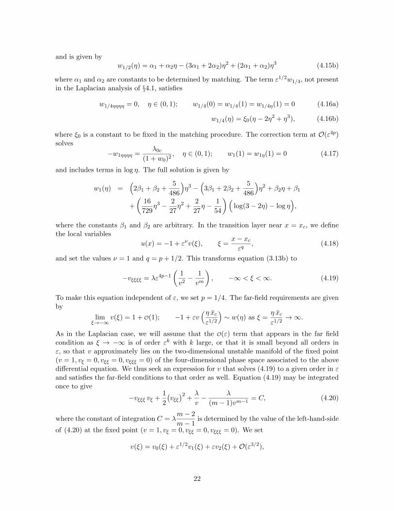
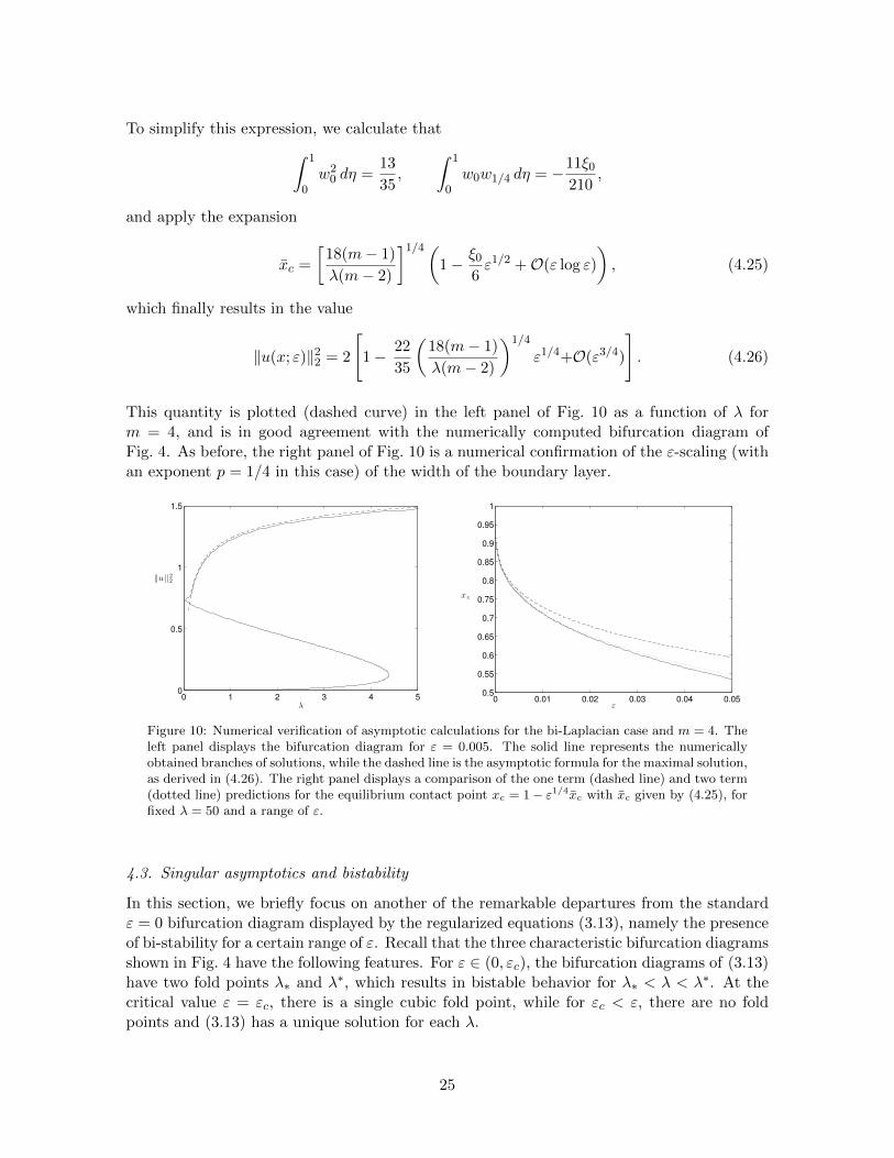
This quantity is plotted (dashed curve) in the left panel of Fig. 10 as a function of λ form = 4, and is in good agreement with the numerically computed bifurcation diagram ofFig. 4. As before, the right panel of Fig. 10 is a numerical confirmation of the ε-scaling (withan exponent p = 1/4 in this case) of the width of the boundary layer.

0 1 2 3 4 50

0.5

1

1.5

λ

‖u‖22

0 0.01 0.02 0.03 0.04 0.050.5

0.55

0.6

0.65

0.7

0.75

0.8

0.85

0.9

0.95

1

ε

x c

Figure 10: Numerical verification of asymptotic calculations for the bi-Laplacian case and m = 4. Theleft panel displays the bifurcation diagram for ε = 0.005. The solid line represents the numericallyobtained branches of solutions, while the dashed line is the asymptotic formula for the maximal solution,as derived in (4.26). The right panel displays a comparison of the one term (dashed line) and two term(dotted line) predictions for the equilibrium contact point xc = 1− ε1/4xc with xc given by (4.25), forfixed λ = 50 and a range of ε.

4.3. Singular asymptotics and bistability

In this section, we briefly focus on another of the remarkable departures from the standardε = 0 bifurcation diagram displayed by the regularized equations (3.13), namely the presenceof bi-stability for a certain range of ε. Recall that the three characteristic bifurcation diagramsshown in Fig. 4 have the following features. For ε ∈ (0, εc), the bifurcation diagrams of (3.13)have two fold points λ∗ and λ∗, which results in bistable behavior for λ∗ < λ < λ∗. At thecritical value ε = εc, there is a single cubic fold point, while for εc < ε, there are no foldpoints and (3.13) has a unique solution for each λ.

25

−1 −0.5 0 0.5 1−1

−0.9

−0.8

−0.7

−0.6

−0.5

−0.4

−0.3

−0.2

−0.1

0

x

u

0.65 0.7 0.75

−0.995

−0.99

−0.985

x

u

Figure 11: Composite asymptotic expansion of equilibrium solutions to (3.13) for values m = 4,λ = 50, ε = 0.01. The solid line is the numerical solution and the dashed line is the compositeasymptotic expansion.

0 0.1 0.2 0.3 0.4 0.50

0.1

0.2

0.3

0.4

0.5

0.6

0.7

0.8

0.9

1

λ

‖u‖22

0 1 2 3 4 5 6 7 80

0.1

0.2

0.3

0.4

0.5

0.6

0.7

0.8

0.9

1

λ

‖u‖22

Figure 12: Numerically obtained bifurcation diagrams of (3.13) for ε = 0.01, 0.025, 0.05, 0.1, 0.15(from left to right) and m = 4. Left panel: Laplacian case (3.13a); right panel: bi-Laplacian case(3.13b).

In Fig. 12, the bifurcation diagrams of (3.13) are displayed for a range of ε ∈ (0, εc) andm = 4. In each case, the fold point λ∗(ε) is observed to depend quite sensitively on theparameter ε, while the principal fold point λ∗(ε) exhibits smaller variations as ε increases.In essence, the regularizing term of the governing equations generates a regular perturbationto solutions of the ε = 0 problem whenever 1 + u = O(1), and a singular perturbation tosolutions of the ε = 0 problems whenever u + 1 ' ε. In each of the cases represented inFig. 12, the two fold points are empirically seen to be increasing functions of ε, with λ∗(ε)increasing faster than λ∗(ε). We therefore expect the two fold points to eventually merge atsome critical εc, where the condition

λ∗(εc) = λ∗(εc) (4.27)

is satisfied. The bistable features of the regularized system are interesting as they give thedevice the capacity to switch robustly between equilibrium states of large and small L2 norm.The relative magnitude of the switching voltage required to transition the device betweenthese two states is given, for ε < εc, by the quantity λ∗(ε)− λ∗(ε).It is therefore desirable to obtain explicit formulae for λ∗(ε) and λ∗(ε) so that the critical

26

parameter εc may be estimated from the condition (4.27) and the bistable nature of theregularized system understood. In a forthcoming paper [36], a detailed singular perturbationanalysis is employed to accurately locate these fold points. The main results are explicitexpansions of form

λ∗(ε) ∼ λ∗0 + εm−2λ∗1 +O(ε2(m−2)), (4.28a)

for the principal fold point in the Laplacian or bi-Laplacian case. The scaling of the secondfold point is quite different for the second and fourth order problems, namely

λ∗(ε) ∼ λ∗0ε+ λ∗1ε2 log ε+ λ∗2ε

2 + · · · (Laplacian)

λ∗(ε) ∼ λ∗0ε3/2 + λ∗1ε

2 + · · · (bi-Laplacian)(4.28b)

In the above formulations, closed form expressions for the coefficients λ∗i and λ∗i are estab-lished in [36].

5. Discussion

In this work we have proposed and analyzed a formulation for regularization of touchdown inMEMS capacitors. These considerations have resulted in a new family of models whose solu-tions remain globally bounded in time for all parameter regimes, followed by equilibration tonew steady states. Interestingly, the presence of these new stable equilibria results in bistablebehavior for a range of parameter values. This may be useful in practical applications sincebistable systems can be used to create robust switches. We have described how equilibriumsolutions depend on the parameters λ and ε in terms of bifurcation diagrams, for both theLaplacian and the bi-Laplacian cases. Using asymptotic analysis, we have also given a com-plete characterization of the scaling properties of the upper branch of equilibrium solutions,which correspond to attracting post-touchdown configurations of the regularized equations.

There are several avenues of future exploration emanating from this study. The method ofregularization used in the present work is a first attempt at understanding the behavior ofMEMS after touchdown. It is natural to ask whether this bistability feature is generic to alarger family of regularized models.

An interesting problem is the characterization of the intermediate dynamics between theinitial regularized touchdown event and the equilibration to the post touchdown states. Asis typical with such obstacle type regularizations, the equations (2.12) give rise to a freeboundary problem for the extent of the touchdown region, which is amenable to analysis. Ina forthcoming paper [35], we describe the dynamic evolution of the periphery of the growingpost-touchdown region, in both one and two spatial dimensions.

Acknowledgments

K.G. acknowledges support from NSF award DMS-0807423. A.E.L acknowledges supportfrom the Carnegie Trust for the Universities of Scotland. A.E.L and J.L. completed themanuscript during a stay at the Henri Poincare Institute in July 2013 and thank them fortheir hospitality.

27

Appendix A. Expressions for v1 and v2

We give below the expressions for v1(ξ) and v2(ξ) such that v = v0 + ε1/2v1 + εv2 +O(ε3/2)solves (4.20) to order ε1/2 and ε respectively.

v1 (x) = a1ξ3 +

3a1c0

2b0ξ2 + c1ξ + d1 +

λ c0a1

2 b04 log (ξ) +

λ a1

b03 ξ log (ξ) +

λ2a1

24 b06

log (ξ)

ξ

+γ1log (ξ)

ξ2− λ

(−36 c0

2a1b0 + 72 d0a1b02 − 24 c1b0

3 − 25λ a1 + 36 δ3a1b02)

288 b06ξ

+g1

ξ2+O

( log (ξ)

ξ3

),

and

v2 (ξ) = a2ξ3 + b2ξ

2 + c2ξ + d2 + κ2 (log (ξ))2 + η3 log (ξ) + η4 ξ log (ξ) + η5 ξ2 log (ξ)

+φ2log (ξ)

ξ+ γ2

log (ξ)

ξ2+f2

ξ+g2

ξ2+O

( log (ξ)

ξ3

),

where

η3 = λ

(−18 δ3a1

2b02 + 16λ a1

2 + 9 a2c0b03 + 9 a1

2c02b0 − 36 a1

2b02d0 + 9 a1c1b0

3)

18 b07 ,

η4 =6λ c0a1

2 + 4λ a2b02

4 b05 , η5 =

3λ a12

2 b04 , κ2 =

λ2a12

12 b07 ,

b2 = −14λ a12 − 12 a2c0b0

3 + 9 a12c0

2b0 − 12 a1c1b03

8 b04 ,

φ2 = −−4λ2a2b02 + 7λ2c0a1

2 + 720 a1γ1b07

96 b08 ,

f2 =λ c0

(36 c0

2b0 + 341λ− 72 b02d0 − 36 δ3b0

2)a1

2

1152 b08

−(λ c0c1 + λ d1b0 + 60 g1b0

4 + 48 γ1b04)a1

8 b05

+λ(−72 b0

2d0 + 25λ+ 36 c02b0 − 36 δ3b0

2)a2

288 b06 +

λ c2

12 b03 .

References

[1] Anubhav Arora, Mark R. Prausnitz, Samir Mitragotri, Micro-scale devices for trans-dermal drug delivery, International Journal of Pharmaceutics, Vol. 364, Issue 2, (2008),pp. 227–236.

[2] R. C. Batra, M. Porfiri, and D. Spinello Effects of van der Waals Force and ThermalStresses on Pull-in Instability of Clamped Rectangular Microplates, Sensors, (2008), 8,pp. 1048–1069.

28

[3] A. J. Bernoff and T. P. Witelski, Stability and dynamics of self-similarity in evolutionequations, Journal of Engineering Mathematics, vol. 66 no. 1-3 (2010), pp. 11–31, ISSN1573–2703.

[4] A. J. Bernoff, A. L. Bertozzi and T. P. Witelski, Axisymmetric surface diffusion: Dy-namics and stability of self-similar pinch-off, J. Stat. Phys. (1998) 93, 725–776.

[5] A. L. Bertozzi, G. Grun and T. P. Witelski, Dewetting films: bifurcations and concen-trations, Nonlinearity 14 (2001) 1569–1592.

[6] A. J. Bernoff and T. P. Witelski, Stability of self-similar solutions for van der Waalsdriven thin film rupture, Physics of Fluids, Vol. 11 No. 9 (1999).

[7] N. D. Brubaker, J. A. Pelesko, Non-linear effects on canonical MEMS models, Euro.Journal of Applied Mathematics, (2011) Vol. 22, No. 5, pp. 455–470.

[8] Doble, N., Williams, D.R., The application of MEMS technology for adaptive optics invision science, IEEE Journal of Selected Topics in Quantum Electronics, Vol. 10, No. 3,pp. 629–635.

[9] J. Escher, Ph. Laurencot, C. Walker, Dynamics of a free boundary problemwith curvature modeling electrostatic MEMS, To appear in Trans. Amer. Math.http://arxiv.org/abs/1302.6026

[10] J. Escher, Ph. Laurencot, C. Walker, Finite time singularity in a free boundary problemmodeling MEMS, C. R. Acad. Sci. Paris Ser. I Math. 351 (2013) 807–812.

[11] P. Esposito, N. Ghoussoub, Y. Guo, Mathematical Analysis of Partial Differential Equa-tions Modeling Electrostatic MEMS, Courant Lecture Notes Vol. 20 (2010).

[12] G. Flores, Dynamics of a damped wave equation arising from MEMS, To Appear SIAMJ. Appl. Math (2014)

[13] G. Flores, G. Mercado, J. A. Pelesko and N. Smyth, Analysis of the dynamics andtouchdown in a Model of Electrostatic MEMS, SIAM J. Appl. Math., (2007), 67(2),pp. 434–446.

[14] N. Ghoussoub, Y. Guo, On the Partial Differential Equations of Electrostatic MEMSDevices: Stationary Case, SIAM J. Math. Anal., 38, No. 5, (2007), pp. 1423–1449.

[15] N. Ghoussoub, Y. Guo, Estimates for the Quenching Time of a Parabolic EquationModeling Electrostatic MEMS, Methods Appl. Anal. Vol. 15, No. 3 (2008), 361–376.

[16] N. Ghoussoub, Y. Guo, On the partial differential equations of electrostatic MEMS de-vices III: Dynamic case, Nonlinear differ. equ. appl. 15 (2008) pp. 115–145.

[17] Y. Guo, Dynamical solutions of singular wave equations modeling electrostatic MEMS,SIAM, J. Appl. Dynamical Systems, 9 (2010), pp. 1135–1163.

[18] Y. Guo, On the partial differential equations of electrostatic MEMS devices III: refinedtouchdown behavior, J. Diff. Eqns. 244 (2008), pp. 2277–2309.

29

[19] Y. Guo, Z. Pan, M. J. Ward, Touchdown and Pull-In Voltage Behaviour of a MEMSDevice with Varying Dielectric Properties, SIAM J. Appl. Math., 66, No. 1, (2005),pp. 309–338.

[20] J-G. Guo, Y-P. Zhao, Influence of van der Waals and Casimir Forces on ElectrostaticTorsional Actuators, Journal of Microelectromechanical systems, Vol. 13, No. 6, 2004,pp. 1027–1035.

[21] J-S Guo, B-C Huang, Hyperbolic Quenching problem with damping in the micro-electromechanical system device, Discrete and Continuous Dynamical Systems Series B, Vol.19, No. 2, (2014), pp. 419–434.

[22] Z. Guo, B. Lai, and D. Ye, Revisiting the biharmonic equation modeling electrostatic ac-tuation in lower dimensions, Proceedings of the American Mathematical Society (2014)

[23] Brian D. Iverson, Suresh V. Garimella, Recent advances in microscale pumping tech-nologies: a review and evaluation., Microfluidics and Nanofluidics, Volume 5, Issue 2,(2008), pp. 145–174.

[24] R. Jordan, D. Kinderlehrer, and F. Otto, The variational formulation of the Fokker-Plank equation, SIAM J. Math. An. 29 (1998).

[25] N. I. Kavallaris, A. A. Lacey, C. V. Nikolopoulos, and D. E. Tzanetis, A hyperbolicnon-local problem modelling MEMS technology, Rocky Mountain J. Math Vol. 41, No. 2(2011), pp. 349–630.

[26] N. Kikuchi, J. T. Oden, Contact problems in elasticity: a study of variational inequalitiesand finite element methods, (1988), SIAM.

[27] M. Kohlmann, A new model for electrostatic MEMS with two free boundaries, Journalof Mathematical Analysis and Applications, (2013), Vol. 408, No. 2, pp. 513–524.

[28] B. Lai, On the Partial Differential Equations of Electrostatic MEMS Devices with Effectsof Casimir Force, Annales Henri Poincare, (2014) DOI: 10.1007/s00023-014-0322-8

[29] Ph. Laurencot, C. Walker, A fourth-order model for MEMS with clamped boundary con-ditions, http://arxiv.org/abs/1304.2296

[30] Ph. Laurencot, C. Walker, A stationary free boundary problem modelling electrostaticMEMS Archive for Rational Mechanics and Analysis 207 (2013) pp. 139–158

[31] Ph. Laurencot, C. Walker, A free boundary problem modeling electrostatic MEMS I.Linear Bending Effects, Math. Ann., to appear.

[32] Ph. Laurencot, C. Walker, A free boundary problem modeling electrostatic MEMS II.Non-Linear Bending Effects, Math. Models Methods Appl. Sci., to appear.

[33] F. H. Lin, Y. Yang, Nonlinear Non-Local Elliptic Equation Modeling Electrostatic Actu-ation, Proc. Roy. Soc. A, 463. (2007), pp. 1323–1337.

[34] A. E. Lindsay, J. Lega, (2012) Multiple quenching solutions of a fourth order parabolicPDE with a singular nonlinearity modelling a MEMS Capacitor, SIAM J. Appl. Math.,72(3), pp. 935–958.

30

[35] A. E. Lindsay, J. Lega, K. B. Glasner (2014) Regularized Model of Post-TouchdownConfigurations in Electrostatic MEMS: Interface Dynamics.

[36] A. E. Lindsay, (2014) Regularized Model of Post-Touchdown Configurations in Electro-static MEMS: Bistability Properties.

[37] A. E. Lindsay, An asymptotic study of blow up multiplicity in fourth order parabolicpartial differential equations, DCDS-B, Vol. 19, No. 1, (2014), pp. 189–215.

[38] A. E. Lindsay, J. Lega, F-J. Sayas (2013), The quenching set of a MEMS capacitor intwo-dimensional geometries, Journal of Nonlinear Science, Vol. 23, No. 5, pp. 807–834.

[39] A. E. Lindsay, M. J. Ward, Asymptotics of Some Nonlinear Eigenvalue Problems fora MEMS Capacitor: Part I: Fold Point Asymptotics, Methods Appl. Anal., 15, No. 3,(2008), pp. 297–325.

[40] A. E. Lindsay, M. J. Ward, Asymptotics of some nonlinear eigenvalue problems for aMEMS capacitor: Part II: Singular Asymptotics, Euro. Jnl of Applied Mathematics(2011), vol. 22, pp. 83–123.

[41] J-L. Lions, Quelques methodes de resolution des problemes aux limites non lineaires,(1969) Vol. 76, Dunod Paris.

[42] J. A. Pelesko, D. H. Bernstein, Modeling MEMS and NEMS, Chapman Hall and CRCPress, (2002).

[43] J. A. Pelesko, Mathematical Modeling of Electrostatic MEMS with Tailored DielectricProperties, SIAM J. Appl. Math., 62, No. 3, (2002), pp. 888–908.

[44] R. Scholz, Numerical solution of the obstacle problem by the penalty method, NumerischeMathematik, Vol. 49, no. 2-3, (1986) pp. 255–268.

[45] Nan-Chyuan Tsai, Chung-Yang Sue, Review of MEMS-based drug delivery and dosingsystems, Volume 134, Issue 2, (2007), pp. 555–564.

[46] B. Watson, J. Friend, L. Yeo, Piezoelectric ultrasonic micro/milli-scale actuators, Sensorsand Actuators A: Physical, 152 (2009) pp. 219–233.

31