Regularization and the small-ball method I: sparse recovery

Guillaume Lecue1,3 Shahar Mendelson2,4,5

January 20, 2016

Abstract

We obtain bounds on estimation error rates for regularization procedures of the form

f ∈ argminf∈F

(1

N

N∑i=1

(Yi − f(Xi))2

+ λΨ(f)

)

when Ψ is a norm and F is convex.Our approach gives a common framework that may be used in the analysis of learning

problems and regularization problems alike. In particular, it sheds some light on therole various notions of sparsity have in regularization and on their connection with thesize of subdifferentials of Ψ in a neighbourhood of the true minimizer.

As ‘proof of concept’ we extend the known estimates for the LASSO, SLOPE andtrace norm regularization.

1 Introduction

The focus of this article is on regularization, which is one of the most significant methodsin modern statistics. To give some intuition on the method and on the reasons behind itsintroduction, consider the following standard problem.

Let (Ω, µ) be a probability space and set X to be distributed according to µ. F is aclass of real-valued functions defined on Ω and Y is the unknown random variable that onewould like to approximate using functions in F . Specifically, one would like to identify thebest approximation to Y in F , say in the L2 sense, and find the function f∗ that minimizesin F the squared loss functional f → E(f(X)− Y )2; that is,

f∗ = argminf∈FE(f(X)− Y )2,

with the underlying assumption that f∗ exists and is unique.Unlike problems in approximation theory, neither the target Y nor the underlying mea-

sure µ are known. Therefore, computing the L2 distance between functions in F and Y is

1CNRS, CREST, ENSAE, 3, avenue Pierre Larousse, 92245 MALAKOFF. France.2Department of Mathematics, Technion, I.I.T., Haifa, Israel and Mathematical Sciences Institute, The

Australian National University, Canberra, Australia3Email: guillaume.lecue@ensae.fr4Email: shahar@tx.technion.ac.il5Supported by the Israel Science Foundation.

1

impossible. Instead, one is given partial information: a random sample (Xi, Yi)Ni=1, selected

independently according to the joint distribution of X and Y .Because of the random nature of the sample and the limited information it provides,

there is no real hope of identifying f∗, but rather, only of approximating it. In an estimationproblem one uses the sample to produce a random function f ∈ F , and the success of thechoice is measured by the distance between f and f∗ in the L2(µ) sense. Thus, one wouldlike to ensure that with high probability with respect to the samples (Xi, Yi)

Ni=1, the error

rate ∥∥∥f − f∗∥∥∥2

L2(µ)= E

((f(X)− f∗(X)

)2|(Xi, Yi)Ni=1

)is small. More accurately, the question is to identify the way in which the error rate dependson the structure of the class F and scales with the sample size N and the required degreeof confidence (probability estimate).

It is not surprising (and rather straightforward to verify) that the problem becomesharder the larger F is. In contrast, if F is small, chances are that f∗(X) is very far fromY , and identifying it, let alone approximating it, is pointless.

In situations we shall refer to as learning problems, the underlying assumption is thatF is indeed small, and the issue of the approximation error – the distance between Y andf∗ is ignored.

While the analysis of learning problems is an important and well-studied topic, theassumption that F is reasonably small seems somewhat restrictive; it certainly does noteliminate the need for methods that allow one to deal with very large classes.

Regularization was introduced as an alternative to the assumption on the ‘size’ of F .One may consider large classes, but combine it with the belief that f∗ belongs to a relativelysmall substructure in F . The idea is to penalize a choice of a function that is far from thatsubstructure, which forces the learner to choose a function in the ‘right part’ of F .

Formally, let E be a vector space, assume that F ⊂ E is a closed and convex set andlet Ψ : E → R+ be the penalty. Here, we will only consider the case in which Ψ is a normon E.

Let λ > 0 and for a sample (Xi, Yi)Ni=1, set

f ∈ argminf∈F

(1

N

N∑i=1

(Yi − f(Xi))2 + λΨ(f)

);

f is called a regularization procedure, Ψ is the regularization function and λ is the regular-ization parameter.

In the classical approach to regularization, the substructure of f∗ is quantified directlyby Ψ. The underlying belief is that Ψ(f∗) is not ‘too big’ and one expects the procedureto produce f for which Ψ(f) is of the order of Ψ(f∗). Moreover, the anticipated error rate‖f − f∗‖L2(µ) depends on Ψ(f∗). In fact, an optimistic viewpoint is that regularizationcould perform as well as the best learning procedure in the class f : Ψ(f) ≤ Ψ(f∗), butwithout knowing Ψ(f∗) beforehand.

2

Among the regularization schemes that are based on the classical approach are repro-ducing kernel Hilbert spaces (RKHS), in which the RKHS norm serves at the penalty. SinceRKHS norms capture various notions of smoothness, in RKHS regularization one is driventowards a choice of a smooth f – as smooth as f∗ is.

In more modern regularization problems the situation is very different. Even whenpenalizing with a norm Ψ, one no longer cares whether or not Ψ(f∗) is small; rather, oneknows (or at least believes) that f∗ is sparse in some sense, and the hope is that this sparsitywill be reflected in the error rate.

In other words, although one uses certain norms as regularization functions – normsthat seemingly have nothing to do with ‘sparsity’ – the hope is that the sparse nature of f∗

will be exposed by the regularization procedure, while Ψ(f∗) will be of little importance.

The most significant example in the context of sparsity-driven regularization is thecelebrated LASSO estimator [34]. Let F =

⟨t, ·⟩

: t ∈ Rd and set t∗ to be a minimizer inRd of the functional t→ E(

⟨t,X

⟩− Y )2. The LASSO is defined by

t ∈ argmint∈Rd

( 1

N

N∑i=1

(⟨t,Xi

⟩− Yi

)2+ λΨ(t)

)for the choice Ψ(t) = ‖t‖1 =

∑di=1 |ti|.

The remarkable property of the LASSO (see [8] and [3]) is that for a well-chosen reg-ularization parameter λ, if t∗ is supported on at most s coordinates (and under variousassumptions on X and Y to which we will return later), then with high probability,

‖t− t∗‖22 .s log(ed)

N.

Thus, the error rate of the LASSO does not depend on Ψ(t∗) = ‖t∗‖1, but rather on thedegree of sparsity of t∗, measured here by the cardinality of its support ‖t∗‖0 = |i : t∗i 6= 0|.

This fact seems almost magical, because to the naked eye, the regularization function‖t‖1 has nothing to with sparsity; yet `1 regularization leads to a sparsity-driven error rate.

A standard (yet somewhat unconvincing) explanation of this phenomenon is that thepenalty ‖t‖1 is a convexified version of ‖t‖0 = |i : ti 6= 0|, though this loose connectionhardly explains why ‖t∗‖0 has any effect on the error rate of the LASSO.

A similar phenomenon occurs for other choices of Ψ, such as the SLOPE and trace-normregularization, which will be explored in detail in what follows. In all these cases and otherslike them, the regularization function is a norm that does not appear to be connected tosparsity, nor to other natural notions of low-dimensional structures for that matter. Yet, andquite mysteriously, the respective regularization procedure emphasize those very propertiesof t∗.

The aim of this note is to offer a framework that can be used to tackle standard learningproblems (small F ) and regularized problems alike. Moreover, using the framework, onemay explain how certain norms lead to the emergence of sparsity-based bounds.

In what follows we will show that two parameters determine the error rate of regulariza-tion problems. The first one captures the ‘complexity’ of each set in the natural hierarchy

3

in FFρ = f ∈ F : Ψ(f − f∗) ≤ ρ.

Applying results from [22, 24, 21], the ‘complexity’ of each Fρ turns out to be the optimal(in the minimax sense) error rate of the learning problem in that set.

To be more precise, the main ingredient in obtaining a sharp error rate in a learningproblem in a class H is an accurate analysis of the empirical excess squared loss functional

f → PNLf =1

N

N∑i=1

(f(Xi)− Yi)2 − 1

N

N∑i=1

(f∗(Xi)− Yi)2. (1.1)

Since the minimizer f of the functional (1.1) satisfies PNLf ≤ 0, one may obtain an estimate

on the error rate by showing that with high probability, if ‖f−f∗‖L2(µ) ≥ r then PNLf > 0.This excludes functions in the set f ∈ H : ‖f − f∗‖L2(µ) ≥ r as potential empiricalminimizers.

One may show that this ‘critical level’ is the correct (minimax) error rate of a learningproblem in H, and that the same parameter is of central importance in regularizationproblems: namely, the ‘critical level’ r(ρ) for each one of the sets f ∈ F : Ψ(f − f∗) ≤ ρ(see Section 2.1 for an accurate definition of r(ρ) and its role in the analysis of learningproblems and regularization problems).

The second parameter, which is the main ingredient in our analysis of regularizationproblems, measures the ‘size’ of the subdifferential of Ψ in points that are close to f∗ –recall that the subdifferential of Ψ in f is

(∂Ψ)f = z∗ ∈ E∗ : Ψ(f + h) ≥ Ψ(f) + z∗(h) for every h ∈ E

where E∗ is the dual space of (E,Ψ).Indeed, fix ρ > 0, and let Γf∗(ρ) be the collection of functionals that belong to the

subdifferential (∂Ψ)f for some f ∈ F that satisfies Ψ(f − f∗) ≤ ρ/20. Set

Hρ = f ∈ F : Ψ(f − f∗) = ρ and ‖f − f∗‖L2(µ) ≤ r(ρ)

and let∆(ρ) = inf

h∈Hρsup

z∗∈Γf∗ (ρ)z∗(h− f∗).

It is well known that the subdifferential of a norm Ψ in f consists of all the norm one linearfunctionals z∗ for which z∗(f) = Ψ(f). Hence, Γf∗(ρ) is a subset of the unit sphere of E∗.And, since Hρ consists of functions whose Ψ norm is ρ, ∆(ρ) ≤ ρ. Therefore, the fact that∆(ρ) ≥ αρ implies that Γf∗(ρ) is rather large: for every h ∈ Hρ there is some z∗ ∈ Γf∗(ρ)for which z∗(h) is ‘almost extremal’: at least αρ.

Our main result (Theorem 3.2 below) is that if Γf∗(ρ) is large enough toensure that ∆(ρ) ≥ 4ρ/5, and the regularization parameter λ is set to be of the

order of r2(ρ)ρ , then with high probability, the regularized minimizer in F , f ,

satisfies that ‖f − f∗‖L2(µ) ≤ r(ρ) and Ψ(f − f∗) ≤ ρ.

4

Theorem 3.2 implies that one may address a regularization problem by selecting ρ wisely,keeping in mind that points in a Ψ-ball of radius ∼ ρ around f∗ must generate a sufficientlylarge class of subdifferentials.

f∗f∗

It is essential that the functionals in Γf∗(ρ) need to be ‘almost extremal’ only for pointsin Hρ rather than for the entire sphere; otherwise, it would have forced Γf∗(ρ) to be unrea-sonably large – close to the entire dual sphere.

One may show that sparsity, combined with the right choice of Ψ, contributes in twoplaces: firstly, if f∗ is sparse in some sense, and Ψ is not smooth on sparse elements, thenΓf∗(ρ), which contains the subdifferential (∂Ψ)f∗ is large; secondly, for the right choiceof ρ the ‘localization’ Hρ consists of elements that are well placed: if Ψ(f − f∗) = ρ and‖f − f∗‖L2(µ) ≤ r(ρ), there is some z∗ ∈ Γf∗(ρ) for which z∗(f − f∗) is large enough –and thus ∆(ρ) is large enough. The fact that Hρ is well placed is an outcome of somecompatibility between Ψ and the L2(µ) norm.

Of course, to find the right choice of ρ one must first identify r(ρ), which is, in itself, awell-studied yet nontrivial problem.

Before we dive into technical details, let us formulate some outcomes of our main result.We will show how it can be used to obtain sparsity-driven error rates in three regularizationprocedures: the LASSO, SLOPE and trace norm regularization. In all three cases ourresults actually extend the known estimates in various directions.

The LASSO.The LASSO is obtained when F =

⟨t, ·⟩

: t ∈ Rd. Identifying the linear functional⟨t, ·⟩

with t, the regularization function is

Ψ(t) = ‖t‖1 =

d∑i=1

|ti|,

and the resulting regularization problem is

t ∈ argmint∈Rd

( 1

N

N∑i=1

(⟨t,Xi

⟩− Yi

)2+ λ‖t‖1

).

The LASSO has been studied extensively in the last two decades. It has been THE bench-mark estimator of high-dimensional statistics because the high dimensional parameter spacedoes not significantly affect its performance as long as t∗ is sparse. This is indeed the casefor estimation and sparse oracle inequalities in [3, 15, 36, 37, 19, 28, 35], support recovery

5

results in [17, 39, 2] or testing and confidence intervals results in [16, 18]. We refer thereader to the books [5, 8] for more results and references on the LASSO.

SLOPE.In some sense, SLOPE, introduced in [4, 32], is actually an extension of the LASSO,

even though it has been introduced as an extension of multiple-test procedures. Again,the underlying class is F =

⟨t, ·⟩

: t ∈ Rd, and to define the regularization function letβ1 ≥ β2 ≥ ... ≥ βd > 0 and set

Ψ(t) =

d∑i=1

βit∗i ,

where (t∗i )di=1 denotes the non-increasing re-arrangement of (|ti|)di=1. Thus, the SLOPE

norm is a sorted, weighted `1-norm, and for (β1, ..., βd) = (1, ..., 1), SLOPE regularizationcoincides with the LASSO.

Trace-norm regularization.Consider the trace inner-product on Rm×T . Let F =

⟨A, ·⟩

: A ∈ Rm×T and given atarget Y put A∗ to be the matrix that minimizes A→ E(

⟨A,X

⟩− Y )2.

The regularization function is the trace norm.

Definition 1.1 Let A be a matrix and set (σi(A)) to be its singular values, arranged ina non-increasing order. For p ≥ 1, ‖A‖p = (

∑σpi (A))1/p is the p-Schatten norm. The

trace-norm is the 1-Schatten norm, the Hilbert-Schmidt norm is the 2-Schatten norm andthe operator norm is the ∞-Schatten norm.

The trace norm regularization procedure is

A ∈ argminA∈Rm×T

( 1

N

N∑i=1

(Yi −⟨Xi, A

⟩)2 + λ‖A‖1

)and it was introduced for the reconstruction of low-rank, high-dimensional matrices [29, 9,30, 6, 7, 27].

As will be explained in what follows, our main result holds in rather general situationsand it may be implemented in examples once the ‘critical levels’ r(ρ) are identified. Sincethe examples we present serve mainly as “proof of concept”, we will focus only on onescenario in which r(ρ) may be completely characterized for an arbitrary class of functions.

Definition 1.2 Let `M2 be an M -dimensional inner product space and let µ be a measureon `M2 . The measure µ is isotropic if for every x ∈ `M2 ,∫ ⟨

x, t⟩2dµ(t) = ‖x‖2

`M2;

it is L-subgaussian if for every p ≥ 2 and every x ∈ `M2 ,

‖⟨x, ·⟩‖Lp(µ) ≤ L

√p‖⟨x, ·⟩‖L2(µ).

6

Hence, the covariance structure of an isotropic measure coincides with the inner product in`M2 , and if µ is an L-subgaussian measure the Lp(µ) norm of a linear form does not growfaster than the Lp norm of the corresponding gaussian variable.

Assumption 1.1 Assume that the underlying measure µ is isotropic and L-subgaussian,and that for f∗ =

⟨t∗, ·⟩

(or f∗ =⟨A∗, ·

⟩), the noise1 ξ = f∗(X)−Y belongs to Lq for some

q > 2.

When dealing with the LASSO and SLOPE, the natural Euclidean structure is thestandard one in Rd, and for trace norm regularization, the Euclidean structure is endowedby the trace inner product in Rm×T .

The second part of Assumption 1.1, that ξ ∈ Lq for some q > 2, is rather minimal.Indeed, for the functional f → E(f(X) − Y )2 to be well defined, one must assume thatf(X)− Y ∈ L2; the assumption here is only slightly stronger.

Applying our main result we will show the following:

Theorem 1.3 Consider the LASSO under Assumption 1.1. Let 0 < δ < 1. Assume thatthere is some v ∈ Rd supported on at most s coordinates for which

‖t∗ − v‖1 ≤ c1(δ)‖ξ‖Lqs√

log(ed)

N.

If λ = c2(L, δ)‖ξ‖Lq√

log(ed)/N , then with probability at least 1 − δ the LASSO estimatorwith regularization parameter λ satisfies that for every 1 ≤ p ≤ 2

∥∥t− t∗∥∥p≤ c3(L, δ)‖ξ‖Lqs1/p

√log(ed)

N.

The error rate in Theorem 1.3 coincides with the standard estimate on the LASSO (cf. [3]),but in a broader context: t∗ need not be sparse but only approximated by a sparse vector;the target Y is arbitrary and the noise ξ may be heavy tailed and need not be independentof X.

Turning to SLOPE, let us recall the estimates from [32], where the setup is somewhatrestricted:

Let X be a gaussian vector on Rd, set W to be a gaussian random variable with varianceσ2 that is independent of X and put Y =

⟨t∗, X

⟩+W . Consider some q ∈ (0, 1), let Φ−1(α)

be the α-th quantile of the standard normal distribution and put βi = Φ−1(1− iq/(2d)).

1In what follows we will refer to ξ as ‘the noise’ even though it depends in general on Y and X. Thereason for using that term comes from the situation in which Y = f∗(X) −W for a symmetric randomvariable W that is independent of X (independent noise); thus ξ = W . We have opted to call ξ ‘the noise’because its role in the general case and its impact on the error rate is rather similar to what happens forindependent noise.

7

Theorem 1.4 [32] Let 1 ≤ s ≤ d satisfy that s/d = o(1) and (s log d)/N = o(1) whenN → ∞. If 0 < ε < 1, N → ∞ and λ = 2σ/

√N , the SLOPE estimator with weights

(βi)di=1 and regularization parameter λ satisfies

sup‖t∗‖0≤s

Pr( N

∥∥t− t∗∥∥2

2

2σ2s log(d/s)> 1 + 3ε

)→ 0.

Note that Theorem 1.4 is asymptotic in nature and not ‘high-dimensional’. Moreover,it only holds for a gaussian X, independent gaussian noise W , a specific choice of weights(βi)

di=1 and t∗ that is s-sparse.

We consider a more general situation. Let βi ≤ C√

log(ed/i) and set Ψ(t) =∑d

i=1 t∗iβi.

Theorem 1.5 There exists constants c1, c2 and c3 that depend only on L, δ and C forwhich the following holds.

Under Assumption 1.1, if there is v ∈ Rd that satisfies |supp(v)| ≤ s and

Ψ(t∗ − v) ≤ c1‖ξ‖Lqs√N

log(eds

),

then for N ≥ c2s log(ed/s) and with the choice of λ = c2‖ξ‖Lq/√N , one has

Ψ(t− t∗) ≤ c3‖ξ‖Lqs√N

log(eds

)and

∥∥t− t∗∥∥2

2≤ c3‖ξ‖2Lq

s

Nlog(eds

)with probability at least 1− δ.

Finally, let us consider trace norm regularization.

Theorem 1.6 Under Assumption 1.1 and if there is V ∈ Rm×T that satisfies that rank(V ) ≤s and

‖A∗ − V ‖1 ≤ c1‖ξ‖Lqs√

maxm,TN

,

one has the following. Let N ≥ c2smaxm,T and λ = c3‖ξ‖Lq√

maxm,TN . Then with

probability at least 1− δ, for any 1 ≤ p ≤ 2∥∥∥A−A∗∥∥∥p≤ c4‖ξ‖Lqs1/p

√maxm,T

N.

The constants c1, c2, c3 and c4 depends only on L and δ.

A result of a similar flavour to Theorem 1.6 is Theorem 9.2 from [8].

Theorem 1.7 Let X be an isotropic and L-subgaussian vector, and W that is mean-zero,independent of X and belongs to the Orlicz space Lψα for some α ≥ 1. If Y =

⟨A∗, X

⟩+W

and

λ ≥ c1(L) max

‖ξ‖2

√m(t+ logm)

N, ‖ξ‖ψα log1/α

(‖ξ‖ψα‖ξ‖L2

)√m(t+ logN)(t+ logm)

N

,

8

then with probability at least 1− 3 exp(−t)− exp(−c2(L)N)∥∥∥A−A∗∥∥∥2

2≤ c3 min

λ ‖A∗‖1 , λ

2rank(A∗). (1.2)

Clearly, the assumptions of Theorem 1.7 are more restrictive than those of Theorem1.6, as the latter holds for a heavy tailed ξ that need not be independent of X, and for A∗

that can be approximated by a low-rank matrix. Moreover, if ‖A∗‖1 is relatively large andthe error rate in Theorem 1.7 is the sparsity-dominated λ2rank(A∗), then the error rate inTheorem 1.6 is better by a logarithmic factor.

The proofs of the error rates in all the three examples will be presented in Section 5.

1.1 Notation

We end the introduction with some standard notation.Throughout, absolute constants are denoted by c, c1..., etc. Their value may change from

line to line. When a constant depends on a parameter α it will be denoted by c(α). A . Bmeans that A ≤ cB for an absolute constant c, and the analogous two-sided inequality isdenoted by A ∼ B. In a similar fashion, A .α B implies that A ≤ c(α)B, etc.

Let E ⊂ L2(µ) be a vector space and set Ψ to be a norm on E. For a set A ⊂ E, t ∈ Eand r > 0, let rA+ t = ra+ t : a ∈ A.

Denote by BΨ = w ∈ E : Ψ(w) ≤ 1 the unit ball of (E,Ψ) and set SΨ = f ∈ E :Ψ(f) = 1 to be the corresponding unit sphere. BΨ(ρ, f) is the ball of radius ρ centred inf and SΨ(ρ, f) is the corresponding sphere. Also, set D to be the unit ball in L2(µ), S isthe unit sphere there, and D(ρ, f) and S(ρ, f) are the ball and sphere centred in f and ofradius ρ, respectively.

A class of spaces we will be interested in are `dp, that is, Rd endowed with the `p norm;

Bdp denotes the unit ball in `dp and S(`dp) is the unit sphere.

For every x = (xi)di=1, (x∗i )

di=1 denotes the non-increasing rearrangement of (|xi|)di=1.

Finally, if (Xi, Yi)Ni=1 is a sample, PNh = 1

N

∑Ni=1 h(Xi, Yi) is the empirical mean of h.

2 Preliminaries: The regularized functional

Let F ⊂ E be a closed and convex class of functions. Recall that for target Y , f∗ is theminimizer in F of the functional f → E(f(X) − Y )2. Since F is closed and convex, theminimum exists and is unique.

Let Lf (X,Y ) = (f(X)− Y )2 − (f∗(X)− Y )2 be the excess squared loss functional andfor λ > 0 let

Lλf (X,Y ) = Lf + λ(Ψ(f)−Ψ(f∗))

be its regularized counterpart. Thus, for a random sample (Xi, Yi)Ni=1, the empirical (regu-

larized) excess loss functional is

PNLλf =1

N

N∑i=1

Lf (Xi, Yi) + λ(Ψ(f)−Ψ(f∗)),

9

Note that if `f (x, y) = (y−f(x))2 and f minimizes PN`f +λΨ(f) then f also minimizesPNLλf . Moreover, since Lλf∗ = 0, it is evident that PNLλf ≤ 0.

This simple observation shows that the random set f ∈ F : PNLλf > 0 may beexcluded from our considerations, as it does not contain potential minimizers. Therefore, ifone can show that with high probability,

f ∈ F : PNLλf ≤ 0 ⊂ f ∈ F : ‖f − f∗‖L2(µ) ≤ r,

then on that event, ‖f − f∗‖L2(µ) ≤ r.We will study when PNLλf > 0 by considering the two parts of the empirical functional:

the empirical excess loss PNLf and the regularized part λ(Ψ(f)−Ψ(f∗)).

Because of its crucial role in obtaining error estimates in learning problems, the func-tional f → PNLf has been studied extensively using the small-ball method, (see, e.g.,[22, 24, 21]). Thus, the first component in the machinery we require for explaining bothlearning problems and regularization problems is well understood and ready-to-use; its de-tails are outlined below.

2.1 The natural decomposition of PNLfSet ξ = ξ(X,Y ) = f∗(X)− Y and observe that

Lf (X,Y ) =(f − f∗)2(X) + 2(f − f∗)(X) · (f∗(X)− Y )

=(f − f∗)2(X) + 2ξ(f − f∗)(X).

Since F is convex, the characterization of the nearest point map in a Hilbert space showsthat

E(f − f∗)(X) · (f∗(X)− Y ) ≥ 0

for every f ∈ F . Hence, setting ξi = f∗(Xi)− Yi, one has

PNLλf ≥1

N

N∑i=1

(f − f∗)2(Xi) + 2( 1

N

N∑i=1

ξi(f − f∗)(Xi)− Eξ(f − f∗)(X))

+λ(Ψ(f)−Ψ(f∗)).

To simplify notation, for w ∈ L2(µ) set Qw = w2 and Mw = ξw − Eξw. Thus, for everyf ∈ F ,

PNLλf ≥ PNQf−f∗ + 2PNMf−f∗ + λ(Ψ(f)−Ψ(f∗)). (2.1)

The decomposition of the empirical excess loss to the quadratic component (Qf−f∗) andthe multiplier one (Mf−f∗) is the first step in applying the small-ball method to learningproblems. One may show that on a large event, if ‖f − f∗‖L2(µ) is larger than some criticallevel then PNQf−f∗ ≥ θ‖f − f∗‖2L2

and dominates PNMf−f∗ ; hence PNLf > 0.

To identify this critical level, let us define the following parameters:

10

Definition 2.1 Let H ⊂ F be a convex class that contains f∗. Let (εi)Ni=1 be independent,

symmetric, −1, 1-valued random variables that are independent of (Xi, Yi)Ni=1.

For γQ, γM > 0 set

rQ(H, γQ) = inf

r > 0 : E sup

h∈H∩D(r,f∗)

∣∣∣∣∣ 1

N

N∑i=1

εi(h− f∗)(Xi)

∣∣∣∣∣ ≤ γQr,

let

φN (H, s) = suph∈H∩D(s,f∗)

∣∣∣∣∣ 1√N

N∑i=1

εiξi(h− f∗)(Xi)

∣∣∣∣∣ ,and put

rM (H, γM , δ) = infs > 0 : Pr

(φN (H, s) ≤ γMs2

√N)≥ 1− δ

.

The main outcome of the small-ball method is that for the right choices of γM and γQ,r = maxrM , rQ is the above-mentioned ‘critical level’ in H, once H satisfies a weaksmall-ball condition.

Assumption 2.1 (The small ball condition) Assume that there are constants κ > 0and 0 < ε ≤ 1, for which, for every f, h ∈ F ∪ 0,

Pr(|f − h| ≥ κ‖f − h‖L2(µ)

)≥ ε.

There are numerous examples in which the small-ball condition may be verified for κ and εthat are absolute constants. We refer the reader to [12, 21, 10, 23, 24, 31] for some of them.

Theorem 2.2 ([24]) Let H be a closed, convex class of functions that contains f∗ andsatisfies Assumption 2.1 with constants κ and ε. If θ = κ2ε/16 then for every 0 < δ < 1,with probability at least 1− δ − 2 exp(−Nε2/2) one has:

• for every f ∈ H,

|PNMf−f∗ | ≤θ

8max

‖f − f∗‖2L2(µ), r

2M (H, θ/10, δ/4)

,

• If f ∈ H and ‖f − f∗‖L2(µ) ≥ rQ (H,κε/32) then

PNQf−f∗ ≥ θ‖f − f∗‖2L2(µ).

In particular, with probability at least 1− δ − 2 exp(−Nε2/2),

PNLf ≥θ

2‖f − f∗‖2L2(µ)

for every f ∈ H that satisfies

‖f − f∗‖L2(µ) ≥ max rM (H, θ/10, δ/4) , rQ (H,κε/32) .

11

From now on, we will assume that F satisfies the small-ball condition with constants κand ε, and that θ = κ2ε/16.

Definition 2.3 Let ρ > 0 and set

rM (ρ) = rM(F ∩BΨ(ρ, f∗),

θ

10,δ

4

)and rQ(ρ) = rQ

(F ∩BΨ(ρ, f∗),

κε

32

).

In what follows we will abuse notation and omit the dependence of rM and rQ on f∗, κ, εand δ.

Let r(·) be a function that satisfies

r(ρ) ≥ supf∗∈F

maxrQ(ρ), rM (ρ).

Finally, putO(ρ) = sup

f∈F∩BΨ(ρ,f∗)∩D(r(ρ),f∗)

∣∣PNMf−f∗∣∣.

Theorem 2.2 implies the following:

Corollary 2.4 ([24]) Using the notation introduced above, on an event of probability atleast 1− δ − 2 exp(−Nε2/2), if f ∈ F ∩BΨ(ρ, f∗) and ‖f − f∗‖L2(µ) ≥ r(ρ) then

PNLf ≥θ

2‖f − f∗‖2L2(µ).

Moreover, on the same event,

O(ρ) ≤ θ

8r2(ρ).

Remark 2.5 Let us stress once again that r(ρ) plays a central role in the analysis of em-pirical risk minimization in the set F ∩ BΨ(ρ, f∗). Theorem 2.2 implies that with highprobability, the empirical risk minimizer h in F ∩BΨ(ρ, f∗) satisfies

‖h− h∗‖L2(µ) ≤ r(ρ).

Moreover, if follows from [11] and [25] that under mild structural assumptions on F , r(ρ)is the best possible error rate of any learning procedure in F ∩BΨ(ρ, f∗) – i.e., the minimaxrate in that class.

Let A be the event from Corollary 2.4 and set

γO(ρ) = supw∈AO(ρ).

γO will be of little importance in what follows, because it may be upper bounded by(θ/8)r2(ρ). However, it will be of the utmost importance in [13], where complexity-basedregularization is studied (see Section 6 for more details).

12

3 The main result

Let us turn to the second part of the regularized functional – namely, λ(Ψ(f)−Ψ(f∗)). LetE∗ be the dual space to (E,Ψ) and set Ψ∗ to be the dual norm. BΨ∗ and SΨ∗ denote thedual unit ball and unit sphere, respectively; i.e., BΨ∗ consists of all the linear functionalsz∗ on E for which supΨ(x)=1 |z∗(x)| ≤ 1.

Definition 3.1 The functional z∗ ∈ SΨ∗ is a norming functional for z ∈ E if z∗(z) = Ψ(z).

In the language of convex functions, a functional is norming for x if and only if it belongsto (∂Ψ)x, the subdifferential of Ψ in x.

Let Γf∗(ρ) be the collection of functionals that are norming for some f ∈ BΨ(ρ/20, f∗).In particular, Γf∗(ρ) contains all the norming functionals of f∗.

Set∆(ρ) = inf

hsup

z∗∈Γf∗ (ρ)z∗(h− f∗),

where the infimum is taken in the set

F ∩ SΨ(ρ, f∗) ∩D(r(ρ), f∗) = h ∈ F : Ψ(h− f∗) = ρ and ‖h− f∗‖L2(µ) ≤ r(ρ).

Note that if z∗ ∈ Γf∗(ρ) and h ∈ SΨ(ρ, f∗) then |z∗(h − f∗)| ≤ Ψ(h − f∗) = ρ. Thus,a lower bound of the form ∆(ρ) ≥ (1 − δ)ρ implies that Γf∗(ρ) is a relatively large subsetof the dual unit sphere: each point in F ∩ SΨ(ρ, f∗) ∩D(r(ρ), f∗) has an ‘almost norming’functional in Γf∗(ρ).

Our main result is that if Γf∗(ρ) is indeed large enough to ensure that ∆(ρ) ≥ 4/5ρ

then with high probability ‖f − f∗‖L2(µ) ≤ r(ρ) and Ψ(f − f∗) ≤ ρ.

Theorem 3.2 Let ρ > 0 and set A to be an event on which Corollary 2.4 holds. If ∆(ρ) ≥4ρ/5 and

3γO(ρ)

ρ≤ λ ≤ θ

2· r

2(ρ)

ρ,

then on the event A, a regularized empirical minimizer f ∈ argminf∈FPNLλf satisfies

Ψ(f − f∗) ≤ ρ and ‖f − f∗‖L2(µ) ≤ r(ρ).

Moreover, since rO(ρ) ≤ (θ/8)r2(ρ), the same assertion holds if

3θ

8· r

2(ρ)

ρ≤ λ ≤ θ

2· r

2(ρ)

ρ,

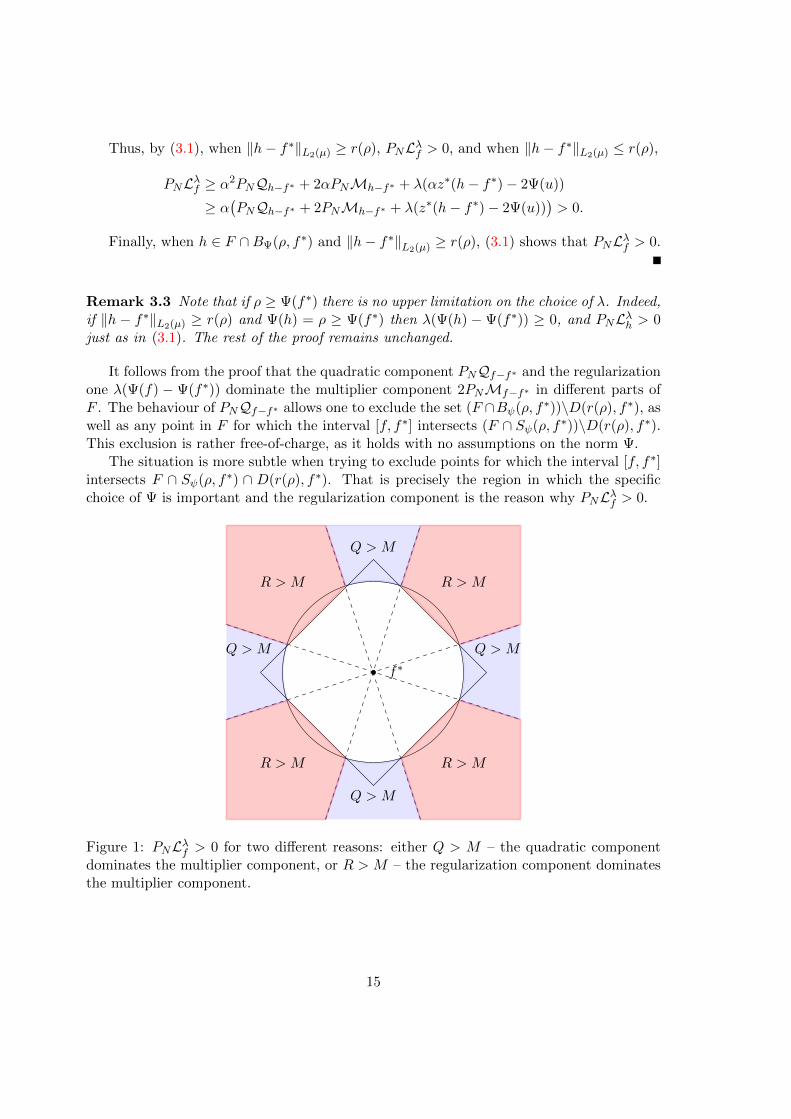
The proof of the theorem follows in three steps: first, one has to show that PNLλf ispositive on the set F ∩ SΨ(ρ, f∗). Second, thanks to certain homogeneity properties of thefunctional, it is positive in F\BΨ(ρ, f∗), because it is positive on the ‘sphere’ F ∩SΨ(ρ, f∗).Finally, one has to study the functional in F ∩ BΨ(ρ, f∗) and verify that it is positive inthat set, provided that ‖f − f∗‖L2(µ) ≥ r(ρ).

13

f∗ SΨ(ρ, f∗)

D(r(ρ), f∗)

f

h

Proof. Fix h ∈ F ∩SΨ(ρ, f∗) and we shall treat two different cases: when ‖h− f∗‖L2(µ) ≥r(ρ) and when ‖h− f∗‖L2(µ) ≤ r(ρ).

If ‖h− f∗‖L2 ≥ r(ρ), then by the triangle inequality for Ψ,

Ψ(h)−Ψ(f∗) = Ψ(h− f∗ + f∗)−Ψ(f∗) ≥ −Ψ(h− f∗).

Hence, for (Xi, Yi)Ni=1 ∈ A and by the upper estimate in the choice of λ,

PNLλh ≥θ

2‖h− f∗‖2L2(µ) − λΨ(h− f∗) ≥ θ

2r2(ρ)− λρ > 0. (3.1)

Next, if ‖h− f∗‖L2(µ) ≤ r(ρ) then

PNLλh ≥ −2O(ρ) + λ(Ψ(h)−Ψ(f∗)).

Consider u, v ∈ E that satisfy f∗ = u + v and Ψ(u) ≤ ρ/20. Let z∗ be any normingfunctional of v; thus, z∗ ∈ SΨ∗ and z∗(v) = Ψ(v). Since Ψ(h) = supx∗∈BΨ∗

x∗(h) it followsthat

Ψ(h)−Ψ(f∗) ≥Ψ(h)−Ψ(v)−Ψ(u) ≥ z∗(h− v)−Ψ(u) ≥ z∗(h− f∗)− 2Ψ(u).

This holds for any v ∈ BΨ(ρ/20, f∗), and by the definition of ∆(ρ) and for an optimal choiceof z∗,

PNLλh ≥ −2O(ρ) + λ(z∗(h− f∗)− 2Ψ(u)) ≥ −2O(ρ) + λ(∆(ρ)− ρ/10) > 0, (3.2)

where the last inequality holds because ∆(ρ) ≥ 4ρ/5 and λ ≥ 3γO(ρ)/ρ. Also, sinceγO(ρ) ≤ (θ/8)r2(ρ), it suffices that λ ≥ (3θ/8)r2(ρ)/ρ to ensure that PNLλh > 0 in (3.2).This completes the proof of the first step – that PNLλh > 0 on F ∩ SΨ(ρ, f∗).

Turning to the second step, one has to establish a similar inequality for functions outsideBΨ(ρ, f∗). To that end, let f ∈ F\BΨ(ρ, f∗). Since F is convex and Ψ is homogeneous,f = f∗ + α(h− f∗) for some h ∈ F ∩ SΨ(ρ, f∗) and α > 1. Therefore,

PNQf−f∗ = α2PNQh−f∗ and PNMf−f∗ = αPNMh−f∗ ;

moreover, Ψ(f − f∗) = αΨ(h− f∗) and for every functional z∗, z∗(f − f∗) = αz∗(h− f∗).

14

Thus, by (3.1), when ‖h− f∗‖L2(µ) ≥ r(ρ), PNLλf > 0, and when ‖h− f∗‖L2(µ) ≤ r(ρ),

PNLλf ≥ α2PNQh−f∗ + 2αPNMh−f∗ + λ(αz∗(h− f∗)− 2Ψ(u))

≥ α(PNQh−f∗ + 2PNMh−f∗ + λ(z∗(h− f∗)− 2Ψ(u))

)> 0.

Finally, when h ∈ F ∩BΨ(ρ, f∗) and ‖h− f∗‖L2(µ) ≥ r(ρ), (3.1) shows that PNLλf > 0.

Remark 3.3 Note that if ρ ≥ Ψ(f∗) there is no upper limitation on the choice of λ. Indeed,if ‖h − f∗‖L2(µ) ≥ r(ρ) and Ψ(h) = ρ ≥ Ψ(f∗) then λ(Ψ(h) − Ψ(f∗)) ≥ 0, and PNLλh > 0just as in (3.1). The rest of the proof remains unchanged.

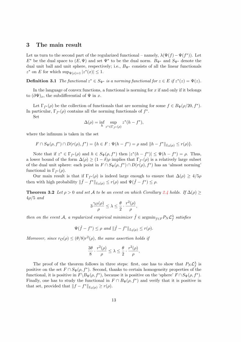
It follows from the proof that the quadratic component PNQf−f∗ and the regularizationone λ(Ψ(f) − Ψ(f∗)) dominate the multiplier component 2PNMf−f∗ in different parts ofF . The behaviour of PNQf−f∗ allows one to exclude the set (F ∩Bψ(ρ, f∗))\D(r(ρ), f∗), aswell as any point in F for which the interval [f, f∗] intersects (F ∩ Sψ(ρ, f∗))\D(r(ρ), f∗).This exclusion is rather free-of-charge, as it holds with no assumptions on the norm Ψ.

The situation is more subtle when trying to exclude points for which the interval [f, f∗]intersects F ∩ Sψ(ρ, f∗) ∩ D(r(ρ), f∗). That is precisely the region in which the specificchoice of Ψ is important and the regularization component is the reason why PNLλf > 0.

f∗

R > MR > M

R > MR > M

Q > M

Q > M Q > M

Q > M

Figure 1: PNLλf > 0 for two different reasons: either Q > M – the quadratic componentdominates the multiplier component, or R > M – the regularization component dominatesthe multiplier component.

15

4 The role of ∆(ρ)

It is clear that ∆(ρ) plays a crucial role in the proof of Theorem 3.2, and that the largerΓf∗(ρ) is, the better the lower bound on ∆(ρ).

Having many norming functionals of points in BΨ(ρ/20, f∗) can be achieved somewhatartificially, by taking ρ ∼ Ψ(f∗). If ρ is large enough, BΨ(ρ/20, f∗) contains a Ψ-ball centredin 0. Therefore, Γf∗(ρ) is the entire dual sphere and ∆(ρ) = ρ. This is the situation whenone attempts to derive complexity-based bounds (see Section 6 and [13]), i.e., when onewishes to find f that inherits some of f∗’s ‘good qualities’ that are captured by Ψ(f∗).

Here, we are interested in cases in which ρ may be significantly smaller than Ψ(f∗) andenough norming functionals have to be generated by other means.

If Ψ is smooth, each f 6= 0 has a unique norming functional, and for a small ρ, thenorming functionals of points in BΨ(ρ/20, f∗) are close to the (unique) norming functionalof f∗; hence there is little hope that Γf∗(ρ) will be large enough to ensure that ∆(ρ) ∼ ρ.It is therefore reasonable to choose Ψ that is not smooth in f∗ or in a neighbourhood of f∗.

Another important fact is that Γf∗(ρ) need not be as large as the entire dual sphere toensure that ∆(ρ) ∼ ρ. Indeed, it suffices if Γf∗(ρ) contains ‘almost norming’ functionalsonly to points that satisfy ‖w‖L2(µ) ≤ r(ρ)/ρ and Ψ(w) = 1, rather than to every point inthe sphere SΨ.

4.1 ∆(ρ) and sparsity

It turns out that the combination of the right notion of sparsity with a wise choice of anorm Ψ ensures that Γf∗(ρ) contains enough ‘almost norming’ functionals precisely for thesubset of the sphere one is interested in.

To give an indication of how this happens, let us show the following:

Lemma 4.1 Let Z ⊂ SΨ∗, W ⊂ SΨ and 0 < η1, η2 < 1. If every w ∈ W can be written asw = w1 + w2, where Ψ(w1) ≤ η1Ψ(w) and supz∗∈Z z

∗(w2) ≥ (1− η2)Ψ(w2), then

infw∈W

supz∗∈Z

z∗(w) ≥ (1− η1)(1− η2)− η1

In particular, if η1, η2 ≤ 1/20 then infw∈W supz∗∈Z z∗(w) ≥ 4/5.

Proof. Let w = w1 +w2 and observe that Ψ(w2) ≥ Ψ(w)−Ψ(w1) ≥ (1− η1)Ψ(w). Thus,for the optimal choice of z∗ ∈ Z,

z∗(w1 + w2) ≥(1− η2)Ψ(w2) + z∗(w1) ≥ (1− η2)Ψ(w2)− η1Ψ(w).

≥((1− η1)(1− η2)− η1

)Ψ(w),

and the claim follows because w ∈ SΨ.

Let E = Rd viewed as a class of linear functionals on Rd. Set µ to be an isotropicmeasure on Rd; thus t ∈ Rd : E

⟨t,X

⟩2 ≤ 1 = Bd2 .

Assume that for t ∈ Rd that is supported on I ⊂ 1, ..., d, the set of its normingfunctionals consists of functionals of the form z∗0 + (1 − η2)u∗ for some fixed z∗0 that is

16

supported on I and any u ∈ BΨ∗ that is supported on Ic (such is the case, for example,when E = `d1).

For every such t, consider w ∈ ρSΨ and set w1 = PIw and w2 = PIcw, the coordinateprojections of w onto span(ei)i∈I and span(ei)i∈Ic , respectively. Hence, there is a functionalz∗ = z∗0 + (1− η2)u∗ that is norming for t and also satisfies

z∗(w2) = (1− η2)u∗(w2) = (1− η2)Ψ(w2).

Therefore, Lemma 4.1 may be applied once Ψ(PIw) ≤ η1Ψ(w).Naturally, such a shrinking phenomenon need not be true for every w ∈ SΨ; fortunately,

it is only required for w ∈ SΨ ∩ (r(ρ)/ρ)D – and we will show that it is indeed the casein the three examples we present. In all three, the combination of sparsity and the rightchoice of the norm helps in establishing a lower bound on ∆(ρ) in two ways: firstly, the setΓt∗(ρ) consists of functionals that are ‘almost norming’ for any x whose support is disjointfrom the support of t∗; and secondly, a coordinate projection ‘shrinks’ the Ψ norm of pointsin ρSΨ ∩ r(ρ)D.

4.2 ∆(ρ) in the three examples

Let us show that in the three examples, the LASSO, SLOPE and trace norm regularization,∆(ρ) ≥ (4/5)ρ for the right choice of ρ, and that choice depends on the degree of sparsityin each case.

In all three examples, we will assume that the underlying measure is isotropic; thus theL2(µ) norm coincides with the natural Euclidean structure: the `d2 norm for the LASSOand SLOPE, and the Hilbert-Schmidt norm for trace-norm regularization.

The LASSO.Observe that if

⟨t∗, ·⟩

is the true minimizer of the functional⟨t, ·⟩→ E(

⟨t,X

⟩− Y )2,

then any function ht =⟨t, ·⟩

for which ‖ht−f∗‖L2 ≤ r(ρ) and Ψ(ht−f∗) = ρ is of the formht =

⟨t, ·⟩

=⟨w + t∗, ·

⟩, where

w ∈ ρS(`d1) ∩ r(ρ)Bd2 .

Recall that the dual norm to ‖ · ‖1 is ‖ · ‖∞, and thus

∆(ρ) = infw∈ρS(`d1)∩r(ρ)Bd2

supz∈Γt∗ (ρ)

⟨z, w

⟩,

where Γt∗(ρ) is the set of all vectors z∗ ∈ Rd that satisfy

‖z∗‖∞ = 1 and z∗(v) = ‖v‖1 for some v, ‖v − t∗‖1 ≤ ρ/20.

Lemma 4.2 There exists an absolute constant c for which the following hold. If t∗ = v+ufor u ∈ (ρ/20)Bd

1 and |supp(v)| ≤ c(ρ/r(ρ))2 then ∆(ρ) ≥ 4ρ/5.

In other words, if t∗ is well approximated with respect to the `d1 norm by some v ∈ Rd thatis s-sparse, and s is small enough relative to the ratio (ρ/r(ρ))2, then ∆(ρ) ≥ (4/5)ρ.

17

Just as noted earlier, we shall use two key properties of the `1 norm and sparse vectors:firstly, that if x and y have disjoint supports, there is a functional that is simultaneouslynorming for x and y, i.e., z∗ ∈ Bd

∞ for which

z∗(x) = ‖x‖1 and z∗(y) = ‖y‖1; (4.1)

secondly, that if ‖x‖1 = ρ and ‖x‖2 is significantly smaller than ρ, a coordinate projection‘shrinks’ the `d1 norm: ‖PIx‖1 is much smaller than ‖x‖1.Proof. Let w ∈ ρS(`d1) ∩ r(ρ)Bd

2 . Since ‖t∗ − v‖1 ≤ ρ/20 there exists z∗ ∈ Γt∗(ρ) that isnorming for v. Moreover, if I = supp(v), then according to (4.1) one can choose z∗ that isalso norming for PIcw. Thus, ‖PIcw‖1 = z∗(PIcw) and

z∗(w) = z∗(PIw) + z∗(PIcw) ≥ ‖PIcw‖1 − ‖PIw‖1 ≥ ‖w‖1 − 2 ‖PIw‖1 .

Since ‖w‖2 ≤ r(ρ), one has ‖PIw‖1 ≤√s ‖PIw‖2 ≤

√sr(ρ). Therefore,⟨

z, w⟩≥ ρ− 2

√sr(ρ) ≥ 4ρ/5

when 100s ≤ (ρ/r(ρ))2.

SLOPE.Let β1 ≥ β2 ≥ ... ≥ βd > 0, and recall that Ψ(t) =

∑di=1 βit

∗i .

Note that Ψ(t) = supz∈Z⟨z, t⟩, for

Z =

d∑i=1

εiβπiei : (εi)di=1 ∈ −1, 1d, π is a permulation of 1, ..., d

.

Therefore, the extreme points of the dual unit ball are of the form∑d

i=1 εiβπiei.Following the argument outlined above, let us show that if x is supported on a reason-

ably small I ⊂ 1, ..., d, the set of norming functionals of x consists of ‘almost norming’functionals for any y that is supported on Ic. Moreover, and just like the `d1 norm, ifΨ(x) = ρ and ‖x‖2 is significantly smaller than ρ, a coordinate projection of x ‘shrinks’ itsΨ norm.

Lemma 4.3 There exists an absolute constant c for which the following holds. Let 1 ≤ s ≤d and set Bs =

∑i≤s βi/

√i. If t∗ is ρ/20 approximated (relative to Ψ) by an s-sparse vector

and if Bs ≤ cρ/r(ρ) then ∆(ρ) ≥ 4ρ/5.

Proof. Let t∗ = u+ v, for v that is supported on at most s coordinates and u ∈ (ρ/20)BΨ.Set I ⊂ 1, ..., d to be the support of v and let z = (zi)

di=1 be a norming functional for v

to be specified later; thus, z ∈ Γt∗(ρ).

18

Given t for which Ψ(t− t∗) = ρ and ‖t− t∗‖2 ≤ r(ρ), one has

z(t− t∗) = z(t− v)− z(u) = z(PIc(t− v)) + z(PI(t− v))− z(u)

≥∑i∈Ic

zi(t− v)i +∑i∈I

zi(t− v)i −Ψ(u)

≥∑i∈Ic

zi(t− v)i −∑i≤s

βi(t− v − u)∗i − 2Ψ(u)

=∑i∈Ic

zi(t− v)i −∑i≤s

βi(t− t∗)∗i − 2Ψ(u) = (∗).

Since v is supported in I, one may optimize the choice of z by selecting the right permutationof the coordinates in Ic, and∑

i∈Iczi(t− v)i ≥

∑i>s

βi(t− v)∗i ≥∑i>s

βi(t− v − u)∗i −Ψ(u)

=

d∑i=1

βi(t− t∗)∗i −∑i≤s

βi(t− t∗)∗i −Ψ(u).

Therefore,

(∗) ≥d∑i=1

βi(t− t∗)∗i − 2∑i≤s

βi(t− t∗)∗i − 3Ψ(u) ≥ 17

20ρ− 2

∑i≤s

βi(t− t∗)∗i .

Since ‖t− t∗‖2 ≤ r(ρ), it is evident that (t− t∗)∗i ≤ r(ρ)/√i, and

s∑i=1

βi(t− t∗)∗i ≤ r(ρ)

s∑i=1

βi√i

= r(ρ)Bs.

Hence, if ρ ≥ 40r(ρ)Bs then ∆(ρ) ≥ 4ρ/5.

Trace-norm regularization.The trace norm has similar properties to the `1 norm. Firstly, one may show that the

dual norm to ‖ · ‖1 is ‖ · ‖∞, which is simply the standard operator norm. Moreover, onemay find a functional that is simultaneously norming for any two elements with ‘disjointsupport’ (and of course, the meaning of ‘disjoint support’ has to be interpreted correctlyhere). Finally, it satisfies a ‘shrinking’ phenomenon for matrices whose Hilbert-Schmidtnorm is significantly smaller than their trace norm.

Lemma 4.4 There exists an absolute constant c for which the following hold. If A∗ =V + U , where ‖U‖1 ≤ ρ/20 and rank(V ) ≤ c(ρ/r(ρ))2, then ∆(ρ) ≥ 4ρ/5.

The fact that a low-rank matrix has many norming functionals is well known and follows,for example, from [38].

19

Lemma 4.5 Let V ∈ Rm×T and assume that V = PIV PJ for appropriate orthogonalprojections onto subspaces I ⊂ Rm and J ⊂ RT . Then, for every W ∈ Rm×T there is amatrix Z that satisfies ‖Z‖∞ = 1, and⟨

Z, V⟩

= ‖V ‖1,⟨Z,PI⊥WPJ⊥

⟩= ‖PI⊥WPJ⊥‖1,⟨

Z,PIWPJ⊥⟩

= 0 and⟨Z,PI⊥WPJ

⟩= 0.

Lemma 4.5 describes a similar phenomenon to the situation in `d1, but with a different notionof ‘disjoint support’: if V is low-rank and the projections PI and PJ are non-trivial, onemay find a functional that is norming both for V and for the part of W that is ‘disjoint’ ofV . Moreover, the functional vanishes on the ‘mixed’ parts PIWPJ⊥ and PI⊥WPJ .

Proof of Lemma 4.4. Recall that S1 is the unit sphere of the trace norm and that B2 isthe unit ball of the Hilbert-Schmidt norm. Hence,

∆(ρ) = infW∈ρS1∩r(ρ)B2

supZ∈ΓA∗ (ρ)

⟨Z,W

⟩where ΓA∗(ρ) is the set of all matrices Z ∈ Rm×T that satisfy ‖Z‖∞ = 1 and

⟨Z, V

⟩= 1

for some V for which ‖A∗ − V ‖1 ≤ ρ/20.Fix a rank-s matrix V = PIV PJ , for orthogonal projections PI and PJ that are onto

subspaces of dimension s. Consider W ∈ Rm×T for which ‖W‖1 = ρ and ‖W‖2 ≤ r(ρ) andput Z to be a norming functional of V as in Lemma 4.5. Thus, Z ∈ ΓA∗(ρ) and⟨

Z,W⟩

=⟨Z,PI⊥WPJ⊥

⟩+⟨Z,PIWPJ

⟩= ‖PI⊥WPJ⊥‖1 − ‖PIWPJ‖1

≥‖W‖1 − ‖PIWPJ⊥‖1 − ‖PI⊥WPJ‖1 − 2‖PIWPJ‖1.

All that remains is to estimate the trace norms of the three components that are believedto be ‘low-dimension’ - in the sense that their rank is at most s.

Recall that (σi(A)) are the singular values of A arranged in a non-increasing order.It is straightforward to verify (e.g., using the characterization of the singular values vialow-dimensional approximation), that

σi(PIWPJ⊥), σi(PI⊥WPJ), σi(PIWPJ) ≤ σi(W ).

Moreover, ‖W‖2 ≤ r(ρ), therefore, being rank-s operators, one has

‖PIWPJ⊥‖1, ‖PI⊥WPJ‖1, ‖PIWPJ‖1 ≤s∑i=1

σi(W ) ≤√s( s∑i=1

σ2i (W )

)1/2≤√sr(ρ),

implying that ⟨Z,W

⟩≥ ρ− 4r(ρ)

√s.

Therefore, if 400s ≤ (r/r(ρ))2, then ∆(ρ) ≥ 4ρ/5.

20

5 The three examples revisited

The estimates on ∆(ρ) presented above show that in all three examples, when f∗ is wellapproximated by a function whose ‘degree of sparsity’ is . (ρ/r(ρ))2, then ∆(ρ) ≥ 4ρ/5and Theorem 3.2 may be used. Clearly, the resulting error rates depend on the right choiceof ρ, and thus on r(ρ).

Because r(ρ) happens to be the minimax rate of the learning problem in the classF ∩ BΨ(ρ, f∗), its properties have been studied extensively. Obtaining an estimate of r(ρ)involves some assumptions on X and ξ, and the one setup in which it can be characterizedfor an arbitrary class F is when the class is L-subgaussian and ξ ∈ Lq for some q > 2 (thoughξ need not be independent of X). It is straightforward to verify that an L-subgaussian classsatisfies the small-ball condition of Assumption 2.1 for κ = 1/2 and ε = c/L4 where cis an absolute constant. Moreover, if the class is L-subgaussian, the natural complexityparameter associated with it is the expectation of the supremum of the canonical gaussianprocess indexed by the class.

Definition 5.1 Let F ⊂ L2(µ) and set Gf : f ∈ F to be the canonical gaussian processindexed by F ; that is, each Gf is a centred gaussian variable and the covariance structureof the process is endowed by the inner product in L2(µ). The expectation of the supremumof the process is defined by

`∗(F ) = supE supf∈F ′

Gf : F ′ ⊂ F is finite.

It follows from a standard chaining argument that if F is L-subgaussian then

E supf∈F

∣∣∣ 1

N

N∑i=1

εi(h− f∗)(Xi)∣∣∣ . L

`∗(F )√N

.

Therefore, ifFρ,r = F ∩BΨ(ρ, f∗) ∩D(r, f∗)

then for every ρ > 0 and f∗ ∈ F

rQ(ρ) ≤ infr > 0 : `∗(Fρ,r) ≤ C(L)r

√N.

Turning to rM , we shall require the following fact from [20].

Theorem 5.2 ([20]) Let q > 2 and L ≥ 1. For every 0 < δ < 1 there is a constantc = c(δ, L, q) for which the following holds. If H is an L-subgaussian class and ξ ∈ Lq, thenwith probability at least 1− δ,

suph∈H

∣∣∣∣∣ 1√N

N∑i=1

εiξih(Xi)

∣∣∣∣∣ ≤ c‖ξ‖Lq`∗(H).

21

The complete version of Theorem 5.2 includes a sharp estimate on the constant c. However,obtaining accurate probability estimates is not the main feature of this note and derivingsuch estimates leads to a cumbersome presentation. To keep our message to the point, wehave chosen not to present the best possible probability estimates in what follows.

A straightforward application of Theorem 5.2 shows that

rM (ρ) ≤ infr > 0 : ‖ξ‖Lq `∗(Fρ,r) ≤ cr

2√N

for a constant c that depends on L, q and δ.

Recall that we have assumed that X is isotropic, which means that the L2(µ) normcoincides with the natural Euclidean structure on the space: the standard `d2 norm for theLASSO and SLOPE and the Hilbert-Schmidt norm for trace norm regularization. Since thecovariance structure of the indexing gaussian process is endowed by the inner product, itfollows that

`∗(ρBΨ ∩ rD) = E supw∈ρBΨ∩rB2

⟨G,w

⟩for the standard gaussian vector G = (g1, ..., gd) in the case of the LASSO and SLOPE andthe gaussian matrix G = (gij) in the case of trace norm minimization. Hence, one mayobtain a bound on r(ρ) by estimating this expectation in each case.

The LASSO and SLOPE. Let (βi)di=1 be a non-increasing positive sequence and set

Ψ(t) =∑d

i=1 t∗iβi.

Since the LASSO corresponds to the choice of (βi)di=1 = (1, ..., 1), it suffices to identify

`∗(ρBΨ ∩ rBd2) for the SLOPE norm and a general choice of weights.

Lemma 5.3 There exists an absolute constant C for which the following holds. If β andΨ are as above, then

E supw∈ρBΨ∩rBd2

⟨G,w

⟩≤ C min

k

r

√(k − 1) log

( ed

k − 1

)+ ρmax

i≥k

√log(ed/i)

βi

(and if k = 1, the first term is set to be 0).

Proof. Fix 1 ≤ k ≤ d. Let J be the set of indices of the k largest coordinates of (|gi|)di=1,and for every w let Iw be the sets of indices of the k largest coordinates of (|wi|)di=1. PutJw = J ∪ Iw and note that |Jw| ≤ 2k. Hence,

supw∈ρBΨ∩rBd2

d∑i=1

wigi ≤ supw∈rBd2

∑i∈Jw

wigi + supw∈ρBΨ

∑i∈Jcw

wigi

. r

(∑i<k

(g∗i )2

)1/2

+ supw∈ρBΨ

∑i≥k

w∗i βig∗iβi

. r

(∑i<k

(g∗i )2

)1/2

+ ρmaxi≥k

g∗iβi.

22

As a starting point, note that a standard binomial estimate shows that

Pr(g∗i ≥ t

√log(ed/i)

)≤(d

i

)Pri

(|g| ≥ t

√log(ed/i)

)≤2 exp(i log(ed/i)− i log(ed/i) · t2/2).

Applying the union bound one has that for t ≥ 4, with probability at least 1−2 exp(−(t2/2)k log(ed/k)),

g∗i ≤ c3t√

log(ed/i) for every i ≥ k. (5.1)

The same argument shows that E(g∗i )2 . log(ed/i).

Let Uk be the set of vectors on the Euclidean sphere that are supported on at most kcoordinates. Set

‖x‖[k] =(∑i≤k

(x∗i )2)1/2

= supu∈Uk

⟨x, u

⟩and recall that by the gaussian concentration of measure theorem (see, e.g., Theorem 7.1in [14]), (

E‖G‖q[k]

)1/q≤ E‖G‖[k] + c

√q supu∈Uk

‖⟨G, u

⟩‖L2 ≤ E‖G‖[k] + c1

√q.

Moreover, since E(g∗i )2 . log(ed/i), one has

E‖G‖[k] ≤(E∑i≤k

(g∗i )2)1/2

.√k log(ed/k).

Therefore, by Chebyshev’s inequality for q ∼ k log(ed/k), for t ≥ 1, with probability atleast 1− 2t−c1k log(ed/k), (∑

i≤k(g∗i )

2)1/2

≤ c2t√k log(ed/k).

Turning to the ‘small coordinates’, by (5.1),

maxi≥k

g∗iβi

. tmaxi≥k

√log(ed/i)

βi.

It follows that for every choice of 1 ≤ k ≤ d,

E supw∈ρBΨ∩rBd2

⟨G,w

⟩. rE

(∑i<k

(g∗i )2)1/2

+ ρEmaxi≥k

g∗iβi

.r√

(k − 1) log(ed/(k − 1)) + ρmaxi≥k

√log(ed/i)

βi,

and, if k = 1, the first term is set to be 0.

23

If β = (1, ..., 1) (which corresponds to the LASSO), then BΨ = Bd1 , and one may select√

k ∼ ρ/r, provided that r ≤ ρ ≤ r√d. In that case,

E supw∈ρBd1∩rBd2

⟨G,w

⟩. ρ√

log(edr2/ρ2).

The estimates when r ≥ ρ or r√d ≤ ρ are straightforward. Indeed, if r ≥ ρ then ρBd

1 ⊂ rBd2

and`∗(ρB

d1 ∩ rBd

2) = `∗(ρBd1) ∼ ρ

√log(ed),

while if r√d ≤ ρ then rBd

2 ⊂ ρBd1 , and

`∗(ρBd1 ∩ rBd

2) = `∗(rBd2) ∼ r

√d.

The LASSO.A straightforward computation shows that

r2M (ρ) .L,q,δ

‖ξ‖2LqdN if ρ2N &L,q,δ ‖ξ‖2Lq d

2

ρ ‖ξ‖Lq

√1N log

(e‖ξ‖Lqdρ√N

)otherwise,

and

r2Q(ρ) .L

0 if N &L d

ρ2

N log(c(L)dN

)otherwise.

Proof of Theorem 1.3. We will actually prove a slightly stronger result, which gives animproved estimation error if one has prior information on the degree of sparsity.

Using the estimates on rM and rQ, it is straightforward to verify that the sparsitycondition of Lemma 4.2 holds when N &L,q,δ s log(ed/s) and for any

ρ &L,q,δ ‖ξ‖Lqs√

1

Nlog(eds

).

It follows from Lemma 4.2 that if there is an s-sparse vector that belongs to t∗+ (ρ/20)Bd1 ,

then ∆(ρ) ≥ 4ρ/5. Finally, Theorem 3.2 yields the stated bounds on ‖t− t∗‖1 and ‖t− t∗‖2once we set

λ ∼ r2(ρ)

ρ∼L,q,δ ‖ξ‖Lq

√1

Nlog(eds

).

The estimates on ‖t− t∗‖p for 1 ≤ p ≤ 2 can be easily verified because

‖x‖p ≤ ‖x‖−1+2/p1 ‖x‖2−2/p

2 .

In case one has no prior information on s, one may take

ρ ∼L,q,δ ‖ξ‖Lqs√

1

Nlog(ed)

and

λ ∼L,q,δ ‖ξ‖Lq

√log(ed)

N.

The rest of the argument remains unchanged.

24

SLOPEAssume that βi ≤ C

√log(ed/i), which is the standard assumption for SLOPE [4, 32].

By considering the cases k = 1 and k = d,

E supw∈ρBΨ∩rBd2

⟨G,w

⟩. minCρ,

√dr.

Thus, one may show that

r2Q(ρ) .L

0 if N &L d

ρ2

N otherwise,

and r2M (ρ) .L,q,δ

‖ξ‖2Lq

dN if ρ2N &L,q,δ ‖ξ‖2Lqd

2

‖ξ‖Lqρ√N

otherwise.

Proof of Theorem 1.5. Recall that Bs =∑

i≤s βi/√i, and when βi ≤ C

√log(ed/i), one

may verify thatBs . C

√s log(ed/s).

Hence, the condition Bs . ρ/r(ρ) holds when N &L,q,δ s log(ed/s) and

ρ &L,q,δ ‖ξ‖Lqs√N

log(eds

).

It follows from Lemma 4.3 that ∆(ρ) ≥ 4ρ/5 when there is an s-sparse vector in t∗ +(ρ/20)BΨ; therefore, one may apply Theorem 3.2 for the choice of

λ ∼ r2(ρ)

ρ∼L,q,δ

‖ξ‖Lq√N

.

The trace-norm.Recall that B1 is the unit ball of the trace norm, that B2 is the unit ball of the Hilbert-

Schmidt norm, and that the canonical gaussian vector here is the gaussian matrix G = (gij).Since the operator norm is the dual to the trace norm,

`∗(B1) = Eσ1(G) .√

maxm,T,

and clearly,`∗(B2) = E ‖G‖2 .

√mT.

Thus,

`∗(ρBΨ ∩ rB2) = `∗(ρB1 ∩ rB2) ≤ minρ`∗(B1), r`∗(B2)

. minρ

√maxm,T, r

√mT.

Therefore,

r2Q(ρ) .L

0 if N &L mT

ρ2 maxm,TN otherwise,

25

and

r2M (ρ) .L,q,δ

‖ξ‖2Lq

mTN if ρ2N &L,q,δ ‖ξ‖2Lq(mT )(minm,T)2

ρ‖ξ‖Lq√

maxm,TN otherwise.

Proof of Theorem 1.6. It is straightforward to verify that if N &L,q,δ smaxm,T thens . (ρ/r(ρ))2 when

ρ &L,q,δ ‖ξ‖Lqs√

maxm,TN

as required in Lemma 4.4. Moreover, if there is some V ∈ Rm×T for which ‖V −A∗‖1 . ρand rank(V ) ≤ s, it follows that ∆(ρ) ≥ 4ρ/5. Setting

λ ∼ r2(ρ∗)

ρ∗∼L,q,δ ‖ξ‖Lq

√maxm,T

N,

Theorem 3.2 yields the bounds on ‖A−A∗‖1 and ‖A−A∗‖2. The bounds on the Schatten

norms ‖A−A∗‖p for 1 ≤ p ≤ 2 hold because ‖A‖p ≤ ‖A‖−1+2/p1 ‖A‖2−2/p

2 .

6 Concluding Remarks

As noted earlier, the method we present may be implemented in classical regularizationproblems as well, leading to an error rate that depends on Ψ(f∗) – by applying the trivialbound on ∆(ρ) when ρ ∼ Ψ(f∗).

The key issue in classical regularization schemes is the price that one has to pay for notknowing Ψ(f∗) in advance. Indeed, given information on Ψ(f∗), one may use a learningprocedure taking values in f ∈ F : Ψ(f) ≤ Ψ(f∗) such as Empirical Risk Minimization.This approach would result in an error rate of r(cΨ(f∗)), and the hope is that the errorrate of the regularized procedure is close that – without having prior knowledge on Ψ(f∗).Surprisingly, as we will show in [13], that is indeed the case.

The problem with applying Theorem 3.2 to the classical setup is the choice of λ. One hasno information on Ψ(f∗), and thus setting λ ∼ r2(ρ)/ρ for ρ ∼ Ψ(f∗) is clearly impossible.

A first attempt of bypassing this obstacle is Remark 3.3: if ρ & Ψ(f∗), there is no upper

constraint on the choice of λ. Thus, one may consider λ ∼ supρ>0r2(ρ)ρ , which suites any

ρ > 0. Unfortunately, that choice will not do, because in many important examples thesupremum happens to be infinite. Instead, one may opt for the lower constraint on λ andselect

λ ∼ supρ>0

γO(ρ)

ρ, (6.1)

which is also a legitimate choice for any ρ, and is always finite.We will show in [13] that the choice in (6.1) leads to optimal bounds in many interesting

examples – thanks to the first part of Theorem 3.2.

26

An essential component in the analysis of regularization problems is bounding r(ρ),and we only considered the subgaussian case and completely ignored the question of theprobability estimate. In that sense, the method we presented falls short of being completelysatisfactory.

Addressing both these issues requires sharp upper estimates on empirical and multiplierprocesses, preferably in terms of some natural geometric feature of the underlying class.Unfortunately, this is a notoriously difficult problem. Indeed, the final component in thechaining-based analysis used to study empirical and multiplier processes is to translatea metric complexity parameter (e.g., Talagrand’s γ-functionals) to a geometric one (forexample, the mean-width of the set). Such estimates are known almost exclusively in thesubgaussian case – which is, in a nutshell, Talagrand’s Majorizing Measures theory [33].

The chaining process in [20] is based on a more sensitive metric parameter than thestandard subgaussian one. This leads to satisfactory results for other choices of randomvectors that are not necessarily subgaussian, for example, unconditional log-concave. Still,it is far from a complete theory – as a general version of the Majorizing Measures Theoremis not known.

Another relevant fact is from [26]. It turns out that if V is a class of linear functionalson Rd that satisfies a relatively minor symmetry property, and X is an isotropic and sub-gaussian vector for which

supt∈Sd−1

‖⟨X, t

⟩‖Lp ≤ L

√p for 2 ≤ p . log d, (6.2)

then the empirical and multiplier processes indexed by V behave as if X were a subgaussianvector. In other words, it suffices to have a subgaussian moment growth up to p ∼ log d toensure a subgaussian behaviour.

This fact is useful because all the indexing sets considered here (and in many othersparsity-based regularization procedures as well) satisfy the required symmetry property.

Finally, a word about the probability estimate in Theorem 5.2. The actual result from[20] leads to a probability estimate governed by two factors: the Lq space to which ξ belongsand the ‘effective dimension’ of the class. For a class of linear functionals on Rd and anisotropic vector X, this effective dimension is

D(V ) =

(`∗(V )

d2(V )

)2

,

where `∗(V ) = E supv∈V |⟨G, v

⟩| and d2(V ) = supv∈V ‖v‖`d2 .

One may show that with probability at least

1− c1w−qN−((q/2)−1) logqN − 2 exp(−c2u

2D(V )),

supv∈V

∣∣∣∣∣ 1√N

N∑i=1

(ξi⟨V,Xi

⟩− Eξ

⟨X, v

⟩)∣∣∣∣∣ . Lwu‖ξ‖Lq`∗(V ). (6.3)

If ξ has better tail behaviour, the probability estimate improves; for example, if ξ is sub-gaussian then (6.3) holds with probability at least 1− 2 exp(−cw2N)− 2 exp(−cu2D(V )).

27

The obvious complication is that one has to obtain a lower bound on the effective di-mension D(V ). And while it is clear that D(v) & 1, in many cases (including our threeexamples) a much better bound is true.

Let us mention that the effective dimension is perhaps the most important parameter inAsymptotic Geometric Analysis. Milman’s version of Dvoretzky’s Theorem (see, e.g., [1])shows that D(V ) captures the largest dimension of a Euclidean structure hiding in V . Infact, this geometric observation exhibits why that part of the probability estimate in (6.3)cannot be improved.

References

[1] Shiri Artstein-Avidan, Apostolos Giannopoulos, and Vitali D. Milman. Asymptotic geometric analy-sis. Part I, volume 202 of Mathematical Surveys and Monographs. American Mathematical Society,Providence, RI, 2015.

[2] Francis R. Bach. Structured sparsity-inducing norms through submodular functions. In Advances inNeural Information Processing Systems 23: 24th Annual Conference on Neural Information ProcessingSystems 2010. Proceedings of a meeting held 6-9 December 2010, Vancouver, British Columbia, Canada.,pages 118–126, 2010.

[3] Peter J. Bickel, Ya’acov Ritov, and Alexandre B. Tsybakov. Simultaneous analysis of lasso and Dantzigselector. Ann. Statist., 37(4):1705–1732, 2009.

[4] Ma lgorzata Bogdan, Ewout van den Berg, Chiara Sabatti, Weijie Su, and Emmanuel J. Candes.SLOPE—Adaptive variable selection via convex optimization. Ann. Appl. Stat., 9(3):1103–1140, 2015.

[5] Peter Buhlmann and Sara van de Geer. Statistics for high-dimensional data. Springer Series in Statistics.Springer, Heidelberg, 2011. Methods, theory and applications.

[6] Emmanuel J. Candes and Yaniv Plan. Tight oracle inequalities for low-rank matrix recovery from aminimal number of noisy random measurements. IEEE Trans. Inform. Theory, 57(4):2342–2359, 2011.

[7] David Gross. Recovering low-rank matrices from few coefficients in any basis. IEEE Trans. Inform.Theory, 57(3):1548–1566, 2011.

[8] Vladimir Koltchinskii. Oracle inequalities in empirical risk minimization and sparse recovery problems,volume 2033 of Lecture Notes in Mathematics. Springer, Heidelberg, 2011. Lectures from the 38thProbability Summer School held in Saint-Flour, 2008, Ecole d’Ete de Probabilites de Saint-Flour.[Saint-Flour Probability Summer School].

[9] Vladimir Koltchinskii, Karim Lounici, and Alexandre B. Tsybakov. Nuclear-norm penalization andoptimal rates for noisy low-rank matrix completion. Ann. Statist., 39(5):2302–2329, 2011.

[10] Vladimir Koltchinskii and Shahar Mendelson. Bounding the Smallest Singular Value of a RandomMatrix Without Concentration. Int. Math. Res. Not. IMRN, (23):12991–13008, 2015.

[11] Guillaume Lecue and Shahar Mendelson. Learning subgaussian classes: Upper and minimax bounds.Technical report, CNRS, Ecole polytechnique and Technion, 2013.

[12] Guillaume Lecue and Shahar Mendelson. Sparse recovery under weak moment assumptions. Techni-cal report, CNRS, Ecole Polytechnique and Technion, 2014. To appear in Journal of the EuropeanMathematical Society.

[13] Guillaume Lecue and Shahar Mendelson. Regularization and the small-ball method ii: complexity-basedbounds. Technical report, CNRS, ENSAE and Technion, I.I.T., 2015.

[14] Michel Ledoux. The concentration of measure phenomenon, volume 89 of Mathematical Surveys andMonographs. American Mathematical Society, Providence, RI, 2001.

[15] Karim Lounici. Sup-norm convergence rate and sign concentration property of Lasso and Dantzigestimators. Electron. J. Stat., 2:90–102, 2008.

[16] Nicolai Meinshausen. Hierarchical testing of variable importance. Biometrika, 95(2):265–278, 2008.

28

[17] Nicolai Meinshausen and Peter Buhlmann. High-dimensional graphs and variable selection with thelasso. Ann. Statist., 34(3):1436–1462, 2006.

[18] Nicolai Meinshausen, Lukas Meier, and Peter Buhlmann. p-values for high-dimensional regression. J.Amer. Statist. Assoc., 104(488):1671–1681, 2009.

[19] Nicolai Meinshausen and Bin Yu. Lasso-type recovery of sparse representations for high-dimensionaldata. Ann. Statist., 37(1):246–270, 2009.

[20] Shahar Mendelson. Upper bounds on product and multiplier empirical processes. Technical report. Toappear in Stochastic Processes and their Applications.

[21] Shahar Mendelson. Learning without concentration for general loss function. Technical report, Tech-nion, I.I.T., 2013. arXiv:1410.3192.

[22] Shahar Mendelson. Learning without concentration. In Proceedings of the 27th annual conference onLearning Theory COLT14, pages pp 25–39. 2014.

[23] Shahar Mendelson. A remark on the diameter of random sections of convex bodies. In Geometricaspects of functional analysis, volume 2116 of Lecture Notes in Math., pages 395–404. Springer, Cham,2014.

[24] Shahar Mendelson. Learning without concentration. J. ACM, 62(3):Art. 21, 25, 2015.

[25] Shahar Mendelson. ’local vs. global parameters’, breaking the gaussian compexity barrier. Technicalreport, Technion, I.I.T., 2015.

[26] Shahar Mendelson. On multiplier processes under weak moment assumptions. Technical report, Tech-nion, I.I.T., 2015.

[27] Sahand Negahban and Martin J. Wainwright. Restricted strong convexity and weighted matrix com-pletion: optimal bounds with noise. J. Mach. Learn. Res., 13:1665–1697, 2012.

[28] Sahand N. Negahban, Pradeep Ravikumar, Martin J. Wainwright, and Bin Yu. A unified framework forhigh-dimensional analysis of M -estimators with decomposable regularizers. Statist. Sci., 27(4):538–557,2012.

[29] Benjamin Recht, Maryam Fazel, and Pablo A. Parrilo. Guaranteed minimum-rank solutions of linearmatrix equations via nuclear norm minimization. SIAM Rev., 52(3):471–501, 2010.

[30] Angelika Rohde and Alexandre B. Tsybakov. Estimation of high-dimensional low-rank matrices. Ann.Statist., 39(2):887–930, 2011.

[31] Mark Rudelson and Roman Vershynin. Small ball probabilities for linear images of high dimensionaldistributions. Technical report, University of Michigan, 2014. International Mathematics ResearchNotices, to appear. [arXiv:1402.4492].

[32] W. Su and E. J. Candes. Slope is adaptive to unknown sparsity and asymptotically minimax. Technicalreport, Stanford University, 2015. To appear in The Annals of Statistics.

[33] Michel Talagrand. Upper and lower bounds for stochastic processes, volume 60 of Ergebnisse derMathematik und ihrer Grenzgebiete. 3. Folge. A Series of Modern Surveys in Mathematics [Resultsin Mathematics and Related Areas. 3rd Series. A Series of Modern Surveys in Mathematics]. Springer,Heidelberg, 2014. Modern methods and classical problems.

[34] Robert Tibshirani. Regression shrinkage and selection via the lasso. J. Roy. Statist. Soc. Ser. B,58(1):267–288, 1996.

[35] Sara van de Geer. Weakly decomposable regularization penalties and structured sparsity. Scand. J.Stat., 41(1):72–86, 2014.

[36] Sara A. van de Geer. The deterministic lasso. Technical report, ETH Zurich, 2007.http://www.stat.math.ethz.ch/ geer/lasso.pdf.

[37] Sara A. van de Geer. High-dimensional generalized linear models and the lasso. Ann. Statist., 36(2):614–645, 2008.

[38] G. A. Watson. Characterization of the subdifferential of some matrix norms. Linear Algebra Appl.,170:33–45, 1992.

[39] Peng Zhao and Bin Yu. On model selection consistency of Lasso. J. Mach. Learn. Res., 7:2541–2563,2006.

29