Departamento de MatemáticasFacultad de CienciasUniversidad de Chile

26 September 2012, Santiago, Chile

Regularity and Qualitative Propertiesfor Solutions of Some Evolution

Equations

Author : Juan Carlos Pozo Vera

Advisor 1 : Verónica Poblete Oviedo

Advisor 2 : Carlos Lizama Yañez

Thesis Submitted to the Department of Mathematics of Universidad de Chile in

partial fulfillment of requirements for the degree of Doctor of Mathematic

Author’s e-mail: jpozo@ug.uchile.cl

Contents

Agradecimientos i

Abstract ii

Resumen iii

Introduction iv

1 Preliminaries 11.1 Families M–bounded and n–regular sequences . . . . . . . . . . . . . . . . 11.2 Vector–valued Besov and Triebel–Lizorkin spaces . . . . . . . . . . . . . . . 21.3 Operator–valued Fourier multipliers . . . . . . . . . . . . . . . . . . . . . . . 41.4 Lp –maximal regularity of evolution equations . . . . . . . . . . . . . . . . . 51.5 Measure of Non–compactness . . . . . . . . . . . . . . . . . . . . . . . . . . 8

2 Mild Solution of a Non–local Integro–Differential Equation 102.1 Main Results . . . . . . . . . . . . . . . . . . . . . . . . . . . . . . . . . . . . . 112.2 An Example . . . . . . . . . . . . . . . . . . . . . . . . . . . . . . . . . . . . . 19

3 Mild solutions for a Non–local Second Order Non–autonomous Problem 223.1 Main Results . . . . . . . . . . . . . . . . . . . . . . . . . . . . . . . . . . . . . 253.2 Examples . . . . . . . . . . . . . . . . . . . . . . . . . . . . . . . . . . . . . . . 32

4 Periodic Solutions of a Third–Order Differential Equation 354.1 Lebesgue Periodic Solutions. . . . . . . . . . . . . . . . . . . . . . . . . . . . 364.2 Besov Periodic Solutions . . . . . . . . . . . . . . . . . . . . . . . . . . . . . . 424.3 Triebel–Lizorkin Periodic Solutions. . . . . . . . . . . . . . . . . . . . . . . . 444.4 Examples. . . . . . . . . . . . . . . . . . . . . . . . . . . . . . . . . . . . . . . 47

1

5 Periodic Solutions of a Fractional Neutral Equation 515.1 Periodic Strong B s

p,q –solution. . . . . . . . . . . . . . . . . . . . . . . . . . . 545.2 Periodic Strong B s

p,q –solutions of a Neutral Fractional Differential Equa-tion with Finite Delay . . . . . . . . . . . . . . . . . . . . . . . . . . . . . . . . 62

5.3 Periodic Strong F sp,q –solution. . . . . . . . . . . . . . . . . . . . . . . . . . . 64

5.4 Periodic Strong F sp,q –solutions of a Neutral Fractional Differential Equa-

tion with Finite Delay . . . . . . . . . . . . . . . . . . . . . . . . . . . . . . . . 685.5 Examples. . . . . . . . . . . . . . . . . . . . . . . . . . . . . . . . . . . . . . . 69

Bibliography 81

2

Agradecimientos

Quiero expresar mi más sincera gratitud a todas aquellas personas que de una u otramanera influyeron en la redacción y realización de esta tesis.

En primer lugar, quiero agradecer a MECESUP, en particular al proyecto PUC 0711,por financiar mis estudios durante mi permanencia en el programa de doctorado deMatemáticas, sin este apoyo hubiese sido bastante difícil concluir.

Además, agradezco a la doctora Verónica Poblete, quien no sólo me introdujo en eltema de Ecuaciones de Evolución y aceptó ser mi tutora de tesis, sino que además tuvola generosidad de compartir sus conocimientos y opiniones en varias horas de charlay discusiones. Además me incentivó a realizar varias estadías en el extranjero paraampliar mis horizontes y mis contactos matemáticos.

Agradezco los doctores Carlos Lizama y Hernán Henríquez, por todos los valiosos co-mentarios e importantes sugerencias que hicieron al momento de trabajar con ellos.

Deseo agradecer a todo el personal, tanto académico como administrativo, del Depar-tamento de Matemática de la Facultad de Ciencias de la Universidad de Chile, por en-tregarme todas las herramientas necesarias para afrontar de buena manera un trabajode investigación como lo es una tesis doctoral.

Por último, pero no menos importante quiero agradecer profundamente a mi familia,y hermano, a quienes durante todo este tiempo los he sentido junto a mi apoyándome,ya sea estando a unos pocos metros o a miles de kilómetros de distancia. Y, con todomi corazón, a mi amor Sofía, a quien le debo el haber tenido que soportarme todo estetiempo con infinita paciencia.

i

Abstract

The main objective of this doctoral thesis is the study of existence and uniqueness, aswell as qualitative properties of solutions for evolution equations defined in abstractBanach spaces.

Concerning to evolution equations, one of main subject of study is the study of exis-tence of solutions. For this reason, we find sufficient conditions that guarantee exis-tence of mild solutions for some evolution equations. Specifically, we study conditionswhich guarantee existence of mild solutions for an integro–differential equation withnon–local initial conditions and a non–autonomous second order differential equationwith non–local initial conditions. Our approach is based on resolvent operator theory.

On th other hand, it is well known that concerning to evolution equations, another im-portant subject of interest is the study of qualitative properties of their solutions. Moti-vated by this, we study existence and uniqueness of periodic strong solutions for someinteresting evolution equations having maximal regularity property. Specifically, westudy maximal regularity property on periodic Lebesgue, Besov and Triebel–Lizorkinspaces for a third–order differential equation and a fractional order differential equa-tion with finite delay. In the case of periodic Lebesgue spaces our results involve thenotion of U MD–spaces and the concept of R–boundedness of some families of opera-tors. In the cases of Besov and Triebel–Lizorkin spaces our results only involve bound-edness conditions for some families of operators. Our approach is based on operator–valued Fourier multipliers theorems.

ii

Resumen

El objetivo principal de esta tesis doctoral es el estudio de existencia y unicidad, asícomo también, propiedades cualitativas de soluciones de ecuaciones de evolucióndefinidas en espacios de Banach abstractos.

En relación a una ecuación de evolución, uno de los principales temas de estudio esla existencia de soluciones. Por este motivo, nosotros encontramos condiciones sufi-cientes que garantizan existencia de soluciones mild para algunas ecuaciones de evolu-ción. Específicamente, estudiamos condiciones que aseguran existencia de solucionesmild para una ecuación integro–diferencial con condiciones iniciales no locales y unaecuación diferencial de segundo orden no autónoma con condiciones iniciales no lo-cales. Nuestros métodos están basados en la teoría de operador resolvente.

Por otro lado, es un hecho conocido que en relación a una ecuación de evolución otrotópico de interés es el estudio de propiedades cualitativas de sus soluciones. Motiva-dos por esto, estudiamos existencia y unicidad de soluciones periódicas fuertes paraalgunas interesantes ecuaciones de evolución teniendo la propiedad de regularidadmaximal. Específicamente, estudiamos la propiedad de regularidad maximal en espa-cios periódicos de Lebesgue, Besov y Triebel–Lizorkin para una ecuación diferencialde tercer orden y una ecuación diferencial de orden fraccionario con retardo finito.En el caso de espacios periódicos de Lebesgue, nuestros resultados involucran la no-ción de espacios U MD y el concepto de R–acotamiento de algunas familias de oper-adores. En los casos de espacios periódicos de Besov y Triebel–Lizorkin, nuestros resul-tados involucran sólo condiciones de acotamiento de estas familias de operadores. Losmétodos usados están basados en teoremas operador–valuados de multiplicadores deFourier.

iii

Introduction

Because many natural phenomena arising from applied fields can be described by par-tial differential equations and their generalizations, the study of properties of the solu-tions of these equations is a very important and active field of research. In many cases,partial differential equations can be transformed into an ordinary differential equa-tion with values in an infinite dimensional space. This motivates the study of evolutionequations in abstract spaces, especially in Banach spaces.

This thesis is concerned with the study of existence, uniqueness and qualitative prop-erties of solutions for some classes of abstract evolution equations. This work is theoutcome of the author’s research during his Math Ph.D. study at Universidad de Chile(March 2009 – September 2012). The main results obtained in this research work areavailable through the following four articles made in this period

1) C. Lizama, J.C. Pozo, Existence of mild solutions for semilinear integro–differentialequations with non–local conditions. Submitted

2) V. Poblete, J.C. Pozo, Periodic solutions of an abstract third–order differential equa-tion. Submitted

3) V. Poblete, J.C. Pozo, Periodic solutions for a fractional order abstract neutral differ-ential equation with finite delay. Preprint

4) H. R. Henríquez, V.Poblete, J.C. Pozo, Existence of mild–solutions of a non–autonomoussecond order evolution equation with non–local initial conditions. Preprint

iv

Most of the results in the thesis is based on two methods of theory of evolution equa-tions.

1. Theory of resolvent operators and variation of parameters formula.

2. Maximal regularity property and operator–valued Fourier multipliers.

It is well known that concerning to an evolution equation, one of the main subject ofstudy is the existence of a solution. However, there exist several notions of solutionof an evolution equation. Strong solution is the best, but more demanding notion. Aweaker concept of solution is the concept of mild solution. In fact, a strong solution isa mild solution that satisfies additional differentiability properties. Many author proveexistence of strong solutions proving existence of mild solutions and giving smooth-ness conditions in the initial value. Reader can see the works [83, 84, 125, 147] andreferences therein.

The theory of resolvent operator has been subject of increasing interest in past decades,because it is a central issue for the study of mild solutions of evolution equations.The resolvent operator is applied to inhomogeneous equations to derive various vari-ation of parameters formula. In this direction, we refer the works made by de Andradeand Lizama [50], Arjunan, dos Santos and Cuevas [54], Lizama and N’Guérékata [111],Prüss [131,132]. Moreover, there exists several methods for proving existence theoremsfor the resolvent, for example operational calculus in Hilbert spaces, perturbation ar-guments, and Laplace–transform method, (for more information see the works madeby Grimmer and Prüss [69] and Prüss [133, 134]). In Chapters 2 and 3, we study theexistence of mild solutions for two very interesting evolution equations. Our approachis based in resolvent operator theory and variation of parameters formula.

Another important subject of research concerning to evolution equations is the studyof qualitative properties of their solutions. In particular, the problem of existence ofsolutions having a periodicity property has been considered by several authors, thereader can see [13, 77, 79, 80, 114] and references therein. In the same manner, thestudy of regularity properties of solutions for evolution equations has been an activetopic of research in last decades. In particular, maximal regularity property has re-ceived much attention in recent years due to its applications to evolution equations.Indeed, maximal regularity is an important tool in the study of the following problems:

• Existence and uniqueness of solutions of quasi-linear and non-linear partial dif-ferential equations.

• Existence and uniqueness of solutions of Volterra integral equations.

• Existence and uniqueness of solutions of neutral equations.

• Existence and uniqueness of solutions of non-autonomous evolution equations.

v

In these applications, maximal regularity is usually used to reduce, via a fixed-pointargument, a non-linear (respectively a non-autonomous) problem to a linear (respec-tively an autonomous) problem. In some cases, maximal regularity is needed to applyan implicit function theorem. (See [46, p.72]).

Several techniques are used to study the problem of maximal regularity of evolutionequations. One of these is the Fourier multipliers or symbols. There exists an exten-sive literature about vector–valued Fourier theorems and concrete applications. Thereader can see the works made by, Amann [5], Arendt, Batty and Bu [8], Arendt andBu [10, 11, 12], Bu [26], Bu and Fang [27, 28, 29, 30], Bu and Kim [25, 31, 32], Clément,de Pagter, Sukochev and Witvliet [43], Denk, Hieber and Prüss [52], Girardi and Weis[61, 62], Kalton and Lancien [90], Keyantuo and Lizama [93, 94, 95, 96], Lizama [110],Poblete [126, 127] and references therein.

As we have mentioned, this thesis consists in the study of 4 problems, two of them arerelated with guarantee existence of mild solutions for some interesting evolution equa-tions; the other two problems are related with guarantee existence of strong solutionwith periodicity and maximal regularity properties for evolution equations. In whatfollows, we will give a brief description of each Chapter of this thesis.

Chapter 1 contains notation and preliminary results. Furthermore, in this chapter,for reader’s convenience, we have summarized some relevant concepts and Theorems,concerning to general evolution equations.

In Chapter 2, we study the following problem. Find conditions that guarantee exis-tence of a mild solution of the semi–linear integro–differential equation with non–localinitial conditions

u′(t ) = Au(t )+∫ t

0B(t − s)u(s)d s + f (t ,u(t )), t ∈ [0,1]

u(0) = g (u).

(1)

where A : D(A) ⊆ X → X and B(t ) : D(B(t )) ⊆ X → X for t ∈ I = [0,1] are closed linearoperators in a Banach space X . We assume that D(A) ⊆ D(B(t )) for every t ∈ I andf : I ×X → X , g : C (I ; X ) → X are given X –valued functions.

Evolution equations with non–local initial conditions are more realistic to describenatural phenomena than classical initial value problem, because additional informa-tion is taken into account. For this reason, in recent decades there has been a lot ofinterest in this type of problems and applications. For importance of non–local initialconditions in different fields of applied sciences the reader can see [42, 155, 156] andthe references cited therein.

First investigations in this area were made by Byszewski in the papers [36, 37, 38, 39].Thenceforth, many authors have worked in evolution equations with non–local initialconditions, the reader can see [16,57,88,115,121,158] for abstract results and concreteapplications.

vi

The initial–valued problem (1), that is u(0) = u0 for some u0 ∈ X , has been the subjectof many research papers in recent years, because it has many applications in differentfields such as thermodynamics, electrodynamics, continuum mechanics among oth-ers, see [134]. For this reason, the study of non–local initial for equation (1) is a veryinteresting problem.

The main tool that we use is resolvent operator theory. In fact, to achieve our goal weuse a mixed method, combining existence of a family R(t )t∈I called resolvent opera-tor for equation (1), a formula of variation of parameters and a fixed–point argumentused in [158].

We prove existence of mild solution of equation (1), under conditions of compactnessof g and norm continuity of R(t ) for t > 0. Moreover, in the special case B(t ) = b(t )A,where the operator A is defined on a Hilbert space and the kernel b is a scalar map,we are able to give sufficient conditions for existence of mild solutions only in termsof spectral properties of the operator A and regularity properties of the kernel b. Weremark that, this type of spectral conditions is a new feature that has not been observedeven in the special case B ≡ 0. Finally, to prove the feasibility of the abstract results, weconsider an example for a particular choice of b(t ) and A, which is defined by

(Ax)(t , z) =n∑

i , j=1ai j (z)

∂x(t , z)

∂zi∂z j+

n∑i=1

bi (z)x(t , z)

∂zi+ c(z)x(t , z),

where the given coefficients ai j ,b j ,c (i , j = 1,2, . . . ,n) satisfy the usual uniformly ellip-ticity conditions. We remark that the results of this Chapter can be found in the jointwork made by Lizama–Pozo [115]

In Chapter 3, we study the following problem. Find conditions that guarantee exis-tence of a mild solution of second order non–autonomous equation with non–localinitial conditions.

u′′(t ) = A(t )u(t )+ f (t ,u(t )), t ∈ [0, a]u(0) = g (u),

u′(0) = h(u).

(2)

where A(t ) : D(A(t )) ⊆ X → X for t ∈ J = [0, a] denote closed linear operators de-fined in a Banach space X . We assume that D(A(t )) = D for all t ∈ J . The functionf : J × C (J ; X ) → X satisfies Carathéodory type conditions, and the functionsg ,h : C (J ; X ) → X are continuous maps.

The study of second order evolution equations is very interesting problem, becausethis type of equation arises in several natural phenomena. In the autonomous case,this is A(t ) = A for all t , there exists an extensive literature. The existence of solutionsare closely related with the concept of cosine family. For abstract results and concreteapplications we refer the reader to [17, 41, 58, 140, 144] and references therein. In the

vii

non–autonomous case, the study of solutions becomes much more complicated. How-ever, we prove existence of mild– solutions for equation (2) imposing very general con-ditions for the operators A(t ) and the functions f , g and h.

The principal tool which we use is resolvent operator theory. In fact, we prove theexistence of an evolution operator S(t , s)t ,s∈J , and then we derive a variation of pa-rameters formula. Finally, we check the feasibility of our abstract results in the specialcase A(t ) = A +B(t ) where the operator A is the generator of a cosine family and theoperators B(t ) satisfy appropriate conditions.

We remark that the results of this Chapter can be found in the joint work made byHenríquez–Poblete–Pozo [82] .

In Chapter 4, we study the following problem. Find a characterization of maximalregularity for a linear abstract third–order differential equation.

Recent investigations have demonstrated that third order differential equations de-scribe several models arising from very interesting natural phenomena, such as wavepropagation in viscous thermally relaxing fluids, flexible space structure with internaldamping, a thin uniform rectangular panel, like a solar cell array, or a spacecraft withflexible attachments (cf. e.g., [18, 19, 20, 21, 65, 66, 67]).

Motivated by this fact, many authors have worked in abstract third–order differentialequations. In particular, the following equation has been widely studied

αu′′′(t )+u′′(t ) =βAu(t )+γAu′(t )+F (t ,u(t )), for t ∈R+ (3)

where A is a closed linear operator defined on a Banach space X , the function F isa given and X –valued, and α,β,γ ∈ R+. We mention some aspects that equation (3)has been analyzed. In [45], a characterization of solutions for its linear version, i.e.F (t ,u(t )) = f (t ), have been obtained in Hölder spaces C s(R; X ) by Cuevas and Lizama.In the same manner, Fernández, Lizama and Poblete in [59] characterize well-posednessin Lebesgue spaces, Lp (R; X ). In addition, Fernández, Lizama and Poblete, in [60],study regularity of mild and strong solutions defined in R when the underlying spacesare Hilbert spaces and some qualitative properties of their solutions. On the otherhand, existence of bounded mild solutions of the semi-linear equation (3) is studiedby De Andrade and Lizama in [50].

However, the existence of periodic strong solutions of equation (3) has not been ad-dressed in the existing literature. For this reason, Chapter 4 is devoted to study theexistence of periodic strong solutions for the following abstract third–order equation

αu′′′(t )+u′′(t ) =βAu(t )+γBu′(t )+ f (t ), t ∈ [0,2π], (4)

with boundary conditions u(0) = u(2π), u′(0) = u′(2π) and u′′(0) = u′′(2π), where theoperators A and B are closed linear operators defined on a Banach space X satisfying

viii

D(A)∩D(B) 6= 0, the constantsα,β,γ ∈R+, and f belongs to either periodic Lebesguespaces , or periodic Besov spaces, or periodic Triebel–Lizorkin spaces. We remark, thestudy of existence of solutions for equation (4) in the particular case A ≡ B is a mannerto study periodic solutions of equation (3).

Our approach is based in maximal regularity property for evolution equations andoperator–valued Fourier multiplier theorems. In case of periodic Lebesgue spaces, ourresults involve the key notions of U MD–spaces and R–boundedness (see Chapter 1section 1.4 for definition and related results) of the families of operators

kB(iαk3 +k2 + iγkB +βA)−1)

k∈Z and

i k3(iαk3 +k2 + iγkB +βA)−1

k∈Z.

On the other hand, in the case of periodic Besov or Triebel–Lizorkin spaces, our resultsonly involve boundedness condition of the preceding families.

In general, it is not easy to verify the R–boundedness or boundedness condition ofa specific family of operators, especially when two different operators are involved.However, we verify our hypothesis in the special case B = A1/2 where A is a sectorialoperator; the scalar values α,β, and γ related with equation (4) play a crucial role inthis proof.We remark that the results of this Chapter can be found in the joint work made byPoblete–Pozo [129].

In Chapter 5, we study the following problem. Find sufficient conditions that guar-antee the existence of a periodic strong solution for a fractional neutral equation withfinite delay.

The fractional calculus which allows us to consider integration and differentiation ofany order, not necessarily integer, has been the object of extensive study for analyz-ing not only anomalous diffusion on fractals (physical objects of fractional dimen-sion, like some amorphous semiconductors or strongly porous materials; see [6, 118]and references therein), but also fractional phenomena in optimal control (see, e.g.,[119, 130, 137]). As indicated in [68, 117, 137] and the related references given there, theadvantages of fractional derivatives become apparent in modelling mechanical andelectrical properties of real materials, as well as in the description of rheological prop-erties of rocks, and in many other fields. One of the emerging branches of the study isthe Cauchy problems of abstract differential equations involving fractional derivativesin time. In recent decades there has been a lot of interest in this type of problems, itsapplications and various generalizations (cf. e.g., [1,3,44,85] and references therein). Itis significant to study this class of problems, because, in this way, one is more realisticto describe the memory and hereditary properties of various materials and processes(cf. [86, 100, 119, 130]).

In the same manner, several systems of great interest in science and engineering aremodeled by partial neutral functional differential equations. The reader can see [64,

ix

74, 75, 149, 151, 152, 157]. Many of these equation can be written as an abstract neutralfunctional differential equation (ANFDE). Additionally, it is well known that one of themost interesting topics, both from a theoretical as practical point of view, of the quali-tative theory of differential equations and functional differential equations is the exis-tence of periodic solutions. In particular, the existence of periodic solutions of ANFDEhas been considered in several works [71, 89, 116, 145, 146, 153].Motivated by both practical and theoretical considerations, this Chapter is devoted tothe study sufficient conditions that guarantee existence and uniqueness of strong so-lution for the following fractional neutral differential equation with finite delay

Dα(u(t )−Bu(t − r )

)= Au(t )+Fut +GDβut + f (t ), t ∈ [0,2π], (5)

with 0 < β < α 6 2, where r > 0 is a fixed number and A : D(A) ⊆ X → X andB : D(B) ⊆ X → X are linear closed operators defined in a Banach space X such thatD(A) ⊆ D(B). Here the function ut is given by ut (θ) = u(t + θ) for θ in an appropri-ate domain, denotes the history of the function u(·) at t and Dβut (·) is defined byDβut (·) = (

Dβu)

t (·). The delay operators F and G are bounded linear map definedon an suitable space and f is a given function that belongs to either periodic Besovspaces, or periodic Triebel–Lizorkin spaces.

Our approach is based in a mixed method. We prove and use maximal regularity onperiodic Besov spaces (respectively periodic Triebel–Lizorkin spaces) of an auxiliaryequation and a fixed–point argument to proving existence of a strong B s

p,q –solution(respectively F s

p,q –solution) of equation (5). Here the auxiliary equation is given by

Dαu(t ) = Au(t )+Fut +GDβut + f (t ), t ∈ [0,2π], and 0 <β<α6 2. (6)

with boundary periodic conditions. All terms in preceding equation are defined in thesame manner as equation (5).

Our main results involve, among other considerations, boundedness of the family ofoperators,

(i k)α((i k)α−Fk − (i k)βGk − A

)−1k∈Z

and regularity of the families of bounded operators Fk k∈Z and Gk k∈Z. Here the fam-ilies of operators Fk k∈Z and Gk k∈Z are defined by

Fk x = F (ek x) and Gk x =G(ek x), where ek x(·) = e i k·x for x ∈ X .

In last section of this chapter, to prove the feasibility of the abstract results, we considertwo examples for particular choices of operators A , B ,F and G .

We remark that the main results of this Chapter can be found in the joint work madeby Poblete–Pozo [128].

x

CHAPTER 1

Preliminaries

In this thesis X and Y always are complex Banach spaces. We denote the space of alllinear operators from X to Y by L (X ,Y ). In the case X = Y , we will write briefly L (X ).Let A be an operator defined on X . We will denote its domain by D(A), its domainendowed with the graph norm by [D(A)], its resolvent set by ρ(A), and its spectrum setby σ(A) =C\ρ(A).

We denote by C ([0, a]; X ) the space of continuous functions f : [0, a] 7→ X .

Let f ∈ L1loc (R; X ), we adopt the following notation for Fourier transform and Laplace

transform,

f (ξ) = 1

2π

∫ 2π

0e iξt f (t )d t , and f (λ) =

∫ ∞

0e−ωt f (t )d t ,

respectively.

1.1 Families M –bounded and n–regular sequences

In order to give certain conditions which we will need in Chapters 4 and 5, we establishthe following notation. Let Lk k∈Z ⊂L (X ,Y ) be a sequence of operators. Set

(∆0Lk ) = Lk , (∆Lk ) = (∆1Lk ) = Lk+1 −Lk

and for n = 2,3, ... , set(∆nLk ) =∆(∆n−1Lk ).

Definition 1.1. [96] We will say that a family of operators Lk k∈Z ⊂ L (X ,Y ) isM –bounded of order n (n ∈N∪ 0) if

sup06l6n

supk∈Z

‖k l (∆l Lk )‖ <∞. (1.1)

1

Note that, for j ∈ Z fixed, sup06l6n

supk∈Z

‖k l (∆l Lk )‖ < ∞ if and only if

sup06l6n

supk∈Z

‖k l (∆l Lk+ j )‖ <∞. The statement follows directly from the binomial formula.

In the preceding definition when n = 0, the M–boundedness of order n for Lk k∈Zsimply means that Lk k∈Z is bounded.When n = 1, this is equivalent to

supk∈Z

‖Lk‖ <∞ and supk∈Z

‖k (Lk+1 −Lk )‖ <∞. (1.2)

When n = 2, in addition to (1.2), we must have

supk∈Z

‖k2 (Lk+2 −2Lk+1 +Lk )‖ <∞ . (1.3)

When n = 3, in addition to (1.2) and (1.3), we must have

supk∈Z

‖k3 (Lk+3 −3Lk+2 +3Lk+1 −Lk )‖ <∞ . (1.4)

In the scalar case, that is, ak k∈Z ⊆C, we will write ∆n ak =∆(∆n−1ak ).

Definition 1.2. [91] A sequence ak k∈Z ⊆C\ 0 is called

a) 1–regular if the sequence

k(∆1ak )

ak

k∈Z is bounded;

b) 2–regular if it is 1–regular and the sequence

k2 (∆2ak )

ak

k∈Z is bounded;

c) 3–regular if it is 2–regular and the sequence

k3 (∆3ak )

ak

k∈Z is bounded.

For useful properties and further details about n–regularity, see [99].

Remark 1.1. Note that if ak k∈Z is an 1–regular sequence then, for all j ∈ Z fixed, the

sequence

kak+ j −ak

ak+ j

k∈Z is bounded. In the cases n = 2,3, analogous properties hold.

1.2 Vector–valued Besov and Triebel–Lizorkin spaces

Periodic Besov and Triebel–Lizorkin spaces form part of functions spaces which are ofspecial interest. They behave in a similar manner to Sobolev spaces and the propertyof maximal regularity can be stated elegantly on them. Furthermore, they generalizemany important spaces. For example, periodic Hölder continuous functions of indexs with 0 < s < 1, is a particular case of periodic Besov spaces, see [12] for more details.

2

However, the main reason to work in these spaces is that a certain form of Mikhlin’smultiplier theorem holds for operator–valued symbols on arbitrary Banach spaces X ,unlike Lebesgue spaces Lp (T; X ), where this property is valid if and only if p = 2 (formore information [61]).

Let S (R; X ) be the Schwartz space on R, let S ′(R; X ) be the space of all the tempereddistributions on R and let D′(T; X ) be the space of the X –valued 2π–periodic distribu-tions. Let Φ(R) be the set of all systems φ = φ j j>0 ⊆ S (R; X ) satisfyingsupp(φ0) ⊆ [−2,2], and

supp(φ j ) ⊆ [−2 j+1,−2 j−1]∪ [2 j−1,2 j+1],∑j>0

φ j (t ) = 1, for t ∈R

and, for α ∈ N∪ 0, there is a Cα > 0 such that supj>0,x∈R

2α j‖φ(α)j (x)‖ 6 Cα. It is a well

known fact from Littlewood–Paley decomposition theory that this type of systems thereexist. More information about this can be found in [4, 5, 9, 12].

Definition 1.3. [12] Let 1 6 p, q 6 ∞, s ∈ R and φ = (φ j ) j>0 ∈ Φ(R). The X –valuedperiodic Besov spaces are defined by

B s,φp,q (T; X )) =

f ∈D′(T; X ) : ‖ f ‖B

s,φp,q

<∞where

‖ f ‖B

s,φp,q

=( ∑

j>02 j sq

∥∥∥∑k∈Z

ek ⊗φ j (k) f (k)∥∥∥q

p

) 1q

with usual modifications when p =∞ or q =∞.

The space B s,φp,q is independent of φ ∈ Φ(R) and different choices of φ ∈ Φ(R) generate

equivalent norms. As consequence, we will denote ‖ ·‖B

s,φp,q

simply by ‖ ·‖B sp,q

.

We recall some important properties of these spaces:

(a) Let 16 p, q 6∞, s ∈R be fixed. The X –valued periodic space B sp,q (T; X ) is a Banach

space.

(b) Let 16 p, q 6∞be fixed. If s > 0, the natural injection from B sp,q (T; X ) into Lp (T; X )

is a continuous linear operator.

(c) (Lifting property) Let 16 p, q 6∞, s ∈R, f ∈D′(T; X ) and α ∈R then f ∈ B sp,q (T; X )

if and only if∑

k 6=0 ek ⊗ (i k)α f (k) ∈ B s−αp,q (T; X ).

To define the X –valued periodic Triebel–Lizorkin spaces, we use the same notation forS (R; X ), S ′(R; X ), D′(T; X ) andΦ(R) as those of definition of X –valued periodic Besovspaces.

3

Definition 1.4. [25] Let φ = (φ)k∈N0 ∈ Φ(R) be fixed, for 1 6 p, q 6 ∞, and s ∈ R.The X –valued periodic Triebel–Lizorkin spaces are defined by

F s,φp,q (T; X ) =

f ∈D′(T; X ) : ‖ f ‖F

s,φp,q

<∞where

‖ f ‖F

s,φp,q

=∥∥∥( ∑

j>02 j sq

∥∥∥∑k∈Z

ek ⊗φ j (k) f (k)∥∥∥q

X

) 1q∥∥∥

p

with the usual modification when p =∞ or q =∞.

The space F s,φp,q is independent of φ ∈ Φ(R) and different choices of φ ∈ Φ(R) generate

equivalent norms. Consequently, we simply denote ‖ ·‖F

s,φp,q

by ‖ ·‖F sp,q

.

Note that X –valued periodic Triebel–Lizorkin spaces have analogous properties as thoseof X –valued periodic Besov spaces, the reader can see [25,32]. We summarize the mostimportant properties as follows

(a) Let 16 p, q 6∞, s ∈R be fixed. The X –valued periodic space F sp,q (T; X ) is a Banach

space.

(b) Let 1 6 p, q 6∞ be fixed. If s > 0, then the natural injection from F sp,q (T; X ) into

Lp (T; X ) is a continuous linear operator.

(c) (Lifting property) Let 16 p, q 6∞, s ∈R, f ∈D′(T; X ) and α ∈R then f ∈ F sp,q (T; X )

if and only if∑

k 6=0 ek ⊗ (i k)α f (k) ∈ F s−αp,q (T; X ).

1.3 Operator–valued Fourier multipliers

In this section, we recall some operator–valued Fourier multipliers theorems, that weshall use to characterize maximal regularity of problems with periodic boundary con-ditions in Chapters 4 and 5.

We denote the space consisting of all 2π–periodic, X –valued functions by E(T; X ). Thefollowing definitions will be used in Chapters 4 and 5 with Lebesgue, Besov and Triebel–Lizorkin spaces.

Definition 1.5. We say that the sequence Lk k∈Z ⊆ L (X ,Y ) is an (E(X ),E(Y ))– multi-plier if for each f ∈ E(T; X ), there exists a function u ∈ E(T;Y ) such that

u(k) = Lk f (k) , for all k ∈Z.

In the case X = Y , we will say that Lk k∈Z is an E–multiplier.

4

The next Theorem, proved by Arendt and Bu in [10], establishes a sufficient conditionthat guarantees when a family Lk k∈Z is a Lp –multiplier. It is remarkable, in order to dothis the key concepts of family of operator R–bounded and U MD–spaces are needed(see section 1.4).

Theorem 1.1. Let p ∈ (1,∞), and let X be U MD–space. Assume that Lk k∈Z ⊆ L (X ).If the families of operators Lk k∈Z and k(∆1Lk )k∈Z are R–bounded, then Lk k∈Z is anLp –multiplier.

The following Theorem, proved by Arendt and Bu in [12], establishes a sufficient con-dition that guarantees when a family Lk k∈Z is a B s

p,q –multiplier. We remark, this the-orem impose stronger conditions than Theorem 1.1 for family of operators Lk k∈Z,however it is valid on an arbitrary Banach space X .

Theorem 1.2. Let 1 6 p, q 6 ∞, and s ∈ R. Let X be a Banach space. If the familyLk k∈Z ⊆L (X ) is M–bounded of order 2, then Lk k∈Z is a B s

p,q –multiplier.

The following Theorem, proved by Bu and Kim in [32] , establishes a sufficient con-dition that guarantees when a family Lk k∈Z is a F s

p,q –multiplier. We remark, as wellas in Theorem 1.2, this theorem is valid for arbitrary Banach space X , however moreconditions are imposed for the family of operators Lk k∈Z.

Theorem 1.3. Let 1 6 p, q 6 ∞, and s ∈ R. Let X be a Banach space. If the familyLk k∈Z ⊆L (X ) is M–bounded of order 3, then Lk k∈Z is a F s

p,q –multiplier.

1.4 Lp–maximal regularity of evolution equations

The Lp –maximal regularity property is a special topic of evolution equations because isa fundamental tool for the study of non–linear problems. It is remarkable that classicaltheorems on Lp –multipliers are no longer valid for operator–valued functions unlessthe underlying space is isomorphic to a Hilbert space. However, Weis in [148] givesa characterization of Lp –maximal regularity in U MD–spaces using the key notion ofR–boundedness and Fourier multipliers techniques. Thenceforth, many authors haveused this concept in the study of Lp –maximal regularity. The reader can see [7, 10, 29,30, 43, 59, 63, 97, 127]. In Chapter 4 we characterize Lp –maximal regularity of a third–order differential equation in U MD–spaces, using R–boundedness for some familiesof operators. We state in this section the necessary definitions.

Let S (R; X ) be the Schwartz space, consisting of all the rapidly decreasing X –valuedfunctions. A Banach space will be called a U MD–space if the Hilbert transform canbe extended to a bounded linear operator in Lp (R; X ), for some (and hence for all)p ∈ (1,∞). Here the Hilbert transform H of a function f ∈S (R; X ) is defined by

(H f )(s) = limε→0

1

π

∫ε<|t |< 1

ε

f (t − s)

td t .

5

Examples of U MD–spaces include Hilbert spaces, Sobolev spaces W sp (Ω), with

1 < p <∞, the Schatten–von Neumann classes Cp (H) of operators on Hilbert spacesfor 1 < p <∞, the Lebesgue spaces Lp (Ω,µ) and Lp (Ω,µ; X ), with 1 < p <∞ and X aU MD–space. Moreover, every closed subspace of a U MD–space is an U MD–space.On the other hand, every U MD–space is reflexive, and therefore, L1(Ω,µ), L∞(Ω,µ)(if Ω is an unbounded set) and periodic Hölder spaces of index α with 0 < α < 1,Cα([0,2π]; X ) are not U MD–spaces. For further information about these spaces, see[23, 33, 34].

As we have mentioned, the notion R–boundedness has proved to be a significant toolin the study of abstract multiplier operators. Preliminary concepts for the definitionand properties of R–boundedness that we will use may be found in [52, 87, 90].

For j ∈N, denote by r j the j−th Rademacher function on [0,1], i.e. r j (t ) = sg n(sin(2 jπt )).For x ∈ X we write r j x for the vector–valued function t → r j (t )x. The definition ofR–boundedness is given as follows.

Definition 1.6. Let X and Y be Banach spaces. A family of operators T ⊆ L (X ,Y )is called R–bounded if there exist a constant C > 0 and p ∈ [1,∞) such that for eachn ∈N, T j ∈T , x j ∈ X such that the inequality∥∥∥ n∑

j=1r j T j x j

∥∥∥Lp ((0,1);Y )

6C∥∥∥ n∑

j=1r j x j

∥∥∥Lp ((0,1);X )

holds. The smallest such C > 0 is called an R–bound of T , denoted Rp (T ).

Remark 1.2. We remark that large classes of operators are R–bounded, (the reader cansee [63, 87, 143] and references therein). Several properties of R–bounded families can befounded in the monograph of Denk-Hieber-Prüss [52]. For the reader convenience wehave summarized the most important of them.

(i) If T ⊆L (X ,Y ) is R–bounded, then it is uniformly bounded with

sup‖T ‖ : T ∈T 6Rp (T ).

(ii) The definition of R–boundedness is independent of p ∈ [1,∞).

(iii) When X and Y are Hilbert spaces, T ⊆ L (X ,Y ) is R–bounded if and only if T isuniformly bounded.

(iv) Let X , Y be Banach spaces and T , S ⊆L (X ,Y ) be R–bounded. Then

T +S = T +S : T ∈T ,S ∈S

is R–bounded as well, and Rp (T +S )6Rp (T )+Rp (S ).

6

(v) Let X , Y and Z be Banach spaces and T ⊆ L (X ,Y ), and S ⊆ L (Y , Z ) be R–bounded. Then

T S = T S : T ∈T ,S ∈S

is R–bounded as well, and Rp (T S )6Rp (T )Rp (S ).

(vi) Let X , Y be Banach spaces and T ⊆L (X ,Y ) be R–bounded. If αk k∈Z is a boundedsequence, then αk T : k ∈Z , T ∈T is R–bounded.

The next Proposition proved in [10] relates Lp –multipliers and R–bounded families ofoperators.

Proposition 1.1. Let p ∈ (1,∞), and let X and Y be UMD–spaces. Assume thatLk k∈Z ⊆L (X ,Y ). If the family Lk k∈Z is an (Lp (X ),Lp (Y ))–multiplier, then Lk k∈Z isR–bounded.

In order to work with Lp –maximal regularity for evolution equations, various researchersintroduce the following vector–valued spaces of functions. See [10, 93, 99].

Definition 1.7. Let p ∈ [1,∞), and let n ∈N. Let X and Y be Banach spaces. We definethe following vector–valued function spaces.

H n,pper (X ,Y ) =

u ∈ Lp (T; X ) : ∃ v ∈ Lp (T;Y ) such that v(k) = (i k)nu(k), for all k ∈Z.

In the case X = Y , we just write H n,pper (X ). We highlight two important properties of

these spaces:

• Let n,m ∈N. If n 6m, then H m,pper (X ,Y ) ⊆ H n,p

per (X ,Y ).

• If u ∈ H n,pper (X ), then for all 06 k 6 n −1, we have u(k)(0) = u(k)(2π).

Remark 1.3. For 1 6 p 6∞, by [10, Lemma 2.2], for all n ∈ N the family of operatorskn Mk k∈Z is an Lp –multiplier if and only if Lk k∈Z is an (Lp (X ), H n,p

per (X ))–multiplier.

Lemma 1.1. [10] Let f , g ∈ Lp (T; X ), with p ∈ [1,∞). If A is a closed operator in a Banachspace X , then the following two assertions are equivalent.

(i) f (t ) ∈ D(A) and that A f (t ) = g (t ) a.e.

(ii) f (k) ∈ D(A) and that A f (k) = g (k), for all k ∈Z.

7

1.5 Measure of Non–compactness

The theory of measures of non–compactness has many applications in Topology, Func-tional analysis and Operator theory. For more information the reader can see [14]. Inthis thesis we use the notion of Hausdorff measure of non–compactness.

Definition 1.8. Let B be a bounded subset of a semi–normed linear space Y . The Haus-dorff measure of non–compactness is defined by

γ(B) = infε> 0 : B has a finite cover by balls of radius ε

Remark 1.4. This measure of non–compactness satisfies important properties, we havesummarized the most important for our work. For more details see [14].

(a) If A ⊆ B then γ(A)6 γ(B).

(b) γ(A) = γ(A), where A denotes the closure of A.

(c) γ(A) = 0 if and only if A is totally bounded.

(d) γ(λA) = |λ|γ(A) with λ ∈R.

(e) γ(A∪B) = maxγ(A),γ(B)

(f) γ(A+B)6 γ(A)+γ(B), where A+B = a +b : a ∈ A, b ∈ B.

(g) γ(A) = γ(co(A)) where co(A) is the closed convex hull of A.

The following Lemmas will be necessary for the problems that we study in Chapter2 and Chapter 3. In what follows, we denote by ζ the Hausdorff measure of non–compactness on X and byγ the Hausdorff measure of non–compactness on C ([0, a]; X ).

Lemma 1.2. Let S ⊆ C ([0, a]; X ). If S is bounded and equicontinuous, then the set offunctions co(S) ⊆ C ([0, a]; X ) is also bounded and equicontinuous. Here co(S) denotesthe convex hull of S.

Lemma 1.3. [14] Let W ⊆ C ([0, a]; X ). If W is bounded, then ζ(W (t )) 6 γ(W ) for allt ∈ [0, a], where W (t ) = x(t ) : x ∈ W ⊆ X . Furthermore, if W is equicontinuous on[0, a], then ζ(W (t )) is continuous on [0, a], and

γ(W ) = supζ(W (t )) : t ∈ [0, a].

Lemma 1.4. [22]. If W is a bounded set, then for each ε > 0, there exists a sequenceunn∈N ⊆W such that

γ(W )6 2γ(unn∈N)+ε.

8

Lemma 1.5. [108]. Suposse that 0 < ε< 1 and h > 0 and let

Sn = εn +C n1 ε

n−1h +C n2 ε

n−2 h2

2!+·· ·+ hn

n!, n ∈N

then limn→∞Sn = 0, where for 06m 6 n and the constants are defined by C n

m = (nm

).

The following results are the key in the proof of the Theorems of Chapter 2 and Chapter3. The first one was proved by Sadovskii [136] in 1967. In 1955 Darbo [48] proved thesame result for γ–k–set contractions, k < 1. The second one is a sharpening of the firstone and it is due to Liu, Guo, C. Wu, Y. Wu [108].

Definition 1.9. A mapping F : C ([0, a]; X ) → C ([0, a]; X ) is said to be a γ–k–set con-traction, k ∈ (0,1), if F is continuous and if for all bounded subsets B of C ([0, a]; X ),γ(F (B)) 6 kγ(B). F is said to be γ–condensing if F is continuous and γ(F (A)) < γ(A)for every bounded subset A of C ([0, a]; X ) with γ(A) > 0.

Theorem 1.4. Suppose M is a nonempty bounded closed and convex subset of a Banachspace X and suppose F : M → M is γ–condensing . Then F has a fixed point in M.

Theorem 1.5. Let B be a closed and convex subset of a complex Banach space X , letF : B → B be a continuous operator such that F (B) is bounded. For each bounded subsetC ⊆ B, set

F 1(C ) = F (C ) and F n(C ) = F (co(F n−1(C ))), n = 2,3, . . .

If there exist a constant 06 r < 1 and n0 ∈N such that for each bounded subset C ⊆ B

γ(F n0 (C ))6 rγ(C )

then F has a fixed point in B.

9

CHAPTER 2

Mild Solutions for an Integro–DifferentialEquation with Non–local Initial

Conditions

As we have mention in Introduction, evolution equations with non–local initial con-ditions generalize evolution equations with classical initial conditions. This notionis more complete for describing nature phenomena than the classical one becauseadditional information is taken into account. For the importance of nonlocal condi-tions in different fields of applied sciences see [42,53,155,156] and the references citedtherein. For example, in [51] the author describes the diffusion phenomenon of a small

amount of gas in a transparent tube by using the formula g (u) =p∑

i=0ci u(ti ), where ci ,

i = 0,1, . . . , p, are given constants and 0 < t0 < t1 < ·· · < tp < 1.

The earliest works in this area were made by Byszewski in [36,37,38,39]. In these works,using semigroup methods and Banach fixed point theorem the author prove existenceand uniqueness of mild and strong solutions of the problem

u′(t ) = Au(t )+ f (t ,u(t )) t ∈ [0,1]x(0) = g (u).

(2.1)

when A is an operator defined in a Banach space X and generates a semigroup T (t )t>0,f and g are given X –valued functions.

Thenceforth, problem (2.1) has been extensively examined. In fact, in [40] Byszewskiand Lakshmikantham have studied existence and uniqueness of mild solution whenf and g satisfy Lipschitz-type conditions. In [121, 122] Ntouyas and Tsamatos havestudied this problem under conditions of compactness of the function g and the semi-

10

group generated by A. Recently, in [158], Zhu, Song and Li have treated this problemwithout conditions of compactness on the semigroup T (t )t>0 and the function f .

On the other hand, the study of integro–differential equations has been an active topicof research in recent years since it has many applications in different areas. In addition,there exists an extensive literature about integro–differential equations with non–localinitial conditions, (cf. e.g., [16, 56, 57, 88, 106, 115, 121, 122, 123, 158]). Our work is acontribution to this theory. In fact, this Chapter is devoted to the study of the exis-tence of mild solutions for semi–linear integro–differential evolution equations. Moreprecisely, we consider the following problem on an abstract Banach space X

u′(t ) = Au(t )+∫ t

0B(t − s)u(s)d s + f (t ,u(t )), t ∈ [0,1]

u(0) = g (u).

(2.2)

where A : D(A) ⊆ X → X and B(t ) : D(B(t )) ⊆ X → X for t ∈ I = [0,1] are closed linearoperators in a Banach space X . We assume that D(A) ⊆ D(B(t )) for every t ∈ I andf : I ×X → X , g : C (I ; X ) → X are given X –valued functions.

The initial valued version of equation (2.2) has been extensively studied by many re-searchers because it is very important in different fields such as thermodynamics, elec-trodynamics, continuum mechanics and population biology, among others. For moreinformation see [15, 47, 134]. For this reason the study of mild solutions for equation(2.2) is a very interesting problem.

2.1 Main Results

Most of authors obtain the existence, uniqueness of solutions and well–posedness forequation (2.2) establishing the existence of a resolvent operator R(t )t∈I (see Grimmerand Prüss [69, 134]).

Next, we include some preliminaries concerning to resolvent operator R(t )t∈I relatedwith equation (2.2).

Definition 2.1. A family R(t )t∈I of bounded linear operators on X is called a resolventoperator of equation (2.2) if the following conditions are fulfilled.

(R1) For each x ∈ X , R(0)x = x and R(·)x ∈C ([0,1]; X ).

(R2) The map R : [0,1] →L ([D(A)]) is strongly continuous.

(R3) For each y ∈ D(A), the function t → R(t )y is continuously differentiable and

d

d tR(t )y = AR(t )y +

∫ t

0B(t − s)R(s)yd s =

= R(t )Ay +∫ t

0R(t − s)B(s)yd s, t ∈ I .

(2.3)

11

Furthermore, we will say that the resolvent operator of equation (2.2), R(t )t∈I , has theproperty (EP) if the application from C (I ; X ) to C (I ; X ) defined byu(·) → R(·)g (u) takes bounded sets into equicontinuous sets.

Remark 2.1. There exists several situations where the resolvent operator of equation(2.2), R(t )t∈I , has property (EP), for example

a) If the function t → R(t ) is continuous from (0,+∞) to L (X ) endowed with the uni-form operator norm ‖ ·‖L (X ).

b) If function g takes values in D(A).

c) If function g is a compact operator.

As we have mentioned, the existence of mild solutions of the linear classical version ofequation (2.2), this is

u′(t ) = Au(t )+∫ t

0B(t − s)u(s)d s + f (t ), t ∈ I

u(0) = u0 ∈ X ,

(2.4)

has been studied by Grimmer and Prüss. Assuming that the function f ∈ L1(I ; X ) theyprove that

u(t ) = R(t )u0 +∫ t

0R(t − s) f (s)d s, t ∈ I , (2.5)

is a mild solution of the problem (2.4). Motivated by this result, we adopt the followingconcept of solution.

Definition 2.2. A function u ∈C (I ; X ) is called a mild solution of equation (2.2) if sat-isfies the equation

u(t ) = R(t )g (u)+∫ t

0R(t − s) f (s,u(s))d s t ∈ I . (2.6)

Clearly, a manner to guarantee the existence of a mild solution of equation (2.2) is usinga fixed–point argument. For this reason, we apply an adaptation of the method usedin [158] where the authors prove that equation (2.1) has a mild solution. The crucialconcept that is involved by this technique is Hausdorff measure of non–compactness.See Chapter (1) Preliminaries for definition, properties and results related.

12

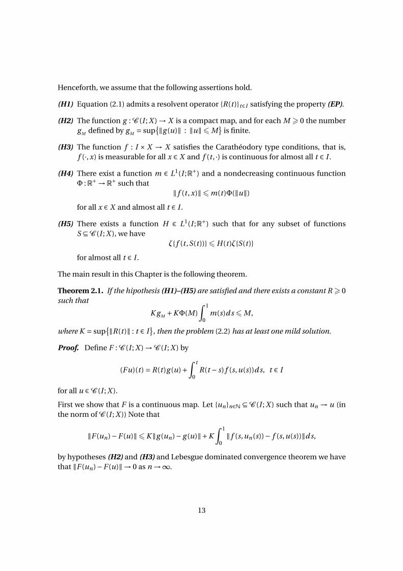
Henceforth, we assume that the following assertions hold.

(H1) Equation (2.1) admits a resolvent operator R(t )t∈I satisfying the property (EP).

(H2) The function g : C (I ; X ) → X is a compact map, and for each M > 0 the numbergM defined by gM = sup

‖g (u)‖ : ‖u‖6 M

is finite.

(H3) The function f : I × X → X satisfies the Carathéodory type conditions, that is,f (·, x) is measurable for all x ∈ X and f (t , ·) is continuous for almost all t ∈ I .

(H4) There exist a function m ∈ L1(I ;R+) and a nondecreasing continuous functionΦ :R+ →R+ such that

‖ f (t , x)‖6m(t )Φ(‖u‖)

for all x ∈ X and almost all t ∈ I .

(H5) There exists a function H ∈ L1(I ;R+) such that for any subset of functionsS ⊆C (I ; X ), we have

ζ f (t ,S(t ))6 H(t )ζS(t )

for almost all t ∈ I .

The main result in this Chapter is the following theorem.

Theorem 2.1. If the hipothesis (H1)–(H5) are satisfied and there exists a constant R > 0such that

K gM +KΦ(M)∫ 1

0m(s)d s 6 M ,

where K = sup‖R(t )‖ : t ∈ I

, then the problem (2.2) has at least one mild solution.

Proof. Define F : C (I ; X ) →C (I ; X ) by

(Fu)(t ) = R(t )g (u)+∫ t

0R(t − s) f (s,u(s))d s, t ∈ I

for all u ∈C (I ; X ).

First we show that F is a continuous map. Let unn∈N ⊆ C (I ; X ) such that un → u (inthe norm of C (I ; X )) Note that

‖F (un)−F (u)‖6K ‖g (un)− g (u)‖+K∫ 1

0‖ f (s,un(s))− f (s,u(s))‖d s,

by hypotheses (H2) and (H3) and Lebesgue dominated convergence theorem we havethat ‖F (un)−F (u)‖→ 0 as n →∞.

13

Now denote by BM = u ∈ C (I ; X ) : ‖u(t )‖X 6 M , for all t ∈ I and note that for anyu ∈ BM we have

‖(Fu)(t )‖6 ‖R(t )g (u)‖+∥∥∥∥∫ t

0R(t − s) f (s,u(s))d s

∥∥∥∥6K gM +KΦ(M)

∫ 1

0m(s)d s 6 M .

Therefore, F : BM → BM and F (BM ) is a bounded set. Moreover, since the family ofoperators R(t )t∈I has the property (EP), we have that F (BM ) is an equicontinuous setof functions.

Define B= co(F (BM )). It follows from Lemma 1.4 that the set B is equicontinuous andthe operator F : B→B is bounded and continuous. In addition, F (B) is a boundedset of functions.

From properties of Hausdorff measure of non–compactness we have that

ζ(F (B(t )))6 ζR(t )g (B)

+ζ(∫ t

0R(t − s) f (s,B(s))d s

)6K ζg (B)+K

∫ t

0ζ f (s,B(s))d s

6K∫ t

0H(s)ζB(s)d s 6Kγ(B)

∫ t

0H(s)d s

Since H ∈ L1(I ; X ) for δ< 1/K there existsϕ ∈C (I ;R+) satisfying∫ 1

0|H(s)−ϕ(s)|d s < δ.

Therefore,

ζ(F (B(t )))6Kγ(B)

[∫ t

0|H(s)−ϕ(s)|d s +

∫ t

0ϕ(s)d s

]6Kγ(B) [δ+N t ] ,

where N = ‖ϕ‖∞. Thus , we have

ζ(F (B(t )))6 (a +bt )γ(B), where a = δK and b = K N .

Since (F (B) is an equicontinuous set of functions we have that

γ(F (B))6 (a +b)γ(B).

In the same manner, it follows from properties of Hausdorff measure of non–compactnessthat

14

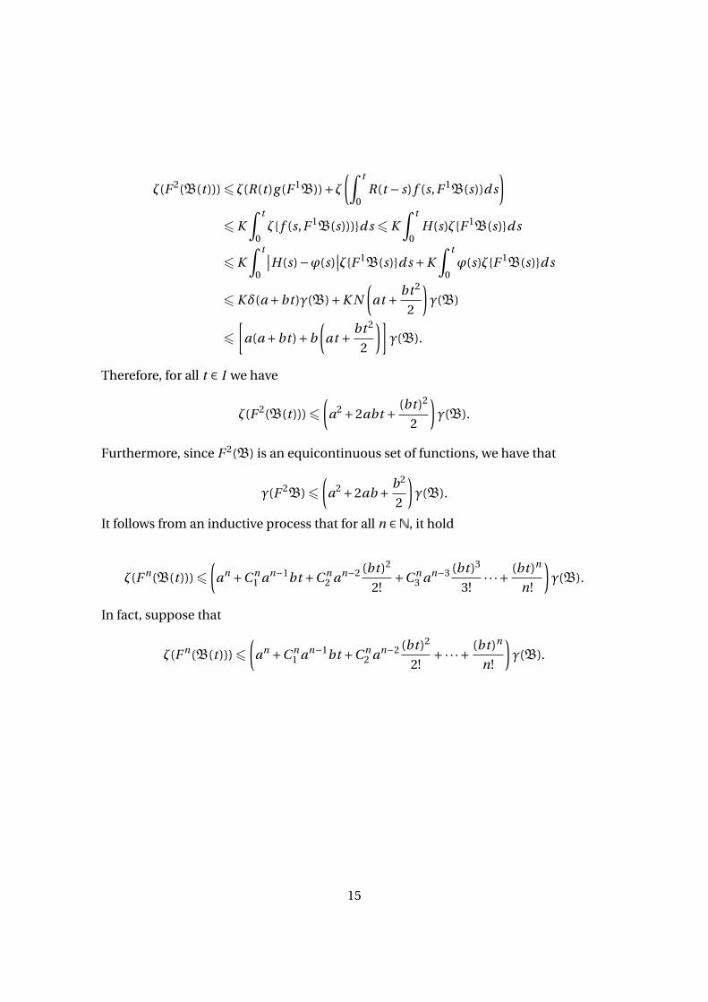
ζ(F 2(B(t )))6 ζ(R(t )g (F 1B))+ζ(∫ t

0R(t − s) f (s,F 1B(s))d s

)6K

∫ t

0ζ f (s,F 1B(s)))d s 6K

∫ t

0H(s)ζF 1B(s)d s

6K∫ t

0

∣∣H(s)−ϕ(s)∣∣ζF 1B(s)d s +K

∫ t

0ϕ(s)ζF 1B(s)d s

6Kδ(a +bt )γ(B)+K N

(at + bt 2

2

)γ(B)

6[

a(a +bt )+b

(at + bt 2

2

)]γ(B).

Therefore, for all t ∈ I we have

ζ(F 2(B(t )))6(

a2 +2abt + (bt )2

2

)γ(B).

Furthermore, since F 2(B) is an equicontinuous set of functions, we have that

γ(F 2B)6(

a2 +2ab + b2

2

)γ(B).

It follows from an inductive process that for all n ∈N, it hold

ζ(F n(B(t )))6(

an +C n1 an−1bt +C n

2 an−2 (bt )2

2!+C n

3 an−3 (bt )3

3!· · ·+ (bt )n

n!

)γ(B).

In fact, suppose that

ζ(F n(B(t )))6(

an +C n1 an−1bt +C n

2 an−2 (bt )2

2!+·· ·+ (bt )n

n!

)γ(B).

15

By properties of Hausdorff measure of non–compactness we have that for (n + 1) itholds

ζ(F n+1(B(t )))6 ζR(t )g (F n(B))+ζ(∫ t

0R(t − s) f (s,F n(B(s)))d s

)6K

∫ t

0ζ f (s,F nB(s)))d s 6K

∫ t

0H(s)ζF nB(s)d s

6K∫ t

0

∣∣H(s)−ϕ(s)∣∣ζF nB(s)d s +K

∫ t

0ϕ(s)ζF nB(s)d s

6Kδ

(an +C n

1 an−1bt +C n2 an−2 (bt )2

2!+·· ·+ (bt )n

n!

)γ(B)

+K N

(an t +C n

1 an−1 bt 2

2+C n

2 an−2 b2t 3

3!+·· ·+ bn t n+1

(n +1)!

)γ(B)

6 a

(an +C n

1 an−1bt +C n2 an−2 (bt )2

2!+·· ·+ (bt )n

n!

)γ(B)

+b

(an t +C n

1 an−1 bt 2

2+C n

2 an−2 b2t 3

3!+·· ·+ bn t n+1

(n +1)!

)γ(B).

From the fact that, for all 16m 6 n, it holds C nm−1 +C n

m =C n+1m we have have

ζ(F n+1(B(t )))6(

an+1 +C n+11 an(bt )+C n+1

2 an−1 (bt )2

2!+·· ·+ (bt )n+1

(n +1)!

)γ(B).

Hence, for all n ∈N, it hold

ζ(F n(B(t )))6(

an +C n1 an−1bt +C n

2 an−2 (bt )2

2!+C n

3 an−3 (bt )3

3!· · ·+ (bt )n

n!

)γ(B).

Since, for all n ∈N the set of functions F n(B) is equicontinuous we have that

γ(F n(B))6(

an +C 1n an−1b +C 2

n an−2 b2

2!+C 3

n an−3 b3

3!· · ·+ bn

n!

)γ(B).

Furthermore, since 0 6 a < 1 and b > 0, it follows from Lemma 1.4 that there existsn0 ∈N such that

an0 +C 1n0

an0−1b +C 2n0

an0−2 b2

2!+·· ·+ bn0

n0!= r < 1

Therefore, there exists n0 ∈ N such that γ(F n0 (B)) 6 rγ(B), with r < 1.It follows from Theorem 1.5 that F has a fixed point in B. This fixed point is a mildsolution of equation (2.2).

16

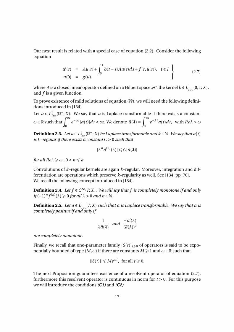
Our next result is related with a special case of equation (2.2). Consider the followingequation

u′(t ) = Au(t )+∫ t

0b(t − s)Au(s)d s + f (t ,u(t )), t ∈ I

u(0) = g (u).

(2.7)

where A is a closed linear operator defined on a Hilbert space H , the kernel b ∈ L1l oc (0,1; X ),

and f is a given function.

To prove existence of mild solutions of equation (??), we will need the following defini-tions introduced in [134].

Let a ∈ L1l oc (R+; X ). We say that a is Laplace transformable if there exists a constant

ω ∈R such that∫ ∞

0e−ωt |a(t )|d t <∞. We denote a(λ) =

∫ ∞

0e−λt a(t )d t , with Reλ>ω

Definition 2.3. Let a ∈ L1l oc (R+; X ) be Laplace transformable and k ∈N. We say that a(t )

is k–regular if there exists a constant C > 0 such that

|λn a(n)(λ)|6C |a(λ)|

for all Reλ>ω , 0 < n 6 k.

Convolutions of k–regular kernels are again k–regular. Moreover, integration and dif-ferentiation are operations which preserve k–regularity as well. See [134, pp. 70].We recall the following concept introduced in [134].

Definition 2.4. Let f ∈C∞(I ; X ). We will say that f is completely monotone if and onlyif (−1)n f (n)(λ)> 0 for all λ> 0 and n ∈N.

Definition 2.5. Let a ∈ L1loc (I ; X ) such that a is Laplace transformable. We say that a is

completely positive if and only if

1

λa(λ)and

−a′(λ)

(a(λ))2

are completely monotone.

Finally, we recall that one-parameter family S(t )t>0 of operators is said to be expo-nentially bounded of type (M ,ω) if there are constants M > 1 and ω ∈R such that

‖S(t )‖6 Meωt , for all t > 0.

The next Proposition guarantees existence of a resolvent operator of equation (2.7),furthermore this resolvent operator is continuous in norm for t > 0. For this purposewe will introduce the conditions (C1) and (C2).

17

(C1) For all t ∈ I , the kernel a defined by a(t ) =∫ t

0b(s)d s +1, for all t ∈ I , is 2–regular

and completely positive.

(C2) There exists µ0 >ω such that

lim|µ|→∞

∥∥∥∥∥ 1

b(µ0 + iµ)+1

(µ0 + iµ

b(µ0 + iµ)+1− A

)−1∥∥∥∥∥= 0

Proposition 2.1. Suppose that A is the generates a C0–semigroup of type (M ,ω) on H

a Hilbert space. If the conditions (C1)–(C2) are satisfied then, there exists a resolventoperator R(t )t∈I for equation (2.7) which is continuous in norm for t > 0.

Proof. Integrating on time equation (2.7) we get

u(t ) =∫ t

0a(t − s)Au(s)d s +

∫ t

0f (s,u(s))+ g (u). (2.8)

Since the scalar kernel a is completely positive and A generates a C0–semigroup, itfollows from [134, Theorem 4.2] that there exists a family of operators R(t )t∈I stronglycontinuous, exponentially bounded that commutes with A, satisfying

R(t )x = x +∫ t

0a(t − s)AR(s)xd s. (2.9)

On the other hand, using hypothesis (C2) and since the scalar kernel a is 2–regular, itfollows from [109, Theorem 2.2] that R(t )t∈I is continuous on L (H ) for t > 0. Fur-ther, since a ∈ C 1(R+), it follows from equation (2.9) that R(t ) is differentiable for allt > 0 and satisfies

d

d tR(t )x = AR(t )x +

∫ t

0b(t − s)AR(s)xd s, t > 0. (2.10)

From the preceding equality, we conclude that R(t )t∈I is a resolvent operator forequation (2.7) which is norm continuous.

Corollary 2.1. Suppose that A generates a C0–semigroup of type (M ,ω) on H a Hilbertspace and conditions (C1)–(C2) are fulfilled. If the hypothesis (H2)–(H5) are satisfiedand there exists M > 0 such that

K gM +KΦ(M)∫ 1

0m(s)d s 6 M , where K = sup‖R(t )‖ : t ∈ I ,

then equation (2.7) has at least a mild solution.

Proof. It follows from Proposition 2.1 that the equation (2.7) admits a resolvent op-erator R(t )t∈I satisfying the property (EP). Moreover, since hypothesis (H2)-(H5) aresatisfied, we apply Theorem 2.1 and conclude that equation (2.7) has a mild solution.

18

2.2 An Example

In this section we prove the feasibility of our abstract results applying them to a con-crete partial differential equation with non–local initial condition. Let X = L2(Rn) andconsider the following integro-differential equation

∂w(t ,ξ)

∂t= Aw(t ,ξ)+

∫ t

0βe−α(t−s) Aw(s,ξ)d s + t−1/3 cos(w(t ,ξ)), t ∈ I .

w(0,ξ) =N∑

i=1

∫Rn

qk(ξ, y)w(ti , y)d y, ξ ∈Rn .

(2.11)

where N is a positive integer, 0 < t1 < t2 < ·· · < tN < 1; k ∈ L2(Rn ×Rn ;R+), q ∈ R+, theconstants α,β satisfy −α6β6 06α. The operator A is defined by

(Aw)(t ,ξ) =n∑

i , j=1ai j (z)

∂w(t ,ξ)

∂ξi∂ξ j+

n∑i=1

bi (ξ)∂w(t ,ξ)

∂ξi+ c(ξ)w(t ,ξ),

with given coefficients ai j , bi , c, (i , j = 1,2, . . . ,n) satisfying the usual uniformly ellip-ticity conditions, and D(A) = v ∈ X : v ∈ H 2(Rn).

We will prove that there exists q > 0 sufficiently small such that equation (2.11) has amild solution on X .In what follows, we identify u(t ) = w(t , ·). With this identification the preceding equa-tion takes the abstract form

u′(t ) = Au(t )+∫ t

0b(t − s)Au(s)d s + f (t ,u(t )), t ∈ I

u(0) = g (u),

(2.12)

where the function g : C (I ; X ) → X is given by g (u) =N∑

i=1qkg (u(ti )) with

(kg v)(ξ) =∫Rn

k(ξ, y)v(y)d y, for v ∈ X ,ξ ∈Rn ,

the function f : I × X → X is defined by f (t ,u(t )) = t−1/3 cos(u(t )) = t−1/3 cos(w(t , ·)),and the kernel b is given by b(t ) =βe−αt .

Note that ‖g (u)‖6 qN(∫Rn

∫Rn

k2(z, y)d yd z)1/2‖u‖, and the function kg is completely

continuous.Furthermore, the function f satisfies ‖ f (t ,u(t ))‖6 t−1/3Φ(‖u‖), with Φ(‖u‖) ≡ 1 and‖ f (t ,u1)− f (t ,u2)‖6 t−1/3‖u1 −u2‖.Therefore, conditions (H2)–(H5) are fulfilled.

19

Define a(t ) =∫ t

0βe−αsd s +1, for all t ∈ I . Since the kernel b defined by b(t ) = βe−αt

is 2–regular, it follows that a is 2–regular. Furthermore, we claim that a is completelypositive. In fact, we have

a(λ) = λ+α+βλ(λ+α)

.

Define the functions f1 and f2 by f1(λ) = 1

λa(λ)and f2(λ) = −a ′(λ)

[a(λ)]2respectively. In

another words

f1(λ) = λ+αλ+α+β and f2(λ) = λ2 +2(α+β)λ+αβ+α2

(λ+α+β)2.

Direct calculation shows that

f (n)1 (λ) = (−1)n+1β(n +1)!

(λ+α+β)n+1and f (n)

2 (λ) = (−1)n+1β(α+β)(n +1)!

(λ+α+β)n+2for n ∈N.

Since −α 6 β 6 0 6 α, we have that f1 and f2 are completely monotone. Thus, thekernel a is completely positive.

On the other hand, it follows from [55] that A generates an analytic, non compact semi-group T (t )t>0 on L2(Rn). Furthermore, there exists a constant M > 0 such that

M = sup‖T (t )‖ : t > 0 <+∞.

It follows from this fact and Hille–Yosida theorem that z ∈ ρ(A) for Re(z) > 0.A direct calculation shows that,

Re

(µ0 + iµ

b(µ0 + iµ)+1

)= µ3

0 +µ20α+µ2

0(α+β)+µ0α(α+β)+µ0µ2 −µ2β

(α+β)2 +2µ0(α+β)+µ20 +µ2

.

Hence, for µ0 > 0, we have that, Re

(µ0 + iµ

b(µ0 + iµ)+1

)> 0. This implies that

(µ0 + iµ

b(µ0 + iµ)+1− A

)−1

∈L (X ).

Moreover, ∥∥∥∥∥ 1

b(µ0 + iµ)+1

(µ0 + iµ

b(µ0 + iµ)+1− A

)−1∥∥∥∥∥6∥∥∥∥ M

µ0 + iµ

∥∥∥∥ .

20

Therefore,

lim|µ|→∞

∥∥∥∥∥ 1

b(µ0 + iµ)+1

(µ0 + iµ

b(µ0 + iµ)+1− A

)−1∥∥∥∥∥= 0.

It follows from Proposition 2.1, equation (2.11) admits a resolvent operator R(t )t∈I

satisfying property (EP). Let K = sup‖R(t )‖ : t ∈ I and c = N(∫Rn

∫Rn

k2(z, y)d yd z)1/2

.

A direct computation shows that for each M > 0 the number gM is equal to gM = qcM .

Therefore the expression gM K +KΦ(M)∫ 1

0m(s)d s, is equivalent to qcK M + 3K

2.

Since, there exists q > 0 such that qcK < 1 it follows that, there exists M > 0 satisfying

qcK M + 3K

26 M .

From Corollary 2.1 we conclude that there exists a mild solution of equation (2.11).

21

CHAPTER 3

Mild Solutions of Second OrderNon–autonomous Cauchy Problem with

non–local initial conditions

As we have mentioned in preceding Chapter, the study of mild solutions of evolutionequations is very important because it has a lot of applications. In particular, the studymild solutions for problems with non–local initial conditions have taken great interestin last decades.

This chapter is devoted to study the existence of mild solutions of non–local initialvalue problem described as a second order non–autonomous abstract differential prob-lem

u′′(t ) = A(t )u(t )+ f (t ,u(t )) t ∈ [0, a]u(0) = g (u)

u′(0) = h(u)

(3.1)

For t ∈ J = [0, a], A(t ) : D(A(t )) ⊆ X → X for t ∈ J = [0, a] denote closed linear operatorsdefined in a Banach space X . We assume that D(A(t )) = D for all t ∈ J . The functionf : J × C (J ; X ) → X satisfies Carathéodory type conditions, and the functionsg ,h : C (J ; X ) → X are continuous maps.

There exists an extensive literature concerning second order problems. In the au-tonomous case, this is A(t ) ≡ A, for all t ∈ J , the solutions of these equations are closelyrelated with the concept of cosine families. We refer the reader to [58,140,141,142,144]for basic concepts about these families.

In the same manner, the study of mild solutions of equation (3.1) are closely relatedwith the concept of evolution operator S(t , s)t ,s∈J . In the literature several techniques

22

have been discussed to establish the existence of the evolution operatorS(t , s)t ,s∈J . In particular, a very studied situation is that A(t ) is the perturbation of anoperator A that generates a cosine operator function. For this reason, below we brieflyreview some essential properties of the theory of cosine functions. We will mention afew of properties and notations needed to establish our main results.

Let A : D(A) ⊆ X → X be the infinitesimal generator of a strongly continuous cosinefamily C0(t )t>0 of bounded linear operators in X and let S0(t )t>0 be the sine family

associated with C0(t )t>0, which is defined by S0(t )x =∫ t

0C0(s)xd s, for x ∈ X and

t ∈R. It is immediate that

C0(t )x −x = A∫ t

0S0(s)xd s, for all x ∈ X and t > 0.

The notation E stands for the space consisting of vectors x ∈ X such that the functionC0(·)x is of class C 1. Kisynski in [101] has proved that E endowed with the norm

‖x‖1 = ‖x‖+ sup06t61

‖AS0(t )x‖, x ∈ E ,

is a Banach space. It is known that the operator valued function G(t ) =[

C0(t ) S0(t )AS0(t ) C0(t )

]is a strongly continuous group of bounded linear operators on the space E ×X . gener-

ated by the operator A =[

0 IA 0

]defined on D(A)×E . It follows from this property that

S0(t ) : X → E is a bounded linear operator such that the operator valued map S0(·) isstrongly continuous and AS0(t ) : E → X is a bounded linear operator such that, foreach x ∈ E , satisfies AS0(t )x → 0 as t → 0. Furthermore, recall that, if f : [0,∞) → X is a

locally integrable function, then u(t ) =∫ t

0S0(t − s) f (s)d s defines an E–valued contin-

uous function.We finally mention that the function u(·) given by

u(t ) =C0(t − s)x +S0(t − s)y +∫ t

sS0(t −ξ) f (ξ)dξ, t ∈ J , (3.2)

is called mild solution of the problem

u′′(t ) = Au(t )+ f (t ), t ∈ J ,u(s) = x,

u′(s) = y.

(3.3)

If x ∈ E , the function u(·) given by (3.2) is continuously differentiable and

u′(t ) = AS0(t − s)x +C0(t − s)y +∫ t

sC0(t −ξ) f (ξ)dξ, t ∈ J . (3.4)

23

If x ∈ D(A), y ∈ E and f is a continuously differentiable function, then the function u(·)is a classical solution of problem (3.3).

Non–autonomous second order problems have received much attention in recent yearsdue their applications in different fields. Specially, many authors have studied the ini-tial value Cauchy equation

u′′(t ) = A(t )u(t )+ f (t ) t ∈ Ju(s) = x

u′(s) = y.

(3.5)

We refer the reader to [17, 78, 107, 138, 150]. As we have mentioned, the existenceof solutions of this equation is related with the existence of the evolution operatorS(t , s)t ,s∈J for homogeneous equation

u′′(t ) = A(t )u(t ), t ∈ J .u(s) = x

u′(s) = y.

(3.6)

In this thesis, we will use the concept of evolution operator S(t , s)t ,s∈J associated withequation (3.6) introduced by Kozak in [103]. With this purpose, we assume that thedomain of A(t ) is a subspace D dense in X and independent of t ∈ J , and for eachx ∈ D the function t → A(t )x is continuous.

Definition 3.1. A map S : J × J → L (X ) is said to be an evolution operator of equa-tion (3.6) if the following conditions are fulfilled:

(D1) For each x ∈ X the map (t , s) → S(t , s)x is continuously differentiable and

(a) For each t ∈ J , S(t , t ) = 0.

(b) For all t , s ∈ J and each x ∈ X , ∂∂t S(t , s)x |t=s = x and ∂

∂s S(t , s)x |t=s =−x.

(D2) For all t , s ∈ J , if x ∈ D, then S(t , s)x ∈ D, the map (t , s) → S(t , s)x is of class C 2 and

(a) ∂2

∂t 2 S(t , s)x = A(t )S(t , s)x.

(b) ∂2

∂s2 S(t , s)x = S(t , s)A(s)x.

(c) ∂2

∂s∂t S(t , s)x |t=s = 0.

(D3) For all s, t ∈ J , if x ∈ D then ∂∂t S(t , s)x ∈ D. Further, there exist ∂3

∂t 2∂sS(t , s)x, ∂3

∂s2∂tS(t , s)x

and

(a) ∂3

∂t 2∂sS(t , s)x = A(t ) ∂

∂s S(t , s)x. Moreover, the map (t , s) → A(t ) ∂∂s S(t , s)x is con-

tinuous.

(b) ∂3

∂s2∂tS(t , s)x = A(t ) ∂

∂t S(t , s)x.

24

Assuming that f : J → X is an integrable function, Kozak in [103] has proved that thefunction u : J → X given by

u(t ) =− ∂

∂sS(t , s)x +S(t , s)y +

∫ t

sS(t ,ξ) f (ξ)dξ, (3.7)

is a mild solution of equation (3.6). Motivated by this result, we will say that a functionu ∈C (J ; X ) is a mild solution of problem (3.1) if verifies

u(t ) =− ∂

∂sS(t ,0)g (u)+S(t ,0)h(u)+

∫ t

0S(t ,ξ) f (ξ,u(ξ))dξ. (3.8)

Henceforth, we assume that there exists an evolution operator S(t , s)t6s,t6a associ-ated with equation (3.6). To abbreviate the text, we introduce the operatorC (t , s) =−∂S(t ,s)

∂s . With this notation, the mild solution of problem (3.1) is

u(t ) =C (t ,0)g (u)+S(t ,0)h(u)+∫ t

0S(t ,ξ) f (ξ,u(ξ))dξ. (3.9)

In addition, we set K > 0 such that

supt ,s∈J

‖S(t , s)‖6K and supt ,s∈J

‖C (t , s)‖6K . (3.10)

We denote N1 a positive constant such that

‖S(t +h, s)−S(t , s)‖6 N1|h| for all t , s, t +h ∈ J . (3.11)

3.1 Main Results

In this section we will present our main results. In the same manner as that of Chapter2, an argument to prove existence of mild solution of non–autonomous problem (3.1)is using fixed–point Theorems. The Theorems that we will use are related with theconcept of measure of non–compactness.

Similarly to Chapter 2, in order to give a condition that we will need in the proof ofmain results of this Chapter, we consider the following list of assertions.

(Cgh1) The functions g and h are continuous maps. Further, for each M > 0 the num-bers gM and hM defined by

gM = sup‖g (u)‖ : ‖u‖6 M

and hM = sup

‖h(u)‖ : ‖u‖6 M

are finite.

25

(Cgh2) The functions f and g satisfy

γ(g (B))+γ(h(B)) < 1

2Kγ(B)

for all bounded set of continuous functions B . Here the constant K is defined asin inequality (3.10).

(Cg1) The map from C (J ; X ) to C (J ; X ) given by u(·) → C (·,0)g (u) takes bounded setsinto equicontinuous sets.

(Cg2) The function g : C (J ; X ) → X satisfies γ(g (B)) < 1

Kγ(B) for all bounded set of

functions B ⊆C (J ; X ). Here the constant K is defined as in equation 3.10.

(CS1) The evolution operator S(t , s)t ,s∈J is a compact family of operators.

(Cf1) The map f : J × X → X satisfies the Carathéodory type conditions, that is, f (·, x)is measurable for all x ∈ X and f (t , ·) is continuous for almost all t ∈ J .

(Cf2) There exist functions m ∈ L1(J ;R+) and non–decreasing continuous functionΦ :R+ →R+ such that

‖ f (t , x)‖6m(t )Φ(‖x‖)

for all x ∈ X and almost all t ∈ J .

(Cf3) There exists a function H ∈ L1(J ;R+) such that for any subset of functionsS ⊆C (J ; X ), we have

ζ( f (t ,S(t )))6 H(t )ζ(S(t ))

for almost all t ∈ J .

Condition (Cg1) play a crucial role in the proof of Theorem 3.1, for this reason we willshow several situations where this condition is valid.

Lemma 3.1. Let g : C (J ; X ) → X be a continuous map. If g is a compact function thenthe function u(·) →C (·,0)g (u) takes bounded sets into equicontinuous sets.

Proof. Let S ⊆ C (J ; X ) be a bounded set of continuous functions, this is, there existsM > 0 such that ‖u‖ 6 M for all u ∈ S. Let ε > 0 be an arbitrary positive number.Since the function g is compact we have that there exist x1, x2, . . . , xp ∈ X such that

g (S) ⊆p⋃

i=1B

(xi ,

ε

4K

).

For i ∈ 1,2 . . . , p, define the functions fi : J → X given by fi (t ) = C (t ,0)xi . Clearlythese functions are continuous. Furthermore, since all functions fi are defined in a

26

compact set it follows that for all i ∈ 1,2, . . . , p the functions fi are uniformly con-tinuous. Hence, for i ∈ 1,2, . . . , p there exists hi > 0 such that for all t ∈ J we have

‖(C (t +hi ,0)−C (t ,0))xi‖6 ε

2.

Denote δ= minhi : i = 1,2, . . . , p

. Thus, we have that ‖(C (t +δ,0)−C (t ,0))xi‖6 ε

2for

all t ∈ J and i ∈ 1,2 . . . , p.

Let u ∈ S, we know that there exists i ∈ 1,2, . . . , p such that ‖g (u)−xi‖6 ε

2. Therefore

‖C (t +δ,0)g (u)−C (t ,0)g (u)‖6 ‖(C (t +δ,0)−C (t ,0))(g (u)−xi )‖+‖(C (t +δ,0)−C (t ,0))xi‖6 2K ‖g (u)−xi‖+ ε

26 ε.

This argument is valid for any u ∈ S. Since, δ is independent of u and t we have thatthe set

C (·,0)g (u) : u ∈ S

is an equicontinuous set of continuous functions.

Lemma 3.2. Assume that A(t ) = A+B(t ) for all t ∈ J , here the operator A is the generatorof a cosine family C0(t )t∈J defined on X , and B(t ) ∈ L (E ; X ) for all t ∈ J ,and B(t )z ∈ C 1(J ; X ) for z ∈ E. Let g : C (J ; X ) → X be a continuous map such thatg (u) ∈ E for all u ∈C (J ; X ), then the function u(·) →C (·,0)g (u) takes bounded sets intoequicontinuous sets.

Proof. Under the hypothesis, it has been proved by Serizawa and Watanabe in [139]that C (t , s)t ,s∈J is differentiable in E .

In the same manner as that of Chapter 2, henceforth we assume that the followingassertions hold:

Theorem 3.1. Suppose that the function g and h are compact maps and the conditions(Cgh1), (Cf1), (Cf2) and (Cf3) are fulfilled. If there exists a constant R > 0 such that

K (gM +hM )+KΦ(M)∫ a

0m(s)d s 6 M ,

then the problem (3.1) has at least one mild solution.

Proof. Define F : C (J ; X ) →C (J ; X ) by

(Fu)(t ) =C (t ,0)g (u)+S(t ,0)h(u)+∫ t

0S(t , s) f (s,u(s))d s, t ∈ J .

27

First, we show that F is a continuous map. Let unn∈N ⊆ C (J ; X ) such that un → u (inthe norm of C (J ; X )) Note that

‖F (un)−F (u)‖6K ‖g (un)− g (u)‖+K ‖h(un)−h(u)‖+K

∫ a

0‖ f (s,un(s))− f (s,u(s))‖d s.

Since, the functions g and h are continuous maps, it follows from Lebesgue dominatedtheorem that ‖F (un) → F (u)‖→ 0 as n →∞.Now denote by BM =

u ∈C (J ; X ) : ‖u(t )‖6 M for all t ∈ J

and note that for any u ∈ BM

we have

‖(Fu)(t )‖6 ‖C (t ,0)g (u)‖+6 ‖S(t ,0)h(u)‖+∥∥∥∥∫ t

0S(t , s) f (s,u(s))d s

∥∥∥∥6K (gM +hM )+KΦ(M)

∫ a

0m(s)d s 6 M .

Therefore, F : BM → BM and F (BM ) is a bounded set. Moreover, F (BM ) is an equicontin-uous set of functions. In fact, let ε> 0 be an arbitrary positive number. By Lemma 3.1

there exists δ1 > 0 such that ‖(C (t +δ1,0)−C (t ,0))g (u)‖6 ε

4. Choose δ2 > 0 such that

δ2 < min

δ1,

ε

4hM N1,

ε

4KΦ(M)M,

ε

4Φ(M)‖m‖1

,

where m∞ is defined by m∞ = supm(t ) : t ∈ J

and ‖m‖1 denotes the integral norm

of function m defined in condition (Cf2), the function Φ is defined in condition (Cf2),and K and N1 have been chosen as inequalities (3.10) and (3.11). The constant hM isdefined in condition (Cgh1)For all |t2 − t1| < δ2 and for all u ∈ BM we have

‖(Fu)(t2)− (Fu)(t1)‖6 ‖C (t2)g (u)−C (t1)g (u)‖+‖S(t2)h(u)−S(t1)h(u)‖

+KΦ(M)∫ t2

t1

m(s)d s +Φ(M)∫ t1

0‖S(t2, s)−S(t1, s)‖m(s)d s

6ε

4+ ε

4+ ε

4+ ε

4= ε.

Define B= co(F (BM )). It follows from Lemma 1.2 that the set B is equicontinuous andthe operator F : B→B is bounded and continuous. In addition, F (B) is a boundedset of functions. Same argument made to show that F (BM ) is an equicontinuous set offunctions show that F (B) is an equicontinuous set of functions.

From properties of Hausdorff measure of non–compactness we have that

28

ζ(F (B(t )))6 ζC (t ,0)g (B)

+ζS(t ,0)h(B)+ζ(∫ t

0S(t , s) f (s,B(·))d s

)6K ζg (B)+K ζh(B)+K

∫ t

0ζ f (s,B(s))d s

6Kγ(B)∫ t

0H(s)d s

Since H ∈ L1(J ;R+) for δ < 1/K there is ϕ ∈ C (J ;R+) such that∫ a

0|H(s)−ϕ(s)|d s < δ.

Therefore,

ζ(F (B(t )))6Kγ(B)

[∫ t

0|H(s)−ϕ(s)|d s +

∫ t

0|ϕ(s)|d s

]6Kδγ(B)+K N t ,

where N = ‖ϕ‖∞. Thus, we have

γ(F (B(t )))6 (A+B t )γ(B) where A = Kδ and B = K N .

Following the same arguments as those of proof of Theorem 2.1 in Chapter 2, we havethat

γ(F n(B))6(

An +C n1 An−1B a +C n

2 An−2 (B a)2

2!+·· ·+ (B a)n

n!

)γ(B).

Furthermore, since 0 6 A < 1 and B a > 0, it follows from Lemma 1.4 that there existsn0 ∈N such that

An0 +C n01 An0−1B +C n0

2 An0−2 B 2

2!+·· ·+ B n0

n0!= r < 1

Therefore, γ(F n0 (B)) 6 rγ(B), with r < 1. It follows from Theorem 1.5 that F has afixed point in B. This fixed point is a mild solution of equation (3.1).

Theorem 3.1 imposes some restrictive conditions about functions g and h. In fact,non–local initial conditions that arise in specific applications, are very often condens-ing maps. Motivated by this, the next result imposes much more weak restrictions forg and h.

Theorem 3.2. Suppose that the functions g and h are condensing maps and the condi-tions (Cgh1), (Cgh2), (Cf1) and(Cf2) are fulfilled. If there exists a constant R > 0 suchthat

K (gM +hM )+KΦ(M)∫ a

0m(s)d s 6 M ,

then the problem (3.1) has at least one mild solution.

29

Proof. Define F : C (J ; X ) →C (J ; X ) by

(Fu)(t ) =C (t ,0)g (u)+S(t ,0)h(u)+∫ t

0S(t , s) f (s,u(s))d s, t ∈ J

for all u ∈C (J ; X ).Following the same argument as that of proof of Theorem 3.1, we prove that F is acontinuous map. We introduce the mappings

F1 : C (J ; X ) →C (J ; X ) defined by (F1u)(t ) =C (t ,0)g (u)+S(t ,0)h(u), t ∈ J .

and

F2 : C (J ; X ) →C (J ; X ) defined by (F2u)(t ) =∫ t

0S(t , s) f (s,u(s))d s, t ∈ J

Since S(t , s)t ,s∈J is a family of operators such that

‖S(t +h, s)−S(t , s)‖6 N1|h| for all t , s, t +h ∈ J ,

it follows from Arzela–Ascoli theorem that F2 is a compact map. On the other hand F1

is a γ–condensing map. In fact, γ(F1B) 6 γ(C (·,0)g (B))+γ(S(·,0)g (B)) < γ(B) for allbounded set of functions B .By hypothesis, there exists a constant R > 0 such that

K (gM +hM )+KΦ(M)∫ a

0m(s)d s 6R.

Therefore, F : BM → BM . It follows from Theorem 1.4 that F has a fixed point in BM andthis fixed point is a mild solution of equation (3.1).

Assume now that A(t ) = A +B(t ) for all t ∈ J , where B(·) : J → L (E ; X ) is a map suchthat the function t → B(t )x is continuously differentiable in X for each x ∈ E . It hasbeen established by Serizawa and Watanabe [139] that for each (y, z) ∈ D(A)×E thenon–autonomous abstract Cauchy problem

u′′(t ) = (A+B(t ))u(t ), t ∈ Ju(0) = x,

u′(0) = y,

(3.12)

has a unique solution u(·) such that the function t → u(t ) is continuously differentiablein E . It is clear that the same argument allows us to conclude that equation

u′′(t ) = (A+B(t ))u(t ), t ∈ Ju(s) = x,

u′(s) = y,

(3.13)

30

has a unique solution u(·, s) such that the function t → u(t , s) is continuously differen-tiable in E . It follows from (3.7) that

u(t , s) =C0(t − s)x +S0(t − s)y +∫ t

sS0(t −ξ)B(ξ)u(ξ, s)dξ

In particular, for x = 0 we have

u(t , s) = S0(t − s)y +∫ t

sS0(t −ξ)B(ξ)u(ξ, s)dξ

Consequently,

‖u(t , s)‖1 6 ‖S0(t − s)‖L (X ,E)‖z‖+

∫ t

s‖S0(t −ξ)‖

L (X ,E)‖B(ξ)‖L (X ,E)‖u(ξ, s)‖1dξ.

Applying the Gronwall–Bellman lemma, there exists a constant N > 0 such that‖u(t , s)‖1 6 N‖z‖, s, t ∈ J .

We define the operator S(t , s)y = u(t , s). It follows from the previous estimate thatS(t , s) is a bounded linear map on E . Since E is dense in X , we can extend S(t , s) toX . We keep the notation S(t , s) for this extension.

It is well known that, except in the case dim(X ) < ∞, the cosine function C0(t ) can-not be compact for all t ∈ R. By contrast, for the cosine functions that arise in spe-cific applications, the sine function S0(t ) is very often a compact operator for all t ∈ R.This motivates the following result proved by Henríquez in [78]. We remark, this resultshows a situation where the condition (CS1) is valid.

Lemma 3.3. Under the preceding conditions, S(·, ·) is an evolution operator for equation(3.14). Moreover, if S0(t ) is compact for all t ∈R, then S(t , s) is also compact for all s 6 t .

Now consider the particular case of equation (3.1).

u′′(t ) = (A+B(t ))u(t )+ f (t ,u(t )), t ∈ Ju(s) = g (u),

u′(s) = h(u).

(3.14)

Next Theorem gives sufficient conditions to guarantee existence of a mild solution ofequation (3.14). We remark, this results imposes much more weak conditions for func-tion h. In same manner as those of Theorems 3.1 and 3.2, we enumerate followingconditions.

Theorem 3.3. Suppose that the functions g and h are condensing maps and the condi-tions (Cgh1), (Cg2), (Cf1) and (Cf2) are fulfilled. If the evolution operator S0(t )t∈J is acompact family of operators and if there exists a constant M > 0 such that

K (gM +hM )+KΦ(M)∫ a

0m(s)d s 6 M ,

then the problem (3.14) has at least one mild solution.

31

Proof. Define F : C (J ; X ) →C (J ; X ) by

(Fu)(t ) =C (t ,0)g (u)+S(t ,0)h(u)+∫ t

0S(t , s) f (s,u(s))d s, t ∈ J .

Following the same argument as that of proof of Theorem 3.1, we obtain that F is acontinuous map. We introduce the mappings

F1 : C (J ; X ) →C (J ; X ) defined by (F1u)(t ) =C (t ,0)g (u), t ∈ J ,

and

F2 : C (J ; X ) →C (J ; X ) defined by (F2u)(t ) = S(t ,0)h(u)+∫ t

0S(t , s) f (s,u(s))d s, t ∈ J .

It follows from Lemma 3.2 that S(t , s)t ,s∈J is a compact evolution operator, followingsame argument of proof of Theorem 3.2 we have that F2 is a compact map. Thus, forall B ⊆C (J ; X ) we have

γ(F (B))6 γ(F1B) < γ(B).

Therefore, F is a γ–condensing operator. By Hypothesis, there exists M > 0 such thatF : BM → BM . It follows from Theorem 1.4 that F has a fixed point in BM , and this fixed–point is a mild solution of equation (3.14).

Remark 3.1. Note that proof of Theorem 3.3 still is valid for general A(·) such that thecorresponding evolution operator S(t , s)t ,s∈J of equation (3.1) is a compact evolutionoperator.

3.2 Examples

The one–dimensional wave equation modeled as an abstract Cauchy problem has beenstudied extensievolutionvely. See for example [154]. In this section, we apply the ab-stract results established in preceding section to study the existence of solutions of thenon–autonomous wave equation with non–local initial conditions. Specifically, we willstudy the following problem

∂2w(t ,ξ)

∂t 2= ∂2w(t ,ξ)

∂ξ2+b(t )

∂w(t ,ξ)

∂ξ+F (t , w(t ,ξ)), t ∈ J , and 06 ξ6 2π

w(t ,0) = w(t ,2π) t ∈ J

w(0,ξ) =m∑

i=0gi w(ti ,ξ)

∂w(0,ξ)

∂t=

m∑i=0

hi w(ti ,ξ)

32

We model this problem in the space X = L2(T;R), where the group T is defined asthe quotient R/2πZ. We will use the identification between functions on T and 2π–periodic functions on R. Specifically, in what follows we denote by L2(T;R) the spaceof 2π–periodic 2–integrable functions from R into R. Similarly, H 2(T;R) denotes theSobolev space of 2π–periodic functions u :R 7→R such that u′′ ∈ L2(T;R).

In what follows, we use the identification u(t ) = w(t , ·) for all t ∈ J . In another words,for all t ∈ J , we have the the function u(t ) : [0,2π] → R defined by u(t )(ξ) = w(t ,ξ).Furthermore, consider the operator A defined by

Az = d 2z(ξ)

dξ2with domain D(A) = z ∈ L2(T;R) : z ∈ H 2(T;R).

For t ∈ J the operators B(t ) are defined by

B(t )z = b(t )d z(ξ)

dξwith domain D = z ∈ L2(T;C) : z ∈ H 1(T;C),

and the functions g and h defined by

g (u) =p∑

i=0gi u(ti ) and h(u) =

p∑i=0

hi u(ti ),

for i = 0,1, . . . , p, the numbers gi and hi , are given constants and 0 < t0 < ·· · < tp < a.

Assume thatp∑

i=0(g i +hi ) < 1.

With this considerations preceding equation can be written in the abstract form

u′′(t ) = (A+B(t ))u(t )+ f (t ,u(t )), t ∈ Ju(0) = g (u),

u′(0) = h(u).

(3.15)

It is well known that A is the infinitesimal generator of a strongly continuous cosinefunction C0(t )t∈J in X . Moreover, A has discrete spectrum, the spectrum of A consistsof eigenvalues −n2 for n ∈Zwith associated eigenvectors

zn(ξ) = 1p2π

e i nξ for n ∈Z.

Furthermore, the set zn : n ∈Z is an orthonormal basis of X . In particular,

Az = ∑n∈Z

−n2⟨z, zn⟩zn

for z ∈ D(A). The cosine function C0(t ) is given by

C0(t )z = ∑n∈Z

cos(nt )⟨z, zn⟩zn , t ∈R,

33

with associated sine function

S0(t )z = t⟨z, z0⟩z0 +∑

n∈Z\0

sin(nt )

n⟨z, zn⟩zn t ∈R.

It is clear that ‖C0(t )‖6 1 for all t ∈R. Thus, C0(·) is uniformly bounded onR. Moreover,the family S0(t )t∈R is compact family of operators such that ‖S0(t )‖6 1 for all t ∈R.It has been proved by Henríquez in [78] that the equation (3.2) admits an evolution op-erator S(t , s)06t ,s6a . From Lemma 3.1 we have that the evolution operator S(t , s)t ,s∈J

is compact.

Consider the function f (t ,u(t )) = α(t )β(u(t )) for all t ∈ J , where α is an integrablefunction and β is a bounded map.

By direct computation, the conditions (Cgh1), (Cg2), (Cf1) and (Cf2) are satisfied. Inaddition, since

p∑i=0

(gi +hi ) < 1,

there exists M > 0 such that

Mp∑

i=0(gi +hi )+L‖α‖1 6 M ,

where L is the bound of function β and ‖α‖1 =∫ a

0‖α(t )‖d t .

It follows from Theorem 3.3 that there exists a mild solution for equation (3.15) inL2(Rn ;R).

34

CHAPTER 4

Periodic Solutions of an AbstractThird–Order Differential Equation

Recent investigations have demonstrated that third–order differential equations de-scribe several models arising from natural phenomena, such as wave propagation inviscous thermally relaxing fluids or flexible space structures with internal damping, forexample, a thin uniform rectangular panel, like a solar cell array, and a spacecraft withflexible attachments. For more information see [18, 19, 20, 21, 65, 66, 67] and referencestherein.

Considering the influence of an external force, many of these equations take the ab-stract form

αu′′′(t )+u′′(t ) =βAu(t )+γAu′(t )+F (t ,u(t )), for t ∈R+, (4.1)

where A is a closed linear operator defined on a Banach space X , the function F is agiven and X –valued map, and the constants α,β,γ ∈R+.

Equation (4.1) has been studied in many aspects. Next, we just mention a few of them.A characterization of solutions for its linear version, i.e. F (t ,u(t )) = f (t ), have beenobtained in Hölder spaces C s(R; X ) by Cuevas and Lizama in [45]. In the same man-ner, Fernández, Lizama and Poblete in [59] characterize well-posedness in Lebesguespaces, Lp (R; X ). Further, Fernández, Lizama and Poblete, in [60], study regularity andqualitative properties of mild and strong solutions defined in R+ where the underlyingspace is a Hilbert space. On the other hand, existence of bounded mild solutions of thesemi–linear equation (4.1) is studied in [50] by De Andrade and Lizama.

As we have said in Introduction, concerning to abstract evolution equations, the studyof solutions having periodicity property is a very important subject of research. How-ever, for abstract third–order differential equation (4.1), this aspect has not been ad-dressed in the existing literature. For this reason, this Chapter is dedicated to study

35

existence and uniqueness of periodic strong solutions for abstract third–order equa-tion

αu′′′(t )+u′′(t ) =βAu(t )+γBu′(t )+ f (t ), t ∈ [0,2π], (4.2)

with boundary conditions u(0) = u(2π), u′(0) = u′(2π) and u′′(0) = u′′(2π). Here A andB are closed linear operators defined on a Banach space X with D(A)∩D(B) 6= 0, theconstants α,β,γ ∈ R+, and f belongs to either periodic Lebesgue spaces , or periodicBesov spaces, or periodic Triebel–Lizorkin spaces. Our approach is based in vector–valued Fourier theorems and maximal regularity property. We remark, the study ofexistence of solutions for equation (4.2) in the particular case A ≡ B is a manner tostudy periodic solutions of equation (4.1).

With a specific norm, we will denote the space consisting of all 2π–periodic, X –valuedfunctions by E(T; X ), and denote the set consisting of all functions in E(T; X ) whichare n times differentiable by E n(T; X ) . The following definitions will be used in subse-quent sections with either periodic Lebesgue spaces, periodic Besov spaces or periodicTriebel–Lizorkin spaces.

Definition 4.1. A function u is called a strong E–solution of equation (4.2) ifu ∈ E 3(T; X )∩E 1(T; [D(B)])∩E(T; X ) and equation (4.2) holds a.e. in [0,2π].

Definition 4.2. We say that solutions of equation (4.2) has E–maximal regularity if foreach f ∈ E(T; X ), equation (4.2) has a unique strong E–solution.

For the rest of this chapter we introduce the following notation. Given α,β,γ> 0, andclosed linear operators A and B defined on a Banach space X , with D(A)∩D(B) 6= 0.For k ∈Z, we will write

ak = i k3 and bk = iαk3 +k2, (4.3)

and the operators

Nk = (bk + iγkB +βA)−1 and Mk = ak Nk . (4.4)

Furthermore, we denote

ρ(A,B) = k ∈Z : Nk exists and is bounded and σ(A,B) =Z\ρ(A,B) .

4.1 Maximal regularity for a third–order differential equa-tion in periodic Lebesgue spaces

In this section, we give a characterization of Lp –maximal regularity for equation (4.2).For this reason we prove Theorem 4.1 and to carry out its proof, we need the followingresults.

36

Lemma 4.1. Let α,β,γ > 0, and let A and B be closed linear operators defined on aBanach space X . If Mk k∈Z and kB Nk k∈Z are R–bounded families of operators, then

kak (∆1Nk )k∈Z and k2B(∆1Nk )k∈Zare R–bounded families of operators.

Proof. First note that ak Nk k∈Z is R–bounded if and only if bk Nk k∈Z is R–bounded.Furthermore, for all j ∈ Z fixed, we have ak Nk+ j k∈Z and that kB Nk+ j k∈Z are R–bounded families. For k ∈Z, we have

(∆1Nk ) = Nk+1(bk −bk+1 − iγB)Nk =−(∆1bk )Nk+1Nk − iγNk+1B Nk . (4.5)

Hence, for all k ∈Z\ 0 we have

kak (∆1Nk ) =−k(∆1bk )

bk

bk

akak Nk+1Mk +γak Nk+1kB Nk

and,

k2B(∆1Nk ) =−k(∆1bk )kB Nk+1Nk − iγkB Nk+1kB Nk

=−k(∆1bk )

bk

bk

akkB Nk+1Mk − iγkB Nk+1kB Nk .

Direct computation shows that if k = 0 the operators k1ak (∆1Nk ) and k2B(∆1Nk ) arebounded. In addition, bk k∈Z is a 1–regular sequence and sup

k∈Z\0

∣∣bk /ak∣∣ < ∞. The

Lemma results from the properties of R–bounded families.

Lemma 4.2. Let p ∈ (1,∞), and let X be a U MD–space. If α,β,γ> 0, and A and B areclosed linear operators defined on X , then the following two assertions are equivalent.

(i) The families kB Nk k∈Z and Mk k∈Z are R–bounded.

(ii) The families kB Nk k∈Z and Mk k∈Z are Lp –multipliers.

Proof. (i ) ⇒ (i i ). By hypothesis, Mk k∈Z and kB Nk k∈Z are R–bounded families ofoperators. According to Theorem 1.1, it suffices to show that the families

k(∆1Mk )k∈Z and k(∆1kB Nk )k∈Zare R–bounded. For this, note that

k(∆1Mk ) = k(∆1ak )

akak Nk+1 +kak (∆1Nk ) .

Similarly, we writek(∆1kB Nk ) = k2B(∆1Nk )+kB Nk+1.

Since ak k∈Z is a 1–regular sequence, statement (i i ) results from Lemma 4.1 and theproperties of R–bounded families.(i i ) ⇒ (i ). Statement (i ) follows from Proposition 1.1.

37

Theorem 4.1. Let p ∈ (1,∞), and let X be a U MD–space. The following two assertionsare equivalent.

(i) Equation (4.2) has Lp –maximal regularity.

(ii) σ(A,B) =;. The families Mk k∈Z and kB Nk k∈Z are R–bounded.

Proof. (i ) ⇒ (i i ). Let k ∈ Z be fixed, and let x ∈ X . Define h(t ) = e i kt x. A simplecomputation shows that h(k) = x. By hypothesis, there exists a function u ∈ H 3,p

per (X )∩H 1,p

per (X ; [D(B)])∩Lp (T; [D(A)]) such that, for almost all t ∈ [0,2π], we have

αu′′′(t )+u′′(t ) =βAu(t )+γBu′(t )+h(t ) .

Applying Fourier transform to both sides of the preceding equality, we obtain

(−iαk3 −k2 − iγkB −βA)u(k) = x.

Since x is arbitrary, we have that (−bk − iγkB −βA) is surjective.

On the other hand, let z ∈ D(A)∩D(B), and assume (−bk−iγkB−βA)z = 0. Substitutingu(t ) = e i kt z in equation (4.2), we see that u is a periodic solution of this equation whenf ≡ 0. The uniqueness of the solution implies that z = 0.

Now suppose (bk + iγkB +βA) has no bounded inverse. Then for each k ∈ Z, thereexists a sequence yk,nn∈Z ⊆ X such that∥∥yn,k

∥∥6 1 and∥∥Nk yk,n

∥∥> n2, for all n ∈Z .

Write xk = yk,k . We obtain ‖Nk xk‖> k2, for all k ∈Z.

Let g (t ) = ∑k∈Z\0

xk

k2e i kt . Note that g ∈ Lp (T; X ). By hypothesis, there exists a unique

strong Lp –solution u ∈ Lp (T; X ). Applying Fourier transform to equation (4.2), we haveu(k) =−Nk g (k) , for all k ∈Z. We know

u(t ) = ∑k∈Z\0

−xk

k2e i kt Nk , for almost t ∈ [0,2π].

For all k ∈ Z, we have∥∥∥xk

k2Nk

∥∥∥> 1 and conclude that u ∉ Lp (T; X ). Since u is a strong

Lp –solution of equation (4.2), this is a contradiction. Hence Nk ∈ L (X ), for all k ∈ Z.Therefore, σ(A,B) =;.

Next let f ∈ Lp (T; X ). By hypothesis, there exits a unique function u ∈ H 3,pper (X ) ∩

H 1,pper (X ; [D(B)])∩Lp (T; [D(A)]) such that

αu′′′(t )+u′′(t ) =βAu(t )+γBu′(t )+ f (t )

38

for almost all t ∈ [0,2π]. Applying Fourier transform to both sides of the precedingequation, we have

(−bk − iγkB −βA)u(k) = f (k)

for all k ∈Z. Since σ(A,B) =; , we have

u(k) = (−bk − iγkB −βA)−1 f (k) , for all k ∈Z.

Multiplying by iγk on both sides of the preceding equality, we obtain

iγku(k) =−iγk(bk + iγkB +βA)−1 f (k).

Since u ∈ H 1,pper (X ; [D(B)]), there is a function v ∈ Lp (T; [D(B)]) satisfying v(k) = iγku(k),

for all k ∈Z. Therefore,

v(k) =−iγk(bk + iγkB +βA)−1 f (k) , for all k ∈Z.

Define w = B v . Since v ∈ Lp (T; [D(B)]), we conclude w ∈ Lp (T; X ). Since B is a closedlinear operator, it follows from Lemma 1.1 that,

w(k) =−iγkB Nk f (k), for all k ∈Z .

This implies that the family kB Nk k∈Z is an Lp –multiplier.

On the other hand, since u ∈ Lp (T; [D(A)]), we define r = −βAu, and we have r ∈Lp (T; X ). Since A is linear and closed, it follows from Lemma 1.1 that

r (k) =−βANk f (k), for all k ∈Z .

Hence, the family −βANk k∈Z is an Lp –multiplier. Now for all k ∈Z, we have

bk Nk = I − iγkB Nk −βANk .

Since the sum of Lp –multipliers is also an Lp –multiplier, we conclude bk Nk k∈Z is anLp –multiplier. Since, the sequence

ak /bk

k∈Z\0 is bounded and ak

bkbk Nk = Mk , we

have that Mk k∈Z an Lp –multiplier. It now follows from Proposition 1.1 that Mk k∈Zand kB Nk k∈Z are R–bounded families.

(i i ) ⇒ (i ). By hypothesis, the conditions of Lemma 4.2 are satisfied. Therefore, Mk k∈Zand kB Nk k∈Z are Lp –multipliers. From Remark 1.1 we conclude that (−bk − iγkB −βA)−1k∈Z is an (Lp (X ), H 3,p

per (X ))–multiplier. Thus, given a function f ∈ Lp (T; X ), there

exists a function u ∈ H 3,pper (X ) such that, for all k ∈Z,

u(k) = (−bk −βA− iγkB)−1 f (k). (4.6)

Moreover, from Lemma 1.1 we have that u(t ) ∈ D(A)∩D(B) for almost all t ∈ [0,2π].

39

As we have shown, the family i kB(−bk − iγkB −βA)−1k∈Z is an Lp –multiplier. Thenthere exists a function v ∈ Lp (T; X ) satisfying

v(k) = i kB(−bk − iγkB −βA)−1 f (k)

for all k. According to equality (4.6), we have v(k) = i kBu(k), for all k ∈Z.On the another hand, since H 3,p

per (X ) ⊆ H 1,pper (X ), there exists a function w ∈ Lp (T; X )

such that w(k) = i ku(k), for all k ∈Z. Since B is closed linear operator, we have

v(k) = B(i ku(k)) = B w(k) = B w(k)

for all k ∈ Z. By the uniqueness of the Fourier coefficients, v = B w . This implies thatw ∈ Lp (T; [D(B)]). Therefore, u ∈ H 1,p

per (X ; [D(B)]). We claim that u ∈ Lp (T; [D(A)]). Infact, using the identity

βA(bk + iγkB +βA)−1 = I −bk (bk + iγkB +βA)−1 − iγkB(bk + iγkB +βA)−1

we see thatβA(bk+iγkB+βA)−1

k∈Z is an Lp –multiplier. Thus, there exists a function

h ∈ Lp (T; X ) satisfyingh(k) = A(bk + iγB +βA)−1 f (k)

for all k. It follows from equality (4.2) that h(k) = Au(k), for all k ∈ Z. By the unique-ness of the Fourier coefficients, we have h = Au. This implies that u ∈ Lp (T; [D(A)]) asasserted. Therefore, u ∈ H 3,p

per (X )∩H 1,pper (X ; [D(B)])∩Lp (T; [D(A)]).

We have shown that u ∈ H 3,pper (X ). Thus, u(0) = u(2π), u′(0) = u′(2π), and u′′(0) =

u′′(2π). Since A and B are closed linear operators, it now follows from equality (4.3)that

αu′′′(k)+ u′′(k) =βAu(k)+γBu(k)+ f (k), for all k ∈Z.

From the uniqueness of the Fourier coefficients we conclude that equation (4.2) holdsa.e. in [0,2π]. Therefore, u is a strong Lp –solution of equation (4.2). It remains to showthat this solution is unique. Indeed, let f ∈ Lp (T; X ). Suppose equation (4.2) has twostrong Lp –solutions, u1 and u2. A direct computation shows that

(−bk − iγkB −βA)[u1(k)− u2(k)

]= 0

for all k ∈ Z. Since (−bk − iγkB −βA) is invertible, we have u1(k) = u2(k) for all k ∈ Z.By the uniqueness of the Fourier coefficients, u1 ≡ u2. Therefore, equation (4.2) hasLp –maximal regularity.

It is not easy to verify the R–boundedness condition of a specific family of operators,especially when two different operators are involved. Our next Corollary require ad-ditional conditions about the operators A and B , however is a more practical result tocheck that families ak Nk k∈Z and kB Nk k∈Z are R–bounded. With this purpose, for

k ∈Z define the operators Sk =(−bk

β− A

)−1.

40

Corollary 4.1. Let 1 < p <∞, and let X be a U MD–space. Supose that for all k ∈ Z we

have −bk

β∈ ρ(A). Assume that the families of operators F1 = ak Sk : k ∈ Z and F2 =

i kγ

βBSk : k ∈ Z

are R–bounded. If Rp (F2) < 1 then equation (4.2) has

Lp –maximal regularity.

Proof. According to [81, Lemma 3.17], the family(I − i kγ

βBSk

)−1k∈Z

is R–bounded. For k ∈Z the operators Mk = ak Sk

(I − i kγ

βBSk

)−1

kB Nk = kBSk

(I − i kγ

βBSk

)−1

.

By properties of R–boundedness, we conclude the families Mk k∈Z and kB Nk k∈Z areR–bounded. The Corollary results from Theorem 4.1.

Following corollary is given as an answer to the study of existence of periodic solutionsfor equation (4.1). With this purpose, we denote the complex sequence dk k∈Z givenby

dk =− iαk3 +k2

iγk +β for k ∈Z.

Corollary 4.2. Let p ∈ (1,∞), and let X be a U MD−space. The following two assertionsare equivalent.

(i) Equation (4.2), with B ≡ A, has Lp –maximal regularity.

(ii) dk k∈Z ⊆ ρ(A) and that dk (dk − A)−1k∈Z is R–bounded.

Proof. (i ) ⇒ (i i ). According to Theorem 4.1, we have that σ(A, A) = ; and that theoperators (iαk3+k2+ iγk A+βA)−1 ∈L (X ), for all k ∈Z. In addition, i k3(iαk3+k2+iγk A +βA)−1k∈Z is R−bounded. Hence, this family of operators is bounded. Thenthere exists a constant C > 0 such that sup

k∈Z

∥∥i k3(iαk3 +k2 + iγk A+βA)−1∥∥6C .

This implies

‖(dk − A)−1‖6 |iγk +β||i k3| C , for all k ∈Z\ 0.

Since 0 ∈ ρ(A, A) if and only if 0 ∈ ρ(A), we have dk k∈Z ⊆ ρ(A). Properties of R−boundedfamilies and the equality

dk (dk − A)−1 = iαk3 +k2

i k3i k3(iαk3 +k2 + (iγk +β)A)−1

show that dk (dk − A)−1k∈Z is R−bounded.

41

(i i ) ⇒ (i ). For this, note that assertion (ii) guarantees that condition (ii) of Theorem 4.1is satisfied. In fact, let k ∈Z, by hypothesis dk ∈ ρ(A), this implies that (dk −A)−1 is welldefined in L (X ). Since dk (dk − A)−1k∈Z is R−bounded, there exists a constant C > 0such that

supk∈Z

‖dk (dk − A)−1‖ = supk∈Z

|iαk3 +k2| ‖(iαk3 +k2 + (iγk +β)A)−1‖6C .

Then, for all k ∈Z\ 0, we obtain

‖(−iαk3 −k2 − (iγk +β)A)−1‖6 C

|iαk3 +k2| .

Since 0 ∈ ρ(A) if and only if 0 ∈ ρ(A, A), we have σ(A, A) =;.We combine properties of R−bounded families with the identities

i k3(iαk3 +k2 + iγk A+βA)−1 = i k3

iαk3 +k2dk (dk − A)−1

and

k A(iαk3 +k2 + iγk A+βA)−1 = −k

iγk +β (dk (dk − A)−1 − I )

to obtain that the families i k3(bk + iγk A +βA)−1k∈Z and k A(bk + iγk A +βA)−1k∈Zare R−bounded.

4.2 Maximal regularity for a third–order differential equa-tion in periodic Besov spaces

In this section, we give a characterization of B sp,q –maximal regularity for equation (4.2).

For this reason we prove Theorem 4.2 and to carry out its proof, we need the followingresults.

Lemma 4.3. Let α,β,γ > 0, and let A and B be closed linear operators defined on X . IfMk k∈Z and kB Nk k∈Z are bounded families of operators, then

k2ak (∆2Nk )k∈Z and k3B(∆2Nk )k∈Z

are bounded families of operators.

Proof. We make the same considerations as that of Lemma 4.1. We have that ak Nk k∈Zis bounded if and only if bk Nk k∈Z is bounded. Further, for all j ∈Z fixed, we have that

ak Nk+ j

k∈Z and kB Nk+ j k∈Z are bounded families. For k ∈Z\ 0, we have

42

k2ak (∆2Nk ) = iγkak (Nk −Nk+2)kB Nk+1 −Mk k2 (∆2bk )

bk

bk

akak Nk+1

+kak (Nk+2 −Nk )k(∆1bk+1)

bk

bk

akak Nk+1

and

k3B(∆2Nk ) = k2B(Nk −Nk+2)kB Nk+1 −kB Nk k2 (∆2bk )

bk

bk

akak Nk+1

−k2B(Nk+2 −Nk )k(∆1bk+1)

bk

bk

akak Nk+1.

A direct computation shows that if k = 0 the operators k2ak (∆2Nk ) and k3B(∆2Nk ) arebounded. Since bk k∈Z is a 2–regular sequence, same calculation made in proof ofLemma 4.1 shows that the families of operators k2ak (∆2Nk )k∈Z and k3B(∆2Nk )k∈Zare bounded.

Lemma 4.4. Let 16 p, q 6∞, and s > 0. Letα,β,γ ∈R+, and let A and B be closed linearoperators defined on a Banach space X . The following two assertions are equivalent.

(i) The families kB Nk k∈Z and Mk k∈Z are bounded.

(ii) The families kB Nk k∈Z and Mk k∈Z are B sp,q –multiplier.

Proof. (i ) ⇒ (i i ). According to Theorem 1.2 , we need to show that the families Mk k∈Zand kB Nk k∈Z are M–bounded of order 2. Exactly, the same calculation made in proofof Lemma 4.2 displays that k(∆1Mk )k∈Z and k(∆1kB Nk )k∈Z are bounded. Now notethat

k2(∆2Mk ) = k2ak (∆2Nk )+k2 (∆2ak )

akak Nk+1 −k

(∆1ak )

akkak (Nk −Nk+2) .

Alsok2(∆2kB Nk ) = k3B(∆2Nk )+k2B(Nk+2 −Nk ).

A simple verification shows that if k = 0 the operator k2(∆2Mk ) is bounded. Further-more, it follows from Lemma 4.1 and Lemma 4.3 that Mk k∈Z and kB Nk k∈Z are M–bounded of order 2.(i i ) ⇒ (i ). It follows from the Closed Graph theorem that there exists a C > 0 (indepen-dent of f ) such that, for f ∈ B s

p,q (T; X ), we have∥∥∥∑k∈Z

ek ⊗Mk f (k)∥∥∥

B sp,q

6C‖ f ‖B sp,q

.

43

Let x ∈ X , and define f (t ) = e i kt x for k ∈Z fixed. The preceding inequality implies

‖ek‖B sp,q

‖Mk x‖B sp,q

= ‖ek Mk x‖B sp,q

6C‖ek‖B sp,q

‖x‖B sp,q

.

Hence for all k ∈ Z we have ‖Mk‖ 6 C . Consequently, supk∈Z

‖Mk‖ < ∞ . Similarly,

supk∈Z

‖kB Nk‖ <∞.

The following Theorem gives a characterization of maximal regularity on periodic Besovspaces for equation (4.2). Its proof is very similar to as that of Theorem (4.1), so we willpass over it.

Theorem 4.2. Let 1 6 p, q 6∞, and s > 0. Let X be a Banach space. The following twoassertions are equivalent.

(i) Equation (4.2) has B sp,q –maximal regularity.

(ii) σ(A,B) =;. The families Mk k∈Z and kB Nk k∈Z are bounded.

In the same manner as preceding section, we give a more practical criteria to checkingboundedness condition about families ak Nk k∈Z and kB Nk k∈Z. We use the samenotation introduced in Corollary 4.1 for the family Sk k∈Z. We do not give its proofbecause it follows the same lines as those of proof of Corollary 4.1.

Corollary 4.3. Let 1 6 p, q 6 ∞, s > 0 and X a Banach space. Suppose that for all

k ∈ Z we have −bk

β∈ ρ(A). Assume that the families ak Sk k∈Z and

iγk

βBSk

k∈Z are

bounded. If supk∈Z

‖ak Sk‖ < 1 , then the equation (4.2) has B sp,q –maximal regularity.

As Corollary 4.2 in preceding section, the following result is an answer to the study ofexistence of periodic solutions for equation (4.1). Its proof follows the same lines asthose of proof of Corollary 4.2, so we pass over it.

Corollary 4.4. Let X a Banach space and 1 6 p, q 6∞ and s > 0 The following asser-tions are equivalent,

(i) The equation (4.1) with B ≡ A, has B sp,q –maximal regularity.

(ii) dk k∈Z ⊆ ρ(A) and dk (dk − A)−1k∈Z is bounded.

4.3 Maximal regularity for a third–order differential equa-tion in periodic Triebel–Lizorkin spaces

In this section, we give a characterization of F sp,q –maximal regularity for Equation (4.2).

For this reason we prove Theorem 4.3, its proof will depend on our next results.

44

Lemma 4.5. Let α,β,γ > 0, and let A and B be closed linear operators defined on X . IfMk k∈Z and kB Nk k∈Z are bounded families, then

k3ak (∆3Nk )k∈Z k4B(∆3Nk )k∈Z

are bounded families.

Proof. We make the same considerations as those of Lemmas 4.1 and 4.3. We havethat ak Nk k∈Z is bounded if and only if bk Nk k∈Z is bounded. Further, for all j ∈ Zfixed, we have that

ak Nk+ j

k∈Z and kB Nk+ j k∈Z are bounded families. Using the

calculations as those of Lemma 4.3, for all k ∈Zwe see that

∆2Nk = (Nk+2 −Nk )(−(∆1bk+2)− iγB)Nk+1 −Nk (∆2bk )Nk+1.

Therefore, for k ∈Z\ 0, we have

k3ak (∆3Nk ) = k2ak((∆2Nk+1)+ (∆2Nk )

)k (−(∆bk+2)− iγB)Nk+2 (4.7)

−kak (Nk+2 −Nk ) k2 (∆2bk+1)

bk

bk

akak Nk+2

+kak (Nk+2 −Nk ) k2(−(∆bk+1)− iγB)(∆1Nk+1)

−k3 (∆3bk )

bkak Nk+1 bk Nk+2 −k2 (∆2bk )

bkkak (∆1Nk )bk Nk+2

−k2 (∆2bk )

bkbk Nk kak (Nk+2 −Nk ),

and

k4B(∆3Nk ) = k3B(∆2Nk+1) k(−(∆1bk+2)− iγB)Nk+2 (4.8)

+k3B(∆2Nk ) k(−(∆2bk+2)− iγB)Nk+2

+k2B(Nk+2 −Nk ) k2 (∆2bk+1)

bk+2bk+2Nk+2

−k2B(Nk+2 −Nk ) k2(−(∆2bk+2)− iγB)(Nk+2 −Nk )

+ k3(∆3bk )

bkak Nk+1bk Nk+2 −

k2(∆2bk )

bkk2B(∆1Nk )bk Nk+2

− k2(∆2bk )

bkbk B Nk k2(Nk+2 −Nk ).

A direct computation shows that if k = 0 the operators k3ak (∆3Nk ) and k4B(∆3Nk ) arebounded. Since bk k∈Z is a 3–regular sequence, it follows from Lemmas 4.1 and 4.3that all of the terms on the right side of identities (4.7) and (4.8) are uniformly bounded.Therefore, k3ak (∆3Nk )k∈Z and k4B(∆3Nk )k∈Z are bounded families.

45

Lemma 4.6. Let 1 6 p, q 6 ∞, and s > 0, and let A and B be closed linear operatorsdefined on a Banach space X . The following two assertions are equivalent.

(i) The families kB Nk k∈Z and Mk k∈Z are bounded.

(ii) The families kB Nk k∈Z and Mk k∈Z are F sp,q –multiplier.

Proof. (i ) ⇒ (i i ). The proof of Lemma 4.4 shows that Mk k∈Z and kB Nk k∈Z, areM–bounded of order 2. Moreover, we have

k3(∆3Mk ) = k3ak (∆3Nk )+k3(ak+3 −ak )(∆2Nk+1)+k3(∆2ak+1)(∆1Nk+1)

−2k3(∆2ak )(∆1Nk+1)+ (∆3ak )Nk+2,

andk3(∆3kB Nk ) = k4B(∆3Nk )+3k3B(∆2Nk+1).

It follows from Lemmas 4.1, 4.3 and 4.5 that Mk k∈Z and kB Nk are M–bounded oforder 3. Statement (i i ) now follows from Theorem 1.3.

(i i ) ⇒ (i ). The proof follows the same lines as that of Theorem 4.4.

The following Theorem gives a characterization of maximal regularity for equation(4.2) on periodic Triebel–Lizorkin spaces. Its proof is similar to proof of Theorems 4.1and 4.3, so we pass over it.

Theorem 4.3. Let 16 p and q 6∞. If s > 0 and X is a Banach space, then the followingtwo assertions are equivalent.

(i) Equation (4.2) has F sp,q –maximal regularity.

(ii) σ(A,B) =;. The families Mk k∈Z and kB Nk k∈Z are bounded.

In the same manner as preceding sections, we give a more practical criteria to checkingboundedness condition about families ak Nk k∈Z and kB Nk k∈Z. We use the samenotation introduced in Corollary 4.1 for the family Sk k∈Z. We do not give its proofbecause it follows the same lines as those of proof of Corollary 4.1.

Corollary 4.5. Let 16 p, q 6∞, s > 0 and X a Banach space. Supose that for all k ∈Zwe

have −bk

β∈ ρ(A). Assume that the families ak Sk k∈Z and

iγk

βBSk

k∈Z are bounded.

If supk∈Z

‖ak Sk‖ < 1 , then the equation (4.2) has F sp,q –maximal regularity.

As Corollary 4.1 and 4.3 in preceding sections, the following result is an answer to thestudy of existence of periodic solutions for equation (4.1). Its proof follows the samelines as those of proof of Corollary 4.1, so we pass over it.

Corollary 4.6. Let X a Banach space and 1 6 p, q 6∞ and s > 0 The following asser-tions are equivalent,

(i) The equation (4.1) with B ≡ A, has F sp,q –maximal regularity.

(ii) dk k∈Z ⊆ ρ(A) and dk (dk − A)−1k∈Z is bounded.

46

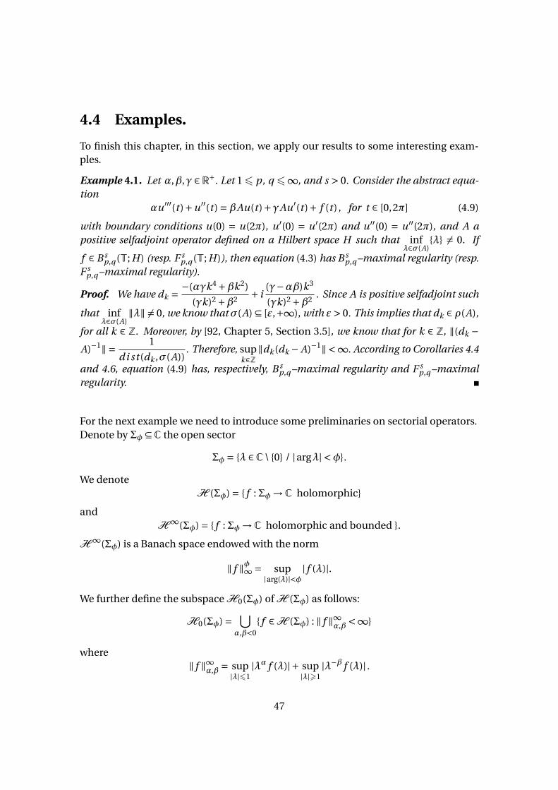
4.4 Examples.

To finish this chapter, in this section, we apply our results to some interesting exam-ples.

Example 4.1. Let α,β,γ ∈ R+. Let 1 6 p, q 6∞, and s > 0. Consider the abstract equa-tion

αu′′′(t )+u′′(t ) =βAu(t )+γAu′(t )+ f (t ) , for t ∈ [0,2π] (4.9)

with boundary conditions u(0) = u(2π), u′(0) = u′(2π) and u′′(0) = u′′(2π), and A apositive selfadjoint operator defined on a Hilbert space H such that inf

λ∈σ(A)λ 6= 0. If

f ∈ B sp,q (T; H) (resp. F s

p,q (T; H)), then equation (4.3) has B sp,q –maximal regularity (resp.

F sp,q –maximal regularity).

Proof. We have dk = −(αγk4 +βk2)

(γk)2 +β2+ i

(γ−αβ)k3

(γk)2 +β2. Since A is positive selfadjoint such

that infλ∈σ(A)

‖λ‖ 6= 0, we know thatσ(A) ⊆ [ε,+∞), with ε> 0. This implies that dk ∈ ρ(A),

for all k ∈ Z. Moreover, by [92, Chapter 5, Section 3.5], we know that for k ∈ Z, ‖(dk −A)−1‖ = 1

di st (dk ,σ(A)). Therefore, sup

k∈Z‖dk (dk − A)−1‖ <∞. According to Corollaries 4.4

and 4.6, equation (4.9) has, respectively, B sp,q –maximal regularity and F s

p,q –maximalregularity.

For the next example we need to introduce some preliminaries on sectorial operators.Denote by Σφ ⊆C the open sector

Σφ = λ ∈C\ 0 / |argλ| <φ.

We denoteH (Σφ) = f :Σφ→C holomorphic

andH ∞(Σφ) = f :Σφ→C holomorphic and bounded .

H ∞(Σφ) is a Banach space endowed with the norm

‖ f ‖φ∞ = sup|arg(λ)|<φ

| f (λ)|.

We further define the subspace H0(Σφ) of H (Σφ) as follows:

H0(Σφ) = ⋃α,β<0

f ∈H (Σφ) : ‖ f ‖∞α,β <∞

where‖ f ‖∞α,β = sup

|λ|61|λα f (λ)|+ sup

|λ|>1|λ−β f (λ)| .

47

Definition 4.3. [91] A closed linear operator A in X is called sectorial if the followingtwo conditions hold.

(i) We have D(A) = X , R(A) = X , and (−∞,0) ⊆ ρ(A).

(ii) We have supt>0 ‖t (t + A)−1‖6 M , for some M > 0.

A is called R–sectorial if the family t (t + A)−1t>0 is R–bounded. We denote the class ofsectorial operators (resp. R–sectorial operators) in X by S(X ) (resp. RS(X )).

If A ∈ S(X ), then Σφ ⊆ ρ(−A) , for some φ> 0 and sup|arg(λ)|<φ

‖λ(λ+ A)−1‖ <∞.

We denote the spectral angle of A ∈ S(X ) by

φA = infφ : Σπ−φ ⊆ ρ(−A) , sup

λ∈Σπ−φ‖λ(λ+ A)−1‖ <∞

Definition 4.4. Let A be a sectorial operator. If there exist φ>φA and a constant Kφ > 0such that

‖ f (A)‖6Kφ‖ f ‖φ∞ , for all f ∈H0(Σφ)

then we say that a sectorial operator A admits a bounded H ∞–calculus.

We denote the class of sectorial operators A which admit a bounded H ∞–calculus byH ∞(X ). Moreover, the H ∞–angle is defined by

φ∞A = infφ>φA : Definition (4.4) holds.

Remark 4.1. Let A be a sectorial operator which admits a bounded H ∞–calculus. If theset

h(A) : h ∈H ∞(Σθ) , ‖h‖θ∞6 1

is R–bounded for some θ > 0, we say that A admits an R–bounded H ∞–calculus. Wedenote the class of such operators by RH ∞(X ). The RH ∞–angle is analogous to theH ∞–angle, and is denoted θR∞

A . For further information about sectorial and R–sectorialoperators, see [91].

We state the following Proposition from functional calculus theory without proof (com-pare [52]). The proof of Lemma of 4.7 depends on this result.

Proposition 4.1. Let A ∈ RH ∞(X ) and suppose that hλλ∈Λ ⊆ H ∞(Σθ) is uniformlybounded for some θ > θR∞

A , where Λ is an arbitrary index set. Then the set hλ(A)λ∈Λ isR–bounded.

Lemma 4.7. Letα,β ∈R+. Assume that X is a U MD–space. Suppose that A ∈RH ∞(X ),with RH ∞–angle θR∞

A < π2 , then the families of operators

i k3(− iαk3 +k2

β− A

)−1k∈Z

and

i k A1/2

(− iαk3 +k2

β− A

)−1k∈Z

are R–bounded.

48

Proof. For every λ ∈C and z ∈Σπ/2, we define the functions

F 1(λ, z) = βλ3

αλ3 +λ2 −βzand F 2(λ, z) = βλz1/2

αλ3 +λ2 −βz.

We claim that there is a constant M > 0 such that supk∈Z

∥∥F j (i k, ·)∥∥H ∞(Σπ/2) 6 M ,

for j = 1,2. Indeed, note that

(αλ3 +λ2 −βz) = (αλ3 +λ2)(1− βz

αλ3 +λ2

).

Hence, there exists a constant M1 > 0 such that

|F 1(i k, z)| = |iβk3||iαk3 +k2|

∣∣∣1+ βziαk3+k2

∣∣∣ 6 M1∣∣∣1+ βziαk3+k2

∣∣∣ .

On the other hand, note also that

(αλ3 +λ2 −βz) =pαλ3 +λ2z1/2

(1− β1/2z1/2

pαλ3+λ2

)(β1/2 +

pαλ3+λ2

z1/2

).

Thus, there exists M2 > 0 such that

|F 2(i k, z)|6 M2∣∣∣1− β1/2z1/2p−iαk3−k2

∣∣∣∣∣∣β1/2 +p−iαk3−k2

z1/2

∣∣∣ .

Since z ∈Σπ/2, we have that the denominators never vanish. In addition, F 1(0, z) = 0 =F 2(0, z). Therefore, there exists M > 0 such that sup

k∈Z

∥∥F j (i k, ·)∥∥H ∞(Σπ/2) 6 M , for j = 1,2.

It follows from Proposition 4.1 that the sets F j (i k, A)k∈Z with j = 1,2 are R–bounded.In particular, for all k ∈Z the operators (−iαk3 −k2 −βA)−1 exist. Furthermore, for all

k ∈Z the operators(− iαk3 +k2

β− A

)−1exist in L (X ), and

i k3

(− iαk3 +k2

β− A

)−1k∈Z and

i k A1/2

(− iαk3 +k2

β− A

)−1k∈Z

are R–bounded families of operators.

Example 4.2. Let X be a U MD–space, and let p ∈ (1,∞). Suppose A ∈ RH ∞(X ), withRH ∞–angle θR∞

A < π2 . Consider the family of operators

F =

i k A1/2(− iαk3 +k2

β− A

)−1: k ∈Z

49

with α,β> 0. If γ> 0 is such that γβRp (F ) < 1, then the equation

αu′′′(t )+u′′(t ) =βAu(t )+γA1/2u′(t )+ f (t ), for t ∈ [0,2π] (4.10)

with boundary conditions u(0) = u(2π), u′(0) = u′(2π) and u′′(0) = u′′(2π), has Lp –maximal regularity.Proof. According to Lemma 4.7, the families of operators

i k A1/2(− iαk3 +k2

β− A

)−1

k∈Zand

i k3

(− iαk3 +k2

β− A

)−1k∈Z

are R–bounded. Sinceγ

βRp (F ) < 1, it follows from Corollary 4.1 that equation (4.10)

has Lp –maximal regularity.

50

CHAPTER 5

Periodic Solutions of a Fractional NeutralDifferential Equation with Finite Delay

It is well known that neutral functional differential equations are used to represent im-portant physical systems. We refer to [72, 76, 102] for a discussion about this aspect ofthe theory. Similarly, motivated by the fact that abstract neutral functional differentialequations (abbreviated, ANFDE) arise in many areas of applied mathematics, this typeof equations has received much attention in recent years ([49, 73, 76]). On the otherhand, because several important physical phenomena are modeled by abstract frac-tional differential equations, this type of equations have been studied extensively lasttime for many authors. We refer the reader to the works [2, 104, 120, 124, 135] and thereferences listed therein for recent information on this subject.

There exists several notions of fractional differentiation. In this thesis we use the frac-tional differentiation in sense of Liouville–Grünwald–Letnikov. This concept was in-troduced in [70, 105] and has been widely studied by several authors. In these worksthe fractional derivative is defined directly as a limit of a fractional difference quotient.In [35], the authors apply this approach based on fractional differences to study frac-tional differentiation of periodic scalar functions. This idea has been used to extendthe definition of fractional differentiation to vector–valued functions, (see [98]). In thecase of periodic functions this concept enables one to set up a fractional calculus inthe Lp setting with the usual rules, as well as provides a connection with the classicalWeyl fractional derivative (see [137]).

Let α> 0. Given f ∈ Lp (T; X ) for 16 p <∞ the Riemann difference

∆αt f (x) :=∞∑

j=0(−1) j

(α

j

)f (x − t j ),

51

(where

(α

j

)= α(α−1) · · · (α− j −1)

j !

)exists almost everywhere and

‖∆αt f ‖Lp (T;X ) 6∞∑

j=0

∣∣∣∣∣(α

j

)∣∣∣∣∣‖ f ‖Lp (T;X )

since∑∞

j=0 |(α

j

)| <∞ (see [35]).

The following definition is a direct extension of Definition 2.1 in [35] to vector–valuedcase. See [98] for its connection with differential equations.

Definition 5.1. Let X be a complex Banach space,α> 0 and 16 p <∞. Let f ∈ Lp (T; X ).If there exists g ∈ Lp (T; X ) such that limt→0+ t−α∆αt f = g in the Lp (T; X ) norm, then g iscalled the αth–Liouville–Grünwald–Letnikov derivative of f in the mean of order p.

We abbreviate this terminology by αth-derivative and we denote it by Dα f = g .

Example 5.1. Theαth-derivative of e i ax for any real a is given by (i a)e i ax . In particular,Dα sin x = sin

(x + π

2α)

and Dα cos x = cos(x + π

2α).

We also mention here a few properties of this fractional derivative. The proof followsthe same steps as in the scalar case given in Proposition 4.1 in [35].

Proposition 5.1. Let 1 6 p <∞ and f ∈ Lp (T; X ). For α,β > 0 the following propertieshold:

(a) If Dα f ∈ Lp (T; X ), then Dβ f ∈ Lp (T; X ) for all 0 <β<α.

(b) DαDβ f = Dα+β f whenever one of the two sides is well defined.

Let f ∈ Lp (T; X ) and α > 0. It has been proved by Butzer and Westphal [35] thatDα f ∈ Lp (T; X ) if and only if there exists g ∈ Lp (T; X ) such that (i k)α f (k) = g (k), where

(i k)α = |k|αeπiα

2 sgn(k). In this case Dα f = g .

In this chapter, we study a characterization of maximal regularity on Besov and Triebel–Lizorkin spaces of fractional differential equation with finite delay

Dαu(t ) = Au(t )+Fut +GDβut + f (t ), t ∈ [0,2π], and 0 <β<α6 2. (5.1)

with different periodic boundary conditions depending on the values of α and β. Theyare

u(0) = u(2π) if 0 <β<α6 1

Dα−1u(0) = Dα−1(2π) and u(0) = u(2π) if 0 <β< 1 <α6 2

Dα−1u(0) = Dα−1(2π) , u(0) = u(2π) andDβ−1u(0) = Dβ−1(2π) if 1 <β<α6 2

52

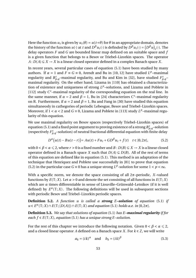
Here the function ut is given by ut (θ) = u(t+θ) for θ in an appropriate domain, denotesthe history of the function u(·) at t and Dβut (·) is definded by Dβut (·) = (

Dβu)

t (·). Thedelay operators F and G are bounded linear map defined on an suitable space and fis a given function that belongs to a Besov or Triebel–Lizorkin spaces. The operatorA : D(A) ⊆ X → X is a linear closed operator defined in a complex Banach space X .

In recent years, several particular cases of equation (5.1) have been studied by manyauthors. If α = 1 and F ≡ G ≡ 0, Arendt and Bu in [10, 12] have studied Lp –maximalregularity and B s

p,q –maximal regularity, and Bu and Kim in [32], have studied F sp,q –

maximal regularity. On the other hand, Lizama in [110] has obtained a characteriza-tion of existence and uniqueness of strong Lp –solutions, and Lizama and Poblete in[112] study C s–maximal regularity of the corresponding equation on the real line. Inthe same manner, if α = 2 and β = 1, Bu in [24] characterizes C s–maximal regularityon R. Furthermore, if α = 2 and β = 1, Bu and Fang in [30] have studied this equationsimultaneosly in cathegories of periodic Lebesgue, Besov and Triebel–Lizorkin spaces.Moreover, if 1 <α< 2 and G ≡ 0, Lizama and Poblete in [113] study Lp –maximal regu-larity of this equation.

We use maximal regularity on Besov spaces (respectively Triebel–Lizorkin spaces) ofequation (5.1) and a fixed point argument to proving existence of a strong B s

p,q –solution(respectively F s

p,q –solution) of neutral fractional differential equation with finite delay

Dα(u(t )−Bu(t − r )

)= Au(t )+Fut +GDβut + f (t ) t ∈ [0,2π], (5.2)

with 0 <β<α6 2, where r > 0 is a fixed number and B : D(B) ⊆ X → X is a linear closedoperator defined in a Banach space X such that D(A) ⊆ D(B). All of the rest of termsof this equation are defined like in equation (5.1). This method is an adaptation of thetechnique that Henriquez and Poblete use successfully in [81] to prove that equation(5.2) in the particular case G ≡ 0 has a unique strong Lp -solution for some 1 < p <∞.

With a specific norm, we denote the space consisting of all 2π–periodic, X –valuedfunctions by E(T; X ). Let α> 0 and denote the set consisting of all functions in E(T; X )which are α times differentiable in sense of Liouville–Grünwald–Letnikov (if it is welldefined) by Eα(T; X ) . The following definitions will be used in subsequent sectionswith periodic Besov and Triebel–Lizorkin periodic spaces.

Definition 5.2. A function u is called a strong E–solution of equation (5.1) ifu ∈ Eα(T; X )∩E(T; [D(A)])∩E(T; X ) and equation (5.1) holds a.e. in [0,2π].

Definition 5.3. We say that solutions of equation (5.1) has E–maximal regularity if foreach f ∈ E(T; X ), equation (5.1) has a unique strong E–solution.

For the rest of this chapter we introduce the following notation. Given 0 < β < α6 2,and a closed linear operator A defined on a Banach space X . For k ∈Z, we will write

ak = (i k)α and bk = (i k)β (5.3)

53

and the bounded operators Fk and Gk defined by

Fk x = F (ek x) and Gk x =G(ek x), where ek x(t ) = e i kt x. (5.4)

Moreover, we will denote

Nk = (ak I −Fk −bkGk − A)−1. (5.5)

andMk = ak

(ak I −bkGk −Fk − A

)−1 = ak Nk (5.6)

In order to give conditions which we will need later, we say that Fk k∈Z satisfies thecondition

(F2) If the family of operators

k2

ak

(∆2Fk

)k∈Z\0

is a bounded.

(F3) If Fk k∈Z satisfies (F2) and the family

k3

ak

(∆3Fk

)k∈Z\0

is bounded.

In the same manner, we say that the family Gk k∈Z satisfies the condition

(G2) If the families of operators

kbk

ak

(∆1Gk

)k∈Z\0

and

k2bk

ak

(∆2Gk

)k∈Z\0

are

bounded.

(G3) If Gk k∈Z satisfies (G2) and the family

k3bk

ak

(∆3Gk

)k∈Z\0

is bounded.

5.1 Periodic Strong B sp,q–solution.

The first objective of this section is the study B sp,q –maximal regularity of equation (5.1).

For this purpose, givenα> 0 we present a characterization of the Besov space B s+αp,q (T; X )

in terms of Liouville–Grünwald–Letnikov fractional derivative.

Proposition 5.2. Let α > 0 and a function u ∈ B sp,q (T; X ) with 1 6 p, q 6∞ and s > 0.

Dαu ∈ B sp,q (T; X ) if and only if there exists g ∈ B s

p,q (T; X ) such that (i k)αu(k) = g (k),and in this case Dαu = g . In fact we have

B s+αp,q (T; X ) = u ∈ B s

p,q (T; X ) : Dαu ∈ B sp,q (T; X ).

54

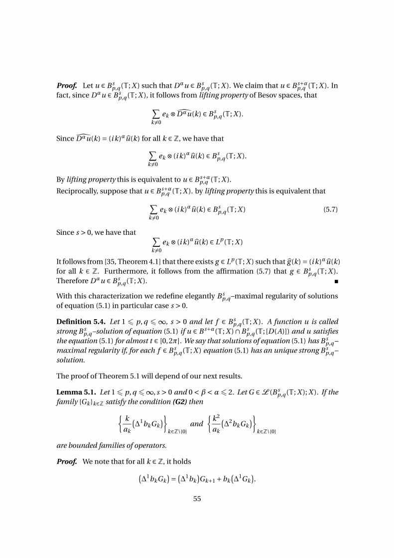
Proof. Let u ∈ B sp,q (T; X ) such that Dαu ∈ B s

p,q (T; X ). We claim that u ∈ B s+αp,q (T; X ). In

fact, since Dαu ∈ B sp,q (T; X ), it follows from lifting property of Besov spaces, that∑

k 6=0ek ⊗ Dαu(k) ∈ B s

p,q (T; X ).

Since Dαu(k) = (i k)αu(k) for all k ∈Z, we have that∑k 6=0

ek ⊗ (i k)αu(k) ∈ B sp,q (T; X ).

By lifting property this is equivalent to u ∈ B s+αp,q (T; X ).

Reciprocally, suppose that u ∈ B s+αp,q (T; X ). by lifting property this is equivalent that∑

k 6=0ek ⊗ (i k)αu(k) ∈ B s

p,q (T; X ) (5.7)

Since s > 0, we have that ∑k 6=0

ek ⊗ (i k)αu(k) ∈ Lp (T; X )

It follows from [35, Theorem 4.1] that there exists g ∈ Lp (T; X ) such that g (k) = (i k)αu(k)for all k ∈ Z. Furthermore, it follows from the affirmation (5.7) that g ∈ B s

p,q (T; X ).Therefore Dαu ∈ B s

p,q (T; X ).

With this characterization we redefine elegantly B sp,q –maximal regularity of solutions

of equation (5.1) in particular case s > 0.

Definition 5.4. Let 1 6 p, q 6 ∞, s > 0 and let f ∈ B sp,q (T; X ). A function u is called

strong B sp,q –solution of equation (5.1) if u ∈ B s+α(T; X )∩B s

p,q (T; [D(A)]) and u satisfiesthe equation (5.1) for almost t ∈ [0,2π]. We say that solutions of equation (5.1) has B s

p,q –maximal regularity if, for each f ∈ B s

p,q (T; X ) equation (5.1) has an unique strong B sp,q –

solution.

The proof of Theorem 5.1 will depend of our next results.

Lemma 5.1. Let 1 6 p, q 6∞, s > 0 and 0 < β< α6 2. Let G ∈ L (B sp,q (T; X ); X ). If the

family Gk k∈Z satisfy the condition (G2) thenk

ak

(∆1bkGk

)k∈Z\0

and

k2

ak

(∆2bkGk

)k∈Z\0

are bounded families of operators.

Proof. We note that for all k ∈Z, it holds(∆1bkGk

)= (∆1bk

)Gk+1 +bk

(∆1Gk

).

55

Therefore, for all k ∈Z\ 0,

k

ak(∆1bkGk ) = k

(∆1bk

)bk

bk

akGk+1 +

kbk

ak

(∆1Gk

).

On the other hand, for all k ∈Zwe have(∆2bkGk

)= (∆1bk+1

)[(∆1Gk+1)+ (∆1Gk )

]+ (∆2bk

)Gk +bk+1

(∆2Gk

).

Therefore, for all k ∈Z\ 0 we have,

k2

ak(∆2bkGk ) = k(∆1bk+1)

bk

kbk

ak[(∆1Gk+1)+ (∆1Gk )]+ k2(∆2bk )

bk

bk

akGk +

k2bk+1

ak(∆2Gk ).

Since the sequence bk k∈Z is 2–regular and supk∈Z

‖Gk‖6C‖G‖ for some C > 0, it follows

from the hypothesis thatk

ak

(∆1bkGk

)k∈Z\0

and

k2

ak

(∆2bkGk

)k∈Z\0

are bounded families.

Lemma 5.2. Let 1 6 p, q 6∞, s > 0 and 0 <β<α6 2. Let A be a linear closed operatordefined in a Banach space X and F,G ∈L (B s

p,q (T; X ); X ). Assume that for all k ∈Z, theoperators Nk are well defined in L (X ). If the family Fk k∈Z satisfies the condition (F2)and Gk k∈Z satisfies (G2) and the family of operators Mk k∈Z is bounded then

kak(∆1Nk

)k∈Z and

k2ak

(∆2Nk

)k∈Z

are bounded families of operators.

Proof. We note that for all k ∈Z it holds(∆1Nk

) = Nk+1(ak −Fk −bkGk −ak+1 +Fk+1 +bk+1Gk+1

)Nk

= (−∆ak)Nk+1Nk +Nk+1

(∆1Fk

)Nk +Nk+1

(∆1bkGk

)Nk .

(5.8)

Therefore, for all k ∈Z\ 0

kak(∆1Nk

)= k

(−∆1ak)

akak Nk+1Mk +

k

akak Nk+1

(∆1Fk

)Mk +ak Nk+1

k

ak

(∆1bkGk

)Mk .

A direct computation, shows that kak(∆1Nk

)is bounded if k = 0. Since the sequence

ak k∈Z is 2–regular and the families of operators Fk k∈Z and Gk k∈Z are bounded, itfollows from Lemma 5.1 that

kak

(∆1Nk

)k∈Z is a bounded family of operators.

56

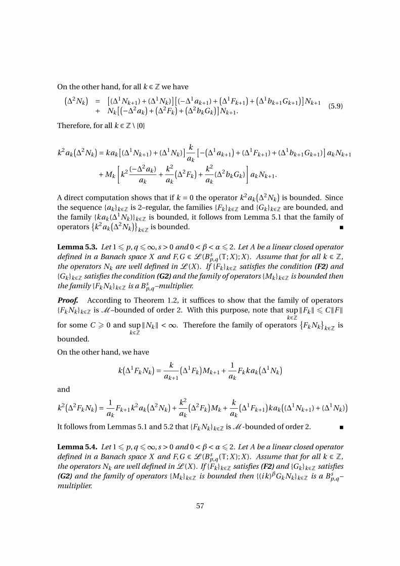
On the other hand, for all k ∈Zwe have(∆2Nk

) = [(∆1Nk+1)+ (∆1Nk )

][(−∆1ak+1)+ (

∆1Fk+1)+ (

∆1bk+1Gk+1)]

Nk+1

+ Nk[(−∆2ak

)+ (∆2Fk

)+ (∆2bkGk

)]Nk+1.

(5.9)

Therefore, for all k ∈Z\ 0

k2ak(∆2Nk

)= kak[(∆1Nk+1)+ (∆1Nk )

] k

ak

[−(∆1ak+1

)+ (∆1Fk+1)+ (∆1bk+1Gk+1)]

ak Nk+1

+Mk

[k2 (−∆2ak )

ak+ k2

ak

(∆2Fk

)+ k2

ak(∆2bkGk )

]ak Nk+1.

A direct computation shows that if k = 0 the operator k2ak(∆2Nk

)is bounded. Since

the sequence ak k∈Z is 2–regular, the families Fk k∈Z and Gk k∈Z are bounded, andthe family kak (∆1Nk )k∈Z is bounded, it follows from Lemma 5.1 that the family ofoperators

k2ak

(∆2Nk

)k∈Z is bounded.

Lemma 5.3. Let 1 6 p, q 6∞, s > 0 and 0 <β<α6 2. Let A be a linear closed operatordefined in a Banach space X and F,G ∈ L (B s

p,q (T; X ); X ). Assume that for all k ∈ Z,the operators Nk are well defined in L (X ). If Fk k∈Z satisfies the condition (F2) andGk k∈Z satisfies the condition (G2) and the family of operators Mk k∈Z is bounded thenthe family Fk Nk k∈Z is a B s

p,q –multiplier.

Proof. According to Theorem 1.2, it suffices to show that the family of operatorsFk Nk k∈Z is M–bounded of order 2. With this purpose, note that sup

k∈Z‖Fk‖ 6 C‖F‖

for some C > 0 and supk∈Z

‖Nk‖ < ∞. Therefore the family of operatorsFk Nk

k∈Z is

bounded.

On the other hand, we have

k(∆1Fk Nk

)= k

ak+1

(∆1Fk

)Mk+1 +

1

akFk kak

(∆1Nk

)and

k2(∆2Fk Nk)= 1

akFk+1k2ak

(∆2Nk

)+ k2

ak

(∆2Fk

)Mk +

k

ak

(∆1Fk+1

)kak

((∆1Nk+1)+ (∆1Nk )

)It follows from Lemmas 5.1 and 5.2 that Fk Nk k∈Z is M -bounded of order 2.

Lemma 5.4. Let 1 6 p, q 6∞, s > 0 and 0 <β<α6 2. Let A be a linear closed operatordefined in a Banach space X and F,G ∈ L (B s

p,q (T; X ); X ). Assume that for all k ∈ Z,the operators Nk are well defined in L (X ). If Fk k∈Z satisfies (F2) and Gk k∈Z satisfies(G2) and the family of operators Mk k∈Z is bounded then (i k)βGk Nk k∈Z is a B s

p,q –multiplier.

57

Proof. According to Theorem 1.2 it suffices to show that the family of operators(i k)βGk Nk k∈Z is M–bounded of order 2.For this, note that sup

k∈Z‖Gk‖6C‖G‖ for some C > 0 and sup

k∈Z‖bk Nk‖ <∞.

Therefore(i k)βGk Nk

k∈Z is bounded.

On the other hand, we have

k(∆1bkGk Nk

)= k

ak

(∆1bkGk

)ak Nk+1 +

bk

akGk kak

(∆1Nk

)and

k2(∆2bkGk Nk)= k

ak

(∆1bk+1Gk+1

)kak

[(∆1Nk+1

)+ (∆1Nk

)]+ k2

ak(∆2bkGk )Mk

+ bk+1

akGk+1k2ak

(∆2Nk

).

It follows from Lemmas 5.1 and 5.2 that (i k)βGk Nk k∈Z is M -bounded of order 2.

Lemma 5.5. Let 1 6 p, q 6∞, s > 0 and 0 <β<α6 2. Let A be a linear closed operatordefined in a Banach space X and F,G ∈L (B s

p,q (T; X ); X ). Assume that for all k ∈Z, theoperators Nk are well defined in L (X ). If Fk k∈Z satisfies (F2) and Gk k∈Z satisfies (G2)then the following assertions are equivalent

(i) The family of operators Mk k∈Z is a bounded.

(ii) The family of operators Mk k∈Z is a B sp,q –multiplier.

Proof. (i ) ⇒ (i i ). According Theorem 1.2 it suffices to show that that Mk k∈Z isM–bounded of order 2. By hypothesis, sup

k∈Z‖Mk‖ <∞. We note that

k(∆1Mk ) = k(∆1ak )

ak+1Mk+1 +kak (∆1Nk ).

On the other hand, we have

k2(∆2Mk)= k

(∆1ak+1

)ak

kak[(∆1Nk+1)+ (∆1Nk

)]+ k2(∆2ak

)ak

Mk +k2ak+1(∆2Nk

).

Since the sequence ak k∈Z is 2–regular, it follows from Lemmas 5.1 and 5.2 that Mk k∈Zis M–bounded of order 2.

(i i ) ⇒ (i ). It follows from Closed Graph Theorem that there exists C > 0 (independentof f ) such that for f ∈ B s

p,q (T; X ) we have,∥∥∥∑k∈Z

ek ⊗Mk f (k)∥∥∥

B sp,q

6C∥∥ f

∥∥B s

p,q.

58

Let x ∈ X and define f (t ) = e i kt x for k ∈Z fixed. Then the above inequality implies

‖ek‖B sp,q

‖Mk x‖B sp,q

= ‖ek Mk x‖B sp,q

6C‖ek‖B sp,q

‖x‖B sp,q

.

Hence for all k ∈Zwe have ‖Mk‖6C . Thus supk∈Z

‖Mk‖ <∞.

Next Theorem establishes a characterization of B sp,q –maximal regularity of solution of

equation (5.1).

Theorem 5.1. Let 1 6 p, q 6∞, s > 0. Let be X a Banach space. If the families Fk k∈Zand Gk k∈Z, defined by the operators F and G of equation (5.1) satisfy the conditions(F2) and (G2) respectively, then the following assertions are equivalent

(i) The solution of equation (5.1) has B sp,q –maximal regularity.

(ii) Nk k∈Z ⊆L (X ) and the family Mk k∈Z is bounded.

Proof. (i ) ⇒ (i i ). We show that for k ∈ Z the operators ((i k)αI − (i k)βGk − Fk − A)are invertible. For this, let k ∈ Z fixed and x ∈ X , and define h(t ) = e i kt x, a direct cal-culation shows that h(k) = x. By hypothesis there exists a function u ∈ B s+α

p,q (T; X )∩B s

p,q (T; [D(A)]) such that , for almost all t ∈ [0,2π], we have

Dαu(t ) = Au(t )+Fut +GDβut +h(t ).

Applying Fourier transform to both sides of the preceding equality, we obtain((i k)α−Fk − (i k)βGk − A

)u(k) = h(k) = x,

since x and k are arbitrary, we have that for k ∈Z the operators((i k)α−Fk−(i k)βGk−A

)are surjective.

On the other hand, let z ∈ D(A), and assume that ((i k)α−Fk − (i k)βGk − A)z = 0. Sub-stituting u(t ) = e i kt z in the equation (5.1) we see that u is a periodic solution of thisequation when f ≡ 0. The uniqueness of solution implies that z = 0.

Since for all k ∈Z the linear operators Nk are closed defined in whole space X , it followsfrom Closed Graph Theorem that Nk ∈L (X ). Thus Nk k∈Z ⊆L (X ).

Let f ∈ B sp,q (T; X ). By hypothesis, there exists a function u ∈ B s+α

p,q (T, X )∩B sp,q (T, [D(A)])

such that u is the unique strong solution of the equation

Dαu(t ) = Au(t )+Fut +GDβut + f (t ), t ∈ [0,2π].

Applying Fourier transform to both sides of the preceding equation, we have((i k)α−Fk − (i k)βGk − A

)u(k) = f (k)

59

for all k ∈ Z. Since for all k ∈ Z the operator((i k)α−Fk − (i k)βGk − A

)is invertible, we

haveu(k) = (

(i k)α−Fk − (i k)βGk − A)−1 f (k) for all k ∈Z.

Hence, (i k)αu(k) = Dαu(k) = (i k)αNk f (k) = Mk f (k) for all k ∈Z.Since u ∈ B s+α

p,q (T; X ), by Proposition 5.2 we have that Dαu ∈ B sp,q (T; X ). Therefore

the family Mk k∈Z is a B sp,q –multiplier. It follows from Lemma 5.5 that Mk k∈Z is a

bounded family of operators.

(i i ) ⇒ (i ). By hypothesis, the conditions of Lemma 5.5 are satisfied. Therefore, Mk k∈Zis a B s

p,q –multiplier. Define the family of operator Ik k∈Z, by Ik = 1(i k)α I when k 6= 0 and

I0 = I . It follows from Theorem 1.2 that Ik k∈Z is a B sp,q –multiplier. Since Nk = Ik Lk

for all k ∈ Z \ 0 we have Nk k∈Z is a B sp,q –multiplier. Accordingly, given a arbitrary

function f ∈ B sp,q (T; X ) there exist functions u, w ∈ B s

p,q (T, X ) such that

u(k) = Nk f (k) and w(k) = (i k)αNk f (k) for all k ∈Z. (5.10)

Therefore,w(k) = (i k)αu(k) = Dαu(k) for all k ∈Z.

By the uniqueness of the Fourier coefficients, Dαu = w . This implies that that Dαu ∈B s

p,q (T; X ). It follows from Proposition 5.2 that u ∈ B s+αp,q (T; X ).

On the other hand, it follows from Lemma 5.3 that Fk Nk k∈Z is a B sp,q –multiplier. Con-

sequently, there exists a function g ∈ B sp,q (T; X ) such that

g (k) = Fk Nk f (k) for all k ∈Z.

By equality (5.10) we have

g (k) = Fk u(k) for all k ∈Z.

A direct computation shows that Fut (k) = Fk u(k) for all k ∈Z. By the uniqueness of theFourier coefficients, Fut = g . This implies that that Fut ∈ B s

p,q (T; X ).

In the same manner, it follows from Lemma 5.4 that (i k)βGk Nk k∈Z is a B sp,q –multiplier.

Hence there exists a function h ∈ B sp,q (T; X ) such that

h(k) = (i k)βGk Nk f (k) for all k ∈Z.

By equality (5.10) we have

h(k) = (i k)βGk u(k) for all k ∈Z.

A direct computation shows that (i k)βGk u(k) = àGDβut (k) for all k ∈Z. By the unique-ness of the Fourier coefficients, GDβut = h. This implies that that GDβut ∈ B s

p,q (T; X ).

60

It follows from equality (5.10) that

u(k) = ((i k)α−Fk − (i k)βGk − A

)−1 f (k).

Thus, ((i k)α−Fk − (i k)βGk − A

)u(k) = f (k)

for all k ∈ Z. Using the fact that A is a closed operator, we have that u(t ) ∈ D(A) foralmost t ∈ [0,2π]. Moreover, by uniqueness of Fourier coefficients we have

Dαt u(t ) = Au(t )+Fut +GDβut + f (t )

for almost t ∈ [0,2π]. Since f ,Fut ,GDβut and Dαu ∈ B sp,q (T; X ), we conclude that Au ∈

B sp,q (T; X ). This implies that u ∈ B s

p,q (T; [D(A)]). Therefore, u is a strong B sp,q –solution

of equation (5.1).

Since((i k)αI −(i k)βGk −Fk −A

)−1 is invertible for all k ∈Z, this strong B sp,q –solution is

unique. Therefore the solution of equation (5.1) has B sp,q –maximal regularity.

As we have mentioned, the verification of assumptions concerning the family Nk k∈Zis not an easy work. Our next Corollary require additional conditions about the opera-tors A, F and G , however is a more practical result to check that (i k)αNk is bounded.Let α> 1, define the operators Sk = ((i k)α− A)−1, for all k ∈Z.

Corollary 5.1. Let 1 6 p, q 6 ∞, s > 0. Let be X a Banach space. Assume that(i k)αk∈Z ⊆ ρ(A) and the families Fk k∈Z and Gk k∈Z, defined by the operators F andG of equation (5.1) satisfy the conditions (F2) and (G2) respectively. If the family of oper-

ators(i k)α

((i k)α− A

)−1k∈Z is bounded, and supk∈Z

∥∥∥((i k)βGk +Fk

)Sk

∥∥∥< 1 then equation

(5.1) has B sp,q –maximal regularity.

Proof. Since supk∈Z

∥∥((i k)βGk +Fk

)Sk

∥∥< 1, we have that the family

(I − (

(i k)βGk +Fk)Sk

)−1

k∈Z

is bounded. In addition

Nk =[(

(i k)α− A)(

I − ((i k)βGk +Fk

)Sk

)]−1

= (I − (

(i k)βGk +Fk)Sk

)−1((i k)α− A)−1.

Therefore the family (i k)αNk k∈Z is bounded. Since the families Fk k∈Z and Gk k∈Zsatisfy the conditions (F2) and (G2) respectively, it follows from Theorem 5.1 that equa-tion (5.1) has B s

p,q –maximal regularity.

61

5.2 Periodic Strong B sp,q–solutions of a Neutral Fractional

Differential Equation with Finite Delay

In this section, as we have said, we use the results about B sp,q –maximal regularity of

solution of equation (5.1) to prove that fractional neutral differential equation

Dα(u(t )−Bu(t − r )

)= Au(t )+Fut +GDβut + f (t ), (5.11)

has a periodic strong B sp,q –solution.

Note that, if equation (5.1) has B sp,q –maximal regularity for some 1 6 p, q 6 ∞ and

s > 0, the linear map Ψ : B sp,q (T; X ) → B s

p,q (T; X ) given by Ψ(g ) = Dαv , is well defined.Here v is the unique strong B s

p,q –solution of the equation

Dαv = Au +Fut +GDβut + g (t ). (5.12)

Lemma 5.6. Let 1 6 p, q 6 ∞, s > 0, and 1 6 β 6 α. Let be X a Banach space. As-sume that B is a bounded operator, for all k ∈ Z the operators Nk is well defined inL (X ) and the families Fk k∈Z and Gk k∈Z defined by the operators F and G of equa-tion (5.11) satisfy the conditions (F2) and (G2) respectively. If (i k)αNk k∈Z is a boundedfamily of operators, such that supk∈Z |k|α‖B‖‖Nk‖ < 1 and ‖B‖‖Ψ‖ < 1, then the family(I −e−i kr (i k)αB Nk )−1k∈Z is a B s

p,q –multiplier.

Proof. Denote Rk = (I −e−i kr (i k)αB Nk )−1 for all k ∈Z. Since supk∈Z

|k|α‖B‖‖Nk‖ < 1, the

family Rk k∈Z ⊆L (X ). Let f ∈ B sp,q (T; X ). Define the map P : B s

p,q (T; X ) → B sp,q (T; X )

byPϕ(t ) = BΨ(ϕ)(t − r )+ f (t ).

By Theorem 5.1 the map P is well defined. Moreover P is a contraction, thus thereexists a function g ∈ B s

p,q (T; X ) such that

g (t ) = BΨ(g )(t − r )+ f (t ) = BDαu(t − r )+ f (t ), (5.13)

where u is the unique strong B sp,q –solution of the equation

Dαu(t ) = Au(t )+Fut +GDβut + g (t ) t ∈ [0,2π], 0 <β<α6 2. (5.14)

Applying Fourier transform to both side of equation (5.13) we have

g (k) = e−i kr (i k)αBu(k)+ f (k) for all k ∈Z (5.15)

On the other hand, applying Fourier transform to both sides of equation (5.14) we have

u(k) = Nk g (k) for all k ∈Z (5.16)

62

Thereforeg (k) = e−i kr (i k)αB Nk g (k)+ f (k) for all k ∈Z.

This implies that g (k) = Rk f (k) for all k ∈Z.Hence, the family of operators (I −e−i kr (i k)αB Nk )−1k∈Z is a B s

p,q –multiplier.

Next Theorem gives sufficient condition that guarantee existence of a strongB s

p,q –solution of equation (5.11). We use the notation introduced in preceding Lemma.

Theorem 5.2. Let 1 6 p, q 6 ∞, s > 0, and 0 < β < α 6 2. Let be X a Banach space.Assume that B is a bounded operator, for all k ∈ Z the operators Nk is well defined inL (X ) and the families Fk k∈Z and Gk k∈Z defined by the operators F and G of equation(5.11) satisfy the conditions (F2) and (G2) respectively. If (i k)αNk k∈Z is a boundedfamily of operators, such that supk∈Z |k|α‖B‖‖Nk‖ < 1 and ‖B‖‖Ψ‖ < 1, then for everyf ∈ B s

p,q (T; X ) there exists an unique strong B sp,q –solution of Equation (5.11).

Proof. It follows from Lemma 5.6 that the family of operators (I−e−i kr (i k)αB Nk )−1k∈Zis a B s

p,q –multiplier. Denote Rk = (I − e−i kr (i k)αB Nk )−1. Let f ∈ B sp,q (T; X ). Since

Rk k∈Z is B sp,q –multiplier, there exists g ∈ B s

p,q (T; X ) such that

g (k) = Rk f (k) for all k ∈Z. (5.17)

On the other hand, by Theorem 5.1, there exists a function u ∈ B sp,q (T; X ) such that u is

the unique strong B sp,q –solution of equation

Dαu(t ) = Au(t )+Fut +GDβut + g (t ), t ∈ [0,2π], 0 <β<α6 2. (5.18)

Applying Fourier transform to both side of the preceding equality we have

u(k) = Nk g (k) for all k ∈Z. (5.19)

It follows from equality (5.17) that

u(k) = Nk Rk f (k) for all k ∈Z. (5.20)

Note that

Nk Rk = ((i k)α−e−i kr (i k)αB − (i k)βGk −Fk − A

)−1 for all k ∈Z.

Thus, ((i k)α−e−i kr (i k)αB − (i k)βGk −Fk − A

)u(k) = f (k) for all k ∈Z.

Since A is a closed linear operator, it follows from uniqueness of Fourier coefficientsthat u satisfies the equation

Dα(u(t )−Bu(t − r )

)= Au(t )+Fut +GDβut + f (t ) for almost t ∈ [0,2π].

63

Therefore u is a strong B sp,q –solution of equation (5.11). It only remains to show that

the strong B sp,q –solution is unique. Indeed let f ∈ B s

p,q (T; X ). Suppose equation (5.11)has two strong B s

p,q –solutions, u1 and u2. A direct computation shows that((i k)α−e−i kr (i k)αB − (i k)βGk −Fk − A

)(u1(k)− u2(k)) = 0

for all k ∈Z. Since((i k)α−e−i kr (i k)αB − (i k)βGk −Fk − A

)is invertible, for all k ∈Zwe

have that u1(k) = u2(k). By the uniqueness of the Fourier coefficients, u1 ≡ u2.

5.3 Periodic Strong F sp,q–solution.

Recall, we are studying the equations

Dαu(t ) = Au(t )+Fut +GDβut + f (t ), (5.21)

and

Dα(u(t )−Bu(t − r )

)= Au(t )+Fut +GDβut + f (t ), (5.22)

where all terms of these equations are defined in (5.1) and (5.2). Our approach is simi-lar as that of preceding section. For this reason, the first objective of this section is thestudy F s

p,q –maximal regularity of equation (5.21). For this purpose, in the same mannerof preceding section, given α> 0 we present a characterization of the Triebel–Lizorkinspace F s+α

p,q (T; X ) in terms of Liouville–Grünwald–Letnikov fractional derivative.

Proposition 5.3. Let α > 0 and a function u ∈ F sp,q (T; X ) with 1 6 p, q 6∞ and s > 0.

Dαu ∈ F sp,q (T; X ) if and only if there exists g ∈ F s

p,q (T; X ) such that (i k)αu(k) = g (k), andin this case Dαu = g . In fact we have

F s+αp,q (T; X ) = u ∈ F s

p,q (T; X ) : Dαu ∈ F sp,q (T; X ).

Proof. The proof follows the same lines as those of proof Proposition 5.2

With this characterization we redefine elegantly F sp,q –maximal regularity of solutions

of equation (5.21) when s > 0.

Definition 5.5. Let 1 6 p, q 6 ∞, s > 0 and let f ∈ F sp,q (T; X ). A function u is called

strong F sp,q –solution of equation (5.21) if u ∈ F s+α(T; X )∩F s

p,q (T; [D(A)]) and u satisfiesthe equation (5.21) for almost t ∈ [0,2π]. We say that equation (5.21) has F s

p,q –maximalregularity if, for each f ∈ F s

p,q (T; X ) equation (5.21) has a unique strong F sp,q –solution.

The proof of Theorem 5.3 will depend of our next results.

64

Lemma 5.7. Let 1 6 p, q 6 ∞, s > 0 and 0 < β < α 6 2. Let G ∈ L (F sp,q (T; X ); X ). If

Gk k∈Z satisfy (G3) then k3

ak

(∆3bkGk

)k∈Z\0

is a bounded family of operators.

Proof. We note that for all k ∈Z it holds

(∆3bkGk ) = bk (∆3Gk )+ (bk+3 −bk )(∆2Gk+1)+ (∆2bk+1)(∆1Gk+1)

+ (∆3bk )Gk+2 −2(∆2bk )(∆1Gk+1).

Therefore, for all k ∈Z\ 0 we have

k3

ak(∆3bkGk ) = kbk

ak(∆3Gk )+ k(bk+3 −bk )

bk

k2bk

ak(∆2Gk+1)+ k2(∆2bk+1)

bk

kbk

ak(∆1Gk+1)

+ k3(∆3bk )

bk

bk

akGk+2 −2

k2(∆2bk )

bk

kbk

ak(∆1Gk+1).

Since the sequence bk k∈Z is 3–regular and Gk k∈Z is a bounded family satisfying con-dition (G3) it follows from Lemma 5.1 that

k3

ak

(∆3bkGk

)k∈Z\0

is a bounded family of operators.

Lemma 5.8. Let 1 6 p, q 6∞, s > 0 and 0 <β<α6 2. Let A be a linear closed operatordefined in a Banach space X and F,G ∈L (F s

p,q (T; X ); X ). Assume that for all k ∈Z, theoperators Nk are well defined in L (X ). If the family Fk k∈Z satisfies the condition (F3)and Gk k∈Z satisfies (G3) and the family of operators Mk k∈Z is bounded then

k3ak(∆3Nk

)k∈Z

is a bounded family of operators.

Proof. We note that for all k ∈Z it holds

(∆3Nk ) = [(∆2Nk+1)+ (∆2Nk )

][(−∆1ak+2)+ (∆1Fk+2)+ (∆1bk+2Gk+2)

]Nk+1

+ [(∆1Nk+1)+ (∆1Nk )

][(−∆2ak+1)+ (∆2Fk )+ (∆2bk+1Gk+1)

]Nk+1

+ [(∆1Nk+1)+ (∆1Nk )

][(−∆1ak+1)+ (∆1Fk )+ (∆1bk+1Gk+1)

](∆1Nk )

+ (∆1Nk )[(−∆2ak+1)+ (∆2Fk+1)+ (∆2bk+1Gk+1)

]Nk+2

+ Nk[(−∆3ak )+ (∆3Fk )+ (∆3bkGk )

]Nk+2

+ Nk[(−∆2ak )+ (∆2Fk )+ (∆2bkGk )

](∆1Nk+1).

65

Therefore,

k3ak (∆3Nk ) = k2ak[(∆2Nk+1)+ (∆2Nk )

] k

ak+1

[(−∆1ak+2)+ (∆1Fk+2)+ (∆1bk+2Gk+2)

]Mk+1

+kak[(∆1Nk+1)+ (∆1Nk )

] k2

ak

[(−∆2ak+1)+ (∆2Fk )+ (∆2bk+1Gk+1)

]Mk+1

+kak[(∆1Nk+1)+ (∆1Nk )

] k

ak

[(−∆1ak+1)+ (∆1Fk )+ (∆1bk+1Gk+1)

]kak (∆1Nk )

+kak (∆1Nk )k2

ak+1

[(−∆2ak+1)+ (∆2Fk+1)+ (∆2bk+1Gk+1)

]ak Nk+2

+Mkk3

ak

[(−∆3ak )+ (∆3Fk )+ (∆3bkGk )

]ak Nk+2

+Mkk2

ak

[(−∆2ak )+ (∆2Fk )+ (∆2bkGk )

]kak (∆1Nk+1).

Direct computation shows that k3ak (∆3Nk ) is a bounded operator in the particularcase k = 0. Since the sequence ak k∈Z is 3–regular, it follows from Lemmas 5.1 and 5.2,and hypothesis that the family

k3ak (∆3Nk )

k∈Z is bounded.

Lemma 5.9. Let 1 6 p, q 6∞, s > 0 and 0 <β<α6 2. Let A be a linear closed operatordefined in a Banach space X and F,G ∈L (F s

p,q (T; X ); X ). Assume that for all k ∈Z, theoperators Nk are well defined. If Fk k∈Z satisfy (F3) and Gk k∈Z satisfy (G3) and thefamily of operators Mk k∈Z is bounded then the family Fk Nk k∈Z is a F s

p,q –multiplier.

Proof. According to Theorem 1.3, it suffices to show that the family of operatorsFk Nk k∈Z is M–bounded of order 3. It follows from Lemma 5.3 that Fk Nk k∈Z is M–bounded of order 2. It remains to show that k3(∆3Fk Nk )k∈Z is bounded. For this wenote that

(∆3Fk Nk ) = Fk (∆3Nk )+ (Fk+3 −Fk )(∆2Nk+1)+ (∆2Fk+1)(∆1Nk+1)

+ (∆3Fk )Nk+2 −2(∆2Fk )(∆1Nk+1).

Therefore, for all k ∈Z\ 0 we have

k3(∆3Fk Nk ) = 1

akFk k3ak (∆3Nk )+ k

ak(Fk+3 −Fk )k2ak (∆2Nk+1)+ k2

ak(∆2Fk+1)kak (∆1Nk+1)

+ k3

ak(∆3Fk )ak Nk+2 −2

k2

ak(∆2Fk )kak (∆1Nk+1).

Clearly, if k = 0 the operator k3(∆3Fk Nk ) is bounded. Since Fk k∈Z satisfies the condi-tion (F3), it follows that Fk Nk k∈Z is M–bounded of order 3.

66

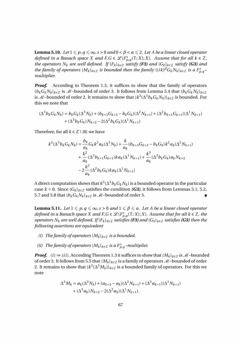
Lemma 5.10. Let 16 p, q 6∞, s > 0 and 0 <β<α6 2. Let A be a linear closed operatordefined in a Banach space X and F,G ∈ L (F s

p,q (T; X ); X ). Assume that for all k ∈ Z,the operators Nk are well defined. If Fk k∈Z satisfy (F3) and Gk k∈Z satisfy (G3) andthe family of operators Mk k∈Z is bounded then the family (i k)βGk Nk k∈Z is a F s

p,q –multiplier.

Proof. According to Theorem 1.3, it suffices to show that the family of operatorsbkGk Nk k∈Z is M–bounded of order 3. It follows from Lemma 5.4 that bkGk Nk k∈Zis M–bounded of order 2. It remains to show that k3(∆3bkGk Nk )k∈Z is bounded. Forthis we note that

(∆3bkGk Nk ) = bkGk (∆3Nk )+ (bk+3Gk+3 −bkGk )(∆2Nk+1)+ (∆2bk+1Gk+1)(∆1Nk+1)

+ (∆3bkGk )Nk+2 −2(∆2bkGk )(∆1Nk+1)

Therefore, for all k ∈Z\ 0 we have

k3(∆3bkGk Nk ) = bk

akGk k3ak (∆3Nk )+ k

ak(bk+3Gk+3 −bkGk )k2ak (∆2Nk+1)

+ k2

ak(∆2bk+1Gk+1)kak (∆1Nk+1)+ k3

ak(∆3bkGk )ak Nk+2

−2k2

ak(∆2bkGk )kak (∆1Nk+1)

A direct computation shows that k3(∆3bkGk Nk ) is a bounded operator in the particularcase k = 0. Since Gk k∈Z satisfies the condition (G3), it follows from Lemmas 5.1, 5.2,5.7 and 5.8 that bkGk Nk k∈Z is M–bounded of order 3.

Lemma 5.11. Let 1 6 p, q 6∞, s > 0 and 1 6 β6 α. Let A be a linear closed operatordefined in a Banach space X and F,G ∈L (F s

p,q (T; X ); X ). Assume that for all k ∈Z, theoperators Nk are well defined. If Fk k∈Z satisfies (F3) and Gk k∈Z satisfies (G3) then thefollowing assertions are equivalent

(i) The family of operators Mk k∈Z is a bounded.

(ii) The family of operators Mk k∈Z is a F sp,q –multiplier.

Proof. (i ) ⇒ (i i ). According Theorem 1.3 it suffices to show that Mk k∈Z is M–boundedof order 3. It follows from 5.5 that Mk k∈Z is a family of operators M–bounded of order2. It remains to show that k3(∆3Mk )k∈Z is a bounded family of operators. For this wenote

∆3Mk = ak (∆3Nk )+ (ak+3 −ak )(∆2Nk+1)+ (∆2ak+1)(∆1Nk+1)

+ (∆3ak )Nk+2 −2(∆2ak )(∆1Nk+1).

67

Therefore,

k3(∆3Mk ) = k3ak (∆3Nk )+ k(ak+3 −ak )

akkak (∆2Nk+1)+ k2

ak(∆2ak+1)kak (∆1Nk+1)

+ k3(∆3ak )

akak Nk+2 −

2k2(∆2ak )

akkak (∆1Nk+1).

Clearly, if k = 0 the operator k3(∆3Fk Nk ) is bounded. Since the sequence ak k∈Z is3–regular, it follows from Lemma 5.2 and Lemma 5.8 that the family Mk k∈Z is M–bounded of order 3.(i i ) ⇒ (i ) The proof follows the same lines as those of Lemma 5.5.

Theorem 5.3. Let 16 p, q 6∞, s > 0 and 0 <β<α6 2. Let A be a linear closed operatordefined in a Banach space X and F,G ∈ L (F s

p,q (T; X ); X ). If Fk k∈Z satisfies (F3) andGk k∈Z satisfies (G3) then the following assertions are equivalent,

(i) The solution of equation (5.21) has F sp,q –maximal regularity.

(ii) Nk k∈Z ⊆L (X ) and the family Mk k∈Z is bounded.

Proof. The proof follows the same lines as that of Theorem 5.1.

As we have mentioned, the verification of assumptions concerning the family Nk k∈Zis not an easy work. Our next Corollary require additional conditions about the op-erators A, F and G , however is a more practical result to check that these families arebounded. Define the operators Sk = (ak − A)−1, for all k ∈Z.

Corollary 5.2. Let 1 6 p, q 6 ∞, s > 0. Let be X a Banach space. Assume that(i k)αk∈Z ⊆ ρ(A) and the families Fk k∈Z and Gk k∈Z, defined by the operators F andG of equation (5.21) satisfy the conditions (F3) and (G3) respectively. If the family of op-

erators(i k)α

((i k)α− A

)−1k∈Z is bounded, and supk∈Z

∥∥∥((i k)βGk +Fk

)((i k)α− A

)−1∥∥∥ < 1

then equation (5.21) has F sp,q –maximal regularity.

Proof. The proof follows the same lines as those of Corollary 5.1.

5.4 Periodic Strong F sp,q–solutions of a Neutral Fractional

Differential Equation with Finite Delay

Now, we use the results about maximal regularity on periodic Triebel–Lizorkin spacesto prove that equation (5.22) has a strong F s

p,q –solution.

Note that, if equation (5.21) has F sp,q –maximal regularity for some 1 6 p, q 6 ∞ and

s ∈ R, the linear map Ψ : F sp,q (T; X ) → F s

p,q (T; X ) given by Ψ(g ) = Dαv , where v is theunique strong F s

p,q –solution of the equation (5.21), is well defined.

68

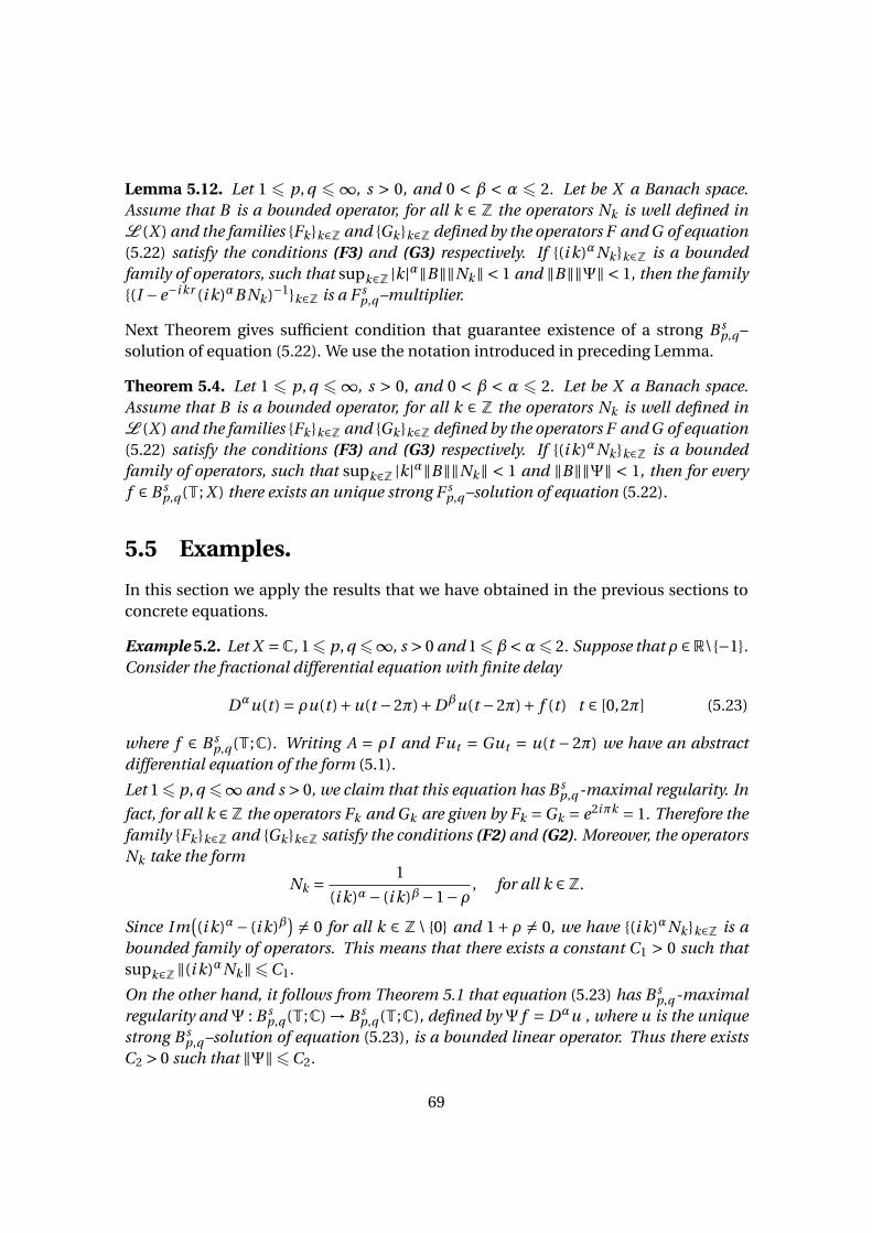
Lemma 5.12. Let 1 6 p, q 6 ∞, s > 0, and 0 < β < α 6 2. Let be X a Banach space.Assume that B is a bounded operator, for all k ∈ Z the operators Nk is well defined inL (X ) and the families Fk k∈Z and Gk k∈Z defined by the operators F and G of equation(5.22) satisfy the conditions (F3) and (G3) respectively. If (i k)αNk k∈Z is a boundedfamily of operators, such that supk∈Z |k|α‖B‖‖Nk‖ < 1 and ‖B‖‖Ψ‖ < 1, then the family(I −e−i kr (i k)αB Nk )−1k∈Z is a F s

p,q –multiplier.

Next Theorem gives sufficient condition that guarantee existence of a strong B sp,q –

solution of equation (5.22). We use the notation introduced in preceding Lemma.

Theorem 5.4. Let 1 6 p, q 6 ∞, s > 0, and 0 < β < α 6 2. Let be X a Banach space.Assume that B is a bounded operator, for all k ∈ Z the operators Nk is well defined inL (X ) and the families Fk k∈Z and Gk k∈Z defined by the operators F and G of equation(5.22) satisfy the conditions (F3) and (G3) respectively. If (i k)αNk k∈Z is a boundedfamily of operators, such that supk∈Z |k|α‖B‖‖Nk‖ < 1 and ‖B‖‖Ψ‖ < 1, then for everyf ∈ B s

p,q (T; X ) there exists an unique strong F sp,q –solution of equation (5.22).

5.5 Examples.

In this section we apply the results that we have obtained in the previous sections toconcrete equations.

Example 5.2. Let X =C, 16 p, q 6∞, s > 0 and 16β<α6 2. Suppose that ρ ∈R\−1.Consider the fractional differential equation with finite delay

Dαu(t ) = ρu(t )+u(t −2π)+Dβu(t −2π)+ f (t ) t ∈ [0,2π] (5.23)

where f ∈ B sp,q (T;C). Writing A = ρI and Fut = Gut = u(t − 2π) we have an abstract

differential equation of the form (5.1).

Let 16 p, q 6∞ and s > 0, we claim that this equation has B sp,q -maximal regularity. In

fact, for all k ∈Z the operators Fk and Gk are given by Fk =Gk = e2iπk = 1. Therefore thefamily Fk k∈Z and Gk k∈Z satisfy the conditions (F2) and (G2). Moreover, the operatorsNk take the form

Nk = 1

(i k)α− (i k)β−1−ρ , for all k ∈Z.

Since Im((i k)α− (i k)β

) 6= 0 for all k ∈ Z \ 0 and 1+ρ 6= 0, we have (i k)αNk k∈Z is abounded family of operators. This means that there exists a constant C1 > 0 such thatsupk∈Z ‖(i k)αNk‖6C1.

On the other hand, it follows from Theorem 5.1 that equation (5.23) has B sp,q -maximal

regularity andΨ : B sp,q (T;C) → B s

p,q (T;C), defined byΨ f = Dαu , where u is the uniquestrong B s

p,q –solution of equation (5.23), is a bounded linear operator. Thus there existsC2 > 0 such that ‖Ψ‖6C2.

69

Suppose that ‖B‖ < min

1C1

, 1C2

, it follows from Theorem 5.2 that equation

Dα(u(t )−Bu(t − r )

)= ρu(t )+u(t −2π)+Dβu(t −2π)+ f (t ) t ∈ [0,2π] (5.24)

has a unique strong B sp,q –solution.

Example 5.3. Let 1 6 p, q 6 ∞ and s > 0. Consider the following neutral fractionaldifferential equation with finite delay

∂α

∂tα(u(t , x)−bu(t −2π, x)

) = ∂2u(t , x)

∂x2+

∫ 0

−2πq1γ(s)u(t + s, x)d s

+∫ 0

−2πq2γ(s)Dβu(t + s, x)d s + f (t , x),

(5.25)

with 1 < β < α < 2. We will show that there exists b > 0 sufficiently small such thatthe equation (5.25) has B s

p,q –maximal regularity. For this purpose, we assume that γ :[−2π,0] → L (X ) is a function twice strongly continuously differentiable. Furthermore,q1 and q2 are positive numbers such that

∣∣q1 +q2 cos(βπ

2

)∣∣6 ∣∣q2 cos(βπ

2)∣∣

andq2Cγ < sin(

απ

2),

where Cγ =(∫ 0

−2πγ2(s)d s

)1/2

. The function f satisfies Carathéodory type conditions.

Considering the space X = L2([0,π]) and the operators A,B ,F and G given by

Av = ∂2v(x)

∂x2with domain D(A) = v ∈ X : v ∈ H 2([0,π]), v(0) = v(π) = 0

B v = bv for all v ∈ X with b ∈R+

F v =∫ 0

−2πq1γ(s)v(s)d s Gv =

∫ 0

−2πq2γ(s)v(s)d s for all v ∈ X .

equation (5.25) takes the abstract form of equation (5.1).

Clearly ‖F‖6 q1Cγ and ‖G‖6 q2Cγ. Define, for all k ∈Z the operators

Fk =∫ 0

−2πq1e i ksγ(s)d s and Gk =

∫ 0

−2πq2e i ksγ(s)d s

A direct computation shows that for all k ∈Z\ 0

Fk = i q1[γ(−2π)−γ(0)]

k− q1[γ′(−2π)−γ′(0)]

k2− i q1

k2

∫ 0

−2πe i ksγ′′(s)d s

70

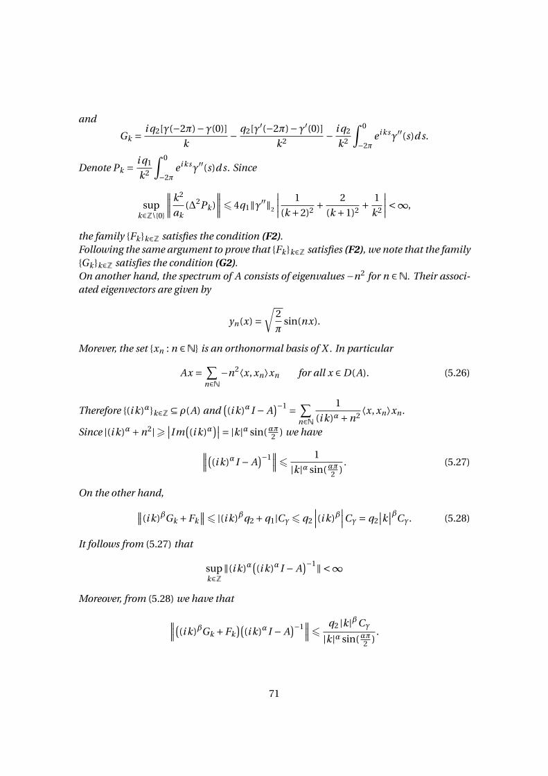
and

Gk = i q2[γ(−2π)−γ(0)]

k− q2[γ′(−2π)−γ′(0)]

k2− i q2

k2

∫ 0

−2πe i ksγ′′(s)d s.

Denote Pk = i q1

k2

∫ 0

−2πe i ksγ′′(s)d s. Since

supk∈Z\0

∥∥∥∥ k2

ak(∆2Pk )

∥∥∥∥6 4q1‖γ′′‖2

∣∣∣∣ 1

(k +2)2+ 2

(k +1)2+ 1

k2

∣∣∣∣<∞,

the family Fk k∈Z satisfies the condition (F2).Following the same argument to prove that Fk k∈Z satisfies (F2), we note that the familyGk k∈Z satisfies the condition (G2).On another hand, the spectrum of A consists of eigenvalues −n2 for n ∈N. Their associ-ated eigenvectors are given by

yn(x) =√

2

πsin(nx).

Morever, the set xn : n ∈N is an orthonormal basis of X . In particular

Ax = ∑n∈N

−n2⟨x, xn⟩xn for all x ∈ D(A). (5.26)

Therefore (i k)αk∈Z ⊆ ρ(A) and((i k)αI − A

)−1 = ∑n∈N

1

(i k)α+n2⟨x, xn⟩xn .

Since |(i k)α+n2|> ∣∣Im((i k)α

)∣∣= |k|α sin(απ2 ) we have∥∥∥((i k)αI − A

)−1∥∥∥6 1

|k|α sin(απ2 ). (5.27)

On the other hand,∥∥(i k)βGk +Fk∥∥6 |(i k)βq2 +q1|Cγ6 q2

∣∣∣(i k)β∣∣∣Cγ = q2

∣∣k∣∣βCγ. (5.28)

It follows from (5.27) that

supk∈Z

‖(i k)α((i k)αI − A

)−1‖ <∞

Moreover, from (5.28) we have that

∥∥∥((i k)βGk +Fk

)((i k)αI − A

)−1∥∥∥6 q2 |k|βCγ

|k|α sin(απ2 ).

71

Since q2Cγ < sin(απ2 ) we have supk∈Z

∥∥∥((i k)βGk +Fk

)Sk

∥∥∥< 1. From Corollary 5.1, it follows

that fractional delay equation

∂α

∂tαu(t , x) = ∂2u(t , x)

∂x2+

∫ 0

−2πq1γ(s)u(t + s, x)d s

+∫ 0

−2πq2γ(s)Dβu(t + s, x)d s + f (t , x)

(5.29)

has B sp,q –maximal regularity, for 16 p, q 6∞ and s > 0.

Thus the mapΨ : B sp,q (T; X ) → B s

p,q (T; X ), defined byΨ( f ) = Dαu where u is the uniquestrong B s

p,q –solution of equation (5.29), is a bounded linear operator. Therefore thereexists C2 > 0 such that ‖Ψ‖6C2.Moreover, there exists C1 > 0 such that sup

k∈Z|k|α‖Nk‖6C1. If the constant b > 0 satisfies

the condition b < min

1C1

, 1C2

we have

supk∈Z

|k|α‖B‖‖Nk‖ < 1 and supk∈Z

‖B‖‖Ψ‖ < 1

It follows from Theorem 5.2 that equation (5.25) has a unique strong B sp,q -solution.

72

Bibliography

[1] R. P. Agarwal, Y. Zhou, and Y. He, Existence of fractional neutral functional differential equations,Comput. Math. Appl. 59 (2010), no. 3, 1095–1100. MR2579474 (2010h:34170)

[2] R. P. Agarwal, M. Benchohra, and S. Hamani, A survey on existence results for boundary value prob-lems of nonlinear fractional differential equations and inclusions, Acta Appl. Math. 109 (2010),no. 3, 973–1033. MR2596185 (2011a:34008)

[3] R. P. Agarwal, V. Lakshmikantham, and J. J. Nieto, On the concept of solution for fractional dif-ferential equations with uncertainty, Nonlinear Anal. 72 (2010), no. 6, 2859–2862. MR2580143(2010m:34003)

[4] H. Amann, Linear and quasilinear parabolic problems. Vol. I, Monographs in Mathematics, vol. 89,Birkhäuser Boston Inc., Boston, MA, 1995. Abstract linear theory. MR1345385 (96g:34088)

[5] H. Amann, Operator-valued Fourier multipliers, vector-valued Besov spaces, and applications,Math. Nachr. 186 (1997), 5–56. MR1461211 (98h:46033)

[6] V. V. Anh and N. N. Leonenko, Spectral analysis of fractional kinetic equations with random data,J. Statist. Phys. 104 (2001), no. 5-6, 1349–1387. MR1859007 (2002m:82053)

[7] W. Arendt and M. Duelli, Maximal Lp -regularity for parabolic and elliptic equations on the line, J.Evol. Equ. 6 (2006), no. 4, 773–790. MR2267707 (2007k:34193)

[8] W. Arendt, C. Batty, and S. Bu, Fourier multipliers for Hölder continuous functions and maximalregularity, Studia Math. 160 (2004), no. 1, 23–51. MR2029738 (2005j:42006)

[9] W. Arendt, C. J. K. Batty, M. Hieber, and F. Neubrander, Vector-valued Laplace transforms andCauchy problems, Second, Monographs in Mathematics, vol. 96, Birkhäuser/Springer Basel AG,Basel, 2011. MR2798103 (2012b:47109)

[10] W. Arendt and S. Bu, The operator-valued Marcinkiewicz multiplier theorem and maximal regu-larity, Math. Z. 240 (2002), no. 2, 311–343. MR1900314 (2003i:42016)

[11] W. Arendt and S. Bu, Tools for maximal regularity, Math. Proc. Cambridge Philos. Soc. 134 (2003),no. 2, 317–336. MR1972141 (2004d:47078)

[12] W. Arendt and S. Bu, Operator-valued Fourier multipliers on periodic Besov spaces and applica-tions, Proc. Edinb. Math. Soc. (2) 47 (2004), no. 1, 15–33. MR2064734 (2005e:42040)

73

[13] W. Arendt and P. J. Rabier, Linear evolution operators on spaces of periodic functions, Commun.Pure Appl. Anal. 8 (2009), no. 1, 5–36. MR2449097 (2009i:34130)

[14] J. Banas and K. Goebel, Measures of noncompactness in Banach spaces, Lecture Notes in Pure andApplied Mathematics, vol. 60, Marcel Dekker Inc., New York, 1980. MR591679 (82f:47066)

[15] A. Bátkai and S. Piazzera, Semigroups for delay equations, Research Notes in Mathematics, vol. 10,A K Peters Ltd., Wellesley, MA, 2005. MR2181405 (2006j:34001)

[16] M. Benchohra and S. K. Ntouyas, Nonlocal Cauchy problems for neutral functional differentialand integrodifferential inclusions in Banach spaces, J. Math. Anal. Appl. 258 (2001), no. 2, 573–590.MR1835560 (2002d:34130)

[17] J. Bochenek, Existence of the fundamental solution of a second order evolution equation, Ann.Polon. Math. 66 (1997), 15–35. Volume dedicated to the memory of Włodzimierz Mlak. MR1438326(99c:34125)

[18] S. K. Bose and G. C. Gorain, Exact controllability and boundary stabilization of flexural vibrationsof an internally damped flexible space structure, Appl. Math. Comput. 126 (2002), no. 2-3, 341–360.MR1879167 (2002j:93008)

[19] S. K. Bose and G. C. Gorain, Uniform stability of damped nonlinear vibrations of an elastic string,Proc. Indian Acad. Sci. Math. Sci. 113 (2003), no. 4, 443–449. MR2020076 (2004i:74056)

[20] S. K. Bose and G. C. Gorain, Exact controllability and boundary stabilization of torsional vibrationsof an internally damped flexible space structure, J. Optim. Theory Appl. 99 (1998), no. 2, 423–442.MR1657037 (99i:93032)

[21] S. K. Bose and G. C. Gorain, Stability of the boundary stabilised internally damped wave equa-tion y ′′+λy ′′′ = c2(∆y +µ∆y ′) in a bounded domain in Rn , Indian J. Math. 40 (1998), no. 1, 1–15.MR1654783 (99i:35106)

[22] D. Bothe, Multivalued perturbations of m-accretive differential inclusions, Israel J. Math. 108(1998), 109–138. MR1669396 (2000a:34124)

[23] J. Bourgain, Some remarks on Banach spaces in which martingale difference sequences are uncon-ditional, Ark. Mat. 21 (1983), no. 2, 163–168. MR727340 (85a:46011)

[24] S. Q. Bu, Maximal regularity of second order delay equations in Banach spaces, Acta Math. Sin.(Engl. Ser.) 25 (2009), no. 1, 21–28. MR2465519 (2009j:34198)

[25] S. Q. Bu and J. M. Kim, Operator-valued Fourier multipliers on periodic Triebel spaces, Acta Math.Sin. (Engl. Ser.) 21 (2005), no. 5, 1049–1056. MR2176315 (2006g:42014)

[26] S. Bu, Mild well-posedness of vector-valued problems, Arch. Math. (Basel) 95 (2010), no. 1, 63–73.MR2671239 (2011k:34127)

[27] S. Bu and Y. Fang, Maximal regularity for integro-differential equation on periodic Triebel-Lizorkinspaces, Taiwanese J. Math. 12 (2008), no. 2, 281–292. MR2402114 (2009j:47158)

[28] S. Bu and Y. Fang, Periodic solutions for second order integro-differential equations with infinitedelay in Banach spaces, Studia Math. 184 (2008), no. 2, 103–119. MR2365804 (2008h:34097)

[29] S. Bu and Y. Fang, Periodic solutions of delay equations in Besov spaces and Triebel-Lizorkin spaces,Taiwanese J. Math. 13 (2009), no. 3, 1063–1076. MR2526359 (2010e:34129)

[30] S. Bu and Y. Fang, Maximal regularity of second order delay equations in Banach spaces, Sci. ChinaMath. 53 (2010), no. 1, 51–62. MR2594746 (2011b:34158)

74

[31] S. Bu and J.-M. Kim, Operator-valued Fourier multiplier theorems on Lp -spaces onTd , Arch. Math.(Basel) 82 (2004), no. 5, 404–414. MR2061447 (2005e:42041)

[32] S. Bu and J.-M. Kim, Operator-valued Fourier multiplier theorems on Triebel spaces, Acta Math.Sci. Ser. B Engl. Ed. 25 (2005), no. 4, 599–609. MR2175925 (2006k:42013)

[33] D. L. Burkholder, A geometric condition that implies the existence of certain singular integrals ofBanach-space-valued functions, Conference on harmonic analysis in honor of Antoni Zygmund,Vol. I, II (Chicago, Ill., 1981), 1983, pp. 270–286. MR730072 (85i:42020)

[34] D. L. Burkholder, Martingales and singular integrals in Banach spaces, Handbook of the geometryof Banach spaces, Vol. I, 2001, pp. 233–269. MR1863694 (2003b:46009)

[35] P. L. Butzer and U. Westphal, An access to fractional differentiation via fractional difference quo-tients, Fractional calculus and its applications (Proc. Internat. Conf., Univ. New Haven, WestHaven, Conn., 1974), 1975, pp. 116–145. Lecture Notes in Math., Vol. 457. MR0492115 (58 #11267)

[36] L. Byszewski, Uniqueness criterion for solution of abstract nonlocal Cauchy problem, J. Appl. Math.Stochastic Anal. 6 (1993), no. 1, 49–54. MR1214305 (94k:34119)

[37] L. Byszewski, Strong maximum principles for parabolic nonlinear problems with nonlocal inequal-ities together with arbitrary functionals, J. Math. Anal. Appl. 156 (1991), no. 2, 457–470. MR1103024(92b:35032)

[38] L. Byszewski, Theorem about existence and uniqueness of continuous solution of nonlocal problemfor nonlinear hyperbolic equation, Appl. Anal. 40 (1991), no. 2-3, 173–180. MR1095412 (92d:35197)

[39] L. Byszewski, Theorems about the existence and uniqueness of solutions of a semilinear evolutionnonlocal Cauchy problem, J. Math. Anal. Appl. 162 (1991), no. 2, 494–505. MR1137634 (92m:35005)

[40] L. Byszewski and V. Lakshmikantham, Theorem about the existence and uniqueness of a solutionof a nonlocal abstract Cauchy problem in a Banach space, Appl. Anal. 40 (1991), no. 1, 11–19.MR1121321 (92h:34121)

[41] L. Byszewski and T. Winiarska, An abstract nonlocal second order evolution problem, OpusculaMath. 32 (2012), no. 1, 75–82. MR2852470

[42] M. Chandrasekaran, Nonlocal Cauchy problem for quasilinear integrodifferential equations in Ba-nach spaces, Electron. J. Differential Equations (2007), No. 33, 6 pp. (electronic). MR2299587(2008a:34140)

[43] P. Clément, B. de Pagter, F. A. Sukochev, and H. Witvliet, Schauder decomposition and multipliertheorems, Studia Math. 138 (2000), no. 2, 135–163. MR1749077 (2002c:47036)

[44] C. Cuevas and J. C. de Souza, S-asymptotically ω-periodic solutions of semilinear frac-tional integro-differential equations, Appl. Math. Lett. 22 (2009), no. 6, 865–870. MR2523596(2010f:45017)

[45] C. Cuevas and C. Lizama, Well posedness for a class of flexible structure in Hölder spaces, Math.Probl. Eng. (2009), Art. ID 358329, 13. MR2530061 (2010i:35399)

[46] G. Da Prato, P. C. Kunstmann, I. Lasiecka, A. Lunardi, R. Schnaubelt, and L. Weis, Functional an-alytic methods for evolution equations, Lecture Notes in Mathematics, vol. 1855, Springer-Verlag,Berlin, 2004. Edited by M. Iannelli, R. Nagel and S. Piazzera. MR2108957 (2005f:35003)

[47] C. M. Dafermos, An abstract Volterra equation with applications to linear viscoelasticity, J. Differ-ential Equations 7 (1970), 554–569. MR0259670 (41 #4305)

[48] G. Darbo, Punti uniti in trasformazioni a codominio non compatto, Rend. Sem. Mat. Univ. Padova24 (1955), 84–92. MR0070164 (16,1140f)

75

[49] R. Datko, Linear autonomous neutral differential equations in a Banach space, J. Diff. Equations25 (1977), no. 2, 258–274. MR0447743 (56 #6053)

[50] B. de Andrade and C. Lizama, Existence of asymptotically almost periodic solutions for dampedwave equations, J. Math. Anal. Appl. 382 (2011), no. 2, 761–771. MR2810829 (2012e:35167)

[51] K. Deng, Exponential decay of solutions of semilinear parabolic equations with nonlocal initialconditions, J. Math. Anal. Appl. 179 (1993), no. 2, 630–637. MR1249842 (95a:35076)

[52] R. Denk, M. Hieber, and J. Prüss, R-boundedness, Fourier multipliers and problems of elliptic andparabolic type, Mem. Amer. Math. Soc. 166 (2003), no. 788, viii+114. MR2006641 (2004i:35002)

[53] Q. Dong and G. Li, Existence of solutions for semilinear differential equations with nonlocal con-ditions in Banach spaces, Electron. J. Qual. Theory Differ. Equ. (2009), No. 47, 13. MR2524984(2010g:34192)

[54] J. P. C. dos Santos, M. M. Arjunan, and C. Cuevas, Existence results for fractional neutral integro-differential equations with state-dependent delay, Comput. Math. Appl. 62 (2011), no. 3, 1275–1283. MR2824714 (2012d:45012)

[55] K.-J. Engel and R. Nagel, One-parameter semigroups for linear evolution equations, Graduate Textsin Mathematics, vol. 194, Springer-Verlag, New York, 2000. With contributions by S. Brendle, M.Campiti, T. Hahn, G. Metafune, G. Nickel, D. Pallara, C. Perazzoli, A. Rhandi, S. Romanelli and R.Schnaubelt. MR1721989 (2000i:47075)

[56] K. Ezzinbi and X. Fu, Existence and regularity of solutions for some neutral partial differentialequations with nonlocal conditions, Nonlinear Anal. 57 (2004), no. 7-8, 1029–1041. MR2070623(2005f:34232)

[57] K. Ezzinbi, X. Fu, and K. Hilal, Existence and regularity in the α-norm for some neutral par-tial differential equations with nonlocal conditions, Nonlinear Anal. 67 (2007), no. 5, 1613–1622.MR2323307 (2008g:35204)

[58] H. O. Fattorini, Second order linear differential equations in Banach spaces, North-Holland Math-ematics Studies, vol. 108, North-Holland Publishing Co., Amsterdam, 1985. Notas de Matemática[Mathematical Notes], 99. MR797071 (87b:34001)

[59] C. Fernández, C. Lizama, and V. Poblete, Maximal regularity for flexible structural systems inLebesgue spaces, Math. Probl. Eng. (2010), Art. ID 196956, 15. MR2610518 (2011h:34123)

[60] C. Fernández, C. Lizama, and V. Poblete, Regularity of solutions for a third order differentialequation in Hilbert spaces, Appl. Math. Comput. 217 (2011), no. 21, 8522–8533. MR2802263(2012f:34146)

[61] M. Girardi and L. Weis, Criteria for R-boundedness of operator families, Evolution equations, 2003,pp. 203–221. MR2073746 (2005e:47086)

[62] M. Girardi and L. Weis, Operator-valued Fourier multiplier theorems on Besov spaces, Math. Nachr.251 (2003), 34–51. MR1960803 (2003m:46050)

[63] M. Girardi and L. Weis, Operator-valued Fourier multiplier theorems on Lp (X ) and geometry ofBanach spaces, J. Funct. Anal. 204 (2003), no. 2, 320–354. MR2017318 (2004g:42019)

[64] K. Gopalsamy and P. xuan Weng, Oscillations in systems of linear neutral differential equations,Chinese Quart. J. Math. 16 (2001), no. 4, 61–68. MR1898009 (2003b:34136)

[65] G. C. Gorain, Exponential energy decay estimate for the solutions of internally damped wave equa-tion in a bounded domain, J. Math. Anal. Appl. 216 (1997), no. 2, 510–520. MR1489594 (98i:35111)

76

[66] G. C. Gorain, Boundary stabilization of nonlinear vibrations of a flexible structure in a boundeddomain in Rn , J. Math. Anal. Appl. 319 (2006), no. 2, 635–650. MR2227928 (2007b:93114)

[67] G. C. Gorain, Stabilization for the vibrations modeled by the ‘standard linear model’ of viscoelastic-ity, Proc. Indian Acad. Sci. Math. Sci. 120 (2010), no. 4, 495–506. MR2761788 (2011j:74014)

[68] R. Gorenflo and F. Mainardi, Fractional calculus: integral and differential equations of fractionalorder, Fractals and fractional calculus in continuum mechanics (Udine, 1996), 1997, pp. 223–276.MR1611585 (99g:26015)

[69] R. Grimmer and J. Prüss, On linear Volterra equations in Banach spaces, Comput. Math. Appl. 11(1985), no. 1-3, 189–205. Hyperbolic partial differential equations, II. MR787436 (86h:45004)

[70] A. Grünwald, Uber begrenzte derivationen und deren anwendung, Math. Phys. 12 (1867), 441–480.

[71] L. X. Guo, S. P. Lu, B. Du, and F. Liang, Existence of periodic solutions to a second-order neutralfunctional differential equation with deviating arguments, J. Math. (Wuhan) 30 (2010), no. 5, 839–847. MR2731674 (2011i:34115)

[72] S. Guo, Equivariant normal forms for neutral functional differential equations, Nonlinear Dynam.61 (2010), no. 1-2, 311–329. MR2661804 (2011j:34232)

[73] S. Hadd, Singular functional differential equations of neutral type in Banach spaces, J. Funct. Anal.254 (2008), no. 8, 2069–2091. MR2402084 (2010b:34180)

[74] J. K. Hale, Coupled oscillators on a circle, Resenhas 1 (1994), no. 4, 441–457. Dynamical phase tran-sitions (São Paulo, 1994). MR1357945 (97d:58143)

[75] J. K. Hale, Partial neutral functional-differential equations, Rev. Roumaine Math. Pures Appl. 39(1994), no. 4, 339–344. MR1317773 (96g:35204)

[76] J. K. Hale and S. M. Verduyn Lunel, Introduction to functional-differential equations, AppliedMathematical Sciences, vol. 99, Springer-Verlag, New York, 1993. MR1243878 (94m:34169)

[77] H. R. Henríquez, Periodic solutions of quasi-linear partial functional-differential equations withunbounded delay, Funkcial. Ekvac. 37 (1994), no. 2, 329–343. MR1299869 (96a:34150)

[78] H. R. Henríquez, Existence of solutions of non-autonomous second order functional differen-tial equations with infinite delay, Nonlinear Anal. 74 (2011), no. 10, 3333–3352. MR2793566(2012c:34260)

[79] H. R. Henríquez and C. Lizama, Periodic solutions of abstract functional differential equations withinfinite delay, Nonlinear Anal. 75 (2012), no. 4, 2016–2023. MR2870895

[80] H. R. Henríquez, M. Pierri, and A. Prokopczyk, Periodic solutions of abstract neutral functionaldifferential equations, J. Math. Anal. Appl. 385 (2012), no. 2, 608–621. MR2834838 (2012f:34172)

[81] H. R. Henríquez and V. Poblete, Periodic solutions of neutral fractional differential equations. Pre-Fint.

[82] H. R. Henríquez, V. Poblete, and J. C. Pozo, Existence of mild–solutions of a non–autonomous sec-ond order evolution equation with non–local initial conditions. Preprint.

[83] H. R. Henríquez and C. H. Vásquez, Differentiabilty of solutions of the second order abstract Cauchyproblem, Semigroup Forum 64 (2002), no. 3, 472–488. MR1896382 (2003a:34084)

[84] H. R. Henríquez and C. H. Vásquez, Differentiability of solutions of second-order functional differ-ential equations with unbounded delay, J. Math. Anal. Appl. 280 (2003), no. 2, 284–312. MR1977912(2004b:34201)

77

[85] E. Hernández, D. O’Regan, and K. Balachandran, On recent developments in the theory of abstractdifferential equations with fractional derivatives, Nonlinear Anal. 73 (2010), no. 10, 3462–3471.MR2680040 (2011g:35413)

[86] R. Hilfer, Applications of fractional calculus in physics (R. Hilfer, ed.), World Scientific PublishingCo. Inc., River Edge, NJ, 2000. MR1890104 (2002j:00009)

[87] T. Hytönen and M. Veraar, R-boundedness of smooth operator-valued functions, Integral EquationsOperator Theory 63 (2009), no. 3, 373–402. MR2491037 (2010b:47037)

[88] S. Ji and G. Li, Existence results for impulsive differential inclusions with nonlocal conditions, Com-put. Math. Appl. 62 (2011), no. 4, 1908–1915. MR2834816

[89] M. Jia, X. P. Liu, W. G. Ge, and Y. P. Guo, Periodic solutions to a neutral integro-differential equationwith three delays, J. Systems Sci. Math. Sci. 27 (2007), no. 4, 615–623. MR2349985 (2008g:34181)

[90] N. J. Kalton and G. Lancien, A solution to the problem of Lp -maximal regularity, Math. Z. 235(2000), no. 3, 559–568. MR1800212 (2001k:47062)

[91] N. J. Kalton and L. Weis, The H∞-calculus and sums of closed operators, Math. Ann. 321 (2001),no. 2, 319–345. MR1866491 (2003a:47038)

[92] T. Kato, Perturbation theory for linear operators, Classics in Mathematics, Springer-Verlag, Berlin,1995. Reprint of the 1980 edition. MR1335452 (96a:47025)

[93] V. Keyantuo and C. Lizama, Fourier multipliers and integro-differential equations in Banachspaces, J. London Math. Soc. (2) 69 (2004), no. 3, 737–750. MR2050043 (2005h:45015)

[94] V. Keyantuo and C. Lizama, Maximal regularity for a class of integro-differential equations withinfinite delay in Banach spaces, Studia Math. 168 (2005), no. 1, 25–50. MR2133386 (2005k:35418)

[95] V. Keyantuo and C. Lizama, Hölder continuous solutions for integro-differential equations andmaximal regularity, J. Differential Equations 230 (2006), no. 2, 634–660. MR2269937 (2007k:45011)

[96] V. Keyantuo and C. Lizama, Periodic solutions of second order differential equations in Banachspaces, Math. Z. 253 (2006), no. 3, 489–514. MR2221083 (2007d:34114)

[97] V. Keyantuo and C. Lizama, Mild well-posedness of abstract differential equations, Functional anal-ysis and evolution equations, 2008, pp. 371–387. MR2402741 (2009j:47080)

[98] V. Keyantuo and C. Lizama, A characterization of periodic solutions for time-fractional differentialequations in U MD spaces and applications, Math. Nachr. 284 (2011), no. 4, 494–506. MR2789193(2012d:34147)

[99] V. Keyantuo, C. Lizama, and V. Poblete, Periodic solutions of integro-differential equations invector-valued function spaces, J. Differential Equations 246 (2009), no. 3, 1007–1037. MR2474584(2009i:45024)

[100] A. A. Kilbas, H. M. Srivastava, and J. J. Trujillo, Theory and applications of fractional differentialequations, North-Holland Mathematics Studies, vol. 204, Elsevier Science B.V., Amsterdam, 2006.MR2218073 (2007a:34002)

[101] J. Kisynski, On cosine operator functions and one-parameter groups of operators, Studia Math. 44(1972), 93–105. Collection of articles honoring the completion by Antoni Zygmund of 50 years ofscientific activity. I. MR0312328 (47 #890)

[102] V. Kolmanovskii and A. Myshkis, Introduction to the theory and applications of functional-differential equations, Mathematics and its Applications, vol. 463, Kluwer Academic Publishers,Dordrecht, 1999. MR1680144 (2000c:34164)

78

[103] M. Kozak, A fundamental solution of a second-order differential equation in a Banach space, Univ.Iagel. Acta Math. 32 (1995), 275–289. MR1345144 (96k:34126)

[104] V. Lakshmikantham and J. V. Devi, Theory of fractional differential equations in a Banach space,Eur. J. Pure Appl. Math. 1 (2008), no. 1, 38–45. MR2379647 (2009a:34102)

[105] A. V. Letnikov, Theory and differentiation of fractional order, Mat. Sb. 3, 1–68.

[106] Y. P. Lin and J. H. Liu, Semilinear integrodifferential equations with nonlocal Cauchy problem, Non-linear Anal. 26 (1996), no. 5, 1023–1033. MR1362770 (96j:34112)

[107] Y. Lin, Time-dependent perturbation theory for abstract evolution equations of second order, StudiaMath. 130 (1998), no. 3, 263–274. MR1624819 (99i:34080)

[108] L. Liu, F. Guo, C. Wu, and Y. Wu, Existence theorems of global solutions for nonlinear Volterra typeintegral equations in Banach spaces, J. Math. Anal. Appl. 309 (2005), no. 2, 638–649. MR2154141(2006c:45004)

[109] C. Lizama, A characterization of uniform continuity for Volterra equations in Hilbert spaces, Proc.Amer. Math. Soc. 126 (1998), no. 12, 3581–3587. MR1469423 (99b:45008)

[110] C. Lizama, Fourier multipliers and periodic solutions of delay equations in Banach spaces, J. Math.Anal. Appl. 324 (2006), no. 2, 921–933. MR2265090 (2007g:34139)

[111] C. Lizama and G. M. N’Guérékata, Bounded mild solutions for semilinear integro differential equa-tions in Banach spaces, Integral Equations Operator Theory 68 (2010), no. 2, 207–227. MR2721083(2011k:45016)

[112] C. Lizama and V. Poblete, Maximal regularity of delay equations in Banach spaces, Studia Math.175 (2006), no. 1, 91–102. MR2261702 (2007g:34170)

[113] C. Lizama and V. Poblete, Periodic solutions of fractional differential equations with delay, J. Evol.Equ. 11 (2011), no. 1, 57–70. MR2780573 (2012b:34191)

[114] C. Lizama and R. Ponce, Periodic solutions of degenerate differential equations in vector-valuedfunction spaces, Studia Math. 202 (2011), no. 1, 49–63. MR2756012 (2012b:34152)

[115] C. Lizama and J. C. Pozo, Existence of mild solutions for semilinear integrodifferential equationswith nonlocal conditions. Submitted.

[116] S. Ma, Z. Wang, and Q. Xu, Periodic solutions of linear neutral integro-differential equations, ActaMath. Sci. Ser. B Engl. Ed. 24 (2004), no. 3, 337–348. MR2073250 (2005e:34242)

[117] R. Metzler and J. Klafter, Boundary value problems for fractional diffusion equations, Phys. A 278(2000), no. 1-2, 107–125. MR1763650 (2001b:35138)

[118] R. Metzler and J. Klafter, The random walk’s guide to anomalous diffusion: a fractional dynamicsapproach, Phys. Rep. 339 (2000), no. 1, 77. MR1809268 (2001k:82082)

[119] K. S. Miller and B. Ross, An introduction to the fractional calculus and fractional differential equa-tions, A Wiley-Interscience Publication, John Wiley & Sons Inc., New York, 1993. MR1219954(94e:26013)

[120] G. M. Mophou and G. M. N’Guérékata, On integral solutions of some nonlocal fractional differen-tial equations with nondense domain, Nonlinear Anal. 71 (2009), no. 10, 4668–4675. MR2548700

[121] S. K. Ntouyas and P. Ch. Tsamatos, Global existence for second order semilinear ordinary and de-lay integrodifferential equations with nonlocal conditions, Appl. Anal. 67 (1997), no. 3-4, 245–257.MR1614061 (98k:34103)

79

[122] S. K. Ntouyas and P. Ch. Tsamatos, Global existence for semilinear evolution equations with nonlo-cal conditions, J. Math. Anal. Appl. 210 (1997), no. 2, 679–687. MR1453198 (98e:34116)

[123] S. K. Ntouyas and P. Ch. Tsamatos, Global existence for semilinear evolution integrodifferentialequations with delay and nonlocal conditions, Appl. Anal. 64 (1997), no. 1-2, 99–105. MR1460074(98e:45008)

[124] D. N. Pandey, A. Ujlayan, and D. Bahuguna, On a solution to fractional order integrodifferentialequations with analytic semigroups, Nonlinear Anal. 71 (2009), no. 9, 3690–3698. MR2536279(2010g:34122)

[125] A. Pazy, Semigroups of linear operators and applications to partial differential equations, AppliedMathematical Sciences, vol. 44, Springer-Verlag, New York, 1983. MR710486 (85g:47061)

[126] V. Poblete, Solutions of second-order integro-differential equations on periodic Besov spaces, Proc.Edinb. Math. Soc. (2) 50 (2007), no. 2, 477–492. MR2334958 (2008h:45003)

[127] V. Poblete, Maximal regularity of second-order equations with delay, J. Differential Equations 246(2009), no. 1, 261–276. MR2467023 (2009h:34086)

[128] V. Poblete and J. C. Pozo, Periodic solutions for a fractional order abstract neutral differential equa-tion with finite delay. Preprint.

[129] V. Poblete and J. C. Pozo, Periodic solutions of an abstract third–order differential equation. Sub-mitted.

[130] I. Podlubny, I. Petráš, B. M. Vinagre, P. O’Leary, and L’. Dorcák, Analogue realizations of fractional-order controllers, Nonlinear Dynam. 29 (2002), no. 1-4, 281–296. Fractional order calculus and itsapplications. MR1926477

[131] J. Prüss, On linear Volterra equations of parabolic type in Banach spaces, Trans. Amer. Math. Soc.301 (1987), no. 2, 691–721. MR882711 (88f:45019)

[132] J. Prüss, Positivity and regularity of hyperbolic Volterra equations in Banach spaces, Math. Ann. 279(1987), no. 2, 317–344. MR919509 (89h:45004)

[133] J. Prüss, A positivity method for linear Volterra equations, Nonlinear analysis and applications (Ar-lington, Tex., 1986), 1987, pp. 483–488. MR912329

[134] J. Prüss, Evolutionary integral equations and applications, Monographs in Mathematics, vol. 87,Birkhäuser Verlag, Basel, 1993. MR1238939 (94h:45010)

[135] Y. Ren, Y. Qin, and R. Sakthivel, Existence results for fractional order semilinear integro-differentialevolution equations with infinite delay, Integral Equations Operator Theory 67 (2010), no. 1, 33–49. MR2629975 (2011c:34200)

[136] B. N. Sadovskiı, On a fixed point principle, Funkcional. Anal. i Priložen. 1 (1967), no. 2, 74–76.MR0211302 (35 #2184)

[137] S. G. Samko, A. A. Kilbas, and O. I. Marichev, Fractional integrals and derivatives, Gordon andBreach Science Publishers, Yverdon, 1993. Theory and applications, Edited and with a forewordby S. M. Nikolskiı, Translated from the 1987 Russian original, Revised by the authors. MR1347689(96d:26012)

[138] H. Serizawa and M. Watanabe, Perturbation for cosine families in Banach spaces, Houston J. Math.12 (1986), no. 1, 117–124. MR855797 (87k:34104)

[139] H. Serizawa and M. Watanabe, Time-dependent perturbation for cosine families in Banach spaces,Houston J. Math. 12 (1986), no. 4, 579–586. MR873652 (88e:34107)

80

[140] C. C. Travis and G. F. Webb, Compactness, regularity, and uniform continuity properties of stronglycontinuous cosine families, Houston J. Math. 3 (1977), no. 4, 555–567. MR0500288 (58 #17957)

[141] C. C. Travis and G. F. Webb, Cosine families and abstract nonlinear second order differential equa-tions, Acta Math. Acad. Sci. Hungar. 32 (1978), no. 1-2, 75–96. MR0499581 (58 #17404)

[142] C. C. Travis and G. F. Webb, Second order differential equations in Banach space, Nonlinear equa-tions in abstract spaces (Proc. Internat. Sympos., Univ. Texas, Arlington, Tex., 1977), 1978, pp. 331–361. MR502551 (81j:34110)

[143] O. van Gaans, On R-boundedness of unions of sets of operators, Partial differential equations andfunctional analysis, 2006, pp. 97–111. MR2240055 (2007h:47065)

[144] V. V. Vasil’ev and S. I. Piskarev, Differential equations in Banach spaces. II. Theory of cosine oper-ator functions, J. Math. Sci. (N. Y.) 122 (2004), no. 2, 3055–3174. Functional analysis. MR2084186(2005d:34133)

[145] K. Wang, On the unique existence of periodic solutions of neutral Volterra integro-differential equa-tions, Period. Math. Hungar. 21 (1990), no. 1, 21–29. MR1066407 (91e:45017)

[146] X. Wang, Z. X. Li, and H. Zhang, Existence of periodic solutions to a neutral integro-differentialequation with infinite delay, Math. Appl. (Wuhan) 19 (2006), no. 4, 804–811. MR2257884(2007i:34108)

[147] G. F. Webb, Regularity of solutions to an abstract inhomogeneous linear differential equation, Proc.Amer. Math. Soc. 62 (1977), no. 2, 271–277. MR0432996 (55 #5975)

[148] L. Weis, Operator-valued Fourier multiplier theorems and maximal Lp -regularity, Math. Ann. 319(2001), no. 4, 735–758. MR1825406 (2002c:42016)

[149] P. Weng, Oscillation in periodic neutral parabolic differential system, Bull. Inst. Math. Acad. Sinica24 (1996), no. 1, 33–47. MR1379663 (97a:35248)

[150] T. Winiarska, Evolution equations of second order with operator depending on t , Selected problemsof mathematics, 1995, pp. 299–311. MR1438076 (97m:34118)

[151] J. Wu and H. Xia, Rotating waves in neutral partial functional-differential equations, J. Dynam.Differential Equations 11 (1999), no. 2, 209–238. MR1695243 (2000h:35160)

[152] J. Wu and H. Xia, Self-sustained oscillations in a ring array of coupled lossless transmission lines, J.Differential Equations 124 (1996), no. 1, 247–278. MR1368068 (97c:34148)

[153] J. Wu, H. Xia, and B. Zhang, Topological transversality and periodic solutions of neutral functional-differential equations, Proc. Roy. Soc. Edinburgh Sect. A 129 (1999), no. 1, 199–220. MR1669185(2000a:34141)

[154] T. J. Xiao and J. Liang, The Cauchy problem for higher order abstract differential equations, ChineseJ. Contemp. Math. 14 (1993), no. 4, 305–321. MR1277672 (96m:34115)

[155] X. Xue, Existence of solutions for semilinear nonlocal Cauchy problems in Banach spaces, Electron.J. Differential Equations (2005), No. 64, 7 pp. (electronic). MR2147144 (2006a:34180)

[156] X. Xue, Nonlinear differential equations with nonlocal conditions in Banach spaces, NonlinearAnal. 63 (2005), no. 4, 575–586. MR2175816 (2006g:34140)

[157] B. G. Zhang and K. Gopalsamy, Oscillation and nonoscillation in a nonautonomous delay-logisticequation, Quart. Appl. Math. 46 (1988), no. 2, 267–273. MR950601 (89k:34128)

[158] T. Zhu, C. Song, and G. Li, Existence of mild solutions for abstract semilinear evolution equationsin Banach spaces, Nonlinear Anal. 75 (2012), no. 1, 177–181. MR2846791

81