Regression with Radial Basis Function artificial neural networks using QLP decomposition to prune hidden nodes with different functional form

EDWIRDE LUIZ SILVA , PAULO J.G. LISBOA AND ANDRÉS GONZÁLEZ CARMONA

Departamento de Matemática e Estatística Universidade Estadual da Paraíba - UEPB

Rua Juvêncio Arruda, S/N Campus Universitário (Bodocongó). Cep: 58.109 - 790 Campina Grande - Paraíba

BRASIL School of Computing and Mathematical Sciences

Liverpool John Moores University Byrom Street, Liverpool, L3 3AF

ENGLAND Universidad de Granada

Departamento de Estadística e Investigación Operativa ESPAÑA

edwirde http://www.uepb.edu.br p.j.lisboa http://www.ilmu.ac.uk

andr http://www.ugr.es

Abstract: - Radial Basis Function networks with linear output are often used in regression problems because they can be substantially faster to train than Multi-layer Perceptrons. We show how radial base Cauchy, multiquadric and Inverse multiquadric type functions can be used to approximate a rapidly changing continuous test function. In this paper, the performance of the reduced matrix design by QLP decomposition is compared with model selection criteria as the Schwartz Bayesian Information Criterion (BIC). We introduce the concept of linear basis function models and matrix design reduced by QLP decomposition, followed by an application of the QLP methodology to prune networks with different choices of radial basis function. The QLP method proves to be effective for reducing the network size by pruning hidden nodes, resulting is a parsimonious model with accurate prediction of a sinusoidal test function. Key-Words: - Radial Basis Function, Pivoted QLP Decomposition, adjust function, BIC, FPE. 1 Introduction Radial basis function methods have their origins in techniques for performing exact interpolation of a set of data points in a multi-dimensional space [2]. We already know the Radial basis function (RBF) Gaussian type function for regression problem using QLP decomposition [1]. The RBF networks with linear outputs are often used in regression problems because they can be substantially faster to train than Multi-layer Perceptrons (MLP). In this paper we show how RBFs with reduction neuron from the network decomposition using QLP (a lower diagonal matrix L between orthogonal matrices Q and P [2]) can resulting adjust problems. The performance of the RBF reduction with QLP [8] is compared with three different basis functions networks: Cauchy and multiquadric and inverse multiquadric. The rest the paper is organized as follows. Section II presents the Linear Basis Function Models, section

III Detection of the Numerical rank of the QLP, Section IV Design RBF neural regression, in the section V reports the performance comparisons for the pruned RBF networks, Simulation results in the section VI. Finally, section VII offers conclusions from this study. 2 Linear Basis Function Models 2.1 Generalising linear regression The RBF mappings discussed so far provide an interpolating function which passes exactly through every data point. We use one specific function sine to illustrate our algorithms. In general RBF mappings are carefully designed to minimize overfitting [11] provide an interpolating function which passes exactly through every data point.

Proceedings of the 8th WSEAS International Conference on Neural Networks, Vancouver, British Columbia, Canada, June 19-21, 2007 7

The simplest regression function is a linear combination of the input variables

FFo xwxwwwxy +++= ...),( 11 (1)

Where . This is well known as linear regression. The key property of this model is that is a linear function of the parameters . It is also; however, the linearity as a function of the input variables imposes significant limitations on the ability of the model to fit complex functions. It is common practice in the literature to extend this class of models by considering linear combinations of fixed nonlinear functions of the input variables, of the form

TFxxx ),...,( 1=

Fo ww ,...,

ix

∑−

=

+=1

1

)(),(N

iiio xwwwxy θ (2)

where )(xiθ are known as basis functions with total number parameters in this model will be N. The bias (not to be confused with “bias” in a statistic sense). In general used

ow

1)( == xw oo θ so that [4]

)()(),(1

1

xwxwwxy TN

iii θθ ==∑

−

=

(3)

where and . TNo www ),...,( 1−= T

No ),...,( 1−= ϕϕθ If the original variables comprise the vector x, then the features can be expressed in terms of the basis functions )}({ xiθ . We assume that target variable t is given by a deterministic function with additive Gaussian noise so that

),( wxzε+= ),( wxyt , where ε is a

zero mean Gaussian random variable with precision (inverse variance) ψ . Thus we have:

)),,(|(),,|( 1−= ψψ wxytNwxtp (4) Now consider a data set of inputs with corresponding target values . Making the assumption that these data points are drawn independently from the distribution (4), we obtain the following expression for the likelihood function, which is a function of the adjustable parameters and

},...,{ 1 NxxX =

Ntt ,...,1

w ψ , in

the form [4], ,

where we have used form (3). Note that in supervised learning problems such as regression (and classification), we are not seeking to model the distribution of the input variables. Thus x will always appear in the set of conditioning variables, and so from now on we will drop the explicit x from expressions

such as

)),(|(),,|(ln 1

1

−

=Π= ψθψ n

Tn

N

nxwtNwXtp

),,|( ψwxtp in order to keep the notation uncluttered [4]. Taking the logarithm of the likelihood function, and making use of the standard form for the univariate Gaussian, we have [4]

∑=

−=N

nn

Tn xwtNwtp

1

1)),(|(ln),|(ln ψθψ )()2(ln2

ln2

wENNDψπψ −−= (6)

Where the sum-of-squares error function is defined by

∑=

−=N

nn

TnD xwtwE

1

2)}({21)( θ (7)

The maximization of the likelihood function under a conditional Gaussian noise distribution for a linear model is equivalent to minimizing a sum-of-squares error function given by . The gradient of the log likelihood function (6) takes the form

, setting this

gradient to zero gives

)(wED

∑=

−=∇N

n

Tnn

Tn xxwtwtp

1

)()}({),|(ln θθψ

0)()()(1 1

=⎟⎟⎠

⎞⎜⎜⎝

⎛−∑ ∑

= =

N

n

N

n

Tnn

TTnn xxwxt θθθ

Solving for we obtain: w ( ) tw TT ΘΘΘ=−1

, which are knows as the normal equations for the least squares problem. Here Θ is an NxM matrix, called the

design matrix. The quantity (8) is knows in statistic as the Moore-Penrose pseudo-inverse of the matrix

( ) TTt ΘΘΘ≡Θ−1

Θ [5,6]. 3 Detection of the Numerical rank of the QLP The QLP (a lower diagonal matrix L between orthogonal matrices Q and P) decomposition [3] is computed by applying pivoted orthogonal triangularization to the columns of the matrix design Θ in question to get an upper triangular factor R and then applying the same procedure to the rows of R to get a lower triangular matrix L. The diagonal elements of R are called the R-values of ; those of L are called the L-values [3]

Θ

Numerical examples show that the L-values track the singular values of Θ with considerable fidelity-far better than the R-values. At a gap in the L-values the decomposition provides orthonormal bases of analogues of row, column, and null spaces provided of Θ . The decomposition requires no more than twice the work required for a pivoted QR decomposition [3]. The computation of R and L can be interleaved, so that the computation can be terminated at any suitable point, which makes the decomposition especially suitable for low-rank determination problems. We will

Proceedings of the 8th WSEAS International Conference on Neural Networks, Vancouver, British Columbia, Canada, June 19-21, 2007 8

call the diagonals of R the R-values of Θ . The folklore has it that the R-values track the singular values well enough to expose gaps in the latter. For example, a matrix design of order 100 was generated in the form:

)100,100(1.0 50 randnQLP σ+=Θ (9)

where L is formed by creating a diagonal matrix (of size 100x100) decreasing geometrically from one to 10-3 and setting the last fifty diagonal elements to zero. Thus

represents a matrix design of rank 50 perturbed by an error whose elements are one-tenth the size the size of the last nonzero singular value. In Figure 2, the values of and shows that there is a well-market gap in the R-values, though not as marked as the gap in the singular values. The QR and SVD showing that the evidence occurs close to the point of best for QLP decomposition, this is, the QLP shows us a simple gap considered between the ranges and , and a highlight gap in

Θ

50,50r 51,51r

51,51r

50,50r 51,51r

26,26r

Fig 1. Decompositions SVD, QR and QLP for the data

matrix design Θ The implementation of the Matlab package permits the QLP: [P,Q,L,pr,pl]=qlp( ) to determine the numerical rank of matrix design applied on the Cauchy and Multiquadric and inverse multiquadric.

ΘΘ

Thus, we have a simple QLP algorithm as follows:

1. define matrix design Θ , which consists of (9). Θ

2. calculate the orthonormal matrices Q and P which reduce the matrix design Θ to lower diagonal form.

3. identify the diagonal of lower-triangular matrix L

4. sort the diagonal elements by size. Table 1 shows the computational speed advantage by over an order of magnitude from using QLP decomposition compared with the SVD algorithm. The speed to resulting the QLP [7,8] of matrix design on the training RBF network also makes them attractive for use as a component in more complex model [11]

Table 1 Comparison between the times required to calculate matrix design Θ using SVD and QR and QLP

decompositions

Decompositions Cauchy Mul InvMul QLP and QR 0.01 0.01 0.02

SVD 0.02 0.03 0.03 Moreover, it is likely that the pivoted QLP decomposition may also provide better approximations to the singular values of the original matrix design. Table 1 show that the QLP and QR for multiquadric matrix design RBF are on average 3 times faster than decomposition SVD. 4 Design RBF Neural Regression Figure 2 depicts the architecture for a fully connected RBF network. The network consists of n input features x, M hidden units with center c is real variable to be decided by users for the RBF and y output. The jϕ are the basis functions, and are the output layer weights. The basis function activations are then calculated using a method which depends on the nature of the function. Suppose at a set of fixed point ,

kjw

jxx ,...,1

)(xjj ϕϕ = can be

Table 2. BRF based interpolation

Cauchy cr

xj +=

1)(θ

Multiquadric 22)( crxj +=θ Inverse Multiquadric 22/1)( crxj +=θ

We shall write the RBF network mapping in the following form:

LnwxwxyM

jnojnjn ,...,2,1,)()(

1

=+=∑=

ϕ (11)

Finally the network outputs are calculated by

LnwxwxyM

jnojnjn ,...,2,1,)()(

1

=⎥⎥⎦

⎤

⎢⎢⎣

⎡+= ∑

=

ϕσ

where nσ is a linear transfer function. This paper we show how different view of the RBF network, which uses results from linear smoothing theory, gives insight into how non-local basis functions such as Cauchy and Multiquadric and Inverse

Proceedings of the 8th WSEAS International Conference on Neural Networks, Vancouver, British Columbia, Canada, June 19-21, 2007 9

Multiquadrid functions can give useful results with pruning by QLP decomposition. 4.1 Equivalence to regularization In the regularization approach to function approximation, the over-fitting problem is addressed differently in that explicit smoothness constraints are folded into the optimization process. The idea of adding a regularization term to an error function (7) in order to control over-fitting, so that the total error function to be minimized takes the form [4] )()( wEwE WD λ+ ,where

λ is the regularization coefficient that controls

the relative importance of the data-dependent error and the regularization term . If consider

the sum-of-squares error function given by [4] )(wED )(wEW

∑=

=−=N

nn

Tn xwtwE

1

2)}({21)( ϕ ∑

=

+−N

n

Tn

Tn wwxwt

1

2

2)}({

21 λϕ (14)

This value that relative importance of the data-dependent error and the regularization term

before and after QLP decomposition. Specifically, setting the gradient of (14) with respect to

to zero, and solving for as before, we

obtain . This represents a simple extension of the least squares solution [11].

)(wED

)(wEW

w w

( ) yIw TT ΦΦΦ+=−1

λ

4.2 Proposed reduction RBF to identification Consider using a RBF network to approximate a rapidly changing continuous function [9]

)().10sin().2.0exp(.8.0)( xnxxxz +−= , 100 ≤≤ x where x is obviously scalar and is Gaussian noise with a maximum possible amplitude equal to 1:

. Each iteration with a RBF network requires a single matrix inversion. The first process is the creation of the matrix design Φ composed with inputs and centre. Initially the design matrix has constant radius and centers positioned at each data point. In comparison others values arbitrary of radio, the value 0.1 is a good choice.

)(xn

)1,0(~)( Nxn

5 Performance estimation 5.1 BIC Shwartz Bayesian Information Criterion This generic function calculates the Bayesian information criterion, also known as Schwarz's Bayesian criterion (SBC), for one or several fitted model objects

for which a log-likelihood value can be obtained, according to the formula

)log(.log_2 nobsnparlikehood +− , where npar represents the number of parameters and nobs the number of observations in the fitted model [10]. The number of parameters here considered is

)(Ptracep −=τ [15] , where is the number of

rows in the design matrix , and is

projection matrix, where is the variance matrix, U is the upper triangular transform of dimension 100x100 and parameters of regularization. On the one hand, large number of parameters (and of corresponding basis function) ensures good quality of data description but, on the other hand, it complicates the model excessively.

100=p

Φ Tp AIP ΦΦ−= −1

)( UIUA TT +ΦΦ=

310−== λI

The BIC criterion is defined as [11]

pyPyNBIC Tbic /)( 2= , where

ττ

−−+

=p

ppNbic)).1)(log(( is

the effective number of parameters and is input training data. In this paper the model is the best due to the fact that it shows the least BIC value. The value of the BIC statistic suggests also that the errors are not correlated.

y

5.2 Final Prediction Error (FPE) The FPE is a network performance function is defined

as [10] , where: pyPyNFPE Tfpe /)( 2=

gpgpNfpe −

+= is

the effective number of parameters. 6 Simulation results One hundred training data were generated by the function ε+= )(xzy , where the input x was uniformly distributed in and the noise ]10,0[ ε was Gaussian with zero mean and standard deviation 1. There are 1000 testing data with randomly distributed in the range (0,10) . Here we generate 1000 data sets, independently from the sinusoidal curve z. The data set are indexed by

),( ii zx

Ll ,...,1= , where L = 100, and for each data set we fit a model with 100 Cauchy or Multiquadric or inverse multiquadric and regularized by 001.0=λ to give a prediction function as show in Figures 6, 9 and 11. All basis function was used with a kernel 1.0=r . All the 100 training data points were used as the candidate RBF center set for . jC We assume that these input samples have a uniform distribution. The design matrix from the input

ix

Proceedings of the 8th WSEAS International Conference on Neural Networks, Vancouver, British Columbia, Canada, June 19-21, 2007 10

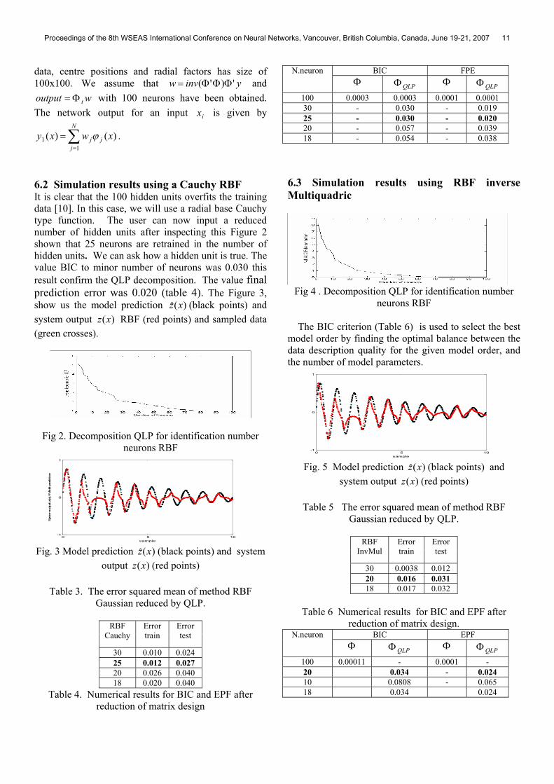
data, centre positions and radial factors has size of 100x100. We assume that and

with 100 neurons have been obtained. The network output for an input is given by

.

yinvw ')'( ΦΦΦ=woutput tΦ=

ix

∑=

=N

jjj xwxy

11 )()( ϕ

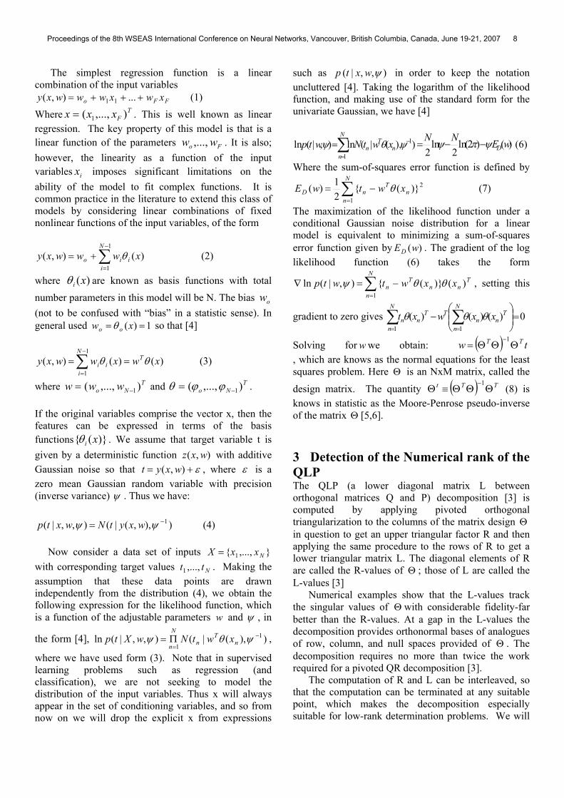
6.2 Simulation results using a Cauchy RBF It is clear that the 100 hidden units overfits the training data [10]. In this case, we will use a radial base Cauchy type function. The user can now input a reduced number of hidden units after inspecting this Figure 2 shown that 25 neurons are retrained in the number of hidden units. We can ask how a hidden unit is true. The value BIC to minor number of neurons was 0.030 this result confirm the QLP decomposition. The value final prediction error was 0.020 (table 4). The Figure 3, show us the model prediction (black points) and system output RBF (red points) and sampled data (green crosses).

)(ˆ xz)(xz

Fig 2. Decomposition QLP for identification number neurons RBF

0 5 10-1

0

1

sample

Sys

tem outpu

t z(x) / M

odel prediction

Fig. 3 Model prediction (black points) and system

output (red points) )(ˆ xz

)(xz

Table 3. The error squared mean of method RBF Gaussian reduced by QLP.

RBF

Cauchy Error train

Error test

30 0.010 0.024 25 0.012 0.027 20 0.026 0.040 18 0.020 0.040

Table 4. Numerical results for BIC and EPF after reduction of matrix design

BIC FPE N.neuron Φ QLPΦ Φ QLPΦ

100 0.0003 0.0003 0.0001 0.0001 30 - 0.030 - 0.019 25 - 0.030 - 0.020 20 - 0.057 - 0.039 18 - 0.054 - 0.038

6.3 Simulation results using RBF inverse Multiquadric

Fig 4 . Decomposition QLP for identification number

neurons RBF

The BIC criterion (Table 6) is used to select the best model order by finding the optimal balance between the data description quality for the given model order, and the number of model parameters.

0 5 10-1

0

1

sample Fig. 5 Model prediction (black points) and

system output (red points) )(ˆ xz

)(xz

Table 5 The error squared mean of method RBF Gaussian reduced by QLP.

RBF

InvMul Error train

Error test

30 0.0038 0.012 20 0.016 0.031 18 0.017 0.032

Table 6 Numerical results for BIC and EPF after

reduction of matrix design. BIC EPF N.neuron

Φ QLPΦ Φ QLPΦ

100 0.00011 - 0.0001 - 20 0.034 - 0.024 10 0.0808 - 0.065 18 0.034 0.024

Proceedings of the 8th WSEAS International Conference on Neural Networks, Vancouver, British Columbia, Canada, June 19-21, 2007 11

6.4 Simulation results using a Multiquadratic RBF The QLP shown in Fig. 8 for the RBF reduced by QLP, the pruning threshold is chosen as 10.

Fig 6. Decomposition QLP for identification number

neurons RBF

In the Fig. 11, the model prediction shows difficulties predicting. The result obtained by our model prediction is slightly inferior to that reported in the experiment Gaussian and Cauchy basis function reduced. The error training and validation (Table 9) was superior that experiments Gaussian and Cauchy.

0 5 10-1

0

1

sample

System output / Model prediction

Fig. 7 Model prediction (black points) and

system output (red points) )(ˆ xz

)(xz

Table 7 The error squared mean of method RBF Multiquadratic reduced by QLP.

RBF Mul

Error train

Error test

12 0.057 0.071 10 0.066 0.081 8 0.066 0.081 5 0.072 0.080

Table 8 Numerical results for BIC and EPF after

reduction of matrix design.

BIC FPE N.neuron Φ QLPΦ Φ QLPΦ

100 0.00024 0.0001 12 - 0.093 - 0.073 10 - 0.101 - 0.081 8 - 0.093 - 0.078 5 - 0.089 - 0.079

7 Conclusions This paper has introduced an automatic model construction algorithm for RBF networks for regression. The main investigations in this study concern the

pruning of RBF hidden nodes by QLP using different radial basis function types. The experimental results demonstrate the potential of our proposed techniques, indicating that QLP is effective when the RBF centres are not adjusted and the regularization parameters are kept fixed. Figures 3 and 5 shows the RBF network predictions after the reduction in the number of hidden units. We also showed that mean square error of selection RBF Cauchy for training and validation were 0.012 and 0.027 respectively, these value is better in comparison with RBF multiquadric and inverse multiquadric. Specifying the basis function as inverse multiquadric was second best with error of training and validation of 0.016 and 0.031 respectively. Demonstration of RBF function type multiquadratic trained with 10, 12 and 15 hiddens units was less successful. We fitted function to data sets by RBF reduced by QLP.

)(xz

References: [1] Edwirde, L.S, Paulo. J.G. Lisboa and González Carmona, A. Pruning RBF networks with QLP decomposition, Conference WEAS Vancouver, Canada, 2007?. [2] Powell, M.J.D. Radial Basis Function for Multivariate Interpolation. A Review. In: Algorithms for Approximation. J.C. Mason and M.G. Cox, (eds). Clarendon Press. Oxford, U.K., 1987. [3] Stewart, G.W, On an Inexpensive Triangular Approximation to the Singular Value Decomposition. Department of Computer Science and Institute for USA, 1998, pp.1-16. [4] Bishop, C.M, Pattern Recognition and Machine Learning. Computer Science. Ed. Springer, U.K., 2006. [6] Golub, G.H and C.F. Van Loan. Matrix Computations (third ed.). John Hopkins University Press. [7] Edwirde, L.S, Paulo. J.G. Lisboa. Comparison of Wiener Filter solution by SVD with decompositions QR and QLP. Conference WEAS Corfu Greece, 2007. [8] Edwirde, L.S, Paulo. J.G. Lisboa. Differentiating features for the Weibull, Gamma, Log-normal and normal distributions through RBF network pruning with QLP. Conference WEAS Corfu Greece, 2007. [9] Guang-Bin Huang and P. Saractchandran. An Efficient Sequential Learning Algorithm for Growing and Pruning RBF (GAP-RBF) Networks. IEEE, Singapure, 2004, pp. 2284-2291. [10] Mark. J. L.Orr. Matlab Routines for selection and Ridge regression in Linear Neural Network, Edinburg University, Scotland, U.K. 1997. [11] Ian T. Nabney. NETLAB. Algorithms for Pattern Recognition. Birmingham, U.K., 2002.

Proceedings of the 8th WSEAS International Conference on Neural Networks, Vancouver, British Columbia, Canada, June 19-21, 2007 12