University of South CarolinaScholar Commons

Senior Theses Honors College

Spring 5-5-2016

Regression Analysis of Success in Major LeagueBaseballJohnathon Tyler ClarkUniversity of South Carolina - Columbia

Follow this and additional works at: https://scholarcommons.sc.edu/senior_theses

Part of the Mathematics Commons

This Thesis is brought to you by the Honors College at Scholar Commons. It has been accepted for inclusion in Senior Theses by an authorizedadministrator of Scholar Commons. For more information, please contact dillarda@mailbox.sc.edu.

Recommended CitationClark, Johnathon Tyler, "Regression Analysis of Success in Major League Baseball" (2016). Senior Theses. 101.https://scholarcommons.sc.edu/senior_theses/101

Clark 1

Major League Baseball (MLB) is the oldest professional sports league in the United

States and Canada. Not surprisingly, after surviving multiple world wars, the Great Depression,

and over 125 years, it is commonly referred to as “America’s Past-time”.

Baseball is “A Thinking Man’s Game”, and arguably more than any other sport, a game

of numbers. No other sport can be explained and studied as precisely with numbers. Indeed,

some of the earliest attempts at using advanced metrics to study sports were performed in the

mid-twentieth century in Earnshaw Cook’s Percentage Baseball (Cook). After failing to attract

the attention of major sports organizations, Bill James introduced Sabermetrics in the late 1970s,

which is the empirical analysis of athletic performance in baseball (Sabermetrics is named after

SABR, or the Society for American Baseball Research). Perhaps the most famous use of a

statistical approach to baseball is described in Moneyball, the 2003 book by Michael Lewis about

Billy Beane, the manager of the Oakland A’s professional baseball team (Lewis). In an

organization with minimal amounts of money to spend, Beane went against the grain of

managerial baseball and used an analytical approach to finding the right players to help his team

rise far above expectations and compete at the same level as the richest teams in the MLB.

This thesis is designed to explore whether a team’s success in any given season can be

predicted or explained by any number of statistics in that season. There are thirty teams in the

MLB; of these thirty, ten make the postseason bracket-style playoffs. The MLB is divided up

into two leagues, the American League and the National League; these two leagues are then

divided up into three divisions each, the West Division, the Central Division, and the East

Division. To make the playoffs a team must either have the most wins in its division after the last

game of the season is played, or it can obtain a Wild Card slot by having either the best or

second best record among the non-divisional champions.

Clark 2

It is considered a great accomplishment for a team if it makes the postseason playoffs;

indeed, since 1996, out of a 162-game season, the lowest number of wins a team has made the

playoffs with is 82, with the average being just above 94. This thesis will investigate whether a

team’s likelihood of making the playoffs, as measured by their regular season win percentage,

can be predicted by offensive and defensive statistics, and then investigate which of these

offensive and defensive statistics have the most impact on win percentage.

Because baseball is so numbers-heavy, there are many different statistics to consider

when searching for the best predictors of team success. There are offensive statistics (offense

meaning when a team is batting) and defensive statistics (defense meaning when a team is in the

field). These categories can be broken up into many more subcategories. However, for the

purpose of this thesis, batting statistics, pitching statistics, and team statistics will be the only

categories studied.

The batting statistics that will be used in this study are R/G, 1B, 2B, 3B, HR, RBI, SB,

CS, BB, SO, BA, OBP, SLG, E, and DP. Below is a description of what each statistic means:

R/G- Runs per game. Calculated by taking the total number of runs a team scores in its

season divided by the number of games it plays.

1B- total singles for a team in a season. A single is defined as when a player hits the ball

and arrives safely at first base on the play, assuming no errors by the fielding team.

Denoted as ‘X1B’ in this study.

2B- total number of doubles for a team in a season. A double is defined as when a player

hits the ball and arrives safely at second base on the play, assuming no errors by the

fielding team. Denoted as ‘X2B’ in this study.

Clark 3

3B- total number of triples for a team in a season. A triple is defined as when a player

hits the ball and arrives safely at third base on the play, assuming no errors by the

fielding team. Denoted as ‘X3B’ in this study.

HR- total number of home runs for a team in a season. A home run is defined as when a

player either hits the ball over the outfield fence in the air or hits the ball and runs all the

way around the bases back to home plate, assuming no errors by the fielding team.

RBI- total number of runs batted in for a team in a season, calculated as runs a team

scores that were the result of a hit.

SB- total number of stolen bases for a team in a season, calculated as when a baserunner

advances to the next base and not as a result of a hit.

CS- total number of times a runner is tagged out attempting to steal a base for a team in a

season.

BB- total number of walks for a team in a season. A walk is defined as four balls thrown

to a batter, with a ball being any pitch thrown outside the strike-zone.

SO- total number of strikeouts for a team in a season. A strikeout is defined as three

pitches thrown for strikes to a batter, with a strike being any pitch hit foul by a batter or

thrown in the strike zone, and the third strike not tipped by the batter or it is tipped foul

while attempting a bunt.

BA- a team’s total batting average, calculated by dividing the total number of hits a team

gets by its total number of at-bats (not including at-bats that result in walks).

OBP- a team’s total on-base percentage, calculated by dividing the total number of times

an at-bat results in the batter getting on base by the total number of at-bats.

Clark 4

SLG- a team’s total slugging percentage, which weights hits for the number of bases that

hit awards the batter. Calculated by dividing the total number of bases all batters are

awarded over their at-bats by total at-bats.

E- total number of errors all opposing teams commit in a season.

DP- total number of double plays turned against a team in a season. A double play is

when two outs are recorded in a single play.

The pitching statistics that will be used in this study are RA/G, ERA, CG, tSho, SV, IP,

H, ER, HR, BB, SO, WHIP, E, DP, and Fld%. Below is a description of what each statistic

means:

RA/G- runs allowed per game, defined as the total number of runs a team allows in a

season divided by the total number of games played.

ERA- earned run average, or a team’s number of earned runs given up divided by total

number of innings pitched.

CG- complete games, or number of games in which the starting pitcher for a team pitches

the entire game for that team.

tSho- team shutouts, defined as the number of games a team does not allow a single run

among all of its pitchers for that game.

SV- total saves for a team. A save is defined as when a pitcher enters the game with a

lead of no more than three runs and pitches for at least one inning and wins; or when a

pitcher enters the game regardless of score, with the potential tying run either on base, at-

bat, or next at-bat and wins; or a pitcher comes in and pitches for at least three innings

and wins.

Clark 5

IP- innings pitched, calculated as the total number of innings pitched by a team in a

season.

H- hits, calculated as total number of hits allowed by a team in a season. Denoted as

‘p_H’ in this study.

ER- earned runs, calculated as total number of earned runs allowed by a team in a season.

An earned run differs from a run in that the run has to be from a hit, and cannot be the

result of an error.

HR- home runs, calculated as total number of home runs allowed by a team in a season.

Denoted as ‘p_HR’ in this study.

BB- walks, calculated as total number of walks allowed by a team in a season. Denoted

as ‘p_BB’ in this study.

SO- strikeouts, calculated as total number of strikeouts by a team’s pitchers in a season.

Denoted as ‘p_SO’ in this study.

WHIP- walks and hits per inning pitched, calculated as the total number of walks and hits

allowed by a team divided by the total number of innings pitched for the team.

E- errors, calculated as total number of errors committed by a team in a season. Denoted

as ‘p_E’ in this study.

DP- double plays, calculated as total number of double plays a team makes in a season.

Denoted as ‘p_DP’ in this study.

Fld%- fielding percentage, defined as the percentage of times a defensive player properly

handles a ball that has been put in play. It is calculated by dividing the sum of putouts

and assists by the sum of putouts, assists, and errors; in other words, the percentage of

time the team’s defense has a chance to make a play and does make the play.

Clark 6

The team statistics that will be used in this study are W, L, T, W-L%, Finish, GB,

Playoffs, R, and RA. Below is a description of what each statistic means:

W- wins, calculated as total number of wins by a team in a season.

L- losses, calculated as total number of losses by a team in a season.

T- ties, calculated as total number of ties by a team in a season. Note, only in extreme

circumstances will regular season games end in a tie (playoff games will never end in a

tie); such circumstances include if the game has been played at least half-way and the

score is tied and the game cannot be finished due to weather and cannot be made up.

W_L_pct- win/loss percentage, calculated by dividing total number of wins by a team in

a season by the total number of games played by that team in that season, and then

multiplying by 100 to get a true percent. Making it a true percent will make it easier to

interpret the coefficients of the independent variables in the regression.

Finish- this is the place in the team’s respective division that the team ended at in a

season; there are currently five teams in each division.

GB- games behind, calculated as the number of wins the leading team got in a given

team’s division minus the number of wins the given team had.

Playoffs- calculated as either a team made the playoffs in a given year or it did not make

the playoffs in the given year.

R- runs scored by a team in a season.

RA- runs allowed by a team in a season.

All of the aforementioned statistics are taken from Baseball-Reference.com (Baseball

Reference). The website has all of the hitting, pitching, and overall statistics for each team going

back as far as the team has been in existence. Since 1961, the MLB has had 162-game seasons.

Clark 7

In 1994 and 1995, the MLB regular season was shortened due to strikes by the players. In 1996,

the strikes ended and the 162-game seasons resumed, and this number of games per season has

remained through today. In order to have seasonal data from only 162-game seasons, and to keep

as many teams as possible in the study, data from the present day back until 1996 will be

collected for each team. This will ensure that the statistics are comparable across season.

Furthermore, all of the statistical analytics will be performed in the statistical software package R

(R Core Team).

The first step in this study is to select the independent variables, or predictors, and the

dependent variable. Once the variables are initially selected, a preliminary regression equation

will be fit to the data in R. Then variable selection will be undertaken to determine which of the

variables are necessary and which are not. Next, the assumptions of the model must be checked

to make sure they hold for the data, we must check for multicollinearity, and we must check for

outliers or influential observations.

Deciding on Candidate Independent Variables

The dependent variable, or regular season success, can be represented by the continuous

W_L_pct variable (Win-Loss percentage), or be represented in the logistic transformation form

of Yes/No for if the team in question made the playoffs that year or not (or 1/0, 1 if the team

made the playoffs and 0 if the team did not make the playoffs). In the absence of evidence that a

transformation of the dependent variable for regular season success is needed, we will use Win-

Loss percentage.

Before the independent variables can be narrowed down from all of the available ones, it

is a good idea to quickly plot all of the possible independent variables against Win-Loss

Clark 8

percentage to check whether any of the independent variables need to be transformed, e.g.,

logarithmically or exponentially, etc. If the plot of a variable has a curved shape or any otherwise

abnormal shape, as opposed to a scattered appearance or roughly linear shape, the variable might

need to be transformed. To obtain the plot, an example code can be seen below, plotting the

dependent variable W_L_pct against the independent variable of X2B:

>plot(X2B,W_L_pct)

To obtain the plot for every independent variable, one simply interchanges a new independent

variable for ‘X2B’ in the code above. An examination of these plots shows that none of the

independent variables have anything other than a scattered or linear shape, so no transformation

should be necessary.

Once the independent variables have been initially checked, candidate independent

variables can be selected. Baseball success certainly has many aspects and a team’s success

cannot be boiled down to one or two statistics; however, it is the aim of this study to determine

whether a relatively small number of statistics can give an accurate representation of how well a

team does in a season, so the set of independent variables will have to be narrowed down.

The hitting statistics that will be initially considered as predictors will be R_G, X1B,

X2B, X3B, HR, RBI, SB, CS, BB, SO, BA, OBP, SLG, BatAge, and DP. The pitching statistics

that will be initially considered as predictors will be RA_G, ERA, p_H, p_HR, ER, p_BB, p_SO,

WHIP, p_E, p_DP, p_Fld_pct, and PAge.

Fitting the Preliminary Regression

Clark 9

Now that the variables have been selected, they can be fit into a linear regression. To do

this, we use the following code in R:

> linreg_regseason <- lm(W_L_pct*100~RA_G + ERA + p_H + p_HR + ER + p_BB +

p_SO + WHIP + p_E + p_DP + p_Fld_pct + PAge + R_G + X1B + X2B + X3B + HR +

RBI + SB + CS + BB + SO + BA + OBP + SLG + DP + BatAge,

data=complete.data.used)

This linear regression produces the following coefficients for the respective independent

variables, which are found in the ‘Estimate’ column:

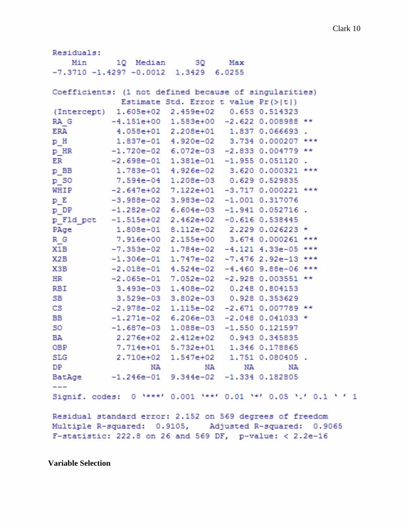
Clark 10

Variable Selection

Clark 11

Now that we have a preliminary regression fit to the data, we can narrow down the

variables in our model using tests that can shed light on which variables are unnecessary. We

begin with a stepwise procedure. We call a ‘step’ function in R, which goes through the variables

in the regression and through a series of additions or deletions of variables based on their values

in the regression, and provides a list of necessary variables. To do this, we first use a step

function that starts with no variables and works its way up until it reaches the correct number and

combination of variables:

> step(null, scope=list(lower=null, upper=linreg_regseason), direction="both")

This function gives us the following regression fit:

As can be seen, the regression we originally chose has been narrowed down from 27 variables to

16.

Now, we use the same step function, but use backward elimination. This reverses

directions so it starts with all the variables and whittles the regression down to the necessary

number and combination, to compare the list of variables to the stepwise list:

> step(linreg_regseason, scope=list(lower=null, upper=linreg_regseason),

direction="backward")

This function gives us the following regression fit:

Clark 12

This time, the regression narrowed the 27 variables down to 18; the only difference between the

two is the backward step function added p_H and WHIP. Thus, moving forward, we will keep all

of the variables provided by either step function, or, essentially, the regression provided by the

backward step function. Furthermore, CS was included in both but SB was not, so seemingly the

number of times a team is caught stealing is more influential than the number of times it

successfully steals a base. I would like to examine the effect of SB further, so I will add SB to

the regression, giving us a total of 19 variables.

As a subsequent method for variable selection, we run a ‘leaps’ function in R (Lumley).

For our data, this gives us the best-fitting regression equations for any fixed number of variables

we want to include. In this case, we give it a total of 19 variables to test, so it provides the two

best-fitting one-variable regression equations, the two best-fitting two-variable regression

equations, and so on, up to the two best-fitting 18-variable regression equations and then the lone

19-variable regression equation. It then provides the adjusted r-squared value for each regression

equation. Adjusted r-squared is a measure of how well a regression equation fits its data, while

penalizing the model for having a higher number of variables; in essence, a model is unlikely to

have a high adjusted r-squared value if it fits the data well but has several unnecessary variables.

The code for this test is:

> leaps(x = cbind(SB, RA_G, R_G, X3B, PAge, ERA ,ER, SLG, X2B, HR, X1B, p_BB,

p_HR, CS, BB, p_DP, p_E, p_H, WHIP), y = W_L_pct*100, nbest = 2, method =

"adjr2")

Clark 13

This code produces a very large table, but the adjusted r-squared values for the 37 different

equations are:

Note, adjusted r-squared values can be at most 1, so the highest value, .9066517, (value [35])

indicates that regression is a very good fit. This equation is one in which all the variables are

used except SB; however, I am still interested in investigating its effects, so we will keep it in the

model, and stay at 19 variables.

These 19 variables are then entered into a new regression:

> reg_better = lm(W_L_pct*100 ~ SB+ RA_G+ R_G+ X3B+ PAge+ ERA +ER+ SLG+

X2B+ HR+ X1B+ p_BB+ p_HR+ CS+ BB+ p_DP+ p_E+ p_H+ WHIP)

We also investigate multicollinearity. Multicollinearity is when some predictors are linear

combinations of others; for example, the two variables ‘Height in feet’ and ‘Height in inches’

would be collinear, as ‘Height in feet’ can be expressed as (1/12)* ‘Height in inches’. When

there is multicollinearity present, problems occur in the estimation of the coefficients of the

linear regression. Next, we create a function that can take a regression equation and provide the

VIF’s for the variables. VIF, or Variance Inflation Factor, is a test used to search for

multicollinearity; that is, it compares the inflation of the variance of estimated regression

coefficients in a linear relationship with the variance of estimated regression coefficients in a

non-linear relationship. Lower values are desired, as it means variables most likely are not in a

Clark 14

linear relationship with each other, and thus are necessary. The function can be seen below

(Hitchcock):

Now, to view the VIFs of our regression equation, we type vif(*name of our equation), or:

> vif(reg_better)

and the VIFs are provided:

Here, we can see RA_G, ERA, ER, SLG, HR, p_BB, p_H, and WHIP initially have incredibly

high VIFs. This can be explained easily, as we would expect RA_G to be closely related to ERA

and ER; SLG to be potentially related to HR; and p_H and p_BB to be closely related to WHIP.

Clark 15

Thus, we will eliminate RA_G, ER, SLG, and WHIP, as they can be expressed by the remaining

variables. We then create a new regression analysis, and find the VIFs of this new equation:

> reg_better2 = lm(W_L_pct*100 ~ SB+ R_G+ X3B+ PAge+ ERA + X2B+ HR+ X1B+

p_BB+ p_HR+ CS+ BB+ p_DP+ p_E+ p_H)

These VIFs are much more manageable; however, the VIFs of R_G and ERA are still a little too

high to be accepted and these predictors could be related to other variables, so we will eliminate

them from the regression analysis, and repeat the steps:

> reg_better3 = lm(W_L_pct*100 ~ SB+ X3B+ PAge + X2B+ HR+ X1B+ p_BB+

p_HR+ CS+ BB+ p_DP+ p_E+ p_H)

These VIFs are very small, within the acceptable range, so we move on to check the model

assumptions for our regression.

Checking Model Assumptions

When checking to see whether our model assumptions hold for the data, we need to

check for constant error variance (is the variance of the errors a constant value or does it depend

on some variable?); model specification (is the data best represented by a linear or nonlinear

regression?); normality of errors (do the errors closely follow a normal distribution or are they

Clark 16

distributed irregularly?); and independent errors (are the errors independent of one another or are

they related?).

An initial test for these assumptions is to plot the residuals of the linear regression against

the fitted values of the observations. To do this, the following code is used, and the following

chart produced:

>plot(fitted(reg_better3),residuals(reg_better3),xlab="Fitted",ylab="Residuals”)

Clark 17

This plot tells us a few things about the data. First of all, because the spread of the residuals does

not increase or decrease with the fitted values, there is not an issue of heteroscedasticity

(heteroscedasticity meaning the variance of the regression changes for larger or smaller fitted

values). This means the error variance of the data is constant, meeting the constant error variance

assumption. Additionally, because the plot displays random scatter, there is no indication that the

regression relationship is nonlinear (as opposed to if the plot had, say, a parabolic shape), so a

linear regression is the appropriate model specification for this data.

To provide added clarity for detecting nonconstant variance, the predicted values of the

regression are plotted against the absolute value of the residuals. This folds up the bottom half of

the above plot to help provide insight into any patterns that could be missed in the above plot.

This is done with the following code, and produces the following plot:

>plot(fitted(reg_better3),abs(residuals(reg_better3)),xlab="Fitted",ylab="|Residuals|")

Clark 18

Again, there does not seem to be any sort of heteroscedastic or nonlinear issue with this plot, and

thus there does not seem to be an issue with nonconstant variance.

The testing that we are using assumes the errors are normally distributed. To check for

this, a Q-Q plot is created, which compares the residuals with what we would expect as normal

observations. To do this, the following code is used and the following plot is produced:

> qqnorm(residuals(reg_better3),ylab="Residuals")

Clark 19

If the errors are indeed normally distributed, then the plot should produce a relatively straight

line of observations. Because the plot above approximately can be seen to follow a straight line,

the residuals meet the normality assumption.

Lastly, the tests assume the errors are uncorrelated; however, for time-based data, there

may be some correlation. To check for this, the residuals will be plotted against time, using the

following R code and producing the following plot:

Clark 20

> plot(Year,residuals(reg_better3),xlab="Year",ylab="Residuals")

Because there is no change in the pattern of residuals over the years, the errors can be assumed to

be uncorrelated, meeting the last test assumption.

Checking for Outliers or Influential Observations

An outlier is a data observation that does not fit with the regression; if the linear

regression accurately predicts 99 out of 100 data observations but the last prediction is far from

Clark 21

the observed value, that point is an outlier. If an observation has an unduly strong effect on the

regression fit, it is called influential. Testing for outliers and influential observations is important

because if present, they may affect the fit of a regression.

To check for influential observations, we use the code:

>influence.measures(reg_better3)

This produces a very large table that gives several measures of how influential each observation

is (with each observation being a specific year for a specific team). We will look more closely at

the measure ‘dffits’; if dffits is greater than twice the square root of one plus the number of

variables in the regression divided by the total number of observations, it can be considered an

influential observation. To test for this, and knowing that after working out the numbers we are

looking for dffits with absolute values greater than .2954 (m=12, n=596), we use the following

code:

> (1:596)[abs(dffits(reg_better3))>.2954]

This gives us the following specific observations which have been, by our criteria, defined as

influential observations:

This is a fairly long list of influential observations, so we can narrow it down and see how many

are exceptionally influential:

> (1:596)[abs(dffits(reg_better3))>.5]

This tells us that there is one exceptionally influential observation:

Clark 22

The observation ‘191’ is the 2003 Detroit Tigers, who finished 5th in the American League

Central Division:

To figure out if this observation negatively affects our regression, we will compare a statistical

summary of the regression with the observation included against a summary without it. If the

observation is very influential, then the coefficients of the variables will have a significant

change when the observation is left out of the regression.

Clark 23

Now, we create a new regression, without the influential observation:

Clark 24

As can be seen in comparing the two regression summaries, including the influential observation

has a very minimal effect on the coefficients themselves and on their significance (as defined by

their p-values). Thus, we will keep the observation in our regression.

We can further validate the model by checking the PRESS, or predictive residual sum of

squares. This function goes through the regression and for each observation in the data set,

removes that observation, fits a new regression with one less observation, and measures how

closely the removed observation would have been predicted by the new regression. We can

Clark 25

compare it to the SSE, or sum of squared residuals; we expect the PRESS to be slightly larger

than SSE, and hope that it is not too much larger:

> PRESS.statistic <- sum((resid(reg_better3)/(1-hatvalues(reg_better3)))^2)

Doing this gives us a value of 5838.724, as can be seen below:

The anova, or analysis of variance for our chosen regression model, shows we get a SSE of

5563.5, which can be seen below:

Because 5838.724 is not much larger than 5563.5, we further accept that the regression fits the

data well.

Clark 26

Prediction Intervals

Prediction intervals can be handy for measuring intervals where future observations will

fall, given certain predictors; in this case, we could use them to predict an interval for a team’s

winning percentage given certain factors, such as Batting Average, Hits, etc. However, we can

also use prediction intervals to see how well our model fits the data; we can estimate prediction

intervals for our data, and hope to see a large portion of our response values fall within their

respective intervals.

To do this, we first create the prediction intervals at a 95% level; this means we hope to

see at least 95% of our response values fall in the prediction intervals. Next, we calculate in R

the percent of winning percentages that do fall in the prediction intervals.

> mypreds=predict(reg_better3,interval="prediction",level=0.95)

We are further satisfied with our model, having 95.6378% of our response values fall within the

prediction intervals.

Sample Predictions

Now that we have our regression, and have validated the model and checked to ensure the

model assumptions hold, we can use it to predict the winning percentage of teams with specific

statistics; for example, we can predict the winning percentage of a team with hypothetical

statistics, and we can predict the winning percentage of a team in a long ago season to see how it

would fare in today’s world of baseball based on its statistics back then. This is significant

Clark 27

because the game of baseball, like everything else in life, changes over time, and what may have

been key for winning games 40 years ago might not be key for winning games today.

First, we will make up a team’s statistics, and create a dataframe with these statistics:

> stats_madeup <-

data.frame(cbind(SB=70,X3B=30,PAge=27,X2B=375,HR=215,X1B=1000,p_BB=450,p

_HR=160,CS=38,BB=525,p_DP=165,p_E=80,p_H=1400))

We then predict the hypothetical team’s winning percentage for those given statistics:

So by the calculations in R, the team with the given statistics is predicted to win 62.77% of their

games; and if there were many, many teams with those given statistics, 95% of the teams would

be predicted to have a winning percentage between 56.58% and 68.97%.

Now, we can predict the winning percentage of a historical team; for example, the 1969

“Miracle Mets”. The New York Mets surprised the country and overcame a late-season

divisional gap between them and the divisional leaders, the Chicago Cubs, and ended up winning

the World Series. They ended the regular season with a 61.7% winning percentage. To calculate

the Miracle Mets’ predicted winning percentage, we repeat the above steps using the Mets’ stats

from that year:

> miracle_mets <-

data.frame(cbind(SB=66,X3B=41,PAge=25.8,X2B=184,HR=109,X1B=977,p_BB=517,p

_HR=119,BB=527,p_DP=146,p_E=122,p_H=1217,CS=43))

Clark 28

Thus, based on our regression, we would have predicted the Mets’ winning percentage to be

52.06%; given the statistics, if there were many identical teams, 95% of the teams would have a

winning percentage between 45.8% and 58.34%. The fact that the actual winning percentage of

the team was much higher either means the statistics that helped them win that year are not as

significant in this time period, or they had a lucky season, as their nickname suggests.

Interpretation of Regression

The final regression that we came up with, along with the coefficients, is:

Below is a concise list of the variables that were included:

SB- stolen bases for a team in a season. The coefficient can be interpreted as for each

additional stolen base, a team’s winning percentage can be expected to increase .0115%,

adjusting for the other predictors in the model.

X3B- triples hit for a team in a season. The coefficient can be interpreted as for each

additional triple hit, a team’s winning percentage can be expected to increase .0314%,

adjusting for the other predictors in the model.

Clark 29

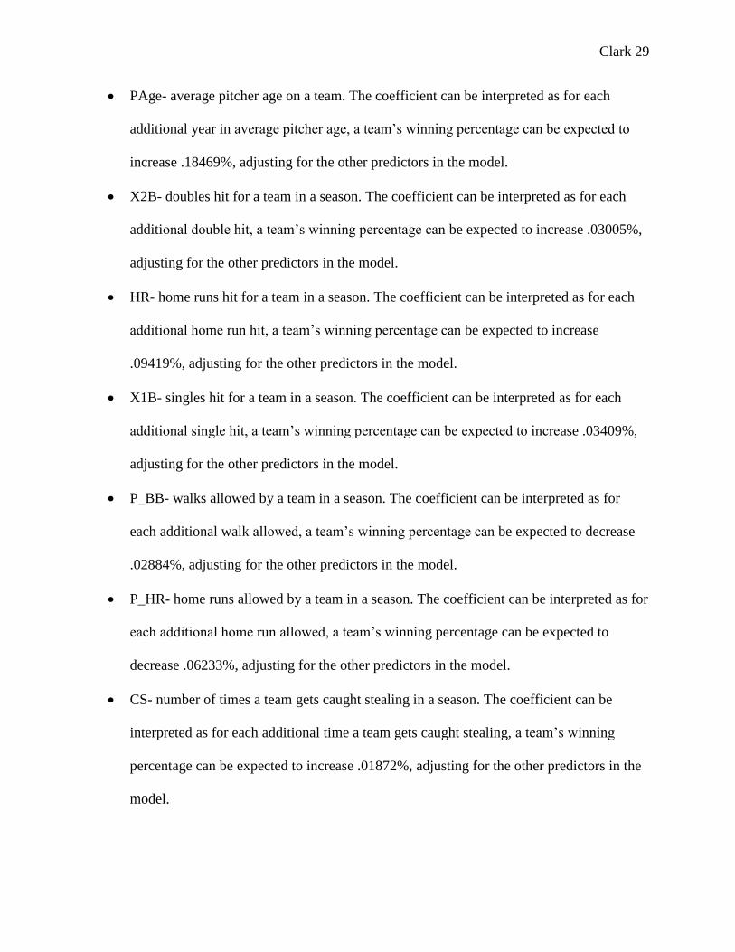
PAge- average pitcher age on a team. The coefficient can be interpreted as for each

additional year in average pitcher age, a team’s winning percentage can be expected to

increase .18469%, adjusting for the other predictors in the model.

X2B- doubles hit for a team in a season. The coefficient can be interpreted as for each

additional double hit, a team’s winning percentage can be expected to increase .03005%,

adjusting for the other predictors in the model.

HR- home runs hit for a team in a season. The coefficient can be interpreted as for each

additional home run hit, a team’s winning percentage can be expected to increase

.09419%, adjusting for the other predictors in the model.

X1B- singles hit for a team in a season. The coefficient can be interpreted as for each

additional single hit, a team’s winning percentage can be expected to increase .03409%,

adjusting for the other predictors in the model.

P_BB- walks allowed by a team in a season. The coefficient can be interpreted as for

each additional walk allowed, a team’s winning percentage can be expected to decrease

.02884%, adjusting for the other predictors in the model.

P_HR- home runs allowed by a team in a season. The coefficient can be interpreted as for

each additional home run allowed, a team’s winning percentage can be expected to

decrease .06233%, adjusting for the other predictors in the model.

CS- number of times a team gets caught stealing in a season. The coefficient can be

interpreted as for each additional time a team gets caught stealing, a team’s winning

percentage can be expected to increase .01872%, adjusting for the other predictors in the

model.

Clark 30

BB- walks for a team in a season. The coefficient can be interpreted as for each

additional walk earned, a team’s winning percentage can be expected to increase

.02282%, adjusting for the other predictors in the model.

P_DP- double plays turned by a team in a season. The coefficient can be interpreted as

for each additional double play turned, a team’s winning percentage can be expected to

increase .00741%, adjusting for the other predictors in the model.

P_E- errors by a team’s defense in a season. The coefficient can be interpreted as for each

additional error, a team’s winning percentage can be expected to decrease .02681%,

adjusting for the other predictors in the model.

P_H- hits given up by a team in a season. The coefficient can be interpreted as for each

additional hit allowed, a team’s winning percentage can be expected to decrease

.03402%, adjusting for the other predictors in the model.

Below is a graph of the predictor variables in the regression and their corresponding t-

statistics. The t-statistic measures how significant that variable is in predicting win percentage,

being measured by dividing the estimated coefficient by the standard error of that coefficient.

(The blue bars are positive t-statistics and the red bars are negative t-statistics).

Clark 31

The coefficients, for the most part, make sense. All of the variables have the same sign

(positive or negative) as what would be expected; all except CS, or caught stealing. One would

think that the more times a team gets caught stealing, the less baserunners would score, and the

less wins a team would get. However, the coefficient having a positive sign means the more

times a team gets caught stealing the more wins it gets. Perhaps this is because more times

caught stealing implies more aggressive base-running and more runners on base to begin with,

and thus perhaps more runs scored and more wins, but this is mere speculation. However, an

examination of the t-test about the coefficient of CS shows that it is not significantly different

from zero (P-value=0.18), so little importance should be assigned to its positive estimated

coefficient.

Furthermore, while PAge, for example, has a positive coefficient, this does not mean that

steadily increasing a team’s average pitcher age will steadily increase the team’s winning

percentage. At some point increasing the average age by another year will not result in a higher

winning percentage, and will obviously start to negatively affect the winning percentage as the

pitchers get older and older (while a 35-year old pitcher might be argued to be more beneficial to

Clark 32

a team than a 32-year old pitcher, a 70-year old pitcher will undoubtedly be much worse for a

team than a 35-year old pitcher). Looking at the positive coefficient and assuming this implies

that increasing the average age will always increase the winning percentage is called

extrapolation. We cannot assume that what we know about relationships between variables

applies to data outside that range. Such an erroneous assumption is illustrated by the simple

example above about a 70-year old pitcher.

Conclusion

In completing this regression analysis, I was able to put together skills I learned from my

statistics courses to investigate something that is interesting to me. From start to finish, I pulled

statistics from a database, edited them into a form that I could use, and manipulated statistical

software to answer the research questions I was interested in learning about.

I learned how to research in textbooks and online, and how to use all of the resources

available to me to both learn technical skills and then use them to accomplish a goal. Being able

to use statistical software to learn about trends in data, and being able to learn new procedures in

statistical software, is important to me going into a career as an actuary. With this experience, I

was able to put to use my education in mathematics and statistics in the culmination of my time

as a student of USC, and gain experience that will greatly benefit me in my career in the

workplace.

Clark 33

Works Cited

Baseball Reference. (2016, April 17). Retrieved March/April, 2016, from http://www.baseball-

reference.com/

Cook, E. (1966). Percentage baseball. Cambridge: M.I.T. Press.

Faraway, J. J. (2005). Linear models with R. Boca Raton: Chapman & Hall/CRC.

Clark 34

Hitchcock, D. (n.d.). Retrieved March/April, 2016, from

http://people.stat.sc.edu/hitchcock/teaching.html

Lewis, M. (2003). Moneyball: The Art of Winning an Unfair Game. New York: W.W. Norton.

Lumley, Thomas using Fortran code by Alan Miller. (2009). Leaps: Regression subset selection

(Version 2.9) [Computer software]. Retrieved from http://CRAN.R-

project.org/package=leaps

R Core Team. (2015). R: A Language and Environment for Statistical Computing [Computer

software]. Retrieved from https://www.R-project.org/