SAN FRANCISCO ESTUARY INSTITUTE • CLEAN WATER PROGRAM / RMP • 4911 CENTRAL AVE., RICHMOND, CA 94804 • www.sfei.org

CONTRIBUTION NO. 811

JANUARY 2017

Prepared by

Jing Wu, Alicia Gilbreath and Lester McKee, San Francisco Estuary Institute

For

Regional Monitoring Program for Water Quality in San Francisco Bay (RMP)

Sources Pathways and Loadings Workgroup (SPLWG)

Small Tributaries Loading Strategy (STLS)

Regional WatershedSpreadsheet Model (RWSM)Year 6 Final Report

Wu, J., Gilbreath, A.N., McKee, L.J., 2017. Regional Watershed Spreadsheet Model (RWSM): Year 6 Progress Report. A technical report prepared for the Regional Monitoring Program for Water Quality in San Francisco Bay (RMP), Sources, Pathways and Loadings Workgroup (SPLWG), Small Tributaries Loading Strategy (STLS). Contribution No. 811. San Francisco Estuary Institute, Richmond, California.

2016 RWSM:FINAL resultsJing Wu, Alicia Gilbreath, and Lester McKee 1/23/2017

Introduction

The purpose of this “annotated PowerPoint presentation” is to document the efforts made with the allotted RMP 2016 budget ($35k) to improve the regional watershed spreadsheet model (RWSM) for both PCBs and Hg, and to present an initial outline of the work proposed for use of the allotted RMP 2017 budget ($40K).

The project has been supported by review and oversight from members of the STLS team and external peer-review from Michael Stenstrom and Peter Mangarella

2016 Conclusions

● Improved hydrology calibration provides better basis for PCB/Hg models

● Weaknesses remain in the GIS data used for supporting the model

● Pollutant models generally follow expected relative concentrations and yields in relation to land use/source area conceptual models

● Manual calibration appears more robust than automated calibration, as the parameter coefficients can be chosen to follow the conceptual model. But the auto-calibration provides insights on the boundary conditions defined through the manual calibration and also an estimate of errors.

● The choice of calibration data set influences the PCB model outputs greatly - this remains a concern that needs to be addressed

● PCB/Hg regional loads appear reasonable, but since source areas could not be modeled as a unique parameter due to lack of observed data and GIS weaknesses, local loads might be more biased by virtue of outliers like Pulgas - but less so for regional.

Suggested work plan for use of 2017 funds

● Add WY 2016 recon data to calibration dataset (increasing total dataset from ~40 to ~60 watersheds), try new calibrations, and make decision on the final choice of calibration dataset.

● Analyze calibration watershed subsets to try to determine which subset is suitable to use for model calibration

● Further improve GIS layers where possible, perhaps use improved GIS data from Santa Clara and San Mateo programs for model calibration

● Further investigate and define rationale for boundary constraints of lesser influential coefficients (Ag/Open/New Urban and Old Residential for PCBs, New Urban and Old Industrial/Source Areas for Hg) since the calibration process is less sensitive to these coefficients

● Initiate further stakeholder discussion of proposed uses, target users, and how to package the RWSM

Model intent and history

● Model developed primarily to estimate regional loads and secondarily to provide additional “weight of evidence” for management at finer scales (Bay margins, single watersheds, subwatersheds, or older built-out areas)

● 2010/11/12: Development of the hydrological model and conceptual basis for the pollutant models (Lent and McKee, 2011; Lent et al., 2012)

● 2013/14: Development of the suspended sediment model and sediment-based PCB and Hg models but efforts largely unsuccessful (McKee et al., 2014)

● 2015/16: Switched to water-based PCB and Hg models. Calibrated to a range of targets to add error bars to model parameters (25th & 75th%iles). Ok calibration for PCBs; questionable calibration for Hg (Wu et al., 2016)

Summary of changes made in 2016

● GIS○ Eliminated expected less-dirty source areas○ Trimmed buffers on cement and crematoria source areas

● Hydrology model○ Prism rainfall layer updated to 2010 - aligns better with the pollutant data○ Flow calibration data normalized to 1980-2010 averaging period to be consistent with the rainfall data○ Ettie St., Laurelwood and Victor-Nelo PS watersheds removed from calibration; Pulgas PS South and

North Richmond PS watersheds added to calibration.○ Separated the region into 3 micro-climate subregions for independent calibrations○ Applied region-wide initial abstraction coefficient (7 inches) (this still needs expert review)

● Pollutant models○ Investigated outliers to learn about model○ Adjusted parameter groupings○ Calibrated manually to develop coefficient ranges and used these to constrain the auto-calibration○ Increased the calibration data set 23 to a maximum of 41 watersheds

Land use groupings

Note that the source area parameter groupings cover a mix of source release mechanisms.

Different combinations of land use groupings were further explored. Ultimately, it was concluded that source areas are unpredictable and uneven (sometimes very polluted, sometimes not) and so it was decided to eliminate source areas that are generally expected to be less polluted, and to group Source Areas with Old Industrial area.

Source Areas eliminated:

Manufacture - MetalsRecycling - AutoRecycling - MarineRecycling - MetalsRecycling - WasteTransportation - Shipping

Buffer Widths reduced:

Cement - from 2000m to 500mCrematoria - from 2000m to 30m

Hydrology model re-calibration

East Bay North Bay South Bay/ Peninsula

The hydrology model was re-calibrated using the updated rainfall data layer (PRISM 2010) and a slightly new mix of calibration watersheds (excluding Ettie St, Laurelwood and Victor-Nelo PS watersheds, and including N Richmond PS and Pulgas Ck PS watersheds). The region was also divided into 3 subregions, following the Rantz classification of the climatic region in relation to runoff, and calibrated separately. Finally, an initial abstraction coefficient was applied to the entire region.

Calibration results:

Mean bias = +1%Median bias = 0%Range = +- 30%

Pollutant models - outlier investigation

As recommended by our expert reviewers, we investigated the watersheds that presented as outliers in the results. The investigation included primarily a closer look at the pollutant data inputs and the land use in those watersheds as represented in the land use layer versus recent aerial photographs. As a result, two watersheds (Lower Penitencia Ck and Zone 5 Line M) were excluded from the calibration.

Example of land use changes in Lower Penitencia Creek watershed in recent times, leading to a misclassification of these areas in the land use layer. Many areas in Lower Penitencia Creek watershed have been redeveloped more recently, providing logical explanation for why the model simulated much higher concentrations than observed.

Pollutant models - manual calibration

Guiding principles applied:

● Relative order of concentrations for each land use group in order of conceptual model of cleanest to dirtiest (Lent and McKee, 2011)

● Parameter with lowest yield smaller than cleanest watershed for each model

● Parameter with highest yield guided by dirtier watersheds for each model

● Minimize RMSE and percent bias between modeled and observed concentrations across 3 subsets of calibration watersheds: all watersheds, watersheds > 4km2, and well-sampled watersheds

Choices for calibration data sets

● Well-sampled Watersheds: Category includes few but very well-sampled watersheds; eliminates the weakness associated with characterizing EMCs based on a single storm composite sample

● Watersheds > 4km2: Category is inclusive of about half the available watersheds; at least partially removes the biases associated with GIS mapping challenges if we assume mapping errors are more likely to be averaged out in the larger watersheds

● All watersheds: Biased toward the inclusion of smaller watersheds with large areas of old industrial and source areas, but which have EMCs based on a single storm composite.

○ Adding even more more watersheds during future calibration runs, even if only with single-storm composites, may help to improve the representativeness of this calibration dataset by averaging out the errors associated with characterizing EMCs based on a single storm composite sample

PCBs calibration constraints (ng/L)

The manual calibration enabled us to better define the upper and lower bounds of the calibration coefficients for the auto calibration. You will see in the next slide that, in some cases, the auto calibration results pushed against either the upper or lower boundary constraints. This is particularly true for the two parameters with lower coefficients and suggests the need for further investigation even though these don’t account for much of the regional load.

Ag/Open/New Urban

Old Industrial + Source Areas

Old Residential

Old Commercial + Old Transportation

Recommended auto calibration minimum boundary 0.2 100 4 20

Recommended auto calibration maximum boundary 1.5 400 16 70

Results - PCB auto calibration (ng/L)

Parameter

(Land uses and source

areas)

Coefficients for calibration of

watersheds > 4km2

Coefficients for calibration of

well-sampled watersheds

low

25%ile

best

50th%

high

75%ile

low

25%ile

best

50th%

high

75%ile

New urban, ag, and open 0.2 0.2 1 0.2 0.2 0.2

Old Residential 4 4 16 4 4 16

Old Commercial and

Transportation20 20 37 20 50 70

Old Industrial and Source

Areas100 123 155 100 201 400

Total Regional Load (kg) 12 14 22 12 25 45

Three subsets of calibration watersheds were proposed: 1) all calibration watersheds (n=37), 2) calibration watersheds > 4km2 (n=17), and well-sampled calibration watersheds (n=8). Per discussion with the STLS, calibration to the whole watershed set was dropped. Resulting coefficients from calibration to two remaining subsets yields very different results for PCBs.

Watersheds >4km2

● More watersheds included may mean better representation of land use and area?

● These include less well-sampled watersheds that likely have low EMC bias

Well-sampled watersheds● Based on concentrations and

particle ratios, these watersheds span the full breadth of observations made to date.

● However, these watersheds are possibly disproportionately biased towards sampling dirtier than average Old Industrial and Source Area areas.

Given the differences in regional loads based on each choice, a final decision needs to be made on the calibration dataset.

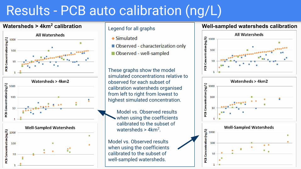
Legend for all graphs

These graphs show the model simulated concentrations relative to observed for each subset of calibration watersheds organised from left to right from lowest to highest simulated concentration.

Model vs. Observed results when using the coefficients calibrated to the subset of watersheds > 4km2.

Model vs. Observed results when using the coefficients calibrated to the subset of well-sampled watersheds.

Results - PCB auto calibration (ng/L)These graphs show the model simulated concentrations relative to observed for each subset of calibration watersheds.

Several watersheds in the “All watersheds” dataset show simulated concentrations much higher than observed concentrations.

Simulated results using the coefficients obtained from the calibration to watersheds >4km2 are generally lower than when using coefficients obtained from the calibration to well-sampled watersheds.

Legend for all graphs

Watersheds > 4km2 calibration Well-sampled watersheds calibration

PCB average yields (g/km2) by parameter group

The choice of calibration watersheds makes a large difference to the resulting yields for each land use category.Note that these yields differ from those published by BASMAA (g/km2/y): Source property: 1004; Old industrial: 21; Old urban: 7.5; New urban: 0.9; Other: 0.9; Open space: 1.1

Hg calibration constraints (ng/L)

The manual calibration enabled us to better define the upper and lower bounds of the calibration coefficients for the auto calibration. You will see in the next slide that, in some cases, the auto calibration results pushed against either the upper or lower boundary constraints. This was particularly notable for Old Industrial+Source areas and indicates a need to further explore the constraints for this parameter even though it doesn’t account for much of the regional load.

Ag/Open New Urban Old Industrial + Source Areas

Old Urban

Recommended auto calibration minimum boundary 35 3 40 35

Recommended auto calibration maximum boundary 105 9 120 105

Results - Hg auto calibration (ng/L)

Parameter

(Land uses and source

areas)

Coefficients for calibration of

watersheds > 4km2

Coefficients for calibration of

well-sampled watersheds

low

25%ile

best

50th%

high

75%ile

low

25%ile

best

50th%

high

75%ile

Ag and open 50 71 95 47 72 105

New Urban 3 3 9 3 3 9

Old Industrial and Source

Areas40 40 40 40 40 40

Old Urban59 68 86 48 63 85

Total Regional Load (kg) 70 93 122 64 92 131

Three subsets of calibration watersheds were proposed: 1) all calibration watersheds (n=35), 2) calibration watersheds > 4km2 (n=14), and well-sampled calibration watersheds (n=6). Per discussion with the STLS, calibration to the whole watershed set was dropped. Resulting coefficients from calibration to two remaining subsets yields similar results for Hg.

For Hg, it matters little which calibration data set is used.

Results - Hg auto calibration (ng/L)These graphs show the model simulated concentrations relative to observed for each subset of calibration watersheds.

Several watersheds in the “All watersheds” dataset that are simulated concentrations much higher than observed concentrations.

Results change little between the two sets of calibration coefficients.

Legend for all graphs

Watersheds > 4km2 calibration Well-sampled watersheds calibrationLegend for all graphs

These graphs show the model simulated concentrations relative to observed for each subset of calibration watersheds organised from left to right from lowest to highest simulated concentration.

Model vs. Observed results when using the coefficients calibrated to the subset of watersheds > 4km2.

Model vs. Observed results when using the coefficients calibrated to the subset of well-sampled watersheds.

Hg average yields (g/km2) by parameter group

The choice of calibration watersheds makes little difference to the resulting yields for each land use category.Note that these yields differ from those published by BASMAA (g/km2/y): Source property: 321; Old industrial: 321; Old urban: 53; New urban: 8.2; Other: 6.4; Open space: 8.2

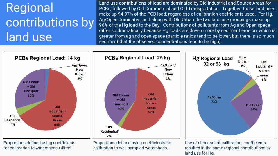
Regional contributions by land use

Regional Load: 14 kg

Land use contributions of load are dominated by Old Industrial and Source Areas for PCBs, followed by Old Commercial and Old Transportation. Together, those land uses make up 94-97% of the PCB load, regardless of calibration coefficients used. For Hg, Ag/Open dominates, and along with Old Urban the two land use groupings make up 96% of the Hg load to the Bay. Contributions of pollutants from Ag and Open space differ so dramatically because Hg loads are driven more by sediment erosion, which is greater from ag and open space (particle ratios tend to be lower, but there is so much sediment that the observed concentrations tend to be high).

Regional Load: 25 kg Regional Load 92 or 93 kg

Proportions defined using coefficients for calibration to watersheds >4km2.

Proportions defined using coefficients for calibration to well-sampled watersheds.

Use of either set of calibration coefficients resulted in the same regional contributions by land use for Hg.

Subembayment loads and yields

San Pablo Suisun

Central

South

DumbartonSouth

A Loads and yields calculated using coefficients from calibration to the watersheds >4km2.B Loads and yields calculated using coefficients from calibration to the well-sampled watersheds.

Do model results make sense? Generally yes, but not always...

● Concentrations ○ For new urban/ag/open, a PCB concentration of 0.2 ng/L may be a little low but model tends to

push against low boundary○ For old industrial/source areas, a PCB concentration of 201 ng/L may be about right given much

greater concentrations was observed in mixed land use watersheds, in addition to the model calibrating roughly in the middle of the imposed boundaries

● Yields○ PCB yields for ag/open/new urb are 10x lower than observed in Marsh Ck. May not be reasonable○ PCB yields for old industrial/source areas of either 37 or 61 g/km2 are less than observed in Pulgas

which probably makes sense given the watershed is a uniquely polluted watershed

● Loads○ Regional PCB loads of 25 kg is about right, but does focus on industrial areas/sources in well

sampled watersheds appropriately balance lack of a unique source area parameter in the model?

References

Lent, M.A. and McKee, L.J., 2011. Development of regional suspended sediment and pollutant load estimates for San Francisco Bay Area tributaries using the regional watershed spreadsheet model (RWSM): Year 1 progress report. A technical report for the Regional Monitoring Program for Water Quality, Small Tributaries Loading Strategy (STLS). Contribution No. 666. San Francisco Estuary Institute, Richmond, CA. http://www.sfei.org/sites/default/files/RWSM_EMC_Year1_report_FINAL.pdf

Lent, M.A., Gilbreath, A.N., and McKee, L.J., 2012. Development of regional suspended sediment and pollutant load estimates for San Francisco Bay Area tributaries using the regional watershed spreadsheet model (RWSM): Year 2 progress report. A technical progress report prepared for the Regional Monitoring Program for Water Quality in San Francisco Bay (RMP), Small Tributaries Loading Strategy (STLS). Contribution No. 667. San Francisco Estuary Institute, Richmond, California. http://www.sfei.org/sites/default/files/RWSM_EMC_Year2_report_FINAL.pdf

McKee, L.J., Gilbreath, A.N., Wu, J., Kunze, M.S., Hunt, J.A., 2014. Estimating Regional Pollutant Loads for San Francisco Bay Area Tributaries using the Regional Watershed Spreadsheet Model (RWSM): Year’s 3 and 4 Progress Report. A technical report prepared for the Regional Monitoring Program for Water Quality in San Francisco Bay (RMP), Sources, Pathways and Loadings Workgroup (SPLWG), Small Tributaries Loading Strategy (STLS). Contribution No. 737. San Francisco Estuary Institute, Richmond, California. http://www.sfei.org/documents/estimating-regional-pollutant-loads-san-francisco-bay-area-tributaries-using-regional-wate

Wu, J., Gilbreath, A.N., McKee, L.J., 2016. Regional Watershed Spreadsheet Model (RWSM): Year 5 Progress Report. A technical report prepared for the Regional Monitoring Program for Water Quality in San Francisco Bay (RMP), Sources, Pathways and Loadings Workgroup (SPLWG), Small Tributaries Loading Strategy (STLS). Contribution No. 788. San Francisco Estuary Institute, Richmond, California. http://www.sfei.org/sites/default/files/biblio_files/RWSM%202015%20FINAL.pdf