Regional Trade Agreement and Agricultural Trade...

African Journal of Economic Review, Volume IV, Issue 2, July 2016

279

Regional Trade Agreement and Agricultural Trade in East African Community.

Duncan Ouma59

Abstract

According to World Bank statistics, agricultural activities contribute about 33 per cent of the

East African Community’s Gross Domestic Product, and up to 80 per cent of the populace

depends on agriculture directly and indirectly for food, employment and income, while about 40

million people in EAC suffer from hunger. Intra-EAC trade is very low, that is, at 9 per cent of

the total regional trade, but it is on upward trend. Agricultural trade accounts for over 40 per cent

of the intra-EAC trade. This study investigated the effect of EAC regional trade agreement on the

regions agricultural trade by analyzing the degree of trade creation and diversion effects. Several

Augmented gravity models were estimated using the Pseudo Poisson Maximum Likelihood

(PPML) Approach. Panel data from UNCOMTRADE, International Financial Statistics and

World Development Indicators for the period 2000 – 2012 on the five EAC members and other

77 trade partners were used. The empirical findings showed mixed results for the different EAC

member states. EAC regionalism had no significant effect on agricultural exports of Burundi,

Rwanda and Uganda, while Kenya and Tanzania had reported significant effect of regionalism

on their agricultural exports. This study concluded that EAC regional trade agreement has a

potential of promoting EAC regional agricultural trade.

Keywords: Regional Trade Agreement, Agricultural Trade, East African Community, Gravity

Model, Pseudo Poisson Maximum Likelihood, Kenya, Uganda, Tanzania, Rwanda, Burundi

59 School of Economics, Kenyatta University, P.O. Box 43844 , 00100 Nairobi, Kenya.


280

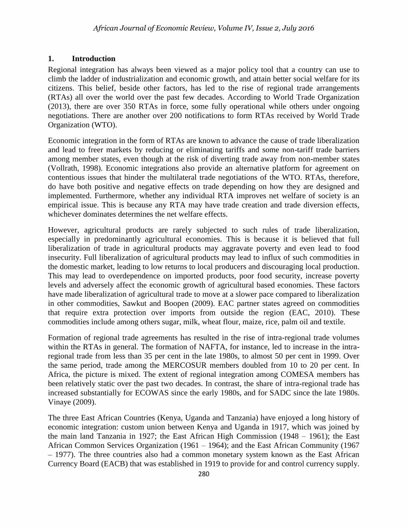
1. Introduction

Regional integration has always been viewed as a major policy tool that a country can use to

climb the ladder of industrialization and economic growth, and attain better social welfare for its

citizens. This belief, beside other factors, has led to the rise of regional trade arrangements

(RTAs) all over the world over the past few decades. According to World Trade Organization

(2013), there are over 350 RTAs in force, some fully operational while others under ongoing

negotiations. There are another over 200 notifications to form RTAs received by World Trade

Organization (WTO).

Economic integration in the form of RTAs are known to advance the cause of trade liberalization

and lead to freer markets by reducing or eliminating tariffs and some non-tariff trade barriers

among member states, even though at the risk of diverting trade away from non-member states

(Vollrath, 1998). Economic integrations also provide an alternative platform for agreement on

contentious issues that hinder the multilateral trade negotiations of the WTO. RTAs, therefore,

do have both positive and negative effects on trade depending on how they are designed and

implemented. Furthermore, whether any individual RTA improves net welfare of society is an

empirical issue. This is because any RTA may have trade creation and trade diversion effects,

whichever dominates determines the net welfare effects.

However, agricultural products are rarely subjected to such rules of trade liberalization,

especially in predominantly agricultural economies. This is because it is believed that full

liberalization of trade in agricultural products may aggravate poverty and even lead to food

insecurity. Full liberalization of agricultural products may lead to influx of such commodities in

the domestic market, leading to low returns to local producers and discouraging local production.

This may lead to overdependence on imported products, poor food security, increase poverty

levels and adversely affect the economic growth of agricultural based economies. These factors

have made liberalization of agricultural trade to move at a slower pace compared to liberalization

in other commodities, Sawkut and Boopen (2009). EAC partner states agreed on commodities

that require extra protection over imports from outside the region (EAC, 2010). These

commodities include among others sugar, milk, wheat flour, maize, rice, palm oil and textile.

Formation of regional trade agreements has resulted in the rise of intra-regional trade volumes

within the RTAs in general. The formation of NAFTA, for instance, led to increase in the intra-

regional trade from less than 35 per cent in the late 1980s, to almost 50 per cent in 1999. Over

the same period, trade among the MERCOSUR members doubled from 10 to 20 per cent. In

Africa, the picture is mixed. The extent of regional integration among COMESA members has

been relatively static over the past two decades. In contrast, the share of intra-regional trade has

increased substantially for ECOWAS since the early 1980s, and for SADC since the late 1980s.

Vinaye (2009).

The three East African Countries (Kenya, Uganda and Tanzania) have enjoyed a long history of

economic integration: custom union between Kenya and Uganda in 1917, which was joined by

the main land Tanzania in 1927; the East African High Commission (1948 – 1961); the East

African Common Services Organization (1961 – 1964); and the East African Community (1967

– 1977). The three countries also had a common monetary system known as the East African

Currency Board (EACB) that was established in 1919 to provide for and control currency supply.


281

However, the EACB ceased functioning in 1966 following the creation of the independent

central banks by the three countries.

The demise of the earlier East African Community in 1977 was owing to perceived trade and

industrial benefits imbalances created by the colonial era against Uganda and Tanzania, and in

favour of Kenya. This led to the lesser developed members (Uganda and Tanzania) imposing

tariffs on imports from a country with which they had trade deficit to protect their infant

industries (Goldstein and Ndung’u, 2001). Other factors that contributed to the collapse of East

African Community formed in 1967 included: divergent and conflicting political and economic

ideology by the partner states; increasing animosity among the leaders of the EAC countries,

especially following Idi Amin’s forceful takeover of power in Uganda in 1971; worsening

relationship between Uganda and Tanzania that resulted in to war between the two countries; and

failure of the three Heads of State to meet anymore. Eventually the East African Community

(EAC) was officially dissolved in 1983.

The EAC was, however, re-established in 1999 following successful negotiations and the signing

of the treaty by the Heads of State of the three countries. Under the EAC treaty implemented

officially in 2001, the first entry point to the community was the establishment of a customs

union, then a common market, subsequently a monetary union and ultimately a political

federation of the East African States. Rwanda and Burundi were officially admitted into EAC in

July 2007.

Progress has been made in liberalizing trade among the member states by establishing a custom

union. The East Africa Custom Union (EACU) commenced operations in 2005 following the

signing of the protocol establishing it in 2004. As a way of addressing former trade imbalances

that lead to the collapse of the old EAC, member countries resolved to apply the principle of

asymmetry in the elimination of internal tariff, whereas the goods from Uganda and Tanzania

were to enter Kenya duty-free, whereas the two countries were to impose a tariff at reducing

rates on selected imports from Kenya for five years. The protocol establishing the East African

Common Market was signed in 2009 and came into force on July 1, 2010. The establishment of

the customs union and the common market has continued to pave way for free movement of

goods and services, and labor within the region.

The intra-EAC trade remains low despite the fact that EAC member countries have over the

years, since the revival of the custom union in 1999, put more efforts in coming up with policies

and strategies to increase transaction and exchange among the member states. Intra-EAC trade

averaged at about 9 per cent of the total trade of the region, compared to other RTAs such as EU

(66 per cent), East Asia (55 per cent), NAFTA (44 per cent), ASEAN (27 per cent) and SADC

(13 per cent). (See World Bank, 2009; Keane, Cali and Kenan, 2010 and Sally, 2010). As

documented in EAC trade report 2008, the five EAC countries are forming both economic and

political integration with the main objective of attaining sustainable and equitable growth and

development, with the aim of improving the standards of living of the populace through

increased competitiveness, value-added production, trade and investment (EAC, 2010).

The EAC partner countries ratified the Common Market Protocol, with the aim of increasing

trade among member states. Other steps taken by EAC countries to promote trade among the

members include: immediate elimination and gradual reduction of tariffs (asymmetrical


282

reduction of tariffs, which was to reach 0 per cent in January 2010); removal of tariff equivalent

charges on internal trade; exemption of selected products; establishing and maintaining a

Common External Tariff (CET); and elimination of all non-tariff barriers (NTBs), which was

successfully implemented through establishment and operationalization of the National

Monitoring Committees (NMCs) on NTBs in all partner states. The NTBs to be eliminated or

reduced were categorized into the following eight clusters: custom documentation procedures;

immigration procedures; cumbersome inspection requirements; police road blocks; varying trade

regulations among the EAC countries; varying cumbersome and costly transiting procedures in

the EAC countries, duplication of functions within agencies involved in custom activities; and

business registration and licensing (EAC, 2010).

One of the main objectives of countries joining common RTAs is to promote trade amongst

themselves. In Africa, leaders adopted regionalism during the post-colonial meetings in 1958 and

1960 as a strategy to navigate economic constraints imposed by smallness and fragmented

national markets, (Vinaye, 2009). However, these RTAs have been found to have different

effects on regional trade. Previous studies have shown that such movements do lead to trade

creation, trade diversion, or both, (see Vollrath, 1998; Yang and Gupta, 2005; Grant and

Lambert, 2005 and Moghaddasi, 2012).

It has been assumed that a RTA would be welfare improving since tariffs, which are in general

welfare reducing, would fall. However, it has been empirically shown that RTAs would not

necessarily improve welfare, since the tariff reductions occur in a world of the “second best”,

Viner (1950). Thus, a RTA would be beneficial if on balance it is “trade creating” and harmful if

it is “trade diverting”. In general, trade creation means that a regional trade agreement generates

trade that would not have existed otherwise. As a result, supply occurs from a more efficient

producer of the product. In all cases, trade creation would raise a country's national welfare,

while trade diversion would reduce national welfare. This study therefore investigates the effects

of EAC-TRA on the region’s agricultural trade.

In the face of the above background, the objective of this study is to investigate the effect of

regional trade agreement, that is, the EAC, on the region’s agricultural exports. The study

investigated if membership to EAC create or divert the members’ agricultural exports. The study

specified and estimated gravity equations involving agricultural exports of each member state to

other selected 77 trading partners across the globe, the GDP of the exporter and importers,

population of the exporter and importers, exchange rates, distance between capital cities,

common language dummy, adjacency dummy and a dummy for EAC membership. The

empirical findings showed mixed results for the different EAC member states. EAC regionalism

had no significant effect on agricultural exports of Burundi, Rwanda and Uganda, while Kenya

and Tanzania had reported significant effect of regionalism on their agricultural exports.

The remainder of this study is organized as follows. Section 2 reviews the empirical literature on

regional trade agreement and trade, section 3 provides the methodology adopted in the study,

while the study findings and policy implications are presented and discussed in section 4.


283

2. Empirical Literature

Vollrath (1998) assessed agricultural trade in six RTAs, including AFTA, APEC, ANZCER,

CUSTA, MERCOSUR and the EU, using data for 1953-1959 and 1959-1970. The study showed

that both APEC and AFTA had neither positive nor negative effect on agricultural trade flows.

On the other hand, ANZCER, CUSTA and MERCOSUR were found to be more trade creating

than diverting, welfare improving and helped in opening up the member-countries to the world

agricultural economy. And EU was found to be more agricultural trade diverting than creating,

hence, welfare reducing. However, Vollrath’s work fell short of describing the estimation

technique employed in the study to arrive at the econometric results discussed.

Grant and Lambert (2005) adopted the augmented gravity framework to analyze the effect of

regionalism on the volume of agricultural trade. Using a sample of nine (9) agricultural goods in

eight (8) RTAs across the world involving 87 countries, they estimated pooled, cross section and

time series regressions on the augmented gravity equation for the period between 1985 and 2002.

A total of 11 regressions were run, 9 for each individual agricultural product, 1 for all

agricultural products and 1 for all non-agricultural products. Out of the 8 RTAs, 3 were in sub-

Saharan Africa (that is, SACU, SADC and COMESA) and referred to as ‘Africa’ in the study.

They found that in ‘Africa’, 4 of the 9 commodities experienced trade diversion from non-

member sources. However, the effects were found to be generally small and in all cases trade

diversion did not outweigh trade creation. On the other hand, NAFTA and EU showed

significant trade creation effects in 8 and 6 individual agricultural products, respectively.

Grant and Lambert’s work, despite its intellectual appeal, is fraught with several methodological

problems, which significantly reduce its value (Vinaye, 2009). First, the choice of RTAs was

rather limited, and the idea of grouping the three African RTAs was objectionable, since they

were at different levels of integration. Second, the estimation method used was not clear.

Although the gravity equations were estimated using panel data, no panel data techniques were

employed. The use of the Ordinary Least Squares method could lead to biased estimates to the

extent that zero trade values are ignored from the effective sample. However, as recent

developments in the estimation of gravity equations suggest, even the use of Tobit is subject to

the criticism that they result in inconsistent estimates.

Vinaye (2009) examined the intra-SADC’s agricultural trade using panel data set of 68 exporting

and 222 importing countries (both SADC members and non-member trading partners) for the

period 2000 – 2007. Vinaye computed several trade indices and estimated the gravity equation

using Pseudo Poisson Maximum Likelihood (PPML) technique. The study revealed limited trade

complementarity among SADC economies, which implied low potential for intra-regional

agricultural trade. This methodology was a significant deviation from the norm where

researchers would transform the gravity equation into logarithm form and apply the usual

estimation techniques such as OLS or Tobit. Silva and Tenreyro (2006) argued that the use of

OLS or Tobit in estimating gravity model would constitute a misuse of Jensen’s inequality, that

is, log-linearizing economic relationships in the presence of heteroskedasticity in the data could

lead to biased and inconsistent estimates. They suggested the use of PPML technique as an

alternative estimation procedure, which would maintain the gravity equation in its multiplicative

form and still yield consistent estimates.


284

Moghaddasi (2012) studied the relationship between regionalism and Iran’s export of processed

agricultural products. Iran is a member of Economic Cooperation Organization (ECO) together

with nine (9) other countries. Using generalized gravity model, the study employed panel and

pooled data techniques, that is, OLS estimator, one-way Fixed Effects Model (FEM) and one-

way Random Effects Model (REM). The results revealed a positive and significant impact of the

regionalism on the Iran’s agricultural exports. However, the methodology adopted in this study

has been criticized in its ability to give consistent and efficient results in cases where zero trade

is reported between the trading partners. The study also does not evaluate the causes of

agricultural trade among the ECO member states.

3. Methodology

Based on the theory of the consumer behaviour, the study used the gravity model developed by

Tinbergen (1962) and later augmented by Anderson (1979), and Anderson and Wincoop (2003).

Anderson (1979) presented a theoretical foundation for the gravity model based on the constant

elasticity of substitution (CES) preferences and goods differentiated by place (country or region)

of origin. Two key assumptions in the theoretical derivation of the gravity model include: goods

are differentiated by place of origin, and identical and homothetic preferences approximated by a

CES utility function.

If cij denotes the consumptions of residents of country j (importer) of goods from country i

(exporter), then the consumers in country j maximize utility given as

)1..(................................................................................)1/(/)1(/)1(

ijij cU

Subject to the budget constraint

)2....(.................................................................................................... j

jijij ycp

where σ is elasticity of substitution between all goods, βi is a positive distribution parameter, yj is

the nominal income of country j’s residents and pij is the price of country i’s goods to country j’s

consumers.

Due to trade costs, which are not observable, prices differ in the countries. If pi is the exporter’s

supply price and tij is trade cost factor between i and j, thenijiij tpp

. The assumption is that the

exporter bears the trade costs. For each good shipped from i to j, the exporter incurs export cost

equal to )1( ijt of country i goods. These trade costs are passed on to the importer in form of

higher prices. The nominal value of i’s exports isijijij cpx

The total income of country i now become i

iji xy , and ijijij cpx

Demand for country i’s exports by country j’s consumers that satisfy the optimization problem in

equations (1) and (2) above is

)3.......(................................................................................

)1(

j

j

ijii

ij yP

tpx


285

Equation (3) is a Marshallian demand function. Demand for imported goods is directly

proportional to consumers’ income and inversely proportional to price. where Pj is the consumer

price index of country j given by

)4.(................................................................................)(

)1/(1

1

i

ijiij tpP

The general equilibrium structure of the model imposes market clearing condition, which implies

that

j

iji xy

That is;

j j j

jjijiijjiijiiji yPtpyPptxy )5.......(..........)/()()/( 111

To derive the gravity equation, the study follows Anderson (1979) and Deardorff (1998), by

using the market clearing condition in equation (5) above to solve for the coefficients βi while

imposing the choice of units such that all supply prices pi were equal to one (the equilibrium

scaled prices, βipi), and then substituting into the import demand equation (3).

Let the world nominal income be yw, such that

j

j

w yy

And the income shares be θj, such that;

wj

j y

y

Then the technique gives;

)6.....(................................................................................

1

ji

ij

w

ji

ijP

t

y

yyx

where )7....(......................................................................)/(

)1/(1

1

i

jjij Pt

Substituting the equilibrium scaled prices into equation (4), gives

)8.(......................................................................)/(

)1/(1

1

i

jiijj tP

Solving equations (7) and (8) together for all πi’s and Pi’s in terms of income shares, bilateral

trade barriers and σ, and assuming that trade barriers (trade costs factor) are symmetric (that is,

tij=tji), then a solution to (7) and (3.8) is πi=Pi, with

)9...(................................................................................111 i

ijiij tPP

This gives an implicit solution to the price indices as a function of all bilateral trade barriers and

income shares. The gravity equation, therefore, becomes


286

)10..(................................................................................

1

ji

ij

w

ji

ijPP

t

y

yyx

The price indices are referred to as ‘multilateral resistance’ variables, since they depend on all

the bilateral resistances tij. Increase in trade barriers raises the index. The gravity equation above,

therefore, tells us that bilateral trade depends on the economic sizes of the trading partners

(measured by the proportion of their income to world’s income) as attracting forces and the

resistance factors (bilateral trade barriers) in form of trade costs that can be measured by various

trade obstacles such as the distance between trading partners and lack of common currency.

Equation (10) can therefore be expressed as;

)11.(............................................................).........,,( ijjiij TCGDPGDPfEXP

Where EXPij is the exports from country i to country j; or total trade, GDP is the measure of

economic size and TC is trade costs (which captures various resistance factors; distance,

language barrier, among others).

The standard gravity equation given in equation (11) tends to ignore many other variables that

could have either positive or negative impact on trade volumes between the trading partners,

which results to misspecification bias (Vinaye, 2009). To address this problem, the standard

approach has been to specify an augmented gravity model by addition of relevant variables to the

traditional model, most of which are inspired by theory and motivated by various testable

hypotheses (Vinaye 2009). Most estimates of GM add a certain number of dummy variables to

the original gravity equation that test for specific effects. These refer sharing of a common land

border and commonality of language, among others. With inclusion of dummy variables of trade

agreements, GM has broader implications in terms of the trade creation and trade diversion,

which may have influence on the extent of IIT within the region. However, necessary caution

must be taken since too many dummies may cause the problem of dummy trap in the data

analysis. Equation (11) can therefore be re-written as

)12........().........,,,,,,,( ijijijijjijiij ADCLDISEXRTPOPPOPGDPGDPfEXP

Where:

EXP - is the real value of the total annual exports of agricultural products of the exporting

country to the trade partner.

GDP - is the annual real GPD of a country measured in constant 2000 US dollars. GDPi

is the real GDP of the exporting country while GDPj is the real GDP of the importing

country.

POP - is the population of the country. POPi is the population of the exporting country

while POPj is the population of the importing country.

EXRT - is the real exchange rate between the currency of the exporting country and that

of the importing country


287

DIS - is the geographical distance between the economic centres (in most cases the

capital cities) of two trading partners

CL - is a dummy representing common national language between trading partners

AD - is a dummy representing common border between trading partners.

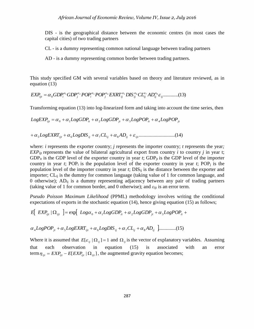
This study specified GM with several variables based on theory and literature reviewed, as in

equation (13)

)13..(..........87654321

0 ijijijijijjijiijt ADCLDISEXRTPOPPOPGDPGDPEXP

Transforming equation (13) into log-linearized form and taking into account the time series, then

)14.........(....................8765

43210

ijtijijijijt

jtitjtitijt

ADCLLogDISLogEXRT

LogPOPLogPOPLogGDPLogGDPLogEXP

where: i represents the exporter country; j represents the importer country; t represents the year;

EXPijt represents the value of bilateral agricultural export from country i to country j in year t;

GDPit is the GDP level of the exporter country in year t; GDPjt is the GDP level of the importer

country in year t; POPi is the population level of the exporter country in year t; POPj is the

population level of the importer country in year t; DISij is the distance between the exporter and

importer; CLij is the dummy for common language (taking value of 1 for common language, and

0 otherwise); ADij is a dummy representing adjacency between any pair of trading partners

(taking value of 1 for common border, and 0 otherwise); and εijt is an error term.

Pseudo Poisson Maximum Likelihood (PPML) methodology involves writing the conditional

expectations of exports in the stochastic equation (14), hence giving equation (15) as follows;

)15....(..........

exp|

87654

3210

ijijijijtjt

itjtitijtijt

ADCLLogDISLogEXRTLogPOP

LogPOPLogGDPLogGDPLogEXPE

Where it is assumed that 1]|[ ijijE and ij is the vector of explanatory variables. Assuming

that each observation in equation (15) is associated with an error

term ]|[ ijtijtijtijt EXPEEXP , the augmented gravity equation becomes;


288

)16....(..........

exp

8765

43210

ijtijijijijt

jtitjtitijt

ADCLLogDISLogEXRT

LogPOPLogPOPLogGDPLogGDPLogEXP

where EXPijt > 0 and 0]|[ ijtijt EXPE .

Equation (16) was estimated using the PPML technique to analyze the causes of intra-EAC

exports, after carrying out all the necessary diagnosis tests.

To evaluate trade creation and/or trade diversion effects of the EAC regional trade agreement, a

variable for membership to the EAC was added to equation (16) to get equation (17).

)17.........(................................................................................

exp

9

87654

3210

ijtijt

ijijijijtjt

itjtitijt

EAC


LogPOPLogGDPLogGDPLogEXP

Where EACijt is a dummy variable indicating the existence of EAC-RTA between countries i and

j. Following Sawkut and Boopen (2009), equation (17) can be modified to capture more

precisely the impact of the EAC-RTA on trade. To capture the degree of trade creation and trade

diversion effects of EAC-RTA, the study employed two EAC dummies rather than one, that is,

EAC1ijt and EAC2ijt to capture trade creation effects and trade diversion effects, respectively.

Equation (17) can now be re-written as;

)18........(............................................................21

exp

109

87654

3210

ijtijtijt

ijijijijtjt

itjtitijt

EACEAC


LogPOPLogGDPLogGDPLogEXP

Where: EAC1ijt is a binary variable which is unitary if both i and j belong to the EAC regional

trade agreement and zero otherwise, (degree of trade creation effects). EAC2ijt is a binary

variable which is unitary if i belongs to EAC regional trade agreement and j does not or vice

versa, and zero otherwise (degree of trade diversion effects). Using data from the five (5) EAC

members and the other 77 trading partners, equation (18) was estimated using the PPML

technique. Whether to employ PPML technique under fixed effects or random effects, the

Hausman test was performed and random effects model (REM) was estimated. The 77 trading

partners were selected on the basis of data availability. Only countries that recorded consistent

agricultural trade with the EAC members over the period of the study were selected. The list of

all the 82 countries under the study is provided in the appendices. The study employed secondary

data retrieved from publications on EAC countries and their trading partners for the period 2000-


289

2012. Specific data sources included UNCOMTRADE online database, International Financial

Statistics (IFS) CD-ROM, World Development Indicators (WDI).

The gravity equation can be estimated through various econometric estimation techniques such

as; OLS, GMM, MLE, and the latest approach, the PPML. The main challenges of applying OLS

and GMM in estimation of the gravity model is how to deal with zero trade values reported, and

how to isolate the effects of regionalism from the effects of other factors on the intra-regional

trade. This is due to the fact that estimation using these techniques requires transformation of the

gravity equation into a log–linearized form, yet the logarithm of zero is undefined, leading to

biased and inconsistent results. PPML approach is superior due to its ability to maintain the

gravity equation in its multiplicative form hence resulting in unbiased and consistent results.

Additionally, PPML estimation technique is superior in estimation of gravity model of trade and

give reliable and robust results, despite the common characteristic of bilateral trade where some

data may be zero in some periods.

4. Results, Discussion and Policy Implications

The study used a panel data involving the five EAC countries and other 77 trading partners, and

estimated panel Poisson gravity equations under random effects using the Pseudo Poisson

Maximum Likelihood (PPML) technique. The panel root test was performed to investigate if

there was any variable that was non-stationary. The presence of unit root in any variable may

lead to spurious regression where the regression results may be misleading. The Im-Peseran-Shin

panel unit-root test developed by Im, Pesaran and Shin (1997) was adopted in this study.

The Im-Pesaran-Shim (IPS) test is based on the famous Dickey-Fuller test and it involves testing

for the presence of unit roots in panels that combines information from the time series dimension

with that from the cross section dimension, such that fewer time observations are required for the

test to have power. IPS test is therefore superior to Augmented Dickey Fuller (ADF) test and

other unit root test techniques in analyzing long-run relationships in panel data with fewer time

observations (Im, Pesaran and Shin - IPS 1997). The test allows for individual effects, common

time effects and time trends. The Im-Pesaran-Shin panel unit root test hypotheses are as

follows:Ho: All panels contain unit root; Ha: Some panels are stationary. The results of the unit-

root test for all the panels are presented in Table 1.

The results of unit root tests showed the rejection of null hypothesis at one per cent level of

significance for exports (which was the dependent variable in the study) at levels for all the five

exporters. On the contrary, all other variables were non-stationary at levels, implying the

presence of unit root. However, all variables, except the population of the importer, became

stationary at 1% level of significance upon first differencing. This implies that the dependent

variable is integrated of order zero, I(0), while the independent variables are integrated of order

one, I(1). Based on these findings, augmented gravity equations were specified with the

dependent variable (Agricultural Exports), the dummies and distance at levels, while the other

independent variables (GDP, Population, Exchange rate) at first difference using the PPML

technique. However, population of the importers was dropped from all the equations because of

failing to be stationary even after first differencing and de-trending, and also being highly

collinear with the GDP of the importer.


290

Table 1: Results for unit-root test (Im-Pesaran-Shin panel unit-root test)

***,** and * denotes rejection of the null hypothesis at 1%, 5% and 10% levels of significant.

Source: Study Data (2015)

Hausman test helps in determining which between random effect moydel (REM) and fixed

effects model (FEM) is the most appropriate for the study data. Hausman (1978) suggested a test

for correlation between the unobserved effect (the country-specific effect) and the explanatory

variables as comparison between the fixed effect and random effect estimates, assuming that the

idiosyncratic errors and explanatory variables are uncorrelated across all time periods. REM

assumes that there are random/probabilistic variations across the panel, while FEM assumes

individual heterogeneity.

The results of Hausman test presented in Table 2 in the appendices reject the null hypothesis of

“no systematic difference in random and fixed effects coefficients” for all the data sets. The test

Exporter Variable t-bar statistic

Levels First

Difference

Levels with

time trend

Kenya

Log Exports -1.9052*** -4.2410*** -3.2065***

Log GDP Exporter 0.4977 -1.9695*** -1.8627***

Log GDP Importer -0.4387 -2.4146*** -1.6340

Log Population Exporter -0.1985 -2.2990*** -1.1934

Log Population Importer -1.8430 -3.0190 -3.5130

Log Exchange Rate -3.2725 -4.3879*** -3.5050

Uganda

Log Exports -2.4292*** -4.8217*** -3.1965***

Log GDP Exporter -0.8223 -2.2867*** -0.9318

Log GDP Importer -0.7194 -2.7091*** -1.7288

Log Population Exporter 0.2301 -3.9864*** -2.0202***

Log Population Importer -0.8071 -2.1557** -1.9534


Tanzania

Log Exports -1.8820*** -4.0893*** -2.6512***

Log GDP Exporter -0.3377 -4.0648*** -1.5427**

Log GDP Importer -0.6841 -2.7112*** -1.7507

Log Population Exporter 13.5235 -2.4425*** -4.0569

Log Population Importer -2.2635 -2.0045 -2.0797

Log Exchange Rate -1.4324 -3.0027*** -2.0978***

Rwanda

Log Exports -2.3150*** -4.0252*** -2.7248***

Log GDP Exporter -0.2019 -5.0295*** -2.9567***

Log GDP Importer -0.8590 -2.7095*** -1.5656

Log Population Exporter 2.7140 -1.0619** -0.7786

Log Population Importer 1.5326 -1.8489 -1.6386


Burundi

Log Exports -2.5195*** -3.3583*** -2.1447

Log GDP Exporter 0.9861 -4.5261*** -1.9115***

Log GDP Importer -0.5918 -3.0774*** -2.0289

Log Population Exporter 2.1113 -6.2177*** -7.1182***

Log Population Importer 0.8516 -2.4563** -2.1147

Log Exchange Rate -2.1769 -3.1000*** -2.8437**


291

results show that Chi-square statistics and the corresponding p-values for the difference between

FEM and REM were 2.20 (0.9005), 2.92 (0.6110), 2.65 (0.8310), 2.86 (0.7216) and 8.66

(0.1235) for Kenya, Tanzania, Uganda, Rwanda and Burundi, respectively. All the p-values were

larger than the critical values of 0.01 (at one per cent), 0.05 (at five per cent) and 0.1 (at 10 per

cent) implying that the REM is most suitable for the study data.

The regression results (see Table 3) show that membership to EAC regional trade agreement has

different effects on the region’s agricultural exports across the member states. The integration

trade diversion effects were evident in case of Rwanda exports. However, the effects were found

to be statistically insignificant at all levels. Results from all the other countries show effects of

trade creation, with that of Uganda and Burundi being statistically insignificant, while the

coefficients of EAC1 (trade creation dummy) was found to be highly significant at one per cent

level of significance and with the right positive sign for both Kenya and Tanzania.

This implies that Kenya and Tanzania, on average, tend to export more agricultural products to

the EAC region as a result of the regional trade agreement. More specifically, the results show

that there is a 14.3 percentage effect on Kenyan agricultural exports to EAC as a result of being a

member of the RTA, while Tanzania realized 20.5 percentage effect on its agricultural exports to

EAC as a result of being a member of the RTA. This implies that the most open countries tend to

benefit more from regionalization compared to less open economies. According to World Bank’s

trade tariff restrictiveness index (TTRI) that gauges openness, Tanzania is the most open country

in EAC at 7.8, followed by Kenya at 8.2, while Rwanda is the least open country in EAC at 16.2

(Society for International Development, 2011). Additionally, the failure of Rwanda and Burundi

to realize any significant effect of regionalism on their agricultural exports may be due to the fact

that the two countries joined the block late (that is, in July 2007) and could have taken time to

implement EAC policies that could have had significant effect.

The results further indicate that EAC integration has not been effective in promoting agricultural

exports from Uganda, Rwanda and Burundi to the region, as the coefficients are all insignificant

statistically. This implies that EAC as a regional agreement has very limited potential to increase

or expand intra-EAC agricultural trade. This probably may be due to the fact that most countries

in the region can only meet a small share of the region’s import demands. Based on similar

results, Yung and Gupta (2005) suggested that policies aimed at boosting African trade on short

to medium term must focus on promoting trade with the rest of the world, rather than within

African RTAs.

These findings are in agreement with the findings of other studies on effects of regionalism on

trade. As much as it may be expected that regionalism promotes trade, this may not necessarily

be the case. Elbadawi (1997) found that African RTAs increased intra-regional trade by 31% on

average without causing trade diversion for the period 1980-1984, but thereafter, substantial

trade diversion and decrease in both intra-regional and overall trade was reported. Vollrath

(1998) found that APEC and AFTA had no effect at all on the regional agricultural trade flows.

ANZCER, CUSTA and MERCOSOR were more trade creating than diverting, while EU was

more trade diverting than creating. Additionally, Moghaddasi (2012) found ECO to have a

positive and significant effect on Iran’s agricultural exports to the other nine ECO members.


292

This study therefore recommends that EAC secretariat and the respective governments in EAC

member countries should implement strategies that enhance regional integration among the

member states. This is because the results show that membership to EAC has significant effect

on agricultural trade volumes in Kenya and Tanzania. Kenyan and Tanzanian governments

should come up with incentives that would encourage the other three state members to remain in

the integration and promote regionalism. Such policies may include but not limited to adhering

to EAC’s liberalization and harmonization schedules, reduction or elimination of import duties

on commodities, lowering or liberalizing import requirements and procedures.

On the other hand, Uganda, Rwanda and Burundi, which are yet to benefit from the integration

in terms of agricultural exports, should also implement strategies that would enhance regional

integration. This is because empirical results show that integration is likely to promote

agricultural exports of member states, as in the case of Kenya and Tanzania. These policies

should include reduction and/or elimination of non-tariff barriers (NTBs).

5. References

EAC (2010). Trade Report 2008, East African Community Secretariat, Arusha.

Elbadawi, I (1997). The Impact of Regional Trade and Monetary Schemes on Intra-Sub-Saharan

Africa Trade. Regional Integration and Trade Liberalization in Sub-Saharan Africa,

Hounmills, Basingstoke.

Goldstein, A. and S. Ndung’u. ( 2001) Regional Integration Experience in the Eastern African

Region. (online). Paris : OECD. Technical Papers No. 171, CD/DOC(2001)3, March

Grant, J.H. and Lambert, D.M. (2005), Regionalism in world agricultural trade: Lessons from

gravity model estimation. Mimeo, Purdue University.

Im, K.S., Pesaran, M.H., and Shin, Y. (1997), .’Testing for Unit Roots in Heterogeneous Panels’,

DAE, Working Paper 9526, University of Cambridge

Keane, J., Cali. M. and Kennan, J. (2010), Impediments to Intra-Regional Trade in Sub-Saharan

Africa. Commonwealth Secretariat.

Moghaddasi, R. (2012). ‘Study on the Relationship between Regionalism and Iran Export of

Processed Agricultural Products’. Islamic Azad University, Tehran.

Musonda, F. M. (1997). ‘Intra-Industry Trade between Members of the PTA/COMESA Regional

Trading Arrangements’. AERC Research Papers, 64, 10-17.

Ng’ang’a, W. (2006). The “New” East African Community: Effects on Trade, Welfare and

Productive Activities in East Africa. Master of Arts Thesis, University of Saakatchewan,

Saskatoon.


293

Ouma, D. (2010). ‘An Empirical Analysis of the Determinants of Intra-Industry Trade between

Kenya and the East African Countries – The Gravity Model’. MA Thesis, The University

of Mauritius.

Sally, R. (2010). Regional Economic Integration in Asia: The Track Record And Prospects.

ECIPE Occasional Paper No. 2/2010.

Sawkut, R. and Boopen, S. (2009). ‘Do RTAs Create Members’ Agricultural Trade?’ University

of Mauritius, Reduit.

Silva, J.M.C. and Tenreyro, S. (2006). ‘The log of gravity’, Review of Economics and Statistics,

88: 641-658.

Society for International Development 2011, Available from: http://www.sidw.org/ [January

2014]

Vinaye, A. D. (2009). ‘Assessing the SADC’s potential to promote intra-regional trade in

agricultural goods’. University of Mauritius, Reduit.

Viner, J. (1950). ‘The Customs Union Issue, New York: Carnegie Endowment for International

Peace’. New York.

Vollrath, T.L. (1998). ‘RTAs and Agricultural Trade: A Retrospective Assessment. In M.

Burfisher and E. Jones (eds.), Regional Trade Agreements and U.S. Agriculture’.

Agricultural Economic Report, 771.

World Bank (2009). The Little Data Book on Africa 08/09. World Bank

World Trade Organization 2013, Available from: http://www.wto.org/ [January 2014]

Yang, Y. and Gupta, S. (2005). Regional Trade Arrangements in Africa: Past Performance and

the Way Forward. IMF Working Paper No. 05(36)


294

APPENDICES

Table 1A

1 Afghanistan 22 Eritrea 43 Madagascar 64 Singapore

2 Algeria 23 Finland 44 Malawi 65 South Africa

3 Angola 24 Fomer Sudan 45 Malaysia 66 Spain

4 Australia 25 France 46 Malta 67 Sri Lanka

5 Austria 26 Germany 47 Mauritius 68 Swaziland

6 Bahrain 27 Ghana 48 Morocco 69 Sweden

7 Belgium 28 Greece 49 Mozambique 70 Switzerland

8 Benin 29 Hong Kong SAR 50 Netherlands 71 Tanzania

9 Botswana 30 Hungary 51 New Zealand 72 Thailand

10 Brazil 31 India 52 Nigeria 73 Turkey

11 Bulgaria 32 Indonesia 53 Norway 74 UAE

12 Burundi 33 Iran 54 Oman 75 Uganda

13 Canada 34 Ireland 55 Pakistan 76 UK

14 Chile 35 Israel 56 Poland 77 Ukraine

15 China 36 Italy 57 Portugal 78 USA

16 Comoros 37 Japan 58 Republic Korea 79 Vietnam

17 Cyprus 38 Jordan 59 Russian

Federation

80 Yemen

18 Denmark 39 Kenya 60 Rwanda 81 Zambia

19 Djibouti 40 Korea 61 Saudi Arabia 82 Zimbabwe

20 DRC 41 Kuwait 62 Senegal

21 Egypt 42 Kyrgyzstan 63 Seychelles


295

Table 2: Hausman test results for FEM and REM (Dependent Variable: Log of Exports) KENYA TANZANIA UGANDA RWANDA BURUNDI

FEM REM DIFF. FEM REM DIFF. FEM REM DIFF. FEM REM DIFF. FEM REM DIFF.

Log GDP Exporter 4.22*** 4.20*** 0.02 2.74 2.54 0.20 1.10 3.13 -2.03 4.00 5.92 -1.92 -24.37*** -21.27*** -3.11

Log GDP importer 0.56 0.61*** -0.05 0.51 0.94*** -0.44 2.91** 1.17*** 1.74 1.13 -0.37 1.49 -3.72 0.29 -4.01

Log POP Exporter -2.72 -2.51 -0.21 -3.61 -2.58 -1.034 -2.42 -3.59 1.16 -8.97 -7.62 -1.35 27.22*** 21.39*** 5.84

Log POP Importer 0.40 0.09 0.31 1.66 -0.03 1.69 -1.75* -0.64** -1.11 13.12 0.40 12.72 2.97 -0.59 3.55

Log Exchange Rate -0.07 -0.03 -0.04 0.32 0.10 0.22 -0.25 -0.11 -0.14 0.80 -0.08 0.87 -1.04** -0.38 -0.67

Log Distance -0.34** -1.49*** 1.15 Omitted -1.60** - Omitted -1.70* - Omitted -0.76 - Omitted 0.18 -

Common Language Omitted -0.69** - Omitted 2.09*** - Omitted Omitted - Omitted Omitted - Omitted 0.30 -

Adjacency Omitted -0.64 - -0.94*** 1.37 -2.31 Omitted 2.90* - Omitted -3.08** - Omitted -0.91 -

EAC1 0.53*** 0.50*** 0.02 0.06*** 0.16 -0.10 Omitted -0.45 - -2.27** -0.68 -1.58 Omitted 0.57 -

EAC 2 Omitted Omitted - Omitted Omitted - Omitted Omitted - Omitted Omitted - -1.16*** Omitted -

Constant 15.54 25.36 13.61 30.45 22.39 42.95 -49.37 58.67 -170.57*** -129.23***

No. of Observation 770 770 793 793 481 481 156 156 182 182

R-Squared: Within 0.262 0.260 0.183 0.170 0.287 0.267 0.200 0.152 0.116 0.087

Between 0.219 0.385 0.158 0.517 0.000 0.276 0.071 0.432 0.000 0.011

Overall 0.218 0.362 0.133 0.419 0.001 0.266 0.018 0.245 0.000 0.001

F-statistics - - 7.76 28.71 8.68

Prob>F - - 0.000 0.000 0.001

Chi-square statistics 895.18 2.20 146.29 2.92 53.96 2.65 100.500 2.86 71.95 8.66

Prob>Chi-square 0.0000 0.9005 0.0000 0.611 0.0000 0.8310 0.0009 0.7216 0.0000 0.1235

***, ** and * denote statistical significance at 1, 5 and 10 percent levels, respectively. Source: Study Data (2015)

Table 3: Regression Results by Countries (Dependent Variable: Log of Exports) KENYA TANZANIA UGANDA RWANDA BURUNDI

Coefficient P-values Coefficient P-values Coefficient P-values Coefficient P-values Coefficient P-values

Log GDP Exporter 1.543*** 0.002 3.107 0.176 0.004 0.996 -4.413*** 0.002 -0.626 0.649

Log GDP importer -0.085 0.393 -1.119*** 0.003 -1.812*** 0.000 3.827*** 0.002 -0.174 0.898

Log POP Exporter -57.891 0.347 31.706*** 0.000 47.203 0.274 20.753*** 0.007 12.813 0.244

Log Exchange Rate 0.025* 0.074 0.021 0.720 0.059 0.273 -0.055 0.877 -0.043 0.714

Log Distance 0.018 0.229 0.169*** 0.000 -0.001 0.988 -0.160*** 0.000 -0.048 0.114

Common Language -0.063* 0.055 0.108*** 0.000 Dropped Dropped 0.014 0.801

Adjacency 0.221*** 0.000 0.347*** 0.000 0.263*** 0.000 -0.376*** 0.000 -0.119* 0.089

EAC1 0.143*** 0.000 0.205*** 0.000 0.050 0.346 -0.119 0.237 0.024 0.728

Constant 3.423** 0.040 -0.547* 0.063 0.537 0.710 2.990*** 0.000 1.873*** 0.000

No. of Observations 700 732 444 143 168

Pseudo R2 0.082 0.181 0.166 0.211 0.031

Pseudo log-likelihood -1564.938 -1665.405 -988.745 -329.288 -385.343

***, ** and * denote statistical significance at one, five and 10 per cent levels, respectively.

Regional Trade Agreement and Agricultural Trade...

Documents

Transcript of Regional Trade Agreement and Agricultural Trade...