Oxfam India working papers seriesSeptember 2010OIWPS - VI

Amitabh Kundu

K. Varghese

Essential Services

Regional Inequality and ‘Inclusive Growth’ in India under Globalization: Identification of Lagging States for Strategic Intervention

The present paper analyses the trends and patterns of economic inequality across Indian states since the early 1990s. The basic objective here is to understand the dynamics of growth in the country which is resulting in regional imbalances and propose measures for alleviating the problem. The inter-state inequality in per capita income and consumption expenditure show a clear increasing trend during the fi rst and second phase of structural reform. However, the strategy of inclusive growth and balanced regional development launched since 2003-04, has led to acceleration in the average growth in the less developed states, including those in the North-East. Unfortunately, however, this has made only a marginal impact in stalling the trend towards accentuation of regional imbalances. Further, poverty reduction has been relatively less in less developed compared to developed states, resulting in concentration of poverty in a few backward states. The composite indices of economic development, constructed based on a select set of indicators exhibit high correlations with that of social development. This is understandable as the capacity of the governments at the state level to make interventions and bring about social transformations is high in relatively developed states. The correlation of economic development with amenities, although statistically signifi cant, is relatively low, which suggests that the problems pertaining to health, education, and access to other amenities cannot be effectively addressed just by focusing on economic development.

Abstract

Disclaimer:Oxfam India Working Paper Series disseminates the fi nding of the work in progress to encourage the exchange of ideas about development issues. An objective of the series is to get the fi ndings out quickly, even if the presentations are less than fully polished. The papers carry the names of the authors and should be cited accordingly. The fi ndings, interpretations, and conclusion expressed in this paper are entirely those of the authors. They do not necessarily represent the views of Oxfam India.

Produced by: Oxfam India

For more information, please contact:

Avinash KumarTheme Lead - Essential ServicesOxfam IndiaPlot No. 1, Community Centre2nd Floor (Above Sujan Mahinder Hospital)New Friends Colony, New Delhi - 110 025Tel: 91 11 4653 8000Website: www.oxfamindia.org

Authors: Amitabh Kundu and K. Varghese

Amitabh Kundu teaches at Jawaharlal Nehru University, New Delhi. He has been a member of the National Statistical Commission, Government of India and Dean of the School of Social Sciences at JNU. He has been Visiting Professor at Sciences Po, University of Amsterdam, University of Kaiserslautern, among others. He has been Director at the National Institute of Development Research. He has edited India: Urban Poverty Report and India: Social Development. He has prepared background papers on India’s Economic Growth and Inequality for OECD and Human Development Report 2009. Currently, he is chairperson of the Technical Advisory Committee on Housing Start up Index at RBI and Committee to Estimate Shortage of Affordable Housing, Government of India.Email: amit0304@mail.jnu.ac.in

K. Varghese is working as a Systems Analyst at the Centre for the Study of Regional Development, Jawaharlal Nehru University, New Delhi. A Post Graduate in Statistics, he has a number of professional certifi cates in software applications. He is teaching Quantitative Techniques to student of MA Geography and conducts training programmes and laboratory practicals on database management and statistical techniques, computer cartography, GIS and Remote Sensing.Email: varghese@mail.jnu.ac.in

Study Supported by Oxfam India in collaboration with Institute for Human Development, New Delhi

Copyright @ 2010 Oxfam India

Reproduction of this publication for educational or other non-commercial purposes is authorized, without prior written permission, provided the source is fully acknowledged.

1. Introduction

The Indian development scenario looks optimistic, not only in terms of the pace of

economic growth but also in its capability to stand out in periods of global

economic crises. In the context of growth in employment, too, the economy has

done reasonably well over the past decade, allaying fears of jobless growth, the

key concern that emerged in the late 1990s. The growth rates, as per all three

alternate definitions of employment adopted by National Sample Survey

Organization, namely usual status, weekly status, and daily status, have been

exceptionally high since the early years of the present decade. The impact of

growth in poverty reduction, too, has been significant, although the estimated

elasticity of poverty reduction has been lower than several countries in the South

Asian region (Devarajan and Nabi: 2006).

The high growth in employment can partly be attributed to demographic dividend

the country is currently enjoying due to decline in the natural growth rate in

population. Many of the states, particularly in southern India, like Kerala and Tamil

Nadu have experienced fertility decline over the past couple of decades, making

the Net Reproduction Rate equal to or less than unity. The growth of population in

several other states, especially in north and central India has, however, been high,

reporting either no decline, or in some cases, even an increase, in recent years,

which is a cause for concern. However, as a result of general reduction in fertility,

the percentage of adults in the age group 20–35 is expected to grow rapidly over

the next few decades. This would help these states to pick up their growth

momentum, provided the incremental adult population can be meaningfully

absorbed in productive sectors. In the absence of such employment opportunities,

a north-south transfer of adult population on a massive scale would have to be

considered, which has serious societal implications. Such transfers may indeed be

difficult due to the emerging socio-political scenario in the country, which would put

enormous pressure on land and infrastructure in many less developed states.

There seems to be a shared concern that the country has not been very successful

in transforming its growth into development, which manifests most significantly in

serious regional imbalances despite very positive macro economic trends,1 as

discussed above. The major questions confronting policymakers today are: (i)

which are the states getting excluded in the development process and how can

these be brought into the mainstream of development? (ii) what are the

deficiencies in the macro economic growth strategy or the special programmes

launched as a part of the policy of inclusive growth and how can these be

remedied? The present paper attempts to address these questions.

A class of methodology for constructing composite indices has emerged which is

being widely used globally, as also within the country, for identification of backward

states or regions in academic as well as policy literature. Taking development as a

multi dimensional concept, researchers within and outside the governmental set-up

have identified a set of indicators for assessing or articulating the manifestation of

development process in different socio-economic dimensions. As the indicators

reflect different aspects of socio-economic well-being, these are measured along

different scales. Researchers have made the indicators ‘scale free’ by applying

suitable statistical techniques. Standard statistical packages are then applied for

working out a set of weightages for the indicators and aggregating these into a

composite index. By setting a cut-off point on the composite index, the lagging

regions have been identified. Alternately, these regions have been identified using

socio-economic distance matrices, constructed on the basis of the scale free

indicators through application of the clustering technique. This approach avoids the

need for compositing different dimensions of development and identifies lagging

regions based on their level and pattern of development.

The standard procedures mentioned above have not been considered appropriate

for the present study due to a number of reasons. It is well documented that

regionalization, based on composition exercises or discriminant

1 Datt and Ravallion (2002) noted that ‘States with relatively low levels of rural development and human capital development were not well suited to reduce poverty in response to economic growth’.

functions/clustering method applied on the distance values, becomes mechanical

wherein the judgment or development perspective of the researcher/ policymakers

plays a minor role. Weightages emerge out of the black box and there is little

scope for qualitative judgment of the researcher regarding the process of regional

development. It has, therefore, been considered appropriate here to start by

analysing the pattern of development across states through a limited set of

‘economic’ indicators to understand the nature of regional disparity and identify the

key determinants of it. Using the scores of different states in these indicators along

with the exogenous information and judgment about the nature of structural

parameters an attempt would then made to identify the lagging regions in the first

stage.

Needless to say, lagging regions should not be identified based only on indicators

of the present level of economic well-being. As the term ‘lagging’ reflects the

presence of certain structural constraints upon their growth, inclusion of indicators

that reflect possibilities of growth would be important. This makes a case for

bringing in a number of indicators pertaining to provision of basic amenities and

social development within the analytical framework. Given the diversity of the

dimensions and their movements in different directions, it may be useful to

combine these through a statistical method of aggregation. Most importantly,

lagging regions are likely to exhibit certain characteristics in terms of distribution of

population in space, hierarchy of urban centres, and mobility of population from

rural to urban areas or its absence, within and outside the state. An analysis of

these demographic indicators is likely to shed light on the nature and causes of

underdevelopment of the regions and help in identification of lagging regions.

In view of the above perspective, the present paper analyses the trends and

patterns of spatial inequality in terms of per capita income, consumption

expenditure, investment, and poverty focusing on the period since the early 1990s.

This has been attempted in the second section, constructing the indicators for rural

and urban segments separately, when possible. The basic objective here is to

understand the dynamics of growth in the country which is resulting in regional

imbalances. An analysis of the states’ performance in terms of state domestic

product (SDP) and its growth is attempted in the next section by considering yearly

figures, as also three-yearly averages. In the fourth section, three sets of indicators

pertaining to economic development, amenities, and social development have

been culled from the current development literature that seem to have significant

bearing on the process of economic development in the country. Composite

indices have been constructed for these dimensions and their patterns and

relationships have been discussed. The fifth section attempts to understand the

impact of state interventions through an analysis of the pattern of interdependency

among a select set of development and policy linked indicators. The implications of

a decline in the rates of migration and urbanization at the macro level in the face of

growing regional inequality have been discussed in the following section, to assess

how the absence of a balanced settlement hierarchy can become a drag on the

growth of a regional economy. The purpose here is to enquire if the rates and

patterns of migration and urbanization can become useful bases for determining

lagging regions. The final section proposes a multi-stage iterative framework for

identification of lagging regions. The initial identification of the lagging regions has

then been made based on per capita income and income growth. Subsequently,

using the composite indices of three development dimensions, the final set of

states has been identified. This helps in bringing in not only the current levels of

economic well-being or growth therein into the framework, but also the social and

infrastructural dimensions, constraining development in the long run. These states

can be taken as a starting point for ushering in strategy of balanced regional

development in the country by any national or international agency.

2. Trends and Patterns of Economic Inequality across States

It would be important to begin an exploration of the regional scenario of

development in the country by looking at the trend of certain indices that articulate

regional disparity. The comparisons have to be made over time, and hence, it

would be appropriate to compute relative measures rather than absolute ones,

since the average income figures have gone up significantly over the years. And

then, there is the issue of considering each state as one unit or assigning it weight

proportional to its population, which cannot be easily resolved.

It is a matter of concern that the values of the Coefficient of Variation (CV) and Gini

Index for per capita state domestic product (SDP) have gone up systematically

during the period from the early 1990s to the middle of the present decade. It is,

however, not for the first time that regional inequality has shown an increasing

trend in the country. It had gone up during 1960s, and was attributed then to the

Green Revolution and its regional concentration in north-west India and a few

southern districts (Bhalla: 2006). Similarly, the later half of the 1970s saw an

increase in inequality explained in terms of industrial stagnation in backward states

(Mathur: 2003). However, the 1980s saw little increase in regional disparity.2 This

is extremely important since this has been considered a period of financial

instability resulting in macro economic crisis, compelling the policy makers to opt

for policies of economic liberalization in 1990–1.

The period since the early 1990s has come under closer scrutiny as the emphasis

has been on economic efficiency, reduction of subsidy, and greater accountability

under the strategy of globalization. The latter, that have been impacting, and even

reshaping, the programmes and schemes for infrastructural development, have

favoured the relatively developed regions. Consequently, except for a year or two

in mid-1990s, inequality has been on the increase over the past decade and a half.

Table 1: Disparity in Per Capita GSDP: Weighted and Unweighted Indices

Year Ratio of Min To Max per

Capita GSDP (in per cent)

CV (Weighted by population)

CV Unweighted

Gini Coefficient

(Weighted by population)

1993–4 30.527 34.549 38.33 0.19171996–7 27.586 36.781 NA 0.20711999–2000 28.899 37.417 35.09 0.2173

2 For example, Ahluwalia (2000) using per capita gross state domestic product noted that ‘Gini Coefficient was fairly stable up to 1986-87, but began to increase in the late 1980s and this trend continued through 1990s’.

2001–2 21.556 35.610 NA 0.20782002–3 21.608 36.686 NA 0.27712003–4 22.705 36.230 NA 0.22902004–5 20.105 (a) 38.44

(b) 38.90(a) 29.81 (b) 34.15

0.2409

Note: The values for 1993–4, 1996–7 and 1999–2000 are based on 1993–4 series

while those for 2001–2 are based on 1999–2000 Series at current prices, as

obtained from the State Domestic Income Tables available at the website of the

Central Statistical Organisation. The weighted CV for the year 2004-5 is computed

using the values of all the states except Goa (which is an outlier), comparable with

the estimates for the years from 2001-2 on wards, is given as estimate (a). The

estimate (b) is based on the values of 14 states comparable with those of the years

upto 1999–2000. Similarly, the unweighted CV for the year 2004–5 is computed

using the values of all the states except Goa (a) and only 14 states (b).

Figure 1. Trend in Inter-State Inequality in Per Capita Income:

Unweighted and Weighted Indices

Source: Table 1.

It is important to note that the inequality indices are much higher when these are

worked out by weighing the state figures by their population, compared to when

each state figure is given equal weight (Table 1 and Figure 1). This can be

attributed to the fact that the states with low levels of per capita income have high

shares in the population. Furthermore, the weighted indices report a slightly

sharper increase during the 1990s than the unweighted indices and this trend has

continued till 2004-05. One would infer that the states with low population share

have done relatively better than those having large shares in the population.

It has been argued that the governmental strategy of regional development,

particularly of federal resource allocations, has not gone simply by the

development deficit of the states and their population share, but also by other

socio-political considerations. One can take a critical view of this as reflecting

vested interests influencing the process of planning and resource allocation, which

is responsible for poorer states with a larger share in the population not being able

to improve their economic conditions3. One can, however, argue that a federal

system would always force governments to take into account various social, ethnic,

and historical factors in designing development strategy, particularly in devolution

of central resources. Understandably, emerging regional identities, aspirations,

feelings of deprivation, etc., besides the vulnerability of states due to locations at

the national borders, would weigh the system of fund disbursal.

It has been noted that the special category states in India that have small shares in

the country’s population received relatively higher shares in central assistance,

which is responsible for their somewhat better economic performance. As a result,

we observe that the weighted CVs are larger than the unweighted CVs. Further,

the latter, computed for the 27 states for 2004–5 (estimate (a)) is significantly

3 The Gadgil Formula, used as the basis for determining allocations of plan funds across the states, has evolved overtime in a way that it places larger size states at a disadvantage. Further, since the size is fixed in terms of population in 1971, the states registering high population growth get less and less over time in per capita terms. Large size states being also poor, backwardness also tends to get penalized. The plea of the developed states that efficiency in fiscal management and governance should be punished in resource allocation, has led to larger weightages being assigned to tax collections and other efforts at resource mobilization.

below that for the 14 general category states (estimate (b)) (Table 1). The inclusion

of the special category states, thus, brings down the regional inequality, as these

are slightly better off than the ‘average’ state. In contrast, the value of the weighted

index computed using 27 states, estimate (a), is less than for 14 states, estimate

(b), only in decimal points. This can be explained by the fact that these states have

low population weight in national aggregative calculations, and hence, do not alter

the result.

The inter-state inequality for the other catch-all economic indicator—per capita

consumption expenditure—also shows a clear increasing trend as is the case with

income4. The unweighted CV has increased from 17.6 per cent in 1993–4 to 24.4

per cent in 2004–5, for which data are available (Figure 2). A similar trend is noted

in case of weighted CV as well (Kundu and Sarangi: 2010). This all-India pattern

can be observed when we compute separate figures for rural areas and smaller

urban centres5, across the states and construct CV. The inter-state inequality in

case of metro cities, however, shows temporal fluctuations, reporting a rise during

1993–4 to 1999-2000, and then a decline during 1999–2000 to 2004–5. The Gini

Index also shows a similar rising pattern for all-India, rural areas and smaller towns

during this period, while the metro cities report a decline between 1999–2000 and

2004–5. One would infer that regional imbalance has gone up during the 1990s

and in the following five years – the period which has seen the first and second

phase of structural reform. Furthermore, there has been significant increase in

unweighted inequality in poverty across the (fourteen) states, both in rural and

urban areas since the late 1980s (Kundu and Sarangi: 2010). One would get larger

values if one computed inequality by attaching population weights. One can,

therefore, argue with a fair degree of confidence that poverty reduction has been

relatively less in less developed compared to developed states, in both rural and

urban areas. This has resulted in concentration of poverty in a few backward

4 All the subsequent discussion on inequality and correlation coefficients are based on unweighted indices. 5 The consumption expenditure data are available for rural and urban areas. Urban areas are further separated in two categories—Class 1 towns with 10 lakh or above population, and other urban areas having population below 10 lakh. Such disaggregated data on per capita income are not available.

states, and possibly in remote regions within the state that are more difficult to

access6. The elasticity of poverty reduction to income growth, therefore, is likely to

be less in the Eleventh Plan compared to that of earlier plans.

3. A State Level Analysis

Given the main objective of the paper to identify a set of lagging states for directed

policy intervention, it would be important to probe into the state level scenario in a

disaggregative manner by considering the performance of each state separately. In

a study undertaken as a part of background research for the World Development

Report, 2009, Ahmad and Narain (2008) classify the Indian states into ‘high’,

‘medium’ and ‘low’ income categories. The north-eastern states that belong to a

special category, and thereby enjoy special grants from the Finance Commission,

as well as other preferential treatment, constitute a separate category7. The study

shows that most of the states that had low levels of per capita income recorded low

income growth, not only in the 1980s, but also in the 1990s. The low income

category states and the north-eastern states were noted to have registered growth

rates of 2.5 per cent and 2.8 per cent respectively during the 1980s, which was

much below the national average. These went down further to 2.3 and 2.5 per cent

respectively during the 1990s. These states were in the bottom rung even in the

early 1970s8. The growth rates for the high and middle income states, on the other

hand, increased from about 3.4 and 3.2 per cent to 3.6 and 4.9 respectively during

this period.

6 Sivaramakrishnan, Kundu and Singh (2005) 7 Importantly, Jammu and Kashmir, Himachal Pradesh, and Uttarakhand too are classified as special category states, although the latter two have per capita income higher than the national average. 8 Madhya Pradesh and Rajasthan are the only states that emerge as exceptions (see Ahmad and Narain: 2008)

Figure 2. Inter-State Inequality in Per Capita Consumption Expenditure:

Unweighted Coefficients of Variation

19.3

12.2

18.8

17.6

24.9

18.9

19.6

23.2

26.4

17.6 2

0.1

24.4

0.0

5.0

10.0

15.0

20.0

25.0

30.0

Rural areas Urban (Class 1) Urban (Other) All India

1993-94 1999-00 2004-05

Note: The calculation of CV is based on NSS per capita consumption expenditure for 24 states for

which comparable data for 1993–4 through 2004–5 are available. Therefore, the 2004–5 figure for

Bihar gives combined estimate of Bihar and Jharkhand, the same for Madhya Pradesh presents

the combined estimate of Madhya Pradesh and Chattisgarh. Also, Uttar Pradesh figures for 2004–5

are combined estimates of Uttar Pradesh and Uttarakhand.

Source: Computed from NSS unit records CD data

Considering the growth performance of individual states, one would note that the

low income states like Assam, Bihar (including Jharkhand), Madhya Pradesh

(including Chhattisgarh), Orissa, and Uttar Pradesh (including Uttarakhand) have

reported very low average growth rates during the 1980s, which has further gone

down in the 1990s. A more alarming fact about these states (excluding Rajasthan)

is the instability in growth rates as assessed through their coefficient of variation

over time. Furthermore, these states have reported a decline in the absolute figure

of per capita income or no growth in at least two years during the 1990s, a problem

not encountered in the middle or high income states. What compounds the

problem of the former is that there is marginal or no decline in their population

growth rates and these continue to be much above the national average. Himachal

Pradesh and Rajasthan seem to emerge as exceptions as they have reported high

growth rates in the 1990s - comparable to or even higher than that of the 1980s

(Bhattacharya and Sakthivel: 2004) and instability in growth is low. Several other

studies using other economic indicators9 at the state level confirm the increasing

trend in inequality during the last two decades of the past century, thus confirming

the thesis of accentuation of regional imbalance. Based on the level of per capita

SDP and the growth therein, a set of eight states (including three newly formed

states) can be identified as belonging to the lagging region category in the first

stage operation. These are Bihar, Jharkhand, Orissa, Madhya Pradesh,

Chhattisgarh, Uttar Pradesh, Uttarakhand, and Assam.

One may, however, note a few limitations of the analysis in Table 1, as also in the

studies reviewed above. These are based on yearly data that are subject to

seasonal fluctuation and the terminal year is the middle of the present decade.

Furthermore, the analyses are based largely on the data pertaining to the

undivided states of Uttar Pradesh, Madhya Pradesh, and Bihar. An attempt has,

therefore, been made to compute three yearly averages for SDP for 20 large states

including the newly formed states, providing the basis for the computation of per

capita income as also the growth rates, as presented in Table 2a. The problem of

non-availability of data on per capita income for the latest year in a few cases has

been taken care of by projecting the figures, using the average of the growth rates

for all the preceding years in the decade for each state separately10.

The average per capita SDP and growth in SDP at constant prices for the late

1990s, the middle of the present decade, and for the final years of the present

decade, provide interesting insights in to the dynamics of regional development

(Table 2a). It may be noted that eight of the backward states such as Bihar, Uttar

9 Singh (2008) 10 For the states of Maharashtra, West Bengal, Gujarat, Kerala, Delhi, Jammu and Kashmir, Himachal Pradesh Tripura and Goa, the per capita income figures for the years 2008-09 are estimated using the average of their respective growth rates of all the preceding years in the present decade.

Pradesh, Rajasthan, Assam, Orissa, Madhya Pradesh, Chhattisgarh, and

Jharkhand occupy the bottom positions in terms of per capita SDP during the latest

triennium, 2007–9. Uttarakhand is the only state, identified as backward by Ahmad

and Narain (2008) as a part of the state of Uttar Pradesh, wherein the average

SDP is about the national average. Considering the growth scenario in SDP, the

less developed states reported low figures in the late 1990s, especially during

1998–2000. The situation, however, seems to be changing rapidly. Three of the

states, viz., Madhya Pradesh, Rajasthan, and Orissa, showed high income growth

during 2004–6. The distinct change in the spatial thrust in growth in favour of

backward states has further increased in the subsequent period, as almost all

these nine states record high growth rates.

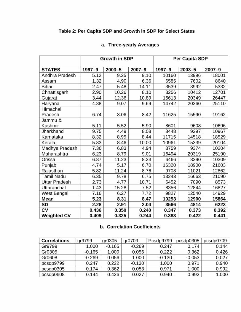
Table 2: Per Capita SDP and Growth in SDP for Select States

a. Three-yearly Averages

Growth in SDP

Per Capita SDP

STATES 1997–9 2003–5 2007–9 1997–9 2003–5 2007–9 Andhra Pradesh 5.12 9.25 9.10 10160 13996 18001Assam 1.32 4.90 6.36 6585 7602 8640Bihar 2.47 5.48 14.11 3539 3992 5332Chhattisgarh 2.90 10.26 8.10 8256 10412 12701Gujarat 3.44 12.36 10.89 15613 20349 26447Haryana 4.88 9.07 9.69 14742 20260 25110Himachal Pradesh 6.74 8.06 8.42 11625 15590 19162Jammu & Kashmir 5.11 5.52 5.90 8601 9608 10696Jharkhand 9.75 4.49 8.08 8448 9297 10967Karnataka 8.32 8.95 8.44 11715 14518 18529Kerala 5.83 8.46 10.00 10961 15339 20104Madhya Pradesh 7.36 6.83 4.94 8759 9374 10204Maharashtra 6.23 8.79 9.01 16494 20319 25190Orissa 6.87 11.23 8.23 6466 8290 10309Punjab 4.74 5.17 6.70 16320 18900 21603Rajasthan 5.82 11.24 8.76 9708 11021 12862Tamil Nadu 6.35 9.78 6.75 13243 16663 21090Uttar Pradesh 2.73 4.77 10.71 6452 7090 8573Uttaranchal 1.43 15.28 7.52 8356 12844 16827West Bengal 7.16 6.27 7.72 9827 12540 14929Mean 5.23 8.31 8.47 10293 12900 15864SD 2.28 2.91 2.04 3566 4814 6223CV 0.436 0.350 0.240 0.347 0.373 0.392Weighted CV 0.409 0.325 0.244 0.383 0.422 0.441

b. Correlation Coefficients

Correlations gr9799 gr0305 gr0709 Pcsdp9799 pcsdp0305 pcsdp0709Gr9799 1.000 -0.165 -0.269 0.247 0.174 0.144Gr0305 -0.165 1.000 0.056 0.222 0.362 0.426Gr0608 -0.269 0.056 1.000 -0.130 -0.053 0.027pcsdp9799 0.247 0.222 -0.130 1.000 0.971 0.940pcsdp0305 0.174 0.362 -0.053 0.971 1.000 0.992pcsdp0608 0.144 0.426 0.027 0.940 0.992 1.000

The CV (unweighted) in the growth rate has gone down from 44 per cent in late

1990s to 35 per cent in the middle of the present decade due to high growth in less

developed states, as discussed above. It has gone down further to 24 per cent in

the later years of the decade. The most important point is that the weighted CV of

the growth rates works out to be marginally below the unweighted figure, implying

that more populated states had a marginal advantage over the others, in the early

1990s. This advantage of the former seems to be evening out in recent years, the

inter-state growth differentials becoming less than before. There is no evidence of

the growth being higher in more developed states as the correlation between level

and growth in income is statistically insignificant (Table 2b). The importance of this

more equitable growth pattern notwithstanding, one must note that this,

unfortunately, has not made a dent on the trend of regional imbalance. The

inequality in per capita SDP has gone up consistently including the recent periods,

by both weighted and unweighted CV, as presented in Table 2a. Furthermore, the

Gini Index too has maintained a rising trend, as exhibited in the 1990s, as

presented in Figure 3, along with the CVs.

Figure 3: Trend in Inter-State Inequality in Per Capita Income based on Three

Yearly Averages: Unweighted and Weighted Indices

15

20

25

30

35

40

45

50

1997 - 99 2003 - 05 2006 - 08

Per

cen

t

CV Weighted CV Gini Weighted Gini

Source: Computed by the authors based on the State Domestic Income Tables

available at the website of the Central Statistical Organisation

Understandably, the growth pattern across the states in recent years is significantly

different from the pattern of growth in earlier years. This may be inferred from the

fact that the correlations of growth indicators with per capita SDP turn out to be

statistically insignificant. The correlations between the rates of growth for the three-

yearly periods across the states work out to be negative, although not statistically

significant (Table 2b). This is because a high growth rate has been recorded in

recent years in many of the less developed states that recorded low growth in

earlier years, as discussed above. Three newly formed states – Chhattisgarh,

Uttarakhand, and Jharkhand have grown faster than the average in the present

decade, marking a departure from the trend in late 1990s.

The Plan-wise growth figures, including those for the Eleventh Plan, as projected

by the Planning Commission (2008), confirm the above conclusions. The growth

rate of less developed states was less than 4 per cent, much below the average of

the developed states during the Eighth and the Ninth Plans (Table 3). The figures

for the former during the Tenth Plan period are similar to that of the national

average or that of the developed states. The same can be said about their

projected growth rates during the Eleventh Plan period, suggesting that there has

been a paradigm shift in the growth pattern in the country. Happily, the actual

growth rates for the less developed states in the first couple of years in this Plan

have turned out to be even higher than projected. The same is true for the Special

Category States in the North-East. Their growth rates, too, were less than the

national average in the Eighth and Ninth Plans, but have caught up with it in the

Tenth Plan period. More importantly, these are expected to be above the national

average in the Eleventh Plan. One can, therefore, stipulate that the strategy of

inclusive growth and balanced regional development has led to acceleration in the

average growth rate of the less developed states, including those in the North-

East, and this would continue in future. Unfortunately, however, this has made little

impact on the trend towards accentuation of regional imbalances measured

through per capita SDP.

Table 3: Annual Growth Rates in State Domestic Product in Different Plan Periods

S.No. State/UT Eighth Plan (1992–7)

Ninth Plan (1997–2002)

Tenth Plan (2002–7)

Eleventh Plan (2007–

12) Non Special Category States

1 Andhra Pradesh 5.4 4.6 6.7 9.52 Bihar 2.2 4.0 4.7 7.63 Chhattisgarh NA NA 9.2 8.64 Goa 8.9 5.5 7.8 12.15 Gujarat 12.4 4.0 10.6 11.26 Haryana 5.2 4.1 7.6 11.07 Jharkhand NA NA 11.1 9.88 Karnataka 6.2 7.2 7.0 11.29 Kerala 6.5 5.7 7.2 9.5

10 Madhya Pradesh 6.3 4.0 4.3 6.711 Maharashtra 8.9 4.7 7.9 9.112 Orissa 2.1 5.1 9.1 8.813 Punjab 4.7 4.4 4.5 5.914 Rajasthan 7.5 3.5 5.0 7.415 Tamil Nadu 7.0 6.3 6.6 8.516 Uttar Pradesh 4.9 4.0 4.6 6.117 West Bengal 6.3 6.9 6.1 9.7

Special Category States 1 Arunachal Pradesh 5.1 4.4 5.8 6.42 Assam 2.8 2.1 6.1 6.53 Himachal Pradesh 6.5 5.9 7.3 9.54 Jammu & Kashmir 5.0 5.2 5.2 6.45 Manipur 4.6 6.4 11.6 5.96 Meghalaya 3.8 6.2 5.6 7.37 Mizoram NA NA 5.9 7.18 Nagaland 8.9 2.6 8.3 9.39 Sikkim 5.3 8.3 7.7 6.7

10 Tripura 6.6 7.4 8.7 6.911 Uttarakhand NA NA 8.8 9.9 All India GDP 6.5 5.5 7.7 9.0 Developed States 7.2 5.2 7.0 9.6 Special Cat States 5.7 5.8 7.3 7.3 Less Dev States 3.7 3.8 7.2 8.0 CV in Growth

Rates 38.8 29.9 27.8 21.7

Note: Average of 2002–3 to 2005–6 for all States except J&K, Mizoram, Nagaland (2002–3 to 2004–5) and Tripura (2002–3 to 2003–4).

Source: CSO (base 1999–2000 constant price) as on 31.8.2007.

4. Identification of Socio-Economic Dimensions and Indicators of Development and Composite Indices

(a) Economic Development

In order to understand the nature and pattern of the contemporary process of

development, (i) economic, (ii) basic amenities, and (iii) social, have been

considered the three important dimensions. For articulating the dimension of

economic development, the indicator of average per capita state domestic product,

analysed above has been taken as the first in the list. This has been computed by

taking the average of the SDP figures for three years, 2006–7, 2007–8, and 2008–

9 at 1993–4 prices. The second indicator is the average of the annual growth rates

for the three years ending in 2008–9.

It is well acknowledged in development literature that analyses based on the levels

of SDP in per capita terms and growth rates therein do not capture several

important aspects of economic development at the macro- or state-level. Inclusion

of a number of other indicators reflecting other aspects of economic well-being has

been considered indispensable. Like per capita SDP, per capita consumption

expenditure is an important summary measure for assessing the volume of goods

and services at the command of individuals. The advantage here is that separate

figures are available for rural and urban areas. The data on this are obtained from

National Sample Survey for the year 2004–5. Similarly, poverty figures in rural and

urban areas are taken from the Eleventh Five Year Plan document for assessing

the level of economic deprivation of the population. Subtracting these from 100, the

figures of non-poor population have been obtained, which becomes a positive

indicator of economic development. Per capita foreign direct investment is the

other important economic indicator, reflecting present and potential development in

a state. This could also be a proxy for infrastructural development. Although a part

of its outcome is captured in the current income levels, its impact is likely to

manifest in future years as well. An average figure of investment for three years

ending in 2005–6, has therefore, been included in assessing the economic

dimension. The percentage of state income coming from the industrial sector is

included in the list as it reflects the strength of the economic base of a state.

Similarly, the income derived from the tertiary sector reflects the extent of

diversification in the economy as also the impetus it can provide to growth in the

period of globalization. It may be noted that separate indicators of infrastructure

have not been included in order to limit the number of indicators for the economic

dimension, as also because the indicators pertaining to investment and income

from industry and the tertiary sector would capture their impact. The indicators that

constitute the dimension of economic development are given along with the

sources of the data in Table 4a. A composite index of economic development has

then been constructed based on these nine indicators, after making these scale-

free by dividing the values of each indicator by its arithmetic mean. The

composition has been done through the process of two-stage composition. In the

first stage, the figures of monthly per capita expenditure have been aggregated for

rural and urban areas by giving these equal weightages of 0.5. The aggregative

indicator for the non-poor population percentage has been constructed in a similar

fashion by combining the rural and urban figures.

Table 4a: Indicators pertaining to the Dimension of Economic Development

S.No Indicator Source of Data

1 Average PC Income 2007–9 Unpublished data, Central Statistical Organization

2 Average Growth in SDP 2007–9 Unpublished data, Central Statistical Organization

3 Per Capita Expenditure Rural 2004–5

NSSO Report

4 Per Capita Expenditure Urban 2004–5

NSSO Report

5 Per cent Non Poor Rural 2004–5 Planning Commission (2008),11th 5 year Plan

6 Per cent Non Poor Urban 2004–5 Planning Commission (2008), 11th 5 year Plan

7 Average Percentage Income from Secondary Sector 2007–9

Unpublished data, Central Statistical Organization

8 Average Percentage Income from Tertiary Sector 2007–9

Unpublished data, Central Statistical Organization

9 Average Per Capita FDI 2003–5 Lok Sabha Unstarred Question 182, dated 01.03.2005 and 1032, dated 01.08.2006

(b) Basic Amenities

A set of nine indicators pertaining to basic amenities have been selected, as given

in Table 4b. All these have been taken from the National Health and Family

Survey III and pertain to the year 2005–6. The percentages of female and male

literates have been included to reflect the level and access to educational facilities

in the states. These have been considered more appropriate than the information

on the facilities given by the individual states. The percentages of men and women

reading newspapers have been taken as a proxy of transportation and social

linkages of the distant rural and urban areas to the nearby large centres. These

linkages contribute in a significant way to the dissemination of growth impulses in

a region. The percentage of households having electricity, improved source of

drinking water, toilet facility, non-solid fuel for cooking, and residing in pucca

houses are direct measures of availability of basic amenities, and consequently,

have been included under this dimension.

Table 4b: Indicators pertaining to the Dimension of Basic Amenities

S. No Indicator 1 Education Female2 Education Male

3 Per cent women (15–49) reading newspaper at least once a week

4 Per cent men (15–49) reading newspaper at least once a week

5 Percentage of household with electricity

6 Percentage of household with improved source of drinking water

7 Percentage of household with toilet facility8 Percentage of household using non-solid fuel for cooking 9 Percentage of household living in a pucca house

Source: International Institute of Population Sciences: 2007

The composite index for the dimension of basic amenities has been computed

using a two-stage model, as in case of economic development discussed above.

Aggregative indices for education and newspaper reading have been constructed

in the first stage of composition under the dimension of basic amenities by

combining the values for men and women. In view of the key role played by female

literacy and social mobilization of women in the process of development, the

indicators pertaining to the women have been given twice the weightage as that for

men. These two aggregative indices have then been combined with the remaining

five indicators of amenities, by assigning these equal weightages after making

these scale-free through division by the mean.

(c) Social Development

Ten indicators identified under the dimension of social development, as presented

in Table 4c, reflect ‘deficit in development’ and can be described as negative

indicators. The first two indicators—infant mortality rate and total fertility rate—

articulate the basic demographic character of the state. In a way these two bring

out the sum total of the developmental interventions on the demographic front. The

indicators of malnourished children in the age group of 0–3 years and of under-

weight children below 5 years reveal the physical health of the children. The

indicator pertaining to anemia in women captures the health status for persons in

the reproductive age group. The sixth and seventh indicators reflect the pre-natal

and post-natal facilities to expectant women, young mothers, and children. The

eighth indicator captures malnutrition among people as also absence of preventive

facilities against tuberculosis. The last two indicators have been included to

articulate the prevalence of modern values relating to family planning among men

and women.

Table 4c: Indicators pertaining to the Dimension of Social Development

S.No Indicator 1 Infant Mortality Rate Current2 Total Fertility Rate Current3 Malnutrition of Children (0–3 Years) Current

4 Percentage of children under age 5 years with weight for age -3SD

5 Anemia among Women (15–49 Years) Current

6 Percentage of women who had no antenatal care by doctor

7 Percentage of children (Below 6 years) who has not received any ICDS service

8 Number of persons per 100,000 suffering from Tuberculosis

9 Percentage of Women (15–49) wanting children10 Percentage of Men (15–49) wanting children

Source: International Institute of Population Sciences: 2007

The composite indices reflecting the absence of social development have been

worked out in two stages, as in the case of basic amenities. In view of the

overlapping of information between the indicators pertaining to malnourished and

underweight children, these two have been aggregated in the first stage by giving

them equal weightages. The total number of indicators, thus, gets reduced to nine.

All these have been composited in one shot at the second stage by assigning

them equal weightages. The reciprocal of these composite values reflect the levels

of social development.

The three composite indices pertaining to economic development, basic amenities,

and social development are presented in Table 5. The values of the indices have

been placed under three categories—low, medium, and high—identifying the cut-

off points based on ‘natural breaks’ in the distribution. These are shown in Maps 1,

2, and 3 that clearly bring out the areas of overlap among the states.

Table 5: The Composite Indices Articulating Three Different Dimensions of Development and their Correlations

States Economic Amenities Social Andhra Pradesh 1.12 0.98 1.10 Arunachal Pradesh 0.76 0.81 0.67 Assam 0.75 0.85 0.81 Bihar 0.72 0.58 0.66 Chhattisgarh 0.89 0.68 1.04 Goa 1.90 1.51 1.52 Gujarat 1.49 1.18 0.94 Haryana 1.20 1.05 1.05 Himachal Pradesh 1.10 1.13 1.50 Jammu & Kashmir 0.78 1.03 1.47 Jharkhand 0.82 0.58 0.75 Karnataka 1.41 1.06 1.44 Kerala 1.13 1.51 1.58 Madhya Pradesh 0.69 0.74 0.91 Maharashtra 1.76 1.25 1.31 Manipur 0.74 1.14 0.89 Meghalaya 0.77 0.96 0.78 Mizoram 0.79 1.52 1.00 Nagaland 0.83 0.95 0.95 Orissa 0.73 0.67 1.00 Punjab 1.45 1.22 1.38 Rajasthan 0.84 0.83 0.91 Sikkim 0.77 1.05 1.04 Tamil Nadu 1.17 1.15 1.17 Tripura 0.74 0.92 0.92 Uttar Pradesh 0.78 0.73 0.83 Uttarakhand 0.92 1.06 1.10 West Bengal 0.94 0.88 0.95

Source: Computed by the authors

Map – 1

INDIA Economic Development

N

Composite Index> 1.20 (High)0.90 - 1.20 (Medium)< 0.90 (Low)

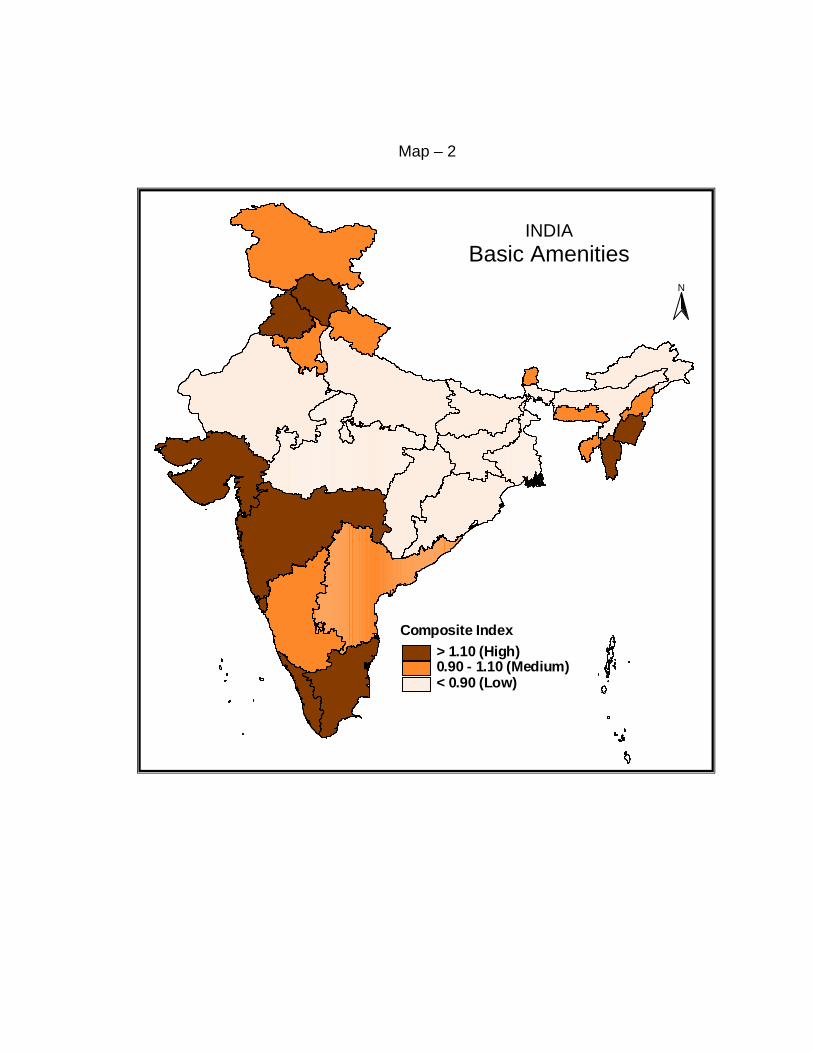
Map – 2

INDIA Basic Amenities

N

Composite Index

> 1.10 (High)0.90 - 1.10 (Medium)< 0.90 (Low)

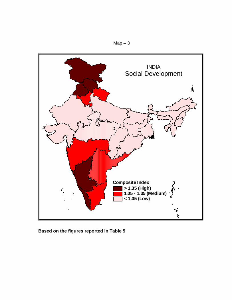
Map – 3

Based on the figures reported in Table 5

INDIA Social Development

N

Composite Index> 1.35 (High)1.05 - 1.35 (Medium)< 1.05 (Low)

The composite index of amenities exhibits a very high correlation with that of social

development (Table 6). This is because they pertain to the similar aspects,

capturing inputs or the outcomes. Economic development, too, has a high

correlation with social development. This is understandable as the capacity of the

governments at the state level to make interventions and bring about social

transformations would be higher in relatively developed states. The correlation of

economic development with amenities, although statistically significant, is relatively

low, which suggests that the problems pertaining to health, education, and access

to other amenities cannot be effectively tackled in all the states, just by focusing on

economic development.

Table 6: Coefficients of Correlation among the Three Composite Indices

Economic Amenities Social Economic 1 Amenities 0.603 1 Social 0.645 0.680 1

Source: Computed by the authors

5. State Interventions and Changing Face of Regional Development

An analysis of the pattern of interdependency among a select set of development

and policy linked indicators would be helpful in identifying the factors that are

responsible for accentuation of regional inequality. Based on a review of literature

and policy documents, 15 indicators have been identified pertaining to economic

growth and state intervention in terms of financial allocation under major

developmental programmes and the stipulated growth rates in different sectors for

the period of the Eleventh Plan. The specifications of the indicators and their

average values along with their coefficients of variation (unweighted) are given in

Table 711.

11 The matrix of correlation coefficients is not included in the paper which can be obtained on request from the author.

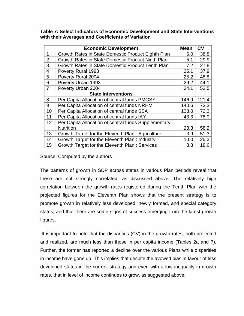
Table 7: Select Indicators of Economic Development and State Interventions with their Averages and Coefficients of Variation

Economic Development Mean CV 1 Growth Rates in State Domestic Product Eighth Plan 6.0 38.82 Growth Rates in State Domestic Product Ninth Plan 5.1 29.93 Growth Rates in State Domestic Product Tenth Plan 7.2 27.84 Poverty Rural 1993 35.1 37.95 Poverty Rural 2004 25.2 48.86 Poverty Urban 1993 29.2 44.17 Poverty Urban 2004 24.1 52.5

State Interventions 8 Per Capita Allocation of central funds PMGSY 146.9 121.49 Per Capita Allocation of central funds NRHM 140.6 73.310 Per Capita Allocation of central funds SSA 133.0 72.311 Per Capita Allocation of central funds IAY 43.3 78.012 Per Capita Allocation of central funds Supplementary

Nutrition 23.3 58.213 Growth Target for the Eleventh Plan : Agriculture 3.9 51.314 Growth Target for the Eleventh Plan : Industry 10.0 25.315 Growth Target for the Eleventh Plan : Services 8.8 18.6

Source: Computed by the authors

The patterns of growth in SDP across states in various Plan periods reveal that

these are not strongly correlated, as discussed above. The relatively high

correlation between the growth rates registered during the Tenth Plan with the

projected figures for the Eleventh Plan shows that the present strategy is to

promote growth in relatively less developed, newly formed, and special category

states, and that there are some signs of success emerging from the latest growth

figures.

It is important to note that the disparities (CV) in the growth rates, both projected

and realized, are much less than those in per capita income (Tables 2a and 7).

Further, the former has reported a decline over the various Plans while disparities

in income have gone up. This implies that despite the avowed bias in favour of less

developed states in the current strategy and even with a low inequality in growth

rates, that in level of income continues to grow, as suggested above.

A distinct bias in allocation in favour of backward states under all these flagship

programmes may be inferred from the negative correlation of per capita allocations

with per capita income of the state. Furthermore, the latter shows negative

correlation with the share of the states in the Planning Commission Assistance for

the current year as also the Twelfth Finance Commission transfers. Poverty levels

in rural and urban areas are negatively correlated with per capita income, while

their relations with per capita allocation for the central sector schemes are positive.

These correlations, although not always statistically significant, reveal a concern

on the part of the Central Government to make larger resources available to

backward states under the policy of inclusive development.

The allocations, made by the Planning Commission and Finance Commission,

however, do not exhibit positive correlation with the proposed income growth rates

or the projected per capita SDP, implying that the allocations would not

immediately turn into higher growth outcomes. It would, indeed, be unreasonable

to expect that these higher allocations in the laggard states by themselves would

be able to push up the overall growth in the states or their income levels. One

cannot expect the income scenario at the state level to change in five to seven

years. There is, thus, ‘a strong case for proactive public policy to induce more

investment in backward states either through public investment or through fiscal

incentives’ directed towards infrastructural facilities and basic amenities

(Bhattacharya and Sakthivel: 2004).

Many of the relatively backward states that have large shares in population and

are experiencing rapid demographic growth have, understandably, not been able

to address the problems of underdevelopment and poverty due to their low rates of

economic growth, as well as their inability to put up strong anti-poverty

programmes. The capacity of their governments to mobilize resources in the

market or institutional sources is low. This has come in the way of their launching

development projects on their own, despite opportunities provided to them through

measures of decentralization and devolution of powers and responsibilities.

It is thus evident that the devolution of resources to state governments through the

institutional mechanisms of the Finance Commission and the Planning

Commission is inadequate to alleviate the normative budgetary deficits, or meet a

desirable level of Plan expenditure in less developed states. The government

undertook major expenditure cuts during the 1990s as a policy package of reforms

for achieving targeted fiscal ‘balance’. Instead of increasing revenues through

tax—direct and indirect—massive reductions were made in capital expenditure. As

a result, the capital expenditure of central government as a proportion of GDP,

declined steadily from 7.01 per cent in 1986–7 to as low as 1.66 per cent in 2006–

7 (Figure 4). Public investments in crucial areas like agriculture, rural

development, infrastructure development, and industry were scaled down.

The progressiveness in allocation by these central level institutions has declined in

recent decades along with the total volume of resources. They could not make

larger allocation in favour of less developed states that have large shares in

population. The problem has become more serious in recent years due to

measures of fiscal reforms with the launching of the programmes of globalization.

This has adversely affected the already fragile infrastructure in the less developed

states and led to a setback in public services like education, public health and

sanitation.

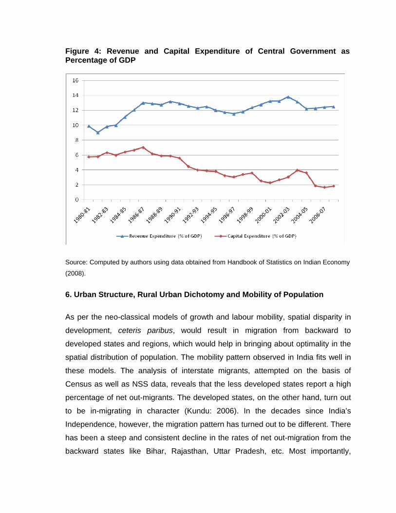
Figure 4: Revenue and Capital Expenditure of Central Government as Percentage of GDP

Source: Computed by authors using data obtained from Handbook of Statistics on Indian Economy

(2008).

6. Urban Structure, Rural Urban Dichotomy and Mobility of Population

As per the neo-classical models of growth and labour mobility, spatial disparity in

development, ceteris paribus, would result in migration from backward to

developed states and regions, which would help in bringing about optimality in the

spatial distribution of population. The mobility pattern observed in India fits well in

these models. The analysis of interstate migrants, attempted on the basis of

Census as well as NSS data, reveals that the less developed states report a high

percentage of net out-migrants. The developed states, on the other hand, turn out

to be in-migrating in character (Kundu: 2006). In the decades since India’s

Independence, however, the migration pattern has turned out to be different. There

has been a steep and consistent decline in the rates of net out-migration from the

backward states like Bihar, Rajasthan, Uttar Pradesh, etc. Most importantly,

Madhya Pradesh and Orissa stand out as exceptions as these report net inflow of

population. This could be explained in terms of massive public sector investment,

resulting in creation of job opportunities in industry and business. The local

population, unfortunately, is unable to take advantage of this due to their low level

of literacy and skill. The developed states like Maharashtra, Tamil Nadu, West

Bengal, Karnataka, Gujarat, etc. that had attracted large scale in-migration during

the colonial period now report decline in in-migration rates (Kundu: 2006)12.

There has been marginal improvement in internal mobility during the decade of

1991–2001, which can be attributed to transitional factors and globalization13. The

percentage of migrants as per the 2001 Census, nonetheless, works out to be less

than that in 1961 and 1971. The data from NSS for the period from 1983 to 1999–

2000, too, confirm the declining trend of migration for males, both in rural and

urban areas, although the fall is less than that reported in the Census. The general

conclusion thus emerging is unmistakably that mobility of men, which is often

linked to the strategy of seeking livelihood (women’s mobility getting affected by a

host of socio-cultural factors), has gone down systematically over the past few

decades. This would certainly come in the way of the poor in deprived regions

finding their strategy of survival or improving their economic well-being.

Decline in the rate of migration, despite accentuation of regional imbalance and

improvement in transport and communication facilities, is a matter of concern.

Scholars have tried to explain this in terms of growing assertion of regional identity,

education in regional languages up to high school, adoption of Master Plans and

land use restrictions at the city level, etc., all directly or indirectly discouraging

migration. This seriously discounts the proposition that the mobility of labour,

operationalized through market, would ensure optimal distribution of economic

activities in space.

12 The state of Gujarat does not show this declining trend due to its growing dominance in the industrial map of India. Similarly, Haryana reporting high in-migration rates during recent decades can be explained in terms of migration from Punjab due to political instability and communal tensions.

13 Many of the illegal migrants from neighbouring countries being recorded as interstate migrants could also explain the rising migration trend in the 1990s.

In a fast globalizing economy like India, new employment opportunities are coming

up in selective sectors and in a few regions/urban centres. While the poor

constitute a large proportion among the migrants, a substantial number belong to

the middle and high income categories, grabbing the new opportunities thrown up

by the process of globalization. It would, therefore, be erroneous to consider most

migrants to be destitute or economically and socially displaced persons, moving

from place to place as a part of their survival strategy.

The fact that the percentage of migrants has declined and their economic and

social status is better than that of non-migrants and has even improved over time,

reflects barriers to mobility for the poor. With the present rigidities in the agrarian

system, growing regionalism, changes in skill requirements in labour market etc.,

the emerging productive and institutional structure in the cities too has become

hostile to newcomers. This has made the migration process selective wherein poor

and unskilled labourers are finding it difficult to access the livelihood opportunities

coming up in developed regions and large cities. A major factor responsible for

persistence of high poverty in the backward states is the difficulty encountered by

the poor trying to move into developed states.

The low rate of urbanization and declining percentage share of migrants,

particularly among urban males, can be attributed to provision of basic amenities

based on market affordability and inhospitable social environment in cities and

towns,. The pattern is similar for their female counterparts, although the rate of

decline in migration in their case is less than that noted for the male counterpart. A

fall in the rate of urbanization during 1981–2001 confirms this thesis and questions

the UN projections of urban explosion in India and the Asian region. Urban

population grew at an annual exponential rate of 3.8 per cent per annum during

1971–81 which was the highest in the last century. Despite the growing rural-urban

(RU) disparity, improvements in transport and communication facilities,

modernization resulting in relaxation of traditional social barriers, etc., the rate

came down to 3.1 per cent and 2.7 per cent respectively during the 1980s and

1990s.

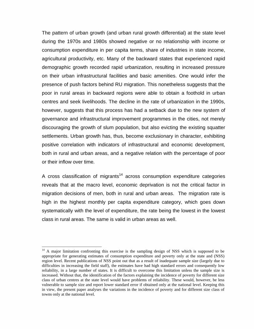
The pattern of urban growth (and urban rural growth differential) at the state level

during the 1970s and 1980s showed negative or no relationship with income or

consumption expenditure in per capita terms, share of industries in state income,

agricultural productivity, etc. Many of the backward states that experienced rapid

demographic growth recorded rapid urbanization, resulting in increased pressure

on their urban infrastructural facilities and basic amenities. One would infer the

presence of push factors behind RU migration. This nonetheless suggests that the

poor in rural areas in backward regions were able to obtain a foothold in urban

centres and seek livelihoods. The decline in the rate of urbanization in the 1990s,

however, suggests that this process has had a setback due to the new system of

governance and infrastructural improvement programmes in the cities, not merely

discouraging the growth of slum population, but also evicting the existing squatter

settlements. Urban growth has, thus, become exclusionary in character, exhibiting

positive correlation with indicators of infrastructural and economic development,

both in rural and urban areas, and a negative relation with the percentage of poor

or their inflow over time.

A cross classification of migrants14 across consumption expenditure categories

reveals that at the macro level, economic deprivation is not the critical factor in

migration decisions of men, both in rural and urban areas. The migration rate is

high in the highest monthly per capita expenditure category, which goes down

systematically with the level of expenditure, the rate being the lowest in the lowest

class in rural areas. The same is valid in urban areas as well.

14 A major limitation confronting this exercise is the sampling design of NSS which is supposed to be appropriate for generating estimates of consumption expenditure and poverty only at the state and (NSS) region level. Recent publications of NSS point out that as a result of inadequate sample size (largely due to difficulties in increasing the field staff), the estimates have had high standard errors and consequently low reliability, in a large number of states. It is difficult to overcome this limitation unless the sample size is increased. Without that, the identification of the factors explaining the incidence of poverty for different size class of urban centres at the state level would have problems of reliability. These would, however, be less vulnerable to sample size and report lower standard error if obtained only at the national level. Keeping this in view, the present paper analyses the variations in the incidence of poverty and for different size class of towns only at the national level.

Based on the differences in consumption expenditure of migrant and non-migrant

households in rural and urban areas, one can argue that migration is an instrument

of improving economic well-being. However, it is not only the poor who benefit from

it as the non-poor constitute a large segment of the migrants. Economic gains of

migration are higher in large cities compared to lower order cities/towns (Kundu

and Sarangi: 2007). Further, education or skill emerges as the most important

factor in reducing the risk of a person falling below the poverty line, both for

migrant and non-migrant population, irrespective of the size class of cities/towns.

One observes that better-off sections of the population with higher levels of skills

find it easier to get absorbed in the city economy and avail the ‘opportunity’ offered

through migration. Unfortunately, poor and unskilled male labourers (seeking

absorption in informal activities as casual workers) are finding it increasingly

difficult to become a part of the process and avail the benefits in large cities.

Understandably, their migration rate has gone down, which is reflected in a

significant decline in the percentage of poor in metropolitan and Class I cities

during the last decade and a half. They are able to obtain a foothold in small and

medium towns but here opportunities for employment and poverty alleviation are

low, as noted above. As a result of these factors, migration for poverty alleviation

has become a less important component in the mobility stream and it is likely to

become an even smaller one over time.

The most disconcerting fact is that there has been a deceleration in rural to urban

migration during the 1990s despite increase in economic inequality, which confirms

the fact that urban centres have become less hospitable and less accommodating

for the poor. The propositions of spatially unbalanced growth through ‘dispersal of

concentrations’ and then of reaching out to the poor through a human settlement

strategy (World Bank, 2009), therefore, needs to be examined with empirical

rigour. Migration becoming an instrument of sharing the benefits of uneven growth

across states and districts needs to be questioned in the context of increasing

social and economic costs of migration which the conventional models, including

those employed in this paper, fail to incorporate or highlight.

7. Identification of Lagging States for Targeted Intervention

The identification of lagging states, as also the factors constraining these in picking

up growth momentum and thereby resulting in accentuation of inequality, has not

been very definitive in India. The planning apparatus in the country being

essentially centralized, there has not been serious empirical research to determine

the policies that drive the growth process at the state level. Indeed, without the

state-focused studies, it is impossible to answer this issue with a reasonable level

of empirical rigour. The neglect of state-level policies and decentralized

governance has led to persistence of poverty surrounding islands or enclaves of

economic affluence.

From the 1950s through to the ‘70s, attempts were made, mostly as a part of the

federal system, to determine and guide investments in different states and regions,

as also to control credit and financial markets. With the launching of the reform

measures, the share of public investment—mostly made by the central government

agencies and that backed up by targeted credit delivery—in the overall investment

has been steadily declining. Globalization has led to erosion of capability of the

federal machinery to determine the overall resource allocations in the economy

and control the institutional framework at the state level, which is responsible for

micro level programme implementation.

Based on the figures of per capita SDP and growth in SDP upto 2004-05, a set of

eight states was identified as economically lagging in our initial exercise presented

in Section 3. These states had very high poverty ratios in 1993-94, with Assam (41

per cent), Bihar (including Jharkhand) (55 per cent), Madhya Pradesh (including

Chhattisgarh) (43 per cent), Orissa (49 per cent) and Uttar Pradesh (including

Uttarakhand (41 per cent). These states altogether had 44 per cent of the Indian

poor in 1973–4, 48 per cent in 1987–8, and 52 per cent in 1993–4. These states

accounted for 60 per cent of the Indian poor in 2004–5.

The north-eastern states, except Assam, are excluded from the category due to

their relatively high growth in income in recent years, as also for enjoying higher

per capita central government allocations. It would be important that the central

government pursues this policy of giving greater attention to these special states

due to economic, social, as also political reasons. The non-governmental

organizations, especially those with international character, may then focus on the

other, less developed states in the country, as identified above. The accentuation

of regional inequality, when a weighed measure of disparity is used, reveals that

states that have a relatively higher share in population have received less of

central government transfers in per capita terms and are more deprived in terms of

economic and social development outcomes as also access to basic amenities.

The analysis in the paper shows that the bottom nine positions in terms of the

composite index of economic development are occupied by the eight lagging

states identified above. Jammu and Kashmir, however, occupies the fifth position

and Uttarakhand is pushed out of the list. Among the identified lagging states, the

latter is the only one which records a relatively high score of economic

development. It can be bracketed with the other special category state of Himachal

Pradesh, as they enjoy a relatively higher level of economic well-being (Table 5).

One must note that Rajasthan, which was not identified as a lagging state in the

earlier analysis, belongs to the list of the bottom nine in terms of economic

development. This is because the state registered significant decline in its growth

in SDP in recent years, and consequently, it went down in terms of the composite

score on economic development

It is noted that Jammu and Kashmir, along with many others in the North-East,

report low scores in economic development (Table 5). It can, however, be argued

that the figures of per capita SDP in all these states do not adequately capture

economic well-being because of serious data problems. A large part of the income

derived by households from land resources goes unrecorded. Also, governmental

subsidies tend to distort the prices, and consequently, the income figures do not

reflect the real well-being of the population. More importantly, all these states,

except Assam, are doing reasonably well in terms of amenities and social

development. It is, therefore, proposed that these states need to be distinguished

from the other backward states in the country. In view of the location and geo-

political factors, it is argued that development of these states may be best left to

the central and state governments, as international NGOs may face operational

and logistic problems. These problems and data difficulties are less serious in case

of Assam, and hence, its inclusion in the list of laggard states can be justified.

Uttarakhand, however, is not among the bottom nine states in terms of any of the

three composite indices. It is a special category category state but does not

emerge as extremely deprived in terms of different dimensions of development.

Even in terms of per capita income and growth in SDP, it is at the top among the

less developed states. One may, therefore, propose to replace Uttarakhand by

Rajasthan, the latter belonging to the low category as per all the three dimensions

of development.

Table 7: States with Population over 5 million ranked by Composite Indices

of Development in Selected Dimensions

S.No States Economic Amenities Social 1 MP 0.69 Jharkhand 0.58 Bihar 0.662 Bihar 0.72 Bihar 0.58 Jharkhand 0.753 Orissa 0.73 Orissa 0.67 Assam 0.814 Assam 0.75 Chhattisgarh 0.68 UP 0.835 J & K 0.78 UP 0.73 MP 0.916 UP 0.78 MP 0.74 Rajasthan 0.917 Jharkhand 0.82 Rajasthan 0.83 Gujarat 0.948 Rajasthan 0.84 Assam 0.85 West Bengal 0.959 Chhattisgarh 0.89 West Bengal 0.88 Orissa 1.00

10 Uttarakhand 0.92 AP 0.98 Chhattisgarh 1.0411 West Bengal 0.94 J & K 1.03 Haryana 1.0512 HP 1.10 Haryana 1.05 AP 1.10

13 Andhra Pradesh 1.12 Karnataka 1.06 Uttarakhand 1.10

14 Kerala 1.13 Uttarakhand 1.06 Tamil Nadu 1.1715 Tamil Nadu 1.17 HP 1.13 Maharashtra 1.3116 Haryana 1.20 Tamil Nadu 1.15 Punjab 1.3817 Karnataka 1.41 Gujarat 1.18 Karnataka 1.4418 Punjab 1.45 Punjab 1.22 J & K 1.4719 Gujarat 1.49 Maharashtra 1.25 HP 1.50

20 Maharashtra 1.76 Goa 1.51 Goa 1.5221 Goa 1.90 Kerala 1.51 Kerala 1.58

Source: Computed by the authors

The subsequent analysis shows that these eight states are also characterized by a

low level of urbanization and deceleration in the rate of urban growth in the past

couple of decades. These have been highly out-migrating in the years after

Independence, but the rate of out-migration has declined in the last few decades.

These states also have a highly lopsided urban structure with a large percentage

of urban population being concentrated in a few large cities. Further, there has

been significant deceleration in the economic and demographic growth in their

small and medium towns, many of these getting declassified from the urban

category while several others face serious threat on this account.

Many of the state governments have taken initiatives for creating the necessary

policy framework and supporting infrastructural environment to attract private

capital from within and outside the country. This has created an unhealthy

competition among states wherein the lagging states stand at a disadvantage. The

challenge of establishing a system of governance in these states which can

maintain law and order, provide quick and effective dispute resolution mechanism

through an adjudication system, and attract industrial and infrastructural

investment, would now have to be taken up. The states must also mobilize internal

resources to meet the infrastructure deficiency in critical areas and empower the

general mass of the population socially to partake in the development process. As

provision of basic amenities and social development fall largely within the purview

of the states and their capabilities to tackle the problem is very low due to their

levels of development, serious development deficits have persisted over the years.

The international NGOs can play an effective role in addressing these problems.

The paradigm shift in the formulation and implementation of the Eleventh Plan is

reflected in the greater role being assigned to the state and local governments,

along with civil society organizations. Detailed guidelines have been issued to the

states for preparing district plans and sub-plans through the district/block level

committees and other Constitutional bodies created for this purpose. In fact, these

plans are a pre-requisite for accessing funds in many of the new central sector

schemes. This shift would hopefully provide ‘an institutional basis for the regular

and systematic study of intra-state disparities as part of the Annual Plan and Five

Year Plan processes’ (Planning Commission: 2008) and help in addressing the

root causes responsible for accentuation of inequity and perpetuation of poverty.

The new paradigm of participatory governance, backed up by area and social

group targeting, can help these lagging states in preparing and implementing a

comprehensive plan for infrastructure, basic amenities and social development in

collaboration with the major national and international partners.

References

Ahluwalia, M. S. (2000), ‘Economic Performance of States in Post Reform Era’, Economic and Political Weekly, Vol 35, No. 19, pp 1638-48, May 2000

Ahmad, Ahsan and Ashish Narain (2008), ‘Towards Understanding Development in Lagging Regions of India’, paper presented at the Conference on Growth and Development in the Lagging Regions of India, Administrative Staff College of India, Hyderabad

Bhattacharya, B.B. and S. Sakthivel (2004): ‘Regional Growth and Disparity in India: Comparison of Pre- and Post-Reform Decades’, Economic and Political Weekly, Vol 39, No. 10, pp. 1071-7, March 2004

Datt, G. and M. Ravallion (2002), ‘Is India's Economic Growth Leaving the Poor Behind?’ Policy Research Working Paper 2846, The World Bank, Washington DC

Devarajan, S. and I. Nabi (2006), Economic Growth in South Asia, World Bank, South Asia Region, Washington DC.

International Institute of Population Sciences (2007) National Family Health Survey (NFHS-3) vol I, International Institute of Population Sciences, Mumbai

Kundu, A. (2006), ‘Globalization and the Emerging Urban Structure: Regional Inequality and Population Mobility’, India: Social Development Report, Oxford, New Delhi

Kundu, A. and N. Sarangi (2010), ‘‘Inclusive Growth’ and Income Inequality in India under Globalisation: Causes, Consequences and Policy Responses’, Proceedings of the Conference of Regional Disparities in Asia, UNDP, Colombo

Kundu, A. and N. Sarangi (2007), ‘Migration, Employment Status and Poverty: An Analysis Across Urban Centres in India’, Economic and Political Weekly, Vol 42, No. 04, pp 301-6, January, 2007

Planning Commission (2008), Eleventh Five Year Plan 2007-2012, Vol. I, Government of India, New Delhi

Sivaramakrishna, K. C., A. Kundu, and B. N. Singh (2005), Handbook of Urbanisation, Oxford University Press, New Delhi

World Bank (2009), World Development Report 2009: Reshaping Economic Geography, Oxford University Press, New York

Oxfam India, Plot No. 1, Community Centre, 2nd Floor (Above Sujan Mahinder Hospital), New Friends Colony, New Delhi - 110 025Ph: 91 11 4653 8000; www.oxfamindia.org