Regional Economic Outlook: Asia and Pacific
144
Regional Economic Outlook World Economic and Financial Surveys I N T E R N A T I O N A L M O N E T A R Y F U N D 16 APR Asia and Pacific Building on Asia’s Strengths during Turbulent Times
-
Upload
- -
Category
News & Politics
-
view
848 -
download
6
Transcript of Regional Economic Outlook: Asia and Pacific
Regional Economic OutlookAsia and Pacific, April 2016
Regional Economic Outlook
World Economic and Financia l Surveys
I N T E R N A T I O N A L M O N E T A R Y F U N D
16AP
R
Asia and PacificBuilding on Asia’s Strengths during Turbulent Times
World Economic and Financial Surveys
Reg iona l Economic Out look
I N T E R N A T I O N A L M O N E T A R Y F U N D
Asia and Pacific Building on Asia’s Strengths during Turbulent Times
16AP
R
Cataloging-in-Publication Data
Regional economic outlook. Asia and Pacific. – Washington, D.C. : International Monetary Fund, 2005–
v. ; cm. – (World economic and financial surveys, 0258-7440)
Once a year.Began in 2005.Some issues have also thematic titles.
1. Economic forecasting – Asia – Periodicals. 2. Economic forecasting – Pacific Area – Periodicals. 3. Asia – Economic conditions – 1945- – Periodicals. 4. Pacific Area – Economic conditions – Periodicals. 5. Economic development – Asia – Periodicals. 6. Economic development – Pacific Area – Periodicals. I. Title: Asia and Pacific. II. International Monetary Fund. III. Series: World economic and financial surveys.
HC412.R445
ISBN-13: 978-1-49835-092-1 (Paper) ISBN-13: 978-1-48433-943-5 (Web PDF)
The Regional Economic Outlook: Asia and Pacific is published annually in the spring to review developments in the Asia-Pacific region. Both projections and policy considerations are those of the IMF staff and do not necessarily represent the views of the IMF, its Executive Board, or IMF Management.
Please send orders to:International Monetary Fund, Publication Services700 19th St. N.W., Washington, D.C. 20431, U.S.A.
Tel.: (202) 623-7430 Telefax: (202) 623-7201E-mail: [email protected]
Internet: www.imf.org
©2016 International Monetary Fund
iii
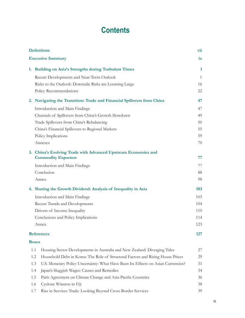
Contents
Definitions vii
ExecutiveSummary ix
1. BuildingonAsia’sStrengthsduringTurbulentTimes 1
Recent Developments and Near-Term Outlook 1 Risks to the Outlook: Downside Risks are Looming Large 16 Policy Recommendations 22
2. NavigatingtheTransition:TradeandFinancialSpilloversfromChina 47
Introduction and Main Findings 47 Channels of Spillovers from China’s Growth Slowdown 49 Trade Spillovers from China’s Rebalancing 50 China’s Financial Spillovers to Regional Markets 55 Policy Implications 59 Annexes 70
3. China’sEvolvingTradewithAdvancedUpstreamEconomiesand CommodityExporters 77
Introduction and Main Findings 77 Conclusion 88 Annex 98
4. SharingtheGrowthDividend:Analysisof InequalityinAsia 103
Introduction and Main Findings 103 Recent Trends and Developments 104 Drivers of Income Inequality 110 Conclusions and Policy Implications 114 Annex 123
References 127
Boxes
1.1 Housing Sector Developments in Australia and New Zealand: Diverging Tales 27 1.2 Household Debt in Korea: The Role of Structural Factors and Rising House Prices 29 1.3 U.S. Monetary Policy Uncertainty: What Have Been Its Effects on Asian Currencies? 31 1.4 Japan’s Sluggish Wages: Causes and Remedies 34 1.5 Paris Agreement on Climate Change and Asia-Pacific Countries 36 1.6 Cyclone Winston in Fiji 38 1.7 Rise in Services Trade: Looking Beyond Cross-Border Services 39
iv
REGIONAL ECONOMIC OUTLOOK: ASIA AND PACIFIC
2.1 Regional Consequences of a Growth Slowdown in China 64 2.2 China’s Import Slowdown 66 2.3 China Opening Up: The Evolution of Financial Linkages 68 3.1 The Evolution of China’s Labor-Intensive Exports 90 3.2 Food Consumption Patterns in China 94 3.3 The Contribution of China’s Growth Transition to Commodity Price Declines 96 4.1 Understanding Rising Inequality in China and India 117 4.2 What Explains Declining Inequality in Malaysia, the Philippines, and Thailand? 119 4.3 Labor Share and Income Inequality 121Tables
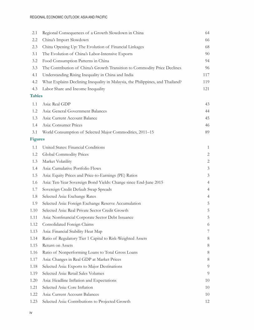
1.1 Asia: Real GDP 43 1.2 Asia: General Government Balances 44 1.3 Asia: Current Account Balance 45 1.4 Asia: Consumer Prices 46 3.1 World Consumption of Selected Major Commodities, 2011–15 89Figures
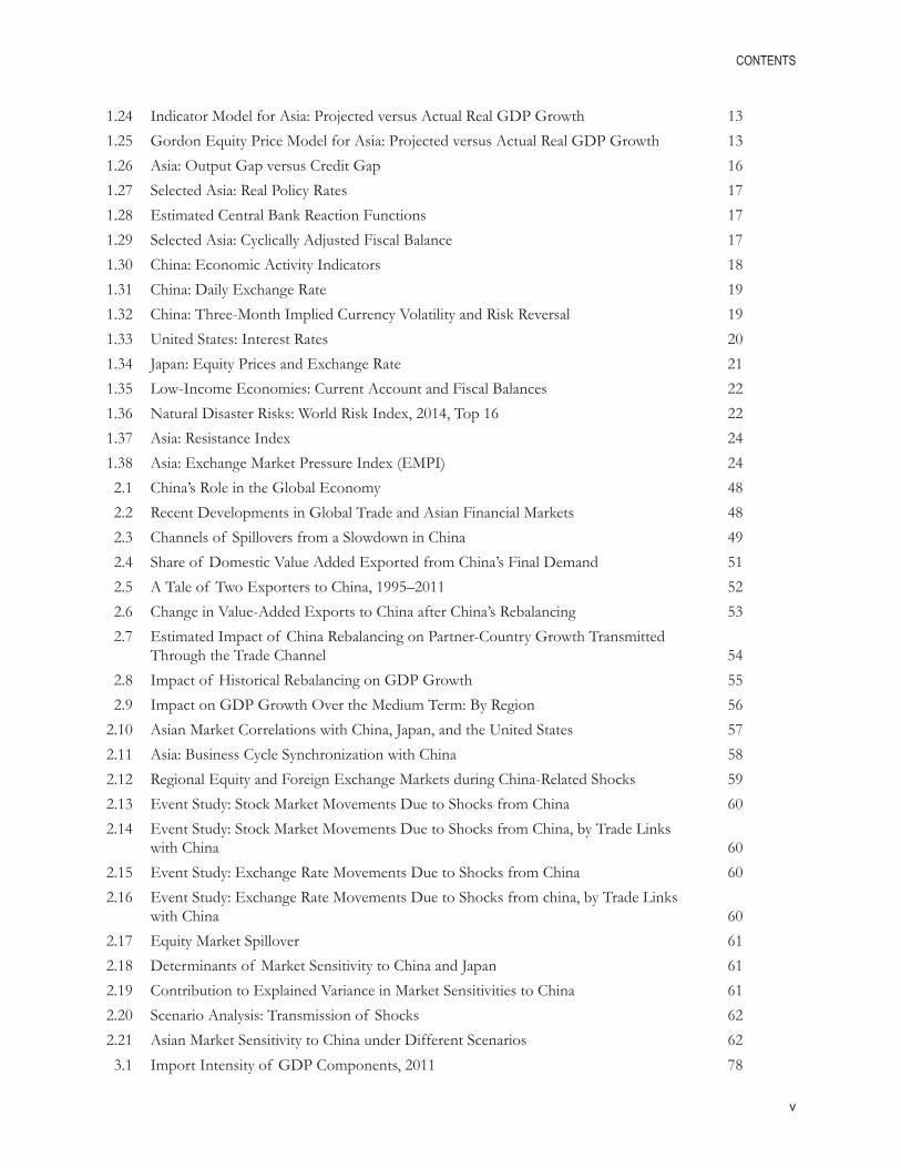
1.1 United States: Financial Conditions 1 1.2 Global Commodity Prices 2 1.3 Market Volatility 2 1.4 Asia: Cumulative Portfolio Flows 3 1.5 Asia: Equity Prices and Price-to-Earnings (PE) Ratios 3 1.6 Asia: Ten-Year Sovereign Bond Yields: Change since End-June 2015 4 1.7 Sovereign Credit Default Swap Spreads 4 1.8 Selected Asia: Exchange Rates 4 1.9 Selected Asia: Foreign Exchange Reserve Accumulation 5 1.10 Selected Asia: Real Private Sector Credit Growth 5 1.11 Asia: Nonfinancial Corporate Sector Debt Issuance 5 1.12 Consolidated Foreign Claims 6 1.13 Asia: Financial Stability Heat Map 7 1.14 Ratio of Regulatory Tier 1 Capital to Risk-Weighted Assets 8 1.15 Return on Assets 8 1.16 Ratio of Nonperforming Loans to Total Gross Loans 8 1.17 Asia: Changes in Real GDP at Market Prices 8 1.18 Selected Asia: Exports to Major Destinations 9 1.19 Selected Asia: Retail Sales Volumes 9 1.20 Asia: Headline Inflation and Expectations 10 1.21 Selected Asia: Core Inflation 10 1.22 Asia: Current Account Balances 10 1.23 Selected Asia: Contributions to Projected Growth 12
CONTENTS
v
1.24 Indicator Model for Asia: Projected versus Actual Real GDP Growth 13 1.25 Gordon Equity Price Model for Asia: Projected versus Actual Real GDP Growth 13 1.26 Asia: Output Gap versus Credit Gap 16 1.27 Selected Asia: Real Policy Rates 17 1.28 Estimated Central Bank Reaction Functions 17 1.29 Selected Asia: Cyclically Adjusted Fiscal Balance 17 1.30 China: Economic Activity Indicators 18 1.31 China: Daily Exchange Rate 19 1.32 China: Three-Month Implied Currency Volatility and Risk Reversal 19 1.33 United States: Interest Rates 20 1.34 Japan: Equity Prices and Exchange Rate 21 1.35 Low-Income Economies: Current Account and Fiscal Balances 22 1.36 Natural Disaster Risks: World Risk Index, 2014, Top 16 22 1.37 Asia: Resistance Index 24 1.38 Asia: Exchange Market Pressure Index (EMPI) 24 2.1 China’s Role in the Global Economy 48 2.2 Recent Developments in Global Trade and Asian Financial Markets 48 2.3 Channels of Spillovers from a Slowdown in China 49 2.4 Share of Domestic Value Added Exported from China’s Final Demand 51 2.5 A Tale of Two Exporters to China, 1995–2011 52 2.6 Change in Value-Added Exports to China after China’s Rebalancing 53 2.7 Estimated Impact of China Rebalancing on Partner-Country Growth Transmitted
Through the Trade Channel 54 2.8 Impact of Historical Rebalancing on GDP Growth 55 2.9 Impact on GDP Growth Over the Medium Term: By Region 56 2.10 Asian Market Correlations with China, Japan, and the United States 57 2.11 Asia: Business Cycle Synchronization with China 58 2.12 Regional Equity and Foreign Exchange Markets during China-Related Shocks 59 2.13 Event Study: Stock Market Movements Due to Shocks from China 60 2.14 Event Study: Stock Market Movements Due to Shocks from China, by Trade Links
with China 60 2.15 Event Study: Exchange Rate Movements Due to Shocks from China 60 2.16 Event Study: Exchange Rate Movements Due to Shocks from china, by Trade Links
with China 60 2.17 Equity Market Spillover 61 2.18 Determinants of Market Sensitivity to China and Japan 61 2.19 Contribution to Explained Variance in Market Sensitivities to China 61 2.20 Scenario Analysis: Transmission of Shocks 62 2.21 Asian Market Sensitivity to China under Different Scenarios 62 3.1 Import Intensity of GDP Components, 2011 78
vi
REGIONAL ECONOMIC OUTLOOK: ASIA AND PACIFIC
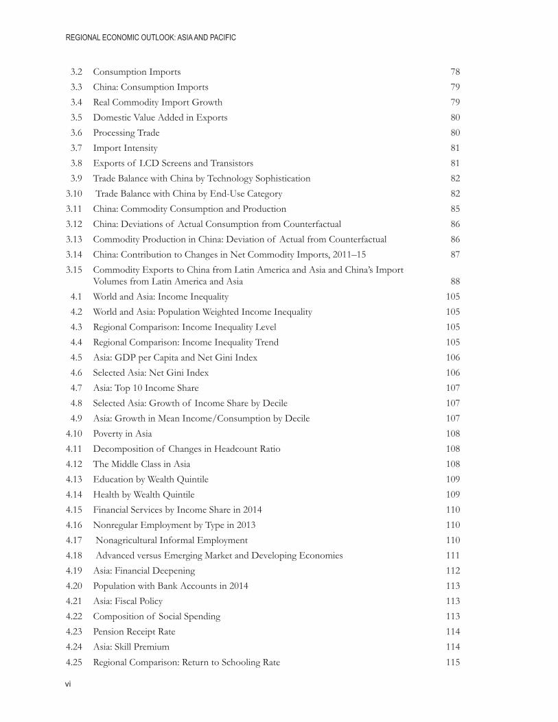
3.2 Consumption Imports 78 3.3 China: Consumption Imports 79 3.4 Real Commodity Import Growth 79 3.5 Domestic Value Added in Exports 80 3.6 Processing Trade 80 3.7 Import Intensity 81 3.8 Exports of LCD Screens and Transistors 81 3.9 Trade Balance with China by Technology Sophistication 82 3.10 Trade Balance with China by End-Use Category 82 3.11 China: Commodity Consumption and Production 85 3.12 China: Deviations of Actual Consumption from Counterfactual 86 3.13 Commodity Production in China: Deviation of Actual from Counterfactual 86 3.14 China: Contribution to Changes in Net Commodity Imports, 2011–15 87 3.15 Commodity Exports to China from Latin America and Asia and China’s Import
Volumes from Latin America and Asia 88 4.1 World and Asia: Income Inequality 105 4.2 World and Asia: Population Weighted Income Inequality 105 4.3 Regional Comparison: Income Inequality Level 105 4.4 Regional Comparison: Income Inequality Trend 105 4.5 Asia: GDP per Capita and Net Gini Index 106 4.6 Selected Asia: Net Gini Index 106 4.7 Asia: Top 10 Income Share 107 4.8 Selected Asia: Growth of Income Share by Decile 107 4.9 Asia: Growth in Mean Income/Consumption by Decile 107 4.10 Poverty in Asia 108 4.11 Decomposition of Changes in Headcount Ratio 108 4.12 The Middle Class in Asia 108 4.13 Education by Wealth Quintile 109 4.14 Health by Wealth Quintile 109 4.15 Financial Services by Income Share in 2014 110 4.16 Nonregular Employment by Type in 2013 110 4.17 Nonagricultural Informal Employment 110 4.18 Advanced versus Emerging Market and Developing Economies 111 4.19 Asia: Financial Deepening 112 4.20 Population with Bank Accounts in 2014 113 4.21 Asia: Fiscal Policy 113 4.22 Composition of Social Spending 113 4.23 Pension Receipt Rate 114 4.24 Asia: Skill Premium 114 4.25 Regional Comparison: Return to Schooling Rate 115
vii
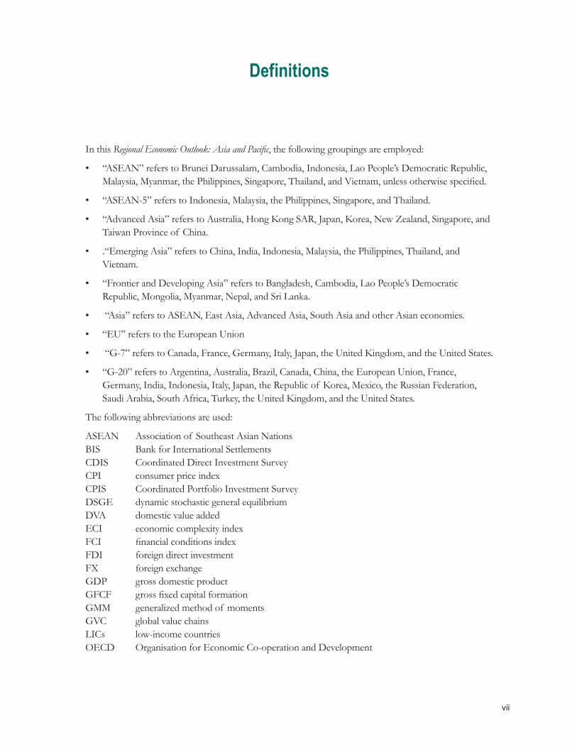
In this Regional Economic Outlook: Asia and Pacific, the following groupings are employed:
• “ASEAN” refers to Brunei Darussalam, Cambodia, Indonesia, Lao People’s Democratic Republic, Malaysia, Myanmar, the Philippines, Singapore, Thailand, and Vietnam, unless otherwise specified.
• “ASEAN-5” refers to Indonesia, Malaysia, the Philippines, Singapore, and Thailand.
• “Advanced Asia” refers to Australia, Hong Kong SAR, Japan, Korea, New Zealand, Singapore, and Taiwan Province of China.
• .“Emerging Asia” refers to China, India, Indonesia, Malaysia, the Philippines, Thailand, and Vietnam.
• “Frontier and Developing Asia” refers to Bangladesh, Cambodia, Lao People’s Democratic Republic, Mongolia, Myanmar, Nepal, and Sri Lanka.
• “Asia” refers to ASEAN, East Asia, Advanced Asia, South Asia and other Asian economies.
• “EU” refers to the European Union
• “G-7” refers to Canada, France, Germany, Italy, Japan, the United Kingdom, and the United States.
• “G-20” refers to Argentina, Australia, Brazil, Canada, China, the European Union, France, Germany, India, Indonesia, Italy, Japan, the Republic of Korea, Mexico, the Russian Federation, Saudi Arabia, South Africa, Turkey, the United Kingdom, and the United States.
The following abbreviations are used:
ASEAN Association of Southeast Asian NationsBIS Bank for International SettlementsCDIS Coordinated Direct Investment SurveyCPI consumer price indexCPIS Coordinated Portfolio Investment SurveyDSGE dynamic stochastic general equilibriumDVA domestic value addedECI economic complexity indexFCI financial conditions indexFDI foreign direct investmentFX foreign exchangeGDP gross domestic productGFCF gross fixed capital formationGMM generalized method of momentsGVC global value chainsLICs low-income countriesOECD Organisation for Economic Co-operation and Development
Definitions
viii
REGIONAL ECONOMIC OUTLOOK: ASIA AND PACIFIC
PICs Pacific island countriesQQE quantitative and qualitative easingR&D research and developmentREER real effective exchange rateVAR vector autoregressionVIX Chicago Board Options Exchange Market Volatility IndexWEO World Economic OutlookWTO World Trade Organization
The following conventions are used:
• In tables, a blank cell indicates “not applicable,” ellipsis points (. . .) indicate “not available,” and 0 or 0.0 indicates “zero” or “negligible.” Minor discrepancies between sums of constituent figures and totals are due to rounding.
• In figures and tables, shaded areas show IMF projections.
• An en dash (–) between years or months (for example, 2007–08 or January–June) indicates the years or months covered, including the beginning and ending years or months; a slash or virgule (/) between years or months (for example, 2007/08) indicates a fiscal or financial year, as does the abbreviation FY (for example, FY2009).
• An em dash (—) indicates the figure is zero or less than half the final digit shown.
• “Billion” means a thousand million; “trillion” means a thousand billion.
• “Basis points” refer to hundredths of 1 percentage point (for example, 25 basis points are equivalent to ¼ of 1 percentage point).
As used in this report, the term “country” does not in all cases refer to a territorial entity that is a state as understood by international law and practice. As used here, the term also covers some territorial entities that are not states but for which statistical data are maintained on a separate and independent basis.
This Regional Economic Outlook: Asia and Pacific was prepared by a team coordinated by Ranil Salgado of the IMF’s Asia and Pacific Department, under the overall direction of Changyong Rhee and Kalpana Kochhar. Contributors include Serkan Arslanalp, Michael Robert Dalesio, Ding Ding, Luc Everaert, Giovanni Ganelli, Geoff Gottlieb, Roberto Guimarães Filho, Thomas Helbling, Gee Hee Hong, Sonali Jain Chandra, Tidiane Kinda, Wei Liao, Yihan Liu, Jaewoo Lee, Rui Mano, Koshy Mathai, Adil Mohommad, Dan Nyberg, Shi Piao, Sohrab Rafiq, Jacqueline Pia Rothfels, Johanna Schauer, and Dulani Seneviratne. Shi Piao and Dulani Seneviratne provided research assistance. Kathie Jamasali and Socorro Santayana provided production assistance. Rosanne Heller, former IMF APD editor, and Joanne Creary Johnson of the IMF’s Communications Department edited the volume. Joanne Creary Johnson coordinated its publication and release. This report is based on data available as of April 1 and includes comments from other departments and some Executive Directors.
ix
Executive Summary
Asia remains the most dynamic part of the global economy but is facing severe headwinds from a still weak global recovery, slowing global trade, and the short-term impact of China’s growth transition. Still, the region is well positioned to meet the challenges ahead, provided it strengthens its reform efforts. To strengthen its resilience to global risks and remain a source of dynamism, policymakers in the region should push ahead with structural reforms to raise productivity and create fiscal space while supporting demand as needed.
Growth in the Asia-Pacific economies is expected to decelerate slightly to about 5¼ percent during 2016–17, partly reflecting the sluggish global recovery. As external demand remains relatively subdued and global financial conditions have started to tighten, domestic demand is expected to be a major driver of activity across most of the region. Domestic demand, particularly consumption, will continue to be propelled by robust labor market conditions, lower commodity prices, and disposable income growth, along with, in some economies, macroeconomic stimulus.
Downside risks continue to dominate the economic landscape. Slower-than-expected global growth and tighter global financial conditions combined with high leverage in the region could have an adverse effect on regional growth. In particular, the turning of the credit and financial cycles amid high debt poses a significant risk to growth in Asia, especially because debt levels have increased markedly over the past decade across most of the major economies in the region, including China and Japan.
Moreover, although China’s economic transition toward more sustainable growth is critical over the medium term for both China and the global economy, adverse spillovers could emerge in the near term. Chapter 2 assesses potential spillovers from China’s rebalancing on regional economies and financial markets. Overall, the region has become more sensitive to the Chinese economy. While China’s rebalancing will have medium-term growth benefits, there are likely to be adverse short-term effects, though the impact will be relatively more positive for economies more exposed to China’s consumption demand. Financial spillovers from China to regional markets—in particular equity and foreign exchange markets—have risen since the global financial crisis and are stronger for those economies with stronger trade linkages.
Chapter 3 examines how China’s rebalancing has affected advanced economies that are upstream in production or value chains, and commodity exporters. It offers evidence that the former have lost market shares for some products, as China has onshored the production of previously imported intermediate goods and started exporting them. Commodity consumption growth has also slowed with China’s rebalancing, but only some exporters have seen their export volume growth decline substantially. Many exporters have been more affected by global commodity price declines, only part of which can be attributed to China’s rebalancing.
The region faces other important downside risks, including natural disasters and trade disruptions. While Abenomics has been supportive, durable gains in growth in Japan have so far not materialized. A further growth slowdown there could lead to an overreliance on expansionary monetary policy. More broadly, domestic political and international geopolitical tensions could cause significant trade disruptions, leading to a generalized slowdown. Finally, natural disasters are a major perennial risk to most Asian and
x
REGIONAL ECONOMIC OUTLOOK: ASIA AND PACIFIC
Pacific economies. Because of their poorer infrastructure and their geographical susceptibility to natural disasters and climate change, low-income, frontier, and developing economies as well as Pacific island countries are particularly at risk.
On the upside, regional and multilateral trade agreements could provide a boost to trade and growth. Further progress on these agreements, including, for example, a broadening of the Trans-Pacific Partnership, could benefit many economies in the region.
What is the role of policies in helping Asia to address its challenges and maintain its leadership in the global economy? Harnessing Asia’s potential will require supporting demand, cushioning the blow from external shocks, and implementing a wide-ranging policy agenda. Structural reforms, aided by macroeconomic policies, should support economic transitions and bolster potential growth. While gradual fiscal consolidation is desirable for most economies, in order to rebuild policy space, it should generally be undertaken together with adjustments to the composition of spending to allow, where needed, for further infrastructure and social spending. Monetary policy should remain focused on supporting demand and addressing near-term risks, including from large exchange rate depreciations and deflationary shocks. Recent bouts of financial volatility underscore the need for flexible and proactive monetary and exchange rate policies. Effective communication of policy goals can also play a role in bolstering confidence and lowering market volatility. Policies to manage risks associated with high leverage and financial volatility will play an important role, including exchange rate flexibility, targeted macroprudential policies, and, in some cases, capital flow measures.
Pushing ahead with structural reforms will be critical to ensure that Asia remains the global growth leader. Structural reforms are needed to help rebalance demand and supply, reduce vulnerabilities, and increase economic efficiency and potential growth. In a number of economies, reforms can also help address climate change and improve the environment, particularly in large countries that rely heavily on fossil fuels. Past reforms have shown themselves to have been highly effective, including by fostering economic and trade diversification and facilitating Asia’s entry into global markets, but a new wave of high-impact reforms is needed, ranging from state-owned enterprise reform in China to labor and product market reforms in Japan and reforms to remove bottlenecks in India and elsewhere in the region.
Reforms will also be needed to foster more inclusive growth, including by reducing income inequality, which in contrast to other regions has risen in most of Asia. Chapter 4 finds that, unlike in the past, fast growing Asian economies have been unable to replicate the “growth with equity” miracle. The chapter argues that it is imperative to address inequality of opportunities, in particular to broaden access to education and health and promote financial and gender inclusion. In this connection, fiscal policy is an important tool to address rising inequality, including by expanding and broadening the coverage of social spending and improving tax progressivity.
International Monetary Fund | April 2016
Recent Developments and Near-Term Outlook Although growth in the Asia-Pacific economies is expected to decelerate slightly to about 5¼ percent during 2016–17, the area remains the most dynamic region of the global economy. Asia’s growth moderation partly reflects a still-weak global recovery and ongoing but necessary rebalancing in China. Downside risks have also increased. With external demand faltering, domes-tic demand should remain a major driver of activity across most of the region. Domestic demand, particularly consumption, will continue to be propelled by robust labor market conditions, lower commodity prices, and disposable income growth, along with, in some countries, macroeconomic stimulus. These factors will partially cushion the blow from languid external demand and increasingly tighter financial conditions. To strengthen the region’s resilience to global risks, policymakers should push ahead with structural reforms to raise productivity and create fiscal space while supporting demand as needed.
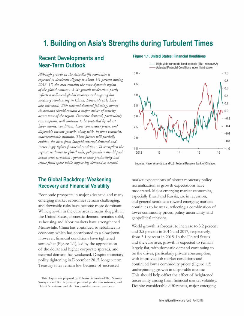
The Global Backdrop: Weakening Recovery and Financial VolatilityEconomic prospects in major advanced and many emerging market economies remain challenging, and downside risks have become more dominant. While growth in the euro area remains sluggish, in the United States, domestic demand remains solid, as housing and labor markets have strengthened. Meanwhile, China has continued to rebalance its economy, which has contributed to a slowdown. However, financial conditions have tightened somewhat (Figure 1.1), led by the appreciation of the dollar and higher corporate spreads, and external demand has weakened. Despite monetary policy tightening in December 2015, longer-term Treasury rates remain low because of increased
This chapter was prepared by Roberto Guimarães-Filho. Socorro Santayana and Kathie Jamasali provided production assistance, and Dulani Seneviratne and Shi Piao provided research assistance.
market expectations of slower monetary policy normalization as growth expectations have moderated. Major emerging market economies, especially Brazil and Russia, are in recession, and general sentiment toward emerging markets continues to be weak, reflecting a combination of lower commodity prices, policy uncertainty, and geopolitical tensions.
World growth is forecast to increase to 3.2 percent and 3.5 percent in 2016 and 2017, respectively, from 3.1 percent in 2015. In the United States and the euro area, growth is expected to remain largely flat, with domestic demand continuing to be the driver, particularly private consumption, with improved job market conditions and continued lower commodity prices (Figure 1.2) underpinning growth in disposable income. This should help offset the effect of heightened uncertainty arising from financial market volatility. Despite considerable differences, major emerging
–0.2
–0.4
–0.6
–0.8
–1.0
0.0
0.2
0.4
0.6
0.8
1.0
1.5
2.0
2.5
3.0
3.5
4.0
4.5
5.0
2012 13 14 15 16
High-yield corporate bond spreads (BB+ minus AAA)Adjusted Financial Conditions Index (right scale)
Figure 1.1. United States: Financial Conditions
Sources: Haver Analytics; and U.S. Federal Reserve Bank of Chicago.
1. Building on Asia’s Strengths during Turbulent Times
2
REGIONAL ECONOMIC OUTLOOK: AsIA ANd PACIfIC
International Monetary Fund | April 2016
market economies are projected to see a modest acceleration in growth, especially in 2017, though this partly reflects a projected gradual improvement in countries currently in recession.
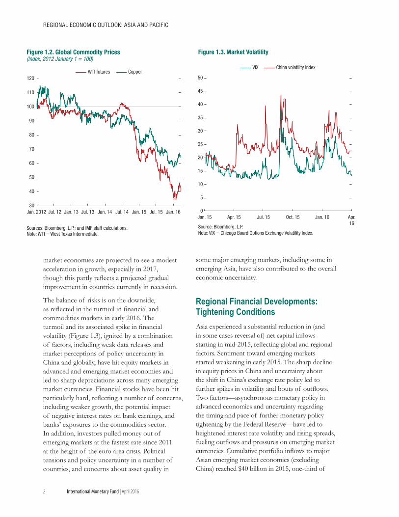
The balance of risks is on the downside, as reflected in the turmoil in financial and commodities markets in early 2016. The turmoil and its associated spike in financial volatility (Figure 1.3), ignited by a combination of factors, including weak data releases and market perceptions of policy uncertainty in China and globally, have hit equity markets in advanced and emerging market economies and led to sharp depreciations across many emerging market currencies. Financial stocks have been hit particularly hard, reflecting a number of concerns, including weaker growth, the potential impact of negative interest rates on bank earnings, and banks’ exposures to the commodities sector. In addition, investors pulled money out of emerging markets at the fastest rate since 2011 at the height of the euro area crisis. Political tensions and policy uncertainty in a number of countries, and concerns about asset quality in
some major emerging markets, including some in emerging Asia, have also contributed to the overall economic uncertainty.
Regional Financial Developments: Tightening ConditionsAsia experienced a substantial reduction in (and in some cases reversal of) net capital inflows starting in mid-2015, reflecting global and regional factors. Sentiment toward emerging markets started weakening in early 2015. The sharp decline in equity prices in China and uncertainty about the shift in China’s exchange rate policy led to further spikes in volatility and bouts of outflows. Two factors—asynchronous monetary policy in advanced economies and uncertainty regarding the timing and pace of further monetary policy tightening by the Federal Reserve—have led to heightened interest rate volatility and rising spreads, fueling outflows and pressures on emerging market currencies. Cumulative portfolio inflows to major Asian emerging market economies (excluding China) reached $40 billion in 2015, one-third of
Sources: Bloomberg, L.P.; and IMF staff calculations.Note: WTI = West Texas Intermediate.
30
40
50
60
70
80
90
100
110
120
Jan. 2012 Jul. 12 Jan. 13 Jul. 13 Jan. 14 Jul. 14 Jan. 15 Jul. 15 Jan. 16
WTI futures Copper
Figure 1.2. Global Commodity Prices(Index, 2012 January 1 = 100)
0
5
10
15
20
25
30
35
40
45
50
Jan. 15 Apr. 15 Jul. 15 Oct. 15 Apr.16
Jan. 16
VIX China volatility index
Figure 1.3. Market Volatility
Source: Bloomberg, L.P.Note: VIX = Chicago Board Options Exchange Volatility Index.
3
1. BUILdING ON AsIA’s sTRENGThs dURING TURBULENT TIMEs
International Monetary Fund | April 2016
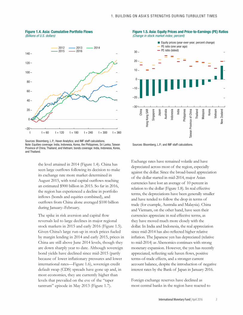
the level attained in 2014 (Figure 1.4). China has seen large outflows following its decision to make its exchange rate more market determined in August 2015, with total capital outflows reaching an estimated $900 billion in 2015. So far in 2016, the region has experienced a decline in portfolio inflows (bonds and equities combined), and outflows from China alone averaged $100 billion during January–February.
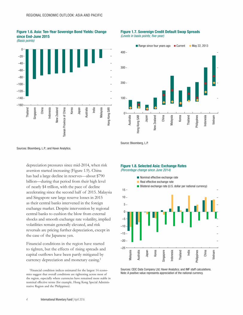
The spike in risk aversion and capital flow reversals led to large declines in major regional stock markets in 2015 and early 2016 (Figure 1.5). Given China’s large run-up in stock prices fueled by margin lending in 2014 and early 2015, prices in China are still above June 2014 levels, though they are down sharply year to date. Although sovereign bond yields have declined since mid-2015 (partly because of lower inflationary pressures and lower international rates—Figure 1.6), sovereign credit default swap (CDS) spreads have gone up and, in most economies, they are currently higher than levels that prevailed on the eve of the “taper tantrum” episode in May 2013 (Figure 1.7).
Exchange rates have remained volatile and have depreciated across most of the region, especially against the dollar. Since the broad-based appreciation of the dollar started in mid-2014, major Asian currencies have lost an average of 10 percent in relation to the dollar (Figure 1.8). In real effective terms, the depreciations have been generally smaller and have tended to follow the drop in terms of trade (for example, Australia and Malaysia). China and Vietnam, on the other hand, have seen their currencies appreciate in real effective terms, as they have moved much more closely with the dollar. In India and Indonesia, the real appreciation since mid-2014 has also reflected higher relative inflation. The Japanese yen has depreciated (relative to mid-2014) as Abenomics continues with strong monetary expansion. However, the yen has recently appreciated, reflecting safe haven flows, positive terms-of-trade effects, and a stronger current account balance, despite the introduction of negative interest rates by the Bank of Japan in January 2016.
Foreign exchange reserves have declined as most central banks in the region have reacted to
–20
0
20
40
60
80
100
120
140
t t + 60 t + 120 t + 180 t + 240 t + 300 t + 360
2012 2013 20142015 2016
Figure 1.4. Asia: Cumulative Portfolio Flows(Billions of U.S. dollars)
Sources: Bloomberg, L.P.; Haver Analytics; and IMF staff calculations.Note: Equities coverage: India, Indonesia, Korea, the Philippines, Sri Lanka, Taiwan Province of China, Thailand, and Vietnam; bonds coverage: India, Indonesia, Korea, and Thailand.
–20
–30
–10
0
10
20
30
Equity prices (year-over-year; percent change)PE ratio (one year ago)PE ratio (latest)
Sources: Bloomberg, L.P.; and IMF staff calculations.
Figure 1.5. Asia: Equity Prices and Price-to-Earnings (PE) Ratios(Change in stock market index; percent)
Chin
a
Hong
Kon
g SA
R
Sing
apor
e
Japa
n
Aust
ralia
Indo
nesi
a
Indi
a
Phili
ppin
es
Thai
land
Mal
aysi
a
Kore
a
Viet
nam
New
Zea
land
Taiw
an P
rovi
nce
of C
hina
4
REGIONAL ECONOMIC OUTLOOK: AsIA ANd PACIfIC
International Monetary Fund | April 2016
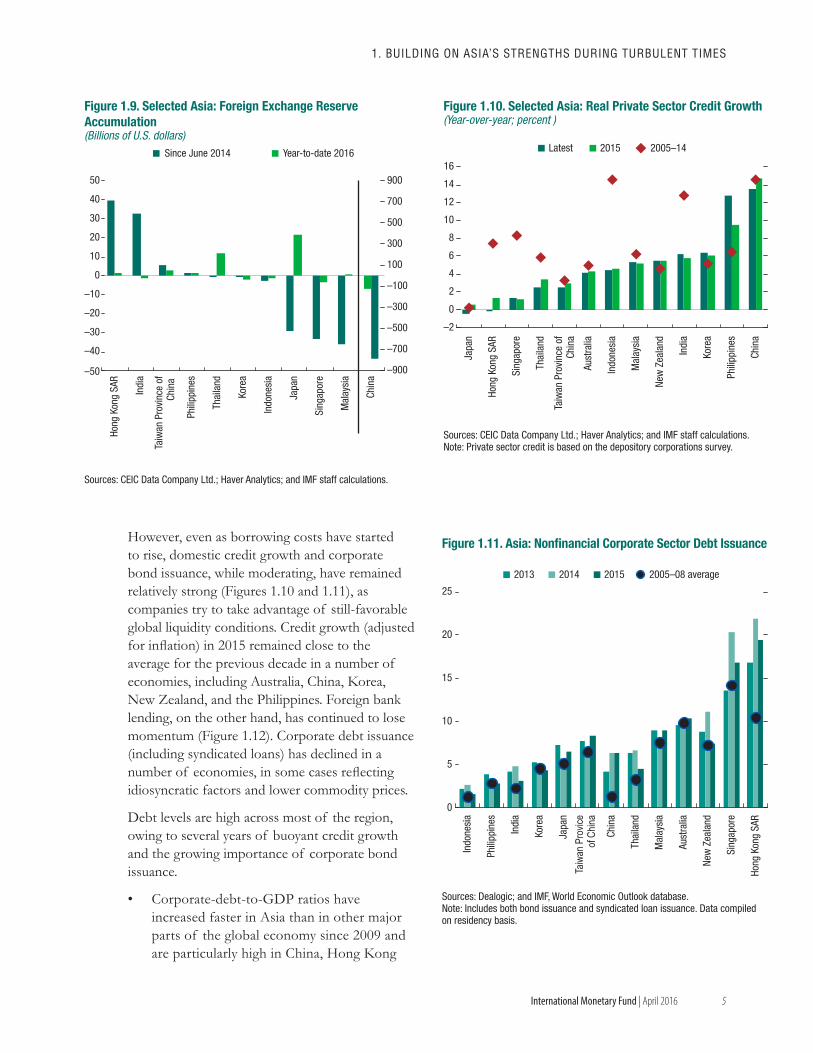
depreciation pressures since mid-2014, when risk aversion started increasing (Figure 1.9). China has had a large decline in reserves—about $790 billion—during that period from their high level of nearly $4 trillion, with the pace of decline accelerating since the second half of 2015. Malaysia and Singapore saw large reserve losses in 2015 as their central banks intervened in the foreign exchange market. Despite intervention by regional central banks to cushion the blow from external shocks and smooth exchange rate volatility, implied volatilities remain generally elevated, and risk reversals are pricing further depreciation, except in the case of the Japanese yen.
Financial conditions in the region have started to tighten, but the effects of rising spreads and capital outflows have been partly mitigated by currency depreciation and monetary easing.1
1Financial condition indices estimated for the largest 14 econo-mies suggest that overall conditions are tightening across most of the region, especially where currencies have remained more stable in nominal effective terms (for example, Hong Kong Special Adminis-trative Region and the Philippines).
0
Sources: Bloomberg, L.P.; and Haver Analytics.
–20
–100
–40
–60
–80
–120
–160
–140
Figure 1.6. Asia: Ten-Year Sovereign Bond Yields: Change since End-June 2015(Basis points)
Thai
land
Sing
apor
e
Chin
a
Indo
nesi
a
New
Zea
land
Taiw
an P
rovi
nce
of C
hina
Kore
a
Japa
n
Aust
ralia
Indi
a
Mal
aysi
a
Hong
Kon
g SA
R
Source: Bloomberg, L.P.
0
100
200
300
400
Aust
ralia
Hong
Kon
g SA
R
Japa
n
New
Zea
land
Chin
a
Mal
aysi
a
Kore
a
Thai
land
Phili
ppin
es
Indo
nesi
a
Viet
nam
May 22, 2013Range since four years ago Current
Figure 1.7. Sovereign Credit Default Swap Spreads(Levels in basis points; five-year)
–5
–10
–15
–20
–25
0
5
10
15
Mal
aysi
a
Aust
ralia
Japa
n
Kore
a
Sing
apor
e
Indo
nesi
a
Thai
land
Indi
a
Phili
ppin
es
Chin
a
Viet
nam
Nominal effective exchange rateReal effective exchange rateBilateral exchange rate (U.S. dollar per national currency)
Figure 1.8. Selected Asia: Exchange Rates(Percentage change since June 2014)
Sources: CEIC Data Company Ltd; Haver Analytics; and IMF staff calculations.Note: A positive value represents appreciation of the national currency.
5
1. BUILdING ON AsIA’s sTRENGThs dURING TURBULENT TIMEs
International Monetary Fund | April 2016
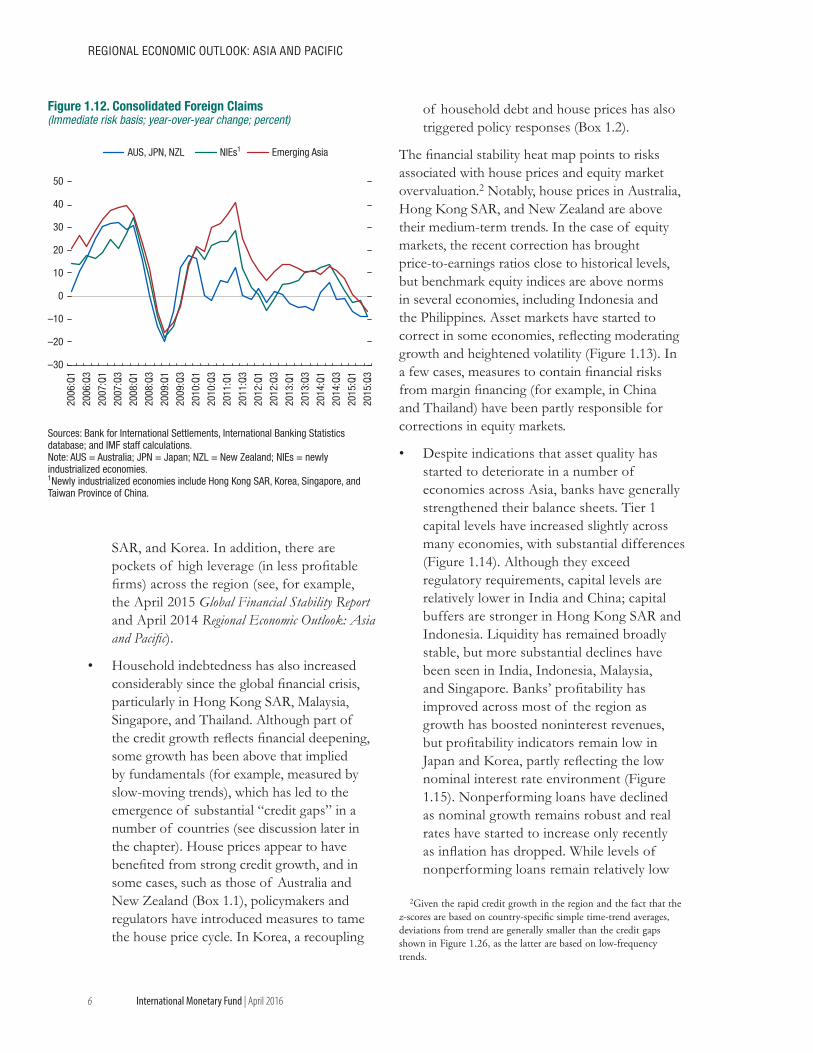
However, even as borrowing costs have started to rise, domestic credit growth and corporate bond issuance, while moderating, have remained relatively strong (Figures 1.10 and 1.11), as companies try to take advantage of still-favorable global liquidity conditions. Credit growth (adjusted for inflation) in 2015 remained close to the average for the previous decade in a number of economies, including Australia, China, Korea, New Zealand, and the Philippines. Foreign bank lending, on the other hand, has continued to lose momentum (Figure 1.12). Corporate debt issuance (including syndicated loans) has declined in a number of economies, in some cases reflecting idiosyncratic factors and lower commodity prices.
Debt levels are high across most of the region, owing to several years of buoyant credit growth and the growing importance of corporate bond issuance.
• Corporate-debt-to-GDP ratios have increased faster in Asia than in other major parts of the global economy since 2009 and are particularly high in China, Hong Kong
100
300
500
700
900
–10–100
–300
–500
–700
–900
–20
–30
–40
–50
0
10
20
30
40
50
Hong
Kon
g SA
R
Indi
a
Phili
ppin
es
Thai
land
Kore
a
Indo
nesi
a
Japa
n
Sing
apor
e
Mal
aysi
a
Chin
a
Since June 2014 Year-to-date 2016Ta
iwan
Pro
vinc
e of
Chin
a
Sources: CEIC Data Company Ltd.; Haver Analytics; and IMF staff calculations.
Figure 1.9. Selected Asia: Foreign Exchange Reserve Accumulation(Billions of U.S. dollars)
Sources: CEIC Data Company Ltd.; Haver Analytics; and IMF staff calculations.Note: Private sector credit is based on the depository corporations survey.
–2
0
2
4
6
8
10
12
14
16
Japa
n
Hong
Kon
g SA
R
Sing
apor
e
Thai
land
Aust
ralia
Indo
nesi
a
Mal
aysi
a
New
Zea
land
Indi
a
Kore
a
Phili
ppin
es
Chin
a
Taiw
an P
rovi
nce
ofCh
ina
2005–142015Latest
Figure 1.10. Selected Asia: Real Private Sector Credit Growth(Year-over-year; percent )
0
5
10
15
20
25
Indo
nesi
a
Phili
ppin
es
Indi
a
Kore
a
Japa
n
Chin
a
Thai
land
Mal
aysi
a
Aust
ralia
New
Zea
land
Sing
apor
e
Hong
Kon
g SA
R
2013 2014 2015 2005–08 averageTa
iwan
Pro
vice
of Ch
ina
Figure 1.11. Asia: Nonfinancial Corporate Sector Debt Issuance
Sources: Dealogic; and IMF, World Economic Outlook database.Note: Includes both bond issuance and syndicated loan issuance. Data compiled on residency basis.
6
REGIONAL ECONOMIC OUTLOOK: AsIA ANd PACIfIC
International Monetary Fund | April 2016
SAR, and Korea. In addition, there are pockets of high leverage (in less profitable firms) across the region (see, for example, the April 2015 Global Financial Stability Report and April 2014 Regional Economic Outlook: Asia and Pacific).
• Household indebtedness has also increased considerably since the global financial crisis, particularly in Hong Kong SAR, Malaysia, Singapore, and Thailand. Although part of the credit growth reflects financial deepening, some growth has been above that implied by fundamentals (for example, measured by slow-moving trends), which has led to the emergence of substantial “credit gaps” in a number of countries (see discussion later in the chapter). House prices appear to have benefited from strong credit growth, and in some cases, such as those of Australia and New Zealand (Box 1.1), policymakers and regulators have introduced measures to tame the house price cycle. In Korea, a recoupling
of household debt and house prices has also triggered policy responses (Box 1.2).
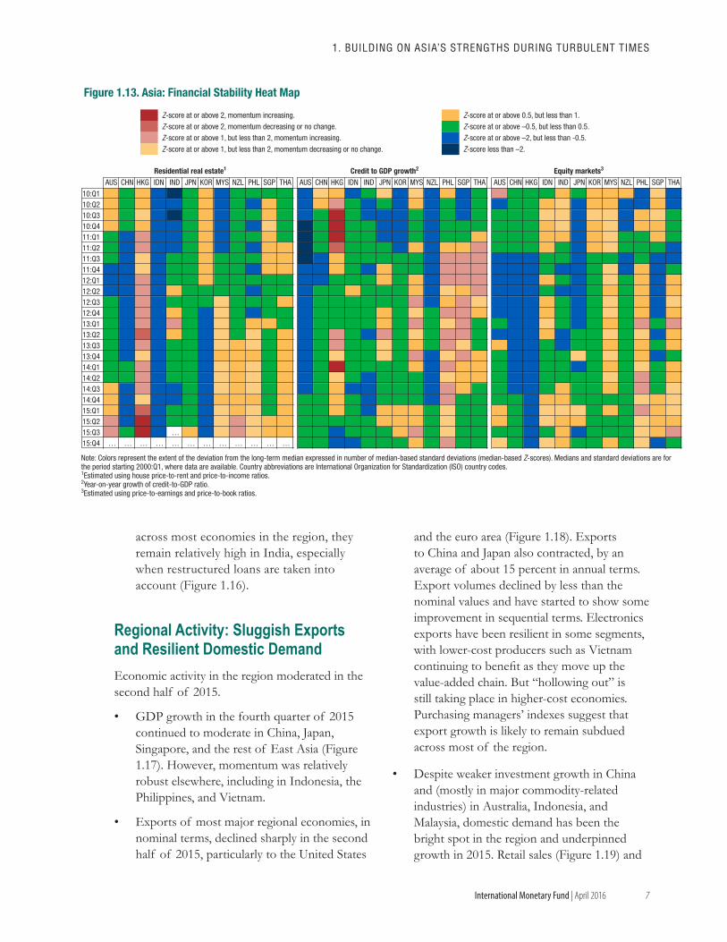
The financial stability heat map points to risks associated with house prices and equity market overvaluation.2 Notably, house prices in Australia, Hong Kong SAR, and New Zealand are above their medium-term trends. In the case of equity markets, the recent correction has brought price-to-earnings ratios close to historical levels, but benchmark equity indices are above norms in several economies, including Indonesia and the Philippines. Asset markets have started to correct in some economies, reflecting moderating growth and heightened volatility (Figure 1.13). In a few cases, measures to contain financial risks from margin financing (for example, in China and Thailand) have been partly responsible for corrections in equity markets.
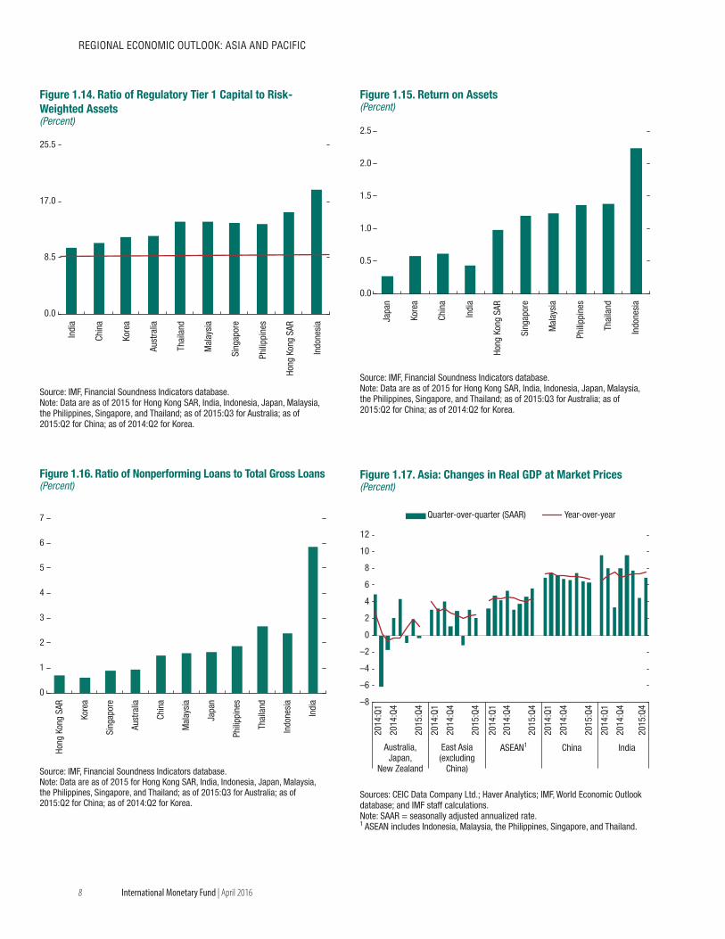
• Despite indications that asset quality has started to deteriorate in a number of economies across Asia, banks have generally strengthened their balance sheets. Tier 1 capital levels have increased slightly across many economies, with substantial differences (Figure 1.14). Although they exceed regulatory requirements, capital levels are relatively lower in India and China; capital buffers are stronger in Hong Kong SAR and Indonesia. Liquidity has remained broadly stable, but more substantial declines have been seen in India, Indonesia, Malaysia, and Singapore. Banks’ profitability has improved across most of the region as growth has boosted noninterest revenues, but profitability indicators remain low in Japan and Korea, partly reflecting the low nominal interest rate environment (Figure 1.15). Nonperforming loans have declined as nominal growth remains robust and real rates have started to increase only recently as inflation has dropped. While levels of nonperforming loans remain relatively low
2Given the rapid credit growth in the region and the fact that the z-scores are based on country-specific simple time-trend averages, deviations from trend are generally smaller than the credit gaps shown in Figure 1.26, as the latter are based on low-frequency trends.
2006
:Q1
2006
:Q3
2007
:Q1
2007
:Q3
2008
:Q1
2008
:Q3
2009
:Q1
2009
:Q3
2010
:Q1
2010
:Q3
2011
:Q1
2011
:Q3
2012
:Q1
2012
:Q3
2013
:Q1
2013
:Q3
2014
:Q1
2014
:Q3
2015
:Q1
2015
:Q3
–30
–20
–10
0
10
20
30
40
50
AUS, JPN, NZL NIEs1 Emerging Asia
Figure 1.12. Consolidated Foreign Claims(Immediate risk basis; year-over-year change; percent)
Sources: Bank for International Settlements, International Banking Statistics database; and IMF staff calculations.Note: AUS = Australia; JPN = Japan; NZL = New Zealand; NIEs = newly industrialized economies.1Newly industrialized economies include Hong Kong SAR, Korea, Singapore, and Taiwan Province of China.
7
1. BUILdING ON AsIA’s sTRENGThs dURING TURBULENT TIMEs
International Monetary Fund | April 2016
across most economies in the region, they remain relatively high in India, especially when restructured loans are taken into account (Figure 1.16).
Regional Activity: Sluggish Exports and Resilient Domestic Demand Economic activity in the region moderated in the second half of 2015.
• GDP growth in the fourth quarter of 2015 continued to moderate in China, Japan, Singapore, and the rest of East Asia (Figure 1.17). However, momentum was relatively robust elsewhere, including in Indonesia, the Philippines, and Vietnam.
• Exports of most major regional economies, in nominal terms, declined sharply in the second half of 2015, particularly to the United States
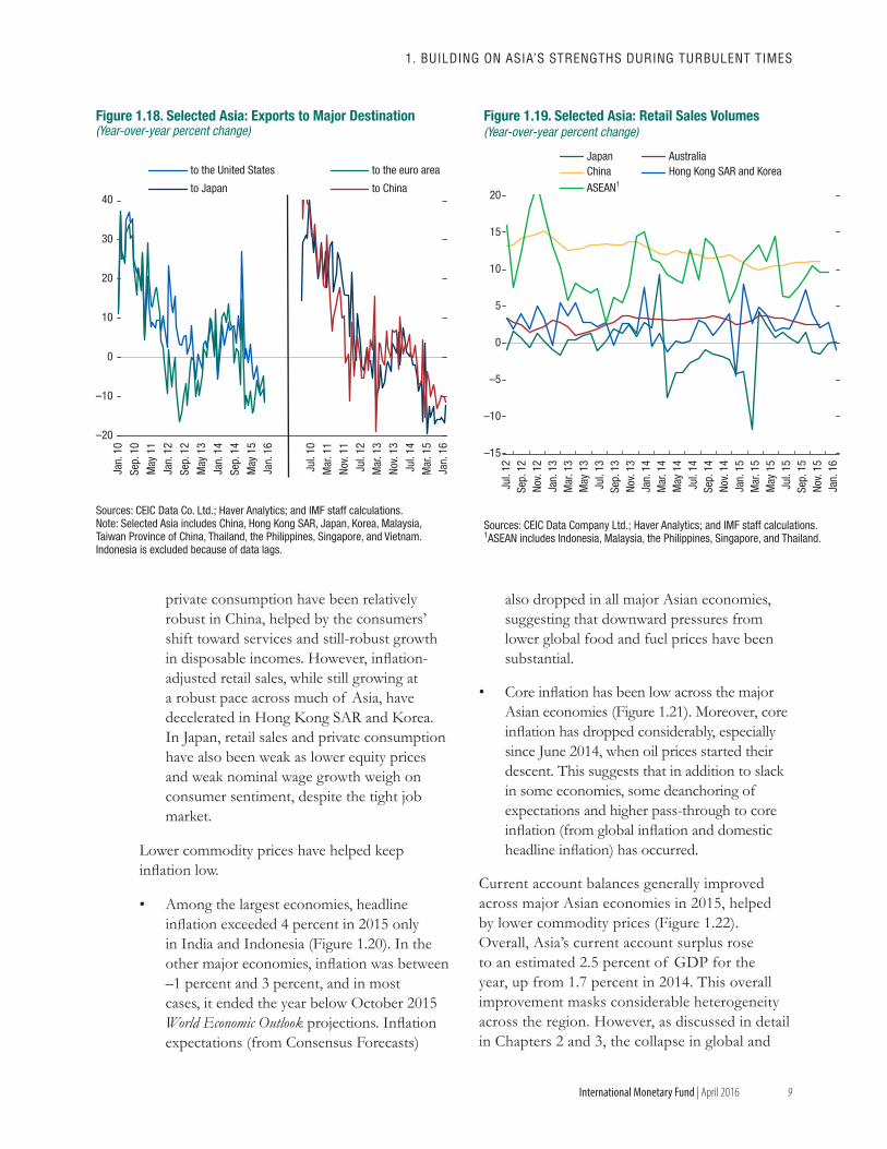
and the euro area (Figure 1.18). Exports to China and Japan also contracted, by an average of about 15 percent in annual terms. Export volumes declined by less than the nominal values and have started to show some improvement in sequential terms. Electronics exports have been resilient in some segments, with lower-cost producers such as Vietnam continuing to benefit as they move up the value-added chain. But “hollowing out” is still taking place in higher-cost economies. Purchasing managers’ indexes suggest that export growth is likely to remain subdued across most of the region.
• Despite weaker investment growth in China and (mostly in major commodity-related industries) in Australia, Indonesia, and Malaysia, domestic demand has been the bright spot in the region and underpinned growth in 2015. Retail sales (Figure 1.19) and
Z-score at or above 2, momentum increasing. Z-score at or above 0.5, but less than 1.
Z-score at or above 2, momentum decreasing or no change. Z-score at or above –0.5, but less than 0.5.
Z-score at or above 1, but less than 2, momentum increasing. Z-score at or above –2, but less than -0.5.
Z-score at or above 1, but less than 2, momentum decreasing or no change. Z-score less than –2.
AUS CHN HKG IDN IND JPN KOR MYS NZL PHL SGP THA AUS CHN HKG IDN IND JPN KOR MYS NZL PHL SGP THA AUS CHN HKG IDN IND JPN KOR MYS NZL PHL SGP THA
10:Q110:Q210:Q310:Q411:Q111:Q211:Q311:Q412:Q112:Q212:Q312:Q413:Q113:Q213:Q313:Q414:Q114:Q214:Q314:Q415:Q115:Q215:Q3 …15:Q4 … … … … … … … … … … … …
Residential real estate1 Credit to GDP growth2 Equity markets3
Figure 1.13. Asia: Financial Stability Heat Map
Note: Colors represent the extent of the deviation from the long-term median expressed in number of median-based standard deviations (median-based Z-scores). Medians and standard deviations are for the period starting 2000:Q1, where data are available. Country abbreviations are International Organization for Standardization (ISO) country codes.1Estimated using house price-to-rent and price-to-income ratios.2Year-on-year growth of credit-to-GDP ratio. 3Estimated using price-to-earnings and price-to-book ratios.
8
REGIONAL ECONOMIC OUTLOOK: AsIA ANd PACIfIC
International Monetary Fund | April 2016
Source: IMF, Financial Soundness Indicators database.Note: Data are as of 2015 for Hong Kong SAR, India, Indonesia, Japan, Malaysia, the Philippines, Singapore, and Thailand; as of 2015:Q3 for Australia; as of 2015:Q2 for China; as of 2014:Q2 for Korea.
0.0
8.5
17.0
25.5
Indi
a
Chin
a
Kore
a
Aust
ralia
Thai
land
Mal
aysi
a
Sing
apor
e
Phili
ppin
es
Hong
Kon
g SA
R
Indo
nesi
a
Figure 1.14. Ratio of Regulatory Tier 1 Capital to Risk- Weighted Assets(Percent)
Source: IMF, Financial Soundness Indicators database.Note: Data are as of 2015 for Hong Kong SAR, India, Indonesia, Japan, Malaysia, the Philippines, Singapore, and Thailand; as of 2015:Q3 for Australia; as of 2015:Q2 for China; as of 2014:Q2 for Korea.
0.0
0.5
1.0
1.5
2.0
2.5
Japa
n
Kore
a
Chin
a
Indi
a
Hong
Kon
g SA
R
Sing
apor
e
Mal
aysi
a
Phili
ppin
es
Thai
land
Indo
nesi
a
Figure 1.15. Return on Assets(Percent)
Hong
Kon
g SA
R
Kore
a
Sing
apor
e
Aust
ralia
Chin
a
Mal
aysi
a
Japa
n
Phili
ppin
es
Thai
land
Indo
nesi
a
Indi
a
Figure 1.16. Ratio of Nonperforming Loans to Total Gross Loans(Percent)
Source: IMF, Financial Soundness Indicators database.Note: Data are as of 2015 for Hong Kong SAR, India, Indonesia, Japan, Malaysia, the Philippines, Singapore, and Thailand; as of 2015:Q3 for Australia; as of 2015:Q2 for China; as of 2014:Q2 for Korea.
0
1
2
3
4
5
6
7
–8
–6
–4
–2
0
2
4
6
8
10
12
2014
:Q1
2014
:Q4
2015
:Q4
2014
:Q1
2014
:Q4
2015
:Q4
2014
:Q1
2014
:Q4
2015
:Q4
2014
:Q1
2014
:Q4
2015
:Q4
2014
:Q1
2014
:Q4
2015
:Q4
Australia,Japan,
New Zealand
East Asia(excluding
China)
ASEAN1 China India
Quarter-over-quarter (SAAR) Year-over-year
Figure 1.17. Asia: Changes in Real GDP at Market Prices(Percent)
Sources: CEIC Data Company Ltd.; Haver Analytics; IMF, World Economic Outlook database; and IMF staff calculations.Note: SAAR = seasonally adjusted annualized rate.1 ASEAN includes Indonesia, Malaysia, the Philippines, Singapore, and Thailand.
9
1. BUILdING ON AsIA’s sTRENGThs dURING TURBULENT TIMEs
International Monetary Fund | April 2016
private consumption have been relatively robust in China, helped by the consumers’ shift toward services and still-robust growth in disposable incomes. However, inflation-adjusted retail sales, while still growing at a robust pace across much of Asia, have decelerated in Hong Kong SAR and Korea. In Japan, retail sales and private consumption have also been weak as lower equity prices and weak nominal wage growth weigh on consumer sentiment, despite the tight job market.
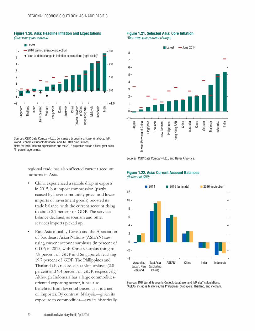
Lower commodity prices have helped keep inflation low.
• Among the largest economies, headline inflation exceeded 4 percent in 2015 only in India and Indonesia (Figure 1.20). In the other major economies, inflation was between –1 percent and 3 percent, and in most cases, it ended the year below October 2015 World Economic Outlook projections. Inflation expectations (from Consensus Forecasts)
also dropped in all major Asian economies, suggesting that downward pressures from lower global food and fuel prices have been substantial.
• Core inflation has been low across the major Asian economies (Figure 1.21). Moreover, core inflation has dropped considerably, especially since June 2014, when oil prices started their descent. This suggests that in addition to slack in some economies, some deanchoring of expectations and higher pass-through to core inflation (from global inflation and domestic headline inflation) has occurred.
Current account balances generally improved across major Asian economies in 2015, helped by lower commodity prices (Figure 1.22). Overall, Asia’s current account surplus rose to an estimated 2.5 percent of GDP for the year, up from 1.7 percent in 2014. This overall improvement masks considerable heterogeneity across the region. However, as discussed in detail in Chapters 2 and 3, the collapse in global and
–20
–10
0
10
20
30
40
Jan.
10
Sep.
10
May
11
Jan.
12
Sep.
12
May
13
Jan.
14
Sep.
14
May
15
Jul.
10M
ar. 1
1No
v. 11
Jul.
12M
ar. 1
3No
v. 13
Jul.
14M
ar. 1
5
to the United States to the euro area
to Japan to China
Figure 1.18. Selected Asia: Exports to Major Destination(Year-over-year percent change)
Jan.
16
Jan.
16
Sources: CEIC Data Co. Ltd.; Haver Analytics; and IMF staff calculations.Note: Selected Asia includes China, Hong Kong SAR, Japan, Korea, Malaysia, Taiwan Province of China, Thailand, the Philippines, Singapore, and Vietnam. Indonesia is excluded because of data lags.
–15
–10
–5
0
5
10
15
20
Jul.
12Se
p. 1
2No
v. 12
Jan.
13
Jul.
14Se
p. 1
4No
v. 14
Jan.
15
Mar
. 13
May
13
Jul.
13Se
p. 1
3No
v. 13
Jan.
14
Mar
. 15
May
15
Jul.
15Se
p. 1
5No
v. 15
Jan.
16
Mar
. 14
May
14
Japan AustraliaChina Hong Kong SAR and KoreaASEAN1
Figure 1.19. Selected Asia: Retail Sales Volumes(Year-over-year percent change)
Sources: CEIC Data Company Ltd.; Haver Analytics; and IMF staff calculations.1ASEAN includes Indonesia, Malaysia, the Philippines, Singapore, and Thailand.
10
REGIONAL ECONOMIC OUTLOOK: AsIA ANd PACIfIC
International Monetary Fund | April 2016
regional trade has also affected current account outturns in Asia.
• China experienced a sizable drop in exports in 2015, but import compression (partly caused by lower commodity prices and lower imports of investment goods) boosted its trade balance, with the current account rising to about 2.7 percent of GDP. The services balance declined, as tourism and other services imports picked up.
• East Asia (notably Korea) and the Association of Southeast Asian Nations (ASEAN) saw rising current account surpluses (in percent of GDP) in 2015, with Korea’s surplus rising to 7.8 percent of GDP and Singapore’s reaching 19.7 percent of GDP. The Philippines and Thailand also recorded sizable surpluses (2.8 percent and 9.4 percent of GDP, respectively). Although Indonesia has a large commodities-oriented exporting sector, it has also benefited from lower oil prices, as it is a net oil importer. By contrast, Malaysia—given its exposure to commodities—saw its historically
–1.0
0.0
2.0
1.0
3.0
–2
–1
0
2
1
3
4
5
6
Sing
apor
e
Thai
land
Japa
n
New
Zea
land
Viet
nam
Phili
ppin
es
Kore
a
Aust
ralia
Chin
a
Hong
Kon
g SA
R
Mal
aysi
a
Indo
nesi
a
Indi
a
Latest
2016 (period average projection)
Year-to-date change in inflation expectations (right scale)1
Taiw
an P
rovi
nce
of C
hina
Figure 1.20. Asia: Headline Inflation and Expectations(Year-over-year; percent)
Sources: CEIC Data Company Ltd.; Consensus Economics; Haver Analytics; IMF, World Economic Outlook database; and IMF staff calculations.Note: For India, inflation expectations and the 2016 projection are on a fiscal-year basis.1In percentage points.
–1
0
1
2
3
4
5
6
7
8
Japa
n
Sing
apor
e
Thai
land
New
Zea
land
Phili
ppin
es
Hong
Kon
g SA
R
Chin
a
Aust
ralia
Kore
a
Viet
nam
Mal
aysi
a
Indo
nesi
a
Indi
a
Latest June 2014
Taiw
an P
rovi
nce
of C
hina
Figure 1.21. Selected Asia: Core Inflation(Year-over-year percent change)
Sources: CEIC Data Company Ltd.; and Haver Analytics.
–4
–2
0
2
4
6
8
10
12
Australia,Japan, New
Zealand
East Asia(excluding
China)
ASEAN1 China India Indonesia
2014 2015 (estimate) 2016 (projection)
Figure 1.22. Asia: Current Account Balances(Percent of GDP)
Sources: IMF, World Economic Outlook database; and IMF staff calculations.1ASEAN includes Malaysia, the Philippines, Singapore, Thailand, and Vietnam.
11
1. BUILdING ON AsIA’s sTRENGThs dURING TURBULENT TIMEs
International Monetary Fund | April 2016
large surplus drop by about one-third to 2.9 percent of GDP in 2015.
• Meanwhile, India experienced an improvement in its trade balance in 2015, as it benefited from the lower global oil prices, although this was partly offset by weaker exports. Compared with those in 2013/14 (when oil prices averaged close to $100 a barrel), India’s trade and current account balances improved by 0.8 percent and 0.4 percent of GDP, respectively.
Developments in specific countries show considerable heterogeneity:
• In China, growth slowed to 6.9 percent in 2015, in line with the official target of about 7 percent. Growth was largely underpinned by the services sector, as manufacturing activity and construction decelerated sharply, particularly in nominal terms. Robust labor markets in urban areas and steady disposable income growth supported domestic consumption (particularly in services), partly offsetting weaknesses in investment and manufacturing. As in other regional economies, exports have decelerated sharply, but as noted above, the contribution from net exports was only slightly negative at –0.2 percentage point given the sharp contraction of imports. While headline GDP suggests steady growth, the momentum weakened at the end of the year. For example, fourth-quarter growth (seasonally adjusted annual rate) dropped to 6.4 percent, nearly half a percentage point lower than the average of the first three quarters. In addition, nominal growth decelerated faster than real growth, reaching 5.9 percent in 2015 (4.5 percent in the second half of the year). Nominal growth was also particularly weak in the manufacturing sector, which has hurt corporate profitability.
• Japan’s GDP growth picked up to 0.5 percent in 2015, reflecting inventory accumulation and a higher contribution from net exports, which was supported by the weaker yen. Private consumption remained weak, despite
a pickup in real labor income and lower oil prices. Investment in plants and equipment was subdued as well. Although export growth moderated, the contribution of net exports to growth was positive, and services exports were robust (particularly tourism). Growth disappointed in the fourth quarter (–1.1 percent in seasonally adjusted annual rate terms), especially as domestic demand, particularly private consumption, lost momentum. The decline in fuel prices put substantial downward pressure on headline inflation, but core inflation edged up. Inflation expectations of households and firms trended downward.
• India remains on a strong recovery path, with growth reaching 7.3 percent in 2015. Growth was supported by the large terms-of-trade gain (about 2½ percent of GDP), which also lowered inflation and reduced the current account deficit. That, in turn, helped bolster business and consumer sentiment. Growth also benefited from large foreign direct investment (FDI) inflows.
• Australia’s economy decelerated in 2015 following years of a mining-led boom, with growth slowing to 2.5 percent in 2015. However, growth picked up in the second half of 2015, helped by robust labor market conditions and residential investment. New Zealand recorded 3.2 percent growth in 2015, benefiting from the earthquake reconstruction efforts.
• In Korea, growth decelerated to 2.6 percent in 2015, with the momentum weakening in the last quarter. External sector performance was substantially weaker than expected, and domestic demand indicators were generally sluggish. Hong Kong SAR experienced a drop in growth in 2015, with GDP advancing by 2.4 percent, as both domestic and external demand faced strong headwinds and with a noticeable decline in tourist inflows from China.
• ASEAN economies experienced steady growth in 2015 (averaging more than 4½ percent during 2014–15), but economic
12
REGIONAL ECONOMIC OUTLOOK: AsIA ANd PACIfIC
International Monetary Fund | April 2016
cycles within ASEAN continue to diverge. The growth momentum lost some steam in Malaysia, mostly because of the terms-of-trade deterioration (which had an impact on the contribution from net exports) and fiscal tightening, and decelerated slightly in Indonesia, despite robust growth in disposable income and consumption. Despite the impact of lower net exports, real GDP growth remained robust in the Philippines, with domestic demand benefiting from favorable terms of trade. Thailand saw a pickup in growth, especially as public investment accelerated and private consumption grew more strongly. Net exports contributed to growth as terms of trade improved and tourism recovered. Vietnam continued to capitalize on strong demand for its exports and FDI in manufacturing; as a result, growth accelerated.
• Growth in frontier economies and small states has, on average, been relatively robust and steady over the past couple of years, though there have been variations. Bangladesh, for example, experienced solid growth in 2015 as it continued to benefit from lower commodity prices and strong FDI inflows, while Sri Lanka’s economy grew at 4.8 percent. Bhutan, Fiji, and the Solomon Islands recorded steady growth on the back of natural-resources-related sectors (not affected by the decline in commodity prices) and tourism.3 Growth in Mongolia, on the other hand, dropped sharply in 2015 on weak commodity prices and policy tightening, and in Maldives following policy uncertainty and political tension.
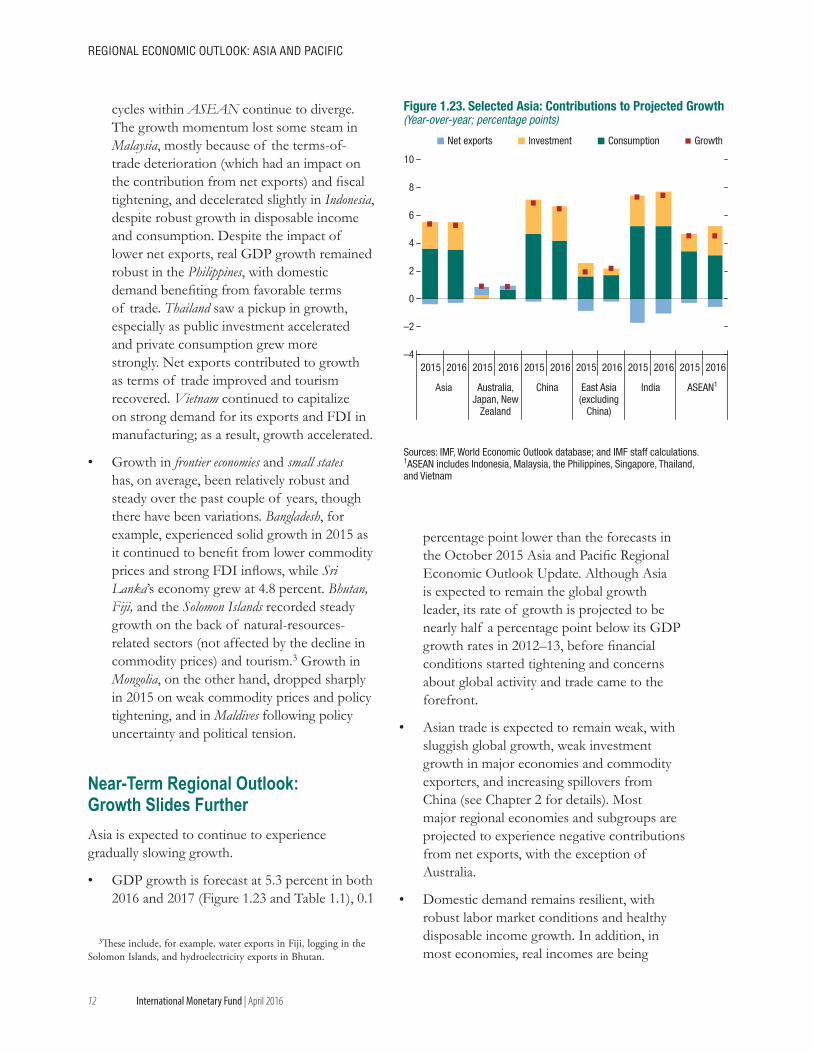
Near-Term Regional Outlook: Growth Slides Further Asia is expected to continue to experience gradually slowing growth.
• GDP growth is forecast at 5.3 percent in both 2016 and 2017 (Figure 1.23 and Table 1.1), 0.1
3These include, for example, water exports in Fiji, logging in the Solomon Islands, and hydroelectricity exports in Bhutan.
percentage point lower than the forecasts in the October 2015 Asia and Pacific Regional Economic Outlook Update. Although Asia is expected to remain the global growth leader, its rate of growth is projected to be nearly half a percentage point below its GDP growth rates in 2012–13, before financial conditions started tightening and concerns about global activity and trade came to the forefront.
• Asian trade is expected to remain weak, with sluggish global growth, weak investment growth in major economies and commodity exporters, and increasing spillovers from China (see Chapter 2 for details). Most major regional economies and subgroups are projected to experience negative contributions from net exports, with the exception of Australia.
• Domestic demand remains resilient, with robust labor market conditions and healthy disposable income growth. In addition, in most economies, real incomes are being
–4
–2
0
2
4
6
8
10
2015 2016 2015 2016 2015 2016 2015 2016 2015 2016 2015 2016
Australia,Japan, New
Zealand
China India
Net exports Investment Consumption Growth
Asia
Sources: IMF, World Economic Outlook database; and IMF staff calculations.1ASEAN includes Indonesia, Malaysia, the Philippines, Singapore, Thailand, and Vietnam
East Asia(excluding
China)
ASEAN1
Figure 1.23. Selected Asia: Contributions to Projected Growth(Year-over-year; percentage points)
13
1. BUILdING ON AsIA’s sTRENGThs dURING TURBULENT TIMEs
International Monetary Fund | April 2016
boosted by lower commodity prices and low inflation. However, despite still-robust credit growth, what has hitherto been the dynamism of domestic demand in the region will be partly sapped by high household and corporate leverage, as well as tightening financial conditions. Heightened volatility in financial markets has led to lowered risk appetite and dented business and consumer sentiment in many economies.
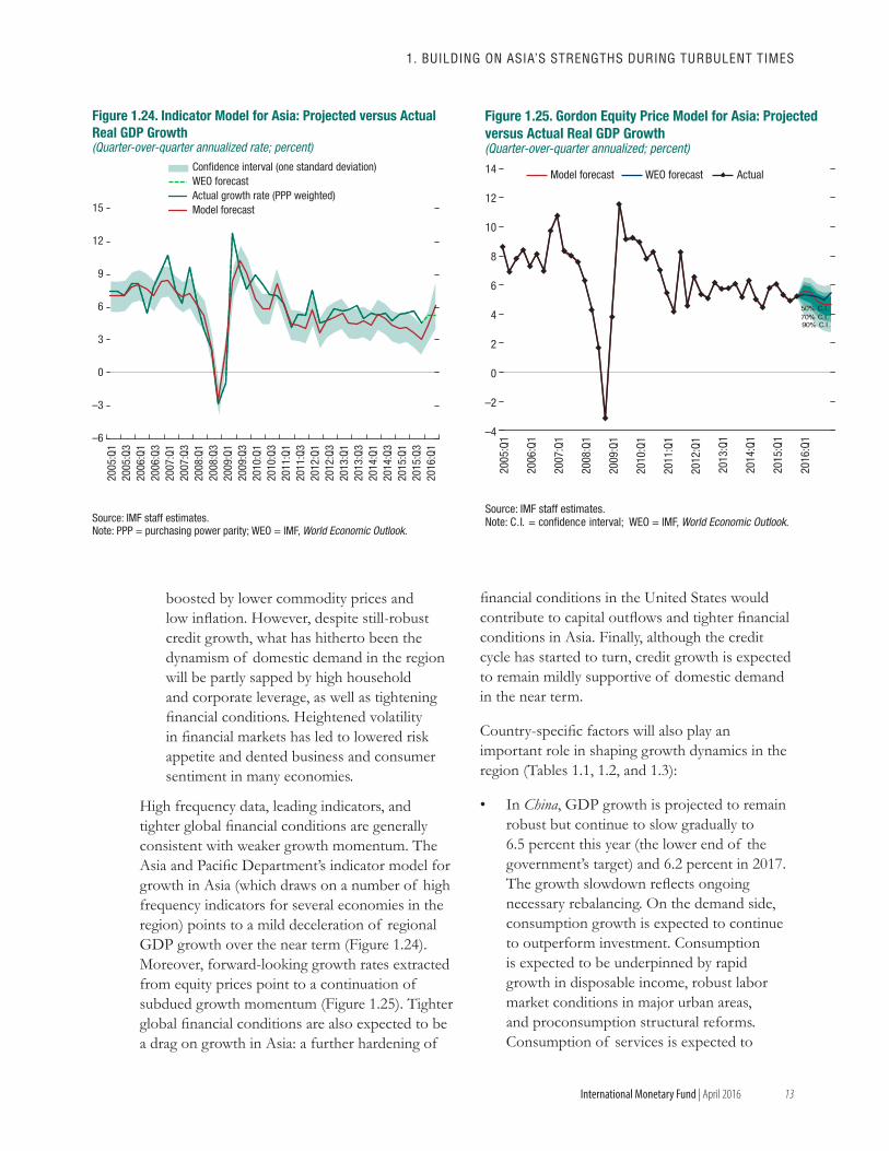
High frequency data, leading indicators, and tighter global financial conditions are generally consistent with weaker growth momentum. The Asia and Pacific Department’s indicator model for growth in Asia (which draws on a number of high frequency indicators for several economies in the region) points to a mild deceleration of regional GDP growth over the near term (Figure 1.24). Moreover, forward-looking growth rates extracted from equity prices point to a continuation of subdued growth momentum (Figure 1.25). Tighter global financial conditions are also expected to be a drag on growth in Asia: a further hardening of
financial conditions in the United States would contribute to capital outflows and tighter financial conditions in Asia. Finally, although the credit cycle has started to turn, credit growth is expected to remain mildly supportive of domestic demand in the near term.
Country-specific factors will also play an important role in shaping growth dynamics in the region (Tables 1.1, 1.2, and 1.3):
• In China, GDP growth is projected to remain robust but continue to slow gradually to 6.5 percent this year (the lower end of the government’s target) and 6.2 percent in 2017. The growth slowdown reflects ongoing necessary rebalancing. On the demand side, consumption growth is expected to continue to outperform investment. Consumption is expected to be underpinned by rapid growth in disposable income, robust labor market conditions in major urban areas, and proconsumption structural reforms. Consumption of services is expected to
–6
–3
0
3
6
9
12
15
2005
:Q1
2005
:Q3
2006
:Q1
2006
:Q3
2007
:Q1
2007
:Q3
2008
:Q1
2008
:Q3
2009
:Q1
2009
:Q3
2010
:Q1
2010
:Q3
2011
:Q1
2011
:Q3
2012
:Q1
2012
:Q3
2013
:Q1
2013
:Q3
2014
:Q1
2014
:Q3
2015
:Q1
2015
:Q3
2016
:Q1
Confidence interval (one standard deviation)WEO forecastActual growth rate (PPP weighted)Model forecast
Source: IMF staff estimates.Note: PPP = purchasing power parity; WEO = IMF, World Economic Outlook.
Figure 1.24. Indicator Model for Asia: Projected versus Actual Real GDP Growth(Quarter-over-quarter annualized rate; percent)
Source: IMF staff estimates.Note: C.I. = confidence interval; WEO = IMF, World Economic Outlook.
–4
–2
0
2
4
6
8
10
12
14 Model forecast WEO forecast Actual
Figure 1.25. Gordon Equity Price Model for Asia: Projected versus Actual Real GDP Growth(Quarter-over-quarter annualized; percent)
2005
:Q1
2006
:Q1
2007
:Q1
2008
:Q1
2009
:Q1
2010
:Q1
2011
:Q1
2012
:Q1
2013
:Q1
2014
:Q1
2015
:Q1
2016
:Q1
50% C.I.70% C.I.90% C.I.
14
REGIONAL ECONOMIC OUTLOOK: AsIA ANd PACIfIC
International Monetary Fund | April 2016
remain particularly strong. The slowdown in investment, which is necessary for durable rebalancing, will be driven mostly by continued unwinding of overcapacity, especially in real estate and related upstream industries such as coal and steel. Monetary accommodation (following a series of interest rate and reserve requirement cuts in 2015) and an easing bias to monetary policy as well as the announced on-budget fiscal stimulus should provide some offset.
• In Japan, GDP growth is projected to remain at 0.5 percent in 2016, slowing to –0.1 percent in 2017 as the widely anticipated consumption tax rate hike (from 8 to 10 percent) takes effect. Fiscal stimulus measures adopted through the supplementary budget provide an important offset and are expected to boost growth by about 0.5 percentage point. The trade slowdown, particularly in China and other major emerging markets, and the recent appreciation of the yen are expected to be a drag on investment and exports. Private consumption is projected to grow modestly, underpinned by lower commodity prices, targeted fiscal transfers, and rising labor force participation, while nominal wage growth is expected to remain subdued. The Bank of Japan has taken further accommodative measures as part of its quantitative and qualitative easing (QQE) program, such as introducing negative interest rates on marginal excess deposits. QQE is expected to support private demand by further lowering longer-term interest rates and spreads, which will help by maintaining accommodative financial conditions.
• India’s growth is projected to strengthen to 7.5 percent in 2016 and 2017. Activity is expected to continue to be underpinned by private consumption, which has benefited from lower energy prices and higher real incomes. An incipient recovery of private investment is expected to help broaden the recovery. Higher levels of public infrastructure investment and government measures to reignite investment projects should help crowd-in private investment.
Weak exports and sluggish credit growth (stemming from weaknesses in corporate sector and public sector banks’ balance sheets) will weigh on the economy.
• Australia’s growth is expected to remain stable at 2.5 percent in 2016 (below potential) and pick up in 2017. Mining investment will continue to contract, but fiscal automatic stabilizers and the exchange rate depreciation are expected to provide some offset. In New Zealand, growth is expected to drop to 2.0 percent in 2016 before rising in 2017, moving the economy closer to potential.
• In Korea, growth is expected to rise to 2.7 percent this year and to 2.9 percent in 2017. Domestic demand will be underpinned by an improving housing market, lower oil prices, and last year’s monetary easing. Exports have continued to disappoint owing to weak growth in trading partners.
• In Hong Kong SAR, growth is expected to decelerate to 2.2 percent in 2016 before picking up modestly to 2.4 percent in 2017. While headwinds from higher interest rates and slower growth in China are expected to have an impact on tourism and retail sales, an expansionary fiscal impulse of about 1 percent of GDP in 2016/17 should provide a boost to domestic demand.
• Developments in ASEAN will remain uneven, reflecting the bloc’s heterogeneity. In a number of major ASEAN economies, the turning of the credit and housing cycles and the rise in benchmark lending rates and spreads are expected to have an impact on domestic demand, and recent declines in equity markets have dented sentiment. Headwinds from the weak global recovery, a broader tightening of financial conditions, and high debt are also expected to exert a drag on growth.
o In Indonesia, GDP is projected at 4.9 percent in 2016 and at 5.3 percent in 2017. Exports are expected to remain weak as low commodity prices hit major exporting
15
1. BUILdING ON AsIA’s sTRENGThs dURING TURBULENT TIMEs
International Monetary Fund | April 2016
sectors, but domestic demand is projected to remain resilient, partly owing to strong public investment (including that by state-owned enterprises). Private consumption will be helped by lower fuel prices, but gains in this area will be partly offset by lower disposable income growth in rural areas and cuts in electricity subsidies.
o In Thailand, growth is expected to continue to recover slightly to 3 percent this year and to 3.2 percent in 2017, driven by public spending, a pickup in private consumption, and the continued growth of tourism. Public infrastructure investment is critical to domestic demand in the near term, both directly and by crowding-in private investment, which has been sluggish. Continued monetary accommodation, a modest fiscal stimulus, and lower energy prices will support domestic demand.
o Growth in the Philippines is projected to increase to 6 percent this year and to 6.2 percent in 2017. The modest uptick in growth is expected to be driven by the continued strength of domestic demand, which will more than offset the drag from net exports. The latter will remain subdued, but spillovers from China are and will continue to be smaller than in other parts of the region (see Chapter 2). Domestic demand will benefit from higher public consumption and investment growth, but private demand is also expected to remain buoyant, helped by low unemployment, low oil prices, and higher workers’ remittances. Private investment growth is expected to remain robust owing to improvements in public infrastructure and implementation of public-private partnership projects.
o Growth in Malaysia is projected to moderate to a still-robust 4.4 percent in 2016 before recovering to 4.8 percent in 2017. Domestic demand is expected to remain resilient, and while credit growth is projected to slow, monetary conditions should remain
supportive. Consumption growth will also be supported by a temporary cut in pension contributions, tax relief for lower-income taxpayers, and expanded federal transfers to lower-income groups. Investment will decelerate somewhat, partly because of weakness in the export sector, low commodity prices, and political uncertainty.
o Singapore’s growth has slowed sharply and is projected to decelerate further to 1.8 percent this year before recovering to 2.3 percent in 2017, reflecting structural and cyclical factors. Growth is constrained by the aging of the labor force, tighter limits on inflows of foreign workers, and the transition costs of ongoing economic restructuring.
o In Vietnam, exports and FDI are expected to perform well as cost-sensitive producers continue to be attracted by the country’s large labor force and generally low wages. GDP growth is expected to decelerate to a still-robust 6.3 percent in 2016 and to 6.2 percent in 2017.
• Frontier economies and small states are expected to continue to record steady growth. On the strong side, Bangladesh’s growth is expected to accelerate to 6.6 percent in 2016 and to 6.9 percent in 2017, helped by lower commodity prices and strong investment in the manufacturing sector. In Myanmar, growth is projected to accelerate, partly helped by lower levels of political uncertainty and strong investment. By contrast, Mongolia’s growth is projected to further slow to less than 1 percent this year, reflecting weak mining output. Some small states will also experience a mild growth slowdown as tourism revenues and remittances grow more slowly. Fiji, for instance, is expected to grow at 2.5 percent in 2016 as tourism and other sectors are affected by the supply-side disruptions in the aftermath of the recent cyclone. Despite the expected slowdown in logging, the economy of the Solomon Islands is projected to grow by 3 percent.
Inflation dynamics are expected to remain benign across most of the region. Headline inflation is
16
REGIONAL ECONOMIC OUTLOOK: AsIA ANd PACIfIC
International Monetary Fund | April 2016
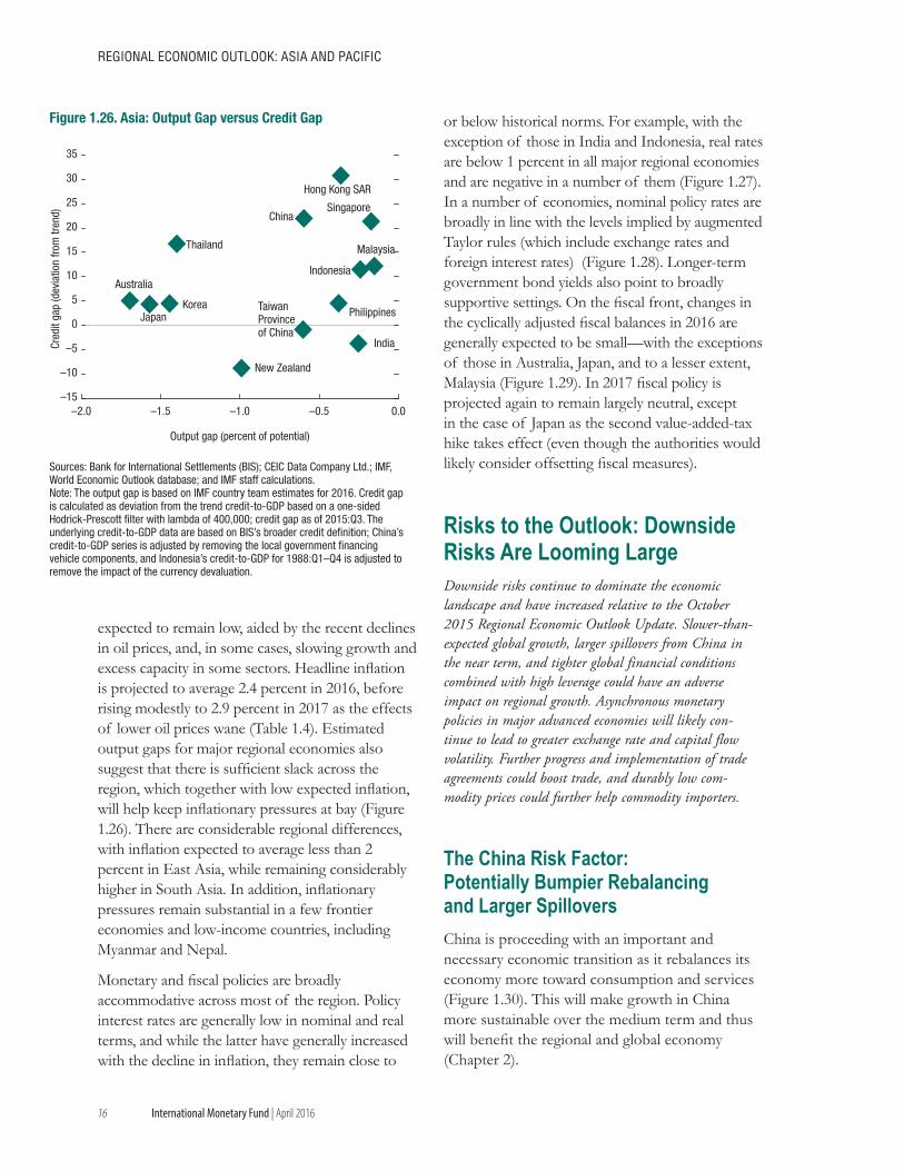
expected to remain low, aided by the recent declines in oil prices, and, in some cases, slowing growth and excess capacity in some sectors. Headline inflation is projected to average 2.4 percent in 2016, before rising modestly to 2.9 percent in 2017 as the effects of lower oil prices wane (Table 1.4). Estimated output gaps for major regional economies also suggest that there is sufficient slack across the region, which together with low expected inflation, will help keep inflationary pressures at bay (Figure 1.26). There are considerable regional differences, with inflation expected to average less than 2 percent in East Asia, while remaining considerably higher in South Asia. In addition, inflationary pressures remain substantial in a few frontier economies and low-income countries, including Myanmar and Nepal.
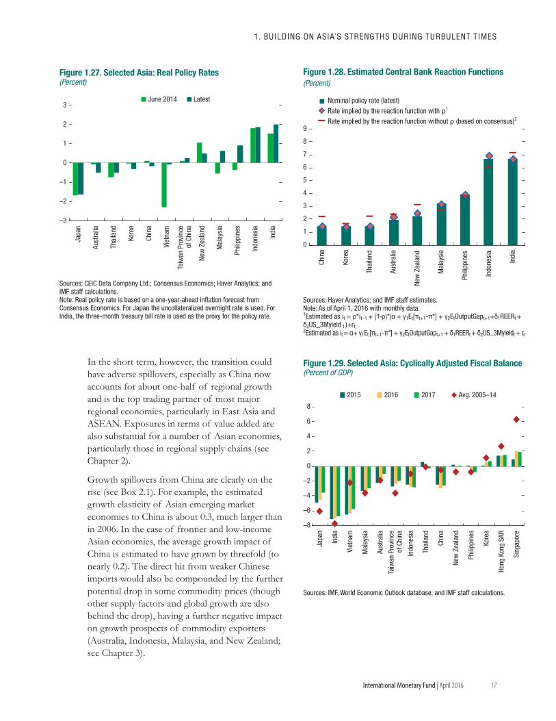
Monetary and fiscal policies are broadly accommodative across most of the region. Policy interest rates are generally low in nominal and real terms, and while the latter have generally increased with the decline in inflation, they remain close to
or below historical norms. For example, with the exception of those in India and Indonesia, real rates are below 1 percent in all major regional economies and are negative in a number of them (Figure 1.27). In a number of economies, nominal policy rates are broadly in line with the levels implied by augmented Taylor rules (which include exchange rates and foreign interest rates) (Figure 1.28). Longer-term government bond yields also point to broadly supportive settings. On the fiscal front, changes in the cyclically adjusted fiscal balances in 2016 are generally expected to be small—with the exceptions of those in Australia, Japan, and to a lesser extent, Malaysia (Figure 1.29). In 2017 fiscal policy is projected again to remain largely neutral, except in the case of Japan as the second value-added-tax hike takes effect (even though the authorities would likely consider offsetting fiscal measures).
Risks to the Outlook: Downside Risks Are Looming LargeDownside risks continue to dominate the economic landscape and have increased relative to the October 2015 Regional Economic Outlook Update. Slower-than- expected global growth, larger spillovers from China in the near term, and tighter global financial conditions combined with high leverage could have an adverse impact on regional growth. Asynchronous monetary policies in major advanced economies will likely con-tinue to lead to greater exchange rate and capital flow volatility. Further progress and implementation of trade agreements could boost trade, and durably low com-modity prices could further help commodity importers.
The China Risk Factor: Potentially Bumpier Rebalancing and Larger Spillovers China is proceeding with an important and necessary economic transition as it rebalances its economy more toward consumption and services (Figure 1.30). This will make growth in China more sustainable over the medium term and thus will benefit the regional and global economy (Chapter 2).
–15
–10
–5
0
5
10
15
20
25
30
35
–2.0 –1.5 –1.0 –0.5 0.0
Cred
it ga
p (d
evia
tion
from
tren
d)
Output gap (percent of potential)
Figure 1.26. Asia: Output Gap versus Credit Gap
Japan
Australia
New Zealand
Hong Kong SAR
Korea
Singapore
TaiwanProvinceof China
Indonesia
Malaysia
Philippines
Thailand
China
India
Sources: Bank for International Settlements (BIS); CEIC Data Company Ltd.; IMF, World Economic Outlook database; and IMF staff calculations.Note: The output gap is based on IMF country team estimates for 2016. Credit gap is calculated as deviation from the trend credit-to-GDP based on a one-sided Hodrick-Prescott filter with lambda of 400,000; credit gap as of 2015:Q3. The underlying credit-to-GDP data are based on BIS’s broader credit definition; China’s credit-to-GDP series is adjusted by removing the local government financing vehicle components, and Indonesia’s credit-to-GDP for 1988:Q1–Q4 is adjusted to remove the impact of the currency devaluation.
17
1. BUILdING ON AsIA’s sTRENGThs dURING TURBULENT TIMEs
International Monetary Fund | April 2016
In the short term, however, the transition could have adverse spillovers, especially as China now accounts for about one-half of regional growth and is the top trading partner of most major regional economies, particularly in East Asia and ASEAN. Exposures in terms of value added are also substantial for a number of Asian economies, particularly those in regional supply chains (see Chapter 2).
Growth spillovers from China are clearly on the rise (see Box 2.1). For example, the estimated growth elasticity of Asian emerging market economies to China is about 0.3, much larger than in 2006. In the case of frontier and low-income Asian economies, the average growth impact of China is estimated to have grown by threefold (to nearly 0.2). The direct hit from weaker Chinese imports would also be compounded by the further potential drop in some commodity prices (though other supply factors and global growth are also behind the drop), having a further negative impact on growth prospects of commodity exporters (Australia, Indonesia, Malaysia, and New Zealand; see Chapter 3).
Sources: CEIC Data Company Ltd.; Consensus Economics; Haver Analytics; and IMF staff calculations.Note: Real policy rate is based on a one-year-ahead inflation forecast from Consensus Economics. For Japan the uncollateralized overnight rate is used. For India, the three-month treasury bill rate is used as the proxy for the policy rate.
Japa
n
Aust
ralia
Thai
land
Kore
a
Viet
nam
Chin
a
New
Zea
land
Mal
aysi
a
Phili
ppin
es
Indo
nesi
a
Indi
a
June 2014 Latest
Taiw
an P
rovi
nce
of C
hina
Figure 1.27. Selected Asia: Real Policy Rates(Percent)
0
1
2
3
–3
–2
–1
0
1
2
3
4
5
6
7
8
9
Chin
a
Kore
a
Thai
land
Aust
ralia
New
Zea
land
Mal
aysi
a
Phili
ppin
es
Indo
nesi
a
Indi
a
Nominal policy rate (latest)Rate implied by the reaction function with ρ1
Rate implied by the reaction function without ρ (based on consensus)2
Figure 1.28. Estimated Central Bank Reaction Functions(Percent)
Sources: Haver Analytics; and IMF staff estimates.Note: As of April 1, 2016 with monthly data.1Estimated as it = ρ*it–1 + (1-ρ)*(α + γ1Et[πt+1-π*] + γ2EtOutputGapt+1+δ1REERt + δ2US_3Myield t )+εt2Estimated as it = α+ γ1Et [πt+1-π*] + γ2EtOutputGapt+1 + δ1REERt + δ2US_3Myieldt + εt
–2
–4
–6
–8
0
2
4
6
8
Japa
n
Indi
a
Viet
nam
Mal
aysi
a
Aust
ralia
Taiw
an P
rovi
nce
of C
hina
Indo
nesi
a
Thai
land
Chin
a
New
Zea
land
Phili
ppin
es
Kore
a
Hong
Kon
g SA
R
Sing
apor
e
2015 2016 2017 Avg. 2005–14
Sources: IMF, World Economic Outlook database; and IMF staff calculations.
Figure 1.29. Selected Asia: Cyclically Adjusted Fiscal Balance(Percent of GDP)
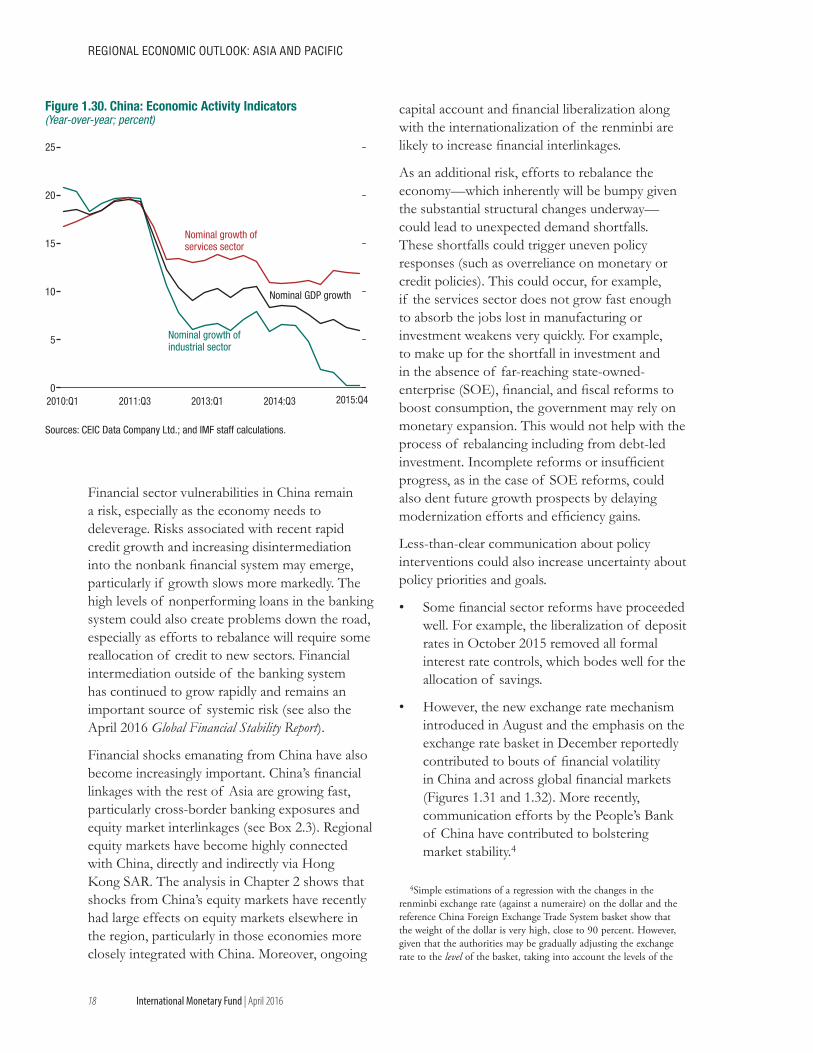
18
REGIONAL ECONOMIC OUTLOOK: AsIA ANd PACIfIC
International Monetary Fund | April 2016
Financial sector vulnerabilities in China remain a risk, especially as the economy needs to deleverage. Risks associated with recent rapid credit growth and increasing disintermediation into the nonbank financial system may emerge, particularly if growth slows more markedly. The high levels of nonperforming loans in the banking system could also create problems down the road, especially as efforts to rebalance will require some reallocation of credit to new sectors. Financial intermediation outside of the banking system has continued to grow rapidly and remains an important source of systemic risk (see also the April 2016 Global Financial Stability Report).
Financial shocks emanating from China have also become increasingly important. China’s financial linkages with the rest of Asia are growing fast, particularly cross-border banking exposures and equity market interlinkages (see Box 2.3). Regional equity markets have become highly connected with China, directly and indirectly via Hong Kong SAR. The analysis in Chapter 2 shows that shocks from China’s equity markets have recently had large effects on equity markets elsewhere in the region, particularly in those economies more closely integrated with China. Moreover, ongoing
capital account and financial liberalization along with the internationalization of the renminbi are likely to increase financial interlinkages.
As an additional risk, efforts to rebalance the economy—which inherently will be bumpy given the substantial structural changes underway—could lead to unexpected demand shortfalls. These shortfalls could trigger uneven policy responses (such as overreliance on monetary or credit policies). This could occur, for example, if the services sector does not grow fast enough to absorb the jobs lost in manufacturing or investment weakens very quickly. For example, to make up for the shortfall in investment and in the absence of far-reaching state-owned-enterprise (SOE), financial, and fiscal reforms to boost consumption, the government may rely on monetary expansion. This would not help with the process of rebalancing including from debt-led investment. Incomplete reforms or insufficient progress, as in the case of SOE reforms, could also dent future growth prospects by delaying modernization efforts and efficiency gains.
Less-than-clear communication about policy interventions could also increase uncertainty about policy priorities and goals.
• Some financial sector reforms have proceeded well. For example, the liberalization of deposit rates in October 2015 removed all formal interest rate controls, which bodes well for the allocation of savings.
• However, the new exchange rate mechanism introduced in August and the emphasis on the exchange rate basket in December reportedly contributed to bouts of financial volatility in China and across global financial markets (Figures 1.31 and 1.32). More recently, communication efforts by the People’s Bank of China have contributed to bolstering market stability.4
4Simple estimations of a regression with the changes in the renminbi exchange rate (against a numeraire) on the dollar and the reference China Foreign Exchange Trade System basket show that the weight of the dollar is very high, close to 90 percent. However, given that the authorities may be gradually adjusting the exchange rate to the level of the basket, taking into account the levels of the
0
5
10
15
20
25
2010:Q1 2011:Q3 2013:Q1 2014:Q3 2015:Q4
Figure 1.30. China: Economic Activity Indicators(Year-over-year; percent)
Nominal growth ofindustrial sector
Nominal growth of services sector
Sources: CEIC Data Company Ltd.; and IMF staff calculations.
Nominal GDP growth
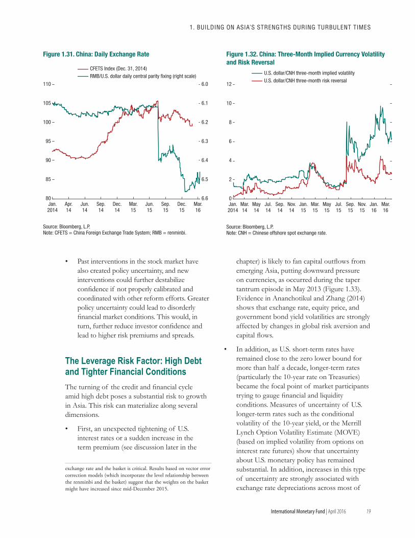
19
1. BUILdING ON AsIA’s sTRENGThs dURING TURBULENT TIMEs
International Monetary Fund | April 2016
• Past interventions in the stock market have also created policy uncertainty, and new interventions could further destabilize confidence if not properly calibrated and coordinated with other reform efforts. Greater policy uncertainty could lead to disorderly financial market conditions. This would, in turn, further reduce investor confidence and lead to higher risk premiums and spreads.
The Leverage Risk Factor: High Debt and Tighter Financial ConditionsThe turning of the credit and financial cycle amid high debt poses a substantial risk to growth in Asia. This risk can materialize along several dimensions.
• First, an unexpected tightening of U.S. interest rates or a sudden increase in the term premium (see discussion later in the
exchange rate and the basket is critical. Results based on vector error correction models (which incorporate the level relationship between the renminbi and the basket) suggest that the weights on the basket might have increased since mid-December 2015.
chapter) is likely to fan capital outflows from emerging Asia, putting downward pressure on currencies, as occurred during the taper tantrum episode in May 2013 (Figure 1.33). Evidence in Ananchotikul and Zhang (2014) shows that exchange rate, equity price, and government bond yield volatilities are strongly affected by changes in global risk aversion and capital flows.
• In addition, as U.S. short-term rates have remained close to the zero lower bound for more than half a decade, longer-term rates (particularly the 10-year rate on Treasuries) became the focal point of market participants trying to gauge financial and liquidity conditions. Measures of uncertainty of U.S. longer-term rates such as the conditional volatility of the 10-year yield, or the Merrill Lynch Option Volatility Estimate (MOVE) (based on implied volatility from options on interest rate futures) show that uncertainty about U.S. monetary policy has remained substantial. In addition, increases in this type of uncertainty are strongly associated with exchange rate depreciations across most of
6.0
6.1
6.2
6.3
6.4
6.5
6.680
85
90
95
100
105
110
Jan.2014
Apr.14
Jun.14
Sep.14
Dec.14
Mar.15
Jun.15
Sep.15
Dec.15
Mar.16
CFETS Index (Dec. 31, 2014)RMB/U.S. dollar daily central parity fixing (right scale)
Figure 1.31. China: Daily Exchange Rate
Source: Bloomberg, L.P.Note: CFETS = China Foreign Exchange Trade System; RMB = renminbi.
0
2
4
6
8
10
12
U.S. dollar/CNH three-month implied volatilityU.S. dollar/CNH three-month risk reversal
Source: Bloomberg, L.P.Note: CNH = Chinese offshore spot exchange rate.
Jan.2014
Mar.14
Jul.14
May14
Sep.14
Nov.14
Jan.15
Mar.15
Jan.16
Mar.16
Jul.15
May15
Sep.15
Nov.15
Figure 1.32. China: Three-Month Implied Currency Volatility and Risk Reversal
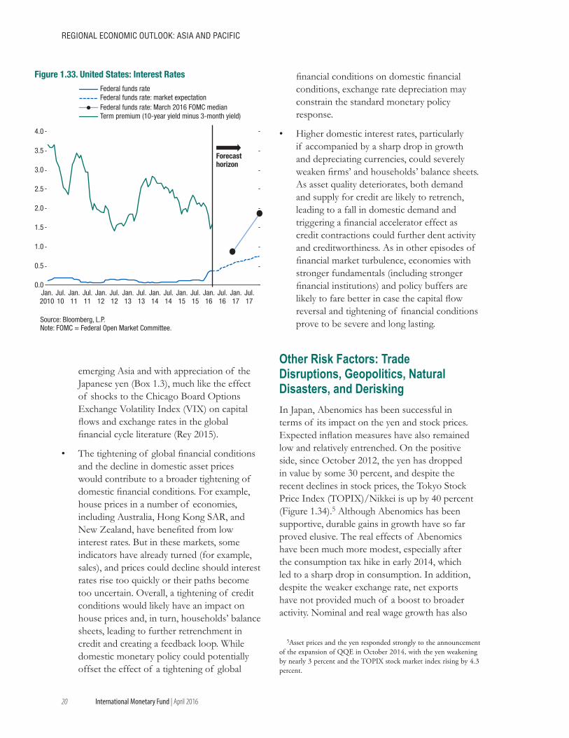
20
REGIONAL ECONOMIC OUTLOOK: AsIA ANd PACIfIC
International Monetary Fund | April 2016
emerging Asia and with appreciation of the Japanese yen (Box 1.3), much like the effect of shocks to the Chicago Board Options Exchange Volatility Index (VIX) on capital flows and exchange rates in the global financial cycle literature (Rey 2015).
• The tightening of global financial conditions and the decline in domestic asset prices would contribute to a broader tightening of domestic financial conditions. For example, house prices in a number of economies, including Australia, Hong Kong SAR, and New Zealand, have benefited from low interest rates. But in these markets, some indicators have already turned (for example, sales), and prices could decline should interest rates rise too quickly or their paths become too uncertain. Overall, a tightening of credit conditions would likely have an impact on house prices and, in turn, households’ balance sheets, leading to further retrenchment in credit and creating a feedback loop. While domestic monetary policy could potentially offset the effect of a tightening of global
financial conditions on domestic financial conditions, exchange rate depreciation may constrain the standard monetary policy response.
• Higher domestic interest rates, particularly if accompanied by a sharp drop in growth and depreciating currencies, could severely weaken firms’ and households’ balance sheets. As asset quality deteriorates, both demand and supply for credit are likely to retrench, leading to a fall in domestic demand and triggering a financial accelerator effect as credit contractions could further dent activity and creditworthiness. As in other episodes of financial market turbulence, economies with stronger fundamentals (including stronger financial institutions) and policy buffers are likely to fare better in case the capital flow reversal and tightening of financial conditions prove to be severe and long lasting.
Other Risk Factors: Trade Disruptions, Geopolitics, Natural Disasters, and DeriskingIn Japan, Abenomics has been successful in terms of its impact on the yen and stock prices. Expected inflation measures have also remained low and relatively entrenched. On the positive side, since October 2012, the yen has dropped in value by some 30 percent, and despite the recent declines in stock prices, the Tokyo Stock Price Index (TOPIX)/Nikkei is up by 40 percent (Figure 1.34).5 Although Abenomics has been supportive, durable gains in growth have so far proved elusive. The real effects of Abenomics have been much more modest, especially after the consumption tax hike in early 2014, which led to a sharp drop in consumption. In addition, despite the weaker exchange rate, net exports have not provided much of a boost to broader activity. Nominal and real wage growth has also
5Asset prices and the yen responded strongly to the announcement of the expansion of QQE in October 2014, with the yen weakening by nearly 3 percent and the TOPIX stock market index rising by 4.3 percent.
0.0
0.5
1.0
1.5
2.0
2.5
3.0
3.5
4.0
Federal funds rateFederal funds rate: market expectationFederal funds rate: March 2016 FOMC medianTerm premium (10-year yield minus 3-month yield)
Figure 1.33. United States: Interest Rates
Forecasthorizon
Source: Bloomberg, L.P.Note: FOMC = Federal Open Market Committee.
Jan.2010
Jul.10
Jan.11
Jul.11
Jan.12
Jul.12
Jan.13
Jul.13
Jan.14
Jul.14
Jan.15
Jul.15
Jan.16
Jul.16
Jan.17
Jul.17
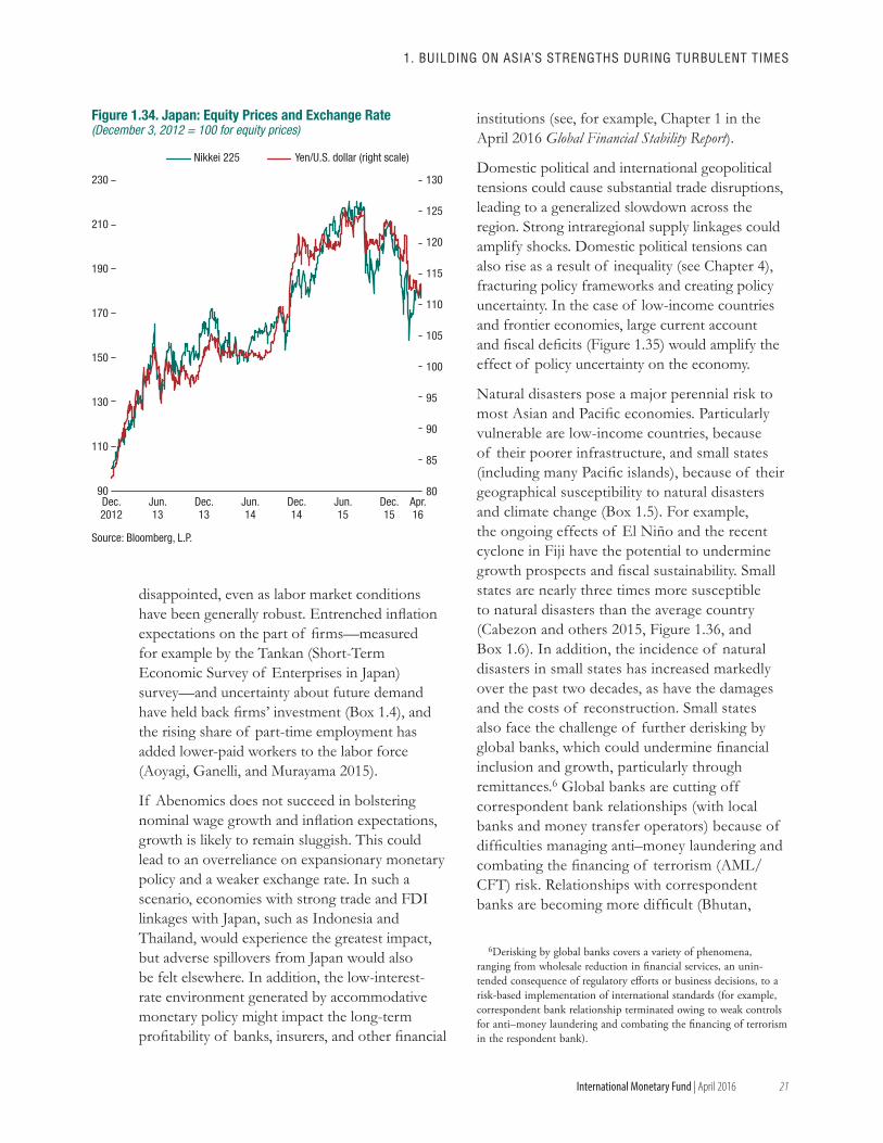
21
1. BUILdING ON AsIA’s sTRENGThs dURING TURBULENT TIMEs
International Monetary Fund | April 2016
disappointed, even as labor market conditions have been generally robust. Entrenched inflation expectations on the part of firms—measured for example by the Tankan (Short-Term Economic Survey of Enterprises in Japan) survey—and uncertainty about future demand have held back firms’ investment (Box 1.4), and the rising share of part-time employment has added lower-paid workers to the labor force (Aoyagi, Ganelli, and Murayama 2015).
If Abenomics does not succeed in bolstering nominal wage growth and inflation expectations, growth is likely to remain sluggish. This could lead to an overreliance on expansionary monetary policy and a weaker exchange rate. In such a scenario, economies with strong trade and FDI linkages with Japan, such as Indonesia and Thailand, would experience the greatest impact, but adverse spillovers from Japan would also be felt elsewhere. In addition, the low-interest-rate environment generated by accommodative monetary policy might impact the long-term profitability of banks, insurers, and other financial
institutions (see, for example, Chapter 1 in the April 2016 Global Financial Stability Report).
Domestic political and international geopolitical tensions could cause substantial trade disruptions, leading to a generalized slowdown across the region. Strong intraregional supply linkages could amplify shocks. Domestic political tensions can also rise as a result of inequality (see Chapter 4), fracturing policy frameworks and creating policy uncertainty. In the case of low-income countries and frontier economies, large current account and fiscal deficits (Figure 1.35) would amplify the effect of policy uncertainty on the economy.
Natural disasters pose a major perennial risk to most Asian and Pacific economies. Particularly vulnerable are low-income countries, because of their poorer infrastructure, and small states (including many Pacific islands), because of their geographical susceptibility to natural disasters and climate change (Box 1.5). For example, the ongoing effects of El Niño and the recent cyclone in Fiji have the potential to undermine growth prospects and fiscal sustainability. Small states are nearly three times more susceptible to natural disasters than the average country (Cabezon and others 2015, Figure 1.36, and Box 1.6). In addition, the incidence of natural disasters in small states has increased markedly over the past two decades, as have the damages and the costs of reconstruction. Small states also face the challenge of further derisking by global banks, which could undermine financial inclusion and growth, particularly through remittances.6 Global banks are cutting off correspondent bank relationships (with local banks and money transfer operators) because of difficulties managing anti–money laundering and combating the financing of terrorism (AML/CFT) risk. Relationships with correspondent banks are becoming more difficult (Bhutan,
6Derisking by global banks covers a variety of phenomena, ranging from wholesale reduction in financial services, an unin-tended consequence of regulatory efforts or business decisions, to a risk-based implementation of international standards (for example, correspondent bank relationship terminated owing to weak controls for anti–money laundering and combating the financing of terrorism in the respondent bank).
Nikkei 225 Yen/U.S. dollar (right scale)
Figure 1.34. Japan: Equity Prices and Exchange Rate(December 3, 2012 = 100 for equity prices)
Source: Bloomberg, L.P.
80
85
90
95
100
105
110
115
120
125
130
90
110
130
150
170
190
210
230
Jun.13
Dec.14
Dec.2012
Jun.15
Dec.13
Jun.14
Dec.15
Apr.16
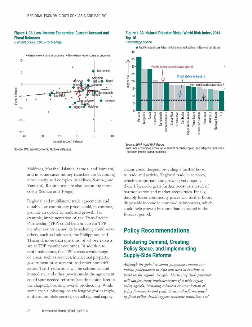
22
REGIONAL ECONOMIC OUTLOOK: AsIA ANd PACIfIC
International Monetary Fund | April 2016
Maldives, Marshall Islands, Samoa, and Vanuatu), and in some cases money transfers are becoming more costly and complex (Maldives, Samoa, and Vanuatu). Remittances are also becoming more costly (Samoa and Tonga).
Regional and multilateral trade agreements and durably low commodity prices could, in contrast, provide an upside to trade and growth. For example, implementation of the Trans-Pacific Partnership (TPP) could benefit current TPP member countries, and its broadening could serve others, such as Indonesia, the Philippines, and Thailand, more than one-third of whose exports are to TPP member countries. In addition to tariff reductions, the TPP covers a wide range of areas, such as services, intellectual property, government procurement, and other nontariff issues. Tariff reductions will be substantial and immediate, and other provisions in the agreement could spur needed reforms (see discussion later in the chapter), boosting overall productivity. While some special phasing-ins are lengthy (for example, in the automobile sector), overall regional supply
chains could deepen, providing a further boost to trade and activity. Regional trade in services, which is important and growing very rapidly (Box 1.7), could get a further boost as a result of harmonization and market access rules. Finally, durably lower commodity prices will further boost disposable income in commodity importers, which could help growth by more than expected in the forecast period.
Policy Recommendations Bolstering Demand, Creating Policy Space, and Implementing Supply-Side ReformsAlthough the global economic panorama remains tur-bulent, policymakers in Asia will need to continue to build on the region’s strengths. Harnessing Asia’s potential will call for strong implementation of a wide-raging policy agenda, including enhanced communication of policy frameworks and goals. Structural reforms, aided by fiscal policy, should support economic transitions and
–20
–15
–10
–5
0
5
10
–40 –30 –20 –10 0 10
BangladeshBhutanCambodia
Lao P.D.R.
Maldives
Marshall Islands
Micronesia
Mongolia
Myanmar
Nepal
Papua New Guinea
Solomon Islands
Samoa
TongaVanuatu
Vietnam
Fisc
al b
alan
ce
Current account balance
Asian low-income economies Non-Asian low-income economies
Source: IMF, World Economic Outlook database.
Figure 1.35. Low-Income Economies: Current Account and Fiscal Balances(Percent of GDP, 2013–15 average)
0
5
10
15
20
25
30
35
40
Vanu
atu
Phili
ppin
es
Tong
a
Guat
emal
a
Bang
lade
sh
Solo
mon
Isla
nds
Cost
a Ri
ca
El S
alva
dor
Cam
bodi
a
Papu
a Ne
w G
uine
a
Tim
or-L
este
Brun
ei D
arus
sala
m
Nica
ragu
a
Mau
ritiu
s
Guin
ea-B
issa
u
Fiji
Pacific island countries African small states Non–small states
High
erris
k
Pacific island countries average: 19
Non–small states average: 7
Small states average: 81
Figure 1.36. Natural Disaster Risks: World Risk Index, 2014, Top 16(Percentage points)
Source: 2014 World Risk Report.Note: Index combines exposure to natural hazards, coping, and adaptive capacities.1Excludes Pacific island countries.
23
1. BUILdING ON AsIA’s sTRENGThs dURING TURBULENT TIMEs
International Monetary Fund | April 2016
bolster potential growth. Monetary policy should remain focused on supporting demand and addressing near-term risks, including from large exchange rate depreciations and deflationary shocks. Policies to manage risks asso-ciated with high leverage and financial volatility will play an important role, including exchange rate flexi-bility, targeted macroprudential policies, and in some cases, capital flow measures. Finally, policy recalibra-tion should not lead to a buildup in vulnerabilities.
Flexible Monetary, Exchange Rate, and Macroprudential PoliciesRecent bouts of financial volatility underscore the need for flexible and proactive monetary and exchange rate policies. Effective communication of policy goals can also play a role in bolstering confidence and lowering market volatility.
With monetary policy broadly in line with historical patterns (see Figure 1.27), current monetary settings are appropriate to support growth while providing insurance against risks. Nonetheless, should growth disappoint, monetary policy could be used to support demand, as most economies have relatively subdued prospects for inflation, particularly if fiscal space is limited. But in some cases, large exchange rate depreciations and balance of payments pressures may warrant a more cautious approach. In the case of economies with high policy credibility and low inflation, central banks should use monetary support to offset the effects of global uncertainty and tighter global liquidity on domestic financial conditions (see Box 1.3).
• The cases of Japan and China are quite distinct from those of most other economies. In Japan, monetary policy actions should remain focused on lifting inflation expectations, which will require long-lasting and credible monetary expansion. In addition, monetary policy should be coordinated with other policies to restore the inflation momentum and improve the transmission mechanism. In China, the challenge is to ensure that credit growth slows gradually and flows to more productive sectors. This goal
will require a vigilant approach to monetary policy and avoid easing policy too aggressively, as it would likely contribute to overcapacity and the buildup of systemic risks. Most emerging Asian economies (excluding China) have room to cut policy rates as inflationary pressures remain relatively low and inflation expectations are generally low and stable.
Exchange rates should remain the first line of defense against external shocks. Recent episodes of financial volatility have shown that even large reserve buffers can be insufficient to arrest such volatility. Although exchange rate flexibility should remain the main shock absorber as in the recent past (Figures 1.37 and 1.38), foreign exchange intervention should be deployed to reduce risks of disorderly market conditions. However, foreign exchange intervention should not be used to resist currency movements reflecting changing fundamentals or as a substitute for macroeconomic policy adjustments.
Macroprudential and financial policies should continue to be used to bolster financial stability and mitigate systemic risks. As volatile capital flows and asset prices will continue to create challenges and risks to financial and macroeconomic stability, the proactive use of macroprudential policies will be needed along with measures to rebuild buffers to prepare for market volatility. Asia’s wide use of macroprudential policies and its regulatory apparatus have contributed to bolster financial stability, but closer monitoring of risks and intersectoral linkages (across different segments of the financial system) will also be critical to identify the sources of risks and their transmission channels. In other areas, including the corporate and household sectors, efforts should be stepped up to better identify the pockets of leverage and fragility stemming from the concentration of debt (across, for example, households with different income levels and other financial buffers). For example, more recently, a number of economies in the region (Korea, Hong Kong SAR, New Zealand, and Singapore) have leaned heavily on macroprudential tools to contain risks associated with rising house prices and household leverage. Capital flow measures could
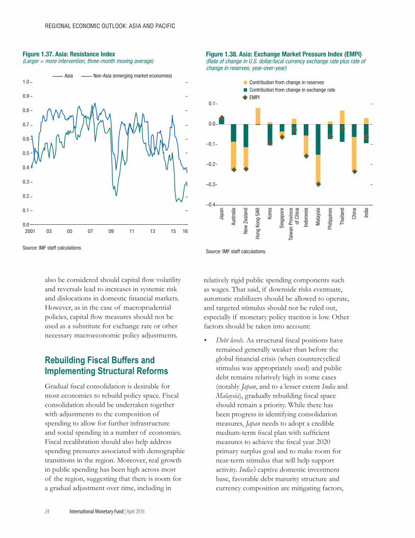
24
REGIONAL ECONOMIC OUTLOOK: AsIA ANd PACIfIC
International Monetary Fund | April 2016
also be considered should capital flow volatility and reversals lead to increases in systemic risk and dislocations in domestic financial markets. However, as in the case of macroprudential policies, capital flow measures should not be used as a substitute for exchange rate or other necessary macroeconomic policy adjustments.
Rebuilding Fiscal Buffers and Implementing Structural Reforms Gradual fiscal consolidation is desirable for most economies to rebuild policy space. Fiscal consolidation should be undertaken together with adjustments to the composition of spending to allow for further infrastructure and social spending in a number of economies. Fiscal recalibration should also help address spending pressures associated with demographic transitions in the region. Moreover, real growth in public spending has been high across most of the region, suggesting that there is room for a gradual adjustment over time, including in
relatively rigid public spending components such as wages. That said, if downside risks eventuate, automatic stabilizers should be allowed to operate, and targeted stimulus should not be ruled out, especially if monetary policy traction is low. Other factors should be taken into account:
• Debt levels. As structural fiscal positions have remained generally weaker than before the global financial crisis (when countercyclical stimulus was appropriately used) and public debt remains relatively high in some cases (notably Japan, and to a lesser extent India and Malaysia), gradually rebuilding fiscal space should remain a priority. While there has been progress in identifying consolidation measures, Japan needs to adopt a credible medium-term fiscal plan with sufficient measures to achieve the fiscal year 2020 primary surplus goal and to make room for near-term stimulus that will help support activity. India’s captive domestic investment base, favorable debt maturity structure and currency composition are mitigating factors,
0.0
0.1
0.2
0.3
0.4
0.5
0.6
0.7
0.8
0.9
1.0
2001 03 05 07 09 11 13 15
Asia Non-Asia (emerging market economies)
16
Figure 1.37. Asia: Resistance Index(Larger = more intervention; three-month moving average)
Source: IMF staff calculations.
–0.4
–0.3
–0.2
–0.1
0.0
0.1
Japa
n
Aust
ralia
New
Zea
land
Hong
Kon
g SA
R
Kore
a
Sing
apor
e
Taiw
an P
rovi
nce
of C
hina
Indo
nesi
a
Mal
aysi
a
Phili
ppin
es
Thai
land
Chin
a
Indi
a
Contribution from change in reservesContribution from change in exchange rateEMPI
Source: IMF staff calculations.
Figure 1.38. Asia: Exchange Market Pressure Index (EMPI)(Rate of change in U.S. dollar/local currency exchange rate plus rate of change in reserves; year-over-year)
25
1. BUILdING ON AsIA’s sTRENGThs dURING TURBULENT TIMEs
International Monetary Fund | April 2016
but a concrete fiscal adjustment path would help. Where debt levels are low (for example, Korea), fiscal stimulus to counter demand shortfalls should be considered.
• Need to support broader reforms and structural change. Fiscal adjustment needs to be weighed against the need to cushion the blow from economic rebalancing and, in certain circumstances, the negative short-term impact of structural reforms (see the April 2016 World Economic Outlook, Chapter 3). In the case of China, as central government debt is relatively low, on-budget fiscal support that boosts consumption, reduces precautionary savings, and increases the productivity of the services sector should be considered. Scaling down off-budget investment should also be part of the policy measures aimed at helping rebalancing. At the same time, fiscal reforms to bolster local government finances, the quality of expenditures, and fiscal consolidation over the medium term are important. In Vietnam, where debt levels are high, fiscal consolidation is needed to provide space for potential bank and SOE restructuring costs.
• Revenue mobilization and infrastructure needs. Domestic revenue mobilization efforts should proceed, especially in Indonesia and frontier and lower income countries (for example, Cambodia, Mongolia, Myanmar, and Vietnam), where revenue ratios are generally low and infrastructure gaps are large. In some cases where debt levels are low and fiscal risks are more manageable, deficit-financed infrastructure investment could also be considered provided that it is of high growth impact.
• Dependence on commodities. In commodity exporters, fiscal consolidation should continue because fiscal stimulus could increase fiscal vulnerabilities, triggering spikes in risk premiums and capital flow reversals. Reductions in fiscal vulnerabilities are likely to lessen external risks as well. Malaysia, for instance, has reduced its budget’s
dependence on oil- and gas-related revenues and broadened the tax base through the introduction of the goods and services tax in April 2015.
• Risk of natural disasters. In small states and some low-income countries, revenue mobilization and prudent fiscal policies are critical to build large buffers to deal with costly (and frequent) natural disasters. Natural disaster risks in many countries in the region have been on the rise, and fiscal policy is often the primary tool to reignite reconstruction efforts and prevent sharp and sustained drops in growth.
Pushing ahead with structural reforms will be critical to ensure that Asia remains the global growth leader. Structural reforms are needed to help rebalance demand and supply, reduce domestic and external vulnerabilities, increase economic efficiency and potential growth, reduce inequality (see Chapter 4), and foster more inclusive growth. In a number of economies, reforms can also help address climate change and improve the environment, particularly in large countries that rely heavily on fossil fuels such as China, India, and Indonesia. Past reforms (for example, those in India in the early 1990s and in China starting in the late 1970s) have been shown to have been highly effective, including by fostering economic and trade diversification and facilitating Asia’s entry in global markets. Recent reforms to rationalize subsidies are also encouraging, as most major economies in the region have eliminated fuel subsidies, which will bolster fiscal positions if oil prices go up. The agenda varies across economies:
• In China, reforms should focus on improving the allocation of credit and reducing the dependence of growth on credit. This would rebalance the economy away from debt-led investment. In this connection, leveling the playing field between SOEs and the private sector, and continuing with the reforms to improve corporate governance to rekindle the equity markets as a source of corporate financing will remain priorities. A
26
REGIONAL ECONOMIC OUTLOOK: AsIA ANd PACIfIC
International Monetary Fund | April 2016
comprehensive strategy to address weak firms and excessive debt and eliminating implicit guarantees will also be important in this context. Other reforms to facilitate investment in the services sector are also priorities. Fiscal reforms to enhance social safety nets will be critical to reduce precautionary savings and sustain the consumption growth.
• In Japan, reforms to reduce the extent of duality in the labor market are needed, which will help unclog the transmission from labor market conditions to wage increases. Reforms to increase female labor force participation and to deregulate product markets that would improve labor productivity (especially in the services sector), will also be important. Finally, implementing further corporate governance reform could help spur corporate investment by deploying firms’ cash holdings.
• In India, policymakers should capitalize on the favorable economic momentum to speed up structural reform implementation. Additional steps in relaxing long-standing supply bottlenecks, especially in the mining and power sectors, as well as further labor market reforms to increase labor market flexibility
in the formal sector, are crucial to achieving faster and more inclusive growth. The long-awaited goods and services tax should be implemented, as it would create a single national market, enhance economic efficiency, and boost GDP growth.
• Across ASEAN and low-income countries, reforms to improve the business climate and address the infrastructure gap are needed. The estimated infrastructure gap exceeds 50 percent of GDP in ASEAN countries (McKinsey Global Institute 2015), and financial sector reforms would be critical to allow a more efficient and risk-based intermediation of savings toward those investments. As banks are not best positioned to finance long-duration projects, further developing bond markets and other forms of long-term finance remain high on the agenda. In frontier economies such as Vietnam, reforms to improve economic efficiency need to be reinvigorated, including progress on SOEs and state banking reforms. To address derisking in small states, authorities and international stakeholders should clarify regulatory expectations, including on AML/CFT systems.
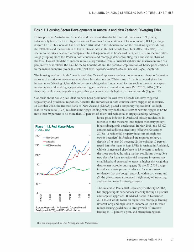
27
1. BUILdING ON AsIA’s sTRENGThs dURING TURBULENT TIMEs
International Monetary Fund | April 2016
House prices in Australia and New Zealand have more than doubled in real terms since 1990, rising substantially faster than the Organisation for Economic Co-operation and Development (OECD) average (Figure 1.1.1). This increase has often been attributed to the liberalization of their banking systems during the 1980–90s and the transition to lower interest rates in the last decade (see Hunt 2015; Ellis 2005). The rise in house prices has been accompanied by a sharp increase in household debt, with debt-to-income ratios roughly tripling since the 1990s in both countries and mortgage debt accounting for a substantial share of the total. Household debt-to-income ratio is a key variable from a financial stability and macroeconomic risk perspective as it reflects the risks borne by households and the possible amplification of house price declines to the macro economy (Debelle 2004; April 2014 Regional Economic Outlook: Asia and Pacific, Chapter 2).
The housing market in both Australia and New Zealand appears to reflect moderate overvaluation. Valuation ratios such as price to income are now above historical norms. While some of that is expected given low interest rates (allowing higher debt to be serviceable), other fundamental factors such as income per capita, interest rates, and working-age population suggest moderate overvaluation (see IMF 2015a, 2016c). The financial stability heat map also suggests that prices are currently higher than recent trends (Figure 1.13).
Concerns about house price inflation have been prominent for well over a decade and have triggered regulatory and prudential responses. Recently, the authorities in both countries have stepped up measures. In October 2013, the Reserve Bank of New Zealand (RBNZ) placed a temporary “speed limit” on high loan-to-value ratio (LVR) residential mortgage lending, whereby banks must restrict new mortgages at LVRs more than 80 percent to no more than 10 percent of their total residential mortgage lending. Although
house price inflation in Auckland initially moderated in response to the measures (and tighter monetary policy), it has subsequently accelerated. In May 2015, the RBNZ announced additional measures (effective November 2015): (1) residential property investors (though not owner-occupiers) in Auckland are required to have a deposit of at least 30 percent; (2) the existing 10 percent speed limit for loans at high LVRs is retained in Auckland, while it is increased elsewhere to 15 percent to reflect the more subdued housing market conditions there; (3) a new class for loans to residential property investors was established and expected to attract a higher risk weighting than owner-occupier mortgages; (4) the 2015/16 budget introduced a new property sales tax for nonprimary residences that are bought and sold within two years; and (5) the government announced a tightening of reporting and taxation rules for foreign buyers.
The Australian Prudential Regulatory Authority (APRA) has stepped up its supervisory intensity through a gradual and targeted approach. It advised banks in December 2014 that it would focus on higher-risk mortgage lending (interest-only and high loan-to-income or loan-to-value ratios), issuing guidelines to limit growth of investor lending to 10 percent a year, and strengthening loan
This box was prepared by Dan Nyberg and Adil Mohommad.
Figure 1.1.1. Real House Prices(1990 = 100)
0
50
100
150
200
250
300
1990
:Q1
95:Q
1
2000
:Q1
05:Q
1
10:Q
1
15:Q
1
New Zealand
Australia
OECD countries
Sources: Organisation for Economic Co-operation and Development (OECD); and IMF staff calculations.
Box 1.1. Housing Sector Developments in Australia and New Zealand: Diverging Tales
28
REGIONAL ECONOMIC OUTLOOK: AsIA ANd PACIfIC
International Monetary Fund | April 2016
affordability. In response to the recommendations of the Financial Sector Inquiry, APRA announced that large banks would need to hold more capital against residential mortgage exposures by raising the average risk weight (to 25 percent) for large banks. Recent data suggest that house price inflation is gradually responding to the regulatory measures, but it is too early to assess whether such inflation is at more sustainable rates.
Can the banking sector withstand a housing downturn? Four large Australian-owned banks account for the bulk of banking sector assets in both Australia and New Zealand. Against this background, the authorities in both countries have collaborated on stress testing, including a combined scenario with a severe downturn in the housing market (40 percent cumulative decline) (APRA 2014). While this extreme scenario would have a substantial adverse impact on profitability and capital ratios, with losses on residential mortgages accounting for about one-third of total credit losses, minimum capital requirements are not breached. However, banks with substantially reduced capital ratios would be constrained in their ability to raise funding, impacting credit growth and aggregate demand.
Box 1.1 (continued)
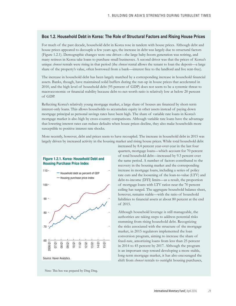
29
1. BUILdING ON AsIA’s sTRENGThs dURING TURBULENT TIMEs
International Monetary Fund | April 2016
For much of the past decade, household debt in Korea rose in tandem with house prices. Although debt and house prices appeared to decouple a few years ago, the increase in debt was largely due to structural factors (Figure 1.2.1). Demographic changes were one driver—the large baby-boom generation was retiring, and many retirees in Korea take loans to purchase small businesses. A second driver was that the prices of Korea’s unique chonsei rentals were rising in that period (the chonsei rental allows the tenant to loan the deposit—a large share of the property’s value, often borrowed from a bank—interest free to the landlord and live rent-free).
The increase in household debt has been largely matched by a corresponding increase in household financial assets. Banks, though, have maintained solid buffers during the run-up in house prices that accelerated in 2010, and the high level of household debt (95 percent of GDP) does not seem to be a systemic threat to macroeconomic or financial stability because debt-to-net-worth ratio is relatively low at below 20 percent of GDP.
Reflecting Korea’s relatively young mortgage market, a large share of houses are financed by short-term interest-only loans. This allows households to accumulate equity in other assets instead of paying down mortgage principal as personal savings rates have been high. The share of variable rate loans in Korea’s mortgage market is also high by cross-country comparisons. Although variable rate loans have the advantage that lowering interest rates can reduce defaults when house prices decline, they also make households more susceptible to positive interest rate shocks.
More recently, however, debt and prices seem to have recoupled. The increase in household debt in 2015 was largely driven by increased activity in the housing market and rising house prices. While total household debt
increased by 8.4 percent year-over-year in the last four quarters, mortgage loans—which account for 70 percent of total household debt—increased by 9.3 percent over the same period. A number of factors contributed to the recovery in the housing market and the corresponding increase in mortgage loans, including a series of policy rate cuts and the loosening of the loan-to-value (LTV) and debt-to-income (DTI) limits—as a result, the proportion of mortgage loans with LTV ratios near the 70 percent ceiling has surged. The aggregate household balance sheet, however, remains stable—with the ratio of household liabilities to financial assets at about 80 percent at the end of 2015.
Although household leverage is still manageable, the authorities are taking steps to address potential risks stemming from rising household debt. Recognizing the risks associated with the structure of the mortgage market, in 2015 regulators implemented the loan conversion program, aiming to increase the share of fixed-rate, amortizing loans from less than 25 percent in 2014 to 45 percent by 2017. Although the program is an important step toward developing a more stable, long-term mortgage market, it has also encouraged the shift from chonsei rentals to outright housing purchases,
Note: This box was prepared by Ding Ding.
Source: Haver Analytics.
60
70
80
90
100
110
2006
:Q1
07:Q
1
08:Q
1
09:Q
1
10:Q
1
11:Q
1
12:Q
1
13:Q
1
14:Q
1
15:Q
1
Household debt as percent of GDP
Housing purchase price index
Figure 1.2.1. Korea: Household Debt andHousing Purchase Price Index
Box 1.2. Household Debt in Korea: The Role of Structural Factors and Rising House Prices
30
REGIONAL ECONOMIC OUTLOOK: AsIA ANd PACIfIC
International Monetary Fund | April 2016
bolstering the demand for mortgage refinancing. In addition, regulators announced a set of measures to strengthen the evaluation of debtors’ repayment capacity, tightened control over household debt growth in the nonbanking sector, and phased out interest-only loans. Regulators are also closely monitoring several indicators (for example, the average and the distribution of LTV and DTI ratios across new loans over a period and outstanding loans at a given point in time, and house price growth by region and type of properties), and as in the past, have tightened the macroprudential policies to address signs of a buildup of systemic risks in the housing sector.
Box 1.2 (continued)
31
1. BUILdING ON AsIA’s sTRENGThs dURING TURBULENT TIMEs
International Monetary Fund | April 2016
After seven years, the era of zero policy interest rates in the United States has come to an end. The accommodative stance resulted in loose global liquidity conditions and large capital inflows to emerging market economies. As discussed in the main text, further interest rate hikes by the Federal Reserve could lead to a further tightening of global liquidity and capital outflows from emerging Asia and other emerging market economies. In addition, the uncertainty surrounding the path of short-term interest rates has also contributed to financial volatility.
Although the federal funds rate target is expected to increase as the U.S. economy continues to recover, the pace and magnitude of adjustment are uncertain. First, the global economic environment is more uncertain. Second, spillovers from emerging market economies might be sizable, especially for the manufacturing sector, which currently is decelerating and is generally more sensitive to the strength of the dollar. These factors have generated uncertainty about how fast and for how long the Federal Reserve will continue to remove monetary policy accommodation. The disagreement between market participants and the Federal Reserve’s Federal Open Market Committee (FOMC) is reflected in the large discrepancy between the future path of the federal funds rate futures and the expectations of FOMC participants, the “dots chart” (Figure 1.33 in the main text).
The uncertainty about U.S. monetary policy increased after the global financial crisis, and examining its effects is important for understanding spillover channels. For example, the dollar has appreciated sharply on expectations of further Federal Reserve tightening, but volatility has also increased as monetary policy in major advanced economies became increasingly asynchronous (with the United States tightening and the euro area and Japan continuing with monetary accommodation). Given the low interest rate environment, market expectations have shifted to longer-term rates and other aspects of monetary policy such as instruments used to implement quantitative easing (interest rate on reserves, asset purchases, and so on). Moreover, as the quantitative easing (QE) program was focused on lowering long-term rates, news about QE was associated with movements in capital flows (Cho and Rhee 2013).
Given the increasing importance of U.S. monetary policy uncertainty, this box first examines uncertainty measures and then quantifies their effects on Asian currencies. Following the work of Rey (2015) on the global financial cycle and earlier work by Benigno, Benigno, and Nisticò (2012) on the effect of risk on exchange rates, the empirical framework applied here uses three measures of financial volatility, because it is important to control for other forms of uncertainty when trying to measure the effects of U.S. monetary policy uncertainty. First, the Chicago Board Options Exchange Volatility Index (VIX) is included to control for broader uncertainty affecting financial markets. The second uncertainty measure is the realized volatility of the federal funds rate augmented with the shadow rate for the postcrisis period. The third measure of uncertainty is the realized volatility of the 10-year Treasury rate.1 The last two volatility measures try to capture the overall uncertainty about U.S. monetary policy, both at the short-end and long-end of the yield curve. Although there is no attempt to explicitly model uncertainty about other aspects of monetary policy, it is reasonable to assume that other monetary policy instruments would have an impact on either short- or long-term interest rates. The data show that, like the VIX, uncertainty about interest rates exhibits substantial fluctuations, with spikes during the global financial crisis and more recently during the taper tantrum and in early 2016 (Figure 1.3.1). Although the effects of the VIX have been well studied and proved to be the important driver of the global financial cycle (Rey 2015), the effects of U.S. monetary policy uncertainty are also potentially important and have not been researched as much. Intuitively, greater uncertainty about U.S. monetary policy lowers the risk-adjusted return of foreign investments (for U.S.-based investors), essentially
This box was prepared by Roberto Guimarães-Filho and Wei Liao.1The VIX and other implied volatilities (the Merrill Lynch Option Volatility Estimate—MOVE) are filtered by an autoregressive
equation to yield a conditional, and hence observable, measure of uncertainty that is then used in the estimations.
Box 1.3. U.S. Monetary Policy Uncertainty: What Have Been Its Effects on Asian Currencies?
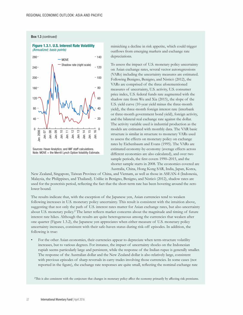
32
REGIONAL ECONOMIC OUTLOOK: AsIA ANd PACIfIC
International Monetary Fund | April 2016
mimicking a decline in risk appetite, which could trigger outflows from emerging markets and exchange rate depreciations.
To assess the impact of U.S. monetary policy uncertainty on Asian exchange rates, several vector autoregressions (VARs) including the uncertainty measures are estimated. Following Benigno, Benigno, and Nisticò (2012), the VARs are comprised of the three aforementioned measures of uncertainty, U.S. activity, U.S. consumer price index, U.S. federal funds rate augmented with the shadow rate from Wu and Xia (2015), the slope of the U.S. yield curve (10-year yield minus the three-month yield), the three-month foreign interest rate (interbank or three-month government bond yield), foreign activity, and the bilateral real exchange rate against the dollar. The activity variable used is industrial production as the models are estimated with monthly data. The VAR basic structure is similar in structure to monetary VARs used to assess the effects on monetary policy on exchange rates by Eichenbaum and Evans (1995). The VARs are estimated economy-by-economy (average effects across different economies are also calculated), and over two sample periods, the first covers 1990–2015, and the shorter sample starts in 2008. The economies covered are Australia, China, Hong Kong SAR, India, Japan, Korea,
New Zealand, Singapore, Taiwan Province of China, and Vietnam, as well as those in ASEAN-4 (Indonesia, Malaysia, the Philippines, and Thailand). Unlike in Benigno, Benigno, and Nisticò (2012), shadow rates are used for the postcrisis period, reflecting the fact that the short-term rate has been hovering around the zero lower bound.
The results indicate that, with the exception of the Japanese yen, Asian currencies tend to weaken following increases in U.S. monetary policy uncertainty. This result is consistent with the intuition above, suggesting that not only the path of U.S. interest rates matter for Asian exchange rates, but also uncertainty about U.S. monetary policy.2 The latter reflects market concerns about the magnitude and timing of future interest rate hikes. Although the results are quite heterogeneous among the currencies that weaken after one quarter (Figure 1.3.2), the Japanese yen appreciates when either measure of U.S. monetary policy uncertainty increases, consistent with their safe-haven status during risk-off episodes. In addition, the following is true:
• For the other Asian economies, their currencies appear to depreciate when term-structure volatility increases, but to various degrees. For instance, the impact of uncertainty shocks on the Indonesian rupiah seems particularly large and persistent, while the response of the Indian rupee is generally smaller. The response of the Australian dollar and the New Zealand dollar is also relatively large, consistent with previous episodes of sharp reversals in carry trades involving those currencies. In some cases (not reported in the figure), the exchange rate responses are quite small, reflecting the nominal exchange rate
2This is also consistent with the conjecture that changes in monetary policy affect the economy primarily by affecting risk premiums.
Figure 1.3.1. U.S. Interest Rate Volatility(Annualized; basis points)
Sources: Haver Analytics; and IMF staff calculations.Note: MOVE = the Merrill Lynch Option Volatility Estimate.
0
40
80
120
160
200
240
280
0
20
40
60
80
100
120
140
Jan.
200
6
Jan.
07
Jan.
08
Jan.
09
Jan.
10
Jan.
11
Jan.
12
Jan.
13
Jan.
14
Jan.
15
Jan.
16
MOVE
Shadow rate (right scale)
Box 1.3 (continued)
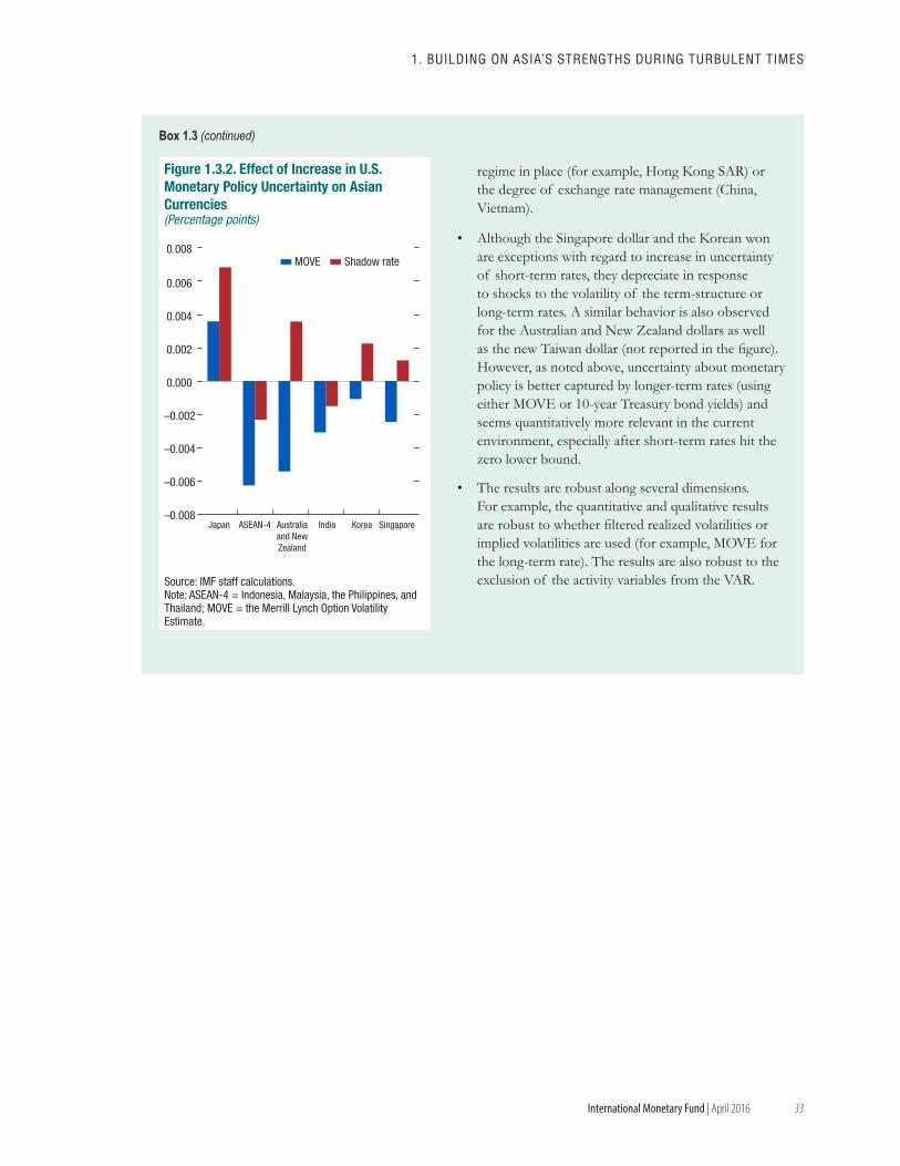
33
1. BUILdING ON AsIA’s sTRENGThs dURING TURBULENT TIMEs
International Monetary Fund | April 2016
regime in place (for example, Hong Kong SAR) or the degree of exchange rate management (China, Vietnam).
• Although the Singapore dollar and the Korean won are exceptions with regard to increase in uncertainty of short-term rates, they depreciate in response to shocks to the volatility of the term-structure or long-term rates. A similar behavior is also observed for the Australian and New Zealand dollars as well as the new Taiwan dollar (not reported in the figure). However, as noted above, uncertainty about monetary policy is better captured by longer-term rates (using either MOVE or 10-year Treasury bond yields) and seems quantitatively more relevant in the current environment, especially after short-term rates hit the zero lower bound.
• The results are robust along several dimensions. For example, the quantitative and qualitative results are robust to whether filtered realized volatilities or implied volatilities are used (for example, MOVE for the long-term rate). The results are also robust to the exclusion of the activity variables from the VAR.
–0.008
–0.006
–0.004
–0.002
0.000
0.002
0.004
0.006
0.008
Japan ASEAN-4 India Korea Singapore
MOVE Shadow rate
Australiaand NewZealand
Figure 1.3.2. Effect of Increase in U.S. Monetary Policy Uncertainty on Asian Currencies(Percentage points)
Source: IMF staff calculations.Note: ASEAN-4 = Indonesia, Malaysia, the Philippines, and Thailand; MOVE = the Merrill Lynch Option Volatility Estimate.
Box 1.3 (continued)
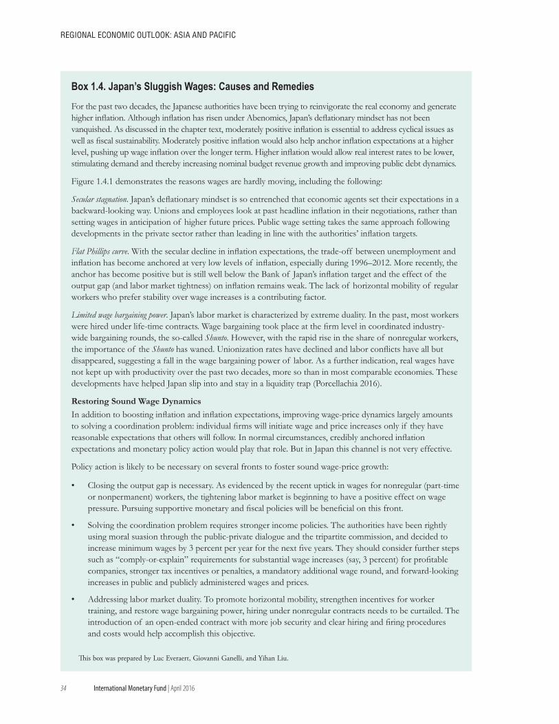
34
REGIONAL ECONOMIC OUTLOOK: AsIA ANd PACIfIC
International Monetary Fund | April 2016
For the past two decades, the Japanese authorities have been trying to reinvigorate the real economy and generate higher inflation. Although inflation has risen under Abenomics, Japan’s deflationary mindset has not been vanquished. As discussed in the chapter text, moderately positive inflation is essential to address cyclical issues as well as fiscal sustainability. Moderately positive inflation would also help anchor inflation expectations at a higher level, pushing up wage inflation over the longer term. Higher inflation would allow real interest rates to be lower, stimulating demand and thereby increasing nominal budget revenue growth and improving public debt dynamics.
Figure 1.4.1 demonstrates the reasons wages are hardly moving, including the following:
Secular stagnation. Japan’s deflationary mindset is so entrenched that economic agents set their expectations in a backward-looking way. Unions and employees look at past headline inflation in their negotiations, rather than setting wages in anticipation of higher future prices. Public wage setting takes the same approach following developments in the private sector rather than leading in line with the authorities’ inflation targets.
Flat Phillips curve. With the secular decline in inflation expectations, the trade-off between unemployment and inflation has become anchored at very low levels of inflation, especially during 1996–2012. More recently, the anchor has become positive but is still well below the Bank of Japan’s inflation target and the effect of the output gap (and labor market tightness) on inflation remains weak. The lack of horizontal mobility of regular workers who prefer stability over wage increases is a contributing factor.
Limited wage bargaining power. Japan’s labor market is characterized by extreme duality. In the past, most workers were hired under life-time contracts. Wage bargaining took place at the firm level in coordinated industry-wide bargaining rounds, the so-called Shunto. However, with the rapid rise in the share of nonregular workers, the importance of the Shunto has waned. Unionization rates have declined and labor conflicts have all but disappeared, suggesting a fall in the wage bargaining power of labor. As a further indication, real wages have not kept up with productivity over the past two decades, more so than in most comparable economies. These developments have helped Japan slip into and stay in a liquidity trap (Porcellachia 2016).
Restoring Sound Wage Dynamics In addition to boosting inflation and inflation expectations, improving wage-price dynamics largely amounts to solving a coordination problem: individual firms will initiate wage and price increases only if they have reasonable expectations that others will follow. In normal circumstances, credibly anchored inflation expectations and monetary policy action would play that role. But in Japan this channel is not very effective.
Policy action is likely to be necessary on several fronts to foster sound wage-price growth:
• Closing the output gap is necessary. As evidenced by the recent uptick in wages for nonregular (part-time or nonpermanent) workers, the tightening labor market is beginning to have a positive effect on wage pressure. Pursuing supportive monetary and fiscal policies will be beneficial on this front.
• Solving the coordination problem requires stronger income policies. The authorities have been rightly using moral suasion through the public-private dialogue and the tripartite commission, and decided to increase minimum wages by 3 percent per year for the next five years. They should consider further steps such as “comply-or-explain” requirements for substantial wage increases (say, 3 percent) for profitable companies, stronger tax incentives or penalties, a mandatory additional wage round, and forward-looking increases in public and publicly administered wages and prices.
• Addressing labor market duality. To promote horizontal mobility, strengthen incentives for worker training, and restore wage bargaining power, hiring under nonregular contracts needs to be curtailed. The introduction of an open-ended contract with more job security and clear hiring and firing procedures and costs would help accomplish this objective.
This box was prepared by Luc Everaert, Giovanni Ganelli, and Yihan Liu.
Box 1.4. Japan’s Sluggish Wages: Causes and Remedies
35
1. BUILdING ON AsIA’s sTRENGThs dURING TURBULENT TIMEs
International Monetary Fund | April 2016
Regular workers excluding executives (left scale)Nonregular workers (left scale)Share of nonregular workers (right scale)
–1
0
1
2
3
4
5
0 1 2 3 4 5
–2
–1
0
1
2
3
4
–10 –5 0 52.0
3.0
4.0
5.0
6.0
0.0
0.5
1.0
1.5
2.0
1992 95 98 01 04 07 10 13 15
5-year inflation expectation10-year inflation expectationHeadline without VATCore (excluding food and energy) without VAT
–2.0
–1.0
0.0
1.0
2.0
3.0
1992 93 94 95 96 97 98 99
2000 01 02 03 04 05 06 07 08 09 10 11 12 13 14 15
Composition effectChange in full-time wagesEmployment Compensation growth
3. Labor Market 4. Phillips Curve
Unemployment rateJob-opening-to-application ratio (right scale)
A: 1983:Q1–1995:Q4 y = 0.3x + 2.0
B: 1996:Q1–2012:Q3 y = 0.1x – 0.2
C: 2012:Q4–2015:Q3 y = 0.2x + 0.4
A
BC
Output gap
5. Regular and Nonregular Workers1 6. Real Wage and Productivity Growth2
(Percent)
Real
wag
e gr
owth
Labor productivity growth
45-degree line
Canada United KingdomUnited States
GermanyJapanItaly
France Korea
–4.0
–2.0
0.0
2.0
4.0
6.0
1994 97
2000 03 06 09 12 15
(Per
cent
)
(Ann
ual c
hang
e or
thou
sand
per
sons
)
Figure 1.4.1. Japan's Labor Market
–200–150–100–50050
100150
1015202530354045
1992 95 98 01 04 07 10 13 15
Escaping from deflation remains a challenge... ...as full time wages are hardly moving.
The labor market is very tight... ...but the Phillips curve is very flat.
Hiring consists mostly of nonregular workers... ...with real wages lagging productivity more thanelsewhere.
CPI a
ll ite
ms
min
us fo
od a
nden
ergy
with
out V
AT e
ffect
(yea
r-ov
er-y
ear)
Sources: Bank of Japan; Bloomberg, L.P.; Cabinet Office; Haver Analytics; Ministry of Internal Affairs and Communications; Organisation for Economic Co-operation and Development; and IMF staff estimates.Note: CPI = consumer price index; VAT = value added tax.1February 1985–2001, 2002–2015 January–March average.2Average of 1992–2014.
1. Inflation and Headline Inflation Expectations (Year-over-year; percent change)
2. Wage Growth (Year-over-year; percent change)
Box 1.4 (continued)
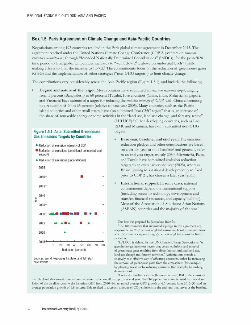
36
REGIONAL ECONOMIC OUTLOOK: AsIA ANd PACIfIC
International Monetary Fund | April 2016
Negotiations among 195 countries resulted in the Paris global climate agreement in December 2015. The agreement reached under the United Nations Climate Change Conference (COP 21) centers on national voluntary commitments, through “Intended Nationally Determined Contributions” (INDCs), for the post-2020 time period to limit global temperature increases to “well below 2°C above pre-industrial levels” (while making efforts to limit the increase to 1.5°C).1 The commitments focus on the reduction of greenhouse gases (GHG) and the implementation of other strategies (“non-GHG targets”) to limit climate change.
The contributions vary considerably across the Asia-Pacific region (Figure 1.5.1), and include the following:
• Degree and nature of the target: Most countries have submitted an emission reduction target, ranging from 5 percent (Bangladesh) to 60 percent (Tuvalu). Five countries (China, India, Malaysia, Singapore, and Vietnam) have submitted a target for reducing the emission intensity of GDP, with China committing to a reduction of 60 to 65 percent (relative to base year 2005). Many countries, such as the Pacific island countries and other small states, have also submitted “non-GHG targets,” that is, an increase of the share of renewable energy or some activities in the “land use, land-use change, and forestry sector”
(LULUCF).2 Other developing countries, such as Lao P.D.R. and Myanmar, have only submitted non-GHG targets.
• Base year, baseline, and end year: The emission reduction pledges and other contributions are based on a certain year or on a baseline3 and generally refer to an end year target, mostly 2030. Micronesia, Palau, and Tuvalu have committed emission reduction targets to an even earlier end year (2025), whereas Brunei, owing to a national development plan fixed prior to COP 21, has chosen a later year (2035).
• International support: In some cases, national commitments depend on international support (including access to technology development and transfer, financial resources, and capacity building). Most of the Association of Southeast Asian Nations (ASEAN) countries and the majority of the small
This box was prepared by Jacqueline Rothfels.1The 188 countries that submitted a pledge in this agreement are
responsible for 98.7 percent of global emissions. It will come into force when 55 countries representing 55 percent of global emissions have ratified it.
2LULUCF is defined by the UN Climate Change Secretariat as "A greenhouse gas inventory sector that covers emissions and removal of greenhouse gases resulting from direct human-induced land use, land-use change and forestry activities.” Activities can provide a relatively cost-effective way of offsetting emissions, either by increasing the removal of greenhouse gases from the atmosphere (for example, by planting trees), or by reducing emissions (for example, by curbing deforestation).
3Under the baseline scenario (business as usual, BAU), the emissions are calculated that would arise without emission reduction efforts up to the end year. The Philippines, for example, used for the calcu-lation of the baseline scenario the historical GDP from 2010–14, an annual average GDP growth of 6.5 percent from 2015–30, and an average population growth of 1.9 percent. This resulted in a certain amount of CO2 emissions in the end year that serves as the baseline.
Figure 1.5.1. Asia: Submitted GreenhouseGas Emissions Targets by Countries
Sources: World Resources Institute; and IMF staffcalculations.
2015
2020
2025
2030
2035
2040
2045
2050
2055
0 10 20 30 40 50 60 70 80
Reduction of emission intensity of GDP
Reduction of emissions (conditional on internationalsupport)
Reduction of emissions (unconditional)
Year
Reduction (percent)
Box 1.5. Paris Agreement on Climate Change and Asia-Pacific Countries
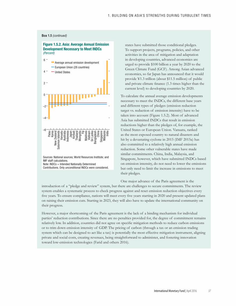
37
1. BUILdING ON AsIA’s sTRENGThs dURING TURBULENT TIMEs
International Monetary Fund | April 2016
states have submitted those conditional pledges. To support projects, programs, policies, and other activities in the area of mitigation and adaptation in developing countries, advanced economies are urged to provide $100 billion a year by 2020 to the Green Climate Fund (GCF). Among Asian advanced economies, so far Japan has announced that it would provide ¥1.3 trillion (about $11.5 million) of public and private climate finance (1.3 times higher than the current level) to developing countries by 2020.
To calculate the annual average emission developments necessary to meet the INDCs, the different base years and different types of pledges (emission reduction target vs. reduction of emission intensity) have to be taken into account (Figure 1.5.2). Most of advanced Asia has submitted INDCs that result in emission reductions higher than the pledges of, for example, the United States or European Union. Vanuatu, ranked as the most exposed country to natural disasters and hit by a devastating cyclone in 2015 (IMF 2015a) has also committed to a relatively high annual emission reduction. Some other vulnerable states have made similar commitments. China, India, Malaysia, and Singapore, however, which have submitted INDCs based on emission intensity, do not need to lower the emissions but only need to limit the increase in emissions to meet their pledges.
One major advance of the Paris agreement is the introduction of a “pledge and review” system, but there are challenges to secure commitments. The review system enables a systematic process to check progress against and reset emission reduction objectives every five years. To ensure compliance, nations will meet every five years starting in 2020 and present updated plans on raising their emission cuts. Starting in 2023, they will also have to update the international community on their progress.
However, a major shortcoming of the Paris agreement is the lack of a binding mechanism for individual parties’ reduction contributions. Since there are no penalties provided for, the degree of commitment remains relatively low. In addition, countries did not agree on specific mitigation methods to reduce carbon emissions or to trim down emission intensity of GDP. The pricing of carbon (through a tax or an emission trading system which can be designed to act like a tax) is potentially the most effective mitigation instrument, aligning private and social costs, creating revenues, being straightforward to administer, and fostering innovation toward low-emission technologies (Farid and others 2016).
Sources: National sources; World Resources Institute; and IMF staff calculations.Note: INDCs = Intended Nationally Determined Contributions. Only unconditional INDCs were considered.
–6
–4
–2
0
2
4
6
Pala
uKo
rea
New
Zea
land
Solo
mon
Isla
nds
Vanu
atu
Aust
ralia
Indo
nesi
aJa
pan
Kirib
ati
Thai
land
Mon
golia
Fi
jiM
aldi
ves
Viet
nam
Sri L
anka
Bang
lade
shCh
ina
Sing
apor
eM
alay
sia
Indi
a
Average annual emission development
European Union (28 countries)
United States
Figure 1.5.2. Asia: Average Annual Emission Development Necessary to Meet INDCs(Percent)
Box 1.5 (continued)
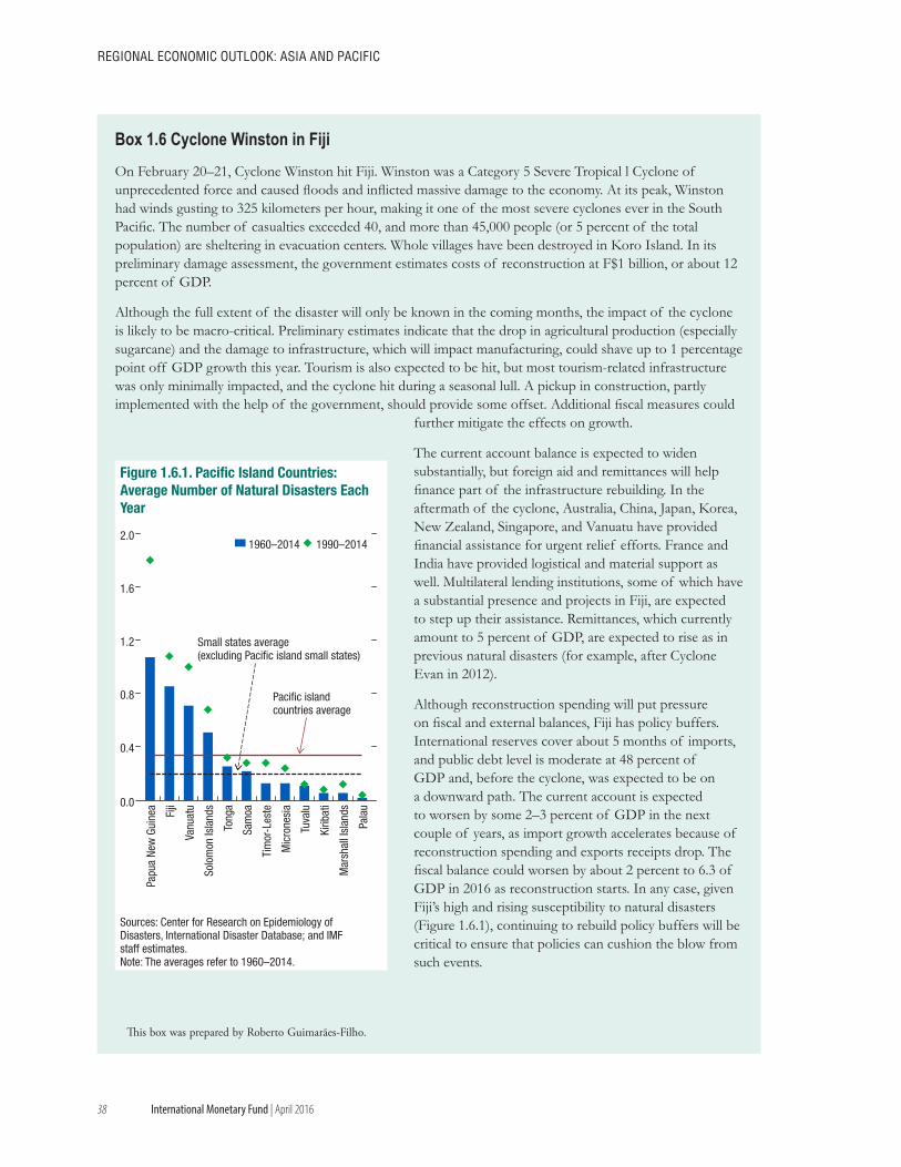
38
REGIONAL ECONOMIC OUTLOOK: AsIA ANd PACIfIC
International Monetary Fund | April 2016
On February 20–21, Cyclone Winston hit Fiji. Winston was a Category 5 Severe Tropical l Cyclone of unprecedented force and caused floods and inflicted massive damage to the economy. At its peak, Winston had winds gusting to 325 kilometers per hour, making it one of the most severe cyclones ever in the South Pacific. The number of casualties exceeded 40, and more than 45,000 people (or 5 percent of the total population) are sheltering in evacuation centers. Whole villages have been destroyed in Koro Island. In its preliminary damage assessment, the government estimates costs of reconstruction at F$1 billion, or about 12 percent of GDP.
Although the full extent of the disaster will only be known in the coming months, the impact of the cyclone is likely to be macro-critical. Preliminary estimates indicate that the drop in agricultural production (especially sugarcane) and the damage to infrastructure, which will impact manufacturing, could shave up to 1 percentage point off GDP growth this year. Tourism is also expected to be hit, but most tourism-related infrastructure was only minimally impacted, and the cyclone hit during a seasonal lull. A pickup in construction, partly implemented with the help of the government, should provide some offset. Additional fiscal measures could
further mitigate the effects on growth.
The current account balance is expected to widen substantially, but foreign aid and remittances will help finance part of the infrastructure rebuilding. In the aftermath of the cyclone, Australia, China, Japan, Korea, New Zealand, Singapore, and Vanuatu have provided financial assistance for urgent relief efforts. France and India have provided logistical and material support as well. Multilateral lending institutions, some of which have a substantial presence and projects in Fiji, are expected to step up their assistance. Remittances, which currently amount to 5 percent of GDP, are expected to rise as in previous natural disasters (for example, after Cyclone Evan in 2012).
Although reconstruction spending will put pressure on fiscal and external balances, Fiji has policy buffers. International reserves cover about 5 months of imports, and public debt level is moderate at 48 percent of GDP and, before the cyclone, was expected to be on a downward path. The current account is expected to worsen by some 2–3 percent of GDP in the next couple of years, as import growth accelerates because of reconstruction spending and exports receipts drop. The fiscal balance could worsen by about 2 percent to 6.3 of GDP in 2016 as reconstruction starts. In any case, given Fiji’s high and rising susceptibility to natural disasters (Figure 1.6.1), continuing to rebuild policy buffers will be critical to ensure that policies can cushion the blow from such events.
This box was prepared by Roberto Guimarães-Filho.
0.0
0.4
0.8
1.2
1.6
2.0
Papu
a Ne
w G
uine
a
Fiji
Vanu
atu
Solo
mon
Isla
nds
Tong
a
Sam
oa
Tim
or-L
este
Mic
rone
sia
Tuva
lu
Kirib
ati
Mar
shal
l Isl
ands
Pala
u
1960–2014 1990–2014
Small states average(excluding Pacific island small states)
Pacific islandcountries average
Figure 1.6.1. Pacific Island Countries: Average Number of Natural Disasters Each Year
Sources: Center for Research on Epidemiology of Disasters, International Disaster Database; and IMF staff estimates.Note: The averages refer to 1960–2014.
Box 1.6 Cyclone Winston in Fiji
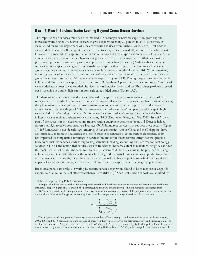
39
1. BUILdING ON AsIA’s sTRENGThs dURING TURBULENT TIMEs
International Monetary Fund | April 2016
The importance of services trade has risen markedly in recent years. Services exports in gross exports increased fivefold since 1995, with its share in gross exports reaching 20 percent in 2014. Moreover, in value-added terms, the importance of services exports has risen even further. For instance, latest trade in value added data as of 2011 suggest that services sectors’ exports surpassed 30 percent of the total exports. However, this may still not capture the full scope of services in gross exports as some tradable services may also be hidden in cross-border merchandise categories in the form of indirect services (that is, industries providing inputs into fragmented production processes in merchandise sectors).1 Although such indirect services are not explicitly categorized as cross-border exports, they amplify the importance of services in global trade by providing domestic services tasks such as research and development (R&D), procurement, marketing, and legal services. Hence when these indirect services are accounted for, the share of services in global trade rises to more than 50 percent of total exports (Figure 1.7.1). During the past two decades, both indirect and direct services exports have grown annually by about 7 percent on average in terms of both total value added and domestic value added. Services sectors in China, India, and the Philippines particularly stood out by growing at double-digit rates in domestic value-added terms (Figure 1.7.2).
The share of indirect services in domestic value-added exports also remains as substantial as that of direct services. Nearly one-third of services content in domestic value added in exports come from indirect services; this phenomenon is now common in many Asian economies as well as emerging market and advanced economies outside Asia (Figure 1.7.3). For instance, advanced economies’ comparative advantage in high value-added manufacturing products often relies on the comparative advantage these economies have in indirect services such as business services including R&D (Koopman, Wang, and Wei 2012). In Asia’s case, part of the success in the electronics and transportation equipment sectors in Japan and Korea is indeed driven by a high revealed comparative advantage (RCA) in indirect services that support these sectors (Figure 1.7.4).2 Compared to two decades ago, emerging Asian economies such as China and the Philippines have also attained a comparative advantage in services tasks in merchandise sectors such as electronics. India has improved its comparative advantage in services, but mostly in direct services categories that provide horizontal business services, such as supporting activities including accounting and information technology services. All in all, the notion that services are not tradable to the same extent as manufactured goods and for the most part do not exhibit the same technology dynamism could be misleading in the presence of rising indirect services that not only enter the value added of goods exported, but also increase productivity and competitiveness of a country’s merchandise exports. Against this backdrop, it is important to account for the impact of exchange rate changes on indirect and direct services exports when gauging competitiveness.
Based on a panel data analysis covering 18 sectors, services exports are found to be as responsive as goods exports to changes in the real effective exchange rates (REERs).3 Specifically, when exports are adjusted by
This box was prepared by Dulani Seneviratne.1Examples of indirect services include industry-specific research and development in industries such as electronics and machinery,
intellectual property rights, clinical trials in the pharmaceutical industry, and industry-specific risk management research tasks.2RCA in services is defined as the proportion of services in sector s in country i, as a ratio of the proportion of services in sector s in
the world. An RCA above 1 suggests that country i has a revealed comparative advantage in services tasks in that sector.
RCA = ( DVAi ,s ) Σs=1…nDVAi,s
( DVAw ,s ) Σs=1…nDVAw,s
3The analysis is based on a panel with country-industry-time fixed effects covering 18 industries and 52 countries for years 1995, 2000, 2005, and 2010; standard errors are clustered at country-industry level to correct for heteroskedasticity and autocorrelation. The baseline specification is: ∆Xi,s,t = at + ai,s +at,s + ai,t + β1∆REERi,s,t + β2∆Yw,t + εi,s,t , where ∆Xi,s,t is the change in volume of exports at time t measured by domestic value added in exports deflated using GDP deflators, ∆REERi,s,t is the change in country-industry-specific
Box 1.7. Rise in Services Trade: Looking Beyond Cross-Border Services
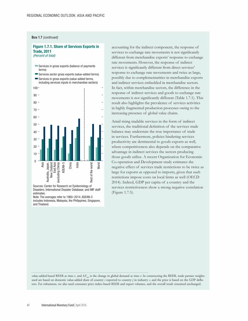
REGIONAL ECONOMIC OUTLOOK: AsIA ANd PACIfIC
40 International Monetary Fund | April 2016
accounting for the indirect component, the response of services to exchange rate movements is not significantly different from merchandise exports’ response to exchange rate movements. However, the response of indirect services is significantly different from direct services’ response to exchange rate movements and twice as large, possibly due to complementarities in merchandise exports and indirect services embedded in merchandise sectors. In fact, within merchandise sectors, the difference in the response of indirect services and goods to exchange rate movements is not significantly different (Table 1.7.1). This result also highlights the prevalence of services activities in highly fragmented production processes owing to the increasing presence of global value chains.
Amid rising tradable services in the form of indirect services, the traditional definition of the services trade balance may understate the true importance of trade in services. Furthermore, policies hindering services productivity are detrimental to goods exports as well, where competitiveness also depends on the comparative advantage in indirect services the sectors producing those goods utilize. A recent Organization for Economic Co-operation and Development study estimates the negative effect of services trade restrictions to be twice as large for exports as opposed to imports, given that such restrictions impose costs on local firms as well (OECD 2014). Indeed, GDP per capita of a country and the services restrictiveness show a strong negative correlation (Figure 1.7.5).
value-added-based REER at time t, and ∆Yw,t is the change in global demand at time t. In constructing the REER, trade partner weights used are based on domestic value-added share of country i exported to country j in industry s, and the price is based on the GDP defla-tors. For robustness, we also used consumer price index–based REER and export volumes, and the overall result remained unchanged.
0
10
20
30
40
50
60
70
80
90
100
Services in gross exports (balance of paymentsterms) Services sector gross exports (value-added terms)Services in gross exports (value-added terms,including services inputs in merchandise sectors)
Figure 1.7.1. Share of Services Exports in Trade, 2011(Percent of total)
Sources: Center for Research on Epidemiology of Disasters, International Disaster Database; and IMF staff estimates.Note: The averages refer to 1960–2014. ASEAN-5 includes Indonesia, Malaysia, the Philippines, Singapore, and Thailand.
Aust
ralia
, Jap
an,
New
Zea
land
East
Asi
a(e
xclu
ding
Chi
na)
ASEA
N-5
Chin
a
Indi
a
Asia
Wor
ld
Rest
of t
he w
orld
Box 1.7 (continued)
1. BUILdING ON AsIA’s sTRENGThs dURING TURBULENT TIMEs
41International Monetary Fund | April 2016
0
5
10
15
20
25
Merchandise exports
Direct services exports
Indirect services
Aust
ralia
, Jap
an,
New
Zea
land
East
Asi
a(e
xclu
ding
Chi
na)
ASEA
N-5
Chin
a
Indi
a
Rest
of t
he w
orld
Wor
ld
Figure 1.7.2. Annual Average Growth in Domestic Value-Added Content in Exports, 1995–2011(Percent)
Sources: IMF, Balance of Payments Yearbook database; Organisation for Economic Co-operation and Development and World Trade Organization, Trade in Value-Added database; and IMF staff calculations.Note: ASEAN-5 includes Indonesia, Malaysia, the Philippines, Singapore, and Thailand.
0
20
40
60
80
Aust
ralia
, Jap
an,
New
Zea
land
East
Asi
a (e
xclu
ding
Chi
na)
ASEA
N-5
Chin
a
Indi
a
Rest
of t
he w
orld
3449
2634
3730
171415121721
Services exports
Indirect services in merchandise exports
Figure 1.7.3. Share of Direct and Indirect Services Content in Domestic Value Added in Exports, 2011(Percent of total domestic value added in exports)
Sources: IMF, Balance of Payments Yearbook database; Organisation for Economic Co-operation and Development and World Trade Organization, Trade in Value-Added database; and IMF staff calculations.Note: ASEAN-5 includes Indonesia, Malaysia, the Philippines, Singapore, and Thailand.
Figure 1.7.4. Revealed Comparative Advantage (RCA) in Services Tasks in Selected Merchandise and Services Sectors
RCA above 1 RCA above 2
Food andbeverages Textiles Chemicals Basic metals Electronics
Transport equipment
Machinery, equipment
(other)
Wholesale, retail, hotels
Transportation and Com.
Financial intermediation
Business services
Australia 2.3 0.3 0.6 2.1 0.1 0.3 0.5 0.3 0.5 1.6 0.3 0.6Japan 0.1 0.3 1.3 1.7 2.6 2.4 1.9 1.7 0.8 1.3 0.2 0.2Korea 0.3 0.9 0.9 1.2 2.6 1.8 1.2 0.3 1.0 1.4 0.5 0.6New Zealand 5.7 1.0 0.5 0.9 0.3 0.1 0.3 0.4 1.4 1.1 0.1 0.3China 0.5 5.0 0.8 1.4 3.5 0.5 1.4 2.7 1.4 0.3 0.0 0.4Taiwan Province of China 0.2 1.3 1.3 1.9 3.9 0.5 0.9 0.8 1.8 0.6 0.2 0.1Hong Kong SAR 0.0 0.0 0.2 0.0 0.1 0.0 0.0 0.0 3.3 1.1 1.8 0.9India 0.5 1.8 0.7 0.7 0.9 0.4 0.4 4.1 0.6 0.5 0.5 2.7Indonesia 2.9 2.7 1.0 1.0 1.1 0.4 1.2 1.5 0.7 1.3 0.1 0.4Malaysia 0.6 0.5 1.8 0.2 0.8 0.1 0.7 0.2 1.4 1.1 0.3 0.4Philippines 0.1 0.7 0.1 0.1 4.0 0.4 0.2 0.1 2.7 0.8 0.7 0.4Singapore 0.2 0.0 1.4 0.2 0.7 0.2 0.4 0.3 1.9 1.5 1.7 0.7Thailand 1.7 2.3 0.6 0.4 1.8 0.2 0.3 2.2 2.1 1.6 0.0 0.3
Source: IMF staff calculations.
Manufacturing(other)
Box 1.7 (continued)
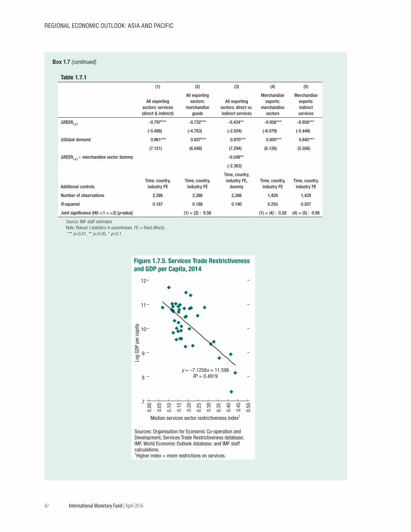
REGIONAL ECONOMIC OUTLOOK: AsIA ANd PACIfIC
42 International Monetary Fund | April 2016
Figure 1.7.5. Services Trade Restrictivenessand GDP per Capita, 2014
7
8
9
10
11
12
0.00
0.05
0.10
0.15
0.20
0.25
0.30
0.35
0.40
0.45
0.50
Log
GDP
per c
apita
Median services sector restrictiveness index1
y = –7.1258x + 11.598R² = 0.4919
Sources: Organisation for Economic Co-operation and Development, Services Trade Restrictiveness database; IMF, World Economic Outlook database; and IMF staff calculations.1Higher index = more restrictions on services.
Table 1.7.1(1) (2) (3) (4) (5)
All exporting sectors: services (direct & indirect)
All exporting sectors:
merchandise goods
All exporting sectors: direct vs. indirect services
Merchandise exports:
merchandise sectors
Merchandise exports: indirect services
ΔREERi,s,t -0.797*** -0.732*** -0.434** -0.956*** -0.958***
(-5.488) (-4.783) (-2.024) (-6.079) (-5.446)
ΔGlobal demand 0.961*** 0.937*** 0.970*** 0.805*** 0.845***
(7.151) (6.048) (7.294) (6.126) (5.506)
ΔREERi,s,t × merchandise sector dummy -0.549**
(-2.363)
Additional controlsTime, country,
industry FETime, country,
industry FE
Time, country, industry FE,
dummyTime, country,
industry FETime, country,
industry FE
Number of observations 2,386 2,386 2,386 1,428 1,428
R-squared 0.187 0.188 0.190 0.255 0.207
Joint significance (H0: a1 = a2) [p-value] (1) = (2) : 0.56 (1) = (4) : 0.28 (4) = (5) : 0.98
Source: IMF staff estimatesNote: Robust t-statistics in parentheses. FE = fixed effects. *** p<0.01, ** p<0.05, * p<0.1.
Box 1.7 (continued)
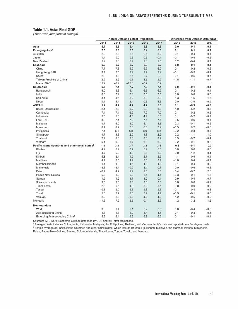
1. BUILdING ON AsIA’s sTRENGThs dURING TURBULENT TIMEs
43International Monetary Fund | April 2016
1. BUILdING ON AsIA’s sTRENGThs dURING TURBULENT TIMEs
International Monetary Fund | April 2016
Table 1.1. Asia: Real GDP(Year-over-year percent change)
Actual Data and Latest Projections Difference from October 2015 WEO2013 2014 2015 2016 2017 2015 2016 2017
Asia 5.7 5.6 5.4 5.3 5.3 0.0 –0.1 –0.1Emerging Asia1 7.0 6.8 6.6 6.4 6.3 0.1 0.1 0.1Australia 2.0 2.6 2.5 2.5 3.0 0.1 –0.4 –0.1Japan 1.4 0.0 0.5 0.5 –0.1 –0.1 –0.5 –0.5New Zealand 1.7 3.0 3.4 2.0 2.5 1.2 –0.4 0.1East Asia 6.9 6.7 6.2 5.9 5.7 0.0 0.1 0.1
China 7.7 7.3 6.9 6.5 6.2 0.1 0.2 0.2Hong Kong SAR 3.1 2.6 2.4 2.2 2.4 –0.1 –0.5 –0.4Korea 2.9 3.3 2.6 2.7 2.9 –0.1 –0.5 –0.7Taiwan Province of China 2.2 3.9 0.7 1.5 2.2 –1.5 –1.1 –0.7Macao SAR 11.2 –0.9 –20.3 –7.2 0.7 … … …
South Asia 6.5 7.1 7.2 7.3 7.4 0.0 –0.1 –0.1Bangladesh 6.0 6.3 6.4 6.6 6.9 –0.1 –0.2 –0.1India 6.6 7.2 7.3 7.5 7.5 0.0 0.0 0.0Sri Lanka 3.4 4.5 5.2 5.0 5.0 –1.3 –1.5 –1.5Nepal 4.1 5.4 3.4 0.5 4.5 0.0 –3.9 –0.9
ASEAN 5.2 4.7 4.7 4.7 5.0 0.1 –0.3 –0.3Brunei Darussalam –2.1 –2.3 –0.2 –2.0 3.0 1.0 –5.2 –0.8Cambodia 7.4 7.1 6.9 7.0 7.0 –0.1 –0.2 –0.2Indonesia 5.6 5.0 4.8 4.9 5.3 0.1 –0.2 –0.2Lao P.D.R. 8.0 7.4 7.0 7.4 7.4 –0.5 –0.6 –0.1Malaysia 4.7 6.0 5.0 4.4 4.8 0.3 –0.1 –0.2Myanmar 8.4 8.7 7.0 8.6 7.7 –1.5 0.2 –0.6Philippines 7.1 6.1 5.8 6.0 6.2 –0.2 –0.3 –0.3Singapore 4.7 3.3 2.0 1.8 2.2 –0.2 –1.1 –1.0Thailand 2.7 0.8 2.8 3.0 3.2 0.3 –0.2 –0.4Vietnam 5.4 6.0 6.7 6.3 6.2 0.2 –0.1 0.2
Pacific island countries and other small states2 1.8 3.3 3.7 3.3 3.4 0.1 –0.1 0.3Bhutan 4.9 6.4 7.7 8.4 8.6 0.0 0.0 0.0Fiji 4.7 5.3 4.3 2.5 3.9 0.0 –1.2 0.4Kiribati 5.8 2.4 4.2 2.7 2.5 1.1 0.9 0.4Maldives 4.7 6.5 1.9 3.5 3.9 –1.0 0.4 –0.1Marshall Islands –1.1 1.0 1.6 1.8 1.8 –0.1 –0.4 0.0Micronesia –3.6 –3.4 –0.2 1.1 0.7 0.0 –0.6 –0.3Palau –2.4 4.2 9.4 2.0 5.0 5.4 –0.7 2.5Papua New Guinea 5.5 8.5 9.0 3.1 4.4 –3.3 0.1 1.3Samoa –1.9 1.2 1.7 1.2 –0.1 –0.9 –0.4 0.7Solomon Islands 3.0 2.0 3.3 3.0 3.3 0.0 0.0 –0.2Timor-Leste 2.8 5.5 4.3 5.0 5.5 0.0 0.0 0.0Tonga –0.6 2.0 2.6 2.8 2.6 –0.1 0.4 0.6Tuvalu 1.3 2.2 2.6 3.9 1.9 –0.9 –0.1 0.0Vanuatu 2.0 2.3 –0.8 4.5 4.0 1.2 –0.5 –0.5
Mongolia 11.6 7.9 2.3 0.4 2.5 –1.2 –3.2 –1.2
MemorandumWorld 3.3 3.4 3.1 3.2 3.5 0.0 –0.4 –0.3Asia excluding China 4.3 4.3 4.2 4.4 4.6 –0.1 –0.3 –0.3Emerging Asia excluding China1 5.9 6.1 6.2 6.3 6.5 0.1 –0.1 –0.1
Sources: IMF, World Economic Outlook database (WEO); and IMF staff projections.1 Emerging Asia includes China, India, Indonesia, Malaysia, the Philippines, Thailand, and Vietnam. India's data are reported on a fiscal-year basis. 2 Simple average of Pacific island countries and other small states, which include Bhutan, Fiji, Kiribati, Maldives, the Marshall Islands, Micronesia, Palau, Papua New Guinea, Samoa, Solomon Islands, Timor-Leste, Tonga, Tuvalu, and Vanuatu.
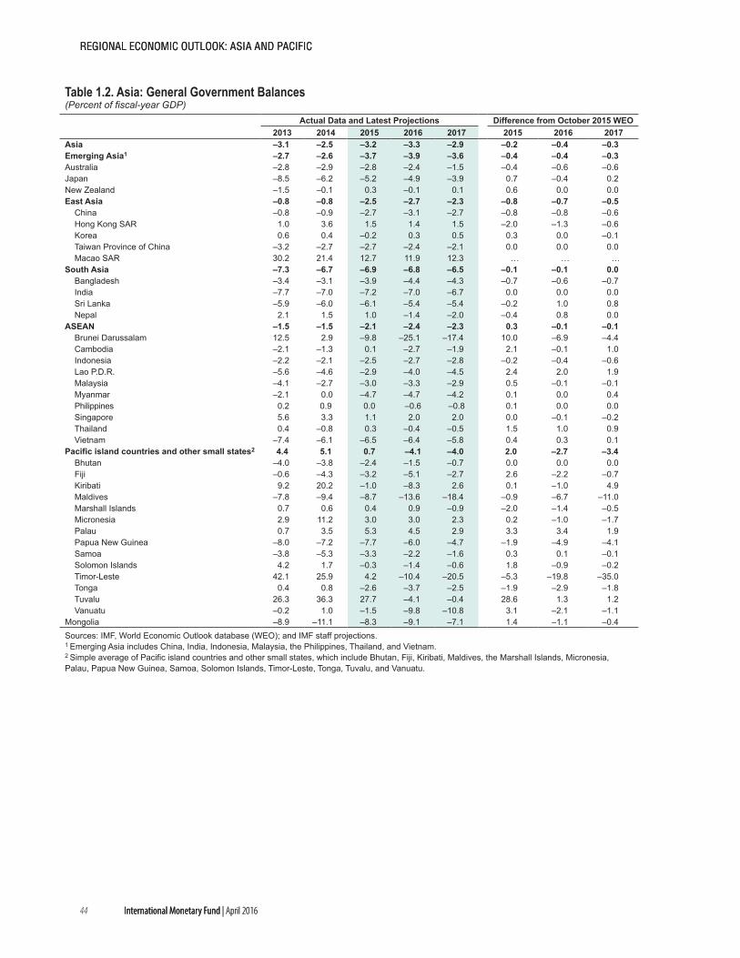
REGIONAL ECONOMIC OUTLOOK: AsIA ANd PACIfIC
44 International Monetary Fund | April 2016
REGIONAL ECONOMIC OUTLOOK: AsIA ANd PACIfIC
International Monetary Fund | April 2016
Table 1.2. Asia: General Government Balances(Percent of fiscal-year GDP)
Actual Data and Latest Projections Difference from October 2015 WEO2013 2014 2015 2016 2017 2015 2016 2017
Asia –3.1 –2.5 –3.2 –3.3 –2.9 –0.2 –0.4 –0.3Emerging Asia1 –2.7 –2.6 –3.7 –3.9 –3.6 –0.4 –0.4 –0.3Australia –2.8 –2.9 –2.8 –2.4 –1.5 –0.4 –0.6 –0.6Japan –8.5 –6.2 –5.2 –4.9 –3.9 0.7 –0.4 0.2New Zealand –1.5 –0.1 0.3 –0.1 0.1 0.6 0.0 0.0East Asia –0.8 –0.8 –2.5 –2.7 –2.3 –0.8 –0.7 –0.5
China –0.8 –0.9 –2.7 –3.1 –2.7 –0.8 –0.8 –0.6Hong Kong SAR 1.0 3.6 1.5 1.4 1.5 –2.0 –1.3 –0.6Korea 0.6 0.4 –0.2 0.3 0.5 0.3 0.0 –0.1Taiwan Province of China –3.2 –2.7 –2.7 –2.4 –2.1 0.0 0.0 0.0Macao SAR 30.2 21.4 12.7 11.9 12.3 … … …
South Asia –7.3 –6.7 –6.9 –6.8 –6.5 –0.1 –0.1 0.0Bangladesh –3.4 –3.1 –3.9 –4.4 –4.3 –0.7 –0.6 –0.7India –7.7 –7.0 –7.2 –7.0 –6.7 0.0 0.0 0.0Sri Lanka –5.9 –6.0 –6.1 –5.4 –5.4 –0.2 1.0 0.8Nepal 2.1 1.5 1.0 –1.4 –2.0 –0.4 0.8 0.0
ASEAN –1.5 –1.5 –2.1 –2.4 –2.3 0.3 –0.1 –0.1Brunei Darussalam 12.5 2.9 –9.8 –25.1 –17.4 10.0 –6.9 –4.4Cambodia –2.1 –1.3 0.1 –2.7 –1.9 2.1 –0.1 1.0Indonesia –2.2 –2.1 –2.5 –2.7 –2.8 –0.2 –0.4 –0.6Lao P.D.R. –5.6 –4.6 –2.9 –4.0 –4.5 2.4 2.0 1.9Malaysia –4.1 –2.7 –3.0 –3.3 –2.9 0.5 –0.1 –0.1Myanmar –2.1 0.0 –4.7 –4.7 –4.2 0.1 0.0 0.4Philippines 0.2 0.9 0.0 –0.6 –0.8 0.1 0.0 0.0Singapore 5.6 3.3 1.1 2.0 2.0 0.0 –0.1 –0.2Thailand 0.4 –0.8 0.3 –0.4 –0.5 1.5 1.0 0.9Vietnam –7.4 –6.1 –6.5 –6.4 –5.8 0.4 0.3 0.1
Pacific island countries and other small states2 4.4 5.1 0.7 –4.1 –4.0 2.0 –2.7 –3.4Bhutan –4.0 –3.8 –2.4 –1.5 –0.7 0.0 0.0 0.0Fiji –0.6 –4.3 –3.2 –5.1 –2.7 2.6 –2.2 –0.7Kiribati 9.2 20.2 –1.0 –8.3 2.6 0.1 –1.0 4.9Maldives –7.8 –9.4 –8.7 –13.6 –18.4 –0.9 –6.7 –11.0Marshall Islands 0.7 0.6 0.4 0.9 –0.9 –2.0 –1.4 –0.5Micronesia 2.9 11.2 3.0 3.0 2.3 0.2 –1.0 –1.7Palau 0.7 3.5 5.3 4.5 2.9 3.3 3.4 1.9Papua New Guinea –8.0 –7.2 –7.7 –6.0 –4.7 –1.9 –4.9 –4.1Samoa –3.8 –5.3 –3.3 –2.2 –1.6 0.3 0.1 –0.1Solomon Islands 4.2 1.7 –0.3 –1.4 –0.6 1.8 –0.9 –0.2Timor-Leste 42.1 25.9 4.2 –10.4 –20.5 –5.3 –19.8 –35.0Tonga 0.4 0.8 –2.6 –3.7 –2.5 –1.9 –2.9 –1.8Tuvalu 26.3 36.3 27.7 –4.1 –0.4 28.6 1.3 1.2Vanuatu –0.2 1.0 –1.5 –9.8 –10.8 3.1 –2.1 –1.1
Mongolia –8.9 –11.1 –8.3 –9.1 –7.1 1.4 –1.1 –0.4Sources: IMF, World Economic Outlook database (WEO); and IMF staff projections.1 Emerging Asia includes China, India, Indonesia, Malaysia, the Philippines, Thailand, and Vietnam. 2 Simple average of Pacific island countries and other small states, which include Bhutan, Fiji, Kiribati, Maldives, the Marshall Islands, Micronesia, Palau, Papua New Guinea, Samoa, Solomon Islands, Timor-Leste, Tonga, Tuvalu, and Vanuatu.
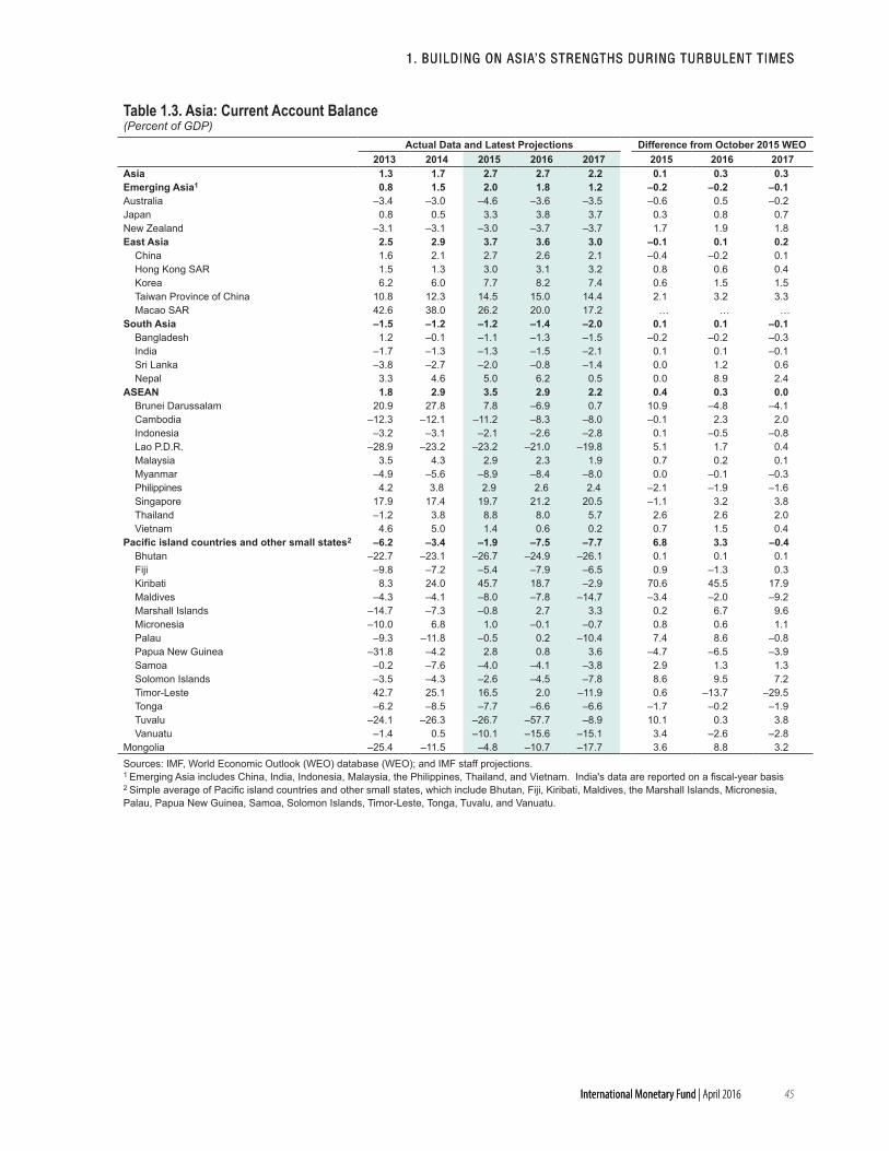
1. BUILdING ON AsIA’s sTRENGThs dURING TURBULENT TIMEs
45International Monetary Fund | April 2016
1. BUILdING ON AsIA’s sTRENGThs dURING TURBULENT TIMEs
International Monetary Fund | April 2016
Table 1.3. Asia: Current Account Balance(Percent of GDP)
Actual Data and Latest Projections Difference from October 2015 WEO2013 2014 2015 2016 2017 2015 2016 2017
Asia 1.3 1.7 2.7 2.7 2.2 0.1 0.3 0.3Emerging Asia1 0.8 1.5 2.0 1.8 1.2 –0.2 –0.2 –0.1Australia –3.4 –3.0 –4.6 –3.6 –3.5 –0.6 0.5 –0.2Japan 0.8 0.5 3.3 3.8 3.7 0.3 0.8 0.7New Zealand –3.1 –3.1 –3.0 –3.7 –3.7 1.7 1.9 1.8East Asia 2.5 2.9 3.7 3.6 3.0 –0.1 0.1 0.2
China 1.6 2.1 2.7 2.6 2.1 –0.4 –0.2 0.1Hong Kong SAR 1.5 1.3 3.0 3.1 3.2 0.8 0.6 0.4Korea 6.2 6.0 7.7 8.2 7.4 0.6 1.5 1.5Taiwan Province of China 10.8 12.3 14.5 15.0 14.4 2.1 3.2 3.3Macao SAR 42.6 38.0 26.2 20.0 17.2 … … …
South Asia –1.5 –1.2 –1.2 –1.4 –2.0 0.1 0.1 –0.1Bangladesh 1.2 –0.1 –1.1 –1.3 –1.5 –0.2 –0.2 –0.3India –1.7 –1.3 –1.3 –1.5 –2.1 0.1 0.1 –0.1Sri Lanka –3.8 –2.7 –2.0 –0.8 –1.4 0.0 1.2 0.6Nepal 3.3 4.6 5.0 6.2 0.5 0.0 8.9 2.4
ASEAN 1.8 2.9 3.5 2.9 2.2 0.4 0.3 0.0Brunei Darussalam 20.9 27.8 7.8 –6.9 0.7 10.9 –4.8 –4.1Cambodia –12.3 –12.1 –11.2 –8.3 –8.0 –0.1 2.3 2.0Indonesia –3.2 –3.1 –2.1 –2.6 –2.8 0.1 –0.5 –0.8Lao P.D.R. –28.9 –23.2 –23.2 –21.0 –19.8 5.1 1.7 0.4Malaysia 3.5 4.3 2.9 2.3 1.9 0.7 0.2 0.1Myanmar –4.9 –5.6 –8.9 –8.4 –8.0 0.0 –0.1 –0.3Philippines 4.2 3.8 2.9 2.6 2.4 –2.1 –1.9 –1.6Singapore 17.9 17.4 19.7 21.2 20.5 –1.1 3.2 3.8Thailand –1.2 3.8 8.8 8.0 5.7 2.6 2.6 2.0Vietnam 4.6 5.0 1.4 0.6 0.2 0.7 1.5 0.4
Pacific island countries and other small states2 –6.2 –3.4 –1.9 –7.5 –7.7 6.8 3.3 –0.4Bhutan –22.7 –23.1 –26.7 –24.9 –26.1 0.1 0.1 0.1Fiji –9.8 –7.2 –5.4 –7.9 –6.5 0.9 –1.3 0.3Kiribati 8.3 24.0 45.7 18.7 –2.9 70.6 45.5 17.9Maldives –4.3 –4.1 –8.0 –7.8 –14.7 –3.4 –2.0 –9.2Marshall Islands –14.7 –7.3 –0.8 2.7 3.3 0.2 6.7 9.6Micronesia –10.0 6.8 1.0 –0.1 –0.7 0.8 0.6 1.1Palau –9.3 –11.8 –0.5 0.2 –10.4 7.4 8.6 –0.8Papua New Guinea –31.8 –4.2 2.8 0.8 3.6 –4.7 –6.5 –3.9Samoa –0.2 –7.6 –4.0 –4.1 –3.8 2.9 1.3 1.3Solomon Islands –3.5 –4.3 –2.6 –4.5 –7.8 8.6 9.5 7.2Timor-Leste 42.7 25.1 16.5 2.0 –11.9 0.6 –13.7 –29.5Tonga –6.2 –8.5 –7.7 –6.6 –6.6 –1.7 –0.2 –1.9Tuvalu –24.1 –26.3 –26.7 –57.7 –8.9 10.1 0.3 3.8Vanuatu –1.4 0.5 –10.1 –15.6 –15.1 3.4 –2.6 –2.8
Mongolia –25.4 –11.5 –4.8 –10.7 –17.7 3.6 8.8 3.2Sources: IMF, World Economic Outlook (WEO) database (WEO); and IMF staff projections.1 Emerging Asia includes China, India, Indonesia, Malaysia, the Philippines, Thailand, and Vietnam. India's data are reported on a fiscal-year basis 2 Simple average of Pacific island countries and other small states, which include Bhutan, Fiji, Kiribati, Maldives, the Marshall Islands, Micronesia, Palau, Papua New Guinea, Samoa, Solomon Islands, Timor-Leste, Tonga, Tuvalu, and Vanuatu.
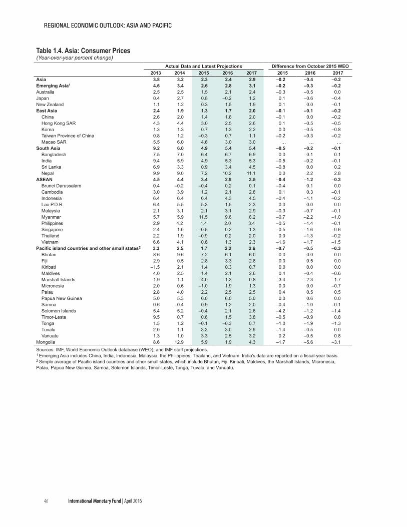
REGIONAL ECONOMIC OUTLOOK: AsIA ANd PACIfIC
46 International Monetary Fund | April 2016
REGIONAL ECONOMIC OUTLOOK: AsIA ANd PACIfIC
International Monetary Fund | April 2016
Table 1.4. Asia: Consumer Prices(Year-over-year percent change)
Actual Data and Latest Projections Difference from October 2015 WEO2013 2014 2015 2016 2017 2015 2016 2017
Asia 3.8 3.2 2.3 2.4 2.9 –0.2 –0.4 –0.2Emerging Asia1 4.6 3.4 2.6 2.8 3.1 –0.2 –0.3 –0.2Australia 2.5 2.5 1.5 2.1 2.4 –0.3 –0.5 0.0Japan 0.4 2.7 0.8 –0.2 1.2 0.1 –0.6 –0.4New Zealand 1.1 1.2 0.3 1.5 1.9 0.1 0.0 –0.1East Asia 2.4 1.9 1.3 1.7 2.0 –0.1 –0.1 –0.2
China 2.6 2.0 1.4 1.8 2.0 –0.1 0.0 –0.2Hong Kong SAR 4.3 4.4 3.0 2.5 2.6 0.1 –0.5 –0.5Korea 1.3 1.3 0.7 1.3 2.2 0.0 –0.5 –0.8Taiwan Province of China 0.8 1.2 –0.3 0.7 1.1 –0.2 –0.3 –0.2Macao SAR 5.5 6.0 4.6 3.0 3.0 … … …
South Asia 9.2 6.0 4.9 5.4 5.4 –0.5 –0.2 –0.1Bangladesh 7.5 7.0 6.4 6.7 6.9 0.0 0.1 0.1India 9.4 5.9 4.9 5.3 5.3 –0.5 –0.2 –0.1Sri Lanka 6.9 3.3 0.9 3.4 4.5 –0.8 0.0 0.2Nepal 9.9 9.0 7.2 10.2 11.1 0.0 2.2 2.8
ASEAN 4.5 4.4 3.4 2.9 3.5 –0.4 –1.2 –0.3Brunei Darussalam 0.4 –0.2 –0.4 0.2 0.1 –0.4 0.1 0.0Cambodia 3.0 3.9 1.2 2.1 2.8 0.1 0.3 –0.1Indonesia 6.4 6.4 6.4 4.3 4.5 –0.4 –1.1 –0.2Lao P.D.R. 6.4 5.5 5.3 1.5 2.3 0.0 0.0 0.0Malaysia 2.1 3.1 2.1 3.1 2.9 –0.3 –0.7 –0.1Myanmar 5.7 5.9 11.5 9.6 8.2 –0.7 –2.2 –1.0Philippines 2.9 4.2 1.4 2.0 3.4 –0.5 –1.4 –0.1Singapore 2.4 1.0 –0.5 0.2 1.3 –0.5 –1.6 –0.6Thailand 2.2 1.9 –0.9 0.2 2.0 0.0 –1.3 –0.2Vietnam 6.6 4.1 0.6 1.3 2.3 –1.6 –1.7 –1.5
Pacific island countries and other small states2 3.3 2.5 1.7 2.2 2.6 –0.7 –0.5 –0.3Bhutan 8.6 9.6 7.2 6.1 6.0 0.0 0.0 0.0Fiji 2.9 0.5 2.8 3.3 2.8 0.0 0.5 0.0Kiribati –1.5 2.1 1.4 0.3 0.7 0.0 0.0 0.0Maldives 4.0 2.5 1.4 2.1 2.6 0.4 –0.4 –0.6Marshall Islands 1.9 1.1 –4.0 –1.3 0.8 –3.4 –2.3 –1.7Micronesia 2.0 0.6 –1.0 1.9 1.3 0.0 0.0 –0.7Palau 2.8 4.0 2.2 2.5 2.5 0.4 0.5 0.5Papua New Guinea 5.0 5.3 6.0 6.0 5.0 0.0 0.6 0.0Samoa 0.6 –0.4 0.9 1.2 2.0 –0.4 –1.0 –0.1Solomon Islands 5.4 5.2 –0.4 2.1 2.6 –4.2 –1.2 –1.4Timor-Leste 9.5 0.7 0.6 1.5 3.8 –0.5 –0.9 0.8Tonga 1.5 1.2 –0.1 –0.3 0.7 –1.0 –1.9 –1.3Tuvalu 2.0 1.1 3.3 3.0 2.9 –1.4 –0.5 0.0Vanuatu 1.3 1.0 3.3 2.5 3.2 0.2 –0.5 0.8
Mongolia 8.6 12.9 5.9 1.9 4.3 –1.7 –5.6 –3.1Sources: IMF, World Economic Outlook database (WEO); and IMF staff projections.1 Emerging Asia includes China, India, Indonesia, Malaysia, the Philippines, Thailand, and Vietnam. India's data are reported on a fiscal-year basis. 2 Simple average of Pacific island countries and other small states, which include Bhutan, Fiji, Kiribati, Maldives, the Marshall Islands, Micronesia, Palau, Papua New Guinea, Samoa, Solomon Islands, Timor-Leste, Tonga, Tuvalu, and Vanuatu.
International Monetary Fund | April 2016
Introduction and Main FindingsThe Chinese economy is undergoing substantial structural change to a model driven increasingly by consumption and services (rather than public investment and exports), with growth gradually slowing to a more sustainable pace. This transition is a desirable outcome that is good for China and good for the world, benefiting global growth and reducing tail risks in the long term. In the short term, however, this shift will likely be bumpy—as exemplified by recent market turbulence—and is likely to entail substantial spillovers.
The rise of China—now the world’s second largest economy at market exchange rates—has been a key driver of global growth in recent years. During 2000–15, China accounted for nearly one-third of global growth (Figure 2.1). Over the same period, exports to China increased dramatically from 3 percent to 9 percent of world exports and from 9 percent to 22 percent of Asian exports.
Although China’s economy continues to make a leading contribution to global growth, the country’s size and integration into the global economy mean that its performance affects those around it. Spillovers from its economic rebalancing can be a concern, and recent experience suggests that spillovers to China’s neighbors in Asia might have become even larger lately, coming through not only trade but also financial linkages (IMF 2016d; Rhee 2015). These developments are occurring against the background of sluggish global trade, falling commodity prices, and elevated market volatility in the region since the summer of 2015 (Figure 2.2). In particular, China’s contribution to the global trade slowdown was unusually large in 2015: as shown in panel 1 of Figure 2.2, its large negative contribution to the global trade
This chapter was prepared by Serkan Arslanalp and Jaewoo Lee (lead authors), Gee Hee Hong, Wei Liao, Shi Piao, and Dulani Seneviratne.
slowdown (measured by import volume of goods) marked a clear contrast to the global financial crisis of 2008–09 when many economies other than China contributed to the global trade slowdown. It should also be noted that other emerging market economies made a larger negative contribution to import volume growth than China in 2015.
This chapter addresses in three stages the questions arising from these developments. First, it provides an overview of potential spillover channels from China’s growth slowdown and reviews several recent IMF estimates of their impact. Second, it explores growth and trade spillovers from China’s rebalancing from investment toward consumption. Third, it examines financial spillovers from China to regional markets. Separately, the next chapter (Chapter 3) discusses potential spillovers from China to commodity markets.
The main findings of this chapter are:
• Spillovers from China have increased over time, as China’s economy has grown in size and integrated more closely with the region and the world, both in trade and finance. Recent estimates suggest that a 1 percentage point slowdown in Chinese growth translates into a 0.15–0.30 percentage point decline in growth for other Asian countries in the short term (Box 2.1). At the same time, China’s reform and rebalancing are likely to bring about growth dividends for both China and its trading partners, with larger medium-term benefits for Asian countries with greater exposure to China than the rest of the world.
• Trade spillovers from China in the short term will vary with each country’s level and type of exposure to China. While ongoing rebalancing in China will weigh more heavily on Asian countries with higher exposure to China’s domestic investment, exposure to China’s consumption will provide a buffer and may
2. Navigating the Transition: Trade and Financial Spillovers from China
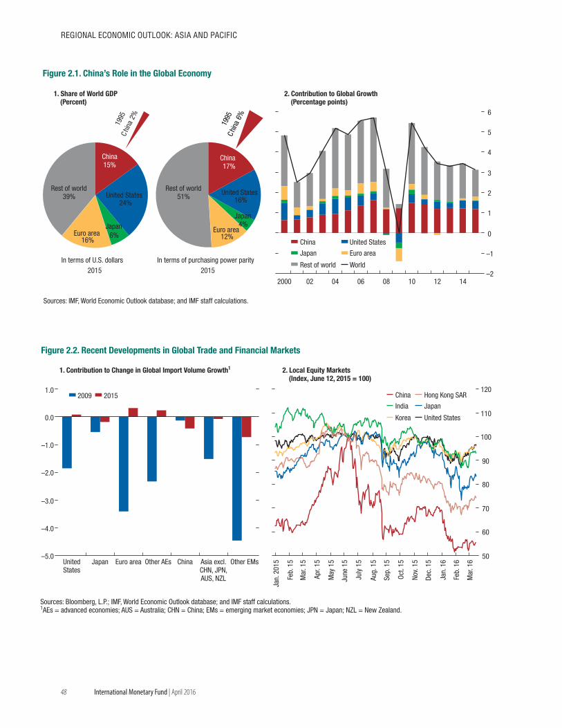
48
REGIONAL ECONOMIC OUTLOOK: AsIA ANd PACIfIC
International Monetary Fund | April 2016
Rest of world39%
Euro area16%
Japan6%
United States24%
China15%
Sources: IMF, World Economic Outlook database; and IMF staff calculations.
Figure 2.1. China’s Role in the Global Economy
–2
–1
0
1
2
3
4
5
6
2000 02 04 06 08 10 12 14
China United States
Japan Euro area
Rest of world World
1995
Chi
na2%
In terms of U.S. dollars2015
Rest of world51%
Euro area12%
Japan4%
United States16%
China17%
In terms of purchasing power parity2015
2. Contribution to Global Growth(Percentage points)
1. Share of World GDP(Percent)
1995
China
6%
–5.0
–4.0
–3.0
–2.0
–1.0
0.0
1.0
UnitedStates
Japan Euro area Other AEs China Other EMs
Sources: Bloomberg, L.P.; IMF, World Economic Outlook database; and IMF staff calculations.1AEs = advanced economies; AUS = Australia; CHN = China; EMs = emerging market economies; JPN = Japan; NZL = New Zealand.
Figure 2.2. Recent Developments in Global Trade and Financial Markets
2009 2015
50
60
70
80
90
100
110
120
Jan.
201
5
Feb.
15
Mar
. 15
Apr.
15
May
15
June
15
July
15
Aug.
15
Sep.
15
Oct.
15
Nov.
15
Dec.
15
Jan.
16
Feb.
16
Mar
. 16
China Hong Kong SAR
India Japan
Korea United States
1. Contribution to Change in Global Import Volume Growth1 2. Local Equity Markets(Index, June 12, 2015 = 100)
Asia excl.CHN, JPN,AUS, NZL
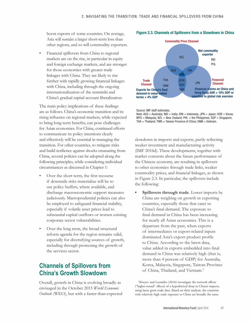
49
2. NAvIGATING ThE TRANsITION: TRAdE ANd fINANCIAL sPILLOvERs fROM ChINA
International Monetary Fund | April 2016
boost exports of some countries. On average, Asia will sustain a larger short-term loss than other regions, and so will commodity exporters.
• Financial spillovers from China to regional markets are on the rise, in particular in equity and foreign exchange markets, and are stronger for those economies with greater trade linkages with China. They are likely to rise further with rapidly growing financial linkages with China, including through the ongoing internationalization of the renminbi and China’s gradual capital account liberalization.
The main policy implications of these findings are as follows. China’s economic transition and its rising influence on regional markets, while expected to bring long-term benefits, can pose challenges for Asian economies. For China, continued efforts to communicate its policy intentions clearly and effectively will be essential in managing the transition. For other countries, to mitigate risks and build resilience against shocks emanating from China, several policies can be adopted along the following principles, while considering individual circumstances as discussed in Chapter 1:
• Over the short term, the first recourse if downside risks materialize will be to use policy buffers, where available, and discharge macroeconomic support measures judiciously. Macroprudential policies can also be employed to safeguard financial stability, especially if volatile asset prices lead to substantial capital outflows or worsen existing corporate sector vulnerabilities.
• Over the long term, the broad structural reform agenda for the region remains valid, especially for diversifying sources of growth, including through promoting the growth of the services sector.
Channels of Spillovers from China’s Growth SlowdownOverall, growth in China is evolving broadly as envisaged in the October 2015 World Economic Outlook (WEO), but with a faster-than-expected
slowdown in imports and exports, partly reflecting weaker investment and manufacturing activity (IMF 2016d). These developments, together with market concerns about the future performance of the Chinese economy, are resulting in spillovers to other economies through trade links, weaker commodity prices, and financial linkages, as shown in Figure 2.3. In particular, the spillovers include the following:
• Spillovers through trade. Lower imports by China are weighing on growth in exporting countries, especially those that cater to China’s final demand. The exposure to final demand in China has been increasing for nearly all Asian economies. This is a departure from the past, when exports of intermediates or export-related inputs dominated Asia’s export product profile to China. According to the latest data, value added in exports embedded into final demand in China was relatively high (that is, more than 4 percent of GDP) for Australia, Korea, Malaysia, Singapore, Taiwan Province of China, Thailand, and Vietnam.1
1Kireyev and Leonidov (2016) investigate the network effects (“higher-round” effects) of a hypothetical drop in China’s imports, using latest gross trade data. Based on their analysis, the countries with relatively high trade exposure to China are broadly the same.
Source: IMF staff estimates.Note: AUS = Australia; IND = India; IDN = Indonesia, JPN = Japan; KOR = Korea; MYS = Malaysia; NZL = New Zealand; PHL = the Philippines; SGP = Singapore; THA = Thailand; TWN = Taiwan Province of China; VNM = Vietnam.
NZL
JPN THA
VNM
Commodity Price Channel
TradeChannel
FinancialChannel
MYS
KOR SGP
TWN
IND PHL
Exports for China's finaldemand in value-addedterms > 4% GDP
Financial claims on China andHong Kong SAR > 10% GDP or
sensitive to global risk aversion
Net commodityexporter
AUS IDN
Figure 2.3. Channels of Spillovers from a Slowdown in China
50
REGIONAL ECONOMIC OUTLOOK: AsIA ANd PACIfIC
International Monetary Fund | April 2016
• Spillovers through commodity prices. To the extent that China’s slowdown and rebalancing contribute to lower commodity prices, net commodity exporters in the region, such as Australia, Indonesia, Malaysia, and New Zealand, can also be affected. The next chapter (Chapter 3) describes the impact of China on commodity markets in more detail, including for commodity producers outside the region.
• Spillovers through financial links. Several economies, such as Korea, Singapore, and Taiwan Province of China, have substantial financial links with China, both directly and through Hong Kong Special Administrative Region (SAR). Moreover, several other countries, such as Japan, Indonesia, and Malaysia, are affected by episodes of global risk aversion (“risk-off ” episodes).2 To the extent that uncertainty about China’s growth and policy outlook contribute to global risk aversion episodes, these countries may also be affected.
Hence, although a gradual slowdown in China’s growth is a natural consequence of successful economic development, it is bound to have negative spillover effects in the short term on regional economies. According to several IMF studies, reviewed in Box 2.1, a 1 percentage point change in China’s real GDP growth is estimated to affect the real GDP growth of the median Asian economy by 0.15–0.30 of a percentage point. This statistical variation among spillover-effect estimates reflects differences in the sample and econometric methodology.
A few general patterns emerge. First, the spillover effects are generally found to be stronger for countries with stronger trade linkages with China. Similarly, the effects have been strengthening over time, reflecting rising trade links with China.
2These “risk-off” episodes have become more frequent and severe since 2007, with the last two happening in August 2015 and January 2016 (De Bock and de Carvalho Filho 2015). During these episodes, the Japanese yen tends to appreciate against the U.S. dollar, while emerging market currencies—notably the Malaysian ringgit and the Indonesian rupiah in the region—tend to depreciate.
Moreover, the negative growth spillovers from China can become more severe when global financial markets are under stress. These results beckon further investigation of trade and financial spillovers, as addressed in the rest of this chapter.
Trade Spillovers from China’s Rebalancing China has been rebalancing gradually on multiple and interrelated fronts: from exports to domestic demand, from manufacturing to services, and from investment to consumption (IMF 2015b). The gradual changes add up to a meaningful magnitude over a longer horizon, and have already played a substantial role in the slowdown of China’s imports (Box 2.2). The rebalancing will continue for some time, likely gaining speed if the authorities make headway on key structural reforms.
This section explores trade spillovers of rebalancing from investment to consumption—the core of the multifaceted rebalancing process—by addressing the following questions:3
• How big a role did rebalancing play in the recent slowdown in China’s import growth?
• What are the implications of rebalancing on exports to China and overall GDP growth of economies exposed to China through trade linkages?
• Which economies are likely to benefit or lose from that rebalancing process?
These questions can be answered by understanding the demand for imports for China’s final consumption and final investment.
3The three dimensions of rebalancing are interlinked: less exports, less manufacturing, and less investment will proceed simultaneously with a large overlap. By focusing on the rebalancing from investment to consumption, we incorporate a sizable portion of the other two dimensions of rebalancing. However, the overlap is not complete, and the effect of rebalancing will be larger if the nonoverlapping part of the other two dimensions are fully incorporated. For example, the rebalancing from exports to domestic (consumption) demand will have similar implications on partner-country exports, as exports and investment have similar values of import intensity (Figure 2.2.2 in Box 2.2).
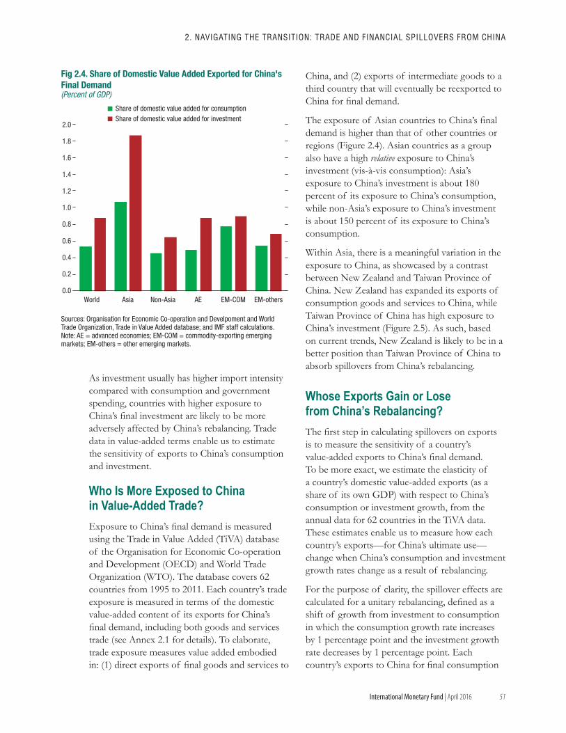
51
2. NAvIGATING ThE TRANsITION: TRAdE ANd fINANCIAL sPILLOvERs fROM ChINA
International Monetary Fund | April 2016
As investment usually has higher import intensity compared with consumption and government spending, countries with higher exposure to China’s final investment are likely to be more adversely affected by China’s rebalancing. Trade data in value-added terms enable us to estimate the sensitivity of exports to China’s consumption and investment.
Who Is More Exposed to China in Value-Added Trade?Exposure to China’s final demand is measured using the Trade in Value Added (TiVA) database of the Organisation for Economic Co-operation and Development (OECD) and World Trade Organization (WTO). The database covers 62 countries from 1995 to 2011. Each country’s trade exposure is measured in terms of the domestic value-added content of its exports for China’s final demand, including both goods and services trade (see Annex 2.1 for details). To elaborate, trade exposure measures value added embodied in: (1) direct exports of final goods and services to
China, and (2) exports of intermediate goods to a third country that will eventually be reexported to China for final demand.
The exposure of Asian countries to China’s final demand is higher than that of other countries or regions (Figure 2.4). Asian countries as a group also have a high relative exposure to China’s investment (vis-à-vis consumption): Asia’s exposure to China’s investment is about 180 percent of its exposure to China’s consumption, while non-Asia’s exposure to China’s investment is about 150 percent of its exposure to China’s consumption.
Within Asia, there is a meaningful variation in the exposure to China, as showcased by a contrast between New Zealand and Taiwan Province of China. New Zealand has expanded its exports of consumption goods and services to China, while Taiwan Province of China has high exposure to China’s investment (Figure 2.5). As such, based on current trends, New Zealand is likely to be in a better position than Taiwan Province of China to absorb spillovers from China’s rebalancing.
Whose Exports Gain or Lose from China’s Rebalancing? The first step in calculating spillovers on exports is to measure the sensitivity of a country’s value-added exports to China’s final demand. To be more exact, we estimate the elasticity of a country’s domestic value-added exports (as a share of its own GDP) with respect to China’s consumption or investment growth, from the annual data for 62 countries in the TiVA data. These estimates enable us to measure how each country’s exports—for China’s ultimate use—change when China’s consumption and investment growth rates change as a result of rebalancing.
For the purpose of clarity, the spillover effects are calculated for a unitary rebalancing, defined as a shift of growth from investment to consumption in which the consumption growth rate increases by 1 percentage point and the investment growth rate decreases by 1 percentage point. Each country’s exports to China for final consumption
0.0
0.2
0.4
0.6
0.8
1.0
1.2
1.4
1.6
1.8
2.0
World Asia Non-Asia AE EM-COM EM-others
Share of domestic value added for consumptionShare of domestic value added for investment
Fig 2.4. Share of Domestic Value Added Exported for China's Final Demand(Percent of GDP)
Sources: Organisation for Economic Co-operation and Develpoment and World Trade Organization, Trade in Value Added database; and IMF staff calculations.Note: AE = advanced economies; EM-COM = commodity-exporting emerging markets; EM-others = other emerging markets.
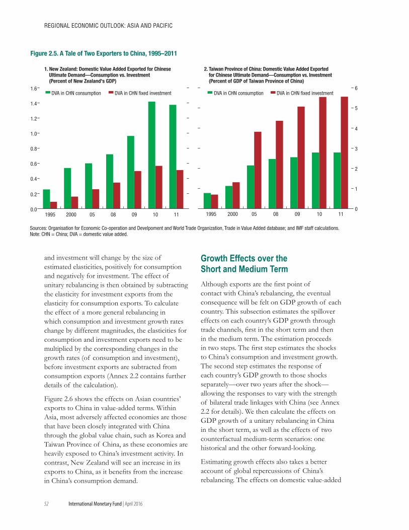
52
REGIONAL ECONOMIC OUTLOOK: AsIA ANd PACIfIC
International Monetary Fund | April 2016
and investment will change by the size of estimated elasticities, positively for consumption and negatively for investment. The effect of unitary rebalancing is then obtained by subtracting the elasticity for investment exports from the elasticity for consumption exports. To calculate the effect of a more general rebalancing in which consumption and investment growth rates change by different magnitudes, the elasticities for consumption and investment exports need to be multiplied by the corresponding changes in the growth rates (of consumption and investment), before investment exports are subtracted from consumption exports (Annex 2.2 contains further details of the calculation).
Figure 2.6 shows the effects on Asian countries’ exports to China in value-added terms. Within Asia, most adversely affected economies are those that have been closely integrated with China through the global value chain, such as Korea and Taiwan Province of China, as these economies are heavily exposed to China’s investment activity. In contrast, New Zealand will see an increase in its exports to China, as it benefits from the increase in China’s consumption demand.
Growth Effects over the Short and Medium Term Although exports are the first point of contact with China’s rebalancing, the eventual consequence will be felt on GDP growth of each country. This subsection estimates the spillover effects on each country’s GDP growth through trade channels, first in the short term and then in the medium term. The estimation proceeds in two steps. The first step estimates the shocks to China’s consumption and investment growth. The second step estimates the response of each country’s GDP growth to those shocks separately—over two years after the shock—allowing the responses to vary with the strength of bilateral trade linkages with China (see Annex 2.2 for details). We then calculate the effects on GDP growth of a unitary rebalancing in China in the short term, as well as the effects of two counterfactual medium-term scenarios: one historical and the other forward-looking.
Estimating growth effects also takes a better account of global repercussions of China’s rebalancing. The effects on domestic value-added
0.0
0.2
0.4
0.6
0.8
1.0
1.2
1.4
1.6
1995 2000 05 08 09 10 11
Sources: Organisation for Economic Co-operation and Develpoment and World Trade Organization, Trade in Value Added database; and IMF staff calculations.Note: CHN = China; DVA = domestic value added.
Figure 2.5. A Tale of Two Exporters to China, 1995–2011
DVA in CHN consumption DVA in CHN fixed investment
0
1
2
3
4
5
6
1995 2000 05 08 09 10 11
DVA in CHN consumption DVA in CHN fixed investment
2. Taiwan Province of China: Domestic Value Added Exported for Chinese Ultimate Demand—Consumption vs. Investment(Percent of GDP of Taiwan Province of China)
1. New Zealand: Domestic Value Added Exported for Chinese Ultimate Demand—Consumption vs. Investment(Percent of New Zealand's GDP)
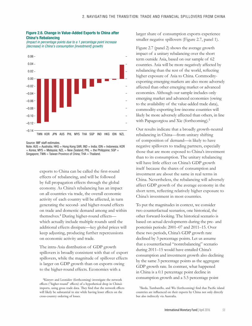
53
2. NAvIGATING ThE TRANsITION: TRAdE ANd fINANCIAL sPILLOvERs fROM ChINA
International Monetary Fund | April 2016
exports to China can be called the first-round effects of rebalancing, and will be followed by full propagation effects through the global economy. As China’s rebalancing has an impact on all countries via trade, the overall economic activity of each country will be affected, in turn generating the second- and higher-round effects on trade and domestic demand among and within themselves.4 During higher-round effects—which actually include multiple rounds until the additional effects dissipate—key global prices will keep adjusting, producing further repercussions on economic activity and trade.
The intra-Asia distribution of GDP growth spillovers is broadly consistent with that of export spillovers, while the magnitude of spillover effects is larger on GDP growth than on exports owing to the higher-round effects. Economies with a
4Kireyev and Leonidov (forthcoming) investigate the network effects (“higher-round” effects) of a hypothetical drop in China’s imports, using gross trade data. They find that the network effects will likely be substantial in size while having lesser effects on the cross-country ordering of losses.
larger share of consumption exports experience smaller negative spillovers (Figure 2.7, panel 1).
Figure 2.7 (panel 2) shows the average growth impact of a unitary rebalancing over the short term outside Asia, based on our sample of 62 countries. Asia will be more negatively affected by rebalancing than the rest of the world, reflecting higher exposure of Asia to China. Commodity-exporting emerging markets are also more adversely affected than other emerging market or advanced economies. Although our sample includes only emerging market and advanced economies (owing to the availability of the value-added trade data), commodity-exporting low-income countries will likely be more adversely affected than others, in line with Papageorgiou and Xie (forthcoming).5
Our results indicate that a broadly growth-neutral rebalancing in China—from unitary shifting of composition of demand—is likely to have negative spillovers to trading partners, especially those that are more exposed to China’s investment than to its consumption. The unitary rebalancing will have little effect on China’s GDP growth itself because the shares of consumption and investment are about the same in real terms in China. Nevertheless, the rebalancing will adversely affect GDP growth of the average economy in the short term, reflecting relatively higher exposure to China’s investment in most countries.
To put the magnitudes in context, we consider two counterfactual scenarios, one historical, the other forward-looking. The historical scenario is based on actual developments during the pre- and postcrisis periods: 2001–07 and 2011 –15. Over these two periods, China’s GDP growth rate declined by 3 percentage points. Let us assume that a counterfactual “nonrebalancing” scenario during 2011–15 would have entailed China’s consumption and investment growth also declining by the same 3 percentage points as the aggregate GDP growth rate. In contrast, what happened in China is a 0.1 percentage point decline in consumption growth and a 5.5 percentage point
5Ikeda, Tumbarello, and Wu (forthcoming) find that Pacific island countries are influenced on their exports by China not only directly but also indirectly via Australia.
Source: IMF staff estimates.Note: AUS = Australia; HKG = Hong Kong SAR; IND = India; IDN = Indonesia; KOR = Korea; MYS = Malaysia; NZL = New Zealand; PHL = the Philippine; SGP = Singapore; TWN = Taiwan Province of China; THA = Thailand.
–0.14
–0.12
–0.10
–0.08
–0.06
–0.04
–0.02
0.00
0.02
0.04
0.06
TWN KOR JPN AUS PHL MYS THA SGP IND HKG IDN NZL
Figure 2.6. Change in Value-Added Exports to China after China's Rebalancing(Impact in percentage points due to a 1 percentage point increase [decrease] in China's consumption [investment] growth)
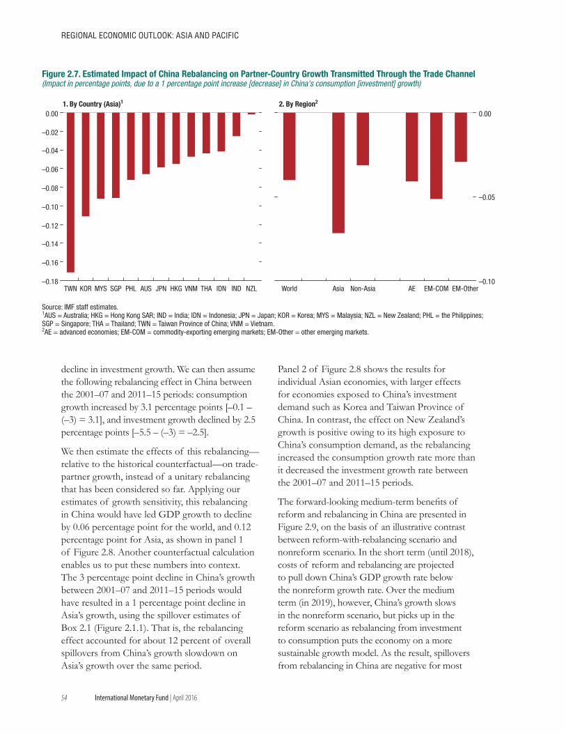
54
REGIONAL ECONOMIC OUTLOOK: AsIA ANd PACIfIC
International Monetary Fund | April 2016
decline in investment growth. We can then assume the following rebalancing effect in China between the 2001–07 and 2011–15 periods: consumption growth increased by 3.1 percentage points [–0.1 – (–3) = 3.1], and investment growth declined by 2.5 percentage points [–5.5 – (–3) = –2.5].
We then estimate the effects of this rebalancing—relative to the historical counterfactual—on trade-partner growth, instead of a unitary rebalancing that has been considered so far. Applying our estimates of growth sensitivity, this rebalancing in China would have led GDP growth to decline by 0.06 percentage point for the world, and 0.12 percentage point for Asia, as shown in panel 1 of Figure 2.8. Another counterfactual calculation enables us to put these numbers into context. The 3 percentage point decline in China’s growth between 2001–07 and 2011–15 periods would have resulted in a 1 percentage point decline in Asia’s growth, using the spillover estimates of Box 2.1 (Figure 2.1.1). That is, the rebalancing effect accounted for about 12 percent of overall spillovers from China’s growth slowdown on Asia’s growth over the same period.
Panel 2 of Figure 2.8 shows the results for individual Asian economies, with larger effects for economies exposed to China’s investment demand such as Korea and Taiwan Province of China. In contrast, the effect on New Zealand’s growth is positive owing to its high exposure to China’s consumption demand, as the rebalancing increased the consumption growth rate more than it decreased the investment growth rate between the 2001–07 and 2011–15 periods.
The forward-looking medium-term benefits of reform and rebalancing in China are presented in Figure 2.9, on the basis of an illustrative contrast between reform-with-rebalancing scenario and nonreform scenario. In the short term (until 2018), costs of reform and rebalancing are projected to pull down China’s GDP growth rate below the nonreform growth rate. Over the medium term (in 2019), however, China’s growth slows in the nonreform scenario, but picks up in the reform scenario as rebalancing from investment to consumption puts the economy on a more sustainable growth model. As the result, spillovers from rebalancing in China are negative for most
–0.18
–0.16
–0.14
–0.12
–0.10
–0.08
–0.06
–0.04
–0.02
0.00
TWN KOR MYS SGP PHL AUS JPN HKG VNM THA IDN IND NZL
Figure 2.7. Estimated Impact of China Rebalancing on Partner-Country Growth Transmitted Through the Trade Channel(Impact in percentage points, due to a 1 percentage point increase [decrease] in China's consumption [investment] growth)
–0.10
–0.05
0.00
World Asia Non-Asia AE EM-COM EM-Other
1. By Country (Asia)1 2. By Region2
Source: IMF staff estimates.1AUS = Australia; HKG = Hong Kong SAR; IND = India; IDN = Indonesia; JPN = Japan; KOR = Korea; MYS = Malaysia; NZL = New Zealand; PHL = the Philippines; SGP = Singapore; THA = Thailand; TWN = Taiwan Province of China; VNM = Vietnam.2AE = advanced economies; EM-COM = commodity-exporting emerging markets; EM-Other = other emerging markets.
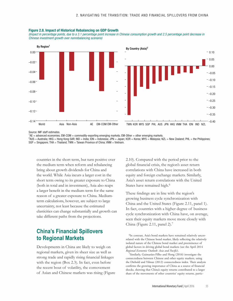
55
2. NAvIGATING ThE TRANsITION: TRAdE ANd fINANCIAL sPILLOvERs fROM ChINA
International Monetary Fund | April 2016
countries in the short term, but turn positive over the medium term when reform and rebalancing bring about growth dividends for China and the world. While Asia incurs a larger cost in the short term owing to its greater exposure to China (both in total and in investment), Asia also reaps a larger benefit in the medium term for the same reason of a greater exposure to China. Medium-term calculations, however, are subject to large uncertainty, not least because the estimated elasticities can change substantially and growth can take different paths from the projections.
China’s Financial Spillovers to Regional MarketsDevelopments in China are likely to weigh on regional markets, given its sheer size as well as strong trade and rapidly rising financial linkages with the region (Box 2.3). In fact, even before the recent bout of volatility, the comovement of Asian and Chinese markets was rising (Figure
2.10). Compared with the period prior to the global financial crisis, the region’s asset return correlations with China have increased in both equity and foreign exchange markets. Similarly, Asia’s asset return correlations with the United States have remained high.6
These findings are in line with the region’s growing business cycle synchronization with China and the United States (Figure 2.11, panel 1). In fact, countries with a higher degree of business cycle synchronization with China have, on average, seen their equity markets move more closely with China (Figure 2.11, panel 2).7
6In contrast, Asia’s bond markets have remained relatively uncor-related with the Chinese bond market, likely reflecting the relatively isolated nature of the Chinese bond market and preeminence of global factors in driving global bond markets (see the April 2014 Regional Economic Outlook: Asia and Pacific).
7Similarly, Guimarães-Filho and Hong (2016) investigate the connectedness between Chinese and other equity markets, using the Diebold and Yilmaz (2012) connectedness index. Their analysis confirms the growing importance of China as a source of financial shocks, showing that China’s equity returns contributed to a larger share of the movements of other countries’ equity returns, partic-
Source: IMF staff estimates.1AE = advanced economies; EM-COM = commodity-exporting emerging markets; EM-Other = other emerging markets.2AUS = Australia; HKG = Hong Kong SAR; IND = India; IDN = Indonesia; JPN = Japan; KOR = Korea; MYS = Malaysia; NZL = New Zealand; PHL = the Philippines; SGP = Singapore; THA = Thailand; TWN = Taiwan Province of China; VNM = Vietnam.
TWN KOR MYS SGP PHL AUS JPN HKG VNM THA IDN IND NZL–0.40
–0.35
–0.30
–0.25
–0.20
–0.15
–0.10
–0.05
0.00
0.05
0.10By Country (Asia)2
World Asia Non-Asia AE EM-COM EM-Other–0.14
–0.12
–0.10
–0.08
–0.06
–0.04
–0.02
0.00
By Region1
Figure 2.8. Impact of Historical Rebalancing on GDP Growth(Impact in percentage points, due to a 3.1 percentage point increase in Chinese consumption growth and 2.5 percentage point decrease in Chinese investment growth over nonrebalancing scenario)
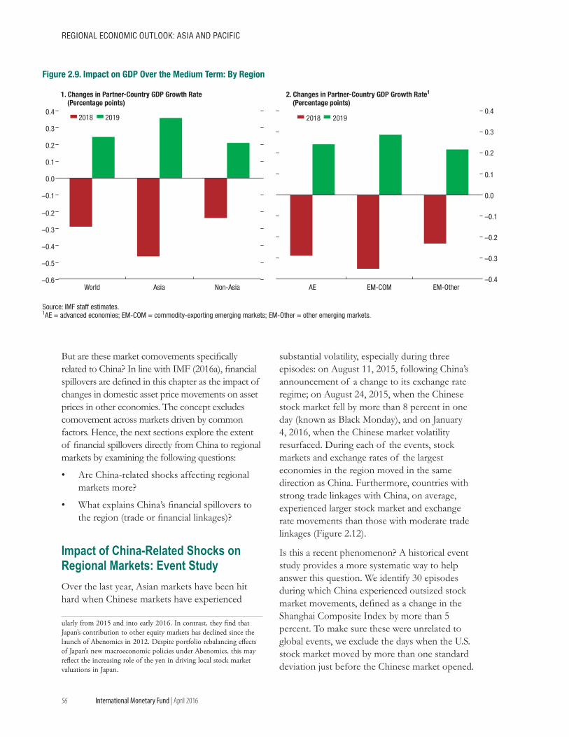
56
REGIONAL ECONOMIC OUTLOOK: AsIA ANd PACIfIC
International Monetary Fund | April 2016
But are these market comovements specifically related to China? In line with IMF (2016a), financial spillovers are defined in this chapter as the impact of changes in domestic asset price movements on asset prices in other economies. The concept excludes comovement across markets driven by common factors. Hence, the next sections explore the extent of financial spillovers directly from China to regional markets by examining the following questions:
• Are China-related shocks affecting regional markets more?
• What explains China’s financial spillovers to the region (trade or financial linkages)?
Impact of China-Related Shocks on Regional Markets: Event StudyOver the last year, Asian markets have been hit hard when Chinese markets have experienced
ularly from 2015 and into early 2016. In contrast, they find that Japan’s contribution to other equity markets has declined since the launch of Abenomics in 2012. Despite portfolio rebalancing effects of Japan’s new macroeconomic policies under Abenomics, this may reflect the increasing role of the yen in driving local stock market valuations in Japan.
substantial volatility, especially during three episodes: on August 11, 2015, following China’s announcement of a change to its exchange rate regime; on August 24, 2015, when the Chinese stock market fell by more than 8 percent in one day (known as Black Monday), and on January 4, 2016, when the Chinese market volatility resurfaced. During each of the events, stock markets and exchange rates of the largest economies in the region moved in the same direction as China. Furthermore, countries with strong trade linkages with China, on average, experienced larger stock market and exchange rate movements than those with moderate trade linkages (Figure 2.12).
Is this a recent phenomenon? A historical event study provides a more systematic way to help answer this question. We identify 30 episodes during which China experienced outsized stock market movements, defined as a change in the Shanghai Composite Index by more than 5 percent. To make sure these were unrelated to global events, we exclude the days when the U.S. stock market moved by more than one standard deviation just before the Chinese market opened.
–0.6
–0.5
–0.4
–0.3
–0.2
–0.1
–0.4
–0.3
–0.2
–0.1
0.0
0.1
0.2
0.3
0.4
World Asia Non-Asia
Figure 2.9. Impact on GDP Over the Medium Term: By Region
1. Changes in Partner-Country GDP Growth Rate(Percentage points)
2. Changes in Partner-Country GDP Growth Rate1
(Percentage points)
2018 2019
0.0
0.1
0.2
0.3
0.4
AE EM-COM EM-Other
Source: IMF staff estimates.1AE = advanced economies; EM-COM = commodity-exporting emerging markets; EM-Other = other emerging markets.
2018 2019
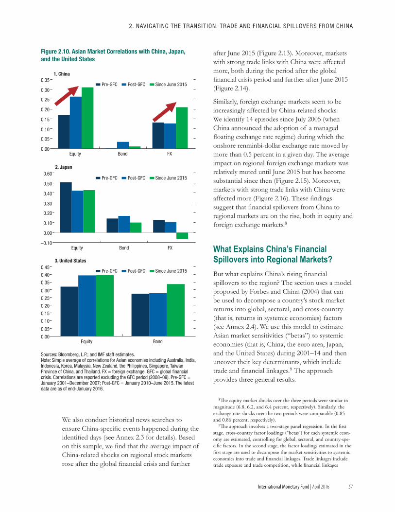
57
2. NAvIGATING ThE TRANsITION: TRAdE ANd fINANCIAL sPILLOvERs fROM ChINA
International Monetary Fund | April 2016
We also conduct historical news searches to ensure China-specific events happened during the identified days (see Annex 2.3 for details). Based on this sample, we find that the average impact of China-related shocks on regional stock markets rose after the global financial crisis and further
after June 2015 (Figure 2.13). Moreover, markets with strong trade links with China were affected more, both during the period after the global financial crisis period and further after June 2015 (Figure 2.14).
Similarly, foreign exchange markets seem to be increasingly affected by China-related shocks. We identify 14 episodes since July 2005 (when China announced the adoption of a managed floating exchange rate regime) during which the onshore renminbi-dollar exchange rate moved by more than 0.5 percent in a given day. The average impact on regional foreign exchange markets was relatively muted until June 2015 but has become substantial since then (Figure 2.15). Moreover, markets with strong trade links with China were affected more (Figure 2.16). These findings suggest that financial spillovers from China to regional markets are on the rise, both in equity and foreign exchange markets.8
What Explains China’s Financial Spillovers into Regional Markets?But what explains China’s rising financial spillovers to the region? The section uses a model proposed by Forbes and Chinn (2004) that can be used to decompose a country’s stock market returns into global, sectoral, and cross-country (that is, returns in systemic economies) factors (see Annex 2.4). We use this model to estimate Asian market sensitivities (“betas”) to systemic economies (that is, China, the euro area, Japan, and the United States) during 2001–14 and then uncover their key determinants, which include trade and financial linkages.9 The approach provides three general results.
8The equity market shocks over the three periods were similar in magnitude (6.8, 6.2, and 6.4 percent, respectively). Similarly, the exchange rate shocks over the two periods were comparable (0.85 and 0.86 percent, respectively).
9The approach involves a two-stage panel regression. In the first stage, cross-country factor loadings (“betas”) for each systemic econ-omy are estimated, controlling for global, sectoral, and country-spe-cific factors. In the second stage, the factor loadings estimated in the first stage are used to decompose the market sensitivities to systemic economies into trade and financial linkages. Trade linkages include trade exposure and trade competition, while financial linkages
Sources: Bloomberg, L.P.; and IMF staff estimates.Note: Simple average of correlations for Asian economies including Australia, India, Indonesia, Korea, Malaysia, New Zealand, the Philippines, Singapore, Taiwan Province of China, and Thailand. FX = foreign exchange; GFC = global financial crisis. Correlations are reported excluding the GFC period (2008–09). Pre-GFC = January 2001–December 2007; Post-GFC = January 2010–June 2015. The latest data are as of end-January 2016.
–0.10
0.00
0.10
0.20
0.30
0.40
0.50
0.60
Equity Bond FX
0.00
0.05
0.10
0.15
0.20
0.25
0.30
0.35
Equity Bond FX
1. China
Pre-GFC Post-GFC Since June 2015
Pre-GFC Post-GFC Since June 2015
Pre-GFC Post-GFC Since June 2015
2. Japan
0.00
0.05
0.10
0.15
0.20
0.25
0.30
0.35
0.40
0.45
Equity Bond
3. United States
Figure 2.10. Asian Market Correlations with China, Japan, and the United States
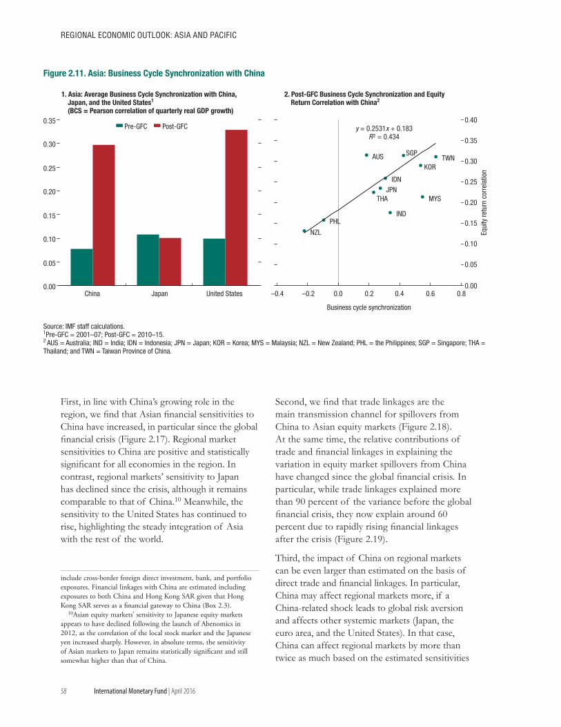
58
REGIONAL ECONOMIC OUTLOOK: AsIA ANd PACIfIC
International Monetary Fund | April 2016
First, in line with China’s growing role in the region, we find that Asian financial sensitivities to China have increased, in particular since the global financial crisis (Figure 2.17). Regional market sensitivities to China are positive and statistically significant for all economies in the region. In contrast, regional markets’ sensitivity to Japan has declined since the crisis, although it remains comparable to that of China.10 Meanwhile, the sensitivity to the United States has continued to rise, highlighting the steady integration of Asia with the rest of the world.
include cross-border foreign direct investment, bank, and portfolio exposures. Financial linkages with China are estimated including exposures to both China and Hong Kong SAR given that Hong Kong SAR serves as a financial gateway to China (Box 2.3).
10Asian equity markets’ sensitivity to Japanese equity markets appears to have declined following the launch of Abenomics in 2012, as the correlation of the local stock market and the Japanese yen increased sharply. However, in absolute terms, the sensitivity of Asian markets to Japan remains statistically significant and still somewhat higher than that of China.
Second, we find that trade linkages are the main transmission channel for spillovers from China to Asian equity markets (Figure 2.18). At the same time, the relative contributions of trade and financial linkages in explaining the variation in equity market spillovers from China have changed since the global financial crisis. In particular, while trade linkages explained more than 90 percent of the variance before the global financial crisis, they now explain around 60 percent due to rapidly rising financial linkages after the crisis (Figure 2.19).
Third, the impact of China on regional markets can be even larger than estimated on the basis of direct trade and financial linkages. In particular, China may affect regional markets more, if a China-related shock leads to global risk aversion and affects other systemic markets (Japan, the euro area, and the United States). In that case, China can affect regional markets by more than twice as much based on the estimated sensitivities
0.00
0.05
0.10
0.15
0.20
0.25
0.30
0.35
China Japan United States
Figure 2.11. Asia: Business Cycle Synchronization with China
Pre-GFC Post-GFC
Equi
ty re
turn
cor
rela
tion
Business cycle synchronization
y = 0.2531x + 0.183R² = 0.434
0.00
0.05
0.10
0.15
0.20
0.25
0.30
0.35
0.40
–0.4 –0.2 0.0 0.2 0.4 0.6 0.8
IND
THA
PHL
MYS
IDN
TWNSGP
KOR
NZL
AUS
JPN
Source: IMF staff calculations.1Pre-GFC = 2001–07; Post-GFC = 2010–15.2 AUS = Australia; IND = India; IDN = Indonesia; JPN = Japan; KOR = Korea; MYS = Malaysia; NZL = New Zealand; PHL = the Philippines; SGP = Singapore; THA = Thailand; and TWN = Taiwan Province of China.
2. Post-GFC Business Cycle Synchronization and Equity Return Correlation with China2
1. Asia: Average Business Cycle Synchronization with China, Japan, and the United States1
(BCS = Pearson correlation of quarterly real GDP growth)
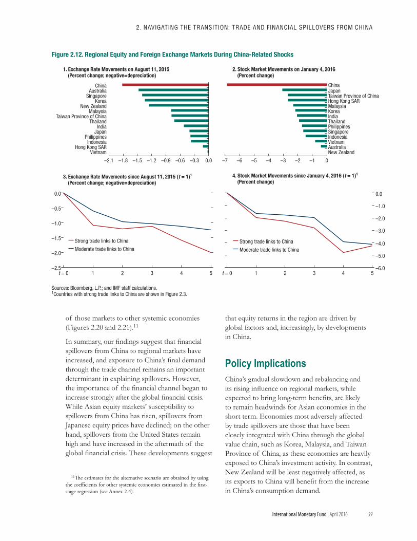
59
2. NAvIGATING ThE TRANsITION: TRAdE ANd fINANCIAL sPILLOvERs fROM ChINA
International Monetary Fund | April 2016
of those markets to other systemic economies (Figures 2.20 and 2.21).11
In summary, our findings suggest that financial spillovers from China to regional markets have increased, and exposure to China’s final demand through the trade channel remains an important determinant in explaining spillovers. However, the importance of the financial channel began to increase strongly after the global financial crisis. While Asian equity markets’ susceptibility to spillovers from China has risen, spillovers from Japanese equity prices have declined; on the other hand, spillovers from the United States remain high and have increased in the aftermath of the global financial crisis. These developments suggest
11The estimates for the alternative scenario are obtained by using the coefficients for other systemic economies estimated in the first-stage regression (see Annex 2.4).
that equity returns in the region are driven by global factors and, increasingly, by developments in China.
Policy ImplicationsChina’s gradual slowdown and rebalancing and its rising influence on regional markets, while expected to bring long-term benefits, are likely to remain headwinds for Asian economies in the short term. Economies most adversely affected by trade spillovers are those that have been closely integrated with China through the global value chain, such as Korea, Malaysia, and Taiwan Province of China, as these economies are heavily exposed to China’s investment activity. In contrast, New Zealand will be least negatively affected, as its exports to China will benefit from the increase in China’s consumption demand.
Figure 2.12. Regional Equity and Foreign Exchange Markets During China-Related Shocks
–2.5
–2.0
–1.5
–1.0
–0.5
0.0
t = 0 1 2 3 4 5
Sources: Bloomberg, L.P.; and IMF staff calculations.1Countries with strong trade links to China are shown in Figure 2.3.
1. Exchange Rate Movements on August 11, 2015(Percent change; negative=depreciation)
2. Stock Market Movements on January 4, 2016(Percent change)
3. Exchange Rate Movements since August 11, 2015 (t = 1)1
(Percent change; negative=depreciation)4. Stock Market Movements since January 4, 2016 (t = 1)1
(Percent change)
Strong trade links to China
Moderate trade links to China
Strong trade links to China
Moderate trade links to China
–1.0
–2.0
–3.0
–4.0
–5.0
–6.0
0.0
t = 0 1 2 3 4 5
–2.1 –1.8 –1.5 –1.2 –0.9 –0.6 –0.3 0.0
VietnamHong Kong SAR
IndonesiaPhilippines
JapanIndia
ThailandTaiwan Province of China
MalaysiaNew Zealand
KoreaSingapore
AustraliaChina
–7 –6 –5 –4 –3 –2 –1 0
New ZealandAustraliaVietnamIndonesiaSingaporePhilippinesThailandIndiaKoreaMalaysiaHong Kong SARTaiwan Province of ChinaJapanChina
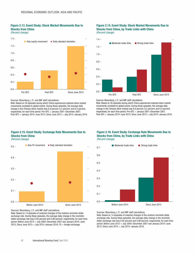
60
REGIONAL ECONOMIC OUTLOOK: AsIA ANd PACIfIC
International Monetary Fund | April 2016
Sources: Bloomberg, L.P.; and IMF staff calculations.Note: Based on 30 episodes during which China experienced outsized stock market movements unrelated to global events. During these episodes, the average daily change in the Chinese stock market was 6.8 percent, 6.2 percent, and 6.4 percent, respectively, for each time period. Pre-GFC = January 2001–December 2007; Post-GFC = January 2010–June 2015; Since June 2015 = July 2015–January 2016.
0.0
0.2
0.4
0.6
0.8
1.0
1.2
1.4
Pre-GFC Post-GFC Since June 2015
Asia equity movement Daily standard deviation
Figure 2.13. Event Study: Stock Market Movements Due to Shocks from China(Percent change)
Sources: Bloomberg, L.P.; and IMF staff calculations.Note: Based on 30 episodes during which China experienced outsized stock market movements unrelated to global events. During these episodes, the average daily change in the Chinese stock market was 6.8 percent, 6.2 percent, and 6.4 percent, respectively, for each time period. Pre-GFC = January 2001–December 2007; Post-GFC = January 2010–June 2015; Since June 2015 = July 2015–January 2016.
0.0
0.2
0.4
0.6
0.8
1.0
1.2
1.4
Pre-GFC Post-GFC Since June 2015
Moderate trade links Strong trade links
Figure 2.14. Event Study: Stock Market Movements Due to Shocks from China, by Trade Links with China(Percent change)
Sources: Bloomberg, L.P.; and IMF staff calculations.Note: Based on 14 episodes of outsized changes of the onshore renminbi-dollar exchange rate. During these episodes, the average daily change in the renminbi- dollar exchange rate was 0.85 percent and 0.86 percent, respectively, for each time period. Before June 2015 = July 2005–December 2007 and January 2010–June 2015; Since June 2015 = July 2015–January 2016. FX = foreign exchange.
0.0
0.1
0.2
0.3
0.4
0.5
Before June 2015 Since June 2015
Asia FX movement Daily standard deviation
Figure 2.15. Event Study: Exchange Rate Movements Due to Shocks from China(Percent change)
Sources: Bloomberg, L.P.; and IMF staff calculations.Note: Based on 14 episodes of outsized changes of the onshore renminbi-dollar exchange rate. During these episodes, the average daily change in the renminbi- dollar exchange rate was 0.85 percent and 0.86 percent, respectively, for each time period. Before June 2015 = July 2005–December 2007 and January 2010–June 2015; Since June 2015 = July 2015–January 2016.
0.0
0.1
0.2
0.3
0.4
0.5
0.6
0.7
Before June 2015 Since June 2015
Moderate trade links Strong trade links
Figure 2.16. Event Study: Exchange Rate Movements Due to Shocks from China, by Trade Links with China(Percent change)
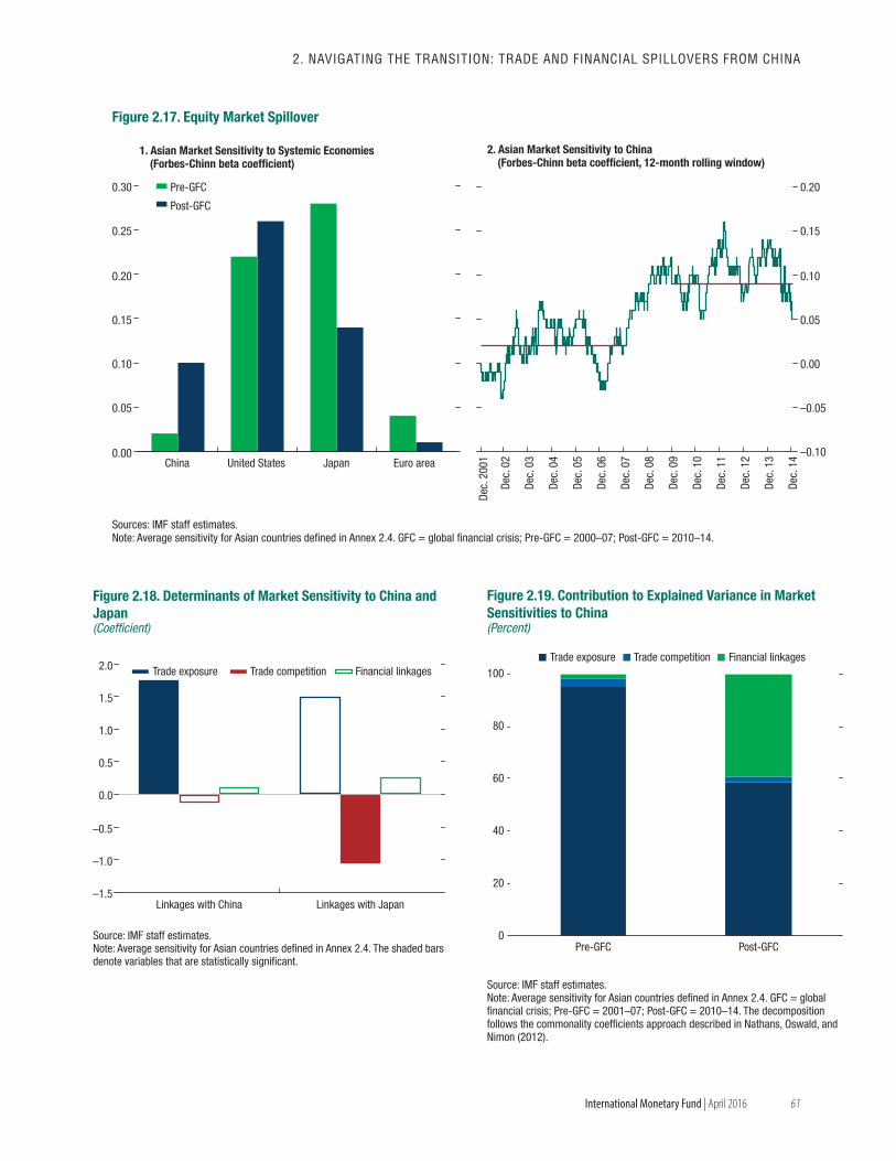
61
2. NAvIGATING ThE TRANsITION: TRAdE ANd fINANCIAL sPILLOvERs fROM ChINA
International Monetary Fund | April 2016
0.00
0.05
0.10
0.15
0.20
0.25
0.30
China United States Japan Euro area
Sources: IMF staff estimates.Note: Average sensitivity for Asian countries defined in Annex 2.4. GFC = global financial crisis; Pre-GFC = 2000–07; Post-GFC = 2010–14.
Figure 2.17. Equity Market Spillover
Pre-GFC
Post-GFC
–0.10
–0.05
0.00
0.05
0.10
0.15
0.20
Dec.
200
1
Dec.
02
Dec.
03
Dec.
04
Dec.
05
Dec.
06
Dec.
07
Dec.
08
Dec.
09
Dec.
10
Dec.
11
Dec.
12
Dec.
13
Dec.
14
1. Asian Market Sensitivity to Systemic Economies(Forbes-Chinn beta coefficient)
2. Asian Market Sensitivity to China(Forbes-Chinn beta coefficient, 12-month rolling window)
–1.5
–1.0
–0.5
0.0
0.5
1.0
1.5
2.0
Linkages with China Linkages with Japan
Trade exposure Trade competition Financial linkages
Figure 2.18. Determinants of Market Sensitivity to China and Japan(Coefficient)
Source: IMF staff estimates.Note: Average sensitivity for Asian countries defined in Annex 2.4. The shaded bars denote variables that are statistically significant.
Source: IMF staff estimates.Note: Average sensitivity for Asian countries defined in Annex 2.4. GFC = global financial crisis; Pre-GFC = 2001–07; Post-GFC = 2010–14. The decomposition follows the commonality coefficients approach described in Nathans, Oswald, and Nimon (2012).
0
20
40
60
80
100
Pre-GFC Post-GFC
Trade exposure Trade competition Financial linkages
Figure 2.19. Contribution to Explained Variance in Market Sensitivities to China(Percent)
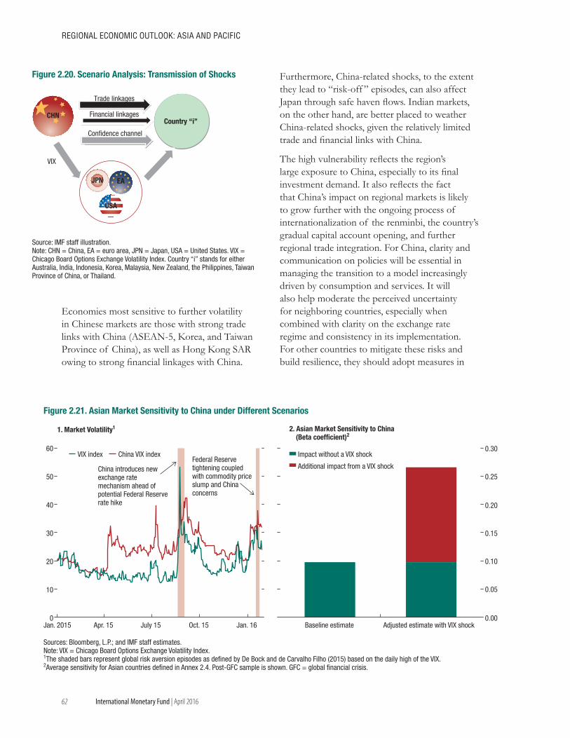
62
REGIONAL ECONOMIC OUTLOOK: AsIA ANd PACIfIC
International Monetary Fund | April 2016
Economies most sensitive to further volatility in Chinese markets are those with strong trade links with China (ASEAN-5, Korea, and Taiwan Province of China), as well as Hong Kong SAR owing to strong financial linkages with China.
Furthermore, China-related shocks, to the extent they lead to “risk-off ” episodes, can also affect Japan through safe haven flows. Indian markets, on the other hand, are better placed to weather China-related shocks, given the relatively limited trade and financial links with China.
The high vulnerability reflects the region’s large exposure to China, especially to its final investment demand. It also reflects the fact that China’s impact on regional markets is likely to grow further with the ongoing process of internationalization of the renminbi, the country’s gradual capital account opening, and further regional trade integration. For China, clarity and communication on policies will be essential in managing the transition to a model increasingly driven by consumption and services. It will also help moderate the perceived uncertainty for neighboring countries, especially when combined with clarity on the exchange rate regime and consistency in its implementation. For other countries to mitigate these risks and build resilience, they should adopt measures in
Country “i”
Trade linkages
Financial linkages
Confidence channel
VIX
CHN
JPN EA
USA
Source: IMF staff illustration. Note: CHN = China, EA = euro area, JPN = Japan, USA = United States. VIX = Chicago Board Options Exchange Volatility Index. Country “i” stands for either Australia, India, Indonesia, Korea, Malaysia, New Zealand, the Philippines, Taiwan Province of China, or Thailand.
Figure 2.20. Scenario Analysis: Transmission of Shocks
0
10
20
30
40
50
60
Jan. 2015 Apr. 15 July 15 Oct. 15 Jan. 16
China introduces newexchange ratemechanism ahead ofpotential Federal Reserve rate hike
Figure 2.21. Asian Market Sensitivity to China under Different Scenarios
VIX index China VIX index
0.00
0.05
0.10
0.15
0.20
0.25
0.30
Baseline estimate Adjusted estimate with VIX shock
Federal Reserve tightening coupledwith commodity priceslump and Chinaconcerns
Impact without a VIX shock
Additional impact from a VIX shock
2. Asian Market Sensitivity to China(Beta coefficient)2
1. Market Volatility1
Sources: Bloomberg, L.P.; and IMF staff estimates.Note: VIX = Chicago Board Options Exchange Volatility Index.1The shaded bars represent global risk aversion episodes as defined by De Bock and de Carvalho Filho (2015) based on the daily high of the VIX.2Average sensitivity for Asian countries defined in Annex 2.4. Post-GFC sample is shown. GFC = global financial crisis.
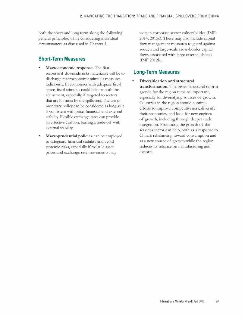
63
2. NAvIGATING ThE TRANsITION: TRAdE ANd fINANCIAL sPILLOvERs fROM ChINA
International Monetary Fund | April 2016
both the short and long term along the following general principles, while considering individual circumstances as discussed in Chapter 1.
Short-Term Measures• Macroeconomic response. The first
recourse if downside risks materialize will be to discharge macroeconomic stimulus measures judiciously. In economies with adequate fiscal space, fiscal stimulus could help smooth the adjustment, especially if targeted to sectors that are hit most by the spillovers. The use of monetary policy can be considered as long as it is consistent with price, financial, and external stability. Flexible exchange rates can provide an effective cushion, barring a trade-off with external stability.
• Macroprudential policies can be employed to safeguard financial stability and avoid systemic risks, especially if volatile asset prices and exchange rate movements may
worsen corporate sector vulnerabilities (IMF 2014, 2015c). These may also include capital flow management measures to guard against sudden and large-scale cross-border capital flows associated with large external shocks (IMF 2012b).
Long-Term Measures• Diversification and structural
transformation. The broad structural reform agenda for the region remains important, especially for diversifying sources of growth. Countries in the region should continue efforts to improve competitiveness, diversify their economies, and look for new engines of growth, including through deeper trade integration. Promoting the growth of the services sector can help, both as a response to China’s rebalancing toward consumption and as a new source of growth while the region reduces its reliance on manufacturing and exports.
64
REGIONAL ECONOMIC OUTLOOK: AsIA ANd PACIfIC
International Monetary Fund | April 2016
Spillovers from China have intensified over time, as linkages with China strengthen in both trade and financial terms. Growth spillover effects are estimated to be 0.15–0.30 of a percentage point for each percentage point change in China’s growth, applying to both a possible slowdown in the short term and the post-reform growth dividend over the medium term.
Duval and others (2014) estimate the growth spillover effect of about 0.3 of a percentage point for the median Asian economy, in line with the estimates in Ahuja and Nabar (2012), based on a macro panel approach (Figure 2.1.1).1 Duval and others (2014) also find that each country’s sensitivity to China increases with its exposure to China in terms of value-added trade.
Cashin, Mohaddes, and Raissi (2016) obtain spillover estimates, based on a global vector autoregression (GVAR) model for 26 countries and/or regions during 1981–2013, that are similar to the estimates above for the five largest economies in the Association of Southeast Asian Nations, Indonesia, Malaysia, the Philippines, Singapore, and Thailand—ASEAN-5, but smaller for a median Asian economy. The estimates for the median Asian and ASEAN-5 economies are presented in Figure 2.1.2, while individual country results can be found in Cashin, Mohaddes, and Raissi (2016). The implications of China’s slowdown and rebalancing for the ASEAN-5 are also discussed in Dizioli and others (forthcoming).
To gauge the effects of the changing trade relationship between China and individual countries, Cashin, Mohaddes, and Raissi (2016) estimate a GVAR model with time-varying weights, with the earliest in 1982
The authors of this box are Sohrab Rafiq and Dulani Seneviratne.1Estimates by Duval and others (2014) are based on a panel estimation for 62 countries during 1995–2011, linking each country’s
GDP growth to a shock to China’s GDP growth.
0.0
Asia(Median
country pair)
ASEAN-5(Median
country pair)
Non-Asia(Median
country pair)
–0.4
–0.3
–0.2
–0.1
Source: IMF staff estimates.Note: Estimates based on column (3) of Table 5 in Duval and others (2014); ASEAN-5 = Indonesia, Malaysia, the Philippines, Singapore, and Thailand.
Figure 2.1.1. Effect of a 1 Percent Growth Surprise in China(Median GDP growth impact after one year, in percentage points)
–0.30
–0.25
–0.20
–0.15
–0.10
–0.05
0.00
Asia ASEAN-5
Source: IMF staff estimates based on Cashin, Mohaddes, and Raissi (2016).Note: Depicts percent change in GDP of a given country after one year associated with a 1 percent permanent decline in China's GDP (equivalent to a one-off 1 percent shock to GDP growth in China) using the 2012 bilateral trade weights; ASEAN-5 = Indonesia, Malaysia, the Philippines, Singapore, and Thailand.
Figure 2.1.2. Effect of a 1 Percent Negative GDP Shock in China(Percent change in GDP after one year for a median country)
Box 2.1. Regional Consequences of a Growth Slowdown in China
65
2. NAvIGATING ThE TRANsITION: TRAdE ANd fINANCIAL sPILLOvERs fROM ChINA
International Monetary Fund | April 2016
and the latest in 2012 (Figure 2.1.3). The effects increase substantially over time, reflecting the rising weight of China in the trade of each country. To take the median
country, the growth spillover effects increased twofold between 1992 and 2012. In addition, negative growth spillovers from China become more severe when global financial markets are under stress.
Rafiq (forthcoming) finds similar growth spillover effects on four ASEAN emerging markets (Indonesia, Malaysia, the Philippines, and Thailand), but somewhat smaller spillover effects on ASEAN frontier economies (Cambodia, Lao P.D.R., and Vietnam—Table 2.1.1). Growth spillovers from China to these countries rose after the global financial crisis, more than doubling in many cases. Moreover, financial conditions in the four ASEAN emerging market economies are found to tighten in response to a growth slowdown in China, as reflected in declining equity prices.2
2Rafiq (forthcoming) uses a state-dependent structural factor model to capture the time-varying relationship between a panel of ASEAN countries and China real and financial variables.
0.00
1982 1992 2012
–0.12
–0.14
–0.16
–0.10
–0.08
–0.06
–0.04
–0.02
Source: IMF staff estimates based on Cashin, Mohaddes, and Raissi (2016).Note: Using time-varying weights. See Figure 2.1.2.
Figure 2.1.3. Effect of a 1 Percent Negative GDP Shock in China(Percent change in GDP after one year for a median country)
Table 2.1.1. Time-Varying Elasticity of ASEAN Growth on China's Economic Activity
Effect in
Jul-06 Jun-15
Cambodia 0.07 0.17
Lao P.D.R. 0.03 0.21
Vietnam 0.04 0.13
FDE average 0.05 0.16
Malaysia 0.12 0.28
Indonesia 0.11 0.23
Philippines 0.10 0.26
Thailand 0.06 0.24
EME average 0.10 0.26
Source: IMF staff estimates based on Rafiq (forthcoming).Note: Elasticity values are expressed in terms of 1 percent change in China's economic activity. ASEAN = Association of Southeast Asian Nations; EME = emerging market economies; FDE = frontier and developing Asia.
Box 2.1 (continued)
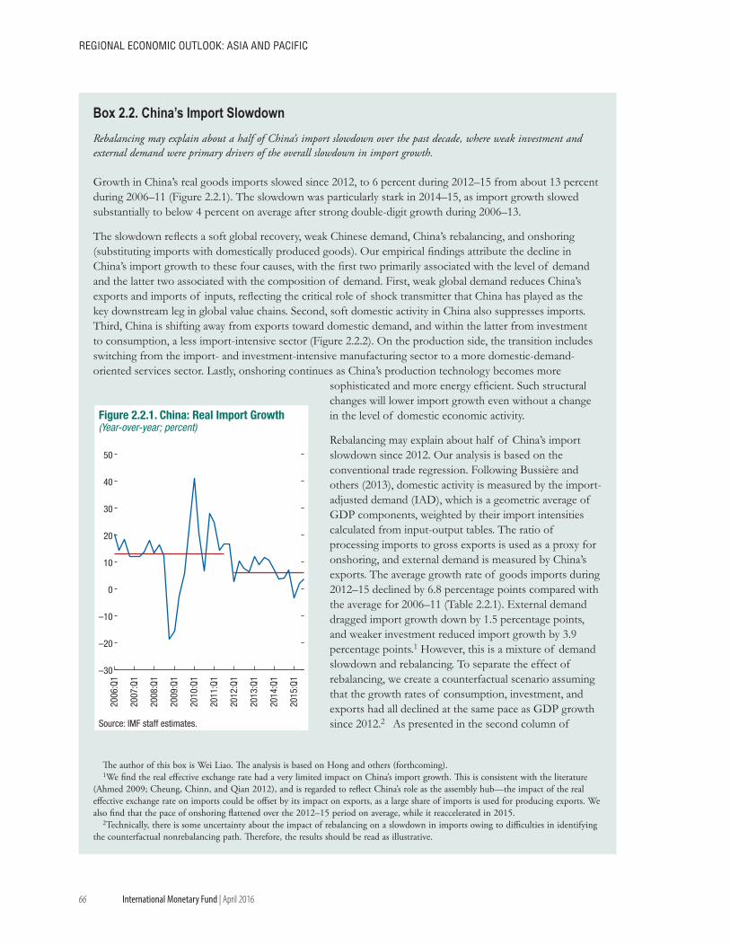
66
REGIONAL ECONOMIC OUTLOOK: AsIA ANd PACIfIC
International Monetary Fund | April 2016
Rebalancing may explain about a half of China’s import slowdown over the past decade, where weak investment and external demand were primary drivers of the overall slowdown in import growth.
Growth in China’s real goods imports slowed since 2012, to 6 percent during 2012–15 from about 13 percent during 2006–11 (Figure 2.2.1). The slowdown was particularly stark in 2014–15, as import growth slowed substantially to below 4 percent on average after strong double-digit growth during 2006–13.
The slowdown reflects a soft global recovery, weak Chinese demand, China’s rebalancing, and onshoring (substituting imports with domestically produced goods). Our empirical findings attribute the decline in China’s import growth to these four causes, with the first two primarily associated with the level of demand and the latter two associated with the composition of demand. First, weak global demand reduces China’s exports and imports of inputs, reflecting the critical role of shock transmitter that China has played as the key downstream leg in global value chains. Second, soft domestic activity in China also suppresses imports. Third, China is shifting away from exports toward domestic demand, and within the latter from investment to consumption, a less import-intensive sector (Figure 2.2.2). On the production side, the transition includes switching from the import- and investment-intensive manufacturing sector to a more domestic-demand-oriented services sector. Lastly, onshoring continues as China’s production technology becomes more
sophisticated and more energy efficient. Such structural changes will lower import growth even without a change in the level of domestic economic activity.
Rebalancing may explain about half of China’s import slowdown since 2012. Our analysis is based on the conventional trade regression. Following Bussière and others (2013), domestic activity is measured by the import-adjusted demand (IAD), which is a geometric average of GDP components, weighted by their import intensities calculated from input-output tables. The ratio of processing imports to gross exports is used as a proxy for onshoring, and external demand is measured by China’s exports. The average growth rate of goods imports during 2012–15 declined by 6.8 percentage points compared with the average for 2006–11 (Table 2.2.1). External demand dragged import growth down by 1.5 percentage points, and weaker investment reduced import growth by 3.9 percentage points.1 However, this is a mixture of demand slowdown and rebalancing. To separate the effect of rebalancing, we create a counterfactual scenario assuming that the growth rates of consumption, investment, and exports had all declined at the same pace as GDP growth since 2012.2 As presented in the second column of
The author of this box is Wei Liao. The analysis is based on Hong and others (forthcoming).1We find the real effective exchange rate had a very limited impact on China’s import growth. This is consistent with the literature
(Ahmed 2009; Cheung, Chinn, and Qian 2012), and is regarded to reflect China’s role as the assembly hub—the impact of the real effective exchange rate on imports could be offset by its impact on exports, as a large share of imports is used for producing exports. We also find that the pace of onshoring flattened over the 2012–15 period on average, while it reaccelerated in 2015.
2Technically, there is some uncertainty about the impact of rebalancing on a slowdown in imports owing to difficulties in identifying the counterfactual nonrebalancing path. Therefore, the results should be read as illustrative.
–30
–20
–10
0
10
20
30
40
50
2006
:Q1
2007
:Q1
2008
:Q1
2009
:Q1
2010
:Q1
2011
:Q1
2012
:Q1
2013
:Q1
2014
:Q1
2015
:Q1
Source: IMF staff estimates.
Figure 2.2.1. China: Real Import Growth(Year-over-year; percent)
Box 2.2. China’s Import Slowdown
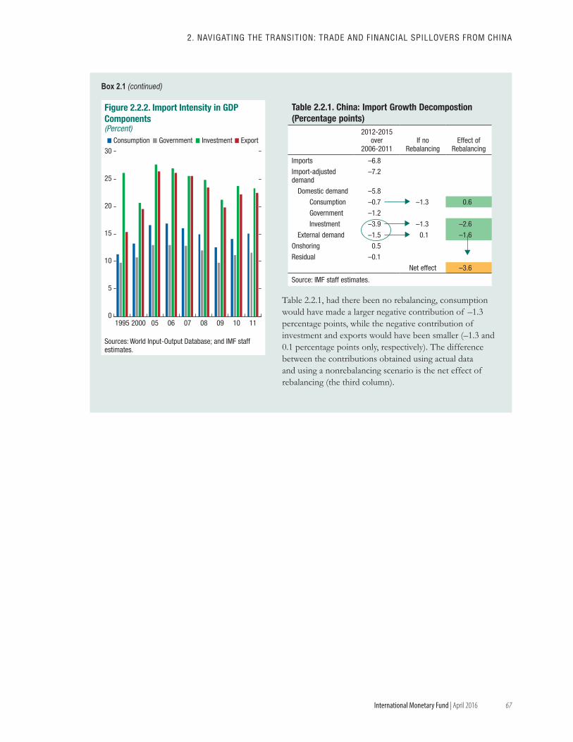
67
2. NAvIGATING ThE TRANsITION: TRAdE ANd fINANCIAL sPILLOvERs fROM ChINA
International Monetary Fund | April 2016
Table 2.2.1, had there been no rebalancing, consumption would have made a larger negative contribution of –1.3 percentage points, while the negative contribution of investment and exports would have been smaller (–1.3 and 0.1 percentage points only, respectively). The difference between the contributions obtained using actual data and using a nonrebalancing scenario is the net effect of rebalancing (the third column).
0
5
10
15
20
25
30
1995 2000 05 06 07 08 09 10 11
Consumption Government Investment Export
Figure 2.2.2. Import Intensity in GDP Components(Percent)
Sources: World Input-Output Database; and IMF staff estimates.
Table 2.2.1. China: Import Growth Decompostion(Percentage points)
2012-2015 over
2006-2011If no
RebalancingEffect of
Rebalancing
Imports –6.8
Import-adjusted demand
–7.2
Domestic demand –5.8
Consumption –0.7 –1.3 0.6
Government –1.2
Investment –3.9 –1.3 –2.6
External demand –1.5 0.1 –1.6
Onshoring 0.5
Residual –0.1
Net effect –3.6
Source: IMF staff estimates.
Box 2.1 (continued)
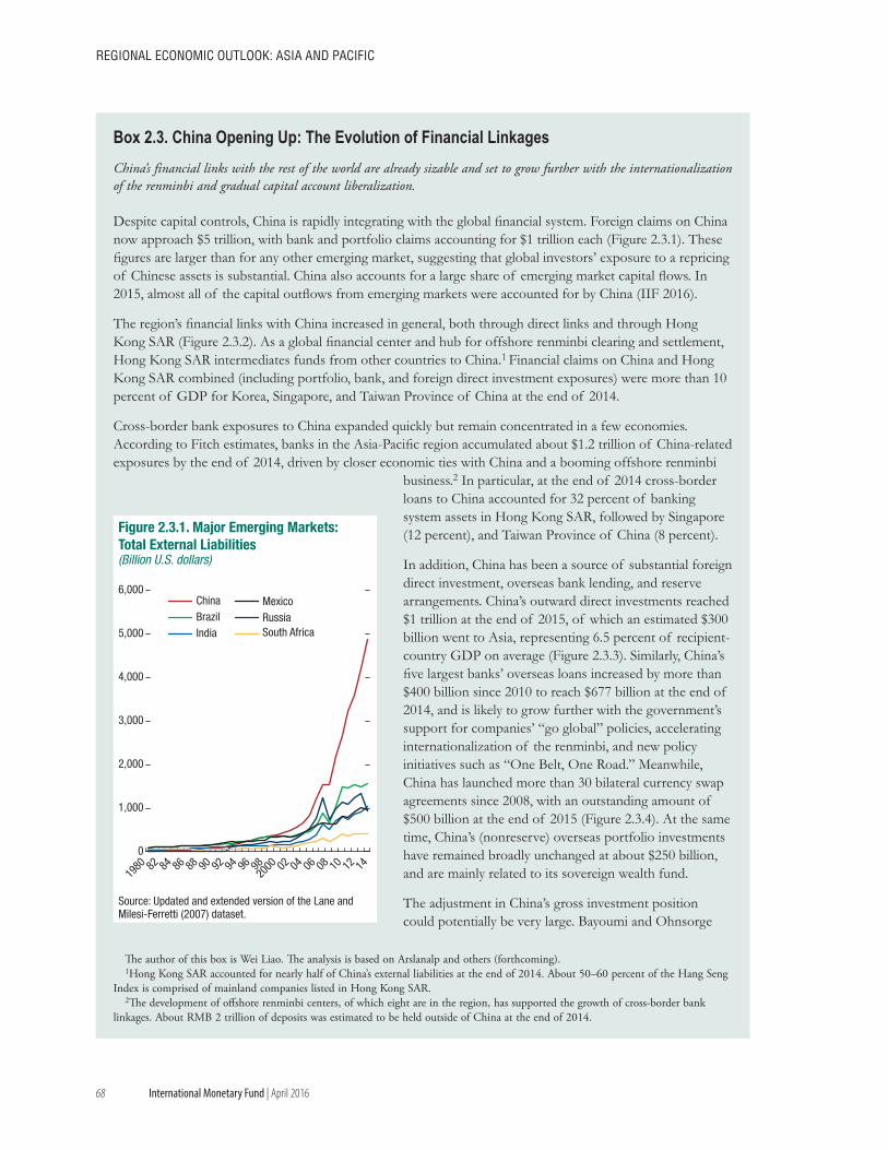
68
REGIONAL ECONOMIC OUTLOOK: AsIA ANd PACIfIC
International Monetary Fund | April 2016
China’s financial links with the rest of the world are already sizable and set to grow further with the internationalization of the renminbi and gradual capital account liberalization.
Despite capital controls, China is rapidly integrating with the global financial system. Foreign claims on China now approach $5 trillion, with bank and portfolio claims accounting for $1 trillion each (Figure 2.3.1). These figures are larger than for any other emerging market, suggesting that global investors’ exposure to a repricing of Chinese assets is substantial. China also accounts for a large share of emerging market capital flows. In 2015, almost all of the capital outflows from emerging markets were accounted for by China (IIF 2016).
The region’s financial links with China increased in general, both through direct links and through Hong Kong SAR (Figure 2.3.2). As a global financial center and hub for offshore renminbi clearing and settlement, Hong Kong SAR intermediates funds from other countries to China.1 Financial claims on China and Hong Kong SAR combined (including portfolio, bank, and foreign direct investment exposures) were more than 10 percent of GDP for Korea, Singapore, and Taiwan Province of China at the end of 2014.
Cross-border bank exposures to China expanded quickly but remain concentrated in a few economies. According to Fitch estimates, banks in the Asia-Pacific region accumulated about $1.2 trillion of China-related exposures by the end of 2014, driven by closer economic ties with China and a booming offshore renminbi
business.2 In particular, at the end of 2014 cross-border loans to China accounted for 32 percent of banking system assets in Hong Kong SAR, followed by Singapore (12 percent), and Taiwan Province of China (8 percent).
In addition, China has been a source of substantial foreign direct investment, overseas bank lending, and reserve arrangements. China’s outward direct investments reached $1 trillion at the end of 2015, of which an estimated $300 billion went to Asia, representing 6.5 percent of recipient-country GDP on average (Figure 2.3.3). Similarly, China’s five largest banks’ overseas loans increased by more than $400 billion since 2010 to reach $677 billion at the end of 2014, and is likely to grow further with the government’s support for companies’ “go global” policies, accelerating internationalization of the renminbi, and new policy initiatives such as “One Belt, One Road.” Meanwhile, China has launched more than 30 bilateral currency swap agreements since 2008, with an outstanding amount of $500 billion at the end of 2015 (Figure 2.3.4). At the same time, China’s (nonreserve) overseas portfolio investments have remained broadly unchanged at about $250 billion, and are mainly related to its sovereign wealth fund.
The adjustment in China’s gross investment position could potentially be very large. Bayoumi and Ohnsorge
The author of this box is Wei Liao. The analysis is based on Arslanalp and others (forthcoming).1Hong Kong SAR accounted for nearly half of China’s external liabilities at the end of 2014. About 50–60 percent of the Hang Seng
Index is comprised of mainland companies listed in Hong Kong SAR.2The development of offshore renminbi centers, of which eight are in the region, has supported the growth of cross-border bank
linkages. About RMB 2 trillion of deposits was estimated to be held outside of China at the end of 2014.
Source: Updated and extended version of the Lane and Milesi-Ferretti (2007) dataset.
0
1,000
1980 82 84 86 88 90 92 94 02 04 06 08 10 12 1496 98
2000
2,000
3,000
4,000
5,000
6,000ChinaBrazilIndia
MexicoRussiaSouth Africa
Figure 2.3.1. Major Emerging Markets: Total External Liabilities(Billion U.S. dollars)
Box 2.3. China Opening Up: The Evolution of Financial Linkages
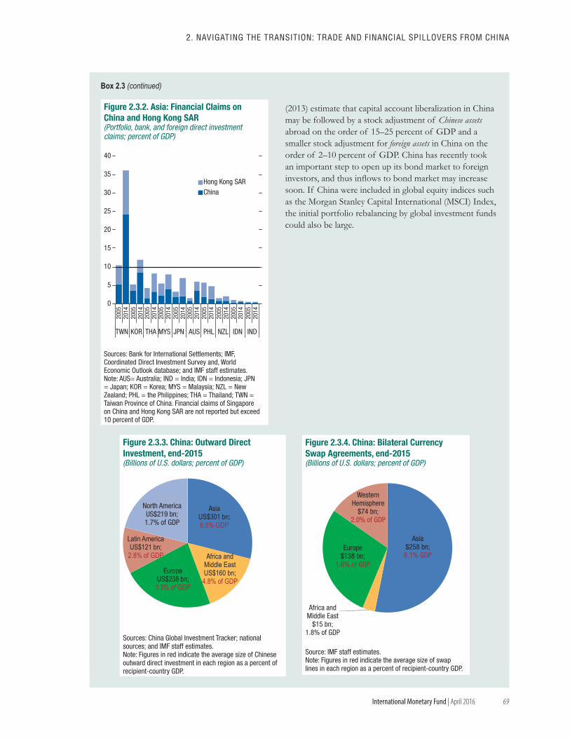
69
2. NAvIGATING ThE TRANsITION: TRAdE ANd fINANCIAL sPILLOvERs fROM ChINA
International Monetary Fund | April 2016
(2013) estimate that capital account liberalization in China may be followed by a stock adjustment of Chinese assetsabroad on the order of 15–25 percent of GDP and a smaller stock adjustment for foreign assets in China on the order of 2–10 percent of GDP. China has recently took an important step to open up its bond market to foreign investors, and thus infl ows to bond market may increase soon. If China were included in global equity indices such as the Morgan Stanley Capital International (MSCI) Index, the initial portfolio rebalancing by global investment funds could also be large.
Sources: Bank for International Settlements; IMF, Coordinated Direct Investment Survey and, World Economic Outlook database; and IMF staff estimates.Note: AUS= Australia; IND = India; IDN = Indonesia; JPN = Japan; KOR = Korea; MYS = Malaysia; NZL = New Zealand; PHL = the Philippines; THA = Thailand; TWN = Taiwan Province of China. Financial claims of Singapore on China and Hong Kong SAR are not reported but exceed 10 percent of GDP.
0
5
10
15
20
25
30
35
40
2005
2014
2005
2014
2005
2014
2005
2014
2005
2014
2005
2014
2005
2014
2005
2014
2005
2014
2005
2014
TWN KOR THA MYS JPN AUS PHL NZL IDN IND
Hong Kong SARChina
Figure 2.3.2. Asia: Financial Claims on China and Hong Kong SAR(Portfolio, bank, and foreign direct investment claims; percent of GDP)
Source: IMF staff estimates.Note: Figures in red indicate the average size of swap lines in each region as a percent of recipient-country GDP.
Asia$258 bn;6.1% GDP
Europe$138 bn;
1.8% of GDP
WesternHemisphere
$74 bn;2.0% of GDP
Africa andMiddle East
$15 bn;1.8% of GDP
Figure 2.3.4. China: Bilateral Currency Swap Agreements, end-2015(Billions of U.S. dollars; percent of GDP)
AsiaUS$301 bn;6.5% GDP
Africa andMiddle EastUS$160 bn;4.8% of GDP
EuropeUS$238 bn;1.3% of GDP
Latin AmericaUS$121 bn;2.8% of GDP
North AmericaUS$219 bn;1.7% of GDP
Figure 2.3.3. China: Outward Direct Investment, end-2015(Billions of U.S. dollars; percent of GDP)
Sources: China Global Investment Tracker; national sources; and IMF staff estimates.Note: Figures in red indicate the average size of Chinese outward direct investment in each region as a percent of recipient-country GDP.
Box 2.3 (continued)
70
REGIONAL ECONOMIC OUTLOOK: AsIA ANd PACIfIC
International Monetary Fund | April 2016
Annex 2.1. Measures of Trade and Financial Linkages and Financial Market Data
Measures of Trade and Financial LinkagesThe data span the period from 2001 to 2014 and include nine Asian economies (Australia, India, Indonesia, Korea, Malaysia, New Zealand, the Philippines, Taiwan Province of China, and Thailand) and four “center” economies (China, Japan, the euro area, and the United States). The regional economies are denoted by i and the center economies are denoted by c.
• Trade exposure. Trade exposure between country i and country c is measured by the domestic value added produced by country i and embodied in the final demand by country c, capturing both direct and indirect trade linkages. Specifically, this measure includes two types of value added embodied in (1) direct exports of final goods and services from country i to country c and (2) exports of intermediate goods from country i to other countries that will eventually be re-exported to country c for final demand. The data are sourced from the OECD-WTO TiVA database covering the years 1995, 2000, 2005, and 2008–11. A continuous time series through 2014 is constructed by following as closely as possible the OECD-WTO methodology but using the United Nation’s Comtrade data and national income accounts statistics. The methodology is explained in detail in Appendix A of a recently published Journal of International Economics article on value-added trade and business cycle synchronization (Duval and others 2015); furthermore, the approach of using Comtrade data along with national accounts data to separate intermediate inputs trade from final goods trade is also similar to Johnson and Noguera (2012a; 2012b) and Timmer (2012).
The main author of this annex is Dulani Seneviratne. The analysis is based on Arslanalp and others (forthcoming).
• Trade competition. Trade competition is proxied by constructing the export similarity index (ESI) at the five-digit level, as in: ESIi,c = Σk[min (Xi,k,Xc,k)], where Xi,k and Xc,k are industry k’s export shares in country i’s and country c’s exports. Product-level data for ESI calculations are obtained from the UN Comtrade database. For instance, if markets are pricing in downside risks in country c corresponding to a depreciation of country c’s exchange rate, this could improve country c’s trade competitiveness; hence, yielding a negative effect on asset price returns of country i that are important trade competitors. All in all, this variable allows us to look into modalities of trade in addition to the degree of trade captured by the trade exposure variable.
• Direct financial linkages. Financial linkages include portfolio investment, cross-border bank lending, and foreign direct investment by country i in country c (in percent of country i’s GDP) to capture exposure to losses that may arise from a repricing of assets in country c. Data on stock of bilateral portfolio investment positions are obtained from the IMF’s Coordinated Portfolio Investment Survey database and data on stock of bilateral direct investment positions subsequent to 2009 are obtained from the IMF’s Coordinated Direct Investment Survey database. Direct investment series prior to that are constructed by using data from databases from the United Nations Conference on Trade and Development. Bilateral cross-border lending data are based on unpublished bilateral locational banking statistics from the Bank for International Settlements. Direct financial linkages with China are estimated including exposures to both China and Hong Kong SAR given that Hong Kong SAR serves as a financial gateway to China.
Financial Market VariablesOur data set includes daily data from January 2001 to January 2016 covering nine Asian economies
71
2. NAvIGATING ThE TRANsITION: TRAdE ANd fINANCIAL sPILLOvERs fROM ChINA
International Monetary Fund | April 2016
(Australia, India, Indonesia, Korea, Malaysia, New Zealand, the Philippines, Taiwan Province of China, and Thailand) and four “center” economies (China, Japan, the euro area, and the United States).
• Asset market returns. Equity market returns are measured by the first differences in local-currency national equity indices in logs.1 Foreign exchange returns are measured by the change in the local currency against the dollar (first differences in logs). Bond market returns are measured by the 10-year local-currency government bond yield (first differences in percentage points). The data are sourced from Bloomberg, L.P.2
1The specific stock indices in the analysis are the Shanghai Com-posite Index (China), NIKKEI 225 (Japan), ASX 200 (Australia), NZX 50 (New Zealand), KOSPI (Korea), TWSE (Taiwan Province of China), Jakarta Composite (Indonesia), FTSE/KLCI (Malaysia), PSE Composite Index (the Philippines), SET Index (Thailand), and BSE SENSEX 30 (India).
2One issue to address in calculating the returns is the different time zones of the Asian financial markets, euro zone, and United States. As Asian trading is ahead of the United States, shocks from Asian markets are always incorporated into U.S. asset prices, while shocks to U.S. markets can only affect Asian trading on the next trading day. Following the practice in the literature (Forbes and Rigobon 2002), we use two-day rolling average returns in the analysis.
• Global risk appetite is measured by the Chicago Board Options Exchange Volatility Index (VIX).
• The world interest rate is measured by the U.S. “shadow” policy rate, which takes into account unconventional monetary policies. The data come from Wu and Xia (2015).
• Commodity prices are measured by the Bloomberg Commodity Index. This is a comprehensive commodity index covering 22 commodities in seven sectors.
• Country risk is measured by the country credit default swap spreads and, if not available, by the J.P. Morgan Emerging Market Bond Index-Global (EMBIG) sovereign spread.
72
REGIONAL ECONOMIC OUTLOOK: AsIA ANd PACIfIC
International Monetary Fund | April 2016
Annex 2.2. Estimating Spillovers from Rebalancing to Exports and Growth
From Rebalancing to Exports The baseline country-specific regression is the following ordinary least square regression:
DVAD i,t /GDPi,t = ai + βD
i DCHN,t + εi,t,where i refers to a country, t to time, and D to China’s consumption or investment in log. DVAD
i,t /GDPi,t is the ratio of domestic value-added exports to China to a country’s GDP, also in log. Coefficient βD
i is the elasticity of the DVA/GDP ratio to a 1 percent change in China’s consumption (or investment).
Winners and losers from rebalancing can be calculated as follows. Assume a rebalancing scenario in which China’s consumption grows by x c,R% and investment by y c,R%. Also, let China’s consumption and investment growth under the no-rebalancing scenario be x c,N% and y c,N%. Let x c,R > x c,N and y c,R > y c,N. So, the net change in the exports to China from each country will be
∆i = (xc,R – xc,N) * βC i *
DVAC i,t
GDPi,t + (yc,R – yc,N)
* βI i *
DVAI i,t
GDPi,t .
If net change ∆i>0, the country gains from rebalancing. If negative, the country loses from rebalancing.
From Rebalancing to Growth Shocks to China’s consumption and investment growth are estimated on the basis of a four-variable vector autoregression where shocks are identified by Cholesky decomposition with the following ordering:
The authors of this annex are Gee Hee Hong and Dulani Senevi-ratne. The analysis is based on Hong and others (forthcoming)
Qt = [YWLD,t,YCHN,t,CCHN,t,ICHN,t]1 and Qt = ΦQt–1 + ut
where t is year. Shocks estimated above are used to calculate the growth effect of shocks to consumption and investment as follows, allowing for two-year lagged effects:
gi,t = ai + βt + Φ1(1)shockD CHN,t
+ Φ2(1)shockDCHN,tTradeExpD
CHN,t–1 + Φa(1)TradeExpD
CHN,t–1 + γX’it + ui,t,
where gi,t stands for GDP growth of country i at time t; superscript D stands for China’s consumption or investment demand; shockD
CHN,t denotes shocks to growth in China’s D (consumption or investment); and X’
it denotes other controls including the VIX to control for global financial uncertainty and global commodity prices. TradeExpCHN,t–1 captures direct and indirect bilateral trade exposure to China measured as domestic valued added of country i exported for Chinese final consumption/investment, in percent of country i’s GDP in the previous year.
The propagation of investment/consumption growth shocks originating from China to each country’s growth incorporates the interaction term between the demand shock and trade exposure:
ϕ1(1) + ϕ2(1)TradeExpDCHN,t–1
The net effect of rebalancing on GDP growth is constructed in the equivalent way as in the effects on exports, by applying the growth rate differentials to the estimated growth effects of shocks to D.
1YWLD,t = global GDP; YCHN,t = GDP growth; CCHN,t = Consump-tion growth; ICHN,t = Investment growth. To test for robustness, we also used shocks estimated using different ordering, and results remain broadly unchanged.
73
2. NAvIGATING ThE TRANsITION: TRAdE ANd fINANCIAL sPILLOvERs fROM ChINA
International Monetary Fund | April 2016
Annex 2.3. Event StudyThe event study used in the chapter is implemented by identifying outsized movements (shocks) in the Chinese stock market. We then explore how these shocks were transmitted to other markets, especially to countries with strong trade links with China (the treatment group) versus others (the control group).
Chinese market shocks are defined as days when the movement in the Shanghai Composite Index was more than 5 percentage points (either up or down). From this sample, we exclude days that were likely driven by global events happening outside of China by taking out days when the U.S. stock market closed substantially higher or lower (by one standard deviation) before the Chinese market opened. Finally, for the remaining sample (of 30 episodes), we conduct a thorough news search to link the Chinese stock market movements to specific news or policy actions happening during that day (Annex Table 2.3.1).
The main author of this annex is Shi Piao. The analysis is based on Arslanalp and others (forthcoming).
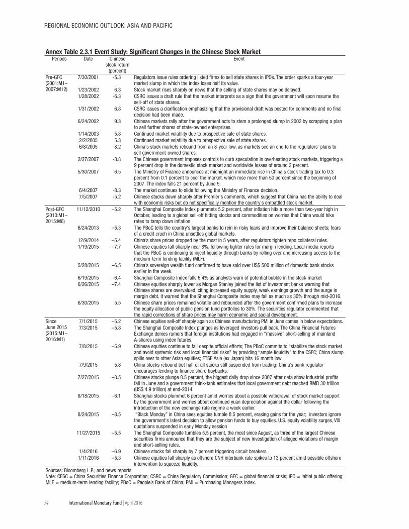
74
REGIONAL ECONOMIC OUTLOOK: AsIA ANd PACIfIC
International Monetary Fund | April 2016
Annex Table 2.3.1 Event Study: Significant Changes in the Chinese Stock MarketPeriods Date Chinese
stock return (percent)
Event
Pre-GFC (2001:M1–2007:M12)
7/30/2001 -5.3 Regulators issue rules ordering listed firms to sell state shares in IPOs. The order sparks a four-year market slump in which the index loses half its value.
1/23/2002 6.3 Stock market rises sharply on news that the selling of state shares may be delayed.1/28/2002 -6.3 CSRC issues a draft rule that the market interprets as a sign that the government will soon resume the
sell-off of state shares.1/31/2002 6.8 CSRC issues a clarification emphasizing that the provisional draft was posted for comments and no final
decision had been made.6/24/2002 9.3 Chinese markets rally after the government acts to stem a prolonged slump in 2002 by scrapping a plan
to sell further shares of state-owned enterprises.1/14/2003 5.8 Continued market volatility due to prospective sale of state shares.2/2/2005 5.3 Continued market volatility due to prospective sale of state shares.6/8/2005 8.2 China's stock markets rebound from an 8-year low, as markets see an end to the regulators' plans to
sell government-owned shares.2/27/2007 -8.8 The Chinese government imposes controls to curb speculation in overheating stock markets, triggering a
9 percent drop in the domestic stock market and worldwide losses of around 2 percent.5/30/2007 -6.5 The Ministry of Finance announces at midnight an immediate rise in China's stock trading tax to 0.3
percent from 0.1 percent to cool the market, which rose more than 50 percent since the beginning of 2007. The index falls 21 percent by June 5.
6/4/2007 -8.3 The market continues to slide following the Ministry of Finance decision.7/5/2007 -5.2 Chinese stocks down sharply after Premier's comments, which suggest that China has the ability to deal
with economic risks but do not specifically mention the country's embattled stock market.Post-GFC (2010:M1–2015:M6)
11/12/2010 –5.2 The Shanghai Composite Index plummets 5.2 percent, after inflation hits a more than two-year high in October, leading to a global sell-off hitting stocks and commodities on worries that China would hike rates to tamp down inflation.
6/24/2013 –5.3 The PBoC tells the country's largest banks to rein in risky loans and improve their balance sheets; fears of a credit cruch in China unsettles global markets.
12/9/2014 –5.4 China’s share prices dropped by the most in 5 years, after regulators tighten repo collateral rules. 1/19/2015 –7.7 Chinese equities fall sharply near 8%, following tighter rules for margin lending. Local media reports
that the PBoC is continuing to inject liquidity through banks by rolling over and increasing access to the medium-term lending facility (MLF).
5/28/2015 –6.5 China’s sovereign wealth fund confirmed to have sold over US$ 500 million of domestic bank stocks earlier in the week.
6/19/2015 –6.4 Shanghai Composite Index falls 6.4% as analysts warn of potential bubble in the stock market6/26/2015 –7.4 Chinese equities sharply lower as Morgan Stanley joined the list of investment banks warning that
Chinese shares are overvalued, citing increased equity supply, weak earnings growth and the surge in margin debt. It warned that the Shanghai Composite index may fall as much as 30% through mid-2016.
6/30/2015 5.5 Chinese share prices remained volatile and rebounded after the government confirmed plans to increase the equity allocation of public pension fund portfolios to 30%. The securities regulator commented that the rapid corrections of share prices may harm economic and social development.
Since June 2015 (2015:M1–2016:M1)
7/1/2015 –5.2 Chinese equities sell-off sharply again as Chinese manufacturing PMI in June comes in below expectations.7/3/2015 –5.8 The Shanghai Composite Index plunges as leveraged investors pull back. The China Financial Futures
Exchange denies rumors that foreign institutions had engaged in “massive” short-selling of mainland A-shares using index futures.
7/8/2015 –5.9 Chinese equities continue to fall despite official efforts; The PBoC commits to “stabilize the stock market and avoid systemic risk and local financial risks” by providing “ample liquidity” to the CSFC; China slump spills over to other Asian equities; FTSE Asia (ex Japan) hits 16 month low.
7/9/2015 5.8 China stocks rebound but half of all stocks still suspended from trading; China’s bank regulator encourages lending to finance share buybacks.
7/27/2015 –8.5 Chinese stocks plunge 8.5 percent, the biggest daily drop since 2007 after data show industrial profits fall in June and a government think-tank estimates that local government debt reached RMB 30 trillion (US$ 4.9 trillion) at end-2014.
8/18/2015 –6.1 Shanghai stocks plummet 6 percent amid worries about a possible withdrawal of stock market support by the government and worries about continued yuan depreciation against the dollar following the introduction of the new exchange rate regime a week earlier.
8/24/2015 –8.5 “Black Monday” in China sees equities tumble 8.5 percent, erasing gains for the year; investors ignore the government's latest decision to allow pension funds to buy equities. U.S. equity volatility surges, VIX quotations suspended in early Monday session
11/27/2015 –5.5 The Shanghai Composite tumbles 5.5 percent, the most since August, as three of the largest Chinese securities firms announce that they are the subject of new investigation of alleged violations of margin and short-selling rules.
1/4/2016 –6.9 Chinese stocks fall sharply by 7 percent triggering circuit breakers. 1/11/2016 –5.3 Chinese equities fall sharply as offshore CNH interbank rate spikes to 13 percent amid possible offshore
intervention to squeeze liquidity.Sources: Bloomberg L.P.; and news reports. Note: CFSC = China Securities Finance Corporation; CSRC = China Regulatory Commission; GFC = global financial crisis; IPO = initial public offering; MLF = medium-term lending facility; PBoC = People’s Bank of China; PMI = Purchasing Managers Index.
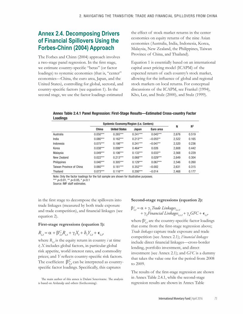
75
2. NAvIGATING ThE TRANsITION: TRAdE ANd fINANCIAL sPILLOvERs fROM ChINA
International Monetary Fund | April 2016
Annex 2.4. Decomposing Drivers of Financial Spillovers Using the Forbes-Chinn (2004) ApproachThe Forbes and Chinn (2004) approach involves a two-stage panel regression. In the first stage, we estimate country-specific “betas” (or factor loadings) to systemic economies (that is, “center” economies—China, the euro area, Japan, and the United States), controlling for global, sectoral, and country-specific factors (see equation 1). In the second stage, we use the factor loadings estimated
in the first stage to decompose the spillovers into trade linkages (measured by both trade exposure and trade competition), and financial linkages (see equation 2).
First-stage regressions (equation 1):
Ri,t = a + βC i,tRs,t + γiXt + δiYi,t + i,t,
where Ri,t is the equity return in country i at time t; X includes global factors, in particular global risk appetite, world interest rates, and commodity prices; and Y reflects country-specific risk factors. The coefficient βC
i,t can be interpreted as country-specific factor loadings. Specifically, this captures
The main author of this annex is Dulani Seneviratne. The analysis is based on Arslanalp and others (forthcoming).
the effect of stock market returns in the center economies on equity returns of the nine Asian economies (Australia, India, Indonesia, Korea, Malaysia, New Zealand, the Philippines, Taiwan Province of China, and Thailand).
Equation 1 is essentially based on an international capital asset pricing model (ICAPM) of the expected return of each country’s stock market, allowing for the influence of global and regional stock markets on local returns. For conceptual discussions of the ICAPM, see Frankel (1994), Kho, Lee, and Stulz (2000), and Stulz (1999).
Second-stage regressions (equation 2):
βc i,t = a + γ1Trade Linkagesi,c,t
+ γ2Financial Linkagesi,c,t + γaGFC + i,t,
where βc i,t are the country-specific factor loadings
that come from the first-stage regression above; Trade linkages capture trade exposure and trade competition (see Annex 2.1); Financial linkages include direct financial linkages—cross-border lending, portfolio investment, and direct investment (see Annex 2.1); and GFC is a dummy that takes the value one for the period from 2008 to 2009.
The results of the first-stage regression are shown in Annex Table 2.4.1, while the second-stage regression results are shown in Annex Table
Annex Table 2.4.1 Panel Regression: First-Stage Results—Estimated Cross-country Factor Loadings
Systemic Economy/Region (i.e. Centers)N R2
China United States Japan Euro area
Australia 0.050*** 0.265*** 0.241*** 0.045*** 2,676 0.519
India 0.080*** 0.162*** 0.213*** –0.055** 2,522 0.165
Indonesia 0.075*** 0.198*** 0.241*** –0.047** 2,520 0.236
Korea 0.038*** 0.099*** 0.464*** 0.026 2,608 0.442
Malaysia 0.049*** 0.106*** 0.133*** 0.033** 2,568 0.229
New Zealand 0.022*** 0.213*** 0.068*** 0.029*** 2,649 0.304
Philippines 0.040*** 0.305*** 0.129*** 0.067*** 2,546 0.260
Taiwan Province of China 0.060*** 0.181*** 0.352*** –0.002 2,631 0.315
Thailand 0.073*** 0.116*** 0.200*** –0.014 2,468 0.177
Note: Only the factor loadings for the full sample are shown for illustrative purposes.*** p<0.01, ** p<0.05, * p<0.1Source: IMF staff estimates.
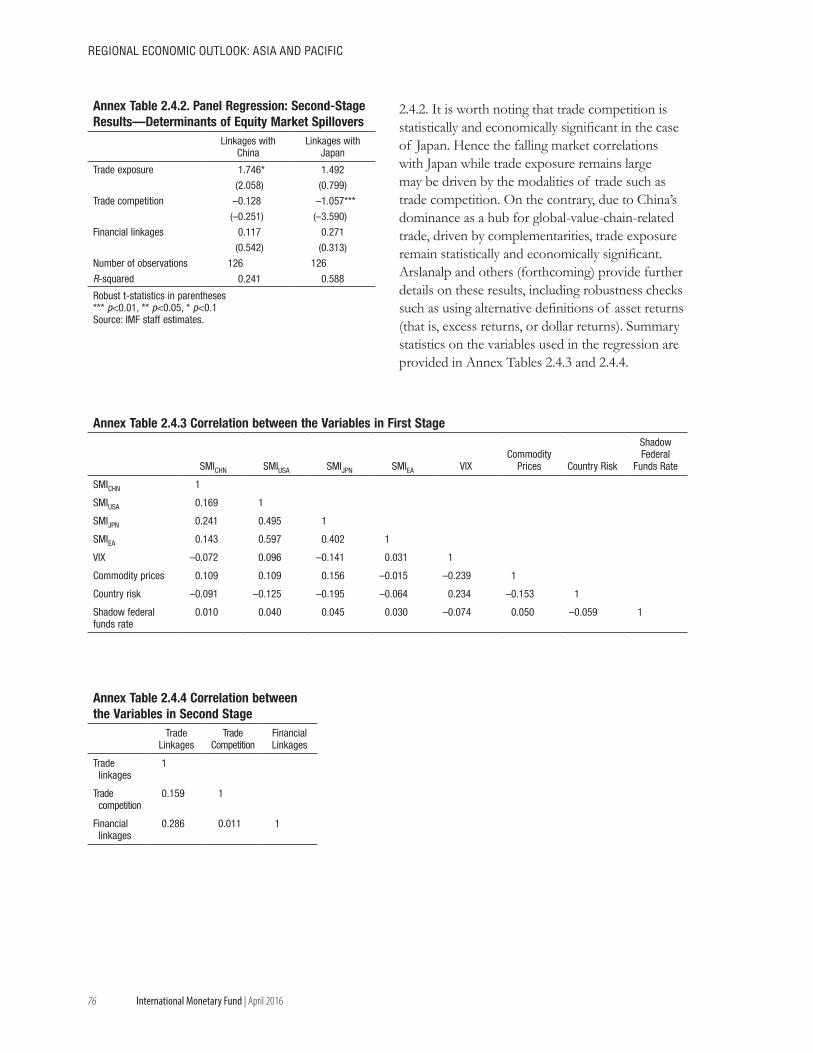
76
REGIONAL ECONOMIC OUTLOOK: AsIA ANd PACIfIC
International Monetary Fund | April 2016
2.4.2. It is worth noting that trade competition is statistically and economically significant in the case of Japan. Hence the falling market correlations with Japan while trade exposure remains large may be driven by the modalities of trade such as trade competition. On the contrary, due to China’s dominance as a hub for global-value-chain-related trade, driven by complementarities, trade exposure remain statistically and economically significant. Arslanalp and others (forthcoming) provide further details on these results, including robustness checks such as using alternative definitions of asset returns (that is, excess returns, or dollar returns). Summary statistics on the variables used in the regression are provided in Annex Tables 2.4.3 and 2.4.4.
Annex Table 2.4.4 Correlation between the Variables in Second Stage
Trade Linkages
Trade Competition
Financial Linkages
Trade linkages
1
Trade competition
0.159 1
Financial linkages
0.286 0.011 1
Annex Table 2.4.2. Panel Regression: Second-Stage Results—Determinants of Equity Market Spillovers
Linkages with China
Linkages with Japan
Trade exposure 1.746* 1.492
(2.058) (0.799)
Trade competition –0.128 –1.057***
(–0.251) (–3.590)
Financial linkages 0.117 0.271
(0.542) (0.313)
Number of observations 126 126
R-squared 0.241 0.588
Robust t-statistics in parentheses*** p<0.01, ** p<0.05, * p<0.1Source: IMF staff estimates.
Annex Table 2.4.3 Correlation between the Variables in First Stage
SMICHN SMIUSA SMIJPN SMIEA VIXCommodity
Prices Country Risk
Shadow Federal
Funds Rate
SMICHN 1
SMIUSA 0.169 1
SMIJPN 0.241 0.495 1
SMIEA 0.143 0.597 0.402 1
VIX –0.072 0.096 –0.141 0.031 1
Commodity prices 0.109 0.109 0.156 –0.015 –0.239 1
Country risk –0.091 –0.125 –0.195 –0.064 0.234 –0.153 1
Shadow federal funds rate
0.010 0.040 0.045 0.030 –0.074 0.050 –0.059 1
International Monetary Fund | April 2016
Introduction and Main FindingsChina is in the midst of a fundamental transformation. Growth has been slowing since 2012 as the economy has been rebalancing to a more sustainable growth model. This process of rebalancing or growth transition in China involves not only lower growth but also a shift from heavy industry and construction to more advanced manufacturing and services in production, and from investment and export to consumption in final demand. This transition has profound implications for China’s trade patterns, as import intensities vary across sectors and components of final demand. At the same time, trade patterns are also changing because of China’s evolving comparative advantage, driven in part by demographics and the implied changes for the relative labor supply, as well as by increasing human capital.
This chapter reviews recent changes in China’s broad merchandise trade patterns and examines their implications for trading partners.1 These changes in trade patterns are part of the channels through which China’s growth transition has affected growth and macroeconomic conditions in trading partners and other economies. Chapter 2 reviews and analyzes in detail such spillovers from China’s transition. The analysis in this chapter is less concerned with the spillovers as it seeks to understand the changes in the trade patterns on their own, thereby contributing to the broader understanding of the changing spillover patterns highlighted in Chapter 2.
The changes in trade patterns are broad, and the chapter focuses on advanced upstream economies
This chapter was prepared by Thomas Helbling (co-lead), Koshy Mathai (co-lead), Michael Dalesio, Geoff Gottlieb, Gee Hee Hong, Rui Mano, Adil Mohommad, and Dulani Seneviratne.
1The chapter takes China’s rise as an export powerhouse as a given. For recent analysis of the factors at play see Chinn (2015), Gaulier and others (2015), and Veenendaal and others (2015).
and commodity exporters. This analysis builds on recent work examining the implications of changes in these trade patterns for China’s neighboring low-income countries. Specifically, the chapter first examines whether China’s growing competitiveness in producing upstream parts and components has affected exports of five major trading partners—Japan, Korea, and Taiwan Province of China within the Asia economic region, and Germany and the United States—in China’s home market and in third markets. The chapter then examines China’s impact on commodity exporters and global commodity markets more generally. Rebalancing and structural change are also likely to profoundly affect trade patterns in services. Indeed, advanced economies facing growing competition from China in manufacturing have benefited from increased Chinese demand for tourism and other services—an issue that is beyond the scope of this chapter.
This chapter offers evidence that for some higher-technology goods, advanced upstream countries have lost market share to China since the beginning of rebalancing. The loss is most noticeable and strongest in China’s domestic market, as reflected in the onshoring of production of previously imported parts and components. But China’s exports of such goods to other countries have also started rising. The chapter also shows that China’s growth transition has contributed to a slowing of demand for commodities, particularly those used primarily in investment, heavy industry, and construction. Export values of many commodity exporters have been affected as a result. But for some exporters, values have been affected more by declining global prices than by changes in export volumes. In this regard, other factors have also contributed to recent commodity price declines—research presented in the chapter suggests that China’s rebalancing might account for between one-fifth and one-half of the declines in broad commodity
3. China’s Evolving Trade with Advanced Upstream Economies and Commodity Exporters
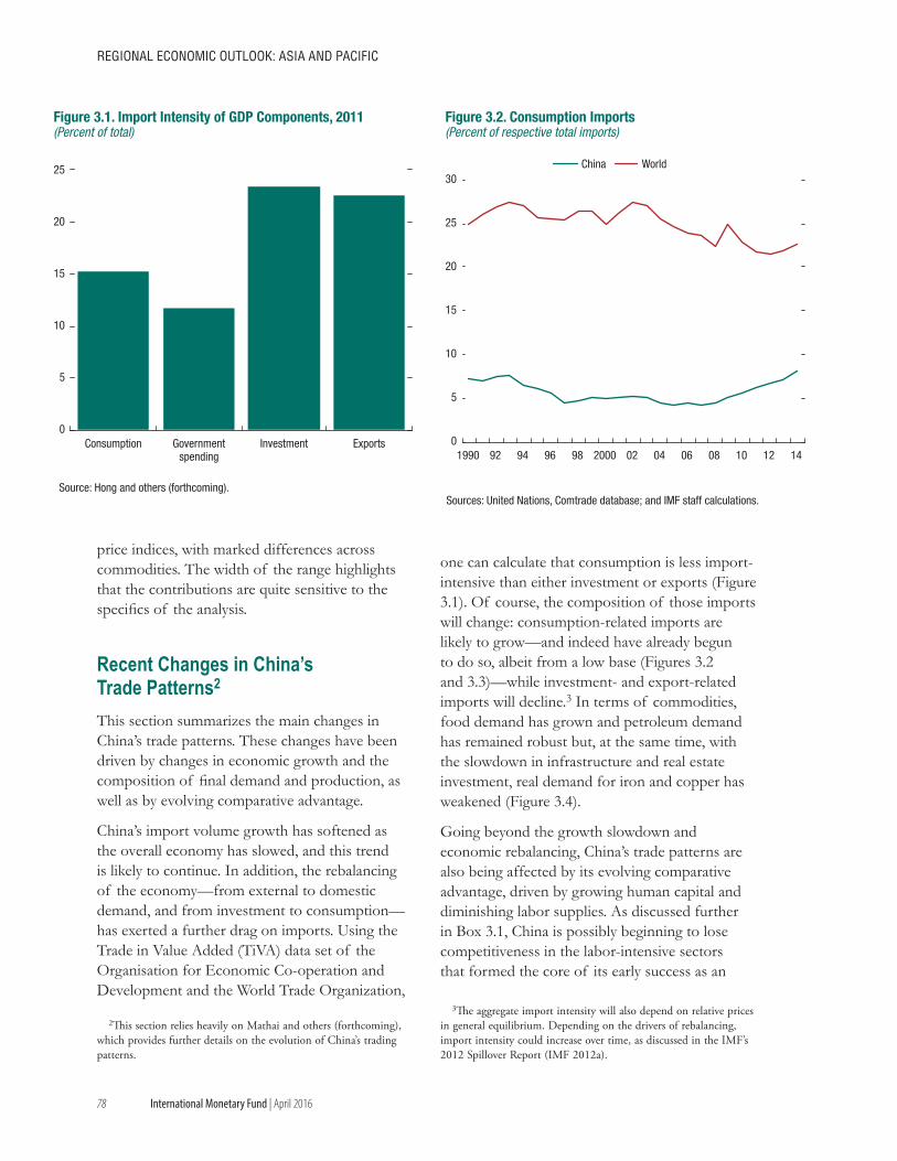
78
REGIONAL ECONOMIC OUTLOOK: AsIA ANd PACIfIC
International Monetary Fund | April 2016
price indices, with marked differences across commodities. The width of the range highlights that the contributions are quite sensitive to the specifics of the analysis.
Recent Changes in China’s Trade Patterns2
This section summarizes the main changes in China’s trade patterns. These changes have been driven by changes in economic growth and the composition of final demand and production, as well as by evolving comparative advantage.
China’s import volume growth has softened as the overall economy has slowed, and this trend is likely to continue. In addition, the rebalancing of the economy—from external to domestic demand, and from investment to consumption—has exerted a further drag on imports. Using the Trade in Value Added (TiVA) data set of the Organisation for Economic Co-operation and Development and the World Trade Organization,
2This section relies heavily on Mathai and others (forthcoming), which provides further details on the evolution of China’s trading patterns.
one can calculate that consumption is less import-intensive than either investment or exports (Figure 3.1). Of course, the composition of those imports will change: consumption-related imports are likely to grow—and indeed have already begun to do so, albeit from a low base (Figures 3.2 and 3.3)—while investment- and export-related imports will decline.3 In terms of commodities, food demand has grown and petroleum demand has remained robust but, at the same time, with the slowdown in infrastructure and real estate investment, real demand for iron and copper has weakened (Figure 3.4).
Going beyond the growth slowdown and economic rebalancing, China’s trade patterns are also being affected by its evolving comparative advantage, driven by growing human capital and diminishing labor supplies. As discussed further in Box 3.1, China is possibly beginning to lose competitiveness in the labor-intensive sectors that formed the core of its early success as an
3The aggregate import intensity will also depend on relative prices in general equilibrium. Depending on the drivers of rebalancing, import intensity could increase over time, as discussed in the IMF’s 2012 Spillover Report (IMF 2012a).
0
5
10
15
20
25
Consumption Governmentspending
Investment Exports
Source: Hong and others (forthcoming).
Figure 3.1. Import Intensity of GDP Components, 2011(Percent of total)
Sources: United Nations, Comtrade database; and IMF staff calculations.
0
5
10
15
20
25
30
1990 92 94 96 98 2000 02 04 06 08 10 12 14
China World
Figure 3.2. Consumption Imports(Percent of respective total imports)
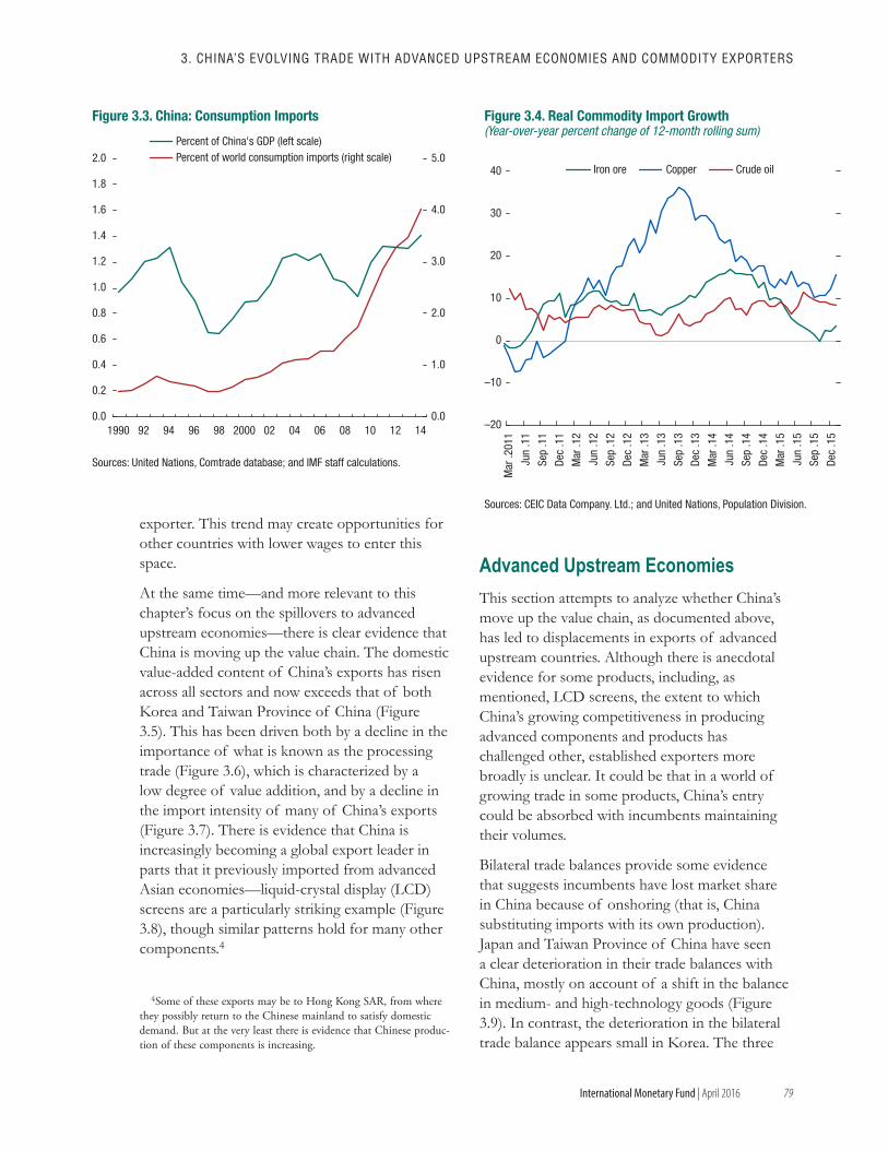
79
3. ChINA’s EvOLvING TRAdE wITh AdvANCEd UPsTREAM ECONOMIEs ANd COMMOdITy ExPORTERs
International Monetary Fund | April 2016
exporter. This trend may create opportunities for other countries with lower wages to enter this space.
At the same time—and more relevant to this chapter’s focus on the spillovers to advanced upstream economies—there is clear evidence that China is moving up the value chain. The domestic value-added content of China’s exports has risen across all sectors and now exceeds that of both Korea and Taiwan Province of China (Figure 3.5). This has been driven both by a decline in the importance of what is known as the processing trade (Figure 3.6), which is characterized by a low degree of value addition, and by a decline in the import intensity of many of China’s exports (Figure 3.7). There is evidence that China is increasingly becoming a global export leader in parts that it previously imported from advanced Asian economies—liquid-crystal display (LCD) screens are a particularly striking example (Figure 3.8), though similar patterns hold for many other components.4
4Some of these exports may be to Hong Kong SAR, from where they possibly return to the Chinese mainland to satisfy domestic demand. But at the very least there is evidence that Chinese produc-tion of these components is increasing.
Advanced Upstream EconomiesThis section attempts to analyze whether China’s move up the value chain, as documented above, has led to displacements in exports of advanced upstream countries. Although there is anecdotal evidence for some products, including, as mentioned, LCD screens, the extent to which China’s growing competitiveness in producing advanced components and products has challenged other, established exporters more broadly is unclear. It could be that in a world of growing trade in some products, China’s entry could be absorbed with incumbents maintaining their volumes.
Bilateral trade balances provide some evidence that suggests incumbents have lost market share in China because of onshoring (that is, China substituting imports with its own production). Japan and Taiwan Province of China have seen a clear deterioration in their trade balances with China, mostly on account of a shift in the balance in medium- and high-technology goods (Figure 3.9). In contrast, the deterioration in the bilateral trade balance appears small in Korea. The three
0.0
1.0
2.0
3.0
4.0
5.0
0.0
0.2
0.4
0.6
0.8
1.0
1.2
1.4
1.6
1.8
2.0
1990 92 94 96 98 2000 02 04 06 08 10 12 14
Percent of China's GDP (left scale)Percent of world consumption imports (right scale)
Figure 3.3. China: Consumption Imports
Sources: United Nations, Comtrade database; and IMF staff calculations.
–20
–10
0
10
20
30
40
Mar
.201
1
Jun
.11
Sep
.11
Dec
.11
Mar
.12
Jun
.12
Sep
.12
Dec
.12
Mar
.13
Jun
.13
Sep
.13
Dec
.13
Mar
.14
Jun
.14
Sep
.14
Dec
.14
Mar
.15
Jun
.15
Sep
.15
Dec
.15
Iron ore Copper Crude oil
Sources: CEIC Data Company. Ltd.; and United Nations, Population Division.
Figure 3.4. Real Commodity Import Growth(Year-over-year percent change of 12-month rolling sum)
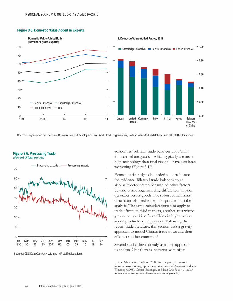
80
REGIONAL ECONOMIC OUTLOOK: AsIA ANd PACIfIC
International Monetary Fund | April 2016
economies’ bilateral trade balances with China in intermediate goods—which typically are more high-technology than final goods—have also been worsening (Figure 3.10).
Econometric analysis is needed to corroborate the evidence. Bilateral trade balances could also have deteriorated because of other factors beyond onshoring, including differences in price dynamics across goods. For robust conclusions, other controls need to be incorporated into the analysis. The same considerations also apply to trade effects in third markets, another area where greater competition from China in higher-value-added products could play out. Following the recent trade literature, this section uses a gravity approach to model China’s trade flows and their effects on other countries.5
Several studies have already used this approach to analyze China’s trade patterns, with often
5See Baldwin and Taglioni (2006) for the panel framework followed here, building upon the seminal work of Anderson and van Wincoop (2003). Crozet, Emlinger, and Jean (2015) use a similar framework to study trade determinants more generally.
0
10
20
30
40
50
60
70
80
1995 2000 05 08 11
Sources: Organisation for Economic Co-operation and Development and World Trade Organization, Trade in Value Added database; and IMF staff calculations.
Figure 3.5. Domestic Value Added in Exports
Capital-intensive Knowledge-intensive
Labor-intensive Total
0.00
0.20
0.40
0.60
0.80
1.00
Japan UnitedStates
Germany Italy China Korea
1. Domestic Value-Added Ratio(Percent of gross exports)
2. Domestic Value-Added Ratios, 2011
Knowledge-intensive Capital-intensive Labor-intensive
TaiwanProvinceof China
0
10
20
30
40
50
60
70
Jan.1993
Mar.95
May97
Jul.99
Sep.2001
Nov.03
Jan.06
Mar.08
May10
Jul.12
Sep.14
Processing exports Processing imports
Figure 3.6. Processing Trade(Percent of total exports)
Sources: CEIC Data Company Ltd.; and IMF staff calculations.
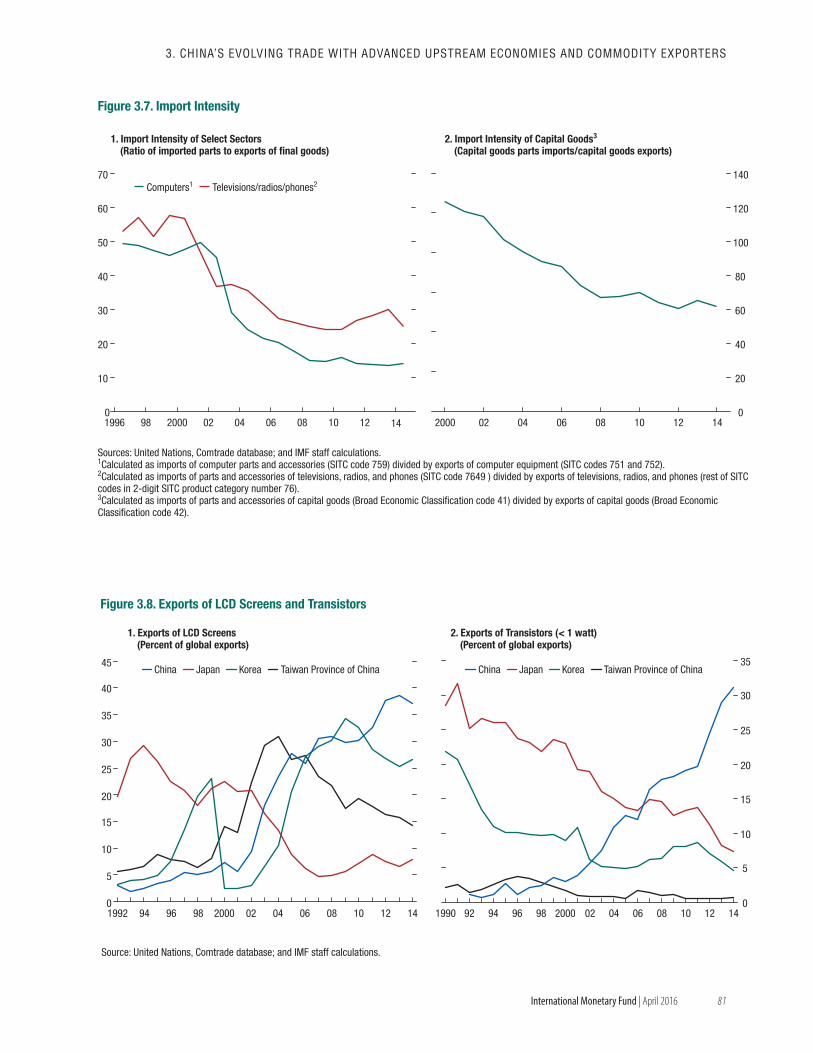
81
3. ChINA’s EvOLvING TRAdE wITh AdvANCEd UPsTREAM ECONOMIEs ANd COMMOdITy ExPORTERs
International Monetary Fund | April 2016
Sources: United Nations, Comtrade database; and IMF staff calculations.1Calculated as imports of computer parts and accessories (SITC code 759) divided by exports of computer equipment (SITC codes 751 and 752).2Calculated as imports of parts and accessories of televisions, radios, and phones (SITC code 7649 ) divided by exports of televisions, radios, and phones (rest of SITC codes in 2-digit SITC product category number 76).3Calculated as imports of parts and accessories of capital goods (Broad Economic Classification code 41) divided by exports of capital goods (Broad Economic Classification code 42).
2. Import Intensity of Capital Goods3
(Capital goods parts imports/capital goods exports)
0
20
40
60
80
100
120
140
2000 02 04 06 08 10 12 140
10
20
30
40
50
60
70
1996 98 2000 02 04 06 08 10 12 14
1. Import Intensity of Select Sectors(Ratio of imported parts to exports of final goods)
Computers1 Televisions/radios/phones2
Figure 3.7. Import Intensity
0
5
10
15
20
25
30
35
40
45
1992 94 96 98 2000 02 04 06 08 10 12 14
Source: United Nations, Comtrade database; and IMF staff calculations.
Figure 3.8. Exports of LCD Screens and Transistors
China Japan Korea Taiwan Province of China
0
5
10
15
20
25
30
35
1990 92 94 96 98 2000 02 04 06 08 10 12 14
1. Exports of LCD Screens(Percent of global exports)
2. Exports of Transistors (< 1 watt)(Percent of global exports)
China Japan Korea Taiwan Province of China
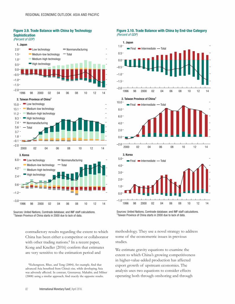
82
REGIONAL ECONOMIC OUTLOOK: AsIA ANd PACIfIC
International Monetary Fund | April 2016
contradictory results regarding the extent to which China has been either a competitor or collaborator with other trading nations.6 In a recent paper, Kong and Kneller (2016) confirm that estimates are very sensitive to the estimation period and
6Eichengreen, Rhee, and Tong (2004), for example, find that advanced Asia benefited from China’s rise, while developing Asia was adversely affected. In contrast, Greenaway, Mahabir, and Milner (2008) using a similar approach, find exactly the opposite results.
methodology. They use a novel strategy to address some of the econometric issues in previous studies.
We estimate gravity equations to examine the extent to which China’s growing competitiveness in higher-value-added production has affected export growth of upstream economies. The analysis uses two equations to consider effects operating both through onshoring and through
1. Japan
2. Taiwan Province of China1
–2.0
–2.0
–0.1
–3.0
–1.2
–1.5
–1.0
–0.5
0.0
0.5
1.0
1.5
2.0
1996 98 2000 02 04 06 08 10 12 14
Low technology Nonmanufacturing
Medium-low technology Total
Medium-high technology
Medium-low technology
Medium-high technology
Medium-low technology
Medium-high technology
High technology
1.8
3.7
5.6
7.49.3
11.2
13.1
15.0
2000 02 04 06 08 10 12 14
Low technology
High technology
Nonmanufacturing
Total
3. Korea
0.6
2.4
4.2
6.0
1996 98 2000 02 04 06 08 10 12 14
Low technology Nonmanufacturing
Total
High technology
Sources: United Nations, Comtrade database; and IMF staff calculations.1Taiwan Province of China starts in 2000 due to lack of data.
Figure 3.9. Trade Balance with China by Technology Sophistication(Percent of GDP)
Sources: United Nations, Comtrade database; and IMF staff calculations.1Taiwan Province of China starts in 2000 due to lack of data.
3. Korea
–1.0
0.0
1.0
2.0
3.0
4.0
5.0
1996 98 2000 02 04 06 08 10 12 14
Final Intermediate Total
–2.0
0.0
2.0
4.0
6.0
8.0
10.0
2000 02 04 06 08 10 12 14
2. Taiwan Province of China1
Final Intermediate Total
–2.0
–1.5
–1.0
–0.5
0.0
0.5
1.0
1996 98 2000 02 04 06 08 10 12 14
Final Intermediate Total
1. Japan
Figure 3.10. Trade Balance with China by End-Use Category(Percent of GDP)
83
3. ChINA’s EvOLvING TRAdE wITh AdvANCEd UPsTREAM ECONOMIEs ANd COMMOdITy ExPORTERs
International Monetary Fund | April 2016
exports to other markets on account of competition from Chinese exports (‘third market effects”). We estimate these effects using two panel data sets for growth in export values.7 The first one is a panel based on foreign value added from the five upstream countries to China and domestic value added in China from the TiVA data set for the period 2000–11. The second one is based on gross exports data for 180 countries and territories for the period 2000–14. Given the relatively short time period, we distinguish between a precrisis period of five and seven years, respectively, and a postcrisis period of four years, depending on the underlying export data. Given the extensive time and country-pair fixed effects used, identification rests on cross-sectoral variation of changes in trade flows.
The analysis suggests that some export categories of advanced upstream economies are indeed adversely affected by China’s move up the value chain. Sectors in which China has grown increasingly competitive are those in which economies such as Germany, Japan, Korea, Taiwan Province of China, and the United States have seen a fall in their exports both to China and to third markets. The competitive effect is only apparent in the postcrisis part of the sample; in fact, earlier on, as global supply chains were developing, there appears to have been some complementarity between China’s exports and those of its advanced partner countries. (See Annex 3.1 for the econometric specifications and detailed regression results.)
Moreover, China’s imports from advanced economies are increasingly affected by the rise of China’s competitiveness in high-technology, knowledge-intensive, and more complex goods. In third markets, that shift is less pronounced. There, exports from advanced economies were
7We use trade values rather than volumes in the analysis because of data availability issues. This choice should not affect results meaningfully, given the set-up of our empirical analysis. While departures to the law of one price in different directions between China and partner countries could, in principle, mean that results could be influenced by price changes for reasons other than changes in comparative advantage, this seems unlikely, given that we control for common and country-specific factors, as well as trade costs and total exports at the level of individual goods.
initially competed away in low-technology and labor-intensive goods, while in the postcrisis part of the sample we find evidence that China is now competing in medium-tech, capital-intensive goods and, to a lesser extent, in higher-technology, knowledge-intensive goods.
It is worth keeping in mind that this analysis of trade patterns does not consider issues of ownership, which are important to accurately assess the impact on relative national incomes. Indeed, China’s rise as an exporter of manufactured goods has to a substantial degree been driven by foreign-owned firms. As a result, although China’s labor force benefited from the wage income associated with the relocation to China of production from upstream producers elsewhere, the returns on the related investments have accrued to foreign investors. Still, the increase in foreign direct investment in China has led to a transfer of technology to the broader economy, which, over time, has also enabled an increasing number of domestically owned firms to become exporters of manufacturing goods.
Commodity ExportersThis section explores how evolving Chinese trade patterns are affecting commodity exporters and commodity markets more generally. The section documents the changes in commodity use, production, and imports in China since the rebalancing started; examines what this has meant for key commodity producers; and explores how much of the recent decline in global commodity prices can plausibly be attributed to China, as opposed to other factors such as slowing demand in other economies or supply response to the pickup in global commodity demand in the early 2000s.
China’s growth transition affects global commodity markets through a number of channels. First and foremost, lower output growth will generally translate into lower growth in commodity demand volumes and thus commodity imports. And, insofar as the shock to China’s growth spills over to other countries’ growth,
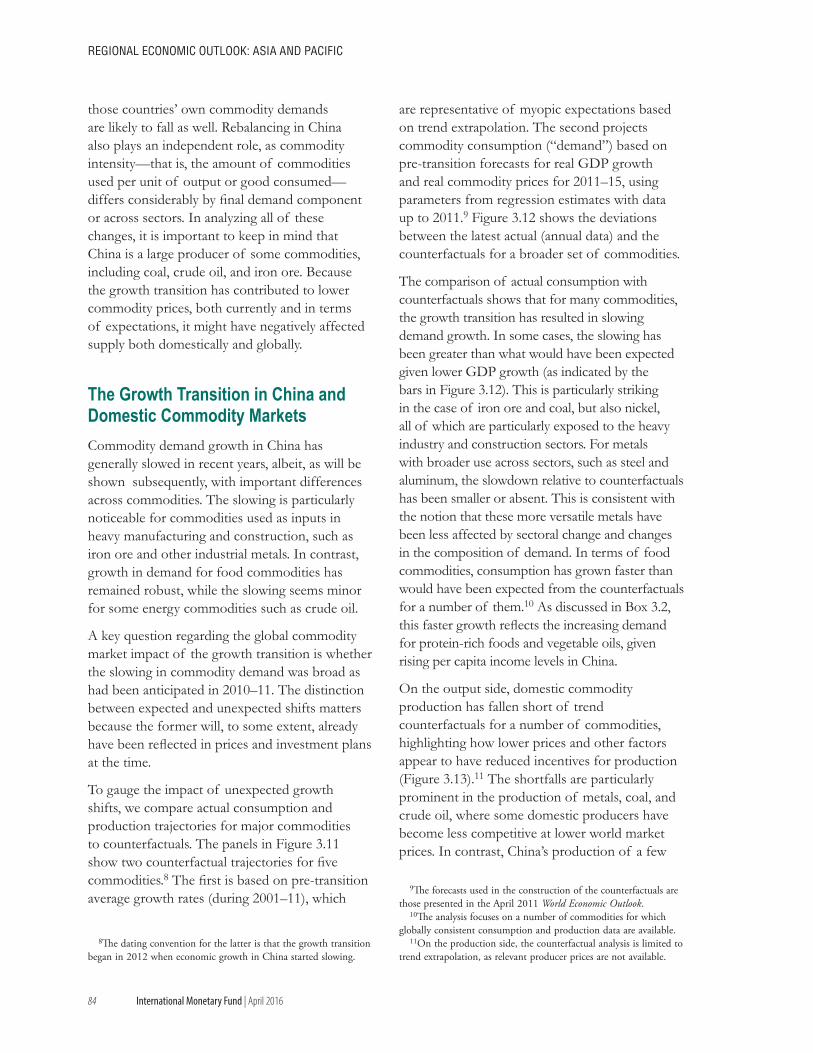
84
REGIONAL ECONOMIC OUTLOOK: AsIA ANd PACIfIC
International Monetary Fund | April 2016
those countries’ own commodity demands are likely to fall as well. Rebalancing in China also plays an independent role, as commodity intensity—that is, the amount of commodities used per unit of output or good consumed—differs considerably by final demand component or across sectors. In analyzing all of these changes, it is important to keep in mind that China is a large producer of some commodities, including coal, crude oil, and iron ore. Because the growth transition has contributed to lower commodity prices, both currently and in terms of expectations, it might have negatively affected supply both domestically and globally.
The Growth Transition in China and Domestic Commodity MarketsCommodity demand growth in China has generally slowed in recent years, albeit, as will be shown subsequently, with important differences across commodities. The slowing is particularly noticeable for commodities used as inputs in heavy manufacturing and construction, such as iron ore and other industrial metals. In contrast, growth in demand for food commodities has remained robust, while the slowing seems minor for some energy commodities such as crude oil.
A key question regarding the global commodity market impact of the growth transition is whether the slowing in commodity demand was broad as had been anticipated in 2010–11. The distinction between expected and unexpected shifts matters because the former will, to some extent, already have been reflected in prices and investment plans at the time.
To gauge the impact of unexpected growth shifts, we compare actual consumption and production trajectories for major commodities to counterfactuals. The panels in Figure 3.11 show two counterfactual trajectories for five commodities.8 The first is based on pre-transition average growth rates (during 2001–11), which
8The dating convention for the latter is that the growth transition began in 2012 when economic growth in China started slowing.
are representative of myopic expectations based on trend extrapolation. The second projects commodity consumption (“demand”) based on pre-transition forecasts for real GDP growth and real commodity prices for 2011–15, using parameters from regression estimates with data up to 2011.9 Figure 3.12 shows the deviations between the latest actual (annual data) and the counterfactuals for a broader set of commodities.
The comparison of actual consumption with counterfactuals shows that for many commodities, the growth transition has resulted in slowing demand growth. In some cases, the slowing has been greater than what would have been expected given lower GDP growth (as indicated by the bars in Figure 3.12). This is particularly striking in the case of iron ore and coal, but also nickel, all of which are particularly exposed to the heavy industry and construction sectors. For metals with broader use across sectors, such as steel and aluminum, the slowdown relative to counterfactuals has been smaller or absent. This is consistent with the notion that these more versatile metals have been less affected by sectoral change and changes in the composition of demand. In terms of food commodities, consumption has grown faster than would have been expected from the counterfactuals for a number of them.10 As discussed in Box 3.2, this faster growth reflects the increasing demand for protein-rich foods and vegetable oils, given rising per capita income levels in China.
On the output side, domestic commodity production has fallen short of trend counterfactuals for a number of commodities, highlighting how lower prices and other factors appear to have reduced incentives for production (Figure 3.13).11 The shortfalls are particularly prominent in the production of metals, coal, and crude oil, where some domestic producers have become less competitive at lower world market prices. In contrast, China’s production of a few
9The forecasts used in the construction of the counterfactuals are those presented in the April 2011 World Economic Outlook.
10The analysis focuses on a number of commodities for which globally consistent consumption and production data are available.
11On the production side, the counterfactual analysis is limited to trend extrapolation, as relevant producer prices are not available.
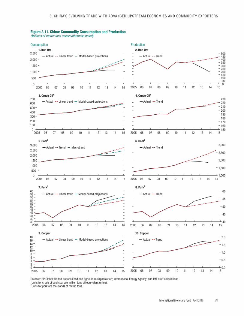
85
3. ChINA’s EvOLvING TRAdE wITh AdvANCEd UPsTREAM ECONOMIEs ANd COMMOdITy ExPORTERs
International Monetary Fund | April 2016
Sources: BP Global; United Nations Food and Agriculture Organization; International Energy Agency; and IMF staff calculations.1Units for crude oil and coal are million tons oil equivalent (mtoe).2Units for pork are thousands of metric tons.
1,000
1,500
2,000
2,500
3,000
2005 06 07 08 09 10 11 12 13 14 150
500
1,000
1,500
2,000
2,500
3,000
2005 06 07 08 09 10 11 12 13 14 15
0100200300400500600700
2005 06 07 08 09 10 11 12 13 14 15
0
500
1,000
1,500
2,000
2,500
2005 06 07 08 09 10 11 12 13 14 15
Actual Linear trend Model-based projections
Actual Linear trend Model-based projections
Actual Trend Macrotrend
Actual Linear trend Model-based projections
Actual Linear trend Model-based projections
Actual Trend
150160170180190200210220230
2005 06 07 08 09 10 11 12 13 14 15
Actual Trend
050100150200250300350400450500
2005 06 07 08 09 10 11 12 13 14 15
Actual Trend
40
45
50
55
60
2005 06 07 08 09 10 11 12 13 14 15
Actual Trend
0.0
0.5
1.0
1.5
2.0
2005 06 07 08 09 10 11 12 13 14 15
Actual Trend
4042444648505254565860
2005 06 07 08 09 10 11 12 13 14 15
02468
1012141618
2005 06 07 08 09 10 11 12 13 14 15
1. Iron Ore
3. Crude Oil1
5. Coal1
7. Pork2
2. Iron Ore
4. Crude Oil1
6. Coal1
8. Pork2
Consumption Production
9. Copper 10. Copper
Figure 3.11. China: Commodity Consumption and Production(Millions of metric tons unless otherwise noted)
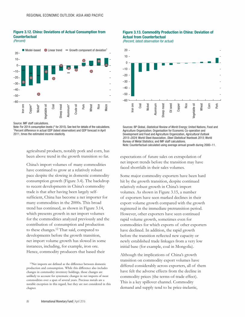
86
REGIONAL ECONOMIC OUTLOOK: AsIA ANd PACIfIC
International Monetary Fund | April 2016
agricultural products, notably pork and corn, has been above trend in the growth transition so far.
China’s import volumes of many commodities have continued to grow at a relatively robust pace despite the slowing in domestic commodity consumption growth (Figure 3.4). The backdrop to recent developments in China’s commodity trade is that after having been largely self-sufficient, China has become a net importer for many commodities in the 2000s. This broad trend has continued, as shown in Figure 3.14, which presents growth in net import volumes for the commodities analyzed previously and the contribution of consumption and production to these changes.12 That said, compared to developments before the growth transition, net import volume growth has slowed in some instances, including, for example, iron ore. Hence, commodity producers that based their
12Net imports are defined as the difference between domestic production and consumption. While this difference also includes changes in commodity inventory holdings, those changes are unlikely to account for systematic changes in net imports of most commodities over a span of several years. Precious metals are a notable exception in this regard, but they are not considered in this chapter.
expectations of future sales on extrapolation of net import trends before the transition may have faced shortfalls in their sales volumes.
Some major commodity exporters have been hard hit by the growth transition, despite continued relatively robust growth in China’s import volumes. As shown in Figure 3.15, a number of exporters have seen marked declines in their export volume growth compared with the growth registered in the immediate pretransition period. However, other exporters have seen continued rapid volume growth, sometimes even for commodities for which exports of other exporters have declined. In addition, the rapid growth before the transition reflected new capacity or newly established trade linkages from a very low initial base (for example, coal in Mongolia).
Although the implications of China’s growth transition on commodity export volumes have differed considerably across exporters, all of them have felt the adverse effects from the decline in commodity prices (the terms-of-trade effect). This is a key spillover channel. Commodity demand and supply tend to be price-inelastic,
Sources: BP Global, Statistical Review of World Energy; United Nations, Food and Agriculture Organization; Organisation for Economic Co-operation and Development and Food and Agriculture Organization, Agricultural Outlook 2015–2024; World Steel Association, Steel Statistical Yearbook 2015; World Bureau of Metal Statistics; and IMF staff calculations.Note: Counterfactual calculated using average annual growth during 2000–11.
–60
–50
–40
–30
–20
–10
0
10
20
Iron
ore
Coal
Nick
el
Alum
inum
Shee
p m
eat
Oil s
eed
Copp
er
Rice
Vege
tabl
e oi
l
Whe
at
Corn
Pork
Figure 3.13. Commodity Production in China: Deviation of Actual from Counterfactual(Percent, latest observation for actual)
Source: IMF staff calculations.Note: For 2014 consumption levels (* for 2015). See text for details of the calculations.1Percent difference in actual GDP (latest observation) and GDP forecast in April 2011, times the estimated income elasticity.
Iron
ore
Copp
er*
Nick
el*
Vege
tabl
e oi
l
Coal
Shee
p m
eat
Alum
inum
*
Crud
e oi
l
Pork
Whe
at
Rice
Mai
ze
–10
–20
–30
–40
–50
–60
0
10
20Model-based Linear trend Growth component of deviation1
Figure 3.12. China: Deviations of Actual Consumption from Counterfactual(Percent)
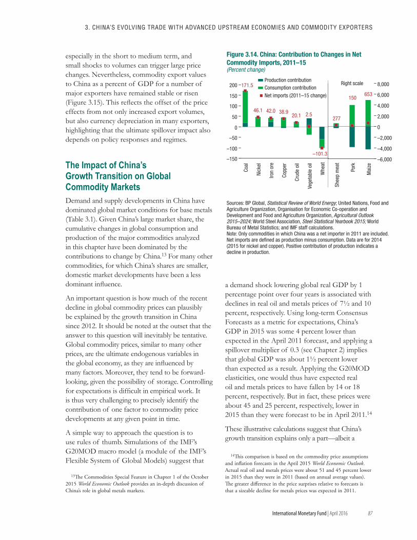
87
3. ChINA’s EvOLvING TRAdE wITh AdvANCEd UPsTREAM ECONOMIEs ANd COMMOdITy ExPORTERs
International Monetary Fund | April 2016
especially in the short to medium term, and small shocks to volumes can trigger large price changes. Nevertheless, commodity export values to China as a percent of GDP for a number of major exporters have remained stable or risen (Figure 3.15). This reflects the offset of the price effects from not only increased export volumes, but also currency depreciation in many exporters, highlighting that the ultimate spillover impact also depends on policy responses and regimes.
The Impact of China’s Growth Transition on Global Commodity Markets Demand and supply developments in China have dominated global market conditions for base metals (Table 3.1). Given China’s large market share, the cumulative changes in global consumption and production of the major commodities analyzed in this chapter have been dominated by the contributions to change by China.13 For many other commodities, for which China’s shares are smaller, domestic market developments have been a less dominant influence.
An important question is how much of the recent decline in global commodity prices can plausibly be explained by the growth transition in China since 2012. It should be noted at the outset that the answer to this question will inevitably be tentative. Global commodity prices, similar to many other prices, are the ultimate endogenous variables in the global economy, as they are influenced by many factors. Moreover, they tend to be forward-looking, given the possibility of storage. Controlling for expectations is difficult in empirical work. It is thus very challenging to precisely identify the contribution of one factor to commodity price developments at any given point in time.
A simple way to approach the question is to use rules of thumb. Simulations of the IMF’s G20MOD macro model (a module of the IMF’s Flexible System of Global Models) suggest that
13The Commodities Special Feature in Chapter 1 of the October 2015 World Economic Outlook provides an in-depth discussion of China’s role in global metals markets.
a demand shock lowering global real GDP by 1 percentage point over four years is associated with declines in real oil and metals prices of 7½ and 10 percent, respectively. Using long-term Consensus Forecasts as a metric for expectations, China’s GDP in 2015 was some 4 percent lower than expected in the April 2011 forecast, and applying a spillover multiplier of 0.3 (see Chapter 2) implies that global GDP was about 1½ percent lower than expected as a result. Applying the G20MOD elasticities, one would thus have expected real oil and metals prices to have fallen by 14 or 18 percent, respectively. But in fact, these prices were about 45 and 25 percent, respectively, lower in 2015 than they were forecast to be in April 2011.14
These illustrative calculations suggest that China’s growth transition explains only a part—albeit a
14This comparison is based on the commodity price assumptions and inflation forecasts in the April 2015 World Economic Outlook. Actual real oil and metals prices were about 51 and 45 percent lower in 2015 than they were in 2011 (based on annual average values). The greater difference in the price surprises relative to forecasts is that a sizeable decline for metals prices was expected in 2011.
Sources: BP Global, Statistical Review of World Energy; United Nations, Food and Agriculture Organization, Organisation for Economic Co-operation and Development and Food and Agriculture Organization, Agricultural Outlook 2015–2024; World Steel Association, Steel Statistical Yearbook 2015; World Bureau of Metal Statistics; and IMF staff calculations.Note: Only commodities in which China was a net importer in 2011 are included. Net imports are defined as production minus consumption. Data are for 2014 (2015 for nickel and copper). Positive contribution of production indicates a decline in production.
–150
–100
–50
0
50
100
150
200
Coal
Nick
el
Iron
ore
Copp
er
Crud
e oi
l
Vege
tabl
e oi
l
Whe
at
–101.3
2.520.138.942.046.1
171.5
–6,000
–4,000
–2,000
0
2,000
4,000
6,000
8,000
Shee
p m
eat
Pork
Mai
ze
653150
277
Right scaleProduction contributionConsumption contributionNet imports (2011–15 change)
Figure 3.14. China: Contribution to Changes in Net Commodity Imports, 2011–15(Percent change)
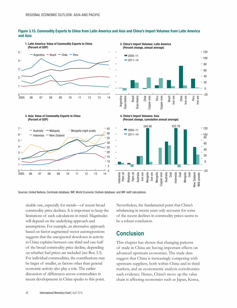
88
REGIONAL ECONOMIC OUTLOOK: AsIA ANd PACIfIC
International Monetary Fund | April 2016
sizable one, especially for metals—of recent broad commodity price declines. It is important to keep the limitations of such calculations in mind. Magnitudes will depend on the underlying approach and assumptions. For example, an alternative approach based on factor-augmented vector autoregressions suggests that the unexpected slowdown in activity in China explains between one-third and one-half of the broad commodity price decline, depending on whether fuel prices are included (see Box 3.3). For individual commodities, the contributions may be larger of smaller, as factors other than general economic activity also play a role. The earlier discussion of differences across commodities in recent developments in China speaks to this point.
Nevertheless, the fundamental point that China’s rebalancing in recent years only accounts for some of the recent declines in commodity prices seems to be a robust conclusion.
ConclusionThis chapter has shown that changing patterns of trade in China are having important effects on advanced upstream economies. The trade data suggest that China is increasingly competing with upstream suppliers, both within China and in third markets, and an econometric analysis corroborates such evidence. Hence, China’s move up the value chain is affecting economies such as Japan, Korea,
–20
0
20
40
60
80
100
120
Arge
ntin
aSo
ya b
eans
Braz
ilSo
ya b
eans
Chile
Copp
er o
res
Peru
Copp
er o
res
Braz
ilIro
n or
e
Chile
Iron
ore
Peru
Iron
ore0
1
2
3
4
5
2005 06 07 08 09 10 11 12 13 14
1. Latin America: Value of Commodity Exports to China(Percent of GDP)
2. China's Import Volumes: Latin America(Percent change, annual average)
3. Asia: Value of Commodity Exports to China(Percent of GDP)
4. China's Import Volumes: Asia(Percent change, cumulative annual average)
Sources: United Nations, Comtrade database; IMF, World Economic Outlook database; and IMF staff calculations.
0
1
2
3
4
5
6
7
0
5
10
15
20
25
30
35
40
45
2005 06 07 08 09 10 11 12 13 14
Argentina Brazil Chile Peru
Australia Malaysia Mongolia (right scale)
Indonesia New Zealand
–20
0
20
40
60
80100
120
Indo
nesi
aPa
lm o
il
Mal
aysi
aPa
lm o
il
Aust
ralia
Iron
ore
Mon
golia
Iron
ore
Mon
golia
Copp
er o
res
Aust
ralia
Coal
Indo
nesi
aCo
al
Mon
golia
Coal
New
Zea
land
Milk
pow
der
422.79545.80
2005–112011–14
2005–112011–14
Figure 3.15. Commodity Exports to China from Latin America and Asia and China’s Import Volumes from Latin America and Asia
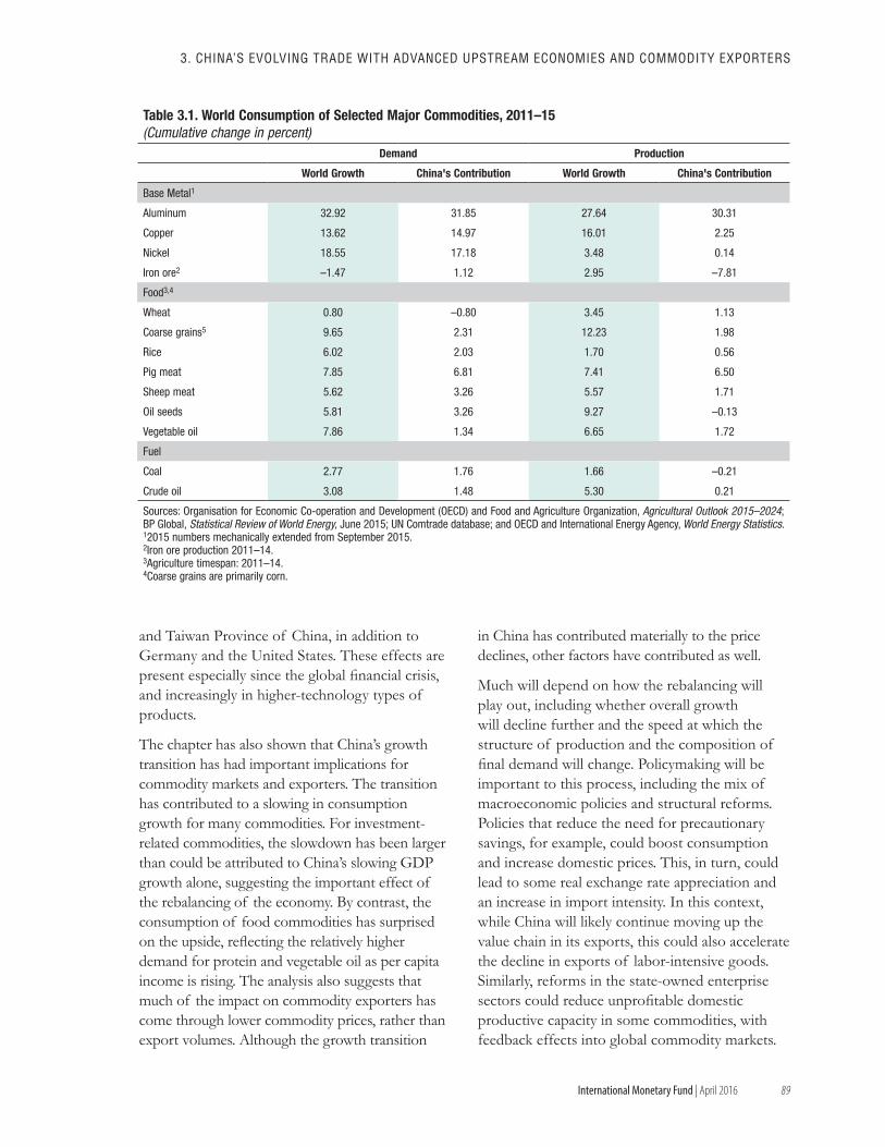
89
3. ChINA’s EvOLvING TRAdE wITh AdvANCEd UPsTREAM ECONOMIEs ANd COMMOdITy ExPORTERs
International Monetary Fund | April 2016
and Taiwan Province of China, in addition to Germany and the United States. These effects are present especially since the global financial crisis, and increasingly in higher-technology types of products.
The chapter has also shown that China’s growth transition has had important implications for commodity markets and exporters. The transition has contributed to a slowing in consumption growth for many commodities. For investment-related commodities, the slowdown has been larger than could be attributed to China’s slowing GDP growth alone, suggesting the important effect of the rebalancing of the economy. By contrast, the consumption of food commodities has surprised on the upside, reflecting the relatively higher demand for protein and vegetable oil as per capita income is rising. The analysis also suggests that much of the impact on commodity exporters has come through lower commodity prices, rather than export volumes. Although the growth transition
in China has contributed materially to the price declines, other factors have contributed as well.
Much will depend on how the rebalancing will play out, including whether overall growth will decline further and the speed at which the structure of production and the composition of final demand will change. Policymaking will be important to this process, including the mix of macroeconomic policies and structural reforms. Policies that reduce the need for precautionary savings, for example, could boost consumption and increase domestic prices. This, in turn, could lead to some real exchange rate appreciation and an increase in import intensity. In this context, while China will likely continue moving up the value chain in its exports, this could also accelerate the decline in exports of labor-intensive goods. Similarly, reforms in the state-owned enterprise sectors could reduce unprofitable domestic productive capacity in some commodities, with feedback effects into global commodity markets.
Table 3.1. World Consumption of Selected Major Commodities, 2011–15(Cumulative change in percent)
Demand Production
World Growth China's Contribution World Growth China's Contribution
Base Metal1
Aluminum 32.92 31.85 27.64 30.31
Copper 13.62 14.97 16.01 2.25
Nickel 18.55 17.18 3.48 0.14
Iron ore2 –1.47 1.12 2.95 –7.81
Food3,4
Wheat 0.80 –0.80 3.45 1.13
Coarse grains5 9.65 2.31 12.23 1.98
Rice 6.02 2.03 1.70 0.56
Pig meat 7.85 6.81 7.41 6.50
Sheep meat 5.62 3.26 5.57 1.71
Oil seeds 5.81 3.26 9.27 –0.13
Vegetable oil 7.86 1.34 6.65 1.72
Fuel
Coal 2.77 1.76 1.66 –0.21
Crude oil 3.08 1.48 5.30 0.21
Sources: Organisation for Economic Co-operation and Development (OECD) and Food and Agriculture Organization, Agricultural Outlook 2015–2024; BP Global, Statistical Review of World Energy, June 2015; UN Comtrade database; and OECD and International Energy Agency, World Energy Statistics.12015 numbers mechanically extended from September 2015.2Iron ore production 2011–14.3Agriculture timespan: 2011–14.4Coarse grains are primarily corn.
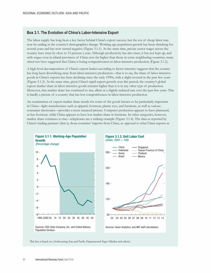
90
REGIONAL ECONOMIC OUTLOOK: AsIA ANd PACIfIC
International Monetary Fund | April 2016
The labor supply has long been a key factor behind China’s export success, but the era of cheap labor may now be ending as the country’s demographics change. Working-age population growth has been shrinking for several years and has now turned negative (Figure 3.1.1). At the same time, private sector wages across the country have risen by close to 15 percent a year. Although productivity has also risen, it has not kept up, and with wages even in inland provinces of China now far higher than those in some neighboring countries, many observers have suggested that China is losing competitiveness in labor-intensive production (Figure 3.1.2).
A high-level decomposition of China’s export basket according to factor intensity suggests that the country has long been diversifying away from labor-intensive production—that is to say, the share of labor-intensive goods in China’s exports has been declining since the early 1990s, with a slight reversal in the past few years (Figure 3.1.3). At the same time, given China’s rapid export growth over this period, the country’s global export market share in labor-intensive goods remains higher than it is in any other type of production. Moreover, that market share has continued to rise, albeit at a slightly reduced rate over the past few years. This is hardly a picture of a country that has lost competitiveness in labor-intensive production.
An examination of export market share trends for some of the goods known to be particularly important in China—light manufactures such as apparel, footwear, plastic toys, and furniture, as well as various consumer electronics—provides a more nuanced picture. Computer production appears to have plateaued, as has footwear, while China appears to have lost market share in furniture. In other categories, however, market share continues to rise—telephones are a striking example (Figure 3.1.4). The data as reported by China’s trading partners (that is, those countries’ imports from China, as opposed to what China reports as
This box is based on a forthcoming Asia and Pacific Departmental Paper (Mathai and others).
–8
–6
–4
–2
0
2
4
6
8
10
1995 2000 05 10 15 20 25 30 35 40 45 50
Sources: CEIC Data Company Ltd.; and United Nations, Population Division.
Figure 3.1.1. Working-Age Population Growth(Percentage change)
80
130
180
230
280
02 03 04 05 06 07 08 09 10 11 12 13 14
ChinaIndonesiaKorea
SingaporeTaiwan Province of ChinaThailand
Brazil Mexico
Sources: Haver Analytics; and IMF staff calculations.
Figure 3.1.2. Unit Labor Cost(Index; 2002 = 100)
Box 3.1. The Evolution of China’s Labor-Intensive Export
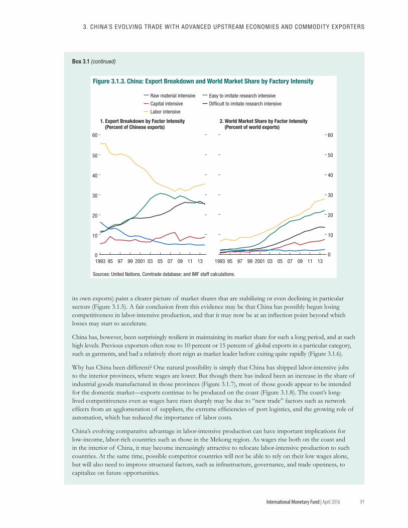
91
3. ChINA’s EvOLvING TRAdE wITh AdvANCEd UPsTREAM ECONOMIEs ANd COMMOdITy ExPORTERs
International Monetary Fund | April 2016
its own exports) paint a clearer picture of market shares that are stabilizing or even declining in particular sectors (Figure 3.1.5). A fair conclusion from this evidence may be that China has possibly begun losing competitiveness in labor-intensive production, and that it may now be at an inflection point beyond which losses may start to accelerate.
China has, however, been surprisingly resilient in maintaining its market share for such a long period, and at such high levels. Previous exporters often rose to 10 percent or 15 percent of global exports in a particular category, such as garments, and had a relatively short reign as market leader before exiting quite rapidly (Figure 3.1.6).
Why has China been different? One natural possibility is simply that China has shipped labor-intensive jobs to the interior provinces, where wages are lower. But though there has indeed been an increase in the share of industrial goods manufactured in those provinces (Figure 3.1.7), most of those goods appear to be intended for the domestic market—exports continue to be produced on the coast (Figure 3.1.8). The coast’s long-lived competitiveness even as wages have risen sharply may be due to “new trade” factors such as network effects from an agglomeration of suppliers, the extreme efficiencies of port logistics, and the growing role of automation, which has reduced the importance of labor costs.
China’s evolving comparative advantage in labor-intensive production can have important implications for low-income, labor-rich countries such as those in the Mekong region. As wages rise both on the coast and in the interior of China, it may become increasingly attractive to relocate labor-intensive production to such countries. At the same time, possible competitor countries will not be able to rely on their low wages alone, but will also need to improve structural factors, such as infrastructure, governance, and trade openness, to capitalize on future opportunities.
0
10
20
30
40
50
60
1993 95 97 99 2001 03 05 07 09 11 13
Sources: United Nations, Comtrade database; and IMF staff calculations.
Figure 3.1.3. China: Export Breakdown and World Market Share by Factory Intensity
1. Export Breakdown by Factor Intensity(Percent of Chinese exports)
2. World Market Share by Factor Intensity(Percent of world exports)
Raw material intensive
Capital intensive
Easy to imitate research intensive
Difficult to imitate research intensive
Labor intensive
0
10
20
30
40
50
60
1993 95 97 99 2001 03 05 07 09 11 13
Box 3.1 (continued)
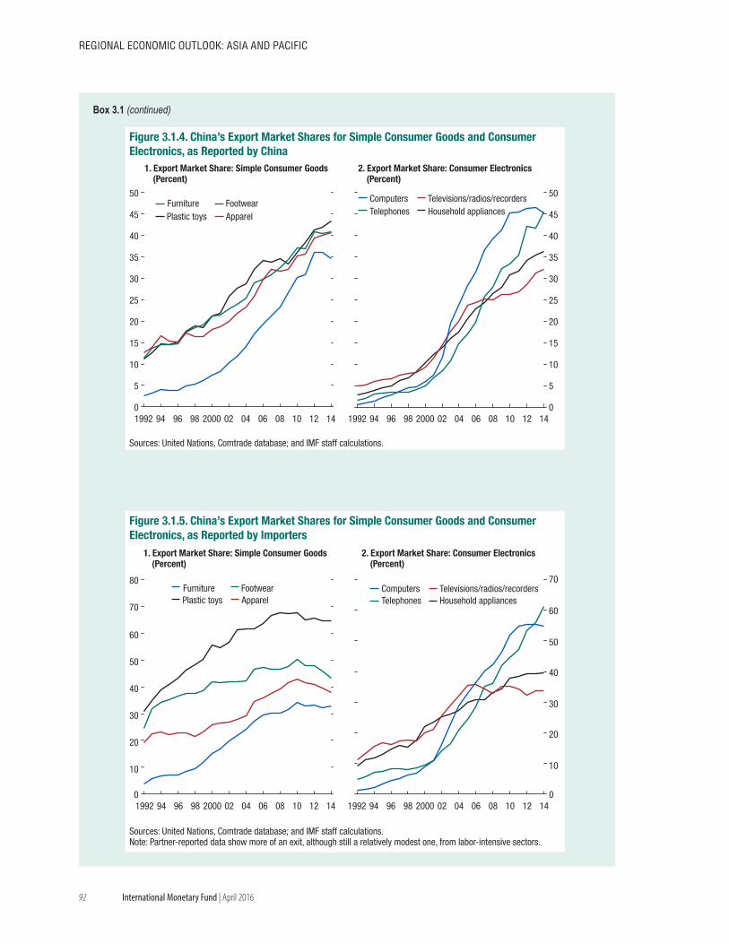
92
REGIONAL ECONOMIC OUTLOOK: AsIA ANd PACIfIC
International Monetary Fund | April 2016
0
5
10
15
20
25
30
35
40
45
50
1992 94 96 98 2000 02 04 06 08 10 12 14
Sources: United Nations, Comtrade database; and IMF staff calculations.
1. Export Market Share: Simple Consumer Goods(Percent)
2. Export Market Share: Consumer Electronics(Percent)
Furniture FootwearPlastic toys Apparel
Computers Televisions/radios/recordersTelephones Household appliances
0
5
10
15
20
25
30
35
40
45
50
1992 94 96 98 2000 02 04 06 08 10 12 14
Figure 3.1.4. China’s Export Market Shares for Simple Consumer Goods and Consumer Electronics, as Reported by China
Sources: United Nations, Comtrade database; and IMF staff calculations.Note: Partner-reported data show more of an exit, although still a relatively modest one, from labor-intensive sectors.
0
10
20
30
40
50
60
70
80
1992 94 96 98 2000 02 04 06 08 10 12 14
1. Export Market Share: Simple Consumer Goods(Percent)
2. Export Market Share: Consumer Electronics(Percent)
Furniture FootwearPlastic toys Apparel
Computers Televisions/radios/recordersTelephones Household appliances
0
10
20
30
40
50
60
70
1992 94 96 98 2000 02 04 06 08 10 12 14
Figure 3.1.5. China’s Export Market Shares for Simple Consumer Goods and Consumer Electronics, as Reported by Importers
Box 3.1 (continued)
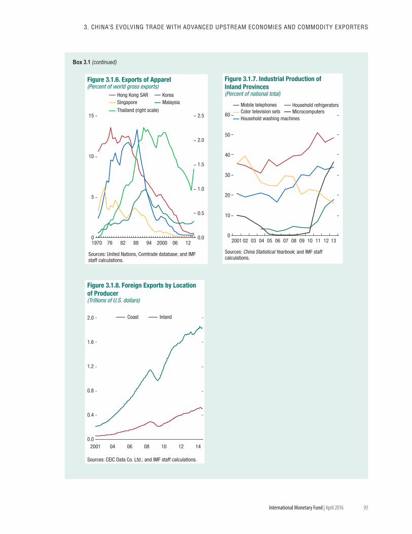
93
3. ChINA’s EvOLvING TRAdE wITh AdvANCEd UPsTREAM ECONOMIEs ANd COMMOdITy ExPORTERs
International Monetary Fund | April 2016
Sources: United Nations, Comtrade database; and IMF staff calculations.
0.0
0.5
1.0
1.5
2.0
2.5
0
5
10
15
1970 76 82 88 94 2000 06 12
Hong Kong SAR KoreaSingapore Malaysia
Thailand (right scale)
Figure 3.1.6. Exports of Apparel(Percent of world gross exports)
0
10
20
30
40
50
60
2001 02 03 04 05 06 07 08 09 10 11 12 13
Household washing machines
Household refrigeratorsMobile telephonesMicrocomputersColor television sets
Figure 3.1.7. Industrial Production of Inland Provinces(Percent of national total)
Sources: China Statistical Yearbook; and IMF staffcalculations.
0.0
0.4
0.8
1.2
1.6
2.0
2001 04 06 08 10 12 14
Coast Inland
Sources: CEIC Data Co. Ltd.; and IMF staff calculations.
Figure 3.1.8. Foreign Exports by Location of Producer(Trillions of U.S. dollars)
Box 3.1 (continued)
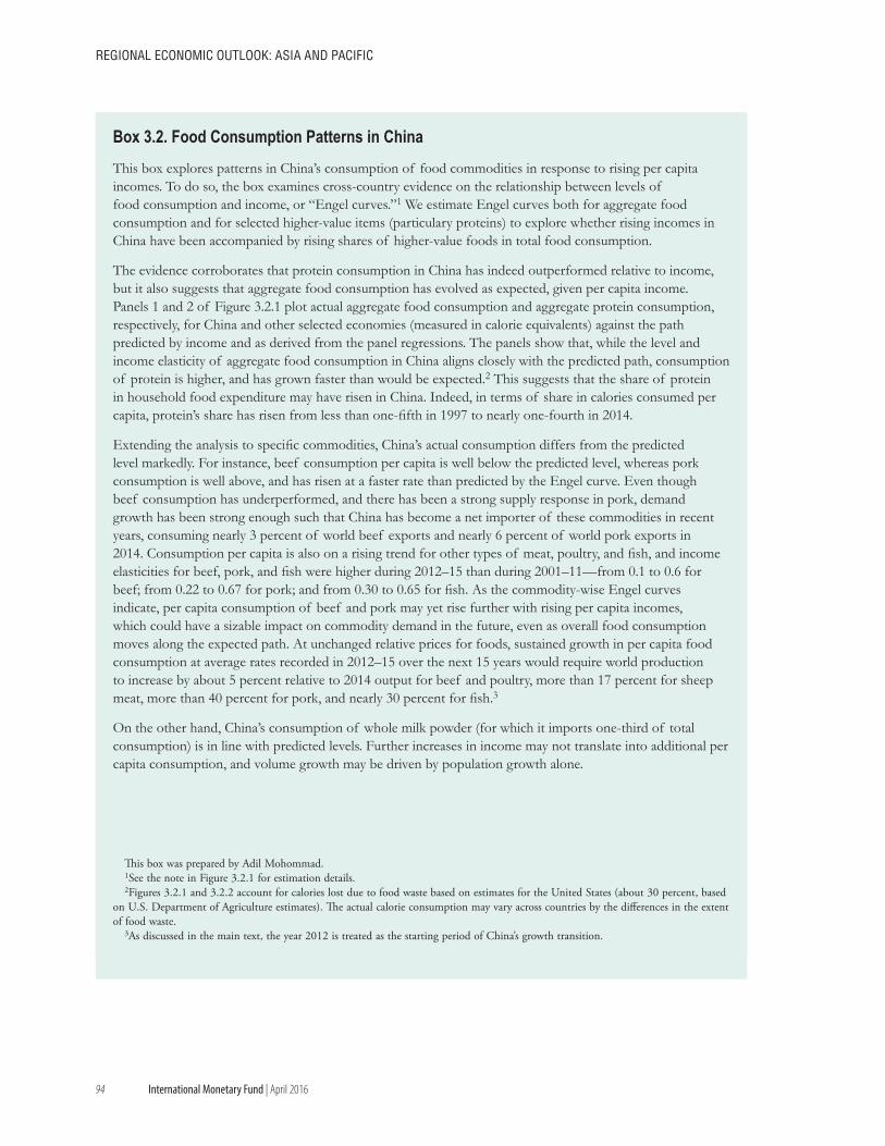
94
REGIONAL ECONOMIC OUTLOOK: AsIA ANd PACIfIC
International Monetary Fund | April 2016
This box explores patterns in China’s consumption of food commodities in response to rising per capita incomes. To do so, the box examines cross-country evidence on the relationship between levels of food consumption and income, or “Engel curves.”1 We estimate Engel curves both for aggregate food consumption and for selected higher-value items (particulary proteins) to explore whether rising incomes in China have been accompanied by rising shares of higher-value foods in total food consumption.
The evidence corroborates that protein consumption in China has indeed outperformed relative to income, but it also suggests that aggregate food consumption has evolved as expected, given per capita income. Panels 1 and 2 of Figure 3.2.1 plot actual aggregate food consumption and aggregate protein consumption, respectively, for China and other selected economies (measured in calorie equivalents) against the path predicted by income and as derived from the panel regressions. The panels show that, while the level and income elasticity of aggregate food consumption in China aligns closely with the predicted path, consumption of protein is higher, and has grown faster than would be expected.2 This suggests that the share of protein in household food expenditure may have risen in China. Indeed, in terms of share in calories consumed per capita, protein’s share has risen from less than one-fifth in 1997 to nearly one-fourth in 2014.
Extending the analysis to specific commodities, China’s actual consumption differs from the predicted level markedly. For instance, beef consumption per capita is well below the predicted level, whereas pork consumption is well above, and has risen at a faster rate than predicted by the Engel curve. Even though beef consumption has underperformed, and there has been a strong supply response in pork, demand growth has been strong enough such that China has become a net importer of these commodities in recent years, consuming nearly 3 percent of world beef exports and nearly 6 percent of world pork exports in 2014. Consumption per capita is also on a rising trend for other types of meat, poultry, and fish, and income elasticities for beef, pork, and fish were higher during 2012–15 than during 2001–11—from 0.1 to 0.6 for beef; from 0.22 to 0.67 for pork; and from 0.30 to 0.65 for fish. As the commodity-wise Engel curves indicate, per capita consumption of beef and pork may yet rise further with rising per capita incomes, which could have a sizable impact on commodity demand in the future, even as overall food consumption moves along the expected path. At unchanged relative prices for foods, sustained growth in per capita food consumption at average rates recorded in 2012–15 over the next 15 years would require world production to increase by about 5 percent relative to 2014 output for beef and poultry, more than 17 percent for sheep meat, more than 40 percent for pork, and nearly 30 percent for fish.3
On the other hand, China’s consumption of whole milk powder (for which it imports one-third of total consumption) is in line with predicted levels. Further increases in income may not translate into additional per capita consumption, and volume growth may be driven by population growth alone.
This box was prepared by Adil Mohommad.1See the note in Figure 3.2.1 for estimation details.2Figures 3.2.1 and 3.2.2 account for calories lost due to food waste based on estimates for the United States (about 30 percent, based
on U.S. Department of Agriculture estimates). The actual calorie consumption may vary across countries by the differences in the extent of food waste.
3As discussed in the main text, the year 2012 is treated as the starting period of China’s growth transition.
Box 3.2. Food Consumption Patterns in China
95
3. ChINA’s EvOLvING TRAdE wITh AdvANCEd UPsTREAM ECONOMIEs ANd COMMOdITy ExPORTERs
International Monetary Fund | April 2016
0
500
1,000
1,500
2,000
2,500
3,000
3,500
0 10 20 30 40 50 60 70Cons
umpt
ion
(In c
alor
ies
per c
apita
, dai
ly)
Income per capita (Thousands of 2011 PPP dollars)
1. Food (Aggregate)
0
200
400
600
800
1,000
1,200
0 10 20 30 40 50 60 70 Cons
umpt
ion
(In c
alor
ies
per c
apita
, dai
ly)
Income per capita (Thousands of 2011 PPP dollars)
2. Protein (Aggregate)
–20
–10
0
10
20
30
40
50
60
70
0 10 20 30 40 50 60
Cons
umpt
ion
(In k
g. p
er c
apita
, ann
ual)
Income per capita (Thousands of 2011 PPP dollars)
3. Vegetable Oil
0
20
40
60
80
100
120
0 10 20 30 40 50 60
Cons
umpt
ion
(In k
g. p
er c
apita
, ann
ual)
Income per capita (Thousands of 2011 PPP dollars)
4. Rice
0
5
10
15
20
25
30
35
40
0 10 20 30 40 50 60
Cons
umpt
ion
(In k
g. p
er c
apita
, ann
ual)
Income per capita (Thousands of 2011 PPP dollars)
5. Sugar
05101520253035404550
0 10 20 30 40 50 60
Cons
umpt
ion
(in k
g. p
er c
apita
, ann
ual)
Income per capita (Thousands of 2011 PPP dollars)
6. Beef and Veal
0
5
10
15
20
25
30
35
40
45
0 10 20 30 40 50 60
Cons
umpt
ion
(In k
g. p
er c
apita
, ann
ual)
Income per capita (Thousands of 2011 PPP dollars)
7. Pork
–1.0
–0.5
0.0
0.5
1.0
1.5
2.0
2.5
3.0
3.5
0 10 20 30 40 50 60
Cons
umpt
ion
(In k
g. p
er c
apita
, ann
ual)
Income per capita (Thousands of 2011 PPP dollars)
8. Whole Milk Powder
Fitted China India Japan Korea United States Fitted China India Japan Korea United States
Fitted China India Japan Korea United States Fitted China India Japan Korea United States
Fitted China India Japan Korea United States Fitted China India Japan Korea United States
Fitted China India Japan Korea United States Fitted China India Japan Korea United States
Figure 3.2.1. Engel Curve Estimates and Consumption per Capita of Selected Food Items(Kilograms/capita; income in 2011 constant purchasing power parity dollars per capita)
Source: IMF staff estimates.Notes: (1) The estimated equations build on the methodology in Box 1.2 in the IMF’s April 2014 World Economic Outlook. Engel curves for each commodity/aggregate are derived from a regression of consumption per capita (in annual calories per capita for aggregate food and aggregate protein, and in annual kilograms per capita for selected items) on a third-order polynomial, relative local food price inflation of the relevant commodity or aggregate, and country fixed effects. (2) The data set used for this analysis consists of the UN Food and Agriculture Organization’s food consumption and local producer prices of 20 agricultural commodities, World Bank purchasing power parity (PPP) GDP in 2011 constant dollars, and local consumer price index inflation and population data from the IMF’s World Economic Outlook database. The panel covers 1996–2014 and includes 42 countries: Bangladesh, Ethiopia, Haiti, Ghana, Mozambique, Tanzania, Vietnam, and Zambia (low-income); Argentina, Brazil, China, Colombia, Chile, Egypt, India, Indonesia, Malaysia, Mexico, Nigeria, Pakistan, Peru, the Philippines, Russia, South Africa, Thailand, Turkey, and Ukraine (emerging); Australia, Canada, Israel, Japan, Korea, New Zealand, Norway, Saudi Arabia, Switzerland, and the United States (high income); and others including Algeria, Iran, Kazakhstan, Paraguay, and Uruguay.
Box 3.2 (continued)
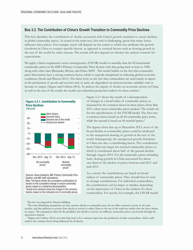
96
REGIONAL ECONOMIC OUTLOOK: AsIA ANd PACIfIC
International Monetary Fund | April 2016
This box identifies the contribution of shocks associated with China’s growth transition to recent declines in global commodity prices. As noted in the main text, this task is challenging, given that many forces influence these prices. For example, much will depend on the extent to which one attributes the growth slowdown in China to country-specific factors, as opposed to external factors such as slowing growth in the rest of the world for other reasons. The results will also depend on whether the analysis controls for expectations.
We apply a factor-augmented vector autoregressive (FAVAR) model to monthly data for 42 benchmark commodity prices in the IMF’s Primary Commodity Price System with data going back at least to 1980, along with other data (Bernanke, Boivin, and Eliasz 2005) . The model builds on the fact that commodity price fluctuations have a strong common factor, which is typically interpreted as reflecting global economic conditions (Stock and Watson 2011). The latter rests on the fact that commodities are used jointly as inputs in the production of goods and services and, as such, are dependent on macroeconomic variables such as income or output (Alquist and Coibion 2014). To analyze the impact of shocks on economic activity in China as well as the rest of the world, the model uses industrial production indices for these entities.1
Figure 3.3.1 shows the results of a decomposition of changes in a broad index of commodity prices, as measured by the common factor in these prices, from May 2011, when most commodity prices peaked. The results are for two specifications of the FAVAR model. The first uses a common factor based on all 42 commodity price series, while the second is based on 40 nonfuel prices.2
The figures show that up to December 2013, most of the broad decline in commodity prices could be attributed to the unexpected slowing of growth in the rest of the world. Subsequently, the unexpected growth slowdown in China was also a contributing factor. The contribution from China was larger for nonfuel commodity prices, to which it contributed about half of the general decline through August 2015. For all commodity prices including fuels, slowing growth in China accounted for about one-third of the decline in prices between mid-2011 and mid-2015.
As a caveat: the contributions are based on broad indices of commodity prices. They should thus be seen as average contributions. For individual commodities, the contributions can be larger or smaller, depending on the importance of China in the markets for these commodities. For metals, for example, the FAVAR model
This box was prepared by Thomas Helbling.1The main identifying assumptions are that common shocks to commodity prices do not affect economic activity in the same
months, and that spillovers to activity from shocks to activity in either China or the rest of the world are smaller than the direct domes-tic impact. The assumptions allow for the possibility that shocks to activity can influence commodity prices concurrently through the expectation channel.
2Alquist and Coibion (2014) note that fuels tend to be a common input into the production of other commodities, which could result in the common factor being influenced by oil shocks.
Sources: Haver Analytics; IMF, Primary Commodity Price System; and IMF staff calculations.Note: The figure shows the cumulative contributions of shocks to the cumulative change in actual commodity prices, based on a historical decomposition.1Actual price declines show the change in the common factors, based on the indicated set of commodity prices.
–30
–40
–20
–10
0
10
20
30
Dec. 2013 Aug. 15 Dec. 2013 Aug. 15
Other factorsDemand ChinaDemand rest of the worldActual price decline
All commodityprices1
Nonfuelcommodity
prices1
Figure 3.3.1. Contribution to Commodity Price Declines(Percent)
Box 3.3. The Contribution of China’s Growth Transition to Commodity Price Declines
97
3. ChINA’s EvOLvING TRAdE wITh AdvANCEd UPsTREAM ECONOMIEs ANd COMMOdITy ExPORTERs
International Monetary Fund | April 2016
suggests larger contributions from China’s growth slowdown. Another caveat is that the analysis does not explicitly consider changes in the composition of aggregate demand. For this reason, results tend to be sensitive to the time period. One should also keep in mind that supply developments are often thought to be more commodity-specific. As such, the fluctuations in broad commodity price indices might lead to an underestimation of the contribution of supply factors to commodity price declines. This can also be seen in the fact that the cumulative declines in the broad indices are smaller than the declines in the prices of a few major commodities where supply shocks have been relatively more important (for example, crude oil or iron ore).
Box 3.3 (continued)
98
REGIONAL ECONOMIC OUTLOOK: AsIA ANd PACIfIC
International Monetary Fund | April 2016
Annex 3.1. Econometric Analysis of Advanced Upstream EconomiesAn initial specification for estimating onshoring, using value-added trade data, is as follows (equation 1):
d lnFVAi,CHN,s,t = a + βd lnVACHN,s,t + γd lnVACHN,s,t × inti,s,t + θXi,j,s,t + δi,t + τt + εi,s,t (1)where:
• d ln is the log difference in two different periods, 2000–05 and 2005–11
• FVAi,j,s,t is the foreign value added from country i to country j in period t and sector s
• VAj,t,s is the ratio of total value added to production in country j in period t and sector s
• Xi,j,s,t includes other controls: dTariffsi,j,s,t and dlnExpAll,World,s,t are changes in bilateral tariffs at the sector level and changes in total world exports in sector s
• inti,s,t is a dummy that captures characteristics of i,j,s or t depending on the specification.
In other words, we estimate whether sectors in which China is growing more competitive (as proxied by increasing Chinese production) are also those in which advanced economy exports to China are declining. Using value-added data, which are available for 62 countries, allows for a matching of production and trade that is difficult with gross data. A major disadvantage, however, is that the value-added data are available only with a substantial lag, with the last observations pertaining to 2011. Also, the value-added data are available only at the two-digit International Standard Industrial Classification (ISIC) level, and at such a high level of aggregation we will be biased toward finding complementarities between Chinese and foreign production. Other factors, such as differences in price dynamics across goods, can also drive in part the behavior of large and heterogeneous sectors.
The results suggest that China is becoming a competitor for upstream countries (Annex Table 3.1.1). While there are complementarities
in the precrisis period 2000–05, this gives way to competition in the latest period. Moreover, competition is strongest in high-technology, knowledge-intensive, and more complex goods.
We complement the analysis with an alternative specification using gross trade data for 180 countries. This allows us to examine more recent data (from 2000 through 2014) at the five-digit level. Here we proxy China’s competitiveness in a sector by its exports in that sector, and again ask whether rising competitiveness has reduced upstream countries’ exports to China (equation 2):
d lnExpi,CHN,s,t = a + βd lnExpCHN,World,s,t + γd lnExpCHN,World,s,t × inti,s,t + θXi,j,s,t + δi,t + τt + εi,s,t (2)
where:
• dln denotes the log difference in two different periods, 2000–07 and 2010–14
• Controls and interactions are the same as in equation (1)
• Expi,s,t are gross exports from country i to country j in period t and five-digit level product s.
Using the specification in equation (2) to test for onshoring is likely an inappropriately demanding test.1 The gross trade data, at the five-digit level, are much more granular than the former data. There may be many goods for which China has developed the competence to produce, but either chooses to continue importing those parts domestically or is not sufficiently competitive in their manufacturing to be able to compete overseas, given trade costs, while being competitive at home. It would be better to use a measure of production in China as a proxy for competitiveness, but matching production and gross trade data at that level of detail is difficult.
Still, the gross trade results are broadly consistent with those obtained from the value-added data (Annex Table 3.1.2). Here too, China’s imports
1The main results referenced in the text focusing on interaction terms are robust to changes to the period of analysis and the time window over which variables are measured.
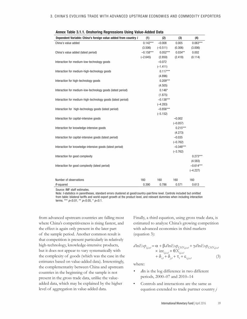
99
3. ChINA’s EvOLvING TRAdE wITh AdvANCEd UPsTREAM ECONOMIEs ANd COMMOdITy ExPORTERs
International Monetary Fund | April 2016
from advanced upstream countries are falling most where China’s competitiveness is rising fastest, and the effect is again only present in the later part of the sample period. Another common result is that competition is present particularly in relatively high-technology, knowledge-intensive products, but it does not appear to vary systematically with the complexity of goods (which was the case in the estimates based on value-added data). Interestingly, the complementarity between China and upstream countries in the beginning of the sample is not present in the gross trade data, unlike the value-added data, which may be explained by the higher level of aggregation in value-added data.
Finally, a third equation, using gross trade data, is estimated to analyze China’s growing competition with advanced economies in third markets (equation 3):
d lnExpi,j,s,t = a + βd lnExpCHN,j,s,t + γd lnExpCHN,j,s,t × inti,j,s,t + θXi,j,s,t + δi,t + δj,t + τt + εi,j,s,t (3)
where:
• dln is the log difference in two different periods, 2000–07 and 2010–14
• Controls and interactions are the same as equation extended to trade partner country j
Annex Table 3.1.1. Onshoring Regressions Using Value-Added DataDependent Variable: China's foreign value added from country i (1) (2) (3) (4)
China's value added 0.142*** –0.008 0.005 0.063***
(3.506) (–0.511) (0.306) (3.006)
China's value added (latest period) –0.158*** 0.052*** 0.034** 0.002
(–2.645) (2.850) (2.418) (0.114)
Interaction for medium-low-technology goods –0.072
(–1.411)
Interaction for medium-high-technology goods 0.117***
(4.896)
Interaction for high-technology goods 0.209***
(4.505)
Interaction for medium-low-technology goods (latest period) 0.146*
(1.875)
Interaction for medium-high-technology goods (latest period) –0.138***
(–4.283)
Interaction for high-technology goods (latest period) –0.856***
(–5.152)
Interaction for capital-intensive goods –0.002
(–0.057)
Interaction for knowledge-intensive goods 0.215***
(4.273)
Interaction for capital-intensive goods (latest period) –0.035
(–0.762)
Interaction for knowledge-intensive goods (latest period) –0.348***
(–3.762)
Interaction for good complexity 0.273***
(4.583)
Interaction for good complexity (latest period) –0.614***
(–4.227)
Number of observations 160 160 160 160
R-squared 0.390 0.786 0.571 0.613
Source: IMF staff estimates.Note: t-statistics in parentheses, standard errors clustered at good/country-pair/time level. Controls included but omitted from table: bilateral tariffs and world export growth at the product level, and relevant dummies when including interaction terms. *** p<0.01, ** p<0.05, * p<0.1.
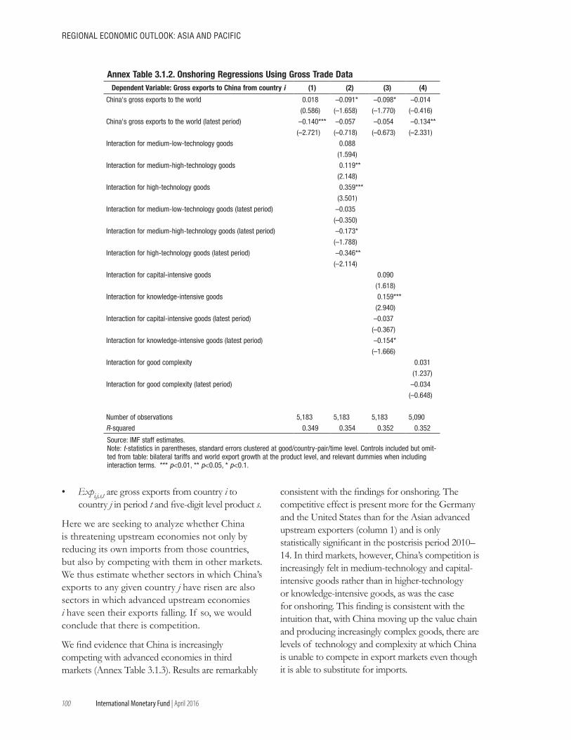
100
REGIONAL ECONOMIC OUTLOOK: AsIA ANd PACIfIC
International Monetary Fund | April 2016
• Expi,j,s,t are gross exports from country i to country j in period t and five-digit level product s.
Here we are seeking to analyze whether China is threatening upstream economies not only by reducing its own imports from those countries, but also by competing with them in other markets. We thus estimate whether sectors in which China’s exports to any given country j have risen are also sectors in which advanced upstream economies i have seen their exports falling. If so, we would conclude that there is competition.
We find evidence that China is increasingly competing with advanced economies in third markets (Annex Table 3.1.3). Results are remarkably
consistent with the findings for onshoring. The competitive effect is present more for the Germany and the United States than for the Asian advanced upstream exporters (column 1) and is only statistically significant in the postcrisis period 2010–14. In third markets, however, China’s competition is increasingly felt in medium-technology and capital-intensive goods rather than in higher-technology or knowledge-intensive goods, as was the case for onshoring. This finding is consistent with the intuition that, with China moving up the value chain and producing increasingly complex goods, there are levels of technology and complexity at which China is unable to compete in export markets even though it is able to substitute for imports.
Annex Table 3.1.2. Onshoring Regressions Using Gross Trade DataDependent Variable: Gross exports to China from country i (1) (2) (3) (4)
China's gross exports to the world 0.018 –0.091* –0.098* –0.014
(0.586) (–1.658) (–1.770) (–0.416)
China's gross exports to the world (latest period) –0.140*** –0.057 –0.054 –0.134**
(–2.721) (–0.718) (–0.673) (–2.331)
Interaction for medium-low-technology goods 0.088
(1.594)
Interaction for medium-high-technology goods 0.119**
(2.148)
Interaction for high-technology goods 0.359***
(3.501)
Interaction for medium-low-technology goods (latest period) –0.035
(–0.350)
Interaction for medium-high-technology goods (latest period) –0.173*
(–1.788)
Interaction for high-technology goods (latest period) –0.346**
(–2.114)
Interaction for capital-intensive goods 0.090
(1.618)
Interaction for knowledge-intensive goods 0.159***
(2.940)
Interaction for capital-intensive goods (latest period) –0.037
(–0.367)
Interaction for knowledge-intensive goods (latest period) –0.154*
(–1.666)
Interaction for good complexity 0.031
(1.237)
Interaction for good complexity (latest period) –0.034
(–0.648)
Number of observations 5,183 5,183 5,183 5,090
R-squared 0.349 0.354 0.352 0.352
Source: IMF staff estimates.Note: t-statistics in parentheses, standard errors clustered at good/country-pair/time level. Controls included but omit-ted from table: bilateral tariffs and world export growth at the product level, and relevant dummies when including interaction terms. *** p<0.01, ** p<0.05, * p<0.1.
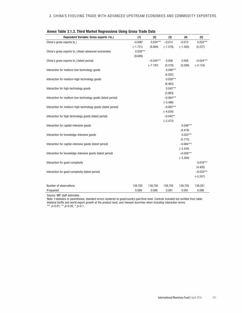
101
3. ChINA’s EvOLvING TRAdE wITh AdvANCEd UPsTREAM ECONOMIEs ANd COMMOdITy ExPORTERs
International Monetary Fund | April 2016
Annex Table 3.1.3. Third Market Regressions Using Gross Trade DataDependent Variable: Gross exports i to j (1) (2) (3) (4) (5)
China's gross exports to j –0.006* 0.034*** –0.014 –0.013 0.024***
(–1.751) (8.664) (–1.579) (–1.505) (5.227)
China's gross exports to j (Asian advanced economies) 0.059***
(9.689)
China's gross exports to j (latest period) –0.045*** 0.008 0.008 –0.024***
(–7.197) (0.578) (0.509) (–3.134)
Interaction for medium-low-technology goods 0.046***
(4.502)
Interaction for medium-high-technology goods 0.058***
(6.463)
Interaction for high-technology goods 0.042***
(3.863)
Interaction for medium-low-technology goods (latest period) –0.064***
(–3.486)
Interaction for medium-high-technology goods (latest period) –0.062***
(–4.054)
Interaction for high-technology goods (latest period) –0.045**
(–2.472)
Interaction for capital-intensive goods 0.046***
(4.418)
Interaction for knowledge-intensive goods 0.053***
(5.775)
Interaction for capital-intensive goods (latest period) –0.064***
(–3.434)
Interaction for knowledge-intensive goods (latest period) –0.056***
(–3.594)
Interaction for good complexity 0.016***
(4.405)
Interaction for good complexity (latest period) –0.033***
(–5.247)
Number of observations 139,705 139,705 139,705 139,705 139,261
R-squared 0.089 0.088 0.091 0.091 0.090
Source: IMF staff estimates. Note: t-statistics in parentheses, standard errors clustered at good/country-pair/time level. Controls included but omitted from table: bilateral tariffs and world export growth at the product level, and relevant dummies when including interaction terms. *** p<0.01, ** p<0.05, * p<0.1.

International Monetary Fund | April 2016
Introduction and Main FindingsRising inequality in many countries has attracted much attention from the public and policymakers alike.1 Until about 1990, Asia grew strongly and secured large gains in poverty reduction while simultaneously achieving a fairly equitable society (Jain-Chandra and others 2016). A large part of this success was due to the “miracle” economies—Hong Kong Special Administrative Region, Korea, Singapore, and Taiwan Province of China—where sustained rapid growth was accompanied by equitable income distribution.
Since the early 1990s, however, the region has witnessed rising income inequality—a break from its own remarkable past that has resulted in high levels of inequality in large Asian emerging markets. This is of concern for two reasons.
First, the recent literature has found that elevated levels of inequality are harmful for the pace and sustainability of growth (Dabla-Norris and others 2015; Easterly 2007; Ostry, Berg, and Tsangarides 2014). In particular, high levels of income inequality can lead to suboptimal investment in health and education, which weighs on growth (Aghion, Caroli, and Garcia-Peñalosa 1999). Widening inequality can also weaken the support for growth-enhancing reforms and may spur governments to adopt populist policies and increase the risk of political instability (Rodrik 1999).
Second, increases in inequality in Asia have had a dampening effect on the impact of growth on poverty reduction, leading to less inclusive and less pro-poor growth compared with Asia’s past (Balakrishnan, Steinberg, and Syed 2013). In
This chapter was prepared by Sonali Jain-Chandra and Tidiane Kinda (lead authors), Shi Piao, and Johanna Schauer. The chapter is based on Jain-Chandra and others (2016).
1This chapter focuses on within-country inequality. Conver-gence of income across economies has led to a decline of inequality between countries during recent decades.
addition to income inequality, Asia, in line with other regions, faces considerable inequality in opportunities.
As Asia faces turbulent times, it is critical for the region to combat rising inequality of income and opportunities. More equal incomes and opportunities would support a path to durable and sustainable growth. Recognizing this, a number of countries have placed the issue of inclusive growth as central to their national goals and, in a number of cases, explicitly in their development plans. China’s Thirteenth Five-Year Plan (2016–20) emphasizes a more balanced, inclusive, and sustainable growth model, as do India’s Twelfth Five-Year Plan (2012–17) and the Philippine Development Plan (2011–16). This objective is also central to development plans in Indonesia and Malaysia.
This chapter revisits the increasingly important topic of widening income inequality, focusing on Asia, home to more than half of the world’s population. It contributes to a growing literature on the evolution and drivers of income inequality. The goal is to document the developments in various measures of income inequality as well as the inequality of opportunities over time in Asian economies. It will also analyze the drivers of income inequality, as well as the extent to which these are different in Asia, and discuss policies to generate more inclusion.
The main findings are the following:
• Within-country income inequality has risen in most of Asia, in contrast to many regions. In some larger countries (such as China and India), spatial disparities, in particular between rural and urban areas, explain much of the increase. In the past, rapid growth in Asia came with equitable distribution of the gains. But more recently, while the fast-growing Asian economies have lifted millions out of poverty they have been unable to replicate the “growth with equity” miracle.
4. Sharing the Growth Dividend: Analysis of Inequality in Asia
104
REGIONAL ECONOMIC OUTLOOK: AsIA ANd PACIfIC
International Monetary Fund | April 2016
Higher income inequality has also lowered the effectiveness of growth to combat poverty and prevented the building of a substantial middle class.
• In addition to inequality of income, Asia also faces considerable inequality of opportunities—with lower-income individuals having relatively limited access to health, education, and financial services—as well as dual labor markets. This is of critical importance as these factors sow the seeds for wider income inequality in the future and delink economic outcomes from an individual’s efforts.
• Global factors, such as skill-biased technological change, have played a particular role in the increase of inequality in Asia, but regional and country-specific factors have also been critical. In some respects the drivers of inequality in Asia are different from those in other regions. Financial deepening has been equalizing in Asia, in contrast to other regions. In addition, much as in the rest of world, greater progressivity in taxation has had an equalizing effect in Asia. On the other hand, expenditure policies such as social sector spending, education spending, and capital expenditure have been associated with higher income inequality in Asia (contrary to the rest of the world), owing to weak coverage and the benefits disproportionately accruing to those at the higher end of the income distribution.
These findings suggest that policies could have a substantial effect on reversing the trend of rising inequality in Asia. It is imperative to address inequality of opportunities, in particular to broaden access to education, health, and financial services, as well as to tackle labor market duality and informality. Strengthening the redistributional effect of fiscal policy is also essential. This includes expanding and broadening the coverage of social spending through well-targeted interventions, while avoiding costly across-the-board subsidy schemes, and further increasing tax progressivity.
Recent Trends and DevelopmentsIncome Inequality in Asia2
Asia has been a growth leader and has achieved remarkably high growth for sustained periods and lifted millions out of poverty. During 1990–2015, the region grew at about 6 percent a year, notwithstanding the sharp slowdowns during the Asian financial crisis and the global financial crisis.
However, this impressive economic performance has been accompanied by rising inequality in a number of Asian economies. The level of the Gini coefficient is now higher in Asia than the average for the rest of the world. Furthermore, apart from that in Asia and Organisation for Economic Co-operation and Development countries, inequality has been trending down in most other regions. The average net Gini coefficient (based on income net of taxes and transfers) rose from 36 in 1990 to 40 in 2013 in Asia. Over the same period, the average Gini for the rest of the world rose by less than 2 points (Figure 4.1). More strikingly, on a population-weighted basis, the net Gini in Asia rose from 37 in 1990 to 48 in 2014, reflecting the sharp rise in inequality in the most populous countries (Figure 4.2). While these changes might seem small, inequality and especially the Gini measure are very persistent over time. On average, the within-country standard deviation in this sample is 2.5 points. Consistent with the rest of the world, the level of inequality is higher in emerging market economies than in advanced economies, and it has been rising faster in the former set of countries (Figures 4.3 and 4.4).
2Any analysis of inequality—and this chapter is no exception—is confronted with a number of challenges, as cross-country compar-isons are highly challenging. High-income countries tend to report income inequality measures, while low- and middle-income coun-tries tend to report consumption-based measures. Major differences can also exist among the same inequality measures, such as the sampling unit, the definition of income (net or gross income), or the time period of expenditures or earnings. This chapter relies on the Standardized World Income Inequality Database (SWIID Version 5.0) assembled by Frederick Solt. This data set has the advantage of maximizing the comparability of income inequality data while main-taining the broadest possible coverage across countries and over time. While it is not adjusted for cross-country comparison, this chapter also uses the PovcalNet database from the World Bank for more detailed information on national distributions of inequality.
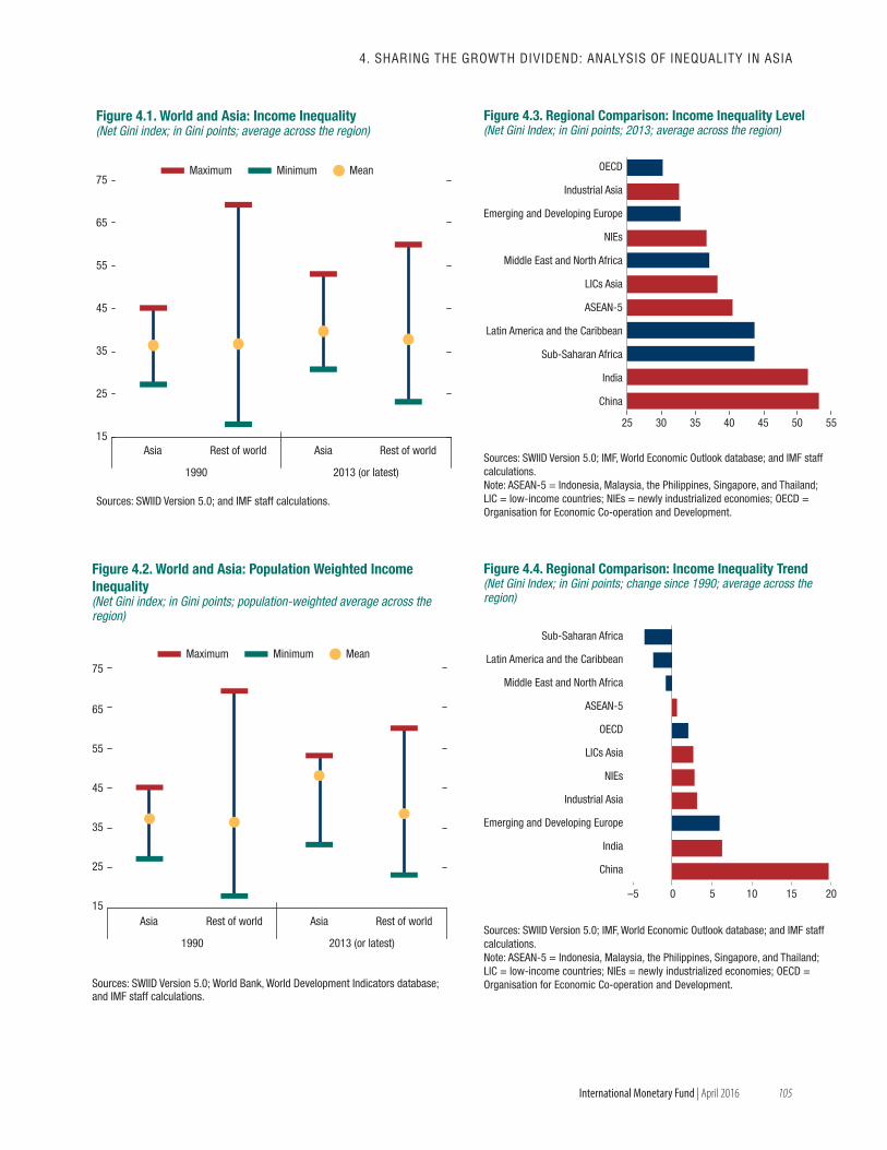
105
4. shARING ThE GROwTh dIvIdENd: ANALysIs Of INEqUALITy IN AsIA
International Monetary Fund | April 2016
15
25
35
45
55
65
75
Asia Rest of world Asia Rest of world
1990 2013 (or latest)
Maximum Minimum Mean
Sources: SWIID Version 5.0; and IMF staff calculations.
Figure 4.1. World and Asia: Income Inequality(Net Gini index; in Gini points; average across the region)
15
25
35
45
55
65
75
Sources: SWIID Version 5.0; World Bank, World Development Indicators database; and IMF staff calculations.
Asia Rest of world Asia Rest of world
1990 2013 (or latest)
Figure 4.2. World and Asia: Population Weighted Income Inequality(Net Gini index; in Gini points; population-weighted average across the region)
Maximum Minimum Mean
Sources: SWIID Version 5.0; IMF, World Economic Outlook database; and IMF staff calculations.Note: ASEAN-5 = Indonesia, Malaysia, the Philippines, Singapore, and Thailand; LIC = low-income countries; NIEs = newly industrialized economies; OECD = Organisation for Economic Co-operation and Development.
25 30 35 40 45 50 55
China
India
Sub-Saharan Africa
Latin America and the Caribbean
ASEAN-5
LICs Asia
Middle East and North Africa
NIEs
Emerging and Developing Europe
Industrial Asia
OECD
Figure 4.3. Regional Comparison: Income Inequality Level(Net Gini Index; in Gini points; 2013; average across the region)
Sources: SWIID Version 5.0; IMF, World Economic Outlook database; and IMF staff calculations.Note: ASEAN-5 = Indonesia, Malaysia, the Philippines, Singapore, and Thailand; LIC = low-income countries; NIEs = newly industrialized economies; OECD = Organisation for Economic Co-operation and Development.
–5 0 5 10 15 20
China
India
Emerging and Developing Europe
Industrial Asia
NIEs
LICs Asia
OECD
ASEAN-5
Middle East and North Africa
Latin America and the Caribbean
Sub-Saharan Africa
Figure 4.4. Regional Comparison: Income Inequality Trend(Net Gini Index; in Gini points; change since 1990; average across the region)
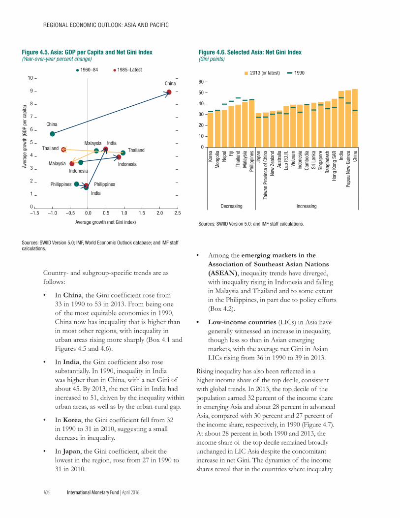
106
REGIONAL ECONOMIC OUTLOOK: AsIA ANd PACIfIC
International Monetary Fund | April 2016
Country- and subgroup-specific trends are as follows:
• In China, the Gini coefficient rose from 33 in 1990 to 53 in 2013. From being one of the most equitable economies in 1990, China now has inequality that is higher than in most other regions, with inequality in urban areas rising more sharply (Box 4.1 and Figures 4.5 and 4.6).
• In India, the Gini coefficient also rose substantially. In 1990, inequality in India was higher than in China, with a net Gini of about 45. By 2013, the net Gini in India had increased to 51, driven by the inequality within urban areas, as well as by the urban-rural gap.
• In Korea, the Gini coefficient fell from 32 in 1990 to 31 in 2010, suggesting a small decrease in inequality.
• In Japan, the Gini coefficient, albeit the lowest in the region, rose from 27 in 1990 to 31 in 2010.
• Among the emerging markets in the Association of Southeast Asian Nations (ASEAN), inequality trends have diverged, with inequality rising in Indonesia and falling in Malaysia and Thailand and to some extent in the Philippines, in part due to policy efforts (Box 4.2).
• Low-income countries (LICs) in Asia have generally witnessed an increase in inequality, though less so than in Asian emerging markets, with the average net Gini in Asian LICs rising from 36 in 1990 to 39 in 2013.
Rising inequality has also been reflected in a higher income share of the top decile, consistent with global trends. In 2013, the top decile of the population earned 32 percent of the income share in emerging Asia and about 28 percent in advanced Asia, compared with 30 percent and 27 percent of the income share, respectively, in 1990 (Figure 4.7). At about 28 percent in both 1990 and 2013, the income share of the top decile remained broadly unchanged in LIC Asia despite the concomitant increase in net Gini. The dynamics of the income shares reveal that in the countries where inequality
Indonesia
Malaysia
Philippines
Thailand
China
Philippines
IndonesiaMalaysia
India
Thailand
China
India
0
1
2
3
4
5
6
7
8
9
10
–1.5 –1.0 –0.5 0.0 0.5 1.0 1.5 2.0 2.5
Aver
age
grow
th (G
DP p
er c
apita
)
Average growth (net Gini index)
1960–84 1985–Latest
Figure 4.5. Asia: GDP per Capita and Net Gini Index(Year-over-year percent change)
Sources: SWIID Version 5.0; IMF, World Economic Outlook database; and IMF staff calculations.
0
10
20
30
40
50
60
Kore
aM
ongo
liaNe
pal
Fiji
Thai
land
Mal
aysi
aPh
ilipp
ines
Japa
nTa
iwan
Pro
vinc
e of
Chi
naNe
w Z
eala
ndAu
stra
liaLa
o P.
D.R.
Viet
nam
Indo
nesi
aCa
mbo
dia
Sri L
anka
Sing
apor
eBa
ngla
desh
Hong
Kon
g SA
RIn
dia
Papu
a Ne
w G
uine
aCh
ina
Decreasing Increasing
2013 (or latest) 1990
Sources: SWIID Version 5.0; and IMF staff calculations.
Figure 4.6. Selected Asia: Net Gini Index(Gini points)
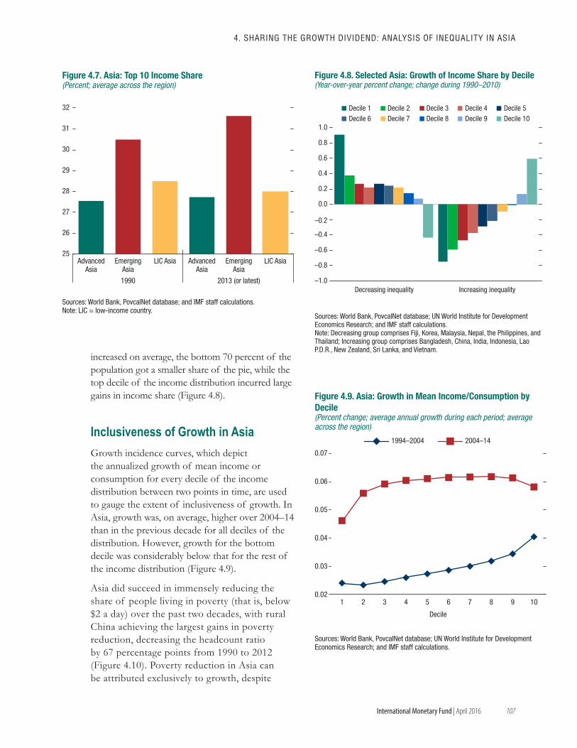
107
4. shARING ThE GROwTh dIvIdENd: ANALysIs Of INEqUALITy IN AsIA
International Monetary Fund | April 2016
increased on average, the bottom 70 percent of the population got a smaller share of the pie, while the top decile of the income distribution incurred large gains in income share (Figure 4.8).
Inclusiveness of Growth in AsiaGrowth incidence curves, which depict the annualized growth of mean income or consumption for every decile of the income distribution between two points in time, are used to gauge the extent of inclusiveness of growth. In Asia, growth was, on average, higher over 2004–14 than in the previous decade for all deciles of the distribution. However, growth for the bottom decile was considerably below that for the rest of the income distribution (Figure 4.9).
Asia did succeed in immensely reducing the share of people living in poverty (that is, below $2 a day) over the past two decades, with rural China achieving the largest gains in poverty reduction, decreasing the headcount ratio by 67 percentage points from 1990 to 2012 (Figure 4.10). Poverty reduction in Asia can be attributed exclusively to growth, despite
25
26
27
28
29
30
31
32
AdvancedAsia
EmergingAsia
LIC Asia AdvancedAsia
EmergingAsia
LIC Asia
1990 2013 (or latest)
Figure 4.7. Asia: Top 10 Income Share(Percent; average across the region)
Sources: World Bank, PovcalNet database; and IMF staff calculations.Note: LIC = low-income country.
Sources: World Bank, PovcalNet database; UN World Institute for Development Economics Research; and IMF staff calculations.Note: Decreasing group comprises Fiji, Korea, Malaysia, Nepal, the Philippines, and Thailand; Increasing group comprises Bangladesh, China, India, Indonesia, Lao P.D.R., New Zealand, Sri Lanka, and Vietnam.
0.0
0.2
0.4
0.6
0.8
1.0
Decreasing inequality Increasing inequality
Decile 1 Decile 2 Decile 3 Decile 4 Decile 5Decile 6 Decile 7 Decile 8 Decile 9 Decile 10
–1.0
–0.8
–0.6
–0.4
–0.2
Figure 4.8. Selected Asia: Growth of Income Share by Decile(Year-over-year percent change; change during 1990–2010)
Sources: World Bank, PovcalNet database; UN World Institute for Development Economics Research; and IMF staff calculations.
0.02
0.03
0.04
0.05
0.06
0.07
1 2 3 4 5 6 7 8 9 10
Decile
1994–2004 2004–14
Figure 4.9. Asia: Growth in Mean Income/Consumption by Decile(Percent change; average annual growth during each period; average across the region)
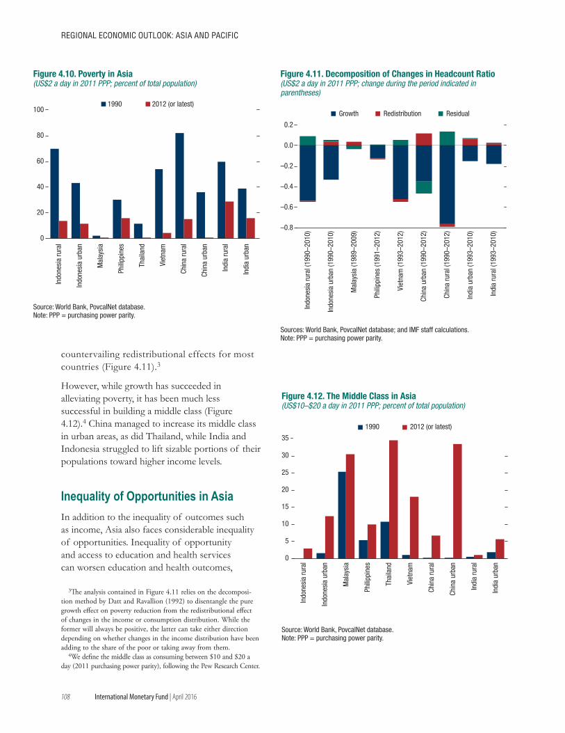
108
REGIONAL ECONOMIC OUTLOOK: AsIA ANd PACIfIC
International Monetary Fund | April 2016
countervailing redistributional effects for most countries (Figure 4.11).3
However, while growth has succeeded in alleviating poverty, it has been much less successful in building a middle class (Figure 4.12).4 China managed to increase its middle class in urban areas, as did Thailand, while India and Indonesia struggled to lift sizable portions of their populations toward higher income levels.
Inequality of Opportunities in AsiaIn addition to the inequality of outcomes such as income, Asia also faces considerable inequality of opportunities. Inequality of opportunity and access to education and health services can worsen education and health outcomes,
3The analysis contained in Figure 4.11 relies on the decomposi-tion method by Datt and Ravallion (1992) to disentangle the pure growth effect on poverty reduction from the redistributional effect of changes in the income or consumption distribution. While the former will always be positive, the latter can take either direction depending on whether changes in the income distribution have been adding to the share of the poor or taking away from them.
4We define the middle class as consuming between $10 and $20 a day (2011 purchasing power parity), following the Pew Research Center.
0
20
40
60
80
100
Indo
nesi
a ru
ral
Indo
nesi
a ur
ban
Mal
aysi
a
Phili
ppin
es
Thai
land
Viet
nam
Chin
a ru
ral
Chin
a ur
ban
Indi
a ru
ral
Indi
a ur
ban
1990 2012 (or latest)
Figure 4.10. Poverty in Asia(US$2 a day in 2011 PPP; percent of total population)
Source: World Bank, PovcalNet database.Note: PPP = purchasing power parity.
–0.8
–0.6
–0.4
–0.2
0.0
0.2
Indo
nesi
a ru
ral (
1990
–201
0)
Indo
nesi
a ur
ban
(199
0–20
10)
Mal
aysi
a (1
989–
2009
)
Phili
ppin
es (1
991–
2012
)
Viet
nam
(199
3–20
12)
Chin
a ur
ban
(199
0–20
12)
Chin
a ru
ral (
1990
–201
2)
Indi
a ur
ban
(199
3–20
10)
Indi
a ru
ral (
1993
–201
0)
Growth Redistribution Residual
Sources: World Bank, PovcalNet database; and IMF staff calculations.Note: PPP = purchasing power parity.
Figure 4.11. Decomposition of Changes in Headcount Ratio(US$2 a day in 2011 PPP; change during the period indicated in parentheses)
0
5
10
15
20
25
30
35
Indo
nesi
a ru
ral
Indo
nesi
a ur
ban
Mal
aysi
a
Phili
ppin
es
Thai
land
Viet
nam
Chin
a ru
ral
Chin
a ur
ban
Indi
a ru
ral
Indi
a ur
ban
1990 2012 (or latest)
Source: World Bank, PovcalNet database.Note: PPP = purchasing power parity.
Figure 4.12. The Middle Class in Asia(US$10–$20 a day in 2011 PPP; percent of total population)
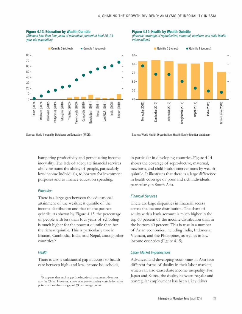
109
4. shARING ThE GROwTh dIvIdENd: ANALysIs Of INEqUALITy IN AsIA
International Monetary Fund | April 2016
hampering productivity and perpetuating income inequality. The lack of adequate financial services also constrains the ability of people, particularly low-income individuals, to borrow for investment purposes and to finance education spending.
Education
There is a large gap between the educational attainment of the wealthiest quintile of the income distribution and that of the poorest quintile. As shown by Figure 4.13, the percentage of people with less than four years of schooling is much higher for the poorest quintile than for the richest quintile. This is particularly true in Bhutan, Cambodia, India, and Nepal, among other countries.5
Health
There is also a substantial gap in access to health care between high- and low-income households,
5It appears that such a gap in educational attainment does not exist in China. However, a look at upper-secondary completion rates points to a rural-urban gap of 39 percentage points.
in particular in developing countries. Figure 4.14 shows the coverage of reproductive, maternal, newborn, and child health interventions by wealth quintile. It illustrates that there is a large difference in health coverage of poor and rich individuals, particularly in South Asia.
Financial Services
There are large disparities in financial access across the income distribution. The share of adults with a bank account is much higher in the top 60 percent of the income distribution than in the bottom 40 percent. This is true in a number of Asian economies, including India, Indonesia, Vietnam, and the Philippines, as well as in low-income countries (Figure 4.15).
Labor Market Imperfections
Advanced and developing economies in Asia face different forms of duality in their labor markets, which can also exacerbate income inequality. For Japan and Korea, the duality between regular and nonregular employment has been a key driver
0
10
20
30
40
50
60
70
80
Chin
a (2
009)
Mal
dive
s (2
009)
Indo
nesi
a (2
012)
Phili
ppin
es (2
013)
Mon
golia
(201
0)
Thai
land
(200
5)
Tim
or-L
este
(200
9)
Cam
bodi
a (2
010)
Bang
lade
sh (2
011)
Nepa
l (20
11)
Lao
P.D.
R. (2
011)
Indi
a (2
005)
Bhut
an (2
010)
Quintile 5 (richest) Quintile 1 (poorest)
Source: World Inequality Database on Education (WIDE).
Figure 4.13. Education by Wealth Quintile(Attained less than four years of education; percent of total 20–24- year-old population)
40
50
60
70
80
90
Mon
golia
(200
5)
Cam
bodi
a (2
010)
Indo
nesi
a (2
012)
Bang
lade
sh (2
011)
Nepa
l (20
11)
Indi
a (2
005)
Tim
or-L
este
(200
9)
Quintile 5 (richest) Quintile 1 (poorest)
Source: World Health Organization, Health Equity Monitor database.
Figure 4.14. Health by Wealth Quintile(Percent; coverage of reproductive, maternal, newborn, and child health interventions)
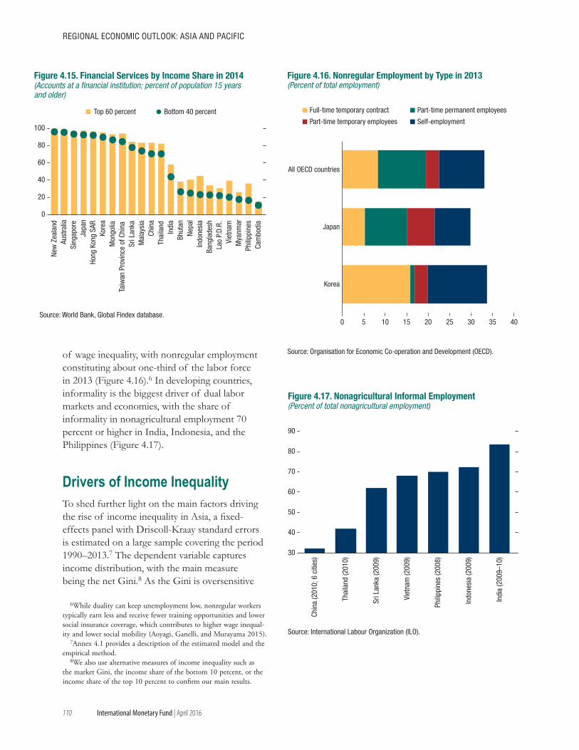
110
REGIONAL ECONOMIC OUTLOOK: AsIA ANd PACIfIC
International Monetary Fund | April 2016
of wage inequality, with nonregular employment constituting about one-third of the labor force in 2013 (Figure 4.16).6 In developing countries, informality is the biggest driver of dual labor markets and economies, with the share of informality in nonagricultural employment 70 percent or higher in India, Indonesia, and the Philippines (Figure 4.17).
Drivers of Income Inequality To shed further light on the main factors driving the rise of income inequality in Asia, a fixed-effects panel with Driscoll-Kraay standard errors is estimated on a large sample covering the period 1990–2013.7 The dependent variable captures income distribution, with the main measure being the net Gini.8 As the Gini is oversensitive
6While duality can keep unemployment low, nonregular workers typically earn less and receive fewer training opportunities and lower social insurance coverage, which contributes to higher wage inequal-ity and lower social mobility (Aoyagi, Ganelli, and Murayama 2015).
7Annex 4.1 provides a description of the estimated model and the empirical method.
8We also use alternative measures of income inequality such as the market Gini, the income share of the bottom 10 percent, or the income share of the top 10 percent to confirm our main results.
0
20
40
60
80
100
New
Zea
land
Aust
ralia
Sing
apor
eJa
pan
Hong
Kon
g SA
RKo
rea
Mon
golia
Taiw
an P
rovi
nce
of C
hina
Sri L
anka
Mal
aysi
aCh
ina
Thai
land
Indi
aBh
utan
Nepa
lIn
done
sia
Bang
lade
shLa
o P.
D.R.
Viet
nam
Mya
nmar
Phili
ppin
esCa
mbo
dia
Top 60 percent Bottom 40 percent
Figure 4.15. Financial Services by Income Share in 2014(Accounts at a financial institution; percent of population 15 years and older)
Source: World Bank, Global Findex database. 0 5 10 15 20 25 30 35 40
Korea
Japan
All OECD countries
Full-time temporary contract Part-time permanent employees
Part-time temporary employees Self-employment
Source: Organisation for Economic Co-operation and Development (OECD).
Figure 4.16. Nonregular Employment by Type in 2013(Percent of total employment)
30
40
50
60
70
80
90
Chin
a (2
010;
6 c
ities
)
Thai
land
(201
0)
Sri L
anka
(200
9)
Viet
nam
(200
9)
Phili
ppin
es (2
008)
Indo
nesi
a (2
009)
Indi
a (2
009–
10)
Figure 4.17. Nonagricultural Informal Employment(Percent of total nonagricultural employment)
Source: International Labour Organization (ILO).
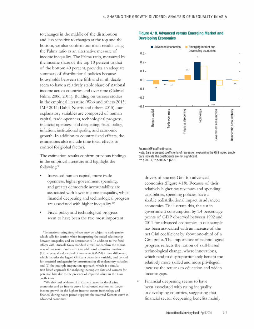
111
4. shARING ThE GROwTh dIvIdENd: ANALysIs Of INEqUALITy IN AsIA
International Monetary Fund | April 2016
to changes in the middle of the distribution and less sensitive to changes at the top and the bottom, we also confirm our main results using the Palma ratio as an alternative measure of income inequality. The Palma ratio, measured by the income share of the top 10 percent to that of the bottom 40 percent, provides an adequate summary of distributional policies because households between the fifth and ninth decile seem to have a relatively stable share of national income across countries and over time (Gabriel Palma 2006, 2011). Building on various studies in the empirical literature (Woo and others 2013; IMF 2014; Dabla-Norris and others 2015), our explanatory variables are composed of human capital, trade openness, technological progress, financial openness and deepening, fiscal policy, inflation, institutional quality, and economic growth. In addition to country fixed effects, the estimations also include time fixed effects to control for global factors.
The estimation results confirm previous findings in the empirical literature and highlight the following:9
• Increased human capital, more trade openness, higher government spending, and greater democratic accountability are associated with lower income inequality, while financial deepening and technological progress are associated with higher inequality.10
• Fiscal policy and technological progress seem to have been the two most important
9Estimations using fixed effects may be subject to endogeneity, which calls for caution when interpreting the causal relationship between inequality and its determinants. In addition to the fixed effects with Driscoll-Kraay standard errors, we confirm the robust-ness of our main results with two additional estimation methods: (1) the generalized method of moments (GMM) in first difference, which includes the lagged Gini as a dependent variable, and control for potential endogeneity by instrumenting all explanatory variables; and (2) the multiple-imputation approach, which is a simula-tion-based approach for analyzing incomplete data and corrects for potential bias due to the presence of imputed values in the Gini coefficients.
10We also find evidence of a Kuznets curve for developing economies and an inverse curve for advanced economies. Larger income growth in the highest-income sectors (technology and finance) during boom period supports the inverted Kuznets curve in advanced economies.
drivers of the net Gini for advanced economies (Figure 4.18). Because of their relatively higher tax revenues and spending capabilities, spending policies have a sizable redistributional impact in advanced economies. To illustrate this, the cut in government consumption by 1.4 percentage points of GDP observed between 1992 and 2011 for advanced economies in our sample has been associated with an increase of the net Gini coefficient by about one-third of a Gini point. The importance of technological progress reflects the notion of skill-biased technological change, where innovations, which tend to disproportionately benefit the relatively more skilled and more privileged, increase the returns to education and widen income gaps.
• Financial deepening seems to have been associated with rising inequality in developing countries, suggesting that financial sector deepening benefits mainly
Source:IMF staff estimates.Note: Bars represent coefficients of regression explaining the Gini Index; empty bars indicate the coefficients are not significant. *** p<0.01, ** p<0.05, * p<0.1.
–0.3
–0.2
–0.1
0.0
0.1
0.2
0.3
Hum
an c
apita
l
Trad
e op
enne
ss
Fina
ncia
l dee
peni
ng
Tech
nolo
gy
Gove
rnm
ent c
onsu
mpt
ion
Dem
ocra
tic a
ccou
ntab
ility
Advanced economies Emerging market and developing economies
**
*
***
****
***
**
Figure 4.18. Advanced versus Emerging Market and Developing Economies
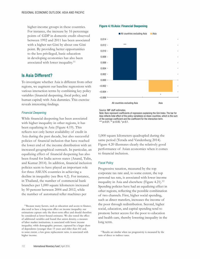
112
REGIONAL ECONOMIC OUTLOOK: AsIA ANd PACIfIC
International Monetary Fund | April 2016
higher-income groups in these countries. For instance, the increase by 16 percentage points of GDP in domestic credit observed between 1992 and 2011 has been associated with a higher net Gini by about one Gini point. By providing better opportunities to the less privileged, basic education in developing economies has also been associated with lower inequality.11
Is Asia Different?To investigate whether Asia is different from other regions, we augment our baseline regressions with various interaction terms by combining key policy variables (financial deepening, fiscal policy, and human capital) with Asia dummies. This exercise reveals interesting findings.
Financial Deepening
While financial deepening has been associated with higher inequality in other regions, it has been equalizing in Asia (Figure 4.19). This reflects not only better availability of credit in Asia during the past decade, but also successful policies of financial inclusion that have reached the lower end of the income distribution with an increased geographical outreach. In particular, an equalizing effect of financial deepening has also been found for India across states (Anand, Tulin, and Kumar 2014). In addition, financial inclusion policies seem to have played an important role for three ASEAN countries in achieving a decline in inequality (see Box 4.2). For instance, in Thailand, the number of commercial bank branches per 1,000 square kilometers increased by 50 percent between 2004 and 2012, while the number of automated teller machines per
11Because many factors, such as education and access to finance, also tend to have a long-term effect on income inequality, our estimations capture only the short-term effect and should therefore be considered as lower-bound estimates. We also tested the effect of additional variables and found that union density, a measure of labor market institutions, is associated with lower income inequality, while demographic pressure, captured by a larger share of dependents (younger than 15 years and older than 64) and, to some extent, a low gross replacement ratio, is associated with higher income.
1,000 square kilometers quadrupled during the same period (Terada and Vandenberg 2014). Figure 4.20 illustrates clearly the relatively good performance of Asian economies when it comes to financial inclusion.
Fiscal Policy
Progressive taxation, measured by the top corporate tax rate and, to some extent, the top personal tax rate, is associated with lower income inequality in Asia and elsewhere (Figure 4.21).12 Spending policies have had an equalizing effect in other regions, reflecting the possible combination of two channels. First, higher social spending, such as direct transfers, increases the income of the poor through redistribution. Second, higher social, education, and capital spending tend to promote better access for the poor to education and health care, thereby lowering inequality in the long term.
12Results are similar when tax progressivity is measured by the ratio of direct to indirect taxes.
Source: IMF staff estimates.Note: Bars represent coefficients of regression explaining the Gini Index. The bar for Asia reflects total effect of the policy variable(s) on Asian countries, which is the sum of the average coefficient and the coefficient for the interaction term. *** p<0.01, ** p<0.05, * p<0.1.
***
*–0.006
–0.004
–0.002
0.000
0.002
0.004
0.006
0.008
0.010
0.012
0.014
All countries excluding Asia Asia
All countries excluding Asia Asia
Figure 4.19.Asia: Financial Deepening
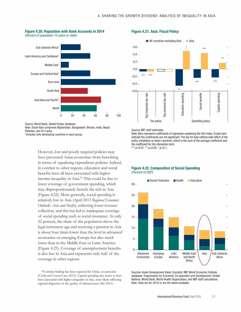
113
4. shARING ThE GROwTh dIvIdENd: ANALysIs Of INEqUALITy IN AsIA
International Monetary Fund | April 2016
However, low and poorly targeted policies may have prevented Asian economies from benefiting in terms of equalizing expenditure policies. Indeed, in contrast to other regions, education and social benefits have all been associated with higher income inequality in Asia.13 This could be due to lower coverage of government spending, which may disproportionately benefit the rich in Asia (Figure 4.22). More generally, social spending is relatively low in Asia (April 2013 Regional Economic Outlook: Asia and Pacific), reflecting lower revenue collection, and this has led to inadequate coverage of social spending such as social insurance. At only 22 percent, the share of the population above the legal retirement age and receiving a pension in Asia is about four times lower than the level in advanced economies or emerging Europe but also much lower than in the Middle East or Latin America (Figure 4.23). Coverage of unemployment benefits is also low in Asia and represents only half of the coverage in other regions.
13A similar finding has been reported for China, in particular (Cevik and Correa-Caro 2015). Capital spending also seems to have been associated with higher inequality in Asia, most likely reflecting regional disparities in the quality of infrastructure (Shi 2012).
Source: World Bank, Global Findex database.Note: South Asia comprises Afghanistan, Bangladesh, Bhutan, India, Nepal, Pakistan, and Sri Lanka.1Includes only developing countries in each group.
0 20 40 60 80 100
World
East Asia and Pacific1
South Asia
Euro area
Europe and Central Asia1
Middle East1
Latin America and Caribbean1
Sub-Saharan Africa1
Figure 4.20. Population with Bank Accounts in 2014(Percent of population 15 years or older)
***
**
*** ***
***
****
**
–0.6
–0.4
–0.2
0.0
0.2
0.4
0.6
Top
corp
orat
e ta
x ra
te
Top
pers
onal
tax
rate
Educ
atio
n sp
endi
ng
Soci
al b
enefi
ts
Capi
tal s
pend
ing
Tax policy Spending policy
All countries excluding Asia Asia
Figure 4.21. Asia: Fiscal Policy
Source: IMF staff estimates.Note: Bars represent coefficients of regression explaining the Gini Index. Empty bars indicate the coefficients are not significant. The bar for Asia reflects total effect of the policy variable(s) on Asian countries, which is the sum of the average coefficient and the coefficient for the interaction term.*** p<0.01, ** p<0.05, * p<0.1.
0
5
10
15
20
25
30
AdvancedEconomies
Social Protection Health Education
Figure 4.22. Composition of Social Spending(Percent of GDP)
EmergingEurope
LatinAmerica
Middle Eastand North
Africa
Asia Sub-SaharanAfrica
Sources: Asian Development Bank; Eurostat; IMF, World Economic Outlook database; Organisation for Economic Co-operation and Development; United Nations; World Bank; World Health Organization; and IMF staff calculations.Note: Data are for 2010 or are the latest available.
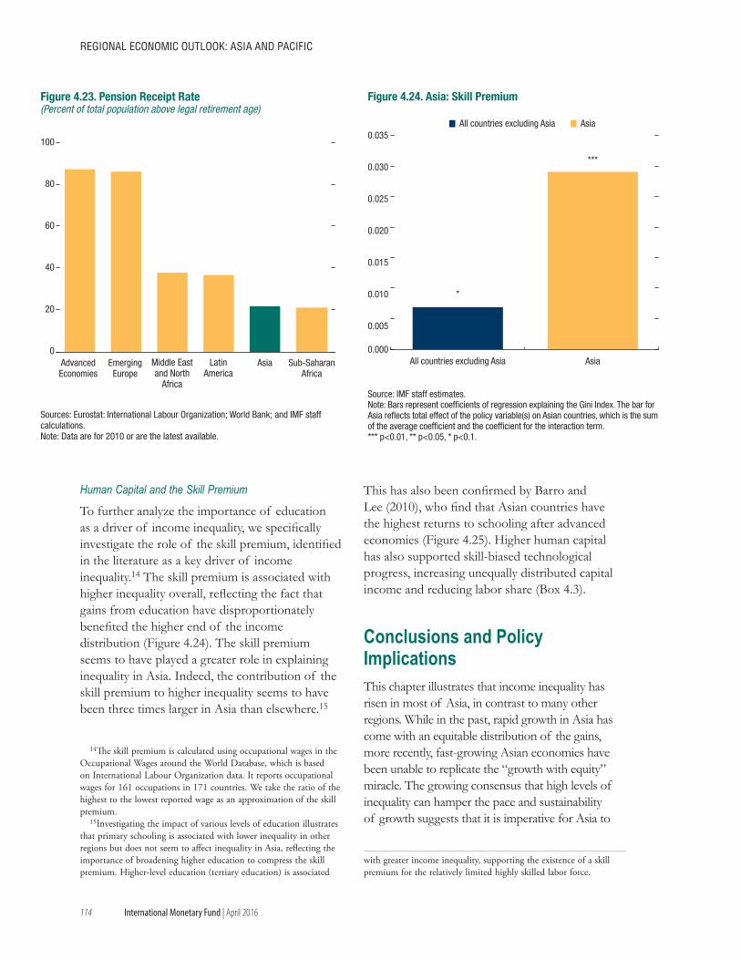
114
REGIONAL ECONOMIC OUTLOOK: AsIA ANd PACIfIC
International Monetary Fund | April 2016
Human Capital and the Skill Premium
To further analyze the importance of education as a driver of income inequality, we specifically investigate the role of the skill premium, identified in the literature as a key driver of income inequality.14 The skill premium is associated with higher inequality overall, reflecting the fact that gains from education have disproportionately benefited the higher end of the income distribution (Figure 4.24). The skill premium seems to have played a greater role in explaining inequality in Asia. Indeed, the contribution of the skill premium to higher inequality seems to have been three times larger in Asia than elsewhere.15
14The skill premium is calculated using occupational wages in the Occupational Wages around the World Database, which is based on International Labour Organization data. It reports occupational wages for 161 occupations in 171 countries. We take the ratio of the highest to the lowest reported wage as an approximation of the skill premium.
15Investigating the impact of various levels of education illustrates that primary schooling is associated with lower inequality in other regions but does not seem to affect inequality in Asia, reflecting the importance of broadening higher education to compress the skill premium. Higher-level education (tertiary education) is associated
This has also been confirmed by Barro and Lee (2010), who find that Asian countries have the highest returns to schooling after advanced economies (Figure 4.25). Higher human capital has also supported skill-biased technological progress, increasing unequally distributed capital income and reducing labor share (Box 4.3).
Conclusions and Policy ImplicationsThis chapter illustrates that income inequality has risen in most of Asia, in contrast to many other regions. While in the past, rapid growth in Asia has come with an equitable distribution of the gains, more recently, fast-growing Asian economies have been unable to replicate the “growth with equity” miracle. The growing consensus that high levels of inequality can hamper the pace and sustainability of growth suggests that it is imperative for Asia to
with greater income inequality, supporting the existence of a skill premium for the relatively limited highly skilled labor force.
0
20
40
60
80
100
AdvancedEconomies
EmergingEurope
LatinAmerica
Middle Eastand North
Africa
Asia Sub-SaharanAfrica
Figure 4.23. Pension Receipt Rate(Percent of total population above legal retirement age)
Sources: Eurostat: International Labour Organization; World Bank; and IMF staff calculations.Note: Data are for 2010 or are the latest available.
Source: IMF staff estimates.Note: Bars represent coefficients of regression explaining the Gini Index. The bar for Asia reflects total effect of the policy variable(s) on Asian countries, which is the sum of the average coefficient and the coefficient for the interaction term.*** p<0.01, ** p<0.05, * p<0.1.
*
***
0.000
0.005
0.010
0.015
0.020
0.025
0.030
0.035
All countries excluding Asia Asia
All countries excluding Asia Asia
Figure 4.24. Asia: Skill Premium
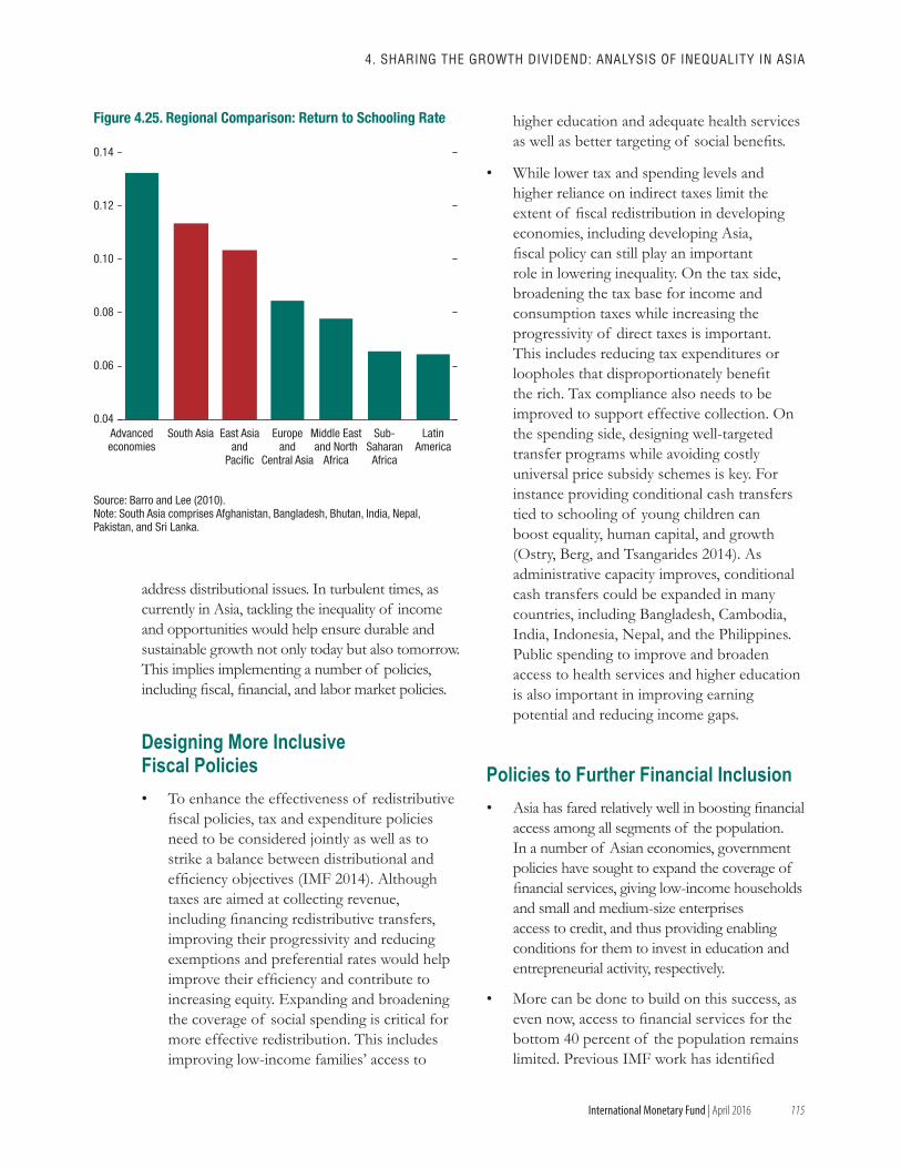
115
4. shARING ThE GROwTh dIvIdENd: ANALysIs Of INEqUALITy IN AsIA
International Monetary Fund | April 2016
address distributional issues. In turbulent times, as currently in Asia, tackling the inequality of income and opportunities would help ensure durable and sustainable growth not only today but also tomorrow. This implies implementing a number of policies, including fiscal, financial, and labor market policies.
Designing More Inclusive Fiscal Policies• To enhance the effectiveness of redistributive
fiscal policies, tax and expenditure policies need to be considered jointly as well as to strike a balance between distributional and efficiency objectives (IMF 2014). Although taxes are aimed at collecting revenue, including financing redistributive transfers, improving their progressivity and reducing exemptions and preferential rates would help improve their efficiency and contribute to increasing equity. Expanding and broadening the coverage of social spending is critical for more effective redistribution. This includes improving low-income families’ access to
higher education and adequate health services as well as better targeting of social benefits.
• While lower tax and spending levels and higher reliance on indirect taxes limit the extent of fiscal redistribution in developing economies, including developing Asia, fiscal policy can still play an important role in lowering inequality. On the tax side, broadening the tax base for income and consumption taxes while increasing the progressivity of direct taxes is important. This includes reducing tax expenditures or loopholes that disproportionately benefit the rich. Tax compliance also needs to be improved to support effective collection. On the spending side, designing well-targeted transfer programs while avoiding costly universal price subsidy schemes is key. For instance providing conditional cash transfers tied to schooling of young children can boost equality, human capital, and growth (Ostry, Berg, and Tsangarides 2014). As administrative capacity improves, conditional cash transfers could be expanded in many countries, including Bangladesh, Cambodia, India, Indonesia, Nepal, and the Philippines. Public spending to improve and broaden access to health services and higher education is also important in improving earning potential and reducing income gaps.
Policies to Further Financial Inclusion • Asia has fared relatively well in boosting financial
access among all segments of the population. In a number of Asian economies, government policies have sought to expand the coverage of financial services, giving low-income households and small and medium-size enterprises access to credit, and thus providing enabling conditions for them to invest in education and entrepreneurial activity, respectively.
• More can be done to build on this success, as even now, access to financial services for the bottom 40 percent of the population remains limited. Previous IMF work has identified
0.04
0.06
0.08
0.10
0.12
0.14
Figure 4.25. Regional Comparison: Return to Schooling Rate
Source: Barro and Lee (2010).Note: South Asia comprises Afghanistan, Bangladesh, Bhutan, India, Nepal, Pakistan, and Sri Lanka.
Advancedeconomies
South Asia LatinAmerica
Middle Eastand North
Africa
Europeand
Central Asia
East Asiaand
Pacific
Sub-SaharanAfrica
116
REGIONAL ECONOMIC OUTLOOK: AsIA ANd PACIfIC
International Monetary Fund | April 2016
benefits from enabling firms to access credit, financing a greater share of investment with bank credit, increasing the number of households with bank accounts, and using bank accounts to receive government transfers and wages (Sahay and others 2015). However, policies to foster financial inclusion have to be designed carefully, mindful of the implications for financial stability and accompanied by upgrades to bank supervision and regulation to protect financial stability.
Tackling Labor Market Duality and Informality• Reducing labor market duality and informality,
while putting in place well-designed labor
market policies to boost job creation, can reduce income inequality. In high-income Asian countries, efforts to reduce labor market duality should be accelerated, particularly by addressing gaps in legal protection for regular and nonregular workers and by encouraging new hiring under contracts that balance job security and flexibility. In low- and middle-income countries, policies to reduce informality could lead to more inclusive growth. Measures to improve the overall business environment, simplify business registration and reduce red tape, and provide incentives to facilitate registration and legal recognition would be helpful in reducing the incentives to remain in the informal sector.
117
4. shARING ThE GROwTh dIvIdENd: ANALysIs Of INEqUALITy IN AsIA
International Monetary Fund | April 2016
Spurred by wide-ranging economic reforms, China and India have grown rapidly and reduced poverty sharply. However, this impressive economic performance has been accompanied by increasing levels of inequality, in contrast to the earlier industrializing Asian economies.
Spatial Inequality Over the past two decades all deciles of the distribution have increased in mean consumption in both countries (Figures 4.1.1–4.1.4). In China, this increase has been most pronounced in urban areas, suggesting that a large contribution to increased inequality stems from differences among rural and urban areas. In India, differences between rural and urban areas have increased, and have been accompanied by rising intra-urban inequality.
Many factors have been identified as key drivers of the inequality between rural and urban areas in China and India. In China, rapid industrialization in particular regions and the concentration of foreign direct investment in coastal areas have led to substantial inequalities between coastal and interior regions, but have decreased in importance in part due to the government’s Western Development Strategy adopted in 2000 (Li, Wan, and Zhuang 2014). Other factors also include low educational attainment and low returns to education in rural areas, with the hukou system constraining rural-urban migration and thereby exacerbating the effects (Liu 2005; Dollar 2007).
Interprovincial inequality is lower in India than in China, and rising inequality in India has been found to be primarily an urban phenomenon (Cain and others 2014). But, in addition, the rural-urban income gap has increased, and higher rural inflation has been found to be a key driver of this (Kanbur and Zhuang 2014; Anand, Tulin, and Kumar 2014). Educational attainment has also been identified as an important factor explaining rising inequality in India over the past two decades (Cain and others 2014).
Fiscal and Inclusive Policies India and China have both struggled with basic service delivery in education and health (Chaudhuri and Ravallion 2006). Despite recent improvements, lower levels of tax revenue compared with other regions and a higher reliance on indirect taxes have constrained fiscal redistribution (Piketty and Qian 2009; Li, Wan, and Zhuang 2014; Cevik and Correa-Caro 2015). The two countries have introduced a number of policies to tackle the rising inequality. China introduced the Minimum Livelihood Guarantee Scheme (Dibao) for social protection in the 1990s. The coverage of the scheme is now nearly universal, but the income provided remains low (Cevik and Correa-Caro 2015). The scheme has not been found to reduce inequality, but has helped to alleviate poverty (Li and Yang 2009). Various social programs are aiming to expand social safety nets and provide support for the development of rural areas (including New Rural Cooperative Medicare, New Rural Pension Scheme, and the Two Exemptions and One Subsidy Program) and western regions (Western Development Strategy) (Li, Wan, and Zhuang 2014), which might explain some of the positive changes in the distribution from 2002 to 2010.
In India, the government introduced the Mahatma Gandhi National Rural Employment Guarantee Act to support rural livelihoods by providing at least 100 days of employment. Programs to improve education include the National Education Scheme and Midday Meal Scheme. The JAM trinity initiative helped India in making substantial advances in financial inclusion. More recently, programs aiming for universal bank account coverage were launched (IMF 2016b; Sahay and others 2015).
The main author of this box is Johanna Schauer.
Box 4.1. Understanding Rising Inequality in China and India
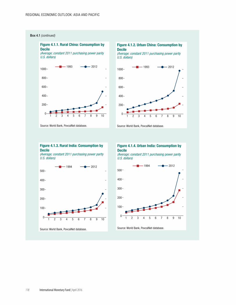
118
REGIONAL ECONOMIC OUTLOOK: AsIA ANd PACIfIC
International Monetary Fund | April 2016
0
100
200
300
400
500
1 2 3 4 5 6 7 8 9 10
1994 2012
Source: World Bank, PovcalNet database.
Figure 4.1.3. Rural India: Consumption by Decile(Average; constant 2011 purchasing power parity U.S. dollars)
0
100
200
300
400
500
1 2 3 4 5 6 7 8 9 10
1994 2012
Source: World Bank, PovcalNet database.
Figure 4.1.4. Urban India: Consumption by Decile(Average; constant 2011 purchasing power parity U.S. dollars)
0
200
400
600
800
1000
1 2 3 4 5 6 7 8 9 10
1993 2012
Source: World Bank, PovcalNet database.
Figure 4.1.1. Rural China: Consumption by Decile(Average; constant 2011 purchasing power parity U.S. dollars)
Source: World Bank, PovcalNet database.
0
200
400
600
800
1000
1 2 3 4 5 6 7 8 9 10
1993 2012
Figure 4.1.2. Urban China: Consumption by Decile(Average; constant 2011 purchasing power parity U.S. dollars)
Box 4.1 (continued)
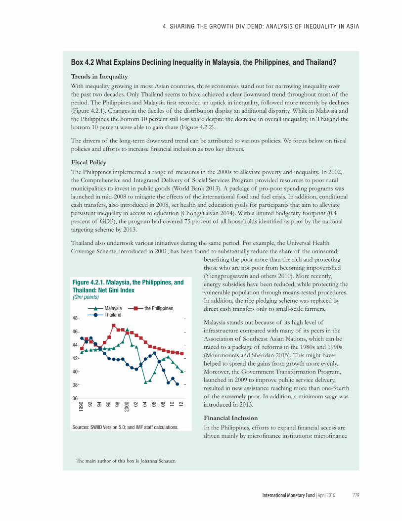
119
4. shARING ThE GROwTh dIvIdENd: ANALysIs Of INEqUALITy IN AsIA
International Monetary Fund | April 2016
Trends in Inequality With inequality growing in most Asian countries, three economies stand out for narrowing inequality over the past two decades. Only Thailand seems to have achieved a clear downward trend throughout most of the period. The Philippines and Malaysia first recorded an uptick in inequality, followed more recently by declines (Figure 4.2.1). Changes in the deciles of the distribution display an additional disparity. While in Malaysia and the Philippines the bottom 10 percent still lost share despite the decrease in overall inequality, in Thailand the bottom 10 percent were able to gain share (Figure 4.2.2).
The drivers of the long-term downward trend can be attributed to various policies. We focus below on fiscal policies and efforts to increase financial inclusion as two key drivers.
Fiscal Policy The Philippines implemented a range of measures in the 2000s to alleviate poverty and inequality. In 2002, the Comprehensive and Integrated Delivery of Social Services Program provided resources to poor rural municipalities to invest in public goods (World Bank 2013). A package of pro-poor spending programs was launched in mid-2008 to mitigate the effects of the international food and fuel crisis. In addition, conditional cash transfers, also introduced in 2008, set health and education goals for participants that aim to alleviate persistent inequality in access to education (Chongvilaivan 2014). With a limited budgetary footprint (0.4 percent of GDP), the program had covered 75 percent of all households identified as poor by the national targeting scheme by 2013.
Thailand also undertook various initiatives during the same period. For example, the Universal Health Coverage Scheme, introduced in 2001, has been found to substantially reduce the share of the uninsured,
benefiting the poor more than the rich and protecting those who are not poor from becoming impoverished (Yiengprugsawan and others 2010). More recently, energy subsidies have been reduced, while protecting the vulnerable population through means-tested procedures. In addition, the rice pledging scheme was replaced by direct cash transfers only to small-scale farmers.
Malaysia stands out because of its high level of infrastructure compared with many of its peers in the Association of Southeast Asian Nations, which can be traced to a package of reforms in the 1980s and 1990s (Mourmouras and Sheridan 2015). This might have helped to spread the gains from growth more evenly. Moreover, the Government Transformation Program, launched in 2009 to improve public service delivery, resulted in new assistance reaching more than one-fourth of the extremely poor. In addition, a minimum wage was introduced in 2013.
Financial Inclusion In the Philippines, efforts to expand financial access are driven mainly by microfinance institutions: microfinance
The main author of this box is Johanna Schauer.
36
38
40
42
44
46
48
1990 92 94 96 98
2000 02 04 06 08 10 12
Malaysia the PhilippinesThailand
Sources: SWIID Version 5.0; and IMF staff calculations.
Figure 4.2.1. Malaysia, the Philippines, and Thailand: Net Gini Index(Gini points)
Box 4.2 What Explains Declining Inequality in Malaysia, the Philippines, and Thailand?
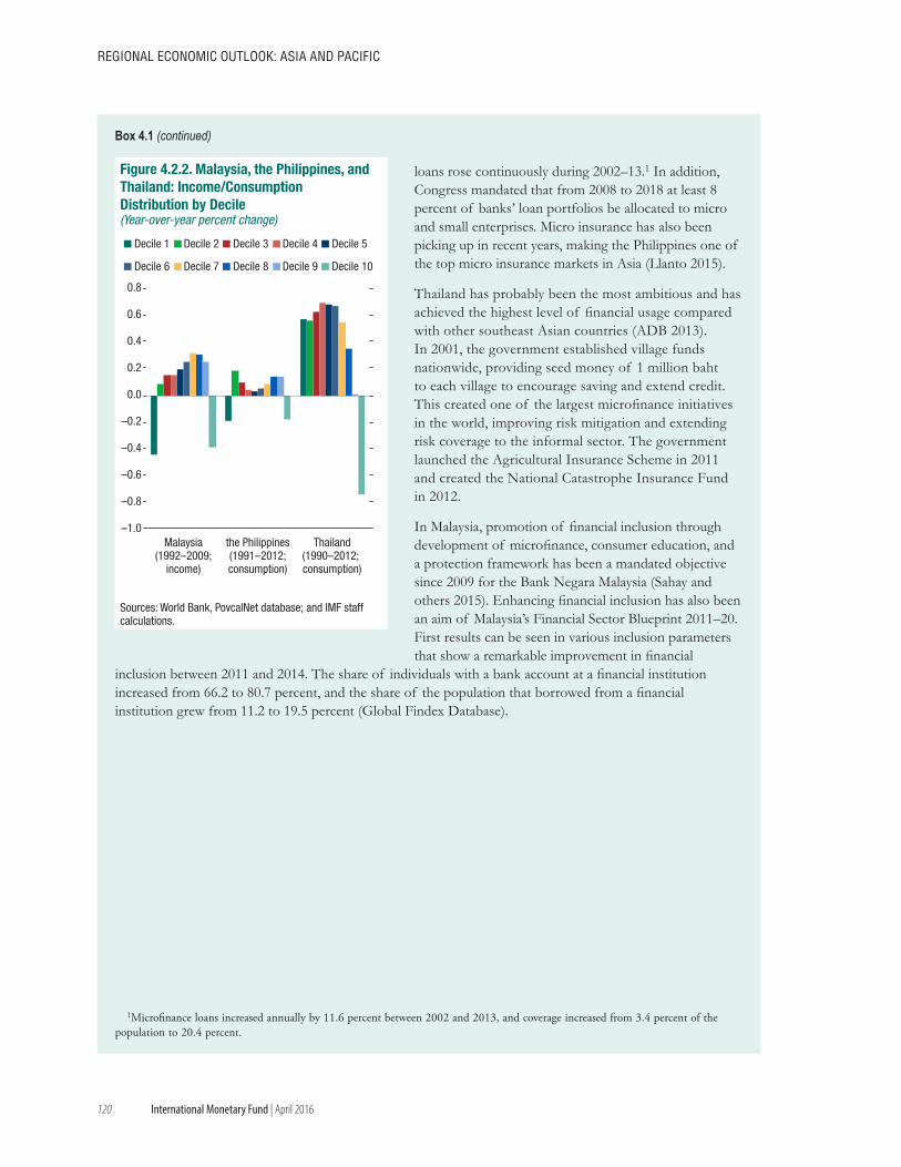
REGIONAL ECONOMIC OUTLOOK: AsIA ANd PACIfIC
120 International Monetary Fund | April 2016
loans rose continuously during 2002–13.1 In addition, Congress mandated that from 2008 to 2018 at least 8 percent of banks’ loan portfolios be allocated to micro and small enterprises. Micro insurance has also been picking up in recent years, making the Philippines one of the top micro insurance markets in Asia (Llanto 2015).
Thailand has probably been the most ambitious and has achieved the highest level of financial usage compared with other southeast Asian countries (ADB 2013). In 2001, the government established village funds nationwide, providing seed money of 1 million baht to each village to encourage saving and extend credit. This created one of the largest microfinance initiatives in the world, improving risk mitigation and extending risk coverage to the informal sector. The government launched the Agricultural Insurance Scheme in 2011 and created the National Catastrophe Insurance Fund in 2012.
In Malaysia, promotion of financial inclusion through development of microfinance, consumer education, and a protection framework has been a mandated objective since 2009 for the Bank Negara Malaysia (Sahay and others 2015). Enhancing financial inclusion has also been an aim of Malaysia’s Financial Sector Blueprint 2011–20. First results can be seen in various inclusion parameters that show a remarkable improvement in financial
inclusion between 2011 and 2014. The share of individuals with a bank account at a financial institution increased from 66.2 to 80.7 percent, and the share of the population that borrowed from a financial institution grew from 11.2 to 19.5 percent (Global Findex Database).
1Microfinance loans increased annually by 11.6 percent between 2002 and 2013, and coverage increased from 3.4 percent of the population to 20.4 percent.
–1.0
–0.8
–0.6
–0.4
–0.2
0.0
0.2
0.4
0.6
0.8
Malaysia(1992–2009;
income)
the Philippines(1991–2012;consumption)
Thailand(1990–2012; consumption)
Decile 1 Decile 2 Decile 3 Decile 4 Decile 5
Decile 6 Decile 7 Decile 8 Decile 9 Decile 10
Sources: World Bank, PovcalNet database; and IMF staffcalculations.
Figure 4.2.2. Malaysia, the Philippines, and Thailand: Income/Consumption Distribution by Decile(Year-over-year percent change)
Box 4.1 (continued)
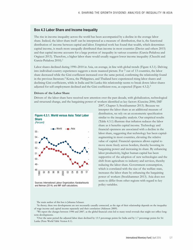
121
4. shARING ThE GROwTh dIvIdENd: ANALysIs Of INEqUALITy IN AsIA
International Monetary Fund | April 2016
The rise in income inequality across the world has been accompanied by a decline in the average labor share. Indeed, the labor share itself can be interpreted as a measure of distribution, that is, the functional distribution of income between capital and labor. Empirical work has found that wealth, which determines capital income, is much more unequally distributed than income in most countries (Davies and others 2015) and that capital income accounts for a large portion of inequality in various countries (Garcia-Peñalosa and Orgiazzi 2013). Therefore, a higher labor share would usually suggest lower income inequality (Checchi and Garcia-Peñalosa 2010).1
Labor shares declined during 1990–2010 in Asia, on average, in line with global trends (Figure 4.3.1). Delving into individual country experiences suggests a more nuanced picture. For 7 out of 13 countries, the labor share decreased while the Gini coefficient increased over the same period, confirming the relationship found in the previous literature.2 Korea, the Philippines, and Thailand have experienced rising labor shares and declining Gini coefficients, while in India and Sri Lanka this relationship seems to break down: labor shares adjusted for self-employment declined and the Gini coefficient rose, as expected (Figure 4.3.2).3
Drivers of the Labor ShareDrivers of the labor share have received new attention over the past decade, with globalization, technological and structural change, and the bargaining power of workers identified as key factors (Guscina 2006; IMF
2007, Chapter 5; Stockhammer 2013). Because we interpret the labor share as an additional measure of distribution, we rely on an econometric specification similar to the inequality analysis. Our empirical results (Table 4.3.1) illustrate that inflation reduces the labor share as it benefits capital income. Technology and financial openness are associated with a decline in the labor share, suggesting that technology has been capital-augmenting in most countries, elevating the relative value of capital. Financial openness allows capital to move more freely across borders, thereby boosting its bargaining power and increasing its share. By enhancing labor productivity, higher human capital has been supportive of the adoption of new technologies and the shift from agriculture to industry and services, thereby reducing the labor share. Government consumption, which is correlated with the size of the welfare state, increases the labor share by enhancing the bargaining power of workers (Stockhammer 2013). Asia does not seem to differ from other regions with regard to key policy variables.
The main author of this box is Johanna Schauer.1In theory, these two developments are not necessarily causally connected, as the sign of their relationship depends on the inequality
of wage income and capital income separately and their correlation (Atkinson 2009).2We report the changes between 1990 and 2007, as the global financial crisis led to many trend reversals that might not reflect long-
term developments.3Over the same period the adjusted labor share declined by 13.5 percentage points for India and by 1.7 percentage points for Sri
Lanka (Penn World Table Version 8.1).
Sources: International Labour Organization; Karabarbounis and Neiman (2014); and IMF staff calculations.
48
49
50
51
52
53
54
55
1990 92 94 96 98
2000 02 04 06 08 10
World Asia
Figure 4.3.1. World versus Asia: Total Labor Share(Percent)
Box 4.3 Labor Share and Income Inequality
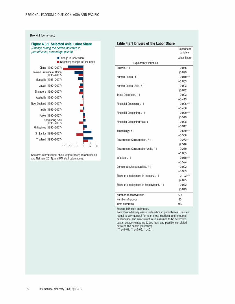
REGIONAL ECONOMIC OUTLOOK: AsIA ANd PACIfIC
122 International Monetary Fund | April 2016
Sources: International Labour Organization; Karabarbounis and Neiman (2014); and IMF staff calculations.
–15 –10 –5 0 5 10
Thailand (1990–2007)
Sri Lanka (1998–2007)
Philippines (1995–2007)
Hong Kong SAR(1995–2007)
Korea (1990–2007)
India (1995–2007)
New Zealand (1990–2007)
Australia (1990–2007)
Singapore (1990–2007)
Japan (1990–2007)
Mongolia (1995–2007)
Taiwan Province of China(1990–2007)
China (1992–2007)
Change in labor share(Negative) change in Gini index
Figure 4.3.2. Selected Asia: Labor Share(Change during the period indicated in parentheses; percentage points)
Table 4.3.1 Drivers of the Labor Share
Explanatory Variables
Dependent Variable:
Labor Share
Growth, t–1 0.036
(0.829)
Human Capital, t–1 –0.019***
(–3.803)
Human Capital*Asia, t–1 0.003
(0.072)
Trade Openness, t–1 –0.003
(–0.443)
Financial Openness, t–1 –0.006***
(–5.406)
Financial Deepening, t–1 0.029***
(5.519)
Financial Deepening*Asia, t–1 –0.008
(–0.947)
Technology, t–1 –0.559***
(–3.550)
Government Consumption, t–1 0.262**
(2.546)
Government Consumption*Asia, t–1 –0.249
(–1.055)
Inflation, t–1 –0.010***
(–3.524)
Democratic Accountability, t–1 –0.002
(–0.983)
Share of employment in Industry, t–1 0.192***
(4.095)
Share of employment in Employment, t–1 0.022
(0.819)
Number of observations 673
Number of groups 60
Time dummies YES
Source: IMF staff estimates.Note: Driscoll-Kraay robust t-statistics in parentheses. They are robust to very general forms of cross-sectional and temporal dependence. The error structure is assumed to be heteroske-dastic, autocorrelated up to two lags, and possibly correlated between the panels (countries).*** p<0.01, ** p<0.05, * p<0.1.
Box 4.1 (continued)
4. shARING ThE GROwTh dIvIdENd: ANALysIs Of INEqUALITy IN AsIA
123International Monetary Fund | April 2016
Annex 4.1 Drivers of Income InequalityThis annex presents the empirical framework and estimates of the drivers of income inequality. It builds on various studies in the empirical literature (Woo and others 2013; IMF 2014; Dabla-Norris and others 2015) to formulate the econometric strategy. The baseline model specification is as follows:
Inequalit = δXit–1 + µi + θt + εit
where Inequal denotes, for each country i and year t, a measure of income distribution, with the main measure being the net Gini.1 Xit–1 is the vector of explanatory variables and comprises human capital, technological progress, financial openness, trade openness, financial deepening, fiscal policy, inflation, and democratic accountability.2 The education variable, from the Penn World Table Version 8.1, captures the average years of schooling (Barro and Lee 2010). Technological progress is measured by the share of information technology capital in the total capital stock (Jorgenson and Vu 2007) and financial openness by the sum of assets and liabilities from the international investment position data over GDP. Trade openness is measured by the sum of exports and imports over GDP, financial deepening by domestic credit to the private sector as a share of GDP, fiscal policy by government consumption over GDP, and inflation by changes in the consumer price index (all from the World Economic Outlook). Democratic accountability (from the International Country Risk Guide data set) captures how responsive government is to its people. µi denote the country-specific fixed effects to control for country-specific factors, including the time-invariant component of the institutional and geographical environments. θt are time-fixed effects to control for global factors, and εit is an error term. All explanatory variables in the estimation are lagged by one year to reduce the risks of endogeneity due to reverse causality.
To investigate whether the drivers of inequality in Asia differ from those in other regions, with a focus on policy variables, we augment our baseline specification
The main author of this annex is Tidiane Kinda.1Our main results are robust with alternative measures of income
inequality, such as market Gini, income share of the bottom 10 percent, income share of the top 10 percent, and the Palma ratio (See Jain-Chandra and others 2016).
2Our baseline regressions also control for income per capita and its squared term to test for the existence of Kuznets curves.
with various interaction terms by combining key policy variables with Asia dummies as illustrated below:
Inequalit = δXit–1 + γAsia * Zit–1 + µi + θt + εit
where all variables are defined as above, and Zit–1 is the vector of policy variables and refers to human capital, financial deepening, and government consumption. We further zoom in on each policy issue separately and use more granular data to assess the way in which that policy affects inequality in Asia. We focus on one policy area at a time to reduce the risk of collinearity while preserving an adequate number of variables and observations for each of our estimations.
The sample covers 82 advanced and developing economies, including 17 Asian countries, during the period 1990–2013. We rely mainly on fixed-effects (FE) panel regressions, with Driscoll-Kraay standard errors for our empirical investigation. The FE with Driscoll-Kraay standard errors are robust to very general forms of cross-sectional and temporal dependence. The error structure under this estimation method is assumed to be heteroscedastic and autocorrelated up to two lags, which helps capture the persistence of income inequality across time. The error is also assumed to be correlated between countries, possibly due to common shocks, for instance those related to technology, international trade, or financial crises.
The results from the baseline regressions are broadly in line with findings in the empirical literature. In particular, fiscal policy and technological progress seem to have been the two most important drivers of the net Gini for advanced economies, while financial deepening has been associated with rising inequality in developing countries (Annex Table 4.1.1).
Analyzing whether the drivers of income inequality in Asia differ from those in other regions highlights interesting findings. While financial deepening has been associated with higher inequality in other regions, it has been an equalizing force in Asia (Annex Table 4.1.2, column 1). Further investigating the specificity of Asia illustrates that limited and poorly targeted policies may have prevented Asian economies from benefiting in terms of equalizing expenditure policies. Indeed, unlike in other regions, education, social benefits, and capital spending seem to have been associated with higher income inequality in Asia (Annex Table 4.1.2, column 2). The contribution of skill premiums to higher inequality appears to have been three times larger in Asia than elsewhere (Annex Table 4.1.3, column 3).
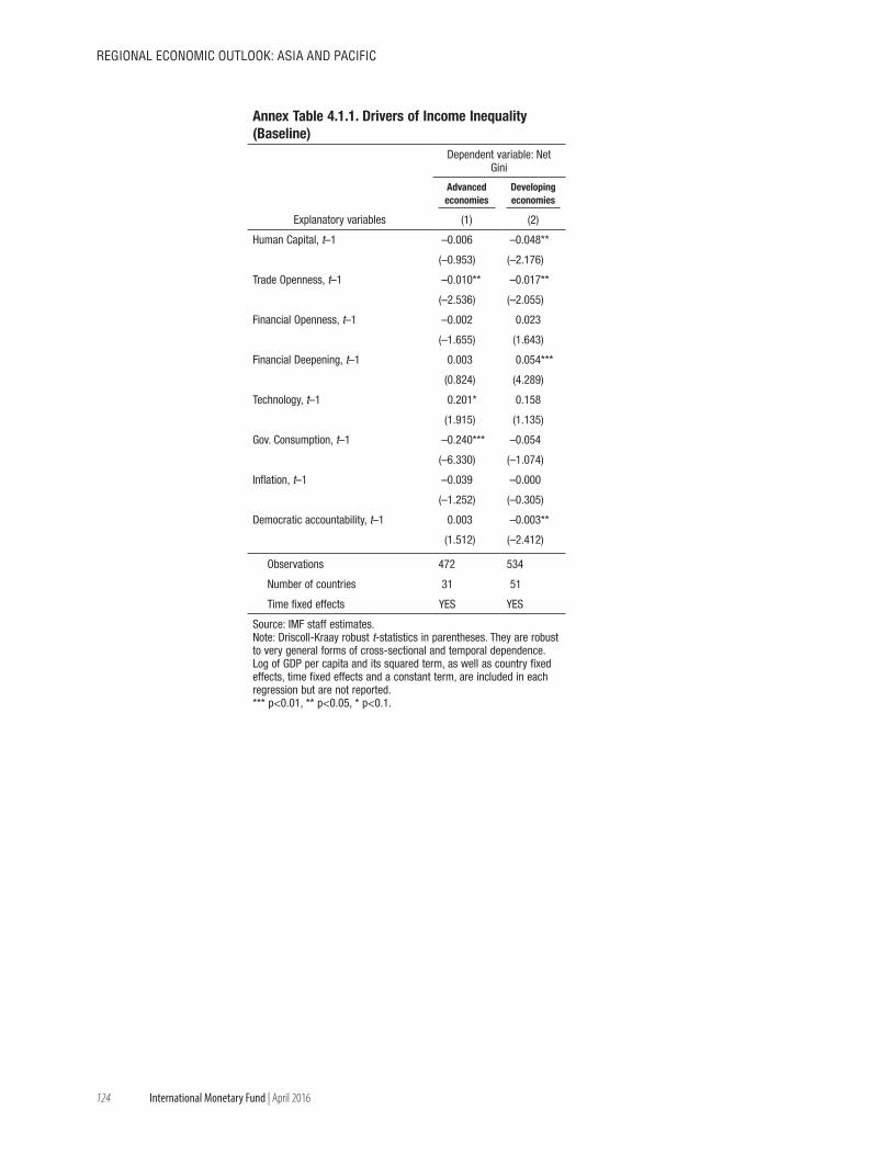
REGIONAL ECONOMIC OUTLOOK: AsIA ANd PACIfIC
124 International Monetary Fund | April 2016
Annex Table 4.1.1. Drivers of Income Inequality (Baseline)
Explanatory variables
Dependent variable: Net Gini
Advanced economies
Developing economies
(1) (2)
Human Capital, t–1 –0.006 –0.048**
(–0.953) (–2.176)
Trade Openness, t–1 –0.010** –0.017**
(–2.536) (–2.055)
Financial Openness, t–1 –0.002 0.023
(–1.655) (1.643)
Financial Deepening, t–1 0.003 0.054***
(0.824) (4.289)
Technology, t–1 0.201* 0.158
(1.915) (1.135)
Gov. Consumption, t–1 –0.240*** –0.054
(–6.330) (–1.074)
Inflation, t–1 –0.039 –0.000
(–1.252) (–0.305)
Democratic accountability, t–1 0.003 –0.003**
(1.512) (–2.412)
Observations 472 534
Number of countries 31 51
Time fixed effects YES YES
Source: IMF staff estimates.Note: Driscoll-Kraay robust t-statistics in parentheses. They are robust to very general forms of cross-sectional and temporal dependence. Log of GDP per capita and its squared term, as well as country fixed effects, time fixed effects and a constant term, are included in each regression but are not reported.*** p<0.01, ** p<0.05, * p<0.1.
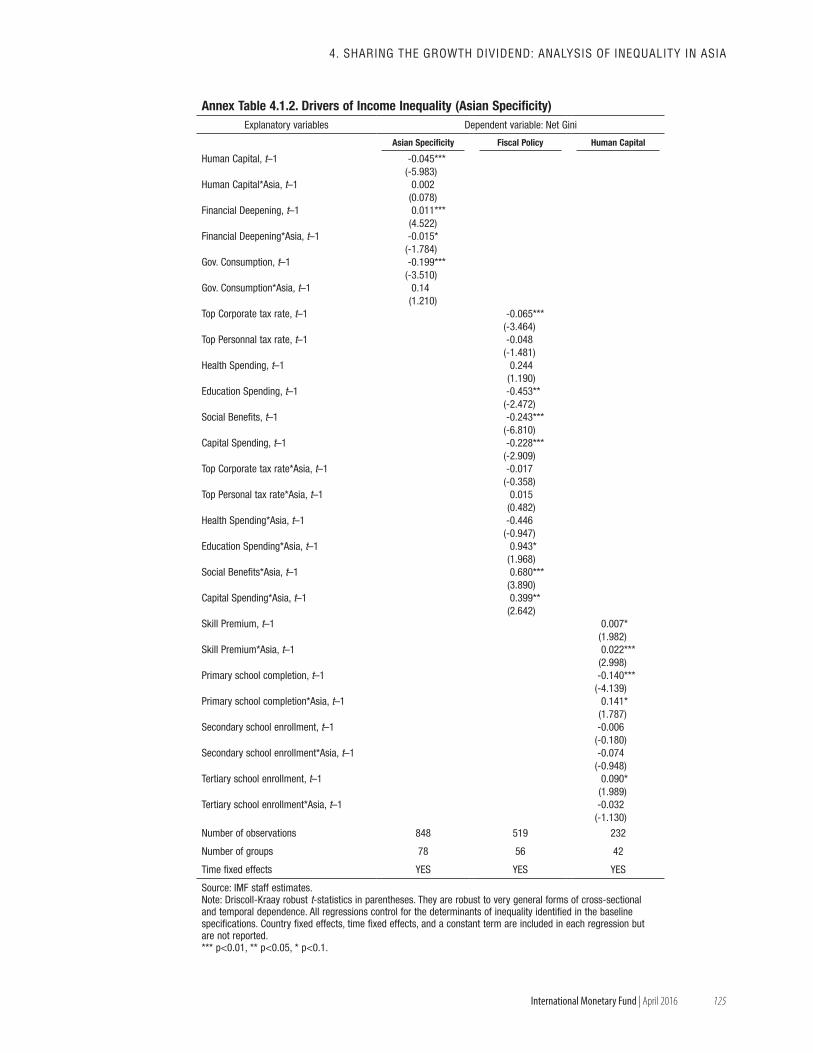
4. shARING ThE GROwTh dIvIdENd: ANALysIs Of INEqUALITy IN AsIA
125International Monetary Fund | April 2016
Annex Table 4.1.2. Drivers of Income Inequality (Asian Specificity)Explanatory variables Dependent variable: Net Gini
Asian Specificity Fiscal Policy Human Capital
Human Capital, t–1 -0.045***(-5.983)
Human Capital*Asia, t–1 0.002(0.078)
Financial Deepening, t–1 0.011***(4.522)
Financial Deepening*Asia, t–1 -0.015*(-1.784)
Gov. Consumption, t–1 -0.199***(-3.510)
Gov. Consumption*Asia, t–1 0.14(1.210)
Top Corporate tax rate, t–1 -0.065***(-3.464)
Top Personnal tax rate, t–1 -0.048(-1.481)
Health Spending, t–1 0.244(1.190)
Education Spending, t–1 -0.453**(-2.472)
Social Benefits, t–1 -0.243***(-6.810)
Capital Spending, t–1 -0.228***(-2.909)
Top Corporate tax rate*Asia, t–1 -0.017(-0.358)
Top Personal tax rate*Asia, t–1 0.015(0.482)
Health Spending*Asia, t–1 -0.446(-0.947)
Education Spending*Asia, t–1 0.943*(1.968)
Social Benefits*Asia, t–1 0.680***(3.890)
Capital Spending*Asia, t–1 0.399**(2.642)
Skill Premium, t–1 0.007*(1.982)
Skill Premium*Asia, t–1 0.022***(2.998)
Primary school completion, t–1 -0.140***(-4.139)
Primary school completion*Asia, t–1 0.141*(1.787)
Secondary school enrollment, t–1 -0.006(-0.180)
Secondary school enrollment*Asia, t–1 -0.074(-0.948)
Tertiary school enrollment, t–1 0.090*(1.989)
Tertiary school enrollment*Asia, t–1 -0.032(-1.130)
Number of observations 848 519 232
Number of groups 78 56 42
Time fixed effects YES YES YES
Source: IMF staff estimates.Note: Driscoll-Kraay robust t-statistics in parentheses. They are robust to very general forms of cross-sectional and temporal dependence. All regressions control for the determinants of inequality identified in the baseline specifications. Country fixed effects, time fixed effects, and a constant term are included in each regression but are not reported.*** p<0.01, ** p<0.05, * p<0.1.

127
References
Aghion, P., E. Caroli, and C. Garcia-Peñalosa. 1999. “Inequality and Economic Growth: The Perspective of the New Growth Theories.” Journal of Economic Literature 37(4): 1615–60.
Ahmed, Shaghil. 2009. “Are Chinese Exports Sensitive to Changes in the Exchange Rate?” In-ternational Finance Discussion Paper 987, Federal Reserve Board, Washington.
Ahuja, A., and M. Nabar. 2012. “Investment-Led Growth in China: Global Spillovers.” IMF Work-ing Paper 12/267, International Monetary Fund, Washington.
Alquist, Ron, and Olivier Coibion. 2014. “Commod-ity-Price Comovement and Global Economic Activ-ity.” NBER Working Paper 20003, National Bureau of Economic Research, Cambridge, Massachusetts.
Ananchotikul, N., and Zhang, L. 2014. “Portfolio Flows, Global Risk Aversion and Asset Prices in Emerging Markets.” IMF Working Paper 14/156, International Monetary Fund, Washington.
Anand, R., V. Tulin, and N. Kumar. 2014. “India: Defining and Explaining Inclusive Growth and Poverty Reduction.” IMF Working Paper 14/63, International Monetary Fund, Washington.
Anderson, James E., and Eric van Wincoop. 2003. “Gravity with Gravitas: A Solution to the Border Puzzle.” American Economic Review 93(1): 170–92.
Aoyagi, C., G. Ganelli, and K. Murayama. 2015. “How Inclusive Is Abenomics?” IMF Working Paper 15/54, International Monetary Fund, Washington.
Arslanalp, S., W. Liao, S. Piao, and D. Seneviratne. Forthcoming. “China’s Financial Spillovers to Regional Markets.” International Monetary Fund, Washington.
Asian Development Bank (ADB). 2013. “Thailand Financial Inclusion Synthesis Assessment Report.” Technical Assistance Consultants’ Report, Manila.
Atkinson, A. 2009. “Factor Shares: The Principal Problem of Political Economy?” Oxford Review of Economic Policy 25(1): 3–16.
Australian Prudential Regulation Authority (APRA). 2014. “Seeking Strength in Adversity: Lesson’s from APRA’s 2014 Stress Test on Australia’s Largest Banks.” Speech at the AB&F Randstad Leaders Lecture Series 2014, Sydney, November 7.
Balakrishnan, R., C. Steinberg, and M. Syed. 2013. “The Elusive Quest for Inclusive Growth: Growth, Poverty, and Inequality in Asia.” IMF Working Paper 13/152, International Monetary Fund, Washington.
Baldwin, Richard, and Daria Taglioni. 2006. “Gravity for Dummies and Dummies for Gravity Equations.” NBER Working Paper 12516, National Bureau of Economic Research, Cambridge, Massachusetts.
Barro, R., and J. Lee. 2010. “A New Data Set of Educational Attainment in the World, 1950–2010.” Journal of Development Economics 104: 184–98.
Bayoumi, T., and F. Ohnsorge. 2013. “Do Inflows or Outflows Dominate? Global Implications of Capital Account Liberalization in China.” IMF Working Paper 13/189, International Monetary Fund, Washington.
Benigno, Gianluca, Pierpaolo Benigno, and Salva-tore Nisticò. 2012. “Risk, Monetary Policy, and the Exchange Rate.” NBER Working Paper 17133, Na-tional Bureau of Economic Research, Cambridge, Massachusetts.
Bernanke, Ben S., Jean Boivin, and Piotr Eliasz. 2005. “Measuring the Effects of Monetary Policy: A Factor-Augmented Vector Autoregressive (FA-VAR) Approach.” Quarterly Journal of Economics 120: 387–422.
Bussière, M., G. Callegari, F. Ghironi, G. Sestieri, and N. Yamano. 2013. “Estimating Trade Elastici-ties: Demand Composition and the Trade Collapse of 2008–2009.” American Economic Journal: Macroeco-nomics 5(3): 118–51.
Cabezon, E., L. Hunter, P. Tumbarello, K. Washimi, and Y. Wu. 2015. “Enhancing Macroeconomic Re-
REGIONAL ECONOMIC OUTLOOK: ASIA AND PACIFIC
128
silience to Natural Disasters and Climate Change in the Small States of the Pacific.” IMF Working Paper 15/125, International Monetary Fund, Washington.
Cain, J., R. Hasan, R. Magsombol, and A. Tandon. 2014. “Accounting for Inequality in India.” In Inequality in Asia and the Pacific: Trends, Drivers, and Policy Implications, edited by R. Kanbur, C. Rhee, and J. Zhuang. London: Routledge.
Cashin, P., K. Mohaddes, and M. Raissi. 2016. “China’s Slowdown and Global Financial Market Volatility: Is World Growth Losing Out?” IMF Working Paper 16/63, International Monetary Fund, Washington.
Cevik, S., and C. Correa-Caro. 2015. “Growing (Un)equal: Fiscal Policy and Income Inequality in China and BRIC+.” IMF Working Paper 15/68, Interna-tional Monetary Fund, Washington.
Chaudhuri, S., and M. Ravallion. 2006. “Partially Awakened Giants: Uneven Growth in China and India.” Policy Research Working Paper 4069, World Bank, Washington.
Checchi, D., and C. Garcia-Peñalosa. 2010. “Labour Market Institutions and the Personal Distribution of Income in the OECD.” Economica 77(307): 413–50.
Cheung, Y. W., M. Chinn, and X. Qian. 2012. “Are Chinese Trade Flows Different?” Journal of Interna-tional Money and Finance 31(8): 2127–46.
Chinn, Menzie D., 2015, “China’s Trade Flows: Some Conjectures.” In The Global Trade Slowdown: A New Normal? edited by Bernard Hoekman. London: CEPR Press.
Cho, Dongchul, and Changyong Rhee. 2013. “Ef-fects of Quantitative Easing on Asia: Capital Flows and Financial Markets,” ADB Working Paper 350, Asian Development Bank, Manila.
Chongvilaivan, A. 2014. “Inequality in Southeast Asia.” In Inequality in Asia and the Pacific: Trends, Drivers and Policy Implications, edited by R. Kanbur, C. Rhee, and J. Zhuang. London: Routledge.
Crozet, Matthieu, Charlotte Emlinger, and Sébastien Jean. 2015. “On the Gravity of World Trade’s Slow-down.” In The Global Trade Slowdown: A New Normal? edited by Bernard Hoekman. London: CEPR Press.
Dabla-Norris, E., K. Kochhar, N. Suphaphiphat, F. Ricka, and E. Tsounta. 2015. “Causes and Con-sequences of Income Inequality: A Global Perspec-tive.” IMF Staff Discussion Note 15/13, Interna-tional Monetary Fund, Washington.
Datt, G., and M. Ravallion. 1992. “Growth and Redistribution Components of Changes in Pov-erty Measures.” Journal of Development Economics 38: 255–95.
Davies, J., A. Koutsoukis, R. Lluberas, A. Shorrocks, and M. Stierli. 2015. “Global Wealth Report 2015.” Credit Suisse AG, Zurich.
De Backer, K., and S. Miroudot. 2013. “Mapping Global Value Chains.” OECD Trade Policy Paper 159, Organisation for Economic Co-operation and Development, Paris.
De Bock, R., and I. de Carvalho Filho. 2015. “The Behavior of Currencies During Risk-off Episodes.” Journal of International Money and Finance 53: 218–34.
Debelle, G. 2004. “Macroeconomic Implications of Rising Household Debt.” BIS Working Paper 153, Bank for International Settlements, Basel.
Diebold, F. X., and K. Yilmaz. 2012. “Better to Give than to Receive: Predictive Directional Measure-ment of Volatility Spillovers.” International Journal of Forecasting 28(1): 57–66.
Dizioli, A., J. Guajardo, V. Klyuev, R. Mano, and M. Raissi. Forthcoming. “Spillovers from China’s Slowdown and Rebalancing to ASEAN-5 Coun-tries.” International Monetary Fund, Washington.
Dollar, D. 2007. “Poverty, Inequality, and Social Disparities During China’s Economic Reform.” Policy Research Working Paper 4253, World Bank, Washington.
Duval, R., K. Cheng, K. H. Oh, R. Saraf, and D. Seneviratne. 2014. “Trade Integration and Busi-ness Cycle Synchronization: A Reappraisal with Focus on Asia.” IMF Working Paper 14/52, Inter-national Monetary Fund, Washington.
Duval, R., N. Li, R. Saraf, and D. Seneviratne. 2015. “Value-Added Trade and Business Cycle Synchroni-zation.” Journal of International Economics 99: 251–62.
RefeRences
129
Easterly, W. 2007. “Inequality Does Cause Under-development: Insights from a New Instrument.” Journal of Development Economics 84(2): 755–76.
Eichenbaum, Martin, and Charles L. Evans. 1995. “Some Empirical Evidence on the Effects of Shocks to Monetary Policy on Exchange Rates.” Quarterly Journal of Economics 110(4): 975–1009.
Eichengreen, Barry, Yeongseop Rhee, and Hui Tong. 2004. “The Impact of China on the Exports of Other Asian Countries.” NBER Working Paper 10768, National Bureau of Economic Research, Cambridge, Massachusetts.
Ellis, L. 2005. “Disinflation and the Dynamics of Mortgage Debt.” In Investigating the Relationship between the Financial and Real Economy, BIS Paper 22, Bank for International Settlements, Basel.
Farid, M., M. Keen, M. Papaioannou, I. Parry, C. Pattillo, A. Ter-Martirosyan, and others. 2016. “After Paris: Fiscal, Macroeconomic, and Financial Implications of Climate Change.” IMF Staff Dis-cussion Note 16/01, International Monetary Fund, Washington.
Forbes, K., and M. Chinn. 2004. “A Decomposi-tion of Global Linkages in Financial Markets Over Time.” Review of Economics and Statistics 86(3): 705–22.
Forbes, K., and R. Rigobon. 2002. “No Contagion, Only Interdependence: Measuring Stock Market Comovements.” Journal of Finance 57(5): 2223–261.
Frankel, J. 1994. “Introduction.” In The Internation-alization of Equity Markets, edited by Jeffrey A. Fran-kel. Chicago and London: University of Chicago Press.
Gabriel Palma, J. 2006. “Globalizing Inequality: ‘Centrifugal’ and ‘Centripetal’ Forces at Work.” DESA Working Paper 35, UN Department of Eco-nomic and Social Affairs, New York.
———. 2011. “Homogeneous Middles vs. Hetero-geneous Tails, and the End of the ‘Inverted-U’: It’s All About the Share of the Rich.” Development and Change 42(1): 87–153.
Garcia-Peñalosa, C., and E. Orgiazzi. 2013. “Fac-tor Components of Inequality: A Cross-Country Study.” Review of Income and Wealth 59(4): 689–727.
Gaulier, Guillaume, Gianluca Santoni, Daria Taglioni, and Soledad Zignago. 2015. “The Power of the Few in Determining Trade Accelerations and Slowdowns.” In The Global Trade Slowdown: A New Normal? edited by Bernard Hoekman. London: CEPR Press.
Greenaway, David, Aruneema Mahabir, and Chris Milner. 2008. “Has China Displaced Other Asian Countries’ Exports?” China Economic Review 19(2): 152–69.
Guimarães-Filho, R., and G. Hong. 2016. “Dynamic Connectedness of Asian Equity Markets.” IMF Working Paper 16/57, International Monetary Fund, Washington.
Guscina, A. 2006. “Effects of Globalization on Labor’s Share in National Income.” IMF Work-ing Paper 06/294, International Monetary Fund, Washington.
Hong, G., J. Lee, W. Liao, and D. Seneviratne. Forthcoming. “China and Asia in the Global Trade Slowdown.” International Monetary Fund, Wash-ington.
Hunt, C. 2015. “Economic Implications of High and Rising Household Indebtedness,” Reserve Bank of New Zealand Bulletin 78(1).
Ikeda, E., P. Tumbarello, and Y. Wu. Forthcom-ing. “Growth Spillovers from China to the Pacific Islands.” International Monetary Fund, Washington.
Institute of International Finance (IIF). 2016. “Capital Flows to Emerging Markets.”
International Monetary Fund. 2007. World Economic Outlook. Washington, April.
———. 2012a. “2012 Spillover Report.” IMF Policy Paper, Washington.
———. 2012b. “The Liberalization and Manage-ment of Capital Flows: An Institutional View.” IMF Policy Paper, Washington. .
———. 2014. “Fiscal Policy and Income Inequal-ity.” IMF Policy Paper, Washington.
———. 2015a. “Australia—2015 Article IV Consultation—Staff Report.” IMF Country Report 15/274, Washington.
REGIONAL ECONOMIC OUTLOOK: ASIA AND PACIFIC
130
———. 2015b. “People’s Republic of China—2015 Article IV Consultation—Staff Report.” IMF Country Report 15/234, Washington.
———. 2015c. Global Financial Stability Report. Washington, October.
———. 2016a. Global Financial Stability Report. Washington, April.
———. 2016b. “India—2016 Article IV Consulta-tion—Staff Report.” IMF Country Report 16/75, Washington.
———. 2016c. “New Zealand—2015 Article IV Consultation—Staff Report.” IMF Country Report 16/39, Washington.
———. 2016d. World Economic Outlook Update. Washington, January.
Jain-Chandra, S., T. Kinda, K. Kochhar, S. Piao, and J. Schauer. 2016. “Sharing the Growth Dividend: Analysis of Inequality in Asia.” IMF Working Paper 16/48, International Monetary Fund, Washington.
Johnson, R., and G. Noguera. 2012a. “Proximity and Production Fragmentation.” American Economic Review (102)3: 407–11.
_____. 2012b. “Fragmentation and Trade in Value Added over Four Decades.” NBER Working Paper 18186. National Bureau of Economic Research, Cambridge, Massachusetts.
Jorgenson, D., and K. Vu. 2007. “Information Technology and the World Growth Resurgence.” German Economic Review 8(2): 125–45.
Kanbur, R., and J. Zhuang. 2014. “Urbanization and Inequality in Asia.” In Inequality in Asia and the Pacific: Trends, Drivers, and Policy Implications, edited by R. Kanbur, C. Rhee, and J. Zhuang. London: Routledge.
Karabarbounis, L., and B. Neiman. 2014. “The Global Decline of the Labor Share.” Quarterly Jour-nal of Economics 129(1): 61–103.
Kho, B., D. Lee, and R. M. Stulz. 2000. “U.S. Banks, Crises, and Bailouts: From Mexico to LTCM.” American Economic Review 90(2): 28–31.
Kireyev, A., and A. Leonidov. 2016. “China’s Import Slowdown: Spillovers, Spillins, and Spillbacks.” IMF Working Paper 16/51, International Monetary Fund, Washington.
Kong, Yoke F., and Richard Kneller. 2016. “Mea-suring the Impact of China’s Export Growth on its Asian Neighbours.” The World Economy 39(2): 195–220.
Koopman, R., Zhi Wang, and Shang-Jin Wei. 2012. “Tracing Value-Added and Double Counting in Gross Exports.” NBER Working Paper 18579, Na-tional Bureau of Economic Research, Cambridge, Massachusetts.
McKinsey Global Institute. 2015. Debt and (Not Much) Deleveraging. New York.
Lane, P. R., and G. M. Milesi-Ferretti. 2007. “The External Wealth of Nations Mark II: Revised and Extended Estimates of Foreign Assets and Liabili-ties, 1970–2004.” Journal of International Economics 73 (2): 223–50.
Li, S., G. Wan, and J. Zhuang. 2014. “Income Inequality and Redistributive Policy in the People’s Republic of China.” In Inequality in Asia and the Pacific: Trends, Drivers and Policy Implications, edited by R. Kanbur, C. Rhee, and J. Zhuang. London: Routledge.
Li, S., and S. Yang. 2009. “Effect of China’s Ur-ban Minimum Living Security System on Income Distribution and Poverty.” China Population Science 5: 19–27.
Liu, Z. 2005. “Institution and Inequality: The Huk-ou System in China.” Journal of Comparative Economics 33(1): 133–57.
Llanto, G. 2015. “Financial Inclusion, Education, and Regulation in the Philippines.” ADBI Work-ing Paper 541, Asian Development Bank Institute, Tokyo.
Mathai, K., G. Gottlieb, G. Hong, S. Jung, J. Schmit-tmann, and J. Yu. Forthcoming. “China and the CLMV: Integration, Evolution, and Implications.” Asia and Pacific Departmental Paper/Cluster Re-port. International Monetary Fund, Washington.
RefeRences
131
Mourmouras, A., and N. Sheridan. 2015. “Ma-laysia: Achieving High-Income Status through Resilience and Inclusive Growth.” IMF Research Bulletin 16(4).
Nathans, L., F. Oswald, and K. Nimon. 2012. “In-terpreting Multiple Linear Regression: A Guide-book of Variable Importance.” Practical Assessment, Research, and Evaluation 17(9): 1–19.
Organisation for Economic Co-operation and De-velopment (OECD). 2014. “Services Trade Restric-tiveness Index: Policy Brief.” Paris.
Ostry, J. D., A. Berg, and C. Tsangarides. 2014. “Re-distribution, Inequality, and Growth.” IMF Staff Discussion Note 14/02, International Monetary Fund, Washington.
Papageorgiou, C., and P. Xie. Forthcoming. “What Does a Global Economic Slowdown Mean to Low-income Countries: An Empirical Investigation of Comovements and Linkages with Trading Part-ners?” International Monetary Fund, Washington.
Piketty, T., and N. Qian. 2009. “Income Inequality and Progressive Income Taxation in China and In-dia, 1986–2015.” American Economic Journal: Applied Economics 1(2): 53–63.
Porcellacchia, Davide. 2016. “Wage-Price Dynam-ics and Structural Reforms in Japan,” IMF Work-ing Paper 16/20, International Monetary Fund, Washington.
Rafiq, S. Forthcoming. “When China Sneezes Does ASEAN Catch a Cold?” International Monetary Fund, Washington.
Rey, Helene. 2015. “International Channels of Transmission of Monetary Policy and the Mundell-ian Trilemma.” IMF Economic Policy Review. Washing-ton: International Monetary Fund.
Rhee, Changyong. 2015. “Managing China’s Eco-nomic Transition.” iMFdirect, October 5.
Rodrik, D. 1999. “Where Did All the Growth Go? External Shocks, Social Conflict, and Growth Col-lapses.” Journal of Economic Growth 4(4): 385–412.
Sahay, R., M. Čihák, P. N’Diaye, A. Barajas, S. Mitra, A. Kyobe, Y. Mooi, and S. Yousefi. 2015. “Financial Inclusion: Can It Meet Multiple Macroeconomic Goals?” IMF Staff Discussion Note 15/17, Inter-national Monetary Fund, Washington.
Shi, Yingying. 2012. “The Role of Infrastructure Capital in China’s Regional Economic Growth.” In-ternational Association of Agricultural Economists Conference Paper, Foz do Iguaçu, Brazil, August 18–24.
Stock, James H., and Mark W. Watson. 2011. “Dy-namic Factor Models.” In The Oxford Handbook of Economic Forecasting, edited by Michael P. Clements and David F. Hendry. Oxford: Oxford University Press.
Stockhammer, E. 2013. “Why Have Wage Shares Fallen?” Conditions of Work and Employment Series 35, International Labour Office, Geneva.
Stulz, R. M. 1999. “International Portfolio Flows and Security Markets.” In International Capital Flows, edited by Martin Feldstein. Chicago: University of Chicago Press.
Terada, Y., and P. Vandenberg. 2014. “Thailand’s State-Led Approach to Financial Inclusion.” In Fi-nancial Inclusion in Asia: Country Surveys. Tokyo: Asian Development Bank Institute.
Timmer, M. ed. 2012. “The World Input-Output Database (WIOD): Contents, Sources and Methods,” World Input Output Database Working Paper 10.
Veenendaal, Paul, Hugo Rojas-Romagosa, Arjan Lejour and Henk Kox. 2015. “A Value-Added Trade Perspective on Recent Patterns in World Trade.” In The Global Trade Slowdown: A New Normal? edited by Bernard Hoekman. London: CEPR Press.
Woo, J., E. Bova, T. Kinda, and Y. Zhang. 2013. “Distributional Consequences of Fiscal Consolida-tion and the Role of Fiscal Policy: What Do the Data Say?” IMF Working Paper 13/195, Interna-tional Monetary Fund, Washington.
World Bank. 2013. “Philippines—The KALAHI-CIDDS Impact Evaluation: A Revised Synthesis Report.” Washington.

REGIONAL ECONOMIC OUTLOOK: ASIA AND PACIFIC
132
Wu, J. C., and F. Dora Xia. 2015. “Measuring the Macroeconomic Impact of Monetary Policy at the Zero Lower Bound.” Chicago Booth Research Pa-per 13–77, University of Chicago–Booth School of Business and University of California, San Diego.
Yiengprugsawan, V., G. Carmichael, L. Lim, S. Seu-bsman, and A. Sleigh. 2010. “Has Universal Health Insurance Reduced Socioeconomic Inequalities in Urban and Rural Health Service Use in Thailand?” Health & Place 16(5): 1030–037.

Regional Economic OutlookAsia and Pacific, April 2016
Regional Economic Outlook
World Economic and Financia l Surveys
I N T E R N A T I O N A L M O N E T A R Y F U N D
16AP
R
Asia and PacificBuilding on Asia’s Strengths during Turbulent Times