Regional Climate Simulations Over The South Pacific: Results For Current And Future Climate

Jack Katzfey, Mohar Chattopadhyay, John McGregor, Kim Nguyen

CAWCR, CMAR, Aspendale, Australia

OUTLINE

• Dynamical downscaling

• PCCSP dynamical downscaled simulations

• Future work

• Summary

What is regional climate modelling?

• Dynamically downscale from some host data at higher resolution

– Dynamically: Use an atmospheric model to calculate the local climate

– Downscale: Output is at higher resolution (spatially and temporally)

– Host data: Inputs to regional model

• Reanalyses

• Global Climate Model

• Regional model (multiple downscaling)

– Resolution

• Typically 50 -> 5 km (or less)

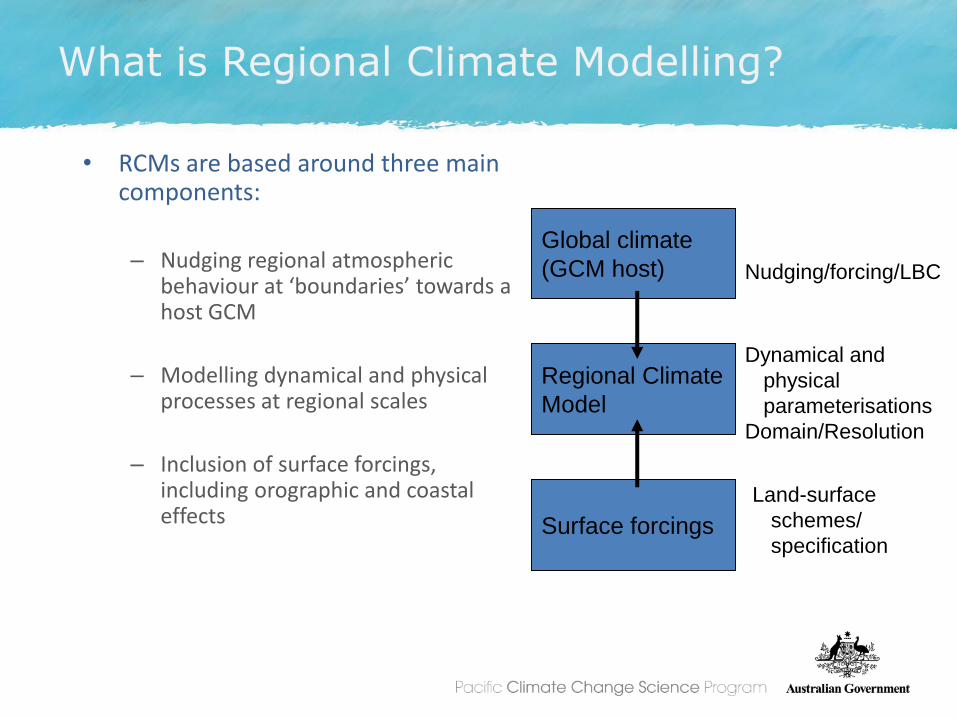
What is Regional Climate Modelling?

• RCMs are based around three main components:

– Nudging regional atmospheric

behaviour at ‘boundaries’ towards a host GCM

– Modelling dynamical and physical processes at regional scales

– Inclusion of surface forcings, including orographic and coastal effects

Regional Climate

Model

Surface forcings

Global climate

(GCM host) Nudging/forcing/LBC

Land-surface

schemes/

specification

Dynamical and

physical

parameterisations

Domain/Resolution

Downscaling methods: Grids and nesting

Scale- selective filter

(frequency domain) Interpolated lateral

boundaries

Global Stretched Grid Model

(CCAM) Limited Area Model

(ACCESS RCM)

One-way

nesting

Coupled to

global

circulation

GCM

Downscaling Strategy

Aims:

• To provide more detailed (and hopefully more accurate) current and future regional climate through better resolved physical processes and surface forcings

– Important to have more detailed surface specification –More realistic weather processes

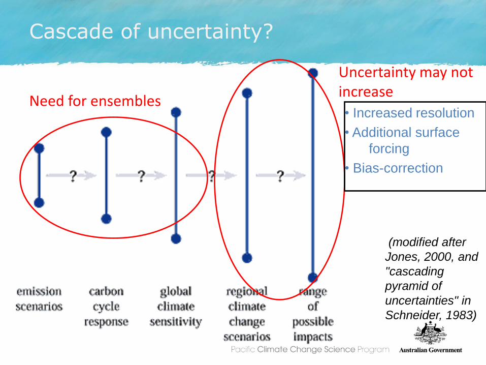
Cascade of uncertainty?

Uncertainty may not increase

• Increased resolution

• Additional surface

forcing

• Bias-correction

(modified after

Jones, 2000, and

"cascading

pyramid of

uncertainties" in

Schneider, 1983)

Need for ensembles

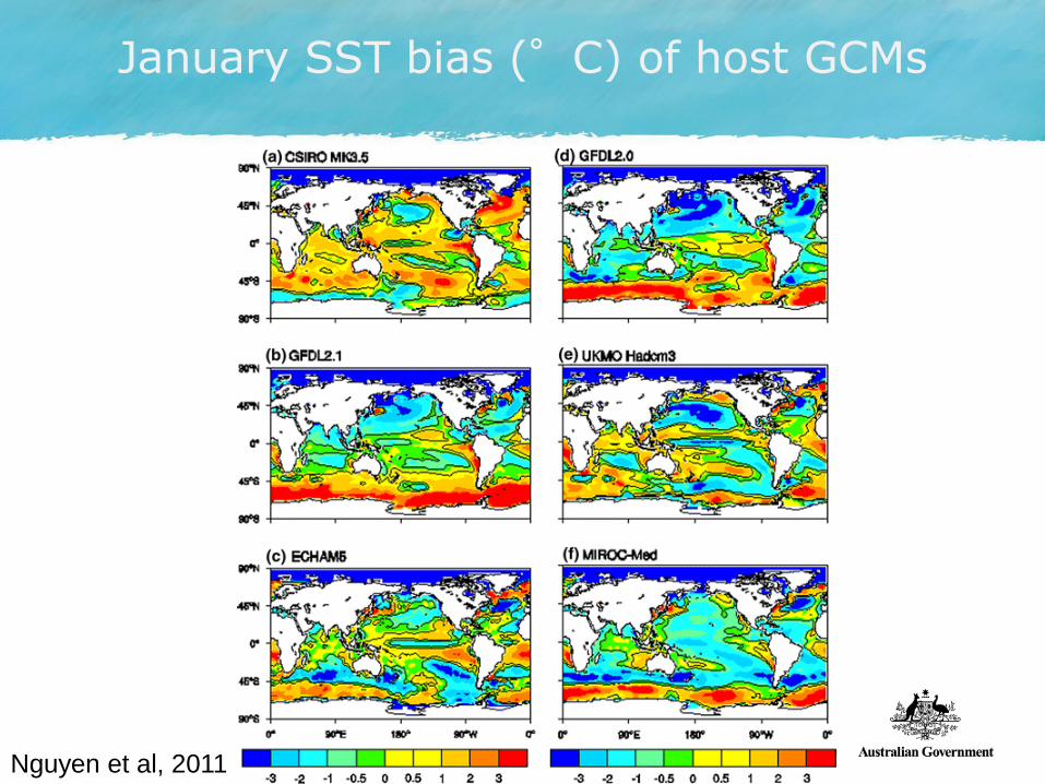
January SST bias (°C) of host GCMs

Nguyen et al, 2011

Large-scale bias-correction

In addition to fixing biases, allows simulation to have more realistic weather systems and how they may change in response to climate change

Surface temperature average

115 E to 155 E, 40 S to 10 S

3 year running average

Model uncertainty/error (2.3C)

Model uncertainty

plus change (3.7C)

Spread of

change signal

(1.4C)

Same mean

Bias adjustment of sea surface temperatures

• Sea surface temperatures is main influence on climate (ENSO, climate change)

• Dommenget, Dietmar, 2009: The Ocean’s Role in Continental Climate Variability and Change. J. Climate, 22, 4939–4952

• Can improve the representation of the current climate by fixing some of the biases

• Ensemble using only one downscale model (CCAM) does not decrease spread of climate change signal

10

Summary of dynamical downscaling conducted in the PCCSP

All future time periods were simulated using the A2 emission scenario.

Bias adjust SSTs

(1961-2099)

6 GCMs

(1980-2000, 2045-2065, 2080-2099) (1980-2000, 2045-2065)

CCiP, 2011

1980-1999 annual mean rainfall (mm/day) for GPCP data (top), CMAP data (middle top), multi-model mean of the six global climate models that were downscaled (middle bottom) and multi-model mean of six CCAM 60-km models (bottom ). (CCiP, 2011)

Annual rainfall (mm/day) GPCP,CMAP, GCMs, CCAM 60 km

• Higher resolution allows better representation of surface forcings and more realistic dynamics

• Bias-correction of SSTs Improves current climate

Additional RCMs Annual Rainfall (mm/day)

(CCiP, 2011)

Western tropical Pacific, including East Timor

15 PCCSP partner countries

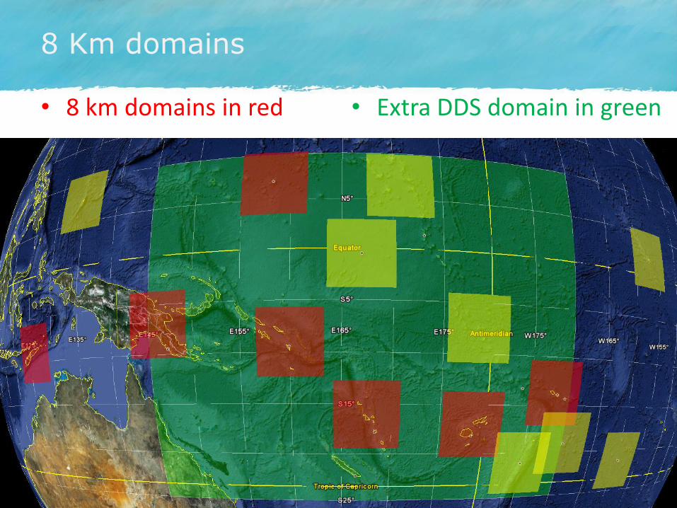
8 Km domains

• 8 km domains in red • Extra DDS domain in green

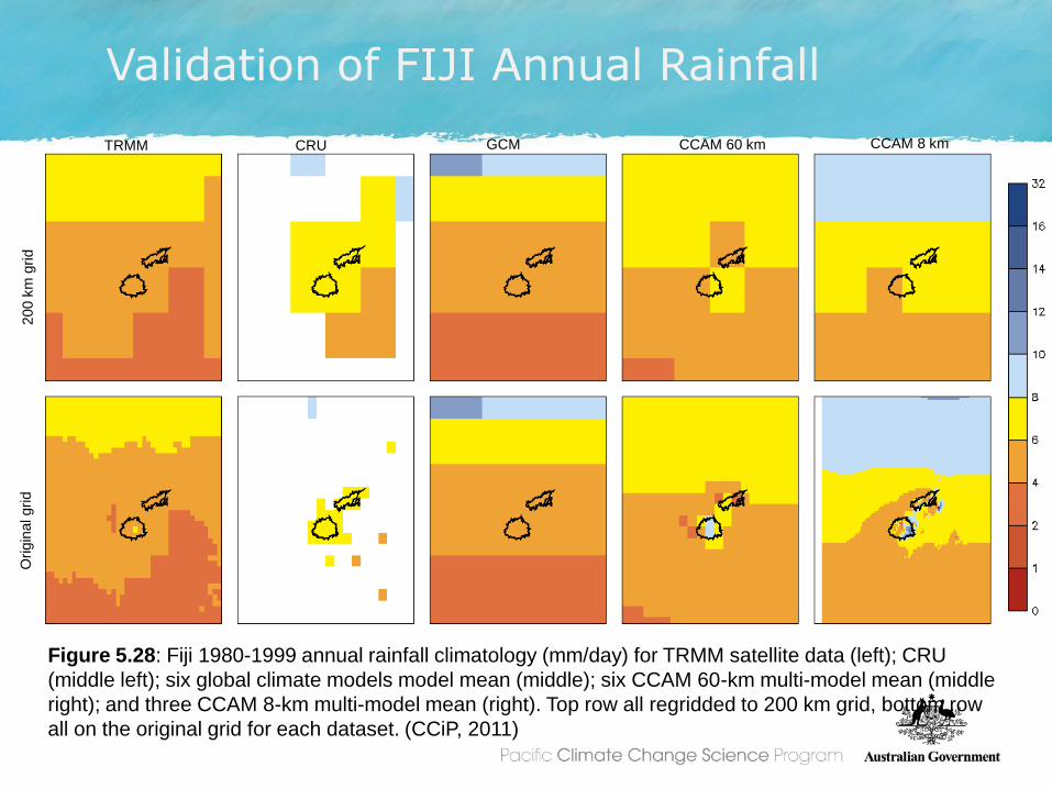
Figure 5.28: Fiji 1980-1999 annual rainfall climatology (mm/day) for TRMM satellite data (left); CRU

(middle left); six global climate models model mean (middle); six CCAM 60-km multi-model mean (middle

right); and three CCAM 8-km multi-model mean (right). Top row all regridded to 200 km grid, bottom row

all on the original grid for each dataset. (CCiP, 2011)

Origin

al grid

200 k

m g

rid

TRMM CRU GCM CCAM 60 km CCAM 8 km

Validation of FIJI Annual Rainfall

Nadi

Nausori

Validation of FIJI

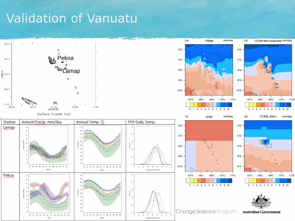
Validation of Vanuatu

Lamap

Pekoa

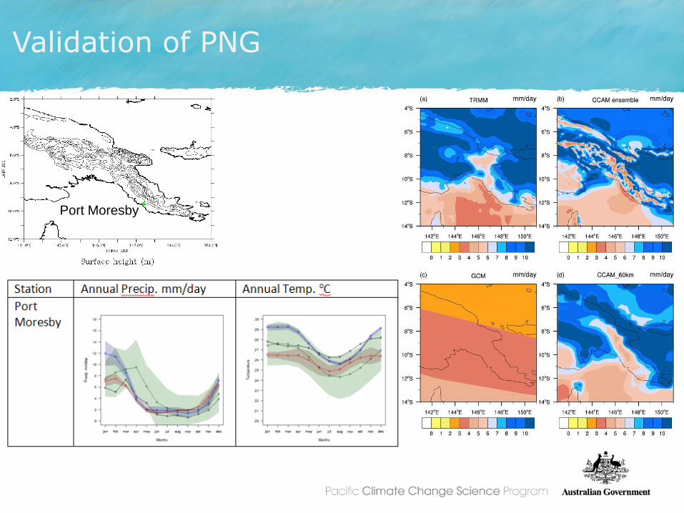
Validation of PNG

Port Moresby

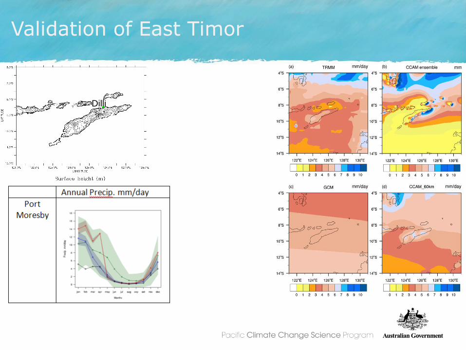
Validation of East Timor

Dilli

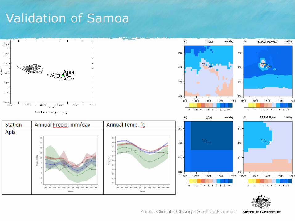
Validation of Samoa

Apia

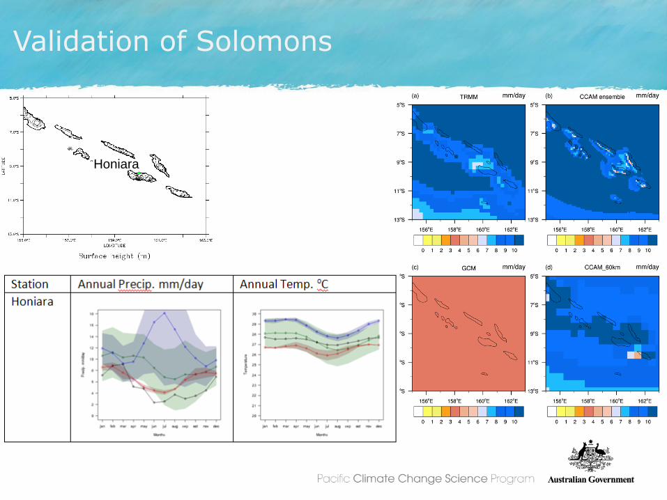
Validation of Solomons

Honiara

Validation of FSM

Pohnpei

Fiji changes 2090 - 1990: 8 km downscaled A2 scenario

Nadi PDF changes

Green-GCM, Blue-60 km, Red-8 km

CCiP, 2011

Annual rainfall change (mm/d)

Figure 7.17: Change in projected annual rainfall (mm/day) from additional downscaling simulations for period 2055 relative to 1990, for the A2 scenario. Note that the changes for the Zetac model are for the Jan-Feb-Mar period only . The host global climate model was the GFDL2.1 model.

Future work

• Additional verification of downscaled simulations

• 8 km simulations

• Extremes

• Additional RCM simulations

• In-depth analysis of climate change effects

• Begin assessment of CMIP5 GCMS for downscaling

• Looking for help!

Why use regional climate models?

• Can provide a spatially and temporally consistent dataset

• Can provide finer resolution datasets

• Can provide physically-based effects caused by local forcings (especially orography)

• Small, statistically-based corrections can be applied if needed

• Caution:

– Downscaling technique can influence results

– As always, results need to be validated

Thank you

Kevin Hennessy

Science Program Manager

Pacific Climate Change

Science Program

Email: kevin.hennessy@csiro.au

Phone: +61 400 572 613

For further information

Jack Katzfey

MMA Team Leader

CAWCR/CMAR

Email: jack.katzfey@csiro.au

Phone: +613 9239 4562