Regional and Institutional Determinants of Poverty: The … and Institutional Determinants of...

Regional and Institutional Determinants of Poverty: The Case of Kenya*

Jane Kabubo-Mariaraa, Domisiano M. Kiriib, Godfrey K. Ndengec, John

Kirimid and Rachel K. Gesamie a:Corresponding author. University of Nairobi, Economics Department, Kenya. [email protected]/[email protected]; b: International Maize and Wheat Improvement Centre (CIMMYT); c: Ministry of Planning and National Development; d: Ministry of Planning and National Development (deceased); d: International Monetary Fund

Final Report Presented for Phase II of the Collaborative Project on Poverty, Income

Distribution and Labour Market Issues in Sub-Saharan Africa, January 2006

ABSTRACT

In this paper, we investigate the impact of institutional factors on regional poverty in Kenya using household survey and district level secondary data. The analysis focuses on the FGT and consumption based measures of poverty. Both descriptive and econometric methods are employed. These results suggest that education attainment, assets and family composition are important correlates of poverty. We also find that except for parliamentary representation, institutional factors are important determinants of poverty when welfare is measure through consumption expenditure, but the results are not robust when welfare is measured through the FGT measures, confirming that consumption functions may be a better approach to measure welfare than poverty functions. The results call for policies that target poor households and regions less endowed with institutions in order to reduce regional disparities in household poverty.

* The authors wish to thank the African Economic Research Consortium for financial support. We are also grateful to Prof. David Sahn, Dr. Stephen Younger and Dr. Peter Glick all of Cornell University for very useful insights at the conceptual stages of this paper. Thanks are also due to Prof. Germano Mwabu of the University of Nairobi for comments on an earlier draft. The usual disclaimer applies.

ii

TABLE OF CONTENTS

Abstract ...................................................................................................................................... i

Table of Contents...................................................................................................................... ii

List of Tables ........................................................................................................................... iii

1 Background ....................................................................................................................... 1

2 Methodology..................................................................................................................... 3

2.1 Analytical issues ....................................................................................................... 3

2.2 Modeling the determinants of poverty. ..................................................................... 5

3 Regional Distribution of Institutions ................................................................................ 8

4 Regional Differentials in Poverty ................................................................................... 14

5 Investigating the Institutional Correlates of Welfare...................................................... 19

5.1 The Primary Data and Variables............................................................................. 19

5.2 Estimation Results .................................................................................................. 23

6 Conclusion ...................................................................................................................... 43

References............................................................................................................................... 45

Appendix................................................................................................................................. 47

iii

LIST OF TABLES

Table 1 Analytical Issues and Data Requirements............................................................. 4

Table 2 Regional institutional structures and associated data sources............................... 5

Table 3: Regional distribution of market institutions per capita, 1997............................... 8

Table 4: Regional Distribution of Trust Land per capita, 1997 .......................................... 9

Table 5: Regional distribution of per capita road infrastructure, 1997 ............................. 10

Table 6: Regional distribution of governance institutions per capita, 1997 ..................... 11

Table 7: Regional distribution of Education and Health inputs, 1997.............................. 12

Table 8: Health Institutions, Hospital beds and Cots by Province, 1997.......................... 13

Table 9: Total per Capita Expenditure on Infrastructure, 1997 (‘000 Kshs) .................... 14

Table 10: Overall Rural Poverty by Region, 1997.............................................................. 15

Table 11: Hardcore Rural Poverty by Region, 1997........................................................... 16

Table12: Urban Differentials in the Incidence of Poverty, 1992-1997.............................. 16

Table 13: Rural Absolute Poverty Ranking by Province .................................................... 18

Table 14: Sample characteristics by poverty status ............................................................ 21

Table 15: Main occupation, sector and position in employment by poverty status............ 22

Table 16: Institutional correlates of poverty; FGT measures 1997..................................... 24

Table 17: Household correlates of poverty: Full Sample ................................................... 27

Table 18: Household Correlates of poverty; Rural Sample, 1997 ...................................... 31

Table 19: Household Correlates of poverty; Urban Sample, 1997 ..................................... 33

Table 21: Household and institutional correlates of poverty; Rural Sample ...................... 39

Table 22: Household and institutional correlates of poverty; Urban Sample ..................... 41

Table A1: Sample Statistics ................................................................................................. 47

1

1 BACKGROUND

The Kenyan economy was regarded as an African success story early into the post-independence years of many African countries. In the 1960s and 1970s, the country achieved a high growth rate of 6.6 per cent per annum. However, this rapid rate of growth was not sustained thereafter. Between 1974 and 1979, the growth rate declined to 5.2 per cent per annum. Further declines occurred in the 1980-89 and 1990-95 periods when the average growth rates averaged 4.1 and 2.5 per cent per annum respectively. Over the plan period 1997-2001, the target was set at 5.9 per cent per annum. However, contrary to expectations, the economy registered a negative growth rate of 0.3 per cent in the year 2000. The decline was reflected in almost all the sectors of the economy. The GDP per capita was estimated at US $ 275 in 1995 and stood at US$ 294 in 2000. Because of this poor economic performance, about 13.6 million Kenyans in 2000 lived under the poverty line, and the situation has continued to worsen. Furthermore, there are market differences in the geographical distribution of poor households in the country. The table shows the status of poverty based on administrative (district) and climatic zones for 1997 and implies that there is no clear relationship between the incidence of poverty and the climatic zone in which a household is located. Thus, additional information about the zone (e.g., differences in institutional structures) is necessary for accurate targeting of public assistance to poor households. Further studies have shown that the Gini coefficient in Kenya rose from 0.40 to 0.49 during 1982–1992, and is believed to have increased since then. The coefficient of variation of social expenditure stands at 0.57 which reflects the poor distribution of public subsidies in the country. Kenya’s national measures of poverty mask a high degree of inequality and access to basic services. In addition to the problem of inequality, Kenya has a very high unemployment rate. Currently, an estimated 3 million of the 13 million (23 per cent) in Kenya’s labour force are unemployed and the figure is higher when the underemployed persons in rural agriculture and informal enterprises are considered. This unfavorable unemployment situation must be a major cause of poverty among people whose main asset is their own labor.

The launch of the National Poverty Eradication Plan (NPEP) 1999-2015 created policy ambivalence in the country concerning poverty reduction strategies. NPEP ushered in a prolonged and uncertain process of preparing a national poverty reduction strategy. Although the preparation of the poverty reduction strategy paper (PRSP) was meant to be inclusive, consultative and locally driven, it excluded key stakeholders, especially the private sector,

2

and was not free from external influences. It is worthwhile to note that the PRSP is a short-run planning document covering 3-5 years, whereas, the NEP is a long term plan encompassing 10-15 years. Under the NPEP, the trend in absolute poverty was to be halted by the year 2001 and reduced by 20% in 2015. Since no aspect of the PRSP has yet been implemented, the NPEP target for 2015 is unlikely to be realized. In addition to these poverty specific targets, the Government is far from meeting the goals set by World Summit for social Development. These goals include attainment of universal access to basic social services (primary education, primary health care, safe drinking water, and decent housing and sanitation). On the health front, as a result of HIV/AIDS, the target for life expectancy of 60 years even by 2005 will certainly not be met. It is unlikely that mortality rates for infants and children under five years will be reduced to 50 per 1,000 live births by 2005. In the context of growing inequalities, and increasing absolute poverty in rural and urban areas, there is need to understand regional and institutional factors associated with poverty. Though a large number of studies now exist on Kenyan poverty, its measurement and determinants (Collier and Lall, 1980; Greer and Thorbecke, 1986; Mukui, 1994; Republic of Kenya, 1998, 2000; Mwabu et al., 2000; Oyugi et al., 2000; Manda et al., 2000; Geda et al.; 2001), there is a deft of empirical studies on institutional determinants of poverty in Kenya. Mwabu et al. (2004) only employ descriptive methods to explain the impact of rural institutions on poverty. This paper is a response to this research gap. We build on the existing studies on determinants of poverty and Mwabu et al. (2004) to analyze the institutional perspectives of poverty. Persistent of high poverty rates in some regions of the country suggest that poverty reduction interventions should be targeted to regions most afflicted with poverty. However, in designing and implementing such interventions, differences in institutional structures in regions need to be considered. This study seeks to address these and related policy concerns. In particular, the study seeks to: identify and analyze regional and institutional determinants of poverty in Kenya, to identify mechanisms for reducing regional growth imbalances in the country and to suggest a regional pattern of investment portfolio that is likely to have the greatest impact on poverty reduction. This paper is one of three papers prepared for Phase II of the collaborative research on poverty, Income distribution and labour market issues in Sub-Saharan Africa. In the other two papers, we address non-monetary determinants of poverty, with specific focus on education and child nutritional status.

3

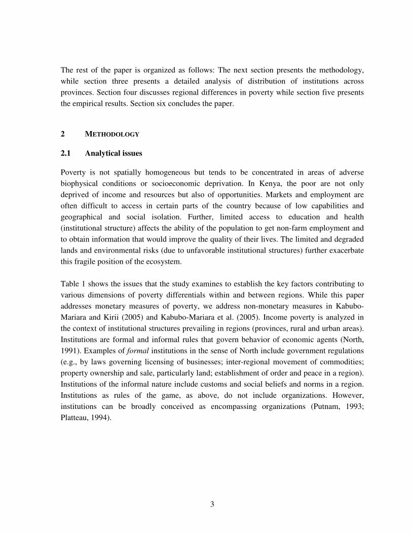
The rest of the paper is organized as follows: The next section presents the methodology, while section three presents a detailed analysis of distribution of institutions across provinces. Section four discusses regional differences in poverty while section five presents the empirical results. Section six concludes the paper.

2 METHODOLOGY

2.1 Analytical issues

Poverty is not spatially homogeneous but tends to be concentrated in areas of adverse biophysical conditions or socioeconomic deprivation. In Kenya, the poor are not only deprived of income and resources but also of opportunities. Markets and employment are often difficult to access in certain parts of the country because of low capabilities and geographical and social isolation. Further, limited access to education and health (institutional structure) affects the ability of the population to get non-farm employment and to obtain information that would improve the quality of their lives. The limited and degraded lands and environmental risks (due to unfavorable institutional structures) further exacerbate this fragile position of the ecosystem. Table 1 shows the issues that the study examines to establish the key factors contributing to various dimensions of poverty differentials within and between regions. While this paper addresses monetary measures of poverty, we address non-monetary measures in Kabubo-Mariara and Kirii (2005) and Kabubo-Mariara et al. (2005). Income poverty is analyzed in the context of institutional structures prevailing in regions (provinces, rural and urban areas). Institutions are formal and informal rules that govern behavior of economic agents (North, 1991). Examples of formal institutions in the sense of North include government regulations (e.g., by laws governing licensing of businesses; inter-regional movement of commodities; property ownership and sale, particularly land; establishment of order and peace in a region). Institutions of the informal nature include customs and social beliefs and norms in a region. Institutions as rules of the game, as above, do not include organizations. However, institutions can be broadly conceived as encompassing organizations (Putnam, 1993; Platteau, 1994).

4

Table 1 Analytical Issues and Data Requirements

Dimension of poverty

Poverty measure or indicator

Poverty line (where applicable)

Data source

A. Income poverty.

FGT indices; household expenditure per capita or per adult equivalent.

CBN Poverty Line adjusted for inflation and regional differentials in price indices

Kenya Welfare Monitoring Survey (WMSIII)

B. Non-income poverty.

Education attainment; child anthropometrics and nutritional status.

Non-money metric poverty lines (see Morrisson et al., 2000).

(WMSIII), Demographic and Health Survey Data

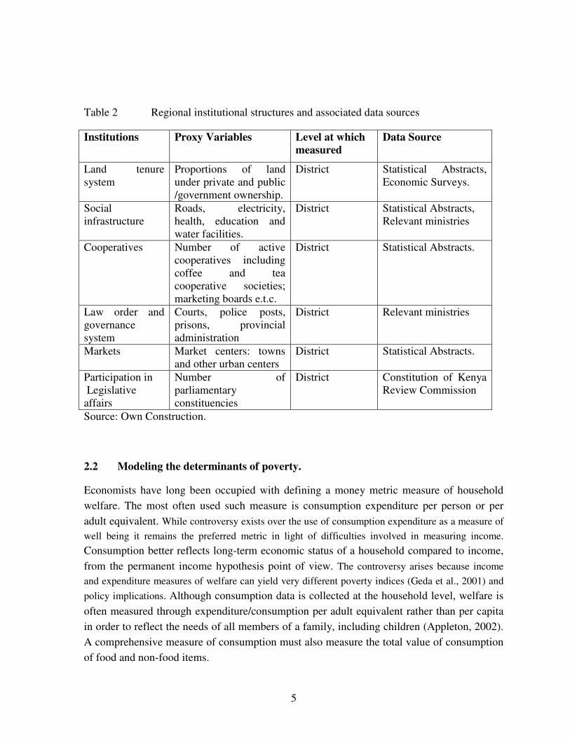
Source: Own construction. This paper uses institutions in the broad sense that includes organizations, such as cooperatives, marketing boards, schools, health facilities, courts, and police stations. Institutions are also used to include public utilities and social capital. Although in the literature, a distinction is made between social capital and institutions (Putnam, 1993); we do not make this differentiation in the empirical analysis of this study because of data limitations. Indicators of social infrastructure, public utilities, social norms and social capital are roughly taken as proxies for institutional structures of regions. Table 2 shows indicators of institutions that are analyzed (with respect to their bearing on poverty), and regional levels at which they are measured. A detailed analysis of the distribution of these institutions across provinces is presented in section 3.

5

Table 2 Regional institutional structures and associated data sources

Institutions Proxy Variables Level at which measured

Data Source

Land tenure system

Proportions of land under private and public /government ownership.

District Statistical Abstracts, Economic Surveys.

Social infrastructure

Roads, electricity, health, education and water facilities.

District Statistical Abstracts, Relevant ministries

Cooperatives Number of active cooperatives including coffee and tea cooperative societies; marketing boards e.t.c.

District Statistical Abstracts.

Law order and governance system

Courts, police posts, prisons, provincial administration

District Relevant ministries

Markets Market centers: towns and other urban centers

District Statistical Abstracts.

Participation in Legislative affairs

Number of parliamentary constituencies

District Constitution of Kenya Review Commission

Source: Own Construction.

2.2 Modeling the determinants of poverty.

Economists have long been occupied with defining a money metric measure of household welfare. The most often used such measure is consumption expenditure per person or per adult equivalent. While controversy exists over the use of consumption expenditure as a measure of well being it remains the preferred metric in light of difficulties involved in measuring income. Consumption better reflects long-term economic status of a household compared to income, from the permanent income hypothesis point of view. The controversy arises because income and expenditure measures of welfare can yield very different poverty indices (Geda et al., 2001) and policy implications. Although consumption data is collected at the household level, welfare is often measured through expenditure/consumption per adult equivalent rather than per capita in order to reflect the needs of all members of a family, including children (Appleton, 2002). A comprehensive measure of consumption must also measure the total value of consumption of food and non-food items.

6

Once the decision to use consumption instead of income has been decided on, the next issue becomes to specify the framework for analyzing the determinants of poverty. There are generally two approaches to the analysis of poverty determinants. In one approach, probabilities of being poor are estimated using logit or probit procedures. This is based on the FGT measures of poverty as the dependent variables. These are in turn based on a pre-determine poverty line, which requires first a food poverty line which is then adjusted for non-food requirements. The FGT poverty measures can be defined as

[ ] 0;)(1 ≥−= � ααα zyznP i , for y < z ……..................................................................... (1)

Where z is the poverty line, yi is a measure of economic welfare of household i (say real per capita household expenditure), ranked as y1� y2...yq� z � yq+1.... � yn. The household equivalents of the headcount index, poverty gap index and the squared poverty gap index are obtained when � = 0, 1 or 2 respectively. The head count index measures household poverty as a binary variable (poor/non poor). The poverty gap is an aggregate of the preferred measure of household poverty: the shortfall of the consumption from the poverty line. A poverty function with the poverty gap gives coefficients that can be readily comparable with those from a consumption function and is therefore preferred to the squared poverty gap index (Appleton, 2002). In the second approach, household welfare functions (proxied by household expenditure functions) are estimated using least squares methods. The two approaches may yield similar results because factors that increase household expenditure, especially on food and assets reduce the probability of a household being poor and vice versa. The first approach has however been criticized because of the arbitrariness of the poverty line and unnecessary loss of information in transforming household expenditure into a binary variable that indicates whether a household is poor or not (Ravallion, 1994, Grootaert, 1994). In addition, the model makes unnecessary distributional assumptions, which do not have to be made using the other approach. Although these limitations make the consumption function approach more attractive, the approach is also imperfect. Some studies show that the two methods can be have equally well in explaining poverty (see for instance Appleton, 2002) To investigate the determinants of poverty, we can specify a consumption based reduced form model of a household’s economic welfare following the works of Glewwe (1991). The model takes the form:

7

ln yi=�’xi + εi ......................................................................................................... (2) where xi is a set of house hold characteristics and other determinants of welfare, � is a vector of parameters to be estimated and εi is a random error term. Modelling the poverty measures/rates using the same principal would yield:

P�i= ��’xi + µi ........................................................................................................... (3)

Where Pai is the FGT measure, �� is a vector of parameters to be estimated and µi is a random error term. In this paper we use both approaches to model determinants of poverty. We use variants of equations (2) and (3) to explain consumption/expenditure and poverty measures respectively. Our innovation is to introduce a vector of district level institutional factors as determinants of welfare. First we estimate a district level variant of each equation to explain the role of institutions at the district level, before mapping the district level data onto the household level data. We base our poverty measures on absolute CBN poverty lines computed by the Central Bureau of Statistics, Republic of Kenya (2000). However, there is controversy in the Kenyan poverty literature as to the appropriate poverty line to use to identify the poor. There are two commonly used techniques for setting poverty lines: the food energy intake (FEI) and the cost of basic needs (CBN) methods. In the Kenyan context (like in other countries), the CBN poverty line has, in general, yielded higher poverty rates than the FEI poverty line (see Mwabu et al., 2000). The FEI method is derived using regression methods, whereas the CBN line is based on cost of a specified basket of basic needs. The cost of a specific basket of basic needs is more easily understood as a standard indicator of a socially desirable level of well being (which everyone in society should attain) than an expenditure level computed from regression coefficients. It is probably for this reason that the poverty rates computed by the Central Bureau of Statistics (Republic of Kenya, 1996; 2000) are based on CBN poverty lines.

8

3 REGIONAL DISTRIBUTION OF INSTITUTIONS

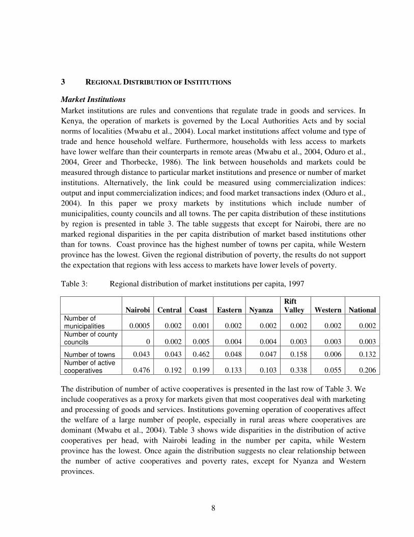
Market Institutions Market institutions are rules and conventions that regulate trade in goods and services. In Kenya, the operation of markets is governed by the Local Authorities Acts and by social norms of localities (Mwabu et al., 2004). Local market institutions affect volume and type of trade and hence household welfare. Furthermore, households with less access to markets have lower welfare than their counterparts in remote areas (Mwabu et al., 2004, Oduro et al., 2004, Greer and Thorbecke, 1986). The link between households and markets could be measured through distance to particular market institutions and presence or number of market institutions. Alternatively, the link could be measured using commercialization indices: output and input commercialization indices; and food market transactions index (Oduro et al., 2004). In this paper we proxy markets by institutions which include number of municipalities, county councils and all towns. The per capita distribution of these institutions by region is presented in table 3. The table suggests that except for Nairobi, there are no marked regional disparities in the per capita distribution of market based institutions other than for towns. Coast province has the highest number of towns per capita, while Western province has the lowest. Given the regional distribution of poverty, the results do not support the expectation that regions with less access to markets have lower levels of poverty. Table 3: Regional distribution of market institutions per capita, 1997

Nairobi Central Coast Eastern Nyanza Rift Valley Western National

Number of municipalities 0.0005 0.002 0.001 0.002 0.002 0.002 0.002 0.002 Number of county councils 0 0.002 0.005 0.004 0.004 0.003 0.003 0.003

Number of towns 0.043 0.043 0.462 0.048 0.047 0.158 0.006 0.132 Number of active cooperatives 0.476 0.192 0.199 0.133 0.103 0.338 0.055 0.206

The distribution of number of active cooperatives is presented in the last row of Table 3. We include cooperatives as a proxy for markets given that most cooperatives deal with marketing and processing of goods and services. Institutions governing operation of cooperatives affect the welfare of a large number of people, especially in rural areas where cooperatives are dominant (Mwabu et al., 2004). Table 3 shows wide disparities in the distribution of active cooperatives per head, with Nairobi leading in the number per capita, while Western province has the lowest. Once again the distribution suggests no clear relationship between the number of active cooperatives and poverty rates, except for Nyanza and Western provinces.

9

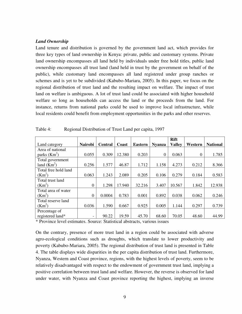
Land Ownership Land tenure and distribution is governed by the government land act, which provides for three key types of land ownership in Kenya: private, public and customary systems. Private land ownership encompasses all land held by individuals under free hold titles, public land ownership encompasses all trust land (land held in trust by the government on behalf of the public), while customary land encompasses all land registered under group ranches or schemes and is yet to be subdivided (Kabubo-Mariara, 2005). In this paper, we focus on the regional distribution of trust land and the resulting impact on welfare. The impact of trust land on welfare is ambiguous. A lot of trust land could be associated with higher household welfare so long as households can access the land or the proceeds from the land. For instance, returns from national parks could be used to improve local infrastructure, while local residents could benefit from employment opportunities in the parks and other reserves. Table 4: Regional Distribution of Trust Land per capita, 1997

Land category Nairobi Central Coast Eastern Nyanza Rift Valley Western National

Area of national parks (Km2) 0.055 0.309 12.380 0.203 0 0.063 0 1.785 Total government land (Km2) 0.256 1.577 46.87 1.712 1.158 4.273 0.212 8.366 Total free hold land (Km2) 0.063 1.243 2.089 0.205 0.106 0.279 0.184 0.583 Total trust land (Km2) 0 1.298 17.940 32.216 3.407 10.567 1.842 12.938 Total area of water (Km2) 0 0.0004 0.783 0.001 0.892 0.038 0.062 0.246 Total reserve land (Km2) 0.036 1.590 0.667 0.925 0.005 1.144 0.297 0.739 Percentage of registered land* - 90.22 19.59 45.70 68.60 70.05 48.60 44.99

* Province level estimates. Source: Statistical abstracts, various issues On the contrary, presence of more trust land in a region could be associated with adverse agro-ecological conditions such as droughts, which translate to lower productivity and poverty (Kabubo-Mariara, 2005). The regional distribution of trust land is presented in Table 4. The table displays wide disparities in the per capita distribution of trust land. Furthermore, Nyanza, Western and Coast province, regions, with the highest levels of poverty, seem to be relatively disadvantaged with respect to the endowment of government trust land, implying a positive correlation between trust land and welfare. However, the reverse is observed for land under water, with Nyanza and Coast province reporting the highest, implying an inverse

10

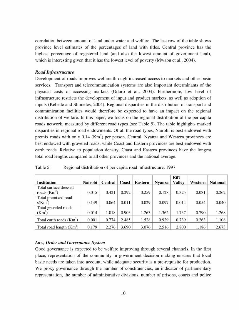
correlation between amount of land under water and welfare. The last row of the table shows province level estimates of the percentages of land with titles. Central province has the highest percentage of registered land (and also the lowest amount of government land), which is interesting given that it has the lowest level of poverty (Mwabu et al., 2004). Road Infrastructure Development of roads improves welfare through increased access to markets and other basic services. Transport and telecommunication systems are also important determinants of the physical costs of accessing markets (Oduro et al., 2004). Furthermore, low level of infrastructure restricts the development of input and product markets, as well as adoption of inputs (Kebede and Shimeles, 2004). Regional disparities in the distribution of transport and communication facilities would therefore be expected to have an impact on the regional distribution of welfare. In this paper, we focus on the regional distribution of the per capita roads network, measured by different road types (see Table 5). The table highlights marked disparities in regional road endowments. Of all the road types, Nairobi is best endowed with premix roads with only 0.14 (Km2) per person. Central, Nyanza and Western provinces are best endowed with graveled roads, while Coast and Eastern provinces are best endowed with earth roads. Relative to population density, Coast and Eastern provinces have the longest total road lengths compared to all other provinces and the national average. Table 5: Regional distribution of per capita road infrastructure, 1997

Institution Nairobi Central Coast Eastern Nyanza Rift Valley Western National

Total surface dressed roads (Km2) 0.015 0.421 0.292 0.259 0.128 0.325 0.081 0.262 Total premixed road s(Km2) 0.149 0.064 0.011 0.029 0.097 0.014 0.054 0.040 Total graveled roads (Km2) 0.014 1.018 0.903 1.263 1.362 1.737 0.790 1.268

Total earth roads (Km2) 0.001 0.774 2.485 1.528 0.929 0.739 0.263 1.108

Total road length (Km2) 0.179 2.276 3.690 3.076 2.516 2.800 1.186 2.673 Law, Order and Governance System Good governance is expected to be welfare improving through several channels. In the first place, representation of the community in government decision making ensures that local basic needs are taken into account, while adequate security is a pre-requisite for production. We proxy governance through the number of constituencies, an indicator of parliamentary representation, the number of administrative divisions, number of prisons, courts and police

11

stations in a given region. The per capita distribution of these institutions is presented in Table 6. Other than for Nairobi, distribution of constituencies shows little variation across provinces. The relatively lower representation for Nairobi is attributable to higher population densities compared to other regions. Central, Western and Nairobi report the lowest number of administrative divisions per capita, while Coast and Eastern have the highest. Rift Valley and Western have the lowest number of courts and police stations per capita compared to all other rural provinces.

Table 6: Regional distribution of governance institutions per capita, 1997

Institution Nairobi Central Coast Eastern Nyanza Rift Valley Western National

Number of Constituencies 0.004 0.008 0.009 0.009 0.008 0.007 0.007 0.008 Number of divisions 0.004 0.010 0.031 0.026 0.023 0.022 0.014 0.022 Number of prisons 0.003 0.003 0.007 0.004 0.002 0.004 0.001 0.004 Number of courts 0.002 0.005 0.009 0.004 0.005 0.003 0.005 0.005 Number of police stations 0.014 0.013 0.022 0.011 0.008 0.013 0.007 0.013

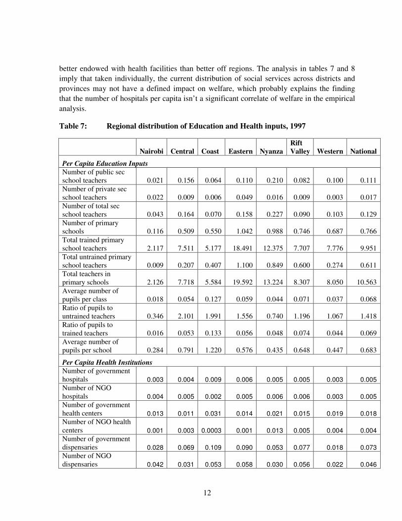
Social Services Access to social services is welfare improving. Oduro et al., (2004) argue that education and skill acquisition are critical factors for explaining the pattern of rural poverty. Education contributes to the process of moulding attitudinal skills and developing technical skills, and also facilitates the adoption and modification of technology Oduro et al., (2004). An unhealthy population cannot participate effectively in employment and other production activities. Access to health facilities and medication is therefore a crucial determinant of household welfare (Kabubo-Mariara, 2004). Van der Berg (2004) also argues that limited access to basic services such as to running water, sanitation on site, grid electricity and health care services is an impediment to escaping from poverty. Table 7 presents the regional distribution of per capita education and health inputs. For all education inputs, it is interesting to note that the poorest provinces (Nyanza and Western) seem to be relatively better off in terms of per capita endowment of social service inputs. On the contrary, Central province, the province with the lowest level of poverty seems to be relatively disadvantaged. With regard to government health institutions, Western, Coast and Central provinces are relatively less disadvantaged. Nyanza province seems to be relatively

12

better endowed with health facilities than better off regions. The analysis in tables 7 and 8 imply that taken individually, the current distribution of social services across districts and provinces may not have a defined impact on welfare, which probably explains the finding that the number of hospitals per capita isn’t a significant correlate of welfare in the empirical analysis. Table 7: Regional distribution of Education and Health inputs, 1997

Nairobi Central Coast Eastern Nyanza Rift Valley Western National

Per Capita Education Inputs Number of public sec school teachers 0.021 0.156 0.064 0.110 0.210 0.082 0.100 0.111 Number of private sec school teachers 0.022 0.009 0.006 0.049 0.016 0.009 0.003 0.017 Number of total sec school teachers 0.043 0.164 0.070 0.158 0.227 0.090 0.103 0.129 Number of primary schools 0.116 0.509 0.550 1.042 0.988 0.746 0.687 0.766 Total trained primary school teachers 2.117 7.511 5.177 18.491 12.375 7.707 7.776 9.951 Total untrained primary school teachers 0.009 0.207 0.407 1.100 0.849 0.600 0.274 0.611 Total teachers in primary schools 2.126 7.718 5.584 19.592 13.224 8.307 8.050 10.563 Average number of pupils per class 0.018 0.054 0.127 0.059 0.044 0.071 0.037 0.068 Ratio of pupils to untrained teachers 0.346 2.101 1.991 1.556 0.740 1.196 1.067 1.418 Ratio of pupils to trained teachers 0.016 0.053 0.133 0.056 0.048 0.074 0.044 0.069 Average number of pupils per school 0.284 0.791 1.220 0.576 0.435 0.648 0.447 0.683

Per Capita Health Institutions Number of government hospitals 0.003 0.004 0.009 0.006 0.005 0.005 0.003 0.005 Number of NGO hospitals 0.004 0.005 0.002 0.005 0.006 0.006 0.003 0.005 Number of government health centers 0.013 0.011 0.031 0.014 0.021 0.015 0.019 0.018 Number of NGO health centers 0.001 0.003 0.0003 0.001 0.013 0.005 0.004 0.004 Number of government dispensaries 0.028 0.069 0.109 0.090 0.053 0.077 0.018 0.073 Number of NGO dispensaries 0.042 0.031 0.053 0.058 0.030 0.056 0.022 0.046

13

The provincial distribution of health institutions however imply that the district level estimates presented above mask a lot of regional inequalities. For instance, the distribution of health facilities implies that 29% of all facilities are in Rift Valley province, while Western province has only 7% (Table 8). However, this distribution does not take into account differences in population densities in the provinces. For rural provinces, the number of beds and cots per 100,000 population is highest for Nyanza, implying that facilities in the province are relatively better equipped than those of other regions. It is surprising that Rift Valley has the lowest number of beds and cots per 100,000 people in spite of having more facilities.

Table 8: Health Institutions, Hospital beds and Cots by Province, 1997

Hospital beds and cots Region

Hospitals

Health centres

Health sub centres and dispensaries

Total (%) No. of

beds and cots

No. per 100,000 population

Nairobi 47 36 297 9.34 6,487 323

Central 45 76 341 11.35 7,009 182

Coast 43 47 358 11.01 4,136 176

Eastern 52 71 660 19.24 6,361 130

Nyanza 79 101 293 11.62 9,625 195

Rift Valley 80 145 954 28.98 10,158 149

Western 46 81 151 6.83 5,567 164

Total 398 566 3,105 100 50,909 176 Source, Statistical Abstract, 1998 Although the availability of social facilities is important, financing of social services is also as important. For instance, availability of hospitals without drugs and personnel would be of little value. In table 9, we present the regional distribution of per capita expenditure on basic social services. The results show that the highest per capita expenditures on water and roads went to the Rift Valley province, while the highest expenditures on rural electrification and health went to Coast and Western provinces respectively. However, Western province was clearly disadvantaged with respect to expenditures on water and rural electrification. Eastern and Coast provinces received the lowest expenditure on roads and health expenditures respectively.

14

Table 9: Total per Capita Expenditure on Infrastructure, 1997 (‘000 Kshs)

Total expenditure on Nairobi Central Coast Eastern Nyanza

Rift Valley Western National

Water 1129.15 51.99 59.37 42.55 67.49 171.75 11.87 109.40 Roads 37.33 19.71 80.53 55.05 122.85 158.19 115.91 99.36 Rural electrification 0.35 4.15 10.14 6.53 9.62 5.36 4.27 6.48 Health 38.16 9.23 7.18 8.59 12.04 8.83 18.34 10.57

The descriptive analysis of regional distribution of institutions in Kenya point at wide disparities in institutional endowments. Though there is no definite pattern of the correlation between poverty and distribution of institutions, the analysis implies that regions with the lowest number of key institutions per capita have relatively lower welfare than their counterparts with more institutions. Taking into account population density, the analysis clearly indicates that Coast province is at a relative advantage in endowment of all institutions except education services. Western province is clearly at a relative disadvantage. Though Nyanza was the poorest province in 1997, there is no evidence that it is the worst in terms of institutional endowments, implying that welfare is a function of the interaction of many factors, and that analysis of the institutional determinants of poverty need to take into account other determinants of poverty as well. 4 REGIONAL DIFFERENTIALS IN POVERTY

Poverty is multidimensional and complex in nature and manifests itself in various forms making its definition difficult. No single definition can exhaustively capture all aspects of poverty. Poverty is perceived differently by different people, some limiting the term to mean a lack of material well-being and others arguing that lack of things like freedom, spiritual well-being, civil rights and nutrition must also contribute to the definition of poverty. Economists have long been occupied with defining a money metric measure of household welfare. The most often used such measure is consumption expenditure per person or per adult equivalent. While controversy exists over the use of consumption expenditure as a measure of well being it remains the preferred metric in light of difficulties involved in measuring income. The controversy arises because income and expenditure measures of welfare can yield very different poverty indices (Geda et al., 2001) and policy implications. Since expenditure is more accurately measured than income, the present study adopts expenditure as a measure of household welfare.

15

Welfare Monitoring Survey analysis in Kenya adopted the material well-being perception of poverty in which the poor are defined as those members of society who are unable to afford minimum basic human needs, comprised of food and non-food items. Although the definition may seem simple, there are several complications in determining the minimum requirements and the amounts of money necessary to meet these requirements (Kabubo-Mariara and Ndenge, 2004). Results of Welfare Monitoring Surveys in Kenya show that poverty is concentrated in rural areas and among vulnerable groups in urban areas. Based on an absolute poverty line, it emerges that Central province had the lowest proportion of households under poverty in 1997, while Nyanza province had the highest. Central province also had the lowest poverty gap and severity of poverty indices while Coast province had the largest (Table 10). However Coast province contributed the least to overall poverty in the country, while Nyanza contributed the most. Table 10: Overall Rural Poverty by Region, 1997

Head count Pα=0 Contribution to poverty Region adult equiv

HHs Mem Poverty Gap, Pα=1

Severity of poverty Pα=0

% of population

Pα=0 Pα=1 Pα=2

Central 31.4 25.7 31.4 9.3 3.9 17.3 10.3 8.3 7.4 Coast 62.1 51.9 62.2 24.4 11.9 6.6 7.7 8.3 8.5 Eastern 58.6 53.1 58.2 22.4 10.7 18.2 20.1 21 21.2 Nyanza 63.1 56.7 62.9 23.4 11.4 19.9 23.7 24.1 24.7 Rift Valley

50.1 44.1 50.2 17.6 8.2 24.5 23.2 22.3 21.8

Western 58.8 53.6 59.3 22.8 11.2 13.5 15 15.9 16.4 Total 52.9 46.4 53.1 19.3 9.2 100 100 100 100 Source: Republic of Kenya, (2000) and WMS(III) database. The poorest province also had the highest proportion of hard core poor in 1997 (Hard core poor are defined as people who cannot afford to meet the basic minimum food requirement even if they allocated all their spending on food). Coast province had the largest proportion of hardcore poor, followed by Nyanza, Western and Eastern provinces (Table 11). Nyanza province with 20% of the national population contributed the most (24%) to hard core poverty (head count index), while Coast province still contributed very little to national hard core poverty. The minimal contribution of Coast province could be attributed to the very low proportion (7%) of the national population in the province.

16

Table 11: Hardcore Rural Poverty by Region, 1997

Head count Pα=0 Contribution to poverty Region

adult equiv

HHs Mem

Poverty Gap, Pα=1

Severity of poverty Pα=0

% of population Pα=0 Pα=1 Pα=2

Central 15.6 12.8 15.6 4.0 1.4 17.4 7.8 6.7 6.0 Coast 44.8 36.8 45.1 13.5 5.4 6.6 8.5 8.6 8.7 Eastern 40.9 36.2 40.6 12.2 4.7 18.1 21.3 21.3 21 Nyanza 41.9 37.8 42.1 13.1 5.5 19.9 24.0 25.3 26.7 Rift Valley

31.7 27.4 31.5 9.1 3.5 24.6 22.3 21.7 21.1

Western 41.7 37.9 41.8 12.5 5.0 13.5 16.1 16.3 16.6 Total 34.8 30.1 34.9 10.3 4.1 100 100 100 100 Source: Republic of Kenya, (2000) and WMS(III) database. Urban poverty is much harder to analyse across regions because of relatively small urban samples across provinces. The bulk of the urban population is concentrated in the cities of Nairobi, Mombasa, Kisumu and in Nakuru town. Analysis of the 1997 Welfare Monitoring Survey shows that almost half (49%) of the total urban population was living below the absolute poverty line, and 38% below the food poverty line. However, only a very small proportion (7.6%) were hard core poor. Kisumu city in Nyanza province was the worst hit by all categories of poverty (food, absolute and hard core poor) in 1997, just like in earlier surveys. Nakuru town in Rift valley province recorded the lowest incidence of food and hardcore poverty in 1997, while Mombasa recorded the least incidence of overall poverty in the same year (Table 12). Table12: Urban Differentials in the Incidence of Poverty, 1992-1997

% of food poor % of overall poor City/town 1992 1994 1997 1992 1994 1997

Nairobi 41.92 27.26 38.38 26.45 25.90 50.24 Mombasa 44.84 33.12 38.57 39.17 33.14 38.32 Kisumu - 44.09 53.39 - 47.75 63.73 Nakuru - 37.18 26.81 - 30.01 40.58 Other towns - 27.07 37.91 - 28.73 43.53 Total urban 45.58 29.23 38.29 29.29 28.95 49.20 Source: Republic of Kenya, (2000) and WMS(III) database.

17

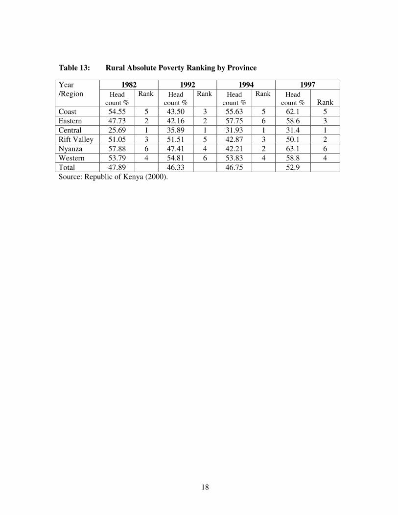
Based on the four Welfare Monitoring Surveys in Kenya, regional differences in poverty across different survey years are presented in Table 13. The estimates show that Central province has consistently emerged the least poor region in all the four surveys. Coast province was ranked number 5 in three of the four surveys and similarly Western region has been ranked 4th in three of the four surveys. This indicates that the poverty trends are somewhat robust in spite of the difficulties of comparing different welfare surveys. However, the design and timing of welfare surveys may have contributed to the poverty dynamics apparent in the table above where some regional poverty rankings have changed over repeated surveys. From table 13 and due to the nature of the surveys, one is unable tell whether the observed changes are real or whether they are statistical artifacts. Similarly the three WMS data sets cannot strictly speaking be used as a panel and it becomes very hard for the analyst to distinguish those households who are transitorily poor from those that are chronically poor. This factor could also explain the implied modest increase in the headcount index between 1981/82 and 1997. Another possible reason for the differentials is the use of unrepresentative prices where regional price deflators and poverty estimates may have under or over estimated the real situation. It is however noted that strict temporal adjustment and comparison of prices when analysing the various survey datasets has not been carried out (Kabubo-Mariara and Ndenge, 2004). Holding differences in survey datasets constant, the regional variations in poverty are a result of regional differences in the determinants of household welfare. These include household and non-household level covariates. Among non-household level covariates, institutional factors are important determinants of poverty more so in rural areas (Nissanke, 2004). Though a large number of studies now exist on poverty and its measurement in Kenya (see Collier and Lall, 1980; Greer and Thorbecke, 1986; Mukui, 1994; Republic of Kenya, 1998, 2000; Mwabu et al., 2000; Oyugi et al., 2000; Manda et al., 2000; Geda et al.; 2001), most of the studies have concentrated on household level based determinants of poverty in Kenya. No empirical study has empirically investigated the institutional determinants of poverty in Kenya. Mwabu et al., (2004) investigate the link between rural poverty and institutions using descriptive methods. We build on this study to investigate the institutional determinants of poverty using econometric procedures.

18

Table 13: Rural Absolute Poverty Ranking by Province

1982 1992 1994 1997 Year /Region Head

count % Rank

Head

count % Rank

Head

count % Rank

Head

count % Rank Coast 54.55 5 43.50 3 55.63 5 62.1 5 Eastern 47.73 2 42.16 2 57.75 6 58.6 3 Central 25.69 1 35.89 1 31.93 1 31.4 1 Rift Valley 51.05 3 51.51 5 42.87 3 50.1 2 Nyanza 57.88 6 47.41 4 42.21 2 63.1 6 Western 53.79 4 54.81 6 53.83 4 58.8 4 Total 47.89 46.33 46.75 52.9 Source: Republic of Kenya (2000).

19

5 INVESTIGATING THE INSTITUTIONAL CORRELATES OF WELFARE

5.1 The Primary Data and Variables

The household level empirical analysis is based on Welfare Monitoring Survey III (WMSIII) data collected by the Central Bureau of Statistics and the Planning Unit of the Ministry of Planning and National Development. The survey was conducted using the National Sample and Evaluation Programme (NASSEP) frame. The NASSEP frame is based on a two stage stratified cluster design for the whole country. First enumeration areas using the national census records were selected with probability proportional to size of expected clusters in the enumeration area. The number of expected clusters was obtained by dividing each primary sampling unit into 100 households. Then clusters were selected randomly and all the households enumerated. From each cluster, 10 households were drawn at random except in the semi-arid districts. Data was collected from a sample of 50,713 individuals from 10,873 households. The survey collected information on socio economic characteristics of the household, economic activities and time use, household asset endowments, consumption and income among other variables of interest. To this data, we map in district level data described earlier. In this section, we present and discuss sample characteristics by poverty status (see also appendix table A1). In the dataset, about 72% of the household heads are male, while 77% are married. 43% of all household heads have at least primary school education, 28% post-primary including university, while the rest have no education at all. We adopt this categorization of education because of the distribution of respondents across different levels of education, since higher levels of education have relatively few observations. In addition, we include variables to capture household composition and size. Due to potential endogeneity of household size, we use dummies for number of family members of different categories (for instance, number of children less than 5 years old, number of children less than 14 years e.t.c.). This is based on the expectation that household members of different age will have different consumption requirements, which have different welfare implications. The data shows that on average, every household has at least one person from each family composition category except for seniors (adults over 65 years). We also include employment sector and main occupation of the head. In the sample, about 48% of all household heads work in the formal sector while 42% are in agricultural sector related activities (appendix table A1). The other variables include distance to source of water (with a mean distance of about 2 and 1 kilometers in rural and urban areas respectively),

20

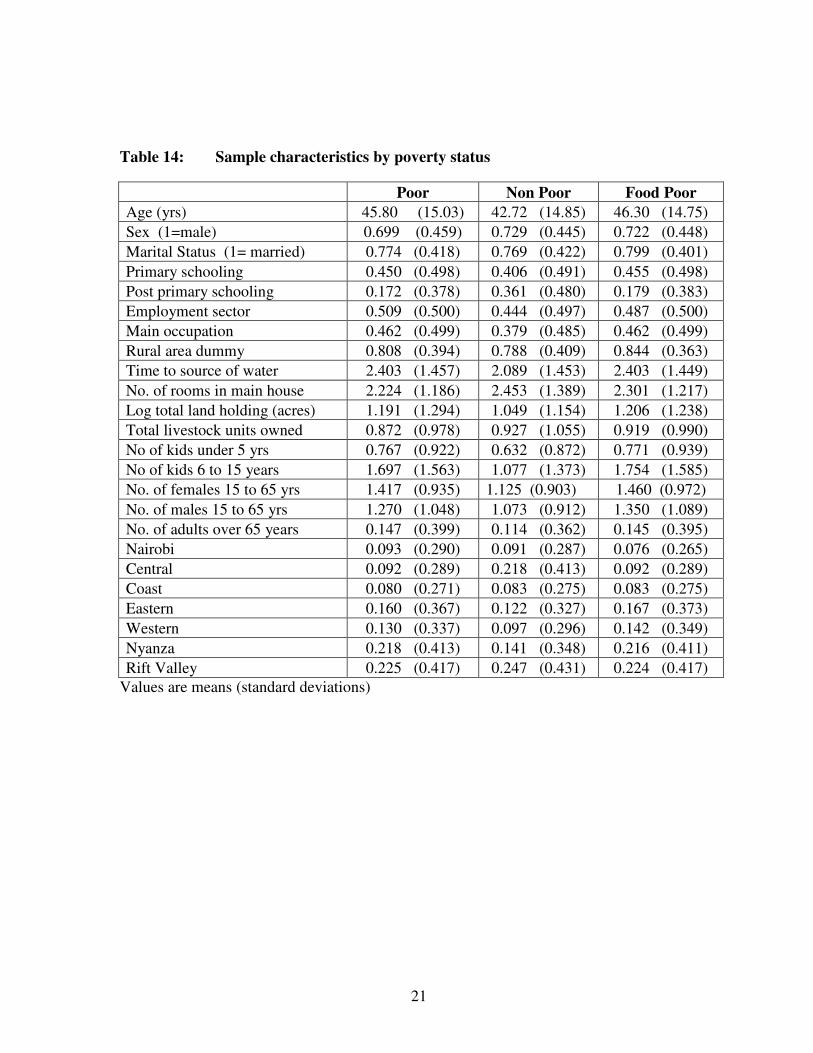
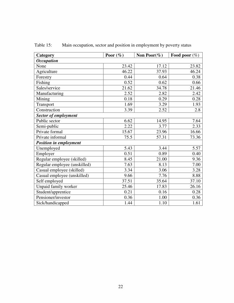
place of residence (80% rural), number of rooms in main house (with a mean of about 2 rooms per house), total land holding in acres and total livestock units owned. Turning to characteristics by poverty status, the data shows that there are marked differences between characteristics of the poor and non-poor. In particular, the poor have significantly lower levels of post primary education than the non-poor and have larger families (Table 14). Though the number of senior members of the household are quite few, the data also implies that poor households have higher dependency ratios than non poor households. In terms of spatial location of the poor, there are large regional differentials in the status of poverty. Less than 10% of all households are poor in Nairobi, Central and Eastern provinces compared to over 20% in Nyanza and the Rift Valley. There is a higher concentration of the absolute and food poor in Nyanza and Rift Valley provinces, while the highest proportion of the non poor are concentrated in Rift valley and Central provinces. The implication here is that given that Rift valley is the largest of the 7 provinces, it has the highest concentration of households in all categories: poor, non poor and food poor. Table 15 shows that the poor are more concentrated in activities of lower economic status. About 70% of the poor and food poor are either unemployed or employed in the agricultural sector compared to only 55% of the non poor (this supports Geda et al., 2001, who argue that the poor are more concentrated in rural areas and in the agricultural sector). A larger proportion of the poor (about 26%) are unpaid family workers, compared to 18% of the non poor. In addition, the poor are more likely to be in the private informal sector than the non poor. The data therefore implies correlation between the sector of employment, occupation and position in employment and the status of poverty. Empirical investigation of this relationship is presented in the next section.

21

Table 14: Sample characteristics by poverty status

Poor Non Poor Food Poor Age (yrs) 45.80 (15.03) 42.72 (14.85) 46.30 (14.75) Sex (1=male) 0.699 (0.459) 0.729 (0.445) 0.722 (0.448) Marital Status (1= married) 0.774 (0.418) 0.769 (0.422) 0.799 (0.401) Primary schooling 0.450 (0.498) 0.406 (0.491) 0.455 (0.498) Post primary schooling 0.172 (0.378) 0.361 (0.480) 0.179 (0.383) Employment sector 0.509 (0.500) 0.444 (0.497) 0.487 (0.500) Main occupation 0.462 (0.499) 0.379 (0.485) 0.462 (0.499) Rural area dummy 0.808 (0.394) 0.788 (0.409) 0.844 (0.363) Time to source of water 2.403 (1.457) 2.089 (1.453) 2.403 (1.449) No. of rooms in main house 2.224 (1.186) 2.453 (1.389) 2.301 (1.217) Log total land holding (acres) 1.191 (1.294) 1.049 (1.154) 1.206 (1.238) Total livestock units owned 0.872 (0.978) 0.927 (1.055) 0.919 (0.990) No of kids under 5 yrs 0.767 (0.922) 0.632 (0.872) 0.771 (0.939) No of kids 6 to 15 years 1.697 (1.563) 1.077 (1.373) 1.754 (1.585) No. of females 15 to 65 yrs 1.417 (0.935) 1.125 (0.903) 1.460 (0.972) No. of males 15 to 65 yrs 1.270 (1.048) 1.073 (0.912) 1.350 (1.089) No. of adults over 65 years 0.147 (0.399) 0.114 (0.362) 0.145 (0.395) Nairobi 0.093 (0.290) 0.091 (0.287) 0.076 (0.265) Central 0.092 (0.289) 0.218 (0.413) 0.092 (0.289) Coast 0.080 (0.271) 0.083 (0.275) 0.083 (0.275) Eastern 0.160 (0.367) 0.122 (0.327) 0.167 (0.373) Western 0.130 (0.337) 0.097 (0.296) 0.142 (0.349) Nyanza 0.218 (0.413) 0.141 (0.348) 0.216 (0.411) Rift Valley 0.225 (0.417) 0.247 (0.431) 0.224 (0.417)

Values are means (standard deviations)

22

Table 15: Main occupation, sector and position in employment by poverty status

Category Poor (%) Non Poor(%) Food poor (%) Occupation None 23.42 17.12 23.82 Agriculture 46.22 37.93 46.24 Forestry 0.44 0.64 0.38 Fishing 0.52 0.62 0.66 Sales/service 21.62 34.78 21.46 Manufacturing 2.52 2.82 2.42 Mining 0.18 0.29 0.28 Transport 1.69 3.29 1.93 Construction 3.39 2.52 2.8 Sector of employment Public sector 6.62 14.95 7.64 Semi-public 2.22 3.77 2.33 Private formal 15.67 23.96 16.66 Private informal 75.5 57.31 73.36 Position in employment Unemployed 5.43 3.44 5.57 Employer 0.51 0.89 0.40 Regular employee (skilled) 8.45 21.00 9.36 Regular employee (unskilled) 7.63 8.13 7.00 Casual employee (skilled) 3.34 3.06 3.28 Casual employee (unskilled) 9.66 7.76 8.88 Self employed 37.51 35.64 37.10 Unpaid family worker 25.46 17.83 26.16 Student/apprentice 0.21 0.16 0.28 Pensioner/investor 0.36 1.00 0.36 Sick/handicapped 1.44 1.10 1.61

23

5.2 Estimation Results

In this section, we investigate empirically the institutional correlates of poverty. Institutions are a very important conduit to transmit globalization effects on rural poverty, playing a key role in explaining the extent, distribution and changes in rural poverty. Institutions and their changes also determine who is poor and who remains poor (Nissanke, 2004). Previous studies on the impact of rural institutions and globalization on poverty in Africa have identified several institutional determinants of poverty. These include road infrastructure, social dysfunction, operations and failure of agricultural factor and product markets, limited access to social services and high levels of corruption (Nissanke, 2004). Nissanke argues that infrastructure, social dysfunction and markets have deteriorated over the last two decades as a direct result of stabilization/liberalization policies. To investigate the impact of institutional factors on welfare, we run three different series of regressions: first we run the district level model of institutional determinants of poverty, second we model the household level determinants of poverty and then we combine household and institutional determinants of poverty in the final set of regressions. We discuss each of these regressions in turn. District level regressions: Institutional determinants of poverty We base these regressions on district level data described earlier. Poverty is measured through a range of variables, namely: the FGT measures, adult equivalent monthly expenditure and food poverty status. All district level models are estimated using ordinary least square regressions. This is because for the status of poverty (both food and absolute), we use district means estimated from binary variables (whether a household is food or absolute poor) in the household data. The estimated means are therefore continuous variables (ranging from 0 to 1), which necessitate use of ordinary least square regressions rather than probit/logit regression methods. Regional models could not be estimated at this level because of issue of degrees of freedom. As expected, correlation analysis shows that most institutional variables described earlier are correlated. After taking care of collinearity, we experiment regressions with a narrow range of selected institutional variables. In the end, the explanatory variables that we settle for in the regressions include the number of constituencies, number of active cooperatives, ratio of public to private secondary school teachers, health facilities, government land and infrastructure. Other than the ratio of public to private secondary school teachers and earth roads, all other variables are at the per capita level. The regression results for the FGT poverty measures are presented in table 16. Since the results are consistent across various FGT measures, we base our discussion on the head count index, food poverty and expenditure functions. Though the F values are quite low, they are all significantly different from zero at all conventional levels of significance, implying that

24

the models fit the data better than the intercept only model. The low F values are most likely due to limited degrees of freedom given a very small sample size. Further, the R2 indicates that the variables explain about 60% of the total variation in poverty rates and about 53% of the variation in adult equivalent expenditure. The number of constituencies per capita, which is a sign of good governance, has the unexpected sign for all poverty measures implying that parliamentary representation may not be an important determinant of poverty. This result is consistent with the results for expenditure. Table 16: Institutional correlates of poverty; FGT measures 1997

Head count ratio

Poverty gap

Poverty gap squared Food Poor

Adult equiv. monthly

expenditure

Variable Parameter estimates

Parameter estimates

Parameter estimates

Parameter estimates

Parameter estimates

No. of constituencies per capita

18.603 (2.50***)

7.325 (2.19**)

3.561 (1.96*)

14.654 (3.09***)

-10.869 (-1.99**)

Number of active cooperatives per capita

-0.048 (-0.70)

-0.039 (-1.26)

-0.023 (-1.36)

-0.059 (-1.35)

0.038 (0.75)

Ratio of public to private teachers

-0.345 (-1.50)

-0.150 (-1.45)

-0.075 (-1.34)

-0.150 (-1.02)

0.289 (1.71*)

Number of hospitals per capita

-1.030 (-2.27**)

-0.521 (-2.56***)

-0.271 (-2.45**)

0.060 (0.21)

0.138 (0.42)

Number of health Centers per capita

-2.953 (-1.71*)

-1.806 (-2.33**)

-1.096 (-2.60***)

-4.074 (-3.71***)

1.922 (1.52)

Total government land per capita

-0.181 (-2.38**)

-0.106 (-3.11***)

-0.061 (-3.30***)

-0.008 (-0.17)

-0.006 (-0.10)

Total area under water per capita

0.507 (2.60***)

0.262 (2.99***)

0.144 (3.01***)

0.388 (3.12***)

-0.074 (-0.51)

Total earth roads (Kms) 0.0001 (1.25)

0.0001 (1.10)

0.00003 (1.05)

-0.00003 (-0.35)

0.00002 (0.02)

Nairobi 0.397 (1.55)

0.139 (1.21)

0.063 (1.01)

0.096 (0.59)

0.141 (0.75)

Central -0.321

(-3.63***) -0.143

(-3.59***) -0.073

(-3.40***) -0.232

(-4.12***) 0.147

(2.26**)

Coast 0.071 (0.76)

0.056 (1.33)

0.036 (1.56)

-0.041 (-0.69)

0.111 (1.62*)

Eastern -0.011 (-0.15)

-0.013 (-0.41)

-0.009 (-0.51)

-0.071 (-1.59)

0.080 (1.57)

Western -0.110 (-1.05)

-0.057 (-1.22)

-0.030 (-1.18)

0.049 (0.75)

-0.019 (-0.25)

Nyanza -0.078 (-0.78)

-0.043 (-0.96)

-0.021 (-0.87)

0.023 (0.37)

-0.054 (-0.73)

Constant 0.670 (7.92)

0.293 (7.71)

0.149 (7.24)

0.468 (8.69)

3.294 (53.16)

No of Observations 44 44 44 44 44 R-squared 0.5828 0.6359 0.6439 0.6234 0.5358 F(14, 29) 2.89*** 3.62*** 3.75*** 3.43*** 2.39**

***, **,* Significant at 1%, 5% and 10% respectively

25

The number of active cooperatives is associated with lower poverty rates and levels though the coefficients are insignificant. This finding supports the argument that membership of a cooperative provides benefits that could have a positive impact on welfare (Oduro et al. 2004). Ratio of public to private trained secondary school teachers is also welfare improving, though the impact is only significant in the expenditure function. Health institutions are also clearly important determinants of welfare though the number of hospitals per capita do not seem to matter for food and absolute poverty. These results support earlier studies which find that access to basic services and infrastructure is important for household welfare (Kebede and Shimeles, 2004). The same result is observed for government land ownership. Total area under water exert a strong positive impact on the poverty rates, implying that districts with a lot of water experience higher levels of poverty than their counterparts with less water. This could be explained by the fact that such districts have lots of waste water (such as large flood plains) which adversely affect productivity and welfare. Except for Nairobi and Coast provinces, all regional dummies exert a negative impact on poverty rates, implying that relative to Rift Valley province, these regions are likely to have lower levels of poverty, which is consistent with the FGT poverty rates (see Table 13). However, only the dummy for Central province is significant.

Household level determinants of poverty Next we turn to investigate the impact of household level determinants of poverty, using the same dependent variables as in the previous section. The sample statistics of the variables used in these regressions are presented in appendix table A1. Before discussing the regression results, first we note that some of the variables used in the models are arguably endogenous though they have been used in a large number of studies. These variables include sector of employment, occupation of the household head, total livestock units owned and ownership of agricultural land. In the face of endogeneity of some variables, instrumental variable methods would be most appropriate, so long as suitable identifying instruments are available in the data. In the absence of suitable variables, the researcher could resort to reduced form models that exclude the predetermined variables. It is however always useful to carry out endogeneity tests to be sure that the problem exists before discarding important determinants of a variable of interest. If the test rejects endogeneity, then these variables can be incorporated in the reduced form model. Due to lack of suitable instruments, we employ the general Hausman specification test to verify whether it is appropriate to incorporate the above variables in our model (Stata Corp, 1999). The test involves determining whether there exist systematic differences in two estimators: a consistent estimator (without endogenous variables) and an efficient estimator (with suspected endogenous variables). The idea is to test whether the efficient estimator is

26

also consistent. The Hausman specification test for each of the suspected variables does not reject the null hypothesis and therefore the suspect variables are unlikely to affect the signs and magnitudes of the coefficients of other variables in the model. We therefore retain the variables in our estimation, though like some other variables, their performance is not consistent in all models. The regression results for the full sample are presented in table 17. We present the marginal effects for the head count index and food poverty functions and OLS parameter estimates for the poverty gap, poverty gap squared and expenditure functions. The results indicate that age and age squared have an inverted U shaped relationship with household welfare, with households getting worse off as the household head becomes older. This result is consistent with hypothesis of life cycle models (Appleton, 2002). The result is consistent across the three models. The results further show that sector of employment, employment in the agricultural sector and distance to source of water are associated with lower household welfare. This is also the case for larger households with all family composition variables exhibiting a positive relationship with the FGT measures and food poverty, but an inverse relationship with adult equivalent monthly expenditures. Distance to source of water is associated with higher levels of poverty, implying that households that have to spend a lot of time collecting water have less time for productive activities and thus lower welfare (Mwabu et al., 2000). The results also show that other than for Central province, all other regions are likely to have higher poverty rates than the Rift Valley province. Male heads and marital status are associated with lower poverty rates but the impact is insignificant. Number of rooms in a house and number of total livestock units owned reduce household poverty rates, implying that assets are important determinants of poverty. Education is an important determinant of household poverty and the result is consistent across the three models. Furthermore, welfare is an increasing function of education attainment. This finding is consistent with earlier findings for Kenya (Geda et al., 2001, Mwabu et al, 2000, Oyugi, 2000). The results for FGT poverty measures differ with those for food poverty in several respects. In the first place, the head count index model fits the data much better than the food poverty model as shown by the differences in the Wald Chi(2) test. However, both models fit the data better than the intercept only model and the variables are jointly significant in explaining variations in household poverty. Second, the signs and significance of a few variables differ in the two models. Rural residence, gender and marital status of the household head are associated with higher levels of food poverty, though the coefficients are insignificant, but the reverse impact is observed for the head count index function. The other difference is in total agricultural land holding, which has the expected impact of reducing food poverty though the impact is insignificant.

27

Table 17: Household correlates of poverty: Full Sample

Head count index Poverty gap

Poverty gap Squared Food Poor

Adult equiv. monthly

expenditure Variable Estimates Estimates Estimates Estimates Estimates

Age (yrs) -0.006

(-2.68***) 0.005

(8.63***) 0.002

(6.23***) -0.004

(-1.58*) 0.467

(80.49***)

Age squared 0.0001

(2.75***) -0.0001

(-5.35***) -0.00001

(-3.22***) 0.0001

(2.18***) -0.005

(-51.02***)

Sex (1=male) -0.008 (-0.53)

0.007 (0.90)

0.004 (0.83)

0.009 (0.62)

0.324 (6.54***)

Marital Status (1= married) -0.007 (-0.44)

0.008 (1.14)

0.006 (1.45)

0.019 (1.23)

-0.073 (-1.23)

Primary schooling -0.107

(-7.59***) -0.042

(-5.60***) -0.024

(-5.44***) -0.057

(-4.15***) 0.987

(20.34***)

Post primary schooling -0.284

(-17.03***) -0.096

-(10.77***) -0.050

(-9.97***) -0.193

(-11.88***) 1.609

(25.32***)

Employment sector 0.036

(3.37***) 0.006 (1.09)

0.0002 (0.07)

0.001 (0.12)

0.228 (6.85***)

Main occupation 0.070

(5.90***) 0.024

(4.51***) 0.013

(4.11***) 0.042

(3.68***) -0.126

(-3.62***)

Rural area dummy -0.126

(-6.47***) -0.025

(-3.31***) -0.014

(-3.06***) 0.023 (1.23)

0.300 (4.51***)

Time to source of water 0.014

(3.85***) 0.008

(4.47***) 0.005

(4.46***) 0.008

(2.09**) 0.079

(6.96***)

No. of rooms in main house -0.052

(-11.00***) -0.017

(-8.12***) -0.008

(-6.57***) -0.042

(-9.17***) 0.067

(5.12***) Log total land holding (acres)

0.007 (1.56)

0.003 (1.00)

0.001 (0.35)

-0.002 (-0.55)

0.016 (0.91)

Log total livestock units -0.068

(-11.50***) -0.025

(-8.45***) -0.013

(-7.43***) -0.053

(-9.28***) 0.026 (1.41)

No of kids under 5 yrs 0.025

(3.95***) 0.010

(3.12***) 0.005

(2.44***) 0.015

(2.48***) 0.126

(6.42***)

No of kids 6 to 15 years 0.080

(19.88***) 0.026

(12.41***) 0.013

(10.69***) 0.065

(17.05***) -0.291

(-24.62***) No. of females 15 to 65 yrs 0.065 0.020 0.009 0.065 -0.168

28

(10.12***) (5.54***) (4.69***) (10.46***) (-7.46***)

No. of males 15 to 65 yrs 0.066

(10.38***) 0.016

(4.94***) 0.007

(3.56***) 0.080

(13.03***) -0.290

(-16.53***)

No. of adults over 65 years 0.075

(3.42***) 0.034

(3.28***) 0.011

(1.87*) 0.043

(2.02**) 1.321

(14.59***) Region (Rift Valley is reference)

Nairobi 0.059

(2.42***) 0.014 (0.86)

-0.0001 (-0.01)

0.057 (2.31)

1.116 (10.39***)

Central -0.132

(-7.50***) -0.040

(-6.23***) -0.019

(-5.49***) -0.140

(-8.27***) 0.427

(8.39***)

Coast 0.011 (0.51)

0.025 (2.95***)

0.015 (3.05***)

0.053 (2.51***)

0.517 (8.05***)

Eastern 0.082

(4.63***) 0.038

(4.64***) 0.020

(4.16***) 0.077

(4.47***) -0.002 (-0.03)

Western 0.125

(6.57***) 0.062

(6.47***) 0.034

(5.95***) 0.135

(7.19***) -0.006 (-0.11)

Nyanza 0.130

(8.02***) 0.051

(6.49***) 0.027

(5.76***) 0.107

(6.69***) -0.045 (-0.95)

No of Observations 10729 10847 10847 10729 10729 LR chi2 (24) 2026.6*** 1750.8*** Log Likelihood -6378.6 -6369.3 R-squared 0.4388 0.3365 0.9885 F( 24, 10823) 192.97 117.65 F(24, 10705)=36231


29

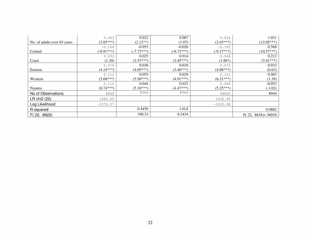
The results for the household determinants of adult equivalent monthly expenditure also differ with the determinants of the poverty rates in several respects: The t values for age and age squared are very high, which is a result of suppressing the constant. When the model is estimated without the constant, the t values are quite low though significant. Suppressing the constant also raises the R squared value from 0.73% to 0.99% implying that the constant alone explains about 25% of the total variation in expenditure. This could probably imply that our model may have omitted important variables. However an R squared of 73% still implies that the variables of the fitted model have a reasonably high explanatory power. Gender of household head is positive and highly significant, implying that female headed households are poorer than male headed households, a finding which is supportive of findings in a large number of studies (Geda et al., Mwabu et al., 2000). Marital status is inversely correlated with expenditure, implying that household whose heads are married are likely to be poorer than single parent households. Although this result is unexpected and surprising, the coefficient is insignificant. Another difference is in the signs of the coefficient for sector of employment, where we find that households headed by formal sector workers are better off than all other households. Distance to source of water has an unexpected positive and significant impact. Number of rooms and livestock ownership have the unexpected impact but only the impact of livestock is significant. The results for household composition imply that the presence of more children below 5 years and more elderly adults (over 65 years) are associated with more expenditure. This result is unexpected and contrary to the poverty functions which give the expected results. The final difference in our model results is that regional dummies indicate that the welfare of households in Nairobi, Central and Coast provinces is higher than households in the Rift Valley province, while households in Eastern, Nyanza and Western are worse off. This conforms to the ranking of provinces by mean adult equivalent expenditures where Rift valley ranks 4th. The results for regional analysis are presented in tables 18 and 19. The rural models fit the data better than for the full sample, while the poverty gap and expenditure functions for urban areas also perform better than the respective full sample and rural functions. Except for the age variables which are clearly unimportant in rural areas, the FGT and food poverty function results for rural areas are consistent with those for the full sample. However, the age variables have a significant impact on expenditure in rural areas. There are more marked differences in the urban model, where age, gender, employment sector and land holdings are more significant determinants of poverty. Marital status has an unexpected negative and significant coefficient in urban areas. Household assets (land and livestock) reduce the

30

likelihood of a household falling into poverty in rural areas, but the signs and magnitudes of the results for the full sample and urban areas are mixed implying that these assets are more critical in rural areas. Regional location does not seem to be important in urban relative to rural areas probably because of the relatively small size of the urban sample across regions. However, Western and Nyanza provinces are clearly worse off than Rift Valley in terms of the head count index and food poverty. The results for expenditure do not support this, but show that all households in urban areas are better off than those in urban Rift Valley, though the coefficients for Western and Nyanza are insignificant.

31

Table 18: Household Correlates of poverty; Rural Sample, 1997

Head count index Poverty Gap Poverty Gap

Squared Food Poor Adult equiv. monthly

expenditure Variable Marginal effects Parameter est. Parameter est. Marginal effects Parameter est.

Age (yrs) -0.0004

(-0.14) 0.004

(7.03***) 0.002

(4.73***) -0.001 (-0.38)

0.455 (83.82***)

Age squared 0.00002

(0.68) -0.00003

(-3.70***) -0.00001 (-1.87**)

0.00003 (1.01)

-0.004 (-50.47***)

Sex (1=male) 0.010 (0.63)

0.005 (0.64)

0.002 (0.40)

0.008 (0.53)

0.210 (4.19***)


0.006 (0.83)

0.005 (1.02)

0.005 (0.31)

0.245 (4.12***)


(-7.14***) -0.041

(-5.63***) -0.022

(-5.01***) -0.053

(-3.62***) 0.879

(18.16***)


(-15.38***) -0.102

(-12.48***) -0.051

(-10.64***) -0.185

(-10.18***) 1.314

(20.51***)

Employment sector 0.009 (0.78)

-0.006 (-1.13)

-0.005 (-1.50)

-0.022 (-1.91**)

0.143 (4.30***)


(6.92***) 0.030

(5.42***) 0.015

(4.64***) 0.055

(4.68***) 0.010 (0.29


(4.14***) 0.008

(4.32***) 0.005

(4.13***) 0.009

(2.28**) 0.094

(8.40***)


(-5.99***) -0.011

(-4.75***) -0.006

(-3.97***) -0.033

(-6.58***) 0.086


-0.008 (-1.47)

-0.002 (-0.59)

-0.001 (-0.64)

-0.005 (-1.03)

0.041 (2.69***)


(-(10.39***) -0.023

(-7.39***) -0.012

(-6.28***) -0.054

(-8.72*** 0.052

(2.98***)


(3.73***) 0.010

(3.10***) 0.005

(2.59***) 0.016

(2.46***) 0.174

(9.11***)


(17.65***) 0.025

(11.54***) 0.013

(9.80***) 0.066

(16.25***) -0.249

(-20.39***)

No. of females 15 to 65 yrs 0.056

(7.83***) 0.015

(4.56***) 0.007

(3.47***) 0.065

(9.43***) -0.241

(-11.50***)


(8.52***) 0.016

(4.72***) 0.008

(3.56***) 0.071

(10.68***) -0.294

(-17.25***)

32


(2.85***) 0.022

(2.12**) 0.007 (1.07)

0.054 (2.45***)

1.031 (12.05***)

Central -0.164

(-8.91***) -0.053

(-7.73***) -0.026

(-6.73***) -0.165

(-9.17***) 0.568

(10.57***)

Coast 0.032 (1.20)

0.025 (2.53***)

0.014 (2.45***)

0.048 (1.88*)

0.213 (3.41***)

Eastern 0.076

(4.14***) 0.036

(4.05***) 0.018

(3.46***) 0.074

(4.08***) 0.033 (0.63)

Western 0.112

(5.68***) 0.055

(5.50***) 0.029

(4.91***) 0.121

(6.21***) 0.083 (1.39)

Nyanza 0.115

(6.74***) 0.044

(5.10***) 0.023

(4.47***) 0.088

(5.25***) -0.052 (-1.02)

No of Observations 8860 8944 8944 48860 8944 LR chi2 (22) 1680.05 1432.45 Log Likelihood -5273.37 -5335.98 R-squared 0.4459 116.8 0.9883 F( 22, 8922) 190.33 0.3434 F( 22, 8838)= 36010

33

Table 19: Household Correlates of poverty; Urban Sample, 1997

Head count index Poverty gap Poverty gap

squared Food Poor Adult equiv. monthly


Age (yrs) -0.018

(-2.10**) 0.005

(2.68***) 0.002

(1.77*) -0.024

(-3.23***) 0.554

(37.32***)

Age squared 0.0001

(1.31) -0.0001

(-2.43***) -0.00002

(-1.43) 0.0003

(3.35***) -0.006

(-24.48***)

Sex (1=male) -0.146

(-2.89***) 0.017 (0.88)

0.015 (1.27)

0.038 (0.86)

0.923 (5.63***)

Marital Status (1= married) 0.076 (1.77*)

0.024 (1.42)

0.013 (1.36)

0.059 (1.55)

-0.964 (-8.42***)


(-2.69***) -0.079

(-2.42***) -0.050

(-2.70***) -0.081

(-2.02**) 0.872

(6.51***)


(-6.20***) -0.116

(-3.41***) -0.065

(-3.51***) -0.203

(-4.76***) 1.308

(9.37***)


(4.32***) 0.047

(3.39***) 0.019

(2.65***) 0.082

(3.38***) 0.323

(4.39***)

Main occupation -0.019 (-0.31)

0.004 (0.19)

0.007 (0.46)

-0.071 (-1.28)

0.515 (2.98***)

Time to source of water 0.009 (0.66)

0.010 (1.52)

0.007 (2.02**)

-0.002 (-0.17)

0.114 (3.31***)


(-9.78***) -0.030

(-6.85***) -0.013

(-5.84***) -0.071

(-6.50***) 0.196


0.048 (4.39***)

0.015 (3.02***)

0.005 (1.76*)

-0.004 (-0.53)

0.041 (1.09)


(-4.91***) -0.031

(-4.58***) -0.015

(-4.07***) -0.056

(-3.66***) 0.080

(1.71*)


(1.87**) 0.005 (0.50)

-0.001 (-0.20)

0.010 (0.68)

-0.011 (-0.22)


(9.5***) 0.042

(6.40***) 0.024

(5.53***) 0.071

(6.13***) -0.345

(-10.61***)

No. of females 15 to 65 yrs 0.081

(4.68***) 0.035

(3.46***) 0.018

(3.32***) 0.077

(5.13***) 0.019 (0.35)


(7.25***) 0.025

(3.34***) 0.009

(2.20**) 0.121

(7.85***) -0.280

(-3.96***)

34

No. of adults over 65 years 0.219 (1.73*)

0.092 (1.85**)

0.031 (1.00)

-0.290 (-2.29***)

3.623 (5.34***)

Nairobi 0.030 (0.87)

0.007 (0.45**)

0.002 (0.28)

0.052 (1.65*)

0.318 (3.37***)

Central 0.031 (0.46)

0.045 (2.63***)

0.027 (2.99***)

0.045 (0.68)

0.224 (1.92**)

Coast -0.011 (-0.25)

0.027 (1.65*)

0.021 (2.31**)

0.088 (2.18**)

0.267 (2.56***)

Eastern 0.070 (1.08)

0.036 (2.14**)

0.025 (2.75***)

0.024 (0.38)

0.203 (1.86**)

Western 0.144

(1.86**) 0.092

(2.82***) 0.066

(2.98***) 0.223

(3.04***) 0.178 (1.28)

Nyanza 0.168

(3.08***) 0.076

(4.28***) 0.045

(4.18***) 0.211

(4.05***) 0.152 (1.49)

No of Observations 1869 1903 1903 1869 1869 LR chi2 (21) 497.61 310.07 Log Likelihood -1028.53 -1006.4 R-squared 0.4516 0.3389 0.9932 F( 23, 1880) 33.71 19.68 F( 23, 1846)= 10187

35

Household and Institutional Determinants of Poverty To model both household and institutional determinants of poverty, we map district level institutional factors onto the household level data, then run models with the relevant determinants. The results for the full model are presented in table 20. The Chow test results and R-squared values show that combining these two sets of determinants significantly improves the fit and stability of the models. The results for household characteristics are consistent with those of regressions with household characteristics alone. However, the impact of land holding is reversed in the expenditure function while livestock ownership has the expected and significant impact. Signs and magnitudes for coefficients of regional dummies are significantly different from those in the household characteristics model. In particular, the results for the expenditure function show that all regions are better off than the Rift Valley province but as before, the result is not consistent for the poverty functions. Household characteristic results for rural and urban areas are also consistent with the household variable only model. However, we also observe differences in behavior of the provincial dummies (see tables 21 and 22). Turning to the institutional factors, per capita endowment of active cooperatives, health centers and ratio of public to private school teachers reduce absolute and food poverty rates. In addition to these factors, government land and total length of earth roads increase expenditures and reduce the likelihood of households falling into absolute poverty. The results for road length and hospitals are not consistent across different welfare measures. Poverty gap and poverty gap squared results are consistent with those of the head count index and food poverty functions. Except for per capita government land ownership and total length of earth roads, the results for the rural sample are consistent with those of the full sample. Overall the results confirm that institutions are important determinants of poverty and the results are consistent with the district level institutional determinants of poverty. But parliamentary representation does not seem to be an important determinant of household welfare. Maybe this could be explained by the fact that parliamentary representation may only help to enhance provision of public goods if at all, which may not have any direct short term impact on household welfare. Turning to regional analysis, results for urban areas are considerably different from those of rural areas. In urban areas, except for parliamentary representation, number of health centers, government land per capita and abundance of earth roads all institutional variables are welfare improving when welfare is measured through the proportion of people below absolute and food poverty lines. However, only length of earth roads and number of hospitals per capita exert a significant impact on welfare in the head count index function. When

36

welfare is measured through expenditure, all institutional factors are welfare improving except for total area under waste water and length of earth roads. The impact of these factors is significantly different from zero. For rural areas, health centers and earth roads are clearly welfare improving, while other institutional factors do not seem to matter for absolute and food poverty. However, only parliamentary representation and total area under water are associated with lower welfare when welfare is measured through expenditure. Comparing the results for different poverty measures for all regions, including the full sample, we conclude that although household variables perform almost equally well in all specifications (Appleton, 2002), welfare measured through consumption expenditure give more robust results than when welfare is measured through the status of poverty.

37

Table 20: Household and institutional correlates of poverty; FGT measures 1997 Head count

index Poverty gap Poverty gap

Squared Food Poor Adult equiv. monthly

expenditure Variable Estimates Estimates Estimates Estimates Estimates

Age (yrs) -0.007

(-2.78***) 0.004

(6.53***) 0.002

(5.46***) -0.003 (-1.27)

0.396 (58.05***)

Age squared 0.0001

(3.03***) -0.00003

(-4.26***) -0.00001

(-3.12***) 0.0001 (2.00**)

-0.004 (-41.41***)

Sex (1=male) 0.010 (0.61)

0.019 (2.59***)

0.011 (2.48***)

0.035 (2.20**)

0.325 (6.66***)


0.0001 (0.02

0.002 (0.44

0.002 (0.15)

-0.109 (-1.93**)


(-7.64***) -0.046

(-5.89***) -0.026

(-5.59***) -0.072

(-4.94***) 0.866

(19.45***)


(-16.11***) -0.096

(-10.29***) -0.050

(-9.71***) -0.202

(-11.73***) 1.496

(25.87***)


(5.01***) 0.012

(2.12**) 0.003 (0.86)

0.024 (2.16**)

0.183 (5.53***)


(6.8***) 0.031

(5.74***) 0.017

(5.29***) 0.054

(4.29***) -0.021 (-0.59)

Rural area dummy 0.017

(4.22***) 0.009

(4.92***) 0.006

(5.15***) 0.002 (0.11)

0.055 (4.69***)

Time to source of water -0.059

(-11.56***) -0.018

(-9.12***) -0.009

(-7.56***) 0.009

(2.29**) 0.057

(4.17***)


(-7.58***) -0.035

(-4.38***) -0.019

(-4.07***) -0.045

(-9.16***) 0.259

(4.39***)

Log total land holding (acres) 0.013

(2.52***) 0.005 (1.58)

0.002 (0.97)

-0.002 (-0.52)

-0.009 (-0.48)


(-12.37***) -0.027

(-9.14***) -0.014

(-7.94***) -0.059

(-9.86***) 0.067

(3.67***)


(4.05***) 0.011

(3.40***) 0.005

(2.5***) 0.019

(2.91***) 0.103

(5.26***)


(18.56***) 0.027

(12.56***) 0.014

(10.77***) 0.064

(15.52***) -0.270

(-22.7***)

No. of females over 14 yrs 0.075

(10.84***) 0.023

(6.21***) 0.011

(5.43***) 0.070

(10.66***) -0.142

(-6.68***) No. of males 15 to 65 yrs 0.066 0.013 0.005 0.078 -0.272

38

(9.63***) (3.90*** (2.53***) (11.97***) (-15.65***)


(2.6***) 0.026

(2.53*** 0.008 (1.33)

0.024 (1.06)

1.128 (12.68***)

Number of constituencies per capita 1.634 (0.68)

-1.636 (-1.48)

-1.052 (-1.62*)

2.011 (0.87)

-63.79 (-8.74***)


-0.050 (-2.12**)

-0.016 (-2.450***)

-0.011 (-3.22***)

-0.027 (-1.18)

0.861 (19.52***)

Ratio of public to private teachers -0.151

(-2.24**) -0.013 (-0.51)

-0.002 (-0.16)

-0.153 (-2.32***)

1.174 (6.7***)

Number of hospitals per capita 0.361

(2.03**) 0.280

(3.61***) 0.143

(3.18***) 0.395

(2.31***) 6.635

(12.24***) Number of health Centers per capita

-2.516 (-3.85***)

-0.852 (-3.64***)

-0.511 (-3.91***)

-3.010 (-4.75***)

17.54 (10.03***)

Total government land per capita -0.024 (-0.86)

-0.001 (-0.06)

-0.002 (-0.30)

-0.005 (-0.17)

0.818 (12.00***)

Total area under water per capita 0.411

(7.05***) 0.113

(4.29***) 0.058

(3.55***) 0.343

(6.25***) -1.993

(-12.45***)

Total earth roads (Kms) 0.000 (1.33)

-0.00001 (-0.46)

-0.00001 (-1.06)

0.00004 (0.97)

0.0001 (0.72)

Nairobi 0.234

(3.92***) 0.037 (1.44)

0.007 (0.46)

0.222 (3.69***)

0.137 (0.84)

Central -0.138

(-5.37***) -0.022

(-2.19**) -0.009

(-1.56*) -0.145

(-5.96***) 1.146

(15.72***)

Coast -0.046 (-1.45)

0.025 (1.89**)

0.017 (2.14**)

-0.004 (-0.12)

1.217 (13.82***)

Eastern 0.049 (1.69*)

0.038 (3.32***)

0.020 (2.96***)

0.065 (2.33**)

0.632 (8.59***)

Western 0.099

(3.18***) 0.080

(5.96***) 0.044

(5.64***) 0.137

(4.47***) 1.378

(14.84***)

Nyanza 0.056 (1.74*)

0.050 (3.50***)

0.029 (3.29***)

0.054 (1.71*)

1.002 (11.36***)

No of Observations 9951 9656 9656 9551 9551 LR chi2 (32) 2077.31 1714.19 Log Likelihood -5505.71 -5513.56

F( 32, 9519) F( 32, 9624) =

132.39 F( 32, 9624)=

80.36 27316 R-squared 0.4413 0.3395 0.9899

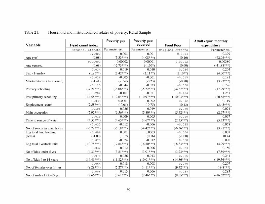
39

Table 21: Household and institutional correlates of poverty; Rural Sample

Variable Head count index Poverty gap Poverty gap


expenditure Marginal effects Parameter est. Parameter est. Marginal effects Parameter est.

Age (yrs) 0.0002

(0.08) 0.003

(5.33***) 0.001

(4.08***) 0.0004

(0.16) 0.399

(62.08***)

Age squared 0.00002

(0.68) -0.00002

(-2.73***) -0.00001 (-1.70*)

0.00002 (0.60)

-0.00380 (-41.88***)

Sex (1=male) 0.034

(1.95**) 0.019

(2.42***) 0.010

(2.11**) 0.036

(2.10**) 0.204

(4.00***)


-0.005 (-0.59)

-0.001 (-0.23)

-0.015 (-0.80)

0.191 (3.23***)


(-7.21***) -0.044

(-6.08***) -0.023

(-5.22***) -0.068

(-4.37***) 0.796

(17.29***)


(-14.58***) -0.101

(-12.64***) -0.051

(-10.97***) -0.194

(-10.03***) 1.287

(20.88***)


(2.58***) -0.0001 (-0.01)

-0.002 (-0.75)

0.002 (0.13)

0.119 (3.43***)


(7.92***) 0.036

(6.56***) 0.019

(5.80***) 0.070

(5.42***) 0.094

(2.67***)


(4.52***) 0.009

(4.65***) 0.005

(4.67***) 0.010

(2.35***) 0.067

(5.73***)


(-5.79***) -0.012

(-5.18***) -0.006

(-4.42***) -0.035

(-6.36***) 0.058


-0.006 (-1.00)

0.001 (0.19)

0.0003 (0.16)

-0.006 (-1.00)

0.007 (0.44


(-10.78***) -0.024

(-7.84***) -0.012

(-6.50***) -0.058

(-8.83***) 0.090

(4.99***)


(4.31***) 0.012

(3.81***) 0.006

(3.01***) 0.023

(3.23***) 0.150

(7.59***)


(16.41***) 0.026

(11.82***) 0.013

(10.01***) 0.065

(14.86***) -0.241

(-19.36***)

No. of females over 14 yrs 0.064

(8.29***) 0.018

(5.27***) 0.008

(4.11***) 0.070

(9.42***) -0.207

(-9.8***)


(7.66***) 0.013

(3.61***) 0.006

(2.46***) 0.068

(9.55***) -0.283

(-16.62***)

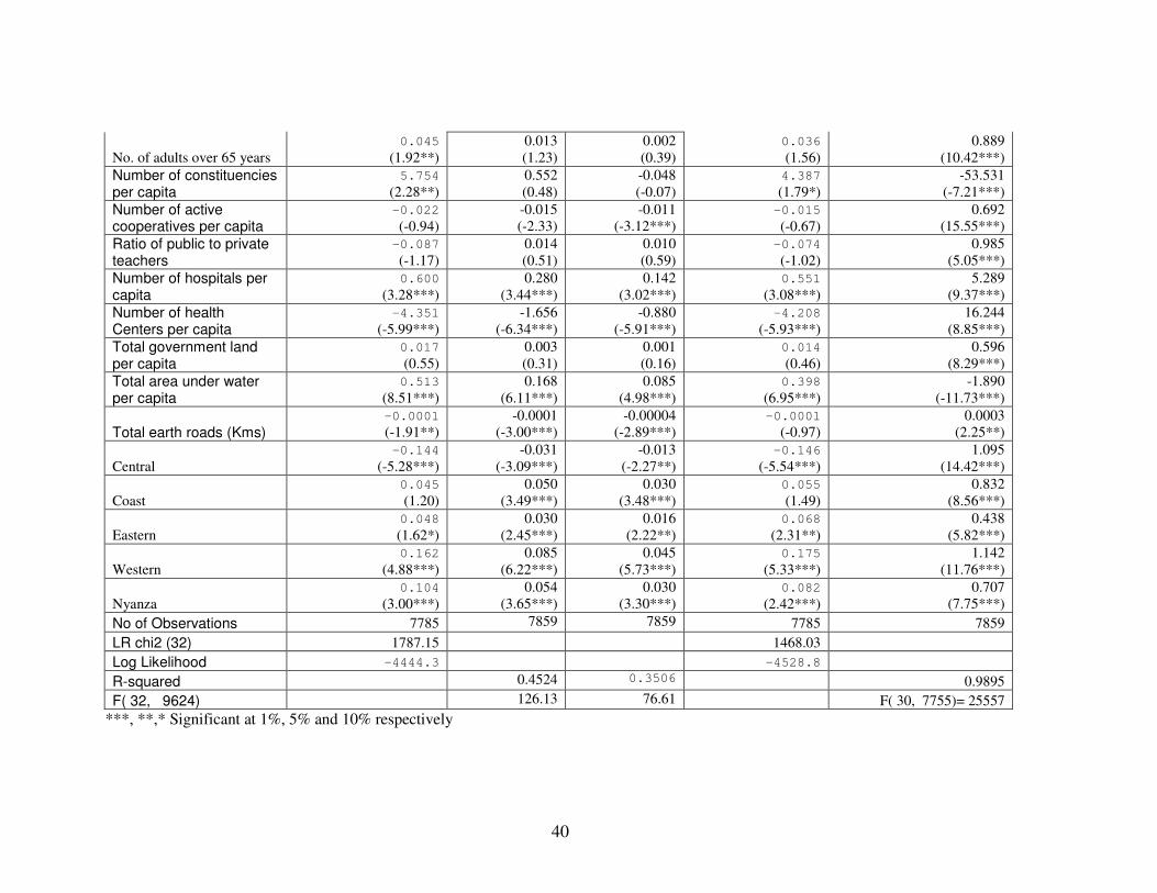
40


(1.92**) 0.013 (1.23)

0.002 (0.39)

0.036 (1.56)

0.889 (10.42***)

Number of constituencies per capita

5.754 (2.28**)

0.552 (0.48)

-0.048 (-0.07)

4.387 (1.79*)

-53.531 (-7.21***)


-0.022 (-0.94)

-0.015 (-2.33)

-0.011 (-3.12***)

-0.015 (-0.67)

0.692 (15.55***)


-0.087 (-1.17)

0.014 (0.51)

0.010 (0.59)

-0.074 (-1.02)

0.985 (5.05***)


0.600 (3.28***)

0.280 (3.44***)

0.142 (3.02***)

0.551 (3.08***)

5.289 (9.37***)


-4.351 (-5.99***)

-1.656 (-6.34***)

-0.880 (-5.91***)

-4.208 (-5.93***)

16.244 (8.85***)


0.017 (0.55)

0.003 (0.31)

0.001 (0.16)

0.014 (0.46)

0.596 (8.29***)


0.513 (8.51***)

0.168 (6.11***)

0.085 (4.98***)

0.398 (6.95***)

-1.890 (-11.73***)

Total earth roads (Kms) -0.0001 (-1.91**)

-0.0001 (-3.00***)

-0.00004 (-2.89***)

-0.0001 (-0.97)

0.0003 (2.25**)

Central -0.144

(-5.28***) -0.031

(-3.09***) -0.013

(-2.27**) -0.146

(-5.54***) 1.095

(14.42***)

Coast 0.045 (1.20)

0.050 (3.49***)

0.030 (3.48***)

0.055 (1.49)

0.832 (8.56***)

Eastern 0.048 (1.62*)

0.030 (2.45***)

0.016 (2.22**)

0.068 (2.31**)

0.438 (5.82***)

Western 0.162

(4.88***) 0.085

(6.22***) 0.045

(5.73***) 0.175

(5.33***) 1.142

(11.76***)

Nyanza 0.104

(3.00***) 0.054

(3.65***) 0.030

(3.30***) 0.082

(2.42***) 0.707

(7.75***) No of Observations 7785 7859 7859 7785 7859 LR chi2 (32) 1787.15 1468.03 Log Likelihood -4444.3 -4528.8 R-squared 0.4524 0.3506 0.9895 F( 32, 9624) 126.13 76.61 F( 30, 7755)= 25557


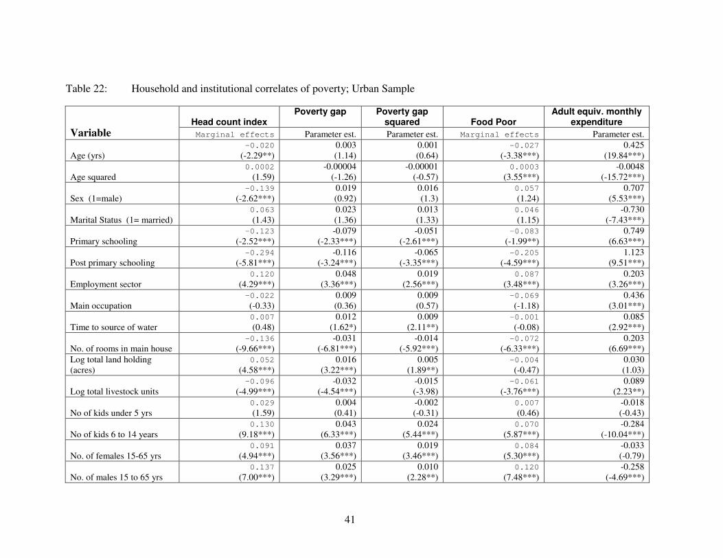
41

Table 22: Household and institutional correlates of poverty; Urban Sample

Head count index Poverty gap Poverty gap



Age (yrs) -0.020

(-2.29**) 0.003 (1.14)

0.001 (0.64)

-0.027 (-3.38***)

0.425 (19.84***)

Age squared 0.0002

(1.59) -0.00004

(-1.26) -0.00001

(-0.57) 0.0003

(3.55***) -0.0048

(-15.72***)

Sex (1=male) -0.139

(-2.62***) 0.019 (0.92)

0.016 (1.3)

0.057 (1.24)

0.707 (5.53***)

Marital Status (1= married) 0.063 (1.43)

0.023 (1.36)

0.013 (1.33)

0.046 (1.15)

-0.730 (-7.43***)


(-2.52***) -0.079

(-2.33***) -0.051

(-2.61***) -0.083

(-1.99**) 0.749

(6.63***)


(-5.81***) -0.116

(-3.24***) -0.065

(-3.35***) -0.205

(-4.59***) 1.123

(9.51***)


(4.29***) 0.048

(3.36***) 0.019

(2.56***) 0.087

(3.48***) 0.203

(3.26***)

Main occupation -0.022 (-0.33)

0.009 (0.36)

0.009 (0.57)

-0.069 (-1.18)

0.436 (3.01***)

Time to source of water 0.007 (0.48)

0.012 (1.62*)

0.009 (2.11**)

-0.001 (-0.08)

0.085 (2.92***)


(-9.66***) -0.031

(-6.81***) -0.014

(-5.92***) -0.072

(-6.33***) 0.203


0.052 (4.58***)

0.016 (3.22***)

0.005 (1.89**)

-0.004 (-0.47)

0.030 (1.03)


(-4.99***) -0.032

(-4.54***) -0.015 (-3.98)

-0.061 (-3.76***)

0.089 (2.23**)

No of kids under 5 yrs 0.029 (1.59)

0.004 (0.41)

-0.002 (-0.31)

0.007 (0.46)

-0.018 (-0.43)


(9.18***) 0.043

(6.33***) 0.024

(5.44***) 0.070

(5.87***) -0.284

(-10.04***)

No. of females 15-65 yrs 0.091

(4.94***) 0.037

(3.56***) 0.019

(3.46***) 0.084

(5.30***) -0.033 (-0.79)


(7.00***) 0.025

(3.29***) 0.010

(2.28**) 0.120

(7.48***) -0.258

(-4.69***)

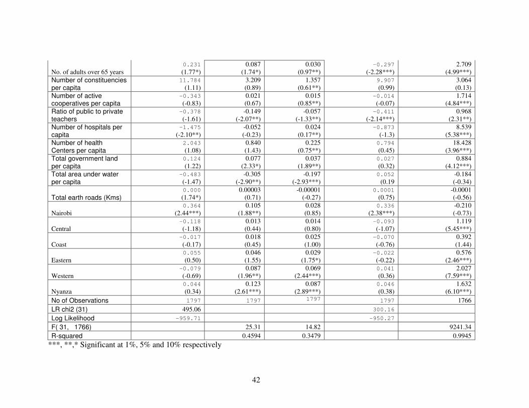
42

No. of adults over 65 years 0.231 (1.77*)

0.087 (1.74*)

0.030 (0.97**)

-0.297 (-2.28***)

2.709 (4.99***)

Number of constituencies per capita

11.784 (1.11)

3.209 (0.89)

1.357 (0.61**)

9.907 (0.99)

3.064 (0.13)


-0.343 (-0.83)

0.021 (0.67)

0.015 (0.85**)

-0.014 (-0.07)

1.714 (4.84***)


-0.378 (-1.61)

-0.149 (-2.07**)

-0.057 (-1.33**)

-0.411 (-2.14***)

0.968 (2.31**)


-1.475 (-2.10**)

-0.052 (-0.23)

0.024 (0.17**)

-0.873 (-1.3)

8.539 (5.38***)


2.043 (1.08)

0.840 (1.43)

0.225 (0.75**)

0.794 (0.45)

18.428 (3.96***)


0.124 (1.22)

0.077 (2.33*)

0.037 (1.89**)

0.027 (0.32)

0.884 (4.12***)


-0.483 (-1.47)

-0.305 (-2.90**)

-0.197 (-2.93***)

0.052 (0.19

-0.184 (-0.34)

Total earth roads (Kms) 0.000 (1.74*)

0.00003 (0.71)

-0.00001 (-0.27)

0.0001 (0.75)

-0.0001 (-0.56)

Nairobi 0.364

(2.44***) 0.105

(1.88**) 0.028 (0.85)

0.336 (2.38***)

-0.210 (-0.73)

Central -0.118 (-1.18)

0.013 (0.44)

0.014 (0.80)

-0.093 (-1.07)

1.119 (5.45***)

Coast -0.017 (-0.17)

0.018 (0.45)

0.025 (1.00)

-0.070 (-0.76)

0.392 (1.44)

Eastern 0.055 (0.50)

0.046 (1.55)

0.029 (1.75*)

-0.022 (-0.22)

0.576 (2.46***)

Western -0.079 (-0.69)

0.087 (1.96**)

0.069 (2.44***)

0.041 (0.36)

2.027 (7.59***)

Nyanza 0.044 (0.34)

0.123 (2.61***)

0.087 (2.89***)

0.046 (0.38)

1.632 (6.10***)

No of Observations 1797 1797 1797 1797 1766 LR chi2 (31) 495.06 300.16 Log Likelihood -959.71 -950.27 F( 31, 1766) 25.31 14.82 9241.34 R-squared 0.4594 0.3479 0.9945


43

6 CONCLUSION

This paper investigates the impact of institutional factors on regional poverty in Kenya using descriptive and econometric methods. We test the hypothesis that institutions improve household welfare and therefore regional disparities in institutional endowments will result to regional disparities in poverty. The paper is based on both secondary and survey data. The secondary data comprises the distribution of institutions across districts in Kenya, and is drawn from government publications and relevant ministries, while the survey data is drawn from the Welfare Monitoring Survey (III) household level data. To achieve the key objective of the paper, we map the district level institutional data onto the WMS dataset. Descriptive statistics suggest that taking into account population density, there seem to be marked regional disparities in the distribution of key institutions in Kenya. Coast province, which ranks 5th poorest of the 6 rural provinces seem to be at a relative advantage in terms of institutional endowments, while Western province is at a relative disadvantage. Nyanza province, the poorest province in 1997, does not seem to fare too badly compared to other regions. These results do not show a clear correlation between institutional endowment and poverty but imply that that analysis of the institutional determinants of poverty need to take into account other determinants of poverty as well. The empirical analysis focuses on the determinants of the FGT poverty measures, the food poverty status and the adult equivalent monthly expenditure. Regressions results uncover no significant effect of parliamentary representation on poverty. However, the results suggest that the number of active cooperatives, ratio of public to private secondary school teachers, government land ownership and social services are important determinants of poverty. More robust results are however found when we measure welfare through consumption expenditures rather than poverty. The findings are consistent with previous studies on institutional determinants of poverty. In addition, we find that household characteristics are important correlates of poverty. Most notable is education attainment, which exerts a significant and increasing impact on welfare. Family composition and assets are also found to be important determinants of welfare. The paper also finds that except for levels of significance, the factors determining poverty in rural areas are also associated with higher poverty in urban areas. These results point to a number of policy options. Concerning household characteristics, the results imply that improvements in education attainment would improve household welfare. Reducing household size and increasing assets would also improve welfare. These results have important bearing on Economic Recovery Strategies (ERS) in Kenya as well as the Millineum Development Goals (MDGS) of reducing extreme incomes poverty and

44

inequality. ERS identify landlessness, lack of education and poor enrollment, low productivity, inequality in land and capital and vulnerability as key development issues. Our results point at the need for policies that target poor households, who are likely to be asset poor and whose members are less likely to go to school. In particular, the state needs to improve access of the poor to productive resources. Employment creation and agricultural sector growth should also be prioritized as outlined in the ERS. Though the government has affirmed its commitment towards this direction, more effort and resources are required in order to accelerate economic growth, raise incomes for the poor and improve equity and quality of welfare, all which have important implication on poverty reduction. Results for institutional factors imply the need for regional targeting in order to balance regional distribution of institutions to reduce regional disparities in poverty.

45

REFERENCES

Appleton S. (2002). ‘The rich are just like us, only richer’: Poverty functions or consumption functions? Journal of African Economies, 10(4): 433-469. Ali, A.G., E. Thorbecke. 2000. The State and Path of Poverty in Sub-Saharan Africa: Some Preliminary Results. Journal of African Economies, 9 (Suppl.1):9-40. Geda A., N. de Jong, G. Mwabu and M.S. Kimenyi. 2001. Determinants of Poverty in Kenya: Household-Level Analysis. The Kenya Institute for Public Policy Research and Analysis (KIPPRA). Discussion Paper Series No. 9. Glewwe, P (1991), Investigating the determinants of household welfare in Cote d‘Ivoire. Journal of development studies, 35:307-337. Greer, J and E. Thorbecke. 1986. “Food Poverty Profile Applied to Kenyan Smallholders,” Economic Development and Cultural Change, 35(1):115-141. Kabubo-Mariara J. 2004. The Labour Market in Kenya: Structure, Reforms and Policy Issues. Mimeo, World Bank, Nairobi Kabubo-Mariara J. 2005. Land Conservation In Kenya: The Role of Property Rights. Final report submitted to African Economic Research Consortium, Nairobi, February. Kabubo-Mariara J. and Kirii, D.M. 2005. Determinants of Demand for Schooling in Kenya: A Regional Analysis. African Economic Research Consortium. Mimeo, Nairobi Kabubo-Mariara J., G.K. Nd’enge and D.M. Kirii, 2005. Evolution and Determinants of Non-monetary Indicators of Poverty in Kenya: Children’s Nutritional Status, 1998-2003. African Economic Research Consortium. Mimeo, Nairobi Kabubo-Mariara J., and G.K., Ndeng’e. 2004. Measuring and Monitoring Poverty: The Case of Kenya. Poverty Analysis and Data Initiative (PADI), Mimeo, Nairobi. http://www.worldbank.org/afr/padi/resources.htm Kebede B. and A. Shimeles. 2004. Institutional Aspects of Rural Poverty: Land Tenure and Vulnerability to Shocks in Ethiopia. FASID, Japan. Morrisson, C., E. Thorbecke, H. Guilmeau and C. Linskens. 2000. “Poverty and Malnutrition in Sub-Saharan Africa,” Cornell Food and Nutrition Policy Program, Cornell University, Ithaca, mimeo. Mukui, J. T. 1994, “Kenya: Poverty Profiles, 1982-92,”Ministry of Finance and Planning, Nairobi, mimeo.

46

Mwabu G., J.B. Kirimi, G. Ndeng’e, R. Gesami and W. Masai. 2004. Rural Poverty and Rural Institutions in a Globalizing Economy: The Case of Kenya. FASID, Japan. Mwabu et al. 2000. “Poverty in Kenya: Profiles and Determinants,” University of Nairobi and Ministry of Finance and Planning, mimeo. Nissanke M. 2004. Poverty in a Globalizing Economy: Overview. FASID, Japan. North, D. 1991. “Institutions,” Journal of Economic Perspectives, 5(1):97-112. Oduro A.D., I. Osei-Akoto and I Acquaye. 2004. Poverty in a Globalizing Economy: The role of Rural Institutions. FASID, Japan. Oyugi L., et al. 2000. “Determinants of Poverty in Kenya,” African Journal of Economic Policy, Vol. 7. Platteau, J-P. 1994. Behind the Market Stage Where Real Societies Exist – Part I: The Role of Public and Private Order Institutions, Journal of Development Studies, 30, pp. 533-577. Putnam, R. D. 1993. Making Democracy Work: Civic Transactions in Modern Italy, Princeton: Princeton University Press. Republic of Kenya. 2000. Second Report on Poverty in Kenya, vol I Incidence and Depth of Poverty, Ministry of Finance and Planning, Nairobi. Republic of Kenya. 1997. Welfare Monitoring Survey III Database. Central Bureau of Statistics. Ministry of Planning and National Development, Nairobi. Republic of Kenya, Statistical Abstract, various issues, Central Bureau of Statistics, Ministry of Planning and National Development, Nairobi. Van der Berg S. 2004. Poverty and the Role of Rural Institutions in a Globalizing South African Economy. FASID, Japan.

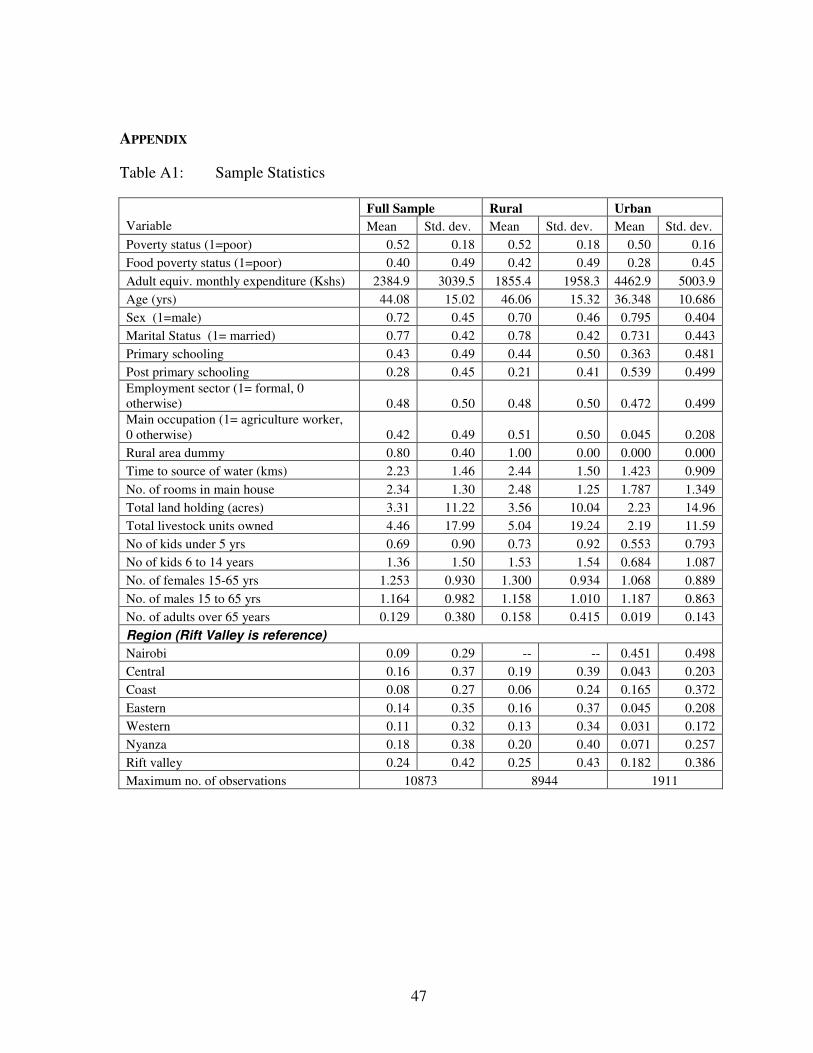
47

APPENDIX

Table A1: Sample Statistics

Full Sample Rural Urban Variable Mean Std. dev. Mean Std. dev. Mean Std. dev. Poverty status (1=poor) 0.52 0.18 0.52 0.18 0.50 0.16 Food poverty status (1=poor) 0.40 0.49 0.42 0.49 0.28 0.45 Adult equiv. monthly expenditure (Kshs) 2384.9 3039.5 1855.4 1958.3 4462.9 5003.9 Age (yrs) 44.08 15.02 46.06 15.32 36.348 10.686 Sex (1=male) 0.72 0.45 0.70 0.46 0.795 0.404 Marital Status (1= married) 0.77 0.42 0.78 0.42 0.731 0.443 Primary schooling 0.43 0.49 0.44 0.50 0.363 0.481 Post primary schooling 0.28 0.45 0.21 0.41 0.539 0.499 Employment sector (1= formal, 0 otherwise) 0.48 0.50 0.48 0.50 0.472 0.499 Main occupation (1= agriculture worker, 0 otherwise) 0.42 0.49 0.51 0.50 0.045 0.208 Rural area dummy 0.80 0.40 1.00 0.00 0.000 0.000 Time to source of water (kms) 2.23 1.46 2.44 1.50 1.423 0.909 No. of rooms in main house 2.34 1.30 2.48 1.25 1.787 1.349 Total land holding (acres) 3.31 11.22 3.56 10.04 2.23 14.96 Total livestock units owned 4.46 17.99 5.04 19.24 2.19 11.59 No of kids under 5 yrs 0.69 0.90 0.73 0.92 0.553 0.793 No of kids 6 to 14 years 1.36 1.50 1.53 1.54 0.684 1.087 No. of females 15-65 yrs 1.253 0.930 1.300 0.934 1.068 0.889 No. of males 15 to 65 yrs 1.164 0.982 1.158 1.010 1.187 0.863 No. of adults over 65 years 0.129 0.380 0.158 0.415 0.019 0.143 Region (Rift Valley is reference) Nairobi 0.09 0.29 -- -- 0.451 0.498 Central 0.16 0.37 0.19 0.39 0.043 0.203 Coast 0.08 0.27 0.06 0.24 0.165 0.372 Eastern 0.14 0.35 0.16 0.37 0.045 0.208 Western 0.11 0.32 0.13 0.34 0.031 0.172 Nyanza 0.18 0.38 0.20 0.40 0.071 0.257 Rift valley 0.24 0.42 0.25 0.43 0.182 0.386 Maximum no. of observations 10873 8944 1911

Regional and Institutional Determinants of Poverty: The … and Institutional Determinants of...

Documents

Transcript of Regional and Institutional Determinants of Poverty: The … and Institutional Determinants of...