M.Sc. ThesisMaster of Science in Engineering

Regime-Based Asset AllocationDo Profitable Strategies Exist?

Peter Nystrup

Kongens LyngbyJuly 2014

Technical University of DenmarkDepartment of Applied Mathematics and Computer ScienceMatematiktorvet, Building 303B2800 Kongens Lyngby, DenmarkPhone +45 4525 3031compute@compute.dtu.dkwww.compute.dtu.dk

Short Contents

Short Contents i

Abstract iii

Resumé v

Preface vii

Acknowledgements ix

Acronyms xi

Contents xiii

1 Introduction 1

2 Index Data 11

3 Markov-Switching Mixtures 27

4 Strategic Asset Allocation 61

5 Regime-Based Asset Allocation 71

6 Summary and Conclusion 83

References 87

A R-code 93

B Parameter Estimates 103

C Additional Figures and Tables 107

ii

Abstract

Regime shifts present a big challenge to traditional strategic asset allocation,demanding a more adaptive approach. In the presence of time-varying invest-ment opportunities, portfolio weights should be adjusted as new informationarrives. Regime-switching models can match the tendency of financial marketsto change their behavior abruptly and the phenomenon that the new behavioroften persists for several periods after a change. They are well suited to capturethe stylized behavior of many financial series including skewness, leptokurtosis,volatility persistence, and time-varying correlations.This thesis builds on this empirical evidence to develop a quantitative frameworkfor regime-based asset allocation. It investigates whether regime-based investingcan effectively respond to changes in financial regimes at the portfolio levelin an effort to provide better long-term results when compared to more staticapproaches. The thesis extends previous work by considering both discrete-timeand continuous-time models, models with different numbers of states, differentunivariate and multivariate state-dependent distributions, and different sojourntime distributions. Out-of-sample success depends on developing a way to modelthe non-linear and non-stationary behavior of asset returns.Dynamic asset allocation strategies are shown to add value over strategies basedon rebalancing to static weights with rebalancing in itself adding value comparedto buy-and-hold strategies in an asset universe consisting of a global stock index,a global government bond index, and a commodity index. The tested strate-gies based on an adaptively estimated two-state Gaussian hidden Markov modeloutperform a rebalancing strategy out of sample after accounting for transac-tion costs, assuming no knowledge of future returns, and with a realistic delaybetween the identification of a regime change and the portfolio adjustment.Keywords: Regime switching; Markov-switching mixtures; Non-linear TimeSeries Modeling; Daily Returns; Adaptivity; Leptokurtic distributions; Volatilityclustering; Dynamic asset allocation.

iv

Resumé

Regimeskift udgør en stor udfordring for traditionel strategisk aktivallokering,da de sætter krav til en mere adaptiv tilgang. Ved tilstedeværelsen af tidsvari-erende investeringsmuligheder bør porteføljevægte opdateres, efterhånden somny information kommer til. Regimeskiftsmodeller kan matche finansielle marked-ers tendens til pludseligt at skifte opførsel og det fænomen, at den nye opførselofte varer ved længe efter et skift. De er velegnede til at fange den stiliseredeopførsel, der er kendetegnende for mange finansielle serier, herunder skævhed,leptokurtosis, volatilitetsklumpning og tidsvarierende korrelationer.Formålet med denne afhandling er at udvikle en kvantitativ ramme for regime-baseret aktivallokering. Det undersøges, hvorvidt regimebaseret investering kanreagere på effektiv vis på ændringer i finansielle regimer på porteføljeniveau meddet formål at skabe bedre langsigtede resultater sammenlignet med mere statisketilgange. Afhandlingen udvider tidligere studier ved at inkludere modeller i bådediskret og kontinuert tid, modeller med forskellige antal regimer, forskellige uni-variate og multivariate regimebetingede fordelinger og forskellige opholdstids-fordelinger. Out-of-sample succes afhænger af udviklingen af en model, derbeskriver finansielle afkasts ikke-lineære og ikke-stationære opførsel.Det bliver vist, at dynamiske aktivallokeringsstrategier tilfører værdi sammen-lignet med strategier baseret på rebalancering til statiske vægte. Rebalancering isig selv tilfører værdi sammenlignet med køb-og-hold strategier i et aktivunivers,der består af et globalt aktieindeks, et globalt statsobligationsindeks og et rå-vareindeks. De testede strategier, baseret på en adaptivt estimeret gaussiskskjult Markov model med to regimer, outperformer en rebalanceringsstrategiout-of-sample efter handelsomkostninger, uden kendskab til fremtidige afkastog med en realistisk forsinkelse mellem identifikationen af et regimeskift og im-plementeringen af portføljetilpasningen.Nøgleord: Regimeskift; Markov-skiftende miksturer; Ikke-lineær tidsrække-modellering; Daglige afkst; Adaptivitet; Leptokurtiske fordelinger; Volatilitets-klumpning; Dynamisk aktivallokering.

vi

Preface

This thesis was prepared at the Department of Applied Mathematics and Com-puter Science at the Technical University of Denmark (DTU) in partial fulfill-ment of the requirements for acquiring the M.Sc. degree in engineering withhonors.The thesis deals with different aspects of mathematical modeling of the stylizedbehavior of financial returns using regime-switching models with the aim ofdeveloping a quantitative framework for regime-based asset allocation. Thedeveloped strategies are tested out of sample under realistic assumptions toensure that the conclusions have practical relevance.The process that led to this thesis began in the spring of 2013 when I attendeda class on hidden Markov models at DTU. In the summer of 2013, I began aspecial course on regime modeling of financial data with Henrik Madsen at DTU.Erik Lindström later joined the special course that led to the preparation of anarticle (Nystrup et al. 2014). I got the idea for the thesis when I read the articleon Markov-switching asset allocation by Bulla et al. (2011). In continuation ofthe work on the article there was an initial focus on the estimation of continuous-time models, but the strategies ended up being based on adaptively estimateddiscrete-time hidden Markov models.

Copenhagen, July 2014

Peter Nystrup

viii

Acknowledgements

I want to thank my supervisors Professor Henrik Madsen (Technical Universityof Denmark) and Associate Professor Erik Lindström (Lund University, Sweden)for the many interesting discussions. Henrik’s calendar is always fully booked,but he spared time to share his vast experience with mathematical modelingand supervise the project anyway. Fortunately, Erik was visiting DTU on aregular basis in the fall of 2013 and the beginning of 2014, so he was able toco-supervise the project. Erik always made time to answer questions and toresearch for new ideas that could contribute to the project.I also want to thank Bo William Hansen, Henrik Olejasz Larsen, and the restof my colleagues at Sampension for their contributions to the project. Bo andHenrik showed a lot of interest in the project right from the beginning andencouraged me to work on the topic. We have had many interesting discussionsand I have drawn on their background in economics and practical experiencewith asset allocation.MSCI Inc., J.P. Morgan, and Standard & Poor’s should be mentioned as thesources of the index data that was accessed through Bloomberg.

x

Acronyms

ACF Autocorrelation function

AIC Akaike information criterion

BIC Bayesian information criterion

CAPM Capital Asset Pricing Model

CDLL Complete-data log-likelihood

CPI Consumer price index

CTHMM Continuous-time hidden Markov model

CVaR Conditional Value-at-Risk

DAA Dynamic asset allocation

DM Developed market

EM Emerging market

EM Expectation–maximization

ER Expected return

ETF Exchange-traded fund

GDP Gross domestic product

GFC Global finacial crisis

GLRT Generalized likelihood ratio test

HMM Hidden Markov model

HSMM Hidden semi-Markov model

xii Acknowledgements

JPM GBI J.P. Morgan Government Bond Index

MCMC Markov chain Monte Carlo

MDD Maximum drawdown

ML Maximum likelihood

MSCI ACWI Morgan Stanley Capital International All Country World Index

RR Realized return

S&P GSCI Standard & Poor’s Goldman Sachs Commodity Index

SAA Strategic asset allocation

SD Standard deviation

SR Sharpe ratio

TAA Tactical asset allocation

VaR Value-at-Risk

VIX Chicago Board Options Exchange Market Volatility Index

Contents

Short Contents i

Abstract iii

Resumé v

Preface vii

Acknowledgements ix

Acronyms xi

Contents xiii

1 Introduction 11.1 Dynamic Asset Allocation . . . . . . . . . . . . . . . . . . . . . . 21.2 Time Horizon . . . . . . . . . . . . . . . . . . . . . . . . . . . . . 31.3 Stylized Facts and Markov-Switching Mixtures . . . . . . . . . . 41.4 Regime-Switching Asset Allocation . . . . . . . . . . . . . . . . . 61.5 Thesis Statement . . . . . . . . . . . . . . . . . . . . . . . . . . . 9

2 Index Data 112.1 The MSCI ACWI . . . . . . . . . . . . . . . . . . . . . . . . . . . 122.2 The JPM GBI . . . . . . . . . . . . . . . . . . . . . . . . . . . . 132.3 The S&P GSCI . . . . . . . . . . . . . . . . . . . . . . . . . . . . 15

The Commodity Risk Premium . . . . . . . . . . . . . . . . . . . 172.4 Distributional Properties . . . . . . . . . . . . . . . . . . . . . . . 17

Log-Returns . . . . . . . . . . . . . . . . . . . . . . . . . . . . . . 192.5 Temporal Properties . . . . . . . . . . . . . . . . . . . . . . . . . 212.6 In-Sample Adjustment . . . . . . . . . . . . . . . . . . . . . . . . 25

3 Markov-Switching Mixtures 27

xiv Contents

3.1 Hidden Markov Models in Discrete Time . . . . . . . . . . . . . . 28The Forward–Backward Algorithm . . . . . . . . . . . . . . . . . 30The Baum–Welch Algorithm . . . . . . . . . . . . . . . . . . . . 31Decoding . . . . . . . . . . . . . . . . . . . . . . . . . . . . . . . 35

3.2 Hidden Semi-Markov Models . . . . . . . . . . . . . . . . . . . . 363.3 Hidden Markov Models in Continuous Time . . . . . . . . . . . . 38

A Continuous-Time Version of the Baum–Welch Algorithm . . . 403.4 Model Estimation and Selection . . . . . . . . . . . . . . . . . . . 42

Exploring the Estimated Models . . . . . . . . . . . . . . . . . . 43Matching the Moments . . . . . . . . . . . . . . . . . . . . . . . . 46Reproducing the Long Memory . . . . . . . . . . . . . . . . . . . 47Model Selection . . . . . . . . . . . . . . . . . . . . . . . . . . . . 47Parameter Stationarity . . . . . . . . . . . . . . . . . . . . . . . . 50

3.5 Gradient-Based Methods . . . . . . . . . . . . . . . . . . . . . . . 50Recursive Estimation . . . . . . . . . . . . . . . . . . . . . . . . . 54Adaptive Estimation . . . . . . . . . . . . . . . . . . . . . . . . . 56

4 Strategic Asset Allocation 614.1 Scenario Generation . . . . . . . . . . . . . . . . . . . . . . . . . 624.2 The Mean–CVaR Model . . . . . . . . . . . . . . . . . . . . . . . 644.3 Results . . . . . . . . . . . . . . . . . . . . . . . . . . . . . . . . . 67

In Sample . . . . . . . . . . . . . . . . . . . . . . . . . . . . . . . 67Rebalancing . . . . . . . . . . . . . . . . . . . . . . . . . . . . . . 68Out of Sample . . . . . . . . . . . . . . . . . . . . . . . . . . . . 70

5 Regime-Based Asset Allocation 715.1 Decoding the Hidden States . . . . . . . . . . . . . . . . . . . . . 725.2 In-Sample Testing . . . . . . . . . . . . . . . . . . . . . . . . . . 775.3 Out-of-Sample Testing . . . . . . . . . . . . . . . . . . . . . . . . 79

6 Summary and Conclusion 836.1 Discussion . . . . . . . . . . . . . . . . . . . . . . . . . . . . . . . 846.2 Future Work . . . . . . . . . . . . . . . . . . . . . . . . . . . . . 85

References 87

A R-code 93A.1 Discrete-time Baum–Welch Algorithm . . . . . . . . . . . . . . . 93A.2 Continuous-time Baum–Welch Algorithm . . . . . . . . . . . . . 96A.3 Mean–CVaR optimization . . . . . . . . . . . . . . . . . . . . . . 101

B Parameter Estimates 103

C Additional Figures and Tables 107

CHAPTER 1Introduction

The behavior of financial markets changes abruptly. While some changes maybe transitory, the changed behavior often persists for many periods. The mean,volatility, and correlation patterns in stock returns, for example, changed dra-matically at the start of, and continued through the global financial crisis (GFC)of 2007–2008. Similar regime changes, some of which can be recurring (recessionsversus expansions) and some of which can be permanent (structural breaks), areprevalent across a wide range of financial markets and in the behavior of manymacro variables (Ang and Timmermann 2011).The observed regimes in financial markets are closely related to the phases ofthe business cycle (see e.g. Campbell 1998, Cochrane 2005). In the long run,the gross domestic product (GDP) tends to follow a trend path (growth). Inthe short to medium term, the GDP fluctuates around the long-term trend.The recurring pattern of recession and expansion is called the business cycle,although the length and severity of the cycles are irregular. The duration ofa full cycle can be anything from one year to ten or twelve years (Burns andMitchell 1946).Regime changes present a big challenge to traditional strategic asset allocation(SAA), demanding a more adaptive approach. Moreover, the time-varying be-havior of risk premiums, volatilities, and correlations have important implica-tions for risk management. Understanding the correlations and their evolutionthrough time is a prerequisite to evaluate the undiversifiable risk associated withthe financial cycle.This thesis examines whether regime-based asset allocation can effectively re-spond to financial regimes in an effort to provide better long-term results when

2 1 Introduction

compared to static approaches. The first chapter introduces the concept ofdynamic asset allocation (DAA), the importance of the time horizon, the useof Markov-switching mixture models to capture the time-varying behavior offinancial returns, and their applicability to regime-based asset allocation.

1.1 Dynamic Asset AllocationAsset allocation is the decision of how to divide a portfolio among the differentmajor asset classes. It is the most important determinant of portfolio perfor-mance (see e.g. Brinson et al. 1986, Ibbotson and Kaplan 2000). Althoughasset class behavior can vary significantly over shifting economic scenarios—nosingle asset class dominates under all economic conditions—traditional SAA ap-proaches make no effort to adapt to such shifts. Traditional approaches insteadseek to develop static “all-weather” portfolios that optimize efficiency across arange of economic scenarios (Sheikh and Sun 2012). If economic conditions arepersistent and strongly linked to asset class performance, then a DAA strategyshould add value over static weights. The purpose of a dynamic strategy isto take advantage of positive economic regimes, as well as withstand adverseeconomic regimes and reduce potential drawdowns.Regime-based investing is distinct from tactical asset allocation (TAA). Whilethe latter is shorter term, higher frequency (i.e., weekly or monthly), and drivenprimarily by valuation considerations, regime-based investing targets a longertime horizon (i.e., a year or more) and is driven by changing economic fun-damentals. A regime-based approach has the flexibility to adapt to changingeconomic conditions within a benchmark-based investment policy which can in-volve more than one rebalancing within a year. It straddles a middle groundbetween strategic and tactical (Sheikh and Sun 2012).Strategic asset allocation is long-term in nature and based on long-term views ofasset class performance although it is not unusual to update the forecasts everyyear and, hence, rebalance annually (Dahlquist and Harvey 2001). Strategicinvestors, such as pension plans, that invest with a long time horizon typicallyface constraints on the size of possible deviations from their benchmark alloca-tion. Although the possible tilts might be small, strategic investors can stillbenefit from reacting to significant regime shifts (see e.g. Kritzman et al. 2012).DAA is more restricted than SAA in terms of the size of the investment oppor-tunity set as it is difficult to invest dynamically in direct real estate, forestry,private equity etc. Investments in illiquid asset classes require a long time hori-zon. This is worth mentioning given that unlisted asset classes have graduallybecome a larger part of professional investors’ portfolios in recent years (Ed-wards and Manjrekar 2014).The goal of DAA is not to predict the next regime shift or future market move-ments. The intention is to identify as fast as possible with as high credibility as

1.2 Time Horizon 3

possible when a regime shift has occurred and then benefit from the persistencein equilibrium returns and volatilities. As a market participant, it is difficult tosee through the daily noise and short-term volatility, therefore a mathematicalmodel that captures the underlying structures in the market data can be useful.

A dynamic strategy can be profitable even if markets are efficient. A capitalmarket is said to be efficient if prices in the market fully reflect available in-formation. When this condition is satisfied, market participants cannot earn ariskless profit on the basis of available information, i.e. there are no arbitrageopportunities (Fama 1970). The term “fully reflect” implies the existence of anequilibrium model which might be stated either in terms of equilibrium pricesor equilibrium expected returns. Trends can be present in efficient markets ifthe equilibrium expected return changes over time.

The existence of a business cycle where the expected rate of return on capitalchanges over time is one example. The business cycle could result from any setof factors, but as long as the business cycle is not a deterministic phenomenon,asset prices need not follow a random walk with a constant or deterministic trend(Levich 2001). In some periods, no significant events will take place to causeprices to change, thus returns will essentially reflect noise. In other periods,several important events will influence returns. A focus on identifying ratherthan predicting regime changes is indeed consistent with a belief in efficientmarkets.

1.2 Time Horizon

It is a common belief that time diversification reduces risk and therefore long-term investors should have a higher proportion of risky assets in their portfoliothan short-term investors (see e.g. Siegel 2007, Guidolin and Timmermann 2007).With a regime-based approach it does not matter whether the horizon is one,two, or ten years because the aim is to rebalance whenever a regime shift hasoccurred. The horizon, however, is assumed to be long enough that it makessense to defray the cost of rebalancing. The portfolio is optimized conditional onbeing in the current regime and asset returns are assumed to follow a randomwalk within each regime. The proportion of risky asset will depend on thecurrent regime and the level of risk aversion, but not the time horizon.

Oftentimes the frequency of the analyzed data is chosen to reflect the lengthof the investment horizon, meaning monthly or annual data for long-term in-vestment decisions. Bulla et al. (2011) were among the first to consider regime-switching asset allocation based on daily returns. By using daily rather thanmonthly data the impact of wrong regime forecasts reduces from an entire monthto a single trading day and the delay in identifying and addressing regime shiftsis shorter. With the shorter response time it is feasible to wait until the same

4 1 Introduction

regime has been decoded for a number of days before changing the allocation inorder to minimize the costs of trading on spurious signals.Bulla et al. (2011) further argued that the use of daily data increases the amountof data available for markets with a short history, but for many financial indicesmonthly data is available with a much longer history than daily data. Theoptimal length of the data period is debatable, but it should span at least thetime needed for a financial cycle to unfold. It would, presumably, be favorable ifthe period included more than one cycle. On the other hand, the longer the datahorizon the more questionable it is whether stationarity of the data-generatingprocess can be assumed.The use of daily data presents some challenges. Daily returns contain a lot ofnoise and extreme observations that are evened out on a monthly basis. For ex-ample, if returns are conditionally normal, conditional on a variance parameterwhich is itself random, then the Central Limit Theorem applies to the result-ing heavy-tailed unconditional distribution as it has a finite variance and finitehigher order moments. Consequently, long-horizon returns will tend to be closerto the normal distribution than short-horizon returns (Campbell et al. 1997). Itcomplicates the modeling significantly and is likely part of the reason why it ismore popular to consider monthly data. In addition, the use of daily data makesthe link to macroeconomic data more difficult. In spite of the complications, thearguments for considering daily rather than monthly data are compelling.

1.3 Stylized Facts and Markov-Switching MixturesThe normal distribution is a poor fit to most financial returns. Mixtures ofnormal distributions provide a better fit as they are able to reproduce both theskewness and leptokurtosis often observed (see e.g. Cont 2001). An extension toa Markov switching mixture model, also referred to as a hidden Markov model(HMM), is often used to capture both the distributional and temporal propertiesof financial returns. The class of Markov-switching models was introduced tofinancial econometrics by Hamilton (1989, 1990). In an HMM, the distributionthat generates an observation depends on the state of an underlying and unob-served Markov chain. Although the states are identified through a statisticalfiltering procedure, they can often be interpreted in terms of economic cycles(see e.g. Ahlgren and Dahl 2010).Rydén et al. (1998) showed the ability of an HMM to reproduce most of thestylized facts of daily return series introduced by Granger and Ding (1995a,b)using daily returns of the S&P 500 stock index from 1928 to 1991. The onestylized fact that they could not reproduce was the persistence of the squareddaily returns (i.e., volatility).According to Bulla and Bulla (2006), the lack of flexibility of an HMM to modelthis temporal higher order dependence can be explained by the implicit assump-

1.3 Stylized Facts and Markov-Switching Mixtures 5

tion of geometrically distributed sojourn times in the hidden states. Silvestrovand Stenberg (2004), among others, argued that the memoryless property of thegeometric distribution is inadequate from an empirical perspective, although itis consistent with the no-arbitrage principle.Bulla and Bulla (2006) considered hidden semi-Markov models (HSMMs) inwhich the sojourn time distribution is modeled explicitly for each hidden stateso that the Markov property is transferred to the imbedded first-order Markovchain. They showed that HSMMs with negative binomial sojourn time distribu-tions reproduced most of the stylized facts comparably well, and often better,than the HMM for eighteen series of daily stock market sector returns from1987 to 2005. Specifically, they found HSMMs to reproduce the long-memoryproperty of squared daily returns much better than the HMM. They did not,however, consider the complicated problem of selecting the most appropriatesojourn time distributions and they only considered models with two hiddenstates.Bulla (2011) later showed that HMMs with t-distributed components reproducemost of the stylized facts as well or better than the Gaussian HMM, while atthe same time increasing the persistence of the visited states and the robustnessto outliers. Bulla (2011) also found that models with three states provided abetter fit than models with two states to daily returns of the S&P 500 indexfrom 1928 to 2007.The fact that increasing the number of states leads to a much better fit to theempirical moments and the persistence of squared daily returns was confirmedin Nystrup et al. (2014). The quadratic increase in the number of parameterswith the number of states is a major limitation of discrete-time HMMs andHSMMs. In Nystrup et al. (2014) it was shown how a continuous-time formula-tion leads to a linear rather than quadratic growth in the number of parameters.A continuous-time hidden Markov model (CTHMM) with four states was foundto provide a better fit to daily returns of the S&P 500 index than the discrete-time models with three states with a similar number of parameters. There wasno indication that the memoryless property of the sojourn time distribution wasinconsistent with the long-memory property of the squared daily returns.Kritzman and Li (2010) used a different approach based on discriminant analysisto show that financial turbulence has been highly persistent and risk-adjustedreturns have been substantially lower during turbulent periods, irrespective ofthe source of turbulence. Their study included monthly returns from 1980 to2009 of six asset-class indices including US and non-US stocks and bonds, com-modities, and listed real estate. Following Chow et al. (1999), they definedfinancial market turbulence as a condition in which asset prices behave in anuncharacteristic fashion given their historical pattern of behavior. Turbulent pe-riods were not necessarily characterized only by low or negative returns. Theyapplied the squared Mahalanobis distance (Mahalanobis 1936) to identify tur-

6 1 Introduction

bulent periods as being returns outside the 75-percent quantile of a multivariatenormal distribution. The Mahalanobis distance takes into account the correla-tion convergence that is part of turbulent periods.The same measure could be used for a cluster analysis rather than just discrim-inating between turbulent or nonturbulent periods. The Mahalanobis distancedoes, however, not take the serial correlation (autocorrelation) into account.Given the observed persistence, it should be beneficial to consider the serial cor-relation in the classification. An HMM takes the autocorrelation into accountand with a multivariate conditional distribution it is possible to include the cor-relation between the assets in the classification. A Markov-switching mixturemodel that captures the stylized behavior of financial returns should be usefulas foundation for a regime-based asset allocation strategy.

1.4 Regime-Switching Asset AllocationAng and Bekaert (2002) were among the first to consider the impact of regimeshifts on asset allocation. They modeled monthly equity returns from Germany,the UK, and the US from the period 1970 to 1997 as a multivariate regime-switching process with two states. The costs of ignoring regime switching weresmall for all-equity portfolios, but much higher when a risk-free asset could beheld. Their main finding was that international diversification was still valu-able in the presence of regime changes despite the increasing correlations andvolatilities in bear markets.In a subsequent study, Ang and Bekaert (2004) extended the analysis by in-cluding further equity indices from around the world. Their sample includedmonthly returns from 1975 through 2000. A regime-switching strategy wasfound to dominate static strategies out of sample for global equity portfolios.They also considered market timing based on a regime-switching model in whichthe transition probabilities depended on a short-term interest rate.1 With an as-set universe consisting of a stock index, cash, and a ten-year constant-maturitybond, the main hedge for volatility was found to be the risk-free asset and notthe bond investment.Bauer et al. (2004) studied monthly returns from 1976 to 2002 of a six-assetportfolio consisting of equities, bonds, commodities, and real estate using themultivariate outlier approach of Chow et al. (1999). They observed changingcorrelations and volatilities among the assets and demonstrated, under the as-sumption of perfect foresight with regard to the prevailing regime, a significantinformation gain by using a regime-switching strategy instead of the standard

1The interest rate had a statistically significant influence on the transition probabilities as theprobability of switching to the high-volatility regime and the probability of staying in the high-volatility regime both increased when the interest rate rose.

1.4 Regime-Switching Asset Allocation 7

mean–variance optimization strategy. After accounting for transaction costs,however, a substantial part of the positive excess return disappeared.Ammann and Verhofen (2006) estimated a multivariate regime-switching model,similar to that of Ang and Bekaert (2002), for the four-factor model of Carhart(1997) using monthly data for the four equity risk factors from 1927 to 2004.They found two clearly separable regimes with different mean returns, volatili-ties, and correlations. One of their key findings was that value stocks providedhigh returns in the high-variance state, whereas momentum stocks and the mar-ket portfolio performed better in the low-variance state.Guidolin and Timmermann (2007) estimated a four-state Markov-switching au-toregressive model to monthly returns on stocks, bonds, and T-bills from 1954to 1991. The optimal asset allocation varied significantly across the regimes.Stock allocations were found to be monotonically increasing as the investmenthorizon got longer in only one of the four regimes. In the other regimes, adownward sloping allocation to stocks was observed. They confirmed the eco-nomic importance of accounting for the presence of regimes in asset returns inout-of-sample forecasting experiments.Bulla et al. (2011) fitted two-state hidden Markov models to daily returns ofstock indices from Germany, Japan, and the US using data from 1985 (1976for some of the indices) to 2006. A strategy of switching to cash in the high-variance regime led to a significant variance reduction when tested out of sample.In addition, all strategies outperformed their respective index in terms of annualreturn after accounting for transaction costs.Kritzman et al. (2012) applied a two-state HMM to forecast regimes in marketturbulence (as defined by Chow et al. 1999), inflation, and economic growth. ADAA strategy based on the forecasted regimes was shown to reduce downsiderisk and improve the ratio of return to Value-at-Risk (VaR) relative to a staticstrategy out of sample when applied to stocks, bonds, and cash. They consideredmonthly returns from 1973 to 2009 in the out-of-sample analysis. Rather thanmaking an assumption about transaction costs, the authors reported the break-even transaction cost that would offset the advantage of the dynamic strategy.Zakamulin (2014) tested two DAA strategies based on unexpected volatility;unexpected volatility being the difference between the forecasted volatility (onemonth ahead) using a GARCH(1,1) model and the realized volatility. Theauthor referred to previous studies that had focused on implied volatility usingthe CBOE Market Volatility Index (VIX). The data included daily and monthlyreturns of the S&P 500 and the Dow Jones Industrial Average index from 1950through 2012. Unexpected volatility was shown to be negatively related toexpected future returns and positively related to expected future volatility. Inthe first strategy, the weight of stocks relative to cash was changed graduallyon a monthly basis based on the level of unexpected volatility, whereas thesecond strategy was either all in stocks or all in cash depending on whether the

8 1 Introduction

unexpected volatility was below or above its historical average. Both strategieswere found to outperform static strategies out of sample.It is important to consider transaction costs when comparing the performanceof dynamic and static strategies. Frequent rebalancing can offset the potentialexcess return of a dynamic strategy as described by Bauer et al. (2004). Angand Bekaert (2002, 2004), Guidolin and Timmermann (2007), and Zakamulin(2014) did not account for transaction costs. Reporting the break-even trans-action, as done by Kritzman et al. (2012), is the most meaningful approach asthe transaction costs faced by private investors are likely to exceed those of pro-fessionals who can implement dynamic strategies in a cost-efficient way usingfinancial derivatives like futures or swaps.Another issue neglected in many studies is out-of-sample testing. Testing amodel on the same data that it was fitted to does not reveal its actual potential.As noted by Bauer et al. (2004), the out-of-sample potential is likely to be lower(than the in-sample performance), as investors do not have perfect foresight. Itis not unusual that non-linear techniques provide a good in-sample fit, yet getoutperformed by a random walk when used for out-of-sample forecasting. Daccoand Satchell (1999) showed that it only takes a small estimation error to loseany advantage from knowing the correct model specification. Thus, a good in-sample fit but no outperformance over a random walk in terms of mean squarederror out of sample does not necessarily imply that a model is overfitting. Daccoand Satchell (1999) argued that the performance should instead be evaluatedby methods appropriate for the particular problem, in this case economic profitor excess return. An example is Ammann and Verhofen (2006), who found aregime-switching strategy to be profitable out of sample although the forecastingability of the underlying model was weak compared to a random walk.A poor out-of-sample performance can also be an indication that the data-generating process is non-stationary. Rydén et al. (1998) found that the pa-rameters of the estimated HMMs varied considerably through the 63-year dataperiod they studied. This can be addressed by applying an adaptive estimationtechnique that allows the parameters of the model to be gradually changingthrough the sample period by assigning more weight to the most recent observa-tions. This is increasingly important the longer the data period is. Adaptivityis often used within other areas for automatic regulation (see e.g. Krstic et al.1995) and modeling and forecasting (see e.g. Pinson and Madsen 2012), but ithas not received the same attention within empirical finance.Of the referenced studies, Kritzman et al. (2012) were the only ones that didnot identify regimes in asset prices, but instead forecasted regimes in importantdrivers of asset returns and then reallocated assets accordingly. If financialmarkets are efficient, the outlook for the economy should be reflected in assetprices to the extent that it can be predicted. The use of macroeconomic data inthis connection is troublesome due to the delay in availability, the low frequency

1.5 Thesis Statement 9

of the data, and the fact that the data is often revised subsequently. Thearguments for modeling financial returns directly are strong as the financialmarkets should be the first to react to changes to the economic outlook withmarket data being available real time. Interestingly, only Bulla et al. (2011)considered daily rather than monthly returns.The majority of the studies included a risk-free asset. The holding of a risk-free asset, of course, yields a volatility reduction, but it raises the questionof what return to expect on a risk-free asset. A lower return on cash woulddilute the performance of the dynamic switching strategies. Furthermore, ifstocks and other risky assets underperform in turbulent periods, then it is worthconsidering a negative exposure to these assets in the most turbulent regimes.The referenced studies, with the exception of Ang and Bekaert (2002, 2004)and Ammann and Verhofen (2006), considered long-only strategies. In practice,there can be restrictions on short positions that prevent the implementation ofother strategies, but it is interesting to establish the potential if not only toknow the cost of a long-only investment policy.The list of studies referenced is not exhaustive, yet it includes various interest-ing approaches to regime-switching asset allocation. Surprisingly, none of thestudies considered model selection in depth. Guidolin (2011) found in his re-view of the literature on applications of Markov-switching models in empiricalfinance that roughly half the studies selected a Markov-switching model basedon economic motivations rather than statistical reasoning. In addition, half thestudies did not consider it a possibility that the number of states could exceedtwo and there was an overweight of studies based on Gaussian mixtures in whichthe underlying Markov chain was assumed to be time-homogeneous. A studyis missing that combines the economic intuition and application with a statis-tical analysis of the model class, the number of states, the type of marginaldistributions as well as the need for time-heterogeneity/adaptivity.

1.5 Thesis StatementThe purpose of this thesis is to compare the performance of a regime-based assetallocation strategy under realistic assumptions to a strategy based on rebalanc-ing to static weights. It will be examined whether the volatility reduction foundin previous studies on dynamic asset allocation can be achieved when there is norisk-free asset, but rather the possibility for diversification by holding a portfolioof assets which may include short positions.As asset allocation is the most important determinant of portfolio performanceit is clearly relevant whether a dynamic strategy can outperform a static strat-egy by taking advantage of favorable economic regimes and reducing potentialdrawdowns. The relevance is supported by the large amount of articles writtenon the subject. A recent survey by Mercer (Edwards and Manjrekar 2014) found

10 1 Introduction

that professional investors are increasingly looking to incorporate some elementof dynamic decision-making within portfolios, both for return enhancement andas a risk management tool.The asset classes considered are limited to stocks, bonds, and commodities tokeep it simple, yet complex enough for diversification possibilities to arise. Thedata includes a global equity index, a global government bond index, and acommodity index. Daily closing prices covering the 20-year period from 1994 to2013 are considered. The data prior to 2009 will be used for in-sample analysisand estimation, while the five years from 2009 to 2013 will be used for out-of-sample testing. The 15-year in-sample data period is special in that it includesthe build-up and burst of two major financial bubbles: the dot-com bubblearound year 2000 and the US housing bubble that triggered the global financialcrisis in 2007.Everything is measured in USD as seen from a US investor’s point of view. Thestock index is global but denominated in USD, the government bond index ishedged to USD, and the commodity index is traded in USD. In this way therewill be no need to consider currency risk.The analysis will include the following steps:

1. Analysis of the distributional and temporal properties of the index data.

2. Estimation and selection of an appropriate time series model.

3. Evaluation of the performance of an optimized SAA portfolio for differentlevels of risk aversion with and without rebalancing in and out of sample.

4. Implementation and evaluation of the performance of different dynamicstrategies in and out of sample.

The statistical software R (R Core Team 2013) will be used for all data analysis,modeling, and simulation. The approach that will be used is through dataanalysis to determine the necessary properties of a time series model that isable to describe the observed characteristics of the index data. Model selectionwill include model class, the number of states, the character of the marginaldistributions, and the need for time-heterogeneity. The SAA portfolios will beoptimized based on scenarios generated using a regime-switching model.

CHAPTER 2Index Data

The featured indices are selected with the aim of keeping it simple and replicable,yet complex enough for diversification possibilities to arise. The indices includea global equity index (MSCI ACWI), a global government bond index (JPMGBI) with weight on developed countries, and a commodity index (S&P GSCI)with low correlation to the other two indices. The developed strategies caneasily be implemented as similar indices are investable through exchange-tradedfunds (ETFs).The 20-year data period goes back almost to the start of the JPM GBI hedgedto USD in mid-1993. The total return version of the MSCI ACWI only goesback to 1999, but the data prior to 1999 can easily be reconstructed based onthe price index that goes back to 1988. The S&P GSCI started trading in 1991,but reconstructed daily data is available back to 1970.The optimal length of the data period is debatable. Other global governmentbond indices have been researched, but none were found to have daily datahedged to USD that goes back further. A 20-year sample is deemed reasonablewith 15 years for in-sample estimation and 5 years for out-of-sample testing.It is questionable whether data that goes back much further than 20 years isrepresentative of today’s market.It is emphasized that the purpose is not to accentuate these particular indices.It is possible to include many other indices and to over or underweight differentregions or sectors compared to the featured indices. The indices are presentedin the next three sections, the distribution of the index data is analyzed insection 2.4, and the temporal properties are considered in section 2.5. An in-sample adjustment of the data is discussed in section 2.6.

12 2 Index Data

2.1 The MSCI ACWI

..

100

.

200

.

300

.

400

. Year.

MSCIACW

I

.1994

.1998

.2002

.2006

.2010

.2014

Figure 2.1: The development in the MSCIACWI in-sample and out-of-sample.

The Morgan Stanley Capital Inter-national All Country World Index2captures large and mid cap represen-tation across 23 Developed Market(DM) and 21 Emerging Market (EM)countries.3 The difference comparedto the more well-known MSCI WorldIndex is the weight on EM countries.The development in the net total re-turn index, denominated in USD, isdepicted in figure 2.1. The data priorto 1999, where the total return indexbegan, has been reconstructed basedon the price index4 by adding the av-erage daily net dividend return over

the period from 1999 to 2013 of 0.007% to the price returns.With 2,434 constituents, the free float-adjusted market capitalization weightedindex covers approximately 85% of all global investable equities. The weightsacross regions and sectors are shown in figure 2.2 as of the end of 2013. Althoughit is a world index, North America makes up almost half the index. The financial

..

North America 52.3%

.Europe 24.8%

.

EM 10.6%

.

Japan 7.8%

.

Pacific 4.4%

.

Israel 0.2%

(a) Regional weights..

Financials 22%

.

IT 13%

.

Cons Discr 12%

.Industrials 11%

.

Health Care 10%

.

Cons Stap 10%

.

Energy 10%

.

Materials 6%

.

Telecom 4%

.

Utilities 3%

(b) Sector weights

Figure 2.2: The weight of the different regions and sectors in the MSCI ACWI at theend of 2013.

2Bloomberg ticker: NDUEACWF Index.3DM countries include: Australia, Austria, Belgium, Canada, Denmark, Finland, France, Ger-

many, Hong Kong, Ireland, Israel, Italy, Japan, Netherlands, New Zealand, Norway, Portugal,Singapore, Spain, Sweden, Switzerland, UK, and US. EM countries include: Brazil, Chile, China,Colombia, Czech Republic, Egypt, Greece, Hungary, India, Indonesia, Korea, Malaysia, Mexico,Peru, Philippines, Poland, Russia, South Africa, Taiwan, Thailand, and Turkey.

4Bloomberg ticker: MXWD Index.

2.2 The JPM GBI 13

Table 2.3In-sample summary statistics for the daily MSCI ACWI log-returns.

Mean SD Skewness Kurtosis ACF(1) Annual SR0.00018 0.0095 -0.40 13 0.15 0.29

sector is by far the largest of the ten sectors in the index. It should be notedthat the weights are constantly changing.The first four central moments are shown in table 2.3 together with the first-order autocorrelation and the annual Sharpe ratio (SR). The SR is the excessreturn per unit risk, i.e. the excess return divided by the standard deviation(SD). The excess return is the mean return minus the risk-free rate, but therisk-free rate can be neglected, since it is the same for all three indices as theyare all denominated in USD. The daily log-returns are left-skewed and highlyleptokurtic. The annual SR of 0.29 would have been a lot higher had the in-sample data period been one year shorter or longer.

2.2 The JPM GBI

..

100

.

150

.

200

.

250

.

300

. Year.

JPMGBI

.1994

.1998

.2002

.2006

.2010

.2014

Figure 2.4: The development in the JPMGBI in-sample and out-of-sample.

The global J.P. Morgan GovernmentBond Index5 measures performanceand quantifies risk across 13 devel-oped fixed income bond markets.6The index measures the total returnin each market hedged to USD. Itincludes only traded issues availableto international investors, with liquid-ity guidelines ensuring that there isno price bias related to infrequentlytraded issues. The constituents areselected from all government bonds,excluding floating rate notes, perpet-uals, bonds targeted at the domesticmarket for tax purposes, and bondswith less than one year to maturity.The weights across countries and maturities are shown in figure 2.5 as of yearend 2013. Only countries with a weight above 5% are shown. The U.S. andJapan are by far the heaviest constituents. Danish government bonds receive atiny weight of 0.56% in the index. The index had a remaining maturity of 8.7

5Bloomberg ticker: JHDCGBIG Index.6The 13 countries included have remained unchanged over time and are Australia, Belgium,

Canada, Denmark, France, Germany, Italy, Japan, Netherlands, Spain, Sweden, UK, and US.

14 2 Index Data

..

USA 36%

.Japan 25%

.

France 7%

.

UK 7%

.

Italy 7%

.

Germany 6%

.

Other 11%

(a) Country weights..

1-3Y 26%

.

3-5Y 21%

.5-7Y 14%

.

7-10Y 15%

.

10+Y 25%

(b) Maturity weights

Figure 2.5: The weight of the different countries and maturities in the JPM GBI atthe end of 2013. Only countries with a weight above 5% are shown.

years and a modified duration of 6.8 at the end of 2013 resulting from a fairlyeven weight distribution across maturities.Compared to the MSCI ACWI the daily log-returns of the JPM GBI are lessleft-skewed, less leptokurtic, exhibit similar first-order autocorrelation, and havea significantly higher Sharpe ratio due to the much lower standard deviation andhigher mean return.The 20-year data period has been characterized by falling interest rates and lowinflation leading to a strong performance for bonds. It is unlikely that the bullishenvironment for bonds will continue forever, at some point interest rates andinflation are likely to start to increasing.7 When that happens, an investmentin commodities can provide some protection against the impact of inflation onreal returns.

Table 2.6In-sample summary statistics for the daily JPM GBI log-returns.

Mean SD Skewness Kurtosis ACF(1) Annual SR0.00026 0.0018 -0.26 4.7 0.16 2.2

7The returns of the JPM GBI exhibit positive autocorrelation at short horizons, but negativeautocorrelation at long horizons (the annual first-order autocorrelation is -0.37). The same meanreversion can be found in the rate of inflation (see e.g. Lee and Wu 2001).

2.3 The S&P GSCI 15

2.3 The S&P GSCI

..

100

.

200

.

300

.

400

.

500

. Year.

S&PGSCI

.1994

.1998

.2002

.2006

.2010

.2014

Figure 2.7: The development in the S&PGSCI in-sample and out-of-sample.

The Standard & Poor’s GoldmanSachs Commodity Index8 quoted inUSD is one of the leading measuresof general commodity price move-ments and inflation in the world econ-omy. The total return index has beentradeable since 1991. It contains asmany commodities as possible, withrules excluding certain commoditiesto maintain liquidity and investabil-ity in the underlying futures markets.The roll schedule is limited to themost liquid nearby contract months.The total return of the index is signif-icantly different than the return frombuying physical commodities.

..Energy 70%

.

Agriculture 15%

.

Industrial Metals 7%

.

Livestock 5%

.

Precious Metals 3%

Figure 2.8: The weight of the different sec-tors in the S&P GSCI in 2013.

At the end of 2013 the index in-cluded futures on 24 physical com-modities. The index is world pro-duction weighted, meaning that theweight assigned to each commodity isin proportion to the amount of thatcommodity flowing through the econ-omy. As commodity prices are af-fected by and have an effect on bothinflation and real economic growth,commodity exposure is a way ofhedging negative shocks to economicgrowth that might result from highercommodity prices (oil in particular).Commodities have traditionally been an important component of the basket ofgoods and services used to measure inflation. Inflation being the annual percent-age change in the US Consumer Price Index (CPI) for all urban consumers.9Food and energy comprise 25% of the US CPI and they account for an evenlarger share, about 75%, of its volatility. Since it is unexpected changes ininflation, more than absolute levels, which affect stock and bond prices, thisvolatility is a major concern for investors (Perrucci and Benaben 2012).

8Bloomberg ticker: SPGSCITR Index.9Bloomberg ticker: CPI YOY Index.

16 2 Index Data

Table 2.9Correlation matrix based on annual returns from 1994 to 2013.

MSCI ACWI JPM GBI S&P GSCI Gold ∆InflationMSCI ACWI 1JPM GBI -0.31 1S&P GSCI 0.30 -0.08 1Gold 0.00 -0.07 0.20 1∆Inflation 0.46 -0.19 0.69 0.24 1

The S&P GSCI has a much higher exposure to energy than the other majorcommodity indices such as the Dow Jones-UBS Commodity Index. The higherexposure to energy makes the S&P GSCI a better protection against unexpectedinflation. Unexpected inflation is notoriously difficult to measure as it requiresknowledge of people’s average inflation expectations. Erb and Harvey (2006)argued that under the assumption that changes in the rate of inflation are un-predictable, a good proxy for unexpected inflation is the actual change in therate of inflation. There are certainly some changes that are predictable, but theassumption is very convenient.Table 2.9 shows the correlations between the three indices, the S&P Gold In-dex10, and the annual changes in the rate of inflation. The S&P GSCI has pro-vided some protection against unexpected inflation with a correlation of 0.69 onan annual basis.A discussion on commodity investing and inflation is not complete without anexplicit mention of gold. The empirical evidence in support of gold as an inflationhedge is not very strong with the correlation between the returns of the S&PGold Index and the changes in inflation being only 0.24. Gold is generallyperceived as a defensive asset and there could be diversification benefits frominvesting in gold as it is almost uncorrelated with both stocks and bonds.Physical commodities may broadly follow inflationary trends and there appearsto be a stronger correlation between commodities and inflation than between tra-ditional asset classes, but commodities are far from perfect or even particularlyefficient hedging vehicles for inflation. A far more enticing benefit of commodityinvestment, even on a passive buy-and-hold basis, is the fact that commoditieshistorically have displayed a low or even negative correlation with traditionalinvestments including stocks and bonds (Perrucci and Benaben 2012).The in-sample mean return of the S&P GSCI is similar to the mean return ofthe MSCI ACWI, but the standard deviation is higher which leads to an annualSharpe ratio of 0.20 compared to 0.29 for the MSCI ACWI. In terms of skewnessand kurtosis, the S&P GSCI is closer to the JPM GBI than the MSCI ACWI.Finally, the S&P GSCI is less autocorrelated than the other two indices.

10Bloomberg ticker: SPGCGCTR Index.

2.4 Distributional Properties 17

Table 2.10In-sample summary statistics for the daily S&P GSCI log-returns.

Mean SD Skewness Kurtosis ACF(1) Annual SR0.00017 0.014 -0.23 6.1 -0.026 0.20

The Commodity Risk PremiumUnderstanding the size and nature of the commodity risk premium is, as for anyother asset class, a necessary precursor to an informed decision about whetherto include commodities in a strategic asset allocation. There is, however, strongdisagreement about the size of the commodity risk premium, if it at all exists.The low correlation with stocks and bonds implies that commodities have a lowbeta (i.e., a low correlation with the market portfolio). Hence, based on theCapital Asset Pricing Model (CAPM) the risk premium is expected to be small.Futures on commodities, however, are not financial claims like stocks and bondsto which the CAPM applies.Futures on commodities are bets in which risk is transferred from one partyto another, but not necessarily increased. This is different from other types ofbetting, such as betting on sports results, that increase the amount of risk inthe world. An investor would expect to be compensated for the transfer of riskundertaken. The insurance premium is the roll return which is the difference inprice of the most nearby futures and the most recent futures. The expected rollreturn is also the expected real return as the price of commodities is expectedto follow the general inflation (Hannam and Lejonvarn 2009).This discussion of the commodity risk premium is not meant to be exhaustive,the purpose is simply to highlight the issue. Based on the data, the character-istics of the S&P GSCI are fairly similar to those of the MSCI ACWI with aslightly lower Sharpe ratio. This indicates that investors have been compensatedhistorically, but past performance is no guarantee of future results.

2.4 Distributional PropertiesThe in-sample development of the three indices is shown in figure 2.11 togetherwith the pre-tax yield to maturity on generic ten-year on-the-run US governmentbonds11. The MSCI ACWI did well until the outbreak of the GFC at the endof 2007. The index went to about 250 before the burst of the dot-com bubblein 2000. From 2003 until the end of 2007 the index went up from about 125 to350, but a large part of the gains were lost in 2008 and the index finished below200 at the end of 2008.

11Bloomberg ticker: USGG10YR Index.

18 2 Index Data

..

100

.

200

.

300

.

400

.

500

. Year.

Index

.1994

.1996

.1998

.2000

.2002

.2004

.2006

.2008

.

2

.

3

.

4

.

5

.

6

.

7

.

8

.

Yield

.

10Y US Govt

.

MSCI ACWI

.

JPM GBI

.

S&P GSCI

Figure 2.11: The development of the three indices in-sample together with the yieldon ten-year US government bonds.

The only points in time where the JPM GBI did not perform well were the firstyear and the beginning of 1996, where the interest rate increased significantly,and then the index traded horizontally in the end of 1998 and the beginningof 1999 while the interest rate was going up. Overall, the bond index has beenmoving upward steadily to about 260. The combination of a strong performanceand a low volatility naturally leads to the exceptionally high SR of 1.3 that isunlikely to be sustainable in the long run.

The S&P GSCI generally trended in the same direction as the MSCI ACWI,but in some periods the index moved in the opposite direction. For example,in 1998 and 2006, the commodity index incurred large drawdowns while thestock index trended up, or at least did not lose ground. The commodity indexexperienced large setbacks in both 2001 and 2008 at the same time as the stockindex, though the turning points of the two indices are not the exact same. Theindex was above 500 and much above the stock index before the free fall in 2008to 175 which was below the stock index.

Commodities have done well in times where there are large interest rate increasesin the beginning of the data period, in 1996, and again in 1999, where thebond index underperformed. An investment in commodities appears to be anattractive supplement to investments in bonds.

2.4 Distributional Properties 19

Table 2.12In-sample summary statistics and the Jarque–Bera test statistic for the three indices.

MSCI ACWI JPM GBI S&P GSCIMean 0.00018 0.00026 0.00017SD 0.0095 0.0018 0.014Skewness -0.40 -0.26 -0.23Kurtosis 13 4.7 6.1ACF(1) 0.15 0.16 -0.026Annual SR 0.29 2.2 0.20JB-stat 16482 483 1548

Log-ReturnsThe index series are not stationary as the mean values are growing and thereare strong local trends. A transformation is needed to obtain stationarity. Alog-transformation narrows the gap between the indices and a difference getsrid of the growing mean values. This leads to the log-return calculated asrt = log (Pt) − log (Pt−1), where Pt is the closing price of the index on dayt and log is the natural logarithm. For returns less than 10%, the log-returnis a good approximation to the discrete return, as it is the first order Taylorapproximation.12

Table 2.12 shows the in-sample summary statistics for the daily log-returns ofthe three indices together with the first-order autocorrelations and the annualSharpe ratios. The distributions are left skew and leptokurtic, as already noted.The critical value for the Jarque–Bera test statistic at a 99.9% confidence levelis 14.13 Thus, the Jarque–Bera test strongly rejects the normal distribution forall three indices.The excess kurtosis relative to the normal distribution is evident from the plotof the kernel density functions in figure 2.13. There is too much mass centeredright around the mean and in the tails compared to the normal distribution.The heavy left tail implies that using a normal distribution to model returnsunderestimates the frequency and magnitude of downside events.There are 56 observations that deviate more than three standard deviations fromthe mean for the MSCI ACWI compared to an expectation of 10 if the returnswere normally distributed. Out of these, 21 are in the right tail compared to35 in the left tail. There are 13 observations that are more than five standard

12rt = log PtPt−1

= log (1 +Rt) = log (1) +Rt −R2

t2!

+R3

t3!

+O(R4

t

)≈ Rt for discrete returns

Rt close to zero.13The Jarque–Bera test statistic is defined as JB = T

(Skewness2

6+

(Kurtosis−3)2

24

), where T is

the number of observations. If the observations are normally distributed, then the JB test statisticis asymptotically chi-squared distributed with two degrees of freedom.

20 2 Index Data

..-4

.-2

.0

.2

.4

.

0.0

.

0.2

.

0.4

.

0.6

. Standardized rt.

Density

.

-7

.

-5

.

-3

..-4

.-2

.0

.2

.4

.

0.0

.

0.2

.

0.4

.

0.6

. Standardized rt.

Density

.

-5

.

-3

..-4

.-2

.0

.2

.4

.

0.0

.

0.2

.

0.4

.

0.6

. Standardized rt.

Density

.

-5

.

-3

Figure 2.13: Kernel estimates of the densities of the standardized daily log-returnstogether with the density function for the standard normal distribution.

deviations from the mean—five in the right tail and eight in the left tail—andthey are all from the last four months of 2008. The phenomenon, that largedrawdowns occur more often than equally large upward movements, is knownas gain/loss asymmetry (Cont 2001).

Given the large number of observations (Tin-sample = 3782), it takes only a fewoutliers to reject the normal distribution with a high degree of confidence. It is ageneral characteristic of financial returns that there are too many extreme valuescompared to the normal distribution, which results in the very large kurtosesobserved.

It is important to distinguish between outliers and extreme observations in thisconnection; extreme observations deviate considerably from the group mean, butmay still represent meaningful conditions, and thus should not be disregarded.Extreme observations should be included in the model estimation in order forthe scenarios to be as realistic as possible. After all, the scenarios should reflectthe possibility of such extreme events, since they are seen to occur.

2.5 Temporal Properties 21

..

-0.05

.

0.00

.

0.05

. Year.

r t

.1994

.1998

.2002

.2006

.2010

.2014

..

0.005

.

0.015

. Year.

SD[r

t]

.1995

.1999

.2003

.2007

.2011

..

-0.010

.

0.000

.

0.010

. Year.

r t

.1994

.1998

.2002

.2006

.2010

.2014

..

0.0012

.

0.0018

.

0.0024

. Year.

SD[r

t]

.1995

.1999

.2003

.2007

.2011

..

-0.05

.

0.00

.

0.05

. Year.

r t

.1994

.1998

.2002

.2006

.2010

.2014

..

0.005

.

0.015

.

0.025

. Year.

SD[r

t]

.1995

.1999

.2003

.2007

.2011

Figure 2.14: The log-returns and their standard deviation estimated using a rollingwindow of 252 trading days.

2.5 Temporal Properties

The log-returns shown in figure 2.14 are seen to be mean stationary, since theyfluctuate around a constant mean level close to zero for all three indices. Thelog-returns are seen to be much more volatile in some periods than others. Thiseffect, that large price movements tend to be followed by large price movementsand vice versa, is referred to as volatility clustering.

The volatility of the commodity index appears to have been increasing throughthe in-sample period. This is not the case for the JPM GBI and only true to alimited degree for the MSCI ACWI.

22 2 Index Data

..0

.20

.40

.60

.80

.100

.

-0.10

.

0.00

.

0.10

. Lag.

ACF(

r t)

..0

.20

.40

.60

.80

.100

.

0.0

.

0.1

.

0.2

.

0.3

.

0.4

.

0.5

. Lag.

ACF(

r2 t)

..0

.20

.40

.60

.80

.100

.

-0.10

.

0.00

.

0.10

. Lag.

ACF(

r t)

..0

.20

.40

.60

.80

.100

.

0.0

.

0.1

.

0.2

.

0.3

.

0.4

.

0.5

. Lag.

ACF(

r2 t)

..0

.20

.40

.60

.80

.100

.

-0.10

.

0.00

.

0.10

. Lag.

ACF(

r t)

..0

.20

.40

.60

.80

.100

.

0.0

.

0.1

.

0.2

.

0.3

.

0.4

.

0.5

. Lag.

ACF(

r2 t)

Figure 2.15: The empirical autocorrelation functions for the log-returns and the squaredlog-returns of the three indices.

The autocorrelation functions (ACFs) for the log-returns and the squared log-returns are shown in figure 2.15. The dashed lines make up approximate 95%confidence intervals under the null hypothesis of independency.14 The first-orderautocorrelation is significant for both the MSCI ACWI and the JPM GBI.The ACFs for the squared log-returns show significant autocorrelation that per-sists all the way up to lag 60 for the MSCI ACWI and even further for the S&P

14The autocorrelation function for a white noise process is asymptotically normally distributedwith mean value zero and variance 1/T at all other lags than zero, when T is the number ofobservations. An approximate 95% confidence interval for the null hypothesis of independency istherefore ±2/

√T (Madsen 2008).

2.5 Temporal Properties 23

..0

.20

.40

.60

.80

.100

.0.0

.0.1

.0.2

.0.3

.0.4

.0.5

. Lag.

ACF(

r2 t)

..0

.20

.40

.60

.80

.100

.

0.0

.

0.1

.

0.2

.

0.3

.

0.4

.

0.5

. Lag.

ACF(

r2 t)

..0

.20

.40

.60

.80

.100

.

0.0

.

0.1

.

0.2

.

0.3

.

0.4

.

0.5

. Lag.

ACF(

r2 t)

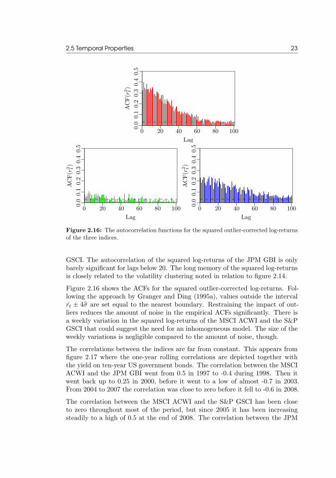
Figure 2.16: The autocorrelation functions for the squared outlier-corrected log-returnsof the three indices.

GSCI. The autocorrelation of the squared log-returns of the JPM GBI is onlybarely significant for lags below 20. The long memory of the squared log-returnsis closely related to the volatility clustering noted in relation to figure 2.14.Figure 2.16 shows the ACFs for the squared outlier-corrected log-returns. Fol-lowing the approach by Granger and Ding (1995a), values outside the intervalrt ± 4σ are set equal to the nearest boundary. Restraining the impact of out-liers reduces the amount of noise in the empirical ACFs significantly. There isa weekly variation in the squared log-returns of the MSCI ACWI and the S&PGSCI that could suggest the need for an inhomogeneous model. The size of theweekly variations is negligible compared to the amount of noise, though.The correlations between the indices are far from constant. This appears fromfigure 2.17 where the one-year rolling correlations are depicted together withthe yield on ten-year US government bonds. The correlation between the MSCIACWI and the JPM GBI went from 0.5 in 1997 to -0.4 during 1998. Then itwent back up to 0.25 in 2000, before it went to a low of almost -0.7 in 2003.From 2004 to 2007 the correlation was close to zero before it fell to -0.6 in 2008.The correlation between the MSCI ACWI and the S&P GSCI has been closeto zero throughout most of the period, but since 2005 it has been increasingsteadily to a high of 0.5 at the end of 2008. The correlation between the JPM

24 2 Index Data

..

-0.5

.

0.0

.

0.5

. Year.

1YRollingCorrelation

.1995

.1997

.1999

.2001

.2003

.2005

.2007

.2009

.

1

.

2

.

3

.

4

.

5

.

6

.

7

.

8

.

Yield

.

10Y US Govt

.

MSCI ACWI, JPM GBI

.

MSCI ACWI, S&P GSCI

.

JPM GBI, S&P GSCI

Figure 2.17: One-year rolling correlations between the indices together with the yieldon ten-year US government bonds.

GBI and the S&P GSCI has also remained close to zero throughout most of thein-sample period, but from 2007 it started decreasing to a low of -0.3 at the endof 2008. The observation that an investment in commodities seemed to provideprotection when the bond index was suffering in figure 2.11 on page 18 is notevident from the one-year correlations.

Figure 2.18 shows the cumulative proportion of variance explained by the firsttwo principal components. Principal component analysis (PCA) uses an or-thogonal transformation to convert a set of observations of possibly correlatedvariables into a set of values of uncorrelated variables called principal compo-nents. The first principal component has as high a variance as possible, meaningthat it accounts for as much of the variability in the dataset as possible. Thesucceeding components, in turn, have the highest variance possible under theconstraint that each one has to be orthogonal to (uncorrelated with) the pre-ceding components. Higher correlations mean greater redundancy and greaterredundancy results in more variation extracted in fewer components.

The solid lines are estimated using a rolling window of 252 trading days. Thedashed orange and purple lines show the cumulative proportion of variancethat can be explained by one and two principal components, respectively, whenlooking at the whole in-sample period. The log-returns were standardized prior

2.6 In-Sample Adjustment 25

to the analysis.

..

0.3

.

0.5

.

0.7

.

0.9

. Year.

Prop.ofVariance

.1995

.1998

.2001

.2004

.2007

.

PC1

.

PC2

Figure 2.18: The cumulative proportion ofvariance explained by the first two principalcomponents for the three indices.

The proportion of variance explainedby the first component varies from0.35 at the lowest to above 0.6 at thehighest. The spikes for componentone in 1996–1997, in 2003, and againfrom the middle of 2007 are coincid-ing with the times where the corre-lation between the MSCI ACWI andthe JPM GBI is significantly strength-ened. During the GFC, the correla-tion between the MSCI ACWI andthe S&P GSCI also increased signif-icantly, which is why the first compo-nent accounted for a larger proportionof the variance at the expense of com-ponent two. Besides the GFC, the sec-ond principal component explains an almost constant proportion of the varianceof about 0.35.The correlations are stronger at the times of high market volatility and stress.Thus, diversification may not materialize precisely when an investor needs it themost. The fact that the correlation between the MSCI ACWI and the JPM GBIgets increasingly negative is not a problem, but the increase in the correlationbetween the MSCI ACWI and the S&P GSCI, in particular during the GFC, isunfavorable. The impact would be more significant if it was two different stockindices, then the correlations would increase even more around year 2000 and2008. Although the correlations increased during the GFC, there are definitelydiversification benefits between asset classes.

2.6 In-Sample AdjustmentThe bond index has clearly outperformed both the stock and commodity indexin-sample following the significant decline in the term structure of interest rateswith corresponding high returns for long-maturity bonds. For other time periods,stocks and commodities are likely to show a more attractive risk/return profilecompared to bonds. Had the in-sample period ended in 2007 rather than 2008,then the Sharpe ratios would have been 0.67 and 0.46 for the MSCI ACWI andthe S&P GSCI, respectively.The end of a major financial crisis, where the level of stress in the markets is atits highest, is a critical time at which to be estimating Sharpe ratios. The SRof 0.29 for the MSCI ACWI is not an unrealistic long-term level. If the SR isset too low, then it will not be profitable to change allocation, and if the SR is

26 2 Index Data

set too high, then it will appear profitable to change allocation very often, asthe excess return will quickly cover the transaction costs.The assumption that will be made when calibrating time series models to the in-sample data to use for scenario generation and asset allocation is that the annualSR of the JPM GBI equals that of the MSCI ACWI. This in attempt to makea neutral assumption although there is no such thing as a neutral assumptionin this context. Leverage aversion could be one reason why stocks and bondsshould not be expected to yield the same risk-adjusted return in the long run(Asness et al. 2012, Frazzini and Pedersen 2014).Then there is the dispute about the commodity risk premium. The point ofdeparture will be to use the returns as they are, meaning that commodities willhave a lower SR than stocks and bonds in-sample. Hence, it is only the in-samplereturns of the JPM GBI that will be adjusted. This is done by subtracting0.022% from the daily log-returns. In this way, the MSCI ACWI and the JPMGBI will both have an in-sample annual SR of 0.29. It should be emphasizedthat the data used for out-of-sample testing will remain untransformed.

CHAPTER 3Markov-Switching

Mixtures

The normal distribution is a poor fit to most financial returns. Mixtures ofnormal distributions provide a much better fit as they are able to reproduceboth the skewness and leptokurtosis often observed. An extension to Markovswitching mixture models, also referred to as hidden Markov models (HMMs),is frequently applied to capture both the distributional and temporal propertiesof financial returns.In an HMM, the distribution that generates an observation depends on the stateof an unobserved Markov chain. The transition probabilities of the Markov chainare assumed to be constant implying that the sojourn times are geometricallydistributed. The memoryless property of the geometric distribution is not alwaysappropriate. An alternative is the hidden semi-Markov model (HSMM) in whichthe sojourn time distribution is modeled explicitly for each hidden state.If the observations are not equidistantly sampled then a continuous-time hiddenMarkov model (CTHMM) that factors in the sampling times of the observationscan be applied. The advantages of a continuous-time formulation include theflexibility to increase the number of states or incorporate inhomogeneity withouta dramatic increase in the number of parameters.The theory of HMMs in discrete time and their estimation is outlined in sec-tion 3.1. The HSMM is introduced in section 3.2 and the CTHMM in section 3.3.The models are fitted to the in-sample returns of the MSCI ACWI in section 3.4and gradient-based methods are considered in section 3.5.

28 3 Markov-Switching Mixtures

3.1 Hidden Markov Models in Discrete TimeIn hidden Markov models, the probability distribution that generates an obser-vation depends on the state of an underlying and unobserved Markov process.HMMs are a particular kind of dependent mixture and are therefore also re-ferred to as Markov-switching mixture models. General references to the sub-ject include Cappé et al. (2005), Frühwirth-Schnatter (2006), and Zucchini andMacDonald (2009).A sequence of discrete random variables {St : t ∈ N} is said to be a first-orderMarkov chain if, for all t ∈ N, it satisfies the Markov property:

Pr (St+1|St, . . . , S1) = Pr (St+1|St) . (3.1)

The conditional probabilities Pr (Su+t = j|Su = i) = γij (t) are called transitionprobabilities. The Markov chain is said to be homogeneous if the transitionprobabilities are independent of u, otherwise inhomogeneous.A Markov chain with transition probability matrix Γ (t) = {γij (t)} has sta-tionary distribution π if πΓ = π and π1′ = 1. The Markov chain is termedstationary if δ = π where δ is the initial distribution, i.e. δi = Pr (S1 = i).If the Markov chain {St} has m states, then the bivariate stochastic process{(St, Xt)} is called an m-state HMM. With X(t) and S(t) representing thevalues from time 1 to time t, the simplest model of this kind can be summarizedby

Pr(St|S(t−1)

)= Pr (St|St−1) , t = 2, 3, . . . , (3.2a)

Pr(Xt|X(t−1),S(t)

)= Pr (Xt|St) , t ∈ N. (3.2b)

When the current state St is known, the distribution of Xt depends only onSt. This causes the autocorrelation of {Xt} to be strongly dependent on thepersistence of {St}.An HMM is a state-space model with finite state space where (3.2a) is the stateequation and (3.2b) is the observation equation. A specific observation canusually arise from more than one state as the support of the conditional distri-butions overlaps. The unobserved state process {St} is therefore not directlyobservable through the observation process {Xt}, but can only be estimated.As an example, consider the two-state model with Gaussian conditional distri-butions:

Xt = µSt + εSt , εSt ∼ N(0, σ2

St

),

where

µSt =

{µ1, if St = 1,

µ2, if St = 2,σ2St

=

{σ21 , if St = 1,

σ22 , if St = 2,

and Γ =

[1− γ12 γ12γ21 1− γ21

].

3.1 Hidden Markov Models in Discrete Time 29

For this model, the first four central moments are

E [Xt| θ] = π1µ1 + (1− π1)µ2,

Var [Xt| θ] = π1σ21 + (1− π1)σ

22 + π1 (1− π1) (µ1 − µ2)

2,

Skewness [Xt| θ] = π1 (1− π1) (µ1 − µ2)(1− 2π1) (µ1 − µ2)

2+ 3

(σ21 − σ2

2

)σ3

,

Kurtosis [Xt| θ] =π1 (1− π1)

σ4

[3(σ21 − σ2

2

)2+ (µ1 − µ2)

4(1− 6π1 (1− π1))

+ 6 (2π1 − 1)(σ22 − σ2

1

)(µ1 − µ2)

2]+ 3.

θ denotes the model parameters and σ2 = Var [Xt| θ] is the unconditional vari-ance (Timmermann 2000, Frühwirth-Schnatter 2006).The unconditional mean is simply the weighted average of the means. A dif-ference in the means across the states enters both the variance, skewness, andkurtosis. In fact, skewness only arises if there is a difference in the mean values.The unconditional variance is not just the weighted average of the variances;a difference in means also imparts an effect because the switch to a new statecontributes to volatility (Ang and Timmermann 2011). Intuitively, the possibil-ity of changing to a new state with a different mean value introduces an extrasource of risk. This is similar to a mixed-effects model where the total variancearises from two sources of variability, namely within-group heterogeneity andbetween-group heterogeneity (see e.g. Madsen and Thyregod 2011).The value of the autocorrelation function at lag k is

ρXt (k| θ) =π1 (1− π1) (µ1 − µ2)

2

σ2λk

and the autocorrelation function for the squared process is

ρX2t(k| θ) =

π1 (1− π1)(µ21 − µ2

2 + σ21 − σ2

2

)2E [X4

t | θ]− E [X2t | θ]

2 λk.

λ = γ11−γ21 is the second largest eigenvalue of Γ (Frühwirth-Schnatter 2006).15It is evident from these expressions, as noted by Rydén et al. (1998), that HMMscan only reproduce an exponentially decaying autocorrelation structure.The ACF of the first-order process becomes zero if the mean values are equal,whereas persistence in the squared process can be induced either by a differencein the means, as for a mixed-effects model, or by a difference in the variancesacross the states. In both cases, the persistence increases with the combinedpersistence of the states as measured by λ (Ang and Timmermann 2011).

15The other eigenvalue of Γ is λ = 1.

30 3 Markov-Switching Mixtures

The sojourn times are implicitly assumed to be geometrically distributed:

Pr (’staying t time steps in state i’) = γt−1ii (1− γii) (3.3)

with the expected duration of state i being

E [ri] =1

1− γii. (3.4)

The geometric distribution is memoryless, implying that the time until the nexttransition out of the current state is independent of the time spent in the state.The parameters of an HMM are usually estimated using the Maximum Like-lihood (ML) method. There are essentially three problems in the context ofHMMs:

1. Evaluating the likelihood of the observations x(T ) given the parameters.

2. Estimating the model parameters θ that maximize the likelihood of theobserved data.

3. Inferring the most likely sequence of states s(T ).

The first question is addressed by a dynamic programming technique, the for-ward–backward algorithm, the second task is carried out using the Baum–Welchalgorithm, and the third problem can be solved efficiently using the Viterbi al-gorithm. The algorithms are outlined in the next three subsections.

The Forward–Backward AlgorithmUnder the assumption that successive observations are independent, the likeli-hood of the observations x(T ) given the parameters θ is

LT = Pr(X(T ) = x(T )

∣∣∣ θ) = δD (x1)ΓD (x2) · · ·ΓD (xT )1′, (3.5)

where D (x) is a diagonal matrix with the state-dependent conditional densitiesdi (x) = Pr (Xt = x|St = i), i ∈ {1, 2, . . . ,m}, as entries. The conditional dis-tribution of Xt may be either discrete or continuous, univariate or multivariate.The forward–backward algorithm is used to compute the likelihood and is alsoemployed in the Baum–Welch algorithm. The ith element of the vector αt isthe forward probability

αt (i) = Pr(X(t) = x(t), St = i

∣∣∣ θ) (3.6)

and the ith element of βt is the backward probability

βt (i) = Pr (Xt+1 = xt+1, . . . , XT = xT |St = i, θ) (3.7)

3.1 Hidden Markov Models in Discrete Time 31

for t = 1, 2, . . . , T and i ∈ {1, 2, . . . ,m}.The forward and the backward probabilities can be computed recursively as

αt+1 = αtΓD (xt+1) (3.8)β′t = ΓD (xt+1)β

′t+1 (3.9)

with initial values α1 = δD (x1) and βT = 1.It follows that

αt (i)βt (i) = Pr(X(T ) = x(T ), St = i

∣∣∣ θ) . (3.10)

Thus, the likelihood of the observed data x(T ) can be evaluated as the sum overall m states:

Pr(X(T ) = x(T )

∣∣∣ θ) =m∑i=1

αt (i)βt (i) = αtβ′t. (3.11)

The likelihood is independent of the time point t at which the forward–backwardvariables are evaluated since

αtβ′t = αt+1β

′t+1.

The forward and backward probabilities should be scaled to avoid numericalunderflow, as described in Zucchini and MacDonald (2009). The complexityof the forward–backward recursions is O

(m2T

)which is feasible in contrast to

the straightforward evaluation of (3.5) which has complexity O(mT)(Dittmer

2008).

The Baum–Welch AlgorithmThe two most popular approaches to maximizing the likelihood are direct nu-merical maximization and the Baum–Welch algorithm, a special case of theexpectation–maximization (EM) algorithm (Baum et al. 1970, Dempster et al.1977). The Baum–Welch algorithm is often preferred due to its larger robust-ness to initial values. The likelihood is guaranteed to increase (or remain thesame) for each iteration when using the EM algorithm, but convergence towardthe maximum might be slow. Another advantage of using the EM algorithm isthat there is no need to transform the parameters.16

16See Cappé et al. (2005) for a discussion of the relative merits of the EM algorithm and directmaximization of the likelihood of an HMM by gradient-based methods.

32 3 Markov-Switching Mixtures

The Baum–Welch algorithm maximizes the logarithm of the complete-data like-lihood (CDLL), i.e. the log-likelihood of the observations x(T ) and the missingdata s(T ), which can be written as

log(Pr(x(T ), s(T )

))= log

(δs1

T∏t=2

γst−1,st

T∏t=1

dst (xt)

)

= log δs1 +T∑

t=2

log γst−1,st +T∑

t=1

log dst (xt) .(3.12)

By introducing the binary random variables

vi (t) = 1 if and only if st = 1

andwij (t) = 1 if and only if st−1 = i and st = j,

the CDLL can be written as

log(Pr(x(T ), s(T )

))=

m∑i=1

vi (1) log δi

+m∑i=1

m∑j=1

(T∑

t=2

wij (t)

)log γij

+m∑i=1

T∑t=1

vi (t) log di (xt) .

(3.13)

The idea of the EM algorithm is to replace the quantities vi (t) and wij (t)by their conditional expectations given the observations x(T ) and the currentparameter estimates. This is the E-step:

vi (t) = Pr(St = i|x(T )

)= αt (i)βt (i) /LT (3.14)

and

wij (t) = Pr(St−1 = i, St = j|x(T )

)= αt−1 (i) γijdj (xt)βt (j) /LT . (3.15)

Having replaced vi (t) and wij (t) by their conditional expectations vi (t) andwij (t) the CDLL (3.13) is maximized with respect to three sets of parameters:the initial distribution δ, the transition probability matrix Γ, and the parametersof the state-dependent distributions (e.g., µ1, . . . , µm and σ2

1 , . . . , σ2m in the case

of Gaussian distributions). This is the M-step.

3.1 Hidden Markov Models in Discrete Time 33

These two steps are repeated until some convergence criterion has been satis-fied, e.g. until the resulting change in θ or the log-likelihood is less than somethreshold. The resulting value of θ is then a stationary point of the likelihood ofthe observed data. The stationary point is not necessarily the global maximum,but can also be a local maximum or a saddle point.

The M-step splits into three independent maximizations since the first term in(3.13) depends only on the initial distribution, the second term depends only onthe transition probabilities, and the third term depends only on the parametersof the state-dependent distributions.

The solution is to setδi =

vi (1)∑mi=1 vi (1)

= vi (1) (3.16)

andγij =

fij (T )∑mj=1 fij (T )

, (3.17)

where fij (T ) =∑T

t=2 wij (t) is the total number of transitions from state i tostate j.

It does not seem reasonable to try to estimate the initial distribution δ basedon just one observation at time t = 1. Another possibility is to maximize thelikelihood conditioned on starting in a particular state. Maximizing the condi-tional likelihood over the m possible starting states is equivalent to maximizingthe unconditional likelihood since δ has to be one of the m unit vectors at amaximum of the likelihood.

If the Markov chain is assumed to be stationary, then δ is completely determinedby the transition probability matrix Γ as δ = δΓ and δ1′ = 1 and the questionof estimating δ falls away. Then the sum of the first two terms in (3.13) has tobe maximized with respect to Γ which generally requires a numerical solution(Bulla and Berzel 2008, Zucchini and MacDonald 2009).

The maximization of the third term in (3.13) may be easy or difficult dependingon the nature of the state-dependent distributions. In some cases numericalmaximization will be necessary, but in the case of conditional univariate nor-mal distributions the maximizing values of the state-dependent parameters aresimply

µi =

∑Tt=1 vi (t)xt∑Tt=1 vi (t)

,

σ2i =

∑Tt=1 vi (t) (xt − µi)

2∑Tt=1 vi (t)

.

34 3 Markov-Switching Mixtures

For conditional multivariate normal distributions the M-step reads

µi =

∑Tt=1 vi (t)xt∑Tt=1 vi (t)

,

Σi =

∑Tt=1 vi (t) (xt − µi) (xt − µi)

′∑Tt=1 vi (t)

.

In the case of conditional t-distributions17 the maximizing values of the state-dependent parameters at iteration k + 1 are

µ(k+1)i =

∑Tt=1 vi (t)u

(k)it xt∑T

t=1 vi (t)u(k)it

,

σ2(k+1)

i =

∑Tt=1 vi (t)u

(k)it

(xt − µ

(k+1)i

)2∑T

t=1 vi (t),

whereu(k)it = σ2(k)

i

ν(k)i + 1

σ2(k)

i ν(k)i +

(xt − µ

(k)i

)2 .The estimator ν(k+1)

i is the unique solution to the equation

1− ψ

(1

2ν(k)i

)+ log

(1

2ν(k)i

)+ ψ

(ν(k)i + 1

2

)− log

(ν(k)i + 1

2

)

+1∑T

t=1 vi (t)

[T∑

t=1

vi (t)(logu(k)it − u

(k)it

)]= 0,

where ψ (z) = {∂Γ (z) /∂z} /Γ (z) is the Digamma function. The solution canbe determined without relevant complications, e.g. using a bisection algorithmor quasi-Newton methods, because the function on the left-hand side is mono-tonically increasing in ν(k)i (Bulla 2011).In order to increase the speed of convergence a hybrid algorithm can be appliedthat starts with the EM algorithm and switches to a Newton-type algorithmwhen a certain stopping criterion is fulfilled as outlined by Bulla and Berzel(2008). The resulting algorithm combines the large circle of convergence fromthe EM algorithm with the superlinear convergence of the Newton-type algo-rithm in the neighborhood of the maximum.

17The univariate Student t-distribution, X ∼ tν(µ, σ2

)with µ ∈ R, σ > 0, and ν > 0, is

defined for x ∈ R. The density is dtν (x) =Γ((ν+1)/2)

Γ(ν/2)√

νπσ2

(1 +

(x−µ)2

νσ2

)−(ν+1)/2.

3.1 Hidden Markov Models in Discrete Time 35

The likelihood function of an HMM is in general a complicated function of theparameters with several local maxima. Depending on the initial values, it caneasily happen that the algorithm identifies a local rather than the global max-imum. A sensible strategy is therefore to try a range of (randomly generated)initial values for the maximization.In the case of continuous state-dependent distributions the likelihood can be un-bounded in the vicinity of certain parameter combinations. For example, if theconditional distribution is Gaussian, then the likelihood can be arbitrarily largeif the mean is equal to one of the observations and the conditional variance tendsto zero (Frühwirth-Schnatter 2006). Podgórski and Wallin (2013) showed howthis can be handled in an elegant way by leaving out the observation that makesthe largest contribution to the likelihood at each step of the maximization.18

Alternatively, the likelihood function can be maximized using a Bayesian ap-proach based on Markov chain Monte Carlo (MCMC) sampling; by includingprior information on the ratio between the conditional variances the likelihoodbecomes bounded (Frühwirth-Schnatter 2006). Rydén (2008) compared the EMand MCMC approaches and found that MCMC can be advantageous for inter-val estimation and inferential problems, whereas EM is a simpler and faster wayof obtaining point estimates.The uncertainties of the parameter estimates can also be obtained through boot-strapping as outlined by Zucchini and MacDonald (2009) or from the inverse ofthe Hessian of the log-likelihood function at the optimum (see e.g. Madsen andThyregod 2011). Lystig and Hughes (2002) described an algorithm for exactcomputation of the score vector and the observed information matrix in HMMsthat can be performed in a single pass through the data. The algorithm wasderived from the forward–backward algorithm. If some of the parameters areon or near the boundary of their parameter space, which is often the case inHMMs, the use of the Hessian to compute standard errors is unreliable. More-over, the conditions for asymptotic normality of the ML estimator are oftenviolated, thus making approximate confidence intervals based on the computedstandard errors unreliable.

DecodingDecoding is the process of determining the states of the Markov chain thatare most likely (under the fitted model) to have given rise to the observationsequence. This can be done either locally by determining the most likely stateat each time t or globally by determining the most likely sequence of states.

18Seo and Kim (2012) proposed a similar strategy for avoiding spurious roots where one or morecomponents are overfitting a small random localized pattern in the data rather than any underlyinggroup structure.

36 3 Markov-Switching Mixtures

Local decoding is the maximization of the conditional distribution of St for eacht = 1, 2, . . . , T given the observations x(T ) and model parameters θ:

argmaxi=1,...,m

Pr(St = i|X(T ) = x(T ), θ

)(3.18)

where the smoothing probabilities can be computed using

Pr(St = i

∣∣∣X(T ) = x(T ), θ)=αt (i)βt (i)

LT. (3.19)

Local decoding can lead to impossible state sequences as it does not take thetransition probabilities into account.Global decoding is the maximization of the conditional probability19

argmaxs(T )

Pr(S(T ) = s(T )

∣∣∣X(T ) = x(T ), θ). (3.20)

Maximizing (3.20) over all possible state sequences by brute force involves mT

function evaluations. The Viterbi algorithm (Viterbi 1967) can be used to com-pute the most likely sequence of states in an efficient manner. This is done bydefining the highest probability along a single path for the first t observationsending in state i at time t:

ξti = argmaxs(t−1)

Pr(S(t−1) = s(t−1), St = i,X(T ) = x(T )

∣∣∣ θ) . (3.21)

The probabilities ξtj can be computed recursively for t = 2, 3, . . . , T and i ∈{1, 2, . . . ,m} using

ξtj =

(argmaxi=1,...,m

ξt−1,iγij

)dj (xt) (3.22)

with the initial condition ξ1i = Pr (S1 = i,X1 = x1) = δidi (x1).The dynamic programming technique is the same as in the forward–backwardalgorithm, the only difference is the substitution of the sum with a maximization.The complexity remains O

(m2T

)(Dittmer 2008).

3.2 Hidden Semi-Markov ModelsIf the assumption of geometrically distributed sojourn times is unsuitable, thenhidden semi-Markov models can be applied. HMMs and HSMMs differ only

19This is equivalent to maximizing the joint probability Pr(X(T ) = x(T ),S(T ) = s(T )

∣∣∣ θ).

3.2 Hidden Semi-Markov Models 37

in the way that the state process is defined. In HSMMs, the sojourn timedistribution is modeled explicitly for each state i:

ri (u) = Pr (St+u+1 = i, St+u−v = i, v = 0, . . . , u− 2|St+1 = i, St = i) (3.23)

and the transition probabilities are defined as

γij = Pr (St+1 = j|St+1 = i, St = i) (3.24)

for each j = i with γii = 0 and∑

j γij = 1.The conditional independence assumption for the observation process is similarto a simple HMM, but the semi-Markov chain associated with HSMMs doesnot have the Markov property at each time t. This property is transferred tothe imbedded first-order Markov chain, that is the sequence of visited states(Bulla and Bulla 2006). In other words, the future states are only conditionallyindependent of the past states when the process changes state.The HMM with geometrically distributed sojourn times is just a special case ofthe HSMM and the EM algorithm as outlined in the previous section can easilybe extended to cover other sojourn time distributions (see Bulla and Bulla 2006).The CDLL of an HSMM includes the sojourn times u1, u2, . . . , uN and the se-quence of visited states s1, s2, . . . , sN , where N is the number of visited states, inaddition to the observations x1, x2, . . . , xT and the hidden states s1, s2, . . . , sT :

log(Pr(x(T ), s(T )

))= log

(δs1ds1 (u1)

N∏n=2

γsn−1,snrsn (un)T∏

t=1

dst (xt)

)

= log δs1 +N∑

n=1

log dsn (un) +N∑

n=2

log γsn−1,sn (3.25)

+T∑

t=1

log dst (xt) .

The four terms in (3.25) can be maximized independently as the first termdepends only on the initial distribution, the second term depends only on theparameters of the sojourn time distributions, the third term depends only on thetransition probabilities, and the fourth term depends only on the parameters ofthe state-dependent distributions.HSMMs provide a considerable flexibility compared to HMMs without compli-cating the estimation significantly, though the maximization of the term thatdepends on the parameters of the sojourn time distributions in (3.25) typicallyrequires a numerical solution. The selection of the most appropriate sojourntime distribution can, however, be a complicated problem (Bulla et al. 2010).

38 3 Markov-Switching Mixtures

3.3 Hidden Markov Models in Continuous TimeIn continuous-time Markov chains, transitions may occur at all times ratherthan at discrete and equidistant time points. There is no smallest time step andthe quantities of interest are the transition probabilities

pij (∆t) = Pr (S (t+∆t) = j|S (t) = i) (3.26)

as ∆t→ 0. Clearly, pij (0) = 0 for different states i and j, and it can be shownthat under certain regularity conditions

limt→0

P (t) = I. (3.27)

Assuming that pij (∆t) is differentiable at 0, the transition rates are defined as

p′ij (0) = lim∆t→0

pij (∆t)− pij (0)

∆t

= lim∆t→0

Pr (S (t+∆t) = j|S (t) = i)

∆t

= qij

(3.28)

with the additional definition qii = qi = −∑

j =i qij . The transition intensitymatrix Q = {qij} has non-negative off-diagonal elements qij , non-positive diag-onal entries qi, and all rows sum to zero.The stationary distribution π, if it exists, is found by solving the system ofequations {

πQ = 0π1′ = 1.

(3.29)

If it has a strictly positive solution (all elements in π are strictly positive), thenthe stationary distribution exists and is independent of the initial distribution.The matrix of transition probabilities P (t) = {pij (t)} can be found as thesolution to Kolmogorov’s differential equation

dP (t)

dt = P (t)Q (3.30)

with the initial condition P (0) = I. The solution being

P (t) = eQtP (0) = eQt. (3.31)

It follows that the transition intensity matrix Q is the matrix-logarithm of theone-step transition probability matrix

Q = logP (1) . (3.32)

3.3 Hidden Markov Models in Continuous Time 39

When the process enters state i, it remains there according to an exponentialdistribution with parameter −qi > 0 before it instantly jumps to another statej = i with probability −qij/qi. A continuous-time Markov chain is fully charac-terized by its initial distribution δ and the transition intensity matrix Q.The exponential distribution is memoryless just like its discrete analogue, thegeometric distribution. By mapping multiple latent states to the same outputdistribution, it is possible to allow for non-exponentially distributed sojourntimes. The distribution of sojourn times will then be a mixture of exponentialdistributions, which is a phase-type distribution, and the Markov property willbe transferred to the imbedded Markov chain as for the HSMM. Phase-typedistributions can be used to approximate any positive-valued distribution witharbitrary precision.It is often reasonable to assume that in a short time interval∆t, the only possibletransitions are to the neighboring states:

pij = o (∆t) , |i− j| ≥ 2,

pii (∆t) = 1− qi∆t+ o (∆t) ,

pi,i−1 (∆t) = wiqi∆t+ o (∆t) ,

pi,i+1 (∆t) = (1− wi) qi∆t+ o (∆t) ,

i ∈ {1, 2, . . . ,m} ,

(3.33)

where lim∆t→0o(∆t)∆t = 0. The notation includes transitions from state 1 to

m and reverse with the definition that state 0 = state m and state (m+ 1) =state 1.The Markov chain {S (t)} is then a birth-and-death process in the sense that itcan change its state index by at most one in each step. Although the processcannot go straight from state i to state i + 2 there is no limit to how fast thetransition can occur. The matrix of transition intensities has the structure

Q =

−q1 (1− w1) q1 0 · · · 0 w1q1w2q2 −q2 (1− w2) q2 · · · 0 0...

...... . . . ...

...(1− wm) qm 0 0 · · · wmqm qm

. (3.34)

The number of parameters increases linearly with the number of states. Thus,a continuous-time Markov chain yields a parameter reduction over its discrete-time analogue if the number of states exceeds three. The higher the numberof states, the larger the reduction. In addition, it is possible to incorporateinhomogeneity without a dramatic increase in the number of parameters usingsplines, harmonic functions, or similar.20

20See Iversen et al. (2013) for an example of the use of splines to reduce the number of parametersin an inhomogeneous Markov model.

40 3 Markov-Switching Mixtures

Another advantage of a continuous-time formulation is the flexibility to usedata with any sampling interval as the data is not assumed to be equidistantlysampled. In a discrete-time model, the trading days are aggregated meaning thatweekends and bank holidays are ignored so that Friday is followed by Mondayin a normal week. A continuous-time model is able to recognize the longertime span between Friday and Monday, which could lead to a different behavior(see e.g. Rogalski 1984, Asai and McAleer 2007). The time span should notnecessarily be three days, the point is that the sampling times are modeled.A Markov process {S (t)} observed at equidistant time points t1 = ς, . . . , tT =ςT defines a discrete Markov chain Y1 = S (ς) , . . . , YT = S (ςT ) with transitionmatrix Γ = eQς . It is not every discrete Markov chain that belongs to a contin-uous Markov process. In other words, not every discrete Markov chain can beimbedded into a continuous-time Markov process. This is called the imbeddingproblem (Dittmer 2008).

A Continuous-Time Version of the Baum–Welch AlgorithmThe CDLL of a CTHMM, i.e. the log-likelihood of the observations x1, . . . , xTand the unobserved states s1, . . . , sT at the discrete time points t1, . . . , tT , is

log(Pr(x(T ), s(T )

))= log

(δs1

T∏i=2

psi−1,si (ti − ti−1)

T∏i=1

dsi (xi)

)

= log δs1 +T∑

i=2

log psi−1,si (ti − ti−1) (3.35)

+

T∑i=1

log dsi (xi) .

The probability of the transitions can be written as the probability of a sojournof a specific length multiplied by the probability of an instant transition toanother state as it was done for the HSMM. With fij (τ) denoting the totalnumber of transitions from state i to j and Ri (τ) the total duration spent instate i the CDLL can be written as

log(Pr(x(T ), s(T )

))= log δs1 +

m∑i=1

∑j =i

fij (τ) log qij

+

m∑i=1

qiRi (τ) +

T∑i=1

log dsi (xi) .(3.36)

In this way the CDLL is expressed in terms of the parameters. The first andthe last term can be dealt with in the same way as for the discrete-time models,but the middle terms require more attention.

3.3 Hidden Markov Models in Continuous Time 41

The maximum likelihood estimator of the transition rates is

qij =fij (τ)

Ri (τ)(3.37)

where the diagonal entries follow from the generator constraint qi = −∑

j =i qij .The problem is that neither f nor R are available and it is not trivial to evaluatetheir expectations.Hobolth and Jensen (2011) considered the problem of estimating the summarystatistics needed in the EM algorithm. The expected time spent in state iconditional on starting in state A at time t1 = 0 and ending in state B at timetT = τ is

E [Ri (τ)|S (0) = A,S (τ) = B] =1

pAB (τ)

ˆ τ

0

pAi (t) piB (τ − t)dt. (3.38)

The expected number of transitions between state i and j conditional on startingin state A at time t1 = 0 and ending in state B at time tT = τ is

E [fij (τ)|S (0) = A,S (τ) = B] =qij

pAB (τ)

ˆ τ

0

pAi (t) pjB (τ − t)dt. (3.39)

The joint expectation integral can be evaluated using eigenvalue decomposi-tion under the assumption that Q has no repeated eigenvalues. If Q is di-agonalizable with real eigenvalues λ1, λ2, . . . , λm, then Q = UΛU−1 whereΛ = diag (λ1, λ2, . . . , λm) is a diagonal matrix with the eigenvalues on the di-agonal and the columns of U are the eigenvectors. The transition probabilitymatrix P (t) = eQt = UeΛtU−1 and the integral can be evaluated asˆ τ

0

pAα (t) pβB (τ − t) dt =ˆ τ

0

(UeΛtU−1)Ai(UeΛ(τ−t)U−1)jBdt

=

m∑i=1

UAiU−1iα

m∑j=1

UβjU−1jB

ˆ τ

0

etλi+(τ−t)λjdt.

The last integral is easy to evaluate in the case of real eigenvalues.Let Ψ(0, τ) be either of the complete-data sufficient statistics Ri (τ) or fij (τ).Ψ(0, τ) is then an additive statistic, that is

Ψ(0, τ) =

T∑l=2

E [Ψ (tl−1, tl) |Sl−1 = sl−1, Sl = sl ] .

It follows from the Markov property that

E[Ψ(0, τ)

∣∣∣s(T )]=

T∑l=2

E [Ψ (tl−1, tl) |Sl−1 = sl−1, Sl = sl ] . (3.40)

42 3 Markov-Switching Mixtures

In the E-step, the expectation that is needed is

E[Ψ(0, τ)

∣∣∣x(T )]=

T∑l=2

m∑i=1

m∑j=1

E [Ψ (tl−1, tl) |Sl−1 = i, Sl = j ]

· Pr(Sl−1 = i, Sl = j

∣∣∣x(T )),

(3.41)

where the conditional probabilities

Pr(Sl−1 = i, Sl = j

∣∣∣x(T ))=αtl−1

(i) pij (tl − tl−1) dj (xl)βtl (j)

LT(3.42)

are outputs from the forward–backward algorithm.Each step of the forward–backward recursions (3.8) and (3.9) requires the calcu-lation of the transition probability matrix P (t) = eQt. This can be done in anefficient manner using the eigenvalue decomposition of Q. The relatively smallsize of the state space in financial applications does not prohibit numerical es-timation of the matrix exponential. It is, however, still desirable to avoid thiscomputationally intensive calculation whenever possible.The scaling by 1/pAB (τ) in (3.38) and (3.39) cancels with the transition proba-bility in (3.42). The evaluation of the expectations of the summary statistics fand R does therefore not require further evaluations of the matrix exponential.The really time-consuming task is the sum over all possible sequences of statesin (3.41).Lange and Minin (2013) reported good results using the R package SQUAREM dueto Varadhan (2012) to accelerate the convergence of the EM algorithm. Theyfound that the accelerated EM algorithm outperformed other optimization ap-proaches including direct maximization of the observed data likelihood by nu-merical methods as implemented in the R package msm due to Jackson (2011)and the EM algorithm of Bureau et al. (2000) that uses numerical maximiza-tion to update the parameter estimates in the M-step. Alternatively, a hybridalgorithm that switches to a Newton-type algorithm in the neighborhood of themaximum can be applied to increase the speed of convergence as outlined insection 3.1. As to the present application, there is no need to consider means ofreducing the time to convergence.

3.4 Model Estimation and SelectionThe focus will be on modeling the stock returns as stocks are typically the largestrisk contributor in a portfolio. Another reason to focus on the stock index isthat stock markets generally lead the economy. Thus, a stock index will oftenbottom (and head higher) before the economy begins to pick up, and top outbefore the economy begins to slow down.

3.4 Model Estimation and Selection 43

The focus will be on univariate models, but a multivariate model will be tested inchapter 5. The models that will be estimated are both discrete and continuous-time HMMs with conditional normal distributions following the approach byRydén et al. (1998) and Nystrup et al. (2014), respectively; discrete-time HMMswith conditional normal distributions and a t-distribution in the state with thehighest volatility following the approach by Bulla (2011); discrete-time HMMswith conditional t-distributions in all the states; and discrete-time HSMMswith negative binomial distributed sojourn times and conditional normal or t-distributions following the approach by Bulla and Bulla (2006).The estimated models will be compared in terms of how they fit the empiricalmoments and the autocorrelation function of the squared log-returns. Finally,the likelihood of the models will be compared to the number of parameters usingmodel selection criteria.The discrete-time models are estimated using the R package hsmm due to Bullaet al. (2010) that implements the EM algorithm for various sojourn time distribu-tions including the geometric and the negative binomial distribution. The onlyexception is the HMM with conditional normal distributions and a t-componentin the state with the highest variance. The hsmm package cannot handle dif-ferent conditional distributions across the states so those models are estimatedusing the implementation of the Baum–Welch algorithm that can be found inappendix A.1 on page 93.The CTHMM is estimated using the implementation of the continuous-timeversion of the Baum–Welch algorithm that can be found in appendix A.2 onpage 96. This algorithm definitely seemed superior to the msm package due toJackson (2011) that is based on direct numerical maximization of the likelihoodfunction. The Baum–Welch algorithm was much more robust towards initialvalues without a notable decrease in the speed of convergence.

Exploring the Estimated ModelsThis subsection will focus on the normal HMMs, but the estimated models allhave the same structure. The estimated parameters for the fitted two, three, andfour-state HMMs with conditional normal distributions are shown in table 3.1.Approximate standard errors of the estimates based on the observed informationare reported in parentheses.21 The stationary distributions are derived from theestimated transition probability matrices. Parameter estimates for all the fittedmodels can be found in appendix B on page 103.The two-state model has a low-variance state with a positive mean return anda high-variance state with a negative mean return implying that turbulence isassociated with lower returns, on average. The two states are mostly identified

21See section 3.1 for comments on the use of the Hessian to compute standard errors.

44 3 Markov-Switching Mixtures

Table 3.1Parameter estimates for the fitted m-state HMMs with conditional normal distributions.m Γ µ× 104 σ2 × 104 δ π

20.987 0.013

(0.003)0.029 0.971(0.008)

6.8(1.2)−10.0(4.6)

0.32(0.01)2.26(0.14)

1

0

0.69

0.31

3

0.988 0.012 0(0.004)

0.012 0.981 0.006(0.004) (0.002)

0 0.043 0.957(0.016)

8.8(1.3)−1.0(2.5)−32.5(16.3)

0.24(0.01)0.88(0.04)6.05(0.65)

1

0

0

0.48

0.45

0.07

4

0.983 0.017 0 0(0.004)

0 0.651 0.331 0.018(0.042) (0.012)

0.033 0.240 0.727 0(0.010) (0.036)

0 0 0.053 0.947(0.014)

8.9(1.2)−69.1(7.7)50.7(6.9)−27.9(16.8)

0.47(0.01)0.71(0.05)0.74(0.05)2.48(0.67)

1

0

0

0

0.49

0.19

0.25

0.07

by the variance as the difference in the mean values is of a similar magnitude asthe variances. Nevertheless, the difference in the mean values is a prerequisitefor the model’s ability to reproduce the observed first-order autocorrelation andskewness. The two states are both very persistent.The main difference compared to the two-state models with conditional t-distri-butions is the longer tails of the t-distribution that lead to a lower varianceand a higher persistence in the high-variance state. Consequently, the station-ary probabilities of the two states are more even in the case of conditionalt-distributions.When adding a third state to the model, an interesting structure emerges wherethe two outer states only communicate through the middle state. The proba-bilities of switching between state one and three are fixed to zero in order tosave two parameters as they were effectively zero anyway. The third state hasa high variance, a low mean return, and is less persistent than the two otherstates. The third state is sometimes referred to as an outlier state due to itslow unconditional probability and high variance (Rydén et al. 1998, Bulla et al.2011).The four-state model has two states that are less persistent with a similar vari-ance. Six of the estimated transition probabilities were effectively zero. The

3.4 Model Estimation and Selection 45

.. rt.

Density

.-0.06

.-0.02

.0.02

.0.06

.0

.10

.30

.50

.. rt.

Density

.-0.06

.-0.02

.0.02

.0.06

.

0

.

10

.

30

.

50

.. rt.

Density

.-0.06

.-0.02

.0.02

.0.06

.

0

.

10

.

30

.

50

Figure 3.2: Density histograms of the MSCI ACWI log-returns together with densityfunctions for the state-dependent normal distributions scaled by the stationary distribu-tion of the underlying Markov chain and the resulting unconditional distribution for theestimated two, three, and four-state models.

high-variance state again has a low unconditional probability. The simple struc-ture of the transition probability matrix offsets the advantage of a continuous-time formulation when the Markov chain is assumed to be homogeneous andthe observations equidistantly sampled.

The conditional densities scaled by the stationary probabilities are shown in fig-ure 3.2 together with the resulting unconditional density and a density histogramof the log-returns of the MSCI ACWI. The unconditional densities appear to bea reasonable fit to the empirical distribution for all three models although thetwo-state model does not fully capture the kurtosis of the empirical distribution.

Looking at the conditional densities for the three and four-state models it isevident that the high-variance state, which is the density lying very close to thefirst axis due to its low unconditional probability, captures the tails on both sidesof the distribution. It illustrates that turbulent periods are not characterizedonly by low or negative returns in agreement with the definition by Chow et al.(1999).

46 3 Markov-Switching Mixtures

Table 3.3The first four moments of the MSCI ACWI daily log-returns and the fitted models.

Model Mean SD Skewness Kurtosisrt 0.00018 0.0095 -0.40 13HMMN (2) 0.00017 0.0097 -0.21 5.9HMMNt (2) 0.00026 0.0095 -0.03 17HMMt (2) 0.00028 0.0095 -0.18 15HSMMN (2) 0.00013 0.0096 -0.31 6.6HSMMt (2) 0.00027 0.0095 -0.20 12HMMN (3) 0.00011 0.0097 -0.48 10HMMNt (3) 0.00015 0.0097 -0.46 19HMMt (3) 0.00018 0.0098 -0.44 18HSMMN (3) 0.00015 0.0096 -0.52 10HSMMt (3) 0.00021 0.0096 -0.55 15HMMN (4) 0.00014 0.0096 -0.42 10HMMNt (4) 0.00016 0.0096 -0.39 15HSMMN (4) 0.00017 0.0094 -0.50 10CTHMMN (4) 0.00021 0.0095 -0.39 10

Matching the MomentsTable 3.3 shows the first four empirical moments of the in-sample log-returnsof the MSCI ACWI together with the moments of the fitted models based on250,000 Monte Carlo simulations. The moments and the autocorrelation func-tions could have been computed numerically, but it would mainly affect themean values; the simulated mean value is relatively far from the empirical meanvalue for some of the models as a result of the large standard deviation. This isnot the case for the theoretical values.The two-state models with conditional normal distributions capture some ofthe observed skewness, but only half of the observed kurtosis. The two-statemodels with one or more t-components are able to reproduce the large kurtosis,but not the skewness. In fact, the two-state HMM with one t-component doesnot capture the observed skewness at all.A much better fit to the empirical moments is obtained by increasing the numberof states from two to three as concluded by Nystrup et al. (2014). The HMMs arethe best at capturing the skewness. The HMMs with one or more t-componentsoverestimate the kurtosis, but the three-state models are all able to reproducethe large kurtosis. For the HMM and the HSMM with conditional t-distributionsthe number of degrees of freedom in the middle state is above 100, meaning thatthe conditional distribution is effectively normal.Increasing the number of states from three to four improves the fit to the em-pirical moments although the improvement is less significant compared to goingfrom two to three states. It was not possible to estimate models with condi-

3.4 Model Estimation and Selection 47

tional t-distributions in all four states as the number of degrees of freedom wenttowards infinity for some of the states. The four-state models provide more orless an equally good fit to the moments.

Reproducing the Long Memory

The empirical autocorrelation function for the squared log-returns and the squaredoutlier-corrected log-returns of the MSCI ACWI and the fitted models are shownin figure 3.4. Of the two-state models, the two models with conditional normaldistributions do the best job at reproducing the shape of the ACF. The fluc-tuations at lag one to ten for the two-state HSMM with conditional normaldistributions is a result of the short expected sojourns of this model.

The models with one or more t-components are very persistent, but at too low ofa level. As pointed out by Bulla (2011), the increased persistence is most likelya result of the excess kurtosis of the t-distributed component(s) that allows forless frequent state changes. Looking at the outlier-corrected squared log-returnsin the right-hand column, the models with conditional normal distributions arestill better at capturing the decay.

Increasing the number of states to three leads to a better fit to the empiricalautocorrelation function of the squared log-returns. The differences between themodels are smaller, but the two models with conditional normal distributionsare still the best fit. Looking at the outlier-corrected squared log-returns, thethree-state models all provide a similar fit.

A further increase in the number of states does not lead to a better fit. TheHMM with one t-component is the worst fit when looking at the squared log-returns, while the differences in performance are small when reducing the impactof outliers.

Model Selection

A generalized likelihood ratio test (GLRT) cannot be applied to choose betweenmodels with different types of conditional distributions as they are not hier-archically nested. Models with the same type of conditional distribution anddifferent numbers of states are hierarchically nested, but the asymptotic distri-bution of the likelihood ratio statistic is not the usual χ2 as there is a continuumof models with m+ 1 states that are equivalent to a model with m states. TheGLRT can be bootstrapped, but it is very time consuming (Rydén 2008).

Instead, penalized likelihood criteria can be used to select the model that isestimated to be closest to the “true” model, as suggested by Zucchini and Mac-Donald (2009). The disadvantage is that model selection criteria provide noinformation about the confidence in the selected model relative to others.

48 3 Markov-Switching Mixtures

..0

.20

.40

.60

.80

.100

.

0.0

.

0.1

.

0.2

.

0.3

.

0.4

.

0.5

. Lag.

ACF(

r2 t)

.

HMMN (2)

.

HMMNt(2)

.

HMMt(2)

.

HSMMN (2)

.

HSMMt(2)

..0

.20

.40

.60

.80

.100

.

0.0

.

0.1

.

0.2

.

0.3

.

0.4

.

0.5

. Lag.

ACF(

r2 t)

.

HMMN (2)

.

HMMNt(2)

.

HMMt(2)

.

HSMMN (2)

.

HSMMt(2)

..0

.20

.40

.60

.80

.100

.

0.0

.

0.1

.

0.2

.

0.3

.

0.4

.

0.5

. Lag.

ACF(

r2 t)

.

HMMN (3)

.

HMMNt(3)

.

HMMt(3)

.

HSMMN (3)

.

HSMMt(3)

..0

.20

.40

.60

.80

.100

.

0.0

.

0.1

.

0.2

.

0.3

.

0.4

.

0.5

. Lag.

ACF(

r2 t)

.

HMMN (3)

.

HMMNt(3)

.

HMMt(3)

.

HSMMN (3)

.

HSMMt(3)

..0

.20

.40

.60

.80

.100

.

0.0

.

0.1

.

0.2

.

0.3

.

0.4

.

0.5

. Lag.

ACF(

r2 t)

.

HMMN (4)

.

HMMNt(4)

.

HSMMN (4)

.

CTHMMN (4)

..0

.20

.40

.60

.80

.100

.

0.0

.

0.1

.

0.2

.

0.3

.

0.4

.

0.5

. Lag.

ACF(

r2 t)

.

HMMN (4)

.

HMMNt(4)

.

HSMMN (4)

.

CTHMMN (4)

Figure 3.4: The empirical autocorrelation function for the squared log-returns (leftcolumn) and the squared outlier-corrected log-returns (right column) of the MSCI ACWIand the fitted models.

3.4 Model Estimation and Selection 49

Table 3.5Model selection based on the Akaike and the Bayesian information criterion.

Model No. of parameters Log-lik AIC BICHMMN (2) 7 12949 -25884 -25840HMMNt (2) 8 13032 -26049 -25999HMMt (2) 9 13037 -26056 -26000HSMMN (2) 9 12991 -25964 -25908HSMMt (2) 11 13048 -26075 -26006HMMN (3) 12 13135 -26246 -26172HMMNt (3) 13 13140 -26253 -26172HMMt (3) 15 13143 -26256 -26162HSMMN (3) 15 13140 -26251 -26157HSMMt (3) 18 13148 -26260 -26147HMMN (4) 17 13174 -26315 -26209HMMNt (4) 18 13178 -26320 -26208HSMMN (4) 21 13198 -26353 -26222CTHMMN (4) 17 13170 -26307 -26201

Table 3.5 shows the number of parameters, the log-likelihood, and the value ofthe Akaike22 and the Bayesian23 information criterion for the estimated mod-els. The four-state models are preferred by the two information criteria. Mostemphasis is put on the BIC as various simulation studies have shown that theAIC tends to select models with too many states as it puts less weight on thenumber of parameters (Bacci et al. 2012). Rydén (2008) remarked that BIC isbased on approximating the distribution of the ML estimator by a normal andmay be unreliable for data of small or moderate size, though.Looking at the two-state models, the models with conditional t-distributions arepreferred by a large margin. The differences between the three and four-statemodels are a lot smaller. The increase in the number of parameters with thenumber of states for the discrete-time models is not quadratic as the estimatedtransition probability matrices have a simple structure where it is not all transi-tions that are possible. As a consequence, the four-state CTHMM has the samenumber of parameters as the four-state HMM and provides a similar fit.The four-state HSMM with conditional normal distributions is preferred by theBIC although the model is not a better fit to the empirical moments nor thelong memory of the squared process than the three-state HMM with conditionalnormal distributions that has 12 instead of 21 parameters. As argued by Daccoand Satchell (1999), the performance of the models should be evaluated by

22The Akaike information criterion is defined as AIC = −2 logL+2p, where p is the number ofparameters.

23The Bayesian information criterion is defined as BIC = −2 logL + p logT , where T is thenumber of observations.

50 3 Markov-Switching Mixtures

methods appropriate for the intended application rather than in-sample fit tothe data. The topic of model selection will, therefore, be revisited in chapter 5.

Parameter StationarityFollowing the approach by Bulla et al. (2011) the parameters of the two-stateHMM with conditional normal distributions are estimated using a rolling win-dow of 2000 trading days corresponding to about eight years. The result isshown in figure 3.6 where the dashed lines are the in-sample ML estimates. Itis evident that the parameters are far from constant throughout the in-sampleperiod. The size of the variations seems consistent with the approximate stan-dard errors reported in table 3.1 on page 44. For all parameters, the movementsat the end of 2008 stand out.Figure 3.7 shows the parameters of a two-state HMM with a conditional t-distribution in the high-variance state estimated using a rolling window of 2000trading days. The parameters are still far from constant, but the variations aresmaller especially towards the end of 2008. It is only the degrees of freedom ofthe t-distribution that change dramatically at the end of 2008. The degrees offreedom vary between 8 and 14 throughout most of the in-sample period beforedropping below the ML estimate of 4.5 in 2008.The length of the rolling window affects the parameter estimates. Bulla et al.(2011) chose 2000 days based on the average length of an economic cycle. If thewindow length is reduced to 1000 days, then the degrees of freedom of the t-distribution exceed 100 throughout most of the in-sample period, meaning thatthe distribution in the high-variance state is effectively normal. It might suggestthat the t-distribution is simply a compensation for inadequacies of the model.The shorter the rolling window, the larger the variations in the parameters, butthe models change character if the window is too short. The parameters of thetwo-state HMM with conditional normal distributions, when estimated usinga rolling window of 1000 trading days, are shown in figure 3.8. Compared tofigure 3.6, the impact of the GFC on the variance parameters is seen to die outbefore the end of the sample period due to the shorter window.To summarize, it is evident that the parameters cannot be assumed to be sta-tionary. This will be particularly important in the out-of-sample testing. As aconsequence of the non-constant transition probabilities, the sojourn time distri-bution becomes a mixture of geometric distributions that does not possess thememoryless property. Accounting for the non-constant transition probabilitiesis, therefore, likely to offset the advantage of an HSMM.

3.5 Gradient-Based MethodsAs pointed out by Cappé et al. (2005) it is possible to evaluate derivativesof the likelihood function with respect to the parameters for any model that

3.5 Gradient-Based Methods 51

..

4e-04

.

6e-04

.

8e-04

.

1e-03

. Year.

µ1

.2002

.2004

.2006

.2008

.2010

.2012

.2014

..-0.0030

.-0.0015

. Year.µ2

.2002

.2004

.2006

.2008

.2010

.2012

.2014

..

2e-05

.

4e-05

.

6e-05

. Year.

σ2 1

.2002

.2004

.2006

.2008

.2010

.2012

.2014

..

1e-04

.

3e-04

.

5e-04

. Year.

σ2 2

.2002

.2004

.2006

.2008

.2010

.2012

.2014

..

0.980

.

0.990

. Year.

γ11

.2002

.2004

.2006

.2008

.2010

.2012

.2014

..

0.95

.

0.96

.

0.97

.

0.98

. Year.

γ22

.2002

.2004

.2006

.2008

.2010

.2012

.2014

Figure 3.6: The parameters of a two-state Gaussian HMM estimated using a rollingwindow of 2000 trading days. The dashed lines are the in-sample ML estimates.

52 3 Markov-Switching Mixtures

..

0.0006

.

0.0010

. Year.

µ1

.2002

.2004

.2006

.2008

.2010

.2012

.2014

..

-0.0012

.

-0.0006

.

0.0000

. Year.µ2

.2002

.2004

.2006

.2008

.2010

.2012

.2014

..

2.0e-05

.

3.0e-05

.

4.0e-05

. Year.

σ2 1

.2002

.2004

.2006

.2008

.2010

.2012

.2014

..

0.00007

.

0.00010

.

0.00013

. Year.

σ2 2

.2002

.2004

.2006

.2008

.2010

.2012

.2014

..

0.980

.

0.984

.

0.988

.

0.992

. Year.

γ11

.2002

.2004

.2006

.2008

.2010

.2012

.2014

..

0.980

.

0.985

.

0.990

. Year.

γ22

.2002

.2004

.2006

.2008

.2010

.2012

.2014

..

4

.

6

.

8

.

10

.

12

.

14

. Year.

ν

.2002

.2004

.2006

.2008

.2010

.2012

.2014

Figure 3.7: The parameters of a two-state HMM with a conditional t-distribution in thehigh-variance state estimated using a rolling window of 2000 trading days. The dashedlines are the in-sample ML estimates.

3.5 Gradient-Based Methods 53

..

0e+00

.

5e-04

.

1e-03

. Year.

µ1

.1998

.2001

.2004

.2007

.2010

.2013

..-0.006

.-0.003

.0.000

. Year.µ2

.1998

.2001

.2004

.2007

.2010

.2013

..

2e-05

.

6e-05

. Year.

σ2 1

.1998

.2001

.2004

.2007

.2010

.2013

..

1e-04

.

3e-04

.

5e-04

.

7e-04

. Year.

σ2 2

.1998

.2001

.2004

.2007

.2010

.2013

..

0.96

.

0.98

.

1.00

. Year.

γ11

.1998

.2001

.2004

.2007

.2010

.2013

..

0.86

.

0.90

.

0.94

.

0.98

. Year.

γ22

.1998

.2001

.2004

.2007

.2010

.2013

Figure 3.8: The parameters of a two-state Gaussian HMM estimated using a rollingwindow of 1000 trading days. The dashed lines are the in-sample ML estimates.

54 3 Markov-Switching Mixtures

the EM algorithm can be applied to. This is obvious because the maximizingquantities in the M-step are derived based on the derivatives of the likelihoodfunction. As a consequence, instead of resorting to a specific algorithm such asthe EM algorithm, the likelihood can maximized using gradient-based optimiza-tion methods.As already argued, the EM algorithm is preferred to direct numerical maximiza-tion of the likelihood function due to its larger robustness to initial values. Thereason for exploring gradient-based methods is the flexibility to make the es-timator recursive and subsequently adaptive. Using the EM algorithm, everyobservation is assumed to be of equal importance no matter how long the sampleperiod is. This approach works well when the sample period is short and theunderlying process is not time-sensitive. The time-varying behavior of the pa-rameters uncovered in the previous section calls for an adaptive approach thatassigns more weight to the most recent observations while keeping in mind thepast patterns at a reduced confidence.

Recursive EstimationThe estimation of the parameters through a maximization of the conditionallog-likelihood function can be done recursively using the estimator

θt = argmaxθ

t∑n=1

logPr(Xn

∣∣∣X(n−1), θ)= argmax

θℓt (θ) . (3.43)

A second order Taylor expansion of ℓt (θ) around θt−1 gives

ℓt (θ) = ℓt

(θt−1

)+∇θℓt

(θt−1

)(θ − θt−1

)+

1

2

(θ − θt−1

)′∇θθℓt

(θt−1

)(θ − θt−1

)+Rt.

(3.44)

This expression is maximized with respect to θ assuming that Rt ≃ 0:

∇θℓt (θ) = ∇θℓt

(θt−1

)+∇θθℓt

(θt−1

)(θ − θt−1

)= 0. (3.45)

The solution is defined as the estimator

θt = θt−1 −[∇θθℓt

(θt−1

)]−1

∇θℓt

(θt−1

). (3.46)

It is typically assumed that near an optimum, the score function is approxi-mately equal to the score function of the latest observation

∇θℓt

(θt−1

)= ∇θ

(ℓt−1

(θt−1

)+ logPr

(Xt

∣∣∣X(t−1), θt−1

))≈ ∇θ logPr

(Xt

∣∣∣X(t−1), θt−1

).

(3.47)

3.5 Gradient-Based Methods 55

The Hessian can be replaced by

∇θθℓt

(θt−1

)=

t∑n=1

∇θθℓn

(θn−1

)≃ t · E

[∇θθℓt

(θt−1

)]= −t · It

(θt−1

),

(3.48)

where It (θ) is the Fisher information, leading to the Fisher scoring algorithm

θt ≈ θt−1 +1

t

[It

(θt−1

)]−1

∇θ logPr(Xt

∣∣∣X(t−1), θt−1

). (3.49)

The approximation of the score function with the score function of the latestobservation is not accurate in this particular case. The algorithm of Lystig andHughes (2002), therefore, has to be run for each iteration, which increases thecomputational complexity significantly.The Fisher information can be updated using the Fisher information identityE [∇θθℓt] = E [∇θℓt∇θℓ

′t]:

It

(θ)= −1

t

t∑n=1

∇θℓn

(θ)∇θℓn

(θ)′

= − t− 1

t

1

t− 1

{t−1∑n=1

∇θℓn

(θ)∇θℓn

(θ)′

+ ∇θ logPr(Xt

∣∣∣X(t−1), θ)∇θ logPr

(Xt

∣∣∣X(t−1), θ)′}

= It−1

(θ)+

1

t

[∇θ logPr

(Xt

∣∣∣X(t−1), θ)

·∇θ logPr(Xt

∣∣∣X(t−1), θ)′

− It−1

(θ)].

(3.50)

This is simply calculating a mean recursively. The Fisher information can beupdated using the matrix inversion lemma, since the estimator only makes useof the inverse of the Fisher information.24 The diagonal elements of the inverseof the Fisher information provide uncertainties of the parameter estimates as aby-product of the algorithm.25

24The matrix inversion lemma is (A+BCD)−1 = A−1 −A−1B(C−1 +DA−1B

)−1DA−1,

where A is an n-by-n matrix, B is n-by-k, C is k-by-k, and D is k-by-n.25See section 3.1 for comments on the use of the Hessian to compute standard errors.

56 3 Markov-Switching Mixtures

The Fisher scoring algorithm is a variant of the Newton-Raphson method. Thealgorithm can be very sensitive to the initial conditions, especially if the Fisherinformation is poorly estimated. The problem is that the algorithm takes verylarge steps initially, when t is small due to the 1

t term in (3.49). There are dif-ferent ways to make sure that the initial steps are small enough. One possibilityis to replace 1

t by aA+t , where 0 < a < 1 and/or A is some number, typically

corresponding to 10% of the size of the total data set. Another possibility isto begin the recursion at some t > 2. Furthermore, it is necessary to apply atransformation to all constrained parameters for the estimator to converge.Figure 3.9 shows the parameters of the two-state HMM with conditional nor-mal distributions estimated using the recursive estimator. The estimation wasstarted at t = 500 in order to avoid very large initial steps. The ML estimatebased on the first 1000 observations was used as initial value with the Fisherinformation being initialized as one fifth of the observed information matrix.The burn-in period is very long as a result of the high persistence of the states.The dynamics of the model are very different when based upon less than 1000observations as evidenced by the low values of γ11 and γ22 in the beginning. Theimpact of the GFC on the estimated parameters is illustrated in that the recur-sive estimates of the variance parameters do not converge to the ML estimateuntil the GFC.

Adaptive EstimationThe recursive estimator (3.43) can be made adaptive by introducing a weighting:

θt = argmaxθ

t∑n=1

wn logPr(Xn

∣∣∣X(n−1), θ)= argmax

θℓt (θ) . (3.51)

A popular choice is to use exponential weights wn = λt−n, where the forgettingfactor 0 < λ < 1 (see e.g. Madsen 2008).

ℓt (θ) can be Taylor expanded around θt−1 similarly to (3.44). Maximizing thesecond order Taylor expansion with respect to θ under the assumption thatRt ≃ 0 and defining the solution as the estimator θt leads to

θt = θt−1 −[∇θθ ℓt

(θt−1

)]−1

∇θ ℓt

(θt−1

). (3.52)

It is typically assumed that near an optimum, the score function is approxi-mately equal to the score function of the latest observation

∇θℓt

(θt−1

)= ∇θ

(ℓt−1

(θt−1

)+ logPr

(Xt

∣∣∣X(t−1), θt−1

))≈ ∇θ logPr

(Xt

∣∣∣X(t−1), θt−1

).

(3.53)

3.5 Gradient-Based Methods 57

..

0.0006

.

0.0009

.

0.0012

. Year.

µ1

.1994

.1998

.2002

.2006

.2010

.2014

..-1e-03

.-6e-04

.-2e-04

. Year.µ2

.1994

.1998

.2002

.2006

.2010

.2014

..

1.0e-05

.

2.0e-05

.

3.0e-05

. Year.

σ2 1

.1994

.1998

.2002

.2006

.2010

.2014

..

0.00005

.

0.00015

.

0.00025

. Year.

σ2 2

.1994

.1998

.2002

.2006

.2010

.2014

..

0.88

.

0.92

.

0.96

. Year.

γ11

.1994

.1998

.2002

.2006

.2010

.2014

..

0.80

.

0.90

. Year.

γ22

.1994

.1998

.2002

.2006

.2010

.2014

Figure 3.9: The parameters of a two-state Gaussian HMM estimated recursively. Thedashed lines are the in-sample ML estimates.

58 3 Markov-Switching Mixtures

The typical assumption, that near an optimum the score function is approxi-mately equal to the score function of the latest observation

∇θ ℓt

(θt−1

)= ∇θ

(λ∇θ ℓt−1

(θt−1

)+ λ0 logPr

(Xt

∣∣∣X(t−1), θt−1

))≈ logPr

(Xt

∣∣∣X(t−1), θt−1

),

(3.54)

is not accurate in this case. In order to compute the weighted score function,the algorithm of Lystig and Hughes (2002) has to be run for each iteration andthe contribution of each observation has to be weighted.The Hessian can be approximated by

∇θθ ℓt

(θt−1

)= ∇θθ

t∑n=1

λt−n logPr(Xn

∣∣∣X(n−1), θt−1

)=

t∑n=1

λt−n∇θθ logPr(Xn

∣∣∣X(n−1), θt−1

)≈

t∑n=1

λt−n(−It

(θt−1

)).

(3.55)

This leads to the recursive, adaptive estimator

θt ≈ θt−1 +1− λ

1− λt

[It

(θt−1

)]−1

∇θ ℓt

(θt−1

), (3.56)

where the Fisher information can be updated recursively using (3.50).26 Thefraction 1−λ

1−λt can be replaced by 1min(t,t0) , where t0 is a constant, in order to

improve the clarity. The two fractions share the property that they decreasetowards a constant when t increases. A forgetting factor of λ = 0.998, forexample, corresponds to an effective window length of t0 = 1

1−0.998 = 500.Figure 3.10 shows the parameters of the two-state HMMwith conditional normaldistributions estimated using the adaptive estimator (3.56) with an effectivewindow length of t0 = 500. The dashed lines show the in-sample ML estimates.The initialization is similar to the recursive estimation. The adaptivity is mostevident through the estimated variance parameters as the impact of the GFCis seen to die out through the out-of-sample period compared to the recursiveestimates in figure 3.9 on page 57. λ = 0.998 is the lowest value of the forgettingfactor that leads to reasonable estimates.Using exponential forgetting the effective window length can be reduced com-pared to using fixed-length forgetting thereby allowing a faster adjustment to

26∑tn=1 λ

t−n = 1−λt

1−λ.

3.5 Gradient-Based Methods 59

..

0e+00

.

5e-04

.

1e-03

. Year.

µ1

.1994

.1998

.2002

.2006

.2010

.2014

..-0.0030

.-0.0015

.0.0000

. Year.µ2

.1994

.1998

.2002

.2006

.2010

.2014

..

2e-05

.

6e-05

. Year.

σ2 1

.1994

.1998

.2002

.2006

.2010

.2014

..

2e-04

.

6e-04

. Year.

σ2 2

.1994

.1998

.2002

.2006

.2010

.2014

..

0.86

.

0.90

.

0.94

.

0.98

. Year.

γ11

.1994

.1998

.2002

.2006

.2010

.2014

..

0.80

.

0.90

. Year.

γ22

.1994

.1998

.2002

.2006

.2010

.2014

Figure 3.10: The parameters of the two-state HMM with conditional normal distribu-tions estimated adaptively using a forgetting factor of λ = 0.998. The dashed lines arethe in-sample ML estimates.

60 3 Markov-Switching Mixtures

changes and a better reproduction of the current parameter values. Exponen-tial forgetting is more meaningful as an observation is not just excluded fromthe estimation from one day to the next. In principle, all past observationsare included in the estimation, but some are assigned an infinitesimally smallweight.

CHAPTER 4Strategic Asset

Allocation

Strategic asset allocation is long-term in nature and based on long-term viewsof asset class performance. Dahlquist and Harvey (2001) distinguished betweenconditional and unconditional allocation based on how information is used todetermine weight changes—unconditional implying no knowledge of the currentregime. This chapter considers SAA in an unconditional framework to clearlydistinguish it from the regime-based asset allocation that is the topic of chap-ter 5.

Based on theoretical arguments, Merton (1973) showed that the optimal allo-cation is affected by the possibility of uncertain changes in future investmentopportunities—such as regime changes—even if the current regime cannot beidentified. A risk averse investor will, to some degree, want to hedge againstchanges to the investment opportunity set. A better description of the behav-ior of financial markets, e.g. using a regime-switching model, will therefore bevaluable, also for SAA.

With an empirical approach based on returns for eight asset classes including USand non-US stocks and bonds, high-yield bonds, EM equities, commodities, andcash equivalents, Chow et al. (1999) found that portfolios optimized based onthe full-sample covariance matrix could be significantly suboptimal in periodsof financial stress. Kritzman and Li (2010) later showed, as an extension ofthe work of Chow et al. (1999), that by considering the conditional behaviorof assets it is possible to construct portfolios that are conditioned to better

62 4 Strategic Asset Allocation

withstand turbulent events and, at the same time, perform relatively well in allmarket conditions.The performance of the optimized portfolios serve as a benchmark for the per-formance of the dynamic strategies that will be tested in the next chapter. Theportfolios are optimized based on scenarios. The scenario generation is dis-cussed in section 4.1 and the portfolios are optimized in section 4.2. Finally,the performance of the portfolios in sample and out of sample is examined insection 4.3.

4.1 Scenario GenerationA general way to describe risk is by using scenarios. A scenario being a re-alization of the future value of all parameters that influence the portfolio. Acollection of scenarios should capture the range of variations that is likely tooccur in these parameters including the impact of the shocks that are likely tocome. These representations of uncertainty are the cornerstone of risk manage-ment. The purpose of generating scenarios is not to forecast what will happen.There are three overall approaches to generating scenarios that should be men-tioned. The first is to generate scenarios by sampling historical data throughbootstrapping. The second approach is to generate scenarios through randomsampling and then accept each scenario if its statistical moments match thoseof the observed data (see e.g. Høyland and Wallace 2001). The third approach,which is the approach that will be emphasized in this chapter, is to develop a the-oretical model with parameters calibrated to historical data and then simulatethe model to generate scenarios. Simple bootstrapping and moment matchingare well suited to capture the empirical moments including the mean, covariance,skewness, and kurtosis, but they are unable to reproduce the autocorrelation.Autocorrelation can reduce risk estimates from a time series by inappropriatelysmoothing the volatility.The frequency of the analyzed data has important implications for the measuredrisk throughout an investment horizon. Risk is typically measured as the prob-ability of a given loss or the amount that can be lost with a given probability atthe end of the investment horizon. Kritzman and Rich (2002) argued that theexposure to loss throughout an investment horizon, not only at its conclusion,is important to investors, as it is substantially greater than investors normallyassume. Scenarios based on daily rather than monthly data lead to more reli-able estimates of the within-horizon exposure to loss, as lower-frequency datasmoothens the estimated risk as discussed in section 1.2.It is a common belief that time diversification reduces risk and as a consequencelong-term investors should have a higher proportion of risky assets in theirportfolio than short-term investors (see e.g. Siegel 2007). It depends crucially onhow the market behaves. Under a random walk, short and long-term investors

4.1 Scenario Generation 63

should have the same exposure to risk as there is no risk-reduction by stayingin the market for an extended period of time, whereas mean reversion generatesa higher proportion of risky assets for long-term investors. The probability oflosses in the long run is never zero, regardless of the market behavior, thus itmust also depend on the level of risk aversion. As noted by Kritzman and Rich(2002), the within-horizon probability of loss rises as the investment horizonexpands even if the end-of-horizon probability of loss diminishes with time.

The time horizon has a significant impact on the optimal allocation in a condi-tional framework as shown by Guidolin and Timmermann (2007). In an uncon-ditional framework, the time horizon is less important, as the initial distributionis assumed to be the stationary distribution. The scenarios generated in thischapter will have a one-year horizon. The one-year horizon reflects that thelong-term views of asset class performance that SAA is based upon are typicallyupdated once a year as noted by Dahlquist and Harvey (2001).

Regime-switching models are well suited to capture the time-varying behaviorof risk premiums, variances, and correlation patterns. A multivariate model ischosen to secure a proper representation of the correlation patterns in financialreturns. As noted by Sheikh and Qiao (2010), the correlations between assetclasses tend to strengthen during periods of high market volatility and stressmeaning that diversification might not materialize when it is needed the most.Inappropriately assuming linearity of correlations can lead to a significant un-derestimation of joint negative returns during a market downturn.

The parameter estimates for the fitted three-state multivariate Gaussian HMMare shown in table 4.1 together with approximate standard errors based on boot-strapping. The multivariate models were estimated using the R package RHmmdue to Taramasco and Bauer (2013) that offers a faster but less comprehensiveimplementation of the EM algorithm. The number of states is selected basedon the results in chapter 3. Based on model selection criteria it would be op-timal with five states to capture the correlation patterns, but there is a strongpreference for a less comprehensive model.

With three states the number of parameters is 35. The structure of the model issimilar to the univariate three-state models estimated in chapter 3; there are twoalmost equally probable states and one recession state with a low unconditionalprobability. The correlation between stocks and bonds is significantly positive inthe bull state and significantly negative in the two other states. The commodityindex has a low correlation with both the stock and the bond index in the bulland bear state, but the size of the correlations increases significantly in therecession state. Three states seem to give a reasonable representation of thetime-varying behavior of the mean values, variances, and correlations. It willremain a possibility for future work to examine the impact of the number ofregimes on the SAA performance.

64 4 Strategic Asset Allocation

Table 4.1Parameter estimates for the fitted three-state multivariate Gaussian HMM.

Γ µ× 104 σ2 × 104

0.984 0.015 0.001(0.004) (0.001)

0.016 0.969 0.015(0.004) (0.005)0.008 0.143 0.850(0.014) (0.039)

7.6 −0.4 7.0(1.3) (0.4) (2.6)−2.5 1.2 3.8(2.5) (0.5) (3.5)−20.5 −0.4 −75.4(21.8) (2.7) (24.0)

0.26 0.03 1.20(0.01) (0.00) (0.07)0.93 0.03 1.90(0.05) (0.00) (0.09)7.60 0.11 8.91(0.93) (0.01) (1.13)

δ π ρACWI, GBI ρACWI, GSCI ρGBI, GSCI1

0

0

0.49

0.46

0.05

0.31(0.03)−0.37(0.03)−0.42(0.09)

0.03(0.02)0.07(0.03)0.43(0.09)

−0.01(0.02)−0.06(0.03)−0.19(0.08)

Figure 4.2 shows ten of the 10,000 simulated scenarios (gray) together with the5%, 25%, 50%, 75%, and 95%-quantile (black), and the maximum drawdown(MDD) scenario (red) for each of the indices. The MDD is the largest relativedecline from a historical peak in the index value. It provides a measure of thewithin-horizon exposure to loss. It is not necessarily the same scenario thatcontains the MDD for all three indices.

With a multivariate model of the conditional behavior of the three indices it isnot necessary to generate scenarios as the unconditional distribution is known.The optimal asset allocation could be inferred directly from the unconditionaldistribution. The reason for exploring scenario generation is the ease at whichit can be implemented and generalized to more complex settings where theunconditional distribution is unknown.

4.2 The Mean–CVaR ModelIn an asset allocation framework that incorporates non-normality, the varianceis ineffective as the primary quantifier of portfolio risk because it equally pe-nalizes desirable upside and undesirable downside movements. Non-normalitycan impact asset allocation as the downside risk associated with different assetclasses is very different (see e.g. Sheikh and Qiao 2010).

The Mean–CVaR model is an alternative to the widely used mean–varianceoptimization introduced by Markowitz (1952). The Conditional Value-at-Riskat level 1 − α (CVaR(1−α)) is defined as the average loss in the 100 (1− α)%worst scenarios. The literature on CVaR has its roots in the calculation of

4.2 The Mean–CVaR Model 65

..0

.50

.100

.150

.200

.250

.40

.80

.120

.160

. Day.

MSCIACW

I

..0

.50

.100

.150

.200

.250

.

90

.

95

.

105

.

115

. Day.

JPMGBI

..0

.50

.100

.150

.200

.250

.

50

.

100

.

200

. Day.

S&PGSCI

Figure 4.2: Ten of the 10,000 simulated scenarios (gray) together with the 5%, 25%,50%, 75%, and 95%-quantile (black), and the maximum drawdown scenario (red).

expected shortfall in insurance where losses are the focus and, therefore, bydefinition positive. The α-quantile of the loss distribution is called the Value-at-Risk (VaR(1−α)). The CVaR, unlike the VaR, is a coherent risk measure(Artzner et al. 1999).

The objective of the Mean–CVaR model is to maximize the expected return(ER) and at the same time minimize the CVaR of the portfolio. The objectivefunction is a weighted combination of risk and return. Each value of the weightλ in the interval [0; 1] yields a portfolio that has the maximum ER for a givenlevel of CVaR or, equivalently, the minimum CVaR for a given level of ER. Theweight λ is a utility parameter measuring the risk aversion. The value λ = 1yields the portfolio that has the lowest possible CVaR and λ = 0 yields theportfolio that has the highest possible ER. In practice, it is advisable to useλ = 0.001 (or some small number greater than zero) to still have some controlof the CVaR when maximizing the ER and similarly λ = 0.999 instead of λ = 1when minimizing the risk.

Model 4.1 outlines the optimization. Here ri is the average return of asset i, rliis the return of asset i in scenario l, xi is the weight of asset i in the optimalportfolio, V aR is the Value-at-Risk, pl is the probability of scenario l, and yl+ =max

[0,−

∑i r

lixi − V aR

]is the maximum of zero and the loss exceeding the

66 4 Strategic Asset Allocation

Model 4.1: Mean–CVaR efficient portfolios

Maximize (1− λ)ER− λ · CV aR (4.1)subject to ER =

∑i

rixi, (4.2)

CV aR = V aR+

∑l p

lyl+(1− α)

, (4.3)

yl+ +∑i

rlixi + V aR ≥ 0, ∀l, (4.4)

yl+ ≥ 0, ∀l, (4.5)∑i

xi = 1, (4.6)

xi ≥ 0, ∀i, (4.7)ER, CV aR, V aR ∈ R. (4.8)

VaR. The CVaR is formulated as the VaR plus the average of the losses exceedingthe VaR in (4.3) in order to make the problem linear. An implementation of theMean–CVaR model using the R package lpSolve (Berkelaar and others 2014)can be found in appendix A.3 on page 101.Bertsimas et al. (2004) showed that mean–CVaR optimization might be prefer-able to the standard mean–variance optimization, even if the distribution ofthe asset returns is in fact normal or elliptical, because in this case it leads toan efficient and stable computation of the same optimal weights and does notrequire the often problematic estimation of large covariance matrices necessaryunder the mean–variance approach.The efficient frontier and the allocations along it based on the 10,000 scenariosgenerated in section 4.1 are shown in figure 4.3. The portfolios on the efficientfrontier are efficient in the sense that they have the highest possible ER for theirlevel of risk. The steeper the slope of the frontier the better the ratio of ER toCVaR.A portfolio consisting only of the S&P GSCI has the maximum CVaR5% of 41%with a one-year horizon. The allocation to the MSCI ACWI is then graduallyincreased until it reaches about 58% and the portfolio has a CVaR5% of 29%.From that point the allocation to the JPM GBI increases while the allocationto the two other indices decreases. The inclusion of the JPM GBI increasesthe steepness of the frontier as the JPM GBI had a better in-sample ratio ofER to CVaR even after the adjustment to equal Sharpe ratios described insection 2.6. The minimum CVaR5% of 4% is not obtained by holding a portfolio

4.3 Results 67

..0.1

.0.2

.0.3

.0.4

.

0.02

.

0.04

.

0.06

. CVaR5%.

ExpectedReturn

(a) Mean–CVaR frontier.. CVaR5%.

Allocation

.0.1

.0.2

.0.3

.0.4

.

0.0

.

0.2

.

0.4

.

0.6

.

0.8

.

1.0

(b) Allocations

Figure 4.3: The efficient frontier and the allocations along it based on 10,000 scenarioswith a one-year horizon.

consisting only of the JPM GBI as an 8% allocation to the MSCI ACWI and a2% allocation to the S&P GSCI is beneficial for diversification purposes.

4.3 ResultsIn SampleTable 4.4 shows the in-sample realized return (RR), standard deviation, max-imum drawdown, and Sharpe ratio starting from three portfolios on or nearthe efficient frontier. The three portfolios realized almost identical annualizedSRs in sample. Using the SR to summarize the performance is ambivalent aftercommenting on the variance being ineffective as a risk measure for non-ellipticaldistributions. The RR should, therefore, also be compared to the MDD, al-though the MDD cannot be annualized in the same way. It is expected that theMDD for the 15-year in-sample period exceeds the one-year CVaR5% as lossescan accumulate over time but the difference is substantial.

Table 4.4The performance of a buy-and-hold strategy over the 15-year in-sample period startingfrom three different portfolios.

wACWI wGBI wGSCI ER CVaR5% RR SD MDD SR0.25 0.6 0.15 0.031 0.10 0.025 0.08 0.37 0.330.5 0.25 0.25 0.047 0.21 0.037 0.11 0.48 0.320.45 0 0.55 0.062 0.30 0.044 0.15 0.58 0.30

68 4 Strategic Asset Allocation

..

w = (0.25, 0.6, 0.15)

. Rt.

Frequency

.-0.5

.0.0

.0.5

.1.0

.

0

.

1000

.

2500

..

w = (0.5, 0.25, 0.25)

. Rt.

Frequency

.-0.5

.0.0

.0.5

.1.0

.

0

.

1000

.

2500

..

w = (0.45, 0, 0.55)

. Rt.

Frequency

.-0.5

.0.0

.0.5

.1.0

.

0

.

1000

.

2500

Figure 4.5: Frequency histograms of the portfolio returns based on the 10,000 scenarios.The dashed green line is the ER and the dashed red line is the CVaR5% with oppositesign.

Frequency histograms of the portfolio returns for the three portfolios are shownin figure 4.5. The dashed green line shows the ER and the dashed red line is theCVaR5% with opposite sign. The realized MDD exceeds the worst-case one-yearscenario for the two portfolios that include the JPM GBI.

RebalancingThe results presented thus far ignore the possibility of rebalancing. Almostimmediately upon implementation, however, the portfolio weights become sub-optimal as changes in asset prices cause the portfolio to drift away from theoptimal targets. The development in the relative weights starting from w =(0.5, 0.25, 0.25) is depicted in figure 4.6a. The divergence from the initial weightsis significant.

Rebalancing is the most basic and fundamental long-run investment strategy,and is naturally counter-cyclical. Rebalancing to constant weights is an exampleof a strategy that leans against the wind. It ensures that the risk level is keptconstant when the current regime is assumed to be unknown. Crockett (2000)suggested that it may be helpful to think of risk as increasing during upswings, asfinancial imbalances build up, and materializing in recessions. If risk increases in

4.3 Results 69

.. Year.

Allocation

.1994

.1997

.2000

.2003

.2006

.

0.0

.

0.2

.

0.4

.

0.6

.

0.8

.

1.0

(a) No rebalancing.. Year.

Allocation

.1994

.1997

.2000

.2003

.2006

.

0.0

.

0.2

.

0.4

.

0.6

.

0.8

.

1.0

(b) Annual rebalancing

Figure 4.6: The development in the portfolio weights in-sample with and withoutrebalancing.

upswings and materializes in recessions it stands to reason that defenses shouldbe built up in upswings so as to be relied upon when the rough times arrive. Byleaning against the wind, it could reduce the amplitude of the financial cycle.

In an idealized world without transaction costs investors would rebalance con-tinually to the optimal weights. In the presence of transaction costs investorsmust trade off the cost of sub-optimality with the cost of restoring the opti-mal weights. Most investors employ heuristics that rebalance the portfolio asa function of the passage of time or the size of the misallocation (see e.g. Sunet al. 2006, Kritzman et al. 2009). Only the effect of periodic rebalancing onthe optimal asset allocation will be considered here.

The development in the relative weights when starting from w = (0.5, 0.25, 0.25)and rebalancing annually is shown in figure 4.6b. The divergence from theoptimal weights within a calendar year can be significant. The result of monthlyrebalancing is shown in table 4.7 after accounting for transactions costs of 0.1%.Similar results for annual rebalancing are shown in table 4.8.

Rebalancing is seen to improve the RR and, at the same time, reduce the MDD.The impact on the realized SD is smaller, but the overall improvement of the

Table 4.7The performance of the three portfolios over the 15-year in-sample period after subtract-ing 0.1% transaction costs when rebalancing monthly.

wACWI wGBI wGSCI ER CVaR5% RR SD MDD SR0.25 0.6 0.15 0.031 0.10 0.028 0.05 0.24 0.530.5 0.25 0.25 0.047 0.21 0.042 0.10 0.42 0.430.45 0 0.55 0.062 0.30 0.051 0.15 0.56 0.35

70 4 Strategic Asset Allocation

Table 4.8The performance of the three portfolios over the 15-year in-sample period after subtract-ing 0.1% transaction costs when rebalancing annually.

wACWI wGBI wGSCI ER CVaR5% RR SD MDD SR0.25 0.6 0.15 0.031 0.10 0.033 0.05 0.22 0.630.5 0.25 0.25 0.047 0.21 0.048 0.10 0.40 0.500.45 0 0.55 0.062 0.30 0.056 0.15 0.57 0.37

Table 4.9The performance of the three portfolios over the five-year out-of-sample period aftersubtracting 0.1% transaction costs when rebalancing annually.

wACWI wGBI wGSCI ER CVaR5% RR SD MDD SR0.25 0.6 0.15 0.031 0.10 0.063 0.06 0.10 0.990.5 0.25 0.25 0.047 0.21 0.094 0.13 0.19 0.750.45 0 0.55 0.062 0.30 0.090 0.18 0.25 0.49

SR is significant. The improvement is most significant for the portfolio thathas a 60% weight on the JPM GBI and this portfolio now outperforms the twoother portfolios in terms of SR. Monthly rebalancing does not appear to reducethe risk beyond what annual rebalancing does, but the higher transaction costslead to a lower RR and, consequently, a lower SR. Based on these results annualrebalancing is preferred to monthly rebalancing. This would be the case even iftransaction costs were only 0.01%.The importance of allowing for rebalancing is evident from the significantly im-proved SR. Given the improvement in performance that can be achieved byrebalancing, a regime-based strategy would be expected to outperform a buy-and-hold strategy as rebalancing is a natural part of a dynamic strategy. Theregime-based strategies should be compared to an SAA strategy with rebal-ancing in order to distinguish the contribution from being regime-based fromrebalancing.

Out of SampleTable 4.9 shows the out-of-sample performance for the three portfolios whenrebalancing annually. The five-year out-of-sample period has been favorable fora strategy based on static weights, as it does not include any major setbacks.The RR by far exceeds the ER and, at the same time, the MDD is belowthe one-year CVaR5%. The out-of-sample SR exceeds the in-sample SR for allthree portfolios by a good margin. Obviously, the in-sample SRs would havebeen higher for two of the portfolios without the adjustment of the JPM GBIdiscussed in section 2.6.

CHAPTER 5Regime-Based Asset

Allocation

If economic conditions are persistent and strongly linked to asset class perfor-mance, then a DAA strategy should add value over static weights. The purposeof a dynamic strategy is to take advantage of favorable economic regimes, aswell as withstand adverse economic regimes and reduce potential drawdowns. Aregime-based approach has the flexibility to adapt to changing economic condi-tions within a benchmark-based investment policy. It straddles a middle groundbetween strategic and tactical asset allocation (Sheikh and Sun 2012).

Previous studies have established a volatility reduction by dynamically shiftinginto cash in the most turbulent periods, with no adverse and sometimes evena positive effect on the realized return. All in all leading to significantly im-proved Sharpe ratios. Not all studies considered out-of-sample testing and theimportance of transaction costs. This chapter examines whether the volatilityreduction found in previous studies on dynamic asset allocation can be achievedwhen there is no risk-free asset, but possibilities for diversification by holding aportfolio of assets which may include short positions.

The asset classes considered are stocks, bonds, and commodities to keep it sim-ple, yet complex enough for diversification possibilities to arise. The focus onmodeling stock returns continues as portfolio risk is typically dominated bystock market risk. The implementation builds on the analysis in chapter 3 thatshowed a need for an adaptive approach. The performance of the regime-basedstrategies is compared to the rebalancing strategies considered in chapter 4.

72 5 Regime-Based Asset Allocation

5.1 Decoding the Hidden States

As discussed in section 3.1, there are two different ways of inferring the mostlikely sequence of hidden states; it can be done locally by determining the mostlikely state at each time t or globally by determining the most likely sequenceof states using the Viterbi algorithm (Viterbi 1967). Intuitively, there is apreference for global decoding as local decoding can lead to impossible statesequences since it does not take the transition probabilities into account, but atthe same time local decoding reduces the probability of misclassification.

..0

.50

.100

.150

.200

.250

.

0.06

.

0.10

. Position.

Misclassifications

.

Global decoding

.

Local decoding

Figure 5.1: The proportion of misclassifi-cations at each position.

Figure 5.1 shows the proportion ofmisclassifications at each positionbased on 50,000 simulated series of252 observations from a three-stateGaussian HMM with parameters es-timated from the MSCI ACWI log-returns. Local decoding gives the low-est number of misclassifications, butboth techniques perform reasonablywell for the larger part of the obser-vations with average errors of 5.9%and 5.2%, respectively. The probabil-ity of misclassification increases withthe number of states as Bulla et al.(2011) reported average errors of 3.5%

and 3.2%, respectively, based on a similar study of a two-state Gaussian HMM.

The proportion of misclassifications increases strongly at the beginning and atthe end of the series to more than 10%. This is problematic as the last positionplays a central role for the state prediction at time T + 1 in an out-of-samplesetting. The difference between local and global decoding is almost 2%-pointsat position 252.

An important feature in relation to the intended application is that global de-coding reduces the number of transitions compared to smoothing. Table 5.2shows the inferred number of in-sample transitions for the estimated modelsbased on global and local decoding, respectively. Looking at the two-state mod-els, it appears that conditional t-distributions lead to a significant reductionin the number of transitions, whereas the semi-Markov models yield too manytransitions. The differences in the number of transitions are smaller betweenthe three-state models. The number of transitions increases dramatically whengoing from three to four states for all the univariate models. The multivariatenormal HMM leads to a large number of transitions compared to the univariatetwo and three-state models, but the increase when expanding the model to fourstates is smaller.

5.1 Decoding the Hidden States 73

Table 5.2The inferred number of transitions during the 15-year in-sample period ending in 2008using global and local decoding, respectively.

Model Global Decoding Local DecodingHMMN (2) 33 61HMMNt (2) 19 31HMMt (2) 17 25HSMMN (2) 221 559HSMMt (2) 67 315MHMMN (2) 53 85HMMN (3) 33 55HMMNt (3) 35 53HMMt (3) 31 41HSMMN (3) 35 55HSMMt (3) 34 51MHMMN (3) 64 90HMMN (4) 361 525HMMNt (4) 359 535HSMMN (4) 581 719MHMMN (4) 69 85CTHMMN (4) 344 528

There is no doubt that the Viterbi path is preferred over the smoothed pathin a setting with perfect foresight with regard to the future returns as it leadsto significantly fewer transitions. Based on the inferred number of transitionsthe four-state models and the multivariate models are ruled out as possiblecandidates for a successful strategy.Figure 5.3 shows the decoded states in sample using the Viterbi algorithm forsix of the models. Similar plots for all the estimated models can be found infigures C.1 and C.2 on page 108. There is a noticeable difference between thedecoded states of the two-state models in the first row. The longer tails ofthe t-distribution increase the persistence of the bear state and lead to fewertransitions. The decoded states of the HMM with conditional t-distributions inboth states are very similar to those shown for the HMM with one conditionalt-distribution. The decoded states of the HSMMs do not look that differentbecause there is a number of sojourns that are too short-lived to be visible.The decoded states of the three-state models in the second row of figure 5.3 aremore alike. The decoded states of the three-state HSMMs are similar to thoseshown for the HMMs. The multivariate models in the last row are seen to leadto more frequent state changes as a consequence of the lower persistence of thebear and recession state in these models.It will be worth testing a two-state normal HMM and a two-state model with aconditional t-distribution in the high-variance state, as there is a considerable

74 5 Regime-Based Asset Allocation

..1994

.1997

.2000

.2003

.2006

.2009

.

100

.

200

.

300

.

HMMN (2)

. Year.

MSCIACW

I

..1994

.1997

.2000

.2003

.2006

.2009

.

100

.

200

.

300

.

HMMNt(2)

. Year.

MSCIACW

I

..1994

.1997

.2000

.2003

.2006

.2009

.

100

.

200

.

300

.

HMMN (3)

. Year.

MSCIACW

I

..1994

.1997

.2000

.2003

.2006

.2009

.

100

.

200

.

300

.

HMMNt(3)

. Year.

MSCIACW

I

..1994

.1997

.2000

.2003

.2006

.2009

.

100

.

200

.

300

.

MHMMN (2)

. Year.

MSCIACW

I

..1994

.1997

.2000

.2003

.2006

.2009

.

100

.

200

.

300

.

MHMMN (3)

. Year.

MSCIACW

I

Figure 5.3: The MSCI ACWI and the decoded states using the Viterbi algorithm. Cyanis the bull state, yellow is the bear state, and red is the recession state.

5.1 Decoding the Hidden States 75

difference between the decoded states of these two models. Since the decodedstates of the three-state models are very similar, it will only be the three-statenormal HMM that will be tested. Based on the results of the decoding, it is notworth testing the HSMMs, the four-state models, and the multivariate models.

The work of Bulla et al. (2011) relied on the Viterbi algorithm for decodingboth in and out of sample. They applied a median filter in their out-of-sampletest to reduce the number of unnecessary state shifts. That is, the predictedstate at time t+ 1 was given by the median of the last six one-day-ahead statepredictions. The filtering procedure reduced the number of state changes by50–65%. A future study should consider alternative filtering procedures such astotal variation regularization (Rudin et al. 1992), a generalization of the medianfilter.

In an in-sample setting with perfect foresight the Viterbi path is the obviouschoice as it is the most likely sequence of states with fewer transitions than thesmoothed path. This is, however, not the case in an out-of-sample setting basedon one-step predictions. The arguments for using the Viterbi algorithm rely onthe knowledge of future returns. Out of sample, where only past returns areknown, it makes more sense to consider the smoothing probabilities in order toobtain the best possible prediction (cf. figure 5.1 on page 72). This facilitatesa filtering procedure based on the confidence in the predicted state rather thanthe number of times the state has been predicted with no minimum delay inresponding to regime changes.

The confidence threshold in the probability filter plays the same role as thetime lag in the median filter; a higher threshold value reduces the number oftransitions at the same time as increasing the risk of delaying the reaction toregime changes. Figure 5.4 shows the predicted states of the MSCI ACWI basedon the adaptively estimated two-state normal HMM analyzed in section 3.5.The dashed lines indicate the 92%-threshold used. If the state of day t + 1 ispredicted to be different from the predicted state for day t and the confidencein the prediction exceeds the threshold, then the state is predicted to change,otherwise the state remains the same.

The predicted states are fairly similar to the Viterbi path shown in figure 5.3.With fewer short-lived sojourns and five less transitions the predicted statesare almost more similar to the Viterbi path for the two-state model that has aconditional t-distribution in the high-variance state. The result is very sensitiveto the selected threshold value as a lower threshold would increase the number ofunnecessary transitions, whereas a higher threshold value would make it difficultto identity any regime changes.

76 5 Regime-Based Asset Allocation

..

150

.

250

.

350

.

Year

.

MSCIACW

I

.

2000

.

2001

.

2002

.

2003

.

2004

.

2005

.

2006

.

2007

.

2008

.

2009

.

0.0

.

0.4

.

0.8

.

Year

.

Pr(S

t+1=

1)

.

2000

.

2001

.

2002

.

2003

.

2004

.

2005

.

2006

.

2007

.

2008

.

2009

.

0.0

.

0.4

.

0.8

. Year.

Pr(S

t+1=

2)

.2000

.2001

.2002

.2003

.2004

.2005

.2006

.2007

.2008

.2009

Figure 5.4: The MSCI ACWI and the predicted states based on an adaptively estimatedtwo-state normal HMM and a probability filter with a 92%-threshold. Cyan is the bullstate and yellow is the bear state.

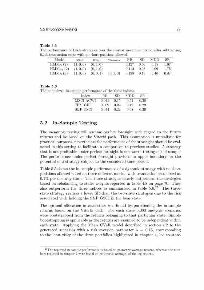
5.2 In-Sample Testing 77

Table 5.5The performance of DAA strategies over the 15-year in-sample period after subtracting0.1% transaction costs with no short positions allowed.

Model wBull wBear wRecession RR SD MDD SRHMMN (2) (1, 0, 0) (0, 1, 0) 0.127 0.08 0.15 1.67HMMNt (2) (1, 0, 0) (0, 1, 0) 0.114 0.06 0.09 1.75HMMN (3) (1, 0, 0) (0, 0, 1) (0, 1, 0) 0.138 0.16 0.46 0.87

Table 5.6The annualized in-sample performance of the three indices.

Index RR SD MDD SRMSCI ACWI 0.045 0.15 0.54 0.30JPM GBI 0.009 0.03 0.12 0.29S&P GSCI 0.044 0.22 0.68 0.20

5.2 In-Sample TestingThe in-sample testing will assume perfect foresight with regard to the futurereturns and be based on the Viterbi path. This assumption is unrealistic forpractical purposes, nevertheless the performance of the strategies should be eval-uated in this setting to facilitate a comparison to previous studies. A strategythat is not profitable under perfect foresight is not worth testing out of sample.The performance under perfect foresight provides an upper boundary for thepotential of a strategy subject to the considered time period.Table 5.5 shows the in-sample performance of a dynamic strategy with no shortpositions allowed based on three different models with transaction costs fixed at0.1% per one-way trade. The three strategies clearly outperform the strategiesbased on rebalancing to static weights reported in table 4.8 on page 70. Theyalso outperform the three indices as summarized in table 5.6.27 The three-state strategy realizes a lower SR than the two-state strategies due to the riskassociated with holding the S&P GSCI in the bear state.The optimal allocation in each state was found by partitioning the in-samplereturns based on the Viterbi path. For each state 5,000 one-year scenarioswere bootstrapped from the returns belonging to that particular state. Simplebootstrapping is applicable as the returns are assumed to be independent withineach state. Applying the Mean–CVaR model described in section 4.2 to thegenerated scenarios with a risk aversion parameter λ = 0.15, correspondingto the least risky of the three portfolios highlighted in chapter 4, led to state-

27The reported in-sample performance is based on geometric average returns, whereas the num-bers reported in chapter 2 were based on arithmetic averages of the log-returns.

78 5 Regime-Based Asset Allocation

Table 5.7The in-sample performance of DAA strategies after subtracting 0.1% transaction costswhen a short position in the stock index is allowed.

Model wBull wBear wRecession RR SD MDD SRHMMN (2) (1, 0, 0) (−1, 0, 0) 0.197 0.15 0.24 1.30HMMNt (2) (1, 0, 0) (−1, 0, 0) 0.182 0.15 0.24 1.20HMMN (3) (1, 0, 0) (−0.32, 0, 0.68) (−1, 0, 0) 0.193 0.16 0.36 1.24

Table 5.8The in-sample performance of DAA strategies after subtracting 0.1% transaction costswhen the deviations from the benchmark allocation are constrained.

Model wBull wBear wRecession RR SD MDD SRHMMN (2) (0.6, 0.15, 0.25) (0.4, 0.35, 0.25) 0.069 0.09 0.35 0.77HMMNt (2) (0.6, 0.15, 0.25) (0.4, 0.35, 0.25) 0.061 0.09 0.37 0.70HMMN (3) (0.6, 0.15, 0.25) (0.4, 0.25, 0.35) (0.4, 0.35, 0.25) 0.065 0.10 0.37 0.68Rebalancing (0.5, 0.25, 0.25) (0.5, 0.25, 0.25) (0.5, 0.25, 0.25) 0.048 0.10 0.40 0.50

dependent allocations that only include one of the indices at a time with theexception of the three-state strategy, when a short position can be held.Table 5.7 shows the in-sample results when a short position in the MSCI ACWIis allowed. A short position does not release any capital for other positionsas it should be thought of as implemented using an inverse ETF. With a riskaversion parameter of 0.15, the optimal allocation in the bear/recession stateis a short position in the MSCI ACWI rather than a long position in the JPMGBI, despite the strong in-sample performance of the JPM GBI. It is possibleto achieve a higher SR by holding the JPM GBI, but a short position in theMSCI ACWI leads to a significant excess return. The three strategies realizesimilar SRs, but the three-state strategy has a higher MDD than the two-statestrategies.As noted by Kritzman et al. (2012), strategic investors that invest with a longtime horizon typically face constraints on the size of possible deviations fromtheir benchmark allocation. It is therefore relevant to establish the potential of adynamic strategy when the possible allocations are less concentrated. Table 5.8reports the results when the possible deviations from the benchmark allocationw = (0.5, 0.25, 0.25) are limited to ±0.1. Kritzman et al. (2012) would refer tothis as a regime-dependent rather than regime-based strategy as opposed to thestocks–bonds and the long–short strategy.The dynamic tilts lead to a higher realized return and a slightly lower SD andMDD compared to rebalancing to the benchmark allocation. The dynamic strat-egy based on the two-state Gaussian HMM has a higher SR than the rebalancingstrategy as long as transaction costs are below 1.53% per one-way transaction(rebalancing also becomes more expensive).

5.3 Out-of-Sample Testing 79

Table 5.10The performance of the DAA strategies over the five-year out-of-sample period aftersubtracting 0.1% transaction costs with a one-day delay in the portfolio adjustment.

Model wBull wBear RR SD MDD SRHMMN (2) (1, 0, 0) (0, 1, 0) 0.116 0.12 0.14 0.99HMMN (2) (1, 0, 0) (−1, 0, 0) 0.082 0.18 0.35 0.47HMMN (2) (0.6, 0.15, 0.25) (0.4, 0.35, 0.25) 0.098 0.13 0.17 0.78Rebalancing (0.5, 0.25, 0.25) (0.5, 0.25, 0.25) 0.094 0.13 0.19 0.75

Table 5.11The annualized out-of-sample performance of the three indices.

Index RR SD MDD SRMSCI ACWI 0.15 0.17 0.26 0.85JPM GBI 0.03 0.03 0.04 1.12S&P GSCI 0.04 0.22 0.28 0.17

To summarize, the in-sample testing has shown that the strategies based onthe two-state models outperform the three-state strategies. As discussed in sec-tion 5.1, an approach based on two rather than three states should reduce theprobability of misclassification, as it is easier to distinguish between two thanthree states. It cannot be ruled out that other more profitable three-state strate-gies exist, but it will remain a possibility for future research to examine moreadvanced strategies. The out-of-sample testing will employ an adaptive estima-tion approach, which should offset the advantage of a conditional t-distribution,as discussed in section 3.5. The out-of-sample testing will, therefore, focus onthe two-state Gaussian HMM.

5.3 Out-of-Sample TestingFigure 5.9 shows the predicted states out of sample based on the adaptivelyestimated two-state Gaussian HMM when applying a probability filter with a92%-threshold. The effective window length used in the estimation was 500trading days. The result of the decoding looks very robust as the identifiedregimes do not appear to be very sensitive to the chosen threshold. It mighthave been optimal with a slightly lower value out of sample as the thresholdinfluences how fast the regime changes are detected.Table 5.10 reports the out-of-sample performance of the three different strategiesbased on the decoded states of the adaptively estimated two-state GaussianHMM. Switching between the MSCI ACWI and the JPM GBI led to a higherreturn and SR than rebalancing to static weights (see table 4.9 on page 70). Italso led to a higher SR and lower drawdown than the MSCI ACWI as shown intable 5.11. Switching between a long and a short position in the MSCI ACWI

80 5 Regime-Based Asset Allocation

..

2009

.

2010

.

2011

.

2012

.

2013

.

2014

.

150

.

250

.

350

.

Year

.

MSCIACW

I

.

2009

.

2010

.

2011

.

2012

.

2013

.

2014

.

0.0

.

0.4

.

0.8

.

Year

.

Pr(S

t+1=

1)

.2009

.2010

.2011

.2012

.2013

.2014

.

0.0

.

0.4

.

0.8

. Year.

Pr(S

t+1=

2)

Figure 5.9: The MSCI ACWI and the predicted states based on the adaptively esti-mated two-state Gaussian HMM and a probability filter with a 92%-threshold. Cyan isthe bull state and yellow is the bear state.

5.3 Out-of-Sample Testing 81

Table 5.12The performance of the DAA strategies over the five-year out-of-sample period aftersubtracting 0.1% transaction costs with no delay in the portfolio adjustment.

Model wBull wBear RR SD MDD SRHMMN (2) (1, 0, 0) (0, 1, 0) 0.138 0.11 0.13 1.21HMMN (2) (1, 0, 0) (−1, 0, 0) 0.130 0.18 0.35 0.74HMMN (2) (0.6, 0.15, 0.25) (0.4, 0.35, 0.25) 0.103 0.12 0.17 0.83

Table 5.13The performance of the DAA strategies over the five-year out-of-sample period aftersubtracting 0.1% transaction costs with a two-day delay in the portfolio adjustment.

Model wBull wBear RR SD MDD SRHMMN (2) (1, 0, 0) (0, 1, 0) 0.129 0.12 0.15 1.10HMMN (2) (1, 0, 0) (−1, 0, 0) 0.104 0.17 0.34 0.59HMMN (2) (0.6, 0.15, 0.25) (0.4, 0.35, 0.25) 0.101 0.13 0.17 0.80

has not been the best strategy in the five-year out-of-sample period, as therehave been no major setbacks. The long–short strategy realized a lower returnthan the two most risky rebalancing strategies and at the same time a largerMDD.The strategy with constrained deviations from the benchmark allocation real-ized a higher return with a slightly lower SD and MDD than the benchmarkallocation in a period that did not favor a dynamic strategy. The dynamicstrategy realized a higher SR and a lower MDD compared to the rebalancingstrategy as long as the transaction costs did not exceed 0.6% per one-way trade.The reported results are based on a one-day delay between the prediction of astate change and the portfolio adjustment. That is, if the predicted state ofday t + 1 based on the closing price at day t is different from the state thatthe allocation at day t is based on and the confidence in the prediction is abovethe 92%-threshold, then the allocation is changed at the closing of day t+ 1. Ifthe reallocation could be implemented at the closing of day t, i.e. with no delay,then the RR would have been a lot higher, as shown in table 5.12, with the SDand MDD remaining largely unchanged.It would also increase the RR if the reallocations were implemented with a tworather than one-day delay as shown in table 5.13. The relatively large differencesin the RR depending on the implementation delay might be a coincidence, butthey can also be a result of the significantly positive first-order autocorrelationthat both the MSCI ACWI and the JPM GBI exhibit and the significantly neg-ative second-order autocorrelation of the MSCI ACWI. A one-day delay causesthe portfolio to miss out on the positive lag-one momentum, at the same timeas being hurt by the day-two correction, which is avoided with a two-day delay.

82 5 Regime-Based Asset Allocation

Table 5.14The performance of the DAA strategies over the five-year out-of-sample period aftersubtracting 0.1% transaction costs and with a one-day delay in the portfolio adjustmentwhen the model is estimated using a rolling window of 1000 trading days.

Model wBull wBear RR SD MDD SRHMMN (2) (1, 0, 0) (0, 1, 0) 0.104 0.12 0.17 0.87HMMN (2) (1, 0, 0) (−1, 0, 0) 0.057 0.18 0.48 0.33HMMN (2) (0.6, 0.15, 0.25) (0.4, 0.35, 0.25) 0.098 0.13 0.17 0.77

The same strategies would have realized lower returns and higher MDDs ifbased on a two-state Gaussian HMM estimated using a rolling window of 1000days. The results, when using a rolling window for the estimation, are shown intable 5.14 based on a one-day delay in the implementation. The performanceof the strategy with dynamic tilts is almost the same. The rolling windowestimation would have led to 13 allocation changes instead of 7 due to somevery short-lived sojourns. Hence, more intelligent adaptivity does add value inparticular in terms of reducing the tail-risk.

CHAPTER 6Summary and

Conclusion

The thesis’ point of departure was that different economic regimes require dif-ferent asset allocations. In the presence of time-varying investment opportuni-ties, portfolio weights should be adjusted as new information arrives. Regime-switching models are well suited to capture the sudden changes of behavior andthe phenomenon that the new dynamics of asset prices persist for several periodsafter a change. The asset classes considered were stocks, bonds, and commodi-ties. Unlike the majority of previous studies on regime-switching strategies,there was no risk-free asset.

The data analysis confirmed well-known stylized facts of financial returns includ-ing skewness, leptokurtosis, volatility persistence, and time-varying correlations.The stylized behavior was most distinct for the stock index, while the suddenchanges in the behavior of the government bond index seemed to be following in-terest rate changes. There was a focus on modeling the stock returns as portfoliorisk is typically dominated by stock market risk.

The estimated models turned out to have a simple structure as only certaintransitions were seen to occur. This offset the advantage of a continuous-timeformulation in relation to the intended use. Even so, the implementation of acontinuous-time version of the Baum–Welch algorithm was an important con-tribution of the project that will be useful for future work on continuous-timehidden Markov models. Three states seemed to be sufficient to reproduce thestylized facts with the most exceptional observations being allocated in a sepa-

84 6 Summary and Conclusion

rate state. A fourth state did not seem to improve the fit significantly comparedto the added complexity and two states were not enough to adequately capturethe stylized behavior. Although a conditional t-distribution in the high-variancestate improved the ability of a two-state model to reproduce the excess kurtosis,it did not lead to a satisfactory fit to the long memory of the squared returns.The estimation identified a call for an adaptive approach as the parametersof the estimated models were far from constant throughout the sample period.Time-varying parameters are likely part of the reason why many studies thatemploy Markov-switching models to financial returns obtain significantly betterresults in sample compared to out of sample. An adaptive estimation methodbased on exponential forgetting compensated for the need for a third state or aconditional t-distribution in the high-variance state to capture the most excep-tional observations. Allowing for non-constant transition probabilities impliesthat the sojourn time distribution can take any shape.A three-state multivariate Gaussian hidden Markov model was estimated andused to generate scenarios useful for a strategic asset allocation decision. Threeefficient portfolios with different levels of risk and expected return were foundbased on mean–CVaR optimization. Rebalancing was shown to improve the re-turn and at the same time reduce the risk—both the variance and the maximumdrawdown—compared to buy-and-hold strategies in sample with an annual fre-quency being optimal. The three portfolios realized significantly higher returnsand Sharpe ratios out of sample compared to in sample.Dynamic asset allocation strategies were shown to add value over strategiesbased on rebalancing to static weights. The considered two-state models werefound to outperform a three-state model in sample as foundation for dynamicasset allocation strategies. One strategy was based on switching between thestock and the bond index, another strategy was either long or short the stockindex, and a third strategy included dynamic tilts of the benchmark allocation tostocks and bonds based on the prevailing regime while keeping a fixed allocationto commodities.The outperformance in sample was very large, among other things, due to themajor setbacks at the end of the period that favored a dynamic strategy. In anout-of-sample period that did not favor a dynamic strategy, the tested strategiesbased on an adaptively estimated two-state Gaussian hidden Markov modelstill outperformed a rebalancing strategy after accounting for transaction costs,assuming no knowledge of future returns, and with a realistic delay between theidentification of a regime change and the portfolio adjustment.

6.1 DiscussionThe thesis extends the work of Bulla et al. (2011) and addresses most of their sug-gestions for future research. The consideration of a continuous-time approach;

6.2 Future Work 85

the model selection and testing of models with more than two states, differentunivariate and multivariate state-dependent distributions, and non-geometricalsojourn time distributions; the adaptive estimation method; and the asset al-location decision between three asset classes allowing for short positions in thestock index are new to the majority of the literature on applications of Markov-switching models in empirical finance as reviewed by Guidolin (2011).Previous studies on regime-based asset allocation have primarily found that itis possible to obtain the same or a slightly higher return and at the same timereduce the portfolio risk by switching to a risk-free asset in the most turbulentperiods. Holding a risk-free asset obviously yields a risk reduction, but leveragewould be needed to significantly increase the return. This is consistent withthe finding that safer assets offer higher risk-adjusted returns than riskier assetsbecause of leverage aversion (Asness et al. 2012, Frazzini and Pedersen 2014).This study has shown that it is possible to obtain a significant excess returnwith the same risk in terms of portfolio variance but a lower drawdown riskby taking advantage of the time-varying investment opportunities rather thanrebalancing to static weights. The documented in-sample improvements of theSharpe ratio exceed those of Bulla et al. (2011) by a good margin while theout-of-sample improvements are of a similar magnitude.The need for an adaptive estimation approach to capture the time-varying behav-ior of the model parameters is consistent with previous studies that have foundhidden semi-Markov models with non-geometric sojourn time distributions tobe better at reproducing some of the stylized facts (Bulla and Bulla 2006) andthat conditional t-distributions increased the persistence of the visited statesand improved the ability to reproduce the excess kurtosis (Bulla 2011).

6.2 Future WorkAdaptive methods are a relatively undiscovered topic within empirical financedespite the strong evidence of non-stationary data-generating processes. Thework done in this thesis has focused on capturing the time-varying behavior ofthe model parameters by assigning more weight to the most recent observationswhich is an extension of the fixed-length forgetting Bulla et al. (2011) applied intheir study. A better description of the time-varying behavior of the parametersis an open route for future research that can be pursued in various ways. Onewould be to allow different forgetting factors for each parameter or consider moreadvanced state-dependent or time-dependent forgetting. Another way would beto formulate a model for the parameter changes.The hierarchical regime-switching model studied by Ang and Bekaert (2004),where the parameters of the regime-switching process depended on an exoge-nous variable (a short-term interest rate) is an interesting extension of the fre-quently used Markov-switching models with seemingly great potential for future

86 6 Summary and Conclusion

work. Testing other possible predictors such as credit spreads or implied volatil-ity is another possibility for future work. It is worth establishing whether anapproach based on modeling regimes in assets returns outperforms approachesbased on forecasting regimes in drivers of asset returns. It would also be rele-vant to do further research on whether an approach based on regime-switchingmodels outperforms more simple approaches based on, for instance, the Maha-lanobis distance, implied volatility, or simple moving average rules as suggestedby Zakamulin (2014).Inclusion of other major asset classes will remain a possibility for future work.This study already extends previous studies that only considered stocks andcash by including both a bond and a commodity index. Stocks, bonds, andcommodities are likely to be three of the main common risk factors across ahigher number of asset classes (see e.g. Ilmanen 2001, Bender et al. 2010). Ratherthan examining a large number of asset classes it would be useful to have a modeldescribing the behavior of a smaller number of common risk factors.A final suggestion for future work is to consider more smooth switching proce-dures for the portfolio adjustment for instance based on the confidence in thepredicted state similar to the idea behind the Black–Litterman model (Blackand Litterman 1992). Rather than doing a separate optimization of the model,the forgetting factor, the probability threshold, and the state-dependent alloca-tions it could all be combined into one large optimization problem, although themagnitude of the problem is likely to make it very difficult to solve.

References

Ahlgren, P., Dahl, H., April 2010. Hidden Markov models—detecting regimesin financial time series. Nykredit Asset Management, 1–9.

Ammann, M., Verhofen, M., 2006. The effect of market regimes on style alloca-tion. Financial Markets and Portfolio Management 20 (3), 309–337.

Ang, A., Bekaert, G., 2002. International asset allocation with regime shifts.Review of Financial Studies 15 (4), 1137–1188.

Ang, A., Bekaert, G., 2004. How regimes affect asset allocation. Financial Ana-lysts Journal 60 (2), 86–99.

Ang, A., Timmermann, A., June 2011. Regime changes and financial markets.Working Paper 17182, National Bureau of Economic Research.

Artzner, P., Delbaen, F., Eber, J.-M., Heath, D., 1999. Coherent measures ofrisk. Mathematical Finance 9 (3), 203–228.

Asai, M., McAleer, M., 2007. Non-trading day effects in asymmetric conditionaland stochastic volatility models. Econometrics Journal 10 (1), 113–123.

Asness, C., Frazzini, A., Pedersen, L. H., 2012. Leverage aversion and risk parity.Financial Analysts Journal 68 (1), 47–59.

Bacci, S., Pandolfi, S., Pennoni, F., 2012. A comparison of some criteria forstates selection in the latent markov model for longitudinal data. ArXiv e-prints.

88 References

Bauer, R., Haerden, R., Molenaar, R., 2004. Asset allocation in stable andunstable times. J. Investing 13 (3), 72–80.

Baum, L. E., Petrie, T., Soules, G., Weiss, N., 1970. A maximization techniqueoccurring in the statistical analysis of probabilistic functions of Markov chains.The Annals of Mathematical Statistics 41 (1), 164–171.

Bender, J., Briand, R., Nielsen, F., Stefek, D., 2010. Portfolio of risk premia: Anew approach to diversification. J. Portfolio Management 36 (2), 17–25.

Berkelaar, M., others, 2014. lpSolve: Interface to Lp_solve v. 5.5 to solve lin-ear/integer programs. R package version 5.6.8.

Bertsimas, D., Lauprete, G. J., Samarov, A., 2004. Shortfall as a risk measure:properties, optimization and applications. J. Economic Dynamics & Control28 (7), 1353–1381.

Black, F., Litterman, R., 1992. Global portfolio optimization. Financial AnalystsJournal 48 (5), 28–43.

Brinson, G. P., Hood, L. R., Beebower, G. L., 1986. Determinants of portfolioperformance. Financial Analysts Journal 42 (4), 39–44.

Bulla, J., 2011. Hidden Markov models with t components. Increased persistenceand other aspects. Quantitative Finance 11 (3), 459–475.

Bulla, J., Berzel, A., 2008. Computational issues in parameter estimation forstationary hidden Markov models. Computational Statistics 23 (1), 1–18.

Bulla, J., Bulla, I., 2006. Stylized facts of financial time series and hidden semi-Markov models. Computational Statistics and Data Analysis 51, 2192–2209.

Bulla, J., Bulla, I., Nenadic, O., 2010. hsmm—an R package for analyzing hid-den semi-Markov models. Computational Statistics and Data Analysis 54,611–619.

Bulla, J., Mergner, S., Bulla, I., Sesboüé, A., Chesneau, C., 2011. Markov-switching asset allocation: Do profitable strategies exist? J. Asset Manage-ment 12 (5), 310–321.

Bureau, A., Hughes, J. P., Shiboski, S. C., 2000. An S-Plus implementation ofhidden Markov models in continuous time. J. Computational and GraphicalStatistics 9 (4), 621–632.

Burns, A. F., Mitchell, W. C., 1946. Measuring Business Cycles. National Bu-reau of Economic Research.

Campbell, J. Y., 1998. Asset prices, consumption, and the business cycle. Work-ing Paper 6485, National Bureau of Economic Research.

References 89

Campbell, J. Y., Lo, A. W., Mackinlay, A. C., 1997. The Econometrics of Fi-nancial Markets. Princeton University Press.

Cappé, O., Moulines, E., Rydén, T., 2005. Inference in hidden Markov models.Springer.

Carhart, M. M., 1997. On persistence in mutual fund performance. J. Finance52 (1), 57–82.

Chow, G., Jacquier, E., Kritzman, M., Lowry, K., 1999. Optimal portfolios ingood times and bad. Financial Analysts Journal 55 (3), 65–73.

Cochrane, J., 2005. Financial markets and the real economy. Working Paper11193, National Bureau of Economic Research.

Cont, R., 2001. Empirical properties of asset returns: stylized facts and statisti-cal issues. Quantitative Finance 1, 223–236.

Crockett, A. D., September 2000. Marry the micro- and macro-prudential dimen-sions of financial stability. Speech at the Eleventh International Conferenceof Banking Supervisors.

Dacco, R., Satchell, S., 1999. Why do regime-switching models forecast so badly?J. Forecasting 18 (1), 1–16.

Dahlquist, M., Harvey, C. R., 2001. Global tactical asset allocation. EmergingMarkets Quarterly 5 (1), 6–14.

Dempster, A. P., Laird, N. M., Rubin, D. B., 1977. Maximum likelihood fromincomplete data via the EM algorithm. J. Royal Statistical Society 39 (1),1–38.

Dittmer, E., November 2008. Hidden Markov models with time-continuous out-put behavior. Ph.D. thesis, Freie University of Berlin.

Edwards, P., Manjrekar, C., 2014. Asset allocation survey. Mercer.

Erb, C. B., Harvey, C. R., 2006. The strategic and tactical value of commodityfutures. Financial Analysts Journal 62 (2), 69–97.

Fama, E. F., 1970. Efficient capital markets: A review of theory and empiricalwork. J. Finance 25 (2), 383–417.

Frazzini, A., Pedersen, L. H., 2014. Betting against beta. J. Financial Economics111 (1), 1–25.

Frühwirth-Schnatter, S., 2006. Finite Mixture and Markov Switching Models.Springer.

90 References

Granger, C. W. J., Ding, Z., 1995a. Some properties of absolute return: Analternative measure of risk. Annales D’Economie Et Statistique (40), 67–92.

Granger, C. W. J., Ding, Z., 1995b. Stylized facts on the temporal and distribu-tional properties of daily data from speculative markets. Unpublished paper,Department of Economics, University of California, San Diego.

Guidolin, M., 2011. Markov switching models in empirical finance. WorkingPaper 415, IGIER, Bocconi University.

Guidolin, M., Timmermann, A., 2007. Asset allocation under multivariateregime switching. J. Economic Dynamics & Control 31 (11), 3503–3544.

Hamilton, J. D., 1989. A new approach to the economic analysis of nonstationarytime series and the business cycle. Econometrica 57 (2), 357–384.

Hamilton, J. D., 1990. Analysis of time series subject to changes in regime. J.Econometrics 45 (1–2), 39–70.

Hannam, M., Lejonvarn, J., 2009. The commodity risk premium.URL http://www.markhannam.com/essays/essay2a.htm

Hobolth, A., Jensen, J. L., 2011. Summary statistics for endpoint-conditionedcontinuous-time Markov chains. J. Applied Probability 48 (4), 901–1204.

Høyland, K., Wallace, S. W., February 2001. Generating scenario trees for mul-tistage decision problems. Management Science 47 (2), 295–307.

Ibbotson, R. G., Kaplan, P. D., 2000. Does asset allocation policy explain 40,90, or 100 percent of performance? Financial Analysts Journal 56 (1), 26–33.

Ilmanen, A., 2001. Expected Returns. Wiley.

Iversen, E. B., Møller, J. K., Morales, J. M., Madsen, H., 2013. InhomogeneousMarkov models for describing driving patterns. Technical report, TechnicalUniversity of Denmark.

Jackson, C. H., 2011. Multi-state models for panel data: The msm package forR. J. Statistical Software 38 (8), 1–29.

Kritzman, M., Li, Y., 2010. Skulls, financial turbulence, and risk management.Financial Analysts Journal 66 (5), 30–41.

Kritzman, M., Myrgren, S., Page, S., 2009. Optimal rebalancing: A scalablesolution. J. Investment Management 7 (1), 9–19.

Kritzman, M., Page, S., Turkington, D., 2012. Regime shifts: Implications fordynamic strategies. Financial Analysts Journal 68 (3), 22–39.

References 91

Kritzman, M., Rich, D., 2002. The mismeasurement of risk. Financial AnalystsJournal 58 (3), 91–99.

Krstic, M., Kanellakopoulos, I., Kokotovic, P. V., 1995. Nonlinear and AdaptiveControl Design. Wiley.

Lange, J. M., Minin, V. N., 2013. Fitting and interpreting continuous-time latentMarkov models for panel data. Statistics in Medicine 32 (26), 4581–4595.

Lee, H.-Y., Wu, J.-L., 2001. Mean reversion of inflation rates: Evidence from13 OECD countries. J. Macroeconomics 23 (3), 477–487.

Levich, R. M., 2001. International Financial Markets: Prices and Policies, 2ndEdition. McGraw–Hill.

Lystig, T. C., Hughes, J. P., 2002. Exact computation of the observed infor-mation matrix for hidden Markov models. J. Computational and GraphicalStatistics 11 (3), 678–689.

Madsen, H., 2008. Time Series Analysis. Chapman & Hall.

Madsen, H., Thyregod, P., 2011. Introduction to General and Generalized LinearModels, 1st Edition. Chapman & Hall.

Mahalanobis, P. C., 1936. On the generalised distance in statistics. Proceedingsof the National Institute of Sciences of India 2 (1), 49–55.

Markowitz, H. M., 1952. Portfolio selection. J. Finance 7 (1), 77–91.

Merton, R. C., 1973. An intertemporal capital asset pricing model. Econometrica41 (5), 867–887.

Nystrup, P., Madsen, H., Lindström, E., 2014. Stylized facts of financial timeseries and hidden Markov models in continuous time. Submitted to Quanti-tative Finance.

Perrucci, S., Benaben, B., 2012. Inflation Sensitive Assets: Instruments andStrategies. Risk Books.

Pinson, P., Madsen, H., 2012. Adaptive modelling and forecasting of offshorewind power fluctuations with Markov-switching autoregressive models. J. Fore-casting 31 (4), 281–313.

Podgórski, K., Wallin, J., 2013. Maximizing leave-one-out likelihood for the lo-cation parameter of unbounded densities. Annals of the Institute of StatisticalMathematics, 1–20.

R Core Team, 2013. R: A Language and Environment for Statistical Computing.R Foundation for Statistical Computing, Vienna, Austria.URL http://www.R-project.org/

92 References

Rogalski, R. J., 1984. New findings regarding day-of-the-week returns over trad-ing and non-trading periods. J. Finance 39 (5), 1603–1614.

Rudin, L. I., Osher, S., Fatemi, E., 1992. Nonlinear total variation based noiseremoval algorithms. Physica D 60 (1–4), 259–268.

Rydén, T., 2008. EM versus Markov chain Monte Carlo for estimation of hid-den Markov models: A computational perspective. Bayesian Analysis 3 (4),659–688.

Rydén, T., Teräsvirta, T., Åsbrink, S., 1998. Stylized facts of daily return seriesand the hidden Markov model. J. Applied Econometrics 13 (3), 217–244.

Seo, B., Kim, D., 2012. Root selection in normal mixture models. ComputationalStatistics and Data Analysis 56 (8), 2454–2470.

Sheikh, A. Z., Qiao, H., 2010. Non-normality of market returns: A frameworkfor asset allocation decision making. J. Alternative Investments 12 (3), 8–35.

Sheikh, A. Z., Sun, J., 2012. Regime change: Implications of macro shifts onasset class and portfolio performance. J. Investing 21 (3), 36–54.

Siegel, J. J., 2007. Stocks for the Long Run, 4th Edition. McGraw–Hill.

Silvestrov, D., Stenberg, F., 2004. A pricing process with stochastic volatilitycontrolled by a semi-markov process. Communications in Statistics - Theoryand Methods 33 (3), 591–608.

Sun, W., Fan, A., Chen, L.-W., Schouwenaars, T., Albota, M. A. ., 2006. Opti-mal rebalancing for institutional portfolios. J. Portfolio Management 32 (2),33–43.

Taramasco, O., Bauer, S., 2013. RHmm: Hidden Markov Models simulationsand estimations. R package version 2.0.3.

Timmermann, A., 2000. Moments of Markov switching models. J. Econometrics96 (1), 75–111.

Varadhan, R., 2012. SQUAREM: Squared extrapolation methods for accelerat-ing fixed-point iterations. R package version 2012.7–1.

Viterbi, A. J., 1967. Error bounds for convolutional codes and an asymptoti-cally optimum decoding algorithm. IEEE Transactions on Information Theory13 (2), 260–269.

Zakamulin, V., 2014. Dynamic asset allocation strategies based on unexpectedvolatility. J. Alternative Investments 16 (4), 37–50.

Zucchini, W., MacDonald, I. L., 2009. Hidden Markov Models for Time Series:An Introduction Using R, 2nd Edition. Chapman & Hall.

APPENDIX AR-code

A.1 Discrete-time Baum–Welch Algorithm

EMNt = function(x, mu, sigma, Gamma, delta, nu, maxiter = 500,tol = 1e-8, print = FALSE){

n = length(x)m = length(mu)mu.next = musigma.next = sigmaGamma.next = Gammadelta.next = deltanu.next = nuu = numeric(n)llk.prev = 0

for (iter in 1:maxiter){lallprobs = matrix(NA, n, m)for (i in 1:n){

for (j in 1:m){if (j < m)lallprobs[i, j] = dnorm(x[i], mean = mu.next[j],

sd = sigma.next[j], log = T)elselallprobs[i, j] = dtmod(x[i], mu.next[j], sigma.next[j],

nu.next, log = T)}

94 A R-code

}fb = lalphabeta(x, mu.next, sigma.next, Gamma.next,

delta.next, nu.next)la = fb$lalb = fb$lbc = max(la[, n])llk = c + log(sum(exp(la[, n] - c)))for (j in 1:m){for (k in 1:m)Gamma.next[j, k] = Gamma[j, k]*sum(exp(la[j, 1:(n-1)] +

lallprobs[2:n, k] + lb[k, 2:n] - llk))if (j < m){mu.next[j] = exp(la[j, ] + lb[j, ] - llk)%*%x/sum(exp(la[j, ] + lb[j, ] - llk))

sigma.next[j] = sqrt((exp(la[j, ] + lb[j, ] - llk)*(x - mu.next[j]))%*%(x - mu.next[j])/sum(exp(la[j, ] + lb[j, ] - llk)))

}else{u = (nu.next + 1)/(nu.next + (x - mu.next[j])*

(x - mu.next[j])/sigma.next[j]^2)w = (exp(la[j, ] + lb[j, ] - llk)*u)%*%xz = exp(la[j, ] + lb[j, ] - llk)%*%umu.next[j] = w/zw = (exp(la[j, ] + lb[j, ] - llk)*u*(x - mu.next[j]))%*%(x - mu.next[j])

sigma.next[j] = sqrt(w/z)w = exp(la[j, ] + lb[j, ] - llk)%*%(log(u) - u)z = sum(exp(la[j, ] + lb[j, ] - llk))estimator = function(nu, frac){-digamma(exp(nu)/2)+log(exp(nu)/2) + 1 + frac +digamma((exp(nu) + 1)/2) - log((exp(nu) + 1)/2)

}nu.next = exp(uniroot(estimator, frac = w/z, lower =

log(0.01), upper = log(500))$root)}

}Gamma.next = Gamma.next/apply(Gamma.next, 1, sum)delta.next = exp(la[, 1] + lb[, 1] - llk)delta.next = delta.next/sum(delta.next)crit = llk - llk.previf(crit < tol){np = (m + 2)*mAIC = -2*(llk - np)

A.1 Discrete-time Baum–Welch Algorithm 95

BIC = -2*llk + np*log(n)return(list(mu = mu, sigma = sigma, Gamma = Gamma,

delta = delta, nu = nu, iterations = iter,mllk = llk, AIC = AIC, BIC = BIC))

}mu = mu.nextsigma = sigma.nextGamma = Gamma.nextdelta = delta.nextnu = nu.nextllk.prev = llkif(print == T)

print(paste('Iteration', iter, 'LogLik', round(llk, 4)))}

print(paste('No convergence after', maxiter, 'iterations'))return(list(mu = mu, sigma = sigma, Gamma = Gamma,

delta = delta, nu = nu, iterations = iter, mllk = llk))}

lalphabeta = function(x, mu, sigma, Gamma, delta, nu){n = length(x)m = length(mu)lalpha = lbeta = matrix(NA, m, n)P = rep(NA, m)for (j in 1:m){if (j < m)

P[j] = dnorm(x[1], mean = mu[j], sd = sigma[j])else

P[j] = dtmod(x[1], mu[j], sigma[j], nu)}foo = delta*Psumfoo = sum(foo)lscale = log(sumfoo)foo = foo/sumfoolalpha[, 1] = log(foo) + lscalefor (i in 2:n){for (j in 1:m){

if (j < m)P[j] = dnorm(x[i], mean = mu[j], sd = sigma[j])

elseP[j] = dtmod(x[i], mu[j], sigma[j], nu)

}foo = foo%*%Gamma*P

96 A R-code

sumfoo = sum(foo)lscale = lscale + log(sumfoo)foo = foo/sumfoolalpha[, i] = log(foo) + lscale

}lbeta[, n] = rep(0, m)foo = rep(1/m, m)lscale = log(m)for (i in (n - 1):1){for (j in 1:m){if (j < m)P[j] = dnorm(x[i + 1], mean = mu[j], sd = sigma[j])

elseP[j] = dtmod(x[i+1], mu[j], sigma[j], nu)

}foo = Gamma%*%(P*foo)lbeta[, i] = log(foo) + lscalesumfoo = sum(foo)foo = foo/sumfoolscale = lscale + log(sumfoo)

}list(la = lalpha, lb = lbeta)

}

dtmod = function(x, mu = 0, sigma = 1, nu = 30, log = FALSE){den1 = try(sigma*beta(1/2, nu/2))num1 = try(nu^(-1/2))den2 = try(nu*sigma^2)num2 = try((x - mu)^2)dtmod = try(num1/den1*(1 + num2/den2)^(-1*(nu + 1)/2))if (log == TRUE)dtmod = log(dtmod)

return (dtmod)}

A.2 Continuous-time Baum–Welch Algorithm

CTEM = function(x, t, mu, sigma, Q, delta, m,maxiter = 100, tol = 1e-8){

n = length(x)mu.next = musigma.next = sigmaQ.next = Q

A.2 Continuous-time Baum–Welch Algorithm 97

delta.next = deltallk.prev = 0

for (iter in 1:maxiter){fb = lalphabeta(x, t, mu.next, sigma.next, Q.next,

delta.next, m)la = fb$lalb = fb$lbc = max(la[, n])llk = c + log(sum(exp(la[, n] - c)))R = numeric(m)N = matrix(0, m, m)tmp = eigen(Q.next)U = tmp$vectorsUinv = solve(U)lambda = tmp$valuesmaxtau = max(diff(t))TiS = array(NA, c(maxtau, m, m, m))Trans = array(NA, c(maxtau, m, m, m, m))for (tau in 1:maxtau){

for (a in 1:m){for (b in 1:m){TiS[tau, a, b, ] = TimeInStates(a, b, tau, U, Uinv,

lambda)Trans[tau, a, b, , ] = Transitions(a, b, tau, U, Uinv,

lambda, Q.next)}

}}for (l in 2:n){

tau = t[l] - t[l - 1]for (a in 1:m){for (b in 1:m){Pab = dnorm(x[l], mean = mu.next[b], sd = sigma.next[b])*

exp(la[a, l - 1] + lb[b, l] - llk)R = R + TiS[tau, a, b, ]*PabN = N + Trans[tau, a, b, , ]*Pab

}}

}Q.next = N/Rdiag(Q.next) = -apply(Q.next, 1, sum)for (j in 1:m){

mu.next[j] = exp(la[j, ] + lb[j, ] - llk)%*%x/

98 A R-code

sum(exp(la[j, ] + lb[j, ] - llk))sigma.next[j] = sqrt((exp(la[j, ] + lb[j, ] - llk)*

(x - mu.next[j]))%*%(x - mu.next[j])/sum(exp(la[j, ] + lb[j, ] - llk)))

}delta.next = exp(la[, 1] + lb[, 1] - llk)delta.next = delta.next/sum(delta.next)crit = llk - llk.previf(crit < tol){np = 5*m - 1AIC = -2*(llk - np)BIC = -2*llk + np*log(n)return(list(mu = mu, sigma = sigma, Q = Q, delta = delta,

iterations = iter, mllk = llk, AIC = AIC, BIC = BIC))}mu = mu.nextsigma = sigma.nextQ = Q.nextdelta = delta.nextllk.prev = llkprint(paste('Iteration', iter, 'LogLik', round(llk, 4)))

}print(paste('No convergence after', maxiter, 'iterations'))return(list(mu = mu, sigma = sigma, Q = Q, delta = delta,

iterations = iter, mllk = llk))}

lalphabeta = function(x, t, mu, sigma, Q, delta, m){n = length(x)lalpha = lbeta = matrix(NA, m, n)P = rep(NA, m)for (j in 1:m)P[j] = dnorm(x[1], mean = mu[j], sd = sigma[j])

foo = delta * Psumfoo = sum(foo)lscale = log(sumfoo)foo = foo/sumfoolalpha[, 1] = log(foo)+lscaletmp = eigen(Q)U = tmp$vectorsUinv = solve(U)lambda = tmp$valuesfor (i in 2:n){for (j in 1:m)

A.2 Continuous-time Baum–Welch Algorithm 99

P[j] = dnorm(x[i], mean = mu[j], sd = sigma[j])tau = t[i] - t[i - 1]Gamma = U%*%diag(exp(tau*lambda))%*%Uinvfoo = foo%*%Gamma*Psumfoo = sum(foo)lscale = lscale+log(sumfoo)foo = foo/sumfoolalpha[, i] = log(foo)+lscale

}lbeta[, n] = rep(0, m)foo = rep(1/m, m)lscale = log(m)for (i in (n - 1):1){for (j in 1:m)

P[j] = dnorm(x[i + 1], mean = mu[j], sd = sigma[j])tau = t[i + 1] - t[i]Gamma = U%*%diag(exp(tau*lambda))%*%Uinvfoo = Gamma%*%(P*foo)lbeta[, i] = log(foo)+lscalesumfoo = sum(foo)foo = foo/sumfoolscale = lscale+log(sumfoo)

}list(la = lalpha, lb = lbeta)

}

TimeInStates = function(a, b, tau, U, Uinv, lambda,epsilon = 1e-7){

m = nrow(U)J = matrix(0, m, m)for (i in 1:m){for (j in 1:m){

if (abs(lambda[i] - lambda[j]) <= epsilon)J[i, j] = tau*exp(tau*lambda[i])

elseJ[i, j] = (exp(tau*lambda[i]) - exp(tau*lambda[j]))/(lambda[i] - lambda[j])

}}Times = numeric(m)for (k in 1:m){second_layer = 0for (i in 1:m){

third_layer = 0

100 A R-code

for (j in 1:m)third_layer = third_layer + U[k, j]*Uinv[j, b]*J[i,j]

second_layer = second_layer + U[a, i]*Uinv[i, k]*third_layer}Times[k] = second_layer

}return(Times)

}

Transitions = function(a, b, tau, U, Uinv, lambda, Q,epsilon = 1e-7){

m = nrow(Q)J = matrix(0, m, m)for (i in 1:m){for (j in 1:m){if (abs(lambda[i] - lambda[j]) <= epsilon)J[i, j] = tau*exp(tau*lambda[i])

elseJ[i, j] = (exp(tau*lambda[i]) - exp(tau*lambda[j]))/(lambda[i] - lambda[j])

}}Transitions = matrix(0, m, m)for (k in 1:m){for (l in 1:m){second_layer = 0if (k != l){for (i in 1:m){third_layer = 0for (j in 1:m)third_layer = third_layer + U[l, j]*Uinv[j, b]*J[i, j]*Q[k, l]

second_layer = second_layer + U[a, i]*Uinv[i, k]*third_layer

}Transitions[k, l] = second_layer

}}

}return(Transitions)

}

A.3 Mean–CVaR optimization 101

A.3 Mean–CVaR optimization

MeanCVaR = function(scenarios, lambda = 0.5, alpha = 0.05,print = FALSE){

require('lpSolve')nassets = ncol(scenarios)nscenarios = nrow(scenarios)nlambda = length(lambda)allocation = matrix(NA, nlambda, nassets)

ER = CVaR = numeric(nlambda)rhat = as.vector(apply(scenarios, 2, mean))A = rbind(c(rep(1, nassets), numeric(nscenarios + 1)),

cbind(scenarios, 1, diag(nscenarios)))b = c(1, numeric(nscenarios))

for (i in 1:nlambda){c = c((1 - lambda[i])*rhat, -lambda[i],

-rep(lambda[i]/(alpha*nscenarios), nscenarios))sol = lp('max', c, A, c('=', rep('>=', nscenarios)), b)allocation[i, ] = sol$solution[1:nassets]ER[i] = allocation[i, ]%*%rhatCVaR[i] = ((1 - lambda[i])*ER[i] - sol$objval)/lambda[i]if(print)

print(i)}

list(lambda = lambda, CVaR = CVaR, ER = ER, Allocation = allocation)}

102

APPENDIX BParameter Estimates

Table B.1Parameter estimates for m-state HMMs with conditional normal distributions fitted tothe daily in-sample log-returns of the MSCI ACWI.

m Γ µ× 104 σ × 102 δ π

2 0.987 0.0130.029 0.971

6.8−10.0

0.561.50

10

0.690.31

30.988 0.012 00.012 0.981 0.0060 0.043 0.957

8.8−1.0−32.5

0.480.942.46

100

0.480.450.07

40.983 0.017 0 00 0.651 0.331 0.018

0.033 0.240 0.727 00 0 0.053 0.947

8.9−69.150.7−27.9

0.470.710.742.48

1000

0.490.190.250.07

104 B Parameter Estimates

Table B.2Parameter estimates form-state HMMs with conditional normal and t-distributions fittedto the daily in-sample log-returns of the MSCI ACWI.m Γ µ× 104 σ × 102 ν δ π

2 0.990 0.0100.012 0.988

8.0−4.8

0.520.98 4.5

10

0.560.44

30.988 0.012 00.012 0.981 0.0070 0.039 0.961

8.7−0.8−29.3

0.480.931.97 6.3

100

0.480.450.07

40.983 0.017 0 00 0.651 0.331 0.018

0.033 0.241 0.726 00 0 0.046 0.954

9.0−68.350.6−24.0

0.470.700.732.00 6.6

1000

0.490.190.250.07

Table B.3Parameter estimates for m-state HMMs with conditional t-distributions fitted to thedaily in-sample log-returns of the MSCI ACWI.m Γ µ× 104 σ × 102 ν δ π

2 0.992 0.0080.010 0.990

8.4−4.8

0.490.98

14.04.5

10

0.560.44

30.991 0.009 00.009 0.984 0.0060 0.038 0.962

8.9−0.8−29.9

0.460.921.98

15.5119.86.4

100

0.480.440.08

B Parameter Estimates 105

Table B.4Parameter estimates for m-state HSMMs with conditional normal distributions fitted tothe daily in-sample log-returns of the MSCI ACWI. p and r are the parameters of thenegative binomial sojourn time distribution.m Γ 1− p r × 10 µ× 104 σ × 102 δ

2 0 11 0

0.9950.964

0.370.81

6.7−12.1

0.551.60

10

30 1 0

0.817 0 0.1830 1 0

0.9970.9410.972

1.2114.595.59

8.6−1.3−32.8

0.490.952.47

100

40 1 0 00 0 0.934 0.066

0.630 0.370 0 00 0 1 0

0.9950.3500.5770.974

0.6439.7416.714.07

8.9−68.159.7−28.3

0.480.720.742.47

1000

Table B.5Parameter estimates for m-state HSMMs with conditional t-distributions fitted to thedaily in-sample log-returns of the MSCI ACWI. p and r are the parameters of the negativebinomial sojourn time distribution and ν is the degrees of freedom for the conditionalt-distributions.m Γ 1− p r × 10 µ× 104 σ × 102 ν δ

2 0 11 0

0.9960.985

0.310.75

8.0−6.7

0.501.08

21.75.1

10

30 1 0

0.79 0 0.210 1 0

0.9970.9400.974

1.2516.935.98

8.9−1.0−29.7

0.460.941.99

17.51382.06.4

100

Table B.6Parameter estimates for a four-state CTHMM with conditional normal distributionsfitted to the daily in-sample log-returns of the MSCI ACWI.

Q µ× 104 σ × 102 δ π−0.016 0.016 0 0

0 −0.492 0.474 0.0180.030 0.353 −0.383 00 0 0.053 −0.053

8.8−67.549.7−27.8

0.470.710.742.47

1000

0.480.200.250.07

106 B Parameter Estimates

Table B.7Parameter estimates for m-state HMMs with conditional multivariate normal distribu-tions fitted to the daily in-sample log-returns of the three indices.m Γ µ× 104 σ × 102

2 0.981 0.0190.045 0.955

7.2 −0.2 6.0−11.6 1.7 −9.0

0.57 0.17 1.161.53 0.21 1.82

δ π ρACWI, GBI ρACWI, GSCI ρGBI, GSCI10

0.710.29

0.16−0.45

0.030.26

−0.01−0.12

m Γ µ× 104 σ × 102

30.984 0.015 0.0010.016 0.969 0.0150.008 0.143 0.850

7.6 −0.4 7.0−2.5 1.2 3.8−20.5 −0.4 −75.4

0.51 0.17 1.100.96 0.17 1.382.76 0.33 2.98

δ π ρACWI, GBI ρACWI, GSCI ρGBI, GSCI100

0.490.460.05

0.31−0.37−0.42

0.030.070.43

−0.01−0.06−0.19

m Γ µ× 104 σ × 102

40.988 0.004 0.009 00.003 0.988 0.008 0.0010.007 0.005 0.973 0.0150 0.008 0.135 0.857

9.2 −0.3 3.65.1 −0.3 7.5−4.3 1.4 5.0−17.2 −1.1 −82.3

0.52 0.14 1.460.54 0.20 0.841.04 0.18 1.312.84 0.34 3.10

δ π ρACWI, GBI ρACWI, GSCI ρGBI, GSCI0100

0.290.270.390.04

0.020.39−0.39−0.42

0.04−0.000.100.44

0.02−0.03−0.09−0.19

APPENDIX CAdditional Figures and

Tables

108 C Additional Figures and Tables

..1994

.1997

.2000

.2003

.2006

.2009

.

100

.

200

.

300

.

HMMN (2)

. Year.

MSCIACW

I

..1994

.1997

.2000

.2003

.2006

.2009

.

100

.

200

.

300

.

HMMNt(2)

. Year.

MSCIACW

I

..1994

.1997

.2000

.2003

.2006

.2009

.

100

.

200

.

300

.

HMMt(2)

. Year.

MSCIACW

I

..1994

.1997

.2000

.2003

.2006

.2009

.

100

.

200

.

300

.

HSMMN (2)

. Year.

MSCIACW

I

..1994

.1997

.2000

.2003

.2006

.2009

.

100

.

200

.

300

.

HSMMt(2)

. Year.

MSCIACW

I

..1994

.1997

.2000

.2003

.2006

.2009

.

100

.

200

.

300

.

MHMMN (2)

. Year.

MSCIACW

I

Figure C.1: The MSCI ACWI and the decoded states of the two-state models usingthe Viterbi algorithm. Cyan is the bull state and yellow is the bear state.

C Additional Figures and Tables 109

..1994

.1997

.2000

.2003

.2006

.2009

.

100

.

200

.

300

.

HMMN (3)

. Year.

MSCIACW

I

..1994

.1997

.2000

.2003

.2006

.2009

.100

.200

.300

.

HMMNt(3)

. Year.MSCIACW

I

..1994

.1997

.2000

.2003

.2006

.2009

.

100

.

200

.

300

.

HMMt(3)

. Year.

MSCIACW

I

..1994

.1997

.2000

.2003

.2006

.2009

.

100

.

200

.

300

.

HSMMN (3)

. Year.

MSCIACW

I

..1994

.1997

.2000

.2003

.2006

.2009

.

100

.

200

.

300

.

HSMMt(3)

. Year.

MSCIACW

I

..1994

.1997

.2000

.2003

.2006

.2009

.

100

.

200

.

300

.

MHMMN (3)

. Year.

MSCIACW

I

Figure C.2: The MSCI ACWI and the decoded states of the three-state models usingthe Viterbi algorithm. Cyan is the bull state, yellow is the bear state, and red is therecession state.