Refraction of swell by surface currents - Harvard...

$: Refraction of swell by surface currents - Harvard Universityeps.harvard.edu/files/eps/files/galletjmr.pdf · Refraction of swell by surface currents ... A case study: the event of$
Journal of Marine Research, 72, 105–126, 2014

Refraction of swell by surface currents

by Basile Gallet1 and William R. Young1,2

ABSTRACTUsing recordings of swell from pitch-and-roll buoys, we have reproduced the classic observations

of long-range surface wave propagation originally made by Munk et al. (1963) using a triangular arrayof bottom pressure measurements. In the modern data, the direction of the incoming swell fluctuatesby about ±10 ◦ on a time scale of one hour. But if the incoming direction is averaged over the durationof an event then, in contrast with the observations by Munk et al. (1963), the sources inferred by great-circle backtracking are most often in good agreement with the location of large storms on weathermaps of the Southern Ocean. However there are a few puzzling failures of great-circle backtracking.For example, in one case, the direct great-circle route is blocked by the Tuamoto Islands and theinferred source falls on New Zealand. Mirages like this occur more frequently in the bottom-pressureobservations of Munk et al. (1963), where several inferred sources fell on the Antarctic continent.

Using spherical ray tracing we investigate the hypothesis that the refraction of waves by surfacecurrents produces the mirages. With reconstructions of surface currents inferred from satellite altime-try, we show that mesoscale vorticity significantly deflects swell away from great-circle propagationso that the source and receiver are connected by a bundle of many rays, none of which precisely followa great circle. The ±10 ◦ directional fluctuations at the receiver result from the arrival of wave packetsthat have travelled along the different rays within this multipath. The occasional failure of great-circlebacktracking, and the associated mirages, probably results from partial topographic obstruction of themultipath, which biases the directional average at the receiver.

1. Introduction

Following the disruption of the 1942 Anglo-American landings on the Atlantic beachesof North Africa by six-foot surf (Atkinson, 2002), the forecasting of surface gravity wavesbecame a wartime priority. These first surface-wave forecasts were based on weather maps,and the relatively predictable propagation of swell, and were used to determine optimal con-ditions for amphibious assault (von Storch and Hasselmann, 2010; Bates, 1949). Wartimework showed that long surface waves, generated in stormy regions of the globe, can travelfor many thousands of kilometers before breaking on distant shores (Barber and Ursell,1948). In the following decades, Munk, Snodgrass, and collaborators observed that swell

1. Scripps Institution of Oceanography, University of California at San Diego, La Jolla, CA 92093-0213.2. Corresponding author e-mail: [email protected]

© 2014 Basile Gallet and William R. Young.

105

106 Journal of Marine Research [72, 2

generated in the ocean surrounding Antarctica travels half way around the Earth (Munk andSnodgrass, 1957; Munk et al., 1963; Snodgrass et al., 1966). Thus, after a transit of 5 to 15days, the waves created by winter storms in the Southern Ocean produce summer surf inCalifornia.

Barber and Ursell (1948) used linear wave theory to relate the range of a distant storm tothe rate of change of peak wave frequency at an observation point. But the formula of Barber& Ursell—see (2) below—provides no information about the direction of the source. Thefirst attempt at measuring the direction of the incoming swell was made by Munk et al. (1963)using an array of three pressure transducers on the sea bottom offshore of San ClementeIsland. The method is analogous to astronomical interferometry and was used to infer thedirection of incoming wave-trains from June to October of 1959. Assuming that swelltravels on great-circle routes, these observers combined Barber and Ursell’s estimate of therange with interferometric direction to locate storms in the Southern Ocean. Although theseinferred sources could be related to storms on weather maps, the location errors for someevents were as much as 10 ◦ of arc along the surface of the Earth, or 1,000 km. Moreover,there is a systematic error in the observations of Munk et al. (1963): the inferred sourceis most often to the south of the actual storm (Munk, personal communication). Becauseof this southwards shift, three of the thirty inferred storms fell on the Antarctic continent,and several others on sea ice. The unavoidable conclusion is that surface waves do nottravel precisely on great-circle routes. Effects such as planetary rotation (Backus, 1962),or the slightly spheroidal figure of the Earth, were shown to be far too small to explain theobserved departure from great-circle propagation. We now believe that these mirages werecaused by a combination of topographic obstruction (Munk, 2013) and refraction by surfacecurrents.

Kenyon (1971) advanced the hypothesis that the refraction of surface gravity waves bymajor ocean currents, particularly the Antarctic Circumpolar Current (ACC), might explainthe discrepancies reported by Munk et al. (1963). A packet of surface waves propagatingthrough these currents is in a medium that varies slowly on the scale of a wavelength. Thecurrents induce a doppler-shift in the surface wave frequency,

Ω(x, k) = √gk + u(x) · k, (1)

with k the wavevector, k = |k|, u the surface velocity, and g the acceleration of gravity.Over many wavelengths refraction by the currents changes the direction of propagation of awave packet so that it departs from a great circle. Given the surface current u(x, t), the rayequations describe the coupled evolution of the local wavevector k(t) and the position ofthe wave packet x(t), just as the propagation of light in a slowly varying medium followsthe rules of geometrical optics (Whitham, 1960; Bühler, 2009; Landau and Lifshitz, 1987).Using an idealized model of the ACC as a parallel shear flow, Kenyon (1971) solved theray-tracing equations and found appreciable deflections for rays making a grazing incidencewith the current.

2014] Gallet and Young: Refraction of swell by surface currents 107

Here we re-visit Kenyon’s hypothesis with the benefit of modern reconstructions of oceansurface currents and wave climate. In Section 2 we analyze modern swell measurementsfrom pitch-and-roll buoys (Kuik et al., 1988). We observe that the direction of incident swellmeasured by a deep-water buoy close to San Clemente Island varies by ±10 ◦ on a time scaleof hours. After averaging over these directional fluctuations to determine the mean direction,we use great-circle backtracking and find that for most events there is excellent agreementbetween the location of the inferred source and wave maxima on weather maps. But, in afew cases, great-circle backtracking places the wave source on land, as much as 10 ◦ fromthe nearest storm on weather maps. Section 3 develops the theory of spherical ray tracing,including the effects of surface currents. In Section 4 we compute ray paths through realisticsurface currents and show that because of deflection by currents the source and the receiverare connected by a bundle of rays (a “multipath”). None of the rays in a multipath follow thegreat circle. In Section 5 we show that refraction by surface currents can explain both themagnitude of the directional fluctuations at the receiver and their quantitative dependenceon wave frequency. We conclude in Section 6 by proposing a mechanism based on theinterplay between surface currents and topography to explain the systematic shift towardsthe South and the frequent inference of sources on land in the observations by Munk et al.(1963).

2. Modern data

We have reproduced the observations of Barber and Ursell (1948) and Munk et al.(1963) using modern measurements provided by recordings of waves from pitch-and-rollbuoys deployed by NOAA’s National Data Buoy Center (NDBC). Using three-dimensionalaccelerometers, these buoys measure the wave height, period and direction (Kuik et al.,1988). The intensity of the swell can be characterized by the Significant Wave Height(SWH), defined as the average height of the highest one-third of the waves, and recordedby the station every hour during a 20-minute sampling period. The SWH is usually of theorder of four times the root-mean-square surface elevation.

NOAA Station 46086 is located in the San Clemente basin at latitude 32.5 ◦N and lon-gitude 118.0 ◦W, close to where Munk et al. (1963) used bottom-pressure transducers tomeasure swell direction. The accelerometer buoy at Station 46086 has the great advantageof floating in 2,000 meters of water, so that the influence of bathymetry is negligible. Bycontrast, the station of Munk et al. (1963) was in approximately 100 meters of water, andrefraction by local bathymetry impacted the measured swell direction (Munk, 2013).

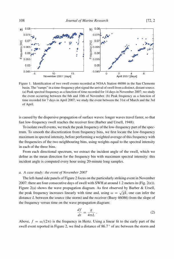
The spectral intensity is provided in frequency bins spaced by 5 mHz in the low-frequencyrange, together with the mean direction of the signal for each one of these bins. Thesedirectional spectra are based on an observation length of twenty minutes and are deliveredevery hour. The arrival of swell from a distinct source at buoy 46086 is indicated a strongspectral peak that shifts towards higher frequencies as time goes on, with a timescale ofseveral days: see Figure 1. The progressive shift of the spectral peak to higher frequencies


Figure 1. Identification of two swell events recorded at NOAA Station 46086 in the San Clementebasin. The “ramps” in a time-frequency plot signal the arrival of swell from a distinct, distant source.(a) Peak spectral frequency as a function of time recorded for 14 days in November 2007; we studythe event occurring between the 6th and 10th of November. (b) Peak frequency as a function oftime recorded for 7 days in April 2007; we study the event between the 31st of March and the 3rdof April.

is caused by the dispersive propagation of surface waves: longer waves travel faster, so thatfast low-frequency swell reaches the receiver first (Barber and Ursell, 1948).

To isolate swell events, we track the peak frequency of the low-frequency part of the spec-trum. To smooth the discretization from frequency bins, we first locate the low-frequencymaximum in spectral intensity, before performing a weighted average of this frequency withthe frequencies of the two neighbouring bins, using weights equal to the spectral intensityin each of the three bins.

From each directional spectrum, we extract the incident angle of the swell, which wedefine as the mean direction for the frequency bin with maximum spectral intensity: thisincident angle is computed every hour using 20-minute long samples.

a. A case study: the event of November 2007

The left-hand side panels of Figure 2 focus on the particularly striking event in November2007: there are four consecutive days of swell with SWH at around 1.2 meters in (Fig. 2(e)).Figure 2(a) shows the wave propagation diagram. As first observed by Barber & Ursell,the peak frequency increases linearly with time and, using ω = √

gk, one can infer thedistance L between the source (the storm) and the receiver (Buoy 46086) from the slope ofthe frequency versus time on the wave propagation diagram:

df

dt= g

4πL. (2)

Above, f = ω/(2π) is the frequency in Hertz. Using a linear fit to the early part of theswell event reported in Figure 2, we find a distance of 86.7 ◦ of arc between the storm and


Figure 2. Two swell events recorded at NOAA Station 46086 in the San Clemente basin. (a), (c), and(e) correspond to a swell event recorded in November 2007, and (b), (d), and (f) to a swell eventrecorded in April 2007. The top panels show the estimated peak frequency f as a function of time.f increases linearly with time due to dispersive propagation of surface waves. The middle panelsshow the incident angle measured clockwise from North by the buoy. The incident angle fluctuatesaround a mean value of 204 ◦ for panel (c) and 224 ◦ for panel (d). The bottom panels show theSWH in meters.


Figure 3. Color contours indicate significant wave height (SWH) in meters from the ECMWF ERAreanalysis on October 30th, 2007, at midnight GMT, shown using a South Polar projection. Thethick black line is the sea ice limit. The solid black grid shows great-circle routes from the NOAAStation 46086, and lines of constant range from this station. The red spot, which is very close tothe region of maximum SWH, indicates the source inferred from swell recorded at Station 46086.

Buoy 46086. The intersection of the fitting line with the f = 0 axis gives the date of birthof the storm which is October 29th 2007, at around 23:00 GMT.

To infer the direction of the source we turn to the incident-angle signal in Figure 2c.There are ±10 ◦ fluctuations in the direction of the incident waves at the buoy. We removethese fluctuations by averaging, and so find that the wave signal at Station 46086 comesfrom 204 ◦, measured clockwise from North. We hypothesize that the ±10 ◦ directionalfluctuations in Figure 2c are too large to be simply instrumental noise, and that there mightbe physical information in the directional measurements. We return to further discussion ofthis point in Section 5, for example see Figure 11 and the supporting discussion.

The inferred range and direction locate the wave source on weather maps that are madeavailable by the European Center for Medium-Range Weather Forecasts (ECMWF). TheECMWF interim reanalysis (Dee et al., 2011) provides sea ice cover, 10-meter wind speed,and also SWH computed using the WAM wave model and assimilation of altimeter data(Hasselmann et al., 1988; Komen et al., 1996). We identify the southern sources of swell,corresponding to southern-ocean storms, as strong local maxima in 10-meter wind speed,and as large SWH. In Figure 3 we compare the relevant ECMWF SWH with the sourceinferred from the accelerometer buoy recordings (the red dot). The buoy data analyzedabove predict a storm at a range of 86.7 ◦ on a great-circle route making an angle of 204 ◦going clockwise from North at the buoy, on October 29th 2007 at 23:00 GMT. The inferred


Figure 4. A mirage: the swell recorded at NOAA Station 46086 seems to originate from New Zealand.The inferred location (the red dot) is displaced by approximately 10 ◦ of arc from the region ofmaximum SWH. Color contours indicate SWH in meters for the ECMWF ERA reanalysis for thestorm of March 23rd, 2007 at 06:00 GMT. The solid black grid shows great-circle routes from theNOAA Station 46086, and lines of constant range from this buoy.

location, shown as a red dot in Figure 3, is in excellent correspondence with the SWHmaximum. In the example of Figure 3, great-circle backtracking works very well: refractionby surface currents and topographic effects do not spoil the inference of the source.

b. Another case study: the event of April 2007

The agreement shown in Figure 3 is the most frequent situation we found in our analysisof the data from accelerometer buoys: for 14 of the 18 swell signals we analyzed, the inferredsource corresponds to a maximum in ECMWF surface wave height within 5 ◦ of arc. Butwe also found a few examples for which the swell signal was very clean (for example,Fig. 1b), yet great-circle backtracking resulted in a bad estimate of source location. In theright-hand panels of Figure 2, and in Figure 4 we focus on this event in April 2007. TheSWH at Station 46086 is of the order of 1 meter and the frequency of the swell increaseslinearly with time. Yet in Figure 4 the direction of the inferred source is approximately10 ◦ from the maximum in ECMWF surface wave height. Moreover, the 10 ◦ error puts theinferred source of this April 2007 event on New Zealand. This mirage is reminiscent of theAntarctic sources inferred by Munk et al. (1963).


Mirages seem to occur preferentially when there is shallow topography, or even land,close to the great-circle route between the storm and the receiver. In the case of Figure 4,a dense part of the Tuamotu Archipelago between 14 ◦ to 18 ◦ South and 148 ◦ to 140 ◦West—see Figure 50 of Munk et al. (1963)—blocks the wave packets propagating on thegreat-circle route between the storm and the receiver. Only rays that are deflected stronglyenough by surface currents to go around this Tuamotu blockage can reach the receiver.In anticipation of results from Section 4, a possibility is that because of the distributionof surface currents, some wave-packets were deflected west of the Tuamotu blockage, sothat the inferred source appears on New Zealand: the mirage in Figure 4 results from theinterplay between Tuamotu blockage and refraction by surface currents.

3. Waves on the surface of a sphere

Modeling the results of Section 2 requires tracing rays on the surface of a sphere, includ-ing the effects of refraction by surface currents. Backus (1962) developed this ray theory,including shallow-water effects and rotation, but without considering ocean currents. In thissection we provide an account of the relevant theory required for the model in Section 4.

a. The ray equations in spherical coordinates

Let us denote the phase of a wavepacket by S(x, t). Then the frequency and local wavevec-tor are respectively −∂tS and k = ∇S. The dispersion relation can be written in terms ofS(x, t) as ∂tS + Ω(x, ∇S) = 0. This partial differential equation is the Hamilton-Jacobiequation for a mechanical system with action S and Hamiltonian Ω. The solution is accom-plished via Hamilton’s equations, which in this context are also called the ray equations.These are evolution equations for the position x(t) and wavevector k(t) of the wave-packet(Bühler, 2009).

For the spherical problem at stake, we use latitude ψ and longitude φ, with unit vectorseψ and eφ. The conjugate momenta are then pψ = ∂ψS and pφ = ∂φS. Using the expressionfor the gradient in terms of latitude and longitude, the wavevector is

k = pψ

Reψ + pφ

R cos ψeφ , (3)

with R the radius of the Earth. The current velocity is u = u(ψ, φ)eφ + v(ψ, φ)eψ, and (1)then gives the Hamiltonian in terms of ψ, φ and their conjugate momenta:

Ω(ψ, φ, pψ, pφ) =√

g

Rp1/2 + pψ

v(ψ, φ)

R+ pφ

u(ψ, φ)

R cos ψ, (4)

where

pdef=

(p2

ψ + p2φ

cos2 ψ

)1/2

. (5)


Figure 5. A ray from a source S to a receiver R is not bent by a uniform current U . The wave vectork is inclined to the ray-path so that part of the group velocity compensates for advection by thecurrent. For clarity, this schematic shows a large value of the angle β − α between the ray RS andk. Realistic surface currents are weak compared to the group velocity vg and hence β−α is at mostone degree.

The spherical ray equations are then obtained from Ω(ψ, φ, pψ, pφ) via:

ψ = ∂pψΩ =

√g

R

pψ

2p3/2+ v

R, (6)

φ = ∂pφΩ =

√g

R

pφ

2p3/2

1

cos2 ψ+ u

R cos ψ, (7)

and

pψ = −∂ψΩ = −√

g

R

p2φ

2p3/2

sin ψ

cos3 ψ− pψ

R∂ψv − pφ

R∂ψ

u

cos ψ, (8)

pφ = −∂φΩ = −pψ

R∂φv − pφ

R

∂φu

cos ψ. (9)

An alternate method for deriving ray equations in spherical geometry is given in Hashaet al. (2008). In the special case of propagation through a still ocean, u = 0, the conjugatemomentum pφ is constant and equations (6) through (9) reduce to those of Backus (1962)and describe great-circle propagation.

b. A special solution

An educational solution of the ray equations is obtained by considering the Cartesiancase with a uniform current U flowing along the axis of x: see Figure 5. If the source S is atthe origin, and the receiver R is at xR = r cos α ex + r sin α ey , then the ray connecting S to


R is a straight line, despite the Doppler shift corresponding to U . Thus, in planar geometry,a uniform current does not bend rays.

This straight-line propagation, while simple in principle, is perhaps counterintuitive.Thus it is worthwhile to understand straight-line propagation through a uniform currentby explicit solution of the ray equations. In cartesian geometry, the dispersion relation is

Ω = √gk +Ukx , with wave vector k = kxex +kyey and total wavenumber k =

√k2x + k2

y .

The cartesian ray equations are

x = ∂kx Ω = U + 1

2

kx

k

√g

ky = ∂ky Ω = 1

2

ky

k

√g

k, (10)

and

kx = −∂xΩ = 0 , ky = −∂yΩ = 0 . (11)

The wave numbers kx and ky are constant, and the solution of (10) is therefore

x = (U + cos β vg

)t , y = sin β vg t , (12)

where (kx , ky) = k(cos β , sin β) and vg = √g/4k is the group velocity. Eliminating t

between x and y in (12), and requiring that the ray pass through the receiver at xR , onefinds that the direction, β, of the wave vector k is given by

vg sin(β − α) = U sin α . (13)

The relevant case in oceanography is U � vg , so that (13) can always be solved for β. InFigure 5 the slight inclination of the wave vector k to the straight-line ray path SR is thesmall angle β − α.

The importance of this simple solution is that it shows there is no relation between raybending and the speed of currents.

The difference between α and β is a previously unremarked source of error for directionalinferences which suppose that the wave vector k is precisely parallel to the direction ofpropagation for example, as assumed by us in Section 2, and previously by Snodgrasset al. (1966) and Munk et al. (1963). With a typical velocity of oceanic surface currentsU = 0.3 m s−1 and swell with 500 m wavelength, we obtain U/vg � 0.02, hence α − β isof the order of 1 ◦: the direction β of the wave vector k is therefore a good, but not perfect,estimate of the direction of the straight ray between S and R. By contrast, in the followingwe show that non-uniform currents induce ray-bending, resulting in the direction of thewave vector k at the receiver being a poor estimate of the direction of the source, witherrors often larger than 10 ◦.


c. Ray bending and the vertical vorticity of currents

Returning to the spherical case, in the absence of currents the solutions of (6) through (9)are great-circle geodesics (analogous to the straight line in Figure 5) connecting the sourceto the receiver. Non-uniform currents will refract or bend the rays away from great-circlepaths. In fact, it is the vertical vorticity of currents that is crucial for bending rays awayfrom great circles (Kenyon, 1971; Dysthe, 2001; Landau and Lifshitz, 1987).

The connection between ray bending and vertical vorticity is simplest in the case whenwaves travel much faster than currents. For example, swell with a wavelength 500 m has agroup velocity vg = √

g/4k of 14 m s−1, which is much faster than the velocity of typicalsurface currents (at most 1 m s−1). In this limit of fast wave-packets, the ray equations (6)through (9) reduce to the simpler and more insightful curvature equation

χ � ξ

vg

, (14)

which is valid to first order in |u|/vg . Above, ξ is the vertical vorticity of the current,

ξ(x)def= ∂φv − ∂ψ(u cos ψ)

R cos ψ, (15)

and χ is the geodesic curvature: χ is the curvature of the trajectory projected onto thelocal horizontal plane. A curve with zero geodesic curvature is a great circle in the presentcontext.

Rays are thus deflected by vorticity just as the horizontal trajectory of a charged particle isbent by a vertical magnetic field: vorticity is analogous to the magnetic field. The magnetic-field analogy is the starting point of an alternate derivation of equation (14): in the limitof slow currents, the magnitude of k varies very little, and the group velocity of the wavesremains almost constant, at the initial value vg(0). Let us approximate the square root in thedispersion relation (1) by the parabola which has the same slope at the initial value of k:

Ω(x, k) � 2v3g(0)

g|k|2 + u·k + constant. (16)

This quadratic expression is the same as the quadratic Hamiltonian for a negatively chargedparticle in a weak magnetic field ∇ × A(x), where A(x) is the vector potential. In dimen-sionless form, the Hamiltonian is:

H(x, p) = 12 |p + A|2 + 1

2 |∇ × A|2 , (17)

� 12 |p|2 + A·p + O(A2), (18)

where p is momentum. The last expression corresponds to the weak-field limit. The chargedparticle experiences a Lorentz force, and its trajectory is well-known to have a local curvatureproportional to the strength of the magnetic field χ = |∇ × A|/|p| (Jackson, 1998). For


the wave-problem governed by the approximate dispersion relation (16), this translates intoray curvature |∇ × u|/vg(0), which is the relation (14).

The significance of (14) is that looking at a map of surface vorticity, one can assess whichfeatures will strongly deflect swell, and in which direction the rays will bend. The result alsoshows that wave propagation through this moving medium is isotropic, despite the directiondetermined by the velocity field u = u(ψ, φ)eφ + v(ψ, φ)eψ. We use (14) to understandand interpret the results obtained by integration of the exact ray equations (6) through (9).

4. Deflection of swell by surface currents

Maps of surface currents u(x, t) are made available by satellite altimetry and scatterom-etry: the Ocean Surface Current Analysis in Real-time (OSCAR) dataset gives the surface-current velocity field with a spatial resolution of one-third of a degree and a temporal res-olution of five days (Bonjean and Lagerloef, 2002). OSCAR estimates the velocity u(x, t)

required to determine the trajectory of swell by integration of the ray equations (6) through(9). We interpolate the OSCAR surface velocity field linearly onto a triangular mesh, beforeintegrating the ray equations (6) through (9) with a forward Euler method.

One-third of a degree does not fully resolve mesoscale vorticity and thus computationsbased on OSCAR underestimate the deflection of gravity waves by currents. This underes-timate indicates unambiguously that surface-current refraction is quantitatively sufficientto explain fluctuations of ±10 ◦ in the direction of the incoming swell shown in Figure 2cand 2d.

a. A point source in the Southern Ocean

To model the observations of Section 2, we begin by considering a point-source in theSouthern Ocean, at latitude 58 ◦S and longitude 160 ◦E. This source emits surface waves inevery direction, and with different wavelengths. For a given initial wavelength, we numeri-cally integrate the exact ray-tracing equations (6) through (9), starting from the source pointand with different initial orientations of the wavevector k. We assume that the emission isisotropic and so we shoot rays with the initial direction of k uniformly distributed on the unitcircle, with a 3 × 10−4 radian step (approximately one minute of arc). Six rays determinedby this procedure are shown in Figure 6. Out of all the emitted rays, an observer receivesonly the few rays which connect the source to the receiver. Thus we keep rays which reachthe receiver within a radius of 30 nautical miles. The thick curve in Figure 6 is an exampleof such a ray. Because the ray connecting the source to the receiver in Figure 6 is not astraight line we conclude that swell is significantly deflected from a great-circle route bythe OSCAR currents. For rays incident on the receiver, we define the deflection angle θ asthe angle between the great-circle route and the direction of the ray at arrival. We use theconvention θ < 0 if the ray at arrival is South of the great-circle route between source andreceiver.


Figure 6. Swell with λ = 500 m emitted by a point-source in the Southern Ocean. This figure uses anazimuthal equidistant projection so that great circles passing through the receiver (and only these)appear as straight lines, that is, the dashed straight lines are great circles. The color scale showsvertical vorticity of OSCAR surface currents, ξ in s−1. The thick-curve is a ray that connects thesource to the receiver. The thin curves are five other rays. Using great-circle backtracking (reddashed line), the inferred source is far from the true source.

If an observer backtracks along the great circle indicated by the direction of arrival of thethick ray in Figure 6, and determines the range with (2), then the inferred source is over seaice and almost on Antarctica. In other words, refraction by OSCAR currents has produceda mirage.

Figure 7 compares the left and right hand sides of equation (14) along a ray connectingthe southern source to the receiver. The two curves coincide almost to within the line width.This validates the weak-current approximation used in (14) and shows that rays are bentfrom great circles only where there is strong surface vorticity i.e., in localized currentsystems such as the Antarctic Circumpolar Current (ACC), the subtropical frontal zone andthe equatorial current system. The thick ray of Figure 6 undergoes strong refraction whencrossing these three features, and then travels more-or-less on great circles between thesecurrent systems. For example, after leaving the Southern Ocean the thick ray in Figure 6 ison a great circle headed away from the receiver. But refraction by a large equatorial eddysubsequently bends the ray onto a great circle passing through the receiver.


Figure 7. For the thick ray in Figure 6 the ray curvature (blue) is almost equal to the surface vorticitydivided by group velocity (red dashed). The smooth black curve is low-pass filtered curvature. Thestrongest refraction occurs when the ray crosses the ACC and equatorial current. Weaker refractionoccurs as the ray transits the subtropical frontal zone.

We conclude that fluctuations in incident direction observed at the receiver are not theresult of accumulation of many small, random deflections. Instead, the model indicates thatthere are two or three large deflections of a ray that are associated with major hydrographicfeatures of the surface current system.

b. An extended source in the Southern Ocean

For a given surface velocity field, several rays—none of which are great circles— connectthe source to the receiver. An example is shown in Figure 8. We refer to the collection ofrays that connect the source to the receiver as a “multipath.”

As we did with the directional data in Figure 2, an observer can construct the “averageinferred source” at the location of the mean position of the multiple inferred sources. Thismean deflection is denoted as 〈θ〉, where the brackets denote averaging over all rays. For apoint-source of swell, the average inferred source is usually significantly displaced from theactual source, with values of the order of ±5 ◦ for swell with initial wavelength λ = 500 m.An extreme example is presented in Figure 8, where refraction by surface currents is sostrong that the average inferred source is on land. However, real storms have a typicalextension of several hundreds of kilometers and should not be considered to be point-sources.


Figure 8. A bundle of rays connects the source to the receiver (λ = 500 m). Blue rays reach thereceiver within 30 nautical miles. The red spot indicates the average inferred source. The insertshows the same analysis performed with an extended source of radius 4 ◦, delimited by the redcircle. The average inferred source coincides with the center of the circle within 2 ◦ (not shown).This figure uses an azimuthal equidistant projection centered on the receiver and the color scaleshows vertical vorticity of OSCAR surface currents, ξ in s−1.

To determine the influence of this spatial extension, we model an extended source by adisk of radius 4 ◦, or 440 km, around a center located at latitude 57 ◦S and longitude 172 ◦E.We assume a uniform density of incoherent point sources inside this disk. It is then easierto solve numerically the backward problem: we shoot rays “backwards” from the receiverwith a constant step of 10−4 radian in initial direction (approximately twenty seconds ofarc). We keep only the rays that have a nonzero intersection with the swell-emitting disk inthe Southern Ocean. To compute the direction of the average inferred source, we performa weighted average of the angular directions of the rays that intersect the extended source.The weight of each ray is equal to the length of its intersection with the swell-emitting disk:the contributions from incoherent sources inside the disk add up on each ray. The insertin Figure 8 shows a typical ray pattern obtained with this extended source for swell withwavelength λ = 500 m. A wide bundle of rays connects the source to the receiver. We findthat the average inferred source is close to the center of the actual source: contributions to the


average deflection from the different points inside the emitting-disk average out to almostzero. Going from one 5-day frame of the OSCAR data to the next one, the average deflection〈θ〉 fluctuates weakly around zero, with a root-mean-square (rms) value of the order of 3 ◦

for swell with 500 m initial wavelength: most often, the average inferred source is insidethe swell-emitting disc. Assuming Gaussian statistics for the average deflection 〈θ〉, such alow 3 ◦ value of the rms fluctuations means that an average deflection of 10 ◦ or higher has aprobability lower than 0.04. This does not rule out the possibility of a large 〈θ〉 occasionallyoccurring because the OSCAR data underestimate the actual vorticity of surface currentsand because 0.04 is not zero: if we analyze 25 events we might hope to see one exampleof a 10 ◦ average deflection. This is consistent with the analysis from Section 2: miragesdue solely to the effect of surface currents are rare events. An additional ingredient seemstherefore necessary to explain the more frequent occurrence of strong average deflections inthe observations by Munk et al., together with the systematic displacement of the inferredsources towards the South of the actual storms. We return to this in Section 6.

5. Fluctuations in the direction of swell

We return now to the ±10 ◦ directional fluctuations in Figure 2c and 2d. Previously,to estimate the location of the source, we removed these fluctuations by averaging. Butin this section we investigate the hypothesis that the frequency dependence of directionalfluctuations contains information about the strength of the surface vorticity field.

Let us assume that, during a storm, surface wave packets are emitted somewhat randomlyalong the different rays that connect the storm to the receiver. These different wave packetswill not reach the receiver at the same time, and thus the direction of the incident swellshould fluctuate in time, with fluctuations of the order of typical values of θ visible inFigure 8. Our hypothesis is that propagation of wave packets along the various componentrays of the multipath in Figure 8 results in the ±10 ◦ fluctuations in incident angle shown inFigure 2c and 2d. To investigate this further we first characterize the fluctuations in directioninduced by surface currents, using the twenty years of OSCAR data to perform a MonteCarlo computation. We then compare this prediction to the pitch-and-roll buoy data.

a. Directional fluctuations in model based on OSCAR currents

To gather statistics on the deflection of the rays, we repeat the point-source analysis ofSection 4 for each 5-day OSCAR surface velocity field recorded between October 1992 andOctober 2011. From this extensive simulation, we compute the probability density function(PDF) of the deflection angle, θ, which is defined as the angle between the ray at arrivaland the great-circle route. This PDF of θ is shown in Figure 9a using four different valuesof initial swell wavelength λ. The root-mean-square (rms) deflection is around 17 ◦ forwavelength λ = 250 m. The rms deflection decreases with increasing wavelength. Indeed,longer waves are faster and thus less refracted according to the curvature equation (14):when considered as a function of θ

√λ, the four PDFs collapse onto a single master curve:


Figure 9. (a) Probability density function of the deflection angle. The typical deflection is around10 ◦, which is consistent with the measurements of Munk et al. and the observation of Section2. Waves with larger wavelength are faster and less refracted. (b) The four PDFs collapse onto amaster PDF when considered a function of θ

√λ.

Figure 10. Bending of a beam of parallel rays by a strong Gaussian vortex ξ = ξ0 exp(−(r/�)2),with ξ0/

√gk = 5/π and �k = 40. In this illustration the vortex is unrealistically strong in order

to show the ray pattern; realistic vortices produce much smaller deflections.

see Figure 9b. This collapse indicates an rms deflection angle proportional to the frequencyof the swell,

θrms = 218f, (19)

with θrms in degrees and f in Hertz.The order of magnitude of typical deflection θ can be understood as follows: according

to the curvature equation (14), when a ray crosses an eddy with size � and typical vorticityξ0 (see Fig. 10), the direction of propagation is deflected by an angle

θ ∼ ξ0�

vg

(20)

= 4πξ0�

gf, (21)

where vg = g/(4πf ) has been used.


Out of the three current systems that refract the swell, the ACC has the most intensevorticity (large ξ0) whereas the equatorial current has the largest eddies (large �). Thesubtropical frontal zone has weaker eddies with small sizes and can be neglected for thisrough estimate. Because the ACC is close to the source and far from the receiver, the ACChas a smaller impact on the deflection θ than the equatorial current system: even after strongrefraction in the ACC, rays escape this first current system rather close to the source point.If the ACC were the only vortical refractor between source and receiver, then the observerwould make only a small error in inferring the position of the source. But the equatorialcurrent system is close to the receiver. Equatorial eddies bend some rays so that they hitthe receiver, which results in large values of θ. Hence an order of magnitude of θ is givenby the angular shift due to a few, or even one, eddy in the equatorial current system. Withλ = 500 m, and using � = 400 km and ξ0 = 10−5 s−1 for a typical eddy in the equatorialcurrent system, one obtains from (21) θ � 9 ◦.

Although Kenyon’s intuition that surface currents refract the swell was correct, he focusedon the time-averaged ACC and neglected both the equatorial current and the role of theeddies. The latter are crucial to explain the directional fluctuations due to OSCAR currents.Indeed, to determine the role of the average currents, we time-averaged the twenty years ofOSCAR data before simulating the same point-source as in Section 4a: the time-averagedsurface currents produce a negligible deflection |θ| of the rays (typically 1.5 ◦ for λ = 500m), which shows that the strong fluctuations visible in Figure 9 are due to the small-scaleeddies, particularly their intense vorticity, and not to the time-averaged currents.

b. Directional fluctuations in the pitch-and-roll buoy data

To gather statistics on the fluctuations of θ in the buoy data shown in Figure 2, we analyzed18 swell events recorded between 2004 and 2007. These 18 events were selected becausethe signal was particularly clean, that is there was no evidence of multiple sources in anyof these 18 events. For each swell event, we removed the mean value and the linear trendin the incident angle signal. We consider the remaining fluctuating θ(t) as a function ofthe peak frequency f (t) instead of time. We divide the signal into small bins in f , and wecompute the root-mean-square θ for each bin. The result is displayed in Figure 11, togetherwith the predictions from the analysis of the OSCAR data. The rms value of θ indeedshows a linear dependence with frequency, as predicted for refraction by surface currents.More surprisingly, the prefactor of the linear law is very well captured by the OSCAR dataanalysis. We were expecting to underestimate the effect of surface currents using the coarseOSCAR data so the agreement in Figure 11 might be fortuitous. However, the orders ofmagnitude are compatible.

The measurements in Figure 11 would also have been hostage to errors in directionalmeasurements at NOAA Station 46086. A significant uncertainty is that the accelerometerson NDBC 3-m discus buoys (such as Buoy 46086) are known to be a little noisy, or at leastnoisier than accelerometers on Datawell Directional Waveriders (O’Reilly et al., 1996).


Figure 11. Root-mean-square fluctuations in incoming swell direction measured by a pitch-and-rollbuoy, averaged over 18 storms, as a function of swell frequency f . Error bars are evaluated usingthe square root of the number of values in each frequency bin. The dashed line is the result (19)from the analysis of OSCAR data.

But even though discus-buoy noise is known to bias estimates of spread, it does not influ-ence estimates of mean direction (O’Reilly et al., 1996). Furthermore, the November 2007case study has been repeated by Sean Crosby (personal communication) using measure-ments made by a Datawell buoy deployed at NOAA NDBC station 46232 (32.530 ◦N and117.431 ◦W). Datawell buoys have the advantage of measuring accurately both the meandirection and the spread of the swell, using 26-minute-long samples. The Datawell direc-tional measurements are consistent with the NDBC results: directional spread increases intime as the peak frequency increases. The fluctuations in incident angle (or “mean direction”signal) are greater than the Datawell noise level, and their magnitude increases between thebeginning and the end of the swell event. These results are consistent with our hypothesisthat some part of the observed directional fluctuations is due to ray bending by surfacecurrents.

6. Discussion and conclusion

Because of refraction by surface currents, a storm and a receiving station are connectednot only by the great-circle route, but by a multipath: a bundle of rays with an angularwidth which is much larger than the angular width of the storm. Wave packets travel onthese many rays before reaching the receiver, which leads to strong temporal fluctuationsin the incoming direction measured at the receiver. The root mean square fluctuations in


Figure 12. Interplay between surface currents and shallow bathymetry. (a) The black line is the great-circle route. The blue and green rays connect the source to the receiving station from Munk et al.(1963). They are deflected by ±10 ◦ by mesoscale vorticity at the equator. The Northern ray hitsCortez bank, and does not reach the receiver. An observer sees only the Southern ray and great-circle backtracking puts the source on Antarctica (dashed red line). (b) Local bathymetry in metersnear San Clemente island. Cortez bank blocks the Northern ray.

the directional signal at pitch-and-roll Buoy 46086 are consistent with predictions usingray-tracing through the mesoscale vorticity of the OSCAR dataset.

Most often, the fluctuations average out in time and the mean direction measured by thebuoy over several days coincides with the actual direction of the storm. However, miragesdo occur. These rare events are observed when most of the swell from a single storm is


deflected in the same direction. The mirage effect can be greatly enhanced by topography:if topographic features close to the great-circle route obstruct part of the ray bundle, thenthe average direction of the incoming swell can be very different from the direction of thestorm.

The historical case of Munk et al. (1963) probably results from such an interplay betweensurface currents and topography, summarized following Munk (2013) in the simplifiedschematic Figure 12. We represent the great-circle route between a storm and the receiver offSan Clemente island, together with the extreme rays experiencing a refraction of respectively+10 ◦ and −10 ◦ by mesoscale vorticity in the equatorial current. Now close to the receiveris Cortez bank, a shallow bathymetric structure that selectively blocks rays that travel Northof the great-circle route without affecting rays that approach from the South. An observertherefore measures mostly wave packets coming from South of the great-circle route, andinfers a source on Antarctica.

Satellite observations provide modern confirmation of long-range propagation of oceanswell (Heimbach and Hasselmann, 2000; Collard et al., 2009). But the source-locationproblem remains an issue: recent inferences of storm sources follow Munk et al. (1963)and backtrack along great circles. This ignores refraction by currents and the resultingincrease in the width of the swell beam. It is interesting that through the curvature formula(14), vorticity ξ emerges as a key environmental variable that controls refraction of surfacegravity waves. NASA’s Surface Water and Ocean Topography satellite promises to greatlyimprove resolution of mesoscale vorticity (Fu et al., 2012; Fu and Ferrari, 2008): betterwave forecasts might be an unexpected outcome of this mission.

Acknowledgments. This research was supported by the National Science Foundation under OCE10-57838; BG was partially supported by a Scripps Postdoctoral Fellowship. We thank Ryan Abernathey,Fabrice Ardhuin, Oliver Bühler, Fabrice Collard, Sean Crosby, Falk Feddersen, and particularly WalterMunk, for many conversations and help with this problem.

The ocean surface current data used in this study was provided by the OSCAR Project Office. Thesignificant wave height data were obtained from the ECMWF data server. The pitch-and-roll buoy datais from the National Data Buoy Center, which is operated by the National Oceanic and AtmosphericAdministration.

REFERENCES

Atkinson, R. 2002. An Army at Dawn—the War in North Africa, 1942–1943. New York: Henry Holtand Co., New York, 768 pp.

Backus, G. E. 1962. The effect of the earth’s rotation on the propagation of ocean waves over longdistances. Deep-Sea Res., 9, 185–197.

Barber, N. F. and F. Ursell. 1948. The generation and propagation of ocean waves and swell. I. Waveperiods and velocities. Philos. Trans. Roy. Soc. Lond., A, 240(824), 527–560.

Bates, C. C. 1949. Utilization of wave forecasting in the invasions of Normandy, Burma, and Japan.Ann. N.Y. Acad Sci., 51(3), 545–572.

Bonjean, F. and G. S. E. Lagerloef. 2002. Diagnostic model and analysis of the surface currents inthe tropical Pacific Ocean. J. Phys. Oceanogr., 32(10).


Bühler, O. 2009. Waves and Mean Flows. Cambridge: Cambridge University Press, 370 pp.Collard, F., F. Ardhuin, and B. Chapron. 2009. Monitoring and analysis of ocean swell fields from

space: New methods for routine observations. J. Geophys. Res - Oc. Atm., 114(C07023).Dee, D., S. Uppala, A. Simmons, P. Berrisford, P. Poli, S. Kobayashi, U. Andrae, et al. 2011. The

ERA-Interim reanalysis: Configuration and performance of the data assimilation system. Quart. J.Roy. Meteor. Soc., 137(656), 553–597.

Dysthe, K. B. 2001. Refraction of gravity waves by weak current gradients. J. Fluid Mech., 442,157–159.

Fu, L.-L., D. Alsdorf, R. Morrow, E. Rodriguez, and N. Mognard, editors. (2012). 2012. SWOT:The Surface Water and Ocean Topography Mission, JPL Publication 12-05, Pasadena: NASA JetPropulsion Laboratory.

Fu, L.-L. and R. Ferrari. 2008. Observing oceanic submesoscale processes from space. EOS, Trans.Am. Geophys. Union, 89(48), 488.

Hasha, A., O. Bühler, and J. Scinocca. 2008. Gravity wave refraction by three-dimensionally varyingwinds and the global transport of angular momentum. J. Atmos. Sci., 66, 2892–2906.

Hasselmann, S., K. Hasselmann, E. Bauer, P. A. E. M. Janssen, G. J. Komen, L. Bertotti, A. Guillaume,et al. 1988. The WAM model—a third generation ocean wave prediction model. J. Phys. Oceanogr.,18(12), 1775–1810.

Heimbach, P. and K. Hasselmann. 2000. Development and application of satellite retrievals of oceanwave spectra, in Satellites, Oceanography and Society, D. Halpern, ed. Amsterdam: Elsevier, 5–33.

Jackson, J. D. 1998. Classical Electrodynamics, 3rd ed. New York: Wiley, 832 pp.Kenyon, K. E. 1971. Wave refraction in ocean currents. Deep-Sea Res., 18, 1023–1034.Komen, G. J., L. Cavaleri, M. Donelan, K. Hasselmann, S. Hasselmann, and P. A. E. M. Janssen.

1996. Dynamics and Modelling of Ocean Waves. Cambridge: Cambridge University Press, 556pp.

Kuik, A. J., G. P. van Vledder, and L. H. Holthuijsen. 1988. A method for the routine analysis ofpitch-and-roll buoy wave data. J. Phys. Oceanogr., 18(7), 1020–1034.

Landau, L. and E. Lifshitz. 1987. Fluid Mechanics, Course of Theoretical Physics, volume 6, 2nd ed.Oxford: Butterworth-Heinemann, 552 pp.

Munk, W. H. 2013. Corrigendum to “Directional recording of swell from distant storms.” Philos.Trans. Roy. Soc. Lond. A., 371(20130039).

Munk, W. H. and F. E. Snodgrass. 1957. Measurement of southern swell at Guadalupe Island. Deep-Sea Res., 4, 272–286.

Munk, W. H., G. R. Miller, F. E. Snodgrass, and N. F. Barber. 1963. Directional recording of swellfrom distant storms. Philos. Trans. Roy. Soc. Lond. A, 255, 505–584.

O’Reilly, W. C., T. H. C. Herbers, R. J. Seymour, and R. T. Guza. 1996. A comparison of directionalbuoy and fixed platform measurements of Pacific swell. J. Atmos. Ocean. Tech., 13(1), 231–238.

Snodgrass, F. E., G. W. Groves, K. F. Hasselmann, G. R. Miller, W. H. Munk, and W. H. Powers. 1966.Propagation of ocean swell across the pacific. Philos. Trans. Roy. Soc. Lond. A, 259, 431–497.

von Storch, H. and K. Hasselmann. 2010. Seventy Years of Exploration in Oceanography: a prolongedweekend discussion with Walter Munk. Berlin: Springer, 190 pp.

Whitham, G. B. 1960. A note on group velocity. J. Fluid Mech., 9, 347–352.

Received: 14 December 2013; revised: 1 July 2014.

Refraction of swell by surface currents - Harvard...

Documents

Transcript of Refraction of swell by surface currents - Harvard...