Reformulation of the CBR ProcedureERDC/GSL TR-12-16; Report 1 ii Abstract The California Bearing...

ERD

C/G

SL T

R-1

2-1

6

Reformulation of the CBR Procedure Report I: Basic Report

Geo

tech

nic

al a

nd

Str

uct

ure

s La

bor

ator

y

Carlos R. Gonzalez, Walter R. Barker, and Alessandra Bianchini

April 2012

Approved for public release; distribution is unlimited.

ERDC/GSL TR-12-16 April 2012

Reformulation of the CBR Procedure Report I: Basic Report


Geotechnical and Structures Laboratory U.S. Army Engineer Research and Development Center 3909 Halls Ferry Road Vicksburg, MS 39180-6199

Report 1 of a series

Approved for public release; distribution is unlimited.

Prepared for U.S. Army Corps of Engineers 441 G Street NW Washington, DC 20314-1000

ERDC/GSL TR-12-16; Report 1 ii

Abstract

The California Bearing Ratio (CBR) procedure has been the principal method used for design of flexible pavements for both military roads and airfields since its development in the 1940s. In recent years, as the use of analytical models, such as the layered elastic and finite elements models, became accepted for pavement design, the CBR design procedure has been criticized as being empirical, overly simplistic, and outdated. A major criticism of the procedure has been the use of an adjustment, or Alpha factor, to account for over-estimation of the equivalent single-wheel load and as a thickness adjustment for traffic volume. The objective of this research was to reformulate the CBR-Alpha procedure so that design would be based on a more mechanistic methodology and to develop performance criteria for use with the reformulation. With this purpose in mind, the report details the developmental steps of the reformulation starting with the original CBR-Alpha procedure and ending with a new procedure based on Fröhlich’s theory for stress distribution. The reformulation was verified through review of historical test data, by prototype testing, and by analyses of an actual airfield pavement failure. The reformulation of the procedure resulted in the elimination of both the equivalent single-wheel load concept and the Alpha factor.

DISCLAIMER: The contents of this report are not to be used for advertising, publication, or promotional purposes. Citation of trade names does not constitute an official endorsement or approval of the use of such commercial products. All product names and trademarks cited are the property of their respective owners. The findings of this report are not to be construed as an official Department of the Army position unless so designated by other authorized documents. DESTROY THIS REPORT WHEN NO LONGER NEEDED. DO NOT RETURN IT TO THE ORIGINATOR.

ERDC/GSL TR-12-16; Report 1 iii

Contents Abstract ................................................................................................................................................... ii

Figures and Tables .................................................................................................................................. v

Preface ................................................................................................................................................... vii

Unit Conversion Factors ...................................................................................................................... viii

1 Introduction ..................................................................................................................................... 1

Background .............................................................................................................................. 1 Objective ................................................................................................................................... 2 Report content .......................................................................................................................... 2

2 History .............................................................................................................................................. 4

The beginning ........................................................................................................................... 4 Extrapolation of California design curves ............................................................................. 10 Validation of tentative design curves .................................................................................... 13 Development of the CBR equation ........................................................................................ 14 Thickness reduction factor for single wheel loading ............................................................ 20 Defining coverages ................................................................................................................. 24 Equivalent-single-wheel-load ................................................................................................. 27 Development of the α-factor .................................................................................................. 35

3 Reformulation of the CBR Equation ........................................................................................... 37

Redevelopment of the CBR equation .................................................................................... 38 Criteria for single-assemblies ................................................................................................ 42 Handling multi-wheel tire groups ........................................................................................... 46

Review of current ESWL approach ............................................................................................ 47

Comparison of the stress-based ESWL with deflection-based ESWL...................................... 49

Criteria for multi-wheel assemblies (with n=2) ......................................................................... 53

Criteria for multi-wheel assemblies (n as function of CBR) ..................................................... 57 Computing coverages and stress repetitions ....................................................................... 64 Comparison of Beta criteria with layer elastic strain criteria ............................................... 64

4 Finalization of the CBR-Beta Design Procedure ....................................................................... 69

Refinement of the CBR-Beta criteria ..................................................................................... 69

5 Summary, Conclusions, and Recommendations ...................................................................... 72

Summary of the findings ........................................................................................................ 72 Conclusions ............................................................................................................................ 73 Recommendation ................................................................................................................... 73

References ............................................................................................................................................ 74

ERDC/GSL TR-12-16; Report 1 iv

Appendix A: Verification of Beta Criteria using Data from Las Cruces Evaluation Report ............................................................................................................................................ 77

Report Documentation Page

ERDC/GSL TR-12-16; Report 1 v

Figures and Tables

Figures

Figure 1. Total thickness of base and surfacing in relation to CBR values. ........................................ 11

Figure 2. Extrapolation of highway pavement thicknesses. ................................................................. 12

Figure 3. Tentative design curves. .......................................................................................................... 13

Figure 4. Comparison of existing design curves with curves from k-values. ...................................... 16

Figure 5. Correlation of design curve with airfield evaluation data. .................................................... 17

Figure 6. Suggested thickness reduction curves. ................................................................................. 23

Figure 7. Relationship between coverage and percent design thickness. .......................................... 25

Figure 8. Schematic diagram of B-29 wheel assembly. ....................................................................... 30

Figure 9. Alpha curves as contained in PCASE. .................................................................................... 36

Figure 10. Relationship between Beta and coverage as developed from single-wheel criteria. .......... 45

Figure 11. Comparison of α criteria with β criteria. ............................................................................... 46

Figure 12. Comparison of thicknesses based on α criteria and β criteria. ......................................... 47

Figure 13. ESWL curves for twin assembly (B-29). ............................................................................... 51

Figure 14. ESWL curves for twin-tandem assembly (Boeing 747). ...................................................... 51

Figure 15. ESWL Curves for triple-tandem assembly Boeing 777). .................................................... 52

Figure 16. Relationship between stress ESWL and deflection ESWL. ................................................ 53

Figure 17. Comparison of thicknesses between α and β criteria for the F-15. .................................. 54

Figure 18. Comparison of thicknesses between α and β criteria for the Boeing 737. ...................... 54

Figure 19. Comparison of thicknesses between α and β criteria for the Boeing 747. ....................... 55

Figure 20. Comparison of thicknesses between α and β criteria for the Boeing 777. ...................... 55

Figure 21. Comparison of n=2 criteria with α criteria. .......................................................................... 57

Figure 22. Comparison of test data for n=2 and n=3. ......................................................................... 58

Figure 23. Relationship between stress concentration factor and CBR. ............................................ 60

Figure 24. Comparison of stress distribution based on layered elastic theory with stress distribution based stress concentration factors.................................................................................... 61

Figure 25. Comparison of relationship between stress distribution and CBR. .................................. 61

Figure 26. Design curves for F-15 using n as function of CBR. ........................................................... 62

Figure 27. Design curves for Boeing 747 using n as function of CBR. ................................................ 63

Figure 28. Design curves for C--17 using n as function of CBR. .......................................................... 63

Figure 29. Comparison of strain criteria. ............................................................................................... 66

Figure 30. Comparison of Beta criteria with criteria from layered elastic criteria. ............................. 67

Figure 31. Comparison of WES criteria with criteria from CROW report. ............................................ 67

Figure 32. Comparison of the criteria from Equations 55 and 56 for low volume traffic. ................ 70

Figure A5. Rutting in asphalt with tire imprints – Runway 22 touchdown area. ................................ 82

Figure A6. Runway asphalt distresses include cracking and rutting. .................................................. 82

ERDC/GSL TR-12-16; Report 1 vi

Figure A7. Beta design criteria military air fields. .................................................................................. 84

Tables

Table 1. K values for CBR equation. ....................................................................................................... 15

Table 2. Data used to develop thickness reduction. ............................................................................. 21

Table 3. Center-to-center tire spacing for twin or tandem gear to insure no stress overlap on subgrades with a CBR of 5 or more. ................................................................................................. 29

Table 4. Thicknesses defining unit behavior. ......................................................................................... 31

Table 5. Criteria comparison for C-17 operations. ................................................................................. 71

Table A1. Based on 3.5 Asphalt Surface over Base Data for B757 at 234655 pounds gross weight. ............................................................................................................................................. 83

Table A2. Based on 3.5 Asphalt Surface over Base Data for C17 at 585000 pounds gross. weight ........................................................................................................................................................ 83

Table A3. Predicted Life based on minimum thickness criteria for asphalt surface. ........................ 83

Table A4. Analysis Based on 12.5" of Surface and Base over Subbase Data for B757 at 234655 pounds gross weight. ................................................................................................................ 84

Table A5. Analysis Based on 12.5" of Surface and Base over Subbase Data for C17 at 585000 pounds gross weight. ................................................................................................................ 84

Table A6. Predicted Life based on min thickness criteria for asphalt surface and base. ................. 84

ERDC/GSL TR-12-16; Report 1 vii

Preface

The California Bearing Ratio (CBR) procedure has been the principal method used for design of flexible pavements for both military roads and airfields since its development in the 1940s. The objective of this research was to reformulate the CBR-Alpha procedure so that design would be based on a more mechanistic methodology and to develop performance criteria for use with the reformulation. This report presents the history of the original CBR procedure, the developmental steps of the reformulation for a new CBR methodology, the development of the performance criteria and data validating the criteria.

Personnel of the U.S. Army Engineer Research and Development Center (ERDC), Geotechnical and Structures Laboratory (GSL), Vicksburg, MS, prepared this publication. The ERDC research team consisted of Dr. Wal-ter R. Barker and Carlos R. Gonzalez, Airfields and Pavements Branch (APB), GSL. Carlos R. Gonzalez, Drs. Alessandra Bianchini and Walter R. Barker prepared this publication under the supervision of Dr. Gary L. Anderton, Chief, APB; Dr. Larry N. Lynch, Chief, Engineering Systems and Materials Division; Dr. William P. Grogan, Deputy Director, GSL; and Dr. David W. Pittman, Director, GSL.

COL Kevin J. Wilson was Commander and Executive Director of ERDC. Dr. Jeffery P. Holland was Director.

ERDC/GSL TR-12-16; Report 1 viii

Unit Conversion Factors

Multiply By To Obtain

feet 0.3048 meters

inches 0.0254 meters

pounds (force) per square inch 6.894757 kilopascals

pounds (mass) 0.45359237 kilograms

square inches 6.4516 E-04 square meters

ERDC/GSL TR-12-16; Report 1 1

1 Introduction

The California Bearing Ratio (CBR) procedure has been the principal method used for design of flexible pavements for both military roads and airfields since its development in the 1940s. In recent years, as the use of analytical models such as the layered elastic and finite element models became accepted for pavement design, the CBR design procedure has been criticized as being empirical, overly simplistic, and outdated. The need for this study originated as a response to the ongoing criticism of the CBR procedure as it was originally formulated in the 1940s.

This report presents a review of the development of the original CBR procedure, a reformulation based on a more mechanistic methodology, and performance criteria to be used with the new formulation.

Background

The CBR procedure was originally developed in the 1940s for the design of flexible pavements to support the new heavy bombers. The original airfield design curves were an extrapolation of the empirically-developed California pavement design curves for highway pavements.

These original airfield design curves employed Boussinesq’s theory of stress distribution in a homogenous half-space and were modified using the results of extensive full-scale field testing. In 1955, the U.S. Army Corps of Engineers proposed the CBR equation as the basis for a design procedure for the design of flexible airfield pavements. With the development of heavy multi-wheel aircraft such as the C-5A and B-747, a thickness adjustment factor (α-factor) was introduced into the CBR equation to account for the effects of traffic repetitions and multi-wheel tire groups. The factor α depends on the number of coverages and number of wheels on the main landing gear, which are employed to calculate the equivalent single-wheel load (ESWL). The factor α is determined in relation to the number of coverages and the selection of the curve representative of the number of wheels used for ESWL computation.

The CBR design procedure has also gained world-wide importance since this procedure is utilized to determine the Aircraft Classification Number (ACN). The 1983 edition of the International Civil Aviation Organization


(ICAO) Aerodrome Design Manual (Doc 9157-AN/901), which is currently in use, prescribed the CBR procedure as the basis for computing the ACN for civilian aircraft. The ACN is a number of great importance to the aircraft industry, because it is instrumental in determining which aircraft the airports are able to accept for operations.

Criticisms of the CBR design procedure were brought up in 2004 by the Information and Technology Platform for Transport, Infrastructure and Public Space (CROW). The 2004 CROW report D04-09, “The PCN Runway Strength Rating and Load Control System,” contained the following statement:

“It is now widely recognized that the U.S. Army Corps of Engineers’ CBR method cannot adequately compute or predict pavement damage caused by new large aircraft.”

In particular, the CBR procedure has come under scrutiny in consideration of pavement design and ACN evaluation for multi-wheel aircraft. A critical element and the center of the controversy, in the ICAO procedure for computing the ACN is the α-factor. The α-factor was deemed to be inadequate in representing multi-wheel aircraft scenarios (Barker 1994, 1994a; Airport Technology Research and Development Branch, 2004).

As a result of the controversy concerning the α-factor, the U.S. Army Engineer Research and Development Center (ERDC) research team felt the need to investigate the design issue by reformulating the CBR procedure. This included a review of the history that lead to the definition of the original CBR procedure. Based on the review and subsequent analysis, the CBR equation was reformulated, eliminating the need for the α-factor in the CBR design procedure for flexible airfield pavements.

Objective

The objective of this research was to reformulate the CBR-Alpha procedure so that the design would be based on a more mechanistic methodology and to develop validated performance criteria for use with the reformulation.

Report content

Chapter 2 contains a review of past studies and analyses that led to the formulation of the original CBR procedure. Chapter 3 explains the different


steps in the reformulation of the CBR procedure. Chapter 4 covers the final development of the new design procedure, and Chapter 5 closes the report with few recommendations about the implementation of the new CBR procedure.


2 History

The beginning

The very beginning of the Army’s involvement with the CBR procedure for the design of flexible airport pavement is well documented by Lenore Fine and Jesse A. Remington (Fine and Remington 1972). The Army’s work on the CBR procedure began on 6 May 1941 when the newly assembled XB-19 aircraft was rolled out from the Douglas Hangar at Clover Field and broke through the hangar apron to a depth of about 1 ft. After the aircraft was towed, with considerable difficulty, to one of the airport’s asphalt runways, the aircraft caused noticeable damage as it taxied over the surface. Not until 27 June, when a recently laid concrete pavement was ready for use, did the XB-19 take off on its maiden flight to March Field. Colonel Kelton of the Los Angeles District reported to General Schley (Chief of Engineers) about the landing at March Field:

“No marking or imprint was evident at the point of landing, but as the ship lost speed, a faint depression and hairline cracks appeared, increasing in severity as the speed was further reduced. At the point where the ship turned to cross the oil-earth landing mat onto the apron, the depressions were at one inch in depth and the cracks quite large.”

Colonel Kelton recognized the magnitude of the pavement problem, since he pointed out that the plane was lightly loaded and conditions were ideal—the weather was dry and the ground water level was low. He warned that worse damage was likely to occur, and after heavy rains, “extreme damage” could result from landings by fully loaded XB-19 aircraft.

As a result of the experience with the XB-19, the Chief of the Air Corps, Gen-eral Brett, insisted that runways should be of the heaviest construction, and in June 1941, he demanded that all new military airstrips should be constructed of Portland cement concrete with beam strength characteristics. General Brett’s runway specifications were: adequate bearing capacity under very heavy loads, high skid resistance, and good visibility for night landings and easy maintenance. General Plank of the Army Engineers considered General Brett’s standards to be wholly unacceptable. Plank stated, “They wanted to introduce artificial concepts into engineering such


as ‘no runway will be built except out of concrete with Portland cement’. But there are other ways to build runways, and we, the Engineers, would not go for that kind of thing.” In an appeal to the construction agency, G-4, on 25 July 1941, Plank asked that engineering decisions be left to the Engineers. Stating that asphalt pavements could be designed to carry even the heaviest planes, he insisted that the surface textures could be altered to increase frictional resistance and the surface colors lightened to enhance visibility. He contended, high-type asphalt runways could be maintained almost as cheaply as concrete. Deciding in favor of the G-4, General Reybold handed down the ruling: airmen would state their functional requirements, and Engineers would take it from there.

When General Schley retired as Chief of Engineers on 1 October 1941, a broadly conceived investigative effort was under way. Formulated by the Engineering Section, Office, Chief of Engineers (OCE), under William H. McAlpine, this effort had a five-fold mission:

Insure adequately designed airports; Eliminate wide variation in designs; Limit the use of unproved theories; Maintain competition between materials; and Lay the basis for further development of pavement criteria through

behavioral studies.

The overall objective was to write a new chapter in civil engineering, and a sizable team of investigators was assigned to this mission. Two of the Corps’ foremost technologists, hydraulic engineer Gail A. Hathaway and soils engineer Thomas A. Middlebrooks, (who was later to become a noted leader in the development of pavement design technology) were assigned to assist in Washington, DC. The research staff of the Waterways Experiment Station (WES) in Vicksburg, MS, was assigned responsibility for undertaking a series of special studies, and district offices throughout the country began conducting tests and experiments. Because the civil organization could not provide all the needed skills, McAlpine brought in specialists from outside the Corps; among these recruits were James L. Land, a mainstay of the Alabama State Highway Department since 1910, and Walter C. Ricketts, a chemical engineer who had worked for the Asphalt Institute. A number of prominent consultants also joined in the endeavor.


Because of General Brett’s strong preference for concrete, the engineers gave close attention to rigid pavements. In 1926, H. H. Westergaard, Dean of Graduate Engineering at Harvard University, had published a theory for determining stresses produced by rolling loads. Essentially a theorist, a man who did his work sitting at his desk, Dean Westergaard was concerned more with the validity of his analysis than with its application. Explaining his attitude, he told one engineer, “I have developed a theory, and it is mathematically sound, but whether it fits the facts of nature is up to you to prove.” In fact, for validation purposes, McAlpine’s primary goal was to verify Westergaard’s theory by experiment. McAlpine’s investigative plan called for large-scale tests at Wright Field and control tests at Langley Field, Virginia. Even before the field experiment was fully under way, a family of design curves was developed using Westergaard’s equations. Then, as data became available from the tests at Wright and Langley, the curves were adjusted. Design curves for wheel loads up to 60,000 lb were soon in use throughout the Corps. Only after further tests with different sets of variables would the curves find a place in the Engineering Manual.

Concurrent with tests on rigid pavements, tests were being conducted on flexible pavements. There was little agreement among highway engineers as to how flexible pavements ought to be designed. Various design methods were implemented; all of them were empirical and none of them proven for wheel loads beyond 12,000 lb. Because the problem was primarily related to soils, McAlpine turned it over to his soils experts, Thomas A. Middlebrooks and George E. Bertram. Both were solidly grounded in the theory of soil mechanics. Middlebrooks had done graduate work in the new science under Dr. Karl von Terzaghi at MIT; and Bertram under Dr. Arthur Casagrande at Harvard. Their early efforts were exploratory. After a cursory look at the methods of state roads departments, their first surmise was that load bearing tests might be the answer.

Middlebrooks and Bertram began their effort with a study of load bearing test characteristics and execution. The two researchers examined plate load tests by trying plates of different sizes, different rates of loading, and different ways of interpreting results. In addition to the plate loading tests, Middlebrooks and Bertram studied pavement failures at Tri-Cities Airport near Bristol, Tennessee. In a paper presented to the Highway Research Board in December 1941, Middlebrooks and Bertram reported two impor-tant discoveries. Their first discovery was that the allowable deflection for asphalt bomber strips would be far smaller than for asphalt roads. Their


experiment showed that this deflection was 0.2 in. in contrast to the Asphalt Institute recommended value of 0.5 in. The second discovery was that load bearing tests produced unsatisfactory outcomes.

When Lieutenant Colonel James H. Stratton reported for duty in December 1941 as head of the Engineering Branch, he found only frag-mentary data on airport design. Deeply concerned, Stratton gave close attention to the investigative effort. Immersing himself in the details of flexible pavement research, he quickly learned where matters stood. Kemp, project engineer at OCE, gave him a rundown on the Langley Field endeavor: experimental sections, designed with the help of the Asphalt Institute, were nearing completion; tests would soon commence. However, Kemp was pessimistic about the outcome, for he questioned the institute’s claim that thick bituminous surfaces provided measurable beam strength. In briefing their new chief, Middlebrooks and Bertram pointed to a possible solution. Their study of state highway practices had led them to conclude that the California method, strongly backed by Land, Alabama State Highway Department representative called as consultant for the project, held considerable promise. Middlebrooks was in correspondence with Thomas E. Stanton, Materials and Research Engineer of the California Division of Highways, and Bertram had been to Sacramento to confer with the originnator of the method (the California method for design of flexible pavements), O. James Porter, Stanton’s assistant.

The Langley tests were decisive. In February 1942, the Virginia airbase was bustling with activity. Each agency had its own representative on the field. Robert F. Jackson was there from the Louisville District to direct the experiments. Frederick C. Field was there as an observer for the Asphalt Institute, and Bertram was there from Washington as Stratton’s representa-tive. A scraper was filled with dirt to apply loads of 13,000 lb on the front tires and 20,000 lb on the rear tires. After 25 passes, 6 of the 14 test sections had begun to rut; after 50 passes, 10 of the sections had failed, and the rest had developed a definite wave. Designed supposedly for wheel loads of 60,000 lb, the Langley pavements rapidly deteriorated under loads of 20,000 lb. On reading Bertram’s report of the experiment, Stratton decided to stop theorizing and to send for O. James Porter at once.

As a junior engineer for the California Division of Highways in the late 1920s, Porter had investigated pavement failures throughout the state. Most of the trouble stemmed from porous, loosely compacted soil, which


took up moisture, became plastic, and remolded as wheels rolled over the pavement. Porter thought of the untouched lodes of disintegrated granite in the mountains of California and the large deposits of gravel in the river valleys. Compacted fills of these materials topped by thin wearing courses seemed to him the common-sense prescription for inexpensive, durable roads. He devised a simple procedure, the California Bearing Ratio (CBR) test, for measuring the shear resistance of base and subbase materials. Experience proved that his test could be relied upon. He also helped to originate a superior method of compaction control, the modified density test associated with the name of Ralph R. Proctor. In time, Porter was able to develop curves showing the relationship between bearing ratios and pavement thicknesses for wheel loads up to 12,000 lb and to correlate these curves with field performance. During the trip to Washington, Porter decided to offer Stratton a “package” plan—compaction method, CBR test, and curves for heavy wheel loads derived from traffic tests.

Shortly after his arrival, Porter was deep in conversation with Middlebrooks and Bertram. They found that their ideas were far apart. When the discussion stretched on fruitlessly for several days, Stratton sent for Dr. A. Casagrande, a world renowned figure in the field of soil mechanics and foundation engineering. After lengthy talks with Middlebrooks and Porter, Casagrande suggested a procedure. Extrapolating Porter’s curves was the first order of business. Working separately and using different methods, they plotted tentative curves for wheel loads up to 70,000 lb. After com-paring notes, they found that their results were close. That afternoon, they began blocking out a series of tests for checking their extrapolations. Before the week was out, Stratton had agreed to the plan.

The test program was labeled “crash.” Early in March 1942, Stratton issued rush orders to five division engineers. Four were to investigate prewar commercial runways, which had been down long enough for the subsoil moisture to equalize. Colonel Bragdon in the South Atlantic Division was to choose an airstrip built on sandy clay, a fairly good subsoil; Colonel Scott in the Southwestern Division, one of lean black clay, a rather poor foundation; Colonel Elliott in the Upper Mississippi Division, one on Fargo clay, a highly plastic material; and Colonel Besson in the Missouri River Division, one on a porous subgrade subject to frost action. Tournapulls with wheel loads of 12,500 to 50,000 lb would be towed over the pavements until failure occurred or 10,000 runs had been made. Each experiment would test one point on the extrapolated curves. Broader in scope and critically important


was the task given Colonel Hannum in the South Pacific Division. At Stockton air base, near Sacramento, Porter would conduct a crucial test. Stockton’s original runway, built by the city in 1936, had failed during the winter of 1940-1941 under the weight of light Army training aircraft. An abandoned taxiway nearby, constructed at the same time and along the same lines—the subgrade was adobe, the base course was six inches of compacted sandy loam, and the surface was a seal coat of emulsified asphalt—remained intact. The plan was to test the taxiway and a special, Porter designed-section to be built on top of the taxiway.

The strenuous endeavors produced quick results. In almost no time Stratton had telegrams reporting the progress of tests on commercial runways at Dothan, Alabama; Corpus Christi, Texas; Fargo, North Dakota; and Lewistown, Montana. In the meantime at Stockton, Porter and company set a blazing pace. On 10 March, Bertram arrived in Sacramento and gave the signal to begin. By the 13th, deflection gages were in place, and Porter was taking readings as a light aircraft taxied over the pavement. By the 20th, the surface had developed hairline cracks, and Porter had seen enough to know that the pavement was incapable of withstanding deflections of 0.1 in. or even 0.05 in. Construction of the test section started the following day. Built to Porter’s specifications (a thoroughly compacted base course of sand and gravel, increasing gradually in thickness from 6 in. to 4 ft and topped by 3 in. of asphalt concrete), the section was complete on the 24th. Tests proceeded rapidly, first with Tournapulls exerting wheel loads of 5,000, 10,000, 25,000, and 40,000 lb and then with a B-24 Liberator bomber. By early April, the experiment had shown that the extrapolated curves were fairly accurate and that allowable deflection was in hundredths rather than in tenths of an inch.

On a Monday morning early in April, Porter faced a skeptical group, the senior soils men of the engineer divisions who had come to Sacramento for a 5-day course in the California method. At the end of the course, one student, styling himself as the principal objector, declared, “Engineering starts with theory, and the California method has no foundation whatever in theory.” In reply to his critics, Porter pointed out, “We are not contending that this tentative design is accurate, but that it is the simplest and most practical method now available.” The news from Sacramento created quite a stir in professional circles. Reports of the meeting, passed by word of mouth, raised eyebrows and produced sharp critics. Professors, researchers, and state highway officials were frankly dubious. Most foundations experts


took a “wait and see” attitude. The Air Corps’ Buildings and Grounds Division was “inclined to be skeptical,” and the Navy’s Bureau of Yards and Docks was openly opposed. Probably the most strenuous objections came from the Asphalt Institute. At several conferences with Middlebrooks and Bertram, Asphalt Institute representatives argued unsuccessfully for thicker asphalt pavements and thinner base courses than Porter prescribed. All those who challenged the Corps’ approach received the assurance:

“It has never been the policy of the Engineer Department to standardize to the extent that research and development would be stifled, and we don’t want to do that now.”

Research contracts with Harvard and MIT testified to the Corps’ interest in developing a rationale, but to evolve a theory might take years. The CBR procedure was available and workable, and Stratton intended to use it. Tests at Stockton would continue, and a chapter on flexible pavement design, soon to appear in the Engineering Manual, would set the Corps’ seal of approval on the California method.

Extrapolation of California design curves

With the acceptance of the California method for the design of flexible pavements for heavy bomber aircraft, the Corps was faced with the problem of extrapolating the highway design curves to design curves appropriate for airfield pavements. In 1942, the California procedure was based on two design curves: Curve A used for light and medium traffic and Curve B used for light traffic (Porter 1949). The curves as presented by Porter are shown in Figure 1.

At the time of selection of the California method, the design curves A and B were not associated with a particular wheel load—only light and medium traffic. Although the highway curves were originally drawn for lighter wheel loads, it was known from service behavior of the pavements that 9,000-lb truck loads were supported without distress throughout the life of the pavement (Middlebrooks 1950). Using engineering logic based on differences between highway traffic and airfield traffic, it was decided that Curve A, in Figure 1 would represent a 12,000-lb airplane wheel load, and Curve B would represent a 7,000-lb wheel load. The 7,000-lb wheel load was chosen as the load for Curve B, since this load was the approximate wheel loading of training planes and represented the lightest traffic require-ment for airfields (Middlebrooks 1950). It was believed that Curve A was


Figure 1. Total thickness of base and surfacing in relation to CBR values (after Porter).

considered the most reliable; therefore, it was used as a basis for the extrapolation (The reason for this belief is not given.). Selection of the methodology for extrapolating the curves was based on the results of static load tests and engineering logic. Static load tests had shown that the deformation, under wheel load, of an adequately designed flexible pavement is comprised of three factors—settlement of the subgrade, compaction of the base and the surface, and elastic deformation (Middlebrooks 1950). By engineering logic, shear deformation was eliminated because, it was reasoned, in a satisfactory pavement, the shearing stress does not exceed the shearing strength. Service behavior records of adequate pavements had indicated that it was necessary for elastic deformation to govern over an extensive period of use. Accordingly, the Office of Civil Engineering (OCE) decided to develop empirical curves by extrapolating the original data on the basis of the elastic theory (Middlebrooks 1950). It was further reasoned that since all bearing tests are essentially shear tests and since shear deformation must be eliminated in a satisfactory pavement, shear stresses should be used as the guide in making the extrapolation.

Based on a review of airplane tire data, a uniform tire pressure of 60 lb/in.2 was determined to represent airplanes in use at the time of the analysis. Wheel loads of 25,000, 40,000, and 70,000 lb were selected to cover the range of heavy aircraft loads. Contact areas, represented by a circular shape, were computed from wheel loads and tire pressures. Stress tables published by Leo Jurgenson in 1934 permitted the computations of shear stress distribution with depth for the different wheel loads as shown in Figure 2 (Middlebrooks 1950).


Figure 2. Extrapolation of highway pavement thicknesses.

Using Curve A of Figure 1, the pavement thicknesses required to support heavy highway traffic for various values of CBR were determined. These thicknesses and the stress distribution curve for the 12,000-lb wheel load allowed the determination of the shear stress at the top of the subgrade for each CBR. The shear stress determined in this manner represented the allowable shear stress for the respective CBR using the allowable shear stresses and stress distribution curves for each of the tire loads. These were the preliminary design curves developed and presented at a meeting of consultants in Washington, DC, which included engineers from the OCE, Porter, and Professor Casagrande. The consultants had each made independent calculations to extrapolate the basic curves. Those of Porter were based on an allowable deformation, whereas those of Professor Casagrande were based on relationships between the relative sizes of the loaded areas. The three sets of computations were in substantial agreement. It was decided that the average thicknesses shown by the three extrapola-tions were reasonable for the low CBR values; however, the majority of the members agreed that the less conservative values should be chosen for the higher CBR values (Middlebrooks 1950). The tentative design curves, shown in Figure 3, were developed from the three extrapolations and the best judgment of the OCE engineers and consultants.

Although the engineering logic applied in the extrapolation may be slightly flawed, in that shear deformation in a flexible pavement can never be completely eliminated but is only reduced to an acceptable amount for a


Figure 3. Tentative design curves (after Porter 1949).

given number of aircraft loadings; the logic does set the foundation for the CBR procedure for design of flexible pavements. This foundation can be stated as a methodology that provides sufficient thickness of pavement structure above each point in the pavement to reduce the shear deformation in the pavement to an acceptable amount.

Validation of tentative design curves

Immediately after adopting the tentative CBR design curves for design of flexible pavements, efforts were undertaken to validate the curves. The first effort at validation, as reported by Fine (Fine and Remington 1972), was to conduct load tests at existing airfields, and to construct a special pavement test section for traffic testing at the Stockton Airbase. The initial results of the test verified the curves sufficiently to include the curves in the Corps’ Engineering Manual. An important outgrowth of the research effort for verifying the California design procedure was the establishment, in 1943, of the Flexible Pavement Laboratory at WES. Early in the investigation, W. J. Turnbull, Chief of the Soils Division at the WES, had been assigned the task of performing an analysis of the CBR test procedure. By spring of 1943, WES had emerged as the leading center of flexible pavement research. Because of the growing research need, Turnbull recruited foundation experts, Charles R. Foster and William H. Jervis, and experienced highway


engineer, John F. Redus, Jr.; W. Keith Boyd, a pioneer in flexible pavement design, was hired to head the research effort. Boyd quickly increased the staff of the research group, and before long, the team reached 25 in number. Two notable additions to the staff were Bruce G. Marshall and Richard Ahlvin. During the latter part of 1943, a long-range research program had been launched, which included laboratory and field investigations of base course design, compaction methods, and moisture conditions under pavements of asphalt surfaces (Fine and Remington 1972). Of the eleven papers presented in the 1950 symposium on the Development of CBR Flexible Pavement Design Method for Airfields, six were written by personnel from the WES. In the symposium, the paper by Foster listed some 93 lines of data that were used for the development of design curves for single wheel loads. Even with the extensive testing and evaluation of flexible pavements, the tentative design curves remained virtually unchanged through 1949 (Middlebrooks 1950; Ahlvin 1991).

Development of the CBR equation

In a letter dated 5 August 1949 from the WES to the OCE concerning studies pertaining to the CBR design curves, it was stated that:

“the Flexible Pavement Laboratory has attempted to reduce the family of curves to a single formula. Such a step would give a better understanding of the functions of each of the variables and would aid in comparing the empirical data for failed and satisfactory pavements. The Flexible Pavement Laboratory has tried several schemes, but in most cases the deviation from the existing curves was excessive. The best scheme developed so far was presented as a discussion paper to the CBR Symposium by Mr. Fergus.”

In the discussion, Fergus made the assumption that for a constant contact pressure, the ratio of the thickness to the radius of the loaded area is a constant. Fergus expressed the relationship by the equation:

P a

z ar a P K Pπp πp

= = = = (1)

where:


z = thickness of required pavement a = arbitrary constant r = radius of loaded area P = total wheel load p = contact pressure K = constant when a and p are constant.

From Equation 2 the value of K is seen to be:

z

KP

= (2)

Using Equation 2 and pavement thicknesses, as determined from the design curves in the Engineering Manual and the Stockton Test section No. 2, Fergus was able to develop the data given in Table 1.

Table 1. K values for CBR equation (from “Mathematical Expression of the CBR Relations, COE Technical Report No. 3-441, November 1956).

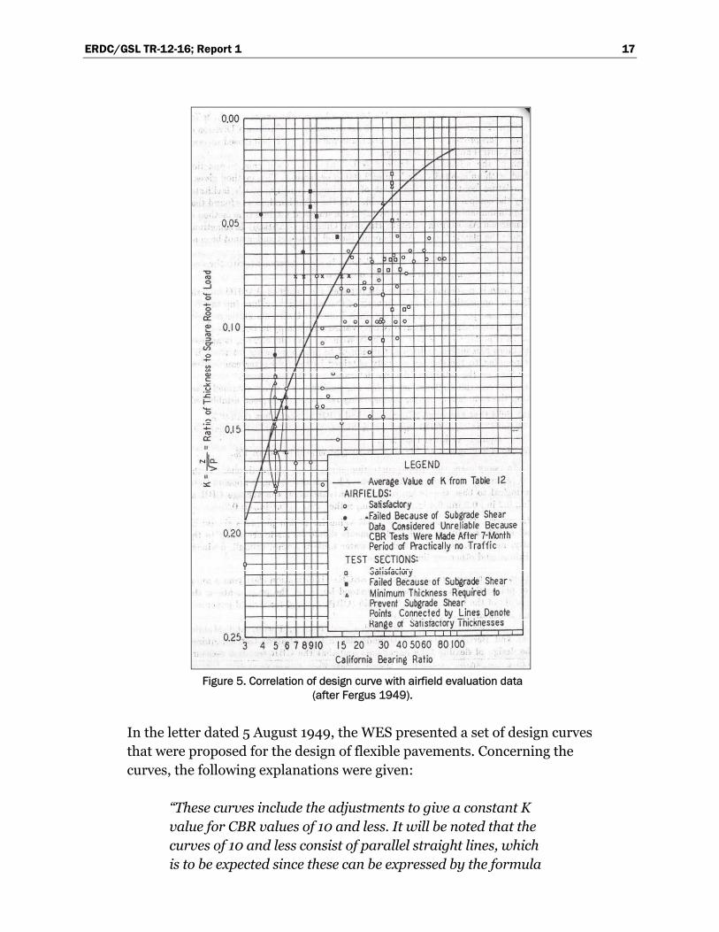
Fergus observed that for a given CBR the value of K could be considered, for all practical purposes, to be constant. Using the average value of K, Fergus developed design curves which he compared (Figure 4) with the design curves in the design manual and with the tentative curves for loads from 5,000 to 200,000 lb. He also used test data from pavement performance studies to validate the design curves. Figure 5 indicates that the relationship between CBR and K tends to divide the data between failed and satisfactory pavements.

0.1240.1330.006220.006660.004620.003480.0680.05920

0.1230.1300.007220.007670.005630.004490.0750.06717

0.1250.1280.008320.008510.006720.005330.0820.07315

0.1230.1250.010240.010410.008650.007230.0930.08512

0.1240.1240.012410.012400.010820.009220.1040.09610

0.1230.1240.013690.013790.012100.010610.1100.1039

0.1240.1240.015520.015500.013920.012320.1180.1118

0.1220.1230.017470.017580.015880.014400.1260.1207

0.1240.1240.020640.020610.019040.017420.1380.1326

0.1230.1240.024700.024790.023100.021610.1520.1475

0.1230.1230.030830.030740.029240.027560.1710.1664

0.1240.1240.041190.041210.039600.038030.1990.1953

CBR ValuesCBR ValuesCBR ValuesCBR ValuesCBR ValuesCBR ValuesCBR ValuesCBR ValuesCBR

For 200-psiFor 100-psiFor 200-psiFor 100-psiFor 200-psiFor 100-psiFor 200-psiFor 100-psi

Values of D x CBRValues of D = K2 + 1/(p*3.14)Values of K2Values of K


Figure 4. Comparison of existing design curves with curves from k-

values (after Fergus 1949).

Fergus noted in his analysis that no value of contact pressure had been assigned for the criteria, although it had been designated as a constant. By reviewing the data and assumptions in deriving the design curves, Fergus considered the curve presented in Figure 5 to be valid for contact pressures up to and including at least 100-psi.


Figure 5. Correlation of design curve with airfield evaluation data

(after Fergus 1949).

In the letter dated 5 August 1949, the WES presented a set of design curves that were proposed for the design of flexible pavements. Concerning the curves, the following explanations were given:

“These curves include the adjustments to give a constant K value for CBR values of 10 and less. It will be noted that the curves of 10 and less consist of parallel straight lines, which is to be expected since these can be expressed by the formula


given previously. The curves for CBR values above 10 cannot be expressed in this manner, and straight line plots were not used. These curves are well validated up to a wheel load of about 50,000 lb, but the curves above 50,000 lb have been drawn to tie into the data from Stockton Test No. 2.”

Thus, it is seen that the expression developed by Fergus was accepted as valid up to a CBR of approximately 10 percent.

Another letter dated 5 December 1949, from the WES to the OCE addressed the issue of adjustment of single wheel design curves to higher tire pressures. The adjustment from the low tire pressure to the higher tire pressure was made by increasing the required thickness of a base and pavement a sufficient amount so that the theoretical deflections produced by the tire with the higher pressure would equal the theoretical deflections produced by the tire with the lower pressure. The theoretical deflections were based on the formula (Equation 3) applicable to an elastic solid with a Poisson’s ratio of 0.5.

( )

=+

12 2 2

3

2

Pw

E r z

(3)

where:

w = deflection under the center of the loaded area E = modulus of elastic P,r,z = previously defined.

The same letter stated, “If r and z represent the values for 100-psi tire pressures and r1 and z1 are values for any given higher pressure, then from Equation 3 at equal deflections it results that:

+ = +2 2 2 21 1r z r z (4)

The WES report (WES 1956) published in 1956 described the efforts which resulted in the development of the classical CBR equation. The engineers engaged in the direction and accomplishment of this work included Messrs. Turnbull, Foster, and Ahlvin. The report showed the relationship, given in Equation 5, linking pavement thickness, load, and tire pressure.


+ =2 1t

DP pπ

(5)

where:

D = constant t = thickness P, p = previously defined.

From Equations 2 and 5, it was apparent that the relationship between D and K could be expressed by Equation 6.

= +2 1D K

pπ (6)

Following the work of Fergus, values of K for 100-psi and 200-psi design curves were determined. Given the values of K and Equation 6, the values of D could be computed for the different values of CBR. The product of D and CBR was found to be substantially constant for CBR values below about 10 to 12. Table 1 contains the data used to develop the constant to represent the product of D and CBR. According to the 1956 WES report, the average value of the product of D and CBR was 0.1236 and had the units of square inches per pound. Equation 7 shows the relationship between D and CBR.

. .

=20 1236 in

DCBR lb

(7)

Equation 7 can also be written as:

.

.=

218 1

inD

CBR lb (8)

The value of D can be substituted into Equation 5 to yield Equation 9, which is one form of the CBR equation.

.

é ùê ú= -ê úë û

1 18 1

t PCBR pπ

(9)


By using the relationship between tire pressure and contact area, Equation 9 can be reformed to give the CBR equation in the classical form of Equation 10.

.

= -8 1P A

tCBR π

(10)

Thickness reduction factor for single wheel loading

A letter dated 18 April 1949 from WES to the OCE (WES June 1951) indicated that the Air Force was considering establishing airfield categories which would be based on a very small amount of traffic. Because of the anticipated Air Force action, WES conducted a study to determine the reduction in design thickness that could be permitted for very light usage. The test data used in the study to make the recommendations for the thickness reduction are given in Table 2. Figure 6 shows the plot of percent of design thickness versus aircraft coverages for the data given in Table 2.

Concerning the data, the following statement is made:

“There is some spread to the data, but there is no doubt that a relationship exists between percentage of design thickness and the coverages required to produce failure.”

In establishing the WES relationship, it was recognized that a conservative curve to incorporate all the data would be of no particular benefit; therefore, the criteria curve was placed through the data. The criteria recommended by WES are stated, “A solid bold curve is shown on the plot which has been established arbitrarily at 33-1/3 percent at 10 (coverages); 50 percent at 100; 75 percent at 500; 90 percent at 1000; and 100 percent of thickness at 2000 coverages.”

The plot in Figure 6 also shows the criteria labeled as Professor Casagrande’s curve and the OCE curve. It is noted that the WES criteria established the 100 percent design thickness to be at 2,000 coverages, whereas Professor Casagrande’s and the OCE criteria considered the design thickness to be at 5,000 coverages. It appears that the OCE criteria could be represented by the following equation:

( )% = +log23 15t C (11)

ERD

C/G

SL TR-1

2-16; Report 1

21

Table 2. Data used to develop thickness reduction (18 April 1949).

Site (1)

Identification (2)

Wheel Load, lb (3)

Thickness, in. (4)

Coverages to Produce Failure (5)

CBR (6)

Design Thickness, in. (7)

Percent of Design 4

×100(7)

(8) Remarks (9)

Stockton No. 1 25,000 12 200 5 23.5 51 Coverage and failure data from plate 15, B-29 report; CBR values from Symposium in January 1949 Proceedings of A.S.C.E. 14.5 300 62

18 500 77

22 1000 94

24.5 2000 104

25 3000 106

40,000 20 200 5 28.5 70 Coverage and failure data from plate 15, B-29 report; CBR values from Symposium in January 1949 Proceedings of A.S.C.E. using extrapolated curve on plate 15. 26.5 500 93

31 1000 109

36 2000 125

38 3000 133

Stockton No. 2 Item 1 200,000 39 150 6 60 65 Stockton Appendix E – page E-14

2a 44 1700 9 48 92 Stockton Appendix E – page E-14

2b 46.5 2000 10 45 103 Stockton Appendix E – page E-14

5a 18 10 14 37 49 Stockton Appendix E – page E-22 CBR values are

5b 20.5 60 16 34 60 Stockton Appendix E – page E-22 average of before

6 24.5 360 13 40 61 Stockton Appendix E – page E-22 and after (using

7 30 1500 13 40 75 Stockton Appendix E – page E-22 values

8 34 1140 17 33 103 Stockton Appendix E – page E-22 recommended

B 30 1300 8 50 78 Stockton Appendix E – page E-44 by W.E.S.).

ERD

C/G

SL TR-1

2-16; Report 1

22

Site (1)

Identification (2)

Wheel Load, lb (3)

Thickness, in. (4)

Coverages to Produce Failure (5)

CBR (6)

Design Thickness, in. (7)

Percent of Design 4

×100(7)

(8) Remarks (9)

Barksdale Item 5 20,000 10.5 250 5 21.5 48 Coverage and failure data from plate 15, B-29 report; CBR values from Symposium in January 1949 Proceedings of A.S.C.E. 13 500 60

15.5 1000 73

17.5 3000 81

18 5000 84

50,000 17.5 200 5.5 29 61 Coverage and failure data from plate 15, B-29 report; CBR values from Symposium in January 1949 Proceedings of A.S.C.E. CBR is average of range of 5 to 6. 20.5 500 71

24 1000 82

26 3000 90

26.5 5000 92

W.E.S. Test Section

Item 1 37,000 9 400 10 17.5 52 Data from Symposium in January 1949 Proceedings of A.S.C.E.

302 37,000 11 100 14 14 78 Data from Symposium in January 1949 Proceedings of A.S.C.E.

4 (1A-2-1 lane b) 37,000 13 About 4 00 13 15 87 Data from asphalt stability report, coverages from diary.

4 (1A-2-1 lane c) 37,000 16 Prior to 400 5 27 59

49 (2A-2-1 lane c) 37,000 16 About 350 4 31 52

60 (3A-2-3 lane c) 37,000 16 Prior to 260 2 45 36

Minden, Nevada Airfield

NE-SW 25,000 18 385 5 23.5 77 Symposium in January 1949 Proceedings of A.S.C.E.

Bergstrom, Texas Airfield

NW-SE Pit 3 15,000 17 358 6 17 100 Symposium in January 1949 Proceedings of A.S.C.E.

Birmingham, Alabama Airfield

NE-SW 23,000 7 194 4 26 27 Symposium in January 1949 Proceedings of A.S.C.E.


Figure 6. Suggested thickness reduction curves (18 April 1949).

where:

C = number of coverages.

In this same letter, the WES presented assumptions and equations for computing coverages. At the time (1949), the assumptions for computing coverages were:

Each runway is serviced by two taxiways, and a cycle (one landing and one take-off) applies one pass to each taxiway and two passes to the runway;

Seventy-five percent of all operations on the runway are such that the tire tracks for each gear are uniformly distributed over a zone 25 ft wide.

All operations at the field are on the same runway.

Based on above assumptions, the equation developed for computing coverages for a taxiway was:

( )

.

. ( )=

0 7512 5 12cnw

C (12)

where:


C = number of coverages c = number of cycles n = number of wheels on each gear w = width of the tire print in inches.

For the runway, the equation to compute coverages was:

( )

. ( )

( )=

0 75 225 12c nw

C (13)

It is noted that, based on Equations 12 and 13 for a given number of cycles of operations, the number of coverages for the runway and taxiway would be the same.

Instruction Report Number 4 (WES 1959) provides the relationship (Figure 7) between percent design thickness and coverages. The relationship in Figure 7 corresponds to the OCE curve of Figure 6. In this case, a capacity operation was defined as 5,000 coverages, and the relationship was extended beyond capacity operations. Actually, at this time, six levels of traffic were defined: 25,000 coverages for very intense channelization, 5,000 coverages for capacity operation, 1,000 coverages for normal full operation, 200 coverages for minimum operation, 40 coverages for emer-gency operation, and 8 coverages for assault operation. To design for the different levels of traffic, the expression for the percent design thickness (Equation 11) was added to the classic CBR equation to give Equation 14.

( )( . . ).

= + -log0 23 0 158 1P A

t CCBR π

(14)

Defining coverages

An earlier section of this report introduces the term coverages as a means of quantifying traffic volume. In the literature review, the term coverages was first encountered in the report on the Stockton No. 2 Test (Department of the Army 1948). A coverage was defined as one repetition of the test load applied to every point in a given traffic lane. In the Stockton No. 2 Test, the traffic was distributed uniformly across the traffic lane. In Instruction Report No. 4, published in 1959, a coverage was defined as a sufficient number of passes of a wheel load in adjacent parallel wheel paths to completely cover a given lane within a pavement. Again, this definition


Figure 7. Relationship between coverage and percent design thickness (Instruction

Report 4 1959).

assumed uniform distribution of traffic across the traffic lane. Equation 13 for computing coverages was based on uniform distributed traffic across the traffic lane.

In the early 1970s, Brown and Thompson (1973) published a report describing the development of improved traffic distribution concepts. In the revised traffic distribution computations, the fundamental concept was that the traffic is normally distributed rather than uniformly distributed, as formerly assumed. For this assumption, Brown and Thompson gave the definition of coverage as the maximum number of tire prints, or partial tire prints, applied to the pavement surface at that point where maximum accumulation occurs. Volume I of the Multi-Wheel Heavy Gear Load (MWHGL) reports (WES November 1971) also presented the development of the methodology of computing coverages. One of the major considera-tions in the computation of coverages for pavement design was the dis-tribution of traffic across the pavement width. Previously, the traffic distribution, referred to as aircraft wander (ww), was defined as the width of pavement in which 75 percent of the aircraft traffic would operate. Also, as stated above, one of the earlier assumptions was that the traffic within the wander width would be uniformly distributed. In the earlier work, the wander width was given as 25 ft for runways and 12.5 ft for taxiways. With the revised traffic distribution concepts, the definition of wander width was maintained as the width of pavement within which 75 percent of the traffic


would operate, but the new concept assumed that the traffic within this width would be normally distributed.

Based on traffic studies reported by Vedros (Vedros 1960), Brown and Thompson (1973) assigned a wander width of 70 in. for the traffic distribu-tion on taxiways and 140 in. for the traffic on runways. Concerning the wander width for military pavements, the MWHGL reports contained the following statement:

“It has been determined, on the basis of an analysis of a small amount of actual military aircraft traffic distribution, that wander widths of 40 and 80 in. should be used in determining pass per coverage ratios for taxiways and runways, respectively. These values represent the best values obtainable from existing data and are subject to change if and when additional actual traffic distribution data are obtained.”

The MWHGL report provided no reference for the analysis of military aircraft distribution, and appeared to be in conflict with the Brown and Thompson’s report. Both reports were published about the same time with the MWHGL referencing the Brown and Thompson report as being in preparation. The conflict between the two reports was not resolved, but the current computer programs for computing coverages are based on wander widths of 70 and 140 in. for taxiways and runways, respectively.

Based on methodology by Brown and Thompson, the equation for computing coverages (Cx) at a particular offset, x0, from the centerline due to n0 operations of an aircraft having m number of tires is the following:

=

= å01

m

x ii

C n P (15)

where:

Pi = probability of tire i to traverse the point o.

The probability that tire i will traverse point o is computed from the function for a normal distribution function by the following equation:


+ æ ö- ÷ç- ÷ç ÷÷çè ø

-

= ò0

0

122

2

1 i

wx

x x

σi

wx

P e dxσ

(16)

where:

Pi = probability that tire i will traverse a point on the pavement located a distance xo from the centerline of the pavement

x0 = distance from the pavement centerline to the point on the pavement for which the probability will apply

xi = distance from the centerline of the aircraft to the centerline of tire i

w = width of the tire contact area σ = standard deviation of the aircraft traffic distribution, which is

equal to one half the wander-width divided by 1.15 (currently the wander-width is 70 in. for taxiways and 140 in. for runways).

The current CBR-Alpha procedure uses Equations 15 and 16 for computing the pass-to-coverage ratio for an aircraft. Based on Equation 15, the definition for the pass-to-coverage ratio for an aircraft for a point on the pavement is the inverse of the sum of the probability of each tire to traverse a point on the pavement. The minimum value of the pass-to-coverage ratio for the points across the pavement is the pass-to-ratio assigned to the aircraft. In the current procedure, the pass-to-coverage ratio is computed at 6-in. intervals across the pavement, and the minimum value is selected as pass-to-coverage ratio for the aircraft under analysis.

Equivalent-single-wheel-load

The equivalent single-wheel load (ESWL) is the load on a single-wheel tire that would have the same detrimental effect on a pavement as a given load on a particular multi-wheel tire group. The single-wheel tire can be defined either as having the same contact area as an individual tire of the multi-wheel tire group or as having the same contact pressure as an individual tire of the multi-wheel tire group. The problem with the above definition is that the effect of traffic on a pavement is a very complex pavement parameter to compute; therefore, the term ESWL must be defined in terms of some other parameter. In the Stockton No. 2 Test, test sections were subjected to both single-wheel traffic and dual-tandem wheel traffic. Deflections and stresses


were measured for both types of gear. Although comparisons were made between the deflections and stresses for the two types of gear, the study was not translated into ESWLs, possibly for two reasons. First, the concept of ESWLs had not been developed and second, no failures ever developed under the multi-wheel traffic, thus pavement performance could not be evaluated. One of the recommendations from the Stockton No. 2 Test report was:

“Before it can definitely be determined how much benefit can be expected from the use of multiple wheels, a traffic test section should be constructed and tested to failure with total thicknesses of pavement and base course designed for such multiple wheels. Such a test could not be performed on this project, because the thicknesses were greater than would be required for such a multiple wheel assembly.”

A letter to the OCE dated 27 April 1948 (WES 1951) from the Flexible Pavement Laboratory addressed a number of issues concerning flexible pavement design. The letter was in response to an earlier letter dated 18 March 1948 from the OCE, which reported difficulties discussed during a Board of Consultant’s meeting of the pavement designer and the airplane designer. Two of the difficulties identified were the issues of multiple wheel assemblies and heavier aircraft, for which the WES letter contained the following statement:

“If the wheels of a multiple-wheel system are spaced far enough apart, the stresses from adjacent wheels will not overlap and the effect on the subgrade will be no more detrimental than for a load equal to that on the individual tire.”

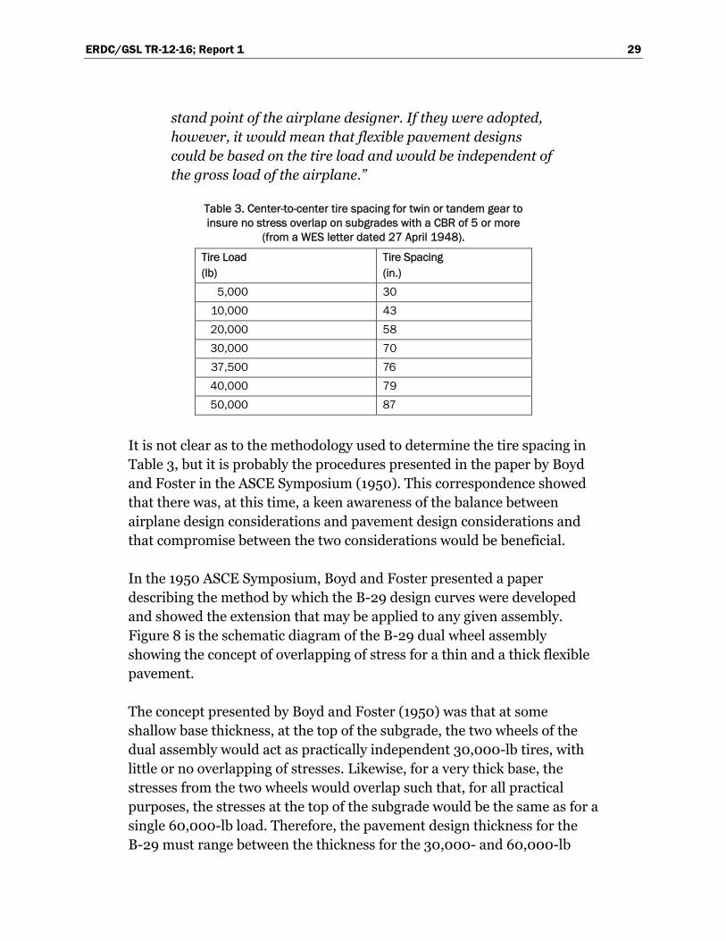
In this letter, the Flexible Pavements Laboratory states that they (the Flexible Pavements Laboratory) had furnished the OCE with procedures for resolving the single-wheel design curve into curves for various assemblies. Table 3 suggested tire spacing for various tire loads which insures no overlap of stress in subgrades with CBR values of 5 and more. In regard to the spacing in Table 3, the following statement is made:

“These spacings are much wider than those now in current use and may be considered entirely impracticable from the


stand point of the airplane designer. If they were adopted, however, it would mean that flexible pavement designs could be based on the tire load and would be independent of the gross load of the airplane.”

Table 3. Center-to-center tire spacing for twin or tandem gear to insure no stress overlap on subgrades with a CBR of 5 or more

(from a WES letter dated 27 April 1948).

Tire Load (lb)

Tire Spacing (in.)

5,000 30

10,000 43

20,000 58

30,000 70

37,500 76

40,000 79

50,000 87

It is not clear as to the methodology used to determine the tire spacing in Table 3, but it is probably the procedures presented in the paper by Boyd and Foster in the ASCE Symposium (1950). This correspondence showed that there was, at this time, a keen awareness of the balance between airplane design considerations and pavement design considerations and that compromise between the two considerations would be beneficial.

In the 1950 ASCE Symposium, Boyd and Foster presented a paper describing the method by which the B-29 design curves were developed and showed the extension that may be applied to any given assembly. Figure 8 is the schematic diagram of the B-29 dual wheel assembly showing the concept of overlapping of stress for a thin and a thick flexible pavement.

The concept presented by Boyd and Foster (1950) was that at some shallow base thickness, at the top of the subgrade, the two wheels of the dual assembly would act as practically independent 30,000-lb tires, with little or no overlapping of stresses. Likewise, for a very thick base, the stresses from the two wheels would overlap such that, for all practical purposes, the stresses at the top of the subgrade would be the same as for a single 60,000-lb load. Therefore, the pavement design thickness for the B-29 must range between the thickness for the 30,000- and 60,000-lb


Figure 8. Schematic diagram of B-29 wheel assembly (Boyd and Foster 1950).

single wheel loads. With this reasoning, the approach for developing the design curves for the B-29 was reduced to:

Finding the thickness at which each tire stresses the subgrade as an independent unit; and

Finding the thickness at which the two tires stress the subgrade as one single unit.

The thickness at which each tire of the B-29 dual assembly acts as an independent unit, and the thickness at which two tires act as a single unit were determined by comparisons of vertical stresses, shearing stresses, and deflections. The vertical and shearing stresses were computed using Boussinesq’s formulas assuming homogeneous material. The deflections were determined using a graphical method described in detail in the Boyd and Foster (1950) paper. For each parameter, Table 4 summarizes the values of maximum thicknesses at which each tire acted as an independent unit, and the minimum thicknesses at which the assembly acts as a single unit.


Table 4. Thicknesses defining unit behavior.

Reference Parameter at Top of Subgrade

Maximum Thickness at which Tires Act as Independent Units (in.)

Minimum Thickness for which Assemble Act as One Single Unit (in.)

Vertical stress 17 80

Shear stress 20 70

Deflection 10 75

Since the 10-in. thickness, as determined based on the subgrade deflection, was more conservative, the deflection was chosen as the parameter on which to develop the design curves for the B-29. For thicknesses of 10 in. and less, the B-29 design would be based on a 30,000-lb single wheel load, and for thicknesses 75 in. and greater, the B-29 design would be based on a 60,000-lb single wheel load. The thickness requirements between these two limits should vary in an orderly manner. From inspection of the dimensions of the B-29 gear (Figure 1), the maximum distance at which the tires would act independently was approximately equal to one-half of the clear distance (d) between the tires, and the minimum distance at the assembly acts as a single unit was approximately twice the centerline spacing (s) of the tires. Based on this analysis, the design curves of any gear assembly was

to be based on the ratios of 2d and s2 .

As the CBR pavement design methodology developed, a number of facets of the Boyd and Foster paper were influential. These facets include:

The concept of the design thickness for multiple-wheel assemblies being based on an equivalent single wheel;

The use of the deflection at the top of the subgrade being the basis for determining the single-wheel load to represent the multiple-wheel assemblies;

The fact that the more conservative approach was chosen for determining the ESWL; and

The establishment of the ratios, 2d and s2 , for determining the depths

for judging the behavior of multiple-wheel assemblies.

In a study reported in Technical Memorandum No. 3-349 (WES 1955), Turnbull, Foster, and Ahlvin re-evaluated the methods for resolving the existing single-wheel design criteria for flexible airfield pavements into


criteria for multiple-wheel assemblies. The methods to be re-evaluated were developed within the studies of pavement design criteria for the B-29, which was reported by Boyd and Foster. The purpose of the study authorized in 1953 was to determine:

Whether or not the present tentative method of resolving single-wheel criteria into criteria for multiple assemblies was adequate;

Means for obtaining better results if the present method was not adequate; and

What additional verification, if any, was needed for the present method of resolution or for a suggested alternate method.

Data from previous studies represented the basis for Turnbull’s study. The referenced publications were:

Report on Certain Requirements for Flexible Pavement Design for B-29 Planes (WES 1645);

Accelerated Traffic Test at Stockton Airfield (Stockton Test No. 2) (Porter 1949);

Design Curves for Very Heavy Multiple-wheel Assemblies (Boyd and Foster 1950);

Investigation of Stress Distribution in a Homogeneous Clayey Silt Test Section (Report No.1) (WES 1951);

The Stress Produced in a Semi-Infinite Solid by Pressure on Part of the Boundary (Love 1929);

Investigation of Stress Distribution in a Homogeneous Sand Test Section (WES 1949); and

Multi-wheel Test Section with Lean-Clay Subgrade (HQDA 1952).

Turnbull’s study also provided more insight into the development of the multiple-wheel criteria by Boyd and Foster that is referred to as the original analysis. In fact, the report stated that:

“The original analysis of deflection data considered that strain was an important criterion and that the critical strain is represented by the rate of change of deflection with offset along the deflection profile.”

It is also stated that, although the slope of deflection profiles was accepted as an important criterion, data were not adequate to develop such profiles,


and it was, therefore, assumed that the maximum deflection was representative of the critical slope. An additional simplification was that the maximum deflection for a dual assembly occurred beneath the center of one wheel. The report clarified that:

“With the additional data now available, deflection profiles can be developed and the magnitudes and positions of maximum deflections beneath multiple-wheel assemblies can be reasonably determined.”

Based on an analysis of the data from multiple-wheel traffic testing, it was concluded that design criteria in the present procedure provided designs that were slightly unconservative and thus considered to be inadequate. This inadequacy led to a determination that a better design procedure was needed. Because of the reasoning that the critical strain is related to deflection, the researchers favored the deflection as the parameter on which to base the computations of the equivalent single wheel load. The rationale given in the report was as follows:

“From this analysis, it appears that a single-wheel load, which yields the same maximum deflection as a multiple-wheel load, will produce equal or more severe strains in the subgrade or base than will the multiple-wheel load. The single load may, therefore, be considered equivalent to the multiple-wheel load for purposes of design, and this equivalent single-wheel load can be used to develop designs for multiple-wheel assemblies.”

Previously, in the development of the design curves, it was stated that the more conservative approach was selected. Now, in this study, it has been stated that the existing procedure is unconservative. In regard to conservatism, this report makes the following statements:

“The slopes of some of the single-wheel deflection profiles in plates 6, 9, and 11 are appreciably greater than their dual-wheel counter parts. Therefore, for design purposes, it might be considered that assuming the single-wheel loads equivalent to their dual counterparts would introduce too much conservatism. As will be shown later, however, the proposed method makes design criteria only a little more


conservative than that currently used, which has been shown to be slightly on the unconservative side.”

This logic and the new methodology for computing deflections under single and multiple-wheel assemblies permitted the development of the procedure for computing the equivalent single wheel. The procedure involved equating the deflections between the single-wheel and the multiple-wheel assemblies. In equating these deflections, the contact area of the single wheel is taken to be constant and the same as that of one wheel of the multiple-wheel assembly. Determining the ESWL for a number of depths assured the definition of the relation between the ESWL and depth. This relationship could then be used with the established single-wheel design criteria to develop further criteria for multiple-wheel assemblies.

A review analysis was also conducted of ESWLs based on the vertical and shear stresses at the top of the subgrade. As reported, the results of the analysis were the same as the initial analysis. With regard to the distribution of stress beneath loads, the following statement was made:

“Additional evidence has become available that shows the distribution of stresses beneath wheel loads or simulated wheel loads to be much as indicated by computations based on the Boussinesq theory of elasticity.”

The stress based methods were dismissed from further consideration because the original analysis concluded that the stress based methods for multiple-wheel assemblies were less conservative than the deflection-based method, and the deflection procedure was already unconservative.

Based on the analyses performed in this report, the following conclusions were reported:

“The present tentative method of resolving single-wheel into multiple-wheel designs gives criteria slightly on the unconservative side.”

“Neither vertical stress nor maximum shear stress provides an adequate basis for relating the effects of single-wheel and multiple-wheel assemblies.”

“Strains, which are in effect the slopes of deflection versus offset curves, provide the best basis for arriving at single-wheel loads that are equivalent, for design purposes, to multiple-wheel loads.”


“These strains are adequately represented in relative magnitude by theoretical maximum deflections, and satisfactory design criteria for multiple-wheel assemblies can be developed from established single-wheel criteria on the basis of equal maximum deflections.”

On the basis of the recommendation in Turnbull’s report, deflections were chosen as the basis of computing the ESWL for multiple-wheel assemblies. Replacing, in Equation 14, the single-wheel load term with the ESWL reformulated the CBR equation to handle multiple-wheel assemblies as Equation 17.

( )( . . ).

= + -log0 23 0 158 1ESWL A

t CCBR π

(17)

Development of the α-factor

As discussed previously, in the 1950s the CBR equation was developed and extended to include a thickness reduction term as shown in Equations 14 and 17. With the proliferation of larger aircraft, both commercial and military, carrying heavy loads on multi-wheel gear, the FAA and U.S. Military joined to collaborate on a testing program to evaluate the effects of heavily loaded multi-wheel gear on airfield pavements. As a result of the collaboration, the U.S. Army Corps of Engineers (USACE) was tasked to construct pavement sections to represent full-scale pavements. Using simulated gear representing the C-5A and Boeing-747 aircraft, the pavements sections were tested to failure. Mr. Jim Sale and Mr. Ahlvin headed the construction of a test load cart, full-scale test pavements, and the pavement testing to failure (Waterways Experiment Station 1971). The test program, referred to as the MWHGL test, produced data which, at the time, were considered the only reliable test data for heavily-loaded multi-wheel gear. Even today the data from the MWHGL test is a major source of design criteria for today’s large aircraft.

The analysis of the data from the MWHGL test program led the reformula-tion of Equation 17 in terms of a load adjustment factor, α, which was a function of traffic volume and number of tires in the multi-wheel tire group. The introduction of the α-factor resulted in the present form of the classical form of the CBR design equation:

.

= -8 1ESWL A

t αCBR π

(18)


Cooksey and Ladd (1971) defined in graphical form the value of α, and discussed the development of the thickness reduction curves. By studying Figures 1 and 2 in the Cooksey and Ladd report, it can be concluded that a large amount of uncertainty exists in the placement of the α-curves for the twin-tandem and 12-wheel tire groups. From the three curves shown in Figure 3 of the Cooksey and Ladd report, the complete set of α-curves were drawn as in Figure 9.

Figure 9. Alpha curves as contained in PCASE.

Significant factors in the development of the α-curves are that the data were very limited, the 12-wheel α-curve was conservatively placed, the curves were extrapolated beyond the bounds of the data, extrapolation of the curves was by engineering judgment, and placement of the set of α-curves was based on the placement of the 12-wheel, 4-wheel, and single-wheel curves. In the 1970s, α-curves were inserted into the pavement design computer program by digitizing the curves by hand and inserting the data into the design program as data statements. Later, the data for each curve was modeled with a third order polynomial.


3 Reformulation of the CBR Equation

When the U.S. Army Corps of Engineers selected the California method, they were accepting empirically developed thickness design curves. In extending the curves to aircraft loads, the Corps employed Boussinesq’s theory of stress distribution in a homogenous half-space. Even with the use of theory to extend the curves to higher loads, the design curves were considered empirical, since they were originally based on empirical curves. The CBR equation developers, without realizing it, formulated an equation that represented a specific stress distribution. Recognizing that the CBR equation represents a specific stress distribution supports the argument that the CBR design method fits the definition of a mechanistic design procedure. That is, the procedure has a model for computing stress and criteria that is based on the ratio of the computed stress with the measured soil strength. The ratio of computed stress to soil strength was related to pavement performance by traffic test data, therefore the design procedure may be defined as mechanistic/empirical.

In extending the design criteria from single-wheel to multiple-wheel assemblies, researchers considered vertical and shear stresses and deflec-tion as the basis for computing the ESWL for a multiple-wheel assemble. The analysis in developing the ESWL methodology indicated the procedures based on stress to be unconservative. On the other hand, the procedure based on deflection was deemed more conservative and provided a better fit for the performance data available at that time. Until this study, the reason why the stress-based CBR procedure would not provide a methodology of handling multiple wheel loads was not clear. This study reformulates the CBR equation to directly consider multiple-wheel assemblies and represents a more complete stress-based mechanistic-empirical procedure.

With the reformulation of the CBR equation, the mechanistic nature of the CBR pavement design procedure is readily apparent. The following paragraphs explain how the CBR equation was redeveloped to show its stress-based origin. The equation is also reformulated to consider traffic volume and multiple-wheel loads in a more direct manner.


Redevelopment of the CBR equation

Stress distribution in a homogeneous half-space can be described by the use of a stress concentration factor. The stress concentration factor was introduced by Professor Otto Karl Fröhlich (Jumikis 1964; Jumikis 1969; Ullidtz 1998) to explain the fact that early measurements of stresses showed that the theory of elasticity was not totally satisfactory. As defined in the Lockbourne No. 2 report, the concentration factor (n) is an empirical exponent introduced into the Boussinesq equation to make computed stresses agree more closely with measured stresses. About Fröhlich’s concentration factor, Jumikis states:

“Thus, by modifying Boussinesq’s isotropic, semi-infinite medium of constant elasticity to an anisotropic, semi-infinite medium, Fröhlich made the subject of the complex stress distribution problem more comprehensible and far-reaching than in Boussinesq’s problem.”

The equation for the vertical stress due to a point load, P, is of great importance in the redevelopment and reformulation of the CBR equation. The general form of the equation as given by Ullidtz (1998) is:

= f22n

t

nPσ cos

πR (19)

where:

P = applied point load at the surface σt = vertical stress at an arbitrary point R = distance from the point load to the location of σt

= angle between the vertical line and the line connecting load application point and an arbitrary point in the soil where to calculate the stress

n = Fröhlich’s concentration factor.

Using Equation 19, the stress at any arbitrary location in a semi-infinite medium due to a loaded area can be determined by integrating over the loaded area. When the concentration factor n is equal to 3, Equation 19 is the same as the Boussinesq equations for stress. For vertical stress at depth t along the centerline of a uniformly distributed circular load, Equation 19 reduces to:


é ùê úê úê úê ú= -ê úæ öæ öê ú÷ç ÷÷ç ç+ê ú÷÷ç ç ÷ç ÷è øçê ú÷çè øë û

02

11

1

t nσ σrt

(20)

where:

r = radius of the load area t = depth to the location of the computed stress n = concentration factor σ0 = applied stress over the loaded area.

For a stress concentration factor, n, equal to 3, Equation 20 is identical to the Boussinesq equation for the vertical stress under a uniformly loaded circular area. When the concentration factor is equal to 2, Equation 20 reduces to Equation 21.

é ùê úê ú

= ê - úê úæ ö÷çê ú+ ÷ç ÷çê è ø úë û

0 2

11

1tσ σ

rt

(21)

Equation 21 can be rewritten in the form of Equation 22.

é ùê úê ú

= ê úê úæ ö÷çê ú+ ÷ç ÷çê è ø úë û

0 2

1

1tσ σ

tr

(22)

The original airfield design curves based on shear stress were an extrapola-tion of the California pavement design curves for highway pavements (American Society of Civil Engineers 1950; Ahlvin 1991).The extrapolated curves were modified and verified by extensive full-scale field testing. The first airfield design curves were represented by the following design equation.

=t k P (23)


where:

P = the wheel load t = thickness k = a constant that was a function of subgrade CBR and tire

contact pressure.

The values of k for the original design curves are given in Table 1. If it is assumed that the load P is applied as a uniform pressure p over a circular area with a radius r, then Equation 23 can be rewritten as:

= 2t k pπr (24)

Equation 24 can be expressed as:

æ ö÷ç =÷ç ÷çè ø

22tk pπ

r (25)

Equation 25 can now be substituted into Equation 22 to obtain Equation 26.

é ùê ú=ê ú+ë û

0 2

11tσ σk pπ

(26)

Since both 0σ and p are the applied pressure over a circular area of radius

r, Equation 26 can be written in the following form.

é ùê úê ú

= ê úæ öê ú÷ç +ê ú÷ç ÷çè øê úë û2

11tσ

π kpπ

(27)

When both sides of Equation 27 are divided by the CBR, Equation 27 can be rewritten as:

=é ùê ú+ê úë û

2

11

tπσ

CBRCBR k

πp

(28)


A common criterion for design of structures is to limit the ratio of the applied stress to strength. Applying this concept to flexible pavements, one criterion is to limit the ratio of stress to the strength occurring at the top of the subgrade. In Equation 28, σt represents the stress at the top of the subgrade, and the CBR represents the strength of the subgrade. Thus, in a properly designed pavement, the left side of the equation should be a constant since all the pavements were to be designed for the same life. The stress σt is the design stress σdesign for a particular subgrade strength. Continuing with the assumption that the left side of Equation 28 is constant, the right side of Equation 28 must also be a constant, and the denominator of the right side of the equation must also be a constant. As shown in Table 1, the value of the denominator can be evaluated for given values of k. It was found that the average value of the denominator of the right side of Equation 28 was approximately 0.123, which resulted in the right side of the equation being a constant with value of 8.1 psi. Such value represents the design criterion for capacity operations. Referring the constant for capacity operation as β1, the design criteria for the design curves developed in the 1940s is represented by Equation 29.

.= =1 8 1designσ πβ psi

CBR (29)

Equation 28 can now be rewritten as Equation 30.

=é ùê ú+ê úë û

12

11

βCBR k

πp

(30)

Using Equation 30, the value of k is found to be:

= -1

1 1k

β CBR πp (31)

Substituting the value of k as given in Equation 31 into Equation 23, the following equation for pavement thickness is obtained.

= -1

1 1t P

β CBR πp (32)


Considering the relationship between P and p, Equation 32 can be rewritten as:

= -1

1pt A

β CBR π (33)

Since β1 is equal to 8.1, Equation 33 can be rewritten to yield one of the classic forms of the CBR equation as follows:

= -1

1t pβ CBR πA

(34)

The previous reasoning showed that Turnbull, Foster, and Ahlvin’s design equation was obtained by considering the stress distribution as defined by Fröhlich’s concentration factor. The earlier development of the CBR equation was based on the imposed requirement that the deflection at a

depth t for constant ratios of rt would be a constant. Such requirement is

also met when the stress distribution is described by Fröhlich with the stress concentration being equal to 2.

The classic form of the CBR equation, Equation 34, can be rearranged to explicitly show the ratio of thickness to the radius of the loaded area, as in Equation 35.

= -1

1t πpr β CBR

(35)

where:

p = pressure applied to loaded area r = radius of the loaded area t = thickness of pavement structure.

Criteria for single-assemblies

As has been discussed, a thickness adjustment factor was introduced into the classic CBR equation to adjust the pavement thickness to account for the requirement of different volumes of traffic. As originally developed, the CBR equation was to define the thickness requirement for a traffic volume for full


operation of an airfield pavement of 5,000 coverages. The first thickness adjustment factor for traffic volume was defined by the expression:

. ( ) .factor = +log0 23 0 15coverage (36)

When Equation 36 is applied, Equation 35 becomes:

( )( . . )= + -log1

0 23 0 15 1t πp

coverager β CBR

(37)

At 5,000 coverages, the value of Equation 36 is approximately 1. Later, Equation 36 was dropped, and the thickness adjustment factor, α, was substituted for Equation 36. The thickness adjustment factor, α, was developed to account for both traffic volume and number of tires in the tire group of the design aircraft. Thus, α became a function of both traffic volume and number of tires in the tire group, and the general form of the CBR became as shown in Equation 38.

= -1

1t πp

αr β CBR

(38)

In Equation 38, the 8.1 is a constant related back to the origin of the CBR equation with the α-factor inserted to consider traffic volume. In Equation 38, α is applied outside of the radical and is a multiplier of both terms under the radical. However, as has been shown, the stress criterion is contained only in the first term under the radical. The effect of applying the thickness adjustment factor outside the radical is to modify the stress criterion. The amount of modification to the criterion is a function of the relative magnitude between the first and the second terms under the radical. If the 8.1 constant is replaced with β which is a function of the traffic volume, then α in Equation 38 can be dropped, and the CBR equation, in terms of β, becomes:

= -1t πpr βCBR

(39)

For a single tire, α is a function only of the traffic volume. Designating α1 as the value of α for a single tire and substituting α1 into Equation 37 for the thickness adjustment factor, the following equation is obtained


.

= -1 18 1

t πpα

r CBR (40)

In Equation 39, β is also a function of traffic volume; therefore, for

identical values of rt , the right side of Equation 39 can be set equal to the

right side of Equation 40 to obtain Equation 41.

.

- = -11 18 1

πp πpα

βCBR CBR (41)

Equation 41 is solved for β to obtain the following relationship between α1 and β.

.

=é ùê ú- +ê úë û

2211 1

8 1

πpβ

πpαCBR α

CBR

(42)

Equation 42 shows that when α1 is equal to 1, the value of β is a constant, which is 8.1, and when α1 is 0, which means no pavement is required, the

value of πβ is equal to p

CBR. Referring back to section 3.2 in Equation 29,

πβ is also equal to

CBR

σdesign; therefore, when

designσp , no pavement is

required. For any other value of α1, the value of β will be a function of the

CBRp ratio. Since α1 is related to single-wheel traffic volume and β is related

to α1 by Equation 42, β can be related to single-wheel traffic volume directly by Equation 42. Figure 10 provides an example of the relationship between β and traffic.

In developing the relationship of Figure 10, p was assumed to be constant at 200 psi. For a level of traffic of approximately 10,000 coverages, β is a constant (8.1) over the range of CBR values used. This represents the level of traffic for which α1 is 1. For levels of traffic lower than 10,000 coverages, β decreases with increasing CBR, and at traffic levels above 10,000 cover-ages, the reverse is true. The mathematical explanation for the difference between α and β is that α is applied outside the radical and, therefore, a multiplier of both terms under the radical, whereas, β is applied to only one term under the radical.


Figure 10. Relationship between Beta and coverage as developed from single-wheel criteria.

The analytical development presented indicates the proper criterion is the stress criterion as represented by β. The data shown in Figure 10 were used to develop an equation for stress criterion based on β. The form of the equation was chosen to be:

( )( )

( )

+=

+log

oglog1

a c coveragesβ

b coverages (43)

The values of a, b, and c were determined by assuming three points of fit for the relationship. The values of β chosen for the fit were 79.4, 8.1, and 5 for traffic levels of 1, 10,000, and 1,000,000 coverages, respectively. The computed values of a, b, and c were 1.9, 0.228, and -0.0411, respectively. Replacing such values in Equation 43, Equation 44 represents the criteria, in terms of β, for single-wheel assemblies.

( ). . ( )

. ( )

-=

+log

loglog

1 9 0 04111 0 228

coveragesβ

coverages (44)

In Figure 10 it is seen that the relationship given by Equation 43 follows very close to the relationship representing a CBR value of 6. With the relationship between β and traffic defined in Equation 44, Equation 39 can be used to compute pavement thicknesses for any level of traffic. Figure 11 provides a comparison between thicknesses computed using the β criteria and the thicknesses computed using the α1 criteria.

1

10

100

10 100 1000 10000 100000

TRAFFIC IN COVERAGE

BE

TA

3 CBR

6 CBR

10 CBR

15 CBR

FITTED CURVE


Figure 11. Comparison of α criteria with β criteria (single wheel).

For thicknesses determined in this manner, the ratio of CBR

σdesign will be a

constant for a given level of traffic. For a traffic level of 10,000 coverages, the thicknesses computed by both procedures are identical. For a CBR value of 6, the thicknesses computed by both procedures are in very close agreement for the entire range of traffic levels. The thicknesses as determined by both procedures are in very close agreement for all values of CBR for traffic levels above 10,000 coverages. The only areas of significant difference between the two procedures are for CBR values of 3 and 15 CBR and low levels of traffic. Figure 12 provides another comparison of α and β criteria for the single wheel loading.

From the above analysis, it is apparent that for a single-wheel loading, the formulation of the CBR equation in terms of β is essentially the same as, but slightly superior to, the original formulation in terms of α1. One important aspect of the new formulation is that the mechanistic nature of the CBR design methodology and the stress criteria are now apparent.

Handling multi-wheel tire groups

Although the new CBR equation is superior to the original formulation when considering single-wheel assemblies, the real benefit of the new formulation is in handling multi-wheel loading. There are two means of pro-viding design criteria for multi-wheel tire groups; the first is through the use of equivalent single-wheel loads in a manner that is used in the current

0

10

20

30

40

50

60

10 100 1000 10000 100000 1000000

CO

MP

UT

ED

TH

ICK

NE

SS

IN IN

CH

ES

.BY ALPHA FACTORS 3 CBR

BY BETA FACTORS 3 CBR

BY ALPHA FACTORS 15 CBR


BY ALPHA FACTORS 6 CBR



Figure 12. Comparison of thicknesses based on α criteria and β criteria.

design procedure. The principle of the equivalent single-wheel for handling multi-wheel assemblies is to determine a single-wheel load that would have the same effect on pavement performance as does the tire group. Since the CBR equation is based on the vertical stress at the top of the subgrade, that vertical stress would be the response parameter on which to base the ESWL. When considering the conversion of the method of ESWL computation from deflection to stress, the 1955 work by Turnbull, Foster, and Ahlvin should be reviewed. They considered shear and vertical stresses along with deflection as a basis for computing the ESWL. Their analysis concluded that the stress based ESWL procedures were unconservative, but that the deflection based ESWL procedure could be used for developing design criteria for multi-wheel assemblies. The fact that in the earlier studies, the stress based ESWL procedure was considered to be unconservative certainly provided reasons to be cautious in developing criteria based on stress. Later, studies conducted in the analysis of the MWHGL test data indicated the deflection based ESWL was overly conservative, and required the introduction in the CBR equation of a thickness correction factor.

Review of current ESWL approach

In the current CBR-Alpha design procedure, the ESWL at a specified depth is defined as the load on a single tire having the same contact area as an individual tire of the tire group that would produce the same elastic deflection at the specified depth in an elastic half-space having a constant elastic modulus and a Poisson’s ratio equal to 0.5, as would the tire group. The elastic deflection at the specified depth is computed for both the tire

0

10

20

30

40

50

60

0 10 20 30 40 50 60

THICKNESS COMPUTED USING ALPHA FACTORS

TH

ICK

NESS C

OM

PU

TED

USIN

G B

ETA

FA

CTO

RS 3 CBR

6 CBR

15 CBR

line of equality


group and for a single tire having the same contact area as an individual tire of the tire group. Since the contact area of the ESWL tire remains constant, and the load is varied by varying the contact pressure, the ESWL is determined by the following equation:

= mwl

swl

δESWL SWL

δ (45)

where:

SWL = load on the single wheel used to compute the single wheel deflection

mwlδ = elastic deflection due to the multi-wheel tire group

swlδ = elastic deflection due to the single tire.

When Cooksey and Ladd (1971) analyzed the performance data from the MGHWL test section, based on the deflection ESWL, they concluded that the deflection ESWL was over-predicting the true ESWL and that the over- prediction was a function of the number of tires. The solution chosen by Cooksey and Ladd was to develop thickness adjustment factors to account for both repetitions and over-predictions of the ESWL. The thickness adjustment factor was referred to as the alpha factor (α-factor). Thus, when Equation 18 is used as the multi-wheel design criteria, the α-factor of Equation 18 is the product of the repetition alpha, (αr), and the load correction alpha, (αl). Since αr for a multi-wheel tire group should ideally be identical to the repetition alpha as is used for a single wheel loading, then the following relationship for αl should hold:

=1

l

αα

α (46)

where:

α = total thickness correction factor needed for a multi-wheel tire group

α1 = thickness correction factor needed for a single tire.

Equation 46 can be used, along with the data in the alpha curves, to compute the load related alpha factor for various tire groups. At 10,000 coverages, α1 has a value of approximately 1; therefore, at


10,000 coverages, the load alpha will equal the total alpha. Applying a thickness adjustment can be approximated by an adjustment to the ESWL. Since the α-thickness adjustment is applied outside the radical, the adjust-ment to the ESWL needed to approximate the α-adjustment is the square of the α-factor. At 10,000 coverages, the following relationship holds

. . .

= - = - » -2 2

8 1 8 1 8 1l lα ESWL α AESWL A ζESWL A

t αCBR π CBR π CBR π

(47)

In Equation 47, ζ is a correction to account for over- or under-estimating the ESWL and is equal to the α-factor squared. Based on the α-curves in current use, the values of α at 10,000 coverages for the 2-tire, 4-tire, and 6-tire assemblies are approximately 0.89, 0.82, and 0.78, respectively. Therefore at 10,000 coverages, the adjustments needed for the ESWL to approximate the thickness adjustments for the 2-tire, 4-tire, and 6-tire assemblies are 0.79, 0.67, and 0.61, respectively. The study by Barker and Gonzalez (2006) showed that more appropriate values of the 10,000 thickness reduction factors α for the 4-tire and 6-tire assemblies are 0.78 and 0.72, respectively. These data produce adjustment factors ζ for the ESWL for the 4-tire and 6-tire assemblies of 0.61 and 0.52, respectively. The above analysis allowed concluding that:

The ESWL based on deflection is an over-estimation of the “true” ESWL.

The over-estimation is a function of the number of tires. At 10,000 coverages, the ratios of the “true” ESWL to the deflection

based ESWL are in the order of 0.79, 0.61, and 0.52 for 2-wheel, 4-wheel, and 6-wheel assemblies, respectively.

Comparison of the stress-based ESWL with deflection-based ESWL

As previously mentioned, the deflection based ESWL was chosen because the stress based ESWL was deemed to yield unconservative results; at the same time the deflection based ESWL was recognized as being slightly conservative. At the time of the 1955 study, multi-wheel test data were not readily available, and one of the recommendations was that additional traffic tests were needed to verify the ESWL methodology. Another factor to consider is that in the 1955 study, Turnbull, Foster, and Ahlvin computed stresses and deflections for the ESWL using the Boussinesq equations which are associated with a stress concentration factor of 3, whereas the CBR


equation is related to a stress concentration factor of 2. The laws of a continuum dictate compatibility between the CBR equation and the method of computing the ESWL. Since the CBR equation is based on the vertical stress computed using a concentration factor of 2, the ESWL should be based on the vertical stress computed based on a concentration factor of 2. It will be shown in the following discussion that the ESWL based vertical stress computed using a concentration factor of 2 rather than the Boussinesq equations results in a more conservative ESWL, although not as conservative as the deflection-based ESWL. Over a limited range of depths and for 10,000 coverages, the ratio of the stress-based ESWL to the deflection-based ESWL is in agreement with the ratio of the “true” ESWL to the deflection-based ESWL.

A modification of the software contained in PCASE allowed the computa-tion of the ESWL based on vertical stress. The modification of the software introduced the calculation of the concentration factor as in Equation 19 to evaluate vertical stresses at any arbitrary point in a half-space due to mul-tiple circular loaded areas. For simplicity, the computed ESWL was for a constant contact area. The modified program permitted the development of ESWL curves based on stress concentration factors of 2 and 3 for the B-29, B-747, and B-777 aircraft. The unmodified version of the program was used to compute the deflection-based ESWL for the same aircraft. For each aircraft, Figures 13, 14, and 15 provide the comparison between the two stress-based ESWL curves (produced for concentration factors of 2 and 3, respectively) and deflection-based ESWL curve.

In each figure, the deflection-based ESWL is greater than the stress-based ESWL. The stress-based ESWL curves indicate that at shallow depths, the ratio of the gross gear load to the ESWL is equal to the inverse of the number of tires, indicating no interaction between tires. In addition, the maximum depths showing interaction between tires are approximately 10 in. for the B-29 and 17 in. for the B-747 and B-777. These depths are in essential agreement with the early concept that the tires would act as independent units down to a depth of approximately d/2. Instead, the deflection-based ESWL indicated interaction between tires even for surface damage.


Figure 13. ESWL curves for twin assembly (B-29).

Figure 14. ESWL curves for twin-tandem assembly (Boeing 747).


Figure 15. ESWL Curves for triple-tandem assembly Boeing 777).

In the early work of the development of pavement design criteria, it was assumed that at a depth of 2 · s, multi-wheel gear began to act as a single unit, and the gear load could be considered as a single-wheel load. Instead, the previous figures show that the multi-wheel assemblies never act as a single tire. For example, the B-29 was considered to act as a single unit at a depth of 75 in., and the ESWL at 75 in. would be 90 percent, 82 percent, and 80 percent of the gear load when computed by the deflection-based procedure, stress-based procedure with n=2, and n=3, respectively. The assumption that the multi-wheel assemblies act as single unit at 2 · s was selected for conservatism. For 10,000 coverages the ratios of the “true” ESWL for the 2-wheel, 4-wheel, and 6-wheel assemblies were 0.79, 0.61, and 0.52, respectively. As a comparison, the ratios of the stress-based ESWL with the deflection-based ESWL are shown in Figure 16 for the three aircraft previously analyzed.

The analysis of the ESWL computing procedures determined that the ratio of the stress-based ESWL to the deflection-based ESWL is a function of the number of tires and the depth to the subgrade. In addition, if the tire spacing were considered, the study most likely would have shown the influence of the tire spacing on the ratio. These findings are not surprising since the ESWL is a function of number of tires, tire spacing, and depth to the subgrade, the ratios of the ESWL as computed by the different methods


Figure 16. Relationship between stress ESWL and deflection ESWL.

would also be a function of these parameters. In large heavy aircraft, the tire spacing within a gear does not vary greatly; therefore, the most significant parameters affecting the stress-based ESWL to deflection-based ESWL ratio are the number of tires and depth to subgrade. Comparing the ζ-factors at 10,000 coverage with the ratio curves of the three aircraft for depths to subgrade of about 30 in. and n=2, the ratio is almost identical to the ζ-factors estimated from the α-factors. The stress-based ESWL for n=3 is more unconservative than the stress-based ESWL for n=2 and the currently accepted α-factors, for a considerable range of depths. This analysis supports the decision that in the reformulated CBR equation the use of the ESWL based on the vertical stress computed with n=2 produces thickness comparable with the current CBR design methodology. However for some depths, such thickness results are slightly more conservative.

Criteria for multi-wheel assemblies (with n=2)

With the assumption that the ESWL computed with n=2 represents the “true” ESWL, the criteria developed for the single-wheel assemblies would be applicable to multi-wheel assemblies. To prove the claim, pavement


thicknesses were computed for 10,000 coverages of single, twin, twin-tandem, and triple-tandem aircraft. These thicknesses were computed for a range of CBR values using the current α-factor design criteria and the single-wheel β-criteria. Figures 17 through 20 provide show thickness comparisons for the F-15, Boeing 737, Boeing 747, and Boeing 777 aircraft.

Figure 17. Comparison of thicknesses between α and β criteria for the F-15.

Figure 18. Comparison of thicknesses between α and β criteria for the Boeing 737.




For the single-wheel assembly, the thicknesses computed with both criteria are essentially identical. This was expected since the β-criteria were mathematically derived from the α-factor criteria, which at 10,000 cover-ages are essentially identical. For multi-wheel assemblies, the differences of thicknesses between the two criteria are a function of the number of tires


and the CBR values. Figure 18 shows that for the twin-tire assembly the computed thickness is greater than for the single-wheel assembly, although the difference is small.

For the single-wheel assembly, the pavement thicknesses range from 17 to 45 in. Figure 16 shows that between this thickness range, for the B-29 with twin-wheel gear, the ratio of the stress-based ESWL to the deflection-based ESWL is in agreement with the deducted ratio of the “true” ESWL to the deflection-based ESWL. For the Boeing-747 and Boeing-777 aircraft and pavement thicknesses up to 45 in., the thicknesses determined using the β criteria is in agreement with the α-factor criteria. For lower values of CBR, which require thicker pavements, the difference in thicknesses computed with the α and β criteria increases significantly for very low CBR values. These results can be related to the data presented in Figure 16 where, for increasing pavement thicknesses, the stress-based ESWL approaches the deflection-based ESWL. With regards to the error, as the pavement thickness increases, the error in computing an ESWL should decrease, yet the current α-based methodology using the thickness adjustment dictates a constant error with thickness.

The above thicknesses were computed based on β criteria developed from the single-wheel α-factor curve. A more direct approach for developing the multi-wheel β criteria consists of back-calculating β from the test section data and developing the relationship between β and test section perfor-mance represented by the number of coverages. Test data tabulated in the Barker and Gonzalez report (Barker and Gonzalez 1994) and test section data collected by the FAA (Hayhoe 2004) allowed formulating the rela-tionship between β and number of coverages for a stress concentration factor of 2. Such a relationship is presented in Equation 48 and Figure 21 shows the curve function along with the criteria for single wheels.

( ). . ( )

. ( )

+=

+log

loglog

1 7782 0 23971 0 5031

Coveragesβ

Coverages (48)

The data plot indicates that the single-wheel criteria, as developed from the single-wheel α-factor curve, does not provide a good fit of the test section data and that a better fit can be obtained using Equation 43. Fitting the data as previously discussed results in the criteria as given by Equation 48.


Figure 21. Comparison of n=2 criteria with α criteria.

In addition, Figure 21 shows that the curve drawn for the multi-wheel fits the data from the test sections; therefore, a single criteria curve could be used for both single-wheel and all multi-wheel assemblies and that the use of the α-factor can be eliminated from the design criteria.

Criteria for multi-wheel assemblies (n as function of CBR)

Using a stress concentration factor equal to 3 defines different criteria that can also be analyzed and compared with the current design procedure. Figure 22 provides a comparison of the multi-wheel test data for concentration factors of 2 and 3. The figure shows that there is minimal offset between the two data sets and no discernable difference in the scatter of the data. This comparison allows inferring that the design criteria could be developed assuming a concentration factor of either 2 or 3. In developing the criteria for different values of the concentration factor, the CBR equa-tion was reformulated in a form for which the concentration was an inde-pendent variable. This aspect allowed for consideration of a different stress distribution when developing the design criteria.

The general form for the CBR equation is shown in Equation 49.

=

--

æ ö÷ç ÷ç ÷ç ÷ç ÷ç ÷ç ÷ç ÷÷ç ÷çè ø

2

1

11

1

n

t

r

βCBR

πp

(49)


Figure 22. Comparison of test data for n=2 and n=3.

The computation of the β values for the test data are based on the assump-tion that the tire loads are represented by uniformly loaded circular areas.

For single-wheel loads, Equation 20 computes the vertical stress for given values of n, whereas Equation 19 is used for multi-wheel loads. With the ability to compute β based on any arbitrary stress concentration factor and with the indication that criteria could be developed for different values for the stress concentration factor, the main objective consists of selecting the most appropriate stress concentration factor. The analysis of measured stresses due to applied loads and computed stresses suggests that the best correlation is obtained for a stress concentration factor between 2 and 3.

According to Fröhlich, the magnitude of the stress concentration factor depends upon the nature of the soil and the size of the loaded area (Jumikis 1969). A stress concentration factor of 3 is applicable for an isotropic body with a constant modulus of elasticity. For sands, according to Fröhlich, a concentration factor of 4 would be applicable. The Stockton No. 2 Test included four instrumented test pavement sections of which stresses were measured for different loading and time of the day. The subgrade of the four sections varied between the three subgrade groups. One section had subgrade with a CBR of 6 which belongs to the “weak” group; another section subgrade was in “medium strength” group with a CBR of 20. The last two sections had subgrade belonging to the “strong” subgrade group


with CBR of 70 and 80, respectively. The asphalt thickness for all of the sections was 6 in.

The measured stress data were compared with theoretical stresses in plots of the vertical distribution of stress with depth. In the plots given in the Stockton No. 2 Test report, it is seen that a large portion of the scatter in the measured data can be explained by the difference in pavement temperature. For each of the items, the low temperature data indicate a Fröhlich theoretical concentration factor of less than 2 to be appropriate. The majority of the data falls between the theoretical curves corresponding to concentration factors of 2 and 4. The high temperature data for all items plotted between the theoretical curves of n = 4 and n = 6. The measured stresses from the sections characterized by a strong subgrade plotted more closely to the theoretical curve of n = 6 than the data from the other sections. It is readily apparent that the lower temperatures and, thus stiffer asphalt, resulted in greater stress distribution and, thus, lower apparent stress concentration factor. The analysis revealed also that stronger granu-lar subgrades resulted in less stress distribution and, thus, higher stress concentration factors.

In the WES stress distribution study, Report No. 1 on the clayey-silt test section data indicated that Boussinesq’s theory underestimates measured stresses. The report included the statement:

“There is consistent trend for the measured stresses to be greater than theoretical values at points directly beneath the loaded area and to be equal to or less than theoretical values elsewhere.”

The sand test section report states that there was a marked trend for the measured vertical stresses to exceed computed stresses. These examples agree with the theoretical studies by Fröhlich that for soil systems where the modulus increases with depth the stress concentration is greater than for a homogenous soil section, thus the stress concentration is greater than 3. Likewise, the stiffer the upper layer is relative to the subgrade, the lower is the stress concentration. The decrease in stress concentration corresponds to an increase of the concentration factor. The Stockton No. 2 Test suggests that for a weaker subgrade (CBR = 6), a stress concentration factor of 2 may apply, and for a medium strength subgrade (CBR = 20), a stress concentra-tion factor of 3 may be more appropriate. Therefore, for stronger subgrades,


a higher stress concentration would apply. For a subgrade with a CBR lower than 6, it is assumed that the stress concentration factor would be lower than 2. In light of this analysis, the immediate conclusion is the stress concentration factor should be expressed as a function of the subgrade CBR. Figure 23 shows one possible relationship between stress concentration factor and subgrade CBR that could be employed in developing the design criteria.

Figure 23. Relationship between stress concentration factor and CBR.

The relationship between CBR and stress concentration factor was compared with the stress distributions obtained using layered elastic theory. Using the material characterization procedure given by Barker and Brab-ston (1975), the stress at the top of the subgrade was computed for different thicknesses of pavement over a range of subgrade CBRs. Figure 24 presents the stress distributions based on the layered elastic analysis along with the stress distributions computed with the stress concentration factor that best matches the layered-elastic computed stresses. The data in Figure 25 indicate that the stress distribution computed using layered elastic theory is a function of CBR. For a range of CBR values from 3 to 15, the n factors that produce equivalent stress distributions range from 1.15 to 1.9.


Figure 24. Comparison of stress distribution based on layered elastic theory with stress

distribution based stress concentration factors.

Figure 25. Comparison of relationship between stress distribution and CBR.

As a reality check on the concept of the variable stress concentration factor, design thicknesses for the F-15, Boeing-747, and C-17 were computed based on n being a function of CBR. The thicknesses were computed for a range of CBR values, 10,000 coverages, and were based on the β-coverage relation-ship developed from the single-wheel α-factor curve. The design curves for


the three aircraft are shown in Figures 26 through 28. From the figures, it is possible to note that the stress distribution, corresponding to a stress concentration factor equal to 2 and as a function of the CBR, results in less pavement thickness for CBR values lower than 6 and greater pavement thickness for CBR values greater than 6. The results obtained using the variable stress concentration factor for the single-wheel aircraft could have been predicted, but predicting the results for the multi-wheel aircraft is more difficult. This is because, as the CBR is decreased, the stress distribution is increased (stress concentration factor decreases). This would lower the vertical stress under the center of a tire but would increase the stress due to adjacent tires; therefore, the net change in the stress would be difficult to predict. As the analysis indicated, the design thickness for a Boeing-747 based on the variable stress concentration factor agrees fairly well with the thickness based on the α-factor. For fixed stress concentration factors, the design thickness corresponding to a CBR of 3 is greater than the thickness calculated with the variable stress concentration factor or the α-factor. The design thickness for the C-17 based on the α-factor is greater than the design thickness based on the stress concentration factor, either fixed or variable. However, it should be recalled that a reanalysis of the test data indicated the α-factor for a 6-wheel gear should be reduced to 0.72, which would result in a better agreement with the thickness based on the variable stress concentration factor. The study of the literature and the

Figure 26. Design curves for F-15 using n as function of CBR.


Figure 27. Design curves for Boeing 747 using n as function of CBR.

Figure 28. Design curves for C--17 using n as function of CBR.

theoretical stress analysis, along with engineering logic, have provided convincing justification to recommend that the pavement design criteria should be based on the concentration factor being a function of the subgrade CBR.


Computing coverages and stress repetitions

Early in the development of the CBR design procedure, the concept of coverages was used to quantify traffic volume. A single coverage for a particular point on a pavement is when the point on the pavement surface is within the tire-print as an aircraft traverses the point. With the develop-ment of the design criteria in terms of a subgrade stress parameter, it can be postulated that, instead of coverages, a more correct parameter to represent traffic volume is the number of stress repetitions at the top of the subgrade. To quantify traffic volume, the layered elastic design procedure, as implemented for the military, counted strain repetitions at the top of the subgrade in relation to aircraft gear geometrics. Since the design thickness for a flexible pavement is relatively insensitive to traffic volume, particularly at the higher volumes of traffic, the value of the refinement in quantifying traffic is questionable. Considering the stage of the development of the β-design methodology, the additional complexity of determining stress repetitions is not justified.

Comparison of Beta criteria with layer elastic strain criteria

In 2005, representatives of some European countries advocated the use of pavement design criteria as given in the CROW report (CROW 2004). The procedure presented in the CROW report consisted of a layered elastic response model and vertical stain criteria identified as “the Shell criteria.” The subgrade strain criterion within the CROW procedure is represented by the following equation.

( ) ( )= +log log0 1s zN C C ε (50)

where:

sN = number of allowable load applications

10 CC , = material constants

zε = compressive strain on top of the subgrade.

For PCN-evaluation purposes, the CROW report recommended the Shell 85 percent relationship with values of 17.289 and -4.00 for 0C and 1C

respectively. The report also included a Shell 50 percent relationship for which 0C and 1C were 17.789 and -4.00 respectively.


Since the CROW criteria were recommended for application to NATO for the evaluation and design of flexible pavements, it is interesting to compare these criteria with the β and the latest layered elastic criteria. The β-criteria for the stress concentration factor of 2 is given by the following equation.

( )( )

( )

+=

+log

loglog1

a c covβ

b cov (51)

where:

a = 1.7782 b = 0.5031 c = 0.2397 cov = coverages

In 1994, WES recommended to the FAA subgrade strain criteria as developed from layered elastic analysis of data from prototype test sections. The criteria were again recommended in 2005 after a reanalysis of the test data which included data from the new FAA pavement test facility. The criteria being recommended for the layered elastic procedure was:

( )( )

( )

+=

+log

loglog1z

a c covε

b cov (52)

where:

a = -2.1582 b = 0.4115 c = -1.3723 εz = strain at the top of the subgrade cov = coverages

Assuming that Es – 1500 CBR, the vertical strain criteria in Equation 52 can be converted to β-criteria by the following relationship.

» 1500zβ πε (53)

Likewise, the β-criteria can be converted to strain criteria by Equation 54.


»1500z

βε

π (54)

Figure 29 shows the vertical strain criteria, derived from the β-criteria, compared with the strain criteria from the CROW report and the criteria recommended to FAA in 1994 and 2005. Also, Figure 29 contains data points from the FAA test facility. The difference between the CROW strain criteria and the WES layered elastic criteria is apparent, whereas the β-criteria agrees in shape and form with the WES layered-elastic criteria.

Figure 29. Comparison of strain criteria.

The offset between the curves of the β-citeria and the layered-elastic criteria was expected since the layered elastic model represents more load distribu-tion than does the stress concentration factor model (with n equal to 2).

The second comparison is shown in Figure 30 and is obtained by converting the WES layered elastic strain criteria to β-criteria.

Again, it is seen that the two criteria appear to be identical except for the offset. This offset is the result differences in the stress distribution and has been discussed earlier in this report. The next comparison is made by con-verting the CROW strain criteria to β-criteria as shown in Figure 31. Again, there is a large difference in the results between the two criteria except for a narrow range from 10,000 coverages to 100,000 coverages.


Figure 30. Comparison of Beta criteria with criteria from layered elastic criteria.

Figure 31. Comparison of WES criteria with criteria from CROW report.


The development of the CROW criteria is not known but it is obvious that the criterion does compare favorably with the WES layered elastic procedure. Another consideration is how traffic is counted. The WES criteria are related to traffic in terms of coverages, but the CROW criterion is in terms of strain repetitions. Since thickness is relatively insensitive to traffic volume, the method of defining traffic would not account for the difference in the criteria.

To conclude, the comparison of the β-criteria with the strain criteria highlights the mechanistic nature of the CBR procedure. For flexible pavement design, the good agreement of the β-criteria with the WES layered-elastic strain criteria provides for a high degree of confidences in using the β-criteria for pavement design supporting multi-wheel heavy aircraft and aircraft having single-wheel gear.


4 Finalization of the CBR-Beta Design Procedure

Analysis of Frohlich’s and Boussinesq’s theories with a review of test data allowed the first formulation of the revised CBR criteria and provided Equation 48 (reproposed below) that essentially links the strength-stress ratio of a pavement subgrade to the number of coverages of the design traffic.

( ). . ( )

. ( )

+=

+log

loglog

1 7782 0 23971 0 503

Coveragesβ

Coverages (48)

The design criteria summarized in Equation 48 went through additional review. A team of consultants from the private industry and Academia reviewed the development of the CBR-Beta procedure and recognized its validity. Nevertheless, the ERDC research team re-analyzed the CBR-Beta procedure including new field data from actual pavement failures.

Refinement of the CBR-Beta criteria

The pavement evaluation performed after a pavement failure at Las Cruces International Airport, NM, (AFCESA 2004) allowed for refining the CBR-Beta procedure when applied to low traffic volumes. In addition, data from the MWHGL full-scale testing were also included to improve the criteria when addressing low-traffic scenarios.

The MWHGL database included three data points which were specific for low-volume traffic. The data points were Test Lane 2A, 50-kip single-wheel assembly on Items 1 and 2, and Test Lane 3B, 240-kip twin-tandem assembly on Item 3. On Item 1, the traffic at failure for the 50-kip single-wheel load was at six coverages, but test records reported that cracking developed during the first pass, whereas at six coverages the rut depth was greater than 1 in. Therefore, the ERDC research team concluded that failure occurred earlier than six coverages.

The Las Cruces pavement evaluation reported that the ruts at the end of the runway were made by one pass (two coverages) of the C-17. Previous assumptions on the Las Cruces failure included a traffic volume of four


coverages composed of at least of one pass of the C-17 and one pass of the B-757 which, because of gears overlapping, produced a total of four coverages. In the absence of gear overlapping, the possible traffic scenario was of only two coverages. The ERDC analysis of the Las Cruces pavement failure is included in the appendix of this report.

The data points from the MWHGL study and the data from Las Cruces were combined to address low-volume traffic. The analysis of the low-volume traffic scenarios with the selected data points produced two criteria which were both acceptable in terms of approximation of the pavement perfor-mance. Equation 55 represents the less conservative curve, whereas Equation 56 is the more conservative design criteria. Due to the limited amount data for the very low traffic level, the more conservative option was chosen. Figure 32 shows the two curves and the position of the field data point.

( ). . ( )

. ( )

+=

+log

loglog

1 8451 0 21441 0 4667

Coveragesβ

Coverages (55)

( ). . ( )

. ( )

+=

+log

loglog

1 5441 0 07301 0 2354

Coveragesβ

Coverages (56)

Figure 32. Comparison of the criteria from Equations 55 and 56 for low volume traffic.

6.5

7

7.5

8

8.5

9

9.5

10

10

20

30

40

50

60

70

80

1 10 100 1000 10000 100000

Value

s of BETA for Coverages >22

37

Value

s of BETA for Coverages<2

237

Traffic in Coverages

Comparison of Criteria Developed to Consider Las Cruces Data

BETA =10^((1.8451+0.2144*LOG10(COV))/(1+0.4667*LOG10(COV))

BETA =10^((1.5441+0.0730*LOG10(COV))/(1+0.2354*LOG10(COV))

Las Cruces Data Point

MWHGL Item 1‐50kip




From a traffic volume of 1 coverage to 300 coverages, the difference between the two criteria may be considered as significant, but for traffic volumes from 300 coverages up to a million coverages, the two criteria almost coincide. In fact, at coverage levels of 2,237 and 300,000, the equations for two criteria dictate that the criteria are identical. Table 5 compares the two criteria in terms of required pavement thickness for operations of the C-17 aircraft.

Table 5. Criteria comparison for C-17 operations.

CBR Passes Coverages

Thickness (in.) Difference (in.) T2-T1 T1 (Eq. 55) T2 (Eq. 56)

3

1 2 13.6 19.9 6.3

5 4 16.8 22.1 5.3

10 7 20.4 24.7 4.3

100 72 31.6 33.7 2.1

1,000 725 42.4 42.9 0.5

5,000 3,623 49.2 49.1 -0.1

50,000 36,232 57.7 57.4 -0.3

100,000 72,464 59.9 59.7 -0.2

6

1 2 7.3 12.4 5.1

5 4 10.0 14.0 4.0

10 7 12.8 15.8 3.0

100 72 20.0 21.1 1.1

1,000 725 25.8 26.1 0.3

5,000 3,623 29.4 29.3 -0.1

50,000 36,232 34.0 33.8 -0.2

100,000 72,464 35.3 35.1 -0.2

10

1 2 0.1 7.6 7.5

5 4 5.0 9.1 4.1

10 7 7.9 10.7 2.8

100 72 14.2 15.1 0.9

1,000 725 18.6 18.8 0.2

5,000 3,623 21.1 21.0 -0.1

50,000 36,232 24.1 24.0 -0.1

100,000 72,464 24.9 24.8 -0.1


5 Summary, Conclusions, and Recommendations

Summary of the findings

A complete review of the CBR flexible pavement design methodology evolved from a study of data evaluating the six-wheel α-factor. The initial analysis of the thickness adjustment factor α revealed that the factor accounted for an over-prediction of the ESWL. It was shown that, in some cases, the “true” ESWL for a six-wheel gear would be only about 50 percent of the computed ESWL. The reformulation of the CBR equation originated from an analysis proposed by Ullidtz (1998) where the permissible vertical stress at the top of the subgrade was computed using Boussinesq’s equation in conjunction with the CBR equation. The analysis of the CBR equation revealed apparent correlation with Fröhlich-defined stress concentration factor of 2. Realizing that the CBR equation represented a stress distribu-tion was the catalyst of the study which led to the identification of the mechanistic nature of the CBR design procedure.

The identification of the stress distribution represented by the CBR equation provided the explanation about the unconservative values of vertical stress obtained in the development of the ESWL. In fact, the ESWL was computed using the Boussinesq equations, whereas the CBR equation is based on a stress distribution with a Fröhlich’s stress concentration factor of 2. Reformulating the CBR equation in terms of stress concentration factor permitted the development of design criteria based on the β parameter which represents the allowable vertical stress. The new CBR equation for which the stress distribution can be defined by any stress concentration factor allows selecting the stress distribution which best models measured data.

An analysis of measured data along with theoretical considerations led to the conclusion that the stress distribution is a function of the subgrade CBR. The data indicated that the stress concentration factor, and therefore the stress distribution, varied from about 1 for low strength subgrades to about 6 for very strong subgrades. In this study, the stress distributions were obtained based on a layered-elastic analysis using the Corps of Engineers’ method for characterizing pavement materials. The analysis indicated that


the stress distributions from the layered-elastic procedures can be approxi-mated by concentration factors of 1.15 for a 3 CBR subgrade, 1.4 for a 6 CBR subgrade, and 1.9 for a 15 CBR subgrade. Comparing measured to layered-elastic computed data indicated that most layered elastic models, to include the WES model, under-predict vertical stress.

The ERDC Research Team believes that the relationship between the stress concentration factor and subgrade CBR provides realistic stress distributions, and therefore the new CBR equation formulation can be adopted as the design model for flexible pavements. The clear mechanistic nature of the Beta methodology is justification for selecting the Beta criteria to replace the current Alpha criteria.

Conclusions

Based on the research conducted in this study, the following conclusions were developed.

The classic CBR equation represents a distribution of vertical stress defined by Fröhlich’s stress concentration factor of 2.

A formulation of the CBR equation has been developed to represent any arbitrary concentration constant.

The distribution of vertical stress in a pavement is a function of the subgrade strength.

Design criteria (Beta criteria) can be developed based on the ratio of vertical stress to CBR, which would be independent of the aircraft landing gear thus eliminating the need for α-factors.

The CBR design procedure represents a mechanistic-empirical design procedure, in which the critical response is computed using the stress distribution described by the revised CBR equation and an appropriate stress concentration factor. The critical response is then transferred to pavement performance using an empirically-derived performance model based on test section data.

Most layered elastic models will under-predict the vertical stress.

Recommendation

The recommendation is made to replace the current CBR-α criteria for design of flexible pavements with the CBR-Beta criteria.


References

Ahlvin, Richard G. 1991. Origin of developments for structural design of pavements. Technical Report GL-91-26. Vicksburg, MS: U.S. Army Corps of Engineers, Waterways Experiment Station.

Air Force Civil Engineer Support Agency (AFCESA). 2004. Pavement Evaluation, Las Cruces International Airport New Mexico, Tyndall Air Force Base, FL.

Airport Technology Research and Development Branch. 2004. Alpha factor determina-tion from NAPTF data. Letter Report Submitted to Associate Administrator for Airports, AAR-410 2004. Revised March 21, 2005.

American Society of Civil Engineers. 1950. Development of CBR flexible pavement design method for airfields a Symposium. Paper No. 2406 Reprinted from Transactions 115:453.

Barker, Walter R. 1994. ACN presentation. FAX to Orv Preston July 8, 1994 (unpub-lished, attachment 2).

Barker, Walter R. 1994. Technical summary, review of alpha factors. FAX to Ed Gervais September 9, 1994 (unpublished, attachment 3).

Barker, W.R., and Gonzalez, C.R. (2006). “Independent Evaluation of 6-Wheel Alpha Factor Report”, Letter Report to the Federal Aviation Administration, U.S. Army Engineer Research and Development Center, Vicksburg, Mississippi.

Barker, Walter R., and William Brabston. 1975. Development of a structural design pro-cedure for flexible airport pavements. U. S. Department of Transportation, Fed-eral Aviation Administration Report No. FAA-RD-74-199. Vicksburg, MS: U.S. Army Corps of Engineers, Waterways Experiment Station.

Barker, Walter R., and Carlos R. Gonzalez. 1994. Super-heavy aircraft study. Technical Report GL-94-12. Vicksburg, MS: Waterways Experiment Station, U.S. Army Corps of Engineers.

Boyd, W.K. and C.R. Foster. 1950. Design Curves for Very Heavy Multiple Wheel Assemblies. In Development of CBR Flexible Pavement Design Method for Airfields: A Symposium. Transactions, ASCE, Vol. 115, Paper 2406, pp.534-546.

Brown, D.N. and O.O. Thompson. 1973. Lateral distribution of aircraft traffic. Miscellaneous paper S-73-56. Vicksburg, MS: Waterways Experiment Station, U.S. Army Corps of Engineers

Cooksey, D. L., and D. M. Ladd. 1971. Pavement design for various levels of traffic vol-ume. Air Force Weapons Laboratory, Air Force Systems Command, Technical Report No. AFWL-TR-70-133 (attachment 1). Vicksburg, MS: Waterways Experi-ment Station.

Department of the Army, Corps of Engineers, Sacramento District. 1948. Accelerated traffic test at Stockton Airfield, Stockton, California.


Fine, L. and J. Remington. 1972. The Corps of Engineers : construction in the United States. Washington, Office of the Chief of Military History, U.S. Army.

Hayhoe, G.F. 2004. Traffic testing results from the FAA’s National Airport Pavement Testing Facility. Proceeding of the 2nd International Conference on Accelerated Pavement Testing, University of Minnesota, Minneapolis, MN

Headquarters, Department of the Army (HQDA). 1952 (Sep). Design of Flexible Airfield Pavements for Multiple-Wheel Land Gear Assemblies, Report No. I Test Section with Lean-Clay Subgrade, Technical Manual TM 3-349, Washington, DC.

Information and Technology Platform for Transport, Infrastructure and Public Space (CROW). 2004. The PCN Runway Strength Rating and Load Control System. Report D04-09. Amsterdam, the Netherlands.

Jumikis, A. R. 1964. Mechanics of soils. Princeton, NJ: D. Van Nostrand Company, Inc.

Jumikis, A. R. 1969. Stress distribution tables for soil under concentrated loads. College of Engineering, Rutgers University, Engineering Research Publication No. 48.

Love, A.E.H. 1929. The Stress Produced in a Semi-Infinite Solid by Pressure on Part of the Boundary. Phil. Trans. R. Soc. 228 (659-669) 377-420, London, England.

Middlebrooks, T.A. and G.E. Bertram. 1950. Adaptation to the Design of Airfield Pavements. Transactions, ASCE, pp.468-470.

Porter, O.J. & Co. 1949. Accelerated Traffic Test at Stockton Airfield Stockton, California (Stockton Test No. 2), Corps of Engineers Sacramento District, Department of the Army

Ullidtz, P. 1998. Modeling flexible pavement response and performance. Polyteknish Forlag.

Vedros, P. J. 1960. Study of lateral distribution of aircraft traffic on runways. Miscella-neous Paper No. 4-369. Vicksburg, MS: U.S. Army Engineer Waterways Experi-ment Station.

Waterways Experiment Station. 1951. Collection of letter reports on flexible pavement design curves. Miscellaneous Paper No. 4-61. Vicksburg, MS: U.S. Army Corps of Engineers.

_____. 1951. Investigations of pressures and deflections for flexible pavements. Technical Memorandum No. 3-323. 1951. Vicksburg, MS: U.S. Army Corps of Engineers.

_____. 1956. Mathematical expression of the CBR relations. Technical Report No. 3-441. Vicksburg, MS: U. S. Army Corps of Engineers.

_____. 1955. Design of flexible airfield pavements for multiple-wheel landing gear assemblies, report No. 2, analysis of existing data. Technical Memorandum No. 3-349, June 1955. Vicksburg, MS: U.S. Army Corps of Engineers.

_____. 1945. Certain Requirements for Flexible Pavement Design for B-29 Planes. Vicksburg, MS: U.S. Army Corps of Engineers.


_____. 1949. Minutes of conference on stress distribution investigation 21-22 December 1949. Conference on Stress Distribution Investigation. Vicksburg, MS: U.S. Army Corps of Engineers.

_____. 1959. Developing a set of CBR design curves. Instruction Report No. 4. Vicksburg, MS: U.S. Army Corps of Engineers.

_____. 1971. Multiple-wheel heavy gear load pavement tests. Technical Report S-71-17. Vicksburg, MS: U.S. Army Corps of Engineers.


Appendix A: Verification of Beta Criteria using Data from Las Cruces Evaluation Report

Introduction: On 30 November and 1 December 2010, external consultants reviewed the proposed CBR-Beta procedure for design of flexible pavements. The recommendation of the consultants was to proceed with the implementation of the proposed pavement design procedure. Attachment 1 is a draft ETL for the implementation of the proposed CBR-Beta design procedure. Following the review of the proposed design procedure, an evaluation report of the Las Cruces airport was received from Dr. Craig Rutland, U.S. Air Force Civil Engineer Support Agency (AFCESA). It was understood that Dr. Rutland would like to use the data contained in the report as additional verification for the CBR-Beta design procedure. Portions of the evaluation report are attached for convenient reference.

Discussion: The evaluation report, dated October 2004, is a report of a pavement investigation conducted as a result of damage to the main runway at Las Cruces, NM, caused by operations of Air Force B-757, C-17 and C-130 aircraft. The damage is described in the following paragraphs taken from the report.

“Pavement Surface Condition

The runway was divided into two features with Runway 12/30 being the dividing line.

The Runway 22 end feature (R01A-1) has a cursory PCI rating of Failed due to ruts within 25 feet of centerline on both sides. The ruts are as deep as 2” on the Runway 22 end and decrease in severity to the Runway 12/30 intersection where they are less than ½” in depth.

The Runway 04 end feature (R01A-2) has a cursory PCI rating of Very Poor due to ruts 25 feet of centerline on both sides. The ruts are ¼” or less on the Runway 04 end with the exception of two small areas that have ruts as deep as ¾”


identified in drawings in Appendix A. The runway asphalt exhibits medium and low severity alligator cracking in areas with heavy rutting, medium and low severity block cracking, depressions, raveling, longitudinal/transverse cracking, and low severity slippage.”

As can be seen in the report, the ruts were as deep as 2” on the Runway 22 end with decreasing rut depth toward the center of the runway. Less severe ruts were present on the Runway 04 end with two small areas of more severe ruts a short distance from the end. The location of photo A-5 is identified as being in the touchdown area of Runway 22. The tire imprints would seem to indicate that the ruts in this area were made by the C-17 aircraft. The location of photo A-6 is not identified but it is assumed that the photograph shows the more severe ruts at the end of Runway 22. Again the pattern of the ruts would indicate the ruts were made by the C-17. The report states the rutting extended 25’ on both sides of the centerline. The outside tires for the B-757 are about 13.5’ from the centerline of the aircraft and outside tires for the C-17 tires are about 16’ from the centerline of the aircraft. With these spacing it is quite likely there is some overlapping of tire paths for the two aircraft. Since the reports states that the operations of the Air Force aircraft had been recent, it is assumed the Runway 22 would have been the primary runway for takeoffs and landing thus the runway end with the greatest damage would have been subjected to takeoff traffic. Traffic volume and the aircraft weights are not given for any of the aircraft. The base, subbase and subgrade strengths were measured using the DCP with correlations made to CBR; no CBR tests were conducted to measure CBR directly. Without traffic volume, aircraft weights and reliable measurements of material strengths, the reliability of the data as a data point would be very low and may even give misleading information. Even though the data are flawed, with a number of assumptions the data can be used to provide a rough verification of the criteria.”

Analysis: To make the analysis, a number of assumptions are necessary. The first assumptions are in regard to the applied aircraft traffic. Since no


aircraft weights are given, it was assumed that on takeoffs, the aircraft would be at the design weights. The C-130 is a much lighter aircraft, and the rutting was at a location wider than the C-130 gear; therefore, the C-130 was not used in the analysis. For traffic volume there had to be at least one takeoff for the C-17 and one for the B-757, and if it is assumed the tires overlapped, there would have been a minimum of four coverages of the aircraft tires. The strength of base was given as 20 CBR and the strength of subbase was given as 6 CBR. The thickness of asphalt above the base was given as 3.5 in. and the thickness above the subbase was given as 12.5 in. It was assumed that the strength and thickness data are averages and that there would be some variability in the data. In the pictures it is seen that the airfield is in a high plains area in which the soil conditions could be unusually uniform. The report states that the runway had recently received a slurry seal treatment; therefore, it was assumed that the asphalt surface contained some type of cracking. The fact that more severe rutting was at the end of the runway than at some distance from the end could indicate that the pavement was either weaker toward the end of the runway or that the decreasing rut depth was due to decreasing load as the aircraft gained speed during takeoff. To show the effect of possible variation in base strengths different base strengths were assumed. For the subbase only, the 6 CBR strength was used (this being about the lowest strength that could be possible).

CBR-Beta Criteria: The data that were developed using the CBR-Beta criteria are given in Tables A-1, A-2, A-4 and A-5. For making a comparison of Beta criteria with the Las Cruces pavement performance the traffic volume to failure was assumed to be four coverages, the strength of the base was assumed to be 20 CBR and the strength of subbase was assumed to be 6 CBR. The comparison developed is shown in Figure 1. The comparison shows the predicted performance to be better than the observed perfor-mance. In the tables it is seen that when considering the 20 CBR base, the CBR-Beta criteria predicts failure at 11 coverages and 22 coverages for the B-757 and C-17, respectively. When considering the subbase as a 6 CBR layer, the predicted coverages to failure are 15 coverages and 7 coverages for the B-757 and C-17, respectively. In analyzing the comparison shown in Figure 1 between the Beta criteria and observed performance, it should be remembered that the four coverages to failure were considered to be a minimum level of traffic applied to the pavement and that the 20 CBR was the average base strength. If the base CBR had been as low as 12 or the traffic volume had been greater than four coverages, the predicted pave-


ment performance would have been in-line with the observed pavement performance. When considering the possibility that the failure could be caused by shear in the subbase, the seven coverages predicted to failure for the C-17 is not too far from the assumed coverages to failure. From these comparisons, it is seen that the proposed design criteria predicts perfor-mance that compares well with the observed performance. Again, it is reiterated that the predicted performance is based on gross assumptions of aircraft loads, traffic volume and material strengths.

Minimum Thickness Criteria: Tables A-3 and A-6 contain data developed using the criteria used in the minimum thickness program. With predicted levels of traffic-to-failure at three coverages and less, it is seen that the criteria used for determining the minimum thickness of surface and base are more conservative than the CBR-Beta criteria. These predicted levels of traffic are all less but very close to the assumed applied traffic.

Conclusions: The conclusions are presented in the absence of reliable data on material strengths, aircraft weights and traffic volume, and should be viewed as having a low degree of reliability. The conclusions are as follows:

The failures observed were likely to have been caused by the C-17 over-loading the subbase material.

The agreement between the predicted traffic level of 7 coverages, as predicted by the CBR-Beta, and the estimated minimum traffic that may have been applied to the pavement is considered to be at an acceptable level.

The criteria for determining the minimum thickness of asphalt surfacing and base is, at low levels of traffic, more conservative than the CBR-Beta criteria.

Given the material strengths, thicknesses and aircraft at the design loads, both the CBR-Beta criteria and the minimum thickness criteria would have predicted early failure of the pavement.

Excerpt from Las Cruces Evaluation Report

PAVEMENT

EVALUATION

LAS CRUCES


INTERNATIONAL

AIRPORT

NEW MEXICO

ICAO: KLRU

OCTOBER 2004 APE-668

Pavement Surface Condition

The runway was divided into two features with Runway 12/30 being the dividing line.

The Runway 22 end feature (R01A-1) has a cursory PCI rating of Failed due to ruts within 25 feet of centerline on both sides. The ruts are as deep as 2” on the Runway 22 end and decrease in severity to the Runway 12/30 intersection where they are less than ½” in depth.

The Runway 04 end feature (R01A-2) has a cursory PCI rating of Very Poor due to ruts 25 feet of centerline on both sides. The ruts are ¼” or less on the Runway 04 end with the exception of two small areas that have ruts as deep as ¾” identified in drawings in Appendix A. The runway asphalt exhibits medium and low severity alligator cracking in areas with heavy rutting, medium and low severity block cracking, depressions, raveling, longitudinal/transverse cracking, and low severity slippage.


Photographs from Las Cruces Evaluation Report:

Figure A5. Rutting in asphalt with tire imprints – Runway 22 touchdown area.

Figure A6. Runway asphalt distresses include cracking and rutting.


Tables from Las Cruces Evaluation Report:

Table A1. Based on 3.5 Asphalt Surface over Base Data for B757 at 234655 pounds gross weight.

Base CBR

Thickness of Asphalt Surface Beta

Predicted Coverage

20 3.5 25 11

18 3.5 28 8

15 3.5 33 5

12 3.5 40 3

Table A2. Based on 3.5 Asphalt Surface over Base Data for C17 at 585000 pounds gross. weight

Base CBR


Predicted Coverage

20 3.5 20 22

18 3.5 23 15

15 3.5 27 9

12 3.5 32 4

Table A3. Predicted Life based on minimum thickness criteria for asphalt surface.

Aircraft Base CBR T of Asphalt Surface

Predicted Coverage

B757 20 3.5 2

C17 20 3.5 3


Table A4. Analysis Based on 12.5" of Surface and Base over Subbase Data for B757 at 234655 pounds gross weight.

Subbase CBR

Thickness of Surface & Base Beta

Predicted Coverage

6 12.5 23 15

Table A5. Analysis Based on 12.5" of Surface and Base over Subbase Data for C17 at 585000 pounds gross weight.

Subbase CBR


Predicted Coverage

6 12.5 29 7

Table A6. Predicted Life based on min thickness criteria for asphalt surface and base.

Aircraft Subbase CBR

T of Asphalt & Base

Predicted Coverage

B757 6 12.5 3

C17 6 12.5 1<

Figure A7. Beta design criteria military air fields.

6

6.5

7

7.5

8

8.5

9

9.5

10

0

10

20

30

40

50

60

70

80

1 10 100 1000 10000 100000

Value of BETA

Aircraft Traffic in Coverages

BETA Design Criteria Military Air Fields

B757 for Base CBR=20

B757 for Subbase CBR=6

C17 for Base CBR=20

C17 for Subbase CBR=6

For values of BETA greater than 10

For values of BETAless than 10

REPORT DOCUMENTATION PAGE Form Approved

OMB No. 0704-0188 Public reporting burden for this collection of information is estimated to average 1 hour per response, including the time for reviewing instructions, searching existing data sources, gathering and maintaining the data needed, and completing and reviewing this collection of information. Send comments regarding this burden estimate or any other aspect of this collection of information, including suggestions for reducing this burden to Department of Defense, Washington Headquarters Services, Directorate for Information Operations and Reports (0704-0188), 1215 Jefferson Davis Highway, Suite 1204, Arlington, VA 22202-4302. Respondents should be aware that notwithstanding any other provision of law, no person shall be subject to any penalty for failing to comply with a collection of information if it does not display a currently valid OMB control number. PLEASE DO NOT RETURN YOUR FORM TO THE ABOVE ADDRESS.

1. REPORT DATE (DD-MM-YYYY) April 2012

2. REPORT TYPE Report 1 of a series

3. DATES COVERED (From - To)

4. TITLE AND SUBTITLE

Reformulation of the CBR Procedure; Report I: Basic Report

5a. CONTRACT NUMBER

5b. GRANT NUMBER

5c. PROGRAM ELEMENT NUMBER

6. AUTHOR(S)


5d. PROJECT NUMBER

5e. TASK NUMBER

5f. WORK UNIT NUMBER

7. PERFORMING ORGANIZATION NAME(S) AND ADDRESS(ES) 8. PERFORMING ORGANIZATION REPORT NUMBER

Geotechnical and Structures Laboratory U.S. Army Engineer Research and Development Center 3909 Halls Ferry Road Vicksburg, MS 39180-6199

ERDC/GSL TR-12-16

9. SPONSORING / MONITORING AGENCY NAME(S) AND ADDRESS(ES) 10. SPONSOR/MONITOR’S ACRONYM(S)

U.S. Army Corps of Engineers 441 G Street NW Washington, DC 20314-100

11. SPONSOR/MONITOR’S REPORT NUMBER(S)

12. DISTRIBUTION / AVAILABILITY STATEMENT Approved for public release; distribution is unlimited.

13. SUPPLEMENTARY NOTES

14. ABSTRACT

The California Bearing Ratio (CBR) procedure has been the principal method used for design of flexible pavements for both military roads and airfields since its development in the 1940s. In recent years, as the use of analytical models, such as the layered elastic and finite elements models, became accepted for pavement design, the CBR design procedure has been criticized as being empirical, overly simplistic, and outdated. A major criticism of the procedure has been the use of an adjustment, or Alpha factor, to account for over estimation of the equivalent single-wheel load and as a thickness adjustment for traffic volume. The objective of this research was to reformulate the CBR-Alpha procedure so that design would be based on a more mechanistic methodology and to develop performance criteria for use with the reformulation. With this purpose in mind, the report details the developmental steps of the reformulation starting with the original CBR-Alpha procedure and ending with a new procedure based on Fröhlich’s theory for stress distribution. The reformulation was verified through review of historical test data, by prototype testing, and by analyses of an actual airfield pavement failure. The reformulation of the procedure resulted in the elimination of both the equivalent single-wheel load concept and the Alpha factor.

15. SUBJECT TERMS

Alpha factor Beta factor

CBR design Equivalent-single wheel load Flexible pavement design

Fröhlich’s stress distribution Layered elastic design procedure Stress concentration factor

16. SECURITY CLASSIFICATION OF: 17. LIMITATION OF ABSTRACT

18. NUMBER OF PAGES

19a. NAME OF RESPONSIBLE PERSON: Carlos R. Gonzalez

a. REPORT

UNCLASSIFIED

b. ABSTRACT

UNCLASSIFIED

c. THIS PAGE

UNCLASSIFIED UNCLASSIFIED 93 19b. TELEPHONE NUMBER (include area code)

(601) 634-2647 Standard Form 298 (Rev. 8-98)

Prescribed by ANSI Std. 239.18

Reformulation of the CBR ProcedureERDC/GSL TR-12-16; Report 1 ii Abstract The California Bearing...

Documents

Transcript of Reformulation of the CBR ProcedureERDC/GSL TR-12-16; Report 1 ii Abstract The California Bearing...