Reflection seismic imaging of the upper crystalline crust ...

Technical Report

TR-01-31

Svensk Kärnbränslehantering ABSwedish Nuclear Fueland Waste Management CoBox 5864SE-102 40 Stockholm SwedenTel 08-459 84 00

+46 8 459 84 00Fax 08-661 57 19

+46 8 661 57 19

Reflection seismic imagingof the upper crystallinecrust for characterizationof potential repository sites:Fine tuning the seismic source

Christopher Juhlin, Hans Palm and Björn Bergman

Uppsala University

September 2001

This report concerns a study which was conducted for SKB. The conclusionsand viewpoints presented in the report are those of the authors and do notnecessarily coincide with those of the client.

Reflection seismic imagingof the upper crystallinecrust for characterizationof potential repository sites:Fine tuning the seismic source

Christopher Juhlin, Hans Palm and Björn Bergman

Uppsala University

September 2001

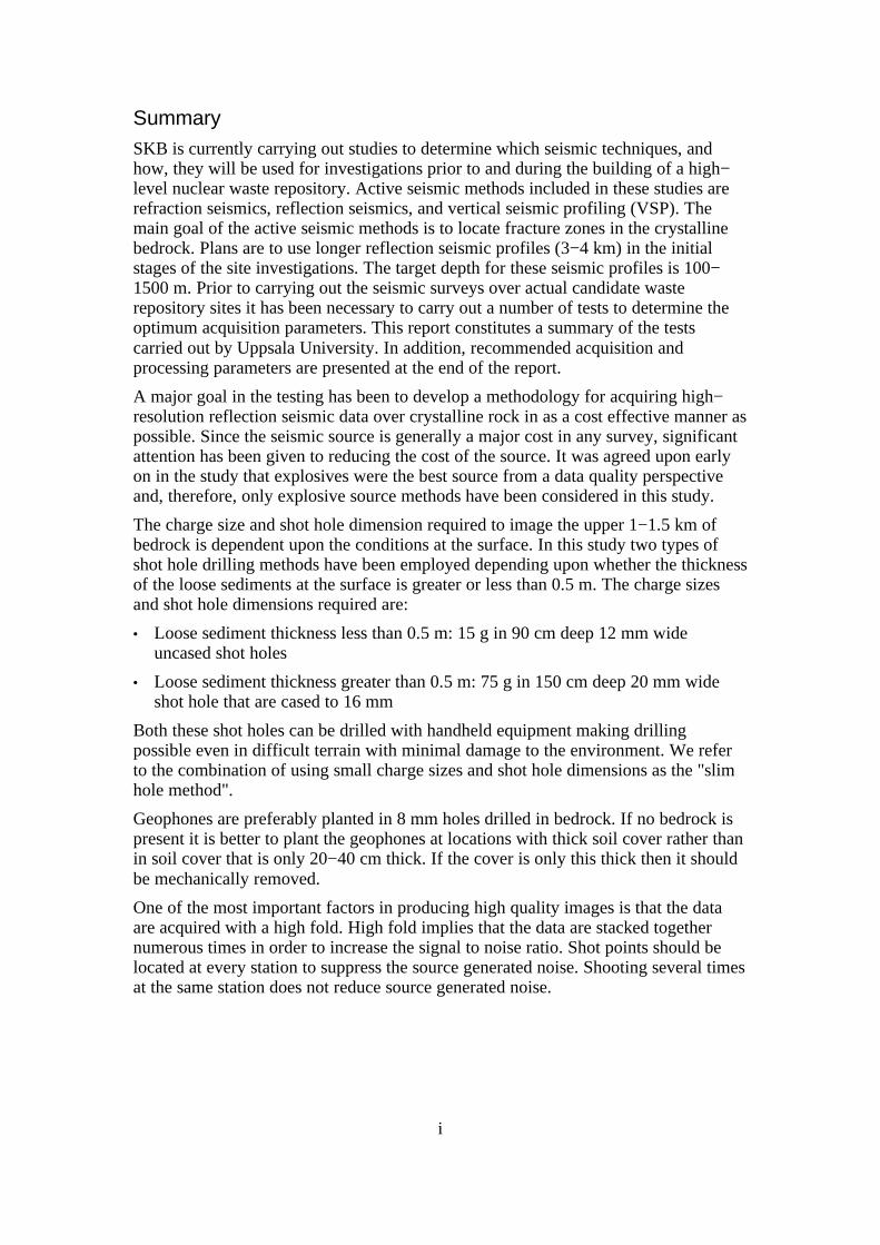
SummarySKB is currently carrying out studies to determine which seismic techniques, andhow, they will be used for investigations prior to and during the building of a high−level nuclear waste repository. Active seismic methods included in these studies arerefraction seismics, reflection seismics, and vertical seismic profiling (VSP). Themain goal of the active seismic methods is to locate fracture zones in the crystallinebedrock. Plans are to use longer reflection seismic profiles (3−4 km) in the initialstages of the site investigations. The target depth for these seismic profiles is 100−1500 m. Prior to carrying out the seismic surveys over actual candidate wasterepository sites it has been necessary to carry out a number of tests to determine theoptimum acquisition parameters. This report constitutes a summary of the testscarried out by Uppsala University. In addition, recommended acquisition andprocessing parameters are presented at the end of the report.

A major goal in the testing has been to develop a methodology for acquiring high−resolution reflection seismic data over crystalline rock in as a cost effective manner aspossible. Since the seismic source is generally a major cost in any survey, significantattention has been given to reducing the cost of the source. It was agreed upon earlyon in the study that explosives were the best source from a data quality perspectiveand, therefore, only explosive source methods have been considered in this study.

The charge size and shot hole dimension required to image the upper 1−1.5 km ofbedrock is dependent upon the conditions at the surface. In this study two types ofshot hole drilling methods have been employed depending upon whether the thicknessof the loose sediments at the surface is greater or less than 0.5 m. The charge sizesand shot hole dimensions required are:

� Loose sediment thickness less than 0.5 m: 15 g in 90 cm deep 12 mm wideuncased shot holes

� Loose sediment thickness greater than 0.5 m: 75 g in 150 cm deep 20 mm wideshot hole that are cased to 16 mm

Both these shot holes can be drilled with handheld equipment making drillingpossible even in difficult terrain with minimal damage to the environment. We referto the combination of using small charge sizes and shot hole dimensions as the "slimhole method".

Geophones are preferably planted in 8 mm holes drilled in bedrock. If no bedrock ispresent it is better to plant the geophones at locations with thick soil cover rather thanin soil cover that is only 20−40 cm thick. If the cover is only this thick then it shouldbe mechanically removed.

One of the most important factors in producing high quality images is that the dataare acquired with a high fold. High fold implies that the data are stacked togethernumerous times in order to increase the signal to noise ratio. Shot points should belocated at every station to suppress the source generated noise. Shooting several timesat the same station does not reduce source generated noise.

i

SammanfattningSKB genomför för närvarande undersökningar för att bestämma vilka seismiskametoder som ska användas och hur de ska användas före och under byggandet av ettdjupförvar för använt kärnbränsle. De seismiska metoder som är aktuella ärrefraktionsseismik, reflektionsseismik och borrhålsseismik (VSP). Huvudsyftet meddessa seismiska metoder är att lokalisera sprickzoner i den kristallina berggrunden.Reflektionsseismiska profiler (3− 4 km) planeras att användas i de inledande stadiernaav platsundersökningarna. Målet för dessa profiler är kartläggning av strukturer från100 till 1500 meters djup. Innan sådana seismiska mätprofiler kan göras vidkommande platsundersökningar har det varit nödvändigt att göra ett flertal tester föratt bestämma de optimala fältparametrarna för datainsamling. Denna rapport utgör ensummering av de tester som utförts av Uppsala Universitet. Dessutom presenterasrekommenderade insamlings− och bearbetningsparametrar i slutet av rapporten.

En viktig målsättning i testerna har varit att utveckla en metodik för insamling avreflektionsseismiska data med hög upplösning på ett så kostnadseffektivt sätt sommöjligt.

Den seismiska källan är vanligtvis huvudkostnaden i all seismik varför ett betydandearbete lagts ner på att reducera kostnaden för källan. I ett tidigt stadium avundersökningarna enades om att sprängmedel är den bästa källan vad gällerdatakvalitet varför endast denna seismiska källa behandlas i denna studie.

För studier av de övre 1− 1.5 km av berggrunden är laddningarnas storlek ochskotthålens dimension beroende av djupet till berggrundsytan i skottpunkten. I dennastudie har två typer av borrningar gjorts beroende på om jorddjupet är mindre ellermer än 0.5 m. De laddningar och borrhål som behövs för seismiska signaler attpenetrera till önskat djup är:

� Jorddjup mindre än 0.5 m: 15 g i 90 cm djupa och 12 mm vida hål. Vid jorddjup0−0.5 m avlägsnas jordtäcket före borrning.

� Jorddjup mer än 0.5 m: 75 g i 150 cm djupa och 20 mm vida hål. Dessa hål harfodrats med rör.

Bägge dessa typer av skotthål kan borras med handburna utrustningar vilketmöjliggör borrning i svår terräng och minimerar markskador. Användandet av småladdningar i borrhål med liten diameter kallar vi för klenhålsmetoden.

Geofonerna placeras helst i 8 mm:s borrhål direkt i berget där detta går i dagen. Omberg i dagen inte finns är det bättre att placera geofonerna i jord med störremäktighet. Om jordtäcket underskrider 0.5 m bör det mekaniskt avlägsnas.

En av de viktigaste faktorerna för att producera seismiska avbildningar avberggrunden av hög kvalitet är att data är insamlat med hög faltning (fold påengelska). Hög faltning innebär att registrerade signaler är adderade ett flertal gångerför att öka signal/brus förhållandet. Sprängning bör ske i varje punkt längs profilenför dämpa det källgenererade bruset. Sprängning ett flertal gånger i samma punktreducerar inte det källgenererade bruset.

ii

Table of Contents1. Introduction............................................................................................................1

1.1. Background.....................................................................................................11.2. Overview of work carried out..........................................................................1

2. Experiments carried out..........................................................................................42.1. Ävrö seismic survey........................................................................................4

2.1.1. Background and goals..............................................................................42.1.2. Location...................................................................................................42.1.3. Acquisition...............................................................................................52.1.4. Results.....................................................................................................5

2.2. Ävrö mini source test.......................................................................................82.2.1. Background and goals..............................................................................82.2.2. Location...................................................................................................82.2.3. Acquisition...............................................................................................92.2.4. Results.....................................................................................................9

2.3. Ängeby mini source test................................................................................142.3.1. Background and goals............................................................................142.3.2. Location.................................................................................................152.3.3. Acquisition.............................................................................................162.3.4. Results...................................................................................................17

2.4. Laxemar seismic survey.................................................................................222.4.1. Background and goals............................................................................222.4.2. Location.................................................................................................232.4.3. Acquisition.............................................................................................232.4.4. Results...................................................................................................24

2.5. Gravberg seismic survey................................................................................272.5.1. Background and goals............................................................................272.5.2. Location.................................................................................................272.5.3. Acquisition.............................................................................................282.5.4. Results...................................................................................................28

3. Discussion.............................................................................................................323.1. Time considerations.......................................................................................333.2. Cost considerations........................................................................................343.3. Environmental considerations........................................................................34

4. Recommended field parameters............................................................................355. Recommended processing parameters...................................................................386. Conclusions...........................................................................................................407. Future Work..........................................................................................................41

iii

1. Introduction

1.1. BackgroundOne of the concerns of SKB in locating a disposal site for high level radioactivewaste is the presence of sub−horizontal to moderately dipping fracture zones whichgroundwater can migrate through (SKB, 2001). These fracture zones are difficult todetect by surface geological mapping. Geophysical logging in boreholes has shownthat fracture zones typically have low sonic velocities, densities and resistivities. Theyvary in thickness (width) from a few meters to over 100 m and are generally morehydraulically conductive than the surrounding rock (Ahlbom et al., 1992). Since thefracture zones have lower velocities and densities compared to the surrounding intactrock, it should be possible to image them with the seismic reflection method.

Early work in Canada showed that reflection seismics is one geophysical methodwhich is well suited for detection of fracture zones (Mair and Green, 1981). With thisbackground, an attempt was made to image a known fracture zone with highhydraulic conductivity at the Finnsjön study site. The zone dips gently to the west atdepths of 100 to 400 m. The initial processing of the data failed to image this fracturezone. Analyses of the data and initial processing steps showed the importance ofapplying refraction statics, bandpass filtering and velocity analyses on this type ofdata (Juhlin, 1995). After reprocessing, a clear image of the gently dipping fracturezone was obtained (Figure 1−2). In addition, several other reflectors were imaged inthe reprocessed section, both gentle and steeply dipping ones. It is likely that thesource of these reflections are also fracture zones.

1.2. Overview of work carried outThe authors have been involved in five additional seismic reflection tests (Figure 1−1) since the Finnsjön study. From this work we have developed a methodology foracquiring and processing 2D high−resolution seismic data over crystalline rock.Special attention has been given to using the most efficient source since this is amajor cost in the surveying. The preferred source is called the slim−hole source andconsists of small charges of dynamite in small diameter shot holes.

The studies carried out were:

Ävrö seismic survey: This study consisted of two crossing lines using the sameacquisition parameters as used at the Finnsjön site. The main goal of the seismicsurvey was to image known fracture zones.

Ävrö mini source test: The main goal of this test was to determine if the charge andshot hole size could be reduced while maintaining a good quality image of the upper1 km.

Ängeby mini source test: This study involved further tests with reduced charge andshot hole dimensions as at Ävrö, but also included tests in glacial till.

Laxemar seismic survey: This study consisted of two full−scale crossing seismicprofiles over the deep KLX02 borehole using the slim−hole method. The terrain wassimilar to that of Ävrö and Finnsjön with about 50% outcrop.

Gravberg seismic survey: This was a full−scale profile using the slim−hole method inglacial till in an area where strong reflectors are known to be present.

1

This report summarizes the above studies by reviewing the acquisition, processingand interpretation aspects of each study. The results are then discussed relative to costtime considerations in acquiring reflection seismic data. Based on our experience, wepresent strategies for acquiring and processing reflection seismic data with the goal ofimaging the uppermost 1 km of crystalline crust. Finally, we summarize the mostimportant conclusions from our work and present some suggestions for future workwithin this field.

2

Figure 1−1. Location of study areas. F−Finnsjön, L−Laxemar, Äv−Ävrö, S−Siljan and Än− Ängeby.Map after Weihed et al.(1992).

3

Figure 1−2. Original and reprocessed Finnsjön section. See Juhlin (1995) for details.

2. Experiments carried out

2.1. Ävrö seismic survey

2.1.1. Background and goals

Reprocessing of the Finnsjön data set confirmed that reflection seismics is a viablemethod for locating sub−horizontal fracture zones in crystalline rocks. Therefore,further testing was carried out by SKB and Uppsala University on Ävrö island(Figure 2−1). Two c. 1 km long crossing high−resolution seismic reflection lineswere acquired in October 1996 in order to (1) test the seismic reflection method forfuture site investigations, (2) map known fracture zones and (3) add to the Swedishdatabase of reflection seismic studies of the shallow crystalline crust.

2.1.2. Location

4

Figure 2−1. Location of the Ävrö seismic profiles. Topography is from the SKB database.

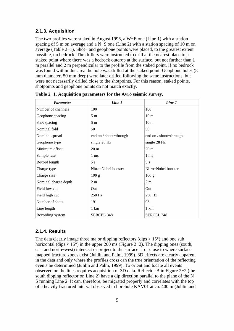
2.1.3. Acquisition

The two profiles were staked in August 1996, a W−E one (Line 1) with a stationspacing of 5 m on average and a N−S one (Line 2) with a station spacing of 10 m onaverage (Table 2−1). Shot− and geophone points were placed, to the greatest extentpossible, on bedrock. The drillers were instructed to drill at the nearest place to astaked point where there was a bedrock outcrop at the surface, but not further than 1m parallel and 2 m perpendicular to the profile from the staked point. If no bedrockwas found within this area the hole was drilled at the staked point. Geophone holes (8mm diameter, 50 mm deep) were later drilled following the same instructions, butwere not necessarily drilled close to the shotpoints. For this reason, staked points,shotpoints and geophone points do not match exactly.

Table 2−1. Acquisition parameters for the Ävrö seismic survey.

Parameter Line 1 Line 2

Number of channels 100 100

Geophone spacing 5 m 10 m

Shot spacing 5 m 10 m

Nominal fold 50 50

Nominal spread end on / shoot−through end on / shoot−through

Geophone type single 28 Hz single 28 Hz

Minimum offset 20 m 20 m

Sample rate 1 ms 1 ms

Record length 5 s 5 s

Charge type Nitro−Nobel booster Nitro−Nobel booster

Charge size 100 g 100 g

Nominal charge depth 2 m 2 m

Field low cut Out Out

Field high cut 250 Hz 250 Hz

Number of shots 191 93

Line length 1 km 1 km

Recording system SERCEL 348 SERCEL 348

2.1.4. Results

The data clearly image three major dipping reflectors (dips > 15°) and one sub−horizontal (dips < 15°) in the upper 200 ms (Figure 2−2). The dipping ones (south,east and north−west) intersect or project to the surface at or close to where surfacemapped fracture zones exist (Juhlin and Palm, 1999). 3D effects are clearly apparentin the data and only where the profiles cross can the true orientation of the reflectingevents be determined (Juhlin and Palm, 1999). To orient and locate all eventsobserved on the lines requires acquisition of 3D data. Reflector B in Figure 2−2 (thesouth dipping reflector on Line 2) have a dip direction parallel to the plane of the N−S running Line 2. It can, therefore, be migrated properly and correlates with the topof a heavily fractured interval observed in borehole KAV01 at ca. 400 m (Juhlin and

5

Palm, 1999). Likewise, a sub−horizontal reflection at ca. 60 ms can also be migratedproperly and it also correlates with a known fracture zone in borehole KAV01.

The processed images from this experiment have proven to be very useful whenintegrated with other geoscientific data (Markström et al., 2001).

Figure 2−3 shows the stacked sections from Lines 1 and 2 plotted to 1.6 s,corresponding to signals arriving from as far away as 5 km. Between 300 and 650 msthere are number of events which do not cross the entire section and are mostapparent on the E−W section (Line 1). These events probably have a fairly localizedorigin and may originate from mafic bodies.

Below 650 ms there is a moderately SW dipping reflector at 700 ms and there are 3deeper N dipping events at about 1.1, 1.2 and 1.4 s. The uppermost of these deeperevents projects to the surface about 8 km to the south of Ävrö in the Baltic Sea. Thisprojection assumes that the reflectors are planes. If they have a listric nature andsteepen as they become shallower the uppermost one will intersect the surface closerthan 8 km from Ävrö. The one at 700 ms projects to the surface about 5 km to the NEof Ävrö. Given the dipping nature (c. 20° dip) of these events, they are tentativelyinterpreted as fracture zones which extend deep into the upper crust.

6

Figure 2−2. Processed section from Lines 1 and 2, Ävrö.

7

Figure 2−3. Lines 1 and 2 processed to 1.6 seconds, Ävrö.

2.2. Ävrö mini source test


The four moderately dipping reflectors imaged at later times from 700 to 1400 ms onthe Ävrö seismic survey (Figure 2−3) indicated signal penetration to at least 4 km.This observation led to the idea that it should be possible to reduce the charge sizeand the shot hole dimensions and still image the uppermost 1000 m of crust. Thereduced shot hole dimension would significantly reduce the cost of the seismicsurvey. This method of seismic acquisition will be referred to in this report as theslim−hole method.

The main goal for the first slim−hole test was to investigate if similar images of theupper 500 ms could be obtained along a short portion of Line 1 of the Ävrö seismicsurvey described in the previous section.

2.2.2. Location

8

Figure 2−4. Location of the Ävrö mini−source test profile relative to Line 1 from the Ävrö seismicsurvey.

2.2.3. Acquisition

In order to test the slim−hole method, a 290 m long test profile was shot along part ofLine 1 (Figure 2−4). Recording was done in parallel on thirty−three 28 Hz and thirty−three 60 Hz single geophones spaced at 10 m (Table 2−2). Two sets of thirty shotswere fired along the line. The first set consisted of 7 grams in a single 12 mm wide 60cm deep shot hole and the second set consisted of 14 grams distributed evenly in two12 mm wide 60 cm deep shot holes. All holes were made by a Hilti TE 55, a 6 kgelectric combi−hammer handheld drilling machine. All the shot holes were drilleddirectly into bedrock. At locations where the bedrock was not observed, the soil wasremoved by use of a powered shovel. All geophones were planted in 8 mm drilledholes in order to avoid the "ringing" that occurs when the soil layer is only 20−40 cmthick. Total drilling time for each shot hole was approximately 10 min. More detailson the acquisition can be found in Appendix 1.

Table 2−2. Acquisition parameters for the Ävrö mini−source test.

Parameter 28 Hz line 60 Hz line




Nominal fold 15 15

Nominal spread shoot−through shoot−through





Charge type Trotyl Trotyl

Charge size 7/14 g 7/14 g

Nominal charge depth 1 x 60 cm / 2 x 60 cm 1 x 60 cm / 2 x 60 cm

Field low cut 8 Hz 8 Hz



Line length 320 m 320 m


2.2.4. Results

Images

To be able to compare the results from the small charge test lines with the data fromLine 1 in Juhlin and Palm (1999), which was recorded with 5 m source and receiverspacing, decimation of the latter data was necessary. Decimation implies that shotpoints and/or receiver points are excluded from the processing. Ideally, the same shotand receiver positions should have been used in the slim−hole test. However, due toacquisition logistics, it was not possible to use exactly the same shot point locations

9

on the small charge test lines as were used on Line 1. Instead, for producing thedecimated Line 1 stack, shots and receivers were limited to the CDP interval 100 to212 and only every other receiver was included in the processing. Every other shotpoint was not chosen since this would have left gaps in the stacked section makingcomparison with the test series difficult. After decimation the data were processed ina similar manner as the small charge test data with minor modification depending ondata character (Table A−1). However, the fold is still higher on the decimated Line 1stack than on the small charge test stacks.

Figure 2−5a shows the complete stacked section from Line 1 without DMO. Theframed area corresponds to that portion which is covered by the small charge testdata. Figure 2−5b shows the Line 1 data when only those shots and every otherreceiver that fall within the range of the small charge test data are included in theprocessing. Adjacent CDPs have been summed to give the same CDP spacing as inthe mini−source test. The difference between this decimated stack and the full foldstack is striking. Figure 2−5c shows the same data as Figure 2−5b, except that thedata have been processed in a manner similar to that for the mini−source test data asshown in Table A−1. The small charge test data stacked sections for both the 28 Hzgeophones (Figure 2−5d) and the 60 Hz geophones (Figure 2−5e) show a muchclearer image at 300−450 ms (ca. 900−1350 m) than the decimated Line 1 stack(Figure 2−5c). Above 300 ms, the two images are comparable, with the Line 1decimated stack probably being somewhat better due to the higher frequency contentof the 100 gram source on Line 1. This apparent paradox of the larger chargesproducing higher frequencies can be explained by intrinsic attenuation where the highfrequencies of the small charges are so weak that they get damped to below the noiselevel in the upper 300 ms. Below 450 ms the decimated Line 1 stack is also superiorto the small charge test data stacks. The 60 Hz 14 gram test series gives the bestoverall stacked section. It is directly comparable to the 28 Hz 14 gram series since thesame acquisition geometries were used for both data sets. A direct comparison withLine 1 is not possible since the acquisition geometries differ somewhat. However, inthe upper 500 ms (c. 1500 m) the data are of comparable or better quality than thedecimated Line 1 data. The single 7 gram charges resulted in poorer images than the14 gram charge data.

10

Spectral analyses

Average spectra were calculated from the 4 shot series (7 and 14 gram charges firedinto 28 and 60 Hz geophones) and the 100 gram charges recorded on Line 1 with 28Hz geophones. The analyses were done in 4 different time intervals (Table 2−3).

11

Figure 2−5. (a) Stacked section from Ävrö island Line 1 without DMO. (b) decimated stackedsection from Line 1 using same processing parameters as in Figure 2−5a. (c) decimated stackedsection from Line 1 using the processing parameters in Table A−1. (d) 28 Hz geophone stackedsection from the small charge test data using the processing parameters in Table A−1(e) 60 Hzgeophone stacked section from the small charge test data using the processing parameters in TableA−1 .

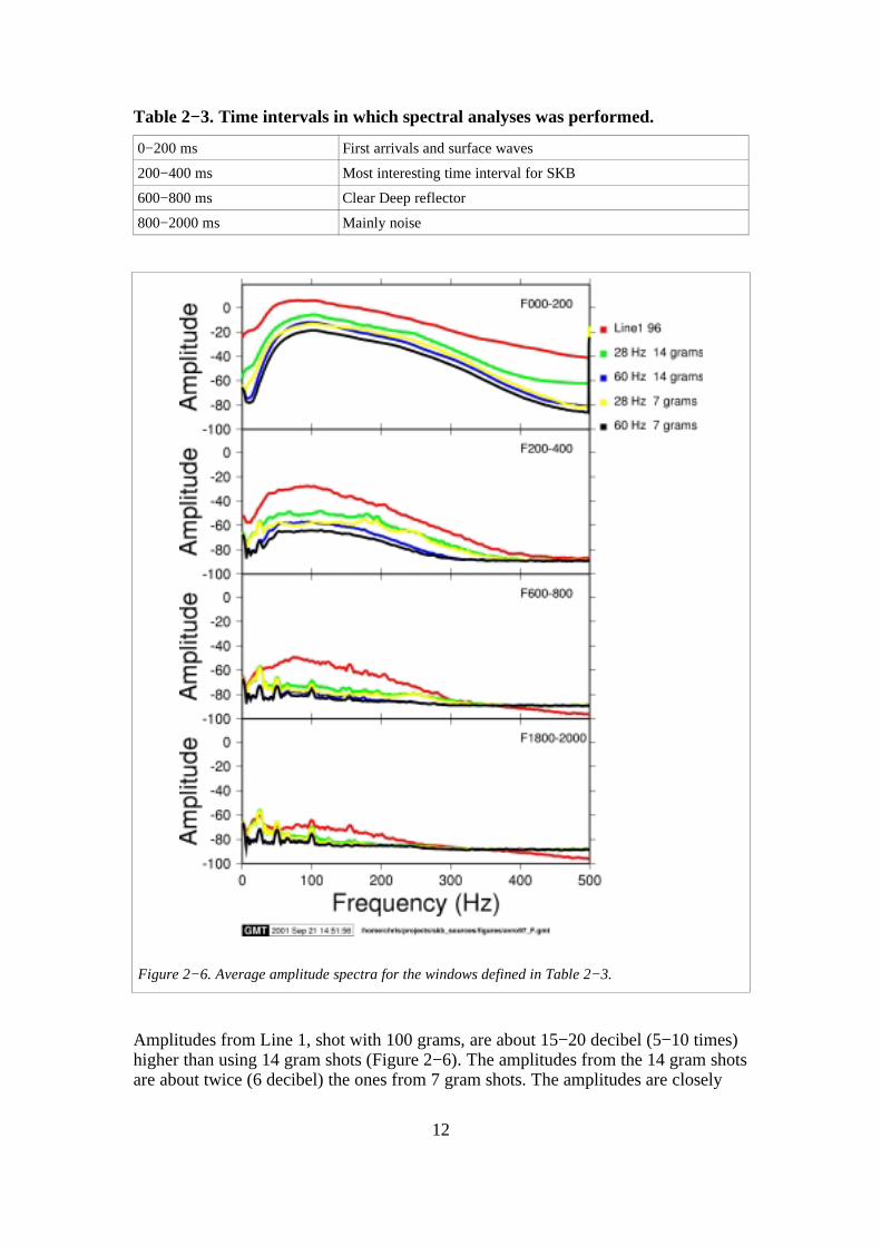
Table 2−3. Time intervals in which spectral analyses was performed.

0−200 ms First arrivals and surface waves

200−400 ms Most interesting time interval for SKB

600−800 ms Clear Deep reflector

800−2000 ms Mainly noise

Amplitudes from Line 1, shot with 100 grams, are about 15−20 decibel (5−10 times)higher than using 14 gram shots (Figure 2−6). The amplitudes from the 14 gram shotsare about twice (6 decibel) the ones from 7 gram shots. The amplitudes are closely

12

Figure 2−6. Average amplitude spectra for the windows defined in Table 2−3.

proportional to charge size. In particular, note the following characteristics of theamplitude spectra in Figure 2−6.

� Frequencies 200−250 Hz, 28 Hz geophones. The amplitude ratio in relation tocharge size is decreasing.

� Frequencies 60−250 Hz. The amplitudes recorded for 28 Hz geophones are almostalways higher than for 60 Hz geophones.

� There is little seismic energy below 50 Hz, almost no source generated lowfrequency ground roll.

� Source generated noise and power disturbances (25, 50, 100 and 200 Hz) dominatethe shot series data below 600 ms. The signals are just above the instrument noiselevel.

Amplitude decay analyses

Average true amplitudes were calculated from the 4 shot series (7 and 14 gramcharges fired into 28 and 60 Hz geophones) and the 100 grams charges recorded onLine 1 with 28 Hz geophones. The analyses were done in the frequency bands, 0−500Hz, 50−100 Hz, 100−200 Hz and 200−400 Hz (Figure 2−7). If the signal penetrationis defined as the time when the amplitude ceases to decrease (Barnes, 1994) then thesignal penetration for the 7 gram shots corresponds to about 600 ms on both the 28and 60 Hz geophones and for the 14 gram shots to about 800 ms. Noise levels areabout 6 dB (2 times) higher on the 28 Hz geophones than the 60 Hz geophones on theunfiltered data (Figure 2−7).

13

2.3. Ängeby mini source test


The aim of this project was to optimize the slim−hole method that is to be used inreflection seismic investigations of the uppermost 1500 m in typical Swedish terraneswith frequent bedrock outcrops and thin glacial deposits. As shown in the previoussection, such areas give excellent conditions for seismic recording down to depths of2−3 kms using 14 gram charges of explosives in slim−holes. However, the greatadvantage with the slim−hole method is that a small handheld electric drill can beused to drill the shot holes. Based on the Ävrö mini−source study the estimated cost

14

Figure 2−7. Average amplitude decay versus time for Line 1 and the test series for unfiltered data(A000−500), bandpass filtered 50−100 Hz (A050−100), 100−200 Hz (A100−200) and 200−400 Hz(A200−400). All shots from each data set have been included.

savings per length of profile was of the order of 4 times when compared to usingdrilling equipment carried by vehicles. The 14 gram shot test profile on Ävrö was,however, chosen in such a way that all shot points were on bedrock outcrops. Adisadvantage with using small charges is, of course, the risk of using too small acharge size when profiling in a new area. A resulting "white section" can beinterpreted in two ways: Either the uppermost crust is truly homogeneous or thesignal/noise ratio is too small to image any discontinuities. One way to avoid thisunwanted situation is to start a reflection investigation in a new area with 10−20larger shots (50−100 grams) recorded to 2−3 seconds. Experiences from 500 kms ofdeep seismic reflection profiling in different areas of Sweden have shown thatreflectors are generally present in the upper 2−3 seconds. If deeper reflectors areobserved, such reflectors will confirm that the uppermost crust is truly homogeneous.

The Ängeby mini−source test study was carried out in a "new area" using a smallhandheld electric drill for shot holes to be used for charge sizes of the order of 50−100 grams. The intention was to drill deeper and larger diameter holes than used forthe 14 gram shots on Ävrö and to combine closely spaced shot holes. The profile waschosen in such a way that parts of it crossed till with a thickness of more than 2meters. Different techniques for making the shot holes in the till were tested. Thestudy also included an investigation of the drilling aspects (time studies, bit wear) anda comparative analysis of the seismic energy generated from different shots. As in theÄvrö mini−source experiment, where only 14 gram shots were used, both 28 Hz and60 Hz geophones were used.

2.3.2. Location

A 320 m long test profile with 10 m station interval was set up in the forest just NE ofthe village of Ängeby, 20 km NE of Uppsala. The profile was staked out by use of a100 m tape measure. It was slightly curved to cross over as much bedrock outcrops aspossible. Figure 2−8 shows the distribution of stations in till and bedrock. Allpositions of shot points and geophones were surveyed by use of a theodolite anddistancer.

15

2.3.3. Acquisition

The handheld electric drill used for drilling in bedrock and in till was the Hilti TE 55,the same one as used in the Ävrö mini−source test. For drilling deeper than 90 cm aminimum bit diameter of 20 mm was used. The drilling program was revised severaltimes because of problems with the 20 mm bits. Drilling with 20 mm bits was muchslower than with 12 mm bits, taking almost twice as much time per drilled length.This is due, in part, to that 20 mm bits have a different construction and, in part, tothat there are more difficulties in bringing the drilling dust to the surface. At depthsgreater than 90 cm the drill often became rapidly stuck and had to be pulled upslightly and restarted. If the upward motion is not done quickly enough the bit steel iseasily broken by twisting it. Therefore, the number of holes drilled to depths greaterthan 80 cm with 20 mm bits was reduced in relation to the original plan.

For drilling in till, 25 mm bits were used. Drilling with the Hilti machine to apredefined depth was easy, at least down to 90 cm. As long as the boulders weresmall enough and the depths were small the boulders were pushed aside. When theresistance was high the machine behaved as in bedrock. The drilling mud fromboulders and bedrock filled in cavities in the till and the drilled hole was normallykept open long enough to set down a plastic casing.

For drilling deeper than 90 cm in till a Pionjär MB−61 was used. Most often thedrilling was stopped at 35−70 cm at a boulder or at bedrock and only at four stationsit was possible to drill deeper. Holes deeper than 90 cm were cased. Most of the holesin the depth range 35−70 cm that were kept open were used for smaller charges.

Data were acquired with the shot and geophone spacing expected to be used for future

16

Figure 2−8. Elevation along the seismic profile with station numbers. Gray corresponds toestimated till thickness, white diamonds are stations on till and black diamonds are stations onbedrock.

site investigations (Table 2−4). More detailed information concerning the acquisitionand processing is given in Appendix 2.

Table 2−4. Acquisition parameters for the Ängeby mini−source test.

Parameter 28 Hz line 60 Hz line




Nominal fold 30 30

Nominal spread shoot−through shoot−through






Charge size variable variable

Nominal charge depth variable variable

Field low cut 8 Hz 8 Hz



Line length 320 m 320 m


2.3.4. Results

Images

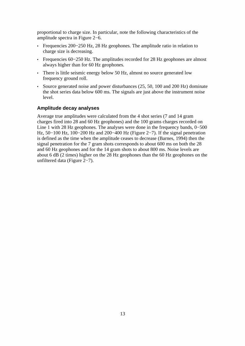
Plots of stacked data from all shots and geophones, regardless of whether they wereplanted in till or bedrock, are shown in (Figure 2−9). Stacks using differentcombinations of shots and geophones in till and bedrock are shown in (Figure 2−11)(28 Hz geophones) and (Figure 2−10) (60 Hz geophones). There are only 14geophones in till compared to 19 in bedrock. For both geophone types (28 and 60Hz), the best images are obtained when all shot and geophone points are used.However, if only geophones in bedrock are used the stacks are only slightly inferior.The importance of using all stations as source points is demonstrated by comparingthe sections where only source and geophone points in bedrock have been used. Thefold becomes too low and the source generated noise prevails in the upper 300 ms.The same is also true when only shots and geophones in till are used with theresulting stacks being quite poor.

There is little differences between the two geophone types, the 60 Hz geophones givea slightly better image in the upper 400 ms and the 28 Hz ones below 400 ms.

17

18

Figure 2−9. Stacked sections without (top) and with (bottom) coherency filtering.

19

Figure 2−10. Stacked sections from the 60 Hz geophone data using different combinations ofsources and geophones in till and bedrock.

Spectral analyses

Plots of amplitude versus frequency for different shot categories show the same trendfor 28 and 60 Hz geophones, regardless of whether the first arrival or the 400−800 mstime window is used. An example of this is shown in Figure 2−12 for the shotcategory 12 mm holes in bedrock. For these shots fired in bedrock the seismic energyincreases as charge size increases

In Figure 2−13 the shots have been divided into five groups. The figure shows thatslightly more energy per gram of explosive is achieved from shots in 12 mm holescompared to 20 mm holes in bedrock. For shots in till it is only the deep (>1 m) casedholes that give energy well above noise level.

20

Figure 2−11. Stacked sections from the 28 Hz geophone data using different combinations ofsources and geophones in till and bedrock.

21

Figure 2−12. Amplitude spectra for various shot configurations using the first arrival window andthe 400−800 ms time window for 28 Hz and 60 Hz geophones.

2.4. Laxemar seismic survey


The prime objective of this experiment was to perform a full−scale test of the slim−hole method using small explosive sources for mapping the upper kilometer of thecrystalline crust. The shot holes were 12/20 mm in diameter and the charges were15/75 grams in bedrock/till. Two deep boreholes had earlier been drilled in the surveyarea, depths of 1700 m (KLX02) and 1078 m (KLX01), that the surface seismicresults could be correlated to. A secondary objective of the experiment was to mapfracture zones in 3D that are present in the area and that intersect the boreholes. Afterthe testing and development described in the previous sections, a good compromisebetween charge size and shot hole dimension had been determined to be 15 grams in90 cm deep 12 mm diameter shot holes in bedrock outcrops and 75 grams in 150 cmdeep 20 mm diameter (cased to 16 mm) shot holes in loose sediments.

22

Figure 2−13. Total amplitude and amplitude normalized by charge size spectra for the major shotconfigurations using the 400−800 ms time window for 60 Hz geophones.

2.4.2. Location

The Laxemar area was an ideal location to test the slim−hole source method due to itsproximity to the Äspö Hard Rock Laboratory (Hammarström and Olsson, 1996) andthe Ävrö area where previous studies had been carried out. In addition, two deep(1700 m and 1078 m) boreholes had been drilled in the area that could be used forcalibration of the surface seismic data. Therefore, two crossing profiles were acquiredover the 1700 m deep KLX02 borehole (Figure 2−14), a 2 km long NE−SW runningone passing over the KLX01 borehole (Line 1) and a 2.5 km long NW−SE runningone (Line 2), with the acquisition parameters that are expected to be used for future2D site surveys.

2.4.3. Acquisition

The two profiles were acquired in December 1999. Both lines had an (average)station spacing of 10 meters (Table 2−5). Shot points and geophones were located tothe greatest extent possible on bedrock. The shot holes were drilled at the closestsuitable location to a staked point where bedrock was present, but not further awaythan 30 cm parallel and 1 m perpendicular to the profile from the staked point. If nobedrock was found within this area, even after removing 50 cm of soil, the shot hole

23

Figure 2−14. Location of the Laxemar (black) and Ävrö (white) seismic experiments and theKLX01 and KLX02 deep boreholes. Red line shows the location of the Äspö Hardrock Laboratorytunnel. Topography is from the SKB database.

was drilled at the staked point. In bedrock, 12 mm shot holes were drilled to 90 cmdepth with an electric drilling machine powered by a gasoline generator. Charge sizesof 15 grams were used in these bedrock shot holes. In soil cover, 20 mm shot holeswere drilled to 150 cm depth with an air pressure drill. These shot holes were casedwith a plastic− or iron−casing having an inner diameter of 16 mm. Charge sizes of 75grams were used in these loose soil sediment shot holes. Geophones were placed in adrilled hole in the bedrock if bedrock was found close to the station, otherwise theywere placed directly in the soil cover. Bedrock shot holes were used on about 50 % ofboth profiles. All shot holes and geophone locations were surveyed with highprecision differential GPS instruments in combination with a standard total station.This combination gave a horizontal and vertical precision of better than 1 percent ofthe station spacing (10 cm). The two lines cross each other near the 1700 m deepKLX02 borehole (Figure 2−14), with Line 1 also passing close to the 1078 m deepKLX01 borehole. The seismic data are of fairly good quality due to the thin soilcover. However, windy and rainy weather conditions had a negative effect on someshot records.

Table 2−5. Acquisition parameters for the Laxemar slim−hole profiles.

Parameter Value

Number of channels 100

Geophone spacing 10 m

Shot spacing 10 m

Nominal fold 50

Nominal spread end on / shoot−through

Geophone type single 28 Hz

Minimum offset 20 m

Sample rate 1 ms

Record length 5 s

Field low cut Out

Field high cut 250 Hz

Recording system SERCEL 348

Bedrock Sediment


Charge size 15 g 75 g

Nominal charge depth 0.9 m 1.5 m

Line 1 Line 2


Line length 2 km 2.5 km

2.4.4. Results

Stacked seismic sections of Lines 1 and 2 are shown in Figure 2−15. Where the twoprofiles cross, it is possible to orient several dipping reflectors and determine wherethey intersect the KLX02 borehole. Based on correlation with borehole data and

24

surface geology, many of these reflectors appear to be related to fracture zones, someof which have high hydraulic conductivity. However, greenstones (mafic rocks) areprobably the source to, or enhance, the stronger more sub−horizontal reflections.Some reflections present only on single lines may originate entirely from greenstonebodies. The signal has generally penetrated to 500 ms (1500 m) along both profiles.Stacking tests using geophones and shot on bedrock versus sediments show similarresults to those for the Ängeby mini−source experiment (section 2.3). Stacks usingonly sources in bedrock and only sources in sediment produce nearly equal qualitysections, but stacks using geophones only in sediment give much poorer qualitysections than those using geophones only in bedrock. For a complete interpretation ofthe results see Bergman et al. (2001a, 2001b).

25

26

Figure 2−15. Stacked seismic sections of Laxemar Lines 1 and 2

2.5. Gravberg seismic survey


The full scale experiment using the slim−hole method at Laxemar, and the earliertests leading up to it, had shown that it was possible to obtain high quality seismicimages of the upper 1−2 km in areas with high percentages of bedrock outcrop, suchas along much of the east coast of Sweden. An open question at this point was if itwas possible to obtain high quality images in areas completely covered by a relativelythick layer of till. Seismic surveys in the mid−1980s had revealed several highamplitude reflectors in the upper 5 km in the Siljan Ring area in central Sweden(Juhlin and Pedersen, 1987). Subsequent deep drilling showed these reflectors to bedolerite sills (Juhlin, 1990). The surface seismic data were acquired using 5−10 kgcharges in about 10 m deep shot holes in an area generally covered by 5−10 m of till.The combination of a known strong reflector at c. 1.5 km in an area covered by tillmade the Siljan Ring area an ideal location for testing the slim−hole method whereoutcrop is absent.

2.5.2. Location

A 3 km long profile was shot along part of the previous "deep" seismic survey in thevicinity of the 6.7 km deep Gravberg−1 borehole (Figure 2−16). Prominent highamplitude reflectors had been drilled at about 1.5, 2.7 and 4.7 km at this location withthe uppermost one of these being the target of the new survey.

27

Figure 2−16. Location of the Gravberg slim−hole test profile relative to the deep Gravberg−1borehole and the previously acquired deep seismic profile.

2.5.3. Acquisition

Two hundred 20 mm wide and 1.5 m deep shot holes were drilled over 4 longworking days in May 2000. Since the profile lies along a gravel road a vehiclemounted drilling rig was used, but the holes could have been drilled with handheldequipment. A sturdy pipe was hammered into the shot holes and pulled out beforecasing was inserted instead of cleaning the holes with compressed air. This resulted inthe casing being better set to the bottom of the shot hole and no cavity was created atthe bottom of the hole. Plastic casing with an inner diameter of 16 mm was used inthe majority of the shot holes, a few shot holes had iron casing.

Data were acquired in the time period 24−30 July 2000 under ideal weatherconditions. Three different charge sizes were used along the profile with thefollowing pattern over six shot points: (1) two 32 gram shots, (2) two 74 gram shots,and (3) two 116 gram shots. The first shot hole of each pair was generally tampedwith sand and the second with sand and water. The pattern was then repeated for eachset of 6 shot holes along the line.

Table 2−6. Acquisition parameters for the Gravberg slim−hole profiles.

Parameter Value

Number of channels 100

Geophone spacing 10 m

Shot spacing 10 m

Nominal fold 50

Nominal spread end on

Geophone type single 28 Hz

Minimum offset 20 m

Sample rate 1 ms

Record length 4 s

Field low cut Out

Field high cut 250 Hz

Recording system SERCEL 348

Charge type Trotyl

Charge size 32, 74 and 116 g

Nominal charge depth 1.5 m

Number of shots 191

Line length 3 km

2.5.4. Results

Standard processing parameters were applied to the data resulting in a stacked sectionwith signal penetration to about 3 km with dolerite sills being imaged at about 0.6 and1.0 s (1500 and 2700 m) at the location of the Gravberg−1 borehole (Figure 2−17).The geometry and location of the reflections on the stacked section agrees well withresults from the earlier "deep" seismic survey (Figure 2−18). Even though theresolution is higher, both in time and space, no new reflections were observed on the

28

slim−hole profile.

Separate stacks were produced for each charge size and the images compared. The116 gram stack gave the best image of the deeper strong reflector at 1.0 s, butotherwise there is very little difference in the upper 0.6 s (1.5 km) between thedifferent stacks. Note that in producing the separate charge size stacks that only onethird of the total number of shots was used in producing each stack, a reduction infold to about 17. This reduction resulted in significantly poorer quality images for theseparate charge stacks compared to the full fold stack in Figure 2−17. Comparison ofstacks using charges tamped with only sand versus those tamped with sand and wateralso showed very little difference between one another.

29

30

Figure 2−17. Stacked section from the Gravberg slim−hole test profile. The deep Gravberg−1borehole is located at CDP 100.

31

Figure 2−18. Stacked section of the previously acquired deep seismic profile and the slim−holeGravberg profile.

3. DiscussionThe experiments carried out show that it is possible to obtain high quality images ofthe upper 1−1.5 km in crystalline rock using the slim−hole method. Below about 1.5km (500 ms), the image becomes poorer due to lack of penetration by the smallersource. Comparison of stacked data from the Ävrö and Laxemar surveys to 1.6 sshows that the deeper reflections below 1 s are not imaged as well on the 15−75 gramcharge slim−hole Laxemar data as on the 100 gram larger diameter shot hole Ävrödata (Figure 3−1). The reflectors at about 1.0 s, which are interpreted to represent thesame structures on the two data sets, dip at about 10° to the north and project to thesurface about 10 km to the south of Laxemar. Sub−horizontal reflections such asthese are often observed on seismic data in Sweden in the upper 2−3 s. It is importantto image these reflections in order to verify that the signal has penetrated sufficientlydeep. If images are obtained at traveltimes of 1−3 s (3−9) km then one can beconfident that the upper 500 ms (1.5 km) contains high quality data even if noreflections are present. The lack of reflections can then be interpreted to implyhomogeneous rock or, at least, that there are no thick sub−horizontal fracture zonesover large areas in the upper 1.5 km.

32

Figure 3−1. Stacked sections to 1.6 s from the Ävrö(left) and Laxemar (right) profiles.

3.1. Time considerationsDrilling of shot holes is not only an expensive component of a seismic reflectionsurvey, but also a time consuming part. For a large field survey, the time required fordrilling must be carefully planned. Daily drilling production rates for the Laxemarseismic survey are given in (Table 3−1). Two drilling machines were active, one forsediment shot holes and the other for bedrock. However, both machines were notdedicated solely to the project and were used for other purposes in the area at thesame time. Therefore, the maximum daily production rates should be viewed astypical values for what a drilling machine can produce for a single day. The tests inÄngeby gave the average drilling time for a shot hole in bedrock to be about 20minutes including overhead for non−drilling activities. This corresponds to 24 shotholes that can be drilled by one machine per 8 hour day. The maximum productionrate at Laxemar of 25 shot holes per day in bedrock is consistent with this estimate.

Drilling rates for shot holes in sediment were generally slower than for bedrock atLaxemar with a maximum of 19 shot holes per day. At Gravberg, daily productionrates averaged 50 holes per day in till. However, a vehicle mounted unit was used andthe drillers worked very long days. For planning purposes, it is probably best to use20 shot holes per day in bedrock and 15 in sediment/till per 8−hour day per drillingmachine.

Table 3−1. Daily production rates for drilling of shot holes.

Number of drilled holes

Date Sediment Bedrock

15/11 6 17

16/11 15 25

17/11 19 21

18/11 7 20

19/11 13 20

22/11 13 16

23/11 2 19

24/11 12 11

25/11 12 11

26/11 17 5

29/11 1 9

30/11 13 11

1/12 10 10

2/12 14 15

3/12 7 5

6/12 13 11

7/12 15 7

8/12 5

33

3.2. Cost considerationsThe cost per shot for some of the experiments are shown in Table 3−2. Personnel,generator, fuel, drilling machine and bits are included in the drilling costs when usinghandheld equipment. Shooting costs include caps and explosives. When drilling inbedrock with the slim−hole method a thin soil cover has to be removed and this costis included in the calculation. The cost is calculated as if soil removal is necessary atevery other shot point. All costs are exclusive of mobilization and demobilization.The drilling costs for 1996 Ävrö seismic survey are based on if the ROC 512 drillingrig had been used to drill all 300 shot holes. The actual costs were higher than thissince the drilling contract was split between two companies.

At Ängeby the material costs per drilled meter of hole was about 400:− for 20 mmbits and about 160:− for 12 mm bits. Personnel costs can vary significantly, a cost of300:− per hour is used for the cost estimates here. This gives a cost of about 300:−pereach 90 cm deep 12 mm hole and 900:− per each 1.5 m deep till hole. The higher costof the till holes is due to longer drilling times (30 minutes versus 20 minutes) and thattwo people are required to operate the till drilling machine.

The higher costs for drilling in bedrock with the slim−hole method at Ängebycompared to Ävrö (for when shot holes with the same dimensions and depths arecompared) can be explained by the rock being more difficult to drill at Ängebyresulting in longer drilling times. The longer drilling times at Ängeby compared toÄvrö also resulted in the material costs being higher there. For drilling in till the costdifference between the slim−hole method and the vehicle mount larger drilling rigs ismuch smaller than for drilling in bedrock. This is due to the higher material costs andthat two people are required to operate the drilling machine efficiently.

Table 3−2. Estimated comparative source costs in SEK.

Drilling Shooting Soil removal Total1996 Avröseismic survey

1300:− 100:− 1400:−

1997 Ävrö mini−source

140:− 70:− 120:− 330:−

1998 Ängebymini−source

Bedrock 260:− 70:− 120:− 450:−

Till 900:− 120:− 1020:−

3.3. Environmental considerationsBy using the slim−hole method the effects on the environment by a seismic surveyare reduced compared to using vehicle mounted drilling rigs. Since heavy equipmentneed not be driven in the forest, there is a large reduction in damage to vegetation, aswell as less scars being left in the ground after the survey. In addition, by usingsmaller charges, less pollutants are spread by the source.

34

4. Recommended field parametersSurface conditions can be divided into the following categories

1. "Ävrö type": about 50% bedrock outcrop, the remaining bedrock is covered by 1−2 m of loose sediments or soil, i.e. clay and sand, with some till

2. Loose sediments: mainly clay, sand and gravel of varying thickness, but reachingup to 100 m thickness in some areas, little or no outcrop

3. Thin till: 5−10 m of till on top of bedrock, little or no outcrop

4. Thick till: till which is greater then 10 m thick, no outcrop

We have only carried out full−scale tests of the slim−hole method in categories 1 and3. However, based on our experience from these type areas we can even recommendacquisition parameters for categories 2 and 4 (Table 4−1). Note that even in "Ävrötype" areas that about 50% of the shot points will require 20 mm holes drilled to 1.5m with 75 g charges. Although, charge size and depth are important factors for thequality of the final processed image, the most important factor is a high fold,assuming that the signal is penetrating to the target depth. High fold can only beobtained by having a large number of shot points along the line. Stacks using onlyshots fired in bedrock or shots fired only in till both have poorer images in theuppermost parts due to a reduction in fold by about one half. This is equivalent toshooting at every other station rather than at every station. Although it is expensive, itis necessary to shoot at every station in order to acquire the best possible image for agiven station spacing.

All data presented have been acquired with the SERCEL 348 recording system. Theminimum sampling interval is 1 ms with this system and a field high cut of 250 Hzhas been used in order to avoid temporal aliasing. In the Ävrö seismic survey,crossline data were also recorded on ABEM Terraloc systems in order to test thepotential of using low−fold 3D data (the results were negative). These data show thatsignificantly higher frequencies than 250 Hz are present in the data. How useful thesehigher frequencies are for improving the seismic image is not known, but with atarget depth of 1 km and 10 m station spacing the improvement would probably bemarginal if a faster sampling rate was used. However, it is recommended that data berecorded at 0.5 ms, if possible, in order not to loose the higher frequency componentof the data.

Stacks using data recorded on 60 Hz geophones have given somewhat better imagesin the upper 500 ms (1.5 km) than those from 28 Hz geophones. However, theimprovement is fairly small and does not warrant any requirement that 60 Hzgeophones be used.

Stacking tests have been made on existing data using minimum offsets ranging from20 m (that used in the actual acquisition) to 100 m. Very small differences areobserved in the stacks with minimum offsets up to 80 m. Stacks with a minimumoffset of 100 m start are poorer in the upper 100 ms. However, our tests were done ondata that had been processed with all offsets. It may be that the offset range 20−80 mis important for refraction static calculations. Therefore, we recommend a minimumoffset of 20 m until further studies are carried out.

If the dynamic range of the acquisition system is high enough then the field low cut

35

filter can be left out. If surface waves appear to be a problem then a field low cutfilter can be considered. The slim−hole method, in general, generates only lowamplitude surface waves and the high frequency geophones also have damping effecton them. These surface waves may provide useful information on the near surface andshould not necessarily be removed in the field.

Table 4−1. Recommended acquisition parameters for various surface conditions.

Parameter Value

Ävrö typeLoose

sedimentsThin till Thick till

Charge type To be decided

Charge size 15/75 g 75 g 75 g 116 g

Nominal charge depth 0.9/1.5 m 1.5 m 1.5 m 1.5 m

Number of channels >100

Geophone spacing

Shot spacing

Nominal fold

Nominal spread

10 m

10 m

>50

end on

Geophone type

Minimum offset

Sample rate

Record length

Field low cut

Field high cut

Recording system

Profile length

single 60 Hz or single 28 Hz

20 m

<1 ms

4 s

Out

>250 Hz

Digital

>3 km

The length of a profile is dependent upon how deep dipping structures are to beimaged (Figure 4−1). Since many structures appear to dip at about 45° and the targetdepth is down to 1 km then in order to image these structures the profiles must extend1 km beyond the limits of the target area. In order to obtain reliable images down to 1km within the target area a minimum of 1 km of profile is required in addition to the1 km extensions on the sides. This implies that profiles should be at least 3 km longin order to obtain unbiased images down to 1 km over a 1 km long section.

36

37

Figure 4−1. For a fixed profile length, the length of the reflecting element imaged decreases as thedip of the reflector increases.

5. Recommended processing parametersSeveral studies have shown that processing is an important component in producingthe final image that is to be interpreted (e. g. Juhlin, 1995; Wu and Mereu, 1992; Wu,1996). Good static corrections are one of the most important factors in obtaining highquality images. It is especially important to have good first break picks in order to getthe best possible initial refraction static corrections. In addition, the presence of bothdipping and sub−horizontal reflections and the long−offsets used relative to the depthof the targets generally require that DMO (dip−moveout) be applied to obtain betterimages of the upper 300 ms. When the data are processed without DMO it is notpossible to image two reflectors with differing dip at the same sub−surface location.Application of DMO allows, in theory, reflectors of all dips to be imagedsimultaneously. Spectral whitening and choice of bandpass filter, as well as velocityanalyses, are other important steps in the processing chain. Recommended processingsteps are given in Table 5−1.

Table 5−1. Recommended processing parameters.

Good refraction static corrections is, perhaps, the most important step in theprocessing. This step is dependent upon that geometry has been applied correctly and

38

Step Process Comment

1 Read raw data CSG2 Spike and noise edit CSG3 Pick first breaks CSG4 CSG

5 CSG 1

6 CSG7 CSG

8 Bandpass filter CSG 1 2 many tests need to be made9 CMP 3

10 Trace top mute CMP 4 remove first arrivals from data11 AGC − Apply and save CRG12 Velocity filtering CRG 513 AGC − remove CRG 214 CMP 615 CMP 7

16 COG

17 NMO COG 3 "true" velocities should now be used18 DMO COG 819 Stack CMP alpha trimmed is generally better20 stack or some other coherency filter21 Trace equalization stack22 Migration stack23 stack

CSG − Common shot gather CMP − Common midpoint gather

CRG − Common receiver gather COG − Common offset gather

Domain

Velocity Analysis

Stack control

Geometric spreading correction

multiply by time is generally sufficeint

Attenuation correction (optional)

some correction must be done at early arrival times

Refraction staticsSurface consistent deconvolution

spectral whitening is also an option, sometimes this step must be skipped

Residual statics − Pass 1

signals are more consistent in CRGs

Residual statics − Pass 2Trim statics (optional) use a very short allowable shift otherwise

you are cheating

AGC or trace equaliztion some kind of equalization generally must be done

F−X Decon

Trace equalization

that the first breaks are picked sufficiently accurately. The importance of verifyingthat the geometry is correct and that the refraction statics show significantimprovement in the coherency of both shot and receiver gathers cannot beoveremphasized.

39

6. ConclusionsFrom our studies we can conclude the following concerning high−resolution seismicacquisition on crystalline rock:

� If possible, shot holes should be drilled in bedrock within an ellipse centered onthe station and that has a major axis perpendicular to the profile that is 20% of thestation spacing and a minor axis that is 6% of the station spacing. If no bedrock isfound within this ellipse the shot hole should be drilled in the loose sediments atthe station.

� Shot holes in loose deposits (soil and till) should not be blown clean withcompressed air. Instead, a pipe should be used to clean them before setting casing.

� Geophones should also be placed in drilled holes in bedrock, if possible, under thesame constraints as for the shot holes.

� Soil and loose sediments should be removed if their thickness is less than 20−40cm at the geophone positions.

� Profiles should extend 1 km further on each side of the target limit in order toimage 45° degree dipping structures to 1 km depth.

� It is important to acquire the sesmic data under good weather conditions.

� Larger charges of 100−200 g can be fired by shooting several slim−holes inparallel. When a new area is being investigated, these larger charges should befired at the start of the field work.

� Proper reconnaissance is necessary prior to starting field work in order to positionin an optimal manner for both geological and logistical reasons.

� Surveying with differential GPS and total station measurements provides a highenough accuracy for reflection seismic processing.

� 60 Hz geophone are preferable to 28 Hz geophones, but the difference in dataquality is marginal. Positioning and planting the geophones optimally is muchmore important.

� A 1 ms sampling rate is adequate, but 0.5 ms would be preferred.

� Sand and water combined is the optimum tamping method.

� A minimum of 96 channels is recommended for 2−D surveys.

� Having high fold in the data is more important than using larger charges. In orderto have high fold, shots should be fired at every station.

40

7. Future WorkAlthough we recommend using single geophones for each station to increaseresolution, we have not specifically tested the trade−off between resolution andincreased signal to noise ratio using an array of geophones for each station. Thiswould require future field work where various arrays are tested against singlegeophones along the same profile.

Another aspect which has not been tested is the precision in the surveying that isnecessary to get reliable images. The combination of GPS and total station used todate has given coordinate accuracy on the order of cms. This may be overkill,however, it is not obvious what the minimum accuracy required is. Testing of this canbe done using existing data and synthetic data by perturbing the coordinates andredoing the processing with various degrees of introduced errors.

41

ReferencesAhlbom, K., Andersson, J.−E., Andersson, P., Ittner, T., Ljunggren, C. and Tirén, S.,1992. Finnsjön study site. Scope of activities and main results. SKB, TR 92−33.

Barnes, A.E., 1994. Moho reflectivity and seismic signal penetration. Tectonophysics,232: 299−307.

Bergman, B. Juhlin, C. and Palm, H., 2001a. Reflexionsseismiska studier inomLaxemarområdet, SKB, R−01−07.

Bergman B., Juhlin C. and Palm H., 2001b. Reflection seismic imaging of the upper 4km of crust using small charges (15−75 grams) at Laxemar, southeastern Sweden.Accepted in Tectonophysics.

Hammarström, M., and Olsson, O., (eds.), 1996. Äspö Hard Rock Laboratory: 10years of research. Stockholm, SKB.

Juhlin, .C, 1990. Interpretation of the reflections in the Siljan Ring area based onresults from the Gravberg−1 borehole. Tectonophysics, 173: 345−360.

Juhlin, C., 1995. Imaging of fracture zones in the Finnsjön area, central Sweden,using the seismic reflection method. Geophysics, 60: 66−75.

Juhlin C. and Palm H., 1999. 3D structure below Ävrö island from high resolutionreflection seismic studies, southeastern Sweden. Geophysics: 64, 662−667.

Juhlin C. and Pedersen L. B., 1987. Reflection seismic investigations of the Siljanimpact structure, Sweden. J. Geophys. Res.: 92, 14113−14122.

Mair, J. A., and Green, A. G., 1981. High−resolution seismic reflection profiles re−veal fracture zones within a "homogeneous" granite batholith, Nature: 294, 439−442.

Markström, I., Stanfors, R. and Juhlin, C., 2001. Äspölaboratoriet − RVSmodellering, Ävrö − slutrapport. SKB report, R−01−06.

SKB, 2001. Site investigations. Investigation methods and general executionprogramme, SKB Report R−01−10.

Weihed, P., Bergman, J., & Bergström, U., 1992. Metallogeny and tectonic evolutionof the early Proterozoic Skellefte district, northern Sweden. Precambrian Research:58, 143−167.

Wu, J., 1996. Potential pitfalls of crooked line seismic reflection surveys.Geophysics: 61, 277−281.

Wu, J., and R. F. Mereu, 1992. Crustal structure of the Kapuskasing uplift fromLithoprobe near−vertical/wide angle seismic reflection data. J. Geophys. Res.: 97,17441−17453.

42

Appendix 1: Acquisition and processing details for the Ävrö mini−source test

Positioning

The test measurements were performed with a stationary spread of 320 m fromstation 1045 to 1109 along Line 1 in Juhlin and Palm (1999). The stations were easilylocated as either remaining stakes, shot holes or small drilled geophone holes. Sincethe coordinates of the station points, shot and geophone holes were known from theearlier profile, the new positions of the shot holes and geophone points could beestablished to sufficient accuracy by use of tape measure and compass.

Soil removal

At 12 of the 33 stations where the soil cover was less then 0.5 m it was removed byuse of a skid steer loader GEHL 5625 equipped with a power shovel. The cleaning ofsoil from the bedrock was done in 30 minutes including transport between thestations. After soil removal all 33 receiver stations were located on bedrock.

Drilling

All holes were made by a Hilti TE 55, a 6 kg electric combihammer drilling machine.The shot holes were drilled with 12 mm bits down to 60 cm depth in the bedrock.Total drilling time for a hole was approx. 10 min. Three shot holes were drilled ateach station. At the westernmost station nine holes were drilled with one meterseparation, three to 60 cm, three to 70 cm and three to 90 cm depth. Total drillingtime to 90 cm was approx. 15 min. For a total of 97 shot holes four 95 cm and six 40cm drills were used up.

The geophone holes, two at each station for 28 and 60 Hz geophones, were made by a8 mm bit down to 3−6 cm.

For the power supply of 230 V a 3kW Honda generator was used consuming 35 litersof petrol for all the drilling.

Loading procedure

A plastic trotyl based explosive was punched into thin hard plastic pipes of 11 mmdiameter. The length of the charges varied from 39 to 155 mm, corresponding to 5 to20 grams. To the pipe lengths 25 mm was added for the electric caps. The explosiveswere tamped with a fluid mixture of drill cuttings and water. For the second shotseries, using two nearby holes, the caps were connected in series.

Recording

All recordings were done during a period of excellent weather conditions with almostno wind and no rain.

Test shots

For testing purposes, at the westernmost station, recordings from the following chargesizes (gram) and depths (cm) were obtained:

43

Depth Charge size

60 5, 10 and 15 grams

70 5, 10 and 15 grams

90 5, 10 and 20 grams

A simple field processing of the nine test shots showed that 5−10 g at 60 cm and 10−15 g at 90 cm gave strongest coherent energy around 340 ms. This reflection is themost easy to detect on raw shot plots. After the test it was decided to shoot one shotseries with 7 g in one 60 cm shot hole at each station and another series with 14 g inone 90 cm shot hole. The 90 cm holes were intended to be done by deepening thealready predrilled 60 cm holes. However, it was found impossible to continue drillingin these holes that were drilled some days earlier because of small amounts of waterin the holes. After drilling a few centimeters cuttings and water mixed to a very stickymaterial and the drill became stuck. Instead of drilling new holes to 90 cm, a thirdhole was drilled to 60 cm approx. 10 cm from one of the other holes. The chargeswere later divided into two 7 gram charges and fired simultaneously.

Shot series

The two shot series (7 and 14 grams) were fired into a fixed spread of 33 stations and66 channels (28 and 60 Hz geophones at each station). In the processing, the nearest 3stations for both geophone groups were excluded.

The shot series with a single 7 gram charge was fired with a mean time interval ofone shot every 11 minutes and the two 7 gram charges in series were fired every 14minutes.

Table A−1. Main Processing steps for small charge test data on Ävrö island.

1 Read SEG2 data

2 Add geometry

3 Trace edit

4 Pick first break

5 Refraction statics

6 Bandpass filter70−140−300−420 Hz 0− 200 ms60−120−300−450 Hz 100−400 ms50−100−300−450 Hz 300−600 ms40− 80−240−360 Hz 500−800 ms30− 60−180−240 Hz 700−2000 ms

7 Velocity analysis

8 Residual statics

9 Split data into subsets for 28 resp. 60 Hz.

10 Sort to CDP domain

11 AGC: 100 ms window

12 NMO

13 Stack: 5% alpha trimmed mean

44

Appendix 2: Acquisition and processing details for the Ängebymini−source testThe drilling schedule used is shown in (Table A−2). For calculation of the total timefor the drilling operation the actual drilling time has been increased by 60 % toinclude moving the generator, electric cables and drill, cleaning bedrock from mossand roots, drilling small geophone holes, fueling the generator, record keeping, etc.

The material costs per drilled meter of hole was SEK 394 for 20 mm bits and SEK158 for 12 mm bits. Personnel costs can vary significantly, but if a cost of SEK 250per hour is used then the cost per 12 mm hole is about SEK 300.

Table A−2. Drilling program, times required to perform the shot holes and thecharges used.

Drillingequipment

Geol.material

Bit diameter(mm)

No. of holes* depth (cm)

Drillingtime (min)

No. of shotpoints indifferent

shotcategories

Charge(grams)

Hilti Bedrock 20 1*115 50 1 1*40

Hilti Bedrock 20 5*100 205 1 5*12

Hilti Bedrock 20 4*100 164 1 4*25

Hilti Bedrock 20 2*100 82 1 2*25Hilti Bedrock 20 5*80 180 1 5*20

Hilti Bedrock 20 3*80 108 2 3*17

4 3*10

Hilti Bedrock 20 2*80 72 1 2*14Hilti Bedrock 12 6*90 126 2 6*15

Hilti Bedrock 12 4*90 84 3 4*12.5

Hilti Bedrock 12 3*90 63 4 3*15

4 3*10Hilti Bedrock 12 1*90 21 6 1*14

Hilti Till 12 1*90 12 (1) 1 1*14

Hilti Till 25 4*90 76 (2) 2 4*15

Hilti Till 25 4*60 64 (2) 2 4*10Hilti Till 25 1*90 19 (2) 4 1*14

Pionjär Till 25 1*200 47 (2) 1 1*100

1 1*75

1 1*50Pionjär Till 25 1*90 20 (2) 1 1*50

Pionjär Till 25 4*30−60 52 2 4*14

Pionjär Till 25 1*35−70 13 9 1*14(1) Only one hole was possible to drill to 90 cm with 12 mm bit and keep open in till out of many tries.

(2) Including time for casing.

Charging procedure

Plastic explosives with a detonation velocity of 6500 m/s were used. In 12 mm holesin bedrock and cased holes in till the charge diameter was 11 mm. In 20 mm bedrock

45

holes and uncased holes in till the charge diameter was 17 mm. The charge lengthwas determined by the desired amount of explosives for each hole and cutaccordingly. The charges used in the different shot holes are shown in (Table A−2).The explosives were tamped with fine grained sand and water. For shots consisting oftwo or more charges in nearby holes, the caps were connected in series.

Recording

A spread of 66 channels was used (33 single 28 Hz and 33 single 60 Hz geophones).The geophones were placed either in drilled holes in bedrock or in till after removing10−20 cm of the top soil. Recordings were done using Sercel field units and ProsolPC central unit.

Four shots, out of total of a 30 using more than one hole, produced falling stonesresulting in noisy records. None of the 25 shots using only one hole caused anyobservable noise in the records.

Table A−3. Processing sequence for the Ängeby mini−source test.

Read SEG2 dataAdd geometryPick first breakElevation staticsRefraction staticsVelocity analysisResidual statics

CDP stacking Spectral analysisSpectral whitening: 30−40−120−140 Hz Chose data from geophones in bedrock,

28 or 60 Hz geophones, shot categoryBandpass filter: 30−50−150−220 Hz True amplitude recoveryNMO NMOCDP stacking Trace mutingFX−Decon (Coherency filtering) Forward FFT

Stack all traces

Processing

The processing objectives were to:

� Produce stacked seismic sections for studying the reflectivity as a function of timewith regards to:

� geophones (28 and 60 Hz).

� shot location (till or bedrock)

� geophone placing (till or bedrock)

� Analyze true amplitudes from shots of different categories. The analyses weredone in two different time intervals:

� 0−20 ms after linear move out correction, corresponding to first arrivals.

46

� 400−800 ms after normal move out correction, Corresponding to a widereflective time window.

CDP stacking

Only 2 or 3 shot records showed reflected energy before processing the data. Thefollowing stacked sections were produced for both the 28 Hz and 60 Hz geophonesusing data from:

� All shot points and geophones (1684 traces, max fold 58)

� Only shot points in bedrock (902 traces, max fold 34)

� Only geophones in bedrock (971 traces, max fold 37)

� Only shot points and geophones in bedrock (498 traces, max fold 29)

� Only shot points in till (782 traces, max fold 27)

� Only geophones in till (713 traces, max fold 29)

� Only shot points and geophones in till (309 traces, max fold 17)

Exactly the same processing steps (Table A−3) were applied to each processingstream. For the important static corrections only the data put into the stream wereused for the residual statics correction, however, all data were used for the refractionstatic correction.

Spectral analysis

All analysis were made for geophones in bedrock since these geophones show thehighest signal/noise ratio, the lowest influence from surface waves and are more freefrom noise bursts. Spectra was created for all combinations of:

28 Hz geophones

60 Hz geophonesx

First arrivals

Time interval 400−800 msx

Individual shots, all traces stacked

Shots in same category stacked

In spite of the fact that individual shots in the same category show great variation allshots in each category have been used in the spectral analysis with one exception. Inthe time interval 400−800 ms four shots were excluded. These shots produced groupsof falling splintered bedrock, partly within the time interval of interest.

47

Appendix 3: Processing parameters for the Laxemar slim−hole test

Table A−4. Main processing steps for slim−hole test at Laxemar

1 Read SEG2 data − 2000 ms2 Spike and noise edit3 Pick first breaks4 Scale by t**25 Refraction statics6 Surface consistent spiking deconvolution

Design gate 0 m: 200−500 ms, 500 m: 350−600 ms

Operator 40 ms

White noise added 1%7 Bandpass filter

70−140−300−420 Hz 0−200 ms

60−120−300−420 Hz 100−400 ms

50−100−300−420 Hz 300−600 ms

40−80−240−360 Hz 500−800 ms

30−60−180−240 Hz 700−2000 ms8 Sort to receiver domain9 Residual statics − Pass 1

10 Trace top mute

0 m: 1 ms

100 m: 18 ms

1000 m: 183 ms11 AGC − Apply and save− 50 ms window12 Velocity filtering − median method

Remove 3000 m/s13 AGC − remove14 Sort to CDP domain15 Velocity analyses16 Residual statics − Pass 217 Trim statics − 2 ms maximum shift18 Sort to common offset domain19 AGC − 50 ms window20 NMO21 Common offset F−K DMO velocity − average DMO velocity22 AGC − 50 ms window23 Trim statics − 2 ms maximum shift24 F−X Decon25 Trace equalization 100−1000 ms26 Kirchoff Depth migration same velocity as DMO 5500 m/s27 Trace equalization 200−500 m

48

Appendix 4: Processing parameters for the Gravberg slim−hole test

Table A−5. Main processing steps for slim−hole test at Gravberg.

1 Read SEG2 data − 4000 ms2 Spike and noise edit3 Pick first breaks4 Scale by t**25 Air−blast attenuation6 Refraction statics7 Spectral whitning

Balancing frequencies

25−40−160−2008 Bandpass filter

50−80−200−400 Hz 0−150 ms

40−60−180−360 Hz 150−300 ms

35−50−150−300 Hz 300−700 ms

30−40−120−240 Hz 700−2000 ms

25−40−100−200 Hz 2000−4000 ms9 Residual statics − Pass 110 Trace top mute

Fb_pick+10 ms11 Sort to CDP domain12 Velocity analyses13 AGC 50 ms window14 NMO15 Stack16 Residual statics − Pass 217 Trim statics − 1 ms maximum shift18 Trace equalization 400−800 m

49

Reflection seismic imaging of the upper crystalline crust ...

Documents

Transcript of Reflection seismic imaging of the upper crystalline crust ...