References and Efficiency Standards

o Clothes Washer Model Number.

Files to Submit for EM&V Review

The following files should be provided to the utility from which the project sponsor seeks to obtain an incentive for each new home completed:

• Reports of QA/QC or M&V

• Documentation for how the as-built home compares to the base home, and modeling and energy savings information

• Relevant modeling files from the approved modeling package

• All input data used to support the modeled energy and peak demand savings, subject to EM&V team approval as part of modeling package approval

• Output results describing energy and peak demand savings, subject to EM&V team approval as part of modeling package approval.

• Savings calculations and/or calculators that perform energy savings calculation outside the model.

References and Efficiency Standards

RESNET accredited software:

http://www.resnet.us/professional/programs/enerqv rating software

ASHRAE 90.1, Energy Standard for Buildings Except Low-rise Residential Buildings

ASHRAE 140, Standard Method of Test for the Evaluation of Building Energy Analysis Programs

ENERGY STAR Multifamily High Rise Program Simulation Guidelines

International Code Council, 2015 International Energy Conservation Code.

Petitions and Rulings

Relevant Standards and Reference Sources

Not applicable.

2-42 Measurement & Verification Protocols Texas Technical Reference Manual, Vol. 4 900 Residential New Construction October 10, 2017

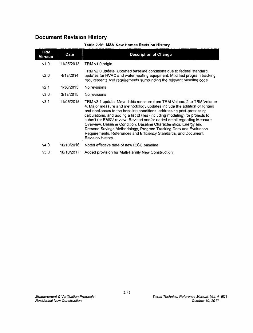
Document Revision History Table 2-16: M&V New Homes Revision History

TRM Version Date Description of Change

v1.0 11/25/2013 TRM v1.0 origin

TRM v2.0 update. Updated baseline conditions due to federal standard

v2.0 4/18/2014 updates for HVAC and water heating equipment. Modified program tracking requirements and requirements surrounding the relevant baseline code.

v2.1

1/30/2015 No revisions

v3.0

3/13/2015 No revisions

v3.1

11/05/2015 TRM v3.1 update. Moved this measure from TRM Volume 2 to TRM Volume 4. Major measure and methodology updates include the addition of lighting and appliances to the baseline conditions, addressing post-processing calculations, and adding a list of files (including modeling) for projects to submit for EM&V review. Revised and/or added detail regarding Measure Overview, Baseline Condition, Baseline Characteristics, Energy and Demand Savings Methodology, Program Tracking Data and Evaluation Requirements, References and Efficiency Standards, and Document Revision History.

v4.0 10/10/2016 Noted effective date of new IECC baseline

v5.0 10/10/2017 Added provision for Multi-Family New Construction

2-43 Measurement & Verification Protocols Texas Technical Reference Manual, Vol. 4 901 Residential New Construction October 10, 2017

2.3 M&V: RENEWABLES

2.3.1 Nonresidential Solar Photovoltaic (PV) Measure Overview

TRM Measure ID: NR-RN-PV

Market Sector: Commercial

Measure Category: Renewables

Applicable Building Types: All

Fuels Affected: Electricity

Decision/Action Type: N/A

Program Delivery Type: Prescriptive

Deemed Savings Type: Simulation Software (kWh), Deemed Values (kW)

Savings Methodology: Model-Calculator (PVWatte).

Measure Description

This section summarizes the savings calculations of the Solar Photovoltaic Standard Offer, Market Transformation, and Pilot programs. These programs are offered by the Texas utilities, with the primary objective to achieve cost-effective energy savings and peak demand savings. Participation in the Solar Photovoltaic program involves the installation of a solar photovoltaic system. The method uses a simulation tool, the National Renewable Energy Laboratorys (NREL) PVWatts@Calculator21 to calculate energy savings. Lookup tables are used to determine deemed summer and winter peak demand savings.

Eligibility Criteria

Only photovoltaic systems that result in reductions of the customers purchased energy and/or peak demand qualify for savings. Off-grid systems are not eligible. Each utility may have additional incentive program eligibility and interconnection requirements, which are not listed here.

Baseline Condition

PV system not currently installed (typical), or an existing system is present but additional capacity (including both panels and inverters) may be added.

High-Efficiency Condition

Not Applicable.

21 See http://pmatts.nrel.clov/ last accessed January 20, 2016. 2-44

Measurement & Verification Protocols Texas Technical Reference Manual, Vol. 4 902 Nonresidential Solar Photovoltaics October 10, 2017

Approximate Temperature Coefficient Module Cover Efficiency of Power Type

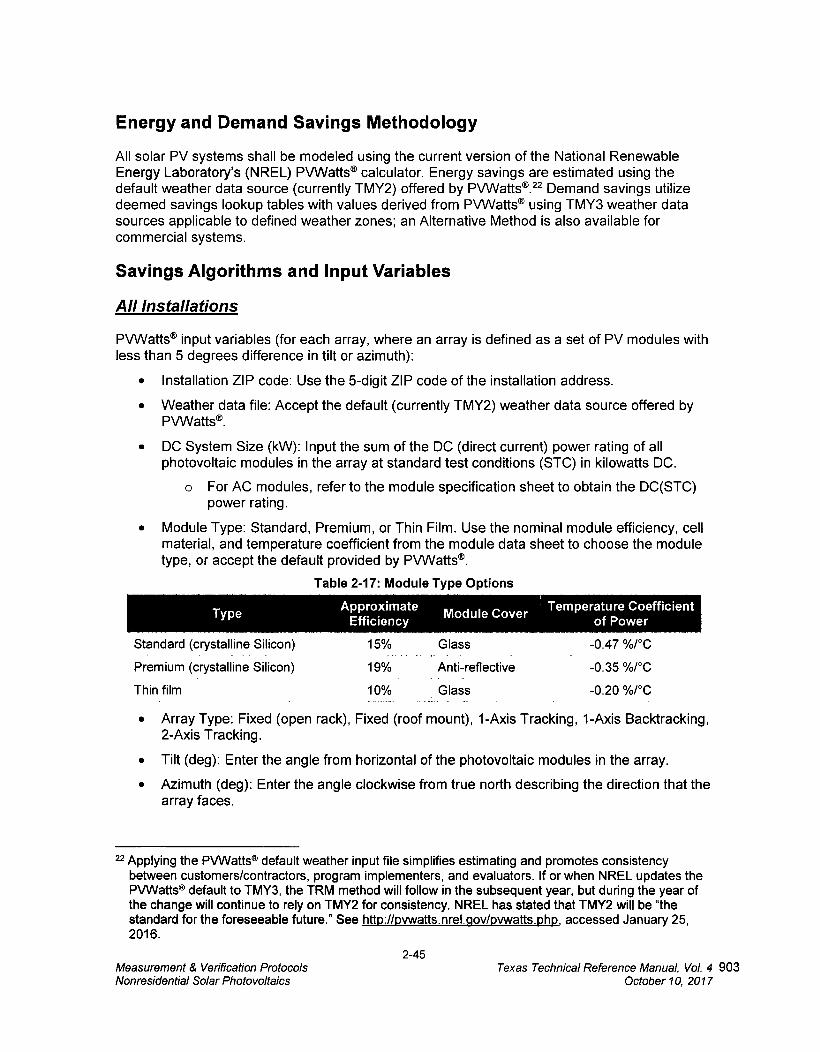
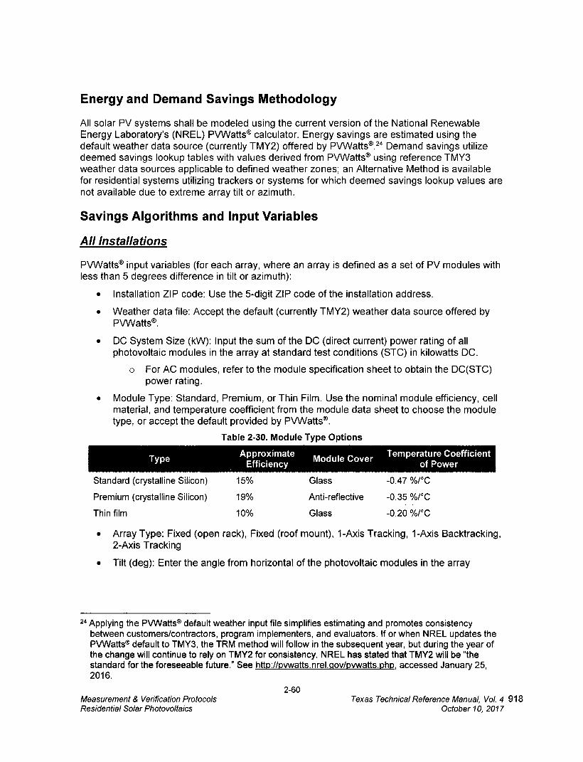
Energy and Demand Savings Methodology

All solar PV systems shall be modeled using the current version of the National Renewable Energy Laboratorys (NREL) PVWatts® calculator. Energy savings are estimated using the default weather data source (currently TMY2) offered by PVWatts®.22 Demand savings utilize deemed savings lookup tables with values derived from PVWatts® using TMY3 weather data sources applicable to defined weather zones; an Alternative Method is also available for commercial systems.

Savings Algorithms and input Variables

All Installations

PVWatts® input variables (for each array, where an array is defined as a set of PV modules with less than 5 degrees difference in tilt or azimuth):

• Installation ZIP code: Use the 5-digit ZIP code of the installation address.

• Weather data file: Accept the default (currently TMY2) weather data source offered by PVWatts®.

• DC System Size (kW): Input the sum of the DC (direct current) power rating of all photovoltaic modules in the array at standard test conditions (STC) in kilowatts DC.

0 For AC modules, refer to the module specification sheet to obtain the DC(STC) power rating.

• Module Type: Standard, Premium, or Thin Film. Use the nominal module efficiency, cell material, and temperature coefficient from the module data sheet to choose the module type, or accept the default provided by PVWatts®.

Table 2-17: Module Type Options

Standard (crystalline Silicon) 15% Glass -0.47 %/°C

Premium (crystalline Silicon) 19% Anti-reflective • -0.35 %/°C

Thin film 10% Glass _ -0.20 %/°C

• Array Type: Fixed (open rack), Fixed (roof mount), 1-Axis Tracking, 1-Axis Backtracking, 2-Axis Tracking.

• Tilt (deg): Enter the angle from horizontal of the photovoltaic modules in the array.

• Azimuth (deg): Enter the angle clockwise from true north describing the direction that the array faces.

22 Applying the PVWatts® default weather input file simplifies estimating and promotes consistency between customers/contractors, program implementers, and evaluators. lf or when NREL updates the PVWatts® default to TMY3, the TRM method will follow in the subsequent year, but during the year of the change will continue to rely on TMY2 for consistency. NREL has stated that TMY2 will be "the standard for the foreseeable future." See httb://bvwatts.nrel.gov/pvwatts.php accessed January 25, 2016.

2-45 Measurement & Verification Protocols Texas Technical Reference Manual, Vol. 4 903 Nonresidential Solar Photovoltaics October 10, 2017

Get Started HELP FEEDBACK

PIREL's PVWatts® Calculator mates tfe trwrqs ocoduchon and cast of energy of gqd corrctod

photavoltee teV; energy systems throughout the world. It alows hornecw-ers, smal buideng owners, reefers and manufacturers to easy deyeit* estenates of the performance of poterce, Pnstaliators.

er-

Ai. AP. Aiers

• All other input variables: Accept the PW/atts® default values.

Annual Energy Savings (kWh)

Given the inputs above, PVVVatts® calculates the estimated annual energy savings for each array.

For systems with multiple arrays, users should derive annual energy savings for each array separately and sum them to obtain the total annual energy savings.

A screenshot (or other save) of Results page, displaying both the annual energy production and model inputs, is typically required in PV incentive applications, and suffices as documentation of the annual energy savings estimate.

Example: A commercial customer in McAllen (zip code 78501) installs a 50 kWdc fixed array comprised of standard crystalline Silicon modules on their rooftop with a tilt of 5 degrees and an azimuth of 175 degrees.

Step 1. The user enters the zip code of the proposed PV system in PVWatts® calculator and presses "Go". See Figure 2-1.

Figure 2-1. Pvwatts® Input Screen for Step 1

PVWatts" Calculator

Peel* 0 nrdert4. *thv-eurT V.. V 5 Enp artm.nr de E ,thce et after., EH, eith-, red eneeieble enerls operated 0, the Adoeue fte Sestso. *We enerp

Weidlie id -edellrel lilltei-xth A ..3edet- rde e sear. Pc ne:t

N. ieee I Secy.*, & ifrrysev I DGcla rr v I 4 EL

2-46 Measurement & Verification Protocols Texas Technical Reference Manual, Vol. 4 904 Nonresidential Solar Photovoltaics

October 10, 2017

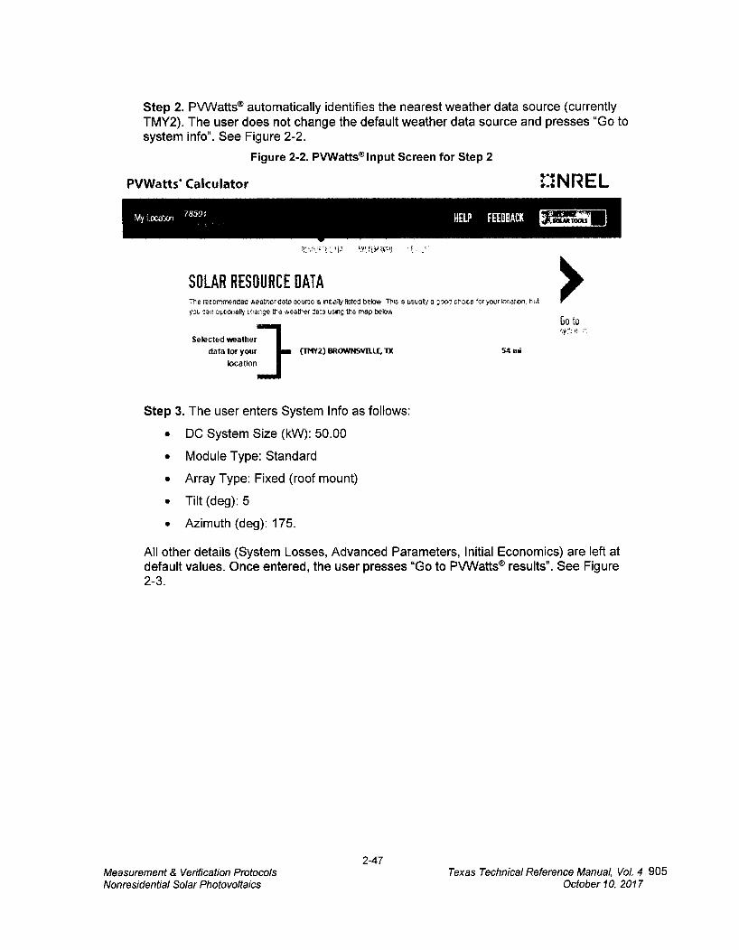
Step 2. PVWatts® automatically identifies the nearest weather data source (currently TMY2). The user does not change the default weather data source and presses "Go to system info". See Figure 2-2.

Figure 2-2. PVWatts® Input Screen for Step 2

PVWatts' Cakulator

r1NREL

Ye_ tO4

SOLAR RESOURCE DATA The recommended weatheraata source is initially tsted below This is usually a ;iood citioxe for your location, but you car optionally charge the weather data using the map below

Selected weather

data for your (THY2) BROWNSVILLE, TX 54 mi

location

Step 3. The user enters System Info as follows:

• DC System Size (kW): 50.00

• Module Type: Standard

• Array Type: Fixed (roof mount)

• Tilt (deg): 5

• Azimuth (deg): 175.

All other details (System Losses, Advanced Parameters, Initial Economics) are left at default values. Once entered, the user presses "Go to PyWatts® results". See Figure 2-3.


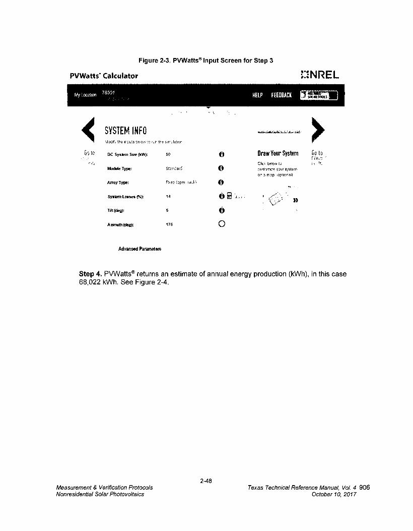
Figure 2-3. Pywatts® Input Screen for Step 3

PVWatts* Calculator

LINREL.

Go to DC System Sae (kW): 50

Module Type: Srar.....!arsi

Array Type: Fr,e-P (opar rack

System Losses (%): 14

Till Megt 5

Azimuth (deg): 175

4 ti....erputs,lo„t..... n.r Me sin% latior

SYSTEM INFO

Draw Your System Go to

tr.F below to 1, it.

zustomce your pisterr or 3 map toptiorall

Advanced Parametets

Step 4. INWatts® returns an estimate of annual energy production (kWh), in this case 68,022 kWh. See Figure 2-4.


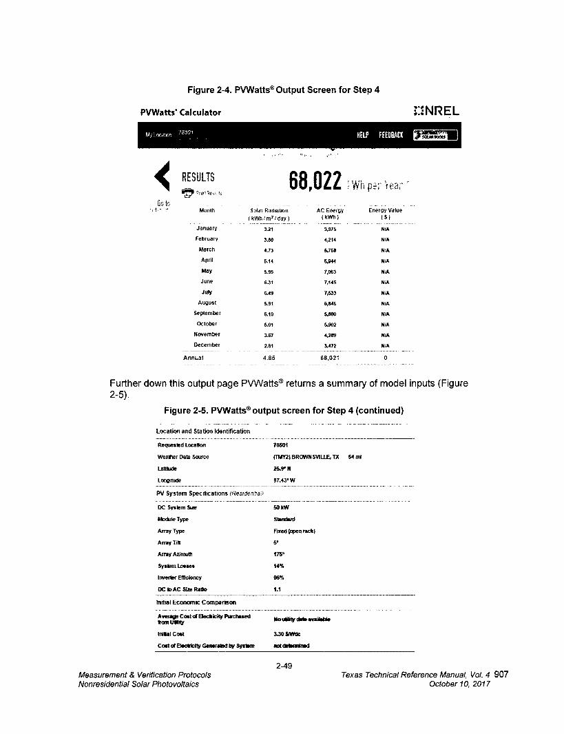
Figure 2-4. PVWatts® Output Screen for Step 4

PA/Watts* Calculator 1:1NREL

RESULTS

68,0221 Wh Co to

Mo-nth Solar Radiation AC Energy En-erg-Y Value —

( kWh m2 day ) kWh ) ( $

January 3.21 3,975 HIA

February 3.80 4,214 HIA

March 4.73 5,758 NIA

April 5.14 6,944 NtA

May 5.95 7,063 NIA

June 6.31 7,145 NIA

July 6.49 7,533 NIA

August 5.91 6,846 NIA

September 6.19 5,880 NtA

October 5.01 5,992 WA

November 3.67 4,289

December 2.81 3,472 N/A

Annual 4.85 68,021 0

Further down this output page PVWatts® returns a summary of model inputs (Figure 2-5).

Figure 2-5. PVWatts® output screen for Step 4 (continued)

Location and Station klentification

Requested Location 76604

Weather Data Source (116W2) BROWNSVILLE,1X 54 mi

Latikide 25.9. N

Longramle 97.43 W

PV System Specifications (Ressdentyail

DC System Size 50 kW

&Iodide Type Standard

Array Type Rxed (open rack}

Array Tilt 5'

Array Azimuth 175°

System Losses 14%

Inverter Efficiency 96%

DC toAC Size P.affiti 1.1

initial Economic Comparison

Average Cost al Bacticity Purchased from UN* No Warty data available

Initial Cost 3-30 SiVidc

Cost of Electicity Genetatedby System affideffionined


The coordinates (latitude and longitude) of the proposed system are also presented. These are useful in determining the appropriate weather zone to use when estimating demand savings.

A screenshot (or PDF) of the complete output page, displaying both the annual energy production and model inputs, is typically required in PV incentive applications, and suffices as documentation of the annual energy savings estimate.

Summer Demand Savings Methodology

Deemed summer demand savings are determined using the weather zone map (Figure 2-6) and summer demand savings lookup values (Table 2-18) provided below. Deemed summer demand savings is the product of the system's DC system size and the appropriate lookup table value.

Deemed Summer Demand Savings

Deemed summer demand savings = DC system size (kW) * Lookup Value

Equation 45

For systems with multiple arrays, users should derive summer demand savings for each array separately and sum them to obtain the total summer demand savings.

Commercial systems may instead be modeled using the Alternative Method described below.

Winter Demand Savings Methodology

Deemed winter demand savings are determined using the weather zone map (Figure 2-6) and winter demand savings lookup values tables (Table 2-18 through Table 2-27) provided below. Deemed winter demand savings is the product of the system's DC system size and the appropriate lookup table value.

Deemed Winter Demand Savings

Deemed winter demand savings = DC system size (k1M * Lookup Value

Equation 46

For systems with multiple arrays, users should derive winter demand savings for each array separately and sum them to obtain the total winter demand savings.

Commercial systems may instead be modeled using the Alternative Method described below.

Deemed Energy Savings Tables

Not applicable.

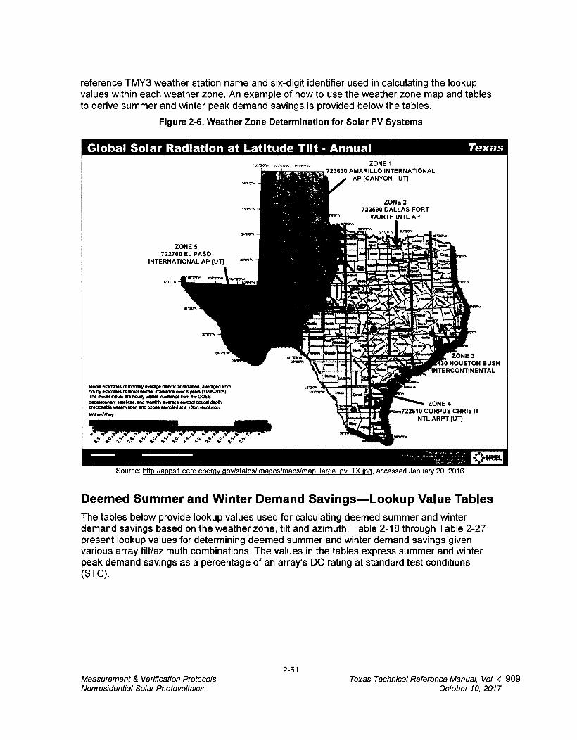
Deemed Summer and Winter Demand Savings—Weather Zone Determination

The appropriate weather zone for each system can be determined by identifying the system's coordinates on the map in Figure 2-6, below. The map identifies weather zones and the

2-50 Measurement & Verification Protocols Texas Technical Reference Manual, Vol 4 908 Nonresidential Solar Photovoltaics October 10, 2017

Global Solar Radiation at Latitude Tilt - Annual

Texas ZONE 1

723630 AMARILLO INTERNATIONAL AP [CANYON - UT]

ZONE 2 722590 DALLAS-FORT

WORTH INTL AP

rAt tem. =:11:1::=PLutz4N

•:4,61 •

tr wv,wi LN-A Firmoits yzare.,„r1

t4-,t

WAOMV ZONE 3 0 HOUSTON BUSH

1ff:A 41 NTERCONTINENTAL

ZONE 4 722510 CORPUS CHRISTI

INTL ARPT [UT]

ZONE 5 722700 EL PASO

INTERNATIONAL AP [UT]

.0r01),

31.017%

Model eernales cd more* mope (lady lotlt radiehon. averaged torn hourly estimates of cared mane Irractance over a years (10n34005) The model Inputs are heady estde radiance kom the GOES oecetatenery Sidellitel. Ind rinnedy "vernal sercad °decal deals pro:4MM weer yew. and awe sampled al s leen reseuteo

IdAtent/Diry

reference TMY3 weather station name and six-digit identifier used in calculating the lookup values within each weather zone. An example of how to use the weather zone map and tables to derive summer and winter peak demand savings is provided below the tables.

Figure 2-6. Weather Zone Determination for Solar PV Systems

Source: http://aonsl eere energy cloy/states/images/maim/may large ov TX.ioq accessed January 20, 2016.

Deemed Summer and Winter Demand Savings—Lookup Value Tables The tables below provide lookup values used for calculating deemed summer and winter demand savings based on the weather zone, tilt and azimuth. Table 2-18 through Table 2-27 present lookup values for determining deemed summer and winter demand savings given various array tilt/azimuth combinations. The values in the tables express summer and winter peak demand savings as a percentage of an arrays DC rating at standard test conditions (STC).

2-51 Measurement & Verification Protocols Texas Technical Reference Manual, Vol 4 909 Nonresidential Solar Photovoltaics October 10, 2017

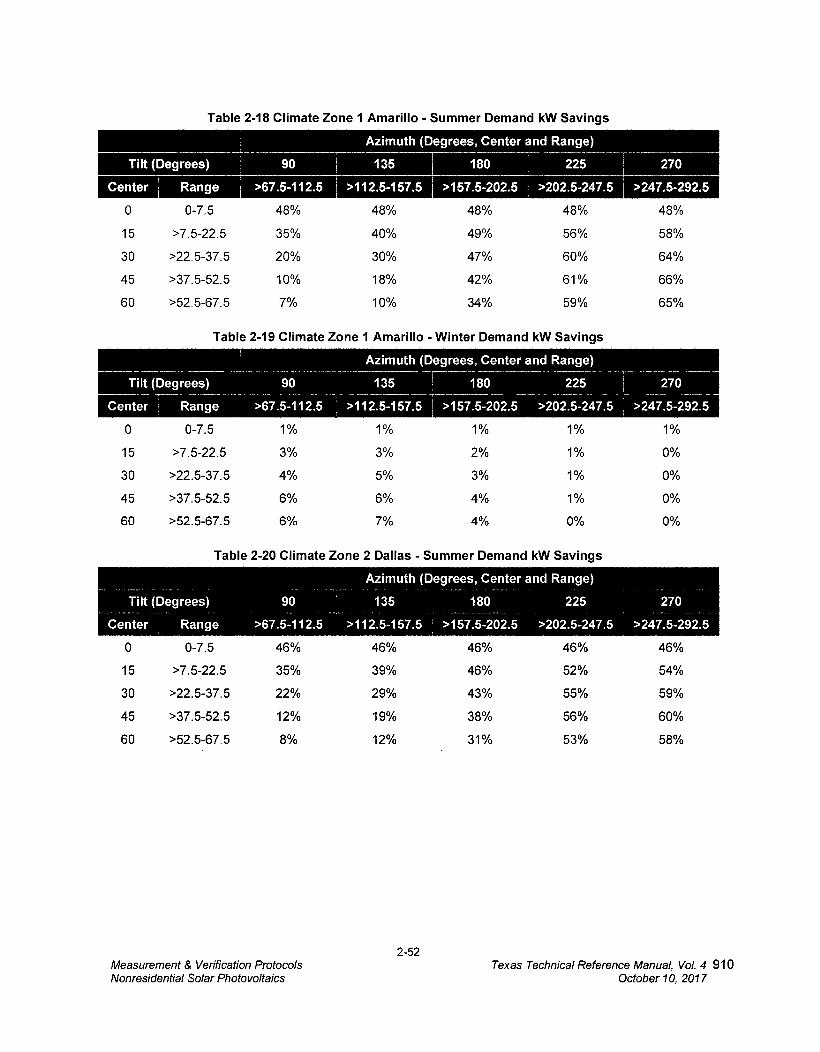
Table 2-18 Climate Zone 1 Amarillo - Summer Demand kW Savings

1 Azimuth (Degrees, Center and Range)

225 T I I

Tilt (Degrees) 90 1-1 — 135 -1—

180 270

Center Range >67.5-112.5 >112.5-157.5 I

>157.5-202.5 >202.5-247.5 1 >247.5-292.5

0 0-7.5 48% 48% 48% 48% 48%

15 >7.5-22.5 35% 40% 49% 56% 58%

30 >22.5-37.5 20% 30% 47% 60% 64%

45 >37.5-52.5 10% 18% 42% 61% 66%

60 >52.5-67.5 7% 10% 34% 59% 65%

Table 2-19 Climate Zone 1 Amarillo - Winter Demand kW Savings

Azimuth (Degrees, Center and Range)

Tilt (Degrees) 90 135 180 225 270 _ Ce 47.5-292.5

0 0-7.5 1% 1% 1% 1% 1%

15 >7.5-22.5 3% 3% 2% 1% 0%

30 >22.5-37.5 4% 5% 3% 1% 0%

45 >37.5-52.5 6% 6% 4% 1% 0%

60 >52.5-67.5 6% 7% 4% 0% 0%

Table 2-20 Climate Zone 2 Dallas - Summer Demand kW Savings


Tilt (Degrees) 90 135 180 225 270

Center Range >67.5-112.5 >112.5-157.5 >157.5-202.5 >202.5-247.5 >247.5-292.5

0 0-7.5 46% 46% 46% 46% 46%

15 >7.5-22.5 35% 39% 46% 52% 54%

30 >22.5-37.5 22% 29% 43% 55% 59%

45 >37.5-52.5 12% 19% 38% 56% 60%

60 >52.5-67.5 8% 12% 31% 53% 58%


0-7.5

>7.5-22.5

>22.5-37.5

>37.5-52.5

>52.5-67.5

0

15

30

45

60

3%

5%

8%

9%

10%

3%

4%

5%

6%

6%

0-7.5

>7.5-22.5

>22.5-37.5

>37.5-52.5

>52.5-67.5

0

15

30

45

60

6%

5%

4%

3%

2%

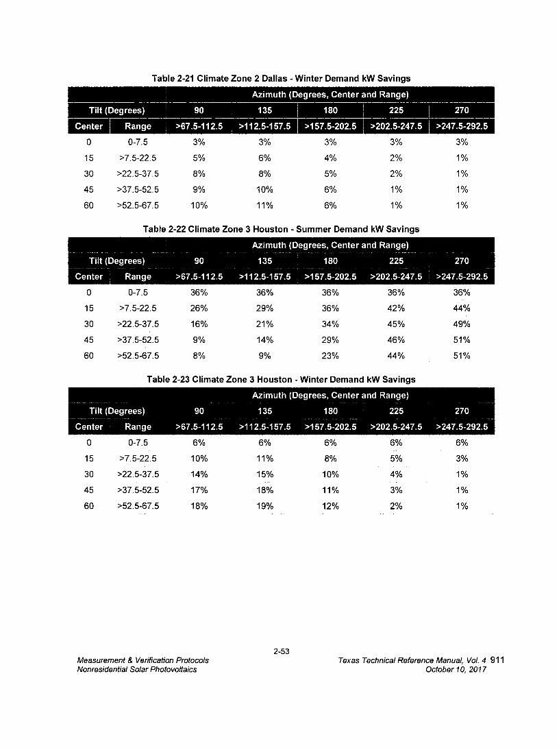
Table 2-21 Climate Zone 2 Dallas - Winter Demand kW Savings


Tilt (Degrees) 90 135 180 I 225 270

Center I Range >67.5-112.5 >112.5-157.5 >157.5-202.5 >202.5-247.5 >247.5-292.5

Table 2-22 Climate Zone 3 Houston - Summer Demand kW Savings


Tilt (Degrees) 90 135 180 225

270

Center Range >67.5-112.5 >112.5-157.5 >157.5-202.5 >202.5-247.5 >247.5-292.5

0

0-7.5

36%

36%

36%

36%

36%

15

>7.5-22.5

26%

29%

36%

42%

44%

30

>22.5-37.5

16%

21%

34%

45%

49%

45

>37.5-52.5

9%

14%

29%

46%

51%

60

>52.5-67.5

8%

9%

23%

44%

51%

Table 2-23 Climate Zone 3 Houston - Winter Demand kW Savings


Tilt (Degrees) 90 135 180 225 270

Center Range >67.5-112.5 >112.5-157.5 >157.5-202.5 >202.5-247.5 >247.5-292.5


0-7.5

>7.5-22.5

>22.5-37.5

>37.5-52.5

>52.5-67.5

0

15

30

45

60

5% 5%

7%

8%

9%

9%

5%

4%

3%

2%

2%

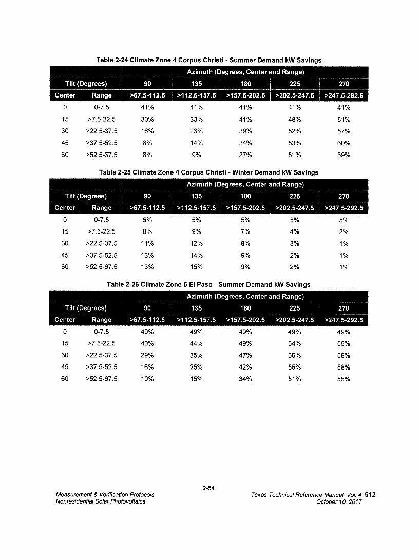
Table 2-24 Climate Zone 4 Corpus Christi - Summer Demand kW Savings


270

>247.5-292.5

41%

51%

57%

60%

59%

Tilt(Degrees)j 90 135 —r

180 225

Center Range >67.5-112.5 >112.5-157.5 ' >157.5-202.5 >202.5-247.5

0

0-7.5

41%

41%

41%

41%

15

>7.5-22.5

30% 33% 41%

48%

30

>22.5-37.5

16%

23%

39%

52%

45

>37.5-52.5

8%

14%

34%

53%

60

>52.5-67.5

8%

9%

27%

51%

Table 2-25 Climate Zone 4 Corpus Christi - Winter Demand kW Savings


Tilt (Degrees) 90 135 180 225 270

Center Range >67.5-112.5 >112.5-157.5 >157.5-202.5 >202.5-247.5 , >247.5-292.5

Table 2-26 Climate Zone 5 El Paso - Summer Demand kW Savings


Tilt (Degrees) 90 135 180 225 270

Center Range >67.5-112.5 >112.5-157.5 >157.5-202.5 >202.5-247.5 >247.5-292.5

0

0-7.5

49%

49%

49%

49%

49%

15

>7.5-22.5

40%

44%

49%

54%

55%

30

>22.5-37.5

29%

35%

47%

56%

58%

45

>37.5-52.5

16%

25%

42%

55%

58%

60

>52.5-67.5

10%

15%

34%

51%

55%


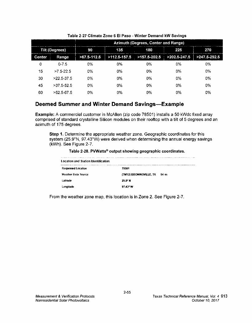
Table 2-27 Climate Zone 5 El Paso - Winter Demand kW Savings


Tilt (Degrees) 90 135 180 225 270

Center Range >67.5-112.5 >112.5-157.5 >157.5-202.5 >202.5-247.5 >247.5-292.5

0 0-7.5 0% 0% 0% 0% 0%

15 >7.5-22.5 0% 0% 0% 0% 0%

30 >22.5-37.5 0% 0% 0% 0% 0%

45 >37.5-52.5 0% 0% 0% 0% 0%

60 >52.5-67.5 0% 0% 0% 0% 0%

Deemed Summer and Winter Demand Savings—Example

Example: A commercial customer in McAllen (zip code 78501) installs a 50 kWdc fixed array comprised of standard crystalline Silicon modules on their rooftop with a tilt of 5 degrees and an azimuth of 175 degrees.

Step 1. Determine the appropriate weather zone. Geographic coordinates for this system (25.9°N, 97.43°W) were derived when determining the annual energy savings (kWh). See Figure 2-7.

Table 2-28. PVWatts® output showing geographic coordinates.

Location and Station kientification

Requested Location

T5501

Weather Data Source

(TMY2) BROWN SVILLE, TX 54 rni

Latitude

25.9° N

Longinide

97.43*W

From the weather zone map, this location is in Zone 2. See Figure 2-7.



Texas

Mods sodmal• onwldv maw 101.0100. sretailpd 61. kAry ....mobla I **a Meow rnOlne* 0.1.1.1,7904 ENT ../.• fp. an fa" VaiMe VeliOna. burn COES siscorabame, salaam mod M.O. an. Wiled MINN

*Mr +AWN ••• ewe famq•Pl • • Kam .141400, ZONE 4 MN) CORPUS CHRI STI

INTL ARPT (UT) ormeiDef

ZONE 1 3430 AMARILLO INTERNATIONAL

AP [CANYON - UT]

ZONE 1 722590 DALLAS-FORT

WORTH INTL AP



ZONE 3 HOUSTON BUSH

INTERCONTINENTAL

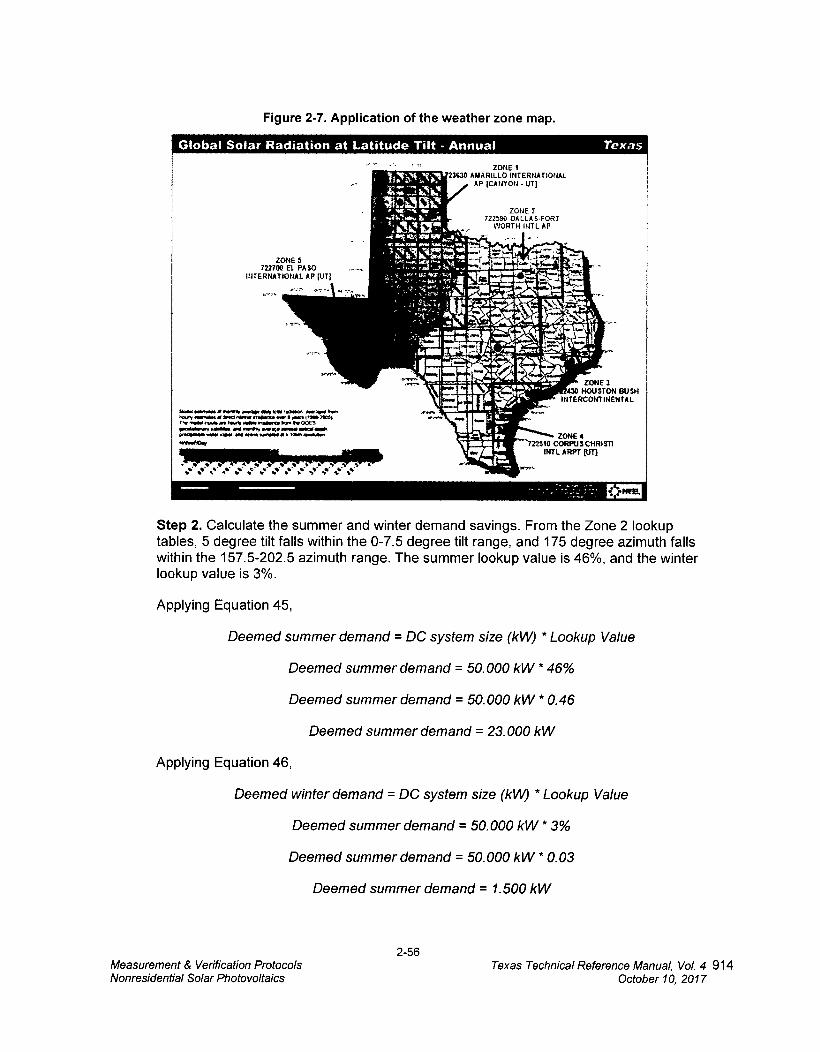
Figure 2-7. Application of the weather zone map.

Step 2. Calculate the summer and winter demand savings. From the Zone 2 lookup tables, 5 degree tilt falls within the 0-7.5 degree tilt range, and 175 degree azimuth falls within the 157.5-202.5 azimuth range. The summer lookup value is 46%, and the winter lookup value is 3%.

Applying Equation 45,

Deemed summer demand = DC system size (k1/10 * Lookup Value

Deemed summer demand = 50.000 kW * 46%

Deemed summer demand = 50.000 kW * 0.46

Deemed summer demand = 23.000 kW


Deemed winter demand = DC system size (kW) * Lookup Value





Summer and Winter Demand Savings—Alternative Method

An alternative method for estimating summer and winter demand savings is also available. To utilize the alternative method, follow these steps:

Step 1. Determine the applicable weather zone of the proposed system using Figure 5, above.

Step 2. Use PVWattse to model the proposed system as described in the Annual Energy Savings (kWh) section above. However, instead of using the zip code/default weather file, select the TMY3 reference location and weather file associated with the applicable weather zone of the proposed system. (For example, a system in McAllen, weather zone 1, would be modeled based on the DALLAS-FORT WORTH INTL AP, TX TMY3 weather file. Leave all other inputs the same.

Step 3. On the PVWatts Results page, select Download Results: Hourly. Save the pywatts_hourly.csv output file to your computer and open it using Microsoft Excel.

Step 4. Open the provided calculation tool TRM 4.0 PV tool YYYYMMDD_Iocked.xlsx (in which the version date is indicated by the YYYYMMDD field) on your computer, and select the Alt. Method Inputs tab.

Step 5. From the PVWatts hourly output file, highlight and copy the output data (A1:K8780). Paste this data to cell M1 on the Alt. Method Inputs tab in TRM 4.0 PV tool YYYYMMDD_Iocked.xlsx (in which the version date is indicated by the YYYYMMDD field).

Step 6. On the Alt. Methods Outputs tab, the tool calculates and displays summer and winter demand savings as AC capacity (kWac) and as a percentage of the DC capacity of the modeled system.

Claimed Peak Demand Savings

Refer to Volume 1, Appendix B: Peak Demand Reduction Documentation for further details on peak demand savings and methodology.

Measure Life and Lifetime Savings

The estimated useful life (EUL) of photovoltaic system is established at 30.0 years. This value is consistent with engineering estimates based on manufacturers warranties and historical data.

Additional Calculators and Tools

TRM 4.0 PV tool YYYYMMDD_locked.xlsx (in which the version date is indicated by the YYYYMMDD field), provided by Frontier Associates, is used to determine summer and winter demand savings. The most current version is posted at the Texas Energy Efficiency website, http://www.texasefficiency.com/. Utilities have the option to create their own versions.


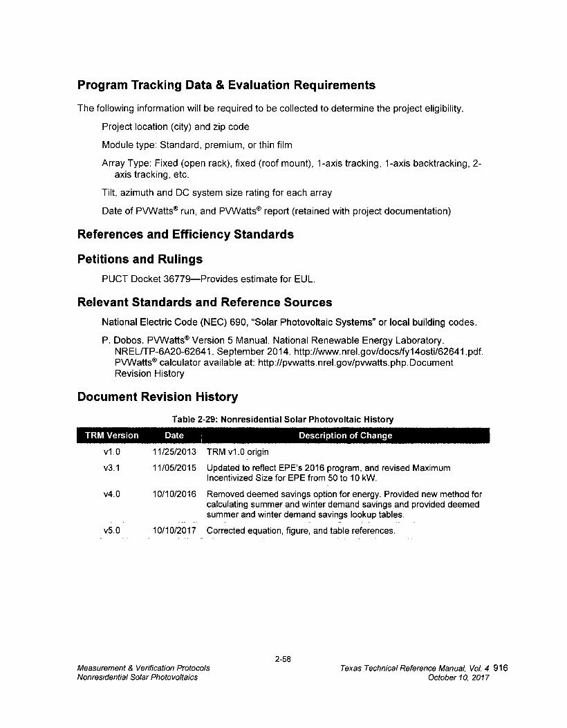
Program Tracking Data & Evaluation Requirements

The following information will be required to be collected to determine the project eligibility.

Project location (city) and zip code

Module type: Standard, premium, or thin film

Array Type: Fixed (open rack), fixed (roof mount), 1-axis tracking, 1-axis backtracking, 2-axis tracking, etc.

Tilt, azimuth and DC system size rating for each array

Date of PVWatts® run, and PVWatts® report (retained with project documentation)



PUCT Docket 36779—Provides estimate for EUL.


National Electric Code (NEC) 690, "Solar Photovoltaic Systeme or local building codes.

P. Dobos. PVWatts® Version 5 Manual. National Renewable Energy Laboratory. NREUTP-6A20-62641. September 2014. http://www.nrel.gov/docs/fyl 4osti/62641.pdf. PVWatts® calculator available at: http://pywatts.nrel.gov/pvwatts.php.Document Revision History

Document Revision History

Table 2-29: Nonresidential Solar Photovoltaic History


v1.0 11/25/2013 TRM v1.0 origin

v3.1 11/05/2015 Updated to reflect EPE's 2016 program, and revised Maximum lncentivized Size for EPE from 50 to 10 kW.

v4.0 10/10/2016 Removed deemed savings option for energy. Provided new method for calculating summer and winter demand savings and provided deemed sumrner and winter demand savings lookup tables.

v5.0 10/10/2017 Corrected equation, figure, and table references.


2.3.2 Residential Solar Photovoltaic (PV) Measure Overview

TRM Measure ID: R-RN-PV

Market Sector: Residential


Applicable Building Types: Single-family, duplex and triplex; Multifamily; Manufactured


Decision/Action Type(s): Retrofit, New Construction

Program Delivery Type(s): Prescriptive

Deemed Savings Type: Simulation Software (kWh), Deemed Values (kW)

Savings Methodology: Model-Calculator (PVWatte).

Measure Description

This section summarizes the savings calculations of the Solar Photovoltaic Standard Offer, Market Transformation, and Pilot programs. The primary objective of these programs is to achieve cost-effective reduction in energy savings and peak demand savings. Participation in the Solar Photovoltaic program involves the installation of a solar photovoltaic system. The method uses a simulation tool, the National Renewable Energy Laboratorys (NREL) PVWatts® Calculator23 to calculate energy savings. Lookup tables are used to determine deemed summer and winter peak demand savings.


Only photovoltaic systems that result in reductions of the customer's purchased energy and/or peak demand qualify for savings. Off-grid systems are not eligible. Each utility may have additional incentive program eligibility and interconnection requirements, which are not listed here.

Baseline Condition

PV system not currently installed (typical), or an existing system is present but additional capacity (including both panels and inverters) may be added.


Not applicable.

23 See httd://ovwatts.n rel.qovi, accessed January 20, 2016. 2-59

Measurement & Verification Protocols Texas Technical Reference Manual, Vol. 4 917 Residential Solar Photovoltaics October 10, 2017

Approximate Temperature Coefficient Module Cover Efficiency of Power Type


All solar PV systems shall be modeled using the current version of the National Renewable Energy Laboratory's (NREL) PVWatts® calculator. Energy savings are estimated using the default weather data source (currently TMY2) offered by PN/Wattse.24 Demand savings utilize deemed savings lookup tables with values derived from PyWatts® using reference TMY3 weather data sources applicable to defined weather zones; an Alternative Method is available for residential systems utilizing trackers or systems for which deemed savings lookup values are not available due to extreme array tilt or azimuth.


All Installations

PVWatts® input variables (for each array, where an array is defined as a set of PV modules with less than 5 degrees difference in tilt or azimuth):

• Installation ZIP code: Use the 5-digit ZIP code of the installation address.

• Weather data file: Accept the default (currently TMY2) weather data source offered by PVWatts®.

• DC System Size (kW): Input the sum of the DC (direct current) power rating of all photovoltaic modules in the array at standard test conditions (STC) in kilowatts DC.

0 For AC modules, refer to the module specification sheet to obtain the DC(STC) power rating.

• Module Type: Standard, Premium, or Thin Film. Use the nominal module efficiency, cell material, and temperature coefficient from the module data sheet to choose the module type, or accept the default provided by PVWatts®.

Table 2-30. Module Type Options

Standard (crystalline Silicon) 15% Glass -0.47 %/°C

Premium (crystalline Silicon) 19% Anti-reflective -0.35 %/°C

Thin film 10% Glass -0.20 %/°C

• Array Type: Fixed (open rack), Fixed (roof mount), 1-Axis Tracking, 1-Axis Backtracking, 2-Axis Tracking

• Tilt (deg): Enter the angle from horizontal of the photovoltaic modules in the array

24 Applying the Pvwatts® default weather input file simplifies estimating and promotes consistency between customers/contractors, program implementers, and evaluators. lf or when NREL updates the PVWatts® default to TMY3, the TRM method will follow in the subsequent year, but during the year of the change will continue to rely on TMY2 for consistency. NREL has stated that TMY2 will be "the standard for the foreseeable future." See htto://pvwatts.nrel.qov/pvwatts.php, accessed January 25, 2016.

2-60 Measurement & Verification Protocols Texas Technical Reference Manual, Vol. 4 918 Residential Solar Photovoltaics October 10, 2017

6et Started: 796C., f4 » HELP FEEDBACK

NREIs PYWatts® Calculator Estmiates the energy productm and cost if o or+ected Photoieuitak- (0t1) energy systems ttiroughpLit inicittalp," nomecvmers, smal buç owners, ets ani.ir mAircr.ixers devebp estimates of the performance of potential PV Estaiatiorts.

— - 107

• Azimuth (deg): Enter the angle clockwise from true north describing the direction that the array faces

• All other input variables: Accept the PyWatts® default values.


Given the inputs above, PVWatts® calculates the estimated annual energy savings for each array.

For systems with multiple arrays, users should derive annual energy savings for each array separately and sum them to obtain the total annual energy savings.

A screenshot (or other save) of the Results page, displaying both the annual energy production and model inputs, is typically required in PV incentive applications, and suffices as documentation of the annual energy savings estimate.

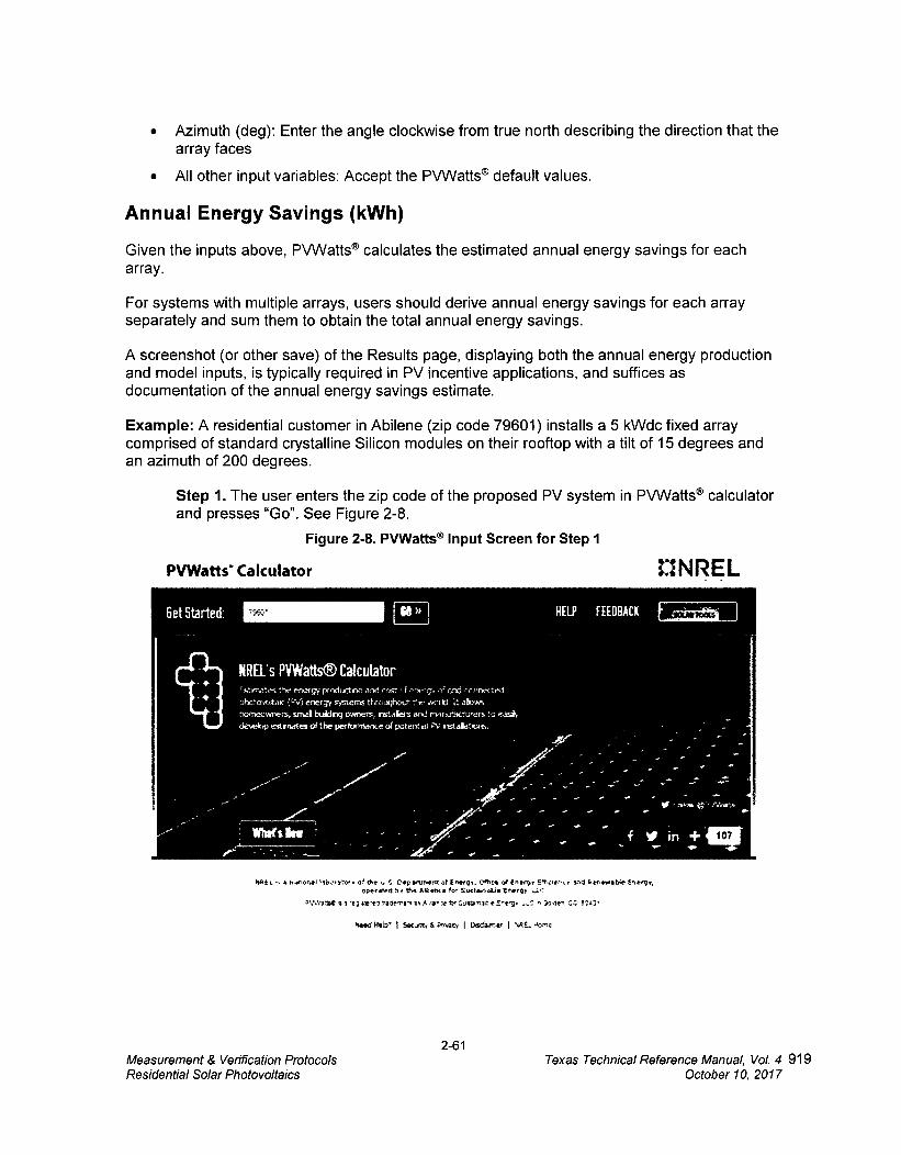
Example: A residential customer in Abilene (zip code 79601) installs a 5 kWdc fixed array comprised of standard crystalline Silicon modules on their rooftop with a tilt of 15 degrees and an azimuth of 200 degrees.

Step 1. The user enters the zip code of the proposed PV system in PVWatts® calculator and presses "Go". See Figure 2-8.

Figure 2-8. PVWatts® Input Screen for Step 1

PVWatts* Calculator 1.1NREL

Wel na.O.isi .&tor. 011 S Oepartt.tre of Enver. Creete of energy Moen,. end Wereeeee ere enee9, Verdeed b 1.e £$..n,n for $1331133A frwrg,

3 "3; ileW3 raavr.on r. A .4. X ter.,A7.1.1 eSlerg. 2a de. CO

hmke IMO Sec-anti iiPnvecy I rksciamv I *AL wwno

2-61 Measurement & Verification Protocols Texas Technical Reference Manual, VoL 4 919 Residential Solar Photovoltaics

October 10, 2017

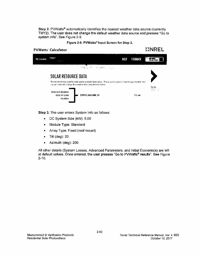
Step 2. Pvwatts® automatically identifies the nearest weather data source (currently TMY2). The user does not change the default weather data source and presses "Go to system info". See Figure 2-9.

Figure 2-9. PVWatts® Input Screen for Step 2.

PVWatts Calculator LINREL

SOLAR RESOURCE OATA The recofrrrerded jseather data sour:e e rlia$, listed belo,s This is Lsuetr, a good choice for you Iodation, bLt

you car optionalt, charge the ,heatter data ',sirs the trap beloir.

Selected weather

data for your

locatton

(11)Y2) ABILENE, TX 7.1mi

Go to

Step 3. The user enters System Info as follows:

• DC System Size (kW): 5.00

• Module Type: Standard

• Array Type: Fixed (roof mount)

• Tilt (deg): 20

• Azimuth (deg): 200.

All other details (System Losses, Advanced Parameters, and Initial Economics) are left at default values. Once entered, the user presses "Go to PVwatts® results". See Figure 2-10.

2-62 Measurement & Verification Protocols Texas Technical Reference Manual, Vol 4 920 Residential Solar Photovoltaics October 10, 2017

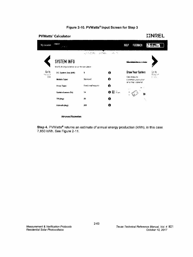
Figure 2-10. FA/watts® Input Screen for Step 3

PVWatts Calculator .1NREL

Go to DC System Stze (kW): 5 a

Module Type: Stancard

Array Type: Feied (roof mount i

System Losses rh): 14

Tilt (deg): 20

Azimuth (deg): 200

O Draw Your System

Click beto% to

customize your system

on a map iciptiorali

))

.44 Modify the iriptits tiebo. to run the sirriulation

SYSTEM INFO

Go to ki",43

Advanced Parameters

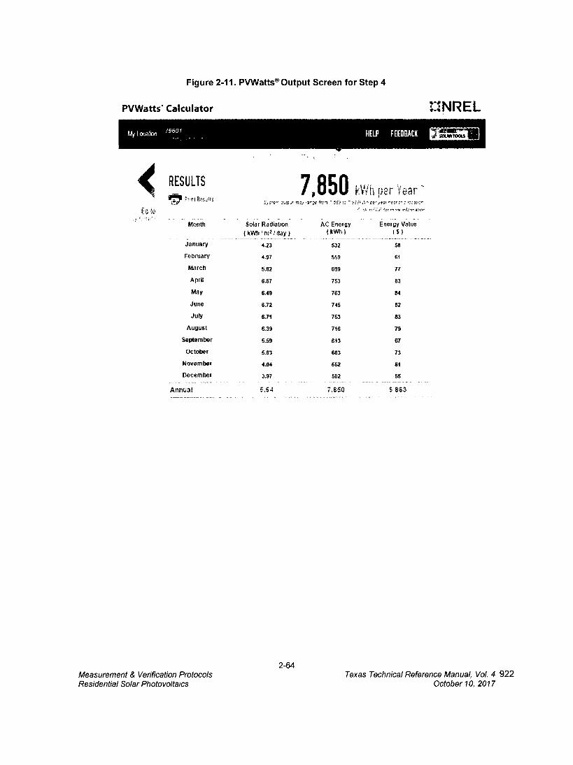
Step 4. P\ANatts® returns an estimate of annual energy production (kWh), in this case 7,850 kWh. See Figure 2-11.


MI PnrlRes.ills

Month

January

February

March

Apnl

May

June

July

August

September

October

November

December

Annual

RESULTS

Co to

Figure 2-11. PVWatte Output Screen for Step 4

PVWatts Calculator NREL

my Locaton 79501 HELP FEEIMACK

7,850 _ kVA per Year E., ps...i 1.1.e..., ms.„.

Solar Radiation

(kWI“m2 /day}

,a-;,c.. fr-.:-,

AC Energy ( kWh l

peita. "earv.: wi!..7.- C :, r, i'F. E f2,•9.:^,e 01.7,13:•0^

Energy Value ( S )

4.23 532 sa

4.97 559 61

5.62 699 n 6.57 753 83

6.49 763 a4

6.72 745 82

6.71 753 83

6.39 716 79

5.59 613 67

5.63 663 73

4.64 552 61

3.97 502 55

5.64 7.850 6 863


Further down this output page Pywatts® returns a summary of model inputs (Figure 2-12).

Figure 2-12. PVWatte Output Screen for Step 4 (continued).

Location and Station IdentifiCation


Weather Data Source (haY2) ABILENE. TX

Latitude 32.43° N

Longitude 99.61° W

PV System Specifications iRendena. I

DC System Size 5 kW

Module Type Standard

Array Type Fixed (roof mount)

Array Tilt 20'

Array Azimuth 200°

System Losses 14%

Inverter Efficiency 96%

DC to AC Size Ratio 1.1

Initial Economic Compahson

Average Cost of Electricity Purchased from Utility 0.11 SAM

Initial Cost 3.30 SMdc

Cost of Electricity Generated by System 0.17 1./kWh

The coordinates (latitude and longitude) of the proposed system are also presented. These are useful in determining the appropriate weather zone to use when estimating demand savings.

A screenshot (or PDF) of the complete output page, displaying both the annual energy production and model inputs, is typically required in PV incentive applications, and suffices as documentation of the annual energy savings estimate.

Summer Demand Savings Methodology

Deemed summer demand savings are determined using the weather zone map (Figure 2-13) and summer demand savings lookup values tables provided below. Deemed summer demand savings is the product of the system's DC system size and the appropriate lookup table value.

Deemed Summer Demand Savings

Deemed summer demand savings = DC system size (kW) * Lookup Value

Equation 47

For systems with multiple arrays, users should derive summer demand savings for each array separately and sum them to obtain the total summer demand savings.


7.1 m

In rare cases, residential systems utilizing trackers or systems for which deemed savings lookup values are not available due to extreme array tilt or azimuth may utilize the Alternative Method described below.

Winter Demand Savings Methodology

Deemed winter demand savings are determined using the weather zone map (Figure 2-13) and winter demand savings lookup values tables (Table 2-18 Climate Zone 1 Amarillo - Summer Demand kW Savings) provided below. Deemed winter demand savings is the product of the system's DC system size and the appropriate lookup table value.

Deemed Winter Demand Savings

Deemed winter demand savings = DC system size OW * Lookup Value

Equation 48

For systems with multiple arrays, users should derive winter demand savings for each array separately and sum them to obtain the total winter demand savings.

In rare cases, residential systems utilizing trackers or systems for which deemed savings lookup values are not available due to extreme array tilt or azimuth may utilize the Alternative Method described below.

Deemed Energy Savings Tables

Not applicable.

Deemed Summer and Winter Demand Savings—Weather Zone Determination The appropriate weather zone for each system can be determined by identifying the system's coordinates on the map in Figure 2-13, below. The figure identifies weather zones and the reference TMY3 weather station name and five-digit identifier used in calculating the lookup values within each weather zone. An example of how to use the weather zone map and tables to derive summer and winter peak demand savings is provided below the tables.



Texas ,Ottfiry,


AP [CANYON - UT]

ZONE 2 722590 DALLAS-FORT w4610,,RTH [VW

Model estimates cti monthly average dady Mal radiatioin. averaged from hourly estimates of rtireel normal IIMOMMOI over It years (1I1O62035) The model Immo am tarty treble graders* trom the GOES peoeitionsty salelitea. and matey average aerosol optical &pet predpaable se* vapor. and omit sampled at a 10kM 11111106.0011 IdAtienirttity

, •t, t, t:.3 4? '59 1, 1,CC

4-1111.144.. minC !lint sum, •

11'11'44 iPtomipagafflogY,.... ?I=

eprrio, k-i*":"7•01;14° 1418P.- • ;"1 ih.1°

RtgiWitiEig.1 .

11.1111.1.tli.,7741;411( ;IQ

= 71 k im INIMIN rANIP4114111

,,,re •

ZONE 4 722510 CORPUS CHRISTI

INTL ARPT [UT1


INTERNATIONAL AP [UT] ,ormr.

r.etrn -crtryr

ZONE 3 722430 HOUSTON BUSH

INTERCONTINENTAL

Figure 2-13. Weather Zone Determination for Solar PV Systems

Source: http.//appsl eere energy oov/stateshmaqes/maps/map large pv TX.ipo accessed January 20, 2016.

Deemed Summer and Winter Demand Savings—Lookup Value Tables

The tables below provide lookup values used for calculating deemed summer and winter demand savings based on the weather zone, tilt and azimuth. Table 2-31 through Table 2-40 present lookup values for determining deemed summer and winter demand savings given various array tilt/azimuth combinations. The values in the tables express summer and winter peak demand savings as a percentage of an arrays DC rating at standard test conditions (STC).


Table 2-31 Climate Zone 1 Amarillo - Summer Demand kW Savings


90 1, 135 180 — 225 270

>67.5-112.5 1 >112.5-157.5 >157.5-202.5 >202.5-247.5 >247.5-292.5

Tilt (Degrees)

Center Range

0

0-7.5

48%

48%

48%

48%

48%

15

>7.5-22.5

35%

40%

49%

56%

58%

30

>22.5-37.5

20%

30%

47%

60%

64%

45

>37.5-52.5

10%

18%

42%

61%

66%

60

>52.5-67.5

7%

10%

34%

59%

65%

Table 2-32 Climate Zone 1 Amarillo - Winter Demand kW Savings

Azimuth (Degrees, Center and Range) -r- -

Tilt (Degrees) , 90 135 180 225 i 270 ,

Center 1 Range I >67.5-112.5 >112.5-157.5 >157.5-202.5 >202.5-247.5 i >247.5-292.5

0 0-7.5 1% 1% 1% 1% 1%

15 >7.5-22.5 3% 3% 2% 1% 0%

30 >22.5-37.5 4% 5% 3% 1% 0%

45 >37.5-52.5 6% 6% 4% 1% 0%

60 >52.5-67.5 6% 7% 4% 0% 0%

Table 2-33 Climate Zone 2 Dallas - Summer Demand kW Savings


Tilt (Degrees) 90 135 180 225 270

Center Range >67.5-112.5 >112.5-157.5 >157.5-202.5 >202.5-247.5 >247.5-292.5

0 0-7.5 46% 46% 46% 46% 46%

15 >7.5-22.5 35% 39% 46% 52% 54%

30 >22.5-37.5 22% 29% 43% 55% 59%

45 >37.5-52.5 12% 19% 38% 56% 60%

60 >52.5-67.5 8% 12% 31% 53% 58%


0 0-7.5

15 >7.5-22.5

30 >22.5-37.5

45 >37.5-52.5

60 >52.5-67.5

6%

5%

4%

3%

2%

6%

3%

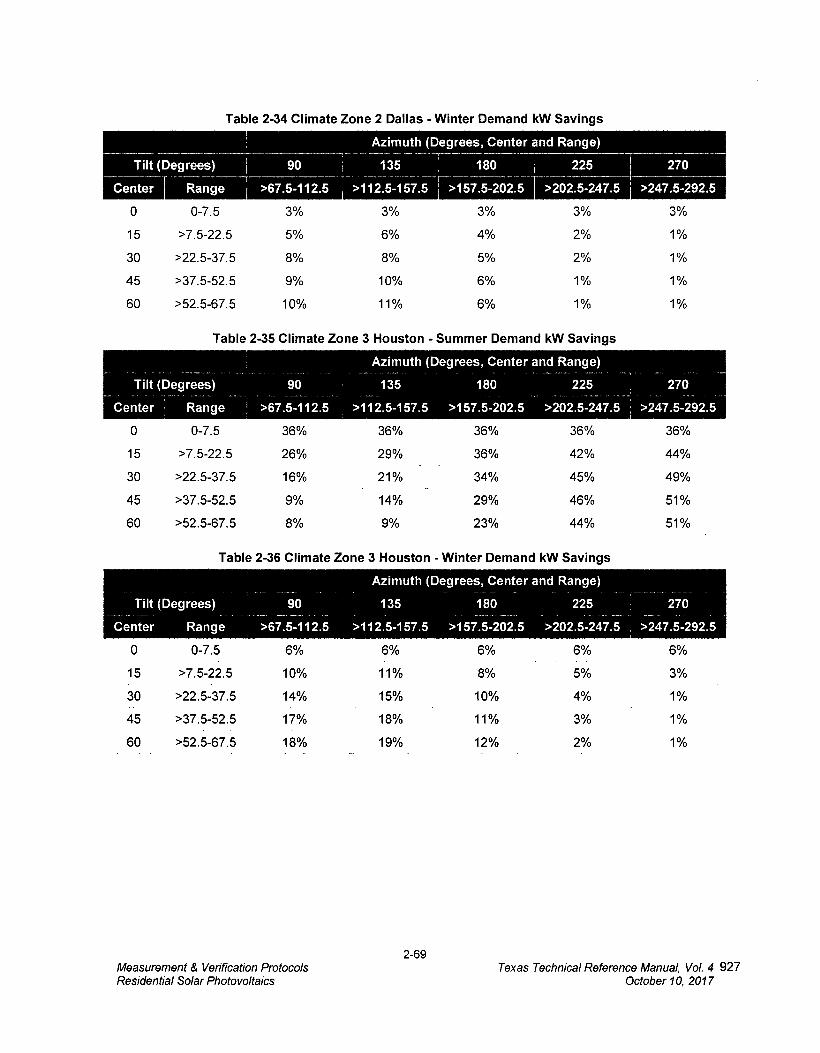
Table 2-34 Climate Zone 2 Dallas - Winter Demand kW Savings


Tilt (Degrees) 90 135 , 180 225 270

Center Range >67.5-112.5 >112.5-157.5 ' >157.5-202.5 >202.5-247.5 >247.5-292.5

0 0-7.5 3%

15 >7.5-22.5 5%

30 >22.5-37.5 8%

45 >37.5-52.5 9%

60 >52.5-67.5 10%

Table 2-35 Climate Zone 3 Houston - Summer Demand kW Savings


Tilt (Degrees) 90 135 180 225

270

Center Range >67.5-112.5 >112.5-157.5 >157.5-202.5 >202.5-247.5 >247.5-292.5

0

0-7.5

36%

36%

36%

36%

36%

15

>7.5-22.5

26%

29%

36%

42%

44%

30

>22.5-37.5

16%

21%

34%

45%

49%

45

>37.5-52.5 9% 14%

29%

46%

51%

60

>52.5-67.5

8%

9%

23%

44%

51%

Table 2-36 Climate Zone 3 Houston - Winter Demand kW Savings


Tilt (Degrees) 90 135 180 225 270

Center Range >67.5-112.5 >112.5-157.5 >157.5-202.5 >202.5-247.5 >247.5-292.5

3% 3%

4%

5%

6%

6%


0-7.5

>7.5-22.5

>22.5-37.5

>37.5-52.5

>52.5-67.5

0

15

30

45

60

5%

7%

8%

9%

9%

5%

4%

3%

2%

2%

5%

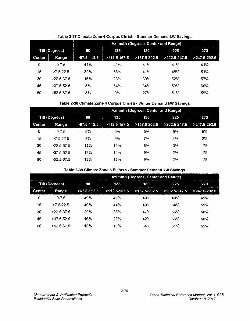
Table 2-37 Climate Zone 4 Corpus Christi - Summer Demand kW Savings

Center Range >67.5-112.5


135 I 180 225 I 270

>112.5-157.5 >157.5-202.5 >202.5-247.5 >247.5-292.5

Tilt (Degrees) 90

0 0-7.5

41%

41%

41%

41%

41%

15 >7.5-22 5

30% 33% 41%

48%

51%

30 >22.5-37.5

16%

23% 39% 52%

57%

45 >37.5-52.5

8%

14%

34% 53% 60%

60 >52.5-67.5

8%

9%

27%

51%

59%

Table 2-38 Climate Zone 4 Corpus Christi - Winter Demand kW Savings


Tilt (Degrees) 90 135 180 225 270 ,

Center Range >67.5-112.5 >112.5-157.5 ; >157.5-202.5 -', >202.5-247.5 >247.5-292.5

Table 2-39 Climate Zone 5 El Paso - Summer Demand kW Savings


Tilt (Degrees) 90 135 180 225 270

Center Range >67.5-112.5 >112.5-157.5 >157.5-202.5 >202.5-247.5 >247.5-292.5

0

0-7.5

49%

49%

49%

49%

49%

15

>7.5-22.5

40%

44%

49%

54% 55%

30

>22.5-37.5

29%

35%

47%

56% 58%

45

>37.5-52.5

16%

25%

42%

55% 58%

60

>52.5-67.5

10%

15%

34%

51% 55%

2-70 Measurement & Verification Protocols Texas Technical Reference Manual, VoL 4 928 Residential Solar Photovoltaics October 10, 2017

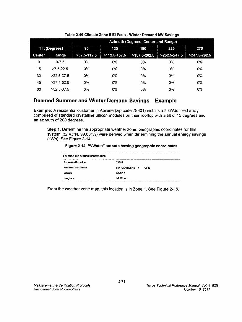
Table 2-40 Climate Zone 5 El Paso - Winter Demand kW Savings

Azimuth (Degrees, Center and Range) -

Tilt (Degrees) 90

Center 1 Range >67.5-112.5 1

1 i 135

-4- , 1 180 ,

: 225 I T

270

>112.5-157.5 >157.5-202.5 >202.5-247.5 I >247.5-292.5

0 0-7.5

15 >7.5-22.5

30 >22.5-37.5

45 >37.5-52.5

60 >52.5-67.5

0% 0% 0% 0% 0 %

0% 0% 0% 0% 0%

0% 0% 0% 0% 0%

0% 0% 0% 0% 0%

0% 0% 0% 0% 0%

Deemed Summer and Winter Demand Savings—Example

Example: A residential customer in Abilene (zip code 79601) installs a 5 kWdc fixed array comprised of standard crystalline Silicon modules on their rooftop with a tilt of 15 degrees and an azimuth of 200 degrees.

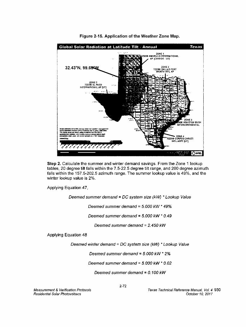
Step 1. Determine the appropriate weather zone. Geographic coordinates for this system (32.43°N, 99.68°W) were derived when determining the annual energy savings (kWh). See Figure 2-14.

Figure 2-14. PI/Watts® output showing geographic coordinates.

Location and Station Identification


Weather Data Source (TMY2) ABILENE, TX 7.1 ITS

Latitude 32.43' N

Longitude 99.8 W

From the weather zone map, this location is in Zone 1. See Figure 2-15.



Texas

32.43°N, 99.6 ZONE 2 722590 DALLAS-FORT

WORTH INTL AP


AP [CANYON - UT]

tairt",

11.60 q4°./..41.14*1 - 1Z: 511."9.2.41 A , NEN- 44,1 EIPIPLVE......•'.1, •eiot.c L.- •

!11t-win• A Mvitiroir 3 I

ZONEM61111X' HOUSTON BUSH

=CI Id WrsP4'. • I ERCONTINENTAL

ZONE I 510 CORPU S CHRISTI

INTL ARPT [UT]



WOO marries w.f., seerve Z.. Iva fill/Ia. sortnerl tor, Now* mingOos Owl... +raid.* mon 1,10140W.

ereadi me ..01 .6W n adortli IVA 0. GOES 0.4.1Manlry 24~ *NNOPy orIsav. row. 4000.1 doe, 11.011.01. saw raw ar4 .0rap 10,010.10 1,1,arm remes.a.

Figure 2-15. Application of the Weather Zone Map.

Step 2. Calculate the summer and winter demand savings. From the Zone 1 lookup tables, 20 degree tilt falls within the 7.5-22.5 degree tilt range, and 200 degree azimuth falls within the 157.5-202.5 azimuth range. The summer lookup value is 49%, and the winter lookup value is 2%.


Deemed summer demand = DC system size (kW) * Lookup Value




Applying Equation 48

Deemed winter demand = DC system size OW * Lookup Value





Summer and Winter Demand Savings—Alternative Method

An alternative method for estimating summer and winter demand savings is available to residential systems utilizing trackers or systems for which deemed savings lookup values are not available due to extreme array tilt or azimuth. To utilize the alternative method, follow these steps:

Step 1. Determine the applicable weather zone of the proposed system using Figure 5, above.

Step 2. Use P\AA/atts® to model the proposed system as described in the Annual Energy Savings (kWh) section above. However, instead of using the zip code/default weather file, select the TMY3 reference location and weather file associated with the applicable weather zone of the proposed system. (For example, a system in Abilene, weather zone 1, would be modeled based on the AMARILLO INTERNATIONAL AP [CANYON-UT], TX TMY3 weather file. Leave all other inputs the same.

Step 3. On the PVWatts Results page, select Download Results: Hourly. Save the pywatts_hourly.csv output file to your computer and open it using Microsoft Excel.

Step 4. Open the provided calculation tool TRM 4.0 PV tool YYYYMMDDlocked.xlsx (in which the version date is indicated by the YYYYMMDD field) on your computer, and select the Alt. Method Inputs tab.

Step 5. From the PVWatts hourly output file, highlight and copy the output data (A1:K8780). Paste this data to cell M1 on the Alt. Method Inputs tab in TRM 4.0 PV tool YYYYMMDD jocked.xlsx (in which the version date is indicated by the YYYYMMDD field).

Step 6. On the Alt. Methods Outputs tab, the tool calculates and displays summer and winter demand savings as AC capacity (kWac) and as a percentage of the DC capacity of the modeled system.


Refer to Volume 1, Appendix B: Peak Demand Reduction Documentation for further details on peak demand savings and methodology.


TRM 4.0 PV tool YYYYMMDD_locked.xlsx (in which the version date is indicated by the YYYYMMDD field), provided by Frontier Associates, is used to determine summer and winter demand savings. The most current version is posted at the Texas Energy Efficiency website, http://www.texasefficiency.com/. Utilities have the option to create their own versions.


The estimated useful life (EUL) of photovoltaic systems is established at 30.0 years. This value is consistent with engineering estimates based on manufacturers warranties and historical data.


Program Tracking Data & Evaluation Requirements

The following information will be required to be collected.

Project location (city) and zip code

Module type: Standard, premium, or thin film

Array Type: Fixed (open rack), fixed (roof mount), 1-axis tracking, 1-axis backtracking, 2-axis tracking, etc.

Tilt, azimuth and DC system size rating for each array

Date of Pvwatts® run, and Pvwatts® report (retained with project documentation) for each array

Selected climate zone and demand method used

For projects using the alternative method, retention of the TRM 4.0 PV tool workbook for each array evaluated.


Petitions and Rulings PUCT Docket 36779—Provides estimate for EUL.

Relevant Standards and Reference Sources • National Electric Code (NEC) 690, "Solar Photovoltaic Systeme or local building codes.

• P. Dobos. PVWatts® Version 5 Manual. National Renewable Energy Laboratory. NREUTP-6A20-62641. September 2014. http://www.nrel.gov/docs/fyl4osti/62641.pdf. PVWatts® calculator available at: http://pvwatts.nrel.qov/pvwatts.php.

Document Revision History Table 2-41: Residential Solar Electric (Photovoltaic) Energy Systems Revision History


v1.0 11/25/2013 TRM v1.0 origin

v2.0 04/18/2014 TRM v2.0 update. Minor edits to language and structure. _ _

v2.1 01/30/2015 No revisions

v3.0 04/10/2015 No revisions _

TRM v4.0 update. Removed deemed savings option for energy.

v4.0 10/10/2016 Provided new method for calculating summer and winter demand savings and provided deemed summer and winter demand savings lookup tables.

_ v5.0 10/10/2017 Corrected equation, figure, and table references.


2.3.3 Solar Shingles Measure Overview

TRM Measure ID: R-RN-SS and NR-RN-SS

Market Sector: Residential and Commercial


Applicable Building Types: All


Decision/Action Types: Retrofit (RET), New Construction (NC)

Program Delivery Type: Custom

Deemed Savings Type: Prescribed Simulation Software EM&V

Savings Methodology: Software Modeling Tool and Calculator-SAM.

Streamlined measurement and verification of solar shingles installations shall consist of the development of a project-specific model of the installed solar shingle system using the System Advisor Model (SAM), developed by the National Renewable Energy Lab (NREL), as specified herein. A solar shingles system consists of all connected arrays and sub-arrays and connected inverter(s).

Measure Description

A solar shingles system consists of all connected arrays and sub-arrays and connected inverter(s). The M&V method used to estimate savings is through a simulation model approach using the National Renewable Energy Laboratorys (NREL) System Advisor Model (SAM). Either version 2015.6.30 or subsequent most recent version of the SAM software shall be used.


Solar shingle systems consisting of connected arrays, sub-arrays and inverter(s).

The installation must meet the following requirements in order to be eligible for incentives:

• Systems shall be installed by a licensed electrical contractor or, in the case of a residential installation by the homeowner, with the approval of the electrical inspector in accordance with the National Electric Code (NEC 690, "Solar Photovoltaic Systems") and/or local building codes.

• If the system is utility interactive the inverter shall be listed and certified by a national testing laboratory authority (e.g., UL 1741, "Static Inverters and Charge Controllers for Use in Photovoltaic Power Systems") as meeting the requirements of the Institute of Electrical and Electronics Engineers (IEEE) Standard 929-2000 "Recommended Practice for Utility Interface of Photovoltaic (PV) Systems."

• The estimated annual energy generation from the solar shingles system shall not exceed the customers annual energy consumption.

2-75 Measurement & Verification Protocols Texas Technical Reference Manual, Vol. 4 933 Solar Shingles October 10, 2017

Baseline Condition PV system not currently installed (typical).


PV systems must meet the eligibility criteria shown above to be eligible for reporting claimed energy impacts. The high-efficiency conditions are estimated based on appropriate use of NREL's SAM software modeling tool for solar shingle installation analysis.



SAM solar shingle installation data, modeling and analysis

SAM can be downloaded from the NREL website.25

SAM Data Input

The following steps present the information and sequence required to accurately model solar shingle projects using the SAM software tool.

1. Create a new solar PV project in SAM.

2. Specify a Solar PV project and select a market segment (e.g., residential/commercial).

3. Solar systems are configured in the SAM main model interface that is organized across a number of screens, selected by a topics menu on the left hand side of the window. The following items must be configured:

Location and Resource. An appropriate weather file must be specified in the subsequent screen. SAM is pre-loaded with a selection of weather files from the NREL NSRDB TMY3 datasets. The user should specify one of the five locations provided in Table 2-14, according to where in Texas the solar shingles are being installed. The map in Figure 2-16 indicates the delineation of the weather zones, by county.

NOTE: It is critical that the TMY3 files be specified in the model for estimating peak demand impacts, AND that the corresponding set of peak hours and relative probabilities from TRM volume 1 Section 4 shall be used to estimate peak demand impacts.

25 As of publication of this version, the latest release of SAM is Version 2015.6.30. Instructions provided herein are intended to be sufficiently generic to allow for successful model creation in this and subsequent iterations of the software; however, it is impossible to anticipate the exact nature of future software revisions.


A Climate Zones

MI I 2

, 3

1111 5 114

Table 2-42: TMY data file by TRM Weather Zone

TRM Weather Zone TMY3 File TMY3 Location

1 Panhandle Region

2 North Region

3 South Region

4 Valley Region

5 West Region

723630

722590

722430

722510

722700

Amarillo Intl AP [Canyon—UT]

Dallas Fort Worth Intl AP

Houston Bush Intercontinental

Corpus Christi Intl AP [UT]

El Paso International AP [UT]

Figure 2-16: Texas Technical Reference Manual Weather Zones

Module. The default action in the Module screen allows the user to select a product for which required performance data has been pre-loaded into the SAM. Several CertainTeed Apollo modules and Dow DPS-XXX modules can be specified in this window. However, modeling options for the PV Module can be modified in SAM 2015.6.30; by selecting the dropdown menu that, by default, is set to " CEC Performance Model with Module Database" (at the top of this window). Other modeling options provide the flexibility needed to adequately model products from other manufacturers.

• Temperature Correction. The module screen includes a "Temperature Correction" window, in which one of two-cell temperature ;models must be specified. The "Nominal operating cell temperature (NOCT) method" should be selected, and within the "Nominal

2-77 Measurement & Verification Protocols Texas Technical Reference Manual, Vol. 4 935 Solar Shingles

October 10, 2017

output cell temperature (NOCT) parameters" section, the "Mounting standoff should be specified as "Building integrated." The "Building integrated" option accounts for the fact that, by their nature, solar shingles are integrated into the buildings on which they are installed.

Inverter. Inverter-specific information must be provided. Similarly to the functioning of the Module screen, an inverter can be selected from the Inverter CEC Database (default), or, for inverters not in the CEC database, by specifying data from the manufacturers datasheet (Inverter Datasheet mode) or by specifying inverter efficiency at different loading rates (Inverter Part Load Curve mode), from which the inverter part load curve can be constructed. Any of these methods should be satisfactory. Note that the number of inverters can be specified on the following (Array) screen, but only one inverter type can be specified here, so when multiple inverters are used with systems modeled in SAM, they must be the same make and model.

System Design (Array). The following array-level information shall be provided:

• System sizing: Specified by solar module capacity and count, and inverter system losses.

• Configuration at Reference Conditions (Modules and Inverters) DC Subarrays. SAM allows for modeling of up to 4 subarrays. If the system being modeled has only one array, the data for this array are entered in the column for subarray 1, and subarrays 2-4 should be left disabled. If there are multiple arrays, check the boxes to enable subarrays 2-4 as needed, and the number of strings in that subarray provided. Pre-inverter derates should be specified as appropriate.

• Estimate of Overall Land Usage. Not needed (used for economic analysis only).

• PV Subarray Voltage Mismatch. For CEC modules (true of CertainTEED and Dow DPS products), losses due to subarray mismatch can be estimated. For arrays with multiple orientations, this option should be selected.

Shading and Snow. A good faith effort should be made to represent features likely to affect incidence of solar radiation on the solar shingle system. Appropriate shading for the installation site should be incorporated; however, it is not necessary to modify the annual average soiling, as first year generation values will be used. Losses. Specify all DC and AC losses.

For the remaining topics/screens listed below, no data entry is required:

• Lifetime

• Battery Storage

• System Costs

• Financial Parameters.

• Incentives

• Electricity Rates

• Electric Load.

2-78 Measurement & Verification Protocols Texas Technical Reference Manual, Vol 4 936 Solar Shingles October 10, 2017

Model Run and Data Output

Execute the model calculations (in 2015.6.30)by clicking "Simulate" in the bottom left corner. SAM generates a large number of output data fields: create an 8760 hourly output file by selecting "Time Seriee at the top of the screen (option appears only after clicking "Simulate") and then selecting "Power generated by system (kW)" from the options on the right hand side of the screen. Output data can be sent to either Excel or CSV by right clicking on the generated plot and selecting the desired option.

Deemed Energy and Demand Savings Tables

There are no lookup tables available for this measure. See SAM software tool guidance in the previous section for calculating energy and demand savings.


Peak demand savings should be extracted from the hourly data file in a manner consistent with the definition of peak demand incorporated in TRM 3.0 and the associated methods for extracting peak demand savings from models producing 8,760 hourly savings using Typical Meteorological Year (TMY) data. See TRM volume 1 section 4.


Not applicable.


Program Tracking Data and Evaluation Requirements

The following primary inputs and contextual data should be specified within the program database to inform the evaluation and apply the savings properly.

• Decision/Action Type: Retrofit, New Construction

• Building Type

• Climate/Weather Zone

• System Latitude

• System Tilt from horizontal

• System Azimuth.

The following files should be provided to the utility from which the project sponsor seeks to obtain an incentive for a solar shingles system installation:

• SAM model file (*.zsam format)

• 8760 hourly output file (csv or similar format)

• Calculator with annual energy savings and peak demand savings estimate.



Petitions and Rulings Not applicable.

Relevant Standards and Reference Sources • National Electric Code (NEC) 690, "Solar Photovoltaic Systems" or local building codes.

• Institute of Electrical and Electronics Engineers (IEEE) Standard 929-2000 "Recommended Practice for Utility Interface of Photovoltaic (PV) Systems." http://standards.ieee.oro/findstds/standard/929-2000.html.

• System Advisor Model (SAM) Version 2014.1.14. National Renewable Energy Laboratory. SAM is available for registration and download at: https://sam.nrel.00v/download.

Document Revision History Table 2-43: M&V Solar Shingles History


v3.0 4/10/2015 TRM v3.0 origin

v3.1 11/05/2015 TRM v3.1 update. Major methodology updates include revising the 1 reference to latest version of SAM software and removal of TMY2 weather data file use. Revised measure details to match format of TRM volumes 2 and 3. This included adding detail regarding Measure Overview, Measure Description, Measure Life, Program Tracking Data and Evaluation Requirements, References and Efficiency Standards, and Document Revision History.

_ 10/10/2016 No revisions v4.0



2.4 M&V: MISCELLANEOUS

2.4.1 Behavioral Measure Overview

TRM Measure ID: NR-MS-BC


Measure Category: Miscellaneous

Applicable Building Types: Commercial


Decision/Action Types: Operation & Maintenance (O&M)


Deemed Savings Type: Not Applicable

Savings Methodology: EM&V and Whole Facility Measurement.

This protocol is used to estimate savings for various behavioral or practice changes that may be implemented on an ongoing (i.e., permanent) basis such that savings remain persistent and reliable long term. The development of the M&V methodology is driven by the desire to create and implement a framework to provide high quality verified savings—keeping within the standards currently applied to commercial energy savings measures—to enable the opportunity to implement measures and report energy savings from a wide variety of energy optimization practices and behaviors.

Measure Description

This measure is not defined, but requires that any behavioral measure develop an M&V plan and report. These documents shall include a complete description of the proposed behavioral changes, how the changes will save energy, and why the behavioral change should be considered as a permanent change on par with high efficiency equipment retrofits. One example is establishing an authorized and enforced facility-wide energy policy with implementation and quality assurance processes.

The projects M&V plan and report shall describe the current case, and proposed new case, that define changes in operations and/or sequence of operations. These documents should fully discuss, describe, and document the logic of the proposed changes and how those changes translate into energy savings impacts.

The measure description should describe how the initial energy savings estimates will be determined to estimate energy and demand savings impacts that will then be verified by measurement and verification analysis following IPMVP criteria.

Eligibility Criteria This measure applies to implementing behavioral measures that establish processes to ensure persistent energy reductions that are measurable at the facility level.

2-81 Measurement & Verification Protocols Texas Technical Reference Manual, Vol. 4 939 Behavioral October 10, 2017

Baseline Condition

The baseline condition for each behavioral measure included in a plan has two facets: 1) to establish the existing operating parameters (e.g., temperatures, hours of operation, loads, etc.) and existing energy use for each behavior change included in the plan, and; 2) establish the proposed new case operating parameters resulting from each behavior change and present the equations proposed to quantify energy savings impact estimates.

The plan should document the source and accuracy/confidence of the various parameters used in the proposed equations to estimate baseline and new case energy use, for each behavior impact (e.g., if interior lights are to be turned off, there may be two sources of energy savings, one attributable directly to the light fixture energy use, the other attributable to reduced internal heat gain and load on the air conditioning system). The plan shall explain all assumptions employed for both baseline and behavior change cases noting source and applicability—logic reasoning.


Demonstrated by conclusive energy savings results of M&V plan following IPMVP protocols.


Savings Algorithms and Input Variables (Used to Estimate Initial Savings Potential ONLY)

Savings equations, algorithms and input variables should be used as an initial means to estimate energy savings prior to measure implementation. These must adhere to standard engineering practices and accepted energy efficiency engineering methods. Initial savings estimates must identify energy savings calculations, algorithms and all pertinent factors used to calculate the estimated energy impacts of the project. Project M&V plans shall appropriately cite technical sources and resources used to develop initial energy savings estimates. These initial savings estimates, although to be replaced with final whole facility EM&V determined savings, should be included in the final M&V report of savings.

Whole Facility EM&V Methodology (Used to Estimate FINAL Savings Potential)

A whole facility EM&V methodology presents a plan for determining energy savings due to significant and persistent facility-wide behavioral changes for a commercial facility. This methodology measures and verifies initial energy savings estimates. The plan follows procedures guided by whole facility Option C in the International Performance Measurement and Verification Protocol (IPMVP). The development of the whole facility measurement methodology is driven by the desire to create and implement a framework to provide high quality verified savings while keeping within the standards currently used to verify commercial measures. The Whole Facility guidance is found in the latest version of the IPMVP Volume 1 EVO 10000-1:2012.


The Option C methodology should be documented in a M&V report and include detail regarding model development, testing, handling of errors, and the information for validating the regression model(s). Model documentation should be transparent and allow for repeating modeling steps and results, including the use of any adjustments made outside of the primary modeling method. Particular procedures to be taken and their respective results should be documented and may include:

• Describe the process taken for how the review of outliers was completed, whether outliers were identified, and how those outliers were addressed in the modeling. Describe how any missing data points or data entry errors were addressed and document what was missing, corrected, or erroneous data were changed from the original data for purposes of the model. Any data that are ultimately removed or changed from the original data set should be annotated with the assignable cause.

• Present the guidelines used to test for the statistical significance of each independent variable and overall model fitment. The results of these statistical tests and results should be presented as part of the presentation of individual model results.

M&V Plan and M&V Report

Preparation of an M&V plan and ultimately an M&V report is a required part of the savings determination. Advanced planning ensures that all data collection and information necessary for savings determination will be available after implementation of the behavioral change(s). The projects M&V plan and M&V report provide a record of the initial energy savings impact estimates, and the data collected during project development and implementation. These documents may also serve multiple purposes throughout a project including recording critical assumptions and conditions, and any changes that may emerge during project implementation. For example, the M&V plan shall describe how major energy drivers will be documented and recorded. The M&V report shall document such findings. Also, other energy savings influences (e.g., equipment retrofits, changes to occupancy) that may have occurred during the baseline and/or reporting periods are to be accounted for and quantified. Such savings development and assumptions should be clearly documented within the M&V report. Documentation should be complete, readily available, clearly organized, and easy to understand.

Changes to the required level of documentation may be possible if a viable comparison group can be used for the analysis, but in using a comparison group, the EM&V team needs to review the make-up and selection of the group and that using a comparison group in lieu of other documentation should be presented in a draft M&V plan.

The methodology described herein involves use of whole facility electric meter data. An important component of a project is to identify the existing base and new case system information.

In addition to documenting existing and new equipment information, IPMVP describes the following requirements as part of the M&V plan and M&V report contents. These requirements are listed below and the user is directed to the current version of IPMVP for further detail and guidance.

• Measure Intent

• Selected IPMVP Option and Measurement Boundary

• Baseline—Period, Energy and Conditions


• Reporting Period

• Basis for Adjustment

• Analysis Procedure

• Energy Prices (as applicable)

• Meter Specifications

• Monitoring Responsibilities

• Expected Accuracy

• Budget (as applicable)

• Report Format

• Quality Assurance.

Deemed Energy and Demand Savings Tables

Not applicable.


Refer to TRM volume 1, section 4.2: Approach to Identifying Peak Hours for further details on peak demand savings and methodology derived using the whole facility EM&V process. This should be presented in the project M&V plan.


The project M&V Plan shall describe analysis calculators or software tools employed and their applicability for project analysis.


The estimated useful life (EUL) is one year.


The following primary inputs and contextual data should be specified and tracked within the program database to inform the evaluation and apply the savings properly.

• Decision/Action Type: O&M

• Building Type

• Climate Zone

• Baseline Equipment Types Affected by Behavior Change

• Baseline Equipment Capacities

• Baseline Equipment Efficiency Ratings

• Baseline Number of Units


• Baseline Operating Practice

• Efficient Operating Practice.


Not Applicable.

Petitions and Rulings • Behavioral programs are allowed energy efficiency programs as specified in the Energy

Efficiency Rule (16 TC 25.181 (c )(12)

Relevant Standards and Reference Sources • Unique to each project and to be documented in M&V plan and report.

Document Revision History Table 2-44: M&V Behavioral History


v3.1

11/05/2015 TRM v3.1 origin

v4.0 10/10/2016 Updated documentation of methodology and measure life.



2.4.2 Air Compressors less than 75 hp Measure Overview

TRM Measure ID: NR-MS-CA


Measure Category: Miscellaneous

Applicable Building Types: Commercial


Decision/Action Types: Early Retirement (ER), New Construction (NC), and Replace-on-Burnout (ROB)



Savings Methodology: EM&V and Whole Facility Measurement.

This protocol is used to estimate savings for compressed air system controls measures for systems with less than 75 horsepower in total compressor power. The development of this compressed air methodology is driven by the desire to create and implement a framework to provide high quality verified savings for smaller compressed air projects. This measure utilizes site collected data and follows savings methodologies as outlined by the Ohio Technical Reference Manual and uses research on compressed air systems conducted by the Long Island Power Authority.

Measure Description

This measure requires the installation of flow controls on existing compressed air systems with a total compressor power of less than 75 hp. This methodology limits the amount of savings that can be claimed to 20 kW and 100,000 kWh for projects. For projects that are expected to exceed 20 kW or 100,000 kWh, full M&V is recommended to claim savings.

Applicable controls measure types include:

• Load/Unload: Load/unload controls allow the motor to run continuously at a constant speed, but unloads the compressor when adequate pressure has been achieved. Efficient load/unload controls utilize storage tank(s) to increase the available compressor air capacity without requiring compressor operation during all load periods. This protocol provides estimated savings for systems that exceed 3 gal/CFM or 5 gal/CFM in storage capacity.

• Modulation: Modulating inlet controls vary the compressor the output of the compressor to meet the flow requirements of the system. Modulating flow controls offer limited energy savings from the potential for a surge in demand the minimum throttling capacity.

• Variable Displacement: Variable displacement systems have compressors that are designed to operate in two or more partially-loaded conditions. Since the compressor has the ability to efficiently operate at multiple output points, it can more closely align with the load of the system.

2-86 Measurement & Verification Protocols Texas Technical Reference Manual, Vol. 4 944 Air Compressors less than 75 hp October 10, 2017

• Variable Speed w/Unloading: Variable speed compressors offer the most savings for compressed air flow control. The compressor motor can be tuned by the controls to precisely match the load of the system, offering the highest efficiency gains. During periods of very low demand, the compressor is unloaded and will operate at the minimum variable speed output until the demand exceeds the minimum output of the compressor, as determined by system flow and pressure.

Eligibility Criteria This measure applies to retrofitting an existing compressed air system with a new, higher efficiency flow control type or the installation of a new compressed air system with eligible flow control types integrated.

Baseline Condition

Existing System Retrofit: The baseline for existing system retrofit shall be the applicable control type from the pre-existing system, from Table 2-45.

Replace-on-Burnout (ROB) and New Construction (NC): The baseline for ROB and NC projects is assumed to be a modulating air compressor with blow down, to align with standard industry practice. The baseline efficiency is given from the Modulation category in Table 2-45.


High-efficiency conditions for compressed air system are given in Table 2-45.

Table 2-45: Air Compressor Energy Factors

Control Type 11 ACEF

Source

Modulation 89.0%

Load/No Load w/ 3 gal/CFM 83.1%

Load/No Load w/ 5 gal/CFM 80.6% LIPA Clean Energy Initiative26

Variable Displacement 76.9%

Variable Speed w/ Unloading 67.5%

26 Data obtained from Long island Power Authoritys Clean Energy Initiative, See ACEF Development section for more details.



Whole Facility EM&V Methodology (Used to Estimate FINAL Savings Potential)

Standard IPMVP Option A procedures will be used to compare stipulated value to actual site conditions. The purpose is to confirm or adjust system values found in the Ohio TRM, Long Island Power Authority's Clean Energy Initiative, Arkansas C&I program and Texas Pilot Program. "Measurement and Verification" (M&V) is the process of using measurement to reliably determine actual savings created within an individual facility by an energy management program. Savings cannot be directly measured, since they represent the absence of energy use. Instead, savings are determined by comparing measured use before and after implementation of a project, making appropriate adjustments for changes in conditions.

Option Type & Measurement Boundary

This measurement and verification plan will follow the guidelines of the 2012 International Performance Measurement and Verification Protocol (IPMVP) Option A—Retrofit Isolation: Key Parameter Measurement. This method calculates energy savings using key energy consumption parameters before the equipment retrofit begins and after the retrofit is completed. The Option A guidelines are described in the latest version of the IPMVP Volume 1 EVO 10000-1:2012.

The key parameters being measured is interval true power (kW).

Baseline and Reporting Period

Two weeks of logging data before and two weeks of logging data after will be collected.

Savings Methodology—Measured Data Analysis

The following equations will be used to calculate energy and demand saving estimates:

Peak Demand Savings (kW) W k ----PDPF,existing kWPDPF,new

Equation 49

Annual Energy Savings (kWh) = ‘--- (kW avg op,existing kWavg op,new) * Hours

Equation 50

Where:

kWFDPF Compressor motor kW from metered data corresponding to PDPF period as outlined in TRM volume 1.27

27 TRM volume 1, section 4.2 provides a basis for estimating peak coincident demand reductions attributable to the implementation of energy efficiency measures in Texas. This is based on measure-specific load during the identified peak hours according to section 4.2.2.


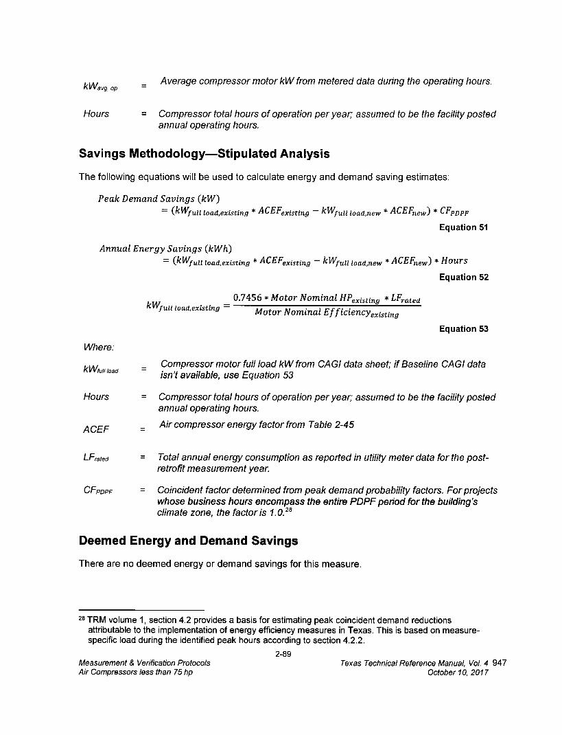
kWavg, op Average compressor motor kW from metered data during the operating hours.

Hours = Compressor total hours of operation per year; assumed to be the facility posted annual operating hours.

Savings Methodology—Stipulated Analysis

The following equations will be used to calculate energy and demand saving estimates:

Peak Demand Savings (kW) * „isting kW — f = (kWfull load,existing ACEF ull load,new * ACEFnew)* CFPDPF

Equation 51


= (kWfull load,existing * ACEFexisting kWfull load,new * ACEFnew)* Hours

Equation 52

kWfull load,existing = 0.7456* Motor Nominal HP - existing * LFrated

Motor Nominal Efficiencyexisting

Equation 53

Where:

Compressor motor full load kW from CAGI data sheet; if Baseline CAG1 data kWfull load isn't available, use Equation 53

Hours = Compressor total hours of operation per year; assumed to be the facility posted annual operating hours.

ACEF = Air compressor energy factor from Table 2-45

LFrated = Total annual energy consumption as reported in utility meter data for the post-retrofit measurement year.

CFPDPF = Coincident factor determined from peak demand probability factors. For projects whose business hours encompass the entire PDPF period for the building's climate zone, the factor is 1.0.28

Deemed Energy and Demand Savings

There are no deemed energy or demand savings for this measure.

28 TRM volume 1, section 4.2 provides a basis for estimating peak coincident demand reductions attributable to the implementation of energy efficiency measures in Texas. This is based on measure-specific load during the identified peak hours according to section 4.2.2.


Claimed Peak Demand Savings A summer peak period value is used for this measure. Refer to Volume 1, Appendix B: Peak Demand Reduction Documentation for further details on peak demand savings and methodology.

Additional Calculators and Tools The regression software used for estimating annual energy use and demand should be clearly specified within the M&V plan and M&V report.

ACEF Development As part of the Long Island Power Authority (LIPA) Clean Energy Initiative, a study of air compressors was conducted. The study collected data on the operating capacity of the compressed air systems. LIPA provided data from this study, which was used as the basis for the ACEF development.

The capacity data was divided into percent of full-load capacity bins to determine the average system loading across the population. This data was weighted by the brake horsepower of each compressor in the population. Then for each capacity bin, the percent power was determined for the control schemes from the Department of Energy air compressor calculator savings calculator (no longer publicly available). The percent power curves were then used with the load profile determined from the study data to develop the average compressor energy factors for each control scheme for this measure.


The EUL for commercial air compressors is set to the Texas default of 10 years pending further research.


The following primary inputs and contextual data should be specified and tracked within the program database to inform the evaluation and apply the savings properly.

• Decision/Action Type; ER, ROB, NC, System Type Conversion

• Building Type

• Climate Zone

• Baseline Equipment Type

• Baseline Equipment Controls

• Baseline Number of Units

• Baseline compressor CAGI data sheets

• For ER ONLY: Baseline Age and Method of Determination (e.g., nameplate, blueprints, customer reported, not available)

• Installed Equipment Type

• Installed Equipment Controls


• Installed Equipment Make and Model

• Installed Number of Units

• Installed compressor CAGI data sheets

• A description of the actual building type, the primary business activity, the business hours, and the operating schedule.


• None


• State of Ohio Energy Efficiency Technical Reference Manual, http://s3.amazonaws.com/zanran storaqe/amppartners.orq/ContentPaqes/2464316647. pdf.

Document Revision History Table 2-46: Air Compressors Less Than 75 HP History


v5.0

10/10/2017

TRM v5.0 origin


2.5 M&V: LOAD MANAGEMENT

2.5.1 Residential Load Curtailment Measure Overview

TRM Measure ID: R-LM-LM

Market Sector: Residential

Measure Category: Demand Response

Applicable Building Types: Single Family, Multifamily, and Manufactured Homes


Decision/Action Types: Operation & Maintenance (O&M)



Savings Methodology: EM&V.

Utilities operate residential load management programs to obtain demand savings: to the extent energy savings are also estimated, they are estimated as a function of the estimated demand savings.29 Demand savings calculations are performed using utility customer interval energy demand data from IDRs or Advanced Meters. Measured and verified Demand Savings for the curtailment period is presented here.

Measure Description

Measures participating in a residential load management program may be air-conditioners, heat pumps, swimming pool pumps, or other electricity loads as specified by utility program designs. Specific methods of load management for this measure are not defined and are determined by individual programs. The savings reflect the cumulative effect of all participant actions to reduce residence-wide demand during a load management event.


A project will be eligible for incentives and reporting demand and energy savings when continuous demand interval recording capability (30-minute intervals or less) and sufficient interval data exists to measure and verify sufficient comparison-days to establish demand baselines as well as interval demands during load management events.

29Some utilities may determine energy savings associated with load management events, which would be calculated as the difference between the baseline and curtailment kW values times the length of the event(s).

2-92 Measurement & Verification Protocols Texas Technical Reference Manual, Vol 4 950 Residential Load Curtailment October 10, 2017

Baseline Condition

The baseline condition is an individual participants load that would have occurred had the load management event and subsequent demand response activities not taken place. 30


Not applicable.



Verified Demand Savings = Baseline Period kW — Curtailment kW

Equation 54

Where:

Baseline Period kW

Curtailment kW

= Baseline average demand calculated according to the High 3 of 5 Baseline Method

= Average demand measured during the curtailment period

High 3 of 5 Baseline with Day-of Adjustment

A High X of Y baseline considers the Y most recent days preceding an event and uses the data from the X days with the highest load within those Y days to calculate the baseline. Day-of adjustments are used to scale the baseline load estimate to the load conditions on the day of the event using data from the two hours prior to the time on the event day when participants were notified of the pending call for curtailment.

Applying this concept to the residential load management measure, the high 3 of 5 baseline for a given curtailment event is estimated by first identifying the five non-holiday weekdays immediately preceding the event in which no prior program curtailment events were called, and calculating each participants average demand during the same hours as the hours for which the curtailment event was implemented on each of those five days. The three highest of these five average like day demand values are then averaged to estimate the "unadjusted high three baseline".

The day-of baseline adjustment is estimated by comparing participants' average demand for electricity on the day of the event during the two hours prior to notification of the pending event (the "adjustment period") to participants' average demand for electricity on the "high three" days during those same two hours. In the situation where notification may not be

3° Some utilities may determine energy savings associated with load management events, which would be calculated as the difference between the baseline and curtailment kW values times the length of the event(s).

2-93 Measurement & Verification Protocols Texas Technical Reference Manual, Vol. 4 951 Residential Load Curtailment October 10, 2017

given, the two hours preceding one hour before the event begins on the event day and baseline days will be used as the adjustment period. The average load of the adjustment period on the event day are compared to the average load of the adjustment periods from the baseline days. The difference (positive or negative) between day-of demand and high three baseline day demand in the adjustment period is the uncapped additive adjustment. To apply the adjustment period to the unadjusted baseline, one of two options are selected in the following steps:

1) Calculate an uncapped additive adjustment. The uncapped additive adjustment is the difference of the adjustment period hours load of the event day subtracted from the baseline days' average adjustment period load. For example, if the baseline days have an adjustment period average load of 3.20 kW and the event day has an adjustment period load of 3.80 kW, the uncapped additive adjustment is 3.80 kW (-) 3.20 kW = 0.60 kW.

2) Calculate an adjustment cap. The adjustment cap is 80 percent of the baseline days' average load during the event hours. For example, if a participant has a load of 4.00 kW during the baseline days' event hours, the adjustment cap is 4.00 kW (x) 0.80 = 3.2 kW.

3) Select the lowest of the adjustment cap and the absolute value of the uncapped additive adjustment to be the additive adjustment. Using the examples of the preceding two steps, the uncapped additive adjustment (0.60 kW) has the lowest magnitude between the two numbers and is selected as the additive adjustment.

4) Add the additive adjustment to the unadjusted High 3 of 5 baseline to calculate the final baseline used for calculating changes to consumption for the demand response event.

Following the calculation of the baseline using the High 3 of 5 method, the following steps are taken to arrive at an events total savings and program savings for the year:

1) For an individual meter, the change in consumption is calculated by subtracting the baseline from the average load recorded during the event. If the result is positive, the meter exhibits savings, whereas a negative result indicates an increase in consumption during the event.

2) For a given demand response event, sum the change in consumption of all participating meters. If documented, those meters enrolled in the program that opt-out of an event may be removed from the summation. If opt-out meters are not documented, an enrolled meter will be considered to have participated in the event. The sum represents the events total change in consumption, presumed to be positive and representing savings.

3) With each events savings results, average the event-level savings. The average of the events' savings represent the program year savings.

An example, below, illustrates the entirety of applying the High 3 of 5 method to calculate load management savings for a single residential participant.


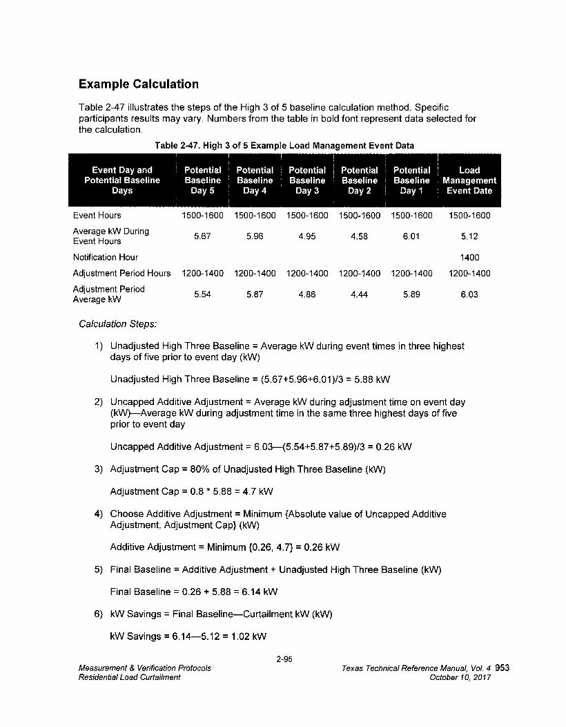
Example Calculation

Table 2-47 illustrates the steps of the High 3 of 5 baseline calculation method. Specific participants results may vary. Numbers from the table in bold font represent data selected for the calculation.

Table 2-47. High 3 of 5 Example Load Management Event Data

Event Day and Potential Baseline

Days

Potential Baseline

Day 5

I Potential Baseline

Day 4

Potential Baseline

Day 3

Potential Baseline

Day 2

Potential Baseline

Day 1

I Load Management Event Date

Event Hours 1500-1600 1500-1600 1500-1600 1500-1600 1500-1600 1500-1600

Average kW During Event Hours 5.67 5.96 4.95 4.58 6.01 5.12

Notification Hour 1400

Adjustment Period Hours 1200-1400 1200-1400 1200-1400 1200-1400 1200-1400 1200-1400

Adjustment Period Average kW 5.54 5.87 4.86 4.44 5.89 6.03

Calculation Steps:

1) Unadjusted High Three Baseline = Average kW during event times in three highest days of five prior to event day (kW)

Unadjusted High Three Baseline = (5.67+5.96+6.01)/3 = 5.88 kW

2) Uncapped Additive Adjustment = Average kW during adjustment time on event day (kW)—Average kW during adjustment time in the same three highest days of five prior to event day

Uncapped Additive Adjustment = 6.03—(5.54+5.87+5.89)/3 = 0.26 kW

3) Adjustment Cap = 80% of Unadjusted High Three Baseline (kW)

Adjustment Cap = 0.8 * 5.88 = 4.7 kW

4) Choose Additive Adjustment = Minimum {Absolute value of Uncapped Additive Adjustment, Adjustment Cap} (kW)

Additive Adjustment = Minimum {0.26, 4.7) = 0.26 kW

5) Final Baseline = Additive Adjustment + Unadjusted High Three Baseline (kW)

Final Baseline = 0.26 + 5.88 = 6.14 kW

6) kW Savings = Final Baseline—Curtailment kW (kW)

kW Savings = 6.14-5.12 = 1.02 kW


Additional Calculation Considerations

In the case that individual meters fail to record data sufficient for applying the High 3 of 5 calculation method, savings may still be calculated under the following conditions and method:

• Less than one percent of participating residential customers experience meter recording failures

• The customer can be confirmed as having participated via the practices of the sponsor operating the program or lack of opt-out notification

• The EM&V team is engaged to discuss applying the average savings and any program participation segmentation, and the specific cases are documented

• Savings for the residential segment will be calculated using the average savings of the segment as calculated via the High 3 of 5 method for the balance of the program or segment.

When selecting baseline days in the High 3 of 5 method, in some cases it is possible that some days have the same load for an individual participant, potentially leading to more than three days that could be selected for the baseline days. In the event that four or more days could be selected as baseline days based on their loads during event hours, the days with the highest loads and closest to the event should be picked for the baseline.

Program year kW load management event savings will be calculated as the average savings of all events. Rounding of savings should occur only at the total program event level or program year average event savings level. Program year kWh load management event savings will be calculated as the average event kW savings multiplied by the total number of event hours in the program year. Deemed Energy and Demand Savings Tables

Not applicable.

Claimed Peak Demand Savings A summer peak period value is used for this measure, based on calculation methodology described for this measure.


Not applicable.

Measure Lifetime

Not applicable.


The following data and information shall be tracked and provided to the EM&V team to enable savings verification:

• For each participant for which savings are being claimed, kWh consumption at intervals no greater than 30-minutes for each event day and for no less than five non-holiday and non-


weekend days prior to each event day. Interval data shall be time-stamped with the date and no less than the time period ending the interval.

• Documentation describing the time stamp and whether the time stamp reflects the forward looking period or period preceding the time stamp

• A list of all load management events affecting residential participants, describing their date, the time the event started, and the time the event ended.

• A list of all participants and addresses with a variable linking to the load or energy consumption interval data and that describes their enrollment date, load management control commissioning date, and any events in which the participant did not participate due to enrollment or equipment installation timing, equipment failures, or other factors known to the implementer or utility.

• Tools, calculators or other datasets that may be useful to the EM&V Team, based on discussion between the EM&V Team, utilities, and/or program implementer. The process for calculating kW and kWh savings should be provided in the program documentation, including any summation and rounding practices.

• Memos, reports, or results of any equipment test or metering data that provides perspectives, calculations, or metrics related to failure rates of load control receivers, thermostats or similar devices used to control participant loads during events.

The evaluation reserves the option to conduct participant level independent metering studies to inform the verification of load management program savings.


Not applicable.


None.


Not applicable.


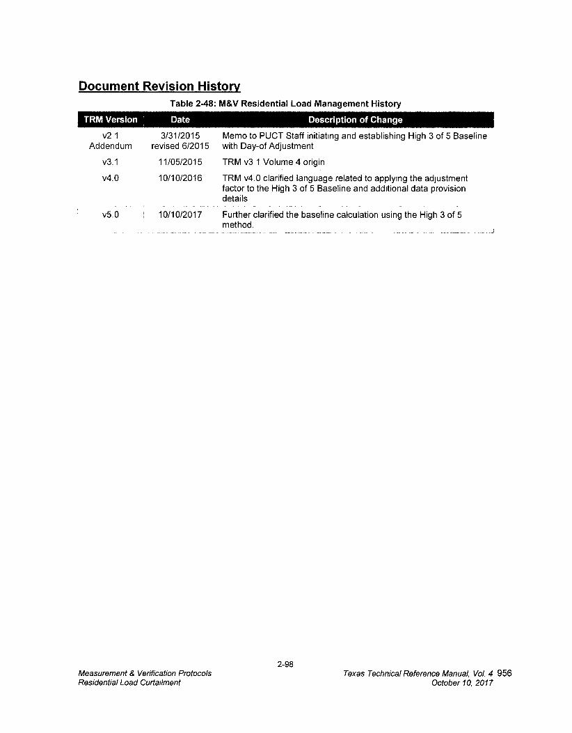
Document Revision History Table 2-48: M&V Residential Load Management History

TRM Version Date

Description of Change

v2 1 Addendum

v3.1

v4.0

3/31/2015 revised 6/2015

11/05/2015

10/10/2016

Memo to PUCT Staff initiating and establishing High 3 of 5 Baseline with Day-of Adjustment

TRM v3 1 Volume 4 origin

TRM v4.0 clarified language related to applying the adjustment factor to the High 3 of 5 Baseline and additional data provision

, details

v5.0 10/10/2017 Further clarified the baseline calculation using the High 3 of 5 I method.

_


2.5.2 Nonresidential Load Curtailment Measure Overview

TRM Measure ID: NR-LM-LM

Market Sector: Nonresidential

Measure Category: Demand Response

Applicable Building Types: Any building that meets minimum facility demand requirements (see Table 2-18)


Decision/Action Type: Operation & Maintenance (O&M)



Savings Methodology: EM&V.

Utilities operate nonresidential load management programs to obtain demand savings: to the extent energy savings are also estimated, they are estimated as a function of the estimated demand savings.31 Demand savings calculations are performed using utility customer interval energy demand data from IDRs or Advanced Meters. Measured and verified Demand Savings for the curtailment period is presented here.

Measure Description

This document presents the deemed savings methodology for participation in a load management program that involves the curtailment of an interruptible load during the summer peak period. Project sponsors, who have agreed to deliver demand savings to the utility from the utilitys customer, must commit to an availability of curtailed load throughout the Summer Peak Demand Period. These project sponsors may include national or local energy efficiency service providers (EESPs), retail electricity providers (REPs) or individual customers. Different utilities offer different details on their programs, but they all have similar eligibility criteria, listed below:


A project will be eligible for rebates under the Load Management SOP program if the following criteria are met:

Each meter included in a project must include a total potential demand savings of a specified minimum kW (varies by utility, as seen in Table 2-49) during the summer peak period.

31Some utilities may determine energy savings associated with load management events, which would be calculated as the difference between the baseline and curtailment kW values times the length of the event(s).

2-99 Measurement & Verification Protocols Texas Technical Reference Manual, Vol. 4 957 Nonresidential Load Curtailment October 10, 2017

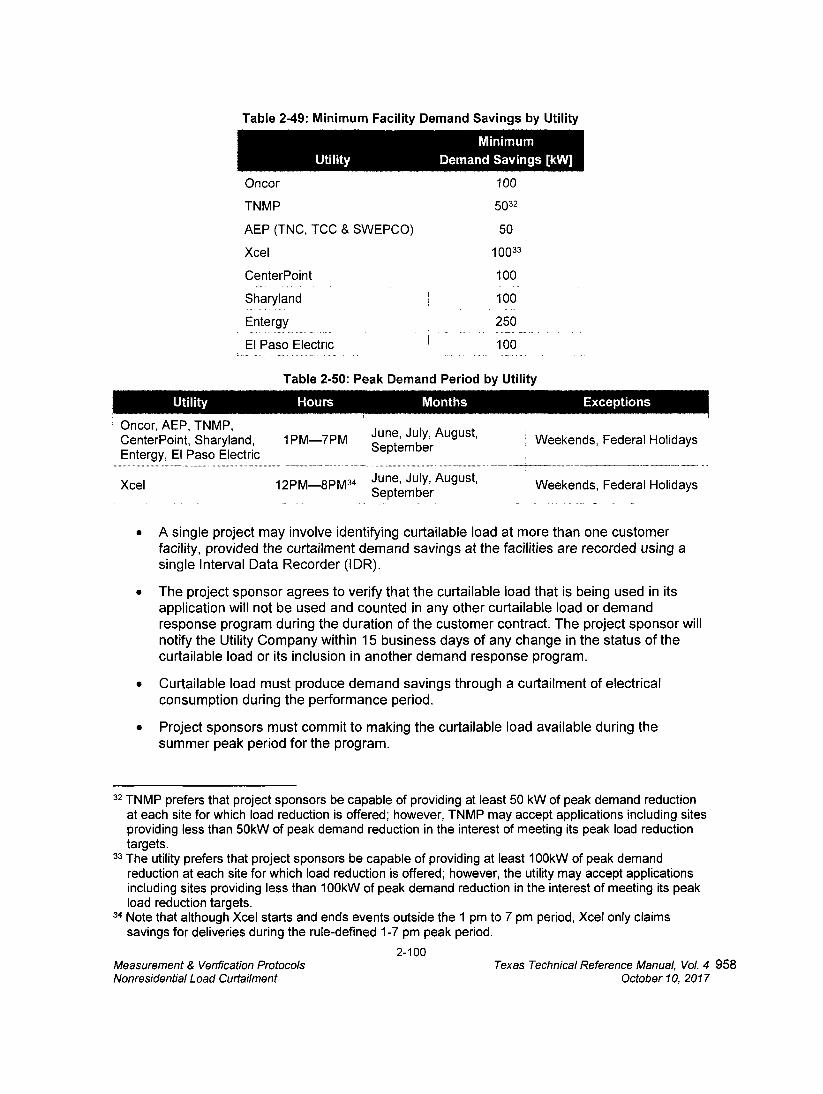
Table 2-49: Minimum Facility Demand Savings by Utility

Utility Minimum

Demand Savings [kW]

Oncor 100

TNMP 5032

AEP (TNC, TCC & SWEPCO) 50

Xcel 10033

CenterPoint _

100

Sharyland 100

Entergy 250

El Paso Electric _

100

Table 2-50: Peak Demand Period by Utility

Utility Hours Months Exceptions

Oncor, AEP, TNMP, CenterPoint, Sharyland, Entergy, El Paso Electric

1PM-7PM June, July, August, September

; Weekends, Federal Holidays

Xcel 12PM-8PM34 June, July, August, September

Weekends, Federal Holidays

• A single project may involve identifying curtailable load at more than one customer facility, provided the curtailment demand savings at the facilities are recorded using a single Interval Data Recorder (IDR).

• The project sponsor agrees to verify that the curtailable load that is being used in its application will not be used and counted in any other curtailable load or demand response program during the duration of the customer contract. The project sponsor will notify the Utility Company within 15 business days of any change in the status of the curtailable load or its inclusion in another demand response program.

• Curtailable load must produce demand savings through a curtailment of electrical consumption during the performance period.

• Project sponsors must commit to making the curtailable load available during the summer peak period for the program.

32 TNMP prefers that project sponsors be capable of providing at least 50 kW of peak demand reduction at each site for which load reduction is offered; however, TNMP may accept applications including sites providing less than 50kW of peak demand reduction in the interest of meeting its peak load reduction targets.

33 The utility prefers that project sponsors be capable of providing at least 100kW of peak demand reduction at each site for which load reduction is offered; however, the utility may accept applications including sites providing less than 100kW of peak demand reduction in the interest of meeting its peak load reduction targets.

34 Note that although Xcel starts and ends events outside the 1 pm to 7 pm period, Xcel only claims savings for deliveries during the rule-defined 1-7 pm peak period.

2-100 Measurement & Venfication Protocols Texas Technical Reference Manual, Vol. 4 958 Nonresidential Load Curtailment October 10, 2017

• Be served by an Interval Data Recorder (IDR) and/or smart meter that is monitored by the utility. A sponsor owned meter may be substituted in the event of a non-systemic utility-owned IDR meter failure. When using a sponsor owned meter, all data must otherwise conform to the High 5 of 10 method and be used for both the baseline and event-day calculations. Documentation of the case must be provided along with all supporting meter data.

• Customer agrees to respond to at least one event (scheduled or unscheduled) per year for the purpose of verifying the load reduction is available for potential calls. Scheduled events are used to provide an estimate of the load reduction in the event that no unscheduled interruptions occur during the season.

• For sponsors on a curtailment tariff, if the event or baseline periods include a tariff-based curtailment, the event day performance for the load management program will be net of firm delivery under the tariff. Documentation must be provided to describe the overlap of load management and tariff-based curtailments along with supporting firm delivery contract amounts.

The following loads are excluded from consideration:

• A customer who has load contracted with a REP where that contract prevents the load from participating in a curtailment.

• Loads where curtailment would result in negative environmental or health effects.

• Curtailable load that receives an incentive through any other energy efficiency program.

• Curtailable load that takes electric service at transmission voltage and that serves a for-profit end-use customer.

Baseline Condition

Standard facility operation.


Requires Load Management customers to participate in a certain number of unscheduled interruptions. Programs will provide a minimum of 30-minute advanced notice, allowing facility managers sufficient time to use non-automated approaches. Another option is for facilities to install a load-control device on specific end-uses, equipment, or circuit loads.

Additional Utility Program Details

Each utility in Texas provides slightly different guidelines for its load management program. These details differ in the length of the unscheduled interruptions (also called curtailments), the maximum number or maximum number of hours of unscheduled interruptions, and the length of notification provided to the project sponsor. Table 2-51 highlights these differences.

Each utility states that participants will be willing to participate in a maximum number of unscheduled interruptions, or a maximum number of scheduled (test) interruption hours. In addition to these, all utilities require that a scheduled interruption be performed. The purpose of this is to ensure that the project sponsor will be able to curtail the requested kW within the required notification time and to provide an estimate of the load reduction in the event that no


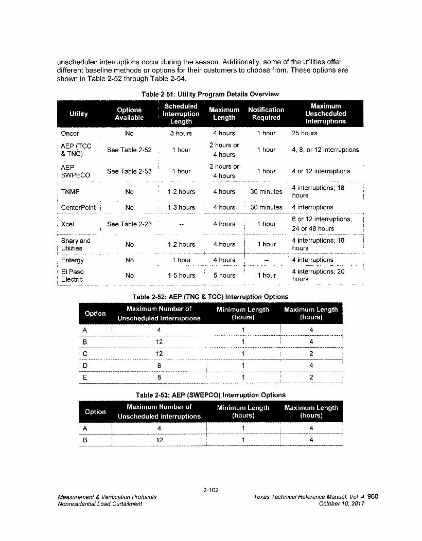
Oncor

No

3 hours

AEP (TCC & TNC)

See Table 2-52 1 hour

4 hours

2 hours or

4 hours

1 hour

25 hours

1 hour 4, 8, or 12 interruptions

1 hour

Maximum Number of Option

Unscheduled Interruptions Minimum Length Maximum Length

(hours) (hours)

1 4 4 A

4 12

2 12

4 D

1 2


Unscheduled Interruptions Minimum Length Maximum Length

(hours) (hours)

1 12

1 A 4 4

Table 2-53: AEP (SWEPCO) Interruption Options

unscheduled interruptions occur during the season. Additionally, some of the utilities offer different baseline methods or options for their customers to choose from. These options are shown in Table 2-52 through Table 2-54.

Table 2-51: Utility Program Details Overview

Utility , Scheduled Maximum

Options Interruption

Maximum Notification Unscheduled

Available Length Required Length Interruptions

1 AEP , 2 hours or

See Table 2-53 1 hour 1 , 1 hour 4 or 12 i SWPECO 4 hours

nterruptions ,

TNMP No 1-2 hours 4 hours 30 minutes 4 interruptions; 18

hours

CenterPoint No 1-3 hours • 4 hours 30 minutes 4 interruptions

6 or 12 interruptions; Xcel See Table 2-23 4 hours 1 hour

24 or 48 hours

No

1-2 hours 4 hours 1 hour

No

1 hour

4 hours

No

1-5 hours 5 hours

Table 2-52: AEP (TNC & TCC) Interruption Options

4 interruptions; 18 hours

4 interruptions

4 interruptions; 20 hours

„

Sharyland Utilities

Entergy

El Paso ; Electric

2-102 Measurement & Verification Protocols

Texas Technical Reference Manual, Vol 4 960

Nonresidential Load Curtailment

October 10, 2017

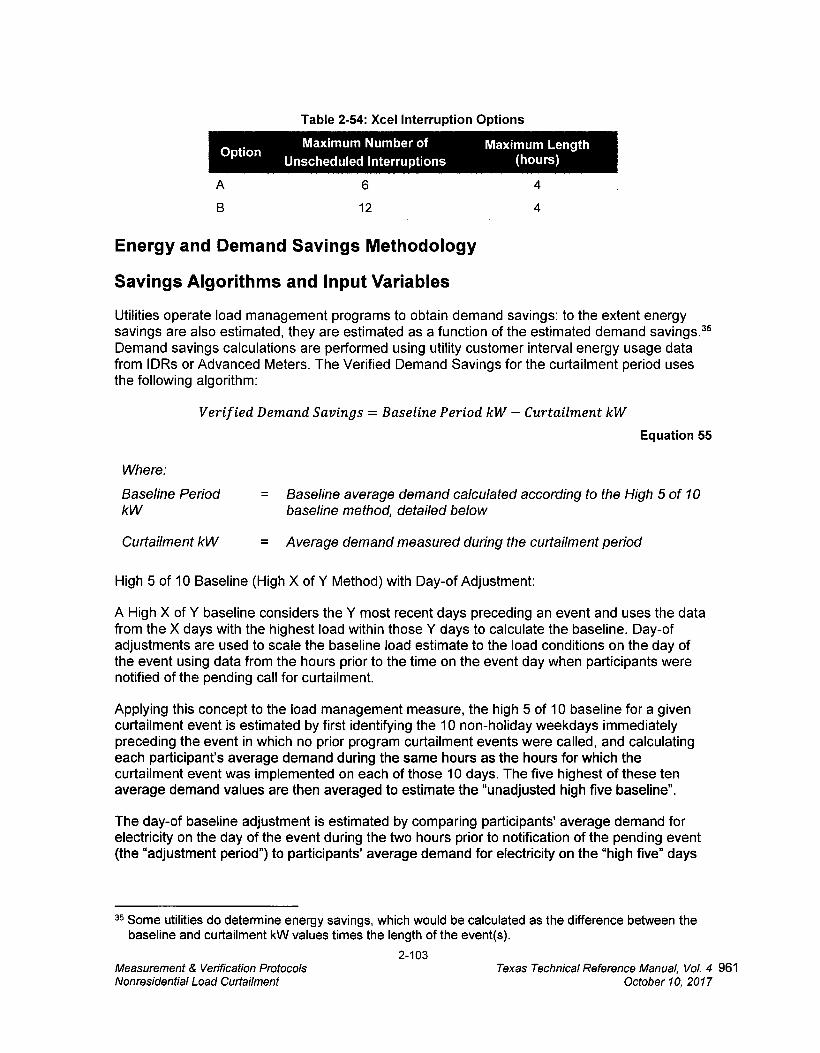
Table 2-54: Xcel Interruption Options


Unscheduled Interruptions Maximum Length

(hours)

A

6

4

12

4



Utilities operate load management programs to obtain demand savings: to the extent energy savings are also estimated, they are estimated as a function of the estimated demand savings.35 Demand savings calculations are performed using utility customer interval energy usage data from IDRs or Advanced Meters. The Verified Demand Savings for the curtailment period uses the following algorithm:

Verified Demand Savings = Baseline Period kW — Curtailment kW

Equation 55

Where:

Baseline Period = Baseline average demand calculated according to the High 5 of 10 kW baseline method, detailed below

Curtailment kW = Average demand measured during the curtailment period

High 5 of 10 Baseline (High X of Y Method) with Day-of Adjustment:

A High X of Y baseline considers the Y most recent days preceding an event and uses the data from the X days with the highest load within those Y days to calculate the baseline. Day-of adjustments are used to scale the baseline load estimate to the load conditions on the day of the event using data from the hours prior to the time on the event day when participants were notified of the pending call for curtailment.

Applying this concept to the load management measure, the high 5 of 10 baseline for a given curtailment event is estimated by first identifying the 10 non-holiday weekdays immediately preceding the event in which no prior program curtailment events were called, and calculating each participants average demand during the same hours as the hours for which the curtailment event was implemented on each of those 10 days. The five highest of these ten average demand values are then averaged to estimate the "unadjusted high five baseline.

The day-of baseline adjustment is estimated by comparing participants average demand for electricity on the day of the event during the two hours prior to notification of the pending event (the "adjustment period") to participants' average demand for electricity on the "high five" days

35 Some utilities do determine energy savings, which would be calculated as the difference between the baseline and curtailment kW values times the length of the event(s).


during those same two hours. The difference (positive or negative) between day-of demand and high five demand in the adjustment period is the "uncapped additive adjustment". In the situation where notification may not be given, the two hours preceding one hour before the event begins on the event day and baseline days will be used as the adjustment period. The average load of the adjustment period on the event day are compared to the average load of the adjustment periods from the baseline days. The difference (positive or negative) between day-of demand and high three baseline day demand in the adjustment period is the uncapped additive adjustment. To apply the adjustment period to the unadjusted baseline, one of two options are selected in the following steps:

1) Calculate an uncapped additive adjustment. The uncapped additive adjustment is the difference of the adjustment period hours load of the event day subtracted from the baseline days' average adjustment period load. For example, if the baseline days have an adjustment period average load of 530.20 kW and the event day has an adjustment period load of 575.80 kW, the uncapped additive adjustment is 575.80 kW (-) 530.20 kW = 45.60 kW.

2) Calculate an adjustment cap. The adjustment cap is 50 percent of the baseline days' average load during the event hours. For example, if a participant has a load of 504.00 kW during the baseline days' event hours, the adjustment cap is 504.00 kW (x) 0.50 = 252.00 kW.

3) Select the lowest of the adjustment cap and the absolute value of the uncapped additive adjustment to be the additive adjustment. Using the examples of the preceding two steps, the uncapped additive adjustment (45.60 kW) has the lowest magnitude between the two numbers and is selected as the additive adjustment.

4) Add the additive adjustment to the unadjusted High 5 of 10 baseline to calculate the final baseline used for calculating savings.

An example, below, illustrates the entirety of applying the High 5 of 10 method to calculate load management savings for a single residential participant.

Example Calculation

Table 2-55 serves to illustrate the steps of the High 5 of 10 baseline calculation method. Specific participants results may vary. Numbers from the table in bold font represent data selected for the calculation.

2-104 Measurement & Verification Protocols Texas Technical Reference Manual, Vol 4 962 Nonresidential Load Curtailment October 10, 2017

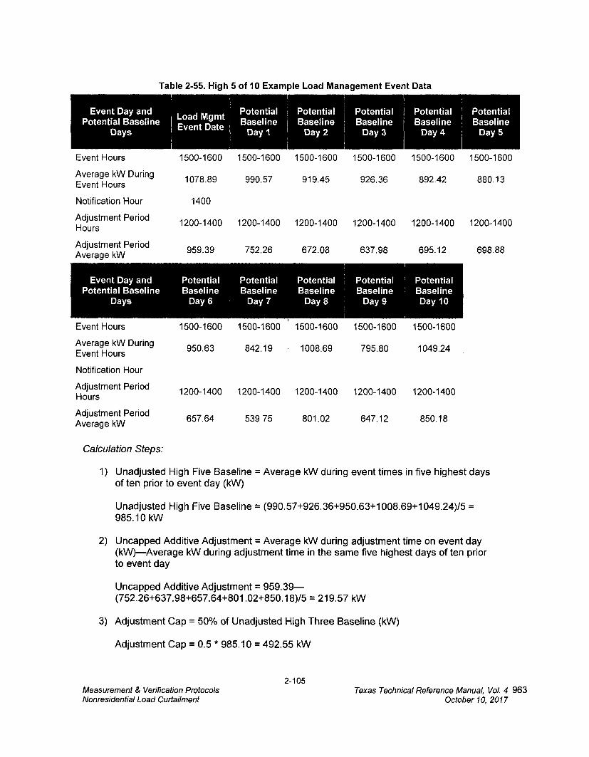
Table 2-55. High 5 of 10 Example Load Management Event Data

Event Day and Load Mgmt Potential Baseline ! Event Date Days

Potential Potential Baseline Baseline

Day '1 Day 2

Potential Potential Potential Baseline Baseline I Baseline

Day 3 Day 4 Day 5

Event Hours

Average kW During Event Hours

Notification Hour

Adjustment Period Hours

Adjustment Period Average kW

1500-1600 1500-1600 1500-1600 1500-1600 1500-1600 1500-1600

1078.89 990.57 919.45 926.36 892.42 880.13

1400

1200-1400 1200-1400 1200-1400 1200-1400 1200-1400 1200-1400

959.39 752.26

672.08 637.98

695.12 698.88

Event Day and Potential Potential Potential Potential Potential Potential Baseline Baseline Baseline Baseline Baseline Baseline

Days Day 6 Day 7 Day 8 Day 9 Day 10

Event Hours

Average kW During Event Hours

Notification Hour

Adjustment Period Hours

Adjustment Period Average kW

1500-1600 1500-1600 1500-1600 1500-1600 1500-1600

950.63 842.19 1008.69 795.80 1049.24

1200-1400 1200-1400 1200-1400 1200-1400 1200-1400

657.64

539 75 801.02

647.12 850.18

Calculation Steps:

1) Unadjusted High Five Baseline = Average kW during event times in five highest days of ten prior to event day (kW)

Unadjusted High Five Baseline = (990.57+926.36+950.63+1008.69+1049.24)/5 = 985.10 kW

2) Uncapped Additive Adjustment = Average kW during adjustment time on event day (kW)—Average kW during adjustment time in the same five highest days of ten prior to event day

Uncapped Additive Adjustment = 959.39— (752.26+637.98+657.64+801.02+850.18)/5 = 219.57 kW

3) Adjustment Cap = 50% of Unadjusted High Three Baseline (kW)

Adjustment Cap = 0.5 * 985.10 = 492.55 kW


4) Choose Additive Adjustment = Minimum {Absolute value of Uncapped Additive Adjustment, Adjustment Cap} (kW)

Additive Adjustment = Minimum {219.57, 492.55} = 219.57 kW

5) Final Baseline = Additive Adjustment + Unadjusted High Three Baseline (kW)

Final Baseline = 219.57 + 985.10 = 1204.67 kW

6) kW Savings = Final Baseline—Curtailment kW (kW)

kW Savings = 1204.67-1078.89 = 125.78 kW

Additional Calculation Considerations

In the case that individual meters fail to record data sufficient for applying the High 5 of 10 calculation method, savings will not be calculated.

When selecting baseline days in the High 5 of 10 method, in some cases it is possible that some days have the same load for an individual participant, potentially leading to more than five days that could be selected for the baseline days. In the event that six or more days could be selected as baseline days based on their loads during event hours, the days with the highest loads and closest to the event should be picked for the baseline.

Program year kW load management event savings will be calculated as the sum of each sponsors average savings of all events in which the sponsor participated. Rounding of savings should occur only at the sponsor level or program year average event savings level. Program year kWh load management event savings will be calculated as the sum of each sponsors hourly kW savings for the program year.


Not applicable.

Program Tracking Data & Evaluation Requirements • IDR or Advanced Meter data associated with the project will be provided by the project

sponsor or retrieved by the utility following an event. Depending on the utility, the data will be provided at 30-minute increments (or smaller) to evaluate both baseline demand usage and demand usage during curtailment.

• Documentation describing the time stamp and whether the time stamp reflects the forward looking period or period preceding the time stamp

• Utilities should provide a description of their practices related to whether scheduled or test events are or are not included in their program year kW savings results. kWh savings will be calculated from all events.

• A list of all load management events affecting nonresidential participants within the program year, describing the date of each event, the time the event started, and the time the event ended.


• A list of all participants and addresses with a variable linking to the load or energy consumption interval data and that describes their enrollment date, load management control commissioning date, and any events in which the participant did not participate due to enrollment or equipment installation timing, equipment failures, or other factors known to the implementer or utility.

• Tools, calculators or other datasets that may be useful to the EM&V Team, based on discussion between the EM&V Team, utilities, and/or program implementer. The process for calculating kW and kWh savings should be provided in the program documentation, including any summation and rounding practices.



None.

Relevant Standards and Reference Sources • El Paso Electric: EOE 2010 Load Management Program Manual.

http://www.epelectricefficiency.com/files/EPE LM 10 ProgramManual.pdf. Accessed 09/06/2013.

• AEP: Texas North Company Load Management SOP 2013 Program Manual. http://www.aepefficiencv.com/loadmanagementfTNC/2013 TNC LM%20Manual Agree ment.pdf. Accessed 02/28/14.

• AEP: Texas Central Company Load Management SOP 2013 Program Manual. http://www.aepefficiency.com/loadmanagementfTCC/2013_TCC_LM_Manual_Agreement.p df. Accessed 09/06/2013; manual no longer available online.

• AEP: Southwestern Electric Power Company Load Management 2013 Program Manual. http://www.swepcogridsmart.com/texas/downloads/Load%20Management Program Manua I.pdf. Accessed 09/06/2013.

• Entergy: 2013 Load Management Handbook. http://www.entergy- texas.com/content/energy efficiencv/documents/Load Management Handbook.pdf. Accessed 09/06/2013.

• CenterPoint: EnergyShare 2013 Program Manual. http://www.centerpointelectric.com/staticfiles/CNP/Common/SiteAssets/doc/2013 Load Ma nagement Program Manual.pdf. Accessed 09/06/2013.

• Texas-New Mexico: Load Management 2013 SOP. http://tnmpefficiencv.com/downloads/Load Management Program Manual.pdf. Accessed 09/06/2013.

• Xcel Energy: 2013 Load Management Pilot Standard Offer Program. http://www.xcelefficiency.comiTX/Xcel_LM_Manual_2013.pdf. Accessed 09/06/2013; pilot program has been replaced.

• Sharyland Utilities: 2013 Load Management SOP. http://www.sharylandefficiency.com/load- management/Sharyland_2013_Peak_Load_Mgmt_Program_Manual.pdf Accessed 09/06/2013; 2013 Manual no longer available online.


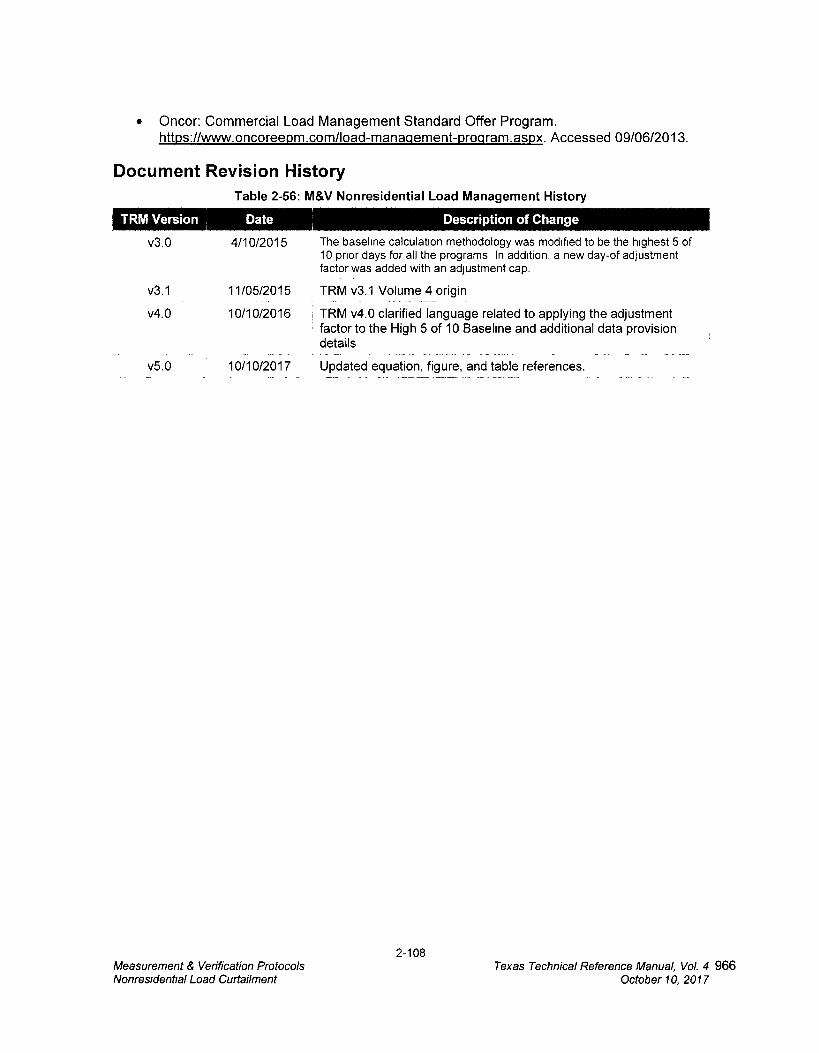
• Oncor: Commercial Load Management Standard Offer Program. https://www.oncoreepm.com/load-management-procram.asox. Accessed 09/06/2013.

Document Revision History

Table 2-56: M&V Nonresidential Load Management History


v3.0

4/10/2015

The baseline calculation methodology was modified to be the highest 5 of 10 prior days for all the programs In addition, a new day-of adjustment factor was added with an adjustment cap.

v3.1 11/05/2015 TRM v3.1 Volume 4 origin _

v4.0 10/10/2016 TRM v4.0 clarified language related to applying the adjustment factor to the High 5 of 10 Baseline and additional data provision details

v5.0 10/10/2017 Updated equation, figure, and table references.


APPENDIX A: M&V METERING SCHEDULE

1.0 Arrive on site and meet customer 1.1 Turn unit on to stabilize and make sure the unit is in full cooling mode (Variable speed

blowers are on high and all compressors in multi-compressor systems are operating). 1.2 Record customer information:

a. Address f. Utility Account Number (from utility bill) b. City g. Altitude [ft] c. Zip h. Residential Program or Commercial Program d. County i. Building Type e. Email j. Phone Number

2.0 Test In: Perform TI procedure to determine system's baseline cooling capacity and energy efficiency ratio (EER). 2.1 Record Unit Information 2.2 Measure and record airflow using 1 of the following methods:

a. Air Flow Method 1: Handheld Anemometer b. Air Flow Method 2: Generic Fan Chart

2.3 Air Flow Power Consumption a. Determine the blower motor type as either "PSC" or "ECM." b. Measure and record the blower voltage and current.

2.4 Condenser and Compressor Measurements a. Compressor Type (Scroll or Reciprocating) b. Refrigerant Type (R22 or R410) c. Metering Device (Fixed Orifice, TXV or Capillary Tube) d. Condenser Model Number e. Condenser Serial Number f. Compressor Phase (Single or Three) g. Multiple Compressor System (Check box for participating utilities) h. Measure and Record Compressor Volts i. Measure and Record Compressor Current j. Measure and Record Ambient Air Dry Bulb Temperature k Measure and Record Ambient Air Wet Bulb Temperature if Required

2.5 Enter Information from Refrigerant Analyzer: a. Suction Pressure [PSI] e. Vapor Line Temperature (VLT) [°F] b. Discharge Pressure [PSI] f. Liquid Line Temperature (LLT) [°F] c. Evaporator Temperature [°F] g. Superheat [°F] d. Condenser Temperature [°F] h. Subcooling [°F]

2.6 Measure and Record Supply and Return Air Conditions: a. Return Air Dry Bulb Temperature[°F] b. Return Air Wet Bulb Temperature[°F] c. Supply Air Dry Bulb Temperature [°F] d. Supply Air Wet Bulb Temperature [°F]

2.7 Review System Performance

A-1 Measurement & Verification Protocols Texas Technical Reference Manual, Vol. 4 967 Appendix A: M&V Metering Schedule October 10, 2017

3.0 Perform Corrective Measures as Needed 3.1 Clean Condenser—required 3.2 Clean Evaporator—required 3.3 Clean Blower—required 3.4 Verify clean filter: change or clean as needed—required

3.5 Verify Airflow within range (+/- 15% of 400 cfm/ton)—required

3.6 Check refrigerant charge; adjust to Manufacturer's Spec's as needed 4.0 Test Out: The Test Out (TO) procedure requires measurements that are used to

determine the performance characteristics of the cooling system after all corrective measures have been implemented.

4.1 Air Flow—Use same method as Test In 4.2 Air Flow Power Consumption

a. For ECMs, make sure it is operating in full cooling mode during the entire tune-up.

b. Measure and record the blower voltage and current. 4.3 Measure and record Supply and Return Air Conditions:

a. Return Air Dry Bulb Temperature [°F] b. Return Air Wet Bulb Temperature [°F] c. Supply Air Dry Bulb Temperature [°F] d. Supply Air Wet Bulb Temperature [°F]

4.4 Condenser and Compressor Measurements a. Compressor Volts b. Compressor Current c. Ambient Air Dry Bulb Temperature d. Ambient Air Wet Bulb Temperature

4.5 Information from Refrigerant Analyzer: a. Suction Pressure [PSI] b. Discharge Pressure [PSI] c. Evaporator Temperature [°F] d. Condenser Temperature [°F] e. Vapor Line Temperature (VLT) [°F] f. Liquid Line Temperature (LLT) [°F] g. Superheat [°F] h. Subcooling [°F]

4.6 Review System Performance

5.0 Generate invoice: A customer signed invoice is required for participation in the program. The following information must be shown on the invoice:

5.1 Customer Address 5.2 Contractor Name and Address 5.3 Project Number Listed on the DCVF 5.4 Corrective Measures Performed 5.5 Charge for Services Performed 5.6 Rebate Amount Applied to Charges

A-2 Measurement & Verification Protocols Texas Technical Reference Manual, Vol. 4 968 Appendix A. M&V Metering Schedule October 10, 2017

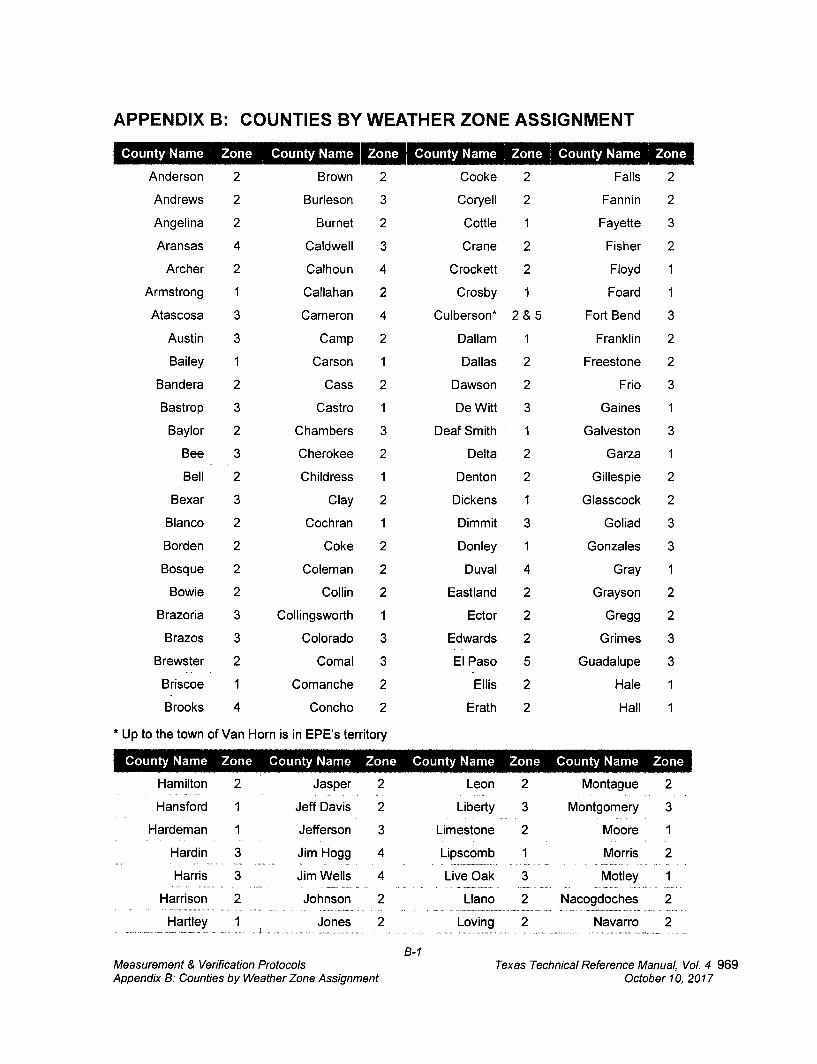
APPENDIX B: COUNTIES BY WEATHER ZONE ASSIGNMENT

Zone County Name ' Zone County Name Zone County Name Zone County Name

Anderson 2 Brown 2 Cooke 2 Falls 2

Andrews 2 Burleson 3 Coryell 2 Fannin 2

Angelina 2 Burnet 2 Cottle 1 Fayette 3

Aransas 4 Caldwell 3 Crane 2 Fisher 2

Archer 2 Calhoun 4 Crockett 2 Floyd 1

Armstrong 1 Callahan 2 Crosby 1 Foard 1

Atascosa 3 Cameron 4 Culberson* 2 & 5 Fort Bend 3

Austin 3 Camp 2 DaIlam 1 Franklin 2

Bailey 1 Carson 1 Dallas 2 Freestone 2

Bandera 2 Cass 2 Dawson 2 Frio 3

Bastrop 3 Castro 1 De Witt 3 Gaines 1

Baylor 2 Chambers 3 Deaf Smith 1 Galveston 3

Bee 3 Cherokee 2 Delta 2 Garza 1

Bell 2 Childress 1 Denton 2 Gillespie 2

Bexar 3 Clay 2 Dickens 1 Glasscock 2

Blanco 2 Cochran 1 Dimmit 3 Goliad 3

Borden 2 Coke 2 Donley 1 Gonzales 3

Bosque 2 Coleman 2 Duval 4 Gray 1

Bowie 2 Collin 2 Eastland 2 Grayson 2

Brazoria 3 Collingsworth 1 Ector 2 Gregg 2

Brazos 3 Colorado 3 Edwards 2 Grimes 3

Brewster 2 Comal 3 El Paso 5 Guadalupe 3

Briscoe 1 Comanche 2 Ellis 2 Hale 1

Brooks 4 Concho 2 Erath 2 Hall 1

* Up to the town of Van Horn is in EPE's territory

County Name Zone County Name Zone County Name Zone County Name Zone

Hamilton _ 2 Jasper 2 Leon 2 Montague 2

Hansford 1 Jeff Davis 2 Liberty 3 Montgomery 3

Hardennan 1 Jefferson 3 Limestone 2 Moore 1

Hardin _ 3 Jim Hogg _ 4 Lipscomb 1 Morris 2

Harris 3 Jim Wells 4 Live Oak -----_

Motley 1

Harrison Johnson 2 Llano 2 Nacogdoches 2

Hartley Jones 2 Loving 2 Navarro 2

B-1 Measurement & Verification Protocols

Texas Technical Reference Manual, Vol. 4 969

Appendix B: Counties by Weather Zone Assignment October 10, 2017

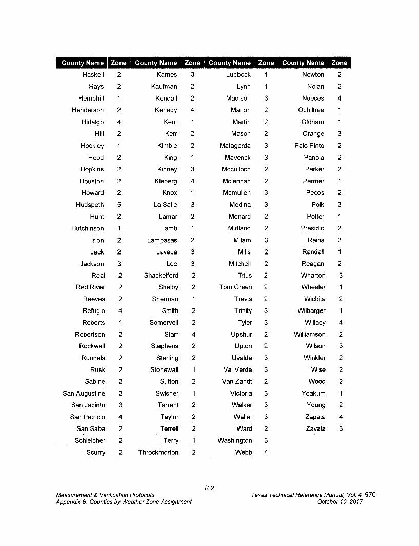
County Name Zone County Name Zone County Name Zone County Name Zone

Haskell 2 Karnes 3 Lubbock Newton

Hays 2 Kaufman 2 Lyn n Nolan

Hemphill 1 Kendall 2 Madison Nueces

Henderson Kenedy 4 Marion Ochiltree

Hidalgo Kent 1 Martin Oldham

Hill Kerr 2 Mason Orange

Hockley Kimble 2 Matagorda Palo Pinto

Hood King 1 Maverick Panola

Hopkins Kinney 3 Mcculloch Parker

Houston Kleberg 4 Mclennan Parmer

Howard Knox 1 Mcmullen Pecos

Hudspeth La Salle 3 Medina Polk

Hunt Lamar 2 Menard Potter

Hutchinson Lamb 1 Midland Presidio

lrion Lampasas 2 Milam Rains

Jack Lavaca 3 Mills Randall

Jackson Lee 3 Mitchell Reagan

Real Shackelford 2 Titus Wharton

Red River Shelby 2 Tom Green Wheeler

Reeves Sherman 1 Travis Wichita

Refugio Smith 2 Trinity Wilbarger

Roberts Somervell 2 Tyler Willacy

Robertson Starr 4 Upshur Williamson

Rockwall Stephens 2 Upton Wilson

Runnels Sterling 2 Uvalde Winkler

Rusk Stonewall 1 Val Verde Wise

Sabine Sutton 2 Van Zandt Wood

San Augustine Swisher 1 Victoria Yoakum

San Jacinto Tarrant 2 Walker Young

San Patricio Taylor 2 Waller Zapata

San Saba Terrell 2 Ward Zavala

Schleicher Terry 1 Washington

Scurry Throckmorton Webb

8-2 Measurement & Verification Protocols Texas Technical Reference Manual, Vol. 4 970 Appendix 8: Counties by Weather Zone Assignment October 10, 2017

Last Revision Date:

October 2017

Public Utility Commission of Texas

Texas Technical Reference Manual

Version 5.0

Volume 5: Implementation Guidance

Program Year (PY) 2018

971

Public Utility Commission of Texas

Texas Technical Reference Manual

Version 5.0

Volume 5: Implementation Guidance

Program Year (PY) 2018

Last Revision Date:

October 2017

972

Table of Contents

1. Introduction 1-1

2. Residential 2-1 2.1 HVAC Early Retirement 2-1

2.1.1 Background 2-1 2.1.2 Rationale for Early Retirement 2-1 2.1.3 Early Retirement in Other Jurisdictions 2-2 2.1.4 Customer Identification and Eligibility for Savings 2-2 2.1.5 EM&V Team Recommendations for Effective Early Retirement 2-2 2.1.6 Savings Calculations: Remaining Useful Lifetime 2-4

3. Commercial 3-1 3.1 Lighting Calculator Building Type 3-1 3.2 Non-Qualifying LEDs 3-3

3.2.1 Background 3-3 3.3 Savings Process 3-4

3.3.1 Step 1: Qualify New Construction Projects 3-4 3.3.2 Step 2: New Construction Projects Only 3-5 3.3.3 Step 3: Retrofit Projects 3-5 3.3.4 Conclusion 3-6

3.4 Project Documentation 3-7 3.4.1 Background 3-7 3.4.2 Additional Documentation Guidance 3-7

3.5 Incentives and Claimed Savings 3-1 1 3.5.1 Background 3-1 1 3.5.2 Considerations 3-1 1 3.5.3 Recommendations 3-12

4. Cross Sector 4-1 4.1 Load Management Programs 4-1

4.1.1 Rounding 4-1 4.1.2 Meter Issues 4-1

4.2 Behavioral Programs 4-2 4.2.1 Background 4-2 4.2.2 Considerations and Recommendations 4-2

4.3 CoolSaver 4-4 4.3.1 Introduction 4-4 4.3.2 Measure Overview 4-4 4.3.3 Reported Tune-Up Savings Methodology 4-5

Implementation Guidance Technical Reference Manual, Vol. 5 973 Table of Contents October 10, 2016

4.3.4 Evaluated Savings 4-5

4.3.5 Evaluation Approach 4-5

4.3.6 Evaluated Results 4-6

4.3.7 Key Findings 4-8

4.3.8 Conclusions 4-10

4.4 Multi-family 4-12

4.4.1 Considerations 4-12

4.5 Upstream Lighting 4-13

4.5.1 Overview 4-13

4.5.2 Recommendations 4-13

4.5.3 Research Summary 4-13

List of Figures

Figure 2-1: Example of Sensitivity of Claimed Savings to RUL 2-5

Figure 3-1: Building Type Decision Making 3-1

Figure 3-2: Non-Qualifying LED Process for Lighting Projects 3-4

Figure 4-1. Texas Average Efficiency Losses by Sector and Year 4-8

List of Tables

Table 2-1: EM&V Recommended Eligibility and Data Tracking Requirements for ER Savings 2-4

Table 4-1. PY2016 Tune-Up Summary by Utility and Program 4-4

Table 4-2. Stipulated Tune-up Efficiency Losses (PY2011-PY2015 averages) 4-5

Table 4-3. PY2016 M&V Summary by Utility 4-5

Table 4-4. M&V Tune-Ups Validated by Year 4-7

Table 4-5. PY2014-PY2016 Texas Efficiency Losses 4-9

Table 4-6: Upstream Lighting Cross-Sector Sales Summaries: Evaluations and TRMs 4-14

11

Implementation Guidance Texas Technical Reference Manual, Vol. 5 974 Table of Contents October 10, 2016

Acknowledgements

The Technical Reference Manual is maintained by the Public Utility Commission of Texas' independent Evaluation, Monitoring and Verification (EM&V) team members—Tetra Tech, The Cadmus Group, Itron, and Johnson Consulting Group.

This version of the Texas Technical Reference Manual was primarily developed from program documentation and measure savings calculators used by the Texas Electric Utilities and their Energy Efficiency Services Providers (EESPs) to support their energy efficiency efforts, and original source material from petitions filed with the Public Utility Commission of Texas by the utilities, their consultants and EESPs such as Frontier Associates (TXu 1-904-705), ICF, CLEAResult and Nexant. Portions of the Technical Reference Manual are copyrighted 2001-2016 by the Electric Utility Marketing Managers of Texas (EUMMOT), while other portions are copyrighted 2001-2016 by Frontier Associates. Certain technical content and updates were added by the EM&V team to provide further explanation and direction as well as consistent structure and level of information.

TRM Technical Support

Technical support and questions can be emailed to the EM&V team's project manager ([email protected]) and PUCT staff ([email protected]).

Implementation Guidance Texas Technical Reference Manual, Vol. 5 975 Acknowledgements October 9, 2017

1. INTRODUCTION

This volume of the TRM contains EM&V team recommendations regarding program implementation that may affect claimed savings. The EM&V contractor drafts guidance memos for the electric utilities energy efficiency programs in order to provide clear direction on calculating or claiming savings. Guidance memos are consistent with the Energy Efficiency Rule 16 TAC 25.181 and the TRM, but address areas where additional direction is needed for consistency and transparency across utilities' claimed savings from the programs. This volume compiles the various guidance memos produced during the course of the EM&V effort.

Implementation guidance contained in this volume is summarized by sector below:

Residential

• HVAC Early Retirement

Commercial

• Lighting Calculator Building Type • Non-qualifying LEDs • Project Documentation • Incentives and Claimed Savings

Cross-Sector

• Load Management Programs • Behavioral Programs • Multi-family Savings • Upstream Lighting Savings

1-1 Implementation Guidance Texas Technical Reference Manual, Vol. 5 977 Introduction October 9, 2017

2. RESIDENTIAL

2.1 HVAC EARLY RETIREMENT

The Texas Technical Reference Manual (TRM) 3.0 for program year 2016 (PY2016) included the expansion of HVAC and appliance early retirement savings from low-income customers to all residential customers, as requested by Frontier Associates on behalf of the electric utilities marketing managers of Texas (EUMMOT). The EM&V team then provided additional guidance to assist the electric utilities in effectively incorporating early retirement of HVAC equipment and appliances into residential programs. The responsible implementation of the expansion puts in place criteria to prevent high rates of misattribution or mischaracterization of projects as early retirement.

2.1.1 Background

Historically, residential HVAC and appliance early retirement savings have been claimed in Texas only by participants who qualify for low-income programs that are recipients of federal funding. Participants in other programs may still claim savings for these projects, but at a lower rate associated with "replace-on-burnour of the old unit. Lower-income customers may lack the resources to replace old or poorly-functioning units, leading to long periods of installation for inefficient units until natural burnout necessitates immediate replacement. These homes are therefore where early retirement projects can achieve the highest savings over the longest period of time. In TRM v3.0, Frontier Associates proposed adopting a methodology consistent with that used by commercial measures,' and allowing non-low-income qualifying customers to claim early retirement savings. As no petition has yet been filed and approved by the Commission for residential measures outlining procedures for claiming early retirement savings, programs conducted under standard offer templates—residential standard offer programs (RSOPs) and hard-to-reach standard offer programs (HTR SOPs)—have not been permitted to claim the additional savings associated with this project type.

2.1.2 Rationale for Early Retirement

Replacement of functioning or repairable appliances and HVAC equipment before the end of their useful lifetime presents an opportunity for additional energy savings beyond a standard replacement of the existing unit at the end of its lifetime. Early retirement projects target homeowners who would otherwise have operated and maintained older, less efficient equipment for a number of years without the program intervention. By encouraging these customers to replace their equipment ahead of schedule, utility programs remove high-consumption units that fall below the baseline and install high-performance units in their place. Moreover, an early retirement strategy can allow Energy Efficiency Service Providers (EESPs) to reach customers before emergency replacement, which provides customers with additional time to review efficient options.

1 See TRM v2.0 Volume 3, Appendix D for detailed savings weighting procedure. The methodology used to calculate remaining useful life (RUL) was introduced in PUCT Docket No. 40083, Appendix A.

2-1 Implementation Guidance Texas Technical Reference Manual, Vol. 5 979 HVAC Early Retirement October 9, 2017

2.1.3 Early Retirement in Other Jurisdictions

Some TRMs developed for other jurisdictions, including those in Ohio, Illinois, Pennsylvania, provide for early retirement savings. At the same time, evaluation research in other jurisdictions has also found that early retirement projects can be difficult to implement cost-effectively and can result in misapplication by contractors or participants.

Without appropriate program safeguards, customers may claim early retirement incentives/savings for replace-on-burnout projects.

2.1.4 Customer Identification and Eligibility for Savings

With the expansion of eligibility for early retirement savings comes an increased risk that early retirement customers will not be properly identified and differentiated from replace-on-burnout customers. Among the lower-income population, it is assumed that lower levels of disposable income do not permit replacement of an installed unit before failure in the absence of program incentives. Extending early retirement savings to all customer types, the increase in savings—and, by extension, incentive payments—may encourage early retirement savings to be claimed when a project would be more properly characterized as a replace-on-burnout. It is therefore incumbent upon the utility to facilitate accurate savings claims by setting up appropriate procedural guidelines and requiring provision of sufficient evidence.

2.1.5 EM&V Team Recommendations for Effective Early Retirement

In order to ensure that early retirement savings are being awarded in an accurate way, the EM&V team recommends a two-fold approach:

1. Provide a framework for proper identification of early retirement projects. High initial costs of new equipment and a lack of urgency to upgrade an old unit may deter residential customers from undertaking an early retirement project, in contrast with a replace-on-burnout scenario. These barriers to participation necessitate a utility-directed approach to encourage early retirement projects where such savings are applicable. In their annual Energy Efficiency Plan and Reports (EEPRs), utilities wishing to claim early retirement savings for RSOP participants should present an outline detailing procedures to properly identify early retirement projects. This plan should also describe verification efforts to ensure that savings are being properly claimed. The EM&V team suggests incorporating the following elements into utility plans to facilitate the identification process:

2-2 Implementation Guidance Texas Technical Reference Manual, Vol 5 980 HVAC Early Retirement October 9, 2017

• Incentive structure. In residential markets, customers may be deterred from undertaking early retirement projects due to the immediate and large capital outlay. Utilities should therefore describe how customers will be encouraged to replace functioning equipment, e.g., through a tiered incentive structure.2

• EESP training. Implementers should consider holding training sessions to educate energy efficiency service providers (EESPs) on procedural guidelines for proper differentiation of early retirement customers versus replace-on-burnout.

• EESP professionalism. Utilities should develop a network of EESPs that have long-established and trustworthy relationships with implementers.

• Documentation and verification activities. Procedural steps should be added to verify and document early retirement projects, including QA/QC visits by the implementer for a percentage of installed measures and through customer survey questionnaires that document the condition of the replaced unit and motivation behind the measure installation.

2. Specifications for tracking data to verify eligibility of early retirement projects. For any program in which a utility seeks to claim early retirement savings, stringent and verifiable eligibility criteria and corresponding data tracking requirements should be outlined in the plan portion of the appropriate Energy Efficiency Plan and Report (EEPR). In TRM 3.0, proposed tracking variables have been noted as "recommended" in the respective Program Tracking Data & Evaluation Requirements sections for applicable measures. These inputs are indicated as recommended for early retirement projects only. In Table 2-1, the EM&V team presents potential requirements at the measure level that seek to prevent misapplication of early retirement savings. These requirements are to ensure that savings are properly claimed given the age and functionality of existing unit. The recommended additional data tracking requirements will also support application of the appropriate baseline for savings calculations.

2 "Two key program drivers are used to motivate homeowners to realize the advantages of immediate action: a tiered incentive structure; and developing well-trained contractors to provide homeowners with the necessary information to make a potentially large financial decision." Cofer, S., and Livingston, J. A Tale of Two Programs: An Analysis of Residential Early Retirement HVAC Programs. 2010 Proceedings of the ACEEE Summer Study of Energy Efficiency in Buildings. Washington, D.C.: American Council for an Energy-Efficient Economy, 2010.


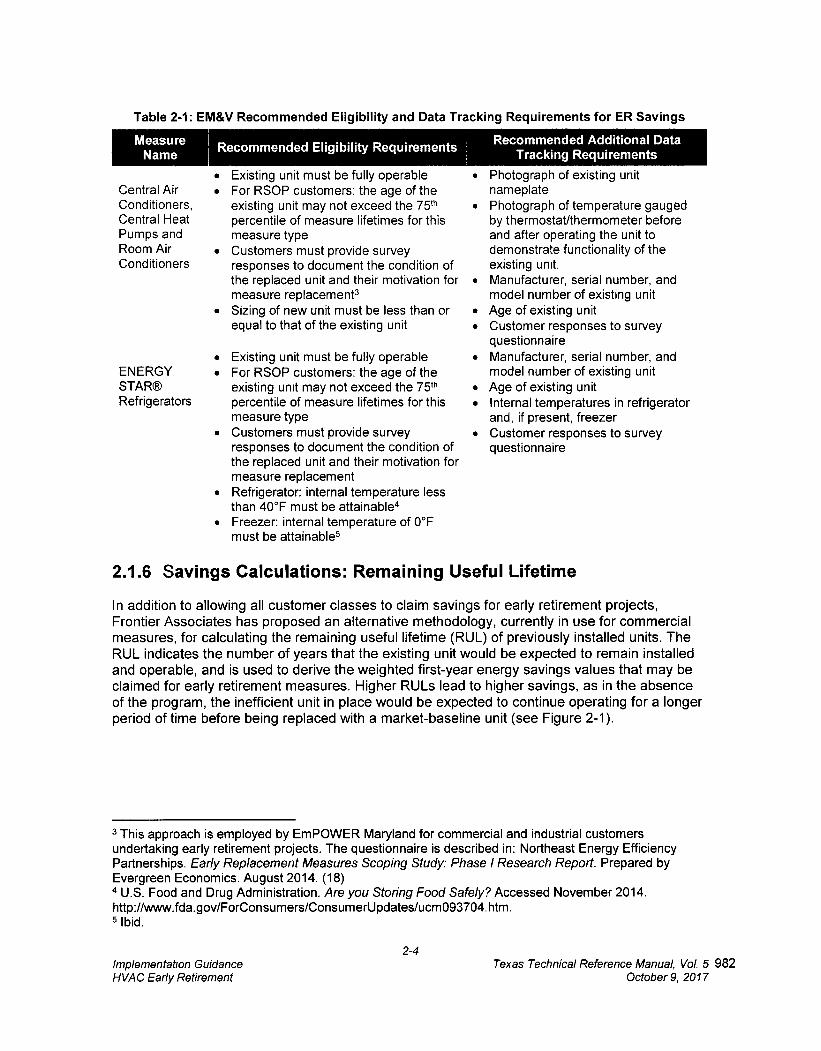
Table 2-1: EM&V Recommended Eligibility and Data Tracking Requirements for ER Savings

Measure I Recommended Eligibility Requirements Name

Recommended Additional Data Tracking Requirements

Central Air Conditioners, Central Heat Pumps and Room Air Conditioners

ENERGY STAR® Refrigerators

• Photograph of existing unit nameplate

• Photograph of temperature gauged by thermostat/thermometer before and after operating the unit to demonstrate functionality of the existing unit.

• Manufacturer, serial number, and model number of existing unit

• Age of existing unit • Customer responses to survey

questionnaire • Manufacturer, serial number, and

model number of existing unit • Age of existing unit • Internal temperatures in refrigerator

and, if present, freezer • Customer responses to survey

questionnaire

• Existing unit must be fully operable • For RSOP customers: the age of the

existing unit may not exceed the 75th percentile of measure lifetimes for this measure type

• Customers must provide survey responses to document the condition of the replaced unit and their motivation for measure replacement3

• Sizing of new unit must be less than or equal to that of the existing unit

• Existing unit must be fully operable • For RSOP customers: the age of the

existing unit may not exceed the 7591 percentile of measure lifetimes for this measure type

• Customers must provide survey responses to document the condition of the replaced unit and their motivation for measure replacement

• Refrigerator: internal temperature less than 40°F must be attainable

• Freezer: internal temperature of 0°F must be attainable5

2.1.6 Savings Calculations: Remaining Useful Lifetime

In addition to allowing all customer classes to claim savings for early retirement projects, Frontier Associates has proposed an alternative methodology, currently in use for commercial measures, for calculating the remaining useful lifetime (RUL) of previously installed units. The RUL indicates the number of years that the existing unit would be expected to remain installed and operable, and is used to derive the weighted first-year energy savings values that may be claimed for early retirement measures. Higher RULs lead to higher savings, as in the absence of the program, the inefficient unit in place would be expected to continue operating for a longer period of time before being replaced with a market-baseline unit (see Figure 2-1).

3 This approach is employed by EmPOWER Maryland for commercial and industrial customers undertaking early retirement projects. The questionnaire is described in: Northeast Energy Efficiency Partnerships. Early Replacement Measures Scoping Study: Phase I Research Report. Prepared by Evergreen Economics. August 2014. (18) 4 U.S. Food and Drug Administration. Are you Storing Food Safely? Accessed November 2014. http://www.fda.gov/ForConsumers/ConsumerUpdates/ucm093704.htm. 5 Ibid.


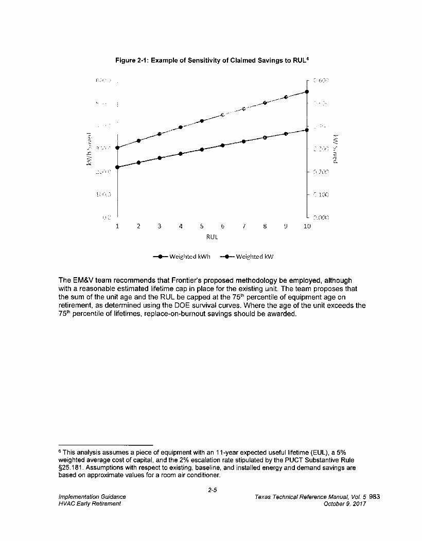
1-.

0200

100.3 Ct 100

Figure 2-1: Example of Sensitivity of Claimed Savings to RUL6

.T1

1 2 3 4 5 6 7 8 9 10

RUL

Weighted kWh —0— Weighted kW

The EM&V team recommends that Frontiers proposed methodology be employed, although with a reasonable estimated lifetime cap in place for the existing unit. The team proposes that the sum of the unit age and the RUL be capped at the 75th percentile of equipment age on retirement, as determined using the DOE survival curves. Where the age of the unit exceeds the 75th percentile of lifetimes, replace-on-burnout savings should be awarded.

6 This analysis assumes a piece of equipment with an 11-year expected useful lifetime (EUL), a 5% weighted average cost of capital, and the 2% escalation rate stipulated by the PUCT Substantive Rule §25.181. Assumptions with respect to existing, baseline, and installed energy and demand savings are based on approximate values for a room air conditioner.


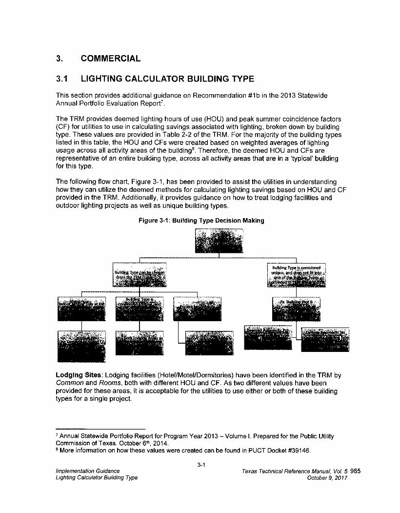
3. COMMERCIAL

3.1 LIGHTING CALCULATOR BUILDING TYPE

This section provides additional guidance on Recommendation #1b in the 2013 Statewide Annual Portfolio Evaluation Report'.

The TRM provides deemed lighting hours of use (HOU) and peak summer coincidence factors (CF) for utilities to use in calculating savings associated with lighting, broken down by building type. These values are provided in Table 2-2 of the TRM. For the majority of the building types listed in this table, the HOU and CFs were created based on weighted averages of lighting usage across all activity areas of the building8. Therefore, the deemed HOU and CFs are representative of an entire building type, across all activity areas that are in a 'typical building for this type.

The following flow chart, Figure 3-1, has been provided to assist the utilities in understanding how they can utilize the deemed methods for calculating lighting savings based on HOU and CF provided in the TRM. Additionally, it provides guidance on how to treat lodging facilities and outdoor lighting projects as well as unique building types.

Figure 3-1: Building Type Decision Making

Lodging Sites: Lodging facilities (Hotel/Motel/Dormitories) have been identified in the TRM by Common and Rooms, both with different HOU and CF. As two different values have been provided for these areas, it is acceptable for the utilities to use either or both of these building types for a single project.

7 Annual Statewide Portfolio Report for Program Year 2013 — Volume l. Prepared for the Public Utility Commission of Texas. October 6th, 2014. 8 More information on how these values were created can be found in PUCT Docket #39146.

3-1 Implementation Guidance Texas Technical Reference Manual, Vol. 5 985 Lighting Calculator Building Type

October 9, 2017

Outdoor Lighting Projects that involve outdoor lighting should be claimed in a separate calculator. The exception to this is walkway lighting that is similar to building operation. In this application, the utilities should use the primary building type as their HOU and CFs have been rolled up into the overall building type calculations. Ex. Walkway lighting between two buildings that operates during business hours.

In situations where multiple TRM building types seem plausible, or a predominant TRM building type is unclear, the utilities have two choices:

Deemed Approach: The deemed approach is a simplified method where the utilities should choose a TRM building type based on the "best fir for the facility. The utilities will use their best judgment in making this decision and provide sufficient, defensible documentation for their decision-making process.

Custom Approach: In more unique situations where the deemed building types in the TRM may not be representative of the project's facility type, or where the facility may represent multiple TRM building types without a clear predominant building type (or the use of a predominant building type may be too conservative in the estimate of savings), the utilities should consider these projects "custom". The deemed methods are only applicable to specific scenarios and cannot be developed for all unique situations. The utility should provide sufficient, defensible documentation for their HOU and CF values used in their savings calculations that can be reviewed by the EM&V team.

3-2 Implementation Guidance Texas Technical Reference Manual, Vol. 5 986 Lighting Calculator Building Type October 9, 2017

3.2 NON-QUALIFYING LEDS

This section provides guidance on assessing and calculating nonresidential lighting project savings that include non-qualifying LEDs. The information should help utilities respond to Recommendation #la from the program year (PY) 2013 Statewide EM&V Portfolio Report:

Recommendation #1a: LED lighting qualification requirements. The EM&V team found that several LED lighting fixtures and lamps were not meeting the qualification requirements specified in the TRM. The new LED fixtures and lamps installed as part of the commercial energy efficiency programs should meet the certification requirement and confirm the eligibility of the LED fixtures and lamps. The qualification requirements are in keeping with national industry practice that protect customers from inferior products and help ensure the energy savings.

la Action Plan: Utilities will require certification for all LEDs with a certification category with the Design Light Consortium (DLC) or ENERGY STAR as specified in the TRM. If a LED has been submitted for certification but has not yet been processed, the utility will check that it is being processed and also request forms LM79 and LM80 to review that the LED meets the required efficiency standards. In cases where a certification category does not address a certain LED usage (i.e., outdoor signage), the utility will inform the EM&V team and discuss a M&V plan and supporting savings information for these LED applications.

3.2.1 Background

The Texas Technical Reference Manual (TRM) includes the following requirement for LEDs: "LED lamps and fixtures need to be certified by Design Lights Consortium (DLC) or ENERGY STARC,' (TRM Volume 3, Section 2.1.1). This requirement is to ensure the quality of the products and resulting savings incentivized through the utility programs.

Oncor Electric Delivery (Oncor) reported to the EM&V team that even though they promote qualified LEDs, they are still receiving projects that have some percent of non-qualifying LEDs. As part of the PY2014 evaluation, Oncor asked the EM&V team for guidance on how to calculate savings for these projects. The EM&V team advised isolating the non-qualifying LEDs when possible including the square footage for new construction projects. The EM&V team also recommended establishing a percent cut-off of non-qualifying LEDs for program participation and not counting savings from non-qualifying LEDs or rebating them. Additional methodologies were discussed for when project conditions do not provide for isolation of the square footage. Since the original discussion, Oncor has been observing the number of projects with some non-qualifying LEDs increase and reports it is difficult to isolate square footage of non-qualifying LEDs in practice. Furthermore, this issue has greatly increased the utility review and approval time of lighting projects. Oncor proposed a streamlined methodology, which the EM&V team reviewed and finds reasonable. This savings process is provided below for all utilities to utilize when projects meet such criteria.

3-3 Implementation Guidance Texas Technical Reference Manual, Vol. 5 987 Non-Qualifying LEDs October 9, 2017

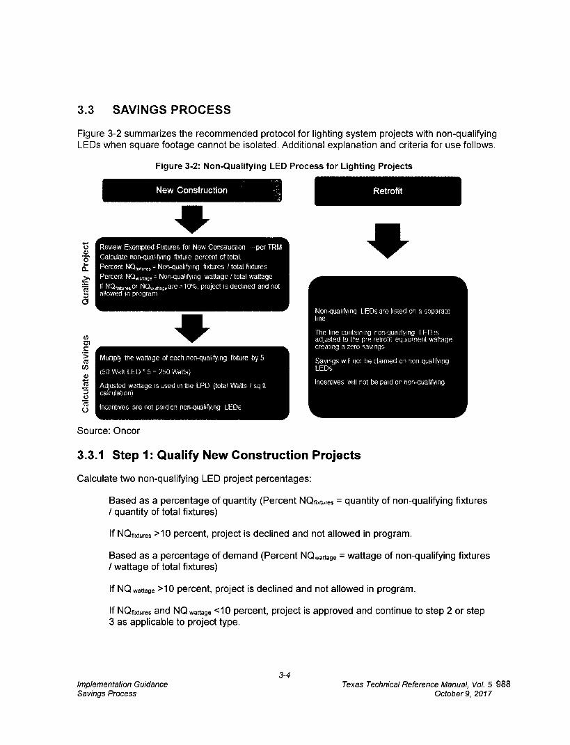
Retrofit

Non-qualifying LEDs are listed on a separate line

The line containing non-qualifying LED is adjusted to the pre-retrofit equipment wattage creating a zero savings

Savings will not be claimed on non-qualifying LEDs

Incentives will not be paid or non-qualifying

3.3 SAVINGS PROCESS

Figure 3-2 summarizes the recommended protocol for lighting system projects with non-qualifying LEDs when square footage cannot be isolated. Additional explanation and criteria for use follows.

Figure 3-2: Non-Qualifying LED Process for Lighting Projects

Qua

lify

Pro

ject

Cal

cula

te S

avi

ngs

New Construction

Review Exempted Fixtures for New Construction — per TRM

Calculate non-qualifying fixture percent of total.

Percent NCIwurti,, Non-qualifying fixtures /total fixtures

Percent NC)..„ase = Non-qualifying wattage / total wattage

If NO rtxtres Or NQwdtia,)e are -,10%, project is declined and riot allowed in program

Murtiply the wattage of each non-qualifying fixture by 5

(50 Watt LED i 5 = 250 Watts)

Adjusted wattage is used in the LPD (total Watts / sq ft calculati on)

Incentives are not paid on non-qualifying LEDs

Source: Oncor

3.3.1 Step 1: Qualify New Construction Projects

Calculate two non-qualifying LED project percentages:

Based as a percentage of quantity (Percent NQfixtures = quantity of non-qualifying fixtures / quantity of total fixtures)

If NQfixtures >10 percent, project is declined and not allowed in program.

Based as a percentage of demand (Percent Nn —.wattage = wattage of non-qualifying fixtures / wattage of total fixtures)

If NQ wattage >10 percent, project is declined and not allowed in program.

If NQfixtures and NQ wattage <10 percent, project is approved and continue to step 2 or step 3 as applicable to project type.

3-4 Implementation Guidance Texas Technical Reference Manual, Vol. 5 988 Savings Process October 9, 2017

The EM&V team finds the 10 percent cut off for project approval reasonable and is consistent with lighting project limits for non-operating fixtures.

3.3.2 Step 2: New Construction Projects Only

Non-qualifying fixtures that pass Step 1, would follow all instructions for excluded fixtures, as provided in the TRM, Volume 3, Section 2.1.1.

List all non-qualifying LEDs in the tool, but exclude from the lighting power density calculation.

List non-qualifying LEDs on separate lines (e.g. separate on lighting inventory worksheet of deemed savings tool). Non-qualifying fixtures are identified by a unique fixture code.

Adjust non-qualifying LED wattage so their demand energy reduction is not included as part of the lighting power density (LPD) code limit requirements. To do so, multiply the rated fixture wattage times five. The adjusted wattage is included as part of the overall LPD calculation, and will increase the calculated watts per square foot of the project.

The EM&V team finds the five times factor conservative, however in line with a typical baseline condition and equivalent and ensures the non-qualifying LED demand is not included with the LPD code allowance requirements.

3.3.3 Step 3: Retrofit Projects

List non-qualifying LEDs on separate lines (e.g. separate on lighting inventory worksheet of deemed savings tool.)

Include a unique identifier/marker for the non-qualifying LED within the fixture code and description (e.g. inputs within the standard wattage table worksheet of the deemed savings tool.)

Adjust non-qualifying LED wattage so their demand and energy savings are not included as part of the project savings. Demand and energy savings for non-qualifying LEDs shall result in zero project savings.

Adjust non-qualifying LED quantities so they are not included as part of the project incentive. Incentives shall not be paid on non-qualifying LEDs.

Provide clear visibility for all changes within the savings calculation (e.g. deemed savings tool), including changes to all input assumptions and calculation methodologies to implement the above procedure.

All other savings procedures and requirements as specified within the TRM for lighting measures apply to all fixtures of a lighting project.

The EM&V team finds this procedure as an acceptable and systematic method to approve and document lighting projects with a small portion of non-qualified LEDs. As more LEDs earn DLC and ENERGY STAR® approval, the procedure may also allow for easier integration into project savings by the programs and the evaluation if such conditions take place within the same program year.


3.3.4 Conclusion

The savings approach in this memo will facilitate utilities responding to PY2013 Recommendation #la in PY2015 in keeping with § 25.181 (q) (9) while recognizing the market and administrative challenges of projects with non-qualifying LEDs.


3.4 PROJECT DOCUMENTATION This section summarizes the progress and current status of the EM&V team's assessment of the utilities efforts to meet and conform to project documentation standards and provides additional guidance for areas still in need of improvement as part of the PY2015 EM&V.

3.4.1 Background For all energy efficiency programs, critical inputs and methodologies needed to replicate claimed savings calculations are captured in a combination of the TRM, program manuals, program tracking data systems, and individual project documentation. Project-level documentation is critical to the transparency of claimed savings as well as facilitates efficient third-party EM&V at the project, program, and porffolio levels. This memo specifically addresses the individual project documentation needs. Individual project documentation includes all relevant site-specific detail (i.e., audit reports, worksheets, program applications, invoices, project overview/description, photos, installation reports, etc.)

Documentation guidance was originally provided in PY2012 with additional status and recommendations in PY2013 as part of the evaluation activities and utility action plan discussions. The sufficiency of program documentation has improved from PY2012 to PY2014 across almost all utilities and programs as noted in the PY2014 Statewide Porffolio Report. However, for some utilities, there is still a need to increase the sufficiency of program documentation for the Commercial Standard Offer Programs (CSOP).

Next, we provide further detail on documentation best practices currently incorporated into many of the Texas programs (based on information gathered during PY2014 evaluation activities) and recommendations for improvement. The objective is to support the utilities in achieving industry-standard degrees of documentation rigor, clarity, and efficacy necessary to clearly organize and manage such information to yield transparency and facilitate efficient and effective oversight.

3.4.2 Additional Documentation Guidance The reader is referred to PY2012 and PY2013 Annual Statewide Porffolio Reports for prior program documentation guidance. In this section, we provide additional guidance geared specifically to help improve CSOP program documentation scores, though the guidance may also be used to support the continued improvement of program documentation for other programs.

Recommendation 1: Clearly organize project files

Organized project files are critical for many reasons including:

• Clear and transparent reporting of documentation used to support claimed savings

• Ease of identification of related program project files that may not have made the data transfer

• Backup support for information within tracking data systems

• Support the use of custom parameters

• Support deviation or enhancement of methodologies in order to gain greater accuracy

3-7 Implementation Guidance Texas Technical Reference Manual, Vol. 5 991 Project Documentation October 9, 2017

An important part of organized project folders, files and documents are clear naming conventions. This assists in keeping files organized and improves consistency in document placement and ease in locating critical documents to support the EM&V efforts. Below are some examples of the difficulty the EM&V team has had with project level folders/files received:

• The project folders often contained inconsistencies with regard to file/document names, locations and contents. Files with similar names often contained disparate information while seemingly identical files contained dissimilar information

• The project folders included multiple copies of project documents. Locating the final documents used to support the reported savings proved difficult for many projects. For example, when numerous photos are provided, locating those that support the key savings assumptions is difficult. Distinguishing between pre versus post equipment photos was also at times difficult.

• Project folders contained documents labeled as Verification Reports when they were still actually M&V plans with no verification data completed. Such plans provided the methodology to verify project savings estimates, yet do not document that they were ever completed.

The project file organization example below provides a list of potential project sub folders and documents that would be ideal to collect whether a pre- and/or post-inspection is completed. Many documents listed are key elements necessary to support custom project assumptions and review.

Project File Organization Example:

Stage Retrofit and New Construction

Pre Project*

• Pre-project calculator • Plans (e.g. drawings, fixture list) • Pre-project/inspection photos • Pre-project audit reports • Project descriptions, sponsor agreements, etc.

Post Project • Post- project/inspection calculator • Post-inspection field notes • Post-project/inspection photos • As-built plans • Installation reports

Supporting • Calculators - old and archived Documents • Spreadsheets or other backup (especially those to support custom calculations)

• Specifications, cut sheets, certifications • Check requests to utility • Partner letters or savings summaries • Material purchase orders/invoices • Email communication • M&V plan — for custom key input assumptions (e.g. operating hours) or custom

savings methodologies Final • Final calculator Documents** • Final M&V plan — for custom projects

• Final verification documents — for custom projects • Final project notes

* New construction projects may not necessarily include these documents. ** These documents also support EM&V on-site minimum requirements for data collection needs.


Recommendation #2: Use photo verifications to support key measure assumptions.

When onsite field work is completed, whether by trade allies, implementation staff or utility staff, photos can assist in documenting and supporting key measure attributes and assumptions. Most programs include some form of photo documentation to support projects. Some programs in Texas even utilize tablets in the field whereby project site and equipment photos are taken by trade allies and automatically uploaded to tracking systems and project folders. Guidance for how photos can assist in supporting documentation of projects are more fully described in the table below for some of the most common commercial project types, lighting and HVAC based projects.

Photo Verification Applications and Examples:

Stage Lighting Projects*

HVAC Projects

Pre Project • Existing lighting system types (e.g. lamp, ballast, fixture)

• Existing lighting equipment quantities • Existing control type • Existing lighting equipment operability/

inoperability • Building type • Air conditioning type

•

•

Existing HVAC equipment types and sizes Existing HVAC equipment quantities Existing HVAC equipment operability/ inoperability (e.g. set point, load display shots) Building type

Post Project • New lighting system types (e.g. lamp, • New HVAC equipment types and sizes ballast, fixture)

• New HVAC equipment quantities • New lighting equipment quantities • New HVAC equipment operability (e.g. • New control type set point, load display shots) • New control schedule automation (e.g. • Building type

building/lighting automation system screen shots)

• New lighting equipment operability • Building type • Air conditioning type

* Note that for large lighting projects, some of these project parameters may not be possible to be captured for all lighting quantities. In these cases, alternative project documentation types may be preferred.

Recommendation #3: Include clear descriptors of measure type as well as QA/QC inspections in tracking system.

Different projects (e.g. retrofit versus new construction projects, inspected versus not inspected sites) have different documentation needs. Capturing participant descriptors can aid evaluation efforts immensely, keep cost burdens low, and facilitate transparency.

Many commercial programs continue to track and describe measure-level savings at the measure-category level (or savings calculator level) instead of the measure-specific level. For example, the tracking system will document the savings associated with a lighting project as captured within a lighting calculator (i.e. Lighting Equipment Survey Form ver 9.02), but the calculator itself includes many different lighting fixture types, effective useful lives and related savings. Tracking project data at the measure-specific level (e.g. Integrated-ballast LED Lamps, Linear Fluorescent, Lighting Controls) rather than the measure-category level will improve the level of transparency in the data as the types of measures and individual savings being claimed can then be readily assessed. This structure also supports ease for calculating cost- effectiveness.


As another example, new construction projects may not have pre-inspection forms or field notes whereas retrofit projects may have many types of pre-project documentation (e.g. pre-project calculator, pre-project plans, pre-inspection photos). Providing information regarding "greenfield" or complete demolition and rebuild projects as a differentiator from retrofits and small remodels up front is a valuable population segmenting descriptor. When descriptors like these are used in tracking systems they become a valuable screening tool and can inform evaluators not to request certain documentation (that may not exist), which can misdirect time and resources. It also allows better budgeting and allocation of resources, improving overall efficacy. Another example are those sites or program participants that have received internal QA/QC, versus those that did not. Some programs have modified their tracking systems to begin logging this data and/or providing a list as part of the EM&V data collection process which notifies the EM&V team that a site will not have particular project level documentation because it was not site inspected, or site verified, etc.

Recommendation #4: Complete M&V plans and reports are needed for custom projects.

The industry standard for M&V plans and reports is based on the guidelines of Efficiency Valuation Organizations (EVO) International Performance Measurement and Verification Protocol (IPMVP). IPMVP Volume I EVO 10000-1:2012 is the current version available, which includes clear recommendations for meeting the minimum information requirements for complying with IPMVP protocols including those specific to M&V Plan Contents summarized in Chapter 5 and M&V Reporting summarized in Chapter 6.

Utilities and their implementation contractors are encouraged to engage and collaborate with the EM&V team, to discuss issues and options, obstacles and possible solutions for M&V plans as new technologies or offerings become part of the Texas porffolios.


3.5 INCENTIVES AND CLAIMED SAVINGS This section provides guidance on claiming savings where a financial incentive does not cover all of the project savings from the implementation of energy efficiency measures°. These recommendations are to begin in PY2016.

3.5.1 Background

To meet various program objectives, it is common practice for utilities to set a ceiling or cap for the financial incentive any one energy efficiency service provider (EESP) or project can receive. These 'individual incentive caps are set as an overall percent of total incentive budget or as a dollar amount. The established caps vary by utility and are noted in their program manuals.

This is a different situation from a 'set incentive. During the application phase, utilities calculate a project incentive based on pre-installation estimated savings, the incentive funds are reserved at this time. There may be some variation in the initial savings estimates that were agreed upon in setting the incentive and the actual post-installation savings once the project is completed. This is due to changes in efficiency levels, quantities or equipment type that take place from the project planning phase to the project implementation phase.

3.5.2 Considerations

In the case of incentive caps, the EM&V team has some concern regarding claiming all of the savings in projects where an incentive cap is reached. Since all of the project savings are not being incentivized at the project planning phase, claiming all of the project savings may result in increased free-ridership. A free-rider is, "a program participant who would have implemented the program measure or practice in the absence of the program." (16 TAC § 25.181 (c) (24))1°.

In the case of set incentives, the EM&V team has some concern that spillover could be claimed incorrectly during post-project inspections. Spillover is, "reductions in energy consumption and/or demand caused by the presence of an energy efficiency program, beyond the program-related gross savings of the participants and without financial or technical assistance from the program." ((16 TAC § 25.181 (c) (53)). Spillover is a component of net savings and claimed savings are based on gross savings. Therefore, spillover should not be included in claimed savings if found on-site during post-project inspections.

9 This guidance does not apply to behavioral, code or other market transformation programs where the primary program strategy is technical assistance and/or education that results in behavioral or operational changes for energy and demand savings.

10 In addition to the incentive caps or set incentives at the individual EESP or customer-level, utilities may also set caps on incentives a customer can receive at the measure level. For example, a utility may cap lighting incentives at 50% of the total project incentive. The EM&V team does not have the same concerns regarding free-ridership for measure-level caps and the recommendations in this memo do not apply to these situations.

3-1 1 Implementation Guidance Texas Technical Reference Manual, Vol. 5 995 Incentives and Claimed Savings October 9, 2017

3.5.3 Recommendations

Individual incentive caps. If utilities are planning to claim savings beyond those incentivized for an individual EESP or project, they are requested to inform the EM&V team and supply project documentation for the specific project. The EM&V team may conduct additional research to determine the influence of the program on the total project savings. The EM&V team's recommendation should be used to adjust the utilities claimed savings for the project(s).

Set incentives. The EM&V team recommends utilities educate internal staff, implementation contractors and EESPs on spillover to help ensure it is not included in claimed savings if found during post-project inspections. However, documenting spillover may be beneficial when net-to-gross ratios are updated.

3-12 Implementation Guidance Texas Technical Reference Manual, Vol. 5 996 Incentives and Claimed Savings October 9, 2017

4. CROSS SECTOR

4.1 LOAD MANAGEMENT PROGRAMS This memo summarizes guidance from the EM&V team on two load management issues raised by one or more of the utilities during PY2014-PY2015 EM&V. These are 1) rounding of demand impacts and 2) meter issues.

4.1.1 Rounding

In the course of the EM&V contractor's effort of evaluating commercial load management programs, the EM&V contractor has found some differences in rounding in the commercial load management programs demand impacts. These rounding differences are minor and are not a concern in the accuracy of the reporting of impacts. However, in response to a request for guidance to address rounding consistently, the EM&V team recommends utilities round commercial load management impacts consistently with how incentives are awarded, which is at the customer-level.

4.1.2 Meter Issues

Utilities are responsible for calling a test event each program year for the load management programs. The test event has several purposes, including assuring the proper functioning of program meters. Utilities are responsible for maintaining working program meters.

Commercial load management programs. Without complete interval meter data to calculate the baseline and event impacts, savings may not be claimed. However, if a customer has alternate interval meter data available, this can be used in lieu of program meter data to calculate claimed savings. Using customer meters for the load management program savings requires that the data meet interval metering requirements presented in the version of the Texas Technical Reference Manual for the program year. In general, it is recommended that customer owned interval meters should only be used in the event that utility interval meters fail. Data from each should not be combined for claiming savings for a specific event and must be able to cover both the event day data and baseline data.

The EM&V team requests utilities notify them in these circumstances. All calculations and data stemming from the use of customer meters should be provided as part of the EM&V data request similarly to when program meter data is used. If requested by the utility, the EM&V team is available to review the use of customer meter data in advance of a program claiming savings from customer meters.

Residential load management programs. If there are random, non-systematic errors in smart meter data for less than one percent of total participants, the average savings from a similar group of participants (i.e., single-family, multi-family) may be used for claimed savings if: (1) the control event technology and intervention are the same, and (2) the control event intervention can be confirmed based on standard program practices for event confirmation.

The EM&V team requests utilities notify them in these circumstances to discuss the approach for determining and applying average savings for those customers with incomplete meter data.

4-1 Implementation Guidance Texas Technical Reference Manual, Vol. 5 997 Load Management Programs October 9, 2017

4.2 BEHAVIORAL PROGRAMS This section provides additional guidance on claiming savings for behavioral programs.

4.2.1 Background

Behavioral programs are newly allowed energy efficiency programs in Texas as specified in the Energy Efficiency Rule (16 TC 25.181 (c) (12)). Guidance for Behavioral Programs M&V protocols was first integrated into Texas Technical Reference Manual (TRM) 3.1: Volume 4.

4.2.2 Considerations and Recommendations

Consideration #1: Sufficient post-program data to estimate savings

The annual reporting of program savings poses a challenge to accurately estimating impacts from behavioral programs in Texas as 12 months pre- and post-data are needed to account for seasonal variations. Having 12-months of data is the recognized industry-standard practice as specified in the Department of Energy's Uniform Methods Project (UMP):

"these [behavioral] programs may influence weather-sensitive energy uses, such as space heating or cooling, so collecting less than 1 year of data to reflect evety season may yield incomplete results"."

Recommendation#1: Behavioral Programs should award incentives and claim savings for 40% of projected savings in the first program year and award the remaining incentives and claim savings the next program year once 12 months of post-program data is available to complete the M&V.

In Texas, a precedence has been established for awarding incentives and claiming savings for custom commercial programs where the required M&V to calculate savings spans program years. In these cases, 40% of the incentives are awarded and savings claimed the first program year based on initial estimated savings. Then in the subsequent program year when M&V is completed, the remaining 60% or true-up' of estimated savings is paid and incentives are awarded. The EM&V team asserts that a similar process should be used to estimate behavioral program savings.

11 The Uniform Methods Project: Methods for Determining Energy Efficiency Savings for Specific Measures, Chapter 17: Residential Behavior Protocol, page 20. While a specific nonresidential behavior protocol is not included in the UMP, this chapter recognizes the same approach is applicable to nonresidential programs though there has been less research and implementation of these programs.

4-2 Implementation Guidance Texas Technical Reference Manual, Vol. 5 998 Behavioral Programs October 9, 2017

Consideration #2: Measure life

The TRM 3.1 Behavioral Program M&V Protocol states that measure life/lifetime savings are not applicable to behavioral programs (p. 2-40) as only annual savings are to be claimed.

Recommendation #2: Utilities should only claim annual savings for behavioral programs until M&V demonstrates measure persistence

The persistence of behavioral savings after the intervention (e.g., program outreach) has ended is still widely debated in the industry and it is recognized that additional research is needed on the persistence of behavioral savings12. While there has been some, though still limited, research for home energy reports for residential programs, there is very little research on savings persistence for nonresidential behavioral programs.

12 The Uniform Methods Project: Methods for Determining Energy Efficiency Savings for Specific Measures, Chapter 17: Residential Behavior Protocol, page 14.

4-3 Implementation Guidance Texas Technical Reference Manual, VoL 5 999 Behavioral Programs October 9, 2017

References and Efficiency Standards

Documents

Transcript of References and Efficiency Standards