Reference Path Estimation forLateral Vehicle ControlMaster’s thesis in Systems, Control and Mechatronics

Arni Thorvaldsson

Vinzenz Bandi

Department of Signals and SystemsCHALMERS UNIVERSITY OF TECHNOLOGYGothenburg, Sweden 2015

Master’s Thesis Ex041/2015

Reference Path Estimation forLateral Vehicle Control

Arni ThorvaldssonVinzenz Bandi

Department of Signals and SystemsChalmers University of Technology

Gothenburg, Sweden 2015

Reference Path Estimation for Lateral Vehicle ControlArni ThorvaldssonVinzenz Bandi

© Arni Thorvaldsson & Vinzenz Bandi, 2015.

Supervisor: Erik Nordin & Mansour Keshavarz, Volvo Group Trucks TechnologyExaminer: Lennart Svensson, Signals and Systems

Master’s Thesis 2015Department of Signals and SystemsChalmers University of TechnologySE-412 96 GothenburgTelephone +46 31 772 1000

Typeset in LATEXGothenburg, Sweden 2015

iv

Reference Path Estimation for Lateral Vehicle ControlArni ThorvaldssonVinzenz BandiDepartment of Signals and SystemsChalmers University of Technology

AbstractAutonomous driving cars have been a hot topic in the media in recent years, withmore and more tech companies and universities presenting projects with fully auto-mated vehicles. Most of these vehicles rely on highly sophisticated and expensivesensors that are not yet feasible for commercial vehicles. On the other hand auto-mated systems that are implemented in commercially available vehicles are largelylimited to active safety scenarios where the system only assists the driver in danger-ous situations such as collision avoidance or lane support.

The goal of this thesis project is to use sensors on commercially available vehi-cles for automating lateral control in selected scenarios. The evaluated scenarios arelimited to roads where the sensors can detect lane markings or a preceding vehicleor both. The approach was to generate two different reference paths, one from lanemarkings and one from the preceding vehicle information. The lane marking pathis generated from filtering measurements from the lane detection cameras using anonlinear Kalman filter. The preceding vehicle path is generated by fusing the radarand camera measurements of the preceding vehicle. In order to develop and tunethe filters a detailed analysis was done on the sensor measurements collected for thisproject.

The implemented filters improve the current system in several ways. When thelane marking are lost for short period of time the prediction from the last mea-surement update can provide a reference while driving up to 40 meters. The pathgenerated from the estimates of the preceding vehicle describe the trajectory whichthe vehicle has driven. This way a more accurate reference signal can be generatedthan using only the current position of the preceding vehicle, especially in turns andat long distances. By having two references paths the lateral control is more robustand an algorithm that takes the covariances of the estimation for both paths intoaccount guarantees a smooth transition between them.

Keywords: Lateral control, autonomous vehicles, sensor fusion, nonlinear kalmanfiltering.

v

AcknowledgementsWe would like to thank Volvo Group Truck Technologies for giving us the oppor-tunity to carry out this master thesis, Lennart Svensson for being our examinerand giving us valuable input, Erik Nordin and Mansour Keshavarz for being oursupervisors at Volvo Group. We would also like to thank our group within VehicleDynamics & Active Safety for the help and support throughout the project.

Arni Thorvaldsson, Vinzenz Bandi, Gothenburg, June 2015

vii

Contents

List of Figures xi

List of Tables xv

1 Introduction 11.1 Background and motivation . . . . . . . . . . . . . . . . . . . . . . . 11.2 Problem Statement . . . . . . . . . . . . . . . . . . . . . . . . . . . . 21.3 Applications . . . . . . . . . . . . . . . . . . . . . . . . . . . . . . . . 21.4 Aims and objectives . . . . . . . . . . . . . . . . . . . . . . . . . . . 31.5 Thesis outline . . . . . . . . . . . . . . . . . . . . . . . . . . . . . . . 3

2 Background 52.1 Sensor Fusion . . . . . . . . . . . . . . . . . . . . . . . . . . . . . . . 5

2.1.1 Bayesian filter . . . . . . . . . . . . . . . . . . . . . . . . . . . 52.1.2 Kalman Filter . . . . . . . . . . . . . . . . . . . . . . . . . . . 62.1.3 Cubature Kalman Filter . . . . . . . . . . . . . . . . . . . . . 72.1.4 Rauch-Tung-Striebel Smoother . . . . . . . . . . . . . . . . . 8

2.2 Control Theory . . . . . . . . . . . . . . . . . . . . . . . . . . . . . . 82.2.1 Feedback . . . . . . . . . . . . . . . . . . . . . . . . . . . . . . 82.2.2 Feedforward . . . . . . . . . . . . . . . . . . . . . . . . . . . . 9

3 Sensors 113.1 Object Detection . . . . . . . . . . . . . . . . . . . . . . . . . . . . . 12

3.1.1 Radar . . . . . . . . . . . . . . . . . . . . . . . . . . . . . . . 123.1.2 Camera . . . . . . . . . . . . . . . . . . . . . . . . . . . . . . 12

3.2 Lane Detection Systems . . . . . . . . . . . . . . . . . . . . . . . . . 123.3 GPS . . . . . . . . . . . . . . . . . . . . . . . . . . . . . . . . . . . . 13

3.3.1 RACELOGIC VBOX System . . . . . . . . . . . . . . . . . . 133.4 Sensor Setup . . . . . . . . . . . . . . . . . . . . . . . . . . . . . . . 13

3.4.1 Object Detection . . . . . . . . . . . . . . . . . . . . . . . . . 133.4.2 Lane Detection . . . . . . . . . . . . . . . . . . . . . . . . . . 143.4.3 Vehicle State Sensors . . . . . . . . . . . . . . . . . . . . . . . 143.4.4 GPS . . . . . . . . . . . . . . . . . . . . . . . . . . . . . . . . 14

4 Methods 174.1 Generating a reference with lane markings . . . . . . . . . . . . . . . 17

4.1.1 Generating a path from lane markings . . . . . . . . . . . . . 18

ix

Contents

4.1.2 Coefficient and Sampled Lane Marking Measurement and Filters 194.2 Coefficient Filter for Lane Marking Path . . . . . . . . . . . . . . . . 19

4.2.1 Prediction step . . . . . . . . . . . . . . . . . . . . . . . . . . 194.2.2 Update step . . . . . . . . . . . . . . . . . . . . . . . . . . . . 20

4.3 Sampled Filter for Lane Marking Path . . . . . . . . . . . . . . . . . 204.3.1 Prediction step . . . . . . . . . . . . . . . . . . . . . . . . . . 204.3.2 Update step . . . . . . . . . . . . . . . . . . . . . . . . . . . . 24

4.4 Generating a reference with preceding vehicle . . . . . . . . . . . . . 244.4.1 Generating reference path . . . . . . . . . . . . . . . . . . . . 24

4.5 Preceding Vehicle Filter . . . . . . . . . . . . . . . . . . . . . . . . . 264.5.1 Prediction step . . . . . . . . . . . . . . . . . . . . . . . . . . 274.5.2 Update step . . . . . . . . . . . . . . . . . . . . . . . . . . . . 27

4.6 Control Signals . . . . . . . . . . . . . . . . . . . . . . . . . . . . . . 284.7 Experimental Data . . . . . . . . . . . . . . . . . . . . . . . . . . . . 30

4.7.1 Setup . . . . . . . . . . . . . . . . . . . . . . . . . . . . . . . 304.7.2 Scenarios . . . . . . . . . . . . . . . . . . . . . . . . . . . . . 30

4.8 Lane Marking Sensor Analysis . . . . . . . . . . . . . . . . . . . . . . 314.8.1 Ground Truth . . . . . . . . . . . . . . . . . . . . . . . . . . . 314.8.2 Evaluating the Measurements . . . . . . . . . . . . . . . . . . 32

4.9 Preceding Vehicle Sensor Analysis . . . . . . . . . . . . . . . . . . . . 334.9.1 Generating ground truth using RTS smoother . . . . . . . . . 33

5 Implementation 355.1 Simulink Implementation . . . . . . . . . . . . . . . . . . . . . . . . . 35

6 Results 376.1 Lane Marking Error Statistics . . . . . . . . . . . . . . . . . . . . . . 37

6.1.1 Absolute Error . . . . . . . . . . . . . . . . . . . . . . . . . . 376.1.2 Error Distribution . . . . . . . . . . . . . . . . . . . . . . . . 37

6.2 Lane Marking Filter Comparison . . . . . . . . . . . . . . . . . . . . 396.3 Lane Marking Filter . . . . . . . . . . . . . . . . . . . . . . . . . . . 40

6.3.1 Performance with original sensor data . . . . . . . . . . . . . . 416.3.2 Filter Performance With Added Noise . . . . . . . . . . . . . 436.3.3 Filter Performance Removed Measurements . . . . . . . . . . 44

6.4 Preceding vehicle filter analysis . . . . . . . . . . . . . . . . . . . . . 466.5 Preceding vehicle path . . . . . . . . . . . . . . . . . . . . . . . . . . 476.6 Outlier rejection . . . . . . . . . . . . . . . . . . . . . . . . . . . . . . 48

7 Conclusion and Discussion 517.1 Implemented filters . . . . . . . . . . . . . . . . . . . . . . . . . . . . 517.2 Reference paths and error signals . . . . . . . . . . . . . . . . . . . . 527.3 Experimental implementation . . . . . . . . . . . . . . . . . . . . . . 52

8 Future Work 53

x

Contents

A Appendix 1 IA.1 Maps . . . . . . . . . . . . . . . . . . . . . . . . . . . . . . . . . . . . IIA.2 Simulink . . . . . . . . . . . . . . . . . . . . . . . . . . . . . . . . . . IV

xi

Contents

xii

List of Figures

3.1 Visualization of ego vehicle and the two target vehicles with thesesignals. (black x,o) radar measurements. (green) position of thetarget vehicles from the Dgps System. (blue) path taken by the egovehicle. (gray) lane markings. (magenta) field of view of the radar andthe camera. (red) estimated positions (x on red line) of the vehiclesfrom fused radar and camera measurements including position of therear corners (connected by red line) and the far corner(x). (cyan)lane marking estimation from the camera. . . . . . . . . . . . . . . . 11

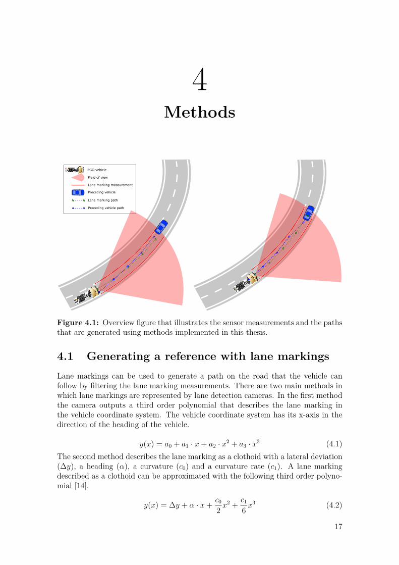
4.1 Overview figure that illustrates the sensor measurements and thepaths that are generated using methods implemented in this thesis. . 17

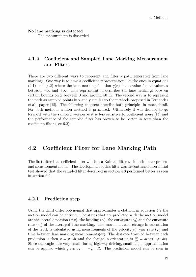
4.2 Shows how the path is sampled for the filter. Like the lane markingmeasurements the sampled path is described in the vehicle coordinatesystem (Vcs) (xv, yv). The samples are distributed equidistantly inx at distance ∆. . . . . . . . . . . . . . . . . . . . . . . . . . . . . . . 21

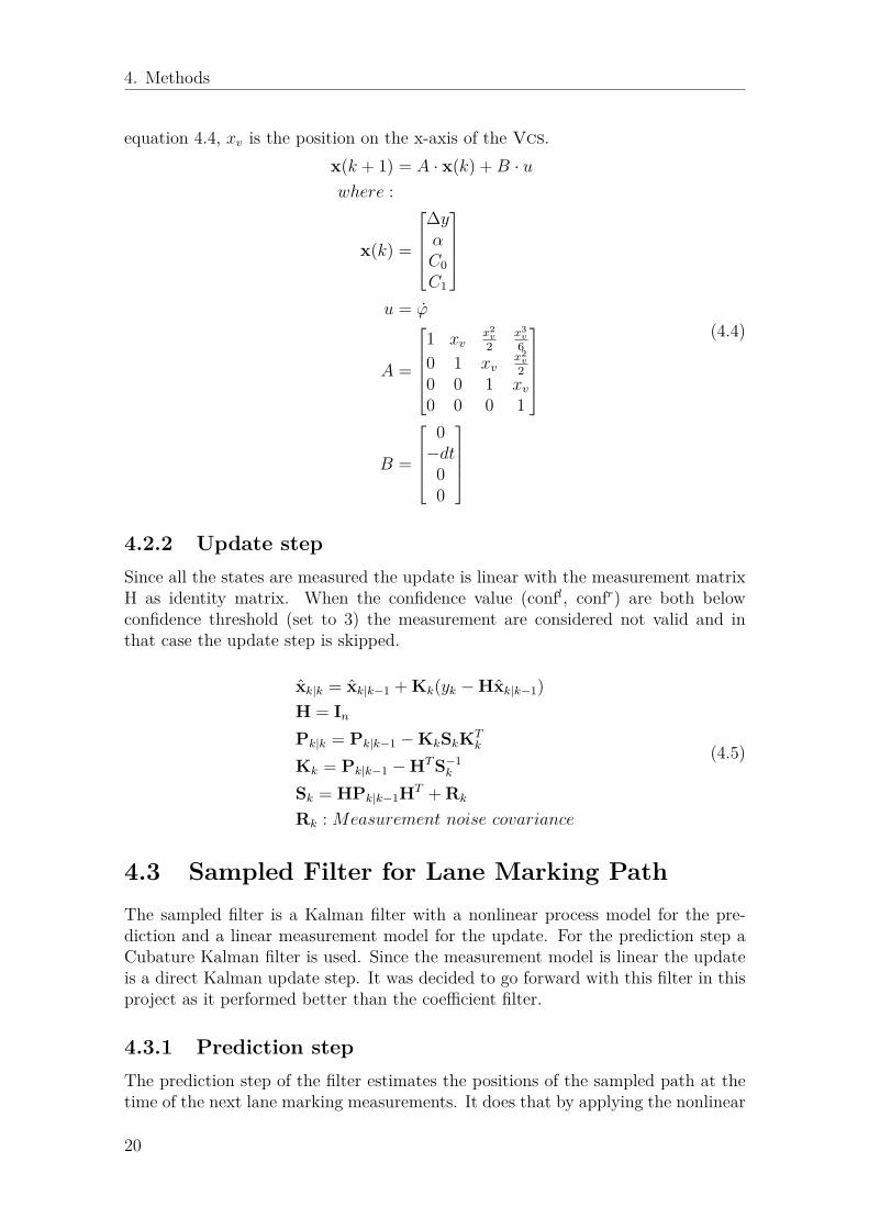
4.3 Moving the coordinate system in the nonlinear function f(x,v, ϕ,dt)inthe prediction step . . . . . . . . . . . . . . . . . . . . . . . . . . . . 22

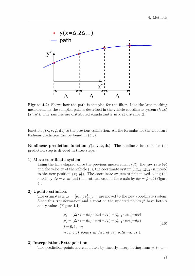
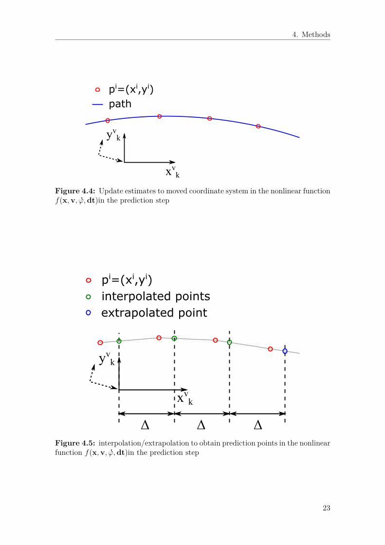
4.4 Update estimates to moved coordinate system in the nonlinear func-tion f(x,v, ϕ,dt)in the prediction step . . . . . . . . . . . . . . . . . 23

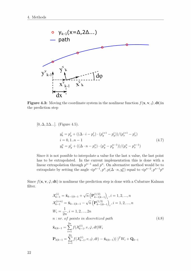
4.5 interpolation/extrapolation to obtain prediction points in the nonlin-ear function f(x,v, ϕ,dt)in the prediction step . . . . . . . . . . . . 23

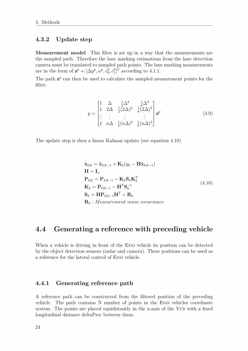
4.6 Initial path from preceding vehicle when a vehicle enters the fieldof view. A) shows how the N points in the path are generated if alane marking path is available by offsetting the lane marking pathand adding the preceding vehicle position as the Nth point and B)shows how the points are generated when no lane marking path isavailable by linear interpolation between the ego vehicle position andthe preceding vehicle position. . . . . . . . . . . . . . . . . . . . . . . 25

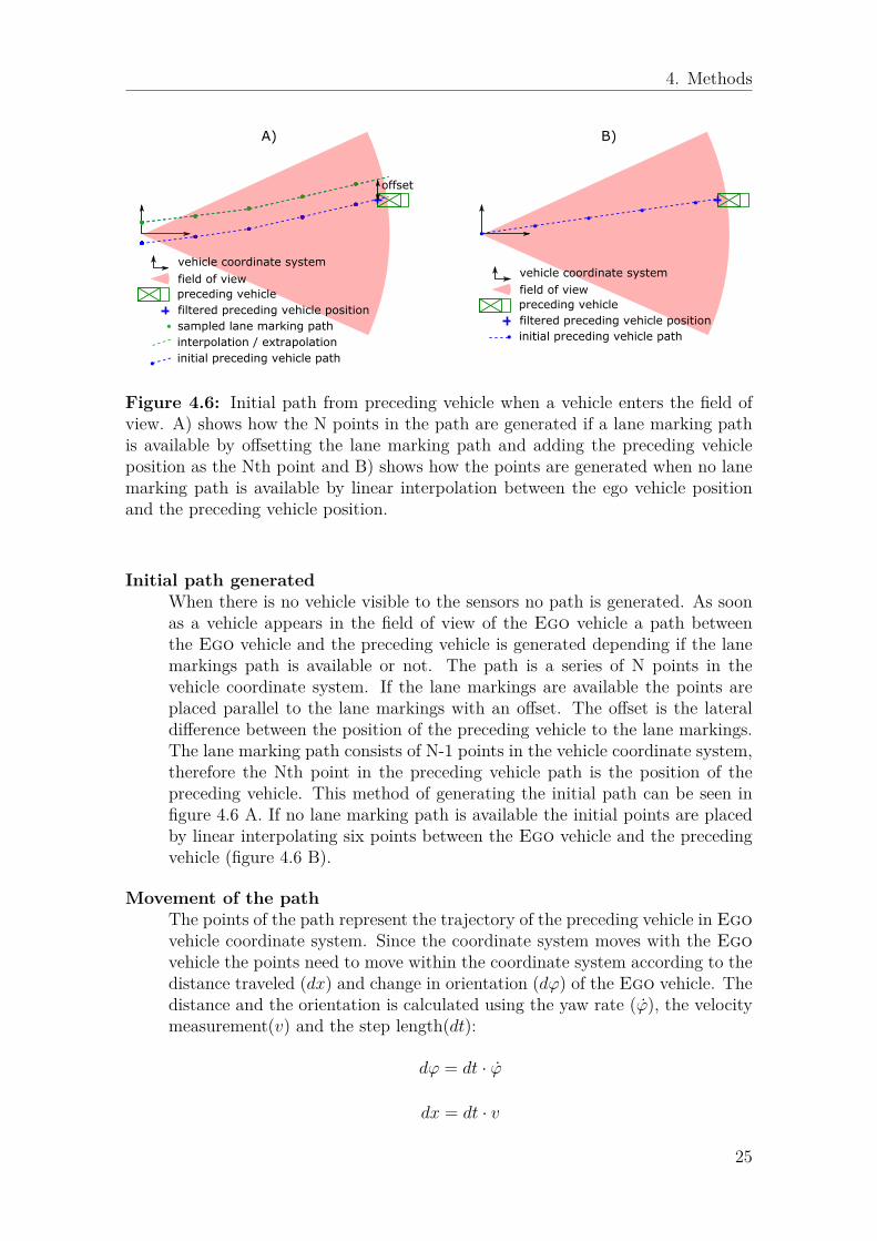
4.7 Updating the preceding vehicle path. Each time the distance be-tween the newest point in the path and the preceding vehicle is largerthan deltaPrec the point furthest away from the preceding vehicle isremoved and the preceding vehicle position is added as new point. . . 26

4.8 Lateral and heading error to the path obtained from the sampledfilter estimates in the Vcs. . . . . . . . . . . . . . . . . . . . . . . . . 29

xiii

List of Figures

4.9 (left) plot of the trajectory the vehicle drove during the measure-ment run in an Enu coordinate system. (right) Cutout of the groundtruth of the lane markings generated with Gps data, lane markingmeasurements using a filter and and Rts-smoother. . . . . . . . . . . 32

4.10 Visualization of the ground truth of the lane markings and a corre-sponding measurement in the VCS. . . . . . . . . . . . . . . . . . . . 33

4.11 Lateral position of the preceding vehicle. The red and green dotsare the camera and radar lateral measurements respectively. Theblue line is the estimated lateral position and the black line is thesmoothed position or the Ground Truth. . . . . . . . . . . . . . . . . 34

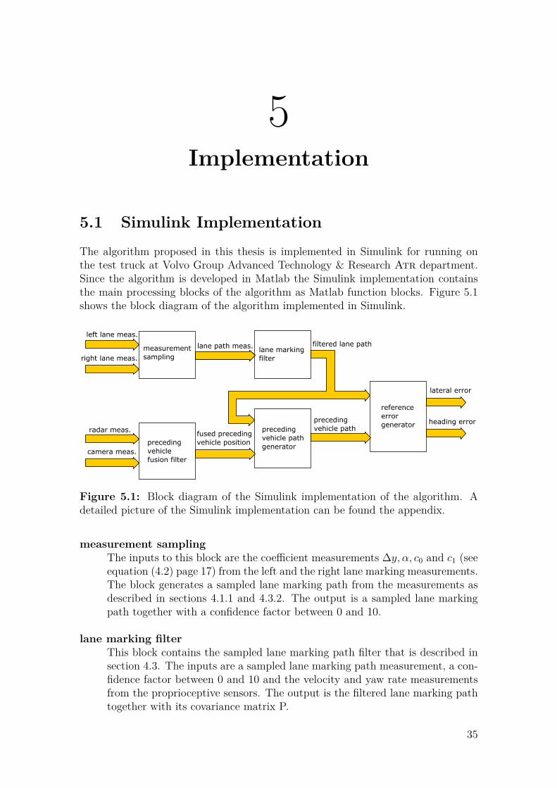
5.1 Block diagram of the Simulink implementation of the algorithm. Adetailed picture of the Simulink implementation can be found theappendix. . . . . . . . . . . . . . . . . . . . . . . . . . . . . . . . . . 35

6.1 Absolute error between lane marking measurements and ground truthat different look ahead distances for the left (top plot) and right (mid-dle plot) lane marking during one measurement run. The curvature ofthe road (bottom plot) as reference to evaluate a correlation betweenroad curvature and measurement error. . . . . . . . . . . . . . . . . . 38

6.2 Distribution of left lane marking measurement error. All the setsare normally distributed, the red curves are the Gaussian probabilitydensity functions with mean values and standard distributions foundin table 6.1. . . . . . . . . . . . . . . . . . . . . . . . . . . . . . . . . 38

6.3 Distribution of right lane marking measurement error. All the setsare normally distributed, the red curves are the Gaussian probabilitydensity functions with mean values and standard distributions foundin table 6.1. . . . . . . . . . . . . . . . . . . . . . . . . . . . . . . . . 39

6.4 The figures illustrate the performance of the prediction step in sam-ple filter and coefficient filter. The gray lanes are the actual measure-ments, red line is the measurements of left and right lanes averaged,green circles are the estimates from the sampled filter and the blueline is the estimate from the coefficient filter. . . . . . . . . . . . . . 40

6.5 Error to ground truth for the unprocessed lane marking path. (topleft) error at look ahead distances x = 0m, 10m, 20m, 30m, 40m, (topright) zoomed part of error, (bottom plots) histograms for the distri-bution of the errors with colors corresponding to signals in the topplots. . . . . . . . . . . . . . . . . . . . . . . . . . . . . . . . . . . . . 41

6.6 Error to ground truth for the filtered lane marking path. (top left) er-ror at look ahead distances x = 0m, 10m, 20m, 30m, 40m, (top right)zoomed part of error, (bottom plots) histograms for the distributionof the errors with colors corresponding to signals in the top plots. . . 42

6.7 (top) lateral control signal generated from ground truth, unprocessedlane path measurements and filtered lane marking path, (bottom left)error to ground truth signal, (bottom right) probability density func-tions for errors. . . . . . . . . . . . . . . . . . . . . . . . . . . . . . . 43

xiv

List of Figures

6.8 Error of the lateral control signal to ground truth for unprocessedmeasurement path and filtered path with added 10% noise to themeasurements. . . . . . . . . . . . . . . . . . . . . . . . . . . . . . . . 43

6.9 Error of the lateral control signal to ground truth for unprocessedmeasurement path and filtered path with added 20% noise to themeasurements. . . . . . . . . . . . . . . . . . . . . . . . . . . . . . . . 44

6.10 Error of the lateral control signal to ground truth for unprocessedmeasurement path and filtered path with 20 % of measurements re-moved from the path. When no measurement is available the lateralcontrol signal for the unprocessed measurement path is set to 0. . . . 45

6.11 Error of the lateral control signal to ground truth for unprocessedmeasurement path and filtered path with 20 % of measurements re-moved from the data set. When no measurement is available thelateral control signal for the unprocessed measurement path is keptconstant at the last value. . . . . . . . . . . . . . . . . . . . . . . . . 45

6.12 Error of the lateral control signal to ground truth for unprocessedmeasurement path and filtered path with 85 % of measurements re-moved from the data set. When no measurement is available thelateral control signal for the unprocessed measurement path is keptconstant at the last value. . . . . . . . . . . . . . . . . . . . . . . . . 46

6.13 Error of the lateral control signal to ground truth for unprocessedmeasurement path and filtered path with 85 % of measurements re-moved from the data set. When no measurement is available thelateral control signal for the unprocessed measurement path is set to 0. 46

6.14 The paths that are generated for the lateral control. The green pathis the lane marking reference path, blue line is the preceding vehiclepath, blue circle is the current estimated position of the precedingvehicle, red cross is the look ahead point and the gray lanes are theright and left lane markings. . . . . . . . . . . . . . . . . . . . . . . . 48

6.15 The radar and camera measurement of lateral position of the pre-ceding vehicle. The standard deviation for the measurements that isestimated by the sensor can be seen in the lower plot. . . . . . . . . 49

A.1 Detailed map of the testing area AstaZero . . . . . . . . . . . . . . . IIA.2 Simulink implementation of the algorithm proposed in this thesis . . IV

xv

List of Figures

xvi

List of Tables

4.1 The sensor information logged during the scenarios . . . . . . . . . . 30

6.1 Distributions of the lane marking measurement errors. Left and rightlane separate and both lanes combined. . . . . . . . . . . . . . . . . . 39

6.2 Mean values and standard deviations of the errors for the datasetswith added noise. . . . . . . . . . . . . . . . . . . . . . . . . . . . . . 44

6.3 Mean values and standard deviations of the errors for the data setswith removed samples. comparison between filtered lane markingpath, unprocessed measurement path with control signal set to 0 whenmeasurement is removed and unprocessed measurement path withcontrol signal kept constant when measurement is removed. . . . . . . 47

6.4 Mean square error of the lateral position. The error is between theground truth and filter estimates with different time step sizes (dt). . 47

xvii

List of Tables

xviii

1Introduction

This chapter will give a brief overview of the thesis project and relevant topics.Problem statement, aims and objectives will also be presented.

1.1 Background and motivation

The availability of driver assistance systems and autonomous functions has increasedrapidly for production vehicles in recent years. Current systems and functions arebeing developed for active safety and aim to assist the driver in selected drivingsituations. Examples of such systems are lane keeping assistance, collision warning,emergency braking and adaptive cruise control. To further develop the technologyand step closer towards fully autonomous vehicles several research projects havebeen initiated. At Volvo Cars "Drive Me" is an autonomous driving project in which100 self-driving cars will be used on selected roads in and around Gothenburg. Thefirst car is expected to be on the roads by 2017. Another project Sartre [1] seeksto improve comfort, safety and energy consumption by developing platooning solu-tions. A platoon can be explained as a group of vehicles that drive in a coordinatedformation. In Sartre the leading vehicle is manually driven while the followingvehicles follow it fully autonomously. By using vehicle to vehicle (V2V) communi-cation together with the vehicles sensors the gap between the vehicles can be keptsmall which leads to reduced fuel consumption and less traffic congestion. One ofthe main obstacles in recent projects and autonomous driving in general is how todeal with inaccurate and unreliable sensors.Within the department of Advance Technologies and Research (Atr) at Volvo GroupTrucks Technology (Gtt) are several projects focused on self-driving trucks. In someof these projects the truck currently relies on a unprocessed sensor measurementsfor lateral control which can cause problems when the conditions for the sensor arenot ideal. The simplest way to get a reference for a lateral control is to use thesensor signal directly. This method is far from optimal and there is a big room forimprovement in how the sensor data are handled. A simple filter that smooth’s thesensor measurements yields better results. An optimal way is to use filters basedon Bayesian statistics. The most common technique to implement Bayesian filteris the Kalman filter, invented in 1950s by Rudolph Emil Kalman [2]. The Kalmanfilter uses a process model that predicts what the new measurement is expected tobe. The estimate is then derived by using the prediction, the measurement andthe uncertainty of both of them. When more than one sensor source is available,the optimal way is to derive the estimate from all of them. Also when the sensor

1

1. Introduction

source is not available for a short period, the prediction can be used as reference.How to handle sensor data in a optimal way using all information available was themotivation for this master thesis.

1.2 Problem StatementThe performance of lateral control is directly connected to the characteristics andability of the used sensor. The sensors that are commercially available today areeither not accurate enough or not reliable under all circumstances to be used indi-vidually. In order to have a robust lateral control all available sensor sources needto be used optimally. In this project a radar sensor, camera sensor and vehicle statesensors will be fused together to generate path for robust lateral control.

1.3 ApplicationsThe sensors used in this project are limited to devices that exist in commerciallyavailable vehicles. These sensors are not capable of providing enough informationfor lateral control in complex urban scenarios. Therefore only selected scenarios aretaken into account. Most of the scenarios take place on highways or roads where fewunexpected things can occur. The work done in this thesis will provide a good basison how to handle sensor data for lateral control in different applications. Some ofthe applications that are currently under development at Volvo ATR are describedhere together with how the reference for lateral control can be obtained in each ofthem.

AutopilotAutopilot is a autonomous driving system for highways. The driver is sup-posed to monitor the system and be prepared to take over the control if thesystem has technical problems or dangerous situations appear in front of thevehicle. The lateral control can be done by using observations of lane mark-ings, position of preceding vehicle and/or Gps measurements together with amap.

PlatooningPlatooning is when multiple vehicles drive in unison, both laterally and longi-tudinally. The leading vehicle is usually manually driven but can also be drivenby an autopilot system. The following vehicles are driven autonomously withpredefined longitudinal distances between each vehicle. Similar to autopilotthe lateral control can be done using the same references but vehicle to vehiclecommunication can be added to ensure string stability within the platoon [3].

Queue AssistIn traffic jam the queue assist system can take over longitudinal and lateralcontrol of the vehicle to relieve the driver. The lateral control can be doneusing observations of lane markings and position of preceding vehicle.

2

1. Introduction

1.4 Aims and objectivesThe aim of this thesis is to improve the robustness of vehicle lateral controller thatcurrently is under development for several projects at Volvo Gtt.To fulfill the aim the following scientific question needs to be answered:"Can multiple sensor input improve robustness of lateral control for automated driv-ing on highways?"The objectives are to collect measurement data from available sensors that can beused for lateral control, analyze the data and use the findings to develop a sensorfusion algorithm that makes use of the sensors optimally to generate reference forlateral control. The algorithm will be tested with simulations and on a test track.

1.5 Thesis outlineThe report is split into 8 chapters. Following the introduction, chapter 2 containsbackground theory and related work.In chapter 3 the production and prototype sensors considered in this thesis arelisted. Each sensors functions are described and how they are used in this project..Also each sensor main characteristics and outputs described. Chapter 4 describesthe methods used for sensor analysis and the development of filters and algorithms.Chapter 5 contains a description of the algorithm implemented for testing on the testtruck. Chapter 6 presents some relevant results from the data analysis and algorithmimplementation. In chapter 7 the conclusion are presented and discussion of mainfindings. Finally, the future work is proposed in chapter 8, with improvements of thecurrent algorithm and outlook on other methods to further improve lateral control.

3

1. Introduction

4

2Background

2.1 Sensor Fusion

Methods in how to handle sensor data by combining different sensors often togetherwith process model is a term called sensor fusion. By adding more informationabout a quantity measured by sensors or predicted by process model a more accu-rate estimate on the true quantity can be achieved than relying on a single sourceof information

Sensor fusion is often referred to in probabilistic robotics [4]. A probabilistic al-gorithm uses the dynamics of the robot and the measurements of its sensors. Thedynamics can be modeled with a process model and state transition distribution de-termined from the uncertainties in the state evolution. The sensors on the robot havea certain noise on the measurements which can be quantified and the measurementdistribution found. Combining the transition distribution and the measurement dis-tribution in a statistical way e.g. using recursive Bayesian filter the estimate of theactual state can be derived.

2.1.1 Bayesian filterA Bayesian filter calculates posterior density of the state recursively which representsa complete statistical description of the state at each time instance [4]. That isan assumption that the Bayesian filter makes called Markov assumption. Markovassumption specifies that if the current state xk|k is known then the past and thefuture data are independent, i.e. the current state is sufficient representation of thepast states. The posterior density is calculated when a new measurement is availablein two steps:

Time updateIn the time update step the Bayesian filter calculates the predicted mean xk|k−1and the predicted covariance Pk|k−1 using the process model and the controlinput. The process model is often called the prediction model. The predictionmodel is usually a set of mathematical equations of the state evolution orhow the systems states change from one time instance to the next one. Theuncertainties of the state evolution come from the fact that modeling thedynamics accurately is often difficult and not computationally efficient andtherefore approximations have to be made.

5

2. Background

Measurement updateThe update model calculates the mean xk|k and covariance Pk|k by using theprediction of the state, the measurements and their distributions. The sensorsand the states are connected through the measurement model which describeshow the sensors observe the states.

2.1.2 Kalman FilterKalman filter is the most common technique to implement a Bayesian filter. It wasdeveloped by Rudolph Emil Kalman [2] and published in 1960. The Kalman filteruses moments representation of Gaussian distribution. The estimates at sample kis represented with the mean xk and the covariance Pk, in probabilistic terms themodel is p(xk|y1:k) = N (xk; xk|k, Pk|k). To make sure that the correct posterior iscalculated and it is Gaussian following properties have to hold:

• The initial belief at x0 must be normally distributed.

• Kalman filter assumes linear dynamics thus the state transition probabilityp(xk|uk, xk−1) must be linear function with additive Gaussian noise:

xk = Akxk−1 +Bkut + qk (2.1)

where xk is the state vector, Ak is the state transition matrix and qk is theadditive Gaussian noise that represents the uncertainty in the state transition.

• The measurement probability p(yk|xk) must be linear with Gaussian addednoise:

yk = Ckxk + rk (2.2)

where yk is the measurement vector, Ck is the measurement matrix and rk isthe added Gaussian noise.

Systems that fulfill these properties are called linear Gaussian systems.The Kalman filter algorithm can be seen in equation 2.3 and 2.4. In equation 2.3the state transition is implemented where the estimate prediction xk|k−1 and thecovariance Pk|k−1 is calculated before incorporating the measurements.

Prediction :xk|k−1 = Ak−1xk−1|k−1

Pk|k−1 = Ak−1Pk−1|k−1ATk−1 + Qk−1

(2.3)

The update step is shown in equation 2.4 where Kk is the Kalman gain, vk is theinnovation, Sk is the innovation covariance, xk|k is the new estimate and Pk|k isthe covariance. The innovation checks how much new information is in the mea-surement and the Kalman gain determines how much the new measurement shouldbe incorporated into the new state estimate. The moments xk|k and Pk|k are thenupdated.

6

2. Background

Update :Kk = Pk|k−1 −HT S−1

k

vk = yk −Hxk|k−1

Sk = HPk|k−1HT + Rk

xk|k = xk|k−1 + Kkvk

Pk|k = Pk|k−1 −KkSkKTk

(2.4)

When considering linear Gaussian dynamic systems, the Kalman filter provides op-timal solutions for estimating the states in minimum mean squared error sense andis computationally efficient. But often systems are nonlinear and not Gaussian andtherefore it is not possible to obtain closed form solutions for the estimates. Inthose cases linear Kalman filter is not applicable and a nonlinear filter is neededthat makes approximation in order to derive the estimates.

2.1.3 Cubature Kalman FilterCubature Kalman filter(Ckf) uses a spherical cubature rule for the approximationof an Gaussian filter [5] and can therefore be applied on nonlinear systems. TheCkf is derivative free, which means there is no need to find the jacobian or hessianand would then not have problems with divergence.In the Ckf prediction step (see equation (2.5)) 2n sigma points X are generatedwhere n is the number of states. The sigma points are then propagated through theprocess model in order to calculate the moments. The moments are the predictedmean xk|k−1 and the predicted covariance Pk|k−1.

Prediction :σ − points :X (i)

k−1 = xk−1|k−1 +√n(P(1/2)

k−1|k−1)i i = 1, 2, ...n

X (i+n)k−1 = xk−1|k−1 −

√n(P(1/2)

k−1|k−1)i i = 1, 2, ...npredicted moments :

xk|k−1 ≈1

2n

2n∑i=1

f(X (i)k−1)

Pk|k−1 ≈1

2n

2n∑i=1

f(X (i)k−1 − xk|k−1)(·)T + Qk−1

(2.5)

In the update step (see equation (2.6)) new sigma points are generated using thepredicted moments. The sigma points are then propagated through the measurementmodel and the predicted measurements yk|k−1 are found. The innovation covariancematrix Sk and the cross covariance matrix Pxy are estimated. Finally the estimateof the state are updated in the mean xk|k and the covariance Pk|k. Note that thePxyS−1

k is the Kalman gain.

7

2. Background

Update :σ − points :X (i)

k = xk|k−1 +√n(P(1/2)

k|k−1)i i = 1, 2, ...n

X (i+n)k = xk|k−1 −

√n(P(1/2)

k|k−1)i i = 1, 2, ...ndesired moments :

yk|k−1 ≈1

2n

2n∑i=1

h(X (i)k )

Pxy ≈1

2n

2n∑i=1

(X (i)k − xk|k−1)h(X (i)

k − yk|k−1)T

Sk ≈1

2n

2n∑i=1

(h(X (i)k − yk|k−1))(·)T + Rk

xk|k = xk|k−1 + PxyS−1k (yk − yk|k−1)

Pk|k = Pk|k−1 −PxyS−1k PT

xy

(2.6)

2.1.4 Rauch-Tung-Striebel SmootherThe Rauch-Tung-Striebel (Rts) smoother is a smoothing algorithm for linear andGaussian systems and was develop by Rauch, Tung and Striebel in the 1960s [6].The Rts smoother is a forward-backward smoother which means it filters forwardusing Kalman filter (see section 2.1.2) computing p(xk|y1:k) for k = 1, 2, 3...K andsmooth’s backward computing p(xk|y1:K) for k = K − 1, K − 2, K − 3...1. Thepredicted moments and moments have to be saved for each time instance in theKalman filtering step. The probabilistic model for Rts smoothing is p(xk|y1:K) =N (xk; xk|K , Pk|K) and the algorithm can be seen in equation 2.7

Gk = Pk|kATk P−1

k+1|k

xk|K = xk|k + Gk(xk+1|K − xk+1|k)Pk|K = Pk|K −Gk(Pk+1|K − Pk+1|k)GT

k

(2.7)

2.2 Control Theory

2.2.1 FeedbackWhen controlling the lateral position of a vehicle, the most frequently used approachis to control the lateral error ∆y at a look ahead distance L to zero [7] [8]. Oneway of obtaining ∆y is to estimate the lateral deviation between the road and thecenter of gravity (CG) of the vehicle (∆yr) and the yaw angle with respect to theroad (εr)and extrapolating to L (∆y = ∆yr + L · εr) [9]. In [10] ε is used instead ofεr to calculate ∆y when Dgps provides the lateral reference. The equation to findε becomes ε = εr + β where β is the slip angle of the vehicle, which means that ε

8

2. Background

is the angle of the velocity vector with respect to the road. These methods do nottake the property of the path into account. If the path is available (e.g. when usinga map or path planning) ∆y can be defined as the lateral deviation from the pathat the look ahead distance. In addition to the yaw angle, the yaw dynamics εr andβ can be used to predict the lateral displacement caused by the curve the vehicle istaking [11]. Vision based systems can measure ∆y at a look ahead distance directly.The lateral deviation ∆y is used in the feedback control of the lateral controller.The look ahead distance L also has influence on the controller, a large L maintainsstability of the control and dampens yaw dynamics, whereas at slow speeds a largeL can cause cutting of sharp corners.

2.2.2 FeedforwardIn addition to a feedback control, the controller performance can be improved byadding a feedforward component. Tai and Tomizuka noted the analogy between avehicle lateral control system on curved road an a mechanical system with coulombfrictions, and proposed feedforward compensation based on road curvatures to im-prove the tracking error without compromising too much of other system perfor-mances [12] [9]. The feedforward control is usually based on the road curvatureand the vehicle model. To estimate the road curvature [8] implemented an observerwhere the road curvature is included in the state vector. In Hasegawa and Konakapaper [13], they propose a method to estimate road curvature with three look-aheadpoints. As this is done in simulation it does not offer a method on how to obtainthese look-ahead points in a real world application.

9

2. Background

10

3Sensors

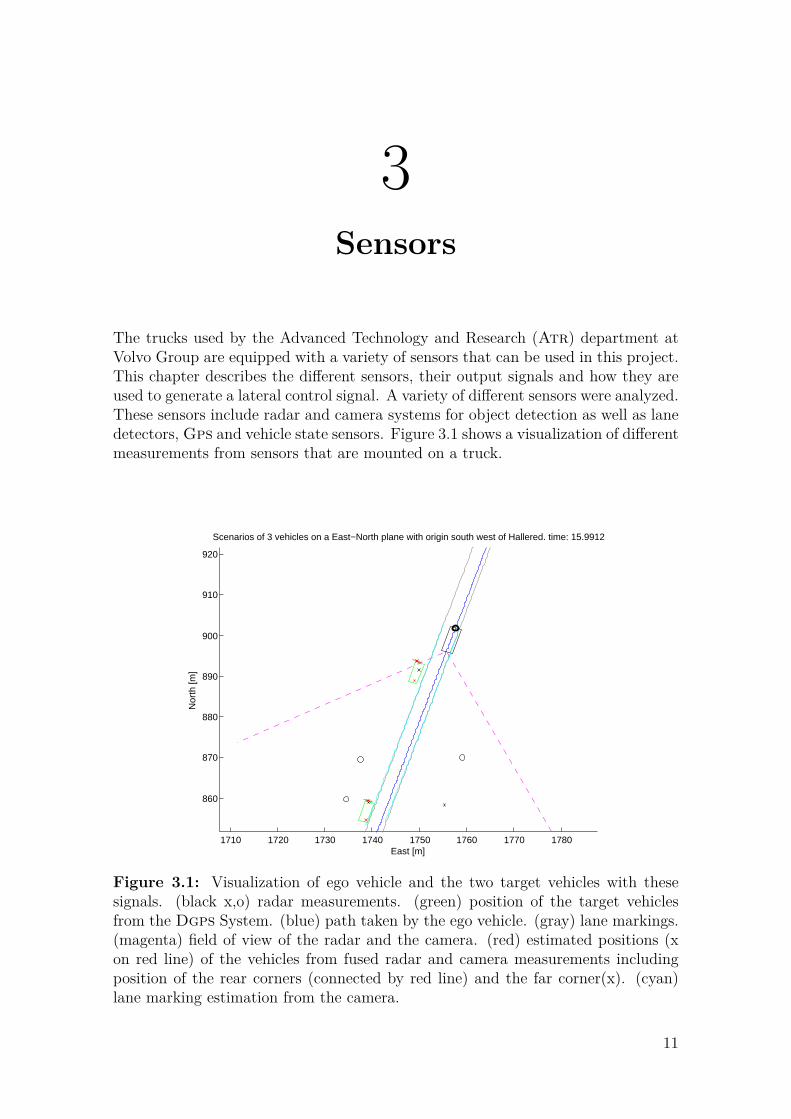
The trucks used by the Advanced Technology and Research (Atr) department atVolvo Group are equipped with a variety of sensors that can be used in this project.This chapter describes the different sensors, their output signals and how they areused to generate a lateral control signal. A variety of different sensors were analyzed.These sensors include radar and camera systems for object detection as well as lanedetectors, Gps and vehicle state sensors. Figure 3.1 shows a visualization of differentmeasurements from sensors that are mounted on a truck.

1710 1720 1730 1740 1750 1760 1770 1780

860

870

880

890

900

910

920

Scenarios of 3 vehicles on a East−North plane with origin south west of Hallered. time: 15.9912

East [m]

Nor

th [m

]

Figure 3.1: Visualization of ego vehicle and the two target vehicles with thesesignals. (black x,o) radar measurements. (green) position of the target vehiclesfrom the Dgps System. (blue) path taken by the ego vehicle. (gray) lane markings.(magenta) field of view of the radar and the camera. (red) estimated positions (xon red line) of the vehicles from fused radar and camera measurements includingposition of the rear corners (connected by red line) and the far corner(x). (cyan)lane marking estimation from the camera.

11

3. Sensors

3.1 Object Detection

The trucks have different sensors that are able to detect objects in the surroundingof the truck. The evaluated sensors include radar and camera. All of the evaluatedsensors are mounted in front of the truck looking forward.

3.1.1 Radar

Radars can detect different objects in front of the Ego vehicle. The radar systemsused in the automotive industry outputs preprocessed data from the radar measure-ments. The systems evaluated in this project can detect and track objects in theirfield of view and classify those. Measurements include the position and velocity oftracked objects in the Ego vehicle coordinate system (Vcs). Classifications canrange from "moving" or "stationary" to more sophisticated classifications such asdifferent kinds of vehicles and stationary objects depending on their size and radarreflectivity.

3.1.2 Camera

Cameras have become increasingly important sensors in the automotive industry.With more sophisticated image processing algorithms and more powerful processors,cameras are very suitable for object detection. Similar to the radar the cameras usedin the automotive industry detect different vehicles and objects in the vicinity of theEgo vehicle. The image processing algorithms detects and follows different objectsand classifies them. More modern cameras also detect traffic signs or traffic lightsas well as turn and brake signals of preceding vehicles.

3.2 Lane Detection Systems

Lane marking measurement systems are based on cameras and detects lane markingsin the field of view of the camera. The measurements from such systems describelane markings in the Ego Vcs. The lane marking measurements can either berepresented as clothoids (z = [∆y, α, c0, c1]T ) where every lane marking measurementhas a lateral deviation from the vehicle (∆y), a heading (α), a curvature (c0) anda curvature rate (c1). Or the measurements are represented as polynomials in theVcs with the following form.

y(x) = a0 + a1 ∗ x+ a2 ∗ x2 + a3 ∗ x3 (3.1)

Clothoid lane markings can be approximated to third order polynomials by usingthe following approximation.

y(x) = ∆y − α · x+ c0

2 x2 + c1

6 x3 (3.2)

12

3. Sensors

3.3 GPS

3.3.1 RACELOGIC VBOX SystemFor test purposes Vbox data loggers by Racelogic are available and can bemounted on the vehicles. The Racelogic Vbox is a Gps data logger that can beused in different setups. To use the system the vehicles have to be equipped with twoGps antennas and radio communication antennas. When one Vbox system is usedas stand alone system absolute Gps coordinates can be logged with an accuracyof 2m. When two vehicles are equipped with a Vbox system each (moving basesetup), the relative positions between the vehicles can be detected with an accuracyof ±2cm while the absolute positions remain at a 2m accuracy. The Vbox can alsobe used in conjunction with a stationary base station. With the base station theabsolute position of a vehicle can be logged with an accuracy of ±2cm. The use ofthe bases station is limited by the radio communication range between the vehicleand the station which is a few hundred meters.

3.4 Sensor SetupThe goal for this project was to develop an application that could be used on acommercially available vehicle. Therefore the sensors used as inputs to the developedalgorithms are all systems that are available in commercial vehicles. The followingsensor systems have been used in the development of the algorithms.

• radar for object detection

• camera for object detection

• camera for lane detection

• vehicle state sensors for dead-reckoning

Apart from the sensors used in the algorithms a Gps system was used was used forgenerating ground truth data to test the algorithms.

3.4.1 Object DetectionTwo different systems for object detection were used in this project, a radar basedsystem and a camera based system. The radar system can detect and track sixdifferent objects in its field of view and classify them into stationary or moving.The measurements include object position and velocity in the Ego Vcs includingthe standard deviations for the measurements. In addition to the radar a camerasystem is used that can detect six different objects and measure the objects positionsin the Ego Vcs. The data from the camera and the radar are fused together tofind an accurate estimated position of the preceding vehicle. This is described inmore detail in section 4.5. A statistical analysis of the sensor data can be found insection 6.4.

13

3. Sensors

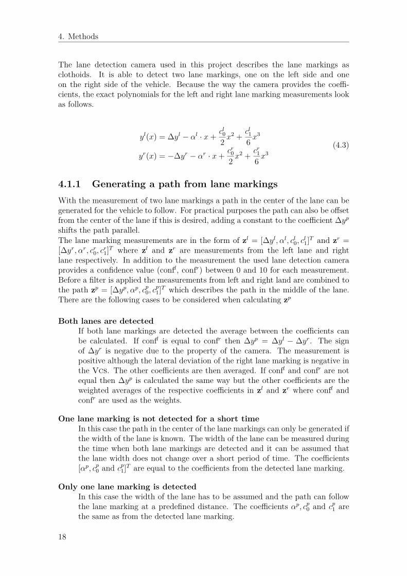
3.4.2 Lane DetectionThe lane detection system used in this project is capable of measuring two differentlane markings, one on each side of the vehicle. The lane markings are measured inthe clothoid representation. The measurements and approximations of the left andright lane markings can be seen in equation (3.3) where xv is the position on thex-axis of the Vcs.

Measurements :zl = [∆yl, αl, cl

0, cl1]T

zr = [∆yr, αr, cr0, c

r1]T

Approximations :

yl(xv) = ∆yl − αl · xv + cl02 x

2v + cl

16 x

3v

yr(xv) = −∆yr − αr · xv + cr02 x

2v + cr

16 x

3v

(3.3)

The functions yl(x) and yr(x) describe the lateral position of the lane marking as afunction of xv in the Ego Vcs. The sign of ∆yr is negative due to the property ofthe camera. The measurement is positive although the lateral deviation of the rightlane marking is negative in the Vcs. The heading angle α is the heading betweenthe lane marking and the vehicle being positive in counter clock wise direction (i.e.it has the opposite to the heading in the Ego Vcs), therefore the coefficient is neg-ative sign in equation (3.3). The coefficients c0 and c1 are are positive for curvaturesand curvature rates in counter clock wise direction. For each measurement of a lanemarking the camera generates a confidence value between 0 and 10. The measure-ments are used to generate a path in the middle of the two detected lane marking.The path is used to generate a lateral reference signal that the vehicle controller issupposed to follow. The filter algorithm with a Ckf prediction and a linear Kalmanupdate is described in more detail in section 4.3. A statistical analysis of the sensordata can be found in section 6.1.

3.4.3 Vehicle State SensorsAll the trucks are equipped with a variety of of internal sensors that monitor thestates of the vehicle. The measurements of these sensors are available on the inter-nal Can (Controller Area Netork) buses of the trucks. In the algorithms developedwithin this project, the vehicle state sensors are used for dead-reckoning. Two differ-ent sensors are used for this part of the algorithms. The velocity measurement fromthe tachometer is used to estimate the distance the vehicle has traveled. The yawrate measurement from the gyroscope is used to estimate the the vehicles rotation.In the filters described in chapter 4 the dead reckoning algorithm is explained inmore detail.

3.4.4 GPSThe Vbox system is used in generating ground truth data for the lane markingmeasurements. To generate those the Gps data are combined with the lane marking

14

3. Sensors

measurements, filtered with a Kalman filter and smoothed with a Rts-smoother.This is described in section 4.1. In all the measurements done for this project theVbox system was configured in a moving base setup without stationary base station.

15

3. Sensors

16

4Methods

EGO vehicle

Preceding vehicle

Lane marking measurement

Field of view

Lane marking path

Preceding vehicle path

Figure 4.1: Overview figure that illustrates the sensor measurements and the pathsthat are generated using methods implemented in this thesis.

4.1 Generating a reference with lane markingsLane markings can be used to generate a path on the road that the vehicle canfollow by filtering the lane marking measurements. There are two main methods inwhich lane markings are represented by lane detection cameras. In the first methodthe camera outputs a third order polynomial that describes the lane marking inthe vehicle coordinate system. The vehicle coordinate system has its x-axis in thedirection of the heading of the vehicle.

y(x) = a0 + a1 · x+ a2 · x2 + a3 · x3 (4.1)The second method describes the lane marking as a clothoid with a lateral deviation(∆y), a heading (α), a curvature (c0) and a curvature rate (c1). A lane markingdescribed as a clothoid can be approximated with the following third order polyno-mial [14].

y(x) = ∆y + α · x+ c0

2 x2 + c1

6 x3 (4.2)

17

4. Methods

The lane detection camera used in this project describes the lane markings asclothoids. It is able to detect two lane markings, one on the left side and oneon the right side of the vehicle. Because the way the camera provides the coeffi-cients, the exact polynomials for the left and right lane marking measurements lookas follows.

yl(x) = ∆yl − αl · x+ cl02 x

2 + cl16 x

3

yr(x) = −∆yr − αr · x+ cr02 x

2 + cr16 x

3(4.3)

4.1.1 Generating a path from lane markingsWith the measurement of two lane markings a path in the center of the lane can begenerated for the vehicle to follow. For practical purposes the path can also be offsetfrom the center of the lane if this is desired, adding a constant to the coefficient ∆yp

shifts the path parallel.The lane marking measurements are in the form of zl = [∆yl, αl, cl

0, cl1]T and zr =

[∆yr, αr, cr0, c

r1]T where zl and zr are measurements from the left lane and right

lane respectively. In addition to the measurement the used lane detection cameraprovides a confidence value (confl, confr) between 0 and 10 for each measurement.Before a filter is applied the measurements from left and right land are combined tothe path zp = [∆yp, αp, cp

0, cp1]T which describes the path in the middle of the lane.

There are the following cases to be considered when calculating zp

Both lanes are detectedIf both lane markings are detected the average between the coefficients canbe calculated. If confl is equal to confr then ∆yp = ∆yl − ∆yr. The signof ∆yr is negative due to the property of the camera. The measurement ispositive although the lateral deviation of the right lane marking is negative inthe Vcs. The other coefficients are then averaged. If confl and confr are notequal then ∆yp is calculated the same way but the other coefficients are theweighted averages of the respective coefficients in zl and zr where confl andconfr are used as the weights.

One lane marking is not detected for a short timeIn this case the path in the center of the lane markings can only be generated ifthe width of the lane is known. The width of the lane can be measured duringthe time when both lane markings are detected and it can be assumed thatthe lane width does not change over a short period of time. The coefficients[αp, cp

0 and cp1]T are equal to the coefficients from the detected lane marking.

Only one lane marking is detectedIn this case the width of the lane has to be assumed and the path can followthe lane marking at a predefined distance. The coefficients αp, cp

0 and cp1 are

the same as from the detected lane marking.

18

4. Methods

No lane marking is detectedThe measurement is discarded.

4.1.2 Coefficient and Sampled Lane Marking Measurementand Filters

There are two different ways to represent and filter a path generated from lanemarkings. One way is to have a coefficient representation like the ones in equations(4.1) and (4.2) where the lane marking function y(x) has a value for all values xbetween −∞ and +∞. This representation describes the lane markings betweencertain bounds on x between 0 and around 50 m. The second way is to representthe path as sampled points in x and y similar to the methods proposed in Fernándeset.al. paper [15]. The following chapters describe both principles in more detail.For both methods a filter method is presented. Ultimately it was decided to goforward with the sampled version as it is less sensitive to coefficient noise [14] andthe performance of the sampled filter has proven to be better in tests than thecoefficient filter (see 6.2).

4.2 Coefficient Filter for Lane Marking Path

The first filter is a coefficient filter which is a Kalman filter with both linear processand measurement model. The development of this filter was discontinued after initialtest showed that the sampled filter described in section 4.3 performed better as seenin section 6.2.

4.2.1 Prediction step

Using the third order polynomial that approximates a clothoid in equation 4.2 themotion model can be derived. The states that are predicted with the motion modelare the lateral deviation (∆y), the heading (α), the curvature (c0) and the curvaturerate (c1) of the averaged lane marking. The movement and change in orientationof the truck is calculated using measurements of the velocity(v), yaw rate (ϕ) andtime between lane marking measurements(dt). The distance traveled between eachprediction is then x = v · dt and the change in orientation is dx

dy= atan(−ϕ · dt).

Since the angles are very small during highway driving, small angle approximationcan be applied which gives dϕ = −ϕ · dt. The prediction model can be seen in

19

4. Methods

equation 4.4, xv is the position on the x-axis of the Vcs.x(k + 1) = A · x(k) +B · uwhere :

x(k) =

∆yαC0C1

u = ϕ

A =

1 xv

x2v

2x3

v

60 1 xv

x2v

20 0 1 xv

0 0 0 1

B =

0−dt

00

(4.4)

4.2.2 Update stepSince all the states are measured the update is linear with the measurement matrixH as identity matrix. When the confidence value (confl, confr) are both belowconfidence threshold (set to 3) the measurement are considered not valid and inthat case the update step is skipped.

xk|k = xk|k−1 + Kk(yk −Hxk|k−1)H = In

Pk|k = Pk|k−1 −KkSkKTk

Kk = Pk|k−1 −HT S−1k

Sk = HPk|k−1HT + Rk

Rk : Measurement noise covariance

(4.5)

4.3 Sampled Filter for Lane Marking PathThe sampled filter is a Kalman filter with a nonlinear process model for the pre-diction and a linear measurement model for the update. For the prediction step aCubature Kalman filter is used. Since the measurement model is linear the updateis a direct Kalman update step. It was decided to go forward with this filter in thisproject as it performed better than the coefficient filter.

4.3.1 Prediction stepThe prediction step of the filter estimates the positions of the sampled path at thetime of the next lane marking measurements. It does that by applying the nonlinear

20

4. Methods

yv

xv

Δ Δ Δ

pathy(x=Δ,2Δ...)

Figure 4.2: Shows how the path is sampled for the filter. Like the lane markingmeasurements the sampled path is described in the vehicle coordinate system (Vcs)(xv, yv). The samples are distributed equidistantly in x at distance ∆.

function f(x,v, ϕ,dt) to the previous estimation. All the formulas for the CubatureKalman prediction can be found in (4.8).

Nonlinear prediction function f(x,v, ϕ,dt) The nonlinear function for theprediction step is divided in three steps.

1) Move coordinate systemUsing the time elapsed since the previous measurement (dt), the yaw rate (ϕ)and the velocity of the vehicle (v), the coordinate system (xv

k−1, yvk−1) is moved

to the new position (xvk, y

vk). The coordinate system is first moved along the

x-axis by dx = v ·dt and then rotated around the z-axis by dϕ = ϕ ·dt (Figure4.3.

2) Update estimatesThe estimates xk−1 = [y0

k−1, y1k−1, ...] are moved to the new coordinate system.

Since this transformation and a rotation the updated points pi have both xand y values (Figure 4.4).

pix = (∆ · i− dx) · cos(−dϕ)− yi

k−1 · sin(−dϕ)pi

y = (∆ · i− dx) · sin(−dϕ) + yik−1 · cos(−dϕ)

i = 0, 1, ...nn : nr. of points in discretized path minus 1

(4.6)

3) Interpolation/ExtrapolationThe prediction points are calculated by linearly interpolating from pi to x =

21

4. Methods

xvk-1 xv k

yvk-1yv k

pathyk-1(x=Δ,2Δ...)

dx

dφ

Figure 4.3: Moving the coordinate system in the nonlinear function f(x,v, ϕ,dt)inthe prediction step

[0,∆, 2∆...]. (Figure 4.5).

yik = pi

y + ((∆ · i− pix) · (pi+1

y − piy))/(pi+1

x − pix)

i = 0, 1..n− 1yn

k = piy + ((∆ · n− pn

x) · (pny − pn−1

y ))/(pnx − pn−1

x )(4.7)

Since it is not possible to interpolate a value for the last x value, the last pointhas to be extrapolated. In the current implementation this is done with alinear extrapolation through pn−1 and pn. On alternative method would be toextrapolate by setting the angle ^pn−1, pn, p(∆ · n, yn

k ) equal to ^pn−2, pn−1pn

Since f(x,v, ϕ,dt) is nonlinear the prediction step is done with a Cubature Kalmanfilter.

X (i)k−1 = xk−1|k−1 +

√n(P(1/2)

k−1|k−1

)i, i = 1, 2, ..., n

X (i+n)k−1 = xk−1|k−1 −

√n(P(1/2)

k−1|k−1

)i, i = 1, 2, ..., n

Wi = 12n, i = 1, 2, ..., 2n

n : nr. of points in discretized path

xk|k−1 =2n∑i=1

f(X (i)k−1, v, ϕ, dt)Wi

Pk|k−1 =2n∑i=1

f(X (i)k−1, v, ϕ, dt)− xk|k−1)(·)TWi + Qk−1

(4.8)

22

4. Methods

yvk

xvk

pathpi=(xi,yi)

Figure 4.4: Update estimates to moved coordinate system in the nonlinear functionf(x,v, ϕ,dt)in the prediction step

yvk

xvk

interpolated pointsextrapolated point

pi=(xi,yi)

Δ Δ ΔFigure 4.5: interpolation/extrapolation to obtain prediction points in the nonlinearfunction f(x,v, ϕ,dt)in the prediction step

23

4. Methods

4.3.2 Update step

Measurement model This filter is set up in a way that the measurements arethe sampled path. Therefore the lane marking estimations from the lane detectioncamera must be translated to sampled path points. The lane marking measurementsare in the form of zp = [∆yp, αp, cp

0, cp1]T according to 4.1.1.

The path zp can then be used to calculate the sampled measurement points for thefilter.

y =

1 ∆ 1

2∆2 16∆3

1 2∆ 12(2∆)2 1

6(2∆)3

... ... ... ...1 n∆ 1

2(n∆)2 16(n∆)3

zp (4.9)

The update step is then a linear Kalman update (see equation 4.10)

xk|k = xk|k−1 + Kk(yk −Hxk|k−1)H = In

Pk|k = Pk|k−1 −KkSkKTk

Kk = Pk|k−1 −HT S−1k

Sk = HPk|k−1HT + Rk

Rk : Measurement noise covariance

(4.10)

4.4 Generating a reference with preceding vehicle

When a vehicle is driving in front of the Ego vehicle its position can be detectedby the object detection sensors (radar and camera). These positions can be used asa reference for the lateral control of Ego vehicle.

4.4.1 Generating reference path

A reference path can be constructed from the filtered position of the precedingvehicle. The path contains N number of points in the Ego vehicles coordinatesystem. The points are placed equidistantly in the x-axis of the Vcs with a fixedlongitudinal distance deltaPrec between them.

24

4. Methods

field of viewfield of viewpreceding vehiclepreceding vehiclefiltered preceding vehicle positionfiltered preceding vehicle positionsampled lane marking path

initial preceding vehicle path

initial preceding vehicle pathinterpolation / extrapolation

vehicle coordinate systemvehicle coordinate system

A) B)

offset

Figure 4.6: Initial path from preceding vehicle when a vehicle enters the field ofview. A) shows how the N points in the path are generated if a lane marking pathis available by offsetting the lane marking path and adding the preceding vehicleposition as the Nth point and B) shows how the points are generated when no lanemarking path is available by linear interpolation between the ego vehicle positionand the preceding vehicle position.

Initial path generatedWhen there is no vehicle visible to the sensors no path is generated. As soonas a vehicle appears in the field of view of the Ego vehicle a path betweenthe Ego vehicle and the preceding vehicle is generated depending if the lanemarkings path is available or not. The path is a series of N points in thevehicle coordinate system. If the lane markings are available the points areplaced parallel to the lane markings with an offset. The offset is the lateraldifference between the position of the preceding vehicle to the lane markings.The lane marking path consists of N-1 points in the vehicle coordinate system,therefore the Nth point in the preceding vehicle path is the position of thepreceding vehicle. This method of generating the initial path can be seen infigure 4.6 A. If no lane marking path is available the initial points are placedby linear interpolating six points between the Ego vehicle and the precedingvehicle (figure 4.6 B).

Movement of the pathThe points of the path represent the trajectory of the preceding vehicle in Egovehicle coordinate system. Since the coordinate system moves with the Egovehicle the points need to move within the coordinate system according to thedistance traveled (dx) and change in orientation (dϕ) of the Ego vehicle. Thedistance and the orientation is calculated using the yaw rate (ϕ), the velocitymeasurement(v) and the step length(dt):

dϕ = dt · ϕ

dx = dt · v

25

4. Methods

Update points of the pathWhen the distance between the point in path which is closest to the precedingvehicle and the current filtered point on the preceding vehicle is equal todeltaPrec, oldest point (furthest away from the preceding vehicle) is discardedand current filtered point added to the path. The update is illustrated in figure4.7.

preceding vehicle

filtered position

vehicle coordinate system

A)

B) preceding vehicle path

new point on path

point removed from path

C) deltaPrec

Figure 4.7: Updating the preceding vehicle path. Each time the distance betweenthe newest point in the path and the preceding vehicle is larger than deltaPrec thepoint furthest away from the preceding vehicle is removed and the preceding vehicleposition is added as new point.

UncertaintiesThe movement of the points can be considered as pure prediction since thereare no measurements of the points in the path to update with. The predictionstep is the same as for the lane marking sampled points and therefore the sameprediction model can be used. The covariance is based on the noise of the yawrate and the velocity. Since there is no update step, the uncertainties increaseover time, which results in very uncertain points on the path especially if thepreceding vehicle is far ahead. By filtering the states of the vehicle such asvehicle and heading a more accurate movement of the vehicle between timeinstances can be achieved. This was not in the scope of this thesis but discussedin future work chapter 8.

4.5 Preceding Vehicle FilterThe position of the preceding vehicle is measured with the camera and radar. Thecamera measures longitudinal and lateral distances to the preceding vehicle relativeto the Ego vehicle. The radar has the same measurements as the camera but alsooutputs the relative velocity in longitudinal and lateral direction. These sensor infor-mation can be fused together to obtain an estimate of the position of the precedingvehicle relative to Ego vehicle. Based on the measurements of the preceding vehiclethe most straight forward choice of a state vector would be [x, y, vx, vy] where x andy is the longitudinal and lateral distances respectively, vx and vy are the correspond-

26

4. Methods

ing velocities in longitudinal and lateral direction. All of the states are relative tothe Ego vehicle.

4.5.1 Prediction step

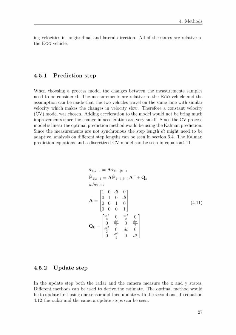
When choosing a process model the changes between the measurements samplesneed to be considered. The measurements are relative to the Ego vehicle and theassumption can be made that the two vehicles travel on the same lane with similarvelocity which makes the changes in velocity slow. Therefore a constant velocity(CV) model was chosen. Adding acceleration to the model would not be bring muchimprovements since the change in acceleration are very small. Since the CV processmodel is linear the optimal prediction method would be using the Kalman prediction.Since the measurements are not synchronous the step length dt might need to beadaptive, analysis on different step lengths can be seen in section 6.4. The Kalmanprediction equations and a discretized CV model can be seen in equation4.11.

xk|k−1 = Axk−1|k−1

Pk|k−1 = APk−1|k−1AT + Qk

where :

A =

1 0 dt 00 1 0 dt0 0 1 00 0 0 1

Qk =

dt3

3 0 dt2

2 00 dt3

3 0 dt2

2dt2

2 0 dt 00 dt2

2 0 dt

(4.11)

4.5.2 Update step

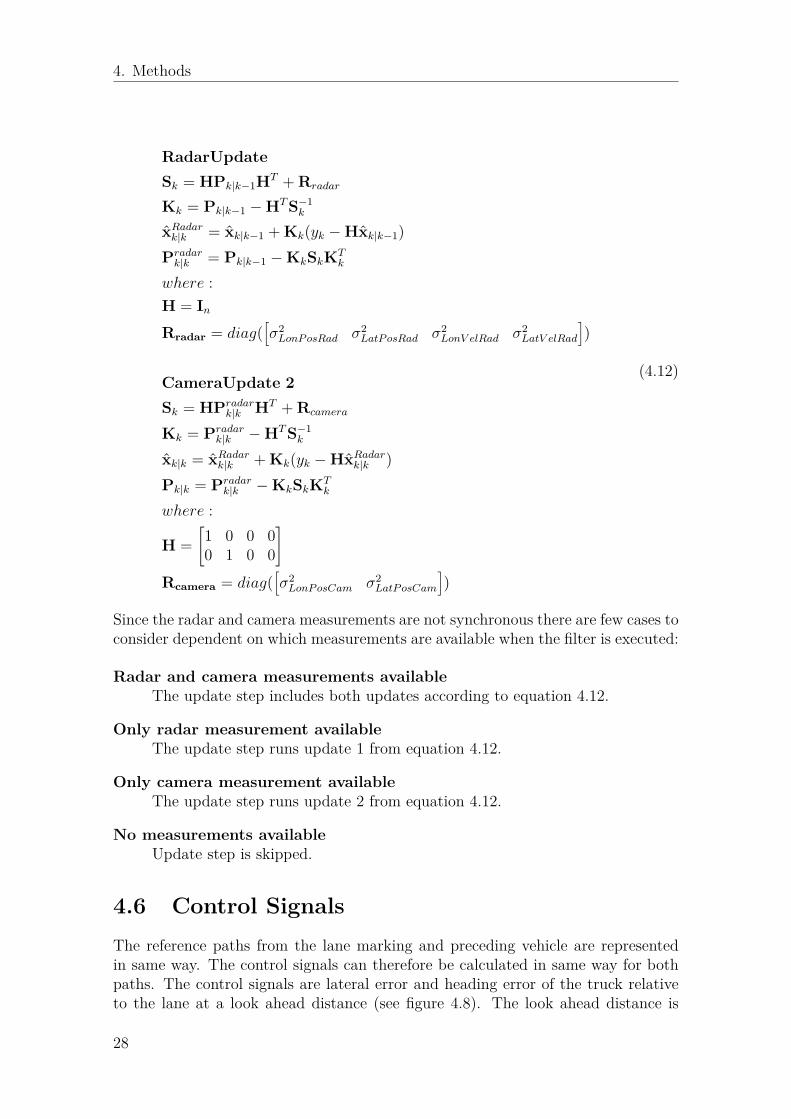
In the update step both the radar and the camera measure the x and y states.Different methods can be used to derive the estimate. The optimal method wouldbe to update first using one sensor and then update with the second one. In equation4.12 the radar and the camera update steps can be seen.

27

4. Methods

RadarUpdateSk = HPk|k−1HT + Rradar

Kk = Pk|k−1 −HT S−1k

xRadark|k = xk|k−1 + Kk(yk −Hxk|k−1)

Pradark|k = Pk|k−1 −KkSkKT

k

where :H = In

Rradar = diag([σ2

LonP osRad σ2LatP osRad σ2

LonV elRad σ2LatV elRad

])

CameraUpdate 2Sk = HPradar

k|k HT + Rcamera

Kk = Pradark|k −HT S−1

k

xk|k = xRadark|k + Kk(yk −HxRadar

k|k )Pk|k = Pradar

k|k −KkSkKTk

where :

H =[1 0 0 00 1 0 0

]Rcamera = diag(

[σ2

LonP osCam σ2LatP osCam

])

(4.12)

Since the radar and camera measurements are not synchronous there are few cases toconsider dependent on which measurements are available when the filter is executed:

Radar and camera measurements availableThe update step includes both updates according to equation 4.12.

Only radar measurement availableThe update step runs update 1 from equation 4.12.

Only camera measurement availableThe update step runs update 2 from equation 4.12.

No measurements availableUpdate step is skipped.

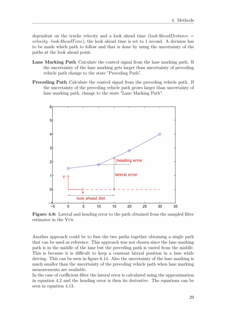
4.6 Control SignalsThe reference paths from the lane marking and preceding vehicle are representedin same way. The control signals can therefore be calculated in same way for bothpaths. The control signals are lateral error and heading error of the truck relativeto the lane at a look ahead distance (see figure 4.8). The look ahead distance is

28

4. Methods

dependent on the trucks velocity and a look ahead time (lookAheadDistance =velocity · lookAheadT ime), the look ahead time is set to 1 second. A decision hasto be made which path to follow and that is done by using the uncertainty of thepaths at the look ahead point.

Lane Marking Path Calculate the control signal from the lane marking path. Ifthe uncertainty of the lane marking gets larger than uncertainty of precedingvehicle path change to the state "Preceding Path".

Preceding Path Calculate the control signal from the preceding vehicle path. Ifthe uncertainty of the preceding vehicle path grows larger than uncertainty oflane marking path, change to the state "Lane Marking Path".

−5 0 5 10 15 20 25 30 35−1

0

1

2

3

4

5

6

lateral error

look ahead dist

x

y

heading error

Figure 4.8: Lateral and heading error to the path obtained from the sampled filterestimates in the Vcs.

Another approach could be to fuse the two paths together obtaining a single paththat can be used as reference. This approach was not chosen since the lane markingpath is in the middle of the lane but the preceding path is varied from the middle.This is because it is difficult to keep a constant lateral position in a lane whiledriving. This can be seen in figure 6.14. Also the uncertainty of the lane marking ismuch smaller than the uncertainty of the preceding vehicle path when lane markingmeasurements are available.In the case of coefficient filter the lateral error is calculated using the approximationin equation 4.2 and the heading error is then its derivative. The equations can beseen in equation 4.13.

29

4. Methods

yref = ∆y + α · x+ c0

2 x2 + c1

6 x3

θref = α + c0 · x+ c1

2 x2

(4.13)

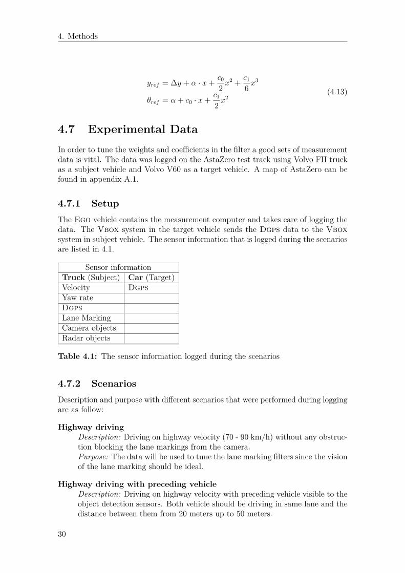
4.7 Experimental DataIn order to tune the weights and coefficients in the filter a good sets of measurementdata is vital. The data was logged on the AstaZero test track using Volvo FH truckas a subject vehicle and Volvo V60 as a target vehicle. A map of AstaZero can befound in appendix A.1.

4.7.1 SetupThe Ego vehicle contains the measurement computer and takes care of logging thedata. The Vbox system in the target vehicle sends the Dgps data to the Vboxsystem in subject vehicle. The sensor information that is logged during the scenariosare listed in 4.1.

Sensor informationTruck (Subject) Car (Target)Velocity DgpsYaw rateDgpsLane MarkingCamera objectsRadar objects

Table 4.1: The sensor information logged during the scenarios

4.7.2 ScenariosDescription and purpose with different scenarios that were performed during loggingare as follow:

Highway drivingDescription: Driving on highway velocity (70 - 90 km/h) without any obstruc-tion blocking the lane markings from the camera.Purpose: The data will be used to tune the lane marking filters since the visionof the lane marking should be ideal.

Highway driving with preceding vehicleDescription: Driving on highway velocity with preceding vehicle visible to theobject detection sensors. Both vehicle should be driving in same lane and thedistance between them from 20 meters up to 50 meters.

30

4. Methods

Purpose: The sensor information from radar and camera on lateral and lon-gitudinal distances of objects ahead will be used to develop filter that tracksthe preceding vehicle.

Traffic jamDescription: The preceding vehicle will simulate a traffic jam by varying thevelocity from standstill to normal highway driving.Purpose: Further develop and tune the prediction step of the filter as wellas handling the transition between different sensor sources. When the car isdriving less than 7 m/s the camera does not detect the lane marking whichneeds to be taken care of by using pure prediction and the detection of thepreceding vehicle. When the car is at standstill it needs to make sure that thefilter covariance matrix does not increase.

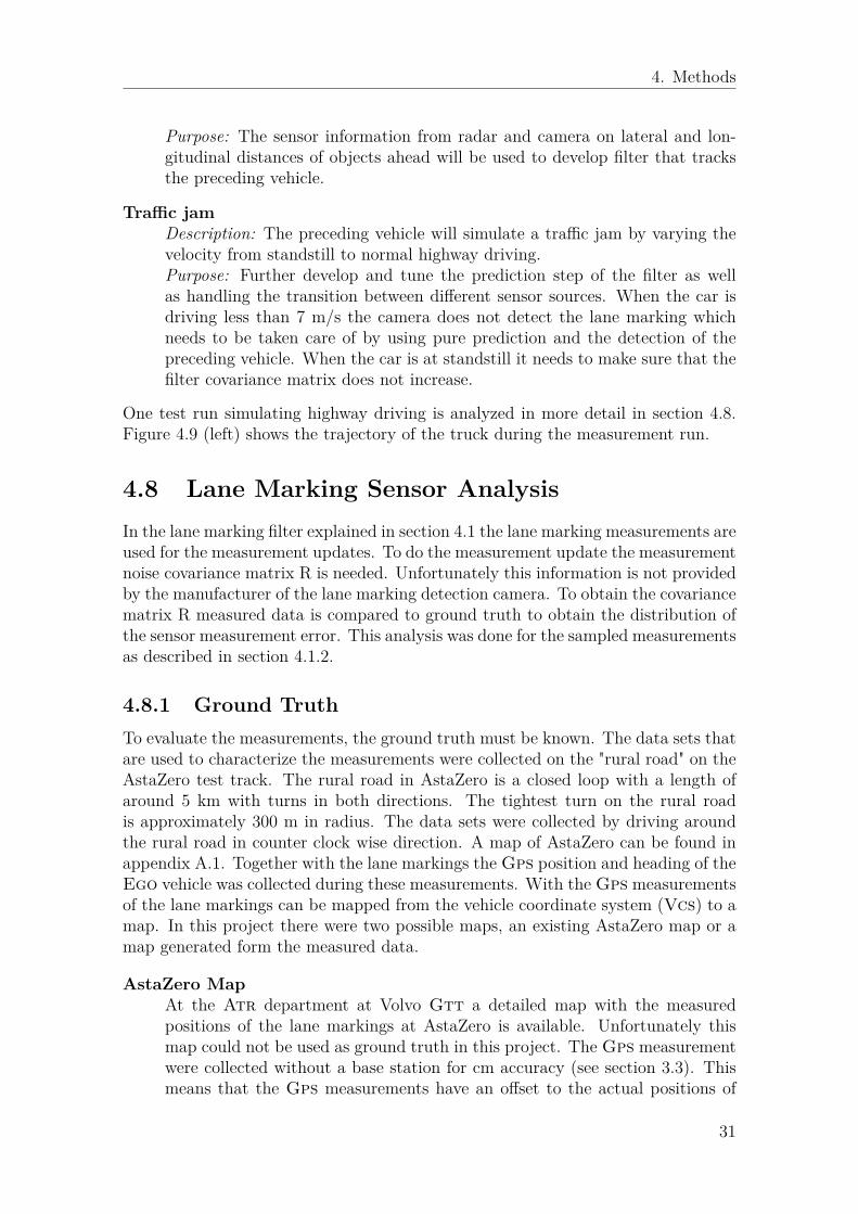
One test run simulating highway driving is analyzed in more detail in section 4.8.Figure 4.9 (left) shows the trajectory of the truck during the measurement run.

4.8 Lane Marking Sensor AnalysisIn the lane marking filter explained in section 4.1 the lane marking measurements areused for the measurement updates. To do the measurement update the measurementnoise covariance matrix R is needed. Unfortunately this information is not providedby the manufacturer of the lane marking detection camera. To obtain the covariancematrix R measured data is compared to ground truth to obtain the distribution ofthe sensor measurement error. This analysis was done for the sampled measurementsas described in section 4.1.2.

4.8.1 Ground TruthTo evaluate the measurements, the ground truth must be known. The data sets thatare used to characterize the measurements were collected on the "rural road" on theAstaZero test track. The rural road in AstaZero is a closed loop with a length ofaround 5 km with turns in both directions. The tightest turn on the rural roadis approximately 300 m in radius. The data sets were collected by driving aroundthe rural road in counter clock wise direction. A map of AstaZero can be found inappendix A.1. Together with the lane markings the Gps position and heading of theEgo vehicle was collected during these measurements. With the Gps measurementsof the lane markings can be mapped from the vehicle coordinate system (Vcs) to amap. In this project there were two possible maps, an existing AstaZero map or amap generated form the measured data.

AstaZero MapAt the Atr department at Volvo Gtt a detailed map with the measuredpositions of the lane markings at AstaZero is available. Unfortunately thismap could not be used as ground truth in this project. The Gps measurementwere collected without a base station for cm accuracy (see section 3.3). Thismeans that the Gps measurements have an offset to the actual positions of

31

4. Methods

the Ego vehicle. It was not possible to map the measured Gps data onto theexisting map with a high enough accuracy.

Generated from Measured DataThe second possibility to get ground truth information is to extract it frommeasurements by combing Gps measurements and lane marking measure-ments. Even though the absolute Gps positions are not exact, the relativeGps position in one measurement run is more accurate. This is because thebias on the measurements primarily depends on atmospheric effects and skyblockage. These are slow changing effects and can therefore be assumed to beconstant during the short time of one measurement run. The distance informa-tion from the lane marking measurement (∆y) was used together with the Gpsmeasurements. For a description of the lane marking measurements see sec-tion 3.2. The Gps measurements are transposed to a East-North-Up (Enu)coordinate system and each lane marking measurement is transposed to itscorresponding vehicle position and heading. This way the two lane markingscan be mapped on an Enu coordinate system. The obtained lane markingspositions are subject to both the Gps measurement noise (not the bias fromthe atmospheric effects) and the measurement noise of the (∆y) measurementof the lane marking camera. The used data set was collected under very goodconditions for the lane marking detection camera i.e. dry roads and no sun-shine. The lane markings are filtered with a Kalman filter with a constantvelocity model and smoothed with an Rts smoother. The path and cutout ofthe measured, filtered and smoothed lane marking can be seen in figure 4.9.

2000 2500 3000

1500

2000

2500

3000

3500

East [m]

Nor

th [m

]

measurements

2311.6 2311.7 2311.8 2311.9 23121705

1710

1715

1720

1725

1730

1735

East [m]

Nor

th [m

]

measurementsfiltered pathsmoothed

Figure 4.9: (left) plot of the trajectory the vehicle drove during the measurementrun in an Enu coordinate system. (right) Cutout of the ground truth of the lanemarkings generated with Gps data, lane marking measurements using a filter andand Rts-smoother.

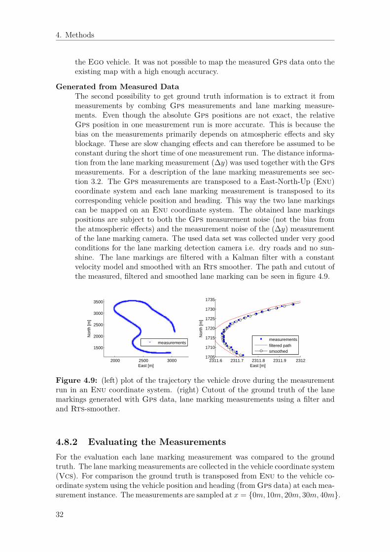
4.8.2 Evaluating the MeasurementsFor the evaluation each lane marking measurement was compared to the groundtruth. The lane marking measurements are collected in the vehicle coordinate system(Vcs). For comparison the ground truth is transposed from Enu to the vehicle co-ordinate system using the vehicle position and heading (from Gps data) at each mea-surement instance. The measurements are sampled at x = {0m, 10m, 20m, 30m, 40m}.

32

4. Methods

0 5 10 15 20 25 30 35 40

−3

−2

−1

0

1

2

3

4

5

6

VCS x [m]

VC

S y

[m]

left lane ground truthsampledright lane ground truthsampeledmeasurementssampeled

Figure 4.10: Visualization of the ground truth of the lane markings and a corre-sponding measurement in the VCS.

To calculate the error, the ground truth is interpolated to the same x positions asthe measurement samples and subtracted from the measurement points. Figure 4.10shows the ground truth lane markings and the measurements in the vehicle coordi-nate system. The error at the sampled x positions is analyzed for each lane markingmeasurement. The results for this can be found in section 6.3

4.9 Preceding Vehicle Sensor Analysis

Initial intention was to use the relative distances between the vehicles measured withthe Vbox system as ground truth for filter implementation. The Vbox system wasnot working as it should and the data was not accurate enough to use as groundtruth so another approach was taken.

4.9.1 Generating ground truth using RTS smoother

Since the actual ground truth of the preceding vehicle is unknown the best knowledgeabout it is from the measurements. To generate the ground truth the measurementare filtered using all the measurements samples available and have adaptive steplength between each prediction. The moments are stored and the back smoothedusing Rts smoother. The ground truth will then be used as reference when evalu-ating the step length used for implementation of the filter. The evaluation can beseen in section 6.4.

33

4. Methods

250 252 254 256 258 260

−0.8

−0.7

−0.6

−0.5

−0.4

−0.3

−0.2

−0.1

0

0.1

Time [s]

Dis

tanc

e [m

]

Lateral Position

cameraradarEstimatesRTS

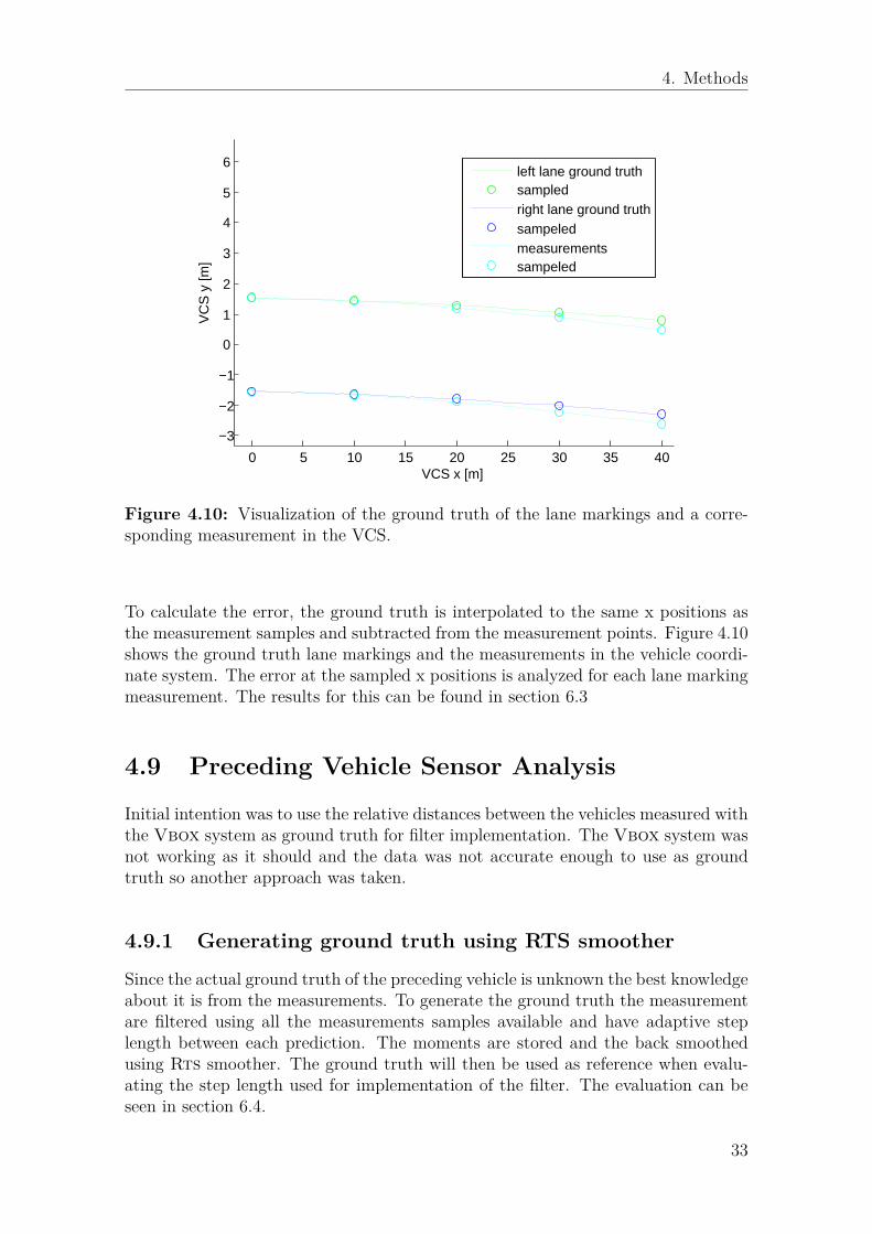
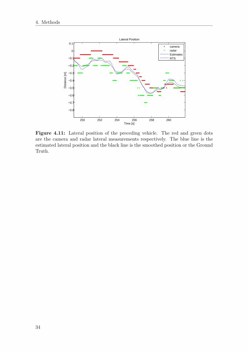
Figure 4.11: Lateral position of the preceding vehicle. The red and green dotsare the camera and radar lateral measurements respectively. The blue line is theestimated lateral position and the black line is the smoothed position or the GroundTruth.

34

5Implementation

5.1 Simulink Implementation

The algorithm proposed in this thesis is implemented in Simulink for running onthe test truck at Volvo Group Advanced Technology & Research Atr department.Since the algorithm is developed in Matlab the Simulink implementation containsthe main processing blocks of the algorithm as Matlab function blocks. Figure 5.1shows the block diagram of the algorithm implemented in Simulink.

measurementsampling

precedingvehiclefusion filter

lane markingfilter

preceding vehicle pathgenerator

reference error generator

left lane meas.

right lane meas.

lane path meas. filtered lane path

radar meas.

camera meas.

fused precedingvehicle position

preceding vehicle path

lateral error

heading error

Figure 5.1: Block diagram of the Simulink implementation of the algorithm. Adetailed picture of the Simulink implementation can be found the appendix.

measurement samplingThe inputs to this block are the coefficient measurements ∆y, α, c0 and c1 (seeequation (4.2) page 17) from the left and the right lane marking measurements.The block generates a sampled lane marking path from the measurements asdescribed in sections 4.1.1 and 4.3.2. The output is a sampled lane markingpath together with a confidence factor between 0 and 10.

lane marking filterThis block contains the sampled lane marking path filter that is described insection 4.3. The inputs are a sampled lane marking path measurement, a con-fidence factor between 0 and 10 and the velocity and yaw rate measurementsfrom the proprioceptive sensors. The output is the filtered lane marking pathtogether with its covariance matrix P.

35

5. Implementation

preceding vehicle fusionThis block contains the filter that fuses the preceding vehicle positions fromthe radar and the camera explained in section 4.5. The inputs are the lateraland longitudinal position of the preceding vehicle in the Vcs from the radarand camera as well as the lateral and longitudinal velocity from the radar.The output is the filtered position of the preceding vehicle.

preceding vehicle path generatorThis block generates the preceding vehicle path using the preceding vehicleposition and measurements from the proprioceptive sensors (see section 4.4).The inputs are the filtered preceding vehicle position, the lane marking pathand the velocity and yaw rate measurements from the proprioceptive sensors.The output is the preceding vehicle path.

reference error generatorThis block uses the path generated from the lane markings and the pathgenerated from the preceding vehicle to calculate a lateral error and headingerror signal for the lateral controller.

36

6Results

6.1 Lane Marking Error StatisticsThis section presents a statistical analysis of the lane marking measurements. Theleft and the right lane marking measurements are analyzed separately. The data setused for this analysis is described in section 4.8. Since there was no dataset availablethat included lane marking measurements and ground truth, the ground truth wasgenerated from the lane marking measurements combined with Gps data.

6.1.1 Absolute ErrorThe sensor measurements are evaluated to determine the standard deviations thatare used in the measurement covariance matrix in the implemented filter (see section4.3. The measurement setup is described in detail in section 4.8. Figure 6.1 showsthe absolute error between the lane marking measurements and the ground truth atdifferent look ahead distances (x = {0, 10m, 20m, 30m, 40m}) as a function of time.It can be seen that the error has a time dependent bias which is noticeable at alllook ahead distances except for 0m. The error and the time dependent bias are verysimilar for both the right and left lane marking. The third plot in figure 6.1 showsthe curvature of the road corresponding to the measured lane markings. There isno visible correlation between the curvature and the error or the time dependentbias. Other possible causes for this bias could be the pitch or roll of the trucks cabinwhere the camera is mounted. Such correlations are not investigated in this project,but it can be subject of future work (see Chapter 8).

6.1.2 Error DistributionA statistical analysis of the error shows that the errors at the evaluated look aheaddistances are zero mean and normally distributed. Figure 6.2 and figure 6.3 show theerror distributions for the left lane marking measurements and right lane markingrespectively. It should be noted that the axis for the histogram for the error at 0m(left most plot in figures 6.2 and 6.3) are different to the axis of the other histograms.The distribution for this error is much narrower than the error distributions atfurther look ahead distances. This can have two causes. Firstly the lane markingmeasurement at 0m only depends on the ∆y coefficient in the polynomial describedin equation (3.2) on page 12 whereas the other measurements are calculated withall the coefficients. Secondly the measurements at 0m were used together with Gpsdata to generate the ground truth which is described in section 4.8.

37

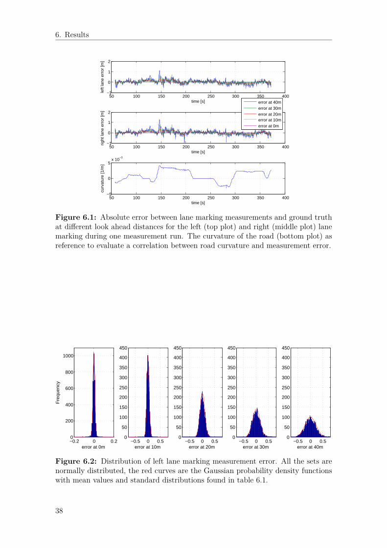
6. Results

50 100 150 200 250 300 350 400−1

0

1

2

time [s]le

ft la

ne e

rror

[m]

50 100 150 200 250 300 350 400−1

0

1

2

time [s]

right

lane

err

or [m

]

error at 40merror at 30merror at 20merror at 10merror at 0m

50 100 150 200 250 300 350 400−5

0

5x 10

−3

time [s]

curv

atur

e [1

/m]

Figure 6.1: Absolute error between lane marking measurements and ground truthat different look ahead distances for the left (top plot) and right (middle plot) lanemarking during one measurement run. The curvature of the road (bottom plot) asreference to evaluate a correlation between road curvature and measurement error.

−0.2 0 0.20

200

400

600

800

1000

error at 0m

Fre

quen

cy

−0.5 0 0.50

50

100

150

200

250

300

350

400

450

error at 10m−0.5 0 0.5

0

50

100

150

200

250

300

350

400

450

error at 20m−0.5 0 0.5

0

50

100

150

200

250

300

350

400

450

error at 30m−0.5 0 0.5

0

50

100

150

200

250

300

350

400

450

error at 40m

Figure 6.2: Distribution of left lane marking measurement error. All the sets arenormally distributed, the red curves are the Gaussian probability density functionswith mean values and standard distributions found in table 6.1.

38

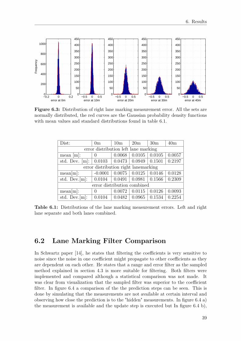
6. Results

−0.2 0 0.20

200

400

600

800

1000

error at 0m

Fre

quen

cy

−0.5 0 0.50

50

100

150

200

250

300

350

400

450

error at 10m−0.5 0 0.5

0

50

100

150

200

250

300

350

400

450

error at 20m−0.5 0 0.5

0

50

100

150

200

250

300

350

400

450

error at 30m−0.5 0 0.5

0

50

100

150

200

250

300

350

400

450

error at 40m

Figure 6.3: Distribution of right lane marking measurement error. All the sets arenormally distributed, the red curves are the Gaussian probability density functionswith mean values and standard distributions found in table 6.1.

Dist: 0m 10m 20m 30m 40merror distribution left lane marking

mean [m]: 0 0.0068 0.0105 0.0105 0.0057std. Dev. [m]: 0.0103 0.0473 0.0949 0.1501 0.2197

error distribution right lanemarkingmean[m]: -0.0001 0.0075 0.0125 0.0146 0.0128std. Dev.[m]: 0.0104 0.0491 0.0981 0.1566 0.2309

error distribution combinedmean[m]: 0 0.0072 0.0115 0.0126 0.0093std. Dev.[m]: 0.0104 0.0482 0.0965 0.1534 0.2254

Table 6.1: Distributions of the lane marking measurement errors. Left and rightlane separate and both lanes combined.

6.2 Lane Marking Filter ComparisonIn Schwartz paper [14], he states that filtering the coefficients is very sensitive tonoise since the noise in one coefficient might propagate to other coefficients as theyare dependent on each other. He states that a range and error filter as the sampledmethod explained in section 4.3 is more suitable for filtering. Both filters wereimplemented and compared although a statistical comparison was not made. Itwas clear from visualization that the sampled filter was superior to the coefficientfilter. In figure 6.4 a comparison of the the prediction steps can be seen. This isdone by simulating that the measurements are not available at certain interval andobserving how close the prediction is to the "hidden" measurements. In figure 6.4 a)the measurement is available and the update step is executed but In figure 6.4 b),

39

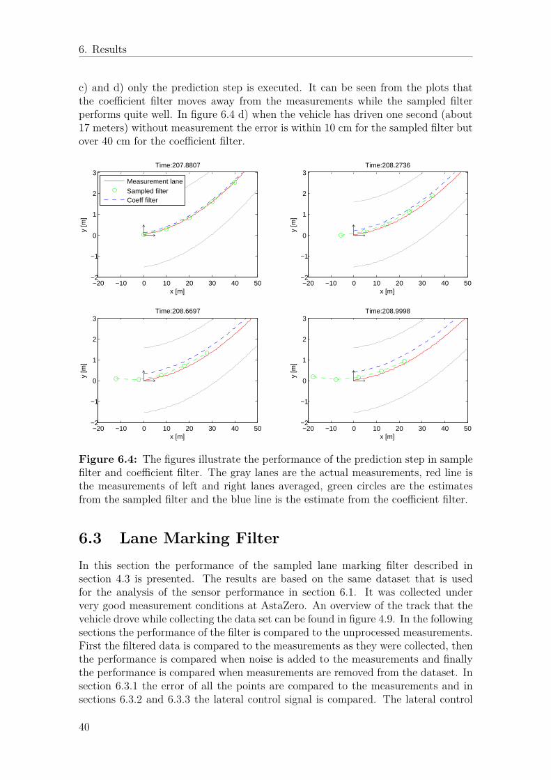
6. Results

c) and d) only the prediction step is executed. It can be seen from the plots thatthe coefficient filter moves away from the measurements while the sampled filterperforms quite well. In figure 6.4 d) when the vehicle has driven one second (about17 meters) without measurement the error is within 10 cm for the sampled filter butover 40 cm for the coefficient filter.

−20 −10 0 10 20 30 40 50−2

−1

0

1

2

3

x [m]

y [m

]

Time:207.8807

Measurement laneSampled filterCoeff filter

−20 −10 0 10 20 30 40 50−2

−1

0

1

2

3Time:208.2736

x [m]y

[m]

−20 −10 0 10 20 30 40 50−2

−1

0

1

2

3Time:208.6697

x [m]

y [m

]

−20 −10 0 10 20 30 40 50−2

−1

0

1

2

3Time:208.9998

x [m]

y [m

]

Figure 6.4: The figures illustrate the performance of the prediction step in samplefilter and coefficient filter. The gray lanes are the actual measurements, red line isthe measurements of left and right lanes averaged, green circles are the estimatesfrom the sampled filter and the blue line is the estimate from the coefficient filter.

6.3 Lane Marking FilterIn this section the performance of the sampled lane marking filter described insection 4.3 is presented. The results are based on the same dataset that is usedfor the analysis of the sensor performance in section 6.1. It was collected undervery good measurement conditions at AstaZero. An overview of the track that thevehicle drove while collecting the data set can be found in figure 4.9. In the followingsections the performance of the filter is compared to the unprocessed measurements.First the filtered data is compared to the measurements as they were collected, thenthe performance is compared when noise is added to the measurements and finallythe performance is compared when measurements are removed from the dataset. Insection 6.3.1 the error of all the points are compared to the measurements and insections 6.3.2 and 6.3.3 the lateral control signal is compared. The lateral control

40

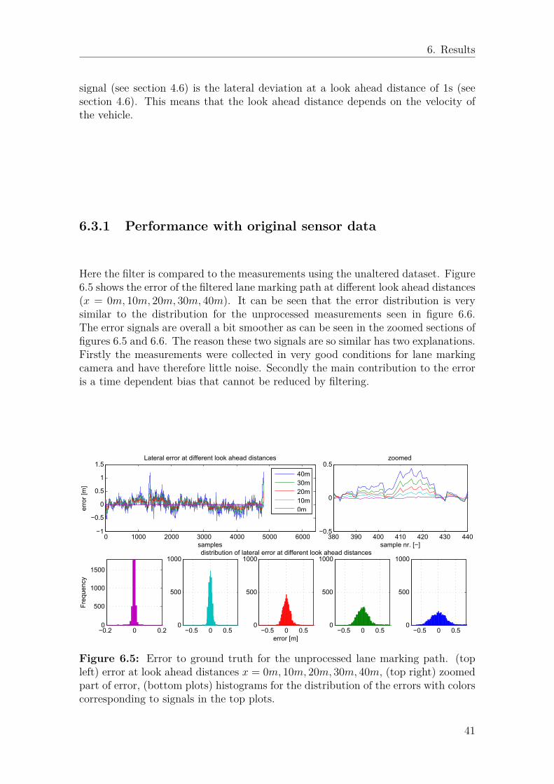
6. Results

signal (see section 4.6) is the lateral deviation at a look ahead distance of 1s (seesection 4.6). This means that the look ahead distance depends on the velocity ofthe vehicle.

6.3.1 Performance with original sensor data

Here the filter is compared to the measurements using the unaltered dataset. Figure6.5 shows the error of the filtered lane marking path at different look ahead distances(x = 0m, 10m, 20m, 30m, 40m). It can be seen that the error distribution is verysimilar to the distribution for the unprocessed measurements seen in figure 6.6.The error signals are overall a bit smoother as can be seen in the zoomed sections offigures 6.5 and 6.6. The reason these two signals are so similar has two explanations.Firstly the measurements were collected in very good conditions for lane markingcamera and have therefore little noise. Secondly the main contribution to the erroris a time dependent bias that cannot be reduced by filtering.

0 1000 2000 3000 4000 5000 6000−1

−0.5

0

0.5

1

1.5

samples

erro

r [m

]

Lateral error at different look ahead distances

380 390 400 410 420 430 440

−0.5

0

0.5

sample nr. [−]

zoomed

−0.2 0 0.20

500

1000

1500

Fre

quen

cy

−0.5 0 0.50

500

1000

−0.5 0 0.50

500

1000

−0.5 0 0.50

500

1000

−0.5 0 0.50

500

1000

error [m]

distribution of lateral error at different look ahead distances

40m30m20m10m0m

Figure 6.5: Error to ground truth for the unprocessed lane marking path. (topleft) error at look ahead distances x = 0m, 10m, 20m, 30m, 40m, (top right) zoomedpart of error, (bottom plots) histograms for the distribution of the errors with colorscorresponding to signals in the top plots.

41

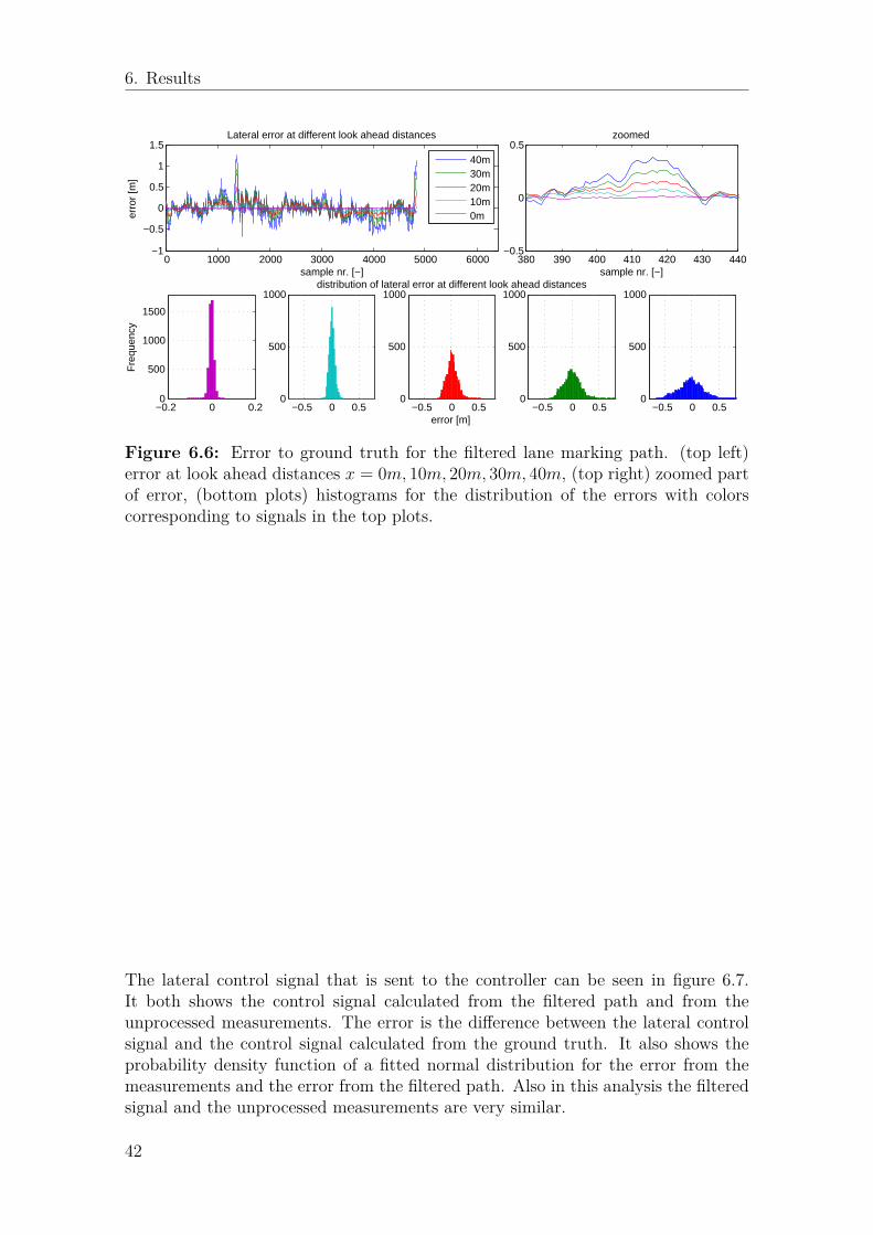
6. Results

0 1000 2000 3000 4000 5000 6000−1

−0.5

0

0.5

1

1.5

sample nr. [−]

erro

r [m

]Lateral error at different look ahead distances

40m30m20m10m0m

380 390 400 410 420 430 440−0.5

0

0.5

sample nr. [−]

zoomed

−0.2 0 0.20

500

1000

1500

Fre

quen

cy

−0.5 0 0.50

500

1000

−0.5 0 0.50

500

1000

−0.5 0 0.50

500

1000

−0.5 0 0.50

500

1000

error [m]

distribution of lateral error at different look ahead distances

Figure 6.6: Error to ground truth for the filtered lane marking path. (top left)error at look ahead distances x = 0m, 10m, 20m, 30m, 40m, (top right) zoomed partof error, (bottom plots) histograms for the distribution of the errors with colorscorresponding to signals in the top plots.

The lateral control signal that is sent to the controller can be seen in figure 6.7.It both shows the control signal calculated from the filtered path and from theunprocessed measurements. The error is the difference between the lateral controlsignal and the control signal calculated from the ground truth. It also shows theprobability density function of a fitted normal distribution for the error from themeasurements and the error from the filtered path. Also in this analysis the filteredsignal and the unprocessed measurements are very similar.

42

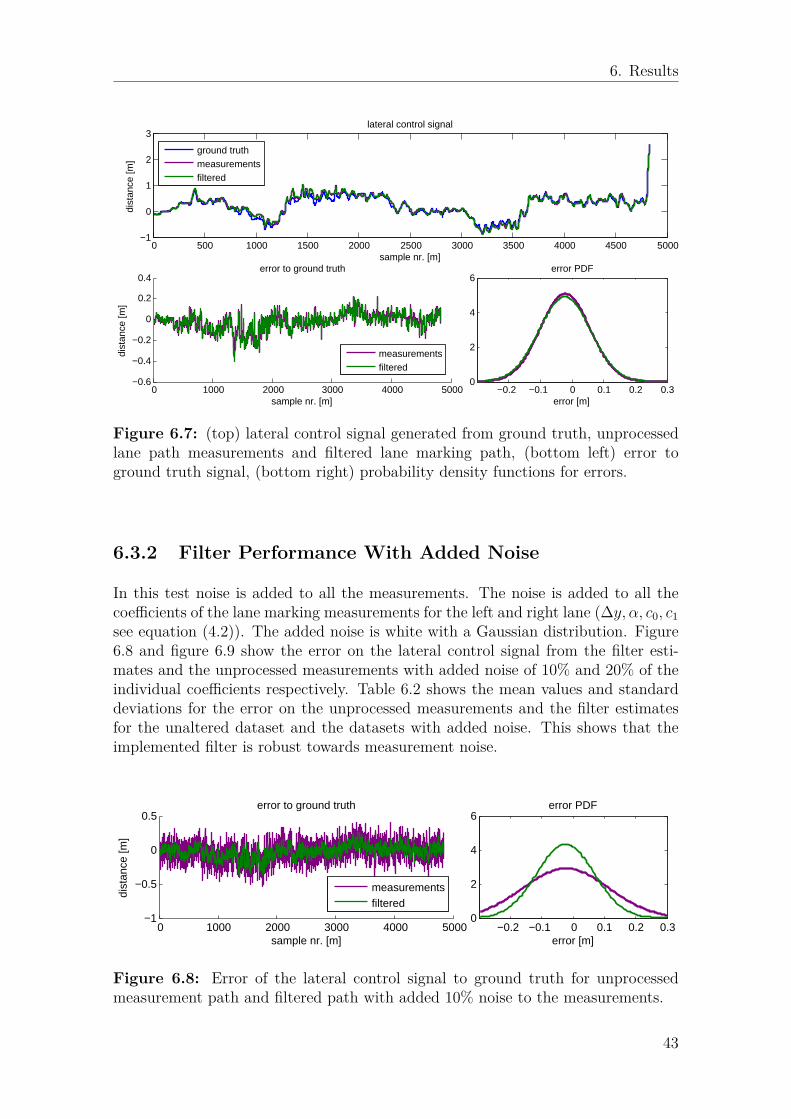
6. Results

0 500 1000 1500 2000 2500 3000 3500 4000 4500 5000−1

0

1

2

3

sample nr. [m]

dist

ance

[m]

lateral control signal

0 1000 2000 3000 4000 5000−0.6

−0.4

−0.2

0

0.2

0.4error to ground truth

sample nr. [m]

dist

ance

[m]

−0.2 −0.1 0 0.1 0.2 0.30

2

4

6

error [m]

error PDF

ground truthmeasurementsfiltered

measurementsfiltered

Figure 6.7: (top) lateral control signal generated from ground truth, unprocessedlane path measurements and filtered lane marking path, (bottom left) error toground truth signal, (bottom right) probability density functions for errors.

6.3.2 Filter Performance With Added Noise

In this test noise is added to all the measurements. The noise is added to all thecoefficients of the lane marking measurements for the left and right lane (∆y, α, c0, c1see equation (4.2)). The added noise is white with a Gaussian distribution. Figure6.8 and figure 6.9 show the error on the lateral control signal from the filter esti-mates and the unprocessed measurements with added noise of 10% and 20% of theindividual coefficients respectively. Table 6.2 shows the mean values and standarddeviations for the error on the unprocessed measurements and the filter estimatesfor the unaltered dataset and the datasets with added noise. This shows that theimplemented filter is robust towards measurement noise.

0 1000 2000 3000 4000 5000−1

−0.5

0

0.5error to ground truth

sample nr. [m]

dist

ance

[m]

measurementsfiltered

−0.2 −0.1 0 0.1 0.2 0.30

2

4

6error PDF

error [m]

Figure 6.8: Error of the lateral control signal to ground truth for unprocessedmeasurement path and filtered path with added 10% noise to the measurements.

43

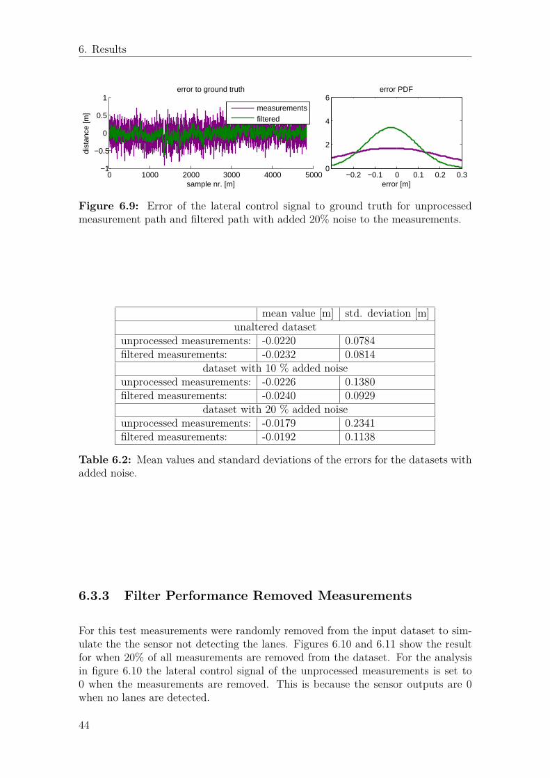
6. Results

0 1000 2000 3000 4000 5000−1

−0.5

0

0.5

1error to ground truth

sample nr. [m]

dist

ance

[m]

measurementsfiltered

−0.2 −0.1 0 0.1 0.2 0.30

2

4

6error PDF

error [m]

Figure 6.9: Error of the lateral control signal to ground truth for unprocessedmeasurement path and filtered path with added 20% noise to the measurements.

mean value [m] std. deviation [m]unaltered dataset

unprocessed measurements: -0.0220 0.0784filtered measurements: -0.0232 0.0814

dataset with 10 % added noiseunprocessed measurements: -0.0226 0.1380filtered measurements: -0.0240 0.0929

dataset with 20 % added noiseunprocessed measurements: -0.0179 0.2341filtered measurements: -0.0192 0.1138

Table 6.2: Mean values and standard deviations of the errors for the datasets withadded noise.

6.3.3 Filter Performance Removed Measurements

For this test measurements were randomly removed from the input dataset to sim-ulate the the sensor not detecting the lanes. Figures 6.10 and 6.11 show the resultfor when 20% of all measurements are removed from the dataset. For the analysisin figure 6.10 the lateral control signal of the unprocessed measurements is set to0 when the measurements are removed. This is because the sensor outputs are 0when no lanes are detected.

44

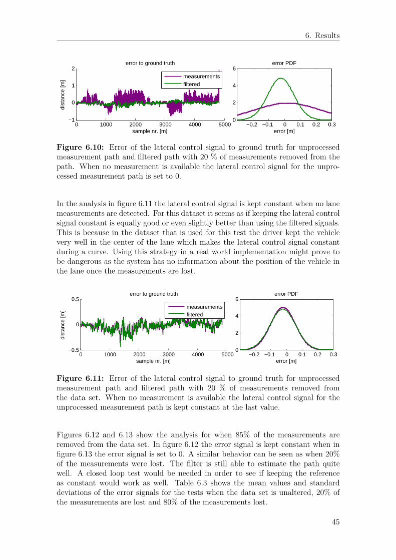
6. Results

0 1000 2000 3000 4000 5000−1

0

1

2error to ground truth

sample nr. [m]

dist

ance

[m]

measurementsfiltered

−0.2 −0.1 0 0.1 0.2 0.30

2

4

6error PDF

error [m]

Figure 6.10: Error of the lateral control signal to ground truth for unprocessedmeasurement path and filtered path with 20 % of measurements removed from thepath. When no measurement is available the lateral control signal for the unpro-cessed measurement path is set to 0.

In the analysis in figure 6.11 the lateral control signal is kept constant when no lanemeasurements are detected. For this dataset it seems as if keeping the lateral controlsignal constant is equally good or even slightly better than using the filtered signals.This is because in the dataset that is used for this test the driver kept the vehiclevery well in the center of the lane which makes the lateral control signal constantduring a curve. Using this strategy in a real world implementation might prove tobe dangerous as the system has no information about the position of the vehicle inthe lane once the measurements are lost.

0 1000 2000 3000 4000 5000−0.5

0

0.5error to ground truth

sample nr. [m]

dist

ance

[m]

measurementsfiltered

−0.2 −0.1 0 0.1 0.2 0.30

2

4

6error PDF

error [m]

Figure 6.11: Error of the lateral control signal to ground truth for unprocessedmeasurement path and filtered path with 20 % of measurements removed fromthe data set. When no measurement is available the lateral control signal for theunprocessed measurement path is kept constant at the last value.

Figures 6.12 and 6.13 show the analysis for when 85% of the measurements areremoved from the data set. In figure 6.12 the error signal is kept constant when infigure 6.13 the error signal is set to 0. A similar behavior can be seen as when 20%of the measurements were lost. The filter is still able to estimate the path quitewell. A closed loop test would be needed in order to see if keeping the referenceas constant would work as well. Table 6.3 shows the mean values and standarddeviations of the error signals for the tests when the data set is unaltered, 20% ofthe measurements are lost and 80% of the measurements lost.

45

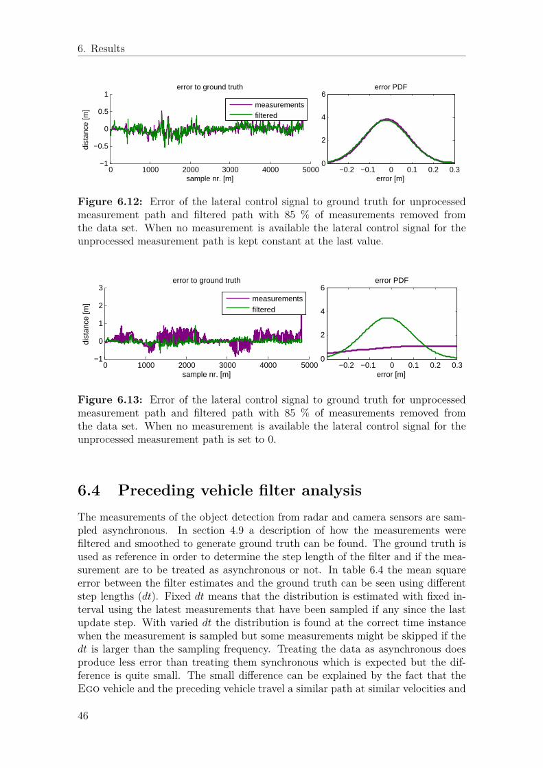
6. Results

0 1000 2000 3000 4000 5000−1

−0.5

0

0.5

1error to ground truth

sample nr. [m]

dist

ance

[m]

measurementsfiltered

−0.2 −0.1 0 0.1 0.2 0.30

2

4

6error PDF

error [m]

Figure 6.12: Error of the lateral control signal to ground truth for unprocessedmeasurement path and filtered path with 85 % of measurements removed fromthe data set. When no measurement is available the lateral control signal for theunprocessed measurement path is kept constant at the last value.

0 1000 2000 3000 4000 5000−1

0

1

2

3error to ground truth

sample nr. [m]

dist

ance

[m]

measurementsfiltered

−0.2 −0.1 0 0.1 0.2 0.30

2

4

6error PDF

error [m]

Figure 6.13: Error of the lateral control signal to ground truth for unprocessedmeasurement path and filtered path with 85 % of measurements removed fromthe data set. When no measurement is available the lateral control signal for theunprocessed measurement path is set to 0.

6.4 Preceding vehicle filter analysisThe measurements of the object detection from radar and camera sensors are sam-pled asynchronous. In section 4.9 a description of how the measurements werefiltered and smoothed to generate ground truth can be found. The ground truth isused as reference in order to determine the step length of the filter and if the mea-surement are to be treated as asynchronous or not. In table 6.4 the mean squareerror between the filter estimates and the ground truth can be seen using differentstep lengths (dt). Fixed dt means that the distribution is estimated with fixed in-terval using the latest measurements that have been sampled if any since the lastupdate step. With varied dt the distribution is found at the correct time instancewhen the measurement is sampled but some measurements might be skipped if thedt is larger than the sampling frequency. Treating the data as asynchronous doesproduce less error than treating them synchronous which is expected but the dif-ference is quite small. The small difference can be explained by the fact that theEgo vehicle and the preceding vehicle travel a similar path at similar velocities and

46

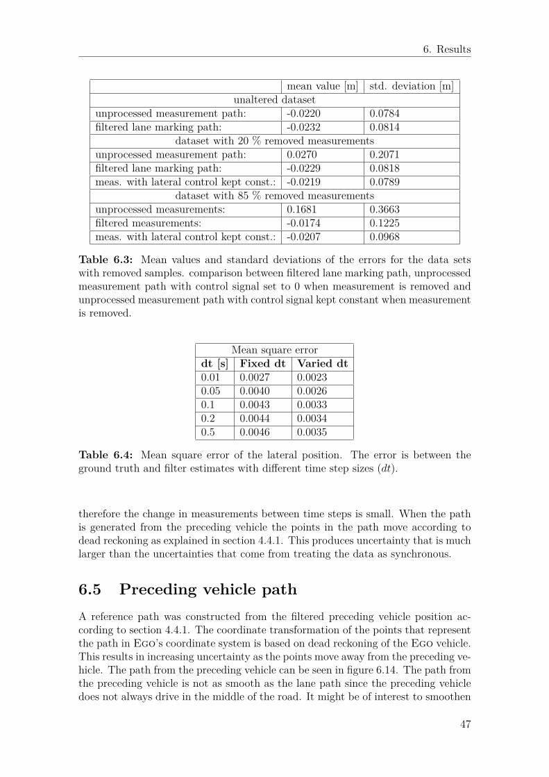
6. Results

mean value [m] std. deviation [m]unaltered dataset

unprocessed measurement path: -0.0220 0.0784filtered lane marking path: -0.0232 0.0814

dataset with 20 % removed measurementsunprocessed measurement path: 0.0270 0.2071filtered lane marking path: -0.0229 0.0818meas. with lateral control kept const.: -0.0219 0.0789

dataset with 85 % removed measurementsunprocessed measurements: 0.1681 0.3663filtered measurements: -0.0174 0.1225meas. with lateral control kept const.: -0.0207 0.0968

Table 6.3: Mean values and standard deviations of the errors for the data setswith removed samples. comparison between filtered lane marking path, unprocessedmeasurement path with control signal set to 0 when measurement is removed andunprocessed measurement path with control signal kept constant when measurementis removed.

Mean square errordt [s] Fixed dt Varied dt0.01 0.0027 0.00230.05 0.0040 0.00260.1 0.0043 0.00330.2 0.0044 0.00340.5 0.0046 0.0035

Table 6.4: Mean square error of the lateral position. The error is between theground truth and filter estimates with different time step sizes (dt).

therefore the change in measurements between time steps is small. When the pathis generated from the preceding vehicle the points in the path move according todead reckoning as explained in section 4.4.1. This produces uncertainty that is muchlarger than the uncertainties that come from treating the data as synchronous.

6.5 Preceding vehicle pathA reference path was constructed from the filtered preceding vehicle position ac-cording to section 4.4.1. The coordinate transformation of the points that representthe path in Ego’s coordinate system is based on dead reckoning of the Ego vehicle.This results in increasing uncertainty as the points move away from the preceding ve-hicle. The path from the preceding vehicle can be seen in figure 6.14. The path fromthe preceding vehicle is not as smooth as the lane path since the preceding vehicledoes not always drive in the middle of the road. It might be of interest to smoothen

47

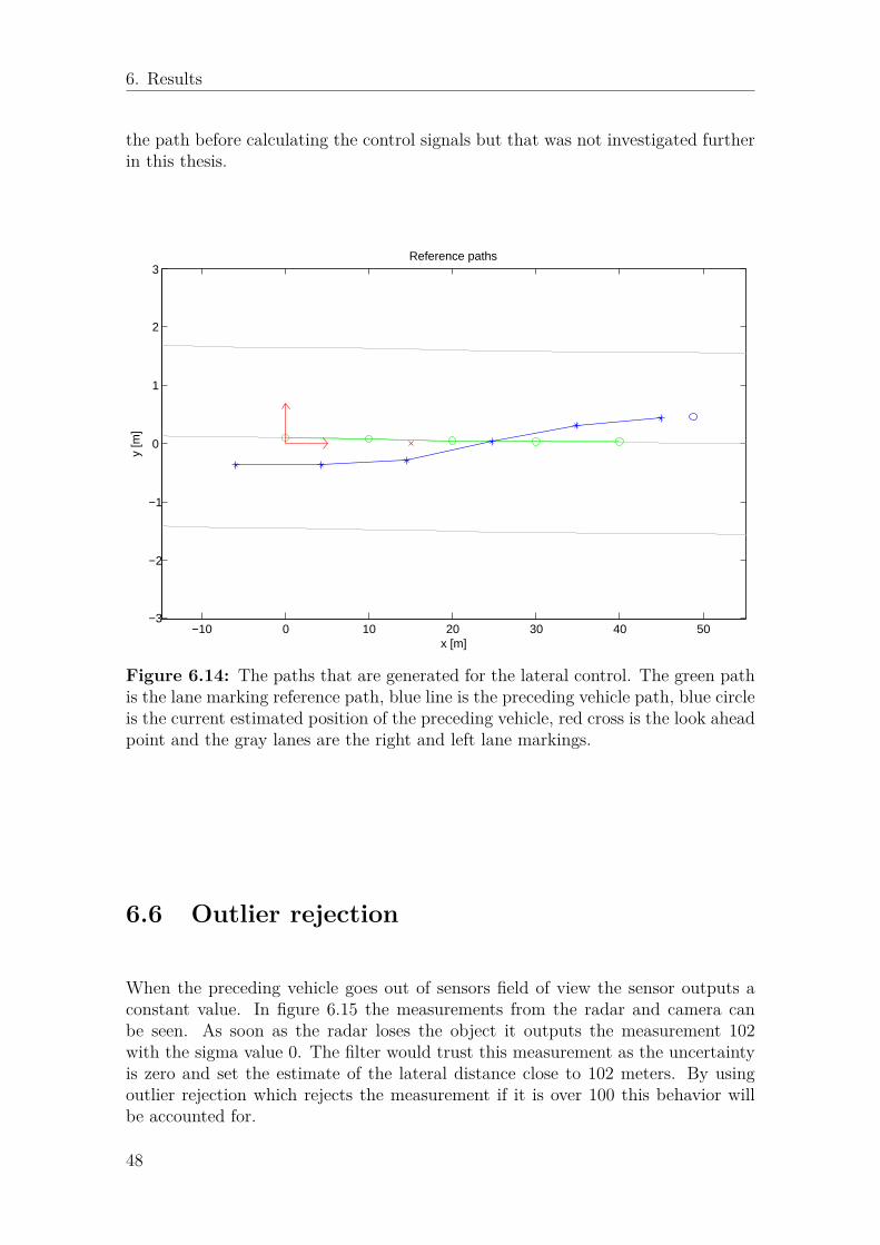
6. Results

the path before calculating the control signals but that was not investigated furtherin this thesis.

−10 0 10 20 30 40 50−3

−2

−1

0

1

2

3Reference paths

x [m]

y [m

]

Figure 6.14: The paths that are generated for the lateral control. The green pathis the lane marking reference path, blue line is the preceding vehicle path, blue circleis the current estimated position of the preceding vehicle, red cross is the look aheadpoint and the gray lanes are the right and left lane markings.

6.6 Outlier rejection

When the preceding vehicle goes out of sensors field of view the sensor outputs aconstant value. In figure 6.15 the measurements from the radar and camera canbe seen. As soon as the radar loses the object it outputs the measurement 102with the sigma value 0. The filter would trust this measurement as the uncertaintyis zero and set the estimate of the lateral distance close to 102 meters. By usingoutlier rejection which rejects the measurement if it is over 100 this behavior willbe accounted for.

48

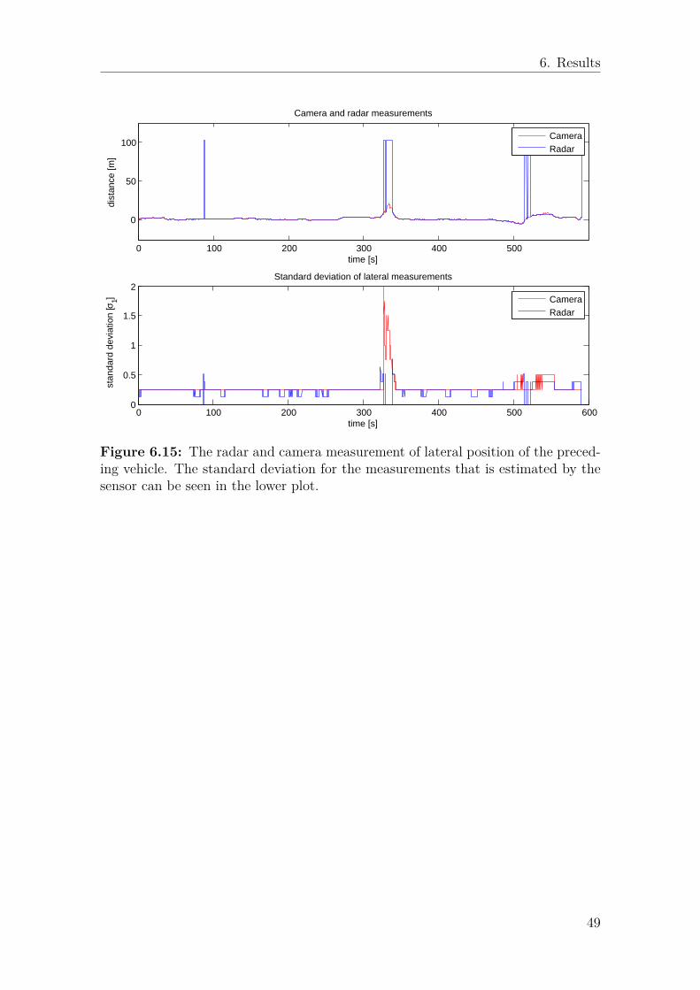
6. Results

0 100 200 300 400 500

0

50

100

Camera and radar measurements

time [s]

dist

ance

[m]

CameraRadar

0 100 200 300 400 500 6000

0.5

1

1.5

2Standard deviation of lateral measurements

time [s]

stan

dard

dev

iatio

n [σ

1]

CameraRadar

Figure 6.15: The radar and camera measurement of lateral position of the preced-ing vehicle. The standard deviation for the measurements that is estimated by thesensor can be seen in the lower plot.

49

6. Results

50

7Conclusion and Discussion

By using the implemented filters in this thesis two reference paths were generated forlateral control. The filters use sensor information from camera and radar to achieverobust lateral reference signal. This method is superior from using a raw measure-ment from a single source as a reference since it can handle noisy measurements andrely on prediction when measurements are lost. In order to have a reference path alane markings or preceding vehicle need to be detected by the sensors. The scope ofthis thesis was to use sensors that are currently available in production vehicles atVolvo Group Trucks Technology. State of the art sensors that are more reliable andaccurate were discarded since they are not yet feasible for commercially availablevehicles.The solution proposed in this thesis is supposed to be used as a base platform forhow sensor data are handled in several projects that are currently in process at theAtr department.

7.1 Implemented filters

The filters were implemented for estimation of lane marking and position of preced-ing vehicle. Two filters were implemented and compared for the lane markings. Thefilter based on range and error (sampled) proved to perform much better than thecoefficient filter as seen in section 6.2 so it was further developed. In the sampledlane marking filter the uncertainties of the camera measurements were quantifiedusing methods described in section 4.8. The resulting uncertainties describe the dis-tribution of the measurements and are important to accurately set the measurementcovariance in the filter. The filter is able to handle measurements that are affectedby large noises as can be seen in section 6.3.2. The main advantages of the lanemarking filter is that if the measurements are lost for short period of time the filtercan still provide reference by using prediction of the path for up to 40 meters. Thiscan be beneficial in scenarios where lane marking is partly obscured by e.g. snow ordirt. The second filter uses the object detection from the camera and radar sensorsand estimates the position and velocity relative to the Ego vehicle. Although theoutputs from the sensors are already processed data we treat them as raw data sincewe do not have access to the raw ones.

51

7. Conclusion and Discussion

7.2 Reference paths and error signalsTwo paths were generated for lateral reference. One path from the lane markingestimates and another from the estimated position of the preceding vehicle. Eachpath has a specific uncertainty throughout the path. The uncertainty in the lanepath is usually much smaller than in the preceding vehicle path. That is mainlycaused by the fact that we have measurements along the entire lane path but onlyat the end of the preceding vehicle path. The control signal is calculated from thelane markings whenever that path is available. As soon as the measurements arelost for the lane and uncertainty increases the reference error is transitioned over tothe preceding vehicle path.

7.3 Experimental implementationThe algorithm was developed using Matlab but then converted to Simulink modelfor implementation in rapid prototype environment (dSpace) which is available inthe Volvo test trucks. Due to time restrictions only one test was done on the model.The model was able to output reasonable references but was not tested in closedloop with the controller. Further tests are scheduled to take place in the upcomingweeks.

52

8Future Work

As our algorithm is a platform in how to handle sensor data for lateral control thereare manz possibilities to add to this platform. Here we list those that we considerthe most important ones.

Other sensor sources

• GPS / map: GPS together with a map could provide useful information.One example is at exits on highways where one lane turns off the highwaywhile the other stays on. This can cause a problem for the lane detectionsensor, when it detects one lane marking following the road and the otherfollowing the exit road. There the vehicle position on a map could provideinformation about which lane to use.

• LIDAR: A LIDAR sensor provides very accurate view of the surround-ings. The information could be used to improve the estimation of thepaths.

• Other camera information: Such as road edges, measurements of lanesnext to the vehicle lane and roadsigns would be useful.

• Additional cameras: In this thesis a front view camera is used. Cam-eras on the side or on the back of the truck could be used to provideinformation on other vehicles surrounding the truck.

• V2V communication: By incorporating vehicle to vehicle (V2V) com-munication information about other vehicles could be useful. A precedingvehicle with the same system as described in this thesis could commu-nicate the paths estimated in it’s vehicle. That path could be used toextend the paths in the Ego vehicle.

State estimator Currently the distance traveled and change in heading is calcu-lated using raw measurements from the speedometer and yaw rate. This couldbe improved by estimating the state of the vehicle using sensor fusion. This es-timator could be used straight into the prediction part of the filters. By usingthe state estimator a more accurate change in heading and distance traveledbetween time steps would be achieved.

Initial preceding vehicle path estimation The estimation of the initial preced-ing vehicle path when no lane marking path is available could be improved. Inthe proposed solution the path is set by linear interpolation between the Ego

53

8. Future Work

vehicle and the preceding vehicle. Since the heading of the Ego vehicle isknown a cubic interpolation could be used to get the estimated path to followthe curve of the road.

Reference paths The reference paths are currently represented with 5 to 6 pointswhich could cause problems for the controller. The paths could be smoothedby drawing a bezier curve through the points before calculating the controlsignal. This method was looked into but not investigated further because oftime constraints on the project.

Time variant bias in lane marking measurements The lane marking measure-ments has a time variant bias. The bias is not correlated with the curvature ofthe road as can be seen in section 6.1. The cause of the bias could be related toorientation of the lane marking camera since it is at the top of the windshieldwhere it is affected by yaw and roll of the cabin. The roll and the yaw ofthe cabin could be measured using accelerometers and compared to the lanemarking error. If there is a correlation it can be accounted for and thereforimprove the measurements.

54

Bibliography

[1] E. Chan, P. Gilhead, P. Jelínek, P. Krejčí, and T. Robinson, “Cooperativecontrol of sartre automated platoon vehicles,” ITS World Congress 2012, 2012.

[2] R. E. Kalman, “A new approach to linear filtering and prediction problems,”Transactions of the ASME–Journal of Basic Engineering, vol. 82, no. Series D,pp. 35–45, 1960.

[3] I. Papadimitriou and M. Tomizuka, “Lateral control of platoons of vehicles onhighways: the autonomous following based approach,” International Journal ofVehicle Design, September 27, vol. 36, no. 1, 2004, pp. 24–37, 2004.

[4] S. Thrun, W. Burgard, and D. Fox, Probabilistic Robotics. The MIT Press,Cambridge, MA, 2005.

[5] I. Arasaratnam and S. Haykin, “Cubature kalman filters,” IEEE Transactionon Automatic Control, vol. 54, no. 6, 2009.

[6] H. Rauch, F. Tung, and C. Striebel, “Maximum likelihood estimates of lineardynamic systems,” AIAA Journal, vol. 3, no. 8, 1965.

[7] J. Kosecka, R. Blasi, C. J. Taylor, and J. Malik, “Vision-based lateral con-trol of vehicles,” IEEE Conference on Intelligent Transportation Systems, 9-12November, Boston, MA, pp. 900 – 905, 1997.

[8] J. Kosecka, R. Blasi, C. J. Taylor, and J. Malik, “A comparative study ofvision-based lateral control strategies for autonomous highway driving,” 1998IEEE International Conference on Robotics and Automation 20-20 May, Leu-ven, Belgium, vol. 3, pp. 1903 – 1908, 1998.

[9] M. Tai and M. Tomizuka, “Experimental study of lateral control of heavy vehi-cles for automated highway systems (ahs),” Proceedings of the American ControlConference, 8-10 May, Anchorage, AK, pp. 851 – 856, 2002.

[10] J. Huang and H.-S. Tan, “Immediate transition for an automated bus us-ing magnetic and dgps sensing systems,” 14th International IEEE Conferenceon Intelligent Transportation Systems, 5-7 October, Washington, DC, USA,pp. 656 – 661, 2011.

55

Bibliography

[11] Y. Hayakawa, R. White, T. Kimura, and G. Naitou, “Driver oriented pathfollowing in its - wide speed-range steering control by multiple look-ahead dis-tances,” Proceedings of IEEE/ASME International Conference on AdvancedIntelligen Mechatronics, 20-24 July, vol. 1, pp. 558 – 563, 2003.

[12] M. Tai and M. Tomizuka, “Feedforward compensation for lateral control ofheavy vehicles for automated highway systam (ahs),” IFAC 15th TriennialWorld Congress, Barcelona, Spain, 2002.

[13] K. Hasegawa and E. Konaka, “Three look-ahead distance scheme for lateralcontrol of vision-based vehicles,” SICE Annual Conference, September 9-12,Hakkaio University, Sapporo, Japan, pp. 660 – 665, 2014.

[14] D. Schwartz, “Clothoid road geometry unsuitable for sensor fusion,” IEEE In-tell. Veh. Symp, pp. 484–488, 2003.

[15] Ángel F. García-Fernández, L. Hammarstrand, M. Fatemi, and L. Svens-son, “Bayesian road estimation using onboard sensors,” IEEE Trans. On ITS,vol. 15, 2014.

56

I

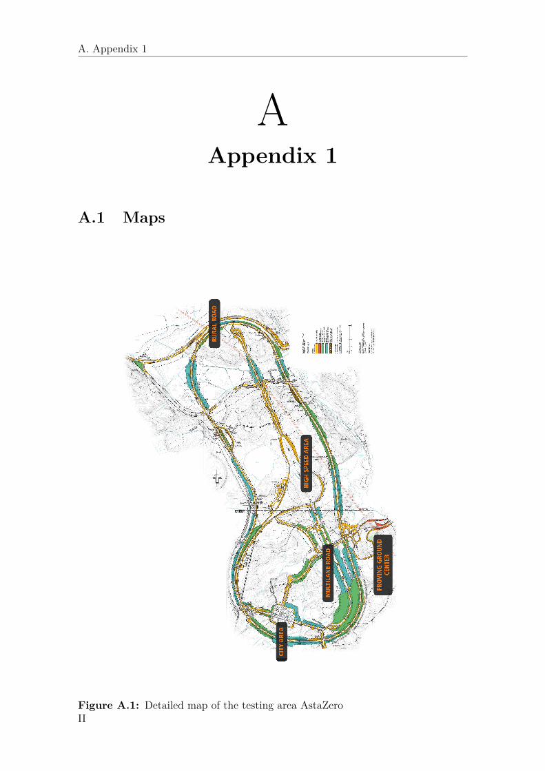
A. Appendix 1

AAppendix 1

A.1 Maps

Figure A.1: Detailed map of the testing area AstaZeroII

A. Appendix 1

III

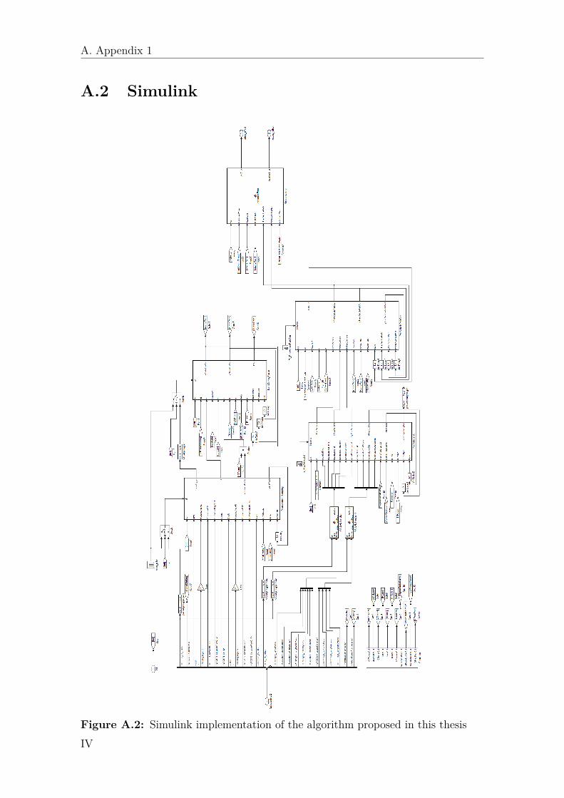
A. Appendix 1

A.2 Simulink

Figure A.2: Simulink implementation of the algorithm proposed in this thesisIV