Reference Manual for X-13ARIMA-SEATS · X-13ARIMA-SEATS Reference Manual Accessible HTML Output...
297
X-13ARIMA-SEATS Reference Manual Accessible HTML Output Version Version 1.1 Time Series Research Staff Center for Statistical Research and Methodology U.S. Census Bureau Washington, DC 20233 phone: 301-763-1649 email: [email protected] WWW: http://www.census.gov/srd/www/x13as/ January 18, 2017
Transcript of Reference Manual for X-13ARIMA-SEATS · X-13ARIMA-SEATS Reference Manual Accessible HTML Output...
X-13ARIMA-SEATS Reference Manual
Accessible HTML Output Version
Version 1.1
Time Series Research StaffCenter for Statistical Research and Methodology
U.S. Census BureauWashington, DC 20233phone: 301-763-1649
email: [email protected]: http://www.census.gov/srd/www/x13as/
January 18, 2017

This page intentionally left blank.
Contents
1 Introduction 1
1.1 Acknowledgements . . . . . . . . . . . . . . . . . . . . . . . . . . . . . . . . . . . . . . . . . . . . 4
1.2 License Information and Disclaimer . . . . . . . . . . . . . . . . . . . . . . . . . . . . . . . . . . . 4
2 Running X-13ARIMA-SEATS 6
2.1 Input . . . . . . . . . . . . . . . . . . . . . . . . . . . . . . . . . . . . . . . . . . . . . . . . . . . . 7
2.2 Output . . . . . . . . . . . . . . . . . . . . . . . . . . . . . . . . . . . . . . . . . . . . . . . . . . 7
2.3 Input errors . . . . . . . . . . . . . . . . . . . . . . . . . . . . . . . . . . . . . . . . . . . . . . . . 7
2.4 Specifying an alternate output filename . . . . . . . . . . . . . . . . . . . . . . . . . . . . . . . . 8
2.5 Running X-13ARIMA-SEATS on more than one series . . . . . . . . . . . . . . . . . . . . . . . . . 8
2.5.1 Running X-13ARIMA-SEATS in multi-spec mode . . . . . . . . . . . . . . . . . . . . . . . . 9
2.5.2 Running X-13ARIMA-SEATS in single spec mode . . . . . . . . . . . . . . . . . . . . . . . . 10
2.5.3 Special Case: File Names Containing Spaces . . . . . . . . . . . . . . . . . . . . . . . . . 11
2.6 Log Files . . . . . . . . . . . . . . . . . . . . . . . . . . . . . . . . . . . . . . . . . . . . . . . . . 12
2.7 Flags . . . . . . . . . . . . . . . . . . . . . . . . . . . . . . . . . . . . . . . . . . . . . . . . . . . . 12
2.8 Program limits . . . . . . . . . . . . . . . . . . . . . . . . . . . . . . . . . . . . . . . . . . . . . . 16
3 The Specification File and Its Syntax 18
3.1 Examples of Input Specification Files . . . . . . . . . . . . . . . . . . . . . . . . . . . . . . . . . . 20
3.2 Print and save . . . . . . . . . . . . . . . . . . . . . . . . . . . . . . . . . . . . . . . . . . . . . . 23
3.3 Dates . . . . . . . . . . . . . . . . . . . . . . . . . . . . . . . . . . . . . . . . . . . . . . . . . . . 24
3.4 General rules of input syntax . . . . . . . . . . . . . . . . . . . . . . . . . . . . . . . . . . . . . . 24
ii
CONTENTS iii
4 RegARIMA modeling Capabilities 27
4.1 General model . . . . . . . . . . . . . . . . . . . . . . . . . . . . . . . . . . . . . . . . . . . . . . 27
4.2 Data input and transformation . . . . . . . . . . . . . . . . . . . . . . . . . . . . . . . . . . . . . 29
4.3 Regression variable specification . . . . . . . . . . . . . . . . . . . . . . . . . . . . . . . . . . . . 29
4.4 Identification and specification of the ARIMA part of the model . . . . . . . . . . . . . . . . . . 36
4.5 Model estimation and inference . . . . . . . . . . . . . . . . . . . . . . . . . . . . . . . . . . . . . 37
4.6 Diagnostic checking including outlier detection . . . . . . . . . . . . . . . . . . . . . . . . . . . . 39
4.7 Forecasting . . . . . . . . . . . . . . . . . . . . . . . . . . . . . . . . . . . . . . . . . . . . . . . . 40
5 Points Related to regARIMA Model Estimation 42
5.1 Initial values for parameters and dealing with convergence problems . . . . . . . . . . . . . . . . 42
5.2 Invertibility (of MA operators) . . . . . . . . . . . . . . . . . . . . . . . . . . . . . . . . . . . . . 43
5.3 Stationarity (of AR operators) . . . . . . . . . . . . . . . . . . . . . . . . . . . . . . . . . . . . . 44
5.4 Cancellation (of AR and MA factors) and overdifferencing . . . . . . . . . . . . . . . . . . . . . . 44
5.5 Use of model selection criteria . . . . . . . . . . . . . . . . . . . . . . . . . . . . . . . . . . . . . . 45
5.5.1 Avoid using the criteria to compare models with different sets of outlier regressors whenpossible . . . . . . . . . . . . . . . . . . . . . . . . . . . . . . . . . . . . . . . . . . . . . . 48
5.5.2 Model comparisons for transformed data . . . . . . . . . . . . . . . . . . . . . . . . . . . . 48
5.5.3 Do not use the criteria to compare models with different differencing operators . . . . . . 50
6 Points Related to Seasonal Adjustment and Modeling Diagnostics 51
6.1 Spectral Plots . . . . . . . . . . . . . . . . . . . . . . . . . . . . . . . . . . . . . . . . . . . . . . . 51
6.1.1 General Information . . . . . . . . . . . . . . . . . . . . . . . . . . . . . . . . . . . . . . . 52
6.1.2 AR spectrum . . . . . . . . . . . . . . . . . . . . . . . . . . . . . . . . . . . . . . . . . . . 53
6.1.3 Tukey Spectrum . . . . . . . . . . . . . . . . . . . . . . . . . . . . . . . . . . . . . . . . . 54
6.2 Sliding Spans Diagnostics . . . . . . . . . . . . . . . . . . . . . . . . . . . . . . . . . . . . . . . . 55
6.3 Revisions History Diagnostics . . . . . . . . . . . . . . . . . . . . . . . . . . . . . . . . . . . . . . 57
7 Documentation for Individual Specs 59
7.1 ARIMA . . . . . . . . . . . . . . . . . . . . . . . . . . . . . . . . . . . . . . . . . . . . . . . . . . 62
7.2 AUTOMDL . . . . . . . . . . . . . . . . . . . . . . . . . . . . . . . . . . . . . . . . . . . . . . . . 66
7.3 CHECK . . . . . . . . . . . . . . . . . . . . . . . . . . . . . . . . . . . . . . . . . . . . . . . . . . 77

iv CONTENTS
7.4 COMPOSITE . . . . . . . . . . . . . . . . . . . . . . . . . . . . . . . . . . . . . . . . . . . . . . . 84
7.5 ESTIMATE . . . . . . . . . . . . . . . . . . . . . . . . . . . . . . . . . . . . . . . . . . . . . . . . 92
7.6 FORCE . . . . . . . . . . . . . . . . . . . . . . . . . . . . . . . . . . . . . . . . . . . . . . . . . . 99
7.7 FORECAST . . . . . . . . . . . . . . . . . . . . . . . . . . . . . . . . . . . . . . . . . . . . . . . 106
7.8 HISTORY . . . . . . . . . . . . . . . . . . . . . . . . . . . . . . . . . . . . . . . . . . . . . . . . . 111
7.9 METADATA . . . . . . . . . . . . . . . . . . . . . . . . . . . . . . . . . . . . . . . . . . . . . . . 121
7.10 IDENTIFY . . . . . . . . . . . . . . . . . . . . . . . . . . . . . . . . . . . . . . . . . . . . . . . . 126
7.11 OUTLIER . . . . . . . . . . . . . . . . . . . . . . . . . . . . . . . . . . . . . . . . . . . . . . . . . 130
7.12 PICKMDL . . . . . . . . . . . . . . . . . . . . . . . . . . . . . . . . . . . . . . . . . . . . . . . . 136
7.13 REGRESSION . . . . . . . . . . . . . . . . . . . . . . . . . . . . . . . . . . . . . . . . . . . . . . 141
7.14 SEATS . . . . . . . . . . . . . . . . . . . . . . . . . . . . . . . . . . . . . . . . . . . . . . . . . . . 166
7.15 SERIES . . . . . . . . . . . . . . . . . . . . . . . . . . . . . . . . . . . . . . . . . . . . . . . . . . 177
7.16 SLIDINGSPANS . . . . . . . . . . . . . . . . . . . . . . . . . . . . . . . . . . . . . . . . . . . . . 188
7.17 SPECTRUM . . . . . . . . . . . . . . . . . . . . . . . . . . . . . . . . . . . . . . . . . . . . . . . 198
7.18 TRANSFORM . . . . . . . . . . . . . . . . . . . . . . . . . . . . . . . . . . . . . . . . . . . . . . 206
7.19 X11 . . . . . . . . . . . . . . . . . . . . . . . . . . . . . . . . . . . . . . . . . . . . . . . . . . . . 217
7.20 X11REGRESSION . . . . . . . . . . . . . . . . . . . . . . . . . . . . . . . . . . . . . . . . . . . . 232
A Graphics Codes 247
B Print and Save Tables 252
B.1 Print and Save Tables Available for X-13ARIMA-SEATS specs . . . . . . . . . . . . . . . . . . . . . 252
B.2 Special Output Related to the seats Spec . . . . . . . . . . . . . . . . . . . . . . . . . . . . . . . 261
B.3 Special Output Related to the spectrum Spec . . . . . . . . . . . . . . . . . . . . . . . . . . . . . 263
B.4 Special tables Used to Save X-13ARIMA-SEATS Output as Percentages . . . . . . . . . . . . . . . 263
C Irregular-component Regression Models Used 265
C.1 Irregular regression models for multiplicative decompositions. . . . . . . . . . . . . . . . . . . . . 265
C.1.1 Obtaining separate trading day and holiday factors . . . . . . . . . . . . . . . . . . . . . . 267
C.1.2 Estimating only holiday effects or stock trading day effects. . . . . . . . . . . . . . . . . . 268
C.1.3 Estimating user-defined flow trading day and/or holiday effects . . . . . . . . . . . . . . . 268
C.2 Irregular regression models for other decomposition modes . . . . . . . . . . . . . . . . . . . . . . 269
CONTENTS v
C.2.1 Additive Decompositions . . . . . . . . . . . . . . . . . . . . . . . . . . . . . . . . . . . . 269
C.2.2 Pseudo-Additive Decompositions . . . . . . . . . . . . . . . . . . . . . . . . . . . . . . . . 270
C.2.3 Log-Additive Decompositions . . . . . . . . . . . . . . . . . . . . . . . . . . . . . . . . . . 270
C.3 When tdprior is used . . . . . . . . . . . . . . . . . . . . . . . . . . . . . . . . . . . . . . . . . . . 271
Bibliography 273
Index 281
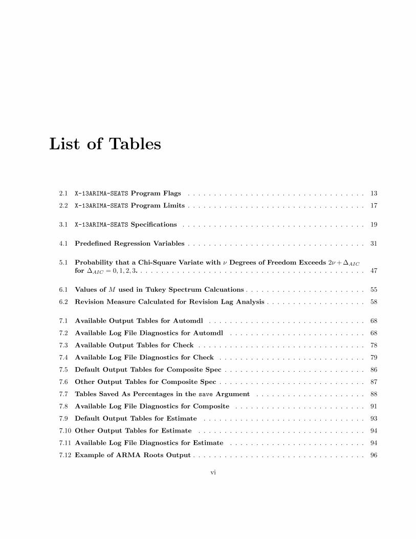
List of Tables
2.1 X-13ARIMA-SEATS Program Flags . . . . . . . . . . . . . . . . . . . . . . . . . . . . . . . . . . 13
2.2 X-13ARIMA-SEATS Program Limits . . . . . . . . . . . . . . . . . . . . . . . . . . . . . . . . . . 17
3.1 X-13ARIMA-SEATS Specifications . . . . . . . . . . . . . . . . . . . . . . . . . . . . . . . . . . . 19
4.1 Predefined Regression Variables . . . . . . . . . . . . . . . . . . . . . . . . . . . . . . . . . . 31
5.1 Probability that a Chi-Square Variate with ν Degrees of Freedom Exceeds 2ν+ ∆AIC
for ∆AIC = 0, 1, 2, 3. . . . . . . . . . . . . . . . . . . . . . . . . . . . . . . . . . . . . . . . . . . . 47
6.1 Values of M used in Tukey Spectrum Calcuations . . . . . . . . . . . . . . . . . . . . . . . 55
6.2 Revision Measure Calculated for Revision Lag Analysis . . . . . . . . . . . . . . . . . . . 58
7.1 Available Output Tables for Automdl . . . . . . . . . . . . . . . . . . . . . . . . . . . . . . 68
7.2 Available Log File Diagnostics for Automdl . . . . . . . . . . . . . . . . . . . . . . . . . . 68
7.3 Available Output Tables for Check . . . . . . . . . . . . . . . . . . . . . . . . . . . . . . . . 78
7.4 Available Log File Diagnostics for Check . . . . . . . . . . . . . . . . . . . . . . . . . . . . 79
7.5 Default Output Tables for Composite Spec . . . . . . . . . . . . . . . . . . . . . . . . . . . 86
7.6 Other Output Tables for Composite Spec . . . . . . . . . . . . . . . . . . . . . . . . . . . . 87
7.7 Tables Saved As Percentages in the save Argument . . . . . . . . . . . . . . . . . . . . . 88
7.8 Available Log File Diagnostics for Composite . . . . . . . . . . . . . . . . . . . . . . . . . 91
7.9 Default Output Tables for Estimate . . . . . . . . . . . . . . . . . . . . . . . . . . . . . . . 93
7.10 Other Output Tables for Estimate . . . . . . . . . . . . . . . . . . . . . . . . . . . . . . . . 94
7.11 Available Log File Diagnostics for Estimate . . . . . . . . . . . . . . . . . . . . . . . . . . 94
7.12 Example of ARMA Roots Output . . . . . . . . . . . . . . . . . . . . . . . . . . . . . . . . . 96
vi
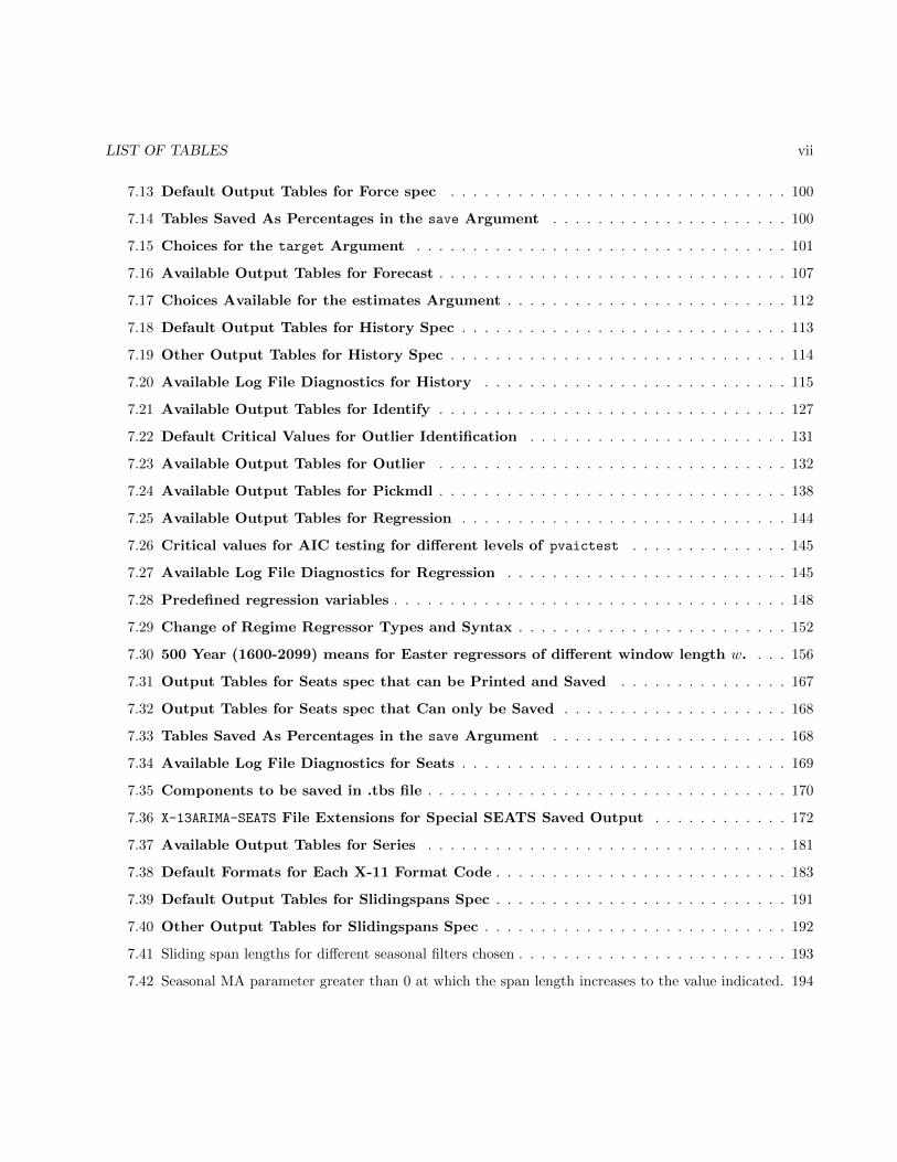
LIST OF TABLES vii
7.13 Default Output Tables for Force spec . . . . . . . . . . . . . . . . . . . . . . . . . . . . . . 100
7.14 Tables Saved As Percentages in the save Argument . . . . . . . . . . . . . . . . . . . . . 100
7.15 Choices for the target Argument . . . . . . . . . . . . . . . . . . . . . . . . . . . . . . . . . 101
7.16 Available Output Tables for Forecast . . . . . . . . . . . . . . . . . . . . . . . . . . . . . . . 107
7.17 Choices Available for the estimates Argument . . . . . . . . . . . . . . . . . . . . . . . . . 112
7.18 Default Output Tables for History Spec . . . . . . . . . . . . . . . . . . . . . . . . . . . . . 113
7.19 Other Output Tables for History Spec . . . . . . . . . . . . . . . . . . . . . . . . . . . . . . 114
7.20 Available Log File Diagnostics for History . . . . . . . . . . . . . . . . . . . . . . . . . . . 115
7.21 Available Output Tables for Identify . . . . . . . . . . . . . . . . . . . . . . . . . . . . . . . 127
7.22 Default Critical Values for Outlier Identification . . . . . . . . . . . . . . . . . . . . . . . 131
7.23 Available Output Tables for Outlier . . . . . . . . . . . . . . . . . . . . . . . . . . . . . . . 132
7.24 Available Output Tables for Pickmdl . . . . . . . . . . . . . . . . . . . . . . . . . . . . . . . 138
7.25 Available Output Tables for Regression . . . . . . . . . . . . . . . . . . . . . . . . . . . . . 144
7.26 Critical values for AIC testing for different levels of pvaictest . . . . . . . . . . . . . . 145
7.27 Available Log File Diagnostics for Regression . . . . . . . . . . . . . . . . . . . . . . . . . 145
7.28 Predefined regression variables . . . . . . . . . . . . . . . . . . . . . . . . . . . . . . . . . . . 148
7.29 Change of Regime Regressor Types and Syntax . . . . . . . . . . . . . . . . . . . . . . . . 152
7.30 500 Year (1600-2099) means for Easter regressors of different window length w. . . . 156
7.31 Output Tables for Seats spec that can be Printed and Saved . . . . . . . . . . . . . . . 167
7.32 Output Tables for Seats spec that Can only be Saved . . . . . . . . . . . . . . . . . . . . 168
7.33 Tables Saved As Percentages in the save Argument . . . . . . . . . . . . . . . . . . . . . 168
7.34 Available Log File Diagnostics for Seats . . . . . . . . . . . . . . . . . . . . . . . . . . . . . 169
7.35 Components to be saved in .tbs file . . . . . . . . . . . . . . . . . . . . . . . . . . . . . . . . 170
7.36 X-13ARIMA-SEATS File Extensions for Special SEATS Saved Output . . . . . . . . . . . . 172
7.37 Available Output Tables for Series . . . . . . . . . . . . . . . . . . . . . . . . . . . . . . . . 181
7.38 Default Formats for Each X-11 Format Code . . . . . . . . . . . . . . . . . . . . . . . . . . 183
7.39 Default Output Tables for Slidingspans Spec . . . . . . . . . . . . . . . . . . . . . . . . . . 191
7.40 Other Output Tables for Slidingspans Spec . . . . . . . . . . . . . . . . . . . . . . . . . . . 192
7.41 Sliding span lengths for different seasonal filters chosen . . . . . . . . . . . . . . . . . . . . . . . . 193
7.42 Seasonal MA parameter greater than 0 at which the span length increases to the value indicated. 194

viii LIST OF TABLES
7.43 Available Output Tables for Spectrum . . . . . . . . . . . . . . . . . . . . . . . . . . . . . . 199
7.44 Output Tables for Spectrum spec that can Only be Saved . . . . . . . . . . . . . . . . . 200
7.45 Available Log File Diagnostics for Spectrum . . . . . . . . . . . . . . . . . . . . . . . . . . 201
7.46 Choices Available for the series Argument . . . . . . . . . . . . . . . . . . . . . . . . . . 201
7.47 Example of QS Statistic Output . . . . . . . . . . . . . . . . . . . . . . . . . . . . . . . . . . 202
7.48 Example of QS Statistic Output Related to qcheck=yes . . . . . . . . . . . . . . . . . . . 204
7.49 Transformations Available Using the function Argument . . . . . . . . . . . . . . . . . . 208
7.50 Available Output Tables for Transform . . . . . . . . . . . . . . . . . . . . . . . . . . . . . 210
7.51 Default Output Tables for X11 spec . . . . . . . . . . . . . . . . . . . . . . . . . . . . . . . 219
7.52 Other Output Tables for X11 . . . . . . . . . . . . . . . . . . . . . . . . . . . . . . . . . . . . 220
7.53 Plots Specified by the print Argument . . . . . . . . . . . . . . . . . . . . . . . . . . . . . . 221
7.54 Tables Saved As Percentages in the save Argument . . . . . . . . . . . . . . . . . . . . . 221
7.55 Available Log File Diagnostics for X11 . . . . . . . . . . . . . . . . . . . . . . . . . . . . . . 222
7.56 X-13ARIMA-SEATS Seasonal Filter Options and Descriptions . . . . . . . . . . . . . . . . . 222
7.57 Modes of Seasonal Adjustment and Their Models . . . . . . . . . . . . . . . . . . . . . . 225
7.58 Number of Surrounding SI-ratios in Table D 8.B Assumed Affected by a Level Shift 227
7.59 Default Output Tables for X11regression . . . . . . . . . . . . . . . . . . . . . . . . . . . . 235
7.60 Other Output Tables for X11regression . . . . . . . . . . . . . . . . . . . . . . . . . . . . . 236
7.61 Predefined regression variables for x11regression . . . . . . . . . . . . . . . . . . . . . . . 241
A.1 Codes Associated with the X-13ARIMA-SEATS Graphics Metafile . . . . . . . . . . . . . . . 247
B.2 Output Tables for Seats spec that can Only be Saved . . . . . . . . . . . . . . . . . . . . 261
B.3 X-13ARIMA-SEATS File Extensions for Special SEATS Saved Output . . . . . . . . . . . . 262
B.4 Components to be saved in .tbs file . . . . . . . . . . . . . . . . . . . . . . . . . . . . . . . . 262
B.5 Output Tables for Spectrum Spec That Can Only be Saved . . . . . . . . . . . . . . . . 263
B.6 Tables That Can Be Saved as Percentages in the save Argument . . . . . . . . . . . . . 264
1 Introduction
Contents1.1 Acknowledgements . . . . . . . . . . . . . . . . . . . . . . . . . . . . . . . . . . . . . . 4
1.2 License Information and Disclaimer . . . . . . . . . . . . . . . . . . . . . . . . . . . 4
The X-13ARIMA-SEATS seasonal adjustment program is an enhanced version of the X-11 Variant of the CensusMethod II seasonal adjustment program (Shiskin, Young, and Musgrave 1967). The enhancements include amore self-explanatory and versatile user interface and a variety of new diagnostics to help the user detect andremedy any inadequacies in the seasonal and calendar effect adjustments obtained under the program optionsselected. The program also includes a variety of new tools to overcome adjustment problems and thereby enlargethe range of economic time series that can be adequately seasonally adjusted. Examples of the use of thesetools can be found in Findley and Hood (1999). Basic information on seasonal adjustment is given in Chapter 2of Dagum and Cholette (2006) and in Chapter 1 of Ladiray and Quenneville (2001), where the X-11 method isthoroughly documented. See also Bell and Hillmer (1984, 1985), den Butter and Fase (1991), and Klein (1991).
The chief source of these new tools is the extensive set of time series model building facilities built into theprogram for fitting what we call regARIMA models. These are regression models with ARIMA (autoregressiveintegrated moving average) errors. More precisely, they are models in which the mean function of the timeseries (or its logs) is described by a linear combination of regressors, and the covariance structure of the seriesis that of an ARIMA process. If no regressors are used, indicating that the mean is assumed to be zero, theregARIMA model reduces to an ARIMA model. There are built-in regressors for directly estimating variousflow and stock trading day effects and holiday effects. There are also regressors for modeling certain kinds ofdisruptions in the series, or sudden changes in level, whose effects need to be temporarily removed from thedata before the X-11 methodology can adequately estimate seasonal adjustments. To address data problemsnot provided for, there is the capability of incorporating user-defined regression variables into the model fitted.The regARIMA modeling module of X-13ARIMA-SEATS was adapted from the regARIMA program developedby the Time Series Staff of U. S. Census Bureau’s Statistical Research Division.
Whether or not special problems requiring the use of regressors are present in the series to be adjusted,a fundamentally important use of regARIMA models is to extend the series with forecasts (and backcasts) inorder to improve the seasonal adjustments of the most recent (and the earliest) data. Doing this mitigatesproblems inherent in the trend estimation and asymmetric seasonal averaging processes of the type used bythe X-11 method near the ends of the series. The provision of this extension was the most important technicalimprovement offered by Statistics Canada’s widely used X-11 program. Its benefits, both theoretical andempirical, have been documented in many publications, including Geweke (1978), Dagum (1988) and Bobbittand Otto (1990) and the articles referenced in these papers.
X-13ARIMA-SEATS is available as an executable program for PC microcomputers (386 or higher with a mathcoprocessor) running DOS (version 3.0 or higher), Sun 4 UNIX workstations, and VAX/VMS computers. Fortransource code is available for users to create executable programs on other computer systems. When it is released,the X-13ARIMA-SEATS program will be in the public domain, and may be copied or transferred. Computer filescontaining the current test version of the program (executables for various machines and source code), this
1
2 CHAPTER 1. INTRODUCTION
documentation, and examples, have been put on the Internet at http://www.census.gov/srd/www/x13as/.Limited program support is available via regular mail, telephone and email (the preferred mode of communi-cation) at the addresses given on the title page. If problems are encountered running a particular input file,providing the input, data and resulting output files will facilitate our identification of the problem.
There are now two seasonal adjustment modules contained in the program. One uses the X-11 seasonaladjustment method detailed in Shiskin, Young, and Musgrave (1967). The program has all the seasonal adjust-ment capabilities of the X-11 and X-11-ARIMA programs. The same seasonal and trend moving averages areavailable, and the program still offers the X-11 calendar and holiday adjustment routines.
The X-11 seasonal adjustment module has also been enhanced by the addition of several new options,including
(a) the sliding spans diagnostic procedures, illustrated in Findley, Monsell, Shulman, and Pugh (1990)(b) the ability to produce the revisions history of a given seasonal adjustment(c) a new Henderson trend filter routine which allows the user to choose any odd number for the length
of the Henderson filter(d) new options for seasonal filters(e) several new outlier detection options for the irregular component of the seasonal adjustment(f) a table of the trading day factors by type of day(g) a pseudo-additive seasonal adjustment mode.
The second seasonal adjustment module uses the ARIMA model based seasonal adjustment procedure fromthe SEATS seasonal adjustment program developed by Victor Gomez and Agustin Maravall at the Bank of Spain.All the capabilities of SEATS are included in this version of X-13ARIMA-SEATS , which can generate stabilityand spectral diagnostics for SEATS seasonal adjustments in the same way as X-11 seasonal adjustments.
For more details on the SEATS seasonal adjustment method, see Maravall (1995), Gomez and Maravall(1996), Gomez and Maravall (2001a), and Gomez and Maravall (2001b). Findley, Lytras, and Maravall (2016)provides a tutorial on the model-based seasonal adjustment method of the SEATS and its implementation inX-13ARIMA-SEATS .
The modeling module of X-13ARIMA-SEATS is designed for regARIMA model building with seasonal economictime series. To this end, several categories of predefined regression variables are available in X-13ARIMA-SEATS
including trend constants or overall means, fixed seasonal effects, trading-day effects, holiday effects, pulse effects(additive outliers), level shifts, temporary change outliers, and ramp effects. User-defined regression variablescan also be easily read in and included in models. The program is designed around specific capabilities neededfor regARIMA modeling, and is not intended as a general purpose statistical package. In particular, X-13-ARIMA-SEATS should be used in conjunction with other (graphics) software capable of producing high resolutionplots of time series.
Observations (data) from a time series to be modelled and/or seasonally adjusted using X-13ARIMA-SEATS
should be quantitative, as opposed to binary or categorical. Observations must be equally spaced in time, andmissing values are not allowed. X-13ARIMA-SEATS handles only univariate time series models, i.e., it does notestimate relationships between different time series.
X-13ARIMA-SEATS uses the standard (p d q)(P D Q)s notation for seasonal ARIMA models. The (p d q)refers to the orders of the nonseasonal autoregressive (AR), differencing, and moving average (MA) operators,
3
respectively. The (P D Q)s refers to the seasonal autoregressive, differencing, and moving average orders.The s subscript denotes the seasonal period, e.g., s = 12 for monthly data. Great flexibility is allowed in thespecification of ARIMA structures: any number of AR, MA, and differencing operators may be used; missinglags are allowed in AR and MA operators; and AR and MA parameters can be fixed at user-specified values.
For the user who wishes to fit customized time series models, X-13ARIMA-SEATS provides capabilities for thethree modeling stages of identification, estimation, and diagnostic checking. The specification of a regARIMAmodel requires specification both of the regression variables to be included in the model and also the typeof ARIMA model for the regression errors (i.e., the orders (p d q)(P D Q)s). Specification of the regressionvariables depends on user knowledge about the series being modelled. Identification of the ARIMA model forthe regression errors follows well-established procedures based on examination of various sample autocorrelationand partial autocorrelation functions produced by the X-13ARIMA-SEATS program. Once a regARIMA modelhas been specified, X-13ARIMA-SEATS will estimate its parameters by maximum likelihood using an iterativegeneralized least squares (IGLS) algorithm. Diagnostic checking involves examination of residuals from thefitted model for signs of model inadequacy. X-13ARIMA-SEATS produces several standard residual diagnosticsfor model checking, as well as providing sophisticated methods for detecting additive outliers and level shifts.Finally, X-13ARIMA-SEATS can produce point forecasts, forecast standard errors, and prediction intervals fromthe fitted regARIMA model.
In addition to these modeling features, X-13ARIMA-SEATS has an automatic model selection procedure basedlargely on the automatic model selection procedure of TRAMO (Gomez and Maravall 1996, documented inGomez and Maravall 2001a). There are also options that use AICC to determine if user-specified regressionvariables (such as trading day or Easter regressors) should be included into a particular series. Also, historiescan be generated for likelihood statistics (such as AICC, a version of Akaike’s AIC that adjusts for the lengthof the series being modelled) and forecasts to facilitate comparisons between competing models.
The next six chapters detail capabilities of the X-13ARIMA-SEATS program.
• Chapter 2 provides an overview of running X-13ARIMA-SEATS and explains program limits that userscan change.
• Chapter 3 provides a general description of the required input file (specification file), and also discussesspecification file syntax and related issues.
• Chapter 4 discusses the general regARIMA model fit by the X-13ARIMA-SEATS program, summarizes thetechnical steps involved in regARIMA modeling and forecasting, and relates these steps to capabilities ofthe program.
• Chapter 5 discusses some key points related to model estimation and inference that all users of themodeling features should be aware of, including some estimation problems that may arise and ways toaddress them.
• Chapter 6 discusses some details of key seasonal adjustment diagnostics: spectrums, sliding spans, andrevisions history.
• Chapter 7 gives detailed documentation for each specification statement that can appear in the specifi-cation file. These statements function as commands that control the flow of X-13ARIMA-SEATS’ executionand select among the various program options.
4 CHAPTER 1. INTRODUCTION
The focus in Chapters 2 through 6 is on giving an overview of the use and capabilities of the X-13ARIMA-SEATS
program. In contrast, Chapter 7 is intended as the primary reference to be used when constructing specificationfiles for running the X-13ARIMA-SEATS program.
1.1 Acknowledgements
We are indebted to Statistics Canada, particularly to Estella Dagum, providing us with the source code fromX-11-ARIMA ( Dagum 1980, Dagum 1988 ) to use as the starting point for the seasonal adjustment routines ofX-13ARIMA-SEATS and giving us helpful advice.
We are grateful to Hirtugu Akaike and Makio Ishiguro of the Institute of Statistical Mathematics for per-mission to incorporate into X-13ARIMA-SEATS the source code of the autoregressive spectrum diagnostics ofBAYSEA (Akaike and Ishiguro 1980).
X-13ARIMA-SEATS would not have been possible without the support of Agustın Maravall while at the Bankof Spain and Gianluca Caporello, who provided us with SEATS source code (including updates) and weregenerous with their advice and expertise.
Further, we are indebted to Victor Gomez for providing us with the Fortran code of TRAMO (Gomezand Maravall 2001a) to enable us to implement an automatic modeling procedure very similar to TRAMO’sin X-13ARIMA-SEATS and to Agustın Maravall, Gianluca Caporello, and contractors at the Bank of Spain forupdates to the TRAMO and SEATS source code and advice.
1.2 License Information and Disclaimer
This Software was created by U.S. Government employees and therefore is not subject to copyright in the UnitedStates (17 U.S.C. §105). The United States/U.S. Department of Commerce (“Commerce”) reserve all rights toseek and obtain copyright protection in countries other than the United States. The United States/Commercehereby grant to User a royalty-free, nonexclusive license to use, copy, and create derivative works of the Softwareoutside of the United States.
The Software is provided to the User and those who may take by, through or under it, “as is,” without anywarranty (whether express or implied) or representation whatsoever, including but not limited to any warrantyof merchantability. The Software is taken hereunder without any right to support or to any improvements,extensions, or modifications, except as may be agreed to separately, in writing, by Commerce.
User, on behalf of itself and all others who take by, through or under it, hereby and forever waives, re-leases, and discharges the United States/Commerce and all its instrumentalities from any and all liabilities andobligations in connection with the use, application, sale or conveyance of the Software. User shall indemnifyand hold harmless the United States/Commerce and its instrumentalities from all claims, liabilities, demands,damages, expenses, and losses arising from or in connection with User’s use, application, sale or conveyance ofthe Software, including those who take by, through or under User whether or not User was directly involved.This provision will survive termination of this Agreement and will include any and all claims or liabilities arisingunder intellectual property rights, such as patents, copyrights, trademarks, and trade secrets. If User of softwareis an Executive Agency of the United States, this clause is not applicable.

1.2. LICENSE INFORMATION AND DISCLAIMER 5
The construction, validity, performance, and effect of this Agreement for all purposes will be governed byFederal law of the United States.
User agrees to make a good faith effort to use the Software in a way that does not cause damage, harm, orembarrassment to the United States/Commerce. The United States/Commerce expressly reserve all rights andremedies.
2 Running X-13ARIMA-SEATS
Contents2.1 Input . . . . . . . . . . . . . . . . . . . . . . . . . . . . . . . . . . . . . . . . . . . . . . 7
2.2 Output . . . . . . . . . . . . . . . . . . . . . . . . . . . . . . . . . . . . . . . . . . . . . 7
2.3 Input errors . . . . . . . . . . . . . . . . . . . . . . . . . . . . . . . . . . . . . . . . . . 7
2.4 Specifying an alternate output filename . . . . . . . . . . . . . . . . . . . . . . . . . 8
2.5 Running X-13ARIMA-SEATS on more than one series . . . . . . . . . . . . . . . . . . 8
2.5.1 Running X-13ARIMA-SEATS in multi-spec mode . . . . . . . . . . . . . . . . . . . . . . 9
2.5.2 Running X-13ARIMA-SEATS in single spec mode . . . . . . . . . . . . . . . . . . . . . . 10
2.5.3 Special Case: File Names Containing Spaces . . . . . . . . . . . . . . . . . . . . . . . 11
2.6 Log Files . . . . . . . . . . . . . . . . . . . . . . . . . . . . . . . . . . . . . . . . . . . . 12
2.7 Flags . . . . . . . . . . . . . . . . . . . . . . . . . . . . . . . . . . . . . . . . . . . . . . 12
2.8 Program limits . . . . . . . . . . . . . . . . . . . . . . . . . . . . . . . . . . . . . . . . 16
Tables2.1 X-13ARIMA-SEATS Program Flags . . . . . . . . . . . . . . . . . . . . . . . . . . . . . . . . . 13
2.2 X-13ARIMA-SEATS Program Limits . . . . . . . . . . . . . . . . . . . . . . . . . . . . . . . . 17
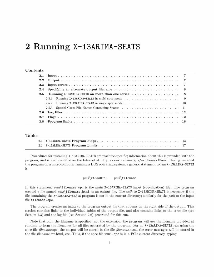
Procedures for installing X-13ARIMA-SEATS are machine-specific; information about this is provided with theprogram, and is also available on the Internet at http://www.census.gov/srd/www/x13as/. Having installedthe program on a microcomputer running a DOS operating system, a generic statement to run X-13ARIMA-SEATS
is
path\x13asHTML path\filename
In this statement path\filename.spc is the main X-13ARIMA-SEATS input (specification) file. The programcreated a file named path\filename.html as an output file. The path to X-13ARIMA-SEATS is necessary if thefile containing the X-13ARIMA-SEATS program is not in the current directory; similarly for the path to the inputfile filename.spc.
The program creates an index to the program output file that appears on the right side of the output. Thissection contains links to the individual tables of the output file, and also contains links to the error file (seeSection 2.3) and the log file (see Section 2.6) generated for this run.
Note that only the filename is specified, not the extension; the program will use the filename provided atruntime to form the filenames for all files generated by the program. For an X-13ARIMA-SEATS run using thespec file filename.spc, the output will be stored in the file filename.html, the error messages will be stored inthe file filename err.html, etc. Thus, if the spec file xuu1.spc is in a PC’s current directory, typing
6
2.1. INPUT 7
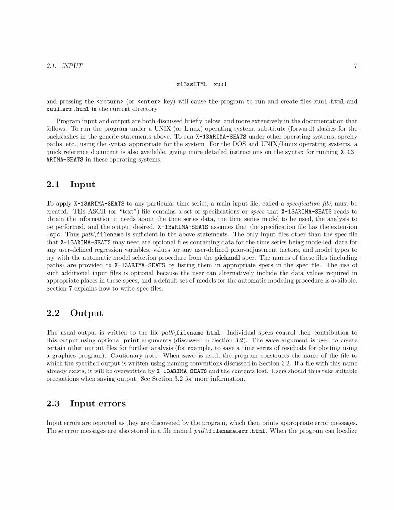
x13asHTML xuu1
and pressing the <return> (or <enter> key) will cause the program to run and create files xuu1.html andxuu1 err.html in the current directory.
Program input and output are both discussed briefly below, and more extensively in the documentation thatfollows. To run the program under a UNIX (or Linux) operating system, substitute (forward) slashes for thebackslashes in the generic statements above. To run X-13ARIMA-SEATS under other operating systems, specifypaths, etc., using the syntax appropriate for the system. For the DOS and UNIX/Linux operating systems, aquick reference document is also available, giving more detailed instructions on the syntax for running X-13-
ARIMA-SEATS in these operating systems.
2.1 Input
To apply X-13ARIMA-SEATS to any particular time series, a main input file, called a specification file, must becreated. This ASCII (or “text”) file contains a set of specifications or specs that X-13ARIMA-SEATS reads toobtain the information it needs about the time series data, the time series model to be used, the analysis tobe performed, and the output desired. X-13ARIMA-SEATS assumes that the specification file has the extension.spc. Thus path\filename is sufficient in the above statements. The only input files other than the spec filethat X-13ARIMA-SEATS may need are optional files containing data for the time series being modelled, data forany user-defined regression variables, values for any user-defined prior-adjustment factors, and model types totry with the automatic model selection procedure from the pickmdl spec. The names of these files (includingpaths) are provided to X-13ARIMA-SEATS by listing them in appropriate specs in the spec file. The use ofsuch additional input files is optional because the user can alternatively include the data values required inappropriate places in these specs, and a default set of models for the automatic modeling procedure is available.Section 7 explains how to write spec files.
2.2 Output
The usual output is written to the file path\filename.html. Individual specs control their contribution tothis output using optional print arguments (discussed in Section 3.2). The save argument is used to createcertain other output files for further analysis (for example, to save a time series of residuals for plotting usinga graphics program). Cautionary note: When save is used, the program constructs the name of the file towhich the specified output is written using naming conventions discussed in Section 3.2. If a file with this namealready exists, it will be overwritten by X-13ARIMA-SEATS and the contents lost. Users should thus take suitableprecautions when saving output. See Section 3.2 for more information.
2.3 Input errors
Input errors are reported as they are discovered by the program, which then prints appropriate error messages.These error messages are also stored in a file named path\filename err.html. When the program can localize
8 CHAPTER 2. RUNNING X-13ARIMA-SEATS
the error, the line in the spec file containing the error will be printed out with a caret (^) positioned underthe error. If the program cannot localize the error, then only the error message will be printed. If the erroris fatal, then ERROR: will be displayed before the error message, sometimes with suggestions about whatto change. For nonfatal errors, WARNING: will be printed before the message. WARNING messages arealso used sometimes to call attention to a situation in which no error has been committed, but some caution isappropriate.
X-13ARIMA-SEATS first reads the whole spec file, reporting all input errors it finds. This way the user cantry to correct more than one input error per run. Frequently, however, the only informative messages are thosefor the first one or two errors. These errors may result in other errors, especially if input errors occur in theseries spec. The program will stop if any fatal errors are detected. Warnings will not stop the program, butshould alert users to check both the input and output carefully to verify that the desired results are produced.
2.4 Specifying an alternate output filename
As was noted before, for an X-13ARIMA-SEATS run using the spec file filename.spc, the output will be stored inthe file filename.html, the error messages will be stored in the file filename err.html, etc. For the purpose ofexamining the effects of different adjustment and modeling options on a given series, it is sometimes desirable touse a different filename for the output than was used for the input. The general form for specifying an alternatefilename for the output files is
path\x13asHTML path\filename path\outname (2.1)
This X-13ARIMA-SEATS run still uses the spec file filename.spc, but the output will be stored in the fileoutname.html, the error messages will be stored in the file outname err.html, etc. All output files generated bythis run will be stored using the path and filename given by the user, not the path and filename of the inputspecification file.
2.5 Running X-13ARIMA-SEATS on more than one series
In a production situation, it is essential to run more than one series in a given X-13ARIMA-SEATS run. X-13-
ARIMA-SEATS allows for running multiple series in two modes:
(a) multi-spec mode, where there are input specification files for every series specified;(b) single spec mode, where every series will be run with the options from a single input specification
file.
Before X-13ARIMA-SEATS can be run in either mode, a metafile must be created. This is an ASCII filewhich contains the names of the files to be processed. Two types of metafiles are used by the X-13ARIMA-SEATS
software: input metafiles (for multi-spec mode) and data metafiles (for single spec mode).
If an error occurs in one of the spec files in a metafile run, the program will print the appropriate errormessages. Execution will stop for that series and the program will continue processing the remaining spec files.A listing of all the input files with errors is given in the X-13ARIMA-SEATS log file, described in Section 2.7.
2.5. RUNNING X-13ARIMA-SEATS ON MORE THAN ONE SERIES 9
2.5.1 Running X-13ARIMA-SEATS in multi-spec mode
Before X-13ARIMA-SEATS can be run in multi-spec mode, an input metafile must first be created. This is anASCII file which contains the names of the files to be processed by X-13ARIMA-SEATS in sequence. An inputmetafile can have up to two entries per line: the filename (and path information, if necessary) of the inputspecification file for a given series, and an optional output filename for the output of that series. If an outputfilename is not given by the user, then the path and filename of the input specification file will be used togenerate the output files. The input specification files are processed in the order in which they appear in theinput metafile.
For example, to run the spec files xuu1.spc, xuu2.spc and xuu3.spc, the input metafile should contain thefollowing:
xuu1
xuu2
xuu3
This assumes that all these spec files are in the current directory. To run these files if they are stored in thec:\export\specs DOS directory, the metafile should read:
c:\export\specs\xuu1c:\export\specs\xuu2c:\export\specs\xuu3
To run X-13ARIMA-SEATS with a input metafile, use the following syntax:
x13asHTML -m metafile
where metafile.mta is the metafile and -m is a flag which informs X-13ARIMA-SEATS of the presence of ametafile.
For example, if the metafile defined above is stored in exports.mta, type
x13asHTML -m exports
and press the return key to run the corresponding spec files.
Note that when the name of the input metafile was given in the example above, only the filename wasspecified, not the extension; .mta is the required extension for the input metafile. Path information should beincluded with the input metafile name, if necessary.
The filenames used by X-13ARIMA-SEATS to generate output files are taken from the spec files listed in themetafile, not from the metafile itself. The example given above would generate output files named xuu1.html,
xuu2.html and xuu3.html corresponding to the individual spec files given in the metafile exports.mta, not acomprehensive output file named exports.html. To specify alternate output filenames for the example above,simply add the desired output filenames to each line of the input metafile, e.g.,
10 CHAPTER 2. RUNNING X-13ARIMA-SEATS
c:\export\specs\xuu1 c:\export\output\xuu1c:\export\specs\xuu2 c:\export\output\xuu2c:\export\specs\xuu3 c:\export\output\xuu3
In addition to the output files from the individual spec files, each metafile run generates a separate indexfile for all the output generated by the metafile. Links to the output, index, error, and log files are organizedinto a metafile index file. For input metafiles, the base filename of the metafile is used to generate the name ofthe metafile index; for the example given above, the metafile index file is stored in exports mta.html.
2.5.2 Running X-13ARIMA-SEATS in single spec mode
To run X-13ARIMA-SEATS on many series using the same specification commands for each series, it is necessaryto create a data metafile. A data metafile can have up to two entries per line: the complete filename (and pathinformation, if necessary) of the data file for a given series, and an optional output filename for the output ofthat series. If an output filename is not given by the user, then the path and filename of the data file will beused to generate the output files. Note: In a data metafile, no extension is assumed for the individual datafiles. The extensions must be specified, along with the path and filename, if the data files are not in the currentdirectory.
The data files are processed in the order in which they appear in the data metafile. The options used toprocess each data file are provided by a single input specification file identified at runtime. This means thatall the data files specified in the data metafile must be in the same format. Also, certain formats supported byX-13ARIMA-SEATS should be avoided; see the description of the series spec in Section 7.15 for more details.
For example, to process the data files xuu1.dat, xuu2.dat and xuu3.dat, the data metafile should containthe following:
xuu1.dat
xuu2.dat
xuu3.dat
This assumes that all these data files are in the current directory. To run these files if they are stored in thec:\export\data DOS directory, the metafile should read:
c:\export\data\xuu1.datc:\export\data\xuu2.datc:\export\data\xuu3.dat
To run X-13ARIMA-SEATS with a data metafile, use the following syntax:
x13asHTML specfile -d metafile
where metafile.dta is the data metafile, -d is a flag which informs X-13ARIMA-SEATS of the presence of a datametafile, and specfile.spc is the single input specification file used for each of the series listed in the datametafile.
For example, if the data metafile with three series used for illustration above is named exports.dta, type
2.5. RUNNING X-13ARIMA-SEATS ON MORE THAN ONE SERIES 11
x13asHTML default -d exports
and press the return key to process the corresponding data files using the default.spc input specification file.
Note that when the name of the data metafile was given in the example above, only the filename wasspecified, not the extension; .dta is the required extension for the input metafile. Path information should beincluded with the data metafile name, if necessary.
The filenames used by X-13ARIMA-SEATS to generate output files are taken from the data files listed in themetafile, not by the metafile itself. The example given above would generate output files named xuu1.html,
xuu2.html and xuu3.html corresponding to the individual data files given in the metafile exports.dta, not acomprehensive output file named exports.html. To specify alternate output filenames for the example above,simply add the desired output filenames to each line of the data metafile, e.g.,
c:\export\data\xuu1.dat c:\export\output\xuu1c:\export\data\xuu2.dat c:\export\output\xuu2c:\export\data\xuu3.dat c:\export\output\xuu3
As with input metafiles, each data metafile run generates a separate index file for all the output generatedby the data metafile. Links to the output, index, error, and log files are organized into a data metafile indexfile. The base filename of the data metafile is used to generate the name of the metafile index; for the examplegiven above, the data metafile index file is stored in exports dta.html.
2.5.3 Special Case: File Names Containing Spaces
In many current operating systems, it is permissable to have blank spaces in file names or paths - for example,c:\My Spec Files\test.spc. When specifying such a file in an input or data metafile, the user must enclosethe entire filename with quotation marks ("). Otherwise, the program will assume that the first entry in themetafile is only the text up to the first space.
For example, if the specfiles used in the second example in Section 2.5.1 were stored in the c:\export specs
DOS directory, then the input metafile should read:
"c:\export specs\xuu1""c:\export specs\xuu2""c:\export specs\xuu3"
Running X-13ARIMA-SEATS on the input metafile given above would generate output files named xuu1.html,
xuu2.html and xuu3.html in the c:\export specs directory.
This convention applies to data metafiles and alternate output filenames provided in metafiles as well. Thefollowing data metafile would read data files from the directory c:\export data and store the output files intothe directory c:\export output
"c:\export data\xuu1.dat" "c:\export output\xuu1 a"
"c:\export data\xuu2.dat" "c:\export output\xuu2 a"
"c:\export data\xuu3.dat" "c:\export output\xuu3 a"
12 CHAPTER 2. RUNNING X-13ARIMA-SEATS
Running X-13ARIMA-SEATS on the data metafile given above would generate output files named xuu1
a.html, xuu2 a.html and xuu3 a.html in the c:\export output directory.1
Be careful that the opening and closing quotation marks fully contain the filenames with no extra spaces,and that there are matching opening and closing quotation marks for each file. Also, there is one exception:you cannot have a space before the file extension. For example, the input specification file My Little Spec
File .spc cannot be run by X-13ARIMA-SEATS either by itself or in a metafile. You will need to remove thespace before the ”.” to run the file.
2.6 Log Files
Every time X-13ARIMA-SEATS is run, a log file is produced where a summary of modeling and seasonal ad-justment diagnostics can be stored for every series or spec file processed. When X-13ARIMA-SEATS is run inmulti-spec or single spec model, as described in the previous section, the log file is stored with the same nameand directory as the metafile (for multi-spec mode) or data metafile (single spec mode), appending log.html
to the base metafile name. For example
x13asHTML -m exports
runs each of the spec files referenced in exports.mta and stores user-selected diagnostics from each of the specfiles into the log file exports log.html.
If only one series is processed, log.html is appended to the output directory and filename to form the nameof the log file.
Users can specify which diagnostics are stored in the log file by using the savelog argument found in theautomdl, check, composite, estimate, history, pickmdl, regression, seats, spectrum, slidingspans,transform, x11, and x11regression specs. The descriptions of the individual specs in Section 7 give moredetails on which diagnostics can be stored in the log file.
As mentioned in the previous section, if an error occurs in one of the spec files in a metafile run, a listing ofall the input files with errors is given in the log file.
2.7 Flags
In the previous section, the flags -m and -d were required in the command line to obtain the desired run. Thereare several other input and output options that are specified on the command line. The general syntax for thecommand line can be given as
path\x13asHTML arg1 arg2 . . . argN
1Note that if you are trying to access the HTML output files in the address bar of a browser, you should replace the spaces with”%20”.
2.7. FLAGS 13
where the arguments given after x13asHTML can be either flags or filenames, depending on the situation.
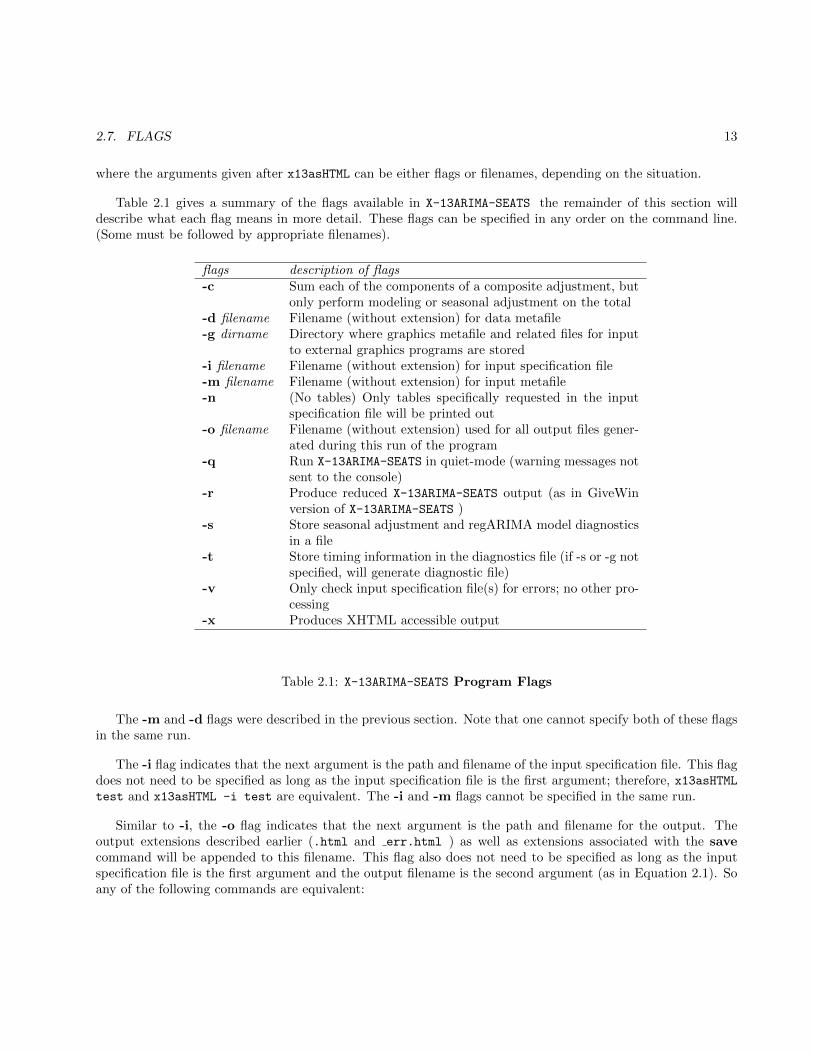
Table 2.1 gives a summary of the flags available in X-13ARIMA-SEATS the remainder of this section willdescribe what each flag means in more detail. These flags can be specified in any order on the command line.(Some must be followed by appropriate filenames).
flags description of flags-c Sum each of the components of a composite adjustment, but
only perform modeling or seasonal adjustment on the total-d filename Filename (without extension) for data metafile-g dirname Directory where graphics metafile and related files for input
to external graphics programs are stored-i filename Filename (without extension) for input specification file-m filename Filename (without extension) for input metafile-n (No tables) Only tables specifically requested in the input
specification file will be printed out-o filename Filename (without extension) used for all output files gener-
ated during this run of the program-q Run X-13ARIMA-SEATS in quiet-mode (warning messages not
sent to the console)-r Produce reduced X-13ARIMA-SEATS output (as in GiveWin
version of X-13ARIMA-SEATS )-s Store seasonal adjustment and regARIMA model diagnostics
in a file-t Store timing information in the diagnostics file (if -s or -g not
specified, will generate diagnostic file)-v Only check input specification file(s) for errors; no other pro-
cessing-x Produces XHTML accessible output
Table 2.1: X-13ARIMA-SEATS Program Flags
The -m and -d flags were described in the previous section. Note that one cannot specify both of these flagsin the same run.
The -i flag indicates that the next argument is the path and filename of the input specification file. This flagdoes not need to be specified as long as the input specification file is the first argument; therefore, x13asHTMLtest and x13asHTML -i test are equivalent. The -i and -m flags cannot be specified in the same run.
Similar to -i, the -o flag indicates that the next argument is the path and filename for the output. Theoutput extensions described earlier (.html and err.html ) as well as extensions associated with the savecommand will be appended to this filename. This flag also does not need to be specified as long as the inputspecification file is the first argument and the output filename is the second argument (as in Equation 2.1). Soany of the following commands are equivalent:
14 CHAPTER 2. RUNNING X-13ARIMA-SEATS
x13asHTML test test2
x13asHTML -i test -o test2
x13asHTML -o test2 -i test
However, x13asHTML -i test test2 will generate an error, since the first argument is the flag -i, not thespec file. The -o flags cannot be specified in the same run as the -m or -d flags. The -o and -m flags cannotbe specified in the same run.
For operating systems that allow blank spaces in file names, the convention for specifying a file name as aflag is similar to that specified in Section 2.5.3. All filenames with at least one space in the filename or pathshould be enclosed in quotation marks (").
So any of the following commands should execute correctly:
x13asHTML "c:\My Spec Files\test" "c:\My Output\test2"x13asHTML -i "c:\My Spec Files\test" -o "c:\My Output\test2"x13asHTML -o "c:\My Output\test2" -i "c:\My Spec Files\test"
x13asHTML -m "c:\My Spec Files\alltest"x13asHTML "c:\My Spec Files\testsrs" -d "c:\My Data Files\testsrs"
The -s flag specifies that certain seasonal adjustment and regARIMA modeling diagnostics that appear inthe main output be saved in file(s) separate from the main output. These include tables in the main output filethat are not tables of time series. Such tables cannot be stored in the format used for individual time seriestables. When the -s flag is used, X-13ARIMA-SEATS automatically stores the most important of these diagnosticsin a separate file that can be used to generate diagnostic summaries. This file (called the diagnostics summaryfile) will have the same path and filename as the main output, with the extension .udg. So for
x13asHTML test -s
the diagnostics summary file will be stored in test.udg, and for
x13asHTML test -s -o testout
the diagnostics summary file will be stored in testout.udg.
The diagnostics summary file is an ASCII database file. Within the diagnostic file, each diagnostic has aunique key to access it’s value. The key is separated from the diagnostic value by a colon (’:’), followed by whitespace. So in the entry below:
freq: 12
The key for this entry would be freq, and the value for the key would be 12. Each record in the file providesa value for a unique key found at the beginning of the line.
User-defined metadata can be stored in the diagnostics summary file (for more details, see the descriptionof the metadata spec in Section 7.9).
2.7. FLAGS 15
A program is available via the Internet at http://www.census.gov/srd/www/x13as/ that reads the seasonaladjustment diagnostics file and produces a summary of the seasonal adjustment diagnostics. This program iswritten in the Icon programming language (see Griswold and Griswold 1997).
The -g flag indicates that the next argument is the complete path name of a directory into which outputwill be stored that is intended as input for a separate graphics program. This output consists of the followingfiles:
(1) files of diagnostic data to be graphed, which are produced by the options specified in the .spc file;
(2) a graphics metafile containing the names of these files;
(3) a diagnostics summary file containing information about the time series being processed, about theregARIMA model fit to the series (if any), and about the seasonal adjustment requested (if any);
The graphics metafile carries the extension .gmt and the diagnostics summary file carries the extension.udg; these files carry the filename used for the main program output. For example, if a user enters
x13asHTML test -g c:\sagraph
the graphics metafile will be stored in c:\sagraph\test.gmt and the diagnostics summary file will be storedin c:\sagraph\test.udg. For
x13asHTML test -g c:\sagraph -o testout
the graphics metafile will be stored in c:\sagraph\testout.gmt and the diagnostics summary file will be storedin c:\sagraph\testout.udg. In both cases, related files needed to generate seasonal adjustment graphics willbe also be stored in the c:\sagraph subdirectory. (NOTE: The directory entered after the -g flag must alreadyhave been created and should be different from the directory used for the output files; it can be a subdirectoryof the latter.)
Two versions of a program named X-13-Graph (see Hood 2002a, Hood 2002c, and Lytras 2015) that useSAS/GRAPH (see SAS Institute Inc. 1990) to produce graphs from the graphics mode output are distributedwith X-13ARIMA-SEATS on the Census Bureau website (http://www.census.gov/srd/www/x13graph/). Inaddition, X-13-Graph Java is an implementation of the X-13-Graph software in Java (Lytras 2013). X-13-Graph Java generates graphics from the output of X-13ARIMA-SEATS and does not require SAS. It has almostall of the functionality of X-13-Graph. For examples of the use of X-13-Graph, see Findley and Hood (1999).For a list of the files stored by X-13ARIMA-SEATS in graphics mode, along with the codes used in the graphicsmetafile to denote these files, see Appendix A.
If both the -g and -s options are used in the same X-13ARIMA-SEATS run, the complete version of the seasonaladjustment diagnostics file will be stored in the directory specified by the -g option (and not in the directoryof the main output file). If a model diagnostics file is also generated, that file will be stored in the graphicsdirectory as well. A warning message is written to the screen and to the log file telling the user that the seasonaladjustment diagnostics file (and the model diagnostics file, if it is produced) is in the graphics directory.
The -n, -r, and -x flags affect the format of program output. The -n option allows the user to restrict thenumber of tables appearing in the main output file. The X-13ARIMA-SEATS program produces a large number
16 CHAPTER 2. RUNNING X-13ARIMA-SEATS
of tables in the main output file. While X-13ARIMA-SEATS is flexible in allowing users to determine which tablesare to be printed out, it is sometimes convenient to restrict the output to only a few tables. To facilitate this,the -n flag specifies that, as the default, no tables will be written to the main output file. Then only thosetables specified by the user in the spec file are written.
The -r flag specifies that output tables and headers will be written in a format that will reduce the amountof output printed out to the main output file. The tables printed out are consolidated, and some blank lines inthe printout are suppressed. This output option was first utilized in the version of X-13ARIMA-SEATS developedfor use with the GiveWin econometrics package (see Doornik and Hendry 2001).
The -x flag specifies that the accessible program output should be generated in XHTML Version 1.0 Transi-tional rather than HTML Version 4.0. XHTML (Extensible HyperText Markup Language) is a family of XMLmarkup languages that mirror or extend versions of the widely used Hypertext Markup Language (HTML). Fora general discussion of XHTML, access Wikipedia Contributers (2013).
The -q flag specifies that X-13ARIMA-SEATS will be run in “quiet mode”. Warning messages that are normallyprinted to the console are suppressed, although error messages shall still be printed to the console. All warningmessages not printed to the screen will be stored in the error file (see Section 2.3).
The -c flag is used only to restrict a composite seasonal adjustment run done with an input metafile (-m). In a composite seasonal adjustment, X-13ARIMA-SEATS usually seasonally adjusts a set of component timeseries, as well as their composite (also called aggregate), which is usually their sum (for more details, see thedescription of the composite spec in Section 7.4). An input specification file is needed for each series. When-c is invoked, the seasonal adjustment and modeling options specified in the input spec files for the componentseries are ignored; the component series are only used to form the composite series. This option is useful whenidentifying a regARIMA model for the composite series.
Finally, the -v flag specifies that X-13ARIMA-SEATS will be run in an input verification mode to enable theuser to see if there are errors in one or more input spec files. This allows the user to check the program optionsfor errors without doing the complete X-13ARIMA-SEATS runs for all the series. The -v flag cannot be used withthe -s, -c, -n, -w, or -p flags.
2.8 Program limits
The X-13ARIMA-SEATS Fortran source code contains limits on the maximum length of series, maximum numberof regression variables in a model, etc. These limits are set at values believed to be sufficiently large for thegreat majority of applications, without being so large as to cause memory problems or to significantly lengthenprogram execution times.
Table 2.2 details those parameter variables in the model.prm, srslen.prm, and stdio.i files correspondingto X-13ARIMA-SEATS program limits that are subject to user modification.
The limits may be modified if required, but the Fortran source code of the program must then be recompiledand relinked to put the new limits into effect. The limits potentially requiring modification for this purposeoccur in parameter statements in the files model.prm, srslen.prm, and stdio.i. We suggest keeping a backupcopy of the original files, in case problems arise from an attempt to modify program limits.

2.8. PROGRAM LIMITS 17
parameter valuevariable (limit) description of parameterpobs 780 maximum length of the series on input. The number,
pobs+ 2× pfcst (see below), is the maximum lengthof input series of user-defined regression variables anduser-defined prior adjustment factors—the additional2×pfcst values are allowed to accommodate values ofregression variables or adjustment factors in a possibleforecast (or backcast) period
pyrs 85 maximum number of years in the forecast and backcastextended series
psp 12 maximum seasonal period, i.e., observations more fre-quent than psp times per year are not allowed
pfcst 120 maximum number of forecastspb 80 maximum number of regression variables in a model
(including predefined and user-defined regression vari-ables specified, plus any regression variables generatedby automatic outlier detection or an AIC test)
pureg 52 maximum number of user-defined regression variablesporder 36 maximum lag corresponding to any AR or MA param-
eterpdflg 3 maximum number of differences in any ARIMA factor
(nonseasonal or seasonal)psrs 10000 maximum number of files that can be processed by a
metafilepfilcr 256 maximum number of characters in a file name includ-
ing path (also maximum size for any argument readby the program at runtime)
Table 2.2: X-13ARIMA-SEATS Program Limits
3 The Specification File and Its Syntax
Contents3.1 Examples of Input Specification Files . . . . . . . . . . . . . . . . . . . . . . . . . . 20
3.2 Print and save . . . . . . . . . . . . . . . . . . . . . . . . . . . . . . . . . . . . . . . . 23
3.3 Dates . . . . . . . . . . . . . . . . . . . . . . . . . . . . . . . . . . . . . . . . . . . . . . 24
3.4 General rules of input syntax . . . . . . . . . . . . . . . . . . . . . . . . . . . . . . . 24
Tables3.1 X-13ARIMA-SEATS Specifications . . . . . . . . . . . . . . . . . . . . . . . . . . . . . . . . . . 19
The main input to X-13ARIMA-SEATS comes from a special input file called an input specification file. Thisfile contains a set of specifications or specs that give X-13ARIMA-SEATS various information about the data andthe desired seasonal adjustment options and output, the time series model to be used, if any, etc. Table 3.1describes the different specs that are currently available in the X-13ARIMA-SEATS program.
Each spec is defined in the spec file by its name, which is followed by braces { } containing argumentsand their assigned values. The arguments and their value assignments take the form argument = value, or, ifmultiple values are required, argument = (value1, value2, . . . ). There are various types of values: titles, variablenames, keywords, numerical values, and dates. These are defined and illustrated in the documentation of theindividual specs in Chapter 7. Because of their occurrence in several specs, detailed discussions of the printand save arguments (Section 3.2), and date argument values (Section 3.3) are given below.
There are no required arguments for any spec other than either series or composite (see below). Mostarguments have default values; these are given in the documentation of each spec. Default values for allarguments are used if no arguments are specified.
Typically, not all specs are included in any one spec file. In fact, for most X-13ARIMA-SEATS runs (any thatis not a composite run) there is only one required spec in the specification file—the series spec. This spec mustinclude either the data or file argument. (The only exception is when a data metafile is used; see Section 2.5.2for more details.) Thus, X-13ARIMA-SEATS will accept the minimal spec file series {data=( data values )} .However, this spec file produces no useful output.
For X-11 seasonal adjustment runs, the x11 spec is needed, unless one or more of the force, x11regression,slidingspans, or history (with the estimates argument set to perform a seasonal adjustment history) specs arepresent. In this case, X-13ARIMA-SEATS behaves exactly as if the x11 spec were present with default arguments,which is equivalent to including x11{} in the spec file. A model based seasonal adjustment can be specifiedwith the seats spec; you cannot specify both an x11 and a seats spec in the same spec file.
For model identification runs, the identify spec is needed. For model estimation, the arima and/or re-gression specs, and the estimate spec are ordinarily included. If the estimate spec is absent, but one or more
18

19
series a required spec except when composite adjustment is done. It specifies thetime series data, start date, seasonal period, span to use in the analysis,and series title,
composite specifies that both a direct and an indirect adjustment of a compositeseries be performed; it is used instead of the series spec,
transform specifies a transformation and/or prior adjustment of the data,x11 specifies X-11 seasonal adjustment options, including mode of adjustment,
seasonal and trend filters, and some seasonal adjustment diagnostics,x11regression specifies irregular regression options, including which regressors are used
and what type of extreme value adjustments will be made to robustify theregression on the irregular component,
seats specifies options to perform an ARIMA model-based seasonal adjustmentas in SEATS, a seasonal adjustment methodology developed by VictorGomez and Agustin Maravall (see Gomez and Maravall (1996)),
force specifies options to force the totals of the seasonally adjusted series to bethe same as the original series,
automdl specifies an automatic model selection procedure based on TRAMO (seeGomez and Maravall 1996 and Gomez and Maravall 2001a,
pickmdl specifies an automatic model selection procedure based on X-11-ARIMA(see Dagum 1988),
arima specifies the ARIMA part of the regARIMA model,regression specifies regression variables used to form the regression part of the reg-
ARIMA model, and to determine the regression effects removed by theidentify spec,
estimate requests estimation or likelihood evaluation of the model specified by theregression and arima specs, and also specifies estimation options,
check produces statistics useful for diagnostic checking of the estimated model,forecast specifies forecasting with the estimated model,outlier specifies automatic detection of additive outliers and/or level shifts using
the estimated model. There is an optional test for temporary level shifts,identify produces autocorrelations and partial autocorrelations for specified orders
of differencing of the data with regression effects (specified by the regres-sion spec) removed for ARIMA model identification,
slidingspans specifies that a sliding spans analysis of seasonal adjustment stability beperformed,
history requests the calculation of a historical record of seasonal adjustment revi-sions and/or regARIMA model performance statistics.
metadata allows users to specify metadata keys and values for storage in the diag-nostics summary file.
spectrum allows users to specify options related to the spectral plots generated bythe program.
Table 3.1: X-13ARIMA-SEATS Specifications

20 CHAPTER 3. THE SPECIFICATION FILE AND ITS SYNTAX
of the outlier, automdl, pickmdl, check, forecast, x11, slidingspans and history specs is present, thisforces estimation of the specified model. In this case, X-13ARIMA-SEATS behaves exactly as if the estimate specwere present with default arguments, which is equivalent to including estimate{} in the spec file. If the arimaspec is absent, estimation proceeds with the default ARIMA(0 0 0) model (white noise). This is equivalent toincluding arima{} in the spec file.
The order of the specification statements in the spec file (with one exception), and the order of argumentswithin the braces of any spec do not matter. The only requirement is that series or composite must be thefirst spec. The spec file is free format, and blank spaces, tabs, and blank lines may be used as desired to makethe spec file more readable. Comments can also be included. The use of comments and other general rulesgoverning input syntax are discussed in Section 3.4. Important: There must be a carriage return at the endof the last line of the spec file, otherwise, this line will not be read. This is a Fortran requirement.
3.1 Examples of Input Specification Files
A very simple spec file producing a default X-11 run is given in Example 3.1. The spectrum diagnostics in theoutput file of this run indicated the presence of a trading day component, and a message saying this was writtenin the output. A regARIMA model can be used to both estimate the trading effect and to extend the series byforecasts prior to seasonal adjustment.
Example 3.1: X-13ARIMA-SEATS spec file for a default X-11 run
series { title = "Monthly Retail Sales of Household Appliance Stores"
data = ( 530 529 526 532 568 785 543 510 554 523 540 599
574 619 619 600 652 877 597 540 594 572 592 590
632 644 621 604 613 828 578 533 582 605 660 677
682 684 700 705 747 1065 692 654 719 690 706 759
769 730 740 765 791 1114 695 680 788 778 780 805
852 823 831 836 913 1265 726 711 823 780 844 870
865 915 920 935 1030 1361 859 852 954 895 993 1109
1094 1173 1120 1159 1189 1539 1022 987 1024 1005 1054 1098
1191 1191 1161 1201 1294 1782 1154 1059 1178 1126 1120 1233
1260 1311 1302 1365 1395 1899 1123 1087 1210 1157 1159 1260
1357 1265 1231 1287 1452 2186 1309 1242 1388 1400 1397 1527
1654 1650 1555 1560 1836 2762 1541 1480 1619 1455 1510 1698
1651 1749 1783 1863 2074 3051 1836 1690 1856 1796 1904 1927
1978 2055 1976 2204 2423 3502 1977 1767 1935 1900 2073 2143
2299 2247 2162 2274 2529 3731 2184 1901 2058 1974 2018 2091
2239 2253 2157 2190 2397 3659 2170 2086 2297 2251 2311 2520
)
start = 1972.jul }
x11{ }
Examples 3.2 and 3.3 illustrate spec files that might be used to identify the ARIMA part of the model beforethe final seasonal and trading day adjustment is achieved in Example 3.4. Alternatively, the X-11 trading dayadjustment procedures described in Section 7.20 could be used.
3.1. EXAMPLES OF INPUT SPECIFICATION FILES 21
It is customary to make at least two runs of X-13ARIMA-SEATS when modeling a time series. The first runis usually done to permit identification of the ARIMA part of the model; the second run is done to estimateand check the regARIMA model, and possibly to use it in forecasting the series. The spec file for the first runrequires the series and identify specs, and may also include the transform and regression specs. The specfile for the second run includes the series, arima, and estimate specs; possibly the transform and regressionspecs; and the outlier, check, and forecast specs as desired. The two runs of X-13ARIMA-SEATS require twodifferent spec files, or, more conveniently, the spec file from the first run can be modified for use in the secondrun. If diagnostic checking suggests changes need to be made to the estimated model, then the spec file can bemodified again to change the model for a third run of the program.
The contents of a typical spec file for the model identification run might follow the same format as Example3.2.
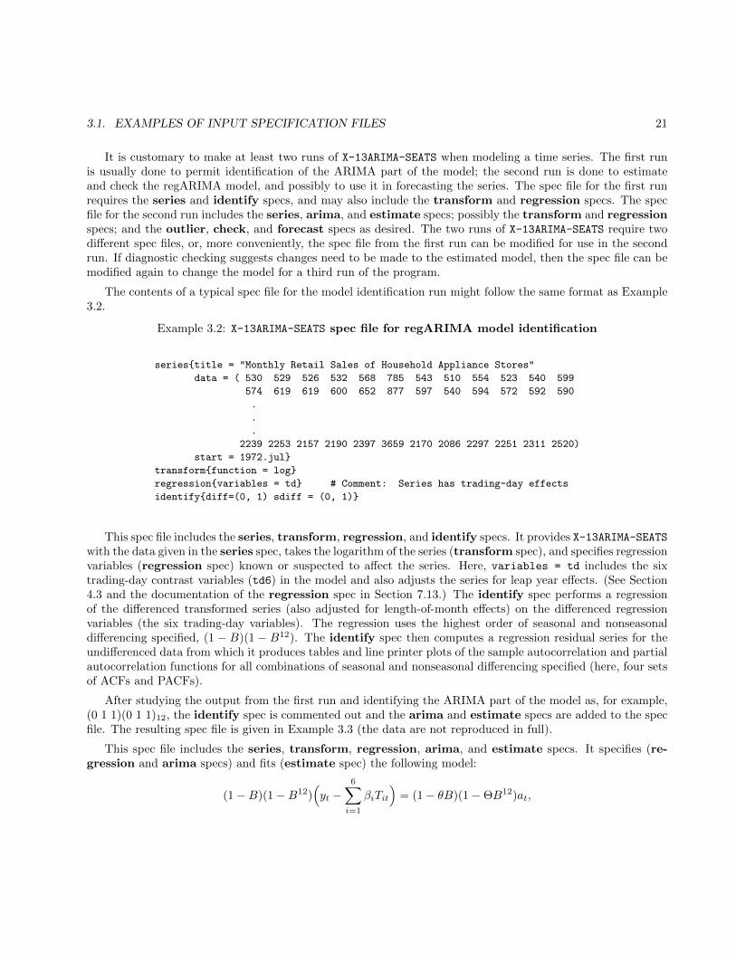
Example 3.2: X-13ARIMA-SEATS spec file for regARIMA model identification
series{title = "Monthly Retail Sales of Household Appliance Stores"
data = ( 530 529 526 532 568 785 543 510 554 523 540 599
574 619 619 600 652 877 597 540 594 572 592 590
.
.
.
2239 2253 2157 2190 2397 3659 2170 2086 2297 2251 2311 2520)
start = 1972.jul}
transform{function = log}
regression{variables = td} # Comment: Series has trading-day effects
identify{diff=(0, 1) sdiff = (0, 1)}
This spec file includes the series, transform, regression, and identify specs. It provides X-13ARIMA-SEATSwith the data given in the series spec, takes the logarithm of the series (transform spec), and specifies regressionvariables (regression spec) known or suspected to affect the series. Here, variables = td includes the sixtrading-day contrast variables (td6) in the model and also adjusts the series for leap year effects. (See Section4.3 and the documentation of the regression spec in Section 7.13.) The identify spec performs a regressionof the differenced transformed series (also adjusted for length-of-month effects) on the differenced regressionvariables (the six trading-day variables). The regression uses the highest order of seasonal and nonseasonaldifferencing specified, (1 − B)(1 − B12). The identify spec then computes a regression residual series for theundifferenced data from which it produces tables and line printer plots of the sample autocorrelation and partialautocorrelation functions for all combinations of seasonal and nonseasonal differencing specified (here, four setsof ACFs and PACFs).
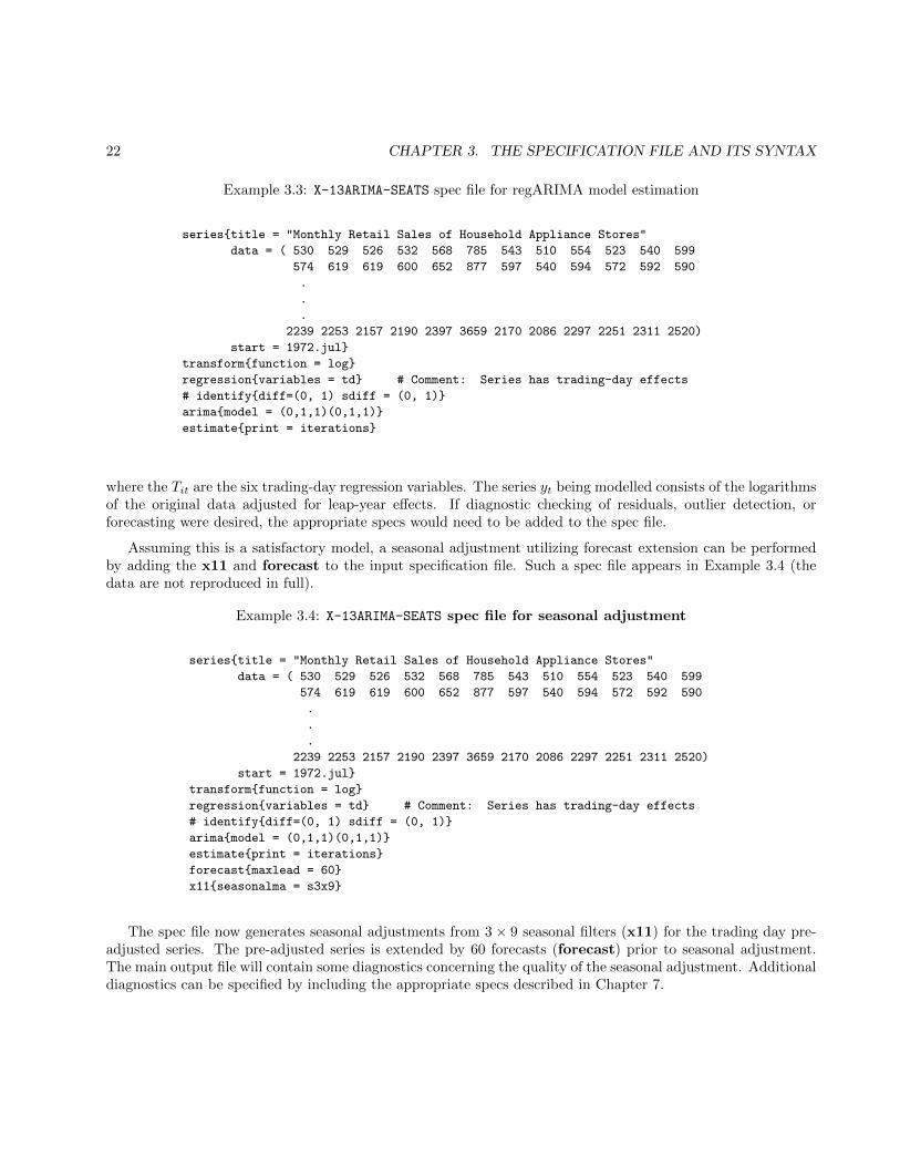
After studying the output from the first run and identifying the ARIMA part of the model as, for example,(0 1 1)(0 1 1)12, the identify spec is commented out and the arima and estimate specs are added to the specfile. The resulting spec file is given in Example 3.3 (the data are not reproduced in full).
This spec file includes the series, transform, regression, arima, and estimate specs. It specifies (re-gression and arima specs) and fits (estimate spec) the following model:
(1−B)(1−B12)(yt −
6∑i=1
βiTit
)= (1− θB)(1−ΘB12)at,
22 CHAPTER 3. THE SPECIFICATION FILE AND ITS SYNTAX
Example 3.3: X-13ARIMA-SEATS spec file for regARIMA model estimation
series{title = "Monthly Retail Sales of Household Appliance Stores"
data = ( 530 529 526 532 568 785 543 510 554 523 540 599
574 619 619 600 652 877 597 540 594 572 592 590
.
.
.
2239 2253 2157 2190 2397 3659 2170 2086 2297 2251 2311 2520)
start = 1972.jul}
transform{function = log}
regression{variables = td} # Comment: Series has trading-day effects
# identify{diff=(0, 1) sdiff = (0, 1)}
arima{model = (0,1,1)(0,1,1)}
estimate{print = iterations}
where the Tit are the six trading-day regression variables. The series yt being modelled consists of the logarithmsof the original data adjusted for leap-year effects. If diagnostic checking of residuals, outlier detection, orforecasting were desired, the appropriate specs would need to be added to the spec file.
Assuming this is a satisfactory model, a seasonal adjustment utilizing forecast extension can be performedby adding the x11 and forecast to the input specification file. Such a spec file appears in Example 3.4 (thedata are not reproduced in full).
Example 3.4: X-13ARIMA-SEATS spec file for seasonal adjustment
series{title = "Monthly Retail Sales of Household Appliance Stores"
data = ( 530 529 526 532 568 785 543 510 554 523 540 599
574 619 619 600 652 877 597 540 594 572 592 590
.
.
.
2239 2253 2157 2190 2397 3659 2170 2086 2297 2251 2311 2520)
start = 1972.jul}
transform{function = log}
regression{variables = td} # Comment: Series has trading-day effects
# identify{diff=(0, 1) sdiff = (0, 1)}
arima{model = (0,1,1)(0,1,1)}
estimate{print = iterations}
forecast{maxlead = 60}
x11{seasonalma = s3x9}
The spec file now generates seasonal adjustments from 3× 9 seasonal filters (x11) for the trading day pre-adjusted series. The pre-adjusted series is extended by 60 forecasts (forecast) prior to seasonal adjustment.The main output file will contain some diagnostics concerning the quality of the seasonal adjustment. Additionaldiagnostics can be specified by including the appropriate specs described in Chapter 7.
3.2. PRINT AND SAVE 23
3.2 Print and save
Control of the output from X-13ARIMA-SEATS is achieved within individual specs by using the print and savearguments. The print argument controls the given spec’s output to the main output file, while the saveargument allows certain output tables to be written to files. For ease of reference we refer to all the individualparts of the output subject to control through print and save as “tables”, even though some of this output(e.g., line printer plots of an ACF) is not in a form that is ordinarily thought of as a table. The tables subject tocontrol through print and save are listed with their default print status and file extensions (for savable tables)under the documentation of the print and save arguments for each spec. Tables output to files using save arewritten in a format with high numerical precision and with minimal or no labelling information to facilitatetheir use for further analysis utilizing other software. Saved tables are also given a consistent format—a singletab separates fields.
Default output from a spec is written to the main output file if the print argument is absent, or ifprint=default or print=() appears in the spec. To stop a spec from writing output to the main outputfile, set print=none. (Note: A few specs write some minor labelling information to the screen even withprint=none.) To have all the available output tables and plots for a spec written to the main output file,set print=all. To have all the available output tables (no plots) for a spec written to the main output file,set print=alltables. To have a small subset of the available output tables for a spec written to the screen,set print=brief. Individual tables may be added to the default, brief, and none print levels by includingtheir names as print argument values. These may (but need not) be preceded by a +. For example, in theestimate spec, print=(+iterations +residuals), which is equivalent to print = (default +iterations
+residuals), requests printing of results from the estimation iterations and the residuals from the estimatedmodel, in addition to the default output. Using print=(none estimates) requests printing of only the param-eter estimates. Individual tables may be suppressed from the default and all print levels by including theirnames preceded by a - as print argument values, e.g., print=brief -acf or print=(all -iterations).
If the user wishes to save any output tables to files, these must be specifically listed in the save argumentsof the appropriate specs, e.g., save=(mdl estimates) in the estimate spec. Those tables that are savablemay be specified in the print and save arguments using either a “long” name, the name listed in the spec’sdescription, or a “short” 3-letter name, which is the same as the file extension used if the table is saved. Forexample, the optional table regcmatrix in the estimate spec can also be specified as rcm. The keywords none,all, alltables, default, and brief defined above are not available for use in the save argument. Also, namesof tables to be saved should not be preceded with a + or -. Not all tables are savable, and not all specs producesavable tables.
The save argument writes the specified tables to individual files. A saved file will be placed in the samedirectory as the output, and will be given the filename of the main output file, but with a distinct 3-letterextension. If a file with this name already exists, it will be overwritten. The extensions used are listed underthe documentation of the print and save arguments for each spec. For example, suppose X-13ARIMA-SEATS isrun (on a DOS machine) from the directory C:\TSERIES using as input a spec file stored in SALES.SPC in thatdirectory. If the estimate spec contains save = (mdl estimates), the resulting saved tables of the model andparameter estimates will be written to the files C:\TSERIES\SALES.MDL and C:\TSERIES\SALES.EST. If fileswith these names already exist, they will be overwritten. Although the extensions used by X-13ARIMA-SEATS
have been chosen to avoid obvious conflicts (examples of extensions not used are .dat, .exe, .com, .for, .spc),users should still exercise caution to prevent unintended overwriting of files by X-13ARIMA-SEATS saves. A listof the files saved, with an * indicating those overwriting existing files, appears at the beginning of the program’s
24 CHAPTER 3. THE SPECIFICATION FILE AND ITS SYNTAX
output. If there are errors in the spec file or the program terminates prematurely for other reasons, some or allof the saved files may not be written.
3.3 Dates
Date arguments occur in several specs, and their values are always specified in the same format. Dates formonthly data are written year.month; this format generalizes to other seasonal periods (e.g., year.quarter). Itis necessary to include all four digits when specifying a year. Thus, 67 means the year AD (or CE) 67, not AD1967.
For monthly data the months can be denoted by either the integers 1–12 or by three-letter month abbrevi-ations (jan, feb, mar, apr, may, jun, jul, aug, sep, oct, nov, and dec). Thus, 1967.12 and 1967.dec areequivalent. For quarterly data or data with other seasonal periods, only integers are allowed, e.g., 1967.1 and1967.4.
For data of any periodicity, a zero can be placed in front of integers from 1 to 9 for padding (for example,2002.02 is an acceptable date specification for February 2002).
Dates are used to define the starting time point of a series, and when defining a subset (span) of a time seriesto analyze. They are also used when defining outlier regression variables. For example, to specify regressionvariables for an additive outlier in April of 1978 and a level shift beginning in September of 1982, we use thefollowing:
regression { variables=(ao1978.apr ls1982.sep) }
The seasonality of the dates used must match the seasonality specified for the data in the series spec, e.g.,ao1972.jan is valid for monthly data but is not permitted for quarterly data.
3.4 General rules of input syntax
Allowable input charactersThe allowable input characters, excepting characters that appear within quotes, are letters, numbers,spaces, tabs, newline characters, and the following:
= . , { } ( ) [ ] + - #
The program will ignore any other ASCII characters in the spec file, but will flag them and generate awarning message. The following additional characters are allowed within quotes:
! % ’ * / : ; < > ? @ \ _ / ~ ^
Also, double quotes are allowed within statements delimited by single quotes and vice-versa.
3.4. GENERAL RULES OF INPUT SYNTAX 25
Braces, parentheses, and bracketsThe { }, ( ), and [ ] characters serve different functions and cannot be used interchangeably. { } is usedto contain arguments in a spec, ( ) is used to contain a list of multiple values for an argument, and [ ] isused (i) to contain values used in defining certain special arguments, such as the duration of an Easterholiday regression variable, e.g., regression {variables = (td Easter[14])}, and (ii) to enclose thelags present in an ARIMA model with missing lags, e.g., arima {model = (0 1 [1,3])}.
Case sensitivitySpec names, arguments, dates, keywords (such as none and all), and predefined regression variable names(such as td and seasonal) are not case sensitive. Thus, TD and td are the same; both are recognized bythe variables argument of the regression and x11regression specs.
CommentsAnything on a line after the # character, unless the # character is in quotes, is taken to be a comment.If parts of a spec are commented out, what remains must still have balanced parentheses, brackets, andbraces.
Equals signThe equals sign, = , is used when assigning values to arguments, e.g., print = none, or title =
"Monthly Retail Sales of Household Appliance Stores".
Line length in the spec fileLines in the spec file are limited to 132 characters—any characters appearing beyond column 132 areignored. In particular, note that if a data set with lines exceeding 132 characters is placed in a specfile this will result in data truncation on input. The 132 characters per line limitation does not apply,however, to data read from a separate file (not the spec file) using the file argument. (The latter wouldbe governed by Fortran input line length restrictions, which may be system specific.)
Multiple argument valuesMultiple argument values must be enclosed together in parentheses, e.g., variables=(td seasonal
const). If an argument accepts only a single value or it accepts multiple values but only one value is given,then parentheses are optional. For example, the following are all valid; variables=td, variables=(td),variables = (td seasonal), start=1967.4, and start=(1967.4).
Null listA null list of arguments is allowed, e.g., outlier{ }. Any implied arguments in the null list then takeon their default values.
Numerical valuesNumerical values can be specified in free format, including the use of exponential notation (e.g., 400,400.0, 400., and 4.e+2 all denote the same real value). Integer notation must be used when an integer isrequired (e.g., 2, not 2.0 or 2.e+0).
OrderingThe only restriction on the ordering of specs is that either series or composite must be the first spec.Except for the b argument of the regression and x11regression specs, there are no restrictions on theordering of arguments within specs (see Sections 7.13 and 7.20 for more details). The ordering of multiplevalues given to arguments matters for certain obvious cases, such as observations in data arguments(series, transform, regression, and x11regression specs), the ARIMA model specification in the
26 CHAPTER 3. THE SPECIFICATION FILE AND ITS SYNTAX
model argument (arima spec), and dates in span arguments (series and outlier specs).
SeparatorsBlank spaces, tabs, and blank lines may be used as separators as desired. Within a list of multiple argu-ment values, single commas may also be used as separators, e.g., data=(0, 1, 2, 3, 4, 5). Commasmust be used to indicate missing argument values that are to be replaced by default values (for argumentsthat require a specific number of values). For example, the span argument requires two values. In thestatement span=(1967.4, ), the presence of the comma after 1967.4 indicates that the second spanargument value is missing, so it takes on its default value (the date of the last observation).
Titles and filenamesA title, such as the name of a time series, must consist of at least one allowable input character (seeabove), even if blank, and must be enclosed in either single or double quotes (’title’ or "title").Lower and upper case of characters is preserved within titles. When the # character appears withinquotes, it is considered part of the title and does not denote the start of a comment. Titles must becompleted on one line and contain no more than 79 characters. Filenames, including the path, mustfollow the same rules as titles.

4 RegARIMA modeling Capabilities
Contents4.1 General model . . . . . . . . . . . . . . . . . . . . . . . . . . . . . . . . . . . . . . . . 27
4.2 Data input and transformation . . . . . . . . . . . . . . . . . . . . . . . . . . . . . . 29
4.3 Regression variable specification . . . . . . . . . . . . . . . . . . . . . . . . . . . . . 29
4.4 Identification and specification of the ARIMA part of the model . . . . . . . . . 36
4.5 Model estimation and inference . . . . . . . . . . . . . . . . . . . . . . . . . . . . . . 37
4.6 Diagnostic checking including outlier detection . . . . . . . . . . . . . . . . . . . . 39
4.7 Forecasting . . . . . . . . . . . . . . . . . . . . . . . . . . . . . . . . . . . . . . . . . . 40
Tables4.1 Predefined Regression Variables . . . . . . . . . . . . . . . . . . . . . . . . . . . . . . . . 31
Section 4.1 describes the general model handled by the X-13ARIMA-SEATS program. Sections 4.2 to 4.7 givesummary descriptions of the capabilities of X-13ARIMA-SEATS for the various stages of regARIMA modeling andforecasting: data input and transformation, regression variable specification, ARIMA model identification andspecification, model estimation and inference, diagnostic checking including outlier detection, and forecasting.These sections also mention which input specification statements (specs) are used to control the execution ofthe capabilities discussed. Detailed documentation of the specs is given in Chapter 7.
When building a regARIMA model, it is strongly recommended that one examine a high resolution plot ofthe time series. Such a plot gives valuable information about seasonal patterns, potential outliers, stochasticnonstationarity, etc. Additional plots may also be useful for examining the effects of possible transformations onthe series, or of applying various differencing operators to the series. Since X-13ARIMA-SEATS does not possesssuch plotting capabilities, other software must be used for this purpose.
4.1 General model
ARIMA models, as discussed by Box and Jenkins (1976), are frequently used for seasonal time series. A generalmultiplicative seasonal ARIMA model for a time series zt can be written
φ(B)Φ(Bs)(1−B)d(1−Bs)Dzt = θ(B)Θ(Bs)at (4.1)
where B is the backshift operator (Bzt = zt−1), s is the seasonal period, φ(B) = (1 − φ1B − · · · − φpBp)is the nonseasonal autoregressive (AR) operator, Φ(Bs) = (1 − Φ1B
s − · · · − ΦPBPs) is the seasonal AR
operator, θ(B) = (1 − θ1B − · · · − θqBq) is the nonseasonal moving average (MA) operator, Θ(Bs) =
(1 − Θ1Bs − · · · − ΘQB
Qs) is the seasonal MA operator, and the ats are i.i.d. with mean zero and variance
27
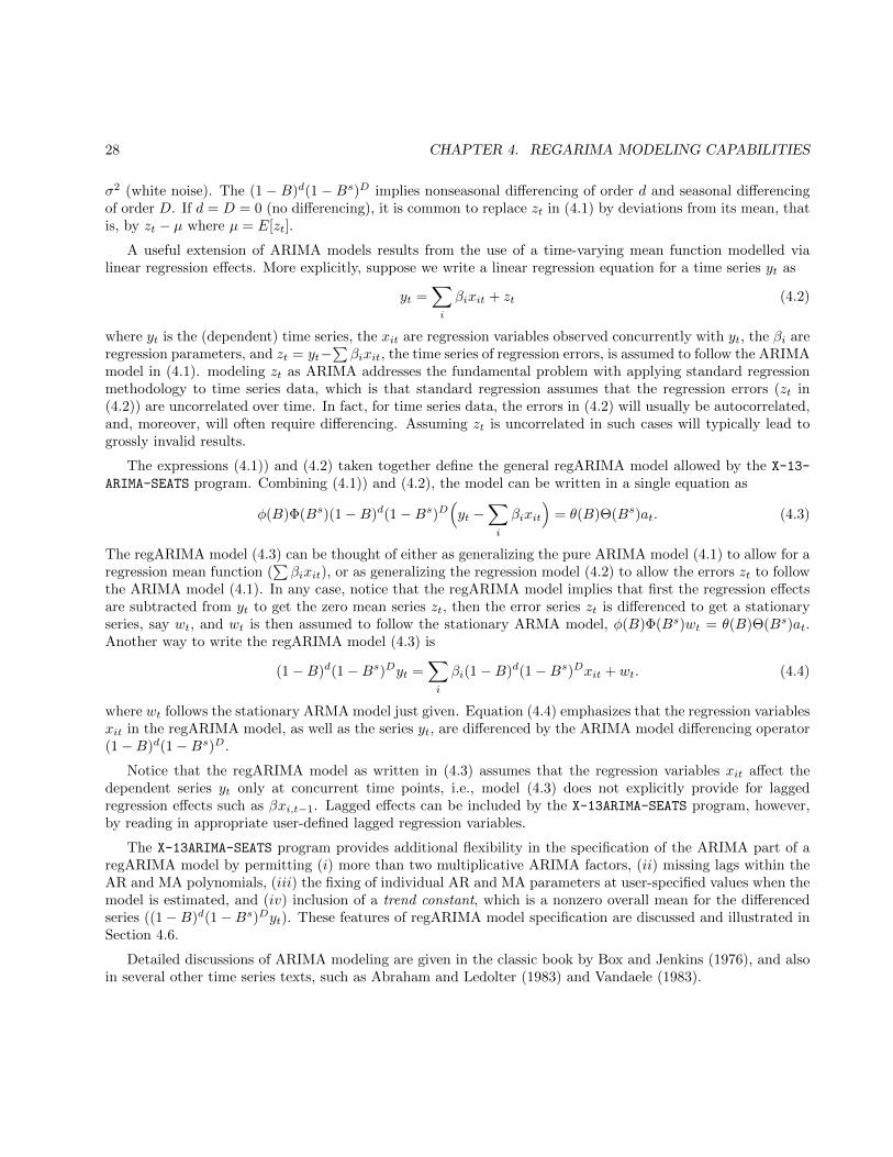
28 CHAPTER 4. REGARIMA MODELING CAPABILITIES
σ2 (white noise). The (1− B)d(1− Bs)D implies nonseasonal differencing of order d and seasonal differencingof order D. If d = D = 0 (no differencing), it is common to replace zt in (4.1) by deviations from its mean, thatis, by zt − µ where µ = E[zt].
A useful extension of ARIMA models results from the use of a time-varying mean function modelled vialinear regression effects. More explicitly, suppose we write a linear regression equation for a time series yt as
yt =∑i
βixit + zt (4.2)
where yt is the (dependent) time series, the xit are regression variables observed concurrently with yt, the βi areregression parameters, and zt = yt−
∑βixit, the time series of regression errors, is assumed to follow the ARIMA
model in (4.1). modeling zt as ARIMA addresses the fundamental problem with applying standard regressionmethodology to time series data, which is that standard regression assumes that the regression errors (zt in(4.2)) are uncorrelated over time. In fact, for time series data, the errors in (4.2) will usually be autocorrelated,and, moreover, will often require differencing. Assuming zt is uncorrelated in such cases will typically lead togrossly invalid results.
The expressions (4.1)) and (4.2) taken together define the general regARIMA model allowed by the X-13-
ARIMA-SEATS program. Combining (4.1)) and (4.2), the model can be written in a single equation as
φ(B)Φ(Bs)(1−B)d(1−Bs)D(yt −
∑i
βixit
)= θ(B)Θ(Bs)at. (4.3)
The regARIMA model (4.3) can be thought of either as generalizing the pure ARIMA model (4.1) to allow for aregression mean function (
∑βixit), or as generalizing the regression model (4.2) to allow the errors zt to follow
the ARIMA model (4.1). In any case, notice that the regARIMA model implies that first the regression effectsare subtracted from yt to get the zero mean series zt, then the error series zt is differenced to get a stationaryseries, say wt, and wt is then assumed to follow the stationary ARMA model, φ(B)Φ(Bs)wt = θ(B)Θ(Bs)at.Another way to write the regARIMA model (4.3) is
(1−B)d(1−Bs)Dyt =∑i
βi(1−B)d(1−Bs)Dxit + wt. (4.4)
where wt follows the stationary ARMA model just given. Equation (4.4) emphasizes that the regression variablesxit in the regARIMA model, as well as the series yt, are differenced by the ARIMA model differencing operator(1−B)d(1−Bs)D.
Notice that the regARIMA model as written in (4.3) assumes that the regression variables xit affect thedependent series yt only at concurrent time points, i.e., model (4.3) does not explicitly provide for laggedregression effects such as βxi,t−1. Lagged effects can be included by the X-13ARIMA-SEATS program, however,by reading in appropriate user-defined lagged regression variables.
The X-13ARIMA-SEATS program provides additional flexibility in the specification of the ARIMA part of aregARIMA model by permitting (i) more than two multiplicative ARIMA factors, (ii) missing lags within theAR and MA polynomials, (iii) the fixing of individual AR and MA parameters at user-specified values when themodel is estimated, and (iv) inclusion of a trend constant, which is a nonzero overall mean for the differencedseries ((1−B)d(1−Bs)Dyt). These features of regARIMA model specification are discussed and illustrated inSection 4.6.
Detailed discussions of ARIMA modeling are given in the classic book by Box and Jenkins (1976), and alsoin several other time series texts, such as Abraham and Ledolter (1983) and Vandaele (1983).
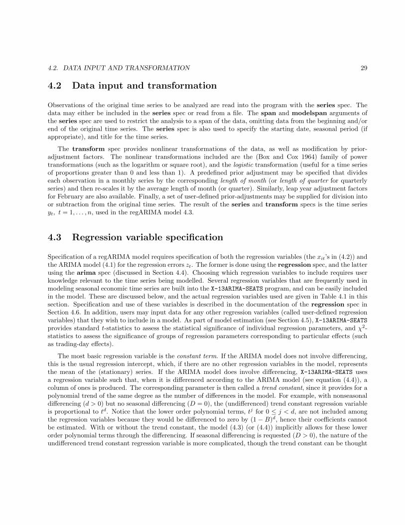
4.2. DATA INPUT AND TRANSFORMATION 29
4.2 Data input and transformation
Observations of the original time series to be analyzed are read into the program with the series spec. Thedata may either be included in the series spec or read from a file. The span and modelspan arguments ofthe series spec are used to restrict the analysis to a span of the data, omitting data from the beginning and/orend of the original time series. The series spec is also used to specify the starting date, seasonal period (ifappropriate), and title for the time series.
The transform spec provides nonlinear transformations of the data, as well as modification by prior-adjustment factors. The nonlinear transformations included are the (Box and Cox 1964) family of powertransformations (such as the logarithm or square root), and the logistic transformation (useful for a time seriesof proportions greater than 0 and less than 1). A predefined prior adjustment may be specified that divideseach observation in a monthly series by the corresponding length of month (or length of quarter for quarterlyseries) and then re-scales it by the average length of month (or quarter). Similarly, leap year adjustment factorsfor February are also available. Finally, a set of user-defined prior-adjustments may be supplied for division intoor subtraction from the original time series. The result of the series and transform specs is the time seriesyt, t = 1, . . . , n, used in the regARIMA model 4.3.
4.3 Regression variable specification
Specification of a regARIMA model requires specification of both the regression variables (the xit’s in (4.2)) andthe ARIMA model (4.1) for the regression errors zt. The former is done using the regression spec, and the latterusing the arima spec (discussed in Section 4.4). Choosing which regression variables to include requires userknowledge relevant to the time series being modelled. Several regression variables that are frequently used inmodeling seasonal economic time series are built into the X-13ARIMA-SEATS program, and can be easily includedin the model. These are discussed below, and the actual regression variables used are given in Table 4.1 in thissection. Specification and use of these variables is described in the documentation of the regression spec inSection 4.6. In addition, users may input data for any other regression variables (called user-defined regressionvariables) that they wish to include in a model. As part of model estimation (see Section 4.5), X-13ARIMA-SEATSprovides standard t-statistics to assess the statistical significance of individual regression parameters, and χ2-statistics to assess the significance of groups of regression parameters corresponding to particular effects (suchas trading-day effects).
The most basic regression variable is the constant term. If the ARIMA model does not involve differencing,this is the usual regression intercept, which, if there are no other regression variables in the model, representsthe mean of the (stationary) series. If the ARIMA model does involve differencing, X-13ARIMA-SEATS usesa regression variable such that, when it is differenced according to the ARIMA model (see equation (4.4)), acolumn of ones is produced. The corresponding parameter is then called a trend constant, since it provides for apolynomial trend of the same degree as the number of differences in the model. For example, with nonseasonaldifferencing (d > 0) but no seasonal differencing (D = 0), the (undifferenced) trend constant regression variableis proportional to td. Notice that the lower order polynomial terms, tj for 0 ≤ j < d, are not included amongthe regression variables because they would be differenced to zero by (1 − B)d, hence their coefficients cannotbe estimated. With or without the trend constant, the model (4.3) (or (4.4)) implicitly allows for these lowerorder polynomial terms through the differencing. If seasonal differencing is requested (D > 0), the nature of theundifferenced trend constant regression variable is more complicated, though the trend constant can be thought

30 CHAPTER 4. REGARIMA MODELING CAPABILITIES
of as allowing for a polynomial of degree d + D. Without a trend constant, model (4.3) implicitly allows for apolynomial of degree d+D − 1.
Fixed seasonal effects in a monthly series can be modelled using 12 indicator variables, one for each calendarmonth. Since these 12 variables always add to one, however, they are confounded with an overall level effect.This leads to one of two singularity problems: collinearity with the usual constant term in a model with nodifferencing; or a singularity in a model with differencing since the 12 variables, when differenced, alwayssum to 0. One appropriate reparameterization instead uses 11 contrasts in the 12 indicator variables. Analternative reparameterization uses 11 variables taken from the Fourier (trigonometric) series representationof a fixed monthly pattern. The variables used for both of these parameterizations are given in Table 4.1.X-13ARIMA-SEATS allows either of these options, and also allows specifying the trigonometric terms only forselected frequencies. For quarterly series, or for series with other seasonal periods, X-13ARIMA-SEATS constructsthe appropriate versions of these variables. Notice that these variables cannot be used in a model with seasonaldifferencing, as they would all be differenced to zero.
Trading-day effects occur when a series is affected by the differing day-of-the-week compositions of thesame calendar month in different years. Trading-day effects can be modelled with 7 variables that represent(no. of Mondays), . . . , (no. of Sundays) in month t. Bell and Hillmer (1983) note, however, that a betterparameterization of the same effects instead uses 6 contrast variables defined as (no. of Mondays) − (no. ofSundays), . . . , (no. of Saturdays) − (no. of Sundays), along with a seventh variable for length of month (lom)or its deseasonalized version, the leap-year regressor (lpyear). In X-13ARIMA-SEATS the 6 contrast variablesare called the tdnolpyear variables. Instead of using a seventh regressor, a simpler and often better way tohandle multiplicative leap-year effects is to re-scale the February values Yt of the original time series beforetransformation to mFebYt/mt, where Yt is the original time series before transformation, mt is the length ofmonth t (28 or 29), and mFeb = 28.25 is the average length of February. (If the regARIMA model includesseasonal effects, these can account for the length of month effect except in Februaries, so the trading day modelonly has to deal with the leap year effect.) When this is done, only the tdnolpyear variables need be includedin the model. X-13ARIMA-SEATS allows explicit choice of either approach, as well as an option (td) that makesa default choice of how to handle length-of-month effects—see the documentation of the regression spec.
The preceding paragraph assumes the time series being modelled represents the aggregation of some dailyseries (typically unobserved) over calendar months. Such series are called monthly flow series. If the seriesinstead represents the value of some daily series at the end of the month, called a monthly stock series, thendifferent regression variables are appropriate. Trading-day effects in end-of-month stock series can be modelledusing 7 indicator variables for the day-of-the-week that the months end on. Since the sum of these variablesis always one, this leads to a singularity problem, so 6 contrast variables are used instead. (See Table 4.1.)X-13ARIMA-SEATS also allows specification of regression variables appropriate for stock series defined as of someother day of the month, e.g., for beginning of the month stock series.
For a general discussion of stock and flow series, access Wikipedia Contributers (2009).
For quarterly flow time series, X-13ARIMA-SEATS allows the same trading-day options as in the monthlycase. Trading-day effects in quarterly series are relatively rare, however, because the calendar composition ofquarters does not vary as much over time, on a percentage basis, as that of months does. Trading-day variablesare not provided for flow time series with seasonal periods other than monthly or quarterly, or for stock seriesother than monthly.
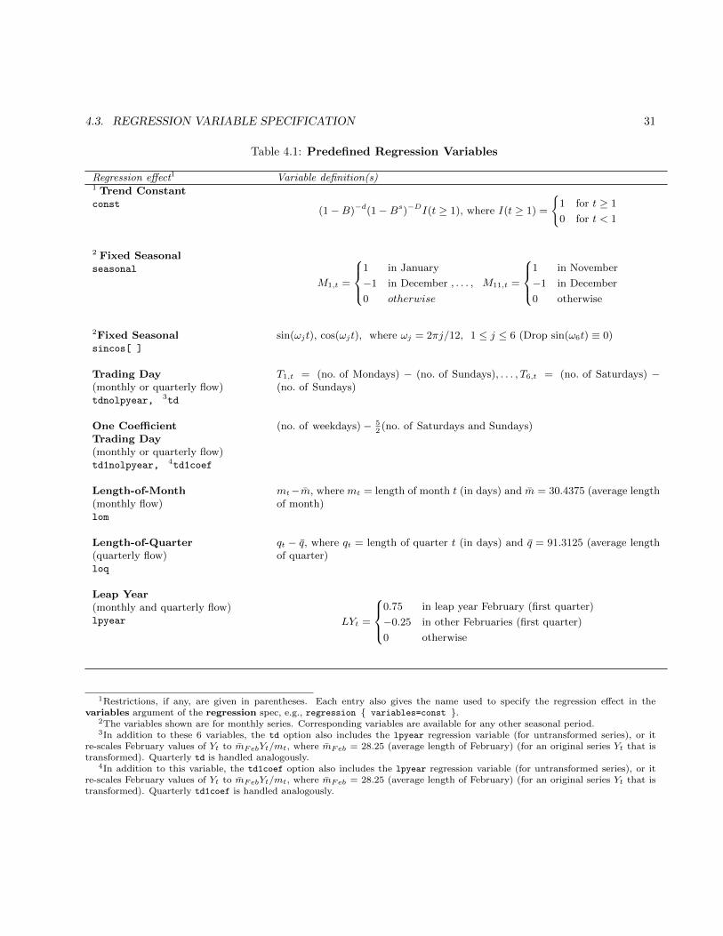
4.3. REGRESSION VARIABLE SPECIFICATION 31
Table 4.1: Predefined Regression Variables
Regression effect1 Variable definition(s)1 Trend Constantconst
(1−B)−d(1−Bs)−DI(t ≥ 1), where I(t ≥ 1) =
{1 for t ≥ 1
0 for t < 1
2 Fixed Seasonalseasonal
M1,t =
1 in January
−1 in December
0 otherwise
, . . . , M11,t =
1 in November
−1 in December
0 otherwise
2Fixed Seasonalsincos[ ]
sin(ωjt), cos(ωjt), where ωj = 2πj/12, 1 ≤ j ≤ 6 (Drop sin(ω6t) ≡ 0)
Trading Day(monthly or quarterly flow)tdnolpyear, 3td
T1,t = (no. of Mondays) − (no. of Sundays), . . . , T6,t = (no. of Saturdays) −(no. of Sundays)
One CoefficientTrading Day(monthly or quarterly flow)td1nolpyear, 4td1coef
(no. of weekdays)− 52(no. of Saturdays and Sundays)
Length-of-Month(monthly flow)lom
mt−m, where mt = length of month t (in days) and m = 30.4375 (average lengthof month)
Length-of-Quarter(quarterly flow)loq
qt − q, where qt = length of quarter t (in days) and q = 91.3125 (average lengthof quarter)
Leap Year(monthly and quarterly flow)lpyear LYt =
0.75 in leap year February (first quarter)
−0.25 in other Februaries (first quarter)
0 otherwise
1Restrictions, if any, are given in parentheses. Each entry also gives the name used to specify the regression effect in thevariables argument of the regression spec, e.g., regression { variables=const }.
2The variables shown are for monthly series. Corresponding variables are available for any other seasonal period.3In addition to these 6 variables, the td option also includes the lpyear regression variable (for untransformed series), or it
re-scales February values of Yt to mFebYt/mt, where mFeb = 28.25 (average length of February) (for an original series Yt that istransformed). Quarterly td is handled analogously.
4In addition to this variable, the td1coef option also includes the lpyear regression variable (for untransformed series), or itre-scales February values of Yt to mFebYt/mt, where mFeb = 28.25 (average length of February) (for an original series Yt that istransformed). Quarterly td1coef is handled analogously.
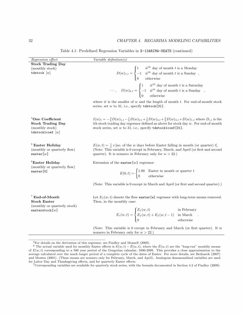
32 CHAPTER 4. REGARIMA MODELING CAPABILITIES
Table 4.1: Predefined Regression Variables in X-13ARIMA-SEATS (continued)
Regression effect Variable definition(s)
Stock Trading Day(monthly stock)tdstock [w] D(w)1,t =
1 wth day of month t is a Monday
−1 wth day of month t is a Sunday
0 otherwise
,
· · · , D(w)6,t =
1 wth day of month t is a Saturday
−1 wth day of month t is a Sunday
0 otherwise
,
where w is the smaller of w and the length of month t. For end-of-month stockseries, set w to 31, i.e., specify tdstock[31].
5One CoefficientStock Trading Day(monthly stock)tdstock1coef [w]
I(w)t = − 35D(w)1,t− 1
5D(w)2,t+ 1
5D(w)3,t+ 3
5D(w)4,t+D(w)1,t where Di,t is the
ith stock trading day regressor defined as above for stock day w. For end-of-monthstock series, set w to 31, i.e., specify tdstock1coef[31].
6 Easter Holiday(monthly or quarterly flow)easter[w]
E(w, t) = 1w×[no. of the w days before Easter falling in month (or quarter) t].
(Note: This variable is 0 except in February, March, and April (or first and secondquarter). It is nonzero in February only for w > 22.)
6Easter Holiday(monthly or quarterly flow)easter[0]
Extension of the easter[w] regressor:
E(0, t) =
{1.00 Easter in month or quarter t
0 otherwise
(Note: This variable is 0 except in March and April (or first and second quarter).)
7 End-of-MonthStock Easter(monthly or quarterly stock)easterstock[w]
Let Ef (w, t) denote the flow easter[w] regressor with long-term means removed.Then, in the monthly case:
Es(w, t) =
Ef (w, t) in February
Ef (w, t) + Ef (w, t− 1) in March
0 otherwise
.
(Note: This variable is 0 except in February and March (or first quarter). It isnonzero in February only for w > 22.)
5For details on the derivation of this regressor, see Findley and Monsell (2009).6 The actual variable used for monthly Easter effects is E(w, t)− E(w, t), where the E(w, t) are the “long-run” monthly means
of E(w, t) corresponding to a 500 year period of the Gregorian calendar, 1600-2099. This provides a close approximation to theaverage calculated over the much longer period of a complete cycle of the dates of Easter. For more details, see Bednarek (2007)and Montes (2001). (These means are nonzero only for February, March, and April). Analogous deseasonalized variables are usedfor Labor Day and Thanksgiving effects, and for quarterly Easter effects.
7Corresponding variables are available for quarterly stock series, with the formula documented in Section 4.2 of Findley (2009).

4.3. REGRESSION VARIABLE SPECIFICATION 33
Table 4.1: Predefined Regression Variables in X-13ARIMA-SEATS (continued)
Regression effect Variable definition(s)
Statistics Canada Easter(monthly or quarterly flow)sceaster[w]
If Easter falls before April w, let nE be the number of the w days on or beforeEaster falling in March. Then:
E(w, t) =
nE/w in March
−nE/w in April
0 otherwise
.
If Easter falls on or after April w, then E(w, t) = 0.(Note: This variable is 0 except in March and April (or first and second quarter).)
6 Labor Day(monthly flow)labor[w]
L(w, t) = 1w×[no. of the w days before Labor Day falling in month t]. (Note:
This variable is 0 except in August and September.)
6 Thanksgiving(monthly flow)thank[w]
ThC (w, t) = proportion of days from w days before Thanksgiving through Decem-ber 24 that fall in month t (negative values of w indicate days after Thanksgiving).(Note: This variable is 0 except in November and December.)
Additive Outlier at t0aodate0
AO(t0)t =
{1 for t = t0
0 for t 6= t0(date0 is the date corresponding to time point t0)
Level Shift at t0lsdate0
LS(t0)t =
{−1 for t < t0
0 for t ≥ t0
Temporary Change at t0tcdate0
TC(t0)t =
{0 for t < t0
αt−t0 for t ≥ t0,
where α is the rate of decay back to the previous level (0 < α < 1).
Seasonal Outlier at t0sodate0
SO(t0)t =
0 for t ≥ t01 for t < t0, t same month/quarter as t0
−1/(s− 1) otherwise
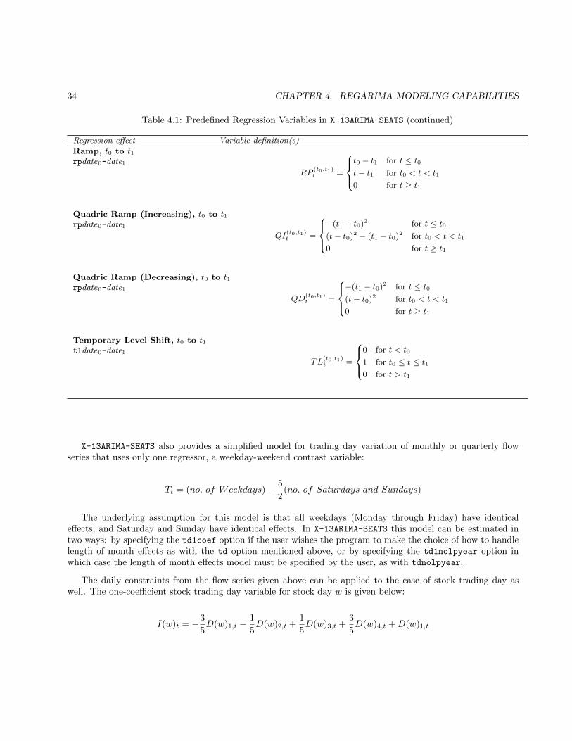
34 CHAPTER 4. REGARIMA MODELING CAPABILITIES
Table 4.1: Predefined Regression Variables in X-13ARIMA-SEATS (continued)
Regression effect Variable definition(s)
Ramp, t0 to t1rpdate0-date1
RP(t0,t1)t =
t0 − t1 for t ≤ t0t− t1 for t0 < t < t1
0 for t ≥ t1
Quadric Ramp (Increasing), t0 to t1rpdate0-date1
QI(t0,t1)t =
−(t1 − t0)2 for t ≤ t0(t− t0)2 − (t1 − t0)2 for t0 < t < t1
0 for t ≥ t1
Quadric Ramp (Decreasing), t0 to t1rpdate0-date1
QD(t0,t1)t =
−(t1 − t0)2 for t ≤ t0(t− t0)2 for t0 < t < t1
0 for t ≥ t1
Temporary Level Shift, t0 to t1tldate0-date1
TL(t0,t1)t =
0 for t < t0
1 for t0 ≤ t ≤ t10 for t > t1
X-13ARIMA-SEATS also provides a simplified model for trading day variation of monthly or quarterly flowseries that uses only one regressor, a weekday-weekend contrast variable:
Tt = (no. of Weekdays)− 5
2(no. of Saturdays and Sundays)
The underlying assumption for this model is that all weekdays (Monday through Friday) have identicaleffects, and Saturday and Sunday have identical effects. In X-13ARIMA-SEATS this model can be estimated intwo ways: by specifying the td1coef option if the user wishes the program to make the choice of how to handlelength of month effects as with the td option mentioned above, or by specifying the td1nolpyear option inwhich case the length of month effects model must be specified by the user, as with tdnolpyear.
The daily constraints from the flow series given above can be applied to the case of stock trading day aswell. The one-coefficient stock trading day variable for stock day w is given below:
I(w)t = −3
5D(w)1,t −
1
5D(w)2,t +
1
5D(w)3,t +
3
5D(w)4,t +D(w)1,t
4.3. REGRESSION VARIABLE SPECIFICATION 35
See Findley and Monsell (2009) for more details, with an application using industrial inventory series.
Holiday effects (in a monthly flow series) arise from holidays whose dates vary over time if (i) the activitymeasured by the series regularly increases or decreases around the date of the holiday, and (ii) this differentiallyaffects two (or more) months depending on the date the holiday occurs each year. (Effects of holidays witha fixed date, such as Christmas, are indistinguishable from fixed seasonal effects.) Easter effects are the mostfrequently found holiday effects in U.S. economic time series, since the date of Easter Sunday varies betweenMarch 22 and April 25. Labor Day and Thanksgiving also are potential, though less common, sources ofholiday effects. The basic model used by X-13ARIMA-SEATS for Easter and Labor Day effects assumes thatthe level of activity changes on the w−th day before the holiday for a specified w, and remains at the newlevel through the day before the holiday. For Thanksgiving the model used assumes that the level of activitychanges on the day that is a specified number of days before or after Thanksgiving and remains at the new levelthrough December 24. The regression variable constructed for the holiday effect is, for a given month t, theproportion of the affected time period that falls in month t. In addition, easter[0] indicates an Easter effectin the month/quarter containing Easter, zero otherwise. (Actually, as noted in Table 4.1, these regressors aredeseasonalized by subtracting off their long-run monthly means.) Essentially the same Easter effect variableapplies also to quarterly flow time series, but Labor Day and Thanksgiving effects are not present in quarterlyseries.
For stock series, the perspective of stocks as accumulations of monthly flows can be used to derive holidayregressors for end of month stock series from cumulative sums of holiday regressors for flow series. A similarapproach has been used to obtain useful stock series trading day regressors by Cleveland and Grupe (1983),Bell (1984, 1995), and Findley and Monsell (2009). While this could be done for any of the moving holidays inX-13ARIMA-SEATS the only holiday currently with an end of month stock implementation is Easter; regressorsare available for both monthly and quarterly series.
Let E(w)flowm,y denote the deseasonalized Easter[w] regressor for a monthly flow series derived for month m
and year y. The end of month stock Easter regressor Estockm,y is generated as follows:
E(w)stockm,y =
0, for m = 1
E(w)flow2,y , for m = 2
E(w)flow2,y + E(w)flow2,y , for m = 3
0, for 4 ≤ m ≤ 12.
When 1 ≤ w ≤ 21, E(w)flowm,y is zero in February, so E(w)stockm,y is nonzero only in March.
See Findley (2009) for more details and an application for manufacturing inventory series, and Titova andMonsell (2009) and Chow and Moore (2009) for applications on US and UK inventory series.
X-13ARIMA-SEATS provides four other types of regression variables to deal with abrupt changes in the levelof a series of a temporary or permanent nature: additive outliers (AOs), level shifts (LSs), temporary changes(TCs), seasonal outliers (SOs), ramps, quadratic ramps (QDs and QIs), and temporary level shifts (TLs). AOsaffect only one observation in the time series, LSs increase or decrease all observations from a certain time pointonward by some constant amount, TCs allow for an abrupt increase or decrease in the level of the series thatreturns to its previous level exponentially rapidly, SOs allow for an abrupt increase or decrease in the level ofthe seasonal pattern that is compensated for in the other months or quarters, ramps allow for a linear increaseor decrease in the level of the series over a specified time interval, and temporary level changes increase or
36 CHAPTER 4. REGARIMA MODELING CAPABILITIES
decrease all observations for a specific time span contained within the series by some constant amount. Thespecific regression variables used to model these effects are given in Table 4.1. (LS regression variables aredefined as −1 and then 0, in preference to an equivalent 0 and then 1 definition, to make the overall level ofthe regression mean function of any forecasts consistent with the most recent level of the time series. Similarconsiderations dictate the definition of ramp variables and seasonal outliers.)
The regression spec allows specification of AOs, LSs, TCs, SOs, TLs, and ramps for cases where priorknowledge suggests such effects at known time points. Often, however, large seasonal movements make itdifficult to identify where such changes in level have occurred. Determination of the location and nature ofpotential outliers is the objective of the outlier detection methodology implemented by the outlier spec—seeSection 4.6 and the outlier spec documentation in Section 7.11. This methodology can be used to detect AOs,TCs, and LSs (not ramps, quadratic ramps, seasonal outliers, or temporary level shifts); any that are detectedare automatically added to the model as regression variables.
Prespecified AOs, LSs, TCs, SOs, TLs, QDs, QIs, and ramps are actually simple forms of interventionsas discussed by Box and Tiao (1975). While X-13ARIMA-SEATS does not provide the full range of dynamicintervention effects discussed by Box and Tiao, often a short sequence of suitably chosen AO, LS, TC, TL,QD, QI, and/or ramp variables can produce reasonable approximations to more complex dynamic interventioneffects, albeit at the cost of an additional parameter or two. Analogous remarks apply to the relation betweenregARIMA models containing (user-defined) regression variables that are themselves stochastic time series, andthe dynamic transfer function models discussed by Box and Jenkins (1976), chapters 10 and 11. Thus, reg-ARIMA models can often be used to approximate more general dynamic transfer function models, althoughtransfer function models require special treatment when forecasting, since future values of stochastic explanatoryvariables are generally unknown. (See Box and Jenkins 1976, Section 11.5).
4.4 Identification and specification of the ARIMA part of the model
The ARIMA part of a regARIMA model is determined by its orders and structure, e.g., (p d q), (P D Q),and s for model (4.1). If no regression variables are included in the model, then determination of the ordersfor the resulting pure ARIMA model (called ARIMA model identification) can be carried out by followingwell-established procedures that rely on examination of the sample autocorrelation function (ACF) and samplepartial autocorrelation function (PACF) of the time series yt and its differences. For regARIMA models, amodified approach is needed, since the presence of regression effects can distort the appearance of the ACFand PACF. Typically, the differencing orders can be identified by examining ACFs of the time series yt and itsdifferences. Then, one should obtain the residuals from a regression of the differenced data on the differencedregression variables. The ACF and PACF of these residuals can then be examined in the usual way to identifythe AR and MA orders of the regression error term in the regARIMA model. This approach to regARIMAmodel identification is discussed and illustrated in Bell and Hillmer (1983).
The key spec used to implement this approach to regARIMA model identification is the identify spec. Forillustration, consider a monthly seasonal time series. The usual ACFs examined to determine the differencingneeded are those of yt, (1 − B)yt, (1 − B12)yt, and (1 − B)(1 − B12)yt. The identify spec can produce allthese ACFs in a single run. Once the differencing has been determined, another run of X-13ARIMA-SEATS can bemade using the identify and regression specs together to (i) regress the differenced yt series on the differencedregression variables, and (ii) produce the ACF and PACF of the regression residuals for use in identifying the
4.5. MODEL ESTIMATION AND INFERENCE 37
AR and MA orders of the model. For example, if one nonseasonal and one seasonal difference are specified(d = 1 and D = 1), the identify and regression specs will fit the model
(1−B)(1−B12)yt =∑i
βi(1−B)(1−B12)xit + wt (4.5)
by ordinary least squares (OLS), and will produce the ACF and PACF of the regression residuals wt in (4.5).
An alternative approach that does not require two runs of the X-13ARIMA-SEATS program can be used ifthe maximum differencing orders (nonseasonal and seasonal) that may be required are assumed known. Forexample, suppose that these maximum differencing orders are d = 1 and D = 1. Then the identify andregression specs can be used to (i) perform OLS regression on (4.5) to produce parameter estimates βi, (ii)compute an estimated (undifferenced) regression error series zt = yt −
∑i βixit, and (iii) produce ACFs and
PACFs of zt, (1 − B)zt, (1 − B12)zt, and (1 − B)(1 − B12)zt. These ACFs and PACFs can be examined todetermine the orders of differencing required, as well as the orders of the AR and MA operators for the model.
There is one exception to the above remarks. If a constant term is specified in the regression spec, thenit will be included when the OLS regression is done on (4.5), but not when the regression effects are removedfrom the data. Thus, actually, zt = yt − Σi≥2βixit if β1x1t is the trend constant term. To explain why thisis done, we consider (4.5). From remarks in Section 4.3, a trend constant variable in model (4.5) allows fora polynomial of degree 2, though the constant and linear terms (for t0 ≡ 1 and t) are implicitly allowed forthrough the differencing by (1−B)(1−B12). Since the constant and linear coefficients cannot be estimated, thefull polynomial effect cannot be subtracted from the undifferenced series yt. Rather than subtract only the t2
term of the polynomial, X-13ARIMA-SEATS ignores the estimated trend constant when creating the undifferencedregression error series zt. Similar remarks apply to the general model (4.4). The only effect that inclusion of atrend constant has on the computations of the identify spec is that its inclusion in (4.4) will affect the regressionestimates βi for i ≥ 2.
4.5 Model estimation and inference
The regression and arima specs specify a regARIMA model. The estimate spec then estimates the modelparameters by exact maximum likelihood, or by a variant known as conditional maximum likelihood (Box andJenkins 1976, pp. 209–212), which is sometimes called conditional least squares. Users may specify maximizationof the fully exact likelihood, or of the likelihood conditional for the AR but exact for the MA parameters, orof the likelihood conditional for both the AR and MA parameters. Differences in AR parameter estimationbetween exact and conditional likelihood maximization are generally small, and there are situations whereeach approach is appropriate. (See Chapter 5.) Differences between exact and conditional likelihood for MAparameter estimation are more fundamental, with exact likelihood being the recommended approach. Theoption of choosing the conditional likelihood for MA parameters is provided in X-13ARIMA-SEATS mainly forcomparison of results with other software, and for occasional use to produce initial estimates for exact maximumlikelihood estimation when convergence problems arise. (See Section 5.1.) The default option is exact maximumlikelihood estimation for both the AR and MA parameters.
Whichever choice of estimation method is made, the resulting log-likelihood for a pure ARIMA model isreduced to a sum of squares function that is then minimized by a nonlinear least squares routine (MINPACK,discussed by More, Garbow, and Hillstrom (1980). To maximize the likelihood for a full regARIMA model, an
38 CHAPTER 4. REGARIMA MODELING CAPABILITIES
iterative generalized least squares (IGLS) algorithm (Otto, Bell, and Burman 1987) is used. This algorithminvolves two general steps: (i) for given values of the AR and MA parameters, the regression parameters thatmaximize the likelihood are obtained by a generalized least squares (GLS) regression (using the covariancestructure of the regression errors, which is determined by their ARIMA model); and (ii) for given values, βi,of the regression parameters, the ARIMA model is fit by maximum likelihood to the time series of regressionerrors, zt = yt−
∑βixit. IGLS iterates between these two general steps until convergence is achieved. (Output
options in the estimate spec allow for display of intermediate results from the estimation iterations, if desired.)The likelihood function (exact or conditional) is evaluated using an approach derived from those suggested byBox and Jenkins (1976), Chapter 7, Ljung and Box (1979), Hillmer and Tiao (1979), and Wilson (1983). Section4.4 discusses certain problems that may arise in model estimation that all users should be aware of.
Statistical inferences about regARIMA model parameters may be made using asymptotic results for max-imum likelihood estimation of ARIMA models (Box and Jenkins 1976, chapter 7; Brockwell and Davis 1991,chapter 8 and regARIMA models (Pierce 1971)). These results state that, under suitable assumptions, theparameter estimates are approximately normally distributed with means equal to the true parameter valuesand with a certain covariance matrix that can be estimated. (The “suitable assumptions” include that the truemodel form is used, that the model’s AR operators are all stationary and its MA operators are all invertible, andthat the series is sufficiently long for the asymptotic results to apply.) Using these results, X-13ARIMA-SEATSprovides standard errors for the ARMA and regression parameter estimates, and, optionally, correlation (orcovariance) matrices for the estimates of both the ARMA and the regression parameters. (The regression pa-rameter estimates are asymptotically uncorrelated with the ARMA parameter estimates.) These results maybe used in the usual way to make normal theory inferences about model parameters, including, as mentionedin Section 4.3, use of t-statistics and χ2-statistics produced by X-13ARIMA-SEATS to assess the statistical signif-icance of individual regression parameters and of groups of regression parameters corresponding to particularregression effects. Also, since X-13ARIMA-SEATS prints out the value of the maximized log-likelihood function,various likelihood ratio tests are possible by making multiple runs of the program with different models.
X-13ARIMA-SEATS uses the maximum likelihood estimate of the residual variance σ2, which is σ2 = SS/(n−d− s ·D), where SS is the residual sum-of-squares and n− d− s ·D is the effective number of observations afterdifferencing. (If the likelihood function that is conditional with respect to the AR parameters is used, replacen−d−s ·D by n−p−d−s ·P −s ·D.) Notice there is no “degrees of freedom” adjustment for model parametersbeing estimated. For this reason, if X-13ARIMA-SEATS is used to fit a pure regression model—a model whoseregression errors follow the ARIMA(0 0 0) model—σ2 will differ from the usual unbiased regression varianceestimate. Consequently, the resulting standard errors, t-statistics, and χ2-statistics for the regression parameterestimates will also differ slightly from those that would be obtained from a standard regression program.
An alternative approach to inference is to use the likelihood-based model selection criteria produced byX-13ARIMA-SEATS: AIC, AICC (also known as the F-adjusted AIC), Hannan-Quinn, and BIC. For each of thesestatistics, the model producing the lower value is preferred. One advantage to these criteria over standard t-sta-tistics, χ2-statistics, and likelihood ratio tests is that they may be used to compare non-nested models—modelsthat differ from each other in such a way that one model cannot be obtained simply by removing parametersfrom another model. (E.g., AR(1) versus MA(1) is a non-nested comparison.) Some caution must be exercisedin use of the model selection criteria. Section 5.5 discusses certain situations that arise in regARIMA modelingfor which the use of these criteria, as well as standard likelihood ratio tests, is invalid.
4.6. DIAGNOSTIC CHECKING INCLUDING OUTLIER DETECTION 39
4.6 Diagnostic checking including outlier detection
Diagnostic checking of a regARIMA model is performed through various analysis of the residuals from modelestimation, the objective being to check if the true residuals (at in (4.3)) appear to be white noise—i.i.d. N(0, σ2).(Note: Normality of the ats is not needed for the large sample estimation and inference results; it is mostimportant for validity of prediction intervals produced in forecasting.) The check spec is used to producevarious diagnostic statistics using the residuals from the fitted model. To check for autocorrelation, X-13-
ARIMA-SEATS can produce ACFs and PACFs of the residuals (with standard errors), along with Ljung and Box(1978) summary Q-statistics. X-13ARIMA-SEATS can also produce basic descriptive statistics of the residualsand a histogram of the standardized residuals. The residuals can be written to a file for further analysis (suchas high resolution plotting) by other software.
The residuals produced by the algorithm used for exact maximum likelihood estimation in X-13ARIMA-SEATS
are the conditional expectations of the innovations at given the data {yt; t = 1, . . . , n}, that is, E[at|{yt}]. (SeeBox and Jenkins 1976, Appendix A7.4.) They are computed using the estimated values of the model parameters.For a nonseasonal ARIMA model of order (p, d, q), the residuals are computed for time points t = d+1−q, . . . , n,which gives n − d + q residuals. For a seasonal ARIMA model with seasonal period s, the first residual wouldbe at t = d + Ds − q − Qs + 1. For the airline model d = q = 1 and D = Q = 1, so there will be n residualsgoing from t = 1, . . . , n. Other algorithms that can be used to evaluate or approximate the likelihood of anARIMA model – e.g., the conditional likelihood option in X-13ARIMA-SEATS , or the Kalman filter (used inother software) – can produce different residuals, even different numbers of residuals (even when the approachesyield the same likelihood value). If the estimated model is invertible, residuals computed in these different wayswill eventually converge to each other as t increases, and so will typically be very close in the latter part of thetime series, and may be very similar for most of the time series.
An important aspect of diagnostic checking of time series models is outlier detection. The outlier spec ofX-13ARIMA-SEATS provides for automatic detection of additive outliers (AOs), temporary change outliers (TCs)and level shifts (LSs). These outlier types (referring to AOs, TCs, and LSs as “outliers”) and their associatedregression variables are defined in Section 4.3. X-13ARIMA-SEATS’ approach to outlier detection is based onthat of Chang and Tiao (1983)—see also Chang, Tiao, and Chen (1988)—with extensions and modifications asdiscussed in Bell (1983) and Otto and Bell (1990). The general approach is similar to stepwise (GLS) regression,where the candidate regression variables are AO, LS, and/or TC variables for all time points at which outlierdetection is being performed—3n variables for detection of AOs, LSs, and TCs over an entire time series oflength n. (Actually, slightly fewer than 3n variables are used in this case for reasons discussed in the DETAILSsection of the outlier spec documentation in Section 7.11.) In brief, this approach involves computing t-statis-tics for the significance of each outlier type at each time point, searching through these t-statistics for significantoutlier(s), and adding the corresponding AO, LS, or TC regression variable(s) to the model. Overly burdensomecomputation is avoided by holding the AR and MA parameters fixed as the outlier t-statistics are computedfor each time point and outlier type. X-13ARIMA-SEATS provides two variations on this general theme. Theaddone method provides full model re-estimation after each single outlier is added to the model, while theaddall method re-estimates the model only after a set of detected outliers is added. A description of both thesemethods is given in the documentation of the outlier spec in Section 7.11, with more details in Appendix B ofFindley, Monsell, Bell, Otto, and Chen (1998).
During outlier detection a robust estimate of the residual standard deviation, 1.48 × the median absolutedeviation of the residuals (Hampel, Ronchetti, Rousseeuw, and Stahel 1986, p. 105), is used. Because outlierdetection involves searching over all (or a specified set of) time points for the most significant outliers, the usual

40 CHAPTER 4. REGARIMA MODELING CAPABILITIES
normal distribution critical values (e.g., 2.0) are too low for judging significance in outlier detection. The defaultcritical value is determined by the number of observations in the interval searched for outliers (see Table 7.22),but this can be changed by the user.
When a model contains two or more level shifts, including those obtained from outlier detection as well asany level shifts specified in the regression spec, X-13ARIMA-SEATS will optionally produce t-statistics for testingnull hypotheses that each run of two, three, etc. successive level shifts actually cancels to form a temporarylevel shift. Two successive level shifts cancel to form a temporary level shift if the effect of one offsets the effectof the other, which implies that the sum of the two corresponding regression parameters is zero. Similarly,three successive level shifts cancel to a temporary level shift if the sum of their three regression parametersis zero, etc. (There is a user-specified limit on the number of successive level shifts in the runs tested.) Thet-statistics produced are the sums of the estimated parameters for each run of successive level shifts dividedby the appropriate standard error. An insignificant temporary level shift t-statistic (say, one less than 2 inmagnitude) fails to reject the null hypothesis that the corresponding level shifts cancel to form a temporarylevel shift. These tests are provided primarily as diagnostics to help users assess the impacts of level shifts in amodel. Of course, if one or more of these t-statistics are significant, the user may wish to re-specify the modelwith the relevant level shift regression variables replaced by appropriate temporary level shift variables. (Thesecan be specified as user-defined regression variables, or can be obtained by fixing the coefficient of the level shiftregressors so that they sum to zero.) The choice between using level shifts (which correspond to permanentchanges in the level of a series) versus temporary level shifts could be important for forecasting a series withlevel shifts near the end of the data.
4.7 Forecasting
For a given regARIMA model with parameters estimated by the X-13ARIMA-SEATS program, the forecast specwill use the model to compute point forecasts, and associated forecast standard errors and prediction intervals.The point forecasts are minimum mean squared error (MMSE) linear predictions of future yts based on thepresent and past yts assuming that the true model is used—which means we assume the regARIMA modelform is correct, that the correct regression variables have been included, that no additive outliers or level shiftswill occur in the forecast period, that the specified ARIMA orders are correct, and that the parameter valuesused (typically estimated parameters) are equal to the true values. These are standard assumptions, thoughobviously unrealistic in practical applications. What is more realistically hoped is that the regARIMA modelwill be a close enough approximation to the true, unknown model for the results to be approximately valid.Two sets of forecast standard errors are produced. One assumes that all parameters are known. The otherallows for additional forecast error that comes from estimating the regression parameters, while still assumingthat the AR and MA parameters are known. For a reasonably long time series, (Box and Jenkins 1976, pp.267–269) observe that the contribution to forecast error of the error in estimating the AR and MA parametersis generally small, thus providing a justification for ignoring this source of error when computing the forecaststandard errors.
If the series has been transformed, then forecasting results are first obtained in the transformed scale, andthen transformed back to the original scale. For example, if one specifies a model of form (4.3) for yt = log(Yt),where Yt is the original time series, then yt is forecasted first, and the resulting point forecasts and predictioninterval limits are exponentiated to produce point and interval forecasts in the original (Yt) scale. The resultingpoint forecasts are MMSE for yt = log(Yt), but not for Yt under the “standard” assumptions mentioned above.
4.7. FORECASTING 41
Analogous procedures are followed for other allowable transformations. If any prior adjustments are made, thesewill also be inverted in the process of transforming the point forecasts and prediction interval limits back to theoriginal scale.
If there are any user-defined regression variables in the model, X-13ARIMA-SEATS requires that the user supplydata for these variables for the forecast period. For the X-13ARIMA-SEATS predefined regression variables, theprogram will generate the future values required. If user-defined prior adjustment factors are specified, valuesfor these should also be supplied for the forecast period.
User-defined regressors are usually deterministic (i.e. nonstochastic) variables, such as special calendar-effect or outlier variables. But when forecasts are of particular interest, it can be appropriate to use stochasticvariables, e.g. economic time series values, as regressors, see Findley (2007).

5 Points Related to regARIMA ModelEstimation
Contents5.1 Initial values for parameters and dealing with convergence problems . . . . . . . 42
5.2 Invertibility (of MA operators) . . . . . . . . . . . . . . . . . . . . . . . . . . . . . . 43
5.3 Stationarity (of AR operators) . . . . . . . . . . . . . . . . . . . . . . . . . . . . . . 44
5.4 Cancellation (of AR and MA factors) and overdifferencing . . . . . . . . . . . . . 44
5.5 Use of model selection criteria . . . . . . . . . . . . . . . . . . . . . . . . . . . . . . 45
5.5.1 Avoid using the criteria to compare models with different sets of outlier regressors whenpossible . . . . . . . . . . . . . . . . . . . . . . . . . . . . . . . . . . . . . . . . . . . . 48
5.5.2 Model comparisons for transformed data . . . . . . . . . . . . . . . . . . . . . . . . . . 48
5.5.3 Do not use the criteria to compare models with different differencing operators . . . . 50
Tables5.1 Probability that a Chi-Square Variate with ν Degrees of Freedom Exceeds 2ν +
∆AIC for ∆AIC = 0, 1, 2, 3. . . . . . . . . . . . . . . . . . . . . . . . . . . . . . . . . . . . . . 47
While the IGLS algorithm and nonlinear least squares routine used by the X-13ARIMA-SEATS programare quite reliable at finding maximum likelihood estimates for regARIMA models, problems in estimationoccasionally do occur. Some problems that can arise in model estimation are discussed below, along withpossible solutions. This is followed by important cautions regarding the use of the model selection criteriaproduced by the X-13ARIMA-SEATS program.
5.1 Initial values for parameters and dealing with convergence prob-lems
Users may supply initial values for AR and MA parameters that are then used to start the iterative likelihoodmaximization. This is rarely necessary, however, and is not generally recommended. The default choice of initialparameter values in X-13ARIMA-SEATS is 0.1 for all AR and MA parameters. (Initial values are not needed forthe regression parameters, which are determined in the GLS regressions.) This default choice of initial valuesappears to be adequate in the great majority of cases. Supplying better initial values (as might be obtained,e.g., by first fitting the model using conditional likelihood) does not seem to speed up convergence enough tomake obtaining the initial estimates generally worth the effort. A possible exception to this occurs if initialestimates that are likely to be extremely accurate are already available, such as when one is re-estimating a
42
5.2. INVERTIBILITY (OF MA OPERATORS) 43
model with a small amount of new data added to a time series. However, the main reason for specifying initialparameter values is to deal with convergence problems that may arise in difficult estimation situations.
When X-13ARIMA-SEATS’ iterative estimation scheme fails to converge, several remedies are available. Ifthe program stopped short of convergence because it reached the maximum number of iterations (indicated bya warning message to this effect and the printing of parameter values at the last iteration), then rerunning theprogram with initial parameter values set at the values obtained at the last iteration may produce convergence.An easier, though computationally slower, alternative is to simply increase the number of iterations allowed andrerun the program. If the program crashed before converging or reaching the maximum number of iterations,then it may help to first fit the model by conditional likelihood, and then use the resulting parameter estimatesas initial values for exact maximum likelihood estimation. On the other hand, it has been our experiencethat convergence problems are often due to the use of a model that is complicated (e.g., high order), or poorlyconditioned. In such cases, the appropriate action is to examine the results and specify a simpler model. Sections5.2 through 5.4 discuss some particular situations that can lead to estimation problems and that suggest specificmodel modifications.
5.2 Invertibility (of MA operators)
An MA polynomial, θ(B) = 1−θ1B− · · · −θqBq, is invertible if all the roots, G1, . . . , Gq, of θ(B) = 0 lie outsidethe unit circle (|Gj | > 1 for all j). As shown in Brockwell and Davis (1991), pp. 123–125, for any invertible MAoperator in an ARIMA model there are one or more corresponding noninvertible MA operators that producethe same autocovariance structure, and hence the same unconditional likelihood function. Although the datathus cannot discriminate between the invertible and corresponding noninvertible models, the preferred choiceis the invertible model. This is essential for forecasting—grossly incorrect forecasting results can be obtainedwith noninvertible models. There is one important exception. MA polynomials with roots on the unit circle(|Gj | = 1), the boundary of the invertibility region, do not cause problems for forecasting when handledappropriately (by exact maximum likelihood for MA models).
Estimation in X-13ARIMA-SEATS enforces invertibility constraints on the MA parameters in the iterative non-linear maximization of the likelihood function. Strictly speaking, then, models estimated by X-13ARIMA-SEATS
are invertible. If the maximum likelihood estimates (MLEs) for a given model are actually on the boundaryof the invertibility region, i.e., the model at the MLEs contains an MA operator with zeroes exactly on theunit circle, then X-13ARIMA-SEATS’ nonlinear search will approach the boundary of the invertibility region fromwithin, and will generally get as close to the boundary as the convergence tolerance dictates or the maximumnumber of iterations allows. X-13ARIMA-SEATS can thus effectively produce estimated models on the boundaryof the invertibility region. Convergence of the estimation iterations in such cases can be slow, since finding themaximum of the likelihood function on the boundary of the constrained parameter space is a difficult optimiza-tion problem. More importantly, convergence of the estimation to the invertibility boundary often indicatesthat the model is poorly conditioned, and should alert users to examine the results (and possibly detailedoutput of the estimation iterations) for signs of this. Section 5.4 discusses the most important causes of poorconditioning—cancellation of factors and overdifferencing—and the appropriate remedies.
Estimation seems most likely to produce a noninvertible model when the model contains a seasonal differenceand a seasonal MA polynomial, e.g., 1−ΘBs when the MLE of Θ is 1. As such models are commonly used forseasonal economic time series, users should be alert to this possibility and be aware of the appropriate actionto take as discussed in Section 5.4.
44 CHAPTER 5. POINTS RELATED TO REGARIMA MODEL ESTIMATION
5.3 Stationarity (of AR operators)
An AR polynomial, φ(B) = 1 − φ1B − · · · − φpBp, is stationary if all roots of φ(B) = 0 lie outside the
unit circle; otherwise, it is nonstationary. (More accurately, the series wt = (1− B)d(1− Bs)Dzt following themodel φ(B)Φ(Bs)wt = θ(B)Θ(Bs)at (derived from equation (1)) is stationary if and only if the zeroes of all theAR polynomials lie outside the unit circle.) The exact (for AR) likelihood function assumes all AR operatorsare stationary. Hence, the exact (for AR) likelihood can be evaluated, and estimation and other analysis (e.g.,forecasting) performed, only if the AR parameters satisfy stationarity constraints. Thus, when the exact (forAR) likelihood function is used, X-13ARIMA-SEATS enforces stationarity constraints on the estimation. Unlesscancellation of factors is present (see the next section), it is unlikely for X-13ARIMA-SEATS’ nonlinear estimationto approach the boundary of the stationary region, since the log-likelihood approaches −∞ as this boundary isapproached.
If the likelihood is defined conditionally with respect to the AR parameters, stationarity is neither assumednor enforced by the X-13ARIMA-SEATS software. Model estimation, forecasting, etc., are not compromised byparameter values outside the stationary region in this case. Inference results, however, are affected, as notedin Section 4.5. Special techniques (as in, e.g., Fuller 1976, Section 8.5) are required for inference about ARparameters outside the stationary region.
5.4 Cancellation (of AR and MA factors) and overdifferencing
Cancellation of AR and MA factors is possible when a model with a mixed ARMA structure is estimated. Amodel as in (1) or (3) is said to have a mixed ARMA structure if either p > 0 and q > 0, or P > 0 andQ > 0. (Technically, a model with p > 0 and Q > 0, or with P > 0 and q > 0, is also mixed, but such mixedmodels are unlikely to lead to cancellation problems.) The simplest example of cancellation occurs with theARMA(1,1) model, (1− φB)zt = (1− θB)at, when φ = θ. Cancelling the (1− φB) factor on both sides of themodel (1 − φB)zt = (1 − φB)at leaves the simplified model, zt = at. Because of this, the likelihood functionwill be nearly constant along the line φ = θ. This can lead to difficulties with convergence of the nonlinearestimation if the MLEs for the ARMA(1,1) model approximately satisfy φ = θ. Analogous problems occur inmore complicated mixed models when an AR polynomial and an MA polynomial have a common zero (e.g., theARIMA (2,1,2)(0,1,1) model that is used as a candidate model for the automdl spec). For a fuller discussionof this topic, see Box and Jenkins (1976), pp. 248-250.
If the X-13ARIMA-SEATS program has difficulty in converging when estimating a mixed model, cancellationof AR and MA factors may be responsible. In any case, possible cancellation can be checked by computingzeroes of the AR and MA polynomials (setting print=roots in the estimate spec), and examining these forzeroes common to an AR and an MA polynomial. If a common zero (or zeroes) is found, then the modelshould be simplified by cancelling the common factor(s) (reducing the order of the corresponding AR and MApolynomials), and the model should be re-estimated. Cancellation need not be exact, but may be indicated byzeroes of an AR and an MA polynomial that are approximately the same.
It is also possible for estimated MA polynomials to have factors that cancel with differencing operators.This occurs when a model has a nonseasonal difference and an estimated nonseasonal MA polynomial containsa (1 − B) factor, or the model has a seasonal difference and an estimated seasonal MA polynomial contains a(1 − Bs) factor. For example, the model (1 − B)(1 − Bs)zt = (1 − θB)(1 − ΘBs)at involves such cancellation

5.5. USE OF MODEL SELECTION CRITERIA 45
if either θ or Θ is estimated to be one. Such cancellation is called “overdifferencing”, since it implies thatthe series was differenced more times than necessary to achieve stationarity. When overdifferencing occurs thecorresponding difference and MA factor may be cancelled to simplify the model, but the user must then also addto the model regression term(s) to account for the deterministic function of time that was previously annihilatedby the cancelled differencing operator. This means that if a nonseasonal difference is cancelled with a (1− θB)
MA factor with θ = 1, then the simplified model should include a trend constant (or overall mean, if the modelhad only this one difference). If a seasonal difference is cancelled with a (1 − ΘBs) seasonal MA factor withΘ = 1, then the simplified model should include both a trend constant (or overall mean) and fixed seasonaleffects. Overdifferencing is discussed by Abraham and Box (1978) and Bell (1987).
If estimation converges to an overdifferenced model, modifying the model by removing the differencingoperator and MA factor that cancel as well as including the appropriate regression terms, and then re-estimatingthe model, is somewhat optional, because this cancellation does not necessarily lead to problems with modelestimation and other results (assuming use of the likelihood function that is exact for the MA parameters).In particular, forecasting results should be the same for both the overdifferenced model and the correspondingmodified model, and regression and ARMA parameter estimates and standard errors under the two modelsshould be approximately the same. (However, log-likelihood values and the corresponding model selectioncriteria will be different for the two models—see the next section.) This contrasts with the situation regardingcancellation of AR and MA factors. Since cancellation of AR and MA factors is more likely to lead to convergenceproblems in estimation, common AR and MA factors should always be removed from the model, and the modelre-estimated.
5.5 Use of model selection criteria
The X-13ARIMA-SEATS program provides the following model selection criteria: AIC (Akaike 1973, see alsoFindley 1985, 1999, and Findley and Wei 2002), AICC (Hurvich and Tsai 1989), a criterion due to Hannan andQuinn (1979), and BIC (Schwarz 1978). Suppose the number of estimated parameters in the model, includingthe white noise variance, is np. If after applying the model’s differencing and seasonal differencing operations,there are N data, and if the estimated maximum value of the exact log likelihood function of the model for theuntransformed data is denoted LN , then the formulas for these criteria are:
AICN = −2LN + 2np
AICCN = −2LN + 2np
(1− np+1
N
)−1
HannanQuinnN = −2LN + 2np log logNBICN = −2LN + np logN.
If a function f of the transform spec is applied before regARIMA model estimation, then the maximized loglikelihood LN of the untransformed data Yt in the formulas above is obtained as follows. Given the regARIMAmodel’s differencing operator as (1−B)d(1−Bs)D, let the transformed data yt = f (Yt) used for modeling bey−(d+sD)+1, . . . , y0, y1, . . . , yN . The number N is called the effective number of observations. Let LyN denotethe regARIMA model’s maximized log likelihood for y1, . . . , yN conditional on y−(d+sD)+1, . . . , y0, which is
calculated as the maximized log likelihood of the regARIMA model for (1−B)d (1−Bs)D yt, 1 ≤ t ≤ N . Then

46 CHAPTER 5. POINTS RELATED TO REGARIMA MODEL ESTIMATION
LN = LyN +
N∑t=1
log
∣∣∣∣df (Yt)
dYt
∣∣∣∣ .The second term on the right is called the transformation adjustment. (It is the Jacobian of the data
transformation Yt = f−1 (yt) , 1 ≤ t ≤ N ; see Chapter 6 of Mood, Graybill, and Boes, 1974.) In the case of
the (natural) log transformation f (Yt) = log Yt, for example, it is −∑Nt=1 log Yt. Defining the model selection
criteria in terms of the untransformed data Yt makes it possible to compare competing transformations for thisdata, for example the log transformation and no transformation, see Section 7.18.
Akaike’s Minimum AIC criterion (MAIC) states that, between any two models, the one with the smallerAIC is preferred; see Akaike (1973) and Findley (1999) for example. Similarly, for each of the other modelselection criteria above, the model with the smaller value is preferred. This property is determined by the signof the difference of the criterion values. Focussing on AIC, given two models, designated model 1 and model 2,
with log maximum likelihood values and numbers of estimated parameters denoted by L(1)N and L
(2)N and n
(1)p
and n(2)p , respectively, we consider the AIC difference
AIC(1)N −AIC
(2)N = −2{L(1)
N − L(2)N } − 2(n(2)
p − n(1)p ). (5.1)
When model 1 is of the correct type and is a special case of (is ”nested in”) model 2, then for long enough
time series, the AIC difference (5.1) varies approximately like a chi-square variate with n(2)p − n(1)
p degrees offreedom, i.e. asymptotically
−2{lnL(1)N − lnL
(2)N } ∼ χ
2
n(2)p −n(1)
p, (5.2)
holds, under standard assumptions, including the requirement that the true model is invertible, i.e. withoutunit magnitude roots in the MA polynomial (see Taniguchi and Kakizawa 2000, p. 61). The same result applies
to AICC differences because(n
(1)p + 1
)/N and
(n
(2)p + 1
)/N tend to zero as N increases.
Under (5.2), the asymptotic probability that model 2 will have a smaller AIC and thus incorrectly bepreferred over model 1 by the MAIC criterion is, from (5.2),
P (AIC(1)N −AIC
(2)N > 0) = P (χ2
n(2)p −n(1)
p> 2(n(2)
p − n(1)p )). (5.3)
Thus, the right hand side of (5.2) gives the asymptotic probability of a Type I error by the Minimum AICcriterion, i.e. of rejecting model 1 in favor of model 2. Some relevant values when the aictest variable of theregression spec (see Section 7.13) is used with trading day and holiday effect regression models of Table 4.1are given in Table 5.1.
Table 5.1 shows the effect on the asymptotic Type I error probability of using certain values ∆AIC of theaicdiff argument in conjunction with the aictest argument to bias the decision toward the model without theregression effect tested. (The default is aicdiff = 0.) The degrees of freedom values ν for which probabilitiesP (χ2
ν > 2ν + ∆AIC) are given apply to certain trading day models defined in Table 4.1, e.g., tdnolpyear
and td1nolpyear, with and without lpyear. However, with td and td1coef in the multiplicative adjustment
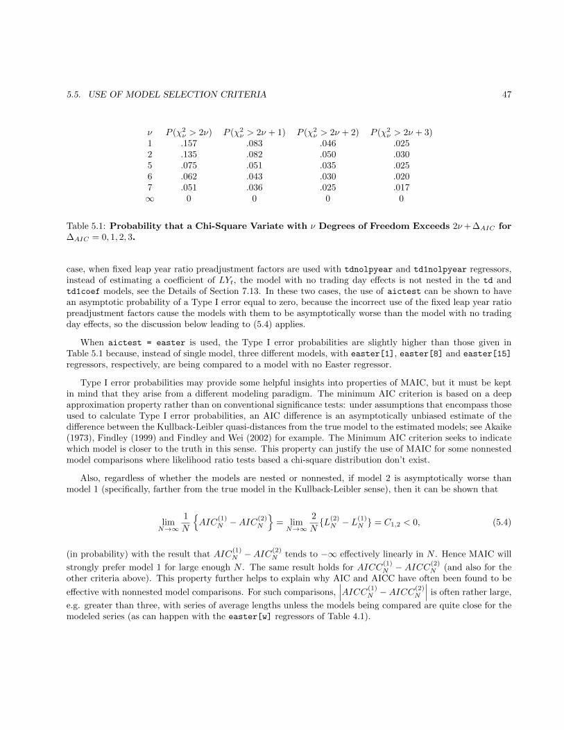
5.5. USE OF MODEL SELECTION CRITERIA 47
ν P (χ2ν > 2ν) P (χ2
ν > 2ν + 1) P (χ2ν > 2ν + 2) P (χ2
ν > 2ν + 3)1 .157 .083 .046 .0252 .135 .082 .050 .0305 .075 .051 .035 .0256 .062 .043 .030 .0207 .051 .036 .025 .017∞ 0 0 0 0
Table 5.1: Probability that a Chi-Square Variate with ν Degrees of Freedom Exceeds 2ν+ ∆AIC for∆AIC = 0, 1, 2, 3.
case, when fixed leap year ratio preadjustment factors are used with tdnolpyear and td1nolpyear regressors,instead of estimating a coefficient of LYt, the model with no trading day effects is not nested in the td andtd1coef models, see the Details of Section 7.13. In these two cases, the use of aictest can be shown to havean asymptotic probability of a Type I error equal to zero, because the incorrect use of the fixed leap year ratiopreadjustment factors cause the models with them to be asymptotically worse than the model with no tradingday effects, so the discussion below leading to (5.4) applies.
When aictest = easter is used, the Type I error probabilities are slightly higher than those given inTable 5.1 because, instead of single model, three different models, with easter[1], easter[8] and easter[15]
regressors, respectively, are being compared to a model with no Easter regressor.
Type I error probabilities may provide some helpful insights into properties of MAIC, but it must be keptin mind that they arise from a different modeling paradigm. The minimum AIC criterion is based on a deepapproximation property rather than on conventional significance tests: under assumptions that encompass thoseused to calculate Type I error probabilities, an AIC difference is an asymptotically unbiased estimate of thedifference between the Kullback-Leibler quasi-distances from the true model to the estimated models; see Akaike(1973), Findley (1999) and Findley and Wei (2002) for example. The Minimum AIC criterion seeks to indicatewhich model is closer to the truth in this sense. This property can justify the use of MAIC for some nonnestedmodel comparisons where likelihood ratio tests based a chi-square distribution don’t exist.
Also, regardless of whether the models are nested or nonnested, if model 2 is asymptotically worse thanmodel 1 (specifically, farther from the true model in the Kullback-Leibler sense), then it can be shown that
limN→∞
1
N
{AIC
(1)N −AIC
(2)N
}= limN→∞
2
N{L(2)
N − L(1)N } = C1,2 < 0, (5.4)
(in probability) with the result that AIC(1)N −AIC
(2)N tends to −∞ effectively linearly in N . Hence MAIC will
strongly prefer model 1 for large enough N . The same result holds for AICC(1)N − AICC(2)
N (and also for theother criteria above). This property further helps to explain why AIC and AICC have often been found to be
effective with nonnested model comparisons. For such comparisons,∣∣∣AICC(1)
N −AICC(2)N
∣∣∣ is often rather large,
e.g. greater than three, with series of average lengths unless the models being compared are quite close for themodeled series (as can happen with the easter[w] regressors of Table 4.1).

48 CHAPTER 5. POINTS RELATED TO REGARIMA MODEL ESTIMATION
In situations in which multiple models are compared (more than two or three, perhaps substantially more),it is worthwhile to consider the model with the second smallest AICC value as well as the minimum AICCmodel, and perhaps other models whose AICC value is close to the minimum value, especially when the modelcomparisons are non-nested. These alternative model sometimes have more desirable features, e.g. severalfewer parameters, better interpretability, greater consistency with the model chosen for several closely relatedseries, etc. Burnham and Anderson (2004) on page 271 offers rough rules of thumb for this situation, thatwe formulate with AICC instead of AIC. With AICCmin denoting the minimum AICC value and AICCalt
denoting the second smallest AICC value or the AICC value of some similarly competitive alternative model,set ∆ = AICCalt − AICCmin. If ∆ ≤ 2, there is substantial support for the alternative model, considerablyless if 4 ≤ ∆ ≤ 7, and essentially no support if ∆ > 10.
We now turn to some situations that require special consideration.
5.5.1 Avoid using the criteria to compare models with different sets of outlierregressors when possible
Critical values near 4.0 or larger are usually used to select outlier regressors with a given ARIMA model, seeTable 7.22. (This is done to compensate for level of significance distortions and loss of power resulting from thelarge number of tests done by the automatic procedure of the outlier spec.) Outliers that enter the model withlarge critical values usually cause the maximum log likelihood to increase quite substantially and AIC and theother criteria to decrease correspondingly.
As a consequence, unless the models being compared have the same outliers (which often have similar effectson both log likelihoods and therefore have effects that almost cancel in differences of criterion values), theoutliers can largely determine the model selection, rather than more relevant data properties. In particular, themodel with the most outliers will often be the one with the smallest criterion value. Therefore, with automaticmodel selection using the model selection criteria, when the outlier sets are not automatically the same, it can beimportant to find out if differences in outlier sets have determined the outcome. This can be done by changingthe specifications of the most competitive models so that all these models have same outlier regressors and thenestimating the modified models and comparing their model selection criteria.
5.5.2 Model comparisons for transformed data
Often a log transformation, or other Box-Cox power transformation,
λ2 +{Y λt − 1
}/λ, λ 6= 0
lnYt, λ = 0,
is applied to the original data Yt prior to regARIMA modeling, see Section 7.18. (Note that the power λ = 1yields Yt, i.e., no transformation.) Frequently this transformation is preceded by division of the series Yt bypositive prior ratio-adjustment factors ct.
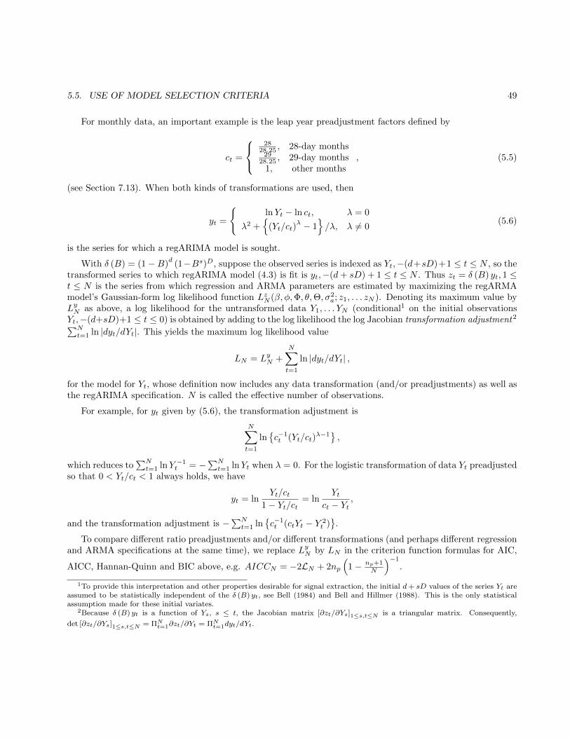
5.5. USE OF MODEL SELECTION CRITERIA 49
For monthly data, an important example is the leap year preadjustment factors defined by
ct =
28
28.25 , 28-day months29
28.25 , 29-day months1, other months
, (5.5)
(see Section 7.13). When both kinds of transformations are used, then
yt =
{lnYt − ln ct, λ = 0
λ2 +{
(Yt/ct)λ − 1
}/λ, λ 6= 0
(5.6)
is the series for which a regARIMA model is sought.
With δ (B) = (1−B)d
(1−Bs)D, suppose the observed series is indexed as Yt,−(d+sD)+1 ≤ t ≤ N , so thetransformed series to which regARIMA model (4.3) is fit is yt,−(d+ sD) + 1 ≤ t ≤ N . Thus zt = δ (B) yt, 1 ≤t ≤ N is the series from which regression and ARMA parameters are estimated by maximizing the regARMAmodel’s Gaussian-form log likelihood function LzN (β, φ,Φ, θ,Θ, σ2
a; z1, . . . zN ). Denoting its maximum value byLyN as above, a log likelihood for the untransformed data Y1, . . . YN (conditional1 on the initial observationsYt,−(d+sD)+1 ≤ t ≤ 0) is obtained by adding to the log likelihood the log Jacobian transformation adjustment2∑Nt=1 ln |dyt/dYt|. This yields the maximum log likelihood value
LN = LyN +
N∑t=1
ln |dyt/dYt| ,
for the model for Yt, whose definition now includes any data transformation (and/or preadjustments) as well asthe regARIMA specification. N is called the effective number of observations.
For example, for yt given by (5.6), the transformation adjustment is
N∑t=1
ln{c−1t (Yt/ct)
λ−1},
which reduces to∑Nt=1 lnY −1
t = −∑Nt=1 lnYt when λ = 0. For the logistic transformation of data Yt preadjusted
so that 0 < Yt/ct < 1 always holds, we have
yt = lnYt/ct
1− Yt/ct= ln
Ytct − Yt
,
and the transformation adjustment is −∑Nt=1 ln
{c−1t (ctYt − Y 2
t )}
.
To compare different ratio preadjustments and/or different transformations (and perhaps different regressionand ARMA specifications at the same time), we replace LyN by LN in the criterion function formulas for AIC,
AICC, Hannan-Quinn and BIC above, e.g. AICCN = −2LN + 2np
(1− np+1
N
)−1
.
1To provide this interpretation and other properties desirable for signal extraction, the initial d+ sD values of the series Yt areassumed to be statistically independent of the δ (B) yt, see Bell (1984) and Bell and Hillmer (1988). This is the only statisticalassumption made for these initial variates.
2Because δ (B) yt is a function of Ys, s ≤ t, the Jacobian matrix [∂zt/∂Ys]1≤s,t≤N is a triangular matrix. Consequently,
det [∂zt/∂Ys]1≤s,t≤N = ΠNt=1∂zt/∂Yt = ΠN
t=1dyt/dYt.
50 CHAPTER 5. POINTS RELATED TO REGARIMA MODEL ESTIMATION
5.5.3 Do not use the criteria to compare models with different differencing oper-ators
The preceding discussion shows that a model with a different differencing operator δ∗ (B) = (1−B)d∗
(1−Bs)D∗such that d∗+sD∗ 6= d+sD, yields a log likelihood function that is for a set of Yt values different from Y1, . . . YN(and that is conditional on a different set of initial values). Therefore its log likelihood function, and hence alsothe value of any of the model selection criteria, is not comparable3 to the values of the same criterion obtainedwith the differencing operator δ (B) = (1−B)
d(1 − Bs)D. To compare models with different differencing
operators, the out-of-sample forecast error output of the history spec (Section 7.8) can be used, with thegraphical diagnostics discussed in Sections 3 and 4 of Findley, Monsell, Bell, Otto, and Chen (1998) when theseries is long enough that regARIMA models can be estimated reliably without the final two years of data,which are withheld for forecasting.
3Ozaki (1977) proposed a rescaling of AICN to compare different orders of differencings of nonseasonal ARIMA models. In theseasonal case, the analogue would be to multiply AICN by (N + d+ sD)/N and use the resulting value in all model comparisons.There is neither theoretical nor systematic emprical support for such a rescaling of any of the criteria, so rescaling this way is notan accepted practice for model selection.
6 Points Related to SeasonalAdjustment and Modeling Diagnostics
Contents6.1 Spectral Plots . . . . . . . . . . . . . . . . . . . . . . . . . . . . . . . . . . . . . . . . 51
6.1.1 General Information . . . . . . . . . . . . . . . . . . . . . . . . . . . . . . . . . . . . . 52
6.1.2 AR spectrum . . . . . . . . . . . . . . . . . . . . . . . . . . . . . . . . . . . . . . . . . 53
6.1.3 Tukey Spectrum . . . . . . . . . . . . . . . . . . . . . . . . . . . . . . . . . . . . . . . 54
6.2 Sliding Spans Diagnostics . . . . . . . . . . . . . . . . . . . . . . . . . . . . . . . . . 55
6.3 Revisions History Diagnostics . . . . . . . . . . . . . . . . . . . . . . . . . . . . . . . 57
Tables6.1 Values of M used in Tukey Spectrum Calcuations . . . . . . . . . . . . . . . . . . . . . 55
6.2 Revision Measure Calculated for Revision Lag Analysis . . . . . . . . . . . . . . . . . 58
The X-13ARIMA-SEATS seasonal adjustment program contains several new diagnostics for modeling, modelselection, adjustment stability, and for judging the quality of indirect as well as direct seasonal adjustments.This chapter deals specifically with three diagnostics that can be generated by the X-13ARIMA-SEATS program.
• Section 6.1 describes the spectral plots that X-13ARIMA-SEATS produces of the original series, the reg-ARIMA residuals, the final seasonal adjustment and the final irregular component. The plots are markedat frequencies commonly associated with seasonal and trading day variation, so the user can easily checkfor residual effects in the model residuals or seasonal adjustment. For more information, see Section 2.1of Findley, Monsell, Bell, Otto, and Chen (1998) and Soukup and Findley (1999).
• Section 6.2 describes the sliding spans diagnostics, which compare seasonal adjustments from overlappingspans of a given time series. This provides an indication of the stability of the seasonal adjustment.
• Section 6.3 describes revisions history diagnostics, another stability diagnostic. The basic revision is thedifference between the initial seasonal adjustment (often referred to as the concurrent adjustment) andthe seasonal adjustment with all the data available at the time of the analysis (often referred to as thefinal adjustment).
6.1 Spectral Plots
X-13ARIMA-SEATS provides spectral plots and associated interpretative messages to alert the user to the presenceof seasonal and trading day effects. Spectral output is available for the original series and as many as three
51
52 CHAPTER 6. POINTS RELATED TO SEASONAL ADJUSTMENT AND MODELING DIAGNOSTICS
series resulting from modeling or seasonal adjustment, namely the model residuals, when modeling is specified,and the adjusted series and irregulars series, when adjustment for seasonal (and possibly also trading day orholiday) effects is specified.
Currently, these plots are provided only for monthly series; a diagnostic to detect residual seasonality in timeseries of other periodicity, including quarterly, is the QS diagnostic from the TRAMO and SEATS programs.This diagnostic’s output options can be specified in the spectrum spec; more information about it is given inthe DETAILS section of Section 7.17.
6.1.1 General Information
For a stationary time series xt with mean µ and autocovariances γk = E (xt − µ) (xt+k − µ), k = 0,±1, . . .,the spectral density (spectrum for short) is a nonnegative function g (λ), 0 ≤ λ ≤ 1/2, which reformulates thecontent of the autocovariances in terms of amplitudes at frequencies of half a cycle per sampling period (monthfor our purposes) or less, in such a way that
γk =
∫ 1/2
0
g (λ) cos 2πkλ g (λ) dλ, k = 0,±1, . . . .
When xt is a stationary ARMA process with the backshift operator polynomial formula ϕ (B) (xt − µ) =ϑ (B) at, then its spectrum can be shown to be given by
g (λ) = σ2
∣∣ϑ (ei2πλ)∣∣2|ϕ (ei2πλ)|2
,
where σ2 is the variance of the white noise at; see Priestley (1981). Here ei2πλ = cos 2πλ+ i sin 2πλ, and for acomplex number u+ iv (u, v real), |u+ iv| =
√u2 + v2.
For the first-differenced original series of the series or composite spec (transformed in accord with thetransform spec), the program’s warning message about “visually significant” seasonal peaks, or the associatedplot, can alert the user to the possibility that the series has a seasonal effect that is predictable (stable) enoughfor X-13ARIMA-SEATS to estimate with reasonable success. (If there are seasonal peaks in the spectrum butnone that meet the criteria for visual significance, see below, then it is likely that any “seasonal” effects in theseries change too rapidly from year to year or are too obscured by “noise” to be estimated reliably or stably.)
For the regARIMA model residuals (when a regARIMA model is estimated), and for the first-differenced,transformed seasonally adjusted series and the irregulars series (when the x11 or seats spec is used), themessages indicate that the model or adjustment procedure for seasonal or trading day effects has either failedto capture such effects or, worse, has induced such effects in the series over the time interval used for spectrumestimation. Because seasonal and trading day patterns can change over time, and because adequate modelingor adjustment is usually most important for recent data, the time interval of the most recent 96 observations isthe default interval for spectrum estimation (or the time interval specified by the applicable modelspan or spanargument when the latter interval has length less than 96). In the case of trading day peaks, a peak (especiallyone at the lower of the two trading day frequencies) shows the need for trading day estimation if this was notdone, and otherwise shows that the trading day regression model used is inadequate for the time interval usedfor spectrum estimation.
6.1. SPECTRAL PLOTS 53
At seasonal frequencies, a peak in the model residuals indicates the need for a better fitting model for thetime interval used for spectrum estimation. A peak in the spectrum from the seasonally adjusted series orirregulars reveals inadequacy of the seasonal adjustment filters for this interval, thereby indicating that differentfilters and/or a shorter data span should be considered. Usually, the spectrum estimator requires 72 data pointsto produce peaks sharply defined enough to trigger warning messages for seasonal or trading day effects.
6.1.2 AR spectrum
The default spectrum estimator used to detect seasonal and trading day effects is an autoregressive spectralestimator. For the series xt (for example, the model residuals) whose spectrum is being estimated from datax1, . . . , xN , autoregressive log-spectrum estimates (in decibel units) have the form
s (λ) = 10 log10
σ2m
2π∣∣∣1−∑m
j=1 φjei2πjλ
∣∣∣2 , 0 ≤ λ ≤ 0.5, (6.1)
where the coefficient estimates φj are those of the linear regression of xt − x on xt−j − x, 1 ≤ j ≤ m for the
data, with x = N−1∑Nt=1 xt, and where σ2
m is the sample variance of the resulting regression residuals. Forlarge enough m (and N), a strong component with period 1/λ0 results in a near-zero value of the denominatorof (6.1) at λ0 and therefore in a peak at λ0 in the graph of (6.1) - unless there is a stronger periodic componentat a nearby frequency. For a discussion of this estimator, see pp. 600–612 of Priestley (1981). Application ofthe proof of Corollary 5.6.3 of Brillinger (1975) to the results of Theorem 6 of Berk (1974) shows that, underBerk’s assumptions, which include invertibility of xt, the log transformation in (6.1) stabilizes the large sample
variance of s(λ), i.e. the limiting value of E (s(λ)− g (λ))2, as m → ∞ in case g (λ) is not an AR process.
However, the constant value for the end point frequencies λ = 0, 1/2 is twice as large as the constant value forthe intermediate frequencies. 0 < λ < 1/2.
X-13ARIMA-SEATS uses m = 30 for monthly series, which yields high resolution of strong components,meaning peaks that are sharply defined in the main output file’s plot of s (λ) (Recall that for the spectra providinginformation about the original series and the seasonal adjustment, the series xt results from suppression of atrend component by differencing or detrending. Trends produce peaks at and near λ = 0 that are so dominantthat they diminish the resolution of all other peaks.) The spectrum plots of X-13ARIMA-SEATS show values ofs (λ) at 61 frequencies that have the form λk = k/120, 0 ≤ k ≤ 60, with two exceptions: for the values k/120closest to the trading day frequencies (0.348, and 0.432 cycles per month for monthly series), λk is assignedthe value of the trading day frequency instead of the value k/120. At trading day frequencies, values of s (λk)are plotted with a column of T’s. At seasonal frequencies (1/12, 2/12,...,6/12 cycles per month for monthlyseries) values of s (λk) are plotted with a column of S’s. At all other frequencies, columns of asterisks (“stars”)are used. These plots are very similar to those of the BAYSEA seasonal adjustment program (Akaike 1980 andAkaike and Ishiguro 1980) and are produced by a modified version of BAYSEA’s Fortran code.
The monthly trading day frequency 0.348 can be derived by noting that a daily component which repeatsevery seven days goes through 4.348
.= 30.4375/7 cycles in a month of average length, 365.25/12 = 30.4375 days.
It is therefore seen to advance 0.348 cycles per month when the data are obtained at twelve equally spaced timesin an 365.25 days, the average length of a year. The connection of peaks at 0.432 cycles/month with tradingday components is weaker, see Cleveland and Devlin (1980), and not as reliable.
54 CHAPTER 6. POINTS RELATED TO SEASONAL ADJUSTMENT AND MODELING DIAGNOSTICS
Note that the time series needs to have at least 60 observations for X-13ARIMA-SEATS to display the tradingday frequencies in the plots and attempt to identify peaks for trading day frequencies.
Because of difficulties associated with statistical significance tests for periodic components in autocorrelateddata, see Chapter 8 of Priestley (1981), such tests are not used for the AR spectrum. The warning messages ofX-13ARIMA-SEATS are based on an empirically obtained criterion of “visual significance” determined as followsfrom the range smax − smin of the s (λk) values, where smax = maxk s (λk) and smin = mink s (λk). To be“visually significant”, the value s (λk) at a trading day or seasonal frequency λk (other than the seasonalfrequency λ60 = 0.5) must be above the median of the plotted values of s (λ) and must be larger than bothneighboring values s (λk−1) and s (λk+1) by at least 6/52 times the range smax − smin. In the main output file’sline printer plots of spectra, smax is plotted 52 lines above smin, so a visually significant peak must be at leastsix lines (six “stars”) high.
Peaks of any size at λ60 = 1/2 are ignored. The theoretical results from Berk (1974) and Brillinger (1975)mentioned above describe how s(λ) will be more randomly variable at λ60 = 1/2 than at other seasonal frequen-cies. More erratic behavior and less reliable performance are to be expected when the spectral density g(λ) ofthe series being estimated is zero or close to zero at some frequency, especially at λ = 1/2, which can happen,particularly with the series of irregulars (see Bell 2010). The empirical finding from practice is that visuallysignificant peaks at λ60 = 1/2 occur too often in the spectra of seasonally adjusted and irregular series thathave few or no other visually significant seasonal peaks.
Also, visually significant peaks at λ50 = 5/12 rather frequently occur when there are no other visuallysignificant peaks. There is no economic explanation for such peaks.
6.1.3 Tukey Spectrum
In addition to the AR spectrum, the program generates a nonparametric Tukey estimate of the spectrum. Thisestimate appears in the TRAMO-SEATS and TSW software and is part of that software’s seasonality tests, seeMaravall (2012) and Jenkins and Watts (1968).
For a series xt with length N (e.g. the differenced SA series or the Irregulars) and for specified M < N , set
gTx (λ) = c0 + 2
M∑k=1
w (k/M) ck cos 2πkλ, 0 ≤ λ ≤ 1/2
with
ck = N−1N−k∑t=1
(xt − x) (xt−k − x) ,
where
x = N−1n∑t=1
xt
and with
w (v) =1
2+
1
2cosπv, 0 ≤ v ≤ 1.
The M parameter is determined by the length and the seasonal frequency of the time series, as well as thevalue of the tukey120 argument in the spectrum spec. Table 6.1 shows how the value of M is set internally.
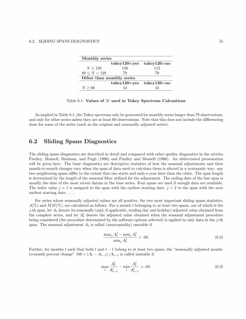
6.2. SLIDING SPANS DIAGNOSTICS 55
Monthly seriestukey120=yes tukey120=no
N ≥ 120 120 11280 ≤ N < 120 79 79Other than monthly series
tukey120=yes tukey120=noN ≥ 60 44 44
Table 6.1: Values of M used in Tukey Spectrum Calcuations
As implied in Table 6.1, the Tukey spectrum only be generated for monthly series longer than 79 observations,and only for other series unless they are at least 60 observations. Note that this does not include the differencingdone for some of the series (such as the original and seasonally adjusted series).
6.2 Sliding Spans Diagnostics
The sliding spans diagnostics are described in detail and compared with other quality diagnostics in the articlesFindley, Monsell, Shulman, and Pugh (1990) and Findley and Monsell (1986). An abbreviated presentationwill be given here. The basic diagnostics are descriptive statistics of how the seasonal adjustments and theirmonth-to-month changes vary when the span of data used to calculate them is altered in a systematic way: anytwo neighboring spans differ to the extent that one starts and ends a year later than the other. The span lengthis determined by the length of the seasonal filter utilized for the adjustment. The ending date of the last span isusually the date of the most recent datum in the time series. Four spans are used if enough data are available.The index value j = 1 is assigned to the span with the earliest starting date, j = 2 to the span with the nextearliest starting date, . . . .
For series whose seasonally adjusted values are all positive, the two most important sliding spans statistics,A(%) and MM(%), are calculated as follows. For a month t belonging to at least two spans, one of which is thej-th span, let At denote its seasonally (and, if applicable, trading day and holiday) adjusted value obtained fromthe complete series, and let Ajt denote the adjusted value obtained when the seasonal adjustment procedurebeing considered (the procedure determined by the software options selected) is applied to only data in the j-thspan. The seasonal adjustment At is called (unacceptably) unstable if
maxj Ajt −minj A
jt
minj Ajt
> .03. (6.2)
Further, for months t such that both t and t− 1 belong to at least two spans, the “seasonally adjusted month-to-month percent change” 100× (At −At−1) /At−1 is called unstable if
maxj
Ajt
Ajt−1
−minj
Ajt
Ajt−1
> .03. (6.3)
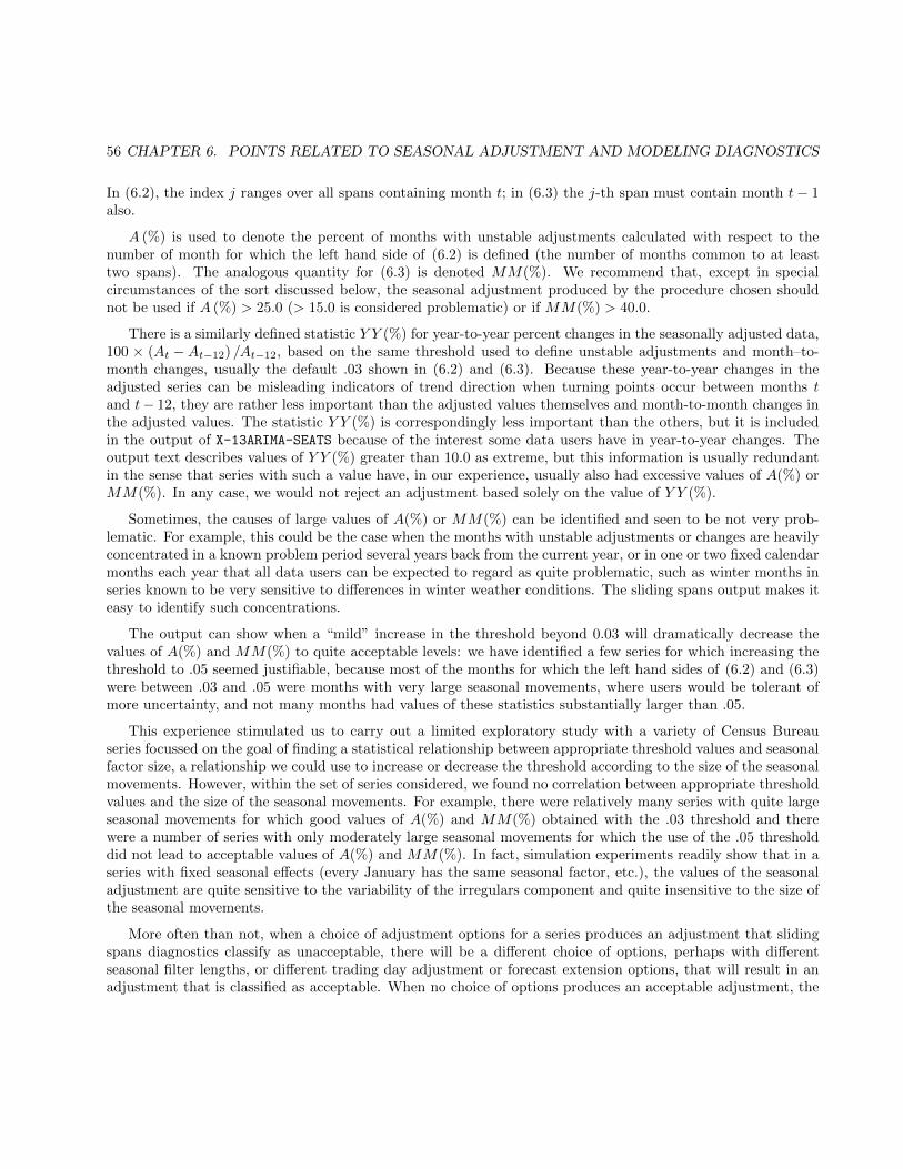
56 CHAPTER 6. POINTS RELATED TO SEASONAL ADJUSTMENT AND MODELING DIAGNOSTICS
In (6.2), the index j ranges over all spans containing month t; in (6.3) the j-th span must contain month t− 1also.
A (%) is used to denote the percent of months with unstable adjustments calculated with respect to thenumber of month for which the left hand side of (6.2) is defined (the number of months common to at leasttwo spans). The analogous quantity for (6.3) is denoted MM(%). We recommend that, except in specialcircumstances of the sort discussed below, the seasonal adjustment produced by the procedure chosen shouldnot be used if A (%) > 25.0 (> 15.0 is considered problematic) or if MM(%) > 40.0.
There is a similarly defined statistic Y Y (%) for year-to-year percent changes in the seasonally adjusted data,100 × (At −At−12) /At−12, based on the same threshold used to define unstable adjustments and month–to-month changes, usually the default .03 shown in (6.2) and (6.3). Because these year-to-year changes in theadjusted series can be misleading indicators of trend direction when turning points occur between months tand t− 12, they are rather less important than the adjusted values themselves and month-to-month changes inthe adjusted values. The statistic Y Y (%) is correspondingly less important than the others, but it is includedin the output of X-13ARIMA-SEATS because of the interest some data users have in year-to-year changes. Theoutput text describes values of Y Y (%) greater than 10.0 as extreme, but this information is usually redundantin the sense that series with such a value have, in our experience, usually also had excessive values of A(%) orMM(%). In any case, we would not reject an adjustment based solely on the value of Y Y (%).
Sometimes, the causes of large values of A(%) or MM(%) can be identified and seen to be not very prob-lematic. For example, this could be the case when the months with unstable adjustments or changes are heavilyconcentrated in a known problem period several years back from the current year, or in one or two fixed calendarmonths each year that all data users can be expected to regard as quite problematic, such as winter months inseries known to be very sensitive to differences in winter weather conditions. The sliding spans output makes iteasy to identify such concentrations.
The output can show when a “mild” increase in the threshold beyond 0.03 will dramatically decrease thevalues of A(%) and MM(%) to quite acceptable levels: we have identified a few series for which increasing thethreshold to .05 seemed justifiable, because most of the months for which the left hand sides of (6.2) and (6.3)were between .03 and .05 were months with very large seasonal movements, where users would be tolerant ofmore uncertainty, and not many months had values of these statistics substantially larger than .05.
This experience stimulated us to carry out a limited exploratory study with a variety of Census Bureauseries focussed on the goal of finding a statistical relationship between appropriate threshold values and seasonalfactor size, a relationship we could use to increase or decrease the threshold according to the size of the seasonalmovements. However, within the set of series considered, we found no correlation between appropriate thresholdvalues and the size of the seasonal movements. For example, there were relatively many series with quite largeseasonal movements for which good values of A(%) and MM(%) obtained with the .03 threshold and therewere a number of series with only moderately large seasonal movements for which the use of the .05 thresholddid not lead to acceptable values of A(%) and MM(%). In fact, simulation experiments readily show that in aseries with fixed seasonal effects (every January has the same seasonal factor, etc.), the values of the seasonaladjustment are quite sensitive to the variability of the irregulars component and quite insensitive to the size ofthe seasonal movements.
More often than not, when a choice of adjustment options for a series produces an adjustment that slidingspans diagnostics classify as unacceptable, there will be a different choice of options, perhaps with differentseasonal filter lengths, or different trading day adjustment or forecast extension options, that will result in anadjustment that is classified as acceptable. When no choice of options produces an acceptable adjustment, the
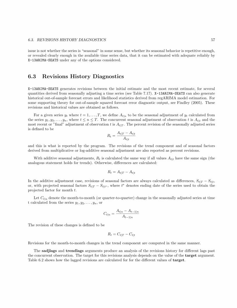
6.3. REVISIONS HISTORY DIAGNOSTICS 57
issue is not whether the series is “seasonal” in some sense, but whether its seasonal behavior is repetitive enough,or revealed clearly enough in the available time series data, that it can be estimated with adequate reliably byX-13ARIMA-SEATS under any of the options considered.
6.3 Revisions History Diagnostics
X-13ARIMA-SEATS generates revisions between the initial estimate and the most recent estimate, for severalquantities derived from seasonally adjusting a time series (see Table 7.17). X-13ARIMA-SEATS can also generatehistorical out-of-sample forecast errors and likelihood statistics derived from regARIMA model estimation. Forsome supporting theory for out-of-sample squared forecast error diagnostic output, see Findley (2005). Theserevisions and historical values are obtained as follows.
For a given series yt where t = 1, . . . , T , we define At|n to be the seasonal adjustment of yt calculated fromthe series y1, y2, . . . , yn, where t ≤ n ≤ T . The concurrent seasonal adjustment of observation t is At|t and themost recent or ”final” adjustment of observation t is At|T . The percent revision of the seasonally adjusted seriesis defined to be
Rt =At|T −At|t
At|t
and this is what is reported by the program. The revisions of the trend component and of seasonal factorsderived from multiplicative or log-additive seasonal adjustment are also reported as percent revisions.
With additive seasonal adjustments, Rt is calculated the same way if all values At|t have the same sign (theanalogous statement holds for trends). Otherwise, differences are calculated:
Rt = At|T −At|t
In the additive adjustment case, revisions of seasonal factors are always calculated as differences, St|T − St|t,or, with projected seasonal factors St|T − St|t∗ , where t∗ denotes ending date of the series used to obtain theprojected factor for month t.
Let Ct|n denote the month-to-month (or quarter-to-quarter) change in the seasonally adjusted series at timet calculated from the series y1, y2, . . . , yn, or
Ct|n =At|n −At−1|n
At−1|n
The revision of these changes is defined to be
Rt = Ct|T − Ct|t
Revisions for the month-to-month changes in the trend component are computed in the same manner.
The sadjlags and trendlags arguments produce an analysis of the revisions history for different lags pastthe concurrent observation. The target for this revisions analysis depends on the value of the target argument.Table 6.2 shows how the lagged revisions are calculated for for the different values of target.
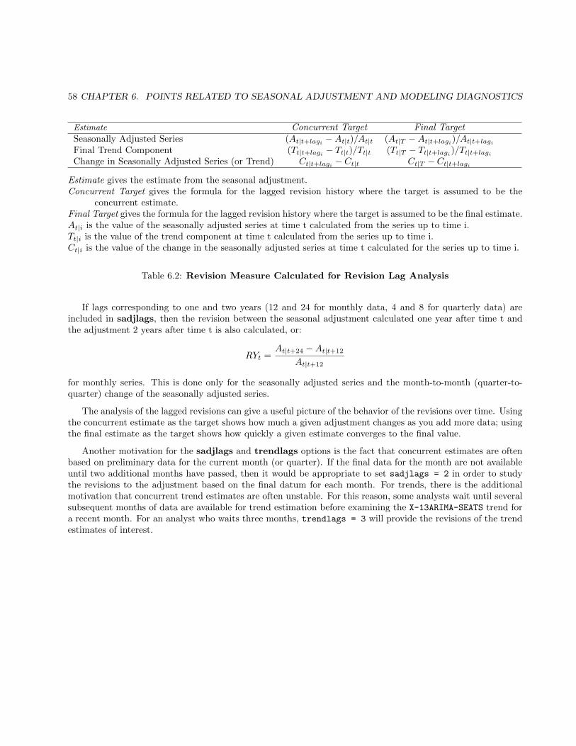
58 CHAPTER 6. POINTS RELATED TO SEASONAL ADJUSTMENT AND MODELING DIAGNOSTICS
Estimate Concurrent Target Final TargetSeasonally Adjusted Series (At|t+lagi −At|t)/At|t (At|T −At|t+lagi)/At|t+lagiFinal Trend Component (Tt|t+lagi − Tt|t)/Tt|t (Tt|T − Tt|t+lagi)/Tt|t+lagiChange in Seasonally Adjusted Series (or Trend) Ct|t+lagi − Ct|t Ct|T − Ct|t+lagi
Estimate gives the estimate from the seasonal adjustment.Concurrent Target gives the formula for the lagged revision history where the target is assumed to be the
concurrent estimate.Final Target gives the formula for the lagged revision history where the target is assumed to be the final estimate.At|i is the value of the seasonally adjusted series at time t calculated from the series up to time i.Tt|i is the value of the trend component at time t calculated from the series up to time i.Ct|i is the value of the change in the seasonally adjusted series at time t calculated for the series up to time i.
Table 6.2: Revision Measure Calculated for Revision Lag Analysis
If lags corresponding to one and two years (12 and 24 for monthly data, 4 and 8 for quarterly data) areincluded in sadjlags, then the revision between the seasonal adjustment calculated one year after time t andthe adjustment 2 years after time t is also calculated, or:
RYt =At|t+24 −At|t+12
At|t+12
for monthly series. This is done only for the seasonally adjusted series and the month-to-month (quarter-to-quarter) change of the seasonally adjusted series.
The analysis of the lagged revisions can give a useful picture of the behavior of the revisions over time. Usingthe concurrent estimate as the target shows how much a given adjustment changes as you add more data; usingthe final estimate as the target shows how quickly a given estimate converges to the final value.
Another motivation for the sadjlags and trendlags options is the fact that concurrent estimates are oftenbased on preliminary data for the current month (or quarter). If the final data for the month are not availableuntil two additional months have passed, then it would be appropriate to set sadjlags = 2 in order to studythe revisions to the adjustment based on the final datum for each month. For trends, there is the additionalmotivation that concurrent trend estimates are often unstable. For this reason, some analysts wait until severalsubsequent months of data are available for trend estimation before examining the X-13ARIMA-SEATS trend fora recent month. For an analyst who waits three months, trendlags = 3 will provide the revisions of the trendestimates of interest.
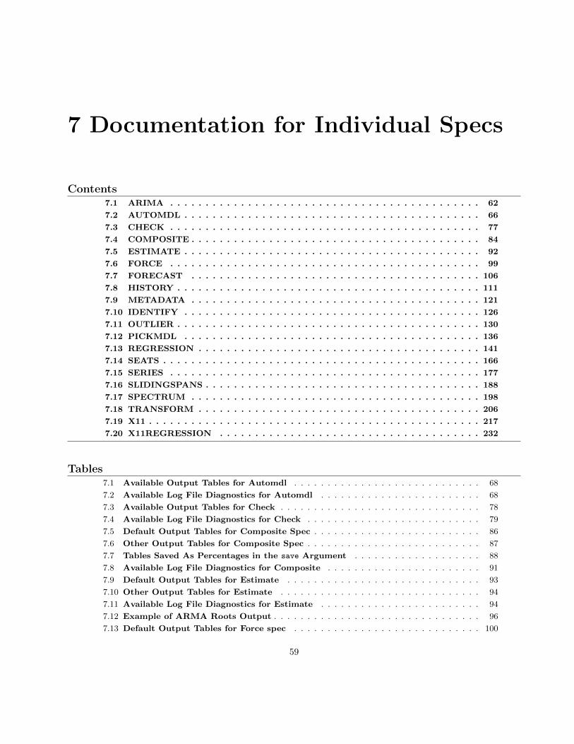
7 Documentation for Individual Specs
Contents7.1 ARIMA . . . . . . . . . . . . . . . . . . . . . . . . . . . . . . . . . . . . . . . . . . . . 62
7.2 AUTOMDL . . . . . . . . . . . . . . . . . . . . . . . . . . . . . . . . . . . . . . . . . . 66
7.3 CHECK . . . . . . . . . . . . . . . . . . . . . . . . . . . . . . . . . . . . . . . . . . . . 77
7.4 COMPOSITE . . . . . . . . . . . . . . . . . . . . . . . . . . . . . . . . . . . . . . . . . 84
7.5 ESTIMATE . . . . . . . . . . . . . . . . . . . . . . . . . . . . . . . . . . . . . . . . . . 92
7.6 FORCE . . . . . . . . . . . . . . . . . . . . . . . . . . . . . . . . . . . . . . . . . . . . 99
7.7 FORECAST . . . . . . . . . . . . . . . . . . . . . . . . . . . . . . . . . . . . . . . . . 106
7.8 HISTORY . . . . . . . . . . . . . . . . . . . . . . . . . . . . . . . . . . . . . . . . . . . 111
7.9 METADATA . . . . . . . . . . . . . . . . . . . . . . . . . . . . . . . . . . . . . . . . . 121
7.10 IDENTIFY . . . . . . . . . . . . . . . . . . . . . . . . . . . . . . . . . . . . . . . . . . 126
7.11 OUTLIER . . . . . . . . . . . . . . . . . . . . . . . . . . . . . . . . . . . . . . . . . . . 130
7.12 PICKMDL . . . . . . . . . . . . . . . . . . . . . . . . . . . . . . . . . . . . . . . . . . 136
7.13 REGRESSION . . . . . . . . . . . . . . . . . . . . . . . . . . . . . . . . . . . . . . . . 141
7.14 SEATS . . . . . . . . . . . . . . . . . . . . . . . . . . . . . . . . . . . . . . . . . . . . . 166
7.15 SERIES . . . . . . . . . . . . . . . . . . . . . . . . . . . . . . . . . . . . . . . . . . . . 177
7.16 SLIDINGSPANS . . . . . . . . . . . . . . . . . . . . . . . . . . . . . . . . . . . . . . . 188
7.17 SPECTRUM . . . . . . . . . . . . . . . . . . . . . . . . . . . . . . . . . . . . . . . . . 198
7.18 TRANSFORM . . . . . . . . . . . . . . . . . . . . . . . . . . . . . . . . . . . . . . . . 206
7.19 X11 . . . . . . . . . . . . . . . . . . . . . . . . . . . . . . . . . . . . . . . . . . . . . . . 217
7.20 X11REGRESSION . . . . . . . . . . . . . . . . . . . . . . . . . . . . . . . . . . . . . 232
Tables7.1 Available Output Tables for Automdl . . . . . . . . . . . . . . . . . . . . . . . . . . . . 68
7.2 Available Log File Diagnostics for Automdl . . . . . . . . . . . . . . . . . . . . . . . . 68
7.3 Available Output Tables for Check . . . . . . . . . . . . . . . . . . . . . . . . . . . . . . 78
7.4 Available Log File Diagnostics for Check . . . . . . . . . . . . . . . . . . . . . . . . . . 79
7.5 Default Output Tables for Composite Spec . . . . . . . . . . . . . . . . . . . . . . . . . 86
7.6 Other Output Tables for Composite Spec . . . . . . . . . . . . . . . . . . . . . . . . . . 87
7.7 Tables Saved As Percentages in the save Argument . . . . . . . . . . . . . . . . . . . 88
7.8 Available Log File Diagnostics for Composite . . . . . . . . . . . . . . . . . . . . . . . 91
7.9 Default Output Tables for Estimate . . . . . . . . . . . . . . . . . . . . . . . . . . . . . 93
7.10 Other Output Tables for Estimate . . . . . . . . . . . . . . . . . . . . . . . . . . . . . . 94
7.11 Available Log File Diagnostics for Estimate . . . . . . . . . . . . . . . . . . . . . . . . 94
7.12 Example of ARMA Roots Output . . . . . . . . . . . . . . . . . . . . . . . . . . . . . . . 96
7.13 Default Output Tables for Force spec . . . . . . . . . . . . . . . . . . . . . . . . . . . . 100
59
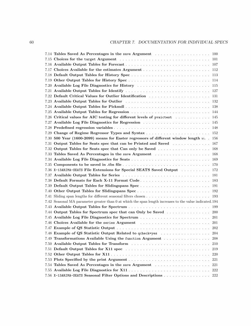
60 CHAPTER 7. DOCUMENTATION FOR INDIVIDUAL SPECS
7.14 Tables Saved As Percentages in the save Argument . . . . . . . . . . . . . . . . . . . 100
7.15 Choices for the target Argument . . . . . . . . . . . . . . . . . . . . . . . . . . . . . . . 101
7.16 Available Output Tables for Forecast . . . . . . . . . . . . . . . . . . . . . . . . . . . . . 107
7.17 Choices Available for the estimates Argument . . . . . . . . . . . . . . . . . . . . . . . 112
7.18 Default Output Tables for History Spec . . . . . . . . . . . . . . . . . . . . . . . . . . . 113
7.19 Other Output Tables for History Spec . . . . . . . . . . . . . . . . . . . . . . . . . . . . 114
7.20 Available Log File Diagnostics for History . . . . . . . . . . . . . . . . . . . . . . . . . 115
7.21 Available Output Tables for Identify . . . . . . . . . . . . . . . . . . . . . . . . . . . . . 127
7.22 Default Critical Values for Outlier Identification . . . . . . . . . . . . . . . . . . . . . 131
7.23 Available Output Tables for Outlier . . . . . . . . . . . . . . . . . . . . . . . . . . . . . 132
7.24 Available Output Tables for Pickmdl . . . . . . . . . . . . . . . . . . . . . . . . . . . . . 138
7.25 Available Output Tables for Regression . . . . . . . . . . . . . . . . . . . . . . . . . . . 144
7.26 Critical values for AIC testing for different levels of pvaictest . . . . . . . . . . . . 145
7.27 Available Log File Diagnostics for Regression . . . . . . . . . . . . . . . . . . . . . . . 145
7.28 Predefined regression variables . . . . . . . . . . . . . . . . . . . . . . . . . . . . . . . . . 148
7.29 Change of Regime Regressor Types and Syntax . . . . . . . . . . . . . . . . . . . . . . 152
7.30 500 Year (1600-2099) means for Easter regressors of different window length w. . 156
7.31 Output Tables for Seats spec that can be Printed and Saved . . . . . . . . . . . . . 167
7.32 Output Tables for Seats spec that Can only be Saved . . . . . . . . . . . . . . . . . . 168
7.33 Tables Saved As Percentages in the save Argument . . . . . . . . . . . . . . . . . . . 168
7.34 Available Log File Diagnostics for Seats . . . . . . . . . . . . . . . . . . . . . . . . . . . 169
7.35 Components to be saved in .tbs file . . . . . . . . . . . . . . . . . . . . . . . . . . . . . . 170
7.36 X-13ARIMA-SEATS File Extensions for Special SEATS Saved Output . . . . . . . . . . 172
7.37 Available Output Tables for Series . . . . . . . . . . . . . . . . . . . . . . . . . . . . . . 181
7.38 Default Formats for Each X-11 Format Code . . . . . . . . . . . . . . . . . . . . . . . . 183
7.39 Default Output Tables for Slidingspans Spec . . . . . . . . . . . . . . . . . . . . . . . . 191
7.40 Other Output Tables for Slidingspans Spec . . . . . . . . . . . . . . . . . . . . . . . . . 192
7.41 Sliding span lengths for different seasonal filters chosen . . . . . . . . . . . . . . . . . . . . . . 193
7.42 Seasonal MA parameter greater than 0 at which the span length increases to the value indicated.194
7.43 Available Output Tables for Spectrum . . . . . . . . . . . . . . . . . . . . . . . . . . . . 199
7.44 Output Tables for Spectrum spec that can Only be Saved . . . . . . . . . . . . . . . 200
7.45 Available Log File Diagnostics for Spectrum . . . . . . . . . . . . . . . . . . . . . . . . 201
7.46 Choices Available for the series Argument . . . . . . . . . . . . . . . . . . . . . . . . 201
7.47 Example of QS Statistic Output . . . . . . . . . . . . . . . . . . . . . . . . . . . . . . . . 202
7.48 Example of QS Statistic Output Related to qcheck=yes . . . . . . . . . . . . . . . . . 204
7.49 Transformations Available Using the function Argument . . . . . . . . . . . . . . . . 208
7.50 Available Output Tables for Transform . . . . . . . . . . . . . . . . . . . . . . . . . . . 210
7.51 Default Output Tables for X11 spec . . . . . . . . . . . . . . . . . . . . . . . . . . . . . 219
7.52 Other Output Tables for X11 . . . . . . . . . . . . . . . . . . . . . . . . . . . . . . . . . . 220
7.53 Plots Specified by the print Argument . . . . . . . . . . . . . . . . . . . . . . . . . . . . 221
7.54 Tables Saved As Percentages in the save Argument . . . . . . . . . . . . . . . . . . . 221
7.55 Available Log File Diagnostics for X11 . . . . . . . . . . . . . . . . . . . . . . . . . . . . 222
7.56 X-13ARIMA-SEATS Seasonal Filter Options and Descriptions . . . . . . . . . . . . . . . . 222
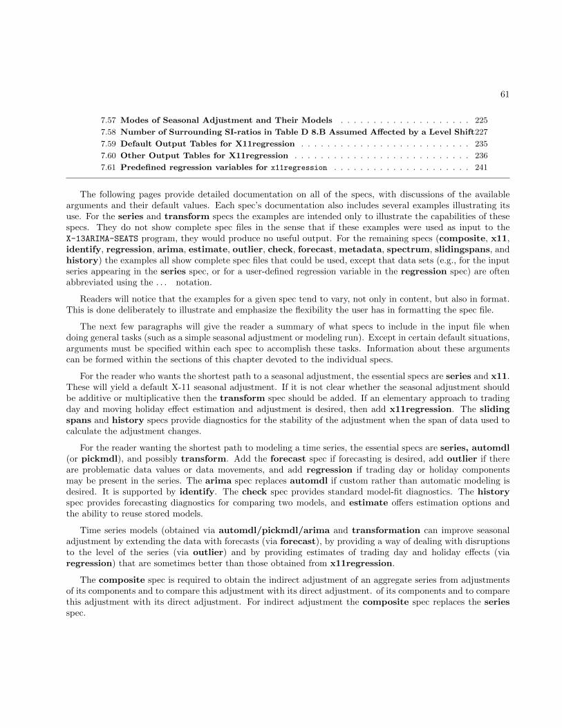
61
7.57 Modes of Seasonal Adjustment and Their Models . . . . . . . . . . . . . . . . . . . . 225
7.58 Number of Surrounding SI-ratios in Table D 8.B Assumed Affected by a Level Shift227
7.59 Default Output Tables for X11regression . . . . . . . . . . . . . . . . . . . . . . . . . . 235
7.60 Other Output Tables for X11regression . . . . . . . . . . . . . . . . . . . . . . . . . . . 236
7.61 Predefined regression variables for x11regression . . . . . . . . . . . . . . . . . . . . . 241
The following pages provide detailed documentation on all of the specs, with discussions of the availablearguments and their default values. Each spec’s documentation also includes several examples illustrating itsuse. For the series and transform specs the examples are intended only to illustrate the capabilities of thesespecs. They do not show complete spec files in the sense that if these examples were used as input to theX-13ARIMA-SEATS program, they would produce no useful output. For the remaining specs (composite, x11,identify, regression, arima, estimate, outlier, check, forecast, metadata, spectrum, slidingspans, andhistory) the examples all show complete spec files that could be used, except that data sets (e.g., for the inputseries appearing in the series spec, or for a user-defined regression variable in the regression spec) are oftenabbreviated using the . . . notation.
Readers will notice that the examples for a given spec tend to vary, not only in content, but also in format.This is done deliberately to illustrate and emphasize the flexibility the user has in formatting the spec file.
The next few paragraphs will give the reader a summary of what specs to include in the input file whendoing general tasks (such as a simple seasonal adjustment or modeling run). Except in certain default situations,arguments must be specified within each spec to accomplish these tasks. Information about these argumentscan be formed within the sections of this chapter devoted to the individual specs.
For the reader who wants the shortest path to a seasonal adjustment, the essential specs are series and x11.These will yield a default X-11 seasonal adjustment. If it is not clear whether the seasonal adjustment shouldbe additive or multiplicative then the transform spec should be added. If an elementary approach to tradingday and moving holiday effect estimation and adjustment is desired, then add x11regression. The slidingspans and history specs provide diagnostics for the stability of the adjustment when the span of data used tocalculate the adjustment changes.
For the reader wanting the shortest path to modeling a time series, the essential specs are series, automdl(or pickmdl), and possibly transform. Add the forecast spec if forecasting is desired, add outlier if thereare problematic data values or data movements, and add regression if trading day or holiday componentsmay be present in the series. The arima spec replaces automdl if custom rather than automatic modeling isdesired. It is supported by identify. The check spec provides standard model-fit diagnostics. The historyspec provides forecasting diagnostics for comparing two models, and estimate offers estimation options andthe ability to reuse stored models.
Time series models (obtained via automdl/pickmdl/arima and transformation can improve seasonaladjustment by extending the data with forecasts (via forecast), by providing a way of dealing with disruptionsto the level of the series (via outlier) and by providing estimates of trading day and holiday effects (viaregression) that are sometimes better than those obtained from x11regression.
The composite spec is required to obtain the indirect adjustment of an aggregate series from adjustmentsof its components and to compare this adjustment with its direct adjustment. of its components and to comparethis adjustment with its direct adjustment. For indirect adjustment the composite spec replaces the seriesspec.
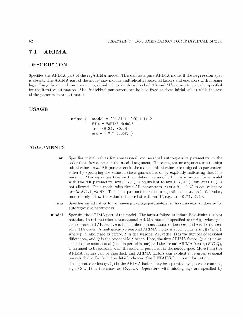
62 CHAPTER 7. DOCUMENTATION FOR INDIVIDUAL SPECS
7.1 ARIMA
DESCRIPTION
Specifies the ARIMA part of the regARIMA model. This defines a pure ARIMA model if the regression specis absent. The ARIMA part of the model may include multiplicative seasonal factors and operators with missinglags. Using the ar and ma arguments, initial values for the individual AR and MA parameters can be specifiedfor the iterative estimation. Also, individual parameters can be held fixed at these initial values while the restof the parameters are estimated.
USAGE
arima { model = ([2 3] 1 1)(0 1 1)12
title = "ARIMA Model"
ar = (0.3f, -0.14)
ma = (-0.7 0.85f) }
ARGUMENTS
ar Specifies initial values for nonseasonal and seasonal autoregressive parameters in theorder that they appear in the model argument. If present, the ar argument must assigninitial values to all AR parameters in the model. Initial values are assigned to parameterseither by specifying the value in the argument list or by explicitly indicating that it ismissing. Missing values take on their default value of 0.1. For example, for a modelwith two AR parameters, ar=(0.7, ) is equivalent to ar=(0.7,0.1), but ar=(0.7) isnot allowed. For a model with three AR parameters, ar=(0.8,,-0.4) is equivalent toar=(0.8,0.1,-0.4). To hold a parameter fixed during estimation at its initial value,immediately follow the value in the ar list with an ‘f ’, e.g., ar=(0.7f, 0.1).
ma Specifies initial values for all moving average parameters in the same way ar does so forautoregressive parameters.
model Specifies the ARIMA part of the model. The format follows standard Box-Jenkins (1976)notation. In this notation a nonseasonal ARIMA model is specified as (p d q), where p isthe nonseasonal AR order, d is the number of nonseasonal differences, and q is the nonsea-sonal MA order. A multiplicative seasonal ARIMA model is specified as (p d q)(P D Q),where p, d, and q are as before, P is the seasonal AR order, D is the number of seasonaldifferences, and Q is the seasonal MA order. Here, the first ARIMA factor, (p d q), is as-sumed to be nonseasonal (i.e., its period is one) and the second ARIMA factor, (P D Q),is assumed to be seasonal with the seasonal period set in the series spec. More than twoARIMA factors can be specified, and ARIMA factors can explicitly be given seasonalperiods that differ from the default choices. See DETAILS for more information.
The operator orders (p d q) in the ARIMA factors may be separated by spaces or commas,e.g., (0 1 1) is the same as (0,1,1). Operators with missing lags are specified by

7.1. ARIMA 63
enclosing those lags present in brackets, with the lags in ascending order. For example,model = ([2 3] 0 0) specifies the model (1− φ2B
2 − φ3B3)zt = at.
print and save No output tables are available for this spec.
title Specifies a title for the ARIMA model, in quotes. It must be less than 80 characters.The title appears above the ARIMA model description and the table of estimates. Thedefault is to print ARIMA Model.
DETAILS
The arima spec cannot be used in the same spec file as the pickmdl or automdl specs; the model, ma, andar arguments of the arima spec cannot be used when the file argument is specified in the estimate spec.
The model argument may include as many ARIMA factors as desired. However, there is a limit of 133 totalAR, MA, and differencing coefficients in the model. Also, the maximum lag of any AR or MA parameter is 36,and the maximum number of differences in any ARIMA factor (nonseasonal or seasonal) is 3. (The latter twolimits can be changed—see Section 2.8.)
In general, ARIMA factors are specified in the standard (p d q)s format, where s is the seasonal period of theoperator. Thus, putting (0 1 1)6 in the model argument includes differencing by 1− B6 and a 1− θ6B
6 MAterm in the model. However, if the seasonal period s is not specified after an ARIMA factor, it is determinedaccording to the following default rules. The first ARIMA factor without a specified seasonal period is assumedto be nonseasonal, i.e., its seasonal period is assumed to be one. The second ARIMA factor without a specifiedseasonal period is assumed to be a seasonal factor with the seasonal period set in the series spec. For example,if period = 12 is specified in the series spec (or if the period is set to 12 because the start date there is givenas year.month), then model = (0 1 1)(0 1 1) and model = (0 1 1)1(0 1 1)12 are equivalent. If additionalARIMA factors are specified, these are assumed to be nonseasonal unless they are explicitly given a seasonalperiod. See Example 7.1 for an illustration of a model with three ARIMA factors. Note that if the seasonalperiod is one, then any ARIMA factors without a specified seasonal period have period one.
Users should not specify initial values for MA parameters that yield an MA polynomial with roots inside theunit circle. (See Section 5.4.) Doing so will cause the program to stop and print an error message asking theuser to re-specify the initial parameters and rerun the program. Initial parameters that yield an MA polynomialwith roots on the unit circle are allowed only if this non-invertible polynomial is not being estimated. Thatis, this is allowed if no estimation is being done, or if the parameters in this polynomial are specified as fixedduring estimation. For example, if a model has a first order seasonal MA parameter as the only MA parameter,then ma=(1.0f) is always allowed, ma=(1.0) is allowed only if no estimation is done, and ma=(1.1) is neverallowed.
If the likelihood function that is exact for AR polynomials is used (exact=arma, which is the default—seethe estimate spec), users should not specify initial values for AR parameters that yield a non-stationary ARpolynomial (one with roots on or inside the unit circle). Doing so will cause the program to stop and print anerror message asking the user to re-specify the initial parameters and rerun the program.
The use of fixed coefficients in the ARIMA model can invalidate AIC and the other model selection statisticsas well as some goodness-of-fit diagnostics, see the Details sections of estimate and check.
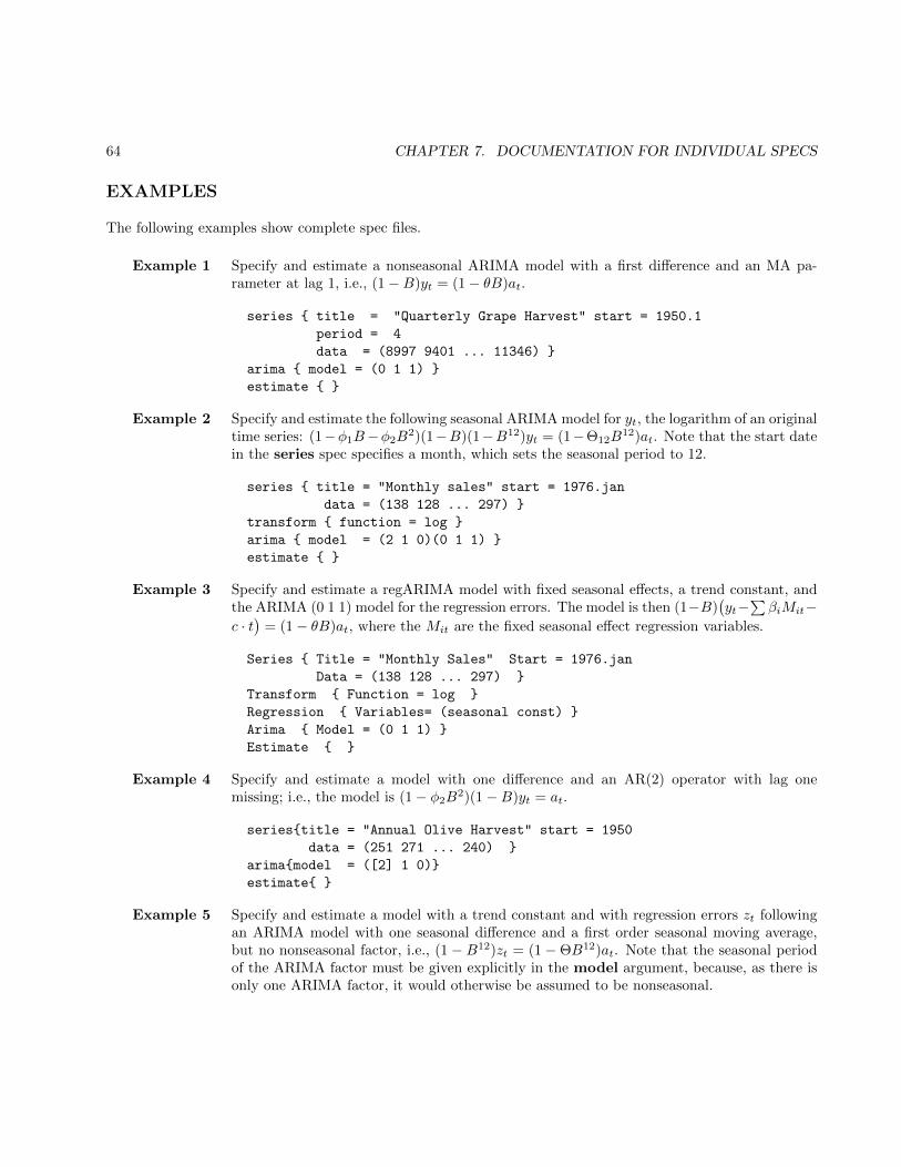
64 CHAPTER 7. DOCUMENTATION FOR INDIVIDUAL SPECS
EXAMPLES
The following examples show complete spec files.
Example 1 Specify and estimate a nonseasonal ARIMA model with a first difference and an MA pa-rameter at lag 1, i.e., (1−B)yt = (1− θB)at.
series { title = "Quarterly Grape Harvest" start = 1950.1
period = 4
data = (8997 9401 ... 11346) }
arima { model = (0 1 1) }
estimate { }
Example 2 Specify and estimate the following seasonal ARIMA model for yt, the logarithm of an originaltime series: (1−φ1B−φ2B
2)(1−B)(1−B12)yt = (1−Θ12B12)at. Note that the start date
in the series spec specifies a month, which sets the seasonal period to 12.
series { title = "Monthly sales" start = 1976.jan
data = (138 128 ... 297) }
transform { function = log }
arima { model = (2 1 0)(0 1 1) }
estimate { }
Example 3 Specify and estimate a regARIMA model with fixed seasonal effects, a trend constant, andthe ARIMA (0 1 1) model for the regression errors. The model is then (1−B)
(yt−
∑βiMit−
c · t)
= (1− θB)at, where the Mit are the fixed seasonal effect regression variables.
Series { Title = "Monthly Sales" Start = 1976.jan
Data = (138 128 ... 297) }
Transform { Function = log }
Regression { Variables= (seasonal const) }
Arima { Model = (0 1 1) }
Estimate { }
Example 4 Specify and estimate a model with one difference and an AR(2) operator with lag onemissing; i.e., the model is (1− φ2B
2)(1−B)yt = at.
series{title = "Annual Olive Harvest" start = 1950
data = (251 271 ... 240) }
arima{model = ([2] 1 0)}
estimate{ }
Example 5 Specify and estimate a model with a trend constant and with regression errors zt followingan ARIMA model with one seasonal difference and a first order seasonal moving average,but no nonseasonal factor, i.e., (1− B12)zt = (1−ΘB12)at. Note that the seasonal periodof the ARIMA factor must be given explicitly in the model argument, because, as there isonly one ARIMA factor, it would otherwise be assumed to be nonseasonal.
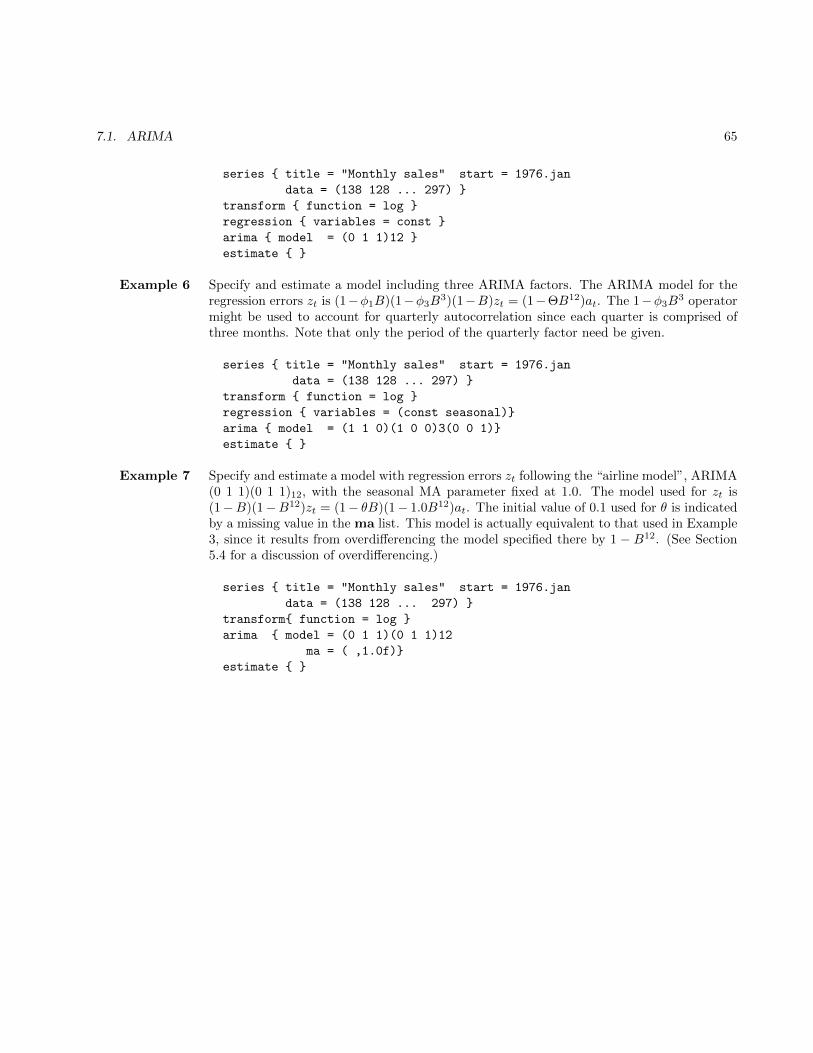
7.1. ARIMA 65
series { title = "Monthly sales" start = 1976.jan
data = (138 128 ... 297) }
transform { function = log }
regression { variables = const }
arima { model = (0 1 1)12 }
estimate { }
Example 6 Specify and estimate a model including three ARIMA factors. The ARIMA model for theregression errors zt is (1−φ1B)(1−φ3B
3)(1−B)zt = (1−ΘB12)at. The 1−φ3B3 operator
might be used to account for quarterly autocorrelation since each quarter is comprised ofthree months. Note that only the period of the quarterly factor need be given.
series { title = "Monthly sales" start = 1976.jan
data = (138 128 ... 297) }
transform { function = log }
regression { variables = (const seasonal)}
arima { model = (1 1 0)(1 0 0)3(0 0 1)}
estimate { }
Example 7 Specify and estimate a model with regression errors zt following the “airline model”, ARIMA(0 1 1)(0 1 1)12, with the seasonal MA parameter fixed at 1.0. The model used for zt is(1−B)(1−B12)zt = (1− θB)(1− 1.0B12)at. The initial value of 0.1 used for θ is indicatedby a missing value in the ma list. This model is actually equivalent to that used in Example3, since it results from overdifferencing the model specified there by 1 − B12. (See Section5.4 for a discussion of overdifferencing.)
series { title = "Monthly sales" start = 1976.jan
data = (138 128 ... 297) }
transform{ function = log }
arima { model = (0 1 1)(0 1 1)12
ma = ( ,1.0f)}
estimate { }
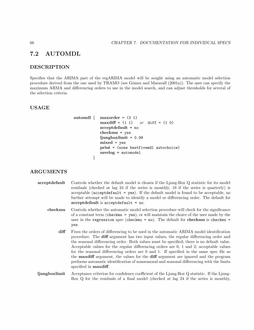
66 CHAPTER 7. DOCUMENTATION FOR INDIVIDUAL SPECS
7.2 AUTOMDL
DESCRIPTION
Specifies that the ARIMA part of the regARIMA model will be sought using an automatic model selectionprocedure derived from the one used by TRAMO (see Gomez and Maravall (2001a)). The user can specify themaximum ARMA and differencing orders to use in the model search, and can adjust thresholds for several ofthe selection criteria.
USAGE
automdl { maxorder = (3 1)
maxdiff = (1 1) or diff = (1 0)
acceptdefault = no
checkmu = yes
ljungboxlimit = 0.99
mixed = yes
print = (none bestfivemdl autochoice)
savelog = automodel
}
ARGUMENTS
acceptdefault Controls whether the default model is chosen if the Ljung-Box Q statistic for its modelresiduals (checked at lag 24 if the series is monthly, 16 if the series is quarterly) isacceptable (acceptdefault = yes). If the default model is found to be acceptable, nofurther attempt will be made to identify a model or differencing order. The default foracceptdefault is acceptdefault = no.
checkmu Controls whether the automatic model selection procedure will check for the significanceof a constant term (checkmu = yes), or will maintain the choice of the user made by theuser in the regression spec (checkmu = no). The default for checkmu is checkmu =
yes.
diff Fixes the orders of differencing to be used in the automatic ARIMA model identificationprocedure. The diff argument has two input values, the regular differencing order andthe seasonal differencing order. Both values must be specified; there is no default value.Acceptable values for the regular differencing orders are 0, 1 and 2; acceptable valuesfor the seasonal differencing orders are 0 and 1. If specified in the same spec file asthe maxdiff argument, the values for the diff argument are ignored and the programperforms automatic identification of nonseasonal and seasonal differencing with the limitsspecified in maxdiff.
ljungboxlimit Acceptance criterion for confidence coefficient of the Ljung-Box Q statistic. If the Ljung-Box Q for the residuals of a final model (checked at lag 24 if the series is monthly,
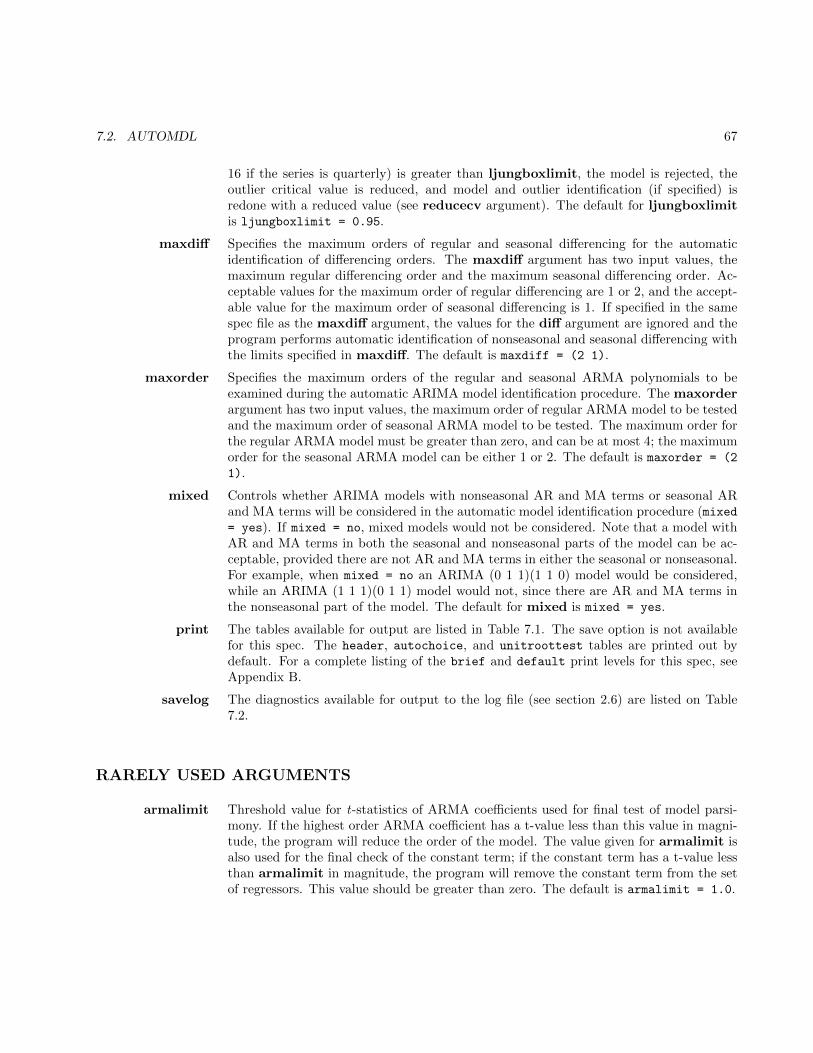
7.2. AUTOMDL 67
16 if the series is quarterly) is greater than ljungboxlimit, the model is rejected, theoutlier critical value is reduced, and model and outlier identification (if specified) isredone with a reduced value (see reducecv argument). The default for ljungboxlimitis ljungboxlimit = 0.95.
maxdiff Specifies the maximum orders of regular and seasonal differencing for the automaticidentification of differencing orders. The maxdiff argument has two input values, themaximum regular differencing order and the maximum seasonal differencing order. Ac-ceptable values for the maximum order of regular differencing are 1 or 2, and the accept-able value for the maximum order of seasonal differencing is 1. If specified in the samespec file as the maxdiff argument, the values for the diff argument are ignored and theprogram performs automatic identification of nonseasonal and seasonal differencing withthe limits specified in maxdiff. The default is maxdiff = (2 1).
maxorder Specifies the maximum orders of the regular and seasonal ARMA polynomials to beexamined during the automatic ARIMA model identification procedure. The maxorderargument has two input values, the maximum order of regular ARMA model to be testedand the maximum order of seasonal ARMA model to be tested. The maximum order forthe regular ARMA model must be greater than zero, and can be at most 4; the maximumorder for the seasonal ARMA model can be either 1 or 2. The default is maxorder = (2
1).
mixed Controls whether ARIMA models with nonseasonal AR and MA terms or seasonal ARand MA terms will be considered in the automatic model identification procedure (mixed= yes). If mixed = no, mixed models would not be considered. Note that a model withAR and MA terms in both the seasonal and nonseasonal parts of the model can be ac-ceptable, provided there are not AR and MA terms in either the seasonal or nonseasonal.For example, when mixed = no an ARIMA (0 1 1)(1 1 0) model would be considered,while an ARIMA (1 1 1)(0 1 1) model would not, since there are AR and MA terms inthe nonseasonal part of the model. The default for mixed is mixed = yes.
print The tables available for output are listed in Table 7.1. The save option is not availablefor this spec. The header, autochoice, and unitroottest tables are printed out bydefault. For a complete listing of the brief and default print levels for this spec, seeAppendix B.
savelog The diagnostics available for output to the log file (see section 2.6) are listed on Table7.2.
RARELY USED ARGUMENTS
armalimit Threshold value for t-statistics of ARMA coefficients used for final test of model parsi-mony. If the highest order ARMA coefficient has a t-value less than this value in magni-tude, the program will reduce the order of the model. The value given for armalimit isalso used for the final check of the constant term; if the constant term has a t-value lessthan armalimit in magnitude, the program will remove the constant term from the setof regressors. This value should be greater than zero. The default is armalimit = 1.0.

68 CHAPTER 7. DOCUMENTATION FOR INDIVIDUAL SPECS
name short description of tableautochoice ach model choice of automatic model procedureautochoicemdl amd summary output for models estimated during choice of
ARMA model ordersautodefaulttests adt tests performed on the default model (usually the air-
line model) of the automatic model identification pro-cedure
autofinaltests aft final tests performed on the model identified by au-tomdl
autoljungboxtest alb check of the residual Ljung-Box statisticbestfivemdl b5m summary of best five models found during choice of
ARMA model ordersheader hdr header for the automatic modeling outputunitroottest urt choice of differencingunitroottestmdl urm summary output for models estimated during difference
order identification
Name gives the name of each table for use with the print argument.Short gives a short name for the tables of the print argument.
Table 7.1: Available Output Tables for Automdl
name short description of diagnosticalldiagnostics all All modeling diagnostics listed in this tableautodiff adf choice of differencing by automatic model identification
procedureautomodel amd choice of ARIMA model by automatic model identification
procedurebestfivemdl b5m summary for best five models found during choice of
ARMA model ordersmean mu choice regarding use of constant term with automatically
identified model
Name gives the name of each diagnostic for use with the savelog argument.Short gives a short name for the diagnostics of the savelog argument.
Table 7.2: Available Log File Diagnostics for Automdl
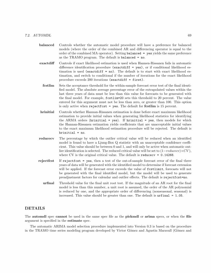
7.2. AUTOMDL 69
balanced Controls whether the automatic model procedure will have a preference for balancedmodels (where the order of the combined AR and differencing operator is equal to theorder of the combined MA operator). Setting balanced = yes yields the same preferenceas the TRAMO program. The default is balanced = no.
exactdiff Controls if exact likelihood estimation is used when Hannen-Rissanen fails in automaticdifference identification procedure (exactdiff = yes), or if conditional likelihood es-timation is used (exactdiff = no). The default is to start with exact likelihood es-timation, and switch to conditional if the number of iterations for the exact likelihoodprocedure exceeds 200 iterations (exactdiff = first).
fcstlim Sets the acceptance threshold for the within-sample forecast error test of the final identi-fied model. The absolute average percentage error of the extrapolated values within thelast three years of data must be less than this value for forecasts to be generated withthe final model. For example, fcstlim=20 sets this threshold to 20 percent. The valueentered for this argument must not be less than zero, or greater than 100. This optionis only active when rejectfcst = yes. The default for fcstlim is 15 percent.
hrinitial Controls whether Hannan-Rissanen estimation is done before exact maximum likelihoodestimation to provide initial values when generating likelihood statistics for identifyingthe ARMA orders (hrinitial = yes). If hrinitial = yes, then models for whichthe Hannan-Rissanen estimation yields coefficients that are unacceptable initial valuesto the exact maximum likelihood estimation procedure will be rejected. The default ishrinitial = no.
reducecv The percentage by which the outlier critical value will be reduced when an identifiedmodel is found to have a Ljung-Box Q statistic with an unacceptable confidence coeffi-cient. This value should be between 0 and 1, and will only be active when automatic out-lier identification is selected. The reduced critical value will be set to (1−reducecv)×CV ),where CV is the original critical value. The default is reducecv = 0.14268.
rejectfcst If rejectfcst = yes, then a test of the out-of-sample forecast error of the final threeyears of data will be generated with the identified model to determine if forecast extensionwill be applied. If the forecast error exceeds the value of fcstlimit, forecasts will notbe generated with the final identified model, but the model will be used to generatepreadjustment factors for calendar and outlier effects. The default is rejectfcst=no.
urfinal Threshold value for the final unit root test. If the magnitude of an AR root for the finalmodel is less than this number, a unit root is assumed, the order of the AR polynomialis reduced by one, and the appropriate order of differencing (nonseasonal, seasonal) isincreased. This value should be greater than one. The default is urfinal = 1.05.
DETAILS
The automdl spec cannot be used in the same spec file as the pickmdl or arima specs, or when the fileargument is specified in the estimate spec.
The automatic ARIMA model selection procedure implemented into Version 0.3 is based on the procedurein the TRAMO time series modeling program developed by Victor Gomez and Agustin Maravall (Gomez and

70 CHAPTER 7. DOCUMENTATION FOR INDIVIDUAL SPECS
Maravall 1996). It is very similar to TRAMO’s procedure but contains modifications to make use of X-13-
ARIMA-SEATS’ different model estimation procedure, regARIMA model options, transformation and outlieridentification procedures and model diagnostics. Also some additional tests have been added. Consequently,the model selected can differ from the model TRAMO would select. Extensive testing has shown that themodels selected are usually at least as good as those selected by TRAMO (preliminary results in Hood 2002a).
The TRAMO procedure is largely documented in Gomez and Maravall (2001a), but the actual implemen-tation of the procedure in the current TRAMO program differs somewhat from the description that appears inthe paper.
An overview of the ARIMA model selection procedure is given below, as given in Monsell (2002, 2006). Theprocedure can be summarized in five stages:
• default model estimation: a default model is estimated, initial outlier identification and regressor testsare performed, and residual diagnostics are generated;
• identification of differencing orders: empirical unit root tests are performed to determine the ordersof differencing needed for the model;
• identification of ARMA model orders: an iterative procedure is applied to determine the order ofARMA parameters;
• comparison of identified model with default model: the identified model is compared to the defaultmodel; and
• final model checks: where the final model is checked for adequacy.
Note that the second stage is optional, as the user can specify the orders of regular and seasonal differencingusing the diff argument.
Default model estimation
The first step of the automatic outlier procedure is to estimate a default model. For monthly and quarterlyseries, this is initially an “airline” model: ARIMA (0 1 1)(0 1 1)s.
The default model is used to perform a number of tasks. If tests for trading day, Easter or user-definedregressors are requested by the user in the regression spec, an initial check for the significance of these effectsis performed using the default model. The X-13ARIMA-SEATS program’s aictest option is used to check thesignificance of the regressors using a small sample variant of AIC called AICC (otherwise known as the F-adjusted Akaike’s Information Criterion, see Hurvich and Tsai 1989). For more details on how AIC tests forregressors are implemented within X-13ARIMA-SEATS see the DETAILS section of the regression spec.
The procedure then checks the significance of including a constant term in the regARIMA model. A t-statistic for the mean of the model residuals is generated, and is checked against a critical value of 1.96.
Once these tests are complete, the program performs automatic outlier identification (if specified by the userin the outlier spec). Details concerning X-13ARIMA-SEATS program’s automatic outlier identification routine
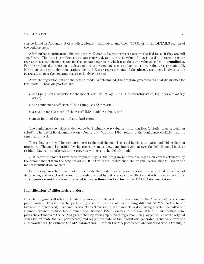
7.2. AUTOMDL 71
can be found in Appendix B of Findley, Monsell, Bell, Otto, and Chen (1998), or in the DETAILS section ofthe outlier spec.
After outlier identification, the trading day, Easter and constant regressors are checked to see if they are stillsignificant. This test is simpler: t-tests are generated, and a critical value of 1.96 is used to determine if theregressors are significant (except for the constant regressor, which uses the same value specified in armalimit).For the trading day regressor, at least one of the regressors needs to have a critical value greater than 1.96.Note that this test is done for trading day and Easter regressors only if the aictest argument is given in theregression spec; the constant regressor is always tested.
After the regression part of the default model is determined, the program generates residual diagnostics forthis model. These diagnostics are:
• the Ljung-Box Q statistic for the model residuals (at lag 24 if this is a monthly series, lag 16 for a quarterlyseries),
• the confidence coefficient of this Ljung-Box Q statistic ,
• a t-value for the mean of the regARIMA model residuals, and
• an estimate of the residual standard error.
The confidence coefficient is defined to be 1 minus the p-value of the Ljung-Box Q statistic, as in Lehman(1986). The TRAMO documentation (Gomez and Maravall 1996) refers to the confidence coefficient as thesignificance level.
These diagnostics will be compared later to those of the model selected by the automatic model identificationprocedure. The model identified by this procedure must show some improvement over the default model in theseresidual diagnostics; otherwise, the program will accept the default model.
Just before the model identification phase begins, the program removes the regression effects estimated bythe default model from the original series. It is this series, rather than the original series, that is used in themodel identification routines.
In this way, an attempt is made to robustify the model identification process, to ensure that the choice ofdifferencing and model orders are not unduly affected by outliers, calendar effects, and other regression effects.This regression residual series is referred to as the linearized series in the TRAMO documentation.
Identification of differencing orders
Now the program will attempt to identify an appropriate order of differencing for the “linearized” series com-puted earlier. This is done by performing a series of unit root tests, fitting different ARMA models to the(sometimes differenced) linearized series. The estimation of these models is done using a technique called theHannan-Rissanen method (see Hannan and Rissanen 1982, Gomez and Maravall 2001a). This method com-putes the estimates of the ARMA parameters by setting up a linear regression using lagged values of the originalseries (to estimate the AR parameters) and lagged estimate of the innovations generated recursively from theautocovariances (to estimate the MA parameters). Biases in the MA parameters are corrected with a technique

72 CHAPTER 7. DOCUMENTATION FOR INDIVIDUAL SPECS
provided by Chen (1985), and the MA parameter estimates are improved when AR parameters are present byapplying Chen’s method to the series filtered by the AR filter (see Gomez 1998).
Step 1 : The first stage of the procedure fits a (2 0 0)(1 0 0)s ARIMA model to the linear series using theHannan-Rissanen method, and examines the real AR roots of the estimated model. The program considers sucha root a unit root if the modulus of the root is less than 1.042, and the order of differencing that correspondsto the root (seasonal or nonseasonal) is increased by one.
If the Hannan-Rissanen procedure estimates a model with roots inside the unit circle, X-13ARIMA-SEATSre-estimates the model using exact maximum likelihood estimation and the modulus test described above isapplied to the resulting estimates.
Step 2 : If differencings were found in Step 1, the linearized series is differenced at the start of Step 2. AnARMA (1 1)(1 1)s model is then fit to the resulting series, and the AR parameters are checked to see if theyare close to one. The criterion for “close to one” depends on whether the program is examining the regular orseasonal AR coefficients.
If an AR coefficient is found that meets the criterion, the program checks to see if there is a common factorin the corresponding AR and MA polynomials of the ARMA model that can be cancelled.
If there is no cancellation, the differencing order changes. The linearized series is differenced using thisnew set of differencing orders. The ARMA model is fit again, and the program checks to see if any furtherdifferencings can be found. This process repeats until no further differencings are found.
Once the differencing orders are determined, a t-statistic for the mean term of the fully differenced series isgenerated based on either the sample mean (if no differencing is identified) or by adding a constant term to theregARIMA model. The critical value of the test is set based on the number of observations in the series.
This is a simplified overview of the actual process. Other tests may be performed if no differencings arefound in Step 2, and the procedure has checks implemented to avoid going from no differencings after Step 1 toboth regular and seasonal differencing after the first stage of Step 2. For more details, see Gomez and Maravall(2001a).
Identification of ARMA model orders
Once an appropriate set of differencing orders has been found, the program turns to the identification ofthe orders of the ARMA model. The basic procedure involves comparing values of the Bayesian InformationCriterion (see Schwarz 1978) of a number of models, up to a maximum order for the regular and seasonal ARMApolynomial which can be specified by the user. As with Akaike’s AIC criterion, the model with the lowest BICis preferred.
The formula below is the classical formula for BIC that is printed out in the X-13ARIMA-SEATS output.
BICN = −2LN + np logN,
where LN is the maximized value of the log likelihood evaluated over N observations, np is the number ofestimated parameters in the model, including the white noise variances, and N is the number of observationsremaining after application of the model’s differencing and seasonal differencing operations.

7.2. AUTOMDL 73
TRAMO uses a variant of this BIC formula in its automatic model identification procedure which dividesthe log likelihood and the penalty term by N . In order to be able to use TRAMO’s final selection criteria,it is necessary that X-13ARIMA-SEATS have a comparable variant of BIC. So X-13ARIMA-SEATS generates thefollowing BIC which is only used for the automatic modeling procedure:
BIC2N = (−2LN + np logN)/N.
The identification procedure allows the user to specify the maximum order of regular AR and MA polynomial(mr, can be as high as 3, default of 2) and seasonal AR and MA polynomial (ms, can be as high as 2, default of1) up to which the program estimates ARIMA models and generates values of BIC2. A three stage procedureis detailed in Gomez and Maravall (2000) that reduces the number of models estimated.
To get an initial estimate for the seasonal model orders, BIC2 is computed for all ARIMA models of theform (3 d 0)(P D Q)s, where d and D are the previously determined or specified regular and seasonal ordersof differencing, respectively, and 0 ≤ P,Q ≤ ms. The program then chooses the pair of values P and Q thatminimize BIC2.
Using these values of P and Q, the program now tries to identify the best model orders for the nonseasonalpart of the ARIMA model. BIC2 is computed for all ARIMA (p d q)(P D Q)s models, where d and D are theregular and seasonal orders of differencing, respectively, and 0 ≤ p, q ≤ mr. The pair of values p and q arechosen that minimize BIC2.
Using these values of p and q, the selection of seasonal model orders is now refined. The program computesBIC2 for all ARIMA (p d q)(P D Q)s models, where d and D are the regular and seasonal orders of differencing,respectively, and 0 ≤ P,Q ≤ ms. The pair of values P and Q are chosen that minimize BIC2.
There is one exception for this third stage of the process: if no seasonal AR was found in the first stage of theprocess, and a seasonal differencing is present, then program only computes BIC2 for ARIMA (p d q)(0 D Q)smodels, where d and D are the regular and seasonal orders of differencing, respectively, and 0 ≤ Q ≤ ms. Thevalues of Q is chosen that minimizes BIC2.
During the ARMA order selection process, X-13ARIMA-SEATS keeps track of the models with the five smallestBIC2s. Once the identification phase is over, the program will compare the BIC2 for the best model with thatof the other 4 models to see if there are models with BIC2s that are “close” enough that there is no “significant”difference between the models. The criteria for “close enough” depends on the length of the series, the magnitudeof the difference between the BICs, and other criteria.
If the program finds a model that is “close” enough to the best model, the program also checks to see whetherthe model with the higher BIC is more parsimonious (especially in the seasonal operator) than the best model.If so, the program will accept the more parsimonious model.
The program also checks for model balance. A model is said to be more balanced than a competing modelif the absolute difference between the total orders of the AR plus differencing and MA operators is smaller forone model than another. While balanced models are useful for model-based seasonal adjustment, it is unclearwhether this criterion is useful for the types of operations X-13ARIMA-SEATS does, as it induces a small biastoward mixed models and mixed ARMA models can be difficult to estimate due to near cancellation. Therefore,X-13ARIMA-SEATS makes checking for model balance at this stage optional; the default is not to test for modelbalance.
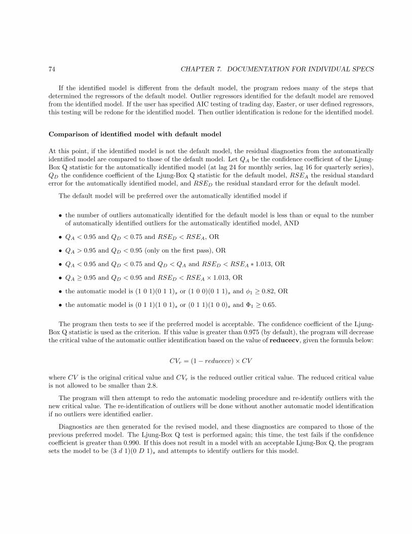
74 CHAPTER 7. DOCUMENTATION FOR INDIVIDUAL SPECS
If the identified model is different from the default model, the program redoes many of the steps thatdetermined the regressors of the default model. Outlier regressors identified for the default model are removedfrom the identified model. If the user has specified AIC testing of trading day, Easter, or user defined regressors,this testing will be redone for the identified model. Then outlier identification is redone for the identified model.
Comparison of identified model with default model
At this point, if the identified model is not the default model, the residual diagnostics from the automaticallyidentified model are compared to those of the default model. Let QA be the confidence coefficient of the Ljung-Box Q statistic for the automatically identified model (at lag 24 for monthly series, lag 16 for quarterly series),QD the confidence coefficient of the Ljung-Box Q statistic for the default model, RSEA the residual standarderror for the automatically identified model, and RSED the residual standard error for the default model.
The default model will be preferred over the automatically identified model if
• the number of outliers automatically identified for the default model is less than or equal to the numberof automatically identified outliers for the automatically identified model, AND
• QA < 0.95 and QD < 0.75 and RSED < RSEA, OR
• QA > 0.95 and QD < 0.95 (only on the first pass), OR
• QA < 0.95 and QD < 0.75 and QD < QA and RSED < RSEA ∗ 1.013, OR
• QA ≥ 0.95 and QD < 0.95 and RSED < RSEA × 1.013, OR
• the automatic model is (1 0 1)(0 1 1)s or (1 0 0)(0 1 1)s and φ1 ≥ 0.82, OR
• the automatic model is (0 1 1)(1 0 1)s or (0 1 1)(1 0 0)s and Φ1 ≥ 0.65.
The program then tests to see if the preferred model is acceptable. The confidence coefficient of the Ljung-Box Q statistic is used as the criterion. If this value is greater than 0.975 (by default), the program will decreasethe critical value of the automatic outlier identification based on the value of reducecv, given the formula below:
CVr = (1− reducecv)× CV
where CV is the original critical value and CVr is the reduced outlier critical value. The reduced critical valueis not allowed to be smaller than 2.8.
The program will then attempt to redo the automatic modeling procedure and re-identify outliers with thenew critical value. The re-identification of outliers will be done without another automatic model identificationif no outliers were identified earlier.
Diagnostics are then generated for the revised model, and these diagnostics are compared to those of theprevious preferred model. The Ljung-Box Q test is performed again; this time, the test fails if the confidencecoefficient is greater than 0.990. If this does not result in a model with an acceptable Ljung-Box Q, the programsets the model to be (3 d 1)(0 D 1)s and attempts to identify outliers for this model.
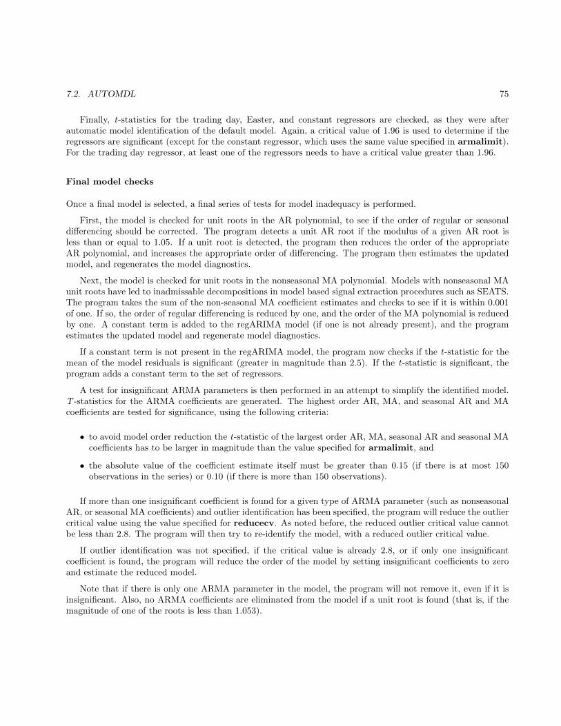
7.2. AUTOMDL 75
Finally, t-statistics for the trading day, Easter, and constant regressors are checked, as they were afterautomatic model identification of the default model. Again, a critical value of 1.96 is used to determine if theregressors are significant (except for the constant regressor, which uses the same value specified in armalimit).For the trading day regressor, at least one of the regressors needs to have a critical value greater than 1.96.
Final model checks
Once a final model is selected, a final series of tests for model inadequacy is performed.
First, the model is checked for unit roots in the AR polynomial, to see if the order of regular or seasonaldifferencing should be corrected. The program detects a unit AR root if the modulus of a given AR root isless than or equal to 1.05. If a unit root is detected, the program then reduces the order of the appropriateAR polynomial, and increases the appropriate order of differencing. The program then estimates the updatedmodel, and regenerates the model diagnostics.
Next, the model is checked for unit roots in the nonseasonal MA polynomial. Models with nonseasonal MAunit roots have led to inadmissable decompositions in model based signal extraction procedures such as SEATS.The program takes the sum of the non-seasonal MA coefficient estimates and checks to see if it is within 0.001of one. If so, the order of regular differencing is reduced by one, and the order of the MA polynomial is reducedby one. A constant term is added to the regARIMA model (if one is not already present), and the programestimates the updated model and regenerate model diagnostics.
If a constant term is not present in the regARIMA model, the program now checks if the t-statistic for themean of the model residuals is significant (greater in magnitude than 2.5). If the t-statistic is significant, theprogram adds a constant term to the set of regressors.
A test for insignificant ARMA parameters is then performed in an attempt to simplify the identified model.T -statistics for the ARMA coefficients are generated. The highest order AR, MA, and seasonal AR and MAcoefficients are tested for significance, using the following criteria:
• to avoid model order reduction the t-statistic of the largest order AR, MA, seasonal AR and seasonal MAcoefficients has to be larger in magnitude than the value specified for armalimit, and
• the absolute value of the coefficient estimate itself must be greater than 0.15 (if there is at most 150observations in the series) or 0.10 (if there is more than 150 observations).
If more than one insignificant coefficient is found for a given type of ARMA parameter (such as nonseasonalAR, or seasonal MA coefficients) and outlier identification has been specified, the program will reduce the outliercritical value using the value specified for reducecv. As noted before, the reduced outlier critical value cannotbe less than 2.8. The program will then try to re-identify the model, with a reduced outlier critical value.
If outlier identification was not specified, if the critical value is already 2.8, or if only one insignificantcoefficient is found, the program will reduce the order of the model by setting insignificant coefficients to zeroand estimate the reduced model.
Note that if there is only one ARMA parameter in the model, the program will not remove it, even if it isinsignificant. Also, no ARMA coefficients are eliminated from the model if a unit root is found (that is, if themagnitude of one of the roots is less than 1.053).
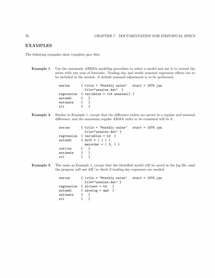
76 CHAPTER 7. DOCUMENTATION FOR INDIVIDUAL SPECS
EXAMPLES
The following examples show complete spec files.
Example 1 Use the automatic ARIMA modeling procedure to select a model and use it to extend theseries with one year of forecasts. Trading day and stable seasonal regression effects are tobe included in the models. A default seasonal adjustment is to be performed.
series { title = "Monthly sales" start = 1976.jan
file="ussales.dat" }
regression { variables = (td seasonal) }
automdl { }
estimate { }
x11 { }
Example 2 Similar to Example 1, except that the difference orders are preset to a regular and seasonaldifference, and the maximum regular ARMA order to be examined will be 3.
series { title = "Monthly sales" start = 1976.jan
file="ussales.dat" }
regression { variables = td }
automdl { diff = ( 1 1 )
maxorder = ( 3, ) }
outlier { }
estimate { }
x11 { }
Example 3 The same as Example 1, except that the identified model will be saved in the log file, amdthe program will use AIC to check if trading day regressors are needed.
series { title = "Monthly sales" start = 1976.jan
file="ussales.dat" }
regression { aictest = td }
automdl { savelog = amd }
estimate { }
x11 { }
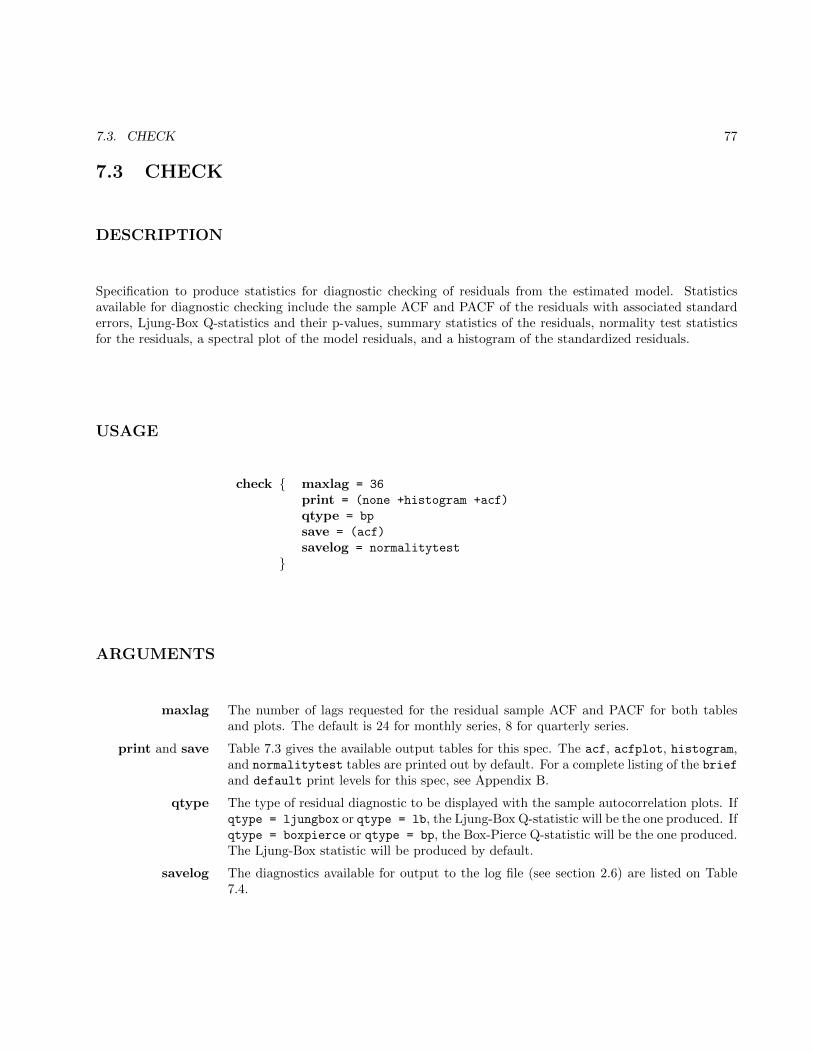
7.3. CHECK 77
7.3 CHECK
DESCRIPTION
Specification to produce statistics for diagnostic checking of residuals from the estimated model. Statisticsavailable for diagnostic checking include the sample ACF and PACF of the residuals with associated standarderrors, Ljung-Box Q-statistics and their p-values, summary statistics of the residuals, normality test statisticsfor the residuals, a spectral plot of the model residuals, and a histogram of the standardized residuals.
USAGE
check { maxlag = 36
print = (none +histogram +acf)
qtype = bp
save = (acf)
savelog = normalitytest
}
ARGUMENTS
maxlag The number of lags requested for the residual sample ACF and PACF for both tablesand plots. The default is 24 for monthly series, 8 for quarterly series.
print and save Table 7.3 gives the available output tables for this spec. The acf, acfplot, histogram,and normalitytest tables are printed out by default. For a complete listing of the briefand default print levels for this spec, see Appendix B.
qtype The type of residual diagnostic to be displayed with the sample autocorrelation plots. Ifqtype = ljungbox or qtype = lb, the Ljung-Box Q-statistic will be the one produced. Ifqtype = boxpierce or qtype = bp, the Box-Pierce Q-statistic will be the one produced.The Ljung-Box statistic will be produced by default.
savelog The diagnostics available for output to the log file (see section 2.6) are listed on Table7.4.
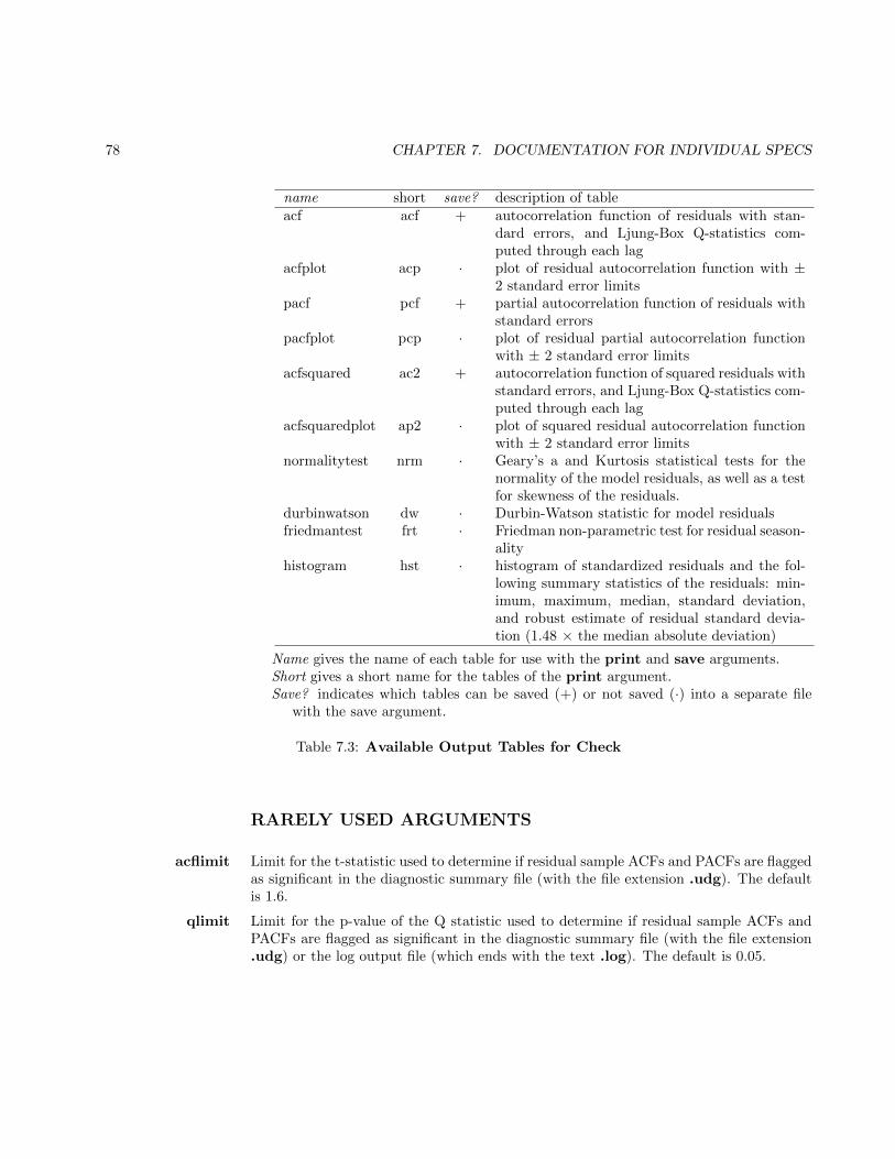
78 CHAPTER 7. DOCUMENTATION FOR INDIVIDUAL SPECS
name short save? description of tableacf acf + autocorrelation function of residuals with stan-
dard errors, and Ljung-Box Q-statistics com-puted through each lag
acfplot acp · plot of residual autocorrelation function with ±2 standard error limits
pacf pcf + partial autocorrelation function of residuals withstandard errors
pacfplot pcp · plot of residual partial autocorrelation functionwith ± 2 standard error limits
acfsquared ac2 + autocorrelation function of squared residuals withstandard errors, and Ljung-Box Q-statistics com-puted through each lag
acfsquaredplot ap2 · plot of squared residual autocorrelation functionwith ± 2 standard error limits
normalitytest nrm · Geary’s a and Kurtosis statistical tests for thenormality of the model residuals, as well as a testfor skewness of the residuals.
durbinwatson dw · Durbin-Watson statistic for model residualsfriedmantest frt · Friedman non-parametric test for residual season-
alityhistogram hst · histogram of standardized residuals and the fol-
lowing summary statistics of the residuals: min-imum, maximum, median, standard deviation,and robust estimate of residual standard devia-tion (1.48 × the median absolute deviation)
Name gives the name of each table for use with the print and save arguments.Short gives a short name for the tables of the print argument.Save? indicates which tables can be saved (+) or not saved (·) into a separate file
with the save argument.
Table 7.3: Available Output Tables for Check
RARELY USED ARGUMENTS
acflimit Limit for the t-statistic used to determine if residual sample ACFs and PACFs are flaggedas significant in the diagnostic summary file (with the file extension .udg). The defaultis 1.6.
qlimit Limit for the p-value of the Q statistic used to determine if residual sample ACFs andPACFs are flagged as significant in the diagnostic summary file (with the file extension.udg) or the log output file (which ends with the text .log). The default is 0.05.
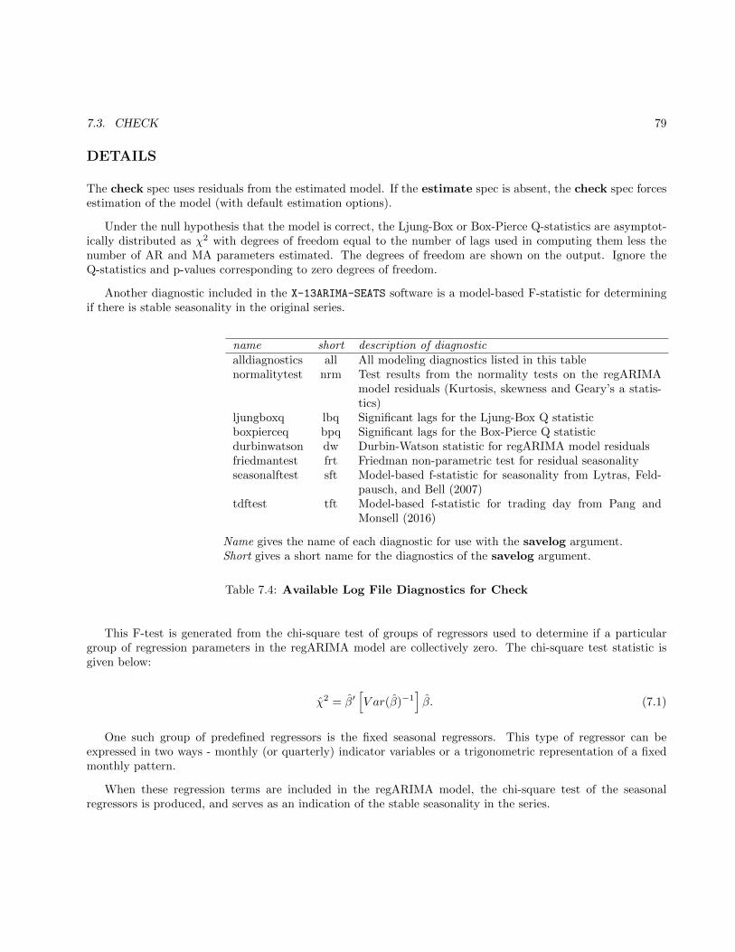
7.3. CHECK 79
DETAILS
The check spec uses residuals from the estimated model. If the estimate spec is absent, the check spec forcesestimation of the model (with default estimation options).
Under the null hypothesis that the model is correct, the Ljung-Box or Box-Pierce Q-statistics are asymptot-ically distributed as χ2 with degrees of freedom equal to the number of lags used in computing them less thenumber of AR and MA parameters estimated. The degrees of freedom are shown on the output. Ignore theQ-statistics and p-values corresponding to zero degrees of freedom.
Another diagnostic included in the X-13ARIMA-SEATS software is a model-based F-statistic for determiningif there is stable seasonality in the original series.
name short description of diagnosticalldiagnostics all All modeling diagnostics listed in this tablenormalitytest nrm Test results from the normality tests on the regARIMA
model residuals (Kurtosis, skewness and Geary’s a statis-tics)
ljungboxq lbq Significant lags for the Ljung-Box Q statisticboxpierceq bpq Significant lags for the Box-Pierce Q statisticdurbinwatson dw Durbin-Watson statistic for regARIMA model residualsfriedmantest frt Friedman non-parametric test for residual seasonalityseasonalftest sft Model-based f-statistic for seasonality from Lytras, Feld-
pausch, and Bell (2007)tdftest tft Model-based f-statistic for trading day from Pang and
Monsell (2016)
Name gives the name of each diagnostic for use with the savelog argument.Short gives a short name for the diagnostics of the savelog argument.
Table 7.4: Available Log File Diagnostics for Check
This F-test is generated from the chi-square test of groups of regressors used to determine if a particulargroup of regression parameters in the regARIMA model are collectively zero. The chi-square test statistic isgiven below:
χ2 = β′[V ar(β)−1
]β. (7.1)
One such group of predefined regressors is the fixed seasonal regressors. This type of regressor can beexpressed in two ways - monthly (or quarterly) indicator variables or a trigonometric representation of a fixedmonthly pattern.
When these regression terms are included in the regARIMA model, the chi-square test of the seasonalregressors is produced, and serves as an indication of the stable seasonality in the series.
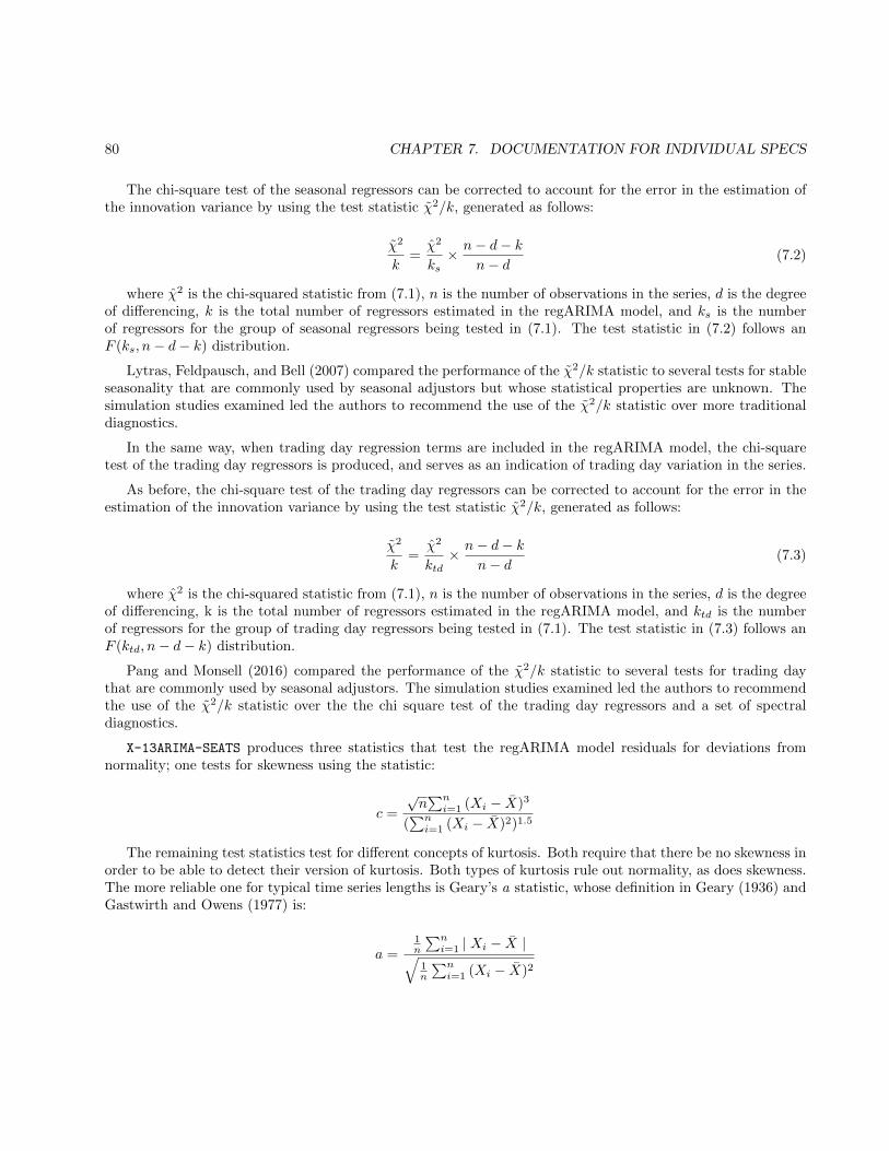
80 CHAPTER 7. DOCUMENTATION FOR INDIVIDUAL SPECS
The chi-square test of the seasonal regressors can be corrected to account for the error in the estimation ofthe innovation variance by using the test statistic χ2/k, generated as follows:
χ2
k=χ2
ks× n− d− k
n− d(7.2)
where χ2 is the chi-squared statistic from (7.1), n is the number of observations in the series, d is the degreeof differencing, k is the total number of regressors estimated in the regARIMA model, and ks is the numberof regressors for the group of seasonal regressors being tested in (7.1). The test statistic in (7.2) follows anF (ks, n− d− k) distribution.
Lytras, Feldpausch, and Bell (2007) compared the performance of the χ2/k statistic to several tests for stableseasonality that are commonly used by seasonal adjustors but whose statistical properties are unknown. Thesimulation studies examined led the authors to recommend the use of the χ2/k statistic over more traditionaldiagnostics.
In the same way, when trading day regression terms are included in the regARIMA model, the chi-squaretest of the trading day regressors is produced, and serves as an indication of trading day variation in the series.
As before, the chi-square test of the trading day regressors can be corrected to account for the error in theestimation of the innovation variance by using the test statistic χ2/k, generated as follows:
χ2
k=χ2
ktd× n− d− k
n− d(7.3)
where χ2 is the chi-squared statistic from (7.1), n is the number of observations in the series, d is the degreeof differencing, k is the total number of regressors estimated in the regARIMA model, and ktd is the numberof regressors for the group of trading day regressors being tested in (7.1). The test statistic in (7.3) follows anF (ktd, n− d− k) distribution.
Pang and Monsell (2016) compared the performance of the χ2/k statistic to several tests for trading daythat are commonly used by seasonal adjustors. The simulation studies examined led the authors to recommendthe use of the χ2/k statistic over the the chi square test of the trading day regressors and a set of spectraldiagnostics.
X-13ARIMA-SEATS produces three statistics that test the regARIMA model residuals for deviations fromnormality; one tests for skewness using the statistic:
c =
√n∑ni=1 (Xi − X)3
(∑ni=1 (Xi − X)2)1.5
The remaining test statistics test for different concepts of kurtosis. Both require that there be no skewness inorder to be able to detect their version of kurtosis. Both types of kurtosis rule out normality, as does skewness.The more reliable one for typical time series lengths is Geary’s a statistic, whose definition in Geary (1936) andGastwirth and Owens (1977) is:
a =1n
∑ni=1 | Xi − X |√
1n
∑ni=1 (Xi − X)2
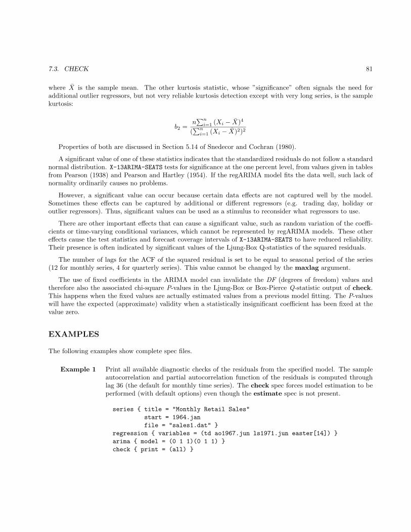
7.3. CHECK 81
where X is the sample mean. The other kurtosis statistic, whose ”significance” often signals the need foradditional outlier regressors, but not very reliable kurtosis detection except with very long series, is the samplekurtosis:
b2 =n∑ni=1 (Xi − X)4
(∑ni=1 (Xi − X)2)2
Properties of both are discussed in Section 5.14 of Snedecor and Cochran (1980).
A significant value of one of these statistics indicates that the standardized residuals do not follow a standardnormal distribution. X-13ARIMA-SEATS tests for significance at the one percent level, from values given in tablesfrom Pearson (1938) and Pearson and Hartley (1954). If the regARIMA model fits the data well, such lack ofnormality ordinarily causes no problems.
However, a significant value can occur because certain data effects are not captured well by the model.Sometimes these effects can be captured by additional or different regressors (e.g. trading day, holiday oroutlier regressors). Thus, significant values can be used as a stimulus to reconsider what regressors to use.
There are other important effects that can cause a significant value, such as random variation of the coeffi-cients or time-varying conditional variances, which cannot be represented by regARIMA models. These othereffects cause the test statistics and forecast coverage intervals of X-13ARIMA-SEATS to have reduced reliability.Their presence is often indicated by significant values of the Ljung-Box Q-statistics of the squared residuals.
The number of lags for the ACF of the squared residual is set to be equal to seasonal period of the series(12 for monthly series, 4 for quarterly series). This value cannot be changed by the maxlag argument.
The use of fixed coefficients in the ARIMA model can invalidate the DF (degrees of freedom) values andtherefore also the associated chi-square P-values in the Ljung-Box or Box-Pierce Q-statistic output of check.This happens when the fixed values are actually estimated values from a previous model fitting. The P-valueswill have the expected (approximate) validity when a statistically insignificant coefficient has been fixed at thevalue zero.
EXAMPLES
The following examples show complete spec files.
Example 1 Print all available diagnostic checks of the residuals from the specified model. The sampleautocorrelation and partial autocorrelation function of the residuals is computed throughlag 36 (the default for monthly time series). The check spec forces model estimation to beperformed (with default options) even though the estimate spec is not present.
series { title = "Monthly Retail Sales"
start = 1964.jan
file = "sales1.dat" }
regression { variables = (td ao1967.jun ls1971.jun easter[14]) }
arima { model = (0 1 1)(0 1 1) }
check { print = (all) }
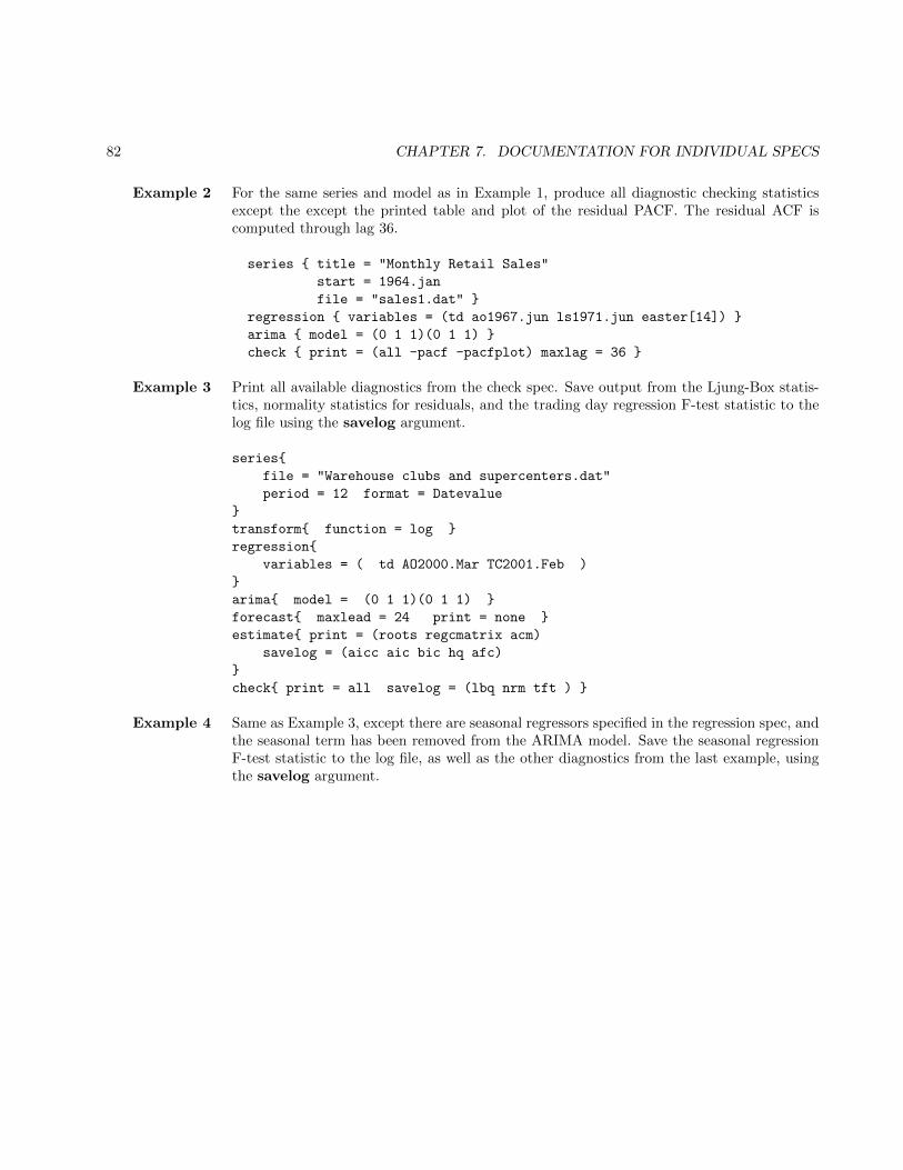
82 CHAPTER 7. DOCUMENTATION FOR INDIVIDUAL SPECS
Example 2 For the same series and model as in Example 1, produce all diagnostic checking statisticsexcept the except the printed table and plot of the residual PACF. The residual ACF iscomputed through lag 36.
series { title = "Monthly Retail Sales"
start = 1964.jan
file = "sales1.dat" }
regression { variables = (td ao1967.jun ls1971.jun easter[14]) }
arima { model = (0 1 1)(0 1 1) }
check { print = (all -pacf -pacfplot) maxlag = 36 }
Example 3 Print all available diagnostics from the check spec. Save output from the Ljung-Box statis-tics, normality statistics for residuals, and the trading day regression F-test statistic to thelog file using the savelog argument.
series{
file = "Warehouse clubs and supercenters.dat"
period = 12 format = Datevalue
}
transform{ function = log }
regression{
variables = ( td AO2000.Mar TC2001.Feb )
}
arima{ model = (0 1 1)(0 1 1) }
forecast{ maxlead = 24 print = none }
estimate{ print = (roots regcmatrix acm)
savelog = (aicc aic bic hq afc)
}
check{ print = all savelog = (lbq nrm tft ) }
Example 4 Same as Example 3, except there are seasonal regressors specified in the regression spec, andthe seasonal term has been removed from the ARIMA model. Save the seasonal regressionF-test statistic to the log file, as well as the other diagnostics from the last example, usingthe savelog argument.
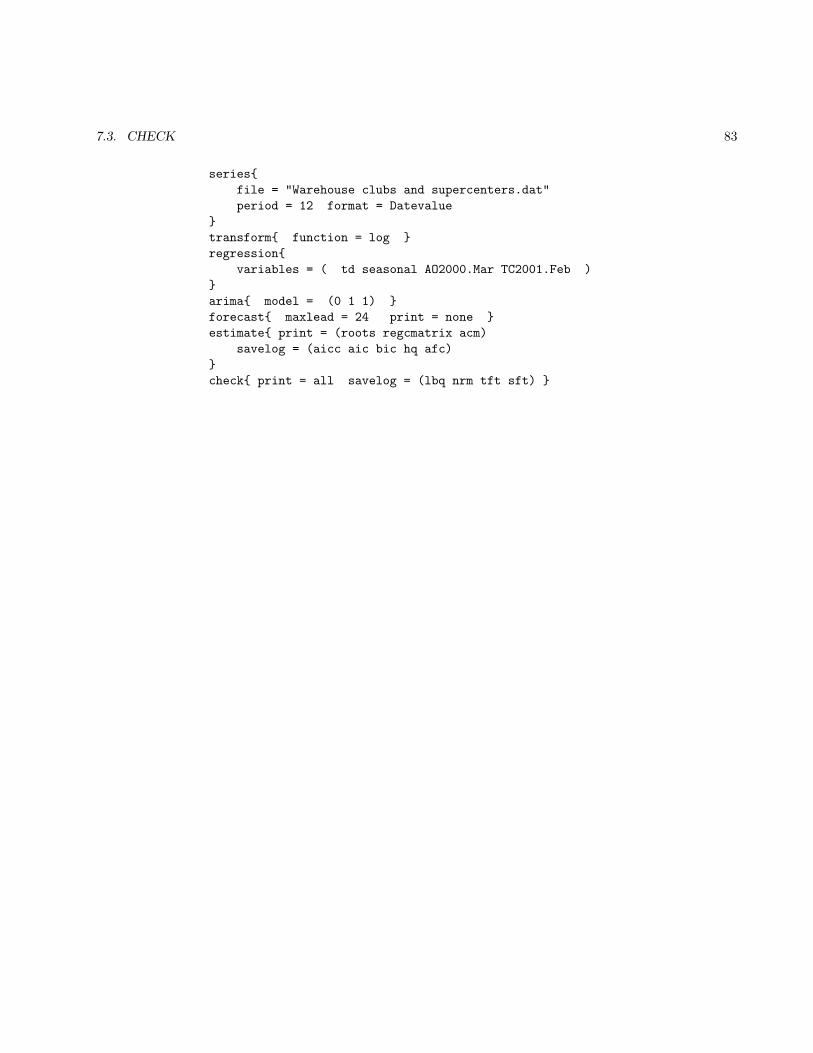
7.3. CHECK 83
series{
file = "Warehouse clubs and supercenters.dat"
period = 12 format = Datevalue
}
transform{ function = log }
regression{
variables = ( td seasonal AO2000.Mar TC2001.Feb )
}
arima{ model = (0 1 1) }
forecast{ maxlead = 24 print = none }
estimate{ print = (roots regcmatrix acm)
savelog = (aicc aic bic hq afc)
}
check{ print = all savelog = (lbq nrm tft sft) }
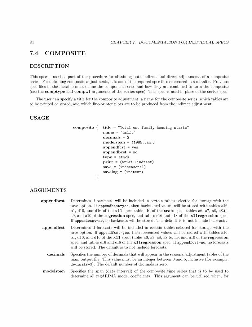
84 CHAPTER 7. DOCUMENTATION FOR INDIVIDUAL SPECS
7.4 COMPOSITE
DESCRIPTION
This spec is used as part of the procedure for obtaining both indirect and direct adjustments of a compositeseries. For obtaining composite adjustments, it is one of the required spec files referenced in a metafile. Previousspec files in the metafile must define the component series and how they are combined to form the composite(see the comptype and compwt arguments of the series spec). This spec is used in place of the series spec.
The user can specify a title for the composite adjustment, a name for the composite series, which tables areto be printed or stored, and which line-printer plots are to be produced from the indirect adjustment.
USAGE
composite { title = "Total one family housing starts"
name = "hs1ft"
decimals = 2
modelspan = (1985.Jan,)
appendfcst = yes
appendbcst = no
type = stock
print = (brief +indtest)
save = (indseasonal)
savelog = (indtest)
}
ARGUMENTS
appendbcst Determines if backcasts will be included in certain tables selected for storage with thesave option. If appendbcst=yes, then backcasted values will be stored with tables a16,b1, d10, and d16 of the x11 spec, table s10 of the seats spec, tables a6, a7, a8, a8.tc,a9, and a10 of the regression spec, and tables c16 and c18 of the x11regression spec.If appendbcst=no, no backcasts will be stored. The default is to not include backcasts.
appendfcst Determines if forecasts will be included in certain tables selected for storage with thesave option. If appendfcst=yes, then forecasted values will be stored with tables a16,b1, d10, and d16 of the x11 spec, tables a6, a7, a8, a8.tc, a9, and a10 of the regressionspec, and tables c16 and c18 of the x11regression spec. If appendfcst=no, no forecastswill be stored. The default is to not include forecasts.
decimals Specifies the number of decimals that will appear in the seasonal adjustment tables of themain output file. This value must be an integer between 0 and 5, inclusive (for example,decimals=3). The default number of decimals is zero.
modelspan Specifies the span (data interval) of the composite time series that is to be used todetermine all regARIMA model coefficients. This argument can be utilized when, for
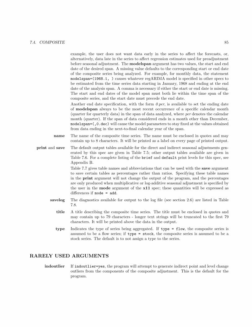
7.4. COMPOSITE 85
example, the user does not want data early in the series to affect the forecasts, or,alternatively, data late in the series to affect regression estimates used for preadjustmentbefore seasonal adjustment. The modelspan argument has two values, the start and enddate of the desired span. A missing value defaults to the corresponding start or end dateof the composite series being analyzed. For example, for monthly data, the statementmodelspan=(1968.1, ) causes whatever regARIMA model is specified in other specs tobe estimated from the time series data starting in January, 1968 and ending at the enddate of the analysis span. A comma is necessary if either the start or end date is missing.The start and end dates of the model span must both lie within the time span of thecomposite series, and the start date must precede the end date.
Another end date specification, with the form 0.per, is available to set the ending dateof modelspan always to be the most recent occurrence of a specific calendar month(quarter for quarterly data) in the span of data analyzed, where per denotes the calendarmonth (quarter). If the span of data considered ends in a month other than December,modelspan=(,0.dec) will cause the model parameters to stay fixed at the values obtainedfrom data ending in the next-to-final calendar year of the span.
name The name of the composite time series. The name must be enclosed in quotes and maycontain up to 8 characters. It will be printed as a label on every page of printed output.
print and save The default output tables available for the direct and indirect seasonal adjustments gen-erated by this spec are given in Table 7.5; other output tables available are given inTable 7.6. For a complete listing of the brief and default print levels for this spec, seeAppendix B.
Table 7.7 gives table names and abbreviations that can be used with the save argumentto save certain tables as percentages rather than ratios. Specifying these table namesin the print argument will not change the output of the program, and the percentagesare only produced when multiplicative or log-additive seasonal adjustment is specified bythe user in the mode argument of the x11 spec; these quantities will be expressed asdifferences if mode = add.
savelog The diagnostics available for output to the log file (see section 2.6) are listed in Table7.8.
title A title describing the composite time series. The title must be enclosed in quotes andmay contain up to 79 characters - longer text strings will be truncated to the first 79characters. It will be printed above the data in the output.
type Indicates the type of series being aggregated. If type = flow, the composite series isassumed to be a flow series; if type = stock, the composite series is assumed to be astock series. The default is to not assign a type to the series.
RARELY USED ARGUMENTS
indoutlier If indoutlier=yes, the program will attempt to generate indirect point and level changeoutliers from the components of the composite adjustment. This is the default for theprogram.
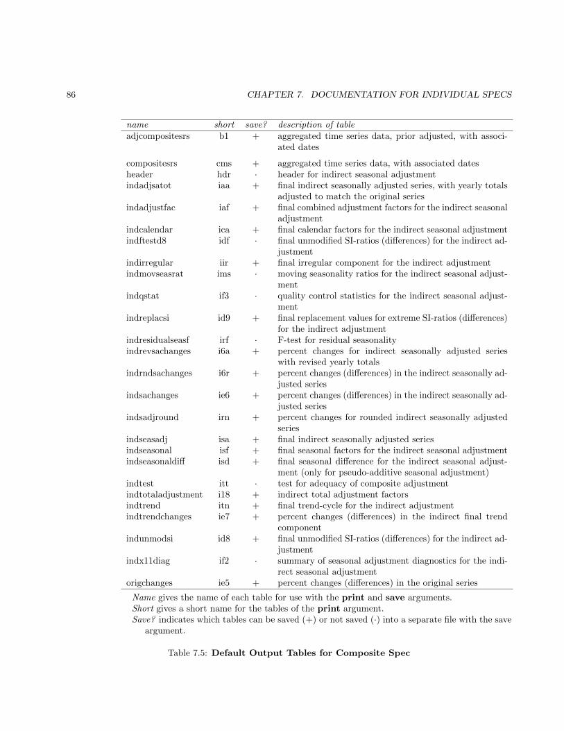
86 CHAPTER 7. DOCUMENTATION FOR INDIVIDUAL SPECS
name short save? description of tableadjcompositesrs b1 + aggregated time series data, prior adjusted, with associ-
ated dates
compositesrs cms + aggregated time series data, with associated datesheader hdr · header for indirect seasonal adjustmentindadjsatot iaa + final indirect seasonally adjusted series, with yearly totals
adjusted to match the original seriesindadjustfac iaf + final combined adjustment factors for the indirect seasonal
adjustmentindcalendar ica + final calendar factors for the indirect seasonal adjustmentindftestd8 idf · final unmodified SI-ratios (differences) for the indirect ad-
justmentindirregular iir + final irregular component for the indirect adjustmentindmovseasrat ims · moving seasonality ratios for the indirect seasonal adjust-
mentindqstat if3 · quality control statistics for the indirect seasonal adjust-
mentindreplacsi id9 + final replacement values for extreme SI-ratios (differences)
for the indirect adjustmentindresidualseasf irf · F-test for residual seasonalityindrevsachanges i6a + percent changes for indirect seasonally adjusted series
with revised yearly totalsindrndsachanges i6r + percent changes (differences) in the indirect seasonally ad-
justed seriesindsachanges ie6 + percent changes (differences) in the indirect seasonally ad-
justed seriesindsadjround irn + percent changes for rounded indirect seasonally adjusted
seriesindseasadj isa + final indirect seasonally adjusted seriesindseasonal isf + final seasonal factors for the indirect seasonal adjustmentindseasonaldiff isd + final seasonal difference for the indirect seasonal adjust-
ment (only for pseudo-additive seasonal adjustment)indtest itt · test for adequacy of composite adjustmentindtotaladjustment i18 + indirect total adjustment factorsindtrend itn + final trend-cycle for the indirect adjustmentindtrendchanges ie7 + percent changes (differences) in the indirect final trend
componentindunmodsi id8 + final unmodified SI-ratios (differences) for the indirect ad-
justmentindx11diag if2 · summary of seasonal adjustment diagnostics for the indi-
rect seasonal adjustmentorigchanges ie5 + percent changes (differences) in the original series
Name gives the name of each table for use with the print and save arguments.Short gives a short name for the tables of the print argument.Save? indicates which tables can be saved (+) or not saved (·) into a separate file with the save
argument.
Table 7.5: Default Output Tables for Composite Spec

7.4. COMPOSITE 87
name short save? description of tableadjcompositesrsplot b1p · plot of the prior adjusted aggregate series
calendaradjcomposite cac + aggregated time series data, adjusted for regARIMAcalendar effects.
compositeplot cmp · plot of the prior adjusted aggregate seriesindaoutlier iao + final indirect AO outliersindirregularplot iip · plot of the final irregular component from the indirect
seasonal adjustmentindlevelshift ils + final indirect LS outliersindmcdmovavg if1 + MCD moving average of the final indirect seasonally
adjusted seriesindmodoriginal ie1 + original series modified for extreme values from the in-
direct seasonal adjustmentindmodsadj ie2 + seasonally adjusted series modified for extreme values
from the indirect seasonal adjustmentindmodirr ie3 + irregular component modified for extreme values from
the indirect seasonal adjustmentindrobustsa iee + final indirect seasonally adjusted series modified for ex-
treme valuesindseasadjplot iap · plot of the final indirect seasonally adjusted seriesindseasonalplot isp · indirect seasonal factor plots, grouped by month or
quarterindtotaladjustment ita + total indirect adjustment factors (only produced if the
original series contains values that are ≤ 0)indtrendplot itp · plot of the final trend-cycle from the indirect seasonal
adjustmentindyrtotals ie4 · ratio of yearly totals of the original series and the indi-
rect seasonally adjusted seriesorigwindsaplot ie0 · plot of the aggregate series with the indirect seasonally
adjusted seriesoutlieradjcomposite oac + aggregated time series data, adjusted for outliers.prioradjcomposite ia3 + composite series adjusted for user-defined prior adjust-
ments applied at the component levelratioplotindsa ir2 · month-to-month (or quarter-to-quarter) ratio plots of
the original seriesratioplotorig ir1 · month-to-month (or quarter-to-quarter) ratio plots of
the indirect seasonally adjusted series
Name gives the name of each table for use with the print and save arguments.Short gives a short name for the tables of the print argument.Save? indicates which tables can be saved (+) or not saved (·) into a separate file with the save
argument.
Table 7.6: Other Output Tables for Composite Spec
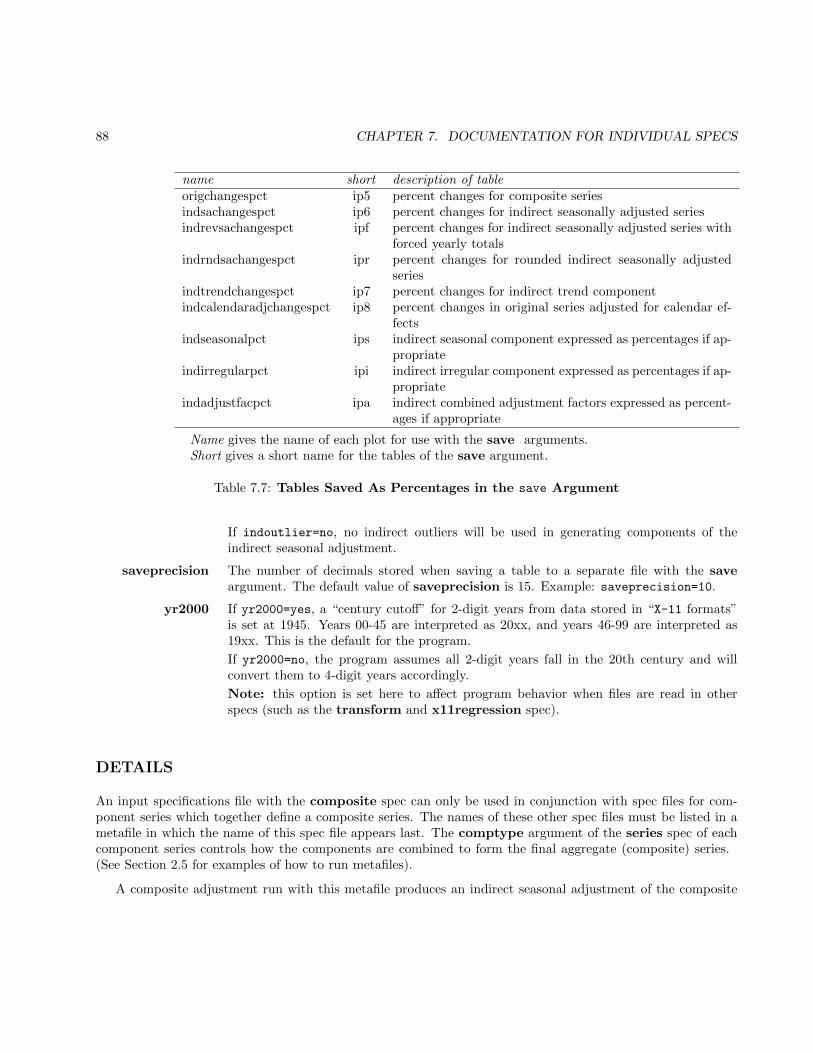
88 CHAPTER 7. DOCUMENTATION FOR INDIVIDUAL SPECS
name short description of tableorigchangespct ip5 percent changes for composite seriesindsachangespct ip6 percent changes for indirect seasonally adjusted seriesindrevsachangespct ipf percent changes for indirect seasonally adjusted series with
forced yearly totalsindrndsachangespct ipr percent changes for rounded indirect seasonally adjusted
seriesindtrendchangespct ip7 percent changes for indirect trend componentindcalendaradjchangespct ip8 percent changes in original series adjusted for calendar ef-
fectsindseasonalpct ips indirect seasonal component expressed as percentages if ap-
propriateindirregularpct ipi indirect irregular component expressed as percentages if ap-
propriateindadjustfacpct ipa indirect combined adjustment factors expressed as percent-
ages if appropriate
Name gives the name of each plot for use with the save arguments.Short gives a short name for the tables of the save argument.
Table 7.7: Tables Saved As Percentages in the save Argument
If indoutlier=no, no indirect outliers will be used in generating components of theindirect seasonal adjustment.
saveprecision The number of decimals stored when saving a table to a separate file with the saveargument. The default value of saveprecision is 15. Example: saveprecision=10.
yr2000 If yr2000=yes, a “century cutoff” for 2-digit years from data stored in “X-11 formats”is set at 1945. Years 00-45 are interpreted as 20xx, and years 46-99 are interpreted as19xx. This is the default for the program.
If yr2000=no, the program assumes all 2-digit years fall in the 20th century and willconvert them to 4-digit years accordingly.
Note: this option is set here to affect program behavior when files are read in otherspecs (such as the transform and x11regression spec).
DETAILS
An input specifications file with the composite spec can only be used in conjunction with spec files for com-ponent series which together define a composite series. The names of these other spec files must be listed in ametafile in which the name of this spec file appears last. The comptype argument of the series spec of eachcomponent series controls how the components are combined to form the final aggregate (composite) series.(See Section 2.5 for examples of how to run metafiles).
A composite adjustment run with this metafile produces an indirect seasonal adjustment of the composite
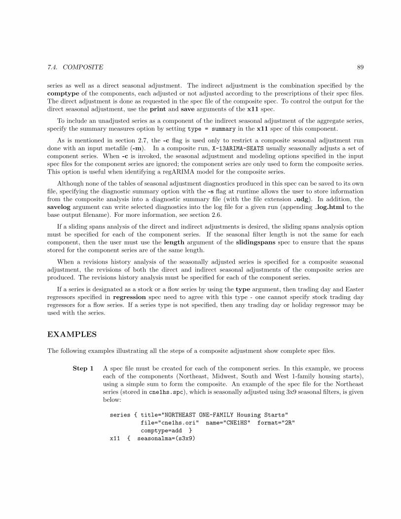
7.4. COMPOSITE 89
series as well as a direct seasonal adjustment. The indirect adjustment is the combination specified by thecomptype of the components, each adjusted or not adjusted according to the prescriptions of their spec files.The direct adjustment is done as requested in the spec file of the composite spec. To control the output for thedirect seasonal adjustment, use the print and save arguments of the x11 spec.
To include an unadjusted series as a component of the indirect seasonal adjustment of the aggregate series,specify the summary measures option by setting type = summary in the x11 spec of this component.
As is mentioned in section 2.7, the -c flag is used only to restrict a composite seasonal adjustment rundone with an input metafile (-m). In a composite run, X-13ARIMA-SEATS usually seasonally adjusts a set ofcomponent series. When -c is invoked, the seasonal adjustment and modeling options specified in the inputspec files for the component series are ignored; the component series are only used to form the composite series.This option is useful when identifying a regARIMA model for the composite series.
Although none of the tables of seasonal adjustment diagnostics produced in this spec can be saved to its ownfile, specifying the diagnostic summary option with the -s flag at runtime allows the user to store informationfrom the composite analysis into a diagnostic summary file (with the file extension .udg). In addition, thesavelog argument can write selected diagnostics into the log file for a given run (appending log.html to thebase output filename). For more information, see section 2.6.
If a sliding spans analysis of the direct and indirect adjustments is desired, the sliding spans analysis optionmust be specified for each of the component series. If the seasonal filter length is not the same for eachcomponent, then the user must use the length argument of the slidingspans spec to ensure that the spansstored for the component series are of the same length.
When a revisions history analysis of the seasonally adjusted series is specified for a composite seasonaladjustment, the revisions of both the direct and indirect seasonal adjustments of the composite series areproduced. The revisions history analysis must be specified for each of the component series.
If a series is designated as a stock or a flow series by using the type argument, then trading day and Easterregressors specified in regression spec need to agree with this type - one cannot specify stock trading dayregressors for a flow series. If a series type is not specified, then any trading day or holiday regressor may beused with the series.
EXAMPLES
The following examples illustrating all the steps of a composite adjustment show complete spec files.
Step 1 A spec file must be created for each of the component series. In this example, we processeach of the components (Northeast, Midwest, South and West 1-family housing starts),using a simple sum to form the composite. An example of the spec file for the Northeastseries (stored in cne1hs.spc), which is seasonally adjusted using 3x9 seasonal filters, is givenbelow:
series { title="NORTHEAST ONE-FAMILY Housing Starts"
file="cne1hs.ori" name="CNE1HS" format="2R"
comptype=add }
x11 { seasonalma=(s3x9)

90 CHAPTER 7. DOCUMENTATION FOR INDIVIDUAL SPECS
title=(
"Component for Composite Adjustment"
"of Total U.S. 1-Family Housing Starts") }
The seasonal adjustment of CNE1HS produced by this spec file will be an addend in thecalculation of the indirect seasonal adjustment of the composite series.
A spec file for a component series that is not seasonally adjusted is given below:
series { title="West ONE-FAMILY Housing Starts"
file="cwt1hs.ori" name="CWT1HS" format="2R"
comptype=add }
x11 { type=summary }
This will cause the unadjusted series stored in cwt1hs.ori to be an addend in the calcula-tion of the indirect seasonal adjustment of the composite series.
Step 2 Create a spec file for the indirect adjustment of total one-family housing starts, the sums offour regional series. The direct seasonal adjustment of the series will be multiplicative andwill use a 3x9 seasonal moving average. Both the seasonal factors from the direct adjustmentand the implied factors from the indirect adjustment will be saved. The spec file (stored inc1fths.spc) appears below:
composite { title="TOTAL ONE-FAMILY Housing Starts"
name="C1FTHS" save=(indseasonal) }
x11 { seasonalma=(s3x9)
title="Composite adj. of 1-Family housing starts"
save=(D10) }
Step 3 Create a metafile for the input specification files of the component and composite series.This metafile, stored in hs1ftot.mta appears below:cne1hs
cmw1hs
cso1hs
cwt1hs
c1fths
Note that the spec file for the composite series is listed last.
Step 4 To run X-13ARIMA-SEATS for this example, enter the following:
x13asHTML -m hs1ftot
and press the return (enter) key.
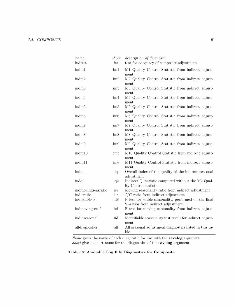
7.4. COMPOSITE 91
name short description of diagnosticindtest itt test for adequacy of composite adjustment
indm1 im1 M1 Quality Control Statistic from indirect adjust-ment
indm2 im2 M2 Quality Control Statistic from indirect adjust-ment
indm3 im3 M3 Quality Control Statistic from indirect adjust-ment
indm4 im4 M4 Quality Control Statistic from indirect adjust-ment
indm5 im5 M5 Quality Control Statistic from indirect adjust-ment
indm6 im6 M6 Quality Control Statistic from indirect adjust-ment
indm7 im7 M7 Quality Control Statistic from indirect adjust-ment
indm8 im8 M8 Quality Control Statistic from indirect adjust-ment
indm9 im9 M9 Quality Control Statistic from indirect adjust-ment
indm10 imt M10 Quality Control Statistic from indirect adjust-ment
indm11 ime M11 Quality Control Statistic from indirect adjust-ment
indq iq Overall index of the quality of the indirect seasonaladjustment
indq2 iq2 Indirect Q statistic computed without the M2 Qual-ity Control statistic
indmovingseasratio isr Moving seasonality ratio from indirect adjustmentindicratio iir I/C ratio from indirect adjustmentindfstabled8 id8 F-test for stable seasonality, performed on the final
SI-ratios from indirect adjustmentindmovingseasf isf F-test for moving seasonality from indirect adjust-
mentindidseasonal iid Identifiable seasonality test result for indirect adjust-
mentalldiagnostics all All seasonal adjustment diagnostics listed in this ta-
ble
Name gives the name of each diagnostic for use with the savelog argument.Short gives a short name for the diagnostics of the savelog argument.
Table 7.8: Available Log File Diagnostics for Composite
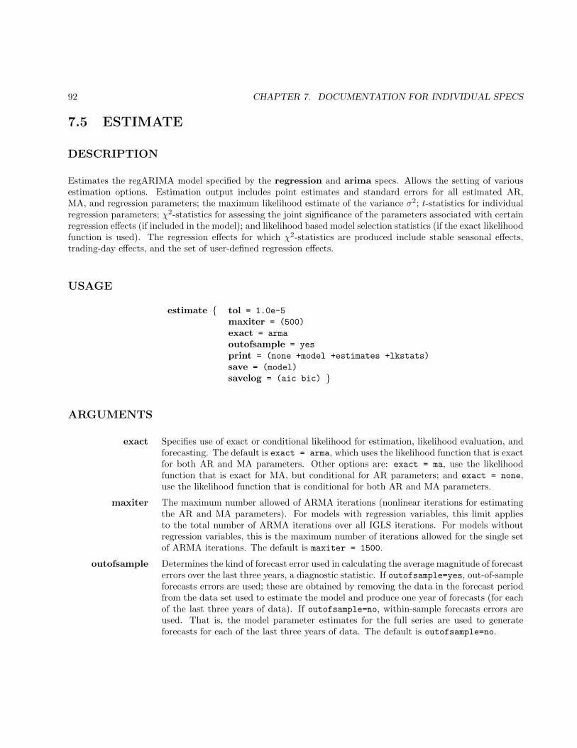
92 CHAPTER 7. DOCUMENTATION FOR INDIVIDUAL SPECS
7.5 ESTIMATE
DESCRIPTION
Estimates the regARIMA model specified by the regression and arima specs. Allows the setting of variousestimation options. Estimation output includes point estimates and standard errors for all estimated AR,MA, and regression parameters; the maximum likelihood estimate of the variance σ2; t-statistics for individualregression parameters; χ2-statistics for assessing the joint significance of the parameters associated with certainregression effects (if included in the model); and likelihood based model selection statistics (if the exact likelihoodfunction is used). The regression effects for which χ2-statistics are produced include stable seasonal effects,trading-day effects, and the set of user-defined regression effects.
USAGE
estimate { tol = 1.0e-5
maxiter = (500)
exact = arma
outofsample = yes
print = (none +model +estimates +lkstats)
save = (model)
savelog = (aic bic) }
ARGUMENTS
exact Specifies use of exact or conditional likelihood for estimation, likelihood evaluation, andforecasting. The default is exact = arma, which uses the likelihood function that is exactfor both AR and MA parameters. Other options are: exact = ma, use the likelihoodfunction that is exact for MA, but conditional for AR parameters; and exact = none,use the likelihood function that is conditional for both AR and MA parameters.
maxiter The maximum number allowed of ARMA iterations (nonlinear iterations for estimatingthe AR and MA parameters). For models with regression variables, this limit appliesto the total number of ARMA iterations over all IGLS iterations. For models withoutregression variables, this is the maximum number of iterations allowed for the single setof ARMA iterations. The default is maxiter = 1500.
outofsample Determines the kind of forecast error used in calculating the average magnitude of forecasterrors over the last three years, a diagnostic statistic. If outofsample=yes, out-of-sampleforecasts errors are used; these are obtained by removing the data in the forecast periodfrom the data set used to estimate the model and produce one year of forecasts (for eachof the last three years of data). If outofsample=no, within-sample forecasts errors areused. That is, the model parameter estimates for the full series are used to generateforecasts for each of the last three years of data. The default is outofsample=no.
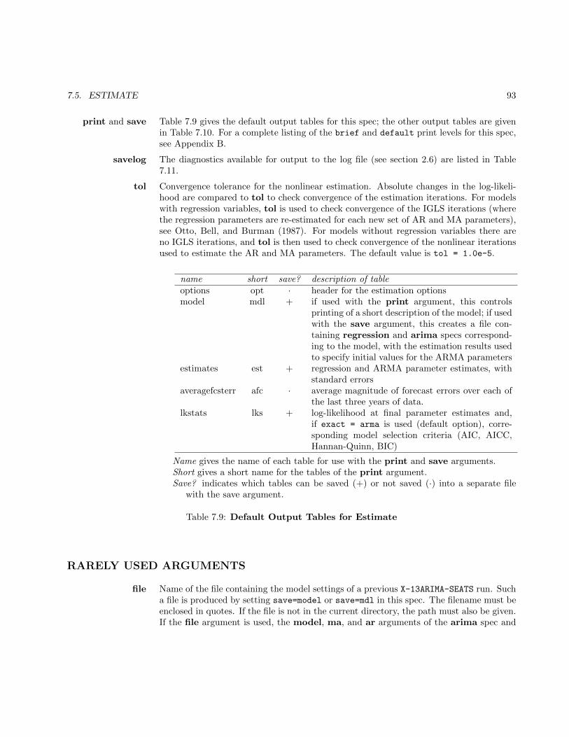
7.5. ESTIMATE 93
print and save Table 7.9 gives the default output tables for this spec; the other output tables are givenin Table 7.10. For a complete listing of the brief and default print levels for this spec,see Appendix B.
savelog The diagnostics available for output to the log file (see section 2.6) are listed in Table7.11.
tol Convergence tolerance for the nonlinear estimation. Absolute changes in the log-likeli-hood are compared to tol to check convergence of the estimation iterations. For modelswith regression variables, tol is used to check convergence of the IGLS iterations (wherethe regression parameters are re-estimated for each new set of AR and MA parameters),see Otto, Bell, and Burman (1987). For models without regression variables there areno IGLS iterations, and tol is then used to check convergence of the nonlinear iterationsused to estimate the AR and MA parameters. The default value is tol = 1.0e-5.
name short save? description of tableoptions opt · header for the estimation optionsmodel mdl + if used with the print argument, this controls
printing of a short description of the model; if usedwith the save argument, this creates a file con-taining regression and arima specs correspond-ing to the model, with the estimation results usedto specify initial values for the ARMA parameters
estimates est + regression and ARMA parameter estimates, withstandard errors
averagefcsterr afc · average magnitude of forecast errors over each ofthe last three years of data.
lkstats lks + log-likelihood at final parameter estimates and,if exact = arma is used (default option), corre-sponding model selection criteria (AIC, AICC,Hannan-Quinn, BIC)
Name gives the name of each table for use with the print and save arguments.Short gives a short name for the tables of the print argument.Save? indicates which tables can be saved (+) or not saved (·) into a separate file
with the save argument.
Table 7.9: Default Output Tables for Estimate
RARELY USED ARGUMENTS
file Name of the file containing the model settings of a previous X-13ARIMA-SEATS run. Sucha file is produced by setting save=model or save=mdl in this spec. The filename must beenclosed in quotes. If the file is not in the current directory, the path must also be given.If the file argument is used, the model, ma, and ar arguments of the arima spec and
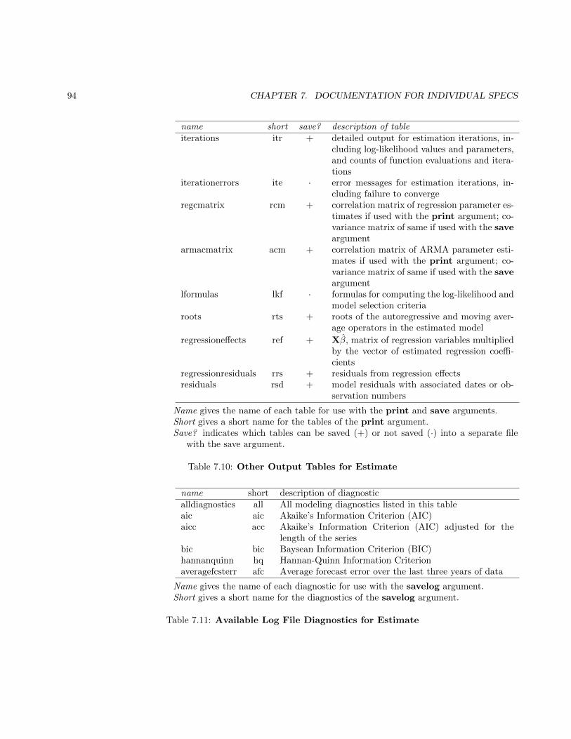
94 CHAPTER 7. DOCUMENTATION FOR INDIVIDUAL SPECS
name short save? description of tableiterations itr + detailed output for estimation iterations, in-
cluding log-likelihood values and parameters,and counts of function evaluations and itera-tions
iterationerrors ite · error messages for estimation iterations, in-cluding failure to converge
regcmatrix rcm + correlation matrix of regression parameter es-timates if used with the print argument; co-variance matrix of same if used with the saveargument
armacmatrix acm + correlation matrix of ARMA parameter esti-mates if used with the print argument; co-variance matrix of same if used with the saveargument
lformulas lkf · formulas for computing the log-likelihood andmodel selection criteria
roots rts + roots of the autoregressive and moving aver-age operators in the estimated model
regressioneffects ref + Xβ, matrix of regression variables multipliedby the vector of estimated regression coeffi-cients
regressionresiduals rrs + residuals from regression effectsresiduals rsd + model residuals with associated dates or ob-
servation numbers
Name gives the name of each table for use with the print and save arguments.Short gives a short name for the tables of the print argument.Save? indicates which tables can be saved (+) or not saved (·) into a separate file
with the save argument.
Table 7.10: Other Output Tables for Estimate
name short description of diagnosticalldiagnostics all All modeling diagnostics listed in this tableaic aic Akaike’s Information Criterion (AIC)aicc acc Akaike’s Information Criterion (AIC) adjusted for the
length of the seriesbic bic Baysean Information Criterion (BIC)hannanquinn hq Hannan-Quinn Information Criterionaveragefcsterr afc Average forecast error over the last three years of data
Name gives the name of each diagnostic for use with the savelog argument.Short gives a short name for the diagnostics of the savelog argument.
Table 7.11: Available Log File Diagnostics for Estimate

7.5. ESTIMATE 95
the variables, user, and b arguments of the regression spec cannot be used, as wellas the pickmdl and automdl specs.
fix Specifies whether certain coefficients found in the model file specified in the file argumentare to be held fixed instead of being used as initializing values for further estimation. Iffix = all, both the regression and ARMA parameter estimates will be held fixed attheir values in the model file. If fix = arma, only ARMA parameter estimates will beheld fixed at their model file values. If fix = none, none of the parameter estimateswill be held fixed. The default is fix = nochange, which will preserve coefficient valuesspecified as fixed in the model file and allow re-estimation of all other coefficients.
DETAILS
The inference results provided by X-13ARIMA-SEATS are asymptotically valid (approximately correct for suffi-ciently long time series) under “standard” assumptions—see Section 4.5. The likelihood based model selectionstatistics are provided only if the exact likelihood function is used. See Section 5.5 for comments on the use ofmodel selection statistics.
If the estimation iterations converge, X-13ARIMA-SEATS prints a message to this effect, and then displays theestimation results. If the iterations fail to converge, X-13ARIMA-SEATS prints a message indicating this and thendisplays the parameter values at the last iteration. These values should not be used as parameter estimates.Instead, the program should be rerun, possibly starting at the parameter values obtained when the iterationsterminated. Potential causes of convergence problems and suggested remedies are discussed in Section 5.
Tol should not be set either “too large” or “too small”. Setting tol too large can result in estimates toofar from the true MLEs, while setting tol too small can result in an unnecessarily large number of iterations orlead to a false impression of the precision of the results. What is too large or too small a value for tol dependson the problem; the default value of tol= 10−5 is offered as a reasonable compromise. Setting tol to a numberless than machine precision for a double precision number (approximately 10−14 for PCs and Sun4 computers)results in an error, but values for tol that even begin to approach machine precision are certainly too small.
For models with regression variables, a second convergence tolerance is needed to determine convergence ofthe ARMA iterations within each IGLS iteration. This tolerance is set by the program to 100 × tol for the firsttwo IGLS iterations, after which it is reset to tol. (Since relatively large changes can be made to the regressionparameters in the initial IGLS iterations, it is not worth determining the ARMA parameters within tol at thestart.) Thus, when tol takes on its default value of 10−5, the ARMA convergence tolerance is 10−3 for the firsttwo IGLS iterations, and thereafter it is 10−5 (= tol). Also, for models with regression variables, a limit isneeded for the maximum number of ARMA iterations allowed within each IGLS iteration. This limit is set to40.
If the ARMA iterations fail to converge on a particular IGLS iteration, this is generally not a problem. Theprogram will continue with the next IGLS iteration, and its ARMA iterations may very well converge. In fact,all that is necessary for overall convergence is that the ARMA iterations of the last IGLS iteration converge,and that the IGLS iterations themselves converge to the tolerance tol within maxiter total ARMA iterations.
Setting print=roots produces a table of roots of all the AR and MA operators of the estimated model. Inaddition to the roots, the table provides the modulus (magnitude) and frequency (on [−.5, .5]) of each root.

96 CHAPTER 7. DOCUMENTATION FOR INDIVIDUAL SPECS
Roots of ARIMA Model
Root Real Imaginary Modulus Frequency
-----------------------------------------------------------
Nonseasonal AR
Root 1 -0.6784 0.8817 1.1125 0.3544
Root 2 -0.6784 -0.8817 1.1125 -0.3544
Nonseasonal MA
Root 1 -7.4107 0.0000 7.4107 0.5000
Seasonal MA
Root 1 1.5583 0.0000 1.5583 0.0000
Table 7.12: Example of ARMA Roots Output
Roots with modulus greater than one lie outside the unit circle, corresponding to stationary AR or invertibleMA operators. (See Section 5.4.) AR roots on or inside the unit circle (modulus ≤ 1) should occur only whenthe likelihood function is defined conditionally for AR parameters (exact = ma or exact = none). MA rootsinside the unit circle (modulus < 1) will never occur, since invertibility is enforced in the estimation. MA rootson the unit circle (modulus = 1) can be estimated within round-off error, or can occur in an MA operator allof whose parameters are specified as fixed during estimation.
In sample output shown in Table 7.12, the nonseasonal AR(2) polynomial has a pair of complex conjugate
roots (zeros), z = x ± iy, with x = −.6784 and y = .8817, whose modulus (magnitude) is r =(x2 + y2
)1/2=
1.1125. Because this number is close to unity (1.000), it is worthwhile to examine the nonnegative frequency ofthe root, i.e. the number λ ≥ 0 such that z = re±i2πλ to determine if the series may contain a deterministicperiodic component. The reasoning behind this is as follows. Whenever a modelled time series has a periodiccomponent f (t) with period 1/λ, i.e. f (t+ 1/λ) = f (t), then an estimated AR polynomial of sufficiently highorder is likely to have a root near e±i2πλ (unless the differencing operators have e±i2πλ as a root). There aretheoretical results that help to explain why this happens, but a heuristic explanation is that for the simplestfunctions with this period,
f (t) = A cos (2πλt+ c) ,
the AR(2) polynomial φ (B) =(1− e−i2πλB
) (1− ei2πλB
), whose roots are e±i2πλ, has the property that
φ (B) f (t) = 0.
Thus this AR(2) factor can perfectly predict f (t) from f (t− 1) and f (t− 2). Fitting a model with an ARoperator of order 2 or higher will tend to make the AR parameters take on values so that φ (B) f (t) = 0. (AnAR(1) polynomial suffices when ei2πλ is real, i.e. when λ = 0, 1/2.) . Hence the occurrence of an AR root withmodulus r
.= 1 suggests the presence of an approximately periodic component in the time series.
For monthly series, the frequencies of seasonal effects are λ = 1/12 , 2/12 , 3/12 , . . . , 6/12 (equivalent to0.0833, 0.1666, 0.2500, . . . , 0.5000, respectively). The frequency λ = 0 is associated with trend movements, andthe frequency λ = 0.3482 with trading day effects. Note that the frequency 0.3544 of the nonseasonal AR rootsin the table above is very close to the trading day frequency. In fact, the time series whose model produced thetable has a strong trading day component, and the automatic modeling procedure added the AR(2) factor toaccount for it, because there were no trading day regressors in the regression spec.
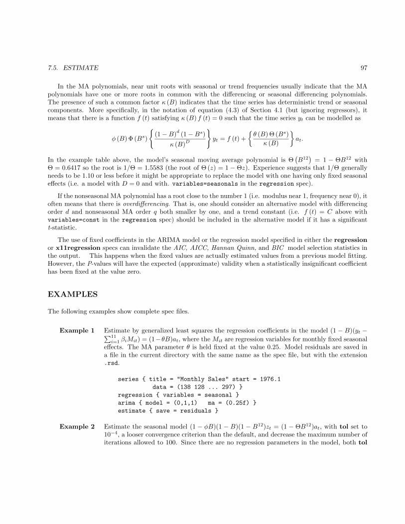
7.5. ESTIMATE 97
In the MA polynomials, near unit roots with seasonal or trend frequencies usually indicate that the MApolynomials have one or more roots in common with the differencing or seasonal differencing polynomials.The presence of such a common factor κ (B) indicates that the time series has deterministic trend or seasonalcomponents. More specifically, in the notation of equation (4.3) of Section 4.1 (but ignoring regressors), itmeans that there is a function f (t) satisfying κ (B) f (t) = 0 such that the time series yt can be modelled as
φ (B) Φ (Bs)
{(1−B)
d(1−Bs)
κ (B)D
}yt = f (t) +
{θ (B) Θ (Bs)
κ (B)
}at.
In the example table above, the model’s seasonal moving average polynomial is Θ(B12
)= 1 − ΘB12 with
Θ = 0.6417 so the root is 1/Θ = 1.5583 (the root of Θ (z) = 1 − Θz). Experience suggests that 1/Θ generallyneeds to be 1.10 or less before it might be appropriate to replace the model with one having only fixed seasonaleffects (i.e. a model with D = 0 and with. variables=seasonals in the regression spec).
If the nonseasonal MA polynomial has a root close to the number 1 (i.e. modulus near 1, frequency near 0), itoften means that there is overdifferencing. That is, one should consider an alternative model with differencingorder d and nonseasonal MA order q both smaller by one, and a trend constant (i.e. f (t) = C above withvariables=const in the regression spec) should be included in the alternative model if it has a significantt-statistic.
The use of fixed coefficients in the ARIMA model or the regression model specified in either the regressionor x11regression specs can invalidate the AIC, AICC, Hannan Quinn, and BIC model selection statistics inthe output. This happens when the fixed values are actually estimated values from a previous model fitting.However, the P-values will have the expected (approximate) validity when a statistically insignificant coefficienthas been fixed at the value zero.
EXAMPLES
The following examples show complete spec files.
Example 1 Estimate by generalized least squares the regression coefficients in the model (1 − B)(yt −∑11i=1 βiMit) = (1−θB)at, where the Mit are regression variables for monthly fixed seasonal
effects. The MA parameter θ is held fixed at the value 0.25. Model residuals are saved ina file in the current directory with the same name as the spec file, but with the extension.rsd.
series { title = "Monthly Sales" start = 1976.1
data = (138 128 ... 297) }
regression { variables = seasonal }
arima { model = (0,1,1) ma = (0.25f) }
estimate { save = residuals }
Example 2 Estimate the seasonal model (1 − φB)(1 − B)(1 − B12)zt = (1 − ΘB12)at, with tol set to10−4, a looser convergence criterion than the default, and decrease the maximum number ofiterations allowed to 100. Since there are no regression parameters in the model, both tol
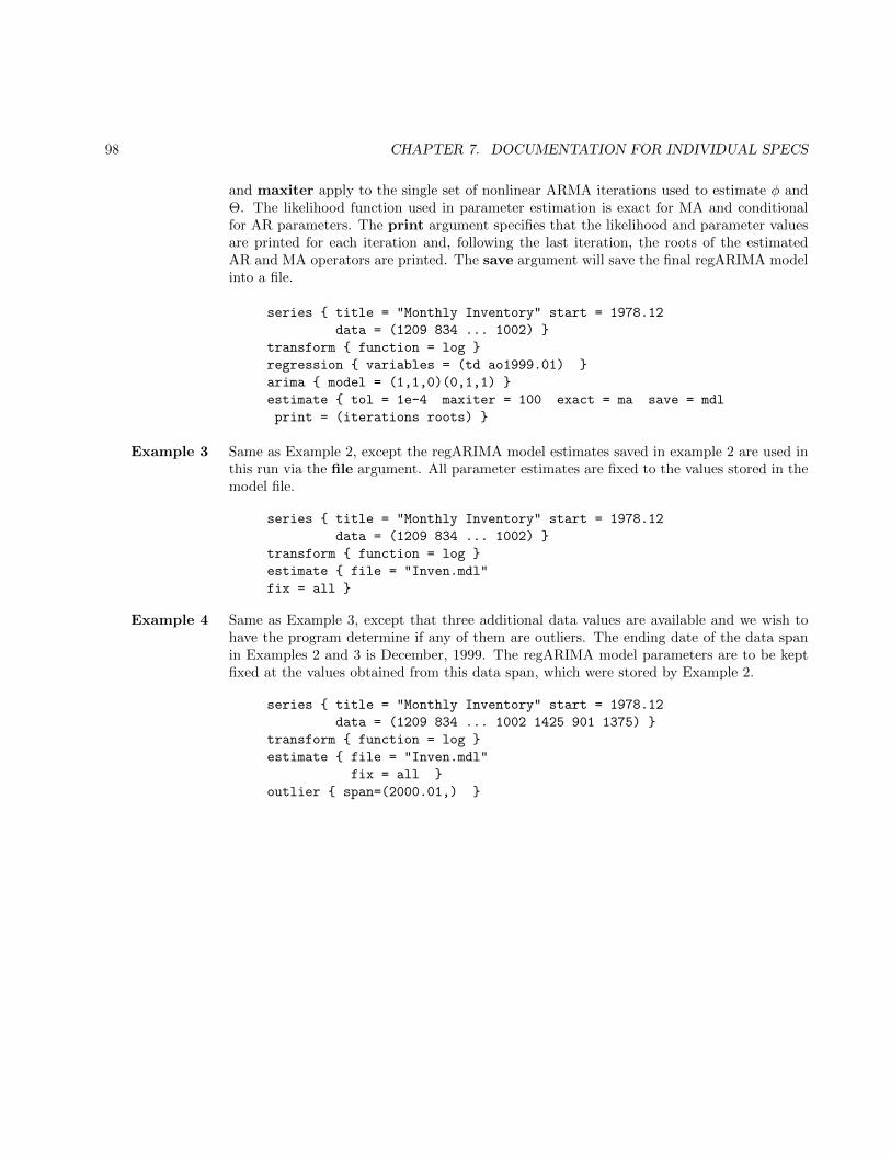
98 CHAPTER 7. DOCUMENTATION FOR INDIVIDUAL SPECS
and maxiter apply to the single set of nonlinear ARMA iterations used to estimate φ andΘ. The likelihood function used in parameter estimation is exact for MA and conditionalfor AR parameters. The print argument specifies that the likelihood and parameter valuesare printed for each iteration and, following the last iteration, the roots of the estimatedAR and MA operators are printed. The save argument will save the final regARIMA modelinto a file.
series { title = "Monthly Inventory" start = 1978.12
data = (1209 834 ... 1002) }
transform { function = log }
regression { variables = (td ao1999.01) }
arima { model = (1,1,0)(0,1,1) }
estimate { tol = 1e-4 maxiter = 100 exact = ma save = mdl
print = (iterations roots) }
Example 3 Same as Example 2, except the regARIMA model estimates saved in example 2 are used inthis run via the file argument. All parameter estimates are fixed to the values stored in themodel file.
series { title = "Monthly Inventory" start = 1978.12
data = (1209 834 ... 1002) }
transform { function = log }
estimate { file = "Inven.mdl"
fix = all }
Example 4 Same as Example 3, except that three additional data values are available and we wish tohave the program determine if any of them are outliers. The ending date of the data spanin Examples 2 and 3 is December, 1999. The regARIMA model parameters are to be keptfixed at the values obtained from this data span, which were stored by Example 2.
series { title = "Monthly Inventory" start = 1978.12
data = (1209 834 ... 1002 1425 901 1375) }
transform { function = log }
estimate { file = "Inven.mdl"
fix = all }
outlier { span=(2000.01,) }
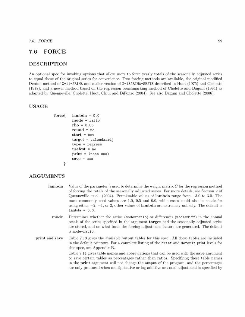
7.6. FORCE 99
7.6 FORCE
DESCRIPTION
An optional spec for invoking options that allow users to force yearly totals of the seasonally adjusted seriesto equal those of the original series for convenience. Two forcing methods are available, the original modifiedDenton method of X-11-ARIMA and earlier version of X-13ARIMA-SEATS described in Huot (1975) and Cholette(1978), and a newer method based on the regression benchmarking method of Cholette and Dagum (1994) asadapted by Quenneville, Cholette, Huot, Chiu, and DiFonzo (2004). See also Dagum and Cholette (2006).
USAGE
force{ lambda = 0.0
mode = ratio
rho = 0.85
round = no
start = oct
target = calendaradj
type = regress
usefcst = no
print = (none saa)
save = saa
}
ARGUMENTS
lambda Value of the parameter λ used to determine the weight matrix C for the regression methodof forcing the totals of the seasonally adjusted series. For more details, see Section 2 ofQuenneville et al. (2004). Permissable values of lambda range from −3.0 to 3.0. Themost commonly used values are 1.0, 0.5 and 0.0, while cases could also be made forusing either −2, −1, or 2; other values of lambda are extremely unlikely. The default islambda = 0.0.
mode Determines whether the ratios (mode=ratio) or differences (mode=diff) in the annualtotals of the series specified in the argument target and the seasonally adjusted seriesare stored, and on what basis the forcing adjustment factors are generated. The defaultis mode=ratio.
print and save Table 7.13 gives the available output tables for this spec. All these tables are includedin the default printout. For a complete listing of the brief and default print levels forthis spec, see Appendix B.
Table 7.14 gives table names and abbreviations that can be used with the save argumentto save certain tables as percentages rather than ratios. Specifying these table namesin the print argument will not change the output of the program, and the percentagesare only produced when multiplicative or log-additive seasonal adjustment is specified by
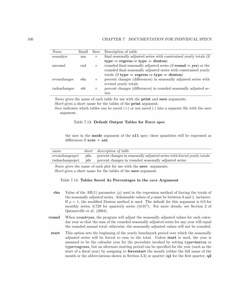
100 CHAPTER 7. DOCUMENTATION FOR INDIVIDUAL SPECS
Name Small Save Description of tableseasadjtot saa + final seasonally adjusted series with constrained yearly totals (if
type = regress or type = denton)saround rnd + rounded final seasonally adjusted series (if round = yes) or the
rounded final seasonally adjusted series with constrained yearlytotals (if type = regress or type = denton)
revsachanges e6a + percent changes (differences) in seasonally adjusted series withrevised yearly totals
rndsachanges e6r + percent changes (differences) in rounded seasonally adjusted se-ries
Name gives the name of each table for use with the print and save arguments.Short gives a short name for the tables of the print argument.Save indicates which tables can be saved (+) or not saved (·) into a separate file with the save
argument.
Table 7.13: Default Output Tables for Force spec
the user in the mode argument of the x11 spec; these quantities will be expressed asdifferences if mode = add.
name short description of tablerevsachangespct p6a percent changes in seasonally adjusted series with forced yearly totalsrndsachangespct p6r percent changes in rounded seasonally adjusted series
Name gives the name of each plot for use with the save arguments.Short gives a short name for the tables of the save argument.
Table 7.14: Tables Saved As Percentages in the save Argument
rho Value of the AR(1) parameter (ρ) used in the regression method of forcing the totals ofthe seasonally adjusted series. Admissable values of ρ must be between 0 and 1, inclusive.If ρ = 1, the modified Denton method is used. The default for this argument is 0.9 formonthly series, 0.729 for quarterly series ((0.9)3). For more details, see Section 2 ofQuenneville et al. (2004).
round When round=yes, the program will adjust the seasonally adjusted values for each calen-dar year so that the sum of the rounded seasonally adjusted series for any year will equalthe rounded annual total; otherwise, the seasonally adjusted values will not be rounded.
start This option sets the beginning of the yearly benchmark period over which the seasonallyadjusted series will be forced to sum to the total. Unless start is used, the year isassumed to be the calendar year for the procedure invoked by setting type=denton ortype=regress, but an alternate starting period can be specified for the year (such as thestart of a fiscal year) by assigning to forcestart the month (either the full name of themonth or the abbreviations shown in Section 3.3) or quarter (q1 for the first quarter, q2
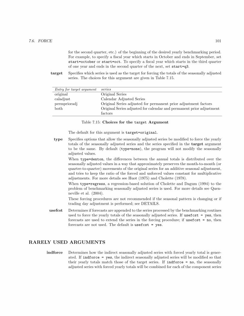
7.6. FORCE 101
for the second quarter, etc.) of the beginning of the desired yearly benchmarking period.For example, to specify a fiscal year which starts in October and ends in September, setstart=october or start=oct. To specify a fiscal year which starts in the third quarterof one year and ends in the second quarter of the next, set start=q3.
target Specifies which series is used as the target for forcing the totals of the seasonally adjustedseries. The choices for this argument are given in Table 7.15.
Entry for target argument seriesoriginal Original Seriescaladjust Calendar Adjusted Seriespermprioradj Original Series adjusted for permanent prior adjustment factorsboth Original Series adjusted for calendar and permanent prior adjustment
factors
Table 7.15: Choices for the target Argument
The default for this argument is target=original.
type Specifies options that allow the seasonally adjusted series be modified to force the yearlytotals of the seasonally adjusted series and the series specified in the target argumentto be the same. By default (type=none), the program will not modify the seasonallyadjusted values.
When type=denton, the differences between the annual totals is distributed over theseasonally adjusted values in a way that approximately preserves the month-to-month (orquarter-to-quarter) movements of the original series for an additive seasonal adjustment,and tries to keep the ratio of the forced and unforced values constant for multiplicativeadjustments. For more details see Huot (1975) and Cholette (1978).
When type=regress, a regression-based solution of Cholette and Dagum (1994) to theproblem of benchmarking seasonally adjusted series is used. For more details see Quen-neville et al. (2004).
These forcing procedures are not recommended if the seasonal pattern is changing or iftrading day adjustment is performed; see DETAILS.
usefcst Determines if forecasts are appended to the series processed by the benchmarking routinesused to force the yearly totals of the seasonally adjusted series. If usefcst = yes, thenforecasts are used to extend the series in the forcing procedure; if usefcst = no, thenforecasts are not used. The default is usefcst = yes.
RARELY USED ARGUMENTS
indforce Determines how the indirect seasonally adjusted series with forced yearly total is gener-ated. If indforce = yes, the indirect seasonally adjusted series will be modified so thattheir yearly totals match those of the target series. If indforce = no, the seasonallyadjusted series with forced yearly totals will be combined for each of the component series
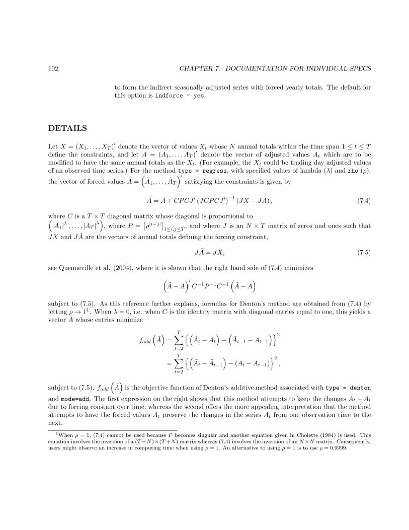
102 CHAPTER 7. DOCUMENTATION FOR INDIVIDUAL SPECS
to form the indirect seasonally adjusted series with forced yearly totals. The default forthis option is indforce = yes.
DETAILS
Let X = (X1, . . . , XT )′
denote the vector of values Xt whose N annual totals within the time span 1 ≤ t ≤ Tdefine the constraints, and let A = (A1, . . . , AT )
′denote the vector of adjusted values At which are to be
modified to have the same annual totals as the Xt. (For example, the Xt could be trading day adjusted valuesof an observed time series.) For the method type = regress, with specified values of lambda (λ) and rho (ρ),
the vector of forced values A =(A1, . . . , AT
)′satisfying the constraints is given by
A = A+ CPCJ ′ (JCPCJ ′)−1
(JX − JA) , (7.4)
where C is a T × T diagonal matrix whose diagonal is proportional to(|A1|λ , . . . , |AT |λ
), where P =
[ρ|i−j|
]1≤i,j≤T , and where J is an N × T matrix of zeros and ones such that
JX and JA are the vectors of annual totals defining the forcing constraint,
JA = JX, (7.5)
see Quenneville et al. (2004), where it is shown that the right hand side of (7.4) minimizes(A−A
)′C−1P−1C−1
(A−A
)subject to (7.5). As this reference further explains, formulas for Denton’s method are obtained from (7.4) byletting ρ→ 11. When λ = 0, i.e. when C is the identity matrix with diagonal entries equal to one, this yields avector A whose entries minimize
fadd
(A)
=
T∑t=2
{(At −At
)−(At−1 −At−1
)}2
=
T∑t=2
{(At − At−1
)− (At −At−1)
}2
,
subject to (7.5). fadd
(A)
is the objective function of Denton’s additive method associated with type = denton
and mode=add. The first expression on the right shows that this method attempts to keep the changes At −Atdue to forcing constant over time, whereas the second offers the more appealing interpretation that the methodattempts to have the forced values At preserve the changes in the series At from one observation time to thenext.
1When ρ = 1, (7.4) cannot be used because P becomes singular and another equation given in Cholette (1984) is used. Thisequation involves the inversion of a (T+N)×(T+N) matrix whereas (7.4) involves the inversion of an N×N matrix. Consequently,users might observe an increase in computing time when using ρ = 1. An alternative to using ρ = 1 is to use ρ = 0.9999.
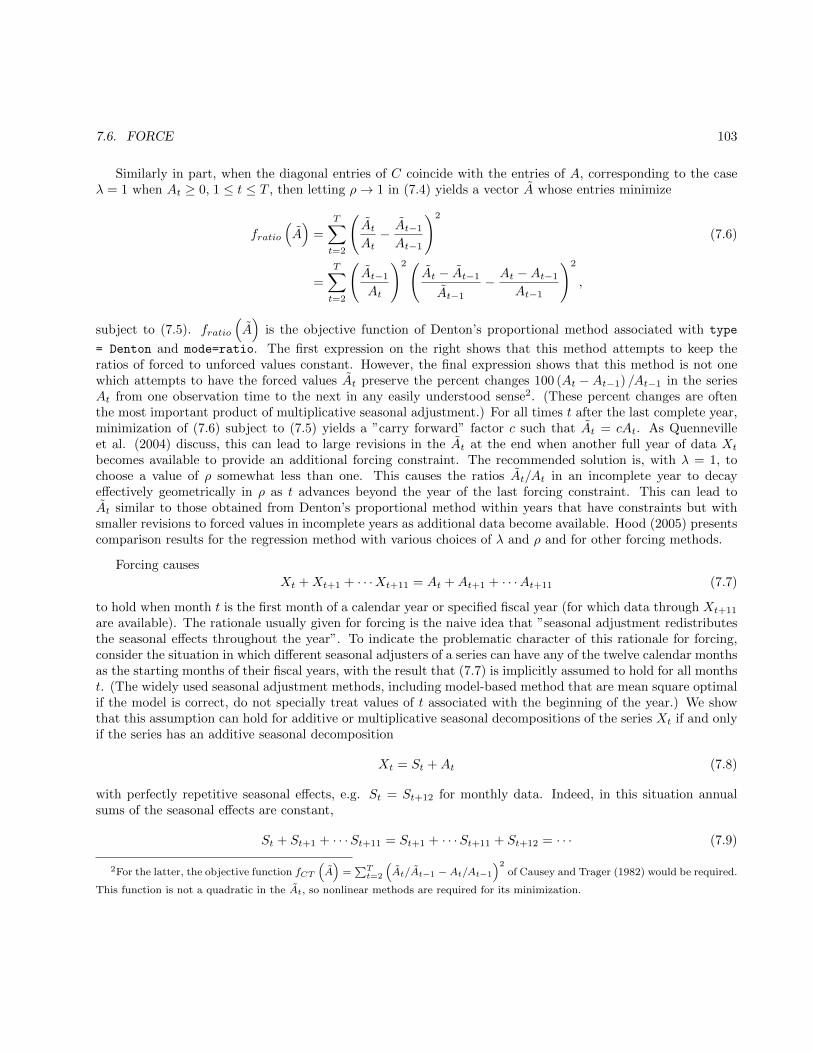
7.6. FORCE 103
Similarly in part, when the diagonal entries of C coincide with the entries of A, corresponding to the caseλ = 1 when At ≥ 0, 1 ≤ t ≤ T , then letting ρ→ 1 in (7.4) yields a vector A whose entries minimize
fratio
(A)
=
T∑t=2
(AtAt− At−1
At−1
)2
(7.6)
=
T∑t=2
(At−1
At
)2(At − At−1
At−1
− At −At−1
At−1
)2
,
subject to (7.5). fratio
(A)
is the objective function of Denton’s proportional method associated with type
= Denton and mode=ratio. The first expression on the right shows that this method attempts to keep theratios of forced to unforced values constant. However, the final expression shows that this method is not onewhich attempts to have the forced values At preserve the percent changes 100 (At −At−1) /At−1 in the seriesAt from one observation time to the next in any easily understood sense2. (These percent changes are oftenthe most important product of multiplicative seasonal adjustment.) For all times t after the last complete year,minimization of (7.6) subject to (7.5) yields a ”carry forward” factor c such that At = cAt. As Quennevilleet al. (2004) discuss, this can lead to large revisions in the At at the end when another full year of data Xt
becomes available to provide an additional forcing constraint. The recommended solution is, with λ = 1, tochoose a value of ρ somewhat less than one. This causes the ratios At/At in an incomplete year to decayeffectively geometrically in ρ as t advances beyond the year of the last forcing constraint. This can lead toAt similar to those obtained from Denton’s proportional method within years that have constraints but withsmaller revisions to forced values in incomplete years as additional data become available. Hood (2005) presentscomparison results for the regression method with various choices of λ and ρ and for other forcing methods.
Forcing causes
Xt +Xt+1 + · · ·Xt+11 = At +At+1 + · · ·At+11 (7.7)
to hold when month t is the first month of a calendar year or specified fiscal year (for which data through Xt+11
are available). The rationale usually given for forcing is the naive idea that ”seasonal adjustment redistributesthe seasonal effects throughout the year”. To indicate the problematic character of this rationale for forcing,consider the situation in which different seasonal adjusters of a series can have any of the twelve calendar monthsas the starting months of their fiscal years, with the result that (7.7) is implicitly assumed to hold for all monthst. (The widely used seasonal adjustment methods, including model-based method that are mean square optimalif the model is correct, do not specially treat values of t associated with the beginning of the year.) We showthat this assumption can hold for additive or multiplicative seasonal decompositions of the series Xt if and onlyif the series has an additive seasonal decomposition
Xt = St +At (7.8)
with perfectly repetitive seasonal effects, e.g. St = St+12 for monthly data. Indeed, in this situation annualsums of the seasonal effects are constant,
St + St+1 + · · ·St+11 = St+1 + · · ·St+11 + St+12 = · · · (7.9)
2For the latter, the objective function fCT
(A)
=∑T
t=2
(At/At−1 −At/At−1
)2of Causey and Trager (1982) would be required.
This function is not a quadratic in the At, so nonlinear methods are required for its minimization.
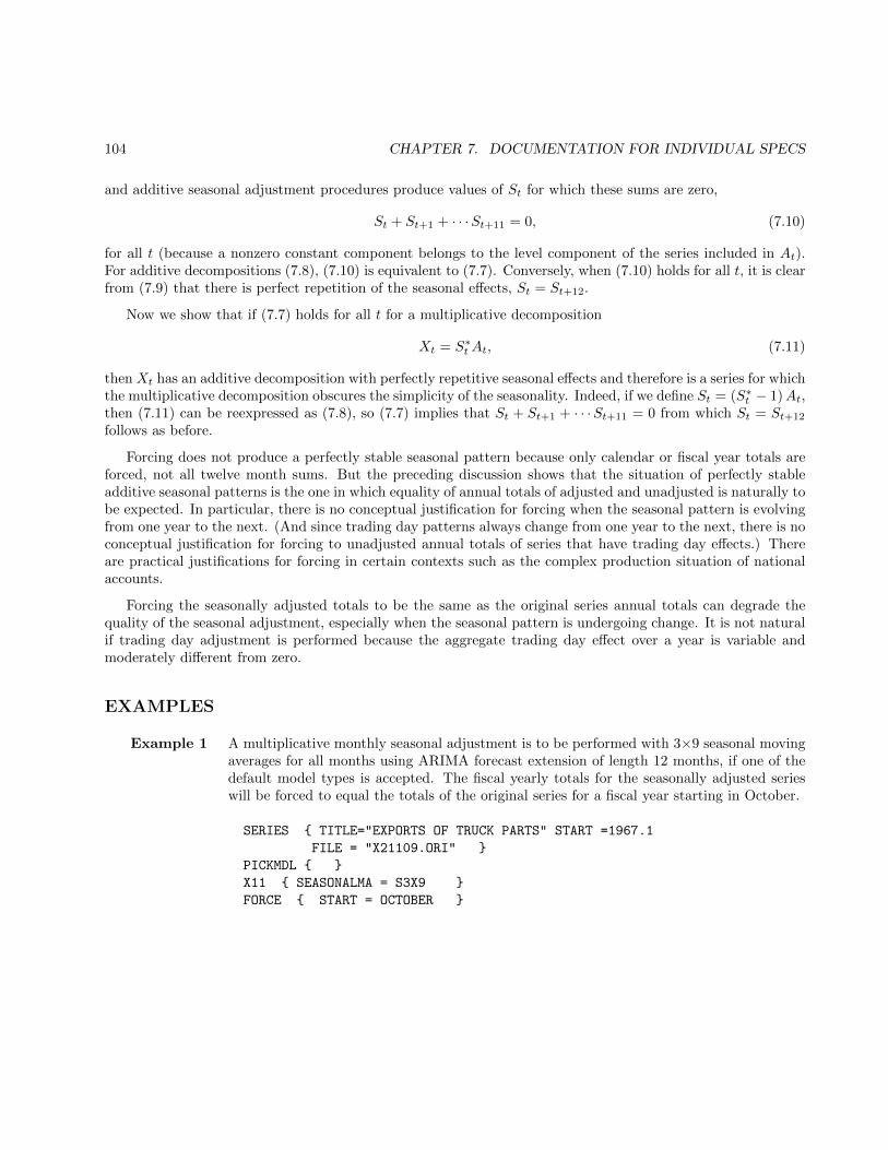
104 CHAPTER 7. DOCUMENTATION FOR INDIVIDUAL SPECS
and additive seasonal adjustment procedures produce values of St for which these sums are zero,
St + St+1 + · · ·St+11 = 0, (7.10)
for all t (because a nonzero constant component belongs to the level component of the series included in At).For additive decompositions (7.8), (7.10) is equivalent to (7.7). Conversely, when (7.10) holds for all t, it is clearfrom (7.9) that there is perfect repetition of the seasonal effects, St = St+12.
Now we show that if (7.7) holds for all t for a multiplicative decomposition
Xt = S∗tAt, (7.11)
then Xt has an additive decomposition with perfectly repetitive seasonal effects and therefore is a series for whichthe multiplicative decomposition obscures the simplicity of the seasonality. Indeed, if we define St = (S∗t − 1)At,then (7.11) can be reexpressed as (7.8), so (7.7) implies that St + St+1 + · · ·St+11 = 0 from which St = St+12
follows as before.
Forcing does not produce a perfectly stable seasonal pattern because only calendar or fiscal year totals areforced, not all twelve month sums. But the preceding discussion shows that the situation of perfectly stableadditive seasonal patterns is the one in which equality of annual totals of adjusted and unadjusted is naturally tobe expected. In particular, there is no conceptual justification for forcing when the seasonal pattern is evolvingfrom one year to the next. (And since trading day patterns always change from one year to the next, there is noconceptual justification for forcing to unadjusted annual totals of series that have trading day effects.) Thereare practical justifications for forcing in certain contexts such as the complex production situation of nationalaccounts.
Forcing the seasonally adjusted totals to be the same as the original series annual totals can degrade thequality of the seasonal adjustment, especially when the seasonal pattern is undergoing change. It is not naturalif trading day adjustment is performed because the aggregate trading day effect over a year is variable andmoderately different from zero.
EXAMPLES
Example 1 A multiplicative monthly seasonal adjustment is to be performed with 3×9 seasonal movingaverages for all months using ARIMA forecast extension of length 12 months, if one of thedefault model types is accepted. The fiscal yearly totals for the seasonally adjusted serieswill be forced to equal the totals of the original series for a fiscal year starting in October.
SERIES { TITLE="EXPORTS OF TRUCK PARTS" START =1967.1
FILE = "X21109.ORI" }
PICKMDL { }
X11 { SEASONALMA = S3X9 }
FORCE { START = OCTOBER }
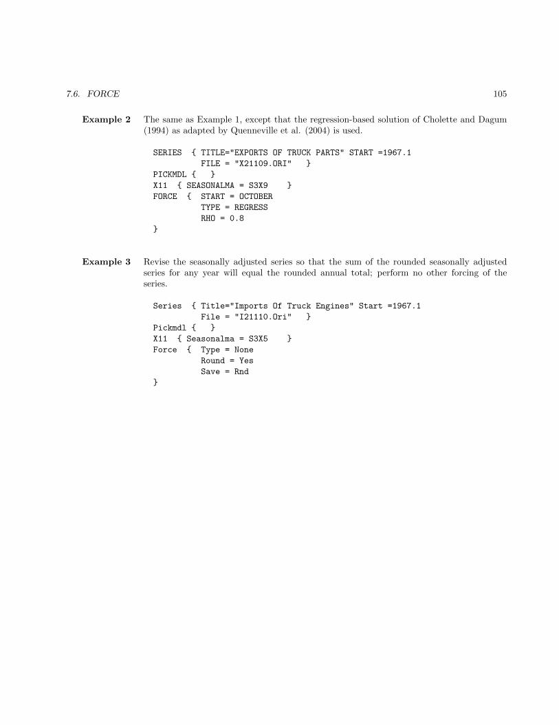
7.6. FORCE 105
Example 2 The same as Example 1, except that the regression-based solution of Cholette and Dagum(1994) as adapted by Quenneville et al. (2004) is used.
SERIES { TITLE="EXPORTS OF TRUCK PARTS" START =1967.1
FILE = "X21109.ORI" }
PICKMDL { }
X11 { SEASONALMA = S3X9 }
FORCE { START = OCTOBER
TYPE = REGRESS
RHO = 0.8
}
Example 3 Revise the seasonally adjusted series so that the sum of the rounded seasonally adjustedseries for any year will equal the rounded annual total; perform no other forcing of theseries.
Series { Title="Imports Of Truck Engines" Start =1967.1
File = "I21110.Ori" }
Pickmdl { }
X11 { Seasonalma = S3X5 }
Force { Type = None
Round = Yes
Save = Rnd
}
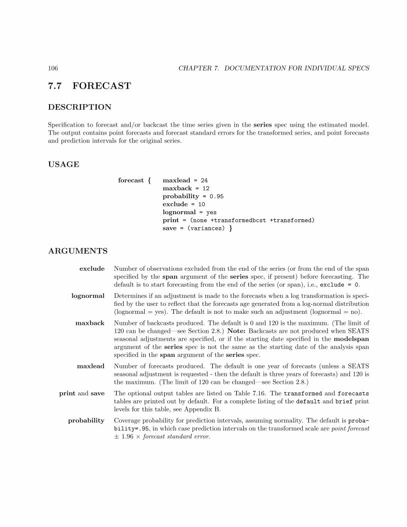
106 CHAPTER 7. DOCUMENTATION FOR INDIVIDUAL SPECS
7.7 FORECAST
DESCRIPTION
Specification to forecast and/or backcast the time series given in the series spec using the estimated model.The output contains point forecasts and forecast standard errors for the transformed series, and point forecastsand prediction intervals for the original series.
USAGE
forecast { maxlead = 24
maxback = 12
probability = 0.95
exclude = 10
lognormal = yes
print = (none +transformedbcst +transformed)
save = (variances) }
ARGUMENTS
exclude Number of observations excluded from the end of the series (or from the end of the spanspecified by the span argument of the series spec, if present) before forecasting. Thedefault is to start forecasting from the end of the series (or span), i.e., exclude = 0.
lognormal Determines if an adjustment is made to the forecasts when a log transformation is speci-fied by the user to reflect that the forecasts age generated from a log-normal distribution(lognormal = yes). The default is not to make such an adjustment (lognormal = no).
maxback Number of backcasts produced. The default is 0 and 120 is the maximum. (The limit of120 can be changed—see Section 2.8.) Note: Backcasts are not produced when SEATSseasonal adjustments are specified, or if the starting date specified in the modelspanargument of the series spec is not the same as the starting date of the analysis spanspecified in the span argument of the series spec.
maxlead Number of forecasts produced. The default is one year of forecasts (unless a SEATSseasonal adjustment is requested - then the default is three years of forecasts) and 120 isthe maximum. (The limit of 120 can be changed—see Section 2.8.)
print and save The optional output tables are listed on Table 7.16. The transformed and forecasts
tables are printed out by default. For a complete listing of the default and brief printlevels for this table, see Appendix B.
probability Coverage probability for prediction intervals, assuming normality. The default is proba-bility=.95, in which case prediction intervals on the transformed scale are point forecast± 1.96 × forecast standard error.
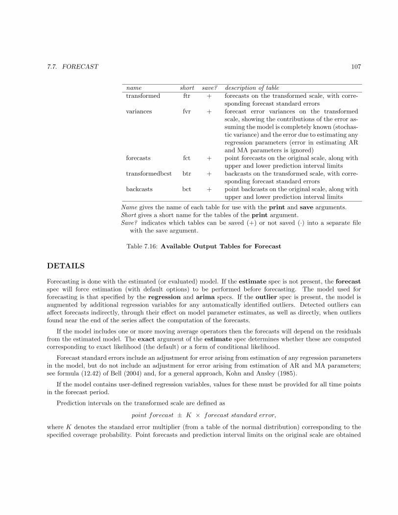
7.7. FORECAST 107
name short save? description of tabletransformed ftr + forecasts on the transformed scale, with corre-
sponding forecast standard errorsvariances fvr + forecast error variances on the transformed
scale, showing the contributions of the error as-suming the model is completely known (stochas-tic variance) and the error due to estimating anyregression parameters (error in estimating ARand MA parameters is ignored)
forecasts fct + point forecasts on the original scale, along withupper and lower prediction interval limits
transformedbcst btr + backcasts on the transformed scale, with corre-sponding forecast standard errors
backcasts bct + point backcasts on the original scale, along withupper and lower prediction interval limits
Name gives the name of each table for use with the print and save arguments.Short gives a short name for the tables of the print argument.Save? indicates which tables can be saved (+) or not saved (·) into a separate file
with the save argument.
Table 7.16: Available Output Tables for Forecast
DETAILS
Forecasting is done with the estimated (or evaluated) model. If the estimate spec is not present, the forecastspec will force estimation (with default options) to be performed before forecasting. The model used forforecasting is that specified by the regression and arima specs. If the outlier spec is present, the model isaugmented by additional regression variables for any automatically identified outliers. Detected outliers canaffect forecasts indirectly, through their effect on model parameter estimates, as well as directly, when outliersfound near the end of the series affect the computation of the forecasts.
If the model includes one or more moving average operators then the forecasts will depend on the residualsfrom the estimated model. The exact argument of the estimate spec determines whether these are computedcorresponding to exact likelihood (the default) or a form of conditional likelihood.
Forecast standard errors include an adjustment for error arising from estimation of any regression parametersin the model, but do not include an adjustment for error arising from estimation of AR and MA parameters;see formula (12.42) of Bell (2004) and, for a general approach, Kohn and Ansley (1985).
If the model contains user-defined regression variables, values for these must be provided for all time pointsin the forecast period.
Prediction intervals on the transformed scale are defined as
point forecast ± K × forecast standard error,
where K denotes the standard error multiplier (from a table of the normal distribution) corresponding to thespecified coverage probability. Point forecasts and prediction interval limits on the original scale are obtained

108 CHAPTER 7. DOCUMENTATION FOR INDIVIDUAL SPECS
by inverse transformation of those on the transformed scale, allowing for both transformation (Box-Cox orlogistic) and prior-adjustment factors (including the length-of-month or length-of-quarter adjustment impliedif variables = td is included in the regression spec). If the transform spec includes user-defined prior-adjustment factors, these must be provided through the forecast period for the results to be inverse transformed.If they are not provided through the forecast period, then they will be assumed to be 1 in the forecast period.In this case, effects of the user-defined adjustments on the forecasts will not be (and cannot be) undone.
A reason for using exclude > 0 is to produce forecasts for some time points whose data are withheld forpurposes of evaluating the forecast performance of the model. X-13ARIMA-SEATS facilitates such comparisons byprinting actual forecast errors (observation − point forecast) at all time points in the forecast period for whichcorresponding (transformed) observed data exist. Setting exclude > 0 produces within-sample comparisons,since the data that are withheld from forecasting are not withheld from model estimation. More realistic out-of-sample forecast comparisons are produced by withholding data from both model estimation and forecasting,which can be accomplished by using the span argument of the series spec. (See Example 4.)
Whenever forecasts and/or backcasts are generated in an X-13ARIMA-SEATS run in which seasonal adjustmentis performed, they are appended to the original series, and the seasonal adjustment procedures are applied tothe forecast and/or backcast extended series. If a seasonal adjustment is specified in a run in which a regARIMAmodel is used but the forecast spec is not, one year of forecasts are generated from the model. The only wayto specify a seasonal adjustment without forecast extension is to set maxlead = 0.
If preadjustments for regARIMA estimated trading day, outlier, holiday or user-defined regression effectsare prior adjusted from the original series, they are also adjusted out of the forecasts and backcasts.
Warning: if seasonal adjustment is specified by the x11 spec, exclude cannot be used to exclude observa-tions from the end of the series. In case it is used, exclude will be set to zero and a warning message will beprinted.
EXAMPLES
The following examples show complete spec files.
Example 1 Forecast up through 12 steps ahead from the end of a monthly time series, and produce95 percent prediction intervals. These are all default options. Though the estimate specis absent, the presence of the forecast spec forces model estimation with default estima-tion options. The point forecasts and prediction interval limits for the transformed seriesare exponentiated and then multiplied by mt/m (to undo the length-of-month adjustmentproduced by variables = td in the regression spec) to convert them back to the originalscale.
SERIES { TITLE = "Monthly sales" START = 1976.JAN
DATA = (138 128 ... 297) }
TRANSFORM { FUNCTION = LOG } REGRESSION { VARIABLES = TD } ARIMA {
MODEL = (0 1 1)(0 1 1)12 } FORECAST { }
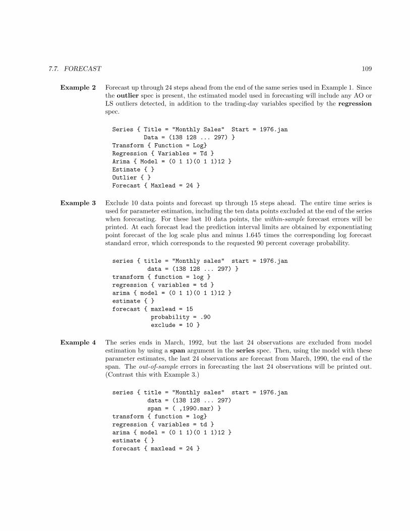
7.7. FORECAST 109
Example 2 Forecast up through 24 steps ahead from the end of the same series used in Example 1. Sincethe outlier spec is present, the estimated model used in forecasting will include any AO orLS outliers detected, in addition to the trading-day variables specified by the regressionspec.
Series { Title = "Monthly Sales" Start = 1976.jan
Data = (138 128 ... 297) }
Transform { Function = Log}
Regression { Variables = Td }
Arima { Model = (0 1 1)(0 1 1)12 }
Estimate { }
Outlier { }
Forecast { Maxlead = 24 }
Example 3 Exclude 10 data points and forecast up through 15 steps ahead. The entire time series isused for parameter estimation, including the ten data points excluded at the end of the serieswhen forecasting. For these last 10 data points, the within-sample forecast errors will beprinted. At each forecast lead the prediction interval limits are obtained by exponentiatingpoint forecast of the log scale plus and minus 1.645 times the corresponding log forecaststandard error, which corresponds to the requested 90 percent coverage probability.
series { title = "Monthly sales" start = 1976.jan
data = (138 128 ... 297) }
transform { function = log }
regression { variables = td }
arima { model = (0 1 1)(0 1 1)12 }
estimate { }
forecast { maxlead = 15
probability = .90
exclude = 10 }
Example 4 The series ends in March, 1992, but the last 24 observations are excluded from modelestimation by using a span argument in the series spec. Then, using the model with theseparameter estimates, the last 24 observations are forecast from March, 1990, the end of thespan. The out-of-sample errors in forecasting the last 24 observations will be printed out.(Contrast this with Example 3.)
series { title = "Monthly sales" start = 1976.jan
data = (138 128 ... 297)
span = ( ,1990.mar) }
transform { function = log}
regression { variables = td }
arima { model = (0 1 1)(0 1 1)12 }
estimate { }
forecast { maxlead = 24 }

110 CHAPTER 7. DOCUMENTATION FOR INDIVIDUAL SPECS
Example 5 Forecast up through 12 months ahead from the end of a monthly time series, and produce95 percent prediction intervals These are all default options. Also produce 12 backcasts ofthe series, and perform a default multiplicative seasonal adjustment of the forecast- andbackcast-extended original series, prior-adjusted for trading day effects.
series { title = "monthly sales" start = 2000.jan
file = "ussales.dat" }
transform { function = log }
regression { variables = td }
arima { model = (0 1 1)(0 1 1)12 }
forecast { maxback=12 }
x11{ }
Example 6 Same as Example 2, except that a log-normal correction will be applied to the forecasts.
Series { Title = "Monthly Sales" Start = 1976.jan
Data = (138 128 ... 297) }
Transform { Function = Log}
Regression { Variables = Td }
Arima { Model = (0 1 1)(0 1 1)12 }
Estimate { }
Outlier { }
Forecast { Maxlead = 24 Lognormal = Yes }
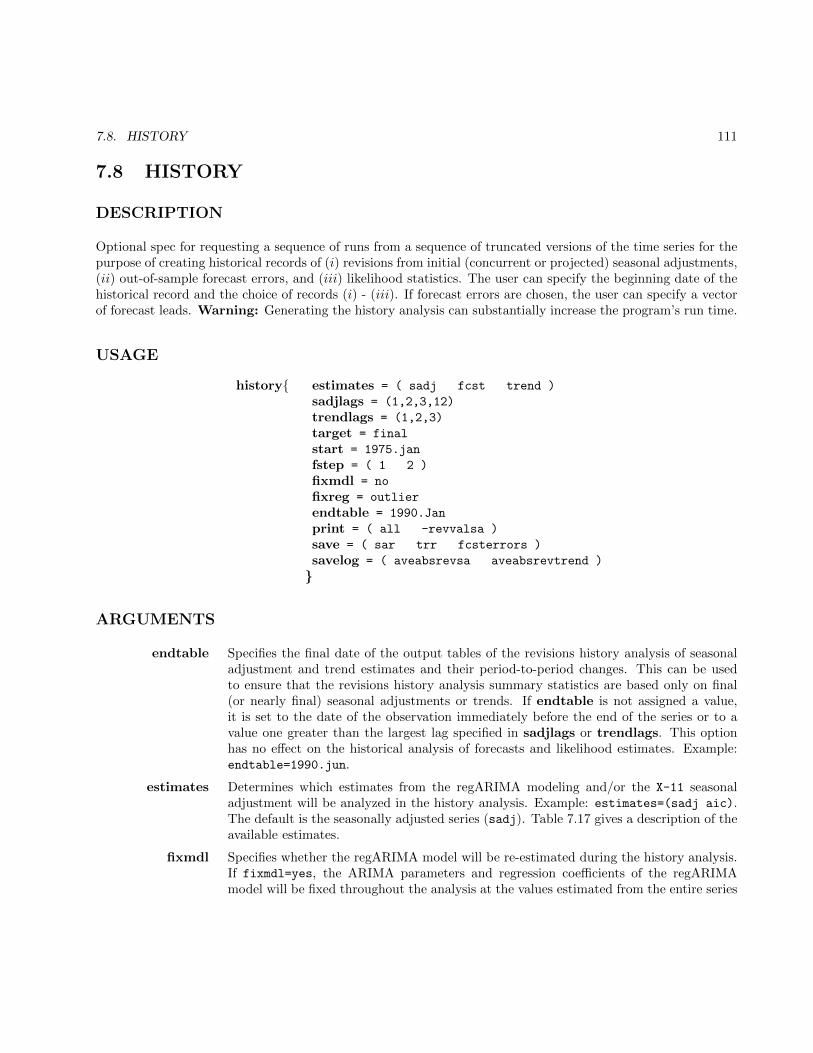
7.8. HISTORY 111
7.8 HISTORY
DESCRIPTION
Optional spec for requesting a sequence of runs from a sequence of truncated versions of the time series for thepurpose of creating historical records of (i) revisions from initial (concurrent or projected) seasonal adjustments,(ii) out-of-sample forecast errors, and (iii) likelihood statistics. The user can specify the beginning date of thehistorical record and the choice of records (i) - (iii). If forecast errors are chosen, the user can specify a vectorof forecast leads. Warning: Generating the history analysis can substantially increase the program’s run time.
USAGE
history{ estimates = ( sadj fcst trend )
sadjlags = (1,2,3,12)
trendlags = (1,2,3)
target = final
start = 1975.jan
fstep = ( 1 2 )
fixmdl = no
fixreg = outlier
endtable = 1990.Jan
print = ( all -revvalsa )
save = ( sar trr fcsterrors )
savelog = ( aveabsrevsa aveabsrevtrend )
}
ARGUMENTS
endtable Specifies the final date of the output tables of the revisions history analysis of seasonaladjustment and trend estimates and their period-to-period changes. This can be usedto ensure that the revisions history analysis summary statistics are based only on final(or nearly final) seasonal adjustments or trends. If endtable is not assigned a value,it is set to the date of the observation immediately before the end of the series or to avalue one greater than the largest lag specified in sadjlags or trendlags. This optionhas no effect on the historical analysis of forecasts and likelihood estimates. Example:endtable=1990.jun.
estimates Determines which estimates from the regARIMA modeling and/or the X-11 seasonaladjustment will be analyzed in the history analysis. Example: estimates=(sadj aic).The default is the seasonally adjusted series (sadj). Table 7.17 gives a description of theavailable estimates.
fixmdl Specifies whether the regARIMA model will be re-estimated during the history analysis.If fixmdl=yes, the ARIMA parameters and regression coefficients of the regARIMAmodel will be fixed throughout the analysis at the values estimated from the entire series
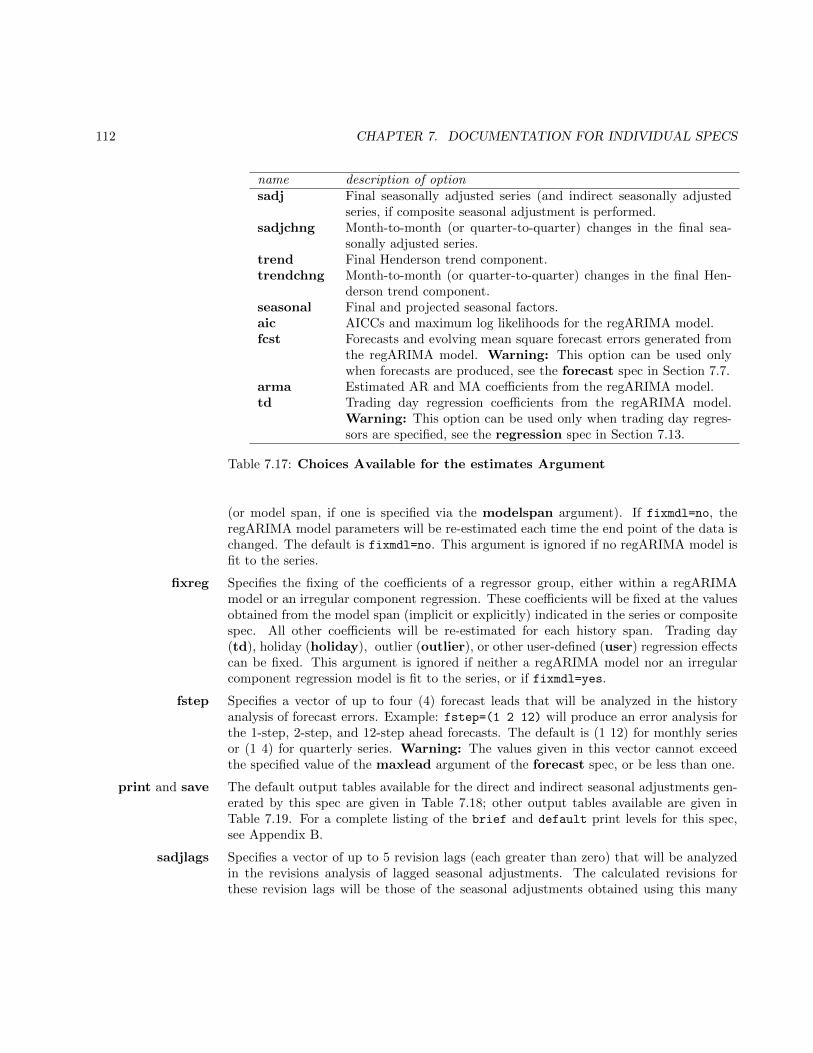
112 CHAPTER 7. DOCUMENTATION FOR INDIVIDUAL SPECS
name description of optionsadj Final seasonally adjusted series (and indirect seasonally adjusted
series, if composite seasonal adjustment is performed.sadjchng Month-to-month (or quarter-to-quarter) changes in the final sea-
sonally adjusted series.trend Final Henderson trend component.trendchng Month-to-month (or quarter-to-quarter) changes in the final Hen-
derson trend component.seasonal Final and projected seasonal factors.aic AICCs and maximum log likelihoods for the regARIMA model.fcst Forecasts and evolving mean square forecast errors generated from
the regARIMA model. Warning: This option can be used onlywhen forecasts are produced, see the forecast spec in Section 7.7.
arma Estimated AR and MA coefficients from the regARIMA model.td Trading day regression coefficients from the regARIMA model.
Warning: This option can be used only when trading day regres-sors are specified, see the regression spec in Section 7.13.
Table 7.17: Choices Available for the estimates Argument
(or model span, if one is specified via the modelspan argument). If fixmdl=no, theregARIMA model parameters will be re-estimated each time the end point of the data ischanged. The default is fixmdl=no. This argument is ignored if no regARIMA model isfit to the series.
fixreg Specifies the fixing of the coefficients of a regressor group, either within a regARIMAmodel or an irregular component regression. These coefficients will be fixed at the valuesobtained from the model span (implicit or explicitly) indicated in the series or compositespec. All other coefficients will be re-estimated for each history span. Trading day(td), holiday (holiday), outlier (outlier), or other user-defined (user) regression effectscan be fixed. This argument is ignored if neither a regARIMA model nor an irregularcomponent regression model is fit to the series, or if fixmdl=yes.
fstep Specifies a vector of up to four (4) forecast leads that will be analyzed in the historyanalysis of forecast errors. Example: fstep=(1 2 12) will produce an error analysis forthe 1-step, 2-step, and 12-step ahead forecasts. The default is (1 12) for monthly seriesor (1 4) for quarterly series. Warning: The values given in this vector cannot exceedthe specified value of the maxlead argument of the forecast spec, or be less than one.
print and save The default output tables available for the direct and indirect seasonal adjustments gen-erated by this spec are given in Table 7.18; other output tables available are given inTable 7.19. For a complete listing of the brief and default print levels for this spec,see Appendix B.
sadjlags Specifies a vector of up to 5 revision lags (each greater than zero) that will be analyzedin the revisions analysis of lagged seasonal adjustments. The calculated revisions forthese revision lags will be those of the seasonal adjustments obtained using this many
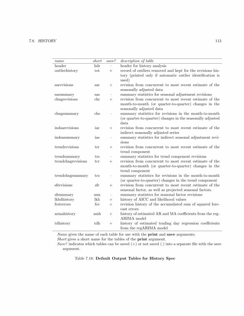
7.8. HISTORY 113
name short save? description of tableheader hdr · header for history analysisoutlierhistory rot + record of outliers removed and kept for the revisions his-
tory (printed only if automatic outlier identification isused)
sarevisions sar + revision from concurrent to most recent estimate of theseasonally adjusted data
sasummary sas · summary statistics for seasonal adjustment revisionschngrevisions chr + revision from concurrent to most recent estimate of the
month-to-month (or quarter-to-quarter) changes in theseasonally adjusted data
chngsummary chs · summary statistics for revisions in the month-to-month(or quarter-to-quarter) changes in the seasonally adjusteddata
indsarevisions iar + revision from concurrent to most recent estimate of theindirect seasonally adjusted series
indsasummary ias · summary statistics for indirect seasonal adjustment revi-sions
trendrevisions trr + revision from concurrent to most recent estimate of thetrend component
trendsummary trs · summary statistics for trend component revisionstrendchngrevisions tcr + revision from concurrent to most recent estimate of the
month-to-month (or quarter-to-quarter) changes in thetrend component
trendchngsummary tcs · summary statistics for revisions in the month-to-month(or quarter-to-quarter) changes in the trend component
sfrevisions sfr + revision from concurrent to most recent estimate of theseasonal factor, as well as projected seasonal factors.
sfsummary ssm · summary statistics for seasonal factor revisionslkhdhistory lkh + history of AICC and likelihood valuesfcsterrors fce + revision history of the accumulated sum of squared fore-
cast errorsarmahistory amh + history of estimated AR and MA coefficients from the reg-
ARIMA modeltdhistory tdh + history of estimated trading day regression coefficients
from the regARIMA model
Name gives the name of each table for use with the print and save arguments.Short gives a short name for the tables of the print argument.Save? indicates which tables can be saved (+) or not saved (·) into a separate file with the save
argument.
Table 7.18: Default Output Tables for History Spec
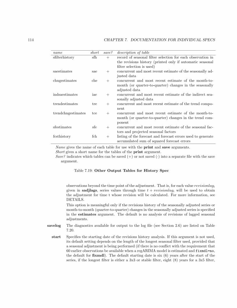
114 CHAPTER 7. DOCUMENTATION FOR INDIVIDUAL SPECS
name short save? description of tablesfilterhistory sfh + record of seasonal filter selection for each observation in
the revisions history (printed only if automatic seasonalfilter selection is used)
saestimates sae + concurrent and most recent estimate of the seasonally ad-justed data
chngestimates che + concurrent and most recent estimate of the month-to-month (or quarter-to-quarter) changes in the seasonallyadjusted data
indsaestimates iae + concurrent and most recent estimate of the indirect sea-sonally adjusted data
trendestimates tre + concurrent and most recent estimate of the trend compo-nent
trendchngestimates tce + concurrent and most recent estimate of the month-to-month (or quarter-to-quarter) changes in the trend com-ponent
sfestimates sfe + concurrent and most recent estimate of the seasonal fac-tors and projected seasonal factors
fcsthistory fch + listing of the forecast and forecast errors used to generateaccumulated sum of squared forecast errors
Name gives the name of each table for use with the print and save arguments.Short gives a short name for the tables of the print argument.Save? indicates which tables can be saved (+) or not saved (·) into a separate file with the save
argument.
Table 7.19: Other Output Tables for History Spec
observations beyond the time point of the adjustment. That is, for each value revisionlagigiven in sadjlags, series values through time t + revisionlagi will be used to obtainthe adjustment for time t whose revision will be calculated. For more information, seeDETAILS.
This option is meaningful only if the revisions history of the seasonally adjusted series ormonth-to-month (quarter-to-quarter) changes in the seasonally adjusted series is specifiedin the estimates argument. The default is no analysis of revisions of lagged seasonaladjustments.
savelog The diagnostics available for output to the log file (see Section 2.6) are listed on Table7.20.
start Specifies the starting date of the revisions history analysis. If this argument is not used,its default setting depends on the length of the longest seasonal filter used, provided thata seasonal adjustment is being performed (if there is no conflict with the requirement that60 earlier observations be available when a regARIMA model is estimated and fixmdl=no,the default for fixmdl). The default starting date is six (6) years after the start of theseries, if the longest filter is either a 3x3 or stable filter, eight (8) years for a 3x5 filter,
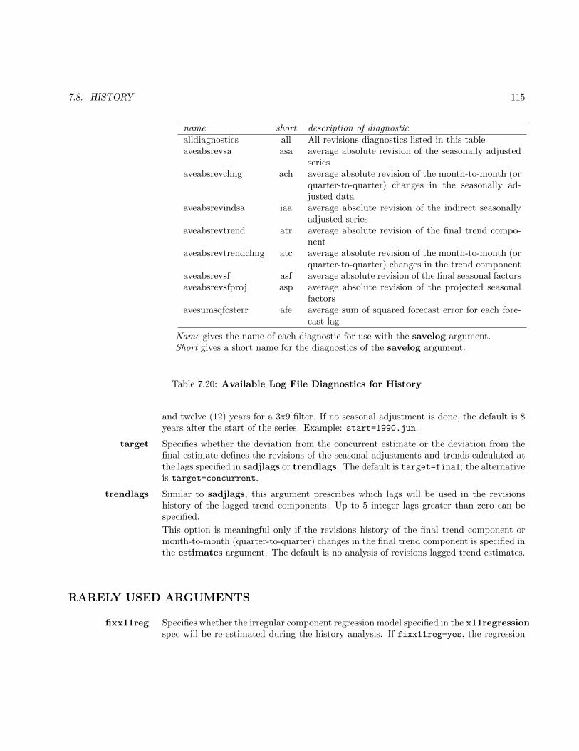
7.8. HISTORY 115
name short description of diagnosticalldiagnostics all All revisions diagnostics listed in this tableaveabsrevsa asa average absolute revision of the seasonally adjusted
seriesaveabsrevchng ach average absolute revision of the month-to-month (or
quarter-to-quarter) changes in the seasonally ad-justed data
aveabsrevindsa iaa average absolute revision of the indirect seasonallyadjusted series
aveabsrevtrend atr average absolute revision of the final trend compo-nent
aveabsrevtrendchng atc average absolute revision of the month-to-month (orquarter-to-quarter) changes in the trend component
aveabsrevsf asf average absolute revision of the final seasonal factorsaveabsrevsfproj asp average absolute revision of the projected seasonal
factorsavesumsqfcsterr afe average sum of squared forecast error for each fore-
cast lag
Name gives the name of each diagnostic for use with the savelog argument.Short gives a short name for the diagnostics of the savelog argument.
Table 7.20: Available Log File Diagnostics for History
and twelve (12) years for a 3x9 filter. If no seasonal adjustment is done, the default is 8years after the start of the series. Example: start=1990.jun.
target Specifies whether the deviation from the concurrent estimate or the deviation from thefinal estimate defines the revisions of the seasonal adjustments and trends calculated atthe lags specified in sadjlags or trendlags. The default is target=final; the alternativeis target=concurrent.
trendlags Similar to sadjlags, this argument prescribes which lags will be used in the revisionshistory of the lagged trend components. Up to 5 integer lags greater than zero can bespecified.
This option is meaningful only if the revisions history of the final trend component ormonth-to-month (quarter-to-quarter) changes in the final trend component is specified inthe estimates argument. The default is no analysis of revisions lagged trend estimates.
RARELY USED ARGUMENTS
fixx11reg Specifies whether the irregular component regression model specified in the x11regressionspec will be re-estimated during the history analysis. If fixx11reg=yes, the regression
116 CHAPTER 7. DOCUMENTATION FOR INDIVIDUAL SPECS
coefficients for the irregular component regression model are fixed throughout the analysisat the values estimated from the entire series. If fixx11reg=no, the irregular componentregression model parameters will be re-estimated each time the end point of the historyinterval is advanced.
The default is fixx11reg=no. This argument is ignored if no irregular component re-gression model is specified.
outlier Specifies whether automatic outlier detection is to be performed whenever the regARIMAmodel is re-estimated during the revisions history analysis. This argument has no effectif the outlier spec is not used.
If outlier=keep, all outliers automatically identified using the full series are kept in theregARIMA model during the revisions history analysis. The coefficients estimating theeffects of these outliers are re-estimated whenever the other regARIMA model parametersare re-estimated. No additional outliers are automatically identified and estimated. Thisis the default setting.
If outlier=remove, those outlier regressors that were added to the regression part ofthe regARIMA model when automatic outlier identification was performed on the fullseries are removed from the regARIMA model during the revisions history analysis.Consequently, their effects are not estimated and removed from the series. This optiongives the user a way to investigate the consequences of not doing automatic outlieridentification.
If outlier=auto, among outliers automatically identified for the full series, only thosethat fall in the time period up to outlierwin observations before the starting date of therevisions history analysis are automatically included in the regARIMA model. In eachrun of the estimation procedure with a truncated version of the original series, automaticoutlier identification is performed only for the last outlierwin+1 observations. An outlierthat is identified is used for the current run, but is only retained for the subsequent runsof the historical analysis if it is at least outlierwin observations from the end of thesubsequent span of data being analyzed.
outlierwin Specifies how many observations before the end of each span will be used for outlieridentification during the revisions history analysis. The default is 12 for monthly seriesand 4 for quarterly series. This argument has an effect only if the outlier spec is used,and if outlier=auto in the history spec.
refresh Specifies which of two sets of initializing values is used for the regARIMA model parame-ter estimation. If refresh=yes, the parameter estimates from the last model evaluationare used as starting values for the current regARIMA model estimation done duringthe revisions history. If refresh=no, then the initial values of the regARIMA modelparameters will be set to the estimates derived from the entire series. The default isrefresh=no.
transformfcst Specifies whether the forecast error output of the history analysis is for forecasts ofthe original data (transformfcst = no) or for the forecasts of the transformed dataspecified by the transform spec (transformfcst = yes). See Details. The default istransformfcst = no.
x11outlier Specifies whether the AO outlier identification will be performed during the history anal-

7.8. HISTORY 117
ysis for all irregular component regressions that result from the x11regression spec. Ifx11outlier=yes, AO outlier identification will be performed for each of the history runs.Those AO outlier regressors that were added to the irregular component regression modelwhen automatic AO outlier identification was done for the full series are removed from theirregular component regression model prior to the history runs. If x11outlier=no, thenthe AO outlier regressors automatically identified are kept for each of the history runs. Ifthe date of an outlier detected for the complete span of data does not occur in the dataspan of one of the history runs, the outlier will be dropped from the model for that run.The coefficients estimating the effects of these AO outliers are re-estimated whenever theother irregular component regression model parameters are re-estimated. However, noadditional AO outliers are automatically identified and estimated. This option is ignoredif the x11regression spec is not used, if the selection of the aictest argument resultsin the program not estimating an irregular component regression model, or if the sigmaargument is used in the x11regression spec. The default is x11outlier=yes.
DETAILS
Section 6.3 gives technical details on revisions history analysis. For some supporting theory for out-of-samplesquared forecast error diagnostic output, see Findley (2005).
When a revision history analysis of the seasonally adjusted series is specified for a composite seasonaladjustment, the revisions of both the direct and indirect seasonally adjusted series can be produced. Therevision history analysis must be specified for each of the component series, even for those component seriesthat are not seasonally adjusted, see the Examples section of composite spec documentation in Section 7.4.
The revision history of the indirect seasonally adjusted series (sadj in Table 7.17) is the only revision historyavailable for indirect seasonal adjustments.
In each input specification file, a starting date for the history analysis must be specified using the startargument of this spec, and this starting date should be the same for each of the components and the compositeseries. If this is not the case, then only the history analysis of the direct seasonal adjustment will be performed.
If the automatic seasonal filter selection option is used, the program will redo the choice of seasonal filtereach time the data span is changed in the revision history analysis. If the seasonal filter should change in thecourse of the analysis, a warning message will be printed out, and a table of the seasonal filter lengths chosenfor each data span will be printed out.
The starting date for the forecast revisions depends on the values given for fstep. The starting date for ahistory of n-step-ahead forecast errors is n periods after the starting date of the history analysis. Example:if fstep = (1 12) and start = 1992.jan, the history for the 1-step and 12-step ahead forecasts will start inFebruary of 1992 and January of 1993, respectively.
In some situations, the program automatically switches to using fixed model coefficients for the historyanalysis. This happens when the start of the revisions history analysis (which can be set by the user with thestart argument) causes some truncated data span to have fewer than 60 observations for regARIMA modelestimation, either because of the series length or a span or modelspan argument value (in the series or
118 CHAPTER 7. DOCUMENTATION FOR INDIVIDUAL SPECS
composite spec). In this case, the coefficients (ARIMA and regression) of the regARIMA model will be heldfixed throughout the analysis at the values estimated from the entire series (or model span, if one is specified).
Fixing of the coefficients will also occur for every truncated data span that contains data later than theending date specified in a modelspan argument. In particular, in the extreme case, when the ending date ofthe model span is earlier than the starting date of the history analysis, the coefficients of the regARIMA modelwill be fixed throughout the history analysis.
Regression models from the x11regression spec are treated similarly. For example, their coefficients arefixed if some truncated data span has fewer than 60 observations because of a date assigned to the spanargument of x11regression.
If an outlier specified by the user occurs in the period after the starting date of the revision history, thatoutlier will be dropped from the model at the start of the revision history analysis. It will be re-introduced intothe regARIMA model when enough data have been added for the outlier variable to be defined. User-definedregressors are treated in the same way.
EXAMPLES
The following examples illustrating all the steps of a composite adjustment show complete spec files.
Example 1 A multiplicative monthly seasonal adjustment is to be performed with 3x9 seasonal movingaverages for all months without using regARIMA model forecasts, backcasts, or regressionoutlier adjustments. A revision history of just the seasonally adjusted series will be per-formed (remember, this is the default history) for all data, after a startup period of twelveyears (because 3x9 seasonal factors are used), with an additional analysis on the estimatesmade 2 periods after the concurrent observation.
Series { Title = "Sales Of Livestock" Start = 1967.1
File = "cattle.ori" }
X11 { SeasonalMA = S3X9 }
History { sadjlags = 2 }
Example 2 Utilize a seasonal ARIMA model with regression variables for outlier and level shift pread-justment. The specified regression variables are a constant, trading day effects, and twolevel shifts, one in May 1972 and one in Sept. 1976. The ARIMA part of the model is(0,1,2)(1,1,0)12. Generate a history of the 1-step ahead forecast errors. Start the analysisin January of 1975; this means the first 1-step ahead forecast error in the analysis is forFebruary of 1975.
series { title = "Exports of Leather goods"
start = 1969.jul file = "expleth.dat" }
regression { variables = (const td ls1972.may ls1976.oct) }
arima { model = (0 1 2)(1 1 0) }
estimate { }
history { estimates = fcst fstep = 1 start=1975.jan }
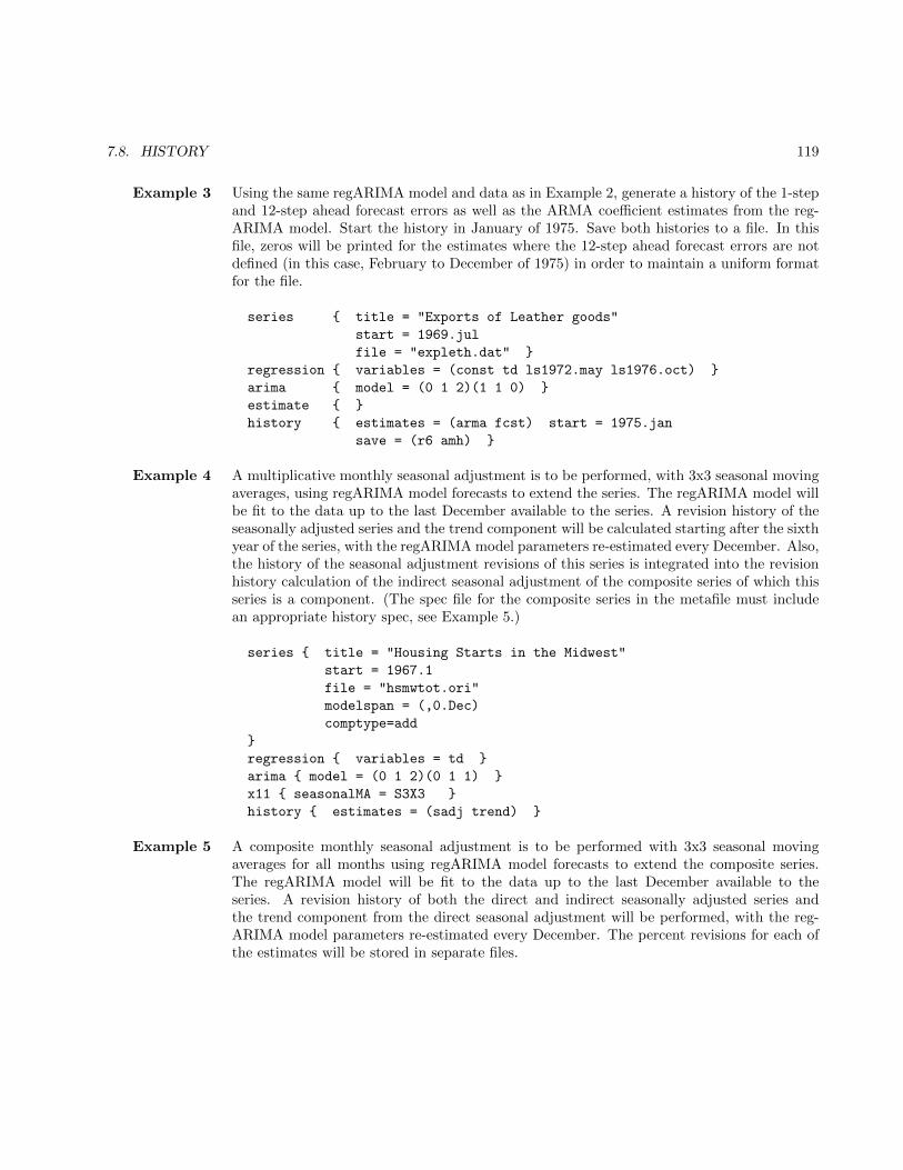
7.8. HISTORY 119
Example 3 Using the same regARIMA model and data as in Example 2, generate a history of the 1-stepand 12-step ahead forecast errors as well as the ARMA coefficient estimates from the reg-ARIMA model. Start the history in January of 1975. Save both histories to a file. In thisfile, zeros will be printed for the estimates where the 12-step ahead forecast errors are notdefined (in this case, February to December of 1975) in order to maintain a uniform formatfor the file.
series { title = "Exports of Leather goods"
start = 1969.jul
file = "expleth.dat" }
regression { variables = (const td ls1972.may ls1976.oct) }
arima { model = (0 1 2)(1 1 0) }
estimate { }
history { estimates = (arma fcst) start = 1975.jan
save = (r6 amh) }
Example 4 A multiplicative monthly seasonal adjustment is to be performed, with 3x3 seasonal movingaverages, using regARIMA model forecasts to extend the series. The regARIMA model willbe fit to the data up to the last December available to the series. A revision history of theseasonally adjusted series and the trend component will be calculated starting after the sixthyear of the series, with the regARIMA model parameters re-estimated every December. Also,the history of the seasonal adjustment revisions of this series is integrated into the revisionhistory calculation of the indirect seasonal adjustment of the composite series of which thisseries is a component. (The spec file for the composite series in the metafile must includean appropriate history spec, see Example 5.)
series { title = "Housing Starts in the Midwest"
start = 1967.1
file = "hsmwtot.ori"
modelspan = (,0.Dec)
comptype=add
}
regression { variables = td }
arima { model = (0 1 2)(0 1 1) }
x11 { seasonalMA = S3X3 }
history { estimates = (sadj trend) }
Example 5 A composite monthly seasonal adjustment is to be performed with 3x3 seasonal movingaverages for all months using regARIMA model forecasts to extend the composite series.The regARIMA model will be fit to the data up to the last December available to theseries. A revision history of both the direct and indirect seasonally adjusted series andthe trend component from the direct seasonal adjustment will be performed, with the reg-ARIMA model parameters re-estimated every December. The percent revisions for each ofthe estimates will be stored in separate files.

120 CHAPTER 7. DOCUMENTATION FOR INDIVIDUAL SPECS
composite{ title = "Total Housing Starts in the US"
modelspan = (,0.Dec)
}
regression { variables = td }
arima { model = (0 1 1)(0 1 1) }
x11 { seasonalMA = S3X3 }
history { estimates = (sadj trend)
save = (sar iar trr) }
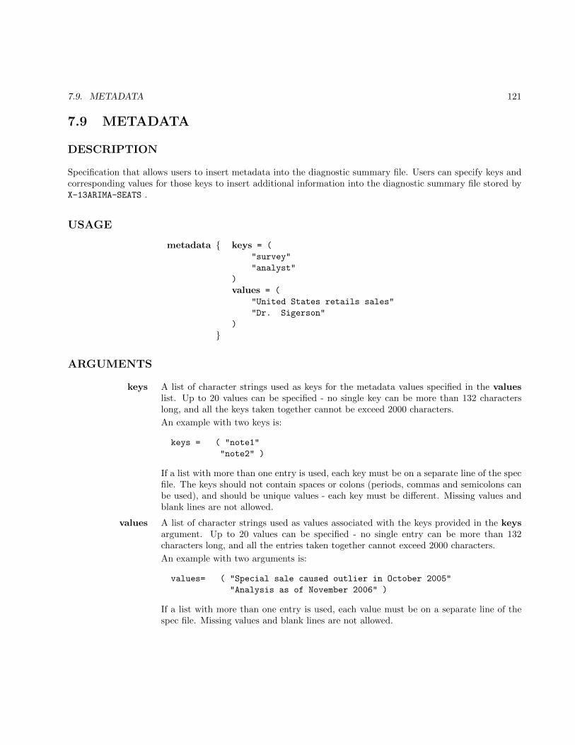
7.9. METADATA 121
7.9 METADATA
DESCRIPTION
Specification that allows users to insert metadata into the diagnostic summary file. Users can specify keys andcorresponding values for those keys to insert additional information into the diagnostic summary file stored byX-13ARIMA-SEATS .
USAGE
metadata { keys = (
"survey"
"analyst"
)
values = (
"United States retails sales"
"Dr. Sigerson"
)
}
ARGUMENTS
keys A list of character strings used as keys for the metadata values specified in the valueslist. Up to 20 values can be specified - no single key can be more than 132 characterslong, and all the keys taken together cannot be exceed 2000 characters.
An example with two keys is:
keys = ( "note1"
"note2" )
If a list with more than one entry is used, each key must be on a separate line of the specfile. The keys should not contain spaces or colons (periods, commas and semicolons canbe used), and should be unique values - each key must be different. Missing values andblank lines are not allowed.
values A list of character strings used as values associated with the keys provided in the keysargument. Up to 20 values can be specified - no single entry can be more than 132characters long, and all the entries taken together cannot exceed 2000 characters.
An example with two arguments is:
values= ( "Special sale caused outlier in October 2005"
"Analysis as of November 2006" )
If a list with more than one entry is used, each value must be on a separate line of thespec file. Missing values and blank lines are not allowed.
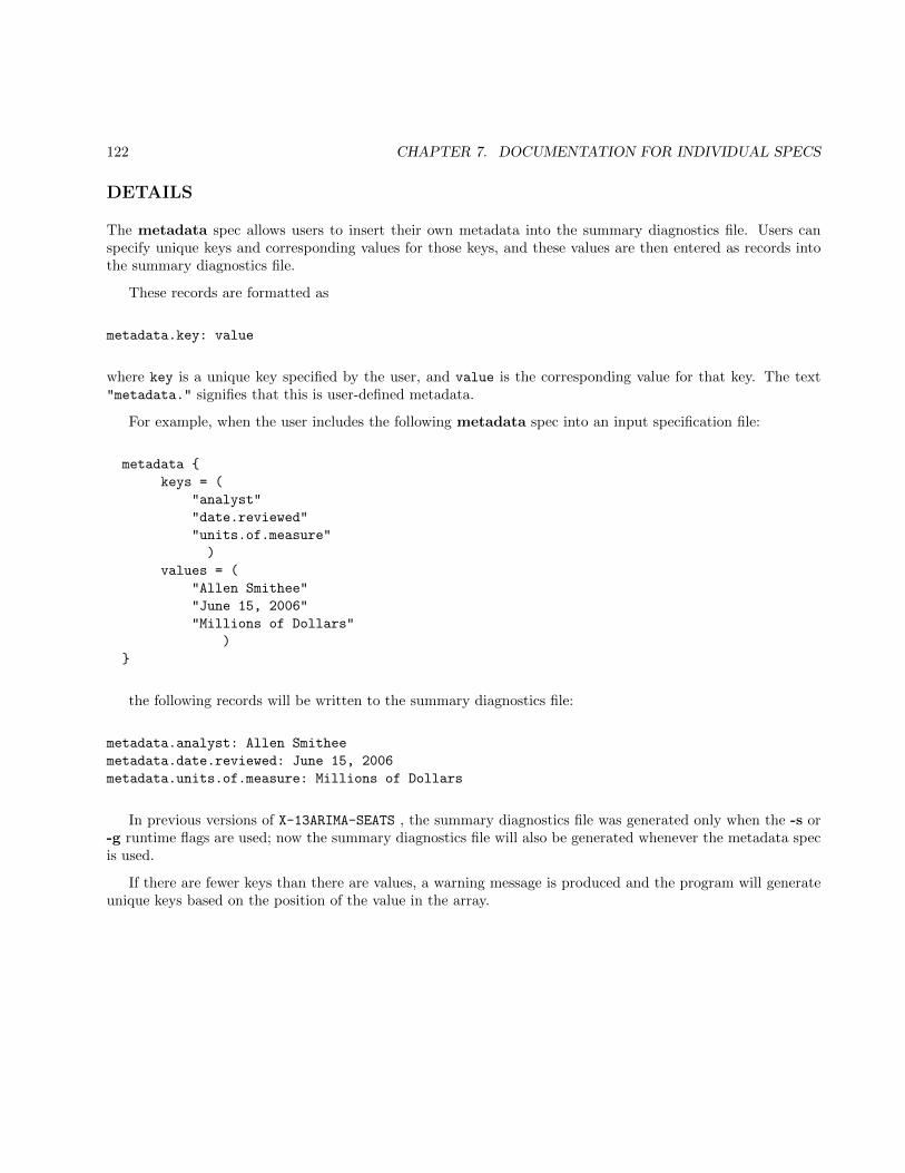
122 CHAPTER 7. DOCUMENTATION FOR INDIVIDUAL SPECS
DETAILS
The metadata spec allows users to insert their own metadata into the summary diagnostics file. Users canspecify unique keys and corresponding values for those keys, and these values are then entered as records intothe summary diagnostics file.
These records are formatted as
metadata.key: value
where key is a unique key specified by the user, and value is the corresponding value for that key. The text"metadata." signifies that this is user-defined metadata.
For example, when the user includes the following metadata spec into an input specification file:
metadata {
keys = (
"analyst"
"date.reviewed"
"units.of.measure"
)
values = (
"Allen Smithee"
"June 15, 2006"
"Millions of Dollars"
)
}
the following records will be written to the summary diagnostics file:
metadata.analyst: Allen Smithee
metadata.date.reviewed: June 15, 2006
metadata.units.of.measure: Millions of Dollars
In previous versions of X-13ARIMA-SEATS , the summary diagnostics file was generated only when the -s or-g runtime flags are used; now the summary diagnostics file will also be generated whenever the metadata specis used.
If there are fewer keys than there are values, a warning message is produced and the program will generateunique keys based on the position of the value in the array.

7.9. METADATA 123
For example, the following metadata spec:
metadata {
keys = (
"analyst"
"date.reviewed"
)
values = (
"Allen Smithee"
"June 15, 2006"
"Millions of Dollars"
)
}
produces the following records in the summary diagnostics file:
metadata.analyst: Allen Smithee
metadata.date.reviewed: June 15, 2006
metadata.key3: Millions of Dollars
Not specifying a key argument at all will force the program to generate unique keys for all the values specified.
metadata {
values = (
"Allen Smithee"
"June 15, 2006"
"Millions of Dollars"
)
}
produces the following records in the summary diagnostics file:
metadata.key1: Allen Smithee
metadata.key2: June 15, 2006
metadata.key3: Millions of Dollars
If more keys are specified than values, execution will cease and an error message will be produced.
Note that the metadata spec can appear in any order relative to the other specs - it can be the first specin the spec file, etc.
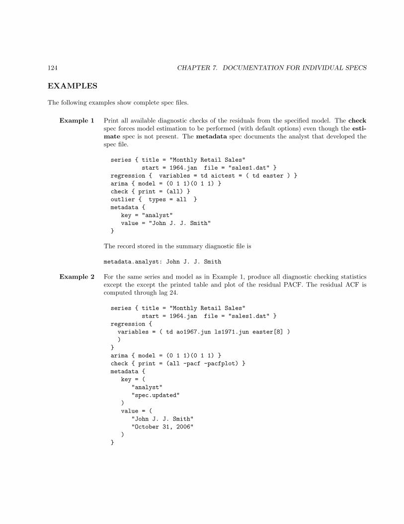
124 CHAPTER 7. DOCUMENTATION FOR INDIVIDUAL SPECS
EXAMPLES
The following examples show complete spec files.
Example 1 Print all available diagnostic checks of the residuals from the specified model. The checkspec forces model estimation to be performed (with default options) even though the esti-mate spec is not present. The metadata spec documents the analyst that developed thespec file.
series { title = "Monthly Retail Sales"
start = 1964.jan file = "sales1.dat" }
regression { variables = td aictest = ( td easter ) }
arima { model = (0 1 1)(0 1 1) }
check { print = (all) }
outlier { types = all }
metadata {
key = "analyst"
value = "John J. J. Smith"
}
The record stored in the summary diagnostic file is
metadata.analyst: John J. J. Smith
Example 2 For the same series and model as in Example 1, produce all diagnostic checking statisticsexcept the except the printed table and plot of the residual PACF. The residual ACF iscomputed through lag 24.
series { title = "Monthly Retail Sales"
start = 1964.jan file = "sales1.dat" }
regression {
variables = ( td ao1967.jun ls1971.jun easter[8] )
)
}
arima { model = (0 1 1)(0 1 1) }
check { print = (all -pacf -pacfplot) }
metadata {
key = (
"analyst"
"spec.updated"
)
value = (
"John J. J. Smith"
"October 31, 2006"
)
}

7.9. METADATA 125
The record stored in the summary diagnostic file is
metadata.analyst: John J. J. Smith
metadata.spec.updated: October 31, 2006
Example 3 For the same series and model as in Example 2, add metadata text to describe the outliersfound by the automatic outlier procedure.
series { title = "Monthly Retail Sales"
start = 1964.jan file = "sales1.dat" }
regression {
variables = (
td ao1967.jun ls1971.jun easter[15]
)
}
arima { model = (0 1 1)(0 1 1) }
check { print = (all -pacf -pacfplot) }
x11 { save = d11 }
metadata {
key = (
"analyst"
"spec.final"
)
value = (
"John J. J. Smith"
"November 10, 2006"
"AO caused by strike, LS caused by survey change"
)
}
The record stored in the summary diagnostic file is
metadata.analyst: John J. J. Smith
metadata.spec.updated: November 10, 2006
metadata.key3: AO caused by strike, LS caused by survey change

126 CHAPTER 7. DOCUMENTATION FOR INDIVIDUAL SPECS
7.10 IDENTIFY
DESCRIPTION
Specification to produce tables and line printer plots of sample ACFs and PACFs for identifying the ARIMApart of a regARIMA model. Sample ACFs and PACFs are produced for all combinations of the nonseasonal andseasonal differences of the data specified by the diff and sdiff arguments. If the regression spec is present, theACFs and PACFs are calculated for the specified differences of a series of regression residuals. If the regressionspec is not present, the ACFs and PACFs are calculated for the specified differences of the original data.
USAGE
identify { diff = (0, 1)
sdiff = (0, 1)
maxlag = 36
print = (none +acf +acfplot +pacf +pacfplot)
save = acf }
ARGUMENTS
diff Orders of nonseasonal differencing specified. The value 0 specifies no differencing, thevalue 1 specifies one nonseasonal difference (1−B), the value 2 specifies two nonseasonaldifferences (1−B)2, etc. The specified ACFs and PACFs will be produced for all orders ofnonseasonal differencing specified, in combination with all orders of seasonal differencingspecified in sdiff. The default is diff=(0).
maxlag The number of lags specified for the ACFs and PACFs for both tables and plots. Thedefault is 36 for monthly series, 12 for quarterly series.
print and save Table 7.21 gives the available output tables for this spec. All these tables are included inthe default printout, except regcoefficients. For a complete listing of the brief anddefault print levels for this spec, see Appendix B.
sdiff Orders of seasonal differencing specified. The value 0 specifies no seasonal differencing,the value 1 specifies one seasonal difference (1−Bs), etc. The specified ACFs and PACFswill be produced for all orders of seasonal differencing specified, in combination with allorders of nonseasonal differencing specified in diff. The default is sdiff=(0).
DETAILS
If the regression spec is present, the program differences the series (after processing by the transform spec) andthe regression variables using the maximum order of differencing specified by the diff and sdiff arguments. Thedifferenced series is then regressed on the differenced regression variables. The resulting regression coefficients(βi) are then used to calculate undifferenced regression effects (
∑i βixit), which are then subtracted from the
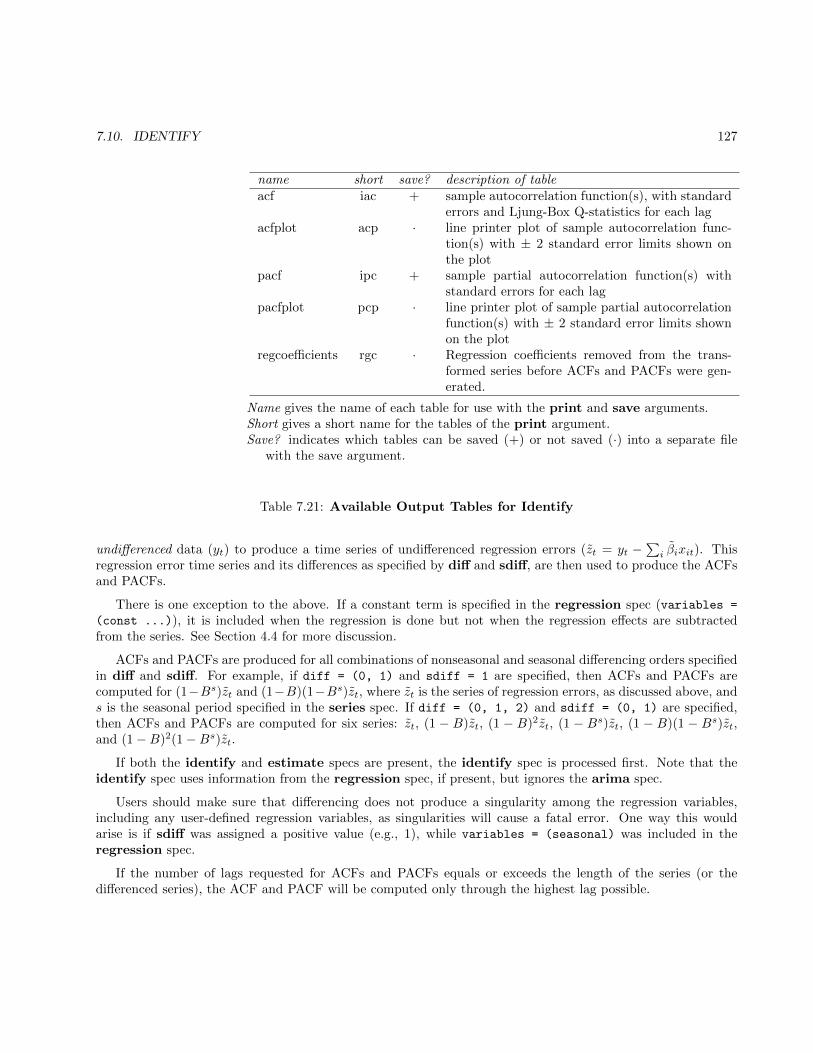
7.10. IDENTIFY 127
name short save? description of tableacf iac + sample autocorrelation function(s), with standard
errors and Ljung-Box Q-statistics for each lagacfplot acp · line printer plot of sample autocorrelation func-
tion(s) with ± 2 standard error limits shown onthe plot
pacf ipc + sample partial autocorrelation function(s) withstandard errors for each lag
pacfplot pcp · line printer plot of sample partial autocorrelationfunction(s) with ± 2 standard error limits shownon the plot
regcoefficients rgc · Regression coefficients removed from the trans-formed series before ACFs and PACFs were gen-erated.
Name gives the name of each table for use with the print and save arguments.Short gives a short name for the tables of the print argument.Save? indicates which tables can be saved (+) or not saved (·) into a separate file
with the save argument.
Table 7.21: Available Output Tables for Identify
undifferenced data (yt) to produce a time series of undifferenced regression errors (zt = yt −∑i βixit). This
regression error time series and its differences as specified by diff and sdiff, are then used to produce the ACFsand PACFs.
There is one exception to the above. If a constant term is specified in the regression spec (variables =
(const ...)), it is included when the regression is done but not when the regression effects are subtractedfrom the series. See Section 4.4 for more discussion.
ACFs and PACFs are produced for all combinations of nonseasonal and seasonal differencing orders specifiedin diff and sdiff. For example, if diff = (0, 1) and sdiff = 1 are specified, then ACFs and PACFs arecomputed for (1−Bs)zt and (1−B)(1−Bs)zt, where zt is the series of regression errors, as discussed above, ands is the seasonal period specified in the series spec. If diff = (0, 1, 2) and sdiff = (0, 1) are specified,then ACFs and PACFs are computed for six series: zt, (1 − B)zt, (1 − B)2zt, (1 − Bs)zt, (1 − B)(1 − Bs)zt,and (1−B)2(1−Bs)zt.
If both the identify and estimate specs are present, the identify spec is processed first. Note that theidentify spec uses information from the regression spec, if present, but ignores the arima spec.
Users should make sure that differencing does not produce a singularity among the regression variables,including any user-defined regression variables, as singularities will cause a fatal error. One way this wouldarise is if sdiff was assigned a positive value (e.g., 1), while variables = (seasonal) was included in theregression spec.
If the number of lags requested for ACFs and PACFs equals or exceeds the length of the series (or thedifferenced series), the ACF and PACF will be computed only through the highest lag possible.
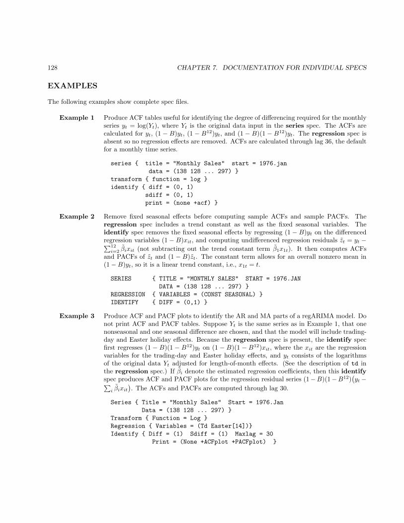
128 CHAPTER 7. DOCUMENTATION FOR INDIVIDUAL SPECS
EXAMPLES
The following examples show complete spec files.
Example 1 Produce ACF tables useful for identifying the degree of differencing required for the monthlyseries yt = log(Yt), where Yt is the original data input in the series spec. The ACFs arecalculated for yt, (1 − B)yt, (1 − B12)yt, and (1 − B)(1 − B12)yt. The regression spec isabsent so no regression effects are removed. ACFs are calculated through lag 36, the defaultfor a monthly time series.
series { title = "Monthly Sales" start = 1976.jan
data = (138 128 ... 297) }
transform { function = log }
identify { diff = (0, 1)
sdiff = (0, 1)
print = (none +acf) }
Example 2 Remove fixed seasonal effects before computing sample ACFs and sample PACFs. Theregression spec includes a trend constant as well as the fixed seasonal variables. Theidentify spec removes the fixed seasonal effects by regressing (1 − B)yt on the differencedregression variables (1− B)xit, and computing undifferenced regression residuals zt = yt −∑12i=2 βixit (not subtracting out the trend constant term β1x1t). It then computes ACFs
and PACFs of zt and (1 − B)zt. The constant term allows for an overall nonzero mean in(1−B)yt, so it is a linear trend constant, i.e., x1t = t.
SERIES { TITLE = "MONTHLY SALES" START = 1976.JAN
DATA = (138 128 ... 297) }
REGRESSION { VARIABLES = (CONST SEASONAL) }
IDENTIFY { DIFF = (0,1) }
Example 3 Produce ACF and PACF plots to identify the AR and MA parts of a regARIMA model. Donot print ACF and PACF tables. Suppose Yt is the same series as in Example 1, that onenonseasonal and one seasonal difference are chosen, and that the model will include trading-day and Easter holiday effects. Because the regression spec is present, the identify specfirst regresses (1 − B)(1 − B12)yt on (1 − B)(1 − B12)xit, where the xit are the regressionvariables for the trading-day and Easter holiday effects, and yt consists of the logarithmsof the original data Yt adjusted for length-of-month effects. (See the description of td inthe regression spec.) If βi denote the estimated regression coefficients, then this identifyspec produces ACF and PACF plots for the regression residual series (1−B)(1−B12)
(yt−∑
i βixit). The ACFs and PACFs are computed through lag 30.
Series { Title = "Monthly Sales" Start = 1976.Jan
Data = (138 128 ... 297) }
Transform { Function = Log }
Regression { Variables = (Td Easter[14])}
Identify { Diff = (1) Sdiff = (1) Maxlag = 30
Print = (None +ACFplot +PACFplot) }
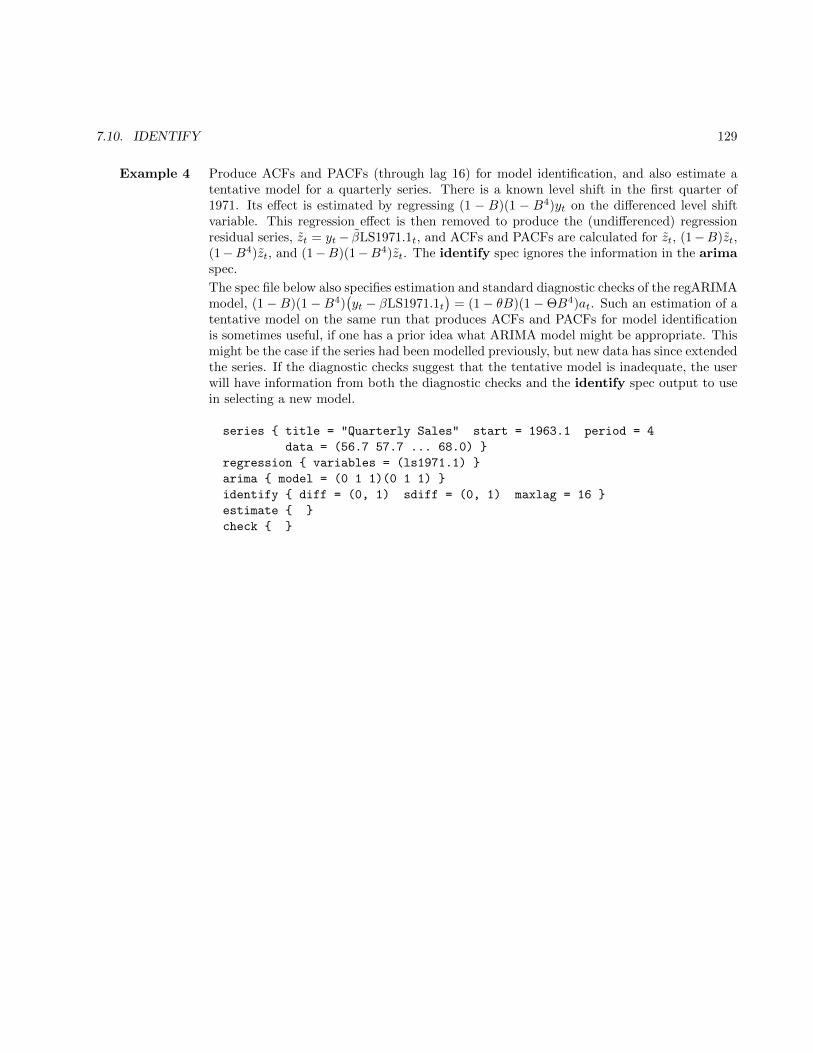
7.10. IDENTIFY 129
Example 4 Produce ACFs and PACFs (through lag 16) for model identification, and also estimate atentative model for a quarterly series. There is a known level shift in the first quarter of1971. Its effect is estimated by regressing (1 − B)(1 − B4)yt on the differenced level shiftvariable. This regression effect is then removed to produce the (undifferenced) regressionresidual series, zt = yt− βLS1971.1t, and ACFs and PACFs are calculated for zt, (1−B)zt,(1−B4)zt, and (1−B)(1−B4)zt. The identify spec ignores the information in the arimaspec.
The spec file below also specifies estimation and standard diagnostic checks of the regARIMAmodel, (1−B)(1−B4)
(yt − βLS1971.1t
)= (1− θB)(1−ΘB4)at. Such an estimation of a
tentative model on the same run that produces ACFs and PACFs for model identificationis sometimes useful, if one has a prior idea what ARIMA model might be appropriate. Thismight be the case if the series had been modelled previously, but new data has since extendedthe series. If the diagnostic checks suggest that the tentative model is inadequate, the userwill have information from both the diagnostic checks and the identify spec output to usein selecting a new model.
series { title = "Quarterly Sales" start = 1963.1 period = 4
data = (56.7 57.7 ... 68.0) }
regression { variables = (ls1971.1) }
arima { model = (0 1 1)(0 1 1) }
identify { diff = (0, 1) sdiff = (0, 1) maxlag = 16 }
estimate { }
check { }
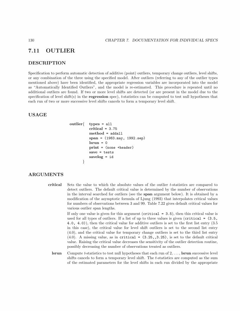
130 CHAPTER 7. DOCUMENTATION FOR INDIVIDUAL SPECS
7.11 OUTLIER
DESCRIPTION
Specification to perform automatic detection of additive (point) outliers, temporary change outliers, level shifts,or any combination of the three using the specified model. After outliers (referring to any of the outlier typesmentioned above) have been identified, the appropriate regression variables are incorporated into the modelas “Automatically Identified Outliers”, and the model is re-estimated. This procedure is repeated until noadditional outliers are found. If two or more level shifts are detected (or are present in the model due to thespecification of level shift(s) in the regression spec), t-statistics can be computed to test null hypotheses thateach run of two or more successive level shifts cancels to form a temporary level shift.
USAGE
outlier{ types = all
critical = 3.75
method = addall
span = (1983.may, 1992.sep)
lsrun = 0
print = (none +header)
save = tests
savelog = id
}
ARGUMENTS
critical Sets the value to which the absolute values of the outlier t-statistics are compared todetect outliers. The default critical value is determined by the number of observationsin the interval searched for outliers (see the span argument below). It is obtained by amodification of the asymptotic formula of Ljung (1993) that interpolates critical valuesfor numbers of observations between 3 and 99. Table 7.22 gives default critical values forvarious outlier span lengths.
If only one value is given for this argument (critical = 3.5), then this critical value isused for all types of outliers. If a list of up to three values is given (critical = (3.5,
4.0, 4.0)), then the critical value for additive outliers is set to the first list entry (3.5in this case), the critical value for level shift outliers is set to the second list entry(4.0), and the critical value for temporary change outliers is set to the third list entry(4.0). A missing value, as in critical = (3.25,,3.25), is set to the default criticalvalue. Raising the critical value decreases the sensitivity of the outlier detection routine,possibly decreasing the number of observations treated as outliers.
lsrun Compute t-statistics to test null hypotheses that each run of 2, . . . , lsrun successive levelshifts cancels to form a temporary level shift. The t-statistics are computed as the sumof the estimated parameters for the level shifts in each run divided by the appropriate
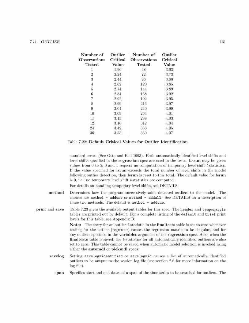
7.11. OUTLIER 131
Number of Outlier Number of OutlierObservations Critical Observations Critical
Tested Value Tested Value1 1.96 48 3.632 2.24 72 3.733 2.44 96 3.804 2.62 120 3.855 2.74 144 3.896 2.84 168 3.927 2.92 192 3.958 2.99 216 3.979 3.04 240 3.9910 3.09 264 4.0111 3.13 288 4.0312 3.16 312 4.0424 3.42 336 4.0536 3.55 360 4.07
Table 7.22: Default Critical Values for Outlier Identification
standard error. (See Otto and Bell 1993). Both automatically identified level shifts andlevel shifts specified in the regression spec are used in the tests. Lsrun may be givenvalues from 0 to 5; 0 and 1 request no computation of temporary level shift t-statistics.If the value specified for lsrun exceeds the total number of level shifts in the modelfollowing outlier detection, then lsrun is reset to this total. The default value for lsrunis 0, i.e., no temporary level shift t-statistics are computed.
For details on handling temporary level shifts, see DETAILS.
method Determines how the program successively adds detected outliers to the model. Thechoices are method = addone or method = addall. See DETAILS for a description ofthese two methods. The default is method = addone.
print and save Table 7.23 gives the available output tables for this spec. The header and temporaryls
tables are printed out by default. For a complete listing of the default and brief printlevels for this table, see Appendix B.
Note: The entry for an outlier t-statistic in the finaltests table is set to zero whenevertesting for the outlier (regressor) causes the regression matrix to be singular, and forany outliers specified in the variables argument of the regression spec. Also, when thefinaltests table is saved, the t-statistics for all automatically identified outliers are alsoset to zero. This table cannot be saved when automatic model selection is invoked usingeither the automdl or pickmdl specs.
savelog Setting savelog=identified or savelog=id causes a list of automatically identifiedoutliers to be output to the session log file (see section 2.6 for more information on thelog file).
span Specifies start and end dates of a span of the time series to be searched for outliers. The
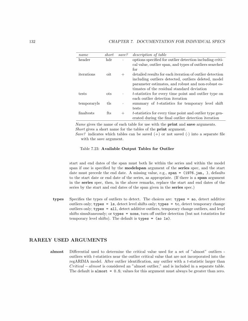
132 CHAPTER 7. DOCUMENTATION FOR INDIVIDUAL SPECS
name short save? description of tableheader hdr · options specified for outlier detection including criti-
cal value, outlier span, and types of outliers searchedfor
iterations oit + detailed results for each iteration of outlier detectionincluding outliers detected, outliers deleted, modelparameter estimates, and robust and non-robust es-timates of the residual standard deviation
tests ots · t-statistics for every time point and outlier type oneach outlier detection iteration
temporaryls tls · summary of t-statistics for temporary level shifttests
finaltests fts + t-statistics for every time point and outlier type gen-erated during the final outlier detection iteration
Name gives the name of each table for use with the print and save arguments.Short gives a short name for the tables of the print argument.Save? indicates which tables can be saved (+) or not saved (·) into a separate file
with the save argument.
Table 7.23: Available Output Tables for Outlier
start and end dates of the span must both lie within the series and within the modelspan if one is specified by the modelspan argument of the series spec, and the startdate must precede the end date. A missing value, e.g., span = (1976.jan, ), defaultsto the start date or end date of the series, as appropriate. (If there is a span argumentin the series spec, then, in the above remarks, replace the start and end dates of theseries by the start and end dates of the span given in the series spec.)
types Specifies the types of outliers to detect. The choices are: types = ao, detect additiveoutliers only; types = ls, detect level shifts only; types = tc, detect temporary changeoutliers only; types = all, detect additive outliers, temporary change outliers, and levelshifts simultaneously; or types = none, turn off outlier detection (but not t-statistics fortemporary level shifts). The default is types = (ao ls).
RARELY USED ARGUMENTS
almost Differential used to determine the critical value used for a set of ”almost” outliers -outliers with t-statistics near the outlier critical value that are not incorporated into theregARIMA model. After outlier identification, any outlier with a t-statistic larger thanCritical − almost is considered an ”almost outlier,” and is included in a separate table.The default is almost = 0.5; values for this argument must always be greater than zero.
7.11. OUTLIER 133
tcrate Defines the rate of decay for the temporary change outlier regressor. This value mustbe a number greater than zero and less than one. The default value is tcrate=0.7
** (12/period), where period is the number of observations in one year (for monthlytime series, 4 for quarterly time series). This formula for the default value of tcrateensures the same rate of decay over an entire year for series of different periodicity. Ifthe frequency of the time series is less than 4 (ie, period < 4), then there is no defaultvalue, and the user will have to enter a value of tcrate if a temporary change outlierwas specified in the variables argument of the regression spec, or if temporary changeoutliers are specified in the types argument of this spec. If this argument is specified inthe regression spec, it is not necessary to include it in this spec.
DETAILS
A level shift (LS) at the first data point cannot be estimated since the level of the series prior to the given datais unknown. Therefore, no LS test statistics is calculated for the first data point. Also, an LS at the last datapoint cannot be distinguished from an AO there, and an LS at the second data point cannot be distinguishedfrom an AO at the first data point. Thus, no LS statistics are calculated for the second and last data points ifAOs are also being detected. LS statistics that are not calculated are set to and printed out as 0.
Similarly, a temporary change (TC) outlier at the last data point cannot be distinguished from an AO there,so no TC statistics is calculated for the last data point if AOs are also being detected. TC statistics that arenot calculated are set to and printed out as 0.
Regarding the outlier regressors, users should be aware that several combinations of AOs and LSs producearithmetically equal effects. For example, (i) an AO at time t0 followed by an LS at t0 + 1; (ii) LSs at both t0and t0 +1; (iii) both an AO and an LS at t0. Note that an LS at t0 followed by an AO at t0 +1 is not equivalentto these other combinations.
Because AOs are assigned to the irregular component and LSs to the trend-cycle, some users might preferone equivalent combination over another.
The addone method works in the following way. The program calculates t-statistics for each type of outlierspecified (AO, TC and/or LS) at all time points for which outlier detection is being performed. If the maximumabsolute outlier t-statistic exceeds the critical value, then an outlier has been detected and the appropriateregression variable is added to the model. The program then estimates the new model (the old model with thedetected outlier added) and looks for an additional outlier. This process is repeated until no additional outliersare found. At this point, a backward deletion process is used to delete “insignificant” outliers (those whoseabsolute t-statistics no longer exceed the critical value) from the model. This is done one at a time beginningwith the least significant outlier, until all outliers remaining in the model are significant. During backwarddeletion the usual (non-robust) residual variance estimate is used, which can yield somewhat different outliert-statistics than those obtained during outlier detection.
The addall method follows the same general steps as the addone method, except that on each outlierdetection pass the addall method adds to the model all outliers with absolute t-statistics exceeding the criticalvalue. Typically several of the outliers added this way will be found to be insignificant when the new model isestimated. The addall method thus depends heavily on the backward deletion process (much more than doesthe addone method) to remove unnecessary outliers added to the model in the detection phase.
134 CHAPTER 7. DOCUMENTATION FOR INDIVIDUAL SPECS
The differences between the addone and addall schemes can produce different final sets of detected outliers.Two practical differences between the methods are worth noting. First, the addone method generally takes morecomputation time than does addall. Second, the addall method may add so many outliers on a detection passthat it exceeds the maximum number of regression variables allowed in a model. In this case the program printsan error message to this effect and stops. Suggested remedies are to raise the cutoff value so fewer outliers aredetected, or to switch to the addone method, for which this phenomenon is much less likely.
For either method, the outlier t-statistics for all possible time points on each detection pass can be printedby specifying print = iterations. This option generates considerable output.
Choosing the critical value requires both judgement and experience. Based on a simulation study involvingseries of length up to 200 generated from low order nonseasonal ARIMA models, Chang, Tiao, and Chen (1988)recommended critical values of 3 for high sensitivity in detection of AO outliers, 3.5 for medium sensitivity, and4 for low sensitivity.
Outlier detection begins with the model specified by the regression and arima specs and with estimatedparameters. If the estimate spec is absent, the outlier spec forces estimation of the model (with defaultestimation options) prior to outlier detection.
If outliers are suspected at specific known time points, then they may be included in the model by addingthe appropriate AO, TC, or LS regression variables to the model in the regression spec.
Outlier detection results can vary depending on the regARIMA model specified: observations are classified asoutliers because the model fits them less well than most of the other observations. Therefore a very inadequateregARIMA model can yield inappropriate outlier adjustments.
If one or more temporary level shift t-statistics indicate that a run of 2 (or more) successive level shiftscancels, a user-defined regressor can be used to capture the temporary level shift effect. In this way, two ormore level shifts can be replaced by one user-defined regressor. The usertype argument should be set to ls forthis regressor, so the user defined regressor is treated as a level shift. For more information on how to specifyuser-defined regressors, see the regression spec documentation in Section 7.13.
Another technique can be used if the span of observations affected by the temporary level shift is small.Individual AO outliers can be specified starting at the point of the first level shift and stopping with the pointbefore the final level shift.
EXAMPLES
The following examples show complete spec files.
Example 1 Simultaneously search for both AO and LS outliers over the entire time series, using theaddone method and a critical value that depends on the number of observations in theinterval searched for outliers (default options). If the number of level shifts present in themodel following outlier detection is two or more, compute t-statistics to test whether eachrun of 2, . . . , 5 successive level shifts cancels to form a temporary level shift. Though theestimate spec is absent, the presence of the outlier spec forces model estimation withdefault estimation options.
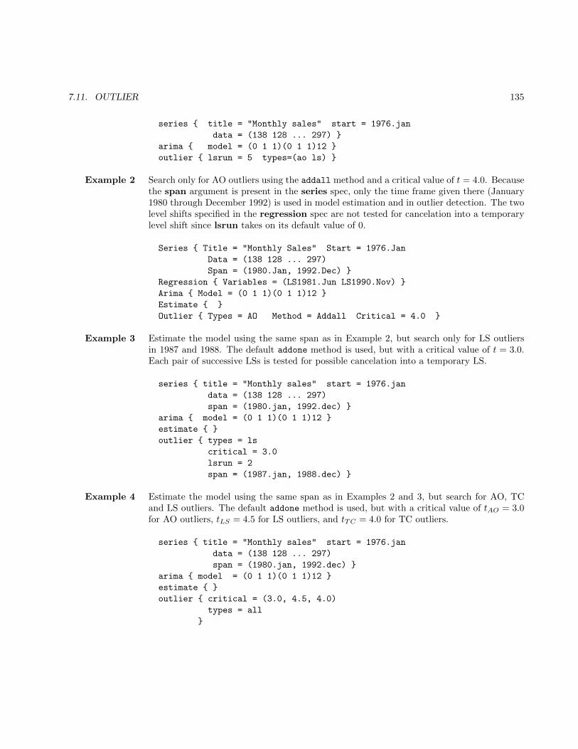
7.11. OUTLIER 135
series { title = "Monthly sales" start = 1976.jan
data = (138 128 ... 297) }
arima { model = (0 1 1)(0 1 1)12 }
outlier { lsrun = 5 types=(ao ls) }
Example 2 Search only for AO outliers using the addall method and a critical value of t = 4.0. Becausethe span argument is present in the series spec, only the time frame given there (January1980 through December 1992) is used in model estimation and in outlier detection. The twolevel shifts specified in the regression spec are not tested for cancelation into a temporarylevel shift since lsrun takes on its default value of 0.
Series { Title = "Monthly Sales" Start = 1976.Jan
Data = (138 128 ... 297)
Span = (1980.Jan, 1992.Dec) }
Regression { Variables = (LS1981.Jun LS1990.Nov) }
Arima { Model = (0 1 1)(0 1 1)12 }
Estimate { }
Outlier { Types = AO Method = Addall Critical = 4.0 }
Example 3 Estimate the model using the same span as in Example 2, but search only for LS outliersin 1987 and 1988. The default addone method is used, but with a critical value of t = 3.0.Each pair of successive LSs is tested for possible cancelation into a temporary LS.
series { title = "Monthly sales" start = 1976.jan
data = (138 128 ... 297)
span = (1980.jan, 1992.dec) }
arima { model = (0 1 1)(0 1 1)12 }
estimate { }
outlier { types = ls
critical = 3.0
lsrun = 2
span = (1987.jan, 1988.dec) }
Example 4 Estimate the model using the same span as in Examples 2 and 3, but search for AO, TCand LS outliers. The default addone method is used, but with a critical value of tAO = 3.0for AO outliers, tLS = 4.5 for LS outliers, and tTC = 4.0 for TC outliers.
series { title = "Monthly sales" start = 1976.jan
data = (138 128 ... 297)
span = (1980.jan, 1992.dec) }
arima { model = (0 1 1)(0 1 1)12 }
estimate { }
outlier { critical = (3.0, 4.5, 4.0)
types = all
}

136 CHAPTER 7. DOCUMENTATION FOR INDIVIDUAL SPECS
7.12 PICKMDL
DESCRIPTION
Specifies that the ARIMA part of the regARIMA model will be sought using an automatic model selectionprocedure similar to the one used by X-11-ARIMA/88 (see Dagum 1988). The user can specify which typesof models are to be fitted to the time series in the procedure and can change the thresholds for the selectioncriteria.
USAGE
pickmdl { mode = both
method = best
file = "my.mdl"
fcstlim = 25.0
bcstlim = 25.0
qlim = 15.0
overdiff = 0.99
identity = all
outofsample = yes
print = (none autochoice)
savelog = automodel
}
ARGUMENTS
bcstlim Sets the acceptance threshold for the within-sample backcast error test when backcastsare specified by setting mode=both. The absolute average percentage error of the back-casted values is then tested against the threshold. For example, bcstlim=25 sets thisthreshold to 25 percent. The value entered for this argument must not be less than zero,or greater than 100. The default for bcstlim is 20 percent.
fcstlim Sets the acceptance threshold for the within-sample forecast error test. The absoluteaverage percentage error of the extrapolated values within the last three years of datamust be less than this value if a model is to be accepted by the pickmdl automaticmodeling selection procedure. For example, fcstlim=20 sets this threshold to 20 percent.The value entered for this argument must not be less than zero, or greater than 100. Thedefault for fcstlim is 15 percent.
file Valid path and filename of the file containing the models used in the pickmdl automaticmodel selection procedure. The models are specified using the same notation as in themodel argument of the arima spec; see DETAILS below. This argument must bespecified; there is no default.
identify Determines how automatic identification of outliers (via the outlier spec) and/or auto-matic trading day regressor identification (via the aictest argument of the regression
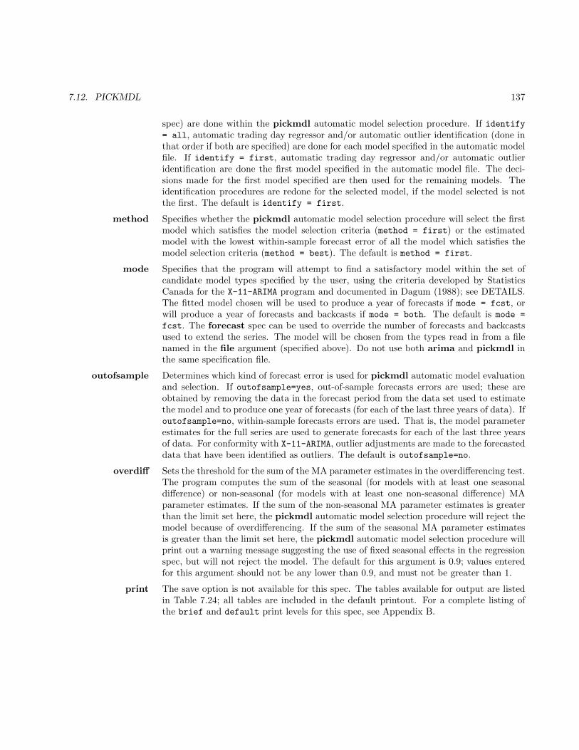
7.12. PICKMDL 137
spec) are done within the pickmdl automatic model selection procedure. If identify= all, automatic trading day regressor and/or automatic outlier identification (done inthat order if both are specified) are done for each model specified in the automatic modelfile. If identify = first, automatic trading day regressor and/or automatic outlieridentification are done the first model specified in the automatic model file. The deci-sions made for the first model specified are then used for the remaining models. Theidentification procedures are redone for the selected model, if the model selected is notthe first. The default is identify = first.
method Specifies whether the pickmdl automatic model selection procedure will select the firstmodel which satisfies the model selection criteria (method = first) or the estimatedmodel with the lowest within-sample forecast error of all the model which satisfies themodel selection criteria (method = best). The default is method = first.
mode Specifies that the program will attempt to find a satisfactory model within the set ofcandidate model types specified by the user, using the criteria developed by StatisticsCanada for the X-11-ARIMA program and documented in Dagum (1988); see DETAILS.The fitted model chosen will be used to produce a year of forecasts if mode = fcst, orwill produce a year of forecasts and backcasts if mode = both. The default is mode =
fcst. The forecast spec can be used to override the number of forecasts and backcastsused to extend the series. The model will be chosen from the types read in from a filenamed in the file argument (specified above). Do not use both arima and pickmdl inthe same specification file.
outofsample Determines which kind of forecast error is used for pickmdl automatic model evaluationand selection. If outofsample=yes, out-of-sample forecasts errors are used; these areobtained by removing the data in the forecast period from the data set used to estimatethe model and to produce one year of forecasts (for each of the last three years of data). Ifoutofsample=no, within-sample forecasts errors are used. That is, the model parameterestimates for the full series are used to generate forecasts for each of the last three yearsof data. For conformity with X-11-ARIMA, outlier adjustments are made to the forecasteddata that have been identified as outliers. The default is outofsample=no.
overdiff Sets the threshold for the sum of the MA parameter estimates in the overdifferencing test.The program computes the sum of the seasonal (for models with at least one seasonaldifference) or non-seasonal (for models with at least one non-seasonal difference) MAparameter estimates. If the sum of the non-seasonal MA parameter estimates is greaterthan the limit set here, the pickmdl automatic model selection procedure will reject themodel because of overdifferencing. If the sum of the seasonal MA parameter estimatesis greater than the limit set here, the pickmdl automatic model selection procedure willprint out a warning message suggesting the use of fixed seasonal effects in the regressionspec, but will not reject the model. The default for this argument is 0.9; values enteredfor this argument should not be any lower than 0.9, and must not be greater than 1.
print The save option is not available for this spec. The tables available for output are listedin Table 7.24; all tables are included in the default printout. For a complete listing ofthe brief and default print levels for this spec, see Appendix B.
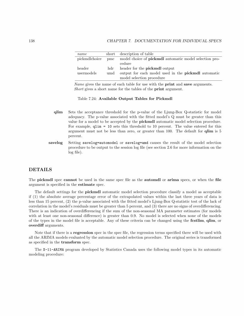
138 CHAPTER 7. DOCUMENTATION FOR INDIVIDUAL SPECS
name short description of tablepickmdlchoice pmc model choice of pickmdl automatic model selection pro-
cedureheader hdr header for the pickmdl outputusermodels umd output for each model used in the pickmdl automatic
model selection procedure
Name gives the name of each table for use with the print and save arguments.Short gives a short name for the tables of the print argument.
Table 7.24: Available Output Tables for Pickmdl
qlim Sets the acceptance threshold for the p-value of the Ljung-Box Q-statistic for modeladequacy. The p-value associated with the fitted model’s Q must be greater than thisvalue for a model to be accepted by the pickmdl automatic model selection procedure.For example, qlim = 10 sets this threshold to 10 percent. The value entered for thisargument must not be less than zero, or greater than 100. The default for qlim is 5percent.
savelog Setting savelog=automodel or savelog=amd causes the result of the model selectionprocedure to be output to the session log file (see section 2.6 for more information on thelog file).
DETAILS
The pickmdl spec cannot be used in the same spec file as the automdl or arima specs, or when the fileargument is specified in the estimate spec.
The default settings for the pickmdl automatic model selection procedure classify a model as acceptableif (1) the absolute average percentage error of the extrapolated values within the last three years of data isless than 15 percent, (2) the p-value associated with the fitted model’s Ljung-Box Q-statistic test of the lack ofcorrelation in the model’s residuals must be greater than 5 percent, and (3) there are no signs of overdifferencing.There is an indication of overdifferencing if the sum of the non-seasonal MA parameter estimates (for modelswith at least one non-seasonal difference) is greater than 0.9. No model is selected when none of the modelsof the types in the model file is acceptable. Any of these criteria can be changed using the fcstlim, qlim, oroverdiff arguments.
Note that if there is a regression spec in the spec file, the regression terms specified there will be used withall the ARIMA models evaluated by the automatic model selection procedure. The original series is transformedas specified in the transform spec.
The X-11-ARIMA program developed by Statistics Canada uses the following model types in its automaticmodeling procedure:
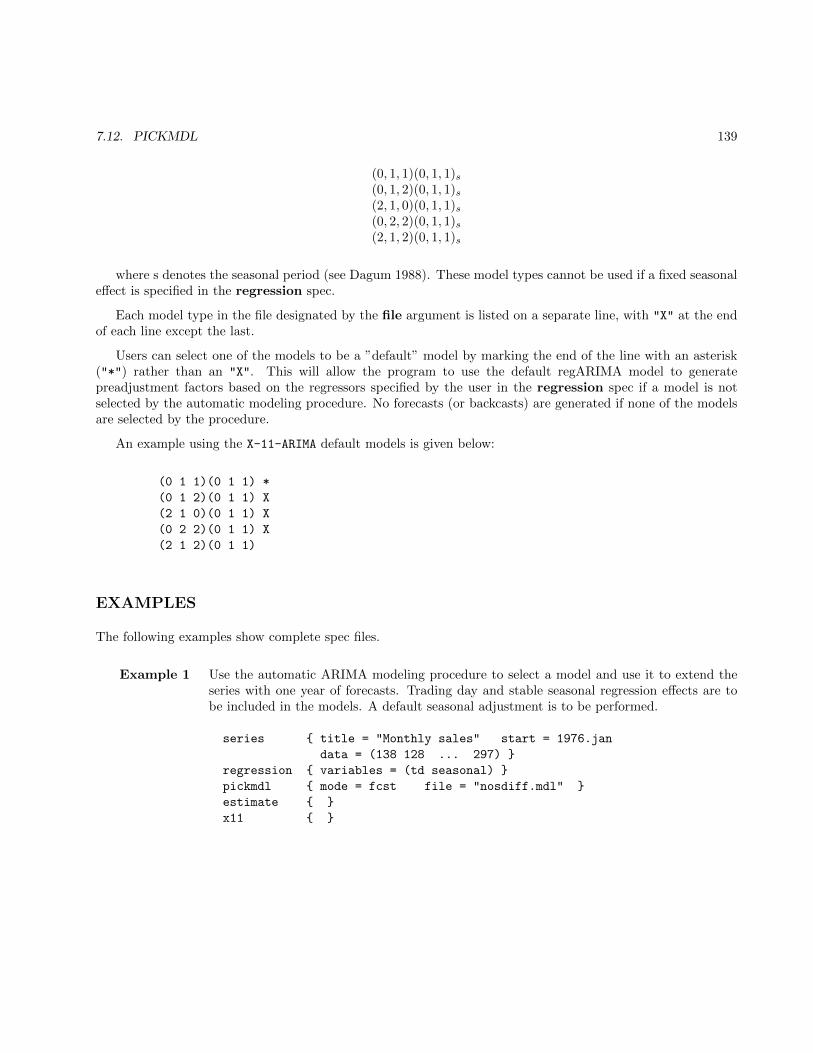
7.12. PICKMDL 139
(0, 1, 1)(0, 1, 1)s(0, 1, 2)(0, 1, 1)s(2, 1, 0)(0, 1, 1)s(0, 2, 2)(0, 1, 1)s(2, 1, 2)(0, 1, 1)s
where s denotes the seasonal period (see Dagum 1988). These model types cannot be used if a fixed seasonaleffect is specified in the regression spec.
Each model type in the file designated by the file argument is listed on a separate line, with "X" at the endof each line except the last.
Users can select one of the models to be a ”default” model by marking the end of the line with an asterisk("*") rather than an "X". This will allow the program to use the default regARIMA model to generatepreadjustment factors based on the regressors specified by the user in the regression spec if a model is notselected by the automatic modeling procedure. No forecasts (or backcasts) are generated if none of the modelsare selected by the procedure.
An example using the X-11-ARIMA default models is given below:
(0 1 1)(0 1 1) *
(0 1 2)(0 1 1) X
(2 1 0)(0 1 1) X
(0 2 2)(0 1 1) X
(2 1 2)(0 1 1)
EXAMPLES
The following examples show complete spec files.
Example 1 Use the automatic ARIMA modeling procedure to select a model and use it to extend theseries with one year of forecasts. Trading day and stable seasonal regression effects are tobe included in the models. A default seasonal adjustment is to be performed.
series { title = "Monthly sales" start = 1976.jan
data = (138 128 ... 297) }
regression { variables = (td seasonal) }
pickmdl { mode = fcst file = "nosdiff.mdl" }
estimate { }
x11 { }
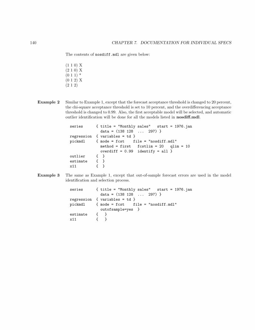
140 CHAPTER 7. DOCUMENTATION FOR INDIVIDUAL SPECS
The contents of nosdiff.mdl are given below:
(1 1 0) X(2 1 0) X(0 1 1) *(0 1 2) X(2 1 2)
Example 2 Similar to Example 1, except that the forecast acceptance threshold is changed to 20 percent,the chi-square acceptance threshold is set to 10 percent, and the overdifferencing acceptancethreshold is changed to 0.99. Also, the first acceptable model will be selected, and automaticoutlier identification will be done for all the models listed in nosdiff.mdl.
series { title = "Monthly sales" start = 1976.jan
data = (138 128 ... 297) }
regression { variables = td }
pickmdl { mode = fcst file = "nosdiff.mdl"
method = first fcstlim = 20 qlim = 10
overdiff = 0.99 identify = all }
outlier { }
estimate { }
x11 { }
Example 3 The same as Example 1, except that out-of-sample forecast errors are used in the modelidentification and selection process.
series { title = "Monthly sales" start = 1976.jan
data = (138 128 ... 297) }
regression { variables = td }
pickmdl { mode = fcst file = "nosdiff.mdl"
outofsample=yes }
estimate { }
x11 { }
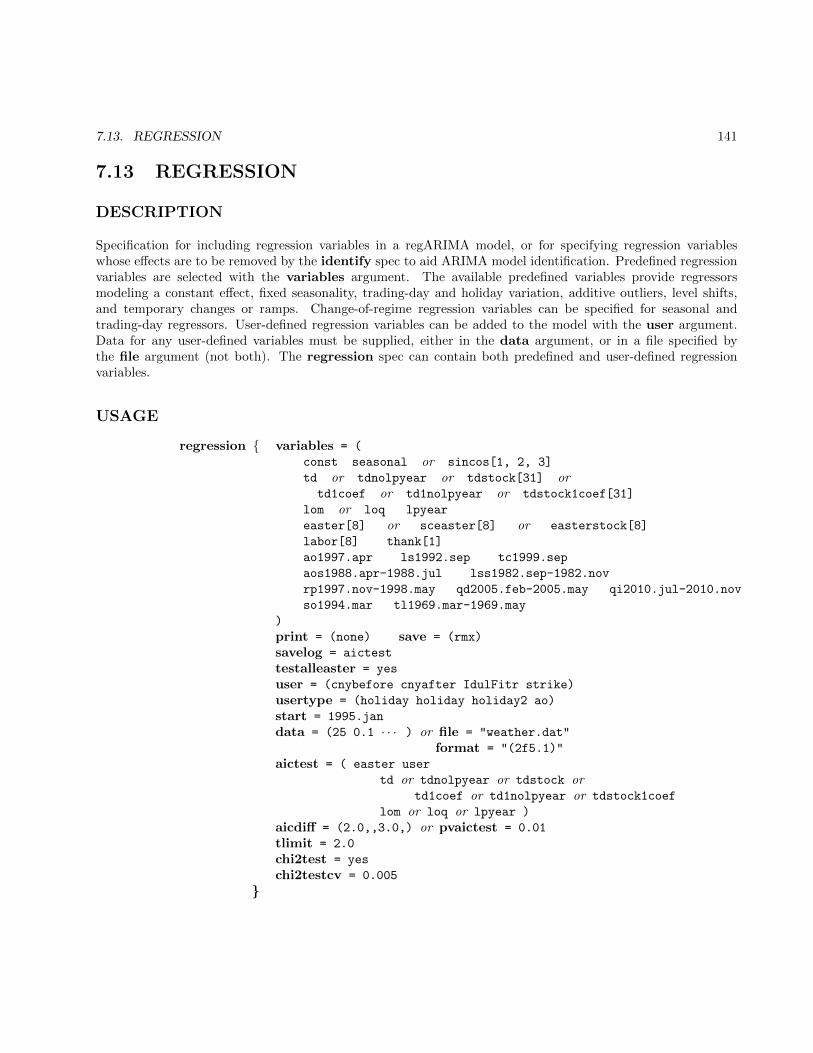
7.13. REGRESSION 141
7.13 REGRESSION
DESCRIPTION
Specification for including regression variables in a regARIMA model, or for specifying regression variableswhose effects are to be removed by the identify spec to aid ARIMA model identification. Predefined regressionvariables are selected with the variables argument. The available predefined variables provide regressorsmodeling a constant effect, fixed seasonality, trading-day and holiday variation, additive outliers, level shifts,and temporary changes or ramps. Change-of-regime regression variables can be specified for seasonal andtrading-day regressors. User-defined regression variables can be added to the model with the user argument.Data for any user-defined variables must be supplied, either in the data argument, or in a file specified bythe file argument (not both). The regression spec can contain both predefined and user-defined regressionvariables.
USAGE
regression { variables = (
const seasonal or sincos[1, 2, 3]
td or tdnolpyear or tdstock[31] ortd1coef or td1nolpyear or tdstock1coef[31]
lom or loq lpyear
easter[8] or sceaster[8] or easterstock[8]
labor[8] thank[1]
ao1997.apr ls1992.sep tc1999.sep
aos1988.apr-1988.jul lss1982.sep-1982.nov
rp1997.nov-1998.may qd2005.feb-2005.may qi2010.jul-2010.nov
so1994.mar tl1969.mar-1969.may
)
print = (none) save = (rmx)
savelog = aictest
testalleaster = yes
user = (cnybefore cnyafter IdulFitr strike)
usertype = (holiday holiday holiday2 ao)
start = 1995.jan
data = (25 0.1 · · · ) or file = "weather.dat"
format = "(2f5.1)"
aictest = ( easter user
td or tdnolpyear or tdstock ortd1coef or td1nolpyear or tdstock1coef
lom or loq or lpyear )
aicdiff = (2.0,,3.0,) or pvaictest = 0.01
tlimit = 2.0
chi2test = yes
chi2testcv = 0.005
}

142 CHAPTER 7. DOCUMENTATION FOR INDIVIDUAL SPECS
ARGUMENTS
aicdiff Defines the amount by which the AIC value (corrected for the length of the series, orAICC) of the model with the regressor(s) specified in the aictest argument must fallbelow the AICC of the model without these regressor(s) in order for the model with theregressors to be chosen. The default value is aicdiff=0.0.
If only one value is given for this argument (aicdiff = 3.5), then this critical value isused for all types of regressors. If a list of up to four values is given (aicdiff = (3.5,
4.0, 4.0, 5.5)), then the AIC difference for trading day regressors is set to the firstlist entry (3.5 in this case), the AIC difference for length of month regressors is set tothe second list entry (4.0), the AIC difference for Easter regressors is set to the thirdlist entry (4.0), and the AIC difference for user-defined regressors is set to the fourthlist entry (5.5). A missing value, as in aicdiff = (3.25,,3.25,), is set to the defaultcritical value.
For more information on how this option is used in conjunction with the aictest argu-ment, see DETAILS.
aictest Specifies that an AIC-based selection will be used to determine if a given set of regressionvariables will be included with the regARIMA model specified. The only entries allowedfor this variable are td, tdnolpyear, tdstock, td1coef, td1nolpyear, tdstock1coef,lom, loq, lpyear, easter, easterstock, and user. If a trading day model selection isspecified, for example, then AIC values (with a correction for the length of the series,henceforth referred to as AICC) are derived for models with and without the specifiedtrading day variable. By default, the model with smaller AICC is used to generateforecasts, identify outliers, etc. If more than one type of regressor is specified, the AIC-tests are performed sequentially in this order: (a) trading day regressors, (b) length ofmonth / length of quarter / leap year regressors, (c) Easter regressors, (d) user-definedregressors. If there are several variables of the same type (for example, several tradingday regressors), then the aictest procedure is applied to them as a group. That is, eitherall variables of this type will be included in the final model or none. See DETAILS formore information on the testing procedure. If this option is not specified, no automaticAIC-based selection is performed.
chi2test Specifies that Chi-squared statistics will be be used to determine if groups of user-definedholiday regressors will be kept in the regARIMA model. When chi2test = yes, Chi-squared statistics will be generated for all user-defined holiday regression groups, andthose who which are not significant (at the level of the argument chi2testcv) are removedfrom the regARIMA model. The default is chi2test = no, where no testing is done.
chi2testcv Sets the probability for the critical value used for the selection procedure in chi2test.The default is 0.01.
data Assigns data values to the user-defined regression variables. The time frame of the datavalues must cover the time frame of the series (or of the span specified by the spanargument of the series spec, if present). It must also cover the time frame of forecastsand backcasts requested in the forecast spec. The data values are read in free format.The numerical values given in this argument are assigned in the order in which the user-defined variables are named in the user argument. This assignment proceeds through all
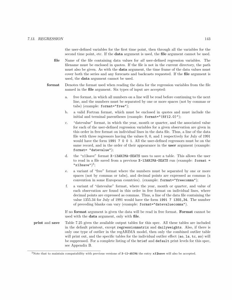
7.13. REGRESSION 143
the user-defined variables for the first time point, then through all the variables for thesecond time point, etc. If the data argument is used, the file argument cannot be used.
file Name of the file containing data values for all user-defined regression variables. Thefilename must be enclosed in quotes. If the file is not in the current directory, the pathmust also be given. As with the data argument, the time frame of the data values mustcover both the series and any forecasts and backcasts requested. If the file argument isused, the data argument cannot be used.
format Denotes the format used when reading the data for the regression variables from the filenamed in the file argument. Six types of input are accepted:
a. free format, in which all numbers on a line will be read before continuing to the nextline, and the numbers must be separated by one or more spaces (not by commas ortabs) (example: format="free");
b. a valid Fortran format, which must be enclosed in quotes and must include theinitial and terminal parentheses (example: format="(6f12.0)");
c. “datevalue” format, in which the year, month or quarter, and the associated valuefor each of the user-defined regression variables for a given observation are given inthis order in free format on individual lines in the data file. Thus, a line of the datafile with three regressors having the values 0, 0, and 1 respectively for July of 1991would have the form 1991 7 0 0 1. All the user-defined regressors must be on thesame record, and in the order of their appearance in the user argument (example:format= "datevalue");
d. the “x13save” format X-13ARIMA-SEATS uses to save a table. This allows the userto read in a file saved from a previous X-13ARIMA-SEATS run (example: format =
"x13save")3;
e. a variant of “free” format where the numbers must be separated by one or morespaces (not by commas or tabs), and decimal points are expressed as commas (aconvention in some European countries). (example: format="freecomma");
f. a variant of “datevalue” format, where the year, month or quarter, and value ofeach observation are found in this order in free format on individual lines, wheredecimal points are expressed as commas. Thus, a line of the data file containing thevalue 1355.34 for July of 1991 would have the form 1991 7 1355,34. The numberof preceding blanks can vary (example: format="datevaluecomma").
If no format argument is given the data will be read in free format. Format cannot beused with the data argument, only with file.
print and save Table 7.25 gives the available output tables for this spec. All these tables are includedin the default printout, except regressionmatrix and dailyweights. Also, if there isonly one type of outlier in the regARIMA model, then only the combined outlier tablewill print out, and the specific tables for the individual outlier effect (ao, ls, tc, so) willbe suppressed. For a complete listing of the brief and default print levels for this spec,see Appendix B.
3Note that to maintain compatability with previous versions of X-12-ARIMA the entry x12save will also be accepted.
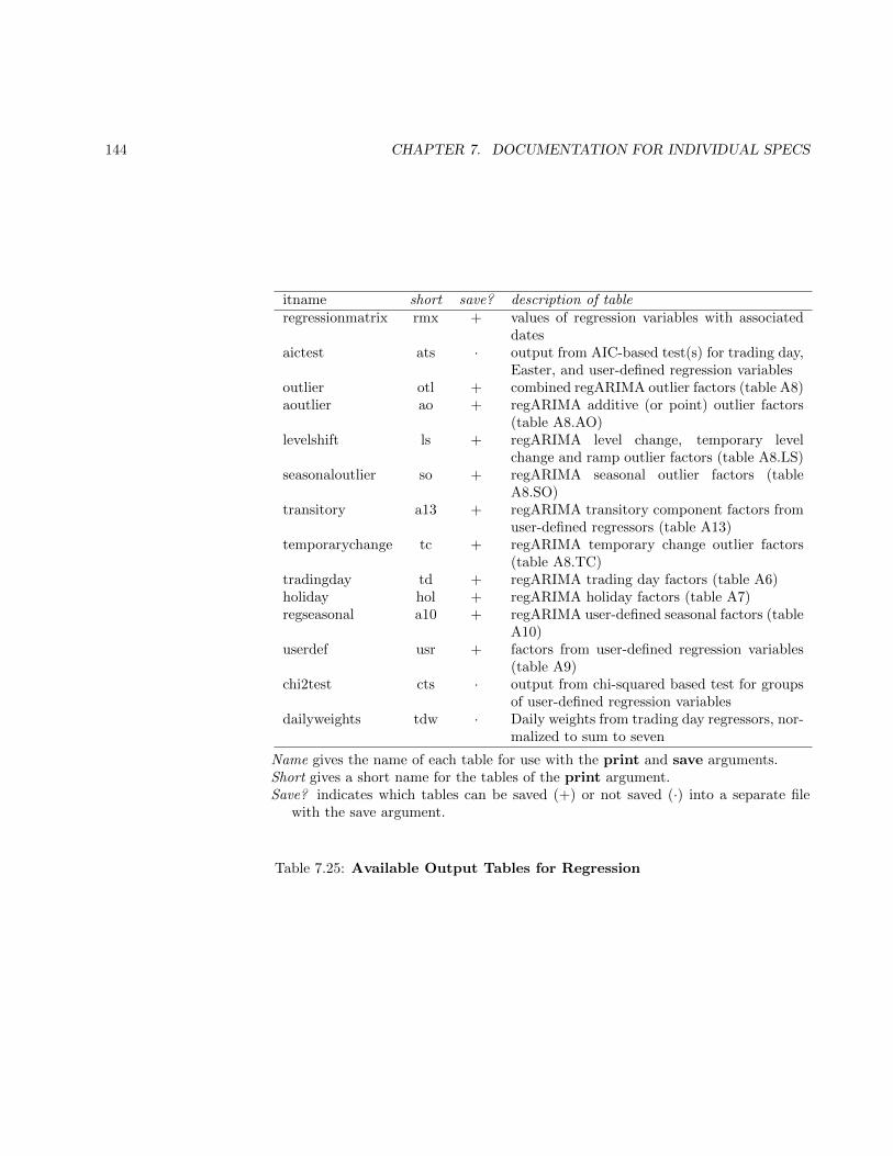
144 CHAPTER 7. DOCUMENTATION FOR INDIVIDUAL SPECS
itname short save? description of tableregressionmatrix rmx + values of regression variables with associated
datesaictest ats · output from AIC-based test(s) for trading day,
Easter, and user-defined regression variablesoutlier otl + combined regARIMA outlier factors (table A8)aoutlier ao + regARIMA additive (or point) outlier factors
(table A8.AO)levelshift ls + regARIMA level change, temporary level
change and ramp outlier factors (table A8.LS)seasonaloutlier so + regARIMA seasonal outlier factors (table
A8.SO)transitory a13 + regARIMA transitory component factors from
user-defined regressors (table A13)temporarychange tc + regARIMA temporary change outlier factors
(table A8.TC)tradingday td + regARIMA trading day factors (table A6)holiday hol + regARIMA holiday factors (table A7)regseasonal a10 + regARIMA user-defined seasonal factors (table
A10)userdef usr + factors from user-defined regression variables
(table A9)chi2test cts · output from chi-squared based test for groups
of user-defined regression variablesdailyweights tdw · Daily weights from trading day regressors, nor-
malized to sum to seven
Name gives the name of each table for use with the print and save arguments.Short gives a short name for the tables of the print argument.Save? indicates which tables can be saved (+) or not saved (·) into a separate file
with the save argument.
Table 7.25: Available Output Tables for Regression

7.13. REGRESSION 145
pvaictest Probability for generating a critical value for any AIC tests specified in this spec. Thisprobablity must be > 0.0 and < 1.0. Table 7.26 shows the critical value generated fordifferent values of pvaictest and different values of ν, the difference in the number ofparameters between two models.
If this argument is not specified, the aicdiff argument is used to set the critical valuefor AIC testing.
Value of pvaictest ν = 1 ν = 2 ν = 3 ν = 4 ν = 5 ν = 6 ν = 70.05 1.8415 1.9915 1.8147 1.4877 1.0705 0.5916 0.06710.01 4.6349 5.2103 5.3449 5.2767 5.0863 4.8119 4.47530.005 5.8794 6.5966 6.8382 6.8603 6.7496 6.5476 6.27770.001 8.8276 9.8155 10.2662 10.4668 10.5150 10.4577 10.3219
Table 7.26: Critical values for AIC testing for different levels of pvaictest
savelog The diagnostics available for output to the log file (see section 2.6) are listed on Table7.27.
name short description of diagnosticaictest ats Test results from the AICC-based regressor selection procedurechi2test cts Test results from the Chi-squared based regressor selection pro-
cedure
Name gives the name of each diagnostic for use with the savelog argument.Short gives a short name for the diagnostics of the savelog argument.
Table 7.27: Available Log File Diagnostics for Regression
start The start date for the data values for the user-defined regression variables. The defaultis the start date of the series. Valid values are any date up to the start date of the series(or up to the start date of the span specified by the span argument of the series spec,if present).
testalleaster Specifies if an extra regression model is evaluated when more than one Easter regressoris specified in the variables argument. When testalleaster = yes, an additionalregARIMA model is estimated which contains all the Easter regressors specified by theuser in the variables argument. An AICC diagnostic is generated from this model,and used in the AIC-based testing procedure as well as the AICCs for model with andwithout the individual Easter regressors. The default is testalleaster = no, only theindividual Easter regressors specified by the user are used in the AIC testing procedure.
tlimit Sets the value to which the absolute values of the t-statistics of AO and LS sequenceregressors are compared to retain those outliers in the regARIMA model. If this argumentis not specified, AO and LS sequence regressors are not checked for significance.
user Specifies names for any user-defined regression variables. Names are required for all user-defined variables to be included in the model. The names given are used to label estimated
146 CHAPTER 7. DOCUMENTATION FOR INDIVIDUAL SPECS
coefficients in the program’s output. Data values for the user-defined variables must besupplied, using either the data or file argument (not both). The maximum number ofuser-defined regression variables is 52. (This limit can be changed—see Section 2.8.)
usertype Assigns a type of model-estimated regression effect to each user-defined regression vari-able. It causes the variable and its estimated effects to be used and be output in thesame way as a predefined regressor of the same type. This option is useful when tryingout alternatives to the regression effects provided by the program.
The type of the user-defined regression effects can be defined as a constant (constant),seasonal (seasonal), trading day (td), length-of-month (lom), length-of-quarter (loq),leap year (lpyear), outlier (ao, ls, or so), a user-defined transitory component for SEATS(transitory) or other user-defined (user) regression effects. In addition to these types,users can specify up to 5 different user-defined holidays (holiday, holiday2, holiday3,holiday4, and holiday5). This gives the user flexibility in specifying more than oneholiday, and the chi-squared statistic is generated separately for these user-defined holi-days.
One effect type can be specified for all the user-defined regression variables defined in theregression spec (usertype=td), or each user-defined regression variable can be given itsown type (usertype=(td td td td td td holiday user)). Once a type other thanuser has been assigned to a user-defined variable, further specifications for the variablein other arguments, such as aictest or noapply, must use this type designation, notuser. If this option is not specified, all user-defined variables have the type user. SeeDETAILS for more information on assigning types to user-defined regressors.
variables List of predefined regression variables to be included in the model. Data values forthese variables are calculated by the program, mostly as functions of the calendar. SeeDETAILS for a discussion and a table of the available predefined variables. Also seeSection 4.3 for additional information and a table defining the actual regression variablesused.
RARELY USED ARGUMENTS
b Specifies initial values for regression parameters in the order that they appear in thevariables and user arguments. If present, the b argument must assign initial valuesto all regression coefficients in the regARIMA model, and must appear in the spec fileafter the variables and user arguments. Initial values are assigned to parameterseither by specifying the value in the argument list or by explicitly indicating that it ismissing as in the example below. Missing values take on their default value of 0.1. Forexample, for a model with two regressors, b=(0.7, ) is equivalent to b=(0.7,0.1), butb=(0.7) is not allowed. For a model with three regressors, b=(0.8,,-0.4) is equivalentto b=(0.8,0.1,-0.4). To hold a parameter fixed at a specified value, immediately followthe value in the b list with an ‘f’, e.g., b=(0.7f, 0.1).
centeruser Specifies the removal of the (sample) mean or the seasonal means from the user-definedregression variables. If centeruser=mean, the mean of each user-defined regressor issubtracted from the regressor. If centeruser=seasonal, means for each calendar month
7.13. REGRESSION 147
(or quarter) are subtracted from each of the user-defined regressors. If this option isnot specified, the user-defined regressors are assumed to already be in an appropriatelycentered form and are not modified.
eastermeans Specifies whether long term (500 year) monthly means are used to remove seasonality fromthe Easter regressor associated with the variable easter[w], as described in footnote 5of Table 4.1 (eastermeans=yes), or, instead, monthly means calculated from the span ofdata used for the calculation of the coefficients of the Easter regressors (eastermeans=no).The default is eastermeans=yes. This argument is ignored if no built-in Easter regressoris included in the regression model, or if the only Easter regressor is sceaster[w] (seeDETAILS).
noapply List of the types of regression effects defined in the regression spec whose model-estimated values are not to be removed from the original series before the seasonaladjustment calculations specified by the x11 spec are performed.
Applicable types are all modelled trading day effects (td), Easter, Labor Day, andThanksgiving-Christmas holiday effects (holiday), point outliers (ao), level changes andramps (ls), temporary changes (tc), seasonal outliers (so), user-defined seasonal regres-sion effects (userseasonal), and the set of user-defined regression effects (user).
tcrate Defines the rate of decay for the temporary change outlier regressor. This value must bea number greater than zero and less than one. The default value is tcrate=0.7 ** (12
/ period), where period is the number of observations in one year (for monthly timeseries, 4 for quarterly time series. This formula for the default value of tcrate ensures thesame rate of decay over an entire year for series of different periodicity. If the frequencyof the time series is less than 4 (ie, period < 4), then there is no default value, and theuser will have to enter a value of tcrate if a temporary change outlier was specified inthe variables argument.
DETAILS
If forecasting is performed, X-13ARIMA-SEATS creates data values for the selected predefined regression variablesfor the entire forecast period. If there are any user-defined regression variables, then data values must also besupplied for them for the entire forecast period (similarly for the backcasts). In addition to the limit of 52 user-defined regression variables, there is an overall limit of 80 regression variables in the model. (These limits canbe changed—see Section 2.8.) The latter limit is on the total number of predefined and user-defined regressionvariables plus the number of regression variables added automatically by the outlier spec. The maximum lengthof the series of user-defined regression variables, not including the forecast period, is 780. (This limit can alsobe changed—see Section 2.8.)
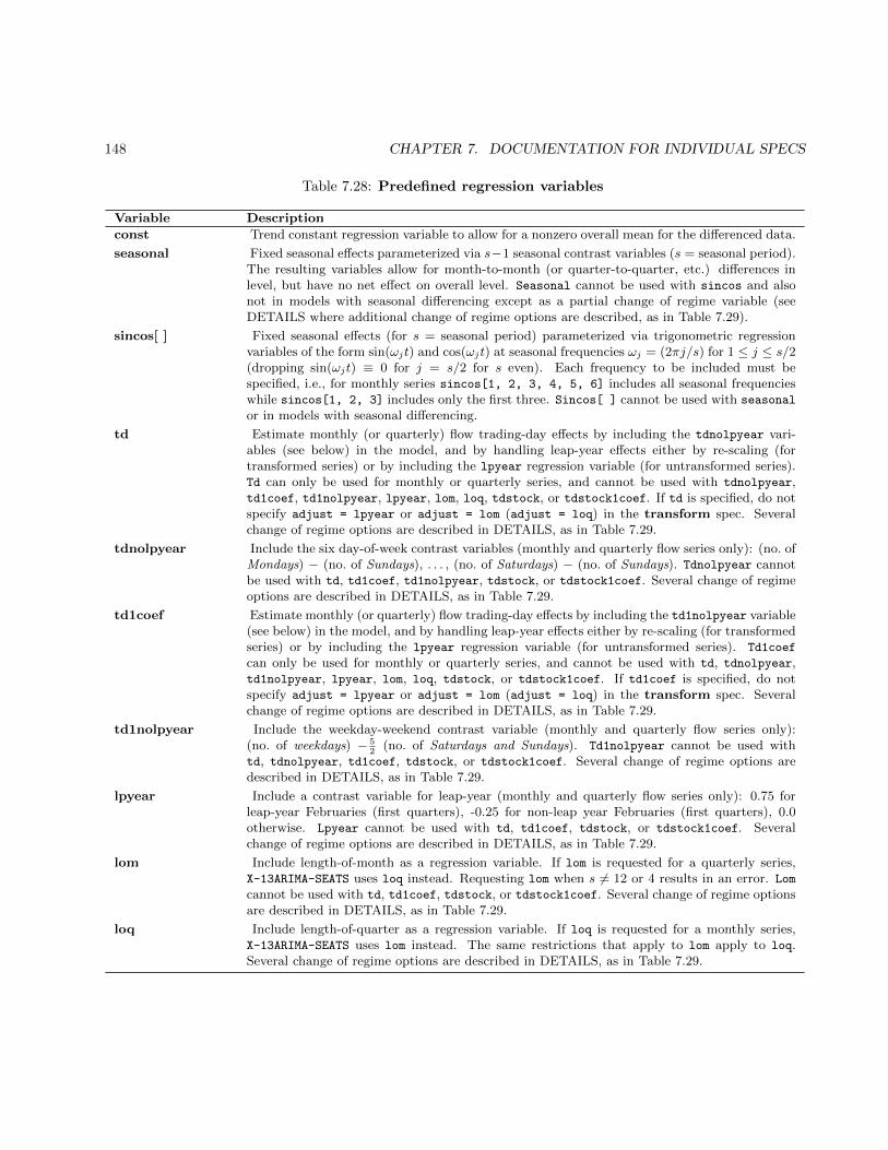
148 CHAPTER 7. DOCUMENTATION FOR INDIVIDUAL SPECS
Table 7.28: Predefined regression variables
Variable Description
const Trend constant regression variable to allow for a nonzero overall mean for the differenced data.
seasonal Fixed seasonal effects parameterized via s−1 seasonal contrast variables (s = seasonal period).The resulting variables allow for month-to-month (or quarter-to-quarter, etc.) differences inlevel, but have no net effect on overall level. Seasonal cannot be used with sincos and alsonot in models with seasonal differencing except as a partial change of regime variable (seeDETAILS where additional change of regime options are described, as in Table 7.29).
sincos[ ] Fixed seasonal effects (for s = seasonal period) parameterized via trigonometric regressionvariables of the form sin(ωjt) and cos(ωjt) at seasonal frequencies ωj = (2πj/s) for 1 ≤ j ≤ s/2(dropping sin(ωjt) ≡ 0 for j = s/2 for s even). Each frequency to be included must bespecified, i.e., for monthly series sincos[1, 2, 3, 4, 5, 6] includes all seasonal frequencieswhile sincos[1, 2, 3] includes only the first three. Sincos[ ] cannot be used with seasonal
or in models with seasonal differencing.
td Estimate monthly (or quarterly) flow trading-day effects by including the tdnolpyear vari-ables (see below) in the model, and by handling leap-year effects either by re-scaling (fortransformed series) or by including the lpyear regression variable (for untransformed series).Td can only be used for monthly or quarterly series, and cannot be used with tdnolpyear,td1coef, td1nolpyear, lpyear, lom, loq, tdstock, or tdstock1coef. If td is specified, do notspecify adjust = lpyear or adjust = lom (adjust = loq) in the transform spec. Severalchange of regime options are described in DETAILS, as in Table 7.29.
tdnolpyear Include the six day-of-week contrast variables (monthly and quarterly flow series only): (no. ofMondays) − (no. of Sundays), . . . , (no. of Saturdays) − (no. of Sundays). Tdnolpyear cannotbe used with td, td1coef, td1nolpyear, tdstock, or tdstock1coef. Several change of regimeoptions are described in DETAILS, as in Table 7.29.
td1coef Estimate monthly (or quarterly) flow trading-day effects by including the td1nolpyear variable(see below) in the model, and by handling leap-year effects either by re-scaling (for transformedseries) or by including the lpyear regression variable (for untransformed series). Td1coef
can only be used for monthly or quarterly series, and cannot be used with td, tdnolpyear,td1nolpyear, lpyear, lom, loq, tdstock, or tdstock1coef. If td1coef is specified, do notspecify adjust = lpyear or adjust = lom (adjust = loq) in the transform spec. Severalchange of regime options are described in DETAILS, as in Table 7.29.
td1nolpyear Include the weekday-weekend contrast variable (monthly and quarterly flow series only):(no. of weekdays) − 5
2(no. of Saturdays and Sundays). Td1nolpyear cannot be used with
td, tdnolpyear, td1coef, tdstock, or tdstock1coef. Several change of regime options aredescribed in DETAILS, as in Table 7.29.
lpyear Include a contrast variable for leap-year (monthly and quarterly flow series only): 0.75 forleap-year Februaries (first quarters), -0.25 for non-leap year Februaries (first quarters), 0.0otherwise. Lpyear cannot be used with td, td1coef, tdstock, or tdstock1coef. Severalchange of regime options are described in DETAILS, as in Table 7.29.
lom Include length-of-month as a regression variable. If lom is requested for a quarterly series,X-13ARIMA-SEATS uses loq instead. Requesting lom when s 6= 12 or 4 results in an error. Lom
cannot be used with td, td1coef, tdstock, or tdstock1coef. Several change of regime optionsare described in DETAILS, as in Table 7.29.
loq Include length-of-quarter as a regression variable. If loq is requested for a monthly series,X-13ARIMA-SEATS uses lom instead. The same restrictions that apply to lom apply to loq.Several change of regime options are described in DETAILS, as in Table 7.29.
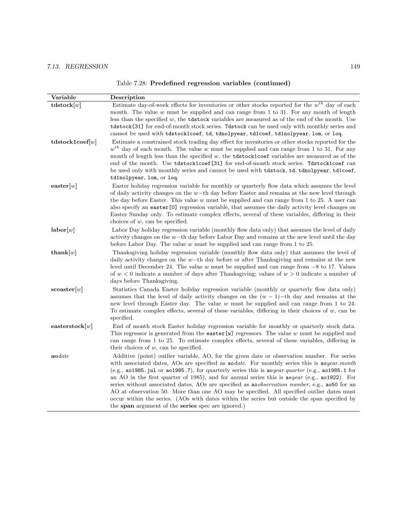
7.13. REGRESSION 149
Table 7.28: Predefined regression variables (continued)
Variable Description
tdstock[w] Estimate day-of-week effects for inventories or other stocks reported for the wth day of eachmonth. The value w must be supplied and can range from 1 to 31. For any month of lengthless than the specified w, the tdstock variables are measured as of the end of the month. Usetdstock[31] for end-of-month stock series. Tdstock can be used only with monthly series andcannot be used with tdstock1coef, td, tdnolpyear, td1coef, td1nolpyear, lom, or loq.
tdstock1coef[w] Estimate a constrained stock trading day effect for inventories or other stocks reported for thewth day of each month. The value w must be supplied and can range from 1 to 31. For anymonth of length less than the specified w, the tdstock1coef variables are measured as of theend of the month. Use tdstock1coef[31] for end-of-month stock series. Tdstock1coef canbe used only with monthly series and cannot be used with tdstock, td, tdnolpyear, td1coef,td1nolpyear, lom, or loq.
easter[w] Easter holiday regression variable for monthly or quarterly flow data which assumes the levelof daily activity changes on the w−th day before Easter and remains at the new level throughthe day before Easter. This value w must be supplied and can range from 1 to 25. A user canalso specify an easter[0] regression variable, that assumes the daily activity level changes onEaster Sunday only. To estimate complex effects, several of these variables, differing in theirchoices of w, can be specified.
labor[w] Labor Day holiday regression variable (monthly flow data only) that assumes the level of dailyactivity changes on the w−th day before Labor Day and remains at the new level until the daybefore Labor Day. The value w must be supplied and can range from 1 to 25.
thank[w] Thanksgiving holiday regression variable (monthly flow data only) that assumes the level ofdaily activity changes on the w−th day before or after Thanksgiving and remains at the newlevel until December 24. The value w must be supplied and can range from −8 to 17. Valuesof w < 0 indicate a number of days after Thanksgiving; values of w > 0 indicate a number ofdays before Thanksgiving.
sceaster[w] Statistics Canada Easter holiday regression variable (monthly or quarterly flow data only)assumes that the level of daily activity changes on the (w − 1)−th day and remains at thenew level through Easter day. The value w must be supplied and can range from 1 to 24.To estimate complex effects, several of these variables, differing in their choices of w, can bespecified.
easterstock[w] End of month stock Easter holiday regression variable for monthly or quarterly stock data.This regressor is generated from the easter[w] regressors. The value w must be supplied andcan range from 1 to 25. To estimate complex effects, several of these variables, differing intheir choices of w, can be specified.
aodate Additive (point) outlier variable, AO, for the given date or observation number. For serieswith associated dates, AOs are specified as aodate. For monthly series this is aoyear.month(e.g., ao1985.jul or ao1985.7), for quarterly series this is aoyear.quarter (e.g., ao1985.1 foran AO in the first quarter of 1985), and for annual series this is aoyear (e.g., ao1922). Forseries without associated dates, AOs are specified as aoobservation number, e.g., ao50 for anAO at observation 50. More than one AO may be specified. All specified outlier dates mustoccur within the series. (AOs with dates within the series but outside the span specified bythe span argument of the series spec are ignored.)
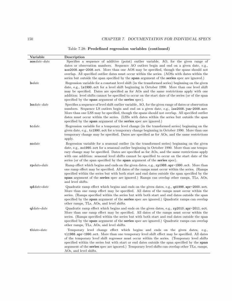
150 CHAPTER 7. DOCUMENTATION FOR INDIVIDUAL SPECS
Table 7.28: Predefined regression variables (continued)
Variable Description
aosdate-date Specifies a sequence of additive (point) outlier variable, AO, for the given range ofdates or observation numbers. Sequence AO outlers begin and end on a given date, e.g.,aos2008.apr-2008.oct. More than one AOS may be specified, though the spans should notoverlap. All specified outlier dates must occur within the series. (AOSs with dates within theseries but outside the span specified by the span argument of the series spec are ignored.)
lsdate Regression variable for a constant level shift (in the transformed series) beginning on the givendate, e.g., ls1990.oct for a level shift beginning in October 1990. More than one level shiftmay be specified. Dates are specified as for AOs and the same restrictions apply with oneaddition: level shifts cannot be specified to occur on the start date of the series (or of the spanspecified by the span argument of the series spec).
lssdate-date Specifies a sequence of level shift outlier variable, AO, for the given range of dates or observationnumbers. Sequence LS outlers begin and end on a given date, e.g., lss2008.jun-2008.nov.More than one LSS may be specified, though the spans should not overlap. All specified outlierdates must occur within the series. (LSSs with dates within the series but outside the spanspecified by the span argument of the series spec are ignored.)
tcdate Regression variable for a temporary level change (in the transformed series) beginning on thegiven date, e.g., tc1990.oct for a temporary change beginning in October 1990. More than onetemporary change may be specified. Dates are specified as for AOs, and the same restrictionsapply.
sodate Regression variable for a seasonal outlier (in the transformed series) beginning on the givendate, e.g., so1990.oct for a seasonal outlier beginning in October 1990. More than one tempo-rary change may be specified. Dates are specified as for AOs, and the same restrictions applywith one addition: seasonal level shifts cannot be specified to occur on the start date of theseries (or of the span specified by the span argument of the series spec).
rpdate-date Ramp effect which begins and ends on the given dates, e.g., rp1988.apr-1990.oct. More thanone ramp effect may be specified. All dates of the ramps must occur within the series. (Rampsspecified within the series but with both start and end dates outside the span specified by thespan argument of the series spec are ignored.) Ramps can overlap other ramps, TLs, AOs,and level shifts.
qddate-date Quadratic ramp effect which begins and ends on the given dates, e.g., qd1998.apr-2000.oct.More than one ramp effect may be specified. All dates of the ramps must occur within theseries. (Ramps specified within the series but with both start and end dates outside the spanspecified by the span argument of the series spec are ignored.) Quadratic ramps can overlapother ramps, TLs, AOs, and level shifts.
qidate-date Quadratic ramp effect which begins and ends on the given dates, e.g., rp2010.apr-2011.oct.More than one ramp effect may be specified. All dates of the ramps must occur within theseries. (Ramps specified within the series but with both start and end dates outside the spanspecified by the span argument of the series spec are ignored.) Quadratic ramps can overlapother ramps, TLs, AOs, and level shifts.
tldate-date Temporary level change effect which begins and ends on the given dates, e.g.,tl1988.apr-1990.oct. More than one temporary level shift effect may be specified. All datesof the temporary level shift regressor must occur within the series. (Temporary level shiftsspecified within the series but with start or end dates outside the span specified by the spanargument of the series spec are ignored.) Temporary level shifts can overlap other TLs, ramps,AOs, and level shifts.

7.13. REGRESSION 151
If const is specified in the variables argument, then the resulting regression variable allows for an a constantterm in the series resulting from any differencing operations in the ARIMA model. If the ARIMA model involvesno differencing, this is simply the usual regression constant term for a nonzero overall mean; if the ARIMAmodel does involve differencing, this regressor is called a trend constant. In the latter case the actual regressionvariable created is defined such that, after differencing, it yields a column of ones. See Section 4.3 for discussion.
We generally recommend specifying td in the variables argument when trading-day effects are thoughtto be present in a monthly flow time series, that is, a series whose values are monthly accumulations of dailyvalues. In this case, how the program handles leap-year effects depends on information from the transformspec. If the series is transformed (Box-Cox or logistic transformation) then leap-year effects are removed byprior adjustment: the series is divided before transformation by a set of factors lpt where lpt = 28.25/29 if t isa leap year February, lpt = 28.25/28 if t is a non-leap year February, and lpt = 1.00 otherwise.
If the series is not transformed, then the leap-year regression variable lpyear is included in the model. Itsvalues, denoted by LPt are given by LPt = 29 − 28.25 if t is a leap year February, LPt = 28 − 28.25 if t is anon-leap year February, and LPt = 0.00 otherwise. In both cases, the tdnolpyear regression variables, (no. ofMondays) − (no. of Sundays), . . . , (no. of Saturdays) − (no. of Sundays), are also included in the model.Leapyear effects are the nonseasonal component of length-of-month effects. When type = trend is used in the x11spec, with the result that there is no seasonal effect estimation and adjustment, then td handles length-of-montheffects instead of leap-year effects. That is, with a transformation, there is prior adjustment by the length-of-month factors described in Table 7.28, and with no transformation, the lom regressor, whose value is the numberof days in the month, is added to the regression with the tdnolpyear regressors.
In any situation in which the user prefers to model length-of-month effects in a transformed series, the leapyear regressor is the nonseasonal component for the length-of-month (quarter) regressor. If the user prefersto model length-of-month effects in a transformed series through the lom regression variable, this can be doneby specifying both lom and tdnolpyear, i.e., variables = (lom tdnolpyear ...). If the user prefers toprior adjust an untransformed series for length-of-month effects, this can be done by specifying variables =
(tdnolpyear ...) in the regression spec and adjust = lom in the transform spec.
If adjust=lom is specified in the transform spec, then including either td or lom in the variables listleads to a conflict. The conflict occurs either because two requests have been made to re-scale the series bydividing by length of month, or because both a length-of-month rescaling and the lom regression variable havebeen requested (which will generally lead to a singular system of equations for the regression coefficients). Inthis case, the user should either (i) remove adjust=lom from the transform spec, or (ii) in the variables list,replace td by tdnolpyear, or drop lom.
For quarterly flow time series the same trading-day options are available, and the above comments applywith lom replaced by loq.
The values lom and loq are equivalent —if either is specified, the seasonal period specified in the seriesspec determines which is used. Thus, period = 12 implies lom and period = 4 implies loq. Also, note thatlom or loq can be specified without tdnolpyear. This could be done to account for fixed seasonality dueto length-of-month (or length-of-quarter) effects for a series with no day-of-week specific effects. Predefinedlength-of-period variables are available only for monthly or quarterly flow series.
For stock series, such as inventories, the program can estimate trading-day effects only for monthly series.Tdstock[w], where w can range from 1 to 31, creates six regression variables contrasting six days of the weekwith the seventh - see Section 4.3. The value w must be specified; it denotes the day of the month for which

152 CHAPTER 7. DOCUMENTATION FOR INDIVIDUAL SPECS
the stock is reported or the last day of the month, whichever is smaller. Therefore, tdstock[31] is used forend-of-month stocks.
The holiday effect regression variables (for Easter, Labor Day, and Thanksgiving) are for flow series. TheEaster variable can be specified for either monthly or quarterly series. The Labor Day and Thanksgivingvariables are only for monthly series.
If a series is designated as a stock or a flow series by using the type argument of the series or compositespec, then trading day and Easter regressors specified in variables argument need to agree with this type - onecannot specify stock trading day regressors for a flow series. If a series type is not specified, then any tradingday or holiday regressor may be used with the series.
Change-of-regime regression variables can be specified for seasonal (seasonal), trigonometric seasonal(sincos), trading day (td, tdnolpyear, tdstock, td1coef, td1nolpyer, or tdstock1coef), leap year(lpyear), length-of-month (lom), and length-of-quarter (loq) regression variables. Two types of change-of-regime regressors are available: full and partial.
As Table 7.29 shows, change of regime regressors are specified by appending the change date, surroundedby one or two slashes, to the name of a regression variable in the variables argument of the regressionspec. The date specified for the change of regime divides the series being modelled into two spans, an earlyspan containing the data for times prior to the change date and a late span containing the data from on andafter this date. Partial change of regime variables are restricted to one of these two spans, being zero in thecomplementary span. The full change of regime variables estimate both the basic regression of interest andthe partial change of regime regression for the early span. For example, the full change of regime specificationvariables = (td/1990.jan/)is equivalent to the specification variables = (td td/1990.jan//). It causesthe program to output the coefficients estimated for td and for td/1990.jan// along with trading day factorsfor their combined effects.
Type Syntax ExampleFull change of regime regressor reg/date/ td/1990.jan/Partial change of regime regressor, zero before change date reg//date/ td//1990.jan/Partial change of regime regressor, zero on and after change date reg/date// td/1990.jan//
Table 7.29: Change of Regime Regressor Types and Syntax
The coefficients resulting from use of a full change of regime regression have convenient interpretations: Letthe basic regressors be denoted by Xjt, and let t0 be the change point. Then the partial change of regimeregressors for the early regime are
XEjt =
{Xjt for t < t0
0 for t ≥ t0
and those for the late regime can be calculated as XLjt = Xjt −XE
jt. For the data transformed as indicated inthe transform spec, the effect estimated by the full change of regime regression has the form
∑j
ajXjt +∑j
bjXEjt =
∑j
ajXLjt +
∑j
(aj + bj)XEjt.
7.13. REGRESSION 153
From the right-hand-side formula, we observe that the coefficients aj of the basic regressors Xjt can beinterpreted at the coefficients of the late-span regressors XL
jt, and the coefficients bj of the XEjt can be interpreted
as measuring the change in the coefficients of the late-span regressors required to obtain coefficients for the early-span effects. Therefore, statistically significant bj indicate the nature of the change of regime.
We illustrate two other natural uses for partial change of regime variables. First, the specification variables
= (td//1990.jan/) can be used to estimate the trading day component of a series that has no statisticallysignificant trading day effects prior to 1990, but possibly significant effects beginning in this year. Second, whenan ARIMA model with seasonal differencing is specified in the arima spec, or in the models estimated by theautomdl spec, then the specification variables = (seasonal//1990.jan/) can be used to estimate a fixedchange in a somewhat variable seasonal pattern that takes place in January of 1990 and to test for the statisticalsignificance of the estimated change.
The effect of the argument aictest can be to delete a regressor set named in the variables list from thislist, or to add a regressor set to the variables list. The effect of a nonzero (positive) value of aicdiff is to makeit more difficult for the aictest procedure to include in the model the variable being tested. Let ∆AICC denotethe value associated with the aicdiff argument, which by default is zero. Let AICCwith (AICCwithout) denotethe AICC value of the model with (without) a set of regressors specified in the aictest argument. If this set isnot named in the variables list, it will be added to the regression model if
AICCwith + ∆AIC < AICCwithout.
If this set is named in the variables list, it will be retained in the regARIMA model only if this inequalityholds.
In the second case, if aictest = (tdstock), it is the end-of-month stock variables, specified by tdstock[31],are the variables added, because 31 is the default value for w in tdstock[w].
There are more possibilities if aictest = (easter) and no Easter effect regressors appear in the variableslist. Then three additional models are considered, the three models obtained by augmenting the specified reg-ARIMA model with the regressor easter[w] for w = 1, 8, 15 respectively. The Easter regressor whose model hasthe smallest AICC is retained if its AICC is smaller than the model with no Easter regressors by at least theamount ∆AIC = 0; otherwise, the model without Easter regressors is selected.
Simulation experiments we have conducted suggest that AICC does not distinguish with high reliabilitybetween easter[w] regressors whose w values differ by less than seven. The out-of-sample forecast diagnosticsproduced by the history spec can sometimes distinguish between such regressors by showing that one providespersistently more accurate forecasts, and therefore presumably better describes the Easter effect in the data.
Similar to the case for Easter, when aictest = (td) and no trading day regressors appear in the variableslist, then additional models are considered. These are the models obtained by augementing the specified reg-ARIMA model with full and one coefficient trading regressors, depending on the type of series (td and td1coeffor flow series, tdstock and tdstock1coef for stock series).
The trading day regressor whose model has the smallest AICC is retained if its AICC is smaller than themodel with no trading day regressors by at least the amount ∆AIC = 0; otherwise, the model without tradindday regressors is selected.
When regressors appear in both the aictest and variables arguments, the type of regressors specified shouldbe identical. An exception for this is for trading day regressors. The entry aictest = td serves as a correct

154 CHAPTER 7. DOCUMENTATION FOR INDIVIDUAL SPECS
entry for any type of flow or stock trading day regressor. The sample day for stock trading day variables andthe date specified for change-of-regime regressors should not be included in the aictest argument; its value willbe taken from the entry in the variables argument. For example, if variables=(tdstock[15] ao1995.jan),then the entry for aictest can be tdstock or td.
Another exception is for Easter regressors. The entry aictest = easter serves as a correct entry for anytype of flow or stock Easter regressor. The window length of the Easter regressor should not be includedin the aictest argument; they will be assumed from the entry in the variables argument. For example, ifvariables=(easterstock[15] ao1995.jan), then the entry for aictest can be easterstock or easter.
Note that this is not affected by setting type = stock or type = flow in the series or composite specs;the entries aictest = td and aictest = easter can still be used for both stock and flow series. However, youcannot set type = flow in the series spec and aictest = tdstock.
Regressors specified by the aictest argument must also be able to be included with other regressors specifiedeither in the variables and the aictest arguments. For example, the following regression spec is incorrectlyspecified, as the td and lom arguments cannot be specified together in the variables argument:
regression{
variables = td
aictest = lom
}
Using tdnolpyear instead would allow a model with the 6 trading day regressors and the length-of-monthregressors.
In addition, users should not specify aictest = lom for series that are not monthly series, and aictest =
loq for series that are not quarterly.
As mentioned above, trading day regressors are always tested before length-of-month (-quarter) or leap yearregressors. If options specified in the regression spec lead to trading day and leap year regressors in the sameregARIMA model, then the program will test the trading day and leap year regressors together if aictest =
td is specified, or will test the sets of regressors separately if aictest = (td lpyear) is specified.
User-defined variables should be input to the program in deseasonalized form (unless they are seasonal re-gressors). The deseasonalization method described in Section C.1.3 is likely to be the appropriate one, becauseregressors are additive components of the regARIMA model. If deseasonalization is not done, then the seasonalfactors will not include all estimated seasonal effects. Another problem is that regressors with seasonal compo-nents are likely to have estimated coefficients, and estimated effects, that are more correlated with one anotherand therefore more difficult to interpret.
If a type is assigned in to a user-defined variable with the usertype argument, the factor derived fromthe user-defined regression variables of that type will be combined with the regression factor from variables ofthe same type specified in the regression spec. The resulting factor will be adjusted out of the series for theseasonal adjustment factor calculations determined by the x11 or seats spec unless the type name appears inthe noapply argument.
Setting usertype=seasonal will cause seasonal factors to be created from the user-defined regressors thatwill be adjusted out of the original series before the seasonal adjustment specified by the x11 or seats spec is
7.13. REGRESSION 155
calculated. Combined seasonal factors are created from the X-11 or SEATS and regression factors. In addition,if noapply=userseasonal is specified, the user-defined seasonal regressors are treated exactly like seasonalregressors specified in the variables argument: the seasonal effect estimated from these regressors will notadjusted out of the series prior to seasonal adjustment. The effects estimated by Table 7.28 seasonal regressorsspecified in the variables argument are not available as output. If it is desired to remove these effects fromthe series prior to seasonal adjustment, this can be done in by setting save=rmx to save the regressors inan output file. From this file, the regressors can be input to the program as user-defined regressors withusertype=seasonal to achieve the desired removal.
Note that if format = "datevalue" or format = "x13save", the starting date of the user defined regres-sor(s) is automatically read from the data file. Therefore, the starting date need not be specified with the startargument of the regression spec.
Trading day and/or holiday regressors may not be specified simultaneously in the regression and x11regressionspecs unless the noapply option is used to specify that the effects estimated by either the regression orx11regression spec not be used to adjust the series.
The two choices for the argument eastermeans yield noticeably different holiday factors. But the choice hasno effect on forecasts (provided the regARIMA model used includes seasonal differencing or the fixed seasonalregressors) and usually has only negligible effects on the combined seasonal and holiday factors, because theseasonal factors change to compensate for the differences between the choices.
Table 7.30 give the monthly means for February, March, and April that are used to obtain deseasonalizedEaster regressors under eastermeans = yes; the means for other months are zero. These calendar meanswere generated from frequencies of the date of Easter for a 500 year period (1600-2099). These frequencieswere computed from dates given in Bednarek (2007) which were checked using information from Montes (2001,1997b, 1997a); the algorithm used by Montes to compute the date of Easter for the Gregorian calendar is givenin Duffet-Smith (1981).
For quarterly series, the mean of the first quarter is equivalent to the sum of the February and March meansfrom Table 7.30, the mean for the second quarter is equivalent to the April mean, and the means for otherquarters are zero.
For a nonseasonal time series, an adjustment for trading day and holiday effects estimated by means of thisspec can be obtained by setting type=trend in the x11 spec.
Regarding the outlier regressors, users should be aware that several combinations of AOs and LSs producearithmetically equal effects. For example, (i) an AO at time t0 followed by an LS at t0 + 1; (ii) LSs at both t0and t0 +1; (iii) both an AO and an LS at t0. Note that an LS at t0 followed by an AO at t0 +1 is not equivalentto these other combinations.
Because AOs are assigned to the irregular component and LSs to the trend-cycle, some users might preferone equivalent combination over another.
When the b=() argument is used to fix coefficients, AIC and the other model selection statistics may becomeinvalid, see the DETAILS section of estimate.
For more information concerning the modeling of holiday effects and the detection and modeling of tradingday effects, see Findley and Soukup (2000) and Lin and Liu (2002).
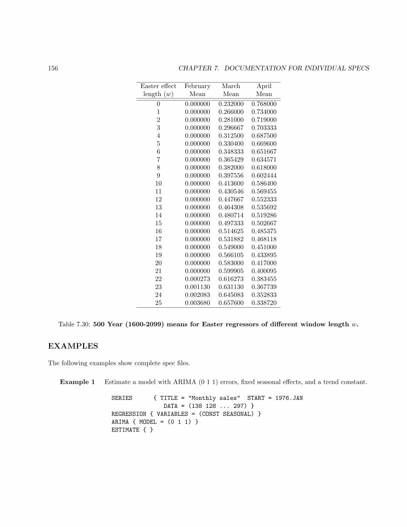
156 CHAPTER 7. DOCUMENTATION FOR INDIVIDUAL SPECS
Easter effect February March Aprillength (w) Mean Mean Mean
0 0.000000 0.232000 0.7680001 0.000000 0.266000 0.7340002 0.000000 0.281000 0.7190003 0.000000 0.296667 0.7033334 0.000000 0.312500 0.6875005 0.000000 0.330400 0.6696006 0.000000 0.348333 0.6516677 0.000000 0.365429 0.6345718 0.000000 0.382000 0.6180009 0.000000 0.397556 0.60244410 0.000000 0.413600 0.58640011 0.000000 0.430546 0.56945512 0.000000 0.447667 0.55233313 0.000000 0.464308 0.53569214 0.000000 0.480714 0.51928615 0.000000 0.497333 0.50266716 0.000000 0.514625 0.48537517 0.000000 0.531882 0.46811818 0.000000 0.549000 0.45100019 0.000000 0.566105 0.43389520 0.000000 0.583000 0.41700021 0.000000 0.599905 0.40009522 0.000273 0.616273 0.38345523 0.001130 0.631130 0.36773924 0.002083 0.645083 0.35283325 0.003680 0.657600 0.338720
Table 7.30: 500 Year (1600-2099) means for Easter regressors of different window length w.
EXAMPLES
The following examples show complete spec files.
Example 1 Estimate a model with ARIMA (0 1 1) errors, fixed seasonal effects, and a trend constant.
SERIES { TITLE = "Monthly sales" START = 1976.JAN
DATA = (138 128 ... 297) }
REGRESSION { VARIABLES = (CONST SEASONAL) }
ARIMA { MODEL = (0 1 1) }
ESTIMATE { }

7.13. REGRESSION 157
Example 2 Specify a model to fit sine and cosine variables with the 4th and 5th seasonal frequencyby ordinary least squares to the final irregular component of a series to test if ”visuallysignificant” spectrum peaks at these frequencies are statistically significant.
series { title = "Irregular Component of Monthly Sales"
start = 1976.jan
file = "sales.d13"
format = "x13save"
}
regression { variables = (const sincos[4,5]) }
estimate { }
spectrum { savelog=peaks }
Example 3 Specify regression variables for trading-day, Easter, Labor Day, and Thanksgiving effects in amonthly time series. The duration in number of days is specified for each holiday effect. Sincetd is specified and the series is log transformed, the original series (before transformation)is divided by the leap-year factors, and the tdnolpyear regression variables are fit to thetransformed series. The regression coefficients are estimated by the identify spec througha regression of the maximally differenced series (after transformation and length-of-monthadjustment) on the correspondingly differenced regression variables. The identify specthen produces various sample ACFs and PACFs (of the regression residuals) to be used foridentifying an ARIMA model for the regression errors.
Series { Title = "Monthly Sales" Start = 1976.Jan
Data = (138 128 ... 297) }
Transform { Function = Log }
Regression { Variables = (TD Easter[8] Labor[10] Thank[3]) }
Identify { Diff = (0 1) SDiff = (0 1) }
Example 4 Estimate a model including the same regressors as in Example 3, and also the lom regressionvariable in place of the division of the series by standard leap-year effects that the argumentvalue td invokes. (Replacing the value of td with tdnolpyear prevents the division bythe standard leap year effects.) Perform a test (using AICC) of the significance of thetrading-day and Easter regressors. Note that the program will test the significance of the6 trading-day regressors first, then the significance of the length-of-month regressor, andfinally the significance of the Easter regressor. An ARIMA (0 1 1)(0 1 1)12 model is usedfor the regression error series.
series { title = "Monthly sales" start = 1976.jan
data = (138 128 ... 297) }
transform { function = log }
regression { variables = (tdnolpyear lom easter[8] labor[10] thank[3])
aictest = (lom td easter) }
arima { model = (0 1 1)(0 1 1) }
estimate { }

158 CHAPTER 7. DOCUMENTATION FOR INDIVIDUAL SPECS
Example 5 Specified regression variables are a one coefficient stock trading day regressor and a end ofmonth stock Easter regressor. Since the sample day specified in the trading day regressor is31, it is an end of month stock regressor as well. Decide (using AICC) if the stock trading-dayand Easter regressors should be kept in the model.
series { title = "Retail inventory of food products"
start = 1990.jan data = "foodri.dat" type = stock
}
regression { variables = ( tdstock1coef[31] easterstock[8] )
aictest = ( td easter )
}
arima { model = (0 1 1)(0 1 1) }
x11 { }
Example 6 Estimate a model with trading-day effects, two AOs, and a ramp outlier for a quarterlyseasonal series. Accounting for these effects, the transformed series follows an ARIMA(0 1 1)(0 1 1)4 model.
Series { Title = "Quarterly Sales" Start = 1990.1 Period = 4
Data = (1039 1241 ... 2210) }
Transform { Function = Log }
Regression { Variables = (AO2007.1 RP2005.2-2005.4 AO1998.1 TD) }
Arima { Model = (0 1 1)(0 1 1) }
Estimate { }
Example 7 Same as Example 6, but using an increasing quadratic ramp instead of the linear rampregressor.
Series { Title = "Quarterly Sales" Start = 1990.1 Period = 4
Data = (1039 1241 ... 2210) }
Transform { Function = Log }
Regression { Variables = (AO2007.1 QI2005.2-2005.4 AO1998.1 TD) }
Arima { Model = (0 1 1)(0 1 1) }
Estimate { }
Example 8 Estimate a user-defined regression variable for a temporary level-shift from the third quarterof 1985 through the first quarter of 1987. The effect of the temporary level shift is removedthrough the regression performed by the identify spec, prior to the computation of ACFsand PACFs for identification of the ARIMA part of the model.
series {title = "Quarterly sales" start = 1981.1
data = (301 294 ... 391) period = 4 }
regression {user = tls
data = (0 0 0 0 0 0 0 0 0 0 0 0 ...
0 0 1 1 1 1 1 1 1 1 1 1 1 0 0 0 0 ... 0) }
identify { diff = (0 1) sdiff = (0 1) }
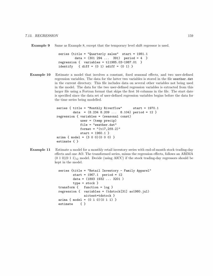
7.13. REGRESSION 159
Example 9 Same as Example 8, except that the temporary level shift regressor is used.
series {title = "Quarterly sales" start = 1981.1
data = (301 294 ... 391) period = 4 }
regression { variables = tl1985.03-1987.01 }
identify { diff = (0 1) sdiff = (0 1) }
Example 10 Estimate a model that involves a constant, fixed seasonal effects, and two user-definedregression variables. The data for the latter two variables is stored in the file weather.dat
in the current directory. This file includes data on several other variables not being usedin the model. The data for the two user-defined regression variables is extracted from thislarger file using a Fortran format that skips the first 16 columns in the file. The start dateis specified since the data set of user-defined regression variables begins before the data forthe time series being modelled.
series { title = "Monthly Riverflow" start = 1970.1
data = (8.234 8.209 ... 8.104) period = 12 }
regression { variables = (seasonal const)
user = (temp precip)
file = "weather.dat"
format = "(t17,2f8.2)"
start = 1960.1 }
arima { model = (3 0 0)(0 0 0) }
estimate { }
Example 11 Estimate a model for a monthly retail inventory series with end-of-month stock trading-dayeffects and one AO. The transformed series, minus the regression effects, follows an ARIMA(0 1 0)(0 1 1)12 model. Decide (using AICC) if the stock trading-day regressors should bekept in the model.
series {title = "Retail Inventory - Family Apparel"
start = 1967.1 period = 12
data = (1893 1932 ... 3201 )
type = stock }
transform { function = log }
regression { variables = (tdstock[31] ao1980.jul)
aictest=tdstock }
arima { model = (0 1 0)(0 1 1) }
estimate { }
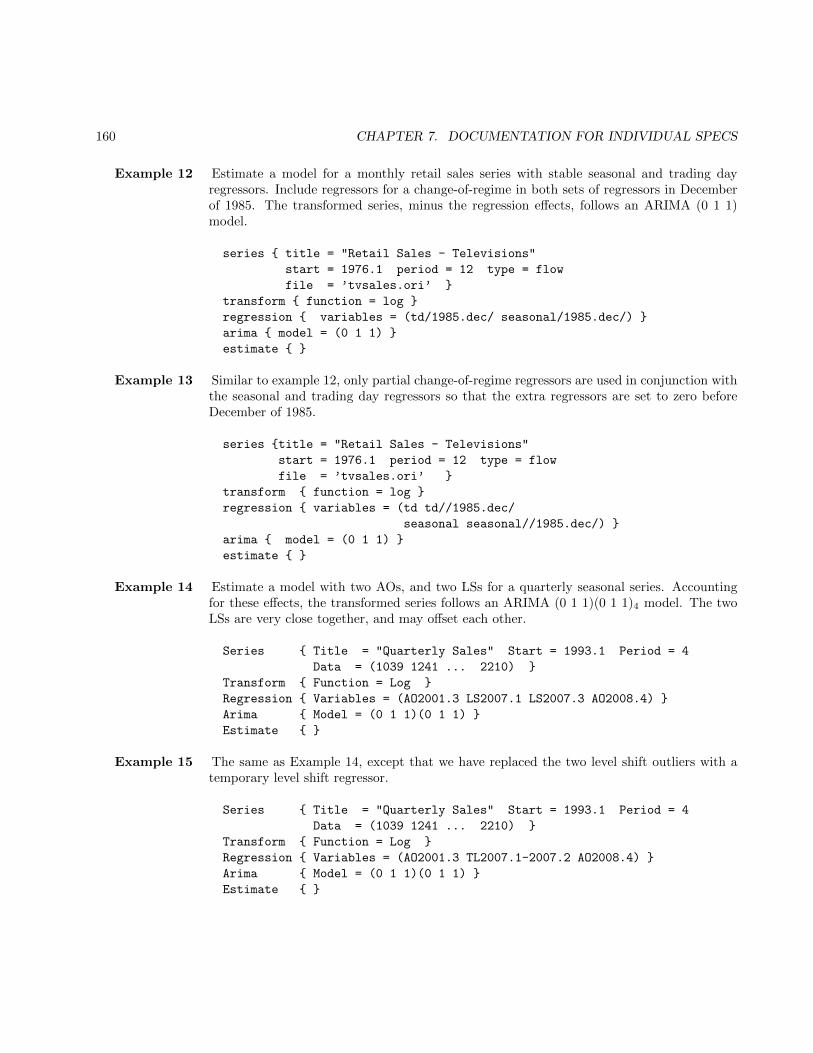
160 CHAPTER 7. DOCUMENTATION FOR INDIVIDUAL SPECS
Example 12 Estimate a model for a monthly retail sales series with stable seasonal and trading dayregressors. Include regressors for a change-of-regime in both sets of regressors in Decemberof 1985. The transformed series, minus the regression effects, follows an ARIMA (0 1 1)model.
series { title = "Retail Sales - Televisions"
start = 1976.1 period = 12 type = flow
file = ’tvsales.ori’ }
transform { function = log }
regression { variables = (td/1985.dec/ seasonal/1985.dec/) }
arima { model = (0 1 1) }
estimate { }
Example 13 Similar to example 12, only partial change-of-regime regressors are used in conjunction withthe seasonal and trading day regressors so that the extra regressors are set to zero beforeDecember of 1985.
series {title = "Retail Sales - Televisions"
start = 1976.1 period = 12 type = flow
file = ’tvsales.ori’ }
transform { function = log }
regression { variables = (td td//1985.dec/
seasonal seasonal//1985.dec/) }
arima { model = (0 1 1) }
estimate { }
Example 14 Estimate a model with two AOs, and two LSs for a quarterly seasonal series. Accountingfor these effects, the transformed series follows an ARIMA (0 1 1)(0 1 1)4 model. The twoLSs are very close together, and may offset each other.
Series { Title = "Quarterly Sales" Start = 1993.1 Period = 4
Data = (1039 1241 ... 2210) }
Transform { Function = Log }
Regression { Variables = (AO2001.3 LS2007.1 LS2007.3 AO2008.4) }
Arima { Model = (0 1 1)(0 1 1) }
Estimate { }
Example 15 The same as Example 14, except that we have replaced the two level shift outliers with atemporary level shift regressor.
Series { Title = "Quarterly Sales" Start = 1993.1 Period = 4
Data = (1039 1241 ... 2210) }
Transform { Function = Log }
Regression { Variables = (AO2001.3 TL2007.1-2007.2 AO2008.4) }
Arima { Model = (0 1 1)(0 1 1) }
Estimate { }
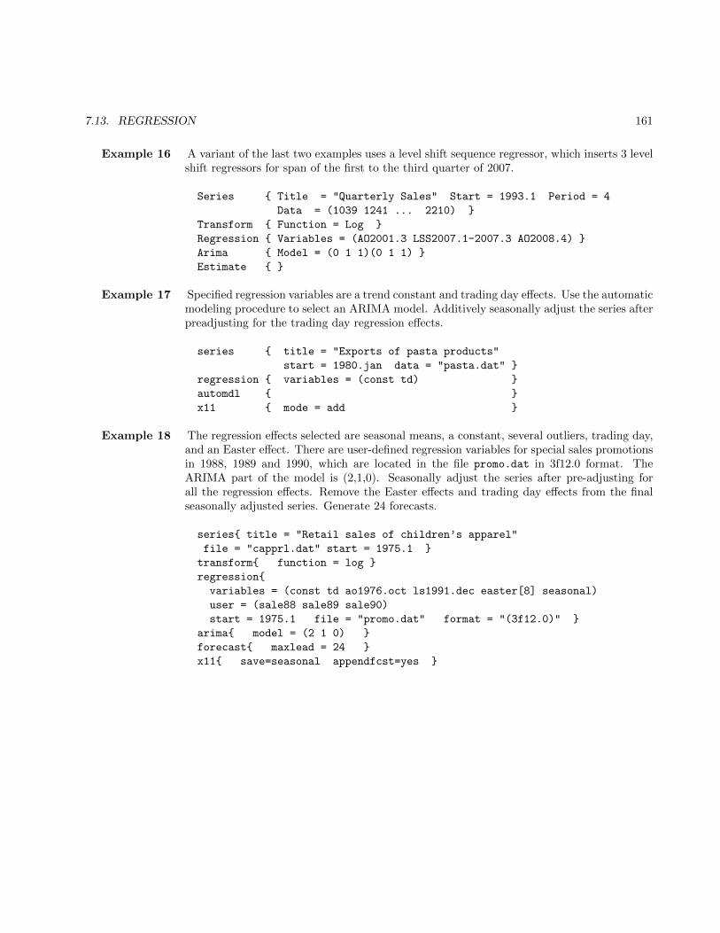
7.13. REGRESSION 161
Example 16 A variant of the last two examples uses a level shift sequence regressor, which inserts 3 levelshift regressors for span of the first to the third quarter of 2007.
Series { Title = "Quarterly Sales" Start = 1993.1 Period = 4
Data = (1039 1241 ... 2210) }
Transform { Function = Log }
Regression { Variables = (AO2001.3 LSS2007.1-2007.3 AO2008.4) }
Arima { Model = (0 1 1)(0 1 1) }
Estimate { }
Example 17 Specified regression variables are a trend constant and trading day effects. Use the automaticmodeling procedure to select an ARIMA model. Additively seasonally adjust the series afterpreadjusting for the trading day regression effects.
series { title = "Exports of pasta products"
start = 1980.jan data = "pasta.dat" }
regression { variables = (const td) }
automdl { }
x11 { mode = add }
Example 18 The regression effects selected are seasonal means, a constant, several outliers, trading day,and an Easter effect. There are user-defined regression variables for special sales promotionsin 1988, 1989 and 1990, which are located in the file promo.dat in 3f12.0 format. TheARIMA part of the model is (2,1,0). Seasonally adjust the series after pre-adjusting forall the regression effects. Remove the Easter effects and trading day effects from the finalseasonally adjusted series. Generate 24 forecasts.
series{ title = "Retail sales of children’s apparel"
file = "capprl.dat" start = 1975.1 }
transform{ function = log }
regression{
variables = (const td ao1976.oct ls1991.dec easter[8] seasonal)
user = (sale88 sale89 sale90)
start = 1975.1 file = "promo.dat" format = "(3f12.0)" }
arima{ model = (2 1 0) }
forecast{ maxlead = 24 }
x11{ save=seasonal appendfcst=yes }

162 CHAPTER 7. DOCUMENTATION FOR INDIVIDUAL SPECS
Example 19 The same as Example 18, except that the user-defined regression effect will be handled thesame way as additive outliers with regard to prior adjustments, final adjustments, print files,and save files.
series{ title = "Retail sales of children’s apparel"
file = "capprl.dat" start = 1975.1 }
transform{ function = log }
regression{
variables = (const td ao1976.oct ls1991.dec easter[8]
seasonal)
user = (sale88 sale89 sale90)
start = 1975.1 file = "promo.dat" format = "(3f12.0)"
usertype = ao
}
arima{ model = (2 1 0) }
forecast{ maxlead = 24 }
x11{ save=seasonal appendfcst=yes }
Example 20 Specify a regARIMA model with trading day and outlier terms. Specify starting values forthe regression coefficients, and hold the coefficients of the outlier regressors fixed at thesevalues. Use this model to generate 12 forecasts (by default, since an x11 spec is present).Perform a default multiplicative seasonal adjustment, after prior adjustment for trading dayand outlier factors.
series{
format = "2L"
title = "Midwest Total Starts"
file = "mwtoths.dat"
name = "MWTOT "
}
transform{ function=log }
arima{ model=(0 1 2 )(0 1 1 ) }
estimate{ save=mdl }
regression{
variables = (ao1977.jan ls1979.jan ls1979.mar ls1980.jan td)
b = ( -0.7946F -0.8739F 0.6773F -0.6850F 0.0209
~0.0107 -0.0022 0.0018 ~0.0088 -0.0074 )
}
x11{ }
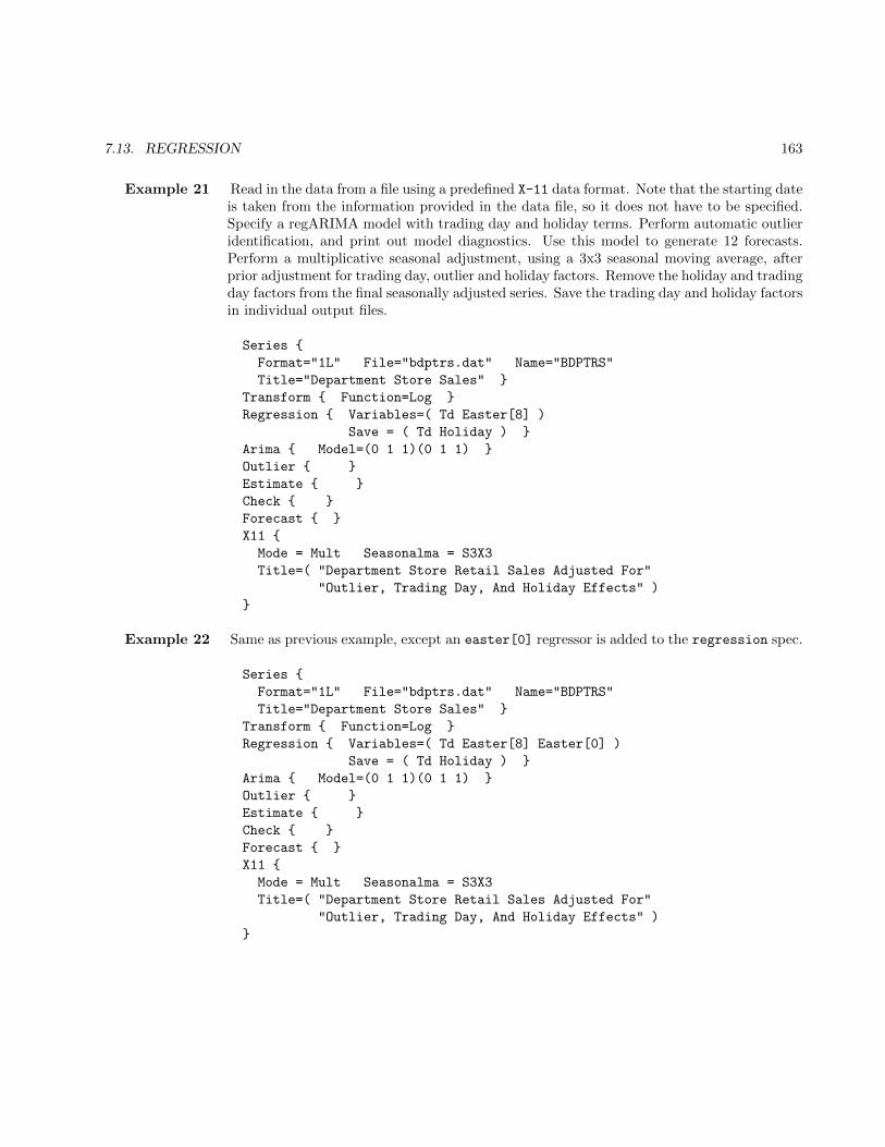
7.13. REGRESSION 163
Example 21 Read in the data from a file using a predefined X-11 data format. Note that the starting dateis taken from the information provided in the data file, so it does not have to be specified.Specify a regARIMA model with trading day and holiday terms. Perform automatic outlieridentification, and print out model diagnostics. Use this model to generate 12 forecasts.Perform a multiplicative seasonal adjustment, using a 3x3 seasonal moving average, afterprior adjustment for trading day, outlier and holiday factors. Remove the holiday and tradingday factors from the final seasonally adjusted series. Save the trading day and holiday factorsin individual output files.
Series {
Format="1L" File="bdptrs.dat" Name="BDPTRS"
Title="Department Store Sales" }
Transform { Function=Log }
Regression { Variables=( Td Easter[8] )
Save = ( Td Holiday ) }
Arima { Model=(0 1 1)(0 1 1) }
Outlier { }
Estimate { }
Check { }
Forecast { }
X11 {
Mode = Mult Seasonalma = S3X3
Title=( "Department Store Retail Sales Adjusted For"
"Outlier, Trading Day, And Holiday Effects" )
}
Example 22 Same as previous example, except an easter[0] regressor is added to the regression spec.
Series {
Format="1L" File="bdptrs.dat" Name="BDPTRS"
Title="Department Store Sales" }
Transform { Function=Log }
Regression { Variables=( Td Easter[8] Easter[0] )
Save = ( Td Holiday ) }
Arima { Model=(0 1 1)(0 1 1) }
Outlier { }
Estimate { }
Check { }
Forecast { }
X11 {
Mode = Mult Seasonalma = S3X3
Title=( "Department Store Retail Sales Adjusted For"
"Outlier, Trading Day, And Holiday Effects" )
}
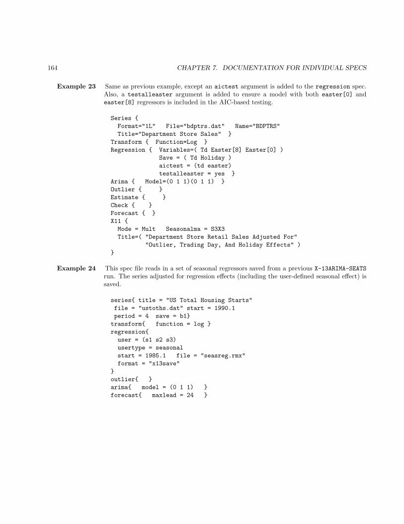
164 CHAPTER 7. DOCUMENTATION FOR INDIVIDUAL SPECS
Example 23 Same as previous example, except an aictest argument is added to the regression spec.Also, a testalleaster argument is added to ensure a model with both easter[0] andeaster[8] regressors is included in the AIC-based testing.
Series {
Format="1L" File="bdptrs.dat" Name="BDPTRS"
Title="Department Store Sales" }
Transform { Function=Log }
Regression { Variables=( Td Easter[8] Easter[0] )
Save = ( Td Holiday )
aictest = (td easter)
testalleaster = yes }
Arima { Model=(0 1 1)(0 1 1) }
Outlier { }
Estimate { }
Check { }
Forecast { }
X11 {
Mode = Mult Seasonalma = S3X3
Title=( "Department Store Retail Sales Adjusted For"
"Outlier, Trading Day, And Holiday Effects" )
}
Example 24 This spec file reads in a set of seasonal regressors saved from a previous X-13ARIMA-SEATS
run. The series adjusted for regression effects (including the user-defined seasonal effect) issaved.
series{ title = "US Total Housing Starts"
file = "ustoths.dat" start = 1990.1
period = 4 save = b1}
transform{ function = log }
regression{
user = (s1 s2 s3)
usertype = seasonal
start = 1985.1 file = "seasreg.rmx"
format = "x13save"
}
outlier{ }
arima{ model = (0 1 1) }
forecast{ maxlead = 24 }
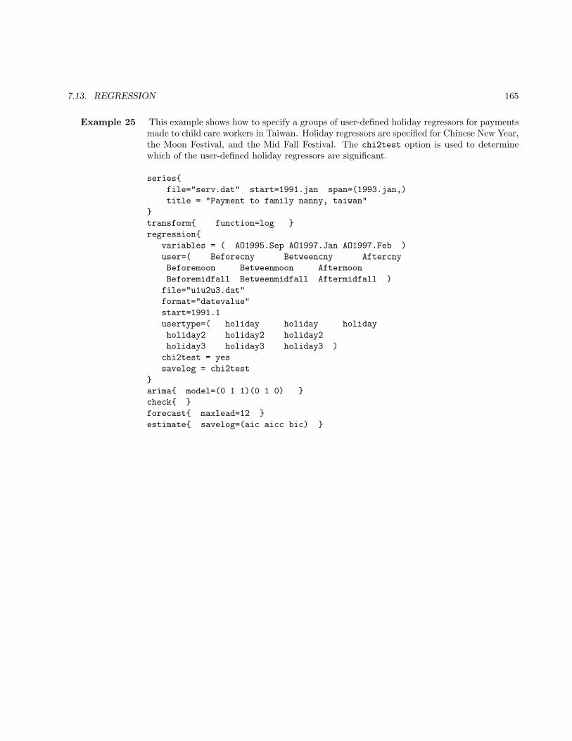
7.13. REGRESSION 165
Example 25 This example shows how to specify a groups of user-defined holiday regressors for paymentsmade to child care workers in Taiwan. Holiday regressors are specified for Chinese New Year,the Moon Festival, and the Mid Fall Festival. The chi2test option is used to determinewhich of the user-defined holiday regressors are significant.
series{
file="serv.dat" start=1991.jan span=(1993.jan,)
title = "Payment to family nanny, taiwan"
}
transform{ function=log }
regression{
variables = ( AO1995.Sep AO1997.Jan AO1997.Feb )
user=( Beforecny Betweencny Aftercny
Beforemoon Betweenmoon Aftermoon
Beforemidfall Betweenmidfall Aftermidfall )
file="u1u2u3.dat"
format="datevalue"
start=1991.1
usertype=( holiday holiday holiday
holiday2 holiday2 holiday2
holiday3 holiday3 holiday3 )
chi2test = yes
savelog = chi2test
}
arima{ model=(0 1 1)(0 1 0) }
check{ }
forecast{ maxlead=12 }
estimate{ savelog=(aic aicc bic) }
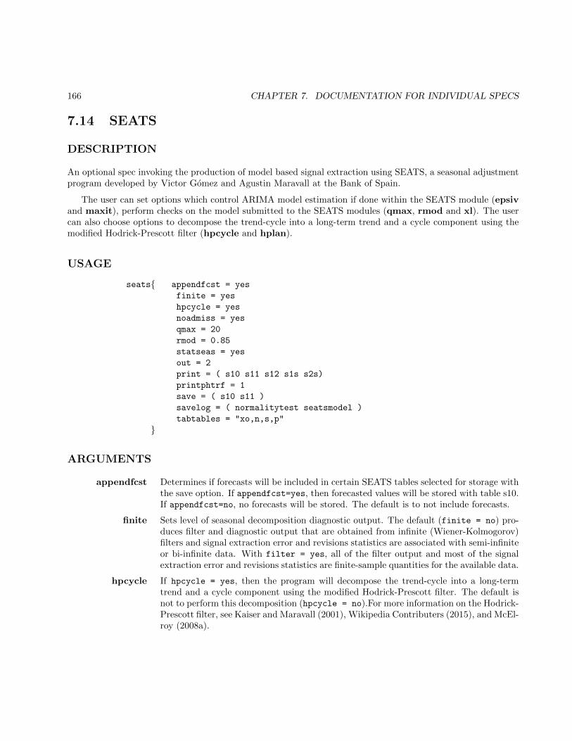
166 CHAPTER 7. DOCUMENTATION FOR INDIVIDUAL SPECS
7.14 SEATS
DESCRIPTION
An optional spec invoking the production of model based signal extraction using SEATS, a seasonal adjustmentprogram developed by Victor Gomez and Agustin Maravall at the Bank of Spain.
The user can set options which control ARIMA model estimation if done within the SEATS module (epsivand maxit), perform checks on the model submitted to the SEATS modules (qmax, rmod and xl). The usercan also choose options to decompose the trend-cycle into a long-term trend and a cycle component using themodified Hodrick-Prescott filter (hpcycle and hplan).
USAGE
seats{ appendfcst = yes
finite = yes
hpcycle = yes
noadmiss = yes
qmax = 20
rmod = 0.85
statseas = yes
out = 2
print = ( s10 s11 s12 s1s s2s)
printphtrf = 1
save = ( s10 s11 )
savelog = ( normalitytest seatsmodel )
tabtables = "xo,n,s,p"
}
ARGUMENTS
appendfcst Determines if forecasts will be included in certain SEATS tables selected for storage withthe save option. If appendfcst=yes, then forecasted values will be stored with table s10.If appendfcst=no, no forecasts will be stored. The default is to not include forecasts.
finite Sets level of seasonal decomposition diagnostic output. The default (finite = no) pro-duces filter and diagnostic output that are obtained from infinite (Wiener-Kolmogorov)filters and signal extraction error and revisions statistics are associated with semi-infiniteor bi-infinite data. With filter = yes, all of the filter output and most of the signalextraction error and revisions statistics are finite-sample quantities for the available data.
hpcycle If hpcycle = yes, then the program will decompose the trend-cycle into a long-termtrend and a cycle component using the modified Hodrick-Prescott filter. The default isnot to perform this decomposition (hpcycle = no).For more information on the Hodrick-Prescott filter, see Kaiser and Maravall (2001), Wikipedia Contributers (2015), and McEl-roy (2008a).
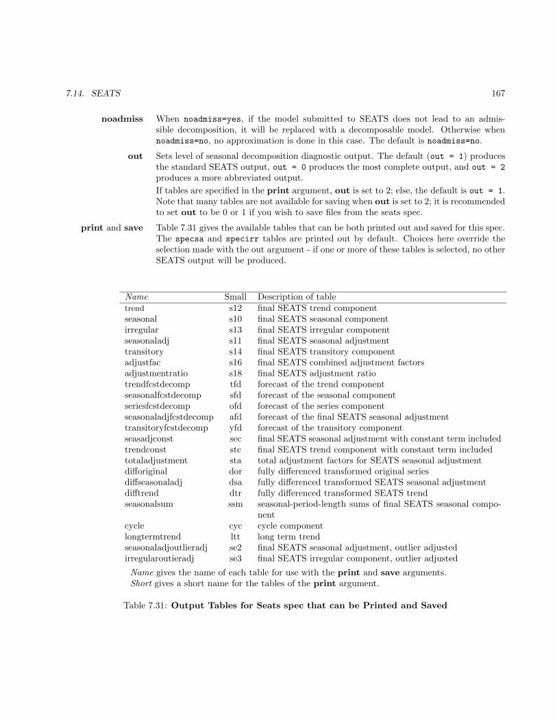
7.14. SEATS 167
noadmiss When noadmiss=yes, if the model submitted to SEATS does not lead to an admis-sible decomposition, it will be replaced with a decomposable model. Otherwise whennoadmiss=no, no approximation is done in this case. The default is noadmiss=no.
out Sets level of seasonal decomposition diagnostic output. The default (out = 1) producesthe standard SEATS output, out = 0 produces the most complete output, and out = 2
produces a more abbreviated output.
If tables are specified in the print argument, out is set to 2; else, the default is out = 1.Note that many tables are not available for saving when out is set to 2; it is recommendedto set out to be 0 or 1 if you wish to save files from the seats spec.
print and save Table 7.31 gives the available tables that can be both printed out and saved for this spec.The specsa and specirr tables are printed out by default. Choices here override theselection made with the out argument - if one or more of these tables is selected, no otherSEATS output will be produced.
Name Small Description of tabletrend s12 final SEATS trend componentseasonal s10 final SEATS seasonal componentirregular s13 final SEATS irregular componentseasonaladj s11 final SEATS seasonal adjustmenttransitory s14 final SEATS transitory componentadjustfac s16 final SEATS combined adjustment factorsadjustmentratio s18 final SEATS adjustment ratiotrendfcstdecomp tfd forecast of the trend componentseasonalfcstdecomp sfd forecast of the seasonal componentseriesfcstdecomp ofd forecast of the series componentseasonaladjfcstdecomp afd forecast of the final SEATS seasonal adjustmenttransitoryfcstdecomp yfd forecast of the transitory componentseasadjconst sec final SEATS seasonal adjustment with constant term includedtrendconst stc final SEATS trend component with constant term includedtotaladjustment sta total adjustment factors for SEATS seasonal adjustmentdifforiginal dor fully differenced transformed original seriesdiffseasonaladj dsa fully differenced transformed SEATS seasonal adjustmentdifftrend dtr fully differenced transformed SEATS trendseasonalsum ssm seasonal-period-length sums of final SEATS seasonal compo-
nentcycle cyc cycle componentlongtermtrend ltt long term trendseasonaladjoutlieradj se2 final SEATS seasonal adjustment, outlier adjustedirregularoutieradj se3 final SEATS irregular component, outlier adjusted
Name gives the name of each table for use with the print and save arguments.Short gives a short name for the tables of the print argument.
Table 7.31: Output Tables for Seats spec that can be Printed and Saved
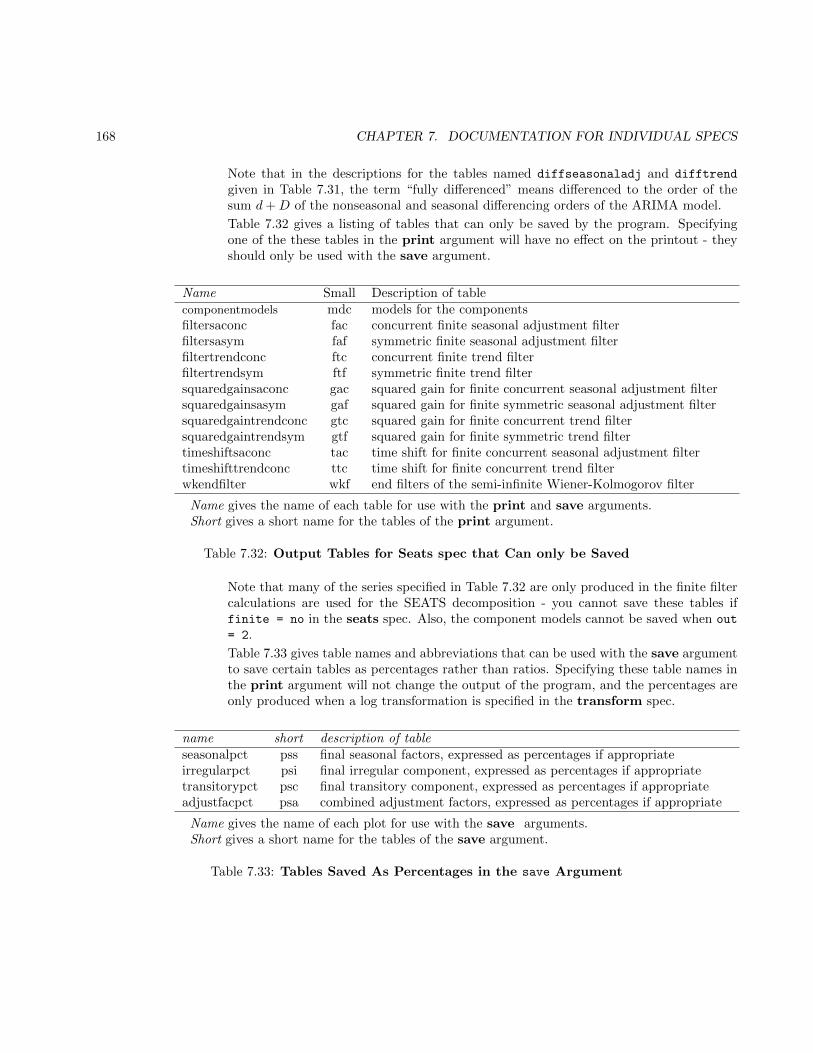
168 CHAPTER 7. DOCUMENTATION FOR INDIVIDUAL SPECS
Note that in the descriptions for the tables named diffseasonaladj and difftrend
given in Table 7.31, the term “fully differenced” means differenced to the order of thesum d+D of the nonseasonal and seasonal differencing orders of the ARIMA model.
Table 7.32 gives a listing of tables that can only be saved by the program. Specifyingone of the these tables in the print argument will have no effect on the printout - theyshould only be used with the save argument.
Name Small Description of tablecomponentmodels mdc models for the componentsfiltersaconc fac concurrent finite seasonal adjustment filterfiltersasym faf symmetric finite seasonal adjustment filterfiltertrendconc ftc concurrent finite trend filterfiltertrendsym ftf symmetric finite trend filtersquaredgainsaconc gac squared gain for finite concurrent seasonal adjustment filtersquaredgainsasym gaf squared gain for finite symmetric seasonal adjustment filtersquaredgaintrendconc gtc squared gain for finite concurrent trend filtersquaredgaintrendsym gtf squared gain for finite symmetric trend filtertimeshiftsaconc tac time shift for finite concurrent seasonal adjustment filtertimeshifttrendconc ttc time shift for finite concurrent trend filterwkendfilter wkf end filters of the semi-infinite Wiener-Kolmogorov filter
Name gives the name of each table for use with the print and save arguments.Short gives a short name for the tables of the print argument.
Table 7.32: Output Tables for Seats spec that Can only be Saved
Note that many of the series specified in Table 7.32 are only produced in the finite filtercalculations are used for the SEATS decomposition - you cannot save these tables iffinite = no in the seats spec. Also, the component models cannot be saved when out
= 2.
Table 7.33 gives table names and abbreviations that can be used with the save argumentto save certain tables as percentages rather than ratios. Specifying these table names inthe print argument will not change the output of the program, and the percentages areonly produced when a log transformation is specified in the transform spec.
name short description of tableseasonalpct pss final seasonal factors, expressed as percentages if appropriateirregularpct psi final irregular component, expressed as percentages if appropriatetransitorypct psc final transitory component, expressed as percentages if appropriateadjustfacpct psa combined adjustment factors, expressed as percentages if appropriate
Name gives the name of each plot for use with the save arguments.Short gives a short name for the tables of the save argument.
Table 7.33: Tables Saved As Percentages in the save Argument
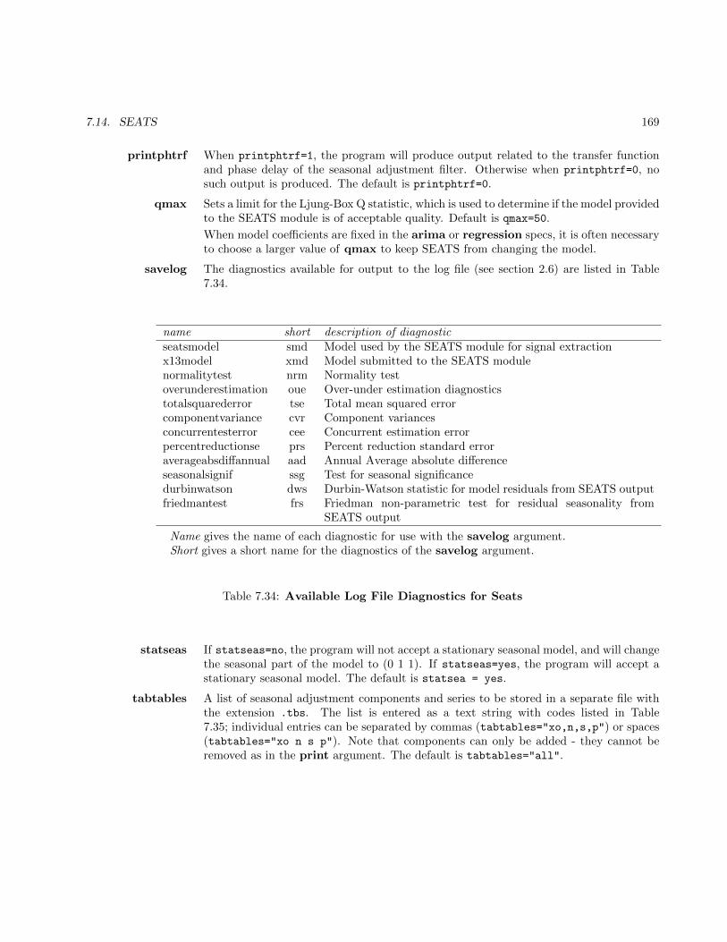
7.14. SEATS 169
printphtrf When printphtrf=1, the program will produce output related to the transfer functionand phase delay of the seasonal adjustment filter. Otherwise when printphtrf=0, nosuch output is produced. The default is printphtrf=0.
qmax Sets a limit for the Ljung-Box Q statistic, which is used to determine if the model providedto the SEATS module is of acceptable quality. Default is qmax=50.
When model coefficients are fixed in the arima or regression specs, it is often necessaryto choose a larger value of qmax to keep SEATS from changing the model.
savelog The diagnostics available for output to the log file (see section 2.6) are listed in Table7.34.
name short description of diagnosticseatsmodel smd Model used by the SEATS module for signal extractionx13model xmd Model submitted to the SEATS modulenormalitytest nrm Normality testoverunderestimation oue Over-under estimation diagnosticstotalsquarederror tse Total mean squared errorcomponentvariance cvr Component variancesconcurrentesterror cee Concurrent estimation errorpercentreductionse prs Percent reduction standard erroraverageabsdiffannual aad Annual Average absolute differenceseasonalsignif ssg Test for seasonal significancedurbinwatson dws Durbin-Watson statistic for model residuals from SEATS outputfriedmantest frs Friedman non-parametric test for residual seasonality from
SEATS output
Name gives the name of each diagnostic for use with the savelog argument.Short gives a short name for the diagnostics of the savelog argument.
Table 7.34: Available Log File Diagnostics for Seats
statseas If statseas=no, the program will not accept a stationary seasonal model, and will changethe seasonal part of the model to (0 1 1). If statseas=yes, the program will accept astationary seasonal model. The default is statsea = yes.
tabtables A list of seasonal adjustment components and series to be stored in a separate file withthe extension .tbs. The list is entered as a text string with codes listed in Table7.35; individual entries can be separated by commas (tabtables="xo,n,s,p") or spaces(tabtables="xo n s p"). Note that components can only be added - they cannot beremoved as in the print argument. The default is tabtables="all".

170 CHAPTER 7. DOCUMENTATION FOR INDIVIDUAL SPECS
Code Description of tableall all seriesxo original seriesn seasonally adjusted seriess seasonal factorsp trend-cycleu irregularc transitorycal calendarpa preadjustment factorcy cycleltp long term trender residualsrg0 separate regression componentrgsa regression component in seasonally adjusted seriesstp stochastic trend cyclestn stochastic seasonally adjusted seriesrtp real time trend cyclertsa teal time seasonally adjusted series
Code gives the code used to specify the series in the tabtables argument.
Table 7.35: Components to be saved in .tbs file
RARELY USED ARGUMENTS
bias Corrects for the bias that may occur in multiplicative decomposition when the period-to-period changes are relatively large when compared to the overall mean. This argumentshould only be set when a log transformation is used.
If Bias = 1, a correction is made for the overall bias for the full length of the series andfor the forecasting period. This is the default value.
If Bias = -1, a correction is made so that, for every year (including the forecasting pe-riod), the annual average of the original series equals the annual average of the seasonallyadjusted series, and also (very approximately) equals the annual average of the trend.
If Bias = 0, no bias correction is done. No other values are allowed.
epsiv Convergence criteria for ARIMA estimation within the SEATS module; this is used whenthe SEATS module determines that a model should be changed or re-estimated. Thisshould be a small positive number; the default is 0.001.
epsphi When Phi(B) contains a complex root, it is allocated to the seasonal if its frequencydifferes from the seasonal fequencies by less than epsphi degrees. Otherwise, it goes tothe cycle. The default is 2.
hplan A parameter that is used to determine the modified Hodrick-Prescott filter. By default,

7.14. SEATS 171
the program will set this parameter automatically according to the seasonal period ofthe series. For more information on the Hodrick-Prescott filter, see Kaiser and Maravall(2001), Wikipedia Contributers (2015), and McElroy (2008a).
imean Indicates if the series is to be mean-corrected (imean = 1). The default is not to removethe mean from the series before signal extraction (imean = 0).
maxit Number of iterations allowed for ARIMA estimation within the SEATS module; shouldbe a positive integer. Default is 20.
rmod Limit for the modulus of an AR root. If the modulus of an AR root is larger than rmod,the root is assigned to the trend; if the modulus of an AR root is smaller than rmod,the root is assigned to the cycle. The default value of rmod is 0.80.
xl When the modulus of an estimated root falls in the range (XL, 1), it is set to 1.00 if theroot is in the AR polynomial. If the root is in the MA polynomial, it is set to xl. Thedefault is 0.99.
DETAILS
The most recent versions of TRAMO and SEATS, as well as more documentation, are available at the Bankof Spain web site (http://www.bde.es/webbde/es/secciones/servicio/software/econom.html). Delays inthe updating of versions may cause slight differences between the X-13ARIMA-SEATS version of SEATS and theone at the Bank of Spain web site.
A tutorial document Findley, Lytras, and Maravall (2016) is available for the ARIMA model-based seasonaladjustment method used by SEATS. For more details on the SEATS seasonal adjustment method and diag-nostics, see Maravall (1995), Gomez and Maravall (1996) and Gomez and Maravall (2001b); for comparisonsof SEATS and X-11 seasonal adjustments and filters, see Hood, Ashley, and Findley (2000), Hood (2002b),Findley and Martin (2003), and Findley, Wills, Aston, Feldpausch, and Hood (2003).
Note that there are other output files that were saved by the SEATS program that are available whenrunning the X-13ARIMA-SEATS program. These output files can contain forecasts, components or diagnosticsgenerated from the SEATS model-based adjustment performed. Table 7.36 shows the file extensions that areused to save the corresponding special output file from SEATS in the same way the short table names are usedas file extensions in storing individual tables to separate files. These extensions do not have to be specifiedin the save argument - these files will be produced for every X-13ARIMA-SEATS run with a SEATS seasonaladjustment. Section 3.2 gives details on the naming conventions used for X-13ARIMA-SEATS saved output.
The matrix formulas of McElroy (2008b) for (nonstationary) ARIMA signal extraction substantially simplifythose of Bell and Hillmer (1988). We will motivate them from re-expressions of the standard regression formulasfor stationary (or more general) linear unobserved component decompositions of mean zero data wt, t = 1, . . . , ninto uncorrelated mean zero components
wt = ut + vt.
Thus, with u = (u1, . . . , un)′, v = (v1, . . . , vn)′, and w = (w1, . . . , wn)′, we require Σuv ≡ Euv′ = 0n×n, whichyields the variance matrix decomposition
Σww = Σuu + Σvv

172 CHAPTER 7. DOCUMENTATION FOR INDIVIDUAL SPECS
SEATS X-13ARIMA-SEATS Contents of filefile name extensionrogtable.out rog Selected statistics from the growth rate outputsummarys.txt sum Summary information and diagnostics from SEATS ad-
justmenttable-s.out tbs Annotated listing of the series, the seasonally adjusted
series, and components of the model-based seasonal ad-justment, saved in columns separated by white space
SEATS file name gives the file name saved by the SEATS program.X-13ARIMA-SEATS extension gives the file extension used to save the output from the corre-
sponding SEATS output file.
Table 7.36: X-13ARIMA-SEATS File Extensions for Special SEATS Saved Output
and the covariance matrix formulaΣuw ≡ Eu (u+ v)
′= Σuu.
Hence, given Σuu and Σvv, the basic formula
β = ΣuwΣ−1ww
for the coefficient matrix minimizing E (u− βw)′(u− βw), which provides the mean square optimal linear
estimate u of u from w,u = βw,
can be evaluated as
β = Σuu (Σuu + Σvv)−1
=(Σ−1uu + Σ−1
vv
)−1Σ−1vv . (7.12)
Similarly, the variance matrix of the error e = u− u reduces to
Σee = Σuu − ΣuuΣ−1wwΣuu
=(Σ−1uu + Σ−1
vv
)−1. (7.13)
The less familiar formulas (7.12) and (7.13) generalize to the ARIMA case.
Now consider ARIMA data Y1 . . . , Yn with differencing polynomial δY (B) = 1 + δ1B1 + · · ·+ δdB
d (d ≥ 1)resulting in mean zero stationary wt = δY (B)Yt, d + 1 ≤ t ≤ n. We assume there is a signal plus noisedecomposition of Yt into difference-stationary components
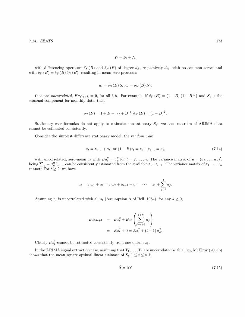
7.14. SEATS 173
Yt = St +Nt
with differencing operators δS (B) and δN (B) of degree dS , respectively dN , with no common zeroes andwith δY (B) = δS (B) δN (B), resulting in mean zero processes
ut = δS (B)St, vt = δN (B)Nt.
that are uncorrelated, Eutvt+h = 0, for all t, h. For example, if δY (B) = (1−B)(1−B12
)and St is the
seasonal component for monthly data, then
δS (B) = 1 +B + · · ·+B11, δN (B) = (1−B)2.
Stationary case formulas do not apply to estimate nonstationary St: variance matrices of ARIMA datacannot be estimated consistently.
Consider the simplest difference stationary model, the random walk :
zt = zt−1 + at or (1−B)zt = zt − zt−1 = at, (7.14)
with uncorrelated, zero-mean at with Ea2t = σ2
a for t = 2, . . . , n. The variance matrix of a = (a2, . . . , an)′,
being∑a = σ2
aIn−1, can be consistently estimated from the available zt−zt−1. The variance matrix of z1, . . . , zncannot: For t ≥ 2, we have
zt = zt−1 + at = zt−2 + at−1 + at = · · · = z1 +
t∑j=2
aj .
Assuming z1 is uncorrelated with all at (Assumption A of Bell, 1984), for any k ≥ 0,
Eztzt+k = Ez2t + Ezt
t+k∑j=t+1
aj
= Ez2
t + 0 = Ez21 + (t− 1)σ2
a.
Clearly Ez21 cannot be estimated consistently from one datum z1.
In the ARIMA signal extraction case, assuming that Y1, . . . , Yd are uncorrelated with all wt, McElroy (2008b)shows that the mean square optimal linear estimate of St, 1 ≤ t ≤ n is
S = βY (7.15)
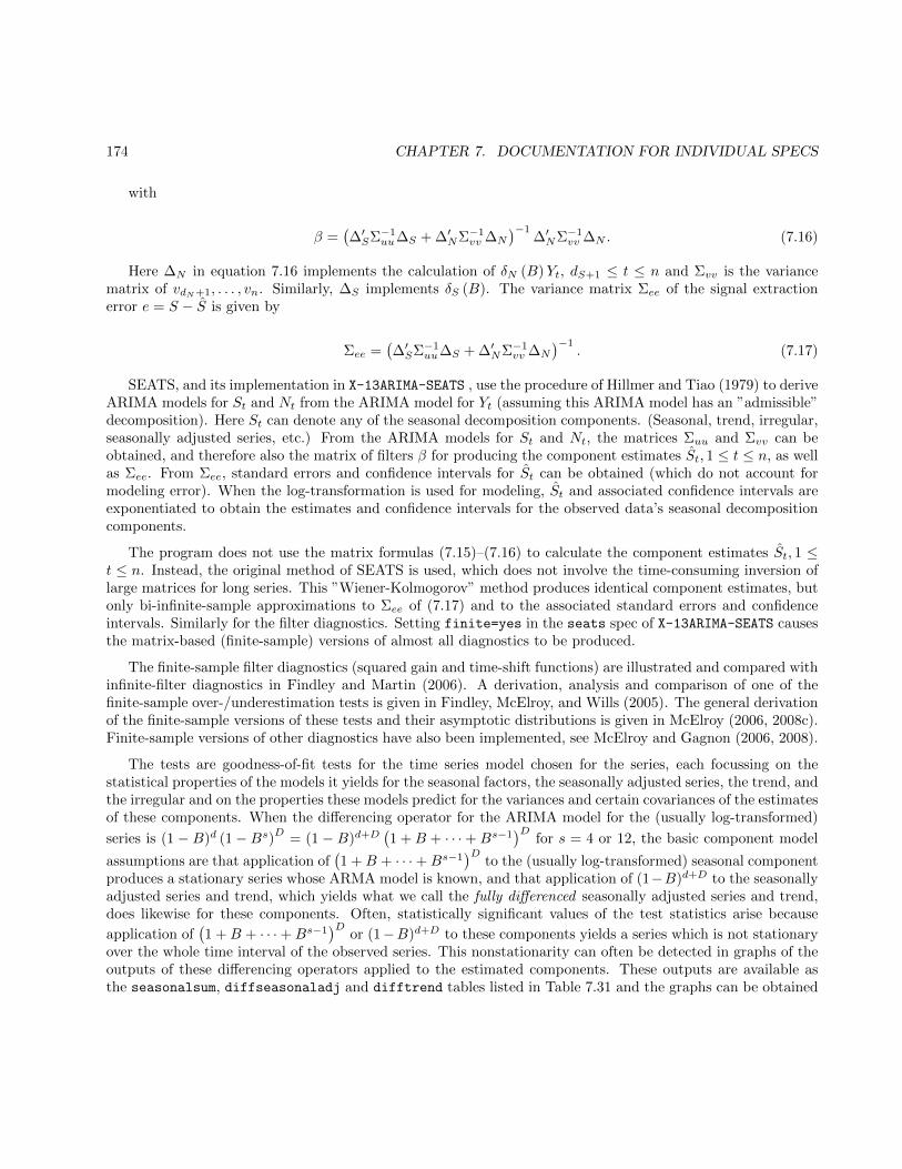
174 CHAPTER 7. DOCUMENTATION FOR INDIVIDUAL SPECS
with
β =(∆′SΣ−1
uu∆S + ∆′NΣ−1vv ∆N
)−1∆′NΣ−1
vv ∆N . (7.16)
Here ∆N in equation 7.16 implements the calculation of δN (B)Yt, dS+1 ≤ t ≤ n and Σvv is the variancematrix of vdN+1, . . . , vn. Similarly, ∆S implements δS (B). The variance matrix Σee of the signal extractionerror e = S − S is given by
Σee =(∆′SΣ−1
uu∆S + ∆′NΣ−1vv ∆N
)−1. (7.17)
SEATS, and its implementation in X-13ARIMA-SEATS , use the procedure of Hillmer and Tiao (1979) to deriveARIMA models for St and Nt from the ARIMA model for Yt (assuming this ARIMA model has an ”admissible”decomposition). Here St can denote any of the seasonal decomposition components. (Seasonal, trend, irregular,seasonally adjusted series, etc.) From the ARIMA models for St and Nt, the matrices Σuu and Σvv can beobtained, and therefore also the matrix of filters β for producing the component estimates St, 1 ≤ t ≤ n, as wellas Σee. From Σee, standard errors and confidence intervals for St can be obtained (which do not account formodeling error). When the log-transformation is used for modeling, St and associated confidence intervals areexponentiated to obtain the estimates and confidence intervals for the observed data’s seasonal decompositioncomponents.
The program does not use the matrix formulas (7.15)–(7.16) to calculate the component estimates St, 1 ≤t ≤ n. Instead, the original method of SEATS is used, which does not involve the time-consuming inversion oflarge matrices for long series. This ”Wiener-Kolmogorov” method produces identical component estimates, butonly bi-infinite-sample approximations to Σee of (7.17) and to the associated standard errors and confidenceintervals. Similarly for the filter diagnostics. Setting finite=yes in the seats spec of X-13ARIMA-SEATS causesthe matrix-based (finite-sample) versions of almost all diagnostics to be produced.
The finite-sample filter diagnostics (squared gain and time-shift functions) are illustrated and compared withinfinite-filter diagnostics in Findley and Martin (2006). A derivation, analysis and comparison of one of thefinite-sample over-/underestimation tests is given in Findley, McElroy, and Wills (2005). The general derivationof the finite-sample versions of these tests and their asymptotic distributions is given in McElroy (2006, 2008c).Finite-sample versions of other diagnostics have also been implemented, see McElroy and Gagnon (2006, 2008).
The tests are goodness-of-fit tests for the time series model chosen for the series, each focussing on thestatistical properties of the models it yields for the seasonal factors, the seasonally adjusted series, the trend, andthe irregular and on the properties these models predict for the variances and certain covariances of the estimatesof these components. When the differencing operator for the ARIMA model for the (usually log-transformed)
series is (1 − B)d (1−Bs)D = (1 − B)d+D(1 +B + · · ·+Bs−1
)Dfor s = 4 or 12, the basic component model
assumptions are that application of(1 +B + · · ·+Bs−1
)Dto the (usually log-transformed) seasonal component
produces a stationary series whose ARMA model is known, and that application of (1−B)d+D to the seasonallyadjusted series and trend, which yields what we call the fully differenced seasonally adjusted series and trend,does likewise for these components. Often, statistically significant values of the test statistics arise because
application of(1 +B + · · ·+Bs−1
)Dor (1−B)d+D to these components yields a series which is not stationary
over the whole time interval of the observed series. This nonstationarity can often be detected in graphs of theoutputs of these differencing operators applied to the estimated components. These outputs are available asthe seasonalsum, diffseasonaladj and difftrend tables listed in Table 7.31 and the graphs can be obtained
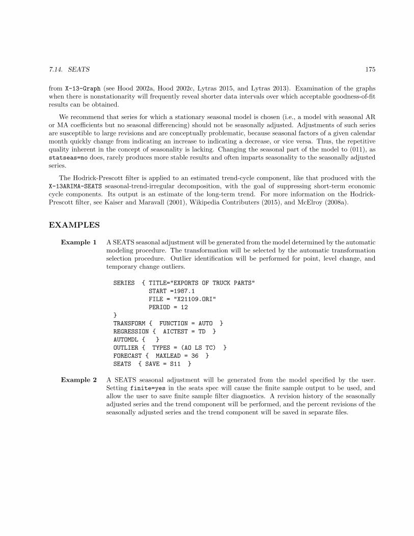
7.14. SEATS 175
from X-13-Graph (see Hood 2002a, Hood 2002c, Lytras 2015, and Lytras 2013). Examination of the graphswhen there is nonstationarity will frequently reveal shorter data intervals over which acceptable goodness-of-fitresults can be obtained.
We recommend that series for which a stationary seasonal model is chosen (i.e., a model with seasonal ARor MA coefficients but no seasonal differencing) should not be seasonally adjusted. Adjustments of such seriesare susceptible to large revisions and are conceptually problematic, because seasonal factors of a given calendarmonth quickly change from indicating an increase to indicating a decrease, or vice versa. Thus, the repetitivequality inherent in the concept of seasonality is lacking. Changing the seasonal part of the model to (011), asstatseas=no does, rarely produces more stable results and often imparts seasonality to the seasonally adjustedseries.
The Hodrick-Prescott filter is applied to an estimated trend-cycle component, like that produced with theX-13ARIMA-SEATS seasonal-trend-irregular decomposition, with the goal of suppressing short-term economiccycle components. Its output is an estimate of the long-term trend. For more information on the Hodrick-Prescott filter, see Kaiser and Maravall (2001), Wikipedia Contributers (2015), and McElroy (2008a).
EXAMPLES
Example 1 A SEATS seasonal adjustment will be generated from the model determined by the automaticmodeling procedure. The transformation will be selected by the automatic transformationselection procedure. Outlier identification will be performed for point, level change, andtemporary change outliers.
SERIES { TITLE="EXPORTS OF TRUCK PARTS"
START =1987.1
FILE = "X21109.ORI"
PERIOD = 12
}
TRANSFORM { FUNCTION = AUTO }
REGRESSION { AICTEST = TD }
AUTOMDL { }
OUTLIER { TYPES = (AO LS TC) }
FORECAST { MAXLEAD = 36 }
SEATS { SAVE = S11 }
Example 2 A SEATS seasonal adjustment will be generated from the model specified by the user.Setting finite=yes in the seats spec will cause the finite sample output to be used, andallow the user to save finite sample filter diagnostics. A revision history of the seasonallyadjusted series and the trend component will be performed, and the percent revisions of theseasonally adjusted series and the trend component will be saved in separate files.
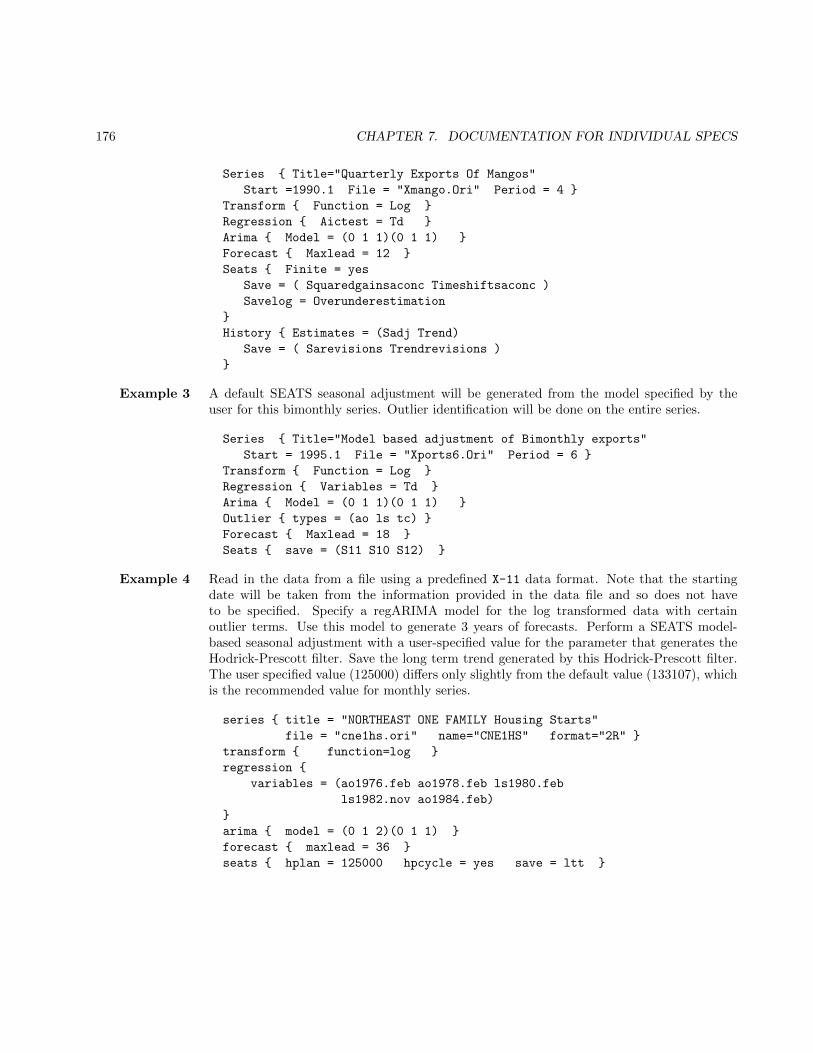
176 CHAPTER 7. DOCUMENTATION FOR INDIVIDUAL SPECS
Series { Title="Quarterly Exports Of Mangos"
Start =1990.1 File = "Xmango.Ori" Period = 4 }
Transform { Function = Log }
Regression { Aictest = Td }
Arima { Model = (0 1 1)(0 1 1) }
Forecast { Maxlead = 12 }
Seats { Finite = yes
Save = ( Squaredgainsaconc Timeshiftsaconc )
Savelog = Overunderestimation
}
History { Estimates = (Sadj Trend)
Save = ( Sarevisions Trendrevisions )
}
Example 3 A default SEATS seasonal adjustment will be generated from the model specified by theuser for this bimonthly series. Outlier identification will be done on the entire series.
Series { Title="Model based adjustment of Bimonthly exports"
Start = 1995.1 File = "Xports6.Ori" Period = 6 }
Transform { Function = Log }
Regression { Variables = Td }
Arima { Model = (0 1 1)(0 1 1) }
Outlier { types = (ao ls tc) }
Forecast { Maxlead = 18 }
Seats { save = (S11 S10 S12) }
Example 4 Read in the data from a file using a predefined X-11 data format. Note that the startingdate will be taken from the information provided in the data file and so does not haveto be specified. Specify a regARIMA model for the log transformed data with certainoutlier terms. Use this model to generate 3 years of forecasts. Perform a SEATS model-based seasonal adjustment with a user-specified value for the parameter that generates theHodrick-Prescott filter. Save the long term trend generated by this Hodrick-Prescott filter.The user specified value (125000) differs only slightly from the default value (133107), whichis the recommended value for monthly series.
series { title = "NORTHEAST ONE FAMILY Housing Starts"
file = "cne1hs.ori" name="CNE1HS" format="2R" }
transform { function=log }
regression {
variables = (ao1976.feb ao1978.feb ls1980.feb
ls1982.nov ao1984.feb)
}
arima { model = (0 1 2)(0 1 1) }
forecast { maxlead = 36 }
seats { hplan = 125000 hpcycle = yes save = ltt }
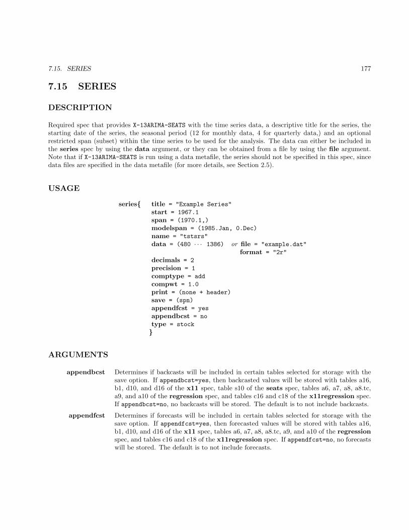
7.15. SERIES 177
7.15 SERIES
DESCRIPTION
Required spec that provides X-13ARIMA-SEATS with the time series data, a descriptive title for the series, thestarting date of the series, the seasonal period (12 for monthly data, 4 for quarterly data,) and an optionalrestricted span (subset) within the time series to be used for the analysis. The data can either be included inthe series spec by using the data argument, or they can be obtained from a file by using the file argument.Note that if X-13ARIMA-SEATS is run using a data metafile, the series should not be specified in this spec, sincedata files are specified in the data metafile (for more details, see Section 2.5).
USAGE
series{ title = "Example Series"
start = 1967.1
span = (1970.1,)
modelspan = (1985.Jan, 0.Dec)
name = "tstsrs"
data = (480 · · · 1386) or file = "example.dat"
format = "2r"
decimals = 2
precision = 1
comptype = add
compwt = 1.0
print = (none + header)
save = (spn)
appendfcst = yes
appendbcst = no
type = stock
}
ARGUMENTS
appendbcst Determines if backcasts will be included in certain tables selected for storage with thesave option. If appendbcst=yes, then backcasted values will be stored with tables a16,b1, d10, and d16 of the x11 spec, table s10 of the seats spec, tables a6, a7, a8, a8.tc,a9, and a10 of the regression spec, and tables c16 and c18 of the x11regression spec.If appendbcst=no, no backcasts will be stored. The default is to not include backcasts.
appendfcst Determines if forecasts will be included in certain tables selected for storage with thesave option. If appendfcst=yes, then forecasted values will be stored with tables a16,b1, d10, and d16 of the x11 spec, tables a6, a7, a8, a8.tc, a9, and a10 of the regressionspec, and tables c16 and c18 of the x11regression spec. If appendfcst=no, no forecastswill be stored. The default is to not include forecasts.
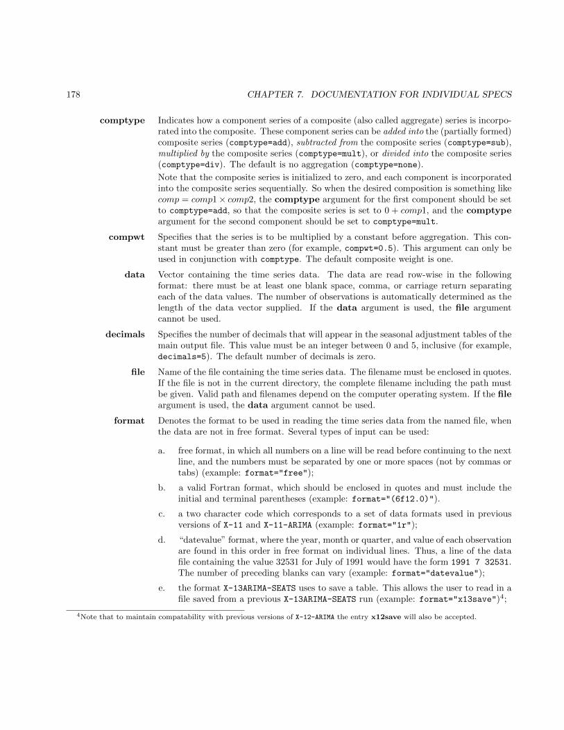
178 CHAPTER 7. DOCUMENTATION FOR INDIVIDUAL SPECS
comptype Indicates how a component series of a composite (also called aggregate) series is incorpo-rated into the composite. These component series can be added into the (partially formed)composite series (comptype=add), subtracted from the composite series (comptype=sub),multiplied by the composite series (comptype=mult), or divided into the composite series(comptype=div). The default is no aggregation (comptype=none).
Note that the composite series is initialized to zero, and each component is incorporatedinto the composite series sequentially. So when the desired composition is something likecomp = comp1× comp2, the comptype argument for the first component should be setto comptype=add, so that the composite series is set to 0 + comp1, and the comptypeargument for the second component should be set to comptype=mult.
compwt Specifies that the series is to be multiplied by a constant before aggregation. This con-stant must be greater than zero (for example, compwt=0.5). This argument can only beused in conjunction with comptype. The default composite weight is one.
data Vector containing the time series data. The data are read row-wise in the followingformat: there must be at least one blank space, comma, or carriage return separatingeach of the data values. The number of observations is automatically determined as thelength of the data vector supplied. If the data argument is used, the file argumentcannot be used.
decimals Specifies the number of decimals that will appear in the seasonal adjustment tables of themain output file. This value must be an integer between 0 and 5, inclusive (for example,decimals=5). The default number of decimals is zero.
file Name of the file containing the time series data. The filename must be enclosed in quotes.If the file is not in the current directory, the complete filename including the path mustbe given. Valid path and filenames depend on the computer operating system. If the fileargument is used, the data argument cannot be used.
format Denotes the format to be used in reading the time series data from the named file, whenthe data are not in free format. Several types of input can be used:
a. free format, in which all numbers on a line will be read before continuing to the nextline, and the numbers must be separated by one or more spaces (not by commas ortabs) (example: format="free");
b. a valid Fortran format, which should be enclosed in quotes and must include theinitial and terminal parentheses (example: format="(6f12.0)").
c. a two character code which corresponds to a set of data formats used in previousversions of X-11 and X-11-ARIMA (example: format="1r");
d. “datevalue” format, where the year, month or quarter, and value of each observationare found in this order in free format on individual lines. Thus, a line of the datafile containing the value 32531 for July of 1991 would have the form 1991 7 32531.The number of preceding blanks can vary (example: format="datevalue");
e. the format X-13ARIMA-SEATS uses to save a table. This allows the user to read in afile saved from a previous X-13ARIMA-SEATS run (example: format="x13save")4;
4Note that to maintain compatability with previous versions of X-12-ARIMA the entry x12save will also be accepted.
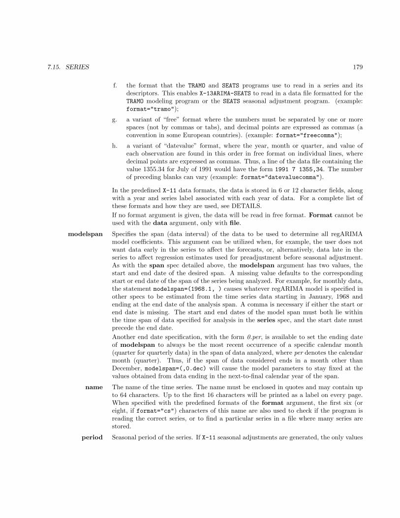
7.15. SERIES 179
f. the format that the TRAMO and SEATS programs use to read in a series and itsdescriptors. This enables X-13ARIMA-SEATS to read in a data file formatted for theTRAMO modeling program or the SEATS seasonal adjustment program. (example:format="tramo");
g. a variant of “free” format where the numbers must be separated by one or morespaces (not by commas or tabs), and decimal points are expressed as commas (aconvention in some European countries). (example: format="freecomma");
h. a variant of “datevalue” format, where the year, month or quarter, and value ofeach observation are found in this order in free format on individual lines, wheredecimal points are expressed as commas. Thus, a line of the data file containing thevalue 1355.34 for July of 1991 would have the form 1991 7 1355,34. The numberof preceding blanks can vary (example: format="datevaluecomma").
In the predefined X-11 data formats, the data is stored in 6 or 12 character fields, alongwith a year and series label associated with each year of data. For a complete list ofthese formats and how they are used, see DETAILS.
If no format argument is given, the data will be read in free format. Format cannot beused with the data argument, only with file.
modelspan Specifies the span (data interval) of the data to be used to determine all regARIMAmodel coefficients. This argument can be utilized when, for example, the user does notwant data early in the series to affect the forecasts, or, alternatively, data late in theseries to affect regression estimates used for preadjustment before seasonal adjustment.As with the span spec detailed above, the modelspan argument has two values, thestart and end date of the desired span. A missing value defaults to the correspondingstart or end date of the span of the series being analyzed. For example, for monthly data,the statement modelspan=(1968.1, ) causes whatever regARIMA model is specified inother specs to be estimated from the time series data starting in January, 1968 andending at the end date of the analysis span. A comma is necessary if either the start orend date is missing. The start and end dates of the model span must both lie withinthe time span of data specified for analysis in the series spec, and the start date mustprecede the end date.
Another end date specification, with the form 0.per, is available to set the ending dateof modelspan to always be the most recent occurrence of a specific calendar month(quarter for quarterly data) in the span of data analyzed, where per denotes the calendarmonth (quarter). Thus, if the span of data considered ends in a month other thanDecember, modelspan=(,0.dec) will cause the model parameters to stay fixed at thevalues obtained from data ending in the next-to-final calendar year of the span.
name The name of the time series. The name must be enclosed in quotes and may contain upto 64 characters. Up to the first 16 characters will be printed as a label on every page.When specified with the predefined formats of the format argument, the first six (oreight, if format="cs") characters of this name are also used to check if the program isreading the correct series, or to find a particular series in a file where many series arestored.
period Seasonal period of the series. If X-11 seasonal adjustments are generated, the only values
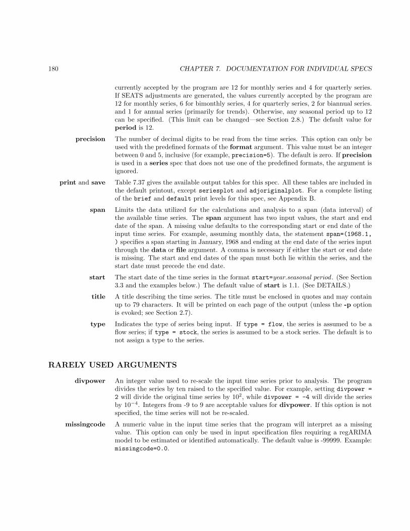
180 CHAPTER 7. DOCUMENTATION FOR INDIVIDUAL SPECS
currently accepted by the program are 12 for monthly series and 4 for quarterly series.If SEATS adjustments are generated, the values currently accepted by the program are12 for monthly series, 6 for bimonthly series, 4 for quarterly series, 2 for biannual series.and 1 for annual series (primarily for trends). Otherwise, any seasonal period up to 12can be specified. (This limit can be changed—see Section 2.8.) The default value forperiod is 12.
precision The number of decimal digits to be read from the time series. This option can only beused with the predefined formats of the format argument. This value must be an integerbetween 0 and 5, inclusive (for example, precision=5). The default is zero. If precisionis used in a series spec that does not use one of the predefined formats, the argument isignored.
print and save Table 7.37 gives the available output tables for this spec. All these tables are included inthe default printout, except seriesplot and adjoriginalplot. For a complete listingof the brief and default print levels for this spec, see Appendix B.
span Limits the data utilized for the calculations and analysis to a span (data interval) ofthe available time series. The span argument has two input values, the start and enddate of the span. A missing value defaults to the corresponding start or end date of theinput time series. For example, assuming monthly data, the statement span=(1968.1,
) specifies a span starting in January, 1968 and ending at the end date of the series inputthrough the data or file argument. A comma is necessary if either the start or end dateis missing. The start and end dates of the span must both lie within the series, and thestart date must precede the end date.
start The start date of the time series in the format start=year.seasonal period . (See Section3.3 and the examples below.) The default value of start is 1.1. (See DETAILS.)
title A title describing the time series. The title must be enclosed in quotes and may containup to 79 characters. It will be printed on each page of the output (unless the -p optionis evoked; see Section 2.7).
type Indicates the type of series being input. If type = flow, the series is assumed to be aflow series; if type = stock, the series is assumed to be a stock series. The default is tonot assign a type to the series.
RARELY USED ARGUMENTS
divpower An integer value used to re-scale the input time series prior to analysis. The programdivides the series by ten raised to the specified value. For example, setting divpower =
2 will divide the original time series by 102, while divpower = -4 will divide the seriesby 10−4. Integers from -9 to 9 are acceptable values for divpower. If this option is notspecified, the time series will not be re-scaled.
missingcode A numeric value in the input time series that the program will interpret as a missingvalue. This option can only be used in input specification files requiring a regARIMAmodel to be estimated or identified automatically. The default value is -99999. Example:missingcode=0.0.
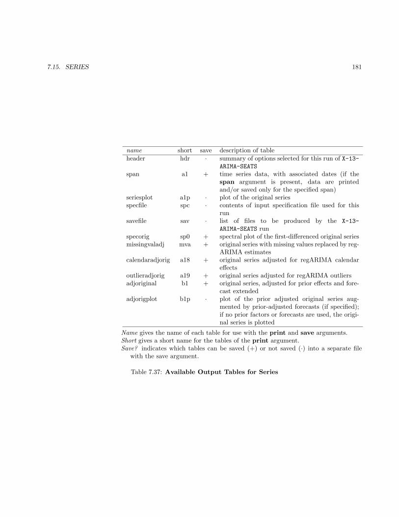
7.15. SERIES 181
name short save description of tableheader hdr · summary of options selected for this run of X-13-
ARIMA-SEATS
span a1 + time series data, with associated dates (if thespan argument is present, data are printedand/or saved only for the specified span)
seriesplot a1p · plot of the original seriesspecfile spc · contents of input specification file used for this
runsavefile sav · list of files to be produced by the X-13-
ARIMA-SEATS runspecorig sp0 + spectral plot of the first-differenced original seriesmissingvaladj mva + original series with missing values replaced by reg-
ARIMA estimatescalendaradjorig a18 + original series adjusted for regARIMA calendar
effectsoutlieradjorig a19 + original series adjusted for regARIMA outliersadjoriginal b1 + original series, adjusted for prior effects and fore-
cast extendedadjorigplot b1p · plot of the prior adjusted original series aug-
mented by prior-adjusted forecasts (if specified);if no prior factors or forecasts are used, the origi-nal series is plotted
Name gives the name of each table for use with the print and save arguments.Short gives a short name for the tables of the print argument.Save? indicates which tables can be saved (+) or not saved (·) into a separate file
with the save argument.
Table 7.37: Available Output Tables for Series
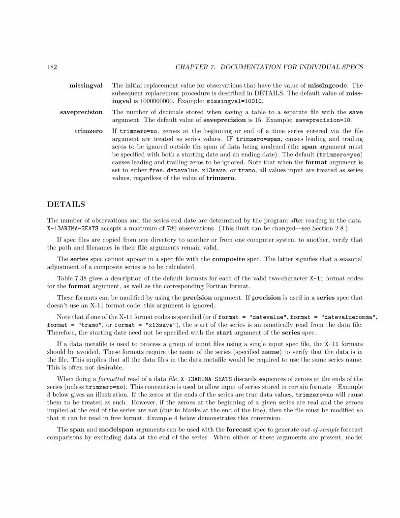
182 CHAPTER 7. DOCUMENTATION FOR INDIVIDUAL SPECS
missingval The initial replacement value for observations that have the value of missingcode. Thesubsequent replacement procedure is described in DETAILS. The default value of miss-ingval is 1000000000. Example: missingval=10D10.
saveprecision The number of decimals stored when saving a table to a separate file with the saveargument. The default value of saveprecision is 15. Example: saveprecision=10.
trimzero If trimzero=no, zeroes at the beginning or end of a time series entered via the fileargument are treated as series values. IF trimzero=span, causes leading and trailingzeros to be ignored outside the span of data being analyzed (the span argument mustbe specified with both a starting date and an ending date). The default (trimzero=yes)causes leading and trailing zeros to be ignored. Note that when the format argument isset to either free, datevalue, x13save, or tramo, all values input are treated as seriesvalues, regardless of the value of trimzero.
DETAILS
The number of observations and the series end date are determined by the program after reading in the data.X-13ARIMA-SEATS accepts a maximum of 780 observations. (This limit can be changed—see Section 2.8.)
If spec files are copied from one directory to another or from one computer system to another, verify thatthe path and filenames in their file arguments remain valid.
The series spec cannot appear in a spec file with the composite spec. The latter signifies that a seasonaladjustment of a composite series is to be calculated.
Table 7.38 gives a description of the default formats for each of the valid two-character X-11 format codesfor the format argument, as well as the corresponding Fortran format.
These formats can be modified by using the precision argument. If precision is used in a series spec thatdoesn’t use an X-11 format code, this argument is ignored.
Note that if one of the X-11 format codes is specified (or if format = "datevalue", format = "datevaluecomma",format = "tramo", or format = "x13save"), the start of the series is automatically read from the data file.Therefore, the starting date need not be specified with the start argument of the series spec.
If a data metafile is used to process a group of input files using a single input spec file, the X-11 formatsshould be avoided. These formats require the name of the series (specified name) to verify that the data is inthe file. This implies that all the data files in the data metafile would be required to use the same series name.This is often not desirable.
When doing a formatted read of a data file, X-13ARIMA-SEATS discards sequences of zeroes at the ends of theseries (unless trimzero=no). This convention is used to allow input of series stored in certain formats—Example3 below gives an illustration. If the zeros at the ends of the series are true data values, trimzero=no will causethem to be treated as such. However, if the zeroes at the beginning of a given series are real and the zeroesimplied at the end of the series are not (due to blanks at the end of the line), then the file must be modified sothat it can be read in free format. Example 4 below demonstrates this conversion.
The span and modelspan arguments can be used with the forecast spec to generate out-of-sample forecastcomparisons by excluding data at the end of the series. When either of these arguments are present, model
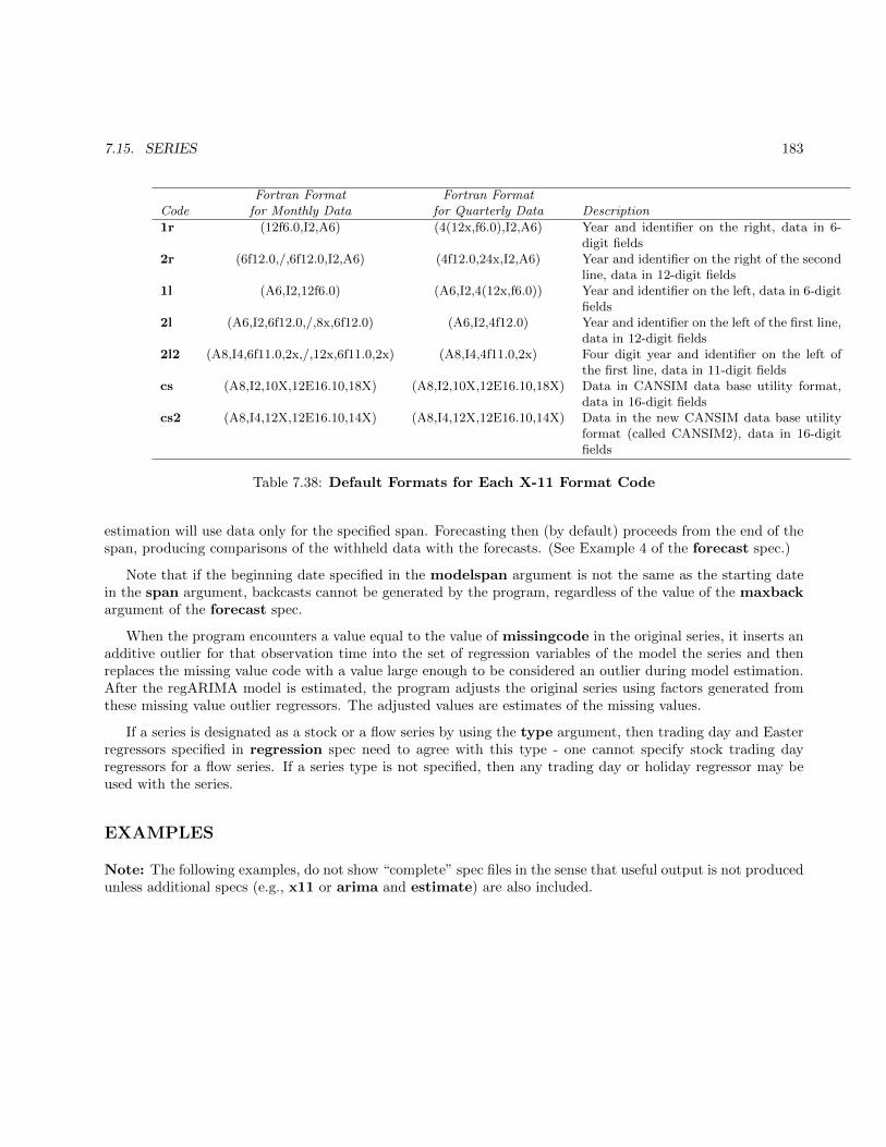
7.15. SERIES 183
Fortran Format Fortran FormatCode for Monthly Data for Quarterly Data Description
1r (12f6.0,I2,A6) (4(12x,f6.0),I2,A6) Year and identifier on the right, data in 6-digit fields
2r (6f12.0,/,6f12.0,I2,A6) (4f12.0,24x,I2,A6) Year and identifier on the right of the secondline, data in 12-digit fields
1l (A6,I2,12f6.0) (A6,I2,4(12x,f6.0)) Year and identifier on the left, data in 6-digitfields
2l (A6,I2,6f12.0,/,8x,6f12.0) (A6,I2,4f12.0) Year and identifier on the left of the first line,data in 12-digit fields
2l2 (A8,I4,6f11.0,2x,/,12x,6f11.0,2x) (A8,I4,4f11.0,2x) Four digit year and identifier on the left ofthe first line, data in 11-digit fields
cs (A8,I2,10X,12E16.10,18X) (A8,I2,10X,12E16.10,18X) Data in CANSIM data base utility format,data in 16-digit fields
cs2 (A8,I4,12X,12E16.10,14X) (A8,I4,12X,12E16.10,14X) Data in the new CANSIM data base utilityformat (called CANSIM2), data in 16-digitfields
Table 7.38: Default Formats for Each X-11 Format Code
estimation will use data only for the specified span. Forecasting then (by default) proceeds from the end of thespan, producing comparisons of the withheld data with the forecasts. (See Example 4 of the forecast spec.)
Note that if the beginning date specified in the modelspan argument is not the same as the starting datein the span argument, backcasts cannot be generated by the program, regardless of the value of the maxbackargument of the forecast spec.
When the program encounters a value equal to the value of missingcode in the original series, it inserts anadditive outlier for that observation time into the set of regression variables of the model the series and thenreplaces the missing value code with a value large enough to be considered an outlier during model estimation.After the regARIMA model is estimated, the program adjusts the original series using factors generated fromthese missing value outlier regressors. The adjusted values are estimates of the missing values.
If a series is designated as a stock or a flow series by using the type argument, then trading day and Easterregressors specified in regression spec need to agree with this type - one cannot specify stock trading dayregressors for a flow series. If a series type is not specified, then any trading day or holiday regressor may beused with the series.
EXAMPLES
Note: The following examples, do not show “complete” spec files in the sense that useful output is not producedunless additional specs (e.g., x11 or arima and estimate) are also included.
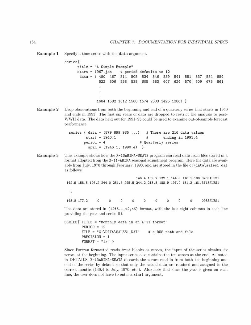
184 CHAPTER 7. DOCUMENTATION FOR INDIVIDUAL SPECS
Example 1 Specify a time series with the data argument.
series{
title = "A Simple Example"
start = 1967.jan # period defaults to 12
data = ( 480 467 514 505 534 546 539 541 551 537 584 854
522 506 558 538 605 583 607 624 570 609 675 861
.
.
.
1684 1582 1512 1508 1574 2303 1425 1386) }
Example 2 Drop observations from both the beginning and end of a quarterly series that starts in 1940and ends in 1993. The first six years of data are dropped to restrict the analysis to post-WWII data. The data held out for 1991–93 could be used to examine out-of-sample forecastperformance.
series { data = (879 899 985 ...) # There are 216 data values
start = 1940.1 # ending in 1993.4
period = 4 # Quarterly series
span = (1946.1, 1990.4) }
Example 3 This example shows how the X-13ARIMA-SEATS program can read data from files stored in aformat adopted from the X-11-ARIMA seasonal adjustment program. Here the data are avail-able from July, 1970 through February, 1993, and are stored in the file c:\data\sales1.datas follows:
146.4 109.2 132.1 144.8 116.1 100.370SALES1
142.9 158.8 196.2 244.0 251.6 245.5 244.2 213.8 188.9 197.2 181.2 161.371SALES1
.
.
.
148.8 177.2 0 0 0 0 0 0 0 0 0 093SALES1
The data are stored in (12f6.1,i2,a6) format, with the last eight columns in each lineproviding the year and series ID.
SERIES{ TITLE = "Monthly data in an X-11 format"
PERIOD = 12
FILE = "C:\DATA\SALES1.DAT" # a DOS path and file
PRECISION = 1
FORMAT = "1r" }
Since Fortran formatted reads treat blanks as zeroes, the input of the series obtains sixzeroes at the beginning. The input series also contains the ten zeroes at the end. As notedin DETAILS, X-13ARIMA-SEATS discards the zeroes read in from both the beginning andend of the series by default so that only the actual data are retained and assigned to thecorrect months (146.4 to July, 1970, etc.). Also note that since the year is given on eachline, the user does not have to enter a start argument.
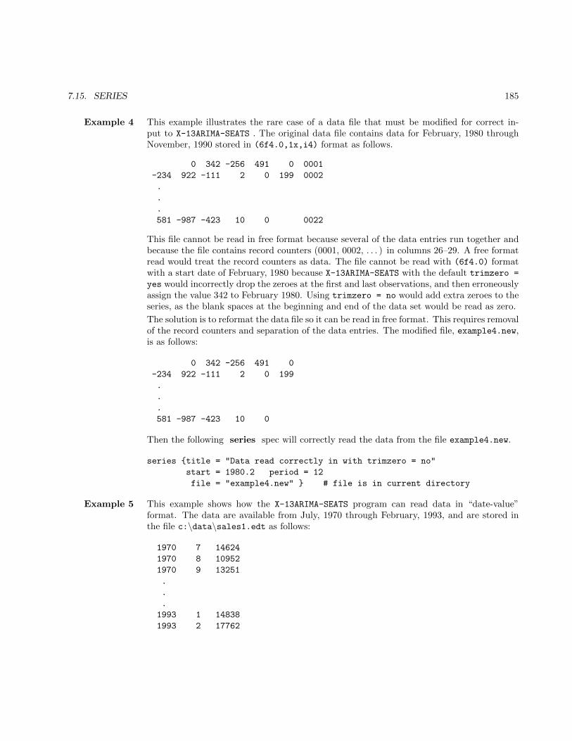
7.15. SERIES 185
Example 4 This example illustrates the rare case of a data file that must be modified for correct in-put to X-13ARIMA-SEATS . The original data file contains data for February, 1980 throughNovember, 1990 stored in (6f4.0,1x,i4) format as follows.
0 342 -256 491 0 0001
-234 922 -111 2 0 199 0002
.
.
.
581 -987 -423 10 0 0022
This file cannot be read in free format because several of the data entries run together andbecause the file contains record counters (0001, 0002, . . . ) in columns 26–29. A free formatread would treat the record counters as data. The file cannot be read with (6f4.0) formatwith a start date of February, 1980 because X-13ARIMA-SEATS with the default trimzero =
yes would incorrectly drop the zeroes at the first and last observations, and then erroneouslyassign the value 342 to February 1980. Using trimzero = no would add extra zeroes to theseries, as the blank spaces at the beginning and end of the data set would be read as zero.
The solution is to reformat the data file so it can be read in free format. This requires removalof the record counters and separation of the data entries. The modified file, example4.new,is as follows:
0 342 -256 491 0
-234 922 -111 2 0 199
.
.
.
581 -987 -423 10 0
Then the following series spec will correctly read the data from the file example4.new.
series {title = "Data read correctly in with trimzero = no"
start = 1980.2 period = 12
file = "example4.new" } # file is in current directory
Example 5 This example shows how the X-13ARIMA-SEATS program can read data in “date-value”format. The data are available from July, 1970 through February, 1993, and are stored inthe file c:\data\sales1.edt as follows:
1970 7 14624
1970 8 10952
1970 9 13251
.
.
.
1993 1 14838
1993 2 17762
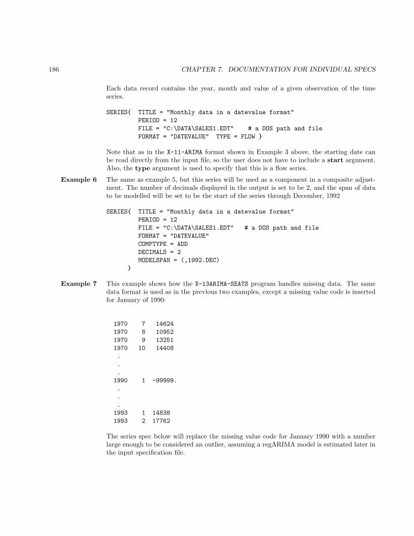
186 CHAPTER 7. DOCUMENTATION FOR INDIVIDUAL SPECS
Each data record contains the year, month and value of a given observation of the timeseries.
SERIES{ TITLE = "Monthly data in a datevalue format"
PERIOD = 12
FILE = "C:\DATA\SALES1.EDT" # a DOS path and file
FORMAT = "DATEVALUE" TYPE = FLOW }
Note that as in the X-11-ARIMA format shown in Example 3 above, the starting date canbe read directly from the input file, so the user does not have to include a start argument.Also, the type argument is used to specify that this is a flow series.
Example 6 The same as example 5, but this series will be used as a component in a composite adjust-ment. The number of decimals displayed in the output is set to be 2, and the span of datato be modelled will be set to be the start of the series through December, 1992
SERIES{ TITLE = "Monthly data in a datevalue format"
PERIOD = 12
FILE = "C:\DATA\SALES1.EDT" # a DOS path and file
FORMAT = "DATEVALUE"
COMPTYPE = ADD
DECIMALS = 2
MODELSPAN = (,1992.DEC)
}
Example 7 This example shows how the X-13ARIMA-SEATS program handles missing data. The samedata format is used as in the previous two examples, except a missing value code is insertedfor January of 1990:
1970 7 14624
1970 8 10952
1970 9 13251
1970 10 14408
.
.
.
1990 1 -99999.
.
.
.
1993 1 14838
1993 2 17762
The series spec below will replace the missing value code for January 1990 with a numberlarge enough to be considered an outlier, assuming a regARIMA model is estimated later inthe input specification file.
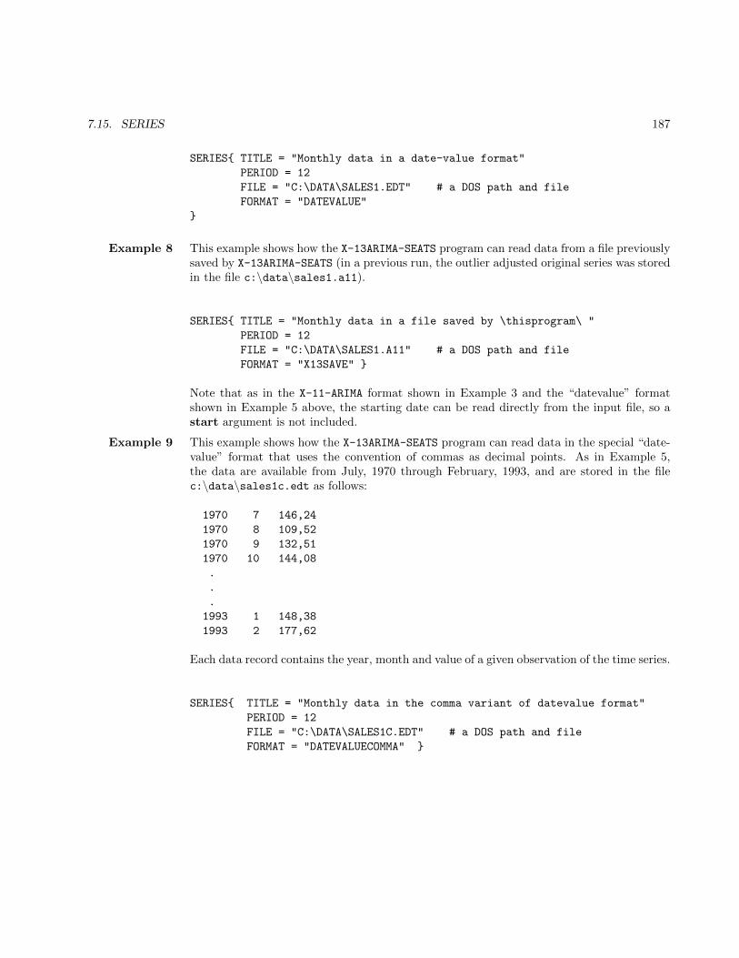
7.15. SERIES 187
SERIES{ TITLE = "Monthly data in a date-value format"
PERIOD = 12
FILE = "C:\DATA\SALES1.EDT" # a DOS path and file
FORMAT = "DATEVALUE"
}
Example 8 This example shows how the X-13ARIMA-SEATS program can read data from a file previouslysaved by X-13ARIMA-SEATS (in a previous run, the outlier adjusted original series was storedin the file c:\data\sales1.a11).
SERIES{ TITLE = "Monthly data in a file saved by \thisprogram\ "
PERIOD = 12
FILE = "C:\DATA\SALES1.A11" # a DOS path and file
FORMAT = "X13SAVE" }
Note that as in the X-11-ARIMA format shown in Example 3 and the “datevalue” formatshown in Example 5 above, the starting date can be read directly from the input file, so astart argument is not included.
Example 9 This example shows how the X-13ARIMA-SEATS program can read data in the special “date-value” format that uses the convention of commas as decimal points. As in Example 5,the data are available from July, 1970 through February, 1993, and are stored in the filec:\data\sales1c.edt as follows:
1970 7 146,24
1970 8 109,52
1970 9 132,51
1970 10 144,08
.
.
.
1993 1 148,38
1993 2 177,62
Each data record contains the year, month and value of a given observation of the time series.
SERIES{ TITLE = "Monthly data in the comma variant of datevalue format"
PERIOD = 12
FILE = "C:\DATA\SALES1C.EDT" # a DOS path and file
FORMAT = "DATEVALUECOMMA" }

188 CHAPTER 7. DOCUMENTATION FOR INDIVIDUAL SPECS
7.16 SLIDINGSPANS
DESCRIPTION
Optional spec providing sliding spans stability analysis. These compare different features of seasonal adjustmentoutput from overlapping subspans of the time series data. The user can specify options to control the startingdate for sliding spans comparisons (start), the length of the sliding spans (length), the threshold values deter-mining sliding spans statistics (cutseas, cuttd, cutchng), how the values of the regARIMA model parameterestimates will be obtained during the sliding spans seasonal adjustment runs (fixmdl), and whether regARIMAautomatic outlier identification is performed (outlier).
USAGE
slidingspans{ start = 1975.jan
length = 132
numspans = 3
cutchng = 3.0
cutseas = 3.0
cuttd = 2.0
outlier = yes
fixmdl = no
fixreg = outlier
print = (long -ssheader)
save = (sfspans)
savelog = (percent)
}
ARGUMENTS
cutchng Threshold value for the month-to-month, quarter-to-quarter, or year-to-year percentchanges in seasonally adjusted series. For a month (quarter) common to more thanone span, if the maximum absolute difference of its period-to-period percent changesfrom the different spans exceeds the threshold value, then the month (quarter) is flaggedas having an unreliable estimate for this period-to-period change. This value must begreater than 0; the default value is 3.0. Example: cutchng=5.0
cutseas Threshold value for the seasonal factors and seasonally adjusted series. For a month(quarter) common to more than one span, if the maximum absolute percent change of itsestimated seasonal factors or adjustments from the different spans exceeds the thresholdvalue, then this month’s (quarter’s) seasonal factor or adjustment is flagged as unreliable.This value must be greater than 0; the default value is 3.0. Example: cutseas=5.0
cuttd Threshold value for the trading day factors. For a month (quarter) common to more thanone span, if the maximum absolute percent change of its estimated trading day factorsfrom the different spans exceeds the threshold value, then this month’s (quarter’s) trading
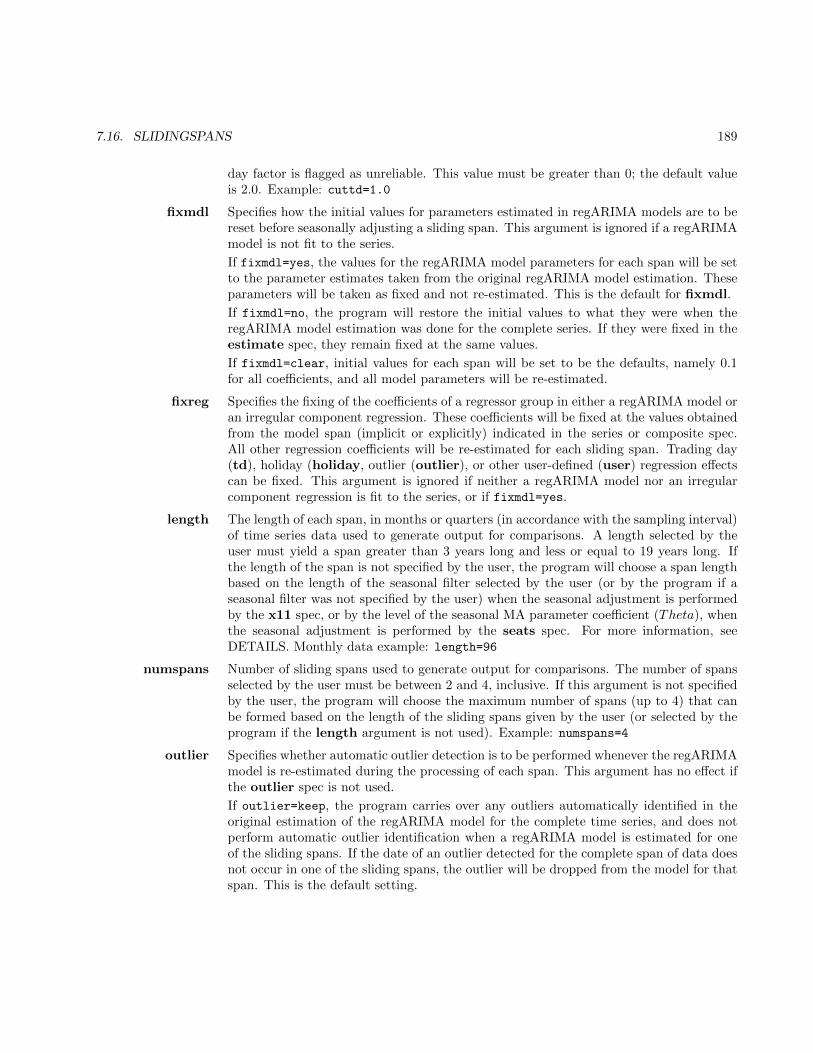
7.16. SLIDINGSPANS 189
day factor is flagged as unreliable. This value must be greater than 0; the default valueis 2.0. Example: cuttd=1.0
fixmdl Specifies how the initial values for parameters estimated in regARIMA models are to bereset before seasonally adjusting a sliding span. This argument is ignored if a regARIMAmodel is not fit to the series.
If fixmdl=yes, the values for the regARIMA model parameters for each span will be setto the parameter estimates taken from the original regARIMA model estimation. Theseparameters will be taken as fixed and not re-estimated. This is the default for fixmdl.
If fixmdl=no, the program will restore the initial values to what they were when theregARIMA model estimation was done for the complete series. If they were fixed in theestimate spec, they remain fixed at the same values.
If fixmdl=clear, initial values for each span will be set to be the defaults, namely 0.1for all coefficients, and all model parameters will be re-estimated.
fixreg Specifies the fixing of the coefficients of a regressor group in either a regARIMA model oran irregular component regression. These coefficients will be fixed at the values obtainedfrom the model span (implicit or explicitly) indicated in the series or composite spec.All other regression coefficients will be re-estimated for each sliding span. Trading day(td), holiday (holiday, outlier (outlier), or other user-defined (user) regression effectscan be fixed. This argument is ignored if neither a regARIMA model nor an irregularcomponent regression is fit to the series, or if fixmdl=yes.
length The length of each span, in months or quarters (in accordance with the sampling interval)of time series data used to generate output for comparisons. A length selected by theuser must yield a span greater than 3 years long and less or equal to 19 years long. Ifthe length of the span is not specified by the user, the program will choose a span lengthbased on the length of the seasonal filter selected by the user (or by the program if aseasonal filter was not specified by the user) when the seasonal adjustment is performedby the x11 spec, or by the level of the seasonal MA parameter coefficient (Theta), whenthe seasonal adjustment is performed by the seats spec. For more information, seeDETAILS. Monthly data example: length=96
numspans Number of sliding spans used to generate output for comparisons. The number of spansselected by the user must be between 2 and 4, inclusive. If this argument is not specifiedby the user, the program will choose the maximum number of spans (up to 4) that canbe formed based on the length of the sliding spans given by the user (or selected by theprogram if the length argument is not used). Example: numspans=4
outlier Specifies whether automatic outlier detection is to be performed whenever the regARIMAmodel is re-estimated during the processing of each span. This argument has no effect ifthe outlier spec is not used.
If outlier=keep, the program carries over any outliers automatically identified in theoriginal estimation of the regARIMA model for the complete time series, and does notperform automatic outlier identification when a regARIMA model is estimated for oneof the sliding spans. If the date of an outlier detected for the complete span of data doesnot occur in one of the sliding spans, the outlier will be dropped from the model for thatspan. This is the default setting.
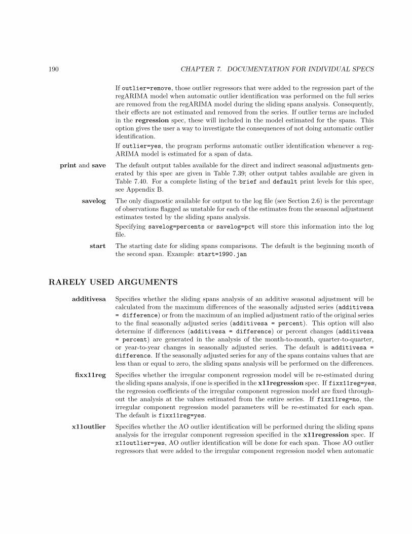
190 CHAPTER 7. DOCUMENTATION FOR INDIVIDUAL SPECS
If outlier=remove, those outlier regressors that were added to the regression part of theregARIMA model when automatic outlier identification was performed on the full seriesare removed from the regARIMA model during the sliding spans analysis. Consequently,their effects are not estimated and removed from the series. If outlier terms are includedin the regression spec, these will included in the model estimated for the spans. Thisoption gives the user a way to investigate the consequences of not doing automatic outlieridentification.
If outlier=yes, the program performs automatic outlier identification whenever a reg-ARIMA model is estimated for a span of data.
print and save The default output tables available for the direct and indirect seasonal adjustments gen-erated by this spec are given in Table 7.39; other output tables available are given inTable 7.40. For a complete listing of the brief and default print levels for this spec,see Appendix B.
savelog The only diagnostic available for output to the log file (see Section 2.6) is the percentageof observations flagged as unstable for each of the estimates from the seasonal adjustmentestimates tested by the sliding spans analysis.
Specifying savelog=percents or savelog=pct will store this information into the logfile.
start The starting date for sliding spans comparisons. The default is the beginning month ofthe second span. Example: start=1990.jan
RARELY USED ARGUMENTS
additivesa Specifies whether the sliding spans analysis of an additive seasonal adjustment will becalculated from the maximum differences of the seasonally adjusted series (additivesa= difference) or from the maximum of an implied adjustment ratio of the original seriesto the final seasonally adjusted series (additivesa = percent). This option will alsodetermine if differences (additivesa = difference) or percent changes (additivesa= percent) are generated in the analysis of the month-to-month, quarter-to-quarter,or year-to-year changes in seasonally adjusted series. The default is additivesa =
difference. If the seasonally adjusted series for any of the spans contains values that areless than or equal to zero, the sliding spans analysis will be performed on the differences.
fixx11reg Specifies whether the irregular component regression model will be re-estimated duringthe sliding spans analysis, if one is specified in the x11regression spec. If fixx11reg=yes,the regression coefficients of the irregular component regression model are fixed through-out the analysis at the values estimated from the entire series. If fixx11reg=no, theirregular component regression model parameters will be re-estimated for each span.The default is fixx11reg=yes.
x11outlier Specifies whether the AO outlier identification will be performed during the sliding spansanalysis for the irregular component regression specified in the x11regression spec. Ifx11outlier=yes, AO outlier identification will be done for each span. Those AO outlierregressors that were added to the irregular component regression model when automatic
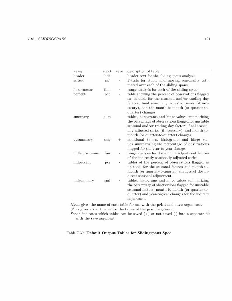
7.16. SLIDINGSPANS 191
name short save description of tableheader hdr · header text for the sliding spans analysisssftest ssf · F-tests for stable and moving seasonality esti-
mated over each of the sliding spansfactormeans fmn · range analysis for each of the sliding spanspercent pct · table showing the percent of observations flagged
as unstable for the seasonal and/or trading dayfactors, final seasonally adjusted series (if nec-essary), and the month-to-month (or quarter-to-quarter) changes
summary sum · tables, histograms and hinge values summarizingthe percentage of observations flagged for unstableseasonal and/or trading day factors, final season-ally adjusted series (if necessary), and month-to-month (or quarter-to-quarter) changes
yysummary smy + additional tables, histograms and hinge val-ues summarizing the percentage of observationsflagged for the year-to-year changes
indfactormeans fmi · range analysis for the implicit adjustment factorsof the indirectly seasonally adjusted series
indpercent pci · tables of the percent of observations flagged asunstable for the seasonal factors and month-to-month (or quarter-to-quarter) changes of the in-direct seasonal adjustment
indsummary smi · tables, histograms and hinge values summarizingthe percentage of observations flagged for unstableseasonal factors, month-to-month (or quarter-to-quarter) and year-to-year changes for the indirectadjustment
Name gives the name of each table for use with the print and save arguments.Short gives a short name for the tables of the print argument.Save? indicates which tables can be saved (+) or not saved (·) into a separate file
with the save argument.
Table 7.39: Default Output Tables for Slidingspans Spec

192 CHAPTER 7. DOCUMENTATION FOR INDIVIDUAL SPECS
name short save description of tableyypercent pcy · additional entry for the percent of observations
flagged as unstable for the year-to-year changessfspans sfs + seasonal factors from all sliding spanschngspans chs + month-to-month (or quarter-to-quarter) changes
from all sliding spanssaspans sas + seasonally adjusted series from all sliding spansychngspans ycs + year-to-year changes from all sliding spanstdspans tds + trading day factors from all sliding spansindyypercent pyi · additonal entry for the percent of observations
flagged as unstable for the year-to-year (orquarter-to-quarter) changes of the indirect sea-sonal adjustment
indyysummary syi · additional tables, histograms and hinge val-ues summarizing the percentage of observationsflagged for the year-to-year changes of the indi-rect seasonal adjustment
indsfspans sis + indirect seasonal factors from all sliding spansindchngspans cis + indirect month-to-month (or quarter-to-quarter)
changes from all sliding spansindsaspans ais + indirect seasonally adjusted series from all sliding
spansindychngspans yis + indirect year-to-year changes from all sliding spans
Name gives the name of each table for use with the print and save arguments.Short gives a short name for the tables of the print argument.Save? indicates which tables can be saved (+) or not saved (·) into a separate file
with the save argument.
Table 7.40: Other Output Tables for Slidingspans Spec
AO outlier identification was done for the full series are removed from the irregularcomponent regression model prior to the sliding spans run. If x11outlier=no, then theautomatically identified AO outlier regressors for the full series are kept for each slidingspans run. If the date of an AO outlier detected for the complete span of data does notoccur in one of the sliding spans, the outlier will be dropped from the model for that span.The coefficients estimating the effects of these AO outliers are re-estimated whenever theother irregular component regression model parameters are re-estimated. However, noadditional AO outliers are automatically identified and estimated. This option is ignoredif the x11regression spec is not used, if the selection of the aictest argument resultsin the program not estimating an irregular component regression model, or if the sigmaargument is used in the x11regression spec. The default is x11outlier=yes.

7.16. SLIDINGSPANS 193
DETAILS
This section provides some additional information about the arguments within the sliding spans spec. Section6.2 contains a description of the sliding spans diagnostics and their interpretation. For more details on thesliding spans procedure, see Findley, Monsell, Shulman, and Pugh (1990).
Different adjustment quantities are examined in a sliding spans analysis, depending on the mode of theseasonal adjustment and whether trading day adjustment is done. For a multiplicative or log-additive seasonaladjustment, the seasonal factors, and the month-to-month and year-to-year changes of the seasonally adjustedseries are analyzed. For a multiplicative or log-additive seasonal and trading day adjustment, the tradingday factors and seasonally adjusted series are analyzed as well. For an additive seasonal adjustment withouttrading day adjustment, the seasonally adjusted series and the month-to-month and year-to-year changes of theseasonally adjusted series are analyzed. If trading day adjustment is done, these analysis are performed for theseasonal and trading day adjusted series.
WARNING: In the additive adjustment case, the presence of relatively small values or negative values inthe adjusted series can render unusable the percent change values which are the basis of almost all of the slidingspans statistics. In this situation, usually only a subjective analysis of the spans of adjusted series obtained byusing saspan in the print or save arguments can be used to detect excessive instability. Further research isneeded to develop more useful sliding spans statistics for additive adjustments.
One important choice that needs to be made in a sliding spans analysis is the length of the overlappingspans. When used with the x11 spec, the length of the span is based on the length of the seasonal filter sincehere seasonal adjustment is performed with fixed length seasonal filters. Table 7.41 gives a listing of how longthe sliding span is by default for different seasonal filters of the x11 spec.
Seasonal Length of Spanfilter (in years)
3-term 63 x 3 63 x 5 83 x 9 113 x 15 17
Table 7.41: Sliding span lengths for different seasonal filters chosen
Note that additional observations are added to the length of the span by default so that each of the slidingspans begin in January (or the first quarter for quarterly series). If different seasonal filters are used for differentmonths or quarters, the longest span length of the seasonal filters chosen will be used.
If a stable seasonal filter is selected, the program will set the span to by dividing the length of the series bythe number of spans used (with the default number of spans set to 4). The length of the span can be no morethan 17 years long, and no shorter than 3 years long.
For model-based seasonal adjustments, the ARIMA model-based seasonal adjustment filters generated inthe seats are always as long as the data span being adjusted (when the ARIMA model specified has a movingaverage component). Findley, Wills, Aston, Feldpausch, and Hood (2003) develops an approach for determining
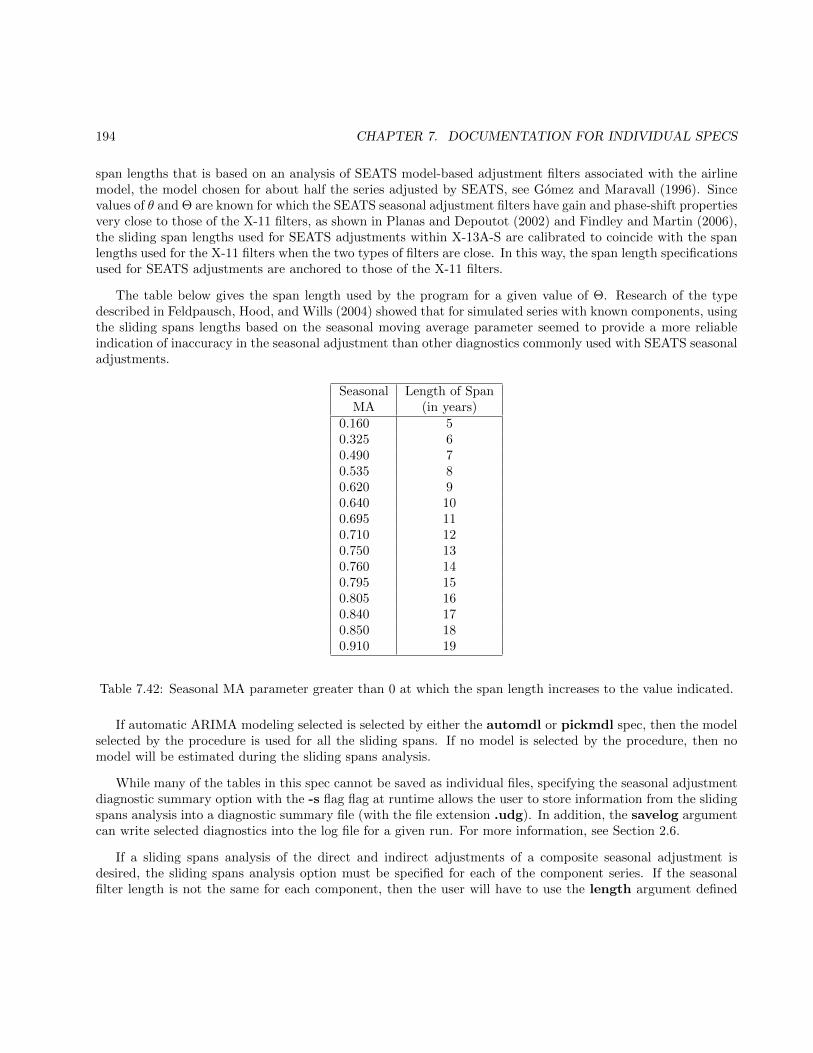
194 CHAPTER 7. DOCUMENTATION FOR INDIVIDUAL SPECS
span lengths that is based on an analysis of SEATS model-based adjustment filters associated with the airlinemodel, the model chosen for about half the series adjusted by SEATS, see Gomez and Maravall (1996). Sincevalues of θ and Θ are known for which the SEATS seasonal adjustment filters have gain and phase-shift propertiesvery close to those of the X-11 filters, as shown in Planas and Depoutot (2002) and Findley and Martin (2006),the sliding span lengths used for SEATS adjustments within X-13A-S are calibrated to coincide with the spanlengths used for the X-11 filters when the two types of filters are close. In this way, the span length specificationsused for SEATS adjustments are anchored to those of the X-11 filters.
The table below gives the span length used by the program for a given value of Θ. Research of the typedescribed in Feldpausch, Hood, and Wills (2004) showed that for simulated series with known components, usingthe sliding spans lengths based on the seasonal moving average parameter seemed to provide a more reliableindication of inaccuracy in the seasonal adjustment than other diagnostics commonly used with SEATS seasonaladjustments.
Seasonal Length of SpanMA (in years)
0.160 50.325 60.490 70.535 80.620 90.640 100.695 110.710 120.750 130.760 140.795 150.805 160.840 170.850 180.910 19
Table 7.42: Seasonal MA parameter greater than 0 at which the span length increases to the value indicated.
If automatic ARIMA modeling selected is selected by either the automdl or pickmdl spec, then the modelselected by the procedure is used for all the sliding spans. If no model is selected by the procedure, then nomodel will be estimated during the sliding spans analysis.
While many of the tables in this spec cannot be saved as individual files, specifying the seasonal adjustmentdiagnostic summary option with the -s flag flag at runtime allows the user to store information from the slidingspans analysis into a diagnostic summary file (with the file extension .udg). In addition, the savelog argumentcan write selected diagnostics into the log file for a given run. For more information, see Section 2.6.
If a sliding spans analysis of the direct and indirect adjustments of a composite seasonal adjustment isdesired, the sliding spans analysis option must be specified for each of the component series. If the seasonalfilter length is not the same for each component, then the user will have to use the length argument defined
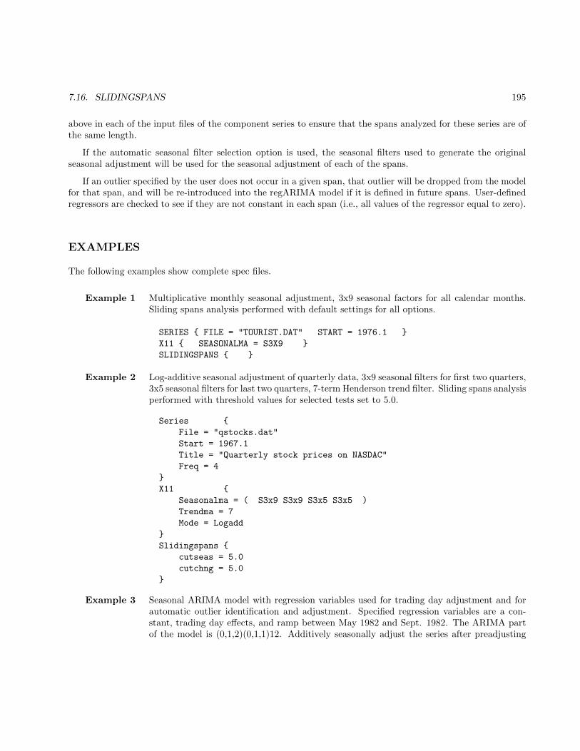
7.16. SLIDINGSPANS 195
above in each of the input files of the component series to ensure that the spans analyzed for these series are ofthe same length.
If the automatic seasonal filter selection option is used, the seasonal filters used to generate the originalseasonal adjustment will be used for the seasonal adjustment of each of the spans.
If an outlier specified by the user does not occur in a given span, that outlier will be dropped from the modelfor that span, and will be re-introduced into the regARIMA model if it is defined in future spans. User-definedregressors are checked to see if they are not constant in each span (i.e., all values of the regressor equal to zero).
EXAMPLES
The following examples show complete spec files.
Example 1 Multiplicative monthly seasonal adjustment, 3x9 seasonal factors for all calendar months.Sliding spans analysis performed with default settings for all options.
SERIES { FILE = "TOURIST.DAT" START = 1976.1 }
X11 { SEASONALMA = S3X9 }
SLIDINGSPANS { }
Example 2 Log-additive seasonal adjustment of quarterly data, 3x9 seasonal filters for first two quarters,3x5 seasonal filters for last two quarters, 7-term Henderson trend filter. Sliding spans analysisperformed with threshold values for selected tests set to 5.0.
Series {
File = "qstocks.dat"
Start = 1967.1
Title = "Quarterly stock prices on NASDAC"
Freq = 4
}
X11 {
Seasonalma = ( S3x9 S3x9 S3x5 S3x5 )
Trendma = 7
Mode = Logadd
}
Slidingspans {
cutseas = 5.0
cutchng = 5.0
}
Example 3 Seasonal ARIMA model with regression variables used for trading day adjustment and forautomatic outlier identification and adjustment. Specified regression variables are a con-stant, trading day effects, and ramp between May 1982 and Sept. 1982. The ARIMA partof the model is (0,1,2)(0,1,1)12. Additively seasonally adjust the series after preadjusting
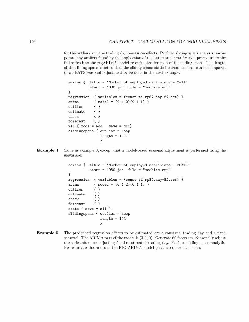
196 CHAPTER 7. DOCUMENTATION FOR INDIVIDUAL SPECS
for the outliers and the trading day regression effects. Perform sliding spans analysis; incor-porate any outliers found by the application of the automatic identification procedure to thefull series into the regARIMA model re-estimated for each of the sliding spans. The lengthof the sliding spans is set so that the sliding spans statistics from this run can be comparedto a SEATS seasonal adjustment to be done in the next example.
series { title = "Number of employed machinists - X-11"
start = 1980.jan file = "machine.emp"
}
regression { variables = (const td rp82.may-82.oct) }
arima { model = (0 1 2)(0 1 1) }
outlier { }
estimate { }
check { }
forecast { }
x11 { mode = add save = d11}
slidingspans { outlier = keep
length = 144
}
Example 4 Same as example 3, except that a model-based seasonal adjustment is performed using theseats spec
series { title = "Number of employed machinists - SEATS"
start = 1980.jan file = "machine.emp"
}
regression { variables = (const td rp82.may-82.oct) }
arima { model = (0 1 2)(0 1 1) }
outlier { }
estimate { }
check { }
forecast { }
seats { save = s11 }
slidingspans { outlier = keep
length = 144
}
Example 5 The predefined regression effects to be estimated are a constant, trading day and a fixedseasonal. The ARIMA part of the model is (3, 1, 0). Generate 60 forecasts. Seasonally adjustthe series after pre-adjusting for the estimated trading day. Perform sliding spans analysis.Re−estimate the values of the REGARIMA model parameters for each span.
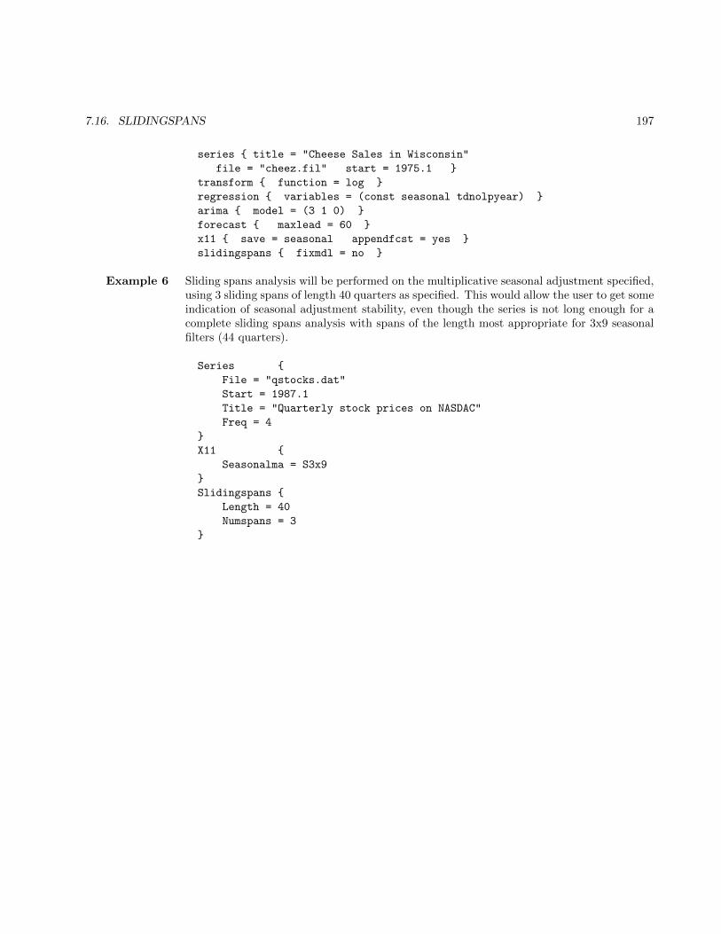
7.16. SLIDINGSPANS 197
series { title = "Cheese Sales in Wisconsin"
file = "cheez.fil" start = 1975.1 }
transform { function = log }
regression { variables = (const seasonal tdnolpyear) }
arima { model = (3 1 0) }
forecast { maxlead = 60 }
x11 { save = seasonal appendfcst = yes }
slidingspans { fixmdl = no }
Example 6 Sliding spans analysis will be performed on the multiplicative seasonal adjustment specified,using 3 sliding spans of length 40 quarters as specified. This would allow the user to get someindication of seasonal adjustment stability, even though the series is not long enough for acomplete sliding spans analysis with spans of the length most appropriate for 3x9 seasonalfilters (44 quarters).
Series {
File = "qstocks.dat"
Start = 1987.1
Title = "Quarterly stock prices on NASDAC"
Freq = 4
}
X11 {
Seasonalma = S3x9
}
Slidingspans {
Length = 40
Numspans = 3
}
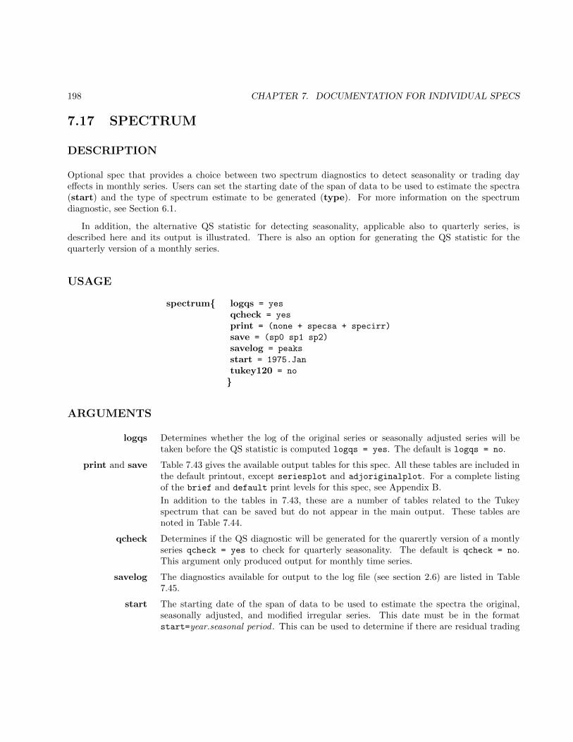
198 CHAPTER 7. DOCUMENTATION FOR INDIVIDUAL SPECS
7.17 SPECTRUM
DESCRIPTION
Optional spec that provides a choice between two spectrum diagnostics to detect seasonality or trading dayeffects in monthly series. Users can set the starting date of the span of data to be used to estimate the spectra(start) and the type of spectrum estimate to be generated (type). For more information on the spectrumdiagnostic, see Section 6.1.
In addition, the alternative QS statistic for detecting seasonality, applicable also to quarterly series, isdescribed here and its output is illustrated. There is also an option for generating the QS statistic for thequarterly version of a monthly series.
USAGE
spectrum{ logqs = yes
qcheck = yes
print = (none + specsa + specirr)
save = (sp0 sp1 sp2)
savelog = peaks
start = 1975.Jan
tukey120 = no
}
ARGUMENTS
logqs Determines whether the log of the original series or seasonally adjusted series will betaken before the QS statistic is computed logqs = yes. The default is logqs = no.
print and save Table 7.43 gives the available output tables for this spec. All these tables are included inthe default printout, except seriesplot and adjoriginalplot. For a complete listingof the brief and default print levels for this spec, see Appendix B.
In addition to the tables in 7.43, these are a number of tables related to the Tukeyspectrum that can be saved but do not appear in the main output. These tables arenoted in Table 7.44.
qcheck Determines if the QS diagnostic will be generated for the quarertly version of a montlyseries qcheck = yes to check for quarterly seasonality. The default is qcheck = no.This argument only produced output for monthly time series.
savelog The diagnostics available for output to the log file (see section 2.6) are listed in Table7.45.
start The starting date of the span of data to be used to estimate the spectra the original,seasonally adjusted, and modified irregular series. This date must be in the formatstart=year.seasonal period . This can be used to determine if there are residual trading
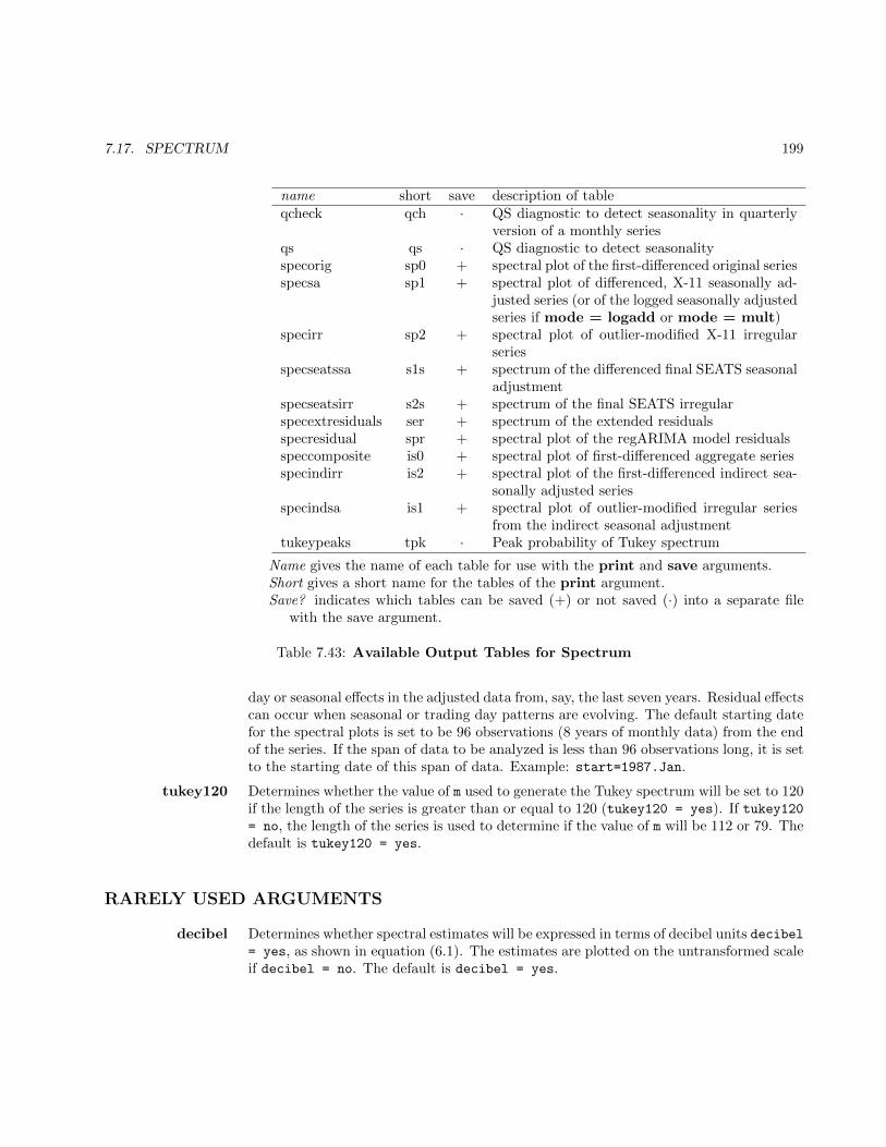
7.17. SPECTRUM 199
name short save description of tableqcheck qch · QS diagnostic to detect seasonality in quarterly
version of a monthly seriesqs qs · QS diagnostic to detect seasonalityspecorig sp0 + spectral plot of the first-differenced original seriesspecsa sp1 + spectral plot of differenced, X-11 seasonally ad-
justed series (or of the logged seasonally adjustedseries if mode = logadd or mode = mult)
specirr sp2 + spectral plot of outlier-modified X-11 irregularseries
specseatssa s1s + spectrum of the differenced final SEATS seasonaladjustment
specseatsirr s2s + spectrum of the final SEATS irregularspecextresiduals ser + spectrum of the extended residualsspecresidual spr + spectral plot of the regARIMA model residualsspeccomposite is0 + spectral plot of first-differenced aggregate seriesspecindirr is2 + spectral plot of the first-differenced indirect sea-
sonally adjusted seriesspecindsa is1 + spectral plot of outlier-modified irregular series
from the indirect seasonal adjustmenttukeypeaks tpk · Peak probability of Tukey spectrum
Name gives the name of each table for use with the print and save arguments.Short gives a short name for the tables of the print argument.Save? indicates which tables can be saved (+) or not saved (·) into a separate file
with the save argument.
Table 7.43: Available Output Tables for Spectrum
day or seasonal effects in the adjusted data from, say, the last seven years. Residual effectscan occur when seasonal or trading day patterns are evolving. The default starting datefor the spectral plots is set to be 96 observations (8 years of monthly data) from the endof the series. If the span of data to be analyzed is less than 96 observations long, it is setto the starting date of this span of data. Example: start=1987.Jan.
tukey120 Determines whether the value of m used to generate the Tukey spectrum will be set to 120if the length of the series is greater than or equal to 120 (tukey120 = yes). If tukey120= no, the length of the series is used to determine if the value of m will be 112 or 79. Thedefault is tukey120 = yes.
RARELY USED ARGUMENTS
decibel Determines whether spectral estimates will be expressed in terms of decibel units decibel= yes, as shown in equation (6.1). The estimates are plotted on the untransformed scaleif decibel = no. The default is decibel = yes.

200 CHAPTER 7. DOCUMENTATION FOR INDIVIDUAL SPECS
name short description of tabletukeyspecorig st0 Tukey spectrum of the first-differenced original se-
riestukeyspecsa st1 Tukey spectrum of the differenced, X-11 season-
ally adjusted series (or of the logged seasonallyadjusted series if mode = logadd or mode =mult)
tukeyspecirr st2 Tukey spectrum of the outlier-modified X-11 irreg-ular series
tukeyspecseatssa st1 Tukey spectrum of the differenced final SEATSseasonal adjustment
tukeyspecseatsirr st2 Tukey spectrum of the final SEATS irregulartukeyspecextresiduals ter Tukey spectrum of the extended residualstukeyspecresidual str Tukey spectrum of the regARIMA model residualstukeyspeccomposite it0 Tukey spectrum of the first-differenced aggregate
seriestukeyspecindirr it2 Tukey spectrum of the first-differenced indirect
seasonally adjusted seriestukeyspecindsa it1 Tukey spectrum of the outlier-modified irregular
series from the indirect seasonal adjustment
Name gives the name of each table for use with the print and save arguments.Short gives a short name for the tables of the print argument.
Table 7.44: Output Tables for Spectrum spec that can Only be Saved
difference If difference=no, the spectrum of the (transformed) original series or seasonally ad-justed series is calculated; if difference=first, the spectrum of the month-to-monthdifferences of these series is calculated. The default (difference=yes) will apply amax(d+D− 1, 1) difference to the (transformed) original series and seasonally adjustedseries before computing the spectrum, where d is the order of regular differencing and Dis the order of seasonal differencing in the regARIMA model specified for the series. Ifno regARIMA model is specified, the default order of differencing is 1.
maxar An integer value used to set the maximum order of the AR spectrum used as the defaulttype of spectrum plot. Integers from 1 to 30 are acceptable values for maxar. If thisoption is not specified, the maximum order will be set to 30.
peakwidth Allows the user to set the width of the band used to determine spectral peaks. Thedefault value is peakwidth = 1.
series Allows the user to select the series used in the spectrum of the original (or composite)series (Table G.0). Table 7.46 shows the series that can be specified with this argument- the default is series = adjoriginal (or b1).
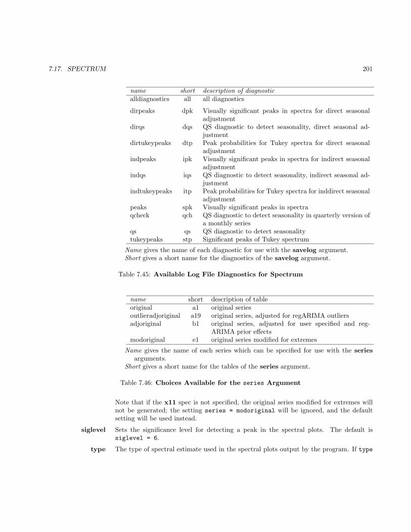
7.17. SPECTRUM 201
name short description of diagnosticalldiagnostics all all diagnostics
dirpeaks dpk Visually significant peaks in spectra for direct seasonaladjustment
dirqs dqs QS diagnostic to detect seasonality, direct seasonal ad-justment
dirtukeypeaks dtp Peak probabilities for Tukey spectra for direct seasonaladjustment
indpeaks ipk Visually significant peaks in spectra for indirect seasonaladjustment
indqs iqs QS diagnostic to detect seasonality, indirect seasonal ad-justment
indtukeypeaks itp Peak probabilities for Tukey spectra for inddirect seasonaladjustment
peaks spk Visually significant peaks in spectraqcheck qch QS diagnostic to detect seasonality in quarterly version of
a monthly seriesqs qs QS diagnostic to detect seasonalitytukeypeaks stp Significant peaks of Tukey spectrum
Name gives the name of each diagnostic for use with the savelog argument.Short gives a short name for the diagnostics of the savelog argument.
Table 7.45: Available Log File Diagnostics for Spectrum
name short description of tableoriginal a1 original seriesoutlieradjoriginal a19 original series, adjusted for regARIMA outliersadjoriginal b1 original series, adjusted for user specified and reg-
ARIMA prior effectsmodoriginal e1 original series modified for extremes
Name gives the name of each series which can be specified for use with the seriesarguments.
Short gives a short name for the tables of the series argument.
Table 7.46: Choices Available for the series Argument
Note that if the x11 spec is not specified, the original series modified for extremes willnot be generated; the setting series = modoriginal will be ignored, and the defaultsetting will be used instead.
siglevel Sets the significance level for detecting a peak in the spectral plots. The default issiglevel = 6.
type The type of spectral estimate used in the spectral plots output by the program. If type
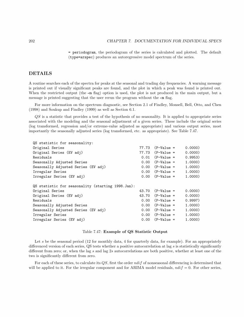
202 CHAPTER 7. DOCUMENTATION FOR INDIVIDUAL SPECS
= periodogram, the periodogram of the series is calculated and plotted. The default(type=arspec) produces an autoregressive model spectrum of the series.
DETAILS
A routine searches each of the spectra for peaks at the seasonal and trading day frequencies. A warning messageis printed out if visually significant peaks are found, and the plot in which a peak was found is printed out.When the restricted output (the -n flag) option is used, the plot is not produced in the main output, but amessage is printed suggesting that the user rerun the program without the -n flag.
For more information on the spectrum diagnostic, see Section 2.1 of Findley, Monsell, Bell, Otto, and Chen(1998) and Soukup and Findley (1999) as well as Section 6.1.
QS is a statistic that provides a test of the hypothesis of no seasonality. It is applied to appropriate seriesassociated with the modeling and the seasonal adjustment of a given series. These include the original series(log transformed, regression and/or extreme-value adjusted as appropriate) and various output series, mostimportantly the seasonally adjusted series (log transformed, etc. as appropriate). See Table 7.47.
QS statistic for seasonality:
Original Series 77.73 (P-Value = 0.0000)
Original Series (EV adj) 77.73 (P-Value = 0.0000)
Residuals 0.01 (P-Value = 0.9953)
Seasonally Adjusted Series 0.00 (P-Value = 1.0000)
Seasonally Adjusted Series (EV adj) 0.00 (P-Value = 1.0000)
Irregular Series 0.00 (P-Value = 1.0000)
Irregular Series (EV adj) 0.00 (P-Value = 1.0000)
QS statistic for seasonality (starting 1998.Jan):
Original Series 43.70 (P-Value = 0.0000)
Original Series (EV adj) 43.70 (P-Value = 0.0000)
Residuals 0.00 (P-Value = 0.9997)
Seasonally Adjusted Series 0.00 (P-Value = 1.0000)
Seasonally Adjusted Series (EV adj) 0.00 (P-Value = 1.0000)
Irregular Series 0.00 (P-Value = 1.0000)
Irregular Series (EV adj) 0.00 (P-Value = 1.0000)
Table 7.47: Example of QS Statistic Output
Let s be the seasonal period (12 for monthly data, 4 for quarterly data, for example). For an appropriatelydifferenced version of each series, QS tests whether a positive autocorrelation at lag s is statistically significantlydifferent from zero; or, when the lag s and lag 2s autocorrelations are both positive, whether at least one of thetwo is significantly different from zero.
For each of these series, to calculate its QS, first the order ndif of nonseasonal differencing is determined thatwill be applied to it. For the irregular component and for ARIMA model residuals, ndif = 0. For other series,
7.17. SPECTRUM 203
when an ARIMA model is available that specifies an order d of differencing and/or an order D of nonseasonaldifferencing for it, then ndif is initially set as
ndif = max(1,min(d+D, 2))
If there is no ARIMA model, ndif is initially set to 1.
To calculate QS, sample autocorrelations are calculated in the usual way from the (always sample-meancentered) ndif -times nonseasonally differenced series. When ndif = 1 these autocorrelations are provisional: acheck is done to see if they decay too slowly from a positive value at lag 1. The criterion depends on s. Whens = 6 or s = 12, the program checks if the autocorrelations at lags 1, 2, 3, 4 and s are positive. When s = 2or s = 4, the program checks if the autocorrelations at lags 1 to s are all greater than 0.2. If either of theseconditions is satisfied, and ndif = 1, then ndif is reset to 2 and the autocorrelations used for QS are obtainedfrom the twice-differenced series.
Let ri denote the lag i autocorrelations for i = s, 2s and let nz denote the length of the series. Setn = nz − ndif and
Ri =
{ri, if ri > 00, if ri ≤ 0.
If Rs > 0, set
QS = n(n+ 2)
{R2s
n− s+
R22s
n− 2s
}.
If Rs = 0, set QS = 0. The statistic QS is assumed to be adequately approximated by a chi-squareddistribution with two degrees of freedom. This is supported by simulations as illustrated in Maravall (2012).
Only when QS is larger than a preset critical value for this distribution, usually that for a .01 significancelevel, does the QS output indicate that seasonality is present.
In the X-13ARIMA-SEATS sample output shown in Table 7.47, the output indicates that there is seasonality inthe original series, no residual seasonality in the seasonally adjusted series, and no seasonality in the regARIMAmodel residuals.
For monthly series, setting qcheck = yes generates QS statistics for the quarterly versions of the originalseries and the original series adjusted for extreme values. If the starting date for the spectrum is different thanthe starting date of the series, QS statistics will be generated for the shortened series as well. An example ofthis output is Given in Table 7.48.
The quarterly series are only formed from complete quarters - quarters where all three months are availablein the monthly series. Sometimes this means that the series will be truncated at either end.
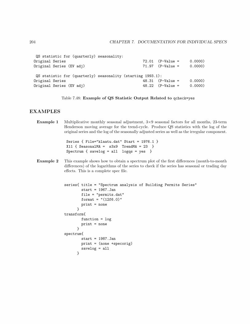
204 CHAPTER 7. DOCUMENTATION FOR INDIVIDUAL SPECS
QS statistic for (quarterly) seasonality:
Original Series 72.01 (P-Value = 0.0000)
Original Series (EV adj) 71.97 (P-Value = 0.0000)
QS statistic for (quarterly) seasonality (starting 1993.1):
Original Series 48.31 (P-Value = 0.0000)
Original Series (EV adj) 48.22 (P-Value = 0.0000)
Table 7.48: Example of QS Statistic Output Related to qcheck=yes
EXAMPLES
Example 1 Multiplicative monthly seasonal adjustment, 3×9 seasonal factors for all months, 23-termHenderson moving average for the trend-cycle. Produce QS statistics with the log of theoriginal series and the log of the seasonally adjusted series as well as the irregular component.
Series { File="klaatu.dat" Start = 1976.1 }
X11 { SeasonalMA = s3x9 TrendMA = 23 }
Spectrum { savelog = all logqs = yes }
Example 2 This example shows how to obtain a spectrum plot of the first differences (month-to-monthdifferences) of the logarithms of the series to check if the series has seasonal or trading dayeffects. This is a complete spec file.
series{ title = "Spectrum analysis of Building Permits Series"
start = 1967.Jan
file = "permits.dat"
format = "(12f6.0)"
print = none
}
transform{
function = log
print = none
}
spectrum{
start = 1987.Jan
print = (none +specorig)
savelog = all
}
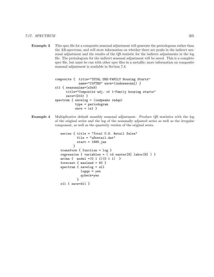
7.17. SPECTRUM 205
Example 3 This spec file for a composite seasonal adjustment will generate the periodogram rather thanthe AR-spectrum, and will store information on whether there are peaks in the indirect sea-sonal adjustment and the results of the QS statistic for the indirect adjustments in the logfile. The periodogram for the indirect seasonal adjustment will be saved. This is a completespec file, but must be run with other spec files in a metafile; more information on compositeseasonal adjustment is available in Section 7.4.
composite { title="TOTAL ONE-FAMILY Housing Starts"
name="C1FTHS" save=(indseasonal) }
x11 { seasonalma=(s3x9)
title="Composite adj. of 1-Family housing starts"
save=(D10) }
spectrum { savelog = (indpeaks indqs)
type = periodogram
save = is1 }
Example 4 Multiplicative default monthly seasonal adjustment. Produce QS statistics with the logof the original series and the log of the seasonally adjusted series as well as the irregularcomponent, as well as the quarterly version of the original series.
series { title = "Total U.S. Retail Sales"
file = "uSretail.dat"
start = 1988.jan
}
transform { function = log }
regression { variables = ( td easter[8] labor[8] ) }
arima { model =(0 1 1)(0 1 1) }
forecast { maxlead = 60 }
spectrum { savelog = all
logqs = yes
qcheck=yes
}
x11 { save=d11 }

206 CHAPTER 7. DOCUMENTATION FOR INDIVIDUAL SPECS
7.18 TRANSFORM
DESCRIPTION
Specification used to transform or adjust the series prior to estimating a regARIMA model. With this specthe series can be Box-Cox (power) or logistically transformed, length-of-month adjusted, and divided by user-defined prior-adjustment factors. Data for any user-defined prior-adjustment factors must be supplied, eitherin the data argument, or in a file specified by the file argument (not both). For seasonal adjustment, a set ofpermanently removed factors can be specified and also a set of factors that are temporarily removed until theseasonal factors are calculated.
USAGE
transform{ function = log or power = 0.0
adjust = lom
title = "prior adjustment factors"
start = 1975.jan
data = (1.25 · · · 1.90) or file = "prioradj.dat"
format = "(6f12.3)"
name = "Adjfac"
aicdiff = 0.0
mode = ratio
type = temporary
print = (none)
save = ( prior prioradjusted )
savelog = atr
}
ARGUMENTS
adjust Perform length-of-month adjustment on monthly data (adjust = lom), length-of-quar-ter adjustment on quarterly data (adjust = loq), or leap year adjustment of monthlyor quarterly data (adjust = lpyear). (See DETAILS.)
Do not use the adjust argument if td or td1coef is specified in the variables argumentof the regression or x11regression specs, or if additive or pseudo-additive seasonaladjustment is specified in the mode argument of the x11 spec. Leap year adjustment(adjust = lpyear) is only allowed when a log transformation is specified in either thepower or function arguments.
aicdiff Defines the difference in AICC needed to accept no transformation when the auto-matic transformation selection option is invoked (function=auto). The default valueis aicdiff = -2.0 for monthly and quarterly series, aicdiff = 0.0 otherwise. Formore information on how this option is used to select a transformation see DETAILS.
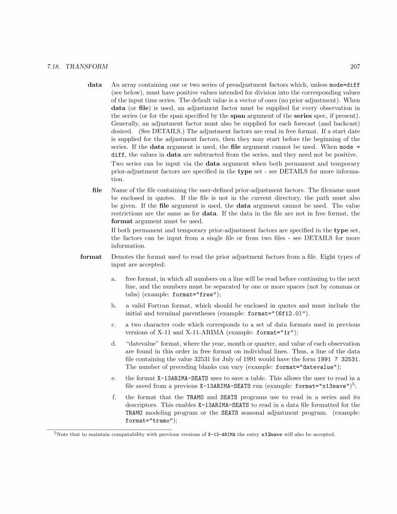
7.18. TRANSFORM 207
data An array containing one or two series of preadjustment factors which, unless mode=diff(see below), must have positive values intended for division into the corresponding valuesof the input time series. The default value is a vector of ones (no prior adjustment). Whendata (or file) is used, an adjustment factor must be supplied for every observation inthe series (or for the span specified by the span argument of the series spec, if present).Generally, an adjustment factor must also be supplied for each forecast (and backcast)desired. (See DETAILS.) The adjustment factors are read in free format. If a start dateis supplied for the adjustment factors, then they may start before the beginning of theseries. If the data argument is used, the file argument cannot be used. When mode =
diff, the values in data are subtracted from the series, and they need not be positive.
Two series can be input via the data argument when both permanent and temporaryprior-adjustment factors are specified in the type set - see DETAILS for more informa-tion.
file Name of the file containing the user-defined prior-adjustment factors. The filename mustbe enclosed in quotes. If the file is not in the current directory, the path must alsobe given. If the file argument is used, the data argument cannot be used. The valuerestrictions are the same as for data. If the data in the file are not in free format, theformat argument must be used.
If both permanent and temporary prior-adjustment factors are specified in the type set,the factors can be input from a single file or from two files - see DETAILS for moreinformation.
format Denotes the format used to read the prior adjustment factors from a file. Eight types ofinput are accepted:
a. free format, in which all numbers on a line will be read before continuing to the nextline, and the numbers must be separated by one or more spaces (not by commas ortabs) (example: format="free");
b. a valid Fortran format, which should be enclosed in quotes and must include theinitial and terminal parentheses (example: format="(6f12.0)").
c. a two character code which corresponds to a set of data formats used in previousversions of X-11 and X-11-ARIMA (example: format="1r");
d. “datevalue” format, where the year, month or quarter, and value of each observationare found in this order in free format on individual lines. Thus, a line of the datafile containing the value 32531 for July of 1991 would have the form 1991 7 32531.The number of preceding blanks can vary (example: format="datevalue");
e. the format X-13ARIMA-SEATS uses to save a table. This allows the user to read in afile saved from a previous X-13ARIMA-SEATS run (example: format="x13save")5;
f. the format that the TRAMO and SEATS programs use to read in a series and itsdescriptors. This enables X-13ARIMA-SEATS to read in a data file formatted for theTRAMO modeling program or the SEATS seasonal adjustment program. (example:format="tramo");
5Note that to maintain compatability with previous versions of X-12-ARIMA the entry x12save will also be accepted.
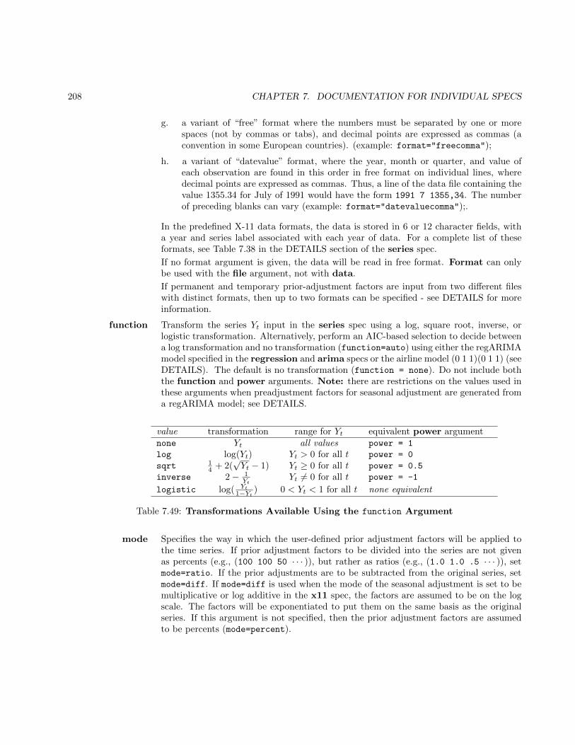
208 CHAPTER 7. DOCUMENTATION FOR INDIVIDUAL SPECS
g. a variant of “free” format where the numbers must be separated by one or morespaces (not by commas or tabs), and decimal points are expressed as commas (aconvention in some European countries). (example: format="freecomma");
h. a variant of “datevalue” format, where the year, month or quarter, and value ofeach observation are found in this order in free format on individual lines, wheredecimal points are expressed as commas. Thus, a line of the data file containing thevalue 1355.34 for July of 1991 would have the form 1991 7 1355,34. The numberof preceding blanks can vary (example: format="datevaluecomma");.
In the predefined X-11 data formats, the data is stored in 6 or 12 character fields, witha year and series label associated with each year of data. For a complete list of theseformats, see Table 7.38 in the DETAILS section of the series spec.
If no format argument is given, the data will be read in free format. Format can onlybe used with the file argument, not with data.
If permanent and temporary prior-adjustment factors are input from two different fileswith distinct formats, then up to two formats can be specified - see DETAILS for moreinformation.
function Transform the series Yt input in the series spec using a log, square root, inverse, orlogistic transformation. Alternatively, perform an AIC-based selection to decide betweena log transformation and no transformation (function=auto) using either the regARIMAmodel specified in the regression and arima specs or the airline model (0 1 1)(0 1 1) (seeDETAILS). The default is no transformation (function = none). Do not include boththe function and power arguments. Note: there are restrictions on the values used inthese arguments when preadjustment factors for seasonal adjustment are generated froma regARIMA model; see DETAILS.
value transformation range for Yt equivalent power argumentnone Yt all values power = 1
log log(Yt) Yt > 0 for all t power = 0
sqrt 14 + 2(
√Yt − 1) Yt ≥ 0 for all t power = 0.5
inverse 2− 1Yt
Yt 6= 0 for all t power = -1
logistic log( Yt
1−Yt) 0 < Yt < 1 for all t none equivalent
Table 7.49: Transformations Available Using the function Argument
mode Specifies the way in which the user-defined prior adjustment factors will be applied tothe time series. If prior adjustment factors to be divided into the series are not givenas percents (e.g., (100 100 50 · · · )), but rather as ratios (e.g., (1.0 1.0 .5 · · · )), setmode=ratio. If the prior adjustments are to be subtracted from the original series, setmode=diff. If mode=diff is used when the mode of the seasonal adjustment is set to bemultiplicative or log additive in the x11 spec, the factors are assumed to be on the logscale. The factors will be exponentiated to put them on the same basis as the originalseries. If this argument is not specified, then the prior adjustment factors are assumedto be percents (mode=percent).
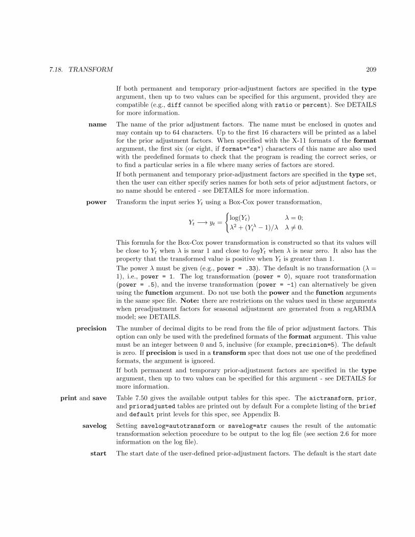
7.18. TRANSFORM 209
If both permanent and temporary prior-adjustment factors are specified in the typeargument, then up to two values can be specified for this argument, provided they arecompatible (e.g., diff cannot be specified along with ratio or percent). See DETAILSfor more information.
name The name of the prior adjustment factors. The name must be enclosed in quotes andmay contain up to 64 characters. Up to the first 16 characters will be printed as a labelfor the prior adjustment factors. When specified with the X-11 formats of the formatargument, the first six (or eight, if format="cs") characters of this name are also usedwith the predefined formats to check that the program is reading the correct series, orto find a particular series in a file where many series of factors are stored.
If both permanent and temporary prior-adjustment factors are specified in the type set,then the user can either specify series names for both sets of prior adjustment factors, orno name should be entered - see DETAILS for more information.
power Transform the input series Yt using a Box-Cox power transformation,
Yt −→ yt =
{log(Yt) λ = 0;
λ2 + (Y λt − 1)/λ λ 6= 0.
This formula for the Box-Cox power transformation is constructed so that its values willbe close to Yt when λ is near 1 and close to logYt when λ is near zero. It also has theproperty that the transformed value is positive when Yt is greater than 1.
The power λ must be given (e.g., power = .33). The default is no transformation (λ =1), i.e., power = 1. The log transformation (power = 0), square root transformation(power = .5), and the inverse transformation (power = -1) can alternatively be givenusing the function argument. Do not use both the power and the function argumentsin the same spec file. Note: there are restrictions on the values used in these argumentswhen preadjustment factors for seasonal adjustment are generated from a regARIMAmodel; see DETAILS.
precision The number of decimal digits to be read from the file of prior adjustment factors. Thisoption can only be used with the predefined formats of the format argument. This valuemust be an integer between 0 and 5, inclusive (for example, precision=5). The defaultis zero. If precision is used in a transform spec that does not use one of the predefinedformats, the argument is ignored.
If both permanent and temporary prior-adjustment factors are specified in the typeargument, then up to two values can be specified for this argument - see DETAILS formore information.
print and save Table 7.50 gives the available output tables for this spec. The aictransform, prior,and prioradjusted tables are printed out by default For a complete listing of the brief
and default print levels for this spec, see Appendix B.
savelog Setting savelog=autotransform or savelog=atr causes the result of the automatictransformation selection procedure to be output to the log file (see section 2.6 for moreinformation on the log file).
start The start date of the user-defined prior-adjustment factors. The default is the start date
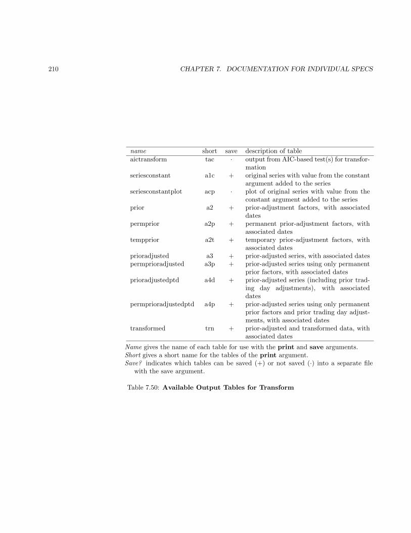
210 CHAPTER 7. DOCUMENTATION FOR INDIVIDUAL SPECS
name short save description of tableaictransform tac · output from AIC-based test(s) for transfor-
mationseriesconstant a1c + original series with value from the constant
argument added to the seriesseriesconstantplot acp · plot of original series with value from the
constant argument added to the seriesprior a2 + prior-adjustment factors, with associated
datespermprior a2p + permanent prior-adjustment factors, with
associated datestempprior a2t + temporary prior-adjustment factors, with
associated datesprioradjusted a3 + prior-adjusted series, with associated datespermprioradjusted a3p + prior-adjusted series using only permanent
prior factors, with associated datesprioradjustedptd a4d + prior-adjusted series (including prior trad-
ing day adjustments), with associateddates
permprioradjustedptd a4p + prior-adjusted series using only permanentprior factors and prior trading day adjust-ments, with associated dates
transformed trn + prior-adjusted and transformed data, withassociated dates
Name gives the name of each table for use with the print and save arguments.Short gives a short name for the tables of the print argument.Save? indicates which tables can be saved (+) or not saved (·) into a separate file
with the save argument.
Table 7.50: Available Output Tables for Transform

7.18. TRANSFORM 211
of the series. Valid values are any date up to the start date of the series (or up to thestart date of the span specified by the span argument of the series spec, if present).
If both permanent and temporary prior-adjustment factors are specified in the type set,then up to two starting dates can be specified to read in the two sets of prior adjustmentfactors - see DETAILS for more information.
title A title for the set of user-defined prior-adjustment factors. The title must be enclosed inquotes and may contain up to 79 characters.
type Specifies whether the user-defined prior-adjustment factors are permanent factors (re-moved from the final seasonally adjusted series as well as the original series) or temporaryfactors (removed from the original series for the purposes of generating seasonal factorsbut not from the final seasonally adjusted series). If only one value is given for this ar-gument (type = temporary), then only one set of user-defined prior-adjustment factorswill be expected. If both types of user-defined prior-adjustment factors are given (type= (temporary permanent)), then two sets of prior adjustment factors will be expected,for more information see DETAILS. The default is type = permanent.
RARELY USED ARGUMENTS
constant Positive constant value that is added to the original series before the program modelsor seasonally adjusts the series. Once the program finishes modeling and/or seasonallyadjusting the series with the constant value added, this constant is removed from theseasonally adjusted series as well as the trend component.
trimzero If trimzero=no, zeroes at the beginning or end of a time series entered via the fileargument are treated as series values. If trimzero=span, causes leading and trailingzeros to be ignored outside the span of data being analyzed (the span argument of theseries spec must be specified with both a starting date and an ending date). The default(trimzero=yes) causes leading and trailing zeros to be ignored. Note that when theformat argument is set to either datevalue, x13save, or tramo, all values input aretreated as series values, regardless of the value of trimzero.
DETAILS
If a Box-Cox or logistic transformation is specified in conjunction with a length-of-month (or leap year) adjust-ment and/or user-defined prior-adjustment factors, the time series is first adjusted for length-of-month and/orprior factors, and then Box-Cox or logistically transformed. If both length-of-month and prior-adjustment fac-tors are specified, then combined adjustment factors (length-of-month × prior adjustment) are used. Length-of-quarter and leap year adjustments are handled in the same way.
If either lom and loq of the adjust argument is specified, the correct adjustment factor is determined by theperiod specified in the series spec. In the case of a monthly input series Yt, each observation is first dividedby the number of days in that month (mt) and then multiplied by the average length-of-month (30.4375),

212 CHAPTER 7. DOCUMENTATION FOR INDIVIDUAL SPECS
resulting in (30.4375× Yt)/mt. Length-of-quarter adjustments are performed in a similar manner, resulting in(91.3125×Yt)/qt, where qt is the length in days of quarter t. Forecasts of the transformed and length-of-monthadjusted data are transformed back to the original scale for output (see the documentation of the forecastspec).
If adjustment factors are supplied for the forecast period, then forecasts of the prior-adjusted series willbe inverse-transformed (multiplied or, if mode = diff, added to) with these factors. If adjustment factors arenot supplied for the forecast period, then inverse-transformation of forecasts will only account for a Box-Cox orlogistic transformation and for any length-of-month (or length-of-quarter) adjustment —this effectively assumesvalues of 1 for the user-defined prior-adjustment factors throughout the forecast period (or 0 if mode = diff).
When seasonal adjustment is requested with the x11 spec, any value of power or function can be usedfor the purpose of forecasting the series with a regARIMA model. However, this is not the case when factorsgenerated from the regression coefficients are used to adjust either the original series or the final seasonallyadjusted series. In this case, the only accepted transformations are the log transformation (for multiplicativeor log-additive seasonal adjustments) and no transformation, which can be specified as power = 1 (for additiveseasonal adjustments).
This restriction of the transformation done because factors derived from the regression coefficients mustbe the same type as factors generated by the seasonal adjustment procedure, so that combined adjustmentfactors can be derived and adjustment diagnostics can be generated. If the regARIMA model is applied to alog-transformed series, the regression factors are expressed in the form of ratios, which is the same form asthe seasonal factors generated by the multiplicative (or log-additive) adjustment modes. Conversely, if the reg-ARIMA model is fit to the original series, the regression factors are measured on the same scale as the originalseries, which matches the scale of the seasonal factors generated by the additive adjustment mode.
If no seasonal adjustment is done, any power transformation can be used.
When function=auto and the series being processed has all positive values, the program will choose betweenno transformation and a log transformation by fitting a regARIMA model to the untransformed and transformedseries and choosing the log transformation except when
AICCnolog −AICClog < ∆AICC or AICClog + ∆AICC > AICCnolog (7.18)
where AICClog is the value of AICC from fitting the regARIMA model to the transformed series, AICCnologis the value of AICC from fitting the regARIMA model to the untransformed series, and ∆AICC is the valueentered for the aicdiff argument, with a default of -2. Negative values of ∆AICC bias the selection in favor ofthe log transformation. The default of -2 is used not for statistical reasons but for convenience. Multiplicativeadjustment is appropriate for the great majority of Census Bureau series and we do not wish to inconvenienceusers accustomed to multiplicative adjustments unless the statistical support for additive adjustment is ratherstrong. The AICC values for the log transformed series (or any transformed series) is obtained by applyingan appropriate (Jacobian) adjustment to the log likelihood to make it compatible with the log likelihood of theestimated model of the untransformed series. (The adjustment is printed in the output if print=lkf is specifiedin the estimate spec.) If the series has a zero or negative value, no transformation is used.
If a regARIMA model has been specified in the regression and/or arima specs, then the procedure willuse this model to generate the AICC statistics needed for the test. If no model is specified, or the automaticmodel identification procedure is specified via the automdl or pickmdl spec, the program will use the airline
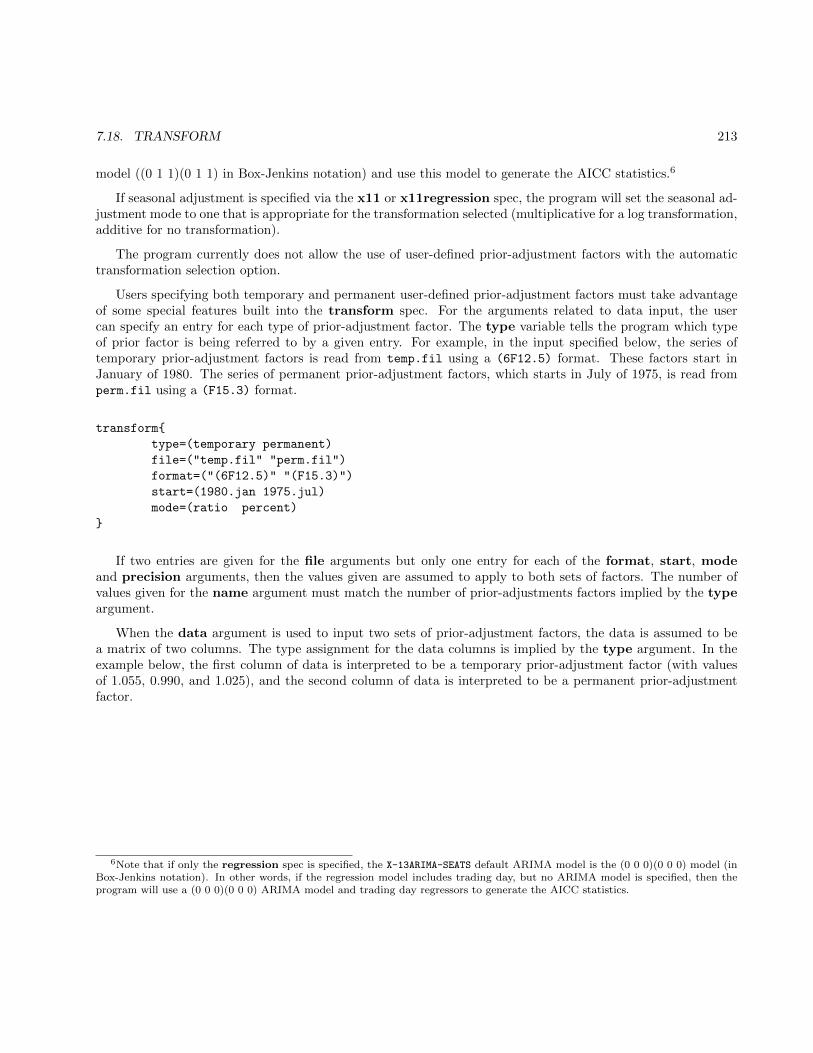
7.18. TRANSFORM 213
model ((0 1 1)(0 1 1) in Box-Jenkins notation) and use this model to generate the AICC statistics.6
If seasonal adjustment is specified via the x11 or x11regression spec, the program will set the seasonal ad-justment mode to one that is appropriate for the transformation selected (multiplicative for a log transformation,additive for no transformation).
The program currently does not allow the use of user-defined prior-adjustment factors with the automatictransformation selection option.
Users specifying both temporary and permanent user-defined prior-adjustment factors must take advantageof some special features built into the transform spec. For the arguments related to data input, the usercan specify an entry for each type of prior-adjustment factor. The type variable tells the program which typeof prior factor is being referred to by a given entry. For example, in the input specified below, the series oftemporary prior-adjustment factors is read from temp.fil using a (6F12.5) format. These factors start inJanuary of 1980. The series of permanent prior-adjustment factors, which starts in July of 1975, is read fromperm.fil using a (F15.3) format.
transform{
type=(temporary permanent)
file=("temp.fil" "perm.fil")
format=("(6F12.5)" "(F15.3)")
start=(1980.jan 1975.jul)
mode=(ratio percent)
}
If two entries are given for the file arguments but only one entry for each of the format, start, modeand precision arguments, then the values given are assumed to apply to both sets of factors. The number ofvalues given for the name argument must match the number of prior-adjustments factors implied by the typeargument.
When the data argument is used to input two sets of prior-adjustment factors, the data is assumed to bea matrix of two columns. The type assignment for the data columns is implied by the type argument. In theexample below, the first column of data is interpreted to be a temporary prior-adjustment factor (with valuesof 1.055, 0.990, and 1.025), and the second column of data is interpreted to be a permanent prior-adjustmentfactor.
6Note that if only the regression spec is specified, the X-13ARIMA-SEATS default ARIMA model is the (0 0 0)(0 0 0) model (inBox-Jenkins notation). In other words, if the regression model includes trading day, but no ARIMA model is specified, then theprogram will use a (0 0 0)(0 0 0) ARIMA model and trading day regressors to generate the AICC statistics.

214 CHAPTER 7. DOCUMENTATION FOR INDIVIDUAL SPECS
transform{
type=(temporary permanent)
data=( 1.055 1.000
0.990 1.000
1.025 1.000
. .
. .
. .
1.033 1.000 )
start=1980.jan
mode=ratio
}
The same assumption is made when only one data file is given for two adjustment types, as in the inputbelow.
transform{
type=(temporary permanent)}
file="both.fil"}
start=1980.jan}
mode=ratio}
}
X-13ARIMA-SEATS accepts a maximum of 780 user-defined prior-adjustment factors of each type (temporaryor permanent), not including the forecast period. (This limit can be changed—see Section 2.8.)
The constant argument is sometimes useful when a series has a number of values either close to zero whereneither multiplicative nor additive seasonal adjustment seems to be effective, or in the case where a series haszero or negative values and the series seems to behave in a manner that usually calls for a multiplicative seasonaladjustment. Strategies for selecting the value of constant, as well as an application to Canadian air travelseries, can be found in Chen and Durk (2005).
EXAMPLES
Note: The following examples do not show “complete” spec files. Useful output is not produced unless addi-tional specs (e.g., x11, identify, or arima and estimate) are added.
Example 1 Specify a user-defined prior adjustment for a strike in March and April of 1967, as well as alength-of-month adjustment.
series { data = (879 899 462 670 985 973 ...)
start = 1967.jan }
transform { data = (1 1 .5 .75 1 1 ...)
mode = ratio
adjust = lom }
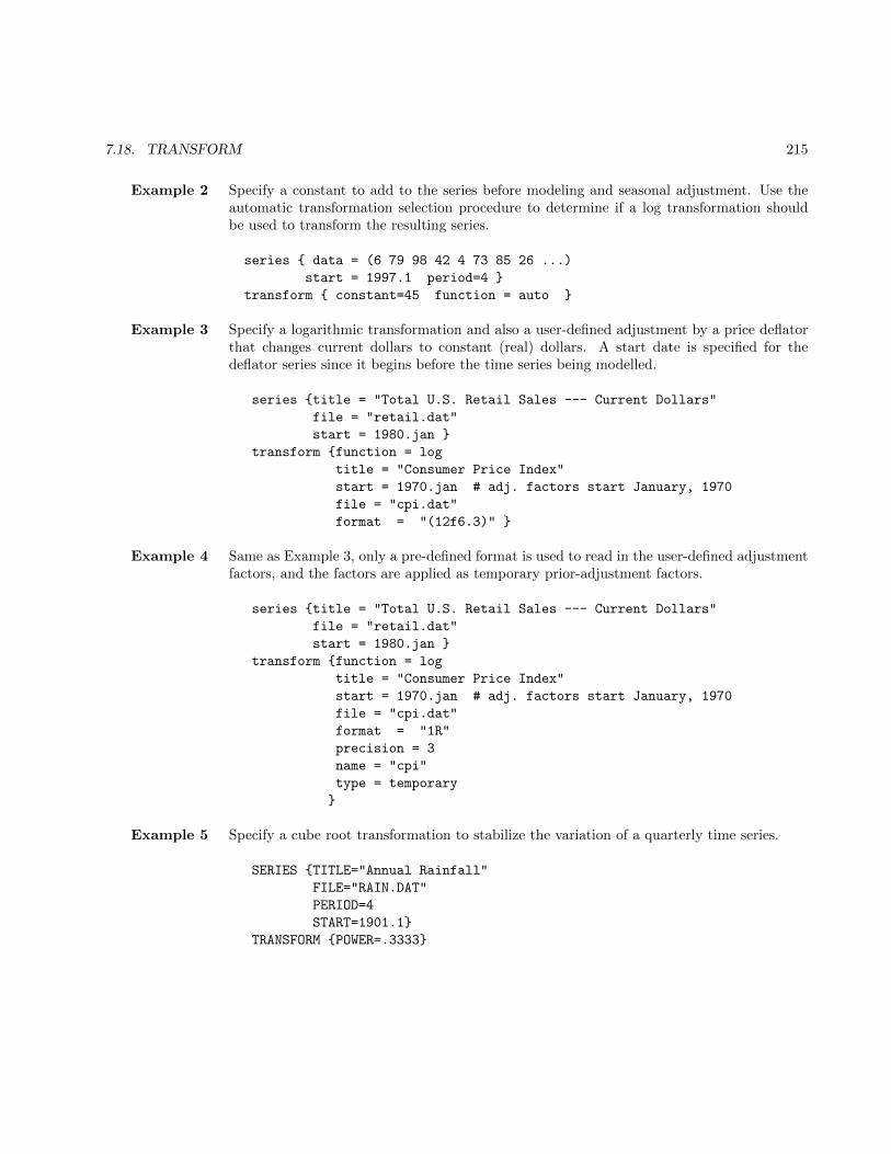
7.18. TRANSFORM 215
Example 2 Specify a constant to add to the series before modeling and seasonal adjustment. Use theautomatic transformation selection procedure to determine if a log transformation shouldbe used to transform the resulting series.
series { data = (6 79 98 42 4 73 85 26 ...)
start = 1997.1 period=4 }
transform { constant=45 function = auto }
Example 3 Specify a logarithmic transformation and also a user-defined adjustment by a price deflatorthat changes current dollars to constant (real) dollars. A start date is specified for thedeflator series since it begins before the time series being modelled.
series {title = "Total U.S. Retail Sales --- Current Dollars"
file = "retail.dat"
start = 1980.jan }
transform {function = log
title = "Consumer Price Index"
start = 1970.jan # adj. factors start January, 1970
file = "cpi.dat"
format = "(12f6.3)" }
Example 4 Same as Example 3, only a pre-defined format is used to read in the user-defined adjustmentfactors, and the factors are applied as temporary prior-adjustment factors.
series {title = "Total U.S. Retail Sales --- Current Dollars"
file = "retail.dat"
start = 1980.jan }
transform {function = log
title = "Consumer Price Index"
start = 1970.jan # adj. factors start January, 1970
file = "cpi.dat"
format = "1R"
precision = 3
name = "cpi"
type = temporary
}
Example 5 Specify a cube root transformation to stabilize the variation of a quarterly time series.
SERIES {TITLE="Annual Rainfall"
FILE="RAIN.DAT"
PERIOD=4
START=1901.1}
TRANSFORM {POWER=.3333}

216 CHAPTER 7. DOCUMENTATION FOR INDIVIDUAL SPECS
Example 6 This example uses two sets of user-defined prior-adjustment factors: one for the ConsumerPrice Index that will be removed from the final seasonally adjusted series to convert thevalue of the series to current dollars (a permanent prior effect), and a set of strike effects (atemporary prior effect). Each set of factors is read from its own file. Since the files have thesame format, single values are entered for format and precision.
series {title = "Retail Sales of computers --- Current Dollars"
file = "rscomp.dat"
start = 1980.jan
}
transform { function = log
title = "Consumer Price Index & Strike Effect"
type = (permanent temporary)
start = 1970.jan # adj. factors start January, 1970
file = ("cpi.dat" "strike.dat")
format = "1R"
precision = 3
name = ("cpi" "strike")
}
Example 7 Use the automatic transformation selection procedure to determine if a log transformationshould be used to transform the series. Since a regARIMA model is not specified, theprogram will use an airline model to generate the AICC values needed for the test. The AICCdifference for the test has been reset to zero, so the program will choose the transformationbased on which model estimation yields the smaller value of AICC.
series {title = "Total U.K. Retail Sales"
file = "ukretail.dat"
start = 1978.jan
}
transform {function = auto
aicdiff = 0.0
}
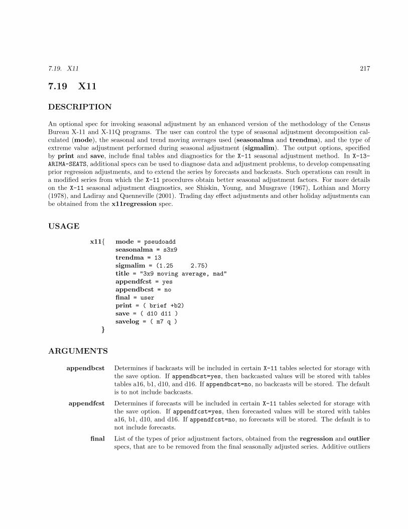
7.19. X11 217
7.19 X11
DESCRIPTION
An optional spec for invoking seasonal adjustment by an enhanced version of the methodology of the CensusBureau X-11 and X-11Q programs. The user can control the type of seasonal adjustment decomposition cal-culated (mode), the seasonal and trend moving averages used (seasonalma and trendma), and the type ofextreme value adjustment performed during seasonal adjustment (sigmalim). The output options, specifiedby print and save, include final tables and diagnostics for the X-11 seasonal adjustment method. In X-13-
ARIMA-SEATS, additional specs can be used to diagnose data and adjustment problems, to develop compensatingprior regression adjustments, and to extend the series by forecasts and backcasts. Such operations can result ina modified series from which the X-11 procedures obtain better seasonal adjustment factors. For more detailson the X-11 seasonal adjustment diagnostics, see Shiskin, Young, and Musgrave (1967), Lothian and Morry(1978), and Ladiray and Quenneville (2001). Trading day effect adjustments and other holiday adjustments canbe obtained from the x11regression spec.
USAGE
x11{ mode = pseudoadd
seasonalma = s3x9
trendma = 13
sigmalim = (1.25 2.75)
title = "3x9 moving average, mad"
appendfcst = yes
appendbcst = no
final = user
print = ( brief +b2)
save = ( d10 d11 )
savelog = ( m7 q )
}
ARGUMENTS
appendbcst Determines if backcasts will be included in certain X-11 tables selected for storage withthe save option. If appendbcst=yes, then backcasted values will be stored with tablestables a16, b1, d10, and d16. If appendbcst=no, no backcasts will be stored. The defaultis to not include backcasts.
appendfcst Determines if forecasts will be included in certain X-11 tables selected for storage withthe save option. If appendfcst=yes, then forecasted values will be stored with tablesa16, b1, d10, and d16. If appendfcst=no, no forecasts will be stored. The default is tonot include forecasts.
final List of the types of prior adjustment factors, obtained from the regression and outlierspecs, that are to be removed from the final seasonally adjusted series. Additive outliers
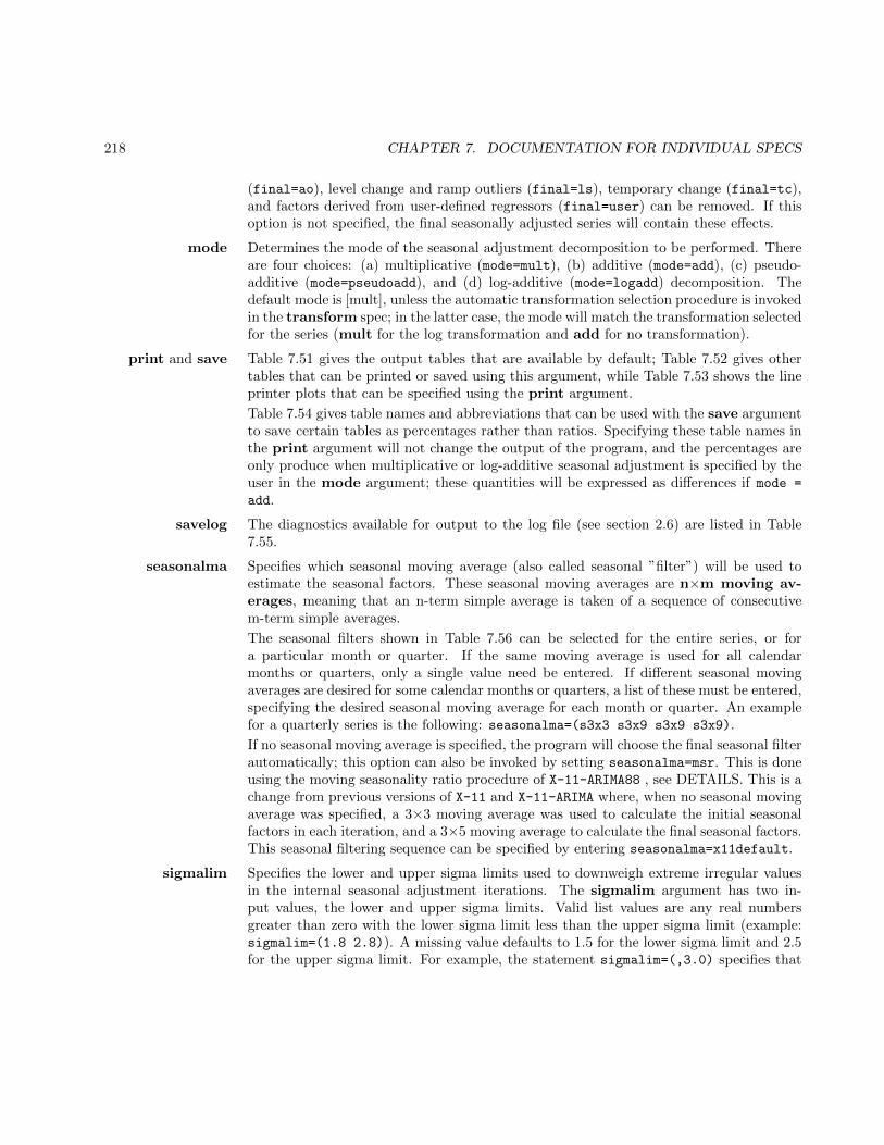
218 CHAPTER 7. DOCUMENTATION FOR INDIVIDUAL SPECS
(final=ao), level change and ramp outliers (final=ls), temporary change (final=tc),and factors derived from user-defined regressors (final=user) can be removed. If thisoption is not specified, the final seasonally adjusted series will contain these effects.
mode Determines the mode of the seasonal adjustment decomposition to be performed. Thereare four choices: (a) multiplicative (mode=mult), (b) additive (mode=add), (c) pseudo-additive (mode=pseudoadd), and (d) log-additive (mode=logadd) decomposition. Thedefault mode is [mult], unless the automatic transformation selection procedure is invokedin the transform spec; in the latter case, the mode will match the transformation selectedfor the series (mult for the log transformation and add for no transformation).
print and save Table 7.51 gives the output tables that are available by default; Table 7.52 gives othertables that can be printed or saved using this argument, while Table 7.53 shows the lineprinter plots that can be specified using the print argument.
Table 7.54 gives table names and abbreviations that can be used with the save argumentto save certain tables as percentages rather than ratios. Specifying these table names inthe print argument will not change the output of the program, and the percentages areonly produce when multiplicative or log-additive seasonal adjustment is specified by theuser in the mode argument; these quantities will be expressed as differences if mode =
add.
savelog The diagnostics available for output to the log file (see section 2.6) are listed in Table7.55.
seasonalma Specifies which seasonal moving average (also called seasonal ”filter”) will be used toestimate the seasonal factors. These seasonal moving averages are n×m moving av-erages, meaning that an n-term simple average is taken of a sequence of consecutivem-term simple averages.
The seasonal filters shown in Table 7.56 can be selected for the entire series, or fora particular month or quarter. If the same moving average is used for all calendarmonths or quarters, only a single value need be entered. If different seasonal movingaverages are desired for some calendar months or quarters, a list of these must be entered,specifying the desired seasonal moving average for each month or quarter. An examplefor a quarterly series is the following: seasonalma=(s3x3 s3x9 s3x9 s3x9).
If no seasonal moving average is specified, the program will choose the final seasonal filterautomatically; this option can also be invoked by setting seasonalma=msr. This is doneusing the moving seasonality ratio procedure of X-11-ARIMA88 , see DETAILS. This is achange from previous versions of X-11 and X-11-ARIMA where, when no seasonal movingaverage was specified, a 3×3 moving average was used to calculate the initial seasonalfactors in each iteration, and a 3×5 moving average to calculate the final seasonal factors.This seasonal filtering sequence can be specified by entering seasonalma=x11default.
sigmalim Specifies the lower and upper sigma limits used to downweigh extreme irregular valuesin the internal seasonal adjustment iterations. The sigmalim argument has two in-put values, the lower and upper sigma limits. Valid list values are any real numbersgreater than zero with the lower sigma limit less than the upper sigma limit (example:sigmalim=(1.8 2.8)). A missing value defaults to 1.5 for the lower sigma limit and 2.5for the upper sigma limit. For example, the statement sigmalim=(,3.0) specifies that

7.19. X11 219
Name Small Save Description of tableadjustdiff fad + final adjustment difference (only for pseudo-additive sea-
sonal adjustment)adjustfac d16 + combined seasonal and trading day factorsadjustmentratio e18 + final adjustment ratios (original series / seasonally ad-
justed series)calendar d18 + combined holiday and trading day factorscalendaradjchanges e8 + percent changes (differences) in original series adjusted for
calendar effectscombholiday chl + combined holiday prior adjustment factors, A16 tableftestd8 d8f · F-tests for stable and moving seasonality, D8irregular d13 + final irregular componentirrwt c17 + final weights for the irregular componentmovseasrat d9a · moving seasonality ratios for each periodorigchanges e5 + percent changes (differences) in original seriesqstat f3 · quality control statisticsreplacsi d9 + final replacement values for extreme SI-ratios (differ-
ences), D iterationresidualseasf rsf · F-test for residual seasonalitysachanges e6 + percent changes (differences) in seasonally adjusted seriesseasadj d11 + final seasonally adjusted seriesseasonal d10 + final seasonal factorsseasonaldiff fsd + final seasonal difference (only for pseudo-additive seasonal
adjustment)tdaytype tdy · trading day factors printed by type of monthtotaladjustment tad + total adjustment factors (only printed out if the original
series contains values that are ≤ 0)trend d12 + final trend-cycletrendchanges e7 + percent changes (differences) in final trend component se-
riesunmodsi d8 + final unmodified SI-ratios (differences)unmodsiox d8b + final unmodified SI-ratios, with labels for outliers and ex-
treme valuesx11diag f2 · summary of seasonal adjustment diagnosticsyrtotals e4 · ratio of yearly totals of original and seasonally adjusted
series
Name gives the name of each table for use with the print and save arguments.Short gives a short name for the tables of the print argument.Save? indicates which tables can be saved (+) or not saved (·) into a separate file with the save
argument.
Table 7.51: Default Output Tables for X11 spec
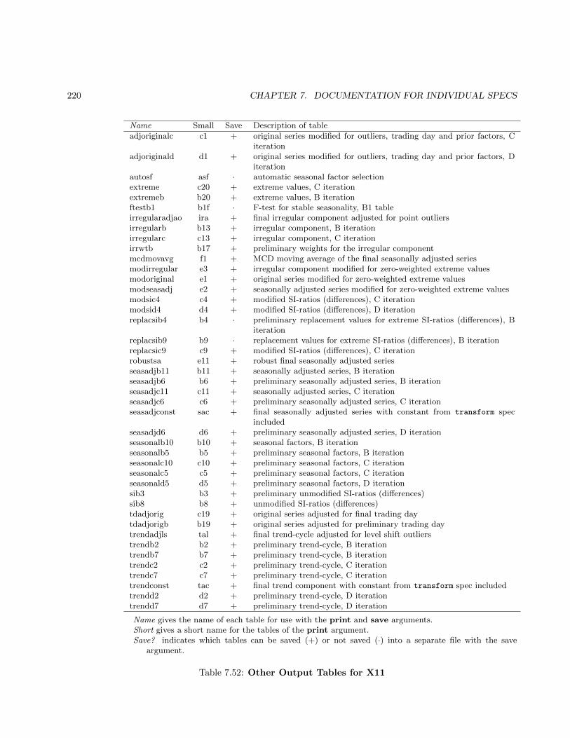
220 CHAPTER 7. DOCUMENTATION FOR INDIVIDUAL SPECS
Name Small Save Description of table
adjoriginalc c1 + original series modified for outliers, trading day and prior factors, Citeration
adjoriginald d1 + original series modified for outliers, trading day and prior factors, Diteration
autosf asf · automatic seasonal factor selectionextreme c20 + extreme values, C iterationextremeb b20 + extreme values, B iterationftestb1 b1f · F-test for stable seasonality, B1 tableirregularadjao ira + final irregular component adjusted for point outliersirregularb b13 + irregular component, B iterationirregularc c13 + irregular component, C iterationirrwtb b17 + preliminary weights for the irregular componentmcdmovavg f1 + MCD moving average of the final seasonally adjusted seriesmodirregular e3 + irregular component modified for zero-weighted extreme valuesmodoriginal e1 + original series modified for zero-weighted extreme valuesmodseasadj e2 + seasonally adjusted series modified for zero-weighted extreme valuesmodsic4 c4 + modified SI-ratios (differences), C iterationmodsid4 d4 + modified SI-ratios (differences), D iterationreplacsib4 b4 · preliminary replacement values for extreme SI-ratios (differences), B
iterationreplacsib9 b9 · replacement values for extreme SI-ratios (differences), B iterationreplacsic9 c9 + modified SI-ratios (differences), C iterationrobustsa e11 + robust final seasonally adjusted seriesseasadjb11 b11 + seasonally adjusted series, B iterationseasadjb6 b6 + preliminary seasonally adjusted series, B iterationseasadjc11 c11 + seasonally adjusted series, C iterationseasadjc6 c6 + preliminary seasonally adjusted series, C iterationseasadjconst sac + final seasonally adjusted series with constant from transform spec
includedseasadjd6 d6 + preliminary seasonally adjusted series, D iterationseasonalb10 b10 + seasonal factors, B iterationseasonalb5 b5 + preliminary seasonal factors, B iterationseasonalc10 c10 + preliminary seasonal factors, C iterationseasonalc5 c5 + preliminary seasonal factors, C iterationseasonald5 d5 + preliminary seasonal factors, D iterationsib3 b3 + preliminary unmodified SI-ratios (differences)sib8 b8 + unmodified SI-ratios (differences)tdadjorig c19 + original series adjusted for final trading daytdadjorigb b19 + original series adjusted for preliminary trading daytrendadjls tal + final trend-cycle adjusted for level shift outlierstrendb2 b2 + preliminary trend-cycle, B iterationtrendb7 b7 + preliminary trend-cycle, B iterationtrendc2 c2 + preliminary trend-cycle, C iterationtrendc7 c7 + preliminary trend-cycle, C iterationtrendconst tac + final trend component with constant from transform spec includedtrendd2 d2 + preliminary trend-cycle, D iterationtrendd7 d7 + preliminary trend-cycle, D iteration
Name gives the name of each table for use with the print and save arguments.Short gives a short name for the tables of the print argument.Save? indicates which tables can be saved (+) or not saved (·) into a separate file with the save
argument.
Table 7.52: Other Output Tables for X11
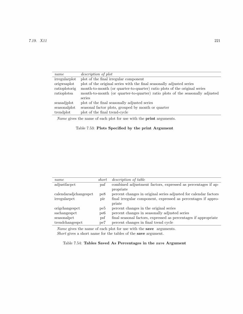
7.19. X11 221
name description of plotirregularplot plot of the final irregular componentorigwsaplot plot of the original series with the final seasonally adjusted seriesratioplotorig month-to-month (or quarter-to-quarter) ratio plots of the original seriesratioplotsa month-to-month (or quarter-to-quarter) ratio plots of the seasonally adjusted
seriesseasadjplot plot of the final seasonally adjusted seriesseasonalplot seasonal factor plots, grouped by month or quartertrendplot plot of the final trend-cycle
Name gives the name of each plot for use with the print arguments.
Table 7.53: Plots Specified by the print Argument
name short description of tableadjustfacpct paf combined adjustment factors, expressed as percentages if ap-
propriatecalendaradjchangespct pe8 percent changes in original series adjusted for calendar factorsirregularpct pir final irregular component, expressed as percentages if appro-
priateorigchangespct pe5 percent changes in the original seriessachangespct pe6 percent changes in seasonally adjusted seriesseasonalpct psf final seasonal factors, expressed as percentages if appropriatetrendchangespct pe7 percent changes in final trend cycle
Name gives the name of each plot for use with the save arguments.Short gives a short name for the tables of the save argument.
Table 7.54: Tables Saved As Percentages in the save Argument
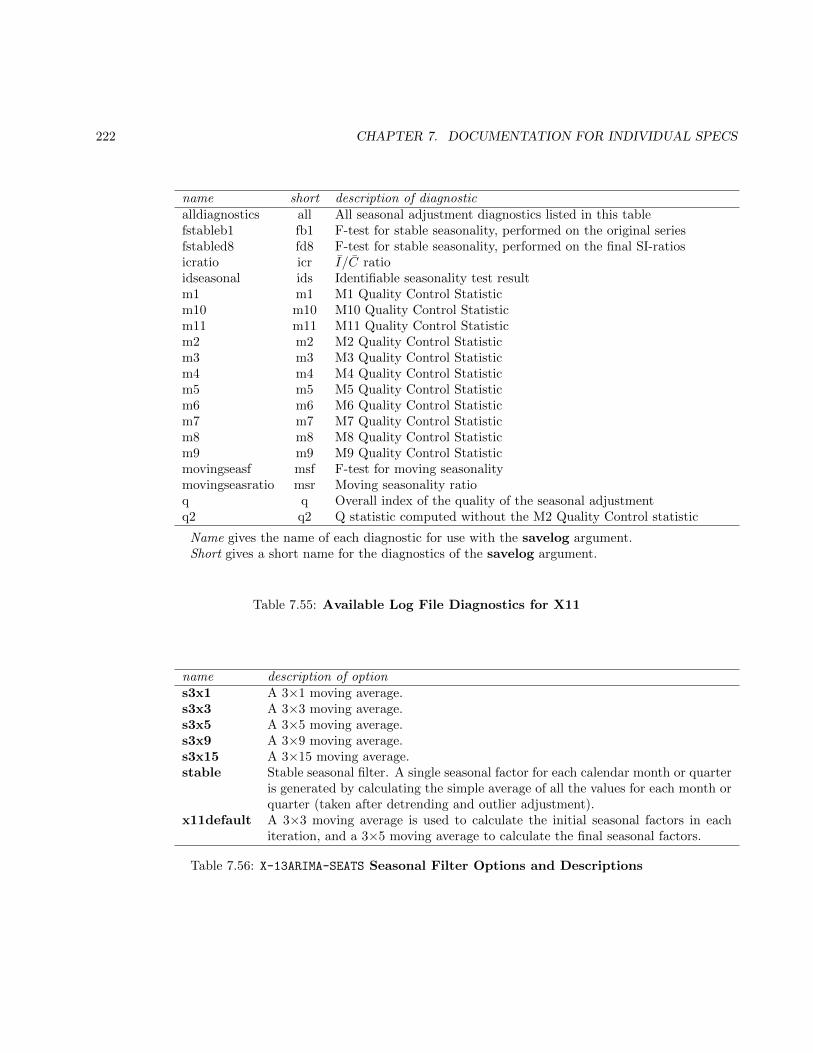
222 CHAPTER 7. DOCUMENTATION FOR INDIVIDUAL SPECS
name short description of diagnosticalldiagnostics all All seasonal adjustment diagnostics listed in this tablefstableb1 fb1 F-test for stable seasonality, performed on the original seriesfstabled8 fd8 F-test for stable seasonality, performed on the final SI-ratiosicratio icr I/C ratioidseasonal ids Identifiable seasonality test resultm1 m1 M1 Quality Control Statisticm10 m10 M10 Quality Control Statisticm11 m11 M11 Quality Control Statisticm2 m2 M2 Quality Control Statisticm3 m3 M3 Quality Control Statisticm4 m4 M4 Quality Control Statisticm5 m5 M5 Quality Control Statisticm6 m6 M6 Quality Control Statisticm7 m7 M7 Quality Control Statisticm8 m8 M8 Quality Control Statisticm9 m9 M9 Quality Control Statisticmovingseasf msf F-test for moving seasonalitymovingseasratio msr Moving seasonality ratioq q Overall index of the quality of the seasonal adjustmentq2 q2 Q statistic computed without the M2 Quality Control statistic
Name gives the name of each diagnostic for use with the savelog argument.Short gives a short name for the diagnostics of the savelog argument.
Table 7.55: Available Log File Diagnostics for X11
name description of options3x1 A 3×1 moving average.s3x3 A 3×3 moving average.s3x5 A 3×5 moving average.s3x9 A 3×9 moving average.s3x15 A 3×15 moving average.stable Stable seasonal filter. A single seasonal factor for each calendar month or quarter
is generated by calculating the simple average of all the values for each month orquarter (taken after detrending and outlier adjustment).
x11default A 3×3 moving average is used to calculate the initial seasonal factors in eachiteration, and a 3×5 moving average to calculate the final seasonal factors.
Table 7.56: X-13ARIMA-SEATS Seasonal Filter Options and Descriptions
7.19. X11 223
the upper sigma limit will be set to 3.0, while the lower sigma limit will remain at the1.5 default. A comma is necessary if either sigma limit is missing. For an explanation ofhow X-13ARIMA-SEATS uses these sigma limits to derive adjustments for extreme values,see DETAILS.
title Title of the seasonal adjustment, in quotes, for the convenience of the user. This can bea single title or a list of up to 8 titles; an example with two titles is:
title= ("3x9, trading day adjustment"
"for sales of sporting goods")
If a list is provided, each title must be on a separate line of the spec file. This list will beprinted on the title page below the series title. There is no default seasonal adjustmenttitle.
trendma Specifies which Henderson moving average will be used to estimate the final trend-cycle.Any odd number greater than one and less than or equal to 101 can be specified. Example:trendma=23. If no selection is made, the program will select a trend moving average basedon statistical characteristics of the data. For monthly series, either a 9-, 13- or 23-termHenderson moving average will be selected. For quarterly series, the program will chooseeither a 5- or a 7-term Henderson moving average.
type When type=summary, the program develops estimates of the trend-cycle, irregular, andrelated diagnostics, along with residual seasonal factors and, optionally, also residualtrading day and holiday factors from an input series which is assumed to be either alreadyseasonally adjusted or nonseasonal. These residual factors are not removed. The outputseries in the final seasonally adjusted series (table D11) is the same as the original series(table A1). When type=trend, the program develops estimates for the final trend-cycleand irregular components without attempting to estimate a seasonal component. Theinput series is assumed to be either already seasonally adjusted or nonseasonal. With thisoption, estimated trading day and holiday effects as well as permanent prior adjustmentfactors are removed to form the adjusted series (table D11) as well as for the calculationof the trend (table D12). When a metafile with a composite spec is used to obtainan indirect adjustment of an aggregate, these options are used for components of theaggregate that are not seasonally adjusted. In the default setting, type=sa, the programcalculates a seasonal decomposition of the series. With all three values of type, the finalseasonally adjusted series (printed in the D11 table of the main output file) is used toform the indirect seasonal adjustment of the composite.
RARELY USED ARGUMENTS
calendarsigma Specifies if the standard errors used for extreme value detection and adjustment are com-puted separately for each calendar month (quarter), or separately for two complementarysets of calendar months (quarters). If calendarsigma=all, the standard errors will becomputed separately for each month (quarter). If calendarsigma=signif, the standarderrors will be computed separately for each month only if Cochran’s hypothesis test de-termines that the irregular component is heteroskedastic by calendar month (quarter).
224 CHAPTER 7. DOCUMENTATION FOR INDIVIDUAL SPECS
If calendarsigma=select, the months (quarters) will be divided into two groups, andthe standard error of each group will be computed. For the select option, the argumentsigmavec must be used to define one of the two groups of months (quarters). If cal-endarsigma is not specified, the standard errors will be computed from 5 year spans ofirregulars, in the manner described in Dagum (1988).
centerseasonal If centerseasonal = yes, the program will center the seasonal factors combined withuser-defined seasonal regression effects. The default is centerseasonal = no.
keepholiday Determines if holiday effects estimated by the program are to be kept in the final sea-sonally adjusted series. In the default setting, keepholiday=no, holiday adjustmentfactors derived from the program are removed from the final seasonally adjusted series.If keepholiday=yes, holiday adjustment factors derived from the program are kept inthe final seasonally adjusted series. The default is used to produce a series adjusted forboth seasonal and holiday effects.
print1stpass If print1stpass=yes, output from the seasonal adjustment needed to generate theirregular components used for the irregular regression adjustment procedures will beprinted out. If print1stpass=no, this output will be suppressed, and only the ta-bles associated with the irregular regression procedures are printed out. The defaultis print1stpass=no. When print1stpass=yes, the print argument controls which ta-bles are actually printed.
sfshort Controls what seasonal filters are used to obtain the seasonal factors if the series is atmost 5 years long. For the default case, sfshort=no, a stable seasonal filter will beused to calculate the seasonal factors, regardless of what is entered for the seasonalmaargument. If sfshort=yes, X-13ARIMA-SEATS will use the central and one sided seasonalfilters associated with the choice given in the seasonalma argument wherever possible.
sigmavec Specifies one of the two groups of months (quarters) for whose irregulars a group stan-dard error will be calculated under the calendarsigma=select option. The user entersthe month(s) (either the full name of the month or the abbreviations shown in Sec-tion 3.3) or quarter(s) (q1 for the first quarter, q2 for the second quarter, etc.) thatcomprise one group; all remaining months or quarters comprise the second group. Exam-ple: sigmavec=(jan feb dec). Warning: This argument can only be specified whencalendarsigma=select.
trendic Specifies the irregular-to-trend variance ratio that will be used to generate the end weightsfor the Henderson moving average. The procedure is taken from Doherty (2001). Ifthis variable is not specified, the value of trendic will depend on the length of theHenderson trend filter. These default values closely reproduce the end weights for theset of Henderson trend filters which originally appeared in X-11 and X-11-ARIMA.
true7term Specifies the end weights used for the seven term Henderson filter. If true7term =
yes, then the asymmetric ends weights for the 7 term Henderson filter are applied forobservations at the end of the series where a central Henderson filter cannot be applied.If true7term = no, then central and asymmetric weights from a 5 term Henderson filterare applied, as in previous versions of the X-11-ARIMA program released by StatisticsCanada. The default is true7term = no.
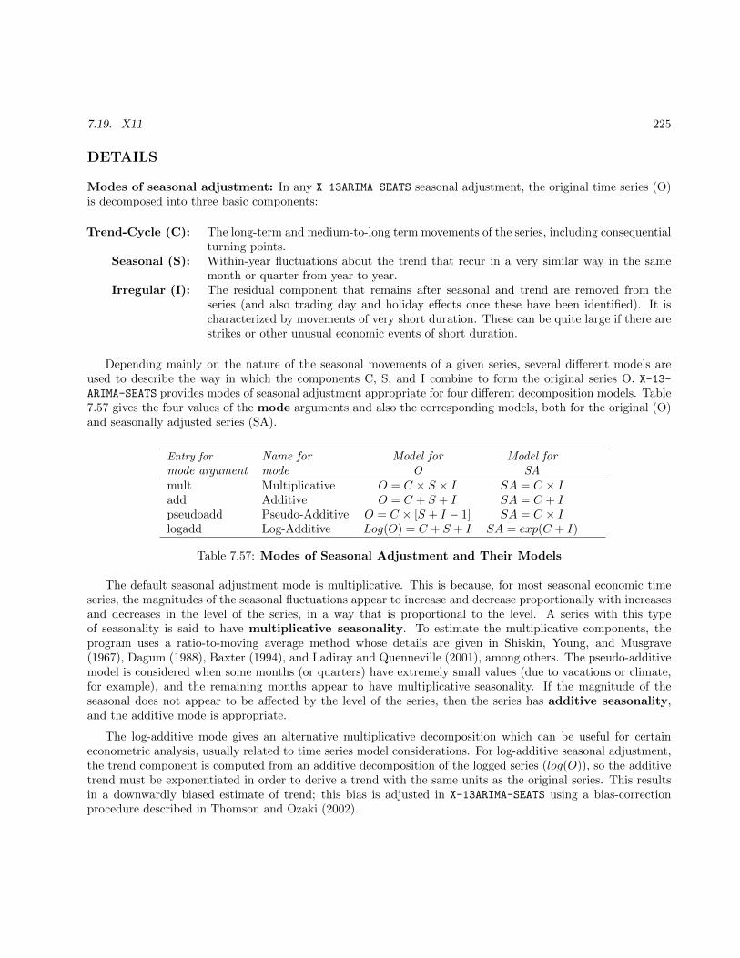
7.19. X11 225
DETAILS
Modes of seasonal adjustment: In any X-13ARIMA-SEATS seasonal adjustment, the original time series (O)is decomposed into three basic components:
Trend-Cycle (C): The long-term and medium-to-long term movements of the series, including consequentialturning points.
Seasonal (S): Within-year fluctuations about the trend that recur in a very similar way in the samemonth or quarter from year to year.
Irregular (I): The residual component that remains after seasonal and trend are removed from theseries (and also trading day and holiday effects once these have been identified). It ischaracterized by movements of very short duration. These can be quite large if there arestrikes or other unusual economic events of short duration.
Depending mainly on the nature of the seasonal movements of a given series, several different models areused to describe the way in which the components C, S, and I combine to form the original series O. X-13-ARIMA-SEATS provides modes of seasonal adjustment appropriate for four different decomposition models. Table7.57 gives the four values of the mode arguments and also the corresponding models, both for the original (O)and seasonally adjusted series (SA).
Entry for Name for Model for Model formode argument mode O SAmult Multiplicative O = C × S × I SA = C × Iadd Additive O = C + S + I SA = C + Ipseudoadd Pseudo-Additive O = C × [S + I − 1] SA = C × Ilogadd Log-Additive Log(O) = C + S + I SA = exp(C + I)
Table 7.57: Modes of Seasonal Adjustment and Their Models
The default seasonal adjustment mode is multiplicative. This is because, for most seasonal economic timeseries, the magnitudes of the seasonal fluctuations appear to increase and decrease proportionally with increasesand decreases in the level of the series, in a way that is proportional to the level. A series with this typeof seasonality is said to have multiplicative seasonality. To estimate the multiplicative components, theprogram uses a ratio-to-moving average method whose details are given in Shiskin, Young, and Musgrave(1967), Dagum (1988), Baxter (1994), and Ladiray and Quenneville (2001), among others. The pseudo-additivemodel is considered when some months (or quarters) have extremely small values (due to vacations or climate,for example), and the remaining months appear to have multiplicative seasonality. If the magnitude of theseasonal does not appear to be affected by the level of the series, then the series has additive seasonality,and the additive mode is appropriate.
The log-additive mode gives an alternative multiplicative decomposition which can be useful for certaineconometric analysis, usually related to time series model considerations. For log-additive seasonal adjustment,the trend component is computed from an additive decomposition of the logged series (log(O)), so the additivetrend must be exponentiated in order to derive a trend with the same units as the original series. This resultsin a downwardly biased estimate of trend; this bias is adjusted in X-13ARIMA-SEATS using a bias-correctionprocedure described in Thomson and Ozaki (2002).

226 CHAPTER 7. DOCUMENTATION FOR INDIVIDUAL SPECS
For multiplicative, pseudo-additive and log-additive seasonal adjustment, the seasonal and irregular com-ponents are assumed to be ratios centered about 1. In the main output they are expressed as percentages sothat they center about 100. For additive seasonal adjustment, the seasonal and irregular components are in thesame units as the original time series and vary about 0.
When a regARIMA model is specified with the regression and arima specs, trading day, holiday, outlier,and other regression effects defined in the regression spec can be derived from the regression coefficients of aregARIMA model and used to adjust the original series prior to seasonal adjustment. In this case, these effectsmust be the same type as factors generated by the seasonal adjustment procedure, so that combined adjustmentfactors can be derived and adjustment diagnostics can be generated. If the regARIMA model is fit to a log-transformed series, the regression factors are expressed in the form of ratios, which is the same form as factorsgenerated by the multiplicative or log-additive adjustment modes. Conversely, if the regARIMA model is fit tothe original series, the regression factors are measured on the same scale as the original series, which matches thescale of the components generated by the additive adjustment mode. Therefore, users should be careful to ensurethat the transformation specified by the function or power arguments of the transform spec is compatiblewith the seasonal adjustment mode specified by the mode argument of the x11 spec. Furthermore, be awarethat the default value for the mode argument is multiplicative seasonal adjustment, which conflicts with thedefault for the function and power arguments of the transform spec, which assume no transformation isdone. Currently, you cannot use regression effects to pre-adjust the original series for a pseudo-additive seasonaladjustment.
Multiplicative and pseudo-additive seasonal adjustment give very similar results for most series with multi-plicative seasonality, unless the seasonal amplitude of the series is large. If the smallest seasonal factor is 0.7 orless, there will be noticeable differences between the multiplicative and pseudo-additive seasonal adjustments.If the smallest seasonal factor is 0.5 or less, this difference is likely to be important. If a multiplicative seasonaladjustment produces many more extreme values (meaning values of less than 100.0 in Table C17, especially 0)in months (or quarters) with small seasonal factors than months with large seasonal factors, then the pseudo-additive seasonal adjustment is likely to be better. For more details on when to use pseudo-additive seasonaladjustment, see Baxter (1994).
For simplicity, this discussion has ignored trading day and holiday effects. When these are estimated, theyadd additional factors to the decomposition and, depending on how they are defined, adjustment for them canlead to larger differences between the annual totals of the adjusted series and the annual totals of the originaltime series.
Downweighting of extreme irregulars: Let µI be the assumed mean of the irregular component (1.0for multiplicative seasonal adjustment, 0.0 for additive). Let σX11 denote an estimate of the standard deviationof the irregular component for a month or quarter. If the absolute value of It − µI is less than the lower sigmalimit multiplied by σX11, the irregular value It receives full weight. If the absolute value of It−µI is more thanthe upper sigma limit multiplied by σX11, the irregular value receives zero weight, meaning that It is replacedby µt for seasonal factor calculations. Otherwise, It is partially downweighted.
Automatic seasonal filter selection: This procedure is taken from X-11-ARIMA88 , see Dagum (1988).For the first two seasonal adjustment iterations, a 3×3 moving average is used to calculate the initial seasonalfactors and a 3×5 moving average is used to calculate the final seasonal factor. In the third and final iteration,a 3×3 moving average is used to calculate the initial seasonal factors, but for the final iteration the programcalculates the moving seasonality ratio ( I/S, also called the global MSR). Then the program chooses whetherto use a 3×3, 3×5, or 3×9 moving average based on the size of the global MSR. For more information on themoving seasonality ratio, see Lothian (1984).
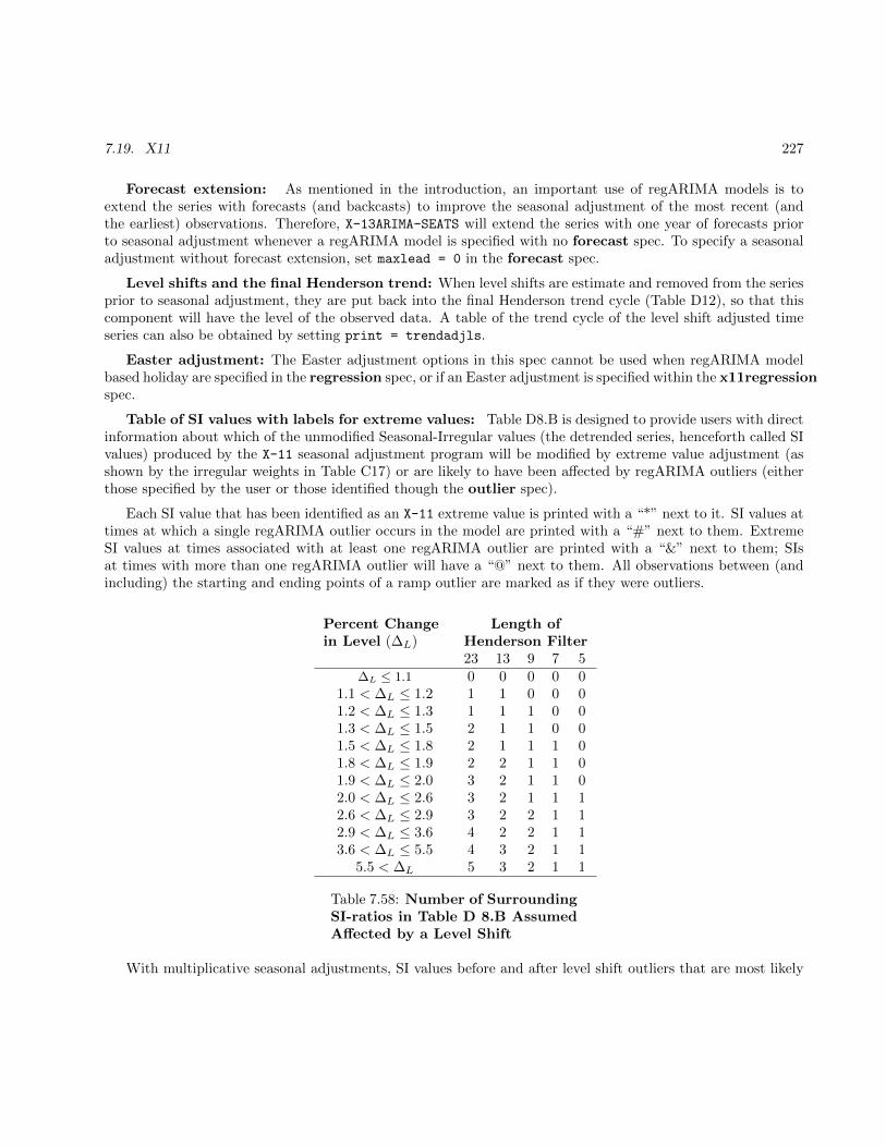
7.19. X11 227
Forecast extension: As mentioned in the introduction, an important use of regARIMA models is toextend the series with forecasts (and backcasts) to improve the seasonal adjustment of the most recent (andthe earliest) observations. Therefore, X-13ARIMA-SEATS will extend the series with one year of forecasts priorto seasonal adjustment whenever a regARIMA model is specified with no forecast spec. To specify a seasonaladjustment without forecast extension, set maxlead = 0 in the forecast spec.
Level shifts and the final Henderson trend: When level shifts are estimate and removed from the seriesprior to seasonal adjustment, they are put back into the final Henderson trend cycle (Table D12), so that thiscomponent will have the level of the observed data. A table of the trend cycle of the level shift adjusted timeseries can also be obtained by setting print = trendadjls.
Easter adjustment: The Easter adjustment options in this spec cannot be used when regARIMA modelbased holiday are specified in the regression spec, or if an Easter adjustment is specified within the x11regressionspec.
Table of SI values with labels for extreme values: Table D8.B is designed to provide users with directinformation about which of the unmodified Seasonal-Irregular values (the detrended series, henceforth called SIvalues) produced by the X-11 seasonal adjustment program will be modified by extreme value adjustment (asshown by the irregular weights in Table C17) or are likely to have been affected by regARIMA outliers (eitherthose specified by the user or those identified though the outlier spec).
Each SI value that has been identified as an X-11 extreme value is printed with a “*” next to it. SI values attimes at which a single regARIMA outlier occurs in the model are printed with a “#” next to them. ExtremeSI values at times associated with at least one regARIMA outlier are printed with a “&” next to them; SIsat times with more than one regARIMA outlier will have a “@” next to them. All observations between (andincluding) the starting and ending points of a ramp outlier are marked as if they were outliers.
Percent Change Length ofin Level (∆L) Henderson Filter
23 13 9 7 5∆L ≤ 1.1 0 0 0 0 0
1.1 < ∆L ≤ 1.2 1 1 0 0 01.2 < ∆L ≤ 1.3 1 1 1 0 01.3 < ∆L ≤ 1.5 2 1 1 0 01.5 < ∆L ≤ 1.8 2 1 1 1 01.8 < ∆L ≤ 1.9 2 2 1 1 01.9 < ∆L ≤ 2.0 3 2 1 1 02.0 < ∆L ≤ 2.6 3 2 1 1 12.6 < ∆L ≤ 2.9 3 2 2 1 12.9 < ∆L ≤ 3.6 4 2 2 1 13.6 < ∆L ≤ 5.5 4 3 2 1 1
5.5 < ∆L 5 3 2 1 1
Table 7.58: Number of SurroundingSI-ratios in Table D 8.B AssumedAffected by a Level Shift
With multiplicative seasonal adjustments, SI values before and after level shift outliers that are most likely
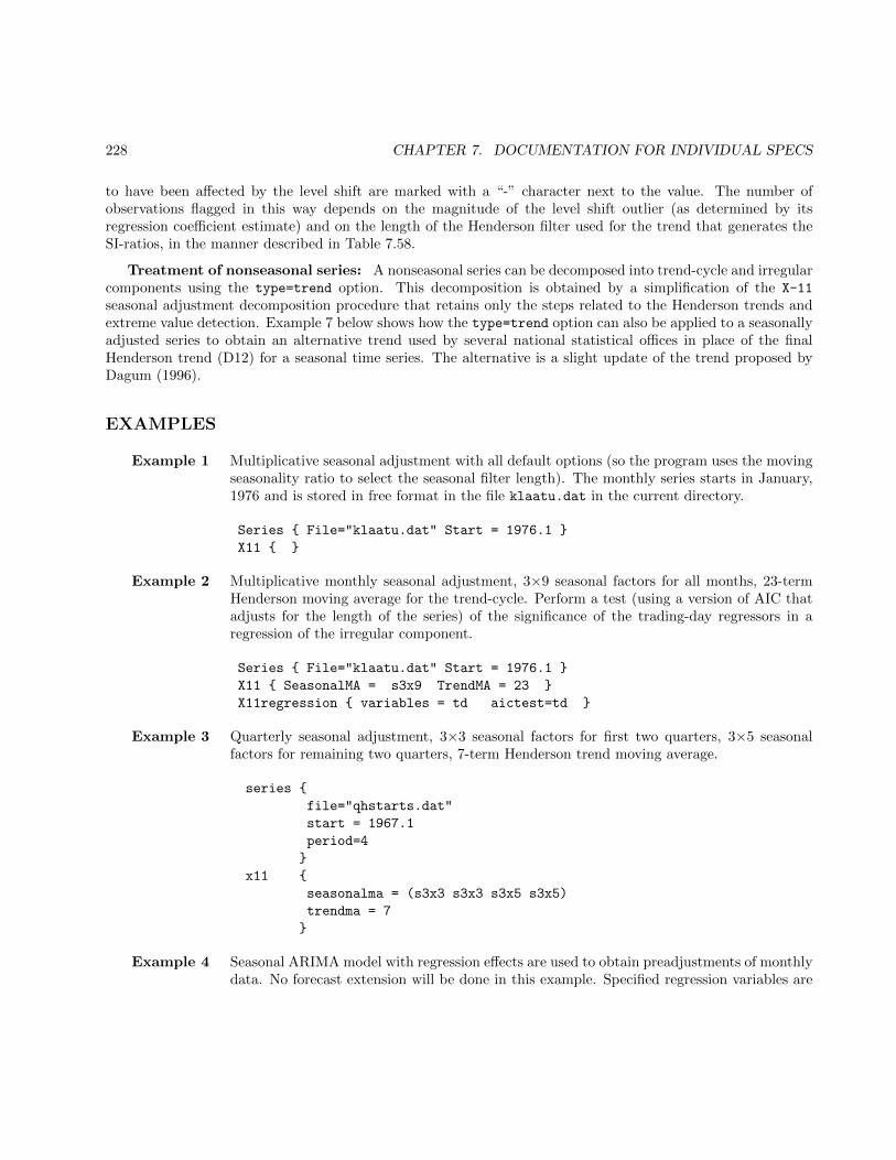
228 CHAPTER 7. DOCUMENTATION FOR INDIVIDUAL SPECS
to have been affected by the level shift are marked with a “-” character next to the value. The number ofobservations flagged in this way depends on the magnitude of the level shift outlier (as determined by itsregression coefficient estimate) and on the length of the Henderson filter used for the trend that generates theSI-ratios, in the manner described in Table 7.58.
Treatment of nonseasonal series: A nonseasonal series can be decomposed into trend-cycle and irregularcomponents using the type=trend option. This decomposition is obtained by a simplification of the X-11
seasonal adjustment decomposition procedure that retains only the steps related to the Henderson trends andextreme value detection. Example 7 below shows how the type=trend option can also be applied to a seasonallyadjusted series to obtain an alternative trend used by several national statistical offices in place of the finalHenderson trend (D12) for a seasonal time series. The alternative is a slight update of the trend proposed byDagum (1996).
EXAMPLES
Example 1 Multiplicative seasonal adjustment with all default options (so the program uses the movingseasonality ratio to select the seasonal filter length). The monthly series starts in January,1976 and is stored in free format in the file klaatu.dat in the current directory.
Series { File="klaatu.dat" Start = 1976.1 }
X11 { }
Example 2 Multiplicative monthly seasonal adjustment, 3×9 seasonal factors for all months, 23-termHenderson moving average for the trend-cycle. Perform a test (using a version of AIC thatadjusts for the length of the series) of the significance of the trading-day regressors in aregression of the irregular component.
Series { File="klaatu.dat" Start = 1976.1 }
X11 { SeasonalMA = s3x9 TrendMA = 23 }
X11regression { variables = td aictest=td }
Example 3 Quarterly seasonal adjustment, 3×3 seasonal factors for first two quarters, 3×5 seasonalfactors for remaining two quarters, 7-term Henderson trend moving average.
series {
file="qhstarts.dat"
start = 1967.1
period=4
}
x11 {
seasonalma = (s3x3 s3x3 s3x5 s3x5)
trendma = 7
}
Example 4 Seasonal ARIMA model with regression effects are used to obtain preadjustments of monthlydata. No forecast extension will be done in this example. Specified regression variables are
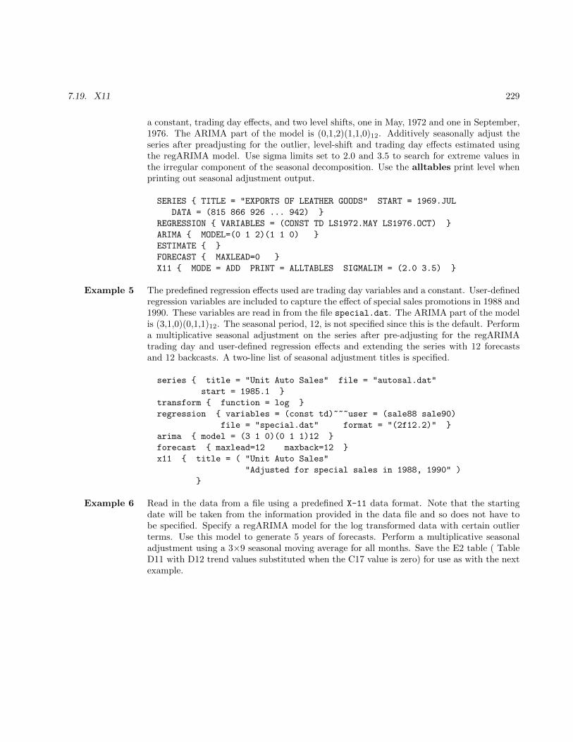
7.19. X11 229
a constant, trading day effects, and two level shifts, one in May, 1972 and one in September,1976. The ARIMA part of the model is (0,1,2)(1,1,0)12. Additively seasonally adjust theseries after preadjusting for the outlier, level-shift and trading day effects estimated usingthe regARIMA model. Use sigma limits set to 2.0 and 3.5 to search for extreme values inthe irregular component of the seasonal decomposition. Use the alltables print level whenprinting out seasonal adjustment output.
SERIES { TITLE = "EXPORTS OF LEATHER GOODS" START = 1969.JUL
DATA = (815 866 926 ... 942) }
REGRESSION { VARIABLES = (CONST TD LS1972.MAY LS1976.OCT) }
ARIMA { MODEL=(0 1 2)(1 1 0) }
ESTIMATE { }
FORECAST { MAXLEAD=0 }
X11 { MODE = ADD PRINT = ALLTABLES SIGMALIM = (2.0 3.5) }
Example 5 The predefined regression effects used are trading day variables and a constant. User-definedregression variables are included to capture the effect of special sales promotions in 1988 and1990. These variables are read in from the file special.dat. The ARIMA part of the modelis (3,1,0)(0,1,1)12. The seasonal period, 12, is not specified since this is the default. Performa multiplicative seasonal adjustment on the series after pre-adjusting for the regARIMAtrading day and user-defined regression effects and extending the series with 12 forecastsand 12 backcasts. A two-line list of seasonal adjustment titles is specified.
series { title = "Unit Auto Sales" file = "autosal.dat"
start = 1985.1 }
transform { function = log }
regression { variables = (const td)~~~user = (sale88 sale90)
file = "special.dat" format = "(2f12.2)" }
arima { model = (3 1 0)(0 1 1)12 }
forecast { maxlead=12 maxback=12 }
x11 { title = ( "Unit Auto Sales"
"Adjusted for special sales in 1988, 1990" )
}
Example 6 Read in the data from a file using a predefined X-11 data format. Note that the startingdate will be taken from the information provided in the data file and so does not have tobe specified. Specify a regARIMA model for the log transformed data with certain outlierterms. Use this model to generate 5 years of forecasts. Perform a multiplicative seasonaladjustment using a 3×9 seasonal moving average for all months. Save the E2 table ( TableD11 with D12 trend values substituted when the C17 value is zero) for use as with the nextexample.

230 CHAPTER 7. DOCUMENTATION FOR INDIVIDUAL SPECS
series { title="NORTHEAST ONE FAMILY Housing Starts"
file="cne1hs.ori" name="CNE1HS" format="2R" }
transform { function=log }
regression {
variables=(ao1976.feb ao1978.feb ls1980.feb
ls1982.nov ao1984.feb)
}
arima { model=(0 1 2)(0 1 1) }
forecast { maxlead=60 }
x11 { seasonalma=(s3x9)
title="Adjustment of 1 family housing starts"
save = e2
}
Example 7 A continuation of Example 6. Use the type=trend option to obtain an alternative to D12trend for seasonal time series due to Dagum (1996) as further evaluated and updated inDagum and Luati (2009) and Darne and Dagum (2009). Read in the data from the seasonallyadjusted series modified for outliers (AO and TC) and extreme values from the E2 file savedin Example 6. The starting date will be taken from the information provided in the E2 fileand so does not have to be specified. The nonseasonal (0 1 1) model with be used to providethe six forecasts of the E2 series so that the symmetric 13 term Henderson filter can beapplied. The AO outliers are commented out in the regression spec as these outliers havealready been removed from the E2 table, and therefore do not have to be accounted for inthe model. The default setting of forecast provides 12 forecasts, so it can be used. Note thevery low values of the sigma limits used to smooth the E2 values. Note also that the logtransformation is not used.
series {
title="Trend for NORTHEAST ONE FAMILY Housing Starts"
file="cne1hs.e2"
format="x13save"
}
regression {
variables=(
# ao1976.feb ao1978.feb ao1984.feb
ls1980.feb ls1982.nov
)
}
arima { model=(0 1 1) }
forecast { }
x11{
type=trend trendma=13
sigmalim=(0.7, 1.0)
title="Updated Dagum (1996) trend of 1 family housing starts"
}
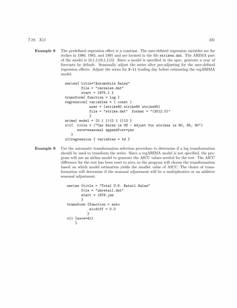
7.19. X11 231
Example 8 The predefined regression effect is a constant. The user-defined regression variables are forstrikes in 1980, 1985, and 1991 and are located in the file strikes.dat. The ARIMA partof the model is (0,1,1)(0,1,1)12. Since a model is specified in the spec, generate a year offorecasts by default. Seasonally adjust the series after pre-adjusting for the user-definedregression effects. Adjust the series for X-11 trading day before estimating the regARIMAmodel.
series{ title="Automobile Sales"
file = "carsales.dat"
start = 1975.1 }
transform{ function = log }
regression{ variables = ( const )
user = (strike80 strike85 strike90)
file = "strike.dat" format = "(3f12.0)"
}
arima{ model = (0 1 1)(0 1 1)12 }
x11{ title = ("Car Sales in US - Adjust for strikes in 80, 85, 90")
save=seasonal appendfcst=yes
}
x11regression { variables = td }
Example 9 Use the automatic transformation selection procedure to determine if a log transformationshould be used to transform the series. Since a regARIMA model is not specified, the pro-gram will use an airline model to generate the AICC values needed for the test. The AICCdifference for the test has been reset to zero, so the program will choose the transformationbased on which model estimation yields the smaller value of AICC. The choice of trans-formation will determine if the seasonal adjustment will be a multiplicative or an additiveseasonal adjustment.
series {title = "Total U.K. Retail Sales"
file = "ukretail.dat"
start = 1978.jan
}
transform {function = auto
aicdiff = 0.0
}
x11 {save=d11
}

232 CHAPTER 7. DOCUMENTATION FOR INDIVIDUAL SPECS
7.20 X11REGRESSION
DESCRIPTION
An optional spec for use in conjunction with the x11 spec for series without missing observations. This specestimates calendar effects by regression modeling of the irregular component with predefined or user-definedregressors. The user can select predefined regression variables with the variables argument. The predefinedvariables are for calendar (trading-day and holiday) variation and additive outliers. A change-of-regime optionis available with trading-day regressors. User-defined calendar effect regression variables can be included inthe model via the user argument. Data for any user-defined variables must be supplied, either in the dataargument, or in a file named in the file argument (not both). The regression model specified can contain bothpredefined and user-defined regression variables.
USAGE
x11regression { variables = (td or td1coef ortdstock[31] or tdstock1coef[31]
easter[8] labor[8]
thank[1]
ao1967.apr )
user = (temperature precip)
start = 1955.jan
data = (25 0.1 ...)
orfile = "weather.dat"
format = "(2f5.1)"
tdprior = ( 1.4 1.4 1.4 1.4 1.4
0.0 0.0 )
aictest = ( easter user
td or td1coef or tdstock or tdstock1coef )
aicdiff = -2.0
span = (1980.jan, 1995.dec)
sigma = 2.75
orcritical = 3.5
outliermethod = addone
outlierspan = (1973.may, 1992.sep)
usertype = holiday
prior = yes
print = ( brief +b15 )
save = ( c16 c18 )
savelog = aictest
}
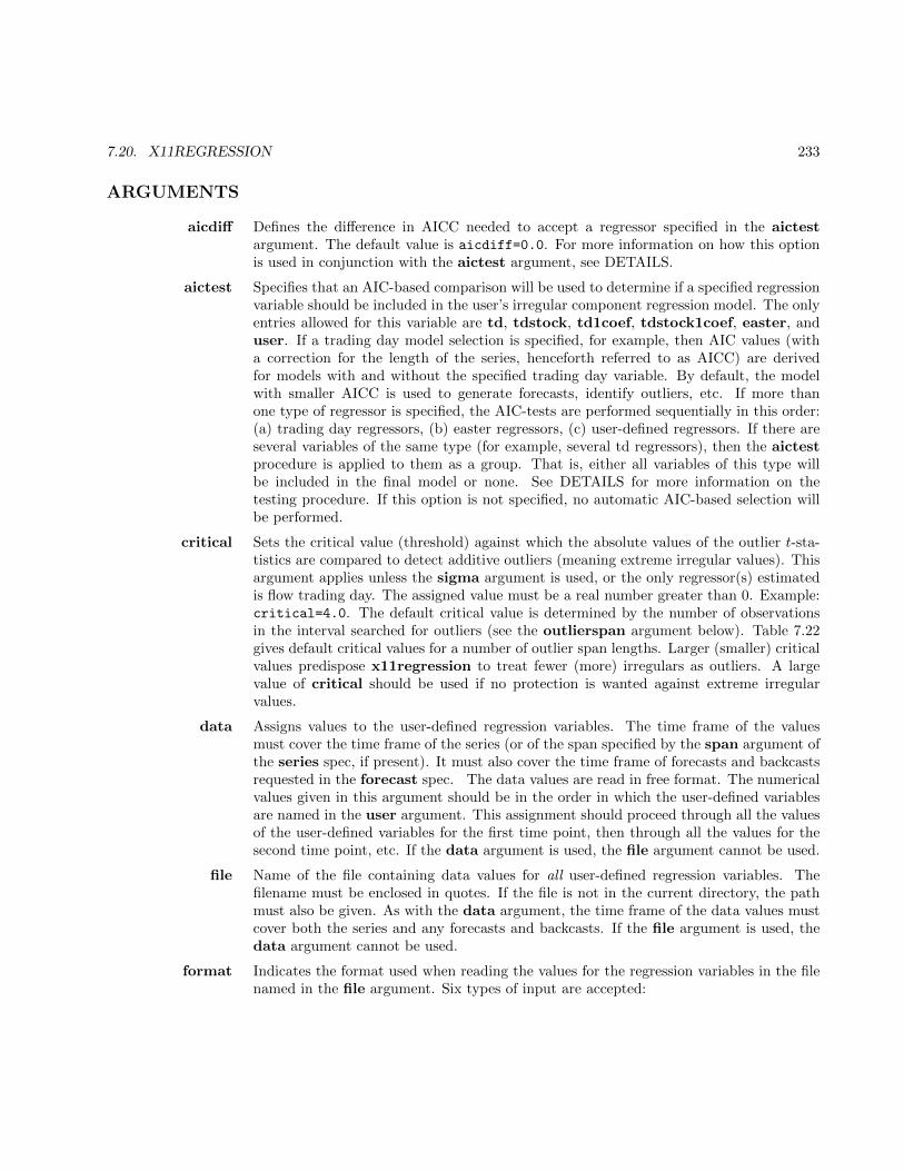
7.20. X11REGRESSION 233
ARGUMENTS
aicdiff Defines the difference in AICC needed to accept a regressor specified in the aictestargument. The default value is aicdiff=0.0. For more information on how this optionis used in conjunction with the aictest argument, see DETAILS.
aictest Specifies that an AIC-based comparison will be used to determine if a specified regressionvariable should be included in the user’s irregular component regression model. The onlyentries allowed for this variable are td, tdstock, td1coef, tdstock1coef, easter, anduser. If a trading day model selection is specified, for example, then AIC values (witha correction for the length of the series, henceforth referred to as AICC) are derivedfor models with and without the specified trading day variable. By default, the modelwith smaller AICC is used to generate forecasts, identify outliers, etc. If more thanone type of regressor is specified, the AIC-tests are performed sequentially in this order:(a) trading day regressors, (b) easter regressors, (c) user-defined regressors. If there areseveral variables of the same type (for example, several td regressors), then the aictestprocedure is applied to them as a group. That is, either all variables of this type willbe included in the final model or none. See DETAILS for more information on thetesting procedure. If this option is not specified, no automatic AIC-based selection willbe performed.
critical Sets the critical value (threshold) against which the absolute values of the outlier t-sta-tistics are compared to detect additive outliers (meaning extreme irregular values). Thisargument applies unless the sigma argument is used, or the only regressor(s) estimatedis flow trading day. The assigned value must be a real number greater than 0. Example:critical=4.0. The default critical value is determined by the number of observationsin the interval searched for outliers (see the outlierspan argument below). Table 7.22gives default critical values for a number of outlier span lengths. Larger (smaller) criticalvalues predispose x11regression to treat fewer (more) irregulars as outliers. A largevalue of critical should be used if no protection is wanted against extreme irregularvalues.
data Assigns values to the user-defined regression variables. The time frame of the valuesmust cover the time frame of the series (or of the span specified by the span argument ofthe series spec, if present). It must also cover the time frame of forecasts and backcastsrequested in the forecast spec. The data values are read in free format. The numericalvalues given in this argument should be in the order in which the user-defined variablesare named in the user argument. This assignment should proceed through all the valuesof the user-defined variables for the first time point, then through all the values for thesecond time point, etc. If the data argument is used, the file argument cannot be used.
file Name of the file containing data values for all user-defined regression variables. Thefilename must be enclosed in quotes. If the file is not in the current directory, the pathmust also be given. As with the data argument, the time frame of the data values mustcover both the series and any forecasts and backcasts. If the file argument is used, thedata argument cannot be used.
format Indicates the format used when reading the values for the regression variables in the filenamed in the file argument. Six types of input are accepted:

234 CHAPTER 7. DOCUMENTATION FOR INDIVIDUAL SPECS
a. free format, in which all numbers on a line will be read before continuing to the nextline, and the numbers must be separated by one or more spaces (not by commas ortabs) (format="free");
b. a valid Fortran format, which must be enclosed in quotes and must include theinitial and terminal parentheses (format="(6f12.0)");
c. “datevalue” format, in which the year, month or quarter, and the associated valuesfor each of the user-defined regression variables for a given observation are given,in this order, in free format on individual lines in the data file. Thus, a line of thedata file with three regressors having the values 0, 0, and 1 respectively for Julyof 1991 would have the form 1991 7 0 0 1. All the user-defined regressors mustbe on the same record, and in the order of their appearance in the user argument(format="datevalue");
d. the “x13save” format X-13ARIMA-SEATS uses to save a table. This allows the userto read in a file saved from a previous X-13ARIMA-SEATS run (format="x13save")7.
e. a variant of “free” format where the numbers must be separated by one or morespaces (not by commas or tabs), and decimal points are expressed as commas (aconvention in some European countries). (format="freecomma");
f. a variant of “datevalue” format, where the year, month or quarter, and valueof each observation are found in this order in free format on individual lines,where decimal points are expressed as commas. Thus, a line of the data file withthree regressors having the values 0.5, 0, and 1.25 respectively for July of 1991would have the form 1991 7 0,5 0 1,25. All the user-defined regressors must beon the same record, and in the order of their appearance in the user argument(format="datevaluecomma").
If no format argument is given the data will be read in free format. In free format, allnumbers on a line will be read before continuing to the next line, and the numbers mustbe separated by one or more spaces (not by commas or tabs). Format cannot be usedwith the data argument, only with file.
outliermethod Determines how the program successively adds detected outliers to the model. Thechoices are method = addone or method = addall. See the DETAILS section of theoutlier spec for a description of these two methods. The default is method = addone.This argument cannot be used if the sigma argument is used.
outlierspan Specifies start and end dates of the span of the irregular component to be searched foroutliers. The start and end dates of the span must both lie within the series, and thestart date must precede the end date. A missing value, e.g., outlierspan = (1976.jan,
), defaults to the start date or end date of the series, as appropriate. (If there is a spanargument in the series spec, then, in the above remarks, replace the start and end datesof the series by the start and end dates of the span given in the series spec.) Thisargument cannot be used with the sigma argument.
7Note that to maintain compatability with previous versions of X-12-ARIMA the entry x12save will also be accepted.
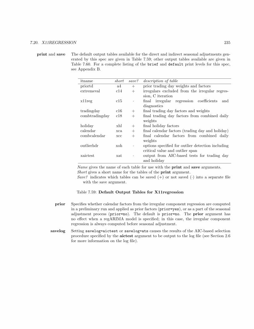
7.20. X11REGRESSION 235
print and save The default output tables available for the direct and indirect seasonal adjustments gen-erated by this spec are given in Table 7.59; other output tables available are given inTable 7.60. For a complete listing of the brief and default print levels for this spec,see Appendix B.
itname short save? description of tablepriortd a4 + prior trading day weights and factorsextremeval c14 + irregulars excluded from the irregular regres-
sion, C iterationx11reg c15 · final irregular regression coefficients and
diagnosticstradingday c16 + final trading day factors and weightscombtradingday c18 + final trading day factors from combined daily
weightsholiday xhl + final holiday factorscalendar xca + final calendar factors (trading day and holiday)combcalendar xcc + final calendar factors from combined daily
weightsoutlierhdr xoh · options specified for outlier detection including
critical value and outlier spanxaictest xat · output from AIC-based tests for trading day
and holiday
Name gives the name of each table for use with the print and save arguments.Short gives a short name for the tables of the print argument.Save? indicates which tables can be saved (+) or not saved (·) into a separate file
with the save argument.
Table 7.59: Default Output Tables for X11regression
prior Specifies whether calendar factors from the irregular component regression are computedin a preliminary run and applied as prior factors (prior=yes), or as a part of the seasonaladjustment process (prior=no). The default is prior=no. The prior argument hasno effect when a regARIMA model is specified; in this case, the irregular componentregression is always computed before seasonal adjustment.
savelog Setting savelog=aictest or savelog=ats causes the results of the AIC-based selectionprocedure specified by the aictest argument to be output to the log file (see Section 2.6for more information on the log file).
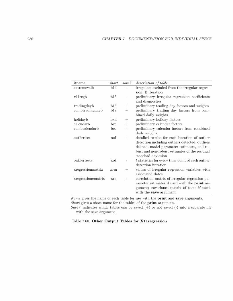
236 CHAPTER 7. DOCUMENTATION FOR INDIVIDUAL SPECS
itname short save? description of tableextremevalb b14 + irregulars excluded from the irregular regres-
sion, B iterationx11regb b15 · preliminary irregular regression coefficients
and diagnosticstradingdayb b16 + preliminary trading day factors and weightscombtradingdayb b18 + preliminary trading day factors from com-
bined daily weightsholidayb bxh + preliminary holiday factorscalendarb bxc + preliminary calendar factorscombcalendarb bcc + preliminary calendar factors from combined
daily weightsoutlieriter xoi + detailed results for each iteration of outlier
detection including outliers detected, outliersdeleted, model parameter estimates, and ro-bust and non-robust estimates of the residualstandard deviation
outliertests xot · t-statistics for every time point of each outlierdetection iteration
xregressionmatrix xrm + values of irregular regression variables withassociated dates
xregressioncmatrix xrc + correlation matrix of irregular regression pa-rameter estimates if used with the print ar-gument; covariance matrix of same if usedwith the save argument
Name gives the name of each table for use with the print and save arguments.Short gives a short name for the tables of the print argument.Save? indicates which tables can be saved (+) or not saved (·) into a separate file
with the save argument.
Table 7.60: Other Output Tables for X11regression

7.20. X11REGRESSION 237
sigma The sigma limit for excluding extreme values of the irregular components before tradingday (only) regression is performed. Irregular values larger than this number of standarddeviations from the mean (1.0 for multiplicative adjustments, 0.0 for additive adjust-ments) are excluded as extreme. Each irregular has a standard error determined by itsmonth (or quarter) type. The month types are determined by the month length, bythe day of the week on which the month starts. This argument cannot be used whenregressors other than flow trading day are present in the model, or when the criticalargument is used. The assigned value must be a real number greater than 0; the defaultis 2.5 (which is invoked only when the flow trading day variable(s) are the only regressorestimated). Example: sigma=3.0.
span Specifies the span (data interval) of irregular component values to be used to estimatethe regression model’s coefficients. This argument can be utilized when, for example,the user does not want data early in the series to affect regression estimates used forpreadjustment before seasonal adjustment. As with the modelspan spec detailed in theseries spec, the span argument has two values, the start and end date of the desiredspan. A missing value defaults to the corresponding start or end date of the span ofthe input series. For example, for monthly data, the statement span=(1968.1, ) causeswhatever irregular regression model is specified to be estimated from the time series datastarting in January, 1968 and ending at the end date of the analysis span. A comma isnecessary if either the start or the end date is missing. The start and end dates of themodel span must both lie within the time span of data specified for analysis in the seriesspec, and the start date must precede the end date.
Another end date specification, with the form 0.per, is available to set the ending dateof span to always be the most recent occurrence of a specific calendar month (quarterfor quarterly data) in the span of data analyzed, where per denotes the calendar month(quarter). Thus, if the span of data considered ends in a month other than December,span=(,0.dec) will cause the regression coefficients to stay fixed at the values obtainedfrom data ending in December of the next-to-final calendar year of the span.
start The start date for the values of the user-defined regression variables. The default is thestart date of the series. Valid values are any date up to the start date of the series (orup to the start date of the span specified by the span argument of the series spec, ifpresent).
tdprior User-input list of seven daily weights, starting with Monday’s weight, which specify adesired X-11 trading day adjustment prior to seasonal adjustment. These weights areadjusted to sum to 7.0 by the program. This option can be used only with multiplicativeand log-additive seasonal adjustments. The values must be real numbers greater than orequal to zero. Example: tdprior=(0.7 0.7 0.7 1.05 1.4 1.4 1.05).
user Specifies the list of names of user-defined regression variables. A name is required for eachuser-defined variable whose coefficients are to be estimated. The names given are used tolabel estimated coefficients in the program’s output. Values for the user-defined variablesmust be supplied, using either the data or the file argument (not both). The maximumnumber of user-defined regression variables is 52. (This limit can be changed—see Section2.8.)
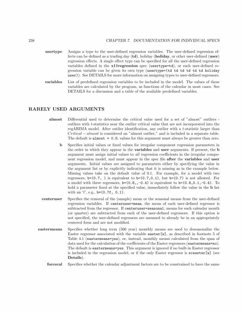
238 CHAPTER 7. DOCUMENTATION FOR INDIVIDUAL SPECS
usertype Assigns a type to the user-defined regression variables. The user-defined regression ef-fects can be defined as a trading day (td), holiday (holiday, or other user-defined (user)regression effects. A single effect type can be specified for all the user-defined regressionvariables defined in the x11regression spec (usertype=td), or each user-defined re-gression variable can be given its own type (usertype=(td td td td td td holiday
user)). See DETAILS for more information on assigning types to user-defined regressors.
variables List of predefined regression variables to be included in the model. The values of thesevariables are calculated by the program, as functions of the calendar in most cases. SeeDETAILS for a discussion and a table of the available predefined variables.
RARELY USED ARGUMENTS
almost Differential used to determine the critical value used for a set of ”almost” outliers -outliers with t-statistics near the outlier critical value that are not incorporated into theregARIMA model. After outlier identification, any outlier with a t-statistic larger thanCritical − almost is considered an ”almost outlier,” and is included in a separate table.The default is almost = 0.5; values for this argument must always be greater than zero.
b Specifies initial values or fixed values for irregular component regression parameters inthe order in which they appear in the variables and user arguments. If present, the bargument must assign initial values to all regression coefficients in the irregular compo-nent regression model, and must appear in the spec file after the variables and userarguments. Initial values are assigned to parameters either by specifying the value inthe argument list or by explicitly indicating that it is missing as in the example below.Missing values take on the default value of 0.1. For example, for a model with tworegressors, b=(0.7, ) is equivalent to b=(0.7,0.1), but b=(0.7) is not allowed. Fora model with three regressors, b=(0.8,,-0.4) is equivalent to b=(0.8,0.1,-0.4). Tohold a parameter fixed at the specified value, immediately follow the value in the b listwith an ‘f’, e.g., b=(0.7f, 0.1).
centeruser Specifies the removal of the (sample) mean or the seasonal means from the user-definedregression variables. If centeruser=mean, the mean of each user-defined regressor issubtracted from the regressor. If centeruser=seasonal, means for each calendar month(or quarter) are subtracted from each of the user-defined regressors. If this option isnot specified, the user-defined regressors are assumed to already be in an appropriatelycentered form and are not modified.
eastermeans Specifies whether long term (500 year) monthly means are used to deseasonalize theEaster regressor associated with the variable easter[w], as described in footnote 5 ofTable 4.1 (eastermeans=yes), or, instead, monthly means calculated from the span ofdata used for the calculation of the coefficients of the Easter regressors (eastermeans=no).The default is eastermeans=yes. This argument is ignored if no built-in Easter regressoris included in the regression model, or if the only Easter regressor is sceaster[w] (seeDetails).
forcecal Specifies whether the calendar adjustment factors are to be constrained to have the same
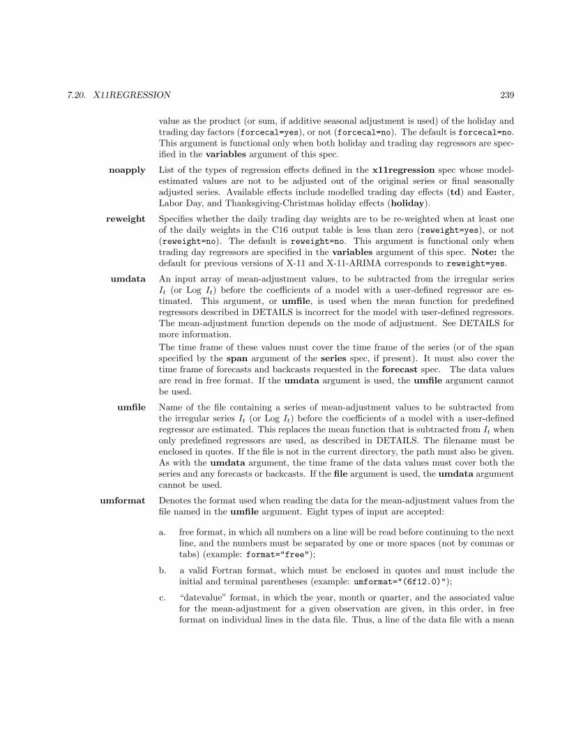
7.20. X11REGRESSION 239
value as the product (or sum, if additive seasonal adjustment is used) of the holiday andtrading day factors (forcecal=yes), or not (forcecal=no). The default is forcecal=no.This argument is functional only when both holiday and trading day regressors are spec-ified in the variables argument of this spec.
noapply List of the types of regression effects defined in the x11regression spec whose model-estimated values are not to be adjusted out of the original series or final seasonallyadjusted series. Available effects include modelled trading day effects (td) and Easter,Labor Day, and Thanksgiving-Christmas holiday effects (holiday).
reweight Specifies whether the daily trading day weights are to be re-weighted when at least oneof the daily weights in the C16 output table is less than zero (reweight=yes), or not(reweight=no). The default is reweight=no. This argument is functional only whentrading day regressors are specified in the variables argument of this spec. Note: thedefault for previous versions of X-11 and X-11-ARIMA corresponds to reweight=yes.
umdata An input array of mean-adjustment values, to be subtracted from the irregular seriesIt (or Log It) before the coefficients of a model with a user-defined regressor are es-timated. This argument, or umfile, is used when the mean function for predefinedregressors described in DETAILS is incorrect for the model with user-defined regressors.The mean-adjustment function depends on the mode of adjustment. See DETAILS formore information.
The time frame of these values must cover the time frame of the series (or of the spanspecified by the span argument of the series spec, if present). It must also cover thetime frame of forecasts and backcasts requested in the forecast spec. The data valuesare read in free format. If the umdata argument is used, the umfile argument cannotbe used.
umfile Name of the file containing a series of mean-adjustment values to be subtracted fromthe irregular series It (or Log It) before the coefficients of a model with a user-definedregressor are estimated. This replaces the mean function that is subtracted from It whenonly predefined regressors are used, as described in DETAILS. The filename must beenclosed in quotes. If the file is not in the current directory, the path must also be given.As with the umdata argument, the time frame of the data values must cover both theseries and any forecasts or backcasts. If the file argument is used, the umdata argumentcannot be used.
umformat Denotes the format used when reading the data for the mean-adjustment values from thefile named in the umfile argument. Eight types of input are accepted:
a. free format, in which all numbers on a line will be read before continuing to the nextline, and the numbers must be separated by one or more spaces (not by commas ortabs) (example: format="free");
b. a valid Fortran format, which must be enclosed in quotes and must include theinitial and terminal parentheses (example: umformat="(6f12.0)");
c. “datevalue” format, in which the year, month or quarter, and the associated valuefor the mean-adjustment for a given observation are given, in this order, in freeformat on individual lines in the data file. Thus, a line of the data file with a mean
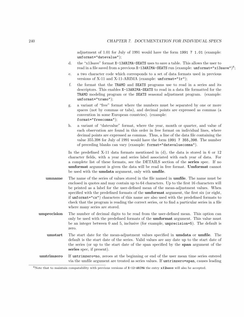
240 CHAPTER 7. DOCUMENTATION FOR INDIVIDUAL SPECS
adjustment of 1.01 for July of 1991 would have the form 1991 7 1.01 (example:umformat="datevalue");
d. the “x13save” format X-13ARIMA-SEATS uses to save a table. This allows the user toread in a file saved from a previous X-13ARIMA-SEATS run (example: umformat="x13save")8;
e. a two character code which corresponds to a set of data formats used in previousversions of X-11 and X-11-ARIMA (example: umformat="1r");
f. the format that the TRAMO and SEATS programs use to read in a series and itsdescriptors. This enables X-13ARIMA-SEATS to read in a data file formatted for theTRAMO modeling program or the SEATS seasonal adjustment program. (example:umformat="tramo");
g. a variant of “free” format where the numbers must be separated by one or morespaces (not by commas or tabs), and decimal points are expressed as commas (aconvention in some European countries). (example:format="freecomma");
h. a variant of “datevalue” format, where the year, month or quarter, and value ofeach observation are found in this order in free format on individual lines, wheredecimal points are expressed as commas. Thus, a line of the data file containing thevalue 355.398 for July of 1991 would have the form 1991 7 355,398. The numberof preceding blanks can vary (example: format="datevaluecomma").
In the predefined X-11 data formats mentioned in (d), the data is stored in 6 or 12character fields, with a year and series label associated with each year of data. Fora complete list of these formats, see the DETAILS section of the series spec. If noumformat argument is given the data will be read in free format. Umformat cannotbe used with the umdata argument, only with umfile.
umname The name of the series of values stored in the file named in umfile. The name must beenclosed in quotes and may contain up to 64 characters. Up to the first 16 characters willbe printed as a label for the user-defined mean of the mean-adjustment values. Whenspecified with the predefined formats of the umformat argument, the first six (or eight,if umformat="cs") characters of this name are also used with the predefined formats tocheck that the program is reading the correct series, or to find a particular series in a filewhere many series are stored.
umprecision The number of decimal digits to be read from the user-defined mean. This option canonly be used with the predefined formats of the umformat argument. This value mustbe an integer between 0 and 5, inclusive (for example, umprecision=5). The default iszero.
umstart The start date for the mean-adjustment values specified in umdata or umfile. Thedefault is the start date of the series. Valid values are any date up to the start date ofthe series (or up to the start date of the span specified by the span argument of theseries spec, if present).
umtrimzero If umtrimzero=no, zeroes at the beginning or end of the user mean time series enteredvia the umfile argument are treated as series values. If umtrimzero=span, causes leading
8Note that to maintain compatability with previous versions of X-12-ARIMA the entry x12save will also be accepted.
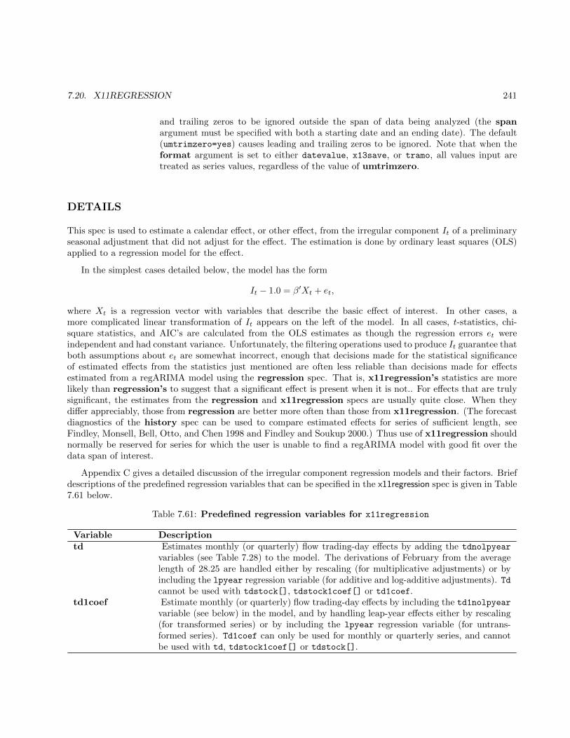
7.20. X11REGRESSION 241
and trailing zeros to be ignored outside the span of data being analyzed (the spanargument must be specified with both a starting date and an ending date). The default(umtrimzero=yes) causes leading and trailing zeros to be ignored. Note that when theformat argument is set to either datevalue, x13save, or tramo, all values input aretreated as series values, regardless of the value of umtrimzero.
DETAILS
This spec is used to estimate a calendar effect, or other effect, from the irregular component It of a preliminaryseasonal adjustment that did not adjust for the effect. The estimation is done by ordinary least squares (OLS)applied to a regression model for the effect.
In the simplest cases detailed below, the model has the form
It − 1.0 = β′Xt + et,
where Xt is a regression vector with variables that describe the basic effect of interest. In other cases, amore complicated linear transformation of It appears on the left of the model. In all cases, t-statistics, chi-square statistics, and AIC’s are calculated from the OLS estimates as though the regression errors et wereindependent and had constant variance. Unfortunately, the filtering operations used to produce It guarantee thatboth assumptions about et are somewhat incorrect, enough that decisions made for the statistical significanceof estimated effects from the statistics just mentioned are often less reliable than decisions made for effectsestimated from a regARIMA model using the regression spec. That is, x11regression’s statistics are morelikely than regression’s to suggest that a significant effect is present when it is not.. For effects that are trulysignificant, the estimates from the regression and x11regression specs are usually quite close. When theydiffer appreciably, those from regression are better more often than those from x11regression. (The forecastdiagnostics of the history spec can be used to compare estimated effects for series of sufficient length, seeFindley, Monsell, Bell, Otto, and Chen 1998 and Findley and Soukup 2000.) Thus use of x11regression shouldnormally be reserved for series for which the user is unable to find a regARIMA model with good fit over thedata span of interest.
Appendix C gives a detailed discussion of the irregular component regression models and their factors. Briefdescriptions of the predefined regression variables that can be specified in the x11regression spec is given in Table7.61 below.
Table 7.61: Predefined regression variables for x11regression
Variable Descriptiontd Estimates monthly (or quarterly) flow trading-day effects by adding the tdnolpyear
variables (see Table 7.28) to the model. The derivations of February from the averagelength of 28.25 are handled either by rescaling (for multiplicative adjustments) or byincluding the lpyear regression variable (for additive and log-additive adjustments). Tdcannot be used with tdstock[], tdstock1coef[] or td1coef.
td1coef Estimate monthly (or quarterly) flow trading-day effects by including the td1nolpyearvariable (see below) in the model, and by handling leap-year effects either by rescaling(for transformed series) or by including the lpyear regression variable (for untrans-formed series). Td1coef can only be used for monthly or quarterly series, and cannotbe used with td, tdstock1coef[] or tdstock[].
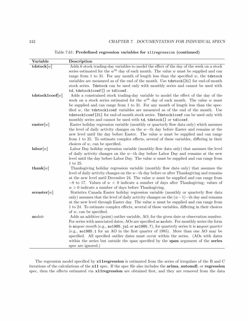
242 CHAPTER 7. DOCUMENTATION FOR INDIVIDUAL SPECS
Table 7.61: Predefined regression variables for x11regression (continued)
Variable Descriptiontdstock[w] Adds 6 stock trading-day variables to model the effect of the day of the week on a stock
series estimated for the wth day of each month. The value w must be supplied and canrange from 1 to 31. For any month of length less than the specified w, the tdstock
variables are measured as of the end of the month. Use tdstock[31] for end-of-monthstock series. Tdstock can be used only with monthly series and cannot be used withtd, tdstock1coef[] or td1coef.
tdstock1coef[w] Adds a constrained stock trading-day variable to model the effect of the day of theweek on a stock series estimated for the wth day of each month. The value w mustbe supplied and can range from 1 to 31. For any month of length less than the spec-ified w, the tdstock1coef variables are measured as of the end of the month. Usetdstock1coef[31] for end-of-month stock series. Tdstock1coef can be used only withmonthly series and cannot be used with td, tdstock[] or td1coef.
easter[w] Easter holiday regression variable (monthly or quarterly flow data only) which assumesthe level of daily activity changes on the w−th day before Easter and remains at thenew level until the day before Easter. The value w must be supplied and can rangefrom 1 to 25. To estimate complex effects, several of these variables, differing in theirchoices of w, can be specified.
labor[w] Labor Day holiday regression variable (monthly flow data only) that assumes the levelof daily activity changes on the w−th day before Labor Day and remains at the newlevel until the day before Labor Day. The value w must be supplied and can range from1 to 25.
thank[w] Thanksgiving holiday regression variable (monthly flow data only) that assumes thelevel of daily activity changes on the w−th day before or after Thanksgiving and remainsat the new level until December 24. The value w must be supplied and can range from−8 to 17. Values of w < 0 indicate a number of days after Thanksgiving; values ofw > 0 indicate a number of days before Thanksgiving.
sceaster[w] Statistics Canada Easter holiday regression variable (monthly or quarterly flow dataonly) assumes that the level of daily activity changes on the (w−1)−th day and remainsat the new level through Easter day. The value w must be supplied and can range from1 to 24. To estimate complex effects, several of these variables, differing in their choicesof w, can be specified.
aodate Adds an additive (point) outlier variable, AO, for the given date or observation number.For series with associated dates, AOs are specified as aodate. For monthly series the formis aoyear.month (e.g., ao1985.jul or ao1985.7), for quarterly series it is aoyear.quarter(e.g., ao1985.1 for an AO in the first quarter of 1985). More than one AO may bespecified. All specified outlier dates must occur within the series. (AOs with dateswithin the series but outside the span specified by the span argument of the seriesspec are ignored.)
The regression model specified by x11regression is estimated from the series of irregulars of the B and Citerations of the calculations of the x11 spec. If the spec file also includes the arima, automdl, or regressionspec, then the effects estimated via x11regression are obtained first, and they are removed from the data
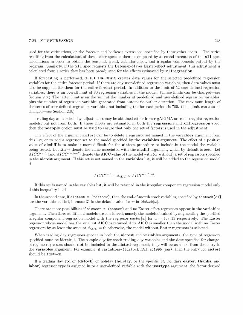
7.20. X11REGRESSION 243
used for the estimations, or the forecast and backcast extensions, specified by these other specs. The seriesresulting from the calculations of these other specs is then decomposed by a second execution of the x11 speccalculations in order to obtain the seasonal, trend, calendar-effect, and irregular components output by theprogram. Similarly, if the x11 spec requests the Bateman-Mayes Easter-effect adjustment, this adjustment iscalculated from a series that has been preadjusted for the effects estimated by x11regression.
If forecasting is performed, X-13ARIMA-SEATS creates data values for the selected predefined regressionvariables for the entire forecast period. If there are any user-defined regression variables, then data values mustalso be supplied for them for the entire forecast period. In addition to the limit of 52 user-defined regressionvariables, there is an overall limit of 80 regression variables in the model. (These limits can be changed—seeSection 2.8.) The latter limit is on the sum of the number of predefined and user-defined regression variables,plus the number of regression variables generated from automatic outlier detection. The maximum length ofthe series of user-defined regression variables, not including the forecast period, is 780. (This limit can also bechanged—see Section 2.8.)
Trading day and/or holiday adjustments may be obtained either from regARIMA or from irregular regressionmodels, but not from both. If these effects are estimated in both the regression and x11regression spec,then the noapply option must be used to ensure that only one set of factors is used in the adjustment.
The effect of the argument aictest can be to delete a regressor set named in the variables argument fromthis list, or to add a regressor set to the model specified by the variables argument. The effect of a positivevalue of aicdiff is to make it more difficult for the aictest procedure to include in the model the variablebeing tested. Let ∆AIC denote the value associated with the aicdiff argument, which by default is zero. LetAICCwith (and AICCwithout) denote the AICC value of the model with (or without) a set of regressors specifiedin the aictest argument. If this set is not named in the variables list, it will be added to the regression modelif
AICCwith + ∆AIC < AICCwithout.
If this set is named in the variables list, it will be retained in the irregular component regression model onlyif this inequality holds.
In the second case, if aictest = (tdstock), then the end-of-month stock variables, specified by tdstock[31],are the variables added, because 31 is the default value for w in tdstock[w].
There are more possibilities if aictest = (easter) and no Easter effect regressors appear in the variablesargument. Then three additional models are considered, namely the models obtained by augmenting the specifiedirregular component regression model with the regressor easter[w] for w = 1, 8, 15 respectively. The Easterregressor whose model has the smallest AICC is retained if its AICC is smaller than the model with no Easterregressors by at least the amount ∆AIC = 0; otherwise, the model without Easter regressors is selected.
When trading day regressors appear in both the aictest and variables arguments, the type of regressorsspecified must be identical. The sample day for stock trading day variables and the date specified for change-of-regime regressors should not be included in the aictest argument; they will be assumed from the entry inthe variables argument. For example, if variables=(tdstock[15] ao1995.jan), then the entry for aictestshould be tdstock.
If a trading day (td or tdstock) or holiday (holiday, or the specific US holidays easter, thanks, andlabor) regressor type is assigned in to a user-defined variable with the usertype argument, the factor derived
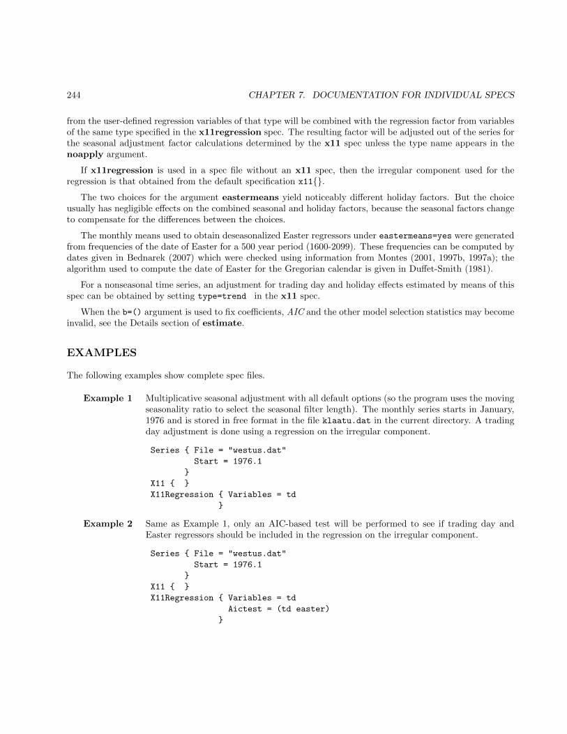
244 CHAPTER 7. DOCUMENTATION FOR INDIVIDUAL SPECS
from the user-defined regression variables of that type will be combined with the regression factor from variablesof the same type specified in the x11regression spec. The resulting factor will be adjusted out of the series forthe seasonal adjustment factor calculations determined by the x11 spec unless the type name appears in thenoapply argument.
If x11regression is used in a spec file without an x11 spec, then the irregular component used for theregression is that obtained from the default specification x11{}.
The two choices for the argument eastermeans yield noticeably different holiday factors. But the choiceusually has negligible effects on the combined seasonal and holiday factors, because the seasonal factors changeto compensate for the differences between the choices.
The monthly means used to obtain deseasonalized Easter regressors under eastermeans=yes were generatedfrom frequencies of the date of Easter for a 500 year period (1600-2099). These frequencies can be computed bydates given in Bednarek (2007) which were checked using information from Montes (2001, 1997b, 1997a); thealgorithm used to compute the date of Easter for the Gregorian calendar is given in Duffet-Smith (1981).
For a nonseasonal time series, an adjustment for trading day and holiday effects estimated by means of thisspec can be obtained by setting type=trend in the x11 spec.
When the b=() argument is used to fix coefficients, AIC and the other model selection statistics may becomeinvalid, see the Details section of estimate.
EXAMPLES
The following examples show complete spec files.
Example 1 Multiplicative seasonal adjustment with all default options (so the program uses the movingseasonality ratio to select the seasonal filter length). The monthly series starts in January,1976 and is stored in free format in the file klaatu.dat in the current directory. A tradingday adjustment is done using a regression on the irregular component.
Series { File = "westus.dat"
Start = 1976.1
}
X11 { }
X11Regression { Variables = td
}
Example 2 Same as Example 1, only an AIC-based test will be performed to see if trading day andEaster regressors should be included in the regression on the irregular component.
Series { File = "westus.dat"
Start = 1976.1
}
X11 { }
X11Regression { Variables = td
Aictest = (td easter)
}

7.20. X11REGRESSION 245
Example 3 User-defined holiday regressors for the period both before and after Easter are included inthe irregular regression along with trading day regressors. AO outlier identification will beperformed during the irregular regression procedure.
series {
file = "ukclothes.dat"
start = 1985.Jan
}
x11 { }
x11regression{
variables = td critical = 4.0
user = (easter1 easter2) file = "ukeaster.dat"
usertype = holiday start = 1980.Jan
}
Example 4 Prior trading day weights are provided with this spec file. The trading day weights calculatedduring the irregular regression will be combined with these weights for a combined tradingday component.
series {
file = "nzstarts.dat" start = 1980.Jan
}
x11 { }
x11regression{
variables = td
tdprior = (1.4 1.4 1.4 1.4 1.4 0.0 0.0)
}
Example 5 Perform a default seasonal adjustment. The trading day regressors in the x11regressionspec will be fixed to their initial values; the Easter holiday regressor will be estimated.
series{
format = ’2R’
title = ’MIDWEST ONE FAMILY Housing Starts’
name = ’CMW1HS’
file = ’cmw1hs.ori’
span = (1964.01,1989.03)
}
x11{ }
x11regression{
variables = (td easter[8])
b = ( 0.4453f 0.8550f -0.3012f 0.2717f
-0.1705f 0.0983f -0.0082)
}
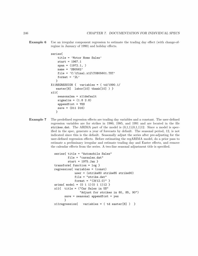
246 CHAPTER 7. DOCUMENTATION FOR INDIVIDUAL SPECS
Example 6 Use an irregular component regression to estimate the trading day effect (with change-of-regime in January of 1990) and holiday effects.
series{
title = ’Motor Home Sales’
start = 1967.1
span = (1972.1, )
name = ’SB0562’
file = ’C:\final.x12\T0B05601.TXT’
format = ’2L’
}
X11REGRESSION { variables = ( td/1990.1/
easter[8] labor[10] thank[10] ) }
x11{
seasonalma = x11default
sigmalim = (1.8 2.8)
appendfcst = YES
save = (D11 D16)
}
Example 7 The predefined regression effects are trading day variables and a constant. The user-definedregression variables are for strikes in 1980, 1985, and 1991 and are located in the filestrikes.dat. The ARIMA part of the model is (0,1,1)(0,1,1)12. Since a model is spec-ified in the spec, generate a year of forecasts by default. The seasonal period, 12, is notindicated since this is the default. Seasonally adjust the series after pre-adjusting for theuser-defined regression effects. Before estimating the regARIMA model, do a prior pass toestimate a preliminary irregular and estimate trading day and Easter effects, and removethe calendar effects from the series. A two-line seasonal adjustment title is specified.
series{ title = "Automobile Sales"
file = "carsales.dat"
start = 1975.Jan }
transform{ function = log }
regression{ variables = (const)
user = (strike80 strike85 strike90)
file = "strike.dat"
format = "(3f12.0)" }
arima{ model = (0 1 1)(0 1 1)12 }
x11{ title = ("Car Sales in US"
"Adjust for strikes in 80, 85, 90")
save = seasonal appendfcst = yes
}
x11regression{ variables = ( td easter[8] ) }
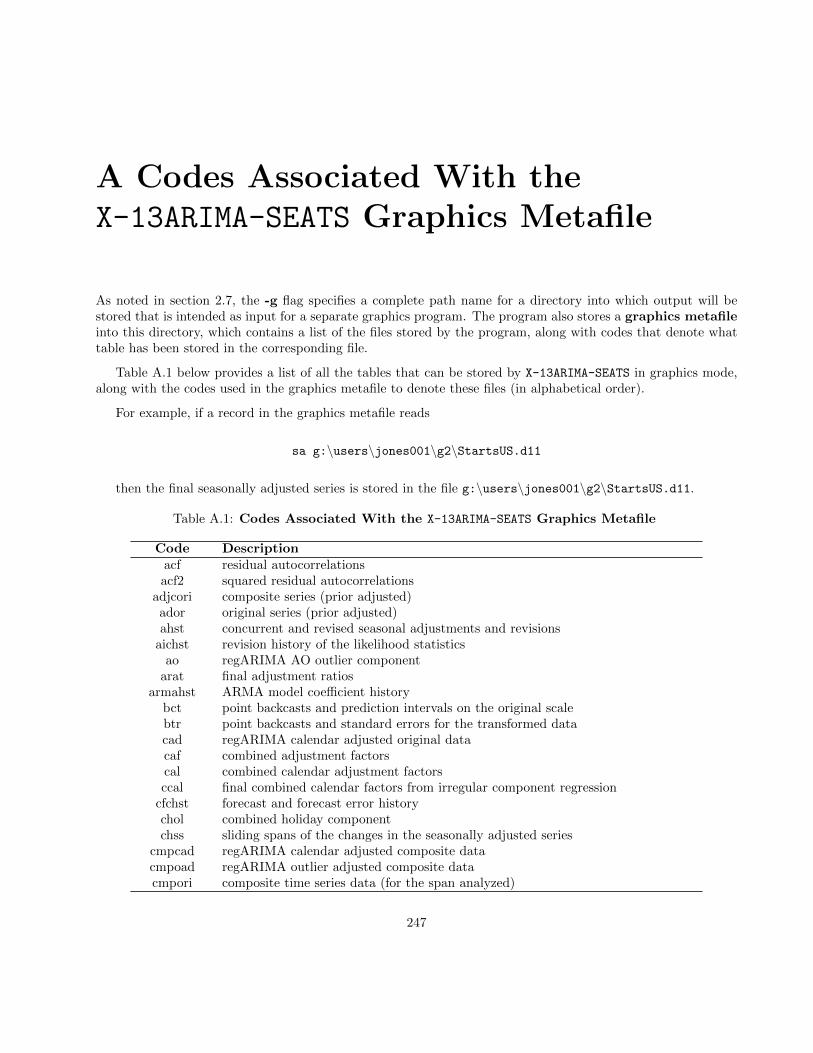
A Codes Associated With theX-13ARIMA-SEATS Graphics Metafile
As noted in section 2.7, the -g flag specifies a complete path name for a directory into which output will bestored that is intended as input for a separate graphics program. The program also stores a graphics metafileinto this directory, which contains a list of the files stored by the program, along with codes that denote whattable has been stored in the corresponding file.
Table A.1 below provides a list of all the tables that can be stored by X-13ARIMA-SEATS in graphics mode,along with the codes used in the graphics metafile to denote these files (in alphabetical order).
For example, if a record in the graphics metafile reads
sa g:\users\jones001\g2\StartsUS.d11
then the final seasonally adjusted series is stored in the file g:\users\jones001\g2\StartsUS.d11.
Table A.1: Codes Associated With the X-13ARIMA-SEATS Graphics Metafile
Code Descriptionacf residual autocorrelationsacf2 squared residual autocorrelations
adjcori composite series (prior adjusted)ador original series (prior adjusted)ahst concurrent and revised seasonal adjustments and revisions
aichst revision history of the likelihood statisticsao regARIMA AO outlier component
arat final adjustment ratiosarmahst ARMA model coefficient history
bct point backcasts and prediction intervals on the original scalebtr point backcasts and standard errors for the transformed datacad regARIMA calendar adjusted original datacaf combined adjustment factorscal combined calendar adjustment factorsccal final combined calendar factors from irregular component regression
cfchst forecast and forecast error historychol combined holiday componentchss sliding spans of the changes in the seasonally adjusted series
cmpcad regARIMA calendar adjusted composite datacmpoad regARIMA outlier adjusted composite datacmpori composite time series data (for the span analyzed)
247
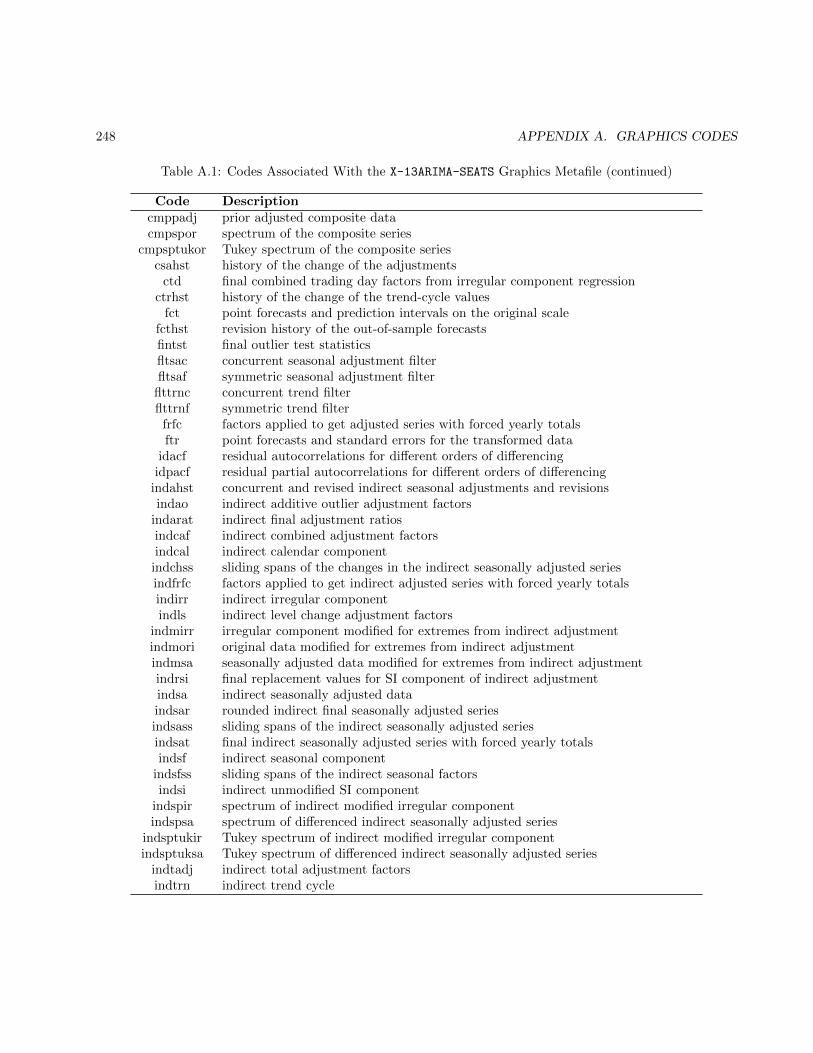
248 APPENDIX A. GRAPHICS CODES
Table A.1: Codes Associated With the X-13ARIMA-SEATS Graphics Metafile (continued)
Code Descriptioncmppadj prior adjusted composite datacmpspor spectrum of the composite series
cmpsptukor Tukey spectrum of the composite seriescsahst history of the change of the adjustments
ctd final combined trading day factors from irregular component regressionctrhst history of the change of the trend-cycle values
fct point forecasts and prediction intervals on the original scalefcthst revision history of the out-of-sample forecastsfintst final outlier test statisticsfltsac concurrent seasonal adjustment filterfltsaf symmetric seasonal adjustment filter
flttrnc concurrent trend filterflttrnf symmetric trend filter
frfc factors applied to get adjusted series with forced yearly totalsftr point forecasts and standard errors for the transformed data
idacf residual autocorrelations for different orders of differencingidpacf residual partial autocorrelations for different orders of differencing
indahst concurrent and revised indirect seasonal adjustments and revisionsindao indirect additive outlier adjustment factors
indarat indirect final adjustment ratiosindcaf indirect combined adjustment factorsindcal indirect calendar componentindchss sliding spans of the changes in the indirect seasonally adjusted seriesindfrfc factors applied to get indirect adjusted series with forced yearly totalsindirr indirect irregular componentindls indirect level change adjustment factors
indmirr irregular component modified for extremes from indirect adjustmentindmori original data modified for extremes from indirect adjustmentindmsa seasonally adjusted data modified for extremes from indirect adjustmentindrsi final replacement values for SI component of indirect adjustmentindsa indirect seasonally adjusted dataindsar rounded indirect final seasonally adjusted seriesindsass sliding spans of the indirect seasonally adjusted seriesindsat final indirect seasonally adjusted series with forced yearly totalsindsf indirect seasonal component
indsfss sliding spans of the indirect seasonal factorsindsi indirect unmodified SI component
indspir spectrum of indirect modified irregular componentindspsa spectrum of differenced indirect seasonally adjusted series
indsptukir Tukey spectrum of indirect modified irregular componentindsptuksa Tukey spectrum of differenced indirect seasonally adjusted series
indtadj indirect total adjustment factorsindtrn indirect trend cycle
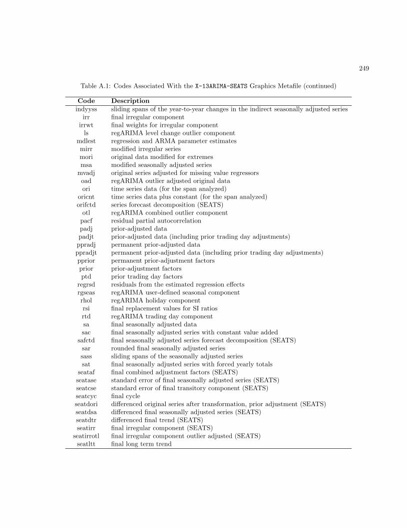
249
Table A.1: Codes Associated With the X-13ARIMA-SEATS Graphics Metafile (continued)
Code Descriptionindyyss sliding spans of the year-to-year changes in the indirect seasonally adjusted series
irr final irregular componentirrwt final weights for irregular component
ls regARIMA level change outlier componentmdlest regression and ARMA parameter estimatesmirr modified irregular seriesmori original data modified for extremesmsa modified seasonally adjusted series
mvadj original series adjusted for missing value regressorsoad regARIMA outlier adjusted original dataori time series data (for the span analyzed)
oricnt time series data plus constant (for the span analyzed)orifctd series forecast decomposition (SEATS)
otl regARIMA combined outlier componentpacf residual partial autocorrelationpadj prior-adjusted datapadjt prior-adjusted data (including prior trading day adjustments)
ppradj permanent prior-adjusted datappradjt permanent prior-adjusted data (including prior trading day adjustments)pprior permanent prior-adjustment factorsprior prior-adjustment factorsptd prior trading day factors
regrsd residuals from the estimated regression effectsrgseas regARIMA user-defined seasonal componentrhol regARIMA holiday componentrsi final replacement values for SI ratiosrtd regARIMA trading day componentsa final seasonally adjusted datasac final seasonally adjusted series with constant value added
safctd final seasonally adjusted series forecast decomposition (SEATS)sar rounded final seasonally adjusted seriessass sliding spans of the seasonally adjusted seriessat final seasonally adjusted series with forced yearly totals
seataf final combined adjustment factors (SEATS)seatase standard error of final seasonally adjusted series (SEATS)seatcse standard error of final transitory component (SEATS)seatcyc final cycleseatdori differenced original series after transformation, prior adjustment (SEATS)seatdsa differenced final seasonally adjusted series (SEATS)seatdtr differenced final trend (SEATS)seatirr final irregular component (SEATS)
seatirrotl final irregular component outlier adjusted (SEATS)seatltt final long term trend
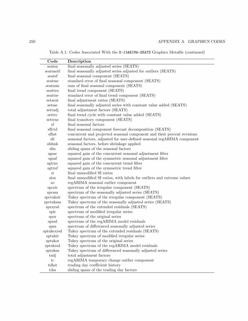
250 APPENDIX A. GRAPHICS CODES
Table A.1: Codes Associated With the X-13ARIMA-SEATS Graphics Metafile (continued)
Code Descriptionseatsa final seasonally adjusted series (SEATS)
seatsaotl final seasonally adjusted series adjusted for outliers (SEATS)seatsf final seasonal component (SEATS)seatsse standard error of final seasonal component (SEATS)seatssm sum of final seasonal component (SEATS)seattrn final trend component (SEATS)seattse standard error of final trend component (SEATS)setarat final adjustment ratios (SEATS)setsac final seasonally adjusted series with constant value added (SEATS)settadj total adjustment factors (SEATS)settrc final trend cycle with constant value added (SEATS)settrns final transitory component (SEATS)
sf final seasonal factorssffctd final seasonal component forecast decomposition (SEATS)sfhst concurrent and projected seasonal component and their percent revisionssfr seasonal factors, adjusted for user-defined seasonal regARIMA component
sfshnk seasonal factors, before shrinkage appliedsfss sliding spans of the seasonal factors
sgsac squared gain of the concurrent seasonal adjustment filtersgsaf squared gain of the symmetric seasonal adjustment filter
sgtrnc squared gain of the concurrent trend filtersgtrnf squared gain of the symmetric trend filter
si final unmodified SI ratiossiox final unmodified SI ratios, with labels for outliers and extreme valuesso regARIMA seasonal outlier component
spcsir spectrum of the irregular component (SEATS)spcssa spectrum of the seasonally adjusted series (SEATS)
spctuksir Tukey spectrum of the irregular component (SEATS)spctukssa Tukey spectrum of the seasonally adjusted series (SEATS)spexrsd spectrum of the extended residuals (SEATS)
spir spectrum of modified irregular seriesspor spectrum of the original seriessprsd spectrum of the regARIMA model residualsspsa spectrum of differenced seasonally adjusted series
sptukexrsd Tukey spectrum of the extended residuals (SEATS)sptukir Tukey spectrum of modified irregular seriessptukor Tukey spectrum of the original seriessptukrsd Tukey spectrum of the regARIMA model residualssptuksa Tukey spectrum of differenced seasonally adjusted series
tadj total adjustment factorstc regARIMA temporary change outlier component
tdhst trading day coefficient historytdss sliding spans of the trading day factors
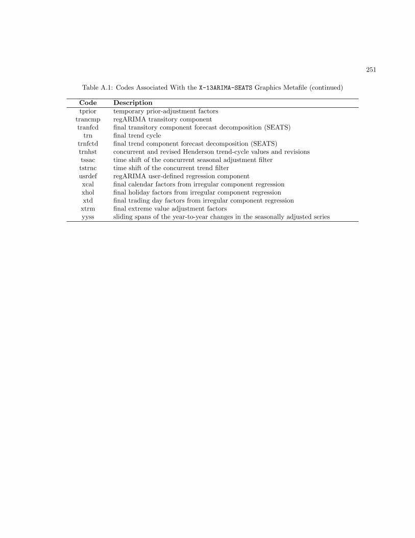
251
Table A.1: Codes Associated With the X-13ARIMA-SEATS Graphics Metafile (continued)
Code Descriptiontprior temporary prior-adjustment factors
trancmp regARIMA transitory componenttranfcd final transitory component forecast decomposition (SEATS)
trn final trend cycletrnfctd final trend component forecast decomposition (SEATS)trnhst concurrent and revised Henderson trend-cycle values and revisionstssac time shift of the concurrent seasonal adjustment filtertstrnc time shift of the concurrent trend filterusrdef regARIMA user-defined regression componentxcal final calendar factors from irregular component regressionxhol final holiday factors from irregular component regressionxtd final trading day factors from irregular component regression
xtrm final extreme value adjustment factorsyyss sliding spans of the year-to-year changes in the seasonally adjusted series

B Print and Save Tables
ContentsB.1 Print and Save Tables Available for X-13ARIMA-SEATS specs . . . . . . . . . . . . . . 252
B.2 Special Output Related to the seats Spec . . . . . . . . . . . . . . . . . . . . . . . . 261
B.3 Special Output Related to the spectrum Spec . . . . . . . . . . . . . . . . . . . . . . 263
B.4 Special tables Used to Save X-13ARIMA-SEATS Output as Percentages . . . . . . . . 263
TablesB.2 Output Tables for Seats spec that can Only be Saved . . . . . . . . . . . . . . . . . . 261
B.3 X-13ARIMA-SEATS File Extensions for Special SEATS Saved Output . . . . . . . . . . 262
B.4 Components to be saved in .tbs file . . . . . . . . . . . . . . . . . . . . . . . . . . . . . . 262
B.5 Output Tables for Spectrum Spec That Can Only be Saved . . . . . . . . . . . . . . 263
B.6 Tables That Can Be Saved as Percentages in the save Argument . . . . . . . . . . . 264
This appendix contains listing of the various output tables that can be printed or saved using the X-13-
ARIMA-SEATS program.
Table B.1 contains a list of tables that are available for printing and saving using the print and savearguments of the individual specs.
A listing of special output tables associated with the seats spec is given in Appendix B.2, and a table withspecial output associated with the spectrum spec is given in Appendix B.3.
A listing of special tables that can be saved as percentages is given in Table B.6 in Appendix B.4.
B.1 Print and Save Tables Available for X-13ARIMA-SEATS specs
Name gives the name of each table for use with the print and save arguments.
Short gives a short name for the tables of the print and short arguments. This name is also used as afile extension if the table is saved.
Save? indicates which tables can be saved (+) into a separate file with the save argument.
Brief indicates which tables are printed (+) when the brief print level is specified. See Section 3.2 formore information on print levels.
Default indicates which tables are printed (+) by default.
Spec indicates which spec the tables are defined for.
252
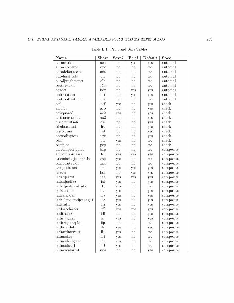
B.1. PRINT AND SAVE TABLES AVAILABLE FOR X-13ARIMA-SEATS SPECS 253
Table B.1: Print and Save Tables
Name Short Save? Brief Default Specautochoice ach no yes yes automdlautochoicemdl amd no no no automdlautodefaulttests adt no no no automdlautofinaltests aft no no no automdlautoljungboxtest alb no no no automdlbestfivemdl b5m no no no automdlheader hdr no yes yes automdlunitroottest urt no yes yes automdlunitroottestmdl urm no no no automdlacf acf yes no yes checkacfplot acp no no yes checkacfsquared ac2 yes no yes checkacfsquaredplot ap2 no no yes checkdurbinwatson dw no no yes checkfriedmantest frt no no yes checkhistogram hst no no yes checknormalitytest nrm no no yes checkpacf pcf yes no no checkpacfplot pcp no no no checkadjcompositeplot b1p no no no compositeadjcompositesrs b1 yes yes yes compositecalendaradjcomposite cac yes no no compositecompositeplot cmp no no no compositecompositesrs cms yes yes yes compositeheader hdr no yes yes compositeindadjsatot iaa yes yes yes compositeindadjustfac iaf yes no yes compositeindadjustmentratio i18 yes no no compositeindaoutlier iao yes no yes compositeindcalendar ica yes no yes compositeindcalendaradjchanges ie8 yes no yes compositeindcratio cri yes no yes compositeindforcefactor iff yes yes yes compositeindftestd8 idf no no yes compositeindirregular iir yes no yes compositeindirregularplot iip no no no compositeindlevelshift ils yes no yes compositeindmcdmovavg if1 yes no no compositeindmodirr ie3 yes no no compositeindmodoriginal ie1 yes no no compositeindmodsadj ie2 yes no no compositeindmovseasrat ims no no yes composite
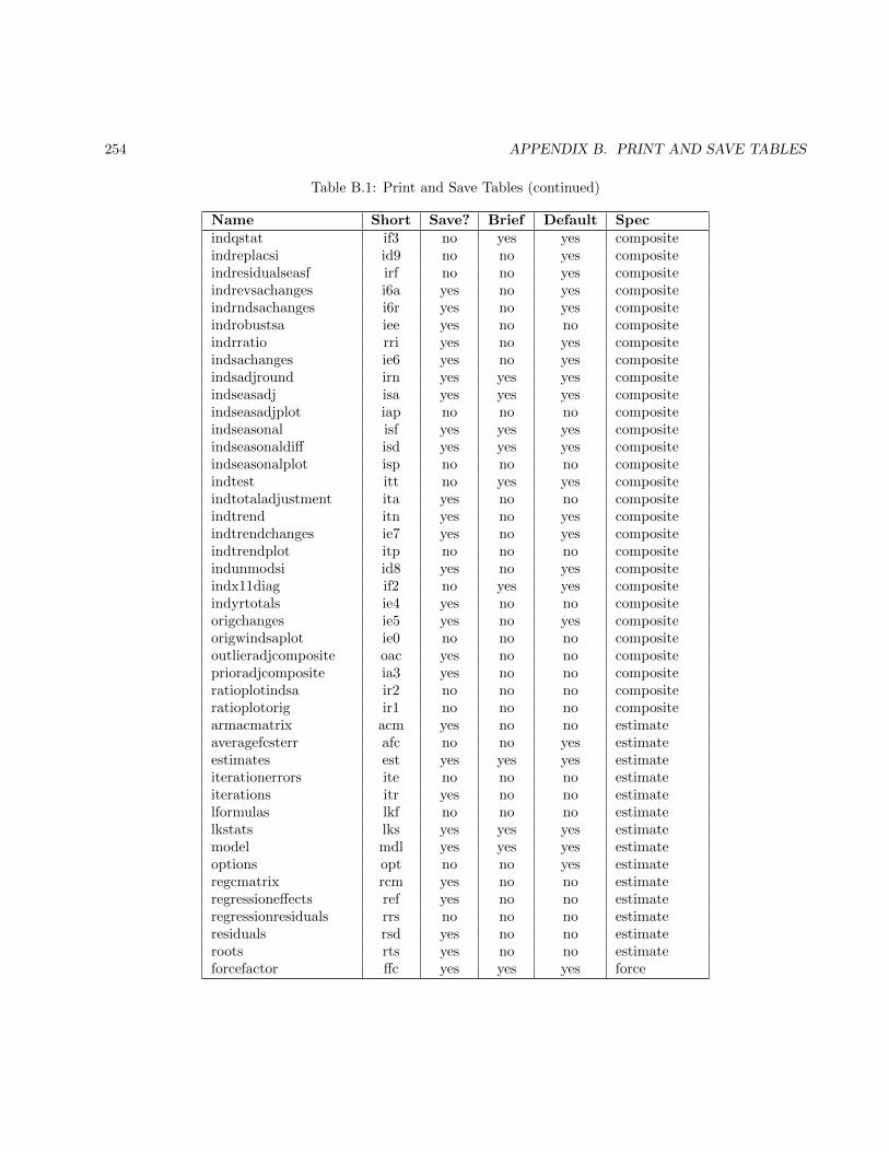
254 APPENDIX B. PRINT AND SAVE TABLES
Table B.1: Print and Save Tables (continued)
Name Short Save? Brief Default Specindqstat if3 no yes yes compositeindreplacsi id9 no no yes compositeindresidualseasf irf no no yes compositeindrevsachanges i6a yes no yes compositeindrndsachanges i6r yes no yes compositeindrobustsa iee yes no no compositeindrratio rri yes no yes compositeindsachanges ie6 yes no yes compositeindsadjround irn yes yes yes compositeindseasadj isa yes yes yes compositeindseasadjplot iap no no no compositeindseasonal isf yes yes yes compositeindseasonaldiff isd yes yes yes compositeindseasonalplot isp no no no compositeindtest itt no yes yes compositeindtotaladjustment ita yes no no compositeindtrend itn yes no yes compositeindtrendchanges ie7 yes no yes compositeindtrendplot itp no no no compositeindunmodsi id8 yes no yes compositeindx11diag if2 no yes yes compositeindyrtotals ie4 yes no no compositeorigchanges ie5 yes no yes compositeorigwindsaplot ie0 no no no compositeoutlieradjcomposite oac yes no no compositeprioradjcomposite ia3 yes no no compositeratioplotindsa ir2 no no no compositeratioplotorig ir1 no no no compositearmacmatrix acm yes no no estimateaveragefcsterr afc no no yes estimateestimates est yes yes yes estimateiterationerrors ite no no no estimateiterations itr yes no no estimatelformulas lkf no no no estimatelkstats lks yes yes yes estimatemodel mdl yes yes yes estimateoptions opt no no yes estimateregcmatrix rcm yes no no estimateregressioneffects ref yes no no estimateregressionresiduals rrs no no no estimateresiduals rsd yes no no estimateroots rts yes no no estimateforcefactor ffc yes yes yes force
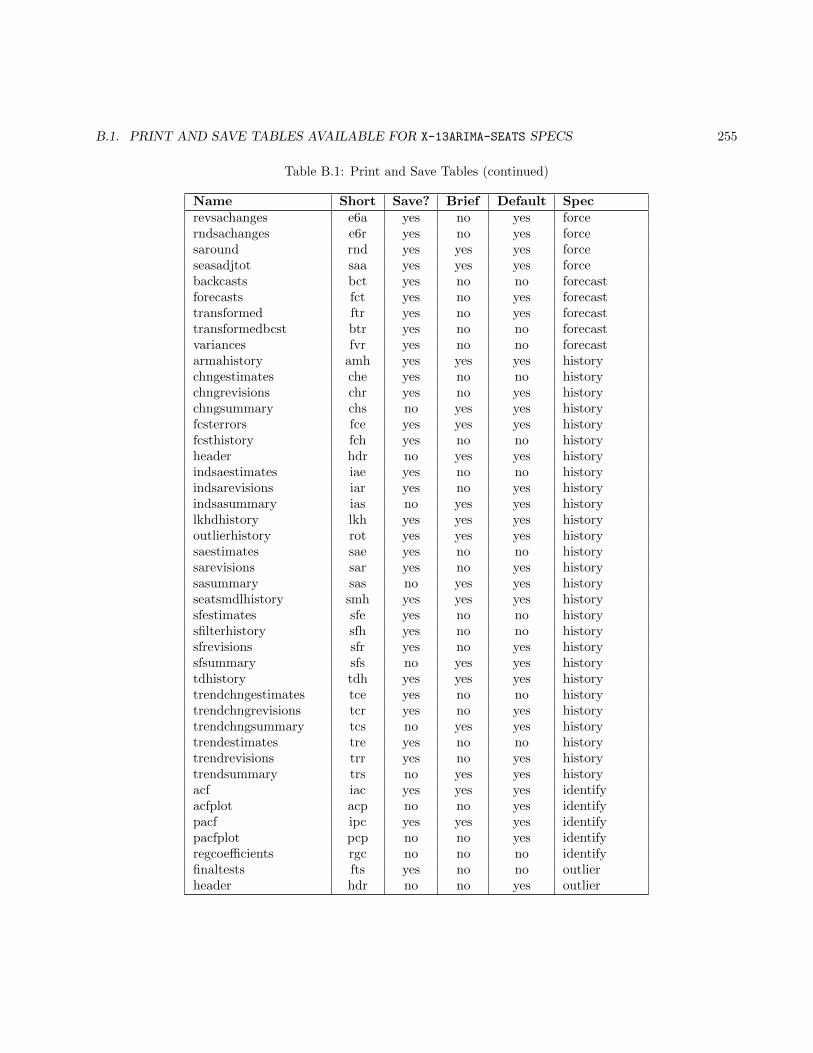
B.1. PRINT AND SAVE TABLES AVAILABLE FOR X-13ARIMA-SEATS SPECS 255
Table B.1: Print and Save Tables (continued)
Name Short Save? Brief Default Specrevsachanges e6a yes no yes forcerndsachanges e6r yes no yes forcesaround rnd yes yes yes forceseasadjtot saa yes yes yes forcebackcasts bct yes no no forecastforecasts fct yes no yes forecasttransformed ftr yes no yes forecasttransformedbcst btr yes no no forecastvariances fvr yes no no forecastarmahistory amh yes yes yes historychngestimates che yes no no historychngrevisions chr yes no yes historychngsummary chs no yes yes historyfcsterrors fce yes yes yes historyfcsthistory fch yes no no historyheader hdr no yes yes historyindsaestimates iae yes no no historyindsarevisions iar yes no yes historyindsasummary ias no yes yes historylkhdhistory lkh yes yes yes historyoutlierhistory rot yes yes yes historysaestimates sae yes no no historysarevisions sar yes no yes historysasummary sas no yes yes historyseatsmdlhistory smh yes yes yes historysfestimates sfe yes no no historysfilterhistory sfh yes no no historysfrevisions sfr yes no yes historysfsummary sfs no yes yes historytdhistory tdh yes yes yes historytrendchngestimates tce yes no no historytrendchngrevisions tcr yes no yes historytrendchngsummary tcs no yes yes historytrendestimates tre yes no no historytrendrevisions trr yes no yes historytrendsummary trs no yes yes historyacf iac yes yes yes identifyacfplot acp no no yes identifypacf ipc yes yes yes identifypacfplot pcp no no yes identifyregcoefficients rgc no no no identifyfinaltests fts yes no no outlierheader hdr no no yes outlier
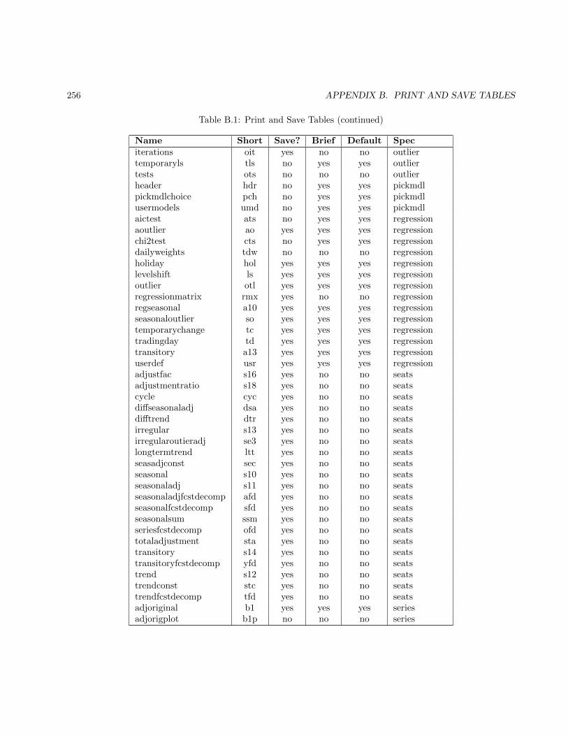
256 APPENDIX B. PRINT AND SAVE TABLES
Table B.1: Print and Save Tables (continued)
Name Short Save? Brief Default Speciterations oit yes no no outliertemporaryls tls no yes yes outliertests ots no no no outlierheader hdr no yes yes pickmdlpickmdlchoice pch no yes yes pickmdlusermodels umd no yes yes pickmdlaictest ats no yes yes regressionaoutlier ao yes yes yes regressionchi2test cts no yes yes regressiondailyweights tdw no no no regressionholiday hol yes yes yes regressionlevelshift ls yes yes yes regressionoutlier otl yes yes yes regressionregressionmatrix rmx yes no no regressionregseasonal a10 yes yes yes regressionseasonaloutlier so yes yes yes regressiontemporarychange tc yes yes yes regressiontradingday td yes yes yes regressiontransitory a13 yes yes yes regressionuserdef usr yes yes yes regressionadjustfac s16 yes no no seatsadjustmentratio s18 yes no no seatscycle cyc yes no no seatsdiffseasonaladj dsa yes no no seatsdifftrend dtr yes no no seatsirregular s13 yes no no seatsirregularoutieradj se3 yes no no seatslongtermtrend ltt yes no no seatsseasadjconst sec yes no no seatsseasonal s10 yes no no seatsseasonaladj s11 yes no no seatsseasonaladjfcstdecomp afd yes no no seatsseasonalfcstdecomp sfd yes no no seatsseasonalsum ssm yes no no seatsseriesfcstdecomp ofd yes no no seatstotaladjustment sta yes no no seatstransitory s14 yes no no seatstransitoryfcstdecomp yfd yes no no seatstrend s12 yes no no seatstrendconst stc yes no no seatstrendfcstdecomp tfd yes no no seatsadjoriginal b1 yes yes yes seriesadjorigplot b1p no no no series
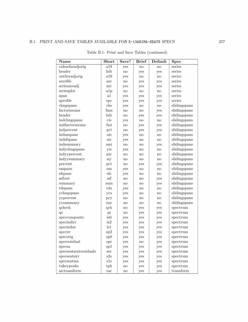
B.1. PRINT AND SAVE TABLES AVAILABLE FOR X-13ARIMA-SEATS SPECS 257
Table B.1: Print and Save Tables (continued)
Name Short Save? Brief Default Speccalendaradjorig a18 yes no no seriesheader hdr no yes yes seriesoutlieradjorig a19 yes no no seriessavefile sav no yes yes seriesseriesmvadj mv yes yes yes seriesseriesplot a1p no no no seriesspan a1 yes yes yes seriesspecfile spc yes yes yes serieschngspans chs yes no no slidingspansfactormeans fmn no no yes slidingspansheader hdr no yes yes slidingspansindchngspans cis yes no no slidingspansindfactormeans fmi no yes yes slidingspansindpercent pci no yes yes slidingspansindsaspans ais yes no no slidingspansindsfspans sis yes no no slidingspansindsummary smi no no yes slidingspansindychngspans yis yes no no slidingspansindyypercent piy no no no slidingspansindyysummary siy no no no slidingspanspercent pct no yes yes slidingspanssaspans sas yes no no slidingspanssfspans sfs yes no no slidingspansssftest ssf no no yes slidingspanssummary sum no no yes slidingspanstdspans tds yes no no slidingspansychngspans ycs yes no no slidingspansyypercent pcy no no no slidingspansyysummary suy no no no slidingspansqcheck qch no yes yes spectrumqs qs no yes yes spectrumspeccomposite is0 yes yes yes spectrumspecindirr is2 yes yes yes spectrumspecindsa is1 yes yes yes spectrumspecirr sp2 yes yes yes spectrumspecorig sp0 yes yes yes spectrumspecresidual spr yes no yes spectrumspecsa sp1 yes yes yes spectrumspecseatsextresiduals ser yes yes yes spectrumspecseatsirr s2s yes yes yes spectrumspecseatssa s1s yes yes yes spectrumtukeypeaks tpk no yes yes spectrumaictransform tac no yes yes transform
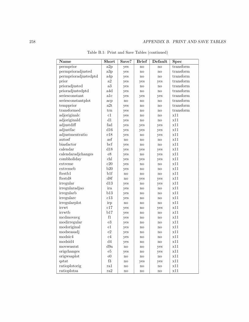
258 APPENDIX B. PRINT AND SAVE TABLES
Table B.1: Print and Save Tables (continued)
Name Short Save? Brief Default Specpermprior a2p yes no no transformpermprioradjusted a3p yes no no transformpermprioradjustedptd a4p yes no no transformprior a2 yes yes yes transformprioradjusted a3 yes no no transformprioradjustedptd a4d yes no no transformseriesconstant a1c yes yes yes transformseriesconstantplot acp no no no transformtempprior a2t yes no no transformtransformed trn yes no no transformadjoriginalc c1 yes no no x11adjoriginald d1 yes no no x11adjustdiff fad yes yes yes x11adjustfac d16 yes yes yes x11adjustmentratio e18 yes no yes x11autosf asf no no no x11biasfactor bcf yes no no x11calendar d18 yes yes yes x11calendaradjchanges e8 yes no yes x11combholiday chl yes yes yes x11extreme c20 yes no no x11extremeb b20 yes no no x11ftestb1 b1f no no no x11ftestd8 d8f no yes yes x11irregular d13 yes no yes x11irregularadjao ira yes no no x11irregularb b13 yes no no x11irregularc c13 yes no no x11irregularplot irp no no no x11irrwt c17 yes no yes x11irrwtb b17 yes no no x11mcdmovavg f1 yes no no x11modirregular e3 yes no no x11modoriginal e1 yes no no x11modseasadj e2 yes no no x11modsic4 c4 yes no no x11modsid4 d4 yes no no x11movseasrat d9a no no yes x11origchanges e5 yes no yes x11origwsaplot e0 no no no x11qstat f3 no yes yes x11ratioplotorig ra1 no no no x11ratioplotsa ra2 no no no x11
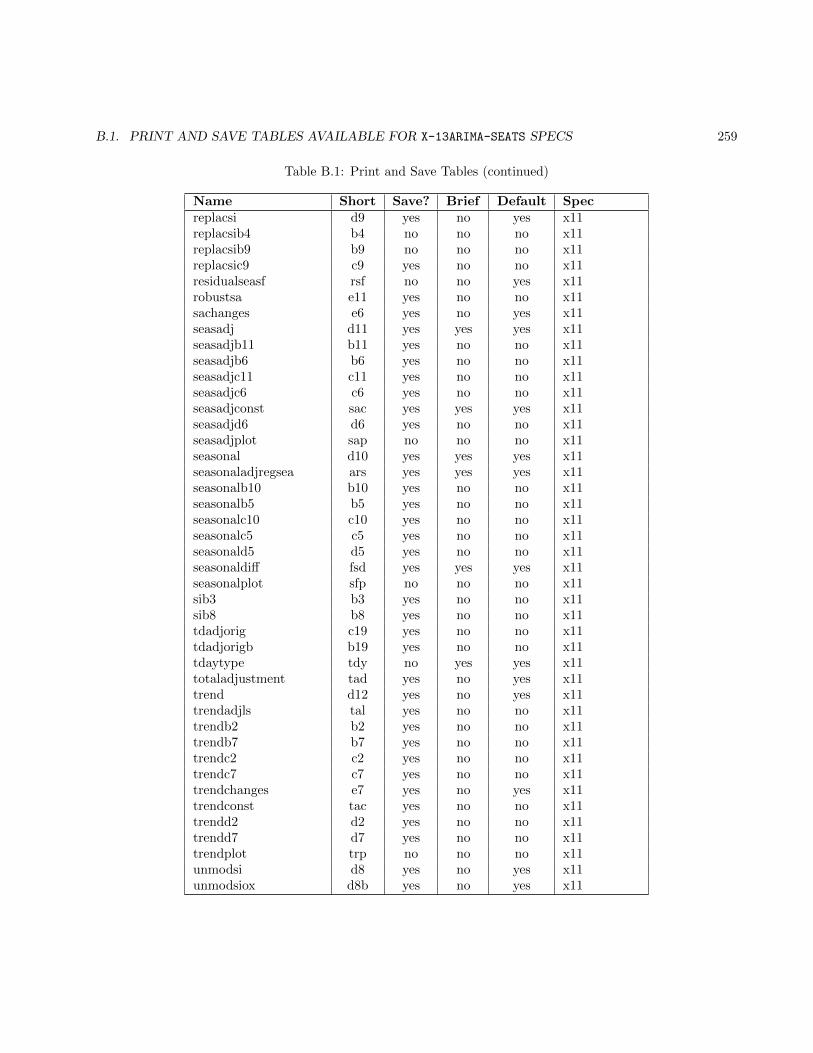
B.1. PRINT AND SAVE TABLES AVAILABLE FOR X-13ARIMA-SEATS SPECS 259
Table B.1: Print and Save Tables (continued)
Name Short Save? Brief Default Specreplacsi d9 yes no yes x11replacsib4 b4 no no no x11replacsib9 b9 no no no x11replacsic9 c9 yes no no x11residualseasf rsf no no yes x11robustsa e11 yes no no x11sachanges e6 yes no yes x11seasadj d11 yes yes yes x11seasadjb11 b11 yes no no x11seasadjb6 b6 yes no no x11seasadjc11 c11 yes no no x11seasadjc6 c6 yes no no x11seasadjconst sac yes yes yes x11seasadjd6 d6 yes no no x11seasadjplot sap no no no x11seasonal d10 yes yes yes x11seasonaladjregsea ars yes yes yes x11seasonalb10 b10 yes no no x11seasonalb5 b5 yes no no x11seasonalc10 c10 yes no no x11seasonalc5 c5 yes no no x11seasonald5 d5 yes no no x11seasonaldiff fsd yes yes yes x11seasonalplot sfp no no no x11sib3 b3 yes no no x11sib8 b8 yes no no x11tdadjorig c19 yes no no x11tdadjorigb b19 yes no no x11tdaytype tdy no yes yes x11totaladjustment tad yes no yes x11trend d12 yes no yes x11trendadjls tal yes no no x11trendb2 b2 yes no no x11trendb7 b7 yes no no x11trendc2 c2 yes no no x11trendc7 c7 yes no no x11trendchanges e7 yes no yes x11trendconst tac yes no no x11trendd2 d2 yes no no x11trendd7 d7 yes no no x11trendplot trp no no no x11unmodsi d8 yes no yes x11unmodsiox d8b yes no yes x11
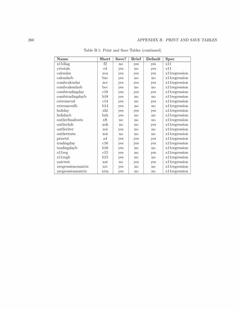
260 APPENDIX B. PRINT AND SAVE TABLES
Table B.1: Print and Save Tables (continued)
Name Short Save? Brief Default Specx11diag f2 no yes yes x11yrtotals e4 yes no yes x11calendar xca yes yes yes x11regressioncalendarb bxc yes no no x11regressioncombcalendar xcc yes yes yes x11regressioncombcalendarb bcc yes no no x11regressioncombtradingday c18 yes yes yes x11regressioncombtradingdayb b18 yes no no x11regressionextremeval c14 yes no yes x11regressionextremevalb b14 yes no no x11regressionholiday xhl yes yes yes x11regressionholidayb bxh yes no no x11regressionoutlierfinaltests xft no no no x11regressionoutlierhdr xoh no no yes x11regressionoutlieriter xoi yes no no x11regressionoutliertests xot no no no x11regressionpriortd a4 yes yes yes x11regressiontradingday c16 yes yes yes x11regressiontradingdayb b16 yes no no x11regressionx11reg c15 yes no yes x11regressionx11regb b15 yes no no x11regressionxaictest xat no yes yes x11regressionxregressioncmatrix xrc yes no no x11regressionxregressionmatrix xrm yes no no x11regression
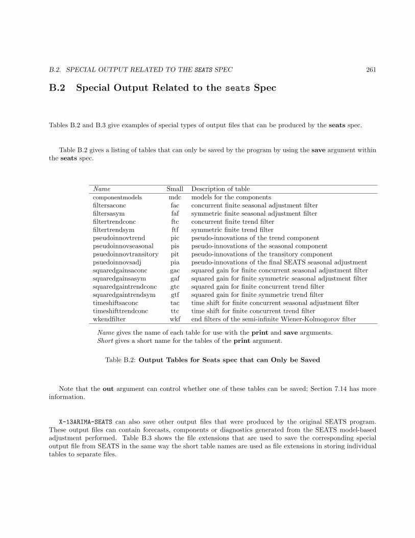
B.2. SPECIAL OUTPUT RELATED TO THE SEATS SPEC 261
B.2 Special Output Related to the seats Spec
Tables B.2 and B.3 give examples of special types of output files that can be produced by the seats spec.
Table B.2 gives a listing of tables that can only be saved by the program by using the save argument withinthe seats spec.
Name Small Description of tablecomponentmodels mdc models for the componentsfiltersaconc fac concurrent finite seasonal adjustment filterfiltersasym faf symmetric finite seasonal adjustment filterfiltertrendconc ftc concurrent finite trend filterfiltertrendsym ftf symmetric finite trend filterpseudoinnovtrend pic pseudo-innovations of the trend componentpseudoinnovseasonal pis pseudo-innovations of the seasonal componentpsuedoinnovtransitory pit pseudo-innovations of the transitory componentpsuedoinnovsadj pia pseudo-innovations of the final SEATS seasonal adjustmentsquaredgainsaconc gac squared gain for finite concurrent seasonal adjustment filtersquaredgainsasym gaf squared gain for finite symmetric seasonal adjustment filtersquaredgaintrendconc gtc squared gain for finite concurrent trend filtersquaredgaintrendsym gtf squared gain for finite symmetric trend filtertimeshiftsaconc tac time shift for finite concurrent seasonal adjustment filtertimeshifttrendconc ttc time shift for finite concurrent trend filterwkendfilter wkf end filters of the semi-infinite Wiener-Kolmogorov filter
Name gives the name of each table for use with the print and save arguments.Short gives a short name for the tables of the print argument.
Table B.2: Output Tables for Seats spec that can Only be Saved
Note that the out argument can control whether one of these tables can be saved; Section 7.14 has moreinformation.
X-13ARIMA-SEATS can also save other output files that were produced by the original SEATS program.These output files can contain forecasts, components or diagnostics generated from the SEATS model-basedadjustment performed. Table B.3 shows the file extensions that are used to save the corresponding specialoutput file from SEATS in the same way the short table names are used as file extensions in storing individualtables to separate files.
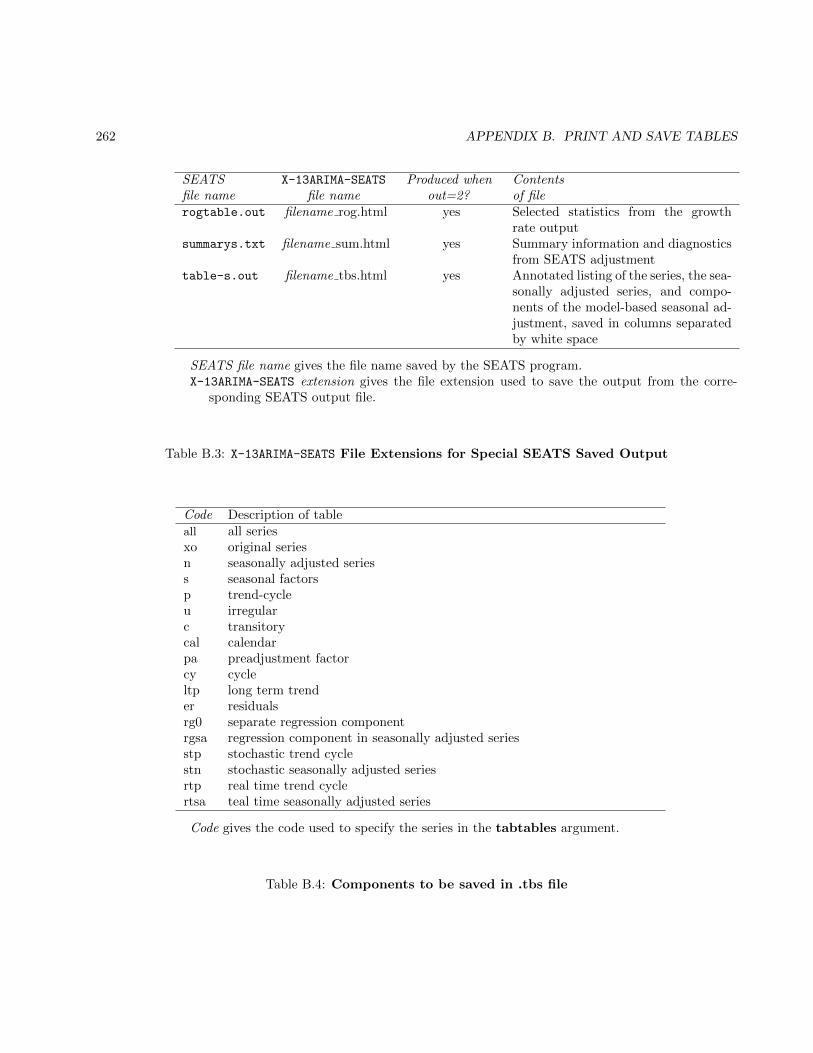
262 APPENDIX B. PRINT AND SAVE TABLES
SEATS X-13ARIMA-SEATS Produced when Contentsfile name file name out=2? of filerogtable.out filename rog.html yes Selected statistics from the growth
rate outputsummarys.txt filename sum.html yes Summary information and diagnostics
from SEATS adjustmenttable-s.out filename tbs.html yes Annotated listing of the series, the sea-
sonally adjusted series, and compo-nents of the model-based seasonal ad-justment, saved in columns separatedby white space
SEATS file name gives the file name saved by the SEATS program.X-13ARIMA-SEATS extension gives the file extension used to save the output from the corre-
sponding SEATS output file.
Table B.3: X-13ARIMA-SEATS File Extensions for Special SEATS Saved Output
Code Description of tableall all seriesxo original seriesn seasonally adjusted seriess seasonal factorsp trend-cycleu irregularc transitorycal calendarpa preadjustment factorcy cycleltp long term trender residualsrg0 separate regression componentrgsa regression component in seasonally adjusted seriesstp stochastic trend cyclestn stochastic seasonally adjusted seriesrtp real time trend cyclertsa teal time seasonally adjusted series
Code gives the code used to specify the series in the tabtables argument.
Table B.4: Components to be saved in .tbs file
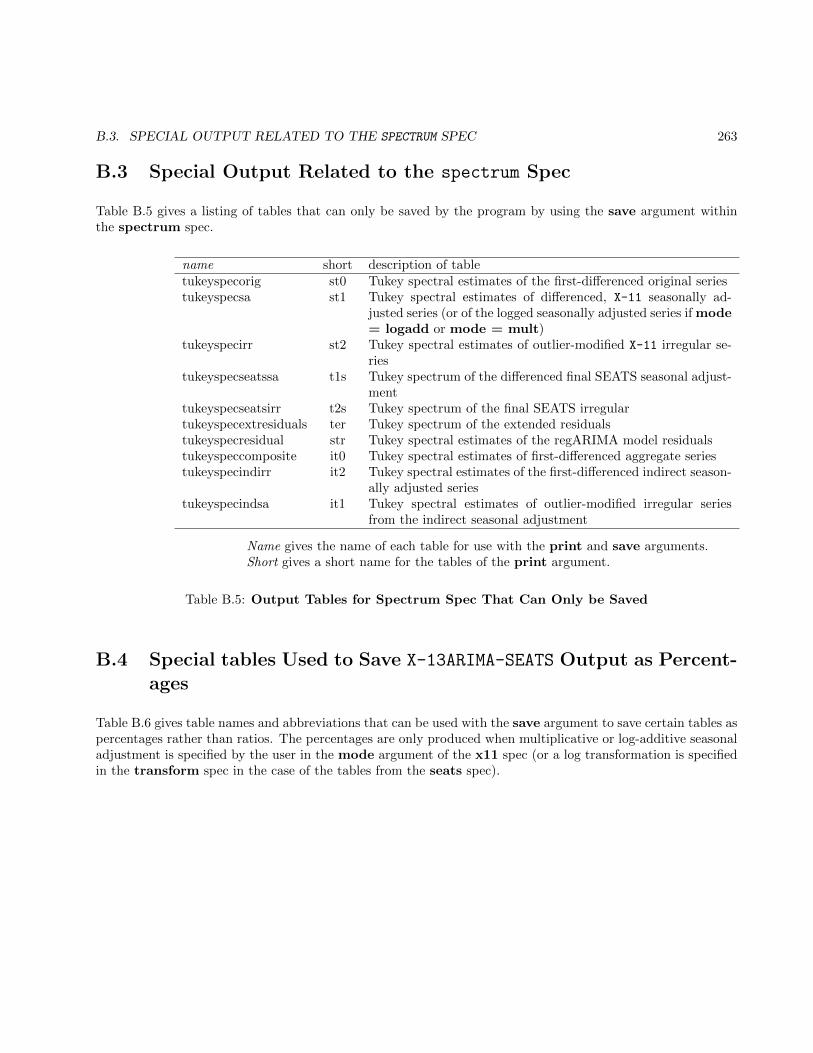
B.3. SPECIAL OUTPUT RELATED TO THE SPECTRUM SPEC 263
B.3 Special Output Related to the spectrum Spec
Table B.5 gives a listing of tables that can only be saved by the program by using the save argument withinthe spectrum spec.
name short description of tabletukeyspecorig st0 Tukey spectral estimates of the first-differenced original seriestukeyspecsa st1 Tukey spectral estimates of differenced, X-11 seasonally ad-
justed series (or of the logged seasonally adjusted series if mode= logadd or mode = mult)
tukeyspecirr st2 Tukey spectral estimates of outlier-modified X-11 irregular se-ries
tukeyspecseatssa t1s Tukey spectrum of the differenced final SEATS seasonal adjust-ment
tukeyspecseatsirr t2s Tukey spectrum of the final SEATS irregulartukeyspecextresiduals ter Tukey spectrum of the extended residualstukeyspecresidual str Tukey spectral estimates of the regARIMA model residualstukeyspeccomposite it0 Tukey spectral estimates of first-differenced aggregate seriestukeyspecindirr it2 Tukey spectral estimates of the first-differenced indirect season-
ally adjusted seriestukeyspecindsa it1 Tukey spectral estimates of outlier-modified irregular series
from the indirect seasonal adjustment
Name gives the name of each table for use with the print and save arguments.Short gives a short name for the tables of the print argument.
Table B.5: Output Tables for Spectrum Spec That Can Only be Saved
B.4 Special tables Used to Save X-13ARIMA-SEATS Output as Percent-ages
Table B.6 gives table names and abbreviations that can be used with the save argument to save certain tables aspercentages rather than ratios. The percentages are only produced when multiplicative or log-additive seasonaladjustment is specified by the user in the mode argument of the x11 spec (or a log transformation is specifiedin the transform spec in the case of the tables from the seats spec).

264 APPENDIX B. PRINT AND SAVE TABLES
name short spec description of tableindadjustfacpct ipa composite indirect combined adjustment factors expressed as
percentages if appropriateindcalendaradjchangespct ip8 composite percent changes in original series adjusted for calen-
dar effectsindirregularpct ipi composite indirect irregular component expressed as percent-
ages if appropriateindrevsachangespct ipf composite percent changes for indirect seasonally adjusted se-
ries with forced yearly totalsindrndsachangespct ipr composite percent changes for rounded indirect seasonally ad-
justed seriesindsachangespct ip6 composite percent changes for indirect seasonally adjusted se-
riesindseasonalpct ips composite indirect seasonal component expressed as percent-
ages if appropriateindtrendchangespct ip7 composite percent changes for indirect trend componentorigchangespct ip5 composite percent changes for composite seriesrevsachangespct p6a force percent changes in seasonally adjusted series with
forced yearly totalsrndsachangespct p6r force percent changes in rounded seasonally adjusted seriesadjustfacpct psa seats combined adjustment factors, expressed as percent-
ages if appropriateirregularpct psi seats final irregular component, expressed as percentages
if appropriatetransitorypct psc seats final transitory component, expressed as percentages
if appropriateseasonalpct pss seats final seasonal factors, expressed as percentages if ap-
propriateadjustfacpct paf x11 combined adjustment factors, expressed as percent-
ages if appropriatecalendaradjchangespct pe8 x11 percent changes in original series adjusted for calen-
dar factorsirregularpct pir x11 final irregular component, expressed as percentages
if appropriateorigchangespct pe5 x11 percent changes in the original seriessachangespct pe6 x11 percent changes in seasonally adjusted seriesseasonalpct psf x11 final seasonal factors, expressed as percentages if ap-
propriatetrendchangespct pe7 x11 percent changes in final trend cycle
Name gives the name of each plot for use with the save arguments.Short gives a short name for the tables of the save argument.Spec indicates which spec the tables are defined for.
Table B.6: Tables That Can Be Saved as Percentages in the save Argument

C Irregular-component RegressionModels Used
ContentsC.1 Irregular regression models for multiplicative decompositions. . . . . . . . . . . . 265
C.1.1 Obtaining separate trading day and holiday factors . . . . . . . . . . . . . . . . . . . . 267
C.1.2 Estimating only holiday effects or stock trading day effects. . . . . . . . . . . . . . . . 268
C.1.3 Estimating user-defined flow trading day and/or holiday effects . . . . . . . . . . . . . 268
C.2 Irregular regression models for other decomposition modes . . . . . . . . . . . . . 269
C.2.1 Additive Decompositions . . . . . . . . . . . . . . . . . . . . . . . . . . . . . . . . . . 269
C.2.2 Pseudo-Additive Decompositions . . . . . . . . . . . . . . . . . . . . . . . . . . . . . . 270
C.2.3 Log-Additive Decompositions . . . . . . . . . . . . . . . . . . . . . . . . . . . . . . . . 270
C.3 When tdprior is used . . . . . . . . . . . . . . . . . . . . . . . . . . . . . . . . . . . . 271
This appendix gives details of the models applied by the X-13ARIMA-SEATS x11regression spec to theirregular component to estimate calendar effects. The regression models detailed in this appendix are used toestimate a calendar effect, or other effect, from the irregular component It of a preliminary seasonal adjustmentthat did not adjust for the effect. The estimation is done by ordinary least squares (OLS) applied to a regressionmodel for the effect. In the simplest cases detailed below, the model has the form
It − 1.0 = β′Xt + et,
where Xt is a regression vector with variables that describe the basic effect of interest.
C.1 Irregular regression models for multiplicative decompositions.
The irregular component is presumed to have no seasonality or trend (beyond a constant level of 1.0, in the caseof a multiplicative decomposition). Hence, the regressors that are used in regression models for the irregularsshould usually not have a seasonal or trend component. For this reason, most trading day and Easter regressionfunctions used in the regression spec (see Tables 4.1 and 7.28) are modified for use in the x11regressionspec (see Table 7.61). The modifications for trading day variables for the various types of seasonal adjustmentdecompositions are derived in section 1.4 of Findley, Monsell, Bell, Otto, and Chen (1998). We will indicate thenature of this modification with a combined monthly flow trading day and holiday regression function of theform
γ0mt +
6∑j=1
γj(dj,t − d7,t) + δ′Ht, (C.1)
where dj,t = no. of weekdays of type j in month t (with j = 1, . . . 7 denoting Monday,. . ., Sunday, respectively),
mt =∑7j=1 dj,t (the length on month t in days), and Ht denotes a (column) vector of holiday regressors.
265
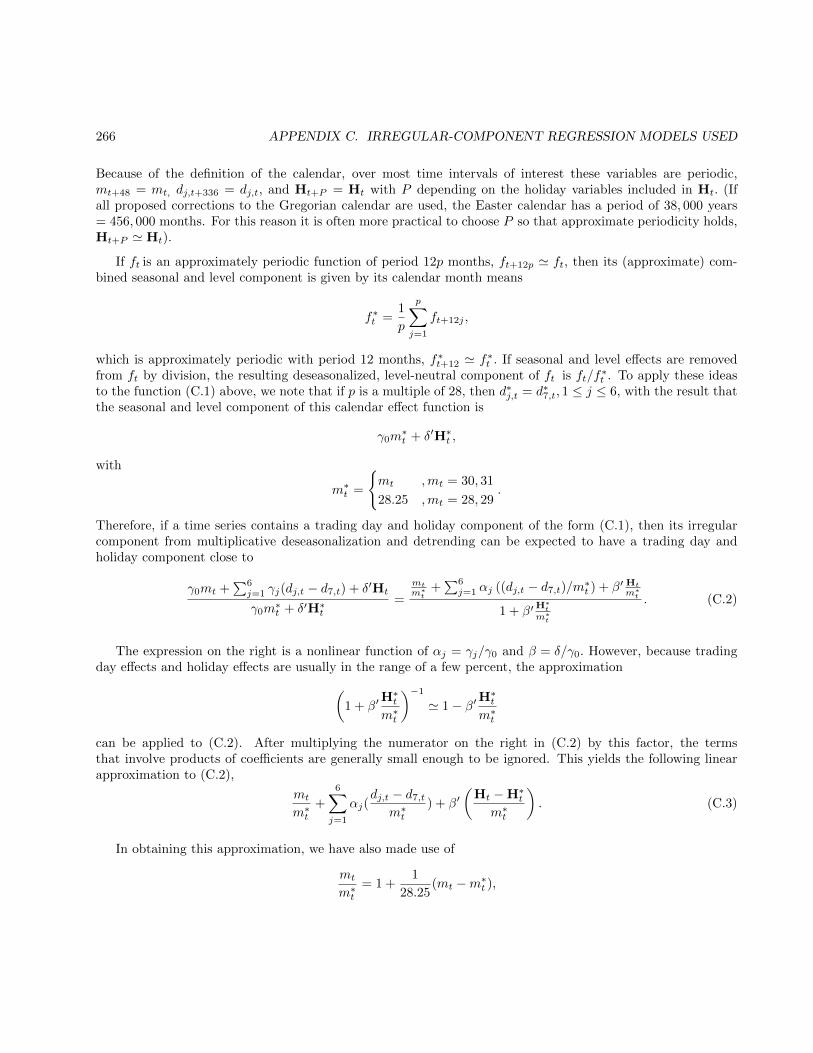
266 APPENDIX C. IRREGULAR-COMPONENT REGRESSION MODELS USED
Because of the definition of the calendar, over most time intervals of interest these variables are periodic,mt+48 = mt, dj,t+336 = dj,t, and Ht+P = Ht with P depending on the holiday variables included in Ht. (Ifall proposed corrections to the Gregorian calendar are used, the Easter calendar has a period of 38, 000 years= 456, 000 months. For this reason it is often more practical to choose P so that approximate periodicity holds,Ht+P ' Ht).
If ft is an approximately periodic function of period 12p months, ft+12p ' ft, then its (approximate) com-bined seasonal and level component is given by its calendar month means
f∗t =1
p
p∑j=1
ft+12j ,
which is approximately periodic with period 12 months, f∗t+12 ' f∗t . If seasonal and level effects are removedfrom ft by division, the resulting deseasonalized, level-neutral component of ft is ft/f
∗t . To apply these ideas
to the function (C.1) above, we note that if p is a multiple of 28, then d∗j,t = d∗7,t, 1 ≤ j ≤ 6, with the result thatthe seasonal and level component of this calendar effect function is
γ0m∗t + δ′H∗t ,
with
m∗t =
{mt ,mt = 30, 31
28.25 ,mt = 28, 29.
Therefore, if a time series contains a trading day and holiday component of the form (C.1), then its irregularcomponent from multiplicative deseasonalization and detrending can be expected to have a trading day andholiday component close to
γ0mt +∑6j=1 γj(dj,t − d7,t) + δ′Ht
γ0m∗t + δ′H∗t=
mt
m∗t
+∑6j=1 αj ((dj,t − d7,t)/m
∗t ) + β′ Ht
m∗t
1 + β′H∗
t
m∗t
. (C.2)
The expression on the right is a nonlinear function of αj = γj/γ0 and β = δ/γ0. However, because tradingday effects and holiday effects are usually in the range of a few percent, the approximation(
1 + β′H∗tm∗t
)−1
' 1− β′H∗t
m∗t
can be applied to (C.2). After multiplying the numerator on the right in (C.2) by this factor, the termsthat involve products of coefficients are generally small enough to be ignored. This yields the following linearapproximation to (C.2),
mt
m∗t+
6∑j=1
αj(dj,t − d7,t
m∗t) + β′
(Ht −H∗tm∗t
). (C.3)
In obtaining this approximation, we have also made use of
mt
m∗t= 1 +
1
28.25(mt −m∗t ),

C.1. IRREGULAR REGRESSION MODELS FOR MULTIPLICATIVE DECOMPOSITIONS. 267
and have treated the term involving the leap year variable LYt = mt − m∗t as one whose product withβ′ (Ht −H∗t ) /m
∗t is negligible. The formula (C.3) suggests a linear regression model for the irregular com-
ponent It of the form
It −mt
m∗t=
6∑j=1
αj
(dj,t − d7,t
m∗t
)+ β′
(Ht −H∗tm∗t
)+ κ′AOt + et,
where AOt, denotes a regression vector containing any needed additive outlier variables. Instead of using thismodel, X-13ARIMA-SEATS, for conformity with the X-11and X-11-ARIMAtrading day regression models, obtainsthe coefficients in (C.3) from ordinary least squares estimation (OLS) of the rescaled model
m∗t It −mt =
6∑j=1
αj(dj,t − d7,t) + β′ (Ht −H∗t ) + κ′AOt + εt (C.4)
whenever td is specified in the variables argument of x11regression, with one or more of the holiday effectspecifications easter[w], labor[w], and thank[w]. As explained in the footnote of Table 4.1, the regressorsassociated with these holiday variables also have the deseasonalized form Ht−H∗t when they are estimated fromthe regression spec. This is done so that seasonal effects occur only in the seasonal part of the model, and onlyin the seasonal factors of the decomposition. For conformity with X-11-ARIMA/88, the regressors associatedwith sceaster[w] are never deseasonalized. In effect, the entries of H∗t in (C.4) associated with any specifiedsceaster[w] regressors are set to zero.
C.1.1 Obtaining separate trading day and holiday factors
The calendar factors (C.3) can be approximately factored as the product of holiday factors
1 + β′(
Ht −H∗tm∗t
)(C.5)
and trading day factors
mt
m∗t+
6∑j=1
αj
(dj,t − d7,t
m∗t
)=
∑7j=1(1 + αj)dj,t
m∗t, (C.6)
(with α7 = −∑6j=1 αj). The numbers 1 +αj are called the daily weights. The trading day factor formula (C.6)
can also be written as
mt
m∗t+
∑(5)j αj
m∗t,
where∑(5)j denotes the sum of the j for which djt = 5. This formula shows that, apart from length of month
effects, the trading day effects depend only on the effects of the days that occur five times in the month. Whenonly trading day effects are estimated, the formulas above apply with β = 0.
If one or more trading day ”weights” 1 + αj are negative and the option reweight has been specified, then,for the trading day factor calculation all αj < −1 are replaced by α′j = −1 and all αj ≥ −1 are replaced by
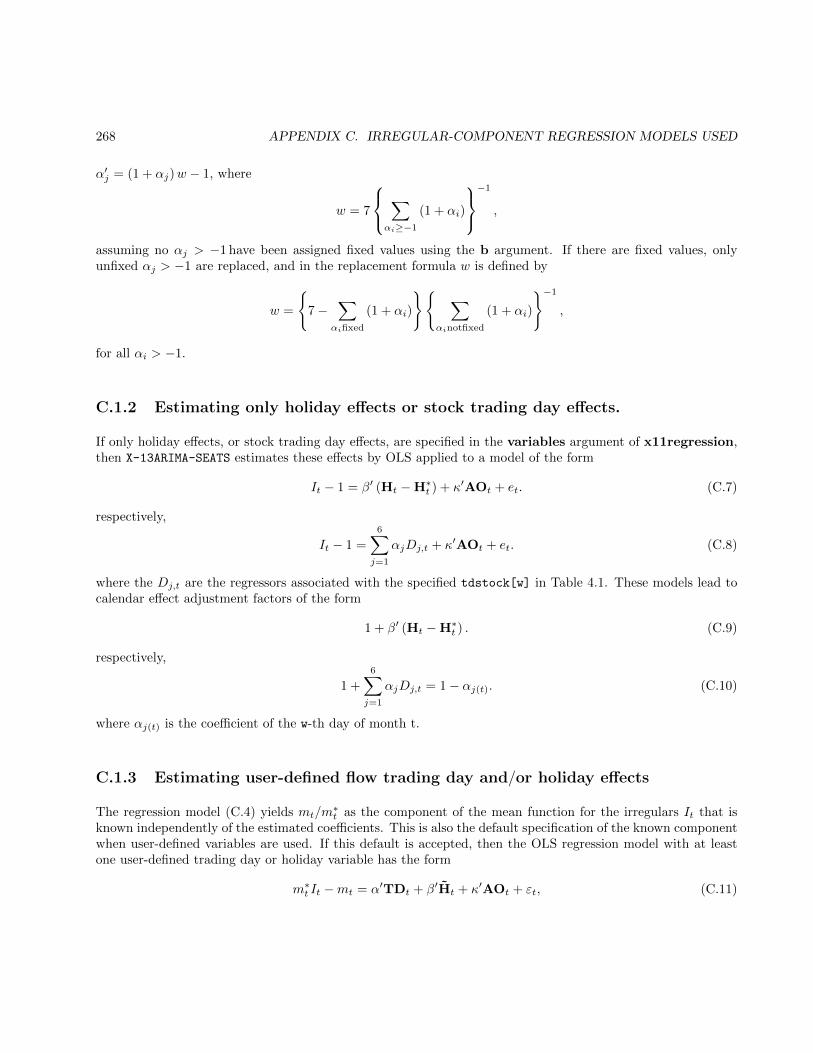
268 APPENDIX C. IRREGULAR-COMPONENT REGRESSION MODELS USED
α′j = (1 + αj)w − 1, where
w = 7
∑αi≥−1
(1 + αi)
−1
,
assuming no αj > −1 have been assigned fixed values using the b argument. If there are fixed values, onlyunfixed αj > −1 are replaced, and in the replacement formula w is defined by
w =
{7−
∑αifixed
(1 + αi)
}{ ∑αinotfixed
(1 + αi)
}−1
,
for all αi > −1.
C.1.2 Estimating only holiday effects or stock trading day effects.
If only holiday effects, or stock trading day effects, are specified in the variables argument of x11regression,then X-13ARIMA-SEATS estimates these effects by OLS applied to a model of the form
It − 1 = β′ (Ht −H∗t ) + κ′AOt + et. (C.7)
respectively,
It − 1 =
6∑j=1
αjDj,t + κ′AOt + et. (C.8)
where the Dj,t are the regressors associated with the specified tdstock[w] in Table 4.1. These models lead tocalendar effect adjustment factors of the form
1 + β′ (Ht −H∗t ) . (C.9)
respectively,
1 +
6∑j=1
αjDj,t = 1− αj(t). (C.10)
where αj(t) is the coefficient of the w-th day of month t.
C.1.3 Estimating user-defined flow trading day and/or holiday effects
The regression model (C.4) yields mt/m∗t as the component of the mean function for the irregulars It that is
known independently of the estimated coefficients. This is also the default specification of the known componentwhen user-defined variables are used. If this default is accepted, then the OLS regression model with at leastone user-defined trading day or holiday variable has the form
m∗t It −mt = α′TDt + β′Ht + κ′AOt + εt, (C.11)
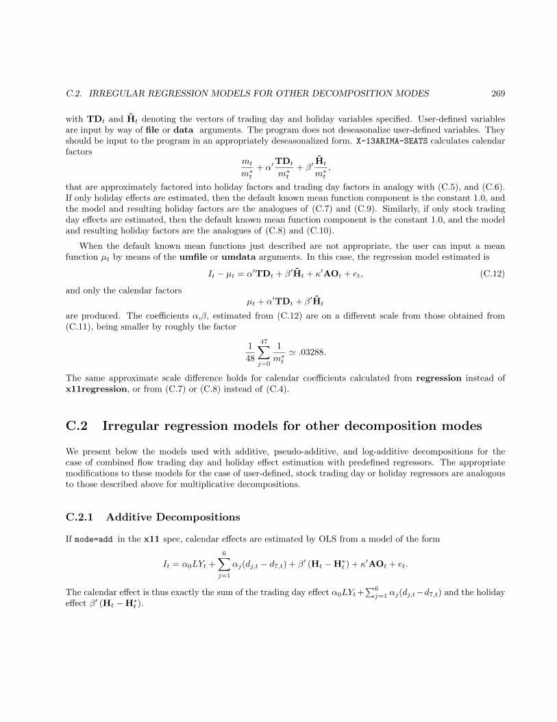
C.2. IRREGULAR REGRESSION MODELS FOR OTHER DECOMPOSITION MODES 269
with TDt and Ht denoting the vectors of trading day and holiday variables specified. User-defined variablesare input by way of file or data arguments. The program does not deseasonalize user-defined variables. Theyshould be input to the program in an appropriately deseasonalized form. X-13ARIMA-SEATS calculates calendarfactors
mt
m∗t+ α′
TDt
m∗t+ β′
Ht
m∗t,
that are approximately factored into holiday factors and trading day factors in analogy with (C.5), and (C.6).If only holiday effects are estimated, then the default known mean function component is the constant 1.0, andthe model and resulting holiday factors are the analogues of (C.7) and (C.9). Similarly, if only stock tradingday effects are estimated, then the default known mean function component is the constant 1.0, and the modeland resulting holiday factors are the analogues of (C.8) and (C.10).
When the default known mean functions just described are not appropriate, the user can input a meanfunction µt by means of the umfile or umdata arguments. In this case, the regression model estimated is
It − µt = α′TDt + β′Ht + κ′AOt + et, (C.12)
and only the calendar factorsµt + α′TDt + β′Ht
are produced. The coefficients α,β, estimated from (C.12) are on a different scale from those obtained from(C.11), being smaller by roughly the factor
1
48
47∑j=0
1
m∗t' .03288.
The same approximate scale difference holds for calendar coefficients calculated from regression instead ofx11regression, or from (C.7) or (C.8) instead of (C.4).
C.2 Irregular regression models for other decomposition modes
We present below the models used with additive, pseudo-additive, and log-additive decompositions for thecase of combined flow trading day and holiday effect estimation with predefined regressors. The appropriatemodifications to these models for the case of user-defined, stock trading day or holiday regressors are analogousto those described above for multiplicative decompositions.
C.2.1 Additive Decompositions
If mode=add in the x11 spec, calendar effects are estimated by OLS from a model of the form
It = α0LYt +
6∑j=1
αj(dj,t − d7,t) + β′ (Ht −H∗t ) + κ′AOt + et.
The calendar effect is thus exactly the sum of the trading day effect α0LYt+∑6j=1 αj(dj,t−d7,t) and the holiday
effect β′ (Ht −H∗t ).
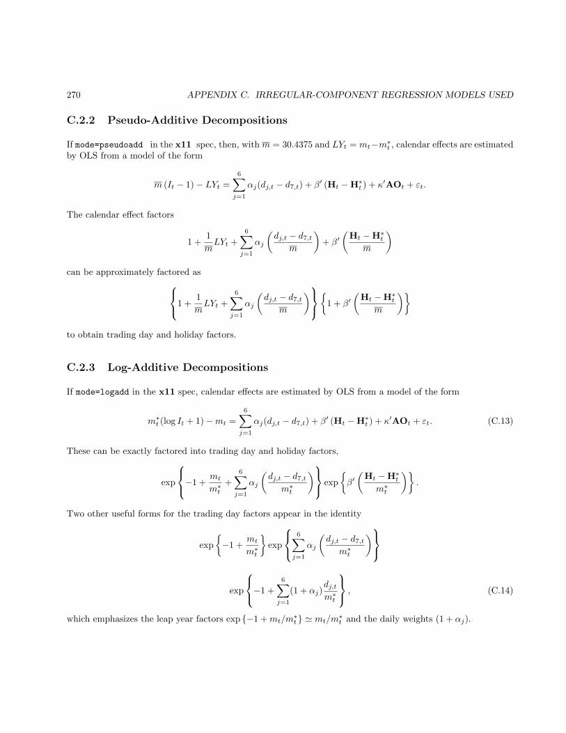
270 APPENDIX C. IRREGULAR-COMPONENT REGRESSION MODELS USED
C.2.2 Pseudo-Additive Decompositions
If mode=pseudoadd in the x11 spec, then, with m = 30.4375 and LYt = mt−m∗t , calendar effects are estimatedby OLS from a model of the form
m (It − 1)− LYt =
6∑j=1
αj(dj,t − d7,t) + β′ (Ht −H∗t ) + κ′AOt + εt.
The calendar effect factors
1 +1
mLYt +
6∑j=1
αj
(dj,t − d7,t
m
)+ β′
(Ht −H∗t
m
)
can be approximately factored as1 +1
mLYt +
6∑j=1
αj
(dj,t − d7,t
m
){
1 + β′(
Ht −H∗tm
)}
to obtain trading day and holiday factors.
C.2.3 Log-Additive Decompositions
If mode=logadd in the x11 spec, calendar effects are estimated by OLS from a model of the form
m∗t (log It + 1)−mt =
6∑j=1
αj(dj,t − d7,t) + β′ (Ht −H∗t ) + κ′AOt + εt. (C.13)
These can be exactly factored into trading day and holiday factors,
exp
−1 +mt
m∗t+
6∑j=1
αj
(dj,t − d7,t
m∗t
) exp
{β′(
Ht −H∗tm∗t
)}.
Two other useful forms for the trading day factors appear in the identity
exp
{−1 +
mt
m∗t
}exp
6∑j=1
αj
(dj,t − d7,t
m∗t
)exp
−1 +
6∑j=1
(1 + αj)dj,tm∗t
, (C.14)
which emphasizes the leap year factors exp {−1 +mt/m∗t } ' mt/m
∗t and the daily weights (1 + αj).
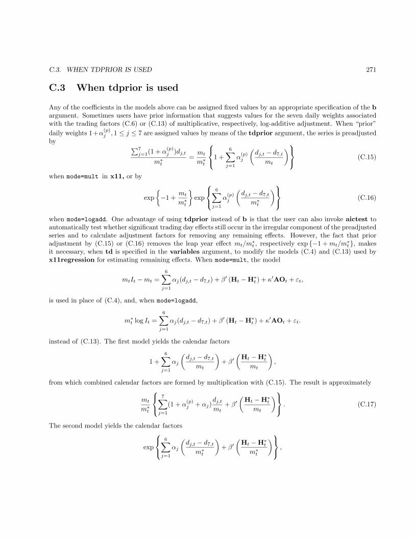
C.3. WHEN TDPRIOR IS USED 271
C.3 When tdprior is used
Any of the coefficients in the models above can be assigned fixed values by an appropriate specification of the bargument. Sometimes users have prior information that suggests values for the seven daily weights associatedwith the trading factors (C.6) or (C.13) of multiplicative, respectively, log-additive adjustment. When “prior”
daily weights 1+α(p)j , 1 ≤ j ≤ 7 are assigned values by means of the tdprior argument, the series is preadjusted
by ∑7j=1(1 + α
(p)j )dj,t
m∗t=mt
m∗t
1 +
6∑j=1
α(p)j
(dj,t − d7,t
mt
) (C.15)
when mode=mult in x11, or by
exp
{−1 +
mt
m∗t
}exp
6∑j=1
α(p)j
(dj,t − d7,t
m∗t
) (C.16)
when mode=logadd. One advantage of using tdprior instead of b is that the user can also invoke aictest toautomatically test whether significant trading day effects still occur in the irregular component of the preadjustedseries and to calculate adjustment factors for removing any remaining effects. However, the fact that prioradjustment by (C.15) or (C.16) removes the leap year effect mt/m
∗t , respectively exp {−1 +mt/m
∗t }, makes
it necessary, when td is specified in the variables argument, to modify the models (C.4) and (C.13) used byx11regression for estimating remaining effects. When mode=mult, the model
mtIt −mt =
6∑j=1
αj(dj,t − d7,t) + β′ (Ht −H∗t ) + κ′AOt + εt,
is used in place of (C.4), and, when mode=logadd,
m∗t log It =
6∑j=1
αj(dj,t − d7,t) + β′ (Ht −H∗t ) + κ′AOt + εt.
instead of (C.13). The first model yields the calendar factors
1 +
6∑j=1
αj
(dj,t − d7,t
mt
)+ β′
(Ht −H∗tmt
),
from which combined calendar factors are formed by multiplication with (C.15). The result is approximately
mt
m∗t
7∑j=1
(1 + α(p)j + αj)
dj,tmt
+ β′(
Ht −H∗tmt
) . (C.17)
The second model yields the calendar factors
exp
6∑j=1
αj
(dj,t − d7,t
m∗t
)+ β′
(Ht −H∗tm∗t
) ,

272 APPENDIX C. IRREGULAR-COMPONENT REGRESSION MODELS USED
and multiplication by (C.16) yields the combined factors
exp
−1 +
6∑j=1
(1 + α(p)j + αj)
dj,tm∗t
. (C.18)
The formulas (C.17) and (C.18) show that a statistically significant t-statistic for a coefficient αj can be inter-
preted as meaning that the prior weight 1 + α(p)j needs significant revision.
Bibliography
Abraham, B. and G. Box (1978). Deterministic and forecast-adaptive time-dependent models. Applied Statis-tics 27, 120–130.
Abraham, B. and J. Ledolter (1983). Statistical Methods for Forecasting. New York: John Wiley and Sons.
Akaike, H. (1973). Information theory and an extension of the likelihood principle. In B. Petrov and F. Czaki(Eds.), Second International Symposium on Information Theory, pp. 267–287. Budapest: Akademia Kiado.
Akaike, H. (1980). Seasonal adjustment by a bayesian modeling. Journal of Time Series Analysis 1, 1–14.
Akaike, H. and M. Ishiguro (1980). BAYSEA, a bayesian seasonal adjustment program. Computer ScienceMonographs No. 13, Tokyo: The Institute for Statistical Mathematics.
Baxter, M. A. (1994). A guide to seasonal adjustment of monthly data with X-11 (third edition). CentralStatistical Office, United Kingdom.
Bednarek, M. (2007). The dates of easter for 500 years. [Online]. Available: http://home.swiftdsl.com.
au/~mbednarek//easter.php [2007, November 18].
Bell, W. R. (1983). A computer program for detecting outliers in time series. Proceedings of the AmericanStatistical Association, Business and Economic Statistics Section, 634–639.
Bell, W. R. (1984). Seasonal decomposition of deterministic effects. SRD Research Report No. 84/01, U. S.Census Bureau http://www.census.gov/srd/papers/pdf/rr84-1.pdf.
Bell, W. R. (1987). A note on overdifferencing and the equivalence of seasonal time series models withmonthly means and models with (0,1,1)12 seasonal parts when θ = 1. Journal of Business and EconomicStatistics 5, 383–387. http://www.census.gov/srd/papers/pdf/rr84-32.pdf.
Bell, W. R. (1995). Correction to seasonal decomposition of deterministic effects. SRD Research Report No.95/01, U. S. Census Bureau http://www.census.gov/srd/papers/pdf/rr95-01.pdf.
Bell, W. R. (2004). On RegComponent time series models and their applications. In A. Harvey, S. J. Koopman,and N. Shephard (Eds.), State Space and Unobserved Component Models: Theory and Applications (Pro-ceedings of a Conference in Honour of James Durbin), pp. 248–283. Cambridge: Cambridge UniversityPress.
Bell, W. R. (2010). Unit root properties of seasonal adjustement and related filters. Research Report StatisticsNumber 2010-08, Research and Methodology Directorate, U. S. Census Bureau http://www.census.gov/
srd/papers/pdf/rrs2010-08.pdf.
Bell, W. R. and S. Hillmer (1988). A matrix approach to likelihood evaluation and signal extraction forARIMA component time series models. Research Report Number 1988/22, Statistical Research Division,U.S. Census Bureau http://www.census.gov/srd/papers/pdf/rr88-22.pdf.
273
274 BIBLIOGRAPHY
Bell, W. R. and S. C. Hillmer (1983). Modeling time series with calendar variation. Journal of the AmericanStatistical Association 78, 526–534.
Bell, W. R. and S. C. Hillmer (1984). Issues involved with the seasonal adjustment of economic time series.Journal of Business and Economic Statistics 2, 299–320. (invited paper with discussion).
Bell, W. R. and S. C. Hillmer (1985). A reply (to comments by Sims in Bell and Hillmer(1984)). Journal ofBusiness and Economic Statistics 3, 95–97.
Berk, K. N. (1974). Consistent autoregressive spectral estimates. Annals of Statistics 2, 489–502.
Bobbitt, L. and M. C. Otto (1990). Effects of forcasts on the revisions of seasonally adjusted values using theX-11 seasonal adjustment procedure. Proceedings of the American Statistical Association, Business andEconomic Statistics Section, 449–453. http://www.census.gov/srd/papers/pdf/rr90-09.pdf.
Box, G. and D. Cox (1964). An analysis of transformations. Journal of Royal Statistical Society B 26, 211–252.
Box, G. E. P. and G. M. Jenkins (1976). Time Series Analysis: Forecasting and Control (2nd ed.). SanFrancisco, CA: Holden-Day.
Box, G. E. P. and G. C. Tiao (1975). Intervention analysis with applications to economic and environmentalproblems. Journal of the American Statistical Association 70, 70–79.
Bozik, J. E. and M. C. Otto (1988). Benchmarking: Evaluating methods that preserve month-to-monthchanges. Research Report Number 88/07, Statistical Research Division, U.S. Census Bureau http://
www.census.gov/srd/papers/pdf/rr88-07.pdf.
Brillinger, D. R. (1975). Time Series–Data Analysis and Theory. New York: Holt Rinehart and Winston.
Brockwell, P. J. and R. A. Davis (1991). Time Series: Theory and Methods. New York: Springer-Verlag.
Burnham, K. P. and D. R. Anderson (2004). Multimodal inference: Understanding AIC and BIC in modelselection. Sociological Methods & Research 33, 261–304.
Causey, B. and M. L. Trager (1982). Derivation of solution to the benchmarking problem: Trend revision.Unpublished research notes, U.S. Census Bureau, reproduced in Appendix C of Bozik and Otto (1988) -http://www.census.gov/srd/papers/pdf/rr88-07.pdf.
Chang, I. and G. C. Tiao (1983). Estimation of time series parameters in the presence of outliers. TechnicalReport No. 8, Statistics Research Center, University of Chicago.
Chang, I., G. C. Tiao, and C. Chen (1988). Estimation of time series parameters in the presence of outliers.Technometrics 30, 193–204.
Chen, Z. (1985). The asymptotic efficiency of a linear procedure of estimation for ARMA models. Journal ofTime Series Analysis 6, 52–62.
Chen, Z.-G. and P. Durk (2005). A therapy for ill-seasonality in X-11 seasonal adjustment. Statistics CanadaWorking Paper BSMD-2005-009E.
Cholette, P. and E. B. Dagum (1994). Benchmarking time series with autocorrelated survey errors. Interna-tional Statistical Review 62, 367–377.
Cholette, P. A. (1978). A comparison and assessment of various adjustment methods of sub-annual series toyearly benchmarks. Research Paper, Seasonal Adjustment and Time Series Staff, Statistics Canada.
Cholette, P. A. (1984). Adjusting sub-annual series to benchmarks. Survey Methodology 10, 35–49.
Chow, J. and K. Moore (2009). Constructing an Easter regressor for a stock series in X-12-ARIMA. Proceedingsof the American Statistical Association, Business and Economic Statistics Section. [CD-ROM] (to appear).
BIBLIOGRAPHY 275
Cleveland, W. P. and M. R. Grupe (1983). Modeling time series when calendar effects are present. In Pro-ceedings of the Conference on Applied Time Series Analysis of Economic Data, pp. 57–73. Washington,DC: U. S. Census Bureau.
Cleveland, W. S. and S. J. Devlin (1980). Calendar effects in monthly time series: Detection by spectrumanalysis and graphical methods. Journal of the American Statistical Association 75, 487–496.
Dagum, E. B. (1980). The X-11-ARIMA seasonal adjustment method. Statistics Canada.
Dagum, E. B. (1988). X-11-ARIMA/88 seasonal adjustment method - Foundations and users manual. Statis-tics Canada.
Dagum, E. B. (1996). A new method to reduce unwanted ripples and revisions in trend-cycle estimates fromX-11-ARIMA. Survey Methodology 22, 77–83.
Dagum, E. B. and P. A. Cholette (2006). Benchmarking, Temporal Distribution, and Reconciliation Methodsfor Time Series. New York: Springer. Lecture Notes in Statistics, Vol. 186.
Dagum, E. B. and A. Luati (2009). A cascade linear filter to reduce revisions and false turning points for realtime trend-cycle estimation. Econometric Reviews 28 (1), 40–59. [Online]. Available: http://www2.stat.unibo.it/beedagum/Papers/Dagum_Luati_2009_ER.pdf [2009, January 9].
Darne, O. and E. B. Dagum (2009). Performance of short-term trend predictors for current economicanalysis. Economics Bulletin. [Online]. Available: http://www2.stat.unibo.it/beedagum/Papers/
Darne-Dagum_EB09.pdf [2009, February 10].
den Butter, F. A. G. and M. M. G. Fase (1991). Seasonal Adjustment as a Practical Problem. Amsterdam:North Holland.
Doherty, M. (2001). Surrogate henderson filters in X-11. Australian and New Zealand Journal of Statistics 43,385–392.
Doornik, J. A. and D. Hendry (2001). GiveWin: An Interface to Empirical Modelling (3rd ed.). London:Timberlake Consultants Press.
Duffet-Smith, P. (1981). Practical Astronomy With Your Calculator (2nd ed.). Cambridge University Press.
Feldpausch, R. M., C. C. H. Hood, and K. C. Wills (2004). Diagnostics for model-based seasonal adjustment.Proceedings of the American Statistical Association, Business and Economic Statistics Section. [CD-ROM]http://www.census.gov/ts/papers/jsm2004rmf.pdf.
Findley, D., T. S. McElroy, and K. C. Wills (2005). Modifications of SEATS’ diagnostic for detectingover- and underestimation of seasonal adjustment components. https://www.census.gov/ts/papers/findleymcelroywills2005.pdf.
Findley, D. F. (1985). On the unbiasedness property of AIC for exact or approximating linear stochastic timeseries models. Journal of Time Series Analysis 6, 229–252.
Findley, D. F. (1999). Akaike’s Information Criterion II. In S. Kotz, C. B. Read, and D. L. Banks (Eds.),Encyclopedia of Statistical Science, Update Volume 3, pp. 2–6. New York: John Wiley and Son.
Findley, D. F. (2005). Asymptotic stationarity properties of out-of-sample forecast errors of misspecifiedregARIMA models and the optimality of GLS for one-step-ahead forecasting. Statistica Sinica 15 (2),447–476.
Findley, D. F. (2007). Optimality of GLS for one-step-ahead forecasting with regARIMA and related modelswhen the regression is misspecified. Econometric Theory 23 (6), 1083–1107.
276 BIBLIOGRAPHY
Findley, D. F. (2009). Stock series holiday regressors generated by flow series holiday regressors. SRD ResearchReport RRS 2009-4, U. S. Census Bureau http://www.census.gov/srd/papers/pdf/rrs2009-04.pdf.
Findley, D. F. and C. C. Hood (1999). X-12-ARIMA and its application to some Italian indicator series. InSeasonal Adjustment Procedures – Experiences and Perspectives, pp. 231–251. Rome: Istituto Nazionaledi Statistica (ISTAT). http://www.census.gov/ts/papers/x12istat.pdf.
Findley, D. F., D. P. Lytras, and A. Maravall (2016). Illuminating ARIMA Model-Based Seasonal Adjustmentwith Three Fundamental Seasonal Models. pp. 1–42. http://dx.doi.org/10.1007/s13209-016-0139-4.
Findley, D. F. and D. E. K. Martin (2003). Frequency domain analysis of SEATS and X-11/X-12-ARIMA sea-sonal adjustment filters for short and moderate length time series. Research Report Number 2003/02, Sta-tistical Research Division, U.S. Census Bureau http://www.census.gov/srd/papers/pdf/rrs2003-02.
pdf.
Findley, D. F. and D. E. K. Martin (2006). Frequency domain analysis of SEATS and X-11/X-12-ARIMAseasonal adjustment filters for short and moderate length time series. Journal of Official Statistics 22 (1),1–34.
Findley, D. F. and B. C. Monsell (1986). New techniques for determining if a time series can be seasonallyadjusted reliably, and their application to U. S. foreign trade series. In M. Perryman (Ed.), RegionalEconomic Modeling, pp. 195–228. Amsterdam: Kluwer-Nijhoff.
Findley, D. F. and B. C. Monsell (2009). Modeling stock trading day effects under flow day-of-week constraints.Journal of Official Statistics 25 (3), 415–430. http://www.jos.nu/Articles/abstract.asp?article=
253415 [Online; accessed 14-October-2009].
Findley, D. F., B. C. Monsell, W. R. Bell, M. C. Otto, and B. C. Chen (1998). New capabilities of the X-12-ARIMA seasonal adjustment program (with discussion). Journal of Business and Economic Statistics 16,127–77. http://www.census.gov/ts/papers/jbes98.pdf.
Findley, D. F., B. C. Monsell, H. B. Shulman, and M. G. Pugh (1990). Sliding spans diagnostics for seasonaland related adjustments. Journal of the American Statistical Association 85, 345–355.
Findley, D. F. and R. J. Soukup (2000). Modeling and model selection for moving holidays. Proceedings ofthe American Statistical Association, Business and Economic Statistics Section, 102–107. http://www.census.gov/ts/papers/asa00_eas.pdf.
Findley, D. F. and C. Z. Wei (2002). AIC, overfitting principles, and the boundedness of moments of inversematrices for autoregressions and related models. Journal of Multivariate Analysis 83, 415–450.
Findley, D. F., K. C. Wills, J. A. D. Aston, R. Feldpausch, and C. C. Hood (2003). Diagnostics for ARIMAmodel-based seasonal adjustment. Proceedings of the American Statistical Association, Business and Eco-nomic Statistics Section. [CD-ROM].
Fuller, W. A. (1976). Introduction to Statistical Time Series. New York: John Wiley and Son.
Gastwirth, J. L. and M. G. B. Owens (1977). On classical test of normality. Biometrika 64, 135–139.
Geary, R. C. (1936). Moments of the ratio of mean deviation to the standard deviation as a test of normality.Biometrika 28, 295–305.
Geweke, J. (1978). Revision of seasonally adjusted time series. SSRI Report No. 7822, University of Wisconsin,Department of Statistics.
BIBLIOGRAPHY 277
Gomez, V. (1998). Automatic model identification in the presence of missing observations and outliers. Work-ing Paper D-98009, Ministerio de Economıa y Hacienda, Dirrection General de Analisis y ProgramacionPresupuestaria, Madrid.
Gomez, V. and A. Maravall (1996). Programs TRAMO and SEATS : Instructions for the user (beta version:June 1997). Banco de Espana, Servicio de Estudios, DT 9628. (Updates and additional documentationcan be found at http://www.bde.es/webbde/es/secciones/servicio/software/econom.html.).
Gomez, V. and A. Maravall (2001a). Automatic modeling methods for univariate series. In D. Pena, G. C.Tiao, and R. S. Tsay (Eds.), A Course in Time Series Analysis. New York, NY: J. Wiley and Sons.
Gomez, V. and A. Maravall (2001b). Seasonal adjustment and signal extraction in economic time series. InD. Pena, G. C. Tiao, and R. S. Tsay (Eds.), A Course in Time Series Analysis. New York, NY: J. Wileyand Sons.
Griswold, R. E. and M. T. Griswold (1997). The ICON Programming Language (3rd ed.). San Jose: Peer-to-Peer Communications.
Hampel, F. R., E. M. Ronchetti, P. J. Rousseeuw, and W. A. Stahel (1986). Robust Statistics: The ApproachBased on Influence Functions. New York, NY: J. Wiley and Sons.
Hannan, E. J. and B. G. Quinn (1979). The determination of the order of an autoregression. Journal of RoyalStatistical Society B 41, 190–195.
Hannan, E. J. and J. Rissanen (1982). Recursive estimation of mixed autoregressive-moving average models.Biometrika 66, 265–270.
Hillmer, S. C. and G. C. Tiao (1979). Likelihood function of stationary multiple autoregressive moving averagemodels,. Journal of the American Statistical Association 74, 652–660.
Hood, C. C. (2002a). Comparing the automatic ARIMA model selection procedures of TRAMO and X-12-ARIMA Version 0.3 and the seasonal adjustments of SEATS and X-12-ARIMA. unpublished workpresented at the Eurostat Working Group on Seasonal Adjustment Meeting, Luxembourg, April 2002.
Hood, C. C. (2002b). Comparison of time series characteristics for seasonal adjustments from SEATS andX-12-ARIMA. American Statistical Association, Proceedings of the Business and Economic StatisticsSection [CD-ROM] http://www.census.gov/ts/papers/choodasa2002.pdf.
Hood, C. C. (2002c). X-12-Graph: A SAS/GRAPH program for X-12-ARIMA output, user’s guide for theX-12-Graph batch for PC/Windows, version 1.2. U. S. Census Bureau, U. S. Department of Commerce.
Hood, C. C., J. D. Ashley, and D. F. Findley (2000). An empirical evaluation of the performance ofTRAMO/SEATS on simulated series. American Statistical Association, Proceedings of the Business andEconomic Statistics Section http://www.census.gov/ts/papers/asa00_ts.pdf.
Hood, C. C. H. (2005). An empirical comparison of methods for benchmarking seasonally adjusted seriesto annual totals. Proceedings of the American Statistical Association, Business and Economic StatisticsSection. [CD-ROM] https://www.census.gov/ts/papers/chood_asa2005.pdf.
Huot, G. (1975). Quadratic minimization adjustment of monthly or quarterly series to annual totals. ResearchPaper, Seasonal Adjustment and Time Series Staff, Statistics Canada.
Hurvich, C. M. and C. Tsai (1989). Regression and time series model selection in small samples. Biometrika 76,297–307.
Jenkins, G. M. and D. G. Watts (1968). Spectral Analysis and Its Applications. San Francisco, CA: Holden-Day.
278 BIBLIOGRAPHY
Kaiser, R. and A. Maravall (2001). Measuring Business-Cycles in Economic Time Series. New York: Springer.Lecture Notes in Statistics, Vol. 154.
Klein, J. L. (1991). Statistical Visions in Time – A History of Time Series Analysis 1662–1938. Cambridge:Cambridge University Press.
Kohn, R. and C. F. Ansley (1985). Efficient estimation and prediction in time series regression models.Biometrika 72, 694–697.
Ladiray, D. and B. Quenneville (2001). Seasonal Adjustment with the X-11 Method. New York: Springer.Lecture Notes in Statistics, Vol. 158.
Lehman, E. L. (1986). Testing Statistical Hypothesis (Second ed.). New York, NY: J. Wiley and Sons.
Lin, J.-L. and T.-S. Liu (2002). Modeling lunar calendar holiday effects in Taiwan. Taiwan Economic Forecastand Policy 33 (1), 1–37. http://www.census.gov/ts/papers/lunar.pdf.
Ljung, G. M. (1993). On outlier detection in time series. Journal of Royal Statistical Society B 55, 559–567.
Ljung, G. M. and G. E. P. Box (1978). On a measure of lack of fit in time series models. Biometrika 65,297–304.
Ljung, G. M. and G. E. P. Box (1979). The likelihood function of stationary autoregressive-moving averagemodels. Biometrika 66, 265–270.
Lothian, J. (1984). The identification and treatment of moving seasonality in X-11. Proceedings of the Businessand Economic Statistics Section of the American Statistical Association, 166–171.
Lothian, J. and M. Morry (1978). A test of quality control statistics for the X-11-ARIMA seasonal adjustmentprogram. Research Paper, Seasonal Adjustment and Time Series Staff, Statistics Canada.
Lytras, D. P. (2013). X-13-Graph Java, Version 2.1. U. S. Census Bureau, U. S. Department of Commercehttp://www.census.gov/srd/www/x13graph/x13gjavadoc/x13graph_java_doc.html.
Lytras, D. P. (2015). X-13-Graph: A SAS/GRAPH Program for X-13ARIMA-SEATS Output, User’s Guidefor the Batch Program on the PC or Unix, Version 2.1. U. S. Census Bureau, U. S. Department ofCommerce http://www.census.gov/srd/www/x13graph/x13gbdoc/x13gbat_doc.html.
Lytras, D. P., R. M. Feldpausch, and W. R. Bell (2007). Determining seasonality: A comparison of diag-nostics from X-12-ARIMA. Proceedings of the International Conference on Establishment Surveys III .(CD-ROM).
Maravall, A. (1995). Unobserved components in economic time series. In M. H. Pesaran and M. Wickens(Eds.), The Handbook of Applied Econometrics. Basil Blackwell.
Maravall, A. (2012). Seasonality tests and automatic model identification in TRAMO-SEATS (version:November 12, 2012). Banco de Espana, Servicio de Estudios.
McElroy, T. S. (2006). Statistical properties of model-based signal extraction diagnostic tests. Research Re-port No. RRS2006/06, Statistical Research Division, U.S. Census Bureau http://www.census.gov/srd/
papers/pdf/rrs2006-06.pdf.
McElroy, T. S. (2008a). Exact formulas for the hodrick-prescott filter. Econometrics Journal 11, 209–217.http://www.census.gov/ts/papers/rrs2006-09.pdf [Preprint].
McElroy, T. S. (2008b). Matrix formulas for nonstationary signal extraction. Econometric Theory 24 (4),1–22.
BIBLIOGRAPHY 279
McElroy, T. S. (2008c). Statistical properties of model-based signal extraction diagnostic tests. Communica-tions in Statistics: Theory and Methods 37 (4), 591–616.
McElroy, T. S. and R. Gagnon (2006). Finite sample revision variances for ARIMA model-based signalextraction. Research Report No. RRS2006/05, Statistical Research Division, U.S. Census Bureau http:
//www.census.gov/srd/papers/pdf/rrs2006-05.pdf.
McElroy, T. S. and R. Gagnon (2008). Finite sample revision variances for ARIMA model-based signalextraction. Journal of Official Statistics 24 (3), 451–467.
Monsell, B. C. (2002). An update on the development of the X-12-ARIMA seasonal adjustment program. InProceedings of the 3rd International Symposium on Frontiers of Time Series Modeling, pp. 1–11. Tokyo:Institute of Statistical Mathematics.
Monsell, B. C. (2006). Recent developments in seasonal adjustment software at the Census Bureau. Pro-ceedings of the Eurostat Conference on Seasonality, Seasonal Adjustment and Their Implications forShort-term Analysis and Forecasting.
Montes, M. J. (1997a). Frequency of the date of Easter 1875 to 2124. http://www.smart.net/~mmontes/freq3.html [Online; accessed 8-December-1999].
Montes, M. J. (1997b). Frequency of the date of Easter over one 400 year Gregorian cycle. http://www.smart.net/~mmontes/freq2.html [Online; accessed 8-December-1999].
Montes, M. J. (2001). Calculation of the ecclesiastical calendar. http://www.smart.net/~mmontes/ec-cal.html [Online; accessed 31-July-2001].
Mood, A. M., F. A. Graybill, and D. C. Boes (1974). Introduction to the Theory of Statistics, 3rd Edition.New York: McGraw-Hill.
More, J. J., B. S. Garbow, and K. E. Hillstrom (1980). User guide for MINPACK-1. Report ANL-80-74,Argonne National Laboratory, Argonne, Illinois.
Otto, M. and W. R. Bell (1993). Detecting temporary changes in level in time series. Proceedings of theAmerican Statistical Association, Business and Economic Statistics Section, 170–174.
Otto, M. C. and W. R. Bell (1990). Two issues in time series outlier detection using indicator variables.Proceedings of the American Statistical Association, Business and Economic Statistics Section, 182–187.
Otto, M. C., W. R. Bell, and J. P. Burman (1987). An iterative GLS approach to maximum likelihoodestimation of regression models with ARIMA errors. Proceedings of the American Statistical Association,Business and Economic Statistics Section, 632–637. (available at http://www.census.gov/srd/papers/pdf/rr87-34.pdf).
Ozaki, T. (1977). On the order determination of ARIMA models. Applied Statistics 26, 290–301.
Pang, O. and B. C. Monsell (2016). Examining diagnostics for trading-day effects from x-13arima-seats.Center for Statistical Research and Methodology Research Report Series Number 2016-02, Research andMethodology Directorate, U. S. Census Bureau http://www.census.gov/srd/papers/pdf/RRS2016-02.
pdf.
Pearson, E. S. (1938). The probability integral transformation for testing goodness of fit and combiningindependent tests of significance. Biometrika 30, 134–148.
Pearson, E. S. and H. O. Hartley (1954). Biometrika Tables for Statisticians, Volume 1. Cambridge: Cam-bridge University Press.
280 BIBLIOGRAPHY
Pierce, D. (1971). Least squares estimation in the regression model with autoregressive-moving average errors.Biometrika 58, 299–312.
Planas, C. and R. Depoutot (2002). Controlling revisions in ARIMA-model-based seasonal adjustment. Jour-nal of Time Series Analysis 23, 193–214.
Priestley, M. (1981). Spectral Analysis and Time Series. London: Academic Press.
Quenneville, B., P. Cholette, G. Huot, K. Chiu, and T. DiFonzo (2004). Adjustment of seasonally adjustedseries to annual totals. Research Report, Statistics Canada.
SAS Institute Inc. (1990). SAS/GRAPH Software: Reference, Version 6, First Edition, Volume 1. Cary, NC:SAS Institute.
Schwarz, G. (1978). Estimating the dimension of a model. Annals of Statistics 6, 461–464.
Shiskin, J., A. H. Young, and J. C. Musgrave (1967). The X-11 variant of the Census Method II seasonaladjustment program. Technical Paper No. 15, U.S. Department of Commerce, U. S. Census Bureau.
Snedecor, G. W. and W. G. Cochran (1980). Statistical Methods (7th ed.). Ames: The Iowa State UniversityPress.
Soukup, R. J. and D. F. Findley (1999). On the spectrum diagnostics used by X-12-ARIMA to indicatethe presence of trading day effects after modeling or adjustment. Proceedings of the American StatisticalAssociation, Business and Economic Statistics Section, 144–149. http://www.census.gov/ts/papers/rr9903s.pdf.
Taniguchi, M. and Y. Kakizawa (2000). Asymptotic Theory of Statistical Inference for Time Series. NewYork: Springer-Verlag.
Thomson, P. and T. Ozaki (2002). Transformation and seasonal-trend decomposition. In Proceedings of the3rd International Symposium on Frontiers of Time Series Modeling, pp. 197–212. Tokyo: Institute ofStatistical Mathematics.
Titova, N. and B. C. Monsell (2009). Detecting stock calendar effects in U. S. Census Bureau inventoryseries. SRD Research Report RRS 2009-6, U. S. Census Bureau http://www.census.gov/srd/papers/
pdf/rrs2009-06.pdf.
Vandaele, W. (1983). Applied Time Series and Box-Jenkins Models. New York: Academic Press.
Wikipedia Contributers (2009). Stock and flow — Wikipedia, the free encyclopedia. http://en.wikipedia.org/wiki/Stock_and_flow [Online; accessed 15-January-2009].
Wikipedia Contributers (2013). Xhtml — Wikipedia, the free encyclopedia. http://en.wikipedia.org/
wiki/XHTML [Online; accessed 2-April-2013].
Wikipedia Contributers (2015). Hodrick-prescott filter — Wikipedia, the free encyclopedia. https://en.
wikipedia.org/wiki/Hodrick%E2%80%93Prescott_filter [Online; accessed 24-March-2015].
Wilson, G. T. (1983). The estimation for time series models, part I. Yet another algorithm for the exactlikelihood of ARMA models. Technical Report No. 2528, Mathematics Research Center, University ofWisconsin-Madison.
Index
additive decomposition, 206, 212, 213, 218, 225, 226sliding spans, 190, 193
aggregate series, see composite seriesAIC, 38, 45, 63, 97, 155AIC test, 46, 47, 142, 153–154
AIC difference, 46, 47, 142, 153, 206, 212irregular regression, 233, 243
AIC difference, 233, 243select transformation, 208, 212–213testing Easter, 145
AICC, 3, 38, 45, 97, 142, 153, 212, 233, 243airline model, 213Akaike, Hirtugu, 3, 4AR spectrum diagnostic, 53–54arima spec
arguments, 62–63ar, 62ma, 62model, 62title, 63
details, 63examples, 64–65usage, 62
ARIMA model, 1, 27airline model, 65cancellation of AR and MA factors, 44convergence, 38, 42–43, 93, 95overdifferencing, 44–45
asymmetric, 1, 224autocovariance, 43automatic model selection, 3
automdl spec, 69–75balanced model, 69, 73
pickmdl spec, 7, 138–139backcasts, 137, 139default model, 139forecasts, 139
automatic outlier identification, 36, 39–40, 74, 133–134critical value, 39, 67, 69, 75, 130, 133, 134irregular regression
critical value, 233revisions history, 116–117
revisions history, 116automdl spec
arguments, 66–67acceptdefault, 66checkmu, 66diff, 66fcstlim, 69ljungboxlimit, 66maxdiff, 67maxorder, 67mixed, 67print, 67rejectfcst, 69savelog, 67
details, 69–75examples, 76rarely used arguments, 67–69usage, 66
backcasts, 1, 106, 142, 147, 207, 227, 233, 239, 243modelspan argument, 183
BIC, 38, 45, 97
calendar effects, 1irregular regression, 2, 241
change-of-regime regressors, 152–153check spec
arguments, 77–78maxlag, 77print, 77qtype, 77save, 77
281
282 INDEX
savelog, 77details, 79–81examples, 81–83rarely used arguments, 78usage, 77, 121
Chi-squared test, 142collinearity, 30composite spec
arguments, 84–85appendbcst, 84appendfcst, 84decimals, 84modelspan, 84name, 85print, 85save, 85savelog, 85title, 85type, 85
details, 88–89examples, 89–90rarely used arguments, 85–88usage, 84
composite series, 16, 61, 88concurrent seasonal adjustment, 115, 118convergence tolerance, 43, 95
Dagum, Estela, 4deterministic, 45, 96, 97detrended series, see SI valuesdifferencing operators, 44, 50direct seasonal adjustment, 89
EasterAIC test, 47, 142
irregular regression, 233, 243regARIMA model, 153
Bateman and Mayes procedure, 224, 227, 243easter[0], 32, 35, 149regressor, 242
flow, 32, 149Statistics Canada, 33, 149, 242stock, 32, 149
removal of mean from regressor, 32, 147, 155, 238,244
effective number of observations, 45, 49
error messages, 6–8, 63, 134estimate spec
arguments, 92–93exact, 92maxiter, 92outofsample, 92print, 93save, 93savelog, 93tol, 93
details, 95–97examples, 97–98rarely used arguments, 93–95usage, 92
extreme valuesexclude from irregular regression, 237X-11, 2, 19, 217, 223, 226–228
calendar sigma, 223–224
flags, 12–16-c, 16, 89-d, 10, 13-g, 15-i, 13-m, 9, 13, 16, 89-n, 15, 16, 202-p, 16, 180-q, 16-r, 16-s, 14–15, 89, 194-v, 16-w, 16
force specarguments, 99–102lambda, 99mode, 99print, 99rho, 100round, 100save, 99start, 100target, 101type, 101usefcst, 101
details, 102–104examples, 104–105
INDEX 283
rarely used arguments, 101usage, 99
forecast specarguments, 106exclude, 106lognormal, 106maxback, 106maxlead, 106print, 106probability, 106save, 106
details, 107–108examples, 108–110usage, 106
forecasts, 40–41, 142, 147, 207, 233, 239, 243forecast extension, 1, 22, 108, 227prediction interval, 40
Gomez, Victor, 2, 4, 19, 69, 166graphics metafile, 15
handling spaces in file names, 11–12, 14Hannan-Quinn criterion, 38, 45, 97Hannan-Rissanen estimation method, 69, 71, 72history spec
arguments, 111–115endtable, 111estimates, 111fixmdl, 111fixreg, 112fstep, 112print, 112sadjlags, 112save, 112savelog, 114start, 114target, 115trendlags, 115
details, 117–118examples, 118–120rarely used arguments, 115–117usage, 111
Hodrick-Prescott filter, 166, 171, 175, 176holiday effects, 35, 61, 155, 239, 244
keep in seasonally adjusted series, 224remove from nonseasonal series, 155, 244
identify specarguments, 126diff, 126maxlag, 126print, 126save, 126sdiff, 126
details, 126–127examples, 128–129usage, 126
inadmissable decomposition, 75index file, 6indirect seasonal adjustment, 89
revision history diagnostics, 89, 117sliding spans diagnostics, 89unadjusted series as component, 88
intervention effects, 36invertible, 38, 43–44irregular component, 225, 226, 228, 232irregular component regression, 224irregular regression
AIC test, 243outlier critical value, 233revisions history, 112, 115, 117sliding spans, 189, 190
Ishiguro, Makio, 4
Jacobian transformation adjustment, 49
kurtosis, 81
leap year adjustment, 29, 151, 206, 211length-of-month adjustment, 29, 151, 206, 211, 212length-of-quarter adjustment, 151, 206, 212Ljung-Box Q-statistic, 39, 66, 69, 71, 74, 77, 79, 81log file, 12log-additive decomposition, 212, 218, 225
sliding spans, 193
Maravall, Agustın, 2, 4, 19, 69, 166metadata spec
arguments, 121keys, 121values, 121
details, 122–123examples, 124–125
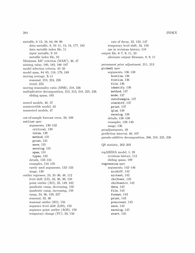
284 INDEX
metafile, 8–13, 16, 84, 88–90data metafile, 8, 10–11, 13, 18, 177, 182data metafile index file, 11input metafile, 9–10metafile index file, 10
Minimum AIC criterion (MAIC), 46, 47missing value, 180, 183, 186–187model selection criteria, 45–50model span, 84–85, 118, 179, 189moving average, X-11
seasonal, 218, 224, 226trend, 223
moving seasonality ratio (MSR), 218, 226multiplicative decomposition, 212, 213, 218, 225, 226
sliding spans, 193
nested models, 46, 47noninvertible model, 43nonnested models, 47
out-of-sample forecast error, 50, 109outlier spec
arguments, 130–132critical, 130lsrun, 130method, 131print, 131save, 131savelog, 131span, 131types, 132
details, 133–134examples, 134–135rarely used arguments, 132–133usage, 130
outlier regressor, 24, 35–36, 48, 112level shift (LS), 33, 36, 39, 150point outlier (AO), 33, 149, 242quadratic ramp, decreasing, 150quadratic ramp, increasing, 150ramp, 34, 36, 150, 227seasonal, 33, 36seasonal outlier (SO), 150sequence level shift (LSS), 150sequence point outlier (AOS), 150temporary change (TC), 33, 150
rate of decay, 33, 133, 147temporary level shift, 34, 150use in revisions history, 118
output file, 6–7, 9, 11, 23alternate output filename, 8, 9, 11
permanent prior adjustment, 211, 213pickmdl spec
arguments, 136–138bcstlim, 136fcstlim, 136file, 136identify, 136method, 137mode, 137outofsample, 137overdiff, 137print, 137qlim, 138savelog, 138
details, 138–139examples, 139–140usage, 136
preadjustments, 49prediction interval, 40, 107pseudo-additive decomposition, 206, 218, 225, 226
QS statistic, 202–203
regARIMA model, 1, 28revisions history, 112sliding spans, 189
regression specarguments, 142–146aicdiff, 142aictest, 142chi2test, 142chi2testcv, 142data, 142file, 143format, 143print, 143pvaictest, 145save, 143savelog, 145start, 145

INDEX 285
testalleaster, 145tlimit, 145user, 145usertype, 146variables, 146
details, 147–155examples, 156–165rarely used arguments, 146–147usage, 141
regression variablesconstant, 29, 31, 148fixed seasonal, 30
seasonal indicator, 31, 148trigonometric, 31, 148
holiday, 112Easter, 35, 149, 242flow, 35Labor Day, 33, 35, 149, 242Statistics Canada Easter, 33, 149, 242stock, 35Stock Easter, 149Thanksgiving, 33, 35, 149, 242
leap year, 31, 148leap year regressor, 151length-of-month, 31, 148length-of-month regressor, 151length-of-quarter, 31, 148outlier, 112outliers, 35–36
level shift (LS), 33, 36, 39, 150point outlier (AO), 33, 149, 242quadratic ramp, decreasing, 150quadratic ramp, increasing, 150ramp outlier, 34, 36, 150seasonal outlier, 33, 36seasonal outlier (SO), 150sequence level shift (LSS), 150sequence point outlier (AOS), 150temporary change (TC), 33, 150temporary level shift outlier, 34, 150
trading day, 30, 112flow, 30, 31, 148, 241one coefficient, 31, 34, 148, 241one coefficient stock, 32, 149stock, 30, 32, 149, 242
rescaling, 151
revision historyAICC, 3forecast error, 3
revision history diagnostics, 89roots, 44, 63, 95–97
saved table, 23seasonal component, 225seats spec
arguments, 166–169appendfcst, 166finite, 166hpcycle, 166out, 167print, 167printphtrf, 169qmax, 169save, 167savelog, 169statseas, 169tabtables, 169
details, 171–175examples, 175–176rarely used arguments, 170–171usage, 166
series specarguments, 177–180appendbcst, 177appendfcst, 177comptype, 178compwt, 178data, 178decimals, 178file, 178format, 178modelspan, 179name, 179period, 179precision, 180print, 180save, 180span, 180start, 180title, 180type, 180
details, 182–183
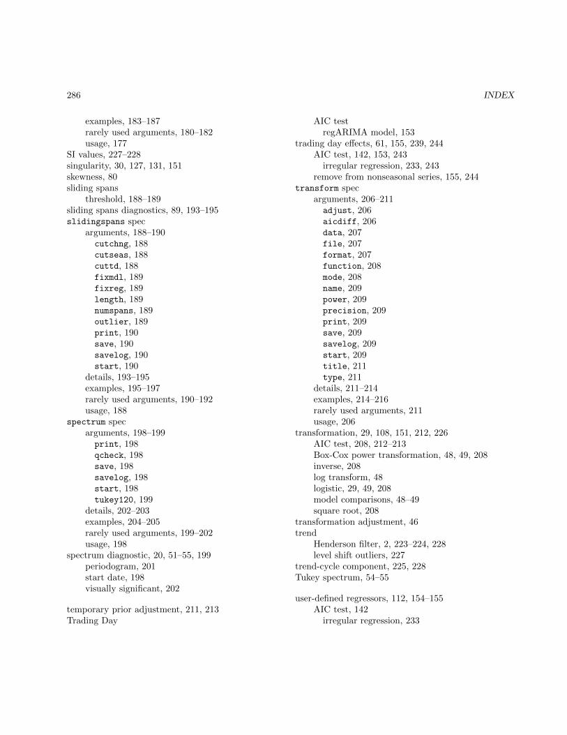
286 INDEX
examples, 183–187rarely used arguments, 180–182usage, 177
SI values, 227–228singularity, 30, 127, 131, 151skewness, 80sliding spans
threshold, 188–189sliding spans diagnostics, 89, 193–195slidingspans spec
arguments, 188–190cutchng, 188cutseas, 188cuttd, 188fixmdl, 189fixreg, 189length, 189numspans, 189outlier, 189print, 190save, 190savelog, 190start, 190
details, 193–195examples, 195–197rarely used arguments, 190–192usage, 188
spectrum specarguments, 198–199print, 198qcheck, 198save, 198savelog, 198start, 198tukey120, 199
details, 202–203examples, 204–205rarely used arguments, 199–202usage, 198
spectrum diagnostic, 20, 51–55, 199periodogram, 201start date, 198visually significant, 202
temporary prior adjustment, 211, 213Trading Day
AIC testregARIMA model, 153
trading day effects, 61, 155, 239, 244AIC test, 142, 153, 243
irregular regression, 233, 243remove from nonseasonal series, 155, 244
transform specarguments, 206–211adjust, 206aicdiff, 206data, 207file, 207format, 207function, 208mode, 208name, 209power, 209precision, 209print, 209save, 209savelog, 209start, 209title, 211type, 211
details, 211–214examples, 214–216rarely used arguments, 211usage, 206
transformation, 29, 108, 151, 212, 226AIC test, 208, 212–213Box-Cox power transformation, 48, 49, 208inverse, 208log transform, 48logistic, 29, 49, 208model comparisons, 48–49square root, 208
transformation adjustment, 46trend
Henderson filter, 2, 223–224, 228level shift outliers, 227
trend-cycle component, 225, 228Tukey spectrum, 54–55
user-defined regressors, 112, 154–155AIC test, 142
irregular regression, 233
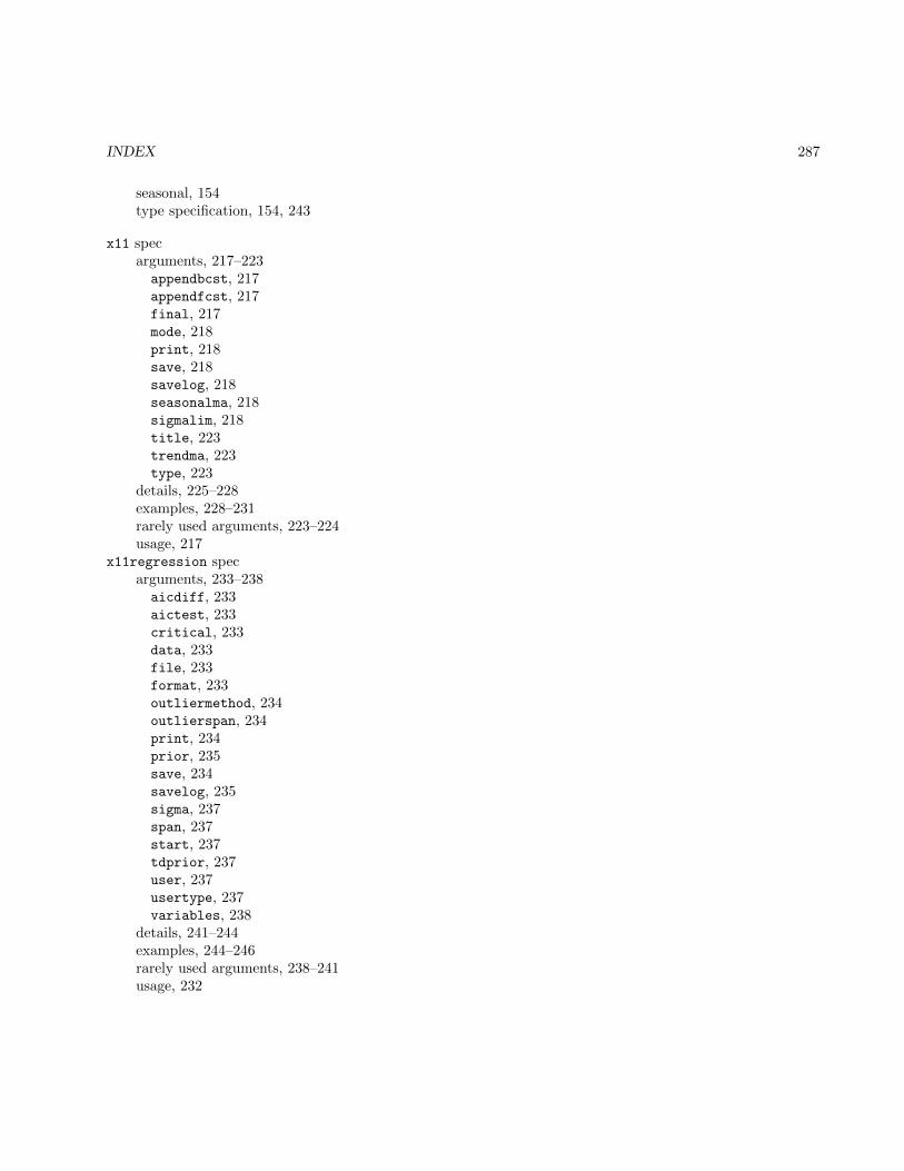
INDEX 287
seasonal, 154type specification, 154, 243
x11 specarguments, 217–223appendbcst, 217appendfcst, 217final, 217mode, 218print, 218save, 218savelog, 218seasonalma, 218sigmalim, 218title, 223trendma, 223type, 223
details, 225–228examples, 228–231rarely used arguments, 223–224usage, 217
x11regression specarguments, 233–238aicdiff, 233aictest, 233critical, 233data, 233file, 233format, 233outliermethod, 234outlierspan, 234print, 234prior, 235save, 234savelog, 235sigma, 237span, 237start, 237tdprior, 237user, 237usertype, 237variables, 238
details, 241–244examples, 244–246rarely used arguments, 238–241usage, 232

288 INDEX