Refactoring, reengineering and evolutionRefactoring, reengineering and evolution: paths to Geant4...

Maria Grazia Pia, INFN Genova

Refactoring, reengineering and evolution: paths to Geant4 uncertainty quantification and

performance improvement!

CHEP 2012 21-25 May 2012

New York City, NY, USA

Maria Grazia Pia

M. Batič, M. Begalli, M. Han, S. Hauf, G. Hoff, C. H. Kim, M. Kuster, P. Saracco, H. Seo, G. Weidenspointner, A. Zoglauer

INFN Genova, Italy

State University of Rio de Janeiro (UERJ), Brazil Hanyang University, Seoul, Korea Darmstadt Tech. Univ., Germany

PUCRS, Porto Alegre, Brazil EU XFEL GmbH, Hamburg, Germany

MPI Halbleiterlabor, Munich, Germany Space Sciences Laboratory, UC Berkeley, USA


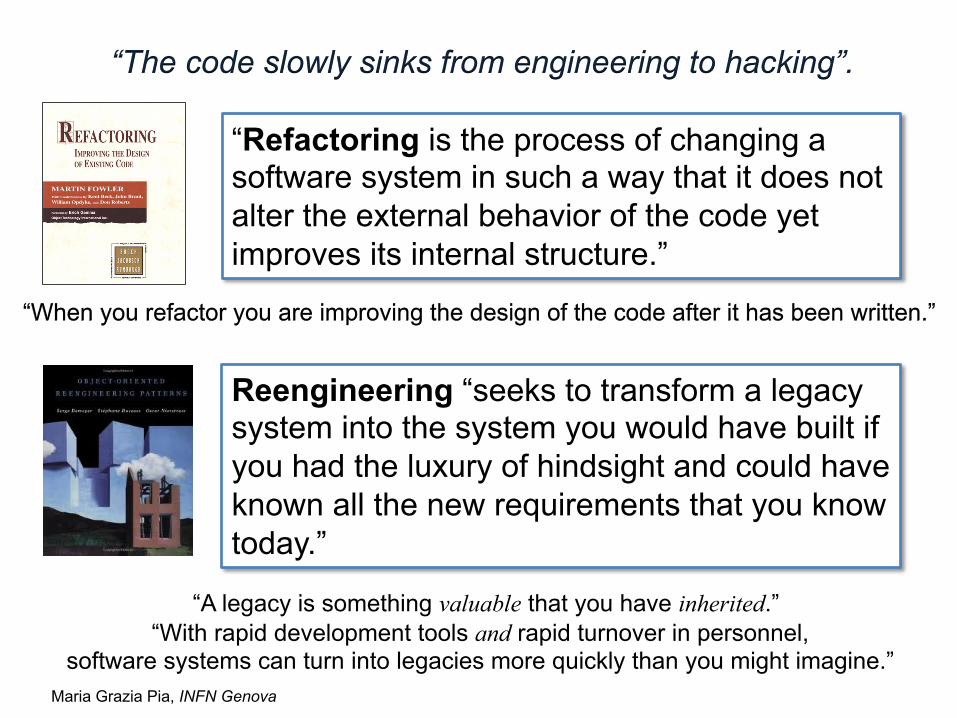
“Refactoring is the process of changing a software system in such a way that it does not alter the external behavior of the code yet improves its internal structure.”

“The code slowly sinks from engineering to hacking”.

“When you refactor you are improving the design of the code after it has been written.”

Reengineering “seeks to transform a legacy system into the system you would have built if you had the luxury of hindsight and could have known all the new requirements that you know today.”

“With rapid development tools and rapid turnover in personnel, software systems can turn into legacies more quickly than you might imagine.”

“A legacy is something valuable that you have inherited.”


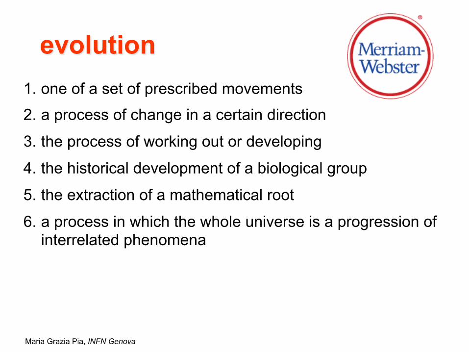
1. one of a set of prescribed movements

2. a process of change in a certain direction

3.  the process of working out or developing

4.  the historical development of a biological group

5.  the extraction of a mathematical root

6. a process in which the whole universe is a progression of interrelated phenomena

evolution


The lantern

State of the art in the physics for Monte Carlo

particle transport

Quantified simulation

Focus on physics and fundamental concepts of particle transport

Produce concrete deliverables

Theoretical and technological challenges

State of the art?


State-of-the-art, quantified

V&V UQ

Software design

Physics

Archival literature

Series of pilot projects

going on since 2008

Highlights No time to go into details


Quantify Geant4 physics

capabilities

Identify experimental requirements

Assess the state of the art

Refactor (Re)design

Prune Improve Extend

New physics New performance

Code Physics

V&V

software physics

current future

theory exp. MC

prototype


Smells

! Duplicated Code ! Long Method ! Large Class ! Long Parameter List ! Divergent Change ! Shotgun Surgery ! Feature Envy ! Data Clumps ! Primitive Obsession ! Switch Statements ! Parallel Inheritance Hierarchies

! Lazy Class ! Speculative Generality ! Temporary Field ! Message Chains ! Middle Man ! Inappropriate Intimacy ! Alternative Classes with

Different Interfaces ! Incomplete Library Class ! Data Class ! Refused Bequest

If it stinks, change it. Grandma Beck, discussing child-rearing philosophy

M. Fowler, K. Beck et al., Refactoring: Improving the Design of Existing Code


Electromagnetic smells

Coupling

σtot and final state modeling have been decoupled in hadronic

physics design since RD44 Final state generation How a process occurs

Whether a process occurs Total cross section

“model”

Dependencies on other parts of the software

One needs a geometry (and a full scale application)

to test (verify) a cross section Difficult to test è no testing often

Problem domain analysis Improve domain decomposition


Benefits

Basic physics V&V can be performed by means of lightweight unit tests

Exploring new models (calculations) is made easier Quantification of accuracy is facilitated

Simplicity of testing for V&V Ease of maintenance

Transparency

Policy-based class design

G4ComptonDataLib<<typedef>>

TCrossSectionTGenerator

G4TRDPhotonProcess

G4CrossSectionDataLib, G4GeneratorComptonDataLib

<<bind>>

G4ComptonPenelope<<typedef>>

G4ComptonStandard<<typedef>>

G4ComptonStandardDataLib<<typedef>>

G4CrossSectionComptonPenelope,G4GeneratorComptonPenelope<<bind>>

G4CrossSectionComptonStandard,G4GeneratorComptonStandard<<bind>>

G4CrossSectionComptonStandard,G4GeneratorComptonDataLib<<bind>>

etc.

Numera ciò che è numerabile, misura ciò che è misurabile, e ciò che non è misurabile rendilo misurabile.

Galileo Galilei (1564-1642)


QED ≠ QCD Electromagnetic processes in particle transport: ! Final state to be generated is well identified ! Theory, rather than model ! Various degrees of refinement in theoretical calculations

‒  e.g. electron at rest, scattering functions, Compton profiles ! Experimental data for validation are (in general) available

Bare-bone physical functionality Decorations on top

Motion of atomic electrons Doppler broadening

Vacancy creation Atomic relaxation Binding effects

scattering functions

Doppler profiles

Shift from shopping list of alternatives

Distinguish genuine modeling alternatives from evolving degree

of complexity


An example: Photon elastic scattering

Penelope Penelope EPDL Relativ. Non-Rel. Modified MFF RFF SM 2001 2008 FF FF FF ASF ASF NT

ε 0.27 0.38 0.38 0.25 0.35 0.49 0.52 0.48 0.77 error ±0.05 ±0.06 ±0.06 ±0.05 ±0.06 ±0.06 ±0.06 ±0.06 ±0.05

Form factor approximation: non relativistic, relativistic, modified + anomalous scattering factors

2nd order S-matrix calculations recent calculations, not yet used in Monte Carlo codes

ε = fraction of test cases compatible with experiment, 0.01 significance

Differential cross sections

State of the art

Quantification Statistical analysis, GoF + categorical


Prune

Two Geant4 models, identical underlying physics content (it used to be different)

Number one in the stink parade is duplicated code

physics

M. Fowler, Refactoring

“Livermore” Penelope EPDL97 EPDL97 0.38±0.06 0.38±0.06

Efficiency w.r.t. experiment

Bremsstrahlung, evaporation, proton elastic scattering etc.

Code bloat Burden on

•  Software design •  Maintenance •  User support

Unnecessary complexity

Objective quantification of smell

−0.04 −0.02 0.00 0.02 0.04

0

100

200

300

400

500

600

(dσPenelope2008

dΩ−dσEPDLdΩ

)dσEPDLdΩ

Counts

mean 0.07%

σ = 1 %

−0.0004 −0.0002 0.0000 0.0002 0.0004

0

1000

2000

3000

4000

5000

σPenelope2008 − σEPDL

σEPDL

Counts

mean 7 10-5 %

σ = 0.008 %

σtotal dσ/dΩ


Trash and redo

Number one in the stink parade is duplicated code

numbers

-0.2

-0.15

-0.1

-0.05

0

0.05

0.1

10-2

10-1

1 10

E (MeV)

Rel

ativ

e di

ffere

nce

p ionisation cross sections difference w.r.t. experiment

EADL Carlson

other

-10

-8

-6

-4

-2

0

2

4

6

8

10

0 10 20 30 40 50 60 70 80 90 100

Atomic number

Diff

eren

ce (e

V)

KL3 Eγ w.r.t. experiment

Carlson Williams

mixed

{ 1.  Bearden & Burr (1967) 2.  Carlson 3.  EADL 4.  Sevier 5.  ToI 1978 (Shirley) 6.  ToI 1996 (Larkins) 7.  Williams

Atomic binding energies

3246 IEEE TRANSACTIONS ON NUCLEAR SCIENCE, VOL. 58, NO. 6, DECEMBER 2011

Evaluation of Atomic Electron Binding Energiesfor Monte Carlo Particle Transport

Maria Grazia Pia, Hee Seo, Matej Batic, Marcia Begalli, Chan Hyeong Kim, Lina Quintieri, and Paolo Saracco

Abstract—A survey of atomic binding energies used by generalpurpose Monte Carlo systems is reported. Various compilations ofthese parameters have been evaluated; their accuracy is estimatedwith respect to experimental data. Their effects on physical quan-tities relevant to Monte Carlo particle transport are highlighted:X-ray fluorescence emission, electron and proton ionization crosssections, and Doppler broadening in Compton scattering. The ef-fects due to different binding energies are quantified with respectto experimental data. Among the examined compilations, EADL isfound in general a less suitable option to optimize simulation ac-curacy; other compilations exhibit distinctive capabilities in spe-cific applications, although in general their effects on simulationaccuracy are rather similar. The results of the analysis providequantitative ground for the selection of binding energies to opti-mize the accuracy of Monte Carlo simulation in experimental usecases. Recommendations on software design dealing with these pa-rameters and on the improvement of data libraries for Monte Carlosimulation are discussed.

Index Terms—Geant4, ionization, Monte Carlo, PIXE, simula-tion, X-ray fluorescence.

I. INTRODUCTION

T HE simulation of particle interactions in matter involvesa number of atomic physics parameters, whose values af-

fect physics models applied to particle transport and experi-mental observables calculated by the simulation. Despite thefundamental character of these parameters, a consensus has notalways been achieved about their values, and different MonteCarlo codes use different sets of parameters.

Atomic parameters are especially relevant to simulation sce-narios that are sensitive to detailed modeling of the propertiesof the interacting medium. Examples include the generation ofcharacteristic lines resulting from X-ray fluorescence or Auger

Manuscript received May 18, 2011; revised August 31, 2011; accepted Oc-tober 10, 2011. Date of current version December 14, 2011.

M. G. Pia and P. Saracco are with the INFN Sezione di Genova, I-16146Genova, Italy (e-mail: [email protected]; [email protected]).

H. Seo and C. H. Kim are with the Department of Nuclear Engineering,Hanyang University, Seoul 133-791, Korea (e-mail: [email protected];[email protected]).

M. Batic is with INFN Sezione di Genova, Genova, Italy, on leave from theJozef Stefan Institute, 1000 Ljubljana, Slovenia (e-mail: [email protected]).

M. Begalli is with the State University of Rio de Janeiro, 20551-030 Rio deJaneiro, Brazil (e-mail: [email protected].).

L. Quintieri is with the INFN Laboratori Nazionali di Frascati, I-00044 Fras-cati, Italy (e-mail: [email protected]).

Color versions of one or more of the figures in this paper are available onlineat http://ieeexplore.ieee.org.

Digital Object Identifier 10.1109/TNS.2011.2172458

electron emission, and precision simulation studies, such as mi-crodosimetry, that involve the description of particle interac-tions with matter down to energies comparable with the scaleof atomic binding energies.

Simulation in these domains has been for an extended timethe object of specialized Monte Carlo codes; some general pur-pose Monte Carlo systems have devoted attention to these areas,introducing functionality for the simulation of fluorescence,PIXE (Particle Induced X-ray Emission) and microdosimetry.In this context, emphasis has been placed on the developmentand validation of the physics models implemented in thesimulation systems, while relatively limited effort has beeninvested into verifying the adequacy of the atomic parametersused by general purpose Monte Carlo codes with regard to therequirements of new application domains.

This paper surveys atomic binding energies used by wellknown Monte Carlo systems, including EGS [1], EGSnrc[2], Geant4 [3], [4], ITS (Integrated Tiger Series) [5],MCNP/MCNPX [6], [7] and Penelope [8], and by somespecialized physics codes. These software systems use a va-riety of compilations of binding energies, which are derivedfrom experimental data or theoretical calculations; this paperinvestigates their accuracy and their effects on simulations.

II. COMPILATIONS OF ELECTRON BINDING ENERGIES

The binding energies considered in this study concern neu-tral atoms in their ground state; several compilations of theirvalues, of experimental and theoretical origin, are available inthe literature.

Compilations based on experimental data are the result of theapplication of selection, evaluation, manipulations (like inter-polation and extrapolation) and semi-empirical criteria to avail-able experimental measurements to produce a set of referencevalues covering the whole periodic system of the elements andthe complete atomic structure of each element.

Most of the collections of electron binding energies based onexperimental data derive from a review published by Beardenand Burr in 1967 [9]. Later compilations introduced further re-finements in the evaluation of experimental data and the cal-culation of binding energies for which no measurements wereavailable; they also accounted for new data taken after the pub-lication of Bearden and Burr’s review.

Experimental atomic binding energies can be affected by var-ious sources of systematic effects; they originate not only fromthe use of different experimental techniques in the measure-ments, but also from physical effects: for instance, binding en-ergies of elements in the solid state are different from those of

0018-9499/$26.00 © 2011 IEEE

Carlson + Williams EADL {

23 pages

Carlson Shirley ( )

Source of epistemic uncertainties?


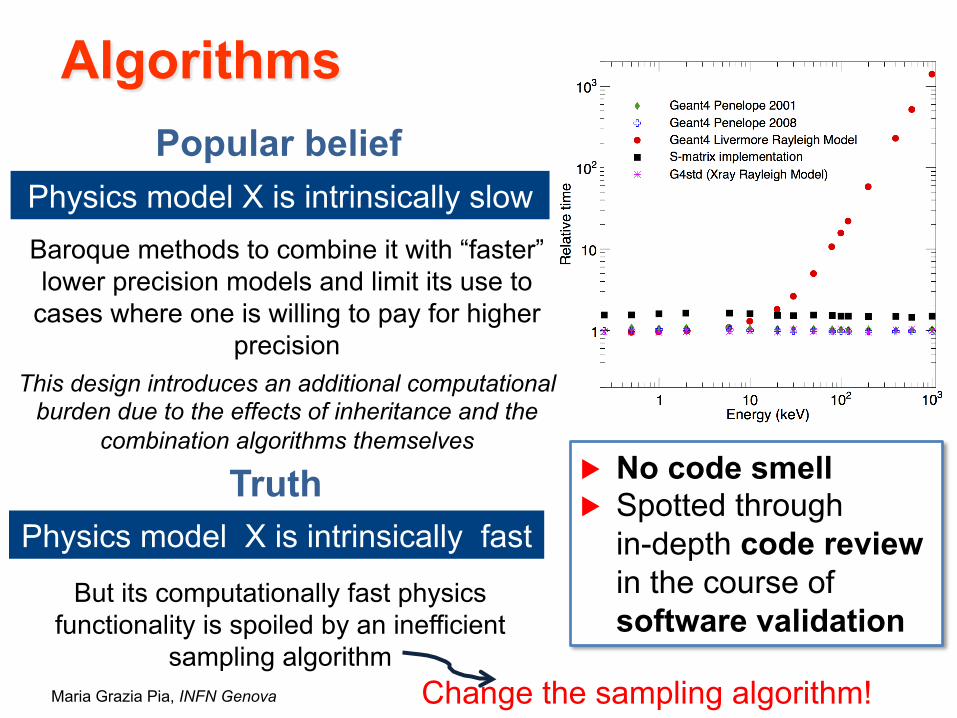
Algorithms Popular belief

Physics model X is intrinsically slow Baroque methods to combine it with “faster” lower precision models and limit its use to

cases where one is willing to pay for higher precision

This design introduces an additional computational burden due to the effects of inheritance and the

combination algorithms themselves

Truth Physics model X is intrinsically fast

But its computationally fast physics functionality is spoiled by an inefficient

sampling algorithm

▶  No code smell ▶  Spotted through o  in-depth code review

in the course of software validation

Change the sampling algorithm!


The fastest algorithm

no algorithm at all

Shift modeling from algorithms to data


Energy (MeV)

Tota

l cro

ss s

ectio

n (M

b)

0.00001 0.0001 0.001 0.01 0.1 1

0

100

200

300

400

500

600

●

●

●

●

●

●

●

●

●

●●●●

●●●

●●●

●●●

●●●

●

●

●

●

●

●

●

●

●

●

●

●

●

●●

●

●

●●

●●●

●●●●●●●●●●●●●●

●

ExperimentFreundBoivinMcCallion

ModelsEEDLDeutsch−MaerkMerged

Energy (MeV)

Tota

l cro

ss s

ectio

n (M

b)

0.0001 0.001 0.01 0

100

200

300

●

●

●

●

●●

●

●

●

●

●

●

●●

●

●

●●

●●●

●●●●●●●●●●●●●●

Mg (Z=12)

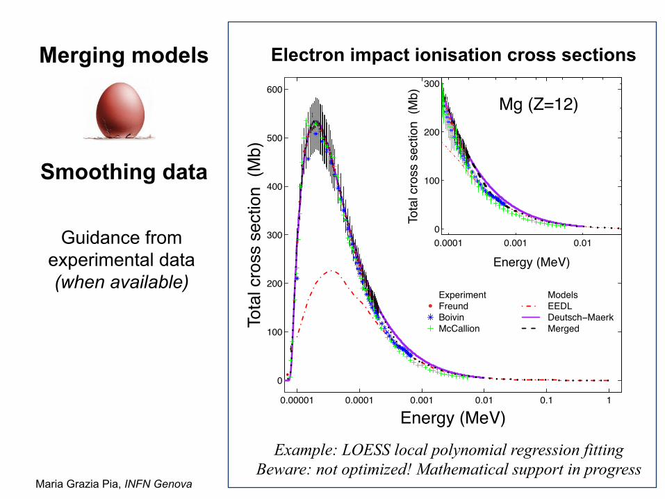
Merging models

Smoothing data

Guidance from experimental data (when available)

Electron impact ionisation cross sections

Example: LOESS local polynomial regression fitting Beware: not optimized! Mathematical support in progress


…no silver bullet

●

●

●

●● ●

●

●

●

●

●●

●

●

●

●

●●●●●

●●

●

●

100 200 500 1000 2000 5000 10000

Z=50

Energy (keV)

dσdΩ

(b

sr)

10−10

10−8

10−6

10−4

10−2

1

●

●

●

●●

●

●

●

●

●

●●

●

●

●

●

●

●●

●●●

●●

●

●

●

●

experimentalSMEPDL

●

● ●

●

●

●

●

●

●

●

●

●

●

●

●

●

●●

●

●●●●

●

●

●

100 200 500 1000 2000 5000

Z=73

Energy (keV)

dσdΩ

(b

sr)

10−9

10−7

10−5

10−3

10−1

●

●●

●

●

●

●

●

●

●

●

●

●

●

●

●

●●●●●●●

●●

●

●

●

experimentalSMEPDL

●

●●

●●

●

●

●

●

●

●

●

●●

●

●

●

●●

●

●

●

●

●

●

●

●

●

●

●

●

●

●

●●

●●●

●

●

●

●

●

●

●

●●●●●●●

●●

●

●

●

●●●

●

●

●

●

●●

●

●

●

●

●●●

●

●●●●

●●

●

●

●●

●●

●

●

●

●

●

●

●

●●●

●

●

●

●

●

●

●

●

●

●

●

●

100 200 500 1000 2000 5000

Z=82

Energy (keV)

dσdΩ

(b

sr)

10−9

10−7

10−5

10−3

10−1●

●

●●●●

●

●

●

●

●●

●●

●

●

●

●●

●

●

●

●

●

●

●

●

●

●

●

●

●

●

●●●●●

●

●

●

●

●

●

●

●●●●●●●

●●

●

●

●

●●●

●●●●●●●●●●●●●●●●●●●●●●●●●●●●●●●●●●●●●●●●●●●●●●●●

●

●

experimentalSMEPDL

●

●●●

●

●

●

●

●

●

●

●

●

●●

●

●

●

●

● ●●

●

●●●

●

●

●

●

●

●●

●●●

●

●●●

●●●●●

●

●●

●

●

100 200 500 1000 2000 5000

Z=92

Energy (keV)

dσdΩ

(b

sr)

10−8

10−6

10−4

10−2

1

●

●●

●

●

●

●

●

●

●

●

●

●

●●●

●

●

●

●

●●●●●●●●●

●●●●

●●●●

●●●●

●●●●●●●

●

●

●

●

experimentalSMEPDL

Smoothing models (or data) that exhibit significantly different

behaviour is not physically justified

Experimental data themselves must be analyzed for inconsistencies and

possible systematics

Photon elastic scattering cross section at 90°

Experimental data by Schumacher et al., Starr et al., Jackson et al., Moreh et al. etc., complete list in a forthcoming publication

How to solve this kind of problems? Better theoretical calculations

New, dedicated experimental data

No easy solution

Here our understanding of the underlying physics phenomena fails


Data libraries

! PIXE (proton ionisation cross sections) ! BEB – DM (electron ionisation cross sections) ! Photon elastic

‒  RTAB (Lynn Kissel) trimmed and reformatted for MC use

R&D in progress

! Interpolation algorithms ! Smoothing techniques ! Data management methods

Experimentally validated Quantified accuracy

Mathematical expertise


Refactoring data management

! Today’s technology ‒  …keeping an eye on the new C++ Standard

! Optimal container ! Pruning data ! Splitting files ! Software design


Big refactoring

G4VRadDecayEmission

+ G4VRadDecayEmission()

+ ~G4VRadDecayEmission()

+ ProduceYourself()

+ DumpInfo()

+ SetParentZA()

+ GetDaughterZ()

+ GetDaughterA()

+ GetParentHalfLife()

+ GetICM()

+ GetTheDecayType()

# SetParentHalfLife()

G4RadioactiveController

+ G4RadioactiveController()

+ ~G4RadioactiveController()

+ ReturnDecayEmissionContainer()

+ ReturnAllDecayEmission()

+ DecayDataAvailable()

+ ReturnNearestParentLevel()

+ SetMinimumHalfLife()

- FileExists()

- BuildDB()

G4RadDecayEmissionContainer

+ G4RadDecayEmissionContainer()

+ ~G4RadDecayEmissionContainer()

+ ProduceEmissionForStatisticalApproach()

+ DumpInfo()

+ SetParentZA()

+ GetParentHalfLife()

+ SetParentHalfLife()

+ AddParticleForStatisticalApproach()

+ AddDecayEmission()

+ ReturnEmissionObject()

+ ReturnAllEmissionObjects()

+ NormalizeLevels()

+ ReturnRecoilFromStatistical()

G4BetaDecayEmission

+ G4BetaDecayEmission()

+ ~G4BetaDecayEmission()

+ ProduceYourself()

+ DumpInfo()

- InitBetaFermi()

G4ITDecayEmission

+ G4ITDecayEmission()

+ ~G4ITDecayEmission()

+ ProduceYourself()

+ DumpInfo()

G4ElectronCaptureEmission

+ G4ElectronCaptureEmission()

+ ~G4ElectronCaptureEmission()

+ ProduceYourself()

+ DumpInfo()

G4AlphaDecayEmission

+ G4AlphaDecayEmission()

+ ~G4AlphaDecayEmission()

+ ProduceYourself()

+ DumpInfo()

G4StatEmissionObject

+ G4StatEmissionObject()

+ G4StatEmissionObject()

+ ~G4StatEmissionObject()

+ GetProbability()

+ GetEnergy()

+ GetHalfLife()

+ GetParticleDef()

G4FluorescenceForRadDecay

+ ProduceYourself()

<<:vector>>

G4BetaFermi

+ G4BetaFermi()

+ ~G4BetaFermi()

+ GetBetaEnergy()

- Initialize()

- Calculate()

G4DecayChainSolver

+ G4DecayChainSolver()

+ ~G4DecayChainSolver()

+ SolveAndReturnData()

+ SetActivityMap()

- InitChain()

- fillMatrix()

- Calculate()

- fillAZ()

- GoThroughChain()

- Chain_Backwards()

- isnan()

G4DecayChainInfo

+ G4DecayChainInfo()

+ G4DecayChainInfo()

+ ~G4DecayChainInfo()

+ GetA()

+ GetZ()

+ GetProb()

+ SetProb()

G4RandomDirection

+ G4RandomDirection()

+ ~G4RandomDirection()

+ GetRandomDirection()

<<map>>

<<map>>

<<map>>

G4RadioactiveDecay

+ G4RadioactiveDecay()


+ ~G4RadioactiveDecay()

+ DecayIt()

+ SetVREmission()

+ GetVREmission()

+ GetVREmission()

+ SetVRN0ForNucleus()

+ SetVRRepeatsPerDecay()

+ SetVRSampleTime()

+ SetMinimumHalfLife()

+ SetMinZ()

+ SetMaxZ()

+ SetMinA()

+ SetMaxA()

+ SetParentLevelTolerance()

+ SetStatisticalApproach()

+ SetInChainEmission()

# GetMeanFreePath()

# GetMeanLifeTime()

- BuildPhysicsTable()

- AtRestGetPhysicalInteractionLength()

- AtRestDoIt()

- PostStepDoIt()

- round()

- SampleEmission()

G4RadioactiveClassicalDeexcitation

+ G4RadioactiveClassicalDeexcitation()

+ ~G4RadioactiveClassicalDeexcitation()

+ DeexciteNucleus()

+ GetShellIndex()

G4RadioactiveDecayMessenger

+ G4RadioactiveDecayMessenger()

+ ~G4RadioactiveDecayMessenger()

+ SetNewValue()

G4NuclearDecayChannel

+ G4NuclearDecayChannel()




+ ~G4NuclearDecayChannel()

+ DecayIt()

+ SetHLThreshold()

+ SetICM()

+ SetARM()

+ GetDecayMode()

+ GetDaughterExcitation()

+ GetDaughterNucleus()

- G4NuclearDecayChannel()



- FillDaughterNucleus()

- BetaDecayIt()

G4RadioactiveDecay


+ ~G4RadioactiveDecay()

+ IsApplicable()

+ IsLoaded()

+ SelectAVolume()

+ DeselectAVolume()

+ SelectAllVolumes()

+ DeselectAllVolumes()

+ SetDecayBias()

+ SetHLThreshold()

+ SetICM()

+ SetARM()

+ SetSourceTimeProfile()

+ IsRateTableReady()

+ AddDecayRateTable()

+ GetDecayRateTable()

+ SetDecayRate()

+ GetTheRadioactivityTables()

+ LoadDecayTable()

+ SetVerboseLevel()

+ GetVerboseLevel()

+ SetNucleusLimits()

+ GetNucleusLimits()

+ SetAnalogueMonteCarlo()

+ SetFBeta()

+ IsAnalogueMonteCarlo()

+ SetBRBias()

+ SetSplitNuclei()

+ GetSplitNuclei()

+ BuildPhysicsTable()

# DecayIt()

# DoDecay()

# GetMeanFreePath()

# GetMeanLifeTime()

# GetTaoTime()

# GetDecayTime()

# GetDecayTimeBin()

- G4RadioactiveDecay()

- operator =()

- AtRestGetPhysicalInteractionLength()

- AtRestDoIt()

- PostStepDoIt()

G4BetaFermiFunction

+ G4BetaFermiFunction()

+ ~G4BetaFermiFunction()

+ GetFF()

+ GetFFN()

- Gamma()

G4AlphaDecayChannel

+ G4AlphaDecayChannel()

+ ~G4AlphaDecayChannel()

G4KshellECDecayChannel

+ G4KshellECDecayChannel()

+ ~G4KshellECDecayChannel()

G4RadioactiveDecayRate

+ G4RadioactiveDecayRate()

+ ~G4RadioactiveDecayRate()

+ G4RadioactiveDecayRate()

+ operator =()

+ operator ==()

+ operator !=()

+ GetZ()

+ GetA()

+ GetE()

+ GetGeneration()

+ GetDecayRateC()

+ GetTaos()

+ SetZ()

+ SetA()

+ SetE()

+ SetGeneration()

+ SetDecayRateC()

+ SetTaos()

+ SetVerboseLevel()

+ GetVerboseLevel()

+ DumpInfo()

G4BetaMinusDecayChannel

+ G4BetaMinusDecayChannel()

+ ~G4BetaMinusDecayChannel()

G4ITDecayChannel

+ G4ITDecayChannel()

+ ~G4ITDecayChannel()

G4RadioactivityTable

+ G4RadioactivityTable()

+ ~G4RadioactivityTable()

+ AddIsotope()

+ GetRate()

+ Entries()

+ GetTheMap()

G4BetaPlusDecayChannel

+ G4BetaPlusDecayChannel()

+ ~G4BetaPlusDecayChannel()

G4MshellECDecayChannel

+ G4MshellECDecayChannel()

+ ~G4MshellECDecayChannel()

G4LshellECDecayChannel

+ G4LshellECDecayChannel()

+ ~G4LshellECDecayChannel()

<<:vector>>

theDecayRateTable

<<:vector>>

theDecayRate

theIsotopeTable<<:vector>>

theRadioactivityTables

<<:vector>>

G4RadiactiveDecayRates

*

<<:vector>>

theRadioactivityTable

G4NucleusLimits

+ G4NucleusLimits()

+ G4NucleusLimits()

+ ~G4NucleusLimits()

+ GetAMin()

+ GetAMax()

+ GetZMin()

+ GetZMax()

+ operator <<()

G4RadioactiveDecayRateVector

+ G4RadioactiveDecayRateVector()

+ ~G4RadioactiveDecayRateVector()

+ G4RadioactiveDecayRateVector()

+ operator =()

+ operator ==()

+ operator !=()

+ GetIonName()

+ GetItsRates()

+ SetIonName()

+ SetItsRates()

G4RIsotopeTable

+ G4RIsotopeTable()

# G4RIsotopeTable()

+ ~G4RIsotopeTable()

+ FindIsotope()

+ GetIsotope()

- GetIsotopeName()

- GetMeanLifeTime()

- GetIsotope()

- GetVerboseLevel()

- Entries()

Geant4 Radioactive Decay

Well defined responsibilities and interactions


New algorithm 214

82Pb 21483Bi

21484Po 210

81Tl

21082Pb

26.8 min 20.0 min

0.16 sec 1.3 min

22.3 yr

21884Po

21083Bi 206

80Hg

ln(2)26.8 min- _________

ln(2)26.8 min_________ ln(2)

20.0 min- _________

ln(2)20.0 min_________

ln(2)20.0 min_________

ln(2)0.16 sec- _________

ln(2)1.3 min- _________

ln(2)0.16 sec_________ ln(2)

1.3 min_________ ln(2)

22.3 yr- _________

ln(2)22.3 yr_________

ln(2)3.1 yr

_________ 0 0

0

0

0 0

0

0

0

0

0 0 0 0

0 0 0

0 0

0 0

0

0

j

i

3.1 min

5 days 8.1 min

Figure 34: An illustration of how the !-matrix is filled using part of the 238U decay chain as an example.

for i > j and

!ii =!ki . (35)

In Equation 34 bi j denotes the branching ratio from the jth to the ith component of the decay chain

with!n

i= j+1 bi j = 1. An example is shown in Figure 34.In computational practice ! can be constructed by iterating through the decay chain and taking ac-

tivation rates into account if necessary. Because ! is independent of the actual nuclei numbers it mustonly be constructed once for each set of nuclei and activations characterizing a given chain. Calculationsusing different nuclei numbers can reuse these initial matrices as needed.

Using the above definitions the number of nuclei of each species in the decay chain in then given by

N(t) = e!tN(0) (36)

which can be rewritten to

N(t) = C e!d t C!1 (37)

as described by Onega. In Equation 37 C is a square matrix with the nth column consisting of thenth eigenvector of !, so that C = [c1,c2, · · · ,cn]. C!1 is its inverse and !d a diagonal matrix with theelements !d,nn being the nth eigenvalue of !.

M. Amaku and coworkers derive an algorithmic approach for calculating the matrices C , C!1 and!d which is computationally less expensive and more accurate than a general approach of numericallydiagonalizing the matrix. The elements of C = [ci j] can be calculated with the recurrence expression

ci j =

!i!1

k= j!ikck j

! j j !!ii

(38)

for i = 2, · · · , n, j = 1, · · · , i ! 1 and cj j = 1. Similarly the elements of C!1 = [c!1i j ] are given by

c!1i j =

i!1"

k= j

cik bk j (39)

67

Statistical Decay

Figure 37: Absolute performance of the new code and the current Geant4 code when decaying the 233Udecay chain. The chain length was varied by setting di!erent initial nuclei.

Auger-electron emission is needed and simulation performance is critical the author thus recommendsthe use of the new statistical approach.

Decay Chain Performance

The decay chain performance comparison is shown in Figure 37. Here one should consider that thecurrent Geant4 code does not take into account the time at which the chain emission is to be sampledat. Instead it is in the user’s responsibility to keep track of relevant emission. This behavior results ina severe performance penalty because much of the sampled emission may actually not be of interest atall. The new code samples the decay chain in such a way that only emissions occurring after a giventime period are actually produced. This explains the increase in computing time needed by the newcode between 233U as the initial isotope and 229Th. As shown in Figure 35 Thorium has a much shorterhalf-life time than Uranium. Since the time period over which the emission from the chain is sampledremains fixed at 3 ! 1013 s = 95120 years much less Uranium than Thorium will have decayed. Thisalso reduces the number of subsequent decays within the chain and hence much less emission has to besampled.

If only the emission of a single isotope within a chain is of interest, the behavior of both codes issimilarly divergent. Again the current Geant4 inefficiently samples all occurring emission, regardless ofthe importance for the simulation result. Instead the user must identify this emission and discard of therest. In contrast the new code allows to select the sampling of individual isotopes within a given chain.Only the emission resulting from such decays will be sampled and passed to tracking. In Figure 37 thisscenario is shown by the two single data points labeled ”End of chain - C” for the new code with classicaldeexcitation sampling and ”End of chain - S” for the new code with statistical deexcitation sampling. Thetime needed by the old code is given by 233U data point of the ”old” curve. In total the performance gainfor decay chains is " 800% when using statistical sampling and still " 450% for classical deexcitationsampling.

71

233U decay

refactored

Geant4

new algorithm

Experiment: Z. W. Bell (ORNL) Validation

Figure 48: The upper part of the plot showsthe measured 133Ba photo-peaks at79.61 keV and 80.99 keV (dots). Alsoshown are the background and peakmodels fitted to the data using HY-PERMET. The background consists ofa constant linear part (lower dashedline) and a step-function modeling thestep of Compton component (upperdashed line). The lower energy peakis shown dotted, while the solid line isthe sum of the second peak and theother components. The low-energy ex-ponential tail is not distinguishable forthese peaks. The lower part showsthe residuals in terms of ! uncertain-ties (solid area: 1!, lines: 3!).

Figure 49: The upper part of the plot showsthe measured 137Cs photo-peak at661.66 keV (dots). Also shown is themodel fitted to the data using HY-PERMET (solid line). Clearly visible isthe exponential tail towards low en-ergies, which is added to the Gaussianpeak. For the 137Cs source this featureis stronger than for the other isotopesas it higher activity leads to more pile-up. The lower part shows the residualsin terms of ! uncertainties (solid area:1!, lines: 3!).

where " is a normalization factor to the amplitude A of the photo-peak and xc is the position ofthe photo-peak’s center; er f c(u) is the complementary error function. The parameters " and #may vary with energy. To account for this the a polynomial model was fitted to the parametersobtained from photo-peaks at different energies as shown in Figures 52 and 53. This polynomialwas then used to determine the parameter energies at arbitrary energies. Figure 49 exemplaryshows a strong exponential component of the 137Cd photo-peak at 661.66 keV.

3. Very strong photo-peaks may exhibit an additional, longer exponential tail, T (x), at energies belowthe peak which can be attributed to surface effects and will also influence lower lying peaks:

T (x) = $Aexp

!

x ! xc

%

"

"1

2erfc

!

x ! xc

µ+µ

2%

"

(47)

The slope parameter % is usually one to two orders of magnitude larger than # while the relativeamplitude $ is one to three orders smaller. The width of the Gaussian noise is again determined by&.

84

33Ba photo-peaks 79.61 and 80.99 keV

Figure 40: Nuclide charts showing the median relative intensity deviations per isotope for gamma(top),conversion-electron(middle) and alpha(bottom) emission. Simulations using the currentGeant4 code are shown on the left; simulations using the new code and employing the statis-tical approach are shown on the right.

76

Absolute validation

Performance


Conclusions

A quantitatively validated, state-of-the-art Monte Carlo code is at reach

Large effort Supported by software design

Refactoring techniques and reengineering patterns contribute to improve computational performance and facilitate validation

a tremendous challenge an inspiring motivation

Physics insight is the key

Refactoring, reengineering and evolutionRefactoring, reengineering and evolution: paths to Geant4...

Documents

Transcript of Refactoring, reengineering and evolutionRefactoring, reengineering and evolution: paths to Geant4...