Reduction of Nord2000 calculation time

RL 1/10

Reduction of Nord2000 calculation time

Rapport nr. 23 Miljøstyrelsens Referencelaboratorium for Støjmålinger

DELTA

2

© DELTA

DELTA, 10 February 2010

Birger Plovsing

Acoustics

3

MILJØSTYRELSENS REFERENCELABORATORIUM FOR STØJMÅLINGER Udøvende institution: DELTA Venlighedsvej 4 2970 Hørsholm Telefon: 72 19 40 00 Telefax: 72 19 40 01 www.referencelaboratoriet.dk

Title Reduction of Nord2000 calculation time

Our ref.: BP/ilk

Performed for Danish Environmental Protection Agency Strandgade 29 1401 Copenhagen K

4

MILJØSTYRELSENS REFERENCELABORATORIUM FOR STØJMÅLINGER

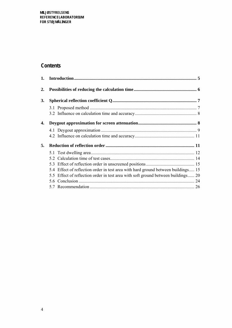
Contents

1. Introduction............................................................................................................. 5

2. Possibilities of reducing the calculation time........................................................ 6

3. Spherical reflection coefficient Q........................................................................... 7 3.1 Proposed method ............................................................................................... 7 3.2 Influence on calculation time and accuracy....................................................... 8

4. Deygout approximation for screen attenuation.................................................... 8 4.1 Deygout approximation ..................................................................................... 9 4.2 Influence on calculation time and accuracy..................................................... 11

5. Reduction of reflection order ............................................................................... 11 5.1 Test dwelling area............................................................................................ 12 5.2 Calculation time of test cases........................................................................... 14 5.3 Effect of reflection order in unscreened positions ........................................... 15 5.4 Effect of reflection order in test area with hard ground between buildings..... 15 5.5 Effect of reflection order in test area with soft ground between buildings...... 20 5.6 Conclusion ....................................................................................................... 24 5.7 Recommendation ............................................................................................. 26

5


1. Introduction A new method for prediction of noise from roads and railways was introduced in Denmark a few years ago. In the method the yearly average of the day-evening-night level Lden shall be calculated using the Nord2000 model. The experience from using the new method is that the calculation time has increased considerably compared to the old calculation model. The increase has been estimated to be between 10 and 100 times of the calculation time of the old methods.

The reasons for the increase in calculation time are:

• Calculations are made in 27 frequency bands instead of as dBA levels

• Multiple sources (normally three) are used to represent the source instead of just one source as in the old methods

• Calculations are made for several terrain segments along the propagation path instead of using just one equivalent flat surface

• When including reflections from vertical surfaces up to third order reflections should be included where only first or second order reflections were used in the old methods

• The yearly average of the noise is determined by repeating the calculation for up to 9 meteo-classes

• Increased complexity in the prediction algorithms.

6


2. Possibilities of reducing the calculation time The purpose of the present project is to consider possible ways of reducing the calculation time of Nord2000 and to select some of them for further investigation. For each the se-lected subjects it is necessary to estimate the effect on the calculation time and on the ac-curacy.

The selected subjects are:

1) Faster method to calculate the spherical wave reflection coefficient Q

2) Use of the Deygout approximation for screen attenuation

3) Possibilities of reducing the reflection order in city environments.

Concerning 1) it is known, that a considerable part of the Nord2000 calculation time is used to calculate the spherical wave reflection coefficient Q. The algorithms are in it self mathematically complicated but furthermore the calculation of Q is often repeated many times for each source-receiver combination. If the calculation of Q could be reduced this would have a considerable overall effect of the Nord2000 calculation time. A method for reducing the calculation time of Q is described in Section 3.

Concerning 2) the diffraction algorithms used for screen effect are mathematically compli-cated and it is therefore possible that the use of the so-called Deygout approximation adop-ted by the Harmonoise method could reduce the calculation time. It was considered to in-vestigate this during the 2006-revision of Nord2000 but it turned out that it was not possi-ble within the framework of the revision. Use of the Deygout approximation is described in Section 4.

Concerning 3) both the Danish guidelines and the Harmonise method prescribe that third order reflections should be used to obtain the “true” noise level. In a highly reflective envi-ronment like a dense multi-storey city area the noise levels in highly screened positions may be severely underestimated by using a reflection order less than three. However, noise map calculations have showed a substantial increase in calculation time when the order of reflections is increased due to the increase in number of propagation paths. Therefore, the calculation time could be reduced if a reflection order less than three could be tolerated. The possibilities of reducing the reflection order are described in Section 5.

It was also considered to investigate the possibility of reducing the number of meteoro-logical classes from 4 to 3 when calculating the yearly average noise levels for noise map-ping purposes. However, it was not possible to investigate both this subject and subject 3) within the project. As the reduction in calculation time of reducing the meteo-classes would only be 25% with no reduction in a city environment where one meteo-class is pre-scribed, the gain from investigating subject 3) was expected to be larger.

7


3. Spherical reflection coefficient Q The algorithms used to calculate the spherical wave reflection coefficient Q are mathe-matically complicated and the calculation of Q is often repeated many times for each source-receiver combination. Therefore, a reduction of the calculation time of Q would have considerable overall effect of the Nord2000 calculation time.

It is not likely that the well established algorithms itself can be simplified without a sig-nificant reduction in accuracy. Another possibility has been to pre-calculate Q for types of surfaces frequently used in calculations and subsequently determine Q by a table look-up. Q is a complex number and particularly the phase of Q has a large influence on the pre-dicted ground effect. It is therefore necessary that the resolution in the table input variables is high. This is fulfilled by the proposed method described in Section 3.1.

3.1 Proposed method

To speed up the Nord2000 calculation the real and imaginary part of the spherical-wave reflection coefficient Q can be pre-calculated and stored in a three dimensional table and the correct value can subsequently be obtained by linear interpolation in the table. In the table, values are given for each frequency f and for values of distance R2 and grazing re-flection angle ψG with a suitable spacing. The spacing of R2 and ψG are made more effi-cient by a transformation of the variables. The spacing and the calculation of the real and imaginary part of Q (Qre and Qim) are defined in Eq. (1). i is the transformed variable of R2 and the table contains integer values of i between 1 and 61. j is the transformed variable of ψG and the table contains integer values of j between 1 and 42. σ is the flow resistivity.

( )

( )

( ) ( ) ( ) ( ) ( )( )σψ

πψ

,,,,,,,,,

42,...,3,2102

1061,...,2,110

2

1042

1021

2

jiRfQjifiQjifQjifQ

j

jj

iiR

Gimre

jG

i

=+=

⎪⎩

⎪⎨⎧

=

==

==

−

−

(1)

When performing the table look-up by linear interpolation the transformed variables i and j are calculated as shown Eq. (2). i and j are in this case real numbers used for interpolation in the Qre and Qim tables.

8


( )

⎪⎪⎩

⎪⎪⎨

⎧

≤<+⎟⎠⎞

⎜⎝⎛

≤≤+=

⎪⎩

⎪⎨

⎧

≥<<+

≤=

22000042

2log10

200000

200001

10000611000001.021log10

01.01

2

22

2

πψππψ

πψψ

GG

GG

j

RRR

Ri

(2)

The calculation of Q described above has been found to be highly accurate for propagation distances from approximately 0.01 m to 10000 m if the grazing angle is not too small. If the angles are very small so that the calculated ground attenuation becomes less than ap-proximately 40-50 dB the prediction becomes substantially poorer. A high accuracy is not considered to be important in case of very large attenuation due to scattering effects and incoherent effects of turbulence but if this is considered a problem in an another connec-tion the accuracy may be increased by adding more values at very low angles (below π/20000).

3.2 Influence on calculation time and accuracy

The proposed method described above has not been developed during this project but at an earlier occasion. However, the method has not previously been described and is therefore included in this note. The reduction in calculation time will depend on the programming but SoundPLAN which already has included the use of look-up tables for Q has estimated that the overall calculation time has been reduced by 3-4 times. The reduction in accuracy of the ground effect has been found to be insignificant. It is possible that method described in Section 3.1 can be made more efficient for a particular program solution. If so, this is permissible as long as it does not reduce the ground effect accuracy compared to the de-scribed method.

4. Deygout approximation for screen attenuation The Hadden/Pierce method used to calculate the diffracted sound pressure behind a finite impedance wedge (described in AV 1851/00, Appendix C) is a mathematically compli-cated method and it was expected that this could have a significant effect on the overall calculation time of the Nord2000 model. The Deygout approximation is described in Sec-tion 4.1.

9


4.1 Deygout approximation

In this section an approximation used by the Harmonoise method shall be described which is called the Deygout approximation. The approximation will is expected to increase the calculation speed when calculating the diffracted sound pressure level. The approximation has been found to produce very good results for high screen where the top of the screen is above the line of sight. A less good but still acceptable accuracy has been found when the top of the screen is close to the line of sight. It is therefore a possibility that the Deygout approximation can be used where slightly less accuracy can be accepted such as noise mapping of large where the calculation time is an issue.

The attenuation according to Deygout is calculated as shown by Eq. (3) where ΔLD is sound pressure level at the receiver relative to the free-field sound pressure level and N is the Fresnel number.

( )

( )⎪⎪⎪

⎩

⎪⎪⎪

⎨

⎧

>−−<<+−

<<−−

<<−−+−

−<

==Δ

1log1016125.088

25.00126

025.0126

25.00

log200

NNNN

NN

NN

N

pp

NL dD (3)

The Fresnel number is defined by Eq. (4) where δ is the path length difference and λ is the wavelength. The path length difference is the difference between the length of the ray path from source to receiver over the top of the screen and from source to receiver directly. If the top of the screen is below the line of sight N shall be multiplied by -1.

λδ2

=N (4)

When using Deygout in Nord2000 it is necessary to extend the range of diffraction angles from 2π to 4π (make allowance for image source on the receiver side of the screen and image receiver on the source side of the screen) as shown in Eq. (5). Furthermore the cal-culation of N has to be based on the diffraction variables used in Nord2000. These varia-bles are:

• The travel time τS from source S to the top of the wedge T

• The travel time τR from receiver R to T

• The travel time τ from S to R over T (normally τ = τS + τR but when used in the proce-dure for a two-edge screen τ may be defined otherwise)

• The travel distance RS from S to T

10


• The travel distance RR from R to T

• The travel distance ℓ from S to R over T (normally ℓ = RS + RR but when used in the procedure for a two-edge screen R may be defined otherwise)

• The source diffraction angle θS re. receiver wedge face

• The receiver diffraction angle θR re. receiver wedge face

• Wedge angle β

• Surface impedance ZS of source wedge face

• Surface impedance ZR of receiver wedge face

( )

( )

( )

( )

( )( )

20

22

642

10,,,,

2cos2

432

NL

RSRS

RSRSSR

RS

RS

RS

SRRS

RS

D

RRp

SignN

RRRRR

andRRRR

where

RR

RRR

Δ

=

−=

−+=

−+

=

⎪⎩

⎪⎨

⎧

>⎟⎟⎠

⎞⎜⎜⎝

⎛+++

≤−+

=

−=

λθθ

λδπα

α

παε

παεεε

παδ

θθα

(5)

The diffracted sound pressure can now be calculated as described in the following. First the grazing reflection angles θS,refl and θR,refl are defined as shown in Eq. (6).

RreflR

SreflS

θθ

θβθ

=

−=

,

, (6)

Then the diffraction angles θS,image and θS,image are defined as shown in Eq. (7).

reflRRimageR

reflSSimageS

,,

,,

2

2

θθθ

θθθ

−=

+= (7)

11


Finally the total sound pressure which is the sum of four ray contributions is calculated by Eq. (8) where p and Q are complex numbers and ω is the angular frequency.

( )( )( )( )

( )( )ωθττ

ωθττ

λθθ

λθθ

λθθλθθ

,,,

,,,

,,,,

,,,,

,,,,,,,,

,2

,1

21423121

,,4

,3

,2

1

RreflRRS

SreflSRS

RSimageRimageS

RSimageRS

RSRimageS

RSRS

ZQQ

ZQQwhere

QQpQpQppp

RRpp

RRpp

RRppRRpp

+=

+=

+++=

=

=

==

(8)

If the diffraction coefficient has to be used it is calculated according to Eq. (9).

l

ωτjpeD = (9)

4.2 Influence on calculation time and accuracy

At an earlier occasion SoundPLAN has tested the use of Deygout approximation and con-cluded that the reduction in overall calculation time is not very significant. It is assumed that the reason is that a screen calculation includes so many calculations of the spherical wave reflection coefficient Q that there is no benefit from applying Deygout. On this basis, the use of it appears not to be an option at present. However, if the calculation time suc-cessfully is reduced in other parts of the model the approach may become an interesting option at a later occasion. The method has not been described previously and is therefore included in this note for possible future use.

5. Reduction of reflection order As mentioned in Section 2 both the Danish guidelines for predicting road and railway noi-se and the Harmonise method prescribe that up to third order reflections should be used to obtain the “true” noise levels. Simple considerations have indicated that if a maximum re-flection order of two is used the calculated noise levels will be around 2 dB less than the “true” noise levels and if only first order reflections are considered the calculated noise levels will be around 5 dB less. However, a more extensive investigation of the deviations for a “real” case has not been carried out. The aim of the present work is to:

• Determine on a more statistical basis the magnitude of errors introduced by reducing the reflection order

12


• To investigate if a calculation with a reduced reflection order combined with some kind of a correction could be applied in order to reduce the overall calculation time

In receiver positions with direct sight from source to receiver the order of reflection will in general have a limited influence on the noise level. On the other hand, in highly screened positions the noise levels may be determined by the reflected sound and in this case the order of reflection might have a high influence on the noise levels. As the influence of the reflection order therefore can vary from position to another it is necessary when applying a correction to the result for a reflection order less than three that some variable is available to distinguish between positions with small and large influence of the reflection order. The hypothesis in this work has been that the shielding effect of house and screens could be such a variable.

To determine the magnitude of errors introduced by reducing the reflection order a test dwelling area was created to simulate a “real” densely built-up city environment with ma-ny reflectors. The test case is described in Section 5.1.

5.1 Test dwelling area

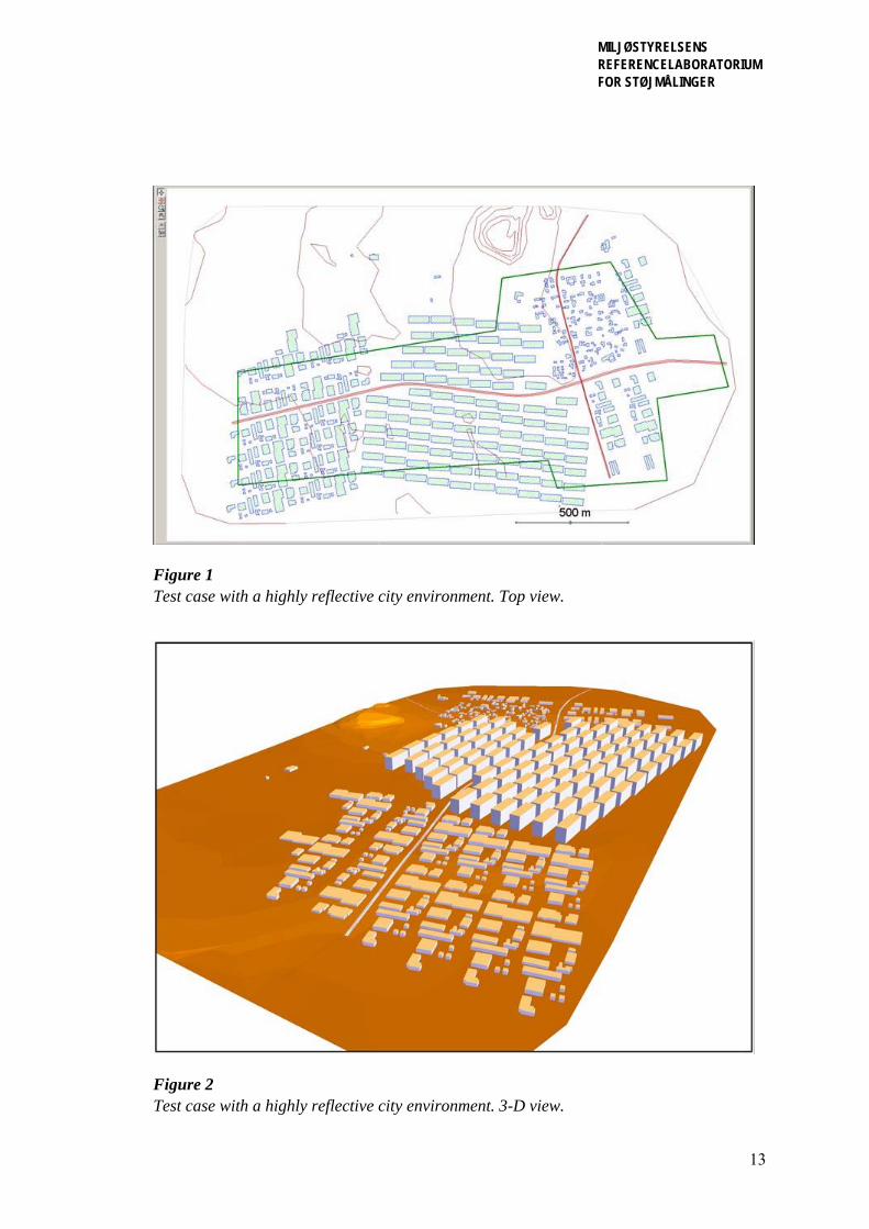
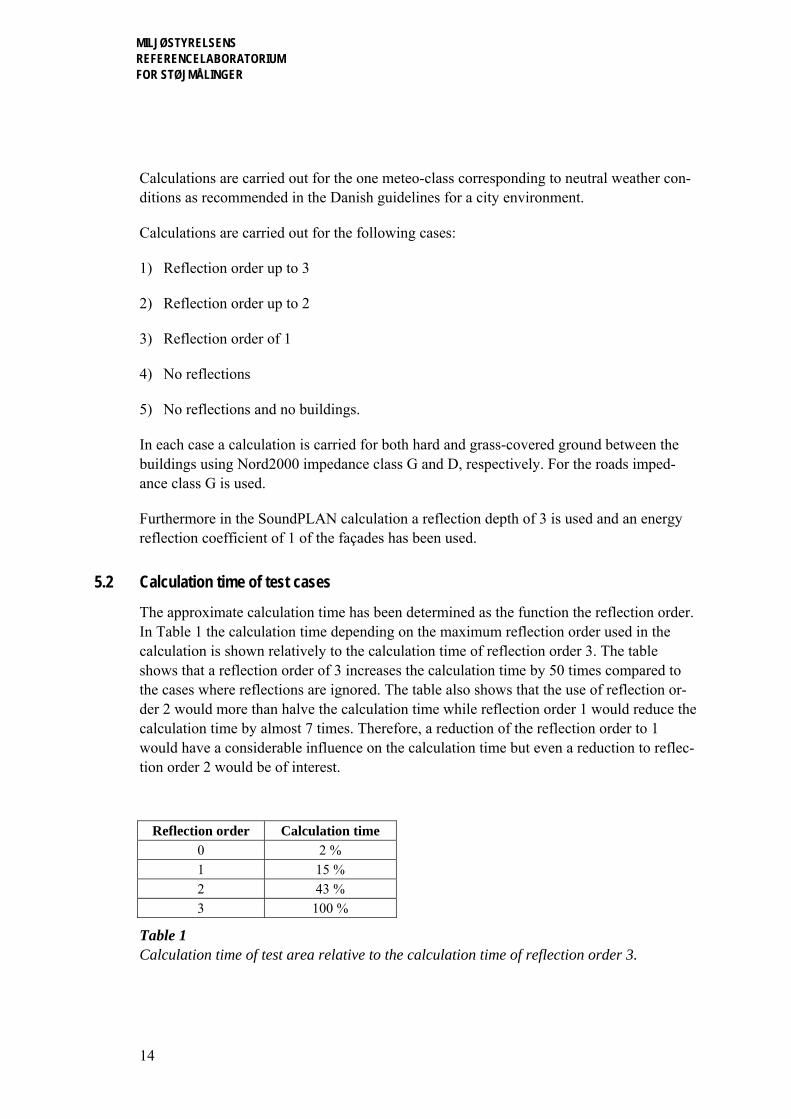
For the analysis the test area shown in Figure 1 was created in the prediction program SoundPLAN. The work of creating the test model in SoundPLAN and running the calcula-tion was carried out by John Klinkby, SoundPLAN Nord ApS. Figure 1 shows a twelve-sided shape drawn with a green colour, which is the area in which calculations of noise levels are carried out. Within this area calculations are performed in a regular grid with a grid size of 15 m and receiver height 2 m. All receiver points in the grid, which are inside buildings, are omitted resulting in 5664 receiver points in the analysis. The red line placed West-East is a major road and the red line placed North-South is a minor road but in the calculations the traffic is the same on the two roads. In the middle of the calculation area is highly reflective environment with buildings of fifteen stories both North and South of the road. West of this is an area with densely placed buildings of mainly one or two stories. In the eastern part of the calculation area is a more open dwelling area with houses of one or two stories. Figure 2 shows the test dwelling area in a 3-D view, where it is possible to get an impression of the height of the buildings.

13


Figure 1 Test case with a highly reflective city environment. Top view.

Figure 2 Test case with a highly reflective city environment. 3-D view.

14


Calculations are carried out for the one meteo-class corresponding to neutral weather con-ditions as recommended in the Danish guidelines for a city environment.

Calculations are carried out for the following cases:

1) Reflection order up to 3

2) Reflection order up to 2

3) Reflection order of 1

4) No reflections

5) No reflections and no buildings.

In each case a calculation is carried for both hard and grass-covered ground between the buildings using Nord2000 impedance class G and D, respectively. For the roads imped-ance class G is used.

Furthermore in the SoundPLAN calculation a reflection depth of 3 is used and an energy reflection coefficient of 1 of the façades has been used.

5.2 Calculation time of test cases

The approximate calculation time has been determined as the function the reflection order. In Table 1 the calculation time depending on the maximum reflection order used in the calculation is shown relatively to the calculation time of reflection order 3. The table shows that a reflection order of 3 increases the calculation time by 50 times compared to the cases where reflections are ignored. The table also shows that the use of reflection or-der 2 would more than halve the calculation time while reflection order 1 would reduce the calculation time by almost 7 times. Therefore, a reduction of the reflection order to 1 would have a considerable influence on the calculation time but even a reduction to reflec-tion order 2 would be of interest.

Reflection order Calculation time 0 2 % 1 15 % 2 43 % 3 100 %

Table 1 Calculation time of test area relative to the calculation time of reflection order 3.

15


5.3 Effect of reflection order in unscreened positions

As mentioned earlier, in receiver positions with direct propagation from source to receiver the order of reflection will in general have a limited influence on the noise level whereas the effect will be much larger in screened position. A façade towards the road is a typical case with direct propagation. In this case the increase in noise levels is determined by the reflections in the façade on the other side of the road and the façade it-self. To determine the “minimum” effect of the reflection order a calculation has been carried out by Nord2000 for a city street with two lanes each with a width of 5 m. The façades on each side of the road are 10 m from centre line of the road and infinitely high. The surface be-tween the façades is assumed to be hard with impedance class G and the energy reflection coefficient of the façades is assumed to be 1.

The calculated noise level depending of the reflection order relative to the noise level us-ing reflection order 3 is shown in Table 2.

Reflection order Change in noise level (dB)

0 -2.1 1 -0.9 2 -0.3 3 0

Table 2 Change in noise level at the façade due to the reflection order relative to the noise level of reflection order 3.

5.4 Effect of reflection order in test area with hard ground between buildings

In order to illustrate the magnitude of errors introduced by using a reflection order less than three the difference between the calculated noise level obtained with reflection order 3 and denoted the “true” value in the following and the calculated noise level obtained with reflection order 2, 1, 0 when the ground between the buildings is hard is shown in Figure 3 through Figure 5, respectively. Furthermore, to test the hypothesis mentioned above that the difference is assumed to be a function of the shielding effect of houses and screens and to consider the possibilities of developing a model for correcting lower reflec-tion order results to obtain the “true” level the differences are shown versus the shielding effect of the chosen reflection order. The shielding effect is defined as the difference be-tween the noise levels calculated using the chosen reflection order (0-2) and the noise level calculated with no reflections and ignoring the buildings and screens. The blue points in the figures are the calculated differences. The red line is a trend line obtained by least-squares-fit of the differences in positions with shielding less than zero. In preparation for a model the trend line is limited downwards to the inverse of the value given by Table 2.

16


-5

0

5

10

15

20

25

30

35

-50 -45 -40 -35 -30 -25 -20 -15 -10 -5 0 5 10

L(2 refl) - L(0 bygn), dB

L(3

refl)

- L(

2 re

fl), d

B

Figure 3 Differences between the “true” noise level and the noise level obtained by reflection order 2 versus the shielding effect based on reflection order 2 (blue points) for hard ground. The red line is the approximate results obtained by the proposed model based on the reflection order 2 results.

-5

0

5

10

15

20

25

30

35

-50 -45 -40 -35 -30 -25 -20 -15 -10 -5 0 5 10


L(3

refl)

- L(

1 re

fl), d

B


17


-5

0

5

10

15

20

25

30

35

-50 -45 -40 -35 -30 -25 -20 -15 -10 -5 0 5 10


L(3

refl)

- L(

0 re

fl), d

B


The proposed models shown by the red lines in Figure 3 through Figure 5 are given by Eq. (10) through (12) where ΔL3-x is the average deviation obtained with reflection order x and ΔLSx is the shielding effect based on reflection order x.

( )⎩⎨⎧

−≥Δ−<Δ++Δ−

=Δ − 24.33.024.33.024.31098.0

2

2223

S

SS

LifLifL

L (10)

( )⎩⎨⎧

−≥Δ−<Δ++Δ−

=Δ − 64.39.064.39.064.32378.0

1

1113

S

SS

LifLifL

L (11)

( )⎩⎨⎧

−≥Δ−<Δ++Δ−

=Δ − 79.31.279.31.279.33867.0

0

0003

S

SS

LifLifL

L (12)

For each of the receiver points the deviation (residual) between the “true” result and pre-dicted result obtained by the proposed model using less than third order reflections has

18


been determined. The mean and standard deviation of the residuals have been calculated for each reflection order and the result is shown in Table 3.

Statistics of residuals Reflection order

Mean (dB) Standard de-viation (dB)

0 0.30 2.87 1 0.20 1.66 2 0.08 0.80

Table 3 Mean and standard deviation of the residuals (deviations between “true” value and pro-posed model) for hard ground.

The distribution of the residuals is also shown in Figure 6 through Figure 8 for each reflec-tion order. Each figure is a histogram showing the frequency in % of a given deviation from the “true” value in bins of 0.5 dB when applying the model.

0

5

10

15

20

25

30

35

40

45

50

-10 -9 -8 -7 -6 -5 -4 -3 -2 -1 0 1 2 3 4 5 6 7 8 9 10

Residuals (dB)

Freq

uenc

y (%

)

Figure 6 Histogram of deviations of the proposed model in 0.5 dB bins for reflection order 2 and hard ground.

19


0

5

10

15

20

25

30

35

40

45

50

-10 -9 -8 -7 -6 -5 -4 -3 -2 -1 0 1 2 3 4 5 6 7 8 9 10

Residuals (dB)

Freq

uenc

y (%

)


0

5

10

15

20

25

30

35

40

45

50

-10 -9 -8 -7 -6 -5 -4 -3 -2 -1 0 1 2 3 4 5 6 7 8 9 10

Residuals (dB)

Freq

uenc

y (%

)


20


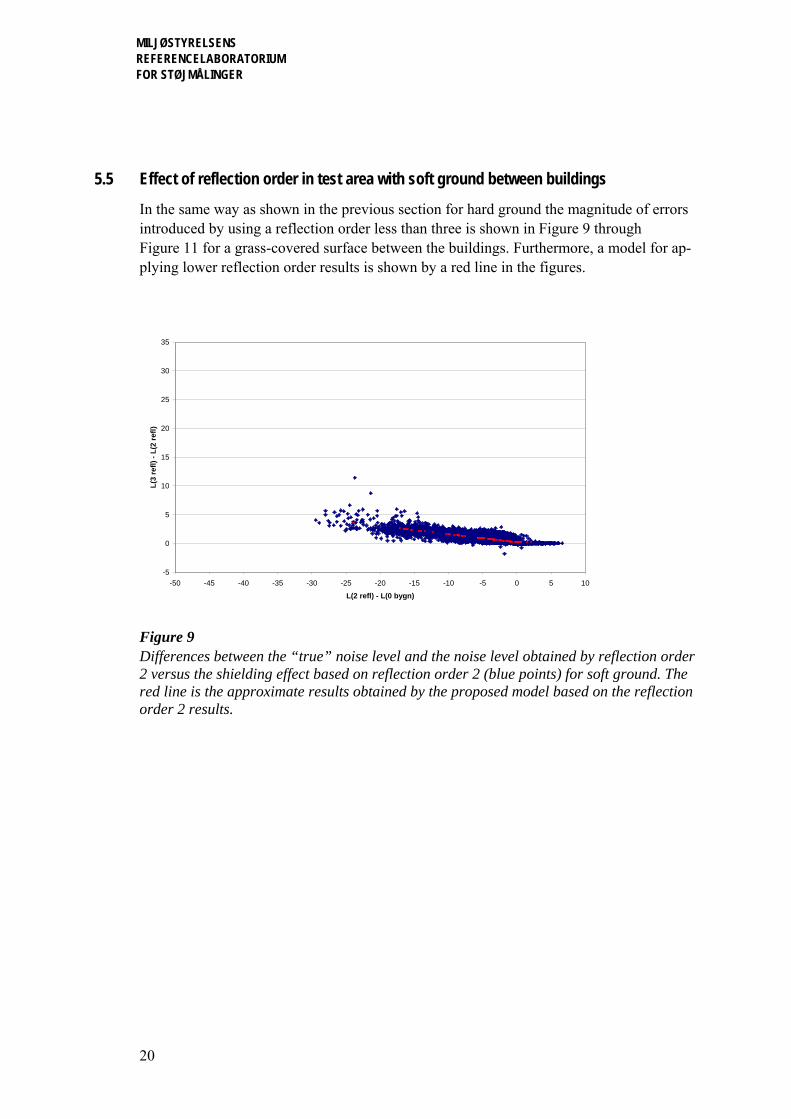
5.5 Effect of reflection order in test area with soft ground between buildings

In the same way as shown in the previous section for hard ground the magnitude of errors introduced by using a reflection order less than three is shown in Figure 9 through Figure 11 for a grass-covered surface between the buildings. Furthermore, a model for ap-plying lower reflection order results is shown by a red line in the figures.

-5

0

5

10

15

20

25

30

35

-50 -45 -40 -35 -30 -25 -20 -15 -10 -5 0 5 10

L(2 refl) - L(0 bygn)

L(3

refl)

- L(

2 re

fl)

Figure 9 Differences between the “true” noise level and the noise level obtained by reflection order 2 versus the shielding effect based on reflection order 2 (blue points) for soft ground. The red line is the approximate results obtained by the proposed model based on the reflection order 2 results.

21


-5

0

5

10

15

20

25

30

35

-50 -45 -40 -35 -30 -25 -20 -15 -10 -5 0 5 10


L(3

refl)

- L(

1 re

fl)


-5

0

5

10

15

20

25

30

35

-50 -45 -40 -35 -30 -25 -20 -15 -10 -5 0 5 10


L(3

refl)

- L(

0 re

fl)


22


In the same way as in the previous section the proposed models shown by the red lines in Figure 9 through Figure 11 are given by Eq. (13) through (15).

( )⎩⎨⎧

−≥Δ−<Δ++Δ−

=Δ − 6.03.06.03.06.01405.0

2

2223

S

SS

LifLifL

L (13)

( )⎩⎨⎧

−≥Δ−<Δ++Δ−

=Δ − 17.19.017.19.017.12937.0

1

1113

S

SS

LifLifL

L (14)

( )⎩⎨⎧

−≥Δ−<Δ++Δ−

=Δ − 24.21.224.21.224.24544.0

0

0003

S

SS

LifLifL

L (15)

The mean and standard deviation of the residuals have again been calculated for each re-flection order and the result is shown in Table 4.

Statistics of residuals Reflection order Mean (dB) Standard de-

viation (dB) 0 0.26 1.79 1 0.17 1.07 2 0.06 0.50

Table 4 Mean and standard deviation of the residuals (deviations between “true” value and pro-posed model) for soft ground.

The distribution of the residuals is shown in Figure 12 through Figure 14 for each reflec-tion order.

23


0

5

10

15

20

25

30

35

40

45

50

-10 -9 -8 -7 -6 -5 -4 -3 -2 -1 0 1 2 3 4 5 6 7 8 9 10

Residuals (dB)

Freq

uenc

y (%

)

Figure 12 Histogram of deviations of the proposed model in 0.5 dB bins for reflection order 2 and soft ground.

0

5

10

15

20

25

30

35

40

45

50

-10 -9 -8 -7 -6 -5 -4 -3 -2 -1 0 1 2 3 4 5 6 7 8 9 10

Residuals (dB)

Freq

uenc

y (%

)


24


0

5

10

15

20

25

30

35

40

45

50

-10 -9 -8 -7 -6 -5 -4 -3 -2 -1 0 1 2 3 4 5 6 7 8 9 10

Residuals (dB)

Freq

uenc

y (%

)


5.6 Conclusion

Based on the results shown in Sections 5.4 and 5.5 the following can be concluded con-cerning underestimation of the noise levels when a reflection order less than three is ap-plied:

• If up to second order reflections are included the noise levels are in most cases under-estimated by less than 5 dB but larger values are observed in a few positions. If the shielding is less than 10 dB the underestimation is below 2-3 dB.

• If only first order reflections are included the noise levels are in most cases underesti-mated by up to 10 dB but larger values may be observed. If the shielding is less than 10 dB the underestimation is below approximately 5 dB.

• If no reflections are included the noise levels are in most cases underestimated by up to 20 dB but larger values may be observed. If the shielding is less than 10 dB the under-estimation is below approximately 10 dB.

• On average the underestimation as a function of shielding is generally slightly larger for soft ground than for hard ground but the scatter of the deviations is largest for hard ground.

25


Corrections defined by Eqs. (10) through (15) to be added to results predicted by a lower reflection order than three as a function of the shielding effect to obtain the “true” noise level are summarized in Figure 15. The corrections depend on the reflection order and whether the ground surface between buildings is hard or soft (grass-covered).

0

5

10

15

20

25

-40 -35 -30 -25 -20 -15 -10 -5 0 5

Shielding effect (dB)

Cor

rect

ion

(dB

)

Hard, 2. order Soft, 2. order Hard, 1. order Soft, 1. order Hard, no refl. Soft, no refl.

Figure 15 Correction models depending on reflection order and type of ground surface.

The uncertainty of the noise level at a receiver position introduced by applying the pro-posed models of Figure 15 is quantified by the standard deviation of the residuals in Table 5. Table 5 shows that the uncertainty in case of hard ground is approximately 60% larger than in case of soft ground. The uncertainty is in general reduced with increasing shielding effect (decreasing shielding). Therefore, less and greater scatter than indicated by Table 5 is observed at high and low noise levels, respectively.

26


Standard deviation of residuals (dB) Reflection order

Hard ground Soft ground 0 2.9 1.8 1 1.7 1.1 2 0.8 0.5

Table 5 Standard deviation of the residuals by applying the proposed the models depending on maxi-mum reflection order and type of ground surface.

The mean deviations of the residuals shown in Table 3 and Table 4 are in general small and not important to the uncertainty at a single receiver position. However, when the number of dwell-ings or people exposed to noise is calculated the small mean deviations will reduce the uncer-tainty of such overall results compared to single receiver position results.

5.7 Recommendation

When the calculation time is not of particularly importance predictions shall be carried out us-ing up to third order reflections. However, in cases with very large calculation time the pro-posed models should be considered for city environments when calculating A-weighted sound pressure levels.

The uncertainty introduced by the model based on a maximum reflection order of 2 has been found to be small and taking into account that a reduction of the calculation time by more than 50% can be achieved this approach is considered justified for time consuming noise mapping in general.

The uncertainty by the model based on a maximum reflection order of 1 has been found to be somewhat larger. However, taking into account that the calculation time can be reduced by 6-7 times this approach should be considered for strategic noise mapping. Strategic noise mapping is among other things used for determining average effects in large areas like the number of dwellings or people exposed to noise. The uncertainty of the proposed models will be less for average results than for single receiver positions results.

The uncertainty by the model where reflections are completely ignored is too large for general purposes. However, considering that the calculation time seems to be reduced by 50 times the approach may be applicable for rough estimates.

On this basis it seems to be desirable in the prediction software that the user may choose a ma-ximum reflection order in the range from 3 to 0 depending on the purpose of the calculation and let the software correct the results to the “true” results obtained by maximum reflection order 3. The user shall also define the area in which the approximated method shall be applied.

27


The sound pressure level is calculated in receiver point inside the area by one of the proposed models but the search for reflecting surfaces shall of course include surfaces outside the area as well.

It is obvious to consider whether the procedure can be simplified further by defining the shield-ing effect as the difference between the noise levels calculated using the chosen reflection or-der (0-2) and the free-field noise level. Using this definition it is possible to leave out the ground effect calculation still included when ignoring the buildings and screens. This will save further calculation time. However, it has not been possible to investigate this without changing the SoundPLAN program which will require the co-operation of the SoundPLAN program-mers.

If the recommended methods are accepted a transition between hard and soft ground and how to deal with other types of surfaces between the buildings has to be described.

If the prediction software developers consider it possible to include the proposed methods in the software the overall effect on noise maps and count of dwelling and people exposed to noi-se can easily be studied in large-scale projects before finally deciding on whether or not to use the approach.

Reduction of Nord2000 calculation time

Documents

Transcript of Reduction of Nord2000 calculation time