Reducing spin-up time for simulations of turbulent channel flowK. S. Nelson, and O. B. Fringer

Citation: Physics of Fluids 29, 105101 (2017); doi: 10.1063/1.4993489View online: http://dx.doi.org/10.1063/1.4993489View Table of Contents: http://aip.scitation.org/toc/phf/29/10Published by the American Institute of Physics

PHYSICS OF FLUIDS 29, 105101 (2017)

Reducing spin-up time for simulations of turbulent channel flowK. S. Nelsona) and O. B. FringerThe Bob and Norma Street Environmental Fluid Mechanics Laboratory, Stanford University, Stanford,California 94305, USA

(Received 29 June 2017; accepted 13 September 2017; published online 4 October 2017)

Spin-up of turbulent channel flow forced with a constant mean pressure gradient is prolonged becausethe flow accelerates due to an imbalance between the driving pressure gradient and total bottomstress. To this end, a method ensuring a time invariant volume-averaged streamwise velocity duringspin-up is presented and compared to simulations forced with a mean pressure gradient for bothlinear and logarithmic initial velocity profiles. The comparisons are made for open-channel flowwith a friction Reynolds number Reτ of 500. Additional simulations with Reτ ranging from 1 to 400are also run to confirm validity of the method for a range of Reynolds numbers. While the methodeliminates spin-up time related to approaching the target volume-averaged velocity, spin-up time is stillrequired for the flow to transition to turbulence and reach statistical equilibrium. Therefore, the timeevolution of turbulence in response to different initial velocity profiles and random perturbations isinvestigated. Simulations initialized with linear velocity profiles trigger turbulence and reach statisticalequilibrium sooner than those initialized with logarithmic profiles given the same initial perturbations,a manifestation of the increased shear created by linear profiles. The results suggest that, combinedwith appropriate initial conditions, ensuring a time invariant volume-averaged streamwise velocitycan reduce the computational time associated with spin-up of turbulent open-channel flows by at leasta factor of five. Published by AIP Publishing. https://doi.org/10.1063/1.4993489

I. INTRODUCTION

The geometric simplicity and ubiquitous nature of tur-bulent channel flow have inspired numerical investigationsfor decades. By applying large-eddy simulation (LES), Dear-dorff1 and Schumann2 were among the first to numericallysimulate wall-bounded turbulence. These pioneering investi-gations did not resolve the viscous wall region, a challengeovercome by Moin and Kim3 and later with higher fidelityby Kim et al.,4 the latter applying direct numerical sim-ulation (DNS). Since then, computing advancements haveenabled resolved turbulent channel flow simulations with everincreasing Reynolds numbers,5–10 domain complexities,11–13

and stratification effects.14–16

Despite tremendous improvements in computing abilities,the primary challenge of simulating turbulent channel flow isthe required computational expense. Millions of central pro-cessing unit (CPU) hours are needed to simulate even modestReynolds number flows. For example, 6× 106 CPU hours wereused by Hoyas and Jimenez7 to simulate channel flow with afriction Reynolds number of 2003. Computational resourcesare expended not only in data collection for flow analyses butalso during spin-up when flow evolves from initial conditionsto statistical equilibrium.

Spin-up time is often minimized by initializing simu-lations with a turbulent dataset expected to be statisticallysimilar to the target flow conditions. Literature review revealsprogression of simulations in which final conditions of onestudy become the initial conditions of the next. For example,

a)Electronic mail: knelson3@stanford.edu

the initial conditions used by Kim et al.4 were obtained fromMoin and Kim,3 who initialized their simulations from adataset passed on by Kim and Moin.17 Even with a startingdataset, a series of grid refinement simulations is sometimesrequired.18 Furthermore, accurate interpolation of an initialthree-dimensional turbulent flow field can be challenging,particularly in complex geometries.

If a dataset for initialization is unavailable, channel flowsimulations are typically initialized with a parabolic Poiseuilleor log-law mean velocity profile plus random perturbationsto trigger turbulence. Simulations are then time advanced bydriving the flow with a mean pressure gradient until the flowbecomes statistically steady. The assigned driving pressuregradient can be constant16,19 or time dependent3–5,20 if a con-stant bulk, or volume-averaged, velocity (u) is desired. Forcingsimulations with a constant pressure gradient is numericallysimple to implement as the driving pressure gradient requiredfor a given Reynolds number is known a priori for statisticallysteady flow. However, during spin-up, the pressure gradienttypically is not balanced by the total bottom stress. This imbal-ance leads to flow acceleration beyond the target mean velocity,prolonging the time to reach statistical equilibrium. As will beshown in Sec. III A, the overshoot is avoided if the drivingpressure force is exactly balanced by the bottom stress.

Since turbulent channel flow is uniquely characterized bythe volume-averaged velocity, the channel height (H), and thekinematic viscosity (ν), the Buckingham Pi theorem impliesthat only one nondimensional parameter characterizes theflow; in this case, the bulk Reynolds number Reb = uH/ν.Alternatively, if instead we use the friction velocity (u∗), thenthe problem is characterized by the friction Reynolds numberReτ = u∗H/ν. We note that only one of u∗ or u can be specified

1070-6631/2017/29(10)/105101/11/$30.00 29, 105101-1 Published by AIP Publishing.

105101-2 K. S. Nelson and O. B. Fringer Phys. Fluids 29, 105101 (2017)

since u∗ and u are not independent. Regardless, if u is heldconstant during a simulation, then the problem is completelyspecified by initializing the flow with the desired volume-averaged velocity. Holding u constant, however, requiresdynamically adjusting the driving pressure gradient as sim-ulations evolve.

Numerous studies have implemented methods for main-taining a constant volume-averaged velocity. However, deriva-tions of the methods and implementation strategies arecommonly omitted from the literature.3–5,20 Moreover, manymethods employ ad hoc coefficients,21,22 do not exactly guar-antee a constant volume-averaged velocity,22,23 or unnecessar-ily require a depth-dependent correction to the velocity field24

that is only applicable for simple rectangular domains. Tothe best of our knowledge, the reduction in time associatedwith constant volume-averaged velocity approaches also hasnot been directly compared to the constant pressure gradientmethod in the literature.

In this paper, we derive (Sec. II B) and outline the imple-mentation (Sec. II C) of a method that exactly enforces a con-stant volume-averaged velocity or flow rate as bottom stressesevolve from a laminar to turbulent state for turbulent chan-nel or open-channel flow. We also explicitly show that themethod significantly reduces the computational time requiredto achieve statistically steady turbulence (Sec. III A). Wepresent the method as applied to a finite-volume frameworkin a curvilinear coordinate system, following Zang et al.,25 ina simple rectangular domain. The method can, however, beimplemented within spectral solvers and can be applied to anydomain shape (for example, with open-channel flow over bedforms). The method also does not require cumbersome interpo-lation of a flow field that was precomputed on a different grid.In Sec. III D, we investigate differences between simulationsinitialized with linear and log-law mean velocity profiles withvarying magnitudes of the initial perturbations to assess theeffects of initial conditions on the time required to transitionto turbulent flow.

II. NUMERICAL IMPLEMENTATIONA. Terminology and notation

In the derivation and analysis that follows, we adopt thenotation of Chou and Fringer.19 For an arbitrary variable φn,we represent discrete volume-averaging with an overbar (φ

n),

planform averaging with a tilde (φn), and time-averaging withangle brackets (〈φn〉), each defined as

φn=

1V

∑x

∑y

∑z

φn∆x∆y∆z, (1)

φn =1A

∑x

∑y

φn∆x∆y, (2)

and

〈φn〉N =1N

n∑j=n−N+1

φj, (3)

where V is the domain volume, A is the planform area ofthe domain, and N is the number of time steps over whichtime averaging is performed. Here, x, y, and z are taken as

the streamwise, spanwise, and vertical directions, respectively,and the superscripts indicate the time step. Velocity fluctua-tions are defined as deviations from the planform average withu′i = ui − ui. Finally, a superscript plus (+) implies nondimen-sionalization of length by the viscous length scale ν/u∗ andvelocity by the friction velocity u∗.

In contrast to traditional channel flow simulations inwhich the top and bottom boundaries employ no-slip condi-tions (u = 3 = 4 = 0), we implement open-channel flow simu-lations with a free-slip top boundary condition (∂zu = ∂zv = 0and 4 = 0). Such a boundary condition is employed becausewe focus on environmental flow problems which representthe free surface with a free-slip, rigid-lid at the top boundary.Although our focus is on open-channel flows, the method canbe applied to traditional channel flow simulations without anymodifications other than changing the boundary conditions.

B. Numerical method

We begin by writing the streamwise momentum (u-velocity component) update equation as a two-step methodwith the addition of a forcing function, S, that varies in timebut is constant in space, viz.,

u = un + ∆tRn+ 12 , (4)

un+1 = u + ∆tSn+ 12 . (5)

The splitting of Eqs. (4) and (5) is performed to illustrate thatthe method is implemented in two primary steps and as a con-ceptual tool in the method derivation. However it is not relatedto pressure projection methods commonly used to simulateincompressible flows because the added forcing function isspatially constant and so does not alter the divergence. On theright-hand side of Eq. (4), Rn+ 1

2 contains the discrete formsof the advection, diffusion, and pressure gradient terms. Timeand volume averaging equations (4) and (5) give

〈u〉N = 〈un〉N + ∆t〈R

n+ 12 〉N , (6)

〈un+1〉N = 〈u〉N + ∆t〈Sn+ 1

2 〉N . (7)

To ensure no net acceleration of the flow,⟨un+1⟩ = u0 is

imposed, where u0 is the target volume-averaged velocity.Rearranging Eq. (7) then gives the evolution equation for〈Sn+ 1

2 〉N as

〈Sn+ 12 〉N =

1∆t

(u0 − 〈u〉N

). (8)

The update for un+1 [Eq. (5)] requires Sn+ 12 and not 〈Sn+ 1

2 〉N .Therefore, Sn+ 1

2 is extracted from the sum in Eq. (8), giving

〈Sn+ 12 〉N =

N − 1N〈Sn〉N−1 +

1N

Sn+ 12 . (9)

When combined with Eq. (8), Sn+ 12 is given by

Sn+ 12 =

N∆t

(u0 − 〈u〉N

)− (N − 1)〈Sn〉N−1. (10)

During the first few time steps when n < N , time averagesmust be taken over the previous n, rather than N, time steps.

105101-3 K. S. Nelson and O. B. Fringer Phys. Fluids 29, 105101 (2017)

Thus, Sn+ 12 is defined by the piecewise function

Sn+ 12 =

N∆t

(u0 − 〈u〉N

)− (N − 1)〈Sn〉N−1 n ≥ N ,

n∆t

(u0 − 〈u〉n

)− (n − 1)〈Sn〉n−1 otherwise.

(11)

Equation (11) can be simplified if the time-averaging windowis relaxed by letting N = 1. Under this simplification,

Sn+ 12 =

1∆t

(u0 − u

). (12)

The effect of various time-averaging windows on spin-up timewas tested and had little effect on the method efficiency. Wetherefore choose N = 1 in what follows. We note that domainswith fewer grid points or more complicated geometries (bedforms or steps) may benefit from extending the time-averagingwindow (i.e., N > 1) if the physical setup of the problem leadsto a domain-averaged velocity that varies significantly overtime scales that are long relative to the flow-through period.

The method is applied during model spin-up while tur-bulence evolves. As shown in the Appendix, we assume thatthe turbulence is developed when the total stress profile isapproximately linear and

2(⟨

P⟩−

⟨ε⟩)

|⟨P⟩| + |

⟨ε⟩|≤ rk , (13)

where⟨P⟩

and 〈ε〉 are the time- and volume-averaged produc-tion and dissipation, respectively. We refer to criterion (13) asthe total kinetic energy (TKE) balance criterion, and note that,although the volume-integrated production and dissipation arein balance, they are locally balanced only in the equilibriumlog layer. The time averaging is taken over one turnover periodTε = H/u∗, where u∗ =

√τB/H is the friction velocity, and

τB is the planform-averaged bottom stress. Upon reaching sta-tistical equilibrium based on criterion (13) with rk = 0.02, weassume

Sn+ 12 = ST =

u2∗

H, (14)

where ST is the forcing required for a given friction Reynoldsnumber once turbulence is statistically steady.

C. Overall solution procedure

The overall solution procedure is as follows:

1. Solve for u using the Navier-Stokes code of choice withEq. (4). u will be the unforced update of un;

2. compute u and store for running average calculation instep 3;

3. compute 〈u〉N ;4. compute Sn+ 1

2 from Eq. (11) and store for running averagecalculation in step 6;

5. compute un+1 from Eq. (5);6. compute 〈Sn+ 1

2 〉N−1 for use in subsequent time step;7. compute

⟨P⟩

and 〈ε〉 (see the Appendix);

8. if the TKE balance criterion (13) is met, let Sn+ 12 = ST ,

otherwise repeat steps 1 through 7.

D. Computational details

We implement the method in the incompressible flowsolver originally developed by Zang et al.25 and later paral-lelized with the Message Passing Interface (MPI) by Cui.26

The governing equations are discretized using a finite-volumemethod on a nonstaggered grid in general curvilinear coordi-nates. All spatial derivatives are discretized using second-ordercentral differencing with the exception of advection, wherea variation of QUICK (quadratic upstream interpolation forconvective kinematics) is employed.27 Time advancement ofdiagonal viscous terms is performed with the second-orderaccurate Crank-Nicolson method, whereas all remaining termsare advanced in time with the second-order accurate Adams-Bashforth method. The fractional step projection method28

is used to enforce a divergence-free velocity field. Becausethe turbulence in our simulations is sufficiently resolved viathe DNS approach, no subgrid-scale turbulence model isapplied.

The computational domain is rectangular with stream-wise, spanwise, and vertical dimensions of 7.5H ×3.12H ×H,discretized with 760×320×128 cells. Grid spacing is constantin the horizontal, with ∆x+ = ∆y+ = 4.88. In the vertical, 5%grid stretching is applied, with a minimum ∆z+ at the bottomwall of 0.60. Grid stretching ceases at a height in which thevertical grid resolution is equal to the horizontal grid resolu-tion. The momentum equations are evolved with a time stepsize that ensures a maximum Courant number of 0.4. Flowboundary conditions are periodic in the horizontal, free-slipat the top boundary (∂zu = ∂zv = 0 and 4 = 0), and no-slip at the bottom boundary (u = 3 = 4 = 0). Following Moinand Kim,3 two-point correlation functions confirm that theturbulent statistics are independent of the periodic boundaryconditions. Simulations are run at the Army Research Labora-tory DoD Supercomputing Resource Center (ARL DSRC) onExcalibur (Cray XC40) using 480 processors per simulation.On average, 1600 processor hours are required to simulate oneturnover period.

E. Test cases

A total of 33 simulations are run, all initialized with u = u0

approximated by the volume average of a log-law velocityprofile (ulog = u∗/κ ln(z/z0)), which gives

u0 =u∗κ

[ln

(Hz0

)+

z0

H− 1

], (15)

where κ is the von Karman constant taken as 0.41, and z0

= ν/(9u∗) is the smooth-wall bottom roughness. Velocity fieldsare initialized with either a log law (with a viscous sublayerfrom z+ = 0 to 11.6) or linear mean profile, u = 2u0z/H,plus a random field uniformly distributed over [�αu0, αu0],where α is varied to test the effect of the initial perturbationmagnitude. We note that it is difficult to determine u0 exactlyfor a given Reτ because of the existence of the wake and thetransition zone between the viscous sublayer and the log law.Nevertheless, the approximate value is sufficiently close tothe target, and as we will show, the true volume-averagedvelocity is achieved soon after the TKE balance criterionis met.

105101-4 K. S. Nelson and O. B. Fringer Phys. Fluids 29, 105101 (2017)

TABLE I. Summary of runs performed.

Run Reτ Initial profile α Forcing

R0 1 Linear 1.0 Eq. (11)R1 500 Log law 1.0 Eq. (11) with the TKE criterionR2 500 Log law 1.0 Constant ST

R3a 500 Linear 1.0 Eq. (11) with the TKE criterionR3b 400 Linear 1.0 Eq. (11) with the TKE criterionR3c 300 Linear 1.0 Eq. (11) with the TKE criterionR3d 200 Linear 1.0 Eq. (11) with the TKE criterionR4a 500 Linear 1.0 Constant ST

R4b 400 Linear 1.0 Constant ST

R4c 300 Linear 1.0 Constant ST

R4d 200 Linear 1.0 Constant ST

R5-R15 500 Log law 0–1 Eq. (11) without the TKE criterionR16-R26 500 Linear 0–1 Eq. (11) without the TKE criterion

Table I summarizes the initial conditions for all simulationruns. Run R0 (Reτ = 1) is simulated to show that the methodproduces the laminar, open-channel, Poiseuille flow solutionwhen implemented for low Reynolds number flows. Runs R1,R2, R3a, and R4a (Reτ = 500) are compared in Sec. III A toillustrate differences between spin-up times using the methodrelative to equivalent simulations driven by a constant forcing(Sn+1/2 = ST ). Applying Sn+ 1

2 = ST is the same as forcing theflow with a constant pressure gradient. Runs R1 and R2 arecomputed for a total simulation time of 15Tε from identicalinitial conditions (log law plus random perturbations with α= 1), but the method is implemented within R1, whereas R2is driven by a constant forcing (Sn+1/2 = ST ). The same is truefor runs R3a and R4a, but initialization consists of a linearrather than a log-law mean velocity profile. In addition to runsR3a and R4a, runs R3b through R3d and runs R4b throughR4d are simulated to confirm the method’s validity for a rangeof Reynolds numbers (Reτ varied from 200 to 500). Runs R5through R26 are simulated for a total time of 10Tε to investi-gate the effects of initial conditions on flow development. Inthese runs, α varies from 0 to 1 in increments of 0.1, and theresulting perturbations are added to both log-law and linearinitial velocity profiles. The purpose of runs R5 through R26is to investigate flow development and the evolution of Sn+ 1

2 .

Accordingly, rather than imposing Sn+1/2 = ST upon achievingthe TKE balance criterion, these runs are forced with valuesof Sn+ 1

2 obtained from Eq. (11) throughout the simulations.

III. RESULTS AND DISCUSSIONA. Flow evolution

Methods for identifying statistical equilibrium of turbu-lent channel flow vary in the literature. Equilibrium is oftenidentified by a time invariant mean velocity profile and a lineartotal stress profile.3,4 Other definitions include the identifi-cation of a “quasi-periodic” total kinetic energy (TKE)4 ortime-invariant material derivatives of the Reynolds stresses.20

Regardless of the definition of equilibrium, u must be con-stant in time when the flow is statistically steady. The timeevolution of u during model spin-up is shown in Fig. 1(a) forruns R1, R2, R3a, and R4a. Because the method is imple-mented in runs R1 and R3a, the volume-averaged velocityis constant until the TKE balance criterion is met and Sn+1/2

= ST is imposed. This switch occurs at t = 10.4Tε for run R1 andt = 4.6Tε for run R3a, as indicated in Fig. 1(a) by the blackcircle and cross, respectively. Once Sn+1/2 = ST is imposed,the flow slightly accelerates because the target value of u0 isslightly under predicted owing to the aforementioned lack ofthe viscous sublayer or wake in Eq. (15). The mean velocityand total stress profiles are steady by t = 13.5Tε and t = 10Tεfor runs R1 and R3a, respectively.

The time evolution of u is different for simulations drivenwith a constant Sn+1/2 = ST (runs R2 and R4a). In thesecases, the flow accelerates during the early stage of spin-up[Fig. 1(a)]. This acceleration is explained by examining theforced, volume-averaged streamwise momentum equation forperiodic open-channel flow with a free-slip top boundary, viz.,

∂u∂t= ST −

τB

ρ0H= S′, (16)

where ρ0 is the fluid density, and S′ = ST − τB/(H ρ0). IfS′ > 0, the driving force exceeds the bottom stress and theflow accelerates. As shown in Figs. 1(a) and 1(b), positivevalues of S

′

correspond to periods of accelerating flow, andnegative values correspond to decelerating flow for runs R2and R4a. Because there is no imbalance between the bottom

FIG. 1. (a) Time evolution of the volume-averagedstreamwise velocity for runs R1, R2, R3a, and R4a, and(b) the bottom stress imbalance for runs R2 and R4a. Thepoints in time at which the TKE balance criterion wasmet are indicated by the cross for run R1 (t = 10.4Tε )and circle for R3a (t = 4.6Tε ).

105101-5 K. S. Nelson and O. B. Fringer Phys. Fluids 29, 105101 (2017)

FIG. 2. Planform-averaged streamwise velocity profileruns R0, R1, R2, R3a, and R4a. Data from the work ofMoser et al.5 and the analytical solution to laminar, open-channel, Poiseuille flow are included for comparison.

stress and the forcing when the method is employed, S′

= 0and there is no acceleration of the volume-averaged velocityfor runs R1 and R3a.

Sharp drops in S′

in Fig. 1(b) indicate the onset of tur-bulence. Once transition to turbulence occurs, high momen-tum fluid mixes toward the lower wall, increasing veloc-ity gradients and the associated bottom shear stress or flowresistance. As this occurs, S

′

decreases, eventually becom-ing negative, and the disproportionately high bottom stressdecelerates the flow. The drop in S

′

occurs sooner for runR4a than it does for run R2, indicating the initial linearvelocity profile transitions to turbulence faster than it doesfor the initial log-law profile. Because of the delayed transi-tion, run R2 accelerates for a longer period before turbulenceis triggered, leading to a larger velocity overshoot than runR4a.

Planform- and time-averaged streamwise velocity profiles(u+ = 〈u〉/u∗) for runs R0 through R4a are compared to resultsfrom the work of Moser et al.5 (Reτ = 590) in Fig. 2. R0 (Reτ= 1) was evolved from a linear velocity profile for one viscoustime scale (H2/ν) to confirm that the method produces the lami-nar, open-channel, Poiseuille flow solution,−∂xp( 1

2 z2−Hz)/µ.Here, µ is the dynamic viscosity. In Fig. 2, z was multipliedby 100 for run R0 for visualization purposes. The resultingstreamwise velocity profile is virtually indistinguishable fromthe analytical solution. For runs R1, R2, R3a, and R4a, timeaverages were taken over the last two turnover periods (2Tε ).Runs R1 and R2 overlap and closely match the work of Moseret al. except near the top boundary. We apply a free-slip bound-ary condition at the top, whereas Moser et al. applied no-slip

boundary conditions to the top and bottom boundaries in adomain with a channel height that is twice the channel heightin our simulations. We only compare our results to those overhalf of the channel in the work of Moser et al.

The velocity overshoot for run R2 (constant forcing withlog-law initialization) is evident in Fig. 2. Run R4a (constantforcing with linear initialization) also overshoots but to a lesserextent. As indicated in Fig. 1, both flows are deceleratingand will eventually reach the same profiles as runs R1 andR3a. However, the deceleration is slow. Based on the decayindicated in Fig. 1(a), we expect run R2 to achieve the cor-rect velocity profile after roughly t = 65Tε and run R4a afterroughly t = 41Tε . This implies that with constant forcing runR2 takes 4.8 times longer than run R1, and run R4a takes4.1 times longer than run R3a. Since the simulations requireroughly 1600 CPU hours for each turnover period, this trans-lates into 82 400 more CPU hours for run R2 over run R1 and49 600 more CPU hours for run R4a over run R3a.

The statistically steady state of runs R1 and R3a is con-firmed by overlapping Reynolds stress profiles. Root-mean-

square velocity fluctuations√

Iu′αu′α (Greek indices implyno summation), and the vertical Reynolds stress component,−u′w ′, are shown in Fig. 3. The profiles for run R3a overlapthose for run R1 in all four panels. Owing to the velocity over-shoot, the magnitude of all Reynolds stress components forrun R2 is larger than those for the equilibrium profiles givenby runs R1 and R3a. The same is true of run R4a, with the

exception of√v ′v ′. Runs R2 and R4a have not converged to a

statistically steady state.

FIG. 3. Profiles of root-mean-squarevelocity fluctuations in the (a) stream-wise, (b) spanwise, and (c) verticaldirections, and (d) the vertical Reynoldsstress component. Runs R1 and R3aoverlap in all plots.

105101-6 K. S. Nelson and O. B. Fringer Phys. Fluids 29, 105101 (2017)

FIG. 4. Time evolution of the volume-averaged stream-wise velocity for runs R3a through R3d and runs R4athrough R4d. Results are plotted for each case up to thepoint when the TKE balance criterion is met. The colorcoding for runs R3a through R3d is the same as for R4athrough R4d, but R3 simulations correspond to solid lines.

Before the onset of turbulence, the flow behaves as laminarPoiseuille flow. The larger the ratio between the laminar toturbulent u for a given pressure gradient, the faster the flowaccelerates. This ratio depends on Reτ and is given by

(u)laminar(u)turbulent

=κReτ

3

[ln

(9Reτ

)+

19Reτ

− 1]−1∼

Reτln(Reτ)

.

(17)

Therefore, increasing Reτ causes a larger initial acceleration.This dependency on Reτ is evident in Fig. 4, where the timeevolution of u is shown for runs R3a through R3d (Reτ 200though 500 forced with the method) and runs R4a through R4d(Reτ 200 through 500 with constant forcing). The color codingfor the R3 runs is the same as the R4 runs, but the R3 runs arerepresented by solid lines. All simulations presented in Fig. 4are initialized with a linear velocity profile plus random per-turbations with α = 1. u is plotted for each simulation pair, forexample, R3a and R4a, up until the point in time at which theTKE balance criterion is met for the simulation forced withthe method (R3a for the example pair). The initial slopes ofthe R4 runs are similar, yet time is normalized by Tε , whichimplies that higher Reτ simulations accelerate faster than lowerReτ simulations (Tε is smaller for larger Reτ). The inflectionpoints for lower Reτ runs occur later in time because the onsetof turbulence is delayed with decreasing Reτ for a given ini-tial velocity profile and perturbation magnitude. The delay iscaused by a reduction in the mean shear stress as will be dis-cussed in Sec. III D. The large overshoot for run R4d illustratesthat enforcing no net acceleration of the flow is more importantwhen the onset of turbulence is delayed. Since run R4d doesnot transition to turbulence, the flow continuously acceleratesthroughout the simulation.

B. Connection between forcing functionand bottom stress

Because Sn+ 12 ensures a time-invariant u over N steps, 〈S〉N

is expected to exactly balance the discrete, time- and planform-

averaged bottom shear stress, 〈τBn+ 1

2 〉N . This is shown by firstcombining Eqs. (6) and (7) to give

〈un+1〉N = 〈u

n〉N + ∆t〈R

n+ 12 〉N + ∆t〈Sn+ 1

2 〉N . (18)

Recognizing the method ensures 〈un+1〉N = 〈u

n〉N = u0; Eq.

(18) reduces to

〈Sn+ 12 〉N = −〈R

n+ 12 〉N , (19)

where Rn+ 12 in Cartesian coordinates is given by

Rn+ 12 =

∂

∂xj

*,−un

j un + ν∂u∂xj

n+ 12 +

-−

1ρ0

∂p∂x

n+ 12

, (20)

where pn+ 12 is the pressure, j = 1, 2, 3, and the Einstein

summation convention is assumed. Although the method isimplemented in curvilinear coordinates, we present the deriva-tion in Cartesian coordinates for simplicity. Taking the discretevolume average of Eq. (20) over a rectangular domain gives

Rn+ 1

2 =1V

∑x

∑y

∑z

Rn+ 12

=1V

∑x

∑y

∑z

∂

∂xj

*,−un

j un + ν∂u∂xj

n+ 12 +

-−

1ρ0

∂p∂x

n+ 12

=1V

∑x

∑y

*,−wnun + ν

∂u∂z

n+ 12 +

-T

−1V

∑x

∑y

*,−wnun + ν

∂un+ 12

∂z+-B

, (21)

where 4 = u3, and the T and B subscripts correspond to thetop and bottom boundaries, respectively. We move from thevolume integration to the surface integration in Eq. (21) byapplying the discrete form of Gauss′ theorem. Terms contain-ing fluxes and the pressure gradient evaluated at sidewalls areeliminated in Eq. (21) due to horizontal periodicity. Assumingno flow through the top and bottom boundaries, 4T = wB = 0,and a free-slip top condition, ∂zu = ∂zv = 0, gives

Rn+ 1

2 = −1V

∑x

∑y

(ν∂u∂z

n+ 12 )

B. (22)

Denoting the viscous bottom stress as

τn+ 1

2B = ρ0

(ν∂u∂z

n+ 12 )

B, (23)

combining Eqs. (19) and (22) gives

〈Sn+ 12 〉N =

⟨1ρ0V

∑x

∑y

τn+ 1

2B

⟩N

=

⟨1ρ0H

( 1A

∑x

∑y

τn+ 1

2B

)⟩N

=1ρ0H〈τB

n+ 12 〉N , (24)

105101-7 K. S. Nelson and O. B. Fringer Phys. Fluids 29, 105101 (2017)

FIG. 5. Time evolution of 〈Sn+ 12 〉 normalized by ST for

runs 15 (initial log law with α = 1) and 26 (initial linearprofile withα = 1). Letters indicate the contour plot timesshown in Fig. 6.

where the domain volume is V = AH. Eq. (24) shows that〈Sn+ 1

2 〉N is the driving force that exactly balances the time-and planform-averaged viscous bottom stress over N timesteps.

The time evolution of⟨Sn+1/2

⟩(or just Sn+1/2 since N = 1)

is plotted for runs R15 (initial log law with α = 1) and R26(initial linear profile with α = 1) in Fig. 5. These simulationsare forced with Sn+ 1

2 defined by Eq. (11) for their entirety(i.e., without setting Sn+ 1

2 = ST when the TKE balance cri-terion is met) to study the behavior of the forcing functionitself. Normalizing 〈Sn+1〉 by ST ensures values near 1 indi-cate turbulent flow. Over the first 7Tε for run R15, the forcingexponentially decays as the initial log-law profile (which hasrelatively high bottom shear stress) is smoothed by viscousdiffusion until reaching a parabolic profile (which has rela-tively low bottom shear stress). This transition to Poiseuilleflow occurs because the laminar flow lacks turbulent verticalmomentum fluxes required to sustain the log-law profile. Theresulting lower near-wall velocity gradients lead to a reductionin the bottom stress and hence the value of

⟨Sn+1/2

⟩.

Instantaneous velocity magnitude contoured over astreamwise plane is shown in Fig. 6 to illustrate flow evo-lution. The time corresponding to each panel is indicatedby letters in Fig. 5. Figure 6(a) is a representative of theflow before the onset of turbulence. As the simulation pro-gresses, disturbances develop near the bottom and initiatethree-dimensional flow structures shown in Fig. 6(b). 〈Sn+ 1

2 〉

then increases to balance the increasing bottom shear stress asturbulent fluxes vertically mix momentum over a time scale ofroughly one turnover period (from approximately 7 < Tε < 8for R15 and 0.6 < Tε < 1.6 for R26 in Fig. 5). The log-law

profile is attained in the time-averaged sense. Figure 6(c)is representative of the flow after it has become fully tur-bulent. Flow evolution for run R26 is similar to run R15,with one notable difference. Because run R26 is initializedwith a linear velocity profile, the initial bottom shear stressis small and is not significantly affected by viscous diffusion.As a result, 〈Sn+ 1

2 〉 is nearly constant until the transition toturbulence.

C. Global turbulence production and dissipation

Volume average turbulent kinetic energy production (P)and dissipation (ε) are computed at each time step fromthe discrete evolution equation for the volume average tur-bulent kinetic energy, k = 0.5u′i u

′i (see the Appendix for

derivation). As shown in the Appendix, the exact discretetime rate of change of the volume-averaged TKE is given by

(kn+1− k

n)/∆t = P − ε .

Time series of the TKE budget terms and the volume-averaged TKE are shown in Fig. 7 for run R1. During theearly part of run R1 (0 ≤ t < 7Tε ), production and dissipationare negligible. However, k steadily increases as instabilitiesdevelop and eventually lead to turbulence (t ≈ 7Tε ). Produc-tion and subsequently dissipation increase rapidly, althoughthe growth of ε lags slightly behind that of P. During tran-sition to turbulence (7Tε < t < 8Tε ), production exceedsdissipation, causing the TKE to grow beyond its equilibriumvalue, followed by a decay over the next three turnover periodswhen dissipation exceeds production. Beyond t ≈ 11Tε (whenthe TKE balance criterion is met), production and dissipation

are roughly in balance, leading to a negligible (kn+1− k

n)/∆t.

FIG. 6. Normalized velocity magnitude [(u2 + 32 +42)1/2/u0] along the channel centerline at different flowdevelopment stages for run 15. The time correspondingto each panel is indicated in Fig. 5.

105101-8 K. S. Nelson and O. B. Fringer Phys. Fluids 29, 105101 (2017)

FIG. 7. Time evolution of P, −ε , and (kn+1−k

n)/∆t (left

vertical axis) and instantaneous k (right vertical axis) forrun R1. The black circle indicates the point in time atwhich the TKE balance criterion is met. All budget termsare normalized by Aε u3

∗/H, where Aε = 6.2 (see theAppendix).

FIG. 8. Nondimensional vertical shear for a log law and a linear velocityprofile, demonstrating how the constant shear for the linear profile exceedsthat for the log law over 93% of the domain (above dotted line).

D. Effect of initial conditions

With the exception of the bottom 7% of the channel, themean shear for a linear velocity profile is greater than thatfor a log-law profile with Reτ = 500 when both have thesame volume-averaged velocity (Fig. 8). Therefore, becauseproduction of TKE is a function of the mean velocity shear,runs initialized with a linear mean velocity profile transitionto turbulence sooner than those initialized with a log law. Theuniform shear over the channel for the linear profile generatesturbulence within t = 10Tε throughout the domain when ini-tializing simulations with α ≥ 0.3. However, for simulations

initialized with a log law, transition to turbulence occurs muchlater in time and only after instabilities develop in the stronglysheared, near-wall region.

We define the normalized volume-averaged mean kineticenergy as

γ =

uiui − u2log

u2log

(25)

to quantify the departure of the simulated mean velocity pro-files from a log-law distribution. For a log-law velocity profile,γ is close to but not identically zero because of the viscous sub-layer and wake. For a linear mean velocity profile, γ = 0.29when Reτ = 500. As shown in Fig. 9, before the onset of tur-bulence, the velocity profile approaches the laminar parabolicvelocity profile (for which γ = 0.17) regardless of the initialcondition. As a result, the value of γ increases for simula-tions initialized with a log law and decreases for simulationsinitialized with a linear profile. However, after transition toturbulence, γ → 0 for all simulations because they approachthe log law.

The magnitude of the initial perturbation given by αaffects the onset of turbulence since production also dependson the velocity fluctuations. Simulations initialized with largerperturbations transition to turbulence sooner, as indicated bythe drop in the value of γ which occurs earlier in time forincreasing values of α in Fig. 9. In order for turbulence todevelop over the period simulated (10Tε ) with an initial linearvelocity profile, α ≥ 0.3. However, owing to the weak shearaway from the bottom, turbulence only develops when α = 1.0when the flow is initialized with a log law. Instabilities beginto develop toward the end of the simulation when α = 0.9

FIG. 9. Time evolution of γ, a measure of the departurefrom the log-law velocity profile, for different values ofthe initial perturbation, α, with initial linear (runs R5-R15) and log-law (runs R6-R26) profiles. The crossesindicate inflection points in γ to quantify the turbulenttransition time, T t . For the linear initial profile, the flowtransitions for values of α = 0.3, 0.4, 0.5, . . . , 1.0, withthe transition time becoming smaller for increasing α.The flow transitions for the initial log-law profile onlywhen α = 1.0.

105101-9 K. S. Nelson and O. B. Fringer Phys. Fluids 29, 105101 (2017)

FIG. 10. Effect of the initial perturbation magnitude, α, on the turbulenttransition time, T t , for initial linear and log-law velocity profiles.

for the log-law initialization, although the flow does not havetime to transition (Fig. 9). Smaller values of α would even-tually lead to transition at later times, but this would incursignificant computational cost. We note that simulations withinitial perturbations drawn from a Gaussian distribution werealso tested (not shown), although the difference in turbulencetransition times compared to a uniform distribution with thesame variance was negligible.

To quantify the time required for the onset of turbulence,we define the turbulent transition time, T t , as the time of theinflection point in γ (denoted by crosses in Fig. 9), whichcorresponds to the zero crossing of the second time deriva-tive of γ. This transition time is plotted against α in Fig. 10for runs R5 through R26. Simulations that do not transitionto turbulence are omitted. For simulations initialized with alinear velocity profile, the turbulence transition time exponen-tially decays with increasing α, asymptotically approachingone eddy turnover period. The eddy turnover period phys-ically represents the time required for the largest turbulentmotions to vertically mix momentum over the channel heightand hence is the expected minimum amount of time needed fortransition to turbulence. Because of the exponential behavior,smaller values of the initial perturbations significantly delaytransition. However, increasing α does not lead to monotonicdecrease in the computation time because of the constraint onthe time step size to ensure numerical stability for large initialperturbations.

IV. SUMMARY AND CONCLUSIONS

We developed a method to ensure a constant volume-averaged streamwise velocity during spin-up of turbulentchannel or open-channel flow. The method computes a stream-wise force that exactly balances the bottom stress at each timestep, thus preventing flow acceleration. Without our method,simulations imposing the target force accelerate beyond thetarget velocity, resulting in a significant increase in computa-tional time required for the flow to become statistically steadyas the volume-averaged velocity slowly decays to the target.

Although the method guarantees a constant volume-averaged velocity, the time to reach statistical equilibrium ishighly dependent on the initial velocity profile and perturba-tion magnitudes. The initial velocity profile affects the timerequired to reach equilibrium because it sets the mean shearcontributing to the production of TKE. At the same time,the magnitude of the initial perturbations also contributes toTKE production by altering the Reynolds stresses. We findthat initialization with a linear mean velocity profile leadsto statistically steady turbulence faster in time than initial-ization with a log-law velocity profile. This time reductionoccurs because the vertical shear in a log law is confined to thenear-wall region, whereas it is constant and larger over morethan 93% of the domain for a linear profile with the sameaverage velocity. When the magnitude of the perturbations issmaller than α = 1, simulations initialized with a log law donot transition to turbulence in less than 10 turnover periodsfor Reτ = 500. However, simulations initialized with a linearprofile transition to turbulence for perturbations as small as α= 0.3, although the time to reach equilibrium asymptoticallyapproaches one turnover period with increasing perturbationmagnitude. Therefore, there is no optimum α that minimizesthe time to reach equilibrium, and large values of α can impactnumerical stability through the Courant number restriction.Our results imply a good balance is achieved with a value ofα = 0.7 for Reτ = 500, which does not impact stability andtransitions the flow to turbulence in 1.2 turnover periods wheninitialized with a linear velocity profile. Although other initialvelocity profiles might further accelerate transition to turbu-lence, it is unlikely that transition would occur in less than oneturnover period.

Given that a simulation driven with a constant force andinitialized with a log law and 100% perturbations could takeover 65 turnover periods to reach statistical equilibrium, theresults in this paper suggest that the simulation time can bereduced by a factor of 6.5 when employing our method, sincethe same simulation initialization with a linear velocity profileand α = 0.7 is statistically steady after just 10 turnover periods.We note that any method ensuring a constant volume-averagedor bulk velocity will result in a similar spin-up reduction time,given the same initial conditions. Although these findingswere obtained with Reτ = 500, the time to reach equilib-rium could be longer with larger Reτ when driving the flowwith a constant forcing because flow acceleration increaseswith increasing Reτ . However, our method guarantees that thevolume-averaged velocity is constant independent of Reτ .

Although we focused on ensuring a constant volume-averaged velocity, the method can also be implemented in away that ensures a constant planform-averaged bottom stressby imposing a force that ensures a desired planform-averagedvelocity for the first grid cell above the wall. However, duringflow spin-up, the lack of the correct Reynolds stresses neededto balance the force outside of the viscous sublayer wouldlead to significant acceleration of the volume-averaged veloc-ity. Turbulence would likely develop quickly in this case due tothe strong near-wall shear, but significant computational timewould be needed for the volume-averaged flow to decelerateto the target. Therefore, it is more appropriate to enforce a con-stant volume-averaged velocity than a constant bottom stress.

105101-10 K. S. Nelson and O. B. Fringer Phys. Fluids 29, 105101 (2017)

Our method can be applied to open-channel flow with avariable bottom, although the force that is computed to main-tain a constant volume-averaged velocity would be one thatbalances both the viscous stress and form drag. Both of theseforces are automatically accounted for in the method regard-less of the shape of the wall or the Reynolds number. Sincethe force by the wall in such a case is typically not known apriori, the only option would be to impose a force that ensuresa constant volume-averaged velocity, rather than a force thatimposes a constant planform-averaged bottom stress.

ACKNOWLEDGMENTS

K.S.N. gratefully acknowledges the Charles H. LeavellGraduate Student Fellowship. K.S.N. and O.B.F. acknowledgethe Stanford Woods Institute for the Environment and Officeof Naval Research (ONR) Grant No. N00014-15-1-2287.

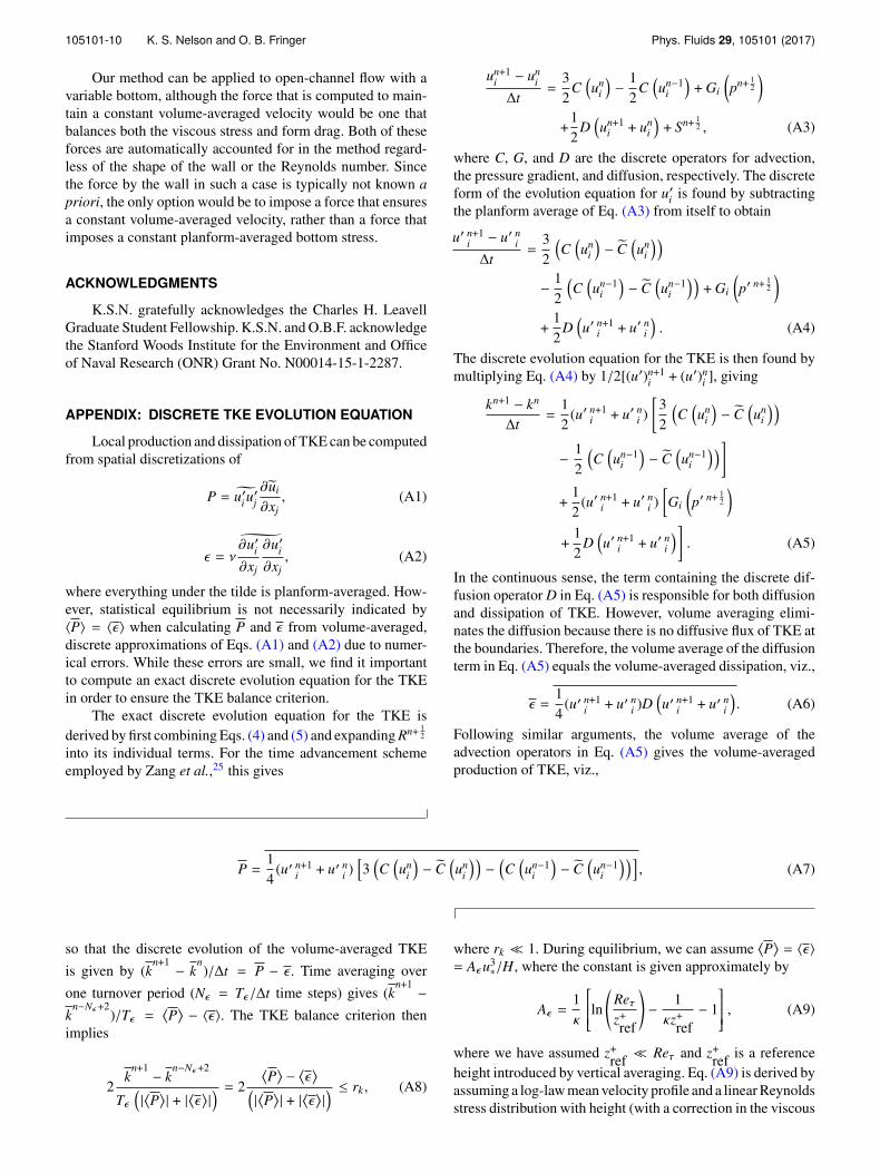
APPENDIX: DISCRETE TKE EVOLUTION EQUATION

Local production and dissipation of TKE can be computedfrom spatial discretizations of

P = u′i u′j

∂ui

∂xj, (A1)

ε = νK∂u′i∂xj

∂u′i∂xj

, (A2)

where everything under the tilde is planform-averaged. How-ever, statistical equilibrium is not necessarily indicated by〈P〉 = 〈ε〉 when calculating P and ε from volume-averaged,discrete approximations of Eqs. (A1) and (A2) due to numer-ical errors. While these errors are small, we find it importantto compute an exact discrete evolution equation for the TKEin order to ensure the TKE balance criterion.

The exact discrete evolution equation for the TKE isderived by first combining Eqs. (4) and (5) and expanding Rn+ 1

2

into its individual terms. For the time advancement schemeemployed by Zang et al.,25 this gives

un+1i − un

i

∆t=

32

C(un

i

)−

12

C(un−1

i

)+ Gi

(pn+ 1

2

)+

12

D(un+1

i + uni

)+ Sn+ 1

2 , (A3)

where C, G, and D are the discrete operators for advection,the pressure gradient, and diffusion, respectively. The discreteform of the evolution equation for u′i is found by subtractingthe planform average of Eq. (A3) from itself to obtain

u′ n+1i − u′ n

i

∆t=

32

(C

(un

i

)− C

(un

i

))−

12

(C

(un−1

i

)− C

(un−1

i

))+ Gi

(p′ n+ 1

2

)+

12

D(u′ n+1

i + u′ ni

). (A4)

The discrete evolution equation for the TKE is then found bymultiplying Eq. (A4) by 1/2[(u′)n+1

i + (u′)ni ], giving

kn+1 − kn

∆t=

12

(u′ n+1i + u′ n

i )

[32

(C

(un

i

)− C

(un

i

))−

12

(C

(un−1

i

)− C

(un−1

i

))]

+12

(u′ n+1i + u′ n

i )[Gi

(p′ n+ 1

2

)+

12

D(u′ n+1

i + u′ ni

)]. (A5)

In the continuous sense, the term containing the discrete dif-fusion operator D in Eq. (A5) is responsible for both diffusionand dissipation of TKE. However, volume averaging elimi-nates the diffusion because there is no diffusive flux of TKE atthe boundaries. Therefore, the volume average of the diffusionterm in Eq. (A5) equals the volume-averaged dissipation, viz.,

ε =14

(u′ n+1i + u′ n

i )D(u′ n+1

i + u′ ni

). (A6)

Following similar arguments, the volume average of theadvection operators in Eq. (A5) gives the volume-averagedproduction of TKE, viz.,

P =14

(u′ n+1i + u′ n

i )[3(C

(un

i

)− C

(un

i

))−

(C

(un−1

i

)− C

(un−1

i

))], (A7)

so that the discrete evolution of the volume-averaged TKE

is given by (kn+1− k

n)/∆t = P − ε . Time averaging over

one turnover period (Nε = Tε/∆t time steps) gives (kn+1−

kn−Nε +2

)/Tε =⟨P⟩− 〈ε〉. The TKE balance criterion then

implies

2k

n+1− k

n−Nε +2

Tε(|⟨P⟩| + |

⟨ε⟩|) = 2

⟨P⟩−

⟨ε⟩(

|⟨P⟩| + |

⟨ε⟩|) ≤ rk , (A8)

where rk � 1. During equilibrium, we can assume⟨P⟩= 〈ε〉

= Aεu3∗/H, where the constant is given approximately by

Aε =1κ

ln *

,

Reτz+ref

+-−

1κz+

ref− 1

, (A9)

where we have assumed z+ref � Reτ and z+

ref is a referenceheight introduced by vertical averaging. Eq. (A9) is derived byassuming a log-law mean velocity profile and a linear Reynoldsstress distribution with height (with a correction in the viscous

105101-11 K. S. Nelson and O. B. Fringer Phys. Fluids 29, 105101 (2017)

sublayer, following Ref. 29) and vertically averaging over zrefto H (z+

ref to Reτ). Choosing z+ref = 11.6, which is where the

theoretical velocity profiles in the viscous sublayer and log lawintersect, and Reτ = 500 gives Aε = 6.2. Substitution gives thesimplified TKE balance criterion,

kn+1− k

n−N+2≤ rkAεu2

∗ . (A10)

Therefore, employing the exact discrete forms of the produc-tion and dissipation terms in Eqs. (A6) and (A7), we guaran-tee that the volume-averaged TKE change over one turnoverperiod is small, and the maximum change based on Eq. (A10)is much smaller than Aεu2

∗ .

1J. W. Deardorff, “A numerical study of three-dimensional turbulent channelflow at large Reynolds numbers,” J. Fluid Mech. 41, 453–480 (1970).

2U. Schumann, “Subgrid scale model for finite difference simulations ofturbulent flows in plane channels and annuli,” J. Comput. Phys. 18, 376–404(1975).

3P. Moin and J. Kim, “Numerical investigation of turbulent channel flow,”J. Fluid Mech. 118, 341–377 (1982).

4J. Kim, P. Moin, and R. Moser, “Turbulence statistics in fully developedchannel flow at low Reynolds number,” J. Fluid Mech. 177, 133–166 (1987).

5R. D. Moser, J. Kim, and N. N. Mansour, “Direct numerical simulation ofturbulent channel flow up to Reτ = 590,” Phys. Fluids 11, 943–945 (1999).

6J. C. Del Alamo, J. Jimenez, P. Zandonade, and R. D. Moser, “Scaling of theenergy spectra of turbulent channels,” J. Fluid Mech. 500, 135–144 (2004).

7S. Hoyas and J. Jimenez, “Scaling of the velocity fluctuations in turbulentchannels up to Reτ = 2003,” Phys. Fluids 18, 011702 (2006).

8X. Wu and P. Moin, “A direct numerical simulation study on the meanvelocity characteristics in turbulent pipe flow,” J. Fluid Mech. 608, 81–112(2008).

9M. Bernardini, S. Pirozzoli, and P. Orlandi, “Velocity statistics in turbulentchannel flow up to Reτ = 400,” J. Fluid Mech. 742, 171–191 (2014).

10A. Lozano-Duran and J. Jimenez, “Effect of the computational domain ondirect simulations of turbulent channels up to Reτ = 4200,” Phys. Fluids 26,011702 (2014).

11H. Choi, P. Moin, and J. Kim, “Direct numerical simulation of turbulentflow over riblets,” J. Fluid Mech. 255, 503–539 (1993).

12P. Cherukat, Y. Na, T. Hanratty, and J. McLaughlin, “Direct numerical simu-lation of a fully developed turbulent flow over a wavy wall,” Theor. Comput.Fluid Dyn. 11, 109–134 (1998).

13V. De Angelis, P. Lombardi, and S. Banerjee, “Direct numerical simulationof turbulent flow over a wavy wall,” Phys. Fluids 9, 2429–2442 (1997).

14R. P. Garg, J. H. Ferziger, S. G. Monismith, and J. R. Koseff, “Stablystratified turbulent channel flows. I. Stratification regimes and turbulencesuppression mechanism,” Phys. Fluids 12, 2569–2594 (2000).

15V. Armenio and S. Sarkar, “An investigation of stably stratified turbulentchannel flow using large-eddy simulation,” J. Fluid Mech. 459, 1–42 (2002).

16M. I. Cantero, S. Balachandar, A. Cantelli, C. Pirmez, and G. Parker, “Tur-bidity current with a roof: Direct numerical simulation of self-stratifiedturbulent channel flow driven by suspended sediment,” J. Geophys. Res.114, 1–20, doi:10.1029/2008jc004978 (2009).

17J. Kim and P. Moin, “Large eddy simulation of turbulent channelflow: ILLIAC 4 calculation,” in Turbulent Bourdary Layers- Experi-ments, Theory, and Modeling, The Hague, The Netherlands, AGARDConference Proceedings (1979), Vol. 271, available at https://ntrs.nasa.gov/search.jsp?R=19790023981.

18M. Lee, R. Ulerich, N. Malaya, and R. D. Moser, “Experiences from leader-ship computing in simulations of turbulent fluid flows,” Comput. Sci. Eng.16, 24–31 (2014).

19Y.-J. Chou and O. B. Fringer, “Modeling dilute sediment suspension usinglarge-eddy simulation with a dynamic mixed model,” Phys. Fluids 20,115103 (2008).

20M. Lee and R. D. Moser, “Direct numerical simulation of turbulent channelflow up to Reτ = 5200,” J. Fluid Mech. 774, 395–415 (2015).

21J. Frohlich, Large Eddy Simulation Turbulenter Stromungen (Springer,2006), Vol. 1.

22S. Koltakov, “Bathymetry inference from free-surface flow features usinglarge-eddy simulation,” Ph.D. thesis, Stanford University, 2013.

23T. Kempe, “A numerical method for interface-resolving simulations ofparticle-laden flows with collisions,” Ph.D. thesis, Technische Universitat,Dresden, 2011.

24M. Quadrio, B. Frohnapfel, and Y. Hasegawa, “Does the choice of the forcingterm affect flow statistics in DNS of turbulent channel flow?,” Eur. J. Mech.B-Fluid. 55, 286–293 (2016).

25Y. Zang, R. L. Street, and J. R. Koseff, “A non-staggered grid, fractionalstep method for time-dependent incompressible Navier-Stokes equations incurvilinear coordinates,” J. Comput. Phys. 114, 18–33 (1994).

26A. Cui, “On the parallel computation of turbulent rotating stratified flows,”Ph.D. thesis, Stanford University, Stanford, CA, USA, 1999.

27B. Leonard, “A stable and accurate convective modelling procedure basedon quadratic upstream interpolation,” Comput. Methods Appl. Mech. Eng.19, 59–98 (1979).

28J. Kim and P. Moin, “Application of a fractional-step method to incompress-ible Navier-Stokes equations,” J. Comput. Phys. 59, 308–323 (1985).

29S. B. Pope, Turbulent Flows (Cambridge University Press, 2000).