REDUCED COMPLEXITY NOISE SUPPRESSION SYSTEM EMPLOYING … · REDUCED COMPLEXITY NOISE SUPPRESSION...

International Journal Of Advance Research In Science And Engineering http://www.ijarse.com

IJARSE, Vol. No.2, Issue No.4, April, 2013 ISSN-2319-8354(E)

145 | P a g e www.ijarse.com

REDUCED COMPLEXITY NOISE SUPPRESSION

SYSTEM EMPLOYING SUB BAND FILTERING

Saurabh Srivastava

1, Dr. O. P. Sahu

2

1Associate Professor, Department of Electronics and Communication Engineering,

College of Engineering, Teerthanker Mahaveer University, Moradabad 2Professor, Department of Electronics and Communication Engineering,

National Institute of Technology, Kurukshetra (India).

ABSTRACT

In this paper we discuss the application of filter banks in sub band processing of signals and the development of

noise suppression system employing filter banks. The filter bank provides the convenience of separating signal

into sub bands, which can further be utilized for signal compression, and provides computationally efficient

polyphase structures for the system. The quality of sub band coder is judged by the Mean Opinion Score (MOS);

our simulations done with MATLAB indicate the system to have a good MOS. In this paper we use 4 channel

octave filter banks, as they are the most widely used filter banks for acoustic or music signals. The composite

system also gives the flexibility of enhancing or suppressing a particular sub band, along with the suppression

of the noise.

Keywords: Octave Filter Bank, Adaptive Filter, Interference Frequency Locations.

I INTRODUCTION

Filter banks are the recent field of research and span from sub band coding of speech signals [1],

transmultiplexer systems [4], to multicarrier communications[5], [8]. Traditionally, a filter bank [1] is a group of

filters derived from a prototype filter but working in different frequency ranges. The simplest filter bank

separates the input frequencies into two bands, namely a high frequency band and a low frequency band. The

bandwidth of sub bands may be same or different depending upon the choice of filter bank; and suitably termed

as uniform filter bank or non-uniform filter bank respectively. A two band uniform filter bank that has mirror

symmetry in their magnitude characteristics of the sub band filters is called as Quadrature Mirror Filter Bank

[1], [4]. The figure below explains the working of multirate filters applied to sub band decomposition using

analysis and synthesis filters. Here 0 ( )H z and 1( )H z are analysis filters and 0 ( )G z and 1( )G z are synthesis

filters.




Figure 1: A two channel analysis synthesis filter bank [4]

For the implementation of non-uniform filter banks [9], such as in communications [2],[5],[8] and audio

compression [12], the octave filter banks are mostly used. The octave filter bank is a filter bank with

exponentially spaced centers of sub bands [2] as shown in the following figure.

Figure 2: a 4 channel octave filter bank analysis filters frequency characteristics [2]

The 4-channel octave bank for perfect reconstruction may be illustrated as below.

( )LH z

( )HH z

2

2

( )LH z

( )HH z

2

2

( )LH z

( )HH z

2

2

2

2

( )LG z

( )HG z

+ A

B

C

x[n]

( )x n

0 ( )H z

1( )H z

2

2

2

2

0 ( )G z

1( )G z

( )y n




Figure 3 : The 4-channel octave filter bank[16]

The octave filter bank may be obtained from a two channel perfect reconstruction filter bank (PRFB). Using the

2 channel perfect reconstruction filter bank, the original signal is separated into four subbands: 1/8 lowest, 1/8

lower, 1/4 low and 1/2 high sub-frequency band. We can then implement a 4 channel octave filter bank as

suggested with the figure below. Matlab was used to design a perfect reconstruction two channel filter bank,

decimator and interpolator and then cascading them. The equivalent filter bank is shown below

Figure 4: 4 Channel Octave Filter Bank Redrawn As Cascade Of Interpolator And Decimator.

An adaptive filter is a filter with an associated adaptive algorithm for updating filter coefficients so that the filter

can be operated in an unknown and changing environment [2]. The adaptive algorithm determines filter

characteristics by adjusting filter coefficients (or tap weights) according to the signal conditions and

performance criteria (or quality assessment). A typical performance criterion is based on an error signal, which

is the difference between the filter output signal and a given reference (or desired) signal. Adaptive filtering

finds practical applications in many diverse fields such as communications [2], [5], [8], radar, sonar, control

systems, navigation[2], seismology[2], biomedical engineering[2], [20]-[25].

x[n]

0 ( )H z

1( )H z

2 ( )H z

3( )H z

8

8

4

2

8

8

4

2

0 ( )G z

1( )G z

2 ( )G z

3( )G z

+

y[n]

A

B

C

2

( )LG z

( )HG z

2

∑ 2

( )LG z

( )HG z

2

∑

y[n]




Figure 5: An Adaptive Filter System [2]

Adaptive filters are widely used for noise suppression in various systems by continuously updating the adaptive

filter taps to provide a close estimate of the desired output []. We consider the system model shown in figure 5.

The primary signal is represented as [ ]x n which equals the sum of acoustic signal [ ]s n

and white noise [ ]w n

i.e. [ ] [ ] [ ])x n s n w n . A reference signal is also provided to adaptive filter that is represented by [ ]rw n .

The filtered reference signal, denoted by ˆ[ ]w n is subtracted from the primary signal and the output i.e. [̂ ]s n

which represents the approximation to the acoustic signal

[ ]s n , is fed back to the adaptive filter to minimize

the error by making the primary signal [ ]x n approximate the acoustic signal [ ]s n by updating of adaptive filter

taps using an adaptation algorithm such as LMS or RLS. The RLS adaptation algorithm suits more to the

stationary signals and the filters with higher orders, but it has poor tracking ability, complexity and lack of

robustness [7], so we prefer using the LMS algorithm than RLS algorithm. Employing the LMS algorithm, the

system working can be stated as following:

The estimated signal can be written as: ˆ ˆ[ ] [ ] ( [ ] [ ])s n s n w n w n

[1]

Therefore, the expectation of the input signal power is

2 2 2ˆ ˆ ˆ{ [ ]} { [ ]} {( [ ] [ ])} 2 { [ ]*( [ ] [ ])}E s n E s n E w n w n E s n w n w n [2]

We assume that the noise and the signal are uncorrelated; therefore the third term can be decoupled and goes to

zero. Hence, 2 2 2ˆ ˆ{ [ ]} { [ ]} {( [ ] [ ])}E s n E s n E w n w n

[3]

Minimization of this expression can be done by minimizing 2ˆ{( [ ] [ ])}E w n w n term. So, the LMS algorithm

makes [̂ ]s n approximate [ ]s n We combine the multirate operations of a filter bank with the adaptive control

system so as to suppress the noise in an acoustic signal. The scheme may be described by the following figure

Output

[̂ ]s n

Primary

signal

Reference

signal Adaptive

filter

[ ] [ ] [ ]x n s n w n

[ ]rw n

ˆ[ ]w n




Figure 6: Adaptive Section Introduced Between Decimator and Interpolators.

System model: As shown in the figure 6 above, the composite system is fed with an input signal (noise

corrupted) to the analysis filters 0 ( )H z and 1( )H z , a reference noise is also fed to the same set of filters. The

adaptive section that follows the decimator works on the principle defined above, uses the reference noise as

training signal, adjusts the filter coefficients, and suppresses the noise in the sub bands obtained after the

decimation process. The corresponding adaptive filter outputs are fed to a synthesis filter bank with filters as

0 ( )G z and 1( )G z . The outputs of 0 ( )G z and 1( )G z are then combined to yield an estimate of the noise

suppressed signal.

If direct noise removal is done using adaptive filters, the system would be slow for real time processing. The

proposed system provides the flexibility of using low order filter, as for long input sequences the adaptive

system requires large order filters, which is eliminated with the use of sub band decomposition of signals. Also,

conventionally adaptive approach using a lower order filter results in large convergence time of the filter

coefficients, which makes the system output delayed very much. Also, the proposed system offers sub bands of

the noise suppressed signals that may be used for any specific processing of the sub band frequency range, i.e.

for compression, generating audio effects for a particular sub band, speech coding of signals.

0 ( )H z

1( )H z

2

2

2

2

0 ( )G z

1( )G z

[ ]y n

Adaptive

section

Adaptive

section

0 ( )H z

1( )H z

2

2

2

2

0 ( )G z

1( )G z

[ ]x n

[ ]rw n [ ]rw n




II ALGORITHM

The algorithm for the implementation of proposed system on MATLAB may be represented as following:

1. Design a two channel filter bank using MATLAB.

2. Generate input signal, input noise and reference noise

3. Add input noise to the input signal

4. Decompose the original signal into two sub bands using the polyphase analysis filter bank

5. Perform adaptive interference suppression using LMS algorithm

6. Reconstruct the estimate of original signal using polyphase synthesis filter bank.

MATLAB was chosen for the implementation of the algorithm as it has built-in functions for the conversion of

polyphase forms of decimator and interpolators. The polyphase structures have reduced complexity than

conventional structures. Further, plotting of various waveforms was quite easy with the help of MATLAB. To

compare the performance of the proposed system in another simulation, RLS algorithm was used against LMS

and the results were analyzed. It was clear from the results that the proposed system works well (within a

specific tolerance limits) to provide a faithful reproduction of original signal from the noise corrupted one.

Further, the use of LMS algorithm provided faster convergence but the larger Mean Square Error (MSE)

between reconstructed noise-suppressed signal and the original signal. On the other hand RLS algorithm

provided slower convergence but the MSE was very small compared to when LMS was used.

Algorithm implementation: For designing the power symmetric filter bank, MATLAB functions were used, and

four FIR filters for the analysis sections ( 0 ( )H z and 1( )H z ) and synthesis section ( 0 ( )G z and 1( )G z ) were

designed. Their direct form polyphase structures were also obtained using MATLAB using the corresponding

filter coefficients.

Initially, a single tone sinusoidal input signal, a two tone noise signal and the reference noise signals having

same frequency but different amplitude and phase with the interfering noise signal, were also generated. The

original signal was then corrupted by the noise and the noise corrupted signal was then fed to the adaptive

section for interference suppression. The adaptive algorithm selected was LMS where the leakage factor was

assumed to be zero (no leakage), the initial states and the coefficients were also selected to be zero.

The outputs of the adaptive section were passed on to the synthesis filters for reconstruction.

The simulation was repeated using a piece of recorded speech signal , and the results were compared by varying

the performance parameters such as the filter bank length, the adaptive filter length, the no. of sub bands in the

filter bank , the interfering noise frequency .

The simulation parameters for the algorithm are shown in table below:

Table I: Simulation parameters

Order of prototype filters (in FB) 49,41,31,21,11,3

Type of filter bank Power symmetric filter bank

Prototype filter forms Direct form polyphase




Method to generate octave filter Cascading prototypes

Signal amplitude 2

Signal frequency 0.005

Noise amplitude 0.1 and 0.2

Noise frequency 0.0213 and 0.0724

Reference noise amplitude 0.3 and 0.5

Phase shift (of noise) 0.2*pi and 0.3*pi

Time range 3000

Adaptive algorithms used LMS & RLS

Adaptive filter length 64, 25, 9,3

RLS forgetting factor 1

RLS initial coefficients Length 64 vector with all zeros

RLS initial states Length 63 vector with all zeros

LMS step size 0.008

LMS leakage factor 1

LMS initial coefficients Length 64 vector with all zeros

LMS initial states Length 63 vector with all zeros

III RESULTS AND DISCUSSION

3.1 Filter bank order

The filter bank order was varied as N=49, 41, 31, 21, 11, 3. It was found that with very short filter length N=3,

is not a good filter bank, as the frequencies are not well separated into two subbands and large overlapping

occurs with huge ripples. Therefore, the signal all have large component in each band and adaptive filters are

very similar in this case. However, as we increase the filter bank length, overlapping becomes less and less and

ripples are suppressed more and more. Therefore, we can expect the low frequency signal maintains well but

high frequency band contains less and less amplitude.

Figure 7(a): Magnitude Response of Four Decimators of Analysis Filters (For N=3)

0 0.1 0.2 0.3 0.4 0.5 0.6 0.7 0.8 0.9

-45

-40

-35

-30

-25

-20

-15

-10

-5

0

Normalized Frequency ( rad/sample)

Magnitu

de (

dB

)

Magnitude Response (dB)

Low est Decimator

Low er Decimator

Low Decimator

High Decimator




Figure 7(b): Magnitude Response of Four Interpolators of Synthesis Filters (For N=3)

Figure 7(c): Coefficient Values For Adaptive Filter Length (L =64)

3.2 Adaptive filter length

The adaptive filter length was varied as 3, 9, 25 and 64. For very short adaptive filter length such as 3, it cannot

perform good noise suppression. As we increase the length, it will start to suppress the noise from large time

index part. It always need some “adaptive” time but this time length become shorter and shorter as we increase

the adaptive filter length.

0 0.1 0.2 0.3 0.4 0.5 0.6 0.7 0.8 0.9

-25

-20

-15

-10

-5

0

5

10

15

Normalized Frequency ( rad/sample)

Magnitu

de (

dB

)Magnitude Response (dB)

Low est Interpolator

Low er Interpolator

Low Interpolator

High Interpolator

0 10 20 30 40 50 60 70-0.04

-0.02

0

0.02

0.04

0.06

0.08

Coefficient Number

Coeff

icie

nt

Valu

e




Figure 8(a): Output Signal For Two Tone Noise Case For Adaptive Filter Length 3 And

Filter Bank Order 49.

Figure 8(b): Output signal for two tone noise case for adaptive filter length 64 and

filter bank order 49.

3.3 LMS step size

The LMS step size was varied as mu= 0.0001, 0.001, 0.01, 0.05, 0.1 and 0.2. As we can see, very large step size

may induce a divergent result (bad adaptive filter).a very small step size also takes too much time for

convergence. For very small step size, it cannot give a good result again. This occurs due to the error

accumulation. In conclusion, LMS step size is optimized around a certain value. For our simulation this value

was chosen to be 0.008 on a trial basis.

0 500 1000 1500 2000 2500 3000-2.5

-2

-1.5

-1

-0.5

0

0.5

1

1.5

2

2.5Output Signal after Two Tone Noise Suppression (LMS)

Am

plit

ude

0 500 1000 1500 2000 2500 3000-2.5

-2

-1.5

-1

-0.5

0

0.5

1

1.5

2


Am

plit

ude




Figure 9(a): Output Signal for mu = 0.0001

Figure 9(b): Output Signal For mu = 0.01

3.4 Interference Frequency Locations

We took the two tone noise signal with frequency as 0.0213 as normal frequency signal and frequency 0.0004 as

low frequency signal. Since we always have an “adaptive” time, we can imagine that if our noise signal has a

very small frequency which may not allow the adaptive filter get enough information within the designated time

range, this part would be hard to remove. As we can see, if we use one “normal” frequency and one “abnormal

slow” signal, only large frequency noise can be effectively removed (we can still see the slow varying trend in

the output signal). Of course, we can expect if our signal sequence is long enough, it will eventually remove the

small frequency noise as well. Hence, we also simulated the model with a longer piece of recorded sound for the

verification purpose.

In our model we assume that the desired signal and the noise are uncorrelated. Uncorrelated for sinusoid signal

simply means they have different frequencies. If we have a noise component which shares the same frequency

0 500 1000 1500 2000 2500 3000-2.5

-2

-1.5

-1

-0.5

0

0.5

1

1.5

2


Am

plit

ude

0 500 1000 1500 2000 2500 3000-2.5

-2

-1.5

-1

-0.5

0

0.5

1

1.5

2


Am

plit

ude




response as the signal, after adaptive process, we can expect the signal itself and the noise will both be removed.

Therefore, this simple model is not good for correlated signals.

Figure 10(a-d): Input-Output Comparison For Uncorrelated Signal Such As An Audio Signal.

Last but not the least, it was found based on the results that the quality of the reconstructed signal was a good

approximation of the original audio signal (have good MOS), except for a change in magnitude of the

reconstructed signal. Moreover, if a certain sub band requires further processing, it can be easily done as we

have incorporated enhancement factor and delay factors for individual sub bands.

We also compared the complexity of the system indirectly by observing the total time elapsed in sub band

processing of the recorded speech signal and their reconstruction (including the delays) , against the order of

filter bank filters, and the results are tabulated in the following table2.

Table II: Time required in processing of the recorded speech signal against order of prototype

filter.

Order of prototype filter Time elapsed (in seconds)

49 3.6841

41 3.6304

31 3.5562

21 3.4756

11 3.4252

3 3.3902

The above table was determined using an average of 10 simulations for every individual prototype filter order.




Figure 11 : Variation of Elapsed Time Against Prototype Filter Order.

As clearly seen from the figure above , there is a minor change in execution time in the proposed model when

the prototype filter order in varied on a large extent. Hence , depending upon the MOS values , the MSE curve

and the execution time , the optimum values of prototype filter order and adaptive filter length can be

determined . a major advantage of the proposed system is that it works for non-stationary inputs also due to the

use of lms algorithm .

Finally , the reconstructed signal was examined to obtain the value of Mean Opinion Score (MOS) which is

defined as the objective measure of the quality of reocnstructed signal. As in our experiments , it was found that

with a prototype filter oder of equal to or greater than 31 , adaptive filter length greater than or equal to 32 , and

LMS algorithm , the MOS was 3.5 . It was against the MOS of 5 with no decomposition of sub bands and using

the same prototype filter length and adaptive filter length.

The primary motivations of using SAF are to reduce the computational complexity and improve the

convergence performance for the input signal, with a large spectral dynamic range. For our model, if we choose

the full band adaptive filter of length M. the sub filters operate with a lower sampling rate with the decimation

factor D , the length of adaptive filters can be reduced to L=M/D. For N sub bands, there are a total of L x N

=MN/D sub band tap weights. Thus, the multiplication required by N sub filters is MN/D2.

, compared to the full

band filtering that requires M multiplications, the computational savings in terms of multiplications is given by:

Complexity of full band filter = D2

Complexity of sub band filter N

For the full band adaptive filter of length M=64, we had the downsampling factor as D=8, which reduced the

length to L = 64/8 =8. For N=4 sub bands, we get L*N= 8*4 = 32 sub band tap weights. Hence, the

multiplication required by N=4 sub band filters are 64*4/64 = 4, whereas for full band filtering, we require 64

multiplications. So, the efficiency of the system also increases by 8*8/4 = 16. Table III a) gives the complexity

0 5 10 15 20 25 30 35 40 45 500

0.5

1

1.5

2

2.5

3

3.5

4

order of prototype filter

ela

psed t

ime (

in s

ec.)




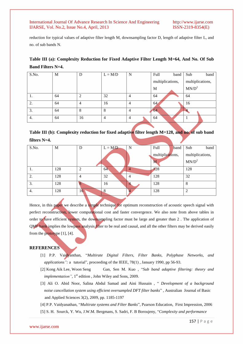
reduction for typical values of adaptive filter length M, downsampling factor D, length of adaptive filter L, and

no. of sub bands N.

Table III (a): Complexity Reduction for Fixed Adaptive Filter Length M=64, And No. Of Sub

Band Filters N=4.

S.No. M D L = M/D N Full band

multiplications,

M

Sub band

multiplications,

MN/D2

1. 64 2 32 4 64 64

2. 64 4 16 4 64 16

3. 64 8 8 4 64 4

4. 64 16 4 4 64 1

Table III (b): Complexity reduction for fixed adaptive filter length M=128, and no. of sub band

filters N=4.

S.No. M D L = M/D N Full band

multiplications,

M

Sub band

multiplications,

MN/D2

1. 128 2 64 4 128 128

2. 128 4 32 4 128 32

3. 128 8 16 4 128 8

4. 128 16 8 4 128 2

Hence, in this paper we describe a simple technique for optimum reconstruction of acoustic speech signal with

perfect reconstruction, lower computational cost and faster convergence. We also note from above tables in

order to have efficient system, the downsampling factor must be large and greater than 2 . The application of

QMF bank implies the lowpass analysis filter to be real and causal, and all the other filters may be derived easily

from the prototype [1], [4].

REFERENCES

[1] P.P. Vaidyanthan, “Multirate Digital Filters, Filter Banks, Polyphase Networks, and

applications”: a tutorial”, proceeding of the IEEE, 78(1) , January 1990, pp 56-93.

[2] Kong Aik Lee, Woon Seng Gan, Sen M. Kuo , “Sub band adaptive filtering: theory and

implementation”, 1st edition , John Wiley and Sons, 2009.

[3] Ali O. Abid Noor, Salina Abdul Samad and Aini Hussain , “ Development of a background

noise cancellation system using efficient oversampled DFT filter banks” , Australian Journal of Basic

and Applied Sciences 3(2), 2009, pp. 1185-1197

[4] P.P. Vaidyanathan, “Multirate systems and Filter Banks”, Pearson Education, First Impression, 2006

[5] S. H. Sourck, Y. Wu, J.W.M. Bergmans, S. Sadri, F. B Boroujeny, “Complexity and performance




comparison of filter bank multicarrier and of dm in uplink of multicarrier multiple access networks”,

IEEE transactions on signal processing, 59(4) ,2011, pp.1907-1912.

[6] Mahbubul Alam, Md. Imdadul Islam, and M. R. Amin , “Performance Comparison of STFT, WT,

LMS and RLS Adaptive Algorithms in Denoising of Speech Signal”, IACSIT International Journal of

Engineering and Technology, 3(3), June 2011, pp. 235-238.

[7] Bernard Widrow and Eugene Walach , “Adaptive Inverse Control: A Signal Processing Approach”,

Reissue Edition, , appendix E, pp. 383-395

[8] Farhang- Boroujeny, B, “OFDM Versus Filter Bank Multicarrier”, IEEE signal processing magazine

, 28(3), 2011, pp. 92-112.

[9] K. Nayebi, T.P. Barnwell ,M.J.T. Smith , “Non uniform filter banks: a reconstruction and design

theory”, IEEE transactions on signal Processing , 41(3), March 1993, pp. 1114-1127.

[10] T. Saramaki & R. Bregovic , “Multirate Systems: Design and Applications”, Idea Group Inc. , 2002.

[11] Z. Cvetkovi´c, J. D. Johnston, “Nonuniform oversampled filter banks for audio signal processing”,

IEEE Transactions on Speech and Audio Processing, 11(5), September 2003, pp 393–399.

[12] Y.Deng, V.J. Mathews, B. Farhang-Boroujeny,, “Low-delay nonuniform pseudo-QMF bank with

application to speech enhancement”, IEEE Trans. on Signal Processing, 55(5),2110–2121, May

2007.

[13] T. Gulzow, T. Ludwig, U. Heute, “Spectral-subtraction speech enhancement in multirate

systems with and without non-uniform and adaptive bandwidths”, Signal Processing, Elsevier, 83(8),

1613–1631, August 2003.

[14] “Subjective comparison of speech enhancement algorithms”, Proc. ICASSP ’06, Tolouse,

France, May 2006.

[15] H. W. Lollmann, P. Vary, “Efficient non-uniform filter-bank equalizer”, Proc. EUSIPCO 2005,

Antalya, Turkey, September 2005.

[16] Nongpiur, R.C.; Shpak, D.J., “Maximizing the Signal-to-Alias Ratio in Non-Uniform Filter Banks

for Acoustic Echo Cancellation” , IEEE transactions on Circuits and Systems I, Regular

Papers, 59(10), 2012, pp. 2315-2325.

[17] S. M. Kuo and D. R. Morgan, “Active Noise Control Systems: Algorithms and DSP

Implementations”, New York: John Wiley & Sons, Inc., 1996.

[18] J.D.Johnston , “Transform coding of audio signals using perceptual noise criteria”, IEEE journal on

selected areas in communication, , 6(2), 1988, pp. 314-323.

[19] M. de Courville and P. Duhamel, IEEE Trans. Signal Processing, “Adaptive filtering in subbands

using a weighted criterion”, 46(9), September 1998, pp. 2359–2371.

REDUCED COMPLEXITY NOISE SUPPRESSION SYSTEM EMPLOYING … · REDUCED COMPLEXITY NOISE SUPPRESSION...

Documents

Transcript of REDUCED COMPLEXITY NOISE SUPPRESSION SYSTEM EMPLOYING … · REDUCED COMPLEXITY NOISE SUPPRESSION...