
Redesigning the Supply Chain to increase Responsiveness ...
84
Frank Dijkgraaf October 2020
Transcript of Redesigning the Supply Chain to increase Responsiveness ...

Frank Dijkgraaf October 2020


Master Thesis
‘Redesigning the supply chain to increase responsiveness with increasing uncertainty of demand.’
Author
Frank Dijkgraaf
University of Twente
Faculty: Behavioural, Management and Social Sciences
Study Program: Industrial Engineering and Management MSc.
Specialisation: Production and Logistics Management
Orientations: Manufacturing Logistics & Supply Chain and Transportation Management
University supervisors DR. M.C. (Matthieu) van der Heijden
Faculty of Behavioural, Management and Social Sciences
Department Industrial Engineering and Business Information Systems
DR. IR. W.J.A. (Wouter) van Heeswijk
Faculty of Behavioural, Management and Social Sciences
Department Industrial Engineering and Business Information Systems
Supervisors Imagebuilders
W.F.C. (Wijnand) Daaleman
Director Operations
F.C. (Fred) Wichmann
Chief Executive Officer
Imagebuilders BV.
Paramariboweg 17, 7333 PA Apeldoorn

Management Summary Problem Setting & Research Design
Imagebuilders (IB) designs, develops and installs the interior of brick-and-mortar stores (called
shopfitting) of mostly clothing retailers for which they source all required items (excluding clothing)
to furnish the interior of the shop such as cash desks and fitting rooms customized to the style of the
customers brand. Stores consist of standard items such as shelfs and cash desks that are Make-to-
Stock and of store-specific items such as wall panels fitted to the dimensions of the store that are
Engineer-to-Order. From an early analysis we found that IB was able complete all activities required
to install a store within the maximum allowable lead time of the customer of 6 weeks by picking the
standard items from high levels of inventory. As uncertainty rises, customers no longer accept
sourcing by bulk ordering or using long-term forecasts. The current supply chain however does not
enable Imagebuilders to meet demand cost-efficiently using short-term forecasts. The goal of this
research is to advise IB on how to design the supply chain for standard items in order to meet the
required level of responsiveness while minimizing supply chain costs. The advice includes selecting a
supply chain design and supplier region, locating inventories and developing safety stocks based on
forecasted and actual demand data. We formulated the following main research question:
“How can Imagebuilders improve their supply chain responsiveness by redesigning their supply chain
network for standard items to meet customer requirements at the lowest possible cost?”
Mapping the Current Situation
In the current supply chain design, standard items are sourced at Chinese suppliers and supplier
regions within Europe. Standard items are stored third party logistics (3PL) in the Netherlands (NL).
The forecast used for bulk ordering forecasted 30 weeks into the future. We found that the relation
between item usage in a store and store size is monotonic and linear for some items. To measure the
forecasting performance, we use the Mean Absolute Percentage Error (MAPE) and the Weighted
Absolute Percentage Error (WAPE) which uses item demand as a weight factor. To measure the
supply chain performance, we set up multiple Key Performance Indicators (KPIs) such as the Order-
Line Fill Rate (OLFR), the Inventory Turnover Rate (ITR) and the total supply chain costs. The achieved
performance is used as a benchmark later on to serve as comparison material with the model results.
Applying Literature from the Literature Review
From our literature review, we developed the supply chain network designs in Table 1 that all allow
IB to achieve the required responsiveness by strategically locating inventories.
In determining the forecast-driven activities upstream the stock location required to meet demand
cost-efficiently, we identified demand anticipation and inventory control as the internal factors that
can be adjusted to meet the level of required responsiveness. In forecasting demand, we use Holt-
Winters Exponential Smoothing to forecast store demand. Subsequently, we use Holt’s Linear Trend
to forecast the expected store size. Thereafter, we use Linear Regression as a causal forecasting
method to forecast item demand that is dependent on the forecasted number of stores and item
demand of which item usage in a store is correlated to store size. By developing a dynamic inventory
management model for each supply chain design with an (R,S) inventory policy as demand is
seasonal and variable, we simulate the performance of each design over demand data of 2019. This
Option Outsourcing Supplier Region Stock Point(s)
1 China 1 at the 3PL in NL
2 China 1 at 3PL in NL and 1 in Supplier Region
3 Europe 1 at the 3PL in NL
4 Europe 1 in Supplier Region
Table 1 - Developed Supply Chain Network Designs
simulation uses the forecasted demand data to determine order quantities and safety stock levels All
different options require custom forecasts to account for the varying lead times. In the two-level
stock design, we can further reduce our inventory costs by splitting replenishments order into
multiple smaller replenishment orders.
Model Construction
We developed a cost minimization model in Microsoft Excel that selects the lowest cost supply chain
on item-level while ensuring Full Container Load (FCL) transport as Less than Container Load
transport increases the transportation costs and adds supply uncertainty. To counter long
computational times required in selecting the optimal supply chain design for all 232 standard items
in a customers’ concept as it is a combinatorial problem, we solve our problem using a heuristic
consisting of two small and fast-to-solve submodels: an item-level supply chain design selection
problem a multi-item transportation problem that helps in ensuring FCL transportation.
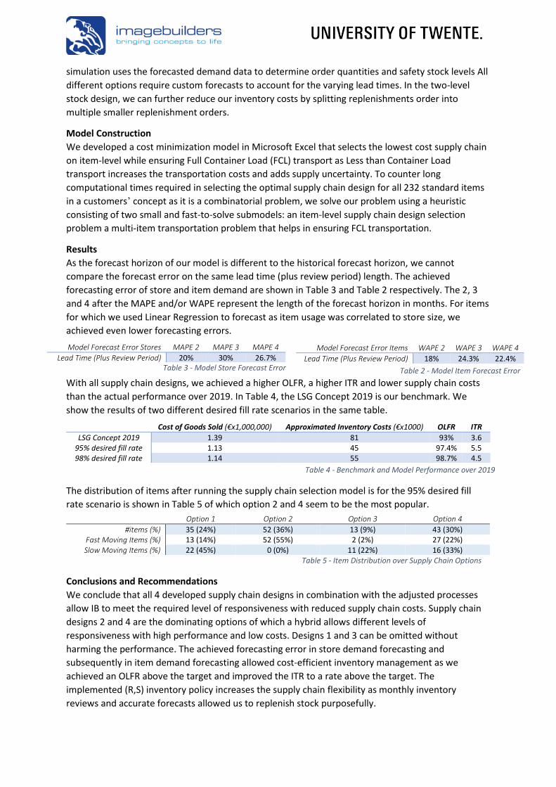
Results
As the forecast horizon of our model is different to the historical forecast horizon, we cannot
compare the forecast error on the same lead time (plus review period) length. The achieved
forecasting error of store and item demand are shown in Table 3 and Table 2 respectively. The 2, 3
and 4 after the MAPE and/or WAPE represent the length of the forecast horizon in months. For items
for which we used Linear Regression to forecast as item usage was correlated to store size, we
achieved even lower forecasting errors.
With all supply chain designs, we achieved a higher OLFR, a higher ITR and lower supply chain costs
than the actual performance over 2019. In Table 4, the LSG Concept 2019 is our benchmark. We
show the results of two different desired fill rate scenarios in the same table.
The distribution of items after running the supply chain selection model is for the 95% desired fill
rate scenario is shown in Table 5 of which option 2 and 4 seem to be the most popular.
Table 5 - Item Distribution over Supply Chain Options
Conclusions and Recommendations
We conclude that all 4 developed supply chain designs in combination with the adjusted processes
allow IB to meet the required level of responsiveness with reduced supply chain costs. Supply chain
designs 2 and 4 are the dominating options of which a hybrid allows different levels of
responsiveness with high performance and low costs. Designs 1 and 3 can be omitted without
harming the performance. The achieved forecasting error in store demand forecasting and
subsequently in item demand forecasting allowed cost-efficient inventory management as we
achieved an OLFR above the target and improved the ITR to a rate above the target. The
implemented (R,S) inventory policy increases the supply chain flexibility as monthly inventory
reviews and accurate forecasts allowed us to replenish stock purposefully.
Table 2 - Model Item Forecast Error Table 3 - Model Store Forecast Error
Model Forecast Error Stores MAPE 2 MAPE 3 MAPE 4
Lead Time (Plus Review Period) 20% 30% 26.7% Model Forecast Error Items WAPE 2 WAPE 3 WAPE 4
Lead Time (Plus Review Period) 18% 24.3% 22.4%
Table 4 - Benchmark and Model Performance over 2019
Cost of Goods Sold (€x1,000,000) Approximated Inventory Costs (€x1000) OLFR ITR
LSG Concept 2019 1.39 81 93% 3.6 95% desired fill rate 1.13 45 97.4% 5.5 98% desired fill rate 1.14 55 98.7% 4.5
Option 1 Option 2 Option 3 Option 4
#items (%) 35 (24%) 52 (36%) 13 (9%) 43 (30%) Fast Moving Items (%) 13 (14%) 52 (55%) 2 (2%) 27 (22%) Slow Moving Items (%) 22 (45%) 0 (0%) 11 (22%) 16 (33%)

Based on our research, we recommend IB the following:
• Create a hybrid of two supply chain designs (option 2 & 4 of Table 1) in which the inventory
policy considers a monthly review and uses the developed safety stocks. Follow the derived
guidelines for design selection to select a design on single item-level.
• Forecast store and item demand monthly, use an (R,S) inventory policy with monthly review and
use safety stock levels as proposed to maintain a high service level with low inventory costs.
• Standardize the data entries and gather and clean as much data as possible to obtain the more
reliable model results. Data preparation is the main challenge in implementing the proposed
models. Furthermore, track performance of the KPIs we introduced.
We also presented IB two future research directions: 1) when demand in other regions starts to
increase and requires a cost-efficient and responsive supply chain and 2) when rail transport
becomes the preferred transport mode.

Preface In order to complete the master Industrial Engineering & Management at the University of Twente, I
worked on a real-life case at Imagebuilders where I was able to do research in a very unique multi-
project environment. Although it has been a strange year with the ongoing pandemic, I was lucky
enough to be able to work in a safe environment at the office for the biggest part of my research. I’m
very thankful towards Imagebuilders for letting me perform this project and for offering me plenty of
office space to work freely on my project.
I would like to thank Matthieu van der Heijden for being the first supervisor and giving very helpful
guidance and feedback throughout the project even when I felt my progression was minimal. Besides
guiding me in finding the direction of my research, the regular feedback helped me develop a more
critical view on my own work. I would also like to thank my second supervisor Wouter van Heeswijk
for providing me with constructive feedback that allowed me to look at my work with another angle
of approach to improve my thesis even further. I would also like to thank them for taking the time to
help me.
Also, I would like to thank Wijnand Daaleman for supervising my graduation project. As a starting
intern, it was very helpful to take me through the processes and set up and attend meetings with the
employees within Imagebuilders who could either help me or should be involved in the project. I
would also like to thank several employees within Imagebuilders, especially Kees Zandsteeg and
Richard Lieferink, in helping me understand the processes within the company, showing me real-life
examples and gathering data I required. Their experience also helped me to validate outcomes of our
model.
After handing in this thesis, my time as a student will come to an end. Although I did not expect to
achieve a master’s degree when I started studying at a university of applied sciences quite some
years ago, I am very grateful I got the opportunity to do so. I would like to thank my parents, friends
and colleague students that supported me and contributed to making these years pleasant and
unforgettable.
Frank Dijkgraaf,
Emst, October 2020

Glossary
Abbreviations
3PL Third Party Logistics
BOM Bill Of Materials
BOQ Bill of Quantities
CODP Customer Order Decoupling Point
DS Downstream Stock Point
ETO Engineer-to-Order
F-AHP Fuzzy Analytical Hierarchy Process
FCL Full Container Load (2 TEU / 40ft. container as standard)
IB Imagebuilders
LCL Less than Container Load
MAD Mean Absolute Deviation
MAPE Mean Absolute Percentage Error
MCDM Multi-Criteria Decision Making
MOQ Minimum Order Quantity
MOV Minimum Order Value
MTO Make-to-Order
MTS Make-to-Stock
OLFR Order Line Fill Rate
P&P Pick-and-Pack
SCR Supply Chain Responsiveness
SKU Stock Keeping Unit
US Upstream Stock Point WAPE Weighted Absolute Percentage Error
Supplier Regions
CN China
TR Turkey
BS The Baltic States (Latvia & Lithuania)
CZ Czech Republic
PL Poland
NL The Netherlands
Other Terms
LSG Store concept code of the main customer last 4-5 years.
CN-1SP Supply Chain Design sourcing in China with 1 stock point in NL
CN-2SP Supply Chain Design sourcing in China with 2 stock points (1 in CN & 1 in NL)
EU-EUSP Supply Chain Design sourcing in Europe with supplier region stock point
EU-NLSP Supply Chain Design sourcing in Europe with stock point in NL

Content Management Summary ..................................................................................................................................... i
Preface ............................................................................................................................................................ iv
Glossary ........................................................................................................................................................... v
1. Introduction ............................................................................................................................................. 1
1.1 Company Introduction ............................................................................................................ 1
1.2 Motivation for the Research ................................................................................................... 2
1.3 Problem Description ................................................................................................................ 2
1.4 Research Scope ........................................................................................................................ 4
1.5 Aim of the Research ................................................................................................................ 5
1.6 Research Design ...................................................................................................................... 5
1.7 Deliverables ............................................................................................................................. 7
2. Analysis of the Current Situation ............................................................................................................. 8
2.1 Distribution Network Design ................................................................................................... 8
2.2 Standard Item Supply Chain Processes ................................................................................... 8
2.3 Store & Standard Item Demand Characteristics ................................................................... 10
2.4 Supply Chain Performance – Setting a Benchmark ............................................................... 11
2.5 Conclusion ............................................................................................................................. 15
3. Literature Review .................................................................................................................................. 16
3.1 Customer Responsive Supply Chain ...................................................................................... 16
3.2 Meeting the Required level of Supply Chain Responsiveness............................................... 16
3.3 Supply Chain Distribution Network Redesign ....................................................................... 17
3.4 Forecast-Driven Activities ...................................................................................................... 17
3.5 Supply Chain Design Selection Problem ................................................................................ 20
3.6 Conclusion ............................................................................................................................. 21
4. Supply Chain Redesign ........................................................................................................................... 22
4.1 Frequently Used Notations ................................................................................................... 22
4.2 Redesign Options ................................................................................................................... 22
4.3 Demand Anticipation by Developing Forecasts .................................................................... 25
4.4 Integral Inventory Management ........................................................................................... 28
4.5 Inventory Cost Savings in the Two-Level Stock Scenario ...................................................... 32
4.6 Conclusion ............................................................................................................................. 34
5. Supply Chain Selection & Optimization .................................................................................................. 35
5.1 Problem Solving Approach .................................................................................................... 35
5.2 Toy Problem – Breakdown of Problem Solving Approach .................................................... 36
5.3 Model Input ........................................................................................................................... 39

5.4 Selecting a Cost-Efficient Supply Chain Design (Submodel 1) ............................................... 41
5.5 Replenishment Frequencies with FCL Transport (Submodel 2) ............................................ 42
5.6 Limitations ............................................................................................................................. 43
5.7 Validation and Verification .................................................................................................... 43
5.8 Conclusion ............................................................................................................................. 44
6. Results ................................................................................................................................................... 45
6.1 Forecast Accuracy .................................................................................................................. 45
6.2 Problem Solving Steps using Real-Life Scenario .................................................................... 46
6.3 Supply Chain Performance .................................................................................................... 47
6.4 Supply Chain Design vs. Item Characteristics ........................................................................ 51
6.5 Sensitivity Analysis ................................................................................................................ 53
6.6 Conclusion ............................................................................................................................. 55
7. Implementation Plan ............................................................................................................................. 56
7.1 Steps to Implement Cost Minimization Model ..................................................................... 56
7.2 MOQs and Minimum Item Fill Rate ....................................................................................... 57
7.3 Multiple-Criteria Decision-Making (MCDM).......................................................................... 57
7.4 Conclusion ............................................................................................................................. 59
8. Conclusions and Recommendations ....................................................................................................... 60
8.1 Conclusions ............................................................................................................................ 60
8.2 Recommendations................................................................................................................. 61
8.3 Further Research Suggestions ............................................................................................... 61
Bibliography ................................................................................................................................................... 62
Appendix 1 – Standard items in the system.................................................................................................... 64
Appendix 2 – Literature .................................................................................................................................. 67
Appendix 3 – Full Results ............................................................................................................................... 68
Appendix 4 – Derivation of Guidelines ........................................................................................................... 69
Appendix 5 – Forecasting Models ................................................................................................................... 72

1
1. Introduction In this chapter, Imagebuilders will be briefly described along with the problem to be solved to
contribute to the goals of Imagebuilders.
1.1 Company Introduction
Imagebuilders currently describes them self as a global shopfitter. They take over the entire project
of designing, sourcing and installing the complete interior of a shop, shop-in-shop or office
customized to the style of the brand. They provide all items within a shop like shelfs, cash desks and
customer signs (see Figure 1). All these items are customer and concept specific. Besides these
projects, Imagebuilders also provides custom-made items like displays, presenters and branding
items. The company is located in Apeldoorn and has its own production facility where custom-made
wooden items can be made in any size. Other finished items required (e.g. metal parts, plastic parts
or combinations) to fulfil customer demand are sourced at suppliers spread over Europe and China.
Imagebuilders has dedicated teams for bigger recurring customers for optimal service.
All projects Imagebuilders takes on are Design-to-Order. The lay-out design of a store, based on the
size of the store, is made up of store-specific Specials (Engineer-to-Order) and Standard items (see
Figure 1). Standard items are mostly Make-to-Stock as the production plus transportation lead time
required for sourcing exceeds the maximum allowable lead time of customers. Imagebuilders and the
customer collaborate to forecast demand to ensure timely delivery of standard items. In some cases,
the specials contain standard items. The standard items are used in almost all stores a customer
plans to open with the same concept. A few examples of standard items are shown in Figure 1. An
item like the big wooden panel attached to the wall in Figure 1 is called a Special as it is custom-made
based on the dimensions of the store. To be able to deliver all standard items required to install a
store within the maximum allowable lead time of the customer, Imagebuilders keeps inventory of
standard items at Third Party Logistics (3PL) in and around Apeldoorn.
Figure 1 - Fitted Stores by Imagebuilders & Example Items
Graphic
(Standard item)
Sign
(Standard Item)
Cash Desk
(Standard item) Cash Desk Extension
(Standard item)
Cupboard
(Standard item) Custom-made
Wall Panel
(Special)

2
1.2 Motivation for the Research
The main reason behind this research is that Imagebuilders’ way of serving recurring customers no
longer matches customers’ requirements and in order to stay competitive, Imagebuilders needs to
adapt to the new requirements. This mismatch arises from the change in customer approval of the
period of forecastable demand (>6 months to ≤3 months) on which Imagebuilders designed their
supply chain to source the standard items used in shop fitting. The supply chain designed to source
special items does match the requirements as demand for these item is one-time only, cannot be
forecasted and sales prices are not fixed as opposed to standard items. This allows Imagebuilders to
either internally produce the special items or outsource to any supplier that is able to meet the
maximum allowable lead time. Customers’ requirements are changing due to the evolving retail
market. E-commerce has become the main driver of an increase in demand uncertainty as retailers
try to find a balance between online and offline stores to create an optimal customer experience
(Nielsen, 2019). The role of brick-and-mortar stores has changed in a way that these stores need to
add value to the customer journey rather than just generate revenue (Nielsen, 2019; McKinsey &
Company, 2019; PwC, 2018). To do so, stores create concepts that raise awareness of a brand and let
customers experience their products. Regularly refreshing the store or brand concept is needed to
match the changing demand and behaviour of customers (McKinsey & Company, 2019). Besides the
changing retail market, Imagebuilders sees opportunities to grow by expanding the current customer
network in the Asia-Pacific and Americas region and expanding into new markets like hospitality and
entertainment. Imagebuilders wants to invest in enlarging the customer base in the Asia-Pacific
region, and especially China, as a new trend named Online-to-Offline is emerging where the retailers
try to push customers to visit a physical store by drawing their attention via online channels. This has
led to an increase of opening stores.
1.3 Problem Description
Imagebuilders designed their supply chain network to source finished standard items based on long-
term forecasted demand (>6 months ahead) with relatively low uncertainty. The long-term forecasts,
made in collaboration with the customer, allowed bulk ordering of standard items at any supplier to
achieve low item cost prices against long lead times (~120 days). Complete bulk orders were sent to
the Netherlands for storage at Third Party Logistics (3PL) which resulted in high inventory levels of
standard items with a low inventory turnover rate and high warehousing costs. Specials are
insourced or outsourced with Just-in-Time delivery based on available capacity, time constraints,
materials used and costs. Imagebuilders was able to pick the standard items within an order from
stock at the 3PL, combine these with Just-in-Time produced special items, transport the complete
order to the store location and install a store within 6 weeks from the moment the customer releases
the final approval of the design while maintaining low standard item cost prices because of the high
inventory levels. The decisions made in procurement, inventory and transport are based on
experience and common sense.
Nowadays, customers refuse to commit to long-term forecasts as they are uncertain of the quantity
of stores to be fitted and the exact location and size of these stores. Also, customers change the
concept of these stores more often. For these reasons, the customers no longer approve
Imagebuilders to order standard items in bulk or having high inventory levels of standard items and
they demand high flexibility. They require Imagebuilders to achieve 6-week delivery times based on
short-term forecasts (≤ 3 months) while keeping minimum inventory levels and the price as low as
possible. The current supply chain design for the standard items does not match these requirements.
The designed supply chain for specials (Engineer-to-Order) is able to match the changing
requirements and therefore we no longer consider these items in this research.

3
Besides the changes in customer requirements, Imagebuilders wants to improve their supply chain
performance for standard items to a) minimize inventory costs and b) minimize the size of invested
capital.
a) Imagebuilders has built an inventory worth over €2,300,000 (January 19th, 2020) for which
they pay the warehousing costs. A 6% warehousing cost inclusion of standard item cost price
covers the first 3 months of warehousing costs for any standard item. As in the past customers
were involved in the bulk ordering and had to agree upon the production of the bulk order,
customers agreed to pay the warehousing costs for items that are on stock longer than 12
months. However, some customers now refuse to fully pay these costs. For items that are on
stock longer than 3 months but shorter than a year (thus 4-12 months), the warehousing costs
are usually paid by Imagebuilders. From Table 6 we can see that items with a purchase value
of almost €2,000,000 are on stock longer than 3 months. Imagebuilders pays the full
warehousing costs for at least an inventory value of €1,300,000.
b) From Table 6 we can see that a total of over €2,300,000 of cost price worth of inventory is on
stock at January 19th of 2020. Until the moment the customer releases an order and has to pay
for the items, the value of the items is an investment made by Imagebuilders that cannot be
invested in e.g. new markets. The value of items on stock that are paid by the customer are
not included in Table 6 as their value is set to 0.
The same discussion that arises with the customer about payment of warehousing costs, arises for
the payment of obsolete items. Although this problem only occurs for customers that are changing
concepts (once every 3-5 years) which makes the items required for the concept phasing out
obsolete, faster moving inventories should help prevent obsolescence costs that are to be paid by
Imagebuilders. Imagebuilders deposited a value of over €60,000 of obsolete items in 2019 which can
be considered as sunk cost. The relation between the observed problems are illustrated in the
problem cluster in Figure 2, the core problems have been numbered 1 to 4. Problem 1, the increase
in uncertainty of customer demand, is an on-going problem that cannot be influenced and thus
cannot be considered a real core problem that can be solved.
Table 6 - Value of inventory and the duration being on stock (Data from 19-01-2020)
Months 0-3 4-12 13-24 25-48 >48 Total
Value (€ x1000) 330 1,300 475 125 50 2,300
Figure 2 - Problem Cluster of Observed Problems
Decision-making based on
experience and common
sense.
3
The Inventory Strategy
only considers keeping
inventory in NL to meet
6-week deadlines
4
The Transportation
Strategy only considers
delivery to customer
location from stock in NL
2
The Outsourcing
Strategy focuses on
achieving low cost
prices based on long-
term forecasts High Invested
Capital
High Warehousing
Costs
High Inventory
levels in NL with a
low turnover
Customers no longer
approve High Inventory
Levels
Customers no
longer give
approval for Bulk
Ordering based on
long-term forecasts
Customers demand
high flexibility (short-
term forecasts &
minimal inventories)
The Supply Chain
design for standard
items conflicts with
changing customer
requirements
The Supply Chain
design for standard
items leads to high
costs and no room for
investment
1
Increase in Customer
Demand Uncertainty
and Concept Changes
Full Orders are sent
to NL for storage at
the 3PL
Bulk Ordering at far
suppliers to achieve
Economies of scale
(unit price & transport)
and meet MOQs
The Supply Chain
design for standard
items is inefficient for
customers in Asia-
Pacific and America

4
Core problem 2 and 3 are the main problems to be solved within this research as they directly lead to
high inventory levels with a low inventory turnover. Imagebuilders sees improvement potential in
meeting customer requirements by selecting the optimal supplier region and inventory location
based on quantitative data. Although core problem 4 is a relevant problem in this research as
currently Imagebuilders mainly serves customers in Europe and wants to expand globally, due to
time and data limitations we only consider European demand. Imagebuilders sees improvement
potential in this area because shipping production orders from the Asia-Pacific region to the
Netherlands, combining all items for a certain project in the Netherlands and then sending the picked
project back to the Asia-Pacific region to a customer location is inefficient.
Problem statement: Imagebuilders’ Supply Chain designed for standard items no longer matches
customer requirements, leads to high costs and high invested capital.
Imagebuilders’ supply chain needs to become more responsive to meet the evolved customer
requirements. The need for an increase in responsiveness in the supply chain becomes evident when
defining responsiveness. The definition of responsiveness in this thesis is the definition of Holweg
(2005):
“Responsiveness is the ability to react purposefully and within an appropriate timescale to customer
demand or changes in the marketplace, to bring about or maintain competitive advantage”.
Although Imagebuilders was already able to react fast to customer demand because of the high
inventory levels, the changing customer requirements including the shortened timescale to respond
to demand ask for an increased ability to react purposefully. Characteristics of a responsive supply
chain as described by Chopra & Meindl (2012) are:
▪ Create item modularity to allow item differentiation postponement
▪ Higher margins in pricing strategies because price is not a prime customer driver
▪ Create buffer production capacity to deal with uncertain demand
▪ Maintain buffer inventories to deal with uncertain demand
▪ Aggressive reduction of lead times
▪ Supplier selection based on speed, flexibility, reliability and quality
In the next section, we describe which of these characteristics are focused on in this research and
which we consider to be out of the scope.
1.4 Research Scope
We define the following points in our research scope to specify the subjects on which we focus in this
thesis:
• We only consider finished standard items that are purchased for customer projects (stores).
Specials are sourced with a Just-In-Time strategy, meaning that these items will not be on stock
and the supplier selection is more focused on lead time and capability. This limitation rules out
the segment of customers that hire Imagebuilders for a one-off project or item.
• The role of the facility of Imagebuilders is fixed. The facility has minimal storage capacity and
mainly produces Engineer-to-Order items. Therefore, the facility of Imagebuilders will not be
considered as a storage location or production location for standard items. Creating item
modularity and creating production capacity buffers will thus be out of the scope.
• The 3PL storage locations in the Netherlands are the only locations considered as storage
locations in the Netherlands as we are not focusing on the optimal storage location within the

5
Netherlands and have the required data of these parties. We do consider research into storage
locations in the regions of the customers and suppliers.
• We do consider redesigning the distribution network for maintaining buffer inventories and lead
time reduction. This includes research into storage locations near customers or suppliers and
merging shipments at intermediate locations. We do not consider customer pickup networks
because Imagebuilders proves on-site installation.
• We do not consider changing the pricing strategy as sales prices of standard items are agreed
upon with the customer for longer periods (≥1 year).
• We only focus on meeting customer demand in Europe as there is no demand data and no
reliable expectations of demand regions outside of Europe. Also, other factors like import duties
and new suppliers in the other regions would have to be considered without data.
• We focus on one specific customer concept (the LSG concept) as this is the concept with the
most available data for a quantitative analysis. This was the concept of Imagebuilders’ main
customer and the concept started in 2016.
1.5 Aim of the Research
Imagebuilders wants to have a model that advises on where to buy, where to locate inventory and
what quantity of items to have on stock based on forecast and actual demand to meet customer
requirements. A clear description of this deliverable is given in Section 1.7.
The goal of this research is to find how Imagebuilders needs to redesign their Supply Chain for
standard items to increase responsiveness to meet customer requirements (Minimal inventory
levels, forecasts of ≤ 3 months, 6-week delivery times) while minimizing supply chain costs. Supply
chain costs are made up of all costs incurred from the ordering until transport to the customer. We
also try to find the supplier region within the redesigned supply chain that is able to match
Imagebuilders’ requirements at low costs. Imagebuilders also wants to ensure Full Container Load
(FCL) transport as this transportation method minimizes transport cost per item transported and has
minimal transportation time variability. Less than Container Load (LCL) transport can be a combined
shipment of which the orders of other customers within the container might be delivered first.
1.6 Research Design
To reach the goal of the research as described in Section 1.5, a main research question and
underlying sub-questions are formulated. The order of the sub-questions indicates the outline of this
thesis. The main research question is formulated as follows:
“How can Imagebuilders improve their supply chain responsiveness by redesigning their supply chain
network for standard items to meet customer requirements at the lowest possible cost?”
To be able to answer the main research question, underlying sub-questions must be answered. The
following sub-questions are formulated:
1. What does Imagebuilders’ current supply chain look like for standard items and what is the supply
chain performance in terms of cost-efficiency and customer responsiveness?
What does the current distribution network and the standard item material flow look like?
What does the ordering strategy for standard items look like?
What are the demand characteristics of the stores and standard items?
Which drivers have impact on the supply chain performance?
What KPIs to measure supply chain performance are currently used?
How does Imagebuilders’ supply chain perform in terms of costs and responsiveness?

6
In Chapter 2, we describe the current supply chain of Imagebuilders’ standard items to get an
indication of the current performance. To do so, we need to know which items and parties are
involved in the supply chain and how these parties can be relevant for changes in the supply chain
design. By measuring the current performance and setting this performance as a benchmark, we can
compare the results of our model in terms of cost-efficiency and responsiveness and recommend
Imagebuilders on how to redesign the supply chain for standard items.
2. What theory and methods exist in literature to improve responsiveness of the supply chain
network for standard items?
We consult scientific sources from existing literature to find methods applicable to Imagebuilders’
standard item supply chain in chapter 3. We consult literature to retrieve methods that focus on how
to meet the required level of responsiveness on the strategical and tactical planning horizon. We also
consult scientific sources to find multi-criteria decision making methods to include multiple factors.
3. How can the found methods be applied to redesign Imagebuilders’ supply chain to meet the
required supply chain responsiveness at the lowest possible cost?
How should the supply chain distribution network be redesigned to meet the required level
of responsiveness?
How can the internal factors be adjusted to meet the level of responsiveness cost-efficiently?
We apply the methods found in the literature study to the situation of Imagebuilders in chapter 4.
We will need actual sales data from the ERP system and interviews to retrieve the data needed to
develop supply chain designs.
4. How should a model be constructed to advise Imagebuilders on supply chain design selection
decision making in the supply chain network for standard items?
How can we select a supply chain design for all items while ensuring FCL transportation?
How do we determine and calculate parameters we need to select a supply chain design?
How do we validate and verify this model?
What are the limitations of our model and how could they be solved?
This model will be designed to provide a multi-item solution in which all items of the considered LSG
concept are taken into account. After validation and verification, we can use forecast demand to
advice on future decisions.
5. What is the supply chain performance of our model and how well does our model perform
compared to Imagebuilders’ actual supply chain performance?
How does our forecasting model perform in terms of the forecasting error?
How does our inventory model perform in terms of purchase costs?
How does our inventory model perform in terms of inventory costs?
How does our inventory model perform in terms of responsiveness?
How can we guide future decision-making on item-level based on item characteristics?
What is the impact of input variables on the performance and outcome?
In chapter 6, we assess the advices from the model including the impact on costs and responsiveness.
We assess different scenarios where we alter the desired item fill rate to counter inaccuracy of the
forecasting model and show the impact of different desired fill rates. In the sensitivity analysis, we
analyse the impact of parameters that were estimated.

7
6. How can Imagebuilders implement this model?
Finally, in chapter 7 we will interview the stakeholders to define the steps and responsible actors
required for implementation. Also, we look at how other additions to the model can be incorporated
like multi-criteria decision making. We need literature study and interviews to define the factors that
play a role in supplier selection including the importance per factor. When all decision making criteria
are known and measurable, Fuzzy AHP can be used to determine criteria weights
In chapter 8 we will end this thesis with conclusions and recommendations towards Imagebuilders.
This will also include directions for further research.
1.7 Deliverables
At the end of our research, we will end up with the following deliverables:
1) A final thesis with conclusions, recommendations and an implementation plan on how to
redesign the supply chain to match customer requirements cost-efficiently.
2) A decision-supporting application (model) that advises Imagebuilders on what supply chain
design to use for different types of items to timely and cost-efficiently fulfil customer
requirements based on forecast and actual historical demand data. This advice will be on the
strategic planning level. It selects a supply chain design on item-level based on a minimum
desired fill rate. In selecting a supply chain design, it selects the supplier region that is
considered within the supply chain design that meets the demand requirements of an item cost-
efficiently. The impact on supply chain cost performance for all options is shown in the model
and we can exclude designs to measure the impact on the performance. This deliverable mainly
focuses on supply chain redesign with a supply chain cost minimization objective.
3) Forecasting models and an inventory management model that allows more accurate forecasts
within the maximum allowable forecast period and purposeful response to demand by placing
production and replenishment orders that allow Imagebuilders to maintain lower inventory
levels while achieving a high customer service level. The forecasting model allows manual
adjustments when forecasting store and item demand as the forecasted quantities can be
adjusted if these are considered to be not realistic or when future demand outlined by the
customer increases in accuracy. The inventory management model can be adjusted to account
for the expansion plans to add supplier and storage locations in other regions like Asia-Pacific.
The model gives an overview of the benefits and drawbacks of each supply chain design option.
We use safety stocks based on forecasting errors to counter demand uncertainty. The
forecasting models and inventory management model are part of the supply chain selection
model but can be used separately to place production and/or replenishment orders.
We also present Imagebuilders an implementation plan to enable decision making using multiple
criteria as Imagebuilders would like. An on-going project at Imagebuilders attempts to retrieve the
CO2 footprint of sourcing an item for all considered supplier regions. This is one of the criteria that is
to be considered as a decision making criteria but is not considered in our research as the data is not
available for the LSG concept. The supply chain costs, CO2 footprint and supplier payment terms are
seen as the main decision-making criteria. Constraints like the Minimum Order Quantity (MOQ) or a
Minimum Order Value (MOV) are not relevant at the moment this research is performed. This is
mainly due to the on-going pandemic which is likely to change in the future. Therefore, we show how
these constraints can be implemented in the model to ensure meeting MOQs or any MOV when
these start playing a role in e.g. supplier region selection.

8
2. Analysis of the Current Situation This chapter answers research question 1: “What does Imagebuilders’ current supply chain look like
for standard items and what is the supply chain performance in terms of cost-efficiency and customer
responsiveness?”. In Section 2.1, we start with an overview of the distribution network design. In
Section 2.2, we describe the supply chain processes to identify possible root causes of the problems.
In Section 2.3, we describe the demand characteristics of store demand as well as item demand to
further identify possible root causes. In Section 2.4 we describe Imagebuilders’ performance based
on the supply chain performance drivers identified by Chopra & Meindl (2012). In Section 2.5, we
conclude our findings that guide our literature review and model construction.
2.1 Distribution Network Design
A general overview of the entities and the flow between these
entities in Imagebuilders’ supply chain is shown in Figure 3.
Currently, the only storage locations are at the 3PL in and around
Apeldoorn. The role of Imagebuilders is producing specials that
are merged with the standard items stored at the 3PL before
transport to a customer. The current supplier base can be divided
into a few regions being China (CN), Baltic States (BS), Turkey
(TR), Czech Republic (CZ), Poland (PL) and the Netherlands (NL).
The suppliers within a supplier region share similar characteristics
in terms of transportation lead times, transportation costs,
material costs and labour costs. It is important to note that the
merge of special and standard items at either Imagebuilders or
the 3PL is considered a requirement for demand in Europe to
deliver complete orders on time for store installation.
2.2 Standard Item Supply Chain Processes
Currently, the majority of standard items are ordered with Bulk orders using long-term forecasts. By
ordering far in advance, Imagebuilders is able to order at suppliers in e.g. China. This strategy will be
discussed including the planning and calculation process before ordering and inventory management
to identify possible root causes of the measured performance in Section 2.4.
Current Planning Horizon The planning horizon, shown in Figure 4, is created to account for the long lead times of orders
placed at Chinese suppliers and to meet the inventory turnover target. The period for which demand
is forecasted, called the Bulk period, starts 20 weeks in the future as all suppliers are able to meet
this lead time. The total order lead time includes planning the order, confirming the order, placing
the order, production, transportation and receipt. It is estimated that goods are ready at the 3PL in
NL after ~17 weeks. The target set for inventory turnover is 4, which means every 3 months (~12
weeks), the inventory needs to be depleted just before the new period starts. This period was agreed
upon with the customer. From the data, replenishment cycles average a length of ~10 weeks.
Supplier
s
In-Transit
Merge
3PL Imagebuilders
Customers
Standard & Special Item Flow
Special Item Flow
Information Flow
Figure 3 - Supply Chain Distribution Network
No Storage Location
Storage Location
~10 weeks ~20 weeks ~ 30 weeks
Current Period Next Period Bulk Period Forecasted Lead-time Demand of Bulk Period
Replenishment Cycle
Weeks ahead →
Figure 4 - Periods in the Planning Horizon
Inventory
Level

9
Bulk Order Strategy The bulk order strategy, displayed in Figure 5, starts off with a long-term forecast of demand for each
period as described above for each customer. Forecasts are outlined by the customer. The bulk order
with the forecasted required quantities to cover demand in the Bulk period is proposed to the
customer. After customer approval, the order can be placed at far suppliers because a) the big
quantities/orders prevent Minimum Order Quantities (MOQ) or volume based Minimum Order Value
(MOV) to become a constraint in the outsourcing decision, b) the lead time is accounted for and c)
low cost prices can be achieved. Placing a few ‘big’ orders per year allows FCL transportation.
Bulk Ordering - Required Quantities Calculation The bulk order calculation consists of three calculations: one for the Current period, one for the Next
period and one for the Bulk order period (see Section 2.2.1 Planning Horizon). The expected end
stock of any period 𝑡, for any item 𝑖, is calculated in the following way:
𝐸𝑛𝑑 𝑆𝑡𝑜𝑐𝑘𝑖,𝑡 = 𝑆𝑡𝑎𝑟𝑡 𝑠𝑡𝑜𝑐𝑘𝑖,𝑡 − 𝐸𝑥𝑝𝑒𝑐𝑡𝑒𝑑 𝑑𝑒𝑚𝑎𝑛𝑑𝑖,𝑡 + 𝑃𝑙𝑎𝑛𝑛𝑒𝑑 𝑖𝑛𝑖,𝑡 = 𝑆𝑡𝑎𝑟𝑡 𝑠𝑡𝑜𝑐𝑘𝑖,𝑡+1
where period 𝑡 can either be the Current, Next or Bulk period and period 𝑡 + 1 is the successor of period 𝑡. Planned incoming orders are retrieved from the MRP system (deterministic). There is high uncertainty in the expected demand in both short as well as long term. For the expectation of demand during any period 𝑡, three types of future demand can be defined (see Figure 6): Received Bill of Quantities (BOQs), Activated Stores and Additional Stores. The required item quantities are confirmed by the customer in Received BOQs. Although the store size is known for Activated stores, item quantities are to be estimated. For Additional stores, both size and item quantities are to be estimated. The average item usage per store is the average quantity of an item used in a store. Expected demand for any item 𝑖 for any period 𝑡 is approximated in the following way:
𝐸𝑥𝑝𝑒𝑐𝑡𝑒𝑑 𝐷𝑒𝑚𝑎𝑛𝑑 𝐼𝑡𝑒𝑚 𝑖 𝑖𝑛 𝑃𝑒𝑟𝑖𝑜𝑑 𝑡
= 𝐶𝑜𝑛𝑓𝑖𝑟𝑚𝑒𝑑 𝐵𝑂𝑄𝑠 𝑖𝑛 𝑃𝑒𝑟𝑖𝑜𝑑 𝑡 ∗ 𝑄𝑢𝑎𝑛𝑡𝑖𝑡𝑦 𝑜𝑓 𝐼𝑡𝑒𝑚 𝑖 𝑝𝑒𝑟 𝐵𝑂𝑄
+ (𝑁𝑢𝑚𝑏𝑒𝑟 𝑜𝑓 𝐴𝑐𝑡𝑖𝑣𝑎𝑡𝑒𝑑 𝑆𝑡𝑜𝑟𝑒𝑠 𝑖𝑛 𝑃𝑒𝑟𝑖𝑜𝑑 𝑡
+ 𝑁𝑢𝑚𝑏𝑒𝑟 𝑜𝑓 𝐴𝑑𝑑𝑖𝑡𝑖𝑜𝑛𝑎𝑙 𝑆𝑡𝑜𝑟𝑒𝑠 𝑖𝑛 𝑃𝑒𝑟𝑖𝑜𝑑 𝑡) ∗ 𝐴𝑣𝑒𝑟𝑎𝑔𝑒 𝐼𝑡𝑒𝑚 𝑖 𝑢𝑠𝑎𝑔𝑒 𝑝𝑒𝑟 𝑠𝑡𝑜𝑟𝑒
where period 𝑡 can either be the Current, Next or Bulk period and period 𝑡 + 1 is the successor of period 𝑡. When the end stock of the Next period is expected to be negative, the expected shortages have to be sourced at suppliers that can meet the required lead time as Chinese suppliers cannot meet this lead time. Using a deterministic planning logic, the expected shortage at the end of the Bulk period represents the proposed order quantity. Although there is no direct safety stock usage, Imagebuilders’ planning team, in consultation with the customer, added extra Additional Stores to serve as a safety stock. An estimation of 10% of the additional stores is added as safety stock.
Figure 6 - Characteristic of different expected demand types
Cycle Inventory in NL
6-8 weeks 6 weeks 12 weeks Bulk Order Plan
& Calculation
Production FCL Transport
6-8
month
forecast
Figure 5 - Bulk Order Strategy Lead Times
Demand Expectation
by Customer
m² m²
Received BOQs Activated Stores Additional Stores
Store Characteristics Confirmed
Item Quantities Confirmed Item Quantities Estimation
Store Characteristics Confirmed
Item Quantities Estimation
Store Characteristics Estimation m²
10
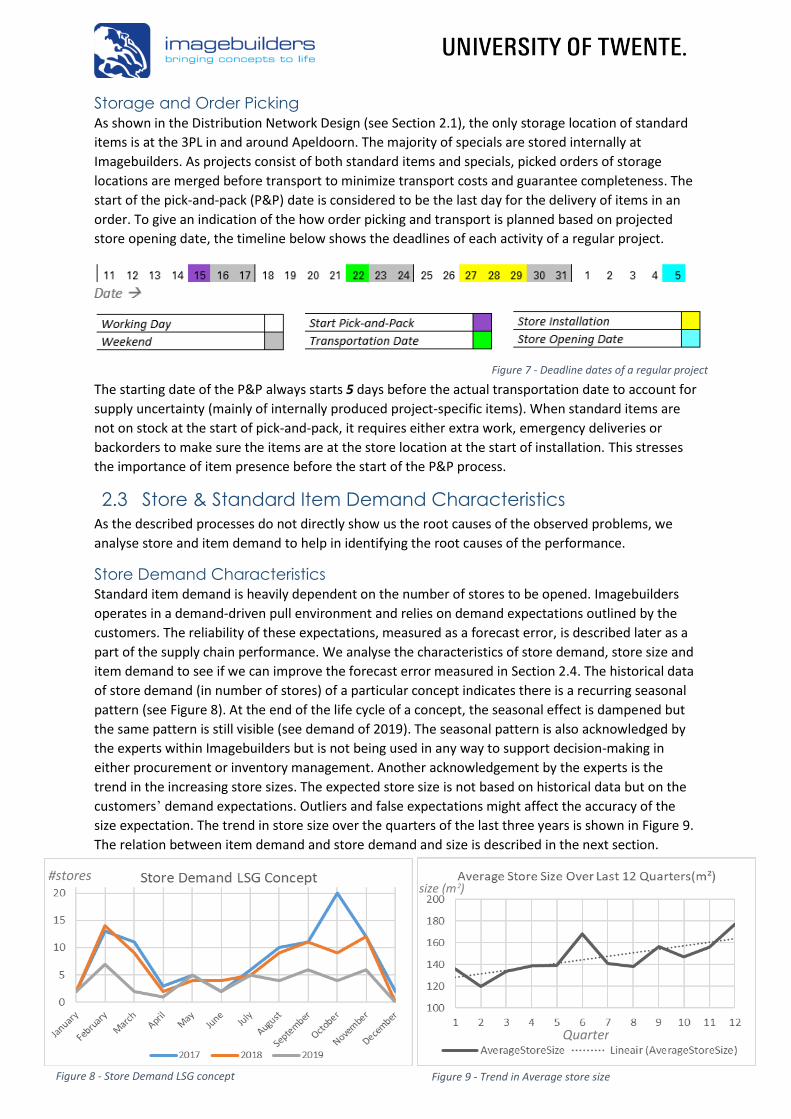
Storage and Order Picking As shown in the Distribution Network Design (see Section 2.1), the only storage location of standard
items is at the 3PL in and around Apeldoorn. The majority of specials are stored internally at
Imagebuilders. As projects consist of both standard items and specials, picked orders of storage
locations are merged before transport to minimize transport costs and guarantee completeness. The
start of the pick-and-pack (P&P) date is considered to be the last day for the delivery of items in an
order. To give an indication of the how order picking and transport is planned based on projected
store opening date, the timeline below shows the deadlines of each activity of a regular project.
The starting date of the P&P always starts 5 days before the actual transportation date to account for
supply uncertainty (mainly of internally produced project-specific items). When standard items are
not on stock at the start of pick-and-pack, it requires either extra work, emergency deliveries or
backorders to make sure the items are at the store location at the start of installation. This stresses
the importance of item presence before the start of the P&P process.
2.3 Store & Standard Item Demand Characteristics
As the described processes do not directly show us the root causes of the observed problems, we
analyse store and item demand to help in identifying the root causes of the performance.
Store Demand Characteristics Standard item demand is heavily dependent on the number of stores to be opened. Imagebuilders
operates in a demand-driven pull environment and relies on demand expectations outlined by the
customers. The reliability of these expectations, measured as a forecast error, is described later as a
part of the supply chain performance. We analyse the characteristics of store demand, store size and
item demand to see if we can improve the forecast error measured in Section 2.4. The historical data
of store demand (in number of stores) of a particular concept indicates there is a recurring seasonal
pattern (see Figure 8). At the end of the life cycle of a concept, the seasonal effect is dampened but
the same pattern is still visible (see demand of 2019). The seasonal pattern is also acknowledged by
the experts within Imagebuilders but is not being used in any way to support decision-making in
either procurement or inventory management. Another acknowledgement by the experts is the
trend in the increasing store sizes. The expected store size is not based on historical data but on the
customers’ demand expectations. Outliers and false expectations might affect the accuracy of the
size expectation. The trend in store size over the quarters of the last three years is shown in Figure 9.
The relation between item demand and store demand and size is described in the next section.
Figure 7 - Deadline dates of a regular project
Figure 8 - Store Demand LSG concept
#stores
Figure 9 - Trend in Average store size
size (m²)
Quarter

11
Standard Item Characteristics During the life cycle of the LSG concept (2016-2020), 1186 standard items with a unique item code
were used to meet customer requirements. Each unique item has its own item code, revision number
and supplier country code as described in Appendix 1. An item gets a new revision number when
customers require a small adjustment or when installers ask for a small modification for installation
ease. As old revisions can be used to create the new revision, we can assume that we can omit the
revision number in item demand. The supplier of the item, indicated by country code, can also be
omitted as it does not matter where the item is procured as long as demand is met. This leaves 495
unique standard items. Of the 495 unique standard items, 338 items have a life cycle of over a year
and ~170 items were active during the entire concept life.
Standard item demand is dependent on store demand and describing the relation between the two
might improve forecasting accuracy. The relationship between store size and item usage of two
random items is shown in Figure 10. If there is a correlation between store size and item usage, the
relation can be used to forecast demand of the item based on store size. When there is no
correlation, individual item demand characteristics such as average demand size become valuable.
The relation between item Y usage and store size seems to be monotonic and linear. If store demand
and store size are forecasted accurately, these characteristics support item demand forecasting.
2.4 Supply Chain Performance – Setting a Benchmark
The supply chain performance of a firm in terms of responsiveness and efficiency is determined by
the interaction between the logistical and cross-functional drivers (Chopra & Meindl, 2012). Although
the 6 drivers defined by Chopra & Meindl can be divided into logistical drivers (Facilities, Inventory &
Transportation) and cross-functional drivers (Information, Sourcing & Pricing), none of the drivers
can operate independently. We measure Imagebuilders’ supply chain performance to set a
benchmark that can be used as comparison material with our results after redesigning the supply
chain and adjusting the internal processes within the supply chain.
Supply Chain Performance Drivers We describe each of the 6 drivers and their impact on Imagebuilders’ supply chain performance to
identify causes of high costs and/or low responsiveness to guide the analysis of the performance.
Pricing – The impact of pricing on the performance is disregarded as prices are agreed upon for long
time periods and there is no room to change item prices to lower costs.
Transportation – Although other transportation modes allow higher level of responsiveness, the item
cost price with included transportation cost of the standard transport mode (FCL via ship and truck)
is fixed. Therefore, the impact of other modes on responsiveness or costs are disregarded.
0
1
2
100 200 300 400 500Item
Dem
and
Qu
anti
ty
Store size (in m²)
Relation Item X usage & Store size
0
100
200
300
400
0 100 200 300 400 500Item
Dem
and
Qu
anti
ty
Store size (in m²)
Relation Item Y usage & Store size
Figure 10 - Relationship of Item X and Y between Store Size and Item Usage

12
Facilities - The role of the facilities impacts the level of responsiveness as the only facilities with a
storage role (3PL in the NL) require a long lead time (~120 days) before goods are ready for P&P to
meet demand. A responsive supply chain seeks to aggressively reduce the lead times (Chopra &
Meindl, 2012). The current role of the facilities also negatively impacts the cost-efficiency as
inventory costs are estimated to be higher in the Netherlands compared to e.g. China.
Inventory - Imagebuilders has no method to compute required safety stock levels to account for
supply and/or demand uncertainty and variability. There are no stock policies and all stock of
standard items is stored at the 3PL in NL. This impacts the supply chain performance as responsive
supply chains for slower moving items require buffer inventories to quickly respond to demand and
efficient supply chains for faster moving items seek to minimize inventories (Chopra & Meindl, 2012).
Replenishment cycles of inventory are long (~10 weeks) and limit the minimization possibilities for
inventory levels, reduce flexibility and increase the forecast error as uncertainty is high.
Information - The accuracy of information is crucial for the supply chain performance in both
efficiency and responsiveness. When demand expectations during the ordering lead time are too
high, the expected starting stock is estimated too high and unnecessary items are ordered. If demand
expectations for a period are too low, the absence of safety stocks forces Imagebuilders to procure
items at European suppliers or to produce internally at a higher unit cost price.
Sourcing - The main goal of the sourcing strategy was to meet demand at the lowest possible cost
regardless of the lead times as customers approved long-term forecasts. Although this allowed the
opportunity for an efficient supply chain, the long lead times in combination with having stock at the
3PL took away any ability to respond to unexpected demand timely at low costs. Under-forecasting
requires Imagebuilders to source at European suppliers at a higher item cost price.
We identified that information is the performance driver that impacts the performance of the
sourcing strategy and subsequently the performance of the inventory strategy. Therefore it is
important to first measure the performance of forecasts to find what part of the performance can be
traced back to the information quality, the sourcing strategy or the inventory strategy.
Measured Performance – The Benchmark Imagebuilders does not keep track of Key Performance Indicators (KPIs). In the measured supply
chain performance in this section, we introduce KPIs to measure performance on both the cost
aspect as well as the responsiveness aspect to allow comparison with the results of our model.
If the expected demand information that is outlined by the customer does not reflect the actual
demand, it impacts the performance of every aspect of the supply chain. Therefore, we start with
analysing the accuracy of store demand information that is used in forecasting demand. We measure
the forecasting error of store demand as the Mean Absolute Percentage Error (MAPE) for both lead
time demand and demand during lead time plus review period. As lead time demand overlaps for
consecutive bulk order periods, we can only consider half of the data to estimate the forecast error.
The average MAPE of store demand in the first two weeks of the lead time averages 8%. The length
of the lead time in Table 7 averages 20 weeks whereas the length of lead time plus review period
averages 30 weeks. The average forecasting errors of these periods are mainly caused by over-
forecasting. Within the non-overlapping lead time demand periods considered in the average MAPE,
103 stores were forecasted in total with an actual demand of 83 stores. Within all non-overlapping
lead time plus review periods considered, 144 stores were forecasted while actual store demand was
122 stores. Thus, demand expectations of the customer are inaccurate. It should be noted that for
the forecast error of any planning period of 10 weeks, it does not matter if the demand of a store is

13
in the first week or during the last week (10th week). This allows the levelling out of demand
throughout the lead time which impacts the measured MAPE. If monthly forecasts were available,
we expect the average MAPE would have been higher as it would then matter in which month of the
lead time the demand takes place.
The over-forecasts in lead time store demand resulted in an over-forecast of item demand and
subsequently an under-estimation of expected item stock levels at the end of a period. This led to
ordering items that were not needed during the Bulk period as the stock levels were already high
enough to meet demand. Although the main factor in over-estimating item demand occurs through
over-forecasting store demand, another factor is over-estimating the item quantities used per store.
For items of which demand is not dependent on store size, this only led to small forecast errors. For
items of which demand does seem to be dependent on store size, over-estimating the store size or
average item usage per store amplifies the forecast error on item level. The amplification of the
forecast error is shown in detail in Figure 11.
In measuring an overall forecasting error during lead time and/or during lead time plus review period
on item level, we have no forecasting data of items that were sourced in the European supplier
regions. We only have access to the forecasts of items sourced in the Chinese supplier region (75% of
items considered in the LSG concept). As shown in Table 8, the average MAPE over all items is higher
than the MAPE of store demand (see Table 7) indicating the relation between item usage and store
demand is described incorrectly in forecasting item demand. We also added the Weighted Absolute
Percentage Error (WAPE) as an error which uses item demand as a weight to the MAPE (described in
Section 3.4). As the WAPE fluctuates around the average MAPE, the size of item demand does not
impact the MAPE.
To show the effect of false demand expectations on the supply chain performance, we analyse the
effects on inventory performance, purchasing performance and customer service level performance.
The annual average value of the inventory for all customers combined in 2019 is shown in Table 9.
This value only takes standard items into account that are stored at the 3PL.
Demand is measured in the number of stores Average MAPE
Lead Time Demand 26.1% Lead Time Plus Review Period Demand 24.8% First Two Weeks of Lead Time Demand 8%
Table 7 - Lead-time Demand Forecast Error of Store Demand
Average Item MAPE WAPE
Lead Time Demand 65.4% 72.7% Lead Time plus Review Period Demand 64.5% 63.1%
Table 8 - Average Item MAPE and Multi-Item WAPE Historical Performance
Months on stock 0-3 >3 Total
Purchase value (€ x1,000,000) 1.3 (40%) 1.8 (60%) 3.1
Table 9 – Annual average inventory value 2019
Figure 11 - Forecast Error of an Item during a Bulk Period
10•Forecast
Number of Stores
138.9•Expected
Average Item usage Per Store
1389•Expected
Item Demand
7•Actual
Number of Stores
124.4•Actual Average
Item usage Per Store
871•Actual
Item Demand
Forecast Error of an Item in a Bulk Period
Percentage Error = ~43%
Percentage Error = ~12%
Percentage Error = ~60%

14
The high value of inventory does not have to be a problem when the inventory turnover is high as
fast moving inventory would minimize inventory costs. We introduce the Inventory Turnover Rate
(ITR) as a KPI that measures the inventory turns in a year. Although the data shown in Table 9 already
indicates this rate is too low, we measure this rate for the LSG concept for comparison purposes with
our model results. The ITR is calculated as shown in Equation 1. The actual starting stock value of the
LSG concept on January 31st 2019 was €600,000. As the ending stock value of 2019 was €86,000,
purchase costs were €872,000 and average inventory value was €385,000, we retrieve an ITR of 3.6.
This rate exceeds the target ITR of 4 in which it would take ~90 days to sell inventory. The cost of
goods sold of the LSG concept equals €1,386,000.
𝐼𝑇𝑅 =𝐶𝑜𝑠𝑡 𝑜𝑓 𝐺𝑜𝑜𝑑𝑠 𝑆𝑜𝑙𝑑
𝐴𝑣𝑒𝑟𝑎𝑔𝑒 𝐼𝑛𝑣𝑒𝑛𝑡𝑜𝑟𝑦 𝑉𝑎𝑙𝑢𝑒=
(𝑆𝑡𝑎𝑟𝑡𝑖𝑛𝑔 𝑆𝑡𝑜𝑐𝑘 𝑉𝑎𝑙𝑢𝑒 − 𝐸𝑛𝑑𝑖𝑛𝑔 𝑆𝑡𝑜𝑐𝑘 𝑉𝑎𝑙𝑢𝑒) + 𝑃𝑢𝑟𝑐ℎ𝑎𝑠𝑒 𝐶𝑜𝑠𝑡𝑠
𝐴𝑣𝑒𝑟𝑎𝑔𝑒 𝐼𝑛𝑣𝑒𝑛𝑡𝑜𝑟𝑦 𝑉𝑎𝑙𝑢𝑒
Equation 1 - Inventory Turnover Rate
The incurred warehousing cost (handling plus storage costs) in 2019 across all 3PL storage locations is
€650,000. The incurred warehousing costs not covered by the warehousing cost inclusion in the item
cost price is approximated to be 60% (~€400,000) as this was the average portion of annual value of
items on stock longer than 3 months. By including the obsolescence costs (~€60,000) into the total
inventory costs, the total inventory costs of 2019 are approximated to be €710,000, of which
€460,000 was paid by Imagebuilders as a result of forecast errors as well as an inefficient supply
chain. The annual holding cost ratio of an item at the 3PL in NL is estimated to be 23% (€710,000
/€3,100,000). As the average inventory value of LSG concept over the months February-December in
2019 was €385,000, we approximate the inventory costs of the LSG concept in our benchmark to be
€81,000.
The costs of under-forecasting are hard to define. For 2019, the total purchased quantities per item
are computed together with the total cost of purchasing using only the data of the LSG concept. This
value is compared to the total purchase costs in case all items were procured at the supplier with the
lowest unit cost price. The difference between the two indicates improvement potential as the
reasons for sourcing differently are not in the data. The total incurred purchasing costs over 2019 for
the LSG concept were €872,000 whereas the costs could have been €716,000 when the same
quantity was purchased at the supplier with the lowest item cost price.
To describe the performance in terms of responsiveness, we compute the customer service level in
terms of the Order Line Fill Rate (OLFR) as it describes the percentage of order lines of standard
items that are on stock at the moment the P&P process starts. We only take standard items into
account in this KPI. As described above, maximizing the fill rate of this moment has the highest
importance as it directly prevents extra costs. The OLFR at the P&P moment is approximated using
the following equation:
𝑃&𝑃 𝑂𝑟𝑑𝑒𝑟 𝐿𝑖𝑛𝑒 𝐹𝑖𝑙𝑙 𝑅𝑎𝑡𝑒 = (𝑁𝑢𝑚𝑏𝑒𝑟 𝑜𝑓 𝑂𝑟𝑑𝑒𝑟 𝐿𝑖𝑛𝑒𝑠 𝑜𝑛 𝑠𝑡𝑜𝑐𝑘 𝑎𝑡 𝑠𝑡𝑎𝑟𝑡 𝑃&𝑃
𝑇𝑜𝑡𝑎𝑙 𝑁𝑢𝑚𝑏𝑒𝑟 𝑜𝑓 𝑂𝑟𝑑𝑒𝑟 𝐿𝑖𝑛𝑒𝑠 ) ∗ 100
Equation 2 - P&P OLFR calculation
The performance of this KPI for LSG in 2019 is approximated by analysing the data of a random
selection of orders (21 orders, ~4000 order lines) as the data collection is a lengthy manual process.
The available data does not allow us to compute a volume fill rate on item level. The P&P OLFR for
the standard items in the LSG concept in 2019 is approximated at 93%. At the moment of transport,
the OLFR is approximated to be 98.5% which means that 1.5% of the order lines is backordered. The
extra costs required for emergency deliveries & backorders are unknown.

15
2.5 Conclusion
This chapter answered research question 1: “What does Imagebuilders’ current supply chain look like
for standard items and what is the supply chain performance in terms of cost-efficiency and customer
responsiveness?”.
Although Imagebuilders was always able to meet customer requirements timely for standard items
by keeping high stock levels, Imagebuilders was not able to meet these requirements cost-efficiently
and will not be able to react timely and cost-efficiently with the changing customer requirements.
The performance measured in forecasting, supply chain costs and responsiveness mainly act as a
benchmark to compare our model results with. In measuring the forecast error of store and item
demand during lead time and during lead time plus review period (Table 10), we found an over-
forecasting bias for most months. The average MAPE of items is higher than the average MAPE of
store demand as item characteristics are not described correctly in forecasting item demand.
In the actual supply chain performance benchmark (see Table 11), we found that the Order-Line Fill
Rate is lower than the desired level of 95% and the Inventory Turnover Rate is below the minimum
target of 4. We also identified that Imagebuilders could have saved over €150,000 if all required
standard items were sourced at the supplier region that offered the lowest item cost price.
Imagebuilders required to source in Europe at a higher cost price due to under-forecasting.
These findings guide our literature review in the following ways:
• Research into strategically locating inventories is needed when redesigning the supply chain as we
have to be able to meet demand in the maximum allowable lead time of the customer.
• Research into forecasting methods that are able to consider the demand characteristics of both
store and individual item demand becomes valuable to develop accurate demand
forecasts/expectations for both store and item demand.
• Research into an inventory policy that allows variable lot sizing and variable inventory levels
becomes valuable to incorporate demand seasonality and to keep higher inventory levels when
uncertainty is high. By simulating the decision-making in an inventory model of a supply chain
design, we can compare results to our benchmark to find improvements.
• Research into safety stock calculation methods becomes valuable to counter demand uncertainty
without keeping excessively high stock levels to achieve a high Order-Line Fill Rate at the moment
the picking process starts.
These findings guide our model construction in the following way:
• To incorporate seasonality and demand uncertainty into an inventory policy, we need a dynamic
inventory model that includes the varying demand throughout the periods. This model should
allow placing production and replenishment orders based on the inventory position of all stock
points considered.
Average Store MAPE Average Item MAPE WAPE
Lead Time Demand 26.1% 65.4% 72.7% Lead Time plus Review Period Demand 24.8% 64.5% 63.1%
Table 10 - Historical Forecasting Performance Store & Item Demand
Total Purchasing
Costs (€x1000)
Approximated Inventory
Costs (€x1000) Total Costs
(€x1000)
Average Inventory
Value (€x1000) OLFR
Value End Inventory (€x1000)
Inventory Turnover
Rate
LSG Concept 2019 872 81 934 385 93% 86 3.6
Table 11 - Supply Chain Performance LSG Concept over 2019

16
3. Literature Review This chapter takes a closer look on scientific literature to answer the second research question:
“What theory and methods exist in literature to improve responsiveness of the supply chain network
for standard items?”. We start Section 3.1 with revisiting the concept of Customer Responsiveness
and how it relates to redesigning the supply chain. In Section 3.2 we review literature on how to
reach the required level of responsiveness on the strategic as well as the tactical planning level. In
Section 3.3, we look into redesigning a supply chain on a strategic planning level. In Section 3.4, we
find methods to adjust the internal factors Demand Anticipation & Inventory Control to meet the
level of required responsiveness on the tactical level. We conclude our findings in Section 3.6 after
addressing the supply chain design and supplier region selection problem in Section 3.5.
3.1 Customer Responsive Supply Chain
Increasing uncertainty in customer demand in combination with the requirement of short lead-times
require an organisation to be able to react quickly to demand. Problems arise for organisations that
operate within a customer-oriented pull system as inventories are needed to quickly respond to
demand (Holweg, 2005). Besides the speed aspect that defines Supply Chain Responsiveness (SCR),
agility is an important aspect of SCR for organisations where demand is highly variable and volumes
are relatively low in order to respond rapidly to changes in demand (Christopher, 2000). To improve
the SCR, an organisation needs to separate external factors that call for a required level of SCR from
internal factors that can enable a potential level of SCR. Holweg & Reichhart (2007) proposed a
conceptual framework for SCR including the internal and external factors. When the required and
potential SCR are aligned, customer requirements can be met cost-efficiently (Holweg & Reichhart,
2007). As not all factors are relevant for this literature review, the framework including all factors can
be found in Appendix 2. The internal factors that are relevant in this thesis, Demand Anticipation and
Inventory Control, are described in this chapter along with methods found to adjust these factors.
3.2 Meeting the Required level of Supply Chain Responsiveness
The internal factors, which determine the achieved level of responsiveness and can be divided into
Operational factors and Supply Chain Integration, describe the material coordination within the
supply chain as it includes the processes that fulfil customer demand. Within this research, only the
Operational internal factors Demand Anticipation and Inventory Control are considered to be in the
scope. For project-driven organisations that perform multiple overlapping projects simultaneously, it
becomes important to plan and control to cope with conflicts of interest (Hans, Herroelen, Leus, &
Wullink, 2007). Within planning and control, numerous sources describe Strategic, Tactical and
Operational as the three planning levels with a corresponding planning horizon that can be found
back in the hierarchical framework for planning and control in multi-project organisations proposed
by Hans et al. (2007) and the division of SCR described by Holweg & Reichhart (2007). On the
strategic level, required processes to fulfil demand need to be designed timely. Hans et al. (2007)
identify supply chain design and warehouse design as strategic material coordination processes. This
stresses the importance of research into supply chain distribution network redesign and positioning of
inventory within the supply chain. On the tactical level, Hans et al. (2007) identify procurement and
purchasing as the planning and control processes within material coordination. As various suppliers
are able to meet quality and item quantity requirements, it becomes important to select the supplier
region and supply chain design that meets these in a cost-efficient manner. Uncertainty and
variability in demand can be countered by anticipating to the expected demand by accurate
forecasting and using buffer stocks. This stresses the importance of research into forecasting methods
and inventory management to meet customer requirements cost-efficiently.

17
Adjustments to the internal factors on the operational level are not considered as these processes
are considered to be mainly order-driven and out of scope.
3.3 Supply Chain Distribution Network Redesign
Strategic decision making for material coordination include long-term decisions based on aggregate
information and forecasts (Hans, Herroelen, Leus, & Wullink, 2007). One of the long-term decisions
to be made is the supply chain design. To select a network design that complies with the needs of a
company, the item characteristics and network requirements need to be analysed (Chopra & Meindl,
2012). A hybrid design combining multiple network designs can be created to get an appropriate
network for each product-characteristic and customer-need combination. The first key decision in
(re)designing a supply chain network is deciding on whether the item requires flow through an
intermediate location or the item requires direct customer delivery/pickup (Chopra S. , 2003).
Besides the internal wish to transport full projects to the customer site at once, direct customer
delivery would require multiple smaller load transports from each supplier which would drastically
increase transportation costs. Customer pickup is also seen as an infeasible option as on-site delivery
and installation is part of the project. Thus, items require flow through an intermediate location. Of
the 6 distribution network design options defined by Chopra & Meindl (2012), only the options that
consider distributor storage or manufacturer storage with in-transit merge can be considered in
redesigning the network.
To find balance between efficiency (e.g. no high inventory levels) and flexibility (quick response to
demand), Naylor et al. (1999) describe that determining the position of the Customer Order
Decoupling Point (CODP) plays a central role. Downstream the CODP, the activities remain demand-
driven. Upstream, all activities are forecast-driven and based on planning. The positioning of the
CODP is dependent on the longest lead-time that the customer is willing to accept (Naylor, Naim, &
Berry, 1999). The feasible supply chain redesign options can be determined by identifying feasible
strategic stock locations at the decoupling point to cope with uncertainty and variability while
meeting demand in the maximum allowable lead time (Figure 12). As standard items are Make-to-
Stock, the required lead time from the stock point until the picking process starts cannot be longer
than the maximum allowable lead time of 2 weeks. The methods required to make sure stock levels
at the stock locations are high enough to meet demand are considered to be the forecast-driven
activities. The methods used to adjust the internal factors Demand Anticipation and Inventory
Control to meet demand cost-efficiently are found in literature and are described in Section 3.4.
3.4 Forecast-Driven Activities
To fit the needs of the supply chain distribution network redesign, the forecast-driven activities
designed to anticipate demand have to allow an organisation to meet customer requirements cost-
efficiently. The first step in doing so is having accurate demand forecasts. The accuracy of the
forecasts can be used directly as an input factor in calculating item safety stocks. When the Demand
Anticipation and Inventory Control processes have been designed to meet customer requirements,
the supply chain design that meets these requirements in the best way has to be selected.
Demand Anticipation by Demand Forecasting Fisher et al. (1994) describe that differentiating easy-to-forecast from hard-to-forecast items allows
accurate response to counter the uncertainty in demand for each type of item. When creating a
Forecast-driven
activities CODP Order-driven
activities
Stock Location Figure 12 - Customer Order Decoupling Point

18
forecasting model, to measure the accuracy of the model, the available historical data set should be
divided into Training data (typically 80% of the available data) and Test data (typically 20% of the
available data) where the model will use Training data to forecast the Test data (Hyndman, 2014).
When the available data set only covers a limited time period, Hyndman (2014) describes the
method of time series cross-validation where multiple training sets are used where every next
training set contains one more observation than the previous one.
Forecasting the Number of Stores & Average Store Size
In cases where it is very common that individual item demand depends on the demand of a final
product, it is natural to forecast the demand of final item (the number of stores) first by using e.g.
historical data (Axsäter, 2006). However, Axsäter describes that it is reasonable to consider other
factors than historical data to forecast the final item demand as the data might not be representative
for the future as e.g. a concept is phasing out. For such events that are hard to model, manual
adjustments should be possible. As the data of store demand seems to follow a monthly seasonal
pattern and trend, a Time-Series Analysis method like Holt-Winters Exponential Smoothing can be
used with the following general model equation based on the Multiplicative trend-seasonal model
(Silver, Pyke, & Thomas, 2017):
𝑥𝑡 = (𝑎𝑡 + 𝑏𝑡)𝐹𝑡 + 𝜀𝑡
Equation 3 - Holt-Winters Exponential Smoothing Method with Seasonal Factor
Each period 𝑡 in which a forecast is made, the values of the parameters level (𝑎𝑡), trend (𝑏𝑡) and
seasonal factor (𝐹𝑡) are obtained by the historical data known at that point in time and thus change
over time. As the trend in average store size over the historical store demand data is solely subject to
trend and not to seasonality, the seasonal factor (𝐹𝑡) can be omitted from Equation 3 to forecast
average store size. As item demand is directly related to the demand in number of stores and the
expected store size, causal models can be used to forecast item demand.
Causal Forecasting of the Required Number of Items
Fisher (1994) suggests differentiating hard-to-forecast items from easy-to-forecast items to be able
to extra effort in forecasting hard-to-forecast items. In differentiating items based on their
‘forecastability’, a significant correlation between store size in m² and item usage classes an item as
easy-to-forecast when the number of stores and average store size are forecasted accurately.
Therefore, the first step in differentiating items is to determine the correlation coefficient and its
significance. In measuring the correlation between two variables, the following correlation
coefficient measures are popular in literature: Pearson’s r, Spearman’s rho and Kendall’s tau. The
underlying assumption of Pearson’s coefficient is that both the variables are normally distributed. As
the data of the store sizes is not normally distributed, Pearson’s correlation coefficient is unusable. A
non-parametric correlation measure is required that allows distribution-free data. Both Spearman’s
rho and Kendall’s tau are usable as correlation measures as they use non-parametric (distribution-
free) data. Both measures use rank correlation where the independent variables are ranked. Croux
and Dehon (2010) state that Kendall’s coefficient is more robust and requires slightly less
computational time compared to the Spearman’s coefficient. Therefore, we consider Kendall’s tau as
the correlation coefficient which is computed using the following equation (Kendall, 1938):
𝜏 = 𝐶 − 𝐷
12
𝑛(𝑛 − 1)
Equation 4 - Kendall's tau calculation
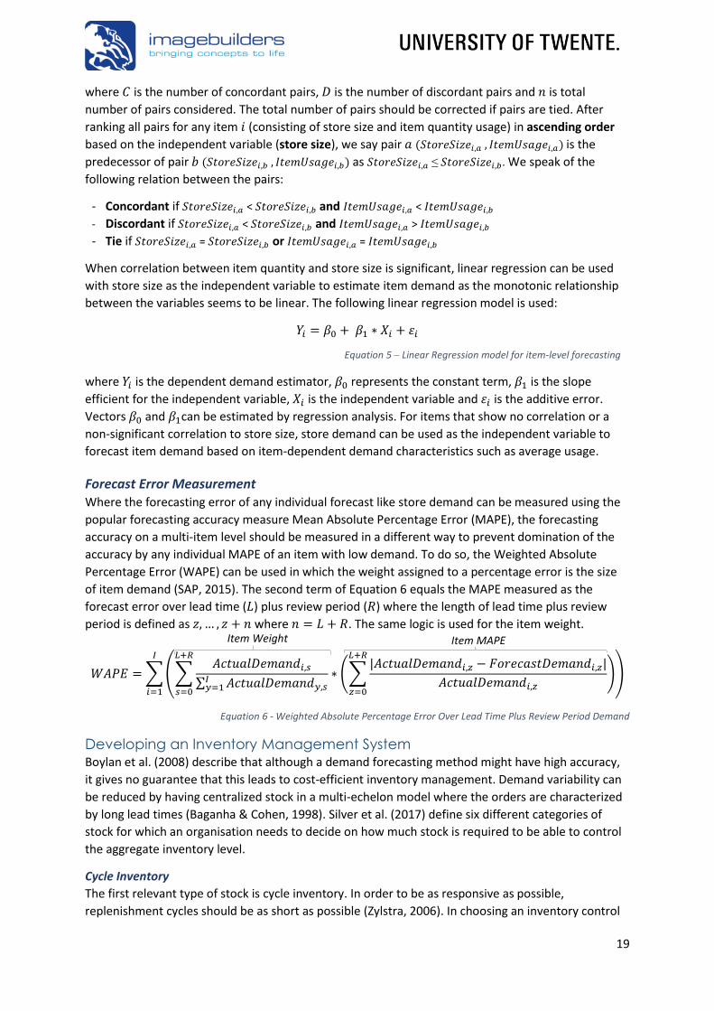
19
where 𝐶 is the number of concordant pairs, 𝐷 is the number of discordant pairs and 𝑛 is total
number of pairs considered. The total number of pairs should be corrected if pairs are tied. After
ranking all pairs for any item 𝑖 (consisting of store size and item quantity usage) in ascending order
based on the independent variable (store size), we say pair 𝑎 (𝑆𝑡𝑜𝑟𝑒𝑆𝑖𝑧𝑒𝑖,𝑎 , 𝐼𝑡𝑒𝑚𝑈𝑠𝑎𝑔𝑒𝑖,𝑎) is the
predecessor of pair 𝑏 (𝑆𝑡𝑜𝑟𝑒𝑆𝑖𝑧𝑒𝑖,𝑏 , 𝐼𝑡𝑒𝑚𝑈𝑠𝑎𝑔𝑒𝑖,𝑏) as 𝑆𝑡𝑜𝑟𝑒𝑆𝑖𝑧𝑒𝑖,𝑎 ≤ 𝑆𝑡𝑜𝑟𝑒𝑆𝑖𝑧𝑒𝑖,𝑏. We speak of the
following relation between the pairs:
- Concordant if 𝑆𝑡𝑜𝑟𝑒𝑆𝑖𝑧𝑒𝑖,𝑎 < 𝑆𝑡𝑜𝑟𝑒𝑆𝑖𝑧𝑒𝑖,𝑏 and 𝐼𝑡𝑒𝑚𝑈𝑠𝑎𝑔𝑒𝑖,𝑎 < 𝐼𝑡𝑒𝑚𝑈𝑠𝑎𝑔𝑒𝑖,𝑏
- Discordant if 𝑆𝑡𝑜𝑟𝑒𝑆𝑖𝑧𝑒𝑖,𝑎 < 𝑆𝑡𝑜𝑟𝑒𝑆𝑖𝑧𝑒𝑖,𝑏 and 𝐼𝑡𝑒𝑚𝑈𝑠𝑎𝑔𝑒𝑖,𝑎 > 𝐼𝑡𝑒𝑚𝑈𝑠𝑎𝑔𝑒𝑖,𝑏
- Tie if 𝑆𝑡𝑜𝑟𝑒𝑆𝑖𝑧𝑒𝑖,𝑎 = 𝑆𝑡𝑜𝑟𝑒𝑆𝑖𝑧𝑒𝑖,𝑏 or 𝐼𝑡𝑒𝑚𝑈𝑠𝑎𝑔𝑒𝑖,𝑎 = 𝐼𝑡𝑒𝑚𝑈𝑠𝑎𝑔𝑒𝑖,𝑏
When correlation between item quantity and store size is significant, linear regression can be used
with store size as the independent variable to estimate item demand as the monotonic relationship
between the variables seems to be linear. The following linear regression model is used:
𝑌𝑖 = 𝛽0 + 𝛽1 ∗ 𝑋𝑖 + 𝜀𝑖
Equation 5 – Linear Regression model for item-level forecasting
where 𝑌𝑖 is the dependent demand estimator, 𝛽0 represents the constant term, 𝛽1 is the slope
efficient for the independent variable, 𝑋𝑖 is the independent variable and 𝜀𝑖 is the additive error.
Vectors 𝛽0 and 𝛽1can be estimated by regression analysis. For items that show no correlation or a
non-significant correlation to store size, store demand can be used as the independent variable to
forecast item demand based on item-dependent demand characteristics such as average usage.
Forecast Error Measurement
Where the forecasting error of any individual forecast like store demand can be measured using the
popular forecasting accuracy measure Mean Absolute Percentage Error (MAPE), the forecasting
accuracy on a multi-item level should be measured in a different way to prevent domination of the
accuracy by any individual MAPE of an item with low demand. To do so, the Weighted Absolute
Percentage Error (WAPE) can be used in which the weight assigned to a percentage error is the size
of item demand (SAP, 2015). The second term of Equation 6 equals the MAPE measured as the
forecast error over lead time (𝐿) plus review period (𝑅) where the length of lead time plus review
period is defined as 𝑧, … , 𝑧 + 𝑛 where 𝑛 = 𝐿 + 𝑅. The same logic is used for the item weight.
𝑊𝐴𝑃𝐸 = ∑ (∑𝐴𝑐𝑡𝑢𝑎𝑙𝐷𝑒𝑚𝑎𝑛𝑑𝑖,𝑠
∑ 𝐴𝑐𝑡𝑢𝑎𝑙𝐷𝑒𝑚𝑎𝑛𝑑𝑦,𝑠𝐼𝑦=1
𝐿+𝑅
𝑠=0
∗ (∑|𝐴𝑐𝑡𝑢𝑎𝑙𝐷𝑒𝑚𝑎𝑛𝑑𝑖,𝑧 − 𝐹𝑜𝑟𝑒𝑐𝑎𝑠𝑡𝐷𝑒𝑚𝑎𝑛𝑑𝑖,𝑧|
𝐴𝑐𝑡𝑢𝑎𝑙𝐷𝑒𝑚𝑎𝑛𝑑𝑖,𝑧
𝐿+𝑅
𝑧=0
))
𝐼
𝑖=1
Equation 6 - Weighted Absolute Percentage Error Over Lead Time Plus Review Period Demand
Developing an Inventory Management System Boylan et al. (2008) describe that although a demand forecasting method might have high accuracy,
it gives no guarantee that this leads to cost-efficient inventory management. Demand variability can
be reduced by having centralized stock in a multi-echelon model where the orders are characterized
by long lead times (Baganha & Cohen, 1998). Silver et al. (2017) define six different categories of
stock for which an organisation needs to decide on how much stock is required to be able to control
the aggregate inventory level.
Cycle Inventory The first relevant type of stock is cycle inventory. In order to be as responsive as possible,
replenishment cycles should be as short as possible (Zylstra, 2006). In choosing an inventory control
Item MAPE Item Weight

20
policy, we have to consider the required inventory status review frequency (Periodically vs.
Continuous) and the type of lot-sizing (Fixed vs. Variable) (van der Heijden & Diks, 1999). The
seasonal store demand pattern requires variable lot-sizing and since supplier regions use fixed
production cycles, the inventory policy required is an (R,S)-policy with periodic review interval R and
a variable order-up-to level S. Silver et al. (2017) describe that the review interval is often dependent
on external factors and for usability the review interval should be restricted to be a “reasonably small
number of feasible discrete values”. When considering a two-level inventory system, the downstream
stock point is responsible in meeting the external customers’ requirements. Although a high fill rate
may be desired at the most downstream stock point, the fill rate of any other upstream stock point
used to replenish the downstream stock point does not require a high fill rate to ensure the high fill
rate downstream (van der Heijden & Diks, 1999). When the starting inventory of a period is too small
to cover all demand during the period due to high uncertainty, the starting inventory of the next
period should be corrected to cover the backlog. If a high fill rate is desired, the backlog is expected
to be minimal and thus the effect of a correction is also expected to be minimal. Splitting a
replenishment order into multiple smaller transport orders is only possible in a supply chain with an
upstream and a downstream stock point. The number of replenishments in a period is a trade-off
between the savings in inventory costs versus the increase in transport cost as it may require
shipping small loads.
Safety Stock
The second relevant type of inventory is safety stock to account for uncertainty in demand and/or
supply. The level of safety stock is directly related to the service level an organisation wants to
achieve (Silver, Pyke, & Thomas, 2017). The service level measured is the volume fill rate which
equals the fraction of demand directly covered by the current stock. The safety stock level for any
stock point in a periodic review system (R,S) can be computed using the following equation where 𝑘
is a safety factor and 𝜎𝐿+𝑅 is the forecast error of lead-time and review period demand.
𝑆𝑎𝑓𝑒𝑡𝑦 𝑆𝑡𝑜𝑐𝑘 = 𝑘 ∗ 𝜎𝐿+𝑅
Equation 7 - Safety Stock Calculation
3.5 Supply Chain Design Selection Problem
When the internal factors Demand Anticipation and Inventory Control have been adjusted to allow
meeting the required level of SCR cost-efficiently using various supply chain designs regardless of the
supplier region, we have to select the supply chain design and thereby a corresponding supplier
region which meets the requirements in the best way. The selection problem in this research is
comparable to the supplier selection problem (SSP) where one option out of multiple options is
chosen based on one or more criteria. In an extensive systematic literature review on decision-
making methods to tackle the SSP, Chai et al. (2013) identify Multicriteria Decision-Making,
Mathematical programming and methods within Artificial intelligence as the three main techniques
used for decision-making. Researchers tend to create a hybrid of techniques in creating a problem-
solving model to allow dealing with smaller subproblems separately (Chai, James, & Ngai, 2013).
Single objective problems can be solved with a Mathematical program by using e.g. (Integer) Linear
Programming. Although this is useful for the cost minimization objective, supporting decision-making
based on multiple objectives becomes more complicated. To be able to recommend outsourcing an
item to a supplier from a finite set of candidates based on multiple criteria that represent the
different objectives (e.g. the criterion ‘costs’ represents the minimal cost objective), the weight of a
criterion should be determined and a candidates score on the criteria should be measurable. The
Analytical Hierarchy Process (AHP), developed by Saaty (1980), is a popular multi-attribute utility
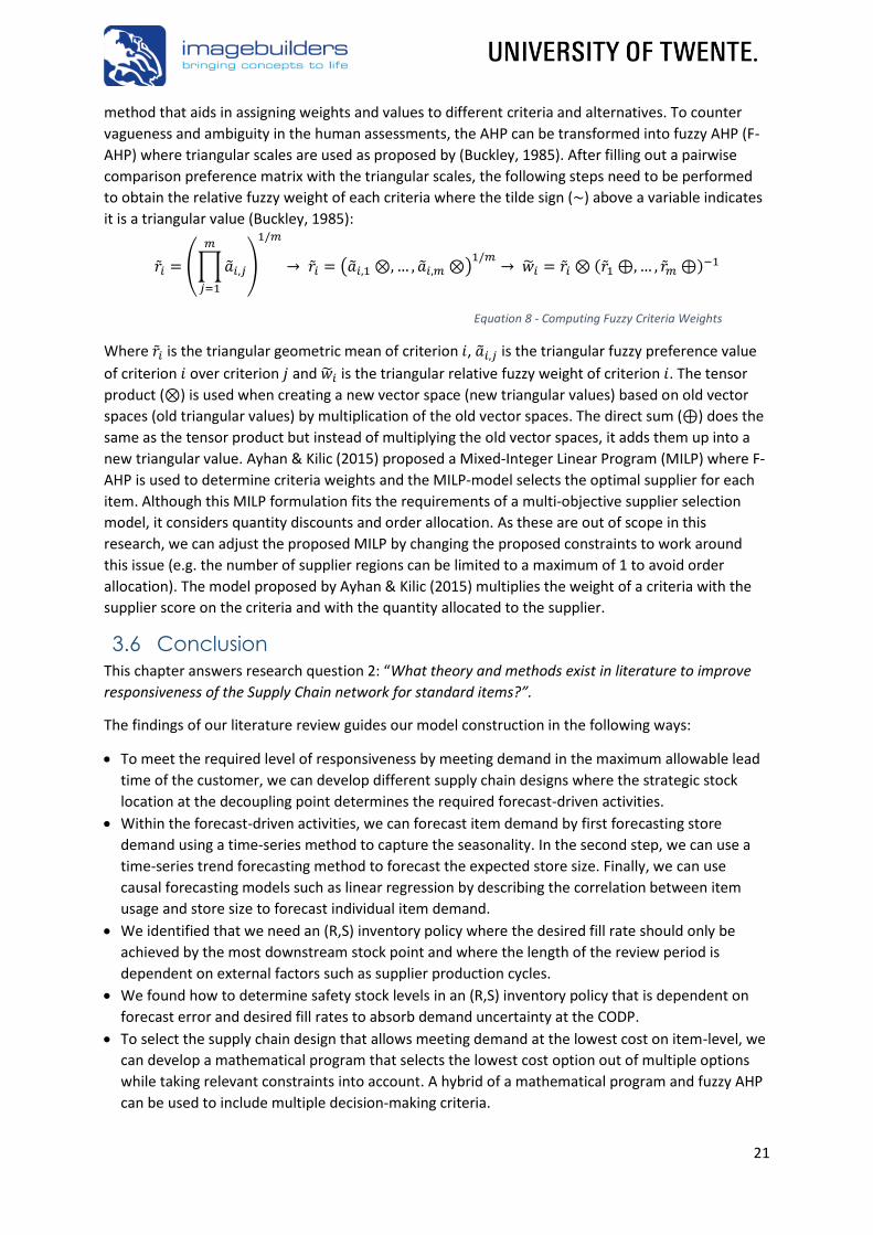
21
method that aids in assigning weights and values to different criteria and alternatives. To counter
vagueness and ambiguity in the human assessments, the AHP can be transformed into fuzzy AHP (F-
AHP) where triangular scales are used as proposed by (Buckley, 1985). After filling out a pairwise
comparison preference matrix with the triangular scales, the following steps need to be performed
to obtain the relative fuzzy weight of each criteria where the tilde sign (~) above a variable indicates
it is a triangular value (Buckley, 1985):
�̃�𝑖 = (∏ �̃�𝑖,𝑗
𝑚
𝑗=1
)
1/𝑚
→ �̃�𝑖 = (�̃�𝑖,1 ⊗, … , �̃�𝑖,𝑚 ⊗)1/𝑚
→ �̃�𝑖 = �̃�𝑖 ⊗ (�̃�1 ⊕, … , �̃�𝑚 ⊕)−1
Equation 8 - Computing Fuzzy Criteria Weights
Where �̃�𝑖 is the triangular geometric mean of criterion 𝑖, �̃�𝑖,𝑗 is the triangular fuzzy preference value
of criterion 𝑖 over criterion 𝑗 and �̃�𝑖 is the triangular relative fuzzy weight of criterion 𝑖. The tensor
product (⊗) is used when creating a new vector space (new triangular values) based on old vector
spaces (old triangular values) by multiplication of the old vector spaces. The direct sum (⊕) does the
same as the tensor product but instead of multiplying the old vector spaces, it adds them up into a
new triangular value. Ayhan & Kilic (2015) proposed a Mixed-Integer Linear Program (MILP) where F-
AHP is used to determine criteria weights and the MILP-model selects the optimal supplier for each
item. Although this MILP formulation fits the requirements of a multi-objective supplier selection
model, it considers quantity discounts and order allocation. As these are out of scope in this
research, we can adjust the proposed MILP by changing the proposed constraints to work around
this issue (e.g. the number of supplier regions can be limited to a maximum of 1 to avoid order
allocation). The model proposed by Ayhan & Kilic (2015) multiplies the weight of a criteria with the
supplier score on the criteria and with the quantity allocated to the supplier.
3.6 Conclusion
This chapter answers research question 2: “What theory and methods exist in literature to improve
responsiveness of the Supply Chain network for standard items?”.
The findings of our literature review guides our model construction in the following ways:
• To meet the required level of responsiveness by meeting demand in the maximum allowable lead
time of the customer, we can develop different supply chain designs where the strategic stock
location at the decoupling point determines the required forecast-driven activities.
• Within the forecast-driven activities, we can forecast item demand by first forecasting store
demand using a time-series method to capture the seasonality. In the second step, we can use a
time-series trend forecasting method to forecast the expected store size. Finally, we can use
causal forecasting models such as linear regression by describing the correlation between item
usage and store size to forecast individual item demand.
• We identified that we need an (R,S) inventory policy where the desired fill rate should only be
achieved by the most downstream stock point and where the length of the review period is
dependent on external factors such as supplier production cycles.
• We found how to determine safety stock levels in an (R,S) inventory policy that is dependent on
forecast error and desired fill rates to absorb demand uncertainty at the CODP.
• To select the supply chain design that allows meeting demand at the lowest cost on item-level, we
can develop a mathematical program that selects the lowest cost option out of multiple options
while taking relevant constraints into account. A hybrid of a mathematical program and fuzzy AHP
can be used to include multiple decision-making criteria.

22
4. Supply Chain Redesign This chapter answers the research question 3: “How can the found methods be applied to redesign
Imagebuilders’ supply chain to meet the required supply chain responsiveness at the lowest possible
cost?”. We start in Section 4.1 by denoting the frequently used notations throughout the remaining
chapters. The rest of the chapter follows the steps of Figure 13. After determining the feasible supply
chain designs, we describe all the required steps to compute the supply chain costs of each option by
simulating the decisions over the 2019 data of the LSG concept. To do so, we need monthly item
demand forecasts over each supply chain design specific forecast horizon. In the supply chain design
with two stock locations, we look into adjusting the replenishment frequency of the downstream
stock point to reduce inventory levels and costs. We conclude our findings in Section 4.6.
4.1 Frequently Used Notations
Let us denote some frequently used notations before explaining the redesign options and the
methods required per option. We use the following indices:
• 𝑖 = item 1,…, I with I being the set of standard items in the LSG concept.
• 𝑗 = supplier region 1,…, J with J being the set of available supplier regions consisting of regions Baltic
States (BS), China (CN), Czech (CZ), the Netherlands (NL), Poland (PL) and Turkey (TR).
• 𝑜 = supply chain design option 1,…, O with O being the set of supply chain options (see Section 4.2)
• 𝑡 = period 2,…,T with T being the set of considered months (February 2019 – December 2019).
• 𝑤 = stock points 1,…,W with W being the set of stock points consisting of stock points in the regions
Baltic States (BS), China (CN), Czech (CZ), the Netherlands (NL), Poland (PL) and Turkey (TR).
Furthermore, we frequently use the following notations:
• 𝑅 = Review period (= 1 period, same for both inventory and production of all stock points 𝑤.
• 𝐿𝑝𝑟 = Lead time for production (= 1 period). The lead time for production, independent of item and
item quantity, is the same for any item in any supplier region in any supply chain option.
• 𝐿𝑡𝑟,𝑜,𝑤 = Lead time for transportation to the stock point 𝑤 considered in option 𝑜 (see Table 12).
The transportation lead time for all items and quantities are the same.
• 𝑆𝑖,𝑜,𝑤,𝑡 = Order-up-to-level of option 𝑜 at stock point 𝑤 for item 𝑖 in period 𝑡.
• 𝑆𝑆𝑖,𝑜,𝑤,𝑡 = Safety stock of option 𝑜 at stock point 𝑤 for item 𝑖 in period 𝑡.
• 𝑥𝑖,𝑜,𝑡,𝑡+𝐿𝑝𝑟+𝐿𝑡𝑟,𝑜,𝑤+𝑅−1,𝑤= Expected European demand of item 𝑖 at stock point 𝑤 in period 𝑡 to
period 𝑡 + 𝐿𝑝𝑟 + 𝐿𝑡𝑟,𝑜,𝑤 + 𝑅 − 1 during lead time and review period in option 𝑜.
• 𝜎𝑖,𝑜,𝑡,𝑡+𝐿𝑝𝑟+𝐿𝑡𝑟,𝑜,𝑤+𝑅−1,𝑤 = Forecast error of item 𝑖 at stock point 𝑤 of period 𝑡 until period 𝑡 + 𝐿𝑝𝑟 +
𝐿𝑡𝑟,𝑜,𝑤 + 𝑅 − 1 to account for the demand uncertainty lead time plus review period in option 𝑜.
4.2 Redesign Options
To meet customer requirements in terms of the maximal allowed customer order lead-time (6 weeks
including delivery, installation and completion), the required items need to be ready for P&P within
the first two weeks as this process usually starts 3-4 weeks ahead of the store opening date.
4.3 (Tactical level) 4.2 (Strategic Level)
Develop feasible supply
chain designs & identify
forecast-driven
activities per design
Forecast Store Demand
Forecast Store Size
Forecast Item Demand
Determine
Forecast Horizons
for all designs
4.4 (Tactical level)
Item-Level
Inventory
Management for
all designs
4.5 (Tactical level)
Adjusting
Replenishment
Frequency of two
stock point supply
chain design
Figure 13 - Structure of the Chapter

23
None of the suppliers within the considered regions are able to meet this lead-time in a different
environment than a Make-To-Stock environment as production lead time is estimated to be 4 weeks
and transportation times from the supplier to Imagebuilders vary between 2-6 weeks depending on
the supplier region. Following the logic by Naylor et al. (1999), inventory is to be located at any
location that allows a delivery from stock within 2 weeks as it is the maximum allowed lead time. For
suppliers with a transportation lead time longer than 2 weeks, e.g. Chinese Suppliers to cover
demand in Europe, an inventory location is needed downstream the supplier. Combining the theory
of Naylor et al. (1999) and Verdouw et al. (2006), we create supply chain designs, determine the
CODPs and locate inventories which all allow Imagebuilders to meet the required level of
responsiveness in serving customers in Europe. Because not all supplier regions can be considered
within each option, we define the feasible supplier regions for each option in Table 12.
Option 1: Outsourcing to China with Single Stock Point (CN-1SP) The first option we consider is the option which Imagebuilders currently uses up until the declining
phase of a store concept where if possible, standard items are sourced from Chinese suppliers. Even
though the costs incurred by using this option were too high as described in Chapter 2, the forecast-
driven decisions within this option can be optimized to reduce costs. The supply chain configuration
of this option is shown in Figure 14. The forecast-driven decisions that need to be made within this
option are 1) the size of the production order (which equals the replenishment order size) placed at
the suppliers in China which is transported to the 3PL in NL upon completion and 2) the safety stock
levels at the 3PL in NL to account for uncertainty in demand. Although we expect that optimizing this
option results in low purchasing costs, we need long-term forecasts to account for the long lead-time
from order placement until receipt at the 3PL in NL. This will likely result in a relatively high
forecasting error which in its turn results in higher safety stock levels to meet a desired customer
service level. Therefore, we expect high inventory costs.
Option 2: Outsourcing to China with Two Stock Points (CN-2SP) The second option we consider (see Figure 15) describes Imagebuilders’ desired option that can be
modified to be used for possible future expansions where Imagebuilders fits shops with the same
standard items in Europe, the Asia-Pacific region and the Americas. Although the current pandemic
has put the tendering processes on hold, we foresee benefits in this option even when Imagebuilders
only serves customers within Europe because the annual holding costs in China are estimated to be
lower than in the Netherlands. This option requires making more forecast-driven decisions as we
now need to determine 1) the size of the production order to replenish the CN stock with, 2) the size
of the replenishment order from CN to the 3PL in NL and 3) the safety stock levels for both storage
locations. We expect an improved level of responsiveness as the lead time to replenish the inventory
Option (𝒐) Outsourcing Supplier Region Stock Point (𝒘) 𝑳𝒕𝒓,𝒐,𝒘 in periods Referred to as:
1 China ( 𝑗 = CN) At the 3PL in NL (𝑤 = NL) 1.5 CN-1SP
2 China ( 𝑗 = CN) At 3PL in NL (𝑤=NL) & In Supplier Region (𝑤=CN) 1.5 & 0 respectively CN-2SP
3 Europe ( 𝑗 = TR, BS, CZ, PL) At the 3PL in NL (𝑤 = NL) 0.5 EU-NLSP
4 Europe ( 𝑗 = TR, BS, CZ, PL, NL) In Supplier Region 𝑗 (𝑤=𝑗) 0 EU-EUSP
Table 12 - Supply Chain Design Options
Call-off Single Project Demand Forecast Information
C
U
S
T
O
M
E
R
CODP
Forecast-driven activities Order-driven activities
Replenishment Order Merge &
Distribution
Suppliers China 3PL in NL
Pick-and-Pack
Single Project Production &
Distribution
Imagebuilders
Figure 14 - Supply Chain Configuration Option 1

24
at the 3PL is shortened and the safety stock at the Chinese suppliers allows us to place a
replenishment order that might include higher item quantities than the quantities produced. We
expect a higher level of cost-efficiency as we can keep stock in China at a lower annual holding cost
rate. There is no investment needed for the CN stock point as stock is kept at the suppliers.
Option 3: Outsourcing in Europe with Single Stock Point (EU-NLSP) In the third option, items are mainly sourced within the European supplier regions (See Figure 16).
Even though this option is very similar to the first option and the decisions to be made are the same,
the shorter transportation lead time allows forecasting on shorter term. The forecast-driven
decisions that need to be made within this option are the same as for option 1 (the size of the
production order and the safety stock levels at the 3PL in the Netherlands) but with different data as
the lead time is different. We foresee that purchasing costs will be significantly higher compared to
sourcing in China as item cost prices in Europe are higher. However, the transportation lead time
allows short-term forecasts which in its turn will likely lead to more accurate forecasts and thus a low
safety stock level. The supplier region in this option and in option 4 is defined as Europe (EU). We use
Europe as an umbrella term that considers the supplier regions within Europe as shown in Table 12.
Option 4: Outsourcing in Europe with a Supplier Region Stock (EU-EUSP) In the final option, we consider the suppliers within a supplier region as a storage location that also
take over the task to Pick-and-Pack single projects before transport to Imagebuilders for transport
merge (see Figure 17). This option can be used as the required transportation time for all European
supplier regions falls within the two weeks in which items should be ready. Using a two-level stock
design for European supplier regions is expected to not add any value as for both stock points we
would require a safety stock and transportation lead times are relatively short. As transport is
planned after the P&P process and falls within the maximum allowable lead time, the total lead time
is reduced while still being able to deliver demand on time. We foresee that the reduced lead times
will reduce the safety stock levels and thus average inventory levels. An additional benefit could be
the annual holding cost ratio of storage locations in the supplier regions. Similar to option 2, we do
not need an investment for the stock point as stock is kept at the suppliers.
Call-off Single Project Demand Forecast Information
C
U
S
T
O
M
E
R
CODP
Forecast-driven activities Order-driven activities
Replenishment Order Merge &
Distribution
Suppliers China 3PL in NL
Pick-and-Pack
Single Project Production
Imagebuilders
Distribution CODP
Call-off Replenishment Order
Figure 15 - Supply Chain Configuration Option 2
Call-off Single Project Demand Forecast Information
C
U
S
T
O
M
E
R
CODP
Forecast-driven activities Order-driven activities
Replenishment Order Merge &
Distribution
Supplier Regions Europe 3PL in NL
Pick-and-Pack
Single Project Production &
Distribution
Imagebuilders
Figure 16 - Supply Chain Configuration Option 3
Call-off Single Project Demand Forecast Information
C
U
S
T
O
M
E
R Forecast-driven
activities
Order-driven activities
Order Merge &
Distribution
Supplier Regions Europe
Production
Imagebuilders
Pick-and-Pack
Single Project
& Distribution CODP
Figure 17 – Supply Chain Design Option 4

25
Recap of the Supply Chain Designs We have identified 4 possible supply chain designs through which an item can be sourced that all
allow Imagebuilders to meet demand within the maximum allowable lead time of 2 weeks. All of the
designs differ from each other in a different way. One of the most important differences among the
options is the forecast horizon required by the option. By using two stock points as shown in option 2
(CN-2SP), we need separate forecasts for both CODPs to compute the required production quantity
and required replenishment quantity separately. The options and expected impact are shown below
in Table 13. The forecasts created to cover the forecast horizon of each option is described in the
next section. The described methods can be adjusted to account for the option-specific lead times.
4.3 Demand Anticipation by Developing Forecasts
To select a developed supply chain option that meets customer requirements in the best way, we
need to approximate the customer requirements accurately to prevent shortages and excessive
stock. In the developed methods to forecast store demand and store size, we use a model that finds
parameter settings to update the level, trend and seasonal factors that minimizes the forecast error
measured in either MAPE or MSE of our model fit. We describe this model in Appendix 5 –
Forecasting Models. In-depth examples of each forecasting method are given in the same appendix.
Let us first explain the used forecast horizons for the different supply chain options. Since we have no
data of demand distribution throughout a period and choose to not add this complexity, we receive a
replenishment order at the start of the replenishment cycle (start of a period 𝑡).
By planning backwards from the moment a replenishment order receipt at the stock point is planned,
we can determine when a) the replenishment order should be transported from the supplier to the
storage location, b) when the production order should be finished and c) when the forecast of store
and item demand should be finished to ensure a timely start of production. Figure 18 illustrates the
backwards planning of supply chain options 1, 2 & 3. The supply chain option 4, which is described
later in this section, requires a different forecast horizon as we have no transportation lead time. In
Figure 18, if we require a replenishment order receipt at the start of 𝑡 = 4 to cover demand during
the replenishment cycle (during 4th time period), we need to make sure the order is shipped at least
2 weeks before 𝑡 = 4 when considering EU supplier regions or 6 weeks before 𝑡 = 4 when considering
the CN supplier region. Production should start 4 weeks prior to the latest allowable transportation
moment depending on the supplier region. When looking at Figure 18, we can see that the moment
to start a production order or to transport a replenishment order falls in the middle of a period. As
we cannot simulate decision making in the middle of a period, we assume we can make them at the
start of a period with the knowledge we would have halfway through a period. As the measured
forecast error of forecasted demand 2 weeks ahead is low (MAPE of ~8%, see Section 2.4), we
assume that in the middle of the first period we have full demand knowledge of the first period. The
expected demand during lead time and review period for supply chain options 1, 2 and 3 at the start
Option (𝒐) Supplier Region Stock Points Expected Impact
1 China 1 in NL Low Purchasing Costs, High Inventory Levels due to Long Lead Times
2 China 1 in NL, 1 in CN Low Purchasing Costs, High Inventory levels but Lower Inventory Costs
3 Europe 1 in NL High Purchasing Costs, Relatively Low Inventory Levels
4 Europe 1 at Supplier Region High Purchasing Costs, Low Inventory Levels due to Short Lead Times
Table 13 - Supply Chain Designs & Expected Impact
𝑡 = 1 𝑡 = 2 𝑡 = 3 𝑡 = 4 𝑡 = 5
Replenishment Cycle
Figure 18 - Backwards developed forecast horizon for supply chain options 1, 2 & 3
Lead Time EU
Production Lead Time CN
Production
Lead Time CN→3PL
NL Transportation
Lead Time EU→3PL
NL Transportation Demand during t = 4

26
of a period 𝑡 can thus be calculated by adding the demand of period 𝑡 to the forecast of the
remaining periods that fall within the considered lead time and review period. Supply chain option 4
only considers production lead time as the suppliers keep the inventory. Therefore, we can make
forecasts at the start of a period 𝑡 and the produced items will be ready at the start of 𝑡 = 2 as
production lead time is 1 period. This option requires a 2-month forecast to forecast demand during
lead time plus review period as shown in Figure 19.
Please note that we develop a forecast at the start of period 𝑡 for all periods that fall in the lead time
plus review period and thus forecast for periods 𝑡,..., 𝑡 + 𝐿𝑝𝑟 + 𝐿𝑡𝑟,𝑜,𝑤 + 𝑅 − 1. The lead time of
transport, if any, is dependent on supply chain option.
Forecasting Store Demand
As Axsäter (2006) described, it is natural to first forecast the demand of the final product (stores) and
to use that forecast to forecast item demand which is dependent on final product demand. We start
off in period 𝑡 with forecasting the number of stores of a specific customer for period 𝑡, … , 𝑡 + 𝑛 resulting in the variable 𝑆𝑡𝑜𝑟𝑒𝐹𝑜𝑟𝑒𝑐𝑎𝑠𝑡𝑡,𝑡+𝑛. At the start of each period 𝑡, a forecast is made for the
periods 𝑡 + 𝑛 where 𝑛 = 0, … , 𝐿𝑝𝑟 + 𝐿𝑡𝑟,𝑜,𝑤 + 𝑅 − 1. Variable 𝑛 is dependent on the supply chain
option as 𝐿𝑡𝑟,𝑜,𝑤 differs per option. Each customer concept requires a separate forecast. The first step
in creating the forecasts of store demand is to separate the Training data and the Test data. Although
Hyndman (2014) described that typically 80% of the available data should be used as Training data
and the remaining 20% should be used as Test data, this would leave us with very limited data to use
for quantitative analysis. The available data of the LSG concept is split as shown in Figure 21.
We use the 31st of January 2019 as this is the first moment in 2019 of which we have accuracy stock
level data. To measure the forecast accuracy of our forecasting model, we use time series cross-
validation where we forecast the number of stores in the periods that fall within the lead time and
review period on a monthly basis. Each month, required forecasting parameters are updated to use
the most up-to-date data. An elaborate example is given in Appendix 5 – Forecasting Models which
resulted in the forecast shown in Figure 20. In the actual demand data of stores, experts within
Imagebuilders acknowledged that in October 2017 (the grey peak in period 10 of Figure 20) there
was an outlier. To prevent this outlier from impacting our final results, we change this store demand
quantity to a value that fits the actual demand pattern. The forecast and the actual demand in the
forecasted periods can be seen in Figure 20 by the green and orange lines respectively.
31st December 2019 31st January 2019
Training Data Test Data
1st January 2017
~70% of data ~30% of data
Figure 21 - Data Division into Training and Test Data
Figure 19 – Planning Horizon of supply chain option 4
𝑡 = 1 𝑡 = 2 𝑡 = 3 𝑡 = 4 𝑡 = 5
Replenishment Cycle
Lead Time EU Production
0
5
10
15
20
1 3 5 7 9 11 13 15 17 19 21 23 25 27 29 31 33 35
Sto
re Q
uan
tity
Period
Store Demand, Model Fit & Forecast
Figure 20 - Historical Demand, Model Fit and Forecasts after finding Smoothing Factors that Minimize MAPE for Model Fit

27
Forecasting Store Size
We forecast the average size of the forecasted stores per customer concept by analysing the trend of
the store size over the last years. As historical data is limited and there seems to be an increase in the
average store size over the years, we forecast the expected average store size rather than forecasting
the number of stores based on size (e.g. the number of small-sized stores). We remove outliers
(2 stores with a size >275m2 with average store size being 159m2) to prevent domination by these
values. This results in the variable 𝐹𝑜𝑟𝑒𝑐𝑎𝑠𝑡𝑒𝑑𝑆𝑡𝑜𝑟𝑒𝑆𝑖𝑧𝑒𝑡,𝑡+𝑛 measured in m2 where in period 𝑡 a
forecast is made of the expected average store size for the stores forecasted in periods 𝑡, … , 𝑡 + 𝑛. At
the start of period 𝑡, a forecast is made for every period within period 𝑡 + 𝑛 where 𝑛 = 0,..., 𝐿𝑝𝑟 +
𝐿𝑡𝑟,𝑜,𝑤 + 𝑅 − 1. We find parameter values by creating a good model fit but as opposed to forecasting
store demand, we now omit the seasonal factors to only use level and trend. The division into
Training and Test data is the same as in store forecast as we forecast the store size of the forecasted
stores. In Appendix 5 we show an example of the usage of the method. The combination of the
forecasts on store demand level and store size are to be used in forecasting item demand.
Forecasting Item Demand
We compute Kendall’s tau (τ𝑖) and the p-value (p𝑖) for all items to test the significance of the
correlation between the item usage within a store (Quantity used per m2) and the actual store size in
m2. Although all the steps to compute the value of Kendall’s tau can be done step by step manually,
the ranges of item usage and store size differ per item which makes it difficult to automate as we
want to test correlation for all items in the LSG concept. Therefore, we wrote a Microsoft Excel Visual
Basic script in which we use the Kendall’s tau function of the Correlation Data Analysis tool pack
developed by Real Statistics that computes the correlation coefficient by only entering the ranges of
the variables that were obtained earlier (Zaiontz, 2020). This function automatically subtracts the
number of ties from the total number of pairs. An example of an item that shows significant
correlation between usage and store size is shown in Appendix 5. The demand of items with a
significant correlation between item usage and store size is forecasted using Equation 9. For items of
which usage is dependent on store size, we use the following regression equation to compute the
forecasted quantities over all stores over periods 𝑡, … , 𝑡 + 𝑛 where 𝑛 = 0, … , 𝐿𝑝𝑟 + 𝐿𝑡𝑟,𝑜,𝑤 + 𝑅 − 1:
𝐼𝑡𝑒𝑚𝐹𝑜𝑟𝑒𝑐𝑎𝑠𝑡𝑖,𝑡,𝑡+𝑛 = 𝑧𝑖 ∗ 𝑆𝑡𝑜𝑟𝑒𝐹𝑜𝑟𝑒𝑐𝑎𝑠𝑡𝑡,𝑡+𝑛 ∗ (𝛽𝑖,0 + 𝛽𝑖,1 ∗ 𝐹𝑜𝑟𝑒𝑐𝑎𝑠𝑡𝑒𝑑𝑆𝑡𝑜𝑟𝑒𝑆𝑖𝑧𝑒𝑡,𝑡+𝑛), ∀𝑖, 𝑡
Equation 9 - Linear Regression model for Store Size Dependent Item Usage Forecasting
The item-dependent vectors 𝛽𝑖,0 and 𝛽𝑖,1 are computed using the Regression Analysis Tool in
Microsoft Excel (See Appendix 5 – Forecasting Models). Variable 𝑧𝑖 is the inter-demand interval of
item 𝑖. For all items, we incorporate the inter-demand interval in the forecast. When an item is used
in all previous stores, we assume it will be used in all future stores. When an item is used in half the
stores fitted previously, we assume we can forecast the demand by multiplying the item forecast
with 𝑧𝑖 = 0.5. This can be set to 0 when an item is phased out. For items of which the item usage per
store shows no significant correlation to the store size, we use Equation 10 where item demand is
only dependent on the number of stores forecasted, the average item usage per store
(𝑆𝑡𝑜𝑟𝑒𝐼𝑡𝑒𝑚𝑈𝑠𝑎𝑔𝑒𝑖) and the inter-demand interval 𝑧𝑖. Non-correlated item usage within a store
tends to be low and/or constant. Therefore, we can use the average item usage per store
(𝑆𝑡𝑜𝑟𝑒𝐼𝑡𝑒𝑚𝑈𝑠𝑎𝑔𝑒𝑖) as the average quantity of item 𝑖 used in a store when there is demand.
Forecasts are made in period 𝑡 over the periods 𝑡, … , 𝑡 + 𝑛 where 𝑛 = 0, … , 𝐿𝑝𝑟 + 𝐿𝑡𝑟,𝑜,𝑤 + 𝑅 − 1.
𝐼𝑡𝑒𝑚𝐹𝑜𝑟𝑒𝑐𝑎𝑠𝑡𝑖,𝑡,𝑡+𝑛 = 𝑧𝑖 ∗ 𝑆𝑡𝑜𝑟𝑒𝐹𝑜𝑟𝑒𝑐𝑎𝑠𝑡𝑡,𝑡+𝑛 ∗ 𝑆𝑡𝑜𝑟𝑒𝐼𝑡𝑒𝑚𝑈𝑠𝑎𝑔𝑒𝑖 , ∀𝑖, 𝑡
Equation 10 – Causal Forecasting Equation for items with no significant correlation to Store Size

28
Now that we have developed the steps to forecast store demand (see Figure 22), store size and
subsequently item demand, we can use these methods to forecast over the Test data and use these
forecasts to simulate the decisions made in the inventory model developed in the next section.
4.4 Integral Inventory Management
To simulate decision-making over the months in 2019 for the LSG concept, we need forecast data
and actual demand data. As we have the methods to develop forecast data and can retrieve demand
data from the ERP-system, we now need the equations to simulate the actual decisions in an (R,S)
inventory policy. Within the identified supply chain design options in Section 4.2, we consider two
types of supply chain networks: one with a single stock location and one with two stock locations. As
the vast majority suppliers work with a 1-month production cycle and reviewing the inventory status
more often than once a month wouldn’t allow us to place a production order that will be performed
simultaneously, we set the value of the review interval to 1 month and thus 1 period 𝑡. In the two
stock point network, we allow a more frequent inventory replenishment of the downstream stock
point as a finished production order is received at the start of a period and replenishment orders can
be split into multiple smaller orders. Although we consider a replenishment frequency of more than
1 per period, we consider the review interval of the downstream stock point inventory level for
replenishment purposes to be 1 too. If we would review our inventory levels more often than once a
period/month, we would need forecasts on either weekly or daily basis which would require the
addition of actual demand dates within a time period. Although this addition would give more insight
in average inventory levels and more realistic replenishment orders, we choose not to add this
complexity due to time constraints and limited data availability. As we do not consider transport lead
times in supply chain option 4, 𝐿𝑡𝑟,4,𝑤 equals 0. Although we could omit 𝐿𝑡𝑟,𝑜,𝑤 in all equations
considering option 4, we keep it in so we can use and refer to the same equations. In the next
sections, we describe the decisions for the different supply chain designs and the equations to do so.
4.4.1 Scenarios with only One-Level Storage Location Options 1 (CN-1SP), 3 (EU-NLSP) and 4 (EU-EUSP) all consider a One-Level Distribution System where
single projects are picked from one stock point. The single location (R,S) inventory policy described
by van der Heijden & Diks (1999) considers non-seasonal demand that is also not of subject to trend.
Although we can use the majority of equations needed to calculate the safety stock levels and the
order-up-to level, we need some modifications to a) swap the mean demand with a standard
deviation with forecasted demand and b) swap the standard deviation over lead-time plus review
period demand by the forecast error of demand during lead-time and review period. In the periodic
review inventory policy with an order-up-to-level that is not fixed, we compute the order-up-to-level
by adding the expected demand to the safety stock level as shown in Equation 11.
𝑆𝑖,𝑜,𝑡,𝑤 = 𝑆𝑆𝑖,𝑜,𝑡,𝑤 + 𝑥𝑖,𝑜,𝑡,𝑡+𝐿𝑝𝑟+𝐿𝑡𝑟,𝑜,𝑤+𝑅−1,𝑤, ∀𝑖, 𝑡, 𝑤 & 𝑜 = 1, 3, 4
Equation 11 - Order-up-to-level of an Item
In calculating the expected demand during lead time plus the review period, options 1 (CN-1SP), 2
(CN-2SP) and 3 (EU-NLSP) all consider forecasting at the middle of a period. The expected demand of
Store Forecasting
(Holt-Winters) Significant Correlation?
( τ𝑖 > 0.4 & p𝑖 < 0.05)
Causal Item Forecasting by
Linear Regression of item usage
with store size (Equation 9)
Causal Item Forecasting by
Average/Constant item usage
(Equation 10)
Store Size
Forecasting
(Holt’s Trend)
Correlation Store
Size & Item usage
Figure 22 - Steps to develop forecasts
𝑆𝑡𝑜𝑟𝑒𝐹𝑜𝑟𝑒𝑐𝑎𝑠𝑡𝑡,𝑡+𝑛 𝐹𝑜𝑟𝑒𝑐𝑎𝑠𝑡𝑒𝑑𝑆𝑡𝑜𝑟𝑒𝑆𝑖𝑧𝑒𝑡,𝑡+𝑛 τ𝑖 & p𝑖
Yes
No

29
an item is the cumulative forecast of demand in the periods that fall in the considered lead time plus
review period as shown in Equation 12. The item forecasts are made at the start of period 𝑡 over the
periods 𝑡 + 1, …, 𝑡 + 𝐿𝑡𝑟,𝑜,𝑤 + 𝐿𝑝𝑟 + 𝑅 − 1 of which the length differs for the different supply chain
options and considered stock points. We use the actual demand of period 𝑡 as the demand during 𝑡 is
assumed to be known as the forecast accuracy of the first few weeks is high (~92%).
𝑥𝑖,𝑜,𝑡,𝑡+𝐿𝑝𝑟+𝐿𝑡𝑟,𝑜,𝑤+𝑅−1,𝑤 = 𝐴𝑐𝑡𝑢𝑎𝑙𝐷𝑒𝑚𝑎𝑛𝑑𝑖,𝑡 + ∑ 𝐼𝑡𝑒𝑚𝐹𝑜𝑟𝑒𝑐𝑎𝑠𝑡𝑖,𝑡+1,𝑡+𝑛
𝐿𝑡𝑟,𝑜,𝑤+𝐿𝑝𝑟+𝑅−1
𝑛=1
Equation 12 - Expected Demand of an Item During Lead-time plus Review Period for Supply Chain Options 1, 2 & 3
For supply chain option 4 (EU-EUSP), we require a forecast made at the beginning of period 𝑡 without
having full knowledge of the demand in this period. The store forecast used to retrieve the item
forecast can be manually adjusted to incorporate the demand knowledge of the first weeks in period
𝑡. We use Equation 13 to determine expected demand of an item during lead time plus review
period. As stated before, 𝐿𝑡𝑟,𝑜,𝑤 equals 0 in this case.
𝑥𝑖,𝑜,𝑡,𝑡+𝐿𝑝𝑟+𝐿𝑡𝑟,𝑜,𝑤+𝑅−1,𝑤 = ∑ 𝐼𝑡𝑒𝑚𝐹𝑜𝑟𝑒𝑐𝑎𝑠𝑡𝑖,𝑡,𝑡+𝑛
𝐿𝑡𝑟,𝑜,𝑤+𝐿𝑝𝑟+𝑅−1
𝑛=0
, ∀𝑖, 𝑡 & 𝑜 = 4 & 𝑤 ≠ 𝑁𝐿, 𝐶𝑁
Equation 13 - Expected Demand at Stock Point of an Item During Lead-time plus Review Period for Supply Chain Option 4
The safety stock of an item is dependent on the forecast error over the lead time and review period.
Improvements of the forecast that decrease the forecast error allows a decrease in the required
safety stock level. In the calculation of the required safety stock level per period as shown in
Equation 14, we multiply the forecasting error over lead time plus review period demand with item,
period and supply chain dependent safety factor 𝑘𝑖,𝑜,𝑡,𝑤 which is directly related to the desired fill
rate. A minimum value for the safety factor can be used to ensure a minimum safety stock level.
𝑆𝑆𝑖,𝑜,𝑡,𝑤 = 𝑘𝑖,𝑜,𝑡,𝑤 ∗ 𝜎𝑖,𝑜,𝑡,𝑡+𝐿𝑝𝑟+𝐿𝑡𝑟,𝑜,𝑤+𝑅−1, ∀𝑖, 𝑡, 𝑤 & 𝑜 = 1,3,4
Equation 14 - Safety Stock Single Stock Point
To compute the safety factor 𝑘𝑖,𝑜,𝑡,𝑤, we separate fast moving items of which demand can be
approximated using a continuous demand distribution (𝑥𝑖,𝑜,𝑡,𝑡+𝐿𝑝𝑟+𝐿𝑡𝑟,𝑜,𝑤+𝑅−1,𝑤 ≥ 10, as Silver et al.
(2017) describe as a rule of thumb) from slow moving items (𝑥𝑖,𝑜,𝑡,𝑡+𝐿𝑝𝑟+𝐿𝑡𝑟,𝑜,𝑤+𝑅−1,𝑤 < 10) to
approximate the forecast error of demand over lead time plus review period. Equation 15 is used to
compute 𝐺(𝑘𝑖,𝑜,𝑡,𝑤). Thereafter, the Goal Seek tool in Microsoft Excel is used to compute the factor
for all supply chain options and safety stock locations. Although the normal loss function should only
be used for items with continuous demand, we can also use it to approximate for slower moving
items as long as it creates reasonable values. A minimum factor prevents negative or too low safety
stocks. We define the desired fill rate for any item of any considered stock point 𝑤 to be 𝐹𝑖𝑙𝑙𝑅𝑎𝑡𝑒𝑖,𝑤.
𝐺(𝑘𝑖,𝑜,𝑡,𝑤) = 𝑥𝑖,𝑜,𝑡,𝑡+𝐿𝑝𝑟+𝐿𝑡𝑟,𝑜,𝑤+𝑅−1,𝑤 ∗ (1 − 𝐹𝑖𝑙𝑙𝑅𝑎𝑡𝑒𝑖,𝑤)
𝜎𝑖,𝑜,𝑡,𝑡+𝐿𝑝𝑟+𝐿𝑡𝑟,𝑜,𝑤+𝑅−1,𝑤, ∀𝑖, 𝑜, 𝑡, 𝑤
Equation 15 - Normal Loss Function to compute the safety factor
In approximating the standard deviation of the forecast error during lead time plus review period, it
is important to notice that consecutive forecast errors overlap in the used time periods and are thus
not independent. This means we cannot use consecutive periods to update the forecast error that is
∀𝑖, 𝑡, 𝑤 & 𝑜 = 1,2,3

30
used as input in the safety stock calculation. The Mean Squared Error (MSE) is used as the forecast
error measure as it directly measures the error over lead time and review period. After we initialize
the MSE for any item by computing the average MSE of previous forecasts, we can update the MSE
once every lead time plus review period cycle (Equation 16). For fast movers, we directly estimate
the forecast error over lead time plus review period by taking the square root of the MSE over lead
time plus review period (Equation 17). Factor 𝜔 is a smoothing factor.
𝑀𝑆𝐸𝑖,𝑜,𝑡,𝑡+𝐿𝑝𝑟+𝐿𝑡𝑟,𝑜,𝑤+𝑅−1,𝑤
= 𝜔 (𝐴𝑐𝑡𝑢𝑎𝑙𝐷𝑒𝑚𝑎𝑛𝑑𝑖,𝑡,𝑡+𝐿𝑝𝑟+𝐿𝑡𝑟,𝑜,𝑤+𝑅−1 − 𝑥𝑖,𝑜,𝑡,𝑡+𝐿𝑝𝑟+𝐿𝑡𝑟,𝑜,𝑤+𝑅−1,𝑤)2
+ (1 − 𝜔)𝑀𝑆𝐸𝑖,𝑜,𝑡−𝐿𝑝𝑟−𝐿𝑡𝑟,𝑜,𝑤−𝑅,𝑡−1,𝑤
Equation 16 - Updating the Forecast Error of Stock Point Using the Previous Forecast Error (Silver, Pyke, & Thomas, 2017)
𝜎𝑖,𝑜,𝑡,𝑡+𝐿𝑝𝑟+𝐿𝑡𝑟,𝑜,𝑤+𝑅−1,𝑤 = √𝑀𝑆𝐸𝑖,𝑜,𝑡,𝑡+𝐿𝑝𝑟+𝐿𝑡𝑟,𝑜,𝑤+𝑅−1,𝑤
Equation 17 – Standard deviation of the forecast error
For slow moving items, Silver et al. (2017) describe that the standard deviation over lead time plus
review period demand should not be developed from forecast errors. Approximating the standard
deviation using a Poisson distribution is a reasonable method as this distribution is likely applicable
to slower moving items using Equation 18 (Silver, Pyke, & Thomas, 2017).
𝜎𝑖,𝑜,𝑡,𝑡+𝐿𝑝𝑟+𝐿𝑡𝑟,𝑜,𝑤+𝑅−1,𝑤 = √𝑥𝑖,𝑜,𝑡,𝑡+𝐿𝑝𝑟+𝐿𝑡𝑟,𝑜,𝑤+𝑅−1,𝑤
Equation 18 - Standard deviation for slow moving items (Silver, Pyke, & Thomas, 2017)
Now that the order-up-to-level can be calculated, we need to incorporate the actual stock levels of
the only stock point to compute the actual order quantity of an item. The inventory position includes
the pipeline inventory. As the replenishment order needed to increase the stock levels to the desired
order-up-to-level equals the production order and represents the to be transported quantities, we
need to produce the number of items required to meet the order-up-to-level. When the inventory
position is higher than the desired order-up-to-level, the production quantity is zero. Using Equation
19, we calculate the required production quantity of item 𝑖 of option 𝑜 in period 𝑡 for stock point 𝑤:
𝑃𝑟𝑜𝑑𝑢𝑐𝑡𝑖𝑜𝑛𝑄𝑢𝑎𝑛𝑡𝑖𝑡𝑦𝑖,𝑜,𝑡 = 𝑀𝑎𝑥{𝑆𝑖,𝑜,𝑡,𝑤 − 𝐼𝑛𝑣𝑒𝑛𝑡𝑜𝑟𝑦𝑃𝑜𝑠𝑖𝑡𝑖𝑜𝑛𝑖,𝑜,𝑡,𝑤 ; 0}
Equation 19 - Production Quantity Computation considering Inventory Position of the Stock Point
Note that for options CN-1SP and EU-NLSP, this equation considers the inventory position and order-
up-to-level of the 3PL in NL and for option EU-EUSP it considers the inventory position and order-up-
to-level of the supplier region storage location. With all the equations above, we are able to simulate
the decisions made (production quantities and safety stocks levels) in a one-level stock design. The
total produced quantity can be computed by summing the production quantity of the considered
periods. We did not cover the average inventory level or the inventory position calculation as these
are straight forward. The average inventory level is the average of the starting inventory and the
ending inventory of a period.
4.4.2 Scenarios with Two-Level Storage Locations In the option that considers a Two-Level Distribution System, the stock point at the CN supplier
region is considered the upstream stock point. Since we only consider European demand, the stock
point at the 3PL in NL is considered as the downstream stock point. This means we do not need an
allocation function of the upstream stock point. Because we want to include the inventory position of
∀𝑖, 𝑜, 𝑡, 𝑤
∀𝑖, 𝑜, 𝑡, 𝑤
∀𝑖, 𝑜, 𝑡, 𝑤
∀𝑖, 𝑡, 𝑤 & 𝑜 = 1,3,4
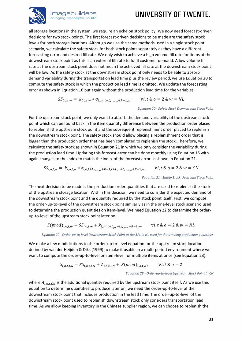
31
all storage locations in the system, we require an echelon stock policy. We now need forecast-driven
decisions for two stock points. The first forecast-driven decisions to be made are the safety stock
levels for both storage locations. Although we use the same methods used in a single stock point
scenario, we calculate the safety stock for both stock points separately as they have a different
forecasting error and desired fill rate. We only wish to achieve a high volume fill rate for items at the
downstream stock point as this is an external fill rate to fulfil customer demand. A low volume fill
rate at the upstream stock point does not mean the achieved fill rate at the downstream stock point
will be low. As the safety stock at the downstream stock point only needs to be able to absorb
demand variability during the transportation lead time plus the review period, we use Equation 20 to
compute the safety stock in which the production lead time is omitted. We update the forecasting
error as shown in Equation 16 but again without the production lead time for the variables.
𝑆𝑆𝑖,𝑜,𝑡,𝑤 = 𝑘𝑖,𝑜,𝑡,𝑤 ∗ 𝜎𝑖,𝑜,𝑡,𝑡+𝐿𝑡𝑟,𝑜,𝑤+𝑅−1,𝑤, ∀𝑖, 𝑡 & 𝑜 = 2 & 𝑤 = 𝑁𝐿
Equation 20 - Safety Stock Downstream Stock Point
For the upstream stock point, we only want to absorb the demand variability of the upstream stock
point which can be found back in the item quantity difference between the production order placed
to replenish the upstream stock point and the subsequent replenishment order placed to replenish
the downstream stock point. The safety stock should allow placing a replenishment order that is
bigger than the production order that has been completed to replenish the stock. Therefore, we
calculate the safety stock as shown in Equation 21 in which we only consider the variability during
the production lead time. Updating this forecast error can be done monthly using Equation 16 with
again changes to the index to match the index of the forecast error as shown in Equation 21.
𝑆𝑆𝑖,𝑜,𝑡,𝑤 = 𝑘𝑖,𝑜,𝑡,𝑤 ∗ 𝜎𝑖,𝑜,𝑡+𝐿𝑡𝑟,𝑜,𝑤+𝑅−1,𝑡+𝐿𝑝𝑟+𝐿𝑡𝑟,𝑜,𝑤+𝑅−1,𝑤, ∀𝑖, 𝑡 & 𝑜 = 2 & 𝑤 = 𝐶𝑁
Equation 21 - Safety Stock Upstream Stock Point
The next decision to be made is the production order quantities that are used to replenish the stock
of the upstream storage location. Within this decision, we need to consider the expected demand of
the downstream stock point and the quantity required by the stock point itself. First, we compute
the order-up-to-level of the downstream stock point similarly as in the one-level stock scenario used
to determine the production quantities on item-level. We need Equation 22 to determine the order-
up-to-level of the upstream stock point later on.
𝑆(𝑝𝑟𝑜𝑑)𝑖,𝑜,𝑡,𝑤 = 𝑆𝑆𝑖,𝑜,𝑡,𝑤 + 𝑥𝑖,𝑜,𝑡,𝑡+𝐿𝑝𝑟+𝐿𝑡𝑟,𝑜,𝑤+𝑅−1,𝑤, ∀𝑖, 𝑡 & 𝑜 = 2 & 𝑤 = 𝑁𝐿
Equation 22 - Order-up-to-level Downstream Stock Point at the 3PL in NL used for determining production quantities
We make a few modifications to the order-up-to-level equation for the upstream stock location
defined by van der Heijden & Diks (1999) to make it usable in a multi-period environment where we
want to compute the order-up-to-level on item-level for multiple items at once (see Equation 23).
𝑆𝑖,𝑜,𝑡,𝐶𝑁 = 𝑆𝑆𝑖,𝑜,𝑡,𝐶𝑁 + 𝐴𝑖,𝑜,𝑡,𝐶𝑁 + 𝑆(𝑝𝑟𝑜𝑑)𝑖,𝑜,𝑡,𝑁𝐿, ∀𝑖, 𝑡 & 𝑜 = 2
Equation 23 - Order-up-to-level Upstream Stock Point in CN
where 𝐴𝑖,𝑜,𝑡,𝐶𝑁 is the additional quantity required by the upstream stock point itself. As we use this
equation to determine quantities to produce later on, we need the order-up-to-level of the
downstream stock point that includes production in the lead time. The order-up-to-level of the
downstream stock point used to replenish downstream stock only considers transportation lead
time. As we allow keeping inventory in the Chinese supplier region, we can choose to replenish the

32
downstream inventory with quantities different to the produced quantities. Therefore, we need an
order-up-to-level of the downstream stock point purely for replenishments (See Equation 24).
𝑆(𝑟𝑒𝑝𝑙)𝑖,𝑜,𝑡,𝑤 = 𝑆𝑆𝑖,𝑜,𝑡,𝑤 + 𝑥𝑖,𝑜,𝑡,𝑡+𝐿𝑡𝑟,𝑜,𝑤+𝑅−1,𝑤, ∀𝑖, 𝑡 & 𝑜 = 2 & 𝑤 = 𝑁𝐿
Equation 24 - Order-up-to-level Downstream Stock Point at the 3PL in NL used for determining replenishment quantities
The computation of the production quantity is dependent on both the inventory position of the
upstream (𝐼𝑛𝑣𝑒𝑛𝑡𝑜𝑟𝑦𝑃𝑜𝑠𝑖𝑡𝑖𝑜𝑛𝑖,𝑜,𝑡,𝐶𝑁) and downstream (𝐼𝑛𝑣𝑒𝑛𝑡𝑜𝑟𝑦𝑃𝑜𝑠𝑖𝑡𝑖𝑜𝑛𝑖,𝑜,𝑡,𝑁𝐿) stock points as we
consider an echelon stock policy. In the first place, if the inventory position of the downstream stock
point is sufficiently high to cover demand during lead time plus review period, we do not need to
produce. Secondly, if the inventory position of the downstream stock point is not sufficient but the
inventory position of the upstream stock point is sufficiently high to cover the required
replenishment orders to the downstream stock point, we do not need to produce. We only need to
produce when the sum of inventory positions is lower than the order-up-to-level of the upstream
stock point as shown in Equation 25. Within the inventory position of the downstream stock point,
we consider actual stock levels at the 3PL in NL and the pipeline inventories of replenishment orders
being transported. The inventory position of the upstream stock point only considers the actual stock
levels at the upstream stock point as the production order of the previous period has been
completed and received.
𝑃𝑟𝑜𝑑𝑢𝑐𝑡𝑖𝑜𝑛𝑄𝑢𝑎𝑛𝑡𝑖𝑡𝑦𝑖,𝑜,𝑡 = 𝑀𝑎𝑥{𝑆𝑖,𝑜,𝑡,𝐶𝑁 − 𝐼𝑛𝑣𝑒𝑛𝑡𝑜𝑟𝑦𝑃𝑜𝑠𝑖𝑡𝑖𝑜𝑛𝑖,𝑜,𝑡,𝐶𝑁 − 𝐼𝑛𝑣𝑒𝑛𝑡𝑜𝑟𝑦𝑃𝑜𝑠𝑖𝑡𝑖𝑜𝑛𝑖,𝑜,𝑡,𝑁𝐿; 0}
Equation 25 - Production Order in a Two-Level Storage System
The last decision to be made is the replenishment order quantity that is used to replenish the
downstream stock point from the upstream stock point. We only need to place a replenishment
order when the inventory position of the downstream stock point is insufficient to cover demand
during transportation lead time plus review period. By subtracting the inventory position of the
downstream stock point from the order-up-to-level, we retrieve the desired replenishment quantity.
In computing the replenishment order quantity, which is the to be transported order, we cannot
place a replenishment order which is bigger than the on-hand inventory at the upstream inventory
location. Therefore, we transport the minimum of the upstream inventory level and the desired
replenishment quantity. Equation 26 is used to compute the total replenishment order quantity in a
period in a two storage location system.
𝑅𝑒𝑝𝑙𝑒𝑛𝑖𝑠ℎ𝑚𝑒𝑛𝑡𝑄𝑢𝑎𝑛𝑡𝑖𝑡𝑦𝑖,𝑜,𝑡
= 𝑀𝑖𝑛 {𝑀𝑎𝑥{𝑆(𝑟𝑒𝑝𝑙)𝑖,𝑜,𝑡,𝑁𝐿 − 𝐼𝑛𝑣𝑒𝑛𝑡𝑜𝑟𝑦𝑃𝑜𝑠𝑖𝑡𝑖𝑜𝑛𝑖,𝑜,𝑡,𝑁𝐿 ; 0} ; 𝐼𝑛𝑣𝑒𝑛𝑡𝑜𝑟𝑦𝐿𝑒𝑣𝑒𝑙𝑖,𝑜,𝑡,𝐶𝑁}
Equation 26 - Replenishment Order Two-Level Storage System
We now have all the required equations to simulate the decision making of both stock points to
determine the production quantities, replenishment quantities and safety stock levels. The average
inventory level in this scenario is not as straight forward as in the one-level stock design as in the
two-level stock scenario we can choose to replenish other quantities than the produced quantities
and we have the choice to split the replenishment into multiple smaller orders. In the next section,
we look into the impact of splitting a replenishment order on inventory levels of the stock points.
4.5 Inventory Cost Savings in the Two-Level Stock Scenario
In the options where we only consider one stock point, the only ways to optimize the supply chain
performance in terms of costs and responsiveness are to reduce lead times and/or improve the
forecast accuracy. These general improvements would however improve the performance of all
∀𝑖, 𝑡 & 𝑜 = 2
∀𝑖, 𝑡 & 𝑜 = 2

33
possible supply chain design options. For option 4 (CN-2SP), where we consider a two-level stock
scenario, the replenishment interval of the downstream stock point can be further optimized to
reduce inventory costs. More frequent call-offs can reduce the average stock levels at the 3PL in NL
as shown in the graphs of Figure 23. When a replenishment order planned for receipt at 𝑡 = 1 +
𝐿𝑡𝑟,𝑜,𝑤 is to cover demand during the replenishment cycle between 𝑡 = 1 + 𝐿𝑡𝑟,𝑜,𝑤 and 𝑡 = 2 +
𝐿𝑡𝑟,𝑜,𝑤, we can divide the replenishment order into smaller batches. During a replenishment cycle,
the entire replenishment order size (Y-axis) is to be received. The replenishment order size can both
represent item quantity as well as the value of the order for any item. Within each call-off scenario,
the first replenishment order is sent at the start of 𝑡 = 1 which arrives at 𝑡 = 1 + 𝐿𝑡𝑟,𝑜,𝑤 at the 3PL in
NL. The variable 𝑆𝑆 in the figure represents safety stock. From the graphs in Figure 23, we find the
following relationships shown in Equation 28 and Equation 27 between the call-off frequency during
a period and the impact on inventory level of item 𝑖 at both stock points that can be used in our
inventory model. Variable 𝑥𝑡 is the call-off frequency used in period 𝑡 which is the same for all items 𝑖
replenished in the period.
𝐴𝑣𝑔𝐼𝑛𝑣𝑅𝑒𝑝𝑙𝑂𝑟𝑑𝑒𝑟𝑖,𝑜,𝑡,𝑤 = (1
2−
1
2𝑥𝑡) ∗ 𝑅𝑒𝑝𝑙𝑒𝑛𝑖𝑠ℎ𝑚𝑒𝑛𝑡𝑂𝑟𝑑𝑒𝑟𝑆𝑖𝑧𝑒𝑖,𝑡 , ∀𝑖, 𝑡 & 𝑜 = 2 & 𝑤 = 𝐶𝑁
Equation 27 - Impact of Call-Off Frequency on Replenishment Order Size and Upstream Inventory Level
𝐴𝑣𝑔𝐼𝑛𝑣𝑅𝑒𝑝𝑙𝑂𝑟𝑑𝑒𝑟𝑖,𝑜,𝑡+𝐿𝑡𝑟,𝑜,𝑤,𝑤 = 1
2𝑥𝑡∗ 𝑅𝑒𝑝𝑙𝑒𝑛𝑖𝑠ℎ𝑚𝑒𝑛𝑡𝑂𝑟𝑑𝑒𝑟𝑆𝑖𝑧𝑒𝑖,𝑡 , ∀𝑖, 𝑡 & 𝑜 = 2 & 𝑤 = 𝑁𝐿
Equation 28 – Impact of Call-Off Frequency on Replenishment Order Size and Downstream Inventory Level
To implement these equations into our inventory model to retrieve the average inventory levels of
both stock points considering we have a starting and ending stock not equal to the safety stock, we
need to look at the characteristics of the impact on both stock points as shown in Figure 23. For the
impact on the total average inventory level at the CN stock point, we can subtract the variable
𝐴𝑣𝑔𝐼𝑛𝑣𝑅𝑒𝑝𝑙𝑂𝑟𝑑𝑒𝑟𝑖,𝑜,𝑡,𝑤 of the starting stock (including the full replenishment order size) at the
upstream stock point of a period 𝑡 for item 𝑖 in supply chain option 2 as the order is leaving the
Figure 23 – Theoretical Replenishment Frequency Impact on Stock Levels
2x Call-off
1x Call-off
4x Call-off
𝐿𝑡𝑟,𝑜,𝑤
𝐿𝑡𝑟,𝑜,𝑤
𝐿𝑡𝑟,𝑜,𝑤
¼
½
¼
⅜ ⅛
, 𝑤
, 𝑤
, 𝑤
, 𝑤
, 𝑤
, 𝑤

34
inventory. At the downstream stock point, the replenishment order is added to the inventory. As
demand during period 𝑡 + 𝐿𝑡𝑟,𝑜,𝑤 can be higher, equal to or lower than the replenishment order size,
we can add variable 𝐴𝑣𝑔𝐼𝑛𝑣𝑅𝑒𝑝𝑙𝑂𝑟𝑑𝑒𝑟𝑖,𝑜,𝑡+𝐿𝑡𝑟,𝑜,𝑤,w to the average of the ending stock of the period
before receipt (𝑡 + 𝐿𝑡𝑟,𝑜,𝑤 − 1) and the ending stock of the period with the receipt (𝑡 + 𝐿𝑡𝑟,𝑜,𝑤) to
obtain the total average inventory of item 𝑖 during period 𝑡 + 𝐿𝑡𝑟,𝑜,𝑤. We cap the number of call-offs
in a period at 4 as holding costs are incurred weekly and multiple replenishments in a week will not
have any positive effect. Although more replenishments lead to smaller replenishment cycles that
help further reduce inventory costs, this might lead to higher transportation costs as the transport
volume of a replenishment decreases.
Imagebuilders prefers to transport Full Container Loads (FCL) using 40ft. containers (or 2 TEU)
because on average it is expected to be cheaper per transported item, the transportation lead time
tends to be shorter and the required transportation time has less uncertainty. In transporting FCL, we
need to ensure the minimum threshold volume to consider FCL transport is exceeded and that the
transported load does not exceed the maximum capacity. The volume of a container as well as an
item are measured in m3. The minimum volume required to even consider FCL transportation is set
to 45% of a 40ft. container volume (~30m3) based on historical data as well as expert opinions within
Imagebuilders. Lower volumes can be shipped using non-FCL transport in which we consider LCL
transport and 20ft. (or 1 TEU) container transport. As items are transported on pallets and some
items cannot be stacked on top of other items, a container is considered full if at most 80% (~53m3)
of its volume is used. To be able to determine feasibility of more frequent replenishments while
using FCL transport, we need to transform our model to a multi-item model. This is needed as we
require the expected volume of all items in a replenishment order to determine if it is possible to
transport partial shipments while still using FCL shipments. The total volume that is to be transported
through supply chain option 2 (CN-2SP) in a period is approximated using Equation 29. The
computation of 𝑇𝑟𝑎𝑛𝑠𝑝𝑜𝑟𝑡𝑉𝑜𝑙𝑢𝑚𝑒𝑖 is described in Appendix 1 – Standard items in the system.
𝑇𝑜𝑡𝑎𝑙𝑇𝑟𝑎𝑛𝑠𝑝𝑜𝑟𝑡𝑉𝑜𝑙𝑢𝑚𝑒𝑜,𝑡 = ∑(𝑅𝑒𝑝𝑙𝑒𝑛𝑖𝑠ℎ𝑚𝑒𝑛𝑡𝑄𝑢𝑎𝑛𝑡𝑖𝑡𝑦𝑖,𝑜,𝑡 ∗ 𝑇𝑟𝑎𝑛𝑠𝑝𝑜𝑟𝑡𝑉𝑜𝑙𝑢𝑚𝑒𝑖)
𝐼
𝑖=1
, ∀𝑡 & 𝑜 = 2
Equation 29 - Transport Volume of a Replenishment Order
4.6 Conclusion
This chapter answers research question 3: “How can the found methods be applied to redesign
Imagebuilders’ supply chain to meet the required supply chain responsiveness at the lowest possible
cost?”.
From this chapter we conclude the following:
• The four developed supply chain designs allow Imagebuilders to meet demand within the
maximum allowable lead time but the expected impact differs. The designs with a relatively long
lead time most likely have higher forecast errors. In combination with a high desired fill rate this
could lead to high safety stock levels. By analysing different desired fill rates in our results, we can
advise Imagebuilders on the desired fill rate in combination with e.g. item characteristics.
• We can now compute the supply chain costs in terms of purchasing costs and inventory costs for
all supply chain designs on single-item level based on actual and forecast data. However, we desire
a solution on multi-item level that fits within the constraints of e.g. FCL transportation.
• The number of replenishments in a period when considering a two level stock design is dependent
on the total volume that is to be transported in the period as each split replenishment orders
should still exceed a minimum threshold volume. This constraint is added in the model.

35
5. Supply Chain Selection & Optimization This chapter answers research question 4: “How should a model be constructed to advice
Imagebuilders on supply chain design selection decision making in the supply chain network for
standard items?”. We start off in Section 5.1 by describing our approach to solve the problem. We
explain all the steps in the approach by breaking the problem down into a toy problem in Section 5.2.
All the input needed to go through the problem solving steps is described in Section 5.3. In Section
5.4, we describe Submodel 1 which focuses on selecting a supply chain design on item level.
Afterwards, we describe Submodel 2 which focuses on the FCL transportation problem on multi-item
level in Section 5.5. Before concluding our findings in Section 5.8, we describe the validation and
verification process and the limitations of our models in Sections 5.6 and 5.7 respectively.
5.1 Problem Solving Approach
Although we require a solution on multi-item level to ensure
FCL transportation, a multi-item mathematical program
taking all items into consideration at the same time would
exceed the capacity of the Excel Solver and require too much
computational time. As each item considered can be sourced
in 11 different ways (see Section 4.2), the number of
combinations to consider is 11𝑛 where 𝑛 is the number of
items. The exponential increase of combinations to consider
with the increase in the number of items indicates a long
computational time to solve the problem to optimality (we
consider 𝑛 = 232 items in the LSG concept). In addition, we
aim to optimize the replenishment frequencies within a
period on a multi item level. As we can choose between 4
different frequencies for all periods considered, a hybrid
model that considers different replenishment strategies and
supply chain selections creates even more combinations to
consider.
To solve these problems, we propose a heuristic in which we
divide the problem into multiple subproblems that can
individually be solved to optimality within reasonable
computation time (see Figure 24). As the proposed problem
solving approach is a heuristic that aims to find the optimal
solution for each submodel, we expect to find a suboptimal
solution on multi-item level. Although we can solve some
subproblems on a multi-item level, the supply chain selection
problem needs to be decomposed into an single-item level
problem.
The steps added into the flowchart can be found back in the
next section where we break down the problem solving
approach by going through the steps one-by-one using a toy
problem. In step 7, we re-do steps 2, 3 and 4. In Section 6.2,
we go through the results of the same steps of an iteration using an actual scenario with all items,
periods and model outcomes using the LSG concept over 2019.
Figure 24 - Flowchart Problem Solving Approach
Step 1
Step 2
Step 3
Step 4
Step 5
Step 6
Step 8
Step 7

36
5.2 Toy Problem – Breakdown of Problem Solving Approach
To clarify the approach shown in the flowchart of Figure 24, we break down the problem by
describing each step in the flowchart by using a toy problem. The data used in this breakdown are
mostly fictional for ease of understanding and explanation purposes. In this section, we only consider
3 fictional items and 3 fictional periods.
Step 1 - Calculating Supply Chain Design Costs on Item-Level Before we can run our submodels, we need to calculate the costs incurred through each supply chain
design for each item individually (single-item level). This is the first step of our flowchart in Figure 24.
As we expect that the inventory costs incurred in the CN-2SP design are minimized with as many
replenishments to the downstream stock point as possible, we set the replenishment frequency for
all periods to the maximum of 4 a period. A minimization of the costs for all supply chain designs
allows us to compare the costs of each design on item-level. Although we know that the
replenishment frequency might not be optimal as most likely LCL transport is needed, we use this
result for our initial solution. Note that in the figure below, we only consider 1 supplier region in the
EU, whereas in the full model we consider 5 supplier regions within EU. The total average inventory
levels in the design CN-2SP is higher compared to the other designs as we have stock in both stock
points including safety stocks (See Figure 25). We use fictional item X for demonstration purposes.
Figure 25 - Calculating Supply Chain Design Costs of Fictional Item X
Annual Holding Cost Ratio
= 23%
CN Supplier EU Supplier
EU Supplier Region
Stock
CN Supplier Region
Stock
3PL NL Stock
Item Cost Price = €30 Item Cost Price = €35
Annual Holding Cost Ratio
= 23%
Annual Holding Cost Ratio
= 12%
Supply Chain Design CN-1SP CN-2SP EU-NLSP EU-EUSP
Replenishments per Period 1 4 1 1
Quantity Purchased 1000 1010 950 940
Average Inventory Level
- NL Stock Point 750 400 700 0
- CN/EU Stock 0 450 0 690
Purchasing Costs (€x1000) 30 30.3 33.25 33
Inventory Costs (€x1000) 5.2 4.4 5.6 5.6
Total Costs (€x1000) 35.2 34.7 38.9 38.6
Fictional Item X

37
Step 2 – Solve Submodel 1 – Select Most Cost-Efficient Supply Chain In step 1, the cost for all possible combinations of items and available supplier regions within each
design have been calculated. Before developing our initial solution, we reset the selection by setting
all selection variables to 0. We use submodel 1 to select the lowest cost design for fictional item X
(single-item level). Although this is an easy task when looking at Figure 25, we use a mathematical
model that allows us to implement constraints on item-level when these become relevant (e.g.
MOQs of a specific Supplier Region). Also, we use this model as not all cost prices are known and a
constraint helps us to omit the options where there is no cost price of a supplier region. The result of
Submodel 1 for item X is shown in Table 14 where we source all items through option 2 (CN-2SP) and
no items through other options. Fictional items Y and Z are added for explanation purposes.
Step 3 – Solve Submodel 2 – Determine Replenishment Strategy After Submodel 1 has selected an optimal supply chain design for all items in step 2, we can calculate
the total transport volume for each period for each supply chain design on a multi-item level (see
example in Table 15). To transport our replenishment orders using only FCL transport, we need to
make sure that the replenishment frequency used to calculate the costs of supply chain allows us to
ship only ‘full’ containers as described in Section 4.5.
All three items are sourced through supply chain design CN-
2SP. The total volume we plan to transport in period 1 is 75m3.
When we only want to use FCL transport, we need to make sure that the average load transported
per 40ft. container exceeds the minimum volume of 33m3 and does not exceed the maximum
volume of 53m3. When decomposing this problem (See Table 16), we see that only the option of
using 2 containers to transport the required volume ensures FCL transportation. Using 1 container is
not feasible and using 3 or 4 containers requires us to use LCL or 20ft. container transport. As the
costs per transported item are estimated to be the lowest for FCL transport, we introduce a penalty
cost when using LCL or 20ft. transport. The cost of the penalty is described in Section 5.3. Submodel
2 selects 2 as the optimal number of containers to be used for transport.
Note that when the average load per container of various options fall within the boundaries of FCL
transport, we choose to use as few containers as possible as we prefer to ship full containers.
Although an extra container might allow more frequent stock replenishments, we foresee that this
small benefit does not outweigh the costs of shipping an extra ‘full’ container as the cost of shipping
a FCL container costs €3,500 and monthly holding costs for the LSG concept are estimated to be
~€7,400. This means that 1 extra replenishment should save us at least €3,500 (47% of inventory
costs) to be beneficial, which is highly unlikely. As Submodel 2 considers multiple periods, we might
get results similar to the ones in Table 17.
CN-1SP CN-2SP EU-NLSP EU-EUSP Impact on Total Costs
Selection for Item X 0 1 0 0 +€34,700 (see Figure 25)
Selection for Item Y 0 1 0 0 +€50,000
Selection for Item Z 0 1 0 0 +€75,000
Total = €159,700
Table 14 - Supply Chain Design Selection on Item Level
Table 15 - Fictional Transport Volume Multi Item Level
Transport Volume Period 1
Item X 30m3
Item Y 20m3
Item Z 25m3
Total 75𝐦𝟑
Number of 40ft. Containers Used For Transport
1 2 3 4 Average Load Per Container 75 m3 37.5 m3 25 m3 18.75 m3
Table 16 - Container Load vs. Number of Containers Used

38
Step 4 – Replenishment Frequency vs. Number of Containers Used In the step 1, we calculated the costs of the supply chain design CN-2SP where a replenishment
frequency of 4 a period was used for each individual item. From Submodel 2 described in the
previous step, we concluded that it would be optimal to use 2 containers to transport the required
volume in period 1 based on multi-item data. To use a replenishment frequency higher than 2
replenishments per period, we need more than 2 containers which requires LCL or 20ft. container
transport against penalty costs. Thus, to ensure FCL transport, we can replenish our inventory only 2
times throughout period 1. As the used replenishment frequency in step 1 is concluded to be
suboptimal, we need to adjust it before recalculating the supply chain costs per item.
Step 5 – Adjusting the Replenishment Frequency For all items transported in periods 1, 2 and 3, we conclude the replenishment frequency shown in
Table 18 to be possible with FCL transport. We enter these frequencies into the model described in
step 1 to be able to recalculate the costs.
Step 6 - Recalculating Supply Chain Design Costs on Item-Level By using less than 4 replenishments in a period, the average stock level for items stored at the 3PL in
NL will increase while the average stock level for any item stored in CN will decrease. This will slightly
increase the inventory costs as the holding cost in NL are higher. In the new situation, costs of the
different options for Item X are as shown in Table 19. The old situation is shown in Figure 25. Before
running another iteration, the costs for item X and thus total costs have now increased by €600.
Step 7 - Reiterating until Convergence After recalculating the supply chain costs on single item level as shown in Table 19, we rerun
submodel 1 to see if the design selection has changed for any items. For item X, the design CN-1SP is
now the most cost-efficient and will be chosen after reiterating. By selecting this design, the impact
on the total costs of item X is now €35,200 instead of the €35,300 of option CN-2SP. This change in
selection will decrease the transport volume for all periods the transport volume of item X is now no
longer available in determining the number of containers required. Submodel 2 is solved again to see
how many containers would be needed in the new situation. If the required containers are in conflict
with the used replenishment frequency, we need to adjust the replenishment frequency accordingly
before running another iteration. When the supply chain selection model no longer leads to a
different selection or when the changed selection does not require us to adjust the used
replenishment frequency, we can move on to the final check before finding our final solution.
Generally, we require 1 more iteration after finding our starting solution in the step 2.
Table 17 - Solution of Submodel 2
Period 1 Period 2 Period 3
Replenishment Frequency 2 4 1
Table 18 - Adjusted Replenishment Frequency per Period
Item X CN-1SP CN-2SP EU-NLSP EU-EUSP
Purchase Costs (€x1000) 30 30.3 33.25 34.3 Inventory Costs (€x1000) 5.2 4.4 5 5.6 6.4 Total Costs (€x1000) 35.2 34.7 35.3 38.85 40.7
Table 19 - Recalculating Supply Chain Costs (Old costs are crossed out)
Transport Volume Required Number of Containers Used Average Container Usage
Period X 75 𝑚3 2 37.5 𝑚3 Period Y 180 𝑚3 4 45 𝑚3 Period Z 50 𝑚3 1 50 𝑚3 m3
m3
m3
m3 m3 m3
1
3 2
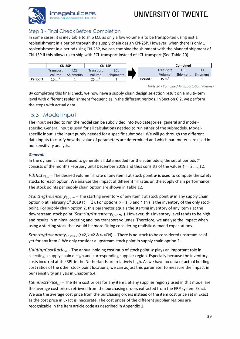
39
Step 8 - Final Check Before Completion In some cases, it is inevitable to ship LCL as only a low volume is to be transported using just 1
replenishment in a period through the supply chain design CN-2SP. However, when there is only 1
replenishment in a period using CN-2SP, we can combine the shipment with the planned shipment of
CN-1SP if this allows us to ship with FCL transport instead of LCL transport (See Table 20).
By completing this final check, we now have a supply chain design selection result on a multi-item
level with different replenishment frequencies in the different periods. In Section 6.2, we perform
the steps with actual data.
5.3 Model Input
The input needed to run the model can be subdivided into two categories: general and model-
specific. General input is used for all calculations needed to run either of the submodels. Model-
specific input is the input purely needed for a specific submodel. We will go through the different
data inputs to clarify how the value of parameters are determined and which parameters are used in
our sensitivity analysis.
General: In the dynamic model used to generate all data needed for the submodels, the set of periods 𝑇
consists of the months February until December 2019 and thus consists of the values 𝑡 = 2, … ,12.
𝐹𝑖𝑙𝑙𝑅𝑎𝑡𝑒𝑖,𝑤 – The desired volume fill rate of any item 𝑖 at stock point 𝑤 is used to compute the safety
stocks for each option. We analyse the impact of different fill rates on the supply chain performance.
The stock points per supply chain option are shown in Table 12.
𝑆𝑡𝑎𝑟𝑡𝑖𝑛𝑔𝐼𝑛𝑣𝑒𝑛𝑡𝑜𝑟𝑦𝑖,𝑜,𝑡,𝑤 – The starting inventory of any item 𝑖 at stock point 𝑤 in any supply chain
option 𝑜 at February 1st 2019 (𝑡 = 2). For options 𝑜 = 1, 3 and 4 this is the inventory of the only stock
point. For supply chain option 2, this parameter equals the starting inventory of any item 𝑖 at the
downstream stock point (𝑆𝑡𝑎𝑟𝑡𝑖𝑛𝑔𝐼𝑛𝑣𝑒𝑛𝑡𝑜𝑟𝑦𝑖,𝑜,𝑡,𝑁𝐿 ). However, this inventory level tends to be high
and results in minimal ordering and low transport volumes. Therefore, we analyse the impact when
using a starting stock that would be more fitting considering realistic demand expectations.
𝑆𝑡𝑎𝑟𝑡𝑖𝑛𝑔𝐼𝑛𝑣𝑒𝑛𝑡𝑜𝑟𝑦𝑖,𝑜,𝑡,𝑤 , (𝑡=2, 𝑜=2 & 𝑤=CN) – There is no stock to be considered upstream as of
yet for any item 𝑖. We only consider a upstream stock point in supply chain option 2.
𝐻𝑜𝑙𝑑𝑖𝑛𝑔𝐶𝑜𝑠𝑡𝑅𝑎𝑡𝑖𝑜𝑤 – The annual holding cost ratio of stock point 𝑤 plays an important role in
selecting a supply chain design and corresponding supplier region. Especially because the inventory
costs incurred at the 3PL in the Netherlands are relatively high. As we have no data of actual holding
cost ratios of the other stock point locations, we can adjust this parameter to measure the impact in
our sensitivity analysis in Chapter 6.4.
𝐼𝑡𝑒𝑚𝐶𝑜𝑠𝑡𝑃𝑟𝑖𝑐𝑒𝑖,𝑗 – The item cost prices for any item 𝑖 at any supplier region 𝑗 used in this model are
the average cost prices retrieved from the purchasing orders extracted from the ERP system Exact.
We use the average cost price from the purchasing orders instead of the item cost price set in Exact
as the cost price in Exact is inaccurate. The cost prices of the different supplier regions are
recognizable in the item article code as described in Appendix 1.
CN-2SP CN-1SP
Transport Volume
LCL Shipments
Transport Volume
LCL Shipments
Period 1 10 m3 1 25 m3 1
Combined
Transport Volume
LCL Shipment
FCL Shipment
Period 1 35 m3 0 1
Table 20 - Combined Transportation Volumes

40
𝐼𝑡𝑒𝑚𝐹𝑜𝑟𝑒𝑐𝑎𝑠𝑡𝑖,𝑡,𝑡+𝑛 – We consider making one forecast in period 𝑡 for periods 𝑡 to 𝑡 + 𝑛 where 𝑛 =
𝑡 + 𝐿𝑡𝑟,𝑜,𝑤 + 𝐿𝑝𝑟 + 𝑅 − 1 dependent on the supply chain option. This goes for all items 𝑖 in every
supply chain option 𝑜 before the using our supply chain design selection model. These values are not
changed throughout the usage of the model or in different scenarios.
𝐴𝑐𝑡𝑢𝑎𝑙𝐷𝑒𝑚𝑎𝑛𝑑𝑖,𝑡 – The actual demand of all items 𝑖 in any period 𝑡.
𝐼𝑡𝑒𝑚𝑀𝑜𝑣𝑒𝑚𝑒𝑛𝑡𝑖 – The movement of any item 𝑖 (defined as either fast or slow) is used for safety
stock calculations. We separate fast moving items from slow moving items as the standard deviation
of the forecast error over lead time demand can be used for items of which the demand can be
approximated used a continuous demand distribution as opposed to slower moving items of which
this parameter is approximated by the square root of expected demand during lead time.
We consider an item to be a ‘fast mover’ when the expected demand during lead time exceeds 10 as
described in Section 4.4.1. The remaining items with are considered to be slow movers.
𝑁𝑢𝑚𝑏𝑒𝑟𝑂𝑓𝑅𝑒𝑝𝑙𝑒𝑛𝑖𝑠ℎ𝑚𝑒𝑛𝑡𝑠𝑜,𝑡 , (𝑜 = 2) – The number of replenishments per period 𝑡 is used as
input to calculate the results of our inventory model to retrieve the average inventory levels at all
stock points considered in supply chain option 2.
Submodel 1: 𝑄𝑢𝑎𝑛𝑡𝑖𝑡𝑦𝑃𝑢𝑟𝑐ℎ𝑎𝑠𝑒𝑑𝑖,𝑜,𝑡 – The total quantity purchased (equals quantity produced) of any item 𝑖 in
any period 𝑡 for a supply chain option 𝑜 is the sum of the quantities produced calculated per period
using Equation 19 or 25 depending on option 𝑜. The quantity is independent of the supplier.
𝐴𝑣𝑒𝑟𝑎𝑔𝑒𝐼𝑛𝑣𝑒𝑛𝑡𝑜𝑟𝑦𝑖.𝑜,𝑡,𝑤 – The average inventory level for any item 𝑖 in a specific period 𝑡
depending on the supply chain option 𝑜 at stock point 𝑤 is calculated using our inventory
management model described in Sections 4.4.1 and 4.4.2. These calculations are done before
running any of the submodels. For the supply chain design CN-2SP, this parameter is impacted by the
replenishment frequency per period as shown in Equation 28 & Equation 27 in Section 4.5.
Submodel 2: 𝑇𝑜𝑡𝑎𝑙𝑇𝑟𝑎𝑛𝑠𝑝𝑜𝑟𝑡𝑉𝑜𝑙𝑢𝑚𝑒𝑜,𝑡 – This volume for any period 𝑡 considering the option 𝑜 = 2 is given after
it has been computed by Equation 29 in Section 4.5 where the item quantities in the replenishment
orders are multiplied with the transport volume of an item.
𝑀𝑖𝑛𝑉𝑜𝑙𝑢𝑚𝑒𝐹𝐶𝐿 – The minimum required volume for FCL transport of a container (~30 m³)
𝑀𝑎𝑥𝑉𝑜𝑙𝑢𝑚𝑒𝐹𝐶𝐿 – The maximum usable volume for FCL transport of a container (~53 m³)
𝑀𝑎𝑥𝑉𝑜𝑙𝑢𝑚𝑒𝐿𝐶𝐿 – The maximum usable volume for LCL transport or 20ft. container (~30 m³)
𝑃𝑒𝑛𝑎𝑙𝑡𝑦𝐶𝑜𝑠𝑡 – The costs to transport a 40ft. container from the CN supplier region to the 3PL in NL
are €3500. The costs to transport a 20ft. container from the CN supplier region to the 3PL in NL are
approximately €3000. To transport the volume of a 40ft. container that falls between the minimum
and maximum volume of FCL transportation, we need two 20ft. containers. This would cost €6000
(€2500 more in total, €1250 per 20ft. container). The extra costs would need to be added to the item
cost price as the transport cost inclusion regards 40ft. container costs. As we do not consider
changing item cost prices, we use a penalty cost of €1250 in transporting 20ft. containers. Since we
have no data of LCL transportation costs, we assume we can use the same penalty fee to avoid non-
FCL transportation.

41
5.4 Selecting a Cost-Efficient Supply Chain Design (Submodel 1)
In selecting a cost-efficient supply chain design for an item, the following submodel has been
developed that aims to minimize the total supply chain costs incurred on single item-level (step 2 of
Section 5.2). Although this primary model contains the transport cost of an item, we need a
secondary model to ensure FCL transportation to make sure the transport costs per item do not
exceed the included transport costs. Although this problem could also be solved using a greedy
algorithm (cheapest supply chain option per item), we were able to redesign the model for a multi-
item problem to solve the problem as intended. The result gives us the supply chain design selection
on item-level over the considered periods. We use the indices as described in Section 4.1.
Objective Function
Our objective function as shown in Equation 30, minimizes the total supply chain costs (Purchasing
cost + inventory costs) by considering sourcing items via the defined supply chain design options at
the different supplier regions that are relevant within an option. We add the costs of purchasing item
𝑖 at supplier region 𝑗 to the inventory costs of storing item 𝑖 at stock point 𝑤.
Equation 30 - Objective Function Cost Minimization Problem
Decision Variable
The choice for a specific supply chain design and thereafter a feasible supplier region is determined
by the decision variable below in Equation 31. For every item, one supply chain design is favourable
considering the consequences of choosing for 1) a supply chain design and 2) a supplier region that is
considered within the design. Quantities purchased and inventory levels are unchangeable data.
𝑆𝑢𝑝𝑝𝑙𝑦𝐶ℎ𝑎𝑖𝑛𝐷𝑒𝑠𝑖𝑔𝑛𝑖,𝑗,𝑜 =
Equation 31 - Decision Variable to Select Supply Chain Option
Constraints
As we restrict any item with forecasted demand to be sourced using just one of the design options
and just one feasible supplier region across all time periods considered, we add the following
constraint in Equation 32 to the model:
∑ ∑ 𝑆𝑢𝑝𝑝𝑙𝑦𝐶ℎ𝑎𝑖𝑛𝐷𝑒𝑠𝑖𝑔𝑛𝑖,𝑗,𝑜
𝐽
𝑗=1
𝑂
𝑜=1
= 1, ∀𝑖
Equation 32 - Each item is restricted to one option and one supplier region
As the item cost price for some supplier region is unknown or there is no supplier within the region
able to produce the item, we need a constraint to prevent selecting such a region when the cost
price equals 0. Equation 33 has been developed to ensure this. We added a multiplication of the cost
price by the high value 𝑀 (>100) in case items with a cost price below €1 are considered.
𝑆𝑢𝑝𝑝𝑙𝑦𝐶ℎ𝑎𝑖𝑛𝐷𝑒𝑠𝑖𝑔𝑛𝑖,𝑗,𝑜 ≤ 𝐼𝑡𝑒𝑚𝐶𝑜𝑠𝑡𝑃𝑟𝑖𝑐𝑒𝑖,𝑗 ∗ 𝑀, ∀𝑖, 𝑗, 𝑜
Equation 33 - Restrict to feasible supplier regions
1, if item i is provided by supplier region j in supply chain design o
0, otherwise {
Purchasing Costs incl. Transport costs
∀𝑖
Inventory Costs
𝑀𝑖𝑛 (∑ ∑ ∑ ∑ ((𝐼𝑡𝑒𝑚𝐶𝑜𝑠𝑡𝑃𝑟𝑖𝑐𝑒𝑖,𝑗 ∗ 𝑄𝑢𝑎𝑛𝑡𝑖𝑡𝑦𝑃𝑢𝑟𝑐ℎ𝑎𝑠𝑒𝑑𝑖,𝑜,𝑡)
𝑇
𝑡=2
𝑊
𝑤=1
𝐽
𝑗=1
𝑂
𝑜=1
+ (𝐴𝑣𝑒𝑟𝑎𝑔𝑒𝐼𝑛𝑣𝑒𝑛𝑡𝑜𝑟𝑦𝑖,𝑜,𝑡,𝑤 ∗ 𝐼𝑡𝑒𝑚𝐶𝑜𝑠𝑡𝑃𝑟𝑖𝑐𝑒𝑖,𝑗 ∗ 𝐻𝑜𝑙𝑑𝑖𝑛𝑔𝐶𝑜𝑠𝑡𝑅𝑎𝑡𝑖𝑜𝑤)) ∗ 𝑆𝑢𝑝𝑝𝑙𝑦𝐶ℎ𝑎𝑖𝑛𝐷𝑒𝑠𝑖𝑔𝑛𝑖,𝑗,𝑜)

42
5.5 Replenishment Frequencies with FCL Transport (Submodel 2)
When a replenishment order is planned for any period 𝑡 through option 2, we allow a split transport
as the produced items are stored at the supplier region. As the holding costs at any storage location
are based on the stock levels at the end of a week, multiple replenishments throughout the week
would yield no benefits. Therefore, as any period has an average length of 4 weeks, we decide to cap
the number of replenishments in a period to a maximum of 4. As the item cost prices include
transportation cost of FCL transport, we do not add any transportation cost when it is used. For LCL
or 20ft. transport (Non-FCL Transport), we apply the penalty cost (𝑃𝑒𝑛𝑎𝑙𝑡𝑦𝐶𝑜𝑠𝑡) as these options are
on average more expensive per item shipped. This submodel represents step 3 of Section 5.2.
Objective Function
The objective function, as shown in Equation 34, aims to minimize costs by trying to avoid non-FCL
transportation from the Chinese stock point to the 3PL in NL.
𝑀𝑖𝑛 ∑ 𝑁𝑜𝑛𝐹𝐶𝐿𝑇𝑟𝑎𝑛𝑠𝑝𝑜𝑟𝑡𝑅𝑒𝑞𝑢𝑖𝑟𝑒𝑑𝑜,𝑡 ∗ 𝑃𝑒𝑛𝑎𝑙𝑡𝑦𝐶𝑜𝑠𝑡
𝑇
𝑡=2
Equation 34 - Objective function to minimize LCL transport
𝐹𝑢𝑙𝑙𝐶𝑜𝑛𝑡𝑎𝑖𝑛𝑒𝑟𝑠𝑈𝑠𝑒𝑑𝑜,𝑡 – Integer variable that shows how many full container loads are used to ship
the replenishment order of a period from the CN stock point to the 3PL in NL in supply chain option
𝑜. With the constraints below we make sure that a minimum average volume is transported as well
as the average volume does not exceed the maximum volume. If the volume of the replenishment
order is too small or the situation requires us to ship a part of the order via LCL or a 20ft. container,
which we define as non-FCL transportation, we apply a penalty (𝑃𝑒𝑛𝑎𝑙𝑡𝑦𝐶𝑜𝑠𝑡) as described in
Section 5.3. The binary variable in Equation 35 is only activated when there is no other option than to
use non-FCL transportation.
𝑁𝑜𝑛𝐹𝐶𝐿𝑇𝑟𝑎𝑛𝑠𝑝𝑜𝑟𝑡𝑅𝑒𝑞𝑢𝑖𝑟𝑒𝑑𝑜,𝑡 =
Equation 35 - Decision variable of non-FCL (20ft. container or LCL) transport
To make sure that a) the total replenishment order volume is transported, b) the minimum transport
volume for FCL is reached and c) the transport volume does not exceed the maximum usable volume
when trying to ensure FCL transport, we implement the following constraints. The parameter value
of 𝑇𝑜𝑡𝑎𝑙𝑇𝑟𝑎𝑛𝑠𝑝𝑜𝑟𝑡𝑉𝑜𝑙𝑢𝑚𝑒𝑜,𝑡 is fixed and calculated up front using Equation 29. The constraint in
Equation 36 makes sure that we cannot use FCL transport when the to be transported volume is too
small. As non-FCL transport does not require a minimum volume, we can omit that in this constraint.
𝑇𝑜𝑡𝑎𝑙𝑇𝑟𝑎𝑛𝑠𝑝𝑜𝑟𝑡𝑉𝑜𝑙𝑢𝑚𝑒𝑜,𝑡 ≥ 𝐹𝑢𝑙𝑙𝐶𝑜𝑛𝑡𝑎𝑖𝑛𝑒𝑟𝑠𝑈𝑠𝑒𝑑𝑜,𝑡 ∗ 𝑀𝑖𝑛𝑉𝑜𝑙𝑢𝑚𝑒𝐹𝐶𝐿 , ∀𝑡 & 𝑜 = 2
Equation 36 - Ensure minimum volume for FCL transport
Equation 37 needs the constraint in Equation 36 to make sure the entire load is transported without
exceeding the maximum usable container volume.
𝑇𝑜𝑡𝑎𝑙𝑇𝑟𝑎𝑛𝑠𝑝𝑜𝑟𝑡𝑉𝑜𝑙𝑢𝑚𝑒𝑜,𝑡
≤ 𝐹𝑢𝑙𝑙𝐶𝑜𝑛𝑡𝑎𝑖𝑛𝑒𝑟𝑠𝑈𝑠𝑒𝑑𝑜,𝑡 ∗ 𝑀𝑎𝑥𝑉𝑜𝑙𝑢𝑚𝑒𝐹𝐶𝐿 + 𝑁𝑜𝑛𝐹𝐶𝐿𝑇𝑟𝑎𝑛𝑠𝑝𝑜𝑟𝑡𝑅𝑒𝑞𝑢𝑖𝑟𝑒𝑑𝑜,𝑡
∗ 𝑀𝑎𝑥𝑉𝑜𝑙𝑢𝑚𝑒𝑁𝑜𝑛𝐹𝐶𝐿
Equation 37 - Volume cannot exceed maximum capacity of a container
In this model, only variables 𝐹𝑢𝑙𝑙𝐶𝑜𝑛𝑡𝑎𝑖𝑛𝑒𝑟𝑠𝑈𝑠𝑒𝑑𝑜,𝑡 and 𝑁𝑜𝑛𝐹𝐶𝐿𝑇𝑟𝑎𝑛𝑠𝑝𝑜𝑟𝑡𝑅𝑒𝑞𝑢𝑖𝑟𝑒𝑑𝑜,𝑡 can be
adjusted to transport the fixed 𝑇𝑜𝑡𝑎𝑙𝑇𝑟𝑎𝑛𝑠𝑝𝑜𝑟𝑡𝑉𝑜𝑙𝑢𝑚𝑒𝑜,𝑡 for any period 𝑡 in supply chain option 2.
1, if either LCL or 20ft. container transport is needed
0, otherwise {
∀𝑡 & 𝑜 = 2
Constraints
Decision Variables

43
5.6 Limitations
The recorded item unit cost prices in the ERP system Exact are inaccurate and therefore we use the
average item cost price found in the sales data. As prices slightly change over time, this price is not
fully accurate either but it gives a better indication of the costs. Another limitation is that not all
items have item cost prices for all supplier regions. There is no data that tells us if the supplier would
be able to produce an item and what the cost price would be. In the ongoing process improvements
at Imagebuilders this is will most likely change and cost prices of all regions will be available.
The volume of an item in transport is not equal to base item volume as e.g. packaging needs to be
included. Although we can approximate the transport volume, more data can improve the accuracy.
The way in which we approximate item volume is shown in Appendix 1. The holding cost ratios of the
supplier regions besides NL are estimated by the experts within Imagebuilders. Therefore, we check
the impact of this parameter in our sensitivity analysis. In this research, we only consider one
concept whereas the benefits of more frequent replenishments are easier to achieve when multiple
different concepts are combined and the transport volume increases. We have no insight or data to
quantify the impact of backorders. Although we do know backorders lead to extra costs and work,
we are unable to quantify these costs as some backorders only require regular transport as these can
be installed after store opening, some require an emergency delivery to prevent delay in store
installation and some require after-service by an employee of Imagebuilders. Adding a criticality
factor to the items in a customer concept can prevent the high impact backorders as the desired fill
rate of these items can be set to a high minimum.
5.7 Validation and Verification
To make sure the model works like it is supposed to do and reflects reality at the same time, we need
to check the correctness of the outcome of our model (Verification) and check if this outcome
reflects the actual situation (Validation). To check the correctness of our inventory model, we can set
the safety stocks to 0 and the forecasted demand equal to the actual demand using historical data.
By using deterministic demand, the expected demand during lead time plus the review period is
known and the order-up-to-level equals the expected demand. At the beginning of a month, a
replenishment order is received with exactly the expected demand and at the end of a month the
inventory has been depleted without any shortages. By manually setting the safety stock to any
value, we can verify the working of the safety stocks by checking the end inventory of a period when
using deterministic demand. The ending inventory of any period should be equal to the safety stock
when the beginning inventory is equal to the expected demand plus safety stock. All coding done in
Excel VBA is checked by going through the code step-by-step and checking the updated screen after
each step. If any errors occur during the code walkthrough, the error can be found easily.
Unfortunately, as we redesigned almost all processes within the material coordination of the supply
chain, we can only validate very few aspects by comparing our calculations to the actual
performance. In the section Standard Item Volume Calculation of Appendix 1 we validate the
transport volumes of individual items and items combined by comparing the total volume of a
transport order to the volume of an actual transported container. As currently Imagebuilders is
looking into using a two-level stock design for future concepts, we validate our results in which we
relate item characteristics to the supply chain design selection in Section 6.3 by discussing the results
with experts to check if these fit with their expectations and to check for questionable outcomes. The
outcomes of our inventory model described in Chapter 4 for each supply chain in terms of purchase
costs and monthly inventory costs are discussed with the experts that have the experience to check if
the outcomes are realistic.

44
5.8 Conclusion
This chapter answered research question 4: “How should a model be constructed to advise
Imagebuilders on supplier selection decision making in the supply chain network for standard items?”
From this chapter, we conclude the following:
• As we require a more sophisticated solving tool and a long computational time to find the
optimal solution of this combinatorial problem, we developed a heuristic consisting of two
submodels that each can be solved to optimality. However, as we use a heuristic, the solution is
suboptimal. On average, we require 2 iterations of our heuristic to obtain the final solution.
• When we have selected a cost-efficient supply chain design for all items, the distribution of the
items along the designs (number of items per design) shows us how to redesign the supply
chain design. If no or very few items are sourced through any design option, we rerun our
model where this option is omitted and thereafter we check the impact on the supply chain
performance. Although the selection shows how to redesign the supply chain on a strategic
level for this specific data set, we look into the relation between a supply chain design selection
and item characteristics such as demand rates and cost price to develop guidelines and to
advise Imagebuilders on the recommended design. The guidelines can be used for concepts
with little or no actual demand data but in which item characteristics can be estimated.
• As a lot of parameters of the model input are estimated or approximated (e.g. holding cost
ratio), we set up different scenarios in analysing our results and perform a sensitivity analysis to
measure the impact of these parameters.
• Because we only consider 1 customer concept (LSG concept) in this thesis, the replenishment
order size and transport volumes are relatively low. The benefits of splitting a replenishment
orders into smaller transport orders might thus not be as big as they would be combining
multiple concepts.

45
6. Results This chapter answers research question 5: “What is the supply chain performance of our model and
how well does our model perform compared to Imagebuilders’ actual supply chain performance?”.
We start off in Section 6.1 by analysing the results of our forecasting model on both store level and
item level. In Section 6.2, we analyse the steps of our problem solving approach using a real-life
scenario. In Section 6.3 we analyse the supply chain performance of our model by comparing it to the
actual performance of Imagebuilders of 2019. In Section 6.4, we try to find relationships between
item characteristics and the supply chain design selection. Before concluding our findings in Section
6.6, we perform a sensitivity analysis in Section 6.5.
6.1 Forecast Accuracy
Due to the difference in lengths of the time buckets used for forecasting in our model and historical
forecasts, a one-on-one comparison of the forecast accuracy of demand during lead time or during
lead time plus review period of our model and the historical performance might not reflect the
forecast accuracy improvement. We only describe the forecast accuracy on the forecast data rather
than the accuracy of our model fit as a good model fit gives no guarantee of accurate forecasting. We
describe the forecast error based on the Training and Test data division as described in Section 4.3.
We separate fast and slow moving items as described in the conclusion of Chapter 4.
Forecasting Error of Forecasting the Number of Stores We calculate the average MAPE over lead time and over lead time plus review period used in the
different supply chain designs (see Table 21). We show the forecasting error of one lead time plus
review period cycle that is also used to assess the forecast error on item level. The full performance
of the store demand forecasting error is given in Appendix 3. We do not show the forecasting
performance of the forecast used in supply chain design option 4 as the forecast horizon of this
option required us to manually adjust the forecast. The historical performance of the forecasting
error measured as MAPE are 26.1% and 24.8% over lead time demand and over lead time demand
plus review period respectively. As the forecast horizons and replenishment cycles were longer, we
expect that the forecasting error of historical performance would have been higher if we would have
monthly forecasting data of the historical performance. In the historical performance, demand could
occur in either week 1 or week 10 of a replenishment cycle without harming the forecasting error.
Forecasting Error of Forecasting Required Item Quantities Although the improved forecasting accuracy of store demand supports accurately forecasting item
demand, it is no guarantee that the forecasting accuracy on item level is as high. We saw in Section
2.4 that the forecasting error of item demand was amplified by the forecasting error in average item
usage per store. We calculate the WAPE using Equation 6. In Table 22, we measure the forecast error
as the average MAPE and as the WAPE for the items that were forecasted in the historical
performance over just one lead time plus review period cycle for ease of understanding. The
numbers 2, 3 and 4 after the MAPE and WAPE in Table 22 and Table 23 represent the length of the
considered lead time plus review period. Although we do forecast other items considered in the
concept that were not forecasted in the historical performance as these were not sourced in China,
we do not take these items into consideration to allow a comparison with the historical performance.
MAPE Store Demand periods t = 6,…,9 Used in Supply chain designs Model Performance
MAPE where Lead Time (Plus Review Period) = 2 periods 3 (EU-NLSP) 20%
MAPE where Lead Time (Plus Review Period) = 3 periods 2 (CN-2SP) 30%
MAPE where Lead Time (Plus Review Period) = 4 periods 1 (CN-1SP) & 2 (CN-2SP) 26.7%
Table 21 - Forecasting Performance Store Demand over periods t = 6,…,9

46
The full model forecasting performance for all items in the concept can be found in Appendix 3. We
find that the forecast error over the considered items is slightly lower than when considering all
items. It is interesting to see that the measured MAPE is similar to the forecasting error of store
demand shown in Table 21. This indicates that the forecasting error in item demand is now only
caused by the forecast error in store demand.
From Table 22, we can see that the WAPE tends to be lower than the MAPE when considering the
same forecasting horizon. This tells us that low demand items have a negative impact on the
measured forecasting error. To show that this is the case, we analyse the WAPE of different item
categories as shown in Table 23. We identify the following interesting findings from Table 23:
• The forecast error of fast moving items is lower than slow moving items, which confirms the
expectation that the overall MAPE is negatively impacted by low demand items.
• The forecasting error of fast moving items that show significant correlation between item usage
and store size is lower than average error of all fast moving items combined. This tells us that
using Linear Regression to forecast these items adds to the accuracy.
• The forecasting error of fast moving items with non-intermittent demand is lower than the error
of fast moving items with intermittent demand. This tells us that the computed inter-demand
interval which was used in forecasting demand of these items needs to be improved to decrease
the forecasting error. This can be done in several ways such as finding good parameter settings
for the smoothing factor to update the inter-demand interval after demand has occurred.
• Overall, only slow moving items and fast moving items with intermittent demand have a
forecasting error higher than the forecasting error on store demand level. Extra effort into
forecasting these types of items can help to further improve the forecasting accuracy.
6.2 Problem Solving Steps using Real-Life Scenario
Before running an iteration, we initialize our supply chain selection model by setting all selection
variables to 0 and by setting the replenishment frequency to 4 for all periods. We are going through
the results of the scenario where we consider a realistic starting stock computed with Equation 43
(described in Section 6.3.2) and a desired fill rate of 95% of all items. We compute the safety stock
levels for all stock points in all supply chain options using the Goal Seek function as described in
Section 4.1.1. After the first iteration, we end up with the following distribution of item selection
across the different supply chain options and supplier regions within each option:
Avg. MAPE 2 Avg. MAPE 3 Avg. MAPE 4 WAPE 2 WAPE 3 WAPE 4
Forecasted Items 22.0% 30.8% 31.9% 18.0% 24.3% 22.4%
Table 22 - Forecast Error on Item-Level
Table 23 - Forecast Errors when Zooming in on Item Characteristics
Item types WAPE 2 WAPE 3 WAPE 4
Fast Moving 17.7% 23.9% 21.9% Slow Moving 31.8% 36.8% 41.6%
Fast + Correlated 16.6% 22.9% 20.1% Fast + Non-intermittent 17.1% 23.8% 21.4%
Fast + intermittent 23.2% 25% 26.2%
Option 1 Option 2 Option 3 Option 4 Supplier Region CN CN TR BS CZ PL TR BS CZ PL NL
#Items 37 58 5 11 1 0 8 20 3 0 71
Table 24 - Supply Chain Selection Distribution

47
The supply chain costs are €945,600 of which €901,000 are purchasing costs and €44,600 are
inventory costs. To transport the items sourced through option 2 with 4 replenishments a period, we
require transport at least 4 FCL or LCL containers per period resulting in total transport costs of
€122,500. After running submodel 2 to find the number of containers to transport per period to
ensure FCL transport, we find the following for each period:
In Table 25, we do not transport any volume in period 2 as the starting inventory in China is 0 for all
items and the first production cycle finishes at the end of the period. This can only be transported at
the start of the period 3. The replenishment frequency for all periods is no longer 4 and therefore we
have to re-run our inventory model with the new replenishment frequencies to check if other supply
chain designs are more cost-efficient. After doing so, we find the following distribution of items
across the supply chain designs:
In the new distribution, only 2 items switched from option 2 to option 1. Generally, a maximum of 10
items change selection (max. ~4-5% of items). This might be due to the fact that cost prices of some
supplier regions are missing. The small number of items that have changed already indicate that the
to be transported volume barely changes and thus the replenishment frequency does not have be
adjusted anymore. In the final check before completion, we find that for period 10 we plan to
transport 21 m³ through supply chain option 2 and 14 m³ through option 1. As we replenish our
inventory once in this period, we can combine both shipments into 1 FCL transport instead of 2 LCL
transports. After doing so, total supply chain costs have increased to €946,200 of which €901,000 are
purchasing costs and €45,200 are inventory costs. Transportation costs are now €74,500. As in most
scenarios, we require 1 more iteration after finding our starting solution to find our final solution.
When looking at the selection distribution of items with more than 1 supplier region as for those
with only 1 supplier region the selection is fixed, we find the following distribution (see of which all
items within option 2 are fast moving items. This already tells us option 2 is most likely the go-to
option for fast moving items. For slow moving items, option 1 seems to be the go-to option when 1
of the supplier regions is China as generally a lower cost price can be achieved. It is interesting to see
that more slow moving (and fast moving items) select option 4 over option 3.
6.3 Supply Chain Performance
In comparing the results of our model to the actual performance of Imagebuilders over 2019 by using
the forecasts and forecast errors as described in Section 6.1, we start off by addressing some issues.
As the starting inventory of the historical data is high for most of the items, the average inventory
level and thus inventory costs incurred over the months considered are suboptimal. The high
Table 25 - Replenishment Frequency Based on Number of Containers to be Transported
Period → 2 3 4 5 6 7 8 9 10
#FCL containers 0 3 1 2 3 3 1 3 0
#LCL containers 0 0 0 0 0 0 1 0 1
Replenishment Frequency 0 3 1 2 3 3 1 3 1
Option 1 Option 2 Option 3 Option 4 Supplier Region CN CN TR BS CZ PL TR BS CZ PL NL
#Items 39 56 5 11 1 0 8 20 3 0 71
Table 26 - New Item Distribution after Supply Chain Selection Re-run
Option 1 Option 2 Option 3 Option 4
#items (%) 35 (24%) 52 (36%) 13 (9%) 43 (30%) Fast Moving Items (%) 14% 55% 2% 22% Slow Moving Items (%) 45% 0% 22% 33%
Table 27 - Item Distribution of Items with at least 2 Supplier Regions

48
inventory levels also impact the number of replenishments needed as the transport volume per
period are lower. The impact of minimizing inventory costs by optimizing the replenishment
frequencies are thus expected to be minimal to none.
• Using the stock levels as measured on the January 31st 2019 with a value of €600,000, we can
analyse the impact of our model on a) purchase costs, b) savings in inventory costs and c)
achieved order line fill rate as the decisions made uses the exact same information as
Imagebuilders had on that moment.
• Using more realistic stock levels as starting stock on January 31st 2019, we can analyse the impact
of our model on a) average value of inventory, b) total inventory costs and c) the achieved fill
rate. The computation of the realistic starting stock levels is described later in this section using
Equation 43. Although we cannot compare the actual purchase costs of 2019 to the purchase
costs of our model as more realistic stock levels require us to purchase more items, we can
approximate the savings by computing the total costs of the goods sold which is described below.
We measure the potential savings in purchase costs by analysing the differences in the costs of goods
sold for all scenarios as it gives an approximation of what the total purchase costs of each scenario
would have been considering the starting stock value, ending stock value and costs to purchase the
required (sold) items. The calculation of the measure is shown in Equation 38.
𝐶𝑜𝑠𝑡 𝑜𝑓 𝐺𝑜𝑜𝑑𝑠 𝑆𝑜𝑙𝑑 (€) = (𝑆𝑡𝑎𝑟𝑡𝑖𝑛𝑔 𝑆𝑡𝑜𝑐𝑘 𝑉𝑎𝑙𝑢𝑒 − 𝐸𝑛𝑑𝑖𝑛𝑔 𝑆𝑡𝑜𝑐𝑘 𝑉𝑎𝑙𝑢𝑒) + 𝑃𝑢𝑟𝑐ℎ𝑎𝑠𝑒 𝐶𝑜𝑠𝑡𝑠
Equation 38 - Cost of Goods Sold
The actual performance of Imagebuilders’ supply chain for the LSG concept in 2019 in the months
February to December shown in Table 28 is used as a benchmark in our analysis. To measure the
impact of different desired service levels on the OLFR, we measure the performance of the scenarios
with different starting stock levels in combination with different service levels. As Imagebuilders
desires to achieve a minimum fill rate of 95% when a concept is phasing out to avoid excess stock
levels and desires to achieve a minimum fill rate of 98% to minimize backorders or extra work, we set
up different fill rate scenarios. We analyse scenarios using a desired fill rate of 98% for all items, 95%
for all items and a division where we desire a fill rate of 98% for fast moving items and 95% for slow
moving items. For experimental purposes, we also added a scenario where we use a desired fill rate
of 95% for fast moving items and 98% for slow moving items.
Although our model allows easy computation of an achieved volume fill rate on item level, the data
of historical performance does not allow us to approximate the achieved volume fill rate on item
level. The only comparison can be made on the Order Line Fill Rate level on a multi-item level. This
requires us to adapt our model to be able to develop an approximation of the performance on this
KPI. To do so, we performed the following steps. The approximated OLFR is comparable to the P&P
OLFR as it considers demand fulfilment at the moment an order is to be picked. The average required
item quantity per order line is approximated by dividing the total quantity of an item used over a
period by the number of stores in the same period in which the item was used. For example, the item
LSG217 had a total demand of 5637 pieces over the months February until December of 2019. The
item was present in 43 stores in those periods and thus there are 43 order lines of the item.
Table 28 - Supply Chain Performance over 2019
Total Purchasing
Costs (€x1000)
Approximated Inventory Costs
(€x1000)
Total Costs
(€x1000)
Average Inventory Value
(€x1000) P&P OLFR
Cost of Goods Sold (€x1000)
Value End Inventory (€x1000)
Inventory Turnover
Rate
LSG Concept 2019 872 81 953 385 93% 1,386 86 3.6

49
Therefore, we approximate the average item usage per order line to be 131 following Equation 39 .
This happens on item-level and is not impacted by the period or any supply chain design.
𝐴𝑣𝑔𝐼𝑡𝑒𝑚𝑈𝑠𝑎𝑔𝑒𝑂𝑟𝑑𝑒𝑟𝐿𝑖𝑛𝑒𝑖 = ∑ 𝐼𝑡𝑒𝑚𝐷𝑒𝑚𝑎𝑛𝑑𝑖,𝑡
𝑇𝑡=2
∑ 𝐼𝑡𝑒𝑚𝑂𝑟𝑑𝑒𝑟𝐿𝑖𝑛𝑒𝑠𝑖,𝑡𝑇𝑡=2
Equation 39 - Approximation of Average item Usage per Order Line
We use this average item usage per order line to approximate the number of order lines with a
shortage for all items 𝑖 in any period 𝑡 considering any supply chain option 𝑜. Our inventory model
calculates the quantity of items that we were short per period per item for each supply chain option.
To obtain a rounded integer number of orders lines with a shortage, we use Equation 40. If for any
item we have an average item order line usage of 10 pieces, a period requires us to deliver 40 pieces
and we have a stock of 25 pieces (15 short in total), we find that the approximation of order lines
with a shortage equals 2. The total approximated number of order lines with a shortage for any item
𝑖 in any supply chain option 𝑜 can be obtained by summing over the considered periods 𝑡=2,..,𝑇.
𝑂𝑟𝑑𝑒𝑟𝐿𝑖𝑛𝑒𝑠𝑊𝑖𝑡ℎ𝑆ℎ𝑜𝑟𝑡𝑎𝑔𝑒𝑖,𝑜,𝑡 = ⌈𝑄𝑢𝑎𝑛𝑡𝑖𝑡𝑦𝑂𝑓𝐼𝑡𝑒𝑚𝑆ℎ𝑜𝑟𝑡𝑖,𝑜,𝑡
𝐴𝑣𝑔𝐼𝑡𝑒𝑚𝑈𝑠𝑎𝑔𝑒𝑂𝑟𝑑𝑒𝑟𝐿𝑖𝑛𝑒𝑖
⌉ , ∀𝑖, 𝑜, 𝑡
Equation 40 - Approximated Item Order Lines with a Shortage
To compute the order line fill rate on a multi-item level after we run our supply chain design
selection model, we first approximate the total number of order lines with a shortage for any item 𝑖
using Equation 41.
𝑇𝑜𝑡𝑎𝑙𝑂𝑟𝑑𝑒𝑟𝐿𝑖𝑛𝑒𝑠𝑊𝑖𝑡ℎ𝑆ℎ𝑜𝑟𝑡𝑎𝑔𝑒𝑖
= (∑ ∑ ∑(𝑂𝑟𝑑𝑒𝑟𝐿𝑖𝑛𝑒𝑠𝑊𝑖𝑡ℎ𝑆ℎ𝑜𝑟𝑡𝑎𝑔𝑒𝑖,𝑜,𝑡)
𝑇
𝑡=2
∗ 𝑆𝑢𝑝𝑝𝑙𝑦𝐶ℎ𝑎𝑖𝑛𝐷𝑒𝑠𝑖𝑔𝑛𝑖,𝑗,𝑜
𝐽
𝑗=1
𝑂
𝑜=1
) , ∀𝑖
Equation 41 - Approximation of Total Order Lines with Shortage for any Item
Now that we have approximated the total number of order lines with a shortage for all items, we can
compute the order line fill rate on a multi-item level to make it comparable to the multi-item level
order fill rate described in Table 28. We do so using Equation 42 which uses the same method as
used for the historical performance on the order line fill rate (see Equation 2). The actual total
number of order lines for any item 𝑖 is independent of supplier region or supply chain option. The
total number of order lines over all items across the periods February until December in 2019 equals
5793.
𝑂𝑟𝑑𝑒𝑟 𝐿𝑖𝑛𝑒 𝐹𝑖𝑙𝑙 𝑅𝑎𝑡𝑒 = 1 − ∑ 𝑇𝑜𝑡𝑎𝑙𝑂𝑟𝑑𝑒𝑟𝐿𝑖𝑛𝑒𝑠𝑊𝑖𝑡ℎ𝑆ℎ𝑜𝑟𝑡𝑎𝑔𝑒𝑖
𝐼𝑖=1
∑ ∑ 𝑇𝑜𝑡𝑎𝑙𝑁𝑢𝑚𝑏𝑒𝑟𝑂𝑓𝑂𝑟𝑑𝑒𝑟𝐿𝑖𝑛𝑒𝑠𝑖,𝑡𝑇𝑡=2
𝐼𝑖=1
Equation 42 - Order Line Fill Rate Approximation on Multi-Item Level
The Order Line Fill Rate computed using Equation 42 can be higher than both the average item-level
volume fill rate and the average item-level Order Line Fill Rate because a missed order line for a slow-
mover heavily impacts both the average item fill rate as well as the average item order line fill rate
but has minimal impact on the total number of order lines of all items combined. To put in
perspective: of the 232 considered items, if there is a slow-moving item with in total 1 order line with
quantity 1 over the set of periods which cannot be fulfilled by stock, missing the order line has an
impact of 1 out of 5793 total order lines on the Order Line Fill Rate but for both averages the impact
is 1 out of 232 items.

50
6.3.1 Actual Starting Stock Levels In Table 29, the results of using different fill rates are shown where in all cases the actual starting
stock is used. The high starting stock levels limit the savings in the inventory costs as these are only
reduced by ~15%, ~26%, ~16% & 23% for the different fill rate scenarios respectively. Even with the
high inventory value, we manage to reduce the cost of goods sold by over €180,000 (~13%). The
improved ITRs (4+ for all scenarios) allow Imagebuilders to account for all inventory costs by the
warehousing cost inclusion to the cost prices as it takes less than 3 months to sell inventory. The
small differences in cost of goods sold can be explained by the difference in achieved OLFR as a
higher OLFR requires us to sell more items and thus have higher purchase costs. In case we would
use a 98% fill rate for all items in the LSG concept, we would have been able to achieve an OLFR
almost as good as the one Imagebuilders achieved at the moment of transportation. The average
item fill rate for the four scenarios are 97.3%, 96.3%, 96.8% & 96.3%. If we average individual item
OLFRs, this average is slightly lower than the average item fill rate. OLFRs and average item fill rates
tend to be higher than the desired fill rate as the out phasing concept led to a slight over-forecast.
6.3.2 Realistic Starting Stock Levels To give a better impression of potential savings in purchase and inventory costs and improvement in
inventory turnover, we run the same experiments using a starting stock that reflects a situation that
is expected to be more realistic if Imagebuilders had used the inventory management policy as
described in Chapter 4. The realistic starting stock is computed using where we omit the forecast for
the review period as this demand can be met. We consider the same starting stock value for all
supply chain options to allow a fair comparison of performance over the same periods. The value of
the realistic starting stock is €386,000 considering the forecast made over the lead time of supply
chain option 1 as it has the longest lead time. If we were to tailor our starting stock based on the lead
times of production and transport of a supply chain option, we expect that the average monthly
inventory value and thereby the total inventory costs would be reduced and the inventory turnover
rate would increase. However, if we do so, supply chains with short lead times would start with a
lower starting stock and would require to purchase more items. For the two-level stock design option
2, the starting stock is placed at the downstream stock point at the 3PL in NL. The stock points 𝑤
considered per option are shown in Table 12 in Chapter 4.
𝑅𝑒𝑎𝑙𝑖𝑠𝑡𝑖𝑐𝑆𝑡𝑎𝑟𝑡𝑖𝑛𝑔𝑆𝑡𝑜𝑐𝑘𝑖,𝑜,𝑡,𝑤 = ∑ 𝐼𝑡𝑒𝑚𝐹𝑜𝑟𝑒𝑐𝑎𝑠𝑡𝑖,𝑡,𝑡+𝑛
2
𝑛=0
, ∀𝑖, 𝑗, 𝑜, 𝑤 & 𝑡 = 2 & 𝑤 ≠ 𝐶𝑁
Equation 43 - Realistic Starting Stock
The results of the different scenarios are shown in Table 30. The savings in cost of goods sold are
around €250,000 (~18%) for the different scenarios. As expected, the savings in inventory costs are
bigger compared to the previous section as for the three scenarios, the percentage inventory costs
savings are ~32%, ~44%, ~33% and ~42% respectively. The achieved OLFR is higher compared to the
OLFR of the actual stock scenarios as we have minimal shortages in the starting months as we
weren’t able to meet all demand in the first months when using actual starting stock levels.
Total Purchasing
Costs
(€x1000)
Total Inventory
Costs
(€x1000)
Total Costs
(€x1000)
Transportation Costs
(€x1000)
Average Monthly
Inventory Value
(€x1000)
Order Line Fill
Rate
Cost of Goods Sold
(€x1000)
Value End Inventory
(€x1000)
Inventory Turnover
Rate
98% all 824 69 894 79 302 98.1% 1,204 220 4
95% all 760 60 820 75 269 96.9% 1,199 161 4.5
98%fast 95% slow 815 68 883 79 294 97.8% 1,201 214 4.1
95%fast 98% slow 770 62 832 73 288 97.1% 1,201 169 4.2
Table 29 - Results of Different Scenarios with Actual Starting Stock Levels

51
The average item fill rate achieved for the four scenarios shown in Table 30 are 98%, 96.6%, 97.1%
and 97.4% respectively. These are higher than the desired fill rate as the concept was phasing out
which led to a small over-forecast. The small difference between the cost of goods sold in Table 30
can be explained by the small difference in the achieved OLFR as a lower OLFR indicates less items
were sold. The results in Table 30 give us a few valuable insights, namely:
- Using a 98% desired fill rate for all items could be beneficial when a concept is in the mature life
cycle phase as we can achieve a OLFR of 98.7% with an ITR of 4.5. As the customer concept is on-
going and the end inventory can be used in future periods, the relative high value of ending
inventory is not a problem. Only ~1.3% of order lines are backordered.
- Using a 95% desired fill rate is beneficial when a concept is phasing out. When a concept is
phasing out, we tend to have a small over-forecast as parameters (such as the trend) are only
updated after demand has already decreased. This means we can still achieve a high OLFR while
minimizing purchasing costs and keeping a low level of inventory. This allows achieving a high ITR
of 5.5 and ending with a low inventory value that helps in reducing the risk of obsolescence costs.
At slightly higher cost, we could use a 98% desired fill rate for slow moving items while still using
a 95% fill rate for fast movers. By doing so, we increase our OLFR by 0.5%.
- The impact of using a 95% fill rate for slow moving items while maintaining a 98% fill rate for fast
moving items is minimal. Although we manage to achieve a OLFR of over 98% and a inventory
turnover of almost 5, the cost reductions are small as the purchasing costs only decrease by
10,000 and the total inventory costs only decrease by 1,000. Using different fill rates based on
item movement does however help in reducing the average monthly inventory value and reduce
the risk of having to dispose obsolete items as the ending inventory is relatively low.
- All achieved Inventory Turnover Rates are above the target of 4.
6.4 Supply Chain Design vs. Item Characteristics
We aim to find a relation between the supply chain design selection result and the characteristics of
the item to guide future decision making when there is little demand data and item characteristics
are to be approximated. We are interested to find the relation between the selection and the
characteristics in terms of Demand Characteristics, Item Value, Number of Item Sources and
Forecastability. Chopra & Meindl (2012) identify the suitability of different supply chain distribution
network designs for all these criteria except Forecastability. As we cannot directly divide our
developed supply chain designs into the 6 different distribution network designs described by Chopra
& Meindl (2012), we categorize our supply chain designs into the following categories:
• Two-Level Stock Design (TLS) - Contains option CN-2SP with manufacturer plus distributor stock
• One-Level Distributor Stock Design (OLDS) - Contains option CN-1SP and EU-NLSP
• One-Level Manufacturer Stock Design (OLMS) - Contains option EU-EUSP
For these analyses we only consider items with more than 1 item source as only for these items the
criteria start to play a role in supply chain selection. This leaves us with 143 standard items in the LSG
Total Purchasing
Costs
(€x1000)
Total Inventory
Costs
(€x1000)
Total Costs
(€x1000)
Transportation Costs
(€x1000)
Average Monthly
Inventory Value
(€x1000)
Order Line Fill
Rate
Cost of Goods Sold
(€x1000)
Value End Inventory
(€x1000)
Inventory Turnover
Rate
98% all 967 55 1,022 90 252 98.7% 1,140 213 4.5
95% all 901 45 946 87 207 97.4% 1,133 154 5.5
98%fast 95% slow 957 54 1011 90 235 98.1% 1,137 206 4.9
95%fast 98% slow 912 47 959 86 221 97.9% 1,137 161 5.1
Table 30 - Results of Different Scenarios with Realistic Starting Stock Levels

52
concept of which 94 fast moving items and 49 slow moving items. We also choose to use the scenario
with realistic starting stock levels and a 95% desired fill rate for all items as this we consider this to be
the most cost-efficient option from the previous section. The 95% fill rate is a desirable fill rate for
Imagebuilders in the current life cycle phase of the concept. The results are discussed with the
experts within Imagebuilders to check for validation and/or questionable results. In all graphs within
this chapter, the bars represent the number of items within the category.
Demand Characteristics – Chopra & Meindl (2012) describe the performance of different supply
chain design options for high and low demand items. When looking at the supply chain selection for
fast moving items and slow moving items, we see that fast moving items (high demand) are mostly
sourced through a TLS design (See Figure 26). Although the option with solely distributor storage is
not the least used option for fast moving items, it is the most used option for slow moving items.
When zooming further into item demand characteristics as shown in Figure 27, we can see that for
items with non-intermittent demand, the TLS design is chosen the most frequently. No new insights
are found when looking at the selection of items with correlation between item usage and store size.
Item Value – Chopra & Meindl (2012) describe the performance of different supply chain design
options for items with either a high or low cost price. Items with a high value tend to be sourced
through the OLDS design. The low average cost price of items sourced through the TLS design is as
expected as the average cost price of fast moving items is lower compared to slow moving items and
the most used category for fast moving items is the TLS design (See Figure 28).
Figure 26 - Number of Items per Category for Fast and Slow moving items
Figure 28 - Average Item Cost Price per Category
Figure 27 - Number of Items per Category with Other Item Demand Characteristics

53
Item Sources – Chopra & Meindl (2012) state that for items with a high number of suppliers, the
most suitable distribution network design considers distributor storage. We consider items with
more than 4 suppliers as items with many sources. Of those items, the majority is sourced through
the TLS design. We cannot make any conclusions to these findings considering slow moving items as
only 6 have 4 or more product sources. For fast moving items with many product sources, the
majority (72%) is sourced through the CN supplier region and 67% is sourced using the TLS design.
Forecastability – Although this option is not described by Chopra & Meindl, we expect that generally
easy-to-forecast items are sourced through any option that considers the Chinese supplier region as
the replenishment orders are accurate and cost prices tend to be low. From Figure 30 we can see
that for items with a MAPE below 20% for both of the forecasting horizons are mostly sourced
through the TLS design. The distribution of items with a lower forecast accuracy (MAPE > 30%) over
the designs is almost the opposite.
The insights gained in this section can guide Imagebuilders in selecting a supply chain design category
when demand data of an item is limited but can be approximated. For example, items that show
correlation between item usage and store size are likely to do so in future customer concepts.
6.5 Sensitivity Analysis
As we use a wide range of input variables to be able to select a supply chain design on item-level, we
want to find the impact of these variables on the final selection. By determining the impact of
different variables such as the annual holding cost ratio, we can support future decision-making as
changing the values of the input variables reflects ‘what-if’ scenarios.
Annual Holding Cost Ratio of Supplier Regions To measure the impact of the estimated holding cost ratios, we create 2 scenarios. Firstly, we
increase the annual holding cost ratio of the storage in the supplier region of China. This means that
now all supplier regions have an equal annual holding cost ratio based on the measured holding cost
ratio at the 3PL in NL (23%). When comparing the results of fill rate scenarios 98% and 95% for all
Figure 30 - Forecastability vs. Supply Chain Design
Figure 29 - Items with more than 4 Product Sources over the Categories

54
items, there was a small shift in the supply chain selection distribution of the items. For the 98%
scenario, 8 items switched from option 2 (CN-2SP) to option 1 (CN-1SP). For the 95% scenario, 14
items switched from option 2 to 1. The inventory costs increased by €5,000 and €4,000 for the
scenarios respectively. The experiment did not lead to items being sourced through European
supplier regions instead of the Chinese supplier regions. Secondly, we decrease the annual holding
cost ratio of the European supplier regions to be equal to the estimated holding cost ratio of the
supplier region China. This means that in this scenario, the holding cost for the 3PL in NL has an
annual holding cost ratio of 23% and the rest of the storage locations use a 11.5% annual holding
cost ratio. Using the 98% fill rate scenario and realistic starting stocks, total inventory costs have
been decreased by almost €3,000 but it had no impact on the ITR. The achieved OLFR has improved
by 0.2% as almost no items are sourced through option 3 (EU-NLSP) anymore but are now sourced
through option 4 (EU-EUSP) of which the shortened lead time allows quicker response to under- and
over-forecasting. This insight might make it valuable for Imagebuilders to do more research into
storage, and especially the annual holding cost ratio, at the supplier region.
Omitting One-Level China Stock Point Option to Optimize Transport As the to be transported volume of the items sourced through the supply chain design CN-1SP makes
it harder to combine transport volumes of options CN-1SP and CN-2SP in the same period while
ensuring FCL, we set the variable 𝑆𝑢𝑝𝑝𝑙𝑦𝐶ℎ𝑎𝑖𝑛𝐷𝑒𝑠𝑖𝑔𝑛𝑖,𝑗,𝑜 for option 1 (CN-1SP) to 0 for every item.
The results are shown in Table 31 where we used the realistic starting stock. In comparing these
results to the results of in Section 6.2, we can see that for the two different fill rate scenarios, the
total costs (purchase + inventory costs) have increased by €6,000 and €7,000 respectively. However,
we now need less containers for transport as the transportation costs have been decreased by
€6,000. The ITR has slightly increased when omitting option 1 as we now keep stock at two stock
points for all items. Omitting supply chain option 1 has minimal impact on the performance when
considering European demand and makes it easier transport FCLs.
All Fast Movers To measure the impact of the division of items into fast and slow moving items, we apply the same
method for all items where we consider all items to be fast moving items. We use the realistic
starting stock computed using Equation 43. Now that all items are treated as fast moving items, the
safety stock computation considers the forecasting error of item demand over lead time plus review
period instead of taking the square root of expected demand. The forecast error, which considers a
squared error (MSE), tends to be higher. As the forecast error of slow moving items tends to be high,
safety stock levels, and thereby average stock levels, increase. The results of running this scenario
different desired fill rates are shown below in Table 32. The effect of a 98% desired fill rate compared
to a 95% fill rate is bigger compared to previous scenarios as total costs are more than €80,000
Total Purchasing
Costs
(€x1000)
Total Inventory
Costs
(€x1000)
Total Costs
(€x1000)
Transportation Costs
(€x1000)
Average Monthly
Inventory Value
(€x1000)
Order Line Fill
Rate
Cost of Goods Sold
(€x1000)
Value End Inventory
(€x1000)
Inventory Turnover
Rate
98% Fill Rate 971 57 1,028 84 261 98.7% 1,141 216 4.4
95% Fill Rate 906 45 951 81 217 97.4% 1,134 158 5.2
Table 31 - Results of Omitting Supply Chain Option 1
Total Purchasing
Costs
(€x1000)
Total Inventory
Costs
(€x1000)
Total Costs
(€x1000)
Transportation Costs
(€x1000)
Average Monthly
Inventory Value
(€x1000)
Order Line Fill
Rate
Cost of Goods Sold
(€x1000)
Value End Inventory
(€x1000)
Inventory Turnover
Rate
98% Fill Rate 1,011 64 1,075 90 313 99% 1,127 270 3.6
95% Fill Rate 940 53 993 86 254 98.3% 1,122 204 4.4
Table 32 - Results when all items are considered fast movers

55
higher when using a 98% desired fill rate for all items. The ‘excessively’ high safety stock level for
slow movers made it possible to meet the demand in almost all order lines. Although the achieved
OLFR has improved and thus backorders are minimized, this does come at a cost as the total
inventory costs increase and the ITR decreases below 4. Any value below 4 means that inventory
costs are incurred that are not accounted for by the inventory cost inclusion in the item cost price.
Compared to the results of Section 6.2, the increase in costs for both scenarios (~€50,000) and
decrease in achieved ITR by 20% makes it questionable if the achieved OLFRs (increase by 0.3% and
0.9%) are worth it.
6.6 Conclusion
This chapter answered research question 5: “What is the supply chain performance of our model and
how well does our model perform compared to Imagebuilders’ actual supply chain performance?”
We find the following interesting insights after measuring the performance of our models:
• In forecasting store demand, we achieved a forecasting error (MAPE) of 20%, 30% and 26.7% for
the forecasting horizons of 2 months, 3 months and 4 months respectively. Although our
forecasting error is similar to the historically forecasting model, the monthly forecasts with the
reasonably good accuracy allow us to make monthly decisions in the inventory model.
• In forecasting item demand using causal forecasting methods such as Linear Regression, we
reduced the effect of wrongly described item demand characteristics on the forecasting error as
the achieved multi-item WAPE and MAPE have a value close to the forecasting error in store
demand. This means that putting effort into accurately describing item demand characteristics
helps improving the forecasting accuracy which in its turn allows smaller safety stocks. The
forecasting error of items that are slow moving and/or have intermittent demand can be improved
by increasing the effort in forecasting.
• In assessing the performance of the supply chain in terms of cost-efficiency for the LSG concept in 2019, we found that when using the actual starting stock levels of January 31st 2019, the improvements show us that the supply chain designs in combination with the adjusted processes in demand anticipation and inventory control allows Imagebuilders to meet a high level of responsiveness (OLFR of 96.9%+) with low inventory costs (ITR of 4+) for all scenarios.
• When analysing the performance of our inventory model in the scenarios where we use a more realistic starting stock for the LSG concept in 2019, we found that this scenario gives a better impression of the potential of the used models when Imagebuilders decides to implement these methods on the long term and succeeds to maintain low inventory levels.
• When demand data of a concept is limited, we found item characteristics such as demand intermittence, correlation between item usage and store size and number of product sources to be helpful in selecting a supply chain design category when there is limited demand data.
• From our sensitivity analysis, we conclude that we can omit supply chain design 1 (sourcing in China with only one stock point at the 3PL in NL) without harming the performance. By doing so, it becomes easier to optimize replenishment frequencies for items sourced through design 2 (sourcing in China with a stock point in China and one at the 3PL in NL).

56
7. Implementation Plan This chapter answers research question 6: “How can Imagebuilders implement this model?”
We start off in Section 7.1 by addressing the steps and issues towards implementation. In Section
7.2, we explain how item-specific MOQs of different supplier regions can be implemented into our
supply chain design selection model. In Section 7.3, we show how multiple criteria can be used to
support decision making in the supply chain design model. We conclude our findings in Section 7.4.
7.1 Steps to Implement Cost Minimization Model
To implement the cost minimization model in order to select the most cost-efficient supply chain on
item-level for the strategic planning level, a few steps and requirements need to be taken care of.
One of the most important requirements for implementing the model is data preparation. As the ERP
system does not record actual store demand and does not keep track of item demand that is solely
coming from store demand, we need to gather and clean these data from other sources. To calculate
the results of the inventory management model, we need to extract the required data such as
demand and the inventory level. When we want to run our model over historical data, data like
monthly forecasts have to be recorded to be able to measure the performance of the different
supply chain options. To run our model in the future, the data of the forecasts should be extractable
from the system. The required steps are shown in Figure 31. Although the steps can individually be
done quickly, we cannot estimate the required time to gather, clean and prepare the data as there is
no standardized way data is stored. For each customer and concept, the quality and quantity of data
differs and therefore the responsible actor for data gathering, cleaning and preparing are the
dedicated teams assigned to a customer. These teams have the most knowledge of the data and
where it is stored. The procurement department, in collaboration with the dedicated teams, is then
responsible for selecting and sourcing through the supply chain that is expected to be the most cost-
efficient. In collaboration with the customer, desired fill rates can be agreed upon.
Without running our model and purely making decisions for the supply chain design selection based
on item characteristics, the guidelines in Figure 32 can be followed. For the derivation of this figure,
see Appendix 4 – Derivation of Guidelines.
Figure 32 - Supply Chain Selection Guidelines
Store Forecast
•Monthly Store-Level Forecast
Item Forecast
•Based on Item Characteristics
Data entry to model
•Fill out the required field in input sheets
Compute Required Safety Stock Levels
•Solve Goal Seek Macro buttons for all options
Reiterate until final solution
•Solve Submodel 1 and 2 until convergence
Figure 31 - Steps towards implementation

57
7.2 MOQs and Minimum Item Fill Rate
In the current situation, suppliers are willing to take on any order independent of size or value. In the
current pandemic, suppliers are willing to take almost any order (size) to stay operational. As it is
expected that eventually the work load of Imagebuilders and their suppliers will increase, MOQs may
start playing a role in selecting a supplier region. Similar to the Minimum Order Value some supplier
regions used, we assume that the MOQs are volume based rather than order based. This means that
an MOQ is reached when the orders for an item over a specified number of periods exceeds the
MOQ over these periods. The constraint in Equation 44, which is already implemented in the cost
minimization model, can be used to ensure outsourcing using a supply chain design that exceeds the
supplier regions MOQ. It is important to remember that not all supplier regions 𝑗 are considered in
every supply chain option 𝑜. The binary variable 𝑆𝑢𝑝𝑝𝑙𝑦𝐶ℎ𝑎𝑖𝑛𝐷𝑒𝑠𝑖𝑔𝑛𝑖,𝑗,𝑜 can only be activated when
the quantity purchased over the periods exceeds the MOQ of the supplier region for that specific
item.
𝑀𝑖𝑛𝑖𝑚𝑢𝑚𝑂𝑟𝑑𝑒𝑟𝑄𝑢𝑎𝑛𝑡𝑖𝑡𝑦𝑖,𝑗 ≤ ∑ 𝑄𝑢𝑎𝑛𝑡𝑖𝑡𝑦𝑃𝑢𝑟𝑐ℎ𝑎𝑠𝑒𝑑𝑖,𝑜,𝑡
𝑇
𝑡
∗ 𝑆𝑢𝑝𝑝𝑙𝑦𝐶ℎ𝑎𝑖𝑛𝐷𝑒𝑠𝑖𝑔𝑛𝑖,𝑗,𝑜, ∀𝑖, 𝑗, 𝑜
Equation 44 - MOQ constraint
The action required by Imagebuilders to make this constraint usable is to obtain the data and put it
into the model. By doing so, it will activate the constraint automatically.
In similar fashion, we can add a minimum level of achieved fill rate. As the achieved fill rates of all
options are known before running the selection model, we can set a minimum fill rate level for all
items as a constraint. As fill rates vary a lot between items, the minimum should be determined for
each item to avoid errors when the achieved fill rate of all options for an item fall below the desired
fill rate. One way to determine the minimum fill rate on item level could be to use the median of all
achieved fill rates as the minimum when at least 1 of the achieved fill rates is too low to consider.
Using the median omits the low values but does not directly avoid usage of ‘in-between’ values that
would be omitted if e.g. the mean of achieved fill rates is used. Equation 45 represents the constraint
that can be implemented to ensure the minimum fill rate on item-level. The equation can be
rewritten to set a maximum to the order lines with a shortage for any item 𝑖 by using the variable
𝑂𝑟𝑑𝑒𝑟𝐿𝑖𝑛𝑒𝑠𝑊𝑖𝑡ℎ𝑆ℎ𝑜𝑟𝑡𝑎𝑔𝑒𝑖,𝑜,𝑡 where we would need to sum over the periods considered.
𝑀𝑖𝑛𝑖𝑚𝑢𝑚𝐼𝑡𝑒𝑚𝐹𝑖𝑙𝑙𝑅𝑎𝑡𝑒𝑖 ≤ 𝐴𝑐ℎ𝑖𝑒𝑣𝑒𝑑𝐹𝑖𝑙𝑙𝑅𝑎𝑡𝑒𝑖,𝑜 ∗ ∑ 𝑆𝑢𝑝𝑝𝑙𝑦𝐶ℎ𝑎𝑖𝑛𝐷𝑒𝑠𝑖𝑔𝑛𝑖,𝑗,𝑜
𝐽
𝑗
, ∀𝑖, 𝑜
Equation 45 - Minimum Fill Rate Constraint
7.3 Multiple-Criteria Decision-Making (MCDM)
Although the model proposed in Section 5.1 allows us to choose the most cost-efficient supply chain
design in a multi-item environment, the decision makers within Imagebuilders wish to make a
decision based on multiple criteria as the incurred costs is not always the only and main decision-
making driver. The financial situation of Imagebuilders might for example lead to a preference of
outsourcing to suppliers with better payment terms so the payment can be postponed. As it is
unlikely that all cost prices and CO2 footprints are recalculated for the ongoing store concepts, we
need to perform the steps of Table 33 to be able to use the MCDM-model to support decision-
making. The calculations and methods used to compute CO2 footprint are as stated in the
deliverables not in our scope. Research was done by an intern to approximate the footprint per item.

58
Decision-Making Criteria The factors that impact decision-making are retrieved from interviews with the decision makers
within Imagebuilders. The following criteria have been identified as the most important decision-
making criteria: Supply Chain Costs, Payment Terms and the CO2-footprint. All these factors can be
analysed on both item level as well as multi-item level. All criteria, including criteria that are to be
added, need to be mutually independent. Although the achieved service level is an eligible criterion,
it is not mutually independent from supply chain costs as higher costs results in a higher service level.
Supply Chain Costs – The supply chain costs are made up of the purchasing costs and the inventory
costs incurred when an item is outsourced to a supplier region using any of the supply chain design
options. These costs are approximated in the same way as in our cost minimization model.
Terms of Payment – The payment terms of a supplier are measured as the maximum number of days
allowed before payment after receipt of an order. This criterion is seen as relevant because the short
payment term of Chinese suppliers require Imagebuilders to pay the full order value at the moment
of receipt opposed to other suppliers that allow Imagebuilders to delay payment (see Table 34).
Although we can simulate the effect of the payment terms on the costs incurred, this would make
the supply chain costs and payment terms mutually dependent.
CO2-Footprint – The CO2-Footprint of outsourcing an item to any supplier region. This criterion will
start to play a role when either the financial position of Imagebuilders allows it or when a customer is
willing to accept higher costs. As stated before, an item-level CO2-footprint calculation is being
developed that approximates the emissions of an item at any supplier region. As the development is
on-going and there is no data of the current customer concepts, we will not consider gathering the
data to fill our model. We do however design our model in such a way that this criterion can be used.
Criteria Weights The criteria weights are obtained using a F-AHP model created in
Excel. The triangular fuzzy values, proposed by Paksoy et al. (2012),
that can be assigned to indicate a level of preference of one criterion
over the other are shown in Table 35. These preferences are used to
fill in the Fuzzy Preference Matrix as shown in Table 36 where
criteria are compared pair-wise. After filling out the preference
matrix with fuzzy values, the geometric mean of the fuzzy values are
calculated in Table 37. These are still triangular values which need to be transformed into relative
fuzzy weights before de-fuzzifying and normalization to obtain non-fuzzy criteria weights. The pair-
wise preferences filled into Table 36 were filled in by the company supervisor.
Activity Time Needed
1: Determine the criteria if new criterion or deletion of criterion - 2: Compute the cost prices for all supplier regions for all items Depends on number of items 3: Compute the CO2 footprint for all supplier regions for all items Depends on number of items 4: Update the payment terms for all supplier regions 1 hour 5: Determine Criteria Weights using F-AHP individually or as a team 1 hour 6: Compute supplier region score on all criteria 1 hour 7: Run the model and reiterate until convergence 2 hours
Table 33 - Steps needed for implementing MCDM
Payment Term China Turkey Baltic States Czech Poland Netherlands
Days after receipt 0 60 45 90 60 60
Table 34 - Payment Term per Supplier Region
Fuzzy Value Preference
(1,1,1) Equally Important (2,3,4) Weakly Important (4,5,6) Fairly Important (6,7,8) Strongly Important (9,9,9) Absolutely Important
Table 35 - Fuzzy Preference Values (Paksoy, Pehlivan, & Kahraman, 2012)
Table 36 - Preference Matrix
Supply Chain Costs Payment Terms CO2 Footprint
Supply Chain Costs 1 1 1 6 7 8 9 9 9
Payment Terms 1/8 1/7 1/6 1 1 1 6 7 8
CO2 Footprint 1/9 1/9 1/9 1/8 1/7 1/6 1 1 1

59
Supplier Region Performance Score Not all criteria can be measured on the same scale. To prevent domination of supplier score by a
criterion measured in a larger scale, we normalize the supplier scores before using them as a
performance score. We use Equation 46 to measure the supplier score on an item for any criteria
where 𝑣𝑐,𝑖,𝑗,𝑜 is the value of the performance by supplier region 𝑗 on criterion 𝑐 for item 𝑖 considering
option 𝑜:
Equation 46 - Supplier Region Score dependent on Criteria
Maximizing Supply Chain & Supplier Region Score Opposed to our problem described in Section 5.4 where we aim to minimize costs, this problem aims
to maximize the total score of the supplier regions within the supply chain designs for each item.
Because of this, we need a new objective function that maximizes this score by selecting the best
supply chain design and supplier region combination as shown in Equation 47 based on the
mathematical program of Ayhan & Kilic (2015). The majority of constraints of the problem in Section
5.4 can be used in this problem.
𝑀𝑎𝑥 ∑ ∑ ∑ 𝑊𝑒𝑖𝑔ℎ𝑡𝑐 ∗ 𝑆𝑢𝑝𝑝𝑙𝑖𝑒𝑟𝑅𝑒𝑔𝑖𝑜𝑛𝑆𝑐𝑜𝑟𝑒𝑐,𝑖,𝑗,𝑜 ∗ 𝑆𝑢𝑝𝑝𝑙𝑦𝐶ℎ𝑎𝑖𝑛𝐷𝑒𝑠𝑖𝑔𝑛𝑖,𝑗,𝑜
𝐽
𝑗
𝑂
𝑜
𝐶
𝑐
, ∀𝑖
Equation 47 - Objective Function To Maximize Supplier Region Score
7.4 Conclusion
This chapter answered research question 6: “How can Imagebuilders implement this model?”
From this chapter, we conclude the following:
• To implement the cost minimization model for other concepts, the main task for Imagebuilders is
data preparation. The duration of this task is different per concept as the data availability is limited
and requires cleaning. Standardization of data entries into e.g. the ERP system can eliminate most
the data preparation tasks.
• In the Multi-Criteria Decision Making model, which requires Imagebuilders to use even more data
and thus require more time before usage, the criterion supply chain costs takes away the
possibility to use criteria like achieved fill rate or the monetized effect of payment terms as they
are mutually dependent. The achieved fill rate criterion can however be turned into a constraint
that uses a threshold value of the minimum allowable (order-line) fill rate on item level.
Criteria Geometric Mean
Supply Chain Costs 3.78 3.98 4.16
Payment Terms 0.91 1.00 1.10
CO2 Footprint 0.24 0.25 0.26
Total 4.93 5.23 5.53
Reverse 0.20 0.19 0.18
Ascending Order 0.18 0.19 0.20
Criteria Relative Fuzzy Weight
Supply Chain Costs 0.68 0.76 0.84 Payment Terms 0.16 0.19 0.22
CO2 Footprint 0.04 0.05 0.05
Criteria Average Weight Normalized Weight
Supply Chain Costs 0.763 0.760 Payment Terms 0.193 0.192
CO2 Footprint 0.048 0.048
Table 37 - Steps to Obtaining Non-Fuzzy Criteria Weights
𝑆𝑢𝑝𝑝𝑙𝑖𝑒𝑟𝑅𝑒𝑔𝑖𝑜𝑛𝑆𝑐𝑜𝑟𝑒𝑐,𝑖,𝑗,𝑜 =
max{𝑣𝑐,𝑖,𝑗,𝑜} − 𝑣𝑐,𝑖,𝑗,𝑜
max{𝑣𝑐,𝑖,𝑗,𝑜} − min{𝑣𝑐,𝑖,𝑗,𝑜}
𝑣𝑐,𝑖,𝑗,𝑜 − min {𝑣𝑐,𝑖,𝑗,𝑜}
max{𝑣𝑐,𝑖,𝑗,𝑜} − min {𝑣𝑐,𝑖,𝑗,𝑜} , If a higher value of the performance
(𝑣𝑐,𝑖,𝑗,𝑜) means a better performance
, If a lower value of the performance
(𝑣𝑐,𝑖,𝑗,𝑜) means a better performance

60
8. Conclusions and Recommendations This chapter concludes our research and aims to answer the main research question: “How can
Imagebuilders improve their supply chain responsiveness by redesigning their supply chain network
for standard items to meet customer requirements at the lowest possible cost?”. We answer this
question in Section 8.1. In Section 8.2, we describe the recommendations towards Imagebuilders
following our research. In Section 8.3, we propose suggestions for future research.
8.1 Conclusions
We conclude that Imagebuilders can improve its responsiveness and at the same time lower the
supply chain costs for standard items by a) using our developed forecasting methods for both store
and item demand, b) using a hybrid of supply chain designs 2 and 4 as described below, c)
redesigning the inventory management system to a (R,S)-policy with safety stock levels based on
forecasting errors and desired fill rate and d) optimizing the replenishment frequency.
We identified that the historically used forecast horizon of ~7 months in combination with wrong
demand expectations and inefficient inventory management resulted in a low Inventory Turnover
Rate of 3.6 and a too low Order-Line Fill Rate of 93%. Under-forecasting cost Imagebuilders
~€150,000 as items had to be sourced in Europe to meet the lead time. Because responsive supply
chains seek to aggressively reduce the required lead times, we developed four possible supply chain
designs to assess that all meet the customer requirements: 1) sourcing in China with only a stock
point in the Netherlands, 2) sourcing in China with a stock point in China as well as in the
Netherlands, 3) sourcing in Europe with a stock point in the Netherlands and 4) sourcing in Europe
with a stock point at the supplier. No investments are needed in any of the designs.
The achieved Mean Absolute Percentage Error in forecasting store demand over lead time plus
review period averages between 15-30% for the different lead times considered of the different
designs. From the forecasting error of item demand, measured as the Weighted Absolute Percentage
Error with item demand as the weight, we see that the average error over all items is similar to the
store demand forecast error. Item characteristics such as correlation between item usage and store
size help us to increase forecast accuracy. After forecasting demand over the 2019 data for one
specific customer concept, we simulated supply chain decision making for all developed supply chain
designs for the data of 2019 with the forecasted demand to select a supply chain design and supplier
region that is able to meet item demand at low costs for every single item. We found the following
results after running our supply chain design selection model with a desired fill rate of 95%:
• The Inventory Turnover Rate increased to a rate of 5.5 . Inventory costs decreased by 44%.
• The Order-Line Fill Rate improved to a value of 97.4%.
• Savings in Cost of Goods sold of just over ~€250,000.
In the results of this scenario, the distribution of items over the 4 design options mentioned above
are 24%, 36%, 9% and 30% of items respectively. Although 24% of standard items are sourced
through the first design option (mainly slow moving items), we can omit this option and source those
items through option 2 without harming the performance as the increase in purchase costs is
outweighed by the savings in transportation costs. By omitting design option 3, the purchase costs
increase slightly but the Order-Line Fill Rate increases to 97.7%. Thus, supply chain designs 2 and 4
are considered to be the designs that allow Imagebuilders to meet the required responsiveness with
low supply chain costs for standard items. The main challenge to implement our models for e.g.
other concepts is the preparation of data as not all required data are recorded in a standardized way.

61
8.2 Recommendations
We propose the following recommendations based on the results of our research as well as obstacles
found during our research.
• We recommend to use the supply chain design with a Chinese stock point when sourcing
standard items in China. The disadvantages of the supply chain option that considers a Chinese
stock point are outweighed by the benefits such as more frequent replenishments.
• We recommend that forecasts and production orders are made monthly and replenishment
cycles of one month are used to achieve a high level of responsiveness.
• When using the supply chain design that considers stock at the 3PL in the Netherlands and at a
stock point in China, replenishment frequencies for each month should maximized to minimize
inventory costs. If items are sourced through supply chain option 2 after omitting option 1, the
transport volumes barely change and we expect no problems in ensuring FCL transport.
• Standardize the data entries and keep the data as clean as possible. Gather and save as much
accurate input data as possible in a central place.
• Keep track of KPIs such as the forecast error, achieved fill rate and inventory turnover rate to
act when the performance is too low and to identify item specific characteristics. Also, we
recommend Imagebuilders to add a criticality factor to items so a high desired fill rate is used
for critical items with high backorder costs.
• Look into the benefits of Vendor Managed Inventories. Vendor Managed Inventories make
suppliers responsible for the inventories based on demand forecasts. Investing in relational
factors might help bring prices down of e.g. holding costs when a supplier is willing to keep
inventory in trade for constant flow of orders or a slight increase in item cost price.
8.3 Further Research Suggestions
In this section, we discuss several topics that weren’t included in this research due to time limitations
or the lack of data. These topics can serve as the base for future research.
Non-European Customer Regions To include demand from the Asia-Pacific Region or the Americas in any supply chain design, the
following things need to be researched:
• We need a stock point in the Americas to meet the maximum allowable lead time for demand in
the Americas as the current stock points do not allow this. We need data of the holding cost of this
stock point, the transportation lead times and costs from supplier regions to the stock point.
• We need to update item cost prices to include the new transportation costs and any relevant
import fees for items that are for example sourced in China and shipped to the United States.
• Addition of supplier regions in the Americas.
We expect that the benefits of using a Chinese stock point increase when Asia-Pacific demand
increases as demand of all regions can be aggregated and risk pooling benefits can be achieved.
Rail Transport Imagebuilders has already experimented with using rail transport when sourcing in China.
Transportation lead times are reduced from 6 weeks to 4 weeks against an increase in transportation
costs. The lead time reduction allows shorter-term forecasting which allows more accurate forecasts
and improves the responsiveness of Imagebuilders. This topic can be combined with this research as
it can be treated as a unique supply chain design option when all the required data such as effect on
item quality and item cost prices due to new transportation costs are known.

62
Bibliography Axsäter, S. (2006). Inventory Control (2nd ed.). New York: Springer.
Ayhan, M., & Kilic, H. (2015). A Two Stage Approach for Supplier Selection Problem in Multi-
Item/Multi-Supplier Environment with Quantity Discounts. Computers & Industrial
Engineering, 85, 1-12.
Baganha, M. P., & Cohen, M. A. (1998). The Stabilizing Effect of Inventory in Supply Chains.
Operations Research, 43(3), S72-S83.
Boylan, J., Syntetos, A., & Karakostas, G. (2008). Classification for Forecasting and Stock Control: A
Case Study. The Journal of the Operational Research Society, 59(4), 473-481.
Buckley, J. (1985). Fuzzy Hierarchical Analysis. Fuzzy Sets Systems, 17(1), 233-247.
Chai, J., James, N. L., & Ngai, E. W. (2013). Application of Decision-Making Techniques in Supplier
Selection: A Systematic Review of Literature. Expert Systems with Applications, 40(10), 3872-
3885.
Chopra, S. (2003). Designing the Distribution Network in a Supply Chain. Transportation Research
Part E Logistics and Transportation Review, 39(2), 123-140.
Chopra, S., & Meindl, P. (2012). Supply Chain Management: Strategy, Planning, and Operation. Upper
Saddle River, N.J.: Prentice Hall.
Christopher, M. (2000). The Agile Supply Chain - Competing in Volatile Markets. Industrial Marketing
Management, 15(5), 37-44.
Croux, C., & Dehon, C. (2010). Influence Functions of the Spearman and Kendall Correlation
Measures. Statistical Methods and Applications, 19(4), 497–515.
Fisher, M. L., Hammond, J. H., & Obermeyer, W. R. (1994). Making Supply Chain Meet Demand in an
Uncertain World. Harvard Business Review, 72(3), 83-93.
Hans, E. W., Herroelen, W., Leus, R., & Wullink, G. (2007). A Hierarchical Approach to Multi-Project
Planning under Uncertainty. Omega, 35(5), 563-577.
Hauke, J., & Kossowski, T. (2011). Comparison of Values of Pearson's and Spearman's Correlation
Coefficients on the Same Sets of Data. Quaestiones Geographicae, 30(2), 87-93.
Holweg, M. (2005). An Investigation into Supplier Responsiveness: Empirical Evidence from the
Automotive Industry. The International Journal of Logistic Management, 1(16), 96-119.
Holweg, M., & Reichhart, A. (2007). Creating the Customer-responsive Supply Chain: A Reconciliation
of Concepts. International Journal of Operations and Production Management, 27(11), 1144-
1172.
Hyndman, R. J. (2014). Measuring Forecast Accuracy. Business Forecasting: Practical Problems and
Solutions, 177-184.
Kendall, M. G. (1938). A New Measure of Rank Correlation. Biometrika, 30, 81-93.
McKinsey & Company. (2019, April). The Ever-changing Store: Taking an Agile, Customer-centric
Approach to Format Redesign. Retrieved March 2020, from McKinsey & Company:

63
https://www.mckinsey.com/industries/retail/our-insights/the-ever-changing-store-taking-
an-agile-customer-centric-approach-to-format-redesign
Naylor, B., Naim, M. M., & Berry, D. (1999). Leagility: Interfacing the Lean and Agile Manufacturing
Paradigm in the Total Supply Chain. International Journal of Production Economics, 62, 107-
118.
Nielsen. (2019, Februari). Debunking the Online vs. Offline Retail Myth. Retrieved March 2020, from
Nielsen Marketing Effectiveness:
https://resources.marketingeffectiveness.nielsen.com/blog/debunking-online-offline-retail-
myth
Paksoy, T., Pehlivan, N., & Kahraman, C. (2012). Organizational Strategy Development in Distribution
Channel Management using Fuzzy AHP and Hierarchical Fuzzy TOPSIS. Expert Systems with
Applications, 39(3), 2822-2841.
PwC, the Gondola Group & The Retail Academy. (2018, Juni). Rethinking Retail: The Role of the
Physical Store. Retrieved March 2020, from PwC:
https://www.pwc.be/en/documents/20180627-rethinking-retail.pdf
Saaty, T. (1980). The Analytical Hierarchy Process. New York: McGraw-Hill.
SAP. (2015). Weighted Absolute percentage Error (WAPE). Retrieved August 2020, from SAP Supply
Chain Management:
https://help.sap.com/saphelp_scm700_ehp03/helpdata/en/76/487053bbe77c1ee10000000
a174cb4/frameset.htm
Silver, E. A., Pyke, D. F., & Thomas, D. J. (2017). Inventory and Production Management in Supply
Chains. (4th ed.). Boca Raton: CRC Press.
van der Heijden, M., & Diks, E. (1999). Verdeel en Heers: Voorraadallocatie in Distributienetwerken.
In Praktijkboek Magazijnen en Distributiecentra (2.7.B ed., Vol. 18).
Verdouw, C. N., Beulens, A. J., Bouwmeester, D., & Trienekens, J. H. (2006). Modelling Demand-
driven Chain Networks using Multiple COPD's. IFIP International Federation for Information
Processing., 257, 433-442.
Zaiontz, C. (2020). Kendall's Correlation Testing with Ties. (Real Statistics) Retrieved July 2020, from
Real Statistics Using Excel: http://www.real-statistics.com/correlation/kendalls-tau-
correlation/kendalls-correlation-testing-with-ties/
Zylstra, K. (2006). Lean Distribution: Apply Lean Manufacturing to Distribution, Logistics, and Supply
Chain. Hoboken, N.J.: John Wiley & Sons.

64
Appendix 1 – Standard items in the system Article number Build-up The article number of each item reveals whether the item was developed as a project-specific or as a
standard item. To show how standard items can be identified in the system, we break down the
build-up of the article numbers in Figure 33. For standard items, the origin of the manufacturer is
useful for specific supplier information (unit cost price, minimum order quantities, etc.) but needs to
be omitted to get the aggregate demand for a specific item revision. The BOM level indicates if the
item is either a finished end item (00) or a sub item (XX). Sub items can be sold directly to customers
or can be used in production for a special or finished standard item. Both small changes in customer
requirements and changes for instalment ease lead to revising an item. When a project-specific item
becomes a standard item because the customer requests the same item for other projects, the
article number will be changed to match the build-up of a standard item. The build-up of the article
numbers can be used to filter out the non-standard items that are out of scope.
Sourcing Orders Standard items are sourced with varying orders with each order having its own specific order number
build-up as shown in Figure 34. The majority of the sourced items are procured with a purchase order
at an external supplier and can be identified in the ERP data by a purchase order number. A minority
of the standard items received are produced internally. These can be recognized by the production
order number that is recorded in the receipt. Imagebuilders only produces batches of standard items
if supplier lead times are too long and there is not enough stock to cover the demand. The other
items that are received are a mix of returns, order cancellation and items shipped to Imagebuilders
by the customer to merge shipments before transport. These receipts get their dedicated project
number as receipt order number. For this research, the entirety of standard items purchased fall
within the scope. For the items sourced via production orders, we only consider the items that could
have been covered by a more responsive supply chain with reasonable lead times. We do not
consider receipts of other items that are received with a project number as order number.
1XXXXXXX 2XXXXXXX PRXXXXXXXXXX
Production Order Purchase Order Project Order
LSG660-00 C NL
Customer &
Concept Code
Item
number
Item Revision
Country of
Manufacturer
LSG 11902226-001
Customer &
Concept Code
Project number
Item Number
Standard item Project-specific item
BOM Level
Figure 33 - Article Number Build-up
Figure 34 - Types of Sourcing Orders

65
Filtering Actual Demand from Procurement Perspective The data extracted from the ERP system contains every receipt and supply order line for any item
used in the LSG concept. The order line break-down described below can be seen in Figure 35. The
number between brackets represents the number of order lines. The first filter applied is to exclude
the project-specific items. The origin of receipts and the destination of a delivery are defined as they
have impact on filtering the demand of procurement. The received items that are received from
customers to be merged for transport are of no interest to Imagebuilders as it is not a demand that
procurement should fulfil. The second group of items that are received are items coming from
production orders. These items can be subdivided into two groups. One group consists of items that
are produced with an underlying subitem and the other group consists of items that are purely made
of raw materials and labour. The items that are made without any subitems are to be considered as
they could have been outsourced. The group of items consisting of a subitem are not of interest since
only the procurement of the subitem is actual demand of the procurement department. The last and
biggest group of receipts are incoming orders from external suppliers. These are obviously to be
considered as actual demand for procurement as they are needed to fulfil a customer order or to be
used in production.
The deliveries consist of two types, the majority of outgoing order lines are sales orders shipped to
customers and the minority of outgoing items are taken from stock to be used in production. The
items that are shipped to the customer consist of standard items received from external suppliers,
items received from customers and items received from production. The items received from
customers and the items with an underlying subitem that are received from production should be
filtered out of the outgoing order lines to the customer as demand for the procurement department.
All LSG Order Lines
Project-Specific (9540)
Standard item
(51976)
Outgoing (39293)
Customer (38124)
Customer order
(38124)
Production (1170)
Subitem (1170)
Receipt (12683)
Customer (708)
Return/Receipt for merging (708)
Production (1161)
With standard subitem (792)
No subitem (369)
Supplier (10814)
Regular procurement
(10814)
Figure 35 - Data Preparation

66
Standard Item Volume Calculation To be able to compute the occupied volume by transporting a single item, we need to obtain the
volume of an item. Although for the majority of items (~70%) the ERP-system is filled with the item’s
length, width and height, for other items the data is not in the system. For some items, we can
retrieve their volume by analysing the packing lists of imported containers. In comparing the item
volume in the ERP-system with the item volume found in shipping documents, we can see that items
occupy more space when transported (due to e.g. packing and protection materials). Ultimately, we
are interested in the item volume for transport. We solve this problem by separating items that have
both ERP and shipping volume and compute percentual difference to find out what the average
increase in volume is when an item is shipped. On average, the volume of a transported item is
130,90% of the volume recorded in the ERP-system. We assume the following equation can be used
to compute item transport volume based on ERP item volume if we have no data of the item
transport volume.
𝑇𝑟𝑎𝑛𝑠𝑝𝑜𝑟𝑡𝑉𝑜𝑙𝑢𝑚𝑒𝑖 = 1.309 ∗ 𝐸𝑅𝑃𝑉𝑜𝑙𝑢𝑚𝑒𝑖
For items with no data of the volume (7% of the remaining items), we approximate the transport
volume by item grouping. To validate the approximation of the transport volume, we compute the
transport volume of actual shipped container loads and compare the actual volume to the
approximated volume. In the two tables below, we approximated the transport volume of items and
a complete transport order. Although in the actual transported container some items were combined
and shipped on the same pallet, the approximated transport volume of the total order is accurate.
Therefore, we assume the approximation of transport volumes reflects reality.
Article Code Qty(pcs) Packages Package SIZE (MM) ACTUAL
CBM(m³) 𝑇𝑟𝑎𝑛𝑠𝑝𝑜𝑟𝑡𝑉𝑜𝑙𝑢𝑚𝑒𝑖 Approximated
CBM (m³) L W H Approximated per item
LSG749-00DCN 150 1 2250 1400 1739 5.5 0,04 5,48
LSG532-00BCN 6 6 1890 915 1340 13,9 2,32 13,90
LSG221-00ACN 300 2 1140 1100 1854 4,7 0,02 4,65
LSG455-00ACN 2 1 (combined)
1750 1000 1337 2,3 0,45 0,91
LSG416-00ACN 2 0,52 1,03
LSG208-00CCN 120 1 2510 1040 87 0,2 0,00 0,23
LSG202-00CCN 140 1 2510 1040 3994 10,4 0,07 10,43
Total = 37 m³ Total = 36,62 m³
Table 38 - Actual vs Approximated Transport Volume
Article Code Qty(pcs) Packages Package SIZE (MM) Actual
CBM(m³)
𝑇𝑟𝑎𝑛𝑠𝑝𝑜𝑟𝑡𝑉𝑜𝑙𝑢𝑚𝑒𝑖 approximated per item
Approximated CBM (m³) L W H
LSG911-00BCN 160 3 2455 1235 1185 10,8 0,067 10,78
LSG508-00BCN 6 6 1890 595 1160 7,8 1,304 7,824
LSG448-02CCN 12 3 990 990 1650 4,9 0,404 4,853
LSG448-02CCN 3 1 990 990 1268 1,2 0,404 1,213
LSG610-00ACN 16 1 1010 1370 1739 2,4 0,15 2,406
LSG110-00BCN 35 1 1360 1030 1794 2,5 0,071 2,49
LSG141-00CCN 25 1 (combined)
1510 1020 1442 2 0,049 1,23
LSG831-00BCN 6 0,14 0,837
Total = 31.8 m³ Total = 31.6 m³
Table 39- Actual vs Approximated Transport Volume 2

67
Appendix 2 – Literature In the figure below, the SCR framework by Holweg & Reichhart (2007) is shown with all the factors.
According to Holweg & Reichhart (2007), the first step for alignment is to identify the required level
of responsiveness. In this step, the external factors that make up the demonstrated SCR need to be
determined to operationalize the level of required SCR. Secondly, adjustments can be made to
relational factors like trust and commitment to reduce the impact of external factors like demand
variability. This step seeks to lower the supply chain costs as it reduces the actual required SCR. After
determining the demonstrated SCR, an appropriate combination of internal factors needs to be
selected to reconfigure the supply chain to meet the demonstrated SCR (Holweg & Reichhart,
Creating the Customer-responsive Supply Chain: A Reconciliation of Concepts., 2007). The way in
which internal factors can be adjusted to meet the demonstrated SCR is described as the potential
SCR that can be enabled.
In the table below, the 6 different distribution network designs and their performance defined by
Chopra & Meindl (2012) are shown.
Table 40 - Distribution Networks with Performance (Chopra & Meindl, 2012)
Design options ►
Criteria ▼
Manufacturer Storage with
Direct Shipping
Manufacturer Storage with
In-Transit Merge & Direct Shipping
Distributor
Storage with Carrier
Delivery
Distributor
Storage with Last-Mile Delivery
Demand Characteristics High -2
-1
0
+1 Medium -1
0
+1
0
Low 0
0
+1
-1 Very low +1
+1
0
-2
Many Item Sources
-1
-1
+2
+1
High Item Value
+2
+1
+1
0
Quick desired response
-2
-2
-1
+1
High item variety
+2
0
+1
0
Low customer effort
+1
+2
+2
+2
Key: +2 = Very Suitable, +1 = Somewhat Suitable, 0 = Neutral, -1 = Somewhat Unsuitable, -2 = Very Unsuitable
Figure 36 - Internal and External Factors of Supply Chain Responsiveness

68
Appendix 3 – Full Results Store Level Forecasting Accuracy In the table below, the forecasting accuracy of the different lead times are shown. We refer to MAPE
3 or WAPE 3 when the length of lead time (plus review period) is 3 periods, this forecast error is
retrieved from the forecast used in design 2 (CN-2SP) and 3 (EU-NLSP). We refer to MAPE 4 or WAPE
4 when the length of lead time plus review period is 4 periods. We present the starting period of the
forecast in the first column of the table below. To illustrate, when the start period is 𝑡=6, the MAPE 2
is the MAPE over 𝑡 =6 & 7 and the MAPE 4 is the MAPE over 𝑡 =6,…,9
Start Period of Forecast MAPE 2 MAPE 3 MAPE 4
t = 2 75% 50% 52,5%
t = 3 0% 20% 15%
t = 4 30% 20% 25%
t = 5 0% 13% 25%
t = 6 20% 30% 27%
t = 7 45% 30% 35%
t = 8 17% 19% 15%
t = 9 13% 14% 14%
t = 10 13% 13% - Table 41 - Store Forecast Error
Item Level Forecasting Accuracy In finding the forecast error on item-level forecasting, we again have to keep in mind that for the
forecasts made with a length of at least 3 periods, we consider a forecast made in the middle of a
period where we assume full demand knowledge for the rest of the period. The forecasts used in
error calculation have been corrected to omit the demand knowledge of the period as we did in store
demand forecast error computation shown above. In the tables below, we refer to a MAPE 2 or
WAPE 2 as the forecast error over a lead time length of 2 periods, which is used in supply chain
option 3 (EU-NLSP). We refer to MAPE 3 or WAPE 3 when the length of lead time (plus review period)
is 3 periods, this forecast error is retrieved from the forecast used in design 2 (CN-2SP) and 3 (EU-
NLSP). We refer to MAPE 4 or WAPE 4 when the length of lead time plus review period is 4 periods.
This is the case for supply chain options 1 (CN-1SP) and 2 (CN-2SP). The forecasting error is measured
starting at period 𝑡 = 6, … , 6 + 𝐿 + 𝑅 − 1 where 𝐿 + 𝑅 is different per supply chain option as
described.
Avg. MAPE 2 Avg. MAPE 3 Avg. MAPE 4 WAPE 2 WAPE 3 WAPE 4
All Items 22% 31% 34% 18.7% 25% 25%
Item types Avg. MAPE 2 Avg. MAPE 3 Avg. MAPE 4 WAPE 2 WAPE 3 WAPE 4
Fast Moving 19.1% 29.7% 30% 18.4% 24.9% 24.7%
Slow Moving 33.7% 35.9% 43.5% 31.2% 35.2% 35.2%
Fast + Correlated 15.3% 25.1% 24% 16.5% 22.9% 22.9%
Fast + Non-intermittent
17.3% 29% 29.3% 17.1% 25.2% 24.8%
Fast + intermittent 23.6% 31.2% 31.5% 24.3% 23.1% 24.3%
Table 42 - Item Forecasting Error

69
Appendix 4 – Derivation of Guidelines In this derivation, we start off with all standard items with 2 or more suppliers as only for these items
the item characteristics play a role in supply chain selection. The sample consists of 138 items. For
items with just 1 possible supplier region, the most frequent design is the One-Level Manufacturer
Stock. We use the results of the scenario with a 98% fill rate for fast moving items, a 95% fill rate for
slow moving items, a realistic starting stock level and omitting supply chain option CN-1SP. This
analysis would become more valuable if all cost prices for all supplier regions for all items are known.
Please note that the values for MAPE, Demand and Item value are based on LSG concept data and
can only be used as guidance when there is no historical demand to adjust these values to.
Step 1 – Separating Fast and Slow movers
As can be seen in the figure below, the supply chain design selection differs for fast movers
compared to slow movers. We consider 94 fast moving items.
Step 2 – Checking for Intermittent Demand in Fast Movers
As can be seen in the figure below, the fast moving items that are non-intermittent are mainly
sourced through the Two-Level Stock Design (47 of the 63, 75%). Therefore, TLS is the go-to option
for fast moving items with non-intermittent demand.
Figure 37 - Guidelines Category Selection
Figure 38 - Step 1 of Guidelines
Figure 39 - Step 2 of Guidelines

70
Step 3 – MAPE of fast and intermittent items
Of the remaining items (31) in this branch, we look into the MAPE of forecast period Lead Time plus
Review period of 4 periods as among the items with a relative high MAPE, the TLS option seems to be
the ‘go-to’ option.
Figure 40 - Step 3 of Guidelines
Step 4 – Categorising remaining fast moving items based on demand volume.
As the sample has decreased even further, it becomes harder to find a criteria that gives an outcome
as obvious as above. Among these items with a MAPE (L+R=4) below 40%, the demand volume
seems to be a decent factor to categorise the remaining items. Demand is measured as the demand
over the considered months in the model (February – December 2019).
Step 5 – Slow moving items with CN supplier
As we have now categorized the fast moving items, we move on to the slow moving items. This
sample contains 44 items. For slow moving items of which the cost price in the Chinese supplier
region is known (and thus number of product sources is high), we see that the TLS design is the most
frequent one. Therefore, if an item has many product sources among which the CN region is one of
them, the TLS design is the most chosen one.
Figure 41 - Step 4 of Guidelines
Figure 42 - Step 5 of Guidelines
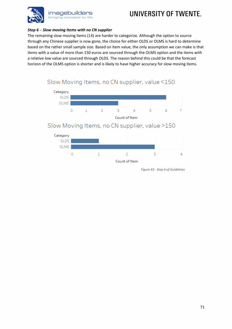
71
Step 6 – Slow moving Items with no CN supplier
The remaining slow moving items (14) are harder to categorize. Although the option to source
through any Chinese supplier is now gone, the choice for either OLDS or OLMS is hard to determine
based on the rather small sample size. Based on item value, the only assumption we can make is that
items with a value of more than 150 euros are sourced through the OLMS option and the items with
a relative low value are sourced through OLDS. The reason behind this could be that the forecast
horizon of the OLMS option is shorter and is likely to have higher accuracy for slow moving items.
Figure 43 - Step 6 of Guidelines

72
Appendix 5 – Forecasting Models We describe the steps and models within our store forecasting model and item forecasting model.
Finding Smoothing Factors that Minimize Forecast Error of Model Fit We can find the values for the smoothing parameters that minimize either the MAPE or MSE and give
a good Model Fit by setting these as the decision variables in a mathematical program. The forecast
error reflects the model fit of the forecasting model that uses these smoothing factors.
Objective Function
For the objective function, we can choose to minimize the MAPE or MSE based on the error that fits
the situation the best.
𝑀𝑖𝑛 𝑀𝐴𝑃𝐸 or 𝑀𝑖𝑛 𝑀𝑆𝐸
Decision Variables The decision variables are the smoothing parameters of the Level, Trend and Seasonal factors.
Changing these automatically adjusts the level, trend and seasonal factors and thereafter the
forecasts made over the known demand data that determines the forecast error.
𝛼, 𝛽 & 𝛾
Constraints The only constraints in this model set a minimum and a maximum to the smoothing factor values.
0 ≤ 𝛼, 𝛽, 𝛾 ≤ 1
Store Demand Forecasting Model We forecast the last months of the Test data (October –December 2019). In the actual demand data
of stores, experts within Imagebuilders acknowledged that in October 2017 (the grey peak in period
10 of Figure 44) there was an outlier. To prevent this outlier from impacting our final results, we
change this store demand quantity to a value that fits the actual demand pattern. After setting up
our forecasting model using the Holt-Winter’s Exponential Smoothing method and obtaining the
parameter values for the level and trend of the last period considered in historical demand (in this
case September 2019, 𝒕 = 𝟑𝟑) , we can find the values of the smoothing factors (𝛼, 𝛽 & 𝛾) that
minimize the forecast error of choice. These parameters are used to update the level, trend and
seasonal factors. The parameters and their values used to forecast demand of the periods 34 until 36
are shown in Table 43 (we do not show the seasonal factors as these are period specific). The
additive error is negative due to the slight over-forecasting bias in our model fit as the concept was
phasing out. The parameter value of gamma, used to smooth the seasonal factors, is high to
incorporate the life cycle of the concept as it was phasing out. The forecast and the actual demand in
those periods can be seen in Figure 44 by the green and orange lines respectively. The MAPE of our
model fit equals 37% and the MAPE of our actual forecast equals 8.3%.
𝒕 = 𝟑𝟑 Additive Error (𝜺𝒕) Level (𝒂𝒕) Trend (𝒃𝒕) Alpha (𝜶) Beta (𝜷) Gamma (𝜸)
Parameter Settings -0.51 3.8 -0.2 0.15 0.22 0.85
Table 43 - Parameter Settings of Model Fit in Store Demand Forecasting
Figure 44 - Historical Demand, Model Fit and Forecasts after finding Smoothing Factors that Minimize MAPE for Model Fit

73
Store Size Forecasting Model In adapting Equation 3 that is also used in store demand forecasts, we need to omit the seasonal
factor variable 𝐹𝑡 before we usage. Similar to the forecasting method of store demand, we set up our
forecast using a level (𝑎𝑡) and trend (𝑏𝑡) and find the near-optimal parameter settings for both
smoothing factor alpha (𝛼) and beta (𝛽) by setting these parameters as decision variables while
minimizing the forecast error. In the forecast made below (Figure 45) using the found parameters as
shown in Table 44, the MAPE of model fit equals 7%.
Correlation Between Item Usage and Store Size To accurately describe the relation between item demand and store demand, we analyse the relation
between item usage and store size for all standard items in the LSG concept. We use Kendall’s tau to
determine if there is a significant correlation between the two. One of the solvable problems in
Kendall’s tau is that after doing the ‘ranking’ based on store size, multiple store size might have the
same value and regardless of item usage we now speak of a tie. As we have ties in our data (either
store size or item usage of different pairs are the same), we need to subtract the tied pairs from the
total number of pairs. We created a Microsoft Excel Visual Basic script in which we a) retrieve all the
relevant demand data (store size & item usage) of any item, b) create a scatterplot of the data, c)
calculate the value of Kendall’s tau using the Correlation Data Analysis Tool designed by Real
Statistics (Zaiontz, 2020), d) calculate the vectors needed for the linear regression model and e)
calculate descriptive statistics of item demand. We calculate the last for items that show no
significant correlation to be able to use a) average demand size and b) inter-demand interval for
forecasting. As the latter is straight forward, we only explain the situation for correlated items.
Below, we run through the calculations of the item LSG217-00 which is a fast-moving item. Firstly, we
create the scatterplot and retrieve the values of tau and the p-value to see if the correlation is
significant. As seen below, the correlation is significant.
𝒕 = 𝟐𝟓 Additive Error (𝜺𝒕) Level (𝒂𝒕) Trend (𝒃𝒕) Alpha (𝜶) Beta (𝜷)
Parameter Settings 2.8 146.4 1.55 0.02 1
Table 44 - Parameter Settings Store Size
LSG217-00
PIONEER STS CORRELATION tau 0,554796446 s.e. 0,06 z 9,80 z-crit 1,96 p-value 0,00 lower 0,44 upper 0,67
Figure 45 - Forecasted Store Size
Figure 46 – Correlation & Item Usage vs. Store Size LSG217-00

74
Next, we run our regression analysis to retrieve the values of the vectors that describe the linear
relationship. We check if the coefficients used to describe the linear relationship are significant. If
they are insignificant, we relation might not be linear. We didn’t stumble across this problem for any
of the correlated items.
Lastly, we retrieve standard descriptive statistics of the
item demand. Although these are not useful for items
with significant correlation, these become valuable for
those without correlation. We can use the Count value
(number of stores in which the item is used) to
compute the inter-demand interval.
For this item, the forecast for any period is made through the following Equation:
𝐼𝑡𝑒𝑚𝐹𝑜𝑟𝑒𝑐𝑎𝑠𝑡𝑖,𝑡,𝑡+𝑛 = 1 ∗ 𝑆𝑡𝑜𝑟𝑒𝐹𝑜𝑟𝑒𝑐𝑎𝑠𝑡𝑡,𝑡+𝑛 ∗ (51,78 + 0,57 ∗ 𝑆𝑡𝑜𝑟𝑒𝑆𝑖𝑧𝑒𝐹𝑜𝑟𝑒𝑐𝑎𝑠𝑡𝑡,𝑡+𝑛)
As the 𝑆𝑡𝑜𝑟𝑒𝐹𝑜𝑟𝑒𝑐𝑎𝑠𝑡𝑡,𝑡+𝑛 for 𝑡 + 1 = 34 is 4 stores and 𝑆𝑡𝑜𝑟𝑒𝑆𝑖𝑧𝑒𝐹𝑜𝑟𝑒𝑐𝑎𝑠𝑡𝑡,𝑡+𝑛 for 𝑡 + 1 = 34 is
150m², the quantity of LSG217-00 forecasted for 𝑡 + 1 = 34 equals 550.
Linear Regression
Regression Residual Total Total Obs.
df 1,00 146,00 147,00 148,00 SS 97779,55 77853,39 175632,94 MS 97779,55 533,24 F 183,37 p-value 0,00 Coefficient Deviation T-Stat p-value
Intercept 51,78 6,26 8,27 0,0 Group1 0,57 0,04 13,54 0,0
𝛽𝑖,0
𝛽𝑖,1
Descriptive Statistics Item Demand
CV 0,26
Mean 132,52
Standard Error 2,84
Median 126,00
Mode 102,00
Standard Deviation 34,57
Sample Variance 1194,78
Maximum 258,00
Minimum 74,00
Sum 19613,00
Count 148,00
Figure 47 - Linear Regression to obtain Vector Values
Figure 48 - Descriptive Statistics of an Item