Red Supergiant Stars as Cosmic Abundance … · Red Supergiant Stars as Cosmic Abundance Probes....
38
Red Supergiant Stars as Cosmic Abundance Probes. III. NLTE effects in J-band Magnesium lines Maria Bergemann Max-Planck Institute for Astronomy, 69117, Heidelberg, Germany [email protected] Rolf-Peter Kudritzki Institute for Astronomy, University of Hawaii, 2680 Woodlawn Drive, Honolulu, HI 96822 [email protected] Zach Gazak Institute for Astronomy, University of Hawaii, 2680 Woodlawn Drive, Honolulu, HI 96822 [email protected] Ben Davies University of Liverpool, UK [email protected] and Bertrand Plez Laboratoire Univers et Particules de Montpellier, Universit´ e Montpellier 2, CNRS, F-34095 Montpellier, France [email protected] and Lyudmila Mashonkina
Transcript of Red Supergiant Stars as Cosmic Abundance … · Red Supergiant Stars as Cosmic Abundance Probes....

Red Supergiant Stars as Cosmic Abundance Probes. III. NLTE effects inJ-band Magnesium lines
Maria Bergemann
Max-Planck Institute for Astronomy, 69117, Heidelberg, Germany
Rolf-Peter Kudritzki
Institute for Astronomy, University of Hawaii, 2680 Woodlawn Drive, Honolulu, HI 96822
Zach Gazak
Institute for Astronomy, University of Hawaii, 2680 Woodlawn Drive, Honolulu, HI 96822
Ben Davies
University of Liverpool, UK
and
Bertrand Plez
Laboratoire Univers et Particules de Montpellier, Universite Montpellier 2, CNRS, F-34095
Montpellier, France
and
Lyudmila Mashonkina

– 2 –
Institute of Astronomy, Russian Academy of Sciences, Russia
Received ; accepted
To appear in Astrophysical Journal
– 3 –
ABSTRACT
Non-LTE calculations for Mg I in red supergiant stellar atmospheres are presented
to investigate the importance of non-LTE for the formation of Mg I lines in the NIR J-
band. Recent work using medium resolution spectroscopy of atomic lines in the J-band
of individual red supergiant stars has demonstrated that technique is a very promising
tool to investigate the chemical composition of the young stellar population in star
forming galaxies. As in previous work, where non-LTE effects were studied for iron,
titanium and silicon, substantial effects are found resulting in significantly stronger
Mg I absorption lines. For the quantitative spectral analysis the non-LTE effects lead to
magnesium abundances significantly smaller than in LTE with the non-LTE abundance
corrections varying smoothly between -0.5 dex to -0.1 dex for effective temperatures
between 3400K to 4400K. We discuss the physical reasons of the non-LTE effects
and the consequences for extragalactic J-band abundance studies using individual red
supergiants in the young massive galactic double cluster h and chi Persei.
Subject headings: galaxies: abundances — line: formation — radiative transfer — stars:
abundances — stars: late-type — supergiants

– 4 –
1. Introduction
Over the last years the quantitative spectroscopic analysis of medium resolution (R ∼ 3200)
J-band spectra of red supergiant stars (RSGs) has been established as a very promising tool to
investigate the chemical evolution of star forming galaxies. RSGs emit most of their enormous
luminosities of 105 to ∼ 106 L/L⊙ at infrared wavelengths and can be easily identified as
individual sources through their brightness and colors (Humphreys and Davidson, 1979, Patrick
et al., 2014, Gazak 2014c). Their J-band spectra are characterized by strong and isolated atomic
lines of iron, titanium, silicon and magnesium, ideal for medium resolution spectroscopy, in
particular because the molecular lines of OH, H2O, CN, and CO which otherwise dominate the
H- and K-band are weak. Detailed recent studies of RSGs in the Milky Way and the Magellanic
Clouds (Davies et al., 2013, 2014, Gazak et al., 2014b), in the Local Group dwarf galaxy NGC
6822 (Patrick et al., 2014) and in the Sculptor group galaxy NGC 300 and 1.9 Mpc (Gazak 2014c)
demonstrate that this new medium resolution J-band technique has an enormous potential and
yields stellar metallicities with an accuracy of ∼ 0.10 dex per individual star. With present-day
NIR multi-object spectrographs attached to large telescopes such as MOSFIRE/KECK and
KMOS/VLT galaxies up to 10 Mpc distance can be studied in this way to determine metallicities
and metallicity gradients providing an important alternative the use of blue supergiant stars (see
for instance Kudritzki et al., 2012, 2013, 2014) or HII regions (see as examples Bresolin et al.,
2011, 2012). In addition, Gazak et al. (2013, 2014a) have shown that the integrated J-band light
of young massive super star clusters (SSCs) is dominated by their population of RSGs as soon
as they are older than 7 Myr and that the same analysis technique can be applied increasing the
potential volume for metallicity determinations in the local universe by a factor of thousand.
With the use of future adaptive optics (AO) MOS IR spectrographs at the next generation of
extremely large telescopes the J-band method will become even more powerful and will render
the possibility to measure stellar metallicities of individual RSGs out to the enormous distance of
70 Mpc (Evans et al., 2011).
– 5 –
A crucial aspect of the spectroscopic J-band analysis technique is to account for the effects
of departures from local thermodynamic equilibrium (LTE) which if neglected at the low densities
of RSG atmospheres could introduce significant systematic errors. In two previous papers
(Bergemann et al., 2012 and 2013 - hereafter Paper I and II) we have carried out non-LTE (NLTE)
line formation calculations for iron, titanium and silicon and investigated the strengths of NLTE
effects which were found to be moderate for iron, but substantial for titanium and silicon. In this
third paper we extend this work to magnesium which shows two strong absorption line features
in the J-band arising from highly excited levels which can provide important information stellar
metallicity and the ratio of α to iron elements. We describe the atomic model and details of
the magnesium line formation calculations in Section 2 and present a discussion of the basic
NLTE-effects in Section 3. In Section 4 we calculate NLTE abundance corrections. Section
5 we compare with observations for a few selected RSG objects in Per OB1 and discuss the
consequences of including Mg I lines for the J-band technique.
2. Model atmospheres, line formation calculations, model atom and spectrum synthesis
2.1. Model atmospheres and line formation
The NLTE line formation calculations require an underlying model atmosphere which
provides the temperature and density stratification together with the number densities of the
most important atomic and molecular species contributing to the continuous and line background
opacities which affect the radiation field in the magnesium radiative transitions. As in Paper I and
II we use MARCS model atmospheres (Gustafsson et al., 2008) for this purpose and calculate a
small grid of models assuming a stellar mass of 15 M⊙with five effective temperatures (Teff =
3400, 3800, 4000, 4200, 4400K), three gravities (logg = 1.0, 0.0, −0.5 (cgs)), three metallicities
([Z]≡ log Z/Z⊙ =−0.5, 0.0, +0.5). Two values are adopted for the microturbulence, ξt = 2 and
5 km/s, respectively. As discussed in Papers I and II, this grid covers the range of atmospheric

– 6 –
parameters expected for RSG’s and allows us to assess the importance of NLTE effects over this
range. In addition, we also compute model atmospheres for the Sun and Arcturus as an additional
test of our magnesium model atom.
The NLTE occupation numbers for magnesium are then calculated using the NLTE code
DETAIL (Butler & Giddings 1985). The final J-band spectrum synthesis is carried out with the
separate code SIU (Reetz 1999) in a slightly modified version as described in Paper I. For all
further details we refer the reader to Papers I and II. In this work, we also implement the new
C12N14 linelist (B. Plez, priv. comm.).
2.2. Mg model atom and statistical equilibrium calculations
Our atomic model consists of three ionisation stages Mg I, Mg II, and Mg III, represented by
85, 6, and 1 levels respectively. The number of radiative transitions in the 1-sf and 2-d stages is
422 and 8. This model was first described in Zhao et al. (1998) and Zhao & Gehren (2000), and
updated by Mashonkina (2013). Electron-impact excitation is computed from the rate coefficients
by Mauas et al. (1988), where available, otherwise Zhao et al. (1998) is used for the remaining
transitions. Ionisation by electronic collisions was calculated from the Seaton (1962) formula with
a mean Gaunt factor set equal to g = 0.1 for Mg I and to 0.2 for Mg II. For H I impact excitations
and charge transfer processes, rate coefficients were taken from the detailed quantum mechanical
calculations of Barklem et al. (2012). The transition probabilities for radiative bound-bound
transitions were taken from Opacity project (Butler et al. 1993). The same source provides
photoionisation cross-sections from the lowest Mg I levels; for the remainder, we use the quantum
defect formulae of Peach (1967). Fig. 1 shows the complete atomic model with the observed
J-band line transitions highlighted in blue.

– 7 –
0
2
4
6
8
E [
eV]
Mg I
3S
3Po
3D
3Fo
3G
3Ho
3I
3Ko
3L
1S
1Po
1D
1Fo
1G
1Ho
1I
1Ko
1L
Fig. 1.— The complete magnesium atomic model. The observed J-band line transitions are high-
lighted in blue.

– 8 –
2.3. Atomic data and spectrum synthesis of J-band magnesium lines
The basic information about the observed magnesium lines in the J-band is given in Table
1. The four lines belong to multiplets 175, 224, and 225. The line at 11828.171 A forms in the
transition between the 3p 1P◦ and 4s 1S levels. The three lines around 12083 A originate in the
transitions between 3d 1D - 4 f 1F◦, and 3d 1D - 4 f 3F◦ levels. In a typical observed spectrum
of a late-type star, the three lines from multiplets 224 and 225 merge and are thus unresolved.
Hereafter, we refer to them as a single line at 12083 A. However, in the line formation and
spectrum synthesis calculations they are treated correctly as three individual lines (see Fig.
6).
Other than for the optical spectral range, where we use oscillator strengths from Chang &
Tang (1990) and Aldenius et al. (2007), there are no good experimental logg f values for the IR
Mg I lines. For the 11828.2 A Mg I lines, Civis et al (2013) calculated logg f =−0.305. For the
triplet at 12083 A, the available data are contradictory. In the Kurucz online database1, we find
−2.155, −9.300, 0.553 for the three lines 12083.264, 12083.346, 12083.662, respectively. For
the transition at 12083.662 A, theoretical calculations by Chang & Tang (1990) and Civis et al.
(2013) provide logg f = 0.41 and logg f = 0.44, respectively. Our previous RSG synthetic grid
(see Paper I) included the following values 0.45, −0.79, 0.415 for the 12083.264, 12083.346,
12083.662, respectively. These datasets come from the VALD database2, however, as our test
calculations have shown, they hugely over-estimate the line depths in the spectrum of the Sun.
In addition, there is a large differences between the Kurucz’ quantum-mechanical values listed
in different online tables for the 12083.278 and 12083.346 lines. Given these largely conflicting
g f -values we decided to extend our NLTE calculations to the Sun with the well established
magnesium abundance of log(Mg/H)+ 12 = 7.53 (Asplund et al. 2009). We then iterate the
1http://kurucz.harvard.edu/atoms/1200/gf1200.pos
2also to be found under http://www.pmp.uni-hannover.de/cgi-bin/ssi/test/kurucz/sekur.html

– 9 –
Table 1. Mg I J-band lines
Elem. λ Elow lower Eup upper log g f log C6
A [eV] level [eV] level
(1) (2) (3) (4) (5) (6) (7) (8)
11828.185 4.35 3p 1Po0 5.39 4s 1S0 -0.305 -29.7
12083.278 5.753 3d 1D2 6.78 4f 3Fo3 -1.500 -29.3
12083.346 5.753 3d 1D2 6.78 4f 3Fo2 -1.500 -29.3
12083.662 5.753 3d 1D2 6.78 4f 1Fo3 0.050 -29.3
Table 2. Stellar parameters of the reference and Per OB1 stars
Star Teff ∆Teff logg ∆ logg [Fe/H] ∆[Fe/H] vmic
K dex dex km/s
(1) (2) (3) (4) (5) (6) (7) (8)
Sun 5777 1 4.44 0.00 0.00 0.05 1.00
Arcturus 4286 35 1.64 0.06 −0.52 0.08 1.50
BD +56 595 4060 25 0.20 0.70 −0.15 0.13 4.00
BD +56 724 3840 25 −0.40 0.50 0.08 0.09 3.00
BD +59 372 3920 25 0.50 0.30 −0.07 0.09 3.20
HD 13136 4030 25 0.20 0.40 −0.10 0.08 4.10
HD 14270 3900 25 0.30 0.30 −0.04 0.09 3.70
HD 14404 4010 25 0.20 0.40 −0.07 0.10 3.90
HD 14469 3820 25 −0.10 0.40 −0.03 0.12 4.00
HD 14488 3690 50 0.00 0.20 0.12 0.10 2.90
HD 14826 3930 26 0.10 0.20 −0.08 0.07 3.70
HD 236979 4080 25 −0.60 0.30 −0.09 0.09 3.10

– 10 –
logg f values until we obtain a satisfactory fit the 12083 A Mg triplet line complex. We obtain as
best fitting values −1.5 for the bluer weak components and 0.05 for the strong red component,
respectively. We then carry out Mg NLTE calculations for the red giant star Arcturus using the
stellar parameters from Bergemann et al. (2012) as given in Table 2. For Arcturus, we adopt a
slight α-enhancement, [Mg/Fe]= 0.2, which is also confirmed by the earlier work on abundances
by Ramirez & Allende Prieto (2011). The comparison with observed J-band Mg lines for the Sun
and Arcturus is shown in Fig. 2 and indicates reasonable agreemeent.
Calculating the relatively strong J-band magnesium lines as in Fig. 2 also requires the
inclusion of spectral line broadening. We account for broadening caused by various mechanisms:
microturbulence (see Table 2), macro-turbulence, and broadening due to elastic collisions with H I
atoms. We tested the α and σ coefficients from the Barklem et al. (2002) quantum-mechanical
calculations, however these data produce spectral lines which are too weak compared with the
observed spectra of our reference stars (Sun, Arcturus). We thus scale these values by +0.3 dex.
The adopted atomic data are given in Table 1.
3. NLTE effects in J-band Mg lines
In general, the NLTE effects which we encounter for our grid of RSG atmospheres are very
similar to those found by previous studies of cool FGK stars (see Zhao et al 1998, and references
therein). The driving mechanism is normal photospheric photoionisation of neutral magnesium
governed by the super-thermal radiation field which escapes the deep photospheres essentially
unchanged once its optical depth has dropped below unity. This mechanism works independently
of the model atom, of course as long as photoionisation cross-sections are not set to zero. We thus
shall not repeat the complete analysis as done in Zhao et al (1998), but only summarise the most
important aspects relevant for the atmospheres of RSGs. For the discussion of NLTE effects, it is

– 11 –
0
0.2
0.4
0.6
0.8
1
11825 11826 11827 11828 11829 11830 11831
Rel
ativ
e F
lux
Wavelength (A)
Sun
Mg 1
3p1Po0 (4.35) - 4s1S0 (5.39)
ObservedLTE
NLTE 0
0.2
0.4
0.6
0.8
1
12083 12083.5 12084 12084.5
Rel
ativ
e F
lux
Wavelength (A)
Sun
Mg 1
3d1D2 (5.75) - 4f1Fo3 (6.78)
ObservedLTE
NLTE
0
0.2
0.4
0.6
0.8
1
11824 11825 11826 11827 11828 11829 11830 11831 11832
Rel
ativ
e F
lux
Wavelength (A)
Arcturus
Mg 1
3p1Po0 (4.35) - 4s1S0 (5.39)
ObservedLTE
NLTE 0
0.2
0.4
0.6
0.8
1
12081.5 12082 12082.5 12083 12083.5 12084 12084.5 12085 12085.5
Rel
ativ
e F
lux
Wavelength (A)
Arcturus
Mg 1
3d1D2 (5.75) - 4f1Fo3 (6.78)
ObservedLTE
NLTE
Fig. 2.— NLTE and LTE line profiles of the Mg I 11828 A (left) and 12083 A (right) computed for
the Sun (top panels) and Arcturus (bottom panels).

– 12 –
convenient to employ the concept of energy level departure coefficients, which are defined as
bi = nNLTEi /nLTE
i (1)
where nNLTEi and nLTE
i are NLTE and LTE atomic level populations [cm−3], respectively.
Fig. 3 shows the departure coefficients bi for a selection of models from our RSG model grid.
The diagrams are somewhat different from the conventional 1D representation of b(i) as a function
of optical depth τ in that on the y-axis we show the level energy, and the colour code indicates
the departure coefficient. In this way we obtain a nice overview of the general trend of the NLTE
effects as a function of excitation energy. Fig. 4 also shows the conventional representation of the
departure coefficients of the upper and lower levels of the J-band transition for the same models
as Fig. 3.
The effects of NLTE are clearly seen in this diagram, in particular for energy levels at 4 - 5 eV
(3p 1P◦, 4s 3S, 4s 1S) with large photo-ionisation cross-sections. Ionization by the super-thermal
UV radiation field becomes important with proximity to the outer atmospheric boundary, and
number densities of energy levels are much lower than the LTE predicts. Conceptually, the
behaviour of Mg I atomic number densities bears a strong resemblance with that of Fe I as
discussed in detail in Bergemann et al. (2012) and in Paper I.
For the IR J-band transitions, the main additional NLTE effect is through radiation transport
in the spectral lines themselves. The lower level of the 12083.660 line is 3d 1D at 5.75 eV, and its
only connection to the lower-lying levels, 1P◦ (2.71 eV) and 3P◦ (4.36 eV), is via the forbidden
magnetic-dipole transitions at ∼ 407 nm ( 3P◦ - 1D) and the allowed transition in the near-IR
(∼ 880 nm, 1P◦ - 1D) respectively (see the energy level diagram, Fig. 1). The lower level of
the line at 11823 A is 3p 1P◦. The level is connected with the ground state through a resonance
line at 2852 A ( 1S - 1P◦), which is optically thick throughout the formation depths of the J-band
Mg I lines and does not effectively participate in the NLTE radiation transport. This configuration
explains the fact that the both J-band lines have a nearly two-level-atom line source function Si j.

– 13 –
0
1
2
3
4
5
6
7
-4 -3 -2 -1 0 1
Ene
rgy
leve
l (eV
)
log tau (500 nm)
3400-0.5-0.5
0
0.2
0.4
0.6
0.8
1
1.2
1.4
Leve
l num
ber
dens
ity (
Non
-LT
E /
LTE
)
0
1
2
3
4
5
6
7
-4 -3 -2 -1 0 1
Ene
rgy
leve
l (eV
)
log tau (500 nm)
3400-0.5+0.5
0
0.2
0.4
0.6
0.8
1
1.2
1.4
Leve
l num
ber
dens
ity (
Non
-LT
E /
LTE
)
0
1
2
3
4
5
6
7
-4 -3 -2 -1 0 1
Ene
rgy
leve
l (eV
)
log tau (500 nm)
4400-0.5-0.5
0
0.2
0.4
0.6
0.8
1
1.2
1.4
Leve
l num
ber
dens
ity (
Non
-LT
E /
LTE
)
0
1
2
3
4
5
6
7
-4 -3 -2 -1 0 1
Ene
rgy
leve
l (eV
)
log tau (500 nm)
4400-0.5+0.5
0
0.2
0.4
0.6
0.8
1
1.2
1.4
Leve
l num
ber
dens
ity (
Non
-LT
E /
LTE
)
Fig. 3.— Mg I NLTE departure coefficients in RSG atmospheres shown for a few examples of the
model grid. Top: Teff = 3400K, log g =−0.5 and [Z] =−0.5 (left) and 0.5 (right). Bottom: same
as top but Teff = 4400K. The value of the departure coefficients is color coded. The y-axis is the
excitation energy of the levels and the x-axis is continuum optical depth at 500 nm.

– 14 –
0
0.2
0.4
0.6
0.8
1
-4 -3 -2 -1 0 1
Ene
rgy
leve
l (eV
)
log tau (500 nm)
3400-0.5-0.5
3p1P*4s1S3d1D4f3F*4f1F*
0
0.2
0.4
0.6
0.8
1
-4 -3 -2 -1 0 1
Ene
rgy
leve
l (eV
)
log tau (500 nm)
3400-0.5+0.5
3p1P*4s1S3d1D4f3F*4f1F*
0
0.2
0.4
0.6
0.8
1
-4 -3 -2 -1 0 1
Ene
rgy
leve
l (eV
)
log tau (500 nm)
4400-0.5-0.5
3p1P*4s1S3d1D4f3F*4f1F*
0
0.2
0.4
0.6
0.8
1
-4 -3 -2 -1 0 1
Ene
rgy
leve
l (eV
)
log tau (500 nm)
4400-0.5+0.5
3p1P*4s1S3d1D4f3F*4f1F*
Fig. 4.— Mg I NLTE departure coefficients of the lower and upper levels of the J-band transitions
shown for the same models as in Fig. 3.

– 15 –
Once the lines have become optically thin, downward cascading electrons over-populate the lower
levels of the transitions relative to the upper levels, and the source functions become sub-thermal,
Si j < Bν (see Fig. 4). Therefore the J-band Mg I lines are stronger in NLTE than in LTE, and the
NLTE effect further increases with decreasing Teff and logg. This is a very similar situation to the
formation of the J-band silicon lines discussed in Paper II. The resulting differences between the
J-band spectral lines profiles in the LTE and non-LTE case are illustrated in Fig. 5.
Beyond this more general discussion of the J-band NLTE effects the formation of the line
profiles of the 12083 A super-line are affected by an additional complication. Since the observed
feature is a blend of three Mg I components from three different multiplets, the result is a highly
asymmetric shape, which varies with stellar parameters (see Fig. 5, bottom four panels). Each of
the components suffers from its own NLTE effect. To illustrate this peculiar effect, we provide
the profiles of each component computed in LTE and NLTE for the model with Teff = 4400,
logg = 0.0, and [Fe/H] = 0.5 in Fig. 6. The bluest line at 12083.275 A which forms in the 3d
1D2 - 3Fo3 transition, is weaker in NLTE than in LTE. With its very small oscillator strength this
line forms in the deeper atmospheric layers where the departure coefficient of the upper level is
larger than the one of the lower level. As a consequence, the NLTE source function becomes
super-thermal, Si j > Bν . On the other hand, the reddest component at 12083.660 A has a much
larger oscillator strength and forms much further out in the atmosphere, where the departure
coefficient of the upper level is always smaller then the one of lower level as already described
above. At very low temperatures and gas pressures, Teff < 4000 K and log(g) < 1, the NLTE
effects in the 12083 A line are more sensitive to Teff compared to the 11828 A line. We also notice
that the upper levels of the 12083 transitions are closer to the Mg II continuum at 7.46 eV, and
more sensitive to recombination cascades from Mg II, which causes their overpopulation in deeper
atmospheric layers.

– 16 –
3400, +0.00, -0.50, 2km/s
1.1826 1.1827 1.1828 1.1829 1.1830Wavelength (µm)
0.0
0.2
0.4
0.6
0.8
1.0
Flu
x
4400, +0.00, -0.50, 2km/s
1.1826 1.1827 1.1828 1.1829 1.1830Wavelength (µm)
0.0
0.2
0.4
0.6
0.8
1.0
Flu
x
3400, +0.00, +0.50, 2km/s
1.1826 1.1827 1.1828 1.1829 1.1830Wavelength (µm)
0.0
0.2
0.4
0.6
0.8
1.0
Flu
x
4400, +0.00, +0.50, 2km/s
1.1826 1.1827 1.1828 1.1829 1.1830Wavelength (µm)
0.0
0.2
0.4
0.6
0.8
1.0
Flu
x
3400, +0.00, -0.50, 2km/s
1.20820 1.20825 1.20830 1.20835 1.20840 1.20845 1.20850Wavelength (µm)
0.0
0.2
0.4
0.6
0.8
1.0
Flu
x
4400, +0.00, -0.50, 2km/s
1.20820 1.20825 1.20830 1.20835 1.20840 1.20845 1.20850Wavelength (µm)
0.0
0.2
0.4
0.6
0.8
1.0
Flu
x
3400, +0.00, +0.50, 2km/s
1.20820 1.20825 1.20830 1.20835 1.20840 1.20845 1.20850Wavelength (µm)
0.0
0.2
0.4
0.6
0.8
1.0
Flu
x
4400, +0.00, +0.50, 2km/s
1.20820 1.20825 1.20830 1.20835 1.20840 1.20845 1.20850Wavelength (µm)
0.0
0.2
0.4
0.6
0.8
1.0
Flu
x
Fig. 5.— Profiles of the J-band Mg I lines computed in LTE (red) and NLTE (blue) for a few
examples of the model atmosphere grid. All models are for logg = 0.0 and ξt = 2 kms. The upper
row is for the line at 11828 A and the bottom row for 12083 A.
LTE
1.20820 1.20825 1.20830 1.20835 1.20840 1.20845 1.20850Wavelength (µm)
0.0
0.2
0.4
0.6
0.8
1.0
Flu
x
NLTE
1.20820 1.20825 1.20830 1.20835 1.20840 1.20845 1.20850Wavelength (µm)
0.0
0.2
0.4
0.6
0.8
1.0
Flu
x
Fig. 6.— Individual line components (dashed) contribution to the total profile (solid) of the J-band
Mg I line at 12083 A computed with Teff = 4400, logg = 0.0, and [Fe/H] = 0.5 in LTE (top) and
NLTE (bottom).

– 17 –
4. NLTE Mg I abundance corrections
Over the whole RSG grid the the J-band Mg I absorption lines are stronger in NLTE than
in LTE. Quantitatively, this information is summarised in Tables 3 and 4 which compile the
equivalent widths for two values of microturbulence, 2 and 5 km/s. As a consequence, magnesium
abundances obtained from a LTE fit of observed J-band lines are systematically too high. This can
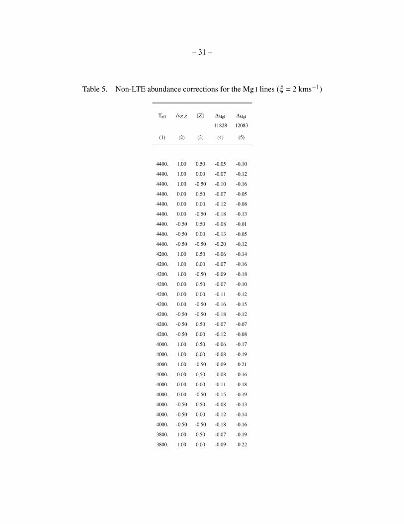
be quantitatively assessed by introducing NLTE abundance corrections ∆.
∆ = logA(Mg)NLTE − logA(Mg)LTE (2)
∆ is the logarithmic correction, which has to be applied to an LTE magnesium abundance
determination of a specific line, logA, to obtain the correct value corresponding to the use of
NLTE line formation. These corrections are obtained at each point of our model grid by matching
the NLTE equivalent width through varying the Mg abundance in the LTE calculations. When
for the same element abundance the NLTE line equivalent width is larger than the LTE one, it
requires a higher LTE abundance to fit the NLTE equivalent width and, thus, the NLTE abundance
corrections become negative. Fig. 7 shows the NLTE abundance corrections computed with two
values of microturbulence, 2 and 5 km s−1. The exact values of the NLTE abundance corrections
are given in Tables 5 and 6. The results for Mg are very similar to those we obtained for the J-band
Si lines (Paper 2). Fig. 8 also shows the effect of varying Mg abundance ([Z] fixed to solar) on the
line profiles for the both Mg I J-band lines and Fig. 9 illustrates the impact of microturbulence
ξt. Clearly, the larger ξt the stronger a spectral line, demonstrating the fundamental degeneracy
between small scale turbulent broadening and abundance. The 11828 A line and the strongest
component of the 12083 line usually occupy the flat part of the curve-of-growth and are very
sensitive to the microturbulence velocity. In contrast, the two weaker components of the J-band
triplet at 12083 A are on the linear part of the curve-of-growth even in very cool atmospheres
(Teff = 3400 K).

– 18 –
11828.18, 2 km/s
3400 3600 3800 4000 4200 4400Teff (K)
-0.6
-0.4
-0.2
-0.0
0.2
∆ (N
LT
E -
LT
E)
log g = -0.5
11828.18, 2 km/s
3400 3600 3800 4000 4200 4400Teff (K)
-0.6
-0.4
-0.2
-0.0
0.2
∆ (N
LT
E -
LT
E)
log g = 0.0
11828.18, 2 km/s
3400 3600 3800 4000 4200 4400Teff (K)
-0.6
-0.4
-0.2
-0.0
0.2
∆ (N
LT
E -
LT
E)
log g = +1.0
[Z] = +0.5[Z] = 0.0[Z] = -0.5
12083.6, 2 km/s
3400 3600 3800 4000 4200 4400Teff (K)
-0.6
-0.4
-0.2
-0.0
0.2
∆ (N
LT
E -
LT
E)
log g = -0.5
12083.6, 2 km/s
3400 3600 3800 4000 4200 4400Teff (K)
-0.6
-0.4
-0.2
-0.0
0.2
∆ (N
LT
E -
LT
E)
log g = 0.0
12083.6, 2 km/s
3400 3600 3800 4000 4200 4400Teff (K)
-0.6
-0.4
-0.2
-0.0
0.2
∆ (N
LT
E -
LT
E)
log g = -0.5
11828.18, 5 km/s
3400 3600 3800 4000 4200 4400Teff (K)
-0.6
-0.4
-0.2
-0.0
0.2
∆ (N
LT
E -
LT
E)
log g = -0.5
11828.18, 5 km/s
3400 3600 3800 4000 4200 4400Teff (K)
-0.6
-0.4
-0.2
-0.0
0.2
∆ (N
LT
E -
LT
E)
log g = 0.0
11828.18, 5 km/s
3400 3600 3800 4000 4200 4400Teff (K)
-0.6
-0.4
-0.2
-0.0
0.2
∆ (N
LT
E -
LT
E)
log g = +1.0
[Z] = +0.5[Z] = 0.0[Z] = -0.5
12083.6, 5 km/s
3400 3600 3800 4000 4200 4400Teff (K)
-0.6
-0.4
-0.2
-0.0
0.2
∆ (N
LT
E -
LT
E)
log g = -0.5
12083.6, 5 km/s
3400 3600 3800 4000 4200 4400Teff (K)
-0.6
-0.4
-0.2
-0.0
0.2
∆ (N
LT
E -
LT
E)
log g = 0.0
12083.6, 5 km/s
3400 3600 3800 4000 4200 4400Teff (K)
-0.6
-0.4
-0.2
-0.0
0.2
∆ (N
LT
E -
LT
E)
log g = -0.5
Fig. 7.— NLTE abundance corrections for the 11828 (top) and 12083 (bottom) A Mg I lines as
a function of effective temperature and metallicity for log g = -0.5 (left), 0.0 (middle), and 1.0
(right). Top panels: microturbulence 2 km s−1; bottom panels: microturbulence 5 km s−1.

– 19 –
LTE, 3400, +0.00, -0.50
1.1826 1.1827 1.1828 1.1829 1.1830Wavelength (µm)
0.0
0.2
0.4
0.6
0.8
1.0
Flu
x
-0.5 < [Mg/Fe] < 0.5
NLTE, 3400, +0.00, -0.50
1.1826 1.1827 1.1828 1.1829 1.1830Wavelength (µm)
0.0
0.2
0.4
0.6
0.8
1.0
Flu
x
-0.5 < [Mg/Fe] < 0.5
LTE, 3400, +0.00, -0.50
1.20820 1.20825 1.20830 1.20835 1.20840 1.20845 1.20850Wavelength (µm)
0.0
0.2
0.4
0.6
0.8
1.0
Flu
x
-0.5 < [Mg/Fe] < 0.5
NLTE, 3400, +0.00, -0.50
1.20820 1.20825 1.20830 1.20835 1.20840 1.20845 1.20850Wavelength (µm)
0.0
0.2
0.4
0.6
0.8
1.0
Flu
x
-0.5 < [Mg/Fe] < 0.5
Fig. 8.— LTE (left) and NLTE (right) lines profiles for the 11828 (top) and 12083 (bottom) A Mg
I lines as a function of Mg abundance. [Mg/Fe] varies from -0.5 to +0.5 with a step of 0.1 dex.

– 20 –
LTE, 3400, +0.00, -0.50
1.1826 1.1827 1.1828 1.1829 1.1830Wavelength (µm)
0.0
0.2
0.4
0.6
0.8
1.0
Flu
x
1 km/s < Vmic < 5 km/s
NLTE, 3400, +0.00, -0.50
1.1826 1.1827 1.1828 1.1829 1.1830Wavelength (µm)
0.0
0.2
0.4
0.6
0.8
1.0
Flu
x
1 km/s < Vmic < 5 km/s
LTE, 3400, +0.00, -0.50
1.20820 1.20825 1.20830 1.20835 1.20840 1.20845 1.20850Wavelength (µm)
0.0
0.2
0.4
0.6
0.8
1.0
Flu
x
1 km/s < Vmic < 5 km/s
NLTE, 3400, +0.00, -0.50
1.20820 1.20825 1.20830 1.20835 1.20840 1.20845 1.20850Wavelength (µm)
0.0
0.2
0.4
0.6
0.8
1.0
Flu
x
1 km/s < Vmic < 5 km/s
Fig. 9.— LTE (left) and NLTE (right) lines profiles for the 11828 (top) and 12083 (bottom) Mg I
lines as a function of microturbulence. ξt varies from 1 to 5 km s−1 with a step of 1 km s−1.

– 21 –
The NLTE abundance corrections are significant with large negative values between −0.5 to
−0.1 dex and are strongest at low metallicity [Z]. We see a clear trend with effective temperature,
the effect being significantly stronger for the 11083 A line. This is a consequence of the much
stronger NLTE effects at lower temperature noticed in the previous section.
5. Mg I J-band lines of Per OB1 red supergiants
Gazak et al. (2014b) investigated high resolution, high S/N J-band spectra of eleven RSGs in
the the young massive stellar double cluster h and χ Persei (Per OB1) in the solar neighbourhood
as a crucial test of the J-band analysis method. While this test nicely confirmed the reliability of
the method with an average cluster metallicity [Z] =−0.04 derived from the spectra, the authors
excluded the Mg I lines from the analysis (see their Figures 1 and 2) because of the obvious
apparent NLTE effects for which no NLTE calculations were available at the time of their analysis
work. Now with our new calculations at hand, we can use the stellar parameters determined by
Gazak et al. and check whether observed and calculated Mg I J-band line profiles agree.
The comparison of NLTE and LTE fits to Mg I lines for the Per OB-1 spectra of 10 stars is
shown in Fig. 10, 11, 12, 13. The stellar parameters are given in Table 2. A solar value is adopted
for the [Mg/Fe] ratio in the calculation. The agreement between the new NLTE calculations and
the observations is much better than with the previous atomic data and LTE. This confirms that
for future work the Mg I J-band lines can be used as an additional constraint of metallicity. In
addition, since the Mg I lines have the highest excitation potential of of the lower levels of their
transitions compared to the iron, titanium and silicon lines used so far in the J-band technique,
they will also be very useful to constrain effective temperature and gravity. This will strengthen
the accuracy of the method significantly.

– 22 –
0
0.2
0.4
0.6
0.8
1
11822 11824 11826 11828 11830 11832 11834
Rel
ativ
e F
lux
Wavelength (A)
BD +56595
ObservedLTE
NLTE 0
0.2
0.4
0.6
0.8
1
11822 11824 11826 11828 11830 11832 11834
Rel
ativ
e F
lux
Wavelength (A)
BD +56724
ObservedLTE
NLTE
0
0.2
0.4
0.6
0.8
1
11822 11824 11826 11828 11830 11832 11834
Rel
ativ
e F
lux
Wavelength (A)
BD +59372
ObservedLTE
NLTE 0
0.2
0.4
0.6
0.8
1
11822 11824 11826 11828 11830 11832 11834
Rel
ativ
e F
lux
Wavelength (A)
HD 13136
ObservedLTE
NLTE
0
0.2
0.4
0.6
0.8
1
11822 11824 11826 11828 11830 11832 11834
Rel
ativ
e F
lux
Wavelength (A)
HD 14270
ObservedLTE
NLTE 0
0.2
0.4
0.6
0.8
1
11822 11824 11826 11828 11830 11832 11834
Rel
ativ
e F
lux
Wavelength (A)
HD 14404
ObservedLTE
NLTE
Fig. 10.— Observed J-band Mg I profiles computed in LTE and NLTE for the atmospheric param-
eters determined by Gazak et al. (2014b) as given in Table 2.
6. Conclusions
With the new Mg I NLTE calculations presented in this work we are now able to able to use
the full J-band spectrum of atomic lines (iron, titanium, silicon and magnesium) for a detailed
analysis of red supergiant stars. This is a major step forward not only for the analysis of individual

– 23 –
0
0.2
0.4
0.6
0.8
1
11822 11824 11826 11828 11830 11832 11834
Rel
ativ
e F
lux
Wavelength (A)
HD 14469
ObservedLTE
NLTE 0
0.2
0.4
0.6
0.8
1
11822 11824 11826 11828 11830 11832 11834
Rel
ativ
e F
lux
Wavelength (A)
HD 14488
ObservedLTE
NLTE
0
0.2
0.4
0.6
0.8
1
11822 11824 11826 11828 11830 11832 11834
Rel
ativ
e F
lux
Wavelength (A)
HD 14826
ObservedLTE
NLTE 0
0.2
0.4
0.6
0.8
1
11822 11824 11826 11828 11830 11832 11834
Rel
ativ
e F
lux
Wavelength (A)
HD 236979
ObservedLTE
NLTE
Fig. 11.— Observed J-band Mg I profiles computed in LTE and NLTE for the atmospheric param-
eters determined by Gazak et al. (2014b) as given in Table 2.

– 24 –
0.4
0.5
0.6
0.7
0.8
0.9
1
1.1
12075 12080 12085 12090 12095
Rel
ativ
e F
lux
Wavelength (A)
BD +56595
ObservedLTE
NLTE 0.4
0.5
0.6
0.7
0.8
0.9
1
1.1
12075 12080 12085 12090 12095
Rel
ativ
e F
lux
Wavelength (A)
BD +56724
ObservedLTE
NLTE
0.4
0.5
0.6
0.7
0.8
0.9
1
1.1
12075 12080 12085 12090 12095
Rel
ativ
e F
lux
Wavelength (A)
BD +59372
ObservedLTE
NLTE 0.4
0.5
0.6
0.7
0.8
0.9
1
1.1
12075 12080 12085 12090 12095
Rel
ativ
e F
lux
Wavelength (A)
HD 13136
ObservedLTE
NLTE
0.4
0.5
0.6
0.7
0.8
0.9
1
1.1
12075 12080 12085 12090 12095
Rel
ativ
e F
lux
Wavelength (A)
HD 14270
ObservedLTE
NLTE 0.4
0.5
0.6
0.7
0.8
0.9
1
1.1
12075 12080 12085 12090 12095
Rel
ativ
e F
lux
Wavelength (A)
HD 14404
ObservedLTE
NLTE
Fig. 12.— Observed J-band Mg I profiles computed in LTE and NLTE for the atmospheric param-
eters determined by Gazak et al. (2014b) as given in Table 2.

– 25 –
0.4
0.5
0.6
0.7
0.8
0.9
1
1.1
12075 12080 12085 12090 12095
Rel
ativ
e F
lux
Wavelength (A)
HD 14469
ObservedLTE
NLTE 0.4
0.5
0.6
0.7
0.8
0.9
1
1.1
12075 12080 12085 12090 12095
Rel
ativ
e F
lux
Wavelength (A)
HD 14488
ObservedLTE
NLTE
0.4
0.5
0.6
0.7
0.8
0.9
1
1.1
12075 12080 12085 12090 12095
Rel
ativ
e F
lux
Wavelength (A)
HD 14826
ObservedLTE
NLTE 0.4
0.5
0.6
0.7
0.8
0.9
1
1.1
12075 12080 12085 12090 12095
Rel
ativ
e F
lux
Wavelength (A)
HD 236979
ObservedLTE
NLTE
Fig. 13.— Observed J-band Mg I profiles computed in LTE and NLTE for the atmospheric param-
eters determined by Gazak et al. (2014b) as given in Table 2.

– 26 –
RSGs (see for instance Gazak et al. 2014b) but also for the spectroscopic analysis of young and
very massive super star cluster (SSCs) for which the J-band spectra are completely dominated by
RSGs once they are older than 7 Myr. Gazak et al. (2014a) have demonstrated that the J-band
technique applied to SSCs yields reliable metallicities, but the accuracy of their was somewhat
compromised by the fact that the Mg I lines could not be used because of the importance of NLTE
effects. With the new calculations available it will be possible to significantly improve this work
and to fully utilize the tremendous potential of the J-band method.

– 27 –
Table 3. Equivalent widths a of the Mg I lines (ξ = 2 kms−1)
Teff log g [Z] Wλ ,MgI Wλ ,MgI Wλ ,MgI Wλ ,MgI
11828 11828 12083 12083
LT E NLT E LT E NLT E
(1) (2) (3) (4) (5) (6) (7)
4400 -0.50 0.00 483.2 511.7 404.8 413.5
4400 -0.50 0.50 582.9 608.4 501.5 504.1
4400 -0.50 -0.50 403.5 436.8 300.6 323.4
4200 -0.50 0.00 519.9 553.1 425.5 439.8
4200 -0.50 0.50 640.5 671.9 519.9 531.6
4200 -0.50 -0.50 434.1 469.7 326.3 348.9
4000 -0.50 0.00 554.9 597.3 427.8 452.7
4000 -0.50 0.50 696.7 738.0 516.4 539.9
4000 -0.50 -0.50 459.7 502.4 336.8 366.4
3800 -0.50 0.00 577.7 632.6 408.4 444.8
3800 -0.50 0.50 730.5 784.7 491.3 526.8
3800 -0.50 -0.50 475.7 528.9 326.4 365.0
3400 -0.50 0.00 554.6 629.2 314.4 366.7
3400 -0.50 0.50 709.0 780.3 394.5 443.6
3400 -0.50 -0.50 456.6 530.2 246.9 297.1
4400 0.00 0.00 497.3 529.2 400.3 414.6
4400 0.00 0.50 612.5 641.8 500.6 509.9
4400 0.00 -0.50 410.1 445.9 299.2 323.6
4400 1.00 0.00 592.0 626.4 394.8 419.7
4400 1.00 0.50 755.4 791.0 497.4 519.7
4400 1.00 -0.50 466.3 501.8 296.2 326.5
4200 0.00 0.00 540.7 577.9 414.1 435.8
4200 0.00 0.50 677.6 713.5 510.0 529.3
4200 0.00 -0.50 443.1 482.4 317.7 345.6
4200 1.00 0.00 662.6 704.0 396.7 429.6
4200 1.00 0.50 845.1 890.1 493.1 524.5
4200 1.00 -0.50 523.4 562.6 305.2 340.6

– 28 –
Table 3—Continued
Teff log g [Z] Wλ ,MgI Wλ ,MgI Wλ ,MgI Wλ ,MgI
11828 11828 12083 12083
LT E NLT E LT E NLT E
(1) (2) (3) (4) (5) (6) (7)
4000 0.00 0.00 581.9 628.6 409.4 441.3
4000 0.00 0.50 732.6 779.6 497.7 528.5
4000 0.00 -0.50 475.1 521.1 321.8 356.9
4000 1.00 0.00 725.1 777.2 381.6 422.3
4000 1.00 0.50 919.1 975.4 471.9 512.5
4000 1.00 -0.50 577.4 623.7 298.1 339.4
3800 0.00 0.00 611.7 671.0 385.2 427.1
3800 0.00 0.50 773.3 832.6 467.5 509.2
3800 0.00 -0.50 498.7 554.6 306.7 348.8
3800 1.00 0.00 749.8 813.4 348.5 395.3
3800 1.00 0.50 940.6 1007.5 434.3 481.7
3800 1.00 -0.50 608.6 664.2 273.5 318.2
3400 0.00 0.00 570.6 645.1 287.0 339.0
3400 0.00 0.50 719.3 791.3 365.4 414.9
3400 0.00 -0.50 472.0 544.3 222.4 271.0
3400 1.00 0.00 642.1 708.7 245.1 292.6
3400 1.00 0.50 795.3 864.0 322.2 368.1
3400 1.00 -0.50 536.7 596.8 186.0 228.7
aequivalent widths Wλ are given in mA
– 29 –
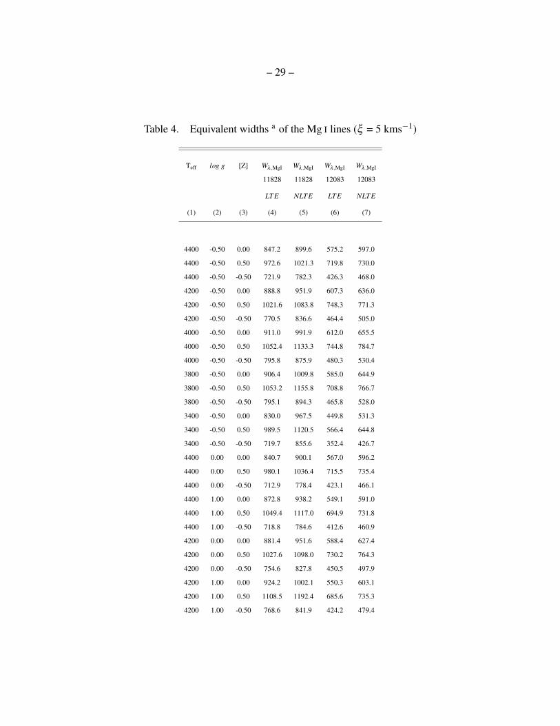
Table 4. Equivalent widths a of the Mg I lines (ξ = 5 kms−1)
Teff log g [Z] Wλ ,MgI Wλ ,MgI Wλ ,MgI Wλ ,MgI
11828 11828 12083 12083
LT E NLT E LT E NLT E
(1) (2) (3) (4) (5) (6) (7)
4400 -0.50 0.00 847.2 899.6 575.2 597.0
4400 -0.50 0.50 972.6 1021.3 719.8 730.0
4400 -0.50 -0.50 721.9 782.3 426.3 468.0
4200 -0.50 0.00 888.8 951.9 607.3 636.0
4200 -0.50 0.50 1021.6 1083.8 748.3 771.3
4200 -0.50 -0.50 770.5 836.6 464.4 505.0
4000 -0.50 0.00 911.0 991.9 612.0 655.5
4000 -0.50 0.50 1052.4 1133.3 744.8 784.7
4000 -0.50 -0.50 795.8 875.9 480.3 530.4
3800 -0.50 0.00 906.4 1009.8 585.0 644.9
3800 -0.50 0.50 1053.2 1155.8 708.8 766.7
3800 -0.50 -0.50 795.1 894.3 465.8 528.0
3400 -0.50 0.00 830.0 967.5 449.8 531.3
3400 -0.50 0.50 989.5 1120.5 566.4 644.8
3400 -0.50 -0.50 719.7 855.6 352.4 426.7
4400 0.00 0.00 840.7 900.1 567.0 596.2
4400 0.00 0.50 980.1 1036.4 715.5 735.4
4400 0.00 -0.50 712.9 778.4 423.1 466.1
4400 1.00 0.00 872.8 938.2 549.1 591.0
4400 1.00 0.50 1049.4 1117.0 694.9 731.8
4400 1.00 -0.50 718.8 784.6 412.6 460.9
4200 0.00 0.00 881.4 951.6 588.4 627.4
4200 0.00 0.50 1027.6 1098.0 730.2 764.3
4200 0.00 -0.50 754.6 827.8 450.5 497.9
4200 1.00 0.00 924.2 1002.1 550.3 603.1
4200 1.00 0.50 1108.5 1192.4 685.6 735.3
4200 1.00 -0.50 768.6 841.9 424.2 479.4

– 30 –
Table 4—Continued
Teff log g [Z] Wλ ,MgI Wλ ,MgI Wλ ,MgI Wλ ,MgI
11828 11828 12083 12083
LT E NLT E LT E NLT E
(1) (2) (3) (4) (5) (6) (7)
4000 0.00 0.00 902.3 990.8 581.9 635.5
4000 0.00 0.50 1052.2 1141.9 712.5 763.1
4000 0.00 -0.50 779.5 865.5 456.7 513.7
4000 1.00 0.00 958.3 1053.6 526.8 590.0
4000 1.00 0.50 1150.6 1253.8 650.8 713.3
4000 1.00 -0.50 803.2 887.6 412.5 475.1
3800 0.00 0.00 900.2 1010.7 546.9 614.7
3800 0.00 0.50 1057.8 1168.5 667.9 734.3
3800 0.00 -0.50 781.9 885.3 434.9 500.9
3800 1.00 0.00 957.4 1071.5 478.3 548.8
3800 1.00 0.50 1152.5 1273.3 593.7 665.6
3800 1.00 -0.50 810.5 908.7 376.3 441.3
3400 0.00 0.00 816.8 953.0 406.3 485.8
3400 0.00 0.50 977.0 1108.6 518.5 596.1
3400 0.00 -0.50 703.6 834.4 314.1 384.2
3400 1.00 0.00 836.8 953.3 334.1 402.2
3400 1.00 0.50 1008.0 1129.9 439.0 507.7
3400 1.00 -0.50 713.4 815.2 252.1 310.2
aequivalent widths Wλ are given in mA
– 31 –
Table 5. Non-LTE abundance corrections for the Mg I lines (ξ = 2 kms−1)
Teff log g [Z] ∆MgI ∆MgI
11828 12083
(1) (2) (3) (4) (5)
4400. 1.00 0.50 -0.05 -0.10
4400. 1.00 0.00 -0.07 -0.12
4400. 1.00 -0.50 -0.10 -0.16
4400. 0.00 0.50 -0.07 -0.05
4400. 0.00 0.00 -0.12 -0.08
4400. 0.00 -0.50 -0.18 -0.13
4400. -0.50 0.50 -0.08 -0.01
4400. -0.50 0.00 -0.13 -0.05
4400. -0.50 -0.50 -0.20 -0.12
4200. 1.00 0.50 -0.06 -0.14
4200. 1.00 0.00 -0.07 -0.16
4200. 1.00 -0.50 -0.09 -0.18
4200. 0.00 0.50 -0.07 -0.10
4200. 0.00 0.00 -0.11 -0.12
4200. 0.00 -0.50 -0.16 -0.15
4200. -0.50 -0.50 -0.18 -0.12
4200. -0.50 0.50 -0.07 -0.07
4200. -0.50 0.00 -0.12 -0.08
4000. 1.00 0.50 -0.06 -0.17
4000. 1.00 0.00 -0.08 -0.19
4000. 1.00 -0.50 -0.09 -0.21
4000. 0.00 0.50 -0.08 -0.16
4000. 0.00 0.00 -0.11 -0.18
4000. 0.00 -0.50 -0.15 -0.19
4000. -0.50 0.50 -0.08 -0.13
4000. -0.50 0.00 -0.12 -0.14
4000. -0.50 -0.50 -0.18 -0.16
3800. 1.00 0.50 -0.07 -0.19
3800. 1.00 0.00 -0.09 -0.22

– 32 –
Table 5—Continued
Teff log g [Z] ∆MgI ∆MgI
11828 12083
(1) (2) (3) (4) (5)
3800. 1.00 -0.50 -0.10 -0.23
3800. 0.00 0.50 -0.08 -0.22
3800. 0.00 0.00 -0.12 -0.24
3800. 0.00 -0.50 -0.15 -0.24
3800. -0.50 0.50 -0.09 -0.20
3800. -0.50 0.00 -0.13 -0.21
3800. -0.50 -0.50 -0.18 -0.22
3400. 1.00 0.50 -0.09 -0.21
3400. 1.00 0.00 -0.11 -0.25
3400. 1.00 -0.50 -0.12 -0.26
3400. 0.00 0.50 -0.11 -0.27
3400. 0.00 0.00 -0.15 -0.31
3400. 0.00 -0.50 -0.18 -0.31
3400. -0.50 0.50 -0.11 -0.28
3400. -0.50 0.00 -0.16 -0.32
3400. -0.50 -0.50 -0.21 -0.32

– 33 –
Table 6. Non-LTE abundance corrections for the Mg I lines (ξ = 5 kms−1)
Teff log g [Z] ∆MgI ∆MgI
11828 12083
(1) (2) (3) (4) (5)
4400. 1.00 0.50 -0.11 -0.13
4400. 1.00 0.00 -0.14 -0.16
4400. 1.00 -0.50 -0.18 -0.19
4400. 0.00 0.50 -0.15 -0.07
4400. 0.00 0.00 -0.20 -0.11
4400. 0.00 -0.50 -0.25 -0.17
4400. -0.50 0.50 -0.15 -0.04
4400. -0.50 0.00 -0.20 -0.08
4400. -0.50 -0.50 -0.25 -0.16
4200. 1.00 0.50 -0.11 -0.17
4200. 1.00 0.00 -0.14 -0.19
4200. 1.00 -0.50 -0.17 -0.22
4200. 0.00 0.50 -0.15 -0.13
4200. 0.00 0.00 -0.20 -0.15
4200. 0.00 -0.50 -0.25 -0.19
4200. -0.50 -0.50 -0.26 -0.15
4200. -0.50 0.50 -0.16 -0.09
4200. -0.50 0.00 -0.21 -0.11
4000. 1.00 0.50 -0.12 -0.21
4000. 1.00 0.00 -0.15 -0.23
4000. 1.00 -0.50 -0.17 -0.24
4000. 0.00 0.50 -0.16 -0.19
4000. 0.00 0.00 -0.21 -0.21
4000. 0.00 -0.50 -0.26 -0.23
4000. -0.50 0.50 -0.17 -0.16
4000. -0.50 0.00 -0.23 -0.17
4000. -0.50 -0.50 -0.28 -0.19
3800. 1.00 0.50 -0.13 -0.24
3800. 1.00 0.00 -0.16 -0.26

– 34 –
This work was supported by the National Science Foundation under grant AST-1108906 to
RPK. Moreover, RPK acknowledges support by the University Observatory Munich, where part
of this work was carried out.

– 35 –
Table 6—Continued
Teff log g [Z] ∆MgI ∆MgI
11828 12083
(1) (2) (3) (4) (5)
3800. 1.00 -0.50 -0.17 -0.26
3800. 0.00 0.50 -0.17 -0.26
3800. 0.00 0.00 -0.23 -0.27
3800. 0.00 -0.50 -0.27 -0.27
3800. -0.50 0.50 -0.18 -0.23
3800. -0.50 0.00 -0.25 -0.24
3800. -0.50 -0.50 -0.31 -0.25
3400. 1.00 0.50 -0.15 -0.26
3400. 1.00 0.00 -0.18 -0.28
3400. 1.00 -0.50 -0.19 -0.27
3400. 0.00 0.50 -0.20 -0.31
3400. 0.00 0.00 -0.26 -0.35
3400. 0.00 -0.50 -0.31 -0.32
3400. -0.50 0.50 -0.21 -0.32
3400. -0.50 0.00 -0.30 -0.36
3400. -0.50 -0.50 -0.36 -0.33

– 36 –
REFERENCES
Allen, C. W. 1973, London: University of London, Athlone Press, —c1973, 3rd ed.,
Allende Prieto, C., Lambert, D. L., & Asplund, M. 2001, ApJ, 556, L63
Asplund, M., Grevesse, N., Sauval, A. J., & Scott, P. 2009, ARA&A, 47, 481
Barklem, P. S., Belyaev, A. K., Guitou, M., et al. 2011, A&A, 530, A94
Bergemann, M., Kudritzki, R.- P., Plez, B., et al. 2012, ApJ, 751, 156
Bergemann, M., Hansen, C. J., Bautista, M., & Ruchti, G. 2012, A&A, 546, A90
Bergemann, M., Lind, K., Collet, R., Magic, Z., & Asplund, M. 2012, MNRAS, 427, 27
Bresolin, F., Gieren, W., Kudritzki, R.-P., et al. 2009, ApJ, 700, 309
Bresolin, F., 2011, ApJ 729, 56
Bresolin, F., Kennicutt, R.C., Ryan-Weber, E., 2012, ApJ 750, 122
Brott, A. M., Hauschildt, P. H., “A PHOENIX Model Atsmophere Grid for GAIA”, ESAsp, 567,
565
Butler, K., Giddings, J. 1985, Newsletter on Analysis of Astronomical Spectra No. 9, University
College London
Chiavassa, A., Freytag, B., Masseron, T., & Plez, B. 2011, A&A, 535, A22
Cox, A. N. 2000, Allen’s Astrophysical Quantities
Cunto W., Mendoza C., Ochsenbein F., Zeippen C.J., 1993, A&A 275, L5
Davies, B., Kudritzki, R. P., & Figer, D. F. 2010, MNRAS, 407, 1203

– 37 –
Davies, B., Kudritzki, R.P., Plez, B., et al., 2013, ApJ 767, 3
Davies, B., Kudritzki, R.P., Gazak, J.Z., Plez, B., Bergemann, M., Evans, C.J., Patrick, L.R., 2014,
submitted to ApJ
Evans, C. J., Davies, B., Kudritzki, R. P., et al. 2011, A&A, 527, 50
Gazak, J. Z., Davies, B., Bastian, N., et al. 2014, ApJ, 787, 142, (a)
Gazak, J. Z., Davies, B., Kudritzki, R., Bergemann, M., & Plez, B. 2014, ApJ, 788, 58, (b)
Gazak, J. Z., 2014, ”Red Supergiants as Luminous Beracons of Cosmic Chemical Abundance:
The Infrared J-band Spectroscopic Technique”, Thesis, Institute for Astronomy, University
of Hawaii at Manoa, (c)
Grevesse, N., Asplund, M,& Sauval, A. J. 2007, Space Sci. Rev., 130, 105
Gustafsson, B., Edvardsson, B., Eriksson, K., Jorgensen, U. G., Nordlund, A, & Plez, B. 2008,
A&A, 486, 951
Kramida, A., Ralchenko, Yu., Reader, J., and NIST ASD Team (2012). NIST Atomic Spectra
Database (ver. 5.0), [Online]. Available: http://physics.nist.gov/asd [2012, August 6].
National Institute of Standards and Technology, Gaithersburg, MD
Humphreys, R. M., & Davidson, K. 1979, ApJ, 232, 409
Kudritzki, R.-P., Urbaneja, M. A., Bresolin, F., et al. 2008, ApJ, 681, 269
Kudritzki, R.-P., Urbaneja, M. A., Gazak, Z., et al. 2012, ApJ, 747, 15
Kudritzki, R.P., Urbaneja, M.A., Gazak, J.Z., Macri, L., Hosek, M.W., Bresolin, F., Przybilla, N.,
2013, ApJ 779, L20
Kudritzki, R.P., Urbaneja, M.A., Bresolin, F., Hosek, M.W., Przybilla, N., 2014, ApJ 788, 56

– 38 –
Kurucz, R.-L. 2007, ”Robert L. Kurucz on-line database of observed and predicted atomic
transitions”, kurucz.harvard.edu
Lambert, D. L. 1993, Physica Scripta Volume T, 47, 186
Patrick, L.R., Evans, C.J., Davies, B., Kudritzki, R.P., Gazak, J.Z., Bergemann, M., Plez, B.,
Ferguson, A.M.N., 2014, submitted to ApJ
Plez, B. 1998, A&A, 337, 495
Plez, B. 2010, ASPC 425, 124
van Regemorter, H. 1962, ApJ, 136, 906
Ramırez, I., & Allende Prieto, C. 2011, ApJ, 743, 135
Reetz, J. 1999, PhD thesis, LMU Munchen
Seaton, M. J. 1962, Atomic and Molecular Processes, 375
Shi, J. R., Gehren, T., Butler, K., Mashonkina, L. I., Zhao, G. 2008, A&A, 486, 303
Steenbock, W., & Holweger, H. 1984, A&A, 130, 319
Wedemeyer, S. 2001, A&A, 373, 998
This manuscript was prepared with the AAS LATEX macros v5.2.