Recursion Theory Notes, Fall 2011

Lecturer: Lou van den Dries

0.1 Introduction

Recursion theory (or: theory of computability) is a branch of mathematical logicstudying the notion of computability from a rather theoretical point of view.This includes giving a lot of attention to what is not computable, or what iscomputable relative to any given, not necessarily computable, function. Thesubject is interesting on philosophical-scientific grounds because of the Church-Turing Thesis and its role in computer science, and because of the intriguingconcept of Kolmogorov complexity. This course tries to keep touch with howrecursion theory actually impacts mathematics and computer science. Thisimpact is small, but it does exist.

Accordingly, the first chapter of the course covers the basics: primitive recur-sion, partial recursive functions and the Church-Turing Thesis, arithmetizationand the theorems of Kleene, the halting problem and Rice’s theorem, recur-sively enumerable sets, selections and reductions, recursive inseparability, andindex systems. (Turing machines are briefly discussed, but the arithmetizationis based on a numerical coding of combinators.)

The second chapter is devoted to the remarkable negative solution (but withpositive aspects) of Hilbert’s 10th Problem. This uses only the most basicnotions of recursion theory, plus some elementary number theory that is worthknowing in any case; the coding aspects of natural numbers are combined hereingeniously with the arithmetic of the semiring of natural numbers.

The last chapter is on Kolmogorov complexity, where concepts of recursiontheory are used to define and study notions of randomness and informationcontent. This also involves a bit of measure theory.

The first and last chapter are largely based on a set of notes written byChristian Rosendal, and in the second chapter I follow mostly the treatment inSmorynski’s excellent book Logical Number Theory I.

An obvious omission in the material above is that of relative computability. Thistopic merges with effective descriptive set theory and deserves to be included,but there is only so much one can do in one semester. I have opted for a rathercareful treatment of fewer topics.

Notation: N = {0, 1, 2, . . .} is the set of natural numbers, including 0, anda, b, c, d, e and k, l,m, n (sometimes with subscripts or accents) range over N.

1

Chapter 1

Basic Recursion Theory

In this chapter, x, y, z, sometimes with subscripts, range over N as well. (Inlater chapters, x, y, z can be something else.)

1.1 Primitive Recursion

We define Fd to be the set of all functions f : Nd → N, and put F :=⋃d Fd.

We identify F0 with N in the obvious way. For i = 1, . . . , d, the ith projectionfunction P id : Nd → N is given by P id(x1, . . . , xd) = xi. The successor functionS : N → N is given by S(x) = x + 1. To denote functions, we sometimesborrow a notation from λ-calculus: if t(x1, . . . , xd) is an expression such thatt(a1, . . . , ad) ∈ N for all a1, . . . , ad, then λx1 . . . xd.t(x1, . . . , xd) denotes thecorresponding function

(a1, . . . , ad) 7→ t(a1, . . . , ad) : Nd → N.

For example, S = λx.x+ 1 and P id = λx1 . . . xd.xi.Now we define substitution. For g ∈ Fn and f1, . . . , fn ∈ Fd, g(f1, . . . , fn)

is the function λx1 . . . xd.g(f1(x1, . . . , xd), . . . , fn(x1, . . . , xd)) in Fd.For any g ∈ Fd and h ∈ Fd+2, there is a unique f ∈ Fd+1 such that for all

x1, . . . , xd, y:

f(x1, . . . , xd, 0) = g(x1, . . . , xd),f(x1, . . . , xd, y + 1) = h(x1, . . . , xd, y, f(x1, . . . , xd, y)).

This function f is said to be obtained by primitive recursion from g and h.

1.1.1 Primitive Recursive Functions

Loosely speaking, the functions obtainable by the above procedures are theprimitive recursive functions. More precisely,

2

Definition 1. The set PR of primitive recursive functions is the smallestsubset of F such that, with PRd := PR ∩ Fd,

(a) all constant functions in F belong to PR;

(b) S ∈ PR1;

(c) P id ∈ PRd for i = 1, . . . , d;

(d) if g ∈ PRn, f1, . . . , fn ∈ PRd, then g(f1, . . . , fn) ∈ PRd (closure undersubstitution);

(e) if g ∈ PRd and h ∈ PRd+2 and f ∈ Fd+1 is obtained by primitive recursionfrom g, h then f ∈ PRd+1 (closure under primitive recursion).

Essentially all functions in F that arise in ordinary mathematical practiceare primitive recursive. For example, the greatest common divisor function gcdis primitive recursive, but proving such facts will be much easier once we havesome lemmas available.

In addition to functions, some sets will be called primitive recursive. Recallthat the characteristic function of a set A ⊆ Nd is the function χA : Nd → Ndefined by χA(~x) = 1 if ~x ∈ A and χA(~x) = 0 if ~x ∈ Nd \A.

Definition 2. A set A ⊆ Nd is said to be primitive recursive if its charac-teristic function χA is primitive recursive.

A set A ⊆ Nd is often construed as a d-ary relation on N, and so, when ~x ∈ A,we often write A(~x) instead of ~x ∈ A.

1.1.2 Basic Examples

• The addition operation + : N2 → N is primitive recursive: let g = P 11 ∈

F1 ∩ E, h = S(P 33 ) ∈ F3 ∩ E, i.e. g(x) = x and h(x, y, z) = z + 1. Then

+ is obtained by primitive recursion from g, h:

x+ 0 = x = g(x), x+ (y + 1) = (x+ y) + 1 = h(x, y, x+ y).

• The multiplication operation · : N2 → N is primitive recursive. For letg ∈ F1 ∩ E, h ∈ F3 ∩ E be given by

g(x) = 0, h(x, y, z) = z + x (= +(P 33 , P

13 )(x, y, z)).

Then · is obtained by primitive recursion from g, h, since x · 0 = 0 = g(x)and x · (y + 1) = xy + x = h(x, y, xy).

• λxy.xy is primitive recursive: x0 = 1, xy+1 = xy · x.

• The monus function −· : N2 → N, where

x−· y ={x− y if x ≥ y,0 otherwise.

3

First, we observe that λx.x −· 1 is primitive recursive, as 0 −· 1 = 0 and(x+1)−· 1 = x. Then −· itself is primitive recursive: x−· 0 = x, x−· (y+1) =(x−· y)−· 1.

• sign : N→ N, given by

sign(x) ={

1 if x > 0,0 if x = 0,

is primitive recursive, for sign(0) = 0, sign(x+ 1) = 1.

• The set A = {(x, y) ∈ N2 : x < y} ⊆ N2 is primitive recursive sinceχA(x, y) = sign(y −· x).

• The diagonal ∆ = {(x, y) ∈ N2 : x = y} ⊆ N2 is primitive recursive:

χ∆(x, y) = 1−· ((x−· y) + (y −· x)).

• For A,B ⊆ Nd we have χ∅ = 0, χA∩B = χA · χB , and χ−A = 1 −· χA.Therefore, the primitive recursive subsets of Nd are the elements of aboolean algebra of subsets of Nd.

• Definition by cases: Suppose A ⊆ Nd and f, g ∈ Fd are primitiverecursive. Then the function h : Nd → N given by

h(~x) ={f(~x) for ~x ∈ A,g(~x) for ~x 6∈ A,

is primitive recursive because h = f · χA + g · χ−A.

• Iterated sums/products: Let f ∈ Fd+1 and let

g = λx1 . . . xdy.

y∑i=0

f(x1, . . . , xd, i).

Note that g(~x, 0) = f(~x, 0) and g(~x, y+ 1) = g(~x, y) + f(~x, y+ 1). Thus iff is primitive recursive, so is g, and vice-versa. Similarly, if f is primitiverecursive, so is

λx1 . . . xdy.

y∏i=0

f(x1, . . . , xd, i).

Notation. Let p(i) be a condition on i ∈ N: for each i ∈ N either p(i) holds, orp(i) does not hold. Then µi≤y p(i) denotes the least i ≤ y such that p(i) holdsif there is such an i, and if no such i exists, then µi≤y p(i) := 0. For example,if A ⊆ N, then µi≤3 i ∈ A is one of the numbers 0, 1, 2, 3.

4

• Bounded search: Let A ⊆ Nd+1, and define f ∈ Fd+1 by

f(~x, y) = µi≤y A(~x, i).

If A is primitive recursive, then so is f . This is because f(~x, 0) = 0 and

f(~x, y + 1) =

f(~x, y) if∑yi=0 χA(~x, i) ≥ 1,

y + 1 if∑yi=0 χA(~x, i) = 0 and A(~x, y + 1),

0 if∑yi=0 χA(~x, i) = 0 and A(~x, y + 1).

More generally, if A ⊆ Nd+1 and g ∈ Fd+1 are primitive recursive, so isthe function λ~xy.µi≤g(~x,y) A(~x, i) (this is a function in Fd+1).

• Bounded quantification: Let A ⊆ Nd+1 and define:

∃∃∃≤A = {(~x, y) ∈ Nd+1 : ∃∃∃i ≤ y A(~x, i)} ⊆ Nd+1,

∀∀∀≤A = {(~x, y) ∈ Nd+1 : ∀∀∀i ≤ y A(~x, i)} ⊆ Nd+1.

Since χ∃∃∃≤A(~x, y) = sign(∑y

i=0 χA(~x, i))

and χ∀∀∀≤A(~x, y) = sign(∏y

i=0 χA(~x, i)),

it follows that if A is primitive recursive, then so are ∃∃∃≤A and ∀∀∀≤A.

Exercise. Prove that gcd : N2 → N is primitive recursive. Here, gcd(0, 0) = 0,and gcd(x, y) is the greatest d such that d|x and d|y, for x, y not both zero.

1.1.3 Coding

Enumerate N2 diagonally as follows:

(0, 0) (1, 0) (0, 1) (2, 0) (1, 1) (0, 2) (3, 0) · · ·l l l l l l l0 1 2 3 4 5 6 · · ·

5

This bijection (x, y) 7→ |x, y| : N2 → N is given by:

|x, y| = (x+ y)(x+ y + 1)2

+ y.

This bijection is primitive recursive: use that

|x, y| = µi≤f(x,y) 2i = f(x, y)

with f : N2 → N given by f(x, y) = (x + y)(x + y + 1) + 2y, so f is primitiverecursive. Note also that x ≤ |x, y| and y ≤ |x, y| for all x, y.

Proposition 3. For d ≥ 1, we have primitive recursive functions

〈 〉d : Nd → N and ( )d1, . . . , ( )dd : N→ N,

such that 〈 〉d is a bijection and 〈(x)d1, . . . , (x)dd〉 = x for all x.

Proof. For d = 1, take both 〈 〉1 and ( )11 as the identity function on N. For

d = 2, take 〈x, y〉2 = |x, y| and define ( )21 and ( )2

2 by bounded search:

(x)21 := µi≤x (∃∃∃y ≤ x |i, y| = x), (x)2

2 = µi≤x (∃∃∃y ≤ x |y, i| = x).

We now proceed by induction. Given 〈 〉d and ( )d1, . . . , ( )dd with the desiredproperties, and d ≥ 2, put

〈x1, . . . , xd, y〉d+1 = |〈x1, . . . , xd〉d, y| and

(x)d+1i = ((x)2

1)di for i = 1, . . . , d, (x)d+1d+1 = (x)2

2.

Note that the identities just displayed also hold for d = 1.

1.1.4 More General Recursions

Let us consider first double recursions: Suppose g, g′ ∈ Fd and h, h′ ∈ Fd+3 areprimitive recursive. Let f, f ′ ∈ Fd+1 be given by:

f(~x, 0) = g(~x), f(~x, y + 1) = h(~x, y, f(~x, y), f ′(~x, y)

),

f ′(~x, 0) = g′(~x), f ′(~x, y + 1) = h′(~x, y, f(~x, y), f ′(~x, y)

).

Then f is primitive recursive. To see this, we use the above coding method anddefine t ∈ Fd+1 by t(~x, 0) = |g(~x), g′(~x)|, and

t(~x, y + 1) = |h(~x, y, (t(~x, y))2

1, (t(~x, y))22

), h′

(~x, y, (t(~x, y))2

1, (t(~x, y))22

)|.

Thus t is primitive recursive. We have f(~x, y) = (t(~x, y))21 and f ′(~x, y) =

(t(~x, y))22, so f and f ′ are primitive recursive.

It turns out that if a function is defined recursively in terms of several ofits previous values (the most general case being that f(~x, y+ 1) is computed interms of f(~x, 0), . . . , f(~x, y)), then it is still primitive recursive. To deal with

6

this situation, we use a Skolem trick. Given f ∈ Fd+1, define f ∈ Fd+1 byf(~x, 0) = f(~x, 0), and f(~x, y) = |f(~x, y), f(~x, y − 1)| for y > 0. So f(~x, y)encodes the values of f at (~x, 0), (~x, 1), . . . , (~x, y).

Let g ∈ Fd and h ∈ Fd+2, and define f ∈ Fd+1 by

f(~x, 0) = g(~x) and f(~x, y + 1) = h(~x, y, f(x, y)).

Claim. If g and h are primitive recursive, then so is f .

Proof. Assume g and h are primitive recursive. To obtain that f is primitiverecursive, it suffices to show that f is primitive recursive, because

f(~x, y) =

{f(~x, y) if y = 0,(f(~x, y))2

1 if y > 0.

But f(~x, 0) = g(~x), and

f(~x, y + 1) = 〈f(~x, y + 1), f(~x, y)〉= 〈h(~x, y, f(~x, y)), f(~x, y)〉,

so f is primitive recursive, as desired.

Exercise. Show that the Fibonacci sequence (Fn) defined by F0 = 0, F1 = 1and Fn = Fn−1 + Fn−2 for n ≥ 2, is primitive recursive.

For later use we also need an encoding of finite sequences of variable length suchthat the length of the sequence can be decoded from its code. We define

〈m1, . . . ,md〉 := 〈m1, . . . ,md, d〉d+1.

Note that then

〈m1, . . . ,md〉 = 〈n1, . . . , ne〉 ⇐⇒ d = e and m1 = n1, . . . ,md = nd.

Define lh : N→ N by lh(n) = (n)22, so that lh(〈n1 . . . , nd〉) = d. It is clear that

lh is primitive recursive. Let B ⊆ N be the set of all 〈n1, . . . , nd〉 for all d.

Claim. B = {b ∈ N : (b)22 > 0} ∪ {0}.

To see this, note that if (b)22 = d > 0, then b = |a, d| with a ∈ N, so a =

〈n1, . . . , nd〉d for suitable n1, . . . , nd, hence b = 〈n1, . . . , nd〉 ∈ B. It remains tonote that the only element 〈n1, . . . , nd〉 of B with d = 0 is 〈0〉1 = 0.

It follows from the claim that B is primitive recursive. Next, we introducea primitive recursive function (n, j) 7→ (n)j : N2 → N such that for n =〈n1, . . . , nd〉 and 1 ≤ j ≤ d we have (n)j = nj , and thus (n)j < n. Firstwe define a primitive recursive f : N2 → N by

f(n, 0) = n, f(n, i+ 1) =(f(n, i)

)21.

7

It is easy to check that for n = 〈nd, nd−1, . . . , n1〉 and 1 ≤ i ≤ d we have

f(n, i) = 〈nd, . . . , ni〉d+1−i.

Now define the primitive recursive function (n, j) 7→ (n)j : N2 → N by

(n)j := f(n, lh(n) + 1−· j)22 for j 6= 1, (n)1 := f(n, lh(n)).

This function has the desired properties as is easily verified.

1.2 Partial Recursive Functions

From the way we defined “primitive recursive”, it is clear that each primitiverecursive function is computable in an intuitive sense. A standard diagonaliza-tion argument, however, yields a computable function f : N → N that is notprimitive recursive. This argument goes as follows: one can effectively producea list f0, f1, f2, . . . of all functions in PR1. (Any primitive recursive functionN → N may appear infinitely often in this list.) Here, effective means that wehave an algorithm/program that on any input (m,n) computes fm(n). Nowdefine

f : N→ N, f(n) := fn(n) + 1.

Then f is computable in the intuitive sense, but f 6= fn for every n, so f cannotbe primitive recursive. More generally, any effective method of characterizingthe intuitive notion of (total) computable function N→ N must fail by a similardiagonalization.

It turns out that we can effectively characterize a more general notion ofpartial computable function N ⇀ N that does correspond to the intuitive notionof what is computable by an algorithm; the key point is that algorithms mayfail to terminate on some inputs. Accordingly, we extend our notion of primitiverecursive function to that of partial recursive function, essentially by allowingunbounded search.

Notation

For sets P,Q, we denote by f : P ⇀ Q a partial function f from P into Q, thatis, a function from a set D(f) ⊆ P into Q; then

f(p) ↓ (in words: f converges at p)

means that p ∈ D(f), and

f(p) ↑ (in words: f diverges at p)

means that p ∈ P but p /∈ D(f).Let f : Nd+1 ⇀ N. Then λ~x. (µyf(~x, y) = 0) denotes the partial function

g : Nd ⇀ N such that for ~x ∈ Nd:

g(~x) ↓ ⇐⇒ ∃y[∀∀∀i ≤ y f(~x, i) ↓ and ∀∀∀i < y f(~x, i) 6= 0 and f(~x, y) = 0

],

8

and if g(~x) ↓, then g(~x) is the unique y witnessing the righthandside in theabove equivalence. Let g : Nn ⇀ N and f1, . . . , fn : Nd ⇀ N. Then

g(f1, . . . , fn) : Nd ⇀ N

is given by:

g(f1, . . . , fn)(~x) ↓ ⇐⇒ f1(~x) ↓, . . . , fn(~x) ↓ and g(f1(~x), . . . , fn(~x)) ↓

and if g(f1, . . . , fn)(~x) ↓, then g(f1, . . . , fn)(~x) = g(f1(~x), . . . , fn(~x)). Giveng : Nd ⇀ N, h : Nd+2 ⇀ N there is clearly a unique f : Nd+1 ⇀ N such that forall ~x ∈ Nd and y ∈ N:

• f(~x, 0) ↓ ⇐⇒ g(~x) ↓; if f(~x, 0) ↓, then f(~x, 0) = g(~x).

• f(~x, y + 1) ↓ ⇐⇒ f(~x, y) ↓, h(~x, y, f(~x, y)) ↓; if f(~x, y + 1) ↓, thenf(~x, y + 1) = h(~x, y, f(~x, y)).

This f is said to be obtained by primitive recursion from g, h.

Definition 4. The set of partial recursive functions is the smallest set of partialfunctions Nd ⇀ N for d = 0, 1, 2, . . . such that:

(a) the function O : N0 → N with value 0 is partial recursive, and the successorfunction S : N→ N is partial recursive;

(b) the functions P id, for 1 ≤ i ≤ d, are partial recursive;

(c) whenever g : Nm ⇀ N, h1, . . . , hm : Nd ⇀ N are partial recursive, so isg(h1, . . . , hm);

(d) whenever g : Nd ⇀ N, h : Nd+2 ⇀ N are partial recursive, then so is thefunction obtained from g, h by primitive recursion;

(e) whenever f : Nd+1 ⇀ N is partial recursive, then so is

λ~x. (µyf(~x, y) = 0) : Nd ⇀ N.

A recursive function is a partial recursive function f : Nd → N, the notationhere indicating that D(f) = Nd. A set A ⊆ Nd is recursive if χA : Nd → N isrecursive. It is easy to check that primitive recursive functions are recursive.

Lemma 5. Given f : Nd → N, the following are equivalent:

(a) f is recursive;

(b) graph(f) ⊆ Nd+1 is recursive.

Proof. Use that χgraph(f)(~x, y) = χ∆(f(~x), y). In the other direction, use

f(~x) = µy(χgraph(f)(~x, y) = 1).

9

By similar arguments as for primitive recursive sets one obtains:

Theorem 6. The class of recursive subsets of Nd is closed under finite unions,intersections and complements. If A ⊆ Nd+1 is recursive, so are ∃∃∃≤A and ∀∀∀≤Aas subsets of Nd.

Exercise. Show that if f : N → N is a recursive bijection, then so is itsinverse. Show that there is a primitive recursive bijection N→ N whose inverseis not primitive recursive. (For the second problem, use that there is a recursivefunction N→ N that is not primitive recursive.)

1.2.1 Turing Machines

Definition 7. A Turing machine consists of a biinfinite tape of successive boxes,

·· ··qi 4

head

and a head that can read, erase, write in the box in case it is blank, andmove to the box on the left or the right. Moreover, there are given

• A finite alphabet Σ = {s0, s1, . . . , sn} with n ≥ 1, si 6= sj when i 6= j, withdistinguished symbols s0 := # for ’blank’, and s1 := 0.

• A finite set of internal states Q = {q0, q1, . . . , qm} with m ≥ 1, qi 6= qj fori 6= j, with distinguished states q0 (the initial state), and qm := qf (thefinal state).

• A finite set {I1, . . . , Ip} of instructions, each of one of the following threetypes:

(a) qasbscqd: if in state qa reading sb, erase sb, write sc in its place, andenter state qd;

(b) qasbRqd: if in state qa reading sb, move to the box on the right, andenter state qd;

(c) qasbLqd: if in state qa reading sb, move to the box on the left, andenter state qd.

This set of instructions should be complete: for each qa 6= qf , and each symbol sbthere is exactly one instruction of the form qasb . . . , and there is no instructionof the form qf . . . ..

Formally, a Turing machine is just a triple (Σ, Q, {I1, . . . , Ip}) as above.

Definition 8. Let M be a Turing machine with alphabet {#, 0, 1}. We say thatM computes the partial function f : Nd ⇀ N if for any input (x1, . . . , xd) asfollows:

10

·· ··] ] 0 1 1 · · · 1 0 1 1 · · · 1 0 · · · · · 0 1 1 · · · 1 0 ] ] ]q0 4

head

︸ ︷︷ ︸x1

︸ ︷︷ ︸x2

︸ ︷︷ ︸xd

the machine, applying the instructions,

• either never enters qf , and then f(~x) ↑.

• or eventually enters state qf , and then f(~x) ↓, with its head and tape asfollows:

·· ··0 1 1 · · · 1 0qf4

head

︸ ︷︷ ︸f(x1,...,xd)

Fact. Turing Computable = Partial Recursive.

Turing gave a compelling analysis of the intuitive concept of computability, in1936, and this led him to identify it with the precise notion of Turing com-putability. Turing machines remain important as a model of computation inconnection with complexity theory. But in the rest of this course we deal di-rectly with partial recursive functions without using Turing machines.

1.3 Arithmetization and Kleene’s Theorems

We shall give numerical codes to the programs that compute partial recursivefunctions. First, we introduce formal expressions that specify these programs.These expressions will be called combinators and they are words on the alphabetwith the following distinct symbols:

(a) the two symbols O and S,

(b) for each pair i, d such that 1 ≤ i ≤ d a symbol Pid,

(c) for each pair m, d, a symbol Smd (a substitution symbol),

(d) for each d a symbol Rd (a primitive recursion symbol),

(e) for each d a symbol Sd (an unbounded search symbol).

Each combinator has a specific arity (a natural number) and each d-ary combi-nator f is a word on this alphabet, and has associated to it a partial recursivefunction f : Nd ⇀ N. The definition is inductive:

(a) The word O of length 1 is a nullary combinator with associated functionN0 → N taking the value 0. The word S of length 1 is a unary combinatorwith associated function x 7→ x+ 1 : N→ N.

11

(b) For 1 ≤ i ≤ d, the word Pid is a d-ary combinator of length 1 with associ-ated function (x1, . . . , xd) 7→ xi : Nd → N.

(c) If g is an m-ary combinator and h1, . . . , hm are d-ary combinators, thenSmd gh1 . . . hm is a d-ary combinator with associated function g(h1, . . . , hm).

(d) If g is a d-ary combinator and h is a (d+ 2)-ary combinator, then Rd gh isa (d+ 1)-ary combinator whose associated function Nd+1 ⇀ N is obtainedby primitive recursion from g and h.

(e) If g is a (d + 1)-ary combinator, then Sd g is a d-ary combinator whoseassociated function is

λx1 . . . xd. (µy (g(x1, . . . , xd, y) = 0) .

Next we associate inductively to each combinator g a number #g ∈ N:

(a) # O = 〈1, 0〉, # S = 〈1, 1〉,

(b) # Pid = 〈2, i, d〉,

(c) #(Smd fg1 . . . gm) = 〈3,#f,#g1, . . . ,#gm, d〉,

(d) #(Rd gh) = 〈4,#g,#h, d+ 1〉,

(e) # Sd g = 〈5,#g, d〉.

Let Co be the set of all combinators. Then # : Co → N is clearly injective.It is easy to check that the primitive recursive function α : N → N given byα(n) := (n)lh(n) has the property that if n = #g with g ∈ Co, then α(n) is thearity of g.

Lemma 9. The set # Co is primitive recursive.

Proof. With B as in subsection 1.1.4, consider the following subsets of B:

(a) B1 := {〈1, 0〉, 〈1, 1〉};

(b) B2 := {n ∈ B : (n)1 = 2, lh(n) = 3, 1 ≤ (n)2 ≤ (n)3};

(c) B3 is the set of all n ∈ B such that (n)1 = 3 and such that m := α((n)2)satisfies lh(n) = m+ 3, α((n)3) = α((n)4) = · · · = α((n)m+2) = (n)lh(n);

(d) B4 := {n ∈ B : (n)1 = 4, lh(n) = 4, α((n)3) = α((n)2) + 2 = (n)4 + 1};

(e) B5 := {n ∈ B : (n)1 = 5, lh(n) = 3, α((n)2) = (n)3 + 1}.

Note that these sets Bi are primitive recursive. Let A := #Co, so χA(n) = 0if n /∈ B, and also if n ∈ B \

⋃5i=1Bi. It remains to describe χA on the Bi.

Clearly, χA(n) = 1 for n ∈ B1 ∪B2. For n ∈ B3 and m := α((n)2) we have

χA(n) =m+2∏i=2

χA((n)i),

12

For n ∈ B4 we have χA(n) = χA((n)2)χA((n)3), and for n ∈ B5 we haveχA(n) = χA((n)2).

Note that for any partial recursive function φ : Nd ⇀ N, there are infinitelymany d-ary combinators f such that f = φ. This is because for any d-arycombinator f we have f = g where g := S1

d P11 f .

We have encoded programs—more precisely, combinators—by numbers, andnext we shall encode terminating computations using these programs.

Given a d-ary combinator f and ~x = (x1, . . . , xd), we also write f(~x) instead off(~x).

Let f be a combinator and f(~x) = y. The latter means that ~x is in the domainof f and f(~x) = y. Then we assign to the triple (f, ~x, y) a number ct(f, ~x, y) ∈N, called the computation tree of f at input ~x. This assignment is definedinductively:

(a) if f is O, S, or Pid, then, with ~x = (x1, . . . , xd),

ct(f, ~x, y) := 〈#f, ~x, y〉 := 〈#f, x1, . . . , xd, y〉;

(b) if f is Smd gh1 . . . hm, then, with ~x = (x1, . . . , xd), h1(~x) = u1, . . . , hm(~x) =um, ~u = (u1, . . . , um), and g(~u) = y = f(~x),

ct(f, ~x, y) := 〈#f, ~x, ct(h1, ~x, u1), . . . , ct(hm, ~x, um), ct(g, ~u, y), y〉;

(c) if f is Rdgh, then, with ~x = (x1, . . . , xd, xd+1) and ~xd := (x1, . . . , xd),

ct(f, ~x, y) :={〈#f, ~xd, 0, ct(g, ~xd, y), y〉 if xd+1 = 0〈#f, ~xd, n+ 1, ct(h, ~xd, n, f(~xd, n), y), y〉 if xd+1 = n+ 1;

(d) if f is Sdg, then, with ~x = (x1, . . . , xd),

ct(f, ~x, y) := 〈#f, ~x, ct(g, ~x, 0, g(~x, 0)), . . . , ct(g, ~x, y, g(~x, y)), y〉.

Lemma 10. The map

(f, ~x, y) 7→ ct(f, ~x, y) : {f a combinator, f(~x) = y} → N

is injective, and its image T ⊆ N is primitive recursive.

Proof. As before.

Recall that we introduced the primitive recursive function

α : N→ N, α(z) := (z)lh(z).

Theorem 11 (Kleene). For each d we have a primitive recursive Td ⊆ Nd+2

such that for every d-ary combinator f and all ~x ∈ Nd:

13

• if f(~x) ↓, then Td(#f, ~x, z) for a unique z and f(~x) = α(z) for this z;

• if f(~x) ↑, then Td(#f, ~x, z) for no z.

Proof. Define Td ⊆ Nd+2 as follows:

Td(e, ~x, z) ⇐⇒ z is the computation tree of some d-ary combinatorf with #f = e at input ~x = (x1, . . . , xd)

⇐⇒ T (z), (z)1 = e, (z)2 = x1, . . . , (z)d+1 = xd, α(e) = d.

Thus, Td is primitive recursive. If f is a d-ary combinator, and f(~x) = y, thenclearly Td(#f, ~x, z) for a unique z, namely z = ct(f, ~x, y), and y = (z)lh(z) =α(z) for this z. If f is a d-ary combinator and f(~x) ↑, then there is no z withTd(#f, ~x, z).

Corollary 12. Suppose φ : Nd ⇀ N is partial recursive. Then φ = f for somed-ary combinator f with exactly one occurrence of an unbounded search symbol.

Proof. Take any d-ary combinator g such that φ = g. Then for all x1, . . . , xd,

φ(x1, . . . , xd) ' α(µz(Td(#g, x1, . . . , xd, z))

).

[Note: The symbol ' indicates that either both sides are defined and equal, orboth sides are undefined.] Thus φ = f for some d-ary combinator f in which Sdoccurs exactly once, and no other unbounded search symbol occurs.

Definition 13. φ(d)e = λx1 . . . xd.α

(µz(Td(e, x1, . . . , xd, z))

): Nd ⇀ N.

Corollary 14. Each φ(d)e is partial recursive, and for each partial recursive

φ : Nd ⇀ N there is an e such that φ = φ(d)e .

Another consequence is that the recursive functions, as defined earlier, areexactly the computable functions, as defined in MATH 570.

Tracing back the definition of Td in terms of combinators and computationtrees we see that if e = #f with f a d-ary combinator, then φ

(d)e = f , while if

e 6= #f for all d-ary combinators f , then φ(d)e is the partial function Nd ⇀ N

with empty domain. This fact is needed to prove:

Lemma 15. Let d ≥ 1 be given. Then there is a primitive recursive functionρ : N2 → N (depending on d) such that for all x1, . . . , xd,

φ(d)e (x1, . . . , xd) ' φ(d−1)

ρ(e,x1)(x2, . . . , xd).

Before giving the proof we note that for all a, d there is a d-ary combinator cdawhose associated function is the constant (total) function Nd → N taking thevalue a. Indeed, one can construct cda in such a way that, for any given d, themap

a 7→ #(cda) : N→ Nis primitive recursive. We leave this construction as an exercise to the reader.

14

Proof. Let f be a d-ary combinator, d ≥ 1. Then

fa := Sdd−1 f cd−1a P1

d−1 · · ·Pd−1d−1

is a (d− 1)-ary combinator such that for all x2, . . . , xd,

fa(x2, . . . , xd) ' f(a, x2, . . . , xd).

Note that

#(fa) = 〈3,#f,#(cd−1a ), 〈2, 1, d− 1〉, . . . , 〈2, d− 1, d− 1〉, d− 1〉.

Thus the primitive recursive function ρ : N2 → N defined by

ρ(e, a) := 〈3, e,#(cd−1a ), 〈2, 1, d− 1〉, . . . , 〈2, d− 1, d− 1〉, d− 1〉

has the property that if f is any d-ary combinator with #f = e, then fa is a(d−1)-ary combinator with #(fa) = ρ(e, a), while if there is no d-ary combinatorf with #f = e, then there is no (d − 1)-ary combinator g with #g = ρ(e, a).It is clear from the remark preceding the lemma that this function ρ has thedesired properties.

If we have to indicate the dependence on d we let ρd be a function ρ as in thelemma. The next consequence has the strange name of “s-m-n theorem”.

Corollary 16. Given m,n, there is a primitive recursive smn : Nm+1 → N suchthat for all e, x1, . . . , xm, y1, . . . , yn :

φ(m+n)e (x1, . . . , xm, y1, . . . , yn) ' φ(n)

smn (e,x1,...,xm)(y1, . . . , yn).

Proof. Take s0n := idN, and put

sm+1n (e, x1, . . . , xm+1) := ρn+1(smn (e, x1, . . . , xm), xm+1).

The next result corresponds to the existence of a universal computer:

Corollary 17. There is a partial recursive ψ : N2 ⇀ N such that for all d, eand ~x ∈ Nd we have

φ(d)e (~x) ' ψ(e, 〈~x〉).

Proof. Exercise.

The next three results are due to Kleene, and are collectively referred to as theRecursion Theorem. They look a bit strange, but are very useful.

Theorem 18. Let f : Nd+1 ⇀ N be partial recursive. Then there exists an e0

such that for all ~x ∈ Nd,f(e0, ~x) ' φ(d)

e0 (~x).

15

Proof. Define partial recursive g : Nd+1 ⇀ N by g(e, ~x) ' f(s1d(e, e), ~x). Take a

such that g = φ(d+1)a . Then for all ~x ∈ Nd,

f(s1d(a, a), ~x) ' g(a, ~x) ' φ(d+1)

a (a, ~x) ' φ(d)

s1d(a,a)(~x).

Thus e0 = s1d(a, a) works.

From now on, φe := φ(1)e , so φ0, φ1, φ2, . . . is an enumeration of the set of partial

recursive functions N ⇀ N.

Note also that the function (e, x) 7→ φe(x) : N2 ⇀ N is partial recursive.

Theorem 19. Let h : N → N be recursive. Then there exists an e0 such thatφe0 = φh(e0).

Proof. Define a partial recursive f : N2 ⇀ N by f(e, x) ' φh(e)(x). By theprevious theorem we get e0 ∈ N such that for all x,

φe0(x) ' f(e0, x) ' φh(e0)(x),

so φe0 = φh(e0).

Theorem 20. There is a primitive recursive β : N → N such that for eachtotal φe,

φβ(e) = φφe(β(e)).

This is a uniform version of the previous theorem: given recursive h : N → Nwith index e, that is, h = φe, the number e0 = β(e) satisfies φe0 = φh(e0).

Proof. We claim that β : N → N defined by β(k) = s11(s1

2(b, k), s12(b, k)) does

the job, where b is an index of the partial recursive function g : N3 ⇀ N definedby g(e, x, y) ' φφe(s11(x,x))(y). Verification of claim:

φβ(e)(y) ' φs11(s12(b,e),s12(b,e))(y)

' φ(2)

s12(b,e)(s1

2(b, e), y)

' φ(3)b (e, s1

2(b, e), y)' g(e, s1

2(b, e), y)' φφe(s11(s12(b,e),s12(b,e)))(y)' φφe(β(e))(y).

16

1.4 The Halting Problem and Rice’s Theorem

Instead of saying that A ⊆ Nd is recursive, we also say that A is decidable.Assuming the Church-Turing Thesis, for A to be decidable means to have aneffective procedure for deciding membership in A, that is, an algorithm thatdecides for any input ~x ∈ Nd whether ~x ∈ A.

Theorem 21 (Turing). The halting problem,

K0 := {(e, n) : φe(n) ↓}

is undecidable.

Proof. Suppose otherwise. Then the set {e : φe(e) ↓} is decidable. Definef : N ⇀ N by

f(e) ={

0 if φe(e) ↑,↑ if φe(e) ↓ .

Note that f is partial recursive since f(e) = µy(y = 0 & φe(e) ↑). So we havean e0 such that f = φe0 . But f(e0) ↑ ⇐⇒ φe0(e0) ↓, that is,

φe0(e0) ↑ ⇐⇒ φe0(e0) ↓,

a contradiction.

This proof also shows that the set

K := {e : φe(e) ↓}

is undecidable. Most natural undecidability results in mathematics can be re-duced to the halting problem, although the reduction is not always obvious.

Let A be a set of partial recursive functions N ⇀ N. In many cases it isnatural to ask whether there is an effective procedure for deciding, for anyunary combinator f , whether the associated partial function f belongs to A.For example, is it decidable whether a unary combinator defines

(a) a partial function with nonempty domain?

(b) a partial function with finite domain?

(c) a partial function with finite image?

(d) a total function?

and so on. Assuming the Church-Turing Thesis, the next theorem of Rice saysthat all such questions have a negative answer. To understand this reading ofRice’s theorem, note that one can effectively compute from any unary combi-nator f its index e = #f , and in the other direction, we can decide for anygiven e whether e is the index of a unary combinator, and if so, find such acombinator. So these decision problems about unary combinators translate toequivalent decision problems about natural numbers.

17

Theorem 22 (Rice). Let A be a nonempty proper subset of the set of all partialrecursive functions N ⇀ N. Then {e : φe ∈ A} is undecidable.

Proof. Suppose {e : φe ∈ A} is decidable. Take a, b such that φa ∈ A andφb /∈ A. Define partial recursive f : N2 ⇀ N by

f(e, n) ' φa(n) if φe /∈ A,f(e, n) ' φb(n) if φe ∈ A.

By the recursion theorem we have an e such that φe = f(e, .). If φe /∈ A, thenφe = f(e, .) = φa ∈ A. If φe ∈ A, then φe = f(e, .) = φb /∈ A. Thus we have acontradiction.

Of course, if A is empty or A is the entire set of partial recursive functionsN ⇀ N, then {e : φe ∈ A} is empty or equal to N, so the restrictions on A inRice’s theorem cannot be dropped.

Corollary 23. The set {(a, b) : φa = φb} is undecidable.

Proof. If {(a, b) : φa = φb} were decidable, so would be the set {a : φa = φ0}.By Rice’s Theorem, the latter set is undecidable, and thus the former must beundecidable.

Here is another typical application of the recursion theorem:

There is an e such that D(φe) = {e}.

To get such an e, let ψ : N2 ⇀ N be the partial recursive function given by

ψ(x, y) '{

0 if x = y,↑ if x 6= y.

The recursion theorem gives an e such that ψ(e, ·) = φe. Then D(φe) = {e}.

1.5 Recursively Enumerable Sets

Definition 24. A set A ⊆ N is called recursively enumerable, abbreviated r.e.(or computably enumerable, abbreviated c.e.) if A = ∅ or A = f(N) for somerecursive f : N→ N.

Proposition 25. Let A ⊆ N. The following are equivalent:

(a) A is recursively enumerable;

(b) A = Im(f) for some partial recursive f : N ⇀ N;

(c) There is a primitive recursive S ⊆ N2 such that for all x,

x ∈ A ⇐⇒ ∃∃∃y S(x, y);

18

(d) A = D(f) for some partial recursive function f : N ⇀ N;

(e) A = ∅, or A = f(N) for some primitive recursive function f : N→ N.

Proof. The case that A = ∅ is trivial, so we assume that A is non-empty. Theimplication (a) =⇒ (b) is clear. For (b) =⇒ (c), let A = Im(φe). Then

y ∈ A ⇐⇒ ∃∃∃x∃∃∃z(T1(e, x, z) & y = α(z)

)⇐⇒ ∃∃∃n

(T1(e, (n)1, (n)2) & y = α((n)2

).

Now use that the set

{(y, n) : T1(e, (n)1, (n)2) & y = α((n)2)}

is primitive recursive. For (c) =⇒ (d), let S be as in (c). Define a partialrecursive function f : N ⇀ N by f(x) ' µy S(x, y). Then A = D(f).

For (d) =⇒ (e), let A = D(φe). Then for all x,

x ∈ A ⇐⇒ ∃∃∃z(T1(e, x, z)

).

Pick a ∈ A and define f : N→ N by

f(n) ={

(n)1 if T1

(e, (n)1, (n)2

),

a otherwise.

Then f is primitive recursive with f(N) = A. It is clear that (e) =⇒ (a).

If A ⊆ N is recursive, then A is recursively enumerable: use (d) above withf : N ⇀ N defined by

f(x) ={

1 if x ∈ A,↑ otherwise.

For arbitrary d we call a set A ⊆ Nd recursively enumerable if there is a partialrecursive function f : Nd ⇀ N such that A = D(f).

Lemma 26. Let A ⊆ Nd. Then A is recursively enumerable iff A = π(S)for some primitive recursive set S ⊆ Nd+1, where π : Nd+1 → Nd is given byπ(x1, . . . , xd, y) = (x1, . . . , xd).

We leave the proof as an exercise. The reader should check that the lemma stillholds when “primitive recursive” is replaced by “recursive”.

Lemma 27. If A,B ⊆ Nd are recursively enumerable, so are A∪B and A∩B.If C ⊆ Nm+n is recursively enumerable, then so is π(C) ⊆ Nm, where

π : Nm+n → Nm, π(x1, . . . , xm, y1, . . . , yn) = (x1, . . . , xm).

If A ⊆ Nd and B ⊆ Ne are recursively enumerable, so is A×B ⊆ Nd+e.

19

Proof. Suppose A′, B′ ⊆ Nd+1 are primitive recursive such that

A = {~x ∈ Nd : ∃∃∃y A′(~x, y)}, B = {~x ∈ Nd : ∃∃∃y B′(~x, y)}.

Then A ∪ B = {~x ∈ Nd : ∃∃∃y(A′(~x, y) or B′(~x, y)

)}. Since A′ ∪ B′ is primitive

recursive, A ∪B is recursively enumerable. Also,

A ∩B = {~x ∈ Nd : ∃∃∃y(A′(~x, (y)1) & B′(~x, (y)2)

)},

hence A ∩B is recursively enumerable.Let C ′ ⊆ Nm+n+1 be primitive recursive and

C = {(~x, ~y) ∈ Nm+n : ∃∃∃z C ′(~x, ~y, z)}.

Thenπ(C) = {~x ∈ Nm : ∃∃∃y C ′(~x, (y)1, . . . , (y)n+1)},

hence C is recursively enumerable.The asssertion on cartesian products of r.e. sets is left as an exercise.

Exercise. Show that if A ⊆ Nd+1 is recursively enumerable, then so is ∀≤A.

Some notation: For i = 1, . . . , n, let fi : Nm ⇀ N be such that D(fi) = D(fj)for i, j ∈ {1, . . . , n}. This yields the partial map f = (f1, . . . , fn) : Nm ⇀ Nn.For A ⊆ Nm and B ⊆ Nn we set

f(A) : = f(A ∩D(f)) = {f(~x) : ~x ∈ A ∩D(f)},f−1(B) : = {~x ∈ D(f) : f(~x) ∈ B}.

We call f partial recursive if each fi is partial recursive.

Lemma 28. For f : Nm ⇀ Nn as above, f is partial recursive iff graph(f) ⊆Nm+n is recursively enumerable.

Proof. We assume n = 1 since the general case follows easily from this case.Suppose f = φ

(m)e . Then for all (~x, y) ∈ Nm+1,

(~x, y) ∈ graph(f) ⇐⇒ ∃∃∃z(Tm(e, ~x, z) & α(z) = y

).

For the converse, suppose graph(f) ⊆ Nm+1 is recursively enumerable. Takerecursive S ⊆ Nm+2 such that for all (~x, y) ∈ Nm+1,

(~x, y) ∈ graph(f) ⇐⇒ ∃∃∃z S(~x, y, z).

Then f(~x) '(µn S(~x, (n)1, (n)2)

)1.

Corollary 29. Let f : Nm ⇀ Nn be partial recursive, and let A ⊆ Nm andB ⊆ Nn be recursively enumerable. Then f(A) ⊆ Nn and f−1(B) ⊆ Nm arerecursively enumerable.

20

Proof. Use that for all ~y ∈ Nn,

~y ∈ f(A) ⇐⇒ ∃∃∃~x(A(~x) & (~x, y) ∈ graph(f)

),

and that projecting a recursively enumerable set to Nn yields a recursivelyenumerable set. Also, for all ~x ∈ Nm,

~x ∈ f−1(B) ⇐⇒ ∃∃∃~y ∈ Nn(B(~y) & (~x, ~y) ∈ graph(f)

),

showing that f−1(B) is recursively enumerable.

It will be convenient to approximate φe by functions φe,s with finite domains.Here s ∈ N and φe,s : N ⇀ N is given by

φe,s(x) '{φe(x) if ∃∃∃z ≤ s

(T1(e, x, z)

),

↑ otherwise.

Note that if T1(e, x, z), then x ≤ z, so D(φe,s) ⊆ {0, . . . , s}.We also use the following traditional notations:

We := D(φe), We,s := D(φe,s).

Note that (We)e∈N is an enumeration of the set of recursively enumerable subsetsof N, and that We = K0(e).

Corollary 30. With these notations, we have:

(a) The halting set

K0 := {(e, n) ∈ N2 : φe(n) ↓} = {(e, n) : ∃z∃z∃z T1(e, n, z)}

is recursively enumerable;

(b) K := {e ∈ N : φe(e) ↓} = {e ∈ N : ∃∃∃z T1(e, e, z)} is recursivelyenumerable;

(c) We,s ⊆We,s+1, and⋃s∈N We,s = We;

(d) The set {(e, n, s) ∈ N3 : n ∈ We,s} = {(e, n, s) ∈ N3 : ∃∃∃z ≤ s(T1(e, n, z))}is primitive recursive.

Theorem 31. Let B ⊆ N be recursively enumerable. Then there is a primitiverecursive function β : N→ N such that for all n, B(n) ⇐⇒ K(β(n)).

Proof. Let B = D(φb). Define a partial recursive function f : N2 ⇀ N byf(x, y) ' φb(x). Take c such that f = φ

(2)c . Then for all n,

B(n) ⇐⇒ φb(n) ↓ ⇐⇒ f(n, s11(c, n)) ↓

⇐⇒ φ(2)c (n, s1

1(c, n)) ↓ ⇐⇒ φs11(c,n)(s11(c, n)) ↓ ⇐⇒ K(s1

1(c, n)).

Thus we can take β(n) := s11(c, n) for this c.

The significance of this result is that deciding membership in any recursivelyenumerable subset of N reduces computably to deciding membership in K.

21

1.6 Selections & Reductions

Theorem 32 (Selection Theorem). Let A ⊆ Nd+1 be recursively enumerable.Then there is a partial recursive function f : Nd ⇀ N such that for all ~x ∈ Nd,

(a) f(~x) ↓ ⇐⇒ ∃∃∃y A(~x, y),

(b) f(~x) ↓ =⇒ A(~x, f(~x)).

Proof. Take a primitive recursive S ⊆ Nd+2 such that for all (~x, y) ∈ Nd+1,A(~x, y) ⇐⇒ ∃∃∃z S(~x, y, z). Define f : Nd ⇀ N by

f(~x) '(µn(S(~x, (n)1, (n)2)

)1.

Then f has the desired properties.

An f as in the theorem above is called a partial recursive selector for A.

Theorem 33 (Reduction Theorem). Let A,B ⊆ N be recursively enumerable.Then there are recursively enumerable sets C,D ⊆ N such that C ⊆ A, D ⊆ B,C ∩D = ∅, and C ∪D = A ∪B.

Proof. Let E := (A×{0})∪ (B×{1}) ⊆ N2. Then E is recursively enumerable.Take a partial recursive selector f : N ⇀ N for E. Let C = f−1(0), D = f−1(1).Then C and D have the desired properties.

Theorem 34 (Post’s Theorem). A set A ⊆ N is recursive iff A and N \ A arerecursively enumerable.

Proof. The left-to-right direction is clear. Assume that A and N \ A are recur-sively enumerable. Let

E := ((N \A)× {1}) ∪ (A× {0}).

By assumption, E ⊆ N2 is recursively enumerable. Take a partial recursiveselector f : N ⇀ N for E. Then D(f) = N, so f is a recursive function. Sincef = χA, we obtain that A is recursive.

Post’s Theorem is easy to explain by the Church-Turing Thesis: Suppose A andN\A are recursively enumerable and nonempty, and let f, g : N→ N computablyenumerate these sets. Since the union of these two sets is N, every naturalnumber must appear in exactly one of the sequences f(0), f(1), f(2), . . . andg(0), g(1), g(2), . . . . Hence the computable sequence

f(0), g(0), f(1), g(1), f(2), g(2), . . .

enumerates all of N, and thus provides a computable way to determine whetheror not a given n is in A.

The sets A,B ⊆ N are called recursively separable if there is a recursive setR ⊆ N such that A ⊆ R and B ∩ R = ∅ (so A and B are disjoint). Such an Ris said to recursively separate A from B.

22

Theorem 35. There are disjoint recursively enumerable sets A,B ⊆ N thatcannot be recursively separated.

Proof. Let A = {e : φe(e) ' 0}, and B = {e : φe(e) ' 1}. Then A and B aredisjoint and recursively enumerable.

Assume that R ⊆ N recursively separates A and B. Let e0 ∈ N satisfyχR = φe0 . Then

e0 ∈ R ⇐⇒ φe0(e0) ' 1 ⇐⇒ e0 ∈ B =⇒ e0 /∈ R,e0 /∈ R ⇐⇒ φe0(e0) ' 0 ⇐⇒ e0 ∈ A =⇒ e0 ∈ R,

a contradiction.

1.7 Trees and Recursive Inseparability

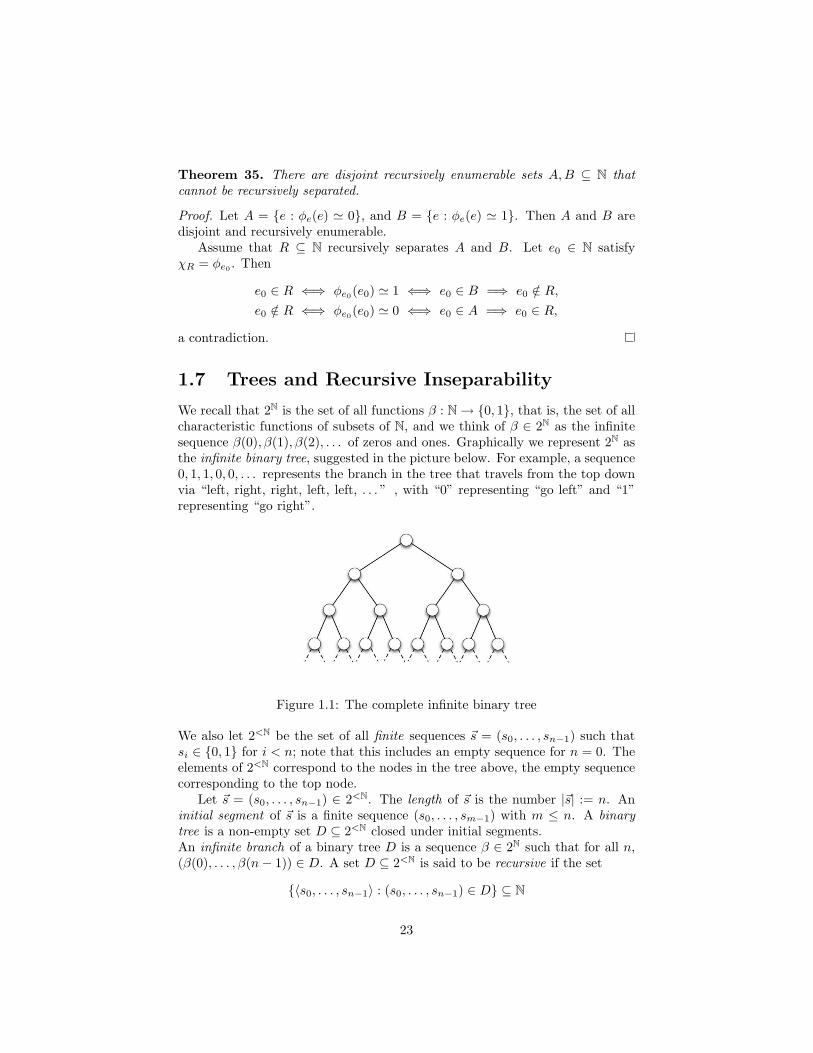
We recall that 2N is the set of all functions β : N→ {0, 1}, that is, the set of allcharacteristic functions of subsets of N, and we think of β ∈ 2N as the infinitesequence β(0), β(1), β(2), . . . of zeros and ones. Graphically we represent 2N asthe infinite binary tree, suggested in the picture below. For example, a sequence0, 1, 1, 0, 0, . . . represents the branch in the tree that travels from the top downvia “left, right, right, left, left, . . . ” , with “0” representing “go left” and “1”representing “go right”.

Figure 1.1: The complete infinite binary tree

We also let 2<N be the set of all finite sequences ~s = (s0, . . . , sn−1) such thatsi ∈ {0, 1} for i < n; note that this includes an empty sequence for n = 0. Theelements of 2<N correspond to the nodes in the tree above, the empty sequencecorresponding to the top node.

Let ~s = (s0, . . . , sn−1) ∈ 2<N. The length of ~s is the number |~s| := n. Aninitial segment of ~s is a finite sequence (s0, . . . , sm−1) with m ≤ n. A binarytree is a non-empty set D ⊆ 2<N closed under initial segments.An infinite branch of a binary tree D is a sequence β ∈ 2N such that for all n,(β(0), . . . , β(n− 1)) ∈ D. A set D ⊆ 2<N is said to be recursive if the set

{〈s0, . . . , sn−1〉 : (s0, . . . , sn−1) ∈ D} ⊆ N

23

Figure 1.2: A binary tree

is recursive.

Lemma 36. The full binary tree 2<N is recursive.

Proof. Let A := {〈s0, . . . , sn−1〉 : (s0, . . . , sn−1) ∈ 2<N}. Then

x ∈ A ⇐⇒ x ∈ B ∧∀∀∀i ≤ lh(x)(i = 0 ∨ (x)i = 0 ∨ (x)i = 1

).

Thus A is recursive.

Lemma 37 (Konig). Every infinite binary tree has an infinite branch.

Proof. Let D be an infinite binary tree. We define β : N → {0, 1} inductivelysuch that β is an infinite branch of D.

β(0) =

{0 if there are infinitely many ~s ∈ D such that s0 = 0,1 otherwise,

and for n > 0

β(n) =

0 if there are infinitely many ~s ∈ D such that|~s| > n, sn = 0 and si = β(i) for i < n,

1 otherwise.

Induction on n shows that for each n there are infinitely many ~s ∈ D such that|~s| > n and β(0) = s0, . . . , β(n) = sn. It follows that β is an infinite branch ofD. (It is actually the “leftmost” such branch.)

Theorem 38. There exists an infinite recursive binary tree with no recursiveinfinite branch.

24

Proof. Let A0, A1 ⊆ N be disjoint and recursively inseparable r.e. sets. Thuswe have recursive sets S0, S1 ⊆ N2 such that for all m,

A0(m) ⇐⇒ ∃∃∃nS0(m,n)A1(m) ⇐⇒ ∃∃∃nS1(m,n)

Next, define D ⊆ 2<N as follows; for ~s = (s0, . . . , sm−1) ∈ 2<N,

~s ∈ D ⇐⇒ ∀∀∀k < m [(∃∃∃n < m (k, n) ∈ Si)⇒ sk = i] for i = 0, 1.

It is easy to check that D is a recursive binary tree. To see that D is infinite weshow how to construct, for any m, a sequence of length m in D. The sequence(s0, . . . , sm−1) defined such that for k < m, if there exists an n < m with(k, n) ∈ S1, then sk = 1 and otherwise sk = 0, satisfies our requirements.

Next we show that for any infinite branch β : N→ {0, 1} of D, the set R ⊆ Nsuch that χR = β, is not recursive. Specifically, we show that R separates A0

and A1, and thus cannot be recursive.Let k ∈ Ai and take n such that (k, n) ∈ Si. Consider any sequence

(β(0), . . . , β(m − 1)) where m > k, n; note that (β(0), . . . , β(m − 1)) ∈ Dby assumption. Then by definition β(k) = i, so k ∈ A0 ⇒ k /∈ R andk ∈ A1 ⇒ k ∈ R, so R ∩ A0 = ∅ and A1 ⊆ R. If R was recursive thiswould contradict that A0 and A1 are not recursively separable.

1.8 Indices and Enumeration

In this section ψ = {ψne } is an index system, that is, for each n,

{ψne : e = 0, 1, . . .} = {f : Nn ⇀ N : f is partial recursive}.

Our earlier work shows that {φ(n)e } is an index system.

Definition 39. We say that ψ satisfies enumeration if for each n there is ana such that

ψn+1a (e, ~x) ' ψne (~x) for all (e, ~x) ∈ N1+n,

equivalently, λe~x.ψne (~x) : N1+n ⇀ N is partial recursive, for each n.We say that ψ satisfies parametrization if for all m,n there is a recursive s :N1+n → N such that

ψns(e,~x)(~y) ' ψm+ne (~x, ~y) for all (e, ~x, ~y) ∈ N1+m+n.

We say that ψ is acceptable if for each n there are recursive fn, gn : N → Nsuch that for all e

ψne = φ(n)fn(e) and φ(n)

e = ψngn(e)

The index system {φ(n)e } is trivially acceptable, and earlier results show that it

satisfies enumeration and parametrization. We put ψe := ψ1e .

25

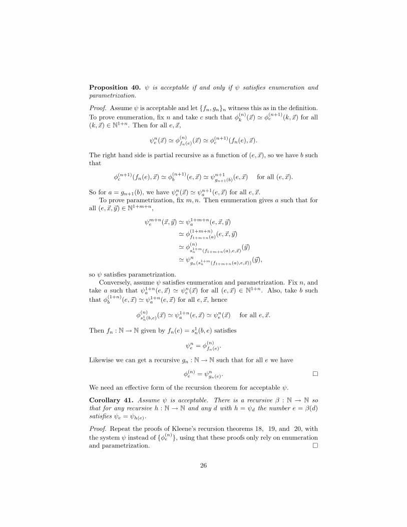
Proposition 40. ψ is acceptable if and only if ψ satisfies enumeration andparametrization.

Proof. Assume ψ is acceptable and let {fn, gn}n witness this as in the definition.To prove enumeration, fix n and take c such that φ(n)

k (~x) ' φ(n+1)c (k, ~x) for all

(k, ~x) ∈ N1+n. Then for all e, ~x,

ψne (~x) ' φ(n)fn(e)(~x) ' φ(n+1)

c (fn(e), ~x).

The right hand side is partial recursive as a function of (e, ~x), so we have b suchthat

φ(n+1)c (fn(e), ~x) ' φ(n+1)

b (e, ~x) ' ψn+1gn+1(b)(e, ~x) for all (e, ~x).

So for a = gn+1(b), we have ψne (~x) ' ψn+1a (e, ~x) for all e, ~x.

To prove parametrization, fix m,n. Then enumeration gives a such that forall (e, ~x, ~y) ∈ N1+m+n,

ψm+ne (~x, ~y) ' ψ1+m+n

a (e, ~x, ~y)

' φ(1+m+n)f1+m+n(a)(e, ~x, ~y)

' φ(n)

s1+mn (f1+m+n(a),e,~x)(~y)

' ψngn(s1+mn (f1+m+n(a),e,~x))

(~y),

so ψ satisfies parametrization.Conversely, assume ψ satisfies enumeration and parametrization. Fix n, and

take a such that ψ1+na (e, ~x) ' ψne (~x) for all (e, ~x) ∈ N1+n. Also, take b such

that φ(1+n)b (e, ~x) ' ψ1+n

a (e, ~x) for all e, ~x, hence

φ(n)s1n(b,e)(~x) ' ψ1+n

a (e, ~x) ' ψne (~x) for all e, ~x.

Then fn : N→ N given by fn(e) = s1n(b, e) satisfies

ψne = φ(n)fn(e).

Likewise we can get a recursive gn : N→ N such that for all e we have

φ(n)e = ψngn(e).

We need an effective form of the recursion theorem for acceptable ψ.

Corollary 41. Assume ψ is acceptable. There is a recursive β : N → N sothat for any recursive h : N → N and any d with h = ψd the number e = β(d)satisfies ψe = ψh(e).

Proof. Repeat the proofs of Kleene’s recursion theorems 18, 19, and 20, withthe system ψ instead of {φ(n)

e }, using that these proofs only rely on enumerationand parametrization.

26

Lemma 42 (Padding Lemma). Assume ψ is acceptable. Then we can effectivelyconstruct, for any a, infinitely many b such that ψa = ψb.

Proof. Given a and finite D ⊆ N such that ψd = ψa for all d ∈ D, we shallconstruct e 6∈ D with ψe = ψa. Define partial recursive g : N2 ⇀ N by

g(e, x) '{ψa(x) if e 6∈ D↑ if e ∈ D.

Enumeration and parametrization give a recursive f : N → N such that for all(e, x) ∈ N2,

ψf(e)(x) ' g(e, x)

The recursion theorem yields e0, effectively from a,D, with ψe0 = ψf(e0). Ifeo 6∈ D, then ψe0 = ψa and we are done. Suppose e0 ∈ D; then ψa = ψe0 , henceD(ψa) = D(ψe0) = ∅. So it remains to construct effectively an index e 6∈ Dwith D(ψe) = ∅. As before, we get a recursive h : N→ N such that

ψh(i)(x) ={

0 if i ∈ D↑ if i 6∈ D

The recursion theorem gives e1 with ψh(e1) = ψe1 . If e1 ∈ D, then

ψa = ψe1 = ψh(e1), a function with nonempty domain,

contradicting D(ψa) = ∅. So e1 6∈ D, hence D(ψe1) = ∅, and we are done.

Theorem 43. The index system ψ is acceptable if and only if for each n, thereis a recursive bijection h : N→ N such that ψne = φ

(n)h(e) for all e.

Proof. Such a bijection for each n witnesses the acceptability condition for ψ.Conversely, suppose ψ is acceptable. We shall construct h as in the theorem forn = 1, and we leave it to the reader to deal with arbitrary n.

We have recursive functions f, g : N→ N such that ψd = φf(d) and φe = ψg(e)for all d, e. We construct h in stages where at each stage n we have a partialfunction hn : N ⇀ N with |D(hn)| = n.

Stage 0: Take h0 with empty domain.

Stage 2n+ 1: Take the least d /∈ D(h2n) and use f and the padding lemma forφ to obtain effectively an e /∈ Im(h2n) such that ψd = φe. Define h2n+1 asan extension of h2n with D(h2n+1) = D(h2n) ∪ {d} with h2n+1(d) = e.

Stage 2n+ 2: Take the least e /∈ Im(h2n+1) and use g and the padding lemmato obtain effectively a d /∈ D(h2n+1) such that ψd = φe. Define h2n+2 asan extension of h2n+1 with D(h2n+2) = D(h2n+1)∪{d} with h2n+2(d) = e.

Then h =⋃hn has the desired properties.

27

Chapter 2

Hilbert’s 10th Problem

2.1 Introduction

Recursively enumerable sets occur outside pure recursion theory, most strikinglyin Hilbert’s 10th Problem, hereafter denoted H10:

Question. Is there an algorithm that decides for any given polynomial

f(X1, . . . , Xn) ∈ Z [X1, . . . , Xn]

whether the equation

f(X1, . . . , Xn) = 0 (2.1)

has a solution in Zn? A solution of (2.1) in Zn (or integer solution of (2.1)) isa tuple (x1, . . . , xn) ∈ Zn such that f(x1, . . . , xn) = 0. Likewise we define whatwe mean by a solution of (2.1) in Nn (or natural number solution).

The answer to H10 is known since 1970: there is no such algorithm. It is stillopen whether such an algorithm exists when n is fixed to be 2.

Observation. The following are equivalent:

(a) There is an algorithm that decides for any f(X1, . . . , Xn) ∈ Z [X1, . . . , Xn]whether (2.1) has a solution in Zn.

(b) There is an algorithm that decides for any f(X1, . . . , Xn) ∈ Z [X1, . . . , Xn]whether (2.1) has a solution in Nn.

Proof. Note that (2.1) has a solution in Zn if and only if one of the 2n equations

f(q1X1, . . . , qnXn) = 0,

with all qi ∈ {1,−1}, has a solution in Nn. This yields (b) =⇒ (a).

28

For the other direction we use Lagrange’s four-square theorem. By thistheorem, (2.1) has a solution in Nn if and only if the equation

f(X211 +X2

12 +X213 +X2

14, . . . , X2n1 +X2

n2 +X2n3 +X2

n4) = 0

has a solution in Zn.

In the following account of H10, we use the Observation above to restrictattention to natural number solutions for equations of type (2.1). Thus fromnow on in this chapter, u, x, y, z (sometimes with subscripts) range over N. Thisis in addition to the convention that a, b, c, d, e, k, l,m, n range over N.

Let A1, . . . , Am, X1, . . . , Xn be distinct polynomial indeterminates, A =(A1, . . . , Am), X = (X1, . . . , Xn), and f(A,X) ∈ Z[A,X]. We consider f(A,X)as defining the family of diophantine equations

f(~a,X) = 0, ~a ∈ Nm.

Definition 44. The diophantine set defined by f(A,X) is

{~a ∈ Nm : ∃∃∃~x (f(~a, ~x) = 0)}

A diophantine set in Nm is a diophantine set defined by some polynomial f(A,X) ∈Z[A,X], where X = (X1, . . . , Xn) and n can be arbitrary.

Lemma 45. Diophantine sets are recursively enumerable.

Proof. Let f = f(A,X) ∈ Z [A,X] be as before, and take g, h ∈ N [A,X] suchthat f = g − h. Then

{(~a, ~x) ∈ Nm+n : f(~a, ~x) = 0} = {(~a, ~x) ∈ Nm+n : g(~a, ~x) = h(~a, ~x)},

so {(~a, ~x) ∈ Nm+n : f(~a, ~x) = 0} is primitive recursive. Thus the set

{~a ∈ Nm : ∃∃∃~x (f(~a, ~x) = 0)}

is recursively enumerable.

Suppose we have a nonrecursive diophantine set D ⊆ Nm. Then, assumingthe Church-Turing Thesis, the answer to H10 is negative. To see why, takef(A,X) ∈ Z [A,X] as above such that

D = {~a ∈ Nm : f(~a,X1, . . . , Xn) = 0 has a solution in Nn}

Since D is not recursive, the Church-Turing Thesis says that there cannotexist an algorithm deciding for any ~a ∈ Nm as input, whether the equationf(~a,X) = 0 has a solution in Nn. In particular, there cannot exist an algorithmas demanded by H10.

The following is the key result. It gives much more than just a nonrecursivediophantine set.

29

Main Theorem [Matiyasevich 1970]. The diophantine sets in Nm are exactlythe recursively enumerable sets in Nm.

It follows that there is no algorithm as required in H10 (assuming the Church-Turing Thesis). Suggestive results in the direction of Matiyasevich’s theoremwere obtained by M. Davis, H. Putnam, and J. Robinson in the 50’s and 60’s.Basically, they reduced the problem to showing that the set

{(a, b) : b = 2a} ⊆ N2

is diophantine. This reduction is given in the next section.

2.2 Reduction to Exponentiation

Lemma 46. The following sets are diophantine.

(a) {(a, b) : a = b} ⊆ N2,

(b) {(a, b) : a ≤ b} ⊆ N2,

(c) {(a, b) : a < b} ⊆ N2,

(d) {(a, b) : a|b} ⊆ N2,

(e) {(a, b, c) : a ≡ b mod c} ⊆ N3,

(f) {(a, b, c) : c = |a, b|} ⊆ N3,

(g) {a : a 6= 2n for all n} ⊆ N.

Proof. Just note the following equivalences:

(a) a = b ⇐⇒ a− b = 0;

(b) a ≤ b ⇐⇒ ∃∃∃x a+ x = b;

(c) a < b ⇐⇒ ∃∃∃x a+ x+ 1 = b;

(d) a|b⇐⇒ ∃∃∃x ax = b;

(e) a ≡ b mod c ⇐⇒ ∃∃∃x∃∃∃y a− b = cx− cy;

(f) c = |a, b| ⇐⇒ 2c = (a+ b)(a+ b+ 1) + 2a;

(g) a 6= 2n for all n ⇐⇒ ∃∃∃x∃∃∃y (2x+ 3)y = a.

Lemma 47. Being diophantine is preserved under certain operations:

(a) If D,E ⊆ Nm are diophantine, so are D ∪ E,D ∩ E ⊆ Nm.

30

(b) If D ⊆ Nm+n is diophantine, so is π(D) ⊆ Nm where π : Nm+n → Nm isdefined by π(x1, . . . , xm, y1, . . . , yn) = (x1, . . . , xm).

(c) A set D ⊆ Nm is diophantine if and only if D is existentially definable inthe ordered semiring (N; 0, 1, +, ·, ≤).

Proof.

(a) Let D,E ⊆ Nm be diophantine, and take f, g ∈ Z [A;X] such that

D = {~a : ∃∃∃~x f(~a, ~x) = 0},E = {~a : ∃∃∃~x g(~a, ~x) = 0}.

Then clearly

D ∪ E = {~a : ∃∃∃~x f(~a, ~x)g(~a, ~x) = 0},D ∩ E = {~a : ∃∃∃~x f(~a, ~x)2 + g(~a, ~x)2 = 0}.

(b) Let D ⊆ Nm+n be diophantine, and take f ∈ Z [A,B,X] such that

D = {(~a,~b) : ∃∃∃~x f(~a,~b, ~x) = 0}

Then π(D) = {~a : ∃∃∃~b ∃∃∃~x f(~a,~b, ~x) = 0}.

(c) For (⇒) use that for each f ∈ Z[A,X] there exist g, h ∈ N [A,X] suchthat f = g − h.

For the (⇐) direction, note that for any quantifier free formula in thelanguage of (N; 0, 1,+, ·, <) you can get rid of inequalities, negations, dis-junctions, and conjunctions at the cost of introducing extra existentiallyquantified variables by means of the following equivalences:

x 6= y ⇔ ∃∃∃z (x+ z + 1 = y ∨ y + z + 1 = x) ,x = 0 ∨ y = 0 ⇔ xy = 0,x = 0 ∧ y = 0 ⇔ x2 + y2 = 0,

x < y ⇔ ∃∃∃z (x+ z + 1 = y) .

Definition 48. A diophantine function f : Nm → N is a function whose graphis a diophantine set in Nm+1.

For example, addition and multiplication are diophantine functions on N2, andso is the monus function. Also gcd : N2 → N is diophantine:

gcd(a, b) = c ⇐⇒ ∃∃∃x, y((ax− by = c ∨ by − ax = c) ∧ c|a ∧ c|b

).

31

Lemma 49. Let f : Nm → N, R ⊆ Nm and g1, . . . , gm : Nn → N be diophantine.Then the function f(g1, . . . , gm) : Nn → N, and the relation R(g1, . . . , gm) ⊆ Nndefined by

R(g1, . . . , gm)(~a) ⇐⇒ R(g1(~a), . . . , gm(~a))

are diophantine.

Proof. Exercise.

Some terminology. A polynomial zero set in Nn is a set {~x ∈ Nn : f(~x) = 0}where f(X) ∈ Z [X]. A projection of a set R ⊆ Nn is a set S = π(R) ⊆ Nmwith m ≤ n and π : Nn → Nm given by π(x1, . . . , xn) = (x1, . . . , xm).

Thus polynomial zero sets are primitive recursive, and the diophantine setsare just the projections of polynomial zero sets.

The bounded universal quantification of a set R ⊆ Nn+2, denoted ∀∀∀≤R, is thesubset of Nn+1 defined by: (∀∀∀≤R)(~x, y) ⇐⇒ ∀∀∀i≤y R(~x, y, i). Let Σ be thesmallest subset of

⋃m P(Nm) that contains all polynomial zero sets and is closed

under taking projections and bounded universal quantifications.

Proposition 50. Σ =⋃m{S : S is a recursively enumerable set in Nm}.

Before we can prove this we need to know that Σ is closed under some elementaryoperations like taking cartesian products and intersections. This is basically anexercise in predicate logic, which we now carry out.

Instead of N and its ordering we may consider in this exercise any nonemptyset A with a binary relation M on A. Till further notice we let a, b, x, y, some-times with indices, range over A, with vector notation like ~a used to denote atuple (a1, . . . , an) of the appropriate length n. For R ⊆ An+2 we define thebounded universal quantification ∀∀∀MR ⊆ An+1 of R by

(∀∀∀MR)(~a, b) :⇐⇒ ∀∀∀yMbR(~a, b, y) :⇐⇒ ∀∀∀y(y M b ⇒ R(~a, b, y)

),

For n ≥ m, let πnm : An → Am be given by πnm(x1, . . . , xn) = (x1, . . . , xm).Taking cartesian products commutes with projecting:

D ⊆ Ad, m ≤ n, S ⊆ An =⇒ D × πnm(S) = πd+nd+m(D × S).

It also commutes with bounded universal quantification:

D ⊆ Ad, R ⊆ An+2 =⇒ ∀∀∀M(D ×R) = D ×∀∀∀MR.

For λ : {1, . . . ,m} → {1, . . . , n} and S ⊆ Am we define

λ(S) := {(x1, . . . , xn) : (xλ(1), . . . , xλ(m)) ∈ S} ⊆ An.

Let for each n a collection Cn of subsets of An be given such that:

• A0 ∈ C0 and ∆ := {(x, y) : x = y} ∈ C2;

32

• C,D ∈ Cn =⇒ C ∩D ∈ Cn;

• λ : {1, . . . ,m} → {1, . . . , n} is injective, C ∈ Cm ⇒ λ(C) ∈ Cn.

With m = 0 in the last condition we obtain An ∈ C for all n. More generally,the inclusion map {1, . . . ,m} → {1, . . . ,m + n} shows that if C ∈ Cm, thenC × An ∈ Cn. Using also permutations of coordinates we see that if D ∈ Cn,then Am ×D ∈ Cm+n, and thus by intersecting C ×An and Am ×D,

C ∈ Cm, D ∈ Cn =⇒ C ×D ∈ Cm+n.

Also, if 1 ≤ i < j ≤ n, then ∆ni,j := {(x1, . . . , xn) : xi = xj} ∈ Cn.

An example of a family (Cn) with the properties above is obtained by takingCn to be the set of polynomial zerosets in Nn, with (A,M) = (N,≤).

Let C :=⋃n Cn, a subset of the disjoint union

⋃n P(An), and define Σ(C)

to be the smallest subset of⋃n P(An) that includes C, and is closed under

projection and bounded universal quantification. (In the example above for(A,M) = (N,≤) this gives Σ(C) = Σ.) Below we show that the conditionsimposed on C are inherited by Σ(C). The main issue is to deal with the factthat bounded universal quantification does not commute with some coordinatereindexings given by maps λ : {1, . . . ,m} → {1, . . . , n}.

Lemma 51. If D ∈ C, and S ∈ Σ(C), then D × S ∈ Σ(C).

Proof. Let D ∈ Cd. Define the subset Σ′ of Σ(C) to have as elements theS ∈ Σ(C) such that D × S ∈ Σ(C). Note that C ⊆ Σ′. Since projectionand bounded universal quantification commute with the operation of takingthe cartesian product with D as first factor, it follows that Σ′ is closed underprojection and bounded universal quantification. Thus Σ′ = Σ(C).

Lemma 52. If S ∈ Σ(C), S ⊆ Am, then:

(1) C ∩ S ∈ Σ(C) for all C ∈ Cm;

(2) λ(S) ∈ Σ(C) for all injective λ : {1, . . . ,m} → {1, . . . , n}.

Proof. Define the subset Σ′ of Σ(C) to have as its elements the S ⊆ Am, m =0, 1, 2 . . . , such that S ∈ Σ(C) and D ∩ λ(S) ∈ Σ(C) for all D ∈ Cn and injectiveλ : {1, . . . ,m} → {1, . . . , n}. Then C ⊆ Σ′. Next we show that Σ′ is closed underprojection. Let m ≤ n and S ⊆ An, S ∈ Σ′. To show that πnmS ∈ Σ′, let λ :{1, . . . ,m} → {1, . . . , k} be injective and D ∈ Ck. Then for ~a = (a1, . . . , ak) ∈Ak and with ~x = (x1, . . . , xn−m) ranging over An−m,(

D ∩ λ(πnmS))(~a) ⇔ D(~a) & (πnmS)(aλ(1), . . . , aλ(m))⇔ D(~a) & ∃∃∃~x S(aλ(1), . . . , aλ(m), ~x)

⇔ ∃∃∃~x(D(~a) & S(aλ(1), . . . , aλ(m), ~x)

)⇔ ∃∃∃~x

(D(~a) & (µS)(~a, ~x)

), where

µ : {1, . . . , n} → {1, . . . , k + n−m} is given byµ(j) = λ(j) for 1 ≤ j ≤ m, µ(m+ j) = k + j for 1 ≤ j ≤ n−m,

33

Since S ∈ Σ′, the set (D ×An−m) ∩ µS belongs to Σ(C), and so does

D ∩ λ(πnmS) = πk+n−mk

((D ×An−m) ∩ µS

).

Thus Σ′ is closed under projection. It remains to show that Σ′ is closed underbounded universal quantification, so let R ⊆ Am+2, R ∈ Σ′. To get ∀∀∀MR ∈ Σ′,let λ : {1, . . . ,m + 1} → {1, . . . , n} be injective and D ∈ Cn. Then for S =D ∩ λ(∀∀∀MR) and ~a = (a1, . . . , an),

S(~a) ⇔ D(~a) & (∀∀∀MR)(aλ(1), . . . , aλ(m+1))⇔ D(~a) & ∀∀∀yMaλ(m+1)R(aλ(1), . . . , aλ(m+1), y)

⇔ ∃∃∃x(D(~a) & x = aλ(m+1)& ∀∀∀yMxR(aλ(1), . . . , aλ(m), x, y)

)⇔ ∃∃∃x∀∀∀yMx

(D(~a) & x = aλ(m+1) & (µR)(~a, x, y)

), where

µ : {1, . . . ,m+ 2} → {1, . . . , n+ 2} is given byµ(j) = λ(j) for 1 ≤ j ≤ m, µ(m+ 1) = n+ 1, µ(m+ 2) = n+ 2.

Arguing as before this gives S ∈ Σ(C), and so Σ′ is closed under boundeduniversal quantification.

Corollary 53. If S, T ∈ Σ(C), then S × T ∈ Σ(C). If S, T ∈ Σ(C) and alsoS, T ⊆ An, then S ∩ T ∈ Σ(C).

Proof. Let S ⊆ An and S ∈ Σ(C). Define Σ′ to be the subset of Σ(C) whoseelements are the T ∈ Σ(C) with S × T ∈ Σ(C). It follows from Lemma 51and (2) of Lemma 52 that C ⊆ Σ′. Also, projection and bounded universalquantification commute with taking cartesian products with S as first factor,so Σ′ is closed under projection and bounded universal quantification. HenceΣ′ = Σ(C), which gives the first claim of the corollary. Now, with also T ⊆ An

and T ∈ Σ(C), we have

S ∩ T = π2nn

(∆2n

1,n+1 ∩ · · · ∩∆2nn,2n ∩ (S × T )

),

and so S ∩ T ∈ Σ(C) by (1) of Lemma 52.

We have now shown that Σ(C) inherits the conditions that we imposed on C.In particular, with (A,M) = (N,≤), it follows that Σ is closed under cartesianproducts and intersections. We now return to the setting where variables likea, b, x, y range over N and give the proof of Proposition 50:

Proof. For ⊆, note that the polynomial zero sets are primitive recursive, andhence recursively enumerable. Now use that the class of recursively enumerablesets is closed under taking projections and bounded universal quantifications.

For ⊇ we use the familiar inductive definition of “recursive function” to showthat these functions are in Σ, that is, their graphs are. It is clear that this holdsfor the initial functions (addition, multiplication, . . . ). Assume inductively that

34

the graphs of f : Nn → N and g1, . . . , gn : Nm → N belong to Σ. Then with~a = (a1, . . . , am) and ~x = (x1, . . . , xn) we have the equivalence

f(g1, . . . , gn)(~a) = b ⇐⇒ ∃∃∃~x(g1(~a) = x1 & . . .& gn(~a) = xn & f(~x) = b

),

which shows that the graph of f(g1, . . . , gn) belongs to Σ. Next, assume thatthe graph of g : Nn+1 → N is in Σ, that for all ~x ∈ Nn there is y such thatg(~x, y) = 0 and that f : Nn → N is given by f(~x) = µy g(~x, y) = 0. Then

f(~x) = y ⇐⇒ g(~x, y) = 0 & ∀∀∀i<y∃∃∃z g(~x, y) = z + 1,

so the graph of f belongs to Σ. It follows that every recursive set S ⊆ Nmis in Σ. It remains to use that recursively enumerable sets are projections ofrecursive sets.

It follows from Proposition 50 that to obtain the Main Theorem, it suffices toshow that if D ⊆ Nm+2 is diophantine, so is ∀≤D ⊆ Nm+1. Thus we have toeliminate a bounded universal quantifier in favour of existential quantifiers. Weshall be able to do this, but at the cost of introducing non-polynomial functionslike 2x. This reduces our task to showing that these functions are diophantine.

In order to eliminate bounded universal quantifiers, it helps to introduce thefunctions qu, rem : N2 → N (quotient and remainder), defined by

x = qu(x, y) · y + rem(x, y), whererem(x, y) < y if y 6= 0, rem(x, 0) = qu(x, 0) = x.

It is easy to check that qu and rem are diophantine. We also need the functionsx 7→ x! : N→ N and (x, y) 7→

(xy

): N2 → N, where(

x

y

)=

x(x− 1) . . . (x− y + 1)y!

={ x!

y!(x−y)! if x ≥ y,0 otherwise.

Lemma 54. If the function 2x is diophantine, so are xy,(xy

)and x!.

Proof. Trivially, 2xy ≡ x mod 2xy − x, so (2xy)y ≡ xy mod 2xy − x, that is,

2xy2≡ xy mod 2xy − x.

As xy < 2xy − x for y > 1, we have xy = rem(2xy2, 2xy − x) for y > 1. This

expression shows that if 2x is diophantine, so is xy.

For(xy

), note that 2x = (1 + 1)x =

∑xy=0

(xy

), so

(xy

)< 2x for x > 0. Also, we

have (1 + d)x =∑xy=0

(xy

)dy, which gives the base d expansion of (1 + d)x when

d ≥ 2x. In other words, for all x > 0, 0 ≤ y ≤ x and all n:(x

y

)= n⇐⇒ ∃∃∃c, d

[d = 2x, n < d, c < dy, (1 + d)x ≡ c+ ndy mod dy+1

].

35

This equivalence shows that if 2x is diophantine, then(xy

)is diophantine.

For x!, note that if y > x > 1 then(y

x

)=

y(y − 1) . . . (y − x+ 1)x!

=yx(1− 1

y ) . . . (1− x−1y )

x!.

An easy induction on n shows that for 0 ≤ ε1, . . . , εn ≤ 1 we have

n∏i=1

(1− εi) ≥ 1−n∑i=1

εi.

For x > 1 and y ≥ x2 this gives

x!(y

x

)≤ yx = x!

(y

x

)1

(1− 1y ) . . . (1− x−1

y )

≤ x!(y

x

)(1 +

x2

y

)= x!

(y

x

)+x2x!y

(y

x

).

Hence, if x2x!y < 1, then x! = qu(yx,

(yx

)). But x2x!

y < 1 for y ≥ 2xx+2, and thusx! = qu(yx,

(yx

)) for y = 2xx+2, x > 1. Therefore, x! is diophantine if 2x is.

We are going to reduce the proof of the Main Theorem to showing that 2x is adiophantine function. This reduction can be viewed as an elaborated version ofGodel’s coding lemma, which we review here for the reader’s convenience, sinceits proof is suggestive of what comes later.

Lemma 55. Let b1, . . . , bn ≤ B ∈ N. Then there is a unique β ∈ N such that

β <

n∏i=1

(1 + i · n!B) and bi = rem(β, 1 + i · n!B) for i = 1, . . . , n.

Proof. The numbers 1 + i ·n! ·B for i = 1, . . . , n are pairwise coprime: if p werea common prime factor of 1 + i · n!B and 1 + j · n!B with 1 ≤ i < j ≤ n, thenp | (j − i) · n!B, so p | n! or p | B, a contradiction.

Therefore, by the Chinese Remainder Theorem, there exists β ∈ N such thatβ ≡ bi mod 1 + i · n!B for i = 1, . . . , n and such a β is uniquely determinedmodulo

∏ni=1(1 + i · n! ·B).

Since bi < 1 + i · n! · B for i = 1, . . . , n, the unique β <∏ni=1(1 + i · n! · B)

with β ≡ bi mod 1 + i · n! ·B for i = 1, . . . , n has the desired property.

36

It will be convenient to fix some notation in the remainder of this section:

~a := (a1, . . . , am), ~b := (b1, . . . , bn), ~v := (v1, . . . , vn),~v ≤ y :⇐⇒ v1 ≤ y, . . . , vn ≤ y.

We showed that, for each m, the recursively enumerable sets in Nm are exactlythe subsets of Nm that are in Σ. Hence, to obtain the Main Theorem, it sufficesto prove: If D ⊆ Nm+2 is diophantine, then so is ∀∀∀≤D ⊆ Nm+1.

We first make a small further reduction. Let the diophantine set D ⊆ Nm+2 begiven by the equivalence

D(~a, x, u) ⇐⇒ ∃∃∃~v F (~a, x, u,~v) = 0

where F (A,X,U, V ) ∈ Z [A,X,U, V ], A = (A1, . . . , Am), V = (V1, . . . , Vn)and where A1, . . . , Am, X, U, V1, . . . , Vn are distinct polynomial indeterminates.Then for all ~a, x we have:

(∀≤D)(~a, x) ⇐⇒ ∀∀∀u≤x D(~a, x, u)⇐⇒ ∀∀∀u≤x ∃∃∃~v F (~a, x, u,~v) = 0⇐⇒ ∃∃∃y ∀∀∀u≤x ∃∃∃~v ≤ y F (~a, x, u,~v) = 0.

Thus it remains to show that for any F (A,X,U, V ) ∈ Z [A,X,U, V ], the set

{(~a, x, y) : ∀∀∀u≤x ∃∃∃~v≤y F (~a, x, u,~v) = 0} ⊆ Nm+2

is diophantine. The next result goes under the name of Bounded QuantifierTheorem. Besides the polynomial indeterminates in (A,X,U, V ), we let Y bean extra indeterminate which we allow also to occur in F :

Theorem 56. Suppose F (A,X, Y, U, V ) in Z[A,X, Y, U, V ] and G(A,X, Y ) inN[A,X, Y ] are polynomials such that for all ~a, x, y and all u ≤ x and ~v ≤ y,

G(~a, x, y) > |F (~a, x, y, u,~v)|+ 2x+ y + 2.

Then the following equivalence holds for all ~a, x, y, with g := G(~a, x, y):

∀∀∀u≤x ∃∃∃~v≤y F (~a, x, y, u,~v) = 0⇐⇒

∃∃∃~b[(

b1y+1

)≡ · · · ≡

(bny+1

)≡ F (~a, x, y, g!− 1,~b) ≡ 0 mod

(g!−1x+1

)]Before we start the proof, note that for any F ∈ Z[A,X, Y, U, V ] we obtainG(A,X, Y ) ∈ N[A,X, Y ] as in the hypothesis of the lemma as follows: LetF ∗ ∈ N[A,X, Y, U, V ] be obtained from F by replacing each coefficient with itsabsolute value and put

G(A,X, Y ) := F ∗(A,X, Y,X, Y, . . . , Y ) + 2X + Y + 3.

37

Proof. We shall refer to the equivalence in the Bounded Quantifier Theorem asthe BQ-equivalence. Let ~a, x, and y be given and put g = G(~a, x, y). Then(

g!− 1x+ 1

)=

(g!− 1)(g!− 2) . . . (g!− x− 1)1 · 2 · · · · · (x+ 1)

=g!− 1

1· g!− 2

2· · · · · g!− x− 1

x+ 1

=(g!1− 1)(

g!2− 1). . .

(g!

x+ 1− 1).

Since g > x+ 2, all x+ 1 factors in this last product are in N>1.

Claim 1. Each prime factor of(g!−1x+1

)is greater than g.

This is because g ≥ 2x+ 2, so every prime p ≤ g divides g!u+1 for each u ≤ x, so

no prime p ≤ g divides(g!−1x+1

).

Claim 2. The factors g!1 − 1, g!2 − 1, . . . , g!

x+1 − 1 are pairwise coprime.

To see why, suppose p is a prime factor of g!i −1, and g!j −1, with 1 ≤ i < j ≤ x+1.

Then p > g, but p | g!− i, p | g!− j, so p | j − i, contradicting j − i ≤ g.

For each u ≤ x, take a prime factor pu of g!u+1 − 1. Then

pu > g,g!

u+ 1− 1 ≡ 0 mod pu,

so g! ≡ u+ 1 mod pu, hence g!− 1 ≡ u mod pu. Thus for all ~b and all u ≤ x:

F (~a, x, y, g!− 1,~b) ≡ F (~a, x, y, u, rem(b1, pu), . . . , rem(bn, pu)) mod pu.

Now, assume that for each u ≤ x we have natural numbers vu1, vu2, . . . , vun ≤ ysuch that

F (~a, x, y, u, vu1, . . . , vun) = 0.

For i = 1, . . . , n, the Chinese Remainder Theorem provides bi <(g!−1x+1

)such

that bi ≡ vui mod g!u+1 − 1 for all u ≤ x. In other words,

g!u+ 1

− 1 | bi(bi − 1) · · · (bi − y) for i = 1, . . . , n and all u ≤ x.

Then by Claim 2,(g!−1x+1

)| bi(bi − 1) . . . (bi − y). By Claim 1 and g > y + 1, all

prime factors of(g!−1x+1

)are greater than y + 1. So,(

g!− 1x+ 1

)| bi(bi − 1) . . . (bi − y)

(y + 1)!=(

biy + 1

).

Hence, (b1

y + 1

)≡ · · · ≡

(bny + 1

)≡ 0 mod

(g!− 1x+ 1

).

38

For u ≤ x,(

g!u+1 − 1

)(u+ 1) = g!− (u+ 1) = (g!− 1)− u, so

g!− 1 ≡ u modg!

u+ 1− 1, hence

F (~a, x, y, g!− 1,~b) ≡ F (~a, x, y, u,~vu)

≡ 0 modg!

u+ 1− 1.

Thus, by the second claim, F (~a, x, y, g!− 1,~b) ≡ 0 mod(g!−1x+1

). This proves the

forward direction of the BQ-equivalence.

For the converse, let ~b be such that(b1

y + 1

)≡ · · · ≡

(bny + 1

)≡ F (a, x, y, g!− 1,~b) ≡ 0 mod

(g!− 1x+ 1

).

Then for 1 ≤ i ≤ n, u ≤ x:(bi

y + 1

)≡ 0 mod pu, so pu | bi(bi − 1) . . . (bi − y),

hence pu|bi − k for some k ≤ y, which gives rem(bi, pu) ≤ y. Hence

|F (~a, x, y, u, rem(b1, pu), . . . , rem(bn, pu))| < g < pu |(g!− 1x+ 1

),

and thus F (~a, x, y, u, rem(b1, pu), . . . , rem(bn, pu)) = 0, as desired.

Lemma 54 and The Bounded Quantifier Theorem reduce the proof of the MainTheorem to showing that the function 2x is diophantine. This will be achievedby exploiting subtle properties of solutions of Pell equations. In the next sectionwe derive the relevant facts about these equations. We finish this section witha digression on exponentially diophantine equations. Readers who want to takethe shortest path to a proof of the Main Theorem can skip this.

Exponentially diophantine sets. Some results above are conditional on thefunction 2x being diophantine. A nice way to eliminate the conditional natureof these results without proving outright that 2x is diophantine is as follows.Call a set E ⊆ Nm exponentially diophantine if for some polynomial

F (A,X, Y ) ∈Z[A,X, Y ], withA = (A1, . . . , Am), X = (X1, . . . , Xn), Y = (Y1, . . . , Yn),

the following equivalence holds for all ~a ∈ Nm:

E(~a) ⇐⇒ ∃∃∃~x F (~a, ~x, 2~x) = 0,

where 2~x := (2x1 , . . . , 2xn) for ~x = (x1, . . . , xn) ∈ Nn. Clearly, if E ⊆ Nm isdiophantine, then E is exponentially diophantine. Note that Lemma 45 goes

39

through with “exponentially diophantine” instead of “diophantine”. So doesLemma 47, where in part (c) the ordered semiring (N; 0, 1,+, ·,≤) is replacedby the ordered exponential semiring (N; 0, 1,+, ·, exp,≤) with exp(x) := 2x.A function f : Nm → N is said to be exponentially diophantine if its graph(as a subset of Nm+1) is exponentially diophantine. Then Lemma 49 goesthrough with “exponentially diophantine” instead of “diophantine”. The proofof Lemma 54 shows (unconditionally) that the functions xy,

(xy

), and x! are

exponentially diophantine. We are now approaching a proof of the followingunconditional result.

Theorem 57. For each set S ⊆ Nm,

S is recursively enumerable ⇐⇒ S is exponentially diophantine.

As stated, this is of course a consequence of the Main Theorem to be proved inthe next section, but it seems worth deriving this exponential version using justthe facts we have already established. Moreover, this exponential version holdsin an enhanced form that we briefly touch on at the end of this digression. Onemight try to prove Theorem 57 by an exponential analogue of the BQ-Theorem.However, the proof of that theorem doesn’t go through, since it can happen thatx ≡ y mod m, but 2x 6≡ 2y mod m.

Instead we shall focus on improving Proposition 50, which says that anygiven recursively enumerable set can be obtained from a polynomial zero setby a finite sequence of projections and bounded universal quantifications. Themain point is to show that bounded universal quantification is needed only oncein such a description of a given recursively enumerable set. This is an old resultdue to Martin Davis, the Davis Normal Form:

Proposition 58. Given any recursively enumerable set S ⊆ Nd, there is adiophantine set D ⊆ Nd+m+2 with the property that for all ~a ∈ Nd,

S(~a) ⇐⇒ ∃∃∃x1 . . .∃∃∃xm∃∃∃x ∀∀∀u≤x D(~a, x1, . . . , xm, x, u).

Proof. We first show how to interchange the order of bounded universal quan-tification and existential quantification. Let S ⊆ Nm+3. Using the ChineseRemainder Theorem to code finite sequences as in the proof of Lemma 55 wehave for all (~a, b) ∈ Nm+1,

∀∀∀u≤b ∃∃∃x S(~a, b, u, x)⇐⇒

∃∃∃y, z ∀∀∀u≤b S(~a, b, u, rem(y, 1 + (u+ 1)z)

).

Next, we show how to contract two successive bounded universal quantificationsinto a single bounded universal quantification, at the cost of an extra existentialquantification. Let L,R : N → N be the functions such that n = |L(n), R(n)|for all n. It is easy to check that L,R are diophantine. Let now S ⊆ Nm+4.

40

Then for all (~a, b, c) ∈ Nm+2:

∀∀∀u≤b ∀∀∀v≤c S(~a, b, c, u, v)⇐⇒

∀∀∀x≤|b,c|[(L(x) ≤ b & R(x) ≤ c) ⇒ S(~a, b, c, L(x), R(x))

]⇐⇒

∃∃∃y ∀∀∀x≤y[y = |b, c| & {

(L(x) ≤ b & R(x) ≤ c

)⇒ S(~a, b, c, L(x), R(x))

}]

Now an inductive argument using Proposition 50 yields the desired result.

The BQ-theorem in combination with Proposition 58 and the facts mentionedearlier on exponentially diophantine sets and functions show that any recursivelyenumerable set S ⊆ Nd is exponentially diophantine. This concludes the proofof Theorem 57.

2.3 Pell Equations

Below we assume that d ∈ N is not a square, that is,

d 6∈ sq(N) := {n2 : n = 0, 1, 2, . . . } = {0, 1, 4, 9, . . . }.

So 2, 3, 5, 6, 7, 8, 10, . . . are the possible values of d. Then

X2 − dY 2 = 1 (P)

is called a Pell equation. Note that (P) has the solution (1, 0), which we callthe trivial solution. Given any solution (a, b), we have the factorization

a2 − db2 = (a+ b√d)(a− b

√d) = 1,

which yields (a+ b√d)n(a− b

√d)n = 1, and taking a′, b′ such that

(a+ b√d)n = a′ + b′

√d, (a− b

√d)n = a′ − b′

√d,

we see that (a′, b′) is also a solution of (P).

Example. Consider the case d = 2. Then X2 − 2Y 2 = 1 has the non-trivialsolution (3, 2), and

(3 + 2√

2)2 = 9 + 12√

2 + 8 = 17 + 12√

2,

(3− 2√

2)2 = 9− 12√

2 + 8 = 17− 12√

2,

yielding another solution (17, 12).

A key fact in connection with H10 is that the solutions of (P) in N2 form a se-quence (xn, yn), n = 0, 1, 2, . . . where xn and yn grow roughly as an exponentialfunction of n. Our short term goal is to establish this fact.

41

Lemma 59. G := {x± y√d : x2 − dy2 = 1} is a subgroup of the multiplicative

group R>0 of positive real numbers.

Proof. First, 1 = 1 + 0√d, so 1 ∈ G. We have x2 − dy2 = (x+ y

√d)(x− y

√d),

so if x2 − dy2 = 1, then x− y√d = 1

x+y√d. Also,

(x1 + y1

√d)(x2 + y2

√d) = (x1x2 + dy1y2) + (x1y2 + x2y1)

√d

(x1 − y1

√d)(x2 − y2

√d) = (x1x2 + dy1y2)− (x1y2 + x2y1)

√d

Hence, if x21 − dy2

1 = x22 − dy2

2 = 1, then x2 − dy2 = 1 where

x := x1x2 + dy1y2, y := ±(x1y2 + x2y1).

Note that the x+ y√d ∈ G are ≥ 1 and the x− y

√d ∈ G are ≤ 1.

Corollary 60. Suppose (P) has a nontrivial solution in N2. Let (x1, y1) be sucha solution with minimal x1 > 1. Then the solutions in N2 of (P) are exactly the(xn, yn) ∈ N2 given by

(x1 + y1

√d)n = xn + yn

√d, n = 0, 1, 2, . . .

Proof. Put r := x1 + y1

√d, so r is the least element of G which is greater

than 1. We have 1 < r < r2 < . . . and rn → ∞ as n → ∞. Let (x, y)be a solution of (P). Take the unique n such that rn ≤ x + y

√d < rn+1.

Then 1 ≤ (x + y√d)r−n < r. By the previous lemma, (x + y

√d)r−n ∈ G, so

(x+ y√d)r−n = 1, that is, x+ y

√d = rn, so x = xn, y = yn.

If there is a non-trivial solution of (P) in N2, then (x1, y1) as in Corollary 60 iscalled the minimal solution of (P). Note that in this corollary, n = 0 yields thetrivial solution, and n = 1 the minimal solution.

We record two rules for solutions of (P), assuming there is a non-trivialsolution of (P) in N2. First, the addition rules:

xm+n = xmxn + dymyn, ym+n = xmyn + xnym,

which follow from the definitions of xn and yn, and the doubling rules, whichfollow from the addition rules:

x2n = 2x2n − 1, y2n = 2xnyn.

Our next goal is Lagrange’s theorem that non-trivial solutions of (P) in N2 doexist. First a lemma.

Lemma 61. Let ξ ∈ R>1 be irrational. Then there are infinitely many (x, y)with y > 0 such that

∣∣∣ξ − xy

∣∣∣ < 1y2 .

42

The obvious bound would be 1y , so the lemma says that there are much better

rational approximations to ξ, in terms of the size of the denominator. One canshow that replacing y2 in the lemma by yr with a fixed real number r > 2 wouldresult in a false statement for ξ =

√2.

Proof. Let n ≥ 1; we claim that there are x, y > 0 such that y ≤ n and∣∣∣∣ξ − x

y

∣∣∣∣ < 1ny≤ 1y2.

For y = 0, 1, 2, . . . , n, we have yξ = x + ε(y), where x ∈ N and 0 ≤ ε(y) < 1.Divide the interval [0, 1) into the n subintervals

[0, 1/n), [1/n, 2/n), . . . , [(n− 1)/n, 1).

By the pigeonhole principle, two of the n+ 1 numbers ε(0), ε(1), . . . , ε(n) mustlie in the same subinterval. Thus we have y1 < y2, both in {0, 1, . . . , n} suchthat |ε(y1)− ε(y2)| < 1/n. This gives x1 ≤ x2 such that

y1ξ = x1 + ε(y1), y2ξ = x2 + ε(y2).

Now set y = y2 − y1 and x = x2 − x1. We get yξ = x+ ε(y2)− ε(y1). So

|yξ − x| < 1n, and thus

∣∣∣∣ξ − x

y

∣∣∣∣ < 1ny.

We have x > 0 because ξ > 1 and 1ny < 1. For each n ≥ 1, take x(n), y(n) ∈ N>0

such that y(n) ≤ n and ∣∣∣∣ξ − x(n)y(n)

∣∣∣∣ < 1ny≤ 1y2.

As n goes to infinity, we have x(n)y(n) → ξ, so the set

{(x(n), y(n)) : n = 1, 2, 3, . . .}

is infinite.

Theorem 62. The equation (P) has a nontrivial solution in N2.

This theorem is due to Lagrange, but we give Dirichlet’s proof.

Proof. If x, y ∈ N>0 and∣∣∣√d− x/y∣∣∣ < 1/y2, then

0 <∣∣∣∣d− x2

y2

∣∣∣∣ =∣∣∣∣√d− x

y

∣∣∣∣ ∣∣∣∣√d+x

y

∣∣∣∣ < 1y2

(1 + 2

√d),

so0 <

∣∣x2 − dy2∣∣ < 1 + 2

√d.

43

By the previous lemma we have therefore a nonzero integer λ with |λ| < 1+2√d,

such that the equation

X2 − dY 2 = λ, (Pλ)

has infinitely many solutions (x, y) with x, y ∈ N>0. Consider two such solutionsof (Pλ), (x1, y1) and (x2, y2). Then:

x21 − dy2

1 = (x1 + y1

√d)(x1 − y1

√d) = λ,

x22 − dy2

2 = (x2 + y2

√d)(x2 − y2

√d) = λ,

so (x1 + y1

√d

x2 + y2

√d

)(x1 − y1

√d

x2 − y2

√d

)= 1.

Now we remove square roots from denominators:

x1 + y1

√d

x2 + y2

√d

=(x1 + y1

√d)(x2 − y2

√d)

(x2 + y2

√d)(x2 − y2

√d)

=(x1x2 − dy1y2) + (x2y1 − x1y2)

√d

λ,

x1 − y1

√d

x2 − y2

√d

=(x1 − y1

√d)(x2 + y2

√d)

(x2 − y2

√d)(x2 + y2

√d)

=(x1x2 − dy1y2)− (x2y1 − x1y2)

√d

λ.

Thus, setting

s :=∣∣∣∣x1x2 − dy1y2

λ

∣∣∣∣ , t :=∣∣∣∣x2y1 − x1y2

λ

∣∣∣∣ ,we get s2−dt2 = 1. The problem is that s and t might not be integers. However,(Pλ) has infinitely many solutions (x, y), so by the pigeonhole principle we canchoose (x1, y1) and (x2, y2) as above so that x1 ≡ x2 mod λ and y1 ≡ y2

mod λ, and (x1, y1) 6= (x2, y2). Then

x1x2 − dy1y2 ≡ x21 − dy2

1 ≡ 0 mod λ,

and x2y1 − x1y2 ≡ 0 mod λ, so s, t ∈ N.It remains to show that (s, t) is not the trivial solution to (P). Suppose

towards a contradiction that s = 1 and t = 0. Then x2y1 − x1y2 = 0, sox2/x1 = y2/y1. We can assume x2 > x1; set r = x2/x1 > 1. Then

x22 − dy2

2 = r2(x21 − dy2

1) = r2λ 6= λ,

a contradiction. So (s, t) is a nontrivial solution of (P) in N2.

Although this proof appears non-constructive, one can actually derive from itan explicit upper bound on the minimal solution: our use of the pigeonholeprinciple does not really need infinitely many solutions to (Pλ), but only morethan λ2, and we have |λ| < 1 + 2

√d.

44

The minimal solution of a Pell equation X2 − dY 2 = 0 varies rather wildlywith d. For our purpose we can restrict attention to a situation where theminimal solution is obvious: let a ≥ 2 and consider a Pell equation

X2 − (a2 − 1)Y 2 = 1, (Pa).

Its minimal solution is (a, 1). Now define xa(n), ya(n) ∈ N by

xa(n) + ya(n)√a2 − 1 = (a+

√a2 − 1)n.

By previous results, {(xa(n), ya(n)) : n = 0, 1, 2, . . .} is the set of all solutionsin N2. We now list several rules, most of which follow trivially from the earlieraddition and doubling rules. First of all, we have the addition rules:

xa(m+ n) = xa(m)xa(n) + (a2 − 1)ya(m)ya(n),ya(m+ n) = xa(m)ya(n) + xa(n)ya(m),

next, the doubling formulae:

xa(2n) = 2xa(n)2 − 1,ya(2n) = 2xa(n)ya(n),

the simultaneous recursion equations:

xa(0) = 1, xa(n+ 1) = axa(n) + (a2 − 1)ya(n),ya(0) = 0, ya(n+ 1) = xa(n) + aya(n),

and the course-of-values recursion:

xa(0) = 1, xa(1) = a, xa(n+ 2) = 2axa(n+ 1)− xa(n),ya(0) = 0, ya(1) = 1, ya(n+ 2) = 2aya(n+ 1)− ya(n).

One can prove the course-of-values recursion, for example, as follows:

xa(n+ 2) = axa(n+ 1) + (a2 − 1)ya(n+ 1)= axa(n+ 1) + (a2 − 1) [xa(n) + aya(n)]= axa(n+ 1) + (a2 − 1)xa(n) + a [xa(n+ 1)− axa(n)]= 2axa(n+ 1)− xa(n).

In addition we have a result about growth:

(2a− 1)n ≤ ya(n+ 1) < (2a)n

2n ≤ ya(n) for n ≥ 2

Exercise. Prove the growth result.

Finally, we state some congruence rules: for a, b ≥ 2 we have

ya(n) ≡ n mod (a− 1)ya(n) ≡ yb(n) mod (a− b)

45

Proof. For the first result, we have ya(0) = 0 ≡ 0 mod (a−1) and ya(1) = 1 ≡ 1mod (a− 1). Thus we can apply induction:

ya(n+ 2) ≡ 2ya(n+ 1)− ya(n) mod (a− 1)≡ 2(n+ 1)− n≡ n+ 2 mod (a− 1).

For the second result, we note that it holds for n = 0, 1, and also that a ≡ bmod (a− b). Thus,

ya(n+ 2) ≡ 2bya(n+ 1)− ya(n) mod (a− b),

which shows that ya(n) satisfies the same recursion as yb(n) modulo (a−b).

Lemma 63 (Periodicity). Suppose m,n > 0 and ya(n) ≡ 0 mod m. Then forall k, l, if k ≡ l mod 2n, then ya(k) ≡ ya(l) mod m.

Thus the remainder rem(ya(k),m) is periodic as a function of k, with perioddividing 2n, where the period is the least p ∈ N>0 such that

rem(ya(k),m) = rem(ya(k + lp),m) for all k, l.

Proof. Just observe the following equalities and congruences:

ya(k + 2n) = xa(k)ya(2n) + xa(2n)ya(k)= 2xa(k)xa(n)ya(n) + (2xa(n)2 − 1)ya(k)≡ (2xa(n)2 − 1)ya(k) mod m

≡[2((a2 − 1)ya(n)2 + 1

)− 1]ya(k) mod m

≡ ya(k) mod m.

We note also that for any m > 0, there is an n > 0 so that ya(n) ≡ 0 mod m.This is because for d := m2(a2 − 1) the Pell equation X2 − dY 2 = 1 has anon-trivial solution, say (x, y). Then (x,my) is a nontrivial solution to (Pa).

Next we prove some “step-down” lemmas. Roughly speaking, these pro-vide more precise information about the period in the sequence of remaindersrem(ya(k),m) when m has a special form. In addition, they provide informationabout n from information about ya(n).

Lemma 64 (First Step-Down Lemma). Let m,n > 0. Then:

ya(m)|ya(n) ⇐⇒ m|n,ya(m)2|ya(n) ⇐⇒ mya(m)|n.

46

Proof. Assume first that m|n, so n = mk, k > 0. Then

xa(n) + ya(n)√a2 − 1 = (a+

√a2 − 1)mk

=((a+

√a2 − 1

)m)k=

(xa(m) + ya(m)

√a2 − 1

)k.

Expanding the right hand side by the binomial theorem and comparing coeffi-cients of

√a2 − 1, we get

(∗) ya(n) = kxa(m)k−1ya(m) + ya(m)3 · (integer).

In particular, (*) yields that ya(m) divides ya(n), proving the backwards direc-tion of the implication.

Conversely, assume that ya(m)|ya(n). Towards a contradiction, let m - n.Then n = qm+ r with q, r ∈ N and 0 < r < m. By the addition formula,

ya(n) = ya(qm+ r) = xa(qm)ya(r) + xa(r)ya(qm).

From ya(m)|ya(qm), we obtain ya(m)|xa(qm)ya(r). But ya(qm) and xa(qm)are coprime, so ya(m) and xa(qm) are coprime. Hence ya(m)|ya(r), whichcontradicts 0 < ya(r) < ya(m). This proves the first equivalence.

For the second, first note that both sides of the equivalence imply m|n, sowe can assume n = mk, with k ∈ N>0. Then we again apply (*):

ya(m)2|ya(n) ⇐⇒ ya(m)2|kxa(m)k−1ya(m)⇐⇒ ya(m)|kxa(m)k−1

⇐⇒ ya(m)|k⇐⇒ mya(m)|n.

Lemma 65 (Second Step-Down Lemma). Let n ≥ 1 and suppose that ya(k) ≡ya(l) mod xa(n). Then k ≡ ±l mod 2n.

Proof. Let i, j ∈ N. Then the following congruences hold:

ya(2n+ i) ≡ −ya(i) mod xa(n)ya(2n− i) ≡ ya(i) mod xa(n) for 0 ≤ i ≤ nya(4n+ i) ≡ ya(i) mod xa(n)ya(4n− i) ≡ −ya(i) mod xa(n) for 0 ≤ i ≤ n

We prove the first of these congruences, leave the second as an exercise, andnote that the third and fourth follow easily from applications of the first andsecond. The proof of the first congruence is as follows.

ya(2n+ i) = xa(2n)ya(i) + xa(i)ya(2n)≡ xa(2n)ya(i) mod xa(n)≡ (2xa(n)2 − 1)ya(i) mod xa(n)≡ −ya(i) mod xa(n)

47

The second line here uses xa(n)|ya(2n), which follows from the doubling formula.Next we have two incongruences to the effect that the congruences above are insome sense best possible:

ya(i) 6≡ ±ya(j) mod xa(n) for 0 ≤ i < j ≤ n,ya(i) 6≡ −ya(i) mod xa(n) for 0 < i ≤ n.

To prove these incongruences we assume a > 2, and leave the somewhat specialcase a = 2 to the reader. Then

xa(n) =√

(a2 − 1)ya(n)2 + 1 > ya(n)√a2 − 1 > 2ya(n)

The first incongruence now follows because for 0 ≤ i < j ≤ n,

xa(n) > 2ya(n) ≥ ya(j)± ya(i).

The second incongruence holds because if 0 < i ≤ n, then

xa(n) > 2ya(n) ≥ 2ya(i) > 0.

Now put i = rem(k, 4n), j = rem(l, 4n). Then

ya(i) ≡ ya(j) mod xa(n).

If i = j then k ≡ l mod 4n, so k ≡ l mod 2n. If i 6= j, then a close lookat the four initial congruences and the two incongruences above yields i ≡ −jmod 2n, so k ≡ −l mod 2n.

2.4 Proof of the Main Theorem

We are now ready to show that {(a, n, y) : a ≥ 2, y = ya(n)} ⊆ N3 is diophan-tine. In the next result and its proof, all variables range over N.

Theorem 66. Let a, y, n ≥ 2. Then the following are equivalent

• y = ya(n);

• there are x, u, v, s, t, b such that

(i) 2n ≤ y (vi) b ≡ 1 mod y

(ii) x2 − (a2 − 1)y2 = 1 (vii) t ≡ y mod u

(iii) v ≥ 1 & u2 − (a2 − 1)v2 = 1 (viii) t ≡ n mod y

(iv) b ≥ 2 & s2 − (b2 − 1)t2 = 1 (ix) y2|v.(v) b ≡ a mod u

48

Proof. Let x, u, v, s, t, b be as in (i)–(ix). Then take k, l,m such that

y = ya(k), u = xa(l), t = yb(m).

We shall prove that k = n, so y = ya(n). By (iii), l ≥ 1. By the congruencerules we have yb(m) ≡ ya(m) mod b− a, and so by (v),

yb(m) ≡ ya(m) mod xa(l).

By (vii) we have yb(m) ≡ ya(k) mod xa(l), so

ya(m) ≡ ya(k) mod xa(l)

By the second step down lemma,

m ≡ ±k mod 2l

By (ix), ya(k)2|ya(l), so by the first step down lemma, kya(k)|l, so y|l and thus

m ≡ ±k mod y (2.2)

By the congruence rules, yb(m) ≡ m mod (b− 1), so

yb(m) ≡ m mod y by (vi),yb(m) ≡ n mod y by (viii)

n ≡ m mod y and thus by (2.2),n ≡ ±k mod y (2.3)

By (i) and an earlier result on the bounds on solutions of Pa we have 2n ≤ y,2k ≤ y, which in view of (2.3) yields n = k, so y = ya(n), as desired.

For the converse, assume ya(n) = y. Then (ii) holds with x = xa(n). Take

l := nya(n), u := xa(l), v := ya(l).

Then (iii) holds. By the first step down lemma,

y2 = (ya(n))2|ya(l) = v ≥ 1

and (ix) holds. By (iii), u, v are coprime, and y|v, so u, y are coprime. By theChinese Remainder Theorem we get b ≥ 2 such that

b ≡ a mod u

b ≡ 1 mod y

Then (v) and (vi) hold. Now take s := xb(n), t := yb(n). Then (iv) holds, andthe congruence rules yield (vii) and (viii).

Corollary 67. The function x 7→ 2x is diophantine.

49

Proof. Let a ≥ 2. Then

(2a− 1)n ≤ ya(n+ 1) ≤ (2a)n, (4a− 1)n ≤ y2a(n+ 1) ≤ (4a)n.

Therefore

2n(

1− 14a

)n=

(4a− 1)n

(2a)n≤ y2a(n+ 1)

ya(n+ 1)≤ (4a)n

(2a− 1)n= 2n

(1 +

12a− 1

)n.

For fixed n, with a→∞,(1 +

12a− 1

)n→ 1,

(1− 1

4a

)n→ 1.

So for some B(n) ∈ N>0, whenever a > B(n), then∣∣∣∣y2a(n+ 1)ya(n+ 1)

− 2n∣∣∣∣ < 1

2,

hence for all a > B(n) and all m,

2n = m ⇐⇒ 2 |y2a(n+ 1)−mya(n+ 1)| < ya(n+ 1).

So it only remains to show that there is a diophantine function B : N → N>0

such that for all n and all a > B(n),∣∣∣∣y2a(n+ 1)ya(n+ 1)

− 2n∣∣∣∣ < 1

2.

We have

2n(

1− 14a

)n≥ 2n

(1− n

4a

)= 2n − n2n

4a,

so if 4a > 2n2n, then 2n(1− 1

4a

)n> 2n − 1

2 . Also,

2n(

1 +1

2a− 1

)n≤ 2n

(1 +

n2n

2a− 1

)= 2n +

n22n

2a− 1,

so if 2a−1 > 2n22n, then 2n(

1 + 12a−1

)n< 2n+ 1

2 . As 5n ≤ y3(n+1) ≤ 6n, we

can take B(n) := 2ny3(n + 1) + 1. Then B(n) > 2n22n, so B is a diophantinefunction as desired.

The main theorem has now been established. It gives much more than a negativesolution to H10.

Exercise. Show that there is no algorithm determining for any system

P1(X1, . . . , Xn) = · · · = Pm(X1, . . . , Xn) = 0

50

with all Pi ∈ Z[X1, . . . , Xn] of degree ≤ 2, whether the system has a solutionin Zn. Using this, show that there is no algorithm determining for any givenequation

P (X1, . . . , Xn) = 0

with P ∈ Z[X1, . . . , Xn] of degree ≤ 4 whether the equation has a solution inZn.

The answer to H10 is not even known for polynomial equations in two variables.There is, however, an algorithm to decide for any given P ∈ Z[X,Y ] whetherP (X,Y ) = 0 has infinitely many integer solutions. This follows from a deeptheorem due to C.L. Siegel (1929), with some extra work. There is also analgorithm based on other work by Siegel to decide whether a given polynomialequation P (X1, . . . , Xn) = 0 with P ∈ Z[X1, . . . , Xn] of degree 2, has an integersolution.

It is not known whether H10 has a positive answer when we allow rationalsolutions instead of integer solutions. On the other hand, H10 does have apositive answer when we allow real solutions, or p-adic solutions; this followsfrom the stronger result that the elementary theory of the real field is decidable(Tarski), and likewise for the elementary theory of each p-adic field (Ax–Kochen& Ersov).

51

Chapter 3

Kolmogorov Complexity

This is a theory about randomness using concepts of recursion theory. The ideais that a long finite string of 0’s and 1’s is random if any program to computethe string is about as long as the string itself.

Instead of natural numbers it is more convenient to work with finite stringsof 0’s and 1’s, that is, elements of 2<N, as the inputs and outputs of algorithms.We let x, y, z, π, ρ, σ, τ range over 2<N. For σ = (σ0, . . . , σn−1) we defined itslength |σ| = n; the concatenation of x, y is denoted xy. The tree coding of 2<N

is the bijection tr : 2<N → N indicated in the picture below:

∅�

��

��

QQQQQ0

���

@@@

1�

��

@@@00

���

BBB

01���

BBB

10���

BBB

11���

BBB

000 001 010 011 100 101 110 111

-tr

0�

����

QQQQQ1

���

@@@

2���

@@@3

���

BBB

4���

BBB

5���

BBB

6���

BBB

7 8 9 10 11 12 13 14

In words, tr is the unique bijection 2<N → N such that tr(σ) < tr(τ) if |σ| < |τ |,or |σ| = |τ | and σ precedes τ lexicographically. Via this bijection the notionof partial recursive function Nd ⇀ N can be transferred to a notion of partialrecursive function (2<N)d ⇀ 2<N. Precisely, a partial function f : (2<N)d ⇀ 2<N

is declared to be partial recursive if the partial function g : Nd ⇀ N such that

g(tr(x1), . . . , tr(xd)) ' tr(f(x1, . . . xd))

is partial recursive. Note: 2|σ| − 1 ≤ tr(σ) ≤ 2|σ|+1 − 2.

52

3.1 Plain Kolmogorov Complexity

Let f : 2<N ⇀ 2<N be a partial recursive function. The (plain) Kolmogorovcomplexity of σ with respect to f is

Cf (σ) ={

min{|ρ| : f(ρ) = σ} if there is ρ ∈ Df such that f(ρ) = σ,∞ otherwise.

We say that σ is Kolmogorov random with respect to f if Cf (σ) ≥ |σ|.Let U : 2<N × 2<N ⇀ 2<N be a universal partial recursive function. That is,

U is partial recursive and

{U(π, ·) : π ∈ 2<N} = {f : 2<N ⇀ 2<N : f is partial recursive}.

Define the partial recursive function u : 2<N ⇀ 2<N by

u(0|π|1πρ) ' U(π, ρ),

u(σ) ↑ if σ does not have the form 0|π|1πρ.

Then 1 ≤ Cu(σ) < ∞ for all σ: the left inequality holds because u(∅) ↑, andthe right inequality holds because U(π, ·) = id2<N for some π. This complexityfunction Cu is as good as any, up to an additive constant:

Lemma 68. For all partial recursive f : 2<N ⇀ 2<N and all σ,

Cu(σ) ≤ Cf (σ) + const(f).

Here and later const(f) denotes a constant in N depending only on f . Likewise,const denotes an absolute constant in N. (Of course, the possible values of constmay vary with the context.)

Proof. Let π be such that f = U(π, ·). If ρ ∈ Df and f(ρ) = σ, thenu(0|π|1πρ) = σ and |0|π|1πρ| = |ρ|+ 2|π|+ 1. Thus for all σ:

Cu(σ) ≤ Cf (σ) + 2|π|+ 1.

Definition 69. C := Cu : 2<N → N.

This complexity function C depends on the initial choice of U , but only in aninessential way: Let U ′ : 2<N× 2<N ⇀ 2<N also be a universal partial recursivefunction, with C ′ : 2<N → N as its associated complexity function. Then thereis a constant c ∈ N such that |C(σ) − C ′(σ)| ≤ c for all σ. Our interest isin the behaviour of C on sufficiently long strings, and we regard C and C ′ asequivalent for this purpose.

Lemma 70. The following hold:

(a) C(x) ≤ |x|+ const;

53

(b) C(xx) ≤ |x|+ const;

(c) if h : 2<N → 2<N is recursive, then for all x

C(h(x)) ≤ C(x) + const(h).

Proof. For f = id2<N we have Cf (x) = |x|. So C(x) ≤ |x| + const. This gives(a). Let h : 2<N → 2<N be recursive, and put f := h ◦ u. Then

C(h(x)) ≤ Cf (h(x)) + const(f)≤ Cu(x) + const(f)= C(x) + const(h).

This yields (c), and (b) is a special case of (c).

Call x random if C(x) ≥ |x|. For each n, there is a random x with |x| = n. Thisfollows from the pigeon hole principle:

|{τ : |τ | < n}| = 20 + 21 + · · ·+ 2n−1 = 2n − 1,

and |{τ : |τ | = n}| = 2n, so the partial map

σ 7→ u(σ) : {σ : |σ| < n} ⇀ {x : |x| = n}

cannot be surjective. More precisely, we have the following result.

Lemma 71. For all n and all k ∈ {0, . . . , n},

|{x : |x| = n, C(x) ≥ n− k}| > 2n(1− 12k

).

Proof. We have |{τ : |τ | < n − k}| = 20 + 21 + · · · + 2n−k−1 = 2n−k − 1, so|{x : |x| = n, C(x) ≥ n− k}| ≥ 2n − (2n−k − 1) > 2n(1− 1

2k).

Thus C(x) ≥ 90 for more than 99.9% of the strings x of length 100.

Lemma 72 (Martin-Lof). Let k ∈ N be given. Then any sufficiently long z hasan initial segment x with C(x) < |x| − k.

Proof. Let f : 2<N → 2<N be the recursive function satisfying f(σ) = ρσ, wheretr(ρ) = |σ|. Take ∆ ∈ N such that C < Cf + ∆. Let z be a string satisfying|z| > 2k+∆+2, and let ρ be the initial segment of z with |ρ| = k + ∆. Letr = tr(ρ); then 2|ρ|−1 ≤ r < 2|ρ|+1−1, hence |ρ|+r < k+∆+2k+∆+1−1 ≤ |z|.

Take x = z||ρ|+r (the initial segment of z of length |ρ| + r). Then x = ρσ,with |σ| = r, so f(σ) = ρσ = x. Hence,

C(x) < Cf (x) + ∆ ≤ |σ|+ ∆ = (|ρ| − (∆ + k)) + |σ|+ ∆= |ρ|+ |σ| − k = |x| − k.

54

Corollary 73. For all sufficiently long random z, there are x, y such that z =xy, but C(x) + C(y) < C(z).

Proof. Take k ∈ N such that for all σ, C(σ) ≤ |σ|+ k. Let z be random and solong that it has an initial segment x with C(x) < |x| − k. Take y with z = xy.Then C(x) + C(y) < |x| − k + |y|+ k = |x|+ |y| = |z| ≤ C(z).

Call a string σ compressible if C(σ) < |σ|. Then the Martin-Lof lemma saysthat any sufficiently long string has compressible initial segments, and any suf-ficiently long random string can be decomposed into two strings the sum ofwhose complexities is strictly less than that of the original string. Thus, the de-composition itself stores information additional to that contained in the stringsseparately.

The logarithms below are with respect to base 2, so log 2n = n.

Lemma 74. C(xy) ≤ C(x) + C(y) + 2 logC(x) + const.

Proof. Let f : 2<N ⇀ 2<N be the partial recursive function that takes as inputsthe strings 0|ρ|1ρστ , where |σ| = tr(ρ), with output f(0|ρ|1ρστ) := u(σ)u(τ).

Let x,y be given. Take σ,τ be of minimum length such that u(σ) = x andu(τ) = y. Then C(x) = |σ| > 0, and C(y) = |τ | > 0. Take ρ such that|σ| = tr(ρ). Then 2|ρ|−1 ≤ 2|ρ| − 1 ≤ |σ| = C(x), so logC(x) ≥ |ρ| − 1. Thenf(0|ρ|1ρστ) = xy, and

|0|ρ|1ρστ | = |σ|+ |τ |+ 2|ρ|+ 1 ≤ C(x) + C(y) + 2(log(C(x))− 1) + 1= C(x) + C(y) + 2 log(C(x))− 1,

hence

C(xy) ≤ Cf (xy) + const(f) ≤ C(x) + C(y) + 2 logC(x) + const.

The next result has a striking consequence for the incompleteness of any givenaxiomatic framework for mathematics, as we discuss after the proof.

Proposition 75. The set A = {x : C(x) ≥ |x|2 } of half-random strings is

immune; that is, A has no infinite recursively enumerable subset. In particular,A is not recursively enumerable, and thus C : 2<N → N is not recursive.

Proof. Suppose B is an infinite r.e. subset of A. We can find a recursive functionh : 2<N → 2<N such that for all σ, h(σ) ∈ B and |h(σ)| ≥ tr(σ). Then we haveC(h(σ)) ≥ |h(σ)|

2 ≥ tr(σ)2 , and C(h(σ)) ≤ C(σ) + const ≤ |σ| + const. Thus,

tr(σ)2 ≤ |σ|+ const, a contradiction.

By Lemma 71, almost all strings are half random: the probability that a stringof length n is half random goes to 1 very rapidly as n→∞. As a consequenceof Proposition 75, however, there are only finitely many σ for which ZFC can

55

prove that σ is half random, assuming of course that ZFC is consistent. (HereZFC is the standard axiomatic set theory in which essentially all of mathematicscan be formally derived, including the entire contents of this course.) The sameremains true for any recursively axiomatized consistent extension of ZFC.

3.2 Prefix-Free Sets

We say that σ and τ are comparable if σ is an initial segment of τ or τ is an initialsegment of σ. We call a set A ⊆ 2<N prefix-free if any two distinct σ, τ ∈ Aare incomparable. Finite strings are going to be treated as initial segments ofinfinite strings of zeros and ones, and in the rest of this chapter we let α, β besuch infinite strings, that is α, β : N→ {0, 1}; we consider α, β also as points ofthe so-called Cantor space 2N. We let α|n := (α(0), . . . , α(n− 1)) ∈ 2<N be theinitial segment of α of length n.

We make 2N a topological space by giving it the product topology, where{0, 1} is given the discrete topology. So 2N has the clopen sets

Nσ := {α : α(i) = σ(i) for all i < |σ|}

as a basis for its topology. Note that N∅ = 2N, and that σ and τ are incompa-rable iff Nσ ∩Nτ = ∅.

Let µ be the probability measure on the σ-algebra of Borel subsets of 2N

(the σ-algebra on 2N generated by the Nσ) given by µ(Nσ) = 2−|σ|.

Lemma 76. Suppose A ⊆ 2<N is prefix-free. Then∑σ∈A

12|σ|≤ 1.

Proof.∑σ∈A

12|σ|

=∑σ∈A µ(Nσ) = µ(

⋃σ∈ANσ) ≤ µ(2N) = 1.

Theorem 77 (Kraft-Chaitin). Let (di)i∈N be a sequence of natural numberssuch that

∑∞i=0

12di≤ 1. Then there is an injective sequence (σi)i∈N such that

|σi| = di for all i and {σi : i ∈ N} is prefix-free.

Proof. We can assume that d0 ≤ d1 ≤ d2 ≤ . . . . Then we choose σ0, σ1, σ2, . . .successively by always choosing the left-most possibility. For example, whend0, d1, d2, d3 are 2, 3, 3, 4, this is illustrated by the following picture.

���

��

QQQQQ

���

@@@

���

@@@

σ0 ���

BBB

���

BBB

���

BBB

σ1 σ2 ���

DDD

σ3

���

DDD

���

DDD

���

DDD

56

The assumption that∑∞i=0

12di≤ 1 guarantees that we can always continue

this process. We make this precise as follows. Take σ0 = 0 . . . 0, with |σ0| =d0. By the induction hypothesis, suppose that at stage n, we have pairwiseincomparable σ0, . . . , σn satisfying |σi| = di for i = 0, . . . , n and such that allα with tr(α|dn) ≤ tr(σn) belong to Nσ0 ∪ · · · ∪ Nσn . Then there is a σ with|σ| = dn and tr(σ) > tr(σn); otherwise, all α would belong to Nσ0 ∪ · · · ∪Nσn ,yielding 1 = µ(Nσ0 ∪ · · · ∪Nσn) =

∑ni=0

12di

<∑∞i=0

12di≤ 1, a contradiction.

Let σ satisfy |σ| = dn and tr(σ) = tr(σn) + 1. Define σn+1 := σ0 . . . 0 with|σn+1| = dn+1. It is easy to verify that σ0, . . . , σn+1 are pairwise incomparable,and all α with tr(α|dn+1) ≤ tr(σn+1) belong to Nσ0 ∪ · · · ∪Nσn+1 .

This proof contains an inconstructive step, namely the initial rearrangementof the di in increasing order. It is desirable to have a more constructive proofwhich avoids this.

Constructive proof. We make the inductive assumption that at stage n, we haveσ0, . . . , σn with |σi| = di for i = 0, . . . , n, and for 0 ≤ i < j ≤ n, σi and σj areincomparable and that in addition we have τn1 , . . . , τ

np , p ≥ 1, such that

|τn1 | < · · · < |τnp |, 2N = Nσ0 t · · · tNσn tNτn1 t · · · tNτnp ,

where the square union signs indicate a disjoint union. Here p depends on n.For n = 0, the inductive assumption is realized as follows: note that d0 > 0 andput σ0 = 0 . . . 0, with |σ0| = d0. If d0 = 1, set p = 1, and τ0

1 = 1; if d0 ≥ 2, setp = d0, and τ0

i = 0 . . . 01, with |τ0i | = i.

Given stage n, we construct σn+1 at stage n + 1 as follows. We are givendn+1. If |τni | = dn+1, 1 ≤ i ≤ p, then we set σn+1 := τni , so

2N = Nσ0 t · · · tNσn tNσn+1 tNτn1 t · · · tNτni−1tNτni+1

t · · · tNτnp .

We put

τn+1j =

{τnj if 1 ≤ j ≤ i− 1τnj+1 if i+ 1 ≤ j ≤ p.

Now suppose that for all i ∈ {1, . . . , p}, |τni | 6= dn+1. It is easy to check that|τn1 | < dn+1. Take i ∈ {1, . . . , p} maximal such that |τni | < dn+1. Set k :=dn+1−|τni |. Take ρ1, . . . , ρk, σn+1 such that ρj = τni 0 . . . 01, with |ρj | = |τni |+ j(so |ρk| = dn+1) for 1 ≤ j ≤ k, and σn+1 = τni 0 . . . 0, with |σn+1| = dn+1. Then

Nτni = Nρ1 t · · · tNρk tNσn+1 .

Thus replacing τni in the sequence τn1 , . . . , τnp by ρ1, . . . , ρk yields a sequence

τn+11 , . . . , τn+1

p+k−1 with the desired properties.

This constructive proof of the Kraft-Chaitin Theorem yields:

Proposition 78. Let i 7→ di : N → N be recursive such that∑∞i=0 2−di ≤ 1.

Then there is a recursive injective map i 7→ σi : N → 2<N such that |σi| = difor all i and {σi : i ∈ N} is prefix-free.

57

Here a function f : N→ 2<N is said to be recursive if tr(f) : N→ N is recursive.

Exercise. Show that for each Y ⊆ 2<N there is a prefix-free X ⊆ Y such that⋃σ∈Y

Nσ =⋃σ∈X

Nσ.

3.3 Prefix-Free Complexity

A partial recursive function f : 2<N ⇀ 2<N is said to be prefix-free if its domainD(f) ⊆ 2<N is prefix-free. In order to construct an effective enumeration of

{f : 2<N ⇀ 2<N| f is partial recursive and prefix-free},

we first associate to each partial recursive f : N ⇀ N the partial recursivef : 2<N ⇀ 2<N by tr(f(σ)) ' f(tr(σ)). Next, recall our enumeration (φe) of{f : N ⇀ N| f is partial recursive}. We defined φe,s : N ⇀ N for s ∈ N by

φe,s(x) '{φe(x) if ∃∃∃z ≤ s T1(e, x, z)↑ otherwise

with D(φe,s) ⊆ {0, . . . , s}, φe =⋃s φe,s. This yields an enumeration (φe) of

{f : 2<N ⇀ 2<N| f is partial recursive}

and for each s a function φe,s : 2<N ⇀ 2<N with

D(φe,s) ⊆ {σ : tr(σ) ∈ {0, . . . , s}},

such that φe =⋃s φe,s for each e. Define ψe,s : 2<N ⇀ 2<N by recursion on s :

ψe,0 = φe,0

ψe,s+1 ={φe,s+1 if φe,s+1 is prefix-freeψe,s otherwise

So φe,0 ⊆ ψe,1 ⊆ ψe,2 ⊆ . . . . Put

ψe :=⋃s

ψe,s : 2<N ⇀ 2<N.

A bit of thought shows:

(a) each ψe is partial recursive and prefix-free;

(b) (ψe) is an enumeration of

{f : 2<N ⇀ 2<N | f is partial recursive and prefix-free};

(c) there is a recursive ι : N→ N such that ψe = φι(e) for all e.

58

Define Ψ : 2<N ⇀ 2<N by

Ψ(0e1σ) ' ψe(σ),Ψ(ρ) ↑ if ρ 6= 0e1σ for all e and σ.

Note: Ψ is partial recursive, prefix-free, surjective, and CΨ(σ) ∈ N>0 for all σ.

Lemma 79. Let f : 2<N ⇀ 2<N be prefix-free and partial recursive. Then

CΨ ≤ Cf + const(f)

Proof. Take e such that f = ψe. Then CΨ ≤ Cf + (e+ 1).

Definition 80. The prefix-free complexity of a string σ is

K(σ) := CΨ(σ) ∈ N>0.

Lemma 81. There are infinitely many σ such that K(σ) > |σ|+ log |σ|.

Proof. Suppose K(σ) ≤ |σ| + log |σ| for all but finitely many σ. Then, with σranging over the nonempty strings, we have∑

σ

2−K(σ) ≥∑σ

2−(|σ|+log |σ|) + const

=∞∑n=1

∑|σ|=n

2−(n+logn) + const

=∞∑n=1

2n2−(n+log n) + const

=∞∑n=1

1n

+ const =∞.

Since Ψ is surjective, we have an injective map σ 7→ σ′ : 2<N → D(Ψ) such thatΨ(σ′) = σ and K(σ) = |σ′|. for all σ. Since Ψ is prefix-free,

1 ≥∑

ρ∈D(Ψ)

2−|ρ| ≥∑σ

2−|σ′| =

∑σ

2−K(σ) =∞,

a contradiction.

The only fact about log that we used is that∑∞n=1 2− logn = ∞. The same

proof yields the following generalization:

Lemma 82. If f : N>0 → R>0 satisfies∑∞n=1 2−f(n) = ∞, then there are

infinitely many σ such that K(σ) > |σ|+ f(|σ|).

Let n∗ ∈ 2<N be the string such that tr(n∗) = n. For example, if σ has length1000 ≈ 210, then |σ|∗ is the string whose tree code is 1000, thus |σ|∗ has lengthabout 10. More generally, length(|σ|∗) ≈ log(length(σ)).

59

Proposition 83. K(σ) < |σ|+ 2 log|σ|+ const for nonempty σ.

Proof. It suffices to find a prefix-free partial recursive f : 2<N ⇀ 2<N and ac ∈ N such that for all nonempty σ there exists ρ with

f(ρ) ' σ, |ρ| < |σ|+ 2 log|σ|+ c.

We shall construct such f via the effective version of the Kraft-Chaitin Theorem,using

∑k=0

110(k+1)2 ≤ 1. Let nk = b 2k+1

10(k+1)2 c ∈ N. Note that nk → ∞ ask →∞. Define di ∈ N by

di = 1 for 0 ≤ i < n0,

di = 2 for n0 ≤ i < n0 + n1,

di = 3 for n0 + n1 ≤ i < n0 + n1 + n2,

...di = k + 1 for n0 + n1 + · · ·+ nk−1 ≤ i < n0 + n1 + · · ·+ nk.

Then∞∑i=0

2−di = n02−1 + n12−2 + . . .

=∞∑k=0

nk2−(k+1)

≤∞∑k=0

2k+1

10(k + 1)2· 2−(k+1)

=∞∑k=0

110(k + 1)2

≤ 1.

The function i 7→ di : N→ N is recursive, so by the Kraft-Chaitin Theorem wehave an injective recursive map i 7→ ρi : N → 2<N such that |ρi| = di for all i,and {ρi : i ∈ N} is prefix-free. Now define f : {ρi : i ∈ N} → 2<N by f(ρn) = n∗.Note that f : 2<N ⇀ 2<N is prefix-free, partial recursive, and surjective.

To show f has the above property, note first that there are nk strings in{ρi : i ∈ N} of length k + 1. For m > 0 and k = bm+ 2 logm+ cc, c ∈ N,

60

nk ≥ 2k+1

10(k + 1)2− 1

≥ 2m+2 logm+c

10(m+ 2 logm+ c+ 1)2− 1

≥ 2m · 2logm2 · 2c

10(m+ 2 logm+ c+ 1)2− 1

≥ 2m ·m2 · 2c

10(m+ 2 logm+ c+ 1)2− 1

≥ 2m+1 for c = 10.

Therefore, if 0 < |σ| ≤ m, we obtain ρi such that

|ρi| ≤ m+ 2 logm+ 11, and f(ρi) = σ.

Theorem 84. K(σ) ≤ |σ|+K(|σ|∗) + const.

Proof. Since Ψ is prefix-free, each string σ has at most initial segment ρ ∈ D(Ψ).So we can define a prefix-free f : 2<N → 2<N by

f(σ) ' τ ⇐⇒ ∃∃∃ρ (σ = ρτ and Ψ(ρ) ' |τ |∗).

Then f is partial recursive, so K(τ) = CΨ(τ) ≤ Cf (τ) + const.We claim that Cf (τ) ≤ |τ |+ K(|τ |∗). To see this, take ρ of minimal length

such that Ψ(ρ) ' |τ |∗. Then |ρ| = K(|τ |∗), and f(ρτ) ' τ. Hence,

Cf (τ) ≤ |ρτ | = |τ |+ |ρ| = |τ |+K(|τ |∗).

From this claim, we obtain

K(τ) ≤ Cf (τ) + const ≤ |τ |+K(|τ |∗) + const .

3.4 Information Content Measures

Here and below we let k range over N.

Definition 85. An information content measure (icm) is a partial functionI : 2<N ⇀ N such that

(a)∑σ∈D(I) 2−I(σ) ≤ 1;

(b) the set {(σ, k) : σ ∈ D(I), I(σ) ≤ k} ⊆ 2<N ×N is recursively enumerable.

61

The next two results establish a close connection between partial recursiveprefix-free functions and icm’s, almost a one-to-one correspondence.

Lemma 86. Let ψ : 2<N ⇀ 2<N be prefix-free partial recursive. Then the partialfunction Iψ : 2<N ⇀ N with D(Iψ) = Im(ψ), and Iψ(σ) = Cψ(σ) for σ ∈ Im(ψ)is an icm.

Proof. ∑σ∈D(Iψ)

2−Iψ(σ) =∑

σ∈Im(ψ)

2−Cψ(σ) ≤∑

ρ∈D(ψ)

2−|ρ| ≤ 1.

Also, σ ∈ D(Iψ), Iψ(σ) ≤ k ⇐⇒ ∃∃∃ρ(|ρ| ≤ k, ψ(ρ) ' σ

). Therefore, the set

{(σ, k) : σ ∈ D(Iψ), Iψ(σ) ≤ k} ⊆ 2<N × N

is recursively enumerable.

For ψ = Ψ, this yields Iψ = K, so K is an icm. Conversely,

Lemma 87. Let I be an icm with infinite domain D(I). Then there is a prefix-free partial recursive map ψ : 2<N ⇀ 2<N such that

(a) D(I) = Im(ψ);

(b) I(σ) + 1 = Cψ(σ) for all σ ∈ D(I).

Proof. Take a recursive map i 7→ (σi, ki) : N→ 2<N × N with image

{(σ, k) : σ ∈ D(I), I(σ) ≤ k}.

We construct a set A ⊆ {(σ, k + 1) : σ ∈ D(I), I(σ) ≤ k} in stages.

• Stage 0: Put (σ0, k0 + 1) in A.

• Stage s + 1: Compute (σs+1, ks+1), see whether ks+1 < ki for all i ≤ swith σi = σs+1, and if so, put (σs+1, ks+1 + 1) in A.

Note: σ ∈ D(I)⇐⇒ ∃∃∃d(σ, d) ∈ A: the direction ⇐ is clear, and ⇒ holds in themore precise form that if σ ∈ D(I), then min{d : (σ, d) ∈ A} = I(σ) + 1.

Put A(σ) := {d : (σ, d) ∈ A}. Then, for σ ∈ D(I),∑d∈A(σ)

2−d ≤ 2−(I(σ)+1) + 2−(I(σ)+2) + · · · ≤ 2 · 2−(I(σ)+1) = 2−I(σ), so

∑(σ,d)∈A

2−d =∑

σ∈D(I)

∑d∈A(σ)

2−d ≤∑

σ∈D(I)

2−I(σ) ≤ 1.

By construction, A is r.e. and infinite, so there is an injective recursive map

i 7→ (σ′i, di) : N→ 2<N × N

62

with image A. By the last inequality we have∑∞i=0 2−di ≤ 1, so the recursive

version of Kraft-Chaitin yields a recursive injective map i 7→ ρi : N→ 2<N suchthat |ρi| = di for all i, and {ρi : i ∈ N} is prefix-free. Now define ψ : 2<N ⇀ N tohave domain D(ψ) = {ρi : i ∈ N} and ψ(ρi) = σ′i for all i. Then ψ is prefix-freepartial recursive and Im(ψ) = D(I). It remains to check that (b) is satisfied:

Let σ ∈ D(I) = Im(ψ). Then

Cψ(σ) = min{di : i ∈ N, σ = σ′i} = min{d : (σ, d) ∈ A} = I(σ) + 1.

The next lemma follows from K being an icm with D(K) = 2<N.

Lemma 88. The set

{(m,n, k) :∑|σ|=m

2−K(σ) ≥ n

2k} ⊆ N3

is recursively enumerable.

Proof. Just note that∑|σ|=m 2−K(σ) ≥ n

2kif and only if there is a tuple

(nσ)|σ|=m of natural numbers such that∑|σ|=m

2−nσ ≥ n

2kand K(σ) ≤ nσ for each σ with |σ| = m.

Lemma 89. There is an enumeration (Ie)e∈N of the set of icms such that

{(σ, e, k) ∈ 2<N × N× N : σ ∈ D(Ie), Ie(σ) ≤ k}

is recursively enumerable.

Proof. Note that we have a recursive bijection

(σ, n) 7→ | tr(σ), n| : 2<N × N→ N.

Using this bijection the sets We and their finite approximations We,s yield anenumeration (Ve) of the set of recursively enumerable subsets of 2<N ×N and afamily (Ve,s) of finite subsets of 2<N × N with the following properties:

(a) Ve,s ⊆ {(σ, n) : | tr(σ), n| ≤ s};

(b) |Ve,0| ≤ 1, Ve,s ⊆ Ve,s+1, and⋃s Ve,s = Ve;

(c) {(σ, n, e, s) ∈ 2<N × N3 : (σ, n) ∈ Ve,s} is recursive.

63

Define ηe,s : 2<N ⇀ N by ηe,s(σ) := µn((σ, n) ∈ Ve,s

), so D(ηe,s) is finite,

D(ηe,s) ⊆ D(ηe,s+1), and ηe,s+1(σ) ≤ ηe,s(σ) for all σ ∈ D(ηe,s). Moreover, thepartial map

(e, s, σ) 7→ ηe,s(σ) : N2 × 2<N ⇀ N

is partial recursive and has recursive domain. Next, define Ie,s : 2<N ⇀ N byrecursion on s: Ie,0 := ηe,0 , Ie,s+1 = ηe,s+1 if ηe,s+1 is an icm, and Ie,s+1 = Ie,sotherwise. Identifying functions with their graphs, it is easy to check that Ie,sis a finite icm, D(Ie,s) ⊆ D(Ie,s+1), and Ie,s+1(σ) ≤ Ie,s(σ) for all σ ∈ D(Ie,s),and

(e, s, σ) 7→ Ie,s(σ) : N2 × 2<N ⇀ N

is partial recursive and has recursive domain. In particular, the set

{(σ, n, e, s) ∈ 2<N × N3 : Ie,s(σ) ' n}

is recursive. Define Ie : 2<N ⇀ N by

D(Ie) =⋃s

D(Ie,s), Ie(σ) = min{Ie,s(σ) : σ ∈ D(Ie,s)}.

Given any icm I, take e such that Ve = {(σ, k) : σ ∈ D(I), I(σ) ≤ k}, and notethat then I = Ie. It follows easily that (Ie) is an enumeration of the set of icmsas required by the lemma.

Fix an enumeration (Ie) of the set of icms as in the lemma above. This allowsus to define K : 2<N → N by

K(σ) := min{Ie(σ) + e+ 1 : Ie(σ) ↓}

Lemma 90. K is an icm.

Proof. Condition (a) in the definition of icm holds for K:

∑σ

2−K(σ) ≤∞∑e=0

∑σ∈D(Ie)

2−(Ie(σ)+e+1)

=∞∑e=0

2−(e+1)∑

σ∈D(Ie)

2−Ie(σ)

≤∞∑e=0

2−(e+1) = 1.

Condition (b) is satisfied by K, since

K(σ) ≤ k ⇐⇒ ∃∃∃e(σ ∈ D(Ie), Ie(σ) + e+ 1 ≤ k).

64

This icm K is also called the minimal icm. We can use it to prove results aboutK because of the following fact.

Corollary 91. |K − K| ≤ const.

Proof. We already know that K ≤ K + const. Since K is an icm, Lemma 87gives a prefix-free partial recursive ψ : 2<N ⇀ 2<N such that Cψ = K + 1.Hence, K(σ) ≤ Cψ(σ) + const = K(σ) + 1 + const.

Theorem 92 (Counting Theorem). We have

(a) |{σ : |σ| = n, K(σ) < n+K(n∗)− k}| ≤ 2n−k+const;

(b) n+K(n∗) + const ≤ max{K(σ) : |σ| = n} ≤ n+K(n∗) + const.

Proof. Assuming (a) for the moment, we show how (b) follows. Let c ∈ N be avalue of const for which (a) holds. Then

|{σ : |σ| = n, K(σ) < n+K(n∗)− c− 1}| ≤ 2n−1 < 2n.

So we get σ with |σ| = n such that K(σ) ≥ n + K(n∗) − c − 1. This gives thelower bound in (b). The upper bound is given by Theorem 84.

To prove (b), note first that

1 ≥∑σ

2−K(σ)

=∞∑n=0

∑|σ|=n

2−K(σ)

=∑ρ

∑|σ|=tr(ρ)

2−K(σ).

Take I(ρ) ∈ [1,∞) with 2−I(ρ) =∑|σ|=tr(ρ) 2−K(σ), that is,

I(ρ) = − log

∑|σ|=tr(ρ)

2−K(σ)

.

Then∑ρ 2−I(ρ) ≤ 1, so I is like an icm, except that I may have values not in

N. So we modify I to I : 2<N → N>0 by I(ρ) := dI(ρ)e.

Claim. I is an information content measure.

To prove this claim, note that∑ρ 2−I(ρ) ≤

∑ρ 2−I(ρ) ≤ 1, and

I(ρ) ≤ k ⇐⇒ I(ρ) ≤ k⇐⇒ 2−I(ρ) ≥ 2−k

⇐⇒∑

|σ|=tr(ρ)

2−K(σ) ≥ 2−k.

65

Using for example lemma 88 it follows that the set

{(ρ, k) : I(ρ) ≤ k} = {(ρ, k) :∑

|σ|=tr(ρ)

2−K(σ) ≥ 2−k}

is recursively enumerable. This finishes the proof of the claim.This claim and earlier results yield a c ∈ N such that K(σ) ≤ I(σ) + c for

all σ. Then

K(n∗) ≤ I(n∗) + c

≤ I(n∗) + c+ 1

= − log

∑|σ|=n

2−K(σ)

+ c+ 1.

Therefore,2−K(n∗)+c+1 ≥

∑|σ|=n

2−K(σ).

Let F := {σ : |σ| = n, K(σ) < n + K(n∗) − k}, and assume |F| ≥ 2n−k+c+1.Then by the above,

2−K(n∗)+c+1 ≥∑|σ|=n

2−K(σ)

≥∑σ∈F

2−K(σ)

> 2n−k+c+1 · 2−n−K(n∗)+k

= 2−K(n∗)+c+1,

a contradiction.

Likewise, we obtain the following.

Proposition 93. |{σ : |σ| = n, K(σ) < n− k}| ≤ 2n−K(n∗)−k+const.

Proof. Take c as in the previous proof. Let F := {σ : |σ| = n,K(σ) < n − k}.Assume |F| > 2n−K(n∗)−k+c+1. Then

2−K(n∗)+c+1 ≥∑|σ|=n

2−K(σ)

≥∑σ∈F

2−K(σ)

> 2n−K(n∗)−k+c+1 · 2−(n−k)

= 2−K(n∗)+c+1,

a contradiction.

66

3.5 Martin-Lof Randomness

A set T ⊆ N× 2<N is called a Martin-Lof test if T is recursively enumerableand for all n,

µ

⋃σ∈T (n)

Nσ

≤ 2−n where T (n) = {σ : (n, σ) ∈ T}.

A set B ⊆ 2N is said to have effective measure zero if there is a Martin-Lof testT such that B ⊆

⋂n

(⋃σ∈T (n)Nσ

). Note that µ(B) = 0 for such B, and that

every Martin-Lof test T determines a largest subset of 2N of effective measurezero witnessed by T , namely

NT :=⋂n

⋃σ∈T (n)

Nσ

.

We say that α passes the Martin-Lof test T if α /∈ NT . We say that α is 1-random if it passes every Martin-Lof test. We are going to show that thereis Martin-Lof test such that passing it is equivalent to passing all Martin-Loftests. Such a Martin-Lof test is said to be universal. Note that if T is a universalMartin-Lof test, then NT is the largest subset of 2N of effective measure zero;in particular, this set is independent of the choice of universal Martin-Lof test.This is somewhat remarkable, since for, say, Lebesgue measure on R, there isobviously no largest subset of R of measure zero.

Theorem 94 (Martin-Lof). There exists a universal Martin-Lof test.

Proof. Let R ⊆ N × N × 2<N be recursively enumerable such that (R(e))e∈Nenumerates

{S ⊆ N× 2<N : S is recursively enumerable}and such that for all e there exists infinitely many e′ with R(e) = R(e′). Takea recursive function f : N→ N× N× 2<N such that Image(f) = R and define

Rt = {f(0), f(1), . . . , f(t)} ⊆ R, t ∈ N.

Then R0 ⊆ R1 ⊆ . . . , R =⋃t∈N Rt and

Rt(e, n, σ)⇐⇒ ∃∃∃s ≤ t [f(s) = (e, n, σ)] ,

so the set{(t, e, n, σ) : Rt(e, n, σ)} ⊆ N× N× N× 2<N

is recursive.

Define T ⊆ N× 2<N by

T (k, σ) ⇐⇒ ∃∃∃n≥k+1 ∃∃∃t

Rt(n, n, σ) & µ

⋃τ∈Rt(n,n)

Nτ

≤ 2−n

.67

It is is rather clear from the Church-Turing Thesis that T is recursively enu-merable. Note also that T (0) ⊇ T (1) ⊇ T (2) ⊇ . . . . Put Bnt :=

⋃τ∈Rt(n,n)Nτ ,

so Bn0 ⊆ Bn1 ⊆ . . . . Moreover,

µ

⋃σ∈T (k)

Nσ

= µ

⋃n≥k+1

⋃µ(Bnt )≤2−n

Bnt

≤

∑n≥k+1

µ

⋃µ(Bnt )≤2−n

Bnt

≤

∑n≥k+1

2−n

= 2−k.

Thus T is a Martin-Lof test. To see that T is universal, let S ⊆ N× 2<N be anyMartin-Lof test and take m such that R(m) = S. Fix any k and take n ≥ k+ 1such that R(n) = R(m) = S. Then

NS =⋂l∈N

⋃σ∈S(l)

Nσ =⋂l∈N

⋃σ∈R(n,l)

Nσ ⊆⋃

σ∈R(n,n)

Nσ.

Now Bnt ⊆⋃σ∈R(n,n)Nσ for each t, and R(n) is a Martin-Lof test, so

µ (Bnt ) ≤ µ

⋃σ∈R(n,n)

Nσ

≤ 2−n.

In particular, σ ∈ R(n, n) ⇒ σ ∈ T (k). Hence,⋂l

⋃σ∈S(l)Nσ ⊆

⋃σ∈T (k)Nσ.

Since k was arbitrary, we obtain

NS =⋂l

⋃σ∈S(l)

Nσ ⊆⋂k

⋃σ∈T (k)

Nσ = NT ,

so NT is a largest set of effective measure zero.

Corollary 95. The set {α : α is 1-random} has measure 1. In other words,almost all α are 1-random.

Exercise. Show that no recursive α is 1-random.

We say that α is LGC-random if there exists c ∈ N such that K(α|n) ≥ n − cfor all n. Note that α|n = α(0), α(1), . . . , α(n− 1) is the initial segment of α oflength n.

It wouldn’t be interesting to replace K by C in this definition, as by Martin-Lof’scompressability lemma, given any α and any and c ∈ N, there exists infinitelymany n such that C(α|n) < n− c.

68

Theorem 96 (Schnorr).

α is LGC-random ⇐⇒ α is 1-random.

Proof. (of ⇐) Define T ⊆ N× 2<N by T (k, σ)⇐⇒ K(σ) ≤ |σ| − k.

Claim. T is a Martin-Lof test.

To prove this claim note first that T is recursively enumerable. Moreover,

µ

⋃σ∈T (k)

Nσ

≤∑

K(σ)≤|σ|−k

2−|σ|

≤∑σ

2−K(σ)−k

= 2−k∑σ

2−K(σ)

≤ 2−k.

Thus T is a Martin-Lof test. Now suppose α is 1-random. Then α passes T , sowe obtain k such that α 6∈

⋃σ∈T (k)Nσ, that is,

K(α|n) > |σ| − k for all n,

so α is LGC-random.

For the converse we need:

Lemma 97. Let T ⊆ N × 2<N be a ML-test. Then there exists an ML-testT ⊆ N× 2<N such that for all k,

(a) ⋃σ∈T (k)

Nσ =⋃

σ∈T (k)

Nσ,

(b) T (k) ⊆ 2<N is prefix-free.

Proof. Let f : N → N × 2<N be recursive and such that Im(f) = T . In addi-tion, we let s, k range over N for the remainder of the proof. Now, we define,recursively, a sequence

T0 ⊆ T1 ⊆ T3 ⊆ . . .

of finite subsets of N × 2<N such that Ts(k) is prefix-free for all s, k. TakeT0 = {f(0)}, and assume inductively that T0 ⊆ . . . ⊆ Ts are finite subsets ofN × 2<N with Ts(k) prefix-free for all k. Then Ts+1 is obtained as follows: letf(s+ 1) = (k, σ), and let

(k, τ1), . . . , (k, τn)

69

be the distinct elements of Ts whose first component is k. Note that it is possibleto find σ1, . . . , σm such that

Nσ \ (Nτ1 t . . . tNτn) = Nσ1 t . . . tNσmwhere the unions are disjoint, and then we take

Ts+1 = Ts ∪ {(k, σ1), . . . , (k, σm)} .

For T we take the union of this sequence of sets:

T =⋃s∈N

Ts.

Then T is an ML-test satisfying (a) and (b).

Note also the following property of ML-tests; if T is a ML-test and σ ∈ T (n),then 2−|σ| ≤ 2−n, and hence |σ| ≥ n. We now continue with the other directionof Schnorr’s theorem.

Proof of ⇒ in Schnorr’s theorem. We prove the contrapositive. Suppose α isnot 1-random; take a ML-test T such that α fails T . That is,

α ∈⋂n

⋃σ∈T (n)

Nσ

By Lemma 97, we can assume that T (k) is prefix-free for all k. Define

I : 2<N ⇀ N by D(I) := {σ : σ ∈ T (2n) for some n ≥ 1} , andI(σ) := min{|σ| − n : σ ∈ T (2n) for some n ≥ 1} for σ ∈ D(I).

Then ∑σ∈D(I)

2−I(σ) ≤∑n≥1

∑σ∈T (2n)

2−(|σ|−n) ≤∑n≥1

2n∑

σ∈T (2n)

2−|σ|

≤∑n≥1

2n2−2n =∑n≥1

2−n = 1.

Thus one of the two conditions for I to be be an icm is satisfied; we leave it asan exercise to check that the other condition is satisfied as well. So I is an icm.

By earlier results we have, for σ ∈ D(I)

K(σ) ≤ I(σ) + const(I) = min ({|σ| − n : σ ∈ T (2n), n ≥ 1}) + const(I).

Now let c ∈ N; it remains to show that K(α|k) < k − c for some k. Considerany n ≥ 1. Because α ∈

⋃σ∈T (2n)Nσ, we can find σ ∈ T (2n) such that σ is an

initial segment of α. Set k = |σ|, so α|k = σ, hence k = |σ| ≥ 2n, σ ∈ D(I),and

K(α|k) = K(σ) ≤ |σ| − n+ const(I) = k − n+ const(I) < k − c

provided n > const(I) + c. Now choose n to satisfy this inequality.

70

3.6 Solovay Randomness

The definition of Solovay randomness proceeds from a corresponding notion ofa Solovay test.

Definition 98. A Solovay test is a recursively enumerable set S ⊆ 2<N suchthat ∑

σ∈S2−|σ| <∞.

Given a Solovay test S ⊆ 2<N we say that α passes S if only finitely many initialsegments of α lie in S. In other words, α fails S iff α has infinitely many initialsegments in S, iff α ∈ Nσ for infinitely many σ ∈ S. We say that α is Solovayrandom if α passes all Solovay tests.

Theorem 99. α is Solovay random ⇐⇒ α is 1-random.

Proof. For the (⇒) direction, take a universal ML-test T and define

S :=⋃n

T (n) ⊆ 2<N, so

∑σ∈S

2−|σ| ≤∑n

∑σ∈T (n)

2−|σ| ≤∑n

2−n ≤ 2.

Using the equivalence

σ ∈ S ⇐⇒ ∃∃∃n ((σ, n) ∈ T )

it is clear that S is recursively enumerable, so S is a Solovay test.Let α be Solovay random. Then α passes S, so there are only finitely many

initial segments of α in S. Take m such that α|n /∈ S for all n > m. So forn > m we have α /∈

⋃σ∈T (n)Nσ, because |σ| ≥ n for all σ ∈ T (n). Thus,

α /∈⋂n

⋃σ∈T (n)

Nσ,

that is, α passes T .As to the direction (⇐), let α be 1-random, and let S be a Solovay test. We

are going to show that α passes S. Removing finitely many elements from S,we arrange that ∑

σ∈S2−|σ| ≤ 1.

Define Uk ⊆ 2N by

Uk :={β | there are at least 2k many σ ∈ S with β ∈ Nσ

}.

Then clearly β passes S if and only if β /∈⋂k Uk. Next, take T ⊆ N× 2<N such

that (k, σ) ∈ T if and only if there are at least 2k many initial segments of σ in

71

S. Then β ∈ Uk is equivalent to there being at least 2k many initial segmentsof β in S, and thus equivalent to β ∈

⋃σ∈T (k)Nσ. So Uk =

⋃σ∈T (k)Nσ. Hence

β passes S ⇐⇒ β /∈⋂k

⋃σ∈T (k)

Nσ.

So, assuming T is a ML-test, we have that α passes T , which implies that αpasses S, as promised.

To show that T is, indeed, a ML-test, we leave it as an exercise to check thatT is recursively enumerable. It remains to show that µ(Uk) ≤ 2−k for every k.Take finite subsets St of S, with t ∈ N, such that

S0 ⊆ S1 ⊆ S2 ⊆ . . . , and S =⋃t

St.

Put

U tk :={β | there are at least 2k many initial segments of β in St

},

soU0k ⊆ U1

k ⊆ U2k ⊆ . . . , and Uk =

⋃t

U tk.

It suffices to show that for all t, k,

µ(U tk) ≤ 2−k.

Fix t and let σ1, . . . , σn be the distinct elements of St. Then∫β

(χNσ1 (β) + · · ·+ χNσn (β)

)dµ(β)

≥∫β∈Utk

(χNσ1 (β) + · · ·+ χNσn (β)

)dµ(β) ≥ 2kµ(U tk)

and also,∫β

(χNσ1 (β) + · · ·+ χNσn (β)

)dµ(β) =

n∑i=1

∫β

χNσi (β) dµ(β)

=n∑i=1

µ(Nσi) =n∑i=1

2−|σi| ≤∑σ∈S

2−|σ| ≤ 1.

Thus, µ(U tk) ≤ 2−k as required.

As a consequence of the Theorem and the argument for the (⇒) direction, theset S =

⋃n T (n) with T a universal ML-test is a universal Solovay test in the

sense that passing S is equivalent to passing all Solovay tests.

We use the following notation for the initial segment relation on 2<N:

ρ ⊆ σ :⇐⇒ ρ is an initial segment of σ

72

Theorem 100 (Miller and Yu).

α is 1-random ⇐⇒∑n

2n−K(α|n) <∞

Proof. (⇐) We prove the contrapositive; assume α is not 1-random, so α is notLGC-random, hence K(α|n) < n for infinitely many n, and thus n−K(α|n) > 0for infinitely many n. Therefore,∑

n

2n−K(α|n) =∞.

To prove the other (⇒) direction, first note that∑|σ|=m

∑n≤m

2n−K(σ|n) =∑|σ|=m

∑ρ⊆σ

2|ρ|−K(ρ)

=∑|ρ|≤m

2m−|ρ| · 2|ρ|−K(ρ) = 2m∑|ρ|≤m

2−K(ρ) ≤ 2m

where we use that K is an icm. Let p ∈ N≥1 in what follows. Then∣∣∣∣∣∣σ : |σ| = m,

∑n≤m

2n−K(σ|n) ≥ p

∣∣∣∣∣∣ ≤ 2m

p,

so for each m,

µ

α :∑n≤m

2n−K(α|n) ≥ p

≤ 1

p.

We introduce the following subsets of 2N:

Up,m :=

α :∑n≤m

2n−K(α|n) ≥ p

,

soUp,0 ⊆ Up,1 ⊆ Up,2 ⊆ . . .

In addition, define Up :=⋃m∈N Up,m; note that µ(Up) ≤ 1

p .Now, let T ⊆ N× 2<N be defined by the equivalence

T (k, σ) :⇐⇒∑n≤|σ|

2n−K(σ|n) ≥ 2k.

Along the lines of the proof of Lemma 88 we see that T is recursively enumerable,and so to prove that T is a ML-test we have only to show that for all k

µ

⋃σ∈T (k)

Nσ

≤ 2−k.

73

To see why this holds, note the following equivalences

α ∈⋃

σ∈T (k)

Nσ ⇔ ∃∃∃m (α|m ∈ T (k))

⇔ ∃∃∃m

∑n≤m

2n−K(α|n) ≥ 2k

⇔ α ∈ U2k ,

and so⋃σ∈T (k)Nσ = U2k . Hence

µ

⋃σ∈T (k)

Nσ

= µ (U2k) ≤ 12k,

which proves that T is a ML-test. Assume now that α is 1-random. Then we getk such that α /∈ U2k , and so α /∈ U2k,m for each m, that is,

∑n≤m 2n−K(α|n) < 2k

for each m, and thus∑n 2n−K(α|n) ≤ 2k <∞.

We proved earlier that there are infinitely many σ such that

K(σ) > |σ|+ log |σ|.

The following corollary is much stronger.

Corollary 101. Suppose f : N → R satisfies∑n 2−f(n) = ∞. Given any

1-random α, there are infinitely many n such that K(α|n) > n+ f(n).

Proof. Let α be 1-random. If K(α|n) ≤ n + f(n) for almost all n, then alson−K(α|n) ≥ −f(n) for almost all n. So∑

n

2n−K(α|n) ≥∑n

2−f(n) + const =∞,

which is a contradiction.

As an example for the corollary just proved, let f take the value f(n) = log nfor n > 0. Then ∑

n

2−f(n) ≥∞∑n=1

1n

=∞,

so if α is 1-random, then there are infinitely many n with K(α|n) > n+ log n.

3.7 Martingales

A martingale is a function f : 2<N → [0,∞) such that for all σ ∈ 2<N,

f(σ) =f(σ0) + f(σ1)

2

74

Observation 102. If f and g are martingales, then so are f + g and rf forr ∈ [0,∞). Note also that if f is a martingale with f(∅) = 0, then f(σ) = 0 forall σ.

Observation 103. Let f be a martingale and σ ≤ τ ; then 2−|σ|f(σ) ≥ 2−|τ |f(τ),that is, f(σ) ≥ (1/2|τ |−|σ|)f(τ). For τ = σ0 and τ = σ1 the inequality reducesto f(σ) ≥ 1

2f(τ), which holds trivially. The general case follows by inductionon |τ | − |σ|.

Theorem 104 (First Kolmogorov Inequality). Let f be a martingale, σ a string,and let X ⊆ {τ : σ ≤ τ} be prefix-free. Then

2−|σ|f(σ) ≥∑τ∈X

2−|τ |f(τ).

Proof. We can assume that X is finite. The theorem holds for X = ∅ and when|X| = 1. Let n ≥ 1, assume inductively that the inequality holds for all Xof size at most n, and suppose that |X| = n + 1. Let π ∈ 2<N be the uniquelongest common initial segment of the elements of X, so σ ⊆ π. For i = 0, 1, setXi := {τ ∈ X : πi ≤ τ}, and note that Xi has size at most n. So X = X0 ∪X1

and by induction we have∑τ∈X

2−|τ |f(τ) =∑τ∈X0

2−|τ |f(τ) +∑τ∈X1

2−|τ |f(τ)

≤ 2−|π0|f(π0) + 2−|π1|f(π1)

= 2−|π|f(π0) + f(π1)

2= 2−|π|f(π) ≥ 2−|σ|f(σ),

which concludes the proof.

Recall from the section on prefix-free sets that for each Y ⊆ 2<N there is aprefix-free X ⊆ Y such that ⋃

τ∈YNτ =

⋃τ∈X

Nτ .

Theorem 105 (Second Kolmogorov Inequality). Let f be a martingale, r ∈(0,∞), and put Sr(f) := {τ : f(τ) ≥ r}. Then

µ

⋃τ∈Sr(f)

Nτ

≤ f(∅)r.

Proof. Take a prefix-free X ⊆ Sr(f) such that⋃τ∈Sr(f)

Nτ =⋃τ∈X

Nτ .

75

Then

µ

⋃τ∈Sr(f)

Nτ

= µ

( ⋃τ∈X

Nτ

)=∑τ∈X

2−|τ |.

Applying the first Kolmogorov inequality gives

rµ

⋃τ∈Sr(f)

Nτ

=∑τ∈X

2−|τ |r ≤∑τ∈X

2−|τ |f(τ) ≤ f(∅).

Definition 106. A martingale f is said to be effective if there is a recursiveF : 2<N × N→ Q≥0 such that, for each σ, we have

F (σ, 0) ≤ F (σ, 1) ≤ F (σ, 2) ≤ . . . and F (σ, n)→ f(σ) as n→∞.

Here we code a nonnegative rational q as the unique pair (a, b) ∈ N2 such thata and b are coprime, b 6= 0 and q = a/b.

Definition 107. A martingale f succeeds on α if lim supn→∞ f(α|n) = ∞,that is, f(α|n) takes arbitrarily large values.

These definitions allow us to characterize 1-randomness as follows.

Theorem 108 (Schnorr).

α is 1-random ⇐⇒ no effective martingale succeeds on α.

Proof. We do the forward direction here; the backward direction is proved in astronger form in the next proposition.

Let f be an effective martingale given by F . Take q ∈ Q>0 such that themartingale g = qf satisfies g(∅) ≤ 1. Define T ⊆ N× 2<N by

T (k, σ)⇔ g(σ) > 2k.

It is easy to see that T is recursively enumerable. In addition,

µ

⋃σ∈T (k)

Nσ

≤ µ ⋃σ∈S2k (g)

Nσ

≤ g(∅)2k≤ 1

2k,

so T is an ML-test. Now we have the following equivalences:

α fails T ⇐⇒ α ∈⋂k

⋃σ∈T (k)

Nσ

⇐⇒ for every k there is n with g(α|n) > 2k

⇐⇒ lim supn→∞

g(α|n) =∞

⇐⇒ lim supn→∞

f(α|n) =∞.

This concludes the proof of ⇒. For the converse, see below.

76

Proposition 109. Let T be an ML-test. Then there is an effective martingaledT such that for all α, if α fails T , then limk→∞ dT (α|k) =∞.

Proof. By Lemma 97 we can assume that T (n) is prefix-free for all n. Definethe martingale dσ by

dσ(τ) =

1 if σ ⊆ τ2|τ |−|σ| if τ ⊆ σ0 if σ, τ are incomparable.

Define dT : 2<N → [0,∞] by

dT (τ) =∑

σ∈∪nT (n)

dσ(τ).

Note that

dT (τ) =dT (τ0) + dT (τ1)

2,

so dT is a martingale if dT (∅) 6= ∞ (in which case all values of dT are finite).We have

dT (∅) =∑

σ∈Sn T (n)

dσ(∅)

=∑

σ∈Sn T (n)

2−|σ|

=∑n

∑σ∈T (n)

2−|σ|

≤∑n

2−n

= 2 <∞,

so dT is a martingale. The map (σ, τ) 7→ dσ(τ) into Q≥0 is recursive and⋃n T (n) is recursively enumerable, from which it follows easily that the infinite

sum dT of the dσ is an effective martingale.Suppose α fails T , that is,

α ∈⋂n

⋃σ∈T (n)

Nσ.

Then for all n there is k ≥ n with α|k ∈ T (n). We claim that, given any m, wehave dT (α|k) ≥ m for all sufficiently large k. To see why this claim is true, letm be given. Beginnning with n = 0, take k0 so that α|k0 ∈ T (0). Then (usingn = k0 + 1) take k1 > k0 with α|k1 ∈ T (k0 + 1). Proceeding in this fashion,we get an increasing sequence k0 < k1 < . . . with α|ki ∈ T (ki−1 + 1) for eachi. Thus for k ≥ km + 1 each α|ki with i < m contributes 1 to the sum formingdT (α|k), so dT (α|k) ≥ m for all k ≥ km + 1. This proves the claim.

77

The ⇐ direction of Schnorr’s theorem now follows by considering the contra-positive.

Corollary 110. There is a universal effective martingale d, that is, d is aneffective martingale such that for all α the following are equivalent:

(i) α is 1-random,

(ii) lim supn→∞ d(α|n) <∞,

(iii) lim infn→∞ d(α|n) <∞.

Proof. Let T be a universal ML-test, and let d = dT be the correspondingeffective martingale. Then clearly (i) ⇒ (ii) ⇒ (iii) by Schnorr’s theorem, and(iii) ⇒ α passes T , by the proposition, giving (i).

78