RECURRENT NEURAL NETWORKS - core.ac.uk · optimal solution to the optimization problem of MUD. ......
166
MULTIUSER DETECTION EMPLOYING RECURRENT NEURAL NETWORKS FOR DS-CDMA SYSTEMS Navem Moodley April 2006 Submitted in fulfilment of the academic requirements for the degree of MScEng in the School of Electrical, Electronic and Computer Engineering, University of KwaZulu-Natal, Durban, South Africa.
Transcript of RECURRENT NEURAL NETWORKS - core.ac.uk · optimal solution to the optimization problem of MUD. ......

MULTIUSER DETECTION EMPLOYING
RECURRENT NEURAL NETWORKS
FOR DS-CDMA SYSTEMS
Navem Moodley
April 2006
Submitted in fulfilment of the academic requirements for the degree of MScEngin the School of Electrical, Electronic and Computer Engineering,
University of KwaZulu-Natal, Durban, South Africa.

ii
Abstract
Over the last decade, access to personal wireless communication networks has
evolved to a point of necessity. Attached to the phenomenal growth of the
telecommunications industry in recent times is an escalating demand for higher data
rates and efficient spectrum utilization. This demand is fuelling the advancement of
third generation (3G), as well as future, wireless networks. Current 3G technologies
are adding a dimension of mobility to services that have become an integral part of
modem everyday life.
Wideband code division multiple access (WCDMA) is the standardized multiple
access scheme for 3G Universal Mobile Telecommunication System (UMTS). As an
air interface solution, CDMA has received considerable interest over the past two
decades and a great deal of current research is concerned with improving the
application of CDMA in 3G systems. A factoring component of CDMA is multiuser
detection (MUD), which is aimed at enhancing system capacity and performance, by
optimally demodulating multiple interfering signals that overlap in time and
frequency. This is a major research problem in multipoint-to-point communications.
Due to the complexity associated with optimal maximum likelihood detection, many
different sub-optimal solutions have been proposed.
This focus of this dissertation is the application of neural networks for MUD, in a
direct sequence CDMA (DS-CDMA) system. Specifically, it explores how the
Hopfield recurrent neural network (RNN) can be employed to give yet another sub
optimal solution to the optimization problem of MUD. There is great scope for
neural networks in fields encompassing communications. This is primarily attributed
to their non-linearity, adaptivity and key function as data classifiers. In the context of
optimum multiuser detection, neural networks have been successfully employed to
solve similar combinatorial optimization problems.

Abstract iii
The concepts of CDMA and MUD are discussed. The use of a vector-valued
transmission model for DS-CDMA is illustrated, and common linear sub-optimal
MUD schemes, as well as the maximum likelihood criterion, are reviewed. The
performance of these sub-optimal MUD schemes is demonstrated. The Hopfield
neural network (HNN) for combinatorial optimization is discussed. Basic concepts
and techniques related to the field of statistical mechanics are introduced and it is
shown how they may be employed to analyze neural classification. Stochastic
techniques are considered in the context of improving the performance of the HNN.
A neural-based receiver, which employs a stochastic HNN and a simulated annealing
technique, is proposed. Its performance is analyzed in a communication channel that
is affected by additive white Gaussian noise (AWGN) by way of simulation. The
performance of the proposed scheme is compared to that of the single-user matched
filter, linear decorrelating and minimum mean-square error detectors, as well as the
classical HNN and the stochastic Hopfield network (SHN) detectors. Concluding, the
feasibility of neural networks (in this case the HNN) for MUD in a DS-CDMA
system is explored by quantifying the relative performance of the proposed model
using simulation results and in view of implementation issues.

iv
Preface
The research work presented in this dissertation was performed by Navern Moodley,
under the supervision of Professor S. H. Mneney, in the Centre of Radio Access
Technologies situated in the School of Electrical, Electronic and Computer
Engineering at the University of KwaZulu-Natal, Howard College Campus.
Parts of this dissertation have been presented at and published in the conference
journals of the SATNAC 2004 (Stellenbosch, SA), AFRICON 2004 (Gaborone,
Botswana) and lCT 2005 (Cape Town, SA) conferences. Some of the work has also
been accepted for publication in the transactions of the SAlEE.
This dissertation is completely the own work of the author and has not otherwise
been submitted in any form, for any other degree or diploma, to any other tertiary
institution. Where use has been made of the published or unpublished work of others
it is duly acknowledged in the text.

v
Acknowledgements
I would like to express my sincerest gratitude to my supervisor, Professor S.H.
Mneney, for his guidance, time and effort throughout my studies. Thank you for
being so accommodating, for having confidence in me, and for always taking time to
sit down and problem solve, no matter how big or small my concern was. I
acknowledge Telkom S.A. LTD. and Alcatel S.A. for their financial assistance and
for providing the equipment necessary for the completion of this research.
To my family, thank you for putting up with the mood swings of a sometimes
frustrated student, for your relentless encouragement and for the thoughtful, yet
sometimes tiresome, questions. It certainly spurred me on. I am, undoubtedly, most
indebted to my mother and father for giving me the opportunity to learn and for
supporting me during my studies; and to my grandmother, for always being there.
To my friends, your advice, in both work and life, was invaluable. I will miss our
talks about all things concerned. Indeed, it helped relieve the stresses of work. I am
grateful to have met and studied in the company of such diverse, intelligent minds. I
also extend my appreciation to the pleasant secretarial staff in the School of
Electrical, Electronic and Computer Engineering, for kindly assisting me with both
postgraduate and work-related issues, always without hesitation.
This dissertation has been printed with the consoling thought that it has been proof
read and formatted to a fairly acceptable degree. For that, I thank my friends and
family, in particular, Kumaran, for all his editing skills and insight, Jayesh, for his
invaluable assistance, as well as Prebantha, Catherine and especially Karusha, all of
whom kindly helped to proof-read various parts of this work.
It has been a memorable and rewarding experience. For that and more, I thank God.

Contents
Abstract
Preface
Acknowledgements
List of Acronyms
List of Notations and Mathematical Symbols
List of Figures
VI
ii
IV
V
ix
xii
xvi
1 Introduction
2 Multiple Access Systems and Standards
1.1
1.2
1.3
1.4
2.1
2.2
2.3
2.4
2.5
3G and Beyond
Problem Formulation
Dissertation Outline
Original Contribution
Introduction
Frequency Division Multiple Access
Time Division Multiple Access
Code Division Multiple Access
2.4.1 Origins
2.4.2 Frequency Hopping Spread Spectrum
2.4.3 Direct Sequence Spread Spectrum
2.4.4 DS-CDMA
2.4.5 Spreading Sequences
Summary
1
2
6
9
11
13
13
14
15
18
20
21
23
25
27
29

Contents VII
3 DS-CDMA and Multiuser Detection 30
3.1 Introduction 30
3.2 The DS-CDMA Model 34
3.3 Conventional Receiver 39
3.4 Decorrelating Detector 45
3.5 Minimum Mean-Square Error Detector 48
3.6 Optimum Multiuser Detection 52
3.7 Summary 55
4 Neural Networks 57
4.1 Introduction 57
4.1.1 Brief History 604.2 Conceptual Architecture of Neural Networks 62
4.3 Recurrent Hopfield Neural Network 68
4.3.1 The Energy Function 754.3.2 Stability and Capacity 76
4.4 Summary 81
5 Multiuser Detection Employing Neural Networks 83
5.1 Introduction 83
5.2 Problem Mapping 88
5.3 Statistical Mechanics 92
5.3.1 Metropolis Algorithm 945.3.2 Simulated Annealing 955.3.3 Annealing Schedule 98
5.4 Stochastic Techniques for the HNN 100
5.4.1 Stochastic Hopfield Network for MUD 1015.4.2 Probabilistic HNN with SA 102
5.5 Results 1045.6 Summary 117

Contents viii
References
Bibliography
Appendix D: The Logistic Distribution
Appendix E: Software Documentation
El. Simulation Parameters
E2. Simulation Files
120
120
124
125
125
127
129
130
130
132
134
136
136
136
140
147
Conclusion
6.1 Dissertation Summary
6.2 Future Work
6
Appendix A: Spreading Sequences
AI. Maximal-length Sequences
A2. Gold Sequences
Appendix B: Gaussian Approximation in DS-CDMA Systems
Appendix C: The Hopfield Network
Cl. Pattern Stability and Stable Points
C2. Trivial Sample Calculation: Auto-association

List ofAcronyms
IX
2G
3G
AF
AMPS
AWGN
BER
BP
BPSK
CAM
CDMA
COP
DECT
DS
DS-CDMA
DS-SS
EDGE
ETSI
FDD
FDMA
FH
FH-CDMA
Second Generation Systems
Third Generation Systems
Activation Function
Advanced Mobile Phone System
Additive White Gaussian Noise
Bit Error Rate
Back Propagation
Binary Phase Shift Keying
Content Addressable Memory
Code Division Multiple Access
Combinatorial Optimization Problem
Digital Enhanced Cordless Telecommunications
Direct Sequence
Direct Sequence CDMA
Direct Sequence Spread Spectrum
Enhanced Data Rates for GSM Evolution
European Telecommunications Standard Institute
Frequency Division Duplexing
Frequency Division Multiple Access
Frequency Hopping
Frequency Hopping CDMA

List of Acronyms
FH-SS
GPRS
GSM
HNN
IC
IMT-2000
ISI
ITU
LDD
LPI
MAl
MC-CDMA
MLP
MLS
MLSE
MSE
MMSE
MSD
MUD
NN
NP
OCDMA
OFDM
OMD
Frequency Hopping Spread Spectrum
General Packet Radio Service
Global System for Mobile Communications
Hopfield Neural Network
Interference Cancellation
International Mobile Telecommunications 2000
Inter-symbol Interference
International Telecommunications Union
Linear Decorrelating Detector
Low Probability of Intercept
Multiple Access Interference
Multi-carrier CDMA
Multi-layer Perceptron
Maximum Likelihood Sequence
MLS Estimation
Mean-square Error
Minimum Mean-square Error
Multi-stage Detector
Multiuser Detection
Neural Network
Non-deterministic Polynomial
Orthogonal CDMA
Orthogonal Frequency Division Multiplexing
Optimum Multiuser Detector
x

List of Acronyms
PHN
PHN-SA
PlC
PN
PSK
RBF
RNN
SHN
SA
SIC
SNR
SS
SSA
SUMF
TDD
TDMA
TD-SCDMA
TSP
UMTS
UTRA
UWC
WCDMA
WLAN
Probabilistic Hopfield Network
Probabilistic Hopfield Network with Simulated Annealing
Parallel IC
Pseudonoise
Phase Shift Keying
Radial Basis Functions
Recurrent Neural Network
Stochastic Hopfield Network
Simulated Annealing
Serial IC
Signal-to-Noise Ratio
Spread Spectrum
Stochastic SA
Single-User Matched Filter
Time Division Duplexing
Time Division Multiple Access
Time Division Synchronous CDMA
Travelling Salesman Problem
Universal Mobile Telecommunications System
UMTS Terrestrial Radio Access
Universal Wireless Communications
Wideband CDMA
Wireless Local Area Network
Xl

XII
List of Notations and Mathematical Symbols
Common Notations
(-)* Complex conjugate
(.y Transpose
Bold capital Matrix
Bold lower case Column vector
Capital superscript Refers to the model under discussion, unless otherwise stated
Mathematical Symbols
Attenuation of the kth signal due to lth path
Leakage coefficient
5{t)
flk (t)
.-t(k)
Delta function
Error vector (between transmitted and estimated symbols)
Convolution of the kth user's impulse response and spreadingwaveform
Continuous correlation matrix of dyadic convolutions between
fli(t) and flAt)
Load parameter in the HNN
Critical point of loading in the HNN
Annealing/Cooling function
SHN cooling factor

List of Notations and Mathematical Symbols xiii
v(k)
OJ
nO
b
b
B
SHN annealing/cooling function
ith normalized discrete-time correlation matrix
Delay associated with the kth user
Synchronous cross-correlation between the jth and kth user
Variance of AWGN with single sided power spectral density
Delay of the kth user due to the lth path
Internal random noise variable in the SHN
Weight vector in the OMD
OMD objective function
ith bit of the uth fundamental pattern/memory
Amplitude of the kth user's signal
Diagonal matrix of all user amplitudes
Binary baseband information signal of the kth user
K x I Column vector of the ith transmitted symbol of all users
Estimated symbol of the kth user
KM x I Column vector of transmitted symbols of all users
KM x I Column vector of estimated symbols of all users
Bandwidth of information signal
Bandwidth of spread signal
Discrete spreading sequence of the kth user
Criterion for reaching (possible) equilibrium

List of Notations and Mathematical Symbols xiv
e(t)
erf
E
F(.)
H
K
L
m
M
M
A
M
n(t)
n[i]
n(t)
N
~,k
qk(t)
Chip pulse-shaping waveform function
Error function
Hopfield energy function
External bias associated with the ith neuron
Neuron activation function
Channel impulse response of the kth user
Un-normalized correlation matrix
Identity matrix of dimension k x k
Boltzmann constant
Number of users in DS-CDMA system
Number of paths associated with a multipath fading channel
Number of layers in a neural network
Length of a linear feedback shift register
Symbol packet size per user per frame
Linear transformation
Total number of neurons in the network
AWGN random variable
Discrete filtered AWGN vector ofthe ith symbol of all users
Vector of filtered AWGN from all K matched filters
Length of spreading sequence (Processing gain)
Probability of error for the kth user
Transmitted DS-CDMA signal of the kth user

List of Notations and Mathematical Symbols xv
Q
r(t)
R
u
w
Yk(t)
y[i]
y ={y[i]}
Q-Function
Received signal at the input to the DS-CDMA receiver
Packet channel cross-correlation matrix
Chip Rate
Spreading waveform of the kth user
Symbol (bit) duration
Chip duration
Pseudo-temperature at the kth iteration (k = 0~ initial value)
Number of fundamental patterns in the HNN
Effective input to the ith neuron
Weight between output of neuron m and input of neuron n
Hopfield weight matrix
State ofith neuron (or input from neuron i)
Output of the kth user's matched filter
K x 1Column vector of the ith estimated bit of all users
KM x 1Column vector of all estimated bits of all users
Final output of ith neuron

XVI
List of Figures
Figure 1.1 Overview of 30 technologies under the ITU IMT-2000 standard,
including their respective air interface schemes. 5
Figure 2.1 Multiple access achieved by frequency division of the available
bandwidth into individual frequency channels (FDMA). 14
Figure 2.2 Multiple access achieved by time division of the available
bandwidth into individual time slots (TDMA). 16
Figure 2.3 TDMA scheme showing frames divided into non-overlapping
time slots with guard times inserted between slots. 16
Figure 2.4 CDMA with signals superimposed in time and frequency. 19
Figure 2.5 Block diagram ofa basic FH-SS system. 21
Figure 2.6 Block diagram of a basic DS-SS transmitter. 23
Figure 2.7 Block diagram of a basic DS-SS receiver. 24
Figure 3.1 Classification of CDMA receivers. 33
Figure 3.2 A conventional DS-CDMA receiver (Bank of K correlators). 39
Figure 3.3 BER performance of the conventional detector with 2
synchronous users, for varying powers of the interfering user.
K =2, Pkl =0.2 . 43
Figure 3.4 Linear decorrelating detector model (synchronous channel). 45

List of Figures XVII
Figure 3.5 Comparative BER performance (for user 1) of the LDD and the
SUMF detector for K = 2 users, with respective bounds. 47
Figure 3.6 Model of the MMSE detector (for the synchronous channel). 48
Figure 3.7 BER performance of MMSE detector, in a synchronous AWGN
channel, with equal power users. K =8, PkI = 0.1. 51
Figure 3.8 Block diagram of the Optimum Multiuser Detector. 52
Figure 4.1 Two basic network types with a common structure. Operation is
either static (a) or dynamic (b). Data processing may occur over
multiple layers. 63
Figure 4.2 Non-linear model of a neuron. 65
Figure 4.3 Schematic view of the auto-associative HNN. Neurons provide
both inputs and outputs. (No self-feedback). 68
Figure 4.4 Schematic view of a configuration space (with four attractors). 69
Figure 4.5 The Hopfield architecture, with N neurons. 70
Figure 4.6 Pattern retrieval and error performance of the classical HNN
model. U =8, if =100. 73
Figure 4.7 Effect of varymg radius of the basin of attraction on the
performance of the classical HNN. U =8, if =100 . 74
Figure 4.8 Probability of pattern bit error on memory recall. The point of
critical loading is denoted by 17c . 80
Figure 5.1 Multiuser detector model employing a neural network for post-
processing of the matched filter outputs. 89

List of Figures XVIII
Figure 5.2 Schematic diagram of the Hopfield-based MUD, presented as a
2D array with rows and columns signifying users and symbols,
respectively. Each symbol is allocated a single neuron [32]. 91
Figure 5.3 BER performance of user 1, for K = 10 equal-power
asynchronous users. 106
Figure 5.4 BER performance of the worst and best users (using SUMF
detection) in the 10-user, asynchronous system. 107
Figure 5.5 BER performance of the worst and best users (based on PHN-SA
model) in the 10-user, asynchronous system. 107
Figure 5.6 BER performance of user 1, for varying powers of the interfering
user. K=2,pi} =0.2Vi,j. 108
Figure 5.7 BER of user 1 as a function of the near-far ratio A2 /A, , at 8 dB,
for K = 2, with Pi} = 0.2 V i, j (i =t= j). 109
Figure 5.8 BER of user 1 in the presence of 9 equal-power users. K = 10,
AE{0.05,0.10,0.5,0.7,0.8}, Pi} =0.2. 110
Figure 5.9 BER performance for a simulated cross-correlation of Pi} = 0.3,
for K = 5 users. 111
Figure 5.10 Convergence of the PHN-SA and SHN detectors over 20
iterations, shown by the BER performance of user 1 at intervals
of (a) 3 dB, (b) 6 dB. K = 5,p = 0.2 Vi,j (i =t= j). 112
Figure 5.11 Convergence of the PHN-SA and SHN detectors over 20
iterations, shown by the BER performance of user 1 at intervals
of (c) 9dB, (d) 12 dB. K=5,p=0.2Vi,j(i=t=j). 113

List of Figures XIX
Figure 5.12 Convergence of the PHN-SA and SHN detectors over 30
iterations, shown by (a) the BER performance of user 1 and (b)
the average HNN energy, at 4 dB and 12 dB. K = 5,
P =0.3 Vi,} (i"* i). 114
Figure 5.13 Convergence of the PHN-SA model over 40 iterations, for the
1O-user asynchronous system. 115
Figure 5.14 BER performance of a synchronous DS-CDMA system
employing length-31 Gold codes, with K = 33 users. 116
Figure 5.15 BER performance, at 12 dB, as a function of the number of users
(K) in a DS-CDMA system, employing length-31 Gold codes. 117
Figure B1.1 Gaussian approximations of BER achieved In a DS-CDMA
system, for varying N and K . 129
Figure Dl.l Logistic distribution function (a = 0). 134
Figure D1.2 Logistic probability density function (a = 0). 135

1 Introduction
The field of wireless communications is emerging as one of the fastest growing
industries in the world. This phenomenon is demonstrated by the statistics of mobile
consumer subscription and usage, in recent times. Economic and political
implications aside, it is evident that the rapid growth in wireless subscribers is
greatly helping to fuel the research and development of enhanced wireless services.
Since its inception, wireless communications has clearly evolved to a point of
necessity, where many more people have come to rely on some basic wireless service
in their day-to-day work or personal life. Telecommunications, in general, is
becoming a pivotal part of the societal infrastructure. A clear example of this may be
found in the South African mobile telecommunication industry, which boasts almost
23 million subscribers (2005) since 1994. In Africa the average annual subscriber
growth was estimated around 60 percent, which was twice the global average [1].
Worldwide, mobile telephony is dominated by the second generation (2G) GSM
standard. It accounts for 1.6 billion subscribers and is growing, with a recorded 28
percent increase in subscribers over the last year [2]. Currently, the technology of
public interest and the focus of activity of the wireless research community is the
third generation (3G) of mobile networks. Collective statistics (for 2G and 3G)
revealed that approximately 285 million of the total mobile phone usage constituted
CDMA-based network subscriptions, increasing by 26 percent, in 2005 [3]. On its
own, the 3G standard (3GSM) has grown by a staggering 226 percent over 2005 [2].
The full picture indicates that, with a world population of about 6.5 billion, at least 1
in 5 people communicate wirelessly, which is up from 1 in every 12, three years ago
[4]. The explosive growth of GSM and the telecommunications industry in general,
has intensified the demand for higher data rates, accessibility to flexible multimedia
services and convenience of use. These demands are explicit and expected. It is easy

Introduction 2
to see that this is the general direction for progression of cellular networks, as history
has shown; these requirements outline basic evolutionary steps, in this case, from an
era dominated by 2G networks towards a new age of 3G networks and beyond.
The objective of fully commercialized 3G systems is to achieve these demands. In
the process it is laying the foundation for future generation networks, to which the
term 4G now refers to. The 3G statistics are a global reflection of places like Japan
and USA, where 3G networks have been in operation for over two years. Research is
well into 4G systems and it is predicted that future mobile and wireless applications
will require significantly higher speeds and lower costs.
In South Africa, mobile users are still accustoming themselves to concepts such as
video conferencing and broadband internet access, due to the fact that 3G services
have only recently been introduced by the respective service providers. Nevertheless,
the popularity of combined wireless internet, high data rate services and mobile
telephony is on the rise and soon we will completely evolve to a stage where
"wireless" will exceed "wired" services. Since 2002, the number of mobile
subscribers has exceeded fixed-line subscribers, worldwide [4]. This has significantly
impacted on public access to basic telecommunication services and to information
and communication technologies (leT); it is now seen as a tool for creating
opportunities for social and economic development. From a business point of view,
the development of new technology applicable to telecommunications, particularly
mobile telephony, creates opportunities for developing existing services further and
for introducing completely new ones. This benefits customers and network operators.
This is the task of current 3G and future 4G systems.
1.1 3G and Beyond
In simple terms, 3G services combine high speed mobile access with internet
protocol (IP)-based services. The list of official targets for 3G systems is long and

Introduction 3
diverse. These targets are collectively aimed at enhancing and extending mobility
through a simple concept of "anywhere, anytime" access. In addition to voice and
data, 3G offers high-speed access to the internet, entertainment, information and e
commerce services, all at a supposed convenience. Hence, mobile devices like
cellular phones, multimedia devices, personal digital assistants and laptop computers
are targeted for 3G services. 3G allows for an always-online connection, and the
costs incurred depend on the amount of information transferred and not the length of
time of the connection. It is an agreement among industry that 3G systems must be·
affordable to encourage interest by operators and consumers, world over. Other
targets include spectrum efficiency, seamless roaming and a global standard with a
high degree of commonality [5]. Beyond spectrum usage, mobility and
interoperability, the flexible introduction of new services and applications is a key
target for these networks, so as to attract new users and satisfy existing ones.
The standardization for 3G radio networks is overseen by the International
Telecommunication Union (ITU). The ITU is located within the United Nations and
is responsible for the coordination and planning of global telecommunication
services, including standardization and spectrum regulation. Together with industry
bodies from around the world, ITU defines and approves technical requirements,
standards and frequency allocation for 3G systems under the IMT-2000
(International Telecommunication Union-2000) program. It is also concerned with
tariffs and billing, technical assistance and studies on regulatory and policy aspects.
IMT-2000 allows for the proVISIOn of value-added servIces (e.g. entertainment,
information and location-based services) and applications on the basis of a global
standard for 3G wireless communications, as defined by a set of inter-dependent ITU
recommendations. It provides the platform for distributing converged fixed and
mobile services for voice, data, internet and multimedia. The IMT-2000 standard
accommodates five radio interfaces as part of the ITU-R (Radiocommunications)
recommendation, which is responsible for the frequency spectrum and system
aspects of IMT-2000. These interfaces are based on three different access

Introduction 4
technologies, namely frequency division, time division and code division multiple
access (i.e. FDMA, TDMA and CDMA, respectively).
There are several reasons why this so-called family of 3G systems is composed of
the different radio interfaces that fall under IMT-2000. First, it benefits operators
worldwide that employ anyone of the various 2G standards and that have to make
provision for 3G services using the available infrastructure, at least temporarily. This
concept ensures ease of convergence, i.e. the smooth introduction and growth of 3G
systems in different locations, by maintaining backward compatibility with existing
2G standards. The different access technologies are based on the proposals of several
international standard bodies, namely ETSI (European Telecommunications Standard
Institute) in Europe, ARIB (Association of Radio Industry Board) in Japan, TIA
(Telecommunications Industry Association) III the USA, and TTA
(Telecommunication Technology Industry) in Korea.
Universal Mobile Telecommunications System (UMTS) is the ETSI proposal to
answer the IMT-2000 requirements for 3G systems. It is one of several in the family
of 3G mobile radio technologies that is identified by the ITV. It is managed by the
Third Generation Partnership Project (3GPP) which is also responsible for managing
GSM, GPRS and EDGE. UMTS is a successor to GSM. It is also known as 3GSM,
emphasizing the combination of the 3G nature of the technology and GSM. In
keeping with 3G network specifications, UMTS is an integrated solution for mobile
voice and data with wide area coverage and represents an evolution in terms of
capacity, data speeds and new service capabilities from 2G mobile networks. This is
achieved by employing WCDMA as the air interface standard.
Most of the underlying technological aspects of UMTS are common among all
WCDMA variants. WCDMA (as per the definition ofIMT-2000) is the air interface.
However, it is frequently used to refer to the family of 3G standards that employ
WCDMA, in particular UMTS. The ETSI 3G network solution, known as UTRA
(UMTS Terrestrial Radio Access), is based on the UMTS standard. It is divided into

Introduction 5
two WCDMA modes for paired and unpaired frequency bands. The result is UTRA
TDD (time division duplex) and UTRA FDD (frequency division duplex).
Today, UMTS is commercially available m 25 countries through 60 network
operators [4]. Current work within 3GPP is aimed at increasing speeds of the
WCDMA radio access network through standardized high speed downlink packet
access (HSDPA) and high speed uplink packet access (HSUPA) technologies. Trials
have commenced. In Japan it is predicted that by 2006 the move from 2G to 3G will
be completed, allowing for the implementation of the 3.5G (HSDPA) stage to get
underway. Even faster (downlink) speeds, as high as 14.4 Mbps, will greatly help to
position UMTS as a true "mobile broadband" provider.
The other significant 3G standard is CDMA2000, proposed by TIA. It is derived
from the 2G CDMA IS-95 standards, known as cdmaOne. It is employed mainly in
the USA and Korea and is managed by 3GPP2, which is separate and independent
from 3GPP. CDMA2000 now represents a family of technologies. It shares a
common CDMA air interface with UMTS. However, unlike UMTS, which employs
direct sequence WCDMA, CDMA2000 is based on multi-carrier CDMA (MC
CDMA). Figure 1.1 provides a summary of the IMT-2000 global standard for 3G
services. An overview of multiple access air interface for IMT-2000 can be found in
[5]. An overview ofWCDMA and its viability for 3G systems is provided in [6].
MC-CDMA
CDMA
UTRAFDDj".._- .."jL. DS-~CP'1Aj
EDGE(UWC-136)
SinfjleC8!Oer
I - --_._-~.".
I IMT-2000L n__ j__nJ
Figure I.l Overview of 3G technologies under the ITU IMT-2000 standard,
including their respective air interface schemes.

Introduction
1.2 Problem Formulation
6
CDMA is the standardized multiple access scheme for UMTS and CDMA2000
systems. Among the different proposed air interfaces, it has attracted a great amount
of research. A key area of design of the WCDMA air interface is the receiver. To
achieve the capacity requirements of CDMA-based systems, the suppression of
multiple access interference (MAl), which is the sum of interference resulting from
multiple transmissions in a cell and from neighbouring cells, is required. By reducing
MAl, the amount of users that can be supported theoretically increases.
Interference suppreSSIOn can be achieved through the use of signal processmg
techniques which attempt to jointly detect multiple users that are transmitting
simultaneously in the same noisy channel. This joint detection technique is known as
multiuser detection (MUD) and it is an important topic in multiple access
communications. In addition to interference suppression and the theoretical capacity
increase, MUD increases spectral efficiency and reduces the need for tight and
accurate power control that is needed in the conventional matched filter receiver, or
the RAKE receiver in the case of a multipath channel.
The conventional receiver for DS-CDMA is interference limited. As the number of
users increases, the MAl increases, which lowers the bit error rate (BER)
performance of the receiver. Furthermore, the performance degrades when users
transmit with different powers; users near the base station are more powerful than
those far away and add to the interference that is encountered during the detection of
the weaker user. This is known as the near-far effect. It is a severe problem that is
usually combated by employing some form of power control. The optimum near-far
resistant receiver for MUD, proposed by Verdu [7], is achieved by the minimization
of an integer quadratic objective function. However, this is a computationally
intensive task, i.e. minimizing the optimal objective function is a combinatorial hard
problem. These concepts are revisited in the proceeding chapters, although the point
to note is that the optimum detector is far too complex for practical implementation.

Introduction 7
Various research studies into sub-optimal detection strategies are aimed at offering a
trade-off between practical implementation and performance. Sub-optimal detectors,
which exhibit good near-far resistance properties with low computational complexity
and BER performance comparable to that of the optimum multiuser detector, have
been proposed. Numerous attempts have been based on linear and non-linear
detection algorithms. This research explores how neural networks may be employed
to give yet another sub-optimal solution to the MUD optimization problem.
Neural networks are not unfamiliar to the communications field. They have been
successfully applied to the area of channel equalization in communications as non
linear adaptive filters [8], [9]. There are several characteristics of neural networks
that justify their application in multiuser receivers for CDMA communications.
Neural networks perform a non-linear form of statistical signal processing. The
feedback types, which we are concerned with, are useful for pattern classification
and association. In addition, they have been used extensively in optimization
problems. Multiuser detection encompasses both these problem fields and it has been
demonstrated that feedback-type neural networks are able to efficiently solve the
famous Travelling Salesman Problem (TSP) [10], which is a combinatorial
optimization problem (COP). Multilayered networks are capable of solving for
arbitrary (non-linear) decision boundaries in classification problems [11]; it has been
shown that the optimum MUD decision boundary is non-linear.
The various network topologies share the feature of being massively interconnected
and capable of parallel distributed processing. This affords the property of
robustness, which is desirable for solving a complex task like (optimum) MUD that
depends on several parameters, some of which mayor may not be known. The very
nature of a neural network is adaptive; it has the ability to learn dynamical mappings
and track changes in the surrounding environment, which is appropriate for use in a
typically time-varying communication channel. There are, as it will be shown,
several works that have identified neural-based techniques for MUD, and the results
of which substantiate the efficiency of neural networks for such a task.

Introduction 8
This thesis investigates the use of a recurrent neural network (RNN), based on the
Hopfield model, for sub-optimal MUD in a DS-CDMA system. In particular, the
research investigates the feasibility of employing the Hopfield neural network
(HNN), and variations thereof, for MUD by comparing it to other popular sub
optimal MUD schemes. Although preventative measures exist, which bypass some of
the cost and complexity of using signal processing techniques to cancel out multiuser
interference at the receiver, the aim of this research is to provide a neural-based sub
optimal solution and to demonstrate the usefulness of neural networks in such a field.
This is best illustrated by assuming that no preventative measures (advanced signal
processing techniques or otherwise) have been employed at the transmitter.
The HNN is structured and operates in a manner that makes it applicable to
combinatorial optimizations problems (like optimal MUD); its success is evident in
the TSP [10]. It is primarily used for pattern association, i.e. it stores patterns and
recalls them, individually, when presented with a suitable input pattern. This is like
the human memory, e.g. a student learning for a test and then recalling the studied
material based on the questions posed to him. In that respect, the HNN is also able to
correct errors in the input pattern when it is noisy. It achieves its overall functionality
by way of feedback connections in a vastly interconnected structure. Correction of
errors in the input pattern is comparable to some sub-optimal MUD schemes that
work to suppress multiuser interference present in a received DS-CDMA signal. It is
therefore an attractive and appropriate alternative solution to optimal MUD.
The problem of MUD is tackled by firstly presenting a method of mapping a
classical HNN to a conventional DS-CDMA receiver. Techniques related to the field
of statistical mechanics, which greatly improve the performance of the HNN, are
introduced. The underlying process in the HNN is that of optimization, of the
Hopfield energy function. The HNN is able to address and reduce the complexity of
optimizing the optimal MUD objective function through the optimization of its own
Hopfield energy function, which is a much simpler task. This parallel problem of
optimization is then addressed using concepts from statistical mechanics. Thus unlike

Introduction 9
the typical MAl cancellation techniques, the signal processing that occurs within the
HNN is directly related to solving the optimal objective function.
1.3 Dissertation Outline
The introductory chapter provides an overVIew of mobile radio standards and
attempts to illustrate the role of DS-CDMA in 2G and 3G networks. It presents the
framework on which this research is based and, in formulating the problem of
optimal MUD, it motivates the use of neural networks for near-optimal multiuser
demodulation in DS-CDMA communications.
Chapter 2 introduces basic multiple access techniques and the standards which
incorporate them. The view taken is in terms of the evolution of the mobile
communication industry and multiple access techniques, from the first generation
networks to the current 3G networks. The chapter proceeds to focus on CDMA. It
discusses spread spectrum techniques in general and provides motivation for DS
CDMA. Fundamental concepts and properties of this multiple access technique are
reviewed since it is the air interface for the proposed MUD scheme.
Chapter 3 presents the generalized vector-valued transmission model for the uplink
of a DS-CDMA system in an AWGN channel. The central topic is multiuser
detection and some important concepts and performance criteria, that are used to
quantifY the quality of sub-optimal solutions, are reviewed. The conventional
matched filter receiver is described and the fundamental problems surrounding
(optimal) demodulation in multipoint-to-point communications are highlighted. The
use of sub-optimal methods, which offer a trade-off between performance and
complexity, is discussed. In particular, the linear decorrelating detector (LDD) and
the minimum mean-square error (MMSE) detector are reviewed. The chapter
concludes with an overview of optimum multiuser detection.

Introduction 10
Chapter 4 focuses on the topic of neural networks. The basic neural network (NN)
types are discussed briefly and the general NN architecture is viewed in terms of the
simple processing unit (neuron). The recurrent-type Hopfield neural network (HNN),
which is the basis of the MUD proposal in this research, is investigated. Fundamental
properties and functionality (namely, auto-association and optimization) exhibited by
the dynamic HNN are provided, in the context of its intended application. Simulation
results illustrate the associative properties and the optimization pitfall of the classical
HHN. Attention is drawn to the HNN energy function and the inherent process of
energy optimization that occurs during pattern retrieval. The network capacity and
conditions necessary for stability (in terms of convergence) are also considered.
Chapter 5 describes the method of mapping the classical HNN to the conventional
receiver, for developing a Hopfield neural-based MUD scheme. Basic concepts from
statistical mechanics are introduced and simulated annealing (SA) for combinatorial
optimization is reviewed. Stochastic techniques, that help to combat the problem of
localized optimization in the HNN, are discussed. The stochastic Hopfield network
(SHN) detector is reviewed. Thereafter, a stochastic HNN, based on SA techniques
analogous to statistical mechanics, is proposed for MUD. A SA algorithm is
developed in conjunction. The proposed receiver is compared, via simulations, to the
sub-optimal linear and neural-based MUD schemes. These simulations are based on
the uplink of a DS-CDMA system operating in an AWGN channel. The simulation
results are used to quantify the relative performance of the proposed model and the
feasibility of employing a HNN (and stochastic SA techniques) to obtain a sub
optimal solution to the MUD (combinatorial) optimization problem is explored.
Chapter 6 concludes the dissertation with a summary of the work that has been
presented and some remarks to confirm the objectives of the research. It also
discusses concerns and ideas which may be addressed in future work. Appendix A
discusses some basic properties of spreading sequences, utilized in the simulation of
the DS-CDMA system. In Appendix B, the formula for the Gaussian approximation
of the error probability of the conventional receiver is provided. Appendix C

Introduction I1
discusses the issue of pattern stability and stable points in the HNN. It also provides
a sample demonstration of pattern association, using relevant equations. Appendix D
describes the Logistic distribution. Appendix E discusses the software and simulation
environment. It outlines the basic program structure, parameters and functions.
1.4 Original Contribution
In this study, a sub-optimal MUD scheme based on a recurrent HNN technique is
proposed. The HNN has been employed in several previously proposed DS-CDMA
receivers, the results of which justifies its use for MUD in DS-CDMA systems, and
therefore further research into HNN-based multiuser detectors. One drawback of the
HNN is that it suffers from localized optimization. In this research, we investigate
the use of a HNN for MUD and develop a new HNN-based detection strategy which
utilizes stochasticity to overcome the inherent problem of the classical HNN.
Stochastic search techniques are commonplace in optimization problems, in which
globally optimum solutions need to be found. By adding stochasticity to the classical
HNN, its performance as a multiuser receiver is greatly improved. There are a
handful of methods with which stochasticity may be introduced into the HNN. In this
work, we propose using a probabilistic firing mechanism in the neuron model with
which to construct the HNN. This serves to introduce randomness in the Hopfield
model and thus prevent it from getting stuck in local minima.
This new approach combines simple well-known statistical and neural-based
techniques, namely the stochastic neuron model and simulated annealing (SA). It
draws on a thermodynamic metaphor from statistical physics, i.e. the stochastic
neuron model simulates the effects of temperature in a thermodynamic system;
specifically it is linked to random perturbations which result in energy changes in the
system. As such, application of SA is plausible. SA is a heuristic optimization
technique used to locate optimal or near-optimal solutions to large-scale optimization

Introduction 12
problems. It likens solving an optimization problem to finding the low temperature
state of a physical system. In the case of minimization, the idea is to avoid local
minima by permitting fluctuations that may not always lower the cost function, while
in search of a global minimum. The thermodynamic metaphor is appropriate as the
underlying process in an HNN is optimization and the cost function is an energy
function. Together with the development of a probabilistic Hopfield network that
utilizes SA (PHN-SA), an efficient annealing algorithm is derived to search for a
globally optimum solution. It is shown to be independent of the SA cooling factor,
which has been a point of concern in other stochastic-based NN proposals.
Collectively, this study has resulted in several research papers in contribution to the
field of neural-based multiuser receivers. The proposed ideas and results, discussed
above and contained in these papers, constitute some parts of the work presented in
this dissertation. These papers have been presented at, and published in the
proceedings of, national and international conferences, and one work has been
submitted for publication in the transactions of the SAIEE.
• N. Moodley and S. H. Mneney, "Neural network-based multiuser detection in
a simple AWGN CDMA environment", presented at South African
Telecommunications, Networking and Applications Conference
(SATNAC'04), Stellenbosch, Western Cape, SA, Sept. 6-8,2004.
• N. Moodley and S. H. Mneney, "Recurrent neural network techniques for
multiuser detection," in Proc. IEEE AFRICON 2004, Gaborone, Botswana,
Sept. 2004, vol. 1, pp. 89-94.
• N. Moodley and S. H. Mneney, "Simulated annealing for multiuser detection
employing a recurrent neural network," presented at 12th International
Conference on Telecommunications (ICT), Cape Town, SA, May 3-6,2005.
• N. Moodley and S. H. Mneney, "Recurrent neural networks for sub-optimal
multiuser detection," Transactions of the SAIEE: Towards next generation
communications, accepted for publication, April, 2006.

13
2 Multiple Access Systems and Standards
2.1 Introduction
A multiple access system refers to any system III which multiple users
simultaneously access a common channel to transmit information. The basis of
current and future wireless communication networks is determining how the
common transmission medium is shared between users. In mobile radio
communications the available channel bandwidth is a limited resource. Efficient
sharing of this resource is necessary to achieve higher network capacity. This
represents a challenge in any air interface design which must meet the ever
increasing demands oftoday's technologically-accustomed society.
Multiple access techniques l refer to the various ways in which resource-sharing may
be achieved; they define the manner in which the wireless medium is distributed
amongst the users of the system. When spectrum utilization is considered, these
techniques may be classified as either narrowband or wideband. In terms of RF
assignment, they can also be designated as fixed assignment, random access or
demand assignment [12]. A common distinction is based on the most fundamental
dimensions that may be allocated to provide multiple access, namely space, time and
frequency. In context of this research, only time and frequency allocations warrant a
discussion. FDMA, TDMA and CDMA are the three most common multiple access
techniques that are used to share the available spectrum between users in a radio
network. These schemes are the foundation for understanding the several extensions
and hybrid techniques, such as orthogonal CDMA (OCDMA), hybrid
CDMAlTDMA and orthogonal frequency division multiplexing (OFDM). The
1 Multiple access techniques may also be referred to as multiple access schemes. In this dissertation,both terms are used interchangeably.

Multiple Access Systems and Standards 14
following sections provide an overview of the common access techniques, briefly
showing their development and usage. The focus is on CDMA and the basic DS
CDMA process, as well as the general advantages of using spread spectrum methods.
2.2 Frequency Division Multiple Access
FDMA is the most classic of the basic multiple access schemes. It has been in use
since the early days of telecommunications in first generation mobile systems which
used analog transmission for speech services. Today, it is employed in satellite, cable
and radio networks to multiplex analog and digital signals [13]. In FDMA (Figure
2.1), the available system bandwidth is subdivided into non-overlapping frequency
channels which are assigned to different users of the system. When a user is allocated
a unique band in which to transmit or receive on, no other user can utilize that same
frequency band. In practice, a sufficient guard band is left between adjacent spectra
to compensate for imperfect filters, frequency shifts and inter-channel interference.
...Frequency
Figure 2.1 Multiple access achieved by frequency division of the available
bandwidth into individual frequency channels (FDMA).
FDMA is intrinsically narrowband SInce each user is provided with a single
narrowband channel. An example of a FDMA system is the Advanced Mobile Phone
Service (AMPS) in the United States, which has a total bandwidth of 50 MHz. This
is shared between the reverse and forward channels, occupying the bands from 824
849 MHz and 869 - 894 MHz, respectively. FDMA is used to divide these two bands
into 30 KHz channels for FM transmission, of which the usable bandwidth is limited

Multiple Access Systems and Standards 15
to 24 KHz, due to guard bands. In an effort to increase performance, AMPS was
replaced first by the IS-54 standard (D-AMPS) and later by the fully digital IS-136
standard. To ensure backward compatibility with AMPS, the carrier spacing is also
30 KHz. The advantage of these narrowband channels is that each channel
experiences flat fading and so there is a low overhead in combating inter-symbol
interference (ISI). Also, since transmission is continuous (i.e. channels are used on
non-time-sharing basis), fewer bits are required for control as compared to TDMA.
There are, however, several areas of concern in pure FDMA systems. One is the
excessive cost and complexity involved in modulation and demodulation if a network
is to support hundreds or thousands of users, which is currently the situation in
cellular networks. The existence of guard bands, while necessary, lowers the
utilization of the available spectrum and in some cases only a subset of the channels
is used so as to reduce inter-cell interference. Second generation networks basically
targeted higher spectrum efficiency and better data services to succeed FDMA
analog transmission systems. Among the proposed 2G multiple access solutions were
TDMA and CDMA, both of which are utilized 2G and 3G networks (e.g. GSM, IS
95 and UMTS). Even so, frequency division is still employed in TDMA and CDMA
based networks to divide large allocated frequency bands into smaller channels.
2.3 Time Division Multiple Access
With the advent of digital radio transmission in the late 1980's, TDMA was seen as
the likely successor to FDMA. Today it is a prevalent multiple access technique that
is employed in several international cellular standards and proprietary systems. It is
the standard technology for a wide range of second generation networks (GSM,
PDC, IS-136), of which GSM is the most popular network standard overall. Beyond
radio networks, it has found application in satellite and security systems, as well as in
technical specifications of international forums such as the Digital Video
Broadcasting (DVB) project [13].

Multiple Access Systems and Standards 16
TDMA can be implemented either as a narrowband or wideband system, in which
the bandwidth is shared in the time domain. This is shown below in Figure 2.2. In
TDMA-based cellular networks, time is divided into frames and each frame is
divided into multiple non-overlapping time slots. A single time slot, within a frame,
is allocated to each user to transmit or receive information. Accordingly, the carrier
frequency is shared by multiple users, with each using the carrier in separate time
slots. The number of time slots per carrier depends on a combination of factors, such
as available bandwidth, modulation scheme and synchronization information.
Frequency
Figure 2.2 Multiple access achieved by time division of the available
bandwidth into individual time slots (TDMA).
The allocation of time slots (shown in Figure 2.3) occurs in a round robin fashion,
characterizing the buffer-and-burst communication inherent to TDMA. Once a user
accesses a carrier, transmission or reception occurs during the time slot assigned to
that user, within that frame. On the next frame, each user waits for its allotted time
slot to transmit again. In dynamic TDMA schemes, slots are assigned according to
traffic demands so that the time slot assigned to a specific user changes each frame.
'u~~;n! 'User... I K !
TimeFrame
Figure 2.3 TDMA scheme showing frames divided into non-overlapping time
slots with guard times inserted between slots.

Multiple Access Systems and Standards 17
Since transmission is discontinuous, a user's information is buffered over the
previous frame and burst transmitted at a higher rate during the next time slot for that
user. The high data rates in TDMA result in high ISI, thus equalization is of greater
concern than in FDMA. To protect against inter-slot interference due to different
propagation paths, guard times are inserted between adjacent slots (Figure 2.3) [12],
to help negate the adverse effects of the channel and receiver. The short slot duration
imposes strict synchronization between transmitters and receivers as opposed to
asynchronous transmission in FDMA [14]. Thus, there is a significant overhead for
allocating guard times and control information for synchronization purposes.
An advantage of TDMA is that, due to the burst-type communication, a user only
needs to listen and broadcast for its own timeslot. The idle time allows safe handoffs
(when a mobile moves between cells) without any perceptible interruption. However,
the mostly empty time slots at any given time results in only a fraction of the
bandwidth being utilized. This 'dead-time' between slots limits the potential
bandwidth of a TDMA channel. This explains why early efforts to incorporate time
slots into 3G CDMA-based systems (which is now WCDMA) failed, leaving
WCDMA as a purely CDMA technology.
In current second generation networks, TDMA is most often used alongside FDMA
and FDD. This is the case in both GSM and IS-136. In the GSM900 uplink (890
915 MHz) the available bandwidth is split into 124 carriers (using FDMA), each 200
kHz wide. Each carrier is divided in the time domain, using TDMA, into 26 frames
of 8 slots and these carrier frequencies are then assigned to base stations of the GSM
network as required.
The GSM system and its sibling systems operating at 1.8 GHz and 1.9 GHz (which
are known as DCS 1800 and GSM1900, respectively) are regarded as the first
approach towards a true personal communication system. The success of these GSM
systems is attributed to the robust TDMA air interface. It ensures interoperability and
together with international roaming and support for a variety of services including

Multiple Access Systems and Standards 18
data transfer, short message service and supplementary services, GSM comes close
to fulfilling the requirements for a personal communication system. Notably, it is the
basis for Enhanced Data Rates for GSM Evolution (EDGE), which is the only
TDMA-based 3G standard and that is also backward compatible to GSM/IS-136.
EDGE was developed for the purposes of migration from 2G to 3G networks.
Although it has been incorporated into IMT-2000, its capabilities are far exceeded by
WCDMA, and emerging requirements for higher rate data services and better
spectrum efficiency is the main driver for employing spread spectrum techniques in
third generation networks.
2.4 Code Division Multiple Access
Although CDMA was first proposed in the early 1950's, relative to FDMA and
TDMA, it has not shared the same popularity within the telecommunication society.
It was only in the 1970's when CDMA was first introduced into military and
navigational systems, for which it was being developed [6]. It was only considered
for possible commercial cellular applications 10 years later. At that time (1985) the
European telecommunications body, Conference Europeenne des Postes et des
Telecommunications (CEPT), which was responsible for establishing the GSM
standard, disregarded it as a proposed multiple access solution for GSM [15].
CDMA development and trial testing was first carried out by a North American
company called Qualcomm in the early 90's. In 1993, the first second generation
narrowband CDMA-based network standard, known as IS-95, was completed. Thus
it took nearly two decades of technology-pushing by industry and governments
before CDMA was seen as the appropriate choice of technology to meet the
objectives of the third generation of mobile radio networks; to ultimately provide the
average mobile user with high speed "anytime, anywhere" access encompassing a
wide range of multimedia services. CDMA is now established as the standardized
multiple access scheme for 3G wireless personal communication systems.

Multiple Access Systems and Standards 19
In CDMA each user in the system has access to the same available bandwidth all of
the time. Independent information signals may be transmitted simultaneously and, by
concurrently sharing the bandwidth, these individual transmissions overlap in time
and frequency. This is illustrated in Figure 2.4.
Power
Frequency
Figure 2.4 CDMA with signals superimposed in time and frequency.
In current CDMA implementations, each user is assigned a unique pseudorandom2
codeword to distinguish them from other users. The bandwidth of the codeword is
much greater than that of the information-bearing signal so that when superimposed
onto the information signal, the resulting signal is spread in bandwidth and appears
noise-like to every other user during transmission. Hence they are also termed as
spreading codes3. They possess appropriate correlation properties that minimize the
multiple access interference (MAl). By using well designed codes, message privacy
is maintained between users and from other sources of interference. In addition, these
sequences are known only to the respective transmitter and receivers.
Through the use of high-bandwidth sequences, CDMA spreads the bandwidth of the
information-bearing signal over a bandwidth in excess of the minimum bandwidth
required to transmit the signal. Therefore, understanding CDMA in the context of
2 It is also known as pseudonoise (PN) sequences, owing to their noise-like properties.
3 The terms "spreading codes", "codewords" and "sequences" all refer to the pseudorandom bitsequences. These terms are used interchangeably in this dissertation.

Multiple Access Systems and Standards 20
mobile radio communications requires some insight into its origins, namely spread
spectrum (SS) communications. Today, CDMA is often used to refer to one specific
SS technique, namely direct-sequence spread spectrum (DS-SS), which was briefly
described above. DS-SS dominates spread spectrum research. It is employed in all
3G CDMA-based networks [12] and is also the method used in this research.
Technically speaking, however, CDMA refers to a collection of spread spectrum
techniques that employ pseudorandom sequences to achieve multiple access
communications. The manner in which frequency and time resources are utilized and
shared is determined by how the sequences are employed.
2.4.1 Origins
Spread spectrum communication systems have been in existence for several decades,
although, up until the last decade or two, most of these systems have been
predominantly used for military communications [6]. These systems were developed
during World War n, when it was necessary to avoid jamming or interception by
enemy systems. Thus, they were typically designed to be wideband.
Spread spectrum signals are characterized by having a transmission bandwidth
W that is much greater than the information rate R (in bits/s). This type of
transmission has several benefits. Firstly, by spreading the information signal over a
much larger bandwidth using random-like sequences, the spread signal has a noise
like appearance and a low power spectral density, which makes it difficult for a
hostile listener to detect and intercept in the presence of background noise. This
property is known as low-probability-of-intercept (LPI). These systems provide
narrowband interference rejection and anti-jamming capabilities; jamming refers to
the intentional introduction of interference into the system, while other interference
may arise from the channel or from other users. Spread spectrum modulation also
mitigates the effects of ISI due to multipath propagation. However, its effectiveness
depends on the type of modulation that is employed [15].

Multiple Access Systems and Standards 21
Spectral spreading is achieved by using high rate sequences. The combination of
spectral spreading, interference rejection and unique spreading sequences gives to SS
its multiple access capability. As mentioned before, there are several spread spectrum
techniques, each that has a unique method of employing these sequences to spread
the system bandwidth and which are applicable in mobile radio communications. The
two methods discussed herein are DS-SS and frequency-hopping spread spectrum
(FH-SS), with emphasis on the former method due to its pertinence in this research.
2.4.2 Frequency Hopping Spread Spectrum
In FH-SS the carrier frequency of the information signal changes every signaling
interval by hopping from one frequency to another. The available bandwidth is
divided into a large number of contiguous narrowband channels. During a symbol
interval, the transmitted signal may occupy one or more of these channels, but on the
next interval the carrier randomly changes, i.e. a short burst of data is transmitted and
then the transmitter tunes to another frequency and transmits again. The choice of
the frequency slot/carrier is determined by a pseudorandom sequence. The random
changes in the carrier frequency constitute the hopping pattern.
I --------------------------,Information.; FSK I
Modulator!
Transmitter
Frequency
L.~X!~!h!:,~~.':r1_, I,..... t.
,i Frequency 1..I ~ynt~es!zer "
I" f" ... , fN
FSK Information~ -------------~
Demodulator
PN CodeGenerator
Receiver
Figure 2.5 Block diagram of a basic FH-SS system.
A typical FH-SS system is shown in Figure 2.5 above. The information signal is
baseband modulated and then up-converted to a transmission frequency that is

Multiple Access Systems and Standards 22
derived using a frequency synthesizer. The synthesizer is controlled by a PN
sequence generator [15]. At the receiver, locally generated sequences ensure that the
received signal is correctly despread; the receiver must lock on to the PN sequence
and then use a frequency synthesizer to demodulate the narrowband signal at the
appropriate carrier. For this purpose, the hopping patterns need to be synchronized to
that of the received signal. Demodulation is usually non-coherent since it is difficult
to maintain phase coherence as the signal hops from one frequency to another.
The spreading of the transmission bandwidth occurs discretely since only a small
portion of the total bandwidth is used during transmission, at any particular time. For
a signaling interval, all transmitted power is concentrated on one channel. Although
transmission may be regarded as being instantaneously narrowband (for M-FSK
modulation), on average it is wideband because (over many hops) the signal is spread
across the total available bandwidth. On average, DS-SS and FH-SS transmit the
same power in the frequency band.
The occupied bandwidth depends also on the shape of the hopping signal and the rate
at which the carrier frequency changes. The latter, known as the hopping frequency,
dictates the performance that is achievable using FH-SS. Fast frequency hopping
occurs when the hopping rate is greater than the information symbol rate so that the
carrier frequency changes more than once during the transmission of a symbol. In
slow frequency hopping a single symbol or multiple symbols are transmitted over a
single frequency before hopping occurs. In this case, the hopping rate is equal to or
smaller than the symbol rate. Slow frequency-hopping is better suited for cellular
systems since it averages out interference from other cells.
In general, FH-SS is well suited for military and anti-jamming communications [16].
An unintended listener on any narrowband channel will only be able to receive a
small part of the transmission and since the signal is transmitted over several carrier
frequencies the probability of being intercepted is lowered. FH-CDMA is the
multiple access solution based on FH-SS in which each transmitter-receiver pair is

Multiple Access Systems and Standards 23
assigned its own pseudorandom hopping pattern. If interfering users transmit in the
same frequency slot, error correcting codes are used to recover the transmitted
information. Synchronization is easier than in DS-CDMA and higher SS bandwidths
can be employed leading to a greater possible reduction in narrowband interference.
However, this comes at the cost of employing complex frequency synthesizers to
achieve the larger spread bandwidth. FH-CDMA is not commonly used in radio
networks for multiple access control. It is an option in the physical layers of wireless
personal and local area networks (LAN), like IEEE 802.11 WLAN and Bluetooth
[12]. FH is also easily combined with narrowband signaling techniques, as in GSM.
2.4.3 Direct Sequence Spread Spectrum
DS-SS is a technique in which a pseudorandom sequence directly modulates a
modulated data-bearing signal and thus spreads the spectrum. While in principle any
modulation technique can be used [17], the most widespread form is phase shift
keying like BPSK or QPSK. These are employed in WCDMA. In the case of digital
signaling it is convenient to use baseband notation. Typically then, data modulation
is omitted and the binary (antipodal) information signal is directly multiplied to the
PN sequence before modulating a wideband carrier. This basic process is shown
below in Figure 2.6. The process of direct multiplication gives DS-SS its name. In
some circle it is also called direct-spread (DS) spread spectrum.
BasebandInformation ".. "/ \'.
PN CodeGenerator
WidebandModulator
"-
Carrier
Figure 2.6 Block diagram of a basic OS-SS transmitter.

Multiple Access Systems and Standards 24
At the receiver (Figure 2.7), the spread signal is translated back to baseband by
multiplying it with a locally generated sequence. The receiver requires knowledge of
the sequence; sequence generation must be synchronized with the received signal.
There is greater difficulty in acquiring and maintaining synchronization, as compared
to FH-SS, since it has to be kept within a fraction of Tc •
~ Wideband ;Demodulalor:..
BasebandInformation
~ ~
1 ,
, "f _
:Synchronizer '- _i !Tracking , Carrier
PN CodeGenerator
Figure 2.7 Block diagram of a basic OS-SS receiver.
While spectral spreading is the target of DS-SS, there are several ways of modelling
the transmitter and receiver, each varying mostly in modulation and demodulation. In
this dissertation, the DS-SS transmitter and receiver (in Figure 2.6 and Figure 2.7,
resepectivley) illustrates a rudimentary system for BPSK baseband communications.
Spectral spreading is possible by choosing the bit rate, Rc' of the PN sequence to be
much greater than the rate, Rb , of the information-bearing signal. The bit duration of
the information signal is defined as ~ =1/Rb and is a multiple N of the spreading
code bit duration, Tc = 1/Rc' Given that Tcis a fraction of Tb' the spreading sequence
bits are appropriately referred to as 'chips' where Rc and Tc denote the chip rate and
chip duration, respectively. Therefore, N refers to the number of chips per
information bit. By multiplying the wideband sequence with the narrowband
information signal, the spectrum of the information-bearing signal is spread. The new
wideband spread signal occupies a bandwidth equal to that of the spreading sequence

Multiple Access Systems and Standards 25
(under ideal conditions). In this context, N represents the gam achieved in
processing the spread spectrum signal over the unspread signal. It is formally defined
as the processing gain, which is the ratio of the bandwidth of the spread signal Bs to
the bandwidth of the unspread information-bearing signal B . For a fixed duration of
the spreading waveform, the bandwidth is proportional to N. In practical systems,
the processing gain is an integer and is expressed as
(2.1)
The processing gam accounts for many spread spectrum properties. During
despreading of the kth user, the interfering signals that are either narrowband or
wideband (such as all other users) will be spread when multiplied by the kth user's
wideband sequence. The interference power in the information bandwidth is thus
reduced by a factor of N. For the same reason, the LPI property of a SS signal is
enhanced with increasing N, which contributes to the privacy of the system.
Consider that in the absence of background noise, a narrowband interferer with
power up to 1010g,o N dB above the spread signal will induce no errors [14].
2.4.4 DS-CDMA
Multiple access capability is an inherent property of spread spectrum systems, which
is exploited by using spreading sequences. DS-CDMA is a SS spectrum multiple
access technique that employs direct-sequence (DS) techniques. By assigning a
different sequence to each user, it is possible to allow many users to occupy the same
channel bandwidth. Users can transmit simultaneously over the channel and their
individual signals can be separated at the receiver using their own unique sequence.
In a simple synchronous DS-CDMA system with K users, each user's baseband
information signal {hi (t), i =1, 2, ... , K } is spread by multiplication with an assigned
sequence {Si (t ), i =1, 2, ... , K }. The signals simultaneously pass through the channel

Multiple Access Systems and Standards 26
In which nOIse is modeled as AWGN. The received signal4 is the sum of the
wideband spread signals (bi(t)x Si(t) 'v'i =1, 2, ... , K) and Gaussian noise n(t) , i.e.
K
r(t) =Ibi(t)si(t)+n(t).i=1
(2.2)
At the receiver, the jth user's information signal is obtained by multiplying the
received signal with the jth user's spreading sequence S j (t). Despreading results in
the signal of interest bj(t) plus interference and noise, given by Yj(t).
yAt) =sit)[t.s,{t )b,{t) + n{t)]
~ s/{t)b}{t)+ Sj{t{~:,(t Y>j{t)+ n{t)1(2.3)
For transmission privacy to be maintained some level of orthogonal signaling must
be employed i.e. reception of the jth user, free from interference due to other users, is
a consequence of the cross-correlation properties of the spreading sequences. Thus,
there is an (approximate) orthogonality constraint on the pseudorandom sequences to
guarantee acceptable performance. Ideally, fully orthogonal codes are preferred. If
the users are not totally separable then they appear as (multiple access) interference
to other users, as indicated by the second term in (2.3).
As the number of users increases, the MAl accumulates and this in turn reduces the
BER performance of the receiver. This is the behaviour of an interference-limited
system. The number of users that can be supported depends on several factors.
Unlike TDMA and FDMA, this is a soft limit, which typically depends on the
processing gain, the signal-to-noise ratio, correlation between spreading sequences
The complete mathematical derivation of the transmission model for a DS-CDMA system isprovided in Chapter 3.

Multiple Access Systems and Standards 27
and the type of receiver. The spreading gain theoretically represents the maximum
number of users that can be supported in a synchronous orthogonal CDMA system.
The importance of the type of spreading sequences is evident. However, while
orthogonal sequences ensure that interfering signals are transparent at the receiver
during the recovery of a specific signal, orthogonality is not imperative [14]. Even
so, it is practically impossible to maintain orthogonality because the channel
introduces imperfections that result in a loss of orthogonality. It is sufficient to
employ sequences with low cross-correlation. This provides several benefits in
multiuser communications.
2.4.5 Spreading Sequences
Coding and pseudorandornness are two important elements in the design of CDMA
systems. Coding allows for bandwidth expansion and is an efficient way of
introducing redundancy to help overcome the severe levels of interference that may
be experienced during transmission. However, if a digital signal is only encoded, say,
using a type of block or convolutional code, then it may still be possible for a
sophisticated interferer to mimic or decode the signal and disrupt transmission.
Spread spectrum systems employ high rate spreading sequences to lower the
probability of interception and even circumvent this possibility.
Spreading sequences5 have several purposes. It has been discussed that due to their
relatively high chip rate, they spread the bandwidth of the (encoded) information
waveform. They possess noise-like properties which, after spreading, allow the
transmitted signal to be virtually hidden in the background noise. They also increase
the robustness of the transmitted signal to interferers (intentional or otherwise).
Technically, spreading sequences may be classified as being either pseudonoise or
orthogonal. This classification is inherited by the non-orthogonal (PN-CDMA) and
5 Unless otherwise stated, spreading sequences is also used to imply PN sequences, within the text.
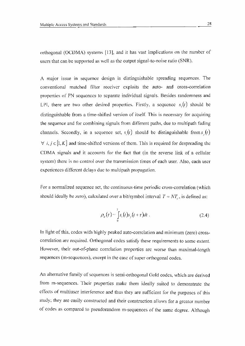
Multiple Access Systems and Standards 28
orthogonal (OCDMA) systems [13], and it has vast implications on the number of
users that can be supported as well as the output signal-to-noise ratio (SNR).
A major Issue III sequence design is distinguishable spreading sequences. The
conventional matched filter receiver exploits the auto- and cross-correlation
properties of PN sequences to separate individual signals. Besides randomness and
LPI, there are two other desired properties. Firstly, a sequence Si (t) should be
distinguishable from a time-shifted version of itself. This is necessary for acquiring
the sequence and for combining signals from different paths, due to multipath fading
channels. Secondly, in a sequence set, Si (t) should be distinguishable from S j (t)
Vi, j E [1, K] and time-shifted versions of them. This is required for despreading the
CDMA signals and it accounts for the fact that (in the reverse link of a cellular
system) there is no control over the transmission times of each user. Also, each user
experiences different delays due to multipath propagation.
For a normalized sequence set, the continuous-time periodic cross-correlation (which
should ideally be zero), calculated over a bit/symbol interval T =NTc ' is defined as:
T
Pij(r) = fSi(t)S/t + r)dt .o
(2.4)
In light of this, codes with highly peaked auto-correlation and minimum (zero) cross
correlation are required. Orthogonal codes satisfy these requirements to some extent.
However, their out-of-phase correlation properties are worse than maximal-length
sequences (m-sequences), except in the case of super orthogonal codes.
An alternative family of sequences is semi-orthogonal Gold codes, which are derived
from m-sequences. Their properties make them ideally suited to demonstrate the
effects of multiuser interference and thus they are sufficient for the purposes of this
study; they are easily constructed and their construction allows for a greater number
of codes as compared to pseudorandom m-sequences of the same degree. Although

Multiple Access Systems and Standards 29
the periodic auto-correlation properties of m-sequences cannot be bettered, gold
sequences have better periodic and aperiodic cross-correlation properties, and hence
they are more favourable. The reader is referred to Appendix A, which presents basic
characteristics and correlation properties of m-sequences and Gold codes.
2.5 Summary
This chapter reviewed the three most basic multiple access schemes. Their current
use in mobile radio communications was indicated. While TDMA and FDMA are
still employed (to a relatively large extent), they are not suited to meet the demands
of future generation systems. Transmission schemes proposed for next generation
wireless networks employ spread spectrum techniques, multi-carrier techniques, or a
combination of these two. Current 3G networks that have recently been deployed in
South Africa are based on wideband DS-CDMA, which is the current standard in
Asia, America and Europe. It is evident that DS-CDMA will play a pivotal role in the
development of next generation networks; this is in view of the wideband DS
CDMA air interface solution which is fulfilling the key requirements of 3G systems.
CDMA has several advantages over TDMA or FDMA. Spread spectrum technology
is inherently resistance to multipath fading. Receivers employing diversity
techniques may take advantage of this and improve the signal-to-noise ratio in fading
channels that are characteristic of urban areas. DS-CDMA systems, employing
pseudorandom (semi-orthogonal) sequences, undergo a gradual degradation in
signal-to-noise ratio as the number of users is increased. This soft capacity limit
allows the number of active users to be increased beyond the design specifications.
Orthogonal systems like FDMA, TDMA and OCDMA do not allow more users
beyond a fixed limit but they can guarantee a minimum quality of service for the
active users, whereas an overloaded CDMA system will see gradually increasing bit
error rates before it begins dropping users. Reception quality is traded for increased
capacity thus making DS-CDMA systems interference limited.

30
3 DS-CDMA and Multiuser Detection
3.1 Introduction
Multiple access interference limits the capacity and performance of DS-CDMA. In a
conventional DS-CDMA system, a bank of matched filter detectors (correlators) is
employed, in which a user's signal is detected by correlating the received signal with
that user's spreading waveform and then performing a simple threshold decision. In
MUD literature, this detector is commonly known as the single-user matched filter
(SUMF) or conventional detector. Detection of a single desired user is made without
regard to other users, i.e. their corrupting influence is not accounted for. In an ideal
situation there is zero cross-correlation between user spreading sequences, so this is
not an issue. If symbol synchronism is maintained and the waveforms are mutually
orthogonal then the channel is decoupled into single-user channels and the SUMF
receiver achieves optimal demodulation [18], in the presence of additive Gaussian
noise. (The conventional receiver is revisited in greater detail in Section 3.3).
However, in practice the conventional receiver is not optimum, unless in the case of
a single user or when orthogonality between spreading sequences is maintained. The
first case is an exception in multiuser communications. Furthermore, asynchronous
transmission is unavoidable, and depending on the type of coding that is employed,
even orthogonal synchronous CDMA transmissions lose their orthogonality once
passed through the channel. This research employs semi-orthogonal Gold codes to
illustrate the effect of MAl, which in turn is used to verify the performance of the
sub-optimal MUD schemes. The finite cross-correlation, resulting from semi
orthogonal spreading sequences and asynchronous transmission, means that users are
not transparent to each other. Thus, the output of a desired user's matched filter
contains some signal information belonging to other users as well. This constitutes
MAl and it is a significant contributor to the total interference seen at the receiver. In

OS-COMA and Multiuser Detection 31
the conventional receiver, MAl is regarded as additive noise in the desired user's
demodulated signal. So even in the absence of receiver thermal noise or inter-cell
interference the error probability of the conventional receiver exhibits a non-zero
floor due to MAL As the number of active users increases, the MAl also increases.
This reduces the achievable bit error rate and leads to low bandwidth efficiency.
Another factor greatly affecting (or responsible for) the amount of MAl that is
experienced, is relative signal power. Severe performance degradation occurs when
the received powers of some users dominate over other users. The conventional
receiver is unable to detect weak signals, typically originating far from the receiver,
in the presence of strong interferers located closer to the base station/receiver. This is
the so-called near-far problem. If some signals are significantly stronger than others
their signal energy/information will overshadow that of the desired user's, thus
making it difficult to separate the signals.
Several strategies exist to mitigate MAL For example, in the CDMA-based IS-95
standard, highly redundant error-correcting codes are employed to reliably detect the
information in the presence of MAl at the output of the matched filters. To account
for a near-far situation, very accurate and fast power control prevents strong
interferers from dominating at receiver, with single-user matched filtering. Even so,
as with the conventional receiver, second generation systems treat the MAl as
background noise and no signal-processing measures are taken to combat it.
However, MAl has considerable structure and is much less random than white
Gaussian background noise [19]. Multiuser detection (MUD) is a signal processing
technique which exploits the structure of MAl to overcome the limitations of the
conventional receiver and enhance the performance of DS-CDMA systems. It
performs, what is referred to as, joint detection by taking into account the
interference that may result from other users in the system i.e. the information about
multiple users is used jointly (for their mutual benefit) to better detect each
individual user. Its main objective, therefore, is to reduce/remove the effect of MAl,

OS-COMA and Multiuser Detection 32
hence it is also known as co-channel interference suppressIOn. Using MUD
algorithms can increase spectral efficiency and capacity (in terms of reducing bit
error rates and increase the number of users), and helps to reduce the need for tight
power control (the level of which is dependent on the algorithm).
Sergio Verdu proposed the first optimal multiuser detector for the AWGN channel in
1986 [7]. MUD has, ever since, gained enormous interest in academic circles and is a
dominant area of research in the field of multiuser communications. There are two
notable reasons for this. Firstly, Verdu [14] showed that the optimum multiuser
detection problem is combinatorially hard. The optimal detector, which is the
maximum likelihood sequence estimator (MLSE), has a computational complexity
that grows exponentially with the number of users. The implementation of such a
receiver is unfeasible in current DS-CDMA systems. This has inspired research of
sub-optimal multiuser detectors to achieve near-optimal performance with reasonable
implementation complexity. Secondly, optimum detection of multiple users in
multipoint-to-point (and its dual, point-to-multipoint) communications is essential for
the growth of personal wireless communications, to satisfy higher data rates,
bandwidth-intensive applications and to provide an overall higher level of service.
A general classification of CDMA detectors is shown in Figure 3.1. We differentiate
between the conventional receiver containing the bank of matched filters (single-user
strategy) and the multiuser detectors that account for MAl. In terms of optimal and
sub-optimal solutions, the MLSE is the only optimal solution; some proposed
schemes are also referred to as near-optimal. Sub-optimal detectors may be classified
as being either linear or interference cancellation (lC) detectors. There are a myriad
of detectors that are a combination of basic architectures. Such detectors constitute
the family of combined (or hybrid) schemes. Schemes that lie outside the linear/non
linear classification have also been proposed [14], [15], [20], [21]. The field of neural
networks is an example of this. However, to date, there has been no classification of
neural-based multiuser detectors (e.g. feedback/feed-forward, memory association,
soft/hard decisions). In Figure 3.1 a novel classification is presented.

DS-CDMA and Multiuser Detection
OS-COMADetectors
33
Optimal
MLSE
MultiuserDetectors
SUb-optimal
Linear
Decorrelator
Sub-optimal
InterferenceCancellation
_·_·_--·---·1
Parallel
Successive.J
SUb-optimal _
Combined :Schemes
HybndlC
DecisionFeedback I
'MMSE/LDO--'PlC
Figure 3.1 Classification of CDMA receivers.
In MUD, the front-end of most receivers is traditionally (but not necessarily) a bank
of matched filters followed by filters that perform linear or nonlinear
transformations. The sampled signals at the output of the matched filter bank
constitute a sufficient statistic of the received continuous-time signal. It is thus
possible to derive a receiver that (optimally) demodulates all transmitted signals.
In the linear schemes, a linear mapping is applied to the soft outputs of the bank of
matched filters. In non-linear le schemes, which employ feedback, the MAl and
multipath induced interference is estimated from the outputs of the conventional
receiver and then subtracted out. The foregoing multiuser detectors depend on
various parameters like amplitude, phase and cross-correlations which change over
time. This has led to research in adaptive and blind detection schemes [14], [20]
[24]. In this regard, MMSE is very attractive from an implementation perspective
because of its natural link to adaptive filtering techniques. Studies have also
incorporated space-time processing, which involves use of multiple transmit and
receive antennas to mitigate the effects of multipath fading in wireless channels

DS-CDMA and Multiuser Detection 34
[25]-[27]. The WCDMA standard supports space-time techniques as a means to
increase system capacity.
In this study, we restrict ourselves to linear detection schemes to draw comparisons
to the neural-based detectors. These are well known sub-optimal multiuser detectors
and serve as a benchmark for many of today's proposed MUD algorithms. The linear
class of receivers have the advantage of performing decentralized demodulation [28]
i.e. the demodulation of each user can be implemented completely independently.
Poor and Verdu [29] showed that the optimum decentralized receiver is a one-shot
detector. It need not concern itself with demodulating every user for which it has a
spreading code, which is an advantage. We discuss, the LDD, MMSE and the OMD
later in this chapter, but first the basic DS-CDMA transmission model is described.
3.2 The DS-CDMA Model
The transmission and reception In a DS-CDMA system can be described by a
discrete-time mathematical model. An asynchronous model for the uplink of a
mobile radio network is considered. It is based on the vector-valued transmission
system, proposed in [30], which has been employed in several neural network-based
detectors [30]-[34] and is applicable to the neural network based multiuser detector
proposed in this work.
Consider a DS-CDMA channel that is shared by K users, simultaneously. The
channel state information is known at the receiver. Each user k E {1, 2, ... , K}
transmits a packet of M bits. For simplicity, binary antipodal' signalling is assumed.
The baseband representation of the kth user's transmitted spread signal is given by:
M
qk (t) =AkIbk[i]Sk(t - iT - Ok)';=\
I Binary antipodal refers to BPSK i.e. bk[i] E {-I, I}.
(3.1)

OS-COMA and Multiuser Detection 35
In (3.1), bk[i] is the ith transmitted symbol of the kth user taking on the values
{-I, + I} with equal probability, T is the bit interval, Ok E [O,T) is the uniformly
distributed relative delay of the kth user, and Ak and Sk are the kth user's amplitude
and signature waveform, respectively. In a synchronous system Ok =°'If k. The
continuous signature waveform (or spreading signal) of user k is defined as:
N
Sk (t)= I Ck[j ]e{t - (j -I)TJ,j=\
(3.2)
where N is the processing gain, Tc =T / N is the chip duration, ck is the kth user's
spreading sequence consisting of N chips {c[j], j = 1, 2, ... , N }, and e{t) is the
pulse shaping waveform of the chip (so as to reproduce simulation results), i.e.
e{t) ={I, °~ t ~ ~0, otherwIse
(3.3)
For short codes, Sk (t) is defined in the interval °~ t ~ T. All signature waveforms
{ Sk (t), k =1, 2, ... , K} are normalized to have unit energy i.e.
rs; (t)lit =1. (3.4)
Without loss of generality, it is assumed that the channel is composed of multiple
paths and is slowly changing such that it is constant during packet transmission. The
kth user's channel impulse response characterizes the adverse effect of the channel
on that user. It may be modelled by a sum of simple attenuators and phase shifters,
Lp
hk{t) =Iak1ok{t-'kl)'1=\
(3.5)
where the complex coefficient a kl represents the attenuation and phase shifting due
to the lth path, 'kl is the propagation delay experienced by the kth user on the lth

OS-COMA and Multiuser Detection 36
path and Lp is the number of multipaths. The signal at the receiver input, r{t), is the
summation of all signals corrupted by AWGN and may be expressed as:
K
r{t) = Ihk{t )*qk{t) + n{t),k=1
(3.6)
where n{t) is zero mean additive Gaussian noise with a constant one sided power
spectral density 20' 2 = No, and where the symbol (*) denotes the convolution
operator. n{t) models the thermal noise plus noise sources that are unrelated to the
transmitted signals [14]. When specifying the discrete-time model, the notation may
be simplified by introducing ~k (t) [34], which is defined as:
~k (t) =Sk(t - Bk)*hk(t) .
By making the substitution of(3.7) into (3.6), then
K M
r{t) =IIAk~k (t - iT)bk [i] + n{t).hI i=1
(3.7)
(3.8)
One way of converting the received signal into a discrete time process is to pass it
through a bank of K matched filters. The kth matched filter has an impulse response
~:(-t) that matches to the kth user's waveform and the channel, where ~: denotes
the complex conjugate of ~k • The matched filter performs a convolution product on
the incoming bit stream and ~: (- t) resulting in the filter output signal Yk (t), i.e.
Yk(t)= ~:(-t)* r(t). (3.9)
It is convenient to define a correlation matrix, (,1){t) that contains the correlation
between ~k (t) and ~j(t) (V k, j =1, 2, ... , K), such that
<D kj =~: (- t)* ~j(t). (3.10)

OS-COMA and Multiuser Detection 37
The output of the kth matched filter in (3.9) may then be expanded, using the
appropriate substitutions, to arrive at (3.11) below. By making the generalization for
all of the K users, the outputs from the bank of matched filters may be expressed in
matrix-vector notation, shown in (3.12).
M
y{t)= AIC1){t-iT)b[i] + ii{t) (3.12)i=1
where
y{t)=[y,{t), , YK{t)Y,
b[i] = [b, [i], , bK [i] Y,ii{t} =~f{-t)* n{t),
A =diag[A, , ... , AK ],
(3.13)
with 9· (-t) ={9:(- t), k=1, 2, ... , K} denoting the vector of impulse responses of
the K channel matched filters; A is the diagonal matrix of all users amplitudes.
By symbol-sampling the output from the bank of matched filters (every T seconds),
the result is a discrete-time model in which b[i] is mapped to y[i] in such a way that,
00
y[i] =A I n[s]b[i - s] + ii[i],S=-<Xl
(3.14)
where n[i] =C1){iT) is the normalized discrete-time cross-correlation matrix,
y[i] = [Y, [i], ... , yAi] Y is a vector of the ith output of all users, and similarly b[i]
and ii[i] are vectors of the ith element of all users. For all i E {I, ... , M}, these vectors
constitute elements of larger vectors of size KM x 1 that are given by:

OS-COMA and Multiuser Detection 38
y=[y) [1], Y2 [1], ... , YK[1], yJ2]' ... , yAM]Y,
b= [b) [1], b2[1], ... , bK[1], b) [2], ... , bAM]Y, (3.15)
n=[n)[I], n2[1], ... , nAI]' n)[2], ... , nK[M] f.
Using the above notation, it is convenient to express the channel matched filter
output (3.14) in matrix-vector product form:
y=RAb+n, (3.16)
where R is the KM x KM packet channel matrix, which is composed of the discrete
time K x K sub-matrices R[i], i E {- M + 1, M -I}. As such it has a block Toeplitz
structure and also has the Hermitian property; its composition is given by:
R=
R[O]R[I]
R[M -1]
R[-I]R[O]
R[I]
R[-M +1]
R[-M +2]
R[O]
(3.17)
The number of non-zero elements (sub-matrices) in R depends on the properties of
the signature waveforms and asynchronous characteristics of the users; usually non
zero R[i] exists for i E {- 2, 2}. The elements of the matrices R[i] are obtained by
the cross-correlation of the user; that is, consider that for k, 1= 1, 2, ... , K and
a, b =1, 2, ... , M, the elements of the arbitrary matrix R[a -b] may be expressed as:
-00
where
Lp Lp 00
Rk,[a-b]= AkA,I Ia,,,,,a'n . fSk(t)s,(t-(a-b)T - D)dt,m=) n=!
(3.18)
(3.19)

OS-COMA and Multiuser Detection
3.3 Conventional Receiver
39
The objective of the front-end of a multiuser detector is to discretize the received
continuous-time waveform. Continuous-to-discrete-time conversion is realized by
conventional sampling or generally correlating the received signal with a
deterministic signal [14]. The simplest strategy to demodulate CDMA signals is to
employ a bank of single-user matched filters (SUMF). This is equivalent to using a
bank of correlators [16]. Each filter is matched to a signature waveform of a different
user and each user is demodulated without any knowledge of the other users.
~ ". -,- hi----., -, -- f. -- ''-----~ .J -'----~
I " Sync Ii
Si (t)
.1'( t) m'" ~J . h... .,g. ,. - •, ..':/.' i Sync 2ReceivedSignal s~ (1 )
I~0 {II- ""- i_I hI
L. ,-r-" •t Sync K L__.1I
SA (I)
Figure 3.2 A conventional OS-COMA receiver (Bank of K correlators).
The received signal at the input to a bank of K correlators (SUMF detector), in
Figure 3.2, is correlated with each of the K spreading sequences. Sampling occurs at
the symbol (or bit) rate i.e. every T seconds. Chip-based receivers are conceptually
simpler but sampling is computationally more intensive. Symbol-based receivers
employ an additional pre-processing stage to reduce the dimensionality of the
received signal by despreading the signal prior to sampling (Figure 3.2). Without loss
of generality, the output from the kth user's correlator yields soft estimates of that
user's signal. A threshold decision is then made on the output of the kth correlator.
The result is antipodal and it represents the kth user's probable transmitted

OS-COMA and Multiuser Detection 40
information. The presence of other users is neglected during detection and detection
is one-shot in the sense that adjacent bits are not incorporated in the final hard
decision. If a bit-synchronous system is assumed then, for the kth user, the output of
the kth correlator, over a bit interval (0 ~ t ~ T), is given by:
(3.20)
where nk(t) IS filtered AWGN with variance equal to (Y2, and Pjk is the
synchronous normalized cross-correlation between the kth and jth users
(Pjk = 1, 'If j = k). They are defined respectively as:
(3.21 )
and
(3.22)
In (3.20), Yk is composed of the transmitted bit Akbk , the MAl due to non-zero cross
correlations between users (sequences) and AWGN nk (t). MAl does not change with
SNR. Thus, a BER floor is always exhibited by the SUMF, regardless of whether the
system is synchronous or asynchronous (unless the sequences are fully orthogonal
and orthogonality is maintained). In the latter case the receiver is more vulnerable to
MAl since time offsets can result in higher cross-correlations depending on the
spreading codes used. Then, the adverse effect of a near-far situation is enhanced.
Similar to the derivations in Section 3.2, (3.20) is written in matrix-vector form as:
y =RAb+o, (3.23)
where R is now the K x K normalized cross-correlation matrix with R = p.. (foru u
the synchronous case) and A is the diagonal matrix containing the amplitudes of all

OS-COMA and Multiuser Detection 41
users. Unless otherwise stated, this definition of R is implied henceforth in this
chapter. The definitions for y, b and A follow closely to those in Section 3.2, with:
y =[)Ii' ... , YKY'
b = [bl' ... , bKy, (3.24)
A =diag[Ai' ... , AK].
The noise vector ii in (3.23) is made up of i.i.d. zero mean Gaussian random
variables with covariance matrix E[iiiiT] =a 2R, where T denotes the transpose
operation. The output of the conventional receiver is determined by the
(symmetrical) hard decision, so the estimated transmitted information is given by:
where
b=sgn(y),
() {+ 1, x ~°sgn x =-1, x <°
(3.25)
(3.26)
For a single-user channel (K =1) the matched filter method is optimal in the sense
that it maximizes the SNR of the decision statistic Y [14], which represents the
output of the SUMF. If the noise is Gaussian then it can be shown that the matched
filter minimizes the probability of error. Its output is a sufficient statistic to achieve
the lowest probability of error [14], given b)'2:S - -(3.27)
The error probability is that of a single user employing binary antipodal signalling---- - -
(BPSK) in an AWGN channel [16]. In synchronous OCDMA (Pjk = 0, j :t k), the-
2 Q{x) denotes the Q-function, which is defined as Q{x) = ~r e _~2 dtv2Jr r
I.--- .--.- Z

DS-CDMA and Multiuser Detection 42
system effectively consists of K non-interfering single-user channels. Thus the same
error probability would be obtained by each user, which is ideal. Therefore, in
practice the error probability for user k of any multiuser detector is lower bounded
by the single-user error probability:
(3.28)
The assumption that the users sharing the channel are transparent to each other is
valid only when the spreading sequences are orthogonal and remain so at the
receiver. However, orthogonality is lost since the signals that pass through the
wireless (fading) channel often arrive at the base station with random delays. In the
non-orthogonal case, the error probability of the SUMF detector is affected by the
cross-correlations between sequences and its performance degrades as the number of
users increases since the MAl increases. This can be seen by considering a simple
two-user scenario [14]. In that case, by expanding (3.20), the correlator outputs are:
(3.29)
(3.30)
Since there are only two synchronous users, it is convenient to adopt the notation in
which PI2 = P21 = p. The error probability of the conventional receiver for user 1 in
the presence of one other interfering user [14] is given as:
(3.31)
By interchanging the roles of user 1 and user 2, the error probability of user 2 can be
obtained [14]. The error probability is the same for both users, provided they have
equal amplitudes. Since the Q-function is monotonically decreasing, (3.31) is
dominated by the term with the smaller argument and so the upper bound is given by,

OS-COMA and Multiuser Detection 43
(3.32)
This shows that, if the interferer is not dominant, the bound is less than 1/2 (due to
the Q-function) and the SNR for the conventional receiver (K = 2) reduces to:
(3.33)
This performance degradation is shown in Figure 3.3 [14], for two equal-power
users. The MAl increases the HER of user 1 beyond the single-user bound (3.28).
When the relative amplitude of the interferer is greater than the desired user, i.e.
(3.34)
then the near-far problem is experienced, as shown in Figure 3.3 (for two users [14]).
141210
I
I===-===-c======i======S==-==:::::::- ---=.=--.:-=-.:-:;::.:=.:-=-.,-- ---_: -: - _::C _:: -::::::::::J: -: - _:-I t- - - - - - ..,. - - - - - -1 - _ __
_L .l --I __
I I ,
42
--e-A;. =A1
~A;.=2A1
~A;.=6A1
- Single User Bound
::::::!:_=:::J:-~ _-- --+- -1 1__
- - --T--------,---- -1--+-------1----- I
I
==-:===:!c======~=====-=:: :: :: =:: :t = .::. _ :: :: = =l == _ _1 __
: - : J: : =- _ - - =- ::::J =- =- : - - =- :,: -- - - - T - - - - - - .., - - - - -1-
------ 1----- I
--r -----...,----- 1- -
I I I
~ ~ ~ ~ ~ ~ =l= ~ ~ ~ ~ ~ ~ ~ ~ ~ ~ ~ ~ ~ =1:: ~ _ ~ ~ :: == ~ ~ ~ ~ ~ ~ ~ i ~ ~ ~ ~ =~ ~ - ~ ~ _~ ~___ - :r- __ :--2:::--::;,:-- -
_L -1 _
I--- - -- ---- ----I
10.2
~..-IDen 10.3
2-a:::UJCO
10.4
10.5
10.6
0
Figure 3.3 BER performance of the conventional detector with 2 synchronous
users, for varying powers of the interfering user. K = 2, PH = 0.2 .

DS-CDMA and Multiuser Detection 44
As the strength of the interferer increases, erroneous decisions occur with
probability 1/2 (Figure 3.3). It clearly emphasizes the need for tight power control
due to the adverse effect that the higher-powered interferer has on the desired user.
The error probability analysis can be extended for K (asynchronous) users [14]. A
Gaussian approximation (in Appendix B) is also useful for showing the effect of
increasing the number of users, when it becomes difficult to compute the K-user
error probability. However they are mostly accurate for low SNR. In DS-CDMA, the
error probability in general depends on the relative amplitudes of the received
signals, (partial) cross-correlation values between spreading sequences and the noise
power. Cross-correlation values are affected by how much one symbol overlaps with
another. This, in turn, depends on the transmission instants of the individual users
and their distances from the base station, which often are time-varying.
The conventional receiver performs optimally in a synchronous DS-CDMA system
with no channel ISI, orthogonal spreading codes, equal-power users and no inter-cell
interference. It is a simple detection strategy with low computational complexity and
is also capable of decentralized demodulation. However, the SUMF is interference
limited i.e. its output is dominated by MAl; a typical mobile radio channel dictates
that no matter the type of spreading sequences, there are always random delays and
received powers for which errors occur even in the absence of white noise.
Although the synonymous near-far problem may be overcome using power control
techniques, such methods come at the cost of complexity. Near-far resistant detectors
are required for this very reason. Furthermore, there is still the problem of MAl,
which lowers the BER performance of the SUMF receiver. Several methods are
aimed at reducing MAl, as well as providing near-far resistance. This includes well
designed spreading sequences, use of smart antennas, channel coding, and
interference cancellation/data detection techniques [20], [21], [26], [27], [35].
Ideally, and in practice, a combination of these methods is required to provide a near
optimal, near-far resistant solution and hence a successful CDMA implementation.

DS-CDMA and Multiuser Detection
3.4 Decorrelating Detector
45
The linear decorrelating detector (LDD), shown in Figure 3.4, was first proposed by
Lupas and Verdu [28]. It is a linear detection scheme in the sense that it performs a
linear transformation on the received vector of samples (which are the soft outputs of
the bank of matched filters). Its objective is to reduce MAl and this is achieved by
decoupling the information ofthe interfering users from the desired user.
Matched Filter User 1
Synd
y( 1)~
ReceivedSignal
I~
Figure 3.4 Linear decorrelating detector model (synchronous channel).
The non-diagonal terms in the cross-correlation matrix R are an indication of the
amount of MAl that will be experienced at the output of the matched filter. It may be
the result of an asynchronous channel, spreading sequences, phase offsets (due to
fading) for example, or a combination of all of these.
The LDD effectively cancels out the effect of the non-diagonal terms by applying the
inverse of the cross-correlation matrix R -I, as the linear transformation, on the soft
outputs of the matched filters (Figure 3.4). In the absence of noise, (3.16) is given by
y =RAb. (3.35)

OS-COMA and Multiuser Detection 46
Then (assuming R is invertible), it can be shown that the transmitted bits are
correctly detected by simply multiplying the matched filter outputs to R -I, i.e.
bDD =sgn(R-1y)
=sgn(R-'RAb)
=b
(3.36)
The signature waveforms of the users are required to be linearly independent [14] to
ensure that R is invertible. Thus, in the absence of noise, each user is perfectly
detected, unlike in the conventional receiver. When the background noise is taken
into consideration, then processing the matched filter outputs with R -I results in:
R-1y =R-'(RAb+ ii)
= Ab+R-'ii.
(3.37)
The output is still free from MAl and the only source of interference is the
background noise. However the noise term ii is now amplified, with the new noise
term now equal to R -lii . Its variance is obtained from
(3.38)
Thus when the background noise is dominant (low SNR), then unless all users are
completely orthogonal to each other, it is possible that the LDD performs worse than
the conventional receiver since the AWGN is enhanced at its output. This may occur
even when the interfering amplitude is small. Furthermore, there exist cross
correlation matrices for which the conventional receiver achieves better performance
(in terms of bit errors) than the LDD, irrespective ofthe SNR [14].
From an implementation standpoint, knowledge of the received amplitudes is not
required, so no estimation is involved. When the amplitudes are unknown the LDD is
optimal in the sense that it corresponds to the maximum-likelihood sequence (MLS)

DS-CDMA and Multiuser Detection 47
detector i.e. it yields the joint maximum-likelihood sequence estimation of the
transmitted bits and their received amplitudes [20]. The LDD is also capable of
optimum near-far resistance [36]. This is evident from the kth user's probability of
error, which is given in [28] as:
(3.39)
where 3 k is the kth column of R without the diagonal elements and R k is the
(K -I)x (K -I) matrix that results by striking out the kth row and kth column in R.
The kth user's probability of error is completely independent of the amplitudes of the
interfering users, indicating that the LDD is optimally near-far resistant. Figure 3.5
illustrates the performance of the LDD. The simulation agrees with the bound
analysis (3.40) for K = 2. Also, the comparatively poor performance at low SNR is
verified, but at higher SNR it clearly outperforms the conventional receiver.
1412108
I
I
I
~~~~~~;~=~~~~~~~~~~==~~====~- ---- 1-------+--- --1--------c::: ::::: _::::::i _=-::
---I- ----+--- --1- - --____ .L _
I
642
--e- SUMF Detector
-- ..-- Decorrelator
• LOO Bound (2 Users)
-- Single User Bound
10.2
a::: 10.3wro
10.4
10.5
10.6
0
=:: :: ==:: ! :: ~ ; : =~ ~ ~ ~ ~ ~ fr =I~ ~~ = :: ~ ~ ~ ~ ~ ~ ~ ~ ~ i ~ :: ==:: ~ _: : : ==: =I=:= == : =: : 3=: :::: ==: : ~ =:= == : :::: : =: :::: L :-~: ~ == == I:= == == =: == =: 3== =: : : : :
I I "to.... II--~---I--- ~----- I
I I I I', I
= = = =-= :: :: i =- =- ==- :: :: :J =- :: :: :: :: :: =1= = =:: :: - :: E: =- :: :: :: :: :: i =: :: _ =:::i::::::::::::- =:+ ==- ===:, : : =t=- ==: : - --: : =====: ==_: ~, ::::j =: : =__: - : : : I : _ : : : :J: : : : : : -. -:-:::: c - : : : : : I : : : : -: :::::_
- - - - + - - - - --l - - - - - - 1- - - - - - I-- - - - - - -+- - - - -t ~, _ _- - - - 1. ---J _ _ _ _I L _ _ _ _ .l- ...J _, ~ __
I
= :::::::: ~ ~ ~ ~ :: :: :: :: ~ ~ :::: :: :: : - = =:= - - - - - : ~ =~ ~ == :: - == :: : ~ ~ ~ :: ~ - : : : ~,~- - - : I : - : =- _ : -.J =- _ =- =- - : -1 : : - - ,- : : _ : : : I - : : : _ =- .J - ---- - T--~---...,------ I --r-~ T----.,
T--~--- I----- T--------,-
I I I
~ ~ ~ ~ ~ ~ i ~ ~ ~ ~ ~ ~ ~ ~ ~ ~ ~ ~ ~ =I~ == ~ ~ ~ ~ =f ~ ~ ~ ~ ~ ~ i ~ ~ ~ ~ ~ ~ ~ ~ ~ =~ =~
--====:_=====~=------- ====-~=-========:==:==:===
SNR
Figure 3.5 Comparative BER performance (for user I) of the LDD and the
SUMP detector for K = 2 users, with respective bounds.

OS-COMA and Multiuser Detection 48
One advantage of the LDD is that each user can be detected independently of the
other users. Furthermore, demodulation can occur over a single bit interval. It has a
lower computational complexity than the MLS detector. However, the computations
required for matrix inversion are difficult to perform in real-time, especially for
asynchronous transmissions (when R is of the order NK). Despite this drawback, it
generally offers greater benefits (performance/capacity gains) than the conventional
receiver and has received relatively more interest than other sub-optimal schemes
[20], [21], [35]. Research into the LDD, has provided several methods, including
hybrid techniques, which reduce the complexity associated with matrix inversion.
3.5 Minimum Mean-Square Error Detector
The linear minimum mean-square error (MMSE) multiuser detector achieves the
balance between the cancellation of MAl and the enhancement of background noise.
It does so by utilizing the knowledge of the received signal powers and accounting
for the noise. Since the matched filter detector is better than the LDD for low SNR, it
makes sense to incorporate the SNR of the different users to achieve better
performance. This is the case with the MMSE solution (Figure 3.6).
h~-S ih .. ....h...:, .........~l '
I'~~ +cr 1A CYi
I
! Matched Filter User 1 .
:~+('l)-~JF $,,;,--: sJt)1 • ._
.r(t)Received
Signal
, Matched Filler User K :
Figure 3.6 Model of the MMSE detector (for the synchronous channel).

OS-COMA and Multiuser Detection 49
This linear detection scheme is based on the MMSE criterion that is used for
equalization. The goal is to find a linear mapping which minimizes the mean-square
error (MSE) between the transmitted data and the output of the detector,
(3.41)
If we define M as the linear filter which processes the output of the conventional
receiver y , then the output of the MMSE detector is
bMMSE = sgn(My). (3.42)
The solution is found by choosing transformation M that satisfies the MSE criterion:
The linear transformation that achieves this minimization [14] is given by
[2 _2}1
M MMSE = R +a A J '
where
[2 2]2 -2 • a a
a A = dlag -2' ... , -2AI AK
(3.43)
(3.44)
(3.45)
The MMSE detector, like the LDD, is capable of decentralized demodulation [37].
For the kth user, the output of the linear MMSE detector (in Figure 3.6) is given by:
AMMSE (() )bk =sgn My k • (3.46)
The compromise that is offered by the MMSE detector can be seen from (3.44); if
the received amplitudes are fixed, then for high SNR (a ~ 0),
(3.47)

DS-CDMA and Multiuser Detection 50
Thus, the MMSE scheme converges to the LDD. This means that it is also capable of
the same optimum near-far resistance. However, for low SNR (0- ~ (0), the MMSE
detector approaches the conventional receiver in the sense that (3.44) becomes a
strongly diagonal matrix [14].
The error probability of the MMSE detector is not as simple as that of the LDD. This
is because the decision statistic at the output is not Gaussian, but is made up of
additive noise plus MAl. To analyze the probability of a bit error we consider,
without loss of generality, the linear detection of bit bl • As shown in [37], for any
linear detector of the form (3.46), it follows from the sufficient output (3.23) that this
bit is given by the decision on
(3.48)
where {p" ... ,PK} are the leakage coefficients defined as
(3.49)
which quantifies the contribution of the kth interferer to the decision statistic, relative
to the contribution of the desired user [7], with
(3.50)
and where
(3.51)
The probability of error is then given by
(3.52)

OS-COMA and Multiuser Detection 51
The computational complexity that results from (3.52) increases exponentially with
the number of users and this complexity is further increased by the calculation of the
leakage coefficients. For simplification, a valid approximation is to replace the
binomial distribution of the MAl, represented by the summation term in (3.48), with
a Gaussian distribution with same variance. The accuracy of this approximation is
supported in [37]. Figure 3.7 indicates the gain in BER performance of the MMSE
detector over the SUMF receiver, for 8 synchronous equal-power users with equal
simulated cross-correlation of Pjk = 0.8 [14]. The single-user AWGN bound (3.27) is
also plotted to compare this sub-optimal scheme to the optimal single-user bound.
1412108642
10° _- =- - - I ===- = =- = :::::I = = = ====1- - ==== ::. t: __ =- =- =- = :t = =- ==== ::J == =
l.:::::::J::::::::::::::c:--_-:i::::::::::i:- _-T------,--------------r-- --T----- ,-- -
- T------.---------- - -- --------- -T-- ---,----- - - ----r------T------..,--
I I
::::::: ==============J:::====================_==:1====_--:!::::::~--
1 .J _
.!. - - - - - - - - - - - - - - ~~-"'-- ....."""-....I
I
:::: :; ~ =~ ~ E~ ~ ~ ~ ~ ~ ~ ~ ~ ~ ~ ~ :: ~,::: ~ ~ ~ ~ =:... :::: == -
_L 1. _
________ I
, ,I I I I--e-- SUMF Detector =,= =c " " ==i" =_ ===r ======'j =c c =_=
=1- - - - - - - t= - : :: =:: : :;:: :: :: _.:. =- ~:: : _::::~ rvt..1SE =- - - - - - - c: ===_==I ======~ =- =~ =
t---- --1"""--- ---1--
-- Single User Bound - - - - - - - - '- - - - - - - " - - - - - - ~ - -10-
6 L::::=---_...:c=====:::L=====-.l.-- :o
SNR
Figure 3.7 BER performance of MMSE detector, in a synchronous AWGN
channel, with equal power users. K =8, Ptl
= 0.1.
The MMSE receIver compromIses between perfect decorrelation and nOIse
amplification. The LDD and SUMF receiver are limiting cases of the MMSE
detector [14], [37]. However, while it accounts for noise and MAl, unlike the LDD, it

OS-COMA and Multiuser Detection 52
does impose the same computational disadvantages such as matrix inversion. In
addition to knowing all the signature waveforms, knowledge of the received powers
of the interfering users is required and thus estimation is necessary. For high SNR, if
the signature waveforms are linearly independent, the complexity incurred for
knowing the received SNR does not justify the performance improvement over the
LDD. The MMSE detector is often implemented adaptively, which does not require
knowledge ofthe signature waveforms, channel and that of the received powers [37].
3.6 Optimum Multiuser Detection
The optimum multiuser detector (OMD) for the AWGN channel, proposed by Verdu
[7], is based on the criterion of maximum likelihood sequence estimation (MLSE), in
which the maximization of a cost function leads to the joint optimum detection of all
users. The K -user MLSE detector (Figure 3.8) employs a bank of matched filters
followed by the Viterbi linear programming algorithm, which estimates the most
likely set of transmitted bits for all the users. Sequence detection has several
advantages over one-shot detection strategies since the observation is taken over the
entire received waveform to produce a sufficient statistic for any symbol decision.
Matched Filler User 1
y( I)
ReceivedSignal
i---(~)--~ r ~------ ~I i -- Sync I
. SI (f) MaximumLikelihoodSequenceEstimation
(ViterbiAlgorithm)
Ma/ched Filter User K
hi....._.._.... ~
hA..... _--+
Figure 3.8 Block diagram ofthe Optimum Multiuser Detector.

OS-COMA and Multiuser Detection 53
The objective of the MLSE detector is to find the input sequence that maximizes the
probability conditioned on the given output sequence i.e. P(b Iy), which is a
globally optimum or maximum likelihood sequence. This probability is referred to as
the joint a posterior probability. If all sequences are equiprobable, then the objective
is to choose the most likely transmitted vector, which is the output of the MLSE
detector, given by b= [bl , ... , bKr, such that it maximizes the probability of
receiving the signal Y on the condition that vector b was sent, i.e.
bOpt =arg max, P(Ylb).bE{-I,J}~
This is equivalent to maximizing the log-likelihood function [7] given by
(3.53)
(3.54)
where Yis the column of matched filter outputs, A is the K x K diagonal matrix of
received amplitudes, such that
Y = [;;1' ... , YKr,A =diag {AI' ... , AK },
and H is the un-normalized cross-correlation matrix [14] defined as
H=ARA.
(3.55)
(3.56)
Equation (3.54) indicates that y is a sufficient statistic for the optimum detection of
the transmitted data b. However, it is solved by performing an exhaustive search
through each of the possible sequences until the combination that maximizes the log
likelihood function is found, which is clearly not feasible for large systems.
The issue surrounding the maximization of (3.54) is discussed shortly but first we
state the fundamental quantity of interest, which is the minimum error probability.

DS-CDMA and Multiuser Detection 54
Optimum performance is attributed to the MLSE detector and the lower bound for
the probability of error, which is derived in [7], is given by:
(3.57)
where OJk,min is the smallest weight OJ(E) , of all the error vectors, with E=b - b
denoting the error vector and OJ(E) denoting the number of non-zero components
(weight) of an error vector that is given by
K
OJ(E) = IICkl,hI
(3.58)
and with dk,min representing one half of the mmlmum distance between two
multiuser signals that differ in the kth bit.
Besides yielding the most likely transmitted sequence, this detector offers optimum
asymptotic multiuser efficiency and near-far resistance [7], [14], [18]. Intuitively,
the average optimum near-far resistance with synchronous random DS-SS
waveforms is a function of the number of users and processing gain. While optimal
(near-far resistant) multiuser demodulation can be achieved via the maximization of
an integer quadratic function, in context of practical implementation, it has several
disadvantages. Besides knowing all the spreading sequences, estimates of the delays,
carrier phases and the receiver power of all the users are required. These are not
known a priori and estimation adds to the overhead incurred during implementation.
The most important issue is the one of computational complexity, since the problem
of solving (3.54) is combinatorially hard. It is for this reason that the optimal
detector is impractical to use in current DS-CDMA systems. This problem is made
clear by considering a K -user system. Over a bit interval, where bk E {-I, I} occurs
with equal probability, there exists 2K different combinations of b, one of which is
the most likely transmitted sequence. In [7] it was shown that the maximum

OS-COMA and Multiuser Detection 55
likelihood sequence receiver, proposed for asynchronous channels, can be
implemented using the Viterbi algorithm. In that case, R is defined according to
(3.17) and a dynamic programming algorithm, such as the Viterbi algorithm,
maximizes (3.54). Without it, in the MLS approach, a brute-force maximization of
(3.54) would require a complexity of O(2KM) [20] i.e. a search through 2MK possible
b vectors. This is not practical, especially if it is considered that the growth in
complexity is exponential in the number of users.
By employing the Viterbi algorithm, the optimal detector has complexity O(2K).
This complexity makes the optimal detector practical when the number of users in
the system is relatively small. Unfortunately, in practice this is seldom the case. No
algorithm is known for optimal multiuser detection whose complexity is polynomial
in the number of users. In optimization literature this is denoted as an NP-complete
problem. It will be shown, in the chapters to follow, that neural networks are well
suited to solve combinatorial optimization problems, and their success in the field of
optimization (e.g. TSP) justifies their application to MUD.
Due to the resulting complexity issues, research has concentrated on sub-optimal
detectors that are near-far resistant, have a relatively low complexity and compare in
performance to the optimal detector. The LDD and MMSE schemes, which have
been discussed, are examples of such sub-optimal MUD strategies and they also
include adaptive and blind detection schemes. Nevertheless, the performance of the
OMD serves as a benchmark for the current and future sub/near-optimal schemes.
3.7 Summary
This chapter highlighted the need for multiuser detection in order to reduce MAl and
overcome the near-far problem in multiuser communications, particularly in the
reverse link (uplink) of a cellular network. The conventional single-user strategy was
discussed, the performance of which motivates the need for joint detection

DS-CDMA and Multiuser Detection 56
techniques. An asynchronous model for a DS-CDMA system was presented, for
which synchronous transmission can easily be adopted. A review of two popular sub
optimal receivers for the CDMA channel was provided. Clearly there is a need for
sub-optimal joint detection schemes which balance complexity and performance. The
linear schemes, discussed herein, have the advantage of being computationally
simpler than non-linear IC schemes. Furthermore, they are able to perform
decentralized demodulation. They have been shown to outperform the SUMF
detector, via simulations, and are capable of near-far resistance.
The benchmark for all sub-optimal schemes is the optimal MUD solution, which due
to its prohibitive computational complexity makes it undesirable for current DS
CDMA applications, despite its optimum near-far resistance property and optimum
BER performance. This is the main reason for sub-optimal schemes, however even
the most popular linear sub-optimal implementations are dependent on information
like spreading sequences and channel parameters such as delays and phases.
Furthermore, while these schemes offer comparable performance, their main
objective is to reduce background noise and MAL It is possible then that detection
strategies which are designed to operate directly on the maximum-likelihood
objective function will be capable of near-optimal performance.

57
4 Neural Networks
4.1 Introduction
Neural networks, or artificial neural networks to be more precise, constitute a major
part of the field of distributed artificial intelligence (AI). In the broad sense, AI
incorporates several areas of computing that attempt to mimic the signal processing
that occurs in the human brain [38]; usually these are the processes that are carried
out without much consciousness. In this regard, it may be defined as the intelligence
exhibited by any manufactured (artificial) system and thus it is also known as
machine intelligence. But this definition begs the question of "what is regarded as
intelligence?" Foremost, AI is the scientific investigation into theory and practical
application of artificially intelligent systems and learning models, all of which is
rooted in the neurosciences [39].
Modem AI research is focussed on application in the engineering fields. While it is
concerned with the production of useful machines to automate human tasks requiring
intelligent behavior, AI is also the source for providing solutions to a number of
diverse underlying engineering problems, especially in research. They find
application in business, medical fields, military installations, and even in our homes,
on our personal computers. It may be software alone or a meId of software and
hardware. Like most sciences, AI is decomposed into a number of sub-disciplines (or
techniques) that, while sharing an essential approach to problem solving, are
concerned with different applications.
The discipline of AI stemmed from the potential of neural computation models,
known as neural networks. Although, it is worth pointing out that neural networks (or
connectionist models) are distinguished from classical AI. In general, classical AI
research involves symbolic manipulation of abstract concepts [38], and is the

Neural Networks 58
methodology used in most expert systems which is one sub-discipline. Expert
systems perform domain-specific problem solving by combining a theoretical
understanding of the problem and a collection of heuristic problem-solving rules that
has shown to be effective. It is likened to a human expert who must use knowledge
and experience to solve a problem. Most expert systems have been written for
relatively specialized fields that are generally well studied and have clearly defined
problem-solving strategies [39]. Problems that depend on a more loosely defined
notion of "common sense" have a greater difficulty in being solved by these means.
Parallel to classical systems are connectionist systems. They attempt to evolve or
learn using intelligence by building systems and then improving on them through
some automatic process rather than systematically designing something to complete
the task. Artificial neural networks are the best-known examples.
In its most general form, a neural network (NN) is an adaptive machine that is
designed to model the way in which the brain performs a particular task or function
of interest [38]. It captures and represents input/output relationships and is able to
perform useful computations through the process oflearning [40]. The relationships
may be linear or complex non-linear and can be learnt from the data being modelled.
The network is characterized by the number and the type of connections between the
simple computing cells which constitutes it, namely neurons, and its operation is
governed mathematically through a set of learning rules. The unique organization
and connection of neurons results in different types of neural networks. It is worth
noting that the term "neural" is used in the sense that these networks have been
inspired by neuroscience (scientific study of the human brain and nervous system)
and not necessarily because they are concerned with faithfully modelling biological
neural phenomena [39]. NN theory, however, still appeals to biological realism.
It is well known that neural networks are viable computational models for a wide
variety of problems. They find application in a diversity of fields such as pattern
recognition, image analysis, signal processing (equalization), clustering algorithms,

Neural Networks 59
computational neuroscIence, statistical physics, and control theory [38], [40].
Consequently, a large variety of mathematical tools and methods are used: statistical
mechanics, probability theory, linear algebra, Lyapunov functions and theory of
dynamical systems, and combinatorial optimization tools. The technology is rooted
in several disciplines, namely engineering, mathematics, physics, statistics, medical
(neuroscience), and geology [38]. Their suitability for use in these fields is the result
of several important factors. Firstly, their operation is usually free from assumptions;
they have the ability to learn and hence generalize. Their inherent distributed
nonlinearity is important for accepting non-linear inputs (such as speech signals).
They are adaptive and can thus respond to changes in the operating environment.
Furthermore, they are able to handle noisy data in difficult non-ideal contexts, even
when the available knowledge is regarded as sufficient to use conventional modelling
or a statistical approach. This type of robust computation depends on the algorithm
that is used to train the network.
The description and ability of a neural network is usually clarified in the context of
formal neurons (described in Section 4.2), and the parallel distributed processing that
is achieved by a network having a vast composition of interconnected neurons
(similar to the human brain). The massive interconnection of these neurons gives to
neural networks its characteristics and functionality in the field of machine learning.
Based on this, a neural network may be defined as a massively parallel distributed
processor with the natural tendency to store knowledge through the process of
learning and to make it available for use [38]. Although there is no universal
definition, there are several other accepted definitions, which have been proposed by
authors and researchers alike, usually expressing the same fundamental idea.
In recent years, neural network research has received a steadily growing interest from
different scientific disciplines, like those mentioned above. This multidisciplinary
atmosphere has proven to be very inspiring and has led to a fairly deep grounding of
neural network theory in classical theoretical approaches as well as to numerous
applications, and importantly in industry. The engineering field has definitely

Neural Networks 60
benefited. In the field of signal processing and communications, neural networks
have been utilized successfully as adaptive equalizers [8], [9], [16] and have
progressed considerably in field of MUD in DS-CDMA [11], [31]-[34], [41]-[54].
Although many classical methods are used, their connection and joint application
yields a number of new results. In some cases known methodology has to be
extended to achieve reasonable results, such as with recurrent type neural networks.
4.1.1 Brief History
The era of neural networks and computational modelling began with work by
McCulloch and Pitts in 1943 [40], however, the idea of modelling biological neurons
was introduced much earlier. McCulloch and Pitts combined neurophysiology with
mathematical logic [39]. In their work, the simple processing unit, called the neuron,
was introduced. The formal neurons were presented as models of biological neurons
and as conceptual components for circuits. They were designed to operate as
switches. The authors showed that, conditioned on a reasonable set of parameters, a
network made up of these units, in principle, could perform universal computation. It
is generally agreed that this paper herald the birth of AI and neural networks.
Over the years, there were several works on the detailed logic of threshold networks.
The robustness of parallel processing was realized and at the same time the
significance of statistical mechanics increased in the context of this subject matter.
Known as neurodynamics, this approach used differential equations to describe the
behaviour of neural activity [40].
A major development (around 1949) was the proposal by Hebb that, biologically, the
connections in the brain change to accommodate for learning different tasks [38].
Hebb introduced the learning rule for synaptic modifications in the brain. This is well
known as Hebb's postulate oflearning, which roughly states that the strength of the
connection between two neurons increases depending on their states. This inspired
the development of models of adaptive (learning) systems.

Neural Networks 61
The idea of artificially intelligent systems that could mimic human behaviour, even
in elaborate context, began as an experimental field (known as AI) in the 1950s with
such pioneers as Allen Newell and Herbert Simon who founded the first artificial
intelligence laboratory at Carnegie Mellon University, and John McCarthy and
Marvin Minsky, who founded the MIT AI Lab in 1959 [39], [40]. Minsky's work in
1961 detailed what is now known as neural networks.
The first learning algorithm was proposed by Frank Rosenblatt. He focused on
finding appropriate weights for certain tasks [40] and introduced a novel method of
supervised learning for pattern recognition, in his work on the perceptron. The
perceptron consists of two layers of neurons with feedforward connections. It was
introduced as a processing element that produced an output based on a decision taken
on the weighted sum of its input signals. Rosenblatt's main contribution was proving
the convergence of the learning rule, for ways of updating the NN weights to perform
specific computations. This paved the way for classifying tasks. It was proven that if
sets of parameters exist for carrying out a task correctly, then the perceptron
algorithm finds one set [39]. During this period, neural networks were considered to
be capable of brain-like computation. Although this was greatly exaggerated, it
resulted in new training algorithms and trainable networks for tasks like adaptive
pattern classification and it also opened up research into multi-layered networks.
In 1969, two authors Minsky and Papert showed that the perceptron was flawed and
that the convergence theorem only applied to certain tasks. Elementary computations
(such as the popular XOR operation) could not be performed by the single-layer
perceptron [40]. They further concluded that this problem (of finding the correct
weights) would exist in multi-layered perceptrons. This saw the demise ofperceptron
research, and except for the neurosciences, it is generally the view that neural
network research fell into a depression thereafter. However, the idea of (associative)
content addressable memory (CAM) was soon revived. In conjunction the field of
self-organizing maps, which employs unsupervised competitive learning that is
motivated by topological ordered maps in the brain, was introduced.

Neural Networks 62
In the 1980's several major contributions to the NN field revived interest. The work
by physicist John Hopfield on the Hopfield neural network (HNN) stands out and
now forms the basis for the recurrent neural network (RNN) [55]. His research
extended on using statistical mechanics in networks utilizing the McCulloch-Pitts
model. He introduced the idea of an energy function and emphasized the notion of
memories as dynamically stable attractors in the energy space of the network.
Moreover, he established the isomorphism between the RNN with symmetric
connections and the Ising model of statistical physics [38], and later drew on spin
glass models. His work drew much interest, as well as some controversy regarding
the originality of the ideas. Nevertheless, the principle of storing and retrieving
information using a dynamically stable RNN was made explicit in Hopfield's paper.
In the related field of combinatorial optimization, simulated annealing (SA) was
introduced by Kirkpatrick et at. [56] to solve combinatorial optimization problems.
Later, Hinton and Sejnowski (cited in [39]) developed the Boltzmann machine using
stochastic neurons. It employs SA and resembles a thermodynamic process. It was
the first successful multi-layered network, which aided in dispelling some of the
damaging work of Minsky and Papert (cited in [40]). The Boltzmann machine is an
extension of the HNN. It helped develop the idea of employing stochastic techniques
and concepts from statistical mechanics for solving optimization problems.
Before discussing the HNN, we first consider the basic neural network architecture in
terms of two basic structures and the fundamental component, the artificial neuron.
4.2 Conceptual Architecture of Neural Networks
The research in neural networks is largely motivated by the idea of wholly artificial
computing networks that have the ability to operate and make decisions without
human intervention. Yet, as the term implies, it was originally aimed more at
modelling networks of real neurons in the brain [40]. From a neurophysiological

Neural Networks 63
viewpoint, the models are very simplified. However, they continue to develop and
provide insight into the brain's ability to compute and make decisions based on
experience while processing difficult tasks.
NI N iI .1I I. I -InputLayer
HiddenLayer(s)
OutputLayer
N NII •1 N1d N".4i
1.1
I II
Input Hidden Layers OutputLayer with feedback Layer
(a) Feedforward based neural network. (b) Feedback based neural network.
Figure 4.1 Two basic network types with a common structure. Operation is
either static (a) or dynamic (b). Data processing may occur over
multiple layers.
It is beyond the scope of our work to provide taxonomy of the different neural
network models, except that which is of concern and unless a general discussion or
comparison is warranted. However, it is noted that a common categorization of
neural networks is the feedforward or feedback type (Figure 4.1). This is important,
as the ability of a neural network to perform specific computational tasks depends on
the organization and interconnection of neurons in the network, to some degree.
In general, a network may be composed of one layer or multiple layers of neurons. A
multi-layered network usually has one input layer, one output layer and may have
one or more hidden layers. A common, though not universal, naming convention is
to denote the set of inputs (source) to the network as the first layer. For a network
composed of L layers, the input layer Ni,) is thus the first layer. It is non-processing

Neural Networks 64
and only supplies input signals to the network. Any intermediate layers N h,i that
may exist (V i = 2, ... , L -1), are responsible for processing the inputs and are called
hidden layers. This is illustrated in Figure 4.1 (a). The hidden and output layer
neurons may be connected to all of the units in the preceding layer (fully connected
network), or only to some units in the preceding layer (partially connected). For most
applications fully-connected networks are well suited.
In a feedforward network, shown in Figure 4.1 (a), signal flow from input to output is
strictly unidirectional. There is no memory as the output depends only on the current
input and it is computed one-shot. Feedforward structures are the most common
networks types, and are usually multi-layered. Since the direction of flow is certain,
feedforward networks are easier to analyze and to a greater degree than feedback
types. It has been shown that they can approximate any given function from static
input values to static output values arbitrarily well. Further, experimental results
show that they often outperform more traditional methods in non-linear
classification, especially in high-dimensional tasks.
Recurrent or feedback networks, shown in Figure 4.1 (b), have internal dynamics as a
result of feedback loops within the network. Biologically they are more plausible
since the human nervous system is composed almost entirely of recurrent networks.
These types of networks are mathematically described by a (non-linear) dynamical
system given by a first order differential equation. In general it is hard to predict
even their qualitative behaviour. Therefore the common RNN in use is the Hopfield
network, which is characterized by a symmetric organization of weights. This
architecture is widely employed as CAM. Other symmetric architectures have been
used to (approximately) solve optimization tasks [57]. Without symmetry the
network dynamics are less tractable, but in general any of these networks are
considered to transform input functions into output functions.
This perspective is developed in greater detail by starting with some non-formal
remarks on the properties of the artificial neuron. The neuron is the basic component

Neural Networks 65
of any NN. It is responsible for processing information and is fundamental to the
operation and functionality of aNN, through a large interconnection of neurons. It
mimics the neurons (nerve cells) in the brain of which there are many different types.
[Bias] I" = WI/l) (= x o)
VI/ !F01 y"L_r
[Weights]
Figure 4.2 Non-linear model of a neuron.
Figure 4.2 illustrates the model of a single neuron. Without loss of generality we
consider the operation of the nth neuron, in the presence of m-I neurons, where m
denotes an arbitrary number of neurons. Neuron n has a number of weighted
connections {wnl ,.·., wnm } over which it is able to communicate with other
neurons. Specifically, wnj is the weight associated with the connection between the
jth and nth neuron; it determines the effect of the jth unit's signal on the nth unit
[38]. These connections represent the synapses of real neurons and the weights
represent the strength of the synapse. The weight wnj is positive if the associated
synapse is excitatory otherwise it is negative if the synapse is inhibitory.
For now, signals {Xl' ... , Xm } denote the inputs (from other neurons) to the neuron
nand f" is an externally applied fixed input (bias term) that represents a general
inclination of whether the neuron fires or not. A propagation rule determines the
effective input Vn of a unit, given its initial inputs and biasing. In most instances, as
in this case, the rule is to perform a summation of the weighted inputs.

Neural Networks 66
FO is the activation function (AF), which determines the state (or output) YI~ of the
nth neuron. (For clarification, the superscript refers to a NN model). It indicates
whether the neuron fires or inhibits; its output is called the activation level of the
neuron. The AF is an important function for configuring the NN, as it is the source of
non-linearity that is responsible for the approximation capabilities of the network.
So the operation of the nth neuron may be described by
m
Vn = L WnjXj + h, ,j~1
and by defining the linear combiner output as Un , the output is given as
wherem
Un =LWnjXj .j~1
(4.1)
(4.2)
(4.3)
The AF determines how the inputs are interpreted and how changes in the network
affect neuron excitation or inhibition, i.e. whether a neuron is firing or non-firing (for
two-state neurons, this simply implies being in the on or off state, respectively). The
type of AF, therefore, assists in providing the neuron, and the network as a whole,
with unique benefits and specific functionality. This may be exploited when soft
outputs are required for feedback, which is the case in some MUD schemes.
The first model of a neuron (McCulloch-Pitts) was viewed as a logical gate with two
internal states: active (excited) and silent (inhibited), and in which the AF is a
threshold function. The McCulloch-Pitts neuron model is the simplest and the most
popular, to date. Its output is given by:
(4.4)

Neural Networks 67
Given the above mathematical description, it can be seen that the bias f" is the
threshold value for the nth neuron; the weighted sum of the inputs must reach or
exceed this threshold for the neuron to fire.
Though simple, it was proven that a synchronous assembly of neurons of this type is
capable of a high level of computation [39]; all logical operations can be
implemented using conveniently associated neurons with a suitable set of
weights wnj • However it is only since the last 20 years that the true potential of
neural computation is being realized.
The McCulloch-Pitts model can also employ the symmetric hard function (3.26). In
that case, the neuron's activation level resides in one oftwo states: +1 (firing) or -1
(non-firing). This is conveniently used when analyzing the RNN, as well as for the
purposes of antipodal signalling in the DS-CDMA system.
Numerous other AF's may also be employed, but it often depends on the network
and the application. One common choice is the hyperbolic tangent function,
F(v) =tanh(v). (4.5)
It takes on a continuous range of values in the range [-1,1] and is easily
differentiable; this provides analytical benefits in some networks such as those based
on back-propagation techniques.
The sigmoid (logistic) function with parameters a and b , indicated in (4.6) below, is
another common AF. Notably, it is the standard choice for modelling the stochastic
neuron. Appendix D provides an overview of this function.
1F(v) = -1--("-v----;"a)/"""'b •
+e(4.6)

Neural Networks
4.3 Recurrent Hopfield Neural Network
68
In principle a feedback network can contain any number of layers with a myriad of
connections between and within different layers. One well-known and well
researched example is the recurrent Hopfield neural network (HNN), which IS
composed of a single layer of symmetrically interconnected neurons (Figure 4.3).
The HNN is rooted in the field of neurodynamics, which describes the combined
theory of non-linear dynamical systems and neural networks. It is primarily used to
perform pattern association (information storage and retrieval) by storing
fundamental patterns (memories) as dynamical attractors in a state space [55], [58]. It
is commonly employed as auto-associative, content addressable memory (CAM) or
as a platform for solving combinatorial optimization problems.
Figure 4.3 Schematic view of the auto-associative HNN. Neurons
provide both inputs and outputs. (No self-feedback).
Feedback networks are often described by dynamical systems that evolve in either
continuous or discrete time; they can be classified as a discrete or a continuous
network. The standard discrete version of the HNN employs the McCulloch-Pitts
neuron model, but other versions exist [58]. Learning of a specific input-output
association is defined without the use of correct examples, i.e. learning is
unsupervised. The only available information is in the correlation of the input data

Neural Networks 69
and data that is stored. The HNN is designed to store a number of patterns by
distributing their information across the network weights. It uses the correlation
information to produce an output associated with the input that is presented to it.
The idea of CAM is to map fundamental patterns to stable points in a state space of a
dynamic system. The HNN stores information in a dynamically stable configuration.
Associative memory models may be described by a configuration space containing
all possible states (Figure 4.4). Within this state space are attractors (stable points)
representing stored patterns. Given sufficient information as a starting point in the
state space and provided that this point lies in a basin of attraction (near an attractor),
the HNN should converge to a stable point, which ideally is the desired pattern. The
state space is idealized for the purposes of explanation, i.e. it should be described by
a set of discrete points (on a hypercube) and not by a continuous region.
Figure 4.4 Schematic view of a configuration space (with four attractors).
The above process occurs internally and it is conceptual. Externally this translates to
the HNN retrieving a pattern when subjected to an initial input, which may be a
noisy or incomplete version of a fundamental pattern. An advantage of CAM is its
insensitivity to small errors in the initial input. This is particularly useful when
detecting signals in the presence of AWGN. The HNN model is shown in Figure 4.5.
The HNN employs feedback to iteratively update neuron states, from an initial state,
until a stable point is reached or when there are no further state changes. The

Neural Networks 70
dynamics of the HNN follows a trajectory to the closest attractor, signifying a stored
pattern (as shown in Figure 4.4). Its symmetrical configuration ensures that all
trajectories are asymptotically stable and that they reach static equilibrium [58]. The
equilibrium state is thus a fundamental pattern, retrieved by applying a suitable input.
However, correct association is not always guaranteed. In general, it depends on the
initial pattern and on stability conditions which must be met. This is discussed later.
f---+--t-t---+ .l'
--. ---,1--__: _ .:-+ F ( )Il..-.--....+---+-...
l oH
I'
Figure 4.5 The Hopfield architecture, with N neurons,
The formulae that mathematically describe the process of pattern storage and
retrieval (as discussed above) are easily derived. Figure 4.5 shows the connection of
the classical Hopfield model with unit delay elements. The output of each neuron is
fed back to every other neuron. Although self-feedback is indicated here, it is usually
avoided in pattern association for stability purposes (See Appendix C).

Neural Networks 71
The operation of the HNN is two-staged, i.e. storage and retrieval. Storage is a one
shot computation since the network learns and obtains its weights once over.
Suppose that a set of U patterns {qu ,u =1, 2, ... , U} is to be stored. For convenience,
each pattern is considered to be made up of independent bits, such that qu,; denotes
the ith element of qu' If each vector is of dimension if, then if neurons are
required, where each neuron state corresponds to one bit.
The one-shot learning rule is a generalization of Hebb' s postulate oflearning, which
says that the synapse wij between neurons i and j should increase if both neurons
are simultaneously activated. This is implemented via the outer product of the
patterns. Therefore the synaptic weights (between pairs of connected neurons) are
defined in the if x if synaptic weight matrix which is given by:
1 ~ ( )T UW =-~ LJqu qu --~ I.M u=l M
(4.7)
In (4.7), 1/if is employed for the purpose of simplification. The second term
indicates that there is no self-feedback by ensuring that wii
=0 V i with I denoting
the identity matrix. This learning rule is used with the aim of simulating the HNN;
however, it will be shown in the subsequent chapter that (4.7) is not explicitly used in
the neural-based MUD implementation.
The primary function of CAM is to retrieve a pattern stored in memory in response to
a presentation of an inconsistent version of that pattern i.e. incomplete or noisy [55].
As long as it shares a reasonable degree of similarity with any of the stored patterns,
the network should be able to find a pattern that most closely resembles the input
pattern. For a network made up on if neurons, the state vector (at the kth time step)
that contains the state of each neuron, may be defined as
(4.8)

Neural Networks 72
During retrieval an input pattern of dimension if is imposed on the HNN as an
initial state, i.e. x(O) = S=initial • Each neuron is then updated (randomly), at a fixed rate,
based on a dynamic rule. State updating at each discrete time step k is therefore
deterministic and each neuron's state is updated according to the state transition rule:
(4.9)
Normally, the AF is given by FO= sgnO, but binary decisions or other non-linear
functions, like those described earlier, may be employed. If the effective input vj
to
neuron j is zero then the state remains the same (See Appendix C). The updating
procedure of (4.9) is repeated for k iterations until there are no state changes to
report or when a fixed point (stable state) has been reached. Then the HNN outputs a
time-invariant state vector, which satisfies (4.9). It is denoted in matrix form as,
NY = X fIXed
=F(Wx fixed + f).
(4.10)
The final state of the neurons that the HNN converges to is given by X fIXed and may
be an element of the solution set ku' U =1, 2, ... , U}, and f is the vector of the
externally applied biases. Updating may be done serially, in which case a single
neuron is updated at a time and its output is used to update the next neuron. This is
known as asynchronous updating; physiologically this is a more natural way. Usually
neurons are chosen at random to be updated, or with some constant probability [40],
or even sequentially. Parallel updating is also possible, but stability is an issue [38].
A useful examination is the generic problem of storing a random set of patterns
drawn from a binomial distribution. The procedure for testing is to check whether
small deviations from these patterns are corrected as the network evolves. Storage of
eight lOO-dimensional patterns was investigated; the probe (initial pattern) presented

Neural Networks 73
to the HNN contained uniformly introduced errors. The result of the simulation is
shown in Figure 4.6, with an expected trend. Large changes in the network do not
reflect over a single bit (i.e. over a single iteration) but over several discrete steps.
This is seen between steps 20 - 50, which accounts for approximately 30 possible
state changes with the error in memory recall approximately 25%, over that time.
35
30
~ 25gw(1)
g> 20C(1)
erf. 15
10
5
OL.c-L--'--l-L-L~---l.--'--.1-----'-----l.---'--'----.L--L--'---'-----'---.L~--'--.L-.!-----'---L--'----''-----'--.-J
o 10 20 30 40 50 60 70 80 90 100 110 120 130 140 150Iterations (n)
Figure 4.6 Pattern retrieval and error performance of the classical
HNN model. U = 8, M = 100.
Error performance of the HNN is largely dependent on capacity of the network. It is
analyzed in the subsequent sections, but it is noted again that there is a limit to the
level of noise that can be tolerated in the initial input pattern; the CAM is only
insensitive to small errors. Convergence onto a specific state depends on the location
of the initial state in the basin of attraction. This is usually quantified in terms of the
radius of the basin, given by the Hamming distance between the pattern under test
and the stored patterns, i.e. the initial error between the initial pattern and the stored
pattern of interest. Correct recall is not always guaranteed and there is a point at

Neural Networks 74
which the memory is in error, as shown in Figure 4.7. However, an initial state that is
relatively closer in the basin of attraction is associated with a fundamental pattern,
within the same discrete-time. It is important to know what causes this effect. What
is the probability of correct memory recall and what does this depend on? How noisy
can the initial pattern be before memory recall deteriorates beyond an acceptable
level? This is analyzed in the proceeding sections. It is shown in Section 4.3.2 that
storage capacity plays a key role in memory recall and the imposing conditions are
important when employing the HNN for tasks in other fields, such as MUD.
""._0_",._.\._\
\\\.
\\\
\
".-.\,.-.\.\.\._._.-.
\ ....~
----- Basin of attraction radius (Hamming dist.) =12_._._ •• Basin of attraction radius (Hamming dist.) =36
-- Basin of attraction radius (Hamming dist.) =39
5
30
35 .~....\.\.
\\'-.
\\'\
\.\ .-' '-'-.•• \ • .1 ~.",
\--~10 \_~ •
\_-\\_-'\
\---\~\----\
-~\-
O~~---'---::-':---'---=-'::~-:'::-"---::,:~-:"-:-~L---L----'-~~LL~-"---->---L--'-----l.--'--.-lL-.L---.Jo 10 20 30 40 50 60 70 80 90 100 110 120 130 140 150
Iterations (n)
.... 25gwQ)
~ 20CQ)
l:?rf 15
Figure 4.7 Effect of varying radius of the basin of attraction on the
performance of the classical HNN. U =8,iI = 100.
In the next section, we introduce the energy function of the HNN and investigate the
role it plays in the dynamics of the network, in pattern association. It is of particular
importance in MUD; it will be shown in Chapter 5 that the energy function shares a
common structure with the objective function of the optimum MUD problem.
Thereafter, pattern stability and network capacity is investigated in Section 4.3.2.

Neural Networks 75
4.3.1 The Energy Function
The energy function, proposed by Hopfield, remains a very important contribution in
neural network theory. The term comes from the analogy to spin (magnetic) systems
of the sort familiar in physics. In [55], [58] the energy function is defined as a
Lyapunov function for a continuous HNN. It supports the concept of stable states.
Graphically, it has its own landscape with many minima that overlaps the
configuration space with its stable states. For a discrete asynchronous model, the
input-output relationships are redefined so that the energy function is given as:
(4.11 )
The energy function is a monotonically decreasing, bounded function. As the system
evolves according to the dynamical rule of (4.9), the energy function continues to
decrease (Appendix C). Viewed in terms of pattern retrieval, the initial input
represents a starting point in the energy landscape, which is an initial state in the
configuration space. According to Lyapunov stability theory, state changes in the
HNN will continue to occur until a local minimum of the energy landscape is
reached, at which point information retrieval stops. The local minima of the energy
landscape correspond to the attractors of the configuration space, which are the
assigned fundamental memories of the network. This is an equilibrium (stable) state.
For a symmetric weight matrix, W, that has zero diagonal elements, the state of the
HNN always converges to a stable state i.e. a local minimum energy solution.
Accordingly, the HNN is globally asymptotically stable; the attractor fixed-points are
energy minima and vice versa [38]. When the local minimum is actually reached, the
algorithm stays there because everywhere else in the close vicinity is an uphill climb.
In dynamical systems, the Lyapunov function, which in this case is the energy
function, serves as a state function that must be minimized to find a stable or
optimum (equilibrium) state. It is sufficient but not a necessary condition for

Neural Networks 76
stability. Furthermore, the conclusion is that the asymptotic behaviours of the
asynchronous dynamics of a symmetrically connected network are fixed points (or
attractors). The neurons must have no self-connections and in general the energy
function exists if wij =wji. However, even the asymptotic behaviour (i.e. settling
into a local minimum) can occur in asymmetric networks, thus symmetry is also not
a necessary condition.
4.3.2 Stability and Capacity
The stability of a particular pattern can be examined using the stability condition that
is implied in the dynamic rule. Consider the general Hopfield model. If the network
is presented with a pattern ~u that is an attractor in the configuration space of the
network then the stability condition is given by
sgn(vi ) = ~U.' , (4.12)
where Vi' in (4.1), is the net input to neuron i after the input of ~u • It is intuitive that
when presented with input ~u , the next state of the network, which is calculated from
(4.9), should result in the stored pattern. Without loss of generality the external
biasing is assumed to be zero, and time dependency is removed. Then the sum of
postsynaptic potentials delivered to all neurons may be written (in matrix form) as:
1 ~ ()1' UV = wx = -~- L..J ~i ~i X - -~- Ix ,M i~1 M
where Wis defined in (4.7) and since the initial state is ~U, (4.13) becomes
(4.13)
(4.14)

Neural Networks 77
If the second term and third terms in (4.14) are zero then it can be concluded that r;u
is stable, according to (4.12). (Appendix C extends on the proof of pattern stability
and stable points). Multiplication by 1/if is now clear, since r;u (r;1I Y=if . Usually,
for asynchronous systems, (4.13) and (4.14) are generalized for neuron i only. It is
simpler to analyze the stability condition by assuming that there is self-feedback. In
that case, by simplifying W, the net (postsynaptic) input to all neurons is given by
(4.15)
The second term is crosstalk between the elements of fundamental memory r;1I and
the other fundamental memories. It is regarded as the noise component. If the
fundamental memories are orthogonal to each other i.e. (r;;Yr;1I =0 , then there is no
noise, resulting in a stable pattern. This is still true if the crosstalk term is small
enough so that it cannot change the sign of ku,i} , which is the case for a small set of
patterns (Appendix C).
The stored patterns are stable in the sense that if the system is initiated from a stable
state, it stays there. The network's error-correcting capability is evident since a
fraction of incorrect bits in the input pattern is overwhelmed by the number of
correct bits. A starting point in the vicinity of {r;u,i} , in terms of Hamming distance
[40], relaxes to kU,i} .The concept is the same as that presented in Figure 4.4 earlier;
it supports the idea of trajectories and basins of attraction.
An approximate upper limit on the storage capacity of the Hopfield (and Hebbian
based) neural networks can be obtained intuitively from (4.14). Assuming the
crosstalk term is zero (in the case of orthogonal patterns and no self-feedback), then
(4.16)

Neural Networks 78
To satisfy the stability condition, v:2: 0 i.e. if the initial state corresponds to an
attractor then the network should remain in that state. Thus, a pattern is stable if
(4.17)
That is, the network can store, at most, the same number of patterns as there are
neurons. However, this is on condition that the different patterns are completely
orthogonal and usually the useful capacity is less than this.
A drawback of the HNN, when storing U patterns via the generalized Hebb leaming
rule, is the occurrence of spurious attractors (or states). These states represent stable
states that are different from the fundamental memories of the network. Fixed points
are located at certain corners of the M -dimensional hypercube, which describes the
energy space. However, other corners of the hypercube, in close proximity to the
fixed points, may have possible spurious states which are also local minima of the
energy function. This is seen by noting that the energy function is symmetric in the
sense that its value remains unchanged if the states of the neurons are reversed, i.e.
(4.18)
This means that the network also stores negative Images of its fundamental
memories. Thus if the HNN was presented with a noisy version of a stored pattern
C;u , with more than half its bits incorrect, then the retrieved pattern would be - C;u .
In addition the network must contend with attractors that represent a linear
combination of an odd number of patterns. Also, for a large number of fundamental
memories, the energy landscape has local minima that are not correlated with any of
the stored memories. This is analogous to spin-glass models of statistical mechanics.
The presence of the crosstalk terms leads to the probable instability of fundamental
memories during retrieval. In addition, the possible existence of spurious states, tend
to decrease the efficiency of a Hopfield network as a content-addressable memory.

Neural Networks 79
The retrieval of a pattern in the presence of crosstalk (or noise), may be equated to
the detection of an information signal in the presence of channel noise in
communication theory.
The existence of spurious states increases with the number of fundamental memories
that are stored in the network. Storage capacity in the HNN is therefore limited.
Several expressions exist for the maximum storage capacity Umax ' First, the
A
assumption is made that the patterns are random, generated from a sequence of MU
Bernoulli trials, with P(~U,i = I) = pku" =-1) =1/2. The noise is thus made up of
M(U -1) independent random variables (since there is no self-feedback) with zero
mean and variance of 1/£12 , due to the scaling factor of 1/£1.
A
For UM» 1, the central limit theorem applies and the noise can be approximated
by a Gaussian distribution with zero mean and variance of (U -1)/M .Therefore the
signal-to-noise ratio, for large Mand U ,is approximated as
A
MSNRHNN ~-.
U(4.19)
To determine the storage capacity, a criterion for acceptable performance is defined
in terms of error probability. The conditional probability of bit error is given by:
(4.20)
The error probability is illustrated in Figure 4.8. An important ratio is the load
parameter TJ that is defined as the reciprocal of the signal-to-noise ratio in (4.19). As
an example, if the performance criterion is p(vi > 0l~u,i =-1)< 0.01 then from (4.20)
A
Umax = 0.152M and therefore rt = 0.152. This is an upper bound. The quality of
memory recalls deteriorates with increasing load parameter.

Neural Networks 80
0.90.80.70.4 0.5 0.6
Load Parameter 770.3
- T - -
0.1 17c 0.2
, ', , ,I I I I I'
----r----r----r----T-- --- T----l--- -1----
I I I I I I I
I I I I __~--.;...'--+'--~-~--lI I I I I
_L... l. __ --J l
I ,,I
" ,- - - - - - - - - - - I - - - - -I - - - - - - - - -
, I
, I I
I I I I I I
t- --+- -4 -1- - -1--- 1-
I I I I I
I I I I I I
I I I I I II _l l___ _ __ 1 J J , _I ,t I' I
I I I
I I
I I I I
r-- ]---r-- --r----T----"1---- .... ----,--- ""1-----1
I I I I1 I I I I
I I I I I I I
---~-~--~ ---}- -}-- ~ ---~----~----~----~----I I I I I I I
I I I I I I
~ L ~ ~ _~ ~ ---~----~-----:----I I I I I I I
I I I I I I
I I
101
10°
10-1
10-2
L0-
gw 10-3
'0~
10-4:.cC1l
oDe10-5Cl.
10-6
10-7
10-8
0
Figure 4.8 Probability of pattern bit error on memory recall. The
point of critical loading is denoted by 17c •
The critical load parameter 17c' indicated in Figure 4.8, is defined as [39]:
(4.21)
An avalanche effect occurs if (4.21) is not observed, which causes bits (neuron
states) to continuously flip until the network's collective state has no resemblance to
a stable state. Then, memory recall becomes non-existent. The critical load parameter
defines the storage capacity with errors on recall. Figure 4.8 shows that ideally
U «M. Thus the approximate upper bound is not a useful capacity measure unless
the errors in some bits are tolerated.
Due to this trend, the capacity is redefined to recall most of the memones with
minimum error. The storage capacity (almost without errors) is now the largest

Neural Networks 81
number of patterns that can be stored with most of them being recalled correctly [38],
[40]. The problem here is determining what is meant by "most". Typically it is
insisted that most patterns be recalled perfectly with some high probability, say with
99% [38]. However, some applications may sacrifice error probability for a greater
number of stored patterns. For our intended application, it is necessary to recall all
patterns perfectly. It can be shown [40] that this is achieved by taking:
~
MU < ~ .
max 41 Moge(4.22)
The above estimates refer to randomly generated fundamental memories. In practice,
the fundamental memories will usually represent certain patterns (information). The
storage capacity will depend on the degree of crosstalk among them and may be
much smaller than stated. In general, the capacity is proportional to the number of
neurons in the network, conditioned on (4.21), if errors in the retrieved pattern are
acceptable. For perfect recollection the capacity is proportional to if/lnif [40]. A
major limitation of the HNN is that the storage capacity must be maintained small for
fundamental patterns to be recovered [38].
There are techniques to overcome the problems associated with spurious states. The
Hebb's learning postulate is not the only way to obtain the weight matrix W. Some
learning modifications allow a network to retrieve any if linearly independent
patterns perfectly VU < if. Capacity increase may also result from the use of
special or modified activation functions. This is beyond the scope of our work.
4.4 Summary
In this chapter an overview of neural networks was presented. Two basic network
types were outlined and the operation of the basic processing unit, the neuron, was
described. When applying neural networks to problems involving nonlinear
dynamical or state dependent systems, neural networks with feedback can in some

Neural Networks 82
cases provide significant advantages over purely feedforward networks. The
feedback connections allow for recursive computation and the ability to represent
state information. The focus of this chapter was the RNN. In particular, the Hopfield
neural network was investigated as it is the network of choice in this research.
The HNN is a well studied network, the theoretical operation of which can be
understood in context of statistical concepts. The Hopfield model was considered in
view of its application as CAM. The process of pattern association was discussed and
the relevant mathematical equations, describing its operation, were provided. The
concept of the HNN energy function was introduced.
The performance of the HNN is adversely affected by spurious states and crosstalk
terms. However, it is shown in Chapter 5, via implementation in MUD, that the HNN
can be improved by employing techniques analogous to spin glass models [39].
These techniques are intended to ultimately prevent local minima that results in
incorrect pattern association. This depends on several factors. It was illustrated, via
simulation, that the number of errors in the initial pattern is responsible for the poor
performance of the HNN. Another important issue in feedback systems, such as the
HNN, is stability. In some cases feedback can be harmful and can lead to
propagation of activation values ad infinitum. Several requirements for stability
exist, which must be met for acceptable error performance and hence successful
pattern association. This limits the capacity of the network.
The most notable feature of this network is the ability to locate minima of the energy
function during pattern association. The minimization of the energy function
corresponds to locating a stable state in the state space of the dynamical system,
which in turn corresponds to a fundamental pattern. The inherent minimization
process lends the Hopfield network for use in the optimization problems of the
combinatorial kind. One well known problem, in which the HNN has shown success,
is the TSP. In Chapter 5, we expand on the idea of optimization, specifically in the
context of the optimization of the optimum multiuser detector objective function.

83
5 Multiuser Detection Employing NeuralNetworks
5.1 Introduction
Many problems in science and engineering have been formulated in terms of neural
networks. The idea is to construct less complex parallel algorithms with which
solutions to the initial problem can be found. This is the basis for solving the optimal
demodulation of multiple users. In the search for sub-optimal solutions to MUD in
DS-CDMA systems, several techniques involving the use of neural networks have
been proposed. The application of neural networks is seen as a viable alternative for
MUD schemes due to their adaptability, non-linearity, and generalization; these
characteristics are, in part, born out of the parallel distributed processing, which now
is achievable at a much greater level in hardware. Furthermore, different neural
networks are specified for, and have proven successful, in pattern classification and
combinatorial optimization [55], [59].
In review of the two basic types of neural networks, multilayered feedforward
networks are useful for pattern classification while recurrent networks are useful for
optimization problems. They share a common function, which is usually to recognize
a pattern either by classification or association. It is not surprising then, that both
have been employed for MUD. In pattern classification the objective is to formulate
decision boundaries to separate the different pattern classes. MUD is a computational
problem that belongs to the class of non-deterministic polynomial (NP) complete
problems; these are the hardest of all NP problems since there is no efficient
algorithm to solve them (in time that increases polynomially with the problem size).
Hopfield and Tank [10] pioneered the use of neural networks to solve optimization
problems with the continuous Hopfield model. The underlying process that occurs in

Multiuser Detection Employing Neural Networks 84
the HNN is the optimization of an energy function; even when it is solely being used
for pattern auto-association the network is expected to find a state space
configuration that ultimately minimizes the energy function. Since the work in [10],
RNN have been successfully employed for combinatorial optimization. If a
combinatorial optimization problem is mapped to the Hopfield model, the cost
function of the problem may be related to the energy function of the HNN and
therefore the final state ofthe network is an optimum solution to the given problem.
Although RNN-based methods, like the HNN, are relatively new to the growing list
of neural-based solutions, they are now a common choice in MUD. In many research
circles, the multi-stage detector (MSD) defined by Varanasi and Aazhang [41] is
regarded as the first multiuser receiver based on the concept of a RNN, although
neither the term "neural networks" nor "Hopfield" was mentioned explicitly.
The MSD is based on a SIC scheme that improves the estimate of a desired
information bit by using an iterative process (i.e. multiple stages), in which the MAl
is subtracted out. The signals at each proceeding stage are a better estimate of the
data, since the MAl obtained from the previous stage is removed. The strongest user
is demodulated first and then its influence is subtracted from the signal during the
next stage. The initial estimates are obtained using matched filters, thus the detector
is susceptible to poor BER performance due to an increasing number of users, or due
to relatively high cross-correlations. Power control is also a major concern since the
order in which users are cancelled affects the performance. Computational
complexity per symbol was shown to increase linearly with the number of users [41].
Aazhang et al. [11] were the first group of researchers to adopt neural networks,
proper, for MUD. They introduced a two-layered perceptron for the demodulation of
DS-SS signals. It was called the multi-layer perceptron (MLP) detector. Training of
the network was achieved using the standard back-propagation (BP) algorithm and a
modified BP rule in which the training is supervised by assuming that the bits of all
users are known a priori. The MLP detector was shown to outperform the

Multiuser Detection Employing Neural Networks 85
conventional detector. For synchronous transmission the decision boundary of the
assisted BP network approximately overlaps the optimum boundary, showing that it
is capable of near optimum performance. However, the two-layer feedforward design
of the MLP is unfavourable in terms of complexity and a priori user information.
Furthermore, convergence of the network was not proven [42]. Nevertheless, the
results did display the gains that could be achieved using neural networks for MUD.
An extension to the work in [11] was provided by Mitra and Poor [42], who
pioneered much work in the field of adaptive techniques. These authors proposed an
adaptive detector based on a single-layered network and analyzed its convergence
using Lyapunov's theorems. It was shown that the proposed network converged to an
optimal set of weights. A radial basis function (RBF) network for adaptive MUD was
also proposed [43]. In both feedforward implementations, the results were acceptable
for a small number of users, but the hardware complexity grows exponentially with
the number of users, i.e. the number of neurons increases exponentially. The RBF
scheme, however, does not necessitate knowledge of other user's information.
Feedforward networks were employed by looking at MUD as a pattern classification
problem to achieve the optimum non-linear boundary decisions. The initial results of
these implementations led to research into RNN-based MUD schemes, established by
authors such as Miyajima et al. [45], Nagaosa et al. [46], Kechriotis et al. [47] and
Teich et al. [32]. Kechriotis et al. [47] was one of the first groups of authors to
investigate the application of the HNN to demodulate information transmitted by
synchronous or asynchronous users over an AWGN channel in a DS-CDMA system.
The NP-complete problem of optimal MUD can be solved by the maximization of an
integer quadratic objective function. In [47], the authors proposed a solution to the
optimization problem rather than in the context of pattern classification. It was
shown that the maximization of the optimal objective function could be equated to
minimizing the HNN energy function, and that it could be solved using dedicated
analog VLSI, for a small number of users. The HNN-based detector was shown to be

Multiuser Detection Employing Neural Networks 86
a generalization of the MSD. Under certain conditions this detector inherits the near
far resistance and BER performance of the MSD. Hence it is capable of achieving the
near-optimal BER of the optimal detector. However, for larger practical systems, a
hardware implementation of the proposed HNN-based detector was not realizable.
A pre-processing stage was later proposed, in [60], to reduce the dimensionality of
the optimization problem. The simulation results of the reduced-detector showed
improved performance over other suboptimal schemes (like the MSD), with lower
computational cost. Another significant result of this work was the ability to provide
real-time multiuser demodulation in a hardware implementation, achieved at low cost
and complexity. The authors displayed this by combining digital microprocessors
and neural network IC's for their HNN-based reduced-detection scheme.
Miyajima et al. [45] (cited in [46]) independently proposed a synchronous RNN
based multiuser detector using the discrete version of the HNN. In [46], Nagaosa et
al. derived a model for M-ary SSMA communications, based on [45], and compared
it to the continuous model. The discrete scheme offers improvements in near-far
resistance and BER performance over the conventional detector, with a complexity
that is linear in the number of users. However, its performance is sub-optimal. In
contrast, the continuous model provides near-optimal BER performance. Results
indicated that it has superior near-far resistance with a lower probability of spurious
states for the same power of interfering users as compared to the discrete model.
The advantage of employing a HNN over a feedforward network is that there is no
difficulty in determining the required number of layers of neurons, as there is only
one layer. Moreover, the number of neurons and weight coefficients can be derived
with relative ease from the parameters characterizing the communication system.
This is due to the structural similarity between the Hopfield energy function and the
log-likelihood function. This relationship was shown explicitly by Teich et al. [32],
in their proposal of a multiuser receiver based on the RNN, known as the MU-RNN
detector. Their work was an extension to the research by Miyajima et al. [45], in

Multiuser Detection Employing Neural Networks 87
which a fading multipath channel was considered. In addition, the same authors later
investigated the use of parallel updating methods in the MU-RNN [61].
There is one major drawback of the HNN; conceptually, the network converges to
the first local minimum in the surface of the energy function since it is a gradient
descent technique. As such, it suffers from localized optimization. In terms of pattern
retrieval, this translates to converging to incorrect neuron states (as shown in Figure
4.7). Due to the number of local optima in the problem of optimum detection of
multiple signals, the main difficulty in using the classical HNN is that it tends to
become trapped in the local optima. Kechriotis and Manolakos [47] showed that,
depending on the size of the problem (i.e. number of users) the HNN-based multiuser
detector may not always provide near-optimal detection. They attempted to solve this
problem using a reduced hybrid detector [60], which was described above.
The beneficial properties of neural networks, in view of the initial results of RNN
based schemes and their relatively good performance for a small number of CDMA
users, has encouraged research into neural-based MUD strategies. In particular, a fair
amount of work focuses on the development of modified (Hopfield) RNN structures
and techniques for MUD. The work is aimed at improving receiver performance (in
varying conditions) and ideally, to also achieve less complex cost-effective solutions.
Modified HNN schemes often introduce ways of avoiding getting stuck in local
minima. Among these methods, stochastic simulated annealing I (SSA) and various
deterministic simulated annealing approaches, such as hardware annealing and mean
field approximate annealing, have been proposed. Yoon and Rao [48] proposed a
neural-based multiuser receiver that employs simulated annealing (SA) which
borrows techniques from statistical physics. Wang et al. [62] introduced a receiver
based on a transiently chaotic NN using chaos theory. Jeney et al. [33], [34]
The process of simulated annealing will be explained later in the chapter, for now it is merelystated for the purposes of the literature review.

Multiuser Detection Employing Neural Networks 88
proposed a stochastic Hopfield network (SHN), in which nOIse IS added, in a
controlled manner, to the Hopfield recursive algorithm, so as to help the model
escape from local minima. This detector has shown to be superior to the classical
Hopfield-based MUD scheme and in a perfectly coherent channel it achieves near
optimal performance. This result was extended in the investigation of a blind
detection scheme using stochastic networks [63].
Stochastic models have shown great promise in achieving sub-optimal performance,
however there is still an area for improvement. In this chapter, an HNN is proposed
for MUD, based on a stochastic technique. We show how the problem of optimum
MUD may be mapped to the problem of minimizing the HNN energy function. The
statistical roots of the HNN are investigated and principle statistical techniques,
which have been applied to neural networks to overcome local minima, are
introduced. We discuss some stochastic methods and review the SHN detector [33].
Finally, the proposed model that incorporates SSA is introduced and its performance
is quantified by comparing it to other sub-optimal MUD schemes, via simulations.
5.2 Problem Mapping
When neural networks are employed to solve a specific problem, the major task
following the selection of an appropriate NN architecture is determining the network
parameters. These parameters usually include the number of layers, number of
neurons and biasing, for example. For use as a parallel algorithm in the external field
(of MUD in CDMA systems), the parameters of the CDMA receiver must be clearly
mapped to the defining parameters of the NN, to ensure that it operates as required.
Figure 5.1 is a block diagram of a typical neural-based multiuser receiver, in which
the outputs from a SUMF detector is input into a NN. The problem is to determine
what the matched filter outputs represent to the NN and, in general, which of the
variables (signals) of the SUMF detector are required to specify the NN completely.

Multiuser Detection Employing Neural Networks
...------------1I Matched Filter User 1 iI 1: (,I: 0 r:Sync II i
: s, (t) :,------------
yet)Received
Signal
~-----------I
1 Matched Filter User K II I
."-i-®- rt~~ K--.: i II '
I SK(f) :1 ------
I .I b,~
INeural I
Network II
89
Figure 5.1 Multiuser detector model employing a neural network
for post-processing of the matched filter outputs.
The HNN is employed for use in MUD by firstly relating the energy function to the
log-likelihood function of the OMD [32], [46], [47]. The view taken is the same as in
many other optimization problems that have been solved using neural networks, i.e.
optimization in MUD can be translated to energy optimization in the HNN. It is
relatively easier to map the parameters of the different systems if their objective
functions are similar. To achieve this, we begin by accounting for the external inputs
to the HNN (bias terms) by redefining (4.11) as:
(5.1)
The energy is a function of the neuron states. By employing a vector-matrix notation,
then during pattern retrieval the HNN maximizes the following quadratic form:
(5.2)
where x(k) = {Xi (k)}, W = {Wij} IS the weight matrix and f = {~} IS the vector
containing all external inputs.

Multiuser Detection Employing Neural Networks
For convenience, (3.54) is reproduced with H = R [32], [46], [48], such that:
90
(5.3)
There is high degree of similarity between the maximum likelihood function (5.3)
and the energy function (5.2). It is possible to determine the parameters of the HNN
from the parameters of the conventional DS-CDMA receiver by letting
E=-Q. (5.4)
Under this premise, it is possible to acquire the most likely transmitted sequence by
solving the optimum decision rule via the HNN energy function. The parameters of
the HNN may now be specified. Firstly, the dimensions of the variables indicate the
size of the network. For K users each transmitting M symbols, the network size is
obtained by assigning a single neuron to a single symbol. Thus, the total number of
neurons in the single-layered HNN is simply given by:
A
M=KxM. (5.5)
Hopfield and Tank [10] showed that for convergence to a stable state, the weight
matrix must be symmetric with zero diagonal elements. To equate the weight matrix
to the packet channel matrix, (5.3) is modified so that H has zero diagonal elements.
The weight matrix W is then defined as [46]:
W =-(H -diag H). (5.6)
By making the substitution for the diagonal matrix (diag H)in (5.3), the term
bT(diagH)bis always positive and does not affect the decision rule [60]. The
external inputs to the HNN are given by the matched filters, i.e. the biasing terms of
the HNN (for unit amplitudes) is obtained from:
f=y. (5.7)

Multiuser Detection Employing Neural Networks 91
Symbols
r'neuron
Al"1neuron
~-Fl[J]_____•.x:~____
••• ,,,
II , I It-------.......-------+---+-;,.------ - T - r -,-..,-
+----+-'------ - +-r-:- -1-I I I ,
xJI]
( )'"Z= KxM-(lvl-1)neuron
(K xM)}"neuron
.. - - -I---+---+_-....--;:-. ----J
••
* = number of the current neuron in question
Figure 5.2 Schematic diagram of the Hopfield-based MUD, presented as a 2D
array with rows and columns signifying users and symbols,
respectively. Each symbol is allocated a single neuron [32].

Multiuser Detection Employing Neural Networks 92
Figure 5.2 shows an internal view of the neural network block depicted in Figure 5.1.
For simplicity, the schematic presents the Hopfield-based MUD in two dimensions:
symbol (time) and users. This scheme is only possible when the parameters are
defined accordingly, using (5.5), (5.6) and (5.7). Under these conditions the (global)
minimum of the energy function corresponds to the maximum of the likelihood
function. Equation (5.5) ensures that there is no conflict in variable dimensions. Once
the network parameters are obtained, the states of the neurons are iteratively updated.
The initial state of the HNN is set to zero so that a jump to either of the two states
{+ 1,-1} occurs with equal probability; neither state is favoured.
The iterative process is typically sequential. Parallel updating is faster [38], [51] but
convergence is not guaranteed and may result in unstable states. A combination of
both techniques is also possible. In [61], a block technique was proposed in which
there are randomly specified blocks of neurons and updating between blocks occurs
sequentially but neurons within a block grouping are updated simultaneously. In the
proposed model we employ sequential updating unless it is stated otherwise.
5.3 Statistical Mechanics
It has been shown how the HNN may be employed to perform MUD on the received
DS-CDMA signal. In this section, we discuss the origin of the Hopfield model in the
context of statistical mechanics and investigate some basic principles on which the
HNN is modelled. The theory of statistical mechanics also lends itself to the
development of many techniques, one of which is proposed herein, to improve the
performance of the HNN and neural-based multiuser receivers in general.
Statistical mechanics is a field of condensed matter physics that investigates the
macroscopic equilibrium properties of large systems (i.e. systems having many
degrees of freedom). These properties are subject to microscopic changes that occur
to the many particles that make up the system, and which adhere to the laws of

Multiuser Detection Employing Neural Networks 93
mechanics [38]. Basically, this research field quantitatively describes the behaviour
of physical systems, usually at or near thermal equilibrium. For the vast amount of
constituent particles, the most probable behaviour of a system at thermal equilibrium
can only be observed in experiments [56]. The overall properties are determined by
the average behaviour of an ensemble of identical systems. In the context of this
research, the theory of neural networks is closely linked to this field. Many neural
models draw on statistical mechanics concepts and analogies to achieve varying
functionality and which are inspired by the operation of physical systems.
Hopfield pointed out that the behaviour of some physical systems could be used as a
form of eAM and this could be achieved using a type ofRNN [55], [59], [64]. In the
Hopfield model, the computation dynamics are characterized by the existence of
stable states similar to a dynamical system. In particular, Hopfield drew analogies
with the simple model of magnetic materials in the proposal of the HNN.
In a magnetic material each atom in the lattice has an associated spin that describes
one of two states: up or down. The model of the magnet is based on the concept of
these interacting spins, which may be represented in an Ising model [39], [40], An
Ising model may simply be viewed as a 2-D configuration space that graphically
shows the possible state of each spin at every lattice site. Possible assigned values are
±1, i.e. a spin is either on (=up) or off (=down). Ising models are quite useful for
describing two-valued variables. Their aim is to imitate the behaviour in which
individual elements (e.g. atoms) respond to the behaviour of neighbouring elements
surrounding them; the interaction and dynamics between elements are necessary to
specify the complete Ising model [40].
It is clear to see that the states in an HNN are much like the states of magnetic spins.
The Ising model is applicable to the neurons which constitute the network and which
may be thought of as spins with firing and non-firing states. Many of the physical
concepts, notably the process of annealing, are therefore also applicable. In statistical
mechanics the question of importance is how the system behaves or what its

Multiuser Detection Employing Neural Networks 94
properties are at the temperatures in which it settles. The Metropolis algorithm
approximates the average behaviour of a many-particle system as a function of
temperature, specifically at thermal equilibrium. It is an ideal tool for bringing
methods in statistical mechanics to bear on optimization problems [56].
5.3.1 Metropolis Algorithm
Formally, the Metropolis algorithm provides an efficient simulation of the evolution
of a solid in a heat bath to thermal equilibrium at a given temperature [65], using
Monte Carlo techniques. In the context of optimization, a brief foray into the
Metropolis algorithm is warranted so as to introduce the principles behind SA. The
discussion is sufficient for the purposes of this study, but it is not an in-depth
explanation of the physical concepts.
At thermal equilibrium, the states of a physical system obey the Gibbs distribution,
which gives the probability of solid being in state i with energy E; at
temperature T. The Metropolis algorithm obtains samples from the Gibbs
distribution [66] and as a result the final state evolves into this distribution. Consider
a system in state i. The next state j is generated by subjecting the system to a small
random perturbation or a randomly displaced atom. The change in the energy of the
system is M . If M :::; 0, state j becomes the new state, i.e. the change in the system
is accepted. However, if M> 0, then state j is only accepted with some specified
probability [56], [66], [67]. This is the basic operation of the Metropolis algorithm.
The probability that the configuration with the displaced atom is accepted is given as:
(5.8)
where T is the temperature and kB is the Boltzmann constant. The probabilistic
mechanism in the algorithm is implemented by drawing a random number from the

Multiuser Detection Employing Neural Networks 95
uniform distribution X ~ U(O, 1) and comparing it to P(M). If it is less than P(M)
then the next state is accepted otherwise the original state remains. Thus, during the
search for the final (global) minimum energy state, the Metropolis algorithm may
allow transitions to states which increase the energy temporarily to avoid local
minima, unlike gradient descent methods. At equilibrium the Gibbs distribution
prevails, indicating that at low temperatures only the minimum-energy states have a
non-zero probability of occurring [68]. By repeating the Metropolis process the
thermal motion of atoms in a solid, subject to temperature T , are simulated.
5.3.2 Simulated Annealing
Simulated annealing (SA) is a heuristic optimization technique that was introduced
by Kirkpatrick et al. [56] as a method for finding optimal or near-optimal solutions to
large scale optimization problems. It originates from the Metropolis algorithm and
employs a thermodynamic metaphor from statistical mechanics, which likens the
process of solving an optimization problem to finding the low temperature (energy)
state of a physical system. The algorithm searches the set of solutions in a similar
manner to how a thermodynamic system changes from one energy state to another.
The fundamental idea is to avoid local minima by permitting fluctuations that may
not always lower the cost function, while ultimately searching for a global minimum.
The thermodynamic metaphor is appropriate considering that the underlying process
in an HNN is one of optimization and the cost function to be minimized is an energy
function. SA is not unfamiliar to neural networks as it was first employed in the
Boltzmann machine [65], thus some of the same concepts are applicable here.
The physical process of annealing is a method of obtaining low energy states of a
solid [65], usually a metal (or glass) which is hardened by first heating it up and then
cooling it down until it reaches a state of its crystalline lattice that is highly packed.
The idea is to minimize the formation of defects resulting from locally optimal lattice
structures. It is achieved by setting the initial temperature very high to get the atoms

Multiuser Detection Employing Neural Networks 96
unstuck from sub-optimal states and then carefully lowering it. When cooled
appropriately, the metal assumes a low energy configuration.
Kirkpatrick et al. [56] generalized the Metropolis algorithm to include a temperature
schedule for efficient searching of the minimum energy states. It was shown that a
process of annealing could be used to generate a sequence of solutions to a COP.
This is achieved by minimizing a cost function in place of the energy function of a
physical many-particle system. The solutions to the COP are equivalent to the states
of the system. There is no equivalent for physical temperature in optimization; we
denote Tp as a pseudo-temperature2, which controls the process of finding the global
minimum. Therefore, based on the physical concept, the simulation of the annealing
process may be viewed as an iteration of a sequence of Metropolis algorithms
executed over time-dependent (decreasing) temperatures.
The mathematical formalism of SA is based on the theory of finite Markov chains.
The description herein is simple in comparison, but sufficient for our purposes. In
practice, there are three specifications for SA. Firstly, a description of the problem
representation is required. This consists of an expression for the cost function and the
state space representation. Secondly, there must be a generation mechanism that
creates a possible new solution (state), and an acceptance mechanism (exemplified
by the Metropolis criterion) that decides if the new solution is acceptable based on
some criteria. The criteria may vary depending on the problem. Finally, for an
efficient annealing schedule, an initial value of the control parameter Tp ' a method of
decreasing Tp and a stopping criterion must be determined.
The following algorithm displays the simplicity and ease of application of SA. The
algorithm starts by generating an initial solution (either randomly or heuristically
constructed) and by initializing the pseudo-temperature. Depending on the problem
2 The pseudo-temperature is also referred to as the control parameter [65].

MuItiuser Detection Employing Neural Networks 97
at hand, this initial temperature, denoted by Tp,o, is estimated to be high enough so
that all transitions are accepted with equal probability. At each successively lower
temperature, the simulation must iterate long enough for equilibrium (steady state) to
be reached, i.e. the "cooling" process must be sufficiently slow. This is achieved by
using parameter Ceq which controls the length of run of the Metropolis algorithm at
a single temperature. The basics of SA are shown below.
Algorithm 5.1: Basics of Simulated Annealing
1: Initialize
1.1. Generate initial state i
1.2. Calculate annealing schedule parameters:1.2.1. Initial temperature, Tp .o
1.2.2. Time to thermal equilibrium, Ceq ; k = 0, C =0
1.2.3. Cooling function/factor, A(k)
2: Annealing
2.1. Generate new state j
2.2. Compute change in cost function E
2.3. Apply acceptance mechanism, e.g. Metropolis criterion:
while c < Ceq {
c= c+l
if LlE ::; 0 then i = j
else {Generate x ~ U(O, 1)if exp(- LlE/Tp .k » x then i = j
}
2.4. Apply annealing schedule:
k =k+l
Tpk+1 =A(k)· Tpk
c=O
3: Stopping Criteria
3.1. Repeat 2 until ~(LlE) =0 or (min Tp
) reached

Multiuser Detection Employing Neural Networks 98
The technique of gradually lowering the temperature ensures that a local minimum
can be avoided without having to spend an infinite amount of time waiting for a
transition out of a local minimum. The sequence of pseudo-temperatures and the
method of reaching equilibrium, at each temperature, define the annealing schedule.
5.3.3 Annealing Schedule
SA helps to escape the local minima by introducing fluctuations in the energy
function. Provided the temperature is lowered slowly, the system will reach thermal
equilibrium at each temperature. Geman and Geman (cited in [65]) were first to show
the convergence of the SA algorithm; if the temperatures are decreased not faster
than logarithmically, i.e. there is a lower bounded such that
TT -~
p,k - In k ' (5.9)
for large T 0 and k» 1, the algorithm will converge to a global optimum if startedp,
in an arbitrary state and given an suitable annealing schedule. Similar conditions for
asymptotic convergence were derived by several other authors cited in [65], [66].
The SA algorithm converges onto the optimal solution set with probability one but
this may occur over an infinite number of iterations [38], [65]]-[67], especially if the
technique synonymous with the Boltzmann machine is used (i.e. with the Gibbs
distribution). Even if the asymptotic behaviour is approximated, the amount of
computation time that is required depends on the scale of the problem. There is a
clear trade-off between the quality (optimality) of the solutions and the time required
to compute them. Polynomial-time approximation of the SA algorithm maintains the
practicality of using this algorithm while maintaining near-optimal performance.
For the intended application, it is useful to employ a finite-time approximation of the
SA algorithm to limit the convergence time. While it may lower the possibility of

Multiuser Detection Employing Neural Networks 99
finding a global minimum, it makes the algorithm practical to use (in the simulation
for MUD) and in most cases a near-optimum solution is still guaranteed [38].
Finite-time approximation may be realized by employing an annealing (cooling)
schedule with two distinguishing features. Firstly, it must have a finite sequence of
pseudo-temperature values. These values are specified, in part, by an initial value
To, a decrement function A(k) (or constant cooling factor A) and a final valuep,
Tp,f = Tp,k-->oo' The latter property depends on a stopping criterion that is used to halt
the overall simulation. Secondly, for each Tp,k' a finite number of transitions must be
allowed (e.g. transitions as determined by the Metropolis criterion). There are several
techniques of decreasing Tp • Commonly, exponential scheduling (for the Gibbs
distribution) is used (as in Algorithm 5.1), such that for A E (0,1),
(5.1 0)
A suitable initial temperature Tp,o is one that results in an average increase of
acceptance probability of about 0.8, i.e. there is an 80% possibility that a change
which increases the objective function will be accepted [56]. The choice of T 0 isp,
problem-specific. The time to thermal equilibrium is specified by Ceq • It satisfies the
requirement of the second feature and limits the number of transitions. It may also
denote the minimum number of accepted transitions for thermal equilibrium to occur
at Tp,k' Irrespective of how Ceq is defined, its value depends on the size of the
problem. For the proposed MUD scheme, we offer yet another definition. The SA
process is terminated when a predefined final temperature T J is reached or whenp,
there are no further changes to report. Other stopping criteria, which dictate the value
of Tp,f' include limiting the number of iterations k, or stopping when the number of
accepted transitions is not achieved at three or more successive temperatures.

Multiuser Detection Employing Neural Networks
5.4 Stochastic Techniques for the HNN
100
What is the purpose of SA in the current application of neural networks for MUD?
SA is a simple method of escaping local minima. Recall that the HNN suffers from
localized optimization; when it evolves, the optimization process that defines pattern
retrieval converges to the first local minimum found in the energy surface (since the
approach is based on a gradient descent technique). This may not be the global
minimum since there are also non-desirable local minima (often representing
spurious states), which are a basic result of the network's non-linearity [68].
Several methods, categorized as either deterministic or stochastic, have been
proposed to improve the performance of the Hopfield model for optimization.
Developments in hardware implementation have also enabled local minima to be
avoided [59]. Stochastic approaches address the problem of poor solution quality
caused by local minima and SA is a stochastic search technique.
To employ SA, we must simulate the effects of temperature in the system,
specifically the effects of the random perturbations which cause changes in the
energy of the individual particles. We can simulate this behaviour in a NN by adding
a stochastic element to its operation. There are a handful of methods, found in
literature, with which stochasticity may be introduced into the HNN [59]. One way is
to employ a stochastic decision-type activation function. Another is the introduction
of noise to either the weights or to the external inputs (biasing) of the network, as it
was done in [33]. A third way is to use a combination of these methods.
It is the general idea of stochastic techniques, and not just SA, to introduce
randomness into the NN so that during convergence the energy is allowed to increase
sometimes, thus allowing an 'uphill' move in the energy surface to escape local
minima [38]. Such search methods are a widely used class of heuristics that are
tailored to solve specific optimization problems. In comparison to iterative or
gradient search methods, stochastic optimization algorithms are not restricted to

Multiuser Detection Employing Neural Networks 101
ordinary iterative improvement i.e. taking only a "downhill" step (gradient descent).
In addition, they may simultaneously explore many different regions of the search
space. However, the objective is to obtain a near-optimal solution; a global optimum
solution is not guaranteed but the probability of this occurring is generally assured
for a relatively large number of iterations. The proceeding sections indicate how
stochastic techniques may be employed in HNN-based multiuser detectors.
5.4.1 Stochastic Hopfield Network for MUD
In [33] a stochastic Hopfield network (SHN) was proposed to overcome local
minima, for use in MUD. The state updating rule of (4.9) was modified by adding a
random internal noise source v(k), which resulted in a stochastic rule given by:
(5.11)
where v(k) is a zero mean random variable with logistic distribution function,
(5.12)
and where
(5.13)
is a positively increasing function of k, (1) 1), i.e. it is a control parameter that limits
the level of noise. It should be noted that 1 is also a cooling factor, but it is
distinguished from A. The range of possible values of A(k) constitutes the
annealing schedule. In standard form, A-I (k) is the scale parameter of the logistic
distribution function [69] (Appendix D). The random variable v(k) is used on
condition that the lim E[ (v(k)r]= 0, i.e. it must have a variance that is cooled withk~oo
k. This is achieved by the SA schedule. Under this condition, and with the use

Multiuser Detection Employing Neural Networks 102
of F(x, k), the SHN model has been shown to asymptotically approach the classical
HNN model [34]. It coincides with the state transitions and converges to the optimal
state. It is interesting to note that the logistic function employed in this model
describes thermal fluctuation in statistical physics. It is shown next that it also is
appropriately used to model stochastic neurons.
5.4.2 Probabilistic HNN with SA
In neuroscience theory there are delays associated with individual transmissions
between neurons. As a result of this, signals arriving at a specific neuron tend to
spread. In addition, the neurons fire with variable strength and random fluctuations
are bound to occur during synaptic transmission. These effects may be regarded as
noise and are often accounted for by using stochastic neuron models. In these models
the deterministic transition rule (4.9) is replaced with a probabilistic firing
mechanism, which says that the jth neuron fires at time (k + 1) with some
probability p(vj ). Mathematically, the stochastic rule is given as:
(5.14)
with the jth neuron inhibited at time (k + 1) with probability 1- p{vj), such that
(5.15)
Returning to the analogy, the method of describing the effect of thermal fluctuations
on spins in an Ising model is based on Glauber dynamics [39]. The Glauber choice
for p{vJ is the logistic function, which is useful for employing concepts from
statistical mechanics. However, since there is no physical temperature in the intended
application, the Boltzmann constant is excluded. In that case, p{vj
) is given as
p{vJ= :2VjT'1+e J P
(5.16)

Multiuser Detection Employing Neural Networks 103
where Tp
is the previously defined pseudo-temperature. At high temperatures all
energy states are possible and the network can easily overcome local minima, since
as the network is cooled, it becomes difficult to jump to higher energy states (which
are possibly spurious states). Then, only the lower energy states will have a non-zero
probability of occurring. Under these circumstances, the SA algorithm applies.
Algorithm 5.2: Modified Simulated Annealing for MUD
I: Initialize Network
1.1. Set: f =Y
1.2. Set: x(O) = OK,,'"
1.3. Calculate annealing schedule parameters:1.3.1. Initial temperature, Tpo
1.3.2. Accepted transitions, C,q; k =0, c =I
1.3.3. Cooling function, A(k)
2: Simulated Annealing
2.1. Calculate vj of (random) neuron j (; # i)2.2. Sequentially update neuron states by applying (5.14) or
(5.15), conditioned on (5.16)
2.3. Accepted transitions?
while c < C,q {
if M:::; 0 then c = c + 1
goto 2.2
2.4. Apply annealing schedule:
k =k+1
Tp,k+' = A(k ) . Tp,k
c=O
3: Stopping Criteria
3.1. Repeat 2 until
3.1.1. "",ax iterations (min TJ reached, or
3.1.2. desired BER, or
3.1.3. no states changes at three successive Tp
.k

Multiuser Detection Employing Neural Networks 104
A modified SA algorithm for possible use in an HNN-based MUD is shown above
(Algorithm 5.2). The generation mechanism is given by v j in (4.1) and neurons are
updated in consecutive order. The acceptance mechanism employs the stochastic
transition rules described by (5.14) and (5.15).
From the discussion in Section 5.3.3, the (stopping) criterion that dictates whether
equilibrium has been attained, given by Ceq , is now defined as the number of
transitions that result in an energy decrease (i.e. the number of accepted transitions).
Alternatively, it may represent the number of transitions that have occurred. These
techniques constitute finite-time approximation methods, as discussed earlier. There
are several ways of terminating the overall process. For MUD, steps 3.1.1 and 3.1.2
are most appropriate. They reduce simulation complexity and hence simulation time.
Finally, the cooling function is left to be determined. In [33] and [34], i(k) was
determined empirically. To date, there is no formal mathematical result that
illustrates the effect of the annealing schedule (or annealing constant) except from
the viewpoint of statistical mechanics.
5.5 Results
In this section, the simulation results for the aforementioned proposed model and the
sub-optimal detectors (SUMF, LDD and MMSE) are presented. Hereafter, the
proposed stochastic HNN-based multiuser detector is denoted as the probabilistic
HNN employing SA, or PHN-SA model. All simulations were performed in Matlab®
and the results obtained are those for the transmission model described in Chapter 3,
for the asynchronous uplink of a DS-CDMA system. Appendix E describes the setup
of the simulation software.
The channel state information is known at the receiver. The channel is assumed to be~ - ---- ------------
affected by AWON only (hk (I) =1V k and I) and, unless otherwise stated, length-31

Multiuser Detection Employing Neural Networks 105
Gold codes (N = 3~) have been used. The frame length was set to M =100 bits. The
BER performance is compared, where appropriate, to the SUMF, LDD and MMSE
detectors, as well as the HNN and SHN neural-based receivers. The single-user
bound refers to the optimum error probability for a single BPSK use ransmitting in
an AWGN channel. For the PHN-SA model, the initial neuron states of the HNN......
were set to zero and updating was sequential.
The SA process is based on Algorithm 5.2. A limit on the maximum number of
iterations was used as a stopping criterion, which is suitable considering the nature of
the application and that the simulated systems vary in size. It was usually set to
kmax = 20, to reduce simulation time, but also depends on the system. For joint
detection, the entire HNN is to be updated, so Ceq was set to the maximum number
of possible transitions, which is the number of neurons. In that case, the
instantaneous energy does not need to be computed. This reduces computational
complexity, especially in the case of relatively large networks (~103 neurons and
with matrices of size 103 xl 03, or greater). The cooling factor for the SHN model
was set to ,.i =1.5 [33] and accordingly we set A =1/1.5 for the PHN-SA model, for
the purposes of comparison. These parameters are assumed throughout, unless
otherwise stipulated. Appendix E provides some of the basic simulation parameters.
First, the BER erformance of the user in a ten-usery~):':nchrono_us systelll-was
ivvesti ated, with all users bein received with e.gual owers. Th~ relative delay of
the kth user was calculated as Ok = (k -l)Tc ' obtained from [33]. This deterministic
approach was taken to investigate the effect of different delays assigned to each user
and it assumes that user k =1 is the first transmitting user, and so on. The results of
the simulation are shown in Figure 5.3. The proposed PHN-SA model outperforms
the SUMF and the linear sub-optimal detectors; at high SNR the performance gain is
about 1.4 dB. Due to the enhancement of MAl, the LDD performs worse than the
SUMF detector at low SNR, which is expected. As the SNR increases the MMSE
approaches the performance of the LDD.

Multiuser Detection Employing Neural Networks 106
c:::WIII
10° ==-::===~- -===::::1=--===== '1 =====~=I:==-_______ ---l - - - - - ,. - - - - - - -t - - - - 1- - - -
-=-:::::::::::::::::::J-- 1 1 ::::::::::::-_ _ _ _ _ _ J _ _ _ _ _ _ I _ _ _ _ _ J __ - - - - _I __
I I I I
I~---~-- -~----~'----~----;---- - :
-- ----..,-I
_ _ _ _ ....J- --------------,:::: :::: _ :::: :::: :::: :::: J ::::_ _ _ _ J
I-------,--- --
I
-.-0- .• SUMF Detector
10-4 -e-- PHN-SA(A= 0.67)
~LDD
----- MMSE-._.- .• Single User Bound
----t------------------
____ 1 _
I-T-------
I
o 2 4 6SNR
8 10 12
Figure 5.3 BER performance of user 1, for K =10 equal-power
asynchronous users.
Figure 5.4 shows the performance of the worst and best users (in terms of BER
performance) [51] resulting from SUMF detection, in the system in Figure 5.3. For'-the same two~s (user 4 and user 8), the PHN-SA model showed little difference
in BER. The gain is at most 1 dB, indicating that the PHN-SA model is resistant to
the errors in the conventional receiver.
Figure 5.5 investigated the BER performance of the (actual) best and worst users
[51] in the PHN-SA detector, namely user 3 and user 10, respectively. These were
the same for the LDD. As compared to the SUMF receiver (Figure 5.4), the
performance difference in the PHN-SA, between its best and worst performing users
is almost 1.3 dB only. Furthermore, the performance of the best user obtained using
decorrelation detection coincided very closely to that of worst user in the PHN-SA
detector. This clearly illustrates the performance improvement that the neural-based
model can achieve.

Multiuser Detection Employing Neural Networks 107
<6cl I): y,~~ I j-J( ')tl f"{f~ I LDU)
~)
id1) : ~'t.f X(J
--4(u&I>,'lri lJ
_ ..J __
___ ..J .J __
I I
I
I-_ ... _ __ --J _
___ J :J::::J--:-J:::-. ..1 ..J ~ ~ __
.... -- - -1-----1---
I---1---
l J_I
I IT----l-
I It-----t--
I I
I I
I Ir------r-
I Ir --T---
L l
--SUMF (Best User =User 4)
----- SUMF (Worst User =User 8)
~ PHN-SA(User4)
--0-- PHN-SA(User 8)
~ Single User Bound
I- - - - t
I
I
I
----1"----
___ L
----t-----t-----t---- +- ----t------r----r----T---;- I------t----
____ L L l. __ ..1
__ =:c::::----r-- --r--------r--- r--------1-----.----1"----.-----
--t--- --;------+-
I
0:::UJCD
o 2 3 4 5SNR
6 7 8 9 10
Figure 5.4 BER performance of the worst and best users (using
SUMF detection) in the ID-user, asynchronous system.
10987
- -, - -, - -
- "I
I
- - r r
-~--'-----'--- !. J_I I I I
I I I Jr~---r --T- r --7-- -,-
I I I I I I
I I I I II I I I I
::::~-:::~:-::.!:-- '::::J:::-1 ::::::::::____ L L __ ~.L __ L ...1 __ .J .J _
-~--r_----r_----T-- ,----,--- , .., _
----r----r----r----r -~-, ---, ---,-1 -~--,--
_.J __ ...1 _
I
I::::1:::-----r ---r----r
====C=--== _I
-~--I------ -------
100
0------,------,-----.-----,----,-------,------,-__,-__,--_-----,I := := := =:: :::! := : := _ ::! _ := := := J =:: :::: _ :::. :1 _ := := := :I=:: :::: =: ::::.L ....l .J ..J 1 1 _
I- ----+ 1 -J. 1 1 __ I- ....l .J ..J --J --J _
!.. __ J. , __ J 1 1 _
I I I I I I~ ----1 .... --J -1 1 __
I I I
_..! I_-
I I
-- LOO (Best User =User 3)
~ LOO (Worst User =User 10)
~ PHN-SA(Best User = User 3)
--00-- PHN-SA (Worst User = User 10)10.
3~==:::L===:L:==:::=L====:L::===:::::t.=~--.L------l--_'____ _._l.__~o 2 3 4 5 6
SNR
0:::UJCD
Figure 5.5 BER performance of the worst and best users (based on
PHN-SA model) in the ID-user, asynchronous system.

Multiuser Detection Employing Neural Networks 108
The near-far resistance of the proposed PHN-SA scheme was investigated in the
same manner as the SUMF detector (in Chapter 3). The case of two synchronous
users was considered for three scenarios: Az = AI' Az =2AI and Az = 6A" with a
constant cross-correlation of p = 0.2 [14]. The cross-correlation values were set so
as to investigate the effects of higher (different) correlations, as carried out in [14]. A
code length of N =31 was still employed. The results of the SUMF detector (in
Figure 3.3) are reproduced for the purpose of comparison. It can be seen from Figure
5.6 that the BER of user 1 is not significantly affected by the increasing amplitude of
the interferer, in the PHN-SA model, i.e. it offers some level of near-far resistance.
:: :: :: :: = :: :: ., :: - :: :: :: :: :: :: 1:- - = - :: :: ::! :: :: =:: :: :: :: :: :: :: == :: :: :: :: :: :t :: :: :: :: :: :: ::- - - - - - - ---j - - - - - - - - r - - - , - - - - - - - -1- - - - - - - - + - - - - - - -
I I --1"- --1--------"1-------
:::~~~~~~_~~~~~~~~_~~~~~-~~~~~~;~~~~~~~~~~-~r~~~~:::
__ SUMF(\=A1
)
.......... SUMF (A2
= 2A1
)
----- SUMF (A2
= 6A1
)
-e-- PHN-SA(A2
= A1
)
PH N-SA (A2
= 2A1
)
• PHN-SA(A2
= 6A1
)
12108
I I- - 1 - - - - - - -1- - - - -
- - -, I
----,----
6SNR (User 1)
_____ I. 1 _ _ _
- - _1- _
I I-------- ---, --
I I
- ----- -==-====-========= =- ----------1--------- - :: :: :: -=t :: :: - - :: :: :: :: 1= :: :: :: - :: :: :: =t :: :: :: :: :: :: -
---- ------I
42o
Figure 5.6 BER performance of user 1, for varying powers of the
interfering user. K = 2, Pij = 0.2 'if i, j .
At first glance, the performance of the PHN-SA detector is similar to that exhibited
by the LDD, in a near-far situation. This is investigated further in Figure 5.7, which
illustrates the BER as a function of the ratio of the received amplitude of the

Multiuser Detection Employing Neural Networks 109
interfering user to the received amplitude of the desired user, which is the near-far
ratio. For the two-user system, the near-far ratio is given by 2010g lO (A)A I ). We
have chosen the arbitrary SNR of 8 dB to evaluate the BER performance of the
desired user (user 1).
Figure 5.7 shows that the performance of the PHN-SA does not deviate far from that
of the LDD; it is near-far resistant to an acceptable degree. For a relatively high
powered interferer the PHN-SA outperforms the SUMF detector and is only slightly
better than the LDD. However, its behaviour changes for sufficiently low interferer
power. The performance of the SUMF detector degrades as the interfering signal
becomes stronger. These results are comparable to and verified by the results in [41].
It was generally found that while the number of iterations was sufficient for the
SUMF receiver, the random nature of the PHN-SA model required more iterations in
the Monte Carlo simulation. A maximum of 20 000 iterations was processed.
r T, ,
,
r,
10.1r-;===::r====r::==;-r--,--,---r-----,--,--~-II I I I I I I I
-----SUMF TT, , -,----,-----,----_ 1. 1.. J __ ~ _ J _ _ _ J I I ,'
-0-- LOD _ ~ ~ ~ _ _ _ ~ ~ : :__ .,~
~-_--,-_-=--_PH_N---,-_S_A---" _ ~ _ _ _ ~ ~ ~ ~ ~ :~( _
I I :: ::: {'- - - - 1- - - - - I - - - - T - ~ - - T - - - - - - - - I - - - I - - - - -I - - - "-1 - - - -
I I I I I I I' I
- - - - ~ - - - - ~ - - - - ~ - - - - ~ - - - - - - - - ...! - - - - I I __,~ __I _I I I I I I I' I
I I I I I ~' II I I I I ,. I
- L L .1. .1. _ _ _ _ _ -.l _ _ _ J ,' I _I I I I I, I
1 I I I I' I
I I I I I,' I
I I I I I' I
- - - - ~ - - - - ~ - - - - ~ - - - - ~ - - - - ~ - - - - ~ - - -/~ - - - - - -: - - - -
I I I I I I,' I I
I I I I I I' I I
I I I I I~' I
I I I I I ,'I II I I I I,; I I
: : : : ;~" I :
I I I I -,' I I I I
====~ ====: ====: =~:"~1~;= ==:====: ====: ==== =====: ====1 I .),.,' 1 I I I 1
_---1--:. I' l-......:..--l.----;.---- ;--.:-~-----:----
I - ~ -
Qjen2-Cl:::wen
-10 -8 -6 -4 -2 0 2 4
Near-far Ratio A2/A1 (dB)6 8 10
Figure 5.7 BER of user 1 as a function of the near-far ratio AdAl ,
at 8 dB, for K =2, with Pij =0.2 Vi, j (i *- j).

Multiuser Detection Employing Neural Networks 110
In [33], a single (empirically determined) annealing constant was employed. In
Figure 5.8, the effect of the annealing constant (A) on the BER performance was
investigated, for several values of A. Except at relatively high cooling factors (close
to 1), the BER performance of the PHN-SA model does not differ very much for
A ~ 0.7 (approximately). This is expected, since as A approaches 1, the cooling
schedule ceases to exist. Although there are (high) values of A for which the PHN
SA model performs worse than the SUMF receiver, the results show that, generally,
there is a low dependency on the annealing schedule. The optimal range for A, or an
optimal cooling factor (if it exists), still needs to be determined. The analysis is left
for possible future work.
I_ L_
-e-- PHN-SA(A.= 0.05)•..••••••• PHN-SA(A.= 0.10)
10.3-- PHN-SA(A.= 0.50)_._._ .• PHN-SA (A. = 0.70)
----- PHN-SA (A. = 0.80)
--SUMF
~LDD10.
4L:::==C::===:J==:::=:::I===::::I==~_ --'---_-'-_--'-_-'- ----l....--
o 2 3 4 5 6 7 8 9 10 11 12
SNR
Figure 5.8 BER of user I in the presence of 9 equal-power users.
K =10, A. E {O.OS, 0.10, 0.5, 0.7, O.g}, Pij =0.2.
The performance of a DS-CDMA system is severely affected by (high) cross
correlation properties of the spreading sequences assigned to the users. This depends
on the family of PN sequences, as well as on the channel characteristics (or system).

Multiuser Detection Employing Neural Networks III
The detection process, when the cross-correlations between the different users are
increased beyond the theoretical cross-correlations (of length-31 Gold codes), was
simulated. The system consisted of 5 synchronous users with Pi} = 0.3 (Vi,); i:t )) ,
i.e. it is assumed to be constant for all pairs of sequences [14]. The problem
associated with the classical HNN model can be seen in Figure 5.9 as it performs
worse than both stochastic HNN-based receivers. However, in comparison, the LDD
achieves the best performance, with a gain of almost 0.6 dB, relative to PHN-SA
model. The reason for this is that the LDD is able to decouple the non-diagonal terms
from the cross-correlation matrix irrespective of how large these terms are. Hence, it
shows an improved BER performance over the neural-based receivers when the non
diagonal correlation terms become larger, which adversely affects their performance.
At high SNR, the SHN only performs slightly better than the PHN-SA. However,
both schemes outperform the SUMF receiver, with a gain of approximately 8 dB.
----- SUMF
-G-HNN10.4 --e-- PHN-SA
~SHN.......... LOO
-- Single User Bound
a::wen
o 2 4 6SNR
10 12
Figure 5.9 BER performance for a simulated cross-correlation of
Pi} =0.3 , for K =5 users.

Multiuser Detection Employing Neural Networks 112
The convergence characteristics of the SHN and PHN-SA were investigated, over 20
iterations, using a constant cross-correlation of Pi} = 0.2 (Vi, j; i * j). The results
are spread over two figures: Figure 5.10 (3 dB and 6 dB) and Figure 5.11 (9 dB and
12 dB). The SHN converges faster than the PHN-SA, but the BER of the PHN-SA is
slightly better at higher SNR. This behaviour depends on the annealing schedule, i.e.
the number of iterations required. It raises the issue of the generally slow
convergence of SA, in which performance is often sacrificed for convergence time.
100 F-=--=-=-~-=-=-~-=-=--=:-=--=-=---=:=--=-=-~-~-=--~~==!::::===C:::==;:l=:: :: ~ =:: =~ :: ===: =:: :: ::::: :: :: :: ~ -=:: ~ =- :: ~::1-- PHN-SA f- - - r ~ - _ : ==_=: ===- ,- ===~ ===' =- _: = --8-- SHN f
__ ~ J 1 I- __ ~ __ ~_ ~
, "- - T - - - --, - - - -I - - - 1- - - r - - T - - - ..., - - - t - - - - r - - -
I , , , I I I I !
-Q - ~ - - - --1 - - - -I - - - 1- - - - I- - - - ..j. - _ -l _ _ -! I- _
, I 1 I I I I I
, I I I I I I I I I
lEI... I I I J I I I I
:: :: :: ~ ::~''G~~-G;n.;~;a-_ ~ :: - :: "=- :: ~ :: - =-'~ =- =.... :: - ::- - .;... -l - - - -I - - - - - - - _ I- - - - 4 --I 1 I- _
---~-- 4-- -1--- - --~ --- 4--- - - +-
L,- - j-,
_ L,,
-1- - 1--- I ---t- - -+_~ 1 L L l_
I I I I I-1----1--- 1- ---t- --"1
I I I I I---1 _ _ _ _I L L ..1 _
I I I I II I I I
~,-' - -
, ,, ,1- - j-
I ,I L,
20181610-2
'-------'------'---------'--_____J'----_L-_--'--_---'---_----'-__'--------.J
o 2 4 6 8 10 12 14iteration k (SNR =3dB)
(a)
201816
Cl\
\ I I' I I t.}l- -!- -l __ -l -- 1_ L L.. __ -!.. __
== == :l!t,= : =~ == == : ~ == == =~ :: : == =: == : == ==:= =- -2== == == ~ == == == ~ : ===
===~ =I!l~';; =- ~ ===~ _=~ =: ====:= ~ __ ~ ===~ ===i -==I '13....EJ.- I I- - - ~ + - - - EJ-ilI~£F-1;F - >-- - - - >-- - - - r
- - - L -l. _ .J _ _ _ _ __1 1_ L .1.,,,
10-2~--:---__:_-~-_____:_------J=__-L---'------'------L.-~o 2 4 6 8 10 12 14
iteration k (SNR = 6dB)
(b)
~ ~ =~ ~ ~ ~ : ~ ~ ~ ~ ~ ~ ~ ~ ~ ~ ~ ~!~ ~ ~ ~:~ ~:~ ~1~:~;~S~1I I I I I 1 I I
- - - r - - T - - .,.. - - ..., - - - -1- - - -1- - r- - - - r - - - rI I I 1 1 1 1 1
" -
Figure 5.10 Convergence of the PHN-SA and SHN detectors over 20 iterations,
shown by the BER performance of user I at intervals of Ca) 3 dB,(b) 6 dB. K=5,p=0.2Vi,j(i*j).

Multiuser Detection Employing Neural Networks 113
10°
10.'
10.2
a::UJco
10.3
a::UJco
10° o:-::---=-=:-r-,.------:J--=-=,.---:r--=-=---=-c,..--::c-=--=--c--:::~=_===s=====~===r == J ==~ :, =:: :: :: ': =: =r ~ ~ :: ~ : ~, ~ I~ -~--Er- _~ ~PSHH NN-~S~ ~~---r-- ,--- -==_1- ==::::c =_ ::::'=--------~- - I
_L ...J_ _ 1- _
, , I
[iJ, I I I I I ,
~ ~ 1~~ ~ ~ ~ ~ ~ ~ ~! ~ ~ ~ ~:- ~ =~ ~ ~ ~ ~ ~ ~ ~ ~ ~ ~ ~ ~ ~:~ ~ ~ ~ ~ ~ ~ ~_____~ ..., I _ _ _ _ r _ _ _ _ _ -, 1_ - - ~ - - -
, I I t I
•• '1· ·nr~-~-~u-~_' .1··· ~ .•• : •• ~ •.,10.
3L-~_~_~-'~_~_ __'__---'L-~_~ u~ u~ U ~ ~ u~: ~ ~ u,uu:~ ~ u1o 2 4 6 8 10 12 14 16 18 20
iteration k (SNR =9dB)
(c)
~ ==~ =~ =~ ~ ~ ~ ~ ~ ~ ~ ~ ~ ~ ~ ~:~ ~ ~ ~:~ =~ ~ ~ - ~-P-HN~S~-
1'!:;.! .. ~!:: ·l···;!~ :;:i:.::;' :~::Hf~ ~ ~--r~--~- -~---~ -----r-- r---r- -
I ~ I I
~ ~ ~ ~; =~'~~ ~: ~ ~ ~ ~ ~;; =~:~ ~ ~ ~:~ ~ ~ ~ ~ ~ ~ =~ ~ ~ ~ ~; ~ ~·;:i.;.i;TIri,.\~-u .: :;;!; .~ .;;•.i.;.!:::I ....S... I
~ ~ ~ ~ ~ =~ ~ ~ ~ ~ ~ ~ ~ ~ ~ ~ ; ~ ~:; =:: ~,= ~~~~=-s~a.~ E ~.G~£l- - r - - - T - - - 1 - - - -I - - - -I - -1- - 1- - - - r - - - T - - -
- - - I" - - I - - - I" - - - -I - I - -1- - - - 1- - - - 1- - - - 'I - - -
10.5 l-_-L_--'-__.L-._-'-_----'-:--_-'-_--'-_----:':-_--:'=-_--:o 2 4 6 8 10 12 14 16 18 20
iteration k (SNR =12dB)
(d)
Figure 5.11 Convergence of the PHN-SA and SHN detectors over 20 iterations,
shown by the BER performance of user I at intervals of (c) 9 dB,
(d) 12 dB. K=5,p=0.2Vi,j(i"#j).
In companson, the convergence behaviour of the system in Figure 5.9, which is
illustrated in Figure 5.12(a) for 30 iterations, shows that at 12 dB the BER of the
SHN model is indeed better. This supports the results presented in Figure 5.9. With
regards to the system simulated in Figure 5.1 0 and Figure 5.11, it may be concluded
that the adverse effect of (high) cross-correlations is more pronounced in the PHN
SA model, which sees a greater loss in perfonnance as compared to the SHN sub-

Multiuser Detection Employing Neural Networks 114
optimal scheme. Furthermore, the PHN-SA requires a few more iterations to
converge (at 12 dB).
3025
- -,,
- -- - -------- ------=~=I~~~===~-=====---------------- =_ 1_::::::::::::::::::::::::1- ---
1--------1-- 1 -.-1 _,
o
100 ~~-=-=-==~--=--o~or=-c====~=-=---==--=-=:--=:=====~~====~~ ~ ~ ~ ~ ~I~ ~ ~ ~ ~ ~ ~:~ =~ ~ =; ~I~ ~:: ~ ~ ~l~ ~ ~ ==~ ~~ ~ ~ ~ =:
_______ ~~-~_~~~,~'~;_-..__ =,_ =_~ ~ ~ ~l- - =_ ==1- - ---_ -- ---1---
"
- - - - - 1-
- - - - - - 1- __,
10-4'-__-L ----L-__--:-'::-__--:';:_
5 10 15 20
iteration k
a::wCD
(3)
o ....
-100
>.
~ -200cWZ~ -300Q)Cl~~ -400<l:
-500
!'oo!loo_ ...............",
\\
\\\
\\\\\\\\\\\\\
"\ ..
-0-- SHN (4 dB)
-0-- SHN (12 dB)
----- PH N-SA (4 dB)
-- PHN-SA(12 dB)
-600 l-__--'- -'---__-'-::---__-:'=-__---::'::-__-=-'
o 5 10 15 20 25 30iteration k
(b)
Figure 5.12 Convergence of the PHN-SA and SHN detectors over 30 iterations,
shown by (a) the BER perfonnance of user 1 and (b) the average
HNN energy, at 4 dB and 12 dB. K =5, P =0.3 Vi,) (i ~)).
Figure 5.12(a) also illustrates the basic idea of stochastic techniques, which simply is
to allow for the search (for a minimum solution) to 'move uphill' sometimes. In
some steps the BER remains the same or increases, before it is reduced. These

Multiuser Detection Employing Neural Networks 115
perturbations are visible in both models. Figure 5.12(b) shows the corresponding
convergence of the energy function. The microscopic changes in BER are not visible
in the energy function as it is not normalized. However, it enforces the point that
pattern retrieval translates to finding a minimum energy (stable) state of the network.
The convergence behaviour ofPHN-SA model for the 10-user asynchronous CDMA
system (Figure 5.3) is investigated in Figure 5.13, which shows the performance of
the best and worst user (Figure 5.5). The maximum number of iterations for the
stopping criterion of the SA algorithm was set to kmax = 40. Although that many
iterations were not required, in comparison to the systems illustrated in Figure 5.10,
Figure 5.11 and Figure 5.12, about 20 iterations were required for the SA process
before the state of the network settled. This is expected, and may be explained in
terms of a physical system. As the number of particles increase, more possible
transitions may occur before equilibrium can be reached.
403530
--PHN-SA(Best User 3 at4 dB)
----- PHN-SA(Worst User 10 at4 dB)
-- PHN-SA (Best User 3 at 8 dB)_._._ .• PHN-SA (Worst User 10 at 8 dB)
15 20 25
iteration k
105
- - --t------I------I---
.,. - - -I - - - - r
-----~------I----- ~
--+ - - - - - -1- - - - - - r-- --
...- ....-;e;-;..:-:...:.- - -: - - - - - - :- - -..j. - - -I ~ __
, ,___ ~ L
, , ,I I I I I
- .1 1 1_ _ __L .1 _
I I ,I II I , I
I I \, I
I • f ' ......__, I I I
=====i======:= ===_1:= ~ ~ ===E~~==?-=-=-=-~~:==~~==T=~-=-=-=-_____ .1 , ';- _ _ _ _ _ _ '--- _ _ _ _ _ _ _
----------- ,- ---- --~-- --- \---- ~ - r---- 1
I \. _, ,, .,-----~-- ---~-,-
I .'.
- - - ~ - - -,- - - - - - - - '"':........~._ ....._._ ........._._._._._._._._...._._., ,,I
I I
- - - - ~ - == == == ::: =: == == == - == := ~ ::: ::: - - -,------------,------------r---------....T---.-_-_-_-1- - - - 1 - - - - - -I - - - - - - 1- - I - -1- - - - - - - I
- - - - T - - - - - -I - - - - - - 1- - - - - 1 J - - - - 1- - - - - T - - - - -
- - - - - "'T - - - -, - - - - - r - - -, - - - - - - r - - - - T - - - - -
o
0:::WIII
Figure 5.13 Convergence of the PHN-SA model over 40 iterations,
for the lO-user asynchronous system.

Multiuser Detection Employing Neural Networks 116
A loaded (synchronous) DS-CDMA system was investigated in Figure 5.14. In the
case of length-31 Gold codes this corresponds to a maximum of K =33 active users.
The problem of the classical HNN-based receiver is illustrated further as its
performance deteriorates relative to that of the PNH-SA multiuser detector. It also
indicates the additional performance gains that are possible when semi-orthogonal
spreading sequences are employed as opposed to the system illustrated in Figure 5.9.
109
-,---- .-- -I- - - - .
I I
I I-1 _ _ _ _ _, _
I I
I I
I I
87
- -,I
- - -I __
I
I
I
64 5SNR
_ 1. __
I
--t----
I
II
32
II I , ,
_ l-- L !. _l. _
I I I I
I I I
I I
I I I
_ ::::C::::==::::L::::_--l ::::I::::::::_- --j------I""----
----r----r-------r--- r -r
- --I-----t-----.,...--
____ !- I
I I___ L L l_
I I I
I I----r----I-----r-
I I II I I
I I I
r----r----r- -T--- ,----,-------
L L .L .1 .1 ...1 .J __
I I I,--------, -! .J
~SUMF I II I I
----- HNN - T - - - - T - - - - 1 - - - - 1I I
-0-- PHN-SA I II
10-3 L===::::L.:::===:::L=='-----L-_---L.-_----'-__l.-_---.L_----.l__l-----.:~o
c:::wco
Figure 5.14 BER performance of a synchronous DS-CDMA system
employing length-31 Gold codes, with K = 33 users.
Lastly, the BER performance of the PHN-SA model (in comparison to the SUMF
detector) was investigated for a varying number of DS-CDMA users, K. Figure 5.15
illustrates the approximate BER trend (at 12 dB) as K increases. For these results, a
maximum number of 10000 frames were processed, due to processing time
constraints. The SUMF receiver is affected to greater degree by the increasing MAL
The results indicate that, for relatively low cross-correlations (such as those of the

Multiuser Detection Employing Neural Networks 117
Gold codes), the PHN-SA multiuser receiver is not interference limited to the extent
that the SUMF receiver is limited, due to (increasing) MAL
100
p-=--=---=-==-I:;C::=-:::=-:::=-:=:'-=-=='i=,:::::::::::-_-_=:::=:::=::=::-=-=-==-=:;,-=-_~:~=~=~="1,~==;:::=;:::=;:::=;:::-;::=.:::;-~-~-;::;-::::.;:-::::::::;-::::.;:-::::;-::::;-~-~-- --,------,- -,----, I ---<:rSU~(12dB)- - - - - J :::: - - - - -1 - ~ - - - ::: :::: :::: :::: _ j :::: :::: :::: :::: - I
~------'-- L ~ -- -: -o-PHN-SA(12dB)-1--- --,-- ---~-- I
I I I I I I I
10-1 I- ~
~ - = ~ ~ ~ ~ ~ ~ ~ :::: =: ~ ~ ~ :: :: ~ ~ ~ ~ ~ ~ - ~ ; ; :: ; =- =: ~ :: ~ ~ ~ ~ ~ :: ~ ~ ~ ~ ;: ~ ~ ~ ~ ~ -==:::: === ~ == === == == =: == == : : : == C:::: :::: =: - - i === == == =-; - === : : : ~ == == == ==: ==== :::: ::::___ -.1 ,___ _ _1
, , '- 1 - - - - -, - - - - 1 - - - - - - - - - - r - - - - - T - - - - -, ,
=_====_ ==== I- ====-±==_==____ =_==== __ ===_c __ ===:!=_===,---- ----r ----T----------- 1------,------,- ----,.- ---
=:1 ==== _L ====- j =====_I _ =====L =====:1 - - - - -I I I I I I
- - - - - - - - - -, - - - - - - ,- - - - - - 1 - - - - - 1- - - - - - I - - - - - T - - - - -
I I I I I (
:~~~~~~~~::~~~~~-~~~~~:~~~~~~~~=~~~~§~=§~~~~~~§~~___ :::: :::: J: :::: :::: :::: :::: :::: ::::.::: :::: :::: - - - - - - - J - - - - - -I - - - - - - 1- :::: :::: :::: :::: :::: 1 - - - - -
.1 1 j _ _ _ _ _ I _ _ _ _ _ .1 _ __
I ", --- ,- - ---, - --, ,
== __ =::: ==__ ==' ====_=*= ==_ _ = =1 _=== __ L ===== :: =====:--==~:::=- ====....:.====: I--=::-t_::==:!:-_===------ -----r--------"1----- 1---- r---- --, - --
____ :::: j :::: :::: - : : =1 ==: - =c =- =:::: _:::: J =- ===- 1 ==- =- :::: =- c =- ==- =- =- 1 =- ===- =_____ ..! I 1 1 _ _ _ _ _ I _ _ I ..! _
I 1 1 I I I I"T - - -I - ( - 1 - - - - - -1- - - - - r - - - - T -
1 I I I10-5 L-__L-__l.--__-'----__.L-__--'---__---'--__---:--__--:"
2 3 4 5 6 7 8 9 10Users, K
Figure 5.15 BERperformance, at 12 dB, as a function of the number
of users (K) in a DS-CDMA system, employing length
31 Gold codes.
5.6 Summary
In this chapter the classical HNN-based MUD architecture for the AWGN channel
was presented. The mapping between the Hopfield model and the conventional
receiver was given. The classical Hopfield model was investigated again, in view of
statistical mechanics, and some basic principles and techniques associated with
physical systems were introduced. Specifically the Metropolis algorithm and the
process of annealing were discussed. These methods combine formidably to solve
combinatorial optimization problems [56].

Multiuser Detection Employing Neural Networks 118
The Hopfield model suffers from localized optimization and therefore it becomes
necessary to employ optimization techniques such as a stochastic global search. In
neural networks that are composed of stochastic neurons, such as the popular
Boltzmann machine, state transitions occur by probabilistic mechanisms. The
Boltzmann machine can be thought of as a generalization of the Hopfield model with
the exception of having hidden layers and being composed of stochastic neurons. The
use of stochastic neurons allows for application of the simulated annealing algorithm
to search for near-optimal solutions.
The approach of simulated annealing and other stochastic techniques is to deal with
the problem of local minima in the HNN. The assumption that the final NN state
follows a Gibbs distribution is motivated by the fact that the Gibbs distribution
provides a mechanism for the characterization of the global minima [67]. The
stochastic Hopfield model [33] was presented. A new strategy for multiuser detection
was presented, which employs stochastic neurons and simulated annealing in order to
sub-optimally detect multiple signals in an AWGN environment. It is based on the
HNN-based multiuser detector and it importantly addresses the problem of local
optimization in the classical HNN.
The results indicate that the proposed PHN-SA model is capable of achieving near
optimal performance in terms of the optimal single-user bound, in both synchronous
and asynchronous systems. It performed better than the LDD and achieved an even
higher performance gain over the SUMF detector. An interesting observation was
that, although the proposed detector utilizes the outputs of the bank of matched
filters, its performance is not severely compromised, unlike in the MSD. This was
indicated by results for the worst and best user, in the case of SUMF detection.
The PHN-SA model was also shown to exhibit near-far resistance to a degree
comparable to that of the LDD, for a range of interferer powers. With regards to
addressing the issues of the classical HNN, the PHN-SA performs better than the
HNN detector for high cross-correlation values (between the spreading sequences),

Multiuser Detection Employing Neural Networks 119
although not as well as the SHN detector. However, while the PHN-SA offers
improved performance, convergence of the simulated annealing process is typically
slow and the performance of the PHN-SA is seen to be affected to a greater extent by
the correlation properties of the spreading sequences, as compared to the other sub
optimal schemes.
For the larger systems (K 210), the PHN-SA detector outperformed the SUMF
receiver and achieved near-optimal performance, in the synchronous case.
Furthermore, it was shown that, for the semi-orthogonal Gold codes, the performance
of the PHN-SA gradually degrades with an increasing number of users. This
degradation is minimal in comparison to the performance of the SUMF detector.

120
6 Conclusion
Wideband DS-CDMA, alongside OFDM, is establishing itself as the one of air
interfaces of choice for future generation networks. In 3G communications, it is
achieving the objectives set out in IMT-2000, which is collectively aimed at
enhancing the mobile user experience and providing a new level of value-added
cellular services. The provision of higher data rates, greater capacity and spectrally
efficient (multimedia) services is possible through advanced signal processing
techniques. It is expected that future generation networks will require even faster
rates and increased system capacity. Joint detection techniques such as optimum
multiuser detection therefore are paramount to the success of multiuser
communication systems.
6.1 Dissertation Summary
The area of this research is in the field of wireless multiuser communications, In
view of the practical importance of CDMA in mobile radio networks, Chapter 1
provided an overview of 3G standards (lMT-2000) and the demands facing current
and future generation networks. It provided motivation for research in the field of
CDMA and the need for near-optimum joint detection techniques.
An overview of the multiple access techniques that are employed in existing (2G and
3G) networks, were discussed in Chapter 2, with emphasis on spread spectrum
systems and CDMA. We discuss the advantages of spread spectrum systems
(CDMA) over FDMA and TDMA systems, by investigating the basic process of
transmission and reception using the different access techniques. We illustrated the
process of spreading the information bandwidth using pseudorandom sequences, in
DS-CDMA, via simple mathematical equations. The success of DS-CDMA relies on

Conclusion 121
the use of semi-orthogonal or orthogonal spreading sequences with good (out-of
phase) auto and cross-correlation properties. Spreading sequences affects the
theoretical number of users (upper limit) that can be supported, the processing gain
and the amount of multiple access interference in the CDMA system. An overview
of spreading sequences was provided, wherein the issue of orthogonality was
discussed and a simple measure of correlation in a synchronous channel.
In Chapter 3, the topic of MUD and its associated advantages over single-user
detection techniques was discussed. A vector transmission model of a DS-CDMA
system was presented, for synchronous and asynchronous transmission. It is a
generalized model which is applicable to fading channels as well. The conventional
matched filter detector was discussed and its performance was evaluated via
simulations. The poor performance in a near-far situation was illustrated. The
structures of two popular sub-optimal MUD schemes, namely the LDD and the
MMSE detectors were also illustrated. Their performance was compared to the
conventional receiver. The performance improvement, in terms of MAl suppression
and near-far resistance, is evident in the linear sub-optimal schemes and it
emphasizes the need for joint detection in multiuser communications. The linear
schemes are important as they constitute the benchmark to which many new sub
optimal (hybrid) schemes are compared to and in this research they are employed to
determine the feasibility of the proposed neural-based MUD scheme.
The optimal multiuser detector was also described. While it achieves optimal
performance and near-far resistance, the optimal objective function cannot be solved
for practical DS-CDMA systems; it is an NP-hard optimization problem. However,
the objective function can be mapped onto a simpler combinatorial problem, which is
the basic idea behind the derivation of the Hopfield MUD scheme.
Chapter 4 introduced the topic of neural networks. It provided a historical overview
of the combined field of artificial intelligence and neural networks. The basic
processing unit that constitutes both feedforward and feedback networks was

Conclusion 122
described. Different networks vary in functionality as a result of the various
arrangements, interconnections and activation functions of the processing units that
make up the networks. Networks with feedback are able to perform recursive
computation and represent state information, thus they can provide considerable
advantages over feedforward networks in problems which involve nonlinear state
dependent systems. The Hopfield recurrent neural network is one such dynamical
system which operates in an unsupervised manner. It is well suited as a platform for
solving combinatorial optimization problems or as content addressable memory and
has been successfully employed to solve the TSP and is commonly applied for
pattern association. Notably, it has found application in several neural-based
detectors. In fact, the most common neural approach to MUD uses the Hopfield
model which was the emphasis of Chapter 4.
The basic Hopfield model was illustrated and its operation was described
mathematically by a dynamic state transition rule. There are two basic stages to its
operation, namely pattern storage, which is one-shot, and pattern retrieval. During
retrieval, state updating is sequential (for the aforementioned tasks). A simple
simulation was carried out for pattern retrieval where the performance of the HNN
was indicated. It was also shown that the performance depends on the initial input to
the network. This is a downfall of an implementation in MUD, as the network must
utilize the outputs of conventional receiver.
The theory of the HNN operation is rooted in the field of statistical physics. Pattern
retrieval is an optimization problem, in which the objective function is the Hopfield
energy function. The search in state space results in the minimization of the energy
function. Research has shown that minimization of the energy function can be
mapped to the maximization of the optimal MUD object function. The chapter
concluded with a discussion on stability and the capacity of the Hopfield network.
Sequential updating ensures that the model converges to a stable state and the
fundamental memories are retrieved under the conditions that there is no self
feedback and that the bound on the network capacity is satisfied.

Conclusion 123
Chapter 5 is the focal point of this dissertation, which combines the concepts in the
previous chapters and is concerned with MUD schemes that employ neural networks,
specifically the Hopfield network. A literature review of some important neural
based multiuser receivers was provided and it indicated how current research
direction has evolved towards recurrent networks and the use of stochastic
techniques, for MUD. The recurrent neural network serves as a post-processing stage
following the conventional receiver, which is very similar to the linear detection
methods. The idea behind the application of the Hopfield model is to perform the
problem of optimization in an alternative and simpler manner. The parameters of the
HNN were defined by finding an appropriate mapping of variables from the optimal
MUD problem to the energy optimization problem in the HNN. It was shown by
simple matrix manipulation that the mapping is achieved by equating the optimal
objective function to the HNN energy function. The neural-based detector that is the
result of this mapping suffers from localized optimization.
A detour into some basic statistical concepts was provided. Stochastic techniques
help prevent local minima by perturbing the energy function. It was shown that
simulated annealing, which is a stochastic search technique that is based on the
Metropolis algorithm, may be employed to search for near-optimal solutions. A HNN
composed of stochastic neurons was defined. These neurons simulate the effects of a
pseudo-temperature in the HNN i.e. the effects of the random displacements which
cause energy changes in the individual particles. The method of SA was employed to
reduce the pseudo-temperature, in an efficient manner. A modified SA algorithm was
proposed for the stochastic HNN-based multiuser receiver.
The simulation results for the proposed model showed that it is capable of near
optimal performance and that it is near-far resistant. In some cases it was found to
outperform the linear sub-optimal detectors. Although SA can be a slow process, for
the systems simulated, the PHN-SA has shown to achieve the objective of obtaining
a sub-optimal MUD solution using a Hopfield RNN. By operating directly on the

Conclusion 124
optimal objective function, the proposed model offers a feasible alternative to
optimum MUD, through the use of stochastic techniques.
6.2 Future Work
Future work in this area of research includes the hardware implementation of the
neural-based receiver, either by FPGA or VLSI implementation, so as to investigate
the real-time application and feasibility of using recurrent neural networks for MUD.
Analysis of the results, shown herein, could be undertaken and performance of the
proposed scheme could be analyzed in fading channels.
The use of antenna arrays in 3G systems improves system capacity, quality and
coverage. The research could be extended to incorporate space-time signal
processing techniques. There are also issues concerning the PHN-SA model which
need to be addressed first. A topic of importance is time-to-converge. This is
especially a problem when the system operates in an adverse channel environment,
resulting in bad cross-correlation (non-diagonal) matrices, and considering that the
SA process can be very slow. In that regard, mean-field annealing techniques could
be investigated to improve convergence time.

125
Appendix A: Spreading Sequences
Multiple access communications in a DS-CDMA system depends, to some degree,
on the auto-correlation and cross-correlation properties of the noise-like spreading
sequences which are employed. Spreading codes are deterministic, since they must
be known to the transmitter and the intended receiver; however, they share many
characteristics of random binary (antipodal) sequences. Due to their noise-like
properties, they appear as random noise to non-intended receivers. Hence they
referred to as pseudorandom or pseudonoise (PN) sequences.
At. Maximal-length Sequences
PN sequences may be generated using linear feedback shift registers, which are
described by generator polynomials. For a shift register composed of m stages, the
maximum period of the generated sequence is 2"' -1. Sequences derived using
primitive generator polynomials are sequences having the maximum period that can
be achieved in m -stage shift register. They are known as maximal-length sequences
or m-sequences, with length N = 2"' -1 and are repeated periodically with period N .
If the output of the shift register IS defined as a[i]E[O,1],i=1,2, ... ,N, then
for c[i] =(-Iy[i] , a typical spreading waveform may be given by
N
s{t) =I c[i]e{t - iTe)'i=1
(ALl)
The properties of m-sequences give rise to a two-valued discrete normalized periodic
auto-correlation defined as:
n=IN
n:t:-IN(Al.2)

Appendix A: Spreading Sequences 126
where I is an integer and N is the period. This is obtained from the discrete periodic
auto-correlation, which is derived from the set of sequences {ck[i]} Vi E {I, 2, ... , N}
and Vk E {I, 2, ... , K}, given by
(AI.3)
with the discrete periodic cross-correlation denoted by
(AlA)
A quantity of measure is the peak correlation defined as the maximum of either Ra'
the maximum out-of-phase auto-correlation (n :t 0), or Rc' the maximum periodic
cross-correlation. It is defined as:
where
Ra =max{lp;;(n~, V l~n~N-I}
Rc =max{lp;;(n~, V O~n~N-I, j:tk}
(AI.S)
(Al.6)
Low out-of-phase auto-correlation allows for easier sequence synchronization, while
low periodic cross-correlation reduces MAL The "goodness" of a set of K sequences
with periodN is obtained by comparing the optimal cross-correlation to the Welch
lower bound, which is given by
(K -1 )1/2
Rmax ~N ---NK-I (Al.7)
There are a limited number of generator polynomials that result in maximal-length
sequences of constant length N. The number of sequences of the same length is
bounded. This bound is defined to be:

Appendix A: Spreading Sequences
N-lK~--
m
127
(A1.8)
When N is prime the number of possible sequences that may be constructed from a
generator polynomial of degree m is equal to the bound.
A2. Gold Sequences
Certain pairs of m-sequences, of length N , exhibit a three-valued cross-correlation
function and are known as preferred pairs. Gold codes are generated by linearly
combining two preferred pairs (constructed from different generator polynomials)
with different offsets. That is, given a pair of preferred sequences 3 1and 3 2 , a set of
Gold sequences is obtained by taking the modulo-2 sum of 3 1 with N cyclically
shifted versions of 3 2 . By including the sequences 3 1 and 3 2 , a set consisting of a
total N + 2 sequences results.
Gold codes have better cross-correlation properties than m-sequences and they
constitute a larger set size, i.e. in comparison, the size of an m-sequence set is
typically smaller than the length of the m-sequences in the set. The three-valued
cross-correlation function takes on the values
where
(A1.9)
{
2(nJ+l)/2 +1t(m)-
- 2(nJ+2)/2 +1(for odd m)(for even m)
(A1. 10)
This also holds true for the off-peak auto-correlation function i.e. (k:j; 0). Gold
sequences are non-maximal length sequences; however, the peak cross-correlation
magnitude is the same as that of a maximal connected set of m-sequences; a

Appendix A: Spreading Sequences 128
collection of m-sequences which has the property that each pair is a preferred pair is
a connected set and the largest possible connected set is a maximal connected set.
Besides, the comparatively large number of codes that can be generated, for a given
generator polynomial these codes have constant and bounded correlation values.
Although they do not have the same auto-correlation properties for phase offsets,
Gold codes are a popular choice of sequences in CDMA applications for their low
cross-correlation. In practical systems they are used in conjunction with orthogonal
codes as scrambling sequences.
Kasami sequences constitute another family of sequences, which are constructed
from preferred polynomials. Several sizes of Kasami sequence sets exist, ranging
from small, large to very large set size. However, the cross-correlation values
increase with the number of codes, which is unsuitable for large systems, from a
performance point of view. Kasami sequences are near-optimum with respect to the
Welch bound. They are also employed as scrambling codes. Orthogonal codes which
have zero cross-correlation for zero delay between sequences are also employed.
However, their properties deteriorate when there are offsets between the sequences.
Thus they are best employed for synchronous transmission. Walsh codes are
orthogonal codes which are employed in the forward link of DS-CDMA systems.

129
Appendix B: Gaussian Approximation inDS-CDMA Systems
Consider the derivation of the probability of bit error for a single user in the presence
of K -1 interferers, in an asynchronous DS-CDMA system. From the central limit
theorem, the summation of K -1 independent random variables can be modelled by
the Gaussian distribution. By assuming that the MAl, due to the K -1 other users, is
a Gaussian random variable, the probability of error (Figure B1.1) is given by
([ ]-o.5Jp _ No + K -1
e,k -Q Eb
3N ' (B1.1)
where Eb is the bit energy, N is the processing gain, K is the number of users and
No is the power spectral density of zero mean AWGN with variance equal to (J2. A
Gaussian approximation such as this becomes inaccurate at relatively high SNR [14].
-O--K=5,N=31
-- - K=10,N=31
.. ··G··· K=20,N=31
--e-- K =5, N =63
--8-- K =10, N =6310.5 ....B ..· K=20,N=63
-- K=5, N= 127
----- K=10 N=127
10'6~1'~"~"'="~"=K===E2
=0:=N~==1=27~1 --:-~:---:------l_--'-------'-_--L.---L_~L° 1 2 3 4 5 6 7 8 9 10 11 12 13 14 15
SNR
Figure B1.1 Gaussian approximations of BER achieved in a DS
CDMA system, for varying Nand K .

130
Appendix C: The Hopfield Network
Cl. Pattern Stability and Stable Points
Stability of all patterns is determined by examining the stability of a particular
Pattern;: . from the set j ~ ., \j i =1, 2, ... , if; u =1, 2, ... , U}. The stability condition,~U.l ~u"
generalized for the net input to neuron i and assuming no biasing, indicates that
when the network converges to a stable point then
(C l.1)
To prove that this is the case, consider the left term within the brackets in (Cl.l). By
expanding it, we arrive at
(Cl.2)
By defining the crosstalk as the second term in (C 1.2), then the stability condition
(C 1.1) is satisfied for
1 if u
M~ I I ~v,lu,lv,lU,j >-1j=l v,v;<u (Cl.3)
In that event, for all i, pattern u is stable and (C 1.1) holds true, However pattern
stability is also dependent on the capacity of the network, as discussed in the text.

Appendix C: The Hopfield Network 131
Looking at convergence, a recurrent network with wji = wij' III which updating
proceeds according to (CIA) below, has stable limit points.
fA
+1 'Lwjixi (k)+ f j >0i=1fA
xj(k+I)= -1 ,LwjixJk)+~ <0i=lfA
xj(k) , LWjixi (k)+ ~ =0i=l
It is noted that with wji =wij' the energy function can be expressed as
(CIA)
(C1.5)
The existence of stable points is proven by first considering that the energy function
is bounded below by x j ' with wij and ~ being constants. Secondly, the energy E is a
monotonically decreasing function. This is shown by expressing the energy change
!1E due to a state change dx j . Since the net potential of neuron j may be written as
(C1.6)
the energy change is therefore given by
(C1.7)
(C1.8)
By analyzing (C1.8), it is evident that if the state of neuron j changes from
-1 ~ +1 => vj > 0, then !1E < o. This is also true if the state of neuron j changes

Appendix C: The Hopfield Network 132
from +1~ -1 ~ vj < O. Otherwise, if the state of neuron j remains unchanged i.e.
f..x j =0 then till =O. This means that E is a monotonically decreasing function.
C2. Trivial Sample Calculation: Auto-association
The process of auto-association is illustrated in the HNN with the use of the relevant
equations. Consider the trivial case of storing three randomly generated patterns
(U =3) of dimension if =7 . The fundamental memories/patterns for storage are:
~I = [1 -1 -1 -1 1 1 -1]
~2 = [1 1 -1 -1 -1 -1 -1]
~3 = [1 1 1 -1 -1 -1 1]
Storage of patterns is achieved by distributing the all pattern information across the
synaptic weights of the weight matrix W , which is determined by
Therefore,
1 U T UW =-~L~u(~J --~I.
M u=] M
0 1 -1 -3 -1 -1 -11 0 1 -1 -3 -3 1
-1 1 0 1 -1 -1 31
~W=- -3 -1 1 0 1 1 17
-1 -3 -1 1 0 3 -1-1 -3 -1 1 3 0 -1-1 1 3 1 -1 -1 0
(C1.9)

Appendix C: The Hopfield Network 133
Assume that ~2 is the pattern to be retrieved. Given a noisy version of ~2' denoted as
~illilial , we wish to make an association to ~2' Assume that sgn(~illilial) is given by:
~initial = [1 -1 1 - 1 -1 1 - 1]
The initial state of the HNN is therefore x 11 (0) = ~inilial • Using the update procedure:
(el.lO)
each neuron {j = 1, 2, ... ,5} is chosen to be updated. For simplicity, updating is done
consecutively, although normally, neurons are chosen randomly. In this case only
two iterations in the procedure are required. The states of the neurons per iteration
are tabulated below:
Table eLl Neuron State Table, derived using (C 1.1 0).
k=O k =1 k=2
x~ I 1 I
x; -1 1 1
x; I -1 -1
x; -1 -I -I
xn -1 1 -15
xn 1 -1 -16
x; -1 -1 -1

134
Appendix D: The Logistic Distribution
The logistic distribution function is defined as
F(x) =_------::-1_~l+exp( __x_~_a)
(D1.1)
where - 00 < x < 00, a is the location parameter (which is also the mean) and b is
the scale parameter. a defines the abscissa of a location point (midpoint) of the
range, while b is the scale of measurement of the quantile x [69]. The variance is
given by Jr2b2/3. The standard logistic function may be denoted by X: 0, 1. The
distribution function is shown in Figure D1.1, for different scale parameter values. In
the case of the stochastic neuron model, which utilizes the logistic function, the trend
in the graph (function) is as a result of the value of the pseudo-temperature.
0.9
0.8
0.7
0.6
0.2 -- b=0.5----- b = I-.-.- .• b = 2
b=5
Figure D1.1 Logistic distribution function (a =0).

Appendix D: The Logistic Distribution 135
The probability density function (Figure D1.2) of the logistic distribution is given by:
( x-a)exp --b-
j(x) = 2
b[l +exp( _ x~a)](Dl.2)
--b=O.5----- b = I-.-.-.- b = 2.......... b=5
0.3
0.2
0.4
0.5
"0.15 \ ,;' ~."...,..-._._.......... -...... "
0.1 ..;f......... .~.~\
J'o"'-' .., ..........".-' J' " ...
0.05 ._..~:::;:::~:.:.;:,1>""":~ .....•. ........................•............. .......-::~ ~.-=..:.:..:::':"... ..._....J'~ ,~
---~~~~ ~~-,~--oe:.=.;;;..;;....'---........"~~'--'--'-~L-'-L~~~L-'-L~"-'--'-..=",,,...,-"'---=
-5 -4 -3 -2 -1 0 2 3 4 5
x
0.35
0.45
~~ 0.25
Figure D1.2 Logistic probability density function (a =0).
For simulation purposes, a transformation from the rectangular (uniform) variate is
often useful for obtaining random numbers of a variate X. By generating random
numbers of the standard rectangular variate R with distribution FAx) = x [69], then
random numbers of the logistic variate X: a, b may be generated using the relation
X : a, b - a +b10g[~]1-R
(Dl.3)
In the Matlab® environment random numbers from R are generated using the rand
function, so the generation of random numbers from X is a straightforward task.

136
Appendix E: Software Documentation
The DS-CDMA system, in terms of transmission and reception (including single user
and multiuser detection) was simulated in Matlab®, for performing matrix
computations. Basic built-in functions were used for random number generation,
matrix inversion (and other matrix functions), and convolution. User-defined
functions were used to perform certain tasks in the DS-CDMA model, such as PN
sequence generation and computation of the correlation matrix. All user-defined
functions are briefly outlined in the proceeding sections ofthis appendix.
El. Simulation Parameters
The simulation environment utilized length-31 Gold codes, constructed from a pair
of preferred sequences [16]. For the calculation of one data point (i.e. a single SNR
value), a Monte Carlo type simulation was employed to obtain a statistical average.
For the DS-CDMA system, a constant frame length of 100 bits was employed with
constant error-checking criterion, however the number of frames that was transmitted
per SNR was limited to 20000 due to the overhead incurred in the processing time.
E2. Simulation Files
Four m-files were employed. The first m-file, "CDMA_MUD.m", simulates the DS
CDMA system and performs linear sub-optimal MUD. The second group of three m
files, "NN_MUDP.m", "NN_MUDS.m", "NN_MUDH.m", collectively simulates
the three neural-based MUD (PHN-SA, SHN and HNN) schemes. Except for the
model, the three neural-based m-files have the same structure. Thus only
"NN_MUDP.m" will be discussed. The user-defined functions that are employed in
each file are briefly described, in the order that they are used. The actual usage of

Appendix E: Software Documentation 137
these functions is provided in the software. The main parameters (variables) required
for the simulation are also listed (as they appear in the m-files).
E2.! CDMA MUD.m
This file simulates the DS-CDMA model (described in Chapter 3), encapsulating the
transmission and reception of K DS-CDMA signals. It performs SUMF detection,
and implements the LDD and MMSE schemes. The workspace, which contains all
the defined variables, is saved in a MAT-file©. The transmitted data and the outputs
of the bank of matched filters, for a single iteration, are saved to text files. The stored
data is required for the simulation of the neural-based schemes.
The main variables and primary user-defined functions are listed below. Variables K,
M and N are defined globally since they are used in several functions. Hence they do
not need to be passed during a call to a function. Other user-defined functions which
are not used directly in "CDMA_MUD.m" are explained in the code.
Defining Variables
K
M
N
minSNR
maxSNR
interval
nlterations
minError
Number of users
Frame length (number of transmitted bits)
Processing gain (N = 31)
Minimum signal-to-noise ratio
Minimum signal-to-noise ratio
Interval (in dB) between each successive SNR
Maximum number of iterations that may be
processed at a single SNR value.
A vector containing the minimum number of errors
that must occur at each SNR.

Appendix E: Software Documentation
User-defined Functions
NewDirName () Creates a name string for the directory that the
workspace and text files are saved to.
GoldCodeGeneration() Generates K length-NGoldcodes (K'S,N+2).
CodesToTransmi t () Normalizes the spreading codes and incorporates
the delays of each user, for (asynchronous)
simulated transmission.
CorrelationMatrix() Generates a KMxKM (Toeplitz) matrix of auto
and cross-correlations between pairs of users, for
each bit interval.
TheoreticalBounds () Computes some of the theoretical error probability
bounds for comparison purposes.
ConvertTime () • Processes the elapsed time to determine the length
oftime for the simulation to run.
Da te Stamp ( ) Creates a string of date and time, for the name of the
MAT-file that the workspace is saved to.
138
E2.2 NN MUDP.m
This file contains the code for the simulation of the PHN-SA detection scheme. It is
representative of the post-processing block in a typical neural-based multiuser
detector (Figure 5.1) because it processes the information from the matched filter
receiver of the DS-CDMA system. Since two separate files are employed, this file
cannot run without first running "CDMA_MUD.m". It requires the simulation results
of the DS-CDMA system to perform the appropriate mapping of variables (in
Section 5.2) to define the HNN; this includes knowing the size of the DS-CDMA
system, the soft outputs of the bank of matched filters, all users amplitudes and the
• These are general functions which are also employed in "NN_MUDP.m".
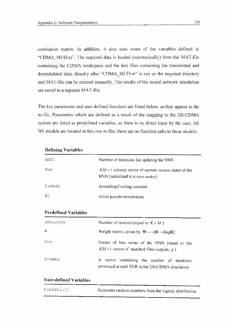
Appendix E: Software Documentation 139
correlation matrix. In addition, it also uses some of the variables defined in
"CDMA_MUD.m". The required data is loaded (automatically) from the MAT-file
containing the CDMA workspace and the text files containing the transmitted and
demodulated data, directly after "CDMA_MUD.m" is run or the required directory
and MAT-file can be entered manually. The results of the neural network simulation
are saved to a separate MAT-file.
The key parameters and user-defined functions are listed below, as they appear in the
m-file. Parameters which are defined as a result of the mapping to the DS-CDMA
system are listed as predefined variables, as there is no direct input by the user. All
NN models are located in this one m-file; there are no function calls to these models.
Defining Variables
nnlt
Ynn
lambda
TO
Predefined Variables
nNeurons
w
Vnn
Frames
User-defined Variables
Logistic ()
Number of iterations for updating the HNN
KM x 1 column vector of current neuron states of the
HNN (initialized to a zero vector)
Annealing/Cooling constant
Initial pseudo-temperature
Number of neurons (equal to K xM)
Weight matrix, given by W = -(R - diagR)
Vector of bias terms of the HNN (equal to the
KM x 1 vector of matched filter outputs, y)
A vector containing the number of iterations
processed at each SNR in the DS-CDMA simulation
Generates random numbers from the logistic distribution.

140
References
[1] ITU (2005, Dec.). leT Statistics. [Online]. Available:
http://www.itu.int/ITU-D/ict/statistics/ict/
(Last Accessed 2006/01/09)
[2] GSMAlWireless Intelligence. (2005, Dec.). GSM Association Statistics Q3
2005. [Online]. Available:
http://www.gsmworld.com/news/statistics/pdf/gsma_stats_q3_05.pdf
(Last Accessed 2006/01/09)
[3] CDMA Development Group. (2005, Sept.). CDG: Worldwide: 3Q 2005 CDMA
Subscribers Statistics. [Online]. Available:
http://www.cdg.org/worldwide/cdma_world_subscriber.asp
(Last Accessed 2006/01/09)
[4] UMTS Forum. (2004, June). Benefits of Mobile Communications for the
Society. UMTS Forum Report 36. [Online]. Available:
http://www.umts-forum.org/servlet/dyconlztumts/umts/Livelenlumts/Resources
_ Reports_36_index
(Last Accessed 2006/01/09)
[5] T. Ojanpera and R. Prasad, "An overview of air interface multiple access for
IMT-2000IUMTS," IEEE Communications Magazine, vol. 36, no. 9, pp. 82
86, Sept. 1998.
[6] L. B. Milstein, "Wideband code division multiple access," IEEE Journal on
Selected Areas in Communications, vol. 18, no. 8, pp. 1344-1354, Aug. 2000.
[7] S. Verdli, "Minimum probability of error for asynchronous Gaussian multiple
access channels," IEEE Transactions on Information Theory, vol. 32, no. 1, pp
85-96, Jan. 1986.
[8] S. Haykin, "Adaptive Systems for Signal Process," in Advanced Signal
Processing Handbook, S. Stergiopoulos, Ed. Boca Raton, Fl. : CRC Press
LLC, 2001, ch. 2.

References 141
[9] G. 1. Kechriotis, E. Zervas, and E. S. Manolakos, "Using recurrent neural
networks for adaptive communication channel equalization," IEEE
Transactions on Neural Networks, vol. 5, no. 2, pp. 267-278, March 1994.
[10] J. J. Hopfield and D. W. Tank, "Neural computation of decisions m
optimization problems," Biological Cybernetics, vol. 52, no. 3, pp. 141-152,
July 1985.
[11] B. Aazhang, B. -Po Paris, and G. C. Orsak, "Neural networks for code-division
multiple-access communications," IEEE Transactions on Communications,
vol. 40, no. 7, pp. 1212-1222, July 1992.
[12] P. Nicopolotidis, M. S. Obaidat, G. 1. Papadimitriou, and A. S. Pomportsis,
Wireless Networks. Chichester, UK: John Wiley & Sons, 2003.
[13] H. Sari, F. Vanhverbeke, and M. Moeneclaey, "Extending the capacity of
multiple access channels," IEEE Communications Magazine, vol. 38, no. 1, pp.
74-82, Jan. 2000.
[14] S. Verdu, Multiuser Detection. New York, NY: Cambridge University Press,
1998.
[15] T. Ojanpera and R. Prasad, Wideband CDMA for Third Generation Mobile
Communications. Norwood, MA: Artech House, 1998.
[16] J. G. Proakis, Digital Communications, 4th ed., New York, NY: McGraw-Hill,
2001.
[17] M. D. Yacoub, Foundations of Mobile Radio Engineering. Boca Raton,
Florida: CRC Press, 1993.
[18] S. Verdu, "Optimum multiuser asymptotic efficiency," IEEE Transactions on
Communications, vol. 34, no. 9, pp. 890-897, Sept. 1986.
[19] S. Verdu, "Wireless bandwidth in the making," IEEE Communications
Magazine, vol. 38, no. 7, pp. 53-58, July 2000.
[20] S. Moshavi, "Multi-user detection for DS-CDMA communications," IEEE
Communications Magazine, vol. 34, no. 10, pp. 126-133, October 1996.
[21] D. Koulakiotis and A. H. Aghvami, "Data detection techniques for DS/CDMA
mobile systems: A review," IEEE Personal Communications, vol. 7, no. 3, pp.
24-30, June 2000.

References 142
[22] S. Verdli, "Adaptive multiuser detection," in Proc. IEEE International
Symposium on Spread Spectrum Techniques and Applications (ISSSTA'94),
Oulu, Finland, July 1994, vol. 1, pp. 43-50.
[23] U. Madhow, "Blind adaptive interference suppreSSIOn for direct-sequence
CDMA", Proc. ofthe IEEE, vol. 86, no. 10, pp. 2049-2069, Oct. 1998
[24] M. Honig, U. Madhow and S. Verdu, "Blind adaptive multiuser detection,"
IEEE Transactions on Information Theory, Vol. 41, No. 4, pp. 944-960, July
1995.
[25] A. Dua, "MPOE based multiuser detection for DS-CDMA communications,"
M.Tech. Thesis, Department of Electrical Engineering, Indian Institute of
Technology, Powai, Mumbai, India, 2002.
[26] J. B. Whitehead, "Space-time multiuser detection of multi-carrier DS-CDMA
systems," M.Sc. Thesis, School of Electrical and Electronic Eng., University of
Natal, Durban, KZN, SA, 2001.
[27] P. van Rooyen, M. LOtter, and D. van Wyk, Space-Time Processingfor CDMA
Mobile Communications. Norwell, MA: Kluwer Academic Publishers, 2000.
[28] R. Lupas and S. Verdli, "Linear multiuser detectors for synchronous code
division multiple-access channels," IEEE Trans. Inform. Theory, vol. 35, no, 1,
pp. 123-136, Jan. 1989.
[29] H. V. Poor and S. Verdli, "Single-user detectors for multiuser channels," IEEE
Transactions on Communications, vol. 36, no. 1, pp. 50-60, Jan. 1988.
[30] J. Lindner, "MC-CDMA and its relation to general multiuser/multi-subchannel
transmission systems," in Proc. IEEE 4th International Symposium on Spread
Spectrum Techniques and Applications Proceedings (ISSSTA '96), Mainz,
Germany, Sept. 1996, vol. 1, pp. 115-121.
[31] J. Lindner, "MC-CDMA in the context of general multiuser/multi-subchannel
transmission methods," European Transactions on Telecommunications, vol.
10, no. 4, pp. 351-367, July/August 1999.
[32] W. G. Teich and M. Seidl, "Code division multiple access communications:
multiuser detection based on a recurrent neural network structure," in Proc.

References 143
IEEE 4th International Symposium on Spread Spectrum Techniques and
Applications (ISSSTA '96), Mainz, Germany, Sept. 1996, vol. 3, pp. 979-984.
[33] G. Jeney, S. Imre, L. Pap, A. Engelhart, T. Dogan, and W. G. Teich,
"Comparison of different multiuser detectors based on recurrent neural
networks," in Proc. COST 262 Workshop on Multiuser Detection in Spread
Spectrum Communications, Reisensburg, Germany, Jan. 2001, pp. 61-70.
[34] G. Jeney, J. Levendovszky, S. Imre, and L. Pap, "Comparison of different
neural network based multi-user detectors," presented at EUNICE 2000 (Open
European Summer School), Enschede, Netherlands, Sept. 13-15,2000.
[35] A. Duel-Hallen, J. Holtzman, and Z. Zvonar, "Multiuser detection for CDMA
systems," IEEE Personal Communications, vol. 2, no. 2, pp. 46-58, Apr. 1995.
[36] R. Lupas and S. Verdu, "Near-far resistance of multiuser detectors in
asynchronous channels," IEEE Transactions on Communications, vol. 38, no,
4, pp. 496-508, April 1990.
[37] H. V. Poor and S. Verdu, "Probability of error in MMSE multiuser detection,"
IEEE Trans. Inform. Theory, vol. 43, no. 3, pp. 858-871, May 1997.
[38] S. Haykin, Neural Networks: A Comprehensive Foundation, 2nd ed., Upper
Saddle River, New Jersey: Prentice-Hall, 1999.
[39] P. Peretto, An Introduction to the Modeling of Neural Networks. Cambridge,
UK: Cambridge University Press, 1992.
[40] J. Hertz, A. Krogh, and R.G. Palmer, Introduction to the Theory of Neural
Computation. Redwood City, CA: Addison-Wesley, 1991.
[41] M. K. Varanasi and B. Aazhang, "Multistage detection in asynchronous code-
division multiple-access communications," IEEE Transactions on
Communications, vol. 38, no. 4, pp. 509-518, April 1990.
[42] U. Mitra and H. V. Poor, "Neural network techniques for multi-user
demodulation," in Proc. IEEE International Conference on Neural Networks,
San Francisco, CA, March/April 1993, vol. 3, no. 9, pp. 1538-1543.
[43] U. Mitra and H. V. Poor, "Neural network techniques for adaptive multiuser
demodulation," IEEE Journal on Selected Areas in Communications, vol. 12,
no. 9,pp. 1460-1470, Dec. 1994.

References 144
[44] U. Mitra and H. V. Poor, "Adaptive receiver algorithms for near-far resistant
CDMA," IEEE Transactions on Communications, vol. 43, no. 234, pp. 1713
1724, Feb.lMar.lApr. 1995.
[45] T. Miyajima, T. Hasegawa, and M. Haneishi, "On the multiuser detection using
a neural network in code-division multiple-access communications," IEICE
Trans. Communications, vol. E76-B, no. 8, pp. 961-968, Aug. 1993.
[46] T. Nagaosa, T. Miyajima and T.Hasegawa, "On the multiuser detection using a
Hopfield network in M-aryISSMA communications," in Proc. PIMRC '94, The
Hague, Netherlands, Sept. 1994, vol. 2, pp. 420-424.
[47] G. 1. Kechriotis and E. S. Manolakos, "Hopfield neural network
implementation of the optimal CDMA multiuser detector," IEEE Transactions
on Neural Networks, vol. 7, no. 1, pp. 131-141, Jan. 1996.
[48] S. H. Yoon and S. S. Rao, "Multiuser detection in CDMA based on the
annealed neural network," presented at IEEE International Conference on
Neural Networks, Washington DC, USA, June 3--6, 1996.
[49] S. S. Yoon and S. S Rao, "High performance neural network based multiuser
detector in CDMA," in Proc. IEEE International Conference on Acoustics,
Speech, and Signal Processing (ICASSP '97), Munich, Germany, April 1997
vol.4,pp.3357-3360.
[50] S. H. Yoon and S. S. Rao, "Annealed neural network based multiuser detector
in code division multiple access communications", lEE Proceedings on
Communications, vol. 147, no. 1, pp. 57-62, Feb. 2000.
[51] A. Engelhart, W. G. Teich, J. Lindner, G. Jeney, S. Irnre, and L. Pap, "A
survey of multiuser/multi-subchannel detection schemes based on recurrent
neural networks," Wireless Communications and Mobile Computing, vol. 2, no.
3, pp. 269-284, May 2002.
[52] F. Carlier, F. Nouve!, and J. Citerne, "Multi-user Detection for CDMA
Communications Based on Self Organized neural network structures," in Proc.
First IEEE International Workshop on Electronic Design, Test and
Applications (DELTA '02), Christchurch, NZ, Jan. 2002, pp. 52-56.

References 145
[53] A. Hottinen, "Self-organizing multiuser detection," in Proc. IEEE
International Symposium on Spread Spectrum Techniques and Applications
(ISSSTA '94), Oulu, Finland, July 1994, vol. 1, pp. 152-156.
[54] N. Moodley and S. H. Mneney, "Recurrent neural network techniques for
multiuser detection," in Proc. IEEE AFRICON 2004, Gaborone, Botswana,
Sept. 2004, vol. 1, pp. 89-94.
[55] J. J. Hopfield, "Neural networks and physical systems with emergent collective
computational abilities," Proceedings of the National Academy of Sciences of
the United States ofAmerica, vol. 79, no. 8, pp. 2554-2558, April 1982.
[56] S. Kirkpatrick, C. D. Gelatt, Jr., and M. P. Vecchi, "Optimization by simulated
annealing," Science, vol. 220, no. 4598, pp. 671-680, May 1983.
[57] J. J. Steil, "Input-output stability of recurrent neural networks," Ph.D. Thesis,
The Technical Faculty, University of Bielefeld, Bielefeld, Germany, 1999.
[58] J. J. Hopfield, "Neurons with graded response have collective computational
properties like those of two-state neurons," Proceedings of the National
Academy ofSciences, vol. 81, no. 10, pp. 3088-3092, May 1984.
[59] K. A. Smith, "Neural network for combinatorial optimization: a review of more
than a decade of research," INFORMS Journal on Computing, vol. 11, no. 1,
pp. 15-34, (Winter) 1999.
[60] G. I. Kechriotis and E. S. Manolakos, "A hybrid digital signal processing
neural network CDMA multiuser detection scheme," IEEE Transactions on
Circuits and Systems If: Analog and Digital Signal Processing, vol. 43, no. 2,
pp. 96-104, Feb. 1996.
[61] W. G. Teich, M. Seidl and M. Nold, "Multiuser detection for DS-CDMA
communication systems based on recurrent neural network structures," in Proc.
IEEE 4th International Symposium on Spread Spectrum Techniques and
Applications (ISSSTA '98), Sun City, South Africa, Sept. 1998, vol. 3, pp. 863
867.
[62] B. Wang, J. Nie, and Z. He, "A transiently chaotic neural-network
implementation of the CDMA multiuser detector," IEEE Transactions on
Neural Networks, vol. 10, no. 5, pp. 1257-1259, Sept. 1999.

References 146
[63] G. Jeney, J. Levendovszky, and L. Kovacs, "Blind adaptive stochastic neural
network for multiuser detection," in Proc. Vehicular Technology Conference
2001, Rhodes Island, Greece, May 2001, vol. 3, pp. 1868-1872.
[64] J. J. Hopfield, "Artificial neural networks," IEEE Circuits and Devices
Magazine, vol. 4, no. 5, pp. 3-10, Sept. 1988.
[65] E. Aarts and J. Korst, Simulated Annealing and Boltzmann Machines: A
Stochastic Approach to Combinatorial Optimization and Neural Computing.
Chichester, UK: John Wiley & Sons, 1990.
[66] S. B. Gelfand and S. K. Mitter, "Simulated annealing," in Stochastics in
Combinatorial Optimization, G. Andreatta, F. Mason, P. Serafini, Ed.
Singapore: World Scientific, 1987, pp. 2-51.
[67] L. Ingber, "Simulated annealing: Practice versus theory," J Math. Comput.
Modelling, vol. 18, no. 11, pp. 29-57, Dec. 1993.
[68] V. Pavlovi6, D. Schonfeld and G. Friedman, "Enhancement of Hopfield neural
networks using stochastic noise processes," presented at IEEE Signal
Processing Society Workshop on Neural Network for Signal Processing
(NNSP), Falmouth, MA, September 10-12,2001.
[69] M. Evans, N. Hastings, and B. Peacock, Statistical Distributions, 2nd ed., New
York, NY: John Wiley & Sons, 1993.

147
Bibliography
[1] R. C. de Lamare and R. Sampaio-Neto, "An approximate minimum BER
approach to multiuser detection using recurrent neural networks," in Proc. 13th
IEEE International Symposium on Personal, Indoor and Mobile Radio
Communications (PIRMC'02), Lisbon, Portugal, Sept. 2002, vol. 3, pp. 1295
1299.
[2] A. Ephremides, "The use of neural networks in optimization problems in
communication networks," in Proc. IEEE Colloquium in South America,
Argentina/BrazillChile, Aug.lSept. 1990, pp. 66-70.
[3] W. C. Y. Lee, "Overview of cellular CDMA," IEEE Transactions on Vehicular
Technology, vol. 40, no. 2, pp. 291-302, May 1991.
[4] T. K. Sarkar, H. Schwarzlander, S. Choi, M. S. Palma, and M. C. Wicks,
"Stochastic versus deterministic models in the analysis of communication
systems," IEEE Antennas and Propagation Magazine, vol. 44, no. 4, pp. 40
50, Aug. 2002.
[5] X. -So Zhang, Neural Networks in Optimization. Dordrecht, Netherlands:
Kluwer Academic Publishers, 2000.