Recurrent Neural Networks 2: LSTM, gates, and …Recurrent Neural Networks 2: LSTM, gates, and...
27
Recurrent Neural Networks 2: LSTM, gates, and current research Steve Renals Machine Learning Practical — MLP Lecture 10 22 November 2017 / 27 November 2017 MLP Lecture 10 Recurrent Neural Networks 2: LSTM, gates, and current research 1
Transcript of Recurrent Neural Networks 2: LSTM, gates, and …Recurrent Neural Networks 2: LSTM, gates, and...
Recurrent Neural Networks 2: LSTM, gates, and current research
Steve Renals
Machine Learning Practical — MLP Lecture 1022 November 2017 / 27 November 2017
MLP Lecture 10 Recurrent Neural Networks 2: LSTM, gates, and current research 1
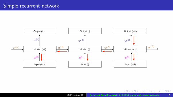
Simple recurrent network
Hidden (t)
Output (t)
Input (t)
Hidden (t-1)
w(1)
w(2)
w(R)
Hidden (t+1)
Input (t-1)
Output (t-1)
Input (t+1)
Output (t+1)
w(2)w(2)
w(1)w(1)
w(R)w(R) w(R)
MLP Lecture 10 Recurrent Neural Networks 2: LSTM, gates, and current research 2
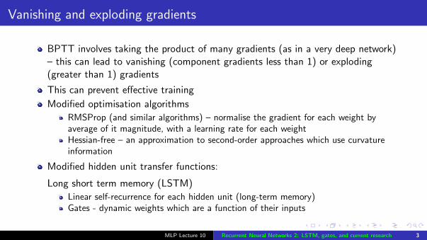
Vanishing and exploding gradients
BPTT involves taking the product of many gradients (as in a very deep network)– this can lead to vanishing (component gradients less than 1) or exploding(greater than 1) gradients
This can prevent effective training
Modified optimisation algorithms
RMSProp (and similar algorithms) – normalise the gradient for each weight byaverage of it magnitude, with a learning rate for each weightHessian-free – an approximation to second-order approaches which use curvatureinformation
Modified hidden unit transfer functions:
Long short term memory (LSTM)
Linear self-recurrence for each hidden unit (long-term memory)Gates - dynamic weights which are a function of their inputs
MLP Lecture 10 Recurrent Neural Networks 2: LSTM, gates, and current research 3
LSTM
MLP Lecture 10 Recurrent Neural Networks 2: LSTM, gates, and current research 4
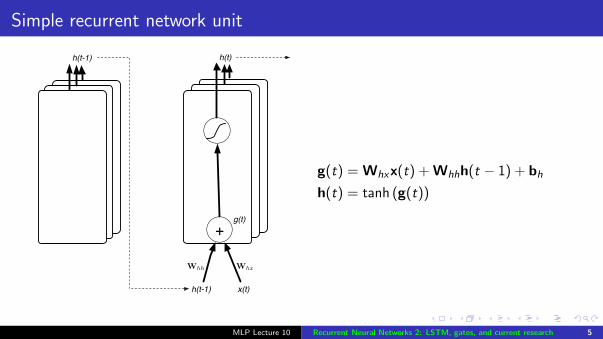
Simple recurrent network unit
x(t)h(t-1)
h(t)
+
h(t-1)
Whh Whx
g(t)
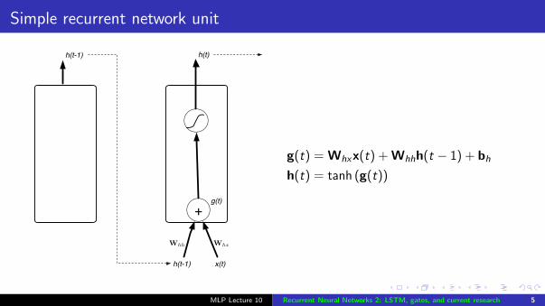
g(t) = Whxx(t) + Whhh(t − 1) + bh
h(t) = tanh (g(t))
MLP Lecture 10 Recurrent Neural Networks 2: LSTM, gates, and current research 5
Simple recurrent network unit
x(t)h(t-1)
h(t)
+
h(t-1)
Whh Whx
g(t)
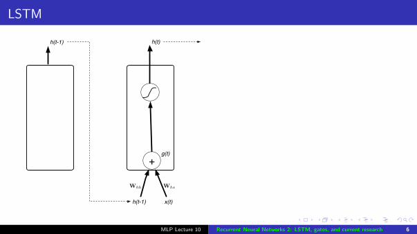
g(t) = Whxx(t) + Whhh(t − 1) + bh
h(t) = tanh (g(t))
MLP Lecture 10 Recurrent Neural Networks 2: LSTM, gates, and current research 5
LSTM
x(t)h(t-1)
h(t)
+
h(t-1)
Whh Whx
g(t)
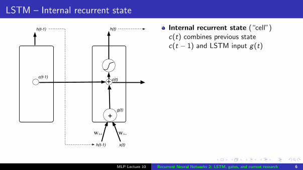
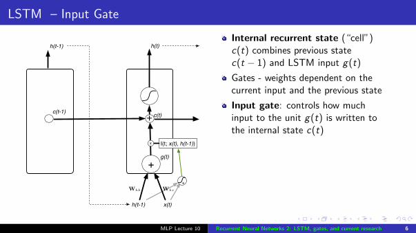
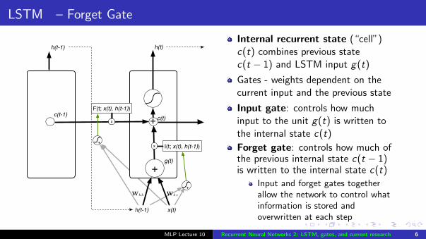
Internal recurrent state (“cell”)c(t) combines previous statec(t − 1) and LSTM input g(t)
Gates - weights dependent on thecurrent input and the previous state
Input gate: controls how muchinput to the unit g(t) is written tothe internal state c(t)
Forget gate: controls how much ofthe previous internal state c(t − 1)is written to the internal state c(t)
Input and forget gates togetherallow the network to control whatinformation is stored andoverwritten at each step
MLP Lecture 10 Recurrent Neural Networks 2: LSTM, gates, and current research 6
LSTM – Internal recurrent state
x(t)h(t-1)
h(t)
+
h(t-1)
c(t-1) c(t)
Whh Whx
g(t)
+
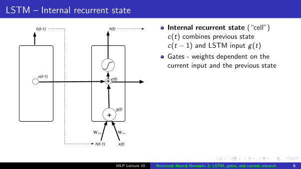
Internal recurrent state (“cell”)c(t) combines previous statec(t − 1) and LSTM input g(t)
Gates - weights dependent on thecurrent input and the previous state
Input gate: controls how muchinput to the unit g(t) is written tothe internal state c(t)
Forget gate: controls how much ofthe previous internal state c(t − 1)is written to the internal state c(t)
Input and forget gates togetherallow the network to control whatinformation is stored andoverwritten at each step
MLP Lecture 10 Recurrent Neural Networks 2: LSTM, gates, and current research 6
LSTM – Input Gate
x(t)h(t-1)
h(t)
+
h(t-1)
c(t-1) c(t)
I(t; x(t), h(t-1))
Whh Whx
g(t)
+
+
x
Internal recurrent state (“cell”)c(t) combines previous statec(t − 1) and LSTM input g(t)
Gates - weights dependent on thecurrent input and the previous state
Input gate: controls how muchinput to the unit g(t) is written tothe internal state c(t)
Forget gate: controls how much ofthe previous internal state c(t − 1)is written to the internal state c(t)
Input and forget gates togetherallow the network to control whatinformation is stored andoverwritten at each step
MLP Lecture 10 Recurrent Neural Networks 2: LSTM, gates, and current research 6
LSTM – Forget Gate
x(t)h(t-1)
h(t)
+
h(t-1)
c(t-1) c(t)
I(t; x(t), h(t-1))
F(t; x(t), h(t-1))
Whh Whx
g(t)
+
+
+
x
x
Internal recurrent state (“cell”)c(t) combines previous statec(t − 1) and LSTM input g(t)
Gates - weights dependent on thecurrent input and the previous state
Input gate: controls how muchinput to the unit g(t) is written tothe internal state c(t)
Forget gate: controls how much ofthe previous internal state c(t − 1)is written to the internal state c(t)
Input and forget gates togetherallow the network to control whatinformation is stored andoverwritten at each step
MLP Lecture 10 Recurrent Neural Networks 2: LSTM, gates, and current research 6
LSTM – Input and Forget Gates
x(t)h(t-1)
h(t)
+
h(t-1)
c(t-1) c(t)
I(t; x(t), h(t-1))
F(t; x(t), h(t-1))
Whh Whx
g(t)
+
+
+
x
x
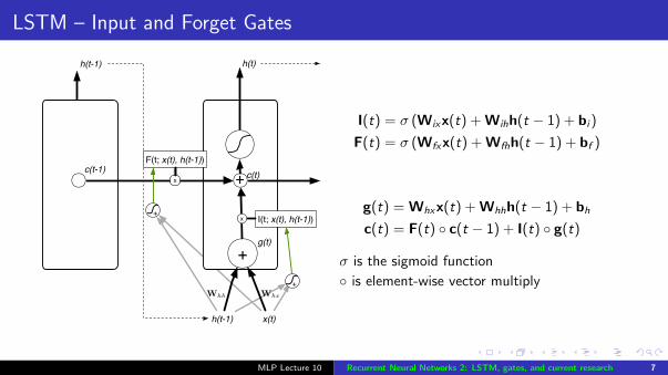
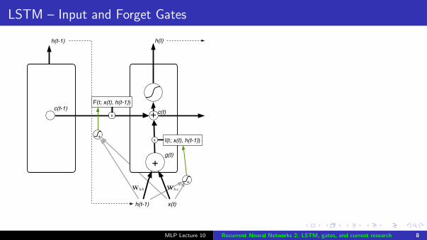
I(t) = σ (Wixx(t) + Wihh(t − 1) + bi )
F(t) = σ (Wfxx(t) + Wfhh(t − 1) + bf )
g(t) = Whxx(t) + Whhh(t − 1) + bh
c(t) = F(t) ◦ c(t − 1) + I(t) ◦ g(t)
σ is the sigmoid function
◦ is element-wise vector multiply
MLP Lecture 10 Recurrent Neural Networks 2: LSTM, gates, and current research 7
LSTM – Input and Forget Gates
x(t)h(t-1)
h(t)
+
h(t-1)
c(t-1) c(t)
I(t; x(t), h(t-1))
F(t; x(t), h(t-1))
Whh Whx
g(t)
+
+
+
x
x
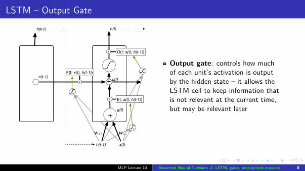
Output gate: controls how muchof each unit’s activation is outputby the hidden state – it allows theLSTM cell to keep information thatis not relevant at the current time,but may be relevant later
MLP Lecture 10 Recurrent Neural Networks 2: LSTM, gates, and current research 8
LSTM – Output Gate
x(t)h(t-1)
h(t)
+
h(t-1)
c(t-1) c(t)
O(t; x(t), h(t-1))
F(t; x(t), h(t-1))
Whh Whx
g(t)
++
+
+
x
x
x
I(t; x(t), h(t-1))
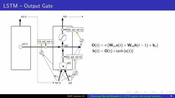
O(t) = σ (Woxx(t) + Wohh(t − 1) + bo)
h(t) = O(t) ◦ tanh (c(t))
MLP Lecture 10 Recurrent Neural Networks 2: LSTM, gates, and current research 9
LSTM equations
x(t)h(t-1)
h(t)
+
h(t-1)
c(t-1) c(t)
I(t; x(t), h(t-1))
O(t; x(t), h(t-1))
F(t; x(t), h(t-1))
Whh Whx
g(t)
+x
x
x
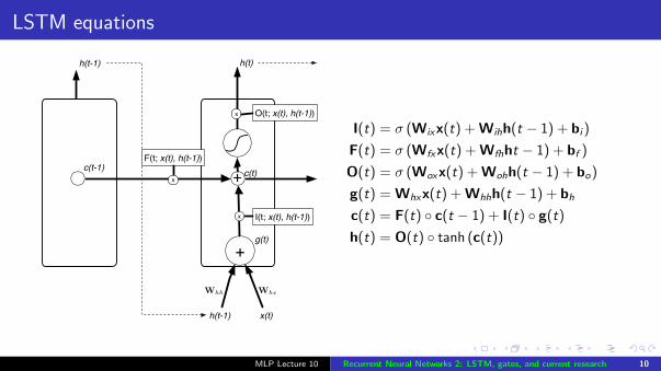
I(t) = σ (Wixx(t) + Wihh(t − 1) + bi )
F(t) = σ (Wfxx(t) + Wfhht − 1) + bf )
O(t) = σ (Woxx(t) + Wohh(t − 1) + bo)
g(t) = Whxx(t) + Whhh(t − 1) + bh
c(t) = F(t) ◦ c(t − 1) + I(t) ◦ g(t)
h(t) = O(t) ◦ tanh (c(t))
MLP Lecture 10 Recurrent Neural Networks 2: LSTM, gates, and current research 10
LSTM/RNN readings
Goodfellow et al, chapter 10
C Olah (2015), Understanding LSTMs,http://colah.github.io/posts/2015-08-Understanding-LSTMs/
A Karpathy et al (2015), Visualizing and Understanding Recurrent Networks,https://arxiv.org/abs/1506.02078
MLP Lecture 10 Recurrent Neural Networks 2: LSTM, gates, and current research 11
More gating units
MLP Lecture 10 Recurrent Neural Networks 2: LSTM, gates, and current research 12
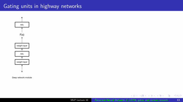
Gating units in highway networks
weight layer
relu
weight layer
relu
x
F(x)
Deep network module
MLP Lecture 10 Recurrent Neural Networks 2: LSTM, gates, and current research 13
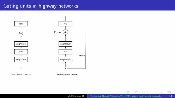
Gating units in highway networks
weight layer
relu
weight layer
relu
x
F(x)
Deep network module
weight layer
relu
weight layer
relu
x
F(x)+x +
identity
Resnet network module
MLP Lecture 10 Recurrent Neural Networks 2: LSTM, gates, and current research 13
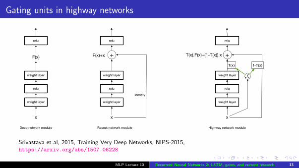
Gating units in highway networks
weight layer
relu
weight layer
relu
x
F(x)
Deep network module
weight layer
relu
weight layer
relu
x
F(x)+x +
identity
Resnet network module
weight layer
relu
weight layer
relu
x
T(x).F(x)+(1-T(x)).x +1-T(x)
+
T(x)
Highway network module
Srivastava et al, 2015, Training Very Deep Networks, NIPS-2015,https://arxiv.org/abs/1507.06228
MLP Lecture 10 Recurrent Neural Networks 2: LSTM, gates, and current research 13
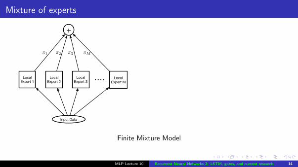
Mixture of experts
LocalExpert 1
LocalExpert 2
LocalExpert 3
LocalExpert M
….
Input Data
+
⇡1 ⇡2 ⇡3 ⇡M
Finite Mixture Model
MLP Lecture 10 Recurrent Neural Networks 2: LSTM, gates, and current research 14
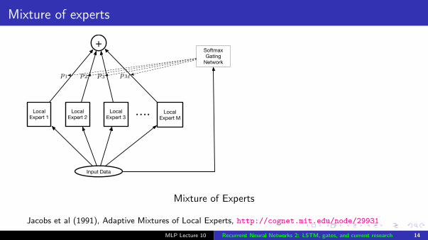
Mixture of experts
LocalExpert 1
LocalExpert 2
LocalExpert 3
LocalExpert M
….
Input Data
+
p1 p2 p3 pM
SoftmaxGating
Network
Mixture of Experts
Jacobs et al (1991), Adaptive Mixtures of Local Experts, http://cognet.mit.edu/node/29931
MLP Lecture 10 Recurrent Neural Networks 2: LSTM, gates, and current research 14
Example applications using RNNs
MLP Lecture 10 Recurrent Neural Networks 2: LSTM, gates, and current research 15
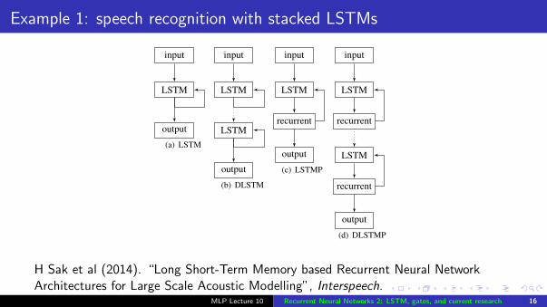
Example 1: speech recognition with stacked LSTMs
inpu
t
g cell h
it
ft
ct
ot
recu
rren
t
outp
ut
xt
mt
rt
rt�1
yt
LSTM memory blocks
Figure 1: LSTMP RNN architecture. A single memory block isshown for clarity.
memory cell. The output gate controls the output flow of cellactivations into the rest of the network. Later, the forget gatewas added to the memory block [18]. This addressed a weak-ness of LSTM models preventing them from processing contin-uous input streams that are not segmented into subsequences.The forget gate scales the internal state of the cell before addingit as input to the cell through the self-recurrent connection ofthe cell, therefore adaptively forgetting or resetting the cell’smemory. In addition, the modern LSTM architecture containspeephole connections from its internal cells to the gates in thesame cell to learn precise timing of the outputs [19].
An LSTM network computes a mapping from an inputsequence x = (x1, ..., xT ) to an output sequence y =(y1, ..., yT ) by calculating the network unit activations usingthe following equations iteratively from t = 1 to T :
it = �(Wixxt + Wimmt�1 + Wicct�1 + bi) (1)ft = �(Wfxxt + Wfmmt�1 + Wfcct�1 + bf ) (2)
ct = ft � ct�1 + it � g(Wcxxt + Wcmmt�1 + bc) (3)ot = �(Woxxt + Wommt�1 + Wocct + bo) (4)
mt = ot � h(ct) (5)yt = �(Wymmt + by) (6)
where the W terms denote weight matrices (e.g. Wix is the ma-trix of weights from the input gate to the input), Wic, Wfc, Woc
are diagonal weight matrices for peephole connections, the bterms denote bias vectors (bi is the input gate bias vector), � isthe logistic sigmoid function, and i, f , o and c are respectivelythe input gate, forget gate, output gate and cell activation vec-tors, all of which are the same size as the cell output activationvector m, � is the element-wise product of the vectors, g and hare the cell input and cell output activation functions, generallyand in this paper tanh, and � is the network output activationfunction, softmax in this paper.
2.2. Deep LSTM
As with DNNs with deeper architectures, deep LSTM RNNshave been successfully used for speech recognition [11, 17, 2].Deep LSTM RNNs are built by stacking multiple LSTM lay-ers. Note that LSTM RNNs are already deep architectures inthe sense that they can be considered as a feed-forward neu-ral network unrolled in time where each layer shares the samemodel parameters. One can see that the inputs to the modelgo through multiple non-linear layers as in DNNs, however thefeatures from a given time instant are only processed by a sin-gle nonlinear layer before contributing the output for that time
input
LSTM
output
(a) LSTM
input
LSTM
LSTM
output
(b) DLSTM
input
LSTM
recurrent
output
(c) LSTMP
input
LSTM
recurrent
LSTM
recurrent
output
(d) DLSTMP
Figure 2: LSTM RNN architectures.
instant. Therefore, the depth in deep LSTM RNNs has an ad-ditional meaning. The input to the network at a given time stepgoes through multiple LSTM layers in addition to propagationthrough time and LSTM layers. It has been argued that deeplayers in RNNs allow the network to learn at different timescales over the input [20]. Deep LSTM RNNs offer anotherbenefit over standard LSTM RNNs: They can make better useof parameters by distributing them over the space through mul-tiple layers. For instance, rather than increasing the memorysize of a standard model by a factor of 2, one can have 4 lay-ers with approximately the same number of parameters. Thisresults in inputs going through more non-linear operations pertime step.
2.3. LSTMP - LSTM with Recurrent Projection Layer
The standard LSTM RNN architecture has an input layer, a re-current LSTM layer and an output layer. The input layer is con-nected to the LSTM layer. The recurrent connections in theLSTM layer are directly from the cell output units to the cellinput units, input gates, output gates and forget gates. The celloutput units are also connected to the output layer of the net-work. The total number of parameters N in a standard LSTMnetwork with one cell in each memory block, ignoring the bi-ases, can be calculated as N = nc ⇥ nc ⇥ 4 + ni ⇥ nc ⇥ 4 +nc ⇥ no + nc ⇥ 3, where nc is the number of memory cells(and number of memory blocks in this case), ni is the numberof input units, and no is the number of output units. The com-putational complexity of learning LSTM models per weight andtime step with the stochastic gradient descent (SGD) optimiza-tion technique is O(1). Therefore, the learning computationalcomplexity per time step is O(N). The learning time for a net-work with a moderate number of inputs is dominated by thenc ⇥ (4 ⇥ nc + no) factor. For the tasks requiring a largenumber of output units and a large number of memory cells tostore temporal contextual information, learning LSTM modelsbecome computationally expensive.
As an alternative to the standard architecture, we proposedthe Long Short-Term Memory Projected (LSTMP) architec-ture to address the computational complexity of learning LSTMmodels [3]. This architecture, shown in Figure 1 has a separatelinear projection layer after the LSTM layer. The recurrent con-nections now connect from this recurrent projection layer to theinput of the LSTM layer. The network output units are con-nected to this recurrent layer. The number of parameters in thismodel is nc⇥nr⇥4+ni⇥nc⇥4+nr⇥no+nc⇥nr +nc⇥3,
339
H Sak et al (2014). “Long Short-Term Memory based Recurrent Neural NetworkArchitectures for Large Scale Acoustic Modelling”, Interspeech.
MLP Lecture 10 Recurrent Neural Networks 2: LSTM, gates, and current research 16
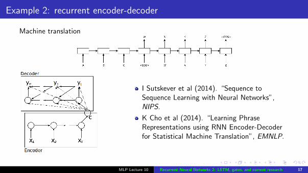
Example 2: recurrent encoder-decoder
Machine translation
I Sutskever et al (2014). “Sequence toSequence Learning with Neural Networks”,NIPS.
K Cho et al (2014). “Learning PhraseRepresentations using RNN Encoder-Decoderfor Statistical Machine Translation”, EMNLP.
MLP Lecture 10 Recurrent Neural Networks 2: LSTM, gates, and current research 17
Summary
Vanishing gradient problem
LSTMs and gating
Applications: stacked LSTMs for speech recognition, encoder-decoder for machinetranslation
More on recurrent networks next semester in NLU, ASR, MT, ....)
MLP Lecture 10 Recurrent Neural Networks 2: LSTM, gates, and current research 18


![CAR-Net: Clairvoyant Attentive Recurrent Network · CAR-Net: Clairvoyant Attentive Recurrent Network 5 in the recurrent module, a long short-term memory (LSTM) network [44] generates](https://static.fdocuments.in/doc/165x107/5f4138c2d25d227723792284/car-net-clairvoyant-attentive-recurrent-network-car-net-clairvoyant-attentive.jpg)