
Recovery of Citric Acid from Fermentation Broth Using ... · PDF filegPROMS general PROcess...
187
Friedrich-Alexander-Universität Erlangen-Nürnberg Lehrstuhl für Thermische Verfahrenstechnik Recovery of Citric Acid from Fermentation Broth Using Simulated Moving Bed Technology - Reinigung von Zitronensäure aus Fermentationslösung durch kontinuierliche Chromatographie Der Technischen Fakultät der Unveriversität Erlangen-Nürnberg vorgelegt zur Erlangung des Grades DOKTOR-INGENIEUR vorgelegt von Dipl.-Ing. Jinglan Wu aus Jiangsu, China Erlangen – 2009
Transcript of Recovery of Citric Acid from Fermentation Broth Using ... · PDF filegPROMS general PROcess...

Friedrich-Alexander-Universität Erlangen-Nürnberg
Lehrstuhl für Thermische Verfahrenstechnik
Recovery of Citric Acid from Fermentation Broth
Using Simulated Moving Bed Technology
-
Reinigung von Zitronensäure aus Fermentationslösung
durch kontinuierliche Chromatographie
Der Technischen Fakultät der Unveriversität Erlangen-Nürnberg
vorgelegt zur Erlangung des Grades
DOKTOR-INGENIEUR
vorgelegt von
Dipl.-Ing. Jinglan Wu
aus Jiangsu, China
Erlangen – 2009

Als Dissertation genehmigt von
der Technischen Fakultät der Universität Erlangen-Nürnberg
Tag der Einreichung: 09.11.2009
Tag der Promotion: 21.12.2009
Dekan: Prof. Dr.-Ing. R. German
Vorsitzender: Prof. Dr. W. Schwieger
1. Berichterstatter: Prof. Dr.-Ing. W. Arlt
2. Betichterstatter: Prof. Dr. R. Buchholz
Weiteres prüfungsberechtigtes Mitglied: Prof. Dr. C. Kryschi

Acknowledgments i
Acknowledgments
This work was carried out at the Lehrstuhl für Thermische Verfahrenstechnik, Friedrich-
Alexander-Universtät Erlangen-Nürnberg, during the years 2005-2009.
First of all, I would like to warmly thank my Doktorvater, Prof. Wolfgang Arlt for
giving me the opportunity for this work, for his optimism and generosity.
I would also like to thank my Chinese professor, Prof. Qijun Peng for the financial aid
to my work and for the support, especially for all the experiments performed in Jiangnan
University, Wuxi, China.
I own a lot of debts to my supervisor Dr. Mirjana Minceva. Without her support and
help, I can hardly finish the work. Also to my previous supervisor, Dr. Dirk-Uwe
Astrath, who is like my older brother and takes care of me since I was first here in
Germany.
I would like to thank Dr. Liudmila Mokrushina and her husband, Dr. Vladimir
Mokrushin, with whom I feel like with my family.
I am also grateful to my kind colleagues and the international entertainment group at
FAU Erlangen-Nürnberg during my stay in Germany. I would like to thank Dr. Stefanie
Herzog, Dr. Jörn Rolker and Dr. Oliver Spuhl for their friendliness and sympathy. I
appreciate my roommate Mr. Florian Lottes for the useful discussions. I also wish to
thank all other staff and colleagues, who are not mentioned here. I will never forget the
international entertainment group from India, Korea and South American, who treated
me bier-drink, shared laughter and foods with me.
I would like to thank all my Chinese friends, especially Wei Wei, Jin Geng and Tao
Tang for their emotional support and help to go through the hardest time with me during
my work. They are always there comforting me when I feel depressed.
I can not finish without saying how grateful to my parents for their patient and
understanding


Table of Contents iii
Table of Contents
Acknowledgments........................................................................................................................................ i
Table of Contents.......................................................................................................................................iii
Nomenclature............................................................................................................................................. vi
Abbreviations............................................................................................................................................. vi
List of Figure Captions............................................................................................................................... x
Abstract ..................................................................................................................................................... xv
Kurzfassung ............................................................................................................................................. xvi
1 Motivation, objectives and outline.................................................................................................... 1
1.1 Properties and usage of citric acid............................................................................................ 1
1.2 Downstream purification processes for recovery of citric acid from the fermentation broth ... 2 1.2.1 Conventional citric acid recovery processes......................................................................... 3 1.2.2 Recovery of citric acid based on chromatography technology ............................................. 8 1.2.3 Novel citric acid purification process based on Simulated Moving Bed technology............ 9
1.3 Objectives and dissertation outline ......................................................................................... 12
2 Introduction to Simulated Moving Bed technology ...................................................................... 16
2.1 Separation principle of liquid chromatography ...................................................................... 16
2.2 Basics of liquid chromatography............................................................................................. 16 2.2.1 Column porosities definitions............................................................................................. 16 2.2.2 Chromatogram and derived parameters .............................................................................. 17
2.2.2.1 Retention time ........................................................................................................... 18 2.2.2.2 Capacity factor and separation factor ........................................................................ 19 2.2.2.3 Peak width................................................................................................................. 19 2.2.2.4 Efficiency of chromatographic separations ............................................................... 20 2.2.2.5 Resolution ................................................................................................................. 20
2.3 Adsorption equilibrium............................................................................................................ 20 2.3.1 Definition of isotherms ....................................................................................................... 20 2.3.2 Models of adsorption isotherms.......................................................................................... 21
2.3.2.1 Linear isotherm ......................................................................................................... 21 2.3.2.2 Langmuir isotherm.................................................................................................... 21 2.3.2.3 Modified Langmuir isotherm .................................................................................... 22
2.3.3 Influence of adsorption isotherm type on the peak shape ................................................... 22
2.4 Hydrodynamics and kinetics.................................................................................................... 24 2.4.1 Axial dispersion.................................................................................................................. 24 2.4.2 Mass transfer resistance ...................................................................................................... 24
2.5 Modelling of chromatographic separation.............................................................................. 25 2.5.1 Transport dispersive model................................................................................................. 27 2.5.2 The lumped rate model with a solid film linear driving force approach............................. 27 2.5.3 Pore diffusion model........................................................................................................... 28 2.5.4 Initial and boundary conditions of the models.................................................................... 29
2.6 Determination of model parameters........................................................................................ 29 2.6.1 Column and particle porosities ........................................................................................... 29 2.6.2 Axial dispersion.................................................................................................................. 31 2.6.3 Adsorption isotherms.......................................................................................................... 32 2.6.4 Kinetic parameters .............................................................................................................. 34

Table of Contents iv
2.7 Operating modes ..................................................................................................................... 34
2.8 Simulated moving bed.............................................................................................................. 35 2.8.1 Principle of SMB technology ............................................................................................. 35 2.8.2 Advantages and disadvantages of SMB technology ........................................................... 36 2.8.3 Modelling of SMB operation.............................................................................................. 38
2.8.3.1 TMB model strategy ................................................................................................. 38 2.8.3.2 Real SMB modelling strategy ................................................................................... 39
2.8.4 SMB design methodologies ................................................................................................ 40 2.8.4.1 Separation triangle methodology............................................................................... 40 2.8.4.2 Separation volume design methodology ................................................................... 43
2.8.5 SMB optimization............................................................................................................... 45 2.8.5.1 Objective function..................................................................................................... 45 2.8.5.2 Optimization variables .............................................................................................. 46 2.8.5.3 Optimization strategy ................................................................................................ 46 2.8.5.4 Optimization algorithm ............................................................................................. 47
3 Modelling of the chromatographic system..................................................................................... 49
3.1 Experiments ............................................................................................................................. 49 3.1.1 Materials ............................................................................................................................. 49
3.1.1.1 Chemicals.................................................................................................................. 49 3.1.2 Equipment........................................................................................................................... 51
3.1.2.1 Semi-preparative chromatographic system ............................................................... 51 3.1.2.2 Preparative chromatographic system......................................................................... 51
3.1.3 Analytical methods ............................................................................................................. 51 3.1.4 Determination of model parameters.................................................................................... 52
3.1.4.1 Column porosity and axial dispersion coefficient ..................................................... 52 3.1.4.2 Adsorption isotherms ................................................................................................ 53 3.1.4.3 Mass transfer parameters........................................................................................... 53
3.1.5 Elution profiles ................................................................................................................... 55
3.2 Numerical method ................................................................................................................... 56
3.3 Results and discussions ........................................................................................................... 57 3.3.1 Chromatographic model parameters ................................................................................... 57
3.3.1.1 Column porosity and axial dispersion ....................................................................... 57 3.3.1.2 Adsorption isotherms ................................................................................................ 58
3.3.2 Single column model selection ........................................................................................... 59 3.3.3 TDM model validation in a preparative chromatographic column ..................................... 62
3.3.3.1 Single component elution profiles............................................................................. 62 3.3.3.2 Fermentation broth elution profiles........................................................................... 64
4 Modelling of an existing pilot-scale SMB unit ............................................................................... 69
4.1 An existing pilot-scale SMB unit ............................................................................................. 69
4.2 Preliminary design of an existing pilot-scale SMB unit operating conditions ........................ 70 4.2.1 TMB and SMB models ....................................................................................................... 70 4.2.2 TMB and SMB unit separation performances .................................................................... 73 4.2.3 Preliminary design of the SMB operating conditions based on separation triangle methodology ...................................................................................................................................... 74
4.3 SMB experiments ..................................................................................................................... 76
4.4 SMB and TMB model verification ........................................................................................... 77 4.4.1 CSS concentration profiles and concentration histories...................................................... 77 4.4.2 Sensitivity Analysis ............................................................................................................ 87
4.4.2.1 Influence of the column numbers on the CSS concentration profiles ....................... 87 4.4.2.2 Influence of the adsorption capacity on the CSS concentration profiles................... 89 4.4.2.3 Influence of the pump flow rates on the CSS concentration profiles ........................ 90
4.4.3 Separation performances .................................................................................................... 92
5 Design of the existing pilot-scale SMB system ............................................................................... 96
Table of Contents v
5.1 Influences of operating conditions on the separation regions and performances ................... 96
5.1.1 Influences of 1m on the separation regions and performances .......................................... 97
5.1.2 Influence of 4m on the SMB performances ...................................................................... 99
5.1.3 Influence of *t on the SMB performances..................................................................... 100 5.1.4 Influence of the SMB configurations on its performances ............................................... 102
5.2 New design of the exiting SMB unit operating conditions..................................................... 104 5.2.1 New SMB separation region............................................................................................. 104 5.2.2 SMB unit operations ......................................................................................................... 104 5.2.3 Analysis of the final CA product ...................................................................................... 109
6 Optimization of the pilot-scale SMB unit..................................................................................... 111
6.1 Direct cyclic steady state modelling strategy ........................................................................ 111 6.1.1 Direct determination of CSS............................................................................................. 111 6.1.2 Comparison of steady state TMB, transient SMB and direct CSS prediction models ...... 115
6.2 Optimization of the existing pilot-scale SMB unit ................................................................. 118 6.2.1 Optimization of the number of SMB columns and SMB unit configurations................... 118 6.2.2 Optimization of the operating conditions for the existing SMB unit ................................ 125 6.2.3 Calculation of the optimal operating conditions ............................................................... 125
6.2.3.1 Experimental validation of the optimized SMB operating conditions .................... 136
6.3 Complete optimal design of a new SMB unit......................................................................... 143 6.3.1 Influence of column lengths on the SMB separation performances ................................. 144 6.3.2 Optimization procedure towards complete SMB unit design ........................................... 146 6.3.3 Pilot scale SMB unit scaling up........................................................................................ 150
7 Conclusions and some suggestions for the future work .............................................................. 155
7.1 Conclusions ........................................................................................................................... 155
7.2 Perspective ............................................................................................................................ 158
Reference List ......................................................................................................................................... 160

Nomenclature vi
Nomenclature Abbreviations
BDNSOL Block Decomposition Nonlinear SOLver
CA Citric Acid
CSS Cyclic Steady State
CVP control vector parameterization
EDM Equilibrium Dispersive Model
GA Genetic Algorithm
Glu glucose
gPROMS general PROcess Modeling System
HETP Height Equivalent to a Theoretical Plate
HPLC High Performance Liquid Chromatography
IPOPT Interior Point Optimizer
LDF lumped rate model with a solid film linear driving force model
MB mass balance
MW molecular weight
NSGA Non-dominated Sorting Genetic Algorithm
OCFEM Orthogonal Collocation on Finite Elements Method
PDM Pore Diffusion Model
PVP tertiary poly (4-vinylpyridine) resin
RCS Readily Carbonizable Substances
SMB Simulated Moving Bed
SS single shooting
SWD standing wave design
TDM Transport Dispersive Model
TMB True Moving Bed
Greek Letters
α separation factor (selectivity) [-]
Aα a constant which accounts for solute-solvent interactions (2.26 for water)
[-]
tε total porosity [-]
ε interstitial porosity [-]
pε particle porosity [-]
γ external tortuosity [-]
λ characterization factor of the packing [-]

Nomenclature vii
µ dynamic viscosity [Pa·s]
tµ first absolute moment [min]
sρ density of the solvent [g/ml]
2
tσ Variance of the peak [min2]
τ dimensionless time [-]
iω peak width of species i [min]
Latin Letters
A strong adsorbed species [-]
cA cross section area of the chromatographic column [cm2]
ia Langmuir isotherm parameters of species i [-]
B less strong adsorbed species [-]
ib Langmuir isotherm parameters of species i [l/g]
C dimensionless concentration [-]
ic concentration of solute i in the fluid phase [g/l]
in
ic inlet concentration of solute i [g/l]
iXc , average concentration of solute i in extract stream [g/l]
iRc , average concentration of solute i in raffinate stream [g/l]
ipc , average concentration in the pores [g/l]
iFc , concentration of solute i in feed stream [g/l]
iRc , concentration of solute i in raffinate stream [g/l]
iXc , concentration of solute i in extract stream [g/l]
axD axial dispersion coefficient [cm2/min]
mD molecular diffusivity [cm2/min]
poreD pore diffusion coefficient [cm2/min]
pd particle diameter [µm]
EC eluent consumption l/kg
)(xerf error function [-]
)(xerfc complementary error function [-]

Nomenclature viii
iH Henry constant of species i in the linear isotherm model [-]
ih modified Langmuir isotherm model parameter of species i
[-]
'
ik capacity factor of species i [-]
ikint, internal mass transfer resistance of species i [min-1]
ifilmk , external mass transfer resistance of species i [min-1]
ieffk , effective mass transfer coefficient of species i [min-1]
seffk , lumped mass transfer coefficient in the solid phase of species i
[min-1]
cL column length [cm]
totcL , total column length [cm]
sM molecular weight of the solvent [g/mol]
jm ratio of net fluid flow to net solid flow in each section [-]
iN number of theoretical plates of species i [-]
cN number of column [-]
Pe Peclet number [-]
PD product dilution [%]
PR productivity [kg/(l•min)]
PUX purity in the extract stream [%]
iq loading, concentration in the stationary phase [g/l]
*
iq
overall solid loading, concentration in the stationary phase
[g/l]
*
eqq
hypothetical solid loading, concentration in the stationary phase
[g/l]
satq adsorbent saturation capacity [g/l]
ElQ eluent flow rate [ml/min]
FQ feed flow rate [ml/min]
RQ raffinate flow rate [ml/min]
sQ volumetric flow rate of solid phase [ml/min]
XQ extract flow rate [ml/min]
TMB
jQ TMB internal volumetric fluid flow rate in each section [ml/min]

Nomenclature ix
SMB
kQ SMB internal volumetric fluid flow rate in each column [ml/min]
0FQ initial feed flow rate [ml/min]
FQ∆ interval of feed flow rate [ml/min]
max,FQ maximum feed flow rate [ml/min]
R Resolution [-]
pr average particle radius [µm]
REX recovery in the extract stream [%]
iRt , retention time of species i [min]
1,0t dead time of pore non-penetrating component [min]
2,0t dead time of pore penetrating component [min]
*t switching time [min]
*0t initial switching time [min]
*t∆ interval of switching time [min]
CV volume of a chromatographic column [ml]
extV volume between the porous stationary phase particles [ml]
intV total volume of pores in the stationary phase particle [ml]
solV particle volume without pores or total volume of the solid [ml]
PV particle volume [ml]
v interstitial velocity [cm/min]
w vertex point in the separation region [-]

List of Figure Captions x
List of Figure Captions
Figure 1-1 Chemical structure of citric acid (C6H8O7) 1
Figure 1-2 Citric acid dissociation curve at 90oC (Kulprathipanja, Oroskar,
1991) 2
Figure 1-3 Flow sheet of the conventional process CA recovery from its
fermentation broth based on precipitation technology 5
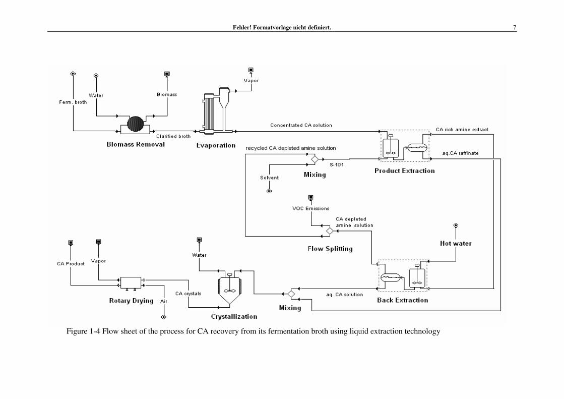
Figure 1-4 Flow sheet of the process for CA recovery from its fermentation
broth using liquid extraction technology 7
Figure 1-5 Flow-sheet of the novel benign process for citric acid recovery
based on the SMB technology 11
Figure 2-1 Fractional volumes inside a chromatographic column 17
Figure 2-2 Chromatogram for the pulse injection of a four-component-mixture
containing two retained and two tracer components of different
molecular weight 18
Figure 2-3 Influence of isotherm type and adsorption kinetics on the
chromatogram (Guiochon et al, 1994) 23
Figure 2-4 Mass transfer phenomena during the adsorption of a molecule 25
Figure 2-5 Classification of different models of a chromatographic column 26
Figure 2-6 Breakthrough curve of one component (Astrath, 2007) 33
Figure 2-7 Principle of TMB and SMB operation 36
Figure 2-8 Separation regions presented in (m2×m3) plane: (a) Linear
isotherms, HA=3, HB=1; (b) Effect of the total feed concentration
(cF), Langmuir adsorption isotherm, qmax,A=50g/l, qmax,B=40g/l ,
KA=0.3l/g, KB=0.2l/g (Mazzotti et al, 1997) 42
Figure 2-9 Effect of the mass transfer resistance on the separation region, k is
the mass transfer coefficient (Rodrigues, Minceva, 2005) 43
Figure 3-1 Chemical structure of the tailor-made stationary phase used to
separate CA from the fermentation broth 51
Figure 3-2 Schematic representation of the experimental preparative
chromatographic setup used for the intermediate pulse injection
experiments 56

List of Figure Captions xi
Figure 3-3 Comparison between the experimental and calculated best fitting
blue dextran breakthrough curves at different flow rates in the
semi-preparative column 58
Figure 3-4 Experimental and calculated adsorption equilibrium isotherms of
citric acid and glucose 59
Figure 3-5 Comparison of the experimental and calculated breakthrough
curves with the TDM, PDM and LDF model for different feed
concentrations: (a) glucose, flow rate: 6ml/min; and (b) CA, flow
rates: 8.3, 8.6 and 9.8ml/min 60
Figure 3-6 Experimental and calculated elution profiles of (a) glucose and (b)
CA in the preparative column: symbols refer to experimental data
and lines represent TDM prediction curves 63
Figure 3-7 Experimental and calculated elution profiles of CA and glucose in
the pretreated fermentation broth in the preparative column at
different flow rates: (a) 60ml/min, (b) 100ml/min, and (c)
120ml/min 66
Figure 4-1 Schematic representation of the existing pilot-scale SMB unit 70
Figure 4-2 CA separation region constructed using the steady state TDM TMB
(PUX≥99.8% and REX≥90%, m1=2.92, m4=-0.21, t*=48.5min,
2-2-2-2 SMB). Points 1, 2 and 3 correspond to three sets of
operating conditions selected for the SMB experimental runs 76
Figure 4-3 Experimental and calculated CA and glucose CSS concentration
profiles in the 16th cycles of run 1 (pretreated fermentation broth
used as a feed, CAFc : 695.1g/l and
GluFc : 14.36g/l) 79
Figure 4-4 Experimental and calculated CA and glucose concentration
histories of run 1: (a) extract stream, and (b) raffinate stream 80
Figure 4-5 Experimental and calculated CA and glucose CSS concentration
profiles in the 16th cycles of run 2 (pretreated fermentation broth
used as a feed, CAFc : 717.3g/l and
GluFc : 44.78g/l) 81
Figure 4-6 Experimental and calculated CA and glucose concentration
histories of run 2: (a) extract stream, and (b) raffinate stream 82
Figure 4-7 Experimental and calculated CA and glucose CSS concentration
profiles in the 16th cycles of run 3 (pretreated fermentation broth
used as a feed, CAFc : 687.5g/l and
GluFc : 33.28g/l) 82

List of Figure Captions xii
Figure 4-8 Experimental and calculated CA and glucose concentration
histories of run 3: (a) extract stream, and (b) raffinate stream 83
Figure 4-9 Calculated CA and glucose CSS concentration profiles with TMB
and SMB models of different column numbers 88
Figure 4-10 Influence of the resin adsorption capacity on the CA CSS
concentration profiles 90
Figure 4-11 Influence of the extract flow rate on the CA CSS concentration
profiles 91
Figure 4-12 Influence of the feed flow rate on the CA CSS concentration
profiles 92
Figure 5-1 Separation regions for different values of m1. (m4: -0.21, t*:
48.5min, SMB configuration: 2-2-2-2) 98
Figure 5-2 Separation regions for different values of m4. (m1: 2.92, t*:
48.5min, SMB configuration: 2-2-2-2) 99
Figure 5-3 Separation regions for different values of t*. (m1: 2.92, m4: -0.21,
SMB configuration: 2-2-2-2) 101
Figure 5-4 Separation regions for different column numbers and SMB
configurations (m1:1.13, m4: 0.08, t*: 25min). Point w
corresponding to the separation region vertex obtained with 8
columns 2-2-2-2 SMB configuration 103
Figure 5-5 CA separation region constructed on the basis of the steady state
TDM TMB model. PUX≥99.8 and REX≥90% as the separation
constraints, m1=1.13, m4=0.08, t*=25min with 2-2-2-2 SMB
configuration. 1’ and 2’ corresponding to two sets of selected
operating conditions for SMB experimental runs 104
Figure 5-6 Experimental and calculated CA and glucose SMB cyclic steady
state concentration profiles in the 16th cycles of run 1’ (pretreated
fermentation broth used as a feed solution, CAFc :658.4g/l and
GluFc :32.8g/l) 106
Figure 5-7 Experimental and calculated concentration histories for run 1’, (a)
extract stream, and (b) raffinate stream 107

List of Figure Captions xiii
Figure 5-8 Experimental and calculated CA and glucose SMB cyclic steady
state concentration profiles in the 16th cycles of run 2’ (pretreated
fermentation broth used as a feed solution, CAFc :638.4g/l and
GluFc :30.9g/l) 107
Figure 5-9 Experimental and calculated concentration histories for run 2’, (a)
extract stream, and (b) raffinate stream 108
Figure 6-1 Comparison of the cyclic steady state concentration profiles
calculated by the transient SMB model and by the direct CSS
prediction model at the middle of the switching time 114
Figure 6-2 Comparison of the concentration history of extract stream
calculated by the transient SMB model with the direct CSS
prediction model 115
Figure 6-3 Flow-sheet of the optimization procedure for maximizing feed flow
rates in the case of different SMB column numbers and SMB unit
configurations 120
Figure 6-4 CSS concentration profiles of CA and glucose calculated with the
direct CSS prediction model at the middle of the switching time for
the optimal operating conditions of case 1 (i.e. maximal feed flow
rate) 122
Figure 6-5 Maximal feed flow rate and product dilution for different number
of SMB columns and different SMB unit configurations 125
Figure 6-6 Flow-sheet of optimization procedure to obtain the optimal
operating conditions for the existing pilot-scale SMB unit 126
Figure 6-7 Comparison of the optimal feed flow rate for different numbers of
SMB column and different flow rates in section 1 in the case of
two different feed concentrations: (a) pre-concentrated (b) clarified
(non-concentrated) fermentation broth 133
Figure 6-8 Comparison of the separation performances for two different feed
concentrations in the case of three different flow rates in section 1
(eight columns SMB, 2-2-2-2 configuration): (a) maximal feed
flow rates; (b) productivities; and (c) eluent consumptions 135
Figure 6-9 Comparison of separation regions obtained in the SMB design and
after SMB optimization for 8 columns SMB (2-2-2-2) and
concentrated fermentation broth as the feed solution 138

List of Figure Captions xiv
Figure 6-10 Experimental and calculated CA and glucose SMB cyclic steady
state concentration profiles in the 16th cycle of run 1(pretreated
fermentation broth used as a feed, CAFc : 670.2g/l and
GluFc :
19.1g/l) 139
Figure 6-11 Experimental and calculated concentration histories for run 1. (a)
extract stream, and (b) raffinate stream 140
Figure 6-12 Experimental and calculated CA and glucose SMB cyclic steady
state concentration profiles in the 11th cycle of run 2 (pretreated
fermentation broth used as a feed, CAFc : 684.3g/l and
GluFc :
15.8g/l) 141
Figure 6-13 Experimental and calculated concentration histories for run 2, (a)
extract, and (b) raffinate 142
Figure 6-14 Calculation of the separation performances for different number of
SMB columns 145
Figure 6-15 Optimization procedure for complete design of a new SMB unit 148

Abstract xv
Abstract
Citric acid (CA) is widely used in the food and pharmaceutical industries. The global
CA production has reached 1.3 million tons per year, with a growing demand of 3.5-
4.5% per year. More than 50% of this volume is being produced in China. One of the
conventional CA downstream recovery processes is based on a calcium salt
precipitation technology which generates huge amounts of CO2 and gypsum. Due to the
restrictions in the environmental pollution, increased requirements on energy
conservation and emission control the outdated CA production capacities must be
replaced in a very close future.
A benign CA purification process based on Simulated Moving Bed (SMB) technology
and a tailor-made CA highly selective resin is proposed. No environmentally harmful
wastes are produced, since deionized water (eluent) is the only substance added to the
separation process. In the proposed process the SMB separation plays an essential role.
This work focuses on modeling, design and optimization of an SMB unit integrated in
the CA downstream process scheme. The costs of the downstream unit operation
following the SMB unit are directly related to the CA concentration in the extract stream.
In order to ensure high CA concentration in the extract, the minimum required CA
recovery and purity were set to 90% and 99.8%, respectively. This implies untypical
SMB application, since normally nearly 100% product purities and recoveries are
required. A systematic model based approach was used for the design of an existing
pilot scale SMB unit.
First the SMB unit operation was modeled on the basis of the experimentally
determined hydrodynamics, adsorption equilibriums and kinetics, using a semi-
preparative chromatographic column (0.3m×0.016m I.D.) and additionally verified in
the pilot scale (1.7m×0.05m I.D.) column.
The mathematical model based SMB design methodology was applied to obtain sets of
operating conditions inside the separation requirements. The designed SMB
performances were obtained experimentally. The required quality of the final CA
product in the form of crystals was also achieved.
Further the operating conditions as well as the number of SMB columns and SMB unit
configuration (number of columns per section) for the existing pilot-scale SMB unit
were consecutively optimized. Experimental results obtained for experiments performed
near the optimal operating conditions had validated the model predictions. The obtained
CA purity, recovery and concentration in the extract stream were 99.8%, 91.3% and
470g/l, respectively. These results were evaluated by a potential industrial user as more
than satisfactory.
Finally the column length was also considered as an additional optimization variable in
the design of a new pilot scale SMB unit. The optimal operating conditions and optimal
column length were obtained for a specific preset switching time, which lead to
maximal SMB productivity and minimal eluent consumptions needed for achievement
of that productivity. The obtained results from this optimization procedure are further
used for SMB unit scale up.

Kurzfassung xvi
Kurzfassung
Zitronensäure (ZS) findet sowohl in der Nahrungsmittel- als auch in der Pharmaindustrie eine breite Anwendung. Die weltweite Produktion hat bereits 1,3 Millionen Jahrestonnen erreicht, wobei der zusätzliche Bedarf mit ca. 3,5 - 4,5% pro Jahr wächst. Mehr als 50% dieses Produktionsvolumens wird in China hergestellt. Einer der konventionellen Herstellungsprozesse basiert auf der Ausfällung eines Calciumsalzes, wodurch jedoch enorme Mengen an CO2 und Gips anfallen. Im Hinblick auf die ökologische Problematik, die immer mehr geforderten Energieeinsparung und die Regelung der Schadstoffemissionen müssen die überalterten Produktionskapazitäten in der nahen Zukunft ersetzt werden. Es wird daher ein neuartiges Aufreinigungskonzept für die Zitronensäureproduktion vorgeschlagen, welches die Simulated-Moving-Bed Technologie (SMB) anwendet und auf dem Einsatz eines maßgeschneiderten, hochselektiven Adsorbens für ZS beruht. Da als alleinige Zusatzkomponente des Trennverfahrens vollentionisiertes Wasser (als Eluent) zum Einsatz kommt, entstehen keinerlei umweltschädliche Nebenprodukte. Im vorgeschlagenen Gesamtprozess stellt die Trennung per SMB den wesentlichen Schritt dar. Die Arbeit konzentriert sich dabei auf die Modelbildung, das Design und die Optimierung einer SMB-Einheit, welche in die Produktionskette der ZS Herstellung integriert ist. Die Kosten der Verfahrensschritte nach der SMB-Einheit sind direkt mit der ZS Konzentration im Extrakt verknüpft. Um daher zu gewährleisten, dass hohe ZS Konzentrationen im Extrakt vorliegen, wurden die geforderte Ausbeute und Konzentration an ZS auf 90% bzw. 99,8% festgelegt. Dies stellt eine eher untypische Anwendung der SMB-Technik dar, da in der Regel nahezu 100% Reinheit und Ausbeute gefordert werden. Ein systematischer, auf mathematischen Modellen beruhender Ansatz wurde gewählt, um eine bereits bestehende SMB-Einheit im Pilotmaßstab neu auszulegen. Zunächst wurde anhand einer semi-präparativen Säule (0.3m×0.016m I.D.) der SMB-Schritt modelliert. Hierbei bildeten die experimentell bestimmten Daten bezüglich der Hydrodynamik, der Adsorptionsisothermen und der Kinetik die Ausgangsbasis. Zusätzlich wurden diese Ergebnisse im Pilotmaßstab validiert (1.7m×0.05m I.D.). Das mathematische SMB-Model wurde verwendet, um Betriebspunkte zu finden, innerhalb derer die Forderungen an die Trennleistung eingehalten wurden. Die Effizienz der ausgelegten SMB-Anlage wurde auf experimentellem Weg ermittelt. Die verlangte Qualität der ZS wurde in Kristallform erreicht. Für die existierende Pilot-SMB-Anlage wurden darüber hinaus die Betriebsparameter sowie die Anzahl der Säulen und deren Konfiguration (die Anzahl pro Trennzone) schrittweise optimiert. Experimentelle Ergebnisse, welche in der Nähe der optimalen Betriebsparameter aufgenommen wurden, konnten die Vorhersagen des Models validieren. Die erhaltene Reinheit, Ausbeute und Konzentration an ZS im Extrakt betrug 99,8%, 91,3% und 470g/l. Diese Ergebnisse wurden von einem potentiellen Anwender aus der Industrie mit „mehr als ausreichend“ beschrieben. Zuletzt wurde zusätzlich die Säulenlänge als ein weiterer Parameter für die Optimierungsrechnung herangezogen, um eine neue SMB-Einheit im Pilotmaßstab auszulegen. Hierbei wurden die optimalen Betriebsparameter und Längen der Säulen für eine vorbestimmte Taktzeit ermittelt. Dies führt schließlich zu einer maximalen Produktivität welche direkt mit einer Minimierung des Eluentenverbrauchs einhergeht. Die aus dieser Optimierung stammenden Ergebnisse werden anschließend für die Maßstabsvergrößerung der SMB-Einheit genutzt.

Fehler! Formatvorlage nicht definiert. 1
1 Motivation, objectives and outline
The aim of this chapter is to introduce the reader to the background, motivation and
objectives of this dissertation.
First the general information concerning the citric acid (CA) physiochemical
properties and its utilization is introduced. Subsequently, the global CA production
capacity is presented, followed by the existing CA downstream processes. These
processes are associated either with high level of environmental pollution or with high
energy consumptions, and thus hinder the further CA production capacity expansion.
In order to overcome these problems, an innovative benign process for recovery of
CA from its fermentation broth based on Simulated Moving Bed (SMB) technology is
proposed in this dissertation. This process is presented in details and the objectives of
this dissertation are disclosed.
At the end of this chapter the outline of the dissertation is given.
1.1 Properties and usage of citric acid
Citric acid (CA, 2-hydroxy-1,2,3-propanetricarboxylic acid, C6H8O7) is a naturally
occurring organic acid which contains three carboxyl groups, Figure 1-1.
Figure 1-1 Chemical structure of citric acid (C6H8O7)
It is a solid at room temperature, melts at 153°C and decomposes at higher
temperatures (Kristiansen et al, 1999). It can undergo one, two or three dissociations
depending on the pH. The distribution of various CA species versus the pH is
presented in Figure 1-2. The first CA dissociation constant pKa1 is equal to 3.13 at
the temperature of 25oC. In the lower pH range, e.g., pH<1.5, CA is present mostly in
its non-ionized form.

Motivation, objectives and outline 2
Figure 1-2 Citric acid dissociation curve at 90oC (Kulprathipanja, Oroskar, 1991)
CA is responsible for the sour taste of various fruits in which it occurs, e.g., lemons,
limes, oranges, pineapples, and gooseberries. The main part of the produced CA (>
60% of total annual production) is used in the food and beverage industries, to
preserve and enhance flavor. Around 25-30% of the total annual production is used
for textile treatment, softening of water and manufacturing of paper. In the
pharmaceutical industry (around 10%), the iron citrate is used as a source of iron and
CA is used as a preservative for stored blood, tablets and ointments, as well as in
cosmetics preparation. Recently, it is being used more and more in the detergent
industry as a replacement for polyphosphates (Harrison et al, 2002).
1.2 Downstream purification processes for recovery of citric acid from the
fermentation broth
CA is a commodity chemical produced and consumed throughout the world. Global
CA production capacity in 2006 was about 1.3 million tons, with an estimated
demand of 3.5-4.5% for the next few years (Soccol et al, 2006). The majority of the
CA production capacities are located in China, Western Europe and the United States.
China covers at least half of the global production capacity, while Western Europe

Fehler! Formatvorlage nicht definiert. 3
and the United States together account for about a third. 65–70% of the global CA
consumption is by Western Europe, the United States and China (Malveda et al,
2006).
CA is commercially produced by submerged microbial fermentation of molasses. The
fermentation process using Aspergillus niger is still the main source of CA worldwide
(Harrison et al, 2002). After fermentation, the fermentation broth, besides CA,
contains residual sugars, proteins, salt and other organic acids, which must be
removed in order to obtain a high quality CA product (Pazouki, Panda, 1998).
1.2.1 Conventional citric acid recovery processes
At present, two processes for CA separation from fermentation broth are used at
industrial scale: a “standard” precipitation (Heding, Gupta, 1975) and liquid-liquid
extraction (Baniel, 1981).
The most frequently used calcium carbonate precipitation technology includes the
following steps (Figure 1-3):
1. Removal of the biomass materials by a rotary vacuum filter;
2. Addition of calcium carbonate (CaCO3) to the clarified fermentation liquor to
precipitate calcium citrate (Ca3(C6H5O7)2);
3. Separation of calcium citrate from the fermentation liquor by a second rotary
vacuum filter;
4. Regeneration of CA by addition of sulfuric acid (H2SO4) to the calcium citrate
cake. Consequently, a precipitate of calcium sulfate (gypsum, CaSO4) is
formed;
5. Precipitation and isolation of the gypsum, leading to an impure CA solution.
This process step is usually repeated several times in order to remove the
readily carbonizable substances (RCS), the main impurities existing in the CA
fermentation broth. The CA product quality is determined by the RCS
presence, lower quantity means higher product quality;
6. Use of anion and cation exchangers to remove the metal ions and other ionic
species, resulting in a high purity CA solution;
7. Decolouration of the CA solution by use of activated carbon;

Motivation, objectives and outline 4
8. Crystallization of the CA, after which the final CA product is obtained in a
form of crystals.
This process consists of many laborious and energy-consuming steps, requires a large
amount of water and auxiliary chemicals (calcium carbonate, sulfuric acid) and
produces significant amount of CO2, waster liquor and gypsum (details are given later
in Section 1.2.3, Table 1-1 and Table 1-2). The gypsum obtained as a side product in
this process has little or no commercial value. The cost for disposal of the waste
materials is approximately $50 per metric ton (Harrison et al, 2002).

Fehler! Formatvorlage nicht definiert. 5
Figure 1-3 Flow sheet of the conventional process CA recovery from its fermentation broth based on precipitation technology

Motivation, objectives and outline 6
Solvent extraction (Baniel, 1981; Baniel, 1991; Baniel, 2001; Baniel et al, 2004) is an
alternative to the classical precipitation method. The recovery of CA from the
fermentation broth by this process consists of the following steps:
1. Removal of the biomass materials by a rotary vacuum filter;
2. Concentration of the fermentation broth by evaporation, up to 80% of the CA
solubility value at ambient temperature;
3. Extraction of CA from the concentrated CA solution with a (recycled) tertiary
amine solution, leading to an amine CA extract and aqueous CA raffinate;
4. Delivery of the aqueous CA raffinate to the crystallization step (step 7);
5. Back extraction of CA from CA rich amine extract with water at higher
temperature (i.e., 80-90oC), to obtain an aqueous CA solution and CA depleted
amine extract;
6. Recycling of the CA depleted amine solution to step 2;
7. Crystallization of the aqueous CA solutions (obtained in steps 4 and 5) to final
CA crystals;
8. Decolouration and ion-exchange may be needed before the final crystallization
step in order to obtain high quality CA product.
The advantage of this process is that the used chemicals are recycled inside the
process, and the problems and cost related to the waste disposal and treatment are
avoided (Pazouki, Panda, 1998). This process is generally economical for aqueous
feeds in the organic acid concentration range 0.1-2.0mol/dm3 (Hartl, Marr, 1993)
Some process related problems are (i) the reagent loss through entrainment, and (ii)
difficulties in efficient phase separation due to formation of third phase and emulsion
(Juang, Chou, 1996). The main disadvantage of the liquid-liquid extraction is that the
organic solvents used are often toxic and/or carcinogenic, which limits its
applicability in the CA production for food industry applications (Soccol et al, 2006).
Fehler! Formatvorlage nicht definiert. 7
Figure 1-4 Flow sheet of the process for CA recovery from its fermentation broth using liquid extraction technology

Motivation, objectives and outline 8
Other separation techniques, i.e., supercritical extraction using compressed carbon
dioxide (Shishikura et al, 1991), eletrodialysis (Novalic et al, 2000; Pinto et al, 2002;
Pinacci, Radaelli, 2002; Widiasa et al, 2004; Luo et al, 2004) and membrane
separation (Friesen et al, 1991), are developed and presented in the literature.
However, these processes are associated with either high cost or high energy
consumption and thus are hardly accepted by the CA industry.
1.2.2 Recovery of citric acid based on chromatography technology
In the patent literature (McQuigg, 1992; Juang, Chang, 1995; Verhoff, 1995; Juang,
Chou, 1996; Takatsuji, Yoshida, 1997; Takatsuji, Yoshida, 1998a; Takatsuji, Yoshida,
1998b; Traving, Bart, 2002; Gluszcz et al, 2004) adsorption chromatography has been
suggested as another feasible technology for recovery of CA from the fermentation
broth. The proposed processes consist of consecutive CA adsorption/desorption steps.
Namely, CA from the fermentation broth is first selectively adsorbed onto the
adsorbent (mainly basic ion-exchange resins) and then desorbed (eluted) by a
desorbent (eluent).
The adsorption equilibrium and kinetics of CA and other organic acids on different
adsorbents were investigated by several researchers (Juang, Chang, 1995; Takatsuji,
Yoshida, 1997; Takatsuji, Yoshida, 1998a; Takatsuji, Yoshida, 1998b; Traving, Bart,
2002; Gluszcz et al, 2004). The results show that the weakly basic ion-exchange
resins have high adsorption capacities for organic acids. The adsorption equilibrium is
generally of Langmuir type. Reilly Industries (Indianapolis, Indiana, USA) issued two
patents in which batch CA adsorption/desorption processes with their own developed
resins are described (McQuigg, 1992; Verhoff, 1995). However, in one of the
proposed processes (McQuigg, 1992), the desorbent is a dilute strong acid solution,
e.g., H2SO4 or HCl. This chemical needs to be removed from the CA product using
additional separation steps. In another patent (Verhoff, 1995), CA is absorbed at a
low temperature (below 30oC) and hot water (temperature above 90oC) is used to
desorb the CA. Although no chemicals are added, the process itself is a batch process
and energy consuming in terms of large scale CA production.
The Simulated Moving Bed (SMB) technology, invented by UOP (Universal Oil
Products, Chicago, Palatine IL, USA) in the 1960s (Broughton, 1961), is a
multicolumn continuous chromatographic separation technology in which the

Fehler! Formatvorlage nicht definiert. 9
adsorption and desorption steps are performed simultaneously. This technology was
original developed for the production-scale applications in the petrochemical industry,
such as the separation of para-xylene from alkyl aromatic C8 fractions. Since late 90´s
SMB technology has found new applications in the areas of pharmaceuticals, fine
chemistry and biotechnology (Sa Gomes et al, 2006).
In 1988, Kulprathipanja introduced the SMB technology into CA recovery from the
fermentation broth (Kulprathipanja, 1988; Kulprathipanja, 1989a; Kulprathipanja,
1989b). Several non-specific commercially available ion-exchange resins have been
used as adsorbent, for instance (i) a neutral polymeric adsorbent, Amberlite XAD
series from Rohm and Haas (Philadelphia, PA, USA) (Kulprathipanja, 1988), (ii) a
weakly anionic exchange resin with teriary amine or pyridine functional groups,
Amberlite IRA series and Dowex 66 sold by Dow Chemical Company (Midland,
Michigan, USA) (Kulprathipanja, 1989b), and (iii) a strongly anionic exchange resin
with quaternary amine functional groups from Dow Chemical Company
(Kulprathipanja, 1989a). In the proposed SMB processes, however, the desorbent
(eluent) used is either a water-aceton-mixture (1 to 1.5% of acetone in water)
(Kulprathipanja, 1988) or a dilute sulfuric or other inorganic acid solution
(Kulprathipanja, 1989a; Kulprathipanja, 1989b). The operating temperature is
between 60oC and 75oC. The pH of the feed (fermentation broth) is kept below the
first ionization constant (pKa1), by using feed solution with CA concentration above
13 wt%, in order to maintain the selectivity of the resin. The added chemicals, i.e.,
acetone and sulfuric acid must be separated from the obtained CA solution. This
requires additional downstream process steps and increases the CA production cost.
1.2.3 Novel citric acid purification process based on Simulated Moving Bed
technology
Recently SMB technology has gained more and more attention in the field of
separation technologies and has emerged as a powerful tool for continuous
countercurrent binary separation of fine chemicals and pharmaceuticals.
A suitable adsorbent is the fundamental necessity to execute a feasible SMB
separation. For the past eight years, a modified tertiary poly (4-vinylpyridine) resin
(PVP) has been developed in the laboratory in Jiangnan University in China for
specific adsorption of CA from its fermentation broth (Peng, 2005). This innovative
resin has a high selectivity to CA, while the other components (impurities) present in

Motivation, objectives and outline 10
the fermentation broth are hardly retained. The bonding energy between CA and the
resin is not as strong as found in the existing commercial resins; therefore pure water
can be used as an eluent. Moreover, the adsorption and desorption processes can be
performed at the same temperature which facilitates the SMB operations.
A benign CA downstream process, which incorporates an SMB unit operated with a
tailor-made adsorbent, is proposed in this dissertation. The CA purification process
scheme is represented in Figure 1-5.
The fermentation broth is first pretreated by filtration (removal of the mycelium and
proteins from the broth). The clarified liquor is then concentrated in a 5-stage
evaporator to more than 80% of the CA solubility in water at room temperature.
Subsequently, the pretreated fermentation liquor is directly fed into the SMB unit.
Hot deionized water at 80oC is used as an eluent. The purified CA aqueous solution is
collected in the extract, while the impurities, mainly readily carbonizable substances
(RCS), are withdrawn in the raffinate. After the SMB separation, the obtained CA
aqueous solution (SMB´s extract stream) is sent to ion-exchange and decoloration
steps. A high quality CA product in the form of crystals is obtained after
crystallization.
In this novel process, the SMB separation unit replaces the overliming and filtration
steps (steps 2-5) in the conventional precipitation process (Figure 1-3) and the steps
3-6 in the solvent extraction process (Figure 1-4), thus the total number of process
steps is reduced. Furthermore, the waste sweet liquor (SMB’s raffinate stream) could
be eventually recycled to the fermentation reactor, after some additional treatment by
which the remained acid and some other tracer substances would be removed, since
only water is added to the system. If this step can be realized, almost no waste
material would be generated in this innovative process.

Fehler! Formatvorlage nicht definiert. 11
Figure 1-5 Flow-sheet of the novel benign process for citric acid recovery based on the SMB technology

Motivation, objectives and outline 12
Table 1-1 compares the chemicals consumption per kilogram of the final CA product
in the conventional precipitation process and in the proposed SMB process
(preliminary calculations). The quantities of discharged waste materials per kilogram
of produced CA (in the form of crystals) in these two processes are presented in Table
1-2. In the new process the use of sulfuric acid and calcium carbonate is avoided. As
a result, no CO2 and gypsum are produced.
Table 1-1 Comparison of the chemicals consumption per kilogram of produced CA in
the conventional and novel CA purification process
H2SO4, kg CaCO3, kg Water, kg
Current 0.96-1.1 1.14-1.2 53-60
New 0 0 5
Table 1-2 Comparison of the discharged waste materials per kilogram of produced
CA in the conventional and novel CA purification processes
CO2, m3 CaSO4, kg Waste Liquor, kg
current 0.03-0.04 2-4 40-50
new 0 0 4
1.3 Objectives and dissertation outline
In the proposed CA purification process, SMB separation plays a crucial role.
However, due to the complexity in the SMB operation (details are given in Chapter 2),
selection of the suitable operating conditions which lead to the desired SMB unit
performances, i.e., productivity, product purity and recovery is not an easy and
straightforward task. The mathematical model based design and optimization of the
SMB unit is essential. The goals of this dissertation are:
1. Design of sets of suitable operating conditions for an existing pilot-scale SMB
unit (16 columns, 1.5m x 0.5m I.D. each), using the novel tertiary poly (4-

Fehler! Formatvorlage nicht definiert. 13
vinylpyridine) resin as stationary phase to recovery CA from the pretreated
fermentation broth. The separation constraints are set to: CA purity higher than
99.8% and recovery higher than 90% in the extract stream. Uncompleted CA
recovery in the extract is selected in order to ensure high CA concentration in
the extract. The CA concentration in the extract stream is an important
criterion and needs to be considered in order to save the energy consumptions
in the process steps following the SMB separation step (see Figure 1-5).
2. The SMB application investigated in this dissertation is different from the
other applications reported in literature. First of all the feed concentration is
rather high. For instance, the CA concentration in the feed is around 700g/l,
which corresponds to the non-linear concentration range of the adsorption
isotherm. Secondly this SMB application is an industrial scale application. A
resin (adsorbent) with a rather large particle size ( pd (90%) = 300±50 µm)
must be used. Hence, the axial dispersion and mass transfer resistance could
not be neglected and would significantly affect the separation efficiency.
Therefore, the selection of a suitable chromatographic model, which is
sufficiently accurate to describe the system and in the same time as simple as
possible is another goal of this dissertation.
3. According to the selected separation constrains (CA purity and recovery in the
extract higher than 99.8% and 90%, respectively) the complete regeneration of
the adsorbent in section 1 is unnecessary. The classic SMB design
methodology, i.e., separation triangle methodology (details given in Chapter 2)
can not be applied directly. Therefore a mathematical model must be used for
the design of the SMB unit. The selection of the SMB configuration and
operating conditions i.e., flow rates in four sections and switching time
through a systematic study of their influence on the SMB performances is the
next objective of this thesis.
4. In the available literature, geometrical parameters, i.e., column length and
diameter, column numbers and configurations are usually excluded in the
SMB unit design and optimization. There is only limited number of studies in
which the influence of these parameters on the SMB separation performances
is investigated. The fourth goal of this dissertation is to develop a systematic
Motivation, objectives and outline 14
and efficient optimization procedure in which the SMB operating conditions
and geometrical parameters would be considered as optimization parameters.
The adsorption isotherm, hydrodynamic and mass transfer parameters
determinate together with an appropriated mathematical model would be
employed in the optimization.
5. The final goal is the scale up of a pilot scale SMB unit to a production scale,
on the basis of the pilot scale SMB unit optimal operating conditions and
geometrical parameters.
With these goals taken into account, this dissertation is organized as follows:
In Chapter 2 the principle of chromatographic separation and fundamental
chromatography theory is presented. The SMB technology is explained and compared
with the batch chromatography. The state of art of SMB modeling, design and
optimization is given at the end of this chapter.
For selection of a proper chromatographic model the parameters affecting a
chromatographic separation must be determined experimentally. In Chapter 3 the
experimental methods and equipments used for measurement of adsorption
equilibrium and hydrodynamics are described. Three commonly used
chromatographic models with different degree of complexity are considered in this
chapter. The model predictions are compared with the experimental CA and glucose
(model substances) elution profiles obtained in the semi-preparative column (0.3m x
0.016m I.D.). Taking into account the model prediction accuracy as well as the
computation time the chromatographic model is selected and validated in one of the
preparative column (1.5m x 0.5m I.D.) from the pilot-scale SMB unit using real pre-
concentrated fermentation broth as feed solution.
Subsequently, in Chapter 4 the equivalent TMB TDM and the rigorous dynamic SMB
TDM models are established based on the single chromatographic column model
selected in the previous chapter. Three SMB experiments are performed in the pilot
scale SMB unit for model prediction validation. The operating conditions for these
experiments were selected using the separation triangle methodology, in which
complete regeneration of section 1 and 4 is assumed. The presented results show that
both models can give accurate prediction of the SMB CA separation performances.
Most important outcome of this chapter is that the separation triangle methodology is
Fehler! Formatvorlage nicht definiert. 15
not an adequate approach for SMB applications where non complete recovery of one
of the products in the product streams is required. Since the designed SMB operating
conditions lead to large eluent consumption, the CA product (extract) was highly
diluted and had little practical value.
In order to improve the SMB separation performances, in particular to increase the
CA concentration in the extract stream, the influences of the operating conditions, i.e.,
the flow rates in section 1 and 4 and switching time as well as the SMB configuration
(number of columns and their distribution in each section) on the separation regions
and the SMB unit performances are studied systematically on the basis of the
“Separation volume” methodology. A new set of the operating conditions leading to
improved SMB performances are consequently obtained. Two of them are selected to
run additional SMB experiments. The new design procedure for solving our specific
separation problem and the obtained results are summarized in Chapter 5.
Chapter 6 focuses on the optimization of the existing pilot-scale SMB plant. An
efficient novel optimization strategy is developed for the complete SMB design
(SMB geometrical parameters and operating conditions). At the end of this chapter
the optimized pilot scale SMB unit plant is scaled up to a production scale plant.
Chapter 7 summarizes the main conclusions and scientific contributions of this thesis
and emphasis some future research work directions.

Introduction to Simulated Moving Bed technology 16
2 Introduction to Simulated Moving Bed technology
In this chapter the fundamental aspects of liquid chromatography are introduced.
Special focus is given to the Simulated Moving Bed (SMB) technology.
The principle of chromatographic separations is briefly explained, followed by the
definition of the most important terms and parameters used for evaluation of a
chromatographic separation. The commonly used chromatographic column model
are presented and the methods used for determination of the model parameters
(adsorption equilibrium, column hydrodynamics and mass transfer parameters) are
described briefly.
The SMB principle of operation is explained in details, the definition of the SMB
performances are introduced and the advantages and disadvantages of this technology,
comparative to the batch-wise chromatography, are discussed. A literature review of
the SMB modeling strategies, design and optimization methodologies is given at the
end of this chapter.
2.1 Separation principle of liquid chromatography
In liquid chromatography, the components to be separated are dissolved in a liquid
(mobile phase or eluent), which percolates through a column packed with solid
porous particles (stationary phase, adsorbent or resin). The separation principle is the
difference in the liquid-solid adsorption equilibrium of the components to be
separated. The difference in adsorption affinities result in distinct migration speeds of
the components along the column and renders separation possible (Snyder, 1968).
2.2 Basics of liquid chromatography
2.2.1 Column porosities definitions
The total volume of a chromatographic column, CV , can be divided into three parts: i)
the volume between the porous stationary phase particles, extV , ii) the total volume of
pores in the stationary phase particle, intV , and iii) the particle volume without pores
or the total volume of the solid, solV (see Figure 2-1) . Using these volumes different
porosities can be defined (Deckert, 1997).

Fehler! Formatvorlage nicht definiert. 17
Figure 2-1 Fractional volumes inside a chromatographic column
The total porosity, tε , is the ratio between the entire volume occupied by the mobile
phase and the total column volume:
C
extt
V
VV += intε Eq. 2-1
The external or bed porosity also sometimes referred as interstitial porosity, ε , is
defined as the ratio of the interstitial volume and the column volume.
C
ext
V
V=ε Eq. 2-2
It is worth noting that the external porosity ε and the total porosity tε are not
independent of each other but coupled by the following equation.
( ) pt εεεε ⋅−+= 1 Eq. 2-3
pε is the particle porosity, which is defined as a ratio of the particle pore volume intV
and the particle volume PV .
P
pV
Vint=ε Eq. 2-4
2.2.2 Chromatogram and derived parameters
In order to evaluate the quality of a chromatographic separation, the mobile phase
exiting the column is introduced in a detector that records the quantity of the

Introduction to Simulated Moving Bed technology 18
dissolved components based on a certain physical principle. The presentation of the
detector signal over time is called a chromatogram. The deflections corresponding to
the detected components are called chromatographic peaks. The information needed
for evaluation of the efficiency of a chromatographic separation is obtained from the
chromatogram. A typical chromatogram resulting from the finite slug (pulse)
injection of mixture containing four different components in analytical amounts is
shown in Figure 2-2.
Figure 2-2 Chromatogram for the pulse injection of a four-component-mixture
containing two retained and two tracer components of different molecular weight
2.2.2.1 Retention time
The interaction strength of each component with the stationary phase is proportional
to its retention time iRt , . The retention time is determined from the peak maximum in
the case of symmetrical peaks. For well-packed columns symmetrical peaks are
normally obtained as long as the amount injected into the column is in the linear
concentration range of the adsorption isotherm. When the injected amount of the
component fits in the nonlinear part of the adsorption isotherm often heavily distorted

Fehler! Formatvorlage nicht definiert. 19
and asymmetric peaks are obtained. The influences of the adsorption types on the
peak shape are discussed in details in Section 2.3.3.
The dead time i
t,0 is the time a non-retained substance (tracer) needs to travel from
the point of sample introduction to the point of sample detection. Tracer molecules
are usually used to determine the dead time. For instance, 1,0t and
2,0t in Figure 2-2
refer to the dead time of a pore non-penetrating component and a pore penetrating
component, respectively.
2.2.2.2 Capacity factor and separation factor
The use of retention time to describe a certain chromatographic separation lacks from
the disadvantage that it depends on the flow velocity of the mobile phase. Thus the
capacity (or retention) factor '
ik , which is calculated from the retention time of a
component and the dead time, is defined as a purely thermodynamic parameter. It
depends only on the distribution of the component between the two phases in the
chromatographic column.
1,0
1,0,'
t
ttk
iR
i
−= Eq. 2-5
In analogy to other separation techniques, a separation factor (or selectivity) is also
used in chromatographic separation. It is defined as a ratio of the relative retention
times for two adjacent peaks.
'
'
01,
02,21
1
2
k
k
tt
tt
R
R=
−
−=α Eq. 2-6
The separation factor gives information on whether a separation of two components is
possible from a purely thermodynamic point of view. Unfortunately a high separation
factor is not a guarantee for satisfactory separation results. Therefore the broadness of
the peaks (peak width) should be taken into consideration as well for evaluation of the
separation efficiency.
2.2.2.3 Peak width
The peak width iω is another important quantity to describe a peak, which is a
measure of the peak broadening inside the column and it is closely related to the
Introduction to Simulated Moving Bed technology 20
efficiency of the separation. It is clear that narrow peaks are beneficial in terms of
separation efficiency.
The column efficiency can be evaluated by the number of theoretical plates N and
the height equivalent to a theoretical plate HETP .
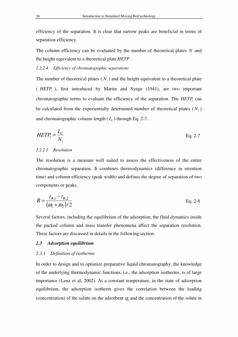
2.2.2.4 Efficiency of chromatographic separations
The number of theoretical plates ( iN ) and the height equivalent to a theoretical plate
( iHETP ), first introduced by Martin and Synge (1941), are two important
chromatographic terms to evaluate the efficiency of the separation. The iHETP can
be calculated from the experientially determined number of theoretical plates ( iN )
and chromatographic column length ( cL ) through Eq. 2-7.
i
Ci
N
LHETP = Eq. 2-7
2.2.2.5 Resolution
The resolution is a measure well suited to assess the effectiveness of the entire
chromatographic separation. It combines thermodynamics (difference in retention
time) and column efficiency (peak width) and defines the degree of separation of two
components or peaks.
( ) 2/21
2,1,
ωω +
−= RR tt
R Eq. 2-8
Several factors, including the equilibrium of the adsorption, the fluid dynamics inside
the packed column and mass transfer phenomena affect the separation resolution.
These factors are discussed in details in the following section.
2.3 Adsorption equilibrium
2.3.1 Definition of isotherms
In order to design and to optimize preparative liquid chromatography, the knowledge
of the underlying thermodynamic functions, i.e., the adsorption isotherms, is of large
importance (Lenz et al, 2002). At a constant temperature, in the state of adsorption
equilibrium, the adsorption isotherm gives the correlation between the loading
(concentration) of the solute on the adsorbent iq and the concentration of the solute in

Fehler! Formatvorlage nicht definiert. 21
the fluid phase ic . The correlation can be represented mathematically by isotherm
models.
2.3.2 Models of adsorption isotherms
In the literature a multitude of different isotherm equations for liquid chromatography
can be found (Snyder, 1968; Guiochon et al, 1994; Ching et al, 2000; Guiochon,
2002). The isotherm models used in this work are presented in the following
subsections.
2.3.2.1 Linear isotherm
The linear adsorption isotherm is the simplest isotherm model, which states that at
equilibrium the solute concentration in the mobile phase ic and the stationary phase
iq are related by a constant factor iH , called Henry constant:
iii cHq ⋅= Eq. 2-9
Usually Eq. 2-9 only holds true as long as the solute concentration in the mobile
phase is low. Since adsorption isotherms in multi-component systems are not
interrelated as long as the concentrations are low, the linear isotherm model can be
applied for multi-component systems as well.
2.3.2.2 Langmuir isotherm
The best known and widely used adsorption isotherm model is the Langmuir isotherm
model. It was derived to describe the uptake on an adsorbent that has a finite,
monolayer adsorption area and can take into account competitive interactions
between different adsorbing components. For an N-component system the stationary
phase/fluid phase equilibrium concentration relationship is usually written as
∑∑ ==⋅+
⋅=
⋅+
⋅=
N
j jj
ii
N
j jj
iisati
cb
ca
cb
cbqq
1111
Eq. 2-10
Where satq is the saturation capacity of the stationary phase, a and b are the
Langmuir isotherm parameters (Langmuir, 1916). Usually iq and ic are
experimentally measured over a range of concentrations, and ia and ib are
calculated by fitting. This model is often useful for fitting multi-component
adsorption data over a limited concentration range.

Introduction to Simulated Moving Bed technology 22
2.3.2.3 Modified Langmuir isotherm
Frequently, the surface of the adsorbent is not homogenous. The simplest way to
account for that is to consider that the surface is composed of two different kinds of
adsorption sites (Schmidt-Traub, 2005). This applies well for chemically bonded
silica gel stationary phase. One part of the surface is covered by the ligand molecules
and the other part is covered with the original silanol groups.
iiN
j jj
iii ch
cb
caq ⋅+
⋅+
⋅=
∑ =11
Eq. 2-11
2.3.3 Influence of adsorption isotherm type on the peak shape
The influence of the isotherm type and the adsorption kinetics on the eluting peak
shape is presented in Figure 2-3 (2a-2c) and Figure 2-3 (3a-3c), respectively.
In ideal chromatogram the influences of the mass transfer kinetics and the axial
dispersion on the band profiles are neglected. The separation is governed only by the
adsorption equilibrium. The solute retention time is calculated using the following
equation:
( )
−+=
ici
i
t
tiiR
dc
dqtct
ε
ε110, Eq. 2-12
( )
⋅
−+= i
t
tiilinR Htct
ε
ε110,, Eq. 2-13
For linear adsorption isotherms, the slope of the isotherm ( ii dcdq ) is constant and
equivalent to the Henry constant, iH . The retention time becomes independent of the
solute concentration (Eq. 2-13). Consequently the band profile does not alter during
the migration process and the elution profile is identical to the injection profile,
namely, an ideally rectangular pulse (see 2a in Figure 2-3).
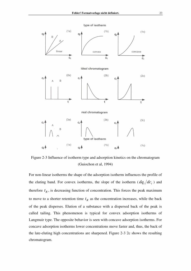
Fehler! Formatvorlage nicht definiert. 23
Figure 2-3 Influence of isotherm type and adsorption kinetics on the chromatogram
(Guiochon et al, 1994)
For non-linear isotherms the shape of the adsorption isotherm influences the profile of
the eluting band. For convex isotherms, the slope of the isotherm ( ii dcdq ) and
therefore Rt , is decreasing function of concentration. This forces the peak maximum
to move to a shorter retention time Rt as the concentration increases, while the back
of the peak disperses. Elution of a substance with a dispersed back of the peak is
called tailing. This phenomenon is typical for convex adsorption isotherms of
Langmuir type. The opposite behavior is seen with concave adsorption isotherms. For
concave adsorption isotherms lower concentrations move faster and, thus, the back of
the late-eluting high concentrations are sharpened. Figure 2-3 2c shows the resulting
chromatogram.
Introduction to Simulated Moving Bed technology 24
In real chromatogram the mass transfer kinetics and the hydrodynamics are taken into
account. These effects tend to disperse and smooth the eluting band profiles, as for
instance, a rectangular concentration profile of the solute at the entrance of the
column soon changes into a Gaussian-shape distribution if the isotherm is linear (see
3a in Figure 2-3).
2.4 Hydrodynamics and kinetics
All preparative and production-scale chromatographic separations aim to collect
target components as highly concentrated as possible. The ideal case would be a
rectangular signal with the same time length and concentration as the pulse injected
into the column. This behavior cannot be achieved in reality. Besides the effects of
the non-linear adsorption isotherms discussed previously, in every chromatographic
system non-idealities of fluid distribution between the stationary phase particle and
mass transfer resistance occur, resulting in a broadening of the eluting peaks of the
solutes. The driving force in the chromatographic separation is actually the sample
dilution occurring as soon as the sample is injected in the column. All hydrodynamic
effects contributing to the total band broadening are coupled in the term axial
dispersion. The rest of the band broadening results from the kinetics of the mass
transfer between the mobile and stationary phase.
2.4.1 Axial dispersion
Molecular and eddy diffusion contribute to axial dispersion. Both effects are additive
and can be expressed with following correlation (Miller, King, 1966):
vdDD Pmax ⋅⋅+⋅= λγ Eq. 2-14
axD is the axial dispersion coefficient. mD is the molecular diffusivity. γ and λ
are the (external) tortuosity and the characterization factor of the packing,
respectively. For typical values (Guiochon et al, 1994)
1256 1010 −−− −≈ scmDm ; ( ) 1243 101.010 −−− =×≈ scmvd p
7.0≈γ ; 1≈λ
Eq. 2-15
2.4.2 Mass transfer resistance
In non-ideal chromatography, the mass transfer between the mobile and the stationary
phase is not instantaneous and the two phases are not in local equilibrium throughout

Fehler! Formatvorlage nicht definiert. 25
the column (Schulte, Epping, 2005). The adsorption process can be subdivided into
different sub-steps presented in Figure 2-4:
• Convective and diffusive transport towards the particle;
• Mass transfer from the bulk phase into the boundary layer of the adsorbent
particle (film diffusion);
• Diffusion inside the pores of the particle (pore diffusion)
• Diffusion along the surface of the solid phase (surface diffusion)
• Adsorption equilibrium or adsorption kinetics
The kinetics of each of these steps contributes to the total band broadening caused by
mass transfer resistances.
Figure 2-4 Mass transfer phenomena during the adsorption of a molecule
2.5 Modelling of chromatographic separation
The effects presented in Figure 2-4 can be described mathematically using
chromatographic models. Different kinds of modeling approaches and mathematical
models, including many analytical solutions, are comprehensively summarized by
Guiochon et al. (1994), Guiochon and Lin (2003), and Ruthven (1984).
The classification of the chromatographic models is shown in Figure 2-5 (Guiochon,
Lin, 2003). The most complex model is so called the “General Rate Model”, which
takes into account the kinetics of the adsorption between the liquid phase in the pores
of the particle and the particle surface, the solute diffusion in the pores, the mass
transport through the film and the convective and dispersive mass transport in the

Introduction to Simulated Moving Bed technology 26
bulk liquid phase (the mobile phase). The simplest model, the “Ideal Model”,
assumes instantaneous adsorption equilibrium between the mobile phase and particle
surface and takes only into account the convective transport in the mobile phase.
Figure 2-5 Classification of different models of a chromatographic column
Chromatographic column models used in this thesis are addressed in detail in the
following section. Namely, the transport dispersive model (TDM), the lumped rate
model with a solid film linear driving force approach (LDF) and the pore diffusion
model (PDM). In all these models, the following assumptions are made in order to
simplify the model complexity.
• The chromatographic process is isothermal;
• The mobile phase velocity remains constant during a run;
• The compressibility of the mobile phase is negligible;
• The packing material is made of porous particles that are spherical and uniform
in size;
• The adsorbent bed is homogeneous;
• The concentration gradient in the radial direction of the adsorbent bed is
negligible;

Fehler! Formatvorlage nicht definiert. 27
• The liquid phase inside the pores is assumed to be stationary and is not affected
by the movement of the mobile phase;
• Axial dispersion flow for the liquid phase.
2.5.1 Transport dispersive model
In the transport dispersive model (TDM) the internal (1/ intk ) and external mass
transfer resistance (1/ filmk ) are lumped in one effective mass transfer coefficient, effk
(Schmidt-Traub, 2005). The mass transfer term is defined by the linear driving force
approach.
( )2
2,
11
x
cD
t
q
t
c
x
c
t
c iax
ip
ip
pii
∂
∂=
∂
∂−+
∂
∂−+
∂
∂+
∂
∂εε
ε
εν Eq. 2-16
The mass transfer in the stationary phase
( ) ( )ipi
p
ieffi
p
ip
p ccr
kt
q
t
c.,
, 31 −=
∂
∂−+
∂
∂εε Eq. 2-17
where, v is the interstitial velocity, t is the time and x is the axial coordinate. The
driving force in Eq. 2-17 is the difference between the concentration ic in the bulk
liquid phase and the average concentration in the pores ipc , , which is assumed to be
in equilibrium with the solid phase concentrations.
The adsorption equilibrium is given by:
( )compNppi ccfq ,1. ,...,= Eq. 2-18
2.5.2 The lumped rate model with a solid film linear driving force approach
Several modifications of the TDM model can be found in the literature. One that is
frequently used considers linear driving force expressed in solid phase concentration
and uses an effective internal mass transfer coefficient ( seffk , ) (Schmidt-Traub,
2005). The linear driving force is modeled as the difference between the average solid
loading *
iq and the loading at the surface of the particle,
*
eqq , which is in equilibrium
with the bulk liquid phase concentration ic . Differential mass balance of component i
in the bulk liquid phase (mobile phase) is:

Introduction to Simulated Moving Bed technology 28
2
2*1
x
cD
t
q
x
c
t
c iax
iii
∂
∂=
∂
∂−+
∂
∂+
∂
∂
ε
εν Eq. 2-19
Differential mass balance of component i in the adsorbent particle (stationary phase)
is:
( )**,,,
* 3iieq
p
iseffi qq
rk
t
q−=
∂
∂ Eq. 2-20
The adsorption equilibrium is given by:
( )compNieq ccfq ,...,1
*, = Eq. 2-21
2.5.3 Pore diffusion model
The pore diffusion model (PDM) is one of the most detailed chromatographic models,
which besides the axial dispersion ( axD ), includes two additional mass transfer effects:
(i) the external mass transfer ( filmk ) through the liquid film around the adsorbent
particle Eq. 2-22; and (ii) the internal mass transfer, governed by the solute diffusion
in the particle’s pores ( poreD ), which results in a radial concentration distribution
inside the adsorbent particle Eq. 2-23 (Gu et al, 1990a; Gu et al, 1990b).
The mass balance in the bulk liquid phase includes the accumulation within the liquid,
convection, axial dispersion and (external) mass transfer through the liquid film
around the particles:
( )[ ]2
2
,,
31
x
cDrrcck
rx
c
t
c iaxpipiifilm
p
ii
∂
∂==−
−+
∂
∂+
∂
∂
ε
εν Eq. 2-22
The differential mass balance for the particles counts for the pore diffusion inside the
particles:
( )
∂
∂
∂
∂=
∂
∂−+
∂
∂
r
cDr
rrt
q
t
c ip
iporepi
p
ip
p
,
,2
2
, 11 εεε
Eq. 2-23
Local adsorption equilibrium is given as:
( )compNppi ccfq ,1. ,...,= Eq. 2-24

Fehler! Formatvorlage nicht definiert. 29
2.5.4 Initial and boundary conditions of the models
Mathematically, all models form a system of (partial) differential and algebraic
equations. For the solution of these models initial and boundary conditions must be
defined. The initial conditions for the concentration and the loading specify their
values at time 0=t . Generally, zero values are assumed:
( ) 0*, === iiipi qqcc Eq. 2-25
Frequently used boundary condition at the chromatographic column inlet is the
classic “closed boundary” condition for dispersive systems derived by Danckwerts
(1953). The outlet boundary condition is generally assumed to be a zero gradient of
the fluid concentration (Danckwerts, 1953):
0=x : ( )iini
iax cc
x
cD −=
∂
∂ν Eq. 2-26
cLx = : ( )0
,=
∂
=∂
x
Lxtc ci Eq. 2-27
For the PDM, two additional boundary conditions are needed, in the particle center
and at the particle surface, respectively:
0=r : 000
,=
∂
∂=
∂
∂
== r
i
r
ip
t
q
t
c Eq. 2-28
prr = : ( )[ ]prr
ip
iporeppipifilmr
cDrrcck
=∂
∂==−
,
,, ε Eq. 2-29
2.6 Determination of model parameters
The model parameters appearing in the above-mentioned models include: (i)
geometrical parameters ( pr , ε , pε ), (ii) fluid dynamics parameters ( axD ), (iii)
adsorption isotherms, and (iv) adsorption kinetics parameters ( effk , seffk , , filmk and
poreD ). The classical methods used for determination of these parameters are
summarized in the following section.
2.6.1 Column and particle porosities
The exact knowledge of the column void volume is of paramount importance for
exploitation of the thermodynamic information contained in the capacity factor ('
k )

Introduction to Simulated Moving Bed technology 30
(Krstulovic et al, 1982). The methods used for determination of the void volumes in a
chromatographic column are extensively reviewed in the publication of Rimmer
(2002). The existing determination methods are classified into two categories: static
and dynamic methods.
The most used static methods is pyconometry, or the weight difference method. The
void volume is calculated according to the mass difference of the same column filled
with two solvents of different densities. It is generally agreed upon that the void
volume determined in this way gives the maximum possible void volume extVV +int
(shown in Figure 2-1).
2,1,
2,1,int
ss
ss
ext
mmVV
ρρ −
−=+ Eq. 2-30
where m is the mass of the column filled with either solvent 1 or 2, and ρ is the
density of the solvent. For normal phase systems methanol and dichloromethane can
be used, for reversed phase systems water and methanol are quite commonly
employed (Guan-Sajonz et al, 1997).
The dynamic chromatographic method is the most common method used to determine
the column porosities experimentally. The method consists of injection of non-
retained tracer component. The elution time of the tracer is used for calculation of the
column porosities. A pore non-penetrating tracer is used to measure the column
external porosity and pore-penetrating tracer to measure the total porosity. In normal
phase liquid chromatography toluene or 1,3,5-tri-tert-butylbenzene are used for
measurement of the total porosity, while in reversed phase liquid chromatography
uracil is the most used component. Blue dextran (MW 2,000,000) is a commonly used
as a pore non-penetrating tracer (Rimmer et al, 2002).
Another alternative dynamic approach is linearization of retention data for
homologous series proposed by Krstulovic et al (1982). The homologous series of
alkanes, alkylbenzenes, methyl esters, chloroalkanes, and alcohols were used.
However, Krstulovic et al. (1982) pointed out that this approach required tedious and
extremely precise data, which makes this method impractical.
In our work, external column porosity was measure by pulse injection of blue dextran.
The determination procedure is described in details in Chapter 3, Section 3.1.4.1.

Fehler! Formatvorlage nicht definiert. 31
2.6.2 Axial dispersion
According to Eq. 2-14, axial dispersion coefficient axD is the sum of the
contributions of eddy diffusion and molecular diffusion. In a preparative liquid
chromatography, however, the contribution of molecular diffusion can be generally
neglected (Duan et al, 1998). Consequently, the axD approximately becomes a linear
function of the interstitial velocity v .
vdD pax ⋅⋅≈ λ Eq. 2-31
Two methods are frequently used to obtain the value of the constant λ . One is the
moment analysis, which is based on the connection between the axD and the second
moment (Schulte, Epping, 2005):
p
c
t
t
p
ax
d
L
dv
Dconst
2.
2
2
µ
σλ =
⋅≈= Eq. 2-32
where tµ is the first absolute moment and 2tσ is the variance which can be
calculated from the second central moment.
( )
( ) dttc
dttct
t
⋅
⋅⋅
=
∫
∫∞
∞
0
0µ Eq. 2-33
( ) ( )
( ) dttc
dttct t
t
⋅
⋅⋅−
=
∫
∫∞
∞
0
0
2
2
µ
σ Eq. 2-34
Alternatively, λ can also be also calculated from the HETP value as (Schmidt-
Traub, 2005):
pd
HETP
2=λ Eq. 2-35

Introduction to Simulated Moving Bed technology 32
Alternative, the axD can also be obtained using the best fitting method. By this
approach the axD is determined by chromatographic model fitting to the
experimentally measured elution profile of a tracer. The best fitting axD values is
obtained by minimization of the difference between measured and calculated
(simulated) elution profiles, i.e., least square fitting technique. This method is used in
our work and explained in details in Chapter 3, Section 3.1.4.1.
2.6.3 Adsorption isotherms
The adsorption isotherm is one of the most important parameters effecting the
chromatographic separation (Seidel-Morgenstern, 2004). In order to achieve good
agreement between simulated (calculated with a model) and experimentally measured
elution profiles, single- and multi-component isotherms have to be determined with
high accuracy. So far, experimental determination method still plays an essential role
in the attainment of the adsorption isotherm data.
The experimental methods for determination of adsorption isotherms can be generally
classified into two groups: static methods and dynamic methods. The static methods
are based on overall mass balances, including batch, adsorption-desorption and
circulation method. However, they are often considered to be more time consuming
and less accurate than dynamic methods (Lenz et al, 2002).
Dynamic methods extract information about the isotherm from the measured
concentration profile (Seidel-Morgenstern, 2004). Frontal analysis is one of the most
popular methods for determination of the adsorption isotherm. In frontal analysis the
solute solution is continuously fed into the column until the equilibrium is achieved,
i.e. solute concentration at the column outlet is equivalent to the solute concentration
in the feed. The detected concentration profile is called breakthrough curve. A
typical breakthrough curve of a single solute is presented in Figure 2-6.
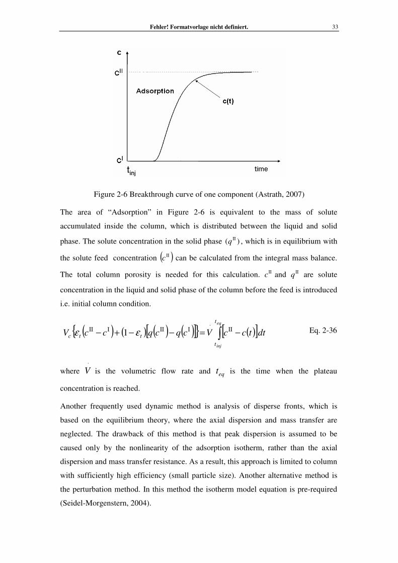
Fehler! Formatvorlage nicht definiert. 33
Figure 2-6 Breakthrough curve of one component (Astrath, 2007)
The area of “Adsorption” in Figure 2-6 is equivalent to the mass of solute
accumulated inside the column, which is distributed between the liquid and solid
phase. The solute concentration in the solid phase )( ΙΙq , which is in equilibrium with
the solute feed concentration ( )ΙΙc can be calculated from the integral mass balance.
The total column porosity is needed for this calculation. ΙΙc and ΙΙq are solute
concentration in the liquid and solid phase of the column before the feed is introduced
i.e. initial column condition.
( ) ( ) ( ) ( )[ ]{ } ( )[ ]dttccVcqcqccV
eq
inj
t
t
ttc ∫ −=−−+− ΙΙ⋅
ΙΙΙΙΙΙ εε 1 Eq. 2-36
where ⋅
V is the volumetric flow rate and eqt is the time when the plateau
concentration is reached.
Another frequently used dynamic method is analysis of disperse fronts, which is
based on the equilibrium theory, where the axial dispersion and mass transfer are
neglected. The drawback of this method is that peak dispersion is assumed to be
caused only by the nonlinearity of the adsorption isotherm, rather than the axial
dispersion and mass transfer resistance. As a result, this approach is limited to column
with sufficiently high efficiency (small particle size). Another alternative method is
the perturbation method. In this method the isotherm model equation is pre-required
(Seidel-Morgenstern, 2004).

Introduction to Simulated Moving Bed technology 34
In this work, frontal analysis method was used to determine the CA and glucose
adsorption isotherms.
2.6.4 Kinetic parameters
Practical determination of kinetic parameters (the external and (or) internal mass
transfer coefficients and the pore diffusivity) suffers from some difficulties. The best
fitting method is usually applied to obtain the mass transfer parameters values from
the experimentally measured solute elution profiles.
An initial guess for the mass transfer parameters values can also be obtained from the
wide range of empirical correlations (Mackie, Meares, 1955; Wilke, Pin, 1955;
Wilson, Geankoplis, 1966). The advantage of using empirical correlation is that
experimental efforts are not needed.
The external mass transfer coefficient ( filmk ), for instance, can be calculated with
Wilson and Geankoplis correlation (1966):
33.009.1
⋅=
m
p
p
mfilm
D
d
d
Dk
νε
ε
Eq. 2-37
where mD is the molecular diffusivity. The pore diffusion coefficient ( poreD ) may be
estimated by the Mackie-Meares correlation (1955):
( ) m
p
p
pore DD2
2 ε
ε
−= Eq. 2-38
The parameter estimation method is used in this work. The correlations involved in
the models are going to be presented in details in Chapter 3, Section 3.1.4.3.
2.7 Operating modes
The classical elution chromatography belongs to the discontinuous (batch) separation
process, which suffers from the following disadvantages:
• A continuous input of the feed mixture or withdrawal of the product streams is
impossible, resulting in a low productivity.
• The efficiency of the stationary phase usage is low. Due to the discontinuous
nature of the process, the actual separation task is only fulfilled in a part of the
chromatographic column (stationary phase volume). Other parts of the

Fehler! Formatvorlage nicht definiert. 35
stationary phase are in a contact with either pure mobile phase or with
components that are already separated. These parts of the stationary phase
(column) do not contribute to the separation.
• The eluent consumption is high, since the stationary phase is normally
completely regenerated before the injection of new portion of the feed mixture.
Due to these drawbacks, the batch elution process is mainly used for analytical
purposes, mixtures quantitative and qualitative analysis. In a production scale
chromatography the continuous operating mode are preferred. The possible
continuous chromatographic separation processes include annular chromatography
(Bart et al, 1996) and Simulated Moving Bed (SMB) technology (Broughton, 1961).
Among them, in an industrial production scale the SMB technology is the most
advantageous in terms of productivity and eluent consumption. This technology was
developed by UOP (Universal Oil Products, Chicago, Palatine IL, USA) in 1960s
(Broughton, 1961) and has emerged as a powerful continuous countercurrent
chromatographic technique. Details regarding this technique are discussed in the
following section.
2.8 Simulated moving bed
2.8.1 Principle of SMB technology
The principle of SMB operation can be best understood by analogy with the
equivalent True Moving Bed (TMB) process. The TMB unit (Figure 2-7a) is divided
into four sections by two inlet streams (feed and eluent) and two outlet streams
(extract and raffinate). The section 1 is located between eluent and extract ports.
Between extract and feed ports positions the section 2. The section 3 is between feed
and raffinate whereas section 4 is between raffinate and eluent.
In TMB unit, the liquid and the solid phase flow in opposite directions, and are
continuously recycled: the liquid flowing out from section 4 is recycled to section 1,
while the solid coming out from section 1 is recycled to section 4. The solid flow rate
is constant all over the unit. However, the liquid flow rates differ from section to
section, due to the introduction or withdrawal of four process streams between the
sections.
Let us consider a feed mixture containing species A, the more retained component
recovered in the extract and species B, the less adsorbed component recovered in the

Introduction to Simulated Moving Bed technology 36
raffinate. In sections 2 and 3, the two components must move in opposite directions.
The less retained component B must be desorbed and carried out with the liquid phase
in direction to the raffinate port, while the more retained species A must be adsorbed
and carried out with the solid phase in direction to the extract port. Section 2 is the
zone of desorption of the less retained species B, while section 3 is the zone of
adsorption of the more retained component A. The role of section 4 is to clean
(regenerate) the eluent, which is then recycled to the section 1, where the adsorbent is
regenerated and free of any adsorbed component recycled back to section 4.
Figure 2-7 Principle of TMB and SMB operation
The major difficulty in TMB operation is the movement of the solid phase. This
problem was overcome by the introduction of SMB technology. In the SMB unit
(Figure 2-7b), the adsorbent is fixed in a set of identical interconnected columns. The
countercurrent movement of the liquid and solid phases is simulated by simultaneous
shift of the inlet and outlet stream ports one column ahead in the direction of the fluid
flow at regular time intervals, called switching time.
2.8.2 Advantages and disadvantages of SMB technology
The SMB technology exhibit a number of advantages with respect to batchwise single
column preparative chromatography. In particular, the continuous nature of the
operation and countercurrent flow of the phases yields to enhanced mass transfer rate
and efficient usage of the stationary and mobile phases, which result in lower eluent
consumption and higher productivity per unit time and unit mass of stationary phase.

Fehler! Formatvorlage nicht definiert. 37
Solvent savings up to 50% and increase of productivity up to two or three times have
been reported (Strube et al, 1998). Moreover, good separation performances can be
achieved even at rather low values of selectivity (for example 1.05) and with a
relatively small number of theoretical plates (less efficient chromatographic columns).
In the SMB unit, contrary to the elution preparative chromatography, the
concentration profiles of the components to be separated are allowed to overlap along
the adsorption beds, since only at the extract and raffinate ports location the
components must be in a pure form.
For a successful SMB chromatographic separation, after selecting a proper adsorbent
and eluent (mobile phase), there are still numerous parameters that must be selected.
These parameters can be classified into two groups.
(i) Operating conditions:
• External flow rates: feed, eluent, raffinate and extract
• Internal flow rates: flow rates in four sections
• Switching time
(ii) Geometrical parameters:
• Column length and diameter
• Total number of columns
• Column configurations
• Particle size
All these parameters are not independent on each other. Finding a proper set of
operating and geometrical parameters, which lead to the desired separation
performances, by a trial-and-error would be extremely difficult and time consuming,
especially for systems with small separation factors, less efficient columns and high
purity requirements. Therefore, modeling and simulation is essential for SMB unit
design and optimization. The SMB modeling strategies are summarized in Section
2.8.3. The aspects regarding model based design and optimization are reviewed in
Section 2.8.4 and 2.8.5, respectively.

Introduction to Simulated Moving Bed technology 38
2.8.3 Modelling of SMB operation
There are two SMB modeling strategies. One is using the equivalent TMB to
represent the SMB operation, in which the countercurrent motion of solid is actually
taken into account. TBM/SMB equivalence relations are used to relate the TMB
operating conditions with those of a real SMB unit. The second modeling strategy
considers real SMB operation, i.e., period shift of the position of the inlet and outlet
streams.
2.8.3.1 TMB model strategy
The most common and easy SMB modeling strategy is the one using the SMB
equivalence with the TMB unit. This approach is easier to understand and more
important it requires shorter computation time, since calculation of TMB unit
operation in steady state is possible. The equivalence relations between TMB and
SMB unit are given in Table 2-1 (Beste et al, 2000).
Table 2-1 SMB/TMB equivalence relationships
TMB SMB
Solid flow rate
sQ
Periodic shift of the stream ports
( ) sc QVt ⋅−= ε1*
Internal flow rates
TMB
jQ , 4,3,2,1=j
Internal flow rates
sTMBj
SMBk QQQ ⋅
−+=
ε
ε
1, cNk ,...,2,1=
where sQ is the volumetric flow rate of the adsorbent in TMB, *t is the SMB
switching time, TMB
jQ is the TMB internal volumetric fluid flow rate in each section,
and SMB
kQ is the SMB internal volumetric fluid flow rate in each column.
With reference to Figure 2-7a, in order to complete a TMB model, besides the
chromatographic model applied to the four sections, additional mass balances around
the inlet and outlet streams ports are needed as well. The complete TDM TMB model
used in this work is given in Chapter 4, Section 4.2.1.

Fehler! Formatvorlage nicht definiert. 39
2.8.3.2 Real SMB modelling strategy
An SMB can be modeled more precisely when its real cyclic operation is assumed in
the model description. Namely, each column is presented individually and the
periodic change of the boundary conditions is taken into account, which leads to
achievement of a cyclic steady state.
The performance of an SMB unit becomes identical to the corresponding TMB unit in
the case of an infinite number of columns, i.e., column length and switching time
approaching to zero. Pais et al (1998) investigated the influences of the column
number on the separation performances prediction using both modeling strategies.
They concluded that the TMB model can be used to predict the performance of an
SMB unit. However, difference in the model predictions increases when SMB units
with small number of columns per section are considered (i.e. one column per
section). In this case, real SMB model has to be used. The main problem associated
with the SMB modeling strategy is the long computation time needed for dynamic
simulation of the unit operation. In order to overcome this problem, direct cyclic
steady state (CSS) prediction method was proposed (Minceva et al, 2003). Generally,
there are two approaches for direct SMB CSS predictions.
The first approach is based on the fact that at CSS the spatially distributed SMB unit
state at the end of a switching time interval is identical to the state at the beginning of
the interval, apart from a shift of exactly one column length (Kloppenburg, Gilles,
1999).
The initial conditions are expressed as:
( ) ( )*,,1,0,,, tzjiczjic += , ( )BAi ,∈ , ( )Nj ,...,2,1∈ , ( )Lz ,0∈ Eq. 2-39
( ) ( )*,,1,0,,, tzjiqzjiq += , ( )BAi ,∈ , ( )Nj ,...,2,1∈ , ( )Lz ,0∈ Eq. 2-40
The second one is based on the fact that at cyclic steady state the conditions at the end
of the cycle are identical to those at its beginning in both liquid and solid phases
(Nilchan, Pantelides, 1998):
( ) ( )cycleTzjiczjic ,,,0,,, = , ( )BAi ,∈ , ( )Nj ,...,2,1∈ , ( )Lz ,0∈ Eq. 2-41
( ) ( )cycleTzjiqzjiq ,,,0,,, = , ( )BAi ,∈ , ( )Nj ,...,2,1∈ , ( )Lz ,0∈ Eq. 2-42

Introduction to Simulated Moving Bed technology 40
These two approaches were used by Minceva et al (2003) for the case of SMB
enantiomers separation. They concluded that both methods lead to same results and
the first approach requires shorter computation time.
This direct CSS modeling strategy has been further used by Kawajiri and Biegler
(2006a; 2006b; 2006c; 2008a; 2008b) in optimization of the SMB configurations and
optimization of different SMB operating schemes and modes. Also, has been applied
in the design and optimization of SMB enatiomers separation by Araujo et al. (2006).
Since the first approach requires shorter computer time it was selected and used in the
SMB optimization in Chapter 6.
2.8.4 SMB design methodologies
The advantages of the continuous SMB technology are achieved by a quite complex
unit layout and operation, which makes its empirical design quite difficult.
The separation triangle methodology developed by Morbidelli´s group (Storti et al,
1993; Storti et al, 1995; Mazzotti et al, 1997), the “Separation volume” proposed by
Azevedo and Rodrigues (2001) and the “Standing wave design” introduced by the
group of Wang (Ma, Wang, 1997; Mallmann et al, 1998; Xie et al, 2000) are three
main SMB design methodologies. All these methodologies are based on the
equivalent TMB modeling strategy. However, the chromatographic models used in
these design methodologies have different degrees of complexity. The simplest SMB
design method is the separation triangle methodology, where the equilibrium theory is
applied. In the “Separation volume” and “Standing wave design” design methodology
models with different level of intricacy in description of the interparticle and
intraparticle mass transfer and adsorption kinetics are applied.
In the following sub-section SMB design methodologies used in this thesis are
described in more details.
2.8.4.1 Separation triangle methodology
The application of the equilibrium theory and TMB modeling strategy which led to
the formulation of the separation triangle methodology (Storti et al, 1993; Storti et al,
1995) was the first theoretical breakthrough in the SMB design field. The idea behind
this SMB design methodology is that some constraints have to be met in order to
recover the more strong adsorbed species (A) in the extract and the less strong
adsorbed species (B) in the raffinate (see Figure 2-7a). On the basis of equilibrium

Fehler! Formatvorlage nicht definiert. 41
model (axial dispersion and mass transfer resistance are neglected) and the
equivalence to the TMB process, these constraints can be expressed in terms of net
fluxes (jm ) of components in each section.
( )ps
ps
TMB
j
jQ
flowsolidnet
flowfluidnetm
ε
ε
−
−==
1 Eq. 2-43
which could be directly linked to the SMB operating conditions with TMB and SMB
equivalence correlations presented in Table 2-1:
( )tc
tc
SMB
j
jV
VtQm
ε
ε
−
−=
1
* Eq. 2-44
For systems with linear uncoupled adsorption isotherms ( iii cHq ×= , H is the
Henry constant), the section constraints for a complete separation of binary feed
mixture (A+B), i.e., component A completely recovered in the extract and component
B completely recovered in the raffinate, are explicit inequalities:
Section 1: ∞<< 1mH A Eq. 2-45
Section 2: AB HmH << 2 Eq. 2-46
Section 3: AB HmH << 3 Eq. 2-47
Section 4: B
p
pHm <<
−
−4
1 ε
ε Eq. 2-48
A plot of 2m versus 3m gives a triangle-shape separation region, shown in Figure
2-8a, commonly called separation triangle. Under the equilibrium theory assumption
all sets of points inside this triangle led to complete A/B separation. It is worth
noticing that the vertex (point “ w ” in Figure 2-8a) of the triangle defines the
operating point with the maximum feed flow rate, since at this point the difference
( 3m - 2m ) is maximal. This point presents the optimal SMB operating conditions, but
it is not a robust operating point. Namely, this point is located at the edge of the
separation region, thus small fluctuations of the flow rates could result in the point
displacement to the regions of impure extract and/or raffinate.
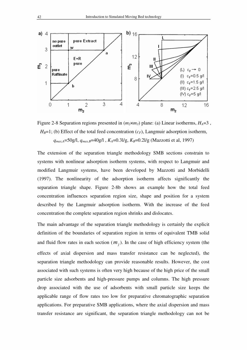
Introduction to Simulated Moving Bed technology 42
Figure 2-8 Separation regions presented in (m2×m3) plane: (a) Linear isotherms, HA=3 ,
HB=1; (b) Effect of the total feed concentration (cF), Langmuir adsorption isotherm,
qmax,A=50g/l, qmax,B=40g/l , KA=0.3l/g, KB=0.2l/g (Mazzotti et al, 1997)
The extension of the separation triangle methodology SMB sections constrain to
systems with nonlinear adsorption isotherm systems, with respect to Langmuir and
modified Langmuir systems, have been developed by Mazzotti and Morbidelli
(1997). The nonlinearity of the adsorption isotherm affects significantly the
separation triangle shape. Figure 2-8b shows an example how the total feed
concentration influences separation region size, shape and position for a system
described by the Langmuir adsorption isotherm. With the increase of the feed
concentration the complete separation region shrinks and dislocates.
The main advantage of the separation triangle methodology is certainly the explicit
definition of the boundaries of separation region in terms of equivalent TMB solid
and fluid flow rates in each section ( jm ). In the case of high efficiency system (the
effects of axial dispersion and mass transfer resistance can be neglected), the
separation triangle methodology can provide reasonable results. However, the cost
associated with such systems is often very high because of the high price of the small
particle size adsorbents and high-pressure pumps and columns. The high pressure
drop associated with the use of adsorbents with small particle size keeps the
applicable range of flow rates too low for preparative chromatographic separation
applications. For preparative SMB applications, where the axial dispersion and mass
transfer resistance are significant, the separation triangle methodology can not be

Fehler! Formatvorlage nicht definiert. 43
applied directly without considering some safety factor in SMB flow rates calculation.
The value of the safety factor is selected empirically and may lead to selection of
SMB operating conditions far from their optimal value.
In Figure 2-9 the influence of the mass transfer resistances on the separation region
size reproduced from Ref. (Rodrigues, Minceva, 2005) is presented. With the
reduction of the mass transfer coefficient ( k ) from 6min-1 to 1.5min-1, the separation
region size decreased significantly. For k =1.5min-1 the corresponding separation
region is almost vanished (see Figure 2-9). For a design of a preparative SMB units
more complex SMB design methodologies, which take into account the system non-
idealities are needed.
Figure 2-9 Effect of the mass transfer resistance on the separation region, k is the
mass transfer coefficient (Rodrigues, Minceva, 2005)
2.8.4.2 Separation volume design methodology
For those systems where the mass transfer resistance is important, the separation
triangle methodology provides only an initial guess for the feasible SMB operating
conditions, since it is derived from the equilibrium theory postulates. In some SMB
applications, the separation triangle methodology assumptions of 100% purity in both

Introduction to Simulated Moving Bed technology 44
product streams (extract and raffinate) and complete regeneration of the adsorbent (in
section 1) and eluent (in section 4) are either unnecessary or would require an
extremely large adsorbent inventory or eluent consumption (Kaspereit et al, 2007) . In
the design of SMB applications with reduced purity or recovery requirements, the
internal fluid flow rates in all four SMB section should be considered as well (Strube
et al, 1999).
The “Separation volume” methodology (Azevedo, Rodrigues, 2001) was developed
to overcome the separation triangle methodology restrictions. This methodology uses
a realistic equivalent TMB mathematical model and explores the influence of the flow
rates in the regeneration sections (section 1 and 4) on the SMB unit performances. In
addition the separation performances requirements, in terms of the products purity
and recovery, can be selected to suite the requirements of any particular SMB
application. The differences of the separation triangle and the “Separation volume”
methodology are summarised in Table 2-2.
Table 2-2 Comparison between separation triangle methodology and “Separation
volume” methodology
Separation triangle Separation volume
Objective Preliminary design of operating
conditions of SMB for a complete
separation (100% product purities)
Design of operating conditions of
SMB for given product purity
and recovery requirements
Mathematical
model
Equilibrium theory (axial dispersion
and mass transfer are neglected)
General models (axial dispersion
and mass transfer are taken into
consideration)
Design
parameters
Flow rates in sections 2 and 3, for
given flow rates in sections 1 and 4
Flow rates in sections 2,3 and 1
(or 4) for given flow rates in
section 4 (or 1)
Constraints in
sections 1 and 4
Complete section regeneration Non-complete section
regeneration can be considered
Design result Separation triangle-two dimensional Separation volume-three
dimensional

Fehler! Formatvorlage nicht definiert. 45
2.8.5 SMB optimization
In the previous subsection, the SMB design methodologies have been reviewed. By
design, we denote the selection of suitable operating conditions or geometric
parameters, which allow achievement of a desired SMB performance. The design
procedure leads to sets of operating conditions under which the SMB unit may be
operated and the required performances can be guaranteed. SMB unit optimization
considers selection of either operating conditions or geometric parameters that
minimize/maximize a given objective function(s), provided that certain constraint(s)
is(are) fulfilled. Namely, the initial sets of parameters defined in the SMB unit design
are therefore reduced by optimization to only one set of optimal parameters.
Several factors, namely, (i) objective function, (ii) optimization variables, namely,
variables to be optimized, (iii) optimization strategy, and (iv) optimization algorithm,
define the optimization problem. In order to summarize the SMB optimization
procedures reported in the open literature, the above-mentioned factors involved in
the SMB optimization problems are discussed individually.
2.8.5.1 Objective function
Any optimization problem begins by selection of the objective function. The
objective function used in the SMB optimization could be classified according to: (i)
the number of objective functions, and (ii) the type of objective functions.
Considering the number of objective functions the optimization problems could be
classified in two groups: single objective (Strube et al, 1999; Beste et al, 2000;
Minceva, Rodrigues, 2005; Xie et al, 2005) and multi-objective (Zhang et al, 2003a;
Kurup et al, 2005; Paredes, Mazzotti, 2007) optimization problems. The single
objective function problems could include one objective (Strube et al, 1999; Beste et
al, 2000; Azevedo, Rodrigues, 2006) or several objectives with different weight
factors (Xie et al, 2005).
When an SMB is designed and constructed the objective is to maximize the unit
productivity and simultaneously improve the product quality and reduce operating
cost. The factors which affect the economics of a given separation process are usually
multiple and are often in conflict with each other. Therefore, it is important to
formulate SMB optimization problems as multi-objective optimization problems. The
multi-objective function, as for instance, maximization of feed flow rate and

Introduction to Simulated Moving Bed technology 46
simultaneously minimization of eluent consumption was used by several authors
(Zhang et al, 2003a; Kurup et al, 2005; Paredes, Mazzotti, 2007). In these multi-
objective optimization problems, however, a best solution (global optimum) with
respect to all objectives is not achieved. Instead, a set of equally good optimal
solutions, known as the Pareto-optimal solutions, is obtained (Kurup et al, 2005).
There are two types of objective functions used in the literature: (i) process
performance parameter (as, for example, productivity, eluent consumption, adsorbent
requirements) mainly used in academic research studies (Strube et al, 1999; Beste et
al, 2000; Zhang et al, 2002; Minceva, Rodrigues, 2005; Kurup et al, 2005), and (ii)
separation cost, objective function preferred by industrial SMB users (Kulprathipanja
et al, 1994; Proll, Kusters, 1998), less used in academia. The cost function includes
two types of costs: separation problem independent costs (over-head costs, wages,
labour, maintenance, etc.) and separation problem dependent costs (cost of the plant,
cost of the adsorbent, cost of the eluent, cost for eluent recycling, feed loss, etc.). In
the SMB separation costs optimization, the precise definition of cost function is of
crucial importance. Chan (2008) have shown that different cost structures of
separation problem led to different optimal design and operating conditions.
2.8.5.2 Optimization variables
The optimization variables for SMB optimization generally include six geometrical
parameters, i.e., particle size, column length, and the number of columns in each
section, and five unit operating conditions (parameters), i.e., four section flow rates
and the switching time. In some cases, the feed concentration should be also taken
into account as an optimization variable (Lee et al, 2008). In the literature, most of the
works deal with the optimization of the operating conditions for an existing SMB unit
(Beste et al, 2000; Yu, Ching, 2002; Toumi et al, 2003; Minceva, Rodrigues, 2005).
Only a few publications consider the column length and particle diameter as
optimization variables in a design of a new SMB unit (Holland, 1975; Jupke et al,
2002; Kurup et al, 2005).
2.8.5.3 Optimization strategy
Most optimization works use a one-level optimization strategy (Beste et al, 2000; Yu,
Ching, 2002; Toumi et al, 2003; Zhang et al, 2003a; Kurup et al, 2005). Namely,
when the objective function(s) and the optimization variables are selected,

Fehler! Formatvorlage nicht definiert. 47
optimization is directly performed to find the optimum solution(s). By using this
strategy to solve the multi-objective function, Pareto optimal set of solutions is
obtained (Zhang et al, 2003a; Kurup et al, 2005; Paredes, Mazzotti, 2007).
In order to obtain the global optimum, multi-level SMB optimization strategy were
developed. Minceva et al. (2005) proposed a two-level optimization procedure based
on the concept of “separation volume” and equivalent TMB model to optimize an
existing SMB unit for p-xylene separation from mixed xylenes. The global solution of
the optimization procedure was obtained that gives the optimal operating conditions
leading to maximum SMB unit productivity with a minimum possible desorbent
consumption for attainment of that SMB productivity.
2.8.5.4 Optimization algorithm
The optimization algorithm is a numerical method which decides the accuracy and
efficiency of the optimization. The Genetic Algorithm (GA) (Holland, 1975) and its
extensions, i.e., the non-dominated sorting genetic algorithm (NSGA) (Srinivas, Deb,
1994), NSGA-II (Deb et al, 2002), NSGA-II-JG (Kasat, Gupta, 2003) algorithms are
widely used in the optimization studies. Zhang et al. (2003a) first applied the NSGA
to the multi-objective optimization of SMB. They compared SMB and Varicol
processes, which were optimized either for maximum purity in both extract and
raffinate products or for maximum throughput with minimal eluent consumption.
Kurup et al. (2005) adapted NSGA-II-JG algorithm for the multi-objective
optimization of ternary-mixture separation of C8 aromatics containing xylene isomers
using modified SMB systems. Recently Lee et al. (2008) developed an optimization
algorithm in which the standing wave design (SWD) was incorporated with NSGA-
II-JG. By their algorithm, SMB operating and geometrical parameters could be
optimized simultaneously.
The above-mentioned GA-based optimization algorithms are very powerful. However,
they suffer from the long computation time when many optimization variables are
considered, because in order to obtain non-dominated solutions, a large number of
simulations need to be performed to search a large space.
Araujo et al. (2006) applied the optimization solver SolvOpt coupled with CSS model
for optimal design of a certain class of asynchronous SMB processes. One of the
reasons for implementation of this optimization algorithm is the low computation

Introduction to Simulated Moving Bed technology 48
time. IPOPT (Interior Point OPTimizer) (Wachter, Biegler, 2006), was employed by
Kawajiri and Biegler (2006a; 2006b; 2006c; 2008a; 2008b) to optimize the SMB unit
configuration, as well as, to optimize an asymmetric operation in SMB. This
algorithm is also applied with success by the group of Mota (2007; 2007a; 2007b) for
optimization of synchronous and asynchronous gas phase SMB separations. The
commercial package gOPT from gPROMS (Process System Enterprise, London, UK)
with a Single (or Multiple) Shooting-Control Vector Parameterisation, are used in the
two level optimization of an Parex® unit (Minceva, Rodrigues, 2005), for optimal
economic design (Chan et al, 2008), and to optimize the operating conditions of
Varicol SMB unit for p-xylene separation (Sa Gomes et al, 2008).

Fehler! Formatvorlage nicht definiert. 49
3 Modelling of the chromatographic system
The mathematical model of a single chromatographic column is the core of the
mathematical model describing the SMB unit operations. In this chapter the single
chromatographic column model is selected based on the experimentally determined
hydrodynamics, adsorption thermodynamics and mass transfer parameters. The
precise mathematical description of a chromatographic separation is crucial for the
successful design and optimization of a SMB unit for separation of CA from its
fermentation broth.
This chapter starts with determination of the model parameters and describes the
experimental methods used to obtain these parameters.
The fermentation broth is a complex mixture and contains diverse impurities. The CA
is the target component and glucose was considered as a model impurity. All
experiments for determination of the hydrodynamics, adsorption thermodynamics and
kinetics parameters were performed in a semi-preparative column (30cm x 1.6cm I.D.)
using a model solutions of pure CA and glucose.
Three commonly used chromatographic models with different degree of complicity,
i.e., PDM, TDM and LDF have been considered for the description of the
experimentally obtained CA and glucose elution profiles. After the selection of the
mathematical model, the model predictions were validate experimentally in one of the
chromatographic columns from the SMB unit (preparative column, 150cm x 5.0cm
I.D.) using a concentrated fermentation broth as a feed mixture, which is later also
considered as a feed stream in the SMB unit.
3.1 Experiments
3.1.1 Materials
3.1.1.1 Chemicals
Glucose (purity ≥ 99%) was purchased from Merck (Darmstadt, Germany). Blue
dextran with MW 2 000 000kg/kmol was acquired from Sigma-Aldrich (Steinheim,
Germany, purity ≥ 99%). CA (purity ≥ 99.5%) and its fermentation broth were kindly
provided by Xielian (Wuxi, China). Deionized and distilled water was used as eluent
(mobile phase) and solvent.

Modelling of the chromatographic system 50
Pretreated fermentation broth: The fermentation broth obtained from Xielian was
first filtrated and then concentrated. The pretreated liquor, used as an SMB feed
solution, had a pH value between 1.5 and 1.7 (below the CA first ionization constant
pKa1 3.13 at a temperature of 25oC). The weight fraction of CA (target product) in the
pretreated fermentation liquor, on a water-free basis, is around 95%. The main
impurities affecting the CA quality are the readily carbonizable substances (RCS)
(Kulprathipanja et al, 1994), with a concentration of about 4wt%. The RCS are
mainly residual sugars, among which over 90% is glucose. The glucose is also
considered as a most difficult component to be separated from the target product.
From the above-listed reason, glucose was selected as a model impurity in our study.
The concentration of CA in the pretreated fermentation liquor was around 700g/l and
that of glucose between 30 to 40g/l.
Stationary phase: The novel tailor-made stationary phase, used in this work, is a new
type of a tertiary poly(4-vinylpyridine, PVP) resin. It is a uniform, water-insoluble,
reticular with weakly acid and basic functional groups, amphoteric ion-exchange
resin (Peng, 2005). The resin was prepared by the conventional suspension
polymerization technique (Li, Leong, 1994).
The copolymer matrix is formed by polymerization of the monomer vinylpyridine
and methacrylate and the cross-linker divinylbenzene. Then the ester group in the
copolymer matrix was converted into carboxylic acid group by hydrolysis. Finally the
surface of the copolymer structure was modified to obtain the desired functionality,
so that it has a high selectivity to CA, while the fermentation broth impurities are only
weakly retained (Peng et al, 1998a; Peng et al, 1998b). In order to minimize the
pressure drop in the SMB unit, the resin with particle size of pd (90%)=300±50µm
was used to pack the columns. The chemical structure of the resin is presented in
Figure 3-1.

Fehler! Formatvorlage nicht definiert. 51
CH CH2
CH2
n
CH2 CH
n
N ··
N ··
CH2 C
COOH
CH3
CH2
COOH
CH3
CCH2
CH2 CH2
Figure 3-1 Chemical structure of the tailor-made stationary phase used to separate CA
from the fermentation broth
3.1.2 Equipment
3.1.2.1 Semi-preparative chromatographic system
The semi-preparative chromatographic system includes a stainless steel semi-
preparative column (30cm x 1.6cm I.D.), a preparative HPLC pump (flow rate 0-
50ml/min, K501, Knauer, Berlin, Germany), and a column oven (0-99.9oC, Hanbang,
Jiangsu, China). The samples were collected at the column outlet and analyzed
manually. This system was used to measure the hydrodynamics and thermodynamic
model parameters, i.e., external porosity, axial dispersion coefficient and adsorption
isotherms.
3.1.2.2 Preparative chromatographic system
This system contains a two-head membrane pump (2J-W10/5, Zhejiang, Jiangsu,
China), a stainless steel preparative column (150cm x 5.0cm I.D., same size as the
columns used in the SMB unit) equipped with a jacket and a recirculation water bath.
The samples were collected at the outlet of the column and analyzed manually. The
system was used to determine the elution profiles of pure CA and glucose, as well as,
of pretreated (concentrated) fermentation broth.
3.1.3 Analytical methods
The single component solutions, i.e., blue dextran, CA and glucose, with
concentrations over 10g/l were analyzed with a refractometer (RHB90, Zhejiang).

Modelling of the chromatographic system 52
Below this concentration the analysis was performed with an analytical HPLC system
equipped with a RI detector (Series 1100, Agilent, USA), using a direct sample
injection through a 20µl injection loop (HPLC column was not used).
In the experiments performed with the pretreated fermentation broth as a feed
solution, the CA concentration was measured with a standard titration method with
sodium hydroxide in presence of phenolphthalein indicator. The RCS determination
method (Kulprathipanja et al, 1994) (from United States Pharmacopeia) was applied
to measure the glucose concentration.
3.1.4 Determination of model parameters
All experiments were carried out at a constant temperature of 80oC since: (1) CA and
glucose can be well separated at this temperature, (2) a temperature over 60oC
decreases the growth of unwanted microorganisms, and (3) the liquid phase viscosity
is lower at this temperature and the pressure drop across the packed bed is thus
reduced. All chromatographic columns were slurry packed with the PVP resin.
3.1.4.1 Column porosity and axial dispersion coefficient
The blue dextran (used as a tracer substance) breakthrough experiments were
performed for the determination of the external column porosity and axial dispersion
coefficient. The breakthrough curves were measured at different flow rates between 5
and 15ml/min. The flow rate at the column outlet was measured during each
experiment. The experimentally measured flow rates were used in the calculations. A
blue dextran aqueous solution with concentration of 3g/l was used in these
experiments.
The equilibrium dispersive model (EDM), in which the adsorption term is neglected,
can be used to simulate a tracer breakthrough curve (Guiochon, Lin, 2003):
2
2
x
cD
x
c
t
cax
∂
∂⋅=
∂
∂⋅+
∂
∂ν Eq. 3-1
where c is the liquid phase concentration, ν is the interstitial velocity (ε⋅
=cA
Qv ) ,
axD is the axial dispersion coefficient, t is the time and x is the axial coordinate. The
axial dispersion coefficient is related to the column fluid dynamics and it is
independent of the solute (tracer) used.

Fehler! Formatvorlage nicht definiert. 53
The analytical solution of the model in dimensionless form is (Guiochon, Lin, 2003):
−⋅⋅+
−⋅+==
ττ
ττ
1
25.0
1
25.05.0
0
Peerfce
Peerf
c
cC
Pe Eq. 3-2
where 0c is the feed concentration, τ is the dimensionless time, which is the ratio
between the elution and retention time, Rt , (Q
Vt c
R
⋅=
ε), Pe is the Peclet number
(ax
c
D
LvPe
⋅= ), )(xerf and )(xerfc are the error function and the complementary error
function, respectively.
For a set of Pe and Rt values the tracer elution profile at the column exit can be
calculated with Eq. 3-2. The least square method was used to obtain the best fitting
parameters ( Pe and Rt ) for the experimental tracer breakthrough curves. The
external column porosity was calculated from the retention time, (Q
Vt cR ⋅=ε ). The
calculations were performed in MATLAB (The MathWorks, Natick, Massachusetts,
USA).
3.1.4.2 Adsorption isotherms
The adsorption isotherm is one of the most important thermodynamic parameters in
the chromatography. Frontal analysis method was used to determine the single
component adsorption isotherms of CA and glucose. The CA and glucose
concentration was in a range between 20 and 500g/l and 100 and 300g/l, respectively.
The flow rates were around 10ml/min for CA and 6ml/min for glucose. For each
glucose (or CA) liquid phase concentration three experiments were performed and the
average value of the equilibrium concentration in the liquid and solid phases were
calculated and used in the presentation of the single component adsorption isotherm.
3.1.4.3 Mass transfer parameters
Mass transfer parameters used in the chromatographic models, given in Section 2.5,
were calculated based on several empirical correlations (Mackie, Meares, 1955;
Wilke, Pin, 1955; Wilson, Geankoplis, 1966), and summarized in Table 3-1. The
molecular diffusivities of CA and glucose ( CAmD , , glumD , ) were calculated using the
Wilke-Chang correlation (1955). The resulting values were Dm,CA =1.27x10⁻³cm
2/min

Modelling of the chromatographic system 54
and Dm,Glu =1.35x10⁻³cm
2/min. It is worth to mention that the Wilke-Chang correlation
was developed for dilute solutions. In our investigation system the CA concentration
in the feed solution is as high as 700g/l. The reasons for selecting this correlation to
calculate the CA diffusivity are: (i) even though the CA concentration is high (700g/l);
the mole fraction of CA in the solution is only 0.1 due to the large CA molar mass
(192g/mol). According to Reid (1987), Dm is assumed to be a representative diffusion
coefficient even for the solute concentration up to 5 and 10 mole percent, (ii) the feed
viscosity is significantly reduced at the operating temperature of 80oC, and (iii) in the
SMB unit the concentration is distributed from 0 to the feed concentration (maximal
concentration) along four sections. Taking the concentration dependence of
diffusivities would significantly affect the model complexity and the computation
time.
The average particle radius ( pr ) of 150µm was assumed, since 90% of the resin
particle size ( pd ) was 300±50µm. Experimental determination of the internal
porosity pε was a challenging task, due to the particle swelling. Therefore 2.0=pε
was assumed. This value fits in the range of a typical ion-exchange resins porosity
values.
Table 3-1 Correlations used for calculation of the mass transfer coefficients in the
PDM, TDM and LDF model
Correlations Model
mD Wilke-Chang correlation,
( )6.0
5.0
8104.7m
sAm
V
TMD
µ
α−×= PDM,
TDM,
LDF
poreD Mackie-Meares correlation, ( ) m
p
p
pore DD2
2 ε
ε
−=
PDM,
TDM
filmk Wilson and Geankoplis correlation,
33.0
09.1
⋅=
m
p
p
mfilm
D
d
d
Dk
νε
ε
PDM,
TDM
effk filmporefilmporep
p
eff kkkD
d
k
111
10
1+=+=
ε TDM

Fehler! Formatvorlage nicht definiert. 55
seffk ,
For linear isotherms: ( )Hk
kpp
eff
seffεε −+
=1
,
For non-linear adsorption isotherm: ( ) )(1 *,
dcdq
kk
eqpp
eff
seffεε −+
=
LDF
3.1.5 Elution profiles
In order to select a proper chromatographic model, which should give sufficient
accurate predictions and be in the same time as simple as possible, a set of
breakthrough curve experiments with single component (CA or glucose) aqueous
solutions were performed in the semi-preparative chromatographic system. The
glucose and CA breakthrough curves were measured for different initial solute
concentrations (glucose:100-300g/l and CA:50-400g/l). The flow rates were set at
6ml/min for glucose and 10ml/min for CA.
Later, for the selected model validation, a set of “intermediate” pulse injection (due to
the large injection volume of 500ml) experiments with single component (CA or
glucose) aqueous solutions and pretreated fermentation broth were performed in the
preparative chromatographic system. For CA, the injection concentration was around
700g/l and for glucose around 300g/l. The experiments were carried out at three
different flow rates: 60, 90 and 120ml/min. For the sake of compatible with the large
size of the preparative column the injection volume of 500ml was selected so that the
sample outlet concentrations could be easily and accurately detected.
Since the injection volume was quite large (500ml), it was difficult to use a normal
six-way valve with an injection loop for injection of the solution into the column.
Therefore, additional injection line was introduced in the preparative
chromatographic system. The schematic presentation of the experimental set-up is
shown in Figure 3-2. In order to eliminate the dead volume of the injection line (the
dash line in Figure 3-2), this line was first filled with the sample solutions. When
injection was performed, valve V2 was open and simultaneously valve V1 was closed.
After the desired amount of sample was injected into the column, V1 was open and
simultaneously closed V2. The experimental injection time (total injection volume,
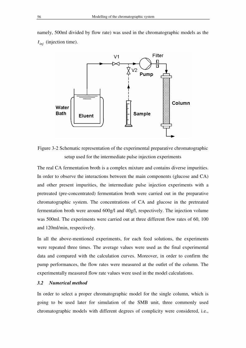
Modelling of the chromatographic system 56
namely, 500ml divided by flow rate) was used in the chromatographic models as the
injt (injection time).
Figure 3-2 Schematic representation of the experimental preparative chromatographic
setup used for the intermediate pulse injection experiments
The real CA fermentation broth is a complex mixture and contains diverse impurities.
In order to observe the interactions between the main components (glucose and CA)
and other present impurities, the intermediate pulse injection experiments with a
pretreated (pre-concentrated) fermentation broth were carried out in the preparative
chromatographic system. The concentrations of CA and glucose in the pretreated
fermentation broth were around 600g/l and 40g/l, respectively. The injection volume
was 500ml. The experiments were carried out at three different flow rates of 60, 100
and 120ml/min, respectively.
In all the above-mentioned experiments, for each feed solutions, the experiments
were repeated three times. The average values were used as the final experimental
data and compared with the calculation curves. Moreover, in order to confirm the
pump performances, the flow rates were measured at the outlet of the column. The
experimentally measured flow rate values were used in the model calculations.
3.2 Numerical method
In order to select a proper chromatographic model for the single column, which is
going to be used later for simulation of the SMB unit, three commonly used
chromatographic models with different degrees of complicity were considered, i.e.,

Fehler! Formatvorlage nicht definiert. 57
pore diffusion model (PDM), transport dispersive model (TDM) and lumped rate
model with a solid film linear driving force approach (LDF). A detailed description of
mathematical model equations for these models was given in Chapter 2, Section 2.5.
The set of model equations was numerically solved with the commercial software
gPROMS® version 3.1.4 (general PROcess Modeling System) (Process Systems
Enterprise, 1998). The axial and radial (in PDM) domain were discretized using a
third order orthogonal collocation on finite elements method (OCFEM). The number
of the elements in the discretization was adjusted for each of the used methods in
order to satisfy the global mass balance relative error (<0.1%). After the discretization
step, the time integration was performed by the ordinary differential equation solver
SRADAU, a fully-implicit Runge-Kutta method that implements a variable time step,
the resulting system of equations was then solved by the gPROMS BDNSOL (Block
decomposition NonLinear SOLver). An absolute and relative tolerance of 10-5 was
used.
3.3 Results and discussions
3.3.1 Chromatographic model parameters
3.3.1.1 Column porosity and axial dispersion
The external porosity ( ε ) and axial dispersion coefficient represented by Peclet
number ( Pe ) were determined experimentally with the tracer substance blue dextran.
Figure 3-3 shows the breakthrough curves of blue dextran at three different flow rates,
together with the best fitting curves calculated with Eq. 3-2.
Good agreement between the fitting curves and experimental data was obtained. The
best fitting Pe values were in the range between 97 and 112, and the ε value
between 0.30 and 0.33. The average values 106=Pe and 31.0=ε were considered in
the following studies.

Modelling of the chromatographic system 58
0.0
0.3
0.6
0.9
1.2
0 1 2 3 4 5 6
c/c
0
7.5ml/min
9.6ml/min
14.5ml/min
Fitting curve
t, min
Figure 3-3 Comparison between the experimental and calculated best fitting blue
dextran breakthrough curves at different flow rates in the semi-preparative column
3.3.1.2 Adsorption isotherms
The experimental adsorption isotherms of glucose and CA are presented in Figure 3-4.
The linear and modified Langmuir adsorption isotherm models were used to describe
glucose and CA adsorption equilibrium on the tailor-made resin, respectively. Good
agreement between the calculated and experimental data was obtained. The
correlation coefficients of glucose and CA isotherms were 0.9981 and 0.9931,
respectively.
The linear and modified Langmuir isotherm models parameters for glucose and CA
are:
Glucose:
GluGlu cq ⋅= 1435.0 (Eq. 3-3)
CA:
CA
CA
CACA c
c
cq ⋅+
⋅+
⋅= 51.0
019.01
04.2 (Eq. 3-4)
The resin has high CA adsorption capacity, whereas glucose is only weakly retained,
indicating that CA and glucose could be easily separated with the resin used.

Fehler! Formatvorlage nicht definiert. 59
0
100
200
300
400
0 100 200 300 400 500
c, g/l
q,
g/l
Glucose
CA
Calculated
Figure 3-4 Experimental and calculated adsorption equilibrium isotherms of citric
acid and glucose
At this point of our study, the non-competitive adsorption between glucose and CA
was assumed. There are two reasons for this assumption: (i) CA concentration in the
pretreated fermentation broth is more than 20 times higher than that of glucose, and
(ii) CA adsorption capacity is significantly higher than that of glucose.
It is expectable that the assumption of a non-competitive adsorption isotherm would
affect more the accuracy in the prediction of the glucose elution behavior than that of
CA (Schmidt-Traub, 2005). Also, should be taken into account that the real
fermentation broth is a complex mixture and contains diverse impurities (including
salts, proteins, mono- and polysaccharides), which even though present in very small
amounts could possibly affect the CA adsorption. Precise prediction of the CA
adsorption isotherm using the real fermentation broth and standard methods for
determination of competitive adsorption isotherms is a quite challenging task.
3.3.2 Single column model selection
Three chromatographic models, PDM, TDM and LDF, were used to predict the
experimental breakthrough curves of glucose and CA. The model equations are given
in Section 2.5. The calculated and experimental single component breakthrough
curves are presented in Figure 3-5a (glucose) and Figure 3-5b (CA).

Modelling of the chromatographic system 60
0
60
120
180
240
300
0 4 8 12 16 20t, min
c,
g/l
Exp.
Sim.-TDM
Sim.-PDM
Sim.-LDF
c: 108.0g/l
c: 199.5g/l
c: 273.5g/l
a)
0
100
200
300
400
0 4 8 12 16 20t, min
c,
g/l
Exp.
Sim.-TDM
Sim.-LDF
Sim.-PDM
c: 51.7g/l
c: 191.7g/l
c: 368.3g/l
b)
Figure 3-5 Comparison of the experimental and calculated breakthrough curves with
the TDM, PDM and LDF model for different feed concentrations: (a) glucose, flow
rate: 6ml/min; and (b) CA, flow rates: 8.3, 8.6 and 9.8ml/min
Generally speaking, all three models give similar simulation results and agree well
with the experimental data.

Fehler! Formatvorlage nicht definiert. 61
In the case of glucose the TDM and LDF models give identical predictions (see
Figure 3-5a), because the mass transfer coefficients effk (in the TDM) and seffk , (in
the LDF) are identical in the condition of linear adsorption isotherm (see Table 3-1).
The PDM shows slightly different predictions from the other two models at the
breakthrough part of the glucose elution profiles.
In the case of CA, all used models give a slight different prediction of the CA
breakthrough curves (see Figure 3-5b). The LDF gives the best fitting among the
models considered. In the LDF model the mass transfer coefficient in the solid phase
( seffk , ) is a function of the solute concentration in the bulk liquid phase (see Table
3-1), which means that the solute concentration affects the adsorption kinetics. This
issue has been subject of several published works (Sajonz et al, 1996; Miyabe,
Guiochon, 2000; Antos et al, 2003). The LDF model precision in the prediction of the
elution profiles also indicates that the column packing, fluid dynamics and adsorption
isotherms parameters have been accurately determined.
The computation time for solving the chromatographic models is presented in Table
3-2 . All simulations were performed on Pentium IV 3.20 GHz processor with 1.00
GB RAM memory. Even though the LDF model gives the best simulation results, it
requires long computation time (more than 10 minutes). Taking into consideration
that the final goal of this work is to model and simulate a multicolumn SMB unit
operation, the TDM model was selected as the most appropriated model. The TDM
model did not give a good prediction of the break through part of the curve, but fits
well the saturation part of the curve. Additionally, the breakthrough curve
computation time was only a few seconds.
Table 3-2 CPU time for solving different chromatographic models
Chromatographic models Number of finite elements CPU time (s)
TDM 20 4
LDF 20 615
PDM 20 (axial), 20 (radial) 608

Modelling of the chromatographic system 62
3.3.3 TDM model validation in a preparative chromatographic column
In the previous section, the TDM model was selected as the most suitable model for
the prediction of elution profiles of CA and glucose obtained in the semi-preparative
chromatographic column. In this section, the TDM model prediction is validated for a
set of intermediate pulse injection experiments performed with: (i) pure glucose and
CA aqueous solutions, and (ii) pretreated fermentation broth, in the preparative
column.
3.3.3.1 Single component elution profiles
The comparison of the glucose and CA experimental data with the calculated elution
profiles are presented in Figure 3-6a (glucose) and Figure 3-6b (CA). The external
column porosity and Pe number values measured in the semi-preparative column
were used in the TDM model calculations.
0
60
120
180
240
0 10 20 30 40 50t, min
c,
g/l
60 ml/min
90 ml/min
120 ml/min
a)

Fehler! Formatvorlage nicht definiert. 63
0
70
140
210
280
0 30 60 90 120 150t, min
c,
g/l
60 ml/min
90 ml/min
120 ml/min
b)
Figure 3-6 Experimental and calculated elution profiles of (a) glucose and (b) CA in
the preparative column: symbols refer to experimental data and lines represent TDM
prediction curves
Good agreement between the experimental data and prediction curves can be
observed in the case of glucose (see Figure 3-6a). At the flow rate of 60ml/min, the
TDM model calculation matches with the experimentally obtained data rather nice.
However, with the increase of the flow rates, discrepancy is noticeable. The
experimental elution profiles become a bit broader than the simulation peaks. Also
the slight tailing of the glucose peak observed at higher mobile phase flow rates is not
well predicted by the used model.
The peak width is mainly determined by the column hydrodynamics (Guiochon et al,
1994). The values of the two important parameters characterizing the column
hydrodynamics, the external porosity and Pe number, used in these TDM simulations
were measured in the semi-preparative column. This can be one of the reasons for the
small observed discrepancy between the experimental and calculated glucose elution
profiles.
In principle, since the glucose adsorption isotherm is of linear type, the glucose
elution profiles should be symmetrical. However, the highest glucose concentration
(270g/l) used for the experimental determination of the adsorption isotherm was
lower than the injection concentrations, which was around 320g/l. It is possible that

Modelling of the chromatographic system 64
the isotherm becomes nonlinear at this concentration range and nonlinear type of
isotherm model would be more precise to describe the glucose adsorption equilibrium
at higher concentrations. Nonetheless, in the real SMB feed solutions, the glucose
concentration is around 40g/l. The selected glucose concentration range for the
adsorption isotherm measurements is therefore more than sufficient for the final
purpose, simulation of a SMB unit for CA separation.
In the case of CA, the agreement between the model calculations and experimental
data is not as good as for glucose. The model fits well the front part of the elution
peak, while at the rear part of the peak the discrepancy between the experimental and
calculated data becomes noticeable (see Figure 3-6b). There is a significant CA peak
tailing not predictable with the used model, which could later possibly affect the
precision in the calculation of the SMB performances. The observed deviation is
mainly caused by difference between the model prediction and experimental data in
the low concentration range, which has been also observed in the semi-preparative
column (see Figure 3-5b). Other possible reasons could be: (i) the imprecision of the
CA adsorption isotherm model predictions in the low CA concentration range (see
Figure 3-4), (ii) slightly different column porosity and Pe number in the preparative
column used to perform these experiments, and (iii) the effects of high injection
concentration (more than 700g/l) on the mass transfer resistance.
Nonetheless, since the TDM model well describes the frontal part of the CA elution
profiles and requires short computation time it was considered to give sufficient
precision in the prediction of CA elution in the preparative column as well.
3.3.3.2 Fermentation broth elution profiles
The intermediate pulse injection experiments with pretreated fermentation broth were
also performed in the preparative column, in order to examine the possible interaction
between CA, glucose and other impurities existing in the fermentation broth and
further more to confirm the non-competitive adsorption between CA and glucose. The
model predictions, together with the experimental data at three different flow rates are
presented in Figure 3-7. The elution profiles were calculated using the single solute
adsorption isotherms of glucose and CA.
Similar with the single component elution profiles, the calculated elution profiles
predict better the glucose than CA experimental elution profiles. For the lowest flow

Fehler! Formatvorlage nicht definiert. 65
rate used (60ml/min) there is a good agreement between the experimental and
calculated curves, as can be seen in Figure 3-7a. With the increase of the flow rate, a
discrepancy between the CA experimental and calculated profile becomes noticeable,
but it is still considered as acceptable. The results of this set of experiments confirm
the assumption of non-competitive adsorption between CA and glucose, and
moreover show that the presence of the fermentation broth impurities does not
influence significantly the precision of the model predictions.
In summary, the TDM model was considered as a suitable model for prediction of the
CA and glucose adsorption kinetics on the PVP resin. This model is going to be used
to formulate the equivalent TDM TMB and real TDM SMB models in Chapter 4.
0
70
140
210
280
0 30 60 90 120
t, min
c,
g/l
Exp.-CA
Exp.-Glucose
Simulation
a)

Modelling of the chromatographic system 66
0
60
120
180
240
0 25 50 75 100t, min
c,
g/l
Exp.-CA
Exp.-Glucose
Simulation
b)
0
50
100
150
200
0 25 50 75 100t, min
c,
g/l
Exp.-CA
Exp.-Glucose
Simulation
c)
Figure 3-7 Experimental and calculated elution profiles of CA and glucose in the
pretreated fermentation broth in the preparative column at different flow rates: (a)
60ml/min, (b) 100ml/min, and (c) 120ml/min

Fehler! Formatvorlage nicht definiert. 67
Summary
Due to the complexity of the SMB unit operation, model-based SMB design and
optimization are essential. The mathematical model of a single chromatographic
column is the core of the mathematical model describing the SMB unit operation.
The CA fermentation broth is a complex mixture and contains diverse impurities. The
target component CA and the main impurity glucose were selected as a model
solution for the sake of simplicity.
Different from the HPLC columns used in small-scale SMB units reported in
literature, the size of the chromatographic columns in the available SMB unit is quite
large, i.e., column length of 150cm and diameter of 50cm. This implies long time of
experiment and high cost (especially for the experiments with blue dextran tracer).
Therefore, a semi-preparative column with the column length of 30cm and the
diameter of 1.6cm was used to measure the model parameters, namely the column
hydrodynamics, the adsorption equilibrium and kinetics parameters, needed for
selection of a single chromatographic column model. The obtained model parameters
were afterward confirmed in the preparative chromatographic column using real pre-
concentrated fermentation broth as a feed solution.
The adsorption isotherms of glucose and CA on the tailor-made resin could be well
described by the linear and modified Langmuir isotherm models. The glucose and CA
isotherm have shown large difference in terms of adsorption capacity, which implied
that the tailor-made resin had strong adsorption ability to CA whereas glucose was
only weakly retained. The CA concentration in the real CA fermentation broth is 25
times larger than that of glucose. Therefore no competitive adsorption between CA
and glucose was assumed. Besides CA and glucose, other impurities, as for instance,
salts, proteins, mono- and polysaccharides, are present in the CA fermentation broth
in very small quantities. It was assumed that these impurities had no influences on the
adsorption behaviors of CA and glucose. These assumptions were verified in the
preparative chromatographic column by the intermediate pulse injection experiments
of real pre-concentrated fermentation broth.
Three commonly used chromatographic models, i.e., TDM (Transport Dispersive
Model), LDF (Linear Driving Force model) and PDM (Pore Diffusion Model), were
used to simulate the CA and glucose breakthrough curves in the semi-preparative

Modelling of the chromatographic system 68
column. According to the model predictions and the computation time, TDM was
selected. This model was further used to predict the elution profiles of pure CA and
glucose solutions as well as of the pretreated fermentation broth obtained
experimentally in the preparative column. Satisfactory prediction results were
obtained. As a consequence, the TDM was selected to create the TDM TMB and
TDM SMB model in Chapter 4.

Fehler! Formatvorlage nicht definiert. 69
4 Modelling of an existing pilot-scale SMB unit
In chapter 3 the TDM model was selected and verified in the single column
chromatographic system. In this chapter the selected TDM model is extended and
used for simulation of the operation of an existing multicolumn pilot-scale SMB unit.
First the equivalent TDM TMB and real TDM SMB models are presented. For the
sake of model verification, SMB experiments are needed. Due to the complicate SMB
operation, finding a set of suitable SMB operating conditions leading to the desired
separation performances by “trial and error” is nearly impossible. Therefore, the
separation triangle methodology was used to select the SMB unit initial operating
conditions. The separation constraints were set at minimum 99.8% CA purity and
minimum 90% CA recovery in the extract stream.
The equivalent steady state TDM TMB model was used to obtain the CA separation
region. Three sets of operating conditions inside this region were selected for
experimental SMB unit runs. The comparison of the experimental and calculated
SMB performances by both TDM TMB and TDM SMB was used for the model
validation.
4.1 An existing pilot-scale SMB unit
The pilot-scale SMB unit (Figure 4-1), built up in the laboratory at Jiangnan
University in China, consists of sixteen identical stainless steel preparative columns
(same size as the one used in the preparative chromatographic system). The columns
and the tubes are insulated with high temperature resistant polyurethane. The SMB
unit is equipped with a thermostatic circulation bath and can operate in a temperature
range between 25 and 90oC. For the measurement of the internal SMB concentration
profiles, samples can be withdrawn at the end of each column.
Five membrane pumps (flow rates up to 150ml/min) are used to deliver the feed and
eluent, to withdraw the extract and raffinate and to recycle the liquid stream from the
last to the first column. 20µm filters (CF3724, Zhejiang) are used to eliminate the
possible solid impurities from the eluent and feed tank. At each pump, the flow rate
and pressure are measured by a flow meter (KEROMATE-RN, Wuxi, China) and
pressure gauge (SP-507, Zhejiang). The unit is constructed to operate up to 50bar.

Modelling of an existing pilot-scale SMB unit 70
Ninety-six two-way valves (V-0124, Zhejiang, Jiangsu,) distributed at the top and
bottom of each column are used to introduce the feed, eluent or recycle streams at the
top of the columns and to withdraw the product streams (extract and raffinate) from
the bottom of the columns. Pneumatic electro valves (Valbia, Maclodio, Italy) are
connected to the ninety-six valves. Also, sixteen two-way valves are used for columns
interconnection.
The system is entirely controlled by the laboratory developed software (Simatic S7-
300, Siemens, Germany).
Figure 4-1 Schematic representation of the existing pilot-scale SMB unit
4.2 Preliminary design of an existing pilot-scale SMB unit operating conditions
4.2.1 TMB and SMB models
The equivalent TDM TMB and the dynamic TDM SMB model equations are
summarized in Table 4-1. To complete the TMB model, besides the single fixed bed
column model for each section, additional mass balances at the two input (feed and
eluent) and two output (extract and raffinate) ports are required. With the TDM TMB
model presented in Table 4-1 the steady state concentration profiles along the
equivalent TMB unit can be calculated, when time derivatives at the left hand side of

Fehler! Formatvorlage nicht definiert. 71
the mass balance equation in the bulk liquid phase and particle are set to 0. The
steady stated TDM TMB was used in the simulations.
The complete model of an SMB unit is constituted by a set of mass balance equations
for each of the Nc columns, connected with each other by material balances at the
connecting nodes. Due to the periodic type of operation in the SMB unit only a cyclic
steady state (CSS) is achieved. This is a result of the switching of the position of the
inlet and outlet ports along the unit. Namely during the port switching, each column
in the SMB unit plays a different function during a whole cycle, depending on its
location (section). With each switching of the inlet and outlet ports, the boundary
conditions of each column are updated in terms of flow rate and inlet concentrations.
The flow rate in each column, according to its location (section), can be calculated by
the mass balance at the inlet and outlet nodes. The inlet concentration of each column
is equal to the outlet concentration of the previous column, except for the feed and
eluent nodes.

Modelling of an existing pilot-scale SMB unit 72
Table 4-1 Transport dispersive equivalent TMB model and transient SMB model
TMB-based model SMB-based model
Mass balance of component i in section j :
in the bulk liquid phase:
( )
−
−−
∂
∂−
∂
∂=
∂
∂jpiji
p
ieff
jiTMBji
jax
jicc
rk
x
cv
x
cD
t
c
j ,,,
,
2
,2
,
, 31
ε
ε
in the particle:
( ) ( )jpiji
p
ieff
ji
p
jpi
ps
jicc
rk
x
q
x
cu
t
q,,,
,,, 31 −+
∂
∂−+
∂
∂=
∂
∂εε
Adsorption equilibrium:
( )jpiji cfq ,, =
Dynamic mass balances of component i in column k :
in the bulk liquid phase:
( )
−
−−
∂
∂−
∂
∂=
∂
∂kpiki
p
ieff
kiSMBk
ki
kax
kicc
rk
x
cv
x
cD
t
c,,,
,
2
,2
,
, 31
ε
ε
in the particle:
( ) ( )kpiki
p
ieff
ki
p
kpi
p ccr
kt
q
t
c,,,
,, 31 −=
∂
∂−+
∂
∂εε
Adsorption equilibrium:
( )kpiki cfq ,, =
Boundary conditions and initial conditions:
( )( )injiji
TMBj
ji
jax ccvx
cD ,,
,
, 0 −=∂
∂ , ( )0
,=
∂
∂
x
Lc cji
For j = 1 to 3, ( ) injpicjpi cLc 1,, += , ( ) ( )01,, += jic
inji qLq
For j = 4, ( ) inpicpi cLc 1,4, = , ( ) ( )c
inii Lqq 4,1, 0 =
( ) 00,, =xc ji, ( ) 00,, =xc jpi
Boundary and initial conditions:
( )( )inkiki
SMBk
ki
kax ccvx
cD ,,
,
, 0 −=∂
∂,
( )0
,=
∂
∂
x
Lc cki
( ) 00,, =xc ki, ( ) 00,, =xc kpi
Node balances:
( )ciTMB
TMBini Lc
Q
Qc 4,
1
41, = , ( )ci
ini Lcc 1,2, =
( ) FiTMB
FciTMB
TMBini c
Q
QLc
Q
Qc ,
3
2,
3
23, += , ( )ci
ini Lcc 3,4, =
Node balances:
For k = 2 to Nc, ( )ckiin
ki Lcc 1,, −= ; for k=1, ( )cNiini Lcc
c,1, =
for columns between the feed and eluent port
( ) FiSMB
FckiSMB
SMBin
ki cQ
QLc
Q
Qc ,
3
1,
3
2, += −
, ( )ckiSMB
SMBin
ki LcQ
Qc 1,
1
4, −=
Fehler! Formatvorlage nicht definiert. 73
The set of the model equations was numerically solved with gPROMS version 3.1.4,
(Process Systems Enterprise, London). The equivalent TMB and SMB global mass
balance (MB) error was less than 0.1%.
MB relative error % = ( )
FiF
RiRXiXFiF
Qc
QcQcQc
,
,,,100
+− Eq. 4-1
The average extract ( iXc , ) and raffinate ( iRc , ) concentrations of each component (i)
over one switching time period were used for the calculation of the SMB global mass
balance error.
∫+
=*
,,*
1 tt
t iXiX dtct
c Eq. 4-2
∫+
=*
,,*
1 tt
t iRiR dtct
c Eq. 4-3
In the simulations of the SMB unit operation, the relative error between the (average)
concentrations of each component (CA and glucose) in the extract and raffinate
streams for two consecutive cycles of less than 1% was used as criteria for the
(cyclic) steady state achievement.
4.2.2 TMB and SMB unit separation performances
The TMB and SMB unit operations are evaluated through the performance
parameters presented in Table 4-2. The CA concentration in the extract represented
by product dilution ( PD ) was considered as an additional SMB performance
parameter. The CA concentration in the extract is related to the energy consumption
in the steps following the SMB separation, i.e., evaporation and CA crystallization
steps.
The separation triangle methodology was used to select the initial operating
conditions of the existing pilot-scale SMB system. These operating conditions were
used to perform preliminary experiments in the SMB unit, needed for the TMB and
SMB mathematical model validation. The CA purity above 99.8% ( %8.99≥PUX )
and the CA recovery in the extract above 90% ( %90≥REX ) were set as SMB
separation constraints. The 8 columns SMB with 2-2-2-2 configuration were used as a
preliminary unit configuration.

Modelling of an existing pilot-scale SMB unit 74
Table 4-2 TMB and SMB performance parameters
Performance TMB SMB
CA Purity (%) in the extract stream, PUX 100×+ Glu
xCAx
CAx
cc
c 100×
+ Glux
CAx
CAx
cc
c
CA recovery (%) in the extract stream, REX 100×⋅
⋅
FCAF
xCAx
Qc
Qc 100×
⋅
⋅
FCAF
xCAx
Qc
Qc
CA productivity (kg/(l•min)) , PR
ads
xCAx
V
Qc ⋅
ads
xCAx
V
Qc ⋅
Eluent consumption (l/kg), EC 1000×⋅ x
CAx
el
Qc
Q
1000×⋅ x
CAx
el
Qc
Q
CA product dilution (%), PD 100100 ×−CAF
CAx
c
c 100100 ×−
CAF
CAx
c
c
4.2.3 Preliminary design of the SMB operating conditions based on separation
triangle methodology
The separation triangle methodology was used to select the initial operating
conditions of the existing pilot-scale SMB system. These operating conditions were
used to perform preliminary experiments in the SMB unit, needed for the TMB and
SMB mathematical model validation. The CA purity above 99.8% ( %8.99≥PUX )
and the CA recovery in the extract above 90% ( %90≥REX ) were set as SMB
separation constraints. The 8 columns SMB with 2-2-2-2 configuration were used as a
preliminary unit configuration.
As described in the previous Section 4.1, the maximum pump flow rate was
150ml/min. Taking this into account, the maximum liquid flow rate in section 1
(SMBQ max,1 ) was fixed at 125ml/min. According to the separation triangle methodology,
1m and 4m have theoretical minimum and maximum values (see Eqs. 2-45 to 2-48),
which are related to the adsorption isotherms of the more retained (CA) and less
retained component (glucose), respectively. These values define the minimum and the

Fehler! Formatvorlage nicht definiert. 75
maximum liquid to solid net flow ratio needed for complete regeneration of the
adsorbent in section 1 and eluent in section 4. Since, the mass transfer resistance
contribution to the CA and glucose adsorption kinetics is significant, a safety factor of
1.14 was used to calculate the actual 1m value
( 92.2)(14.114.11 =+⋅=⋅= CACACA haHm ). Once the 1m value was selected,
the switching time could be calculated by Eq. 2-37. The 4m value (-0.21) was
selected very close to its theoretical minimum value ( ( ) 25.01
4 −=−
−=p
pm
ε
ε) in
order to ensure complete regeneration of the eluent in section 4 and to prevent
contamination of the extract by glucose breakthrough to section 1.
The equivalent steady state TDM TMB model was used to build up the separation
region presented in Figure 4-2. The CA purity ( %8.99≥PUX ) and recovery
( %90≥REX ) requirements are fulfilled for any pair ),( 32 mm values inside this
region. For the model validation purposes three operating conditions (points 1, 2 and
3 in Figure 4-2) were selected to run the SMB unit. The obtained experimental results
could be then compared with the model predictions.

Modelling of an existing pilot-scale SMB unit 76
0.00
0.30
0.60
0.90
1.20
1.50
0.00 0.30 0.60 0.90 1.20 1.50m2
m3
1
2
3
Figure 4-2 CA separation region constructed using the steady state TDM TMB
(PUX≥99.8% and REX≥90%, m1=2.92, m4=-0.21, t*=48.5 min, 2-2-2-2 SMB). Points
1, 2 and 3 correspond to three sets of operating conditions selected for the SMB
experimental runs
4.3 SMB experiments
In the SMB experiments, 8 columns SMB with a 2-2-2-2 configuration were used.
The experiments were performed at 80oC with the pretreated fermentation broth as a
feed stream. The feed concentration and the inlet and outlet streams flow rates were
measured at the beginning of each cycle. The averaged values of the feed
concentration and stream flow rates were used in the SMB unit simulations.
The extract and raffinate streams were collected during each cycle and the
concentrations of CA and glucose were measured experimentally. These data were
used to assess the cyclic steady state (CSS) achievement. Namely, when the CA and
glucose concentrations in the extract and raffinate streams for two consecutive cycles
were identical, it implied that CSS was reached. The SMB unit reached CSS after
around six cycles. In order to ensure the CSS achievement, the SMB unit was run for
an additional ten cycles, namely totally sixteen cycles were performed for each SMB
experiments.

Fehler! Formatvorlage nicht definiert. 77
The transit SMB internal concentration profiles were recorded experimentally during
the 2nd, 6th, 11th and 16th cycle. During a given cycle, the samples were always
collected at the middle of each switching time period at the fixed column position.
For instance, the sample was firstly withdrawn from the sample valve located at the
end of the column 1 (fixed position) at the middle of the first switching time period of
the cycle. Then at the middle of the second switching time period, the sample was
collected again at the same position. This was repeated for 8 times since the cycle for
an 8 columns SMB unit contains 8 switching time periods.
The extract and raffinate concentration histories, as well as, the SMB CSS internal
concentration profiles (16th cycle) were used to verify the TDM TMB and TDM
SMB models. Finally the SMB unit performances were calculated in order to evaluate
the separations.
4.4 SMB and TMB model verification
4.4.1 CSS concentration profiles and concentration histories
The points 1, 2 and 3 in Figure 4-2 correspond to three different feed flow rates, i.e.,
15, 10 and 5ml/min. The SMB unit design and model parameters, together with the
operating conditions (designed and experimentally attained) for run 1 are presented in
Table 4-3. The experimental operating conditions for runs 2 and 3 are also presented
in this table. The deviations between the experimental pump flow rates and the
selected ones (see Table 4-3) for run 1 are less than 2%, indicating that the inlet and
outlet streams flow rates were quite stable and well controlled.

Modelling of an existing pilot-scale SMB unit 78
Table 4-3 Model parameters and SMB operating conditions for runs 1, 2 and 3
Unit geometries Model parameters Operation conditions
105=Pe CTo80= , min5.48* =t
min/10166.5 3, cmk CAeff
−×=
min/10510.5 3, cmk Glueff
−×=
Pretreated fermentation broth for run 3
lgcCAF /1.695= , lgc
GluF /36.14=
Designed Experimentally recorded
CA
CA
CACA c
c
cq 51.0
019.01
04.2+
+=
GluGlu cq 1435.0=
cmLc 150=
cmDc 50=
Number of columns = 8
Configuration: 2-2-2-2
31.0=ε , 2.0=pε , cmrp 015.0=
ElQ
xQ
FQ
SMBQ1
105.0
91.0
15.0
125.0
104.8 (105.2*, 104.8**)
91.3 (89.9*, 87.8**)
14.7 (10.0*, 5.2**)
124.8 (125.2*, 124.9**)
*: in run 2
**: in run 3

Fehler! Formatvorlage nicht definiert. 79
For the evaluation of an SMB unit operation, the CSS internal concentration profiles
and the concentration histories of the exact and raffinate streams are most important.
In order to validate the TDM TMB and TDM SMB models, the model predictions
were compared with these experimental data.
Figure 4-3 presents the CA and glucose CSS internal concentration profiles for run 1
( FQ =15ml/min). The CA and glucose concentration histories in the extract and
raffinate streams for this experiment are shown in Figure 4-4a and Figure 4-4b,
respectively. For run 2 ( FQ =10ml/min) the CA and glucose CSS internal
concentration profiles are given in Figure 4-5, whereas Figure 4-6a and Figure 4-6b
show the CA and glucose concentration histories in the extract and raffinate streams
for this experiment. The CA and glucose CSS internal concentration profiles for run 3
( FQ =5ml/min) are presented in Figure 4-7. Figure 4-8a and Figure 4-8b show the
CA and glucose concentration histories in the extract and raffinate streams.
0
200
400
600
800
0 2 4 6 8column
c,
g/l
CA
Glu
SMB
TMB
Eluent
104.8 ml/min
Extract
91.3 ml/min
Feed
14.7 ml/min
Raffinate
28.2 ml/min
t* = 48.5 min
Q1 = 124.8 ml/min
Figure 4-3 Experimental and calculated CA and glucose CSS concentration profiles
in the 16th cycles of run 1 (pretreated fermentation broth used as a feed, CAFc :
695.1g/l and GluFc : 14.36g/l)

Modelling of an existing pilot-scale SMB unit 80
0
30
60
90
120
0 1 2 3 4 5 6 7 8 9 10 11 12 13 14 15 16
cycle number
c,
g/l
SMB
CA
Glu
a)
0
2
4
6
8
10
0 1 2 3 4 5 6 7 8 9 10 11 12 13 14 15 16
cycle
c,
g/l
SMB
CA
Glu
b)
Figure 4-4 Experimental and calculated CA and glucose concentration histories of run
1: (a) extract stream, and (b) raffinate stream

Fehler! Formatvorlage nicht definiert. 81
0
150
300
450
600
0 2 4 6 8column
c,
g/l
SMB
TMB
CA
Glu
Eluent
105.2 ml/min
Extract
89.9 ml/minFeed
10.0 ml/min
Raffinate
25.3 ml/min
t* = 48.5 min
Q1 = 125.2 ml/min
Figure 4-5 Experimental and calculated CA and glucose CSS concentration profiles
in the 16th cycles of run 2 (pretreated fermentation broth used as a feed, CAFc :
717.3g/l and GluFc : 44.78g/l)
0
20
40
60
80
100
0 1 2 3 4 5 6 7 8 9 10 11 12 13 14 15 16
cycle
c,
g/l
SMB
CA
Glu
a)

Modelling of an existing pilot-scale SMB unit 82
0
5
10
15
20
25
0 1 2 3 4 5 6 7 8 9 10 11 12 13 14 15 16
cycle
c,
g/l SMB
CA
Glu
b)
Figure 4-6 Experimental and calculated CA and glucose concentration histories of run
2: (a) extract stream, and (b) raffinate stream
0
50
100
150
200
0 2 4 6 8column
c,
g/l
SMB
TMB
CA
Glu
Eluent
104.8 ml/min
Extract
87.8 ml/min
Feed
5.2 ml/min
Raffinate
22.2 ml/min
Figure 4-7 Experimental and calculated CA and glucose CSS concentration profiles
in the 16th cycles of run 3 (pretreated fermentation broth used as a feed, CAFc :
687.5g/l and GluFc : 33.28g/l)

Fehler! Formatvorlage nicht definiert. 83
0
10
20
30
40
50
0 1 2 3 4 5 6 7 8 9 10 11 12 13 14 15 16
cycle
c,
g/l SMB
CA
Glu
a)
0
2
4
6
8
10
0 1 2 3 4 5 6 7 8 9 10 11 12 13 14 15 16
cycle
c,g
/l SMB
CA
Glu
b)
Figure 4-8 Experimental and calculated CA and glucose concentration histories of run
3: (a) extract stream, and (b) raffinate stream
First let us focus on the CA and glucose CSS internal concentration profiles in these
three SMB experiments (see Figure 4-3, Figure 4-5 and Figure 4-7). The TDM TMB
and the TDM SMB models give different predictions. The CA and glucose CSS

Modelling of an existing pilot-scale SMB unit 84
concentration profiles calculated with the TDM SMB model are more dispersed than
those obtained with the TDM TMB model. But at the extract and raffinate ports these
two models give nearly identical predictions, and match the experimental data fairly
well. This is important since the CA and glucose concentrations in the extract and
raffinate are used for calculation of the SMB unit separation performances. From this
point of view, we could consider both models could be used to predict the
experimental SMB unit performances.
As have been mentioned in Chapter 2, Section 2.8.3.2, the SMB unit operation is the
ideal case of TMB unit operation when the column length and switching time are
infinitively short. The TMB model can give different predictions, in terms of the
concentration profiles as well as the separation performances, from the SMB model
when the number of columns used in the SMB unit is low, i.e., less than 8 columns
(Pais et al, 1998). In order to confirm this as a possible reason for the difference
between the TMB and SMB model predictions, several SMB simulations were
performed for SMB units with higher number of columns. The results of this study
are presented in the following sub-section.
If we compare the experimental data with the SMB model predictions in these three
SMB experiments, we can see that SMB model give good predictions to the glucose
CSS concentration profiles. The calculated CA concentration profiles does not fit well
the experimental data one column left and right from the feed port. The only
exception is run 3 (see Figure 4-7) where the SMB model predictions show good
agreement with the experimental data.
The column right from the feed port is located in the SMB unit section 3, in which
CA should be adsorbed (the function of this section is to adsorb the strong-retained
species, namely, CA in our case). However, the experimentally obtained CA
concentration at the end of this column is higher than the one predicted with the
model in the case of experiments 1 and 2 (see Figure 4-3 and Figure 4-5). This means
that higher amount of CA still remained in the mobile phase. One of the possible
reasons would be the decrease of the resin adsorption capacity. This could probably
happen due to the competitive adsorption or irreversible adsorption of some of the
impurities presented in the fermentation broth.

Fehler! Formatvorlage nicht definiert. 85
The SMB experiments were performed in following order: first run 3 ( FQ =5ml/min),
then run 2 ( FQ 10ml/min) and finally run 1 ( FQ =15ml/min). In the first SMB
experiment (run 3) the adsorbent (resin) was fresh and the model fits well the
experimental CSS concentration profiles shown in Figure 4-7. However, after this
experiment, small amounts of impurities which have irreversible adsorption
properties could eventually remain and accumulate in the resin leading to the decrease
of the resin CA adsorption capacity. This could be one of the possible reasons for the
observed discrepancy between the experimental data and model predictions in the
following two runs (run 2 and run 1), since same adsorption isotherms (capacity) as in
run 3 was used in the model calculations. Nevertheless, this is only one of the
possible reasons for the difference between the model prediction and experimental
data. In the following sensitivity analysis section, the influence of the adsorption
capacity on the CA CSS concentration profile would be discussed furthermore.
Another possible reason would be the deviations of the pumps flow rates. In Figure
4-3 and Figure 4-5, it can be observed that the CA concentration profile prediction
discrepancy occurs in columns located in sections 2 and 3. If the flow rates in these
two sections would be increased a little bit, one can expect that the CA concentration
profile would be shifted to the mobile phase moving direction and eventually the
prediction curve could match the experimental data (Beste, 2001). The flow rates in
sections 2 and 3 are influenced by the extract and feed flow rates. As have been
mentioned previously, the pump flow rates during the SMB experiments were well
controlled and the deviations were less than 2%. Even though the deviations are very
small, the extract pump flow rate is around 90ml/min, deviation of 2% corresponds to
flow rate deviation of 2ml/min. The influence of the pump flow rates (extract and
feed) on the CA concentration profiles is therefore further studies. The results would
be presented in the sensitivity analysis section.
Other possible reasons for the difference between the SMB experimental and
calculated concentration profiles would be: (i) the TDM model prediction deviations
(observed in the fixed bed and pulse injection experiments, see Figure 3-5), (ii) cross
contamination due to the system dead volume and asymmetry, and (iii) manual
collection of the samples.

Modelling of an existing pilot-scale SMB unit 86
The SMB dead volume and unit asymmetry importance in the design of the SMB
operating conditions and their influence on the unit performances has been subject of
several publications (Migliorini et al, 1999b; Beste et al, 2000; Xie et al, 2003;
Katsuo et al, 2009). The separation regions obtained with the mathematical models
which count for the SMB dead volume are shifted to the higher values of 2m and 3m
in comparison to those determined using models which ignore the SMB column
surrounding equipment (Migliorini et al, 1999b; Katsuo et al, 2009). Our SMB unit
was operated with 8 columns from total 16. Therefore some unit asymmetry was
introduced when the last column was connected to the first one. However, the
influence of SMB dead volume and unit asymmetry on the separation region are
significant in the small-scale SMB unit, i.e., HPLC SMB system, in which the dead
volume can reach more than 10% of the column volume. In our pilot-scale SMB unit,
the dead volume is less than 4%. Therefore, the dead volume and unit asymmetry are
not taken into account in our work.
After finishing the analysis of the prediction of the CSS concentration profiles, let us
now focus on the CA and glucose concentration histories in the extract and raffinate
streams for the three SMB experiments (see Figure 4-4, Figure 4-6 and Figure 4-8).
Generally speaking, the SMB model predictions show nice agreement with the
experimental data, except for the CA concentration in the raffinate stream (see Figure
4-4b, Figure 4-6b and Figure 4-8b). In order to find the reason for this discrepancy,
the CA and glucose concentrations in the extract and raffinate streams obtained
experimentally and calculated by the SMB model are listed in Table 4-4. The global
mass balance (MB) error of SMB model predictions is less than 0.1%, which fulfills
the MB error criteria. The MB error in the SMB experiments is around 2%, which is
acceptable from the experimental point of view.
Comparing the CA concentration in the extract stream (CAxc in Table 4-4) obtained
by the SMB model and experimentally, it can be seen that the calculated
concentration values are always slightly higher than the experimental ones. In terms
of mass balance, consecutively the calculated CA concentration in the raffinate
stream (CARc in Table 4-4), are lower than the experimental ones. Due to the large
value of CAxc , such difference it is not so obvious for the CA concentration in the

Fehler! Formatvorlage nicht definiert. 87
extract stream. However, it becomes pronounced for the CA concentration in the
raffinate stream.
Table 4-4 Calculated and experimental CA concentrations in the extract and raffinate
streams
Run 1
FQ =15ml/min
Run 2
FQ =10ml/min
Run 3
FQ =5ml/min Performance
SMB Exp. SMB Exp. SMB Exp.
CAxc , g/l 111.7 109.0 79.6 77.4 40.9 39.4
CARc , g/l 0.04 1.54 0.03 3.27 0.03 2.10
MB error, % 0.05 2.11 0.05 2.05 0.01 2.43
4.4.2 Sensitivity Analysis
4.4.2.1 Influence of the column numbers on the CSS concentration profiles
In order to check if the difference in the CA and glucose CSS internal concentration
profiles obtained with the TDM SMB and TDM TMB model is due to the low
number of columns in the used SMB unit (8 columns), the SMB column number was
increased from 8 to 12 and then to 16 columns. The CA and glucose CSS
concentration profiles were re-calculated with the SMB model for these SMB units.
In these calculations, the total column length, which is 150cm x 8 = 1200cm was kept
constant. Therefore, when the number of SMB columns was increased, the single
column length was reduced in order to keep the total column length unchanged
(1200cm). Accordingly, the switching time was also reduced. Moreover, in order to
keep the axial dispersion coefficient ( axD ) constant, the Peclet number ( Pe ) should
be also reduced according to the column length of each SMB unit. The resulting
column length ( cL ), switching time ( *t ), and Peclet number ( Pe ) are listed in
Table 4-5. These data were used in the SMB model simulations.
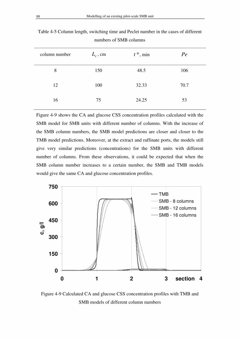
Modelling of an existing pilot-scale SMB unit 88
Table 4-5 Column length, switching time and Peclet number in the cases of different
numbers of SMB columns
column number cL , cm *t , min Pe
8 150 48.5 106
12 100 32.33 70.7
16 75 24.25 53
Figure 4-9 shows the CA and glucose CSS concentration profiles calculated with the
SMB model for SMB units with different number of columns. With the increase of
the SMB column numbers, the SMB model predictions are closer and closer to the
TMB model predictions. Moreover, at the extract and raffinate ports, the models still
give very similar predictions (concentrations) for the SMB units with different
number of columns. From these observations, it could be expected that when the
SMB column number increases to a certain number, the SMB and TMB models
would give the same CA and glucose concentration profiles.
0
150
300
450
600
750
0 1 2 3 4section
c,
g/l
TMB
SMB - 8 columns
SMB - 12 columns
SMB - 16 columns
Figure 4-9 Calculated CA and glucose CSS concentration profiles with TMB and
SMB models of different column numbers

Fehler! Formatvorlage nicht definiert. 89
4.4.2.2 Influence of the adsorption capacity on the CSS concentration profiles
As has been mentioned previously, the resin CA adsorption capacity could be
probably reduced due to the competitive adsorption or irreversible adsorption of some
of the impurities presented in the fermentation broth. In order to study the influence
of the CA adsorption capacity on the CA concentration profiles, the isotherm
parameter “a” of the modified Langmuir adsorption isotherm is reduced by 10% and
20%, respectively. The TDM SMB model was used to calculate the CA CSS
concentration profiles. SMB run 1 was chosen as an example.
The CA CSS concentration profiles for different “a” values are presented in Figure
4-10. As expected, when the adsorption capacity is reduced, the CA concentration
profile becomes dispersed and matches the experimental ones better. Especially when
the adsorption capacity is reduced by 20% (a=1.64). The SMB model prediction
agrees with the experimental data quite nice. Moreover, it can be also observed that
the adsorption capacity influences significantly on the CA concentration profile
between one column left and right of the feed port. Whereas at the extract and
raffinate ports, nearly no influence can be seen. According to Katsuo (2009), a
decrease of the adsorption capacity would lead to the separation region shifts to lower
2m and 3m . Since the CA concentrations at the extract and raffinate ports are nearly
unchanged even in the case of 20% reduction of the CA adsorption capacity, we can
conclude that the selected SMB operating conditions for run 1 still remain inside the
separation region.
Anyhow in reality the CA adsorption capacity decrease of 20% after one SMB run is
rather possible, since the impurities concentration in the feed stream is less than
2wt%.

Modelling of an existing pilot-scale SMB unit 90
0
200
400
600
800
0 2 4 6 8column
c,
g/l
a = 2.04
a = 1.84
a = 1.64
Exp.
Figure 4-10 Influence of the resin adsorption capacity on the CA CSS concentration
profiles
4.4.2.3 Influence of the pump flow rates on the CSS concentration profiles
As has been mentioned previously, the flow rates in sections 2 and 3 would influence
the CA concentration profiles. Increase of the flow rate in these sections would
possibly lead to match between experimental and calculated CA concentration
profiles. According to the node balances (Table 4-1), the flow rates in sections 2 and
3 could be increased (while keeping the flow rates in sections 1 and 4 unchanged), by
increase of the extract flow rate and simultaneously decease of the raffinate flow rate,
in order to maintain flow rate balance closed. Since the model prediction has good
agreement with the experimental data in sections 1 and 4, in this analysis we consider
that the eluent flow rate was well controlled.
The change of extract flow rates was set within 2%. Therefore, only two extract flow
rates, i.e., xQ = 90 and 89ml/min were investigated. The influence of the extract flow
rates on the CA concentration profiles is presented in Figure 4-11. When the extract
flow rate is reduced for only 1% ( xQ = 90ml/min), the calculated CA concentration
profile fit the experimental data. This implies that the extract flow rate has a
significant influence on the CA concentration profile.

Fehler! Formatvorlage nicht definiert. 91
0
200
400
600
800
0 2 4 6 8column
c,
g/l
Qex = 91ml/min
Qex = 90ml/min
Qex = 89ml/min
Exp
Figure 4-11 Influence of the extract flow rate on the CA CSS concentration profiles
Increase of the feed flow rate with simultaneous increase of the raffinate flow rate
would lead to the increase of the section 3 flow rate. Again, 2% of the change in the
feed flow rate was considered. The resulting CA concentration profiles are presented
in Figure 4-12. The influence of the feed flow rate on the CA concentration profile is
not important and could be neglected.
0
200
400
600
800
0 2 4 6 8column
c,
g/l
Qfe = 14.7ml/min
Qfe = 14.8ml/min
Qfe = 15.0ml/min
Exp

Modelling of an existing pilot-scale SMB unit 92
Figure 4-12 Influence of the feed flow rate on the CA CSS concentration profiles
In summary, from the performed sensitivity analysis we can conclude that the
adsorption capacity and the flow rates in sections 2 and 3 have influences on the CA
concentration profile. By decreasing adsorption capacity or increasing extract flow
rate, the model predictions could match the experimental data very well. Among them,
the extract flow rate has the most significant influence on the CA concentration
profile, since the CA concentration profile changes significantly by extract flow rate
increase of only 1%.
4.4.3 Separation performances
For all SMB runs, the experimental and calculated unit performances, with both TMB
and SMB models, are presented in Table 4-6. This comparison was used to evaluate
the accuracy of the TMB and SMB model predictions. The SMB performance
parameters calculated with both models were similar, and also close to the
experimentally obtained values (see Table 4-6). The CA purity and recovery
constraints were fulfilled and the required CA purification was obtained.
The experimental extract and raffinate stream compositions, and thus the SMB unit
performances, can be predicted satisfactorily with the equivalent TDM TMB and
dynamic TDM SMB mathematical models, except the CA recovery in the extract
( REX ) which was overestimated. This was expected because the TDM model was
not able to predict the extensive CA peak tailing observed during the pulse injection
experiments (see Figure 3-5).
Table 4-6 Experimental and calculated separation performances for run 1, 2 and 3
Run No.1
( FQ =15ml/min)
Run No.2
( FQ =10ml/min)
Run No.3
( FQ =5ml/min) Performance
SMB TMB Exp. SMB TMB Exp. SMB TMB Exp.

Fehler! Formatvorlage nicht definiert. 93
PUX , %
REX , %
PD , %
PR , kg/(l•min)
EC , l/kg
100
99.9
83.9
0.63
10.3
100
100
83.9
0.63
10.3
99.9
97.5
84.3
0.61
10.5
100
99.9
88.9
0.44
14.7
100
100
88.8
0.44
14.6
99.9
96.3
89.3
0.43
15.2
100
100
94.0
0.22
29.2
100
100
94.0
0.22
29.2
99.9
94.8
94.4
0.21
30.7
The separation performances, i.e., CA productivity, eluent consumption and product
dilution are improved with the increase of the feed flow rate from 5 to 15ml/min (see
Table 4-6). For the optimal operation condition (corresponding to the vertex of the
separation region), the maximum feed flow rate was 19.8ml/min. The obtained extract
dilution was very high (81%). Such a highly diluted product would be of little
practical interest.
Up to this point, the separation triangle methodology was used to select the flow rates
in the regeneration sections. In this particular SMB separation minimum 90% CA
recovery in the extract was required. Therefore a part of CA could be allowed to pass
from section 1 to section 4. In other words, complete regeneration of adsorbent in
section 1 was unnecessary. Also, the obtained product (CA in extract) was highly
diluted when complete regeneration of section 1 was considered. The CA
concentration in the extract was a crucial parameter for the cost of the following steps
in the CA downstream processing. The CA dilution is related to the eluent flow rate,
which was defined by the values of 1m and 4m and the switching time. Therefore a
more detailed design is needed in order to improve the SMB performances. The key
point for the further design was the fact that complete regeneration of the stationary
phase (in section 1) is not needed, when a close to 100% pure extract and raffinate
were not the target of the SMB separation process. Therefore, the influences of the
operating conditions on the SMB separation performances are going to be explored
systematically in Chapter 5.
Summary
The operating conditions for an existing SMB unit include five parameters, i.e., three
external flow rates, one section flow rates and the switching time. To select a set of
suitable operating conditions leading to the desired SMB separation performances is

Modelling of an existing pilot-scale SMB unit 94
nearly impossible by trial and error. Hence, a SMB design methodology based on the
separation triangle methodology was used for preliminary design of the operating
conditions of our pilot-scale SMB unit. Namely, the operating conditions in terms of
1m and 4m (section 1 and 4) were calculated according to the separation triangle
methodology, using the CA and glucose experimental adsorption isotherms
parameters and a safety factor. Afterwards a complete TMB model was used to
construct the separation region for minimum 99.8% CA purity and 90%CA recovery
in the extract stream.
Three sets of operating conditions were selected to run the pilot-scale SMB unit. The
TMB and SMB models could give good predictions of the concentrations in the
extract and raffinate and consecutively the SMB performances. The SMB model
gives better prediction of the internal concentration profiles than the TMB model, as a
result of the low number of columns in the used SMB unit.
However, there is a discrepancy between experimental CA concentration profiles and
those calculated with the SMB model one column left and right from the feed port.
The operating parameter sensitivity analysis has shown that the extract (and raffinate)
pump flow rates deviation of only 1% could give a very good prediction of the
experimental CA concentration profiles. The other possible reasons are: (i) slight loss
of the resin CA adsorption capacity due to competitive or irreversible adsorption of
some of the impurities present in the fermentation broth, (ii) TDM model prediction
deviations, (iii) cross contamination due to the system dead volume and unit
asymmetry, and (iv) manual collection of the samples.
The desired CA product purity and recovery could be experimentally achieved.
However the obtained product is highly diluted and has little practical value. The CA
dilution is related to the eluent flow rate, which is defined by the values of 1m and
4m selected by the separation triangle methodology. Therefore a more detailed SMB
design is needed in order to improve the SMB performances. The key point for the
further design is the fact that complete regeneration in section 1 and 4 is not needed,
when a pure extract and pure raffinate are not the target of the SMB separation
process. Therefore, the influence of the operating conditions on the SMB separation
performances is going to be explored systematically in Chapter 5.

Fehler! Formatvorlage nicht definiert. 95

Design of the existing pilot-scale SMB system 96
5 Design of the existing pilot-scale SMB system
In the previous chapter the required CA product was obtained by the preliminary
selected SMB operating conditions using the separation triangle methodology. The
only problem was the high CA diluted product (extract) which has low practical value,
due to the high energy cost for the CA recovery in crystalline form.
In this chapter the influences of the operating conditions, namely the flow rates in
sections 1 ( 1m ) and 4 ( 4m ) as well as the switching time ( *t ) on the SMB
separation performances are investigated systematically. Besides the CA purity and
recovery constraints, the CA product dilution lower than 50% was considered as an
additional SMB performance requirement. As a result of the more detailed and
systematic study new 1m and 4m as well as *t values, which lead to the required
separation performances, were attained.
Based on the new designed operating conditions, a new separation region was
constructed subsequently. Inside the region two operating conditions were selected to
run the SMB unit in order to confirm the designed SMB performances.
At the end of this chapter the quality of the final CA product, obtained from the SMB
extract after ion exchange, decolorization and crystallization steps, was analyzed. The
quality of the obtained CA has shown that the SMB technology can be successfully
integrated in the novel process scheme proposed in this thesis for CA recovery from
its fermentation broth.
5.1 Influences of operating conditions on the separation regions and
performances
A systematic study of the influence of the SMB operating conditions on the
separation region and SMB unit performances is presented in this section. The
parameters considered include the flow rate in section 1 ( 1m ), the flow rate in section
4 ( 4m ), the switching time period ( *t ), and the total column number, as well as,
their distribution in the SMB unit sections. For comparison, the preliminary designed
SMB operating conditions and model parameters presented in Table 4-3 are selected
as a reference case. During the study only one operating parameter is changed at once,
while the other parameters are kept unchanged and equal to their values in Table 4-3.

Fehler! Formatvorlage nicht definiert. 97
5.1.1 Influences of 1m on the separation regions and performances
The separation regions are calculated using the equivalent steady state TDM TMB
model for different 1m values. Starting point in this study is the 1m reference case
value (SMB
Q1 = 125ml/min). The eluent flow rate ( ElQ ) is gradually decreased, which
corresponds to the gradual decrease of the 1m value. Since, SMB
Q1 = ElQ + SMB
Q4
and SMB
Q4 remains constant, decrease of ElQ leads to decrease of SMB
Q1 . As long as
*t and cL are unchanged, the change of 1m values is proportional to the change of
SMBQ1 (see Eq. 2-46).
The separation regions obtained for different 1m values are presented in Figure 5-1.
It can be observed that by decreasing 1m , the separation regions shrink gradually
from the right side border, whereas the left side border stays almost unchanged. This
is expected because the right side border is controlled by the CA recovery constraint.
A decrease of 1m leads to an incomplete regeneration of the adsorbent in section 1,
the retained solute in this section (CA) then travels together with the adsorbent to
section 4, where it is desorbed and causes raffinate contamination with CA.
Consequently, a part of CA would be lost in the raffinate, the CA recovery constraint
becomes more and more difficult to fulfill, resulting in shrinkage of the separation
region. The lowest limiting value of 1m for which the CA SMB separation is possible
within the required performances is 0.83 (SMB
Q1
=55ml/min).
The SMB performances for different 1m values, calculated for the operating
conditions corresponding to the vertex of the separation region are presented in Table
5-1. The product dilution and eluent consumption are significantly improved with the
decrease of 1m values. For 1m =0.83, the product dilution is only 33.5%, which
represents a considerable improvement from the industrial scale production point of
view. The CA productivity is just slightly reduced with the decrease of the 1m values
from 2.92 to 0.83.

Design of the existing pilot-scale SMB system 98
0.00
0.40
0.80
1.20
1.60
0.00 0.40 0.80 1.20 1.60
m2
m3
2.92
2.32
1.73
1.13
0.83
m1
Figure 5-1 Separation regions for different values of m1. (m4: -0.21, t*: 48.5min, SMB
configuration: 2-2-2-2)
The 1m =1.13 is set as a new value in the SMB design, since it is far enough from the
minimal 1m value (0.83) and provides acceptable product dilution of around 50%.
Table 5-1 Separation performances for different values of 1m
SMBQ
1
(ml/min)
1m
(-)
PD
(%)
PR
(kg/(l•min))
EC
(l/kg)
125.0
105.0
85.0
65.0
55.0
2.92
2.32
1.73
1.13
0.83
81.0
76.0
67.5
50.6
33.5
0.78
0.77
0.76
0.73
0.69
8.32
6.75
5.24
3.81
3.13

Fehler! Formatvorlage nicht definiert. 99
5.1.2 Influence of 4m on the SMB performances
The starting point in this study is the reference case 4m value ( 4m =-0.21), which is
then gradually increased. This is done by a gradual increase of the flow rate in section
4 (SMB
Q4
). At the same time, in order to keep the 1m value constant, the eluent flow
rate ( ElQ ) must be reduced according to the eluent node balance equation
( ElQ =SMB
Q1
-SMB
Q4
). All other operating conditions and model parameters
correspond to the reference case values (see Table 4-3).
The calculated separation regions for different 4m values are presented in Figure 5-2.
Contrary to the case of 1m , an increase of 4m value results in a separation region
shrinkage from the left-side border, while the right-side border stays unchanged. This
is because the left-side border is related to the extract (CA) purity constraint. Namely,
when 4m (i.e., SMB
Q4
) is increased above the value corresponding to the complete
eluent regeneration in section 4, glucose travels with the liquid stream from section 4
to section 1 and causes extract contamination. Hence, the CA purity constraint is no
more accomplished.
0.00
0.40
0.80
1.20
1.60
0.00 0.40 0.80 1.20 1.60
m2
m3
-0.210.080.130.140.16
m4
Figure 5-2 Separation regions for different values of m4. (m1: 2.92, t*: 48.5min, SMB
configuration: 2-2-2-2)

Design of the existing pilot-scale SMB system 100
The SMB performance at the vertex of the separation regions obtained for different
4m values are presented in Table 5-2. The SMB performances are only slightly
influenced by the increase of the 4m values.
The separation regions start to shrivel significantly for 4m values higher than 0.14,
which corresponds to SMB
Q4
=32.0ml/min. In Table 5-2 one can observe that slight
increase of the SMB
Q4
value (for example only 0.5ml/min, SMB
Q4
=32.5ml/min)
results in a significant separation region size reduction (see Figure 5-2). The
fluctuation of the pump flow rate has to be taken into account when selecting the
most appropriate 4m value. Based on these considerations, 4m =0.08 is selected as a
new value in the SMB design.
Table 5-2 Separation performances for different values of 4m
SMBQ
4
(ml/min)
4m
(-)
PD
(%)
PR
(kg/(l•min))
EC
(l/kg)
20.0
30.0
31.5
32.0
32.5
-0.21
0.08
0.13
0.14
0.16
81.0
81.0
81.0
81.2
81.5
0.78
0.78
0.78
0.77
0.75
8.32
7.52
7.41
7.44
7.58
5.1.3 Influence of *t on the SMB performances
The switching time ( *t ) is directly correlated to the SMB unit productivity. The
lower *t is the higher productivity can be achieved. In this subsection, the effect of
the switching time on the separation region and SMB performances is presented. The
reference case SMB unit configuration, 1m and 4m values and model parameters are
considered in this study (see Table 4-3). In order to keep the 1m and 4m values

Fehler! Formatvorlage nicht definiert. 101
constant, the flow rates in sections 1 and 4 (SMB
Q1
and SMB
Q4
) are recalculated for
each switching time value.
The separation regions obtained for different switching times are presented in Figure
5-3. The switching time does not affect the separation region size and shape for
values higher than 5min. For the times shorter than 5min, the separation region
diminishes from both sides. The separation is not possible for a switching time period
lower than 3min. In this case the switching time might be shorter than the contact
time needed for effective solute mass transfer.
0.00
0.50
1.00
1.50
2.00
0.00 0.40 0.80 1.20 1.60 2.00m2
m3
48.5 min
20.0 min
10.0 min
5.0 min
3.0 min
t*
Figure 5-3 Separation regions for different values of t*. (m1: 2.92, m4: -0.21, SMB
configuration: 2-2-2-2)
The SMB performance parameters for different switching times calculated for the
operating conditions corresponding to the separation region’s vertex are presented in
Table 5-3. The CA productivity increases significantly with the decrease of the
switching time. When *t is reduced to 3.0min, CA productivity is increased to
9.78kg/l, which is more than 10 times higher than that in the reference case (0.78kg/l).
The CA product dilution and eluent consumption are only slightly affected by the
decrease of the switching time.

Design of the existing pilot-scale SMB system 102
As mentioned in Section 4.1 describing the pilot-scale SMB system, the maximum
pump flow rate is 150ml/min. Taking this constraint into account and since the 1m
value has been already set at 1.13, the switching time for the new SMB operating
conditions can be selected according to the following equation:
( )tc
tcSMB
V
VtQm
ε
ε
−
−=
1
*11 . The selected switching time is 25min, because at this
switching time the calculated flow rate in section 1 is 126.1ml/min, within the
maximum pump restriction. Consequently, the flow rate in section 4 is calculated
(58.2ml/min) using the selected 4m value and the switching time.
Table 5-3 Separation performances for different switching times
*t
(min)
SMBQ
1
(ml/min)
SMBQ
4
(ml/min)
PD
(%)
PR
(kg/(l•min))
EC
(l/kg)
48.5
20.0
10.0
5.0
3.0
125.0
303.1
606.3
1212.5
2020.8
20.0
48.5
97.0
194.0
323.3
81.0
81.0
81.2
82.3
85.1
0.78
1.88
3.73
7.01
9.78
8.32
8.33
8.41
8.84
10.68
5.1.4 Influence of the SMB configurations on its performances
So far, the influences of 1m and 4m as well as *t on the SMB performances have
been studied and new values giving improved unit performances are selected,
1m =1.13, 4m =0.08 and *t =25min. Assuming these new operating conditions, the
influences of the total column number and the SMB configuration on the SMB
performances are studied. The 8 column SMB with 2-2-2-2 configuration is still used
as a reference case.
Since the pilot SMB unit consists of 16 columns, the 16 columns SMB with a 4-4-4-4
configuration are first assessed. Additionally, three different 8 columns SMB
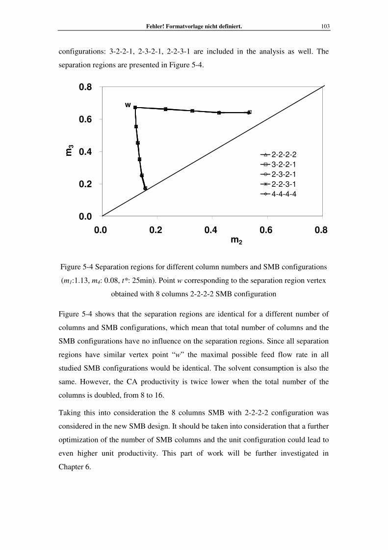
Fehler! Formatvorlage nicht definiert. 103
configurations: 3-2-2-1, 2-3-2-1, 2-2-3-1 are included in the analysis as well. The
separation regions are presented in Figure 5-4.
0.0
0.2
0.4
0.6
0.8
0.0 0.2 0.4 0.6 0.8m2
m3
2-2-2-2
3-2-2-1
2-3-2-1
2-2-3-1
4-4-4-4
w
Figure 5-4 Separation regions for different column numbers and SMB configurations
(m1:1.13, m4: 0.08, t*: 25min). Point w corresponding to the separation region vertex
obtained with 8 columns 2-2-2-2 SMB configuration
Figure 5-4 shows that the separation regions are identical for a different number of
columns and SMB configurations, which mean that total number of columns and the
SMB configurations have no influence on the separation regions. Since all separation
regions have similar vertex point “w” the maximal possible feed flow rate in all
studied SMB configurations would be identical. The solvent consumption is also the
same. However, the CA productivity is twice lower when the total number of the
columns is doubled, from 8 to 16.
Taking this into consideration the 8 columns SMB with 2-2-2-2 configuration was
considered in the new SMB design. It should be taken into consideration that a further
optimization of the number of SMB columns and the unit configuration could lead to
even higher unit productivity. This part of work will be further investigated in
Chapter 6.

Design of the existing pilot-scale SMB system 104
5.2 New design of the exiting SMB unit operating conditions
5.2.1 New SMB separation region
The newly designed SMB operating conditions: 1m =1.13, 4m =0.08 and *t =25min
and 8 columns, 2-2-2-2 SMB configuration are used to construct the new separation
region, presented in Figure 5-5. The separation constraints are the same as in Chapter
4, i.e. %8.99≥PUX and %90≥REX . Two SMB experiments, corresponding to
the points 1’ and 2’ in the separation region, are selected to operate the SMB unit and
confirm the designed SMB unit performances. The feed flow rates are 25ml/min for
point 1’ and 30ml/min for point 2’.
Figure 5-5 CA separation region constructed on the basis of the steady state TDM
TMB model. PUX≥99.8 and REX≥90% as the separation constraints, m1=1.13,
m4=0.08, t*=25min with 2-2-2-2 SMB configuration. 1’ and 2’ corresponding to two
sets of selected operating conditions for SMB experimental runs
5.2.2 SMB unit operations
The CA and glucose experimental and calculated CSS concentration profiles for run
1’ and 2’ are presented in Figure 5-6 and Figure 5-8, respectively. The experimental
internal concentration profiles were measured at the middle of each switching time at
fixed column position during the 16th cycle (CSS). The TDM SMB model
0.00
0.20
0.40
0.60
0.80
1.00
0.00 0.20 0.40 0.60 0.80 1.00
m2
m3 1
2 ‚ ‚

Fehler! Formatvorlage nicht definiert. 105
concentration profiles were calculated as an average concentration value over one
switching time at each axial position. The experimental extract and raffinate
concentration histories for SMB run 1’ and 2’ together with the calculated CA and
glucose concentration are presented in Figure 5-7 and Figure 5-9, respectively.
During the SMB experiments the extract and raffinate were collected during each
cycle and their concentrations were measured. The SMB model concentration
histories presented in the same figures were calculated as an average concentration
value over each cycle.
The CSS concentration profiles of CA and glucose in both SMB experiments are well
predicted by the transient TDM SMB model. The model gives a rather nice prediction
for the glucose. The discrepancy between the experimental and calculated CA
concentration one column left and right from the feed streams, observed in the first
set of experiments (see Section 4.4), appeared also for this two SMB runs. The
possible reasons for this discrepancy have been already extensively discussed in
chapter 4 (Section 4.4). Nevertheless, there is very good agreement between the
experimental and calculated extract and raffinate concentration histories. Better
prediction of CA concentration in the raffinate stream than the one in the first set of
experiments presented in Chapter 4 (Figures 4-4, 4-6, 4-8) as a result of the low
experimental mass balance errors (around 1%) and the high CA concentrations both
in the extract and raffinate streams.

Design of the existing pilot-scale SMB system 106
0
140
280
420
560
700
0 2 4 6 8column
c,
g/l
SMB
CA
Glu
t*=25.0min
Q1=125.9ml/min
Eluent
68.0ml/min
Extract
62.3ml/min
Feed
25.0ml/min
Raffinate
30.7ml/min
Figure 5-6 Experimental and calculated CA and glucose SMB cyclic steady state
concentration profiles in the 16th cycles of run 1’ (pretreated fermentation broth used
as a feed solution, CAFc :658.4g/l and
GluFc :32.8g/l)
0
60
120
180
240
300
0 1 2 3 4 5 6 7 8 9 10 11 12 13 14 15 16
cycle
c,
g/l
SMB
CA
Glu
a)

Fehler! Formatvorlage nicht definiert. 107
0
7
14
21
28
35
0 1 2 3 4 5 6 7 8 9 10 11 12 13 14 15 16
cycle
c,
g/l
b)
Figure 5-7 Experimental and calculated concentration histories for run 1’, (a) extract
stream, and (b) raffinate stream
0
140
280
420
560
700
0 2 4 6 8column
c,
g/l
SMB
CA
Glu
t*=25.0min
Q1=126ml/min
Eluent
68.0ml/min
Extract
64.5ml/min
Feed
29.9ml/min
Raffinate
33.4ml/min
Figure 5-8 Experimental and calculated CA and glucose SMB cyclic steady state
concentration profiles in the 16th cycles of run 2’ (pretreated fermentation broth used
as a feed solution, CAFc :638.4g/l and
GluFc :30.9g/l)

Design of the existing pilot-scale SMB system 108
0
70
140
210
280
350
0 1 2 3 4 5 6 7 8 9 10 11 12 13 14 15 16
cycle number
c,
g/l
SMB
CA
Glucose
a)
0
7
14
21
28
35
0 1 2 3 4 5 6 7 8 9 10 11 12 13 14 15 16
cycle number
c,
g/l
b)
Figure 5-9 Experimental and calculated concentration histories for run 2’, (a) extract
stream, and (b) raffinate stream
The experimental SMB unit separation performances of run 1’ and 2’ are presented in
Table 5-4. The desired CA product is obtained experimentally using the new designed
SMB operating conditions. Moreover, based on the new designed operating
conditions, the attained CA concentration in the extract is only half lower than its

Fehler! Formatvorlage nicht definiert. 109
feed concentration, which is a very advantageous for the reduction of the cost related
to energy consumption for the CA production in a crystalline form.
Table 5-4 Experimental SMB separation performances for run 1’ and 2’
FQ
(ml/min)
PUX
(%)
REX
(%)
PD
(%)
PR
(kg/(l•min))
EC
(l/kg)
30
25
99.8
99.8
96.6
97.2
55.2
61.0
1.14
0.99
3.68
4.25
5.2.3 Analysis of the final CA product
The crystalline form CA, obtained from the extract collected in CSS for SMB run 2’,
after the ion exchange, decolorization and crystallization steps was sent to the Xielian
Company in Wuxi, China for quality analysis. The results are given in Table 5-5. The
composition of the pretreated CA fermentation broth (represented as feed in Table 5-5)
is given as well for comparison. The CA product obtained by SMB separation fulfills
the product specifications very well. This confirms that the SMB separation can be
successfully applied to recovery of CA from its fermentation broth.
Table 5-5 Analysis of citric acid product in crystalline form
Components Feed Product specification SMB product
Citric acid Purity, wt-
% 95.0 99.5 > 99.8
Readily carbonizable
substance (RCS), BU 3.2 ≤1.5 <0.5
Cations, wt-% 0.5 ≤0.05 <0.01
Anions, wt-% 1.2 ≤0.1 <0.03

Design of the existing pilot-scale SMB system 110
Summary
The influences of the operating conditions, in terms of 1m , 4m and *t on the SMB
separation performances were investigated systematically. 1m influences the product
dilution ( PD ) significantly, whereas *t influences the productivity ( PR )
extensively. Taking into account the PD of 50%, new 1m , 4m and *t values were
selected. A new separation region was constructed and operating conditions for two
SMB experiments were selected inside this region. The SMB model gave good
prediction of the experimental data and SMB separation performances.
Under the new designed operating conditions, the desired CA product was obtained.
This time the PD was decreased to 55% and simultaneously the PR as well as EC
(eluent consumption) were improved as well. Obtained extract solution was further
treated to obtain a final product in form of CA crystals. The analysis of the product
quality has shown that SMB separation could be successfully applied in the CA
purification from its fermentation broth. With the designed procedure followed in this
chapter the problem was solved concerning the low CA concentration in the extract
stream obtained when separation triangle methodology approach was used for
selection of operating conditions in sections 1 and 4.
Besides the operating conditions, the influences of the several SMB geometrical
parameters, namely, number of columns and SMB configurations (number of column
per section) on the SMB separation performances were studied as well. The results
implied that the number of SMB columns could be reduced, resulting in the
improvement of PR . Moreover, the influences of 1m , 4m and *t on the separation
performances were investigated individually. The interactions between these
parameters on the SMB performances were not taken into account in this chapter.
This is further studied in Chapter 6.
In summary, when 100% extract and raffinate purities and/or complete regenerations
of the adsorbent in section 1 and eluent in section 4 are not required the mathematical
model based SMB design methodology must be used.

Fehler! Formatvorlage nicht definiert. 111
6 Optimization of the pilot-scale SMB unit
In the previous chapter a set of SMB feasible operating conditions which lead to the
achievement of the desired separation performances was obtained. In order to further
improve the SMB unit performances, optimization of the pilot-scale SMB unit is
carried out in this chapter.
The work starts with optimization of the operating parameters, namely, the flow rates
in the four SMB sections and switching time, as well as, the total number of columns
and the SMB configuration (number of columns per section), for the existing SMB
unit (i.e., fixed column geometry). The attained SMB optimal parameters were
validated experimentally.
The second part of this chapter focuses on the optimal design of a new SMB unit. In
particular, the column length is included as one of the optimization variables. By the
proposed optimization procedure a set of optimal operating conditions and optimal
column lengths is obtained for a specific pre-set switching time, which lead to
maximal SMB productivity and minimal eluent consumptions needed for
achievement of that productivity.
At the end of this chapter the scale-up of optimized SMB unit is addressed.
The direct cyclic steady state (CSS) prediction approach was used in this chapter, in
order to eliminate the inaccuracy of the TMB model in simulation of SMB units with
reduced number of columns.
6.1 Direct cyclic steady state modelling strategy
6.1.1 Direct determination of CSS
The results in Chapter 5, Section 5.1.4 indicated that the number of the columns in the
SMB unit could be possibly further reduced, which would eventually lead to further
improvement of the SMB productivity. Up to now all SMB calculations used for
SMB design has been performed using the steady state TDM TMB model. According
to Pais (2003) there is a discrepancy between simulated results with TMB and SMB
models for SMB unit with low number of columns per section, i.e., less than 2
columns per section. In this case, SMB models should be used for simulation of the
SMB unit operation.

Optimization of the pilot-scale SMB unit 112
As have been mentioned in Chapter 2, Section 2.8.3.2, there are two approaches used
for calculation of cyclic steady state (CSS) SMB unit performances. One approach
uses dynamic simulation, in which SMB unit operation is simulated cycle by cycle
starting from a given initial conditions until the CSS is reached. The other approach
enables direct CSS prediction. The direct CSS prediction approach is based on the
fact that at CSS the spatially distributed SMB unit state at the end of a switching time
interval is identical to the state at the beginning of the interval, apart from a shift of
exactly one column length. The SMB initial conditions are therefore replaced by the
SMB periodic conditions (Eqs. 2-38 and 2-39). The other model equations remain the
same as in the transient SMB model given in Table 4-1 in Chapter 4, Section 4.2.1.
The direct CSS prediction model was solved using gPROMS. For the solution of
direct CSS SMB model in gPROMS, both axial and temporal domains must be
discretized simultaneously. A third order orthogonal collocation method in finite
elements (OCFEM) was applied for discretisation of the spatial domain. The number
of finite elements per column was the same as the one used for the solution of the
transient SMB model. The OCFEM was also used for the discretisation of the
temporal domain. In order to determine the minimum number of finite elements in
OCFEM for the temporal domain (switching time) that enables precise prediction of
the CSS, the global mass balance (MB) relative error of less than 0.1% was used as
criteria.
MB relative error % = ( )
FiF
RiRXiXFiF
Qc
QcQcQc
,
,,,100
+− Eq. 6-1
Some simulations were carried out, starting with 6 finite elements per switching time
until 15 finite elements per switching time. The SMB operating conditions used in
these simulations were the ones used to run the SMB unit in the previous chapter. The
operating conditions are given in Figure 5-8b in Section 5.2.2. The switching time is
set to 25 min.
The MB relative error and CPU time obtained for different number of finite elements
per switching time are presented in Table 6-1.
In all simulations the MB relative error is far bellow the minimum required value
(0.1%) and is in the same order of magnitude (10-10). The global mass balance is
closed for all used time steps (=switching time/number of finite elements) values.

Fehler! Formatvorlage nicht definiert. 113
However, the CPU time increases significantly with the increase of the number of
finite elements used in the discretisation of the time domain. Since the direct CSS
model would be later used for SMB unit optimization, ten finite elements per
switching time were selected to guarantee the calculation accuracy. The
corresponding CPU time for this case (541s) is acceptable.
Table 6-1 MB relative error and CPU time for different number of finite elements per
switching time (temporal domain) in the direct CSS prediction
Number of finite elements Time step (min) MB relative error (10-10 %) CPU time (s)
6 4.17 9.91 80
10 2.08 1.03 541
12 2.50 1.01 634
15 1.67 1.01 1913
The CSS concentration profiles at the middle of the switching time calculated by the
transient SMB model and by the direct CSS prediction model are presented in Figure
6-1. Both models give exactly same predictions.

Optimization of the pilot-scale SMB unit 114
0
140
280
420
560
700
0 1 2 3 4 5 6 7 8column
c,
g/l
transient SMB
direct CSS
Figure 6-1 Comparison of the cyclic steady state concentration profiles calculated by
the transient SMB model and by the direct CSS prediction model at the middle of the
switching time
The extract concentration history at cyclic steady state during one switching time
calculated using both models is shown in Figure 6-2. Again the identical predictions
can be observed. The final conclusion is that in the case of SMB unit with eight
columns, the direct CSS prediction model provides the same predictions as the
transient SMB model. However, the validation of the direct CSS prediction model for
eight columns is not sufficient. In the following sub-section the model would be
further verified for SMB units with different number of columns.

Fehler! Formatvorlage nicht definiert. 115
0
150
300
450
600
0 0.2 0.4 0.6 0.8 1t*, min
c,
g/l
transient SMB
direct CSS - CA
direct CSS - Glu
Figure 6-2 Comparison of the concentration history of extract stream calculated by
the transient SMB model with the direct CSS prediction model
6.1.2 Comparison of steady state TMB, transient SMB and direct CSS prediction
models
In order to find the limiting (minimum) number of SMB columns for which the
steady state TMB model gives precise predictions of SMB unit performances, the
operation of SMB units with different number of columns was calculated using the
equivalent steady state TMB, transient SMB and direct CSS prediction models. The
calculated SMB unit performances using each of these models are presented in Table
6-2.
In the case of a column number equal to eight, three models give identical predictions.
However, when the column number is reduced to seven, a slight difference in SMB
performances calculated with the equivalent steady state TDM TMB and transient
TDM SMB model is obtained. Moreover, this discrepancy becomes noticeable with
the further decrease of the number of columns, especially when the number of
columns is less than six. This indicates that the equivalent steady state TMB model is
not suitable for simulation of SMB units with less than 8 columns. On the other hand
the direct CSS prediction model provides exactly the same predictions as the transient
SMB model. The direct CSS prediction model requires shorter computation time and

Optimization of the pilot-scale SMB unit 116
was therefore selected to be used for the optimization of the SMB unit for CA
separation from its fermentation broth.

Fehler! Formatvorlage nicht definiert. 117
Table 6-2 SMB separation performances calculated based on the equivalent steady state TMB, transient SMB and direct CSS prediction models
8 column (2-2-2-2) 7 column (2-2-2-1) 6 column (1-2-2-1) 5 column (1-2-1-1) 4 column (1-1-1-1) Performances
TMB SMB CSS TMB SMB CSS TMB SMB CSS TMB SMB CSS TMB SMB CSS
PUX , % 100 100 100 100 99.9 99.9 100 99.9 99.9 100 99.9 99.9 100 99.8 99.8
REX , % 97.7 97.7 97.7 97.7 97.4 97.4 97.4 96.3 96.3 95.6 94.3 94.3 95.6 94.3 94.3
PD , % 66.9 66.9 66.9 66.9 67.0 67.0 67.0 67.4 67.4 67.6 68.0 68.0 67.6 68.0 68.0
PR ,
kg/(l•min)
0.85 0.85 0.85 0.98 0.97 0.97 1.13 1.12 1.12 1.33 1.32 1.32 1.67 1.65 1.65
EC , l/kg 4.90 4.90 4.90 4.90 4.91 4.91 4.91 4.97 4.97 5.01 5.07 5.07 5.01 5.07 5.07
Operating conditions: FQ =20.0ml/min, ElQ =67.9ml/min, XQ =59.0ml/min, SMB
Q1
=126.1ml/min, *t =25min

Optimization of the pilot-scale SMB unit 118
6.2 Optimization of the existing pilot-scale SMB unit
As has been mentioned in Chapter 2, Section 2.8.2, the parameters affecting the SMB
unit performances can be grouped in two groups: (i) operating conditions, and (ii)
geometrical parameters. In this section these two groups of parameters would be
optimised individually. The SMB optimization approach used here includes two
steps: (i) optimization of the SMB column number and SMB unit configuration,
keeping the switching time ( *t ) and the 1m , 4m constant, and (ii) optimization of
SMB operating conditions for the optimal SMB unit configuration, obtained in the
previous step.
Subsequently the separation triangle for the optimized SMB unit configuration and
then two sets of operating conditions were selected for experimental SMB runs.
6.2.1 Optimization of the number of SMB columns and SMB unit configurations
For the optimization of the number of SMB column and SMB configuration ten cases
were selected, given in Table 6-3. The total column number was varied between 4 and
8 columns, for each number of columns several possible SMB configurations were
considered. The direct CSS prediction model was used for calculations of SMB CSS
performances. The values of 1m , 4m and *t obtained as a new designed operating
conditions in Chapter 5 are used as a set of fixed parameters. From the values of 1m ,
4m and *t the flow rates in section 1 (SMB
Q1 ) and 4 (SMB
Q4 ) can be calculated
following the definitions of 1m and 4m (Eq. 2-46 in Section 2.8.4.1). The eluent
flow rate can be subsequently calculated from the node balance equation at the eluent
port: ElQ = SMB
Q1 -SMB
Q4 . Since the eluent flow rate is already fixed, the objective
function we set is to maximize the feed flow rate. Moreover, because the eluent flow
rate is preset, there is only one free variable, namely xQ or RQ that should be
optimized in order to obtain the maximal feed flow rate. The extract flow rate ( xQ )
was selected as an optimization variable. The separation requirements are minimum
99% CA purity and minimum 90% CA recovery in the extract. The flow-sheet of the
optimization procedure is given in Figure 6-3.

Fehler! Formatvorlage nicht definiert. 119
Table 6-3 Optimization problems used to obtain the minimum feasible number of SMB columns and SMB unit configuration
Problem No. of columns
Configuration Objective function
Optimization variable
Constraints Fixed Parameter
1 8 2-2-2-2 Max FQ xQ
PUX ≥ 99.8%
REX ≥ 90%
cL = 150cm, cD = 5cm;
1m = 1.13, 4m = 0.08,
*t = 25min, SMB
Q1 = 126.1ml/min;
CAFc = 709.2g/l,
GluFc = 29.51g/l;
2a 7 2-2-2-1
2b 7 2-2-1-2
2c 7 2-1-2-2
2d 7 1-2-2-2
Max FQ
xQ
PUX ≥ 99.8%
REX ≥ 90% Same as Problem 1;
3a 6 1-2-2-1
3b 6 2-2-1-1
3c 6 2-1-2-1
Max FQ xQ
PUX ≥ 99.8%
REX ≥ 90% Same as Problem 1;
4 5 1-2-1-1 Max FQ xQ
PUX ≥ 99.8%
REX ≥ 90% Same as Problem 1;
5 4 1-1-1-1 Max FQ xQ
PUX ≥ 99.8%
REX ≥ 90% Same as Problem 1;

Optimization of the pilot-scale SMB unit 120
Figure 6-3 Flow-sheet of the optimization procedure for maximizing feed flow rates
in the case of different SMB column numbers and SMB unit configurations
The vertex in the separation region corresponds to the maximum difference ( 3m - 2m ),
which gives the maximum possible feed flow rate in the SMB unit, for predefined
separation requirements. Therefore the result of the optimization procedure is the set
of operating conditions corresponding to the vertex point of the separation region.
Besides the maximal feed flow rate obtained with the proposed SMB optimization
procedure, the product dilution was also included as an extra parameter for evaluation
of the SMB optimization results.
Optimize
Maximize ( FQ ) by varying xQ
Subject to
PUX ≥ 99.8 % and REX ≥ 90 %
Optimization Problems SMB column numbers and SMB unit configurations
Fixed parameters:
- Geometrical parameters:
cL = 150cm, cD = 5cm;
- Operating conditions:
1m = 1.13, 4m = 0.08, *t = 25min, and SMB
Q1 = 126.1ml/min;
- Feed concentrations:
CAFc = 709.2g/l,
GluFc = 29.51g/l
Store the optimal values

Fehler! Formatvorlage nicht definiert. 121
First the optimization was performed for the optimization problem 1. The calculated
maximal feed flow rate and the corresponding separation performances are presented
in Table 6-4. In order to validate these results, they were compared with the vertex
point in the separation region (presented in Figure 5-5) constructed using the
equivalent steady state TMB model. It can be seen in Table 6-4 that the TMB
calculations and the CSS optimization procedure results are almost identical, which
implies that the optimization calculation with the direct CSS prediction model are
accurate.
Table 6-4 Optimal SMB separation performances calculated based on the TMB and
CSS optimization procedure
FQ
(ml/min)
PUX
(%)
REX
(%)
PD
(%)
PR
(kg/(l•min))
EC
(l/kg)
TMB 35.8 99.8 90.2 50.7 1.41 2.97
CSS 35.7 99.8 90.1 50.8 1.40 2.98
The CA and glucose CSS concentration profiles for the optimal feed flow rate
( FQ =35.7ml/min), calculated with the direct CSS prediction model and plotted in the
middle of the switching time, are presented in Figure 6-4. These profiles can help us
to analyze how number of the columns in the SMB unit could be further reduced.
Let us first examine the eluent regeneration section (section 4, columns 7 and 8). The
glucose profile reaches zero concentration at the end of column 7 and the CA profile
remains nearly constant in the columns 7 and 8. This indicates that the eluent free of
glucose can be obtained with only column 7. If this is correct, column 8 could be
excluded from the SMB unit and a new SMB unit with 7 columns and configuration
of 2-2-2-1 could be sufficient to perform the required CA separation.

Optimization of the pilot-scale SMB unit 122
Figure 6-4 CSS concentration profiles of CA and glucose calculated with the direct
CSS prediction model at the middle of the switching time for the optimal operating
conditions of case 1 (i.e. maximal feed flow rate)
In the adsorbent regeneration section (section 1, columns 1 and 2) the situation is a
little different from section 4. There is nearly no glucose existing in this section
which is expected since almost 100% of purity ( %8.99≥PUX ) in the extract
stream is required and obtained. However, the CA concentration is changing
(decreasing) significantly between the extract and eluent port. If one of the columns,
i.e., column 1 would be removed from the system, significant amount of CA will
remain adsorbed in the resin and moved to section 4 with the next inlet and outlet port
switch. As a consequence part of CA will be lost in the raffinate, resulting in a
decrease of CA recovery in the extract below the required value of 90%. In order to
avoid this, we could increase the flow rate in section 1 (equal to increase of 1m as
long as the switching time and column length are not changed) and (or) to decrease
the flow rate in section 4 (equal to decrease of 4m as long as the switching time and
column length are not changed). However these could not be applied in our case since
the values of 1m and 4m are already fixed. The other way is to increase the flow rate
in section 2 (equal to increase of 2m value) and (or) decrease the flow rate in section
0
200
400
600
800
0 1 2 3 4 5 6 7 8
column
c,
g/l
CA
Glu
Section 1 Section 2 Section 3 Section 4

Fehler! Formatvorlage nicht definiert. 123
3 (equal to decrease of 3m value). This can be realized by decreasing the extract flow
rate and the feed flow rate, in order to keep the mass balance closed. In summary,
when less columns in the section 1 would be used it is expected that the maximum
feed flow rate that can be used in frame of the separation requirements would be
reduced.
The separation sections, i.e., section 2 (columns 3 and 4) and section 3 (columns 5
and 6), are more sensitive on the number of the columns included than the
regeneration sections. If any of the columns in the separation sections would be
removed, the flow rate in section 2 must be increased or the flow rate in section 3
must be decrease in order to fulfill the separation requirements. Both actions result in
decrease of the maximal SMB feed flow rate.
By analysis of the concentration profiles, we have concluded that the maximal feed
flow rate would be influenced by the reduction of the number of columns in different
sections. But the question is until which degree these would influence the overall
SMB performances. In order to answer this question, five cases of SMBs with
different number of columns and different unit configurations are selected and
optimized (see Table 6-3).
The maximal (optimal) feed flow rate and corresponding product dilution are listed in
Table 6-5 for each case of the 10 cases given in Table 6-3. As expected the maximal
feed flow rate decreases with the reduction of the number of SMB columns. The
decrease is more significant for the cases with lower number of columns in the
separation sections of the SMB unit. The obtained results correspond to our previous
analysis.
The best results (represented in bold letters in Table 6-5) for different number of
SMB columns (4 to 8 columns) are selected and presented in Figure 6-5. It can be
observed that when the number of columns is more than six, there is insignificant
difference in the maximal feed flow rate and product dilutions. However, for less than
six columns are used the maximal feed flow rate drops and the product dilution
increases. Therefore, no less than six SMB columns should be considered for the CA
separation.

Optimization of the pilot-scale SMB unit 124
Table 6-5 Maximal feed flow rate and product dilution for different number of SMB
columns and different SMB unit configurations
Column number Configuration max,FQ , ml/min PD , %
8 2-2-2-2 35.7 50.9
2-2-2-1 34.8 51.5
2-2-1-2 33.9 53.3
2-1-2-2 32.1 53.5
7
1-2-2-2 34.5 52.4
1-2-2-1 33.6 53.1
2-2-1-1 33.0 54.0 6
2-1-2-1 29.2 55.4
5 1-2-1-1 31.4 56.2
4 1-1-1-1 26.6 60.1

Fehler! Formatvorlage nicht definiert. 125
0
15
30
45
60
75
8 (2-2-2-2) 7 (2-2-2-1) 6 (1-2-2-1) 5 (1-2-1-1-) 4 (1-1-1-1)
maximal feed flow rate, ml/min
product dilution, %
Figure 6-5 Maximal feed flow rate and product dilution for different number of SMB
columns and different SMB unit configurations
6.2.2 Optimization of the operating conditions for the existing SMB unit
6.2.3 Calculation of the optimal operating conditions
In chapter 5, the influences of the operating conditions in terms of 1m , 4m and *t on
the separation regions and SMB performances were investigated individually. Safety
margins for 1m and 4m were considered in the SMB unit design. As a result, sets of
feasible operating conditions inside the separation region constructed with the fixed
1m and 4m values, leading to the desired separation performances (CA purity and
recovery in the extract and product dilution), were obtained.
With optimization these sets of operating conditions are reduced to one set of optimal
operating conditions, which fulfills the objective function. Since the inexpensive
water is used as eluent, the eluent consumption is not a cost critical parameter for the
SMB unit for CA separation. The selected objective function is therefore to maximize
the feed flow rate. The optimization constraints are same as those used in the SMB
design, i.e., CA purity and recovery in the extract stream higher than 99.8% and 90%,
respectively. The optimization variables are: the extract and raffinate flow rates, the
flow rate in section 4 and the switching time. The column length and diameter are

Optimization of the pilot-scale SMB unit 126
chosen as the fixed parameters. The flow sheet of the optimization procedure is
shown in Figure 6-6 and the defined optimization problems are presented in Table 6-6.
Figure 6-6 Flow-sheet of optimization procedure to obtain the optimal operating
conditions for the existing pilot-scale SMB unit
Optimize
Maximize ( FQ ) by varying xQ , RQ , SMB
Q4
and *t
Subject to
PUX ≥ 99.8 % and REX ≥ 90 %
Fixed parameters: cL = 150cm, cD = 5cm
Store the optimal values
Optimization problems
- SMB feed solution concentrations;
- Flow rates in section 1
- SMB column numbers and SMB unit configurations

Fehler! Formatvorlage nicht definiert. 127
Table 6-6 Optimization problems to obtain the optimal operating conditions for the existing pilot-scale SMB unit
Problem No. of columns
Configuration Objective function
Optimization variables
Constraints Fixed Parameter
1a 8 2-2-2-2
1b 7 2-2-2-1
1c 6 1-2-2-1
Max FQ xQ , RQ ,
SMBQ
4, *t
PUX ≥ 99.8%
REX ≥ 90%
cL = 150cm, cD =5cm;CAFc = 709.2g/l,
GluFc = 29.51g/l;
SMBQ1 = 150ml/min;
2a 8 2-2-2-2
2b 7 2-2-2-1
2c 6 1-2-2-1
Max FQ xQ , RQ ,
SMBQ
4, *t
PUX ≥ 99.8%
REX ≥ 90%
Same as Problem 1a, 1b and 1c,
except SMB
Q1 = 126ml/min;
3a 8 2-2-2-2
3b 7 2-2-2-1
3c 6 1-2-2-1
Max FQ xQ , RQ ,
SMBQ
4, *t
PUX ≥ 99.8%
REX ≥ 90%
Same as Problem 1a, 1b and 1c,
except SMB
Q1 = 100ml/min;
4a 8 2-2-2-2
4b 7 2-2-2-1
4c 6 1-2-2-1
Max FQ xQ , RQ ,
SMBQ
4, *t
PUX ≥ 99.8%
REX ≥ 90%
Same as Problem 1a, 1b and 1c,
except CAFc = 120g/l,
GluFc = 5g/l;
5a 8 2-2-2-2
5b 7 2-2-2-1
5c 6 1-2-2-1
Max FQ xQ , RQ ,
SMBQ
4, *t
PUX ≥ 99.8%
REX ≥ 90%
Same as Problem 2a, 2b and 2c,
except CAFc = 120g/l,
GluFc = 5g/l;
6a 8 2-2-2-2
6b 7 2-2-2-1
6c 6 1-2-2-1
Max FQ xQ , RQ ,
SMBQ
4, *t
PUX ≥ 99.8%
REX ≥ 90%
Same as Problem 3a, 3b and 3c,
except CAFc = 120g/l,
GluFc = 5g/l;

Optimization of the pilot-scale SMB unit 128
The SMB feed solution used up to now was always the concentrated fermentation
broth ( CAc around 700g/l and Gluc around 30g/l). In the conventional precipitation
process a clarified fermentation broth obtained after filtration without any further
concentration is usually used as a feed stream. The usage of this type of SMB feed
would be convenient for the CA production companies using the conventional CA
down-streaming process, since there would be no need of adding an evaporators’
setup for fermentation broth concentration in the process scheme. This means that the
conventional precipitation could be easily replaced by SMB separation without
additional cost for evaporators’ set-up.
The feed concentration influences the shape and size of the SMB separation region,
from which the maximal feed flow rate for a given separation requirements is defined.
Migliorini et al., (1998; 1999a) have analyzed the effect of the feed concentration on
the complete separation region (obtained on the basis of the Equilibrium theory) in
the ( 2m , 3m ) plane. The results have shown that while increasing the overall feed
concentration, the position of the vertex point (maximal feed flow rate) shifts
downwards to the left in the ( 2m , 3m ) plane and the separation region shrinks. This
implies that when increasing the feed concentration the maximal feed flow rate
decreases. General conclusion is that when low feed concentration is used higher feed
flow rates can be processed in an SMB unit.
However, in these study the values of 1m and 4m were fixed, i.e., the complete
regeneration of adsorbent in section 1 and eluent in section 4 were guaranteed. In our
case since only 90% of CA recovery in extract is required, the complete regeneration
of the adsorbent in section 1 is not necessary. The effect of the feed concentration on
the values of 1m and 4m as well as the separation performances in the case of SMB
separation with uncompleted regeneration in section 1 is an interesting matter for our
specific separation tasks. Therefore, the concentrations of CA and glucose in the
SMB feed stream equal to: (i) clarified and non-concentrated, and (ii) clarified and
pre-concentrated are considered in the SMB optimization study (see optimization
problems 4-6 in Table 6-6).
As have been mentioned in chapter 3, the maximum flow rate (SMB
Q1
) in the pilot
scale SMB unit at Jiangnan University, China is limited to 150ml/min. In order to

Fehler! Formatvorlage nicht definiert. 129
investigate the influence of the flow rate in section 1 (SMB
Q1
) on the separation
performances, three different flow rates were considered in the optimization study. In
the previous Section 6.2.1, we have concluded that the minimum feasible number of
SMB columns is six. Therefore, three SMB units with eight, seven and six columns
with their optimal configurations were optimized.
Totally eighteen sets of SMB optimal operating conditions (presented in Table 6-6),
which lead to the maximal max,FQ for each studied case, were obtained. The optimal
operating conditions for each case are summarized in Table 6-7. The corresponding
optimal jm values, as well as the separation performances are listed in Table 6-8.
The product dilution, PD in Table 6-8, is significantly improved under the attained
optimal operating conditions. Particularly in the case when concentrated CA and
glucose solution is used as a model feed solution, the product dilutions are reduced to
around 20%. The other separation performances, CA productivity ( PR ) and eluent
consumptions ( EC ), are also significantly improved compared with the results
obtained from the SMB design in the previous chapter (Section 5.2.2). This is due to
the reduction of the 1m values obtained with the optimization. Under the optimal
operating conditions, the optimal 1m (around 0.67) in the case of concentrated feed
solutions is two-time lower than the designed one (1.13). Since the safety margin is
not taken into account in the optimization, the optimal 1m and 4m values have
reached their individual limiting boundaries. As a result, significantly improved SMB
separation performances were obtained.

Optimization of the pilot-scale SMB unit 130
Table 6-7 Optimal operating conditions and maximal feed flow rates for different optimization cases
CAFc , g/l
GluFc , g/l Column number configuration SMB
Q1 , ml/min max,FQ , ml/min SMBQ4 , ml/min xQ , ml/min *t , min
8 2-2-2-2 48.0 88.4 56.2 16.3
7 2-2-2-1 47.9 76.1 56.8 16.4
6 1-2-2-1
150
45.4 73.9 58.3 17.0
8 2-2-2-2 40.8 73.1 46.8 19.2
7 2-2-2-1 40.8 67.0 46.7 19.2
6 1-2-2-1
126
37.4 64.9 52.0 20.6
8 2-2-2-2 32.7 48.9 36.4 24.0
7 2-2-2-1 32.7 49.4 36.6 24.0
709.2 29.51
6 1-2-2-1
100
30.2 52.6 39.9 25.4
8 2-2-2-2 70.6 68.1 79.9 21.3
7 2-2-2-1 70.2 58.6 81.7 21.8
6 1-2-2-1
150
63.3 56.2 87.8 24.0
8 2-2-2-2 59.6 48.9 67.2 25.3
7 2-2-2-1 59.5 50.3 68.1 25.6
6 1-2-2-1
126
54.0 48.1 72.9 28.0
8 2-2-2-2 43.6 28.9 57.1 34.7
7 2-2-2-1 42.7 30.9 58.9 35.2
120 4.99
6 1-2-2-1
100
34.5 28.2 62.2 38.9

Fehler! Formatvorlage nicht definiert. 131
Table 6-8 Optimal jm values and separation performances corresponding to the optimal operating conditions
CAFc ,
g/l
GluFc ,
g/l
Number configuration SMBQ1 ,
ml/min
1m 2m 3m 4m PD , % PR ,
kg/(l•min)
EC ,
l/kg
CAxc ,
g/l
8 2-2-2-2 0.69 0.13 0.61 0.07 23.0 1.89 2.01 546.0
7 2-2-2-1 0.70 0.13 0.61 -0.05 24.1 2.15 2.42 538.6
6 1-2-2-1
150
0.76 0.13 0.60 0.01 30.0 2.39 2.59 496.1
8 2-2-2-2 0.68 0.13 0.61 0.05 21.4 1.60 2.03 557.5
7 2-2-2-1 0.68 0.13 0.61 -0.02 21.4 1.83 2.27 557.1
6 1-2-2-1
126
0.79 0.13 0.60 0.01 35.2 1.96 2.56 459.6
8 2-2-2-2 0.66 0.13 0.61 -0.09 19.2 1.28 2.45 572.9
7 2-2-2-1 0.67 0.13 0.61 -0.08 19.5 1.47 2.43 570.9
709.2 29.51
6 1-2-2-1
100
0.75 0.13 0.60 0.01 31.7 1.58 2.45 484.1
8 2-2-2-2 1.15 0.10 1.05 0.08 20.5 0.47 10.74 95.4
7 2-2-2-1 1.20 0.10 1.04 -0.03 22.6 0.53 12.05 92.9
6 1-2-2-1
150
1.40 0.11 1.02 0.02 35.1 0.56 13.73 77.9
8 2-2-2-2 1.15 0.10 1.04 -0.05 20.1 0.40 11.99 95.8
7 2-2-2-1 1.18 0.10 1.04 -0.02 21.3 0.45 11.80 94.4
6 1-2-2-1
126
1.36 0.11 1.02 0.02 33.3 0.48 13.37 80.0
8 2-2-2-2 1.13 0.10 1.04 -0.09 21.9 0.25 12.20 93.7
7 2-2-2-1 1.15 0.10 1.03 -0.06 23.5 0.29 12.34 91.6
120 4.99
6 1-2-2-1
100
1.33 0.11 1.02 0.02 37.3 0.32 13.95 75.3

Optimization of the pilot-scale SMB unit 132
The calculated maximum feed flow rates for different number of SMB columns in the
cases of pre-concentrated feed stream and clarified feed stream (non-concentrated)
are presented in Figure 6-7a and Figure 6-7b, respectively. In both cases (Figure 6-7a
and Figure 6-7b) the maximal feed flow rate increases with the increase of SMB
Q1 ,
resulting in a higher CA productivity and a lower eluent consumption (Table 6-8).
This can be explained by the shorter optimal switching time obtained when higher
flow rates in section 1 (SMB
Q1 ) are used (see Table 6-7). In Table 6-8 we can observe
that for each feed concentration the 1m values are almost constant for all considered
SMBQ1 values. Hence with the increase of the flow rate in section 1 (
SMBQ1 ), the
switching time decreases in order to keep the 1m value unchanged, resulting in an
improvement of the SMB separation performances.
The maximal feed flow rates which can be processed by the optimized SMB units
with eight and seven columns are nearly the same (see Table 6-7). The product
dilution and eluent consumption (see Table 6-8) in the SMB units with eight and
seven columns are also very similar. However, when the number of SMB columns is
reduced to six, the product dilution increases. The productivity ( PR ) increases with
the reduction of the number of the SMB columns. The total column volume is
included in conventionally used SMB productivity definition (Table 4-2). Therefore
productivity increases with the decrease of the total column volume. In conclusion,
the optimized SMB units with eight and seven columns show better overall SMB
separation performances, than the SMB units with six columns.

Fehler! Formatvorlage nicht definiert. 133
0
10
20
30
40
50
8 (2-2-2-2) 7 (2-2-2-1) 6 (1-2-2-1)
QF
,ma
x, m
l/m
in
150 ml/min 126 ml/min 100 ml/min
a)
0
15
30
45
60
75
8 (2-2-2-2) 7 (2-2-2-1) 6 (1-2-2-1)
QF
,max, m
l/m
in
b)
Figure 6-7 Comparison of the optimal feed flow rate for different numbers of SMB
column and different flow rates in section 1 in the case of two different feed
concentrations: (a) pre-concentrated (b) clarified (non-concentrated) fermentation
broth
The comparison of Figure 6-7a with Figure 6-7b, shows that higher feed flow rates
are obtained with lower feed concentration (non-concentrated fermentation broth as a
feed solution). This result agrees with the other author studies (Migliorini et al, 1998;

Optimization of the pilot-scale SMB unit 134
Migliorini et al, 1999a). The comparison of the maximal feed flow rate ( max,FQ ),
productivity ( PR ) and eluent consumption ( EC ) for these two different feed
concentrations, in the cases of three different flow rates in section 1 (SMB
Q1 ) in the
eight columns SMB is presented in Figure 6-8a, Figure 6-8b and Figure 6-8c,
respectively.
0
20
40
60
80
150 126 100Q1
SMB, ml/min
QF
,ma
x, m
l/m
in
concentrated
non-concentrated
a)
0
1
2
3
4
150 126 100
Q1SMB
, ml/min
PR
, kg
/(l*
min
)
concentrated
non-concentrated
b)
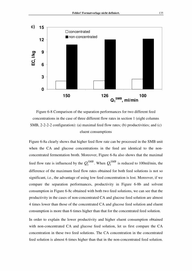
Fehler! Formatvorlage nicht definiert. 135
0
3
6
9
12
15
150 126 100Q1
SMB, ml/min
EC
, l/kg
concentrated
non-concentrated
c)
Figure 6-8 Comparison of the separation performances for two different feed
concentrations in the case of three different flow rates in section 1 (eight columns
SMB, 2-2-2-2 configuration): (a) maximal feed flow rates; (b) productivities; and (c)
eluent consumptions
Figure 6-8a clearly shows that higher feed flow rate can be processed in the SMB unit
when the CA and glucose concentrations in the feed are identical to the non-
concentrated fermentation broth. Moreover, Figure 6-8a also shows that the maximal
feed flow rate is influenced by the SMB
Q1 . When SMB
Q1 is reduced to 100ml/min, the
difference of the maximum feed flow rates obtained for both feed solutions is not so
significant, i.e., the advantage of using low feed concentration is lost. Moreover, if we
compare the separation performances, productivity in Figure 6-8b and solvent
consumption in Figure 6-8c obtained with both two feed solutions, we can see that the
productivity in the cases of non-concentrated CA and glucose feed solution are almost
4 times lower than those of the concentrated CA and glucose feed solution and eluent
consumption is more than 6 times higher than that for the concentrated feed solution.
In order to explain the lower productivity and higher eluent consumption obtained
with non-concentrated CA and glucose feed solution, let us first compare the CA
concentration in these two feed solutions. The CA concentration in the concentrated
feed solution is almost 6 times higher than that in the non-concentrated feed solution.

Optimization of the pilot-scale SMB unit 136
The same ratio is obtained between the CA concentrations in the extract stream for
these two feed solutions (CAxc in Table 6-8). However, the maximal feed and extract
flow rate, as well as the eluent flow rate (not presented, but it can be calculated easily
with SMB
Q1 -SMB
Q4 ) are only around 1.5 times higher when the non-concentrated CA
and glucose is used. Therefore, the productivity is reduced by 4 and the eluent
consumption is increased by 6 times.
The optimal jm , in particular, the 1m values and *t presented in Table 6-8 and
Table 6-7 in the case of SMB unit with eight columns and SMB
Q1 of 150ml/min show
interesting results. When non-concentrated feed solution is used, 1m is 1.7 times
higher than the one obtained when concentrated feed solution is used. This means that
the flow rate in section 1 should be increased when non-concentrated feed solution is
used. But since SMB
Q1 has been already fixed, 1m can be only increased by increasing
the switching time *t . The need of higher flow rates in section 1 in the case of non-
concentrated feed solution is probably related with the favorable type of CA
adsorption isotherm, which makes the regeneration of section 1 at low CA
concentrations more “difficult”. Higher eluent flow rate is therefore required to
desorb CA up to the concentration needed to ensure minimum 90% CA recovery in
the extract.
In summary, the maximal feed flow rate which can be processed in the SMB unit
increases with the decrease of the feed concentration. However, the productivity and
eluent consumption do not change proportionally with the change of the feed
concentration. If the complete regeneration of adsorbent in section 1 is not required,
the 1m value increases when feed solutions with low concentration are used. Hence,
the 1m value plays an important role in the SMB design and optimization.
6.2.3.1 Experimental validation of the optimized SMB operating conditions
In the previous section the optimal SMB operating conditions were obtained based on
the calculations using a model CA and glucose solution as a representation of the
SMB feed stream. Whether the optimal results can be obtained practically is most
important. Therefore, in this subsection eight columns SMB with 2-2-2-2

Fehler! Formatvorlage nicht definiert. 137
configuration, concentrated fermentation broth as the feed solutions and SMB
Q1 of
150ml/min were selected to operate the pilot scale SMB unit in order to verify the
optimization results. The calculated maximal feed flow rate by the optimization
procedure described in the previous section is equal to 48.0ml/min (see Table 6-7).
However, operating the SMB unit using these optimal operating conditions is risky.
Small deviations in the flow rates can destroy the separation completely, since this
would shift the operating point out of the separation region. Therefore, the SMB
separation region with the attained optimal 1m and 4m values were constructed,
within which the feasible operating conditions can be selected to operate the SMB
unit.
The optimal 1m (0.69) and 4m (0.07) as well as *t (16.3min) values for eight
columns SMB (2-2-2-2), SMB
Q1 =150ml/min and concentrated feed solution were
used for the construction of the SMB separation region. The resulting separation
region is shown in Figure 6-9, together with the separation region obtained with the
SMB design procedure used in Chapter 5 (Section 5.2.1, Figure 5-5). The “optimal”
separation region is much smaller than the one obtained in the SMB design. This is
expected because in the optimization process the safety margin is not used in the
calculation of 1m and 4m .
Two operating conditions (points 1 and 2 presented in Figure 6-9) inside the
“optimal” separation region were selected to run the SMB unit. The point 1 refers to
the feed flow rate of 40ml/min and point 2 of 35ml/min.

Optimization of the pilot-scale SMB unit 138
Figure 6-9 Comparison of separation regions obtained in the SMB design and after
SMB optimization for 8 columns SMB (2-2-2-2) and concentrated fermentation broth
as the feed solution
The comparison of the experimental and predicted CA and glucose SMB CSS internal
concentration profiles at the 16th cycle of run 1 is presented in Figure 6-10. The
comparison of the extract and raffinate CA and glucose concentration histories are
presented in Figure 6-11a and Figure 6-11b, respectively. The SMB predictions agree
well with the experimental data. However, there is a discrepancy between the CA
experimental and calculated concentration histories in the raffinate. In order to find
the reason for this discrepancy, the global MB relative error in the SMB simulation
and SMB experiment were analyzed. For the SMB simulation, the error was within
0.1% and for the SMB experiment less than 1%. According to the SMB calculation,
the average CA concentration in the extract stream was 482g/l and that of the
experiment was 473g/l. In the raffinate stream, the calculated CA concentration was
38g/l and experimentally obtained was 48g/l. Due to the extremely high CA
concentration in the extract stream, difference of 10g/l is nearly unnoticeable (Figure
6-11a), but in the raffinate stream such a difference becomes obvious (Figure 6-11b).

Fehler! Formatvorlage nicht definiert. 139
0
140
280
420
560
700
0 2 4 6 8column
c,
g/l
SMB
CA
Glu
Eluent
61.1ml/min
Extract
52.3ml/min
Feed
40.4ml/minRaffinate
49.2ml/min
t*=16.3 min
Q1=150 ml/min
Figure 6-10 Experimental and calculated CA and glucose SMB cyclic steady state
concentration profiles in the 16th cycle of run 1(pretreated fermentation broth used as
a feed, CAFc : 670.2g/l and
GluFc : 19.1g/l)
0
140
280
420
560
0 1 2 3 4 5 6 7 8 9 10 11 12 13 14 15 16
cycle number
c,
g/l
Calculated
CA
Glu
a)

Optimization of the pilot-scale SMB unit 140
0
14
28
42
56
0 1 2 3 4 5 6 7 8 9 10 11 12 13 14 15 16
cycle number
c,
g/l
calculated
CA
Glu
b)
Figure 6-11 Experimental and calculated concentration histories for run 1. (a) extract
stream, and (b) raffinate stream
Since *t and SMB
Q1 are identical for the SMB experiments 1 and 2, the second SMB
experiment ( FQ =35ml/min) was performed immediately after the CSS was reached
in the first SMB experiment. Doing this the CSS state for the SMB experiment 2
could be reached very fast. The extract and raffinate stream concentration histories
presented in Figure 6-13a and Figure 6-13b can prove this. After around 4 cycles, the
CA and glucose concentrations are almost constant. The experiment 2 was stopped
after 11 cycles. The experimental and calculated CA and glucose CSS concentration
profiles in the 11th cycle are shown in Figure 6-12. The simulated CSS concentration
profiles in the previous SMB experiment (run 1, FQ = 40ml/min) were used as the
initial conditions for this SMB calculations. Again good agreement between SMB
predictions and experimental data was obtained. Since as initial conditions in the
second SMB experiment was the CSS state from the previous experiment, and the
feed flow rate was lower than that in experiment 1, the CA and glucose
concentrations in the extract and raffinate streams gradually decrease to their final
CSS concentrations. The CA concentration in the feed solution used in the second
SMB experiment was slightly higher than the one in the first SMB experiment.
Therefore the CA concentration in the extract stream first increased slightly and then

Fehler! Formatvorlage nicht definiert. 141
decreased (Figure 6-13a). The experimental data also follow this concentration
change.
The similar discrepancy between the calculated and experimental CA concentration in
the raffinate stream was observed as in the previous experiment.
0
140
280
420
560
700
0 2 4 6 8column
c,
g/l
SMB
CA
Glu
Eluent
61.4ml/min
Extract
51.5ml/min
Feed
35.7ml/min
Raffinate
45.6ml/min
t*=16.3min
Q1=150ml/min
Figure 6-12 Experimental and calculated CA and glucose SMB cyclic steady state
concentration profiles in the 11th cycle of run 2 (pretreated fermentation broth used
as a feed, CAFc : 684.3g/l and
GluFc : 15.8g/l)

Optimization of the pilot-scale SMB unit 142
0
140
280
420
560
1 2 3 4 5 6 7 8 9 10 11
cycle
c,
g/l
SMB
CA
Glu
a)
0
14
28
42
56
1 2 3 4 5 6 7 8 9 10 11
cycle
c,
g/l
SMB
CA
Glu
b)
Figure 6-13 Experimental and calculated concentration histories for run 2, (a) extract,
and (b) raffinate
The experimental separation performances for these two SMB experiments are listed
in Table 6-9. The desired CA product was obtained. The CA concentration in the
extract stream was more than 450g/l, resulting in a product dilution around only 30%,

Fehler! Formatvorlage nicht definiert. 143
which is a great improvement obtained with the SMB optimization. Besides the
product dilution, the other separation performances were also improved.
Table 6-9 SMB experimental separation performances for run 1 and 2
FQ
(ml/min)
PUX
(%)
REX
(%)
PD
(%)
PR
(kg/(l•min))
EC
(l/kg)
35 99.8 95.0 34.2 24.7 2.65
40 99.8 91.3 29.4 23.2 2.47
6.3 Complete optimal design of a new SMB unit
In the previous section the existing pilot-scale SMB unit in our laboratory was
optimized. In the proposed optimization procedure the column geometry was not
considered as an optimization variable.
The parameters affecting an SMB unit performances are the operating conditions
(flow rates in four sections and switching time) and geometry related parameters.
There are several geometrical parameters, namely, the column length, the column
diameter, total number of columns and SMB configuration (number of columns per
section) and particle size. The complete optimal design of an SMB unit which takes
all these parameters into account is still a challenging task.
A systematic and simple optimization procedure is proposed in the work. Besides the
five operating conditions (flow rates in each section and the switching time), column
length was also considered as one of the optimization variables. With the proposed
procedure the maximal SMB productivity and minimal eluent consumptions needed
for achievement of that productivity are obtained a specific switching time. The
proposed optimization procedure is described in details in Section 6.3.2.
It has been shown that in an SMB unit with a fixed columns total length, the number
of columns i.e. the individual column length and their distribution in different
sections affects the unit separation performances (Pais, Rodrigues, 2003; Kawajiri,
Biegler, 2008a). Therefore, the influence of the number of columns in each section on
the SMB separation performances was first studied.

Optimization of the pilot-scale SMB unit 144
6.3.1 Influence of column lengths on the SMB separation performances
In the study of the influence of the number of columns per section the total column
length was fixed to 1200cm (150cm x 8 = 1200cm). The total number of SMB
columns was varied. For each considered column number the individual column
length was calculated as a ratio between the total column length and total number of
columns. The optimal operating conditions obtained for 8 columns SMB unit with
configuration 2-2-2-2 in Section 6.2.2.2 were used in the simulation study. The
calculation procedure is presented in Figure 6-14. Four cases with different number of
SMB columns were considered (4, 8, 12 and 16 columns). The column number was
selected in such way that for each studied case the sections length was keep constant
and equal to 300cm. As a result, the separation performances of SMB units with
different number of columns could be directly compared. For each column length, the
switching time and Pe number were re-calculated in order to keep the jm values and
axD constants. The column length and the switching time, as well as, Pe number for
each case (4, 8, 12 and 16 columns) are given in Figure 6-14.

Fehler! Formatvorlage nicht definiert. 145
Figure 6-14 Calculation of the separation performances for different number of SMB
columns
The separation performances of SMB units with different number of columns are
presented in Table 6-10. Although the total column length and the operating
conditions are kept the same, the SMB separation performances are influenced by the
column number i.e. column length.
The separation requirements are not fulfilled when 4 long columns are used (case 1).
With the decrease of the column lengths, i.e., increase of the column number, the
separation performances are improved. However, the improvement of the separation
performances achieved by increasing of the number of columns from eight to sixteen
was not so pronounced in our case (see Table 6-10). Consequently, eight columns
SMB with column length of 150cm can be considered as an optimal SMB
Fixed parameters:
- Geometrical parameters:
totcL , = 1200cm, cD = 5cm;
- Operating conditions:
1m =0.69, FQ =48.05, xQ =56.17, RQ =53.42 and SMB
Q1 = 150ml/min;
- Feed concentrations:
CAFc = 709.2g/l,
GluFc = 29.51g/l
Store the separation performances
SMB column numbers and lengths as well as switching times
- Case 1: 4 columns (1-1-1-1), cL = 300cm, *t = 32.52min, Pe = 212;
- Case 2: 8 columns (2-2-2-2), cL =150cm, *t = 16.26min; Pe = 106;
- Case 3: 12 columns (3-3-3-3), cL =100cm, *t = 10.84min; Pe = 70.7;
- Case 4: 16 columns (4-4-4-4), cL = 75cm, *t = 8.13min; Pe = 53;

Optimization of the pilot-scale SMB unit 146
configuration. This SMB configuration was considered in the following section
dealing with the SMB unit optimization.
Table 6-10 Separation performances of SMB units with different number of columns
Number Conf. cL
(cm)
*t
(min)
PUX
(%)
REX
(%)
PD
(%)
PR
(kg/min)
EC
(l/kg)
4 1-1-1-1 300 32.52 99.7 84.4 27.8 28.8 2.14
8 2-2-2-2 150 16.26 99.8 90.0 23.0 30.7 2.01
12 3-3-3-3 100 10.84 99.8 90.7 22.3 30.9 1.99
16 4-4-4-4 75 8.13 99.8 91.1 22.1 31.0 1.98
6.3.2 Optimization procedure towards complete SMB unit design
The complete optimization procedure proposed in this work is presented in Figure
6-15. The column diameter was set to 5cm. The feed concentration corresponds to the
CA and glucose concentration in the pretreated (concentrated) fermentation broth.
Eight columns SMB with 2-2-2-2 configuration was selected. The aim of this
optimization procedure was to obtain a set of optimal operating conditions and
column length for a certain fixed switching time. The optimal operating conditions
and column length would lead to maximal feed flow rate with a minimal eluent
consumption ( EC ), fulfilling the minimal required CA purity ( PUX ) and recovery
( REX ) in the extract.
The procedure started with a certain *0t (initial switching time
*0t =17min) and 0FQ
(initial feed flow rate 0FQ =1ml/min). The default optimization algorithm within
gPROMS (gOPT) package, namely: the CVP_SS, a control vector parameterization
(CVP) approach which assumes that the time-varying control variables are piecewise-
constant functions of time over a specified number of control intervals, with a
“single-shooting” dynamic optimization algorithm (SS), was employed to update
iteratively the values of the optimization variables xQ , RQ , SMB
Q4
and cL and to

Fehler! Formatvorlage nicht definiert. 147
calculated the minimum eluent consumption ( EC ) for a specific switching time and
feed flow rate. Subsequently the feed flow was gradually increased by 1ml/min
(increase interval FQ∆ =1ml/min) and the step of minimization of EC was repeated
till the maximum possible feed flow was obtained. Doing this, the maximum feed
flow rate and the corresponding operating conditions as well as column length were
obtained for a specific switching time *0t . By gradual decrease of the switching time,
*t , (decrease interval *t∆ =1min), the set of optimal operating conditions and
column length for different *t were attained by repeating the procedure described
above. The optimization was stopped externally when the optimal column length was
shorter than 10cm.

Optimization of the pilot-scale SMB unit 148
Figure 6-15 Optimization procedure for complete design of a new SMB unit
The optimal operating conditions represented by the corresponding jm values, the
optimal column length and maximal feed flow rate attained for different switching
times are summarized in Table 6-11, together with the SMB separation performances.
It can be observed that with the decrease of the switching times the optimal column
length and the maximal feed flow rate are reduced. The product dilutions and eluent
consumptions also increase with the decrease of the switching time. The SMB
productivity increases with the decrease of the switching time i.e. column length. This
is because the SMB productivity is expressed on the resin volume basis (see Table
Optimize
Min
xCAx
el
Qc
QECJ
⋅==
End
*t = *0t - *t∆
Fixed parameters:
- Geometrical parameter: cD = 5cm;
- Feed concentrations: CAFc = 709.2g/l,
GluFc = 29.51g/l;
- SMB configuration: eight columns with 2-2-2-2
FQ = 0FQ + FQ∆
PUX ≥ 99.8 %
&
REX ≥ 90 %
Yes No

Fehler! Formatvorlage nicht definiert. 149
4-2). In fact much higher feed flow rates can be processed when longer switching
times are used (see Table 6-11).
Table 6-11 Operating conditions and separation performances obtained with the
complete optimization procedure
No
.
*t
(min)
optcL ,
(cm)
Max. FQ
(ml/min)
1m 2m 3m 4m PD
(%)
PR
(kg/(l•min))
EC
(l/kg)
1 17.0 186.8 50 0.59 0.14 0.56 0.14 14.6 1.58 1.67
2 16.0 105.8 30 0.59 0.14 0.56 0.14 15.4 1.67 1.69
3 15.0 82.9 25 0.59 0.14 0.56 0.14 16.3 1.78 1.71
4 14.0 62.1 20 0.60 0.14 0.56 0.13 17.3 1.90 1.74
5 13.0 52.1 18 0.60 0.14 0.56 0.13 18.5 2.03 1.77
6 12.0 43.0 16 0.61 0.15 0.56 0.13 19.9 2.19 1.81
7 11.0 37.2 15 0.62 0.15 0.56 0.13 21.6 2.37 1.86
8 10.0 27.3 12 0.63 0.15 0.56 0.13 23.5 2.59 1.92
9 9.0 18.6 9 0.64 0.15 0.55 0.13 25.9 2.85 1.99
10 8.0 9.3 5 0.65 0.15 0.55 0.12 28.8 3.17 2.09
Although the optimal column length and feed flow rate change with the change of the
switching time, the jm values remain nearly unchanged (see Table 6-11). This is
expected because the jm values are only influenced by the adsorption
thermodynamics and kinetics parameters. As long as the adsorption isotherms of the
component and the kinetics parameters are unchanged (constant), the jm values are

Optimization of the pilot-scale SMB unit 150
fixed. The vertex in the separation triangle should be the only one no matter what
column length is used in the SMB unit.
However, if we take close look at the 1m and 4m values in Table 6-11, we can find
that the 1m value increases gradually and 4m decreases gradually with the decrease
of the switching time value. This implies that under shorter switching times, the
required eventhough partial regeneration of adsorbent sections 1 and almost complete
eluent regeneration in section 4 becomes more and more difficult.
6.3.3 Pilot scale SMB unit scaling up
The optimal SMB operating conditions presented in Table 6-11 can be used for SMB
unit design or SMB unit scale -up. For instance, if we want to design an SMB unit
which should process 50ml/min of pretreated fermentation broth ( FQ =50ml/min),
two approaches can be used:
(i) The first approach would be to read the optimal SMB operating conditions
and corresponding column length directly from Table 6-11 (optimal result
for case No.1).
(ii) The second approach is first to select the optimal operating conditions and
corresponding column length from Table 6-11 for a lower feed flow rate,
as for instance, feed flow rate of 25ml/min (optimal result of No.3). Then
to calculate the column diameter needed to process 50ml/min feed flow
rate following a simple scale-up rule, applied in chromatography when the
same particle size is used in the reference and scaled-up unit.
The simplest scale-up rule is based on keeping the liquid linear velocity, i.e.,
interstitial velocity in the reference (starting) SMB unit and scale up unit equal. This
scale-up rule is supported by the fact that column length, the adsorbent (stationary
phase) particle diameter and bed porosity are kept unchanged. It is worth to mention
that here the Peclet number and kinetics parameters are assumed to be unchanged as
well.
The interstitial liquid velocity in reference (1) and scale-up unit (2) are:

Fehler! Formatvorlage nicht definiert. 151
22,
2
21,
1
44cc D
Q
D
Qv
⋅⋅
=
⋅⋅
=π
επ
ε
Eq. 6-2
The diameter of the scale-up unit ( 2,cD ) can be then calculated:
1
21,2,
Q
QDD cc ⋅= Eq. 6-3
The two design approaches are evaluated in this section. The evaluation parameters
include: the total volume of columns (related with the volume of the stationary phase),
the streams flow rates (related with the price of pumps), CA concentration in the
extract (related to the cost of the further CA downstream steps) and the separation
performances.
Calculated SMB operating and column geometry parameters using the first SMB
design approach (direct selection from the Table 6-11) and the second approach,
scale-up of an SMB unit with half of the required feed flow rate, are summarized in
Table 6-12.
Table 6-12 Operating parameters calculated using two different SMB design
approaches
FQ
(ml/min)
cL
(cm)
cD
(cm)
Number
(-)
tV
(L)
SMBQ
1
(ml/min)
RQ
(ml/min)
xQ
(ml/min)
*t
(min)
Approach 1 50 186.8 5.00 8 117.3 166.3 50.6 52.7 17.0
Approach 2 50 82.9 7.07 8 104.1 168.0 50.9 53.8 15.0
The direct CSS prediction model was used to calculate the SMB performances for the
SMB units designed with both approaches. The calculated separation performances
are presented in Table 6-13. The PUX and REX constraints were fulfilled.
With the second SMB design approach slightly worse separation performances, in
terms of CA productivity ( PD ) and eluent consumption ( EC ), were obtained.

Optimization of the pilot-scale SMB unit 152
Nevertheless, the CA concentration in the extract stream (CA
xc in Table 6-13) for both
cases is already extremely high and it is in the same concentration range (around
600g/l). This implies that the energy consumption in the following evaporation and
crystallization steps would be similar. The flow rates in the two SMB units SMB
Q1
,
RQ and xQ (Table 6-12) are almost identical as well, therefore pumps with same
specifications can be used.
Table 6-13 Separation performances of the designed SMB units
PUX
(%)
REX
(%)
PD
(%)
PR
(kg/(l•min))
EC
(l/kg)
CAxc
(g/l)
Approach 1 99.8 90.0 14.6 1.58 1.67 605.9
Approach 2 99.8 90.0 16.3 1.78 1.71 593.7
However, the total column volume in the SMB unit designed using the second
approach is around 11% lower than the total column volume of the SMB unit
designed using the first approach. The total column volume is directly related with the
cost for the stationary phase and the columns. The advantage of saving in the
adsorbent volume in the pilot-scale SMB unit is not so obvious. In production scale
SMB unit, the 11% saving in the adsorbent volume and column volume would be
more than important.
Summary
The direct cyclic steady state (CSS) prediction model was used to optimize the
existing pilot-scale SMB unit. First the number of SMB columns and SMB unit
configuration were optimized. The results showed that the SMB separation
performances decrease when the number of SMB columns was less than six. Almost
identical separation performances were obtained for SMB unit with seven and eight
columns.
Subsequently the operating conditions, namely, four sectional flow rates and
switching time were optimized. The influences of feed concentration and flow rate in
section 1 on the separation performances were investigated. In our specific separation

Fehler! Formatvorlage nicht definiert. 153
system, in which the target component (CA) had strong affinity to the adsorbent and
the complete regeneration of adsorbent in section 1 is not necessary, the separation
performances in terms of productivity, eluent consumption and product concentration
were much better when high concentration solution as a feed stream is used. Better
separation performances were obtained when higher flowrates in section 1 were used.
Using the optimal 1m and 4m values, the optimal separation region was constructed.
Inside the region two sets of operating conditions were selected to operate the SMB
unit in order to validate the optimization results. Good agreement was observed
between the experimental results and SMB model predictions. The CA concentration
in the extract stream was improved extensively (470g/l), resulting in a product
dilution of only 30%. That is moss promising, from the industrial production point of
view.
For an existing SMB unit the geometrical parameters, such as, column length and
diameter were fixed. How to optimize the SMB geometrical parameters is still a
challenging task. In this chapter, we modified the optimization procedure and added
the column length as an optimization variable. Since column length ( cL ) and
switching time ( *t ) decide the stationary phase velocity ( *tLu cs = ), these two
parameters can not be used at the same time as optimization variables ( cL and *t ).
Therefore, the *t value was preset. When dealing with multi-objective function
optimization problems (for example, to maximize SMB productivity and
simultaneously to minimize eluent consumption), a Pareto set of optimal solutions
(equally good solutions) is obtained. Namely, the global optimal operating conditions
are not attained by this type of optimization. The user has to select the unit operating
conditions from the Pareto set. In order to obtain the global optimum (maximum
productivity with minimum eluent consumption) different optimization procedure
was proposed in this work. With this procedure the operating conditions and column
length are optimized and the maximum feed flow rate and the minimum eluent
consumption, needed to process this feed flow rate within the separation constrains,
are obtained. Sets of global operating conditions and column length can be calculated
using the proposed optimization procedure for different pre-set value of the switching
time ( *t ). Although different optimal operating conditions and column length were
obtained for each of the preset *t values, the jm values are nearly identical.

Optimization of the pilot-scale SMB unit 154
The results from the performed optimization can be used as a starting point in the
SMB unit scale-up. Hence at the end of this chapter two scale-up approaches, referred
here as direct and indirect approaches were evaluated. The direct approach provides
slightly better separation results than the indirect approach. However, lower column
volume is obtained using the indirect scale-up approach. Although the savings related
with smaller column volume is not so evident in a pilot scale SMB, it would become
significant when a pilot SMB unit would be scaled up to a production scale.

Fehler! Formatvorlage nicht definiert. 155
7 Conclusions and some suggestions for the future work
7.1 Conclusions
The global citric acid (CA) production has reached 1.3 million tons per year, with a
growing demand of 3.5-4.5% per year. More than 50% of this volume is being
produced in China. Commercially CA is produced by fermentation. Besides CA, the
fermentation broth contains residual sugar, protein, colloid matter and other impurities,
which must be removed in order to obtain high quality CA crystals. The commonly
used industrial CA refining process is based on a calcium salt precipitation technology.
This technology is associated to high production costs and huge amounts of
environmentally harmful waste (approximately 30m3 CO2, 40 tons of wastewater and
two tons of gypsum per ton of CA).
Innovative benign process based on a Simulated Moving Bed (SMB) technology and
use of a tailor-made tertiary poly (4-vinylpyridine) resin as stationary phase is
established in this work. The filtered and concentrated liquor from the fermentation
broth is fed into the SMB plant, pure CA is collected in the extract and main
impurities are withdrawn in the raffinate. Deionized water (eluent) is the only
additional compound added to system; therefore no environmental harmful waste is
produced by this process.
The objective of this thesis is to model, design and optimize a pilot scale SMB unit for
above application. The results of this thesis should serve as a staring point in the
evaluation of the feasibility of the proposed technology and basis for a further SMB
unit scale up to production scale. The main results and contribution of the performed
work are:
(i) Modeling of an existing pilot-scale SMB unit: The CA fermentation broth is a
complex mixture and contains diverse impurities. The target component CA and
the main impurity glucose were therefore selected as model components. The
size of the chromatographic columns in the available SMB unit is quite large,
i.e., column length of 150cm and diameter of 5cm. This implies long
experimental time and high cost (especially for the experiments with blue
dextran as tracer). Therefore, a semi-preparative column with a column length of
30cm and diameter of 1.6cm was used to measure the chromatographic model
parameters, namely the column hydrodynamics, the adsorption equilibrium and

Conclusions and some suggestions for the future work 156
kinetics parameters, needed for selection of a single chromatographic column
mathematical model. The obtained model parameters were afterwards confirmed
in the preparative chromatographic column by performing only a few pulse
injection experiments using a real pretreated fermentation broth as a feed
solution. Three commonly used chromatographic column models, i.e., TDM
(Transport Dispersive Model), LDF (Linear Driving Force model) and PDM
(Pore Diffusion Model) were selected to predict the elution profiles of the model
components (pure CA and pure glucose) as well as of the pretreated
fermentation broth. On the basis of the models prediction accuracy and
computation time the TDM was selected as the most suitable one.
(ii) Design and optimization of an existing pilot-scale SMB unit under reduced
purity and recovery requirements: The tailor-made stationary phase (resin)
has a large adsorption capacity to CA while the other impurities present in the
fermentation broth are only weakly retained. From the standpoint of batch
chromatography this is beneficial for the separation. From the SMB operation
standpoint this means that the complete regeneration of the stationary phase in
section 1 is quite difficult (large amount of eluent must be used). In addition the
CA concentration of the solution used as an SMB feed is extremely high (around
700g/l). The classical SMB design methodology separation triangle
methodology is not suitable for the design of the SMB unit for CA separation
from its fermentation broth. The sections 1 and 4 constraints derived from this
methodology assume complete adsorbent and eluent regeneration in sections 1
and 4, respectively. Additionally by this methodology only the preliminary SMB
operating conditions for complete SMB separation (100% pure extract and
raffinate) can be calculated. In the case of CA separation, the operating
conditions calculated by the separation triangle methodology would lead to
highly diluted extract (i.e. highly diluted CA solution) and high cost for the CA
recovery in a crystal form. Therefore we have used a systematic model based
SMB design approach. First the required CA purity and recovery in the extract
stream were set to 99.8% and 90%, respectively. This implies that complete
regeneration of the adsorbent (resin) in section 1 is unnecessary. The operating
condition in section 1 in terms of 1m plays a key role in the SMB design and
optimization, since they directly affect the CA concentration in the extract. The
selection of the best number of SMB columns and SMB configuration in terms

Fehler! Formatvorlage nicht definiert. 157
of separation performances was done first. In the design approach used in this
work the influences of the feed concentration and the flow rate in section 1 on
the SMB separation performances were investigated. Better SMB performances
in terms of productivity, product dilution, and eluent consumption were obtained
when feed solution with high concentration (pre-concentrated fermentation broth)
are used. As long as the system pressure restrictions are satisfied, higher flow
rate in section 1 should be used, since under these conditions better SMB
separation performances are obtained. The final designed SMB performances
were: CA purity of 99.8%, CA recovery of 91.3% and CA concentration in the
extract 470g/l. These results have shown that SMB separation technology could
be successfully applied for CA recovery from its fermentation broth using the
novel tailor-made stationary phase.
(iii) Complete optimal design of an existing SMB unit: An efficient optimization
procedure, which includes the column length as an additional optimization
variable is proposed. The global operating conditions and optimal column length,
which lead to maximal SMB productivity and minimal eluent consumptions
needed for achievement of that productivity, could be calculated for a specific
preset switching time. For each switching time the maximum feed flow rate and
corresponding minimal column length is obtained. The optimization procedure
is repeated for several switching time values. The overall results can be used for
design of SMB unit for a required feed stream.
(iv) Design of a new pilot-scale SMB unit: The direct and indirect design
approaches were proposed in this work. The direct approach is to use the
optimal operating conditions and column length obtained with the previous
procedure used for complete optimal SMB design. Whereas the indirect
approach is first to select a SMB unit where lower feed flow rate is processed
and then to scale it up to a higher required feed flow. As long as the particle size
and column hydrodynamics remain unchanged a simple scaling-up rule, which
considers identical mobile phase velocity in both units can be used. The scale-up
SMB unit will therefore have columns with a same length with the reference
unit, but different column diameter. The SMB separation performances obtained
by these two approaches were compared. The direct approach could provide
slightly better separation results than the indirect approach. However, the total

Conclusions and some suggestions for the future work 158
volume of SMB columns could be reduced using the indirect scale-up approach.
Since, the column volume is directly related to the columns cost and cost of the
adsorbent, significant cost saving can be obtained when comes to SMB unit
scale up to production scale.
7.2 Perspective
Modified SMB unit operation schemes and modes: Recently a number of different
SMB unit operating schemes and modes which lead to better SMB performance have
been proposed. For instance, Varicol mode in which the position of four inlet/outlet
ports is asynchronously shifted (Ludemann-Hombourger et al, 2000); the PowerFeed
where the liquid flow rates are time-variant within the switching time (Zhang et al,
2003b) and the variable feed concentration was suggested by Schramm et al (2002;
2003) in the Modicon operation mode. In a three-section SMB the section 4 is cut off
and the SMB circulation loop is open, the liquid stream coming out from section 3 is
collected as raffinate (Ruthven, Ching, 1989). According to Hashimoto et al. (1987;
1989) three-section SMB is preferred in systems with a high selectivity coefficicent,
when the less binging component has a low capacity factor almost running together
with the mobile phase. Hence, among all the modified SMB unit operation modes, the
three-section SMB unit could eventually bring some advantages in the case of our
application. The function of section 4 is to regenerate the eluent. Since water is used
as eluent in our system, from an economic point of view, whether it is regenerated or
not is not a critical issue in the entire separation process.
Further scaling up of the pilot-scale SMB unit to a production scale: The
productivity of a pilot-scale SMB unit with a feed flow rate of 50ml/min is around 20
tons CA per year, calculated on water free basis. The typical required unit production
scale capacity is between 5,000 ton per year and 100,000 ton per year. The optimal
pilot-scale SMB unit can be scaled up to production scale, after applying safety
margins to the obtained optimal operating conditions and geometric parameters.
When a pilot scale SMB unit is scale up to production scale, assuming that same
particle diameter (300µl) is still reasonable choice, special concern has to be taken to
the parameters affecting the column hydrodynamics, column porosity, packing
homogeneity, the column design in terms of distributors. The sensitivity of the SMB
performances on these parameters can be tested using the models and programs
developed in this thesis. Different combinations of column length to diameter can be

Fehler! Formatvorlage nicht definiert. 159
tested by performing simulations using the operating conditions in (m values)
obtained in this thesis. The cost analysis should be also performed.

Reference List 160
Reference List
Antos D., Kaczmarski K., Wojciech P., and Seidel-Morgenstern A. Concentration dependence of lumped mass transfer coefficients Linear versus non-linear chromatography and isocratic versus gradient operation. Journal of Chromatography, A. 1006 (2003) 61-76.
Araujo J. M. M., Rodrigues R., and Mota J. P. B. Optimal design and operation of a certain class of asynchronous simulated moving bed processes. Journal of Chromatography, A. 1132 (2006) 76-89.
Astrath D.-U. Investigation of inhomogeneity in preparative liquid chromatographic columns. Dissertation: Technische Fakultät Universität Erlangen-Nürnberg, 2007.
Azevedo D. C. S. and Rodrigues A. E. Design and optimization of new simulated moving bed plants. Brazilian Journal of Chemical Engineering. 23 (2006) 171-181.
Azevedo D. C. S. and Rodrigues A. E. Fructose-glucose separation in a simulated moving-bed (SMB) pilot unit: modeling, simulation, design, and operation. AIChE Journal. 47 (2001) 2042-2051.
Baniel A. WO2001027063; Extractive process for the recovery of carboxylic acids. (2001).
Baniel A., Vitner A., Gonen D., Heidel D. WO2004087631; Extraction process for the recovery of citric acid from aqueous fermentation broth. (2004).
Baniel A.M. US4994609; Extraction of citric acid from fermentation broth. (1991).
Baniel A.M. EP49429; Extraction of organic acids from aqueous solution. (1981).
Bart H. J., Messenboeck R. C., Byers C. H., Prior A., and Wolfgang J. Continuous chromatographic separation of fructose, mannitol and sorbitol. Chemical Engineering and Processing. 35 (1996) 459-471.
Beste Y. A. Simulierte Gegenstromchromatographie für Mehrkomponenten- und kinetisch
kontrollierte Systeme. Dissertation: Technische Universität Berlin, 2001.
Beste Y. A., Lisso M., Wozny G., and Arlt W. Optimization of simulated moving bed plants with low efficient stationary phases: separation of fructose and glucose. Journal of Chromatography, A. 868 (2000) 169-188.
Broughton D.B. US2985589; Continuous sorption process. (1961).
Chan S., Titchener-Hooker N., and Sorensen E.

Fehler! Formatvorlage nicht definiert. 161
Optimal Economic Design and Operation of Single- and Multi-column Chromatographic Processes. Biotechnology Progress. 24 (2008) 389-401.
Ching C. B., Arlt W., Lisso M., and Wozny G. Kinetic and Equilibrium Study of the Enantioseparation of Fenoprofen in a Batch Setup. Industrial & Engineering Chemistry Research. 39 (2000) 4365-4369.
Danckwerts P. V. Continuous-flow systems. Distribution of residence times. Chemical Engineering Science. 2 (1953) 1-13.
Deb K., Pratap A., Meyarivan T., and Agarwal S. A fast and elitist multiobjective genetic algorithms. IEEE Transactions on Evolutionary Computation. 6 (2002) 182-197.
Deckert P. Aufbau und Inbetriebnahme einer Pilotanlage zur Simulierten
Gegenstromchromatographie. Dissertation: Technische Universität Berlin, 1997.
Duan G., Ching C. B., and Swarup S. Kinetic and equilibrium study of the separation of propranolol enantiomers by high performance liquid chromatography on a chiral adsorbent. Chemical Engineering Journal (Lausanne). 69 (1998) 111-117.
Friesen D. T., Babcock W. C., Brose D. J., and Chambers A. R. Recovery of citric acid from fermentation beer using supported-liquid membranes. Journal of Membrane Science. 56 (1991) 127-141.
Gluszcz P., Jamroz T., Sencio B., and Ledakowicz S. Equilibrium and dynamic investigations of organic acids adsorption onto ion-exchange resins. Bioprocess and Biosystems Engineering. 26 (2004) 185-190.
Gu T., Tsai G. J., and Tsao G. T. New approach to a general nonlinear multicomponent chromatography model. AIChE Journal. 36 (1990a) 784-788.
Gu T., Tsao G. T., Tsai G. J., and Ladisch M. R. Displacement effect in multicomponent chromatography. AIChE Journal. 36 (1990b) 1156-1162.
Guan-Sajonz H., Guiochon G., Davis E., Gulakowski K., and Smith D. W. Study of the physicochemical properties of some packing materials. III. Pore size and surface area distribution. Journal of Chromatography, A. 773 (1997) 33-51.
Guiochon G. Preparative liquid chromatography. Journal of Chromatography, A. 965 (2002) 129-161.
Guiochon G. , Lin B. Modeling for Preparative Chromatography. Academic Press: San Diego, 2003.
Guiochon G., Shirazi G. S., Katti M. A.

Reference List 162
Fundamentals of Preparative and Nonlinear Chromatography. Academic Press: London, 1994.
Harrison G. R., Todd W. P., Rudge R. S., Petrides D. Bioseparations Science And Engineering. 2002.
Hartl J. and Marr R. Extraction processes for bioproduct separation. Separation Science and Technology. 28 (1993) 805-819.
Hashimoto K., Yamada M., Adachi S., and Shirai Y. A simulated moving-bed adsorber with three zones for continuous separation of L-phenylalanine and sodium chloride. Journal of Chemical Engineering of Japan. 22 (1989) 432-434.
Hashimoto K., Yamada M., Shirai Y., and Adachi S. Continuous separation of glucose-salts mixture with nonlinear and linear adsorption isotherms by using a simulated moving-bed adsorber. Journal of Chemical Engineering of Japan. 20 (1987) 405-410.
Heding L. G. and Gupta J. K. Improvement of conditions for precipitation of citric acid from fermentation mash. Biotechnology and Bioengineering. 17 (1975) 1363-1364.
Holland J. H. Adaptation in Natural and Artificial Systems. Ann Arbor,MI:University of Michigan Press. (1975).
Juang R. S. and Chang H. L. Distribution Equilibrium of Citric Acid between Aqueous Solutions and Tri-n-octylamine-Impregnated Macroporous Resins. Industrial & Engineering Chemistry Research. 34 (1995) 1294-1301.
Juang R. S. and Chou T. C. Sorption of citric acid from aqueous solutions by macroporous resins containing a tertiary amine equilibria. Separation Science and Technology. 31 (1996) 1409-1425.
Jupke A., Epping A., and Schmidt-Traub H. Optimal design of batch and simulated moving bed chromatographic separation processes. Journal of Chromatography, A. 944 (2002) 93-117.
Kasat R. B. and Gupta S. K. Multi-objective optimization of an industrial fluidized-bed catalytic cracking unit (FCCU) using genetic algorithm (GA) with the jumping genes operator. Computers & Chemical Engineering. 27 (2003) 1785-1800.
Kaspereit M., Seidel-Morgenstern A., and Kienle A. Design of simulated moving bed processes under reduced purity requirements. Journal of Chromatography, A. 1162 (2007) 2-13.
Katsuo S., Langel C., Schanen P., and Mazzotti M. Extra-column dead volume in simulated moving bed separations: Theory and experiments. Journal of Chromatography, A. 1216 (2009) 1084-1093.

Fehler! Formatvorlage nicht definiert. 163
Kawajiri Y. and Biegler L. T. Large scale nonlinear optimization for asymmetric operation and design of Simulated Moving Beds. Journal of Chromatography, A. 1133 (2006a) 226-240.
Kawajiri Y. and Biegler L. T. Nonlinear Programming Superstructure for Optimal Dynamic Operations of Simulated Moving Bed Processes. Industrial & Engineering Chemistry Research. 45 (2006b) 8503-8513.
Kawajiri Y. and Biegler L. T. Optimization strategies for simulated moving bed and PowerFeed processes. AIChE Journal. 52 (2006c) 1343-1350.
Kawajiri Y. and Biegler L. T. Comparison of configurations of a four-column simulated moving bed process by multi-objective optimization. Adsorption. 14 (2008a) 433-442.
Kawajiri Y. and Biegler L. T. Large scale optimization strategies for zone configuration of simulated moving beds. Computers & Chemical Engineering. 32 (2008b) 135-144.
Kloppenburg E. and Gilles E. D. A new concept for operating simulated moving-bed processes [Reprint]. Chemical Engineering & Technology. 22 (1999) 813-817.
Kristiansen B., Mattey M., Linden J. Citric Acid Biotechnology. Taylor & Francis: London, 1999.
Krstulovic A. M., Colin H., and Guiochon G. Comparison of methods used for the determination of void volume in reversed-phase liquid chromatography. Analytical Chemistry. 54 (1982) 2438-2443.
Kulprathipanja S., Hobbs S. H., Maher G. F., Penner D. W., and Johnson J. A. Adsorptive separation of organic acids by the Sorbex process. Process Technology Proceedings. 11 (1994) 373-382.
Kulprathipanja S. US4924027; Separation of citrates from fermentation broth with a weakly basic anionic exchange resin. (1988).
Kulprathipanja S. US4851574; Separation of citric acid from fermentation broth with a strongly basic anion exchange resin adsorbent. (1989a).
Kulprathipanja S. US4851573; Separation of citric acid from fermentation broth with a weakly basic anionic exchange resin adsorbent. (1989b).
Kulprathipanja S. , Oroskar A.R. US5068419; Separation of an organic acid from a fermentation broth with an anionic polymeric adsorbent. (1991).
Kurup A. S., Hidajat K., and Ray A. K.

Reference List 164
Optimal Operation of an Industrial-Scale Parex Process for the Recovery of p-Xylene from a Mixture of C8 Aromatics. Industrial & Engineering Chemistry Research. 44 (2005) 5703-5714.
Langmuir I. Constitution and fundamental properties of solids and liquids. I. Solids. Journal of the American Chemical Society. 38 (1916) 2221-2295.
Lee K. B., Kasat R. B., Cox G. B., and Wang N. H. L. Simulated moving bed multiobjective optimization using standing wave design and genetic algorithm. AIChE Journal. 54 (2008) 2852-2871.
Lenz K., Beste Y. A., and Arlt W. Comparison of static and dynamic measurements of adsorption isotherms. Separation Science and Technology. 37 (2002) 1611-1629.
Li N.H. , Leong K. US5288763; Porous polymer beads and their preparation by template polymerization. (1994).
Ludemann-Hombourger O., Nicoud R. M., and Bailly M. The "VARICOL" process: a new multicolumn continuous chromatographic process. Separation Science and Technology. 35 (2000) 1829-1862.
Luo G. S., Shan X. Y., Qi X., and Lu Y. C. Two-phase electro-electrodialysis for recovery and concentration of citric acid. Separation and Purification Technology. 38 (2004) 265-271.
Ma Z. and Wang N.-H. L. Standing wave analysis of SMB chromatography linear systems. AIChE Journal. 43 (1997) 2488-2508.
Mackie J. S. and Meares P. The sorption of electrolytes by a cation-exchange resin membrane. Proceedings the Royal of the Society London, A. 232 (1955) 485-498.
Mallmann T., Burris B. D., Ma Z., and Wang N. H. L. Standing wave design of nonlinear simulated moving-bed (SMB) systems for fructose purification. AIChE Journal. 44 (1998) 2628-2646.
Malveda M., Inoguchi Y., Janshekar H. Citric Acid. Chemical Industries Newsletter. 2006.
http://www.sriconsulting.com/CEH/Public/Reports/636.5000/
Martin A. J. P. and Synge R. L. M. A new form of chromatogram employing two liquid phases. I. A theory of chromatography. II. Application to the microdetermination of the higher monoamino acids in proteins. Biochemical Journal. 35 (1941) 1358-1368.
Mazzotti M., Storti G., and Morbidelli M. Optimal operation of simulated moving bed units for nonlinear chromatographic separations. Journal of Chromatography, A. 769 (1997) 3-24.

Fehler! Formatvorlage nicht definiert. 165
McQuigg D. WO9216490; Process for recovering citric acid. (1992).
Migliorini C., Gentilini A., Mazzotti M., and Morbidelli M. Design of Simulated Moving Bed Units under Nonideal Conditions. Industrial & Engineering Chemistry Research. 38 (1999a) 2400-2410.
Migliorini C., Mazzotti M., and Morbidelli M. Continuous chromatographic separation through simulated moving beds under linear and nonlinear conditions. Journal of Chromatography, A. 827 (1998) 161-173.
Migliorini C., Mazzotti M., and Morbidelli M. Simulated moving-bed units with extra-column dead volume. AIChE Journal. 45 (1999b) 1411-1421.
Miller S. F. and King C. J. Axial dispersion in liquid flow through packed beds. AIChE Journal. 12 (1966) 767-773.
Minceva M., Pais L. S., and Rodrigues A. E. Cyclic steady state of simulated moving bed processes for enantiomers separation. Chemical Engineering and Processing. 42 (2003) 93-104.
Minceva M. and Rodrigues A. E. Two-level optimization of an existing SMB for p-xylene separation. Computers & Chemical Engineering. 29 (2005) 2215-2228.
Miyabe K. and Guiochon G. Kinetic study of the mass transfer of bovine serum albumin in anion-exchange chromatography. Journal of Chromatography, A. 866 (2000) 147-171.
Mota J. P. B., Araujo J. M. M., and Rodrigues R. Optimal design of simulated moving-bed processes under flow rate uncertainty. AIChE Journal. 53 (2007a) 2630-2642.
Mota J. P. B., Esteves I. A. A. C., and Eusebio M. F. J. Synchronous and asynchronous SMB processes for gas separation. AIChE Journal. 53 (2007b) 1192-1203.
Nilchan S. and Pantelides C. C. On the optimization of periodic adsorption processes. Adsorption. 4 (1998) 113-147.
Novalic S., Kongbangkerd T., and Kulbe K. D. Recovery of organic acids with high molecular weight using a combined electrodialytic process. Journal of Membrane Science. 166 (2000) 99-104.
Pais L. S., Loureiro J. M., and Rodrigues A. E. Modeling strategies for enantiomers separation by SMB chromatography. AIChE Journal. 44 (1998) 561-569.
Pais L. S. and Rodrigues A. E. Design of simulated moving bed and Varicol processes for preparative separations with a low number of columns. Journal of Chromatography, A. 1006 (2003) 33-44.

Reference List 166
Paredes G. and Mazzotti M. Optimization of simulated moving bed and column chromatography for a plasmid DNA purification step and for a chiral separation. Journal of Chromatography, A. 1142 (2007) 56-68.
Pazouki M. and Panda T. Recovery of citric acid - a review. Bioprocess Engineering. 19 (1998) 435-439.
Peng Q. CN1733680; Method for purifying organic acid by separating residual sugars from organic acid fermentation broth and corresponding mother liquor of organic acid products. (2005).
Peng Q., He R., Liu X., Yang L., and Zhang J. Function and modification of poly(vinylpyridine) resins. Jingxi Huagong. 15 (1998a) 5-9.
Peng Q., Liu X., He R., and Huang P. Synthesis of poly(vinylpyridine) resins. Jingxi Huagong. 15 (1998b) 18-20.
Pinacci P. and Radaelli M. Recovery of citric acid from fermentation broths by electrodialysis with bipolar membranes. Desalination. 148 (2002) 177-179.
Pinto R. T. P., Lintomen L., Broglio M. I., Luz L. F. L., Jr., Meirelles A. J. A., Maciel Filho R., and Wolf-Maciel M. R. Reactive extraction process for concentrating citric acid using an electrolyte mixed solvent. Computer-Aided Chemical Engineering. 10 (2002) 313-318.
Process Systems Enterprise gPROMS Introductory User Guide. London, 1998.
Proll T. and Kusters E. Optimization strategy for simulated moving bed systems. Journal of Chromatography, A. 800 (1998) 135-150.
Reid R. C., Prausnitz John M., Poling B. E. The properties of gases & liquids, Fourth Edition, Page 598. McGraw-Hill, Inc.: New York, 1987.
Rimmer C. A., Simmons C. R., and Dorsey J. G. The measurement and meaning of void volumes in reversed-phase liquid chromatography. Journal of Chromatography, A. 965 (2002) 219-232.
Rodrigues A. E. and Minceva M. Modelling and simulation in chemical engineering: Tools for process innovation. Computers & Chemical Engineering. 29 (2005) 1167-1183.
Rodrigues R. C. R., Araujo J. M. M., and Mota J. P. B. Optimal design and experimental validation of synchronous, asynchronous and flow-modulated, simulated moving-bed processes using a single-column setup. Journal of Chromatography, A. 1162 (2007) 14-23.

Fehler! Formatvorlage nicht definiert. 167
Ruthven D. M. Principles of Adsorption and Adsorption Processes. Wiley-Interscience: Weinheim, 1984.
Ruthven D. M. and Ching C. B. Counter-current and simulated counter-current adsorption separation processes. Chemical Engineering Science. 44 (1989) 1011-1038.
Sa Gomes P., Minceva M., and Rodrigues A. E. Simulated moving bed technology: old and new. Adsorption. 12 (2006) 375-392.
Sa Gomes P., Minceva M., and Rodrigues A. E. Operation of an Industrial SMB Unit for p-xylene Separation Accounting for Adsorbent Ageing Problems. Separation Science and Technology. 43 (2008) 1974-2002.
Sajonz P., Zhong G., and Guiochon G. Influence of the concentration dependence of the mass transfer properties on the chromatographic band profiles. I. Apparent axial dispersion coefficient in frontal analysis. Journal of Chromatography, A. 728 (1996) 15-23.
Schmidt-Traub H. Preparative Chromatography of Fine Chemicals and Pharmaceutical Agents. WILEY-VCH Verlag Gmbh & Co.KGaA: Weinheim, 2005.
Schramm H., Gruner S., and Kienle A. Optimal operation of simulated moving bed chromatographic processes by means of simple feedback control. Journal of Chromatography, A. 1006 (2003) 3-13.
Schramm H., Kaspereit M., Kienle A., and Seidel-Morgenstern A. Improving simulated moving bed processes by cyclic modulation of the feed concentration. Chemical Engineering & Technology. 25 (2002) 1151-1155.
Schulte M. , Epping A. Fundamentals and General Terminology, in: H. Schmidt-Traub(Ed.), Preparative
Chromatography of Fine Chemicals and Pharmaceutical Agents. Wiley-VCH: Weinheim, 2005.
Seidel-Morgenstern A. Experimental determination of single solute and competitive adsorption isotherms. Journal of Chromatography, A. 1037 (2004) 255-272.
Shishikura A., Kimbara H., Yamaguchi K., Arai K. EP477928; Process for recovering high-purity organic acids. (1991).
Snyder r. L. Principles of Adsorption Chromatography. Marcel Dekker: New York, 1968.
Soccol C. R., Vandenberghe L. P. S., Rodrigues C., Pandey A. New perspectives for citric acid production and application. Food Technology and
Biotechnology. 44 (2006) 141-149.
Srinivas N. and Deb K.

Reference List 168
multiobjective function optimization using non-dominated sorting genetic algorithm. Evolutionary Computation. 2(3) (1994) 221-248.
Storti G., Baciocchi R., Mazzotti M., and Morbidelli M. Design of Optimal Operating Conditions of Simulated Moving Bed Adsorptive Separation Units. Industrial & Engineering Chemistry Research. 34 (1995) 288-301.
Storti G., Mazzotti M., Morbidelli M., and Carra S. Robust design of binary countercurrent adsorption separation processes. AIChE Journal. 39 (1993) 471-492.
Strube J., Haumreisser S., Schmidt-Traub H., Schulte M., and Ditz R. Comparison of batch elution and continuous simulated moving bed chromatography. Organic Process Research & Development. 2 (1998) 305-319.
Strube J., Jupke A., Epping A., Schmidt-Traub H., Schulte M., and Devant R. Design, optimization, and operation of SMB chromatography in the production of enantiomerically pure pharmaceuticals. Chirality. 11 (1999) 440-450.
Takatsuji W. and Yoshida H. Adsorption of organic acids on weakly basic ion exchanger: equilibria. Journal of Chemical Engineering of Japan. 30 (1997) 396-405.
Takatsuji W. and Yoshida H. Adsorption of organic acids on polyaminated highly porous chitosan: equilibria. Industrial & Engineering Chemistry Research. 37 (1998a) 1300-1309.
Takatsuji W. and Yoshida H. Adsorption of organic acids on weakly basic ion exchanger: equilibria for binary systems. AIChE Journal. 44 (1998b) 1216-1221.
Toumi A., Engell S., Ludemann-Hombourger O., Nicoud R. M., and Bailly M. Optimization of simulated moving bed and Varicol processes. Journal of Chromatography, A. 1006 (2003) 15-31.
Traving M. and Bart H. J. Recovery of organic acids using ion exchanger-impregnated resins. Chemical Engineering & Technology. 25 (2002) 997-1003.
Verhoff F.H. WO9521810; Desorption process and apparatus for use with carboxylic acids. (1995).
Wachter A. , Biegler L. T. On the implementation of an interior-point filter line-search algorithm for large-scale nonlinear programming. Mathematical Programming. 106 (2006) 25-57.
Widiasa I. N., Sutrisna P. D., and Wenten I. G. Performance of a novel electrodeionization technique during citric acid recovery. Separation and Purification Technology. 39 (2004) 89-97.
Wilke , Pin C. Correlation of diffusion coefficients in dilute solutions. AIChE Journal. 1 (1955) 264-270.

Fehler! Formatvorlage nicht definiert. 169
Wilson E. J. and Geankoplis C. J. Liquid mass transfer at very low Reynolds numbers in packed beds. Industrial & Engineering Chemistry Fundamentals. 5 (1966) 9-14.
Xie Y., Chin C. Y., Phelps D. S. C., Lee C. H., Lee K. B., Mun S., and Wang N. H. L. A Five-Zone Simulated Moving Bed for the Isolation of Six Sugars from Biomass Hydrolyzate. Industrial & Engineering Chemistry Research. 44 (2005) 9904-9920.
Xie Y., Hritzko B., Chin C. Y., and Wang N. H. L. Separation of FTC-Ester Enantiomers Using a Simulated Moving Bed. Industrial & Engineering Chemistry Research. 42 (2003) 4055-4067.
Xie Y., Wu D., Ma Z., and Wang N.-H. L. Extended Standing Wave Design Method for Simulated Moving Bed Chromatography: Linear Systems. Industrial & Engineering Chemistry Research. 39 (2000) 1993-2005.
Yu H. W. and Ching C. B. Optimization of a simulated moving bed based on an approximated Langmuir model. AIChE Journal. 48 (2002) 2240-2246.
Zhang Z., Hidajat K., Ray A. K., and Morbidelli M. Multiobjective optimization of SMB and Varicol process for chiral separation. AIChE Journal. 48 (2002) 2800-2816.
Zhang Z., Mazzotti M., and Morbidelli M. Multiobjective optimization of simulated moving bed and Varicol processes using a genetic algorithm. Journal of Chromatography, A. 989 (2003a) 95-108.
Zhang Z., Mazzotti M., and Morbidelli M. PowerFeed operation of simulated moving bed units: changing flow-rates during the switching interval. Journal of Chromatography, A. 1006 (2003b) 87-99.