Recovery Implementation Science Team

Hatchery Reform Science

HatcherySpawning

External WFSWild FishSanctuary

Weir

A review of some applications of science to hatchery reform issues

April 9, 2009

2

The Recovery Implementation Science Team (RIST) is an independent science team formed by the NMFS Northwest Fisheries Science Center and Northwest Regional Office to help provide scientific advice on salmon recovery implementation. Information from the RIST is scientific or technical and is intended to inform policy and management decisions: not to prescribe or make decisions. RIST membership Gardner M. Brown, Jr, University of Washington, ret. Craig Busack, Washington Department of Fish and Wildlife Richard Carmichael, Oregon Department of Fish and Wildlife Tom Cooney, Northwest Fisheries Science Center Ken Currens, Northwest Indian Fish Commission Michael Ford, Northwest Fisheries Science Center Gene Helfman, University of Georgia, ret. Jay Hesse, Nez Perce Tribe Department of Fisheries Resources Management Pete Lawson, Northwest Fisheries Science Center Michelle McClure, Northwest Fisheries Science Center Paul McElhany, Northwest Fisheries Science Center Gordon Reeves, US Forest Service Bruce Rieman, US Forest Service, ret. Mary Ruckelshaus, Northwest Fisheries Science Center Brad Thompson, US Fish and Wildlife Service More information on the RIST, as well as an electronic copy of this report, can be found at http://www.nwfsc.noaa.gov/trt/index.cfm.

Executive Summary In June, 2008, the Recovery Implementation Science Team (RIST) received a request from the National Marine Fisheries Service (NMFS) Northwest Regional Office, Salmon Recovery Division, to provide input on several questions related to the scientific basis of hatchery reform. In particular, the request noted that reductions in realized and potential negative effects of hatchery and harvest actions on natural origin salmon are recovery objectives in all of the Evolutionarily Significant Unit (ESU) recovery plans completed to date. Adequately addressing threats from hatcheries and harvest is particularly relevant for ESUs that have been historically subject to large scale hatchery production and high harvest rates, such as Lower Columbia River Chinook and coho salmon, and Puget Sound Chinook salmon. Regional fishery managers and policy makers have found it challenging to develop strategies for reducing hatchery and harvest impacts while attempting to meet sustainable fisheries and treaty rights stewardship objectives that are dependent upon hatchery production. The review request noted that several approaches have been developed for reforming hatchery and harvest regimes to reduce impacts on wild salmon. One approach for adjusting these regimes that is used throughout the region is the Hatchery Science Review Group’s (HSRG) All H Analyzer (AHA) model. The HSRG’s strategy is based in part on the hypothesis that genetic impacts of hatchery production on wild populations can be limited by pursuing one of two general strategies: 1) a ‘segregated’ strategy in which hatchery stocks are maintained as isolated populations with at most very low rates of gene flow into wild populations, or 2) an ‘integrated’ strategy that involves associating a hatchery population with a specific wild population and managing rates of gene flow between the two such that gene flow from the wild to the hatchery aggregation is always substantially higher than from the hatchery into the wild. Both strategies are intended to limit potential reductions in wild population fitness that may result from natural selection for hatchery environments or mating systems. The AHA model is also used to evaluate the effects of pursuing alternative production strategies under alternative assumptions about future habitat quality, harvest regimes, or other recovery actions. The AHA model has been previously reviewed by the Puget Sound Technical Recovery Team (TRT) and the Northwest Fisheries Science Center (NWFSC). However, that review occurred prior to the model’s widespread use as a planning tool. Now that the model has been used to develop recovery strategies, NMFS believed the time was ripe for additional scientific review of the model’s applications. Because the model was recently applied to the Lower Columbia River Chinook ESU (http://www.hatcheryreform.us/) and because this ESU provides a particularly challenging situation for hatchery and harvest reform, the RIST was requested to focus its review in this area. Specific questions the RIST was asked to address included:

4

1) The HSRG approach for evaluating the interaction of hatchery and natural origin spawners incorporates a model that assumes that hatchery propagation leads to reductions of the fitness of hatchery fish in the wild. As implemented, the HSRG analyses assume a common set of relative fitness distributions for hatchery adaptation compared to natural environments for all species (steelhead, stream type and ocean type Chinook salmon). Is there evidence for alternative fitness functions for different species or life history types? How sensitive are model results to alternative assumptions? Summary of RIST response: The RIST approached this question is several different ways.

• There is no single correct way to parameterize the fitness function used in the

AHA model. The AHA fitness model is also, not surprisingly, quite sensitive to variation in its parameters, particularly the strength of selection and heritability.

• Consistent with previous reviews, we strongly recommend caution about putting too much weight on the quantitative results of the AHA model. We believe the general thrust of the HSRG recommendations are scientifically sound and will lead to an improved situation for wild salmon populations, but do not think that the AHA model can accurately predict the outcomes of specific hatchery or habitat actions in a quantitative way.

• As it has been applied, the AHA model has been used to model the expected long-term (decades) consequences of alternative hatchery scenarios. This seems consistent with the HSRG’s intent to provide general guidance on the direction for hatchery reform. It is another reason, however, that the AHA model results should be interpreted as guidelines rather than quantitative predictions.

• We summarized the AHA model fitness parameters that have typically been used by the HSRG in its review of Columbia River Basin hatchery programs. The fitness parameters typically used in applications of the AHA model produced a slower rate of fitness decline that has been measured empirically for one population of hatchery steelhead and inferred from a meta-analysis of 18 other studies of five salmonid species. However, the maximum decline predicted by the AHA model using the typically used parameters is similar to what has been observed empirically for those species and hatchery strategies that have been studied. Because the AHA model has been used to model long-term conditions, the model’s predicted long-term fitness is more relevant to the way it is used than short-term rate of fitness decline.

• We reviewed and summarized 18 published and unpublished studies that directly estimated the relative fitness of hatchery and wild salmonids. Seventeen of the studies were on species that exhibit a ‘stream-type’ life-history pattern typified by at least one year of rearing in freshwater. Only one study, on chum salmon, examined an ‘ocean-type’ life-history typified by a very short freshwater residence time.

• Among hatchery stocks that had been propagated for less than five generations, average relative fitness across studies was 0.65 for steelhead (n = 3; range 0.31 – 0.85), 0.75 for Atlantic salmon (n = 1), 0.85 for Chinook salmon (n = 4; range

5

0.52 – 1.16) and 0.87 for chum salmon (n = 1). Due to the small samples sizes and differences among studies in the life-stage at which fitness was estimated, the RIST concluded that little or no evidence of differences in relative fitness of hatchery fish among species for recently developed hatchery programs could be found from these studies. Obtaining additional estimates of relative fitness, particularly for ocean type species, should be a high priority.

• Among hatchery stocks propagated for greater than five generations, results were even more difficult to interpret due to more confounding factors among studies. However, there were some indications that steelhead hatchery stocks propagated for many generations had particularly low relative fitness.

• We summarize the potential for domestication selection due to hatchery propagation across the salmon life-cycle and conclude that all aspects of the life-cycle are potentially subject to domestication selection in hatcheries. Selective changes can occur both due to selection that acts upon the fish while in the hatchery, and also due to changes in patterns of selection after release. In particular, growth rates and patterns often differ between salmon in hatchery and wild environments, resulting in different distributions of size at age for hatchery fish after release. Such differences typically increase with increasing time in the hatchery; thus hatchery strategies that involve release of fish at earlier life stages probably lead to smaller genetic changes than strategies that involve release of fish at later life-stages.

• We also reviewed studies that reported the standardized variance in family size, a measure of the opportunity for selection, measured at different life stages, for both hatchery and wild salmon. Results of these studies differ considerably between hatchery and wild populations, with hatchery populations tending to show increasing variance in family size when measured at later life-stages, but wild populations tending to have a similar variance when measured at both juvenile and adult life stages. We interpreted this pattern to indicate that in wild populations, much of the variance in family size occurs early in the life-cycle, due to differences in breeding success or very early survival. This pattern suggests that even the relatively brief periods of hatchery rearing typical for some species (pink, chum, sub-yearling release Chinook salmon) may alter natural patterns of selective mortality.

• Overall, the RIST concluded that the available information suggests that releasing hatchery propagated fish early in the life-cycle will probably result in less intense domestication selection. Species or life-history types within species that are typically released as sub-yearlings may therefore be less influenced by domestication selection than species that are typically released as yearlings. However, any artificial breeding and rearing will result in some degree of genetic change, and insufficient information exists on the rate of fitness loss in typical sub-yearling release programs for any species to make strong conclusions about the rate of fitness loss due to hatchery propagation that follows this release strategy.

2) In addition to considering the potential impacts of hatchery introgression on natural production characteristics of a target population, managers need to assess other

6

potential hatchery risks, such as ecological impacts on target and non-target taxa. What information is available to inform systematic assessments of ecological impacts of hatchery programs at the population level? Can existing modeling tools be adapted to incorporate one or more functions that would represent ecological impacts similar to how the AHA framework incorporates the Ford (2002) fitness equations? Summary of RIST response:

• Ecological impacts of hatchery programs include the changes in abundance, productivity, diversity and spatial structure of populations that arise from altering environmental conditions and species interactions by capturing, rearing, and releasing hatchery fish. Such effects are wide ranging and have been shown to occur even in cases where hatchery fish do not interbreed with wild fish. These effects have been the subject of several recent reviews, and include the following: direct predation, support of increased predator populations, predator “swamping”, support of increased fisheries, competition among juveniles or adults, and hatcheries as vectors of fish disease pathogens.

• Ecological effects are not restricted to the immediate areas in which hatchery fish are released. These effects can be found in tributary, mainstem, estuarine and ocean environments.

• Information on ecological effects come from a variety of sources, including direct observations, large scale studies of statistical associations between hatchery fish abundance and wild population performance, and theoretical models that use information on interactions between hatchery and wild fish to predict effects on wild populations.

• About half a dozen recent studies have examined correlations between the abundance of hatchery fish and various measures of wild salmon survival, abundance or productivity. All have found significant negative associations between hatchery fish abundance and wild population abundance or productivity. These estimated effects can be substantial – in some cases suggesting a >50% reduction in estimated wild population productivity. Reductions in hatchery production have also been found to be effective at increasing natural productivity. For example, reductions in hatchery coho releases on the Oregon coast have been estimated to be responsible for a ~23% increase in the productivity of natural Oregon coast coho populations.

• Many of the scenario building tools currently available to recovery planners, including for example AHA, SHIRAZ and SLAM, could be readily adapted to take into account existing information on ecological interactions between hatchery and wild salmon.

• Better information is needed concerning the cumulative effects of multiple hatchery releases on wild fish survival in estuaries and the ocean. Existing information indicates that such effects exist, but quantification is largely lacking.

3) Weirs

7

Continuing to provide sufficient hatchery production to maintain ocean and lower river terminal area fisheries while simultaneously meeting proportionate natural influence (PNI) criteria would require management controls to limit straying of hatchery fish into natural spawning areas. In some populations, constructing or adapting existing mainstem weirs is an option recommended by the HSRG reviews for limiting the number of hatchery origin fish accessing natural spawning areas. What is known about negative ecological or demographic impacts of such weirs in salmon drainages? What risks should be taken into account in evaluating the potential impacts of weirs on the targeted natural population and on other species utilizing the river? Can a risk assessment framework be developed to inform management decisions regarding weir location, design, construction and operation about relative risks and benefits in specific situations? What guidance can the RIST provide for study designs to get at the potential risks and benefits of weirs in representative situations (e.g., Grays River in the Lower Columbia).

Summary of RIST response:

• Weirs are one of several possible methods for genetically isolating hatchery stocks from wild salmon populations. Other potential methods include reduced hatchery production, geographic isolation of hatcheries from wild spawning areas, and selective harvest of hatchery fish.

• A weir is a barrier to fish movement, and biological risks associated with weirs include: isolation of formerly connected populations, limiting or slowing movement of non-target fish species, alteration of stream flow, alteration of streambed and riparian habitat, alteration of the distribution of spawning within a population, increased mortality or stress due to capture and handling, impingement of downstream migrating fish, forced downstream spawning by fish that do not pass through the weir, and increased straying due to either trapping adults that were not intending to spawn above the weir, or displaying adults into other tributaries. By blocking migration and concentrating salmon into a confined area, weirs may also increase predation efficiency of mammalian predators.

• In addition to biological costs, weirs can also have social costs, including effects on boating or other recreational activities and degradation of the scenic character of a river.

• Weirs can be costly to build and operate. Compared to some other options, weirs require continual management to achieve their conservation purpose, and their performance is generally not robust to failure.

• In considering use of a weir to control movement of hatchery fish, it is important to conduct a realistic assessment of weir performance and likelihood of weir failure. An inverse relationship often exists between the ecological impacts of a weir and its performance as a fish sorting tool. The RIST found many examples of weirs that failed to meet their management goals frequently or episodically due either to physical failure of the weir or inability to put a temporary weir in place due to flow conditions.

• The RIST noted some potential consequences about the practice of using weirs to create ‘mixed basin’ management, in which the upper portion of a watershed is

8

managed as a wild fish sanctuary and the lower portion is using for mixed natural and hatchery production. A weir that bisects a natural population may not be effective at isolating the portion of the natural population above the weir from either demographic or genetic influence from the hatchery even if no hatchery fish stray above the weir. As tools for creating ‘wild fish sanctuaries’ isolated from hatchery effects, weirs will therefore be most effective if employed at the level of the demographically independent population.

• Despite concerns about the extensive use of weirs to management movement of hatchery fish, the RIST agrees with the HSRG that the risks of extensive straying by hatchery fish into natural spawning areas are real and need to be considered if the region is to achieve recovery of wild salmon.

• One repeated observation in the literature on weirs is that each stream has unique physical and biological characteristics that vary seasonally and will influence weir function. Thus each specific situation will vary regarding ecological effects and management benefits. We outlined a conceptual process for evaluating these risks and benefits on a case by case basis.

4) Application to Lower Columbia River fall Chinook salmon In its review, the RIST was asked to focus on Lower Columbia River Chinook salmon. We therefore discuss some of the key elements proposed for this ESU by the Hatchery Science Review Group in light of the information in the rest of the report.

• In its review of Lower Columbia River Chinook salmon hatchery programs, the HSRG noted that the current hatchery management strategy produces abundant stray hatchery fish that interact with natural spawning populations. This precludes achievement of stated recovery goals for these populations. Most of this hatchery production is designed to augment fisheries.

• To reduce hatchery risks and promote recovery, while continuing to provide hatchery production to support fisheries, the HSRG made a number of specific and general recommendations:

o Reduce genetic risks to natural populations by reducing or eliminating hatchery releases in some populations, increasing the proportion of natural origin fish in the broodstock of some hatchery programs, using weirs to keep hatchery fish out of natural spawning areas, or a combination of these strategies.

o Use selective fisheries to increase or maintain harvest rates on hatchery fish and reduce harvest on natural fish.

o Improve habitat to increase natural production. • We agree with the HSRG that the available scientific information, both theoretical

and empirical, indicates that gene flow from hatchery populations into natural populations is likely to reduce natural population productivity. Limiting natural spawning by hatchery origin fish will be an effective way to reduce these risks. However, there are currently no results from direct studies of the fitness effects of

9

hatchery propagation on sub-yearling released Chinook salmon. Initiating such studies would therefore appear to be a high priority.

• Some of the specific thresholds recommended by the HSRG, such as limiting the proportion of hatchery strays from segregated programs to 5-10%, may or may not be sufficiently protective to allow full recovery. However, achieving these proportions in the Lower Columbia River would be a large improvement over the current situation. Similarly, the “proportionate natural influence” (PNI) goals of 0.5-0.7 for integrated hatchery programs may or may not be insufficiently protective to ultimately contribute fully to recovery of natural populations, although in many cases they too would be an improvement upon the status quo.

• We agree with the HSRG’s assessment that the current proportions of hatchery fish in many Lower Columbia River Chinook salmon populations are inconsistent with the goal of ESA recovery for this ESU as defined by TRT viability goals and existing recovery plans. Based on our review, we agree with the HSRG that current hatchery practices pose a long-term risk to natural Lower Columbia River salmon populations. It is important to note, however, that other factors, including habitat loss and degradation, are also limiting the recovery of the ESU. The RIST made no attempt to determine which of these various factors is currently most limiting to recovery.

• It remains to be seen whether weirs or other fish sorting barriers can be an effective tool for threading the needle of conflicting policy goals. In many cases effectiveness will depend on the details of how such an approach is implemented. Due to the potential for pseudo-isolation, the negative ecological effects of weirs, weir failure, and the labor intensive nature of using weirs to control fish movement, we suggest that more passive measures – such as geographic isolation of hatchery programs from key natural populations or reducing hatchery production – would be preferable to weirs if such measures can be effectively implemented. There may be cases where controlling hatchery fish through the use of weirs is the best management alternative, however.

• One limitation of the “maintain production and control straying using weirs” approach is that it does not address risks from ecological interactions between hatchery and natural fish that occur downstream of the weirs. The continued release of millions of hatchery produced salmonids in the Lower Columbia River and nearby coastal areas therefore may have a significant negative effect on natural salmon productivity even if the HSRG’s recommendations are implemented. Obtaining good estimates of the relationship between natural population survival and total Lower River hatchery releases should therefore be a high research priority.

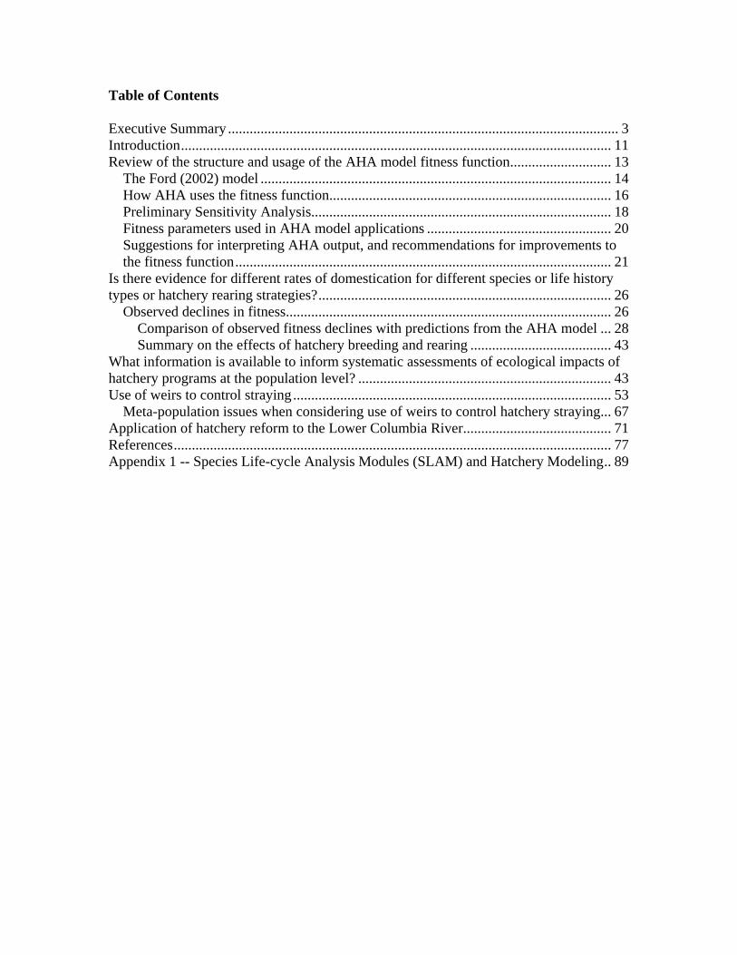
Table of Contents Executive Summary ............................................................................................................ 3 Introduction....................................................................................................................... 11 Review of the structure and usage of the AHA model fitness function............................ 13

The Ford (2002) model ................................................................................................. 14 How AHA uses the fitness function.............................................................................. 16 Preliminary Sensitivity Analysis................................................................................... 18 Fitness parameters used in AHA model applications ................................................... 20 Suggestions for interpreting AHA output, and recommendations for improvements to the fitness function........................................................................................................ 21

Is there evidence for different rates of domestication for different species or life history types or hatchery rearing strategies?................................................................................. 26

Observed declines in fitness.......................................................................................... 26 Comparison of observed fitness declines with predictions from the AHA model ... 28 Summary on the effects of hatchery breeding and rearing ....................................... 43

What information is available to inform systematic assessments of ecological impacts of hatchery programs at the population level? ...................................................................... 43 Use of weirs to control straying........................................................................................ 53

Meta-population issues when considering use of weirs to control hatchery straying... 67 Application of hatchery reform to the Lower Columbia River......................................... 71 References......................................................................................................................... 77 Appendix 1 -- Species Life-cycle Analysis Modules (SLAM) and Hatchery Modeling.. 89

11

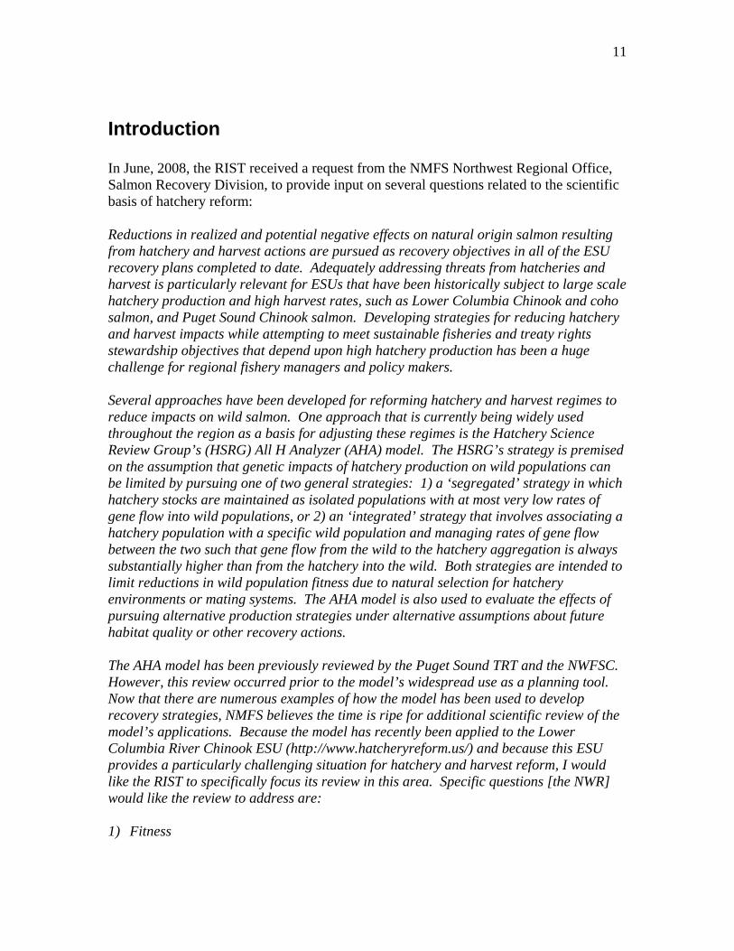
Introduction In June, 2008, the RIST received a request from the NMFS Northwest Regional Office, Salmon Recovery Division, to provide input on several questions related to the scientific basis of hatchery reform: Reductions in realized and potential negative effects on natural origin salmon resulting from hatchery and harvest actions are pursued as recovery objectives in all of the ESU recovery plans completed to date. Adequately addressing threats from hatcheries and harvest is particularly relevant for ESUs that have been historically subject to large scale hatchery production and high harvest rates, such as Lower Columbia Chinook and coho salmon, and Puget Sound Chinook salmon. Developing strategies for reducing hatchery and harvest impacts while attempting to meet sustainable fisheries and treaty rights stewardship objectives that depend upon high hatchery production has been a huge challenge for regional fishery managers and policy makers. Several approaches have been developed for reforming hatchery and harvest regimes to reduce impacts on wild salmon. One approach that is currently being widely used throughout the region as a basis for adjusting these regimes is the Hatchery Science Review Group’s (HSRG) All H Analyzer (AHA) model. The HSRG’s strategy is premised on the assumption that genetic impacts of hatchery production on wild populations can be limited by pursuing one of two general strategies: 1) a ‘segregated’ strategy in which hatchery stocks are maintained as isolated populations with at most very low rates of gene flow into wild populations, or 2) an ‘integrated’ strategy that involves associating a hatchery population with a specific wild population and managing rates of gene flow between the two such that gene flow from the wild to the hatchery aggregation is always substantially higher than from the hatchery into the wild. Both strategies are intended to limit reductions in wild population fitness due to natural selection for hatchery environments or mating systems. The AHA model is also used to evaluate the effects of pursuing alternative production strategies under alternative assumptions about future habitat quality or other recovery actions. The AHA model has been previously reviewed by the Puget Sound TRT and the NWFSC. However, this review occurred prior to the model’s widespread use as a planning tool. Now that there are numerous examples of how the model has been used to develop recovery strategies, NMFS believes the time is ripe for additional scientific review of the model’s applications. Because the model has recently been applied to the Lower Columbia River Chinook ESU (http://www.hatcheryreform.us/) and because this ESU provides a particularly challenging situation for hatchery and harvest reform, I would like the RIST to specifically focus its review in this area. Specific questions [the NWR] would like the review to address are: 1) Fitness

12

The HSRG approach for evaluating the interaction of hatchery and natural origin spawners incorporates a model that assumes that hatchery propagation leads to reductions of the fitness of hatchery fish in the wild (Lynch and O’Hely 2001; Ford 2002). As implemented, the HSRG analyses assume a common set of relative fitness distributions for hatchery adaptation compared to natural environments for all species (steelhead, stream type and ocean type chinook). Is there evidence for alternative fitness functions for different species or life history types? How sensitive are model results to alternative assumptions?

In addition to considering the potential impacts of hatchery introgression on natural production characteristics of a target population, managers need to assess other potential hatchery risks, such as ecological impacts on target and non-target taxa. What information is available to inform systematic assessments of ecological impacts of hatchery programs at the population level? Can existing modeling tools be adapted to incorporate one or more functions that would represent ecological impacts similar to how the AHA framework incorporates the Ford (2002) fitness equations?

2) Weirs

Continuing to provide sufficient hatchery production to maintain ocean and lower river terminal area fisheries while simultaneously meeting proportion natural influence (PNI) criteria would require management controls to limit straying of hatchery fish into natural spawning areas. In some populations, constructing or adapting existing mainstem weirs are an option recommended by the HSRG reviews for limiting the number of hatchery origin fish accessing natural spawning areas. What is known about negative ecological or demographic impacts of such weirs in salmon drainages? What risks should be taken into account in evaluating the potential impacts of weirs on the targeted natural population and on other species utilizing the river? Can a risk assessment framework be developed to inform management decisions regarding weir location, design, construction and operation about relative risks and benefits in specific situations? What guidance can the RIST provide for study designs to get at the potential risks and benefits of weirs in representative situations (e.g., Grays River in the Lower Columbia).

The review request also had several questions related to hatchery/harvest integration, but the RIST has elected to defer these questions to another review. In the report that follows, we change the order of the questions somewhat, and start off with a review of the fitness aspects of the AHA model. This is followed by summary of information related to the question of whether there is evidence for a differential susceptibility for hatchery domestication across species that have different life-history patterns. Next, we briefly review approaches for evaluating ecological effects of hatcheries on wild populations, and offer some suggestions for incorporating such information into models such as AHA. We then move to a brief review of the ecological impacts of weirs and offer a suggested framework for developing a decision support system for helping to

13

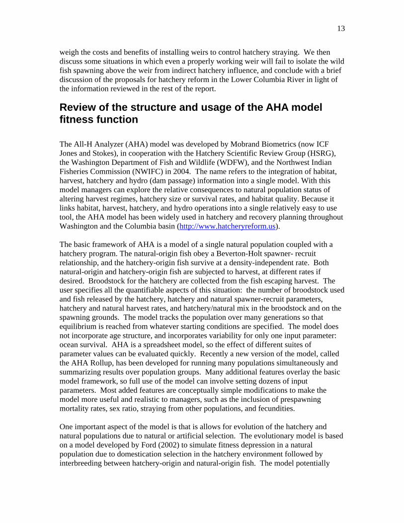
weigh the costs and benefits of installing weirs to control hatchery straying. We then discuss some situations in which even a properly working weir will fail to isolate the wild fish spawning above the weir from indirect hatchery influence, and conclude with a brief discussion of the proposals for hatchery reform in the Lower Columbia River in light of the information reviewed in the rest of the report.

Review of the structure and usage of the AHA model fitness function The All-H Analyzer (AHA) model was developed by Mobrand Biometrics (now ICF Jones and Stokes), in cooperation with the Hatchery Scientific Review Group (HSRG), the Washington Department of Fish and Wildlife (WDFW), and the Northwest Indian Fisheries Commission (NWIFC) in 2004. The name refers to the integration of habitat, harvest, hatchery and hydro (dam passage) information into a single model. With this model managers can explore the relative consequences to natural population status of altering harvest regimes, hatchery size or survival rates, and habitat quality. Because it links habitat, harvest, hatchery, and hydro operations into a single relatively easy to use tool, the AHA model has been widely used in hatchery and recovery planning throughout Washington and the Columbia basin (http://www.hatcheryreform.us). The basic framework of AHA is a model of a single natural population coupled with a hatchery program. The natural-origin fish obey a Beverton-Holt spawner- recruit relationship, and the hatchery-origin fish survive at a density-independent rate. Both natural-origin and hatchery-origin fish are subjected to harvest, at different rates if desired. Broodstock for the hatchery are collected from the fish escaping harvest. The user specifies all the quantifiable aspects of this situation: the number of broodstock used and fish released by the hatchery, hatchery and natural spawner-recruit parameters, hatchery and natural harvest rates, and hatchery/natural mix in the broodstock and on the spawning grounds. The model tracks the population over many generations so that equilibrium is reached from whatever starting conditions are specified. The model does not incorporate age structure, and incorporates variability for only one input parameter: ocean survival. AHA is a spreadsheet model, so the effect of different suites of parameter values can be evaluated quickly. Recently a new version of the model, called the AHA Rollup, has been developed for running many populations simultaneously and summarizing results over population groups. Many additional features overlay the basic model framework, so full use of the model can involve setting dozens of input parameters. Most added features are conceptually simple modifications to make the model more useful and realistic to managers, such as the inclusion of prespawning mortality rates, sex ratio, straying from other populations, and fecundities. One important aspect of the model is that is allows for evolution of the hatchery and natural populations due to natural or artificial selection. The evolutionary model is based on a model developed by Ford (2002) to simulate fitness depression in a natural population due to domestication selection in the hatchery environment followed by interbreeding between hatchery-origin and natural-origin fish. The model potentially

14

offers guidance for management of domestication in integrated hatchery programs through control of the proportion of natural-origin fish in the broodstock (pNOB) and the proportion of hatchery-origin fish on the spawning grounds (pHOS). The two gene flow rates are typically combined in a statistic called proportionate natural influence (PNI) (Busack in prep). The HSRG has recommended specific PNI levels for particular situations. AHA allows users to explore what PNI levels are possible in integrated hatchery programs sited in basins with specified productivity and capacity parameters, under specified harvest regimes. If the fitness function is toggled on, the model attempts to determine the fitness consequence of that PNI value. The Ford (2002) model and its application in AHA is discussed in more detail below. The interest by some agencies in using AHA in recovery planning prompted a 2005 review conducted by the Puget Sound Technical Recovery Team and NWFSC (PSTRT 2005). Five reviewers were asked to address specific questions, and while they provided a variety of responses, a central issue was the fact that the model assumed that certain mechanisms were operative, such as the population obeying a Beverton-Holt production function and domestication operating as per the model of Ford (2002). The primary recommendations of the previous review were that managers should use the model heuristically rather than quantitatively, that better validation and documentation (particularly of the domestication model) was needed, and the model should allow incorporation of uncertainty in parameters and recruitment models. Given the widespread use of the AHA model, the emphasis placed on use of integrated hatchery programs with specified PNI values to limit domestication, and the fact that there really is no unambiguously “correct” way to parameterize the fitness function, it is important to carefully evaluate both the structure of the fitness function and how it is used. In this review we therefore focus on the features and use of the fitness function. Our analysis includes a survey of how fitness parameters have been set in HSRG analyses in the Columbia basin and a limited sensitivity analysis for illustrative purposes. A full sensitivity analysis would be useful and interesting, but would be a major undertaking and was beyond the scope of this review.

The Ford (2002) model The AHA model incorporates a model of fitness evolution that was explored by Ford (2002) and is based on standard quantitative genetic theory (Lande 1976). It considers the mean value of a single trait in a population that is influenced by an integrated hatchery program. The trait is subject to stabilizing selection, but the trait has different optima in the hatchery and the natural environments (Figure 1). The optima are the mean population trait values that would occur at equilibrium if the population existed in only one environment or the other. Adults returning to the population from either environment may spawn in their natal environment, or in the other environment. The proportions of fish from one environment that spawn in the other represent gene flow between the two environments. The mean trait value will eventually equilibrate between the two optima, and the relative position of the equilibrium point between the optima will be a function of

15

heritability, selection strength, and two gene flow rates: the proportion of broodstock consisting of natural-origin fish (PNOB) and the proportion of hatchery-origin fish on the spawning grounds (PHOS) (in Ford’s original notation the two rates are 1-pc and 1-pw, respectively). Required inputs of the model are the trait variance, the trait starting values in the two environments, the selection strengths in the two environments, and the trait optima in the two environments. The key assumptions of the model include:

• The mean fitness of a population is determined by the mean and variance of a single normally distributed trait (e.g., size or run timing).

• The variance of the trait remains constant over time. • The mean of the trait can evolve due to natural selection. • Natural selection is determined by a Gaussian fitness function (i.e., a normal

distribution without the constraint that the area under the curve integrate to 1). • The evolution of the trait in a specific generation is determined by the mean and

variance of the trait in the population, and how far the trait mean is from the optima described by the fitness function.

• The hatchery and natural environment each can be characterized by distinct fitness functions that may have different optima.

• The overall evolution of the trait is due to only to natural selection in the two environments, followed by migration/gene flow between the environments.

H Wpc

pw

1 – pc = pNOB

1 – pw = pHOS

- 3 - 2 - 1 1 2 3

0.2

0.4

0.6

0.8

1

- 4 - 2 2

0.2

0.4

0.6

0.8

1

θΗ θw

Figure 1 -- Illustration of the concepts used to model fitness declines in the AHA model. As has been noted in the previous review of the AHA model (PSTRT 2005), some of these assumptions are not at all realistic, and indeed the original model was primarily used as a heuristic tool to explore the general way that a trait might evolve in a hatchery

16

supplemented population (Ford 2002). In practice, this means that the model is most useful for obtaining a general sense of how supplementation may affect the fitness of a natural population due to differences in natural selection between environments, rather than for specific predictions about population fitness for any particular population. Nonetheless, since the AHA model is being used to explore alternative recovery scenarios for a variety of species, it is important to understand a) how the fitness predictions generated by the AHA model compare to observed data, and b) what information is available to address the question of whether different species differ markedly in the degree to which hatchery propagation results in declines in wild population fitness.

How AHA uses the fitness function The AHA model fitness function incorporates as an option a full demographic implementation of the Ford (2002) model. The function can be toggled on or off. Each generation, new trait means are calculated from Ford’s recursion equations (modified notationally and to allow different heritabilities in the two environments (Busack in prep), based on the input values for starting trait means, optima, selection strengths, heritabilities, and variance. The gene flow rates are based on input PNOB and PHOS goals, but their values at any time depend on what is achievable, given available numbers of fish of the two types. A toggle allows broodstock to be taken randomly, without consideration of origin. All fitness function variables are presented below in Table 1, and the fitness page of AHA, which contains the input variables (except for the toggles and the gene flow goals), is presented in Figure 2. Based on the new trait mean of the natural-origin component, a new fitness value is calculated each generation as (Ford’s equation 4):

( )⎟⎟⎠

⎞⎜⎜⎝

⎛

+−

−

= )(2 22

2

σωθwwz

ew , where wz is the trait mean, is the variance, is the squared selection strength, and

2σ 2ω

wθ is the trait optimum in the natural environment. The fitness value is then used to adjust the productivity and capacity parameters for the next generation. Basically, the productivity and capacity at any generation are the initial productivity and capacity multiplied by the fitness, but the user can incorporate more complexity if desired because the AHA model incorporates a three-stage Beverton-Holt production function (spawner-egg, egg-smolt, smolt-adult), each with its own productivity and capacity parameters. The three production functions are then aggregated (Mousalli and Hilborn, 1986) to create the overall adult-adult function. The AHA model allows the productivity and capacity changes due to fitness change to be distributed proportionately over the three life stages. Thus, if the proportions were 0.2,0.3, and 0.5, the fitnesses for the three stages would be w0.2, w0.3, and w0.5, where w is the overall fitness. One feature of the AHA version of the fitness function that was not part of the original model is a user specified fitness floor below which fitness is not allowed to drop. The reasoning for the fitness floor, as we understand it, is that some populations have been subjected to hatchery influence for many generations and still display substantial

17

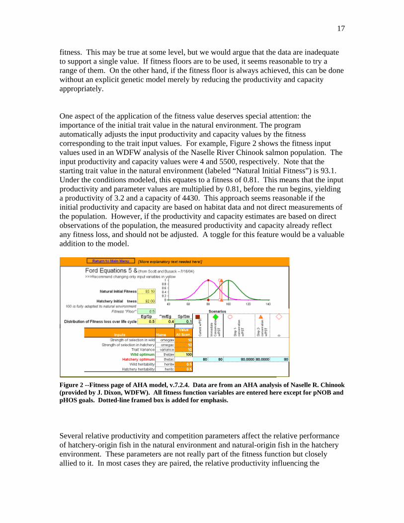
fitness. This may be true at some level, but we would argue that the data are inadequate to support a single value. If fitness floors are to be used, it seems reasonable to try a range of them. On the other hand, if the fitness floor is always achieved, this can be done without an explicit genetic model merely by reducing the productivity and capacity appropriately. One aspect of the application of the fitness value deserves special attention: the importance of the initial trait value in the natural environment. The program automatically adjusts the input productivity and capacity values by the fitness corresponding to the trait input values. For example, Figure 2 shows the fitness input values used in an WDFW analysis of the Naselle River Chinook salmon population. The input productivity and capacity values were 4 and 5500, respectively. Note that the starting trait value in the natural environment (labeled “Natural Initial Fitness”) is 93.1. Under the conditions modeled, this equates to a fitness of 0.81. This means that the input productivity and parameter values are multiplied by 0.81, before the run begins, yielding a productivity of 3.2 and a capacity of 4430. This approach seems reasonable if the initial productivity and capacity are based on habitat data and not direct measurements of the population. However, if the productivity and capacity estimates are based on direct observations of the population, the measured productivity and capacity already reflect any fitness loss, and should not be adjusted. A toggle for this feature would be a valuable addition to the model.

Figure 2 --Fitness page of AHA model, v.7.2.4. Data are from an AHA analysis of Naselle R. Chinook (provided by J. Dixon, WDFW). All fitness function variables are entered here except for pNOB and pHOS goals. Dotted-line framed box is added for emphasis. Several relative productivity and competition parameters affect the relative performance of hatchery-origin fish in the natural environment and natural-origin fish in the hatchery environment. These parameters are not really part of the fitness function but closely allied to it. In most cases they are paired, the relative productivity influencing the

18

numerator of a Beverton-Holt equation, and the competition factor involving the denominator. For example, here is the production function for smolt-adult survival of hatchery-origin fish, from the AHA user’s guide v.7.3:

adsm

HadsmNsmoltsmolt

Hadsmsmoltadult

CppfNH

ppHH

−

−

−

⋅⋅⋅++

⋅⋅= )(1

In this equation and are the basic productivity and capacity parameters, is the relative survival of hatchery-origin fish, and is a competition factor

weighting the importance of natural-origin fish to the survival of hatchery-origin fish. Analysis of the use of these equations was not done due to the constraints of time, but we found little variation in the values used in the Columbia River Basin, and never found a competition factor set to a value other than 1 (see usage section below). Greater use of these competition parameters would be one way to incorporate information on ecological interactions between hatchery and wild salmon into the model applications (see section on ecological effects, below).

adsmp − adsmC −

Hp Nf

Preliminary Sensitivity Analysis We did a simple sensitivity analysis of AHA, using a data set provided by James Dixon (WDFW) for the Chinook salmon population in the Naselle River, in southwest Washington. We ran two scenarios: the original, which used 1476 broodstock and a PNOB goal of 0.12; and a smaller program of 738 broodstock with a PNOB goal of 0.50. We eliminated a broodstock transfer from the model and turned off survival rate variation, but other than the adjustments required to create the reduced scenario, modified only the fitness function inputs. We varied heritabilities and selection strengths over reasonable values, and varied trait starting values and fitness floors. We also modeled situations in which heritabilities and selection strengths differed in the hatchery and natural environments. AHA produces many output values, but we display only mean counts for fish spawning in nature, and fitness for natural-origin fish. The means reported by the model are calculated over 81 generations, beginning at generation 19 (considering the starting conditions generation 0). This limited sensitivity analysis reveals that the model is quite sensitive to the values chosen for the heritabilities and selection strengths. Heritabilities of 0.1 yielded considerably more spawners than heritabilities of 0.5. Larger effects were seen when different heritability values were used in the two environments. The combination of a heritability of 0.5 in the wild and 0.1 in the hatchery yielded considerably more spawners than the default values of 0.5 in each population, and heritability values of 0.1 in the wild and 0.5 in the hatchery yielded considerably fewer spawners. Selection strength had an even larger effect. Increasing selection strength in both environments from 10 to 6, a change from about 3 to 2 in standard deviation units, resulted in population extinction assuming the other parameters remained unchanged. Using different selection strengths in the natural and hatchery environments also has a large effect. Interestingly situations in which selection was stronger in the hatchery environment than in the natural

19

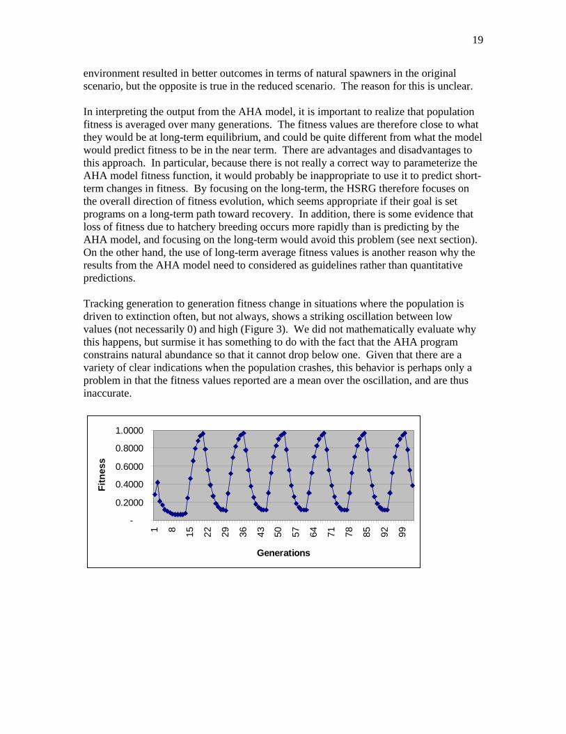
environment resulted in better outcomes in terms of natural spawners in the original scenario, but the opposite is true in the reduced scenario. The reason for this is unclear. In interpreting the output from the AHA model, it is important to realize that population fitness is averaged over many generations. The fitness values are therefore close to what they would be at long-term equilibrium, and could be quite different from what the model would predict fitness to be in the near term. There are advantages and disadvantages to this approach. In particular, because there is not really a correct way to parameterize the AHA model fitness function, it would probably be inappropriate to use it to predict short-term changes in fitness. By focusing on the long-term, the HSRG therefore focuses on the overall direction of fitness evolution, which seems appropriate if their goal is set programs on a long-term path toward recovery. In addition, there is some evidence that loss of fitness due to hatchery breeding occurs more rapidly than is predicting by the AHA model, and focusing on the long-term would avoid this problem (see next section). On the other hand, the use of long-term average fitness values is another reason why the results from the AHA model need to considered as guidelines rather than quantitative predictions. Tracking generation to generation fitness change in situations where the population is driven to extinction often, but not always, shows a striking oscillation between low values (not necessarily 0) and high (Figure 3). We did not mathematically evaluate why this happens, but surmise it has something to do with the fact that the AHA program constrains natural abundance so that it cannot drop below one. Given that there are a variety of clear indications when the population crashes, this behavior is perhaps only a problem in that the fitness values reported are a mean over the oscillation, and are thus inaccurate.

-

0.2000

0.4000

0.6000

0.8000

1.0000

1 8 15 22 29 36 43 50 57 64 71 78 85 92 99

Generations

Fitn

ess

20

-

0.2000

0.4000

0.6000

0.8000

1.0000

1 8 15 22 29 36 43 50 57 64 71 78 85 92 99

Generations

Fitn

ess

Figure 3 -- Oscillating fitness patterns observed in simulations resulting in population extinctions. Upper panel has selection strengths in both environments of 3, lower panel selection strengths of 6. Starting fitness values had very little effect on the model outcomes, presumably because all other factors drive the population to a given equilibrium condition, regardless of where it starts. It appears that populations (except for the nonviable ones) approach an equilibrium soon enough that there is little effect of variation in starting values after 20 generations. The effect of the fitness floor is quite obvious. If fitness never drops below 0.5, severe genetic impacts are screened out and the model outcomes become less sensitive to the choice of fitness parameters. Nearly all model runs in the Columbia River Basin were performed with a fitness floor of 0.5 (Table 1), a practice that seems inconsistent with information that indicates that lower fitness values are possible (see Figure 4 in next section).

Fitness parameters used in AHA model applications To evaluate how the fitness function is being used in actual applications of the AHA model, we examined the input values used in all the HSRG Columbia basin Chinook analyses (provided to us by Greg Blair of ICF Jones and Stokes), using the QC function of the AHA Rollup model (v.2.4). Results are presented in Table 1. The fitness function was always used, with variability in parameter values among populations. PNOB and PHOS goals varied considerably, but this is to be expected because they reflect a variety of hatchery program intents. Other than the gene flow rates, however, only three parameters related to fitness evolution varied among applications of the model: the fitness floor, the starting trait means, and the hatchery optimum. There was some variation in two of the associated relative performance variables: “HOR in Nature Spawn Effectiveness” (variable 46) was usually set to 0.8, but in four cases was set to another value (0.25, 0.352, 0.64, and 1); “HOR in Nature Spawner to Egg Rel.- Prod” (variable 52) was also usually set to 0.8, but also occasional set to 0.85 and 1.

21

There are three potential areas to consider in this usage pattern for the fitness function: 1) the basic Ford parameters, 2) the fitness floor, and 3) the starting values. As previously mentioned, because domestication is not a single trait, there are no clear “correct” heritabilities, selection strengths, optima, or starting values. The best approach to use in AHA would therefore be to use a range of values likely to demonstrate the range of impacts to be expected from domestication. Using equal heritabilities and selection strengths for the two environments is probably not an unreasonable assumption (Roff 1997), although a case could be made for alternatives. Given the results of the sensitivity analysis, it seems wise to investigate a range of heritabilities. As for selection strengths, in a recent review Hard (2004) concluded that natural selection strengths range for the most part from 1 to 4 standard deviations. Thus, the selection strength modeled in the HSRG Columbia runs is on the weak side of the range for a single trait. Using only this value could considerably underestimate the fitness effects of domestication. Even if the selection strength for a single trait is on the order of 3 or 4 standard deviations the cumulative effect of multiple traits could be equivalent to a selection strength of 1 sd or even stronger. A possible approach to parameterization is that of Busack et al. (2005b), who surveyed a group of geneticists for their professional opinions of the fitness consequences of several types of hatchery programs. Initially, we expected the choice of starting values to be a problem, as these cannot be estimated with any certainty, and the uniformity seen in the Columbia runs seemed to run counter to common sense. For example, upper Yakima spring Chinook have been subjected to an integrated program with a PNI of approximately 0.5 for approximately three generations, whereas Washougal fall Chinook have been subjected to a PNI of probably less than 0.1 for more than ten generations. The current state of these two populations in terms of domestication therefore seems unlikely to be the same. However, the sensitivity analysis showed that AHA carries runs out over 100 generations to near-equilibrium conditions, and the equilibrium does not depend on the starting conditions. Thus, the way the model is applied, it doesn’t really matter what the starting points are, within reason. Midway between the optima seems good enough.

Suggestions for interpreting AHA output, and recommendations for improvements to the fitness function The AHA model is already being widely applied, so understanding appropriate ways to interpret the model’s output is important. On this point, we reiterate the recommendation made by Puget Sound TRT in its earlier review. Namely, that the AHA model is useful as a heuristic tool for exploring a broad range of scenarios, but should not be used to quantitatively predict the outcomes of specific management alternatives. The AHA user needs to be aware that: 1) the Ford model is only one of several possible ways to model domestication and almost certainly is incomplete in its approach, 2) it is a single-trait model attempting to simulate a multi-trait phenomenon, and 3) available data are inadequate for confident parameterization. We believe the model is useful for exploring scenarios, but would be concerned if the model were used to fine tune management

22

actions based on small changes in the model’s input parameters. Based on our review of the HSRG’s recommendations for hatchery reform in the Lower Columbia River (see last section of the report), we are concerned that the level of uncertainly associated with the AHA output may not always be adequately characterized. We discuss further some specific aspects of the AHA model application in the Lower Columbia River in the last section of the report. In addition to this general advice, we have some specific recommendations to improve the documentation and application of the AHA fitness function. • Document the fitness function adequately. Currently the AHA user’s guide (we

examined version 7.3, dated 11/2007) contains little in the way of documentation, but promises a paper on the subject in the near future. We suggest that besides clearly describing each variable, the AHA user’s manual should cover three major topics related to the fitness function:

o A description of the model explaining that it models change at a single

hypothetical trait, and that fitness changes arise from the trait change. o A strongly worded caveat about the extent of possible genetic impacts the

fitness function covers and the speculative nature of the results from the fitness function. As stated previously above and in the earlier TRT review, fitness loss can come from factors other than domestication, and these are not modeled. The fitness function looks at domestication in a particular way, which is undoubtedly incomplete. There is no single “correct” way to parameterize the model at this stage of our understanding of domestication.

o It might be worth including suggestions for reasonable parameterization of the model. For example, strong and weak selection strengths should be tried (at minimum use 1 and 4 sds), and the distance between optima should be varied. Consider using the recommendations in Busack et al. (2005b). On other hand, it is probably not worth tweaking the fitness aspects of the model too much if it is used to provide general guidance rather than quantitative predictions.

• Include a toggle for fitness mode of productivity and capacity. As previously

mentioned, immediately reducing the productivity and capacity makes sense if the values are based estimates of what would be expected from a wild population in a particular habitat, but not if they are based on actual fish numbers, because these numbers would already reflect the fitness reduction.

• Revise the fitness page. As previously noted, the use of the terms “Natural Initial

Fitness” and “Hatchery Initial Fitness” is misleading. The terms “Natural Initial Trait Mean” and “Hatchery Initial Trait Mean” should be substituted. Because the optima and initial trait means all refer to a hypothetical trait, not a single real one, there is really no need to include the arbitrary values for these. It would be sufficient, and make clearer to the user what is actually being modeled, if all these inputs were in units of trait standard deviations. The optima could be replaced by a single value indicating the distance (in sd units) between the optima, the selection strengths

23

represented in sd units, and the initial trait values set to the proportion of distance between the optima that they represent. The variance could be dispensed with. The entries in Figure 2, for example would be replaced with the distance between optima of 6.32 sds, ; the initial natural-origin trait mean and hatchery trait means are 65.5% and 60%, respectively, of the distance from hatchery optimum to natural optimum; and the selection strength with 3.16 sds.

24

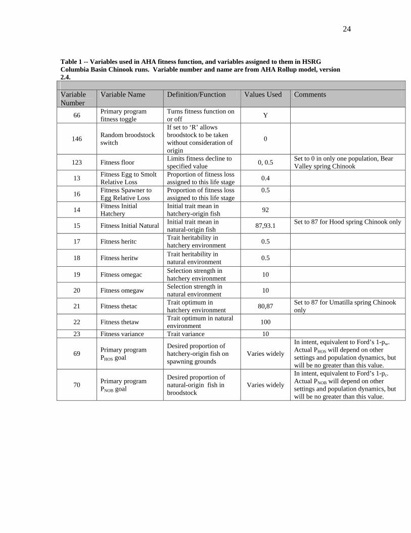
Table 1 -- Variables used in AHA fitness function, and variables assigned to them in HSRG Columbia Basin Chinook runs. Variable number and name are from AHA Rollup model, version 2.4. Variable Number

Variable Name Definition/Function Values Used Comments

66 Primary program fitness toggle

Turns fitness function on or off Y

146 Random broodstock switch

If set to ‘R’ allows broodstock to be taken without consideration of origin

0

123 Fitness floor Limits fitness decline to specified value 0, 0.5 Set to 0 in only one population, Bear

Valley spring Chinook

13 Fitness Egg to Smolt Relative Loss

Proportion of fitness loss assigned to this life stage 0.4

16 Fitness Spawner to Egg Relative Loss

Proportion of fitness loss assigned to this life stage

0.5

14 Fitness Initial Hatchery

Initial trait mean in hatchery-origin fish 92

15 Fitness Initial Natural Initial trait mean in natural-origin fish 87,93.1 Set to 87 for Hood spring Chinook only

17 Fitness heritc Trait heritability in hatchery environment 0.5

18 Fitness heritw Trait heritability in natural environment 0.5

19 Fitness omegac Selection strength in hatchery environment 10

20 Fitness omegaw Selection strength in natural environment 10

21 Fitness thetac Trait optimum in hatchery environment 80,87 Set to 87 for Umatilla spring Chinook

only

22 Fitness thetaw Trait optimum in natural environment 100

23 Fitness variance Trait variance 10

69 Primary program PHOS goal

Desired proportion of hatchery-origin fish on spawning grounds

Varies widely

In intent, equivalent to Ford’s 1-pw. Actual PHOS will depend on other settings and population dynamics, but will be no greater than this value.

70 Primary program PNOB goal

Desired proportion of natural-origin fish in broodstock

Varies widely

In intent, equivalent to Ford’s 1-pc. Actual PNOB will depend on other settings and population dynamics, but will be no greater than this value.

25

Table 2 -- Sensitivity of AHA analysis to variation in heritability, selection strength, starting trait means, and fitness floor. Input data are from Naselle River AHA run, which assumes p=4.0, c=5500, and nonselective harvest of 57.5%. Fitnesses corresponding to initial trait means are 0.81 (93.1), 0.96 (97), and 0.36 (85). Shaded cells denote variation from original values. Spawner numbers and fitnesses are means over approximately 80 generations. Situations where there is only one natural-origin spawner are extinctions, fish numbers and fitnesses in these situations are artifacts of model coding.

Fitness function input values Original Scenario: broodstock 1476 fish, PNOB goal of 0.12.

Reduced Project Scenario: broodstock 738 fish, PNOB goal of 0.50

Initial trait mean in wild

Initial trait mean in hatchery

Selection strength in wild

Selection strength in hatchery

Heritability in wild

Heritability in hatchery

Fitness floor

Natural-origin spawners

Total spawners

Fitness in wild

Natural-origin spawners

Total spawners

Fitness in wild

93.1 92 10 10 0.5 0.5 0.5 792 3239 0.50 376 1599 0.56 93.1 92 10 10 0.5 0.5 0 436 2883 0.29 376 1599 0.56 93.1 92 10 10 0.1 0.1 0 747 3194 0.47 524 1747 0.66 93.1 92 10 10 0.1 0.5 0 245 2692 0.19 1 491 0.24 93.1 92 10 10 0.5 0.1 0 1091 3538 0.70 938 2161 0.94 93.1 92 6 6 0.5 0.5 0 1 783 0.06 1 524 0.24 93.1 92 6 6 0.5 0.5 0.5 792 3239 0.50 281 1504 0.50 93.1 92 10 6 0.5 0.5 0 317 2764 0.23 1 1208 0.31 93.1 92 6 10 0.5 0.5 0 125 2572 0.13 489 1712 0.64 93.1 92 10 3 0.5 0.5 0 273 2720 0.21 1 149 0.23 93.1 92 3 10 0.5 0.5 0 169 2616 0.15 830 2053 0.87 93.1 92 3 3 0.5 0.5 0 1 34 oscillation 1 3 oscillation97 97 10 10 0.5 0.5 0.5 792 3239 0.50 391 1614 0.57 97 97 10 10 0.5 0.5 0 442 2889 0.29 391 1614 0.57 85 85 10 10 0.5 0.5 0.5 792 3239 0.50 350 1573 0.55 85 85 10 10 0.5 0.5 0 427 2874 0.29 347 1570 0.54

26

Is there evidence for different rates of domestication for different species or life history types or hatchery rearing strategies? One question that has come up with respect to the AHA model is how to parameterize the fitness function for different Pacific salmon species or life-history patterns within species. A related issue is to how to vary the model parameters within a species but for different release strategies (e.g., release as subyearling compared to yearlings). The Pacific salmon species are quite variable in their life-histories, and some species also contain considerable intra-specific life-history variation. It would therefore be surprising if all species were exactly equal in their propensity to adapt to hatchery conditions or to lose fitness for survival in the wild. However, there is currently little guidance available to user of the AHA model, or any other scenario building tool, on how to appropriately parameterize the model for different species of different life-history patterns. In this section of the report, we attempt to summarize the available information regarding differences among species and alternative life-history types regarding their propensity for domestication in hatcheries. We first summarize the relatively sparse information that directly bears on this question, and then discuss patterns of variation in a wider variety of traits that may be correlated with propensity for domestication.

Observed declines in fitness Araki et al. (2008) and Berejikian and Ford (2004) recently reviewed published studies that directly estimated the relative fitness of naturally spawning hatchery fish compared to wild fish in the same streams. The main conclusions from Araki et al.’s review are:

• Estimates of relative fitness of hatchery fish compared to wild fish vary considerably, from close to 0 to >1.

• There is a tendency for non-local hatchery broodstocks to have lower relative fitness than locally derived stocks.

• Most published studies have been on steelhead or other species that typically have a prolonged freshwater life-history. As of 2008, there were no published studies on the relative fitness of hatchery propagated species with short (<1 year) freshwater life-histories, such as ocean-type Chinook, chum, or pink salmon (there is now one study – see below).

• Few studies have been designed to partition genetic from environmental effects on fitness.

• Studies that have specifically estimated the reduction in fitness due to heritable effects have found effects ranging from no detectable reduction in relative fitness to reductions of nearly 50% due to heritable causes alone.

27

• There appears to be a rough correlation between generations of hatchery breeding and decline in fitness in the wild (more on this below).

Araki et al. (2008) limited their review to studies that have been published in the primary literature. However, there are quite a number of ongoing studies, some of which have been published in contract reports or other gray literature. Barry Berejikian (NWFSC) has recently compiled a comprehensive summary of relative fitness estimates from both published and unpublished studies (Figure 4). Overall, it is hard to see any general patterns among species in degree of hatchery relative reproductive success, in part because potential differences among species are often confounded with other factors, such as counting progeny at different life-stages. However, if we simply compare the results across species, we obtain the following average relative fitness values for studies using local broodstocks less than 5 generations old: steelhead = 0.67 (n=3; range 0.31 – 0.85), stream-type Chinook = 0.88 (n=4; range 0.52 – 1.16), summer chum = 0.85 (n=1), and Atlantic salmon = 0.75 (n=1). These values suggest the possibility that perhaps hatchery steelhead tend to have lower relative fitness than hatchery salmon, but this patterns is driven entirely by one data point (Figure 4). Considering the small sample sizes and range of life-stages at which progeny were counted to estimate relative fitness, we do not believe that these results provide much evidence to suggest that these species differ much in their susceptibility to fitness loss due to short-term (<5 generations) of hatchery rearing. With the exception of the single estimate from summer chum, however, none of these studies involved ‘ocean-type’ species that have short freshwater life-stages. Studies of hatchery stocks propagated for more than 5 generations are more difficult to directly compare across species because many of these studies involve non-local hatchery stocks or other factors that make direct comparisons difficult. Nonetheless, it is interesting that ‘old’ steelhead stocks appear to have very low relative fitness compared to endemic natural steelhead populations, whereas other species (coho salmon, brook trout, and Atlantic salmon) do not. One potential cause of this difference among species is that all of the ‘old’ steelhead hatchery stocks were not derived from the streams into which they were released, whereas the ‘old’ stocks of the other species were all locally derived (Figure 4). Interpreting this pattern is difficult, however, because high relative fitness values of hatchery fish after a long period of supplementation could either mean that hatchery fish have not lost fitness over time or that they have lost fitness but that this has impacted the wild fish as well, such that the relative fitness of the hatchery fish remains high. Nonetheless, the pattern could also suggest that steelhead are particularly prone to domestication in hatcheries compared to other species.

28

0 5 10 15 20GENERATIONS

0.0

0.5

1.0

1.5R

RS 1

814

15

6

2

16

18

12

11

4

10

3

17

9

13

5

7

Steelheadcoho

Atlantic

ChinookBrook trout

localnon-local Chum

Figure 4 -- Summary of relative fitness estimates by species, broodstock origin, and generations in the hatchery (compiled by Berejikian, NWFSC). 1 - Araki et al. (2007b)), 2 - Araki et al. (2007b), 3 - Leider et al. (1990), 4 - Ford et al. (2006), 5 - Fleming and Gross (1993), 6 - Reisenbichler and McIntyre (1977), 7 - Fleming et al. (2000), 8 - Fleming et al. (1997), 9 - Dannewitz et al. (2003), 10 - Araki et al. (2007a), 11 - Araki et al. (2007a), 12 - Murdoch et al. (2008), 13 - Moran and Waples (2007), 14 - P. Moran (NWFSC, personal communication), 15 - P. Moran (NWFSC, personal communication), 16 – Berejikian et al. (2008), 17 - McGinnity et al. (1997.), 18 – Leth (2005).

Comparison of observed fitness declines with predictions from the AHA model It was beyond the scope of this review to attempt to directly fit the AHA model to each of the individual data points in Figure 4. However, it is useful to ask how the results of the commonly used AHA fitness parameters compare with what has been observed in real populations. The default AHA parameters assume a wild optimum trait value ( wθ ) of 100, a hatchery optimum ( Hθ ) of 80, a selection strength ( ) of 10 in each environment, and heritability of 0.5 (

ωTable 1). The fitness functions associated with these

parameters are illustrated in Figure 2. In evaluating how the predictions associated with the parameters compare with the observation in Figure 4, it useful to first look at the case where fish from an isolated hatchery population at its fitness equilibrium stray into a wild population that is at its own fitness equilibrium. This is the lowest relative fitness of hatchery fish in the wild that the model will produce under normal conditions. Using the default parameters, the mean relative fitness of hatchery fish under these conditions will be 0.16, a value that is fairly similar to lowest values that have been observed Figure 4.

29

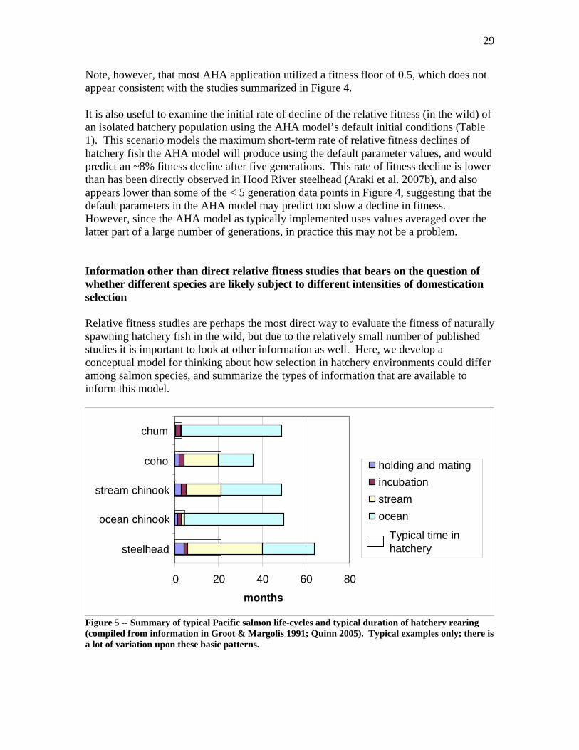
Note, however, that most AHA application utilized a fitness floor of 0.5, which does not appear consistent with the studies summarized in Figure 4. It is also useful to examine the initial rate of decline of the relative fitness (in the wild) of an isolated hatchery population using the AHA model’s default initial conditions (Table 1). This scenario models the maximum short-term rate of relative fitness declines of hatchery fish the AHA model will produce using the default parameter values, and would predict an ~8% fitness decline after five generations. This rate of fitness decline is lower than has been directly observed in Hood River steelhead (Araki et al. 2007b), and also appears lower than some of the < 5 generation data points in Figure 4, suggesting that the default parameters in the AHA model may predict too slow a decline in fitness. However, since the AHA model as typically implemented uses values averaged over the latter part of a large number of generations, in practice this may not be a problem. Information other than direct relative fitness studies that bears on the question of whether different species are likely subject to different intensities of domestication selection Relative fitness studies are perhaps the most direct way to evaluate the fitness of naturally spawning hatchery fish in the wild, but due to the relatively small number of published studies it is important to look at other information as well. Here, we develop a conceptual model for thinking about how selection in hatchery environments could differ among salmon species, and summarize the types of information that are available to inform this model.

0 20 40 60 80

steelhead

ocean chinook

stream chinook

coho

chum

months

holding and matingincubationstreamocean

Typical time in hatchery

Figure 5 -- Summary of typical Pacific salmon life-cycles and typical duration of hatchery rearing (compiled from information in Groot & Margolis 1991; Quinn 2005). Typical examples only; there is a lot of variation upon these basic patterns.

30

The Pacific salmon species differ substantially in the time they spend in freshwater and in the time typical spent rearing in hatcheries, ranging from steelhead which usually spend more than half their lives in freshwater, to pink and chum salmon which spend >90% of their life-cycle in salt water (Figure 5). All species are characterized by high mortality rates in both the freshwater and marine environments. Hatchery rearing results in a large reduction in the early life-stage mortality rates (Figure 6).

Natural spawning and rearing

0 0.1 0.2 0.3 0.4 0.5 0.6 0.7 0.8 0.9

1

holding and matingegg to smoltsmolt to adult

steelhead ocean Chinook

streamChinook

coho chum

Hatchery spawning and rearing

0 0.1 0.2 0.3 0.4 0.5 0.6 0.7 0.8 0.9

1

holding and matingegg to smoltsmolt to adult

steelhead ocean Chinook

streamChinook

coho chum

Figure 6 -- Typical mortality rates in natural versus hatchery settings (compiled from information in Groot & Margolis 1991; compiled from information in Quinn 2005).

31

Below, we discuss the opportunities for selection at each major stage of the lifecycle and how this might vary among species. To simplify the discussion, we characterize salmon as having either a ‘stream type’ or ‘ocean type’ life-history pattern (Healey 1983). This terminology was originally applied to alternative ‘races’ of Chinook salmon (Healey 1983). Here, we use the terms more generally such that a stream-type life-history is characterized by relatively long migration distance, early run timing well prior to sexual maturity, and relatively long freshwater residence as juveniles prior to ocean migration, whereas an ocean-type life-history is characterized by the opposite of these traits. An intermediate life-history, such as coho salmon that spawn in short coastal streams but outmigrate to the ocean as yearlings, has elements of both extremes. Adults in freshwater: Migration -- Salmon spawn in a wide variety of streams and results from many studies have indicated that populations have adaptations to facilitate migration from the ocean to their natal spawning stream. The timing of return to freshwater, for example, is influenced by both temperature (e.g,. Hodgson & Quinn 2002) and the length of freshwater migration (Bartz et al. 2006; Healey 1991); adult spawning morphology has been shown to be influenced by migration length (Fleming & Gross 1989; Healey 1983), and stream morphology and accessibility of fish to predators (e.g. Quinn et al. 2001b). For example, Chinook and coho salmon populations that make long freshwater migrations tend to have lower ratios of gametic to somatic tissues, reflecting the energetic requirements of long migrations (Fleming & Gross 1989; Healey 2001), and sockeye populations that spawn in streams accessible to bears tend to have smaller body sizes than those that spawn in streams with fewer bears (Quinn et al. 2001a). Some of the run timing and other life-history characteristics associated with variation in freshwater migration distance have evolved independently in 20th Century introduction of salmon to New Zealand, suggesting that these are traits are under strong contemporary selection (Kinnison et al. 1998a; Kinnison et al. 1998b). Timing of migration and spawning also appears to be important for survival of the offspring produced. For example, there is likely to be population-specific optima for timing of fry emergence – fry that emerge too early may be subject to increased risks from spring floods whereas fry that emerge too late may fail to establish good feeding territories or to migrate to the estuary at times of high prey abundance (Quinn 2005). Emergence timing is also influenced by development rate, and there is evidence that development rate and spawning timing are highly co-evolved traits (Tallman 1986). Selection in the hatchery has the potential to disrupt natural adaptations related to spawning migrations. For example, it is common for hatchery stocks to have altered run timing as a consequence of selecting broodstock from only a portion of the run (e.g., Ford et al. 2006; Hoffnagle et al. 2008). Quinn et al. (2002) found that in Lake Washington, such selection for early return time was strong enough to counter natural selection for later return time due to higher water temperatures.

32

Surprisingly few estimates of mortality during upstream migration are available (Quinn 2005), but presumably such mortality varies depending on migration distance and difficulty. To our knowledge, there have been no studies that have directly compared the strength of selection in hatcheries on migration characteristics for species or populations with alternative life-histories. In thinking about the requirements for successful natural spawning for stream-type versus ocean-type life-history patterns, it does not seem obvious which would be more susceptible to altered migratory characteristics due to domestication selection in hatcheries. The long freshwater spawning migrations associated with the stream-type life-history pattern appear more complicated than the short migrations often associated with an ocean-type life-history, which might suggest that the stream-type life-history could be more easily disrupted. However, if a hatchery is located near the spawning grounds of the population it is supplementing, then many of the migratory characteristics required for successfully returning to the natural grounds may also be required for a successful return to the hatchery. Mating selection – Sexual selection has been relatively well studied in salmon, and has been found to be a strong force shaping the behavior and morphology of both sexes (Quinn 2005). Females compete with each other for access to good spawning sites, and after spawning females guard their redd in order to minimize disturbance from other females (Foote 1990). Females also actively choose mates by delaying spawning when they are courted by small males (Berejikian et al. 2000). Males compete with each other for access to females, and both size and secondary sexual characteristics (kype, teeth, color changes) are influenced by this selection (Fleming & Gross 1994; Ford et al. 2006; Seamons et al. 2004; Seamons et al. 2007). In an intensive study of both sexual and natural selection on sockeye salmon, Tom Quinn and colleagues have found a complex set of tradeoffs between optimal morphology for obtaining mates versus avoiding predators (Quinn et al. 1996; Quinn & Buck 2001; Quinn et al. 2001a; Quinn et al. 2001b). In particular, bear predation selects for smaller body size in both males and females, whereas sexual selection (males) and selection for higher fecundity (females) are both for larger body size. Other studies have also found that the intensity of size selection for males depends on both spawning density and the operational sex ratio, with high densities and a high male:female ratio leading to stronger size selection (Fleming & Gross 1994; Seamons et al. 2007). The wide spread decline in abundance of salmon in the wild has been hypothesized as a factor that might alter patterns of sexual selection in these species (Einum et al. 2008). There have also been reports of disruptive selection on male size, with very small (sneaker) males having greater success than intermediate-sized males (Gross 1985). Sexual selection has been observed in species and populations with both stream-type (Fleming & Gross 1994; Quinn et al. 2001a; Seamons et al. 2007) and ocean-type (Dickerson et al. 2005) life-histories. Sexual selection might be expected to be stronger for ocean-type species such as chum, pink and sockeye salmon, since spawning densities

33

are typically higher for these species compared to stream-type or intermediate species. On the other hand, these species are often mass spawners at high densities, which may lesson the effect of sexual selection. Mating success (including pre-spawning mortality) is highly variable in salmon populations, with a large fraction of potential breeders typically producing few or no offspring. For example, Ford et al. (2006) estimated that ~55% of naturally spawning coho salmon in Minter Creek, WA, produced no adult offspring. Similarly, Seamons et al. (2007) estimated that ~65% of steelhead spawners in Snow Creek left no adult offspring, and Murdoch et al. (2007) estimated that ~50% of spring Chinook salmon in the Wenatchee River produced no offspring. In contrast, typical pre-spawning mortality rates in hatcheries are ~10%, although this can vary greatly (Waples et al. 2004). Hatchery breeding clearly has the potential to select for sexual traits different from those that are optimal in the wild, since salmon in hatcheries are almost always spawned artificially with no opportunity for the expression of mate choice, intersexual selection, redd construction, or any other type of natural breeding behavior. One might expect that in the absence of sexual selection, traits such as fecundity and ability to tolerate hatchery conditions would be favored. Fleming and Gross (1989) found that female hatchery coho salmon had less developed secondary sexual characteristics, consistent with the hypothesis of relaxed selection for mating behavior in hatchery settings, although some of these differences could also have been environmentally induced. Similarly, several studies have found that hatchery salmon of both sexes exhibit less successful breeding behavior in experimental settings when they are compared with wild fish, although again in most cases it is impossible to know whether the effects measured had a genetic basis or were environmentally induced (Berejikian et al. 2001; Fleming & Gross 1992; Fleming & Gross 1993; Fleming & Gross 1994; Fleming et al. 1996; Fleming et al. 1997). Hatcheries also have the potential to alter the selective balance between survival and fecundity. For example, Fleming and Gross (1989) found that hatchery coho salmon tended to have higher gametic/somatic tissue ratios that wild coho salmon, and hypothesized that this reflected the absence of some sources of viability selection (e.g. predators) as well as reduced sexual selection in hatcheries. Heath et al. (2003) found a similar temporal trend of higher fecundity and smaller egg size in several British Columbia Chinook salmon hatchery populations. They interpreted this pattern in the context of a trade-off between progeny survival and parent fecundity, with hatchery conditions tending to select for fecundity at the expense of larger egg size. Not all selection in the hatchery is necessarily different from what occurs in the wild, however. For example, Ford et al. (2008) found similar selection for large size in male coho salmon in both hatchery and natural environments. In particular, that study found that small males tended to die prior to spawning in both the wild and hatchery environments, suggesting that some of the male-male interactions that occur in the wild might also occur in hatchery holding ponds. Incubation –

34

Timing of fry emergence is a critical trait for salmon, and is determined by a combination of spawning time, stream temperature, and development rate (Beacham & Murray 1990; Brannon 1987; Dickerson et al. 2005; Murray et al. 1990; Quinn 2005). Several studies have identified differences in development rate among both species and populations, and these differences often appear to be adaptive. For example, Tallman (1986) and Tallman and Healey (1991) found that development rate differed among chum salmon populations inhabiting streams of different temperatures that fed into a common estuary. Populations inhabiting the higher temperature stream had a lower (temperature adjusted) development rate than those in the cooler stream, such that fry emergence was similar in both streams, and corresponded to the time of maximum prey availability in the estuary. These findings were consistent with similar observations made earlier on chum salmon in Hood Canal (Koski 1975). Emergence timing is important for both ocean-type and stream-type species, but for somewhat different reasons. Fry of both life-history types need to avoid emerging too early, when environmental conditions are poor due to high flows or cold temperatures. Ocean-type fry, which spend days to at most a few months in the steam environment, need to time their emergence to feeding conditions in the estuary and near shore where they will be spending the early portion of their lives. In contrast, stream-type fry will most likely be spending a full year, and sometimes more, in the relatively nutrient-poor freshwater environment, and need to establish feeding territories in order to survive. Emerging early can therefore confer an advantage because late comers may find fewer good territories (Dickerson et al. 2005; Quinn 2005; Sigurd Einum 2000l). Embryonic development rate has a strong genetic basis in salmon (Robison et al. 2001; Robison et al. 1999), and there is some evidence that embryonic development rate can evolve rapidly, both in the wild and in hatcheries. For example, Hendry et al. (1998) found differences in embryonic development rate among populations of sockeye salmon in Lake Washington that may have arisen over a period of 9-14 generations since the populations were transplanted via hatchery propagation from Baker Lake. In addition numerous studies, such as the chum salmon example cited above, have found differences in development rate among populations more broadly (Beacham & Murray 1990; Konecki et al. 1995). Mortality from eggs to fry is typically quite high in natural setting, with species averages ranging from ~60-90% (summarizing in Table 15-1 of Quinn 2005), although there is considerable annual and spatial variability within species (Groot & Margolis 1991). Egg to fry mortality in hatcheries tends to be much lower, typically ~10% (see e.g. WDFW hatchery reports available at: http://wdfw.wa.gov/hat/hgmp/). Freshwater rearing – Stream-type salmon spend a year or more rearing in freshwater, and experience a high rate of mortality. Selection for appropriate behavior and for rapid growth rate is likely to

35

be intense during this time. The primary limiting resource is food, and juvenile salmon establish and defend feeding territories. In contrast, food is not a limiting factor in hatchery environments and salmon reared to yearling size in hatcheries are typically kept at densities higher than the fish would experience in the wild. In many hatcheries, juvenile fish are also segregated by size, limiting the effects of feeding competition. In the wild, mortality rates are typically very high during the freshwater rearing life-stage, typically averaging 80-90% (Quinn 2005), compared to ~10% for most hatchery populations (see e.g. http://wdfw.wa.gov/hat/hgmp/). There are many physical and biological differences between typical hatchery and typical wild environments, and there have been numerous studies that have found morphological, physiological and behavioral differences between hatchery and wild salmon. In a recent review, Fraser (2008) summarized 30 laboratory studies of genetic differences between hatchery (or farmed) and wild salmonids in traits such as aggression, predator avoidance, and growth rate. The pattern across studies was for hatchery or farmed juveniles to be less wary of predators than wild fish and to grow faster, results consistent with the differences in the expected selection pressures in wild compared to hatchery environments. Differences between hatchery and wild fish were larger for comparisons involving hatchery stocks that had been artificially propagated for multiple generations, were non-local, or experienced deliberate selection for particular traits. Nearly all of these studies focused on stream-type salmonids such as rainbow trout, coho salmon, and stream-type Chinook salmon. It seems reasonable to assume that, because hatchery rearing typically completely replaces this critical portion of the life-cycle for stream-type fish and does so to a much lesser degree or not at all for ocean-type fish, the potential for domestication effects during this life-stage will be considerably greater for stream-type fish than for ocean-type fish. Hatchery rearing can lead to a suite of life history patterns that can continue to manifest themselves after release from the hatchery. In particular, growth rates are typically higher in hatcheries than in natural settings, and the seasonal patterns of growth often differ as well (Thorpe et al. 1998). Higher growth rates can cause salmon reared in hatcheries to differ in a variety of ways from wild salmon, including typically being larger at age while juveniles and maturing at younger ages. For example, rapid growth rates have been found to cause nearly half of the male spring Chinook salmon released from the Cle Elum hatchery mature at age 2, compared to age 4 for wild salmon in the same population (Larsen et al. 2004). Even if such alterations in life-history patterns are predominantly environmentally induced, because natural selection acts on phenotypic variation, such environmental induced changes in trait variation, if consistent over time, are expected to change the way populations are molded by natural selection (Figure 7). Differences in growth rate between hatchery and natural environments are probably more of a concern for programs that involve long-term rearing than for programs that involve less rearing in the hatchery. For example, in the Snake River hatchery spring/summer Chinook salmon smolts are typically ~30% larger than wild spring/summer Chinook salmon when measured at Lower Granite Dam as smolts (Zabel et al. 2005). In Minter Creek (Puget Sound) hatchery coho are also about 30% larger than wild fish from the

36

same stream at time of smolting (M. Ford, unpublished data). In both of these cases, hatchery fish are reared to the yearling stage. Beamish et al. (2008) in a study of the marine ecology of juvenile coho salmon in the Strait of Georgia found that such differences in size persisted throughout the first summer at sea. Chum salmon are typically released after several weeks of rearing at a size of ~56 mm, while wild chum typically migrate to sea as swim up fry at ~40 mm (WDFW HGMPs, available at http://wdfw.wa.gov/hat/hgmp/; Summer Chum Salmon Conservation Initiative, available at http://wdfw.wa.gov/fish/chum/chum.htm). Wild ocean-type, coastal Chinook salmon typically make extensive use of estuaries for rearing and growth and typically range in size from 40 – 80 mm from early spring to early summer (various studies summarized by Healey 1991). Ocean type Chinook salmon released from coastal hatcheries are typically released as subyearlings in late spring at ~80 fish/pound, or ~83mm (WDFW HGMPs, available at http://wdfw.wa.gov/hat/hgmp/). There are also yearling releases of the same stocks, however, and these typically involve releasing fish in late spring at 6 fish/pound, or ~180 mm. In general, it seems likely that the effects of altered growth rates will be greater for populations that spend a full year rearing in a hatchery compared to those that spend only a few weeks or months, if only because there is more opportunity for large differences in size distribution to develop.

Genetic variation

Phenotypic variation

Natural selection

Early rearing environmentwild

hatchery

Direction of selection

Figure 7 -- Conceptual illustration of how trait differences caused by in a hatchery environment can lead to different directions in natural selection on hatchery fish compared to wild fish after release from the hatchery. The bottom curve represents the distribution of genetic variation in a trait such as size. The middle curves represent phenotypic variation in the same trait under two different rearing regimes (e.g., different temperatures). The top curve is the selection function on the trait in

37

the wild for life stage corresponding to after release from the hatchery. In this case, the wild population is at its phenotypic and genetic optimum, so there is no directional selection on the trait. There is direction selection for smaller trait values on the hatchery population, however, due to change in trait distribution caused by the hatchery rearing environment. Migration – The process of smoltification and migration from freshwater to the ocean involves a suite of behavior and physiological changes that vary considerably both among and within species (Groot & Margolis 1991; Quinn 2005). At one extreme, most pink and chum salmon migrate soon after emergence, although there is considerable within and among population variation in timing of emergence and migration (Heard 1991; Salo & Bayliff 1958). At the other extreme, steelhead and cutthroat trout commonly migrate at multiple ages and contain many populations or individuals within populations that do not migrate to sea at all (Quinn 2005). Like other freshwater stages, mortality rates are also typically high during the migration period. In many cases, hatchery fish will experience more or less the same potential migratory environment as wild fish from the same area, but may continue to experience different selection pressures due to differences in timing, size, and behavior compared to wild fish. In some cases, the environmental effects of hatchery rearing may have a large influence on whether a fish will migrate at all. For example, hatchery rearing has been shown to cause high rates of residualism (non-migration) in both stream-type Chinook salmon and steelhead compared to wild fish from the same areas, and the pattern of growth in the hatchery influences these rates (Larsen et al. 2004; Reisenbichler et al. 2004; Sharpe et al. 2007). In steelhead, high residualism rates have been reported to be a particular problem for the hatchery reared progeny of wild fish (Reisenbichler et al. 2004; Sharpe et al. 2007), due to either failure of the juveniles to grow sufficiently fast to smolt after a year in the hatchery or alternatively due to high rates of growth that lead to premature male maturation. Being typically larger at age is likely to lead to some changes in the selective regime experienced by hatchery fish after release compared to wild fish in the same migration corridors. In particular, body size is strongly related to vulnerability to predation (see references in ecological effects section below), and perhaps in consequence hatchery fish released at larger sizes tend to survive at higher rates than those released at smaller sizes (Dickerson et al. 2005; Farmer 1994; Miyakoshi et al. 2001; O'Connor et al. 2006; Quinn 2005; Reinhardt et al. 2001; Salo & Bayliff 1958; Saloniemi et al. 2004) Due to the generally simpler migratory life-history pattern of the more ocean-type life-history patterns, it seems likely that environmental influence of hatchery rearing will have less of an effect on hatchery propagated pink and chum or any program that releases fish at early life-stages. Rearing ocean-type Chinook salmon to the yearling stage has been found to change the subsequent life-history pattern of the fish, presumably leading to the potential for altered selection compared to what the fish would have experienced if reared in the wild or released at an early life-stage from the hatchery. For example, Puget Sound tagged fall Chinook salmon released as fingerlings are recovered at much higher rates in Canadian fisheries than are the same stocks released as yearlings, which are

38

predominately recovered in U.S. sport fisheries (compare Tables E43 and E45 in CTC 2007) Estuary and ocean – The situation in the estuary and ocean is similar to the migration corridor in terms of differences experienced by hatchery compared to wild fish. In particular, although hatchery and wild fish are generally in the same overall environment during these stages, they ‘see’ these environments differently due to differences in size or other traits caused by differences in their earlier rearing environments. For example, Weitkamp (2008) found the hatchery coho salmon sampled from the Columbia River estuary had ~10X higher lipid densities than wild coho salmon sampled in the same area. Because salmon employ changes in lipid density to regulate their buoyancy during the transition from freshwater to salt water large differences between hatchery and wild salmon in lipid density could well lead to alternative selection patterns even though the fish are in the same environment (Weitkamp 2008). In other words, wild and hatchery fish may be experiencing the same environment, but the resulting natural selection is different for hatchery and wild fish because the fish are different. Because differences in size between hatchery and wild fish can persist for a period of several months in the ocean environment (Chittenden et al. 2008; Riddell et al. 2008) hatchery and wild fish are likely to continue to experience different patterns of selection long after release from the hatchery. From the review above, it is clear that there are opportunities for selection to occur throughout the salmon life-cycle. To the degree that the trait distributions seen in wild salmon populations are adaptations to their environments, selection imposed by the hatchery environment could result in reduced fitness of hatchery fish in the wild. If hatchery rearing significantly alters age-specific trait distributions compared to wild fish at the time of release, ‘hatchery selection’ could also continue to manifest itself well past the time the fish are released from the hatchery. Conversely, if the opportunity for selection is more or less evenly distributed across the life-cycle, then one would also expect that hatchery propagation that involves fish spending relatively little time in hatchery environments would be less subject to hatchery-induced changes, including domestication selection pressure, than those spending relatively more time (Figure 5). Direct measurements of the fitness effects of short-term hatchery rearing are for the most part absent. A key question for evaluating the risk of domestication from propagation strategies typically used for ‘ocean-type’ fish is therefore whether the opportunity for selection is in fact evenly distributed across the salmon life-cycle. In particular, since nearly all hatchery programs utilize artificial breeding techniques, it may be useful to compare the opportunities for selection at this life-stage relative to others. If much of the variance in family size in the wild is determined at the time of breeding, this would suggest that even hatchery programs that involve only breeding and incubation would still have the potential to impose significant domestication selection. Crow (1958) defines the opportunity for selection, I, as the V/k2, where V is the variance in fitness (e.g. family size, survival, etc.) and k is the mean fitness. In other words, the

39

opportunity for selection is the variance in relative fitness, and it also is the maximum rate of change of fitness and the maximum rate of change in a trait under natural selection (Arnold & Wade 1984; Crow 1958). We reviewed studies that measured or estimated the mean and variance of family size measured at differed life-stages (Table 3). The studies were of two types: those that marked and tagged families of fish in hatcheries and measured the variance in family size at the time of release and then again as adults, and studies that used genetic markers to estimate the number of progeny produced by naturally spawning (or in some cases hatchery spawned) salmon. One consideration when evaluating the opportunity for selection in the latter studies is how to treat potential parents that produced no sampled offspring. It is a characteristic of nearly all salmon pedigree studies for a significant fraction of the potential parents to have no assigned offspring, either due to sampling a small fraction of the available progeny or because many parents really were unsuccessful at leaving progeny. If the data were available, we therefore calculated the opportunity for selection twice, both including and excluding the parents with no assigned offspring. In evaluating opportunities for selection measured by counting progeny at different life-stages, the expectation if selection occurs independently and with equal intensity across life-stages would be for increasing variance in progeny number (family size) for later life-stages compared to earlier ones (Arnold & Wade 1984). On the other hand, if selection tends to act early in the life-cycle followed by random survival, then the opportunity for selection should be similar when estimated early and later in the life-cycle.

40

Table 3 – Summary of observed opportunities for selection measured at different life stages. Shaded values are estimates made excluding parents that produced no sampled progeny. A) Females Species life-history Location

Chinook ocean Stream 0.37 (14)(2)

Chinook stream Stream 2.97 (8)

chum ocean Stream 2.92 (13)(2)

coho stream Stream 0.10 (1)(2)

coho stream Stream 7.64 (5) 7.18 (5) 4.29 (5)

steelhead stream Stream 5.65 (11)

Chinook ocean Stream 0.37 (14)(2)(4)

chum ocean Stream 1.78 (13)(2)(4)

coho stream Stream 1.16 (4) (5) 1.22 (4)(5) 0.62 (4)(5)

steelhead stream Stream 0.06 (3) (4)(12)

steelhead stream Stream 0.73 (4) (6) 0.78 (4)(6)

average, including 0's 0.10 3.64 5.07 4.97average, excluding 0's 0.06 1.01 1.00 0.62

Chinook stream Hatchery 1.14 (8)

coho stream Hatchery 1.90 (5) 4.39 (5)

Chinook stream Hatchery 0.14 (9)(4)

coho stream Hatchery 0.40 (4) (5) 0.60 (4)(5)

coho stream Hatchery 0.11 (7)(4) 0.65 (7)(4)

pink ocean Hatchery 0.15 (10)(4)

pink ocean Hatchery 1.28 (10)(4)

average, including 0's 1.90 1.14 4.39average, excluding 0's 0.27 0.13 0.84

Selection intensity in various life stagesbreeding subyearlings yearlings adults

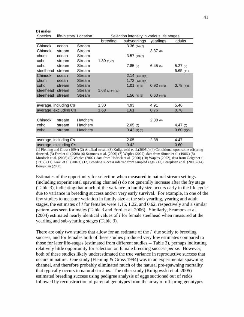
41

B) males Species life-history Location

Chinook ocean Stream 3.36 (14)(2)

Chinook stream Stream 3.37 (8)

chum ocean Stream 3.57 (13)(2)

coho stream Stream 1.30 (1)(2)

coho stream Stream 7.85 (5) 6.45 (5) 5.27 (5)

steelhead stream Stream 5.65 (11)

Chinook ocean Stream 2.14 (14)(2)(4)

chum ocean Stream 1.72 (13)(2)(4)

coho stream Stream 1.01 (4) (5) 0.92 (4)(5) 0.78 (4)(5)

steelhead stream Stream 1.68 (3) (4)(12)

steelhead stream Stream 1.56 (4) (6) 0.60 (4)(6)

average, including 0's 1.30 4.93 4.91 5.46average, excluding 0's 1.68 1.61 0.76 0.78

Chinook stream Hatchery 2.38 (8)

coho stream Hatchery 2.05 (5) 4.47 (5)

coho stream Hatchery 0.42 (4) (5) 0.60 (4)(5)

average, including 0's 2.05 2.38 4.47average, excluding 0's 0.42 0.60

Selection intensity in various life stagesbreeding subyearlings yearlings adults

(1) Fleming and Gross (1994) (2) Artifical stream (3) Kuligowski et al.(2005b) (4) Conditional upon some offspring detected. (5) Ford et al. (2008) (6) Seamons et al. (2006) (7) Waples (2002), data from Simon et al. (1986.) (8) Murdoch et al. (2008) (9) Waples (2002), data from Hedrick et al. (2000) (10) Waples (2002), data from Geiger et al. (1997) (11) Araki et al. (2007a) (12) Breeding success inferred from sampled eggs (13) Berejikian et al. (2008) (14) Berejikian (2008) Estimates of the opportunity for selection when measured in natural stream settings (including experimental spawning channels) do not generally increase after the fry stage (Table 3), indicating that much of the variance in family size occurs early in the life cycle due to variance in breeding success and/or very early survival. For example, in one of the few studies to measure variation in family size at the sub-yearling, yearing and adult stages, the estimates of I for females were 1.16, 1.22, and 0.62, respectively and a similar pattern was seen for males (Table 3 and Ford et al. 2006). Similarly, Seamons et al. (2004) estimated nearly identical values of I for female steelhead when measured at the yearling and sub-yearling stages (Table 3). There are only two studies that allow for an estimate of the I due solely to breeding success, and for females both of these studies produced very low estimates compared to those for later life-stages (estimated from different studies -- Table 3), perhaps indicating relatively little opportunity for selection on female breeding success per se. However, both of these studies likely underestimated the true variance in reproductive success that occurs in nature. One study (Fleming & Gross 1994) was in an experimental spawning channel, and therefore probably eliminated much of the natural pre-spawning mortality that typically occurs in natural streams. The other study (Kuligowski et al. 2005) estimated breeding success using pedigree analysis of eggs suctioned out of redds followed by reconstruction of parental genotypes from the array of offspring genotypes.

42

The fitness estimates were therefore contingent upon a female successfully creating a redd and depositing sufficient eggs to be sampled, a study design that would lead to underestimates of the true variance in fitness since unsuccessful females were not sampled. In contrast to the results from natural stream settings, estimates of I in hatcheries tended to increase when measured at later life-stages, indicating that much of the variance in family size occurs after release from the hatchery (Table 3). This result has been noted previously (Geiger et al. 1997; Simon 1986.; Waples 2002), and interpreted as evidence for natural selection for different genotypes in the marine environment (Geiger et al. 1997). The actual values of I also were lower for the early life stages in the hatchery studies compared to the wild studies. This pattern is consistent with the fact that compared to natural streams, there is often relatively little mortality occurring during hatchery rearing, so there may be less opportunity for selection in the hatchery than in the wild (Figure 6). The relatively low opportunity for selection in hatcheries is important to consider when evaluating the potential for domestication selection. The whole point of hatchery rearing is to avoid much of the early life stage mortality that typically occurs in the wild, and for the most part hatcheries are quite effective at maintaining high spawning adult-to-smolt (or other release stage) survival rates. At first glance, the finding of relatively low variance in family size in hatcheries prior to release therefore appears inconsistent with the hypothesis that strong domestication selection occurs in hatcheries. However, there are several reasons that the actual potential for domestication may be strong in hatcheries even though the potential for selection is ‘relaxed’ compared to what is seen in the wild. First, even though less than in the wild, some of the estimates for the potential for selection in the hatchery are nonetheless quite high (Table 3). In particular, the very low values are all for situations in which prespawning mortality and broodstock selection were not included in the estimate. When these factors are included, variance in fitness in hatcheries when measured at juveniles stages tends to be quite high (I > 2). Second, as was discussed extensively above, considerable selective mortality can occur after release from the hatchery, so at least some of the opportunity for selection measured at the adult life stage may result in patterns of selection caused by hatchery rearing. It is important to note that although the discussion above has been in terms of opportunities for selection, many non-selective phenomena could contribute to variance in family size. For example, egg-fry mortality is likely to be highly correlated across families since many sources of mortality (e.g. bed scour) probably affect entire families of eggs within redds at once. Although some of this mortality might be selective (e.g., on spawning location or redd construction), much of this family-correlated mortality could also be random with respect to families. To the degree that families tend to be spatially correlated, it is easy to imagine similar correlated mortality occurring at later freshwater and marine life-stages as well. Simply having a high opportunity for selection does not, therefore, necessarily imply that strong selection is in fact occurring.

43

Summary on the effects of hatchery breeding and rearing Of the studies we reviewed that directly measured of relative fitness of hatchery salmon in the wild, all but one focused on ‘stream type’ species, such as steelhead, Atlantic salmon, coho salmon, and yearling smolting Chinook salmon. These studies have found a range of outcomes (Figure 4). Nearly all studies of steelhead have found low relative fitness of hatchery fish, even in situations involving local broodstocks that were propagated for few generations. Results from coho and Chinook salmon are more mixed, with some studies finding low relative fitness and others not. We are aware of only one ongoing relative fitness study of an ocean type species, a study of chum salmon (Berejikian et al. 2008). This study estimated a relative fitness of ~1 for males and ~0.7 for females (but not significantly different from 1). Since many hatcheries release salmon with ocean type life-histories, particularly coastal Chinook salmon, initiating relative fitness studies in such systems would clearly be beneficial for helping to appropriately direct hatchery reform efforts.

A review of the salmon life-cycle indicates that there are many potential opportunities for natural selection to influence patterns of variation throughout the life-cycle. The actual variance in family size when measured at different points in the life-cycle in the wild appears to plateau early in the life-cycle, although there are exceptions (see Geiger et al. 1997). Hatcheries appear to be characterized by more ‘relaxed’ (but in some cases still substantial) selection at early life-stages. However, there are considerable opportunities for selection after release from the hatchery, and if phenotypic distributions are significantly altered from what they are in the wild (e.g., by accelerated growth in the hatchery), it is possible for the mortality that occurs after release to be selectively influenced by hatchery breeding. Based on the currently available data and information, there are reasons to suspect that hatchery programs that involve breeding, incubation and no or very brief rearing will be less likely to result in strong domestication selection than programs that involve longer periods of rearing. However, because there is evidence for strong sexual selection of salmon in nature and evidence that much of the total variance in family size occurs before the fry stage, the degree of difference between the two scenarios may not be all that great. Clearly obtaining more direct information on the rate of fitness loss in sub-yearling release programs is important, however.

What information is available to inform systematic assessments of ecological impacts of hatchery programs at the population level? Range of Ecological Impacts of Hatchery Programs

44

Ecological impacts of hatchery programs include the changes in abundance, productivity, diversity and spatial structure of populations that arise from altering environmental conditions and species interactions by capturing, rearing, and releasing hatchery fish. Such effects are wide ranging and have been shown to occur even when genetic impacts are not thought to exist (Kostow et al. 2003; Kostow & Zhou 2006). These effects have been recently reviewed by Kostow (2008) and Pearsons (2008), and include:

• Direct predation. Large, hatchery-reared smolts can prey directly on wild juveniles (Hawkins & Tipping 1999; Ruggerone & Rogers 1992).

• Supporting predator populations. Releases of hatchery fish can help to support an increased predator population (including human predators), thereby increasing predation rates on wild fish (Collis et al. 1995; Hilborn & Eggers 2000; Nickelson 2003).

• Competition among juveniles. Releases of hatchery fish may also increase competition among juveniles for food, territories, and cover from predators, decreasing growth, increasing mortality, and potentially affecting population dynamics by inhibiting density-dependent compensation (Zaporozhets & Zaporozhets 2004)

• Competition among adults. When hatchery-origin adults are allowed to spawn in the wild, they can compete with wild adults, occupying spawning and rearing resources that could be used by the wild population (Kostow & Zhou 2006). This situation can be worsened when hatchery fish are selected to breed early (taking up space) or late (superimposing redds on wild redds) in comparison with wild fish.

• Vectors of disease. Hatchery fish can have higher rates of disease, and be selected for disease resistance, and can pass on disease pathogens to the natural environment (Goede 1986; Snieszko 1974).

Importantly, these effects are not necessarily restricted to the immediate areas in which hatchery fish are released. These effects can be found in tributary, mainstem, estuarine and even ocean environments (Kostow 2008; Pearsons 2008; Ruggerone & Goetz 2004). In addition, some species may have life histories that make them particularly susceptible to realizing these impacts – steelhead, for example, are prone to residualize, increasing the time during which hatchery and wild fish can interact. Moreover, these interactions can be exacerbated when hatchery fish have a physical advantage – being larger, more aggressive or in better condition, for example – over wild fish (Kostow 2008). Finally, these interactions can potentially occur intra-specifically and inter-specifically (e.g. Levin & Williams 2002). This means that the effect of releases of all salmonids – not just those of the same species as the ESU or population of interest – should be considered in any assessment of ecological impacts, although niche partitioning may tend to limit competitive interactions among some species (e.g., Brodeur et al. 2007; Fisher et al. 2007) Available Kinds of Information and Appropriate Uses

45

There are two broad categories of useable information about the ecological impacts of artificially propagated fish on wild populations and ESUs. The first is empirical studies. Observational investigations that identify relationships between, for example, hatchery practices or hatchery fish abundance and some aspect of wild population status are included in this category as well as experimental studies that identify causal links between conditions (e.g. hatchery smolt abundance) and population response. These studies are used to 1) identify impacts and 2) estimate the magnitude of those impacts and conditions under which the impacts are felt. The second category includes modeling or theoretical studies that use the results of empirical studies to estimate effects over an entire life-cycle, in concert with other impacts, or under conditions that have not yet been observed. These kinds of studies have typically been interpreted as predictive (i.e. “if we release X hatchery fish in this place, Z will happen.”); however, it is important to understand that the predictive powers of most models are quite low. In fact, in all modeling exercises, trade-offs between realism, precision, and understanding are inevitable (Levins 1966). This is not to say that they are not useful. Modeling investigations can be used to identify locations or life stages that are particularly sensitive to perturbations; coupled with information from empirical studies indicating impacts at those stages (or locations), a stronger case for allowing or disallowing actions can be made. Similarly, investigating impacts over a range of conditions (e.g. varying density of wild fish, alternative climate, etc.) can identify changes that are harmful or beneficial under many conditions even if there is uncertainty about the magnitude of impact. Modeling can also serve as an evaluation of the plausibility of a scenario – by testing a range of possible impacts, we can assess the likely conditions under which a goal can be met, for instance. Most information available indicates that artificially-propagated fish do have ecological impacts on wild salmonid populations under most conditions. Below, we review first the magnitude of those impacts (empirical studies), and then our ability to incorporate those impacts into modeling frameworks to assess population or ESU-level consequences. Magnitude of Ecological Impacts Overall impact of hatchery fish on wild salmonid survival, abundance and productivity A number of studies have examined the overall impact of hatchery fish on wild salmonid survival, abundance and productivity. Typically, these studies do not draw causal links, nor hypothesize the mechanism of effect. However, they do indicate that there are effects, and that they can be substantial (e.g. a 50% reduction in productivity for steelhead in an Oregon population). Importantly, in some cases, these studies do not identify the source of the impact – the effects could be ecological and genetic. However, in some cases (e.g., Kostow & Zhou 2006), genetic impacts have been ruled out, and the difference in survival is attributed to ecological effects.

46

Table 4 -- Summary of studies that have estimated effects of hatchery releases or naturally spawning hatchery fish on wild fish survival, abundance, or productivity Wild

species Hatchery species

Study summary Summary of effect size

1 Coho Coho Studied 14 populations of Oregon Coast coho. Found significant correlation density corrected productivity and average smolt releases into a population. Negative but not significant relationship between productivity and proportion hatchery spawners. Habitat quality included as a co-variate.

Releases: Ln(a) = -0.13x + 1.71, where x = smolts released X 100,000 (p = 0.003, R2 = 0.53) Spawners: Ln(a) = -0.82x + 1.65, where x = proportion hatchery fish and a is the Ricker productivity parameter (p = 0.127, R2 = 0.19)

2 Steelhead Steelhead Studied 12 populations of Oregon steelhead. Found a negative correlation between density corrected productivity and proportion of hatchery fish on the spawning grounds.

Spawners: Ln(a) = -1.97x + 1.41, where x = proportion hatchery fish and a is the Ricker productivity parameter (p <0.001, R2 = 0.70).

3 Chinook Chinook, coho, steelhead

Large scale path analysis of effects of dams, habitat degredation, harvest, and hatcheries on Chinook salmon abundance and trend. Found negative effects of hatchery production on trend, neutral to positive effects on abundance.

Spawners: Ln(λ ) = -0.33x, where x is the geomean of ln (releases) of Chinook, steelhead, and coho in river basin occupied by natural population.

4 Steelhead Steelhead Found significant effects of hatchery steelhead spawners on productivity and capacity of wild steelhead in an Oregon population.

50% reduction in productivity, 22% reduction in capacity during years of high hatchery proportions.

5 Chinook Chinook Significant effect of hatchery releases on wild Snake River Chinook smolt-adult survival during periods of poor ocean conditions, no effect during good conditions.

Negative slope but could not find formula in paper.

6 Chinook Chinook, steelhead

Significant effect of hatchery steelhead releases on smolt-to-adult survival rates of wild Interior Columbia River Chinook salmon. No significant

Chinook SAR (%) = 3.342 – 0.342x, where is Columbia River steelhead releases in millions.

47

effect of steelhead releases on wild steelhead survival.

7 Coho Coho Updated analysis of Oregon Coast coho (1) to include low release years and improved ocean conditions. Found strong effect of hatchery releases on carrying capacity. Hatchery reductions accounted for 23% increase in wild production after 1996.

Spawners: Sw = - (a + bh Sh)/bw, where Sw is wild spawners/km at capacity, a is intrinsic productivity, bw is the Ricker density term for wild spawners and bh is the Ricker density term for hatchery spawners. Estimates for OC coho were a = 0.82, bw = -0.0071 and bh = -0.05. Releases: Ln(a) = 0.82 -0.47M, where M is smolt releases in millions.

1 -- (Nickelson 2003); 2 -- (Chilcote 2003); 3 -- (Hoekstra et al. 2007); 4 -- (Kostow & Zhou 2006); 5 -- (Levin et al. 2001); 6 -- (Levin & Williams 2002); 7 -- Buhle et al. (in press) Direct predation. Published studies documenting predation on wild juveniles by other salmonids are relatively rare. However, regional agencies have investigated this issue (Busack et al. 2005a), and the piscivory rates documented from studies of salmonid predation in Washington streams are shown in Figure 8. In this set of studies, piscivory typically occurs at less than a 1% rate. However, salmonid-on-salmonid predation can occur at greater rates, and has been documented to affect mortality rates of up to 59% (Ruggerone & Rogers 1992). Such predation has been shown to be size-selective (Hargreaves & Lebrasseur 1986; Parker 1971) and dependent on the abundance of wild prey (Hawkins & Tipping 1999). In addition, different species appear to have different effects, with coho predation on other species relatively well-documented (below and summarized in (Kostow 2008)). Together, this evidence suggests that hatchery releases in areas of high wild density, particularly when the hatchery-origin fish are larger than the wild juveniles, have the potential to exert predation pressure, but that this particular impact might be amenable to mitigation through changes in hatchery practices.

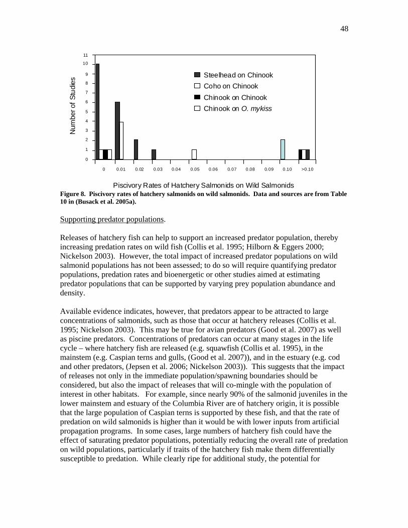
48

Steelhead on ChinookCoho on ChinookChinook on ChinookChinook on O. mykiss

0 0.01 0.02 0.03 0.04 0.05 0.06 0.07 0.08 0.09 0.10 >0.10

1

2

3

4

5

6

7

8

9

10

11

Piscivory Rates of Hatchery Salmonids on Wild Salmonids

Num

ber o

f Stu

dies

0

Figure 8. Piscivory rates of hatchery salmonids on wild salmonids. Data and sources are from Table 10 in (Busack et al. 2005a). Supporting predator populations. Releases of hatchery fish can help to support an increased predator population, thereby increasing predation rates on wild fish (Collis et al. 1995; Hilborn & Eggers 2000; Nickelson 2003). However, the total impact of increased predator populations on wild salmonid populations has not been assessed; to do so will require quantifying predator populations, predation rates and bioenergetic or other studies aimed at estimating predator populations that can be supported by varying prey population abundance and density. Available evidence indicates, however, that predators appear to be attracted to large concentrations of salmonids, such as those that occur at hatchery releases (Collis et al. 1995; Nickelson 2003). This may be true for avian predators (Good et al. 2007) as well as piscine predators. Concentrations of predators can occur at many stages in the life cycle – where hatchery fish are released (e.g. squawfish (Collis et al. 1995), in the mainstem (e.g. Caspian terns and gulls, (Good et al. 2007)), and in the estuary (e.g. cod and other predators, (Jepsen et al. 2006; Nickelson 2003)). This suggests that the impact of releases not only in the immediate population/spawning boundaries should be considered, but also the impact of releases that will co-mingle with the population of interest in other habitats. For example, since nearly 90% of the salmonid juveniles in the lower mainstem and estuary of the Columbia River are of hatchery origin, it is possible that the large population of Caspian terns is supported by these fish, and that the rate of predation on wild salmonids is higher than it would be with lower inputs from artificial propagation programs. In some cases, large numbers of hatchery fish could have the effect of saturating predator populations, potentially reducing the overall rate of predation on wild populations, particularly if traits of the hatchery fish make them differentially susceptible to predation. While clearly ripe for additional study, the potential for

49

artificially inflated predator populations should be considered in evaluations of artificial propagation program impacts. Mixed stock fisheries – a special case of supporting predator populations. Mixed-stock fisheries can be regarded as a special case in which a predator population (fishers) is supported at levels that impose a greater mortality rate on wild fish than would be experienced if only the wild population were in existence. These situations are largely well-understood and accounted for in most reviews of impacts. However, they should be considered a potential impact in the entire range of an ESU’s life cycle, including impacts from catch-and-release fisheries and other recreational fisheries that are aimed primarily at hatchery fish. Competition among juveniles. Freshwater habitats. The freshwater juvenile life stage is the stage at which density-dependent effects are thought to be most strongly felt in anadromous salmonid populations (Cushing 1973; Slaney et al. 1985; Ward & Slaney 1993). And, in fact, density-dependence in the freshwater stages is well-documented in a variety of species (Kostow 2008; reviews in Slaney et al. 1985; Zaporozhets & Zaporozhets 2004). Decreased freshwater survival and juvenile growth have been documented at high densities in several species. Unfortunately, and true to form, the various researchers have not used a common currency in which to record these changes. Here, we try to report these effects in currencies that can be readily understood from studies that examined survival under varying densities. Nickelson (1986) compared stocked and unstocked streams utilized by coastal coho and found that although the total abundance and density of fish was higher in stocked streams, the density of wild fish was 44% lower in stocked streams than in streams without stocking. This suggests that competition between wild and hatchery fish exerts a negative effect on wild fish production. Steelhead have been the object of several studies of this sort. A life-cycle study of steelhead examining adult-to-adult returns, and factoring out ocean and genetic effects (thus targeting freshwater ecological effects, and particularly competition) showed a 50% decline in the Beverton-Holt productivity parameter and a 22% decline in recruits in streams with high levels of hatchery fish (Kostow & Zhou 2006). Studies addressing only the freshwater phase also found increased mortality/decreased survival at high densities. A study that estimated steelhead capacity respectively, and stocked fish at that capacity, 200% of capacity and 400% of capacity found that survival in low food environments decreased from 80% to 40% (Keeley 2001). Another study that stocked at varying densities (0.13, 0.7 and 2.0 fish per m2) found that survival from fry to 1+ parr decreased from 17-26% in low density areas to less than 5% in medium and high density areas (Hume & Parkinson 1987). Density-dependent mortality was also observed at densities above 0.7fish/ m2 in a study of Atlantic salmon (Gee et al. 1978). Ward and Slaney (1993) estimated that density-dependent mortality of steelhead would be expressed at densities above 0.3 steelhead/ m2 in the Keogh River of British Columbia.

50

Together, these results suggest that competition among juvenile salmonids in the freshwater life stage (expressed through density-dependent mortality) is present and that when hatchery fish increase the density of a juvenile population, wild fish may suffer greater mortality than they would have without the supplementation. The magnitude of the effect can be large (more than doubling mortality or halving survival in high-density situations) and can be felt at levels that might not be perceived to be high density (0.3-0.7 fish per square meter). The specific effects will undoubtedly depend, however, on a variety factors, including the size of the hatchery fish and the time and location of hatchery releases. Estuarine and ocean habitats. Cooney and Brodeur (2001) modeled food demands of wild and ranched pink salmon and identified the potential for competition for food in the ocean environment; such competition has been postulated by others as well (Beamish et al. 1997; Peterman 1991). More recent work has supported these hypotheses. In particular, Ruggerone and colleagues have identified reductions in marine survival of two salmonid species in years of high pink salmon abundance. Ruggerone and Goetz (2004) estimated that Chinook salmon in Puget Sound had a 59% lower marine survival rate in years of high pink salmon abundance, while sockeye salmon, occupying more pristine habitats in Alaska showed a reduction in marine survival of 26-44% in the alternate years of high pink salmon production (Ruggerone et al. 2003). Moreover, surviving fish in those alternate years showed a 10-18% decrease in growth rates (Ruggerone et al. 2005). A negative association between number of hatchery Chinook salmon released in the Columbia Basin and marine survival of wild fish (Chinook salmon) in years of relatively poor ocean conditions (Levin et al. 2001) also suggests that competition in marine habitats exists. This body of evidence supports the existence of competition in the ocean when large numbers of salmonids are present. It suggests that competition may occur, decreasing survival and growth in the presence of large numbers of hatchery releases, potentially with the greatest effect in years of relatively poor ocean conditions (low upwelling) when prey abundance is lowest, conditions that could be exacerbated by climate change (Schindler et al. 2008). In addition, it suggests that impacts of total releases – both geographically (at least from a single basin and possibly from larger areas (e.g. Puget Sound, Washington coast)) and taxonomically (i.e. across all species) – should be considered when evaluating the impacts of hatchery programs on ESUs of concern. Competition among spawning adults. Competition among adults is thought to occur in two manners, one mediated through spawn timing (Kostow 2008), and the other primarily via competition for mates. Competition effected through spawn timing can occur both early and late. When returning hatchery-origin spawners spawn earlier than wild fish, their progeny hatch earlier and become large sooner than the progeny of wild fish. This, in turn, can set in motion the competition among juveniles described above. When hatchery-origin

51

spawners return later than their wild counterparts, hatchery-origin redds can be superimposed on top of the redds of wild fish, causing these redds to fail. The magnitude of this effect is dependent upon the amount of available spawning habitat, the number and proportion of hatchery-origin spawners in the wild and the total population size relative to available spawning habitat. In general, this mechanism should be considered a potential problem when hatchery spawners spawn toward the end of the spawning run, or have been bred to spawn later than wild fish, particularly when the population is relatively large relative to available spawning habitat or when the proportion of hatchery spawners on the spawning grounds is large. Hatchery-origin spawners may also compete with wild fish for mates. In general, wild-origin spawners appear to be more desirable mates than hatchery-origin fish (e.g., Berejikian et al. 2001). However, wild and hatchery fish do interbreed, leading to issues described in the genetic section. Competition for mates (leading to interbreeding between wild and hatchery fish) may be a potential problem when the proportion of hatchery fish on the spawning grounds is high. Vectors of disease. The transmission of disease and parasites between wild and hatchery populations is complex, and there is evidence that transmission can occur in both directions. Anderson et al. (2000), for example, documented transfer of infectious hematopoietic necrosis virus (IHNV) from wild kokanee to a hatchery population. The best documented transmission of a pathogen between cultured and wild stocks of salmonids is the case of whirling disease among rainbow trout and steelhead in both the US and Europe. The parasite causing this disease, Myxobolus cerebralis, was amplified among hatchery populations and then spread by stocking activities (Gilbert & Granath 2003). This parasite is currently spreading throughout the western United States. Transfer of sea lice (Lepeophtheirus salmonis) from farmed salmon to wild salmon is another example of how disease associated with aquaculture may impact wild populations (Bakke & Harris 1998; Butler 2002; Krkosek et al. 2005; McVicar 1997; Tully & Whelan 1993). One recent study has suggested that sea lice transferred to wild populations can be a significant source of mortality and extinction risk (Krkosek et al. 2007), although this conclusion has proved to be subject to considerable debate (Brooks & Jones 2008; Brooks & Stucchi 2006; Krkosek et al. 2008a, 2008b; Riddell et al. 2008). Another recent study found a ~50% decline in wild population survival or abundance associated with the presence of fish farms, although the cause of this decline was not identified (Ford & Myers 2008). Although the effects on wild population viability clearly are not completely understood, it is clear that disease transmission can occur in both directions and that the occurrence of a disease can be amplified through culture practices (exacerbating any tendency toward transmission). When considering the potential for disease transmission due to hatchery practices, factors influencing the impact of transmission include the density and

52

abundance of the hatchery stock, the prevalence of the disease in that population, and the particular practices that might enhance transmission (e.g. failure to segregate life stages that would normally not come into contact with each other). Estimating Multiple Impacts in a Modeling Framework. Importantly, the cumulative or interacting effects of multiple hatchery releases have not been incorporated in most of these studies (with the exception of those that evaluate the effect of all releases in a basin on ocean survival). One potential method of estimating the cumulative impacts is to use a modeling approach such as the PCD (Predation-Competition-Disease) Risk model (Busack et al. 2005a). PCD (Predation-Competition-Disease) Risk Model. This model incorporates predation by hatchery fish, competition for resources, and infection as a result of encountering hatchery fish. It provides a distribution of mortality rates of wild fish associated with predation, competition, and disease that could be incorporated into a population model (see below). Figure 9, for example, shows the distribution of mortality rates from hypothetical coho salmon hatchery program. By varying production goals, hatchery strategies, and actions in different analyses, the model provides ways to explore the effects of possible management actions, such as releasing different numbers at different sizes, locations, or times that minimize negative ecological interactions.

Figure 9. Results from a PCD Risk analysis of ecological impacts from a hypothetical coho salmon hatchery program. The results show two different estimates of mortality from competition: mortality due to loss of body weight (starvation) and mortality from other competition induced causes, which is determined by a user-defined threshold.

53

Again, this approach is dependent on data availability, but can still be used to explore alternative scenarios. The PCD Risk Model is currently being used to estimate ecological effects of each Puget Sound region Chinook and coho salmon hatchery program on natural Chinook salmon in a programmatic EIS under preparation by NMFS (T. Tynan, NMFS NWR, personal communication). Including Ecological Impacts in Currently Available Modeling Frameworks Virtually any population model can be adapted to incorporate ecological impacts. The currently existing Shiraz population model as applied in the Wenatchee and Snohomish drainages (Bartz et al. 2006, Honea et al., in press) already incorporates density-dependence at juvenile life stages, thus accounting for simple density effects of hatchery releases. [Both efforts have also indicated that juvenile hatchery fish may be affecting production of wild smolts due to density effects.] The AHA model, another stage-specific Beverton-Holt model, could also be modified to incorporate density-dependent and similar competitive effects from hatchery fish. Leslie matrix models such as those developed in support of the FCRPS Biological Opinion (McClure et al. 2007) and the SLAM model (Appendix 1; http://www.nwfsc.noaa.gov/trt/slam/slam.cfm) are another candidate for adaptation to include ecological impacts. All of the normal concerns about modeling uncertainty would obviously apply in these cases, and the general lack of information will typically require that these efforts be used as an exploration of possible outcomes (see above) rather than as precise predictive tools. Given existing data and modeling frameworks a range of questions could be addressed. Two examples are:

• If we assume density-dependence in the ocean (over a range of scenarios consistent with literature values) in “bad” ocean years, how is productivity of wild populations likely to be affected? At what level of hatchery output by species are decreases in wild productivity for species of concern likely to be seen?

• Over the set of populations for which population models already exist, are there general conclusions that can be drawn about the density or abundance of hatchery juveniles that may lead to depressed wild productivity?

Use of weirs to control straying What is known about negative ecological or demographic impacts of such weirs in salmon drainages? What risks should be taken into account in evaluating the potential impacts of weirs on the targeted natural population and on other species utilizing the river?

54

Can a risk assessment framework be developed to inform management decisions regarding weir location, design, construction and operation about relative risks and benefits in specific situations? What guidance can the RIST provide for study designs to get at the potential risks and benefits of weirs in representative situations (e.g., Grays River in the Lower Columbia).

In response to concerns about the negative impacts of hatcheries, managers have established (and are proposing more) “wild fish sanctuaries” (WFS) that are intended to be mostly free of hatchery fish. There is no established definition of a WFS, but it is generally described as a watershed or part of a watershed from which hatchery juvenile releases and hatchery origin spawners are totally or largely excluded. By excluding hatchery fish, wild fish are expected to be protected from genetic degradation and harmful ecological interactions. Exclusion of hatchery fish in a WSF may not be absolute, and some descriptions of a WFS allow the fraction of hatchery origin fish to be in the 5-10% range (HSRG 2004). An obvious way to create many WFS would be by greatly reducing hatchery releases on a coastwide or regional basis, and some regions have taken steps in this direction (e.g. Oregon coast – Buhle et al. in press). However, in many regions hatcheries provide harvest opportunities that have significant economic, cultural and legal significance, and elimination or substantial reductions in hatchery production would come at a considerable economic and social cost. Therefore, fisheries managers have proposed strategies to create WFS while maintaining high hatchery production (HSRG 2004). If high hatchery production and WFS are to coexist, hatchery fish must be excluded from the WFS. The strategies proposed for excluding hatchery fish from WFS fall into four main non-mutually exclusive categories, 1) reduced hatchery production, 2) geographic isolation, 3) removal of hatchery fish by harvest , 4) fish sorting barriers. Reducing hatchery production sufficiently to reduce straying below a threshold or goal should conceptually be an effective way to create WFS, but may conflict with other societal goals. Geographic isolation relies on the homing instinct of salmon to return to hatcheries which are located in areas geographically distant from the WFS. This approach can be effective if hatchery fish do not stray into WFS at significant levels. Strategies based on removal by harvest and sorting at barriers both require that all hatchery fish have a externally detectable mark (usually adipose fin clip and/or CWT) that allows selective removal of hatchery fish by either harvesters or barrier operators. The creation of WFS could provide substantially improved conditions for wild fish over the status quo in some populations where hatchery and wild fish are completely intermingled. However, the methods proposed for isolating hatchery and wild fish can pose risks of their own, so creating a WFS will usually involve a trade-off between risks. Table 5 provides a list of potential risks to wild fish associated with different WFS strategies, which includes issues such as the overharvest of wild fish in hatchery mark selective harvest programs, negative habitat effects of weirs created for sorting hatchery and wild fish, and ecological effects as wild fish interact with hatchery fish in mainstem and marine areas outside the WFS.

55

Table 5 – Summary of benefits and risks of three methods of creating wild fish sanctuaries that are intended to be demographically, ecologically and genetically isolated from hatchery influence Method Benefits Risks/costs Reduce/eliminate hatchery releases

Addresses both genetic and ecological risks; does not require intensive management

May reduce/eliminate fishing opportunities and be counter to legal mitigation requirements.

Geographic isolation of hatchery

Addresses genetic risks and tributary level ecological interactions; does not require intensive management; may provide localized harvest opportunities.

Does not address ecological risks in shared downstream environments; in some situations will not isolate the WFS from hatchery effects

Selective harvest of hatchery fish

Uses a societal benefit to control a biological risk; may allow for substantial hatchery production;

Harvest rates necessary to achieve isolation may be too high for wild population viability; requires intensive management and is not robust to failure; does control many ecological impacts; may be culturally unacceptable.

Selective migration barrier (weir/dam, etc)

Allows direct control of hatchery fish in WFS; can also serve as broodstock collection point; allows for management to change as a function of wild population status

In some situations will not isolate the WFS from hatchery effects; requires intensive management and is not robust to failure; impacts on fish movement of target and non-target species; impacts river environment; does not control downstream ecological impacts.

The rest of this section focuses on the use of weirs to control movement of hatchery fish. Weirs as fish sorting barriers

Weirs are employed on salmonid spawning streams for a variety of reasons. Primary goals have historically been to aid assessments of numbers and characteristics of upstream and downstream migrators (e.g. Bradford et al. 1997), brood stock collection, and selective removal of predators or non-native fish (Fausch et al. 2006; Harford & McLaughlin 2007). Increasingly weirs are installed, often in association with hatcheries, to control the numbers of hatchery strays or hatchery-origin spawners or to manipulate the ratio of hatchery origin to native origin or wild fish. Although the literature on weir

56

design and placement is extensive (reviewed by NMFS 2008), assessments of weir performance are less common, as are discussions of the decision process concerning weirs versus alternative, non-weir means of achieving similar goals. The RIST surveyed available literature concerning known and potential costs and benefits of weir deployment to aid in this decision process. Although any decision will ultimately be unique and site-specific, some general patterns emerged concerning where weirs are a promising or unappealing method for achieving management goals. Weir Effectiveness Ultimately, the measure of success of a weir-based management strategy depends on whether the weir performs as planned. However, performance measures of weir effectiveness do not appear to be standardized or formalized. Metrics that could go into such calculations would probably focus on:

• percent of total run captured or passed, • percent of strays captured, • frequency with which native fish are blocked and returned downstream (weir

rejection), or with which stray native fish are passed and then spawn upstream (shortstopping, forced straying, displaced spawning), plus

• other issues associated with migration delay and interruption (impingement, mortality, stress, injury), detailed below.

An important consideration in a decision about utilizing weirs is the likelihood of weir failure. Such failure is often described relative to physical destruction of the weir, inadvertent fish passage (leakage), or inability to capture a significant proportion of migrating fish. Capture effectiveness can be heavily dependent on species and migration timing. Fall Chinook are easier to intercept because of low water and species-typical behavior at obstacles (although Chinook and sockeye are also more likely to be shortstopped and spawn downstream, perhaps in suboptimal habitat). Coho and steelhead migrate later and are more likely to “leak” through because they move during periods of higher flow and are more likely to avoid entering ladders and traps (A. Appleby, pers. comm.). Both physical and biological failure are more likely during high water flows and/or ice or debris/sediment build-up that physically damage the weir or allow water and fish to pass over the structure. Flashy streams and streams where high water periods are prolonged are more prone to failure. The potential for failure is therefore an obvious site-specific factor that requires careful pre-design and deployment investigation, as occurred in the decision to forego weir construction in Togiak River, Alaska because of regular high flows and unstable river bed composition (Larson 2001). Weirs do fail and that expectation is often built into the design, as in the floating board and hinged weir types that are pushed down under high water pressure, such as the Gray’s River weir, Washington (Figure 10).

57

 

Figure 10 -- The Gray’s River, WA weir, a resistance board/fixed panel design utilizing fixed wooden panels. Credit R. Walton.

Even relatively large structures can fail to restrict fish movement during high flows (Figure 11), and weir failure at high flows appears to be commonplace, as in the Chiwawa and Twisp River weirs in the Upper Columbia (A. Murdoch, pers. comm.). “Failure” can also occur when associated structures do not perform adequately, as happened at the Vern Freeman facility, Santa Clara River, CA when the river below the dam cut down to the extent that the ladder was completely on dry land, blocking passage of fish diverted by the weir (P. Adams, pers. comm. to C. Jordan).

 

Figure 11 -- Failure of weir to restrict passage during a period of high flows on Minter Creek, WA. Occasional weir failure could have potentially significant effects on the ability of a weir to control genetic impacts from hatchery straying. We used the Ford (2002) model with

58

the typical HSRG parameterization to compare the long term outcome of scenarios in which a weir worked perfectly every generation to those in which the weir failed and allowed high rates of hatchery straying every 10 generations (Table 6). We only explored a few scenarios, but these serve to illustrate that there are likely scenarios in which episodic weir failure is predicted to result in considerably lower long-term wild fitness than would be the case without taking weir failure into account. This is an issue that requires further exploration, but we suspect that the vulnerable cases will be in situations where the management function of the weir is to limit hatchery strays to very low levels and the potential for straying in the absence of the weir is great (e.g., scenario 2 and 3 below). Table 6 -- Example of effects of episodic weir failure on wild population fitness Scenario 1: new supplementation program 1

rw rh kw kh episodic hatchery stray rate

target hatchery stray rate

target wild rate

Wild N Wild fitness

PNI pHOS pNOB

4 10 500 200 -- 0.05 0.2 1537 0.92 0.7 0.04 0.11 4 10 500 200 0.5 0.05 0.2 1494 0.86 0.69 0.07 0.13 4 10 500 200 0.75 0.05 0.2 1507 0.84 0.7 0.08 0.15

Scenario 2: a new weir to help reform an old hatchery 2

4 10 500 1000 -- 0.01 0.2 1440 0.88 0.43 0.02 0.016 4 10 500 1000 0.5 0.01 0.2 1050 0.56 0.44 0.09 0.03 4 10 500 1000 0.75 0.01 0.2 1075 0.53 0.44 0.1 0.04

Scenario 3: domesticated strays low productivity wild population at the wild optimum 3

2 10 500 500 -- 0.05 0 567 0.53 0 0.07 0 2 10 500 500 0.5 0.05 0 133 0.22 0 0.5 0

Note: All cases run for 100 generations. Abundance, fitness, PNI, pHOS and pNOB are averages from generations 50 – 100. In the episodic weir failure scenarios, failures occurred every 10 generations. rw = wild productivity (hockey-stick), rh = hatchery productivity (hockey-stick), kw = wild capacity, kh = hatchery capacity, episodic stray rate is the proportion hatchery fish on the spawning grounds during a period of episodic straying, target hatchery stray rate is the level of straying that is the annual management target (ie, the straying that occurs in the presence of a functional weir), target wild rate is the proportion of wild fish in the hatchery broodstock, wild N is the average wild abundance, wild fitness is the average wild fitness relative to the case of no hatchery, PNI is proportionate natural influence, pHOS is the average realized proportion hatchery fish on the spawning grounds, pNOB is the average realized proportion natural fish in the hatchery broodstock. 1 Example of a new supplementation program for a wild population initially at the wild trait optimum. Production function is a hockey stick model. 4=wr ; 10=hr ; ;

;

500=wk200=hk ( ) ( )00,80,100 ==== zz whwhw θθθ 5.0, 2 =h10, 2 =σ10, =ω .

2 Example of using a new weir to help control straying from an old hatchery. Production function is a hockey stick model. ; 4=wr 10=hr ; 500=wk ; 1000=hk ;

( ) ( ) ,0 = hθ 5.,80,100 == zwhw θθ 0,10 2 == h,10 2= σω0 = zh . 3 Example of strays into a wild population initially at its wild optimum. Production function is a hockey stick model. ; 2=wr 10=hr ; 500=wk ; 500=hk ;

( ) ( ) , == h ωθ 5.0,80,100 2 === hhw θθ 10,10 2 =σ0, zhwθ0, =zw .

59

20 40 60 80 100

0.3

0.4

0.5

0.6

20 40 60 80 100

0.2

0.4

0.6

0.8

20 40 60 80 100

0.3

0.4

0.5

0.6

0.7

0.8

0.9

20 40 60 80 100

0.02

0.04

0.06

0.08

0.1

0.12

fitne

sspH

OS

Generations

No weir failure Episodic weir failure

Figure 12 -- Illustration of effects of episodic weir failure based on scenario 2 of Table 6. For purposes of illustration only; time frame and absolute fitness are not be indicative of any particular population. The Decision Process

A formal decision support framework for weir deployment, such as the Bayesian belief network of Peterson et al. (2008), is desirable but probably unrealistic because every situation will differ. However, certain considerations, factors, and approaches are relatively general and can guide the process. Figure 13 shows such a framework, organized around management goals and needs, intervening factors, design and deployment considerations, assessment of costs and benefits, and an adaptive management approach that incorporates monitoring and revision of objectives, plans, and alternatives. The starting point for the outlined decision process emphasizes a cost-benefit approach, focused on the question of under what conditions can one install a weir that is effective at keeping hatchery salmon from breeding with wild salmon but produce a minimum of undue ecological side effects. Details and examples for the various components of the flow sheet follow.

60

Figure 13-- Example of a decision framework for considering a potential weir.

61

Overall Management Objectives and Goals Assuming the ultimate objective of the project is to promote recovery of a listed salmonid ESU (given applicable federal definitions of recovery), a variety of goals and relevant data are possible. At the outset, expected project benefits need to be defined (e.g., preservation of biological diversity, fishery enhancement, water optimization, habitat protection, blockage of hatchery strays or non-native species) along with explicit statements of targets for ESU traits (abundance, productivity, PNI, fitness, etc) that might be affected by weir operation. Weirs, which function by stopping moving fish long enough to be captured and processed (measured, tagged, removed), have thus been used to enumerate populations, determine population structure, promote genetic diversity, manipulate the proportions of native and non-native spawners (usually hatchery fish) in so-called integrated populations, retain native and non-native strays in the process of creating a Wild Fish Sanctuary (e.g., Grays River weir, WADFG 2001), remove aliens, control predators, manipulate spawner abundance, collect broodstock for hatcheries, and test various population recovery models. Any timetable for planning, deployment, function, and monitoring would ideally also have a target date for weir removal, assuming goals are met or are determined to be unattainable. It is also important to determine if the use of a weir to achieve these goals conflicts with or affects goals or objectives of other projects or activities in the basin. As guidelines, it is important that weir efficiency targets or thresholds be established regarding numbers, proportions, etc. of targeted fish caught, passed, jeopardized/taken, delayed. Even the most effective weirs can fail to capture 10-20% of a run, and mark detection errors can add another 1-2% erroneously passed fish (A. Appleby, pers. comm.), setting a high standard if total segregation is a management goal. Such performance indicators appear to be often lacking except where Biological Opinions are necessitated by ESA requirements regarding listed species. Data Needs & Considerations: Data needs will be largely defined by goals and objectives established at the outset, including potential inputs into existing models. Relevant data (with confidence intervals) include abundance, productivity (progeny-to-parent ratios, survival data by life-stage, or other measures of productivity), current PNI, and a need to interrogate for tags. Discussions within the RIST concluded that a cost-benefit approach to data collection efforts would be especially useful from the outset, e.g., how effective must a weir be to justify risks: if environmental conditions or weir structure preclude trapping >5% of the run, are the objectives being met? Data biases inherent in any trapping program need to be identified, such as known trap shyness, differential entry probability, etc. A sonar-video imaging system set just below a small dam/trap facility on the San Lorenzo River near Santa Cruz, CA documented strong avoidance of the dam-trap facility. Steelhead approached the facility and then turned around, including some fish that did this repeatedly. Such avoidance would

62

greatly influence the accuracy of trap counts (P. B. Adams, pers. comm.). Because trapping always entails an element of risk of injury or mortality, the option of employing non-weir alternatives warrants consideration. Biological Factors. A weir is a barrier to fish movement. How selective will it be for target and non-target species? What migratory and non-migratory species (ocean vs. stream type subpopulations, resident non-salmonids) are likely to be affected, and which of these are listed? How will a barrier impact juveniles and non-target species? Does preventing invasion by hatchery or non-target species come at a cost of isolating native populations (e.g., the invasion-isolation tradeoff of Fausch et al. 2006). Does the design take into consideration the passage ability of non-salmonid species such as suckers, sturgeon, and lampreys, some of which cannot navigate vertical barriers that easily pass salmon (e.g., NRC 2004)? A number of complications arise as a result of migration delay and interruption. How long is too long a delay with respect to successful spawning or survival? Is impingement an issue, especially for juveniles and downstream moving fish such as kelts? What are the likelihoods of mortality, stress, or injury in the holding box? Can natural and hatchery or non-native strays be readily discriminated because strays that are passed are then forced to spawn upstream. If native fish encounter the weir and turn downstream, such non-passed fish are displaced to and may spawn downstream of their natal area. Migration delay and interruption can have undesirable impacts on genetic structure and diversity, upstream and downstream of the weir (e.g. Homel et al. 2008; Pritchard et al. 2007; Wofford et al. 2005). Additionally, delaying or concentrating fish, especially juveniles, exposes them to predation, both human and non-human (de Leaniz 2008). Concentration of fish in the holding box or against the barrier facilitates parasite and pathogen transmission (e.g., Loot et al. 2007, de Leaniz 2008). Impacts on non-salmonids can alter assemblage and community structure and function (e.g. O'Connor et al. 2006; Poulet 2007). And different life history stages of species with differing movement patterns and trap susceptibility can complicate efforts (e.g., Fausch et al. 2006).

Listed Species And Limiting Factors. ESA-listed population(s) that will be directly and incidentally affected by the program need to be identified, including the relative importance of the affected local population to the ESU/DPS. A critical question then is whether potential benefits to ESA-listed salmonids (and non-salmonids) from data collected exceed potential risks to the species due to those efforts, reiterating the cost-benefit approach. Indicative of unacceptable risk would be the determination that weir construction and operation exacerbated a limiting factor identified in a recovery plan. What risk aversion measures can be applied to minimize the likelihood for injury, mortality, stress, adverse genetic or ecological effects to listed fish? A precautionary approach might again mandate use of a non-weir alternative.

63

Permits And Consultations Triggered The presence of federally listed species triggers the need for various permits, consultations, and accountability. These include Hatchery (HGMP) plans, ESA Sec. 7 and Sec. 10 consultations (including relevant Jeopardy, Critical Habitat, or Takings issues), essential fish habitat considerations, impacts on navigable waters, and production of an EIS, BiOp, or other mandated document (see NMFS 2008, Hevlin and Rainey 1993). It would seem obvious that all personnel involved in construction, operation, and maintenance of a weir and accompanying activities be properly trained to minimize impacts. Physical Factors.

Considerable effort needs to be expended in characterizing the physical nature of a potential weir site to determine feasibility, design, placement, and operation. Instream habitat factors that can affect weir operation and effectiveness (and longevity) include bottom type, bedload movement, sediment retention and redistribution, and large woody debris abundance and movement. All vary seasonally. Also critical are geomorphological and hydrological characteristics, including stream flashiness, lows and peaks; flow depths and velocities while deployed; and alterations in width, depth, and pool frequency (e.g. Roni et al. 2006). All of these affect weir performance and are in turn affected by construction and operation of a weir. Riparian issues that need consideration include disturbance during construction, and possible short- and longterm impacts from altered flow and water depth. Baseline daily and seasonal temperature are important as these directly affect fish held in the trap box. Sociological Factors.

Among the sociological variables that can affect siting, construction, and operation of a weir are land ownership and access, designation of a site as wild and scenic or on a list of Most Endangered Rivers. Stakeholder concerns and possible opposition need to be addressed among fishers, boaters, and other resource users. Because animals are being trapped and handled, potential animal rights issues can arise regarding disposition, handling, recycling, predator control, euthanasia, and anesthetic contamination of sport fish. Site security is a common issue because of realized problems of poaching and vandalism. Economic Factors.

Economic factors can affect all aspects of weir deployment. Weirs can be expensive to construct and maintain. Careful estimation of all costs has proven crucial, including construction, maintenance, monitoring, and training costs. Operation of a weir can be time and labor intensive. The Minter Creek, WA weir required 2-4 people working every day (or several days a week early and late in the season) to run the trap and sort out hatchery and wild fish; similar numbers were required to trap and sort fish at Tumwater Dam on the Wenatchee River, WA (M. Ford, pers. comm.).

64

Comparisons among some popular designs (BPA-HRPP 2008) indicate costs running $2.2M to $2.9M for a typical velocity barrier, $1.2M to $1.6M for an hydraulic bottom�hinge picket barrier, and $400k to $500k for a resistance board weir. How these numbers stack up against non-weir alternatives (see below) could be a major determinant of which approach to take. Weir And Box Design, Deployment Locale, And Duration Weir and trap box design guidelines and criteria for adult anadromous salmonids have been adopted by NOAA Fisheries (BOR 2006; BPA-HRPP 2008; NMFS 2008). Weir types (variously called picket weirs, fish weirs, and bar racks; see Stewart 2003, 2004) usually involve closely spaced pickets that allow passage of flow, but preclude upstream passage of adult fish. This general design has several advantages:

• Head loss is minimal, at least under clean and partially plugged conditions; • Pickets function over a wide range of river stages; and • Most picket style barriers can be installed and removed seasonally.

The major disadvantages to this basic design are that such physical barriers only exclude fish larger than the bar spacing. Bar racks require periodic cleaning and are subject to rapid plugging if exposed to high flow events that transport large debris. Another disadvantage is the labor-intensive nature of weirs mentioned earlier, involving commitment of more than one fulltime person when weirs are actively trapping fish or flows are high. BOR (2006) provided an applicable “checklist for predesign of fish screens” that detailed many characteristics regarding placement and orientation (angled orientation minimizing migration delay and jumping), required flows at and around a screen (e.g., attraction flows, importance of streaming vs. plunging flows), screen material characteristics and bar spacing, merits of stationary vs. floating/collapsible structures, bypass design, operation and maintenance requirements, and trap box size and depth and handling considerations (see also NMFS 2008). Deployment Locale And Duration. Ideally, a weir would be placed as near the mouth of a river as possible to intercept all fish before they spawned, but flow rates, water depths, river widths, and conflicts with boats often preclude such placement. Given a goal of manipulating spawning numbers and proportions of native and hatchery origin fish, the next best site is one downstream from major spawning habitat (A. Appleby, pers. comm.). However, if significant spawning occurs downstream of the weir such a placement may not be effective at isolating the upstream area from indirect hatchery effects (pseudo-isolation – see next section). Location can also be affected by the distribution of holing habitat. Determination of weir locale then necessitates extensive, pre-deployment (baseline) assessment of all relevant biological and physical characteristics of the site. Duration of deployment varies among permanent, intermittent, or temporary options. Temporary

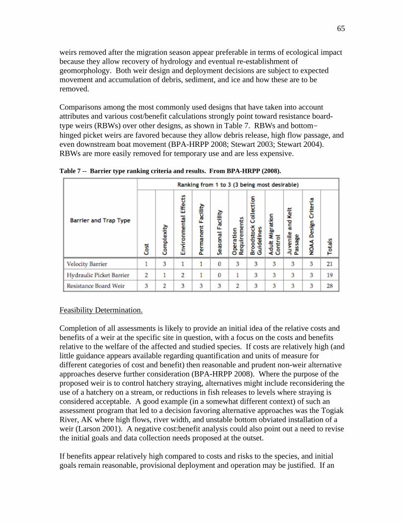
65

weirs removed after the migration season appear preferable in terms of ecological impact because they allow recovery of hydrology and eventual re-establishment of geomorphology. Both weir design and deployment decisions are subject to expected movement and accumulation of debris, sediment, and ice and how these are to be removed. Comparisons among the most commonly used designs that have taken into account attributes and various cost/benefit calculations strongly point toward resistance board-type weirs (RBWs) over other designs, as shown in Table 7. RBWs and bottom-hinged picket weirs are favored because they allow debris release, high flow passage, and even downstream boat movement (BPA-HRPP 2008; Stewart 2003; Stewart 2004). RBWs are more easily removed for temporary use and are less expensive. Table 7 -- Barrier type ranking criteria and results. From BPA-HRPP (2008).

Feasibility Determination. Completion of all assessments is likely to provide an initial idea of the relative costs and benefits of a weir at the specific site in question, with a focus on the costs and benefits relative to the welfare of the affected and studied species. If costs are relatively high (and little guidance appears available regarding quantification and units of measure for different categories of cost and benefit) then reasonable and prudent non-weir alternative approaches deserve further consideration (BPA-HRPP 2008). Where the purpose of the proposed weir is to control hatchery straying, alternatives might include reconsidering the use of a hatchery on a stream, or reductions in fish releases to levels where straying is considered acceptable. A good example (in a somewhat different context) of such an assessment program that led to a decision favoring alternative approaches was the Togiak River, AK where high flows, river width, and unstable bottom obviated installation of a weir (Larson 2001). A negative cost:benefit analysis could also point out a need to revise the initial goals and data collection needs proposed at the outset. If benefits appear relatively high compared to costs and risks to the species, and initial goals remain reasonable, provisional deployment and operation may be justified. If an

66

Operations and Maintenance Plan does not already exist, one should be developed. Monitoring, Surprises, and Adaptive Management. If a weir is the best alternative given goals and relative costs and benefits, it is generally acknowledged (although often overlooked) that provisional deployment include a monitoring component that assessed effectiveness using (admittedly nebulous) performance measures as discussed earlier. Capture efficiencies vary widely, even at the same facility. A floating board weir in Caspar Creek, CA operated for three years to capture coho and steelhead indicated 95% confidence limits for capture effectiveness of coho that were still 100% of the point estimates, whereas the variance about the steelhead estimates improved over time. The probable cause for the lack of precision may be a result of the flashy nature of Caspar Creek where stream flows overtopped and flowed around the weir during storm events, allowing fish to pass (Gallagher et al., unpublished). A similar floating board weir in Scott Creek, CA produced steelhead escapement estimates with 95% confidence limits in <20% of the point estimates over several years (Bond et al. 2008, P. B. Adams, pers. comm.). Among the surprises encountered at various facilities are equipment failure, water loss, flooding, disease transmission, and other unanticipated events that caused injury or mortality to listed species. Forced straying and shortstopping can actually shift spawning locales from upstream of a weir to downstream, suboptimal sites, especially for Chinook (A. Appleby, pers. comm.), making a previously ideal weir location ineffective in capturing spawning fish. Accurate assessment of capture efficiencies would reveal such unintended results and could necessitate opening the weir periodically during a run to make sure more wild fish passed through (while simultaneously permitting more hatchery origin or strays to pass upstream). Careful monitoring and recalculation of costs and benefits can thus lead to revisions in goals, design, the Operation and Maintenance Plan, and even weir location. BPA-HRPP (2008) referred to the process as “Define progress, provide accountability and track changes.”

Because weirs affect the geomorphology, hydrology, and biology of the stream ecosystem, attainment of stated goals and needed data (= project completion) would ideally result in removal of the weir and restoration of affected habitat, with additional monitoring of any impacts resulting from restoration efforts. Conclusion. One repeated observation in the literature on weirs is that each stream has unique physical and biological characteristics that vary among species and run times, all of which influence weir function. Thus each specific situation will vary regarding ecological effects and management benefits.

67

Meta-population issues when considering use of weirs to control hatchery straying An implicit assumption in the use of weirs to control straying of hatchery fish into natural spawning areas is that an effective weir can isolate the upstream natural population from the genetic and demographic effects of hatchery production. However, unless the natural population in question is also isolated from all other natural populations that themselves receive hatchery immigration, a natural population protected from direct hatchery straying by a weir may nonetheless be indirectly influenced by a hatchery through the hatchery’s effects on other natural populations. This issue is explored in detail elsewhere (McElhany, in prep), but several important points are highlighted here. McElhany (in prep) illustrated several scenarios in which a ‘wild fish sanctuary’ (WFS) is established with the goal of being maintained by natural production free from hatchery inputs (Figure 14). Scenario A involves a single WFS exchanging migrants with a single hatchery. Scenario B also involves a single WFS and single hatchery, but with the addition of a blocking weir where hatchery and wild fish could be sorted to filter migrants that enter the WFS. Scenario C is similar to Scenario A, but includes an external spawning sub-population. An external spawning sub-population refers to a group of fish spawning in the natural environment outside of the designated WFS. An external spawning sub-population could consist of both natural origin and hatchery origin fish and can exchange migrants with the WFS.

Scenario D is similar to Scenario C, but includes a weir for sorting fish migrating to the WFS. The hatchery-WFS-external spawning configurations (Scenarios C and D) are relatively common for existing and proposed WFS. The WFS proposed are often only a portion of a watershed, such as above a dam or convenient weir location, and allow free intermingling of wild and hatchery fish in other portions of the watershed, such as downstream of the dam or weir. Even when an entire watershed is designated a WFS, in some cases there is a demographic connection with neighboring watersheds where hatchery fish are not excluded.

68

Hatchery Wild FishSanctuary

HatcherySpawning

External toWFS

Wild FishSanctuary

HatcherySpawning

External WFSWild FishSanctuary

Weir

Hatchery Wild FishSanctuary

Weir

Scenario A

Scenario B

Scenario C

Scenario D

Figure 14 – Four scenarios describing the demographic and genetic relationship between a wild fish sanctuary, a hatchery, and (scenarios C and D) a natural spawning area that is not part of the sanctuary. Red arrows show straying or supplementation by hatchery fish. One important consequence of these demographic connections is that a sorting weir may not provide for an isolated WFS, even if all first generation hatchery fish can be excluded from WFS. There are often areas in the wild adjacent to the WFS where hatchery fish can spawn and the offspring of hatchery spawners can migrate to the WFS. Because these hatchery fish progeny were born in the wild, they have no hatchery markings and would be passed at a sorting weir as wild fish into the WFS. Depending on the number of hatchery spawners in the external spawning area, migration rates between the external spawning area and the WFS, etc., the hatchery can ultimately have a substantial demographic effect on the abundance of “wild” fish in the WFS. In fact, the existence of

69

ANY fish in the WFS can be totally dependant on hatchery production, even if there are no hatchery fish in the WFS (Figure 15).

Figure 15 -- Time series abundance of spawners in WFS (solid line) and external spawning (dashed line) sub-populations. There was no wild spawning in either the WFS or external spawning area in year one, only hatchery inputs. In year 50, hatchery production was abruptly halted resulting in collapse of the both the WFS and the external spawning sub-populations. The productivity in both the WFS and the external spawning area was assumed to be 0.85 (substantially below replacement). The total number of hatchery fish spawning in the external spawning area every generation was 550 (500 direct migrants to the external area and 50 additional redirected by the weir. The migration rate from the WFS to the external spawning area (and vice versa) was 15%. No hatchery fish were ever allowed to spawn in the WFS. The equilibrium number of fish in the WFS was 1,154 and in the external spawning area was 2,512. The total elimination of the WFS in the absence of the hatchery only occurs if the natural productivity of the WFS is less than replacement. However, even if the natural productivity of the WFS is above replacement and the population would be self-sustaining without the hatchery, the hatchery will still have an influence on the mean abundance and demographics of the WFS. In some cases, pseudo-isolation could make it extremely difficult to estimate the productivity in the WFS. The WFS will appear stable (assuming hatchery production is stable), implying productivities above replacement and a density dependent ceiling limiting population growth. But perception about both productivity and capacity could be wrong. Fitting recruitment curves to the WFS time series would be inappropriate because recruitment analysis is predicated on the assumption of a closed population, which would not be the case for a pseudo-isolated WFS. Monitoring considerations for a WFS are challenging – the monitoring program needs to provide data on the migration rates and other parameter values required to detect pseudo-isolation.

70

Pseudo-isolation also raises genetic concerns. One of the primary purposes in creating a WFS is to protect wild fish populations from the potential negative effects of domestication selection in the hatchery. The WFS is supposed to have very little exchange of genes with the hatchery, but the substantial demographic link between a hatchery and a pseudo-isolated WFS implies a substantial genetic link as well. Just because no first generation hatchery fish are observed spawning in the WFS does not mean that the WFS is free from the influence of hatchery domestication. Genetic models should be evaluated that consider the effects of meta-population structures on the fitness of fish in a WFS. Pseudo-isolation has implications for the design of WFS. If the goal for a WFS is to be truly isolated from hatchery effects (which may not be the case for all WFS), the WFS needs to be not only isolated from hatchery input but also from immigration from populations that themselves receive significant hatchery supplementation. The practice of "split basin management", where a weir or dam is used to exclude hatchery fish from the upper part of a watershed, but not the lower part is fairly common, but is exactly the situation likely to produce pseudo-isolation. Bisecting a demographic unit that is assumed to be fairly panmictic (such as a TRT defined population) will not produce an independent WFS. In contrast, migration rates among populations (which usually encompass entire watersheds) should be relatively low, so that a population-scale WFS is more likely to be largely isolated from indirect hatchery influence. This creates substantial practical challenges because it is often very difficult (or impossible) to create a sorting facility that controls an entire population. Building weirs across the mouth of a river may not be technically feasible and it may conflict with other management objectives. In conclusion, WFS, whether created by geographic isolation or weirs, will in many cases reduce genetic risks to wild populations compared to what they face now. However, there are some challenges in developing a truly isolated WFS. In particular, selective harvest alone is not likely to provide sufficient isolation without excessive mortality of wild fish. Isolation by distance or the construction of weirs will only work if implemented at an appropriate spatial scale. The physical presence of weirs or other sorting facilities presents its own habitat and management trade-offs. Neither isolation by harvest, distance or weirs prevents negative ecological interactions between hatchery and wild fish in mainstem and marine areas outside the WFS. Eliminating hatchery production can be effective in establishing a WFS and reducing outside ecological interactions, but may also entail significant societal costs. In the end, it is likely that some combination of selective harvest, appropriately sited and constructed sorting facilities and substantial reduction in hatchery production will be needed for the creation of effective WFS that allow for recovery of wild fish populations.

71

Application of hatchery reform to the Lower Columbia River In its review, the RIST was asked to focus on the Lower Columbia River Chinook salmon, since this ESU is subject to ongoing discussions regarding hatchery reform. In this section of the report, we attempt to apply some of the information and conclusions summarized above to bear on hatchery reform efforts for this ESU as proposed by the Hatchery Science Review Group (HSRG 2004). Recovery criteria for Lower Columbia River Chinook salmon populations have been developed by the Willamette and Lower Columbia River Technical Recovery Team (WLCRTRT) (McElhany et al. 2003; McElhany et al. 2004; McElhany et al. 2006) and, for Washington populations, incorporated into the Lower Columbia River Fish Recovery Board’s recovery plan (LCFRB 2004). Within the ESU, there are 32 populations categorized into several ‘strata’ based on their run timing and ecological characteristics. Most of the hatchery reform issues center on the 21 fall run (“tule”) populations, since most of these have and continue to be subject to high levels of hatchery production. These 21 populations are located in three ecological zones: coastal, Cascades, and Gorge. For fall Chinook populations, the recovery plan identifies “primary”, “contributing” and “stabilizing” populations, which have decreasingly stringent recovery criteria, requiring that the primary populations be distributed across the three ecological zones (Figure 16, top panel).

72

Figure 16 – Top panel: Goals for Lower Columbia River tule fall Chinook populations identified by the Lower Columbia River Fish Recovery Board (LCFRB 2004). Primary and primary* populations must be at low or very low risk of extinction and have minimal hatchery spawners. Bottom panel: recent (2001-2005 mean) percent hatchery origin spawners (Ford et al. 2007).

73

In its review of Lower Columbia River Chinook salmon hatchery programs, the HSRG noted that the current hatchery management situation is inconsistent with the recovery goals for many of the populations (HSRG 2004). In particular, a number of primary and contributing populations currently have fractions of stray hatchery fish among their spawning populations that are too high to be consistent with natural viability (Figure 16, lower panel). In addition, the HSRG noted that most of the Chinook salmon hatchery production in the Lower River is designed to maintain fisheries, and most of the programs are not managed in ways that promote natural population conservation. To reduce hatchery risks and promote recovery, while continuing to provide hatchery production to support fisheries, the HSRG made a number of specific and general recommendations, which we summarize below. The basic HSRG recommendations for fall Chinook salmon can be summarized as follows, and recommendations for specific populations are summarized in Table 8. For simplicity, we focus here only on fall Chinook salmon, but the HSRG also made recommendations for spring Chinook salmon populations, and similar issues and recommendations would apply to Lower Columbia River coho salmon as well.

• Reduce genetic risks to the primary and contributing populations by reducing or eliminating hatchery releases in those populations, increasing the proportion of natural origin fish in the broodstock of hatchery programs, using weirs to keep hatchery fish out of natural spawning areas, or a combination of these strategies.

• Use selective fisheries to increase or maintain harvest rates on hatchery fish and reduce harvest on natural fish.

• Improve habitat to increase natural production.

Table 8 -- Summary of HSRG recommendations for Lower Columbia River fall Chinook salmon populations

Strata State Population LCFRB Goal HSRG Recommendations

Coast Fall WA Grays P

-Small, temporary integrated hatchery program -New weir to reduce strays and collect broodstock -Reduce harvest impacts -Improve habitat

WA Elochomann P

-Small, temporary integrated hatchery program -Rebuild weir to reduce strays and collect broodstock -Reduce harvest impacts -Improve habitat

WA Mill/Abernathy/Germany C

- Change status to stabilizing (due to habitat type)

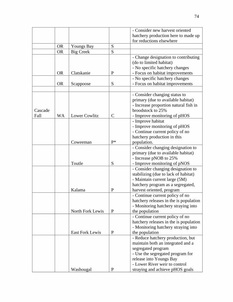
74

- Consider new harvest oriented hatchery production here to made up for reductions elsewhere

OR Youngs Bay S OR Big Creek S

OR Clatskanie P

- Change designation to contributing (do to limited habitat) - No specific hatchery changes - Focus on habitat improvements

OR Scappoose S - No specific hatchery changes - Focus on habitat improvements

Cascade Fall WA Lower Cowlitz C

- Consider changing status to primary (due to available habitat) - Increase proportion natural fish in broodstock to 25% - Improve monitoring of pHOS

Coweeman P*

- Improve habitat - Improve monitoring of pHOS - Continue current policy of no hatchery production in this population.

Toutle S

- Consider changing designation to primary (due to available habitat) - Increase pNOB to 25% - Improve monitoring of pNOS

Kalama P

- Consider changing designation to stabilizing (due to lack of habitat) - Maintain current large (5M) hatchery program as a segregated, harvest oriented, program

North Fork Lewis P

- Continue current policy of no hatchery releases in the is population - Monitoring hatchery straying into the population

East Fork Lewis P

- Continue current policy of no hatchery releases in the is population - Monitoring hatchery straying into the population

Washougal P

- Reduce hatchery production, but maintain both an integrated and a segregated program - Use the segregated program for release into Youngs Bay - Lower River weir to control straying and achieve pHOS goals

75

OR Sandy S

- Continue current policy of no hatchery releases in the is population - Monitoring hatchery straying into the population

Clackamas C - Change status to stabilizing due high hatchery strays

Gorge Fall WA Lower Gorge S - Manage as a stabilizing population

Upper Gorge (includes Wind) C - No recommendations

Big White Salmon C - Consider options to control pHOS

OR Hood S - Monitor strays and manage as stabilizing

The RIST did not think it would be useful to attempt a detailed review of the HSRG’s population-specific recommendations, since it is our understanding that these are considered more a starting point for discussion than a firm set of recommendations. Instead, we thought it would be more useful to discuss the more general recommendations in light of the information summarized in the rest of the report. HSRG recommendation: increase the genetic fitness of natural populations by limiting pHOS and increasing pNOB. For primary and contributing populations, have a PNI of 0.7 (primary) or 0.5 (contributing) for integrated hatchery programs, or pHOS of <0.05 (primary) or <0.10 (contributing) for segregated programs. We agree with the HSRG that the available scientific information, both theoretical and empirical, indicates that gene flow from hatchery populations into natural populations is likely to reduce natural population productivity, although no direct information is available on these effects on ocean-type fall Chinook salmon. Limiting natural spawning by hatchery origin fish should be an effective way to reducing these risks. The values of pHOS of 0.05 and 0.10 for primary and contributing populations associated with segregated program are arbitrary, and at least theoretically there could be significant genetic impacts at these rates (Ford 2002; Lynch & O'Hely 2001). However, in many cases achieving these proportions of hatchery fish in the natural Lower Columbia River fall Chinook salmon populations would be a large improvement over the current situation, so these thresholds seem reasonable as interim goals. Similarly, the PNI goals of 0.7 or 0.5 for integrated programs are also arbitrary, and may or may not be ultimately sufficiently protective to contribute to recovery of natural populations. We also strongly recommend caution about putting too much weight on the quantitative results of the AHA model that are used to make recommendations regarding how to achieve a particular PNI. In other words, we believe the general thrust of the HSRG recommendations are scientifically sound, but do not think that model incorporates enough information to accurately predict the outcomes of specific hatchery or habitat actions in a quantitative way.

76

Use of weirs to control pNOB and pHOS The idea of using weirs to control pHOS largely stems from two conflicting policy goals: protecting natural salmon populations from the deleterious effects of straying from hatchery populations, and maintaining sufficient hatchery production to contribute substantial number of hatchery fish to fisheries. We agree with the HSRG’s assessment that the current proportions of hatchery fish in many Lower Columbia River Chinook salmon populations are inconsistent with the goal of ESA recovery for this ESU as defined by TRT viability goals and existing recovery plans. Based on our review we also agree with the HSRG and other assessments (e.g., LCFRB 2004; Myers 1998) that current hatchery practices pose a long-term risk to natural Lower Columbia River salmon populations. Other factors, including habitat loss and degradation, are also clearly limiting the recovery of the ESU, however, and we made no attempt to determine which of these various factors is currently most limiting to recovery. Whether or not weirs or other fish sorting barriers can be an effective tool for threading the needle of conflicting policy goals remains to be seen, and in many cases will depend on the details of how such an approach is implemented. It is beyond the scope of this report to review in detail each of the proposed weirs in the Lower Columbia River or elsewhere, but the section above describes some of the implementation issues that should be considered. Due to the potential for pseudo-isolation, the potential negative ecological effects of weirs, the potential for weir failure, and the labor intensive nature using weirs to control fish movement, we suggest that more passive measures, such as geographic isolation of hatchery programs from key natural populations, would be preferable to weirs if such measures can be effectively implemented. In some cases weirs may be the best management alternative, however. One limitation of the “maintain production and control straying using weirs” approach is that it does not address risks from ecological interactions between hatchery and natural fish that occur downstream of the weirs. As we discussed in the section on ecological risks above, there is some evidence for density dependent survival of salmon in the ocean. The continued release of millions of hatchery produced salmonids in the Lower Columbia River and nearby coastal areas therefore may have a significant negative effect on natural salmon productivity, although as far we know this effect has not been quantified. Obtaining good estimates of any relationship between natural population survival and Lower River hatchery releases should therefore be a high research priority.

77

References Anderson, E., H. M. Engelking, E. J. Emmenegger, and G. Kurath. 2000. Molecular

Epidemiology Reveals Emergence of a Virulent Infectious Hematopoietic Necrosis (IHN) Virus Strain in Wild Salmon and Its Transmission to Hatchery Fish. Journal of Aquatic Animal Health 12:85-99.

Araki, H., W. Ardren, E. Olsen, B. Cooper, and M. Blouin. 2007a. Reproductive success of captive-bred steelhead trout in the wild: evaluation of three hatchery programs in the Hood River. Conservation Biology 21:181-190.

Araki, H., B. A. Berejikian, M. J. Ford, and M. S. Blouin. 2008. Fitness of hatchery-reared salmonids in the wild. Evolutionary Applications 1:342-355.

Araki, H., B. Cooper, and M. S. Blouin. 2007b. Genetic effects of captive breeding cause a rapid, cumulative fitness decline in the wild. Science 318:100-103.

Arnold, S. J., and M. J. Wade. 1984. On the Measurement of Natural and Sexual Selection - Theory. Evolution 38:709-719.

Bakke, T. A., and P. D. Harris. 1998. Diseases and parasites in wild Atlantic salmon (Salmo salar) populations. Canadian Journal of Fisheries and Aquatic Sciences 55:247-266.

Bartz, K. K., K. M. Lagueux, M. D. Scheuerell, T. Beechie, A. D. Haas, and M. H. Ruckelshaus. 2006. Translating restoration scenarios into habitat conditions: an initial step in evaluating recovery strategies for Chinook salmon (Oncorhynchus tshawytscha). Canadian Journal of Fisheries and Aquatic Sciences 63:1578-1595.

Beacham, T. D., and C. B. Murray. 1990. Temperature, Egg Size, and Development of Embryos and Alevins of 5 Species of Pacific Salmon - a Comparative-Analysis. Transactions of the American Fisheries Society 119:927-945.

Beamish, R. J., C. Mahnken, and C. M. Neville. 1997. Hatchery and wild production of Pacific salmon in relation to large-scale, natural shifts in the productivity of the marine environment. ICES Journal of Marine Science 54:963-964.

Beamish, R. J., R. M. Sweeting, K. L. Lange, and C. M. Neville. 2008. Changes in the population ecology of hatchery and wild coho salmon in the Strait of Georgia. Transactions of the American Fisheries Society 137:503-520.

Berejikian, B., and M. J. Ford. 2004. Review of relative fitness of hatchery and natural salmon. U.S. Dept. Commer., NOAA Tech. Memo. NMFS-NWFSC-61, 28 p.

Berejikian, B. A., E. P. Tezak, and A. L. LaRae. 2000. Female mate choice and spawning behaviour of chinook salmon under experimental conditions. Journal of Fish Biology 57:647-661.

Berejikian, B. A., E. P. Tezak, L. Park, E. LaHood, S. L. Schroder, and E. Beall. 2001. Male competition and breeding success in captively reared and wild coho salmon (Oncorhynchus kisutch). Canadian Journal of Fisheries and Aquatic Sciences 58:804-810.

Berejikian, B. A., D. M. Van Doornik, J. A. Scheurer, and R. Bush. 2008. Reproductive behavior and relative reproductive success of natural- and hatchery-origin Hood

78

Canal summer chum salmon (Oncorhynchus keta). Canadian Journal of Fisheries and Aquatic Sciences, in press.

BOR. 2006. (Bureau of Reclamation) Fish Protection at Water Diversions; a Guide for planning and Designing Fish Exclusion Facilities. Water Resources Technical Publication Denver, Colorado. .

BPA-HRPP. 2008. Revised Master Plan for the Hood River Production Program. Technical Report 2008. DOE/BP-P106494.

Bradford, M. J., G. C. Taylor, and J. A. Allan. 1997. Empirical review of Coho salmon smolt abundance and the prediction of smolt production at the regional level. Transactions Of The American Fisheries Society 126:49-64.

Brannon, E. 1987. Mechanisms stabilizing salmonid fry emergence timing. Canadian Special Publication of Fisheries and Aquatic Sciences 96:120-124.

Brodeur, R. D., E. A. Daly, M. V. Sturdevant, T. W. Miller, J. H. Moss, M. Thiess, M. Trudel, L. A. Weitkamp, J. L. Armstrong, and C. Norton. 2007. Regional comparisons of juvenile salmon feeding in coastal marine waters off of the west coast on North America. American Fisheries Society Symposium 57:183-203.

Brooks, K. M., and S. R. M. Jones. 2008. Perspectives on Pink Salmon and Sea Lice: Scientific Evidence Fails to Support the Extinction Hypothesis. Reviews in Fisheries Science 16:403-412.

Brooks, K. M., and D. J. Stucchi. 2006. The effects of water temperature, salinity and currents on the survival and distribution of the infective copepodid stage of the salmon louse (Lepeophtheirus salmonis) originating on Atlantic salmon farms in the Broughton Archipelago of British Columbia, Canada (Brooks, 2005) - A response to the rebuttal of Krkosek et al. (2005a). Reviews in Fisheries Science 14:13-23.

Busack, C. in prep. Evaluation of the proportionate natural influence (PNI) concept, a tool for managing integrated hatchery programs (in prep).

Busack, C. A., K. P. Currens, T. N. Pearsons, and L. Mobrand. 2005a. Tools for evaluating ecological and genetic risks in hatchery programs. Report to Bonneville Power Administration, publication DOE/ BP-00016399-1, Portland, Oregon.

Busack, C. A., K. P. Currens, T. N. Pearsons, and L. Mobrand. 2005b. Tools for evaluating ecological and genetic risks in hatchery programs. Report to Bonneville Power Administration, publication DOE/ BP-00016399-1, Portland, Oregon.

Butler, J. R. A. 2002. Wild salmonids and sea louse infestations on the west coast of Scotland: sources of infection and implications for the management of marine salmon farms. Pest Management Science 58:595-608.

Chilcote, M. W. 2003. Relationship between natural productivity and the frequency of wild fish in mixed spawning populations of wild and hatchery steelhead (Oncorhynchus mykiss). Canadian Journal of Fisheries and Aquatic Sciences 60:1057-1067.

Chittenden, C. M., S. Sura, K. G. Butterworth, K. F. Cubitt, N. P. Manel-La, S. Balfry, F. Okland, and R. S. McKinley. 2008. Riverine, estuarine and marine migratory behaviour and physiology of wild and hatchery-reared coho salmon

79

Oncorhynchus kisutch (Walbaum) smolts descending the Campbell River, BC, Canada. Journal of Fish Biology 72:614-628.

Collis, K., R. E. Beaty, and B. R. Crain. 1995. Changes in catch rate and diet of northern squawfish associated with the release of hatchery-reared juvenile salmonids in a Columbia River reservoir. North American Journal of Fisheries Management 15:346-357.

Crow, J. F. 1958. Some possibilities for measuring selection intensities in man. Human Biology 30:1-13.

CTC. 2007. Pacific Salmon Commission Joint Chinook Technical Committee Report. Annual report on catch, escapement, exploitation rate analysis and model calibration of Chinook salmon under Pacific Salmon Commission Jurisdiction, 2006. Report TCCHINOOK (07)-1. January 30, 2007. Available at www.psc.org.

Cushing, D. H. 1973. Dependence of recruitment on parent stock. Journal of the Fisheries Research Board, Canada 30:1965-1976.

Dannewitz, J., E. Petersson, T. Prestegaard, and T. Järvi. 2003. Effects of sea-ranching and family background on fitness traits in brown trout Salmo trutta reared under near-natural conditions. Journal of Applied Ecology 40:241-250.

de Leaniz, C. G. 2008. Weir removal in salmonid streams: implications, challenges and practicalities. Hydrobiologia 609:83-96.

Dickerson, B., K. Brinck, M. Willson, P. Bentzen, and T. Quinn. 2005. Relative importance of salmon body size and arrival time at breeding grounds to reproductive success. Ecology 86:347-353.

Einum, S., G. Robertsen, and I. A. Fleming. 2008. Adaptive landscapes and density-dependent selection in declining salmonid populations: going beyond numerical responses to human disturbance. Evolutionary Applications 1:239-251.

Farmer, G. J. 1994. Some Factors Which Influence the Survival of Hatchery Atlantic Salmon (Salmo-Salar) Smolts Utilized for Enhancement Purposes. Aquaculture 121:223-233.

Fast, D. E., D. Neeley, D. T. Lind, M. V. Johnston, C. R. Strom, W. J. Bosch, C. M. Knudsen, S. L. Schroder, and B. D. Watson. 2008. Survival Comparison of Spring Chinook Salmon Reared in a Production Hatchery under Optimum Conventional and Seminatural Conditions. Transactions of the American Fisheries Society 137:1507-1518.

Fausch, K. D., B. E. Rieman, M. K. Young, and J. B. Dunham. 2006. Strategies for Conserving Native Salmonid Populations at Risk From Nonnative Fish Invasions: Tradeoffs in Using Barriers to Upstream Movement. General Technical Report RMRS-GTR-174 Fort Collins, CO: U.S. Department of Agriculture, Forest Service, Rocky Mountain Research Station. 44 p.

Fisher, J., M. Trudel, A. Ammann, J. A. Orsi, J. Piccolo, C. Bucher, E. Casillas, J. A. Harding, R. B. MacFarlane, R. D. Brodeur, J. F. T. Morris, and D. W. Welch. 2007. Comparisons of the Coastal Distributions and Abundances of Juvenile Pacific Salmon from Central California to the Northern Gulf of Alaska American Fisheries Society Symposium 57:31-80.

80

Fleming, I. A., and M. R. Gross. 1989. Evolution of adult female life history and morphology in a Pacific salmon (coho: Oncorhynchus kisutch ). Evolution 43:141-157.

Fleming, I. A., and M. R. Gross. 1992. Reproductive behavior of hatchery and wild coho salmon ( Oncorhynchus kisutch ): does it differ? Aquaculture 103:101-121.

Fleming, I. A., and M. R. Gross. 1993. Breeding success of hatchery and wild coho salmon (Oncorhynchus kisutch ) in competition. Ecological Applications 3:230-245.

Fleming, I. A., and M. R. Gross. 1994. Breeding competition in a Pacific Salmon (coho: Oncorhynchus kisutch): measures of natural and sexual selection. Evolution 48:637-657.

Fleming, I. A., K. Hindar, I. B. Mjolnerod, B. Jonsson, T. Balstad, and A. Lamberg. 2000. Lifetime success and interactions of farm salmon invading a native population. Proceedings of the Royal Society, Series B Biology 267:1517-1523.

Fleming, I. A., B. Jonsson, M. R. Gross, and A. Lamberg. 1996. An experimental study of the reproductive behavior and success of farmed and wild Atlantic salmon. Journal of Applied Ecology 33:893-905.

Fleming, I. A., A. Lamberg, and B. Jonsson. 1997. Effects of early experience on the reproductive performance of Atlantic salmon. Behavioral Ecology 8:470-480.

Foote, C. J. 1990. An Experimental Comparison of Male and Female Spawning Territoriality in a Pacific Salmon. Pages 283-314.

Ford, J. S., and R. A. Myers. 2008. A global assessment of salmon aquaculture impacts on wild salmonids. Plos Biology 6:411-417.

Ford, M., H. Fuss, B. Boelts, E. LaHood, J. Hard, and J. Miller. 2006. Changes in run timing and natural smolt production in a naturally spawning coho salmon (Oncorhynchus kisutch) population after 60 years of intensive hatchery supplementation. Canadian Journal of Fisheries and Aquatic Sciences 63:2343-2355.

Ford, M., J. J. Hard, B. Boelts, E. Lahood, and J. Miller. 2008. Estimates of natural selection in a salmon population in captive and natural environments. Conservation Biology 22:783-794.

Ford, M., N. Sands, P. McElhany, R. Kope, D. Simmons, and P. Dygert. 2007. Analyses to support a review of an ESA jeopardy consultation on fisheries impacting Lower Columbia River tule Chinook salmon. National Marine Fisheries Service Northwest Fisheries Science Center and Northwest Regional Office, Seattle, WA. October 5, 2007. .

Ford, M. J. 2002. Selection in captivity during supportive breeding may reduce fitness in the wild. Conservation Biology 16:815-825.

Ford, M. J., P. Budy, C. Busack, D. Chapman, T. Cooney, T. Fisher, J. Geiselman, T. Hillman, J. Lukas, C. Peven, C. Toole, E. Weber, and P. Wilson. 2001. Upper Columbia River Steelhead and Spring Chinook Salmon Population Structure and Biological Requirements, Final report. Northwest Fisheries Science Center, Seattle, WA.

Gee, A. S., N. J. Milner, and R. J. Hemsworth. 1978. Effect of Density on Mortality in Juvenile Atlantic Salmon (Salmo-Salar). Journal of Animal Ecology 47:497-505.

81

Geiger, H. J., W. W. Smoker, L. A. Zhivotovsky, and A. J. Gharrett. 1997. Variability of family size and marine survival in pink salmon (Oncorhynchus gorbuscha) has implications for conservation biology and human use. Canadian Journal Of Fisheries And Aquatic Sciences 54:2684-2690.

Gilbert, M. A., and W. O. Granath. 2003. Whirling disease of salmonid fish: life cycle, biology, and disease. Journal of Parasitology 89:658-667.

Goede, R. W. 1986. Management considerations in stocking of diseased or carrier fish. Pages 349-355 in R.H. Stroud, ed. Fish culture in fisheries management. American Fisheries Society, Bethesda, Maryland.

Good, T. P., M. M. McClure, B. P. Sandford, K. A. Barnas, D. M. Marsh, B. A. Ryan, and E. Casillas. 2007. Quantifying the effect of Caspian Tern predation on threatened and endangered Pacific salmon in the Columbia River. Endangered Species Research 3:11-21.

Groot, C., and L. Margolis, editors. 1991. Pacific Salmon Life Histories. University of British Columbia Press, Vancouver, B.C.

Gross, M. R. 1985. Disruptive selection for alternative life histories in salmon. Nature 313:47-48.

Hard, J. J. 2004. Evolution of chinook salmon life history under size-selective harvest. Pages 315-337 in A. P. Hendry, and S. C. Stearns, editors. Evolution Illuminated. Salmon and their relatives. Oxford University Press, New York.

Harford, W. J., and R. L. McLaughlin. 2007. Understanding uncertainty in the effect of low-head dams on fishes of great lakes tributaries. Ecological Applications 17:1783-1796.

Hargreaves, N. B., and R. J. Lebrasseur. 1986. Size Selectivity of Coho (Oncorhynchus-Kisutch) Preying on Juvenile Chum Salmon (Oncorhyncus-Keta). Canadian Journal of Fisheries and Aquatic Sciences 43:581-586.

Hawkins, S. W., and J. M. Tipping. 1999. Predation by juvenile hatchery salmonids on wild fall chinook salmon fry in the Lewis River, Washington. California Fish and Game 85:124-129.

Healey, M. C. 1983. Coastwide distribution and ocean migration patterns of stream- and ocean-type chinook salmon, Oncorhynchus tshawytscha. Canadian Field-Naturalist 97:427-433.

Healey, M. C. 1991. The life history of chinook salmon (Oncorhynchus tshawytscha) in C. Groot, and L. Margolis, editors. Life history of Pacific salmon. University of British Columbia Press, Vancouver, B.C.

Healey, M. C. 2001. Patterns of gametic investment by female stream- and ocean-type chinook salmon. Journal of Fish Biology 58:1545-1556.

Heard, W. R. 1991. Life history of pink salmon (Oncorhynchus gorbuscha) in C. Groot, and L. Morgolis, editors. Pacific salmon life histories. UBC Press, Vancouver, B.C.

Heath, D. D., J. W. Heath, C. A. Bryden, R. M. Johnson, and C. W. Fox. 2003. Rapid evolution of egg size in captive salmon. Science 299:1738-1740.

Hendry, A. P., J. E. Hensleigh, and R. R. Reisenbichler. 1998. Incubation temperature, developmental biology, and the divergence of sockeye salmon (Oncorhynchus nerka) within Lake Washington. Canadian Journal of Fisheries and Aquatic Sciences 55:1387-1394.

82

Hilborn, R., and D. Eggers. 2000. A review of the hatchery programs for pink salmon in Prince William Sound and Kodiak Island, Alaska. Transactions of the American Fisheries Society 129:333–350.

Hodgson, S., and T. P. Quinn. 2002. The timing of adult sockeye salmon migration into fresh water: adaptations by populations to prevailing thermal regimes. Canadian Journal of Zoology-Revue Canadienne De Zoologie 80:542-555.

Hoekstra, J. M., K. K. Bartz, M. H. Ruckelshaus, J. M. Moslemi, and T. K. Harms. 2007. Quantitative threat analysis for management of an imperiled species-Chinook salmon (Oncorhynchus tshawytscha). Ecological Applications 17:2061-2073.

Hoffnagle, T. L., R. W. Carmichael, K. A. Frenyea, and P. J. Keniry. 2008. Run timing, spawn timing, and spawning distribution of hatchery- and natural-origin spring Chinook salmon in the Imnaha River, Oregon. North American Journal of Fisheries Management 28:148-164.

Homel, K., P. Budy, M. E. Pfrender, T. A. Whitesel, and K. Mock. 2008. Evaluating genetic structure among resident and migratory forms of bull trout (Salvelinus confluentus) in Northeast Oregon. Ecology Of Freshwater Fish 17:465-474.

HSRG. 2004. Hatchery Reform: Principles and Recommendations of the Hatchery Scientific Review Group.

Hume, J. M. B., and E. A. Parkinson. 1987. Effect of Stocking Density on the Survival, Growth, and Dispersal of Steelhead Trout Fry (Salmo-Gairdneri). Canadian Journal of Fisheries and Aquatic Sciences 44:271-281.

Jepsen, N., E. Holthe, and F. Okland. 2006. Observations of predation on salmon and trout smolts in a river mouth. Fisheries Management and Ecology 13:341-343.

Keeley, E. R. 2001. Demographic responses to food and space competition by juvenile steelhead trout. Ecology 82:1247-1259.

Kinnison, M., M. Unwin, N. Boustead, and T. Quinn. 1998a. Population-specific variation in body dimensions of adult chinook salmon (Oncorhynchus tshawytscha) from New Zealand and their source population, 90 years after introduction. Canadian Journal of Fisheries and Aquatic Sciences 55:554-563.

Kinnison, M. T., M. J. Unwin, W. K. Hershberger, and T. P. Quinn. 1998b. Egg size, fecundity and early development rate of two New Zealand chinook salmon (Oncorhynchus tshawytscha) populations, with a comparison to their ancestral Sacramento River population. Canadian Journal of Fisheries and Aquatic Sciences 55:1946-1953.

Konecki, J. T., C. A. Woody, and T. P. Quinn. 1995. Influence of Temperature on Incubation Rates of Coho Salmon (Oncorhynchus-Kisutch) from 10 Washington Populations. Northwest Science 69:126-132.

Koski, K. v. 1975. The survival and fitness of two stocks of chum salmon (Oncorhynchus keta) from egg deposition to emergence in a controlled-stream environment at Big Beef Creek. Page 212. University of Washington, Seattle.

Kostow, K., A. Marshall, and S. Phelps. 2003. Naturally spawning hatchery steelhead contribute to smolt production but experience low reproductive success. Transactions of the American Fisheries Society 132:780-790.

Kostow, K. E. 2008. Factors that contribute to the ecological risks of salmon and steelhead hatchery programs and some mitigating strategies. Reviews in Fish Biology and Fisheries.

83

Kostow, K. E., and S. J. Zhou. 2006. The effect of an introduced summer steelhead hatchery stock on the productivity of a wild winter steelhead population. Transactions of the American Fisheries Society 135:825-841.

Krkosek, M., J. S. Ford, A. Morton, S. Lele, and M. A. Lewis. 2008a. Response to Comment on "Declining Wild Salmon Populations in Relation to Parasites from Farm Salmon". Science 322.

Krkosek, M., J. S. Ford, A. Morton, S. Lele, and M. A. Lewis. 2008b. Sea Lice and Pink Salmon Declines: A Response to Brooks and Jones (2008). Reviews in Fisheries Science 16:413-436.

Krkosek, M., J. S. Ford, A. Morton, S. Lele, R. A. Myers, and M. A. Lewis. 2007. Declining wild salmon populations in relation to parasites from farm salmon. Science 318:1772-1775.

Krkosek, M., M. A. Lewis, and J. P. Volpe. 2005. Transmission dynamics of parasitic sea lice from farm to wild salmon. Proceedings of the Royal Society B-Biological Sciences 272:689-696.

Kuligowski, D. R., M. J. Ford, and B. A. Berejikian. 2005. Breeding structure of steelhead inferred from patterns of genetic relatedness among nests. Transactions Of The American Fisheries Society 134:1202-1212.

Lande, R. 1976. Natural selection and random genetic drift in phenotypic evolution. Evolution 30:314-334.

Larsen, D., B. Beckman, K. Cooper, D. Barrett, M. Johnston, P. Swanson, and W. Dickhoff. 2004. Assessment of high rates of precocious male maturation in a spring Chinook salmon supplementation hatchery program Transactions of the American Fisheries Society 133:98-120.

Larson, J. 2001. Togiak River Salmon Weir Phase I-- Weir Feasibility Study Togiak National Wildlife Refuge, Alaska. Alaska Fisheries Progress Report 2001-01.

Lawson, P. W., and D. B. Sampson. 1996. Gear-related mortality in selective fisheries for ocean salmon. North American Journal of Fisheries Management 16:512-520.

LCFRB. 2004. Lower Columbia Fish Recovery and Fish and Wildlife Subbasin Plan. Available at: http://www.lcfrb.gen.wa.us/default1.htm.

Leider, S. A., P. L. Hulett, J. J. Loch, and M. W. Chilcote. 1990. Electrophoretic comparison of the reproductive success of naturally spawning transplanted and wild steelhead trout through the returning adult stage. Aquaculture 88:239-252.

Leth, B. D. 2005. Reproductive success of hatchery and natural origin Chinook salmon (Oncorhynchus tshawytscha) in a stream with a history of supplementation management. University of Idaho, Moscow, Idaho.

Levin, P. S., and J. G. Williams. 2002. Interspecific effects of artificially propagated fish: an additional conservation risk for salmon. Conservation Biology 16:1581-1587.

Levin, P. S., R. W. Zabel, and J. G. Williams. 2001. The road to extinction is paved with good intentions: negative associations of fish hatcheries with threatened salmon. Proc. Royal. Soc. Lond. B. 268:1153-1158.

Levins, R. 1966. The strategy of model building in population biology. American Scientist 54:421-431.

Lynch, M., and H. O'Hely. 2001. Captive breeding and the genetic fitness of natural populations. Conservation Genetics 2:363-378.

84

McClure, M., R. W. Zabel, T. Cooney, H. Schaller, C. Petrosky, P. Howell, P. Hassemer, and C. Baldwin. 2007. Assessing the Impact of Climate and Hydropower on Population Productivity for Interior Columbia River Stream-type Chinook and Steelhead Populations. 92pp with figures. http://www.nwfsc.noaa.gov/trt/trt_documents/matrix_model_3.3.pdf.

McElhany, P., T. Backman, B. Busack, S. Heppell, S. Kolmes, A. Maule, J. Myers, D. Rawding, D. Shively*, A. Steel, C. Steward, and T. Whitesel. 2003. INTERIM REPORT ON VIABILITY CRITERIA FOR WILLAMETTE AND LOWER COLUMBIA BASIN PACIFIC SALMONIDS WILLAMETTE/LOWER COLUMBIA TECHNICAL RECOVERY TEAM. Northwest Fisheries Science Center, Seattle.

McElhany, P., T. Backman, C. Busack, S. Kolmes, J. Myers, D. Rawding, A. Steel, C. Steward, T. Whitesel, and C. Willis. 2004. Status evaluation of salmon and steelhead populations in the Willamette and Lower Columbia River Basins. Available at http://www.nwfsc.noaa.gov/trt/wlc_docs/wlc_pop_eval_7_28_04.pdf.

McElhany, P., C. Busack, M. Chilcote, S. Kolmes, B. McIntosh, J. Myers, D. Rawding, A. Steel, C. Steward, D. Ward, T. Whitesel, and C. Willis. 2006. Revised viability criteria for salmon and steelhead in the Willamette and Lower Columbia Basins. Review draft. April 1, 2006. Available at http://www.nwfsc.noaa.gov/trt/wlc_docs/Revised_WLC_Viability_Criteria_Draft_Apr_2006.pdf.

McGinnity, P., Stone, C., Taggart, J.B., Cooke, D., Cotter, D., Hynes, R., McCamley, C., Cross, T. and A. Ferguson. 1997. Genetic impact of escaped farmed Atlantic salmon (Salmo salar L.) on native populations: use of DNA profiling to assess freshwater performance of wild, farmed and hybrid progeny in a natural river environment. J. Marine Sci. 54:in press.

McVicar, A. H. 1997. Disease and parasite implications of the coexistence of wild and cultured Atlantic salmon populations. Ices Journal of Marine Science 54:1093-1103.

Miyakoshi, Y., M. Nagata, and S. Kitada. 2001. Effect of smolt size on postrelease survival of hatchery-reared masu salmon Oncorhynchus masou. Fisheries Science 67:134-137.

Moran, P., and R. S. Waples. 2007. Monitor and evaluate the genetic characteristics of supplemented salmon and steelhead. Project number 1989-096-00. Research Progress Report Oct 5, 2007. Report to Bonneville Power Administration. Available at: http://pisces.bpa.gov/release/documents/documentviewer.aspx?doc=P107430.

Murdoch, A., T. Pearsons, T. Maitland, M. Ford, and K. Williamson. 2007. Monitoring the reproductive success of naturally spawning hatchery and natural spring Chinook salmon in the Wenatchee River. BPA Project No. 2003-039-00. Bonneville Power Administration, Portland, Oregon. Department of Energy, Bonneville Power Administration.

Murdoch, A., T. Pearsons, T. Maitland, M. Ford, and K. Williamson. 2008. Monitoring the reproductive success of naturally spawning hatchery and natural spring Chinook salmon in the Wenatchee River. BPA Project No. 2003-039-00.

85

Bonneville Power Administration, Portland, Oregon. Available at http://pisces.bpa.gov/release/documents/documentviewer.aspx?doc=P106770. Department of Energy, Bonneville Power Administration.

Murray, C. B., T. D. Beacham, and J. D. McPhail. 1990. Influence of Parental Stock and Incubation-Temperature on the Early Development of Coho Salmon (Oncorhynchus-Kisutch) in British-Columbia. Canadian Journal of Zoology-Revue Canadienne De Zoologie 68:347-358.

Myers, J. M., and 10 others. 1998. Status review of chinook salmon from Washington, Idaho, Oregon and California. NOAA Technical Memorandum NMFS-NWFSC-35.

Nickelson, T. E. 2003. The influence of hatchery coho salmon (Oncorhynchus kisutch) on the productivity of wild coho salmon populations in Oregon coastal basins. Canadian Journal of Aquatic and Fisheries Sciences 60:1050-1056.

Nickelson, T. E., M. F. Solazzi, and S. L. Johnson. 1986. Use of hatchery coho salmon ( Oncorhynchus kisutch ) presmolts to rebuild wild populations in Oregon coastal streams. Canadian Journal of Fisheries and Aquatic Sciences 43:2443-2449.

NMFS. 2008. Anadromous Salmonid Passage Facility Design. NMFS, Northwest Region, Portland, Oregon.

NRC. 2004. (National Research Council) Endangered and threatened fishes in the Klamath River basin: causes of decline and strategies for recovery. Washington, DC: National Academies Press.

O'Connor, J. P., D. J. O'Mahony, J. M. O'Mahony, and T. J. Gienane. 2006. Some impacts of low and medium head weirs on downstream fish movement in the Murray-Darling Basin in southeastern Australia. Ecology Of Freshwater Fish 15:419-427.

Parker, R. 1971. Size selective predation among juveniles salmonid fishes in a British Columbia inlet. Journal of the Fisheries Research Board, Canada 28:1503-1510.

Pearsons, T. N. 2008. Misconception, reality, and uncertainty about ecological interactions and risks between hatchery and wild salmonids. Fisheries 33:278-290.

Peterman, R. M. 1991. Density-dependent marine processes in North Pacific salmonids: lessons for experimental design of large-scale manipulations of fish stocks. ICES Marine Science Symposium 192:69–77.

Peterson, D. P., B. E. Rieman, J. B. Dunham, K. D. Fausch, and M. K. Young. 2008. Analysis of trade-offs between threats of invasion by nonnative brook trout (Salvelinus fontinalis) and intentional isolation for native westslope cutthroat trout (Oncorhynchus clarkii lewisi). Canadian Journal Of Fisheries And Aquatic Sciences 65:557-573.

Poulet, N. 2007. Impact of weirs on fish communities in a piedmont stream. River Research And Applications 23:1038-1047.

Pritchard, V. L., K. Jones, and D. E. Cowley. 2007. Genetic diversity within fragmented cutthroat trout populations. Transactions Of The American Fisheries Society 136:606-623.

PSTRT. 2005. Review of the "All-H-Analyzer" model. Puget Sound Technical Recovery Team.

86

Quinn, T. P. 2005. The behavior and ecology of Pacific salmon & trout. American Fisheries Society, Bethesda, Maryland.

Quinn, T. P., M. D. Adkinson, and M. B. Ward. 1996. Behavioral tactics of male sockeye salmon (Oncorhynchus nerka) under varying operational sex ratios. Ethology 102:304-322.

Quinn, T. P., and G. B. Buck. 2001. Size- and sex-selective mortality of adult sockeye salmon: bears, gulls, and fish out of water. Transactions of the American Fisheries Society 130:995-1005.

Quinn, T. P., A. P. Hendry, and G. B. Buck. 2001a. Balancing natural and sexual selection in sockeye salmon: interactions between body size, reproductive opportunity and vulnerability to predation by bears. Evolutionary Ecology Research 3:917-937.

Quinn, T. P., J. A. Peterson, V. F. Gallucci, W. K. Hershberger, and E. L. Brannon. 2002. Artificial selection and environmental change: countervailing factors affecting the timing of spawning by coho and chinook salmon. Transactions of the American Fisheries Society 131:591-598.

Quinn, T. P., L. Wetzel, S. Bishop, K. Overberg, and D. E. Rogers. 2001b. Influence of breeding habitat on bear predation and age at maturity and sexual dimorphism of sockeye salmon populations. Canadian Journal of Zoology 79:1782-1793.

Reinhardt, U. G., T. Yamamoto, and S. Nakano. 2001. Effects of body size and predators on intracohort competition in wild and domesticated juvenile salmon in a stream. Ecological Research 16:327-334.

Reisenbichler, R. R., and J. D. McIntyre. 1977. Genetic differences in growth and survival of juvenile hatchery and wild steelhead trout, Salmo gairdneri. Journal of the Fisheries Research Board of Canada 34:123-128.

Reisenbichler, R. R., S. P. Rubin, L. Wetzel, and S. R. Phelps. 2004. Natural selection after release from a hatchery leads to domestication in steelhead, Oncorhynchus mykiss. Chapter 27 in K. M. Leber, H. L. Blankenship, and S. Kitada, editors. Stock enhancement and sea ranching, II. Blackwell Scientific Publications, Oxford, UK.

Riddell, B. E., R. J. Beamish, L. J. Richards, and J. R. Candy. 2008. Comment on "Declining Wild Salmon Populations in Relation to Parasites from Farm Salmon". Science 322.

Robison, B. D., P. A. Wheeler, K. Sundin, P. Sikka, and G. H. Thorgaard. 2001. Composite interval mapping reveals a major locus influencing embryonic development rate in rainbow trout (Oncorhynchus mykiss). Journal of Heredity 92:16-22.

Robison, B. D., P. A. Wheeler, and G. H. Thorgaard. 1999. Variation in development rate among clonal lines of rainbow trout (Oncorhynchus mykiss). Aquaculture 173:131-141.

Roff, D. A. 1997. Evolutionary quantitative genetics. Chapman and Hall, New York. Roni, P., T. Bennett, S. Morley, G. R. Pess, K. Hanson, D. Van Slyke, and P. Olmstead.

2006. Rehabilitation of bedrock stream channels: The effects of boulder weir placement on aquatic habitat and biota. River Research And Applications 22:967-980.

87

Ruggerone, G. T., E. Farley, J. Nielsen, and P. Hagen. 2005. Seasonal marine growth of Bristol Bay sockeye salmon (Oncorhynchus nerka) in relation to competition with Asian pink salmon (O-gorbuscha) and the 1977 ocean regime shift. Fishery Bulletin 103:355-370.

Ruggerone, G. T., and F. A. Goetz. 2004. Survival of Puget Sound chinook salmon (Oncorhynchus tshawytscha) in response to climate-induced competition with pink salmon (Oncorhynchus gorbuscha). Canadian Journal of Fisheries and Aquatic Sciences 61:1756-1770.

Ruggerone, G. T., and D. E. Rogers. 1992. Predation on Sockeye Salmon Fry by Juvenile Coho Salmon in the Chignik Lakes, Alaska: Implications for Salmon Management. North American Journal of Fisheries Management 12:87-102.

Ruggerone, G. T., M. Zimmermann, K. W. Myers, J. L. Nielsen, and D. E. Rogers. 2003. Competition between Asian pink salmon (Oncorhynchus gorbuscha) and Alaskan sockeye salmon (O-nerka) in the North Pacific Ocean. Fisheries Oceanography 12:209-219.

Salo, E. O., and W. H. Bayliff. 1958. Artificial and natural production of silver salmon (Oncorhynchus kisutch) at Minter Creek, Washington. Washington Department of Fisheries, Olympia.

Saloniemi, I., E. Jokikokko, I. Kallio-Nyberg, E. Jutila, and P. Pasanen. 2004. Survival of reared and wild Atlantic salmon smolts: size matters moire in bad years. Ices Journal of Marine Science 61:782-787.

Schindler, D. E., X. Augerot, E. Fleishman, N. J. Mantua, B. Riddell, M. Ruckelshaus, J. Seeb, and M. Webster. 2008. Climate chantge, ecosystem impacts, and management for Pacific Salmon. Fisheries 33:502-506.

Seamons, T. R., P. Bentzen, and T. P. Quinn. 2004. The effects of adult length and arrival date on individual reproductive success in wild steelhead trout (Oncorhynchus mykiss). Canadian Journal of Fisheries and Aquatic Sciences 61:193-204.

Seamons, T. R., P. Bentzen, and T. P. Quinn. 2007. DNA parentage analysis reveals inter-annual variation in selection: results from 19 consecutive brood years in steelhead trout. Evolutionary Ecology Research 9:409-431.

Sharpe, C. S., B. R. Beckman, K. A. Cooper, and P. L. Hulett. 2007. Growth modulation during juvenile rearing can reduce rates of residualism in the progeny of wild steelhead broodstock. North American Journal of Fisheries Management 27:1355-1368.

Sigurd Einum, I. A. F. 2000. SELECTION AGAINST LATE EMERGENCE AND SMALL OFFSPRING IN ATLANTIC SALMON (<i>SALMO SALAR</i>). Evolution 54:628-639.

Simon, R. C., J.D. McIntyre, and A.R. Hemmingsen. 1986. Family size and effective population size in a hatchery stock of coho salmon (Oncorhynchus kisutch ). Can. J. Fish. Aquat. Sci. 43:2434-2442.

Slaney, T. L., J. D. McPhail, D. Radford, and G. J. Birch. 1985. Review of the effects of enhancement strategies on interactions among juvenile salmonids. Canadian MS Report Fisheries and Aquatic Sciences 72:72.

Snieszko, S. F. 1974. Effects of Environmental Stress on Outbreaks of Infectious-Diseases of Fishes. Journal of Fish Biology 6:197-208.

88

Stewart, R. 2003. Resistance Board Weir Construction Manual. Regional Information Report No. 3A02-21, Alaska Department of Fish and Game, Anchorage, Alaska.

Stewart, R. 2004. Techniques for Installing a Resistance Board Fish Weir. Regional InfoReport No. 3A03-26, Alaska Department of Fish and Game, Anchorage, Alaska. .

Tallman, R. F. 1986. Genetic differentiation among seasonally distinct spawning populations of chum salmon, Oncorhynchus keta. Aquaculture 57:211-217.

Tallman, R. F., and M. C. Healey. 1991. Phenotypic differentiation in seasonal ecotypes of chum salmon, Oncorhynchus keta. Canadian Journal of Fisheries and Aquatic Sciences 48:661-671.

Thorpe, J. E., M. Mangel, N. B. Metcalfe, and F. A. Huntingford. 1998. Modelling the proximate basis of salmonid life-history variation, with application to Atlantic salmon, Salmo salar L. Evolutionary Ecology 12:581-599.

Tully, O., and K. F. Whelan. 1993. Production of Nauplii of Lepeophtheirus-Salmonis (Kroyer) (Copepoda, Caligidae) from Farmed and Wild Salmon and Its Relation to the Infestation of Wild Sea-Trout (Salmo-Trutta L) Off the West-Coast of Ireland in 1991. Fisheries Research 17:187-200.

WADFG. 2001. NMFS ESA Sec. 7 Consultation and MSA EFH Consultation re: Sec. 10(a)(I)(A) permit 13537 to WA DFG for the Installation and Operation of a Weir in the Grays River, WA (NMFS Consultation Number 2008/05610 ); http___bluefin2.nmfs.noaa.gov_pls_pctspub_sxn7.pcts_upload.download_p_file=F26350_200805610_grays_weir_09-23-2008.pdf.

Waples, R. S. 2002. Evaluating the effect of stage-specific survivorship on the N-e/N ratio. Molecular Ecology 11:1029-1037.

Waples, R. S., M. J. Ford, and D. Schmitt. 2004. Empirical results from salmon supplementation: A preliminary assessment. in T. Bert, editor. Ecological and Genetic Implications of Aquaculture Activities. Kluwer Academic Publishers.

Ward, B., and P. Slaney. 1993. Egg-to-smolt survival and fry-to-smolt density dependence of Keogh River steelhead trout in G. RJ, and C. RE, editors. Production of juvenile Atlantic salmon, Salmo salar, in natural waters. Can Spec Pub Fish Aquat Sci No 118:209–217.

Weitkamp, L. A. 2008. Buoyancy regulation by hatchery and wild coho salmon during the transition from freshwater to marine environments. Transactions of the American Fisheries Society 137:860-868.

Wofford, J. E. B., R. E. Gresswell, and M. A. Banks. 2005. Influence of barriers to movement on within-watershed genetic variation of coastal cutthroat trout. Ecological Applications 15:628-637.

Zabel, R. W., T. Wagner, J. L. Congleton, S. G. Smith, and J. G. Williams. 2005. Survival and selection of migrating salmon from capture-recapture models with individual traits. Ecological Applications 15:1427-1439.

Zaporozhets, O. M., and G. V. Zaporozhets. 2004. Interaction between hatchery and wild Pacific salmon in the Far East of Russia: A review. Reviews in Fish Biology and Fisheries 14:305-319.

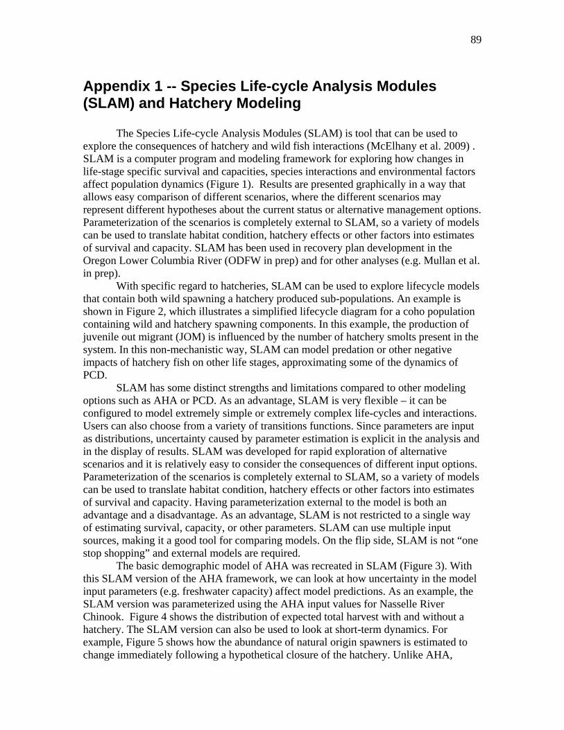
89

Appendix 1 -- Species Life-cycle Analysis Modules (SLAM) and Hatchery Modeling

The Species Life-cycle Analysis Modules (SLAM) is tool that can be used to explore the consequences of hatchery and wild fish interactions (McElhany et al. 2009) . SLAM is a computer program and modeling framework for exploring how changes in life-stage specific survival and capacities, species interactions and environmental factors affect population dynamics (Figure 1). Results are presented graphically in a way that allows easy comparison of different scenarios, where the different scenarios may represent different hypotheses about the current status or alternative management options. Parameterization of the scenarios is completely external to SLAM, so a variety of models can be used to translate habitat condition, hatchery effects or other factors into estimates of survival and capacity. SLAM has been used in recovery plan development in the Oregon Lower Columbia River (ODFW in prep) and for other analyses (e.g. Mullan et al. in prep). With specific regard to hatcheries, SLAM can be used to explore lifecycle models that contain both wild spawning a hatchery produced sub-populations. An example is shown in Figure 2, which illustrates a simplified lifecycle diagram for a coho population containing wild and hatchery spawning components. In this example, the production of juvenile out migrant (JOM) is influenced by the number of hatchery smolts present in the system. In this non-mechanistic way, SLAM can model predation or other negative impacts of hatchery fish on other life stages, approximating some of the dynamics of PCD. SLAM has some distinct strengths and limitations compared to other modeling options such as AHA or PCD. As an advantage, SLAM is very flexible – it can be configured to model extremely simple or extremely complex life-cycles and interactions. Users can also choose from a variety of transitions functions. Since parameters are input as distributions, uncertainty caused by parameter estimation is explicit in the analysis and in the display of results. SLAM was developed for rapid exploration of alternative scenarios and it is relatively easy to consider the consequences of different input options. Parameterization of the scenarios is completely external to SLAM, so a variety of models can be used to translate habitat condition, hatchery effects or other factors into estimates of survival and capacity. Having parameterization external to the model is both an advantage and a disadvantage. As an advantage, SLAM is not restricted to a single way of estimating survival, capacity, or other parameters. SLAM can use multiple input sources, making it a good tool for comparing models. On the flip side, SLAM is not “one stop shopping” and external models are required.

The basic demographic model of AHA was recreated in SLAM (Figure 3). With this SLAM version of the AHA framework, we can look at how uncertainty in the model input parameters (e.g. freshwater capacity) affect model predictions. As an example, the SLAM version was parameterized using the AHA input values for Nasselle River Chinook. Figure 4 shows the distribution of expected total harvest with and without a hatchery. The SLAM version can also be used to look at short-term dynamics. For example, Figure 5 shows how the abundance of natural origin spawners is estimated to change immediately following a hypothetical closure of the hatchery. Unlike AHA,

90

SLAM does not include a genetics model. A genetics model could be partially approximated in SLAM by designating different productivities and survivals for the hatchery and wild components of the population (even having them change over time). Even though this would not explicitly model fitness change, the approximation may be adequate given the uncertainties in parameterizing a complex genetics model. McElhany, Paul and Mirek Kos. 2009. Species Life-cycle Analysis Modules (SLAM). Computer program. NOAA-NWFSC, Seattle, WA http://www.nwfsc.noaa.gov/trt/slam/slam.cfm

Figure 1: Screen shots of steps in SLAM analysis. Analysis begins with a user defined graphic description of the life-cycle, which can include multiple life-stages, sub-populations, spatial locations, competition/facilitation, environmental influences, etc. The user then defines a scenario, which is a set of transitions functions and parameters for the life-cycle, then finally conducts a simulation to examine the future dynamics of all life stages.

1. Life-cycle

2. Scenario (functions and parameters)

3. Simulation

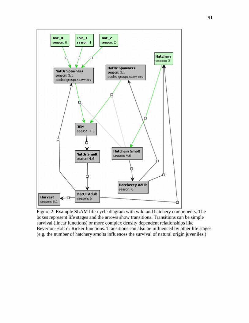
91

Figure 2: Example SLAM life-cycle diagram with wild and hatchery components. The boxes represent life stages and the arrows show transitions. Transitions can be simple survival (linear functions) or more complex density dependent relationships like Beverton-Holt or Ricker functions. Transitions can also be influenced by other life stages (e.g. the number of hatchery smolts influences the survival of natural origin juveniles.)

92

Figure slam-3: Basic AHA life-cycle structure recreated in SLAM.

Figure 4: SLAM estimated distribution of total harvest of Naselle River Chinook with the hatchery in place (blue bars) and in the absence of the hatchery (red bars). Base parameters are from the Naselle River AHA model (Busack pers com). Input parameters were assumed to have 20% estimation error.

93

Figure 5: SLAM estimated Naselle River Chinook dynamics of the of the natural origin wild spawners (red line) and the hatchery origin wild spawners (blue line) during a hypothetical closure of the hatchery at generation 30. The spike at generation 30 occurs because natural origin fish are not being collected as broodstock.