RWTH Aachen University – Energy and Mineral Resources Group

Reconstruction of Tectonic Paleo-Heat Flow for

the Levantine Basin (Eastern Mediterranean)

Implications for Basin and Petroleum System Modelling.

MASTER OF SCIENCE THESIS

by

David Benjamin Halstenberg

23rd of January 2014

Supervisors:

Prof. Dr. Ralf Littke1

Hanneke Verweij, PhD2

1) Institute for Geology and Geochemistry of Petroleum and Coal, EMR Energy and Mineral

Resources Group, RWTH Aachen University, Germany

2) Department of Petroleum Geosciences, TNO, Utrecht, The Netherlands

I

Statutory Declaration

I declare that I have authored this thesis “Reconstruction of Tectonic Paleo-Heat Flow for the

Levantine Basin (Eastern Mediterranean) – Implications for Basin and Petroleum System

Modelling” independently, that I have not used other than the declared sources/resources,

and that I have explicitly marked all material which has been quoted either literally or by

content from used sources.

Place and Date Signature David Benjamin Halstenberg

II

Acknowledgements

First and most of all, I would like to thank my supervisors Prof. Dr. Ralf Littke and Hanneke

Verweij, PhD for giving me the opportunity to conduct a research project and write a master

thesis under their guidance. Their comments and input during the working and learning

process while working on this thesis were always helpful and informative.

I owe Hanneke Verweij my gratitude for introducing me to TNO in Utrecht and helping me

getting started with my research internship in the Netherlands. I always appreciated her

advice. Also, I want to thank her for her remarks on my thesis.

Prof. Dr. Ralf Littke showed a large commitment and helped me in elaborating on my study

at his institute in Aachen and gave me the opportunity to further work on my project there.

Additionally, my thanks go to Fadi H. Nader, PhD at IFP-Energies Nouvelles in Rueil-

Malmaison, for involving me in his research projects with this thesis and for his frequent and

appreciated advice. Further, he gave me the possibility to join the AAPG Technology

Workshop in Beirut in May 2013.

Furthermore, I have to express my great thankfulness to Rader Abdul Fattah at TNO

Utrecht. He was always a great help concerning all kinds of scientific and organizational

questions and everyday challenges. He made the learning process during my project a lot

more joyful.

Moreover, I want to thank Samer Bou Daher at RWTH Aachen University for his continuous

help in creating this thesis and his scientific advice. I further want to express my gratitude for

accompanying me during the stay in Beirut and introducing me to town and country.

Last but not least, I feel grateful towards all my colleagues, friends and especially my

girlfriend, who supported me during the creational process of this work, all scientific,

organizational and personal.

III

Table of Content

Statutory Declaration.............................................................................................................. I

Acknowledgements ............................................................................................................... II

Abstract............................................................................................................................... VII

1) Introduction .................................................................................................................... 1

1.1) Geographic location ............................................................................................ 1

1.2) Exploration and production history....................................................................... 2

1.3) Aim of the study ................................................................................................... 3

2) Geological Background .................................................................................................. 4

2.1) Tectonic development ......................................................................................... 4

2.2) Oceanic vs. continental crust ............................................................................... 9

2.3) Local Heat Flow ................................................................................................. 12

3) Theoretical Background ............................................................................................... 14

3.1) Basin modelling ................................................................................................. 14

3.2) Deposition ......................................................................................................... 14

3.3) Pressure Calculation and Compaction ............................................................... 15

3.4) Heat Flow .......................................................................................................... 15

4) Methodology ................................................................................................................ 17

4.1) Basics of the model ........................................................................................... 17

4.2) Setup of the model ............................................................................................ 24

4.3) Calibration of final models ................................................................................. 28

4.4) 2-D modelling across the basin ......................................................................... 31

5) Results ......................................................................................................................... 33

5.1) Results of the Calibrations .................................................................................... 33

5.2) Sensitivities ....................................................................................................... 33

5.3) Modelled 1-D heat flows .................................................................................... 34

5.4) Dynamic vs. constant heat flow model ............................................................... 36

5.5) Biogenic gas ...................................................................................................... 37

IV

6) Discussion and Interpretation ....................................................................................... 38

6.1) Heat flow modelling ........................................................................................... 38

6.2) Maturity ............................................................................................................. 39

6.3) Biogenic gas ...................................................................................................... 39

6.4) Hydrocarbon potentiality .................................................................................... 40

6.4) Implications on crustal features ......................................................................... 40

6.5) Sensitivities and uncertainties ........................................................................... 41

7) Conclusions and Outlook ............................................................................................. 42

7.1) Conclusions ....................................................................................................... 42

7.2) Outlook .............................................................................................................. 43

8) References .................................................................................................................. 44

Appendix ............................................................................................................................. 48

Appendix 4.1 ................................................................................................................ 48

Appendix 4.2 ................................................................................................................ 51

Appendix 4.3 ................................................................................................................ 54

Appendix 4.4 ................................................................................................................ 56

Appendix 5 ................................................................................................................... 61

List of Figures

Figure 1: Geographical overview map of the Levantine Basin ............................................... 1

Figure 2: Locations of oil and gas wells in the Levantine offshore ......................................... 2

Figure 3: Map with major normal faults formed during the rifting of the Levantine Basin ....... 5

Figure 4: Schematic geologic section across the Helez Fault ................................................ 5

Figure 5: The Paleogeography of the Levantine basin .......................................................... 7

Figure 6: Major structural units of the Levantine Area ........................................................... 9

Figure 7: Possible plate configuration, postulating a Levantine-Sinai microplate ................. 11

Figure 8: Map of IHFC heat flow data and heat flow values by Eckstein.............................. 13

Figure 9: Succession of major geological processes in basin modelling .............................. 14

Figure 10: Two main aspects of heat flow modelling ........................................................... 16

Figure 11: Original 2-D section ............................................................................................ 18

Figure 12: Map view of the profiles ...................................................................................... 18

V

Figure 13: Digitized 2-D profile Depth ratio: 18 .................................................................... 20

Figure 14: Profile with the utilized wells Yam West 1 and Ashqelon 2 ................................. 21

Figure 15: Three zones assigned to the 2-D profile ............................................................. 22

Figure 16: Example of observed subsidence and modelled subsidence .............................. 23

Figure 17: User interface of PetroProb and required input .................................................. 24

Figure 18: Vitrinite reflectance dataset for YW1 .................................................................. 29

Figure 19: Vitrinite reflectance dataset for Mango 1 ............................................................ 29

Figure 20: Temperature dataset for Delta 01 ....................................................................... 29

Figure 21: Calibration result for Delta 01 ............................................................................. 29

Figure 22: Calibration result of Yam West-1 ........................................................................ 30

Figure 23: Calibration result for Mango-1 ............................................................................ 30

Figure 24: Calibration result for Tamar 01 ........................................................................... 30

List of Tables

Table 1: Input data used as sediment and fluid thermal parameters .................................... 19

Table 2: Example of layer-lithologies for the well Yam West 1 ............................................ 25

Table 3 Input for lithosphere parameters in PetroProb ........................................................ 26

Table 4: Petroleum System Elements (PSE) assigned to the 2-D model ............................. 32

Table 5: Heat flow output data from PetroProb used for the three well zones ..................... 35

List of Appendices

Appendix 1: Lithologies in PetroMod and their proportions ................................................... 48

Appendix 2: Layer names and Lithology in the 2D PetroMod layer cake model.................... 50

Appendix 3: Layer definition and composition of lithologies in PetrProb. .............................. 51

Appendix 4: Graphs of the assigned mode of lithospheric stretching for Ashqelon-2, Yam

West-1 and SP01 ............................................................................................ 52

Appendix 5: Graphs of Observed vs. Modelled Tectonic Subsidence, From top to bottom:

Ashqelon-2, SP01, Yam West 1. ..................................................................... 54

Appendix 6: Heat flow trends from 1-D PetroProb models, calibrated in PetroMod 1-D and

applied to PetroMod 2-D model. Top to Bottom: Ashqelon-2, Yam West 1,

SP01. .............................................................................................................. 56

Appendix 7: Paleo water depth trends, assigned to 1-D models and also 2-D PetroMod.

Top to Bottom: Ashqelon-2, Yam West 1, SP01. ............................................. 57

VI

Appendix 8: Sediment-Water-Interface Temperature Trends for the 1-D and models. Top

to Bottom: Ashqelon-2, Yam West 1, SP01. .................................................... 59

Appendix 9: Sensitivity plots between lithosphere thickness and heat flow and crustal

stretching and crustal thickness for the well Yam West 1. ................................ 61

Appendix 10: Heat flow plot of PetroProb output. Top to bottom: Ashqelon-2, SP01, Yam

West 1. .......................................................................................................... 62

Appendix 11: Table of all boundary conditions used for wells in PetroMod ........................... 63

Appendix 12: Modelled present-day Temperatures for dynamic heat flow. Depth ratio:

12.5. .............................................................................................................. 64

Appendix 13: Modelled present-day temperatures for constant heat flow Depth ratio 12.5 ... 64

Appendix 14: Profile of the source rock maturities for modelled heat flow Depth ratio 12.5. . 64

Appendix 15: Profile of source rock maturities for constant heat flow. Depth ratio 12.5 ........ 64

Appendix 16: Dynamic heat flow model maturities for 169.5 Ma BP. Depth ratio: 12.5 ......... 64

Appendix 17: Constant heat flow model maturities for 145 Ma BP. Depth ratio: 12.5 ........... 64

Appendix 18: Dynamic heat flow model maturities at 113 Ma BP. Depth ratio 12.5 .............. 64

Appendix 19: Constant heat flow model maturities at 90 Ma BP. Depth ratio 12.5 ............... 64

Appendix 20: Dynamic heat flow model maturities at 21.4 Ma BP. Depth ratio 12.5 ............. 64

Appendix 21: Dynamic heat flow model maturities at 16.4 Ma BP. Depth ratio: 12.5 ............ 64

Appendix 22: Constant heat flow model maturities at 21.4 Ma BP. Depth ratio: 12.5 ........... 64

Appendix 23: Constant heat flow model maturities at 16.4 Ma BP. Depth ratio: 12.5 ........... 64

Appendix 24: Dynamic heat flow model biogenic gas temperature zone at 7.1 Ma BP.

Depth ratio: 12.5 ............................................................................................ 64

Appendix 25: Dynamic heat flow model biogenic gas temperature zone at 5.3 Ma BP.

Depth ratio: 12.5 ............................................................................................ 64

Appendix 26: Dynamic heat flow model biogenic gas temperature zone at 4.0 Ma BP.

Depth ratio: 12.5 ............................................................................................ 64

Appendix 27: Dynamic heat flow model biogenic gas temperature zone at present-day.

Depth ratio: 12.5 ............................................................................................ 64

Appendix 28: Constant heat flow model biogenic gas temperature zone at 7.1 Ma BP.

Depth ratio: 12.5. ........................................................................................... 64

Appendix 29: Constant heat flow model biogenic gas temperature zone at 5.3 Ma BP.

Depth ratio: 12.5 ............................................................................................ 64

Appendix 30: Constant heat flow model biogenic gas temperature zone at 4 Ma BP. Depth

ratio: 12.5 ...................................................................................................... 64

Appendix 31: Constant heat flow model biogenic gas temperature zone at present-day.

Depth ratio: 12.5 ............................................................................................ 64

VII

Abstract

The Levantine Basin in the Eastern Mediterranean is a new frontier basin and to date is

unexplored offshore Lebanon. Several studies have been conducted offshore Israel and

Sinai and several basin models have been constructed by different authors. Commonly,

basin models consider heat flow as a user input that is constant throughout the basin area

and the history. Heat flow is influenced by many factors such as tectonic subsidence of the

basin, sedimentation and crustal features. This study sets up a 2-D tectonic heat flow model

based on multiple 1-D models throughout the Levantine Basin in a shallow, an intermediate

and a deep water province, which have taken into consideration published, pre-interpreted

profiles and publications. The models are created with the help of the software PetroProb

and PetroMod. The central approaches of this project are to model the tectonic phases

according to the observed basin subsidence derived from backstripping and to keep all

values in the modelling process in realistic ranges, especially those concerning measured

present-day heat flows. The models are calibrated with published temperature and vitrinite

reflectance datasets from adjacent wells. Present-day heat flows comprise of 38.8 mW/m² in

shallow water, 48.3 mW/m² in intermediate water and 41.2 mW/m² in the deep basin. The 2-

D heat flow model reveals temperatures of 16°C in the shallowest sediments in deep sea

and 355°C in the deepest hottest part. Comparison of the 2-D dynamic tectonic heat flow

model with a 2-D constant heat flow model reveals significant differences in maturation

histories. For dynamic heat flow, oil and gas maturation both set in earlier in basin history.

Microbial gas in submessinian and Pliocene to recent sediments may have been generated

and trapped in extensive parts of the basin. Continental crust can be recommended as the

type of crust underlying the basin, based on calibrations. Sensitivity studies identify crustal

and lithospheric thicknesses as two paramount input parameters for tectonic heat flow

models. Tectonic heat flow modelling can be identified as a useful means to approach the

problems of scarce available data in a new frontier basin like the Levantine Basin. The

present model still incorporates many inconveniences that might be overcome with future

research and, drilling of exploration wells in offshore Lebanon.

1

1) Introduction

1.1) Geographic location

The Levantine Basin is an offshore basin located in the easternmost Mediterranean Sea (32°

- 35° N and 33°- 35° E). It is constrained to the east by the Israel and Lebanon coastlines

and the Dead Sea rift and to

the south by the Nile delta fan

and Sinai-Egypt. Its western

and northern boundaries

consist of the Eratosthenes

Seamount and Cyprus and the

Cyprus Arc, respectively

(Figure 1). Its bathymetry

reaches >2000 m in the

central parts and shallows

towards the margin. Several

horst and graben structures

influence the seafloor (see

Geological Background).

Lately, major gas discoveries

have been reported in this

region, indicating important

prospectivity. (see section

1.2).

Figure 1: Geographical overview map of the Levantine Basin. White lines indicate major structural features (faults and subduction zones). Edited from Gardosh et al. (2010).

2

1.2) Exploration and production history

Petroleum exploration in the eastern Mediterranean has a long history, dating back to the

1960’s to 70’s with seven wells drilled by Belpetco into shallow shelf structures of Israel and

northern Sinai, which were all found dry. Nevertheless, they founded the initial geologic

model of the eastern Mediterranean (Gardosh et al. 2008).

From the mid 1970’s to mid-1980’s there were findings of light oil in Early Cretaceous

sandstones in shallow offshore Sinai in the wells Ziv-1 (Oil Exploration Ltd., 1976-1977) and

Mango-1 (Total, 1985). The latter one was able to produce 10000 Bbl/day of 44-50° API

gravity oil. Their performance, however, steadily decreased and the production was stopped

(Gardosh et al. 2008).

During the period of the late 1980’s to late 1990’s, Isramco drilled four offshore wells off the

Israeli coast, targeting structural traps. Reaching down to Middle Jurassic rocks at more than

5000 m depth, they encountered

various gas shows. The Yam Yafo-1

(1994, Fleischer and Varshavsky

2002) and Yam-2 (1989, Fleischer

and Varshavsky 2002) wells

successfully tested 500-800 Bbl/day

of 44-47° API gravity oil from Middle

Jurassic Limestone, but no

commercial production was

achieved. In 1999-2000 the

discovery of several gas fields (~3

TCF reserves) in shallow Pliocene

sands west of the towns Gaza and

Ashqelon pushed the offshore

exploration considerably. The MariB

field, drilled from 2000 to 2001

(Fleischer and Varshavsky, 2002), is

currently produced (Gardosh et al.

2008). Figure 2 shows the locations

of the exploration and production

wells in the eastern Mediterranean

and their drilling year (Gardosh et al.

2008).

Figure 2: Locations of oil and gas wells in the Levantine offshore (from Gardosh et al. 2008, scale estimated).

3

The interest in hydrocarbons in the Levantine Basin is steadily growing, as those recent

findings offshore Israel reassured the presence of hydrocarbons in widespread parts of the

basin. This leads Lebanon and also Cyprus to intensify their efforts towards first licensing

rounds (Ibrahim 2013, N.N 2007).

The successful exploration activities promoted the acquisition of large amounts of new

geophysical data, covering large areas of the eastern Mediterranean, on the basis of which

several interpretations of the structure, stratigraphy, crustal configuration and lithology of the

Levantine Basin were conducted. The acquired geophysical and geological data could be

interpreted and/or turned into basin models to better understand the petroleum systems and

the prospectivity of the Levantine Basin (e.g. Mohamed et al. (2012), Dubille and Thomas

(2012), Roberts and Peace (2007), etc.).

Such basin models are crucial for successful hydrocarbon exploration, because they allow

(among other things) for the prediction of possible maturities of source rocks, expulsion,

migration and accumulation of hydrocarbons as well as eventual leaks or degradations

(Hantschel and Kauerauf 2009). A basic rule is that the better the input, the more reliable the

results. However, in a frontier basin like the Levantine, which is not well explored and under-

drilled, a lack of well-data (e.g. for calibration) is omitting a satisfying amount of input.

One important factor in a basin model is the temperature distribution and history in the basin,

as this is the main factor determining the maturation of source rocks (and production of

hydrocarbons) and degradation. Temperature (or thermal regime) is defined by the heat flow

(Allen and Allen 2005), making it a paramount parameter in the petroleum system model.

1.3) Aim of the study

The aim of this project is to reconstruct heat flow trends through the geological history of the

Levantine Basin. This will provide insights into the related paleo-temperatures and maturities

of potential source rocks. In general, simple heat flow models are used in basin modelling to

evaluate petroleum systems. Heat flow inputs usually rely on present-day measurements of

heat flow from well temperature data. The values are often assumed to be valid for the whole

basin and for the whole geological history of the basin. Assuming a constant heat flow value,

however, neglects temporal and spatial variations which can result in an erroneous

estimation of source rock maturity and hydrocarbon generation.

This study attempts to quantify heat flow variations in the Levantine Basin throughout the

geological history of the basin via tectonic modelling of heat flow. The approach is to

integrate the tectonic and crustal development of the basin into the model, and to investigate

4

their impact on the heat flow history and the according temperatures in the basin (Van Wees

et al. 2009, see chapter 3).

Because of the scarcity of available measured (well) data, published information, such as

interpretations (e.g. seismic data), was used for input data and to construct input models for

the simulations in this research project. Those were particularly already interpreted 2-D

profiles (see chapter 4). The developed models were calibrated and compared to the

published interpretations, if data was available.

The software PetroMod by Schlumberger and PetroProb by TNO were used in this project.

The first was used to digitize the published 2-D profiles and create 1-D extractions, for use in

PetroProb. The latter was utilized to develop the 1-D basal heat flow models from the

PetroMod 1-D extractions, which resulted in input constraints for the PetroMod models. With

the help of this software, the 1-D models were finally calibrated. Further, PetroMod was used

to build the final 2-D basin model (See chapter 3 and 4).

2) Geological Background

2.1) Tectonic development

The development of the Levantine Basin comprises several tectonic events. Besides the

timing of the initial rifting event, the nature of the Crust underlying the basin is still debated

(Gardosh et al. 2008). This chapter lines out the undisputed part of the geological

development and states the different theories concerning the type of rifting and the resulting

crust.

At the present-day, the Levantine Basin can be seen as an African Plate- foreland basin,

forming the southernmost deformation front of the Alpine deformation. It is located in the

region of interaction of the Anatolian, Arabian and African plates (Roberts and Peace 2007,

Vidal et al. 2000). This is the north-western margin of the Arabo-Nubian shield, formed in the

Late Precambrian Pan-African orogeny. In Ediacarian times, the shield was cratonized and

later peneplaned (Gardosh et al. 2008).

Other authors also propose a Levantine-Sinai microplate as a fragment of the African craton.

This microplate shall be bound to the east by the Dead Sea rift and extends from the Red

Sea to approximately 35°N, including the Eratosthenes Seamount (Mascle et al. 2000).

5

A paleo-geographical

reconstruction of the

position of the Levantine

Basin from Cambrian times

on is shown in Figure 5.

In the Palaeozoic (up to

the Permian) the Levant

area, as part of

Gondwana, was situated

southwest of the

Paleotethys Ocean

(Gardosh et al. 2008).

From the late Permian on,

the Pangaean landmass

was rifted in several pulses

in the course of the Tethys

opening until the Early to

Middle Jurassic. Each of

these pulses was

accompanied by volcanic

activity (Gardosh et al.

2010). Gardosh et al

(2008) suggested the start

of rifting to be in the Late

Permian, indicated by a series of

horst and graben structures

(Figure 4) developed throughout

the rifting period. They proclaim

another tectonic extensional

phase during Middle and Late

Triassic, which was followed by a

latest Triassic quiescence. The

last and probably most extensive

rifting phase in the Early to

Middle Jurassic led, among

Figure 4: Map with major normal faults formed during the rifting of the Levantine Basin. The indicated magnetic anomalies show possible rifting-induced intrusions (except Eratosthenes Continental Block). The Helez fault is located along the NW-side of the Gevim High. Edited from Gardosh et al. (2010).

Figure 3: Schematic geologic section across the Helez Fault, developed during the Neotethyan rifting and reversely reactivated in course of the Syrian Arc contraction in the Late Cretaceous (Gardosh and Druckman 2006).

6

others, to the formation of the Helez fault (Figure 4 and 4) which is the best evidence for

Neotethyan rifting in the Levantine area. These structures mostly strike NE-SW, leading to

the conclusion of a NW-SE extensional direction. This extension might be accommodated by

E-W strike-slip motion in the northern Sinai region (Gardosh and Druckmann, 2006).

During the Gondwanian / Pangean breakup starting in the Early Mesozoic, the Eratosthenes

seamount as a continental fragment just like the Tauride block and others, separated from

the African margin and moved to its present position, where it is about to subside under the

Cyprian arc at a speed of approximately 1 cm/a (Netzeband et al. 2006; Gardosh et al.

2010). This is the same period in which the Levantine-Sinai microplate, proposed by Mascle

et al. (2000), is supposed to have developed.

The evolution and the nature of the underlying crust at this stage is a subject of debate. The

nature of crust in the Levantine Basin can have a significant impact on the heat flow in the

basin. This will be discussed in depth in section 2.2.

After rifting, a thermal subsidence of the deep marine eastern Mediterranean and Levantine

basin set in from the Middle Jurassic onwards (Gardosh et al. 2008, 2010). In this passive

continental margin setting (considering a continental crust underlying the basin; Roberts and

Peace 2007), a hinge belt along the eastern margin developed, separating the eastern

shallow marine platform (Egypt-Sinai-Israel-Lebanon coastline) from the now deep marine

basin in the west (Gardosh et al. 2008, 2010). This shelf edge can be identified close to the

present-day northern Egypt to Lebanon shoreline (Gardosh et al. 2010).

7

The Late Cretaceous witnessed the convergence of Eurasia and Afro-Arabia in the course of

the closing of (Neo-)Tethys and Alpine Orogeny (Roberts and Peace 2007). This lead to the

subduction of the Tethys (oceanic) crust beneath present-day Cyprus and Turkey (compare

Figure 1 and Figure 6). The induced far-field stresses led to a reverse reactivation of the

Late Permian to Mid Jurassic normal faults (see also Figure 3) and contraction of the

Levantine Continental Margin. The so-called Syrian Arc evolved, a generally SW-NE striking

fold belt stretching from North-Sinai to Lebanon (Gardosh et al. 2008, 2010, compare Figure

6). This contraction continued throughout the Tertiary. The above mentioned plate motion

caused major uplifts east of the Levantine Basin as well as updoming of the Arabian shield in

the south (Sinai-Negev region) (Gardosh et al. 2008).

Figure 5: The Paleogeography of the Levantine basin, indicated by a red dot, during the Late Cambrian (a), Late Permian (b), Early Triassic (c), Late Jurassic (d) and Late Cretaceous (e). Edited from Scotese (2000).

8

A closure of the Atlantic water supply to the Mediterranean in the upper Miocene (Messinian)

led to the desiccation of the basin and the precipitation of vast layers of evaporites like halite

and anhydrite. This event was termed the Messinian Salinity Crisis (Hsü et al. 1973).

The following re-inundation of the Mediterranean Sea led to the deposition of clastic

sediments onto the evaporites, probably being of Nile Delta origin (Netzeband et al. 2006,

Gardosh et al. 2008).

One of the most recent (and on-going) major tectonic development saw the breakup of the

Afro-Arabian Craton that initiated the Dead Sea Transform Fault (compare Figures 1 & 6). It

connects the spreading centre of the Red Sea with the Taurus collision zone in south

eastern Turkey and sets up the major structural framework for the present-day situation of

the Levantine Basin (Gardosh et al. 2010).

The Levantine Basin, now being a foreland basin, accumulated up to 14,000 m of Mesozoic

to recent sediments (Roberts and Peace 2007).

9

Figure 6: Major structural units of the Levantine Area. Note the Dead Sea Transform, Cyprus Thrust and Trench and the rough position of the Syrian Arc, indicated by the red shade. Edited from Roberts and Peace (2007) and Breman (2006).

10

2.2) Oceanic vs. continental crust

The composition of the crust underlying the Levantine Basin was (and partly still is) widely

debated. Some authors (e.g. Ben-Avraham 2002, Segev and Rybakov 2010) propose

oceanic crust underlying the basin, while others (Hirsch et al. 1995, Vidal et al. 2000,

Netzeband et al. 2006 and Gardosh et al. 2008) assume attenuated continental crust.

What points to oceanic crust is basically its seismic velocity of 6.7 km/s, which is in the range

of typical velocities of oceanic crust, together with its estimated density and the thickness of

8-9 km obtained from gravimetric and magnetic data. Seismic velocity studies have shown a

6.3-6.0 km/s layer beneath Israel, which is representative for typical upper continental crust.

This layer is missing in the centre of the basin (Ben-Avraham 2002).

The missing alternating magnetization patterns, which would be typical for oceanic crust, are

explained by the complex tectonical development of the basin with several rifting pulses and

compressional episodes, which led to the destruction of the magnetization zones (Ben-

Avraham 2002). Another possibility is that the oceanic spreading took place in a period

without changing of the magnetic field. The inverse magnetization that was recognized

points to an Early Cretaceous or Early Jurassic development (Ben-Avraham 2002).

Authors supporting the theory of continental crust beneath the basin argue that the missing

magnetization pattern is more a hint to continental crust. Furthermore, there are several

shear zones found in the Levantine area (e.g. Pelusium Line, Damietta-Latakia Line).

Shearing is more common for stretching of continental crust (Netzeband et al. 2006).

The seismic data obtained by Netzeband et al. (2006) show a Moho-rise, from 26 km below

Israel and 27 km below Gaza (Weber et al. 2004), to 22 km in the basin. This might indicate

a transition to oceanic crust. However, they state that the 7km/s layer which is typically found

in cases of oceanic crust is not present. The thickness of the crust was found to be

approximately 8 km, whereas oceanic crust is usually thinned to <5 km. From these and

other observations, Netzeband et al. (2006) conclude a rifted continental crust which did not

reach the oceanic spreading stage.

Different studies provide values for continental crustal thickness beneath Israel of 18 km

(Ben-Avraham et al. 2002), and up to 40 km beneath Jordan (Netzeband et al. 2006). From

the present crustal thickness in the basin (8 km) determined by Netzeband et al. (2006), the

stretching factors of β=2.25 or β=5 were calculated. Both values can also be found in other

passive margin areas, 2.25 even being a typical value for thinned continental crust

(Netzeband et al. 2006).

11

In a study from 1978, Eckstein already argues for a continental Precambrian foreland basin,

indicated by a heat flow of 38.3 to 49.9 mW/m² in Northern Egypt, which is in the range of

heat flow found in the Levantine Basin. Combining this with a gravity profile and a seismic

refraction layer with a velocity of 6.1 km/s, he concludes that the continental African

Foreland may well extend beneath the basin.

Lastly, the discovered seismic velocities of 6.4-6.9 km/s (Netzeband et al. 2006) seem too

low for oceanic crust, considering its great depth (beneath ~14 km of sediments) and

pressure (Netzeband et al. 2006). Higher values for heat flow might cause lower seismic

velocities for oceanic crust. However, only normal surface heat flow values of 40 – 60

mW/m² and 38 – 67 mW/m² were found in the different studies in the area (according to

Netzeband, 2006). Consequently, the low velocities suggest a continental crust, rather than

an over-heated oceanic crust. This is supported by the 65 mW/m² given as an average heat

flow value for continental crust (Netzeband et al. 2006).

Mascle et al. (2000), postulate a

model where the Levantine-Sinai

is considered as a microplate

(Figure 7) (see above). This

microplate would be bound by

the Dead-Sea Fault and the

Cyprus Thrust, as well as by a

hypothetical continuation of the

Gulf of Suez Transform towards

the north and across the

Eratosthenes Seamount. This

transform crustal fault is

supposed to be covered by Nile

Delta sediments. Also, this study

promotes continental crust in the

basin. But as the evidence for

the continuation of the western

fault zone is not unambiguous,

this theory is not further

considered here.

Appearing more reasonable than oceanic crust, for this study the to-date widely accepted

assumption of strongly attenuated continental crust was adopted.

Figure 7: Possible plate configuration, postulating a Levantine-Sinai microplate, bound between Dead Sea fault (East), Cyprus Trench (North) and Gulf of Suez Transform (West). Thick black arrows indicate sense of plate motion. ESM: Eratosthenes Seamount, FR: Florence Rise (Mascle at al. 2000). Scale estimated.

~100 km

12

2.3) Local Heat Flow

Only few data on the present-day surface heat flow are available in the study area. Eckstein

(1978) postulates values of 38.3 to 49.9 mW/m² in the easternmost Mediterranean (Northern

Egypt). Also, the values published from the International Heat Flow Commission (IHFC,

2010) indicate values between 28 and 44 mW/m² in the basin area, increasing to 50 to >70

mW/m² on the eastern margins and in Israel. This reveals a very cool Levantine Basin,

probably due to the vast sediment infill, or missing oceanic spreading (see section 2.2)

(Eckstein 1978, IHFC 2010). Figure 8 depicts the heat flow values recorded in the study

area.

13

Figure 8: Map of IHFC (2010) heat flow data (red dots with white circle labels) and heat flow values by Eckstein (1978, shaded b/w map: values written diagonally, circles indicate number of measurements in the location) on a structural basemap by Roberts and Peace (2007).

14

3) Theoretical Background

3.1) Basin modelling

Basin modelling describes the numerical

procedure of dynamic simulation of

geological processes over time in a

sedimentary basin. This is done through

forward modelling, which means the

simulation of deposition of the oldest

layer to that of all younger layers until

the present-day. At each time step,

important geological parameters such as

deposition, compaction, erosion, heat

flow, petroleum generation, expulsion,

phase dissolution, migration and

accumulation are calculated (Hantschel

and Kauerauf 2009). In this study, only

deposition, compaction and heat flow

play an important role and are

considered.

Figure 9 indicates the succession of

geological processes that have to be

determined in the course of basin

modelling. The migration timesteps are

not relevant for this study. Also, due to

lack of data, no pressure calculation was performed and hydrostatic conditions were

assumed.

3.2) Deposition

During basin history, layers can be created during sedimentation or removed in phases of

erosion. If the events of hiatuses or phases of depositions are known, paleo depositional

times can be assigned to the layers. From the present-day thickness of the layers and their

lithological parameters, a backstripping to their depositional thickness is performed

(Hantschel and Kauerauf 2009).

Figure 9: Succession of major geological processes in basin modelling, not all considered in the present study (after Hantschel and Kauerauf 2009).

15

3.3) Pressure Calculation and Compaction

Pressure calculation takes place basically as an overburden-driven one phase flow problem.

If the pore pressure is changed, this might result in changing amounts of compaction and

thus changing geometry of the layers. So these two steps take place before the heat flow

calculation (Hantschel and Kauerauf 2009). In the present study, compaction was calculated

based on hydrostatic conditions (see above).

3.4) Heat Flow

Heat flow (commonly noted in mW/m²), as the process transferring heat from the earth’s

interior to its surface, is the key feature for temperature calculation. That again, is the

paramount parameter for the estimation of geochemical reaction rates and with this

maturation of kerogens. Heat flow analysis requires the consideration of heat convection and

conduction and radioactive decay (Hantschel and Kauerauf 2009). The thermal boundary

conditions regulate the influx of heat from the base of the sediment column, namely the

basal heat flow. This is the boundary condition, which this study tries to model and

reconstruct and its basic properties are explained hereafter.

Heat flow is achieved by three principal processes: conduction, convection and radiation. For

heat flow analysis, radiation plays only a minor role. Convection, as the fastest process of

heat transfer, is most dominant in the liquid mantle, whereas conduction is the most

important process in the lithosphere (Allen and Allen 2005). Convection can become

important in zones of high flow rates, such as fractures or permeable aquifers (Hantschel

and Kauerauf 2009). In the present study, structural features or groundwater flow were not

taken into account.

The conductive heat flow through a sedimentary column is induced by the temperature

gradient between the surface temperature (or sediment-water-interface temperature (SWIT)

for submarine environments) and the temperature at the lithosphere-asthenosphere

boundary (LAB) (Hantschel and Kauerauf 2009). The magnitude, orientation and distribution

of the basal heat flow characterizing the lower boundary temperature are defined via thermal

and mechanical parameters of the crustal and mantle rocks (Allen and Allen 2005).

Hantschel and Kauerauf (2009) described the 1D conductive heat flow (q) with equation

3.4.1, where is a tensor with the independent components h (conductivity along a

geological layer) and v (conductivity across a geological layer). is the temperature

gradient.

(3.4.1)

16

At any location, the heat flow vector is oriented into the direction of the steepest negative

temperature gradient from one location (Hantschel and Kauerauf 2009).

Allen and Allen (2005) refer to Fourier’s Law (equation 3.4.2) to describe the fundamentals

of conductive heat flow. Heat flow q is directly proportional to the temperature gradient at

one point.

(3.4.2)

is thermal conductivity coefficient, is the temperature and is the vector into the

direction of the decreasing temperature.

These equations show that the heat flux can be determined, for example, in boreholes, when

the temperature gradient (temperatures measured in boreholes and on the surface) and

thermal conductivity (measured in the lab for certain materials) of the material are known

(Allen and Allen 2005).

The heat flow modelling is generally split into two main aspects: The calculation of the heat

in-flux into the sediments determined by the crustal model and consecutive calculation of

temperature in the sediments (Figure 10, Hantschel and Kauerauf 2009).

The heat flow in a basin is commonly calculated from bottom hole temperatures and surface

temperatures and is usually measured with logging tools. The acquired heat flow value

represents the present-day situation and does only contain very local information (except if

many wells are drilled in an area) (Van Wees et al. 2009, Abdul-Fattah et al. 2013).

Figure 10: Two main aspects of heat flow modelling: a) analysis of influx from mantle into lithosphere and b) heat flow and temperature in the sediments (Hantschel and Kauerauf 2009).

17

As mentioned above (section 1.3), the aim of this study is to conduct a crustal basin model,

using a tectonic heat flow modelling approach. Here, effects of sedimentation and erosion

(burial history), surface temperatures and radiogenic heat production will be considered.

Moreover, the crustal setting and transient effects of basin evolution largely influence the

heat flow and must be taken into account (Van Wees et al. 2009; Abdul-Fattah 2013).

4) Methodology

4.1) Basics of the model

An overview of the general tectonic and heat flow development during the history of the

basin was derived from an interpreted profile by Mohamed et al. (2012) (Figure 11) through

the Levantine Basin (Figure 12) and digitized using Schlumberger’s software PetroMod

2012. The next step was to assign lithologies to the finished layer cake model (Figure 13).

Roberts and Peace (2007) proposed a general lithology for the basin that fits the profile by

Mohamed et al. (2012). Additionally, Gardosh et al.’s (2008) data were used in order to

assign proper lithologies to the layer cake model (Table in Appendix 1). The PetroMod

lithology editor was used to mix lithologies confirming as good as possible with the literature

information. Where possible, sediment thermal parameters were assigned according to

Rybach (1986) and Shalev et al. (2013) (see also below) (Table 1). The procedure was

repeated for another 2-D profile Gardosh et al. (2008), with the corresponding lithologies

taken from the same publication (Figure 12, Figure 14). From these 2-D layer cake models,

3 1-D models at characteristic locations were extracted. As basement, a ~1500 m thick layer

of continental crust composition (see section 2.2) was assumed, as there was no specific

information on the basement provided in the 2-D profiles (see also Appendix 1 and 2).

18

Figure 12: Map view of the profiles from Mohammed et al. (2012, red line) and Gardosh et al. (2008, yellow line).

Figure 11: Original 2-D section along the above indicated wells from Mohammed et al. (2012). For map view see Figure 12.

19

The well Yam-West 1 corresponds with a water depth of up to ~800 m and SP01 with water

depths of >2000 m (Mohamed et al. 2012). The Ashqelon-2 well (Gardosh et al. 2008)

represents the very shallow areas and shoreline. From the simulated heat flow histories of

these 3 wells, 3 heat flow zones were assigned to the 2-D model according to the water-

depth setting, together with individual boundary conditions (Figure 15).

Table 1: Input data used as sediment and fluid thermal parameters

Rock type Thermal Conductivity [W/K/m]

(Shalev et al. 2013)

Heat Generation

[µW/m³] (Rybach

1986)

PetroProb

Standard

Limestone 2.1 0.62

Dolomite 3.5 0.36

Salt 3.2 0.012

Anhydrite - 0.09 5.8 ± 1 W/K/m

Shale 1.2 1.8

Siltstone 2.1 - 1.0 µW/m³

Sandstone

(Arkose) 2.1 0.84

Water - - 0.6 W/K/m

0 µW/m³

HC - - 0.5 W/K/m

0 µW/m³

In order to reconstruct the paleo-heat flow in the Levantine Basin, it seemed crucial to take

into account as many different parameters as possible in the simulation. For this reason, the

TNO-developed software PetroProb was used for 1-D modelling of the heat flow for the

basin model, due to its capability of dealing with several rifting and contraction events (Van

Wees et al. 2009). The McKenzie heat flow simulation of PetroMod is able to calculate heat

flow for only one major rifting and post-rift event (see section 3.4).

PetroProb is a fully probabilistic tool to calculate heat flow and maturation. It calculates paleo

heat flow based on tectonic processes. The calculated tectonic heat flow can easily be used

as input boundary condition in other software such as PetroMod. PetroProb’s integrated

calibration takes into account uncertainties and variation limits in burial history, paleo heat

flow (e.g. variations in crustal/lithosphere thickness, tectonic processes) and sediment

thermal parameters.

20

YW2 SP01 Tamar 01 Dalit 1

Delta 01

YY-1 Mango-1 YW1

Figure 13: Digitized 2-D profile after Mohammed et al (2012). Well abbreviations: YW1: Yam West 1; YW2: Yam West 2; YY-1: Yam Yafo-1. Depth ratio: 18.

21

YW1 ASHQ2

Figure 14: Profile by Gardosh (2008) with the utilized wells Yam West 1 (YW1) and Ashqelon2 (ASHQ2). X-Axis: Depth [m].

22

Figure 15: Three zones assigned to the 2-D profile, according to Ashqelon-2 (Red), Yam West 1 (Yellow) and SP01 (Blue). Each zone has their individual boundary conditions.

23

-3000

-2500

-2000

-1500

-1000

-500

0

Su

bsid

en

ce [

m]

Age [Ma]

Modelled Tectonic Subsidence

Apparent Tectonic Subsidence

In contrast to PetroMod, PetroProb is capable of handling multiple tectonic events. This is

one of the key elements of the present modelling approach. The adopted workflow consist of:

1) Construct the observed tectonic subsidence curve.

2) Fit the modelled tectonic subsidence curve to the observed tectonic subsidence

curves of the 1-D extractions in order to get a most accurate tectonic and basin

stretching model (Figure 16). For this means, the error between modelled and

observed subsidence should be kept as low as possible.

3) Fit the modelled present-day heat flow to the observed present-day heat flow in the

study area (See section 2.4, Figure 8). The pre-rift heat (pre-Permian) flow was set to

55 mW/m² according to the narrow rift mode proposed by Netzeband et al. in 2006.

4) Calibrate predicted temperatures and maturities (based on the modelled tectonic heat

flows) to published temperatures and maturity data from wells in the basin.

Figure 16: Example of observed (apparent) subsidence and modelled subsidence from Yam West 1 with range lines.

24

4.2) Setup of the model

A 1-D model in PetroProb requires the following input in the form of specifically formatted .txt

files (Figure 17):

1) Layer definition: Table that assigns names, ages,

thicknesses and erosion to the layers.

2) Formations fractions: Assigns lithologies to the

layers.

3) Paleo water depth: Assigns the PWD [m] to the

layers.

4) Heat Flow: Defines the basal heat flow [mW/m²]

over time. As this shall be modelled, this input is

not needed.

5) T-Surface: Assigns the surface temperature [°C]

over time. These values are then corrected by the

software to Sediment-Water-Interface

Temperatures (SWIT) according to the PWD.

6) Formations por-depth: This table assigns a

porosity [%] -depth relationship for the different

lithologies, in order to be able to perform a

decompaction/backstripping.

7) Sediment thermal: It assigns the thermal

conductivity [W/K/m] and heat generation [µW/m³]

for the different components.

8) Lithosphere parameters: Defines the values for

the basement, such as lithosphere and crustal

thickness [m], densities [kg/m³] and thermal

conductivities [-] of crust and mantle, heat production of upper and lower crust

[µW/m³], thermal expansion of the lithosphere [-], the lithosphere-asthenosphere

thermal boundary [°C] and density of underplating [kg/m³] (not used).

9) Sampling parameters: Defines the number and positions of wells that shall be

simulated. Not necessary for 1-D.

10) Tectonic steps: Input for the episodes of tectonic activity (e.g. rifting). The different

possible modes of rifting in PetroProb are explained below.

Figure 17: User interface of PetroProb and required input (marked in red).

25

A hypothetical input well has to be assigned, which incorporates all the input and at which

the simulations are then performed.

The general layer definition and formations fractions (lithologies) are derived from the 1-D

extractions from the PetroMod 2-D model and can be seen for every well in Appendix 3.

Three important points should be mentioned: Firstly, the layer names were transformed into

layer ages (e.g. 4.0 represents the layer Pleistocene-Pliocene in PetroMod and so forth) or

named ero-x or hiatus, for erosional or hiatus events, respectively. Other than in PetroMod,

in PetroProb no lithologies are assigned to hiatus or erosional events, as they solely

represent distinct surfaces. Secondly, it is noteworthy that the lithological input into

PetroProb could not be transferred one to one from the PetroMod model. This is due to the

fact that PetroProb does not allow for lithologies as complex as in PetroMod, since fewer

components are available for mixing. With a special Excel tool, it is possible to transfer

slightly more complex lithologies into the PetroProb system. This tool translates the features

of the abundant lithologies into the corresponding lithologies available in PetroProb. The

same tool is used to transfer information like depositional ages and layer thicknesses into

PetroProb models. Lastly, PetroProb supports only a limited number of modelling steps

during its inversion of tectonic subsidence. Thus, in some cases minor layers had to be

merged to one. That is why correlation from the layers in the 1-D PetroMod models is not

always possible one to one to the PetroProb models. An example of the lithology, that was

finally applied to the layers in PetroProb, is presented in Table 2. All similar tables for the

remaining wells can be found in Appendix 3.

Table 2: Example of layer-lithologies for the well Yam West 1. Proportions are in %.

Layer

Name

Sandstone Siltstone Shale Carbonate Halite Anhydrite

4.0 17 0 62 21 0 0

6.1 0 0 0 0 80 20

14.2 91 9 0 0 0 0

39.2 65 5 30 0 0 0

54.8 0 0 0 100 0 0

89.5 0 0 24 76 0 0

112.2 17 3 0 80 0 0

137.3 33 3 64 0 0 0

142.0 0 0 24 76 0 0

150.8 0 49 51 0 0 0

160.1 10 0 0 90 0 0

163.9 20 0 20 60 0 0

172.9 0 0 0 100 0 0

205.7 0 0 0 100 0 0

242.8 0 0 0 100 0 0

296.0 29 0 29 42 0 0

26

Erosional or hiatus events were defined according to literature review, where major or

ubiquitous events are assumed (e.g. red curved lines in Figure 11, curved lines in Figure 14,

Roberts and Peace 2007). It has to be mentioned that PetroProb is not able to cope with

ages older than 490 Ma. Consequently, the heat flow modelling in PetroProb in this study

only starts at that time or at 296 Ma. This does not imply a problem, as there was no real

basin developed prior to 296 Ma and also the models created in PetroMod did not need any

older formations (see section 2.1).

The paleo water depth (PWD) was assumed based on the lithologies compared with the

Standard Facies Zones model published in Flügel (2004) (if applicable), in addition to

lithology assumptions derived from Gardosh et al. (2008) and Bar et al. (2011). The present-

day water depths were taken from the 2-D profile at the locations of available wells.

Table 3 Input for lithosphere parameters in PetroProb. Where there is no source stated, the value is the standard value for PetroProb. The same parameters were used for all wells. Variation limits for the thicknesses are applied to see the impact of crustal and lithosphere thickness on the results of the simulation and to account for the uncertainties, as these parameters are not very well constrained to-date. Thicknesses are initial, pre-rift thicknesses.

Parameter [unit] Value Variation

limit (+/-) Source (proposed values)

Lithosphere thickness [m] 110000 20000 Segev, Rybakov 2006 (~120000)

Crustal thickness [m] 33000 2000 Netzeband et al. 2006 (24000-40000)

ρ crust [kg/m³] 2870 - Segev, Rybakov 2006 (2835-2895)

ρ mantle [kg/m³] 3250 - Segev, Rybakov 2006

Conductivity crust

[W/(m*K)] 2.8 - Shalev et al. 2013

Conductivity mantle

[W/(m*K)] 2.5 - Shalev et al. 2013

Heat generation upper

crust [µW/m³] 1.0 - Shalev et al. 2013

Heat generation lower

crust [µW/m³] 0.5 - Mareschal, Jaupart 2013 (0.2-0.5)

Lithosphere thermal

expansion [K-1] 3.2*10-5 -

PetroProb standard, ~in accordance

with Afonso et al. (2004)

LAB-temperature [°C] 1330 - Segev, Rybakov 2006 (1250-1350)

27

The Messinian Salinity crisis (see section 2.1) was considered as a phase of drop in paleo

sea level, associated with evaporation of the water column rather than tectonic uplift of the

basin. Nevertheless, in modelling the sea level drop could be interpreted as tectonic uplift

and consequently give false results for the crustal processes and stretching. Further to

several tests, the Messinian drop in paleo water depth appears not to have any significant

impact on the result for the heat flow, so it could be neglected in favour of a more realistic

tectonic model and stretching factors, leading again to more satisfying heat flow values.

As discussed in section 2.2, the assumption of thinned continental crust underlying the basin

was adopted in this study. Accordingly, the input data for the lithosphere parameters were

chosen (Table 3). For sediment thermal parameters, values according to Rybach (1986)

(heat generation) and Shalev et al. (2013) (Heat conductivity) were applied as given in Table

1. Where there was no information on the parameters, the default parameters in PetroProb

and also PetroMod were assumed. The resulting heat generation of the different lithologies

are presented in Appendix 2 (PetroMod) and Table 1 (PetroProb). For the latter, the heat

generation for the final mixed lithologies is calculated internally from the given input and

cannot be extracted.

Based on the burial curve of each well, tectonic (rifting) phases with significant subsidence

were assigned in the tectonic steps input. The same applies to uplift during erosional phases

that were derived from literature review or published work. PetroProb allows assigning five

different types of iteration modes to lithospheric stretching phases. Here, β symbolizes the

typical crustal stretching, while δ stands for mantle stretching. In combination they define the

lithospheric stretching. In each mode, the software varies the starting value for β and δ in

order to fit the modelled subsidence to the tectonic subsidence derived from backstripping.

The modes bdcoup and bdfree were used in this project. Bdcoup allows δ (d) and β (b) to

vary in a coupled manner. This means that both values stay constant in relation to each

other, but the value may change. This represents the McKenzie stretching model. Bdfree

allows β and δ to vary freely, also in relation to each other, corresponding to the Royden and

Keen model. This is typically used for rifting phases with abnormally high postrift subsidence

(van Wees 2007). In Appendix 4, there are graphs for the three wells with the assigned

tectonic model steps. It has to be mentioned here that the rifting events are only based on

the observed subsidence for each extracted 1-D well and may thus differ from site to site.

They were adapted during the process of creating the models, in order to get realistic

stretching and heat flow values from the simulations.

28

4.3) Calibration of final models

During the heat flow modelling, attention was paid to the error between the apparent

(observed subsidence and the modelled subsidence (calculated from the defined tectonic

steps), in order not to let the assumed tectonic steps take the subsidence to unrealistic

values. Figure 16 depicts an exemplary plot of an apparent tectonic subsidence and a

modelled tectonic subsidence. Plots for all the modelled wells can be found in Appendix 5.

Generally, the error could be kept within ± 200-300 m between modelled and apparent

subsidence. The modelled heat flows were also compared to available heat flow

measurements in the area (see section 3.4).

The result of the heat flow simulation was used as input for Schlumberger’s PetroMod (see

chapter 5, Appendix 6). The values were used in 1-D extractions from the 2-D profile at the

corresponding well locations (Mohamed et al. 2012). The calibration of the boundary

conditions and amounts of erosion was done with different calibration data. For the well Yam

West 1, a set of vitrinite reflectance data are available (Mohamed et al. (2012), Figure 18).

Further, to calibrate the heat flow trend for the shallow Ashqelon-2 zone, a temperature

dataset from a presentation by Dubille and Thomas (2012) for the well Delta 01 was used

(Figure 20). In the SP 01 province, a temperature value for the Tamar well was delivered by

the same authors, stating 90°C at 4800 m (no figure). Finally, another vitrinite dataset was

available from Shabaan et al. (2006) for a well located further to the south close to the Nile

Delta province (compare Figure 12). This well could still be used to calibrate the heat flow

trend for the southernmost Yam West 1 province as well (Figure 19). For all 3 of the above

mentioned new calibration wells (Delta 01, Tamar, Mango-1), a new 1-D model (PetroMod)

had to be created prior to calibration, as they did not exist yet. Their lithologies are, as for the

initial 1-D models, taken from the extraction from the 2-D profile. All specified boundary

conditions are found in Appendix 11. Figures 21-24 show the outcome of the calibrations.

Yam West-1 could be calibrated with both Mango-1 and Yam West-1 data. The only

difference is the present-day heat flow, where the value from the calibration with data for

Yam West-1 was adopted (see section 5.1).

Generally, for all wells except Ashqelon 2, the p10 values (value above which 10% of all

values lie, inverse 10th percentile) were adopted. For Ashqelon 2, the mean HF trend was

used (Compare Appendix 10 and see also section 5.1).

29

Figure 18: Vitrinite reflectance dataset (black diamond shapes) for YW1 from Mohammed et al. (2012). Black line has to be ignored and represents vitrinite values in original study.

Figure 20: Temperature dataset (crosses) for Delta 01, from Dubille and Thomas (2012). Yellow line has to be ignored and represents vitrinite values in original study.

Figure 19: Vitrinite reflectance dataset (black diamond shapes) for Mango 1 from Shaaban et al. (2006). Also used for Yam West 1. Black line has to be ignored and represents vitrinite values in original study.

Figure 21: Calibration result for Delta 01; in red: calibration dataset (Temperature from Figure 20), blue line: temperature output.

30

Figure 22: Calibration result for Tamar 01; in red: calibration dataset (Temperature, see section 4.3), blue line: temperature output.

Figure 23: Calibration result of Yam West-1; in green: calibration dataset (Vitrinite reflectance from Figure 18), black line: vitrinite output.

Figure 24: Calibration result for Mango-1 (Yam West 1 zone); in green: calibration dataset (Vitrinite reflectance from Figure 19), black line: vitrinite output.

31

4.4) 2-D modelling across the basin

The acquired 1-D heat flow trends are assigned to a heat flow “map” (more a profile, but

PetroMod terms it map) in the 2-D PetroMod model according to the previously defined

zones (Figure 15). Around the borders of the zones, the smooth function was applied on an

area of 8 grid cells, each before and after the contact, in order to soften the transitions from

one zone to another. The different assigned heat flow trends can be seen in Appendix 6.

In the same manner, also the PWD has to be assigned. A 1-D trend was created for each

well-zone that was then assigned according to the above mentioned zones in a 2-D PWD-

map. It is important to note that here previously neglected 0-PWD episodes for erosion

events and also the Messinian crisis were again included, if possible, as they do not

influence the previously modelled heat flow or stretching anymore. Yet, the PWD does still

influence the SWIT. For that reason, the PWD trends were made as realistic as possible for

PetroMod. The three trends are found in Appendix 7.

From the PWD-trends, PetroMod’s automatic SWIT-trend calculation based on Wygrala

(1989) was used to create the respective SWIT-trends which were again assigned to the

well-provinces (Appendix 8).

Finally, erosion events need to be assigned to the 2-D model. Together with well data, also

the present-day topography is considered in creating the erosion maps, so that shallower

areas consequently experienced more erosion than more basinal areas. Still, the erosion is

kept as applied in the 1-D wells, with interpolated transition zones between the well-

provinces.

Table 4 shows the applied Petroleum System Elements (PSE). These were limited to

assigning of source rocks and were chosen according to the assumptions of Shaaban et al.

(2006), Dubille and Thomas (2012) and Mohamed et al. (2012). Because of the more

detailed information on Total Organic Carbon (TOC) and timing, mostly the proposals of

Dubille and Thomas (2012) were applied. No study provided information on the Hydrogen

Index (HI). Consequently, reasonable values were assigned. As the major aim of this study is

to investigate the general paleo-heat flow development of the basin, the assessment of

source rocks is only of secondary importance. Thus, the source rocks and their properties

are only assigned in a generalized way in the stratigraphic unit they are proposed to be in,

not regarding specific lithological parameters or spatial variations. Consequently, in the

results of the model run, the source rocks may only be seen as a general hint on which strata

to pay attention to, rather than an exact assessment of petroleum-relevant formations. The

maturity of the source rock was modelled with Sweeney and Burnham (1990).

32

A second 2-D model was run with the same boundary conditions, but with a constant spatial

and temporal heat flow of 40 mW/m², according to the study of Shaaban et al. (2006).

Comparison of the results of the dynamic and static model is provides further insights on the

implications of heat flow modelling.

Table 4: Petroleum System Elements (PSE) assigned to the 2-D model and according references. Only source rocks considered. HI: Hydrogen Index; TOC: Total Organic Carbon. Note: for maturation simulation in PetroMod, the kinetic model of Sweeny and Burnham (1990) was used for the entire model.

Layer TOC [%] HI [-] Source

Pliocene - Pleistocene Dubille and Thomas (2012)

Upper Miocene Dubille and Thomas (2012)

Middle Miocene Gardosh et al. (2008)

Chattian - Lower Miocene Dubille and Thomas (2012))

Rupelian 1.50 500 Dubille and Thomas (2012)

Uppermost Maastrichtian 8 500 Dubille and Thomas (2012)

Maastrichtian - Campanian 8 500 Dubille and Thomas (2012)

Albian - Aptian 2 200 Dubille and Thomas (2012)

Barremian - Berriasian 2 200 Dubille and Thomas (2012)

Middle Jurassic - Sinemurian 2 200 Dubille and Thomas (2012)

Triassic 2 300 Dubille and Thomas (2012)

33

5) Results

The present study is the first approach of tectonic heat flow modelling for the Levantine

Basin. Thus, the results, besides showing a possible heat flow development and indicating

source rock maturities, may give a hint on the importance of dynamic heat flow basin models

in the process of petroleum system modelling in general and in the Levantine Basin, in

particular.

5.1) Results of the Calibrations

A generic observation is that within the probabilistic variation limits of the heat flow outputs

from PetroProb, the p10 values (value above which 10% of all values lie, Appendix 10)

deliver the best fit to calibration data in the pre-calibration models. Therefore, no unrealistic

adjustment of boundary conditions, crustal properties or erosion was necessary (for

calibrations see Figures 18-24 in section 4.3). Ashqelon 2 exhibits and example, with also

the mean HF being suitable The lithospheric thickness was set to vary between 90 and 130

km in the simulations, thus determining to a large extent the heat flow history’s minima and

maxima (p10 and p90) of the different wells (see also section 5.2). In the same manner, the

initial crustal thickness was allowed to vary between 31 and 35 km.

Appendix 11 lists the (adapted) boundary conditions (heat flow and paleo water depth) and

the assumed erosion in the 1D PetroMod models after calibration. Consistently, the

representative well for one zone and the well it was calibrated with were always assigned the

same amounts of erosion and the same values for heat flow. These pairs are Ashqelon 2 and

Delta-01, Yam West-1 and Mango-1 and finally SP01 and Tamar. The shallow and

intermediate water wells were assigned erosional events after the Messinian and in the

Lowermost Miocene, whereas the deep water wells only contain an erosion event at the

boundary of Mississippian to Pennsylvanian (320 Ma). Remarkably, erosion only had a

visible effect on calibration for the zone of Yam West-1. Paleo-water depths were assigned to

each well individually.

5.2) Sensitivities

Conducting several sensitivity analyses with PetroProb, all wells revealed the same strong

correlations between lithospheric thickness and heat flow (factor -0.967), as well as crustal

thickness and stretching factors (factor -0.994), respectively. The plots are located in

Appendix 9. Only the example from Yam West 1 is shown, as there is no significant

difference between the correlation factors for the different wells. As stated before, in the

simulations both initial lithospheric thickness and initial crustal thickness were allowed to vary

freely between 90 and 130 km and 31 and 33 km, respectively.

34

5.3) Modelled 1-D heat flows

Taking a look at the heat flow results of the 1D PetroProb models reveals significantly

varying heat flow (HF) trends for all well zones (see Appendix 6). Corresponding to the three

zones set up in the Methodology, the HF trends for the three zones, from margin to basin will

be described in the following. The values are also summed up in Table 5.

At the very margin of the basin, the model of Ashqelon 2 was used to define the heat flow

regime. The trend in Appendix 6.1 shows a quite constant development from the initial 55

mW/m² towards 52.8 mW/m² in in the Middle Triassic. After that, a steady decline to 45.3

mW/m² in the Middle Jurassic takes place, followed by a period of only minor HF changes

(between 45.9 and 44.3 mW/m²) throughout the Late Jurassic and Cretaceous until the Late

Eocene. Then the HF experiences a quick drop during the Lower Oligocene, from 44.3 to

36.7 mW/m². Following, there is an even quicker rise of HF to again 45.9 mW/m² in the

Upper Oligocene. Throughout the Miocene, until the present-day, there is a more or less

steady fall again to 38.8 mW/m², with a short stable period of 41.4 to 40.2 mW/m² from Mid-

Miocene times until the end of the Messinian.

The zone of intermediate water depth, represented by Yam West-1 (Appendix 6.2) shows a

quite similar HF development compared to the Ashqelon 2 trend, although with considerably

higher heat flows. From 55 mW/m² a steady but slow rise towards 53.3 mW/m² in the Middle

Triassic takes place. Here again, HF decreases until it reaches 48.8 mW/m² in lowermost

Cretaceous times, followed by a constant period (slightly dipping trend towards 46.9 mW/m²

in Late Middle Eocene). At the Eocene-Oligocene border, HF drops to 44.2 mW/m² and rises

to a peak of 54.2 mW/m² in Middle Miocene. Until the present-day, HF falls to 48.3 mW/m² in

a quite constant manner, disturbed by a minor peak of 52.2 mW/m² right after the Messinian.

In the deep sea zone of SP01, a trend differing from the first two is visible (Appendix 6.3).

The HF decreases more or less steadily from 55 mW/m² to 47.3 mW/m² in the uppermost

Triassic. Following this, there is a rise of HF towards 52.5 mW/m² in the lowermost

Cretaceous. Up to the boundary of Lower and Upper Cretaceous, HF stays quite constant

(52.3 mW/m² at the boundary) and then starts a slow rise to the peak of 55.7 mW/m² at the

Eocene-Oligocene boundary. Up to-date, the HF shows the common decline. With a minor

peak at the end of the Messinian (45.4 mW/m²), the HF reaches 41.2 mW/m² at present-day.

35

Table 5: Heat flow output data from PetroProb used for the three well zones and average heat flow, time-weighted (55 mW/m² at 550 Ma only added in PetroMod, as explained in section 4.1).

Ashqelon 2 Yam West-1 SP01

Age [Ma] Heat Flow [mW/m²] Age [Ma] Heat Flow [mW/m²] Age [Ma] Heat Flow [mW/m²]

0 38.8 0 48.3 0 41.2

5.35 40.2 4 52.2 5.3 45.4

6.1 41.0 5.35 51.6 7.1 44.9

14.2 41.4 6.1 51.6 16.4 49.3

26.9 45.9 14.2 54.2 24 52.1

28 36.7 33.7 44.2 33.9 55.7

33.7 39.9 39.2 46.9 38.7 55.6

39.6 44.3 54.8 47.4 65.5 54.5

54.8 45.1 89.5 48.9 67.6 54.3

89.5 46.1 112.2 49.2 83.5 53.2

112.2 45.9 137.3 48.9 87.5 52.8

137.3 44.6 142 49.0 90 52.6

142 44.7 150.8 49.1 99.6 52.3

150.8 45.7 160.1 49.7 124 52.6

169.2 45.3 163.9 50.1 136.4 52.5

172.9 45.8 169.2 50.5 142.5 52.3

205.7 49.5 172.9 50.8 174.5 49.2

242.8 52.2 205.7 53.8 190 48.0

244.8 52.8 242.8 58.3 206 47.3

296 52.2 244.8 58.0 251 47.9

550 55.0 296 56.8 296 48.2

550 55.0 320 49.9

490 51.1

550 55.0

Avrg. HF 51.1 Avrg. HF 53.5 Avrg. HF 51.2

Comparing the three trends, Ashqelon 2 and Yam West-1 reveal a relatively similar

development, while SP01 differs. The two shallower water trends stay quite constant until the

Mid-Triassic, whereas at the same time the SP01 HF considerably decreases. Contrary to

that, the SP01 HF is rising during the Jurassic, while the other two constantly fall throughout

that period. The Lower Cretaceous HF is constant for all three zones. Ashqelon 2 and Yam

West-1 show constant HF even through the Late Cretaceous until basically the end of the

Eocene. By contrast, during Upper Cretaceous up to the Eocene-Oligocene boundary, the

HF at SP01 rises and reaches its maximum at the above mentioned boundary. All three well

zones expose a decrease in HF since the Pleistocene. However, for Ashqelon 2 and Yam

West-1 this evolution starts in the Miocene, after a first short termed drop in the Oligocene. In

the province of SP01 this decline starts as early as from the Eocene-Oligocene boundary on.

In all three zones, the fall is interrupted by the end-Messinian upward kink.

36

5.4) Dynamic vs. constant heat flow model

In general, comparing the results of the final 2D models (constant and dynamic heat flow)

reveals a significant impact on the temperatures in the basin, and with this, also maturities of

potential source rocks (compare Appendix 12 with Appendix 13 and Appendix 14 with

Appendix 15).

Temperatures and maturities (although at similar depths) tend to be higher towards the north

in both models. Comparing the present-day temperatures, the dynamic heat flow model

reveals a maximum temperature of 355°C, whereas the constant model only yields 295°C.

Below the Messinian, the temperatures in deep sea are 54°C in the dynamic and 51°C in the

constant model, respectively. The temperature of the youngest sediments in the shallow

areas is 47°C for dynamic and only 30°C for constant heat flow. In deep sea, it is 16°C

against 13°C (Appendix 12 and Appendix 13).

Considering maturities (vitrinite reflectance; after Sweeney and Burnham 1990, integrated in

PetroMod), the present-day situation shows differences between the dynamic and the

constant heat flow model (compare Appendix 14 with Appendix 15). Higher gas maturity is

indicated for the dynamic model in the deep part of the younger source rocks and there are

larger overmature areas in the deepest and hottest parts of the basin. Generally, the

proximal parts of the basin reveal more oil and the distal, deeper parts more gas maturity.

The history of source rock maturity in the basin shows significant variations between both

scenarios. For the dynamic heat flow model, the first noticeable oil maturity sets in during the

mid-Jurassic at an age of 169 Ma (Appendix 16), in Triassic source rocks. For the constant

heat flow, this first oil maturity is visible as late as in the uppermost Jurassic at 145 Ma BP

(Appendix 17). In the dynamic model, first gas maturity in Triassic source rocks occurs from

the mid-Lower Cretaceous (113 Ma BP, Appendix 18) on, while this is indicated for Upper

Cretaceous (90 Ma BP, Appendix 19) for the constant model.

From the Lower Oligocene (28 Ma BP) on, a quick sedimentation and subsidence affects the

basin’s deep part up to the Messinian, together with a massive Lower Miocene erosion on

the margins. Consequently, the maturity situation at an age of 21.4 Ma and 16.4 Ma BP did

not change a lot on the margins, while in the centre the younger source rocks reached a

higher maturity (compare Appendix 20, 21 (21.4 Ma) and 22, 23 (16.4 Ma) and also 14, 15).

Generally, the two models get more similar towards more recent times, probably because

sedimentary effects take over from tectonic effects, and recent heat flow is similar in both

models.

37

5.5) Biogenic gas

As the origin of gas in the Levantine Basin is still debated (thermogenic vs.

biogenic/microbial, Gardosh et al. 2008), it is interesting to take a look at the microbial gas

window (20°C – 80°C, Hunt 1996). Generation of biogenic gas is reasonably studied since

the start of the Messinian deposits, as they obviously provide the best sealing lithologies.

However, all over the basin’s history, microbial gas might have been generated in the

shallow layers exposed to the respective temperature zone (as seen in Appendices 24-31

since the Messinian). Also, earlier biogenic gas could be trapped, given proper sealing

lithologies. Nevertheless, if these traps experience burial, it is likely that they undergo

changes due to stresses and strains and eventually break. The escaping gases could

theoretically be caught in other, higher traps, but not in significant amounts.

In the Pliocene to recent sediments the shale and marl content of 35 % and 40%,

respectively, propose possible sealing characteristics of these recent sediments. Lithology

from PetroProb even gives shale contents as high as 62%. Thus, trapping of microbial gas is

possible in these sediments, but of course also beneath the very good seal of the Messinian

evaporites. Appendix 24-31 show the 20°C – 80°C temperature zone before and during the

Messinian and at present-day in the dynamic and the constant model. Microbial gas

eventually trapped in deeper lithologies is of minor relevance, as explained above.

Comparing the two models, both yield a good chance for generation of biogenic gas in the

considered timespan. Nevertheless, in the constant model, the microbial gas zone is more

extended within the submessinian sediments. As stated above, these sediments are a

promising place to look for possible microbial gas that could have been trapped below

Messinian salts. Thus, in the dynamic model, biogenic gas is likely to have been generated

and trapped ever since the start of the Messinian depositions (7.1 Ma, Appendices 24 to 27).

The constant model (Appendices 28 to 31) reveals only minor differences to the dynamic

model, due to the similar present-day heat flow distribution. Nevertheless, the portions of

submessinian sediments within the microbial gas window are slightly larger in the constant

model. Looking at possible biogenic gas in the Pliocene to recent sediments, both models

reveal that in the deep basinal parts, no microbial gas generation is likely, while in the

shallow parts it is well possible.

38

6) Discussion and Interpretation

6.1) Heat flow modelling

The described varying heat flow trends for each well can be explained mainly with the

corresponding subsidence curve. In most cases, this can be related to major postulated

tectonic events in the basin.

For Ashqelon 2 (compare Appendix 4.1 with Appendix 6.1), it is seen that during the slow

subsidence until 242.8 Ma, the heat flow (HF) was not significantly affected. Only during the

slightly steadier subsidence until 172.9 Ma, the HF decreases. This obviously coincides with

the End-Permian start of Gondwanian rifting (see section 2.1). Marked by an erosion event

from 169.5 Ma to 150.8 Ma, from the Middle Permian on, the phase of post rift cooling and

subsidence sets in. It is characterized by a period of only minor HF variations and uniform

subsidence. That phase is proceeded by the closure of Neotethys, starting from the Upper

Cretaceous, and beginning compressional movements. Throughout this period, only

negligible subsidence takes place. Also the HF stays quite constant, with minor decline. The

quiescent period is ended by an Upper Oligocene erosional event, probably induced by

inverse reactivation of Mesozoic normal faults and consequent uplift (Syrian Arc). This leads

to a steep increase in HF from 28.8 Ma to 26.9 Ma. From that point on, there is continuous

moderate to steep subsidence, resulting in a permanent decrease in HF until present-day.

The present-day heat flow of 38.8 mW/m² corresponds well to the nearby IHFC heat flow

measurements of 34 and 36 mW/m² (compare Figure 8).

Similar to Ashqelon 2, also Yam West-1 (see Appendix 4.2 and Appendix 6.2) starts with a

continuous HF, only gently rising until 242.8 Ma, along with a very slow subsidence. The

following steeper subsidence (Gondwanian breakup, see above) leads to a decrease in in HF

throughout the rifting procedure. The postrift phase setting in from 172.9 Ma leads to even

quicker subsidence in the beginning that gradually decreases and finally becomes very minor

when the Neotethys closes. Through the same period, also the decline in HF slowly

decelerates until the trend turns nearly flat between 150.8 Ma and 39.2 Ma. The erosional

phase starting at 33.7 Ma terminates the quiescence, bringing the HF to a peak at 14.2 Ma,

after which the constant subsidence and HF decline until the present-day sets in, disturbed

by minor erosion event after the Messinian. Like for Ashqelon 2, the present-day HF of 48.3

mW/m² fits well the 50.3 mW/m² published by Eckstein (1978) nearby (compare Figure 8).

In comparison to the shallow water Ashqelon 2 and the intermediate Yam West-1 provinces,

the SP01 well zone depicts a slight difference to the other two subsidence and heat flow

trends (compare Appendix 4.3 with Appendix 6.3). For comparability reasons and because

the earlier values are of no significance for the maturity modelling, the model is only analysed

39

from 296 Ma onwards. Until 251.2 Ma, the usual slight pre-rift subsidence is visible. This

phase is followed by the steeper subsidence of the Gondwanian rifting, lasting until 206 Ma.

Nevertheless, the HF is only very gently decreasing to almost constant in that time span.

This might be because crustal thinning and sedimentation nearly compensate their influence

on HF development. The rifting is disturbed by a hiatus event from 206 Ma to 190 Ma,

followed by continued subsidence that decreases from 98.7 Ma on. Post rift subsidence can

be assumed from 142.5 Ma. The HF during this period continuously rises since 206 Ma, and

stays constant from 142.5 Ma onwards, corresponding to the post rift cooling. At 98.7 Ma,

with the start of the Neotethys-closure, HF consequently starts increasing again. At an age of

33.7 Ma, the final subsidence of the basin sets in, interrupted by two erosional events, one at

24 Ma and one at the end of the Messinian, which both do not significantly affect HF. It

subsequently decreases to the present-day. The present-day HF of 41.2 mW/m² complies

well with measured HF of 40.7 mW/m² and 45 mW/m² at the location (Eckstein 1798).

6.2) Maturity

As described in section 5.4, the dynamic and the constant heat flow model yield differences

in their maturity history for possible source rocks, not only at present-day, but especially in

the past. It was already mentioned above that the more similar present-day situation in both

models is caused by the relatively similar present-day heat flows of 38.8 mW/m² for Ashqelon

2 and 48.3 mW/m² as well as 41.2 mW/m² for Yam West-1 and SP01, respectively. They

also all lie close to the 45 mW/m² used as heat flow for the constant model, probably with

exception of Ashqelon 2. However, the time-weighted averages of the heat flows show that

with 51.1 mW/m² for Ashqelon 2, 53.5 mW/m² for Yam West-1 and 51.2 mW/m² they all lie

considerably higher than the 45 mW/m² for the constant model. Even more importantly, these

average values are all significantly higher than the actual simulated and measured present-

day heat flow values in the three locations (compare Figure 8 and section 6.1).

Consequently, the higher paleo-heat flows are the reason that the dynamic model shows

earlier maturation of source rocks than the constant model (see section 5.4).

6.3) Biogenic gas

The described situation concerning the generation of biogenic (or microbial) gas in the

Levantine Basin (section 5.5) shows that basically everywhere in the basin generation and

accumulation since pre-messinian times seem possible. However, in the deep parts of the

basin, the thicker layers and especially the thick Messinian evaporites might provide better

sealing lithologies. On the other hand, the post-messinian sediments do not reach the

temperature window for biogenic gas generation in the deep parts.

40

Generally, it can be said that the accumulation of biogenic gas is likely, whenever a source

rock (Table 4) encounters the temperature zone for microbial gas generation and coincides

with the deposition of, or is overlain by, a sealing lithology. Subsidence of biogenic gas

accumulations can lead to their escape because of structural changes of the seals

6.4) Hydrocarbon potentiality

Looking at hints from the dynamic heat flow model to the hydrocarbon potentiality of the

Levantine Basin confirms in general a highly oil and gas-prone basin. Assuming ubiquitously

extending source rocks, it could be stated that, at present-day, the proximal parts of the

basin appear to be more oil-prone and the distal parts tend towards gas maturities, due to

the deeper burial of the source rocks (compare section 5.4, Appendix 14). Maturity history

indicates that at times of earlier hydrocarbon generation, the basin geometry was more

equilibrated with less pronounced burial depth differences. Thus, the distribution of maturities

was more uniform as well (see Appendices 16, 18, 20). Over time, the differences in

subsidence from proximal to distal parts increased, with consequently higher differences in

maturity distributions.

It is important to note that a ubiquitous distribution of the source rocks throughout the basin is

very unlikely. It is more probable that the lithologies encountered in outcrops onshore change

towards the distal parts and no uniform source rocks can be assumed (Nader 2011). This

implies that statements on possible hydrocarbon potentiality have to be taken with much

caution.

6.4) Implications on crustal features

As stated in section 5.1, calibrating the models required to apply comparatively high heat

flow values within the variation limits (p10 values). This confirms the choice of accepting the

theory of continental crust underlying the basin, because using oceanic crust (0.5 µW/m³ for

average oceanic crust vs. 1.0 µW/m³ for average continental crust) provides a lower heat

generation and consequently lower heat flows (Allen and Allen 2005). Thus, calibration would

have been more difficult and would possibly have required unrealistic erosional events,

crustal or lithospheric parameters or boundary conditions. This gives another input pointing

towards attenuated continental crust in the on-going debate of the Levantine crustal setup.

41

6.5) Sensitivities and uncertainties

As the sensitivity analyses have shown, lithospheric and crustal thicknesses, besides

tectonic subsidence and sedimentation/erosion, have a significant influence on the heat flow

output and with this can be considered as paramount factors in setting up heat flow basin

models. A good knowledge of the crustal parameters, including crustal thickness, type and

concentration of radiogenic elements, is consequently elementary to be able to get good

constraints on the variation limits of a tectonic heat flow model.

The scarcity of available data has certainly limited the quality and reliability of the results.

Especially the use of pre-interpreted (and with this potentially biased) profiles contains a

large source of uncertainty. Further, the lithology used for the models is taken from

publications and is often only stated in written form and is then translated into mixed

lithologies in the software. This again adds some uncertainty. Most of the tectonic phases

(rifting, erosion, etc.) is based on observations of the calculated tectonic subsidence derived

from backstripping and can therefore be improved if more information is available. The

lithospheric and crustal models of the basin (including radiogenic heat production) have

significant impact on the heat flow and its evolution through geologic times. The uncertainties

related to deep structures impose an additional source of uncertainty in the heat flow models.

These uncertainties could be reduced by firstly getting more information on the sources of

insecurities. Some of these can be limited if more calibration data is available, which might

for example constrain the variation limits for parameters such as crustal thickness.

Consequently, more measured well data would provide most of what is needed to achieve

more robust results.

42

7) Conclusions and Outlook

7.1) Conclusions

The results of the present work yielded plenty of results, the most important of which are

summed up in this concluding section.

For the three zones of shallow, intermediate and deep basin, simulated via the wells

Ashqelon 2, Yam West-1 and SP01, present-day heat flows of 38.8 mW/m², 48.3 mW/m² and

41.2 mW/m² were found, respectively.

As indicated by the weighted average heat flows for the three wells (see section 5.3) the past

heat flows are partly considerably higher. The maximum heat flows are 52.8 mW/m²

(Ashqelon 2) and 58.3 mW/m² (Yam West-1) in the lower Middle Triassic and 55.7 mW/m²

(SP01) in the Uppermost Eocene. Ashqelon 2 and Yam West-1 do as well provide secondary

peaks in more recent times of 45.9 mW/m² (Upper Oligocene) and 54.2 mW/m² (Middle

Miocene), respectively (see section 6.1). These peaks promote higher temperatures and

maturation in earlier times, compared to a constant heat flow of 45 mW/m².

Calibration of the 1-D wells promoted thinned continental crust as the best option to underlie

the basin, due to its higher heat production compared to oceanic crust.

The utilization of the acquired 1-D heat flow trends were applied in a 2-D heat flow model

across the basin. Firstly, the results of this 2-D modelling show a present-day temperature

distribution in the Levantine Basin of minimum 16°C for the shallowest deep water sediments

and 34°C for shallowest sediments in shallow water, up to a maximum of 355°C in the

deepest sediments in the hottest part of the basin. Secondly, present-day maturities of

possible source rocks show ubiquitous oil and gas maturities, more oil-prone in the shallower

parts and preferably gas-prone in the deep basinal parts. Lastly, comparing the dynamic 2-D

model with the constant heat flow model during basin history shows that oil (169 Ma BP vs.

145 Ma BP) and gas maturities (113 Ma BP vs. 90 Ma BP) set in considerably earlier for the

dynamic model.

Microbial gas generation and accumulation was found likely throughout the Levantine basin

in shallow layers being in the temperature zone of 20°C-80°C from the start of deposition of

Messinian evaporites onwards. However, for Pliocene to recent sediments this is only true for

the shallower parts of the basin.

Sensitivity analyses identified crustal and lithospheric thicknesses as crucial input

parameters affecting the heat flow simulation in a basin, besides tectonic subsidence and

physical crustal and lithospheric parameters.

43

To assess the implications of the current study on petroleum system modelling, it can be said

that tectonic heat flow modelling is important for predicting the temperature and maturity

parameters of underexplored basins such as the Levantine Basin. However, a certain

amount and quality of data is required in order to ensure reliable results. Obviously, the more

and better the available data are, the more precise the predictions can be. Still, even in areas

with very scarce data like in the present case, tectonic heat flow modelling and basin

modelling in general give a good hint at what thermal regime and thermal history might be

encountered.

7.2) Outlook

Looking into possible future research on the underexplored parts of the Levantine Basin, a lot

of different topics come to mind that could all be incorporated in this or similar models to

make them more accurate.

First of all, there is yet no exploration well drilled in the offshore Lebanon. Information from

such a well, or well data from already drilled wells in other areas, would refine the model a

lot, as detailed information on lithologies, source rocks and depositional history as well as

structural features could be derived and integrated. Additional knowledge about the deep

structures of the basin, including the lithosphere and the upper mantle, would help improving

the heat flow modelling. More scenarios can be implemented to evaluate the impact of

possible intrusions and magmatic activities in the basin on heat flow. Furthermore, this study

did not incorporate any structural features (e.g. extensional and reactivated normal faults or

horst and graben structures), as this would have exceeded the scope of this thesis and was

prohibited by the lack of confidential data such as seismic lines. Also no elaborated

simulation of generation and no calculations on migration and accumulation of hydrocarbons

were performed in this project and would be a goal for future attempts. Lastly, given more

and detailed information, a next step would be to go into 3-D modelling of the heat flow in the

Levantine Basin, leading eventually to a complete and elaborate petroleum system model of

the area.

To conclude, besides the outcomes of the present thesis, a lot of possibilities for future

research exist. Tectonic heat flow is necessary to understand the evolution of the thermal

regime in the Levantine Basin. This will significantly help in understanding and assessing the

petroleum system in the basin. More research and acquisition of better data will

consequently lead to a reliable and funded modelling of petroleum systems that will

contribute a lot to exploration efforts in the Eastern Mediterranean

44

8) References

Afonso CA, Ranalli G, Fernàndez M (2004), Thermal expansivity and elastic

properties of the lithospheric mantle: results from mineral physics of composites.

Physics of the Earth and Planetary Interiors 149, pp. 279-306, Elsevier B.V.,

Philadelphia, USA.

Abdul-Fattah R, Verweij H, Halstenberg B (TNO Utrecht) (2013), Constrained

Tectonic Heat Flow for Basin Modeling – Implications for Exploration in Eastern

Mediterranean Basins. Presentation, AAPG Geoscience Technology Workshop Beirut

2013, Beirut, Lebanon.

Allen PA, Allen JR (2005), Basin Analysis – Principles and Applications. 2nd edition,

Blackwell Publishing, Oxford, UK.

Bar O, Gvirtzman Z; Feinstein S; Zilberman E (2011), Late Tertiary Subsidence of the

Levant Margin: Distinction Between Sedimentary Load and Tectonics. Fundamental

studies for promoting hydrocarbon exploration in Israel, Report GSI/20/2011, 33

pages, Geological Survey of Israel, Jerusalem, Israel.

Ben-Avraham Z, Ginzburg A, Makris J, Eppelbaum, L (2002), Crustal structure of the

Levant Basin, eastern Mediterranean. Tectonophysics 346, pp. 23-43, Elsevier B.V.,

Philadelphia, USA.

Breman E (2006), Oil and gas plays in the East Mediterranean. Extended Abstract, 5th

African Conference of the Petroleum Exploration Society of Great Britain/Houston

Geological Society, London, UK.

Dubille M, Thomas D (Beicip Franlab) (2012), Petroleum System Assessment of the

Offshore Lebanon Thorugh 3D Basin Modeling. Presentation, Lebanese International

Petroleum Exploration Forum (LIPE), Beirut, Lebanon.

Eckstein, Y (1978), Review of heat flow data from the Eastern Mediterranean region.

Pageoph Vol. 117, pp. 150-159, Birkhäuser Verlag, Basel, Switzerland.

Fleischer L, Varshavsky A (2002), A Lithostratigraphic Data Base of Oil and Gas

Wells Drilled in Israel. Geophysical Institute of Israel, Report 874/202/02, Jerusalem,

Israel.

Flügel, E (ed) (2004), Microfacies of Carbonate Rocks: Analysis, Interpretation and

Application. 2nd edition, Springer Verlag, Heidelberg, Germany.

Gardosh M, Druckman Y (2006), Seismic stratigraphy, structure and tectonic

evolution of the Levantine Basin, offshore Israel. In: Robertson AHF, Mountrakis D

(eds), Tectonic Development of the Eastern Mediterranean Region, Special

Publications 260, pp. 201-227, Geological Society, London, UK.

45

Gardosh M, Druckman Y, Buchbinder B, Rybakov M (2008), The Levant Basin

Offshore Israel: Stratigraphy, Structure, Tectonic Evolution and Implications for

Hydrocarbon Exploration. 2nd edition, Geological Survey of Israel, Jerusalem, Israel.

Gardosh M, Garfunkel Z, Druckman Y, Buchbinder B (2010), Tethyan rifting in the

Levant Region and its role in Early Mesozoic crustal evolution. In: Homberg C,

Bachmann M (eds), Evolution of the Levant Margin and Western Arabia Platform

since the Mesozoic, Special Publications 341, pp. 9-36, Geological Society, London,

UK.

Hantschel T, Kauerauf A (2009), Fundamentals of basin and petroleum modelling. 1st

edition, Springer Verlag, Heidelberg, Germany.

Hirsch F, Flexer A, Rosenfeld A, Yellin-Dror A (1995), PALINSPASTIC AND

CRUSTAL SETTING OF THE EASTERN MEDITERRANEAN. Journal of Petroleum

Geology 18, pp. 149-170, Scientific Press Ltd., Beaconsfield, UK.

Hsü KJ, Ryan WBF, Cita MB (1973), Late Miocene Desiccation of the Mediterranean.

Nature 242, pp. 240-244, Nature Publishing Group, London, UK.

Hunt JM (1996), Petroleum geochemistry and geology. 2nd edition, W.H. Freeman,

New York, USA.

Ibrahim AA (2013), LEB Licensing Round. http://www.lebanon-exploration.com/,

Ministry of Energy and Water, Republic of Lebanon, accessed on 11/20/2013.

Mareschal JC, Jaupart C (2013), Radiogenic heat production, thermal regime and

evolution of continental crust. Tectonophysics, In press, Elsevier B.V., Philadelphia,

USA.

Mascle J, Benkhelil J, Bellaiche G, Zitter T, Woodside J, Loncke L (2000), Marine

geologic evidence for a Levantine-Sinai plate – A new piece of the Mediterranean

puzzle. Geology 28, pp. 779-782, Geological Society of America, Boulder, USA.

McKenzie DP (1978), Some Remarks on the Development of Sedimentary Basins.

Earth and Planetary Science Letters 40, pp. 25-32, Elsevier B.V., Philadelphia, USA.

Mohamed HA, Scaife G, Rowlands D, Said M, Al Azhary T (Stratochem Services,

Spectrum) (2012), The Hydrocarbon Potential of the Deepwater Levantine Basin: An

Overview from a Regional Basin Modeling Study of the Eastern Mediterranean.

Presentation, LIPE, Beirut, Lebanon.

Nader FH (2011), The Petroleum Prospectivity of Lebanon: An Overview. Journal of

Petroleum Geology 34, pp. 135-156, Scientific Press Ltd., Beaconsfield, UK.

Netzeband GL, Gohl K, Hübscher CP, Ben-Avraham Z, Dehghani GA, Gajewski D

(2006), The Levantine Basin – Crustal structure and origin. Tectonophysics 418 Vol.

3-4, pp. 167-188, Elsevier B.V., Philadelphia, USA.

46

N. N (2007), Ministry of Energy, Commerce, Industry and Tourism – Hydrocarbon

Exploration – FIRST LICENSING ROUND (2007). Ministry of Energy, Commerce,

Industry and Tourism, Republic of Cyprus, accessed on 11/20/2013.

Roberts G, Peace D (2007), Hydrocarbon Plays and prospectivity of the Levantine

Basin, offshore Lebanon and Syria from modern seismic data. GeoArabia 12 Vol. 3,

pp. 99-124, Gulf PetroLink, Bahrain.

Rybach L (1986), Amount and significance of radioactive heat sources in sediments.

In: Thermal Modeling in Sedimentary Basins, Burrus J (ed), pp. 311-322, Editions

TECHNIP, Paris, France.

Segev A, Rybakov M, Lyakovsky V, Hofstetter A, Tibor G, Goldshmidt V, Ben-

Avraham Z (2006), The structure, isostasy and gravity field of the Levant continental

margin and the southeast Mediterranean area. Tectonophysics 425 Vol. 1-4, pp. 137-

157, Elsevier B.V., Philadelphia, USA.

Segev A, Rybakov M (2010), Effects of Cretaceous plume and convergence and

Early Tertiary tectonomagmatic quiescence on the central and southern Levant

continental margin. Journal of Geological Society, Geological Society of London, UK.

Shaaban F, Lutz R, Littke R, Bueker C, Odisho K (2006), Source-Rock Evaluation

and Basin Modelling in NE Egypt (NE Nile Delta and Northern Sinai). Journal of

Petroleum Geology 29 Vol. 2, pp. 103-124, Scientific Press Ltd., Bucks, UK.

Shalev E, Lyakhovsky V, Weinstein Y, Ben-Avraham Z (2013), The thermal structure

of Israel and the Dead Sea Fault. Tectonophysics Vol. 602, pp. 69-77, Elsevier B.V.,

Philadelphia. USA.

Sweeney JJ, Burnham AK (1990), Evaluation of a Simple Model of Vitrinite

Reflectance Based on Chemical Kinetics. American Association of Petroleum

Engineers Bulletin 74, pp. 1559-1570, AAPG, Tulsa, USA.

Van Wees JD (2007), Installation Manual and getting started – PetroProb Version

1.0. TNO report, Netherlands Institute of Applied Geoscience TNO, Utrecht, The

Netherlands.

Van Wees JD, van Bergen F, David P, Nepveu M, Beekman F, Cloetingh S, Bonté D

(2009), Probabilistic tectonic heat flow modeling for basin maturation: Assessment

method and applications. Marine and Petroleum Geology 26, pp. 536-551, Elsevier

B.V., Philadelphia, USA.

Vidal N, Alvarez-Marrón J, Klaeschen D (2000), Internal Configuration of the

Levantine Basin form seismic reflection data (eastern Mediterranean). Earth and

Planetary Science Letters 180, pp. 77-89, Elsevier B.V., Philadelphia, USA.

47

Weber M, Abu-Ayyash K, Abueladas A, Agnon A, Al-Amoush H, Babeyko A, Bartov

Y, Baumann M, Ben-Avraham Z, Bock G, Bribach J, El-Kelani R, Förster A, Förster

HJ, Frieslander U, Garfunkel Z, Grunewald S, Götze HJ, Haak V, Haberland C,

Hassouneh M, Helwig SL., Hofstetter A, Jaeckel KH, Kesten D, Kind R, Maercklin N,

Mechie J, Mohsen A, Neubauer FM, Oberhänsli R, Qabbani I, Ritter O, Rümpker G,

Rybakov M, Ryberg T, Scherbaum F, Schmidt J, Schulze A, Sobolev SV, Stiller M,

Thoss H, Weckmann U, Wylegalla K (2004), The crustal structure of the Dead Sea

Transform. Geophysical Journal International 156, pp. 655-681, Oxford University

Press, Oxford, UK.

Wygrala BP (1989), Integrated study of an oil field in the southern Po Basin, Northern

Italy. PhD thesis, University of Cologne, Germany.

48

Appendix

Appendix 4.1

Appendix 1: Lithologies, the components they are mixed from in PetroMod and their proportions. Further, the table shows the lithology’s radiogenic heat production for respective porosities.

Lithologies: Mixing Lithologies Proportions

Porosity

Calculated Radiogenic Heat Production

Clay/Marl/Sand Shale 35 0 1.42

Marl 40 10 1.28

Sandstone 25 20 1.14

30 1

40 0.85

Gypsum/Anhydrite Gypsum 49 0 0.06

Anhydrite 42 10 0.06

Salt 9 20 0.05

30 0.04

40 0.04

Marl/Sand/Lime Marl 59 0 1.03

Sandstone 25 10 0.93

Limestone (Chalk, typical) 16 20 0.83

30 0.72

40 0.62

Sand/Marl Sandstone (typical) 0 1.06

Marl 10 0.95

20 0.85

30 0.74

40 0.63

Marl/Congl/Lime Limestone (Chalk, typical) 67 0 0.78

Marl 22 10 0.7

Conglomerate 11 20 0.63

30 0.55

40 0.47

Marl Marl 100 0 1.18

10 1.06

20 0.94

30 0.82

40 0.71

Chalk/Marl Limestone (Chalk, typical) 80 0 0.75

Marl 20 10 0.67

20 0.6

30 0.52

40 0.45

49

Congl/Marl Conglomerate 85 0 0.9

Marl 15 10 0.81

20 0.72

30 0.63

40 0.54

Lime/Marl Limestone (Chalk, typical) 60 0 0.85

Marl 40 10 0.77

20 0.68

30 0.6

40 0.51

Lime/Silt/Sand/Conglomerate

Limestone (Chalk, typical) 50 0 1.08

Siltstone (organic lean) 17.5 10 0.97

Shale (typical) 10 20 0.87

Sandstone (typical) 10 30 0.76

Conglomerate 12.5 40 0.65

Lime/Clay/Sand

Limestone (Chalk, typical) 51 0 1.25

Shale (typical) 42 10 1.12

Sandstone (typical) 7 20 1

30 0.87

40 0.75

Lime/Marl/Clay Limestone (Chalk, typical) 51 0 1.04

Marl 33 10 0.94

Shale (typical) 16 20 0.83

30 0.73

40 0.62

Dol/Sand/Silt Dolomite (typical) 65 0 0.69

Sandstone (typical) 12 10 0.62

Siltstone (organic lean) 12 20 0.55

Limestone (Chalk, typical) 11 30 0.48

40 0.41

Dolo/Anhy Dolomite (typical) 94 0 0.37

Anhydrite 6 10 0.34

20 0.3

30 0.26

40 0.22

Upper Permian Limestone (Chalk, typical) 47 0 1.01

Sandstone (typical) 34 10 0.91

Shale (typical) 19 20 0.81

30 0.71

40 0.61

50

Sandstone (typical) 0 0.95

10 0.86

20 0.76

30 0.67

40 0.57

Upper Crust (Continental, Granite) 0 3.32

10 2.99

20 2.66

30 2.32

40 1.99

Appendix 2: Layer names and Lithology in the 2D PetroMod layer cake model

Layer Name Lithology

Pliocene - Pleistocene Clay/Marl/Sand

Messinian_Facies_1 Gyps/Anhy

Upper Miocene_Facies_1 Marl/Sand/Lime

Middle Miocene_Facies_1 Marl/Sand/Lime

Chattian - Lower Miocene_Facies Marl/Sand/Lime

Rupelian_Facies Sand/Marl

Priabonian - U. Bartonian_Facies Marl/Sand/Lime

M. Bartonian - Paleocene_Facies Marl/Congl/Lime

Uppermost Maastrichtian_Facies Marl

Maastrichtian - Campanian_Facies Chalk/Marl

Santonian - M. Coniacian_Facies Congl/Marl

L. Coniacian_Facies Marl/Sand/Lime

Turonian - Cenomanian_Facies Lime/Marl

Albian - Aptian_Facies Lime/Marl

Barremian - Berriasian_Facies Lime/Silt/Sand/Cong

Middle-Upper Jurassic_Facies_1 Lime/Clay/Sand

Middle Jurassic - Sinemurian_Facies Lime/Marl/Clay

Hettangian_Facies Dol/Sand/silt

Triassic_Facies Dolo/Anhy

Upper-Permian_Facies Upper Permian

Lower-Permian_Facies Sandstone (typical)

BASEMENT_Facies Upper Crust (Continental, Granite)

51

Appendix 4.2

Appendix 3: Layer definition (Ages, Thickness, Erosion) and composition of lithologies [%] of the wells used in PetroProb.

SP01 Lithology

Name Thickness

[m] Erosion

[m] Age [Ma]

Sandst. Siltst. Sha. Carbon. Hal. Anhy.

490 2000 0 490 0 0 0 94 0 6

251 2500 0 251 12 12 0 76 0 0

hiatus 0 0 206

190 798 0 190 0 0 32 68 0 0

174.5 701 0 174.5 7 0 42 51 0 0

142.5 663 0 142.5 20 20 10 50 0 0

136.4 200 0 136.4 0 0 20 80 0 0

124 914 0 124 0 0 10 90 0 0

99.6 157 0 99.6 0 0 20 80 0 0

90 40 0 90 25 0 29 46 0 0

87.5 69 0 87.5 78 7 7 8 0 0

83.5 276 0 83.5 0 0 10 90 0 0

67.6 25 0 67.6 0 0 50 50 0 0

65.5 176 0 65.5 9 2 11 78 0 0

38.7 30 0 38.7 25 0 29 46 0 0

33.9 398 0 33.9 54 0 23 23 0 0

28.4 855 0 28.4 25 0 29 46 0 0

ero-1 0 500 20.3

14.4 2777 0 14.4 25 0 29 46 0 0

7.1 1360 0 7.1 0 0 0 0 9 91

ero-2 0 500 5.3

4 2659 0 4 25 0 55 20 0 0

Yam West 1 Lithology

Name Thickness

[m] Erosion

[m] Age [Ma]

Sandst. Siltst. Sha. Carbon. Hal. Anhy.

296 600 100 296 29 0 29 42 0 0

hiatus 0 1.9 244.8

242.8 1100 0 242.8 0 0 0 100 0 0

205.7 1732 0 205.7 0 0 0 100 0 0

172.9 449 0 172.9 0 0 0 100 0 0

169.2 425 0 169.2 0 0 0 100 0 0

163.9 115 0 163.9 20 0 20 60 0 0

160.1 197 0 160.1 10 0 0 90 0 0

150.8 193 0 150.8 0 49 51 0 0 0

142 104 0 142 0 0 24 76 0 0

137.3 973 0 137.3 33 3 64 0 0 0

112.2 99 0 112.2 17 3 0 80 0 0

89.5 381 0 89.5 0 0 24 76 0 0

54.8 81 0 54.8 0 0 0 100 0 0

39.2 213 0 39.2 65 5 30 0 0 0

ero-2 0 500 33.7

14.2 460 0 14.2 91 9 0 0 0 0

6.1 96 0 6.1 0 0 0 0 80 20

ero-3 0 100 5.35

4 1015 0 4 17 0 62 21 0 0

52

Ashqelon-2 Lithology

Name Thickness

[m] Erosion

[m] Age [Ma]

Sandst. Siltst. Sha. Carbon. Hal. Anhy.

296 600 0 296 29 0 29 42 0 0

hiatus 0 0 244.8

242.8 800 0 242.8 0 0 0 100 0 0

205.7 1428 0 205.7 0 0 0 100 0 0

172.9 459 0 172.9 0 0 0 100 0 0

ero-2 0 500 169.2

150.8 55 0 150.8 0 49 51 0 0 0

142 206 0 142 0 0 24 76 0 0

137.3 741 0 137.3 33 3 64 0 0 0

112.2 598 0 112.2 17 3 0 80 0 0

89.5 162 0 89.5 0 0 24 76 0 0

54.8 96 0 54.8 0 0 0 100 0 0

39.6 150 0 39.6 65 5 30 0 0 0

33.7 61 0 33.7 65 5 30 0 0 0

ero-3 0 500 28

26.9 560 0 26.9 65 5 30 0 0 0

14.2 215 0 14.2 91 9 0 0 0 0

6.1 57 0 6.1 0 0 0 0 80 20

5.35 1038 0 5.35 17 0 62 21 0 0

Appendix 4: From top to bottom: Graphs of the assigned mode of lithospheric stretching (lithosphere model steps) for Ashqelon-2, Yam West-1 and SP01. Red: bdcoup; Yellow: bdfree. For white zones, no stretching was assigned. Thus, no change in δ or β.

53

54

Appendix 4.3

Appendix 5: Graphs of Observed (Apparent) vs. Modelled Tectonic Subsidence with range-lines. From top to bottom: Ashqelon-2, SP01, Yam West 1.

55

56

Appendix 4.4

Appendix 6: Heat flow trends from 1-D PetroProb models, calibrated in PetroMod 1-D and applied to PetroMod 2-D model. Top to Bottom: Ashqelon-2, Yam West 1, SP01.

2

57

Appendix 7: Paleo water depth (PWD) trends, assigned to 1-D models and also 2-D PetroMod. Top to Bottom: Ashqelon-2, Yam West 1, SP01.

ASHQ2 Trend

58

Time [Ma]

59

Appendix 8: Sediment-Water-Interface Temperature Trends calculated with PetroMods Wygrala tool for the 1-D and models. Top to Bottom: Ashqelon-2, Yam West 1, SP01.

60

61

Appendix 5

Appendix 9: Sensitivity plots between lithosphere thickness and heat flow (top) and crustal stretching and crustal thickness (bottom) for the well Yam West 1.

62

Appendix 10: Heat flow plot of PetroProb output. pXX means the value, above which XX % of all values lie (inverse percentile). Mean HF: Arithmetic mean heat flow. Top to bottom: Ashqelon-2, SP01, Yam West 1.

63

Appendix 11: Table of all boundary conditions used for wells in PetroMod. Left side: Initial 1-D wells, right side: 1-D wells used for calibration. Note: Basal heat flow was modelled in PetroProb, thus it is possible that different time steps were simulated in the two programs. In that case, paleo water depth (PWD) is only given for the time steps it was assigned to. The same applies to heat flow.

Ashqelon-2 Delta-01

Age [Ma]

PWD [m]

Heat flow [mW/m²]

Erosion [m]

Age [Ma]

PWD [m]

Heat flow [mW/m²]

Erosion [m]

0 50 43.138206 0 239 43.138206

4 0 44.650284 4 0 44.650284

5.35 0 45.555866 400 5.35 0 45.555866 400

6.1 120 45.96718 6.1 150 45.96718

14.2 140 51.021904 14.2 300 51.021904

16.4 0 40.348705 16.4 0 40.348705

21.4 0 2000 21.4 0 2000

26.9 100 44.08688 26.9 200 44.08688

33.9 130 49.176826 33.9 300 49.176826

39.6 140 50.13845 39.6 300 50.13845

54.8 150 51.245995 54.8 200 51.245995

89.5 150 50.744377 89.5 150 50.744377

137.3 140 49.20223 137.3 175 49.20223

142 50 49.28622 142 50 49.28622

149.7 0 50.3487 149.7 0 50.3487

64

169.5 0 50.05607 500 169.5 0 50.05607 500

172.9 90 50.61431 172.9 100 50.61431

205.7 90 54.27645 205.7 100 54.27645

242.8 80 57.21113 242.8 80 57.21113

244.8 50 57.94662 244.8 50 57.94662

296 0 56.91254 296 0 56.91254

550 0 55 1751 550 0 55 1751

SP01 Tamar

0 1721 41.20729 0 1721 41.20729

5.3 100 45.447945 5.3 100 45.447945

7.1 450 44.93426 7.1 450 44.93426

11.2 500 49.252975 11.2 500 49.252975

16.4 600 52.101364 16.4 600 52.101364

28.4 700 55.723923 28.4 700 55.723923

33.9 750 55.56061 33.9 750 55.56061

38.7 800 54.496372 38.7 800 54.496372

57.24 890 54.33204 57.24 890 54.33204

67.6 900 53.166862 67.6 900 53.166862

83.5 800 52.8402 83.5 800 52.8402

87.5 800 52.64201 87.5 800 52.64201

90 750 52.340622 90 750 52.340622

102.4 697 52.614956 102.4 697 52.614956

122.5 650 52.547836 122.5 650 52.547836

146 596 52.31517 146 596 52.31517

169 523 49.231045 169 523 49.231045

191.7 468 48.02274 191.7 468 48.02274

207.5 422 47.314056 207.5 422 47.314056

251 0 47.85191 251 0 47.85191

272 0 48.228374 272 0 48.228374

296 0 49.909443 296 0 49.909443

320 0 51.12085 1500 320 0 51.12085 1500

490 0 55 490 0 55

Yam West 1 Mango-1

0 621 48.28723 0 682 54

4 0 52.23403 4 0 52.23

5.35 0 51.554592 500 5.35 0 51.55 500

6.1 51.59573 6.1 51.6

7.1 410 7.1 400

11.2 350 11.2 500

14.2 54.218742 14.2 54.22

16.4 0 16.4 0

21.4 0 1300 21.4 0 1300

28.4 400 28.4 400

33.7 470 44.225136 33.7 450 44.23

39.2 550 46.86983 39.2 480 46.87

65

54.8 47.37658 54.8 47.38

65.5 485 65.5 485

67.6 482 67.6 482

83.5 459 83.5 459

87.5 453 87.5 453

89.5 447 48.86477 89.5 447 48.86

99.6 383 99.6 383

112.2 49.22099 112.2 49.22

122.5 292 122.5 292

137.3 48.889534 137.3 48.89

142 48.95143 142 48.95

145.5 230 145.5 230

150.8 49.10398 150.8 49.1

160.1 49.735985 160.1 49.74

163.9 50.12085 163.9 50.12

167.7 86 167.7 210

169.2 50.467632 169.2 50.47

172.9 50.83573 172.9 50.84

193 69 193 190

200 86 200 150

205.7 53.783936 205.7 53.78

242.8 58.297684 242.8 58.3

244.8 58.047718 244.8 58.05

251 56 251 100

272 77 272 77

296 0 56.83812 296 0 56.84

550 0 55 550 0 55

66

Appendix 12: Modelled present-day Temperatures for dynamic (modelled heat flow) in the Levantine Basin. Depth ratio: 12.5. With main stratigraphic units.

Messinian

Permian

Basement

67

Appendix 13: Modelled present-day temperatures for constant heat flow (45 mW/m²) in the Levantine Basin. Depth ratio: 12.5

68

Appendix 14: Profile of the source rock maturities for modelled heat flow in the Levantine Basin. Depth ratio: 12.5.

69

Appendix 15: Profile of source rock maturities for constant heat flow. Depth ratio 12.5. Legend see Appendix 14.

70

Appendix 16: Dynamic heat flow model maturities for 169.5 Ma BP: First oil maturity in Triassic source rocks. Legend see Appendix 14. Depth ratio: 12.5.

71

Appendix 17: Constant heat flow model maturities for 145 Ma BP: First oil maturity in Triassic source rocks. Legend see Appendix 14. Depth ratio: 12.5.

72

Appendix 18: Dynamic heat flow model maturities at 113 Ma BP: First gas maturity in Triassic source rocks. Legend see Appendix 14. Depth ratio 12.5.

73

Appendix 19: Constant heat flow model maturities at 90 Ma BP: First gas maturity in Triassic source rocks. Legend see Appendix 14. Depth ratio 12.5.

74

Appendix 20: Dynamic heat flow model maturities at 21.4 Ma BP. Legend see Appendix 14. Depth ratio: 12.5.

75

Appendix 21: Dynamic heat flow model maturities at 16.4 Ma BP. Legend see Appendix 14. Depth ratio: 12.5.

76

Appendix 22: Constant heat flow model maturities at 21.4 Ma BP. Legend see Appendix 14. Depth ratio: 12.5.

77

Appendix 23: Constant heat flow model maturities at 16.4 Ma BP. Legend see Appendix 14. Depth ratio: 12.5

78

Appendix 24: Dynamic heat flow model biogenic gas temperature zone (blue, 20°C – 80°C) at 7.1 Ma BP. Depth ratio: 12.5.

79

Appendix 25: Dynamic heat flow model biogenic gas temperature zone (blue, 20°C – 80°C) at 5.3 Ma BP. Depth ratio: 12.5.

Messinian

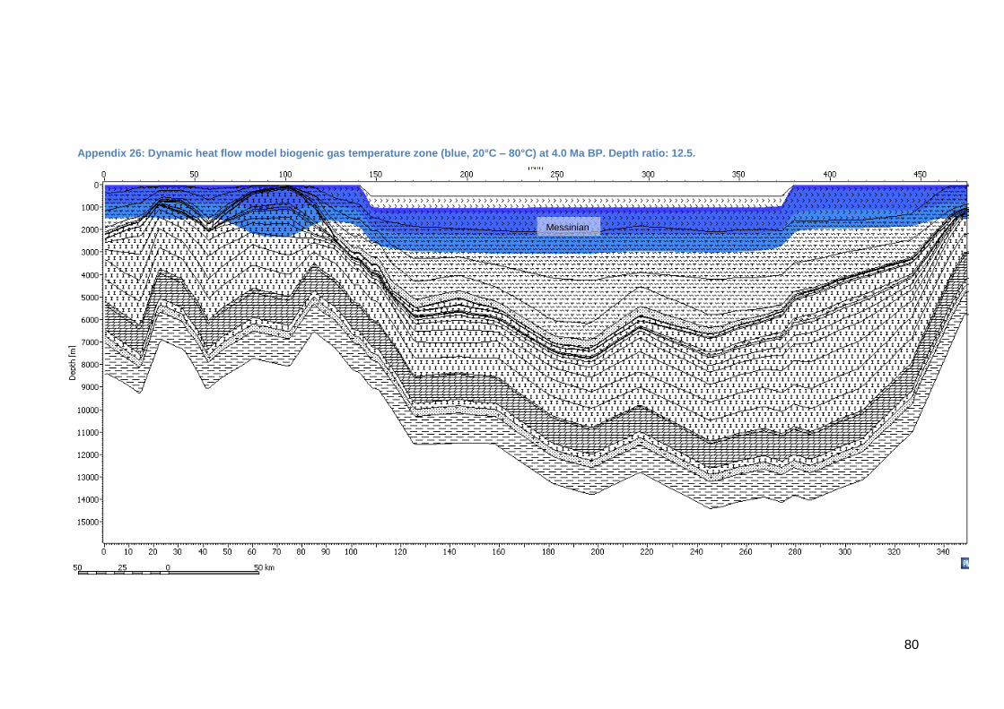
80

Appendix 26: Dynamic heat flow model biogenic gas temperature zone (blue, 20°C – 80°C) at 4.0 Ma BP. Depth ratio: 12.5.

Messinian

81

Appendix 27: Dynamic heat flow model biogenic gas temperature zone (blue, 20°C – 80°C) at present-day. Depth ratio: 12.5.

Messinian

82

Appendix 28: Constant heat flow model biogenic gas temperature zone (blue, 20°C – 80°C) at 7.1 Ma BP. Depth ratio: 12.5.

83

Appendix 29: Constant heat flow model biogenic gas temperature zone (blue, 20°C – 80°C) at 5.3 Ma BP. Depth ratio: 12.5.

Messinian

84

Appendix 30: Constant heat flow model biogenic gas temperature zone (blue, 20°C – 80°C) at 4 Ma BP. Depth ratio: 12.5.

Messinian

85

Appendix 31: Constant heat flow model biogenic gas temperature zone (blue, 20°C – 80°C) at present-day. Depth ratio: 12.5.

Messinian