RECONSTRUCTION, QUANTIFICATION, AND VISUALIZATION …

RECONSTRUCTION, QUANTIFICATION, AND VISUALIZATION OF FOREST

CANOPY BASED ON 3D TRIANGULATIONS OF AIRBORNE LASER SCANNING

POINT DATA

J. Vauhkonen a,b *

a University of Eastern Finland, School of Forest Sciences, Yliopistokatu 7 (P.O. Box 111), FI-80101 Joensuu, Finland –

[email protected] b University of Helsinki, Department of Forest Sciences, Latokartanonkaari 7 (P.O. Box 27), FI-00014 Helsinki, Finland

Commission III, WG III/4

KEY WORDS: Forest inventory, Tree allometry, Light Detection and Ranging (LiDAR), Delaunay triangulation, Alpha shape

ABSTRACT:

Reconstruction of three-dimensional (3D) forest canopy is described and quantified using airborne laser scanning (ALS) data with

densities of 0.6–0.8 points m-2 and field measurements aggregated at resolutions of 400–900 m2. The reconstruction was based on

computational geometry, topological connectivity, and numerical optimization. More precisely, triangulations and their filtrations,

i.e. ordered sets of simplices belonging to the triangulations, based on the point data were analyzed. Triangulating the ALS point

data corresponds to subdividing the underlying space of the points into weighted simplicial complexes with weights quantifying the

(empty) space delimited by the points. Reconstructing the canopy volume populated by biomass will thus likely require filtering to

exclude that volume from canopy voids. The approaches applied for this purpose were (i) to optimize the degree of filtration with

respect to the field measurements, and (ii) to predict this degree by means of analyzing the persistent homology of the obtained

triangulations, which is applied for the first time for vegetation point clouds. When derived from optimized filtrations, the total

tetrahedral volume had a high degree of determination (R2) with the stem volume considered, both alone (R2=0.65) and together with

other predictors (R2=0.78). When derived by analyzing the topological persistence of the point data and without any field input, the

R2 were lower, but the predictions still showed a correlation with the field-measured stem volumes. Finally, producing realistic

visualizations of a forested landscape using the persistent homology approach is demonstrated.

* Corresponding author

1. INTRODUCTION

Airborne laser scanning (ALS) has become a routinely operated

technique for obtaining wall-to-wall data for vast geographical

areas (e.g., White et al., 2013; Maltamo et al., 2014). From a

practical point of view, currently the most interesting ALS data

acquisitions are those carried out by several European countries

for ground elevation modeling (e.g. Nord-Larsen and Riis-

Nielsen, 2010; Dalponte et al., 2011; Gomez-Gutierrez et al.,

2011; Bohlin et al., 2012; Villikka et al., 2012). Due to their

regional to national coverage, these data provide a great

potential also for other applications such as environmental

mapping, monitoring and modelling.

The sparse point densities (<1 pulses m-2) of these data typically

limit the analyses to the use of area-based approaches of the

distributions of height values (e.g., Næsset, 2002). Notably,

such analyses employ only one of the three dimensions

available in the data and ignore the (horizontal) between-point

information. Triangulating point data, i.e. subdividing the

underlying space of the points into simplices, and subsequent

filtering of these triangulations (e.g., Delfinado and

Edelsbrunner, 1995) has been proposed as an alternative means

of representing the 3D canopy surface (Vauhkonen et al. 2014).

Compared to approaches like constructing pixel- or voxel-based

canopy height models from the data, a practical benefit of using

a triangulation-based approach is that instead of needing to

specify an artificial pixel or voxel resolution, the triangulations

are entirely based on the properties of the point data. Applying

filtrations, one can adjust the level of detail in the triangulated

point cloud and thus account for canopy gaps and detailed

properties existing in the data with the parameterization of the

filtration (see Figure 1; Section 2.3.). Finally, the use of

triangulations and filtrations provides means of constructing

genuine 3D visualizations of forested landscapes instead of just

representing counts of height values within pixel or voxel cells.

The filtering step is particularly needed to exclude the volume

populated by canopy biomass from that representing empty

space. A particularly interesting approach for the filtering is the

concept of 3D alpha shapes (Edelsbrunner and Mücke, 1994),

or α-shapes, in which a predefined parameter α is used as a size-

criterion to determine the level of detail in the obtained

triangulation. An important step is thus the selection of α, for

which the selected value should enable separation of void

spaces from those populated by canopy biomass. For this

purpose, Vauhkonen et al. (2014) proposed classifying the

simplices into either canopy biomass or voids based on

numerical optimization with field-measured biomass. This is

laborious due to the requirement of field data.

The main idea here is to test whether the appropriate level of

detail of the filtrations could be determined by analyzing the

inherent algebraic properties of the triangulations such as

simplicial homomorphism and topological persistence

ISPRS Annals of the Photogrammetry, Remote Sensing and Spatial Information Sciences, Volume II-3/W4, 2015 PIA15+HRIGI15 – Joint ISPRS conference 2015, 25–27 March 2015, Munich, Germany

This contribution has been peer-reviewed. The double-blind peer-review was conducted on the basis of the full paper. doi:10.5194/isprsannals-II-3-W4-255-2015

255

(Zomorodian, 2005). Earlier, Martynov (2008), computing

persistent homology groups at different spatial resolutions and

assuming that important features and structures persisted over a

wide range of scales, de-noised geometric models of power line

towers reconstructed from the ALS point data. Other

corresponding approaches to the point data depicting man-made

objects can be pointed out. To the best of the author’s

knowledge, however, the application described in Section 2.4 is

the first ever analysis of persistent homology of vegetation point

clouds.

The purpose of this study was thus to test the potential of

analyzing the persistent homology of the triangulated point data

to generate reliable 3D models of forest canopy. The resulting

triangulations, filtrations and canopy volumes were evaluated

against the field measurements of stem volume, and compared

with predictions based on using an optimized canopy volume

and the conventional height and density metrics for the same

purpose. Finally, the approach is demonstrated for a fully

automated visualization of a forested landscape.

2. METHODS

2.1 Material

2.1.1 Study area: The study area is a typical boreal managed

forest area in eastern Finland (62°31’N, 30°10’E) with Scots

pine (Pinus sylvestris L.) as the dominant tree species. It

represents 73% of the volume, Norway spruce (Picea abies [L.]

Karst.) 16% of the volume, and deciduous trees altogether about

11% of the volume.

2.1.2 Field measurements: Altogether 79 field plots were

measured on May – June 2010. The plots were placed

subjectively, attempting to record the species and size variation

over the area. Sample plot size varied between 20×20 and

30×30 m according to stand development class. The tree

measurements included species, DBH and height (H) for each

tree. Stem volumes (V) were calculated using the DBH and H

estimates in the species-specific volume equations described by

Laasasenaho (1982).

.

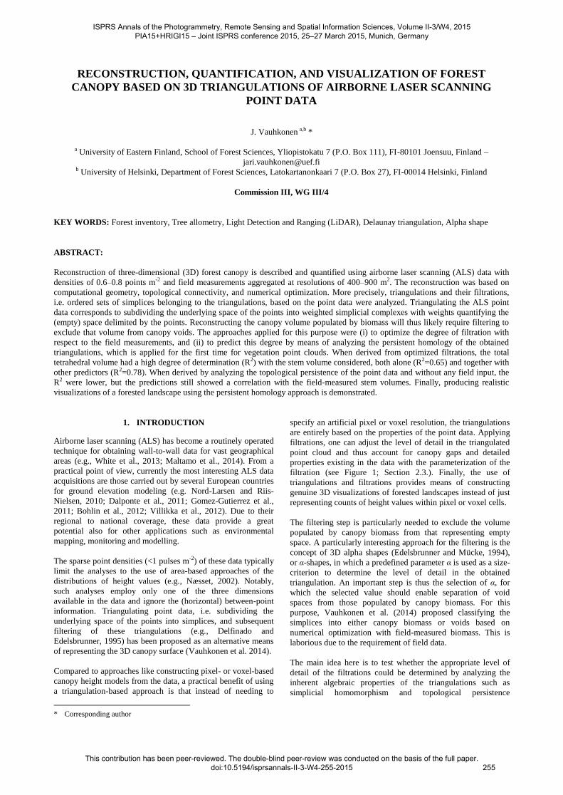
Figure 1. Triangulation and filtration of an example set of 3D points illustrated with symbols corresponding to Section 2.3. Subplot

(A) shows the extreme values of the filtration: the initial set of points (i=0, F[0]=0, C0=∅, and VC,0=0 m3) and the convex hull of the

point data (i=s=2081, F[2081]=∞, C2081=all, and VC,2081=11343.6 m3) denoted by dashed lines. The red lines in subplots B, C, and D

correspond to subcomplexes with F[214]=3.5m and VC,214=206.7 m3, F[746]=7.2m and VC,746=1379.1 m3, and F[1477]=18.7 m and

VC,1477=5206.5 m3, respectively.



256

2.1.3 ALS data: The ALS data used in the study were

acquired in two separate acquisitions. All numerical analyses

were carried out with data collected on 26 June 2009 using

Optech ALTM Gemini system from a flying height of 2000 m

and with a nominal density of 0.65 points m-2. A separate data

set collected on 30 April 2012 with Leica ALS 60 system from

a flying height of 2350 m and a density of 0.79 points m-2 was

further utilized for visualization. Both the data sets were pre-

processed in a similar way, i.e. the ground surface was detected

and classified, and the echo heights normalized with respect to

this surface following a standard TerraScan approach. Only the

first echoes (i.e. ‘only’ and ‘first-of-many’ of multiple echoes

recorded per pulse) extracted employing a ground threshold of 1

m were included in the analyses

2.2 An overview of the methods

The main aim was to model the 3D canopy by means of

triangulating the ALS point data, i.e. subdividing the underlying

space of the points into simplices, which results in weighted

simplicial complexes (e.g. Edelsbrunner, 2011) with weights

quantifying the (empty) space delimited by the points.

Reconstructing the canopy volume populated by biomass will

thus likely require filtering to exclude that volume from canopy

voids (Figure 1). For this purpose, we considered the following

steps, which are explained in detail in the subsequent sections.

1. Define filtering rules to be able to adjust the level of detail in

the triangulation based on the ALS data of separate plots

(Section 2.3.).

2. Define the degree of filtering such that the resulting filtration

corresponded the reference forest measurements as closely as

possible. For this step, we considered two alternatives: (i)

derive the degree of filtering by analyzing the topological

persistence of the point data (Section 2.4.), and (ii) optimize the

degree of filtering with the reference basal area observed from

the plots used in step 1 (Section 2.5.).

3. Evaluate and visualize the predictions obtained (Section

2.6.).

2.3 Deriving triangulations and their filtrations

The terminology and notation in the following are adapted from

Delfinado and Edelsbrunner (1995), to which the reader is

referred for additional details. A triangulation T of a finite set of

points S is a subdivision of the convex hull of S into simplices

according to the rules of the particular triangulation (see, e.g.,

Preparata and Shamos, 1985). T is a simplicial complex that is

subsettable to a finite number of subcomplexes Ci, i=1, 2, …, s,

where i indexes the position and s is the number of different

subcomplexes in a list of potential filter values F defining

which simplices belong to the subcomplex (see the next

paragraph). When F is ordered (here ascendingly), the sequence

Ci constitutes a filtration, in which each complex is a sub-

complex of its successor, and VC,i is the volume of the

underlying space of subcomplex Ci according to this filtration.

The point data of each individual plot were triangulated and

filtered separately. The filtration corresponded to the family of

3D α-shapes (Edelsbrunner and Mücke, 1994), each of which

consist of those simplices of T, which have an empty

circumscribing sphere with a squared radius smaller than α.

Although an α-shape is defined for every non-negative real α,

there are only finitely many different α-complexes (see

Delfinado and Edelsbrunner, 1995, p. 782), and F was thus an

ascending sequence of those α-values which altered the α-shape.

All computations were based on Delaunay triangulations and

implemented with C++ and an open-source Computational

Geometry Algorithms Library (Pion and Teillaud, 2013; Da and

Yvinec, 2013).

2.4 Persistent homology

During the filtration of the data (Figure 1), i.e. by increasing the

considered filtration parameter α, simplices of a dimension d

join together with other d-dimensional simplices to form

structures with a higher dimensionality. Particularly, when the

value of α allows two points (d=0) to connect, an edge with d=1

between these two points is formed. The edges further join to

form facets (d=2) and tetrahedra (d=3), the latter being the

highest dimension considered here. Each simplex can thus be

assigned by a value describing its persistence in the structure

formed. This index of persistence was in this case obtained as

the absolute difference between the index values of α causing

the birth and death of simplices of the given dimension.

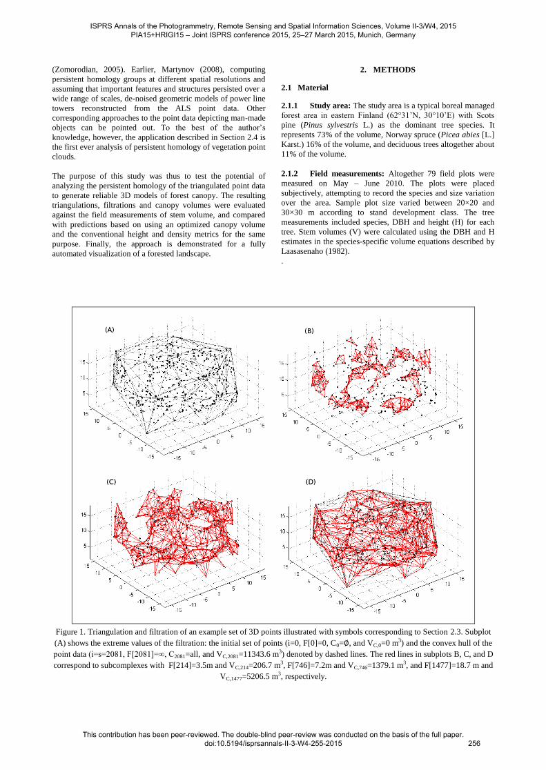
Following the logic of the previous paragraph, a birth and death

diagram (Figure 2) was computed for indices with d=1 and d=2.

Only these dimensions need to be considered, since those with

d=0 or d=3 do not born or die, respectively, in this process. In

the diagram, the most interesting observations are those off-

diagonal: the simplices are interpret to cause the most

fundamental changes to the triangulated structure, typically at

the lowest values of α, while diagonality of the observations

indicates stability (persistence) of those features. The value for

the α parameter was thus decided separately for each plot as the

maximum off-diagonal α at the death of both d=1 and d=2.

The reasoning behind this approach is the attempt to discover

such a value for the parameter α, beyond which the changes to

the filtration were irrelevant in that those did not affect the

primary structures of the obtained filtration. An example birth

and death diagram corresponding to the point data and

triangulation in Figure is given by Figure 2, while the

mathematical formalism of this approach is presented in much

more detail by Edelsbrunner et al. (2002).

Figure 2. An example birth and death diagram, corresponding to

the point data and triangulation of Figure 1. The selected value

of α was approximately 5.8 m for this plot.



257

2.5 Filtering the triangulations by an optimization with

respect to forest biomass in the training plots

To optimize the filtrations, the studied set of field plots was

considered jointly. For convenience, let VC,i,p in the following

text denote the volume of the underlying space of a subcomplex

Ci of the ALS point data of plot p. The optimization was based

on minimizing the residual errors of a linear regression model

Gp = β1 + β2 VC,i,p + εp, (1)

where Gp was the reference basal area, β1 and β2 the model

parameters, and εp the residual error of plot p. Although the

ALS point data could be expected to represent canopy biomass

(branches and foliage) rather than that originating from the

stems, G is the most typical forest biophysical property

measured in forest inventories with strong allometric links to

other forest variables (see further notes in Section 5). Therefore

we optimized Eq. 1 with respect to this variable.

The initial values of β1 and β2 were obtained by fitting the

model to VC,i,p with i selected randomly for each plot. In the

optimization, VC,i,q of plot q which produced the largest residual

error was altered to VC,i+10,q in successive rounds of 500

iterations, until either the error, determined as 1 – the obtained

coefficient of determination (R2), decreased below 0.0009 or

did not change during the last round of iterations. The whole

procedure was repeated 100 times, which resulted in range of

filtration parameters and thus canopy volumes that were in a

quasi-optimal linear relationship with forest biomass in at least

one out of the 100 solutions. The per-plot mean value of these

ranges was used in the subsequent analyses.

2.6 Evaluation, performance measures, and visualization

The numerical evaluation of our approach was based on

assessing the correspondence of the total tetrahedral volume of

the filtrations with the plot-level stem volume measured in the

field. This relationship was quantified by fitting an allometric

power equation (White and Gould, 1965):

yp = b VC,i,pk + εp, (2)

where yp was the reference stem volume, VC,i,p the tetrahedral

volume of the underlying space of the selected subcomplex Ci,p,

b and k the model parameters, and εp the residual error of plot p.

The model fitting was carried out with the nls function of R (R

Core Team, 2012).

The allometric power equation corresponding to Eq. 2 was also

fit between the reference stem volumes and the most common

ALS-based predictor variables (cf. Næsset 2002). The latter

were the mean and standard deviation of the height values, the

proportion of echoes above 2 m, and the 5th, 10th, 20th, …,

90th, and 95th percentiles and the corresponding proportional

densities of the ALS-based canopy height distribution,

calculated according to Korhonen et al. (2008, pp. 502–503).

The correspondence of the estimates with the reference data was

evaluated by graphical assessments and in terms of R2, root

mean squared error (RMSE) and mean difference (bias). The

latter two were calculated using the standard equations

presented by Vauhkonen et al. (2014), for example.

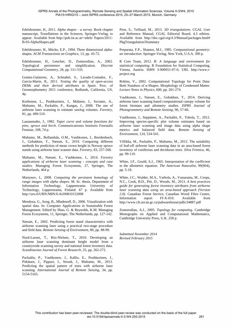
To demonstrate the potential of the proposed approach for 3D

visualizations of forest canopy, the ALS point data of a forested

area of approximately 1000 × 1200 m was divided on a grid

with a cell size of 20 × 20 m. Each cell of this grid was

separately triangulated and analyzed for its persistent homology.

Therefore, the only input for the visualization of the forest was

the ALS point data, while the filtration parameter α

corresponded to the value obtained following Section 2.4. The

locations of the lakes and roads in the area were extracted from

a topographic database maintained by the National Land Survey

of Finland and inserted manually to the image. The image of the

entire forest area was finally drawn with graphical functions of

Matlab.

3. RESULTS

Approximately 50% of the optimized solutions (Eq. 1) yielded

R2 ≥ 0.985 and the average R2 was 0.93. The mean values of the

100 iterations of optimizing Eq. 1 produced a nearly 1:1

relationship with the plot-level basal area used in the

optimization (R2≈1.0). Due to the allometric relationships

between the basal area and other forest attributes, the tetrahedral

volume was in a good correspondence also with the main

evaluated attribute, i.e. the total stem volume. For example, the

optimization produced an R2 of 0.65 between these attributes.

The tetrahedral volume derived by analyzing the persistent

homology of the triangulations was not as accurate as the

reference canopy volume produced by optimization (Table 1,

Figure 3). However, noting that no allometric information on

the forest attributes was used in the derivation (unlike in the

case of the optimized one), the metric deduced from the

properties of the point data is somewhat related to stem volume

as well.

When inserted jointly to Eq. 2, the conventional height and

density metrics showed a better degree of determination

between the predicted and reference values than the volumetric

features (Table 1). However, inserting the tetrahedral volume

obtained by analyzing the persistent homology of the point data

improved the model despite the low degree of determination of

this metric in the first place.

Finally, despite the low degree of determination with the field

measured stem volume, the positions of the canopy elements

derived with the persistent homology approach corresponded

well to those of the field-measured tree stems (Figure 4), which

showed a considerable potential in producing realistic

visualizations of a forested landscape (Figure 5). When looked

more closely and with respect of an aerial or satellite image, the

canopy volume produced by the approach seems to realistically

convey information of the real canopy and existence of canopy

gaps. Furthermore, although there are discontinuities between

the 20 × 20 m cells, these do not seem to prevent a landscape-

level visualization with the approach proposed.

Predictors R2 RMSE, m3/ha bias, m3/ha

CVO 0.65 44.3 -3.5

CVP 0.17 66.7 6.8

H 0.65 43.5 -7.5

D 0.16 67.0 1.1

H + D 0.78 34.0 4.4

H + D + CVP 0.78 33.9 5.4

Table 1. Accuracies of predicting the plot-level stem volume

with Eq. 2 fit with the given predictors. CVO – the tetrahedral

volume of the optimized filtrations, CVP – the tetrahedral

volume derived by persistent homology, H – the most correlated

height feature (90th percentile), D – the most correlated density

feature (proportion of echoes above 1 m height). The average

stem volume was 197.6 m3/ha.



258

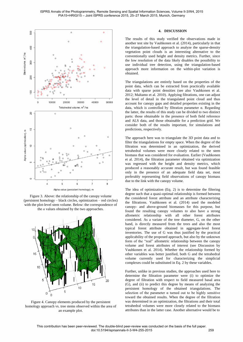
Figure 3. Above: the relationship of the canopy volume

(persistent homology – black circles, optimization – red circles)

with the plot-level stem volume. Below: the correspondence of

the α values obtained by the two approaches.

Figure 4. Canopy elements produced by the persistent

homology approach vs. tree stems observed within the area of

an example plot.

4. DISCUSSION

The results of this study verified the observations made in

another test site by Vauhkonen et al. (2014), particularly in that

the triangulation-based approach to analyze the sparse-density

vegetation point clouds is an interesting alternative to the

conventionally used height and density metrics. Further, since

the low resolution of the data likely disables the possibility to

use individual tree detection, using the triangulation-based

approach more information on the within-plot variation is

obtained.

The triangulations are entirely based on the properties of the

point data, which can be extracted from practically available

data with sparse point densities (see also Vauhkonen et al.

2012; Maltamo et al. 2010). Applying filtrations, one can adjust

the level of detail in the triangulated point cloud and thus

account for canopy gaps and detailed properties existing in the

data, which is controlled by filtration parameter α. Regarding

the latter, the results of this study can be divided to two distinct

parts: those obtainable in the presence of both field reference

and ALS data, and those obtainable for a prediction grid. We

consider both of the results important, for simulations and

predictions, respectively.

The approach here was to triangulate the 3D point data and to

filter the triangulations for empty space. When the degree of the

filtration was determined in an optimization, the derived

tetrahedral volumes were more closely related to the stem

biomass that was considered for evaluation. Earlier (Vauhkonen

et al. 2014), the filtration parameter obtained via optimization

was regressed with the height and density metrics, which

produced a reasonably accurate result, but was found feasible

only in the presence of an adequate field data set, most

preferably representing field observations of canopy biomass

due to the link with the canopy volume.

The idea of optimization (Eq. 2) is to determine the filtering

degree such that a quasi-optimal relationship is formed between

the considered forest attribute and an attribute characterizing

the filtrations. Vauhkonen et al. (2014) used the modeled

canopy- and above-ground biomasses for this purpose, but

found the resulting canopy volumes to also have a strong

allometric relationship with all other forest attributes

considered. As a variate of the tree diameter, G, on the other

hand, is directly measured from the trees and also the most

typical forest attribute obtained in aggregate-level forest

inventories. The use of G was thus justified by the practical

applicability of the proposed approach, but also by the unknown

form of the “real” allometric relationship between the canopy

volume and forest attributes of interest (see Discussion by

Vauhkonen et al. 2014). Whether the relationship formed by

other variables was better justified, both G and the tetrahedral

volume currently used for characterizing the simplicial

complexes could be substituted in Eq. 2 by these variables.

Further, unlike in previous studies, the approaches used here to

determine the filtration parameter were (i) to optimize the

degree of filtration with respect to field measured basal area

(G), and (ii) to predict this degree by means of analyzing the

persistent homology of the obtained triangulations. The

selection of the parameter α turned out to be highly sensitive

toward the obtained results. When the degree of the filtration

was determined in an optimization, the filtrations and their total

tetrahedral volumes were more closely related to the biomass

attributes than in the latter case. Another alternative would be to



259

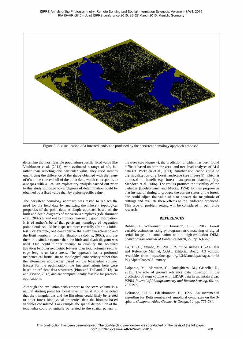
Figure 5. A visualization of a forested landscape produced by the persistent homology approach proposed.

determine the most feasible population-specific fixed value like

Vauhkonen et al. (2012), who evaluated a range of α’s, but

rather than selecting one particular value, they used metrics

quantifying the difference of the shape obtained with the range

of α’s to the convex hull of the point data, which corresponds to

α-shapes with α→∞. An exploratory analysis carried out prior

to this study indicated lower degrees of determination could be

obtained by a fixed value than by a plot-specific value.

The persistent homology approach was tested to replace the

need for the field data by analyzing the inherent topological

properties of the point data. A simple approach based on the

birth and death diagrams of the various simplices (Edelsbrunner

et al., 2002) turned out to produce reasonably good information.

It is of author’s belief that persistent homology of vegetation

point clouds should be inspected more carefully after this initial

test. For example, one could derive the Euler characteristic and

the Betti numbers from the filtrations (Robins, 2002), and use

them in a similar manner than the birth and death diagram was

used. One could further attempt to quantify the obtained

filtration by other geometric features than total volumes such as

edge lengths or facet areas. The approach has a profound

mathematical formalism on topological connectivity rather than

the alternative approaches based on the tetrahedral volume.

Except for the optimization, the implementations here were

based on efficient data structures (Pion and Teillaud, 2013; Da

and Yvinec, 2013) and are computationally feasible for practical

applications.

Although the evaluation with respect to the stem volume is a

natural starting point for forest inventories, it should be noted

that the triangulations and the filtrations could likely be related

to other forest biophysical properties than the biomass-based

variables considered. For example, the spatial distribution of the

tetrahedra could potentially be related to the spatial pattern of

the trees (see Figure 4), the prediction of which has been found

difficult based on both the area- and tree-level analyses of ALS

data (cf. Packalén et al., 2013). Another application could be

the visualization of a forest landscape (see Figure 5), which is

proposed to benefit e.g. forest management planning (e.g.

Mendoza et al. 2006). The results promote the usability of the

α-shapes (Edelsbrunner and Mücke, 1994) for this purpose in

that instead of aiming to produce the current status of the forest,

one could adjust the value of α to present the magnitude of

cuttings and evaluate these effects to the landscape produced.

This type of problem setting will be considered in our future

research.

REFERENCES

Bohlin, J., Wallerman, J., Fransson, J.E.S., 2012. Forest

variable estimation using photogrammetric matching of digital

aerial images in combination with a high-resolution DEM.

Scandinavian Journal of Forest Research, 27, pp. 692-699.

Da, T.K.F., Yvinec, M., 2013. 3D alpha shapes. CGAL User

and Reference Manual, CGAL Editorial Board, 4.3 edition.

Available from http://doc.cgal.org/4.3/Manual/packages.html#

PkgAlphaShapes3Summary

Dalponte, M., Martinez, C., Rodeghiero, M., Gianelle, D.,

2011. The role of ground reference data collection in the

prediction of stem volume with LiDAR data in mountain areas.

ISPRS Journal of Photogrammetry and Remote Sensing, 66, pp.

787-797.

Delfinado, C.J.A., Edelsbrunner, H., 1995. An incremental

algorithm for Betti numbers of simplicial complexes on the 3-

sphere. Computer Aided Geometric Design, 12, pp. 771-784.



260

Edelsbrunner, H., 2011. Alpha shapes – a survey. Book chapter

manuscript, Tessellations in the Sciences, Springer-Verlag, to

appear. Available from http://pub.ist.ac.at/~edels/ Papers/2011-

B-03-AlphaShapes.pdf

Edelsbrunner, H., Mücke, E.P., 1994. Three dimensional alpha-

shapes. ACM Transactions on Graphics, 13, pp. 43-72.

Edelsbrunner, H., Letscher, D., Zomorodian, A., 2002.

Topological persistence and simplification. Discrete

Computational Geometry, 28, pp. 511-533.

Gomez-Gutierrez, A., Schnabel, S., Lavado-Contador, F.,

Garcia-Marin, R., 2011. Testing the quality of open-access

DEMs and their derived attributes in Spain. Proc. of

Geomorphometry 2011 conference, Redlands, California, US,

4p.

Korhonen, L., Peuhkurinen, J., Malinen, J., Suvanto, A.,

Maltamo, M., Packalén, P., Kangas, J., 2008. The use of

airborne laser scanning to estimate sawlog volumes. Forestry,

81, pp. 499-510.

Laasasenaho, J., 1982. Taper curve and volume functions for

pine, spruce and birch. Communicationes Institutis Forestalis

Fenniae, 108, 74 p.

Maltamo, M., Bollandsås, O.M., Vauhkonen, J., Breidenbach,

J., Gobakken, T., Næsset, E., 2010. Comparing different

methods for prediction of mean crown height in Norway spruce

stands using airborne laser scanner data. Forestry, 83, 257-268.

Maltamo, M., Næsset, E., Vauhkonen, J., 2014. Forestry

applications of airborne laser scanning - concepts and case

studies. Managing Forest Ecosystems, 27, Springer, The

Netherlands, 464 p.

Martynov, I., 2008. Computing the persistent homology of

range images with alpha shapes. M. Sc. thesis, Department of

Information Technology, Lappeenranta University of

Technology, Lappeenranta, Finland. 67 p. Available from

http://urn.fi/URN:NBN:fi-fe200810152008

Mendoza, G., Song, B., Mladenoff, D., 2006. Visualization with

spatial data. In: Computer Applications in Sustainable Forest

Management. Edited by Shao, G. & Reynolds, K.M. Managing

Forest Ecosystems, 11, Springer, The Netherlands, pp. 127-142.

Næsset, E., 2002. Predicting forest stand characteristics with

airborne scanning laser using a practical two-stage procedure

and field data. Remote Sensing of Environment, 80, pp. 88-99.

Nord-Larsen, T., Riis-Nielsen, T., 2010. Developing an

airborne laser scanning dominant height model from a

countrywide scanning survey and national forest inventory data.

Scandinavian Journal of Forest Research, 25, pp. 262-272.

Packalén, P., Vauhkonen, J., Kallio, E., Peuhkurinen, J.,

Pitkänen, J., Pippuri, I., Strunk, J., Maltamo, M., 2013.

Predicting the spatial pattern of trees with airborne laser

scanning. International Journal of Remote Sensing, 34, pp.

5154-5165.

Pion, S., Teillaud, M., 2013. 3D triangulations. CGAL User

and Reference Manual, CGAL Editorial Board, 4.3 edition.

Available from http://doc.cgal.org/4.3/Manual/packages.html#

PkgTriangulation3Summary

Preparata, F.P., Shamos, M.I., 1985. Computational geometry:

an introduction. Springer-Verlag, New York, U.S.A. 390 p.

R Core Team, 2012. R: A language and environment for

statistical computing. R Foundation for Statistical Computing,

Vienna, Austria. ISBN 3-900051-07-0, URL http://www.r-

project.org

Robins, V., 2002. Computational Topology for Point Data:

Betti Numbers of α-Shapes. Morphology of Condensed Matter.

Lecture Notes in Physics, 600, pp. 261-274.

Vauhkonen, J., Næsset, E., Gobakken, T., 2014. Deriving

airborne laser scanning based computational canopy volume for

forest biomass and allometry studies. ISPRS Journal of

Photogrammetry and Remote Sensing, 96, 57-66.

Vauhkonen, J., Seppänen, A., Packalén, P., Tokola, T., 2012.

Improving species-specific plot volume estimates based on

airborne laser scanning and image data using alpha shape

metrics and balanced field data. Remote Sensing of

Environment, 124, 534-541.

Villikka, M., Packalén, P., Maltamo, M., 2012. The suitability

of leaf-off airborne laser scanning data in an area-based forest

inventory of coniferous and deciduous trees. Silva Fennica, 46,

pp. 99-110.

White, J.F., Gould, S.J., 1965. Interpretation of the coefficient

in the allometric equation. The American Naturalist, 99(904),

pp. 5-18.

White, J.C., Wulder, M.A., Varhola, A., Vastaranta, M., Coops,

N.C., Cook, B.D., Pitt, D., Woods, M., 2013. A best practices

guide for generating forest inventory attributes from airborne

laser scanning data using an area-based approach (Version

2.0). Canadian Forest Service, Canadian Wood Fibre Centre,

Information report FI-X-010. Available from

http://www.cfs.nrcan.gc.ca/pubwarehouse/pdfs/34887.pdf

Zomorodian, A.J., 2005. Topology for computing. Cambridge

Monographs on Applied and Computational Mathematics,

Cambridge University Press, U.K. 258 p.

Submitted November 2014

Revised February 2015



261

RECONSTRUCTION, QUANTIFICATION, AND VISUALIZATION …

Documents

Transcript of RECONSTRUCTION, QUANTIFICATION, AND VISUALIZATION …