Reconstruction of sound ﬁelds with a spherical microphone ... · Reconstruction of sound ﬁelds...

Reconstruction of sound fields with a spherical microphone array

Efren Fernandez-Grande, Tim Walton

Acoustic Technology, Department of Electrical Engineering, DTUTechnical University of Denmark

ABSTRACTSpherical microphone arrays are very well suited for sound field measurements in enclosures or interior spaces,and generally in acoustic environments where sound waves impinge on the array from multiple directions.Because of their directional properties, they make it possible to resolve sound waves traveling in any direction.In particular, rigid sphere microphone arrays are robust, and have the favorable property that the scatteringintroduced by the array can be compensated for - making the array virtually transparent. This study examines arecently proposed sound field reconstruction method based on a point source expansion, i.e. equivalent sourcemethod, using a rigid spherical array. The study examines the capability of the method to distinguish betweensound waves arriving from different directions (i.e., as a sound field separation method). This is representativeof the potential of the method to perform sound field identification and visualization in non-anechoic spaces,and ultimately for general in-situ measurements.

Keywords: Sound radiation, microphone arrays, spherical arrays, acoustic holography

I-INCE Classification of Subjects Number(s): 74.7, 23.1, 01.2

1. INTRODUCTIONSpherical microphone arrays are particularly convenient for measurements in interior spaces, enclosures, or inacoustic environments where sound waves arrive to the array from multiple directions [1–3], to a large extentbecause of their geometry (other common array configurations cannot distinguish between waves coming fromdifferent sides of the array, or the array properties depend on the direction of incidence of the waves [4]). Inaddition to this, rigid spherical microphone arrays are robust, and the scattering introduced by the array can becompensated for, making the array virtually transparent - which conveys great potential to the measurementprinciple.

This paper deals with the reconstruction of sound fields based on measurements with a rigid sphericalmicrophone array, i.e. to capture a sound field at a measurement surface, to then ‘predict’ the entire soundfield elsewhere, inferring the sound pressure, particle velocity and intensity vector, typically over a three-dimensional space. The approach differs from localization methods, in spite of the underlying similarities [5],in that the aim is not only to determine the direction from which waves arrive to the measurement area, but toestimate all acoustic quantities in any position in space based on the measured data.

Existing spherical holography methods rely on a expansion into spherical harmonics to provide a represen-tation of the sound field. By means of ‘propagating’ the radial functions, they make it possible to predict eitherthe total sound field [6, 7], or the incident sound field without the scattering introduced by the array [8–10].Nevertheless, the domain of validity of existing methods is restricted to a spherical surface concentric to thearray and entirely contained in the free-space (sources outside the domain). This imposes a limitation due tothe obvious geometrical constrains. It is the motivation of the present work to address this matter.2

A method is proposed in this paper based on an equivalent source model [12] that takes into account thescattering introduced by the rigid spherical array. The entire sound field can be reconstructed at any point of thesource-free domain without being restricted to a spherical surface, and the array’s scattering is compensatedfor. The study also examines the capability of the method to distinguish between sound waves arriving fromdifferent directions (i.e., as a sound field separation method), since this is representative of the potential of themethod to perform sound field identification in non-anechoic spaces, and general in-situ measurements.

[email protected] initial study was presented in a recent meeting [11]

Inter-noise 2014 of 8

[email protected]

of 8 Inter-noise 2014

2. THEORY2.1 Background and existing methodsThe existing methodologies for reconstructing sound fields using spherical arrays rely on expanding themeasured sound field into a spherical harmonic expansion, to then make use of the radial functions (sphericalBessel) to reconstruct the sound field elsewhere. The most straightforward case is with an open spherical array;the reconstructed field is [13]

p(r,Ω) =∞

∑n=0

n

∑m=−n

jn(kr)jn(ka)

Y mn (Ω)

∫Ω

p(a,Ω)Y mn (Ω)∗dΩ, (1)

where p(a,Ω) is the measured sound pressure. For notational simplicity the angular dependency is denotedby Ω ≡ (θ ,φ) thus r = (r,θ ,φ) ≡ (r,Ω), and dΩ ≡ sinθdθdφ , so that the integration over the sphere is∫

Ω(·)dΩ ≡

∫ 2π

0∫

π

0 (·)sinθdθdφ . The radius of the sphere is a, jn is the spherical Bessel function of ordern, k is the wavenumber, and (·)∗is the complex conjugate. The time dependency ejωt has been omitted, andthe spherical Hankel functions are of the second kind, defined as h(2)n (x) = jn(x)− jyn(x), where yn(x) is aspherical Neumann function of order n. From here onwards, h(2)n ≡ hn. The Spherical harmonics Y m

n (Ω) aredefined as

Y mn (θ ,φ)≡

√(2n+1)

4π

(n−m)!(n+m)!

Pmn (cos(θ))e−jmφ . (2)

Consider a microphone array flush-mounted on a rigid sphere. The total sound field is naturally composedof the incident and the scattered sound, and it can be expanded into spherical harmonics as [7]

pt(r,Ω) =∞

∑n=0

n

∑m=−n

(ka)2[ jn(kr)y′n(ka)− j′n(ka)yn(kr)]Y mn (Ω)

∫Ω

p(a,Ω)Y mn (Ω)∗dΩ. (3)

Equation (3) makes it possible to reconstruct the total sound field, incident plus scattered, in free-space at anyother radius than measured. This expression is the one used in Ref. [7].

Nevertheless, it is also possible to compensate for the scattering introduced by the rigid sphere array. Theprinciple is to reconstruct the sound field, based on only the basis functions that describe the incident soundfield. The incident pressure can be reconstructed as [9]

pi(r,Ω) = j(ka)2∞

∑n=0

n

∑m=−n

h′n(ka) jn(kr)Y mn (Ω)

∫Ω

p(a,Ω)Y mn (Ω)∗dΩ. (4)

This is the expression given in Ref. [9], although here it has been simplified via the Wronksian relationship.It is apparent from Eqs. (3) and (4) that the reconstruction in all three cases is based upon the propagation

of the radial functions jn(kr) and yn(kr) from the measurement radius (a) to a different one (r). However, thisexpansion - being a solution to the Helmholtz equation, is only valid for the source-free medium, i.e., betweenthe radius of the sphere r = a and the closest source or boundary r = r′. This imposes a limitation due togeometrical constrains, and it is not possible to reconstruct the sound field very close to a source or boundary,unless it is approximately spherical, an unlikely general case. The proposed method overcomes this limitation.

2.2 Sound field due to a point sourceLet there be a point source at r0 = (r0,θ0,φ0) with volume velocity Q, radiating in the presence of a rigidsphere centered at the origin of coordinates. The total sound pressure is a sum of the incident waves and thewaves scattered by the sphere, pt(r,Ω) = pi(r,Ω)+ ps(r,Ω). The incident sound pressure is

pi =jωρQe−jkR

4πR= jωρQ G(r,r0), (5)

where G(r,r0) is the free-field Green’s function and R = |r0− r| is the distance between the observation pointand the position of the point source. In a spherical harmonic expansion, the incident pressure pi takes thegeneral form of a so-called ‘complete solution’

pi(r) =∞

∑n=0

n

∑m=−n

Amn jn(kr)h(2)n (kr0)Y mn (Ω)Y m

n (Ω0)∗, (6)

Page 2 of 8 Inter-noise 2014


and the free-space Green’s function in spherical harmonics is [7]

G(r,r0) =−jk∞

∑n=0

n

∑m=−n

jn(kr)hn(kr0)Y mn (Ω)Y m

n (Ω0)∗. (7)

From which the Amn coefficients are obtained as Amn = ρck2Q. On the other hand, the scattered pressure pstakes the form of a ‘radiation solution’

ps(r) =∞

∑n=0

n

∑m=−n

Bnmhn(kr)Y mn (Ω). (8)

The boundary condition of the problem dictates that the radial component of the particle velocity must vanishat the boundary (r = a), the surface of the rigid sphere, ∂ pi

∂ r

∣∣∣r=a

+ ∂ ps∂ r

∣∣∣r=a

= 0, from which the scattering

coefficients can be calculated, Bmn =−Amnj′n(ka)

h′(2)n (ka)hn(kr0)Y m

n (Ω0)∗, yielding the total sound pressure

pt(r) = ρck2Q∞

∑n=0

n

∑m=−n

(jn(kr)− j′n(ka)

h′n(ka)hn(kr)

)hn(kr0)Y m

n (Ω)Y mn (Ω0)

∗. (9)

Finally making use of the Wronskian relation, the pressure on the surface of the sphere at (a,Ω), due to a pointsource in (r0,Ω0) is simplified to

pt(a,Ω) =−jρcQ

a2

∞

∑n=0

n

∑m=−n

h(2)n (kr0)

h′(2)n (ka)Y m

n (Ω)Y mn (Ω0)

∗. (10)

From the addition theorem, this expression can be simplified further, due to the rotational axisymmetry of thefield around the axis from the center of the sphere to the point source, yielding it only as a function of theLegendre polynomials, with constant azimuth, instead of the full spherical harmonic solution. Nonetheless thelatter general case, Eq. (10), is considered here.

2.3 Method: Point source expansion with a rigid spherical arrayThe essential idea behind the proposed method is to use Eq. (10) as the basis to describe an arbitrary sound

field as a superposition of the waves radiated by a combination of point sources that are placed outside thedomain of interest. This domain can be of arbitrary shape, as opposed to existing methods. The equivalentsources can be placed either inside a source under study (for instance a radiation problem, where the sourceis ‘substituted’ by a combination of point sources), or outside the domain inside which the sound field isreconstructed (if for instance one is concerned with reconstructing the sound field over a certain volume in afree-field, or inside an enclosure, etc.).

The pressure on the surface of the sphere at (a,Ωk), due to a point source in (r0,Ω0) is the one given in Eq.(10). Based on this, the sound pressure measured on each of the K transducers of the array can be expanded asa continuous distribution of point sources over a surface S. This surface is where the point sources are placed,thus S is associated with r0 = (r0,Ω0)

pt(a,Ωk) =∫∫

S

−jρcQ(r0)

a2

∞

∑n=0

n

∑m=−n

h(2)n (kr0)

h′(2)n (ka)Y m

n (Ωk)Y mn (Ω0)

∗ dS, (11)

or, using a discrete distribution of L equivalent sources,

pt(a,Ωk) =L

∑l=1

−jρcQl

a2

∞

∑n=0

n

∑m=−n

h(2)n (kr0,l)

h′(2)n (ka)Y m

n (Ωk)Y mn (Ω0,l)

∗. (12)

Conducting the summation over the angle and radial functions (over m and n), in practice truncated at∑

Nn=0 ∑

nm=−n (see Sect. 3), it is possible to express the total sound pressure pt at a discrete set of K points on

the sphere, in matrix form aspt = GNq, (13)

where pt is a K×1 vector with the measured pressures, q a L×1 vector with the yet unknown source strengths(note that they are jωρQl), and GN a K×L transfer matrix between the source strengths and the total measured

Inter-noise 2014 Page 3 of 8


pressures on the sphere. This is typically an underdetermined problem, ill-posed when r is between the sourceand the array, requiring regularization for it’s inversion [10, 14],

q = G−1N p = VFΣΣΣ

−1UHp. (14)

The regularized inversion (G−1N ) is performed based on a singular value decomposition of GN = UΣΣΣVH ,

where U and VH are unitary vectors and ΣΣΣ contains the singular values of the transfer matrix. The matrixF is a diagonal matrix that contains the regularization filter factors, in this study either truncated at σmaxor using Tikhonov regularization Fii = σ2

i /(σ2i +λ 2), with λ the regularization parameter. This parameter

will determine the ‘weight’ of the singular values in the solution, so that the noisy terms are left out of thereconstruction.3

Once the strength of the sources has been determined, the incident sound pressure can be predictedanywhere in the domain of interest

pi = Gq, (15)where G is a reconstruction matrix that consists of the Green’s function in free-space between the position ofthe sources r0 and the reconstruction points, as in Eq. (5). This fact signifies that the scattering introduced bythe sphere is not present in the reconstructed field, since it is based on the free-field sound pressure radiated byeach point source. The total pressure could be reconstructed using GN instead.

The particle velocity vector can be calculated from Euler’s equation of motion, u = −1jωρ

∇p, or introducingthe gradient of the Green’s function G∇ = ∇G(r,r0)

u =−1jωρ

G∇q, (16)

and correspondingly the sound intensity vector as

I =12

Rep u∗, (17)

where (·)∗ is the complex conjugate. It is apparent from these equations that the reconstruction provides acomplete characterization of the acoustic field. This method can be understood as an extension of the equivalentsource method or wave superposition method to measurements with a rigid sphere microphone array. It can beused to reconstruct over arbitrary geometries, and the scattering introduced by the array is compensated for.

3. NUMERICAL RESULTSA numerical study is conducted to test the proposed method, compare it to the existing ones and examineits accuracy. In the simulated measurements, the array used is a rigid sphere array of radius 9.75 cm, with50 microphones, distributed nearly uniformly, and with a sampling that limits the expansion to N ≤ 5 orders(so that the orthogonality of the spherical wave expansion is satisfied [9]), and also provided that N > ka toprevent spatial aliasing. In the following, the error is calculated as

E[%] = ||ptrue−pi||2/||ptrue||2 (18)

3.1 Comparison with previous methodsIn this section, the proposed method is compared to a previously existing method, spherical near-field

acoustic holography (SNAH), as described by Eq. (4) [9]. The source used is a monopole 40 cm away fromthe center of the array, with volume velocity of 10−5 m3/s. The equivalent sources consist of a grid of 20×20sources over a 10×10 cm2 plane 41 cm away from the center of the array. Additive noise of 30 dB signal-to-noise ratio relative to the measured pressure was added to the simulated measurements. In both cases, theregularization used is truncated singular value decomposition [10] via the filter factors as described in section2.3. The reconstruction positions are shown in Fig. 1, a line from the monopole passing through the center ofthe array.

Figure 2 shows the results from the reconstruction. It is clear how the proposed method (here denotedSpherical-ESM) is much more accurate, particularly far from the array, and also away from the source. Thereason for this is that in the reconstruction with SNAH Eq. (4), the ill-conditioning is due to the amplificationintroduced by the radial functions for r > a, in all angular directions. Contrarily, the proposed Spherical-ESMmethod is only ill-conditioned when the reconstruction takes place between the array and the equivalentsources (which entails a back-propagation of the waves towards the source). In the general case, the equivalentsource method is more suitable for modeling radiation problems.

3In the present study, except in Sect. 3.1, generalized cross validation (GCV) is used for choosing the regularization parameter and Tikhonovregularization to invert the problem.



Figure 1 – Diagram showing the set up for spherical NAH and spherical ESM comparison

Distance to source [m]

SPL[dB

re20µPa]

0 0.2 0.4 0.6 0.860

65

70

75

80

85

90

95TrueS-ESMSNAH

Distance to source [m]SPL

[dB

re20µPa]

0 0.2 0.4 0.6 0.870

75

80

85

90

95

100

105TrueS-ESMSNAH

Figure 2 – Comparison of existing methods. Solid line - true pressure; dashed blue line - the proposedSpherical-ESM; Dash-dotted line - Spherical NAH. Left: ka=0.5. Right: ka=2

3.2 Sound field separationThis section examines the capability of the proposed method to distinguish between waves traveling in

different directions. In this case, two monopole sources are considered, one regarded as the primary source,fixed at a certain position in front of the array, and a secondary source that is moved about and its level changed.Regarding how to model the sound field, two options are illustrated in Fig. 3: An option where there are twosets of equivalent sources, one for the primary source and another for the secondary source (Fig. 3a). The otheroption (Fig. 3b) is to distribute equivalent sources all around the array, with a denser mesh of sources to modelthe primary source. In general, the former option proved to be somewhat more accurate, but it requires that theposition of the secondary source is approximately known.

a) b)Figure 3 – Diagram showing two possible distributions of equivalent sources for sound field separation.

Figure 4 shows the error of the reconstruction as a function of the sound pressure radiated by the primarysource relative to the sound pressure of the secondary source, in the following denoted as the primary-to-secondary source ratio,

PSR = 20log(|ps1/ps2|) |r=0 , (19)

ps1 is the sound pressure due to the primary source in a plane conformal to the equivalent sources that intersectsthe origin of coordinates z = 0 (center of the array) and ps2 is the sound pressure due to the secondary sourceat the same position. The two sources are placed 11 cm away from the surface of the array, and the equivalentsources are retracted 1 cm, they are distributed as in Fig. 4b, for the primary source as in the previous section,



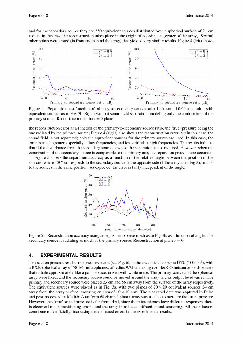
and for the secondary source they are 350 equivalent sources distributed over a spherical surface of 21 cmradius. In this case the reconstruction takes place in the origin of coordinates (center of the array). Severalother points were tested (in front and behind the array) that yielded very similar results. Figure 4 (left) shows

Primary-to-secondary source ratio [dB]

Reconstru

ctionerror[%

]

−10 0 10 200

20

40

60

80

100ka = 0.5ka = 2ka = 4


Reconstru

ctionerror[%

]

−10 0 10 200

20

40

60

80

100ka = 0.5ka = 2ka = 4

Figure 4 – Separation as a function of primary-to-secondary source ratio. Left: sound field separation withequivalent sources as in Fig. 3b. Right: without sound field separation, modeling only the contribution of theprimary source. Reconstruction at the z = 0 plane

the reconstruction error as a function of the primary-to-secondary source ratio, the ‘true’ pressure being theone radiated by the primary source; Figure 4 (right) also shows the reconstruction error, but in this case, thesound field is not separated; only the equivalent sources for the primary source are used. In this case, theerror is much greater, especially at low frequencies, and less critical at high frequencies. The results indicatethat if the disturbance from the secondary source is weak, the separation is not required. However, when thecontribution of the secondary source is comparable to the primary one, the separation proves more accurate.

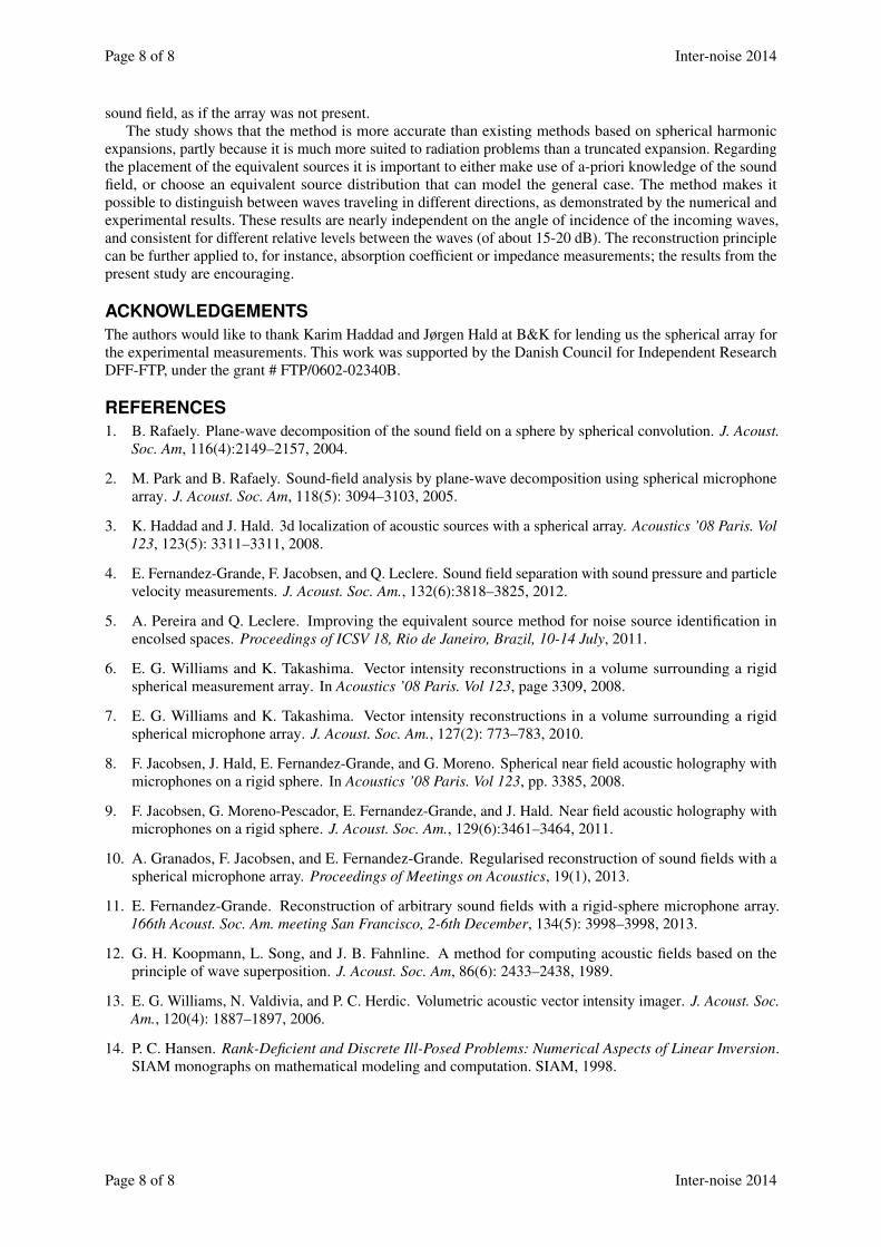
Figure 5 shows the separation accuracy as a function of the relative angle between the position of thesources, where 180o corresponds to the secondary source at the opposite side of the array as in Fig 3a, and 0o

to the sources in the same position. As expected, the error is fairly independent of the angle.

Secondary source ϕ [degrees]

Reconstru

ctionerror[%

]

180 150 120 90 60

10

20

30

40

50ka = 0.5ka = 2ka = 3ka = 4

Figure 5 – Reconstruction accuracy using an equivalent source mesh as in Fig 3b, as a function of angle. Thesecondary source is radiating as much as the primary source. Reconstruction at plane z = 0.

4. EXPERIMENTAL RESULTSThis section presents results from measurements (see Fig. 6), in the anechoic chamber at DTU (1000 m3), witha B&K spherical array of 50 1/4’ microphones, of radius 9.75 cm, using two B&K Omnisource loudspeakersthat radiate approximately like a point source, driven with white noise. The primary source and the sphericalarray were fixed, and the secondary source could be moved around the array and its output level varied. Theprimary and secondary source were placed 23 cm and 56 cm away from the surface of the array respectively.The equivalent sources were placed as in Fig. 3a, with two planes of 20× 20 equivalent sources 24 cmaway from the array surface, covering an area of 10× 10 cm2 .The measured data was captured in Pulseand post-processed in Matlab. A uniform 60 channel planar array was used as to measure the ‘true’ pressure.However, this ‘true’ sound pressure is far from ideal, since the microphones have different responses, thereis electrical noise, positioning errors, and the array introduces diffraction and scattering. All these factorscontribute to ‘artificially’ increasing the estimated errors in the experimental results.



Figure 6 – Pictures of the measurements with the spherical array in the presence of primary and secondarysource (left) and the primary source with the reference planar array used to measure the ‘true’ pressure (right).

x[cm]

z[cm]

SPL [dB re 20 µPa]

−18.75 0 18.75

18.75

0

−18.75

56.5

57

57.5

58

x[cm]

z[cm]

SPL [dB re 20 µPa]

−18.75 0 18.75

18.75

0

−18.7555.5

56

56.5

57

57.5

Figure 7 – Experimental results. Reconstructed sound pressure 20 cm in front of the array of primary sourcewithout secondary source, error 10% (left); reconstructed sound pressure of the primary source when thesecondary source is radiating at the same level from the opposite side, error 18% - Equivalent sources as inFig. 3a, ka = 0.5

Figure 7 (left) shows the magnitude of the reconstructed sound pressure 20 cm in front of the array (10 cmaway from the loudspeaker) when only the primary source is radiating sound (ka = 0.5). The reconstructionerror in this case is of approximately 10 %. Figure 7 (right) shows the reconstructed sound pressure where thesecondary source is radiating as much as the primary one (primary-to-secondary source ratio of 0 dB) from theopposite side. Although the error in this case is slightly higher, 18 %, the overall reconstruction is acceptableand the pressure radiated by the first source is recovered satisfactorily.

Figure 8 (left) shows the error as a function of the primary-to-secondary soruce ratio (Eq. 19), and theangle where the secondary source is positioned (right). The reconstruction errors are significant, but in anycase lower than 27 % (when interpreting the results, it should be considered that the uncertainty in the errorestimation is comparable to the error of the method itself, setting a lower bound). In Fig. 8 (right) it can beseen that the error does not change when the secondary source is at different angles, a result that is expected.


Reconstru

ctionerror[%

]

−5 0 5 10 15 200

10

20

30

40

50ka = 0.5ka = 1ka = 2ka = 3ka = 4

Secondary source ϕ [degrees]

Reconstru

ctionerror[%

]

180 150 120 90 60

10

20

30

40

50ka = 0.5ka = 1ka = 2ka = 3ka = 4

Figure 8 – Experimental results. Error as a function of primary-to-secondary level ratio and relative anglebetween the sources

5. CONCLUSIONSThis paper proposes a sound field reconstruction method based on measurements with a rigid spherical array.The method consists of an equivalent source expansion that takes into account the scattering introduced by thespherical array, and which makes it possible to reconstruct the sound field over any arbitrary geometry (inthe present study just over a planar surface, although it could be any other geometry, separable or not). Thescattering introduced by the sphere can be compensated for, consequently reconstructing only the incident



sound field, as if the array was not present.The study shows that the method is more accurate than existing methods based on spherical harmonic

expansions, partly because it is much more suited to radiation problems than a truncated expansion. Regardingthe placement of the equivalent sources it is important to either make use of a-priori knowledge of the soundfield, or choose an equivalent source distribution that can model the general case. The method makes itpossible to distinguish between waves traveling in different directions, as demonstrated by the numerical andexperimental results. These results are nearly independent on the angle of incidence of the incoming waves,and consistent for different relative levels between the waves (of about 15-20 dB). The reconstruction principlecan be further applied to, for instance, absorption coefficient or impedance measurements; the results from thepresent study are encouraging.

ACKNOWLEDGEMENTSThe authors would like to thank Karim Haddad and Jørgen Hald at B&K for lending us the spherical array forthe experimental measurements. This work was supported by the Danish Council for Independent ResearchDFF-FTP, under the grant # FTP/0602-02340B.

REFERENCES1. B. Rafaely. Plane-wave decomposition of the sound field on a sphere by spherical convolution. J. Acoust.

Soc. Am, 116(4):2149–2157, 2004.

2. M. Park and B. Rafaely. Sound-field analysis by plane-wave decomposition using spherical microphonearray. J. Acoust. Soc. Am, 118(5): 3094–3103, 2005.

3. K. Haddad and J. Hald. 3d localization of acoustic sources with a spherical array. Acoustics ’08 Paris. Vol123, 123(5): 3311–3311, 2008.

4. E. Fernandez-Grande, F. Jacobsen, and Q. Leclere. Sound field separation with sound pressure and particlevelocity measurements. J. Acoust. Soc. Am., 132(6):3818–3825, 2012.

5. A. Pereira and Q. Leclere. Improving the equivalent source method for noise source identification inencolsed spaces. Proceedings of ICSV 18, Rio de Janeiro, Brazil, 10-14 July, 2011.

6. E. G. Williams and K. Takashima. Vector intensity reconstructions in a volume surrounding a rigidspherical measurement array. In Acoustics ’08 Paris. Vol 123, page 3309, 2008.

7. E. G. Williams and K. Takashima. Vector intensity reconstructions in a volume surrounding a rigidspherical microphone array. J. Acoust. Soc. Am., 127(2): 773–783, 2010.

8. F. Jacobsen, J. Hald, E. Fernandez-Grande, and G. Moreno. Spherical near field acoustic holography withmicrophones on a rigid sphere. In Acoustics ’08 Paris. Vol 123, pp. 3385, 2008.

9. F. Jacobsen, G. Moreno-Pescador, E. Fernandez-Grande, and J. Hald. Near field acoustic holography withmicrophones on a rigid sphere. J. Acoust. Soc. Am., 129(6):3461–3464, 2011.

10. A. Granados, F. Jacobsen, and E. Fernandez-Grande. Regularised reconstruction of sound fields with aspherical microphone array. Proceedings of Meetings on Acoustics, 19(1), 2013.

11. E. Fernandez-Grande. Reconstruction of arbitrary sound fields with a rigid-sphere microphone array.166th Acoust. Soc. Am. meeting San Francisco, 2-6th December, 134(5): 3998–3998, 2013.

12. G. H. Koopmann, L. Song, and J. B. Fahnline. A method for computing acoustic fields based on theprinciple of wave superposition. J. Acoust. Soc. Am, 86(6): 2433–2438, 1989.

13. E. G. Williams, N. Valdivia, and P. C. Herdic. Volumetric acoustic vector intensity imager. J. Acoust. Soc.Am., 120(4): 1887–1897, 2006.

14. P. C. Hansen. Rank-Deficient and Discrete Ill-Posed Problems: Numerical Aspects of Linear Inversion.SIAM monographs on mathematical modeling and computation. SIAM, 1998.


Reconstruction of sound ﬁelds with a spherical microphone ... · Reconstruction of sound ﬁelds...

Documents

Transcript of Reconstruction of sound ﬁelds with a spherical microphone ... · Reconstruction of sound ﬁelds...