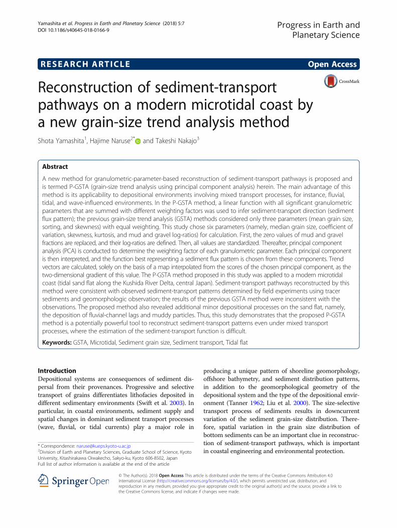
RESEARCH ARTICLE Open Access

Reconstruction of sediment-transportpathways on a modern microtidal coast bya new grain-size trend analysis methodShota Yamashita1, Hajime Naruse2* and Takeshi Nakajo3

Abstract

A new method for granulometric-parameter-based reconstruction of sediment-transport pathways is proposed andis termed P-GSTA (grain-size trend analysis using principal component analysis) herein. The main advantage of thismethod is its applicability to depositional environments involving mixed transport processes, for instance, fluvial,tidal, and wave-influenced environments. In the P-GSTA method, a linear function with all significant granulometricparameters that are summed with different weighting factors was used to infer sediment-transport direction (sedimentflux pattern); the previous grain-size trend analysis (GSTA) methods considered only three parameters (mean grain size,sorting, and skewness) with equal weighting. This study chose six parameters (namely, median grain size, coefficient ofvariation, skewness, kurtosis, and mud and gravel log-ratios) for calculation. First, the zero values of mud and gravelfractions are replaced, and their log-ratios are defined. Then, all values are standardized. Thereafter, principal componentanalysis (PCA) is conducted to determine the weighting factor of each granulometric parameter. Each principal componentis then interpreted, and the function best representing a sediment flux pattern is chosen from these components. Trendvectors are calculated, solely on the basis of a map interpolated from the scores of the chosen principal component, as thetwo-dimensional gradient of this value. The P-GSTA method proposed in this study was applied to a modern microtidalcoast (tidal sand flat along the Kushida River Delta, central Japan). Sediment-transport pathways reconstructed by thismethod were consistent with observed sediment-transport patterns determined by field experiments using tracersediments and geomorphologic observation; the results of the previous GSTA method were inconsistent with theobservations. The proposed method also revealed additional minor depositional processes on the sand flat, namely,the deposition of fluvial-channel lags and muddy particles. Thus, this study demonstrates that the proposed P-GSTAmethod is a potentially powerful tool to reconstruct sediment-transport patterns even under mixed transportprocesses, where the estimation of the sediment-transport function is difficult.

Keywords: GSTA, Microtidal, Sediment grain size, Sediment transport, Tidal flat

IntroductionDepositional systems are consequences of sediment dis-persal from their provenances. Progressive and selectivetransport of grains differentiates lithofacies deposited indifferent sedimentary environments (Swift et al. 2003). Inparticular, in coastal environments, sediment supply andspatial changes in dominant sediment transport processes(wave, fluvial, or tidal currents) play a major role in

producing a unique pattern of shoreline geomorphology,offshore bathymetry, and sediment distribution patterns,in addition to the geomorphological geometry of thedepositional system and the type of the depositional envir-onment (Tanner 1962; Liu et al. 2000). The size-selectivetransport process of sediments results in downcurrentvariation of the sediment grain-size distribution. There-fore, spatial variation in the grain size distribution ofbottom sediments can be an important clue in reconstruc-tion of sediment-transport pathways, which is importantin coastal engineering and environmental protection.

* Correspondence: naruse@kueps.kyoto-u.ac.jp2Division of Earth and Planetary Sciences, Graduate School of Science, KyotoUniversity, Kitashirakawa Oiwakecho, Sakyo-ku, Kyoto 606-8502, JapanFull list of author information is available at the end of the article

Progress in Earth and Planetary Science

© The Author(s). 2018 Open Access This article is distributed under the terms of the Creative Commons Attribution 4.0International License (http://creativecommons.org/licenses/by/4.0/), which permits unrestricted use, distribution, andreproduction in any medium, provided you give appropriate credit to the original author(s) and the source, provide a link tothe Creative Commons license, and indicate if changes were made.

Yamashita et al. Progress in Earth and Planetary Science (2018) 5:7 DOI 10.1186/s40645-018-0166-9

Many researchers have attempted to identify spatial varia-tions of granulometric parameters, which have been re-ferred to as ‘grain-size trends’, associated with net sediment-transport pathways (McCave 1978; McLaren 1981; Le Rouxand Rojas 2007). This is because methods to reconstructsediment-transport pathways from granulometric patternsare inexpensive and easily available compared to directmeasurements of sediment movement. In addition, there isa possibility that ancient sediment-transport patterns canbe reconstructed by applying these methods to subsurfacesediments. Early studies suggested that sediments becomefiner in the direction of transport (e.g., Pettijohn and Ridge1932; Self 1977), while other investigations have indicatedthe opposite trend (e.g., McCave 1978; Nordstrom 1981,1989). In order to address this disparity, McLaren andBowles (1985) discussed the combination of three parame-ters (mean grain size, sorting, and skewness) on the basis offlume experiments and statistical calculations. They con-cluded that sediments always become better sorted duringtransport, whereas the mean grain size and skewness varywith specific combination patterns (FB−: finer mean grainsize, better sorting value, and greater negative skewness; orCB+: coarser mean grain size, better sorting value, andgreater positive skewness).Gao and Collins (1992) applied their theory to two-

dimensional data of grain-size distribution in an inner bayenvironment. In their method, after comparing three gra-nulometric parameters (mean, sorting, and skewnessvalues) of adjacent points, vectors of unit length (100 m)are drawn between two points if they satisfy the conditions(FB− or CB+). These vectors are calculated from everypoint with respect to the eight immediately neighboringgrid points. Summing the vectors at each sample point pro-duces a single-trend vector of sediment transport pathways.This approach is called grain-size trend analysis (GSTA)and has been applied in a variety of depositional environ-ments (e.g., Pedreros et al. 1996; Cheng et al. 2004).It has been reported, however, that there may be

serious discrepancies between the GSTA model andactual sediment-transport patterns (Asselman 1999;Masselink et al. 2008). This is probably because grain-size trends do not always follow the assumptions ofMcLaren and Bowles (1985), especially under mixedtransport processes. Grain-size trends due to sedimenttransport can vary due to the depositional processes,environments, and sediment provenances. Deviationfrom the presumed trend of even a single parameter issufficient to result in the GSTA not accurately reflectingthe trend vectors. Indeed, Flemming (1988) disputedwhether sorting value would always improve duringtransport. In addition, it seems problematic that theGSTA model considers only three equally weightedparameters, but completely ignores other parametersrepresenting grain-size distribution, such as kurtosis and

mud/gravel fractions. In order to address these prob-lems, Rojas et al. (2000), Rojas (2003), and Rojas and LeRoux (2003) proposed a model that combines fourgrain-size parameters (mean grain size, sorting, skew-ness, and kurtosis) into a linear granulometric faciesfunction with differential weighting. These weightingfactors are modified incrementally and iteratively forcomparison with actual sediment-transport directionsmeasured from bedforms or visual observations, so thatthe error between the observed vector and the generatedvector is minimized. This method can determine theoptimum weights of granulometric parameters, but re-quires detailed observational data of existing sediment-transport patterns, and thus vitiates the abovementionedadvantages of grain-size trend analysis.To this end, the present study employs principal com-

ponent analysis (PCA) (Davis 1986; Middleton 2000) forthe purpose of treating multiple grain-size parameterswith appropriate weightings. PCA is a multivariate tech-nique for explaining the correlation between explanatoryvariables and automatically organizing these parametersinto a few linear synthetic variables with differentweights. It is reasonable to regard this spatial variationof grain-size parameters as resulting from the sediment-transport processes. Therefore, it can be expected thatparameters that strongly reflect sediment transport areemphasized by PCA. Hereinafter, this new method ofGSTA employing PCA is referred to as P-GSTA.Previous GSTA methods also include problems in

validation of the methods, as sediment-transport trends varyaccording to the time scale of the observation. Sediment-transport pathways of daily processes such as fair-weatherwaves can counteract those of monthly or yearly transportprocesses such as storms or slope failure events. Thus, thetime scale of the field observation must be specified in orderto validate the method for reconstructing sediment-transport pathways. The time scale of sediment-transportpatterns estimated by any GSTA method is defined by thesampling interval (Gao and Collins 1992). Subsurface sedi-ments in shallower sampling intervals can be entrained andtransported by waves or currents, whereas deeper layers are“historical” sediments that were already fixed and are notentrained by the surface processes. Nevertheless, this prob-lem has been given little attention.To reconstruct the ongoing sediment-transport patterns,

a sampling depth should be assigned to the thickness of theactive layer of the bottom-surface sediments. The activelayer is a concept proposed by Hirano (1971), indicatingthe uppermost layer of the bottom-surface sediments,which are frequently reworked and deposited by currentsand wave processes. Thus, grain-size variation of bottom-surface sediments accompanied by sediment transport oc-curs within this layer (Hirano 1971). It should be noted thatthe thickness of the active layer varies with time under

Yamashita et al. Progress in Earth and Planetary Science (2018) 5:7 Page 2 of 18

non-uniform flow conditions in natural environments; itgenerally becomes thicker in accordance with the timedevelopment of the probability distribution of burial andreworking as functions of depth below the bed surface(Ribberink 1987; Armanini 1995; Parker et al. 2000).A microtidal sand flat along the Kushida River Delta,

Ise Bay, central Japan, was chosen as the study area. Thismicrotidal sand flat is a largely natural environment,lacking breakwaters or dams, and is therefore suitablefor observation of sediment transport. The active-layerthickness and net sediment-transport directions over aspecific time scale were then measured by tracer experi-ments and geomorphological observation. Finally, samplingfor the GSTA method (the proposed P-GSTA and previousGSTA) was conducted according to the active-layer thick-ness, and the results were validated with net sediment-transport patterns recorded by field measurements.The proposed P-GSTA method successfully reproduced

the actual sediment-transport patterns, whereas the resultsof the previous GSTA model were inconsistent. In addition,application of the PCA model revealed details of previouslyunrecognized depositional processes on the sand flat. Tosummarize, this method is flexible because it requires no as-sumption on the sediment transportation processes and theinfluence of sediment transportation is estimated only fromthe characteristics of the obtained data. Thus, the method iseffective under mixed transport processes, in which estima-tion of the sediment-transport function is difficult.

Methods/ExperimentalGranulometric parameters used for P-GSTA methodOn the basis of grain-size measurements of samples, eachof the granulometric parameters (mean grain size μ, sort-ing σ, skewness Sk, and kurtosis kt) is generated by themoment method (Folk 1966; Harrington 1967), as follows:

μ ¼X

pd ð1Þ

σ ¼ffiffiffiffiffiffiffiffiffiffiffiffiffiffiffiffiffiffiffiffiffiffiffiP

p d−μð Þ2100

sð2Þ

Sk ¼P

p d−μð Þ3100σ3

ð3Þ

kt ¼P

p d−μð Þ4100σ4

ð4Þ

where d is the representative value of each grain-sizeclass (in increments of 0.1φ) and p is the weight fraction.

Physical characteristics of mud and gravel are evaluatedas weight percentages (mud and gravel fractions: Fmud

and Fgravel, respectively). The coefficient of variation(CV) is also employed to represent the degree of sedi-ment sorting. CV is the dimensionless sorting valuedivided by mean value, calculated as follows:

CV ¼ σ

μð5Þ

The P-GSTA method employs six parameters (mediangrain size d50, CV, Sk, kt, and fractions of mud and gravelFmud and Fgravel) in a sediment-transport function. Here,the median grain size d50 is employed rather than meangrain size, because median grain size is mathematicallyindependent of the other granulometric parameters,whereas mean grain size is used in the calculation of CV,Sk, and kt. In addition, CV value is employed here in-stead of sorting value (standard deviation) σ. Comparedto sorting value σ, CV value has the advantage of avoid-ing mathematical correlation with mean value. Whencomparing grain-size distributions whose mean valuesare nearly identical, sorting values are a good index ofthe dispersion of the grain-size distribution. However,sorting values cannot be used when comparing grain-size distributions with quite different means becausesorting value (standard deviations) has an inevitablepositive correlation with the mean value of the grain sizedistributions under consideration. In such cases, CVrather than sorting value needs to be used in generalsediment evaluation.

Parametric interpolation by krigingKriging interpolation is employed to estimate spatialvariations of granulometric parameters (Burgess andWebster 1980a, 1980b; Kohsaka 1999). All GSTAmethods have a problem in that the estimated trend vec-tors are potentially affected by the sampling intervals.Asselman (1999) solved this problem using kriging tointerpolate observational data sets (Burgess and Webster1980a, 1980b; Kohsaka 1999). Kriging is an algorithmbased on least squares, which is used to estimate thespatial variation of a real-valued function, and assumesthat spatial variation can be estimated from a linear com-bination of measured values (Kohsaka 1999). Weightingcoefficients are obtained on the basis of the spatialdependence of a variable, which can be represented by asemivariogram, i.e., the scatter diagram of covariance withrespect to spatial distance. The weighting of the runningaverage is then determined by the variogram model func-tion, which is the function fitted to the semivariogram(Burgess and Webster 1980a). Theoretically, the covari-ance of spatial data increases with distance and becomes a

Yamashita et al. Progress in Earth and Planetary Science (2018) 5:7 Page 3 of 18

steady value over some distance (Burgess and Webster1980a, 1980b; Kohsaka 1999). This limited distance is therange within which the data indicate spatial dependence.The spatial dependencies of the data are also shown in thevariances between the estimations, which provide a meas-ure of uncertainty in the interpolation values.

Data preparationPrior to statistical analysis, granulometric parametersshould be converted into appropriate forms for analysisby conventional statistical techniques.It is common to report grain-size fractions in percent-

ages, but such data are not independent, because theymust sum to 100%. Compositional data such as mudand gravel fractions are therefore difficult to use instatistical analyses as they are (Aitchison 1986, 2003;Aitchison and Egozcue 2005). Aitchison (1986, 2003)proposed, instead, to evaluate the relative magnitudes ofconstituents in comparison to other compositional vari-ables and to use logarithms to simplify the computationof the variance and covariance. After taking logarithms,the resulting transformed values are free to vary over theentire range of real numbers. However, a zero value inthe compositional data prohibits log-ratio transform-ation, because the transformed value is −∞, and there-fore cannot be included in the statistical analysis. Inorder to avoid this problem, a multiplicative approach(Martín-Fernández et al. 2003) replaces a zero value witha value that is sufficiently small, as follows:

F̂ j ¼δ j F j ¼ 0

� �1−

PkjFk¼0δk

c

� �F j F j > 0

� �8<: ð6Þ

where Fj and F̂ j denote the original and substitutecompositional values respectively; δj, the input value ofFj; and c, the sum-constraint constant (100%). Themodification of nonzero values is multiplicative, as sug-gested by the simple replacement rule. Generally, δj isthe maximum rounding error, but the range δγ/5 ≤ δj ≤2δγ, where δγ is the maximum rounding error, has beensuggested to be reasonable (Aitchison 1986; Martín-Fer-nández et al. 2003). This nonparametric replacement isstable, i.e., independent of both data numbers and com-ponent numbers, and retains the original information ofthe compositional data (Aitchison 1986; Arai and Ohta2006). In the present study, mud/gravel fractions weretreated via these two transformational processes. First,zero values of mud/gravel fractions were replaced by themaximum rounding error (0.01%). Secondly, the dimen-sionless magnitudes of the mud and gravel fractionswere defined as the mud and gravel log-ratios rmud andrgravel, as follows:

rmud ¼ logF̂mud

100− F̂mud− F̂gravel

!ð7Þ

rgravel ¼ logF̂gravel

100− F̂mud− F̂gravel

!ð8Þ

where F̂mud and F̂gravel are the substitute values formud and gravel fractions (Eq. 6), respectively.The units, mean values, and standard deviation of

variables strongly influence the results of PCA. To avoidthis problem, the following formula was used tostandardize all data:

x�i ¼xi−mx

sxð9Þ

where mx is mean and sx is the standard deviation ofeach granulometric parameter x. This operation trans-forms the mean and standard deviation of each variableinto 1 and 0, respectively.

Weighting (principal component analysis)The new method for defining the linear granulometricfunction proposed in this study is based on principalcomponent analysis (PCA), which is a technique forexplaining the correlation between multiple variablesand accounting for a large variance using only a fewsynthetic variables (principal components) (Davis 1986;Middleton 2000).Let x1, x2, ⋯, xp be variables, and let z1, z2, ⋯, zm

(m ≤ p) be their respective weighted synthetic variables.These synthetic variables are defined as the principalcomponents.

z1 ¼ L11x�1 þ L12x

�2 þ…þ L1px

�p

:zi ¼ Li1x

�1 þ Li2x

�2 þ…þ Lipx

�p

:zm ¼ Lm1x

�1 þ Lm2x

�2 þ…þ Lmpx

�p

8>>>><>>>>:

L2i1 þ L2i2 þ…þ L2ip ¼ 1; i ¼ 1; 2;…;mð Þ

ð10Þ

Here, the matrix (Li1...Lip) is the eigenvector of the ithprincipal component. The m synthetic variables have thefollowing two properties: (1) the correlation of any twosynthetic variables is zero (orthogonal) and (2) thefollowing inequality holds for the variances of syntheticvariables Var(zi): Var(z1) ≥Var(z2) ≥ ... Var(zm). The amp-litude of the variance of principal components can beregarded as the amount of information in each principalcomponent. The factor loading, which represents therelative importance of each variable in the principal

Yamashita et al. Progress in Earth and Planetary Science (2018) 5:7 Page 4 of 18

component, is defined as the product of the root of theeigenvalue and the eigenvector. The absolute value ofthe factor loading is proportional to its significance.

Calculation of trend vectors of sediment transport byP-GSTA methodThe procedures to obtain trend vectors of sedimenttransport by GSTA with principal component analysis(PCA) weighting (P-GSTA) are described herein. As dis-cussed above, this method employs six granulometricparameters (median grain size, CV, skewness, kurtosis,and mud and gravel fractions). First, the zero values ofmud and gravel fractions are replaced (Eq. 6), and mudand gravel log-ratios are defined (Eqs. 7 and 8). Then, allvalues are standardized (Eq. 9). After these preliminaryprocedures, PCA is conducted using these six trans-formed parameters (Eq. 10). Each principal componentis then interpreted, and the first principal component ischosen as the sediment-transport function T(x, y). Thetrend vectors V(x, y) are then calculated, solely on thebasis of the interpolated map of the scores of the chosenprincipal component as the two-dimensional gradient ofthis value, as follows:

V x; yð Þ ¼ ∂T∂x

iþ ∂T∂y

j ð11Þ

where V(x, y) is an estimated trend vector of sedimenttransport, and i and j are unit vectors (magnitude:100 m) in the x and y directions, respectively.

Application of P-GSTA method to microtidal sand flatWe applied our method to a microtidal sand flat locatedat the mouth of the Kushida River. The headwaters ofthe Kushida River are in the Daikou Mountains of Japan;the river flows eastward to the lowlands and then north-ward, to form a delta at Ise Bay (Fig. 1). The catchmentarea of the river is approximately 461 km2. According tothe Japanese Ministry of Land, Infrastructure, andTransportation (MLIT), the annual average fluvial dis-charge was 11.56 m3/s in 2010 (http://www1.river.go.jp/).The delta is lobate or arcuate and is classified as fluvial-dominated or complex fluvial-wave-tide dominated on thebasis of the classification of Galloway (1975).The tidal range monitored on the left bank of the

Kushida River (36° 36′ 0″ N, 136° 33′ 45″ E) is approxi-mately 2 m during a spring tide (microtidal). Waveheights have been measured at the river mouth (34° 22′16″ N, 137° 07′ 40″ E) and in the enclosed section ofIse Bay (34° 55′ 12″ N, 136° 44′ 25″ E) (MLIT). Mea-surements by MLIT in 2002 at the river mouth showedthat waves occur with a period of 5 to 10 s and are 1–2 m in height, increasing to 4–5 m in height during

typhoons and winter storms (http://www.mlit.go.jp/kowan/nowphas/index.html). In the investigated area, wavesmainly wash from the northeast throughout the year, butalso occur from the northwest or north–northwest duringwinter seasons (Nakajo 2004). Tidal residual current ismainly from northwest to southeast in the southwest part

Fig. 1 Index map showing locality of the study area. The data of theresidual current velocity (in a) are from the Coastal OceanographyResearch Committee, The Oceanographic Society of Japan (1985). ‘R’and ‘W’ (in a) are measurement localities of rainfall and water depth,respectively. Data are from the Japan Meteorological Agency (JMA)(see Fig. 10; http://www.data.jma.go.jp/obd/stats/etrn/index.php).Details of the geomorphological features of the study area (dottedline in b) are described in Fig. 2

Yamashita et al. Progress in Earth and Planetary Science (2018) 5:7 Page 5 of 18

of Ise Bay (Coastal Oceanography Research Committee, TheOceanographic Society of Japan 1985; Fig. 1). Typhoonsstruck this area less than five times per year from 2005 to2011 (measured by the Japan Meteorological Agency [JMA]).The geomorphology of the Kushida River Delta is

classified into four components, namely, spit, salt marsh,muddy tidal flat, and tidal sand flat (Fig. 2).

SpitThe spit extends northwest from Matsunase Harbor andbranches into several components. The spit is composedof well-sorted medium- to coarse-grained sand. Branchingchannels from the Kushida River flow behind the spit(Fig. 2). These channels are 20–30 cm in depth andtransport medium- to very coarse-grained sand, includinggranules and pebbles.

Salt marshThe salt marsh lies mainly on the landward side of the spitand is composed of muddy sediment and soil containingabundant organic material (Fig. 2). Sediment coarsenstoward the main fluvial channel (Kushida River).

Muddy tidal flatMuddy tidal flats are located on the landward side of thespit, adjacent to the salt marsh (Fig. 2). The sedimentconsists of mud or poorly sorted sandy mud, includinggravels. Small-scale washover fans are observed on the

muddy flat. Burrows of crustaceans are very common,and mud-flat sediment and coarse sediment of washoverfans are intermixed by their benthic activities.

Tidal sand flatThe microtidal sand flat extends in front of the spit, onthe right bank of the river mouth (Fig. 2). Its maximumarea, during ebb spring tide, is approximately 0.4 km2

(Fig. 2). The offshoreward development of the intertidalsand flat is most prominent around the river mouth andthe southeast part of the study area (adjacent to Matsu-nase Harbor) (Fig. 2). The primary geomorphologicalfeatures of the sand flat consist of sand bars and braidedchannels, and no tidal channels are observed. The sandbars are 60 to 100 cm in height and 50 to 100 m inwavelength (Fig. 2). They are arranged almost parallel tothe shoreline and normal to the direction of incomingwaves (Fig. 2). Breaking waves are found on the crests ofthese sand bars, and wave ripples are abundant on theirsurface. No significant migration of these bars wasobserved in the period from 2002 to 2011 (Nakajo 2004;Yamashita et al. 2009). Braided channels (approximately20–30 cm deep) are observed intermittently on the sandflat, around the river mouth. These channels are tempor-ary braided streams from the river. They are generallyproduced by floods and rapidly migrate and vanish.There are very few muddy particles on the sand flat, exceptfor soon after a fluvial flooding event (Nakajo 2004;Yamashita et al. 2009; Yamashita et al. 2011). Sedimenttransport on the sand flat is mainly controlled by fluvialand wave activities (Yamashita et al. 2009).

Sampling and grain-size measurementsBottom-surface sediments on the microtidal sand flatwere collected during the ebb spring tides on 1 August2011. A total of 60 sampling sites were located athorizontal intervals of approximately 100 m, both paral-lel and perpendicular to the spit, with extension to theriver mouth and the northern margin of the sand flat(Fig. 2). Sediments were excavated by shovel in intervals,from the top of the bedforms to 8 cm below the surface,corresponding to the active layer thickness observed on31 July 2011. Each sample (50–100 g weight) washomogenized before grain-size analysis.The grain-size distribution of sand-sized particles in

the samples was measured by the settling tube method(Gibbs 1974; Tucker 1988) after removing mud-sized (>4φ) and gravel-sized (< − 1φ) particles by sieving. Shellfragments were also removed before measurement.Grain-size distributions were calculated using S-Tubesoftware (Friedman et al. 1992; Naruse 2005). Theconversion method for the settling velocity of grains wasproposed by Ferguson and Church (2004), using anempirical formula for natural sand.

Fig. 2 Geomorphology of the study area and sampling localities forGSTA methods. Geomorphology is after fluvial flooding in July 2011

Yamashita et al. Progress in Earth and Planetary Science (2018) 5:7 Page 6 of 18

Model validation by monitoring of actual sediment-transport patternsActual sediment-transport patterns on the tidal sand flatwere monitored from 16 May to 31 July 2011, to enablevalidation of the GSTA models. Therefore, the sediment-transport patterns were examined in both normal (calm)conditions and in an episodic depositional event. Thethickness of the active layer was also measured; theactive layer was considered to be the mixed layer oftracer grains and natural sands.The JMA reported rainfall measured in the upper

reaches of the Kushida River and the water level of theriver mouth (http://www.data.jma.go.jp/obd/stats/etrn/index.php; Fig. 3). There was moderate rainfall (<15 mm/h) during the period from 16 May to 3 June. Thewater level indicates a usual spring-neap-spring cycle inthis period (Fig. 3). In contrast, heavy rainfall wasrecorded on 8 July (> 45 mm/h) and 17–19 July (max-imum: > 25 mm/h). In particular, unusually high waterlevels during ebb tides were monitored soon after the17–19 July rainfall (18–20 July) (Fig. 3). The rainfallduring this period was due to a typhoon (No. 6, MA-ON). Fluvial flooding events caused by the rainfalls dur-ing this period were reported through an enquiry survey.Tracer experiments and geomorphological observa-

tions revealed net sediment-transport patterns on thetidal sand flat. Blue-colored sand was employed as tracersediment, as it can be clearly identified from naturalsand, both visually and by microscopic observations. Thetracer sediments were well sorted and their mean grainsize was ca. 1.5 φ. The tracer sediments were situated atfive localities (points 1–5) on 16 May 2011 (spring tide)(Fig. 4). GPS and marking poles recorded the localities.At each locality, the bottom surface sediment was exca-vated approximately 0.3 (length) × 0.3 (breadth) × 0.2

(depth) m, and the hole was filled by the tracer sedi-ments (approx. 25 kg). Two weeks after input of thetracer sediments (3 June 2011), bottom surface sedi-ments were collected from four surrounding points thatwere located at a distance of 10 m from each tracer pit.Each sample was homogenized with sufficient stirring byhand in a transparent plastic case (8 × 15 cm basal area,and 3 cm in height). The basal sediment in this plasticcase was scanned at high resolution (2400 dpi), and thenumber of colored sand grains in the basal area wascounted to estimate the volume of surface sedimentstransported in each direction from the original tracersite. Sampling was also conducted 2 months after thetracer sediments were set (31 July), but no tracer grainswere detected.Mean transport direction of sediments θ was estimated

from observed colored sand grains, as follows:

θ ¼ arctan

PsinθiPcosθi

ð12Þ

where θi is a direction from the tracer pit to the sam-pling locality at which the ith grain was detected. Themean resultant length (MRL) LMR of the vector wasemployed as a proxy for concentration of sediment-transport directions, which was calculated as follows:

LMR ¼ffiffiffiffiffiffiffiffiffiffiffiffiffiffiffiffiffiffiffiffiffiffiffiffiffiffiffiffiffiffiffiffiffiffiffiffiffiffiffiffiffiffiffiffiffiffiffiffiffiffiffiffiP

cosθið Þ2 þ Psinθið Þ2

qn

ð13Þ

where n is the number of detected colored grains.Furthermore, the thickness of the active layer of basal

Fig. 3 The rainfall and water level of the Kushida River. The rainfall and the water level were measured respectively at the upper reaches (‘R’ inFig. 1a) and at the river mouth (‘W’ in Fig. 1b) during a period from May 16 to July 31, 2011 (http://www.data.jma.go.jp/obd/stats/etrn/index.php)

Yamashita et al. Progress in Earth and Planetary Science (2018) 5:7 Page 7 of 18

sediment was measured after excavating sediments atthe source points (Fig. 5).The sediment-transport patterns were also estimated

on the basis of the observation of geomorphologicaldevelopment (Figs. 4 and 5) during the period from 16May to 31 July 2011.

ResultsResults of grain-size analysisSpatial distributions of eight granulometric parameters(mean and median grain size, sorting, CV, skewness,kurtosis, and mud and gravel fractions) were calculatedand were interpolated to a grid interval of 100 m by

kriging (Figs. 6 and 7). Semivariograms were calculatedfrom the measured data, and the variogram models werefitted to them by the least-squares method (Fig. 6). Theestimation error is shown as a false-color image, and the

Fig. 4 a The result of the tracer experiment. Sampling was conductedon Jun 2–3, 2011. b The drastic geomorphological changes due to afluvial flooding event in July 2011, and sediment-transport patternssuggested by the directions of channels and bedforms. Data wasobtained on August 1, 2011

Fig. 5 a A photograph of a braided channel formed by the fluvialflooding event in July 2011. The braided channel cuts the spit andflows into the tidal sand flat. b Dunes in the braided channel. The leftside of the photo is seaward. c The appearance of the active layerobserved at point 3 soon after the fluvial flooding (August 1, 2011)

Yamashita et al. Progress in Earth and Planetary Science (2018) 5:7 Page 8 of 18

value of the parameter is shown by an overlying contourmap (Fig. 7).

Mean and median grain sizeThe interpolated maps of the mean and median grainsize show similar characteristics. The coarser sedi-ments (< 1.0 φ) are distributed around the rivermouth (Fig. 7). The grain size becomes finer in aradial pattern from the river mouth, and grain sizesfiner than 1.50φ are found at the southeast part ofthe sand flat (Fig. 7). The variograms of the meanand median grain size reveal their high spatial de-pendency (Fig. 6). Therefore, they have relatively highaccuracy (Fig. 7).

SortingThe highest sorting values (> 0.56) are found in thecentral to southeast part of the sand flat (Fig. 7). Thesorting value tends to decrease seaward, but a lowervalue (< 0.55) is also evident in the river mouth(Fig. 7). The semivariogram of the sorting value sug-gests relatively high spatial dependence (Fig. 6). How-ever, the y intercept of the fitted curve forsemivariance of the sorting value largely deviates fromthe origin (nugget effect), indicating that high meas-urement error exists (Fig. 6).

CV valueThe map of the CV value indicates that highervalues (> 0.7) are distributed in the river mouth. The

Fig. 6 Semivariograms and fitted variogram models of granulometric parameters. Variogram models were fitted by the least-squares method, and themodel that produces the fewest residual errors was chosen from among the Gaussian, spherical, and exponential models. The spherical model wasused for mean and median grain-size, sorting, and gravel fractions, the exponential model was used for the CV value, and the Gaussian model wasused for skewness, kurtosis, and mud fractions

Yamashita et al. Progress in Earth and Planetary Science (2018) 5:7 Page 9 of 18

CV value decreases seaward (Fig. 7). The variogramof the CV value shows high spatial dependency(Fig. 6); therefore, the accuracy of the CV value isrelatively high.

SkewnessThe higher skewness values (> 1.4) are mainly distrib-uted in the river mouth and are also found in the north-ern part of the sand flat (Fig. 7). Skewness tends to

Fig. 7 Contour maps of grain-size parameters interpolated by kriging over raster maps of the estimation variance. The relatively lighter gray colorin each raster map indicates a higher precision of interpolation. The absolute values of the estimation variance are not meaningful because thesevalues depend on the values of the variables and the shapes of the variograms

Yamashita et al. Progress in Earth and Planetary Science (2018) 5:7 Page 10 of 18

decrease to the southeast (Fig. 7). The lowest value (<0.2) is distributed primarily in the southeastern marginof the sand flat (Fig. 7). The accuracy of interpolation islow because of the anomalous value of the semivario-gram in the range of 100 m (Fig. 6).

KurtosisThe higher kurtosis values are mainly distributed in theriver mouth (7.0–9.0), and the value tends to decrease ina seaward direction (Fig. 7). However, high values arealso found in the southeastern margin of the sand flat.The accuracy of interpolation is relatively low becausethe variogram indicates anomalous values in the rangeof 100 m (Fig. 6).

Mud fractionsThe spatial distribution of the mud fractions is quiterandom, and therefore, the accuracy of interpolation isvery low (Fig. 6). Relatively high mud fractions (> 10.0%)are distributed in patches in the northeastern and south-eastern parts of the sand flat (Fig. 7).

Gravel fractionsGravels are abundant in the sediment around the rivermouth (> 9.0%) and decrease seaward, becoming sparsein the southeast part of the sand flat (< 6.0%) (Fig. 7).The variogram shows high spatial dependency of thegravel fractions (Fig. 6); therefore, the accuracy of thisvalue is relatively high (Fig. 7).

Results of principal component analysis of granulometricparametersThe contribution values, which indicate the percentagesof the original information represented by each principalcomponent of PC1 through PC3, are 56.77, 20.32, and11.76, respectively (Table 1). This means that more than80% of the original information is represented by PC1through PC3. Therefore, these three principal compo-nents are interpreted further. Kriging interpolation wasconducted in order to visualize the spatial distributionpatterns of scores of PC1 through PC3, using the same

method as for the original granulometric parameters(Figs. 8 and 9).

PC1: sediment-transport functionPC1 is negatively correlated with the gravel log-ratio(factor loading: − 0.79) and CV value (− 0.92) and ispositively correlated with the median grain size (φ)(0.93) (Table 1). Correlations with skewness (− 0.57),kurtosis (− 0.58), and mud log-ratio (0.65) have relativelyweak influences on this value (Table 1). In other words,the increase of the PC1 value indicates that the sedimentbecomes finer, better sorted, and less gravely (Fig. 10);this means a selective decrease in coarser materials fromgrain-size distribution (Fig. 10). The variogram andinterpolated map of the PC1 scores indicate that thespatial variation of PC1 is high (Figs. 8 and 9). The low-est value of PC1 is found around the river mouth, andthis value increases radially northeastward (Fig. 9). Thescatter diagram of PC1 values against PC2 values indicatesthat the samples take wider values of PC1 (from − 4.5 to4.0) than values of PC2 (from − 3.0 to 2.0); no notableclusters were formed (Fig. 11). Thus, it is interpreted thatPC1 reflects the suite of size-selective sediment-transportprocesses resulting in fining-downcurrent trends withwell-sorted grain-size distributions. The gradual decreaseof coarser materials, which is represented by the increaseof PC1, probably reflects the progressive lowering of bedshear stress of both fluvial and wave activities (Fig. 10).Settling velocity of finer materials is low, so that they havegreater mobility as suspended loads. Therefore, the finestfraction of sediments is broadly dispersed downcurrent,producing the negative skewness of grain-size distribution.The relatively high spatial variation and the radial distribu-tion pattern from the river mouth in PC1 strongly suggestthat the PC1 value represents the sediment supply fromthe Kushida River and the dispersal by waves or tidalcurrents (Fig. 6). Therefore, the decreasing pattern of PC1can be regarded as the sediment-transport function.

PC2: indicator of lag deposit of a fluvial flooding eventPC2 is negatively correlated to the skewness (− 0.65) andkurtosis value (− 0.66), and positively influenced by gravellog-ratio (0.55) (Table 1). Other granulometric parametershave only slight influences on PC2 (Table 1). In otherwords, the increase of the PC2 value indicates the morenegatively skewed and platykurtic shape of grain-sizedistribution and gravely sediment (Fig. 10). The highervalues of PC2 (1.2–2.0) cluster around the breached sec-tion of the spit and the newly formed braided channel onthe sand flat (Fig. 9). This value decreases around the rivermouth and offshore area (< 4.0). The spatial dependencyand precision of interpolation is low because of the anom-alous values of semivariance at approximately 100 m(Fig. 8). The exclusive distribution of higher PC2 values

Table 1 Result of principle component analysis (PCA) for thesamples from the Kushida River Delta. Factor loadings andcontribution values are shown

PC1 PC2 PC3 PC4 PC5 PC6

Median grain size 0.93 − 0.23 − 0.04 − 0.14 − 0.15 0.20

CV − 0.92 0.23 0.16 − 0.05 0.21 0.17

Skewness − 0.57 − 0.65 0.33 0.38 − 0.11 0.03

Kurtosis − 0.58 − 0.66 − 0.02 − 0.47 0.01 − 0.04

Mud log-ratio 0.65 0.09 0.74 − 0.15 0.06 − 0.04

Gravel log-ratio − 0.79 0.50 0.16 − 0.15 − 0.30 0.00

Contribution (%) 56.77 20.32 11.76 7.15 2.78 1.23

Yamashita et al. Progress in Earth and Planetary Science (2018) 5:7 Page 11 of 18

Fig. 8 Semivariograms and fitted variogram models of principal components (PC1–PC3). The variogram models were fitted by the least-squaresmethod, and the model that produces the fewest residual errors was chosen from among the Gaussian, spherical, and exponential models. Theexponential model was used for PC1 and the spherical model for PC2 and PC3

Fig. 9 Contour maps of the principal components interpolated by kriging over raster maps of estimation variance

Yamashita et al. Progress in Earth and Planetary Science (2018) 5:7 Page 12 of 18

around the newly formed braided channel suggests a link-age to the episodic deposition by the fluvial flooding eventduring July 2011. The platykurtic and negatively skewedshape of grain-size distribution as well as the high gravelfraction indicates that the sediments largely consist ofcoarser fractions and this is in agreement with the directobservation of a high gravel fraction (Fig. 10). Thesecoarser fractions can be interpreted as lag deposits inbraided channels. Coarser sediments may have beenepisodically deposited during periods of high shear stressflow at times of fluvial flooding and remained through thesubsequent reworking by wave or tidal currents.

PC3: indicator of muddy particlesPC3 is positively influenced by the mud log-ratio (0.74),and other granulometric parameters show limited influ-ences (from − 0.02 to 0.33) (Table 1). This means that theincrease in the PC3 score suggests muddier sediment. Thevariogram and interpolated map of PC3 show that thespatial dependence of PC3 is weak (Figs. 8 and 9). Thespatial distribution of PC3 is very heterogeneous. Higher

PC3 values (> − 0.3) are found in the northern and south-eastern parts of the sand flat, and this characteristic distri-bution pattern is similar to the map of the mud content(Figs. 7 and 9). The range of variation in PC3 values (from− 2.0 to 2.5) is more limited than for PC1 (from − 4.5 to4.0) (Fig. 11). Very poor correlation between mud log-ratio and other granulometric parameters of sand-sizedparticles indicates that muddy particles are deposited byquite different processes from those associated with sandyparticles. As described above, the rapid deposition ofmuddy particles on the sand flat by a fluvial flood event(17–19 July 2011) is recognized, and these muddy parti-cles preferentially remained in local depressions. The het-erogeneity of the spatial distribution of PC3 might reflecta relic of mud deposition caused by this event and theirlocal resistance to erosion.

Trend vectors obtained by P-GSTA and previous GSTAmethodsGrain-size trend vectors were calculated by the P-GSTAmethod, in which the increase of the PC1 value is

Fig. 10 Typical transformation pattern of the grain-size distribution curves represented by PC1 (left) and PC3 (right). Sampling locations of samplesA–E are shown in Fig. 2. The values of PC1 through PC3 for each sample (A–E) are shown in the scatter diagram of Fig. 11

Fig. 11 Scatter diagrams of PC2 and PC3 with respect to PC1. The shape of the grain-size distribution of samples A–E is shown in Fig. 10

Yamashita et al. Progress in Earth and Planetary Science (2018) 5:7 Page 13 of 18

defined as a sediment-transport function (Fig. 12). Trendvectors directed to the north or northeast are dominantalong the main fluvial channel and northern parts of thesand flat (Fig. 12). Northeastward-directed vectors aredominant around the breached section of the spit. In thecentral part of the sand flat, the vectors are directed tothe southeast. In the southeastern regions, the trendvectors are directed toward the northeast (Fig. 12). Tosummarize, the trend vectors obtained by the P-GSTAmethod show radial dispersion of coastal sediment fromthe river mouth with a small influence from the shore-parallel current.

The previous GSTA model (Gao and Collins 1992;Asselman 1999) was also applied for the purposes ofcomparison. Trend vectors obtained by the previousGSTA method showed quite diverse and inconsistentestimates of sediment transport pathways (Fig. 12).Landward-directed vectors were dominant along themain fluvial channel, while offshore (southeastward)directed vectors were found at the central part of thesand flat. In addition, transport vectors were not definedaround the southeastern region of the study areabecause neither FB− nor CB+ patterns were satisfied inthis region.

Results of tracer experiments and topographic observationsThe tracer experiments clarified the actual sediment-transport patterns during the period 16 May to 3 June(Fig. 4). Along the main fluvial channel, the transportpattern was directed to the northeast (point 5) (Fig. 7)and the degree of concentration (MRL) was relativelyhigh (Fig. 7). In the central part of the sand flat (points 3and 4), southward (landward) transport was dominant(Fig. 4) and the degree of concentration (MRL) wasmoderate (Fig. 4). In the offshore area (point 2), east-ward sediment transport was dominant (Fig. 4) and thedegree of concentration was moderate (Fig. 4). At thesoutheastern margin of the sand flat (point 1), sedimentdispersed in various directions (Fig. 4); northeastwardtransport is dominant, according to the number of tracergrains, but the mean direction indicates east–southeast-ward transport (Fig. 4).On 31 July 2011, no tracer grains were detected from

the samples, probably because they had been highlydispersed. Instead, sediment-transport patterns were es-timated on the basis of the observation of the geomor-phological development derived from a fluvial floodingevent of 17–19 July (Fig. 3). The most prominent featurewas incision of the spit and formation of braided chan-nels (Figs. 4 and 5). The spit was breached at two pointsaround its folding point, 30–50 m in width (Figs. 4 and5). At the breach locations, the spit was incised byshallow, braided channels (0.3–0.5 m in depth), whichwere connected to branched channels behind the spit(Figs. 4 and 5). These channels flowed into the tidal sandflat more than 300 m offshore (Figs. 4 and 5). Sandbodies were deposited on the sand flat 100 m off thebreach point (Figs. 4 and 5). These sand bodies extendedapproximately 100 m northeast and were approximately0.5 m in height (Fig. 4). They were composed ofmedium- to coarse-grained sands, including shell frag-ments, which were similar to sediments comprising thespit and the fluvial channels, and were clearly coarserthan the sediments on the tidal sand flat. This probablymeans that these sand bodies were formed by sedimentsderived from the breached part of the spit and from

Fig. 12 Grain-size trend vectors. The actual sediment-transport directionsduring normal conditions are shown as the mean direction of tracer results(see Fig. 4a). Circles indicate the sampling points. a Grain-size trend vectorscalculated by P-GSTA. b Grain-size trend vectors calculated by the previousGSTA method (Asselman 1999). Some of sampling points lack the trendvector because the GSTA method does not recognize the grain-size trendwhen no surrounded locations satisfy the conditions FB− or CB+

Yamashita et al. Progress in Earth and Planetary Science (2018) 5:7 Page 14 of 18

sediments in the fluvial channels. Dunes of approxi-mately 1.0 m wavelength and 0.15 m amplitude formedin the braided channels (Fig. 5). These dunes exhibitedthe northeastward (offshoreward) current directionsaround points 3 and 5 (Figs. 4 and 5). At the easternpart of the sand flat (around points 1 and 2), muddydeposits were thickly deposited in the troughs betweensand bars. The average thickness of the muddy sedimentwas 1–3 cm, but it occasionally reached 5 cm. No othernotable geomorphological developments were observedin this area.The active layer was clearly shown as the mixed layer

of tracer grains and natural sands, and the boundarywith the underlying substratum was sharp (Fig. 5). Thethickness of the active layer was ca. 8 cm at point 3(Fig. 5). The thickness was not measured at other loca-tions due to the loss of the marking poles.

Actual sediment-transport patterns on the sand flat duringa summer seasonAs discussed above, sediment-transport patterns weremeasured during a summer season (May to July 2011),via tracer experiments and geomorphological observa-tion. The results showed that fluvial discharge, mainlyfrom the braided channels that accompanied the incisionof the spit, supplied sediments to the sand flat; thesedrifted southward at the central part of the sand flat andwere dispersed eastward or northeastward by wave activ-ity during normal conditions.The drastic geomorphological development associated

with the 17–19 July fluvial flooding event revealed episodicsediment-transport processes around the river mouth.Fluvial sediments were supplied to the sand flat toward thenortheast, mainly from braided channels incising the spit,rather than from the main fluvial channel (Fig. 4). The inci-sion of the spit and fluvial sediment supply was alsoobserved, in October 2009, by Yamashita et al. (2011), whoreported the northeastward transport of fluvial sedimentinto the sand flat by a fluvial flooding event.It is estimated that the fluvial sediments supplied to the

sand flat were dispersed by wave or tidal currents duringnormal conditions. The eastward transport in a seaward area(points 1 and 2) roughly coincides with the direction ofcoastal (residual) currents (Coastal Oceanography ResearchCommittee, The Oceanographic Society of Japan 1985;Figs. 1 and 4). The landward (southward) transport at points3 and 4 can be interpreted as representing a depositionalwave condition during summer season (Hayes 1972; Fig. 4).

Comparison with trend vectors obtained by P-GSTA andprevious GSTA methodsGrain-size trend vectors calculated by the P-GSTAmethod showed reasonable similarity to the actualsediment-transport patterns described above (Fig. 12). A

north to northeastward trend along the main fluvialchannel and northern parts of the sand flat coincidedwith the net sediment-transport directions observed bythe tracer experiment at point 5. Northeastward-directed vectors were dominant around the breachedsection of the spit, and coincided with the downstreamdirection of the braided channels formed by the fluvialflooding event of July 2011 (Fig. 12). Thus, the trendvector of P-GSTA at point 5 coincides with the sedimenttransport direction estimated from geomorphologicalobservation, whereas it contradicts that derived from thetracer data. In the central part of the sand flat, thevectors were directed to the southeast and coincidedapproximately with the tracer result at point 4 (Fig. 12).In addition, the vectors coincided very well with thetracer result at point 2, in which they were directed east-ward. In the southeastern regions, the trend vectorswere directed toward the northeast (Fig. 12), which is inslight disagreement with the tracer data, indicating east-ward transport (Fig. 12).On the other hand, sediment trend vectors calculated

by the previous GSTA method did not show reasonablenet sediment-transport patterns compared to the resultsfor P-GSTA (Fig. 12). Around point 2, trend vectorsshowed eastward transport patterns and coincided withthe tracer results (Fig. 12). Southeastward vectors foundat the central part of the sand flat (around point 4) werealso comparable with the tracer results. However,landward-directed vectors along the main fluvial channelclearly conflict with the tracer data at point 5 (Fig. 12).In addition, transport vectors were not defined along thebraided channels and in the vicinity of point 3.

DiscussionIn contrast with the results obtained using the previousGSTA method, the grain-size trend analyzed using theP-GSTA method closely matches the actual sediment-transport estimated from the tracer experiments andgeomorphological features observed soon after fluvialflooding events (Gao and Collins 1992; Asselman 1999;Fig. 12). In the GSTA method, trend vectors opposite tothe fluvial downcurrent direction are produced by thelower sorting values in the river mouth (Figs. 7 and 12).The coarse sediment (lower φ value) in the river mouthresults in a lower sorting value due to the inevitablecorrelation between mean grain size and sorting value,and therefore, sorting values cannot represent the actualdegree of sediment sorting, as supposed by the previousmethods. The previous GSTA method performs quitepoorly, in that no trend vector is defined around thebraided channels, despite direct observations of the sedi-ment transport by a fluvial flooding event in July 2011(Figs. 3, 4, 5, and 12). In contrast, sediment-transportpatterns are better reconstructed via the P-GSTA method,

Yamashita et al. Progress in Earth and Planetary Science (2018) 5:7 Page 15 of 18

especially around the river mouth and braided channels(Fig. 12). At point 3, trend vectors are parallel to thedowncurrent direction of braided channels and thusrepresent sediment-transport direction by the fluvialflooding event, rather than during normal conditions indi-cated by tracer experiments (Fig. 12). This is probablybecause the sampling for P-GSTA was conducted after theflooding event while the tracer experiments were con-ducted before the event (Fig. 3).The disparity between trend vectors calculated by the

GSTA method and observational data shows that theassumption of McLaren and Bowles (1985) is not appro-priate in this case, probably because the dominantsediment-transport processes are mixed. In contrast, theP-GSTA method can detect the unique grain-size trendin each depositional setting and is therefore effectiveeven under mixed transport processes, in which theprecise sediment-transport function is difficult to deter-mine. Principal component analysis (PCA) can easilyexplore the characteristic changes of the grain-sizedistribution curves, which result from size-selective sedi-ment transport in a specific depositional setting, by alinear combination of multiple grain-size parameters(Eq. 10). PCA can automatically weight multiple grain-size parameters and combine them into a linear func-tion. In addition, the magnitude of the weighting is pro-portional to the spatial variation within each parameter(Middleton 2000). Therefore, the resultant linear com-bination of grain-size parameters, summarized by thefirst principal component (PC1), represents the predom-inant deformation pattern of the grain-size distributioncurves in the sampling area. In other words, the firstprincipal component can generally be regarded as theprimary function of size-selective sediment-transport inwhich a specific grain-size distribution curve variesspatially. If some minor transport processes exist, it isexpected that the deformation pattern of the grain-sizecurves affected by these processes can be identified bythe subsequent principal components. In the presentstudy, PC2 and PC3 recognized two minor depositionalprocesses (channel-lag deposits and muddy depositsresulting from episodic flooding). Indeed, the trendvectors derived from GSTA show directions incompat-ible with observations in the region around the spit(Fig. 12). In this region, PC2 values are large (1.2–2.0),suggesting the influence of channel-lag deposits formedby washover processes (Fig. 9). It is notable that thetrend vectors of P-GSTA show directions consistent withthe observation of sediment transport (Figs. 5b and 12).On the other hand, PC3 shows smaller values (< − 1.5)around the river mouth and rhythmic bars (Fig. 9),implying the presence of fine-grained flooding deposits.Again, the trend vectors derived from GSTA are incom-patible with the directions of actual sediment transport

(Figs. 5 and 12), which suggests the effectiveness of theP-GSTA method.Although P-GSTA is a very flexible method, a number

of precautions must be taken in applying this method.First, careful selection of the effective parameters thatrepresent the shape of the grain-size curve is necessary.If too many irrelevant parameters are included, theresults of the PCA will be meaningless. Conversely,parameters that have a mathematically inevitable correl-ation will be erroneously emphasized, according to theirspatial variances. Parameters should preferably bedimensionless values that are as independent from eachother as possible. In the present study, median grain sizeand CV value are employed instead of mean grain sizeand sorting value, which are inevitably correlated to othergranulometric parameters. In addition, the consistency ofthe sediment-transport function should be considered insome cases. If more than two sediment-transport func-tions dominate in a depositional setting, PCA alonecannot detect them. To deal with these situations, beforePCA, samples should be divided into several groups onthe basis of the similarities of grain-size characteristics.Furthermore, the applicability of all GSTA methods

should be verified in various depositional environments.GSTA methods preferentially target depositional envi-ronments rather than erosional environments. Thebottom-surface sediments sampled for GSTA methodsshould be grains being actively exchanged with grains ina bedload layer, not the ‘historical layer’ exposed byerosion. In addition, attention should be paid to topo-graphical undulation. Masselink et al. (2008) introduceda case of failure of the previous GSTA method (Gao andCollins 1992) on a tidal shoreface and described this fail-ure in connection with the geomorphological variationsin shoreface bars and runnels. In the case of regionssuch as shoreface bars or runnels where topographicundulation is highly developed, the active-layer thicknessvaries considerably within a depositional environment.Thus, GSTA methods are preferentially applied in depo-sitional environments where topographical undulation isrelatively minor and deposition occurs throughout thesurveyed region; otherwise, the active-layer thicknessshould be identified at all sampling locations.

Conclusions

1. Principal component analysis (PCA) revealed thegrain-size trend in a modern microtidal sand flatalong the Kushida River Delta, central Japan. PCAenables multiple grain-size parameters to beorganized into a simple linear function with differentweights on the basis of their spatial variation.

2. The grain-size trend analysis using the results ofPCA (P-GSTA) revealed that sediment becomes

Yamashita et al. Progress in Earth and Planetary Science (2018) 5:7 Page 16 of 18

finer, better sorted, and less gravely through majortransporting processes and reconstructed sediment-transport pathways in the microtidal sand flat.

3. Application of the P-GSTA method revealed thepresence of local depositional processes on the sandflat: deposition of fluvial-channel lags and muddyparticles.

AbbreviationsCV: Coefficient of variation; GSTA: Grain-size trend analysis; JMA: JapanMeteorological Agency; MLIT: Japanese Ministry of Land, Infrastructure, andTransportation; PC: Principal component; PCA: Principal component analysis;P-GSTA: Grain-size trend analysis using principal component analysis

AcknowledgementsThe authors are sincerely grateful to Prof. Makoto Ito and Dr. Shuji Yoshida(Chiba University) for their scientific discussions. Dr. Tomoyuki Sato, Dr.Naohisa Nishida (AIST), and Dr. Go-ichiro Uramoto (Kochi Core Center)provided constructive comments and warm encouragement. The authorsalso thank Ms. Kazuno Arai, Mr. Yoshinori Nemoto, Ms. Naomi Noguchi, Mr.Hidemichi Konishi, Ms. Kozue Itomine, and Mr. Takuya Ishimaru (ChibaUniversity) for their help during the fieldwork and discussions. Manymembers of the Sedimentology Research Group of Chiba University alsoprovided aid and encouragement. Informational contributions were made byGoogle Inc., Mie Prefecture, the MLIT, the Japan Coast Guard, and the JMA.Full facilities for the tracer experiments were provided by the Chubu AreaDevelopment Bureau of the MLIT, the Fisheries Cooperative Association ofMatsusaka, and the Matsusaka Building Office of Mie Prefecture. All thesource codes and grain-size data used in this study are on the author’swebsite (http://turbidite.secret.jp/P-GSTA/).

FundingThe present thesis was supported by research grants from Chiba University(Research Support Program 2009 for Young Scientists) and a Grant-in-Aidfrom the Japan Society for the Promotion of Science (JSPS) Fellows(22000605).

Availability of data and materialsAll the source codes and grain-size data used in this study are on the author’swebsite (http://turbidite.secret.jp/P-GSTA/).

Authors’ contributionsSY proposed the topic and conceived and designed the study. SY, HN, and TNcarried out the field survey. SY analyzed the data, and HN and TN assisted inthe interpretation. All authors read and approved the final manuscript.

Competing interestsThe authors declare that they have no competing interests.

Publisher’s NoteSpringer Nature remains neutral with regard to jurisdictional claims inpublished maps and institutional affiliations.

Author details1JX Nippon Oil & Gas Exploration Corporation, JX building, 1-1-2, Ote-Machi,Chiyoda-Ku, Tokyo, Japan. 2Division of Earth and Planetary Sciences, GraduateSchool of Science, Kyoto University, Kitashirakawa Oiwakecho, Sakyo-ku,Kyoto 606-8502, Japan. 3Osaka Museum of Natural History, Nagai Park 1-23,Higashi-Sumiyoshi-ku, Osaka 546-0034, Japan.

Received: 6 March 2017 Accepted: 17 January 2018

ReferencesAitchison J (1986) The statistical analysis of compositional data. Chapman & Hall, LondonAitchison J (2003) The statistical analysis of compositional data. Blackburn Press,

HobokenAitchison J, Egozcue JJ (2005) Compositional data analysis: where are we and

where should we be heading? Math Geol 37:829–850

Arai H, Ohta T (2006) Note on zero and missing values in compositional data.Chishitsugaku Zasshi 112:439–451

Armanini A (1995) Non-uniform sediment transport: dynamics of the active layer.J Hydraul Res 33:611–622

Asselman NEM (1999) Grain-size trends used to assess the effective discharge forfloodplain sedimentation, river Waal, the Netherlands. J Sediment Res 69:51–61

Burgess TM, Webster R (1980a) Optimal interpolation and isarithmic mapping I.The semi-variogram and punctual kriging. Eur J Soil Sci 31:315–331

Burgess TM, Webster R (1980b) Optimal interpolation and isarithmic mapping. II.Block kriging. Eur J Soil Sci 31:505–524

Cheng P, Gao S, Bokuniewicz H (2004) Net sediment transport patterns over theBohai strait based on grain size trend analysis. Estuar Coast Shelf Sci 60:203–212

Coastal Oceanography Research Committee, The Oceanographic Society of Japan(1985) Coastal oceanography of Japanese islands. Tokai University Press, Tokyo

Davis JC (1986) Statistical and data analysis in geology, 2nd edn. Wiley, HobokenFerguson RI, Church M (2004) A simple universal equation for grain settling

velocity. J Sediment Res 74:933–937Flemming BW (1988) Process and pattern of sediment mixing in a microtidal

coastal lagoon along the west coast of South Africa. In: de Boer PL, vanGelder A, Nio SD (eds) Tide-influenced sedimentary environments and facies.D. Reidel Publ. Co, Dordrecht

Folk RL (1966) A review of grain-size parameters. Sedimentology 6:344–359Friedman GM, Sanders JE, Kopaska-Merkel DC (1992) Sediments: names, particles,

bulk properties. In: Friedman GM, Sanders JE, Kopaska-Merkel DC (eds) Principlesof sedimentary deposits. Macmillan Publishing Company, New York

Galloway WE (1975) Process framework for describing the morphologic andstratigraphic evolution of deltaic depositional systems. In: Broussard ML (ed)Deltas, models for exploration, Houston Geological Society

Gao S, Collins M (1992) Net sediment transport patterns inferred from grain-sizetrends, based upon definition of “transport vectors”. Sediment Geol 81:47–60

Gibbs RJ (1974) A settling tube system for sand-sized analysis. J Sediment Petrol44:583–588

Harrington RF (1967) Field computation by moment methods, 1st edn. TheMacmillan Co., New York

Hayes MO (1972) Forms of sediment accumulation in the beach zone. Waves onbeaches and resulting sediment transport. In: Meyer RE (ed) Waves onbeaches and resulting sediment transport: proceedings of an advancedseminar conducted by the Mathematics Research Center, the University ofWisconsin, and the Coastal Engineering Research Center, U.S. Army, atMadison October 11–13, 1971. Academic Press, New York

Hirano M (1971) River-bed degradation with armoring. Proc Jpn Soc Civ Eng195:55–65

Kohsaka H (1999) Kriging and its geographic applications. Bulle Nihon Univ CollHum Sci 34:27–35

Le Roux JP, Rojas EM (2007) Sediment transport patterns determined from grainsize parameters: overview and state of the art. Sediment Geol 202:473–488

Liu JT, Huang J, Hsu RT, Chyan J (2000) The coastal depositional system of asmall mountainous river: a perspective from grain-size distributions. Mar Geol165:63–86

Martín-Fernández JA, Barceló-Vidal C, Pawlowsky-Glahn V (2003) Dealing withzeros and missing values in compositional data sets using nonparametricimputation. Math Geol 35:253–278

Masselink G, Buscombe D, Austin M, O’Hare T, Russell P (2008) Sediment trendmodels fail to reproduce small-scale sediment transport patterns on anintertidal beach. Sedimentology 55:667–687

McCave IN (1978) Grain-size trends and transport along beaches: example fromeastern England. Mar Geol 28:43–51

McLaren P (1981) An interpretation of trends in grain size measures. J SedimentRes 51:611–624

McLaren P, Bowles D (1985) The effects of sediment transport on grain-sizedistributions. J Sediment Petrol 55:457–470

Middleton GV (2000) Data analysis in the Earth sciences using MATLAB. Prentice-Hall, Inc., Upper Saddle River

Nakajo T (2004) Geomorphology and sedimentation of microtidal flat in the KushidaRiver estuary, Ise Bay, central Japan. Bull Osaka Mus Nat Hist 58:69–78

Naruse H (2005) Usage and advantages of an application program ‘STube’ forsettling tube grain-size analysis. Taisekigaku Kenkyu 62:55–61

Nordstrom KF (1981) Differences in grain size distribution with shoreline positionin a spit environment. Northeast Geol 3:252–258

Nordstrom KF (1989) Downdrift coarsening of beach foreshore sediments at tidal inlets:an example from the coast of New Jersey. Earth Surf Process Landf 14:691–701

Yamashita et al. Progress in Earth and Planetary Science (2018) 5:7 Page 17 of 18

Parker G, Paola C, Leclair S (2000) Probabilistic Exner sediment continuityequation for mixtures with no active layer. J Hydraul Eng 126:818–826

Pedreros R, Howa HL, Michel D (1996) Application of grain size trend analysis forthe determination of sediment transport pathways in intertidal areas. MarGeol 135:35–49

Pettijohn FG, Ridge JD (1932) A textural variation series of beach sands fromCedar Point, Ohio. J Sediment Petrol 2:76–88

Ribberink JS (1987) Mathematical modeling of one-dimensional morphologicalchanges in rivers with non-uniform sediment. Communications on hydraulicand geotechnical engineering of the Faculty of Civil Engineering, DelftUniversity of Technology, report no. 87-2

Rojas EM (2003) Determinación de vectors de transpote, utilizandoinformaciógranulométrica: aplicación al delta tipo Gilbert, del rìo Pescado,Llago Llanquìhue, X Región, Chile. Masters Thesis, Universidad de Chile

Rojas EM, Le Roux JP (2003) Determinación de vectores de transporte, utilizandoinformación granulométrica: Aplicación al delta tipo gilbert del río pescado,lago llanquíhue, X región, Chile. Proceedings X Congreso Geológico Chileno,Sociedad Geológica de Chile, Santiago (CD-ROM)

Rojas EM, Le Roux JP, Cisternas M (2000) Metodología y algoritmos que permitendeterminar las direcciones de transporte de sedimentos utilizandoparámetros granulométricos: Caso teórico y aplicación a una cuenca active.Abstr Vol IX Congreso Geol Chile 1:539–543

Self RP (1977) Longshore variation in beach sands, Nautla area, Veracruz, Mexico.J Sediment Petrol 47:1437–1443

Swift DJP, Parsons BS, Foyle A, Oertel GF (2003) Between beds and sequences:Stratigraphic organization at intermediate scales in the Quaternary of theVirginia coast, USA. Sedimentology 50:81–111

Tanner WF (1962) Geomorphology and the sediment transport system. SoutheastGeol 4:113–126

Tucker ME (1988) Techniques in sedimentology. Blackwell, OxfordYamashita S, Nakajo T, Naruse H, Sato T (2009) The three-dimensional distribution

of sedimentary facies and characteristics of sediment grain-size distributionin a sandy tidal flat along the Kushida River estuary, Ise Bay, central Japan.Sediment Geol 215:70–82

Yamashita S, Nakajo T, Nishida N, Naruse H (2011) Characteristics anddepositional pattern of fluvial-flood deposits on the river mouth: case studyof a fluvial-flooding event at 2009 in the Kushida River Delta, Ise Bay, centralJapan. Taisekigaku Kenkyu 70:81–92

Yamashita et al. Progress in Earth and Planetary Science (2018) 5:7 Page 18 of 18