2nd

International Conference on Engineering Optimization

September 6 - 9, 2010, Lisbon, Portugal

1

Reconstruction of 3D Surfaces from Cloud Points Based on Deformable Models with

Experimental Verification

Gerardo I. Pizo 1, Jose Mauricio S.T. Motta

2

1 gerardo_idrobo@unb.br, 2 jmmotta@unb.br

Universidade de Brasília, Faculty of Technology, Department of Mechanical Engineering

70.910-900, Brasilia – DF, Brazil

Abstract

This paper presents special algorithms to be used with a specially developed vision-based laser scanning optical

sensor to generate 3D surface digital models aiming at repairing defects on turbine blade geometric profiles with

welding robots. Currently, most of the systems for 3D surface modeling based on vision make use of angular

position sensors for measuring the rotation of a source of light. These sensors impose restrictions in the volume

and range of work of the scanner and the reconstruction is typically based on equations of triangulation which

produce measurement errors due to the non-linear relationship between angle and distance, increasing severely

the errors as a function of the distance from the object targeted. To overcome these difficulties, specialized

computer vision algorithms were developed in this research to eliminate the use of angular measuring sensors

and positioning systems, reducing costs and errors and also allowing larger measurement distances. The system

is also self-calibrated with no need of other measurement systems for camera and laser calibrations. The system

developed so far capture object target points and calculates their 3D position producing a cloud of points. To

generate a 3D surface with sufficient accuracy from the cloud of points, meshes are used models that can deform

trough the position of the point for later used with NURBS modeling and these parametric surfaces are

optimized by using adaptive filters. The system is compact, easy to transport and it is shown the complete system

architecture with one laser diodes and a single camera. Experimental procedures have been specially developed

to estimate the accuracy of the measurement system by locating the center of spherical targets from the surface

generated from the sphere, with promising results. Theoretical basis, hardware implementation and practical

results obtained are also discussed.

Keywords: 3D Vision Sensor; Robot Vision; Surface Modeling; Laser Scanning; Deformable Models;Cloud

Points.

1. Introduction This work presents partial results of an ongoing research which aims to develop a robot capable to repair surface

flaws on hydraulic turbine blades of large electricity power plants eroded and cracked by cavitation and cyclical

loading. The results and discussion are restricted to the 3D surface modeling from point clouds acquired from a

special vision sensor system embedded on the robot arm. The robotic system is supposed to repair surface flaws

by making weld beads in layers. The robot is to have the 3D surface map of the blade from a computer system

developed to transform a 3D cloud of points in a 3D surface digital model.

However, the exact representation of the original surface profile is not always possible. The assessment of the

quality of a 3D object model depends on relations of connectivity between points that form the model and

mostly, the amount of noise from the image acquisition process that contaminates the point clouds. Such noise

can be eliminated or attenuated through filtering. The main objective of filtering is to improve the quality of the

signal according to a performance criterion.

This article discusses adaptive filters as one way to tackle the problem of image noise filtering, since much of the

noise that pollute the cloud of points appears as a stochastic process that cannot be attenuated successfully

through common digital filters (low pass, high pass, band pass) [5]. This article also addresses the combination

of two techniques for 3D surface modeling of objects: reconstruction of surfaces by triangular mesh grids and

parametric functions - NURBS (Non-Uniform Rational B-Splines) [1] [7] [13]. The algorithm performance is

evaluated experimentally by comparing the geometric dimensions of a sphere model constructed by the system

to the actual sphere previously measured with standard measurement devices, showing that the system can be

used to construct 3D object surface models with known geometric accuracy.

2. 3D Vision Sensor and Image Filtering

The 3D vision sensor constructed and used to acquire cloud of points is a laser scanner based system with a high

resolution camera and a laser diode to project one light plane on the object and uses computer vision algorithms

to extract information directly from the image Fig(1). From the geometric distortions of the projected light in the

2

object and knowing the intrinsic camera parameters it is possible to calculate the 3D coordinates of the object

surface points, generating point clouds from the light strips scanning the object surface. However, as in any other

vision system, the camera and the environment generate noise.

Figure 1. Vision sensor hardware

The cloud of points acquired can be modeled as the output of an input image ��, containing the three-

dimensional information of a specific region of the surface Fig.(2). Image �� is fragmented in three components [�� , ��, ��] , through a FIR (finite-duration impulse response) filter with impulse response with finite length N

Eq.(1) [5].

Figure 2. Diagram of the process for attenuating noise in the components [�, �, �] of image (��)

ℎ =�����

ℎ�� ℎ�� ℎ��ℎ�� ℎ�� ℎ��ℎ�� ℎ�� ℎ��⋮ ⋮ ⋮ℎ(���)� ℎ(���)� ℎ(���)������� (1)

The output component [�, �, �] will be: ��(�) = ℎ���(�) + �(�); ��(�) = ℎ���(�) + �(�); ��(�) = ℎ���(�) + �(�); (2)

, where �(�) represents random noise that contaminates the cloud point of the image ".

To attenuation of the random noise signal �(�) must estimate the value of (ℎ) through performance criteria (#)

generated by an adaptive filter:

�´�(�) = #���(�); �´�(�) = #���(�); �´�(�) = #���(�) (3)

CLOUD POINT

LASER SCANNING LASER SCANNING LASER SCANNING

CLOUD POINT CLOUD POINT

CAMERA CAMERA

CAMERA

3

, where

# =���� #�� #�� #��#�� #�� #��#�� #�� #��⋮ ⋮ ⋮#(���)� #(���)� #(���)����

��

(4)

The estimated random noise signal ��(�) can be subtracted from the contaminated signal from the point cloud

(Eq. 2) minus the signal generated by the adaptive filter (Eq.3). $�(�) = ��(�) − �´�(�) = (ℎ� − #�)��(�) + ��(�) $�(�) = ��(�) − �´�(�) = &ℎ� − #�'��(�) + ��(�) $�(�) = ��(�) − �´�(�) = (ℎ� − #�)��(�) + ��(�)

(5)

In an ideal case, # = ℎ and $(�) = �(�), such that the noise would be completely eliminated. However, the

approximation of ℎ by a filter # of finite length restricts full noise elimination.

The value of # is calculated through the algorithm LMS (Least Mean Squares) that uses the steepest descent to

find filter weights through the vector equation given by #(� + 1) = #(�) + 12 *[−∇,-|$/�(�)|0]

(6)

, where * is the step-size parameter and controls the convergence chachteristics of the LMS algorithm; $/�(�) is

the mean square error between the output of each component 1 → -�´, �´, �´0 and the reference signal -�, �, �0.

The chosen adaptive algorithm LMS (Least Mean Square) was select by a higher convergence speed (about 10

times higher) than other known algorithms such as Kalman and Wiener filters.

3. Mesh Construction Based on Deformable Models In the previous section it was presented the mathematical procedure to process the cloud points so that the

resulting sample is more appropriate than the original cloud of points for a specific application.

In this section the technique to organize cloud points in a structured mesh using deformable models by using

only a few steps will be detailed.

The methods based on deformable models are part of a group of algorithms that have been classified by Gois et

al. (2004) in five groups: (1) Space Decomposition Methods (2) Incremental Methods (3) Methods Family Crust,

(4) Implicit methods (5) Methods Based on Deformable Models.

All methods cited above are based on how they organize the cloud points. But other types of classification are

possible, such as divisions based on computational complexity or quality demanded by the sampling algorithms.

The algorithm based on deformable models is divided into three steps, and each step is divided into several sub-

steps [3]: (a) Projection of the cloud of points on the mesh grid, (b) Nodal point repositioning, (c) Reconstruction

of the 3D triangular mesh from the 2D triangular mesh.

3.1 Projection of the cloud of points on the mesh grid

1. A cloud of points is projected from 34 to 3� on the plane 5 (Fig. 3a and Fig. 3b).

2. Adjust the cloud of points inside a parallelogram (angle of 60°, Fig. 3c). This polygon involves all points

of the sample that are to be analyzed in all subsequent steps of the algorithm.

3. Divide the polygon into horizontal and vertical lines separated of a distance 6. This separation influences

the resolution of the 38 surface (Fig 3d and Fig 3e).

4. Diagonal lines are projected from the left to the right of the polygon, forming equilateral triangles

(a) (b)

4

(c) (d) (e) (f)

Figure 3. Projection of the cloud of points on the mesh grid

3.2. Nodal Point Repositioning

Nodal point repositioning is an essential step to adjust a mesh nodal point to a cloud point. In each mesh nodal

point a circle is drawn connecting the adjacent nodal points, in order to select only one point among many that

are within the area enclosed by the circle. The point selected is the one that is closer to the node of the mesh

inscribed in the corresponding circle Fig. 4a. The procedure is repeated for the other node points, and those

points that have not been selected will be deleted.

(a) (b)

(c) (d)

Figure 4: Repositioning of nodal points. (a) Point selection approach, (b) An example case for choosing

projected points using Criterion A, (c) A projected point is selected as the new nodal point position using

Criterion B, (d) Projected point being chosen using Criterion C.

For example, in Fig (4.a), the nearest projected point will be considered as the new position of the nodal point 9/,:.However, if there are two or more points satisfying closer distances, the following criteria should be

established:

Criterion A. If two or more projected points are equal in distance to 9(1, ;) but are located in different triangles,

the projected point at the top (i.e., higher �) will be chosen. For example, in Fig (4b), five points are projected in

equal distances from the nodal point 9(1, ;). Items found in the upper nodal point will be selected. The choice of

the new position of the nodal point will be explained using Criterion B.

Criterion B. If two or more projected points are equal in distance in the same horizontal line Fig (4c), but in

several different triangles, the projected point in the triangle is chosen as the new position of the nodal

point 9(1, ;).

Criterion C. If two or more projected points are equal in distance in the same horizontal line and same triangle,

the projected point with higher value [�] is chosen Fig (4d).

3.3 Reconstruction of the 3D triangular mesh from the 2D triangular mesh.

The 3D triangular mesh can be reconstructed next to the process of displacing the nodes of the 2D mesh Fig (5a)

by using the depth values of each displaced nodal point (criterion A, criterion B or criterion C ) Fig.(5b).

5

(a) (b)

Figure 5. (a) 2D triangular mesh constructed from the projected points next to nodal points repositioning. (b) 3D

triangular mesh is constructed based on its corresponding 2D triangular mesh.

4. Non Uniform Rational B-Spline (NURBS) Surface Representation This section describes the functions NURBS (Non Uniform Rational B-Spline) that are used for

parameterization of surfaces based on the structured mesh constructed described in item (3). Parametric

surfaces are used to fill on the set of points obtained from the 3D Vision Sensor.

The construction of a 3D model using parametric surfaces is a process that requires an adjustment of

approximation between control points that generate structured mesh and functions NURBS in the space R3 [6].

NURBS is an industrial standard tool for modeling and design of simple and complex geometries. The reasons

for such widespread use are: a) based on common mathematical methods to represent free form objects; b)

provides a high flexibility in the design of shapes; c) the processing time is reasonably small; d) are

generalizations of curves and surfaces of < − �"=1�$ and Bezier.

The NURBS surfaces are curve sets of the same type that can be defined as [11].

>(?, @) = ∑ ∑ B/,�(?)B:,C(@)D/,:8/,:E:F�G/F�∑ ∑ B/,�(?)B:,C(@)D/,:E:F�G/F� (7)

where 8/,: are the control points; D/,: are the weights defining how significant will be the control point on the

curve; B/,�and B:,C are the < − �"=1�$ functions defined in two parametric directions. The number of control

points is defined by the surface degree in each parametric direction ("?" and "@"). Therefore, in each direction

there is a number of control points. The < − �"=1�$ functions are functions of the nodes (6H) that are increasing

sequences. So, one can define a < − �"=1�$ function as:

B/,�(?) = I1 6/ ≤ ? ≤ 6/K�0 $=�$ M (8)

With, B/,�(?) = ? − 6/6/KN�� − 6/ ∙ B/,N��(?) + 6/KN − ?6/KN − 6/K� ∙ B/K�,N��(?) (9)

The nodes are represented by a list of numbers that is commonly called the node vector. The node vector needs

to be a sequence of numbers equal or increasing (uniformly or not).

4.1. Problem Formulation

Given a sequence of samples ((?/ , @/), P/) with (i = 0, ..., m), a surface >(?, @) = QR,S,T(?, @) is to be found

that best fits to samples P/, minimizing the mean square error:

]1�D, 8, B ^_>R,S,T(?/, @/) − P/_�E/F� (10)

, where W are the weights, D are the control points and T is the node parametric vector.

Randrianarivony[12] addresses the Eq. (10) as a function of the node parametric vector T, since there is no linear

dependence between > and the parameters D, 8, B. They give solution to the problem, simplifying the task and

adding some penalties that guarantee the mathematical formulation of NURBS functions [2]. Eq. (10) can be

solved as a linear system that optimizes the weights and control points for a sequence values of a knot vector B [4].

6

(D, 8) = (D(B)8(B)) (11)

The Eq. (10) can be written as:

]1�B ^_>`,S(?/ , @/) − P/_�E/F� = ]1�B ^‖b/‖�E

/F�

(12)

Equation (12) can be solved by an optimization method based on nonlinear least squares as Levenberg-

Marquardt algorithm [12] or as a Newton iteration algorithm, which are not addressed in this article.

5. Analysis of continuity of parametric surfaces

The reconstruction of 38 models by using collections of parametric functions still has the problem of the

discontinuity between adjacent surfaces. The work of Hoppe [6] is the most complete in the area of surface

reconstruction, using a set of parameterized functions. The methodology makes use of the division of a volume

generating quadrilateral neighborhoods on irregular three-dimensional models.

5.1 Mathematical formulation

Figure 6. Smoothing the surface by analyzing the continuity of parametric surface

To smooth the surface through the continuity of parametric patches, one must modify the values of some control

points belonging to the slots I, II, III and IV, as shown in Fig(6) . The new values of the control points of the new

structured mesh are:

c�� = (d�� + d�� + d�� + d��)4 ;

c�� = (d�� + d��)2 ;

c�� = (d�� + d��)2 ;

c�� = d�� ;

(13)

The process is repeated for the other parameters using the symmetry of the slots.

6. Results

Figure 7 presents several steps of the 3D surfaces fitting process from cloud of points. The steps are described

below:

1. Figure (7a) shows the object 3D surface to be reconstructed, a metal plate with a weld bead on it. The

object dimensions were measured by means of a caliper guide as: 276 ± 0.01 mm by 164 ± 0.01 mm

and a maximum height of 78 ± 0.01 mm.

2. Figure (7.b) shows the light stripe on the object of the object, projected by the laser scanning system.

3. Figures (7.c) present the construction of a 3D model using meshes before filtering cloud points with

the LMS algorithm.

4. Figures (7.d) present the construction of a 3D model using parametric surfaces. It was assigned a square

grid (4mm). The initial number of points in the point clouds was 132,750 and at the end of the process

of assigning the 3D mesh nodes “Fig. 5.b” the number of points decreased to 4,900 points.

7

(a) (b)

(c) (d)

Figure 7 .Real image and virtual image (observed from different perspectives)

7. Experimental Evaluation

It is extremely important to assess the resolution of a vision sensor as a function of the distance from the target

object. Thus, depending on the details needed in the object image, the distance can be chosen properly. For an

assessment of that resolution and measurement accuracy, a spherical target object was used, with 36.10±0.05

mm

of diameter (a roller ball of an electric generator bearing). The ball was scanned by the sensor and point clouds

were generated at different distances 8/ from a reference Figure(8).

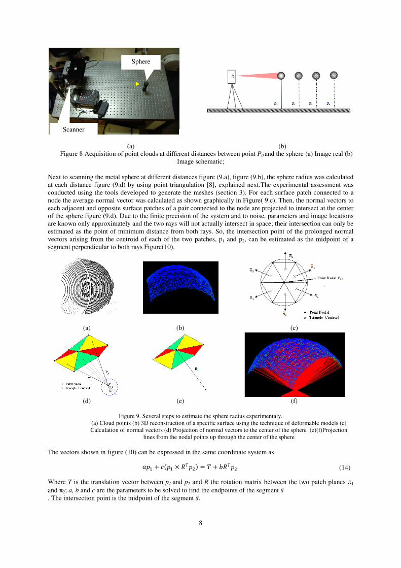
8

(a) (b) Figure 8 Acquisition of point clouds at different distances between point P0 and the sphere (a) Image real (b)

Image schematic;

Next to scanning the metal sphere at different distances figure (9.a), figure (9.b), the sphere radius was calculated

at each distance figure (9.d) by using point triangulation [8], explained next.The experimental assessment was

conducted using the tools developed to generate the meshes (section 3). For each surface patch connected to a

node the average normal vector was calculated as shown graphically in Figure( 9.c). Then, the normal vectors to

each adjacent and opposite surface patches of a pair connected to the node are projected to intersect at the center

of the sphere figure (9.d). Due to the finite precision of the system and to noise, parameters and image locations

are known only approximately and the two rays will not actually intersect in space; their intersection can only be

estimated as the point of minimum distance from both rays. So, the intersection point of the prolonged normal

vectors arising from the centroid of each of the two patches, p1 and p2, can be estimated as the midpoint of a

segment perpendicular to both rays Figure(10).

(a) (b) (c)

(d) (e) (f)

Figure 9. Several steps to estimate the sphere radius experimentaly.

(a) Cloud points (b) 3D reconstruction of a specific surface using the technique of deformable models (c)

Calculation of normal vectors (d) Projection of normal vectors to the center of the sphere (e)(f)Projection

lines from the nodal points up through the center of the sphere

The vectors shown in figure (10) can be expressed in the same coordinate system as k"� + d("� × 3T"�) = B + c3T"�

(14)

Where T is the translation vector between p1 and p2 and R the rotation matrix between the two patch planes π1

and π2; a, b and c are the parameters to be solved to find the endpoints of the segment �̅ . The intersection point is the midpoint of the segment �̅.

Sphere

Scanner

9

Figure 10. Triangulation Point

The radius associated to each pair of patches is the distance from the midpoint of �̅ to the node point. This

process is repeated for the other two pair of patches connected to the same node, as shown in Figure(9.d). The

radius associated to each node is calculated as the average radius of the three pairs of patches, as shown in Figure

(9.e). The sphere radius (Ro) was estimated as Ro = ∑ 3:G:F�� (15)

,where n is the number of nodes. The standard deviation is calculated from

5 = p 1� − 1 (^(Rq − Ro)G/F� )r

(16)

Table (1) presents the results of the sphere radius values calculated at different distances. The distances between

the sensor and the sphere were measured using a breadboard with holes spaced by 25.0±0.5 mm as shown in

Figure(8.b). The sphere was positioned on a metal post. The initial distance was estimated using a manual

caliper.

The results show that the average errors found are within the range of 1mm at distances of 500 mm. The results,

of course, are dependent on the lens size, since the image size is the parameter to influence the object image

physical resolution. It can be observed that the average error did not increase at the same ratio as the distance

sensor-sphere, but the standard deviation. So, with the lens used (focal length = 8.5mm), the vision system

dimensional average accuracy was evaluated as approximately 1:500.

Table 1: Statistical Data

Cloud Points Number of Nodes (s)

tuvwxyvz{ |}z~y�z �y{w�u �o (mm)

Standard

Deviation �

|(~ − �o) | (mm) Distances (mm)

Sphere-Sensor

D1 250 472 17,93 0,287 0,32

D2 275 452 17,93 0,346 0,32

D3 300 424 17,84 0,333 0,41

D4 325 436 17,84 0,411 0,41

D5 350 450 17,73 0,412 0,52

D6 375 472 17,69 0,512 0,56

D7 400 448 17,67 0,528 0,58

D8 425 426 17,60 0,628 0,65

D9 450 388 17,54 0,684 0,71

D10 475 324 17,48 0,762 0,77

D11 500 326 17,39 0,821 0,86

r = measured sphere radius(18,25mm)

8. Conclusions

This article presented the development of a system model to fit 3D surfaces to point clouds acquired by a special

vision sensor used in robot applications where surface details have to be mapped for welding tasks. It is

10

presented and discussed a special technique to generate 3D surfaces from point clouds by using a method based

on deformable models. The construction of a 3D structured mesh is essentially a filtration process. The filtration

process selects the cloud points to be used according to mesh resolution, allowing a decrease in computational

load when the surface is represented.

NURBS functions present a unified mathematical formulation that allows easy implementation and digitization.

It is presented and discussed a technique to generate 3D surfaces from point clouds by using parametric surfaces

– NURBS – with control points defined as nodal points of 3D triangular meshes. The triangular meshes are

constructed from the projection of point clouds onto 2D meshes, next cloud points are selected when closer to

the nodal points of the 2D mesh, then the 2D mesh is deformed to match the nodal points with the selected cloud

points and finally the 2D mesh is projected back into the 3D space. Parametric surfaces are then approximated to

the control points to fit the 3D surface to the mesh grids. A formulation of adaptive filters for point clouds in

images is discussed and the model used presented.

The routines used to smooth the surface are based on the continuity of the parametric patches allowing a precise

representation of the object geometry. The results obtained show that the developed algorithm is valid and

reliable as long as it was compared with a real object by using a special scheme to calculate the error associated

with the approximated surface when compared to the actual object geometry.

Results showed that the system accuracy is fairly enough to guarantee weld quality with sub-millimeter

positioning errors.

9. Acknowledgements

ELETRONORTE (Electrical Power Plants of the North of Brazil) and FINATEC (Scientific and Technological

Enterprises Foundation) are thanked for their finan cial support and collaboration. Our gratitude is especially

conveyed to the staff of ELETRONORTE for their technical support and interest.

10. References

[1] Anderson, C.W.,Crawford-Hines, 2000, “Fast generation of NURBS surfaces from polygonal mesh models

of human anatomy”. Technical Report CS-99-101, Fort Collins, Colorado State University, USA.

[2] Loop, C., 1990, “Generalized B-spline surfaces of arbitrary topology”, Proceedings of the 17th Annual

Conference on Computer Graphics and Interactive Techniques, Dallas, TX, USA pp. 347 - 356

[3] Chui, K.L., Chiu, W.K. and Yu, K. M., 2008, “Direct 5-axis tool-path generation from point cloud input

using 3D biarc fitting”, Vol. 24 , no. 2, p.p. 270-286.

[4] Elsäesser, B. (1998). “Approximation with Rational B-spline Curves and Surfaces”. Proceedings of the

International Conference on Mathematical Methods for Curves and Surfaces II Lillehammer.Vol.1, pp.87-

94.

[5] Haykyn,S., 2001, “Adaptive filter theory”, 4th ed., Prentice Hall, USA, 978 p.

[6] Hoppe, H., 1994, “Piecewise smooth surface reconstruction”, Proceedings of the 21st Annual Conference

on Computer Graphics and Interactive Techniques, Orlando, Florida, pp. 295 – 302.

[7] Farin, G. (2001). “Shape”. Math. Unlimited-2001 and Beyond, 3a. edição, pp 463-466.

[8] Forsyth, D and Ponce, J., 2003, “Computer Vision: A Modern Approach”, Prentice-Hall, New Jersey,

USA.

[9] Ginani, L. and Motta, J. M S. T.., 2007, “A Laser Scanning System for 3D Modeling of Industrial Objects

Based on Computer Vision”, Proceedings of 19th International Congress of Mechanical Engineering, Vol.

1, Brasilia-DF, Brazil, 10 p.

[10] Gois, J. P. (2004) Reconstrução de Superfícies a Partir de Nuvens de Pontos. Dissertação de Mestrado.

Instituto de Ciências Matemáticas e de Computação - Universidade de São Paulo, São Carlos, 155 pp.

[11] Park. K., Yun, I. D. and Lee, S. U., 1999, “Constructing NURBS surface model from scattered and

unorganized range data ”. Proceedings of the Second International Conference on 3D Digital Imaging and

Modeling, pp. 312-320.

[12] Randrianarivony, M. e Brunnett, G., 2002, “Parallel implementation of surface reconstruction from noisy

samples”, Preprintreihe des Chemnitzer SFB 393, 02-16.

[13] Roth, G. and Boulanger, P. 1998, “Cad model building from multiple range images”, Proceedings of Vision

Interface, Vancuver, BC, pp. 431-438.

11. Responsibility Notice

The authors are the only responsible for the printed material included in this paper.