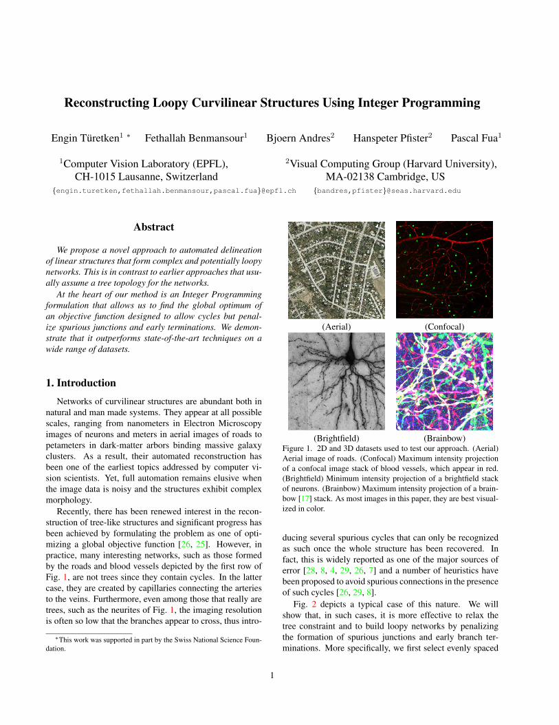
Reconstructing Loopy Curvilinear Structures Using Integer Programming

Engin Turetken1 ∗ Fethallah Benmansour1 Bjoern Andres2 Hanspeter Pfister2 Pascal Fua1

1Computer Vision Laboratory (EPFL), 2Visual Computing Group (Harvard University),CH-1015 Lausanne, Switzerland MA-02138 Cambridge, US

{engin.turetken,fethallah.benmansour,pascal.fua}@epfl.ch {bandres,pfister}@seas.harvard.edu

Abstract

We propose a novel approach to automated delineationof linear structures that form complex and potentially loopynetworks. This is in contrast to earlier approaches that usu-ally assume a tree topology for the networks.

At the heart of our method is an Integer Programmingformulation that allows us to find the global optimum ofan objective function designed to allow cycles but penal-ize spurious junctions and early terminations. We demon-strate that it outperforms state-of-the-art techniques on awide range of datasets.

1. Introduction

Networks of curvilinear structures are abundant both innatural and man made systems. They appear at all possiblescales, ranging from nanometers in Electron Microscopyimages of neurons and meters in aerial images of roads topetameters in dark-matter arbors binding massive galaxyclusters. As a result, their automated reconstruction hasbeen one of the earliest topics addressed by computer vi-sion scientists. Yet, full automation remains elusive whenthe image data is noisy and the structures exhibit complexmorphology.

Recently, there has been renewed interest in the recon-struction of tree-like structures and significant progress hasbeen achieved by formulating the problem as one of opti-mizing a global objective function [26, 25]. However, inpractice, many interesting networks, such as those formedby the roads and blood vessels depicted by the first row ofFig. 1, are not trees since they contain cycles. In the lattercase, they are created by capillaries connecting the arteriesto the veins. Furthermore, even among those that really aretrees, such as the neurites of Fig. 1, the imaging resolutionis often so low that the branches appear to cross, thus intro-

∗This work was supported in part by the Swiss National Science Foun-dation.

(Aerial) (Confocal)

(Brightfield) (Brainbow)Figure 1. 2D and 3D datasets used to test our approach. (Aerial)Aerial image of roads. (Confocal) Maximum intensity projectionof a confocal image stack of blood vessels, which appear in red.(Brightfield) Minimum intensity projection of a brightfield stackof neurons. (Brainbow) Maximum intensity projection of a brain-bow [17] stack. As most images in this paper, they are best visual-ized in color.

ducing several spurious cycles that can only be recognizedas such once the whole structure has been recovered. Infact, this is widely reported as one of the major sources oferror [28, 8, 4, 29, 26, 7] and a number of heuristics havebeen proposed to avoid spurious connections in the presenceof such cycles [26, 29, 8].

Fig. 2 depicts a typical case of this nature. We willshow that, in such cases, it is more effective to relax thetree constraint and to build loopy networks by penalizingthe formation of spurious junctions and early branch ter-minations. More specifically, we first select evenly spaced

1

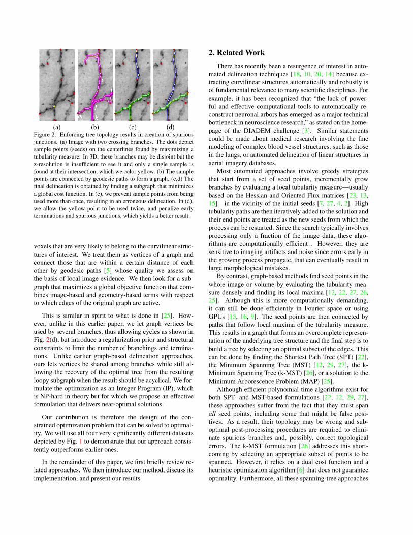
(a) (b) (c) (d)Figure 2. Enforcing tree topology results in creation of spuriousjunctions. (a) Image with two crossing branches. The dots depictsample points (seeds) on the centerlines found by maximizing atubularity measure. In 3D, these branches may be disjoint but thez-resolution is insufficient to see it and only a single sample isfound at their intersection, which we color yellow. (b) The samplepoints are connected by geodesic paths to form a graph. (c,d) Thefinal delineation is obtained by finding a subgraph that minimizesa global cost function. In (c), we prevent sample points from beingused more than once, resulting in an erroneous delineation. In (d),we allow the yellow point to be used twice, and penalize earlyterminations and spurious junctions, which yields a better result.

voxels that are very likely to belong to the curvilinear struc-tures of interest. We treat them as vertices of a graph andconnect those that are within a certain distance of eachother by geodesic paths [5] whose quality we assess onthe basis of local image evidence. We then look for a sub-graph that maximizes a global objective function that com-bines image-based and geometry-based terms with respectto which edges of the original graph are active.

This is similar in spirit to what is done in [25]. How-ever, unlike in this earlier paper, we let graph vertices beused by several branches, thus allowing cycles as shown inFig. 2(d), but introduce a regularization prior and structuralconstraints to limit the number of branchings and termina-tions. Unlike earlier graph-based delineation approaches,ours lets vertices be shared among branches while still al-lowing the recovery of the optimal tree from the resultingloopy subgraph when the result should be acyclical. We for-mulate the optimization as an Integer Program (IP), whichis NP-hard in theory but for which we propose an effectiveformulation that delivers near-optimal solutions.

Our contribution is therefore the design of the con-strained optimization problem that can be solved to optimal-ity. We will use all four very significantly different datasetsdepicted by Fig. 1 to demonstrate that our approach consis-tently outperforms earlier ones.

In the remainder of this paper, we first briefly review re-lated approaches. We then introduce our method, discuss itsimplementation, and present our results.

2. Related WorkThere has recently been a resurgence of interest in auto-

mated delineation techniques [18, 10, 20, 14] because ex-tracting curvilinear structures automatically and robustly isof fundamental relevance to many scientific disciplines. Forexample, it has been recognized that “the lack of power-ful and effective computational tools to automatically re-construct neuronal arbors has emerged as a major technicalbottleneck in neuroscience research,” as stated on the home-page of the DIADEM challenge [3]. Similar statementscould be made about medical research involving the finemodeling of complex blood vessel structures, such as thosein the lungs, or automated delineation of linear structures inaerial imagery databases.

Most automated approaches involve greedy strategiesthat start from a set of seed points, incrementally growbranches by evaluating a local tubularity measure—usuallybased on the Hessian and Oriented Flux matrices [23, 13,15]—in the vicinity of the initial seeds [7, 27, 4, 2]. Hightubularity paths are then iteratively added to the solution andtheir end points are treated as the new seeds from which theprocess can be restarted. Since the search typically involvesprocessing only a fraction of the image data, these algo-rithms are computationally efficient . However, they aresensitive to imaging artifacts and noise since errors early inthe growing process propagate, that can eventually result inlarge morphological mistakes.

By contrast, graph-based methods find seed points in thewhole image or volume by evaluating the tubularity mea-sure densely and finding its local maxima [12, 22, 27, 26,25]. Although this is more computationally demanding,it can still be done efficiently in Fourier space or usingGPUs [15, 16, 9]. The seed points are then connected bypaths that follow local maxima of the tubularity measure.This results in a graph that forms an overcomplete represen-tation of the underlying tree structure and the final step is tobuild a tree by selecting an optimal subset of the edges. Thiscan be done by finding the Shortest Path Tree (SPT) [22],the Minimum Spanning Tree (MST) [12, 29, 27], the k-Minimum Spanning Tree (k-MST) [26], or a solution to theMinimum Arborescence Problem (MAP) [25].

Although efficient polynomial-time algorithms exist forboth SPT- and MST-based formulations [22, 12, 29, 27],these approaches suffer from the fact that they must spanall seed points, including some that might be false posi-tives. As a result, their topology may be wrong and sub-optimal post-processing procedures are required to elimi-nate spurious branches and, possibly, correct topologicalerrors. The k-MST formulation [26] addresses this short-coming by selecting an appropriate subset of points to bespanned. However, it relies on a dual cost function and aheuristic optimization algorithm [6] that does not guaranteeoptimality. Furthermore, all these spanning-tree approaches

evaluate the quality of an edge between two seed pointsby integrating a function of the tubularity measure alonga connecting path. This quality measure usually fails to dis-tinguish legitimate paths along faint curvilinear structuresfrom those that are shortcuts between high-contrast struc-tures. The MAP formulation [25] addresses these issues byusing path classifiers to score the paths and introducing aMixed Integer Programming approach to guaranteeing op-timality of the resulting solution.

However, none of these approaches address the delin-eation problem for loopy structures. For the cases wherespurious loops seem to be present, for example due to insuf-ficient imaging resolution in 3D stacks or due to projectionsof the structures on 2D [24], some of the above-mentionedmethods [26, 29, 8] attempt to distinguish spurious cross-ings from legitimate junctions by penalizing sharp turns andhigh tortuosity paths in the solutions and introducing heuris-tics to locally and greedily resolve the ambiguities. They donot guarantee global optimality and, as a result, easily gettrapped into local minima, as reported in several of these pa-pers. This is what our approach seeks to address by lookingfor the global optimum of a well-defined objective function.

3. Method

Our algorithm, like those of [12, 29, 27, 26, 25] startsby building a weighted graph designed to be an overcom-plete representation for the underlying network of curvilin-ear structures, such as the one of Fig. 2(b). It then findsan optimal subgraph in terms of an appropriately designedobjective function.

The major difference from these earlier approaches isthat instead of constraining the subgraph to be a tree asin Fig. 2(c), we allow it to contain cycles, as in Fig. 2(d),and penalize spurious junctions and early branch termina-tions. In the Result Section, we will show that this yieldsimproved results over very diverse datasets.

In the remainder of this section, we introduce our Inte-ger Programming approach to finding an optimal and poten-tially loopy subgraph.

3.1. Formulation

Our approach to constructing over-complete graphs suchas the one of Fig. 2(b) is similar to that of [25]. For eachpixel or voxel, we first estimate its likelihood of being on thecenterline of a curvilinear structure whose radius is withina given range, using a tubularity measure similar to thosediscussed in Section 2. We then find regularly spaced localmaxima, which will serve as the nodes of our graph, andconnect all those that are within a given distance from eachother. The paths are obtained by minimizing a geodesic dis-tance in (N+1)-D scale space—N spatial dimensions and theradius—as described in [5].

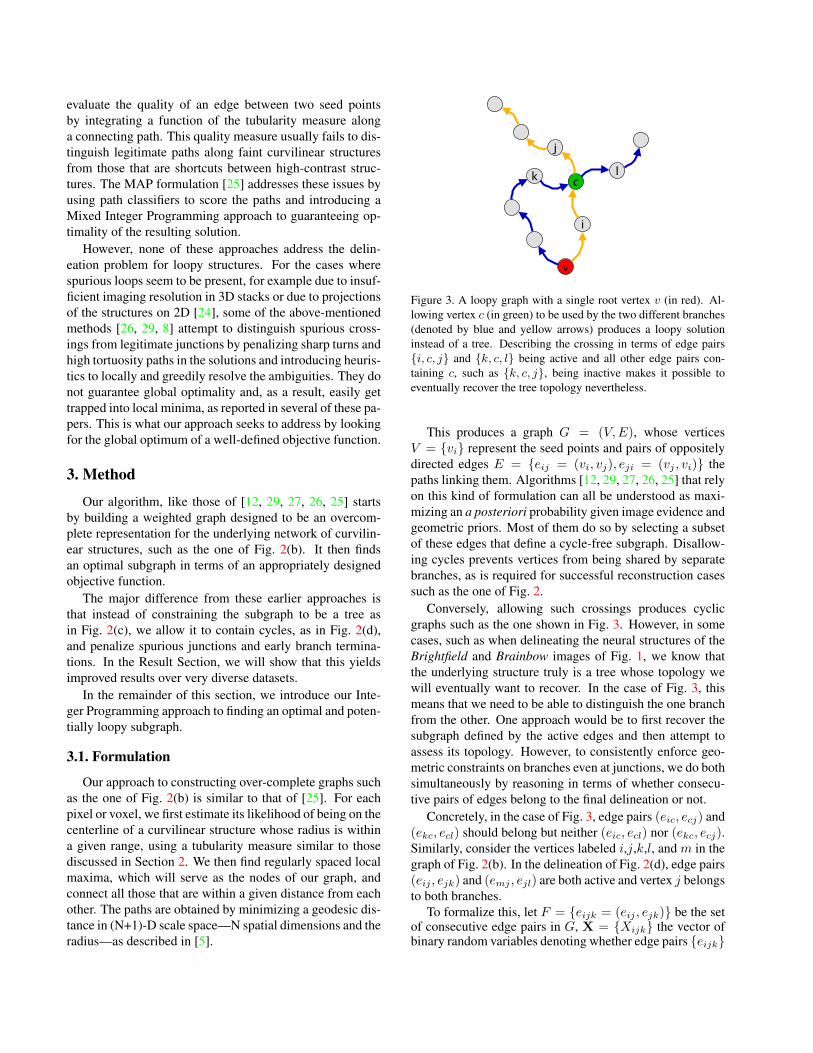
Figure 3. A loopy graph with a single root vertex v (in red). Al-lowing vertex c (in green) to be used by the two different branches(denoted by blue and yellow arrows) produces a loopy solutioninstead of a tree. Describing the crossing in terms of edge pairs{i, c, j} and {k, c, l} being active and all other edge pairs con-taining c, such as {k, c, j}, being inactive makes it possible toeventually recover the tree topology nevertheless.

This produces a graph G = (V,E), whose verticesV = {vi} represent the seed points and pairs of oppositelydirected edges E = {eij = (vi, vj), eji = (vj , vi)} thepaths linking them. Algorithms [12, 29, 27, 26, 25] that relyon this kind of formulation can all be understood as maxi-mizing an a posteriori probability given image evidence andgeometric priors. Most of them do so by selecting a subsetof these edges that define a cycle-free subgraph. Disallow-ing cycles prevents vertices from being shared by separatebranches, as is required for successful reconstruction casessuch as the one of Fig. 2.

Conversely, allowing such crossings produces cyclicgraphs such as the one shown in Fig. 3. However, in somecases, such as when delineating the neural structures of theBrightfield and Brainbow images of Fig. 1, we know thatthe underlying structure truly is a tree whose topology wewill eventually want to recover. In the case of Fig. 3, thismeans that we need to be able to distinguish the one branchfrom the other. One approach would be to first recover thesubgraph defined by the active edges and then attempt toassess its topology. However, to consistently enforce geo-metric constraints on branches even at junctions, we do bothsimultaneously by reasoning in terms of whether consecu-tive pairs of edges belong to the final delineation or not.

Concretely, in the case of Fig. 3, edge pairs (eic, ecj) and(ekc, ecl) should belong but neither (eic, ecl) nor (ekc, ecj).Similarly, consider the vertices labeled i,j,k,l, and m in thegraph of Fig. 2(b). In the delineation of Fig. 2(d), edge pairs(eij , ejk) and (emj , ejl) are both active and vertex j belongsto both branches.

To formalize this, let F = {eijk = (eij , ejk)} be the setof consecutive edge pairs in G, X = {Xijk} the vector ofbinary random variables denoting whether edge pairs {eijk}

truly belong to the underlying curvilinear structure, and x ={xijk} the corresponding vector of indicator variables. Wewill say that eijk is active in the solution if xijk = 1. Giventhe graph and the image evidence I , we look for the optimalsubgraph as the solution of

x∗ = argmaxx∈Pc

P (X = x|I,G) ,

= argmaxx∈Pc

P (I,G|X = x)P (X = x) ,

= argminx∈Pc

− log(P (I,G|X = x))− log(P (X = x)), (1)

where x belongs to the set Pc of binary vectors that definefeasible subgraphs, as defined in the following section. Inother words, we seek to minimize the sum of two negativelog-likelihood terms, which we evaluate as follows.

As we will show in the appendix, assuming conditionalindependence of the image evidence given the true valuesof the random variables Xijk, the first log likelihood termof Eq. 1 can be rewritten as

− log(P (I,G|X = x)) =∑

eijk∈F

wijkxijk, (2)

wherewijk is a cost term that accounts for the quality of thegeodesic paths associated with the edge pair eijk. We usethe path classification approach of [25] to compute it andgive the details of the computation in the appendix. As dis-cussed in Section 2, we have found it more effective at dis-tinguishing legitimate paths from spurious ones than morestandard methods, such as those that integrate a tubularitymeasure along the path.

The second log likelihood term in Eq. 1 is a prior termthat penalizes unwarranted bifurcations or terminations. Wemodel it as a Bayesian network with latent variables Mij =∑emij∈F Xmij and Oij =

∑eijn∈F Xijn, which denote

the true number of incoming and outgoing edge pairs intoor out of edge eij . Furthermore, let

• pt = P (Oij = 0|Mij = 1) be the prior probabilitythat a branch terminates at edge eij ,• pc = P (Oij = 1|Mij = 1) be the prior probability

that a branch continues at edge eij ,• pb = P (Oij = 2|Mij = 1) be the prior probability

that a branch bifurcates at edge eij ,

Assuming that the edge pairs {eijn} are independent of theother edge pairs, given the true state the edge eij , and by in-specting the probability of each admissible event, namelytermination, continuation or bifurcation at edge eij , theprior term − log(P (X = x)) can be rewritten as

−∑eij∈E

[ ∑emi∈E

log(pt)xmij +∑ejn∈E

log

(pc

pt

)xijn +

∑ejn∈E

∑ejk∈Ek<n

log

(pbpt

(pc)2

)xijnxijk

], (3)

which we derive in the appendix. In short, minimizing thenegative log likelihood of Eq. 1 amounts to minimizing,with respect to the indicator variables x, the criterion∑

eijk∈Faijkxijk +

∑eijk,eijn∈F

bijknxijkxijn , (4)

which is the sum of the linear and quadratic terms of Eqs. 2and 3 and whose aijk and bijkn coefficients are obtainedby summing the respective terms.

However, not all choices of binary values for the indica-tor variables give rise to a connected subgraph that repre-sents a plausible delineation. The above minimization musttherefore be carried out subject to a set of constraints thatwe introduce next.

3.2. Constraints

Our images may contain several disconnected structures.To avoid having to process them sequentially in a greedymanner, which may result in some branches being “stolen”by the first structure we reconstruct and therefore a subopti-mal solution, we connect them all. Assuming we are given aset R of seed vertices, one for each structure of interest, wecreate a virtual root vertex vv and connect it to each vr ∈ Rby zero cost edge pairs containing all other vertices to whichvr is connected.

We now define four sets of constraints to ensure that thesolutions to the minimization problem of Eq. 4 are such thatseed vertices are not isolated, branches are edge-disjoint,potential crossovers are consistently handled, and all activeedge pairs are connected.

Non-isolated Seeds: We require the seed vertices vr ∈ Rto be connected to at least one vertex other than the virtualroot vv and to have no incoming edge other than evr. Wewrite this as∑

eri∈Exvri ≥ 1, ∀vr ∈ R , (5)

∑eijr∈F

xijr +∑

eirj∈F :vi 6=vv

xirj = 0, ∀vr ∈ R .

Disjoint Edges: For each edge eij ∈ E, we let at mostone edge pair be active among all those that either containeij or sufficiently overlap with it. We do the first by pre-venting the number of active incoming edge pairs into anedge to be more than one. Second, we treat edges that over-lap more than a certain fraction of their radius as being thesame edge for the purpose of this constraint. Let tij denote

the geodesic path corresponding to edge eij . We write∑ekl∈C(eij)

∑emk∈E:vm 6=vl

xmkl ≤ 1, ∀eij ∈ E : vi 6= vv,

C(eij) ={ekl ∈ E |

(tkl⊂tij)∨(l(tij∩tkl)>αr(tij∩tkl)∧

l(tij)<l(tkl))

}, (6)

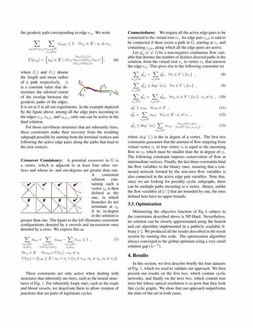
where l(.) and r(.) denotethe length and mean radiusof a path respectively. αis a constant value that de-termines the allowed extentof the overlap between thegeodesic paths of the edges.It is set to 5 in all our experiments. In the example depictedby the figure above, among all the edge pairs incoming tothe edges eij , ek1l1 and ek2l2 , only one can be active in thefinal solution.

For those curvilinear structures that are inherently trees,these constraints make their recovery from the resultingsubgraph possible by starting from the terminal vertices andfollowing the active edge pairs along the paths that lead tothe root vertices.

Crossover Consistency: A potential crossover in G isa vertex, which is adjacent to at least four other ver-tices and whose in- and out-degrees are greater than one.

A consistentsolution con-taining such avertex vp is thendefined as theone, in whichbranches do notterminate at vpif its in-degreein the solution is

greater than one. The figure to the left illustrates consistentconfigurations denoted by a swoosh and inconsistent onesdenoted by a cross. We express this as∑eki∈E:vk 6=vj

xkij +∑

elm∈E:vl 6=vq,vl 6=vj

xlmq −∑

eju∈E:vu 6=vi

xiju ≤ 1 , (7)

∀eij ∈ E ∀emq ∈ C(vj) : vm 6= vi

C(vj) = {enk ∈ E | vk = vj ∨ (vj ∈ tnk, vn 6= vj , vk 6= vj)}

These constraints are only active when dealing withstructures that inherently are trees, such as the neural struc-tures of Fig. 1. For inherently loopy ones, such as the roadsand blood vessels, we deactivate them to allow creation ofjunctions that are parts of legitimate cycles.

Connectedness: We require all the active edge pairs to beconnected to the virtual root vv . An edge pair eijk is said tobe connected if there exists a path in G, starting at vv andcontaining eijk, along which all the edge pairs are active.

Let ylij (i 6= l) be a non-negative continuous flow vari-able that denotes the number of distinct directed paths in thesolution, from the virtual root vv to vertex vl, that traversethe edge eij . This gives rise to the following constraint set∑

evj∈E

ylvj =

∑eil∈E

ylil, ∀vl ∈ V \ {vv} , (8)

∑evj∈E

ylvj ≤ deg−(vl), ∀vl ∈ V \ {vv} , (9)

∑eij∈E

ylij =

∑ejk∈E

yljk, ∀vj , vl ∈ V \ {vv} : vj 6= vl , (10)

ylil ≥ xilk, ∀eilk ∈ F , (11)

ylil =

∑eki∈E

xkil, ∀eil ∈ E : vi 6= vv , (12)

ylij ≤ deg−(vl)

∑eki∈E

xkij ,∀eij∈E:vi 6=vv,

∀vl∈V \{vv,vi,vj} , (13)

where deg−(.) is the in degree of a vertex. The first twoconstraints guarantee that the amount of flow outgoing fromvirtual vertex vv to true vertex vl is equal to the incomingflow to vl, which must be smaller than the in degree of vl.The following constraint imposes conservation of flow atintermediate vertices. Finally, the last three constraints bindthe flow variables to the binary ones, ensuring that a con-nected network formed by the non-zero flow variables isalso connected in the active edge pair variables. Note that,since we are looking for possibly cyclic subgraphs, therecan be multiple paths incoming to a vertex. Hence, unlikethe flow variables of [11] that are bounded by one, the onesdefined here have no upper bounds.

3.3. Optimization

Minimizing the objective function of Eq 4 subject tothe constraints described above is NP-Hard. Nevertheless,its solution can be closely approximated using the branchand cut algorithm implemented in a publicly available li-brary [1]. We produced all the results described in the resultsection by running this code. The optimization algorithmalways converged to the global optimum using a very smallsolution gap (1e−7).

4. ResultsIn this section, we first describe briefly the four datasets

of Fig. 1, which we used to validate our approach. We thenpresent our results on the first two, which contain cyclicnetworks, and finally on the next two, which contain truetrees but whose optical resolution is so poor that they looklike cyclic graphs. We show that our approach outperformsthe state-of-the-art in both cases.

4.1. Datasets and Path Classification

We evaluated our approach on the four different datasetsdepicted by Fig. 1 and described in more detail below:

• Aerial: Aerial images of loopy road networks. Weused 21 grayscale versions of these images for train-ing and 8 for testing.• Confocal: Two image stacks of direction selective reti-

nal ganglion cells were acquired with a confocal mi-croscope. We used a portion of one to train our pathclassifier and both for testing. We only considered thered channel of these stacks since it is the only one usedto label the blood vessels.• Brightfield: Six image stacks were acquired by bright-

field microscopy from biocytin-stained rat brains. Weused three for training and three for testing.• Brainbow: Neurites were visualized by targeting

mice primary visual cortex using the brainbow tech-nique [17] so that each neuronal structure has a distinctcolor. We used one image stack for training and threefor testing.

Many roads of the Aerial dataset are partially occludedby trees while the images from the other datasets are verynoisy, making the delineation task challenging in all cases.Fig. 4 depicts some of our results on these datasets and weprovide additional ones as supplementary material.

To obtain these results, we had to estimate the cost termswijk of Eq 2. To this end, we used the path classifier of [25],which operates on histograms of gradient deviation featuresand was designed for grayscale images. To adapt it to theBrainbow color images, we first converted the stacks intothe CIELAB space and clustered their voxels using the K-Means algorithm. For each cluster, we then computed a nor-malized gray scale image whose voxel values are inverselyproportional to the color distance between the original voxeland the cluster mean. This results in K gray scale images(K is set to 50 in all our experiments) and each voxel is as-sociated to the one its cluster corresponds to. For a pixelalong any given path, the gradient features are computedon this associated image. The result is that only gradientscorresponding to pixels with a similar color are taken intoaccount.

4.2. Roads and Blood Vessels

The roads and blood vessels of the Aerial and Confocaldatasets form graphs in which there are many real cycles.In the case of the blood vessels, this is because there arecapillaries that connect the arteries to the veins and irrigatethe cells along the way.

As can be seen in the first row of Fig. 4, the road net-works are recovered almost perfectly in spite of the occlu-sions. The only errors are driveways that are treated as very

BRBW1 BRBW2 BRBW3 BRF1 BRF2 BRF3HGD-QMIP [25] 0.3692 0.5118 0.4016 0.6114 0.4263 0.6551

L-QMIP 0.8327 0.6897 0.7848 0.7282 0.5122 0.7391

Table 1. DIADEM [3] scores for our results (L-QMIP) and thoseof [25] (HGD-QMIP) for the delineations of 3 Brainbow stacksand the 3 Brightfield ones. They are denoted by BRBWi andBRFi, respectively. Our scores are higher and therefore better.

BRF1 BRF2 BRF3NARAY [21] 0.56 0.65 0.88 0.99 0.64 0.64 0.91 0.99 0.55 0.61 0.87 0.99

L-QMIP 0.14 0.33 0.86 0.76 0.18 0.32 0.89 0.88 0.14 0.32 0.80 0.67

Table 2. NetMets [19] scores for our results (L-QMIP) and thoseobtained with the code made publicly available by the DIADEMchallenge winners [21] (NARAY). The NetMets software outputsfour numbers for each trial, geometric False Positive Rate, geo-metric False Negative Rate, connectivity False Positive Rate, andconnectivity False Negative Rate. We list them here in that orderand ours are lower and therefore better.

short roads and a few roads dead-ending because the con-necting path to the closest junction is severely occluded.The first one could be addressed by introducing a seman-tic threshold on short overhanging segments while the latterwould require a much more sophisticated semantic under-standing. We supply results on the four remaining test im-ages as supplementary material.

The quality of the blood vessel delineations depicted bythe second row is much harder to assess on the printed pagebut becomes clear when looking at the rotating volumes thatwe supply as supplementary material.

4.3. Neural Structures

The neurites of the Brightfield and Brainbow datasetsform tree structures without cycles. However, because ofthe low z-resolution, branches that really are disjoint appearto cross.

Because the ground truth tracings are trees, we were ableto compute the DIADEM scores [3] for the four delineationsdepicted by the bottom two rows of Fig. 4. They are listedin Table 1 along with those results obtained by solving theMixed Integer Program advocated in [25], which is not de-signed to prevent cycles. Since we use the same algorithmto assess the quality of the paths in both cases, the main dif-ference between the two approaches is that ours allows ver-tices to be used more than once and favors creation of cyclesthrough the additional cost terms and constraints, while theother does not, which results in a substantial performancegain.

We also evaluated the curvelet transform based algorithmof [21] on the Brightfield dataset. We used the publiclyavailable code by the winners of the DIADEM challenge.Since the code does not allow the user to provide a set ofroot nodes, the DIADEM score of its output cannot be com-puted. However, the same group recently made available a

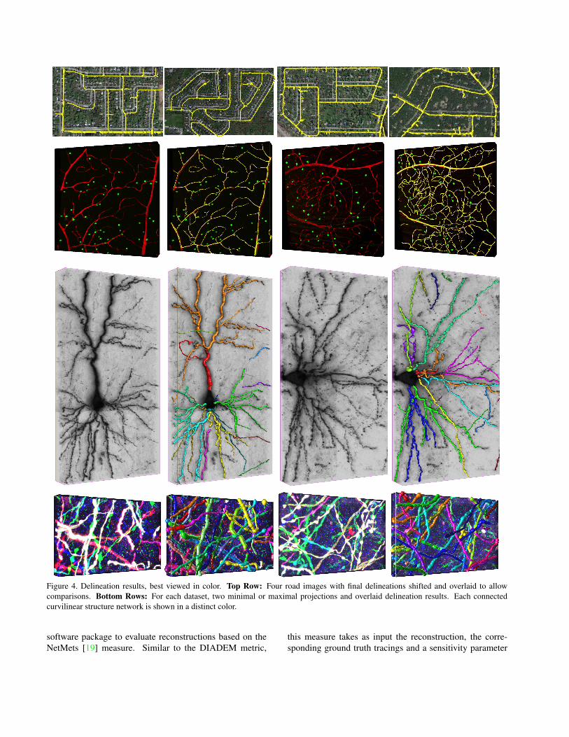
Figure 4. Delineation results, best viewed in color. Top Row: Four road images with final delineations shifted and overlaid to allowcomparisons. Bottom Rows: For each dataset, two minimal or maximal projections and overlaid delineation results. Each connectedcurvilinear structure network is shown in a distinct color.

software package to evaluate reconstructions based on theNetMets [19] measure. Similar to the DIADEM metric,

this measure takes as input the reconstruction, the corre-sponding ground truth tracings and a sensitivity parameter

σ, which is set to twice the minimum image spacing in allour experiments.

We evaluated this measure on both their result and oursand report the outcome in Table 2, which shows that ourapproach brings about a very significant improvement.

5. ConclusionWe have presented a graph-based approach to delineat-

ing complex linear structures in 2D images and 3D imagestacks. Unlike most earlier ones, it explicitly handles thefact that they may be cyclic and builds graphs in which ver-tices may belong to more than one branch. This results in asubstantial performance increase.

However the geometric constraints we impose are stillrelatively local since they bear on consecutive edge pairs. Infuture work, we will focus on imposing more global ones.

References[1] Gurobi Optimizer. http://www.gurobi.com/. 5[2] K. Al-Kofahi, S. Lasek, D. Szarowski, C. Pace, G. Nagy,

J. Turner, and B. Roysam. Rapid Automated Three-Dimensional Tracing of Neurons from Confocal ImageStacks. TITB, 6(2):171–187, 2002. 2

[3] G. A. Ascoli, K. Svoboda, and Y. Liu. Digital Reconstructionof Axonal and Dendritic Morphology Diadem Challenge,2010. http://diademchallenge.org/. 2, 6

[4] E. Bas and D. Erdogmus. Principal Curves as Skeletons ofTubular Objects - Locally Characterizing the Structures ofAxons. Neuroinformatics, 9(2-3):181–191, 2011. 1, 2

[5] F. Benmansour and L. Cohen. Tubular Structure Segmen-tation Based on Minimal Path Method and Anisotropic En-hancement. IJCV, 92(2):192–210, 2011. 2, 3

[6] C. Blum and M. Blesa. Combining Ant Colony Opti-mization with Dynamic Programming for Solving the K-Cardinality Tree Problem. In Computational Intelligence andBioinspired Systems, pages 25–33, 2005. 2

[7] A. Choromanska, S. Chang, and R. Yuste. Automatic Recon-struction of Neural Morphologies with Multi-Scale Graph-Based Tracking. Frontiers in Neural Circuits, 6(25), 2012.1, 2

[8] P. Chothani, V. Mehta, and A. Stepanyants. Automated Trac-ing of Neurites from Light Microscopy Stacks of Images.Neuroinformatics, 9:263–278, 2011. 1, 3

[9] L. Domanski, C. Sun, R. Hassan, P. Vallotton, and D. Wang.Linear Feature Detection on Gpus. 2010. 2

[10] D. Donohue and G. Ascoli. Automated Reconstructionof Neuronal Morphology: An Overview. Brain ResearchReviews, 67:94–102, 2011. 2

[11] C. Duhamel, L. Gouveia, P. Moura, and M. Souza. Mod-els and Heuristics for a Minimum Arborescence Problem.Networks, 51(1):34–47, 2008. 5

[12] M. Fischler, J. Tenenbaum, and H. Wolf. Detection of Roadsand Linear Structures in Low-Resolution Aerial Imagery Us-ing a Multisource Knowledge Integration Technique. CVIP,15(3):201–223, March 1981. 2, 3

[13] A. Frangi, W. Niessen, K. Vincken, and M. Viergever. Mul-tiscale Vessel Enhancement Filtering. Lecture Notes inComputer Science, 1496:130–137, 1998. 2

[14] C. Kirbas and F. Quek. Vessel Extraction Techniques andAlgorithms: A Survey. In Symposium on BioInformaticsand BioEngineering, pages 238–245, 2003. 2

[15] M. Law and A. Chung. Three Dimensional CurvilinearStructure Detection Using Optimally Oriented Flux. InECCV, 2008. 2

[16] M. Law and A. Chung. An Oriented Flux Symmetry BasedActive Contour Model for Three Dimensional Vessel Seg-mentation. In ECCV, pages 720–734, 2010. 2

[17] J. Livet, T. Weissman, H. Kang, R. Draft, J. Lu, R. Bennis,J. Sanes, and J. Lichtman. Transgenic strategies for com-binatorial expression of fluorescent proteins in the nervoussystem. Nature, 450(7166):56–62, 2007. 1, 6

[18] J. Lu. Neuronal Tracing for Connectomic Studies.Neuroinformatics, 9(2-3):159–166, 2011. 2

[19] D. Mayerich, C. Bjornsson, J. Taylor, and B. Roysam. Net-mets: Software for Quantifying and Visualizing Errors in Bi-ological Network Segmentation. BMC Bioinformatics, 13,2012. 6, 7

[20] E. Meijering. Neuron Tracing in Perspective. Cytometry PartA, 77(7):693–704, 2010. 2

[21] A. Narayanaswamy, Y. Wang, and B. Roysam. 3-d imagepre-processing algorithms for improved automated tracing ofneuronal arbors. Neuroinformatics, 9(2-3):219–231, 2011. 6

[22] H. Peng, F. Long, and G. Myers. Automatic 3D Neuron Trac-ing Using All-Path Pruning. Bioinformatics, 27(13):239–247, 2011. 2

[23] Y. Sato, S. Nakajima, H. Atsumi, T. Koller, G. Gerig,S. Yoshida, and R. Kikinis. 3D Multi-Scale Line Filter forSegmentation and Visualization of Curvilinear Structures inMedical Images. MIA, 2:143–168, June 1998. 2

[24] J. Staal, M. Abramoff, M. Niemeijer, M. Viergever, andB. van Ginneken. Ridge Based Vessel Segmentation in ColorImages of the Retina. TMI, 2004. 3

[25] E. Turetken, F. Benmansour, and P. Fua. Automated Recon-struction of Tree Structures Using Path Classifiers and MixedInteger Programming. In CVPR, June 2012. 1, 2, 3, 4, 6

[26] E. Turetken, G. Gonzalez, C. Blum, and P. Fua. AutomatedReconstruction of Dendritic and Axonal Trees by Global Op-timization with Geometric Priors. Neuroinformatics, 9(2-3):279–302, 2011. 1, 2, 3

[27] Y. Wang, A. Narayanaswamy, and B. Roysam. Novel 4DOpen-Curve Active Contour and Curve Completion Ap-proach for Automated Tree Structure Extraction. In CVPR,pages 1105–1112, 2011. 2, 3

[28] Y. Wang, A. Narayanaswamy, C. Tsai, and B. Roysam.A Broadly Applicable 3D Neuron Tracing Method Basedon Open-Curve Snake. Neuroinformatics, 9(2-3):193–217,2011. 1

[29] T. Zhao, J. Xie, F. Amat, N. Clack, P. Ahammad, H. Peng,F. Long, and E. Myers. Automated Reconstruction of Neu-ronal Morphology Based on Local Geometrical and GlobalStructural Models. Neuroinformatics, 9:247–261, May 2011.1, 2, 3