GeoConvention 2017 1

Reconcile Log-Derived and Core Water-Saturation, using Nuclear Magnetic Resonance for lost-from-core Free-Hydrocarbon Porosity

Author information – (1) Robert V Everett, James R Everett, Noga Vaisblatt, Fred Hyland, Herman Vacca, Eric Rops; (2) Kris Vickerman

Affiliation – (1) Robert V Everett Petrophysics, Inc. User Group; (2) Hef Petrophysical Consulting

Summary

We found there is usually a discrepancy between log-derived water saturation and core-measured water saturation so we developed a method to reconcile the two. Basically, the log and the core are looking at different amounts of hydrocarbon in the sample: 1) the core is measured at surface after hydrocarbons have bled and are lost during the core retrieval to surface and 2) the log measurements and calculations are in situ where there has been no loss of hydrocarbons. Hence, we should expect the surface core measurements to provide higher water saturations than the downhole log results. Consequently, core-measured saturations should not be used for reserve calculations of hydrocarbon pore volume (HCPV).

We found the amount of free HCPV varies with the viscosity and permeability of the rock. We checked three rock types: 1) high free-oil in a quartzite with 6-12% porosity, 42 gravity and intrinsic perm ranging from 0.1 to 10 mD; 2) low free-oil in a quartz-carbonate (Montney) with 6-10% porosity, 40 gravity and intrinsic perm ranging from 0.001 to 10 mD; and 3) a tar sand quartzite environment with 20-36% porosity, 9-11 gravity and intrinsic perm ranging from 100 to 10,000 mD.

How can we quantify the difference of surface and insitu Sw’s? We used the same method for all: using a nuclear magnetic resonance measurement of free fluid porosity, we calculate the free hydrocarbons that are lost when the core is retrieved to surface. Then the surface hydrocarbon pore volume (HCPV_surface), (equivalent to core HCPV) is insitu log-derived HCPV minus free hydrocarbon. The method is straightforward and effective, verifying the insitu HCPV before it is used to calculate viscous or non-viscous hydrocarbon reserves.

Introduction

We use a program called Geological Analysis by Maximum Likelihood Systems (‘eGamls’) which has simple-to-use and fantastic clustering capability. In addition, we use a program called Petrophysics Designed to Honour Core (PDHC) to convert elemental capture spectroscopy to minerals used for water saturation, porosity and permeability. At each step of the process we verify log measurements and calculations with core. The fact that core and log water saturations are different, and should be, is now possible to quantify.

Theory and/or Method

The method is first to calculate the free hydrocarbon-filled porosity by constraining the free fluid porosity with total porosity, to allow for bed boundary differences and water saturation to ensure we use only that part of the free fluid porosity containing hydrocarbons. The details are in Appendix 1.

GeoConvention 2017 2

Having found the free oil volume [we use the term oil but it applies to all hydrocarbons] we subtract this from the in situ HCPV to obtain a HCPV_surface that can be compared to core, in terms of either weight of tar or volume of oil or water saturation formats.

Examples

We show three examples, all of which use the same methods. The details on how to do the computation, are in Appendix 1

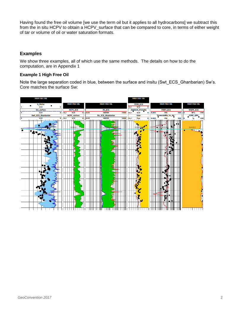
Example 1 High Free Oil

Note the large separation coded in blue, between the surface and insitu (Swt_ECS_Ghanbarian) Sw’s. Core matches the surface Sw:

GeoConvention 2017 3

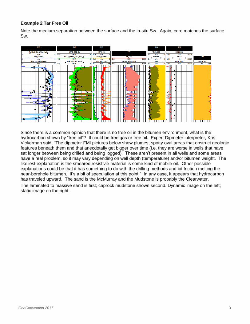
Example 2 Tar Free Oil

Note the medium separation between the surface and the in-situ Sw. Again, core matches the surface Sw.

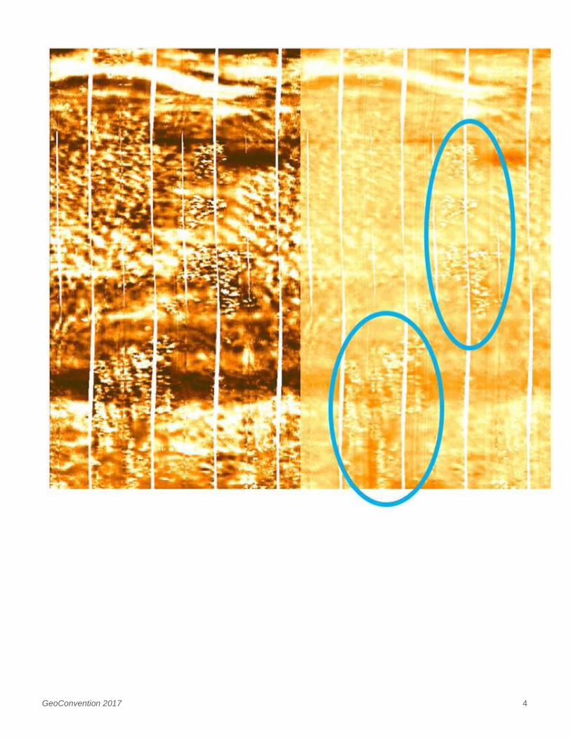
Since there is a common opinion that there is no free oil in the bitumen environment, what is the hydrocarbon shown by “free oil”? It could be free gas or free oil. Expert Dipmeter interpreter, Kris Vickerman said, “The dipmeter FMI pictures below show plumes, spotty oval areas that obstruct geologic features beneath them and that anecdotally get bigger over time (i.e. they are worse in wells that have sat longer between being drilled and being logged). These aren’t present in all wells and some areas have a real problem, so it may vary depending on well depth (temperature) and/or bitumen weight. The likeliest explanation is the smeared resistivie material is some kind of mobile oil. Other possible explanations could be that it has something to do with the drilling methods and bit friction melting the near-borehole bitumen. It’s a bit of speculation at this point.” In any case, it appears that hydrocarbon has traveled upward. The sand is the McMurray and the Mudstone is probably the Clearwater.

The laminated to massive sand is first; caprock mudstone shown second. Dynamic image on the left; static image on the right.

GeoConvention 2017 4

GeoConvention 2017 5

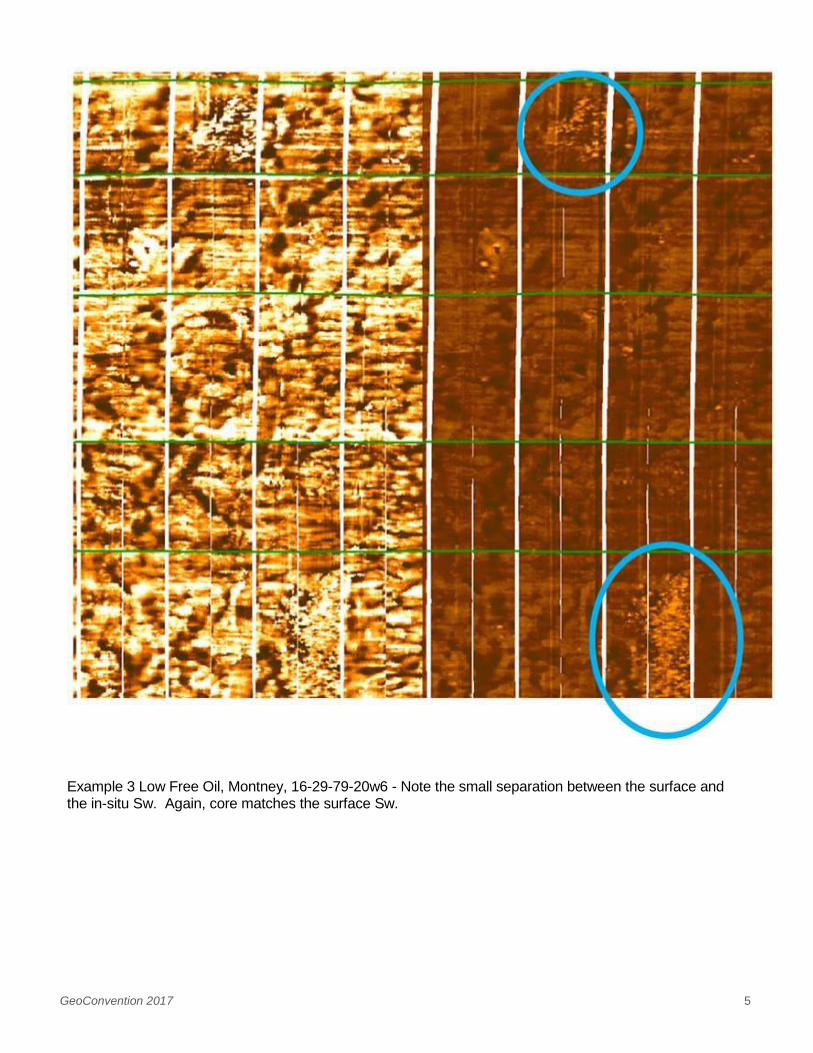
Example 3 Low Free Oil, Montney, 16-29-79-20w6 - Note the small separation between the surface and the in-situ Sw. Again, core matches the surface Sw.

GeoConvention 2017 6

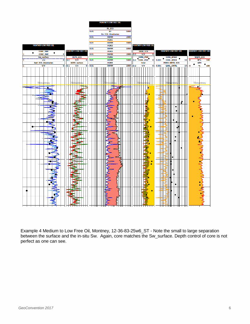
Example 4 Medium to Low Free Oil, Montney, 12-36-83-25w6_ST - Note the small to large separation between the surface and the in-situ Sw. Again, core matches the Sw_surface. Depth control of core is not perfect as one can see.

GeoConvention 2017 7

The 4th example is for 12-36, showing the top core: the blue coding shows the difference between the core measurement and the in situ Sw [from the log calculation with the proper Rw]. The pad resistivity of the dipmeter is normalized to the RLA5 measurement to provide thin bed resolution.

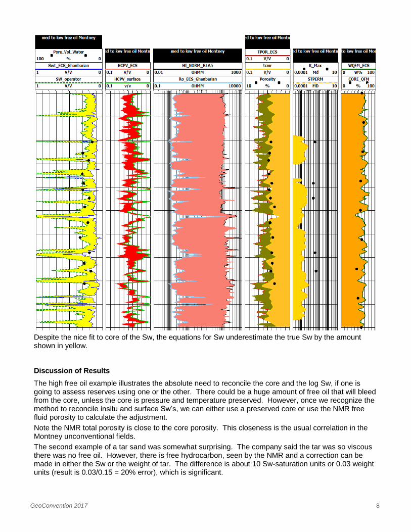
Shown below, is the result where one operator used equations to calculate Sw for the Montney providing a lovely fit to core but leaving the hydrocarbons shown in yellow, uncounted:

GeoConvention 2017 8

Despite the nice fit to core of the Sw, the equations for Sw underestimate the true Sw by the amount shown in yellow.

Discussion of Results

The high free oil example illustrates the absolute need to reconcile the core and the log Sw, if one is going to assess reserves using one or the other. There could be a huge amount of free oil that will bleed from the core, unless the core is pressure and temperature preserved. However, once we recognize the method to reconcile insitu and surface Sw’s, we can either use a preserved core or use the NMR free fluid porosity to calculate the adjustment.

Note the NMR total porosity is close to the core porosity. This closeness is the usual correlation in the Montney unconventional fields.

The second example of a tar sand was somewhat surprising. The company said the tar was so viscous there was no free oil. However, there is free hydrocarbon, seen by the NMR and a correction can be made in either the Sw or the weight of tar. The difference is about 10 Sw-saturation units or 0.03 weight units (result is 0.03/0.15 = 20% error), which is significant.

GeoConvention 2017 9

Note the core porosity in this conventional environment is close to the total density-derived porosity rather than the total NMR porosity. The NMR does not see the viscous oil porosity.

The third example, applicable to the Montney formation, is a low free-oil example. One operator did not expect any free oil effect on either core or log saturations. There is a small effect.

The fourth example, also applicable to the Montney formation, is a medium to low free-oil example. An operator who does extensive core analysis to calibrate log interpretation again did not expect any free oil effect on either core or log saturations. “I do reconcile core to log Sw on all my formations. I’m not sure I’ve made the link of a systematic difference between the two but that may be because I never truly have all the constants (a, m, n etc.) nailed down and typically knob these somewhat to tie the logs back to the core.” Consequently, we see there is a small effect but there may be a large effect. The method illustrated may result in more accurate reserve calculations as both log and core results are reconciled. Incidentally, using the mineral model tied to the ECS, the a = 1, m = n = f (grain density and effective surface area, related to CEC); these factors are designed to be related to pore throat size

Conclusions

The reconciliation of core and log water saturation is possible using the free fluid porosity from the NMR to account for lost fluids as the core is retrieved to surface. This reconciliation is necessary to verify the log as well as the core Sw’s before calculating reserves.

Appendix

Equations used to determine free hydrocarbon

The steps are:

1. Determine the free fluid to use. We recommend the 3 ms value, which in Schlumberger acronym is CMRP_3MS such as 16-19-79-20w6; however, some wells with large free fluid porosity such as 12-36-83-25 ST are better with the lower 33ms cutoff value, CMFF.

2. Find the hydrocarbon portion of the porosity: a. Limit CMRP total porosity from the density log, TPOR, just to be realistic and allow for bed

boundary differences, especially in low porosity. b. Limit to HCPV and 0. This is important as we only want to consider the hydrocarbon

portion of the free porosity. c. Call result FREE_OIL_V d. Change to weight for the Tar sand wells:

i. FREE_OIL_V * Rho_tar/Rhog_matrix ii. Where Rho_Tar = (0.001)*(141.5*1/(API_oil +131.5))*(999.97495*(1-(((((

T_deg_F_ECS-32)*5/9)+(-3.983035))^2)*(((T_deg_F_ECS-32)*5/9)) +0.301797)/(0.5225289*((((T_deg_F_ECS-32)*5/9+6934881))))))

iii. Call result FREE_OIL_WT 3. Find the HCPV_V_surface = HCPV – FREE_OIL_V 4. Find the Sw_surface_CALC = {(1- (HCPV_surface/TPOR))}*SG, where SG = Rho_oil/Rho_water

Usual values of the specific gravity ratio are 0.82/1.23. Additional limits often applied are:

IF((HCPV_ECS-HCPV_surface)<=0.001,Swt_ECS_Ghanbarian,Sw_surface_CALC*0.82/1.23)

IF((HCPV_ECS-HCPV_surface)>=0.1,Sw_surface_CALC*1.23/0.82,Sw_surface_CALC) IF(Sw_surface_CALC<Swt_ECS_Ghanbarian,Swt_ECS_Ghanbarian,Sw_surface_CALC)

GeoConvention 2017 10

5. For the Tar sand wells, find the HCPV_wt_surface = a. WTAR = (1/(1-TPOR_ECS))*HCPV*Rho_tar/Rhog_matrix

b. WTAR_surface = WTAR – FREE_OIL_WT

Nomenclature

Free fluid is measured/interpreted from a Nuclear Magnetic Resonance tool

HCPV is hydrocarbon pore volume, nominally porosity*(1-water saturation)

TPOR_ECS is total porosity derived using a set of equations involving the elements, originally

measured by elemental capture spectroscopy.

Swt_ECS_Ghanbarian is the total water saturation using a set of equations involving the

elements, originally measured by elemental capture spectroscopy. The dual water equation and the Ghanbarian formation factor is used.

HCPV_surface is the hydrocarbon pore volume with the free fluid hydrocarbon removed so that

it is equivalent to a surface measurement of HCPV, done on core.

Sw_surface is the insitu log-derived water saturation with the free fluid HCPV removed so that it

is equivalent to a water saturation measured on core at surface.

Acknowledgements

Assistance from our PDHC User group is acknowledged; Proof reading by Ramona Jones was critical to making the text understandable.

References

1) Eslinger, E., and R. V. Everett, 2012, ‘Petrophysics in gas shales’, in J. A. Breyer, ed., Shale Reservoirs—Giant

resources for the 21st century: AAPG Memoir 97, p. 419–451.

2) Eslinger, E., and Boyle, F., ‘Building a Multi-Well Model for Partitioning Spectroscopy Log Elements into Minerals

Using Core Mineralogy for Calibration’, SPWLA 54thAnnual Logging Symposium, June 22-26, 2013.

3) M. M. Herron, SPE, D. L. Johnson and L. M. Schwartz, Schlumberger-Doll Research, ‘A Robust Permeability

Estimator for Siliciclastics’, SPE 49301, 1998 SPE Annual Technical Conference and Exhibition held in New

Orleans, Louisiana, 27–30 September 1968.

4) Susan L. Herron and Michael M. Herron, ‘APPLICATION OF NUCLEAR SPECTROSCOPY LOGS TO THE

DERIVATION OF FORMATION MATRIX DENSITY’ Paper JJ Presented at the 41st Annual Logging Symposium of

the Society of Professional Well Log Analysts, June 4-7, 2000, Dallas, Texas.

GeoConvention 2017 11

5) Clavier, C., Coates, G., Dumanoir, J., ‘Theoretical and Experimental Basis for the Dual-Water Model for

interpretation of Shaly Sands’, SPE Journal Vol 24 #2, April 1984.

6) Herron, M.M, ‘Geochemical Classification of Terrigenous Sands and Shales from Core or Log Data’, Journal of

Sedimentary Petrology, Vol. 58, No. 5 September, 1988, p. 820-829.

7) Everett, R.V., Berhane, M, Euzen, T., Everett, J.R., Powers, M, ‘Petrophysics Designed to Honour Core –

Duvernay & Triassic’ Geoconvention Focus May 2014.

8) Everett, R. V. ‘CWLS Insite’ Spring 2014.

9) Ghanbarian, B, Hunt, A. G., Ewing, R. P. Skinner, T. E., ‘Universal scaling of the formation factor in porous media

derived by combining percolation and effective medium theories’ Geophysical Research letters,

10.1002/2014GL060180, Ghanbarian-alavijeh.2@wright.edu

10) Herron, S. L., Herron, M. M., Pirie, Iain, Saldungaray, Craddock, Paul, Charsky, Alyssa, Polyakov, Marina, Shray,

Frank, Li, Ting, ‘Application and Quality Control of Core Data for the Development and Validation of Elemental

Spectroscopy Log Interpretation’, SPWLA, 55th Annual Logging Symposium, Abu Dhabi, United Arab Emirates,

May 18-22, 2014.

11) Miller, Mike, Lieber, Bob, Piekenbrock, Gene, McGinness, Thal, ‘Low Permeability Gas Reservoirs How Low Can

You Go?’, ‘CWLS Insite’ 2007, originally prepared for presentation at the SPWLA Middle East Regional

Symposium held in Dubai, April 15-19, 2007.

12) Pyke, Kevin, ‘Unlocking the NMR Potential in Oil Sands’ Geoconvention Calgary 2016.

13) Bouchou, R, Markovic, m, Jiang, w. ‘Heavy Oil Quantification Using Nuclear Magnetic Resonance and Elemental

Spectroscopy Technologies in McMurray Formation, Mannville Group, Lower Cretaceous’, SPE Kuwait, 2014

Paper SPE 172890-MS.

14) Slatt R, internet

GeoConvention 2017 12

http://www.searchanddiscovery.com/documents/2011/80181slatt/ndx_slatt.pdf http://info.drillinginfo.com/seismic-

brittleness-volume-estimation-from-well-logs-in-unconventional-reservoirs-part-iii/